Embed Size (px)
Citation preview
.
Generalized Spatial Structural Equation Models
Melanie M. Wall
Division of Biostatistics
School of Public Health
University of Minnesota,
Co-authors: Xuan Liu, James S. Hodges
1
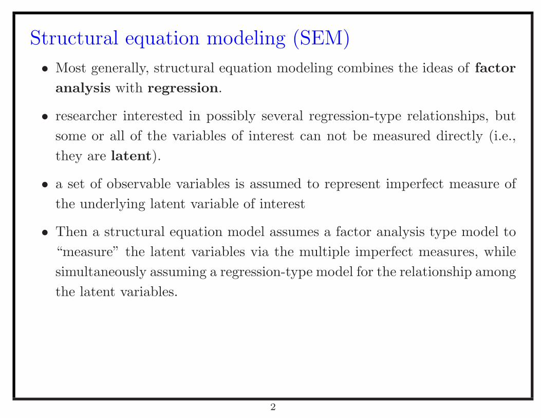
Structural equation modeling (SEM)
• Most generally, structural equation modeling combines the ideas of factor
analysis with regression.
• researcher interested in possibly several regression-type relationships, but
some or all of the variables of interest can not be measured directly (i.e.,
they are latent).
• a set of observable variables is assumed to represent imperfect measure of
the underlying latent variable of interest
• Then a structural equation model assumes a factor analysis type model to
“measure” the latent variables via the multiple imperfect measures, while
simultaneously assuming a regression-type model for the relationship among
the latent variables.
2
SEM - Traditionally
Restricted to:
• normally distributed observed variables
• linear relations among the latent variables
• independently observed individuals
• used in sociology and psychology
3
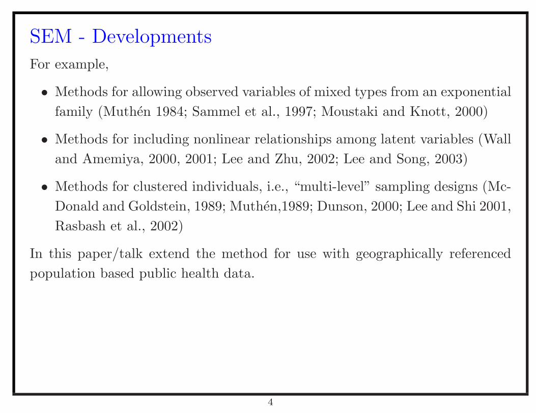
SEM - Developments
For example,
• Methods for allowing observed variables of mixed types from an exponential
family (Muthen 1984; Sammel et al., 1997; Moustaki and Knott, 2000)
• Methods for including nonlinear relationships among latent variables (Wall
and Amemiya, 2000, 2001; Lee and Zhu, 2002; Lee and Song, 2003)
• Methods for clustered individuals, i.e., “multi-level” sampling designs (Mc-
Donald and Goldstein, 1989; Muthen,1989; Dunson, 2000; Lee and Shi 2001,
Rasbash et al., 2002)
In this paper/talk extend the method for use with geographically referenced
population based public health data.
4
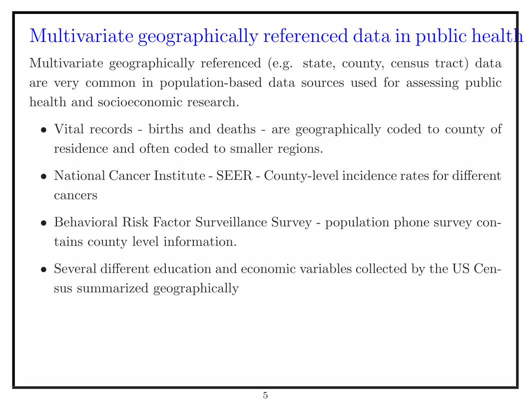
Multivariate geographically referenced data in public health
Multivariate geographically referenced (e.g. state, county, census tract) data
are very common in population-based data sources used for assessing public
health and socioeconomic research.
• Vital records - births and deaths - are geographically coded to county of
residence and often coded to smaller regions.
• National Cancer Institute - SEER - County-level incidence rates for different
cancers
• Behavioral Risk Factor Surveillance Survey - population phone survey con-
tains county level information.
• Several different education and economic variables collected by the US Cen-
sus summarized geographically
5
Multivariate geographically referenced data in public health
• Large number of variables available at each geographic unit
• Possibility of performing ecological-type regressions for investigating influ-
ences of risk factors on outcomes.
• Health Disparities Initiative - Quantify and assess relations between poverty,
minorities, and health.
6
Example - Minnesota cancer mortality data
• Three groups of observed variables of Minnesota counties are used corre-
sponding to three underlying factors.
– Death counts due to esophagus, pancreas, and lung cancer, sharing un-
derlying factor called common cancer risk factor
– Three census variables, high school education, median household income,
and percapita income measuring a underlying factor called social eco-
nomic status (SES)
– Two census variables, public water, and home heat wood measuring a
underlying factor called access to public utilities
• County level smoking prevalence variable of Minnesota - a known covariate
of interest (BRFSS)
• The interest of this study is the relationship between the shared common
cancer factor, social economic status, access to public utilities, and smoking.
7

Example - Minnesota cancer mortality data
8
9
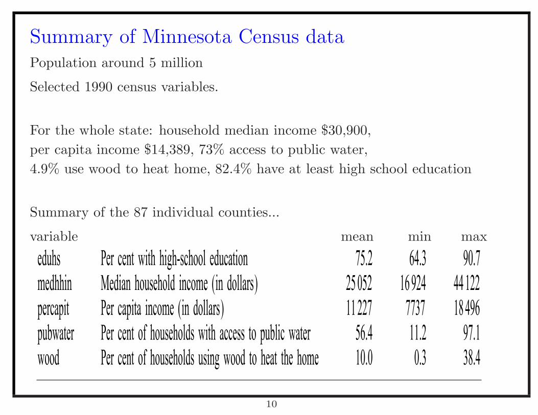
Summary of Minnesota Census dataPopulation around 5 million
Selected 1990 census variables.
For the whole state: household median income $30,900,
per capita income $14,389, 73% access to public water,
4.9% use wood to heat home, 82.4% have at least high school education
Summary of the 87 individual counties...
variable mean min max− − −
eduhs Per cent with high-school education 75.2 64.3 90.7medhhin Median household income (in dollars) 25 052 16 924 44 122percapit Per capita income (in dollars) 11 227 7737 18 496pubwater Per cent of households with access to public water 56.4 11.2 97.1wood Per cent of households using wood to heat the home 10.0 0.3 38.4
10
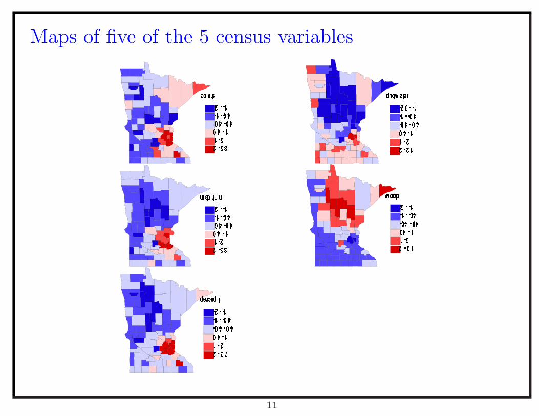
Maps of five of the 5 census variables
��������� �� �
��� ��� �
��� ������ �
��� �������
���� �
�����������! #"$!%�& '($�$!)
$!)*$�$!+�& ,
$!+�& ,($�+�& ,
+�& ,($�))($�%
%($�%�& )
-(.0/�1�1#2 34 5�4�4!6
4 6�4�4 7�8 9
4 7�8 9�4�7�8 9
7�8 9�4�66�4�5
5�4�:�8 :
;*<�<�=> ?@>�>!A
>!AB>�>!C�D E
>!C�D E�>�C�D E
C�D E@>FAAB>0?
?@>FG�D A
H�IKJML�N�HFO PQ R*Q�Q!S
Q S*Q�Q!TVU W
Q TVU W(Q�TVU W
TVU W*Q�SS*Q�R
R*Q�XVU Y
11
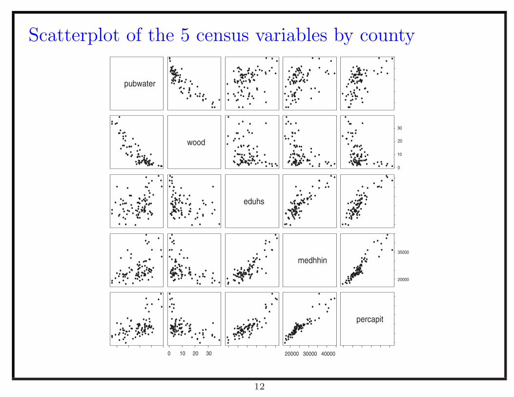
Scatterplot of the 5 census variables by county
•
•
pubwater
•
•
• •
••••
•
•
•
•
•
•
••
•
•
•
•
•
•
•
•••
•
•
•• •
•
•
•
•
•••
•
•
••
•
•
• •
•• •
•
•
••
•
•
•
•
•
•
•
•
•
•
•••
•
•
••
•
••
•••
•
• ••
•••••
•
•
•
•
• •
••••
•
•
•
•
•
•
• •
•
•
•
•
•
•
•
••
•
•
•
•••
•
•
•
•
•••
•
•
• •
•
•
••
•••
•
•
••
•
•
•
•
•
•
•
•
•
•
•••
•
•
• •
•
• •
••
•
•
• ••
• •• ••
•
•
•
•
••
••••
•
•
•
•
•
•
• •
•
•
•
•
•
•
•
••
•
•
•
•••
•
•
•
•
•••
•
•
• •
•
•
• •
•••
•
•
••
•
•
•
•
•
•
•
•
•
•
•••
•
•
• •
•
• •
••
•
•
• ••
• ••••
•
•
•
•
••
••••
•
•
•
•
•
•
• •
•
•
•
•
•
•
•
••
•
•
•
•••
•
•
•
•
•••
•
•
• •
•
•
• •
•••
•
•
••
•
•
•
•
•
•
•
•
•
•
•••
•
•
• •
•
• •
••
•
•
• ••
• ••••
•
•
•
•
•
•
••
•• ••
•
•
•
•
•
•
••
•
•
••
•
•
•
•••
•
•
•
•
•
•
•
••
•
•
•
•
•••
•
•
••
•
••
•••
•
•
•
•
•
•
••
•
•
•
•• ••
•
••
• ••
•••
•
•
•
•
•••
• •••
wood
•
•
••
•• ••
•
•
•
•
•
•
••
•
•
••
•
•
•
•••
•
•
•
•
•
•
•
••
•
•
•
•
••
•
•
•
••
•
••
•••
•
•
•
•
•
•
••
•
•
•
•• ••
•
••
•• •
•••
•
•
•
•
••• • • •
•
•
•
••
•• ••
•
•
•
•
•
•
••
•
•
••
•
•
•
•••
•
•
•
•
•
•
•
••
•
•
•
•
••
•
•
•
••
•
••
•••
•
•
•
•
•
•
••
•
•
•
•• ••
•
••
•• •
•••
•
•
•
•
••••
• ••
0
10
20
30•
•
••
•• ••
•
•
•
•
•
•
••
•
•
••
•
•
•
•••
•
•
•
•
•
•
•
••
•
•
•
•
••
•
•
•
••
•
••
•••
•
•
•
•
•
•
••
•
•
•
•• ••
•
••
•• •
•••
•
•
•
•
•••• • •
•
•• •
•
•• •
•
•
••
•
• •
• •
•
•
•
•
•
••
•
•
••
•
•
••••
•
•
•
•••
•
• •
•
•
•
•
•••
••
•
•
•
••
•
• •• •
••
•
•
••
•
••
•
••
•
• ••
•••
•
•
•
•
••
••
••
•
•••
•
•
••
•
••
••
•
•
•
•
•
••
•
•
••
•
•
• •• •
•
•
•
•••
•
••
•
•
•
•
• ••
••
•
•
•
• •
•
••••
• •
•
•
••
•
••
•
• •
•
•••
• ••
•
•
•
•
••
••
•
eduhs
•
•
•• •
•
•
••
•
• •
••
•
•
•
•
•
•••
•
••
•
•
••••
•
•
•
•••
•
• •
•
•
•
•
• ••
••
•
•
•
••
•
••••••
•
•
••
•
••
•
••
•
• ••
•••
•
•
•
•
••
••
••
•
•• •
•
•
••
•
• •
••
•
•
•
•
•
••
•
•
••
•
•
••••
•
•
•
•••
•
• •
•
•
•
•
• ••
••
•
•
•
••
•
••• •
••
•
•
••
•
••
•
••
•
• ••
•••
•
•
•
•
••
••
•
•
•
•
•
••
•
•
•••
•
••
•
•
•
• ••
•
•
• •••
•
•
•
•
•
•
• •••
•••
•••
•
•
•
••
•
•••
••
•
••
•
• •• ••
•
•
•••
•
•••
•
•
••
•
••••
•
•
•
•
•••
•
•
•
•
• •
•
•
•• •
•
••
•
•
•
•• •
•
•
•• ••
•
•
•
•
•
•
•• ••
• ••
• ••
•
•
•
••
•
•• •
••
•
••
•
•• •••
•
•
•••
•
• ••
•
•
••
•
•• •
•
•
•
•
•
•••
•
•
•
•
• •
•
•
•• •
•
••
•
•
•
•• •
•
•
••••
•
•
•
•
•
•
••••
• ••
•••
•
•
•
••
•
•••
••
•
••
•
••• ••
•
•
•••
•
• ••
•
•
•••
•••
•
•
•
•
•
• ••
•
•
medhhin
20000
35000
•
•
••
•
•
•••
•
••
•
•
•
•• •
•
•
• •••
•
•
•
•
•
•
• •••
• ••
•••
•
•
•
••
•
•••
••
•
••
•
••• ••
•
•
•••
•
•••
•
•
••
•
•••
•
•
•
•
•
•••
•
•
•
•
•
•
••
•
•
•••
•
•
•
•
•
•
•
••
•
•
••
••
•
•
•
•
•
••
••
• ••
••
••
•
•
•
•
••
•••
••
•
••
•
• •• ••
•
•
•
••• •
•
•
•
•
••
•
••
••
•
•
•
•
•••
•
•
3020100
•
•
••
•
•
•• •
•
•
•
•
•
•
•
••
•
•
••
••
•
•
•
•
•
••
••
• ••
••
••
•
•
•
•
••
•• •
••
•
••
•
•••• •
•
•
•
••••
•
•
•
•
••
•
••
••
•
•
•
•
••••
••
•
••
•
•
•• •
•
•
•
•
•
•
•
••
•
•
••
••
•
•
•
•
•
••
••
•••
••
••
•
•
•
•
••
•••
••
•
••
•
••• • •
•
•
•
••••
•
•
•
•
•••
•••
•
•
•
•
•
• ••
•
•
20000 30000 40000
•
•
••
•
•
•••
•
•
•
•
•
•
•
••
•
•
•••
••
•
•
•
•
••••
•••
•••
•
•
•
•
•
••
•••
••
•
••
•
•••••
•
•
•
••••
•
•
•
•
••
•
•••
•
•
•
•
•
•••
•
•
percapit
12
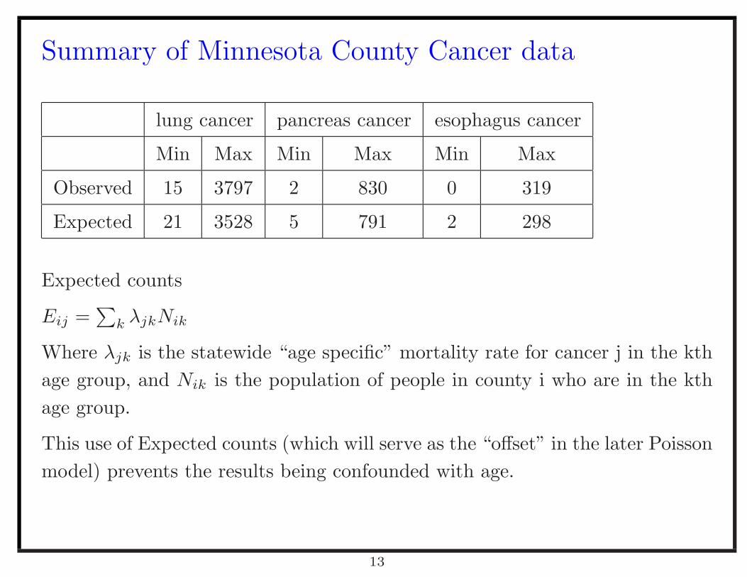
Summary of Minnesota County Cancer data
lung cancer pancreas cancer esophagus cancer
Min Max Min Max Min Max
Observed 15 3797 2 830 0 319
Expected 21 3528 5 791 2 298
Expected counts
Eij =∑
k λjkNik
Where λjk is the statewide “age specific” mortality rate for cancer j in the kth
age group, and Nik is the population of people in county i who are in the kth
age group.
This use of Expected counts (which will serve as the “offset” in the later Poisson
model) prevents the results being confounded with age.
13
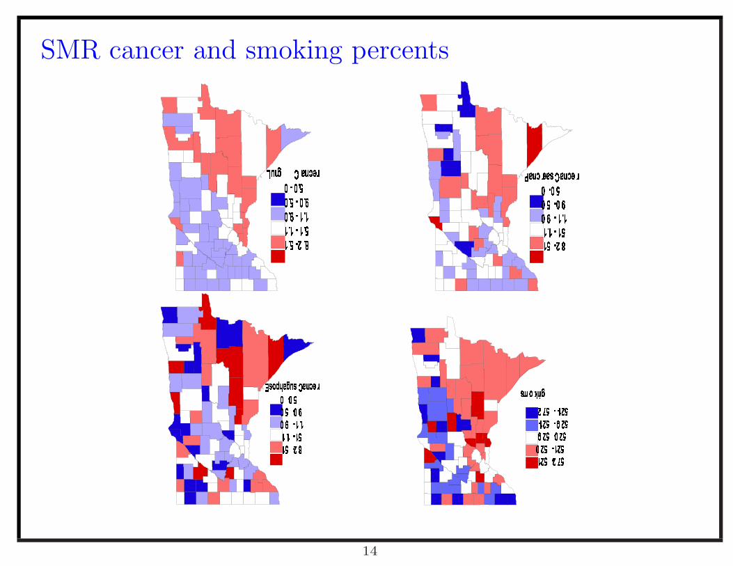
SMR cancer and smoking percents
������� ����� ���
������� ���� ������� �
��� ������� ���� ������� �
��� ������� �
��� � �! "#��$&%'� � #"�!
(*)�( + ,(+ ,&)�( + -
(+ -&)�./+ ..0+ .1)�./+ ,
.0+ ,&)�2 + 3
465#7#8#96:6;#<�5>=�:#?�@�A6B
C&DECF GCF G*DHCF I
CF I*D#J0F JJ0F JKD#J0F G
J0F G*DHLF M
N�O�PRQ0S T#UV WX Y�Z&V�V [0X W�Z
V [0X W�Z&V�V \X W�Z
V \X W�Z&VE\X W�Z
\X W�Z&V#[�X W�Z[0X W�Z&VHW�X Y�Z
14
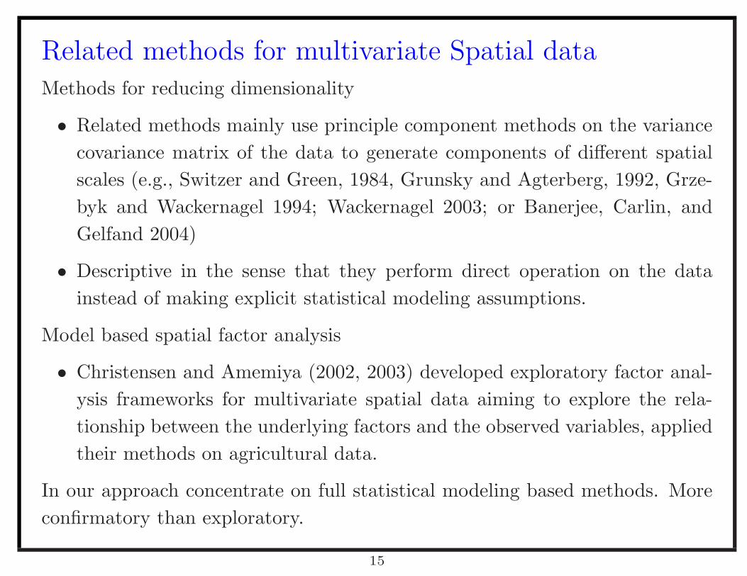
Related methods for multivariate Spatial dataMethods for reducing dimensionality
• Related methods mainly use principle component methods on the variance
covariance matrix of the data to generate components of different spatial
scales (e.g., Switzer and Green, 1984, Grunsky and Agterberg, 1992, Grze-
byk and Wackernagel 1994; Wackernagel 2003; or Banerjee, Carlin, and
Gelfand 2004)
• Descriptive in the sense that they perform direct operation on the data
instead of making explicit statistical modeling assumptions.
Model based spatial factor analysis
• Christensen and Amemiya (2002, 2003) developed exploratory factor anal-
ysis frameworks for multivariate spatial data aiming to explore the rela-
tionship between the underlying factors and the observed variables, applied
their methods on agricultural data.
In our approach concentrate on full statistical modeling based methods. More
confirmatory than exploratory.
15
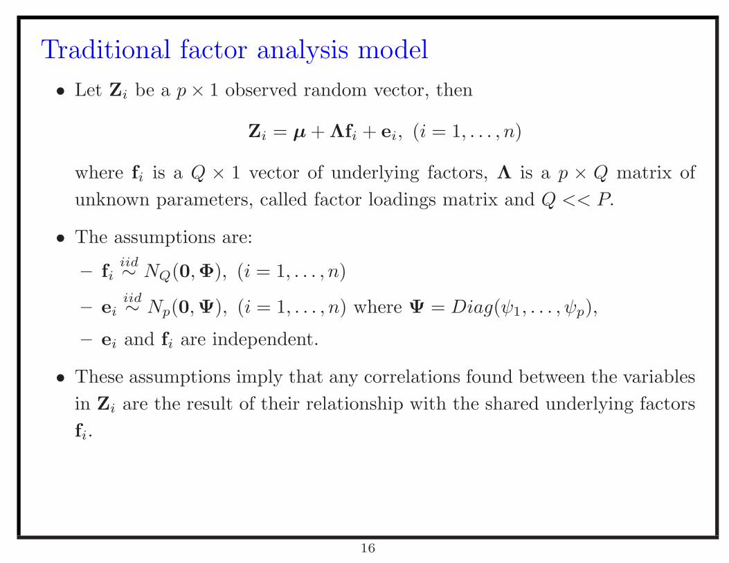
Traditional factor analysis model
• Let Zi be a p× 1 observed random vector, then
Zi = µ + Λfi + ei, (i = 1, . . . , n)
where fi is a Q × 1 vector of underlying factors, Λ is a p × Q matrix of
unknown parameters, called factor loadings matrix and Q << P.
• The assumptions are:
– fiiid∼ NQ(0,Φ), (i = 1, . . . , n)
– eiiid∼ Np(0,Ψ), (i = 1, . . . , n) where Ψ = Diag(ψ1, . . . , ψp),
– ei and fi are independent.
• These assumptions imply that any correlations found between the variables
in Zi are the result of their relationship with the shared underlying factors
fi.
16
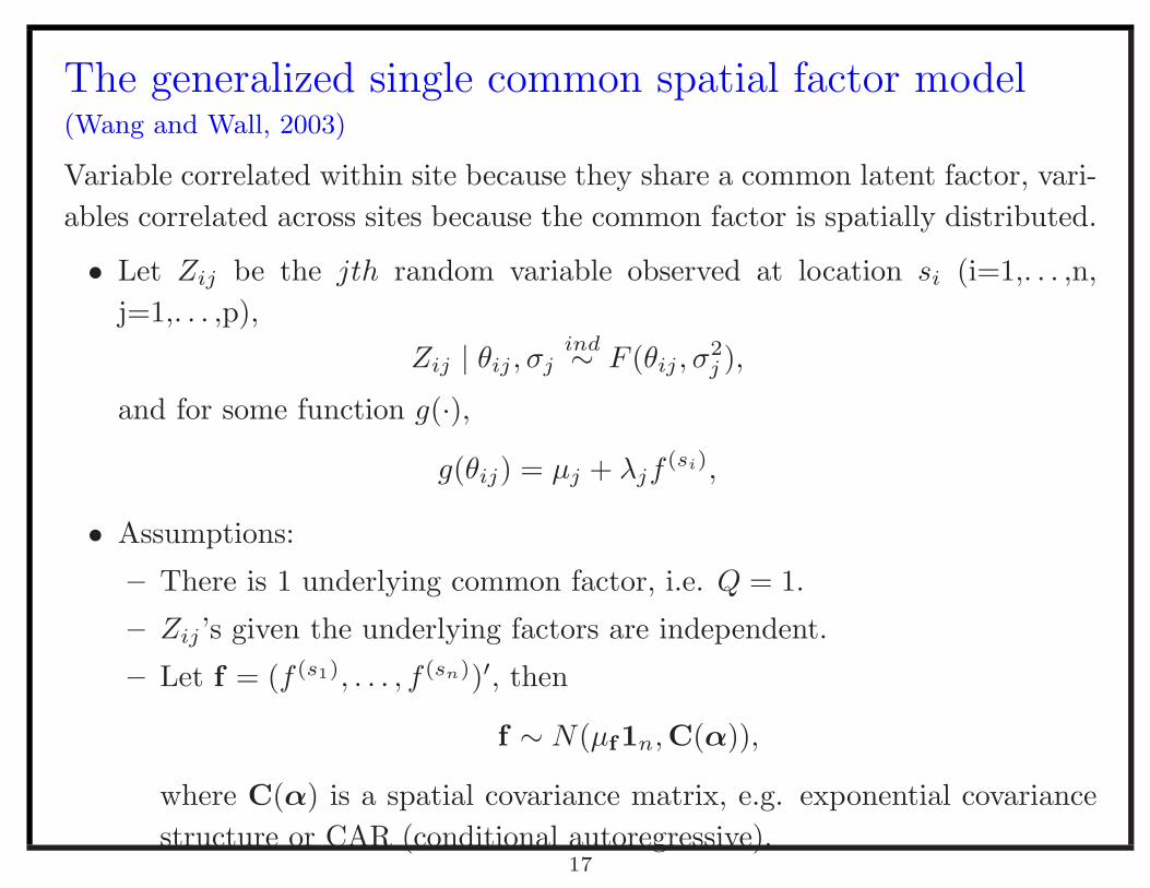
The generalized single common spatial factor model(Wang and Wall, 2003)
Variable correlated within site because they share a common latent factor, vari-
ables correlated across sites because the common factor is spatially distributed.
• Let Zij be the jth random variable observed at location si (i=1,. . . ,n,
j=1,. . . ,p),
Zij | θij , σjind∼ F (θij , σ
2j ),
and for some function g(·),
g(θij) = µj + λjf(si),
• Assumptions:
– There is 1 underlying common factor, i.e. Q = 1.
– Zij ’s given the underlying factors are independent.
– Let f = (f (s1), . . . , f (sn))′, then
f ∼ N(µf1n,C(α)),
where C(α) is a spatial covariance matrix, e.g. exponential covariance
structure or CAR (conditional autoregressive).17
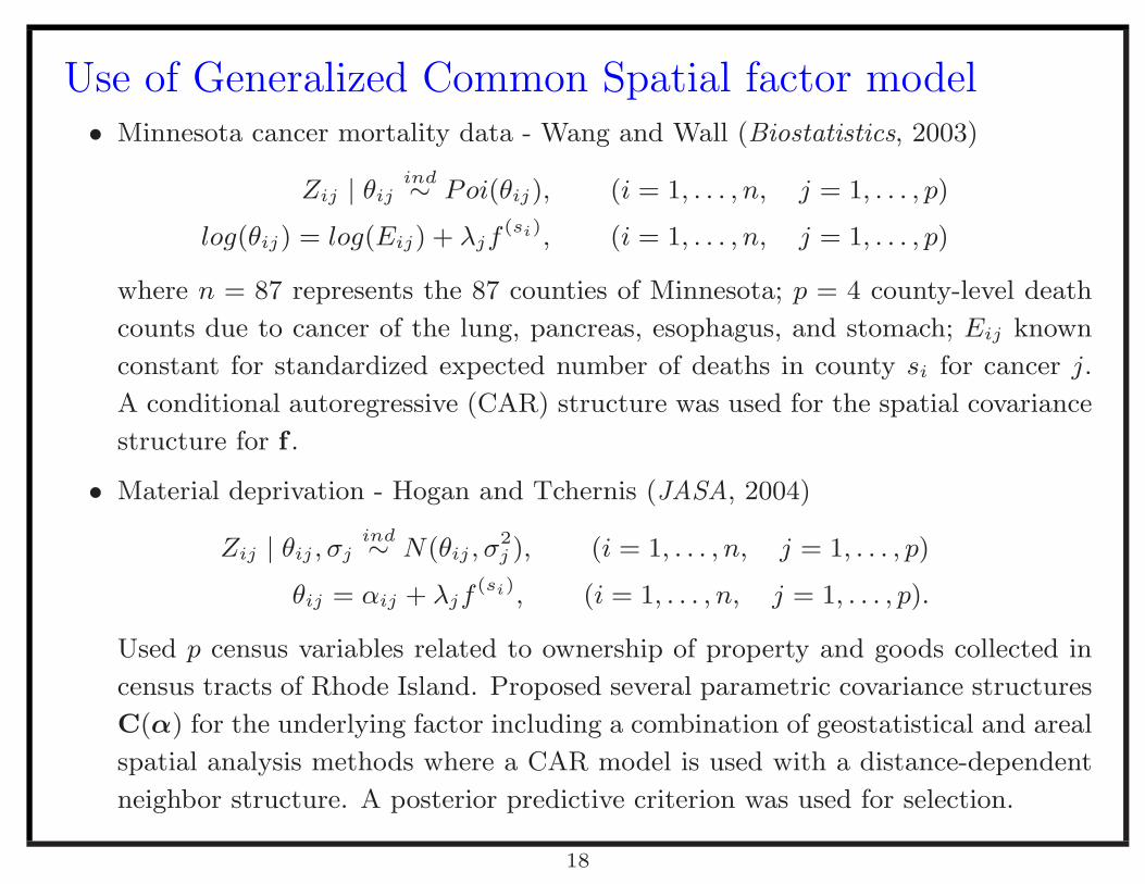
Use of Generalized Common Spatial factor model• Minnesota cancer mortality data - Wang and Wall (Biostatistics, 2003)
Zij | θijind∼ Poi(θij), (i = 1, . . . , n, j = 1, . . . , p)
log(θij) = log(Eij) + λjf(si), (i = 1, . . . , n, j = 1, . . . , p)
where n = 87 represents the 87 counties of Minnesota; p = 4 county-level death
counts due to cancer of the lung, pancreas, esophagus, and stomach; Eij known
constant for standardized expected number of deaths in county si for cancer j.
A conditional autoregressive (CAR) structure was used for the spatial covariance
structure for f .
• Material deprivation - Hogan and Tchernis (JASA, 2004)
Zij | θij , σjind∼ N(θij , σ
2j ), (i = 1, . . . , n, j = 1, . . . , p)
θij = αij + λjf(si), (i = 1, . . . , n, j = 1, . . . , p).
Used p census variables related to ownership of property and goods collected in
census tracts of Rhode Island. Proposed several parametric covariance structures
C(α) for the underlying factor including a combination of geostatistical and areal
spatial analysis methods where a CAR model is used with a distance-dependent
neighbor structure. A posterior predictive criterion was used for selection.
18
Generalized spatial structural equation model (GSSEM):motivation
• Structural equation models (SEM) offer a unified method by combining
factor analysis and regression analysis.
• A SEM incorporates:
– A measurement model - relating observed data to latent variables.
– A structural model - relating latent variables to other latent variables.
• The motivation of GSSEM is to extend the SEM methods to spatial data.
19
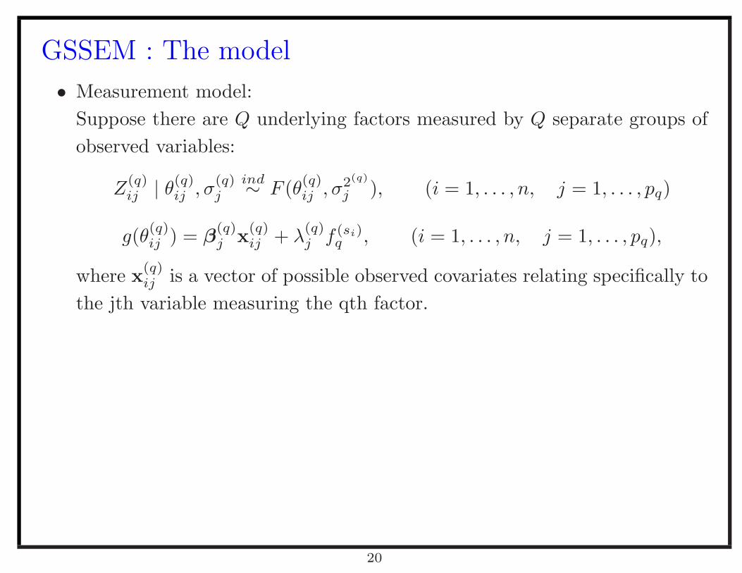
GSSEM : The model
• Measurement model:
Suppose there are Q underlying factors measured by Q separate groups of
observed variables:
Z(q)ij | θ
(q)ij , σ
(q)j
ind∼ F (θ
(q)ij , σ
2(q)
j ), (i = 1, . . . , n, j = 1, . . . , pq)
g(θ(q)ij ) = β
(q)j x
(q)ij + λ
(q)j f (si)
q , (i = 1, . . . , n, j = 1, . . . , pq),
where x(q)ij is a vector of possible observed covariates relating specifically to
the jth variable measuring the qth factor.
20
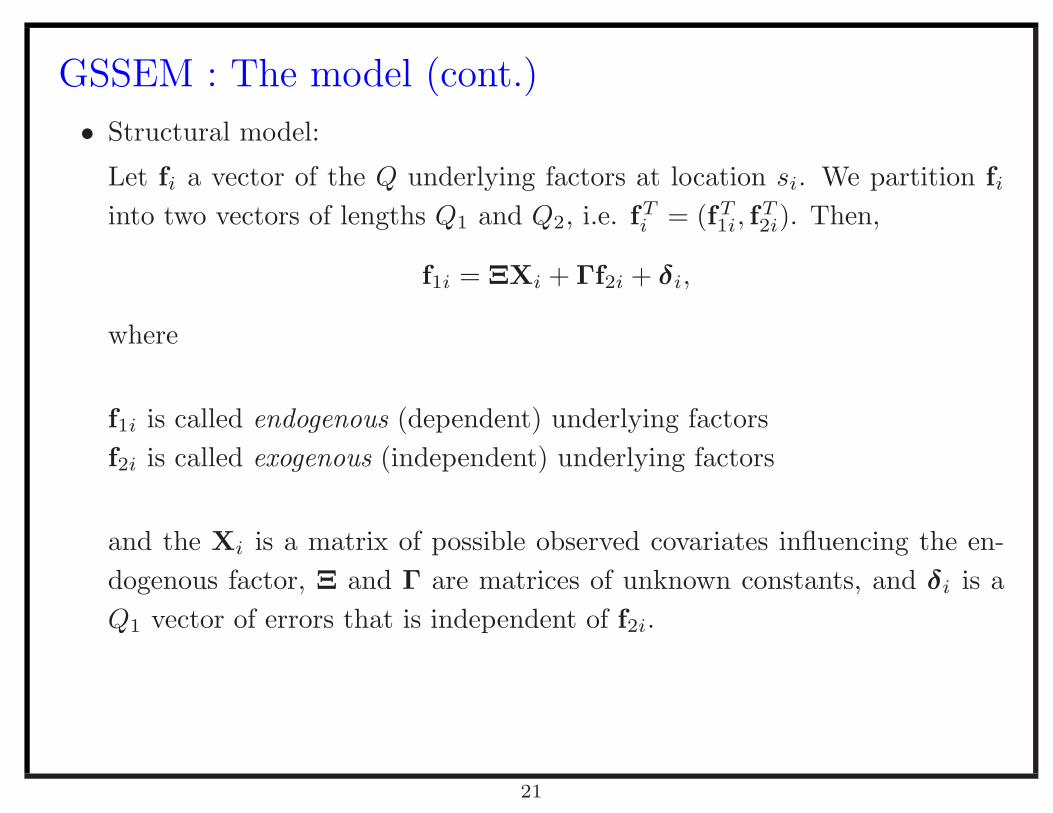
GSSEM : The model (cont.)
• Structural model:
Let fi a vector of the Q underlying factors at location si. We partition fi
into two vectors of lengths Q1 and Q2, i.e. fTi = (fT
1i, fT2i). Then,
f1i = ΞXi + Γf2i + δi,
where
f1i is called endogenous (dependent) underlying factors
f2i is called exogenous (independent) underlying factors
and the Xi is a matrix of possible observed covariates influencing the en-
dogenous factor, Ξ and Γ are matrices of unknown constants, and δi is a
Q1 vector of errors that is independent of f2i.
21
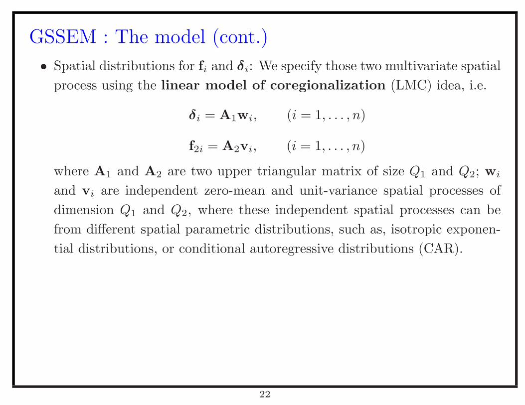
GSSEM : The model (cont.)
• Spatial distributions for fi and δi: We specify those two multivariate spatial
process using the linear model of coregionalization (LMC) idea, i.e.
δi = A1wi, (i = 1, . . . , n)
f2i = A2vi, (i = 1, . . . , n)
where A1 and A2 are two upper triangular matrix of size Q1 and Q2; wi
and vi are independent zero-mean and unit-variance spatial processes of
dimension Q1 and Q2, where these independent spatial processes can be
from different spatial parametric distributions, such as, isotropic exponen-
tial distributions, or conditional autoregressive distributions (CAR).
22
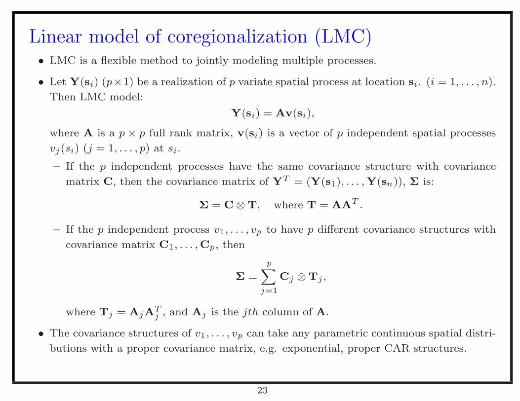
Linear model of coregionalization (LMC)• LMC is a flexible method to jointly modeling multiple processes.
• Let Y(si) (p×1) be a realization of p variate spatial process at location si. (i = 1, . . . , n).
Then LMC model:
Y(si) = Av(si),
where A is a p × p full rank matrix, v(si) is a vector of p independent spatial processes
vj(si) (j = 1, . . . , p) at si.
– If the p independent processes have the same covariance structure with covariance
matrix C, then the covariance matrix of YT = (Y(s1), . . . ,Y(sn)), Σ is:
Σ = C ⊗ T, where T = AAT .
– If the p independent process v1, . . . , vp to have p different covariance structures with
covariance matrix C1, . . . ,Cp, then
Σ =
p∑
j=1
Cj ⊗ Tj ,
where Tj = AjATj , and Aj is the jth column of A.
• The covariance structures of v1, . . . , vp can take any parametric continuous spatial distri-
butions with a proper covariance matrix, e.g. exponential, proper CAR structures.
23
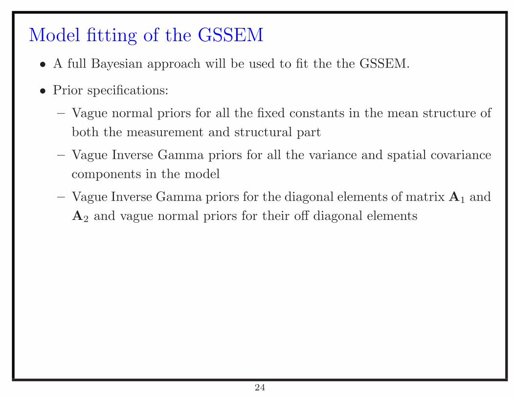
Model fitting of the GSSEM
• A full Bayesian approach will be used to fit the the GSSEM.
• Prior specifications:
– Vague normal priors for all the fixed constants in the mean structure of
both the measurement and structural part
– Vague Inverse Gamma priors for all the variance and spatial covariance
components in the model
– Vague Inverse Gamma priors for the diagonal elements of matrix A1 and
A2 and vague normal priors for their off diagonal elements
24
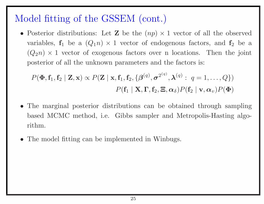
Model fitting of the GSSEM (cont.)
• Posterior distributions: Let Z be the (np) × 1 vector of all the observed
variables, f1 be a (Q1n) × 1 vector of endogenous factors, and f2 be a
(Q2n) × 1 vector of exogenous factors over n locations. Then the joint
posterior of all the unknown parameters and the factors is:
P (Φ, f1, f2 | Z,x) ∝ P (Z | x, f1, f2, {β(q),σ2(q)
,λ(q) : q = 1, . . . , Q})
P (f1 | X,Γ, f2,Ξ,αδ)P (f2 | v,αv)P (Φ)
• The marginal posterior distributions can be obtained through sampling
based MCMC method, i.e. Gibbs sampler and Metropolis-Hasting algo-
rithm.
• The model fitting can be implemented in Winbugs.
25
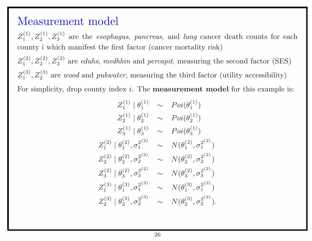
Measurement modelZ
(1)1 , Z
(1)2 , Z
(1)3 are the esophagus, pancreas, and lung cancer death counts for each
county i which manifest the first factor (cancer mortality risk)
Z(2)1 , Z
(2)2 , Z
(2)3 are eduhs, medhhin and percapit, measuring the second factor (SES)
Z(3)1 , Z
(3)2 are wood and pubwater, measuring the third factor (utility accessibility)
For simplicity, drop county index i. The measurement model for this example is:
Z(1)1 | θ
(1)1 ∼ Poi(θ
(1)1 )
Z(1)2 | θ
(1)2 ∼ Poi(θ
(1)2 )
Z(1)3 | θ
(1)3 ∼ Poi(θ
(1)3 )
Z(2)1 | θ
(2)1 , σ
2(2)
1 ∼ N(θ(2)1 , σ
2(2)
1 )
Z(2)2 | θ
(2)2 , σ
2(2)
2 ∼ N(θ(2)2 , σ
2(2)
2 )
Z(2)3 | θ
(2)3 , σ
2(2)
3 ∼ N(θ(2)3 , σ
2(2)
3 )
Z(3)1 | θ
(3)1 , σ
2(3)
1 ∼ N(θ(3)1 , σ
2(3)
1 )
Z(3)2 | θ
(3)2 , σ
2(3)
2 ∼ N(θ(3)2 , σ
2(3)
2 ).
26
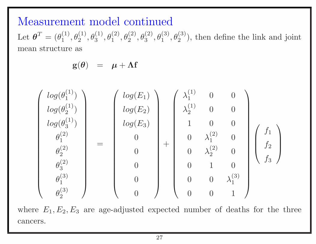
Measurement model continuedLet θT = (θ
(1)1 , θ
(1)2 , θ
(1)3 , θ
(2)1 , θ
(2)2 , θ
(2)3 , θ
(3)1 , θ
(3)2 ), then define the link and joint
mean structure as
g(θ) = µ + Λf
log(θ(1)1 )
log(θ(1)2 )
log(θ(1)3 )
θ(2)1
θ(2)2
θ(2)3
θ(3)1
θ(3)2
=
log(E1)
log(E2)
log(E3)
0
0
0
0
0
+
λ(1)1 0 0
λ(1)2 0 0
1 0 0
0 λ(2)1 0
0 λ(2)2 0
0 1 0
0 0 λ(3)1
0 0 1
f1
f2
f3
where E1, E2, E3 are age-adjusted expected number of deaths for the three
cancers.
27
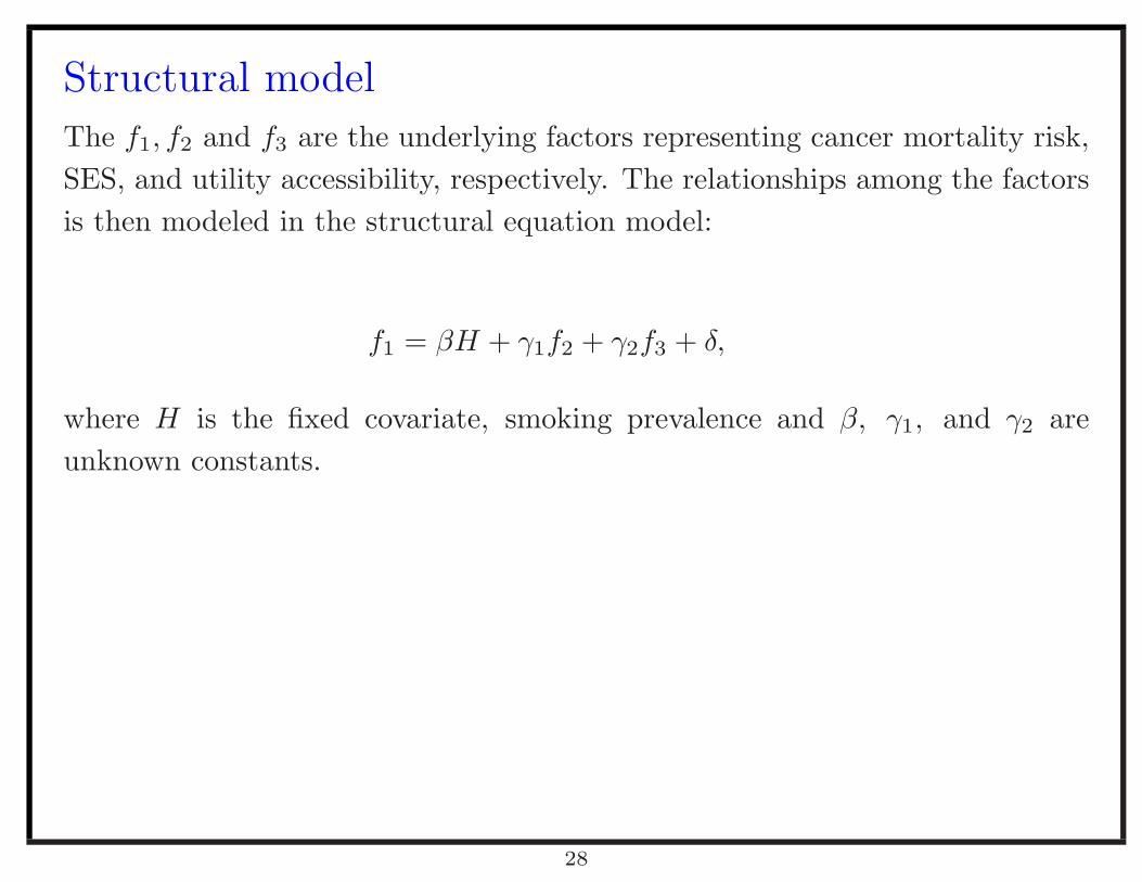
Structural model
The f1, f2 and f3 are the underlying factors representing cancer mortality risk,
SES, and utility accessibility, respectively. The relationships among the factors
is then modeled in the structural equation model:
f1 = βH + γ1f2 + γ2f3 + δ,
where H is the fixed covariate, smoking prevalence and β, γ1, and γ2 are
unknown constants.
28
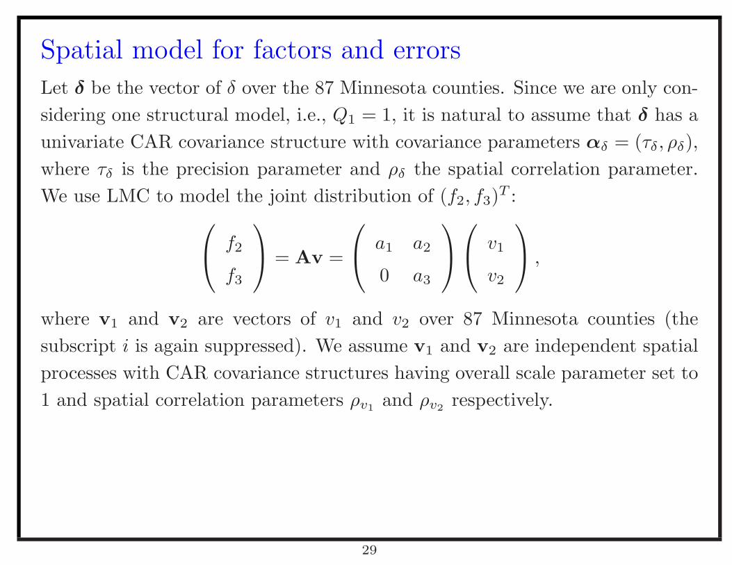
Spatial model for factors and errors
Let δ be the vector of δ over the 87 Minnesota counties. Since we are only con-
sidering one structural model, i.e., Q1 = 1, it is natural to assume that δ has a
univariate CAR covariance structure with covariance parameters αδ = (τδ, ρδ),
where τδ is the precision parameter and ρδ the spatial correlation parameter.
We use LMC to model the joint distribution of (f2, f3)T :
f2
f3
= Av =
a1 a2
0 a3
v1
v2
,
where v1 and v2 are vectors of v1 and v2 over 87 Minnesota counties (the
subscript i is again suppressed). We assume v1 and v2 are independent spatial
processes with CAR covariance structures having overall scale parameter set to
1 and spatial correlation parameters ρv1and ρv2
respectively.
29
Estimation
• Implemented in Winbugs software to obtain posterior summaries for the
parameters.
• Ran three Markov Chains simultaneously started from different initial points.
• Monitor plots show that the three chains mixed well within 5000 iterations.
• The lag 1 posterior sample autocorrelations of most parameters (e.g., λs, β,
γs, and ρs) are lower than 0.5, and the Gelman-Rubin diagnostic plot of the
chains are mostly within the 0.8 to 1.2 band, which suggests satisfactory
convergence.
• We also calculate the posterior summaries at different points of the Markov
Chain, and the result summaries are almost identical after burn-in period.
No thinning on the draws seems necessary.
30
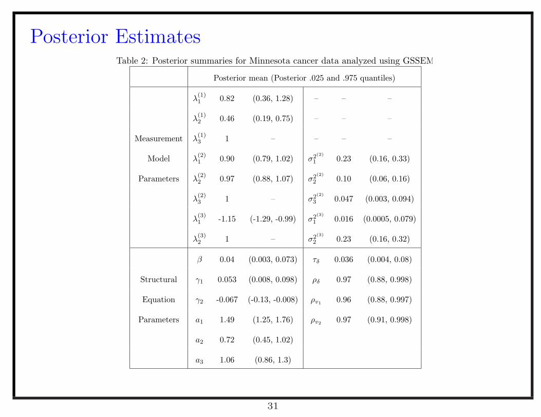
Posterior EstimatesTable 2: Posterior summaries for Minnesota cancer data analyzed using GSSEM
Posterior mean (Posterior .025 and .975 quantiles)
λ(1)1 0.82 (0.36, 1.28) – – –
λ(1)2 0.46 (0.19, 0.75) – – –
Measurement λ(1)3 1 – – – –
Model λ(2)1 0.90 (0.79, 1.02) σ2(2)
1 0.23 (0.16, 0.33)
Parameters λ(2)2 0.97 (0.88, 1.07) σ2(2)
2 0.10 (0.06, 0.16)
λ(2)3 1 – σ2(2)
3 0.047 (0.003, 0.094)
λ(3)1 -1.15 (-1.29, -0.99) σ2(3)
1 0.016 (0.0005, 0.079)
λ(3)2 1 – σ2(3)
2 0.23 (0.16, 0.32)
β 0.04 (0.003, 0.073) τδ 0.036 (0.004, 0.08)
Structural γ1 0.053 (0.008, 0.098) ρδ 0.97 (0.88, 0.998)
Equation γ2 -0.067 (-0.13, -0.008) ρv10.96 (0.88, 0.997)
Parameters a1 1.49 (1.25, 1.76) ρv20.97 (0.91, 0.998)
a2 0.72 (0.45, 1.02)
a3 1.06 (0.86, 1.3)
31
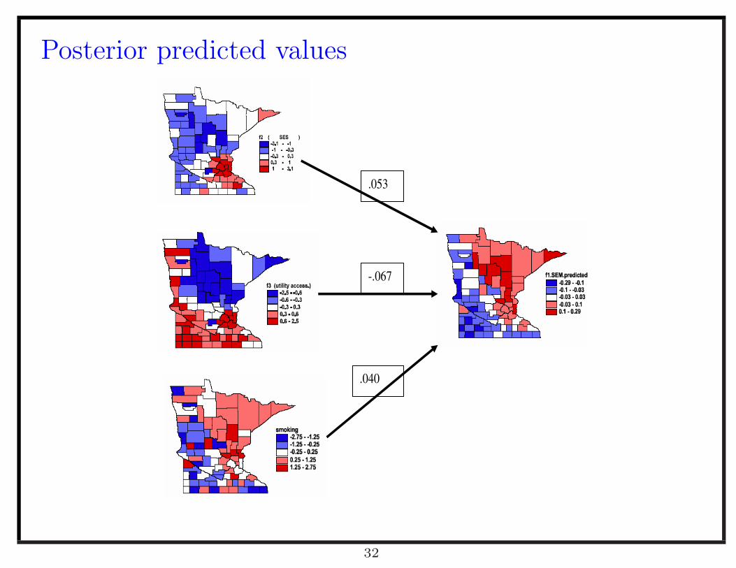
Posterior predicted values
.053
-.067
.040
32
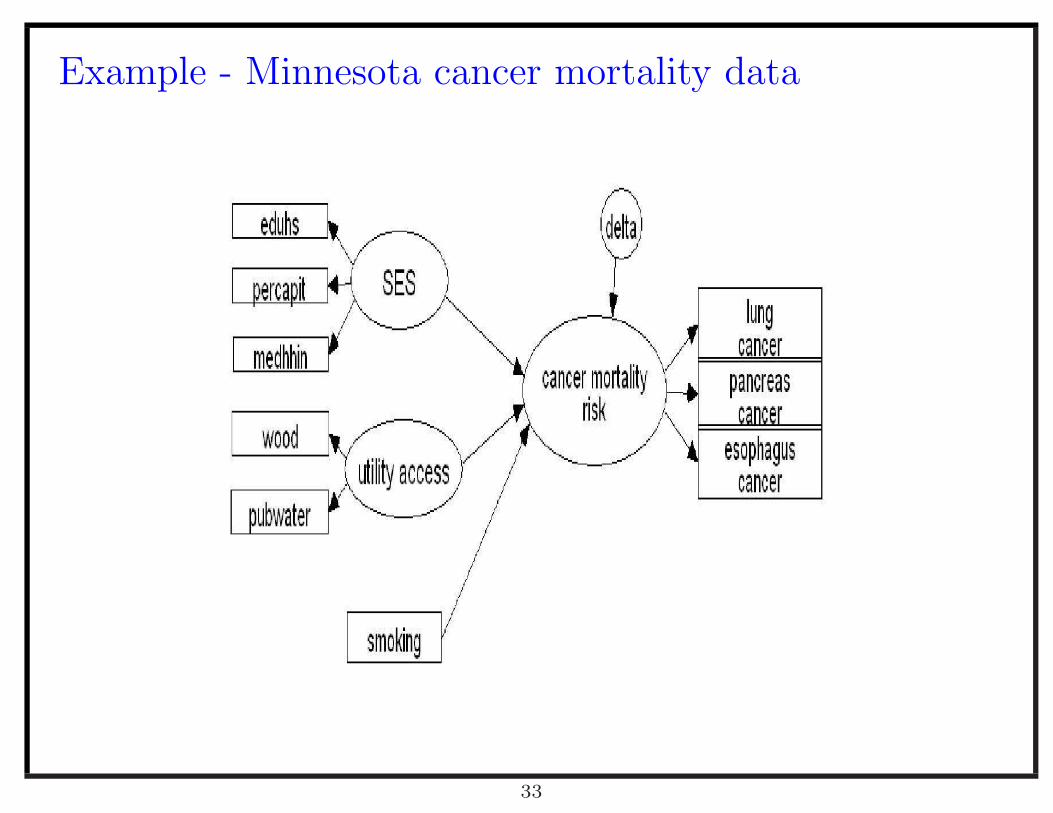
Example - Minnesota cancer mortality data
33
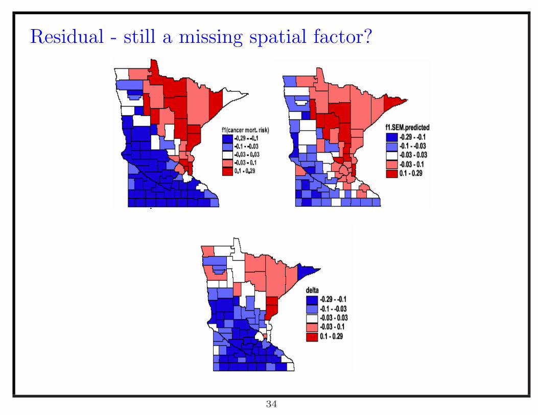
Residual - still a missing spatial factor?
34
Discussion
• Generalized spatial structural equation modeling provides a method for
researchers to perform ecological regressions incorporating many correlated
variables in a meaningful way while taking account of spatial structure.
• Model could be extended to incorporate both space and time.
• Model could be extended to allow underlying cluster process for underlying
factors (factors could be categorical).
35
. .
C’est tout
36