Chaos, Solitons and Fractals 23 (2005) 1605–1611

www.elsevier.com/locate/chaos

Generalized synchronization induced by noise andparameter mismatching in Hindmarsh–Rose neurons

Ying Wu a,*, Jianxue Xu a, Daihai He b, David J.D. Earn b

a Institute of Nonlinear Dynamics, School of Architectural Engineering and Mechanics, Xi�an Jiaotong University,

Xi�an Shaanxi 710049, Chinab Department of Mathematics and Statistics, McMaster University, Hamilton Canada L8S 4K1

Accepted 15 June 2004

Abstract

Synchronization of two simple neuron models has been investigated in many studies. Thresholds for complete syn-

chronization (CS) and phase synchronization (PS) have been obtained for coupling by diffusion or noise. In addition,

it has been shown that it is possible for directional diffusion to induce generalized synchronization (GS) in a pair of

neuron models even if the neurons are not identical (and differ in a single parameter). We study a system of two uncou-

pled, nonidentical Hindmarsh–Rose (HR) neurons and show that GS can be achieved by a combination of noise and

changing the value of a second parameter in one of the neurons (the second parameter mismatch cancels the first). The

significance of this approach will be the greatest in situations where the parameter that is originally mismatched cannot

be controlled, but a suitable controllable parameter can be identified.

� 2004 Elsevier Ltd. All rights reserved.

1. Introduction

The potential for identical and sufficiently strongly coupled chaotic systems to synchronize is well known [1,2]. This

phenomenon is important theoretically because it is unobvious that systems with sensitive dependence on initial con-

ditions should be able to synchronize. It is also of possible practical importance in fields such as communications

[3], neuroscience [4] and ecology [5,6].

Three types of synchronization are frequently discussed. The strongest form, complete synchronization (CS) means

that the distinct oscillators asymptotically approach the same orbit. Phase synchronization (PS) refers to exact entrain-

ment of the phases of distinct oscillators, but with no restriction on their amplitudes. Generalized synchronization (GS),

which is normally defined only for systems involving ‘‘driving’’ and ‘‘receiving’’ components, refers to a situation in

which the states of the ‘‘driver’’ and the ‘‘receiver’’ on their respective attractors are related by a continuous mapping

from the driver state to the receiver state [7]. CS is, of course, the special case of GS in which the relevant mapping is the

identity transformation. PS does not imply GS because the oscillator amplitudes can be uncorrelated in the case of PS.

GS does not imply PS because it is not necessarily possible even to define the phase of a chaotic oscillator.

0960-0779/$ - see front matter � 2004 Elsevier Ltd. All rights reserved.

doi:10.1016/j.chaos.2004.06.077

* Corresponding author.

1606 Y. Wu et al. / Chaos, Solitons and Fractals 23 (2005) 1605–1611

Each of these types of synchronization has been shown to occur in theoretical models [8] and in experiments [9], as a

result of deterministic coupling between the oscillators. In addition, CS and PS have been shown to occur in uncoupled

systems that are subject to common noise [10–13]. The model we focus on in this paper provides an example of noise-

induced GS in a system where CS is impossible.

Synchronization in Hindmarsh–Rose (HR) neurons [14,15] has been studied widely [16,17,20] because of its

physiological significance. Compared with many other mathematical models of excitable cells, the HR model is

simpler. It consists of only three differential equations, which have relatively mild nonlinearities (quadratic and

cubic terms). Like the Lorenz and Rossler equations, which are equally simple, the HR model can generate cha-

otic dynamics. However, the nature of the HR chaotic attractor is quite different from that of the Lorenz and

Rossler attractors; it exhibits multi-time-scaled burst-rest behavior, a phenomenon that has great importance in

neuroscience. Previous work has investigated variations in the periods of oscillation of two coupled identical

HR neurons [16], noise-induced CS between two uncoupled identical HR neurons [17], noise-induced CS and

PS in identical and non-identical chaotic Hodgkin–Huxley neurons [18,19] and PS in two coupled nonidentical

HR neurons [20]. The first experimental observation of noise-induced PS in a pair of uncoupled sensory neurons

was reported in Ref. [21].

The HR neuron model is characterized by three dependent variables: the membrane potential x, the recovery var-

iable y, and a slow adaptation current z. Because the HR model has multiple time-scale dynamics [22], the burst of ac-

tion potentials often consists of a group of spikes. It is believed that neuronal information is mainly transmitted using a

code based on the time intervals between neuronal firings rather than the spiking amplitude [23]. Thus, an important

concept in sensory information is the interspike interval (ISI), which is obtained from the successive spiking peaks of the

membrane potential x.

In this paper, we study Gaussian white noise-induced GS between two uncoupled nonidentical HR neuron models.

The mapping that defines the GS is very simple: two of the variables completely synchronize while the third approaches

a constant difference associated with parameter mismatching.

2. Noise induced GS in nonidentical neurons

We consider a pair of Hindmarsh–Rose (HR) [14] neuron models (i = 1, 2) as follows:

_xi ¼ yi � aix3i þ bix2i � zi þ I i þ DxnðtÞ_yi ¼ ci � dix2i � yi_zi ¼ r½Sðxi � viÞ � zi�

ð1Þ

With the standard parameter values ai = 1.0, bi = 3.0, di = 5.0, S = 4.0, r = 0.006, vi = �1.56, ci = 1.0 and Ii = 3.0, the

two neuron models are identical and chaotic. The noise term n(t) is Gaussian with hn(t)n(t � s)i = d(s). The parameter I

represents the applied current while v is the threshold above which x displays spike behavior. The other parameters do

not have obvious biological meanings; they were introduced in Ref. [14] in order to mimic the dynamical behavior of the

Hodgkin–Huxley neuron model [18] using a simpler mathematical model.

In Ref. [17] it was shown that common additive Gaussian white noise can induce CS between two uncoupled iden-

tical HR neuron models with critical noise intensity Dxc ¼ 2:4 on _x, or Dy

c ¼ 6 on _y. We now consider the implications of

parameter mismatching for synchronization of this two-neuron model.

As a first example, we consider a small mismatching of the parameter c between the two neurons (c1 = 1.05,

c2 = 0.95). With common additive Gaussian white noise acting on _x, CS cannot be achieved when the noise intensity

Dx < 5.0. This is clear in Fig. 1a, which shows (solid line) the ‘‘synchronization error’’ for x, i.e., time-averaged absolute

difference hjx1 � x2ji, as a function of noise intensity Dx. The figure also shows the synchronization errors for y (dot-

dash line) and z (dotted line). A transition occurs near Dx = 2.4, which is the critical point for CS between identical

neurons [17]. Above this intensity, synchronization errors are greatly reduced (note that the errors shown are time-aver-

aged and, in fact, the two systems intermittently synchronize). As a function of Dx, the synchronization error in x de-

creases much more rapidly than the synchronization error in y and z, and beyond the critical point Dx = 2.4, x displays

the smallest synchronization error of the three variables. Since x represents the variable that is usually observed in

experiments, above the critical noise intensity we would expect to observe nearly complete synchronization in practice.

A sample time series, x(t) (for Dx = 2.5), is shown in Fig. 2.

As a second example, we consider the effect of slightly different applied currents on the two neurons (I1 = 3.05,

I2 = 2.95). Again, common additive Gaussian white noise acts on _x; the results, shown in Fig. 1b, resemble those in

Fig. 1a (in panel b, hjy1 � y2ji has a slightly steeper slope near, and a lower value after, the critical noise intensity).

0 1 2 3 4 50

1

2

3

4

DxS

ync

Err

or(a)

0 1 2 3 4 50

1

2

3

4

Dx

Syn

c E

rror

(b)

0 1 2 3 4 50

1

2

3

4

Dx

Syn

c E

rror

(c)

3 4 50

0.1

0.2

3 4 50

0.1

0.2

3 4 50

0.1

0.2

0 1 2 3 4 50

1

2

3

4

Dx

Syn

c E

rror

(d)

Fig. 1. Synchronization errors of two uncoupled HR neurons with mismatched parameters versus additive noise intensity Dx. (a)

Single mismatching c1 = 1.05, c2 � 0.95; (b) single mismatching I1 = 3.05, I2 = 2.95; (c) I1 = 3.05, I2 = 2.95, c1 = 0.95, c2 = 1.05; (d)

a1 = 1.05, a2 = 0.95, I1 = I2 = 3 and c1 = c2 = 1. In all panels, average synchronization error hjx1 � x2ji is denoted by the solid line,

hjy1 � y2ji by the dot-dash line, and hjz1 � z2ji by the dotted line.

0 200 400 600 800 1000–4

–2

0

2

4

Time

X1

(a)

0 200 400 600 800 1000–4

–2

0

2

4

Time

X1–

X2

(b)

Fig. 2. Time evolution of the model with two HR neurons, subject to common additive noise with intensity Dx = 2.5 and mismatched

parameters c1 = 0.95 and c2 = 1.05. (a) A sample time series of the membrane potential x of one of the two neurons. (b) The difference

in membrane potentials of the two neurons.

Y. Wu et al. / Chaos, Solitons and Fractals 23 (2005) 1605–1611 1607

Surprisingly, if we impose simultaneously the above parameter mismatchings in c and I (c1 = 1.05, c2 = 0.95,

I1 = 2.95, I2 = 3.05), GS is achieved above the critical point Dx = 2.4; see Fig. 1c. In this case, the synchronization errors

in x and z are both exactly zero, while hjy1 � y2ji = 0.1. It is worth noting here that the synchronization error in y is

equal to the parameter mismatchings (jc1 � c2j = 0.1 and jI1 � I2j = 0.1).

As a further example, we considered mismatch of the coefficient of the cubic term (a1 = 1.05, a2 = 0.95). The syn-

chronization error curves are shown in Fig. 1d. The reduction in the average synchronization error in y (dot-dash curve)

near the critical noise intensity is much less dramatic than for the parameter mismatchings considered in panels a–c,

while the average synchronization error in z displays a slight increase rather than a decrease. The apparent inability

to achieve GS in this case may be related to the fact that a appears in a nonlinear term in the equations, whereas I

0 2 4–0.2

–0.1

0

0.1

cLE

1,2

(a)

0 2 4 6–0.2

–0.1

0

0.1

I

LE1,

2

(b)

70 75 800

0.1

0.2(c)

70 75 800

0.1

0.2

Freq

uenc

y H

isto

gram

(d)

70 75 800

0.1

0.2

ISI (seconds)

(e)

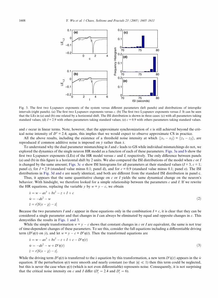
Fig. 3. The first two Lyapunov exponents of the system versus different parameters (left panels) and distributions of interspike

intervals (right panels). (a) The first two Lyapunov exponents versus c. (b) The first two Lyapunov exponents versus I. It can be seen

that the LEs in (a) and (b) one related by a horizontal shift. The ISI distribution is shown in three cases: (c) with all parameters taking

standard values; (d) I = 2.9 with others parameters taking standard values; (e) c = 0.9 with others parameters taking standard values.

1608 Y. Wu et al. / Chaos, Solitons and Fractals 23 (2005) 1605–1611

and c occur in linear terms. Note, however, that the approximate synchronization of x is still achieved beyond the crit-

ical noise intensity of Dx = 2.4; again, this implies that we would expect to observe approximate CS in practice.

All the above results, including the existence of a threshold noise intensity at which hjx1 � x2ji = hjz1 � z2ji, arereproduced if common additive noise is imposed on _y rather than _x.

To understand why the dual parameter mismatching in I and c leads to GS while individual mismatchings do not, we

explored the dynamics of the single neuron HR model as a function of each of these parameters. Figs. 3a and b show the

first two Lyapunov exponents (LEs) of the HR model versus c and I, respectively. The only difference between panels

(a) and (b) in this figure is a horizontal shift by 2 units. We also compared the ISI distributions of the model when c or I

is changed by the same amount; Figs. 3c–e show ISI histograms for all parameters at their standard values (I = 3, c = 1;

panel c), for I = 2.9 (standard value minus 0.1; panel d), and for c = 0.9 (standard value minus 0.1; panel e). The ISI

distributions in Fig. 3d and e are nearly identical, and both are different from the standard ISI distribution in panel c.

Thus, it appears that the same quantitative change on c or I yields the same dynamical change on the neuron�sbehavior. With hindsight, we therefore looked for a simple relationship between the parameters c and I. If we rewrite

the HR equations, replacing the variable y by w = y � c, we obtain

_x ¼ w� ax3 þ bx2 � zþ I þ c

_w ¼ �dx2 � w

_z ¼ r½Sðx� vÞ � z�ð2Þ

Because the two parameters I and c appear in these equations only in the combination I + c, it is clear that they can be

considered a single parameter and that changes in I can always be eliminated by equal and opposite changes in c. This

demystifies the results in Figs. 1 and 3.

While the simple transformation w = y � c shows that constant changes in c or I are equivalent, the same is not true

of time-dependent changes of these parameters. To see this, consider the full equations including a differentiable driving

term (Dyg(t) on _y), and let w = y � c + Dyg(t). Then the transformed equations are

_x ¼ w� ax3 þ bx2 � zþ I þ c� DygðtÞ_w ¼ �dx2 � wþ Dy _gðtÞ_z ¼ r½Sðx� vÞ � z�:

ð3Þ

While the driving term Dyg(t) is transferred to the _x equation by this transformation, a new term Dy _gðtÞ appears in the _wequation. If the perturbation g(t) were smooth and nearly constant (so that j _gj � 1) then this term could be neglected,

but this is never the case when g(t) (which is not even differentiable) represents noise. Consequently, it is not surprising

that the critical noise intensity on c and I differ (Dxc ¼ 2:4 and Dy

c ¼ 6).

0 0.5 10

0.5

1

1.5

2

2.5

Syn

c E

rror

coupling(a)0 0.5 1

0

0.5

1

1.5

2

2.5

Syn

c E

rror

coupling(b)

–0.04 –0.02 0 0.02 0.040

0.05

0.1

0.15

0.2

∆ I

Syn

c E

rror

(c)

0.6 0.8 1–0.1

0

0.1

0.6 0.8 10

0.05

0.1

–0.1 –0.05 00

0.05

0.1

0.15

0.2

(d)

Syn

c E

rror

∆ b

Fig. 4. Synchronization errors versus diffusive coupling strength e (top panels) and versus parameter mismatching (bottom panels). As

in Fig. 1, we show synchronization errors between x1 and x2 (solid line), y1 and y2 (dot-dash line) and z1 and z2 (dotted-solid line). In

panels (a–c), the parameter v is mismatched (v1 = 1.56, v2 = 1.57) while in panel (d) it is d that is mismatched (d1 = 5.05, d2 = 4.95). In

panels (c) and (d), the noise intensity is Dx = 2.5. Panel (c) reveals a critical mismatching of applied current I (D I = 0.02), i.e.,

(I1 = 2.98, I2 = 3.02) at which the synchronization error is minimized.

Y. Wu et al. / Chaos, Solitons and Fractals 23 (2005) 1605–1611 1609

For other models, or for other parameter combinations in the HR model, if similar dual parameter mismatched GS

is observed, it will not necessarily be possible to derive simple parameter relationships analytically to explain the

dynamics. However, the LE spectrum and unstable period distribution can always be computed, as we did in Fig. 3,

and this may signal the existence of such a parameter relationship.

We investigated a variety of other parameter mismatchings for two coupled HR neurons, and in each case we at-

tempted to find an additional mismatching that ‘‘mends’’ the pair of neurons so that they can oscillate synchronously

(by which we mean GS, as for the case of I and c above). We found that ‘‘mending’’ of parameter mismatching can be

achieved in the presence of diffusive coupling, not only when common noise is applied to the system.

It is useful to recall that for two identical HR neurons coupled diffusively without noise, CS occurs for sufficiently

high coupling strength e (Fig. 4a); the form of the coupling used here is to add a term e(x3 � i � xi) to _xi. Moreover,

approximate CS occurs for sufficiently high coupling strength, even if the parameter v is mismatched between the

two neurons [20] (Fig. 4b). In fact, the approximate CS observed in this case is perhaps more accurately described

as approximate GS, since there is a large difference in the magnitudes of the average synchronization errors of x, y

and z (inset panel of Fig. 4b), similar to what is seen in Fig. 1b and c. We remark that, in the spirit of our above dis-

cussion, it is possible to view this approximate GS as induced by ‘‘mending’’ of parameter mismatching, i.e., the cou-

pling strength acts as a parameter that can mend the mismatching of v, leading to approximate GS. Note that, just as c

can be transferred to I via the variable change w = y � c, v can also be transferred to I by the variable change w = z + Sv(i.e., the parameter mismatch in the equation for _z is equivalent to a parameter mismatch in the equation for _x where

coupling occurs).

Returning to the uncoupled situation, if we begin with two uncoupled HR neurons with mismatched v(v1 = �1.56, v2 = � 1.57) and noise intensity Dx = 2.5, then GS can be achieved by introducing parameter mismatching

of I (Fig. 4c). Exact GS is achieved only for the mismatch jI1 � I2j = 0.04, in which case synchronization errors in x and

y are zero while z maintains a constant difference jz1 � z2j = 0.04 between the two neurons. Note that using the variable

change w = z + Sv, it can easily be seen that a given mismatch in v can be mended by a mismatch of magnitude

S(v1 � v2) in I.

Finally, we considered parameter mismatching of d (d1 = 5.05, d2 = 4.95), again with noise intensity Dx = 2.5. No

mismatching of parameter b can mend the system and yield exact GS (Fig. 4d). However, the synchronization errors

can be reduced to half their original values if we impose a particular mismatching of b.

1610 Y. Wu et al. / Chaos, Solitons and Fractals 23 (2005) 1605–1611

3. An electronic model neuron and a map model

We briefly mention two other models for which exact mending of parameter mismatching can be achieved by an

additional imposed parameter mismatching.

The first example is an electronic model neuron (EN), an analog circuit implementation of a four-dimensional neu-

ron model. This model, which is an accurate representation of a real experimental apparatus [24–26], has the form

_x ¼ y þ 3x2 � x3 � zþ Jdc þ JðtÞ_y ¼ 1� 5x2 � y � gw

_z ¼ l½�zþ 4ðxþ hÞ�_w ¼ m½�wþ 3ðy þ lÞ�

ð4Þ

where g, h, l, l, m and Jdc are parameters and J(t) is an external current. Note that the nonlinear terms in this model

involve only the variable x (as in the HR model). As a means of investigating information transfer, in Ref. [25], param-

eter mismatching on Jdc was studied both theoretically and experimentally for two otherwise identical neurons. In fact,

parameter mismatchings on h and l can be eliminated by controlling Jdc in the model, and this control should also be

possible in experiments.

The second example is a minimal formal map model of excitable and bursting cells [27], which can be written

xðt þ 1Þ ¼ tanhxðtÞ � KyðtÞ þ zðtÞ þ IðtÞ

T

� �

yðt þ 1Þ ¼ xðtÞzðt þ 1Þ ¼ ð1� dÞzðtÞ � kðxðtÞ � xRÞ

ð5Þ

where K, T, d, k and xR are parameters and I(t) is an external current. Parameter mismatching of xR can be mended by

introducing a constant difference in the applied current I(t), yielding identical dynamics for the two neurons except for a

constant difference in the variable z, i.e., mending the parameter mismatching with a controllable parameter yields GS.

4. Conclusions

We have shown that two nonidentically parameterized dynamical systems that are coupled either diffusively or by

noise can sometimes be ‘‘mended’’ (i.e., manipulated so as to display generalized synchronization) by imposing an addi-

tional mismatching of another parameter. This possibility will be most important in cases where parameters whose val-

ues differ between the two systems cannot be changed in the real system that is being modelled, but where imposed

changes in controllable parameters can mend the dynamics.

We have given examples, focussing on Hindmarsh–Rose neurons, where a simple variable transformation explains

why certain parameters can be manipulated to mend mismatches of another parameter. More generally, such explan-

atory transformations may not be possible to derive, but mending of parameter mismatching can still be investigated

numerically, as we did in Fig. 3.

In previous work [28,29], it has been shown that increasing parameter mismatching between driver and receiver oscil-

lators can dramatically decrease the critical coupling strength for generalized synchronization between two directionally

coupled Rossler oscillators (because the parameter mismatching effectively enhances the coupling between driver and

receiver. In contrast, the present paper provides an alternative mechanism for GS, based on multiple parameter mis-

matching (rather than increasing mismatching of a single parameter).

Acknowledgments

YW and JXX were supported by the National Natural Science Foundation of PR China (Grant No. 10172067) and

the Key Project of the National Natural Science Foundation of PR China. DJDE was supported by the Canadian Insti-

tutes of Health Research (CIHR), the Natural Sciences and Engineering Research Council of Canada (NSERC), the

Canada Foundation for Innovation (CFI), the Ontario Innovation Trust (OIT) and an Ontario Premier�s Research

Exellence Award.

Y. Wu et al. / Chaos, Solitons and Fractals 23 (2005) 1605–1611 1611

References

[1] Pecora LM, Carroll TL. Phys Rev Lett 1990;64:821.

[2] Pecora LM, Carroll TL. Phys Rev A 1991;44:2374.

[3] Cuomo KM, Oppenheim AV. Phys Rev Lett 1993;71:65.

[4] Rinzel J, Sherman A, Stokes CL. Channels, coupling, and synchronized rhythmic bursting activity. In: Edckman FH, editor.

Analysis and modeling of neural systems. Dordrecht: Kluwer Academic Publishers; 1989. p. 29.

[5] Earn DJD, Rohani P, Grenfell BT. Proc R Soc Lond B 1998;265:7.

[6] Earn DJD, Levin SA, Rohani P. Science 2000;290:1360.

[7] Rulkov NF, Afraimovich VS, Lewis CT, Chazottes J, Cordonet A. Phys Rev E 2001;64:016217.

[8] Boccaletti S, Kurths J, Osipov G, Valladares DL, Zhou CS. Phys Rep 2002;366:1.

[9] Choi M, Volodchenko KV, Rim S, Kye WH, Kim CM, Park YJ, Kim GU. Opt Lett 2003;28:1013.

[10] Pikovsky AS. Phys Lett A 1992;165:33.

[11] Mritan A, Banavar JR. Phys Rev Lett 1994;72:1451.

[12] Lai CH, Zhou CS. Europhys Lett 1998;43:376.

[13] Zhou CS, Kurths J. Phys Rev Lett 2002;88:230602.

[14] Hindmarsh JL, Rose RM. Nature (Lond) 1982;296:162.

[15] Hindmarsh JL, Rose RM. Proc R Soc London B 1984;221:87.

[16] Huerta R, Rabinovich MI. Phys Rev E 1997;55:R2108.

[17] He D, Shi P, Stone L. Phys Rev E 2003;67:027201.

[18] Hodgkin AL, Huxley AF. J Physiol (Lond) 1952;166:500.

[19] Zhou CS, Kurths J. Chaos 2003;13:401.

[20] Shuai JW, Durand DM. Phys Lett A 1999;264:289.

[21] Neiman AB, Russell DF. Phys Rev Lett 2002;88:138103.

[22] Rinzel J, Lee YS. J Math Biol 1987;25:653.

[23] Eccles JC. The understanding of the brain. New York: McGraw-Hill; 1973.

[24] Pinto RD, Varona P, Volkovskii AR, Szucs A, Abarabanel HDI, Rabinovich MI. Phys Rev E 2000;62:2644.

[25] Eguia MC, Rabinovich MI, Abarbanel HDI. Phys Rev E 2000;62:7111.

[26] Szucs A, Elson RC, Rabinovich MI, Abarbanel HDI, Selverston AI. J Neurophysiol 2001;85:1623.

[27] Kuva SM, Lima GF, Kinouchi O, Tragtenberg MHR, Roque AC. Neurocomputing 2001;38–40:255.

[28] Zheng Z, Hu G. Phys Rev E 2000;62:7882.

[29] He D, Stone L, Zheng ZG. Phys Rev E 2002;66:036208.