Embed Size (px)
Citation preview
Chapter 2Generalized Weibull Distributions
2.1 Introduction
Since 1970s, many extensions of the Weibull distribution have been proposed toenhance its capability to fit diverse lifetime data and Murthy et al. (2004) proposesa scheme to classify these distributions. Over the last 40 years papers dealing withvarious extensions of the Weibull distribution and their applications number wellover 4000.
A common factor among the generalized models considered in this chapter isthat the Weibull distribution is a special case of theirs. Either F(t) or h(t) of thesemodified models are related to the corresponding function of the Weibull distributionin some way. The means of these distributions usually do not have a simple expressionalthough their hazard rate functions h(t) are more capable to model diverse problemsthan the Weibull model does.
2.2 Methods of Constructions
Generalized Weibull distributions can be constructed in many ways. Members of thisfamily usually contain the standard Weibull model as a special case. The followingis a brief sketch of some of the common methods. A new generalized distributionmay be obtained by:
• adding a constant λ to the existing hazard rate h(t) of the Weibull distribution ora generalized Weibull model,
• transformations (linear, inverse or log) of the Weibull random variable,• transformations of the distribution F(t) or the survival function �F(t) of the Weibull
distrbution in such a way that the new function remains a distribution or survivalfunction,
• competing risk approach (minimum of two or more Weibull variables),
C.-D. Lai, Generalized Weibull Distributions, SpringerBriefs in Statistics, 23DOI: 10.1007/978-3-642-39106-4_2, © The Author(s) 2014
24 2 Generalized Weibull Distributions
• mixtures of two or more Weibull variables, mixtures of two or more generalizedWeibull variables, mixing a Weibull distribution with a generalized Weibull dis-tribution, etc.
• method of compounding such as letting T = min(X1, X2, . . . , X N ) where X ’s areindependent and identically distributed Weibull variables and N is the compoundedvariable,
• probability integral transform, e.g., let a new density be defined as f (t) =ψ(G(t))g where G is cdf of the Weibull variable with its density function g,ψ is a probability density function having support on the unit interval, or
• by adding a frailty parameter or a tilt parameter, see Chap. 7 of Marshall andMarshall and Olkin (2007).
For a more detailed discussion on constructing life-time distributions, see Lai et al.(2011).
2.3 Four-Parameter Weibull Distribution
This model was proposed by Kies (1958) and its survival function is given by
�F(t) = exp
{−λ
[(t − a)
(b − t)
]α}; 0 < a ≤ t ≤ b < ∞,λ,α > 0. (2.1)
We note that the support of this distribution is a finite interval. Smith and Hoeppner(1990) also presented a similar four-parameter Weibull model. They also applied themodel to fit fatigue and compliance calibration data.
2.4 Five-Parameter Weibull Distribution
Phani (1987) extended the model due to Kies (1958) with survival function given by
�F(t) = exp
{−λ(t − a)α1
(b − t)α2
}; 0 ≤ a < t < b < ∞,α1,α2,λ > 0. (2.2)
The tensile strength of two groups of fused silica optical fibers has been analyzedby Phani (1987) using the above Weibull distribution function.
2.5 Truncated Weibull Distribution
A simple way to construct a new distribution is by truncating the density function,either from above or from below or both. Let G denote the two-parameter Weibull dis-tribution function: G(t) = 1−exp{−(t/β)α} with its corresponding density function
2.5 Truncated Weibull Distribution 25
g = (α/β)(t/β)α−1 exp[−(t/β)α]. Then a doubly truncated Weibull distribution canbe specified by letting
f (t) = g(t)
G(b) − G(a)(2.3)
and
F(t) = G(t) − G(a)
G(b) − G(a), (2.4)
respectively, for 0 ≤ a < t < b < ∞. The density function in (2.3) can be writtenexplicitly as
f (t) = (α/β)(t/β)α−1 exp[−(t/β)α]exp{−(a/β)α} − exp{−(b/β)α} . (2.5)
Two special cases are as follows:
1. a = 0 and b < ∞, a right truncated Weibull model emerges,2. a > 0 and b → ∞, a left truncated Weibull distribution results.
Note: The right truncated and left truncated Weibull distributions are also known asthe upper truncated and lower truncated Weibull distributions, respectively.
We now restrict ourselves to discuss the upper truncated Weibull as the relatedproperties of the lower truncated case can be obtained similarly.
2.5.1 Mean and Variance
General moment expressions were derived in McEwen and Parresol (1991). Themean is
μ = β�(1 + 1/α)
1 − exp[−(b/β)α]and the variance can be shown to be
σ2 = β2{�(1 + 2/α)(1 − exp[−(b/β)α]) − �2(1 + 1/α)
}/(1−exp[−(b/β)α])2.
2.5.2 Hazard Rate Function
The hazard rate function is given by
h(t) = (α/β)(t/β)α−1 exp[−(t/β)α]G(b) − G(t)
, 0 ≤ t ≤ b. (2.6)
26 2 Generalized Weibull Distributions
Because of the right truncation at t = b, it is clear from the above equation thath(t) → ∞ as t → b.
Like the standard Weibull case, the shape of h(t) depends only on the shapeparameter α. Zhang and Xie (2011) showed the following results:
Case 1: α ≥ 1.
(i) In this case, h′(t) > 0 for 0 ≤ t ≤ b, and hence h(t) is an increasing function;(ii) h(0) = 0 if α > 0 and h(0) = 1/{β − β exp[−(b/β)]}, if β = 1.
Case 2: α < 1.
(i) In this case, h(t) → ∞ for t → 0 and t → b;(ii) the hazard rate function has a bathtub shape.
In fact, McEwen and Parresol (1991) have already shown by heuristical argumentsthat the corresponding hazard rate function can be bathtub-shaped.
Zhang and Xie (2011) computed and presented the minimum values of h(t) fordifferent values of α,β and b.
2.5.3 Estimation of Model Parameters
Zhang and Xie (2011) presented two methods: (i) The graphical approach basedon the Weibull probability plot for the truncated Weibull, and (ii) the maximumlikelihood method.
2.5.4 Applications
Several applications were reviewed in Zhang and Xie (2011). The applications ofthe truncated Weibull distribution include:
• engineering fields,• tree diameter and height distributions in forestry,• fire size,• high-cycle fatigue strength prediction, and• seismological data analysis for earthquakes.
2.6 Inverse Weibull Distribution
The inverse Weibull model is also known as the reverse Weibull model in theliterature.
2.6 Inverse Weibull Distribution 27
Let X denote the 2-parameter Weibull model with distribution function 1 −e−(t/β)α . Define T by the inverse transformation:
T = β2
X. (2.7)
Then T has a distribution function given by
F(t) = exp(−(β/t)α), α,β > 0, t ≥ 0. (2.8)
Alternatively, we may express (2.8) as
F(t) = exp(−(t/β)−α), α,β > 0, t ≥ 0. (2.9)
The inverse Weibull is also known as type 2 extreme value or the Fréchet dis-tribution. (Johnson et al. 1995, Chap. 22) whereas the distribution of the negativeof the Weibull random variable is a type 3 extreme value distribution. Weibull andFreéchet (inverse Weibull) distributions are both special cases of the generalizedextreme value distribution.
Erto (1989) has discussed the properties of this distribution and its potential useas a lifetime model. The maximum likelihood estimation and the least squares esti-mation of the parameters of the inverse Weibull distribution have been discussed byCalabria and Pulcini (1990).
2.6.1 Density Function
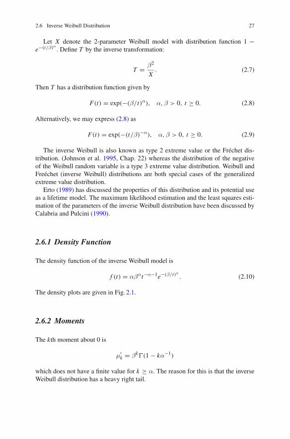
The density function of the inverse Weibull model is
f (t) = αβαt−α−1e−(β/t)α . (2.10)
The density plots are given in Fig. 2.1.
2.6.2 Moments
The kth moment about 0 is
μ′k = βk�(1 − kα−1)
which does not have a finite value for k ≥ α. The reason for this is that the inverseWeibull distribution has a heavy right tail.
28 2 Generalized Weibull Distributions
0 5 10 15 20
0.0
00.
05
0.1
00.
15
0.2
00.
25
t
Inve
rse
Wei
bull
dens
ity
density function
f : α = 0.7, β = 2f : α = 0.8, β =10f : α = 2, β = 5
Fig. 2.1 Inverse Weibull density functions
2.6.3 Hazard Rate Function
The hazard rate function is given by
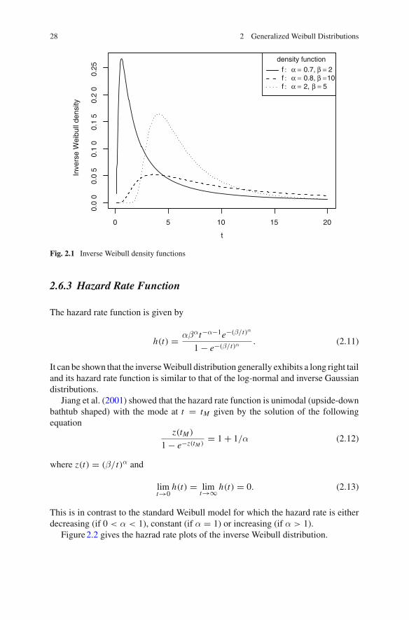
h(t) = αβαt−α−1e−(β/t)α
1 − e−(β/t)α. (2.11)
It can be shown that the inverse Weibull distribution generally exhibits a long right tailand its hazard rate function is similar to that of the log-normal and inverse Gaussiandistributions.
Jiang et al. (2001) showed that the hazard rate function is unimodal (upside-downbathtub shaped) with the mode at t = tM given by the solution of the followingequation
z(tM )
1 − e−z(tM )= 1 + 1/α (2.12)
where z(t) = (β/t)α and
limt→0
h(t) = limt→∞ h(t) = 0. (2.13)
This is in contrast to the standard Weibull model for which the hazard rate is eitherdecreasing (if 0 < α < 1), constant (if α = 1) or increasing (if α > 1).
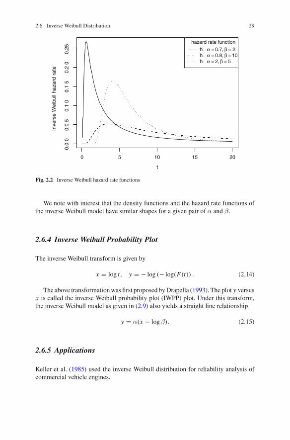
Figure 2.2 gives the hazrad rate plots of the inverse Weibull distribution.
2.6 Inverse Weibull Distribution 29
0 5 10 15 20
0.0
00.
05
0.1
00.
15
0.2
00.
25
t
Inve
rse
Wei
bull
haza
rd r
ate
hazard rate function
h : α = 0.7, β = 2h : α = 0.8, β = 10h : α = 2, β = 5
Fig. 2.2 Inverse Weibull hazard rate functions
We note with interest that the density functions and the hazard rate functions ofthe inverse Weibull model have similar shapes for a given pair of α and β.
2.6.4 Inverse Weibull Probability Plot
The inverse Weibull transform is given by
x = log t, y = − log (− log(F(t)) . (2.14)
The above transformation was first proposed by Drapella (1993). The plot y versusx is called the inverse Weibull probability plot (IWPP) plot. Under this transform,the inverse Weibull model as given in (2.9) also yields a straight line relationship
y = α(x − logβ). (2.15)
2.6.5 Applications
Keller et al. (1985) used the inverse Weibull distribution for reliability analysis ofcommercial vehicle engines.
30 2 Generalized Weibull Distributions
2.6.6 Models Involving Two Inverse Weibull Distributions
This was investigated by Jiang et al. (2001), see also Chap. 3 of this monograph fora more detailed discussion.
2.6.7 The Generalized Inverse Weibull Distribution
de Gusmão et al. (2009) proposed a generalized inverse Weibull distribution byadding another parameter γ to the standard inverse Weibull:
�F(t) = 1 − exp[−γ(β/t)α
]. (2.16)
When γ = 1, it clearly reduces to the inverse Weibull distribution.
Density Function
f (t) = γαβαt−(α+1) exp[−γ(β/t)α
]. (2.17)
Moments
The kth moment about 0 is
μ′k = γ
kα βk�(1 − kα−1)
which does not have a finite value for k ≥ α just as the inverse Weibull distribution.
Hazard Rate Function
The hazard rate function is given by
h(t) = γαβαt−(α+1) exp[−γ(β/t)α
] {1 − exp
[−γ(β/t)α]}−1
. (2.18)
By differentiating the above h(t) with respect to t , we can easily show that h(t)is unimodal (upside-down bathtub shaped) with a maximum value at t∗, where t∗satisfies the nonlinear equation:
γ(β/t∗){1 − exp
[−γ(β/t∗)α]} = 1 + α−1.
2.6 Inverse Weibull Distribution 31
Estimate of Parameter
The maximum likelihood estimates of the parameters with censored data wereobtained and studied in de Gusmão et al. (2009).
Further Extensions
de Gusmão et al. (2009) also considered the mixture of two generalized inverseWeibull distributions. Further, they also proposed the so called ‘The log-generalizedinverse Weibull distribution’.
2.7 Reflected Weibull Distribution
Suppose X has a three-parameter Weibul distribution, then T = −X has a reflectedWeibull whose distribution function is
F(t) = exp
{−(τ − t
β
)α}, α,β > 0,−∞ < t < τ . (2.19)
This is also known as type 3 extreme value distribution (Johnson et al. 1995,Chap. 22). The density function is given by
f (t) =(α
β
)(τ − t
β
)α−1
exp
{−(τ − t
β
)α}, α,β > 0,−∞ < t < ∞.
(2.20)The hazard rate function is given by
h(t) =(α
β
)(τ − t
β
)α−1 exp{−( τ−t
β )α}
1 − exp{−( τ−t
β )α} . (2.21)
Strictly speaking, the reflected Weibull is not suitable for reliability modelling unlessτ > 0 and (τ/β)α ≥ 9 so that Pr(0 < T < τ ) ≈ 1.
The model is fitted to an observed age distribution of holders of a certain type oflife insurance policy by Cohen (1973).
2.8 Log Weibull Distribution
This is an extreme value distribution derived from the logarithmic transformationof the two-parameter Weibull having distribution function as given in (1.4). Thetransformed variable has distribution function given by
32 2 Generalized Weibull Distributions
F(t) = 1 − exp
{− exp
(t − a
b
)}, −∞ < t < ∞, (2.22)
where we have let a = logβ, b = 1/α. This is also known as type 1 extreme valuedistribution or the Gumbel distribution. In fact, it is the most commonly referred toin discussions of extreme value distributions (Johnson et al. 1995, Chap. 22). Thedensity function is already given in (1.7)—though in a different parametrization, i.e.,
f (t) = 1
bexp
(t − a
b
)exp
{− exp
(t − a
b
)}, −∞ < t < ∞. (2.23)
The hazard rate functions is given by
h(t) = f (t)
1 − F(t)= 1
bexp
(t − a
b
). (2.24)
2.8.1 Applications
The log Weibull (Gumbel) distribution is an extreme value distribution. Thus it hasbeen applied to many extreme value data such as flood flows, wind speeds, radioactiveemissions, brittle strength of crystals, and etc. Chapter 22 Sect. 14 of Johnson et al.(1995) lists many applications of this distribution.
2.9 Stacy’s Weibull Distribution
Stacy (1962) proposed a distribution which he called the ‘generalized gamma model’with the pdf and cdf, given by
f (t) = αβ−αc
�(c)tαc−1 exp
{−(t/β)α}
(2.25)
andF(t) = �(c)−1γ
(c, (t/β)α
), (2.26)
respectively, for α,β, c > 0, where γ(·, ·) denotes the incomplete gamma functiondefined by
γ(a, t) =∫ t
0xa−1e−x dx .
2.9 Stacy’s Weibull Distribution 33
2.9.1 Special Cases
For c = 1, it reduces to the standard Weibull distribution. For α = 1, it becomes thetwo-parameter gamma distribution. If c → ∞, it becomes the lognormal distribution.For c = 1/2 and α = 2, it reduces to the half-normal distribution. Further, the chi-square distribution and the Levy distribution are also included as special cases.
2.9.2 Hazard Rate Function
The hazard rate function h(t) can be expressed as
h(t) = αβ−αctαc−1 exp {−(t/β)α}�(c) − γ (c, (t/β)α)
. (2.27)
Glaser (1980) showed that the hazard rate function can exhibit various shapes asgiven below:
Case 1: αc < 1.
(a) If α < 1, then h(t) is decreasing.(b) If α > 1, then h(t) has a bathtub shape.
Case 2: αc > 1.
(a) If α > 1, then h(t) is increasing.(b) If α < 1, then h(t) has a upside-down bathtub shape.
Case 3: αc = 1.
(a) If α = 1, c = 1, then h(t) is a constant.(b) If α < 1, then h(t) is decreasing.(c) If α > 1, then h(t) is increasing.
McDonald and Richards (1987) and Pham and Almhana (1995) also consideredthe shape of the hazard rate function h(t).
2.9.3 Estimation of Parameters
Parameter estimation for Stacy’s generalized Weibull (gamma) distribution has beenwidely treated in the literature. The maximum likelihood method and the method ofmoment are the two common approaches but it has been known that there are variousdifficulties in implementing these methods to this distribution. Other methods such
34 2 Generalized Weibull Distributions
as the heuristics and graphical methods were also proposed. For a literature reviewof these methods see Gomes et al. (2008).
Gomes et al. (2008) proposed a new method of estimation through the powertransformation T = Xc where X has Stacy’s Weibull distribution as given in (2.25)above. Then T has a gamma distribution with shape parameter c and scale parameterβα. Based on this they constructed a heuristic method called algorithm I.E.R.V. whichinvolves looping around the shape parameter α.
2.9.4 Applications
Stacy’s Weibull distribution has applications in many fields such as health costs, civilengineering (flood frequency, e.g, Pham and Almhana 1995), economics (incomedistribution, e.g., Klieber and Kotz 2003) and others.
2.10 Exponentiated Weibull Distribution
Mudholkar and Srivastava (1993) proposed a modification to the standard Weibullmodel through the introduction of an additional parameter ν (0 < ν < ∞). Thedistribution function is
F(t) = [G(t)]ν = [1 − exp{−(t/β)α}]ν, α,β > 0, t ≥ 0, (2.28)
where G(t) is the standard two-parameter Weibull distribution. The support for F is[0,∞).
When ν = 1, the model reduces to the standard two-parameter Weibull model.When ν is an integer, the model is a special case of the multiplicative model to bediscussed in Sect. 3.3 . The distribution has been studied extensively by Mudholkarand Hutson (1996), Jiang and Murthy (1999) and more recently Nassar and Eissa(2003).
2.10.1 Density Function
The density function is given by
f (t) = ν{G(t)}ν−1g(t), (2.29)
where g(t) is the density function of the standard two-parameter Weibull distribution.So
2.10 Exponentiated Weibull Distribution 35
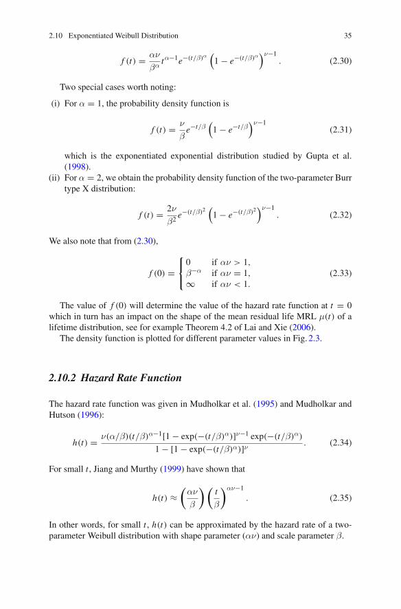
f (t) = αν
βαtα−1e−(t/β)α
(1 − e−(t/β)α
)ν−1. (2.30)
Two special cases worth noting:
(i) For α = 1, the probability density function is
f (t) = ν
βe−t/β
(1 − e−t/β
)ν−1(2.31)
which is the exponentiated exponential distribution studied by Gupta et al.(1998).
(ii) For α = 2, we obtain the probability density function of the two-parameter Burrtype X distribution:
f (t) = 2ν
β2 e−(t/β)2(
1 − e−(t/β)2)ν−1
. (2.32)
We also note that from (2.30),
f (0) =⎧⎨⎩
0 if αν > 1,
β−α if αν = 1,
∞ if αν < 1.
(2.33)
The value of f (0) will determine the value of the hazard rate function at t = 0which in turn has an impact on the shape of the mean residual life MRL μ(t) of alifetime distribution, see for example Theorem 4.2 of Lai and Xie (2006).
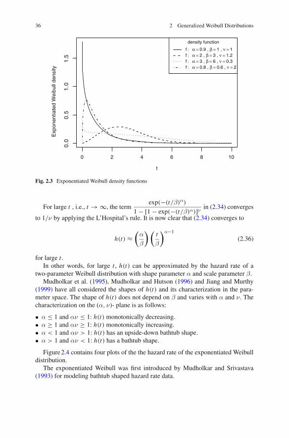
The density function is plotted for different parameter values in Fig. 2.3.
2.10.2 Hazard Rate Function
The hazard rate function was given in Mudholkar et al. (1995) and Mudholkar andHutson (1996):
h(t) = ν(α/β)(t/β)α−1[1 − exp(−(t/β)α)]ν−1 exp(−(t/β)α)
1 − [1 − exp(−(t/β)α)]ν . (2.34)
For small t , Jiang and Murthy (1999) have shown that
h(t) ≈(αν
β
)(t
β
)αν−1
. (2.35)
In other words, for small t , h(t) can be approximated by the hazard rate of a two-parameter Weibull distribution with shape parameter (αν) and scale parameter β.
36 2 Generalized Weibull Distributions
0 2 4 6 8 10
0.0
0.5
1.0
1.5
t
Exp
onen
tiate
d W
eibu
ll de
nsity
density function
f : α = 0.9 , β = 1 , ν = 1f : α = 2 , β = 3 , ν = 1.2f : α = 3 , β = 6 , ν = 0.3f : α = 0.8 , β = 0.6 , ν = 2
Fig. 2.3 Exponentiated Weibull density functions
For large t , i.e., t → ∞, the termexp(−(t/β)α)
1 − [1 − exp(−(t/β)α)]ν in (2.34) converges
to 1/ν by applying the L’Hospital’s rule. It is now clear that (2.34) converges to
h(t) ≈(α
β
)(t
β
)α−1
(2.36)
for large t .In other words, for large t , h(t) can be approximated by the hazard rate of a
two-parameter Weibull distribution with shape parameter α and scale parameter β.Mudholkar et al. (1995), Mudholkar and Hutson (1996) and Jiang and Murthy
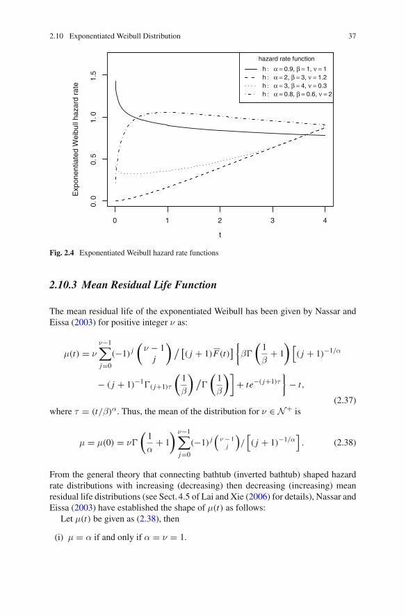
(1999) have all considered the shapes of h(t) and its characterization in the para-meter space. The shape of h(t) does not depend on β and varies with α and ν. Thecharacterization on the (α, ν)- plane is as follows:
• α ≤ 1 and αν ≤ 1: h(t) monotonically decreasing.• α ≥ 1 and αν ≥ 1: h(t) monotonically increasing.• α < 1 and αν > 1: h(t) has an upside-down bathtub shape.• α > 1 and αν < 1: h(t) has a bathtub shape.
Figure 2.4 contains four plots of the the hazard rate of the exponentiated Weibulldistribution.
The exponentiated Weibull was first introduced by Mudholkar and Srivastava(1993) for modeling bathtub shaped hazard rate data.
2.10 Exponentiated Weibull Distribution 37
Exp
onen
tiate
d W
eibu
ll ha
zard
rat
e
0 1 2 3 4
0.0
0.5
1.0
1.5
t
hazard rate function
h : α = 0.9, β = 1, ν = 1h : α = 2, β = 3, ν = 1.2h : α = 3, β = 4, ν = 0.3h : α = 0.8, β = 0.6, ν = 2
Fig. 2.4 Exponentiated Weibull hazard rate functions
2.10.3 Mean Residual Life Function
The mean residual life of the exponentiated Weibull has been given by Nassar andEissa (2003) for positive integer ν as:
μ(t) = ν
ν−1∑j=0
(−1) j(ν − 1
j
)/ [( j + 1)�F(t)
] {β�
(1
β+ 1
)[( j + 1)−1/α
− ( j + 1)−1�( j+1)τ
(1
β
)/�
(1
β
)]+ te−( j+1)τ
}− t,
(2.37)where τ = (t/β)α. Thus, the mean of the distribution for ν ∈ N+ is
μ = μ(0) = ν�
(1
α+ 1
) ν−1∑j=0
(−1) j(ν − 1
j
)/[( j + 1)−1/α
]. (2.38)
From the general theory that connecting bathtub (inverted bathtub) shaped hazardrate distributions with increasing (decreasing) then decreasing (increasing) meanresidual life distributions (see Sect. 4.5 of Lai and Xie (2006) for details), Nassar andEissa (2003) have established the shape of μ(t) as follows:
Let μ(t) be given as (2.38), then
(i) μ = α if and only if α = ν = 1.
38 2 Generalized Weibull Distributions
(ii) μ(t) is decreasing (increasing) if α ≥ 1 and αν ≥ 1 (α ≤ 1 and αν ≤ 1).(iii) μ(t) is decreasing and then increasing with a change point tm if α < 1 and
αν > 1.
(iv) μ(t) is increasing and then decreasing with a change point tm if α > 1 andαν < 1.
Nadarajah and Gupta (2005) obtained the kth moment about the origin as
μ′k = νβk�
(k
α
) ∞∑i=0
(1 − ν)i
i !(i + 1)(k+α)/α, k > −α, (2.39)
where (1 − ν)i = (a)i = a(a + 1) . . . a(a + i − 1).
If ν is an integer, then
μ′k = νβk�
(k
α
) ν−1∑i=0
(1 − ν)i
i !(i + 1)(k+α)/α, k > −α, (2.40)
which was established by Nassar and Eissa (2003). Equation (2.40) follows from(2.39) because (1 − ν)i = 0 for all i ≥ ν.
Xie et al. (2004) have studied the change points of h(t) and μ(t) in terms ofindividual model parameters. The difference D of two change points is tabulated forvarious combinations of the parameters.
2.10.4 Graphical Study
Jiang and Murthy (1999) discussed the shape of the WPP for the exponentiatedWeibull family and gave a parametric characterization of its probability density andhazard rate functions. Their paper also deals with the issues relating to modeling agiven data set and the problem of estimating the model parameters.
2.10.5 Applications
The model has been applied
• to model the bathtub failure rate behavior of the data in Aarset (1987) (Mudholkarand Srivastava 1993)
• to reanalyse the bus motor failure data (Mudholkar et al. 1995), and• to analyse a flood data (Mudholkar and Hutson 1996).
2.11 Beta-Weibull Distribution 39
2.11 Beta-Weibull Distribution
The distribution is a generalization of the exponentiated Weibull distribution dis-cussed in the preceding section. Let G(t) denote the standard two-parameter Weibulldistribution function given as G(t) = 1 − exp{−(t/β)α}.
The beta-Weibull was first proposed by Famoye et al. (2005) by coupling the betadensity and the Weibull distribution function such that the distribution function ofthe new distribution is
F(t) = 1
B(a, b)
∫ G(t)
0ua−1(1 − u)b−1du; 0 < a, b < ∞, (2.41)
where B(a, b) denotes the beta function defined by �(a)�(b)/�(a + b) = ∫ ba xa−1
(1 − x)b−1dx . The same distribution was also proposed by Wahed et al. (2009).Clearly, if b = 1, (2.41) reduces to the exponentiated Weibull distribution. In general,the distribution function cannot be expressed explicitly.
The basic properties are given in Famoye et al. (2005).
2.11.1 Density and Hazard Rate Function
The density function is rather simple:
f (t) = 1
B(a, b)
α
β
(t
β
)α−1 [1 − e−(t/β)α
]a−1e−b(t/β)α . (2.42)
The hazard rate function can be obtained from the preceding two equations as
h(t) = f (t)�F(t)
.
It cannot be expressed explicitly.Lee et al. (2007) examined the shapes of the hazard rate function and we now
summarize them below:
(a) h(t) is a constant b/β if a = α = 1,(b) h(t) is a decreasing function if aα ≤ 1 and α ≤ 1,(c) h(t) is an increasing function if aα ≥ 1 and α ≥ 1,(d) h(t) has a bathtub shape if aα < 1 and α > 1, and(e) h(t) has an upside-down bathtub shape if aα > 1 and α < 1.
40 2 Generalized Weibull Distributions
2.11.2 Comparison with Exponentiated Weibull Distribution
Lee et al. (2007) carried out a simulation study to compare the beta-Weibull modelwith the exponentiated Weibull model. They concluded that the bias of the MLE fromthe beta-Weibull distribution is smaller than the bias of the exponentiated Weibullmodel with comparable standard errors when b < 1. The bias and the standarderrors are, in general, smaller for the exponentiated Weibull distribution when b ≥ 1.(Recall, the beta-Weibull becomes the exponentiated Weibull when b = 1.) For thethree data sets analyzed in Lee et al. (2007), the estimates for the parameter b areless than 1 which suggests the usefulness of the beta-Weibull for describing survivaldata sets.
2.11.3 Applications of Beta-Weibull Model
The model is applied by Lee et al. (2007) to two censored data sets of bus-motorfailures and a censored data set of Arm A (Efron 1988) of the head-and-neck cancerclinical trial.
Wahed et al. (2009) also fitted the model to a breast cancer data set and they con-cluded that the beta-Weibull family is a reasonable candidate for modeling survivaldata.
Log Beta-Weibull Model
Let Y = log T where T has the beta-Weibull distribution given above . Then Y has alog beta-Weibull distribution studied by Ortega et al. (2011). Based on Y , they alsoproposed and studied the log-beta Weibull regression model which they consideredto be very suitable for modeling censored and uncensored data.
2.12 Extended Weibull Model of Marshall and Olkin
Marshall and Olkin (1997) proposed a modification to the standard Weibull modelthrough the introduction of an additional parameter ν (0 < ν < ∞). The model isgiven through its survival function function
�F(t) = νG(t)
1 − (1 − ν)G(t)= νG(t)
G(t) + νG(t)(2.43)
where G(t) is the distribution function of the two-parameter Weibull and �F(t) =1 − F(t).

2.12 Extended Weibull Model of Marshall and Olkin 41
The parameter ν is called a tilt parameter in Marshall and Marshall and Olkin(2007).
The case when G is an exponential distribution function has been considered asthe exponential-geometric distribution studied by Adamidis and Loukas (1998) andMarshall and Olkin (1997).
When ν = 1, �F(t) = G(t) so the model reduces to the standard Weibull model.
2.12.1 Extended Weibull
Using (1.4) as G in (2.43), we then have the distribution function given by
F(t) = 1 − ν exp[−(t/β)α]1 − (1 − ν) exp[−(t/β)α] . (2.44)
Marshall and Olkin (1997) called this the extended Weibull distribution. The meanand variance of the distribution cannot be given in a closed form, but they can beobtained numerically. The model may be considered as a competitor to the three-parameter Weibull distribution defined in (1.19).
Ghitany et al. (2005) showed that this distribution can be obtained by compound-ing the Weibull extension model of Xie et al. (2002) with the exponential distribution.That is, the extended Weibull is the result of mixing the Weibull extension model ofXie et al. with the exponential density. Zhang et al. (2007) also investigated somereliability properties of this model.
The resulting density function associated with (2.44) is given by
f (t) = (αν/β)(t/β)α−1 exp[−(t/β)α]{1 − (1 − ν) exp[−(t/β)α]}2 (2.45)
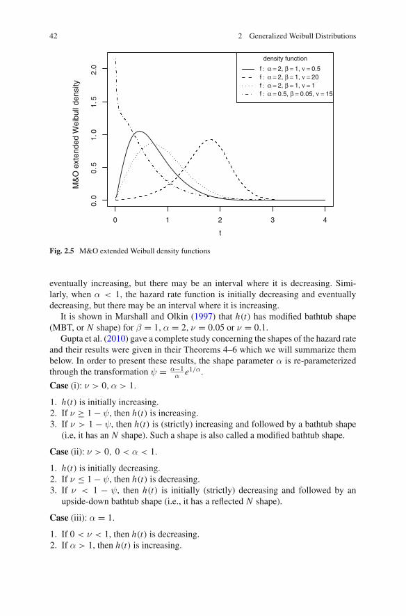
The plots of the density function for different parameter values are given inFig. 2.5.
2.12.2 Shapes of the Hazard Rate Function
The hazard rate function that corresponds to (2.45) is
h(t) = (α/β)(t/β)α−1
1 − (1 − ν) exp[−(t/β)α] . (2.46)
Marshall and Olkin (1997) carried out a partial study on the shape of the hazardrate. They found that h(t) is increasing when ν ≥ 1,α ≥ 1 and decreasing whenν ≤ 1,α ≤ 1. If α > 1, then the hazard rate function is initially increasing and
42 2 Generalized Weibull Distributions
M&
O e
xten
ded
Wei
bull
dens
ity
0 1 2 3 4
0.0
0.5
1.0
1.5
2.0
t
density function
f : α = 2, β = 1, ν = 0.5f : α = 2, β = 1, ν = 20f : α = 2, β = 1, ν = 1f : α = 0.5, β = 0.05, ν = 15
Fig. 2.5 M&O extended Weibull density functions
eventually increasing, but there may be an interval where it is decreasing. Simi-larly, when α < 1, the hazard rate function is initially decreasing and eventuallydecreasing, but there may be an interval where it is increasing.
It is shown in Marshall and Olkin (1997) that h(t) has modified bathtub shape(MBT, or N shape) for β = 1,α = 2, ν = 0.05 or ν = 0.1.
Gupta et al. (2010) gave a complete study concerning the shapes of the hazard rateand their results were given in their Theorems 4–6 which we will summarize thembelow. In order to present these results, the shape parameter α is re-parameterizedthrough the transformation ψ = α−1
α e1/α.
Case (i): ν > 0,α > 1.
1. h(t) is initially increasing.2. If ν ≥ 1 − ψ, then h(t) is increasing.3. If ν > 1 − ψ, then h(t) is (strictly) increasing and followed by a bathtub shape
(i.e, it has an N shape). Such a shape is also called a modified bathtub shape.
Case (ii): ν > 0, 0 < α < 1.
1. h(t) is initially decreasing.2. If ν ≤ 1 − ψ, then h(t) is decreasing.3. If ν < 1 − ψ, then h(t) is initially (strictly) decreasing and followed by an
upside-down bathtub shape (i.e., it has a reflected N shape).
Case (iii): α = 1.
1. If 0 < ν < 1, then h(t) is decreasing.2. If α > 1, then h(t) is increasing.
2.12 Extended Weibull Model of Marshall and Olkin 43
M&
O e
xten
ded
Wei
bull
haza
rd r
ate
0.0 0.5 1.0 1.5 2.0
01
23
45
6
t
hazard rate function
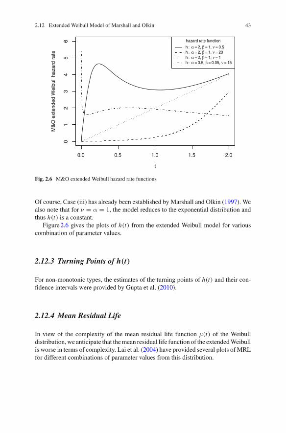
h : α = 2, β = 1, ν = 0.5h : α = 2, β = 1, ν = 20h : α = 2, β = 1, ν = 1h : α = 0.5, β = 0.05, ν = 15
Fig. 2.6 M&O extended Weibull hazard rate functions
Of course, Case (iii) has already been established by Marshall and Olkin (1997). Wealso note that for ν = α = 1, the model reduces to the exponential distribution andthus h(t) is a constant.
Figure 2.6 gives the plots of h(t) from the extended Weibull model for variouscombination of parameter values.
2.12.3 Turning Points of h(t)
For non-monotonic types, the estimates of the turning points of h(t) and their con-fidence intervals were provided by Gupta et al. (2010).
2.12.4 Mean Residual Life
In view of the complexity of the mean residual life function μ(t) of the Weibulldistribution, we anticipate that the mean residual life function of the extended Weibullis worse in terms of complexity. Lai et al. (2004) have provided several plots of MRLfor different combinations of parameter values from this distribution.
44 2 Generalized Weibull Distributions
2.12.5 Application
Zhang et al. (2007) fitted the model to the failure times of a sample of devices froma field-tracking study of a large system.
2.13 The Weibull-Geometric Distribution
The Weibull-geometric distribution, abbreviated as WG, was proposed and studiedby Barreto-Souza et al. (2010).
Let {Xi } be independent and identically distributed Weibull random variableshaving shape and scale parameters α and β, respectively.
Consider T = min{X1, X2, . . . , X Z } where Z is discrete random variable havinga geometric distribution with probability function:
p(z) = (1 − p)pz−1; 0 < p < 1, z = 1, 2, . . . (2.47)
Then T has the Weibull-geometric distribution with density function
f (t) = αβ−α(1 − p)tα−1e−(t/β)α{
1 − pe−(t/β)α}−2 ; α,β > 0. (2.48)
The above model may arise from a situation where failure (of a device for example)occurs due to the presence of an unknown number, say Z , of initial defects of the samekind. The random variables X ′
i s represent their lifetimes (with constant, increasing ordecreasing hazard rate) and each defect can be detected only after causing failure, inwhich case it is repaired perfectly. Thus, the distributional assumptions given earlierlead to the WG distribution for modeling the time of the first failure.
In the derivation of the WG distribution, it is required that 0 < p < 1. However,for negative value of p, Eq. (2.48) is still a proper density function. Thus we canextend the definition of the WG distribution in (2.48) for any p < 1.
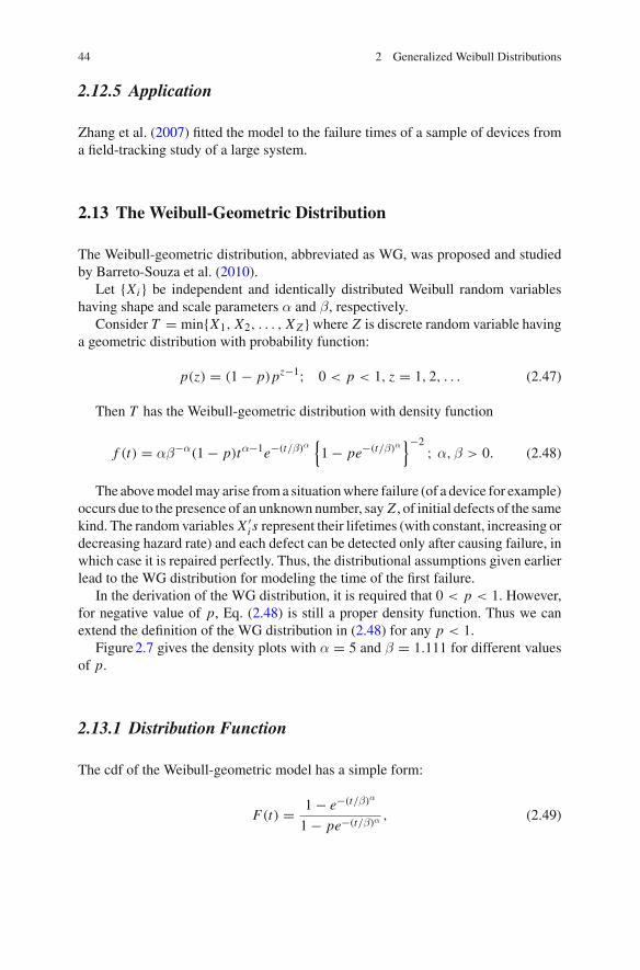
Figure 2.7 gives the density plots with α = 5 and β = 1.111 for different valuesof p.
2.13.1 Distribution Function
The cdf of the Weibull-geometric model has a simple form:
F(t) = 1 − e−(t/β)α
1 − pe−(t/β)α, (2.49)
2.13 The Weibull-Geometric Distribution 45
Wei
bull−
geom
etric
den
sity
0.0 0.5 1.0 1.5 2.0
0.0
0.5
1.0
1.5
2.0
2.5
3.0
t
density function
f : α = 5 , β = 1.111 ,p = − 2f : α = 5 , β = 1.111 ,p = − 0.5f : α = 5 , β = 1.111, p = 0.5f : α = 5 , β = 1.111, p = 0.9
Fig. 2.7 Weibull-geomeric density functions
and the corresponding survival function is
�F(t) = (1 − p)e−(t/β)α
1 − pe−(t/β)α. (2.50)
2.13.2 Hazard Rate Function
The hazard rate function of the Weibull-geometric distribution is
h(t) = αβ−αtα−1{
1 − pe−(t/β)α}−1
. (2.51)
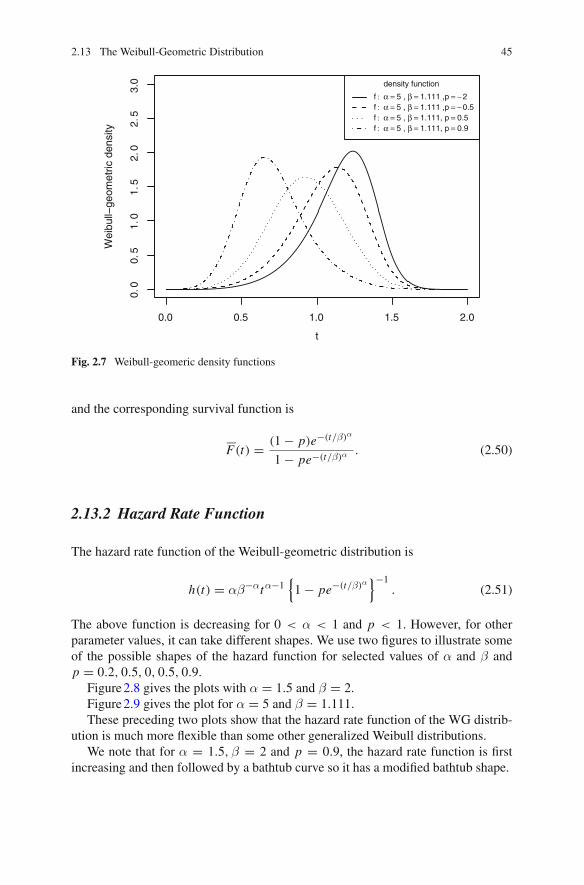
The above function is decreasing for 0 < α < 1 and p < 1. However, for otherparameter values, it can take different shapes. We use two figures to illustrate someof the possible shapes of the hazard function for selected values of α and β andp = 0.2, 0.5, 0, 0.5, 0.9.
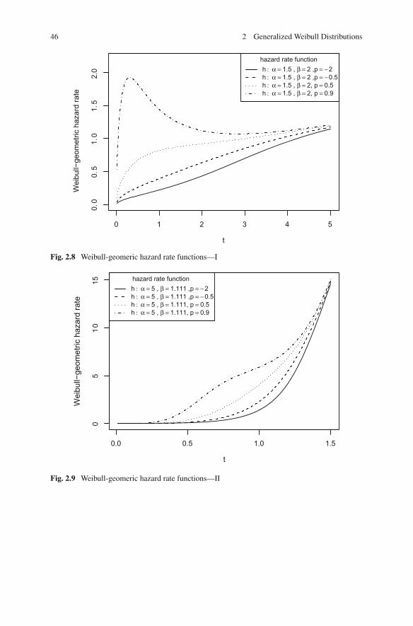
Figure 2.8 gives the plots with α = 1.5 and β = 2.Figure 2.9 gives the plot for α = 5 and β = 1.111.
These preceding two plots show that the hazard rate function of the WG distrib-ution is much more flexible than some other generalized Weibull distributions.
We note that for α = 1.5,β = 2 and p = 0.9, the hazard rate function is firstincreasing and then followed by a bathtub curve so it has a modified bathtub shape.
46 2 Generalized Weibull Distributions
Fig. 2.8 Weibull-geomeric hazard rate functions—I
Wei
bull−
geom
etric
haz
ard
rate
0.0 0.5 1.0 1.5
05
10
15
t
hazard rate function h : α = 5 , β = 1.111 ,p = − 2h : α = 5 , β = 1.111 ,p = − 0.5h : α = 5 , β = 1.111, p = 0.5h : α = 5 , β = 1.111, p = 0.9
Fig. 2.9 Weibull-geomeric hazard rate functions—II
2.13 The Weibull-Geometric Distribution 47
2.13.3 Quantile Function and Moments
The quantile function is
Q(u) = β
{log
(1 − pu
1 − u
)}1/α
(2.52)
and the kth moment about the origin 0 is
μ′k = (1 − p)βk�(k/α+ 1)�(p, k/α, 1) (2.53)
where �(z, s, a) = {�(s)}−1∫∞
0 t s−1e−at (1 − zet )−1dt; z < 1, a, s > 0 is knownas the Lerch’s transcendent function which can be computed via Mathematica orMaple.
2.13.4 Estimation of Parameters
Maximum likelihood estimates and other inferential properties were derived byBarreto-Souza et al. (2010).
2.13.5 Applications
Barreto-Souza et al. (2010) fitted the Weibull-geometric, extended exponential-geometric (EEG), and Weibull models to a real data set given in Meeker and Escobar(1998, p. 149). The data present the fatigue life (rounded to the nearest thousandcycles) for 67 specimens of Alloy T7987 that failed before having accumulated 300thousand cycles of testing:
94, 118, 139, 159, 171, 189, 227, 96, 121, 140, 159, 172, 190, 256, 99, 121, 141,159, 173, 196, 257, 99, 123, 141, 159, 176, 197, 269, 104, 129, 143, 162, 177, 203,271, 108, 131, 144, 168, 180, 205, 274, 112, 133, 149, 168, 180, 211, 291, 114, 135,149, 169, 184, 213, 117, 136, 152, 170, 187, 224, 117, 139, 153, 170, 188, 226.
It was found that the WG model gives a better fit than its competitors.
2.14 Weibull-Poisson Distribution
Hemmati and Khorram (2011) proposed a three-parameter ageing distribution usingthe same construction technique as in the preceding section.
48 2 Generalized Weibull Distributions
Again, let Xi denote the standard Weibull variable and define T = min{X1,
X2, . . . , X Z } where Z denotes the zero truncated Poisson random variable havingprobability function given by
p(z) = e−λλz(1 − e−λ)−1/z!; λ > 0, z = 1, 2, . . . (2.54)
It is easy to show that the resulting density function is given by
f (t) = λα
β(1 − e−λ)(t/β)α−1 exp{−λ−(t/β)α+λe−(t/β)α}; λ,α,β > 0. (2.55)
The survival function is reasonably straightforward and it is given by
�F(t) =(
1 − exp{λe−(t/β)α
})/(1 − eλ). (2.56)
It is clear from either (2.55) or (2.56) that the Weibull-Poisson distribution reducesto the Weibull distribution as λ → 0.
2.14.1 Hazard Rate Function
The hazard rate function of the Weibull-Poisson model is given by
h(t) = αλ(1 − eλ)(t/β)α−1 exp{−λ− (t/β)α + λe−(t/β)α}β(1 − e−λ)(1 − exp{λe−(t/β)α}) . (2.57)
Hemmati and Khorram (2011) showed that h(t) is increasing, decreasing or has amodified bathtub shape (N -shape, i.e., h(t) strictly increasing then then followed bya bathtub shape). Not that h(t) is unable to achieve a bathtub shape.
2.15 Modified Weibull Distribution
Lai et al. (2003) proposed a three-parameter generalized Weibull model which theycalled the modified Weibull distribution. The distribution function is given by
F(t) = 1 − exp(−atαeλt ), t ≥ 0, (2.58)
where the parameters λ > 0, α > 0 and a > 0. For λ = 0, (2.58) reduces toa Weibull distribution. This simple generalization of the Weibull model is able toexhibit a bathtub shaped hazard rate function. We now study this model in somedetail.
2.15 Modified Weibull Distribution 49
Mod
ified
Wei
bull
dens
ity
0 1 2 3 4
01
23
45
67
t
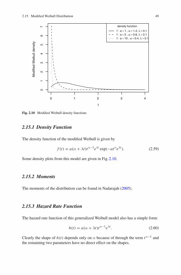
density function
f : a = 1 , α = 1.4, λ = 0.1f : a = 5 , α = 0.8, λ = 0.1f : a = 10 , α = 0.4, λ = 0.1
Fig. 2.10 Modified Weibull density functions
2.15.1 Density Function
The density function of the modified Weibull is given by
f (t) = a(α+ λt)tα−1eλt exp(−atαeλt ). (2.59)
Some density plots from this model are given in Fig. 2.10.
2.15.2 Moments
The moments of the distribution can be found in Nadarajah (2005).
2.15.3 Hazard Rate Function
The hazard rate function of this generalized Weibull model also has a simple form:
h(t) = a(α+ λt)tα−1eλt . (2.60)
Clearly the shape of h(t) depends only on α because of through the term tα−1 andthe remaining two parameters have no direct effect on the shapes.
50 2 Generalized Weibull Distributions
Case (i): α ≥ 1.
1. h(t) is increasing in t , implying an increasing hazard rate function, thus F is IFR.
2. h(0) = 0 if α > 1 and h(0) = a if α = 1.
3. h(t) → ∞ as t → ∞.
Case (ii): For 0 < α < 1.
1. h(t) initially decreases and then increases, implying it has a bathtub shape.
2. h(t) → ∞ as t → 0 and h(t) → ∞ as t → ∞.
3. The change point t∗, the turning point of the hazard rate function, is
t∗ =√α− α
λ. (2.61)
The interesting feature of this hazard curve is that t∗ increases as λ decreases.The limiting case when λ = 0 reduces to the standard Weibull distribution.
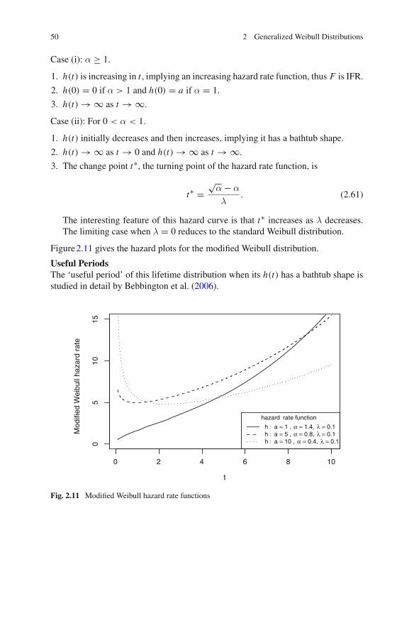
Figure 2.11 gives the hazard plots for the modified Weibull distribution.
Useful PeriodsThe ‘useful period’ of this lifetime distribution when its h(t) has a bathtub shape isstudied in detail by Bebbington et al. (2006).
Mod
ified
Wei
bull
haza
rd r
ate
0 2 4 6 8 10
05
10
15
t
hazard rate function
h : a = 1 , α = 1.4, λ = 0.1h : a = 5 , α = 0.8, λ = 0.1h : a = 10 , α = 0.4, λ = 0.1
Fig. 2.11 Modified Weibull hazard rate functions
2.15 Modified Weibull Distribution 51
2.15.4 Mean Residual Life
In common with many other generalized Weibull distributions, the mean of thisdistribution does not have a closed form. Plots of the mean residual life function μ(t)can be found in Lai et al. (2004) or Xie et al. (2004) for some selected parametervalues. The latter paper also computed the distance between the change points ofh(t) and μ(t).
2.15.5 Estimation of Parameters
A simple method for estimating the parameters of the modified Weibull modelthrough a WPP was given in Lai et al. (2003). Bebbington et al. (2008) have sug-gested an empirical estimator for the turning point t∗ and the theory was illustrated bymeans of real data set. A simulation study was conducted to assess the performanceof the estimators in practice.
2.15.6 Estimates of Parameters for Progressively Type-IICensored Samples
Progressively type-II censoring is often used in life testing. Consider an experimentin which n units are placed on a life test. At the time of the first failure, k1 units arerandomly removed from the remaining n−1 units. At the second failure, k2 units fromthe remaining n − 2 − k1 units are randomly removed. The life test continues untilthe mth failure at which time, all the remaining km = n − m − k1 − k2 − · · · − km−1units are removed.
Ng (2005) studied the estimation of parameters based on a progressively type-II censored sample from the modified Weibull model specified by (2.58). He firstobtained the maximum likelihood estimates of the model parameters. The estimatorsbased on a least-squares fit of a multiple linear regression on a Weibull probabilitypaper plot were also obtained and compared with the MLE via Monte Carlo simula-tions.
Recently, Jiang et al. (2010) also studied maximum likelihood estimation of themodel parameters of the modified Weibull distribution with progressively type-2censored samples. The property of the log-likelihood function was investigated byintroducing a simple transformation to decrease the dimension of the parametervector. Existence and uniqueness of the MLEs of the model parameters were proved.Several examples were presented to illustrate the uniqueness and existence propertyof the MLEs.
52 2 Generalized Weibull Distributions
2.15.7 Application
Failure times data from Aarset (1987) was fitted by this modified Weibull model.
2.15.8 Competing Risk Models Involving Two ModifiedWeibull Distributions
Alwasel (2009) proposed a competing risk model involving two modified Weibulldistributions. The maximum likelihood estimates of the six parameters (since eachof modified Weibull models has three parameters) were also derived although not ina closed form. So a numerical method is required for computing the MLEs of theseparameters.
2.15.9 Beta Modified Weibull Distribution
Silva et al. (2010) proposed a new distribution called the beta modified Weibull basedon the following construction scheme:
F(t) = 1
B(a, b)
∫ G(t)
0ua−1(1 − u)b−1du (2.62)
where G(t) denotes the cdf of the modified Weibull distribution. The density functionis given by
f (t) = 1
B(a, b)G(t)a−1(1 − G)b−1g(u)du (2.63)
where g(t) = G ′(t).The model contains several well known sub-models including the beta-Weibull
studied by Lee et al. (2007).The hazard function h(t) of the beta modified Weibull can be bathtub shaped,
increasing, decreasing or inverted bathtub shaped (UBT) depending on the values ofthe parameters.
2.15.10 Generalized Modified Weibull Family
The survival function of the distribution proposed and studied by Carrasco et al.(2008) is
�F(t) = 1 −(
1 − exp{−atαeλt
})β, λ ≥ 0,α,β, a > 0; t ≥ 0. (2.64)
2.15 Modified Weibull Distribution 53
Clearly, the distribution is a simple extension of the modified Weibull distributionof Lai et al. (2003) since (2.64) reduces to (2.58) when β = 1. In fact, it includesseveral other distributions such as type 1 extreme value, the exponentiated Weibullof Mudholkar and Srivastava (1993) as specified in (2.28) above, and others. Animportant feature of this lifetime (ageing) distribution is its considerable flexibilityin providing hazard rates of various shapes.
2.16 Generalized Weibull Family
The so called generalized Weibull model was derived by Mudholkar and Kollia(1994) and Mudholkar and Hutson (1996) from the basic two-parameter Weibulldistribution by appending an additional parameter. The quantile function for the newmodel is given by
Q(u) = β[θ1 − (1 − u)1/θ
]1/α, θ < ∞
= β[− log(1 − u)]1/α, θ → ∞(2.65)
where the new parameter θ is unconstrained so that −∞ < θ < ∞. It followsimmediately that the survival function is
�F(t) =[
1 −(
t
β
)α/θ
]θ; α,β > 0, (2.66)
where the support is for F(t) is (0, ∞) for θ ≤ 0 and (0,βθ1/α) for θ > 0. So thesupport of the distribution can be a finite interval or unbounded.
Indeed the model reduces to the basic two-parameter Weibull when θ → ∞.Nikulin and Haghighi (2006) observed that the generalized Weibull distribution turnsinto the exponential ifα = 1 and θ → ∞, and the log-logistic distribution if θ = −1,which is often used as a model in survival studies. Further, common distributionssuch as the lognormal and gamma distributions may be well approximated by thisfamily. They also noted that if α ≥ 0 and θ < 0, then the family coincides with BurrXII distributions.
2.16.1 Characterization of Hazard Rate
This generalized family not only contains distributions with bathtub and inverted(upside-down bathtub) hazard rate shapes, but also allows for a broader class ofmontonic hazard rates. The model hazard rate is given by
54 2 Generalized Weibull Distributions
h(t) = α(t/β)α−1
β (1 − (t/β)α/θ). (2.67)
The following classification was obtained by Mudholkar and Hutson (1996):
1. α < 1 and 0 < θ < ∞: h(t) has a bathtub shape.
2. α ≤ 1 and θ ≤ 0: h(t) is decreasing in t .
3. α > 1 and −∞ < θ < 0: h(t) has an inverted bathtub shape.
4. α ≥ 1 and θ ≥ 0: h(t) is increasing in t .
5. α = 1 and θ → ∞: F is exponential (i.e., h(t) is a constant).
It was also shown that the generalized Weibull family (2.68) is closed underproportional hazards relationships, that is, for any ν > 0, �F(t)ν is also a member ofthe family (2.68).
Furthermore, for θ ≤ 0, (2.68) reduces to the hazard rate of the Burr XII distrib-ution, see for example, Sect. 2.3.13 of Lai and Xie (2006).
2.16.2 Estimation of Parameters
The maximum likelihood estimates of the model parameters were obtained byMudholkar and Hutson (1996).
2.16.3 Applications
Mudholkar and Hutson (1996) have successfully fitted the model to the two-armclinical trials data (Head-and-Neck cancer trials) considered by Efron (1988).
2.17 Jeong’s Extension of Generalized Weibull
Jeong (2006) extended the above generalized Weibull model by incorporating anotherparameter with the survival function given as
�F(t) = exp
[−θ1−τ {(t/β)α + θ}τ − θ
τ
]; 0 < α,β, θ < ∞, −∞ < τ < ∞.
(2.68)The distribution becomes the standard Weibull distribution when τ = 1. It reducesto the Mudholkar’s generalized Weibull of (2.66) as τ → 0.
This new parameter family was motivated to parameterize the cumulative inci-dence function (in the context of survival analysis) completely.
The model has an application to breast cancer data.
2.17 Jeong’s Extension of Generalized Weibull 55
2.17.1 Hazard Rate Function
The hazard rate function of Jeong’s extension is
h(t) = α(t/β)αθ1−τ
t [(t/β)α + θ]1−τ . (2.69)
By differentiating log h(t) with respect to t and then setting the derivative to zero,
we find the turning point β{θ(1−α)ατ−1
}1/αexists on the real axis only if (a) α < 1 and
ατ > 1 or (b) α > 1 and ατ < 1.When (a) holds, h(t) has a bathtub shape and if (b) holds then it has an upside-
down bathtub shape (unimodal). Otherwise, h(t) can be a constant, decreasing orincreasing.
2.17.2 Application
The model was applied to two breast cancer data sets from the National SurgicalAdjuvant Breast and Bowel Project.
2.18 Generalized Power Weibull Family
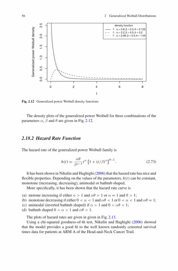
Nikulin and Haghighi (2006) introduced a family of distributions with survival func-tion
�F(t) = exp{
1 − (1 + (t/β)α
)θ} ; α,β, θ > 0. (2.70)
Obviously, the case θ = 1 reduces it to the standard Weibull distribution.
The quantile function is given as below:
Q(p) = β{(1 − log(1 − p))1/θ − 1}1/α; 0 < p < 1. (2.71)
2.18.1 Probability Density Function
The probability density function is given by
f (t) = αθ
βα−1 tα{1 + (t/β)α
}θ−1 exp{
1 − (1 + (t/β)α)θ}
. (2.72)
56 2 Generalized Weibull Distributions
Gen
eral
ized
pow
er W
eibu
ll de
nsity
0 2 4 6 8
0.0
0.5
1.0
1.5
2.0
2.5
t
density function
f : α = 0.8,β = 0.5,θ = 0.125f : α = 2.2,β = 0.5,θ = 0.2f : α = 0.99, β = 0.5,θ = 1.05
Fig. 2.12 Generalized power Weibull density functions
The density plots of the generalized power Weibull for three combinations of theparameters α, β and θ are given in Fig. 2.12.
2.18.2 Hazard Rate Function
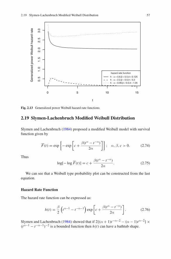
The hazard rate of the generalized power Weibull family is
h(t) = αθ
βα−1 tα{1 + (t/β)α
}θ−1. (2.73)
It has been shown in Nikulin and Haghighi (2006) that the hazard rate has nice andflexible properties. Depending on the values of the parameters, h(t) can be constant,monotone (increasing, decreasing), unimodal or bathtub shaped.
More specifically, it has been shown that the hazard rate curve is
(a) motone increasing if either α > 1 and αθ > 1 or α = 1 and θ > 1;(b) monotone decreasing if either 0 < α < 1 andαθ < 1 or 0 < α < 1 andαθ = 1;(c) unimodal (inverted bathtub shaped) if α > 1 and 0 < αθ < 1;(d) bathtub shaped 0 < α < 1 and αθ > 1.
The plots of hazard rates are given in given in Fig. 2.13.Using a chi-squared goodness-of-fit test, Nikulin and Haghighi (2006) showed
that the model provides a good fit to the well known randomly censored survivaltimes data for patients at ARM A of the Head-and-Neck Cancer Trail.
2.19 Slymen-Lachenbruch Modified Weibull Distribution 57
Gen
eral
ized
pow
er W
eibu
ll ha
zard
rat
e
0 5 10 15
0.5
1.0
1.5
2.0
2.5
3.0
t
hazard rate function
h : α = 0.8,β = 0.5,θ = 0.125h : α = 2.2,β = 0.5,θ = 0.2h : α = 0.99,β = 0.5,θ = 1.05
Fig. 2.13 Generalized power Weibull hazard rate functions
2.19 Slymen-Lachenbruch Modified Weibull Distribution
Slymen and Lachenbruch (1984) proposed a modified Weibull model with survivalfunction given by
�F(t) = exp
{− exp
[c + β(tα − t−α)
2α
]}; α,β, c > 0. (2.74)
Thus
log[− log �F(t)] = c + β(tα − t−α)2α
. (2.75)
We can see that a Weibull type probability plot can be constructed from the lastequation.
Hazard Rate Function
The hazard rate function can be expressed as:
h(t) = β
2
(tα−1 − t−α−1
)exp
[c + β(tα − t−α)
2α
]. (2.76)
Slymen and Lachenbruch (1984) showed that if 2{(α+ 1)t−α−2 − (α− 1)tα−2} ×(tα−1 − t−α−1)−2 is a bounded function then h(t) can have a bathtub shape.
58 2 Generalized Weibull Distributions
2.20 Flexible Weibull
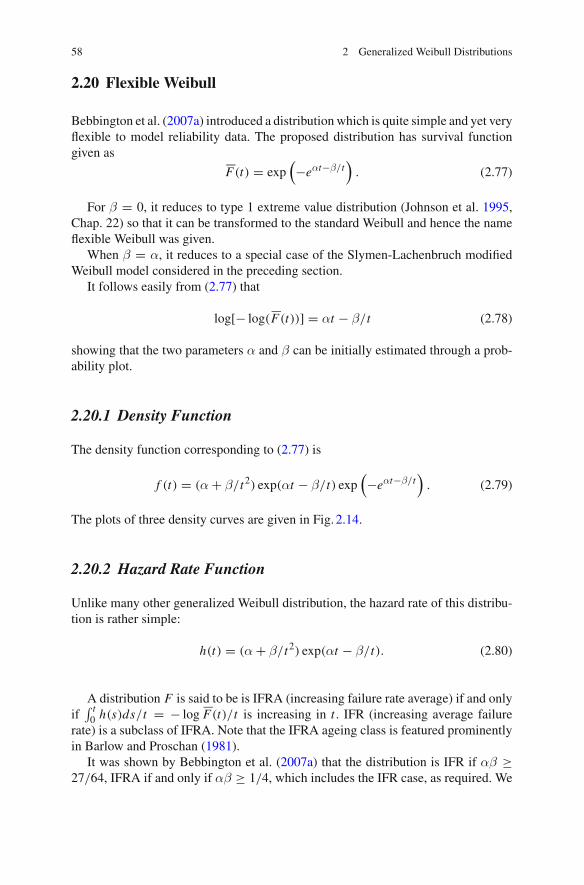
Bebbington et al. (2007a) introduced a distribution which is quite simple and yet veryflexible to model reliability data. The proposed distribution has survival functiongiven as
�F(t) = exp(−eαt−β/t
). (2.77)
For β = 0, it reduces to type 1 extreme value distribution (Johnson et al. 1995,Chap. 22) so that it can be transformed to the standard Weibull and hence the nameflexible Weibull was given.
When β = α, it reduces to a special case of the Slymen-Lachenbruch modifiedWeibull model considered in the preceding section.
It follows easily from (2.77) that
log[− log(�F(t))] = αt − β/t (2.78)
showing that the two parameters α and β can be initially estimated through a prob-ability plot.
2.20.1 Density Function
The density function corresponding to (2.77) is
f (t) = (α+ β/t2) exp(αt − β/t) exp(−eαt−β/t
). (2.79)
The plots of three density curves are given in Fig. 2.14.
2.20.2 Hazard Rate Function
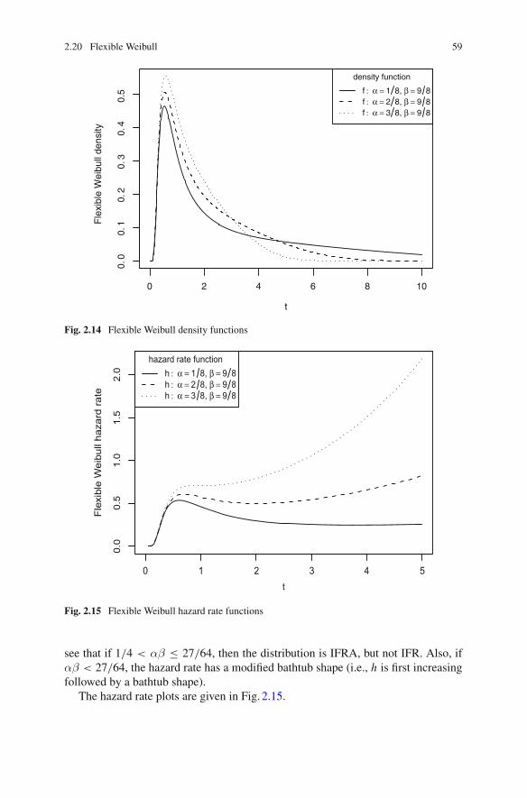
Unlike many other generalized Weibull distribution, the hazard rate of this distribu-tion is rather simple:
h(t) = (α+ β/t2) exp(αt − β/t). (2.80)
A distribution F is said to be is IFRA (increasing failure rate average) if and onlyif∫ t
0 h(s)ds/t = − log �F(t)/t is increasing in t . IFR (increasing average failurerate) is a subclass of IFRA. Note that the IFRA ageing class is featured prominentlyin Barlow and Proschan (1981).
It was shown by Bebbington et al. (2007a) that the distribution is IFR if αβ ≥27/64, IFRA if and only if αβ ≥ 1/4, which includes the IFR case, as required. We
2.20 Flexible Weibull 59
Fle
xibl
e W
eibu
ll de
nsity
0 2 4 6 8 10
0.0
0.1
0.2
0.3
0.4
0.5
t
density function
f : α = 1 8, β = 9 8f : α = 2 8, β = 9 8f : α = 3 8, β = 9 8
Fig. 2.14 Flexible Weibull density functions
0 1 2 3 4 5
0.0
0.5
1.0
1.5
2.0
t
Flex
ible
Wei
bull
haza
rd ra
te
hazard rate function h : α = 1 8, β = 9 8h : α = 2 8, β = 9 8h : α = 3 8, β = 9 8
Fig. 2.15 Flexible Weibull hazard rate functions
see that if 1/4 < αβ ≤ 27/64, then the distribution is IFRA, but not IFR. Also, ifαβ < 27/64, the hazard rate has a modified bathtub shape (i.e., h is first increasingfollowed by a bathtub shape).
The hazard rate plots are given in Fig. 2.15.
60 2 Generalized Weibull Distributions
2.20.3 Parameter Estimation
Bebbington et al. (2007a) showed thatα and β can be estimated through the Weibull-type probability plot using (2.78) above.
The maximum likelihood estimates of two parameters can also be obtained numer-ically through maximizing the likelihood function.
2.20.4 Applications
The flexible Weibull distribution has applications in:
• survival analysis for secondary reactor pumps (Bebbington et al. 2007a),• human mortality study (Bebbington et al. 2007b),• stop over duration of animals in the presence of trap-effects (Choqueta et al. 2013).
2.21 Weibull Extension Model
Another generalization of Weibull was introduced by Xie et al. (2002) and a detailedstatistical analysis was given in Tang et al. (2003). In the latter, the authors simplyreferred their distribution as ‘the Weibull extension model’.
The distribution is in fact a generalization of the model studied by Chen (2000).The cumulative distribution function is given by
F(t) = 1 − exp{−λβ
[e(t/β)α − 1
]}, t ≥ 0,α,β,λ > 0. (2.81)
We see that the distribution approaches to a two-parameter Weibull distributionwhen λ → ∞ with β in such a manner that βα−1/λ is held constant.
For λ = 1, the above distribution is the exponential power distribution consideredand studied by Smith and Bain (1975, 1976). The case with scale parameter β = 1was considered by Chen (2000) who also considered the estimation of parameters.
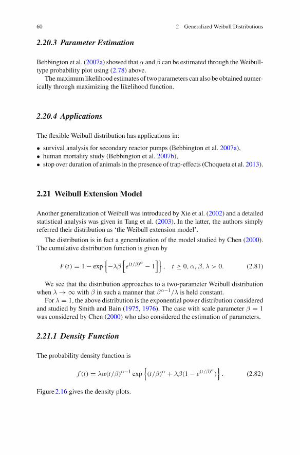
2.21.1 Density Function
The probability density function is
f (t) = λα(t/β)α−1 exp{(t/β)α + λβ(1 − e(t/β)α)
}. (2.82)
Figure 2.16 gives the density plots.
2.21 Weibull Extension Model 61
0 1 2 3 4 5
05
1015
t
Wei
bull e
xten
sion
dens
ity
density function f : α = 0.7, β = 100, λ = 2f : α = 0.8, β = 100, λ = 2f : α = 1.1, β = 100, λ = 2
Fig. 2.16 Weibull extension density functions
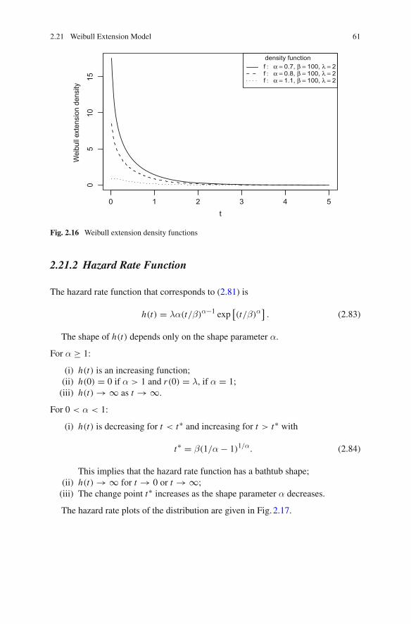
2.21.2 Hazard Rate Function
The hazard rate function that corresponds to (2.81) is
h(t) = λα(t/β)α−1 exp[(t/β)α
]. (2.83)
The shape of h(t) depends only on the shape parameter α.
For α ≥ 1:
(i) h(t) is an increasing function;(ii) h(0) = 0 if α > 1 and r(0) = λ, if α = 1;
(iii) h(t) → ∞ as t → ∞.
For 0 < α < 1:
(i) h(t) is decreasing for t < t∗ and increasing for t > t∗ with
t∗ = β(1/α− 1)1/α. (2.84)
This implies that the hazard rate function has a bathtub shape;(ii) h(t) → ∞ for t → 0 or t → ∞;
(iii) The change point t∗ increases as the shape parameter α decreases.
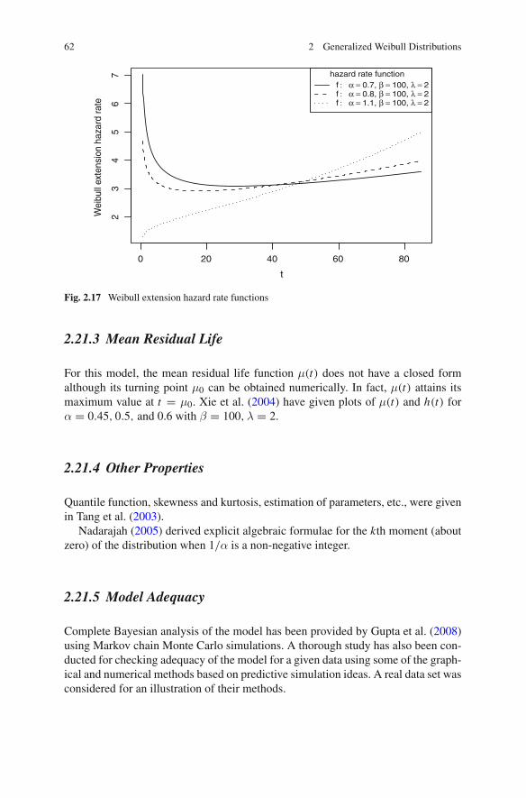
The hazard rate plots of the distribution are given in Fig. 2.17.
62 2 Generalized Weibull Distributions
0 20 40 60 80
23
45
67
t
Wei
bull
exte
nsio
n ha
zard
rate
hazard rate function f : α = 0.7, β = 100, λ = 2f : α = 0.8, β = 100, λ = 2f : α = 1.1, β = 100, λ = 2
Fig. 2.17 Weibull extension hazard rate functions
2.21.3 Mean Residual Life
For this model, the mean residual life function μ(t) does not have a closed formalthough its turning point μ0 can be obtained numerically. In fact, μ(t) attains itsmaximum value at t = μ0. Xie et al. (2004) have given plots of μ(t) and h(t) forα = 0.45, 0.5, and 0.6 with β = 100,λ = 2.
2.21.4 Other Properties
Quantile function, skewness and kurtosis, estimation of parameters, etc., were givenin Tang et al. (2003).
Nadarajah (2005) derived explicit algebraic formulae for the kth moment (aboutzero) of the distribution when 1/α is a non-negative integer.
2.21.5 Model Adequacy
Complete Bayesian analysis of the model has been provided by Gupta et al. (2008)using Markov chain Monte Carlo simulations. A thorough study has also been con-ducted for checking adequacy of the model for a given data using some of the graph-ical and numerical methods based on predictive simulation ideas. A real data set wasconsidered for an illustration of their methods.

2.21 Weibull Extension Model 63
2.21.6 Applications
The model has been fitted to:
• the failure times of Aarset data (Aarset 1987)• the failure times of a sample of devices in a large system (Gupta et al. 2008). The
detailed description of the data set can be found in Meeker and Escobar (1998).
2.22 The Odd Weibull Distribution
Cooray (2006) has constructed a generalized Weibull family called the odd Weibullfamily based on the idea of evaluating the distribution of the ‘odd of death’ of alifetime variable.
2.22.1 Distribution Function
The distribution function of the odd Weibull is given as
F(t) = 1 −(
1 + (e(t/β)α − 1)θ)−1
, (2.85)
with β > 0 be the scale parameter and αθ > 0 as the shape parameter.When θ = 1, F(t) is the cdf of the Weibull distribution. On the other hand, when
θ = −1, F(t) has the inverse Weibull distribution given by F(t) = e−(t/β)α .Jiang et al. (2008) showed that the logit function, the logarithm of the odds, of
the odd Weibull distribution can be written as the product of the logit function of thestandard Weibull and θ. Similarly, it can also be written as the product of the logitfunction of the inverse Weibull and −θ.
The density function is
f (t) =(αθ
t
)(t
β
)e(t/β)α
(e(t/β)α − 1
)θ−1[
1 +(
e(t/β)α − 1)θ]−2
. (2.86)
2.22.2 Quantile Function
The quantile function can be shown to be
Q(u) = β
{log
[1 +
(u
1 − u
)1/θ]}
. (2.87)
64 2 Generalized Weibull Distributions
2.22.3 Hazard Rate Function
The hazard rate function of the odd Weibull distribution is
h(t) =(αθ
t
)(t
β
)e(t/β)α
(e(t/β)α − 1
)θ−1[
1 +(
e(t/β)α − 1)θ]−1
. (2.88)
Cooray (2006) has shown that the odd Weibull family can model various hazardshapes (increasing, decreasing, bathtub, and unimodal); thus the family is proved tobe flexible for fitting reliability and survival data. More precisely, he established that
(1) for α < 0, θ < 0 or α < 1,αθ ≥ 1, h(t) is unimodal,(2) for α > 1,αθ > 1, h(t) is increasing,(3) for α < 1,αθ < 1, h(t) is decreasing, and(4) for α > 1,αθ ≤ 1, h(t) has a bathtub shape.
Cooray (2006) also indicated that in the regions where (α > 1,αθ > 1) and(α < 1,αθ < 1), h(t) may have some other shapes. Jiang et al. (2008) found, usingnumerical analysis, that the ‘other shapes’ are N (modified bathtub) and reflected Nshapes when the model parameters are near the boundary line αθ = 1. The latterauthors also studied the tail behaviours of h(t) in detail.
2.22.4 Weibull Probability Plot Parameter Estimation
The shapes of the Weibull probability plot with different parameters were presentedin Jiang et al. (2008) and the steps of the graphical estimation were also iterated.In estimating parameters of the odd Weibull model by a graphical approach, it isnecessary to determine if the shape parameters are positive or negative. Cooray(2006) suggested to employ the total-time-test (TTT) for this purpose whereas Jianget al. (2008) concluded that it is easy to check the sign of the shape parameters usinga Weibull probability plot.
2.22.5 Optimal Burn-In Time and Useful Period
For a product lifetime exhibiting a bathtub shaped hazard rate, an important issue isto determine the optimal burn-in time. As seen from an earlier subsection, the oddWeibull model can indeed display such a shape. Jiang et al. (2008) observed that thesecond portion (stable period) of the odd Weibull model, when exhibiting a bathtubshape, could be quite long and flat which is a good property in application. Theydiscussed those issues concerning the optimal burn-in time and the useful period forthe model.
2.22 The Odd Weibull Distribution 65
2.22.6 Application
The model has been fitted to a sample of 208 data points, which represent the ages atdeath in weeks for male mice exposed to 240r of gamma radiation (Kimball 1960).
2.23 Generalized Logistic Frailty Model
Vaupel (1990) proposed and examined a logistic frailty model to correct an inherentdeficiency in the Gompertz-Makeham law often used in a mortality study. The Vaupelmodel has incorporated a deceleration parameter s ≥ 0 in such a way that the resultinghazard is a logistic function given by
h(t) = Aet/β
1 + s Aβ(et/β − 1). (2.89)
The survival function corresponding to (2.89) is
�F(t) =[1 + s Aβ(et/β − 1)
]− 1s
(2.90)
which is relatively simple. On differentiation of (2.89), we have
h′(t) = Ae(t/β)(1/β − s A)[1 + s Aβ(et/β − 1)
]2 . (2.91)
From the preceding equation, we see that h(t) is increasing (decreasing) forβs A <
1(s Aβ > 1) and it converges to a constant as t → ∞. For human mortality, the case(s Aβ > 1) is obviously unrealistic as it would imply the immortality of man.
2.23.1 Generalized Logistic Frailty Distribution
In view of its hazard rate function being monotonic, the logistic frailty model haslimited applications in reliability and survival analysis. To provide a more flexiblemodel that is applicable to various disciplines associated with lifetime data, Lai andIzadi (2012) generalized the logistic frailty model in (2.90) by incorporating a shapeparameter:
�F(t) =[1 + s Aβ(e(t/β)α − 1)
]− 1s
(2.92)
66 2 Generalized Weibull Distributions
where A,α,β > 0 and s ≥ 0. Hereα andβ are clearly the shape and scale parameter,respectively. As mentioned earlier, s is a deceleration parameter whereas A is somekind of ‘normalizing constant’, particularly if s = 0.
We will see how this distribution is related to the Weibull in the next subsection.
2.23.2 Limiting Case
As s → 0, (2.92) is reduced to
lims→0
�F(t) = lims→0
[1 + s Aβ(e(t/β)α − 1)
]− 1s
(2.93)
= exp{−Aβ(e(t/β)α − 1)
}.
which is the Weibull extension model of Chen (2000) and Xie et al. (2002). It hasbeen shown in Xie et al. (2002) that (2.93) is either IFR (increasing failure rate),DFR (decreasing failure rate) or a bathtub shaped hazard rate distribution.
2.23.3 Probability Density Function
The density function of the generalized logistic frailty model can be obtained easilyby differentiating (2.92) with respect to t and it is given by
f (t) = Aα(t/β)α−1e(t/β)α[1 + s Aβ(e(t/β)α − 1)
]− s+1s
. (2.94)
2.23.4 Hazard Rate Function
The hazard rate function that corresponds to (2.92) is
h(t) = Aβ(t/β)α−1e(t/β)α
1 + s Aβ(e(t/β)α − 1). (2.95)
Rewriting the above in a slightly different form,
h(t) = Aα(t/β)α−1e(t/β)α/(s Aβ)
e(t/β)α + (1 − s Aβ)/(s Aβ). (2.96)
2.23 Generalized Logistic Frailty Model 67
From the preceding equation, it is clear that h(t) is increasing if s Aβ < 1 andα > 1. We have also mentioned that for s = 0, (2.96) can yield IFR (increasingfailure rate), DFR (decreasing failure rate) or a bathtub shape.
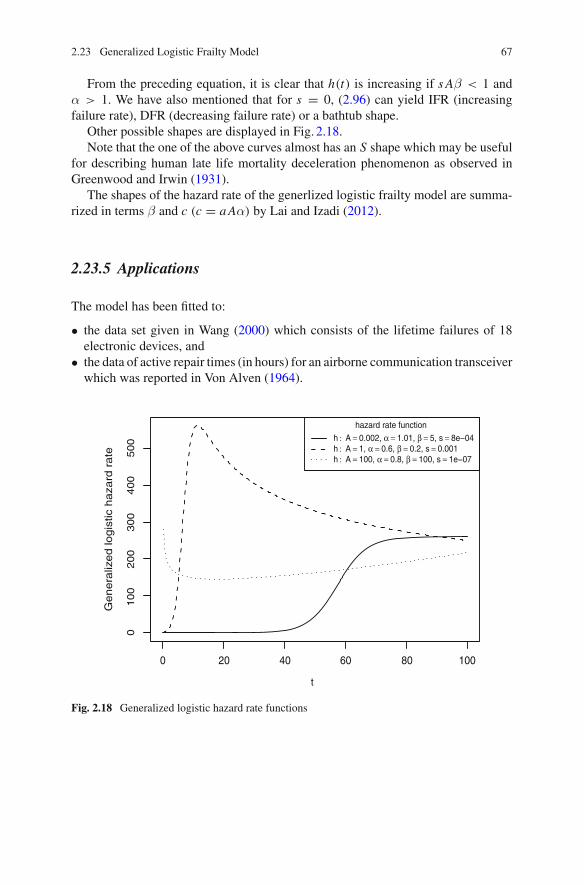
Other possible shapes are displayed in Fig. 2.18.Note that the one of the above curves almost has an S shape which may be useful
for describing human late life mortality deceleration phenomenon as observed inGreenwood and Irwin (1931).
The shapes of the hazard rate of the generlized logistic frailty model are summa-rized in terms β and c (c = a Aα) by Lai and Izadi (2012).
2.23.5 Applications
The model has been fitted to:
• the data set given in Wang (2000) which consists of the lifetime failures of 18electronic devices, and
• the data of active repair times (in hours) for an airborne communication transceiverwhich was reported in Von Alven (1964).
0 20 40 60 80 100
0100
200
300
400
500
t
Genera
lized lo
gis
tic h
aza
rd r
ate
hazard rate function
h : A = 0.002, α = 1.01, β = 5, s = 8e−04h : A = 1, α = 0.6, β = 0.2, s = 0.001h : A = 100, α = 0.8, β = 100, s = 1e−07
Fig. 2.18 Generalized logistic hazard rate functions
68 2 Generalized Weibull Distributions
2.24 Generalized Weibull-Gompertz Distribution
Nadarajah and Kotz (2005) proposed a generalization of the standard Weibull modelwith four parameters having survival function given as below:
R(t) = exp{−atb
(ectd − 1
)}, a, d > 0; b, c ≥ 0; t ≥ 0. (2.97)
Since (2.97) includes the Gompertz (1825) distribution as its special case whenb = 0 and d = 1. For this reason we may refer it as the generalized Weibull-Gompertz distribution. For b = 0 it contains the Weibull extension model of Xieet al. (2002) as given in Sect. 2.21 above. Since the models have four parameters, itmay be considered as an over-parameterized model.
2.25 Generalized Weibull Distribution of Gurvich et al.
It has been pointed by Nadarajah and Kotz (2005) that several of the modificationsof the Weibull distribution discussed in this section can arise from a representationsuggested by Gurvich et al. (1997). This distribution did not arise from a reliabilityperspective but from the context of modeling random length of brittle materials. Thedistribution function of this class is given by
F(t) = 1 − exp {−aG(t)} , (2.98)
where G(t) is a monotonically increasing function in t such that G(t) ≥ 0.
Several distributions we presented in this chapter can be derived by assigningappropriate expressions to G(t). For example,
• the modified Weibull model of Lai et al. (2003) is obtained by setting G(t) =tα exp(λt),
• the Weibull extension model of Xie et al. (2002) is obtained by letting G(t) =α exp(t/β)α − 1,
• the log Weibull model is derived by assigning G(t) = exp ((t − a)/b)), and
• the model considered by Nadarajah and Kotz (2005) follows from taking G(t) =tb(
ectd − 1)
.
Several other Weibull related distributions are also contained in this family.Pham and Lai (2007) have noted that Gurvich’s model is so general in which
G(t) is in fact the cumulative hazard function of an arbitrary lifetime distribution.We note that any survival function �F can be expressed as �F(t) = exp{−∫ t
0 h(t)dt} =exp{−H(t)}. Letting aG(t) = H(t), we see that the Gurvich’s model includes allthe continuous lifetime distributions.
2.26 Weibull Models with Varying Parameters 69
2.26 Weibull Models with Varying Parameters
The parameters of the models discussed so far are held constants. This section dealswith models where some of parameters are
(i) functions of the variable t ,(ii) function of some supplementary variables (denoted by S), or
(iii) random variables (covariates).
2.26.1 Time Varying Parameters
In these models the scale parameter (β) and/or the shape parameter (α) of the standardWeibull model given by (1.4) are function of the variable t .
Examples
(i) Only one of the two parameters is varying with time.(ii) Both α and β are functions of time. For example,
α(t) = a
(1 + 1
t
)b
ec/t , β(t) = a′tb′ec′/t . (2.99)
(iii) F(t) = 1 − exp{−�(t)} where �(t) is a nondecreasing function with �(0)=0and �(∞) = ∞. For example,
�(t) =m∑
i=1
λiφi (t), 1 ≤ i ≤ m. (2.100)
2.26.2 Weibull Accelerated Models
In these models the scale parameter β is a function of some supplementary vari-able (covariate) S. In reliability applications S represents the stress on the item sothe life of the item (a random variable with distribution F) is a function of S. Theshape parameter is unaffected by S and hence a constant. See Sect. 2.6.2 of Murthyet al. (2004).
70 2 Generalized Weibull Distributions
Arrhenius Model
The relationship is given by
β(S) = exp(γ0 + γ1S). (2.101)
(See Jensen (1995) for a summary this model). We see that log(β(S)) is linear in S.
Power Model
The relationship is given by
β(S) = eγ0
Sγ1. (2.102)
The power model is also briefly in Jensen (1995).A more general formulation is one where the scale parameter is expressed as
β(S) = exp
(b0 +
k∑i=1
bi si
)(2.103)
where S = (s1, s2, . . . , sk)′ is a k-dimensional vector of supplementary variables.
One may note that these types of models have been used extensively in acceleratedlife testing in reliability, see for example, Nelson (1990) or Chap. 6 of Lawless (2003).
2.26.3 Weibull Proportional Hazard Models
An alternative approach to modeling the effect of the supplementary variables(covariates) on the survival function �F(t) is through the hazard rate function. Therelationship is given by
h(t |S) = ψ(S)h0(t), (2.104)
where h0(t) is called the baseline hazard for a two-parameter Weibull distribu-tion. The only restriction on the scalar function ψ(·) is that it be positive. The lastequation tells us h(t |S) is proportional to the baseline hazard rate h0 and thus thename ‘proportional hazard’ model.
Many different forms for ψ(·) have been proposed in the literature. One such isthe following:
ψ(S) = exp
(k∑
i=1
bi si
). (2.105)
2.26 Weibull Models with Varying Parameters 71
(See for e.g., Kalbfleisch and Prentice 2002 and Lawless 2003). It now follows from(2.104) that the survival function
�F(t |S) = �F(t)ψ(S). (2.106)
(Note that in the current context, �F(t) is the Weibull survival function, but it coulddenote any other survival functions in a general setting).
When ψ is given by (2.105) and (2.104) becomes
h(t |S) = h0(t) exp
(k∑
i=1
bi si
)(2.107)
The hazard model above is generally known as the Cox proportional hazard model.Taking the natural logarithm of both sides of the preceding equation, we have
log(h(t |S)/h0(t)) =k∑
i=1
bi si (2.108)
We now have a fairly ‘simple’ linear model where the parameters can be readilyestimated.
2.26.4 Applications
In the recent years, the Cox proportional model is a popular survival model whencovariates are involved. Examples of applications include:
• epidemiology and biostatistics, e.g., multiple infection data,• financial analysis, e.g., stock exchange market,• clinical trials, and• survival analysis, e.g., cancer relapse data.
References
Aarset, M. V. (1987). How to identify a bathtub hazard rate. IEEE Transactions on Reliability, 36,106–108.
Adamidis, K., & Loukas, S. (1998). A lifetime with decreasing failure rate. Statistics & ProbabilityLetters, 39, 35–42.
Alwasel, I. A. (2009). Statistical inference of a competing risks model with modified WeibullDistributions. International Journal of Mathematical Analysis, 3(19), 905–918.
Barlow, R. E., & Proschan, F. (1981). Statistical theory of reliability and life testing. To Begin With,Silver Spring.
72 2 Generalized Weibull Distributions
Barreto-Souza, W., de Morais, A. L., & Cordeiro, G. M. (2010). The Weibull-geometric distribution.Journal of Statistical Computation and Simulation (first published on line on June 11, 2010) 1–13.doi:10.1080/00949650903436554.
Bebbington, M., Lai, C. D., & Zitikis, R. (2006). Useful periods for lifetime distributions withbathtub shaped hazard rate functions. IEEE Transactions on Reliability, 55(2), 245–251.
Bebbington, M., Lai, C. D., & Zitikis, R. (2007a). A flexible Weibull extension. Reliability Engi-neering and System Safety, 92, 719–726.
Bebbington, M., Lai, C. D., & Zitikis, R. (2007b). Modeling human mortality using mixtures ofbathtub shaped failure rate distributions. Journal of Theoretical Biology, 245, 528–538.
Bebbington, M., Lai, C. D., & Zitikis, R. (2008). Estimating the turning point of a bathtub shapedfailure distribution. Journal of Statistical Planning and Inference, 138(4), 1157–1166.
Calabria, R., & Pulcini, G. (1990). On the maximum likelihood and least-squares estimation in theinverse Weibull distribution. Statistica Applicata, 2(1), 53–66.
Carrasco, J. M. F., Ortega, E. M. M., & Cordeiro, G. M. (2008). A generalized modified Weibulldistribution for lifetime modeling. Computational Statistics and Data Analysis, 53, 450–462.
Chen, Z. (2000). A new two-parameter lifetime distribution with bathtub shape or increasing failurerate function. Statistics and Probability Letters, 49, 155–161.
Choqueta, R., Guedonb, Y., Besnarda, A., Guillemainc, M., & Pradel, R. (2013). Estimating stopover duration in the presence of trap-effects R. Ecological Modelling, 250, 111–118.
Cohen, A. C. (1973). The reflected Weibull distribution. Technometrics, 15(4), 867–873.Cooray, K. (2006). Generalization of the Weibull distribution: The odd Weibull family. Statistical
Modelling, 6, 265–277.de Gusmão, F. R. S., Ortega, E. M. M., & Cordeiro, G. M., (2009). The generalized inverse Weibull
distribution. Statistical Papers. doi:10.1007/s00362-009-0271-3.Drapella, A. (1993). The complementary Weibull distribution: Unknown or just forgotten. Quality
and Reliability Engineering International, 9, 383–385.Efron, B. (1988). Logistic regression, survival analysis, and the Kaplan-Meier curve. Journal of the
American Statistical Association, 83, 415–425.Erto, P. (1989). Genesis, properties and identification of the inverse Weibull lifetime model. Staistica
Applicata, 1(2), 117–128.Famoye, F., Lee, C., & Olumolade, O. (2005). The beta-Weibull distribution. Journal of Statistical
Theory and Applications, 4, 121–136.Ghitany, M. E., Al-Hussaini, E. K., & Al-Jarallah, R. A. (2005). Marshall-Olkin extended Weibull
distribution and its application to censored data. Journal of applied Statistics, 32(10), 1025–1034.Glaser, R. E. (1980). Bathtub and related failure rate characterizations. Journal of the American
Statistical Association, 75, 667–672.Gomes, O., Combes, C., & Dussauchoy, A. (2008). Parameter estimation of the generalized gamma
distribution. Mathematics and Computers in Simulation, 79, 963–995.Gompertz, B. (1825). On the nature of the function expressive of the law of human mortality, and
on the mode of determining the value of life contingencies. Philosophical Transactions of theRoyal Society, 115, 513–585.
Greenwood, M., & Irwin, J. O. (1931). The biostatistics of senility. Human Biology, 11(1), 1–23.Gupta, R. C., Gupta, R. D., & Gupta, P. L. (1998). Modelling failure time data by Lehman alterna-
tives. Communications in Statistics-Theory and Methods, 27(4), 887–904.Gupta, A., Mukherjee, B., & Upadhyay, S. K. (2008). Weibull extension: A Bayes study
using Markov chain Monte Carlo simulation. Reliability Engineering and System Safety, 93,1434–1443.
Gupta, R. C., Lvin, S., & Peng, C. (2010). Estimating turning points of the failure rate of theextended Weibull distribution. Computational Statistics and Data Analysis, 54, 924–934.
Gurvich, M. R., Dibenedetto, A. T., & Rande, S. V. (1997). A new statistical distributionfor characterizing the random length of brittle materials. Journal of Material Science, 32,2559–2564.
References 73
Hemmati, F., & Khorram, E. (2011). A new three-parameter ageing distribution. Journal of Statis-tical Planning and Inference, 141(7), 2266–2275.
Jensen, F. (1995). Electronic Component Reliability. New York: Wiley.Jeong, J. H. (2006). A new parametric family for modelling cumulative incidence function: appli-
cation to breast cancer data. Journal of the Royal Statistical Society: Series A, 169(2), 289–303.Jiang, R., & Murthy, D. N. P. (1999). The exponentiated Weibull family: A grapgical approach.
IEEE Transactions on Reliability, 48(1), 68–72.Jiang, R., Murthy, D. N. P., & Ji, P. (2001). Models involving two inverse Weibull distributions.
Reliability Engineering and System Safety, 73, 73–81.Jiang, H., Xie, M., & Tang, L. C. (2008). On the odd Weibull distribution. Proceedings of the
Institute of Mechnical Engineers, Part O: Journal of Risk and Reliability, 22, 583–594.Jiang, H., Xie, M., & Tang, L. C. (2010). On MLEs of the parameters of a modified Weibull
distribution for progressively type-2 censored samples. Journal of Applied Statistics, 37(4),617–627.
Johnson, N. L., Kotz, S., & Balakrishan, N. (1995). Continuous Univariate Distributions (2nd ed.,Vol. 2). New York: Wiley.
Kalbfleisch, J. D., & Prentice, R. L. (2002). The statistical analysis of failure time data (2nd ed.).New York: John Wiley & Sons.
Keller, A. Z., Giblin, M. T., & Farnworth, N. R. (1985). Reliability analysis of commercial vehicleengines. Reliability Engineering, 10(1), 15–25.
Kies, J. A. (1958). The strength of glass, Naval Research Lab. Report No.5093, Washington D.C.Kimball A. W. (1960). Estimation of mortality intensities in animal experiments. Biometrics, 16,
505–521.Klieber, C., & Kotz, S. (2003). Statistical size distributions in economic and actuarial sciences.
New York: Wiley-Interscience.Lai, C. D., & Izadi, M. (2012). Generalized logistic frailty model. Statistics and Probability Letters,
82, 1969–1977.Lai, C. D., Xie, M., & Murthy, D. N. P. (2003). Modified Weibull model. IEEE Transactions on
Reliability, 52, 33–37.Lai, C. D., Zhang, L. Y., & Xie, M. (2004). Mean residual life and other properties of Weibull
related bathtub shape failure rate distributions. International Journal of Reliability, Quality andSafety Engineering, 11(2), 113–132.
Lai, C. D., & Xie, M. (2006). Stochastic ageing and dependence for reliability. New York: Springer.Lai, C. D., Murthy, D. N. P., & Xie, M. (2011). Weibull distributions. Wiley Interdisciplinary
Reviews, 3(3), 282–287.Lawless, J. F. (2003). Statistical models and methods for lifetime data. Hoboken: John Wiley &
Sons.Lee, C., Famoye, F., & Olumolade, O. (2007). Beta-Weibull distribution: Some properties and
applications to censored data. Journal of Modern Applied Statistical Methods, 6, 173–186.Marshall, A. W., & Olkin, I. (1997). A new method for adding a parameter to a family of distributions
with application to the exponential and Weibull families. Biometrika, 84, 641–652.Marshall, A. W., & Olkin, I. (2007). Life distributions: Structure of nonparametric, semiparametric,
and parametric families. New York: Springer.McDonald, J. B., & Richards, D. O. (1987). Model selection: Some generalized distributions.
Communications in Statistics-Theory and Methods, 16(4), 1049–1074.McEwen, R. P., & Parresol, B. R. (1991). Moment expressions and summary statistics for the
complete and truncated Weibull distribution. Communications in Statistics-Theory and Methods,20, 1361–1372.
Meeker, W. Q., & Escobar, L. A. (1998). Statistical methods for reliability data. New York: Wiley& Sons.
Mudholkar, G. S., & Srivastava, D. K. (1993). Exponentiated Weibull family for analyzing bathtubfailure-rate data. IEEE Transactions on Reliability, 42, 299–302.
74 2 Generalized Weibull Distributions
Mudholkar, G. S., & Kollia, G. D. (1994). Generalized Weibull family: A structural analysis.Communications in Statistics-Theory and Methods, 23, 1149–1171.
Mudholkar, G. S., Srivastava, D. K., & Freimer, M. (1995). The exponentiated Weibull family: Areanalysis of bus-motor-failure data. Technometrics, 37, 436–445.
Mudholkar, G. S., & Hutson, A. D. (1996). The exponentiated Weibull family: Some properties anda flood data application. Communications in Statistics-Theory and Methods, 25(12), 3059–3083.
Murthy, D. N. P., Xie, M., & Jiang, R. (2004). Weibull models. Hoboken: John Wiley & Sons, Inc.Nadarajah, S. (2005). On the moments of the modified Weibull distribution. Reliability Engineering
and System Safety, 90, 114–117.Nadarajah, S., & Gupta, A. K. (2005). On the moments of the exponentiated Weibull distributions.
Communications in Statistics-Theory and Methods, 34, 253–256.Nadarajah, S., & Kotz, S. (2005). On some recent modifications of Weibull distribution. IEEE
Transactions on Reliability, 54(4), 561–562.Nassar, M. M., & Eissa, F. H. (2003). On the exponentiated Weibull distribution. Communications
in Statistics-Theory and Methods, 32(7), 1317–1336.Nelson, W. (1990). Accelerated life testing: Statistical models, test plans, and data analyses. New
York: Wiley.Ng, H. K. T. (2005). Parameter estimation for a modified Weibull distribution, for progressively
type-II censored samples. IEEE Transactions on Reliability, 54(3), 374–380.Nikulin, M., & Haghighi, F. (2006). A Chi-squared test for the generalized power Weibull family for
the head-and-neck cancer censored data. Journal of Mathematical Sciences, 133(3), 1333–1341.Ortega, E. M. M., Cordeiro, G. M., & Hashimoto, E. M. (2011). A log-linear regression model
for the Beta-Weibull distribution. Communications in Statistics: Simulation and Computation,40(8), 1206–1235.
Pham, T., & Almhana, J. (1995). The generalized Gamma-distribution-its hazard rates and stress-strength model. IEEE Transactions on Reliability, 44, 392–397.
Pham, H., & Lai, C. D. (2007). On recent generalizations of the Weibull distribution. IEEE Trans-actions on Reliability, 56(3), 454–459.
Phani, K. K. (1987). A new modified Weibull distribution function. Communications of the AmericanCeramic Society, 70, 182–184.
Silva, G. O., Ortega, E. M. M., & Cordeiro, G. M. (2010). The beta modified Weibull distribution.Lifetime Data Analysis, 16, 409–430.
Slymen, D. J., & Lachenbruch, P. A. (1984). Survival distributions arising from two families andgenerated by transformations. Communications in Statistics-Theory and Methods, 13, 1179–1201.
Smith, R. M., & Bain, L. J. (1975). An exponential power life-testing distribution. Communicationsin Statistics-Theory and Methods, 4, 469–481.
Smith, R. M., & Bain, L. J. (1976). Correlation-type goodness of fit statistics with censored sampling,life-testing distribution. Communications in Statistics-Theory and Methods, 5, 119–132.
Smith, F., & Hoeppner, D. W. (1990). Use of the four parameter Weibull function for fitting fatigueand compliance calibration data. Engineering Fracture Mechanics, 36, 173–178.
Stacy, E. W. (1962). A generalization of gamma distribution. Annals of Mathematical Statistics, 33,1187–1192.
Tang, Y., Xie, M., & Goh, T. N. (2003). Statistical analysis of a Weibull extension model. Commu-nicationsin Statistics-Theory and Methods, 32(5), 913–928.
Vaupel, J. W. (1990). Kindred lifetimes: Frailty models in population genetics. In J. Adams, D. A.Lam, A. I. Hermalin, & P. E. Smouse (Eds.), Convergent issues in genetics and demography (pp.155–170). Oxford: Oxford University Press.
Von Alven, W. H. (1964). Reliability engineering. New Jersey: Prentice Hall.Wahed, A. S., Luong, T. M., & Jeong, J. H. (2009). A new generalization of Weibull distribution
with application to breast cancer data set. Statistics in Medicine, 28, 2077–2094.Wang, F. K. (2000). A new model with bathtub-shaped failure rate using an additive Burr XII
distribution. Reliability Engineering and System Safety, 70, 305–312.
References 75
Xie, M., Tang, Y., & Goh, T. N. (2002). A modified Weibull extension with bathtub-shaped failurerate function. Reliability Engineering and System Safety, 76, 279–285.
Xie, M., Goh, T. N., & Tang, Y. (2004). On changing points of mean residual life and failure ratefunction for some generalized Weibull distributions. Reliability Engineering and System Safety,84, 293–299.
Zhang, L. F., Xie, M., & Tang, L. C. (2007). A study of two estimation approaches for parametersof Weibull distribution based on WPP. Reliability Engineering and System Safety, 92, 360–368.
Zhang, T., & Xie, M. (2011). On the upper truncated Weibull distribution and its reliability impli-cations. Reliability Engineering and System Safety, 96, 194–200.

http://www.springer.com/978-3-642-39105-7


![THE EXPONENTIATED GENERALIZED FLEXIBLE WEIBULL … · 2018. 9. 8. · Weibull family, Mudholkar and Srivastava [18], beta-Weibull distribution, Famoye et al. [6], generalized modified](https://img.pdfslide.net/doc/110x75/606a7b06ad36ab11840c32be/the-exponentiated-generalized-flexible-weibull-2018-9-8-weibull-family-mudholkar.jpg)