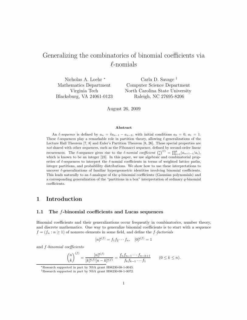
Generalizing the combinatorics of binomial coefficients via

ℓ-nomials

Nicholas A. Loehr ∗

Mathematics Department

Virginia Tech

Blacksburg, VA 24061-0123

Carla D. Savage †

Computer Science Department

North Carolina State University

Raleigh, NC 27695-8206

August 26, 2009

Abstract

An ℓ-sequence is defined by an = ℓan−1 − an−2, with initial conditions a0 = 0, a1 = 1.These ℓ-sequences play a remarkable role in partition theory, allowing ℓ-generalizations of theLecture Hall Theorem [7, 8] and Euler’s Partition Theorem [8, 26]. These special properties arenot shared with other sequences, such as the Fibonacci sequence, defined by second-order linear

recurrences. The ℓ-sequence gives rise to the ℓ-nomial coefficient`

n

k

´(ℓ)=

Q

k

i=1(an+1−i/ai),which is known to be an integer [23]. In this paper, we use algebraic and combinatorial prop-erties of ℓ-sequences to interpret the ℓ-nomial coefficients in terms of weighted lattice paths,integer partitions, and probablility distributions. We show how to use these interpretations touncover ℓ-generalizations of familiar hypergeometric identities involving binomial coefficients.This leads naturally to an ℓ-analogue of the q-binomial coefficients (Gaussian polynomials) anda corresponding generalization of the “partitions in a box” interpretation of ordinary q-binomialcoefficients.

1 Introduction

1.1 The f-binomial coefficients and Lucas sequences

Binomial coefficients and their generalizations occur frequently in combinatorics, number theory,and discrete mathematics. One way to generalize binomial coefficients is to start with a sequencef = (fn : n ≥ 1) of nonzero elements in some field, and define the f -factorials

[n]!(f) = f1f2 · · · fn, [0]!(f) = 1

and f -binomial coefficients(

n

k

)(f)

=[n]!(f)

[k]!(f)[n − k]!(f)=

fnfn−1 · · · fn−k+1

fkfk−1 · · · f1(0 ≤ k ≤ n).

∗Research supported in part by NSA grant H98230-08-1-0045.†Research supported in part by NSA grant H98230-08-1-0072.

1

In many cases of interest, these f -binomial coefficients satisfy certain integrality properties.

Example 1. (a) If fn = n for all n,(

nk

)(f)is the usual binomial coefficient, which is always an

integer. (b) Let q be a variable, and let fn = 1 + q + q2 + · · · + qn−1 = [n]q for n ≥ 1. Then(

nk

)(f)=

[

nk

]

qis the q-binomial coefficient, which is known to be a polynomial in q with nonnegative

integer coefficients (a Gaussian polynomial). (c) If f is the Fibonacci sequence, the quantities(

nk

)(f)

are known to be integers [23], which Hoggatt termed Fibonomials in 1967 [15].

The third example generalizes as follows. Any sequence defined by a recurrence fn = sfn−1 +tfn−2, for integers s and t, with initial conditions (f0, f1) = (0, 1) or (1, s) is known as a Lucassequence. The Fibonacci sequence is one example, as are the ℓ-sequences defined below. Lucassequences are well-studied and are known to have many striking properties, both number-theoreticand combinatorial (see, e.g., [5, 9, 10, 21, 22, 23]). They are even the basis for a proposed public-keycryptosystem, LUC [27].

Dating back at least to the work of Lucas (1878) and Carmichael, it has been known that thef -binomial coefficients are integers when f is a Lucas sequence with initial conditions (f0, f1) =(0, 1) [23, p. 203]. Both number-theoretic and algebraic properties of these f -binomial coefficientshave been studied, especially in the case when f is the Fibonacci sequence [15]. Related work canbe found in [14, 16, 18, 19, 30]. As for combinatorial interpretations, a poset interpretation ofthe Fibonomials was proposed in [20] and recently a tiling interpretation in [4]. Alexanderson andKlosinski [1] confirmed that the q-analogues of the f -binomial coefficients, for Lucas sequences withinitial conditions (f0, f1) = (0, 1), are polynomials with nonnegative integer coefficients. Picon [24]has shown that iterated substitutions of Lucas numbers (defined by f ′

n = ffn, etc.) preserve certain

quotients, such as the one used to define f -binomial coefficients.

1.2 Motivation for studying ℓ-sequences and ℓ-nomial coefficients

The goal of this paper is to give a detailed development of the combinatorial properties of the f -binomial coefficients obtained from ℓ-sequences. These are Lucas sequences given by a0 = 0, a1 = 1,and an = ℓan−1−an−2 for all n ≥ 2, where ℓ ≥ 2 is a fixed integer. We call the a-binomial coefficients

associated to ℓ-sequences ℓ-nomial coefficients and denote them(

nk

)(ℓ).

Why do ℓ-sequences and ℓ-nomial coefficients merit special study? On one hand, the ℓ-sequencesstand out among all Lucas sequences as being a generalization of the nonnegative integers (thecase ℓ = 2). On the other hand, one of our principal motivations in studying ℓ-sequences is theirunexpected appearance in partition theory via the Generalized Lecture Hall Theorem of Bousquet-Melou and Eriksson [7, 8]:

The number of partitions λ = (λ1, λ2, . . . , λn) of N satisfying

λ1

an≥ λ2

an−1≥ λ3

an−2≥ . . . ≥ λn

a1≥ 0 (1)

is equal to the number of partitions of N into parts from the set

{ai + ai−1 | 1 ≤ i ≤ n}.

2

In particular, this theorem says that the generating function for those partitions satisfying theconstraints (1) is

∏ni=1(1 − qai+ai−1)−1. No analogous partition-theoretic results are known for any

other Lucas sequence.

The Generalized Lecture Hall Theorem depends on a polynomial analogue of the fact that forℓ-sequences, the following ratio is integral for all n ≥ 0:

(an)(an + an−1)(an + an−1 + an−2) · · · (an + an−1 + . . . + a1)

anan−1 · · · a1. (2)

It appears that among Lucas sequences, the ℓ-sequences are unique in having this property (this isrelated to a conjecture in [8]).

The ℓ-sequences also play a surprising role in the following generalization of Euler’s Odd-DistinctPartition Theorem, which can be viewed as a certain limit of the Lecture Hall Theorem:

The ℓ-Euler Theorem [8, 26]: Let u = (ℓ +√

ℓ2 − 4)/2. The number of partitions ofN in which the ratio of consecutive parts exceeds u is equal to the number of partitionsof N from the set

{ai + ai−1 | i ≥ 1}.

(When ℓ = 2 this says that the number of partitions of N into distinct parts is equal to the numberof partitions of N into odd parts.)

Although we will not deal explicitly with these partition theorems in the present paper, we hopethat the combinatorics developed here will aid in the resolution of several open problems concerningthe role of ℓ-sequences in partition theory. We shall say more about these problems in Section 5.

1.3 Organization of the paper and main results

Section 2 develops some algebraic and combinatorial properties of (an) and more general ℓ-sequences.For our later work, the most important results in this section are Theorem 9, which gives severalexpressions for ar+s in terms of ar and as, and Theorem 13, which shows that (an) and relatedsequences are enumerators for certain regular languages. The words in these languages are theso-called ℓ-admissible sequences, which provide unique representations for nonnegative integers gen-eralizing base-b expansions. Such sequences were used in [26] for the combinatorial proof of theℓ-Euler theorem, but were discovered earlier by Fraenkel [13] in the context of games.

Our main contributions begin in Section 3. Some general theorems on f -binomial coefficientsare used to deduce two-term recurrences, fermionic formulas, and combinatorial interpretations forℓ-nomial coefficients. One combinatorial model involves weighted lattice paths; other models general-ize integer partitions by filling the Ferrers diagram of a partition with certain ℓ-admissible sequences.These fillings reduce to ordinary partitions in the case ℓ = 2, where only the all-zero sequence isallowed. Section 3.3 explains the relationship between ℓ-nomial coefficients and q-binomial coeffi-

cients. Some consequences include another proof of the integrality of(

nk

)(ℓ)and an ℓ-generalization

of the Chu-Vandermonde identity. We show in Section 3.4 that the ℓ-nomial coefficients satisfy aparticularly simple three-term recurrence. This leads to ℓ-generalizations of the binomial theorem(Section 3.5) and a probabilistic interpretation of ℓ-nomial coefficients in terms of weighted coins(Section 3.6).

3

Section 4 investigates a q-analogue of the ℓ-nomial coefficient. We use a general theorem on(f ◦ f ′)-binomial coefficients to obtain a recurrence characterizing the q-ℓ-nomial coefficients. Thisrecurrence not only proves the positivity and polynomiality of these coefficients, but also leads toa combinatorial formula involving the filled partitions from Section 3. This formula generalizes theusual partition-theoretic interpretation of the q-binomial coefficients.

We conclude in Section 5 by suggesting future directions for study.

2 ℓ-sequences

It will be useful in the sequel to work with the following somewhat more general notion of anℓ-sequence.

Definition 2. Given an integer ℓ ≥ 2, an ℓ-sequence is a sequence (sn)n∈Z of real numbers suchthat sn = ℓsn−1 − sn−2 for all n ∈ Z.

An ℓ-sequence (sn) is uniquely determined by any two consecutive values in the sequence, e.g.,s0 and s1. A linear combination of ℓ-sequences is also an ℓ-sequence. It follows that the set of allℓ-sequences (for a fixed ℓ) is a two-dimensional real vector space. If (sn)n∈Z is an ℓ-sequence andk ∈ Z, then (sn+k)n∈Z and (s−n)n∈Z are ℓ-sequences.

Definition 3. Given an integer ℓ ≥ 2, let a(ℓ), d(ℓ), and p(ℓ) be the unique ℓ-sequences with initialconditions

a(ℓ)0 = 0, a

(ℓ)1 = 1; d

(ℓ)0 = 1, d

(ℓ)1 = 1; p

(ℓ)0 = 2, p

(ℓ)1 = ℓ.

We haved(ℓ)i = a

(ℓ)i − a

(ℓ)i−1 (i ∈ Z),

since both sides are ℓ-sequences that agree for i = 0, 1. Similarly,

p(ℓ)i = a

(ℓ)i+1 − a

(ℓ)i−1 (i ∈ Z).

Example 4. When ℓ = 2, a(2)i = i, d

(2)i = 1, and p

(2)i = 2 for all i ∈ Z. When ℓ = 3,

(a(3)i : i ≥ 0) = (0, 1, 3, 8, 21, 55, 144, 377, 987, 2584, . . .)

(d(3)i : i ≥ 0) = (1, 1, 2, 5, 13, 34, 89, 233, 610, 1597, . . .)

(p(3)i : i ≥ 0) = (2, 3, 7, 18, 47, 123, 322, 843, 2207, 5778, . . .).

One may check that a(3)n = F2n and d

(3)n = F2n−1, where Fi is the i’th Fibonacci number (F0 = 0,

F1 = 1, Fi = Fi−1 +Fi−2). Similarly, p(3)n = L2n where Li is the i’th Lucas number (L0 = 2, L1 = 1,

Li = Li−1 + Li−2). We see that one can recover ordinary integers from ℓ-sequences (when ℓ = 2) orFibonacci and Lucas numbers (when ℓ = 3).

Henceforth, we will omit ℓ’s from the notation when there is no danger of confusion.

Many identities are known for general Lucas sequences, as well as various combinatorial inter-pretations (see, e.g., [5, 9, 21, 23]). In the rest of this section, we highlight and prove some that aremost relevant for our work with ℓ-sequences.

4

2.1 Algebraic properties of ℓ-sequences

Definition 5. Let u = uℓ and v = vℓ be the roots of the polynomial x2 − ℓx + 1, namely

uℓ =ℓ +

√ℓ2 − 4

2, vℓ =

ℓ −√

ℓ2 − 4

2.

Observe thatuℓ + vℓ = ℓ; uℓvℓ = 1.

Theorem 6. For ℓ > 2, the sequences U = (unℓ : n ∈ Z) and V = (vn

ℓ : n ∈ Z) form a basis for thevector space of ℓ-sequences. Moreover,

a(ℓ)n =

unℓ − vn

ℓ

uℓ − vℓ, p(ℓ)

n = unℓ + vn

ℓ .

Proof. For all n ∈ Z, un = un−2u2 = un−2(ℓu− 1) = ℓun−1 − un−2, so U is an ℓ-sequence. SimilarlyV is an ℓ-sequence. Noting that U0 = 1 = V0 and U1 = u 6= v = V1 (since ℓ > 2), we see that{U, V } is linearly independent, hence a basis for the two-dimensional space of ℓ-sequences. Thestated expansions for a(ℓ) and p(ℓ) follow since the two sides agree for n = 0 and n = 1.

For any ℓ ≥ 2 and any real number r, we define pr = p(ℓ)r by the formula pr = ur + vr. Since

uv = 1, it follows thatp−r = pr, p2

r = p2r + 2 (r ∈ R). (3)

Theorem 7. Let (sn)n∈Z be an ℓ-sequence. For n, k ∈ Z, define

g(n, k) = snsk − sn−1sk−1.

(a) For fixed k, (g(n, k))n∈Z is an ℓ-sequence. (b) For all n, k ∈ Z, g(n, k) = g(n − 1, k + 1). (c) Ifs0 = 0 or ℓs0 = 2s1, then g(n, k) = (s2

1 − s20)an+k−1. (d) If s0 = s1, then g(n, k) = s2

0(ℓ− 2)an+k−2.

Proof. (a) holds because (g(n, k))n∈Z is a linear combination of ℓ-sequences. For (b), compute

g(n, k) = snsk − sn−1sk−1 = (ℓsn−1 − sn−2)sk − sn−1sk−1

= sn−1(ℓsk − sk−1) − sn−2sk = sn−1sk+1 − sn−2sk = g(n − 1, k + 1).

(c) Assuming s0 = 0 or ℓs0 = 2s1, we must show that the two ℓ-sequences (g(n, k))n∈Z and ((s21 −

s20)an+k−1)n∈Z have the same values when n = k and n = k + 1. Iteration of (b) gives

g(k, k) = g(k − 1, k + 1) = · · · = g(1, 2k − 1) = s1s2k−1 − s0s2k−2;

g(k + 1, k) = g(k, k + 1) = · · · = g(1, 2k) = s1s2k − s0s2k−1.

It now suffices to show that the ℓ-sequences (s1st−s0st−1)t∈Z and ((s21−s2

0)at)t∈Z are equal. Again,we do this by comparing the initial values t = 0 and t = 1. Both sequences evaluate to s2

1 − s20 when

t = 1. When t = 0, (s21 − s2

0)a0 = 0 = s1s0 − s0s−1, since the hypothesis of (c) guarantees thats0 = 0 or s−1 = ℓs0 − s1 = s1.

(d) Assume s0 = s1. As in (c), we are reduced to verifying that the ℓ-sequences (s1st−s0st−1)t∈Z

and (s20(ℓ− 2)at−1)t∈Z agree for t = 1 and t = 2. Both sequences are zero when t = 1, since s0 = s1.

When t = 2,s1s2 − s0s1 = ℓs2

1 − 2s0s1 = s20(ℓ − 2)a1.

5

Corollary 8. For all n, k ∈ Z,

anak−an−1ak−1 = an+k−1; dndk−dn−1dk−1 = (ℓ−2)an+k−2; pnpk−pn−1pk−1 = (ℓ2−4)an+k−1.

Theorem 9. For all r, s ∈ Z,

ar+s = dsar + dr+1as = ds+1ar + dras

= −as−1ar + ar+1as = as+1ar − ar−1as

= usar + vras = vsar + uras

= (ps/2)ar + (pr/2)as.

Proof. By the first part of the preceding corollary,

dsar + dr+1as = (as − as−1)ar + (ar+1 − ar)as = ar+1as − aras−1 = ar+s;

ds+1ar + dras = (as+1 − as)ar + (ar − ar−1)as = as+1ar − asar−1 = ar+s;

ar+1as − aras−1 = ar+s = as+1ar − asar−1.

On the other hand,

usar + vras = (u − v)−1(us(ur − vr) + vr(us − vs)) = (u − v)−1(ur+s − vr+s) = ar+s;

vsar + uras = (u − v)−1(vs(ur − vr) + ur(us − vs)) = (u − v)−1(ur+s − vr+s) = ar+s.

Adding these equations and dividing by 2 gives (ps/2)ar + (pr/2)as = ar+s.

The proof of Theorem 7 can be readily adapted to establish the following theorem.

Theorem 10. Let (sn)n∈Z be an ℓ-sequence. For n, k ∈ Z, define

f(n, k) = sn−1sk − snsk−1.

(a) For fixed k, (f(n, k))n∈Z is an ℓ-sequence. (b) For all n, k ∈ Z, f(n, k) = f(n − 1, k − 1). (c)For all n, k ∈ Z, f(n, k) = (s2

0 + s21 − ℓs0s1)an−k.

Corollary 11. For all n, k ∈ Z,

an−1ak − anak−1 = an−k; dn−1dk − dndk−1 = (2 − ℓ)an−k; pn−1pk − pnpk−1 = (4 − ℓ2)an−k.

2.2 Combinatorial properties of ℓ-sequences

This section describes some collections of combinatorial objects that are counted by the integers

a(ℓ)n , d

(ℓ)n , and p

(ℓ)n .

Definition 12. For ℓ ≥ 2, an ℓ-admissible word is a word w = w1w2 · · ·wn with 0 ≤ wi < ℓ forall i, such that w contains no subword matching the pattern (ℓ − 1)(ℓ − 2)∗(ℓ − 1), where (ℓ − 2)∗

denotes zero or more occurrences of ℓ − 2. Let W = W (ℓ) be the set of all ℓ-admissible words. LetW ′ (resp. W ′′) be the subset of W consisting of words that do not begin with 0 (resp. 00). For anyset Z of words, let Zn be the set of words in Z of length n. Finally, let W †

n be the set of words inWn that weakly precede the word (ℓ − 2)n in lexicographic order.

6

Theorem 13. For all ℓ ≥ 2: (a) an = |Wn−1| for n ≥ 0; (b) dn = |W ′n−1| = |W †

n−1| for n ≥ 1; (c)pn = |W ′′

n | for n ≥ 1.

Proof. (a) First Proof: Let sn = |Wn−1| for n ≥ 0. We have s0 = 0 = a0 and s1 = 1 = a1, so itsuffices to prove ℓsn−1 = sn + sn−2 for n ≥ 2. We define a bijection h : Wn−2 × {0, 1, . . . , ℓ − 1} →Wn−1 ∪ Wn−3. Fix (w, x) with w ∈ Wn−2 and 0 ≤ x < ℓ. If wx is admissible, let h(w, x) = wx ∈Wn−1. Otherwise, w ends in (ℓ−1)(ℓ−2)∗ and x = ℓ−1, and we define h(w, x) = w1 · · ·wn−3 ∈ Wn−3.To invert h, map z = w1 · · ·wn−1 ∈ Wn−1 to (w1 · · ·wn−2, wn−1), and map z ∈ Wn−3 to (zy, ℓ− 1),where y = ℓ − 2 if z ends in (ℓ − 1)(ℓ − 2)∗, and y = ℓ − 1 otherwise.

Second Proof: Define a “norm map” N : W(ℓ)n−1 → {0, 1, . . . , a

(ℓ)n − 1} by N(w1 · · ·wn−1) =

∑n−1i=1 wia

(ℓ)n−i. It was shown in [26] that N is a bijection such that w ≤lex v in Wn−1 iff N(w) ≤ N(v).

(b) Now let sn = |W ′n−1| for n ≥ 1. Note s1 = 1 = d1 and s2 = ℓ−1 = d2. For n ≥ 3, it is routine

to check that the bijection h defined in part (a) restricts to a bijection h′ : W ′n−2×{0, 1, . . . , ℓ−1} →

W ′n−1 ∪ W ′

n−3, which proves that (sn) and (dn) satisfy the same recursion. Thus, sn = dn for alln ≥ 1. Alternatively, since W ′

n = Wn ∼ {0w : w ∈ Wn−1}, we can deduce |W ′n−1| = dn from (a)

and dn = an − an−1.

Recall that the norm bijection N is compatible with the lexicographic ordering on words. So, toprove that |W †

n−1| = dn, it suffices to verify that the norm of (ℓ − 2)n−1 is dn − 1, or equivalently(ℓ − 2)(a1 + a2 + · · · + an−1) = an − an−1 − 1 for all n ≥ 1. This identity is true for n = 1 andn = 2. Assuming by induction that the identity holds for some n ≥ 2, then the identity also holdsfor n + 1, since

(ℓ − 2)(a1 + · · · + an) = (ℓ − 2)(a1 + · · · + an−1) + (ℓ − 2)an

= (an − an−1 − 1) + ℓan − 2an

= (ℓan − an−1) − an − 1 = an+1 − an − 1.

(c) Now let sn = |W ′′n | for n ≥ 1. Note s1 = ℓ = p1 and s2 = ℓ2 − 2 = p2. For n ≥ 3, it

is routine to check that the bijection h defined in part (a) (with n replaced by n + 1) restricts toa bijection h′′ : W ′′

n−1 × {0, 1, . . . , ℓ − 1} → W ′′n ∪ W ′′

n−2, which proves that (sn) and (pn) satisfythe same recursion. Thus, sn = pn for all n ≥ 1. Alternatively, (c) can be proved using (a) andpn = an+1 − an−1.

Example 14. For ℓ = 3, the 21 words in W3 (in lexicographic order) are:

000 001 002 010 011 012 020 021100 101 102 110 111 112 120 121200 201 202 210 211.

W ′3 consists of the 13 words in the second and third rows, whereas W †

3 consists of the 13 wordsup to and including 111. W ′′

3 consists of the 18 words following 002. We have |W3| = 21 = a4,

|W ′3| = |W †

3 | = 13 = d4, and |W ′′3 | = 18 = p3.

By using an obvious modification of the bijection h in the first proof of Theorem 13(a), one canalso obtain the following result.

Proposition 15. Suppose ℓ ≥ 2, n ≥ 0, and i, j are distinct elements of A = {0, 1, . . . , ℓ−1}. Then

a(ℓ)n is the number of words in An−1 in which i is never immediately followed by j.

7

f

e

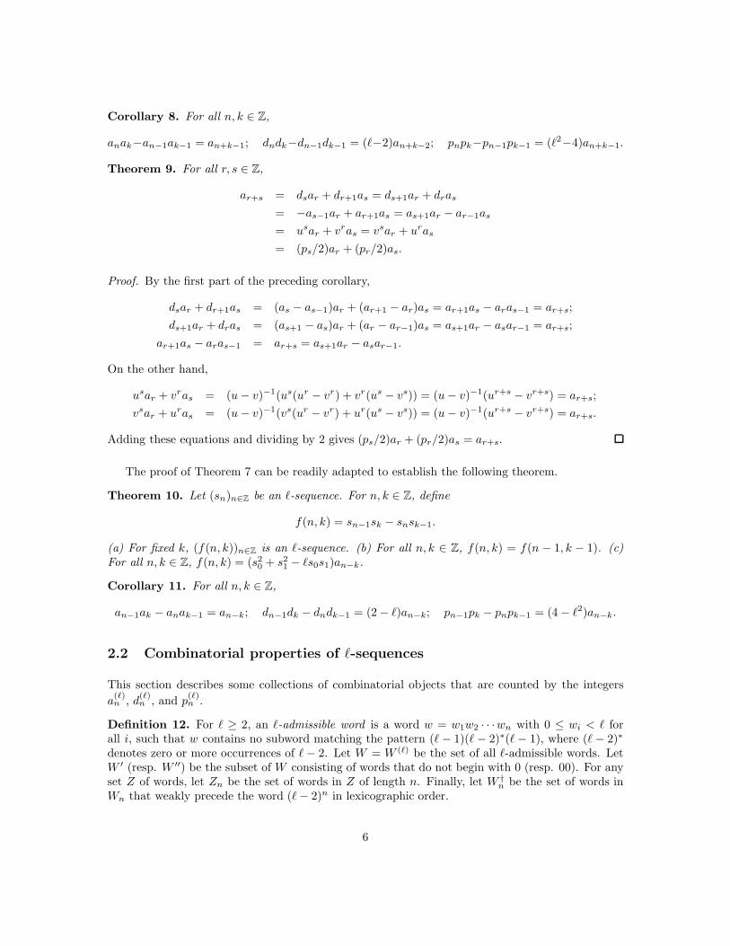
Figure 1: Example of G(6)5 .

The integers a(ℓ)n also have the following graph-theoretic interpretation. (This generalizes prob-

lems 2.2.15 and 2.2.16 in [31].)

Theorem 16. For ℓ ≥ 3 and m ≥ 1, let Gm = G(ℓ)m be any graph consisting of a sequence of

m ℓ-cycles such that neighboring cycles in the sequence share a common edge (see Figure 1 for an

example with ℓ = 6 and m = 5). The number of spanning trees of G(ℓ)m is a

(ℓ)m+1.

Proof. Define G0 to be one of the edges of G1 not belonging to G2. For each m ≥ 0, let Tm be theset of spanning trees of Gm, and let tm = |Tm|. Then t0 = 1 = a1. It suffices to show that t1 = a2

and tm = ℓtm−1 − tm−2 for all m ≥ 2. When m = 1, G(ℓ)m is a single ℓ-cycle. We obtain a spanning

tree by removing any one edge from this cycle, so t1 = ℓ = a2. We now fix m ≥ 2 and prove thatℓtm−1 = tm + tm−2. The expression ℓtm−1 counts pairs (e, T ) where T is a spanning tree of Gm−1

and e is one of the edges on the ℓ-cycle C that we add to Gm−1 to get Gm. It suffices to define abijection h from the set of such pairs to Tm ∪ Tm−2. Let f be the unique edge that belongs to bothC and Gm−1. If e 6= f , let h(e, T ) be the spanning tree of Gm obtained by adding all edges of Cexcept e and f to T . If e = f is an edge of T , let h(e, T ) be the spanning tree of Gm obtained bydeleting e from T and replacing it with all the other edges in C. If e = f is not an edge of T , leth(e, T ) be the spanning tree of Gm−2 obtained by erasing all edges in T that are edges of Gm−1 butnot edges of Gm−2. It is routine to check that h is a bijection.

3 The ℓ-nomial coefficients

Recall that the ℓ-nomial coefficients are defined by

(

n

k

)(ℓ)

=a(ℓ)n a

(ℓ)n−1 · · ·a

(ℓ)n−k+1

a(ℓ)k a

(ℓ)k−1 · · ·a

(ℓ)1

(0 ≤ k ≤ n).

For example,(

9

4

)(3)

=2584 · 987 · 377 · 144

21 · 8 · 3 · 1 = 174, 715, 376.

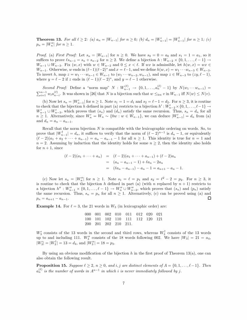
Figure 2 depicts the beginning of “Pascal’s triangle” for 3-nomial coefficients, in which row n from

the top contains(

nk

)(3)for 0 ≤ k ≤ n.

8

11 1

1 3 11 8 8 1

1 21 56 21 11 55 385 385 55 1

1 144 2640 6930 2640 144 1

Figure 2: Pascal’s triangle for 3-nomial coefficients.

3.1 Two-term recursions

Recall that the usual binomial coefficients satisfy the recursion(

nk

)

=(

n−1k

)

+(

n−1k−1

)

. This can be

written more symmetrically using multinomial coefficients as(

r+sr,s

)

=(

r+s−1r−1,s

)

+(

r+s−1r,s−1

)

, for r, s > 0.We would like to find analogous recursions for ℓ-nomial coefficients. We will deduce these from the

following general result for the f -binomial coefficients defined by(

r+sr,s

)(f)= [r+s]!(f)

[r]!(f)[s]!(f) .

Theorem 17. Suppose f = (f(n) : n ∈ N+) is a sequence of nonzero field elements, and g1, g2 are

functions defined on N+ × N

+ such that

f(r + s) = g1(r, s)f(r) + g2(r, s)f(s) (r, s ∈ N+). (4)

Then the f -binomial coefficients satisfy the recursion

(

r + s

r, s

)(f)

= g1(r, s)

(

r + s − 1

r − 1, s

)(f)

+ g2(r, s)

(

r + s − 1

r, s − 1

)(f)

(r, s > 0) (5)

and initial conditions(

rr,0

)(f)= 1 =

(

s0,s

)(f).

Proof. Dividing both sides of (5) by the nonzero common factor [r+s−1]!(f)

[r−1]!(f)[s−1]!(f) , we see that (5) is

equivalent tof(r + s)

f(r)f(s)=

g1(r, s)

f(s)+

g2(r, s)

f(r),

which is clearly equivalent to (4).

Corollary 18. For all ℓ ≥ 2 and all r, s > 0,

(

r + s

r, s

)(ℓ)

= ds

(

r + s − 1

r − 1, s

)(ℓ)

+ dr+1

(

r + s − 1

r, s − 1

)(ℓ)

= ds+1

(

r + s − 1

r − 1, s

)(ℓ)

+ dr

(

r + s − 1

r, s − 1

)(ℓ)

= −as−1

(

r + s − 1

r − 1, s

)(ℓ)

+ ar+1

(

r + s − 1

r, s − 1

)(ℓ)

= as+1

(

r + s − 1

r − 1, s

)(ℓ)

− ar−1

(

r + s − 1

r, s − 1

)(ℓ)

= us

(

r + s − 1

r − 1, s

)(ℓ)

+ vr

(

r + s − 1

r, s − 1

)(ℓ)

= vs

(

r + s − 1

r − 1, s

)(ℓ)

+ ur

(

r + s − 1

r, s − 1

)(ℓ)

=ps

2

(

r + s − 1

r − 1, s

)(ℓ)

+pr

2

(

r + s − 1

r, s − 1

)(ℓ)

In particular, each ℓ-nomial coefficient is a positive integer.

9

Proof. The recursions follow from Theorem 9 and Theorem 17. The integrality assertion followsfrom the first recursion by induction on r + s.

3.2 Annotated lattice paths and partitions

It is well-known that the ordinary binomial coefficient(

r+sr,s

)

counts lattice paths from (0, 0) to (r, s),

which can be identified with words consisting of r copies of E (east step) and s copies of N (northstep). This follows from the recursion

(

r+sr,s

)

=(

r+s−1r−1,s

)

+(

r+s−1r,s−1

)

, which classifies such paths based

on whether they arrive at (r, s) via an east step or a north step. By iterating the recursion (5), weobtain the following analogous result for f -binomial coefficients.

Theorem 19. Assume f(r + s) = g1(r, s)f(r) + g2(r, s)f(s) as in Theorem 17. Let P (r, s) bethe set of lattice paths from (0, 0) to (r, s). For π ∈ P (r, s), let E(π) (resp. N(π)) be the set of(x, y) ∈ N

+ × N+ such that π arrives at (x, y) by an east (resp. north) step. Then, for all r, s ∈ N,

(

r + s

r, s

)(f)

=∑

π∈P (r,s)

∏

(x,y)∈E(π)

g1(x, y)∏

(x,y)∈N(π)

g2(x, y).

If g1 and g2 take values in N (or in N[q]), we obtain a combinatorial interpretation for(

r+sr,s

)(f)

as counting annotated lattice paths ending at (r, s), in which each lattice point (x, y) on the pathin the positive quadrant is labeled by an object counted by g1(x, y) (if (x, y) is reached by an eaststep) or by g2(x, y) (if (x, y) is reached by a north step).

In particular, the first two formulas in Corollary 18 give two interpretations for ℓ-nomial coef-ficients in which points on the lattice path are labeled by words in the language W ′ or W † (seeTheorem 13). If we allow signed objects, the next two formulas in the corollary give interpretationswhere the labels come from the language W . Finally, if we multiply through by suitable powers of

2, the last formula in the corollary gives a combinatorial formula for 2r+s(

r+sr,s

)(ℓ)in which lattice

points are labeled by words in the language W ′′. (One can show that every ps is even for ℓ even, soin this case, we can avoid the extra powers of 2 by passing to a language in which we retain half thewords in each W ′′

n .)

Next we reformulate Theorem 19 in terms of integer partitions. By considering the array oflattice squares to the left of a lattice path, we can identify lattice paths π ending at (r, s) withpartitions λ that fit in an s × r box, i.e., with integer sequences λ = (λ1, . . . , λs) such that

r ≥ λ1 ≥ λ2 ≥ · · · ≥ λs ≥ 0.

Let λ∗ be the complementary partition located below the lattice path (where the parts of λ∗ givethe column heights from right to left), so

s ≥ λ∗1 ≥ λ∗

2 ≥ · · · ≥ λ∗r ≥ 0.

Then a lattice point (x, y) is in N(π) iff λs+1−y = x > 0, whereas a lattice point (x, y) is in E(π) iffλ∗

r+1−x = y > 0. We can now restate Theorem 19 as follows.

Theorem 20. Assume f(r + s) = g1(r, s)f(r) + g2(r, s)f(s) as in Theorem 17. Let P (r, s) be theset of integer partitions that fit in an s × r box. Then, for all r, s ∈ N,

(

r + s

r, s

)(f)

=∑

λ∈P (r,s)

∏

j:λ∗j>0

g1(r + 1 − j, λ∗j )

∏

i:λi>0

g2(λi, s + 1 − i).

10

1

0 0 0 00(0,0)

(5,4)

0 1 1

0

1

1

1

1 0 2

1 0 2 0

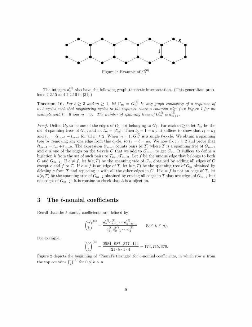
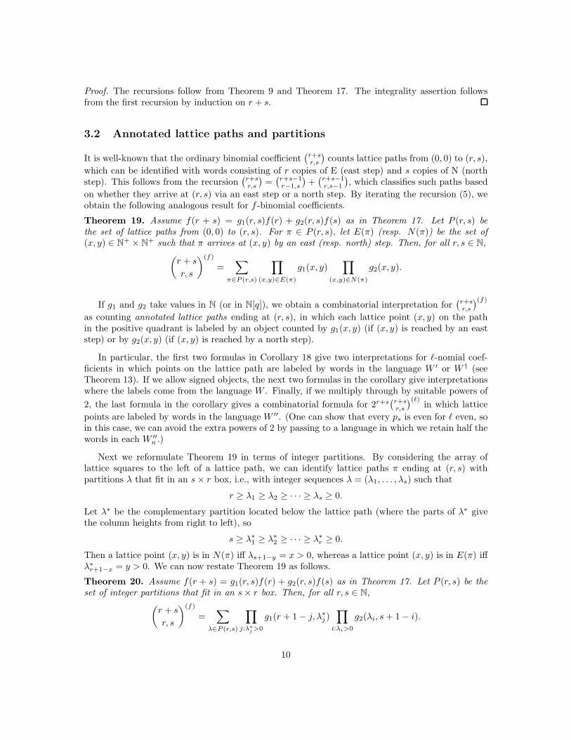
Figure 3: An object counted by(

95,4

)(3).

Example 21. Combining Corollary 18 and Theorem 20, we can write down various “fermionicformulas” expressing ℓ-nomial coefficients as sums of products of a’s, d’s, or p’s. For example,

(

r + s

r, s

)(ℓ)

=∑

λ∈P (r,s)

dλ1+1dλ2+1 · · ·dλ∗1dλ∗

2· · ·

=∑

λ∈P (r,s)

(−1)len(λ∗)aλ1+1aλ2+1 · · · aλ∗1−1aλ∗

2−1 · · ·

= 2−(r+s)∑

λ∈P (r,s)

pλ1pλ2 · · · pλ∗1pλ∗

2· · · ,

where subscripts range over the nonzero λi and λ∗j . We can interpret these formulas combinatorially

by filling the rows of λ and columns of λ∗ with suitable words counted by the a’s, d’s, or p’s (see

Theorem 13). For example, the first equation above tells us that(

r+sr,s

)(ℓ)counts objects constructed

as follows: start with a partition λ ∈ P (r, s); fill each nonzero row of λ (from left to right) with

a word in W †λi

; fill each nonzero column of λ∗ (from bottom to top, say) with a word in 0W †λ∗

j−1.

(The initial zero is added so that every box in the s × r rectangle is filled. One could also use the

languages W ′n instead of W †

n.) For example, Figure 3 illustrates one object counted by(

95,4

)(3).

As in Example 21, we obtain a simple “semi-combinatorial” interpretation of the ℓ-nomial coef-ficient by taking g1(r, s) = us and g2(r, s) = vr:

(

r + s

r, s

)(ℓ)

=∑

λ∈P (r,s)

u|λ|v|λ∗|. (6)

This formula expresses the ℓ-binomial coefficient as a sum over weighted partitions in an s × r box,where the real-valued weight is obtained by filling each box of λ with u = uℓ, filling each box of λ∗

with v = vℓ, and multiplying together the numbers in all the boxes. Here is one application of thisformula.

Theorem 22. For all n ≥ 0 and ℓ ≥ 2,

∞∑

k=0

(

n + k

n, k

)(ℓ)

zk =

n∏

i=0

1

(1 − zuivn−i).

Proof. The left side counts partitions λ ∈⋃

k≥0 P (n, k), weighted by zku|λ|v|λ∗|. The right side

builds all such partitions by choosing, for each i ≤ n, the number of parts of λ equal to i. Each such

11

part contributes zuivn−i to the weight, and the geometric series factor (1 − zuivn−i)−1 allows anynumber of such parts to be chosen.

3.3 Comparison to q-binomial coefficients

There is a close connection between ℓ-nomial coefficients and q-binomial coefficients (see Exam-ple 1(b)). To describe this, we introduce homogenized versions of the q-binomial coefficients. Let xand y be variables, and define

[

r + s

r, s

]

x,y

=

(

r + s

r, s

)(f)

where f(n) = xn−1 + xn−2y1 + xn−3y2 + · · · + yn−1 =xn − yn

x − y(n ≥ 1).

Note that[

r+sr,s

]

q=

[

r+sr,s

]

q,1=

[

r+sr,s

]

1,q. We clearly have

f(r + s) = ysf(r) + xrf(s) = xsf(r) + yrf(s) (r, s > 0).

Using Theorem 17 and Theorem 20, we deduce[

r + s

r, s

]

x,y

= ys

[

r + s − 1

r − 1, s

]

x,y

+ xr

[

r + s − 1

r, s − 1

]

x,y

= xs

[

r + s − 1

r − 1, s

]

x,y

+ yr

[

r + s − 1

r, s − 1

]

x,y

=∑

λ∈P (r,s)

x|λ|y|λ∗| ∈ N[x, y].

Comparing these formulas to those in the last subsection, we see that

(

r + s

r, s

)(ℓ)

=

[

r + s

r, s

]

x,y

∣

∣

∣

∣

∣

x=u,y=v

. (7)

Thus, the ℓ-nomial coefficients are just a particular specialization of the (homogenized) q-binomialcoefficients. We can therefore use known q-binomial identities to deduce identities (involving uand v) for ℓ-nomial coefficients. The proof of Theorem 23 below (which is an ℓ-analogue of theChu-Vandermonde identity) illustrates how this technique can be used to derive integer identities.

We should point out that many combinatorial properties of the ℓ-nomial coefficients are notalways evident from the description in terms of q-binomial coefficients, since u and v are real num-bers. For instance, the integrality of the ℓ-nomial coefficients is not immediately clear from (7).Nevertheless, we can use that equation to give another proof of this integrality, as follows. We seefrom the definitions that

[

r+sr,s

]

x,yis a symmetric polynomial in the variables x and y with integer

coefficients. Therefore, by the fundamental theorem of symmetric polynomials [29], there exists atwo-variable polynomial g with integer coefficients such that

[

r+sr,s

]

x,y= g(e1(x, y), e2(x, y)), where

e1(x, y) = x+y and e2(x, y) = xy are the elementary symmetric polynomials in x and y. Specializing

x = uℓ and y = vℓ, we know that e1(x, y) = ℓ and e2(x, y) = 1 (Definition 5). Thus,(

r+sr,s

)(ℓ)= g(ℓ, 1)

is certainly an integer.

Theorem 23. For all C, D, E ∈ N,

(

C + D + E + 1

C + D + 1, E

)(ℓ)

=

E∑

i=0

(

D + i

D, i

)(ℓ)(C + E − i

C, E − i

)(ℓ) pi(C+1)−(E−i)(D+1)

2.

12

Proof. Classify lattice paths from (0, 0) to (C + D + 1, E) based on the height i of the east stepgoing from x = D to x = D + 1. Weighting area cells above the path by x and area cells below byy, we get

[

C + D + E + 1

C + D + 1, E

]

x,y

=

E∑

i=0

[

D + i

D, i

]

x,y

[

C + E − i

C, E − i

]

x,y

y(C+1)ix(D+1)(E−i).

Since the left side is symmetric in x and y, we also have

[

C + D + E + 1

C + D + 1, E

]

x,y

=

E∑

i=0

[

D + i

D, i

]

x,y

[

C + E − i

C, E − i

]

x,y

x(C+1)iy(D+1)(E−i).

Add these two identities, divide by 2, and set x = u, y = v. The proof is completed by observingthat unvm + umvn = (uv)n(vm−n + um−n) = pm−n = pn−m.

3.4 Three-term recursion

Theorem 24. For all ℓ ≥ 2 and all r, s ∈ N with r + s ≥ 2,

(

r + s

r, s

)(ℓ)

=

(

r + s − 2

r − 2, s

)(ℓ)

+ pr+s−1

(

r + s − 2

r − 1, s − 1

)(ℓ)

+

(

r + s − 2

r, s − 2

)(ℓ)

.

The initial conditions are(

00,0

)(ℓ)=

(

11,0

)(ℓ)=

(

10,1

)(ℓ)= 1 and

(

r+sr,s

)(ℓ)= 0 if r < 0 or s < 0.

Proof. If r ≥ 2 and s ≥ 2, we can use the recursions in Corollary 18 to compute

(

r + s

r, s

)(ℓ)

= us

(

r + s − 1

r − 1, s

)(ℓ)

+ vr

(

r + s − 1

r, s − 1

)(ℓ)

= us

[

vs

(

r + s − 2

r − 2, s

)(ℓ)

+ ur−1

(

r + s − 2

r − 1, s − 1

)(ℓ)]

+vr

[

vs−1

(

r + s − 2

r − 1, s − 1

)(ℓ)

+ ur

(

r + s − 2

r, s − 2

)(ℓ)]

.

Using usvs = vrur = 1 and us+r−1 + vr+s−1 = pr+s−1 completes the proof in this case. Now, if

r = 1 and s ≥ 1, the desired recursion becomes a(ℓ)s+1 = 0 + p

(ℓ)s + a

(ℓ)s−1, which is true. Similarly, the

result holds in the cases: s = 1 and r ≥ 1; s = 0 and r ≥ 2; r = 0 and s ≥ 2.

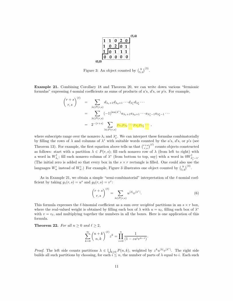
Theorem 25. For all ℓ ≥ 2 and r, s ∈ N,(

r+sr,s

)(ℓ)counts annotated lattice paths satisfying the

following conditions: (a) the path starts at (0, 0) or (1, 0) or (0, 1) and ends at (r, s); (b) each stepin the path is a long east step from (x− 2, y) to (x, y), or a long north step from (x, y − 2) to (x, y),or a diagonal step from (x−1, y−1) to (x, y); (c) each diagonal step, say ending at (x, y), is labeledwith a word in W ′′

x+y−1.

Proof. The labeled paths just described evidently satisfy the three-term recursion and initial condi-tions in Theorem 24, as we see by removing the last step in any such path ending at (r, s).

13

(9,6)

1 2

2

0

0 2 1 1 0 1

1

2

1

1

1 0 0 2 0 1 0 2 1

0

0

2

0

0(0,1)

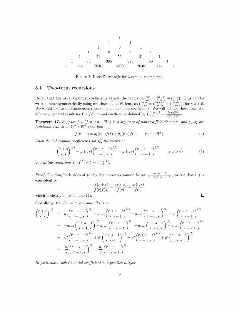
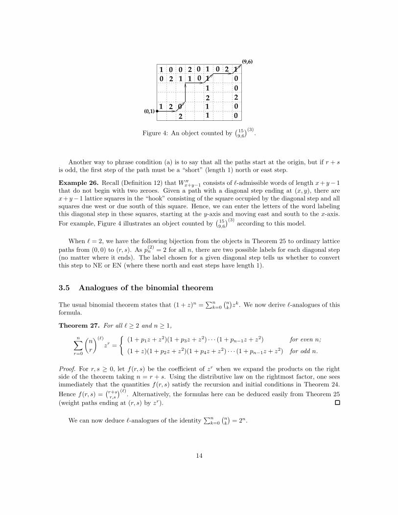
Figure 4: An object counted by(

159,6

)(3).

Another way to phrase condition (a) is to say that all the paths start at the origin, but if r + sis odd, the first step of the path must be a “short” (length 1) north or east step.

Example 26. Recall (Definition 12) that W ′′x+y−1 consists of ℓ-admissible words of length x+ y− 1

that do not begin with two zeroes. Given a path with a diagonal step ending at (x, y), there arex+ y−1 lattice squares in the “hook” consisting of the square occupied by the diagonal step and allsquares due west or due south of this square. Hence, we can enter the letters of the word labelingthis diagonal step in these squares, starting at the y-axis and moving east and south to the x-axis.

For example, Figure 4 illustrates an object counted by(

159,6

)(3)according to this model.

When ℓ = 2, we have the following bijection from the objects in Theorem 25 to ordinary lattice

paths from (0, 0) to (r, s). As p(2)n = 2 for all n, there are two possible labels for each diagonal step

(no matter where it ends). The label chosen for a given diagonal step tells us whether to convertthis step to NE or EN (where these north and east steps have length 1).

3.5 Analogues of the binomial theorem

The usual binomial theorem states that (1 + z)n =∑n

k=0

(

nk

)

zk. We now derive ℓ-analogues of thisformula.

Theorem 27. For all ℓ ≥ 2 and n ≥ 1,

n∑

r=0

(

n

r

)(ℓ)

zr =

{

(1 + p1z + z2)(1 + p3z + z2) · · · (1 + pn−1z + z2) for even n;

(1 + z)(1 + p2z + z2)(1 + p4z + z2) · · · (1 + pn−1z + z2) for odd n.

Proof. For r, s ≥ 0, let f(r, s) be the coefficient of zr when we expand the products on the rightside of the theorem taking n = r + s. Using the distributive law on the rightmost factor, one seesimmediately that the quantities f(r, s) satisfy the recursion and initial conditions in Theorem 24.

Hence f(r, s) =(

r+sr,s

)(ℓ). Alternatively, the formulas here can be deduced easily from Theorem 25

(weight paths ending at (r, s) by zr).

We can now deduce ℓ-analogues of the identity∑n

k=0

(

nk

)

= 2n.

14

Corollary 28.

n∑

r=0

(

n

r

)(ℓ)

=

{

(p1 + 2)(p3 + 2)(p5 + 2) · · · (pn−1 + 2) for even n

2(p2 + 2)(p4 + 2)(p6 + 2) · · · (pn−1 + 2) for odd n

}

=

n−1∏

i=0

pi−(n−1)/2.

Proof. The first equality follows from the theorem by letting z = 1. The second equality then followsfrom (3).

Example 29. When ℓ = 3 and n = 5, the corollary says

1 + 55 + 385 + 385 + 55 + 1 = 882 = 2(7 + 2)(47 + 2) = 7 · 3 · 2 · 3 · 7.

For ℓ = 3 and n = 6, we get

1+144+2640+6930+2640+144+1 = 12, 500 = (3+2)(18+2)(123+2) =√

125√

20√

5√

5√

20√

125.

We can also write the ℓ-nomial theorem in terms of u and v.

Corollary 30. For all ℓ ≥ 2 and n ≥ 1,

n∑

r=0

(

n

r

)(ℓ)

zr =

n−1∏

i=0

(ui−(n−1)/2 + vi−(n−1)/2z).

Proof. Setting j = i − (n − 1)/2, we can rewrite the right side as∏(n−1)/2

j=−(n−1)/2(uj + vjz). For

0 < j ≤ (n − 1)/2, the product of the factor indexed by j and the factor indexed by −j is

(uj + vjz)(u−j + v−jz) = 1 + ((v/u)j + (u/v)j)z + z2 = 1 + p2jz + z2.

Also, if n is odd, the factor indexed by j = 0 is 1 + z. The result therefore follows from Theorem 27and unique factorization of polynomials in R[x].

3.6 Probabilistic interpretation of ℓ-nomial coefficients

Next we give a probabilistic interpretation of ℓ-nomial coefficients. The starting point is the following

formula, which expresses(

nr

)(ℓ)as a sum of weighted r-element subsets of an n-element set.

Theorem 31.(

n

r

)(ℓ)

=∑

S⊆{1,2,...,n}|S|=r

∏

i∈S

vi−(n−1)/2ℓ

∏

i6∈S

ui−(n−1)/2ℓ .

Proof. In Corollary 30, expand the product on the right side using the distributive law, and thenextract the coefficient of zr on both sides.

Definition 32. For any integer ℓ ≥ 2 and real number r, let C(ℓ)r denote a weighted coin that comes

up tails with probability ur/pr and heads with probability vr/pr. (Note that these probabilitiesreduce to 1/2 for all r when ℓ = 2.)

15

Theorem 33. For n ≥ r ≥ 0, the probability of getting exactly r heads when tossing the n coins

C(ℓ)−(n−1)/2, C

(ℓ)1−(n−1)/2, C

(ℓ)2−(n−1)/2, . . . , C

(ℓ)(n−1)/2

is(

nr

)(ℓ)/D, where D =

∏n−1i=0 p

(ℓ)i−(n−1)/2.

Proof. In n tosses, the probability of getting r heads in positions specified by an r-element subsetS ⊆ {1, 2, . . . , n} is D−1

∏

i∈S vi−(n−1)/2∏

i6∈S ui−(n−1)/2. Summing over all possible S and usingTheorem 31 gives the result.

Example 34. Take n = ℓ = 3. We are tossing three coins, which come up heads with probability(3+

√5)/6, 1/2, and (3−

√5)/6, respectively. The denominator in the theorem is D = p−1p0p1 = 3 ·

2 · 3 = 18 =∑3

r=0

(

3r

)(3). We have P (0 heads) = P (3 heads) = 1/18 and P (1 head) = P (2 heads) =

8/18 = 4/9.

4 q-analogues of ℓ-nomial coefficients

Recall that

[n ]q =1 − qn

1 − q= 1 + q + q2 + . . . + qn−1 ∈ N[q].

Definition 35. For n ≥ k ≥ 0, the q-ℓ-nomial coefficient is

[

n

k

](ℓ)

q

=[an ]q[an−1 ]q · · · [an−k+1 ]q

[ak ]q[ak−1 ]q · · · [a1 ]q.

Observe that

[

n

k

](ℓ)

q

is an (f ◦f ′)-binomial coefficient, where f ′(n) = a(ℓ)n and f(m) = [m]q. We

can therefore apply the following general result to obtain properties of the q-ℓ-nomial coefficients.

Theorem 36. Assume f , f ′, g1, g2, g′1, g′2 and h are such that

f(r + s) = g1(r, s)f(r) + g2(r, s)f(s);

f ′(r + s) = g′1(r, s)f′(r) + g′2(r, s)f

′(s);

f(rs) = h(r, s)f(s)

for all r, s. Setting f∗ = f ◦ f ′,

g∗1(r, s) = g1(g′1(r, s)f

′(r), g′2(r, s)f′(s))h(g′1(r, s), f

′(r)),

g∗2(r, s) = g2(g′1(r, s)f

′(r), g′2(r, s)f′(s))h(g′2(r, s), f

′(s)),

we then havef∗(r + s) = g∗1(r, s)f∗(r) + g∗2(r, s)f∗(s).

16

Proof. We compute

f∗(r + s) = f(f ′(r + s)) = f(g′1(r, s)f′(r) + g′2(r, s)f

′(s))

= g1(g′1(r, s)f

′(r), g′2(r, s)f′(s))f(g′1(r, s)f

′(r))

+g2(g′1(r, s)f

′(r), g′2(r, s)f′(s))f(g′2(r, s)f

′(s))

= g1(g′1(r, s)f

′(r), g′2(r, s)f′(s))h(g′1(r, s), f

′(r))f(f ′(r))

+g2(g′1(r, s)f

′(r), g′2(r, s)f′(s))h(g′2(r, s), f

′(s))f(f ′(s))

= g∗1(r, s)f∗(r) + g∗2(r, s)f∗(s).

This theorem immediately yields a profusion of recurrences satisfied by the q-ℓ-nomial coefficients.We state one of these below, which is a q-analogue of the first recurrence in Corollary 18.

Corollary 37. For all ℓ ≥ 2 and all r, s > 0,

[

r + s

r, s

](ℓ)

q

= [ds]qar

[

r + s − 1

r − 1, s

](ℓ)

q

+ qdsar [dr+1]qas

[

r + s − 1

r, s − 1

](ℓ)

q

.

The initial conditions are

[

r

r, 0

](ℓ)

q

=

[

s

0, s

](ℓ)

q

= 1. In particular, each q-ℓ-nomial coefficient is a

polynomial with nonnegative integer coefficients.

Proof. Note that [r + s]q = [r]q + qr[s]q and [rs]q = [r]qs [s]q for r, s ∈ N+. So, Theorem 36

is applicable to the functions given by f(m) = [m]q, f ′(n) = a(ℓ)n , g1(r, s) = 1, g2(r, s) = qr,

g′1(r, s) = ds, g′2(r, s) = dr+1, and h(r, s) = [r]qs . The functions in the conclusion of Theorem 36are given by f∗(n) = [an]q, g∗1(r, s) = [ds]qar , and g∗2(r, s) = qdsar [dr+1]qas . The recurrence in thecorollary now follows from Theorem 17. Polynomiality of the q-ℓ-nomial coefficients follows fromthe recurrence by induction on r + s.

The recurrence in the corollary reduces to the usual recurrence for the q-binomial coefficientswhen ℓ = 2, since in that case, aj = j and dj = 1 for all j > 0. Other recurrences arise byusing g1(r, s) = qs and g2(r, s) = 1, or by using other choices of g′1 and g′2. For example, taking

f(r) = (1− qr)/(1− q) for real r, g1(r, s) = 1, g2(r, s) = qr, h(r, s) = (1− qrs)/(1− qs), f ′(n) = a(ℓ)n ,

g′1(r, s) = us, and g′2(r, s) = vr, we obtain (for suitable real values of q)

[

r + s

r, s

](ℓ)

q

=1 − qusar

1 − qar

[

r + s − 1

r − 1, s

](ℓ)

q

+ qusar1 − qvras

1 − qas

[

r + s − 1

r, s − 1

](ℓ)

q

. (8)

Just as before, Theorem 20 lets us convert recurrences for q-ℓ-nomial coefficients into fermionicformulas. For instance, here is one q-analogue of the first formula from Example 21.

Theorem 38. For all r, s ∈ N+,

[

r + s

r, s

](ℓ)

q

=∑

λ∈P (r,s)

∏

i:λi>0

[dλi+1]qas+1−i qds+1−iaλi

∏

j:λ∗j>0

[dλ∗j]qar+1−j .

17

When ℓ = 2, this again reduces to the usual interpretation of the q-binomial coefficients as thesum over all partitions λ ∈ P (r, s) of q|λ|, since aj = j and dj = 1 for all j > 0.

We can obtain a combinatorial interpretation for q-ℓ-nomial coefficients by assigning a suitable q-weight to each of the filled partitions described in Example 21. Recall that a filled partition consistsof a partition λ ∈ P (r, s), together with a word wi ∈ W †

λifilling each nonzero part λi, and a word

w∗j ∈ 0W †

λ∗j−1 filling each nonzero part λ∗

j . Call the resulting filling F = ({wi}, {w∗j }) of the s × r

box λ-admissible.

We attach q-weights to λ and F as follows. The shape weight of λ is

σ(λ) =

s∑

i=1

ds+1−iaλi.

The fill weight of a λ-admissible filling F is

ρ(λ, F ) =

s∑

i=1

as+1−iN(wi) +

r∑

j=1

ar+1−jN(w∗j ).

Recall from the proof of Theorem 13 that the map N : W †n−1 → {0, 1, . . . , dn − 1} given by

N(w1 · · ·wn−1) =∑n−1

i=0 wian−i is a bijection. It follows that∑

w∈W †n−1

qN(w) = [dn]q. Using this

remark and the preceding definitions, we deduce the following combinatorial version of Theorem 38.

Theorem 39. For all r, s ∈ N+ and ℓ ≥ 2,

[

r + s

r, s

](ℓ)

q

=∑

(λ,F )

qσ(λ)+ρ(λ,F ),

where λ ∈ P (r, s) and F is a λ-admissible filling of the cells of the s × r box using letters from thealphabet {0, 1, . . . , ℓ − 1}.

We can get variations on this theorem by starting with other two-term recurrences for the ℓ-nomial coefficient.

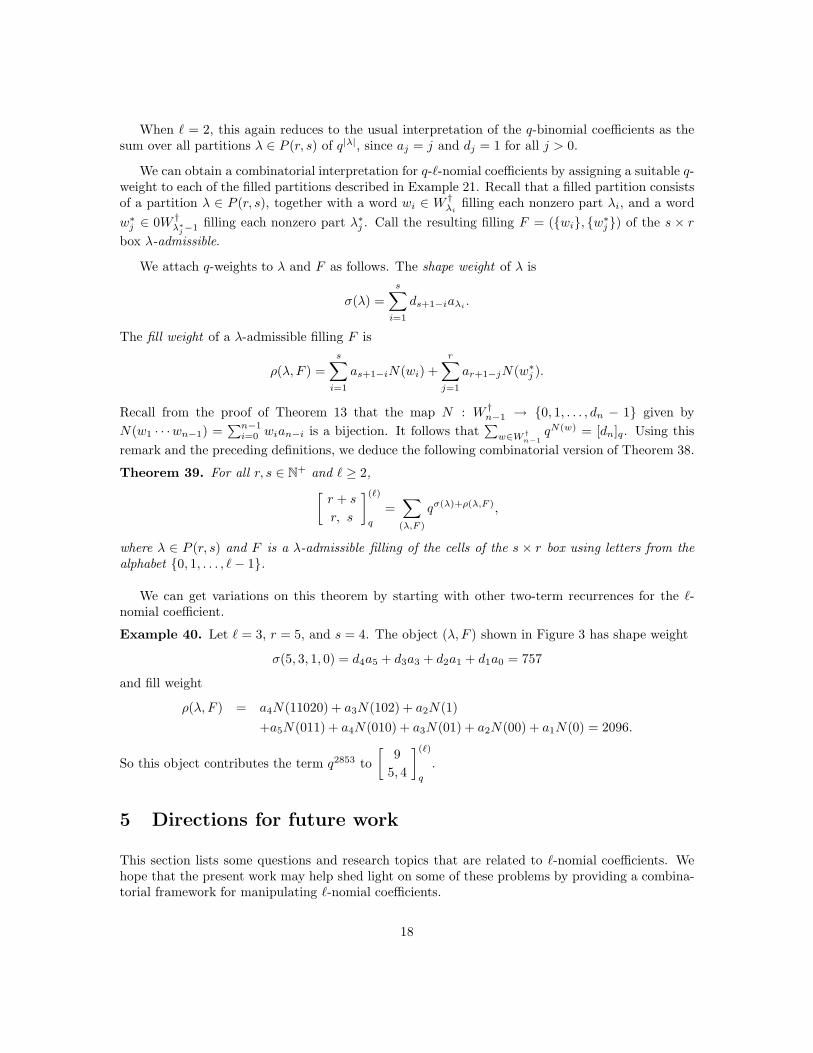
Example 40. Let ℓ = 3, r = 5, and s = 4. The object (λ, F ) shown in Figure 3 has shape weight

σ(5, 3, 1, 0) = d4a5 + d3a3 + d2a1 + d1a0 = 757

and fill weight

ρ(λ, F ) = a4N(11020) + a3N(102) + a2N(1)

+a5N(011) + a4N(010) + a3N(01) + a2N(00) + a1N(0) = 2096.

So this object contributes the term q2853 to

[

9

5, 4

](ℓ)

q

.

5 Directions for future work

This section lists some questions and research topics that are related to ℓ-nomial coefficients. Wehope that the present work may help shed light on some of these problems by providing a combina-torial framework for manipulating ℓ-nomial coefficients.

18

• Hypergeometric identities. We have given several ℓ-analogues of well-known identities such asthe binomial theorem and the Chu-Vandermonde formula. Are there natural ℓ-analogues, orq-ℓ-analogues, for other hypergeometric identities? Can a WZ-type method [32] be developedin this setting?

• Lattice point enumeration. It was shown in [11, 12] that binomial coefficients occur naturallyin the enumeration of lattice points (λ1, . . . , λk) satisfying

λ1

n≥ λ2

n − 1≥ . . . ≥ λk

n + 1 − k≥ 0.

(These are truncated version of the lecture hall partitions of [7, 8]). It is known that ℓ-nomialcoefficients arise in a similar way when enumerating lattice points (λ1, . . . , λk) satisfying

λ1

an≥ λ2

an−1≥ . . . ≥ λk

an+1−k≥ 0,

but the combinatorial or geometric significance of this is not yet understood.

• Partitions and q-series. In [26], the second author and Yee gave a bijective proof of the ℓ-Euler theorem discovered by Bousquet-Melou and Eriksson [8], which relied heavily on thecombinatorics of ℓ-sequences. There are several q-series identities related to Euler’s theorem,such as Lebesgue’s identity [2, 6], the Rogers-Fine identity [3, 33], and Cauchy’s identity[17, 33]. Are there ℓ-analogues or q-ℓ-analogues of any of these? Do any of the classicalpartition identities extend to the filled partitions that are enumerated by ℓ-nomial coefficients?In particular, it was shown in [26] that the partitions involved in the ℓ-Euler theorem have arepresentation as a filling of the shape (n, n − 1, . . . , 1) with ℓ-admissible words such that therows form a lexicographically decreasing sequence. We would like a better understanding ofhow this result is related to our combinatorial interpretations of ℓ-nomial coefficients.

• Extension to real ℓ. We can view an = an(ℓ) as a polynomial in ℓ and therefore consider allreal values of ℓ as arguments. In fact, an(ℓ) = Un(ℓ/2), where Un(x) is the n’th Chebyshevpolynomial of the second kind, defined recursively by Un(x) = 2xUn−1(x) − Un−2(x), withinitial conditions U0(x) = 1 and U1(x) = 1. We have

limℓ→2+

(

n

k

)(ℓ)

=

(

n

k

)

.

This suggests using ℓ-nomial coefficients and continuity arguments to obtain information aboutthe binomial coefficients.

Motivated by work in [25], Stanton [28] considers partitions whose parts are polynomials. Wecan connect this to our work here if we realize a polynomial part fn(x) by a word of lengthn from a language counted by fn(x). It should be worthwhile to investigate interpretations ofthe (q, t) binomial coefficients in [25] in terms of filled partitions.

Acknowledgement. We thank Matthew Schmidt for helpful discussions during the early stages ofthis work.

19

References

[1] G. L. Alexanderson and L. F. Klosinski. A Fibonacci analogue of Gaussian binomial coefficients.Fibonacci Quart., 12:129–132, 1974.

[2] Krishnaswami Alladi and Basil Gordon. Partition identities and a continued fraction of Ra-manujan. J. Combin. Theory Ser. A, 63(2):275–300, 1993.

[3] George E. Andrews. Two theorems of Gauss and allied identities proved arithmetically. PacificJ. Math., 41:563–578, 1972.

[4] Arthur T. Benjamin and Sean S. Plott. A combinatorial approach to Fibonomial coefficients.Fibonacci Quart., 46/47(1):7–9, 2008/09.

[5] Arthur T. Benjamin and Jennifer J. Quinn. Proofs that really count, volume 27 of The DolcianiMathematical Expositions. Mathematical Association of America, Washington, DC, 2003. Theart of combinatorial proof.

[6] Christine Bessenrodt. A bijection for Lebesgue’s partition identity in the spirit of Sylvester.Discrete Math., 132(1-3):1–10, 1994.

[7] Mireille Bousquet-Melou and Kimmo Eriksson. Lecture hall partitions. Ramanujan J., 1(1):101–111, 1997.

[8] Mireille Bousquet-Melou and Kimmo Eriksson. Lecture hall partitions II. Ramanujan J.,1(2):165–185, 1997.

[9] R. D. Carmichael. On the numerical factors of the arithmetic forms αn ± βn. Ann. of Math.(2), 15(1-4):30–48, 1913/14.

[10] R. D. Carmichael. On the numerical factors of the arithmetic forms αn ± βn. Ann. of Math.(2), 15(1-4):49–70, 1913/14.

[11] Sylvie Corteel, Sunyoung Lee, and Carla D. Savage. Enumeration of sequences constrained bythe ratio of consecutive parts. Sem. Lothar. Combin., 54A:Art. B54Aa, 12 pp. (electronic),2005/06.

[12] Sylvie Corteel and Carla D. Savage. Lecture hall theorems, q-series and truncated objects. J.Combin. Theory Ser. A, 108(2):217–245, 2004.

[13] Aviezri S. Fraenkel. Systems of numeration. Amer. Math. Monthly, 92(2):105–114, 1985.

[14] H. W. Gould. The bracket function and Fontene-Ward generalized binomial coefficients withapplication to Fibonomial coefficients. Fibonacci Quart., 7:23–40, 55, 1969.

[15] V. E. Hoggatt, Jr. Fibonacci numbers and generalized binomial coefficients. Fibonacci Quart,5:383–400, 1967.

[16] Dov Jarden and Theodor Motzkin. The product of sequences with a common linear recursionformula of order 2. Riveon Lematematika, 3:25–27, 38, 1949.

[17] Dongsu Kim and Ae Ja Yee. A note on partitions into distinct parts and odd parts. RamanujanJ., 3(2):227–231, 1999.

20

[18] Ron Knott. The Fibonomials. [online] http://www.mcs.surrey.ac.uk/Personal/R.Knott/Fibonacci/Fibonomials.html, 2007.

[19] Donald E. Knuth and Herbert S. Wilf. The power of a prime that divides a generalized binomialcoefficient. J. Reine Angew. Math., 396:212–219, 1989.

[20] A. K. Kwasniewski. Comments on combinatorial interpretation of Fibonomial coefficients—ane-mail style letter. Bull. Inst. Combin. Appl., 42:10–11, 2004.

[21] Edouard Lucas. Theorie des Fonctions Numeriques Simplement Periodiques. Amer. J. Math.,1(2):184–196, 1878.

[22] Edouard Lucas. Theorie des Fonctions Numeriques Simplement Periodiques. Amer. J. Math.,1(4):289–321, 1878.

[23] Edouard Lucas. Theorie des Fonctions Numeriques Simplement Periodiques. [Continued]. Amer.J. Math., 1(3):197–240, 1878.

[24] P. A. Picon. Conservation of the integrality of certain quotients by iterated substitutionsof Lucas numbers. In Seminaire Lotharingien de Combinatoire (Saint-Nabor, 1993), volume1994/21 of Prepubl. Inst. Rech. Math. Av., pages 87–93. Univ. Louis Pasteur, Strasbourg, 1994.

[25] V. Reiner, D. Stanton, and D. White. The cyclic sieving phenomenon. J. Combin. Theory Ser.A, 108(1):17–50, 2004.

[26] Carla D. Savage and Ae Ja Yee. Euler’s partition theorem and the combinatorics of ℓ-sequences.J. Combin. Theory Ser. A, 115(6):967–996, 2008.

[27] P. J. Smith and M. J. J. Lennon. LUC: A new public key system. In Proceedings of theninth IFIP International Symposium on Computer Security, pages 103–117, Amsterdam, 1994.Elsevier Science Publications.

[28] Dennis Stanton. q-analogues of Euler’s odd = distinct theorem. Ramanujan J., 19(1):107–113,2009.

[29] Jean-Pierre Tignol. Galois’ theory of algebraic equations. World Scientific Publishing Co. Inc.,River Edge, NJ, 2001.

[30] Pavel Trojovsky. On some identities for the Fibonomial coefficients via generating function.Discrete Appl. Math., 155(15):2017–2024, 2007.

[31] Douglas B. West. Introduction to graph theory. Prentice Hall Inc., Upper Saddle River, NJ,1996.

[32] Herbert S. Wilf and Doron Zeilberger. Rational functions certify combinatorial identities. J.Amer. Math. Soc., 3(1):147–158, 1990.

[33] Jiang Zeng. The q-variations of Sylvester’s bijection between odd and strict partitions. Ra-manujan J., 9(3):289–303, 2005.

21