Embed Size (px)
Citation preview
Generating Random Permutations
Jorg Arndt
30-October-2009 (revised 10-March-2010)
A thesis submitted for the degree of Doctor of Philosophyof the Australian National University


Declaration
The work in this thesis is my own except where otherwise stated.
Jorg Arndt

CONTENTS v
Contents
Acknowledgments vii
Abstract ix
1 Introduction 1
2 Notation, terminology, and conventions 32.1 Basic definitions and notation . . . . . . . . . . . . . . . . . . . . . . 32.2 Representation in a computer . . . . . . . . . . . . . . . . . . . . . . 42.3 The cycle type . . . . . . . . . . . . . . . . . . . . . . . . . . . . . . 52.4 Stirling cycle numbers . . . . . . . . . . . . . . . . . . . . . . . . . . 52.5 Transpositions and parity . . . . . . . . . . . . . . . . . . . . . . . . 62.6 Uniform projections . . . . . . . . . . . . . . . . . . . . . . . . . . . 72.7 Mixed radix and factorial numbers . . . . . . . . . . . . . . . . . . . 72.8 Ranking and unranking . . . . . . . . . . . . . . . . . . . . . . . . . 82.9 Symbol for ‘precedes’ . . . . . . . . . . . . . . . . . . . . . . . . . . . 82.10 Cyclic shifts . . . . . . . . . . . . . . . . . . . . . . . . . . . . . . . . 92.11 Specifications and floating-point model . . . . . . . . . . . . . . . . . 92.12 Symbols, auxiliary routines, and further remarks . . . . . . . . . . . 9
3 All permutations and cyclic permutations 113.1 Arbitrary permutations . . . . . . . . . . . . . . . . . . . . . . . . . 113.2 Permutations of a multiset . . . . . . . . . . . . . . . . . . . . . . . . 123.3 Prefix of a permutation . . . . . . . . . . . . . . . . . . . . . . . . . 133.4 Permutation modulo cyclic shifts . . . . . . . . . . . . . . . . . . . . 133.5 Cyclic permutations . . . . . . . . . . . . . . . . . . . . . . . . . . . 133.6 Permutations with given parity . . . . . . . . . . . . . . . . . . . . . 163.7 Permutations modulo reversal . . . . . . . . . . . . . . . . . . . . . . 16
4 Putting elements into cycles 194.1 Conversion between array form and CCF . . . . . . . . . . . . . . . 194.2 Prescribed elements in one cycle . . . . . . . . . . . . . . . . . . . . 214.3 Prescribed elements in distinct cycles . . . . . . . . . . . . . . . . . . 224.4 Prescribed sets in distinct cycles . . . . . . . . . . . . . . . . . . . . 22
5 Given cycle type 255.1 Maintenance of the set . . . . . . . . . . . . . . . . . . . . . . . . . . 25
vi CONTENTS
5.2 One cycle of prescribed length . . . . . . . . . . . . . . . . . . . . . . 255.3 Permutations with given cycle type . . . . . . . . . . . . . . . . . . . 27
6 Number of cycles 316.1 Bijection via swaps . . . . . . . . . . . . . . . . . . . . . . . . . . . . 316.2 A property of the bijection . . . . . . . . . . . . . . . . . . . . . . . 346.3 Exactly 2 cycles . . . . . . . . . . . . . . . . . . . . . . . . . . . . . . 356.4 Even or odd number of cycles . . . . . . . . . . . . . . . . . . . . . . 376.5 Exactly m cycles . . . . . . . . . . . . . . . . . . . . . . . . . . . . . 38
7 Inversions 437.1 Inversion table . . . . . . . . . . . . . . . . . . . . . . . . . . . . . . 437.2 Fast conversion to and from the inversion table . . . . . . . . . . . . 457.3 Inversions modulo m . . . . . . . . . . . . . . . . . . . . . . . . . . . 477.4 Fixed number of inversions (open problem) . . . . . . . . . . . . . . 48
8 Connected permutations 498.1 Asymptotics . . . . . . . . . . . . . . . . . . . . . . . . . . . . . . . . 498.2 The rejection method . . . . . . . . . . . . . . . . . . . . . . . . . . 508.3 Improved algorithm . . . . . . . . . . . . . . . . . . . . . . . . . . . 518.4 Implementation . . . . . . . . . . . . . . . . . . . . . . . . . . . . . . 52
9 Involutions 559.1 The number of involutions . . . . . . . . . . . . . . . . . . . . . . . . 559.2 Branching probabilities . . . . . . . . . . . . . . . . . . . . . . . . . . 569.3 Practical algorithm . . . . . . . . . . . . . . . . . . . . . . . . . . . . 579.4 Forward variant . . . . . . . . . . . . . . . . . . . . . . . . . . . . . . 59
10 Cycle spectrum 6310.1 Prescribed maximal cycle spectrum . . . . . . . . . . . . . . . . . . . 6310.2 Outline of the algorithm . . . . . . . . . . . . . . . . . . . . . . . . . 6410.3 Algorithm . . . . . . . . . . . . . . . . . . . . . . . . . . . . . . . . . 6510.4 Implementation . . . . . . . . . . . . . . . . . . . . . . . . . . . . . . 66
11 Derangements 6911.1 The number of derangements . . . . . . . . . . . . . . . . . . . . . . 6911.2 Branching probabilities . . . . . . . . . . . . . . . . . . . . . . . . . . 6911.3 Algorithm . . . . . . . . . . . . . . . . . . . . . . . . . . . . . . . . . 7111.4 Comparison with rejection method . . . . . . . . . . . . . . . . . . . 7211.5 Length of cycles at least m . . . . . . . . . . . . . . . . . . . . . . . 73
A Bit-array 77
B Left-right array 81
Bibliography 87

CONTENTS vii
Acknowledgments
First and foremost I’d like to thank Richard Brent, my supervisor, for giving methe opportunity to do my research in such an inspiring environment. It has been agreat pleasure to work with you.
Thanks go to Adam Rennie for reading through the whole text and suggestingvarious improvements in presentation. I much appreciate that.
The two anonymous examiners gave very detailed and helpful comments on thesubmitted version of this thesis, thanks for that.
With Paul Leopardi I had a great many discussions which I truly enjoyed, thanksman.
Lance Gurney, Greg Stephenson, and Charles Baker were crucial whenever it cameto discussions regarding matters 42. I appreciated that a lot. Thanks guys.
Thanks go to Edith Parzefall for enduring many discussions about Gray codes.
Last but not least, I am indebted to the Australian taxpayer. You provided much ofmy budget which has been converted into the algorithms presented here. I do thankyou all.

CONTENTS ix
Abstract
We give algorithms for generating unbiased random permutations of certain types,such as
• Permutations with prescribed parity.
• Permutations modulo cyclic shifts.
• Permutations modulo reversal.
• Permutations with prescribed elements in one cycle.
• Permutations with prescribed elements in distinct cycles.
• Permutations with prescribed sets of elements in distinct cycles.
• Permutations with prescribed cycle type.
• Permutations with even or odd number of cycles.
• Permutations with prescribed number of cycles.
• Permutations with r inversions modulo m where 2 ≤ m ≤ n (where n is thelength of the permutation).
• Connected (indecomposable) permutations.
• Self-inverse permutations (involutions).
• Permutations with prescribed maximal cycle spectrum.
• Permutations with all cycles of minimum length m.
All algorithms appear to be new and many have optimal (linear) complexity. Imple-mentations are given which can easily be translated into the programming languageof the reader’s choice.

1
Chapter 1
Introduction
Algorithms for the generation of all combinatorial objects are known for most ofthe standard types such as combinations, integer partitions, or permutations (forexample, see [23], [19], or [2]). These algorithms are often used for either testingpurposes or as building blocks for the generation of structures based on the respectivecombinatorial objects.
The fast growth of the number of objects, however, usually makes the actual gener-ation of all objects infeasible in practice. Therefore algorithms for unbiased randomgeneration are desirable. Such algorithms for random subsets, combinations, compo-sitions, permutations, integer partitions, set partitions, and unlabeled rooted treesare given in [19].
In this thesis we restrict our attention to the random generation of special types ofpermutations, such as involutions.
In the following the year of publication is given in parentheses. An algorithm for theunbiased generation of a random permutation by a computer was given by Dursten-feld (1964) [7]. Note that Knuth [13, alg. P, sect. 3.4.2] attributes the algorithmto Fisher and Yates (1938) [9]. The problem of generating random permutations inexternal memory is treated in [11] (2008). An algorithm for cyclic permutations wasgiven by Sattolo (1986) [25].
Given the relative ease by which these algorithms are found one may suspect thatalgorithms for the random generation of special types of permutations such as invo-lutions or permutations with minimum cycles length would be known. However, asof the time of this writing only two such algorithms can be found in the literature:Diaconis et.al. (2001) [6, prop. 2.3, p. 201] give an algorithm for permutations wherean element can be displaced by at most one unit (Fibonacci permutations) andMartınez et.al. (2008) [15] for permutations without fixed points (derangements).
The lack of such algorithms is even more striking as statistical properties of combi-natorial objects is an area of active research and there even is a book on statisticsof permutations by Bona (2004) [3].
The main reason for this appears to be the fact that the algorithms for permuta-tions and cyclic permutations have an unusually simple structure. For most of thealgorithms presented we need to keep track of a set of elements whose processing hasnot yet finished (see section 5.1 on page 25), some branching probabilities have tobe computed (see section 9.2 on page 56 for the case of involutions), and the specific
2 Chapter 1: Introduction
constructions in the (recursive or iterative) steps have to be identified (see section11.3 on page 71 for derangements).
The computation of each probability needs to be done in O(1) time to obtain the bestcomplexity. Indeed all of the important algorithms presented have linear complexitywhich is optimal. These can be expected to appear in all software packages dealingwith combinatorial structures, such as computer algebra systems.
3
Chapter 2
Notation, terminology, andconventions
2.1 Basic definitions and notation
The group Sn of all bijections from the set of n elements to itself is called thesymmetric group. A permutation P is an element of Sn. In the description of thealgorithms and for the implementations we take the set of n elements as either{0, 1 . . . , n − 1} or {1, 2, . . . , n}. A standard form to write down a particularpermutation is the two-line notation
P =(
0p(0)
1p(1)
2p(2)
3p(3)
· · ·· · ·
n− 1p(n− 1)
)(2.1)
The permutation that fixes all elements is the identical permutation (or identity)1n, the unit in Sn. The group multiplication of Sn is given by the composition ofpermutations as follows: For P and Q in Sn define R = QP via
r(i) := q(p(i)) (2.2)
The inverse P−1 of P ∈ Sn is the permutation such that P P−1 = P−1 P = 1n. Theinverse is computed by swapping the upper and lower row in the two-line notation,followed by sorting with respect to the upper line. For example, the inverse of
P =(
04
13
22
30
41
59
68
75
86
97
)(2.3)
is
P−1 =(
40
31
22
03
14
95
86
57
68
79
)=(
03
14
22
31
40
57
68
79
86
95
)(2.4)
We write P j (j ∈ Z) for the j-fold composition of P with itself, where P 0 is theidentity and P j =
(P−1
)−j for j < 0.
Every permutation P is the union of disjoint cycles (because pku(u) = u for someku, where ku is the length of the cycle containing u). The cycle notation of P is(
u, p(u), p2(u), . . . , pku−1(u)) (
v, p(v), p2(v) . . . , pkv−1(v))· · · (2.5)
4 Chapter 2: Notation, terminology, and conventions
For example, the permutation P ∈ S10 whose cycle notation is
(0, 4, 1, 3) (2) (5, 9, 7) (6, 8) (2.6)
has the two-line notation given as relation (2.3). There is some degree of freedomin the cycle notation. Firstly, cyclic shifts (notationally!) of a cycle do not changeit, for example, (1, 2, 3), (2, 3, 1), and (3, 1, 2) all denote the same cycle. Secondly,the order of the cycles is irrelevant.
There are four forms of normalization that are used in practice: starting with small-est element, ending with smallest, starting with largest, or ending with largest. Tomake the notation unique, we start each cycle with the smallest element it contains,and order the cycles by their first elements. If a cycle is written (or representedin memory) such that it starts with its smallest element, we say it is in normalizedform.
A cycle of length 1 is called a fixed point of a permutation. We call a cycle of lengthk a k-cycle.
2.2 Representation in a computer
To represent a permutation in computer memory we mostly use the array notation(or one-line notation), obtained by omitting the top line in the two-line notation:
[p(0), p(1), p(2), . . . , p(n− 1)] (2.7)
To represent the cycle form of a permutation without extra memory (needed to markthe cycle ends), the following convention can be used: write each cycle so that itends with its smallest element (normalization) and sort the cycles with respect totheir last elements. We call this form the canonical cycle form (CCF). For example,
(4, 1, 3, 0) (2) (9, 7, 5) (8, 6) (2.8)
is the CCF of the permutation in (2.3). The array (spaces to highlight cycle ends)
[4, 1, 3, 0, 2, 9, 7, 5, 8, 6] (2.9)
would be the computer representation of this CCF. The same data can also beinterpreted as array notation of the (in general different) permutation(
04
11
23
30
42
59
67
75
88
96
)(2.10)
The bijection via the two interpretations will sometimes be useful in itself.
2.3: The cycle type 5
2.3 The cycle type
The cycle type (or simply type) of a permutation ∈ Sn is the sequence C = [c1, c2 . . . , cn]where ck is the number of cycles of length k. We necessarily have
n = 1 c1 + 2 c2 + . . .+ n cn =n∑
k=1
k ck (2.11)
So C corresponds to an integer partition of n. For the number m of cycles we have
m =n∑
k=1
ck (2.12)
The number Zn,C of permutations of n elements with type C equals [3, p. 80]
Zn,C =n!
c1! c2! c3! . . . cn! 1c1 2c2 3c3 . . . ncn=
n!∏nk=1 ck! kck
(2.13)
The exponential generating function exp(L(z)) where
L(z) =∞∑
k=1
tk zk
k(2.14a)
gives detailed information about all cycle types [24, p. 68]:
exp(L(z)) =∞∑
n=0
[∑C
(Zn,C
∏tckk
)] zn
n!(2.14b)
The exponent of tk indicates how many cycles of length k are present in the givencycle type. For example, the coefficient of z4 is(
1 t41 + 6 t2 t21 + 8 t3 t1 + 3 t22 + 6 t4)/24 (2.15)
That is, there is one permutation ∈ S4 with four fixed points, six with two fixedpoints and one 2-cycle, eight with one fixed point and one 3-cycle, and so on.
2.4 Stirling cycle numbers
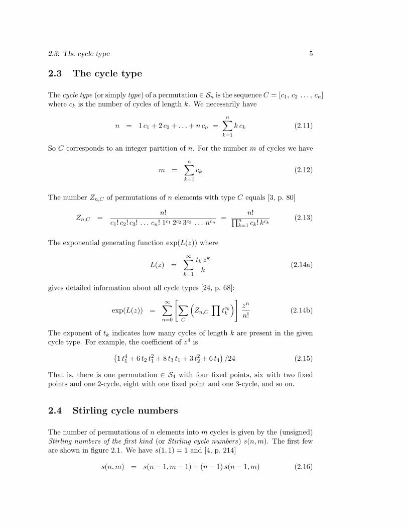
The number of permutations of n elements into m cycles is given by the (unsigned)Stirling numbers of the first kind (or Stirling cycle numbers) s(n,m). The first feware shown in figure 2.1. We have s(1, 1) = 1 and [4, p. 214]
s(n,m) = s(n− 1,m− 1) + (n− 1) s(n− 1,m) (2.16)
6 Chapter 2: Notation, terminology, and conventions
n: total m= 1 2 3 4 5 6 7 8 91: 1 12: 2 1 13: 6 2 3 14: 24 6 11 6 15: 120 24 50 35 10 16: 720 120 274 225 85 15 17: 5040 720 1764 1624 735 175 21 18: 40320 5040 13068 13132 6769 1960 322 28 19: 362880 40320 109584 118124 67284 22449 4536 546 36 1
Figure 2.1: Stirling numbers of the first kind s(n,m) (Stirling cycle numbers).
for n > 0 and m > 0, and s(n, 0) = s(0,m) = 0 except for s(0, 0) = 1. We have
n∑m=1
s(n,m)xm = xn where (2.17a)
xn =n−1∏m=0
(x+m) (2.17b)
A generating function for the Stirling cycle numbers is given by
∞∑n=0
en xn =∞∑
n=0
(n∑
m=0
s(n,m) em)xn (2.18a)
= 1 + e x+(e+ e2
)x2 +
(2e+ 3e2 + e3
)x3 + (2.18b)
+(6e+ 11e2 + 6e3 + e4
)x4 +
+(24e+ 50e2 + 35e3 + 10e4 + e5
)x5 + . . .
2.5 Transpositions and parity
A transposition is a permutation ∈ Sn that consists of a 2-cycle and n − 2 fixedpoints. The minimal number of transpositions whose composition is a k-cycle isk − 1. Write tr(P ) for the minimal number of transpositions whose composition isa permutation P ∈ Sn of cycle type C. We have
tr(P ) =n∑
k=1
ck (k − 1) (2.19)
For a permutation P with m cycles we have (use tr(P ) =∑n
k=1 (ck k − ck), relations(2.11) and (2.12))
tr(P ) = n−m (2.20)
The (nontrivial) homomorphism from Sn into the group of the two elements 0 and1 with addition modulo 2 defines the parity of a permutation. The parity is 0 or 1
2.6: Uniform projections 7
if tr(P ) is even or odd, respectively. An equivalent notion is that of the sign of apermutation, which is +1 or −1 in the respective cases (using the homomorphisminto the group with elements +1 and −1 with multiplication).
The subgroup An ∈ Sn of permutations with even parity is called the alternatinggroup. Permutations P ∈ An are called even permutations (tr(P ) is even). Thereare n!/2 such permutations. Permutations P /∈ An are called odd permutations.
2.6 Uniform projections
A projection is a map f such that f2 = f . We call a projection uniform if thenumber of preimages is the same for every image. For example, let k ≤ n and f bethe map that sorts the first k elements. Then f is uniform because every image hask! preimages. The number of preimages of each image of a uniform projection willbe called the quotient of the projection.
If we have an algorithm for the unbiased random generation of elements a ∈ A anda uniform projection f onto B ⊂ A then an unbiased random element b ∈ B can becomputed as f(a).
2.7 Mixed radix and factorial numbers
rising fact falling fact0: [ . . . ] [ . . . ]1: [ 1 . . ] [ 1 . . ]2: [ . 1 . ] [ 2 . . ]3: [ 1 1 . ] [ 3 . . ]4: [ . 2 . ] [ . 1 . ]5: [ 1 2 . ] [ 1 1 . ]6: [ . . 1 ] [ 2 1 . ]7: [ 1 . 1 ] [ 3 1 . ]8: [ . 1 1 ] [ . 2 . ]9: [ 1 1 1 ] [ 1 2 . ]10: [ . 2 1 ] [ 2 2 . ]11: [ 1 2 1 ] [ 3 2 . ]12: [ . . 2 ] [ . . 1 ]13: [ 1 . 2 ] [ 1 . 1 ]14: [ . 1 2 ] [ 2 . 1 ]15: [ 1 1 2 ] [ 3 . 1 ]16: [ . 2 2 ] [ . 1 1 ]17: [ 1 2 2 ] [ 1 1 1 ]18: [ . . 3 ] [ 2 1 1 ]19: [ 1 . 3 ] [ 3 1 1 ]20: [ . 1 3 ] [ . 2 1 ]21: [ 1 1 3 ] [ 1 2 1 ]22: [ . 2 3 ] [ 2 2 1 ]23: [ 1 2 3 ] [ 3 2 1 ]
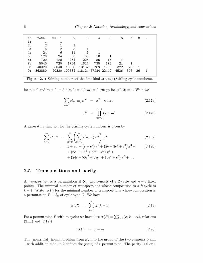
Figure 2.2: Nonnegative integers < 24 expressed in rising (left) and falling (right)factorial base. Dots denote zeros. The least significant digits appear on the left.
The mixed radix representation A = [a0, a1, a2, . . . , an−1] of an integer x with respect
8 Chapter 2: Notation, terminology, and conventions
to a radix vector M = [m0,m1,m2, . . . ,mn−1] is given by
x =n−1∑k=0
ak
k−1∏j=0
mj (2.21)
where 0 ≤ aj < mj (and 0 ≤ x <∏n−1
j=0 mj , so that n digits suffice). Note thatmn−1 is not used in the relation but it determines the range of values of an−1. ForM = [r, r, r, . . . , r] the relation reduces to the radix-r representation:
x =n−1∑k=0
ak rk (2.22)
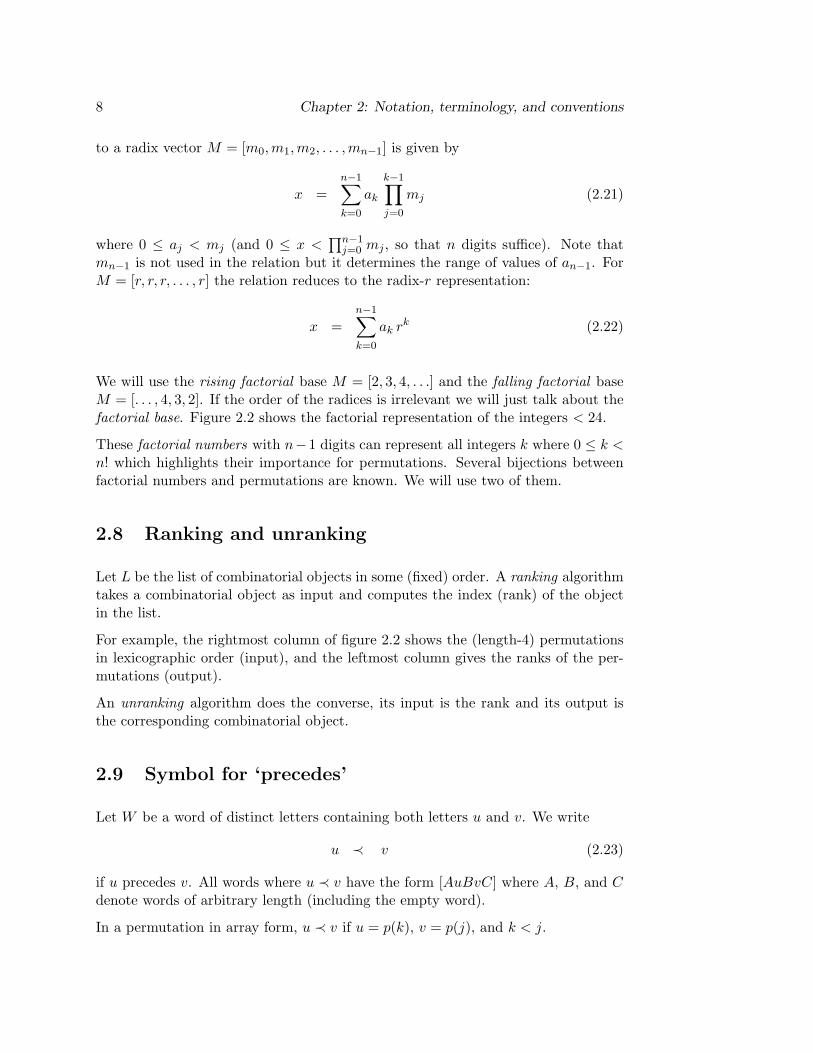
We will use the rising factorial base M = [2, 3, 4, . . .] and the falling factorial baseM = [. . . , 4, 3, 2]. If the order of the radices is irrelevant we will just talk about thefactorial base. Figure 2.2 shows the factorial representation of the integers < 24.
These factorial numbers with n−1 digits can represent all integers k where 0 ≤ k <n! which highlights their importance for permutations. Several bijections betweenfactorial numbers and permutations are known. We will use two of them.
2.8 Ranking and unranking
Let L be the list of combinatorial objects in some (fixed) order. A ranking algorithmtakes a combinatorial object as input and computes the index (rank) of the objectin the list.
For example, the rightmost column of figure 2.2 shows the (length-4) permutationsin lexicographic order (input), and the leftmost column gives the ranks of the per-mutations (output).
An unranking algorithm does the converse, its input is the rank and its output isthe corresponding combinatorial object.
2.9 Symbol for ‘precedes’
Let W be a word of distinct letters containing both letters u and v. We write
u ≺ v (2.23)
if u precedes v. All words where u ≺ v have the form [AuBvC] where A, B, and Cdenote words of arbitrary length (including the empty word).
In a permutation in array form, u ≺ v if u = p(k), v = p(j), and k < j.
2.10: Cyclic shifts 9
2.10 Cyclic shifts
A cyclic shift by k positions of a vector
[a0, a1, . . . , an−1] (2.24)
is the vector
[a0−k, a1−k, . . . , an−1−k] (2.25)
where subscripts are to be taken modulo n. For example, the cyclic shift by oneposition (cyclic right shift) of [a, b, c, d] is [d, a, b, c].
2.11 Specifications and floating-point model
All algorithms sample uniformly (unbiased), except where stated otherwise (e.g.Algorithm 6.6 on page 34). All algorithms generate permutations in array formexcept where stated otherwise (e.g. Algorithm 4.5 on page 23).
Many of the algorithms given here work with floating-point numbers (C-type double)to represent real numbers. Due to the imprecision and roundoff-errors the achieveduniformity is not perfect (even if the random numbers are assumed to be perfect).For all practical purposes the uniformity should suffice, and floating-point numbersof higher (but fixed) precision can be used for even better uniformity.
With sufficient floating-point precision the limiting factor is rather the periodicityof the pseudorandom number generator (PRNG). Even for PRNGs with very longperiods only a subset of all possible permutations (of sufficient length) is possiblygenerated. This problem can be mitigated by using a source of entropy to preventperiodicity.
Perfect uniformity requires both exact arithmetic (e.g. rationals) and a perfect sourceof random numbers. With exact arithmetic, however, the complexity of the algo-rithms will in general be worse because of computations with rapidly growing num-bers. Another approach to perfect uniformity is the use of interval arithmetic, see[5]. No attempt for perfect uniformity is made in this thesis.
2.12 Symbols, auxiliary routines, and further remarks
Most implementations are given in the C++ language. Only a minimum of featuresbeyond plain C are used: essentially only templates and (for the auxiliary routinesin appendix A on page 77 and B on page 81) simple classes. For implementationswhere the details might obscure the underlying algorithm, the GP language [21] isused. A short introduction into the GP language is given in [2, app. C].
In the C++ implementations the type long unsigned int is abbreviated as ulong.They are part of the FXT library [1].
10 Chapter 2: Notation, terminology, and conventions
In the algorithms the symbol Z(k) stands for a uniform random integer ∈ {0, 1, . . . , k−1}, the corresponding C++ function is rand_idx(k), the GP function is random(k).
The symbol R() stands for a uniform random real t where 0 ≤ t < 1, the corre-sponding C++ function is rand01().
The floating-point type used in C++ implementations is the type double, the IEEEdouble precision number having a 53-bit significand (mantissa).
The symbol := is used for assignment in the algorithms and comments appear inparenthesis, for example:
1. Set k′ := k − 1 (there are k′ elements left to process).
11
Chapter 3
All permutations and cyclicpermutations
We recall the known algorithms for generating random permutations and randomcyclic permutations. We also give some algorithms that can be obtained from thesevia uniform projections, such as algorithms for permutations with prescribed parity,permutations modulo cyclic shift, and permutations modulo reversal.
3.1 Arbitrary permutations
A random permutation P = [p(0), p(1), . . . , p(n − 1)] ∈ Sn can be computed asfollows:Algorithm 3.1 (PermS). Generate a random permutation P ∈ Sn.
1. Set S := {0, 1, . . . , n− 1}.
2. For k := 0, 1, . . . , n− 1, do:Select a random element s ∈ S and remove it from S. Set p(k) := s.
The first element (p(0)) is uniformly sampled from all n elements ∈ S, the secondfrom the n−1 elements 6= p(0), and so on. There are n! different ways the algorithmcan proceed, and there are n! permutations altogether.
A practical variant is the following iterative algorithm:Algorithm 3.2 (Perm1). Generate a random permutation P ∈ Sn.
1. Set P := 1n (identical permutation).
2. For k := n, n− 1, . . . , 2 do:Set i := Z(k) (random i ∈ {0, 1, . . . , k − 1}). Swap p(i) with p(k − 1).
This form is due to Durstenfeld [7], it is usually called Fisher-Yates shuffle, some-times also Knuth shuffle see [13, alg. P, sect. 3.4.2]. An alternative version of themethod is (again see [13, alg. P, sect. 3.4.2])Algorithm 3.3 (Perm0). Generate a random permutation P ∈ Sn.
1. Set P := 1n.
2. For k := 1, 2, . . . , n− 1 do:Set i := Z(k + 1) (i ∈ {0, 1, . . . , k}). Swap p(i) with p(k).
12 Chapter 3: All permutations and cyclic permutations
With both methods we can omit the initialization of P as long as P contains datacorresponding to a valid permutation on entry.
If the cycle form of a random permutation is required, simply interpret the data ascanonical cycle form as defined in section 2.2.
To randomly permute an array, one could generate a random permutation and applyit to the array. However, there is a more direct way.Algorithm 3.4 (Perm1F). Apply a random permutation to the elements in F =[f(0), f(1), . . . , f(n− 1)].
1. For k := n, n− 1, . . . , 2 do:Set i := Z(k) (i ∈ {0, 1, . . . , k − 1}). Swap f(i) with f(k − 1).
An implementation is1 template <typename Type>2 void random_permute(Type *f, ulong n)3 // Randomly permute the elements of f[].4 {5 for (ulong k=n; k>1; --k)6 {7 const ulong i = rand_idx(k);8 swap2(f[k-1], f[i]);9 }
10 }
For the routine corresponding to Algorithm 3.3, replace the loop by
1 for (ulong k=1; k<n; ++k)2 {3 const ulong i = rand_idx(k+1);4 swap2(f[k], f[i]);5 }
A Routine for applying a permutation in-place to an array F (i.e. avoiding a tem-porary copy of F ) is given in [2, sect. 2.4].
3.2 Permutations of a multiset
The algorithms can also be used to generate a unbiased random permutation of amultiset, as ignoring the order between certain elements corresponds to a uniformprojection. Consider a multiset with k kinds of elements and mj elements of kindj where 1 ≤ j ≤ k. In any permutation the mj elements of kind j occupy mj
distinct positions. If these elements were distinguishable there would be mj ! waysto arrange them. As we cannot distinguish the elements of one type, there are mj !permutations that correspond to each permutation of the multiset. The same is truefor all kinds of elements, so there are (m1+m2+...+mk)!
m1! m2! ···mk! permutations of the multiset,which is well known.
Another way to see this is by the following (unnecessarily complicated) algorithm:Algorithm 3.5 (MSetPerm). Generate a random permutation of a multiset with kkinds of elements and mj elements of kind j where 1 ≤ j ≤ k.
1. Set n :=∑k
j=1mj . Generate a random permutation ∈ Sn.
3.3: Prefix of a permutation 13
2. Replace the m1 smallest elements with kind 0, the m2 smallest of the remainingelements with kind 1, and so on.
The last step is a uniform projection with quotient m1!m2! · · · mk!.
3.3 Prefix of a permutation
If in a random permutation of a length-n vector F only the first m elements (them-prefix of F ) are of interest, then O(m) operations suffice [22]:Algorithm 3.6 (PrefM). Compute m-prefix where 1 ≤ m ≤ n − 1 of a randompermutation of the elements in F = [f(0), f(1), . . . , f(n− 1)].
1. For k := 0, 1, . . . ,m− 1 do:Set i := k + Z(n− k) (i ∈ {k, k + 1, . . . , n− 1}). Swap f(i) with f(k).
The element f(0) is randomly selected from all n elements, f(1) is selected from alln− 1 remaining elements, and so on.
If m = n− 1 we simply obtain a random permutation of all elements.
3.4 Permutation modulo cyclic shifts
If we consider all cyclic shifts (see section 2.10 on page 9) of a permutation asequivalent, we can use the convention of always having the largest element last.Then a random permutation (modulo the implied equivalence) in array form isobtained by randomly permuting all but the last element.Algorithm 3.7 (PermCS). Generate a random permutation modulo cyclic shifts.
1. Set P := 1n.
2. For k := n− 1, n− 2, . . . , 2 do:Set i := Z(k) (i ∈ {0, 1, . . . , k − 1}). Swap p(i) with p(k − 1).
The algorithm is obtained by omitting the first step (k = n) in the loop of Algorithm3.2.
3.5 Cyclic permutations
A permutation P ∈ Sn that consists of a single cycle of length n is called a cyclicpermutation. Generating a random cyclic permutation is no harder than generatingan arbitrary permutation, we just have to make sure that a swap happens in everystep:Algorithm 3.8 (CyclicS). Generate a random cyclic permutation.
1. Set S := {1, 2, . . . , n− 1}. Set C := (0) (a length-1 cycle).
14 Chapter 3: All permutations and cyclic permutations
2. Until S is empty, do:Select a random element s ∈ S and remove it from S.Append s to the cycle C.
The algorithm is usually given in this form:Algorithm 3.9 (Cyclic1). Generate a random cyclic permutation.
1. Set P := 1n.
2. For k := n− 1, n− 2, . . . , 1 do:Set i := Z(k) (i ∈ {0, 1, . . . , k − 1}). Swap p(i) with p(k).
This variant is called Sattolo’s algorithm, for a proof of its validity see [25].
We now give a slightly different form which is easy to prove correct. The basicingredient is the following: Let p(i) and p(k) be elements of different cycles of apermutation P of lengths li and lk, respectively. Let T be the transposition of thepositions i and k. Then Q := T P has a cycle of length li + lk that contains bothp(i) and p(k). That is, a swap of two elements in different cycles joins the cycles.Algorithm 3.10 (Cyclic0). Generate a random cyclic permutation.
1. Set P := 1n.
2. For k := 1, 2, . . . , n− 1 do:Set i := Z(k) (i ∈ {0, 1, . . . , k − 1}). Swap p(i) with p(k).
Only cyclic permutations are generated: Step k in the loop joins p(k) = k (a fixedpoint) with the length-k cycle given by p(0), p(1), . . . , p(k − 1). Thereby after stepk the permutation contains a single cycle consisting of the first k + 1 elements0, 1, . . . , k. All cyclic permutation are generated: At step k the random numberZ(k) can have k different values, each creating a different (k+ 1)-cycle. So there are1 · 2 · 3 · · · (n − 1) = (n − 1)! different permutations the method can generate, andthere are (n− 1)! cyclic permutations altogether.
The following implementation corresponds to Algorithm 3.10, it permutes the ele-ments of an array F :
1 template <typename Type>2 void random_permute_cyclic(Type *f, ulong n)3 // Permute the elements of f by a random cyclic permutation.4 {5 for (ulong k=1; k<n; ++k)6 {7 const ulong i = rand_idx(k);8 swap2(f[k], f[i]);9 }
10 }
The routine corresponding to Algorithm 3.9 is obtained by replacing the loop with
1 for (ulong k=n-1; k>0; --k)2 {3 const ulong i = rand_idx(k);4 swap2(f[k], f[i]);5 }
To compute a cyclic permutation, use
1 inline void random_cyclic_permutation(ulong *f, ulong n)
3.5: Cyclic permutations 15
2 // Create a random permutation that is cyclic.3 {4 for (ulong k=0; k<n; ++k) f[k] = k;5 random_permute_cyclic(f, n);6 }
The normalized cycle form of a random cyclic permutation can of course be computedby randomly permuting all elements except the first (or the last, as in Algorithm3.7). If the cycle is not required to be normalized, then also a random permutationof all elements can be used.
The following algorithm applies a cyclic permutation to a subset of F .Algorithm 3.11 (Cyclic-Positions1). Apply a random cyclic permutation to thosenp ≥ 2 elements in F = [f(0), f(1), . . . , f(n− 1)] whose positions are given inPs = [ps(0), ps(1), . . . , ps(np − 1)].
1. Set nr := np (number of remaining elements).
2. Set i0 := 0 (cycle leader, no need to take random position).
3. Set nr := nr − 1. If nr = 0 then return.
4. Set i1 := Z(nr) (0 ≤ i1 < nr). Swap f(ps(i0)) with f(ps(i1)) (extend cycle).
5. Swap ps(i0) with ps(nr) (remove ps(i0) from set).
6. Set i0 := i1 and go to step 3.
The removal of elements from the set can be avoided as follows.Algorithm 3.12 (Cyclic-Positions0). Apply a random cyclic permutation to thosenp ≥ 2 elements in F = [f(0), f(1), . . . , f(n− 1)] whose positions are given inPs = [ps(0), ps(1), . . . , ps(np − 1)].
1. Set k := 0.
2. Set k := k + 1. If k = np then return.
3. Set i := Z(k) (0 ≤ i < k). Swap f(ps(k)) with f(ps(i)) (extend cycle).
4. Go to step 2.
An implementation is1 template <typename Type>2 void random_permute_positions_cyclic(Type *f, ulong np, const ulong *ps)3 // Randomly permute the np elements f[ps[0]], f[ps[1], ..., f[ps[np-1]]4 // by a cyclic permutation.5 {6 for (ulong k=1; k<np; ++k)7 {8 const ulong i = rand_idx(k);9 swap2(f[ps[k]], f[ps[i]]);
10 }11 }
For the arbitrary and cyclic permutations we gave versions of the algorithms (Al-gorithm 3.1 and Algorithm 3.8) that involve manipulations of a set. However, thepractical versions did not need these operations, so Algorithm 3.1 and Algorithm
16 Chapter 3: All permutations and cyclic permutations
3.8 might appear unnecessarily complicated. We will see that for other types ofpermutations we usually do need to keep track of the set of unprocessed elements.
3.6 Permutations with given parity
To generate a permutation with prescribed parity we modify Algorithm 3.3 to keeptrack of the parity of the permutation generated: whenever two distinct elementsare swapped the parity changes. If the generated permutation does not have theright parity we swap the first two elements of it.Algorithm 3.13 (PermPar). Generate a random permutation P ∈ Sn (n ≥ 2) withprescribed parity e.
1. Set P := 1n. Set g := 0 (parity of the generated permutation).
2. For k := 1, 2, . . . , n− 1 do:Set i := Z(k + 1) (i ∈ {0, 1, . . . , k}).If i 6= k then swap p(i) with p(k) and set g := 1− g (parity changed).
3. If g 6= e then swap p(0) with p(1) (fix parity via a transposition T ).
The last step is a uniform projection with quotient 2, it corresponds to a multiplica-tion (by a transposition) in the group Sn. The transposition T in the last step is odd.We either obtain one of the n!/2 permutations with required parity e, and return it,or the permutation has the wrong parity and composition with T changes the parityto e. As a map between the even and odd permutations, T is a bijection.
The algorithm can be used to generate a permutation where the parity of the numberm of cycles is prescribed. With t for the number of transpositions we have n = t+m,by relation (2.20). If n is even then m and t are simultaneously even or odd, else mis even if and only if t is odd.
There seems to be no easy way to generalize the method to generate permutationssatisfying other modulo conditions for their number of transpositions, as the distri-butions are nonuniform.
3.7 Permutations modulo reversal
A natural dual of Algorithm 3.13 is the following.Algorithm 3.14 (PermRev). Generate a random permutation P ∈ Sn (n ≥ 2)where 0 ≺ 1.
1. Generate a random permutation P .
2. Find i0 and i1 such that p(i0) = 0 and p(i1) = 1, respectively.
3. If i0 > i1 then swap p(i0) with p(i1) (fix order).
The last step is a uniform projection with quotient 2.
An implementation is
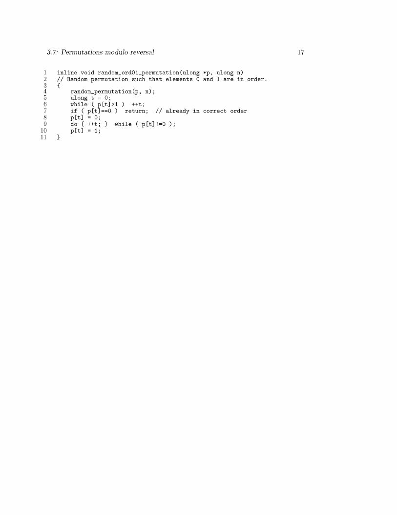
3.7: Permutations modulo reversal 17
1 inline void random_ord01_permutation(ulong *p, ulong n)2 // Random permutation such that elements 0 and 1 are in order.3 {4 random_permutation(p, n);5 ulong t = 0;6 while ( p[t]>1 ) ++t;7 if ( p[t]==0 ) return; // already in correct order8 p[t] = 0;9 do { ++t; } while ( p[t]!=0 );
10 p[t] = 1;11 }

18 Chapter 3: All permutations and cyclic permutations
19
Chapter 4
Putting elements into cycles
We give algorithms for generating random permutations with conditions on whichelements lie in the same or in distinct cycles. The central ingredients are the bijectionbetween array form and canonical cycle form, and uniform projections by sortingcertain elements.
4.1 Conversion between array form and CCF
For the following algorithms we need a routine for the conversion to the canonicalcycle form (CCF). The variables lc and nc are scalars and respectively correspondto lc and nc in the implementation.Algorithm 4.1 (Perm2CCF). Convert permutation P ∈ Sn given in array form tocanonical cycle form (written to length-n array C).
1. Set B := [0, 0, . . . , 0] (length n, tag array for marking elements as processed).
2. Set m := 0 (minimum value of unprocessed elements).
3. Set j := 0 (position in C).
4. Set lc := m (next cycle; m is last element in cycle to be processed).
5. Set nc := p(lc) (next element in cycle).
6. Set C(j) := nc and j := j + 1.
7. Set lc := nc and B(lc) := 1 (mark lc as processed).
8. If lc 6= m then go to step 5.
9. (Find smallest unprocessed element:)for i := m+ 1 . . . , n− 1 do: if B(i) = 0 then set m := i and go to step 4.
The time complexity is O(n) which is optimal.
The implementation uses a bit-array (described in appendix A on page 77):voidperm2ccf(const ulong *p, ulong n, ulong *c, bitarray *tb/*=0*/)// Convert permutation in p[] (array form) into// canonical cycle form (CCF), written to c[].{
bitarray * b = tb;
20 Chapter 4: Putting elements into cycles
if ( 0==tb ) b = new bitarray(n);b->clear_all();
ulong m = 0; // minimum of unprocessed elements (==cycle end)ulong j = 0; // position in c[]while ( m!=n ){
ulong lc = m; // last in cycledo{
ulong nc = p[lc]; // next in cyclec[j] = nc;++j;lc = nc;b->set(lc); // mark as processed
}while ( lc!=m );m = b->next_clear(m+1);
}
if ( 0==tb ) delete b;}
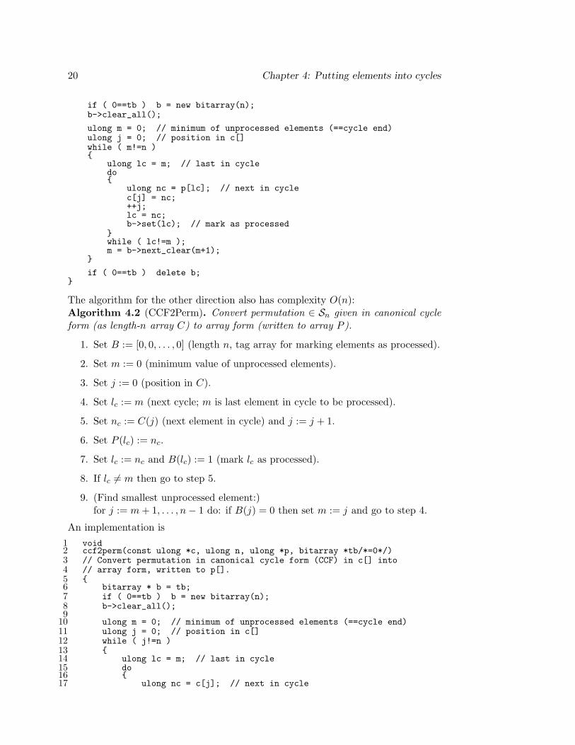
The algorithm for the other direction also has complexity O(n):Algorithm 4.2 (CCF2Perm). Convert permutation ∈ Sn given in canonical cycleform (as length-n array C) to array form (written to array P ).
1. Set B := [0, 0, . . . , 0] (length n, tag array for marking elements as processed).
2. Set m := 0 (minimum value of unprocessed elements).
3. Set j := 0 (position in C).
4. Set lc := m (next cycle; m is last element in cycle to be processed).
5. Set nc := C(j) (next element in cycle) and j := j + 1.
6. Set P (lc) := nc.
7. Set lc := nc and B(lc) := 1 (mark lc as processed).
8. If lc 6= m then go to step 5.
9. (Find smallest unprocessed element:)for j := m+ 1, . . . , n− 1 do: if B(j) = 0 then set m := j and go to step 4.
An implementation is1 void2 ccf2perm(const ulong *c, ulong n, ulong *p, bitarray *tb/*=0*/)3 // Convert permutation in canonical cycle form (CCF) in c[] into4 // array form, written to p[].5 {6 bitarray * b = tb;7 if ( 0==tb ) b = new bitarray(n);8 b->clear_all();9
10 ulong m = 0; // minimum of unprocessed elements (==cycle end)11 ulong j = 0; // position in c[]12 while ( j!=n )13 {14 ulong lc = m; // last in cycle15 do16 {17 ulong nc = c[j]; // next in cycle
4.2: Prescribed elements in one cycle 21
18 ++j;19 p[lc] = nc;20 lc = nc;21 b->set(lc); // mark as processed22 }23 while ( lc!=m ); // until cycle end24 m = b->next_clear(m+1); // ==n if no clear bit present25 }2627 if ( 0==tb ) delete b;28 }
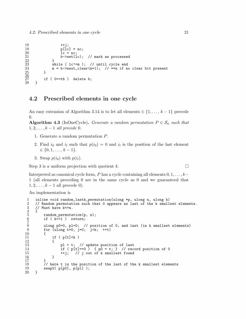
4.2 Prescribed elements in one cycle
An easy extension of Algorithm 3.14 is to let all elements ∈ {1, . . . , k − 1} precede0.Algorithm 4.3 (InOneCycle). Generate a random permutation P ∈ Sn such that1, 2, . . . , k − 1 all precede 0.
1. Generate a random permutation P .
2. Find i0 and il such that p(i0) = 0 and il is the position of the last element∈ {0, 1, . . . , k − 1}.
3. Swap p(i0) with p(il).
Step 3 is a uniform projection with quotient k.
Interpreted as canonical cycle form, P has a cycle containing all elements 0, 1, . . . , k−1 (all elements preceding 0 are in the same cycle as 0 and we guaranteed that1, 2, . . . , k − 1 all precede 0).
An implementation is
1 inline void random_lastk_permutation(ulong *p, ulong n, ulong k)2 // Random permutation such that 0 appears as last of the k smallest elements.3 // Must have k<=n.4 {5 random_permutation(p, n);6 if ( k<=1 ) return;78 ulong p0=0, pl=0; // position of 0, and last (in k smallest elements)9 for (ulong t=0, j=0; j<k; ++t)
10 {11 if ( p[t]<k )12 {13 pl = t; // update position of last14 if ( p[t]==0 ) { p0 = t; } // record position of 015 ++j; // j out of k smallest found16 }17 }18 // here t is the position of the last of the k smallest elements19 swap2( p[p0], p[pl] );20 }
22 Chapter 4: Putting elements into cycles
4.3 Prescribed elements in distinct cycles
Another extension of Algorithm 3.14 is to fix the order of the elements 0, 1, . . . , k−1.Algorithm 4.4 (InDistinctCycles). Generate a random permutation P ∈ Sn suchthat 0 ≺ 1 ≺ 2 ≺ . . . ≺ k − 1.
1. Generate a random permutation P .
2. Set e := 0 and j := 0.
3. While e < k do: (fix order of elements 0, 1, . . . , k − 1)
(a) If p(j) < k then (an element < k was found)set p(j) := e (write next element in the sequence 0, 1, . . . , k − 1)and set e := e+ 1 (next in sequence).
(b) Set j := j + 1.
Step 3 is a uniform projection with quotient k!.
The time complexity is O(n). Interpreted as canonical cycle form, P contains kdistinct cycles, each containing exactly one element < k. An implementation is
1 inline void random_ordk_permutation(ulong *p, ulong n, ulong k)2 // Random permutation such that the k smallest elements are in order.3 // Must have k<=n.4 {5 random_permutation(p, n);6 for (ulong j=0,e=0; e<k; ++j) if ( p[j]<k ) { p[j]=e; ++e; }7 }
4.4 Prescribed sets in distinct cycles
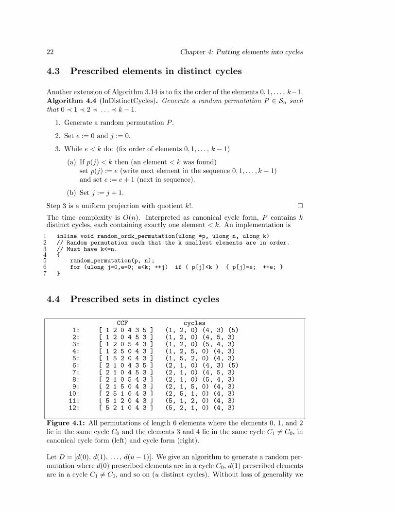
CCF cycles1: [ 1 2 0 4 3 5 ] (1, 2, 0) (4, 3) (5)2: [ 1 2 0 4 5 3 ] (1, 2, 0) (4, 5, 3)3: [ 1 2 0 5 4 3 ] (1, 2, 0) (5, 4, 3)4: [ 1 2 5 0 4 3 ] (1, 2, 5, 0) (4, 3)5: [ 1 5 2 0 4 3 ] (1, 5, 2, 0) (4, 3)6: [ 2 1 0 4 3 5 ] (2, 1, 0) (4, 3) (5)7: [ 2 1 0 4 5 3 ] (2, 1, 0) (4, 5, 3)8: [ 2 1 0 5 4 3 ] (2, 1, 0) (5, 4, 3)9: [ 2 1 5 0 4 3 ] (2, 1, 5, 0) (4, 3)10: [ 2 5 1 0 4 3 ] (2, 5, 1, 0) (4, 3)11: [ 5 1 2 0 4 3 ] (5, 1, 2, 0) (4, 3)12: [ 5 2 1 0 4 3 ] (5, 2, 1, 0) (4, 3)
Figure 4.1: All permutations of length 6 elements where the elements 0, 1, and 2lie in the same cycle C0 and the elements 3 and 4 lie in the same cycle C1 6= C0, incanonical cycle form (left) and cycle form (right).
Let D = [d(0), d(1), . . . , d(u− 1)]. We give an algorithm to generate a random per-mutation where d(0) prescribed elements are in a cycle C0, d(1) prescribed elementsare in a cycle C1 6= C0, and so on (u distinct cycles). Without loss of generality we
4.4: Prescribed sets in distinct cycles 23
choose the d(0) smallest elements for the first cycle, the d(1) next smaller elementsfor the second cycle, and so on.
Note that the cycles do in general contain elements apart from those guaranteed tobe contained. Figure 4.1 shows all permutations of length 6 for u = 2, d(0) = 3, andd(1) = 2.
For example, with D = [3, 4] we need to reorder the first 7 elements such that a ≺ bwhere a ∈ {0, 1, 2} and b ∈ {3, 4, 5, 6}, c ≺ 0 where c ∈ {1, 2}, and d ≺ 3 whered ∈ {4, 5, 6}. For each cycle the order of all but the last element will be takenat random. We will use an auxiliary vector V for that purpose, for our exampleV = [2, 1, 0, 4, 6, 5, 3] would be valid.Algorithm 4.5 (SetsInDistinctCycles). Let D = [d(0), d(1), . . . , d(u− 1)] whered(j) ≥ 1 (the set specification). Generate a random permutation P ∈ Sn in canonicalcycle form (CCF) with (at least) u distinct cycles C0, C1, . . . , Cu−1 such that0, 1, . . . , d(0)−1 lie in C0, d(0), d(0)+1, . . . , d(0)+d(1)−1 lie in C1, d(0)+d(1), d(0)+d(1) + 1, . . . , d(0) + d(1) + d(2)− 1 lie in C2, and so on.
1. Set w :=∑u−1
j=0 d(u). Set V := [v(0), v(1), . . . , v(w − 1)] := 1w.
2. Set e := 0 and j := 0.
3. While e < u do: (compute random vector V consistent with specification)
(a) Swap v(j) with v(j + d(e)− 1) (cycle end).
(b) If d(e) > 2 then randomly permute [v(j), v(j + 1), . . . , v(j + d(e)− 2)](make cycle random).
(c) Set j := j + d(e). Set e := e+ 1.
4. Generate a random permutation P .
5. Set e := 0 and j := 0.
6. While e < w do: (sort w smallest elements in P according to V )
(a) If p(j) < w then set p(j) := v(e) and e := e+ 1.
(b) Set j := j + 1.
The sorting is a uniform projection with quotient
q =
(∑u−1j=0 d(j)
)!∏u−1
j=0 (d(j)− 1)!(4.1)
The numerator is due to sorting all elements specified by D, the denominator isdue to the randomization of all but one element in each of the specified cycles.For the permutations in figure 4.1 we have q = 5!/(2! 1!) = 60, thus 7!/6 = 12permutations.
The algorithm has time complexity O(n). An implementation is
1 inline void random_sdc_permutation(ulong *p, ulong n,2 const ulong *d, ulong nd,
24 Chapter 4: Putting elements into cycles
3 ulong *tv=0)4 // sdc := Sets into Distinct Cycles.5 //6 // Let NN={0,1,...,n-1},7 // S0 be the set of the d[0] smallest elements of NN,8 // S1 be the set of the d[1] smallest elements of NN \ S09 // S2 be the set of the d[2] smallest elements of NN \ { S0 union S1 }
10 // and so on.11 // Let m0 = min(S0), m1 = min(S1) etc.,12 // write a<<b for "a precedes b".13 //14 // Generate random permutation such that15 // x << m0 for all elements (!=m0) of S0,16 // m0 << x << m1 for all elements (!=m1) of S1,17 // m1 << x << m2 for all elements (!=m2) of S2,18 // and so on.19 //20 // As canonical cycle form (CCF):21 // The elements of S0 are in one cycle C0,22 // the elements of S1 are in one cycle C1!=C0,23 // the elements of S2 are in one cycle C2!=C1, C2!=C0,24 // and so on.25 {26 ulong w = 0; // number of elements specified via d[]27 for (ulong k=0; k<nd; ++k) w += d[k];2829 ulong *v = tv;30 if ( tv==0 ) v = new ulong[w];31 for (ulong k=0; k<w; ++k) v[k] = k;3233 ulong e = 0, j = 0;34 while ( e<nd )35 {36 const ulong de = d[e];37 swap2( v[j], v[j+de-1] ); // cycle end38 if ( de>2 ) random_permute( v+j, de-1 ); // make cycle random39 j += de; ++e;40 }4142 random_permutation(p, n);4344 e = 0; j = 0;45 while ( e<w ) // sort w smallest elements in p[] according to v[]46 {47 if ( p[j]<w ) { p[j]=v[e]; ++e; }48 ++j;49 }5051 if ( tv==0 ) delete [] v;52 }
25
Chapter 5
Given cycle type
We introduce the techniques for maintaining the set of unprocessed elements andfor creating random cycles. These are used in many of the algorithms that follow inthis thesis.
5.1 Maintenance of the set
For most of the algorithms we need to keep track of a set S of the positions of theelements not processed so far.
The following two operations should be efficient: unbiased random selection of anelement s ∈ S and removal of an element s from the set.
We represent the set S as an arrayR = [R(0), R(1), R(2), . . .], initially containing allpositions. During processing the elements still ∈ S will be in positions 0, 1, . . . , r−1where r = |S|.
To randomly select an element s, set s := Ri where i = Z(r) ∈ {0, 1, . . . , r − 1}.To remove the element s = R(i), swap R(i) with R(r − 1) and set r := r − 1. Bothoperations are obviously O(1) which is optimal. This technique is given in [8].
The order of the elements is in general lost during processing. This, however, doesnot interfere with the operations just described.
5.2 One cycle of prescribed length
We first give an auxiliary algorithm to create a cycle. It is used in the algorithmsthat appear in this chapter.
The subscripted variables k0 and kp are scalars. They respectively correspond tothe variables k0 and kp in the implementation.Algorithm 5.1 (Cycle). Let P be a permutation with r ≥ 1 fixed points. LetR = [R(0), R(1), R(2), . . .] be an array whose first r elements contain the positionsof the unprocessed elements of P . Generate a random length-c cycle (1 ≤ c ≤ r)whose elements are a subset of the unprocessed elements in P .
1. Select cycle leader from unprocessed elements:
26 Chapter 5: Given cycle type
(a) Set i := Z(r), set k0 := R(i) (k0 is the cycle leader).
(b) Set r := r − 1 and swap R(i) with R(r) (remove R(i) from set).
2. Set kp := k0 (predecessor in cycle).
3. Set c := c− 1 (number of elements to process).
4. While c 6= 0 repeat: (append random element to cycle)
(a) Set i := Z(r), set k := R(i) (k will be appended to the cycle).
(b) Set r := r − 1 and swap R(i) with R(r) (remove R(i) from set).
(c) Set p(kp) := p(k) (= k, append to cycle).
(d) Set kp := k (update predecessor).
(e) Set c := c− 1.
5. Set p(kp) := p(k0) (= k0, close cycle).
That a length-c cycle is created is clear from construction. Each cycle is generatedequally often: the set of elements it contains is sampled uniformly and the order ofthese c elements is a random permutation of them. Thereby any particular cyclecan be generated in c!/(c− 1)! = c ways.
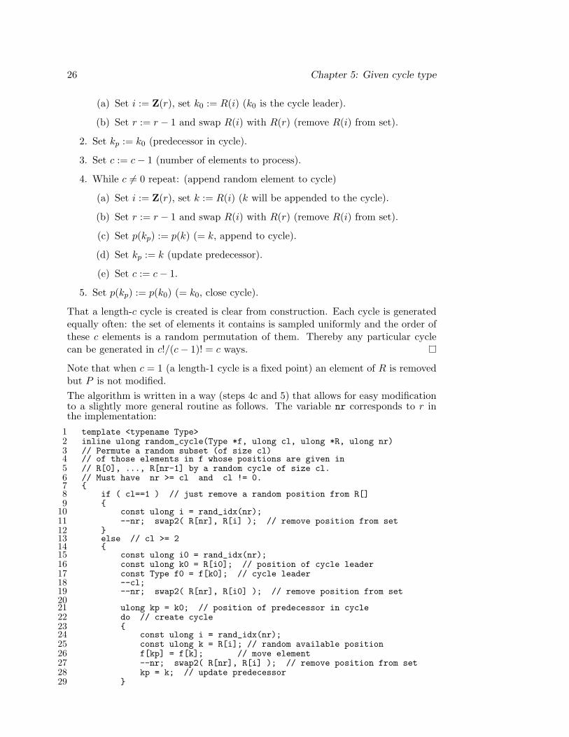
Note that when c = 1 (a length-1 cycle is a fixed point) an element of R is removedbut P is not modified.The algorithm is written in a way (steps 4c and 5) that allows for easy modificationto a slightly more general routine as follows. The variable nr corresponds to r inthe implementation:
1 template <typename Type>2 inline ulong random_cycle(Type *f, ulong cl, ulong *R, ulong nr)3 // Permute a random subset (of size cl)4 // of those elements in f whose positions are given in5 // R[0], ..., R[nr-1] by a random cycle of size cl.6 // Must have nr >= cl and cl != 0.7 {8 if ( cl==1 ) // just remove a random position from R[]9 {
10 const ulong i = rand_idx(nr);11 --nr; swap2( R[nr], R[i] ); // remove position from set12 }13 else // cl >= 214 {15 const ulong i0 = rand_idx(nr);16 const ulong k0 = R[i0]; // position of cycle leader17 const Type f0 = f[k0]; // cycle leader18 --cl;19 --nr; swap2( R[nr], R[i0] ); // remove position from set2021 ulong kp = k0; // position of predecessor in cycle22 do // create cycle23 {24 const ulong i = rand_idx(nr);25 const ulong k = R[i]; // random available position26 f[kp] = f[k]; // move element27 --nr; swap2( R[nr], R[i] ); // remove position from set28 kp = k; // update predecessor29 }
5.3: Permutations with given cycle type 27
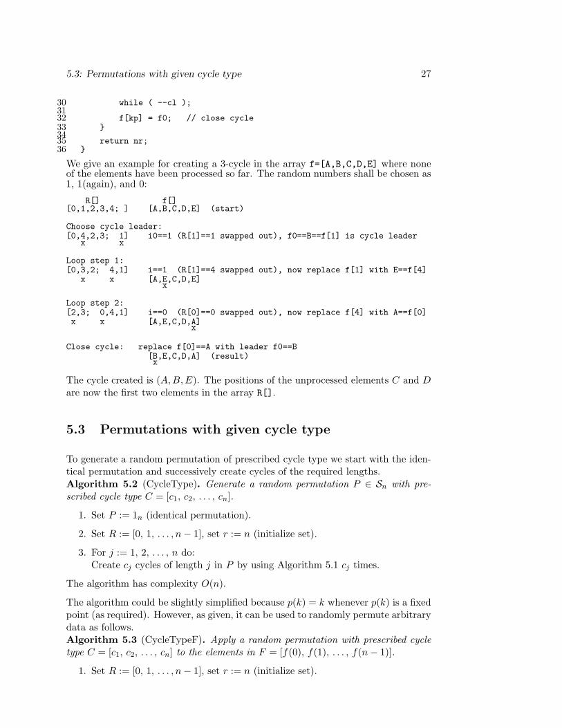
30 while ( --cl );3132 f[kp] = f0; // close cycle33 }3435 return nr;36 }
We give an example for creating a 3-cycle in the array f=[A,B,C,D,E] where noneof the elements have been processed so far. The random numbers shall be chosen as1, 1(again), and 0:
R[] f[][0,1,2,3,4; ] [A,B,C,D,E] (start)
Choose cycle leader:[0,4,2,3; 1] i0==1 (R[1]==1 swapped out), f0==B==f[1] is cycle leader
x x
Loop step 1:[0,3,2; 4,1] i==1 (R[1]==4 swapped out), now replace f[1] with E==f[4]
x x [A,E,C,D,E]x
Loop step 2:[2,3; 0,4,1] i==0 (R[0]==0 swapped out), now replace f[4] with A==f[0]x x [A,E,C,D,A]
x
Close cycle: replace f[0]==A with leader f0==B[B,E,C,D,A] (result)x
The cycle created is (A,B,E). The positions of the unprocessed elements C and Dare now the first two elements in the array R[].
5.3 Permutations with given cycle type
To generate a random permutation of prescribed cycle type we start with the iden-tical permutation and successively create cycles of the required lengths.Algorithm 5.2 (CycleType). Generate a random permutation P ∈ Sn with pre-scribed cycle type C = [c1, c2, . . . , cn].
1. Set P := 1n (identical permutation).
2. Set R := [0, 1, . . . , n− 1], set r := n (initialize set).
3. For j := 1, 2, . . . , n do:Create cj cycles of length j in P by using Algorithm 5.1 cj times.
The algorithm has complexity O(n).
The algorithm could be slightly simplified because p(k) = k whenever p(k) is a fixedpoint (as required). However, as given, it can be used to randomly permute arbitrarydata as follows.Algorithm 5.3 (CycleTypeF). Apply a random permutation with prescribed cycletype C = [c1, c2, . . . , cn] to the elements in F = [f(0), f(1), . . . , f(n− 1)].
1. Set R := [0, 1, . . . , n− 1], set r := n (initialize set).
28 Chapter 5: Given cycle type
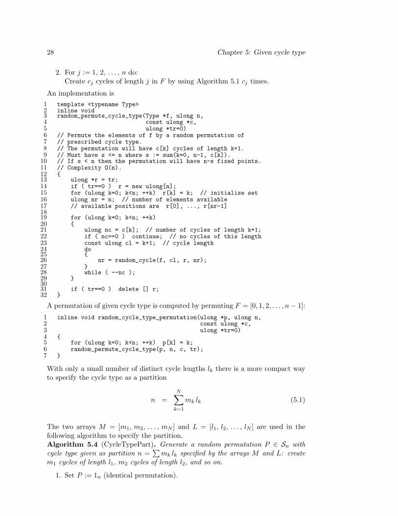
2. For j := 1, 2, . . . , n do:Create cj cycles of length j in F by using Algorithm 5.1 cj times.
An implementation is1 template <typename Type>2 inline void3 random_permute_cycle_type(Type *f, ulong n,4 const ulong *c,5 ulong *tr=0)6 // Permute the elements of f by a random permutation of7 // prescribed cycle type.8 // The permutation will have c[k] cycles of length k+1.9 // Must have s <= n where s := sum(k=0, n-1, c[k]).
10 // If s < n then the permutation will have n-s fixed points.11 // Complexity O(n).12 {13 ulong *r = tr;14 if ( tr==0 ) r = new ulong[n];15 for (ulong k=0; k<n; ++k) r[k] = k; // initialize set16 ulong nr = n; // number of elements available17 // available positions are r[0], ..., r[nr-1]1819 for (ulong k=0; k<n; ++k)20 {21 ulong nc = c[k]; // number of cycles of length k+1;22 if ( nc==0 ) continue; // no cycles of this length23 const ulong cl = k+1; // cycle length24 do25 {26 nr = random_cycle(f, cl, r, nr);27 }28 while ( --nc );29 }3031 if ( tr==0 ) delete [] r;32 }
A permutation of given cycle type is computed by permuting F = [0, 1, 2, . . . , n− 1]:
1 inline void random_cycle_type_permutation(ulong *p, ulong n,2 const ulong *c,3 ulong *tr=0)4 {5 for (ulong k=0; k<n; ++k) p[k] = k;6 random_permute_cycle_type(p, n, c, tr);7 }
With only a small number of distinct cycle lengths lk there is a more compact wayto specify the cycle type as a partition
n =N∑
k=1
mk lk (5.1)
The two arrays M = [m1, m2, . . . , mN ] and L = [l1, l2, . . . , lN ] are used in thefollowing algorithm to specify the partition.Algorithm 5.4 (CycleTypePart). Generate a random permutation P ∈ Sn withcycle type given as partition n =
∑mk lk specified by the arrays M and L: create
m1 cycles of length l1, m2 cycles of length l2, and so on.
1. Set P := 1n (identical permutation).
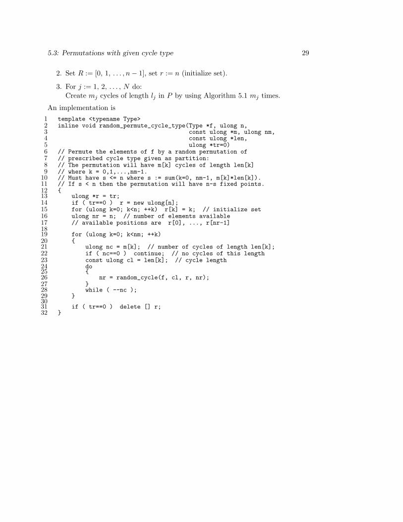
5.3: Permutations with given cycle type 29
2. Set R := [0, 1, . . . , n− 1], set r := n (initialize set).
3. For j := 1, 2, . . . , N do:Create mj cycles of length lj in P by using Algorithm 5.1 mj times.
An implementation is1 template <typename Type>2 inline void random_permute_cycle_type(Type *f, ulong n,3 const ulong *m, ulong nm,4 const ulong *len,5 ulong *tr=0)6 // Permute the elements of f by a random permutation of7 // prescribed cycle type given as partition:8 // The permutation will have m[k] cycles of length len[k]9 // where k = 0,1,...,nm-1.
10 // Must have s <= n where s := sum(k=0, nm-1, m[k]*len[k]).11 // If s < n then the permutation will have n-s fixed points.12 {13 ulong *r = tr;14 if ( tr==0 ) r = new ulong[n];15 for (ulong k=0; k<n; ++k) r[k] = k; // initialize set16 ulong nr = n; // number of elements available17 // available positions are r[0], ..., r[nr-1]1819 for (ulong k=0; k<nm; ++k)20 {21 ulong nc = m[k]; // number of cycles of length len[k];22 if ( nc==0 ) continue; // no cycles of this length23 const ulong cl = len[k]; // cycle length24 do25 {26 nr = random_cycle(f, cl, r, nr);27 }28 while ( --nc );29 }3031 if ( tr==0 ) delete [] r;32 }

30 Chapter 5: Given cycle type
31
Chapter 6
Number of cycles
We give algorithms to generate random permutations with conditions on the numberof cycles.
6.1 Bijection via swaps
Let the vector F = [f(1), f(2), . . . , f(n− 1)] be a mixed radix number in risingfactorial base, that is, 0 ≤ f(j) ≤ j (there are j + 1 choices for the digit f(j)). Thefollowing algorithm generates a permutation of n elements from a given F with n−1elements.Algorithm 6.1 (RFact2PermSwp). Convert the mixed radix number in rising fac-torial base given as vector F into a permutation P ∈ Sn:
1. Set P := 1n.
2. For k := 1, 2, . . . , n− 1 do:Set i := f(k) (i ∈ {0, 1, . . . , k}). Swap p(k − i) with p(k).
The algorithm is obviously O(n). We could have used a swap of p(i) with p(k) in thelast step, but in the form given the all-zeros word in F corresponds to the identicalpermutation.
Each of the 2 · 3 · 4 · · ·n = n! numbers F corresponds to a unique permutation. Tosee this, we generate a random permutation in two steps:Algorithm 6.2 (PermSwaps). Generate a random permutation P ∈ Sn:
1. For k := 1, 2, . . . , n− 1 do: Set i := Z(k + 1) (i ∈ {0, 1, . . . , k}), set f(k) := i.
2. Convert F into a permutation via Algorithm 6.1.
The vector F = [f(1), f(2), . . . , f(n− 1)] created in step 1 is a random mixed radixnumber in rising factorial base.
We can improve Algorithm 6.1 as follows. In step 2 we have p(k) = k, so the swapcan be replaced by the assignments p(k) := p(i) and p(i) := k. Then step 1 can bereplaced by p(0) := 0, saving O(n) writes to memory. Now the arrays F and P canshare the same storage, as follows.
32 Chapter 6: Number of cycles
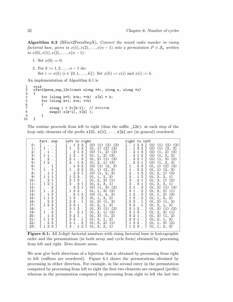
Algorithm 6.3 (RFact2PermSwpX). Convert the mixed radix number in risingfactorial base, given in x(1), x(2), . . . , x(n − 1) into a permutation P ∈ Sn writtento x(0), x(1), x(2), . . . , x(n− 1):
1. Set x(0) := 0.
2. For k := 1, 2, . . . , n− 1 do:Set i := x(k) (i ∈ {0, 1, . . . , k}). Set x(k) := x(i) and x(i) := k.
An implementation of Algorithm 6.1 is1 void2 rfact2perm_swp_l2r(const ulong *fc, ulong n, ulong *x)3 {4 for (ulong k=0; k<n; ++k) x[k] = k;5 for (ulong k=1; k<n; ++k)6 {7 ulong i = fc[k-1]; // 0<=i<=k8 swap2( x[k-i], x[k] );9 }
10 }
The routine proceeds from left to right (thus the suffix _l2r): at each step of theloop only elements of the prefix x[0], x[1], . . . , x[k] are (in general) reordered.
fact. num. left to right right to left0: [ . . . ] [ . 1 2 3 ] (0) (1) (2) (3) [ . 1 2 3 ] (0) (1) (2) (3)1: [ 1 . . ] [ 1 . 2 3 ] (0, 1) (2) (3) [ . 1 3 2 ] (0) (1) (2, 3)2: [ . 1 . ] [ . 2 1 3 ] (0) (1, 2) (3) [ . 2 1 3 ] (0) (1, 2) (3)3: [ 1 1 . ] [ 1 2 . 3 ] (0, 1, 2) (3) [ . 3 1 2 ] (0) (1, 3, 2)4: [ . 2 . ] [ 2 1 . 3 ] (0, 2) (1) (3) [ . 3 2 1 ] (0) (1, 3) (2)5: [ 1 2 . ] [ 2 . 1 3 ] (0, 2, 1) (3) [ . 2 3 1 ] (0) (1, 2, 3)6: [ . . 1 ] [ . 1 3 2 ] (0) (1) (2, 3) [ 1 . 2 3 ] (0, 1) (2) (3)7: [ 1 . 1 ] [ 1 . 3 2 ] (0, 1) (2, 3) [ 1 . 3 2 ] (0, 1) (2, 3)8: [ . 1 1 ] [ . 2 3 1 ] (0) (1, 2, 3) [ 2 . 1 3 ] (0, 2, 1) (3)9: [ 1 1 1 ] [ 1 2 3 . ] (0, 1, 2, 3) [ 3 . 1 2 ] (0, 3, 2, 1)
10: [ . 2 1 ] [ 2 1 3 . ] (0, 2, 3) (1) [ 3 . 2 1 ] (0, 3, 1) (2)11: [ 1 2 1 ] [ 2 . 3 1 ] (0, 2, 3, 1) [ 2 . 3 1 ] (0, 2, 3, 1)12: [ . . 2 ] [ . 3 2 1 ] (0) (1, 3) (2) [ 2 1 . 3 ] (0, 2) (1) (3)13: [ 1 . 2 ] [ 1 3 2 . ] (0, 1, 3) (2) [ 3 1 . 2 ] (0, 3, 2) (1)14: [ . 1 2 ] [ . 3 1 2 ] (0) (1, 3, 2) [ 1 2 . 3 ] (0, 1, 2) (3)15: [ 1 1 2 ] [ 1 3 . 2 ] (0, 1, 3, 2) [ 1 3 . 2 ] (0, 1, 3, 2)16: [ . 2 2 ] [ 2 3 . 1 ] (0, 2) (1, 3) [ 2 3 . 1 ] (0, 2) (1, 3)17: [ 1 2 2 ] [ 2 3 1 . ] (0, 2, 1, 3) [ 3 2 . 1 ] (0, 3, 1, 2)18: [ . . 3 ] [ 3 1 2 . ] (0, 3) (1) (2) [ 3 1 2 . ] (0, 3) (1) (2)19: [ 1 . 3 ] [ 3 . 2 1 ] (0, 3, 1) (2) [ 2 1 3 . ] (0, 2, 3) (1)20: [ . 1 3 ] [ 3 2 1 . ] (0, 3) (1, 2) [ 3 2 1 . ] (0, 3) (1, 2)21: [ 1 1 3 ] [ 3 2 . 1 ] (0, 3, 1, 2) [ 2 3 1 . ] (0, 2, 1, 3)22: [ . 2 3 ] [ 3 1 . 2 ] (0, 3, 2) (1) [ 1 3 2 . ] (0, 1, 3) (2)23: [ 1 2 3 ] [ 3 . 1 2 ] (0, 3, 2, 1) [ 1 2 3 . ] (0, 1, 2, 3)
Figure 6.1: All 3-digit factorial numbers with rising factorial base in lexicographicorder and the permutations (in both array and cycle form) obtained by processingfrom left and right. Dots denote zeros.
We now give both directions of a bijection that is obtained by processing from rightto left (suffixes are reordered). Figure 6.1 shows the permutations obtained byprocessing in either direction. For example, in the second entry in the permutationcomputed by processing from left to right the first two elements are swapped (prefix)whereas in the permutation computed by processing from right to left the last two
6.1: Bijection via swaps 33
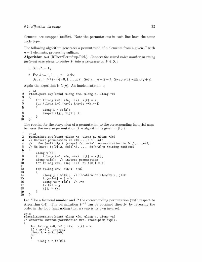
elements are swapped (suffix). Note the permutations in each line have the samecycle type.
The following algorithm generates a permutation of n elements from a given F withn− 1 elements, processing suffixes.Algorithm 6.4 (RFact2PermSwp-R2L). Convert the mixed radix number in risingfactorial base given as vector F into a permutation P ∈ Sn:
1. Set P := 1n.
2. For k := 1, 2, . . . , n− 2 do:Set i := f(k) (i ∈ {0, 1, . . . , k}). Set j = n− 2− k. Swap p(j) with p(j + i).
Again the algorithm is O(n). An implementation is
1 void2 rfact2perm_swp(const ulong *fc, ulong n, ulong *x)3 {4 for (ulong k=0; k<n; ++k) x[k] = k;5 for (ulong k=0,j=n-2; k<n-1; ++k,--j)6 {7 ulong i = fc[k];8 swap2( x[j], x[j+i] );9 }
10 }
The routine for the conversion of a permutation to the corresponding factorial num-ber uses the inverse permutation (the algorithm is given in [16]).
1 void2 perm2rfact_swp(const ulong *x, ulong n, ulong *fc)3 // Convert permutation in x[0,...,n-1] into4 // the (n-1) digit (swaps) factorial representation in fc[0,...,n-2].5 // We have: fc[0]<2, fc[1]<3, ..., fc[n-2]<n (rising radices)6 {7 ulong t[n];8 for (ulong k=0; k<n; ++k) t[k] = x[k];9 ulong ti[n]; // inverse permutation
10 for (ulong k=0; k<n; ++k) ti[t[k]] = k;1112 for (ulong k=0; k<n-1; ++k)13 {14 ulong j = ti[k]; // location of element k, j>=k15 fc[n-2-k] = j - k;16 ulong tk = t[k]; // >=k17 ti[tk] = j;18 t[j] = tk;19 }20 }
Let F be a factorial number and P the corresponding permutation (with respect toAlgorithm 6.4). The permutation P−1 can be obtained directly, by reversing theorder in the loop (and noting that a swap is its own inverse).voidrfact2invperm_swp(const ulong *fc, ulong n, ulong *x)// Generate inverse permutation wrt. rfact2perm_swp().{
for (ulong k=0; k<n; ++k) x[k] = k;if ( n<=1 ) return;ulong k = n-2, j=0;do{
ulong i = fc[k];
34 Chapter 6: Number of cycles
swap2( x[j], x[j+i] );++j;
}while ( k-- );
}
The explicit computation of the permutation can be avoided if only its action is ofinterest.
1 template <typename Type>2 void rfact2perm_swp_apply(const ulong *fc, ulong n, Type *x)3 // Permute x by permutation corresponding to rfact2perm_swp().4 {5 for (ulong k=0,j=n-2; k<n-1; ++k,--j)6 {7 ulong i = fc[k];8 swap2( x[j], x[j+i] );9 }
10 }
6.2 A property of the bijection
We now fix n and consider integers N where 0 ≤ N < n!. The factorial representa-tion F of integers N where 0 ≤ N < n! has at most n − 1 nonzero digits. In whatfollows we let F refer to the first n− 1 digits (ignoring infinitely many zeros to theright). See figure 2.2 on page 7 for an example with n = 4 (and n− 1 = 3 digits).
Let Z(F ) be the number of zeros in F and P ∈ Sn the corresponding permutation.We haveLemma 6.5. The permutation P consists of Z(F ) + 1 disjoint cycles.
Consider step 2 of Algorithm 6.1. Before the swap we have p(j) = j for j ≥ k (onlyfixed points at the right). Now if f(k) 6= 0 then the element k is joined to one ofthe cycles at the left. If f(k) = 0 then the element k lies in its own cycle (initially afixed point). The cycle containing k is never joined to any cycle so far generated asthe algorithm proceeds: each element j > k is either joined to the cycle containingk or to a cycle not containing k.
Note that Algorithm 3.10 on page 14 is obtained by disallowing zeros in F , a cyclicpermutation consists of one cycle so Z(F ) = 0.
Now a permutation into exactly m cycles can be generated as follows.Algorithm 6.6 (NumCycles-BIASED). Generate a random permutation P ∈ Sn
(where n ≥ m) with exactly m cycles. Non-uniform(!) sampling.
1. For k := 1, 2, . . . , n − 2 set f(k) := 1 + Z(k) (random factorial number Fwithout zero digits).
2. Choose a random subset of m− 1 elements U ⊆ {0, 1, . . . , n− 2}.
3. For all u ∈ U set f(u) := 0 (now F has m− 1 zeros).
4. Convert F into a permutation, using Algorithm 6.1.
6.3: Exactly 2 cycles 35
The distribution of the generated permutations is uniform only for m = 1 (cyclicpermutations) and m = n (identity). To remove the bias, the choice in step 2 hasto be made according to the statistics of the permutations.
The simplest cases are m = n − 1 (one transposition, which we omit) and m = 2which will be treated next.
6.3 Exactly 2 cycles
Let s(n,m) be the Stirling cycle numbers (see section 2.4 on page 5). There ares(n, 2) permutations with exactly two cycles. In the next algorithm we will generatea factorial number F with n− 1 digits, all except one nonzero. There are (n− 1)!/ksuch F with digit k zero. So we find
s(n, 2) = (n− 1)!n−1∑k=1
1k
= (n− 1)
In the algorithm we use the harmonic numbers Hk =∑k
j=1 1/j as (unnormalized,cumulative) probabilities.
The identity can also be obtained from relation (2.16) on page 5 (with m = 2):
s(n, 2) = s(n− 1, 1) + (n− 1) s(n− 1, 2) (6.2a)= (n− 2)! + (n− 1) s(n− 1, 2) (6.2b)
Here we used s(n, 1) = (n− 1)!. So we find
s(n, 2) = (n− 1)
Repeated use of this relation gives the desired result:
= (n− 1)![
1n− 1
+1
(n− 2)!(n− 2)!
[1
n− 2+
1(n− 3)!
s(n− 2, 2)]]
(6.2d)
= (n− 1)![
1n− 1
+1
n− 2+
1(n− 3)!
s(n− 2, 2)]
(6.2e)
and so on.
In the following algorithm we assume that an array of cumulative probabilities b(k) =Hk+1 has been precomputed.Algorithm 6.7 (TwoCycles). Generate a permutation P ∈ Sn (where n ≥ 1) withexactly 2 cycles.
1. Set t := b(n− 2) ·R() (random real number where 0 ≤ t < Hn−1).
2. Determine smallest index s such that b(s) ≥ t (using binary search).
3. For j := 1, 2, . . . , n−1 set f(j) := 1+Z(j) (factorial number F without zeros).Set f(s) := 0.
36 Chapter 6: Number of cycles
4. Convert F into a permutation, using Algorithm 6.1.
We now give an algorithm for the precomputation of the cumulative probabilities.Algorithm 6.8 (Harmonic). Set b(k) = Hk+1 for k ∈ {0, 1, . . . , n− 1}.
1. Set h := 1.0 and j := 1.0 (floating-point types).
2. For k := 0, 1, . . . , n− 1 do
(a) Set b(k) := h (= Hk+1);
(b) Set j := j + 1.0, then set h := h+ 1.0/j (update h).
This can be implemented as
1 inline void init_harmonic(double *b, ulong n)2 // Set b[k] = sum( j=1, k+1, 1/j )3 {4 double h = 1.0, j = 1.0;5 for (ulong k=0; k<n; ++k) { b[k]=h; j+=1.0; h+=1.0/j; }6 }
In the main routine for Algorithm 6.7 the digits f(k) are generated as we proceed(instead of being written to an array). Also the array to be permuted is supplied, apermutation is obtained by setting it to the identical permutation before the call.
1 template <typename Type>2 inline void random_permute_2cycles(Type *f, ulong n,3 double *tb=0, bool bi=false)4 // Permute the elements of f by a random permutation5 // consisting of exactly two cycles (must have n>1).6 // Set bi:=true to signal that the sums tb[k] = sum( j=1, k+1, 1/j )7 // have been precomputed (via init_harmonic()).8 {9 if ( n<=2 ) return;
1011 double *b = tb;12 if ( tb==0 ) { b = new double[n]; bi=false; }13 if ( !bi ) init_harmonic(b, n);1415 const double hn = b[n-2];16 const double t = rnd01() * hn;17 const ulong s = bsearch_geq(b, n-1, t) + 1; // 1<s<n1819 for (ulong k=1; k<s; ++k)20 {21 const ulong i = rand_idx(k);22 swap2(f[k], f[i]);23 }24 // skipping index s here25 for (ulong k=s+1; k<n; ++k)26 {27 const ulong i = rand_idx(k);28 swap2(f[k], f[i]);29 }3031 if ( tb==0 ) delete [] b;32 }
The binary search routine used is1 template <typename Type>2 ulong bsearch_geq(const Type *f, ulong n, const Type v)3 // Return index of first element in f[] that is >= v4 // Return n if there is no such element.5 // f[] must be sorted in ascending order.
6.4: Even or odd number of cycles 37
6 // Must have n!=07 {8 ulong nlo=0, nhi=n-1;9 while ( nlo != nhi )
10 {11 ulong t = (nhi+nlo)/2;1213 if ( f[t] < v ) nlo = t + 1;14 else nhi = t;15 }1617 if ( f[nhi]>=v ) return nhi;18 else return n;19 }
We note a generalization of relation (6.1) that is found by counting mixed radixnumbers with m− 1 zeros:
s(n,m) = (n− 1)!∑
0<l1<l2<...<lm−1<n
1l1 l2 . . . lm−1
(6.3)
Compare to the following sum over compositions of n into at most m parts [3, ex.18, p. 116], here the sum is over integer partitions:
s(n,m) =n!m!
∑l1+l2+...+lm=n
1l1 l2 . . . lm
(6.4)
6.4 Even or odd number of cycles
In the following algorithm we toggle the value of f(0) if necessary to keep the parityof the number of cycles even or odd according to the value of r:Algorithm 6.9 (CyclesPar). Generate a permutation P ∈ Sn (where n ≥ 2) suchthat the number of cycles modulo 2 equals r.
1. For j := 1, 2, . . . , n− 1 set f(j) := Z(j + 1) (random factorial number).
2. Set z := 1. For j := 0, 1, . . . , n− 2 if f(j) = 0 set z := 1− z.
3. (Here z is the number of cycles modulo 2).
4. If z 6= r then set f(0) := 1− f(0) (adjust number of cycles).
5. Using Algorithm 6.1 convert F to a permutation P .
The adjustment in step 4 is a uniform projection with quotient 2.
The following routine permutes the elements of the array x:1 template <typename Type>2 void random_permute_ncm2(Type *x, ulong n, ulong r, ulong *tf=0)3 // Apply random permutation with number of cycles == r mod 24 // ncm2 := Number of Cycles Modulo 25 // Must have n>=2.6 {7 ulong *f = tf;8 if ( tf==0 ) f = new ulong[n];9
10 for (ulong j=0; j<n-1; ++j) f[j] = rand_idx(j+2);
38 Chapter 6: Number of cycles
1112 ulong z = 1; // number cycles in factorial number13 for (ulong j=0; j<n-1; ++j) z += (f[j] == 0);14 z &= 1; // mod 215 if ( z!=r ) f[0] = 1 - f[0]; // adjust num cycles mod 21617 rfact2perm_swp_apply(f, n, x);1819 if ( tf==0 ) delete [] f;20 }
A permutation can be computed as follows:1 void2 random_ncm2_permutation(ulong *p, ulong n, ulong r, ulong *tf=0)3 // Generate a random permutation with number of cycles == r mod 24 {5 for (ulong k=0; k<n; ++k) p[k] = k; // identity6 random_permute_ncm2(p, n, r, tf);7 }
6.5 Exactly m cycles
The recurrence for the Stirling cycle numbers (relation (2.16) on page 5)
s(n,m) = s(n− 1,m− 1) + (n− 1) s(n− 1,m) (6.5)
can be interpreted as follows: a length-n permutation into m cycles (term s(n,m))can be obtained from a permutation of length n − 1 in two ways. Consider thegreatest element of the permutation. It is either a fixed point and the remainingelements are a permutation into m− 1 cycles (term s(n− 1,m− 1)), or it is insertedinto a cycle in a permutation with m cycles (and there are n − 1 ways to do this,term (n− 1) s(n− 1,m)).
We generate a random permutation in two steps. The first step computes a recipeR = [r1, r2, r3, . . . , rm] where r1 = 1, rj < rj+1 for all j, and rm ≤ n. The secondstep converts the recipe into a permutation: the entries rj are permutation sizeswhere a fixed point has to be added. The algorithm for generating a recipe worksfor N ≥ 1 and 1 ≤M ≤ N .Algorithm 6.10 (NumCyclesRecipe). Generate a recipe R = [r1, r2, r3, . . . , rM ]for a random permutation P ∈ SN with exactly M cycles.
1. Set m := M (cycles in remaining permutation) and c = m (write position inrecipe).
2. For n := N,N − 1, . . . , 1 do:
(a) If m = 1 then set r1 := 1 and terminate this loop (one cycle).
(b) Set r := Z (a) where a := s(n,m).
(c) If r < s(n− 1,m− 1) then (a fixed point will be added):set rc := n, c := c− 1, and m := m− 1.
3. Return R = [r1, r2, r3, . . . , rm].
6.5: Exactly m cycles 39
As given the algorithm has a complexity worse than O(n) because the numberss(n,m) cannot be stored in space O(1). Using instead a table of the probabilitiesb(n,m) = s(n−1,m−1)/s(n,m), stored as floating-point numbers, would give linearcomplexity. Then steps 2b and 2c would be replaced by
Set r := R() (random real number 0 ≤ r < 1).
If r < b(n,m) then (add fixed point, same assignments as before).
The following algorithm converts a recipe into a permutation.Algorithm 6.11 (Recipe2Perm). Convert a recipe R = [r1, r2, r3, . . . , rM ] into arandom permutation P ∈ SN with exactly M cycles.
1. Set P = [p(1), p(2), . . . , p(n)] := [1, 2, . . . , n] (one-based).
2. Set n := 1.
3. For a := 1, 2, . . . ,m do:
(a) For j := n, n+ 1, . . . , ra do: (join elements to cycles)set i := 1 + Z(j − 1) and swap p(i) with p(j).
(b) (add a fixed point for j = ra, this is a no-op).
(c) Set n := ra + 1.
4. For j := n, n+ 1, . . . , N do: (join remaining elements to cycles)set i := 1 + Z(j − 1) and swap p(i) with p(j).
The algorithm has complexity O(n).
The following routines are written in the GP scripting language [21]. The imple-mentation uses a precomputed table of the Stirling cycle numbers s(n,m) where1 ≤ n ≤ N and 1 ≤ m ≤ M . We use an auxiliary routine for updating a vector ofcycle numbers s(n− 1,m) (where 1 ≤ m ≤M) to numbers s(n,m).
1 st1_next(s, n1)=2 \\ Let s be a vector of the Stirling cycle numbers3 \\ s(n,1), s(n,2), ..., s(n,m) and n1=n-1.4 \\ Return the vector of the cycle numbers5 \\ s(n+1,1), s(n+1,2), ..., s(n+1,m).6 {7 local(k, sn);8 k = length(s);9 sn = vector(k);
10 sn[1] = n1*s[1];11 for (m=2, k, sn[m] = s[m-1] + n1*s[m]; );12 return( sn );13 }
The routine for the computation of the table T is
1 st1_tab(N, M)=2 \\ Compute table T of Stirling cycle numbers3 \\ T[n][m] == s(n,m) for 1<=n<=N and 1<=m<=M.4 {5 local(s, T);6 s = vector(M);7 s[1] = 1;8 T = vector(N);9 T[1] = s;
10 for (n=2, N,
40 Chapter 6: Number of cycles
11 s = st1_next(s, n-1);12 T[n] = s;13 );14 return( T );15 }
The routine for computing a recipe is
1 recipe_num_cyc(N, M)=2 \\ Generate a recipe for a random length-n permutation into m cycles.3 \\ Uses global variable T, the table of Stirling cycle numbers.4 {5 local( R, ct, m );6 R = vector(M); \\ recipe7 ct = M; \\ write position in R8 m = M; \\ cycles in remaining permutation9 forstep(n = N, 1, -1,
1011 if ( m==1, \\ only one cycle left12 R[ct]=1; \\ ==R[1]13 ct-=1;14 break()15 );161718 st0 = (n-1) * T[n-1][m]; \\ probability of joining to cycle19 st1 = T[n-1][m-1]; \\ probability of adding a fixed point20 rd = random( st0 + st1 ); \\ 0 <= rd < st0+st121 if ( rd < st1,22 \\ THEN add fixed point at step n23 m -= 1;24 R[ct] = n;25 ct -= 1;26 \\ ELSE connect to any cycle27 );28 );2930 return( R );31 }
The following routine converts a recipe to a random permutation:
1 recipe2perm(R, N)=2 \\ Convert recipe to a length-n permutation.3 {4 local(P, n, t);5 P = vector(N,j,j); \\ permutation6 n = 1; \\ position in permutation7 for (a=1, length(R),8 for (j=n, R[a]-1,9 i = 1 + random(j-1); \\ one-based arrays
10 t=P[i]; P[i]=P[j]; P[j]=t; \\ join to cycle (swap)11 );12 \\ and add fixed point (no-op)13 n = R[a] + 1;14 );1516 for (j=n, N, \\ (elements left for processing)17 i = 1 + random(j-1); \\ one-based arrays18 t=P[i]; P[i]=P[j]; P[j]=t; \\ join to cycle (swap)19 );2021 return(P);22 }
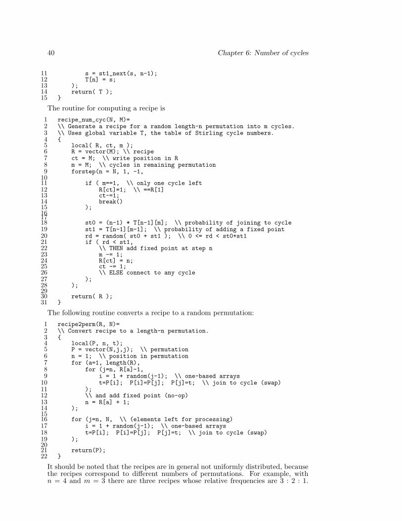
It should be noted that the recipes are in general not uniformly distributed, becausethe recipes correspond to different numbers of permutations. For example, withn = 4 and m = 3 there are three recipes whose relative frequencies are 3 : 2 : 1.
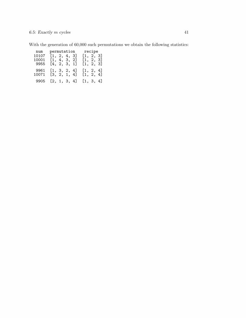
6.5: Exactly m cycles 41
With the generation of 60,000 such permutations we obtain the following statistics:num permutation recipe
10107 [1, 2, 4, 3] [1, 2, 3]10001 [1, 4, 3, 2] [1, 2, 3]9955 [4, 2, 3, 1] [1, 2, 3]
9961 [1, 3, 2, 4] [1, 2, 4]10071 [3, 2, 1, 4] [1, 2, 4]
9905 [2, 1, 3, 4] [1, 3, 4]

42 Chapter 6: Number of cycles
43
Chapter 7
Inversions
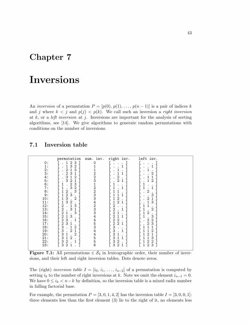
An inversion of a permutation P = [p(0), p(1), . . . , p(n− 1)] is a pair of indices kand j where k < j and p(j) < p(k). We call such an inversion a right inversionat k, or a left inversion at j. Inversions are important for the analysis of sortingalgorithms, see [14]. We give algorithms to generate random permutations withconditions on the number of inversions.
7.1 Inversion table
permutation num. inv. right inv. left inv.0: [ . 1 2 3 ] 0 [ . . . ] [ . . . ]1: [ . 1 3 2 ] 1 [ . . 1 ] [ . . 1 ]2: [ . 2 1 3 ] 1 [ . 1 . ] [ . 1 . ]3: [ . 2 3 1 ] 2 [ . 1 1 ] [ . . 2 ]4: [ . 3 1 2 ] 2 [ . 2 . ] [ . 1 1 ]5: [ . 3 2 1 ] 3 [ . 2 1 ] [ . 1 2 ]6: [ 1 . 2 3 ] 1 [ 1 . . ] [ 1 . . ]7: [ 1 . 3 2 ] 2 [ 1 . 1 ] [ 1 . 1 ]8: [ 1 2 . 3 ] 2 [ 1 1 . ] [ . 2 . ]9: [ 1 2 3 . ] 3 [ 1 1 1 ] [ . . 3 ]10: [ 1 3 . 2 ] 3 [ 1 2 . ] [ . 2 1 ]11: [ 1 3 2 . ] 4 [ 1 2 1 ] [ . 1 3 ]12: [ 2 . 1 3 ] 2 [ 2 . . ] [ 1 1 . ]13: [ 2 . 3 1 ] 3 [ 2 . 1 ] [ 1 . 2 ]14: [ 2 1 . 3 ] 3 [ 2 1 . ] [ 1 2 . ]15: [ 2 1 3 . ] 4 [ 2 1 1 ] [ 1 . 3 ]16: [ 2 3 . 1 ] 4 [ 2 2 . ] [ . 2 2 ]17: [ 2 3 1 . ] 5 [ 2 2 1 ] [ . 2 3 ]18: [ 3 . 1 2 ] 3 [ 3 . . ] [ 1 1 1 ]19: [ 3 . 2 1 ] 4 [ 3 . 1 ] [ 1 1 2 ]20: [ 3 1 . 2 ] 4 [ 3 1 . ] [ 1 2 1 ]21: [ 3 1 2 . ] 5 [ 3 1 1 ] [ 1 1 3 ]22: [ 3 2 . 1 ] 5 [ 3 2 . ] [ 1 2 2 ]23: [ 3 2 1 . ] 6 [ 3 2 1 ] [ 1 2 3 ]
Figure 7.1: All permutations ∈ S4 in lexicographic order, their number of inver-sions, and their left and right inversion tables. Dots denote zeros.
The (right) inversion table I = [i0, i1, . . . , in−2] of a permutation is computed bysetting ik to the number of right inversions at k. Note we omit the element in−1 = 0.We have 0 ≤ ik < n−k by definition, so the inversion table is a mixed radix numberin falling factorial base.
For example, the permutation P = [3, 0, 1, 4, 2] has the inversion table I = [3, 0, 0, 1]:three elements less than the first element (3) lie to the right of it, no elements less
44 Chapter 7: Inversions
than the second (0) or third (1) elements lie right to them, and one element lessthan 4 lies right of it.
We could similarly define a left inversion table, figure 7.1 shows both types of inver-sion tables for all permutations ∈ S4.
The obvious algorithm for computing the inversion table is to count, for each elementp(k), the number of elements p(j) right to it (j > k) that are smaller than p(k). Animplementation is
1 void perm2ffact(const ulong *x, ulong n, ulong *ff)2 // Convert permutation in x[0,...,n-1] into3 // the (n-1) digit falling factorial representation in ff[0,...,n-2].4 // We have: ff[0]<n, ff[1]<n-1, ..., ff[n-2]<2 (falling radices)5 {6 for (ulong k=0; k<n-1; ++k)7 {8 ulong xk = x[k];9 ulong i = 0;
10 for (ulong j=k+1; j<n; ++j) if ( x[j]<xk ) ++i;11 ff[k] = i;12 }13 }
The complexity is O(n2), also for the other direction. We first give the algorithm.Algorithm 7.1 (FFact2Perm-Rot). Convert the right inversion table F into thecorresponding permutation P ∈ Sn.
1. For j := 0, 1, . . . , n− 1 do: set p(j) := j (identical permutation).
2. For k := 0, 1, 2, . . . , n− 2 do: (rotations)
(a) Set s := f(k).
(b) Cyclically rotate [p(k), p(k + 1), . . . , p(k + s)] (s + 1 elements) by oneposition to the right (no-op if s = 0).
As an example we compute the length-5 permutation corresponding to the inversiontable [3, 0, 0, 1]:
[0, 1, 2, 3, 4] (start, identity)> > > >[3, 0, 1, 2, 4] (rotate 4=3+1 elements, starting from k=0)
>[3, 0, 1, 2, 4] (rotate 1=0+1 elements, starting from k=1, no-op)
>[3, 0, 1, 2, 4] (rotate 1=0+1 elements, starting from k=2, no-op)
> >[3, 0, 1, 4, 2] (rotate 2=1+1 elements, starting from k=3)
The underlying trick is that the rotation starting at position k leaves the suffixstarting at position k + 1 in ascending order. The following right shifts by oneposition move the last element of the shifted range to its front, leaving s smallerelements (all from the shifted part) to the right of it.
An implementation is1 void2 ffact2perm(const ulong *ff, ulong n, ulong *x)3 // Convert the (n-1) digit falling factorial representation4 // in ff[0,...,n-2] into a permutation in x[0,...,n-1].5 // into permutation in x[0,...,n-1]6 // Must have: ff[0]<n, ff[1]<n-1, ..., ff[n-2]<2 (falling radices)
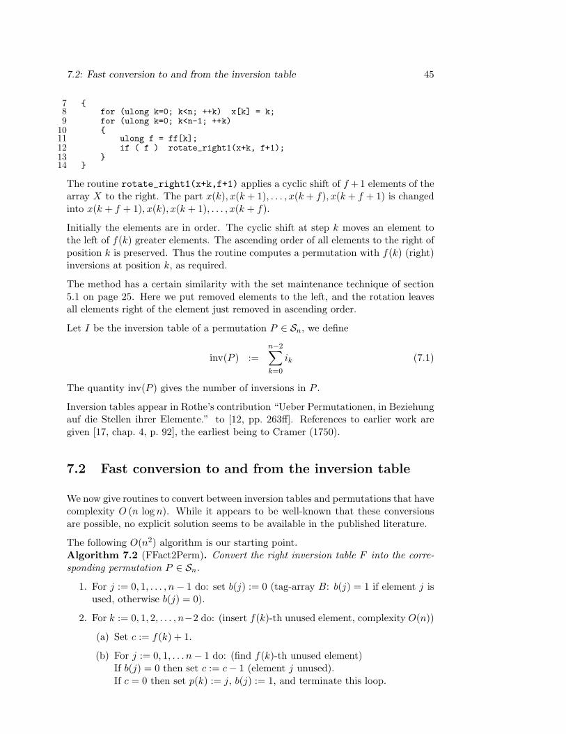
7.2: Fast conversion to and from the inversion table 45
7 {8 for (ulong k=0; k<n; ++k) x[k] = k;9 for (ulong k=0; k<n-1; ++k)
10 {11 ulong f = ff[k];12 if ( f ) rotate_right1(x+k, f+1);13 }14 }
The routine rotate_right1(x+k,f+1) applies a cyclic shift of f + 1 elements of thearray X to the right. The part x(k), x(k + 1), . . . , x(k + f), x(k + f + 1) is changedinto x(k + f + 1), x(k), x(k + 1), . . . , x(k + f).
Initially the elements are in order. The cyclic shift at step k moves an element tothe left of f(k) greater elements. The ascending order of all elements to the right ofposition k is preserved. Thus the routine computes a permutation with f(k) (right)inversions at position k, as required.
The method has a certain similarity with the set maintenance technique of section5.1 on page 25. Here we put removed elements to the left, and the rotation leavesall elements right of the element just removed in ascending order.
Let I be the inversion table of a permutation P ∈ Sn, we define
inv(P ) :=n−2∑k=0
ik (7.1)
The quantity inv(P ) gives the number of inversions in P .
Inversion tables appear in Rothe’s contribution “Ueber Permutationen, in Beziehungauf die Stellen ihrer Elemente.” to [12, pp. 263ff]. References to earlier work aregiven [17, chap. 4, p. 92], the earliest being to Cramer (1750).
7.2 Fast conversion to and from the inversion table
We now give routines to convert between inversion tables and permutations that havecomplexity O (n log n). While it appears to be well-known that these conversionsare possible, no explicit solution seems to be available in the published literature.
The following O(n2) algorithm is our starting point.Algorithm 7.2 (FFact2Perm). Convert the right inversion table F into the corre-sponding permutation P ∈ Sn.
1. For j := 0, 1, . . . , n− 1 do: set b(j) := 0 (tag-array B: b(j) = 1 if element j isused, otherwise b(j) = 0).
2. For k := 0, 1, 2, . . . , n−2 do: (insert f(k)-th unused element, complexity O(n))
(a) Set c := f(k) + 1.
(b) For j := 0, 1, . . . n− 1 do: (find f(k)-th unused element)If b(j) = 0 then set c := c− 1 (element j unused).If c = 0 then set p(k) := j, b(j) := 1, and terminate this loop.
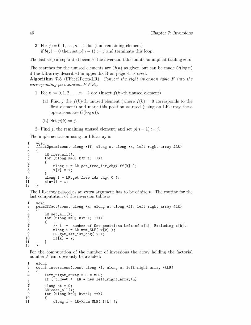
46 Chapter 7: Inversions
3. For j := 0, 1, . . . , n− 1 do: (find remaining element)if b(j) = 0 then set p(n− 1) := j and terminate this loop.
The last step is separated because the inversion table omits an implicit trailing zero.
The searches for the unused elements are O(n) as given but can be made O(log n)if the LR-array described in appendix B on page 81 is used.Algorithm 7.3 (FFact2Perm-LR). Convert the right inversion table F into thecorresponding permutation P ∈ Sn.
1. For k := 0, 1, 2, . . . , n− 2 do: (insert f(k)-th unused element)
(a) Find j the f(k)-th unused element (where f(k) = 0 corresponds to thefirst element) and mark this position as used (using an LR-array theseoperations are O(log n)).
(b) Set p(k) := j.
2. Find j, the remaining unused element, and set p(n− 1) := j.
The implementation using an LR-array is1 void2 ffact2perm(const ulong *ff, ulong n, ulong *x, left_right_array &LR)3 {4 LR.free_all();5 for (ulong k=0; k<n-1; ++k)6 {7 ulong i = LR.get_free_idx_chg( ff[k] );8 x[k] = i;9 }
10 ulong i = LR.get_free_idx_chg( 0 );11 x[n-1] = i;12 }
The LR-array passed as an extra argument has to be of size n. The routine for thefast computation of the inversion table is
1 void2 perm2ffact(const ulong *x, ulong n, ulong *ff, left_right_array &LR)3 {4 LR.set_all();5 for (ulong k=0; k<n-1; ++k)6 {7 // i := number of Set positions Left of x[k], Excluding x[k].8 ulong i = LR.num_SLE( x[k] );9 LR.get_set_idx_chg( i );
10 ff[k] = i;11 }12 }
For the computation of the number of inversions the array holding the factorialnumber F can obviously be avoided:
1 ulong2 count_inversions(const ulong *f, ulong n, left_right_array *tLR)3 {4 left_right_array *LR = tLR;5 if ( tLR==0 ) LR = new left_right_array(n);67 ulong ct = 0;8 LR->set_all();9 for (ulong k=0; k<n-1; ++k)
10 {11 ulong i = LR->num_SLE( f[k] );
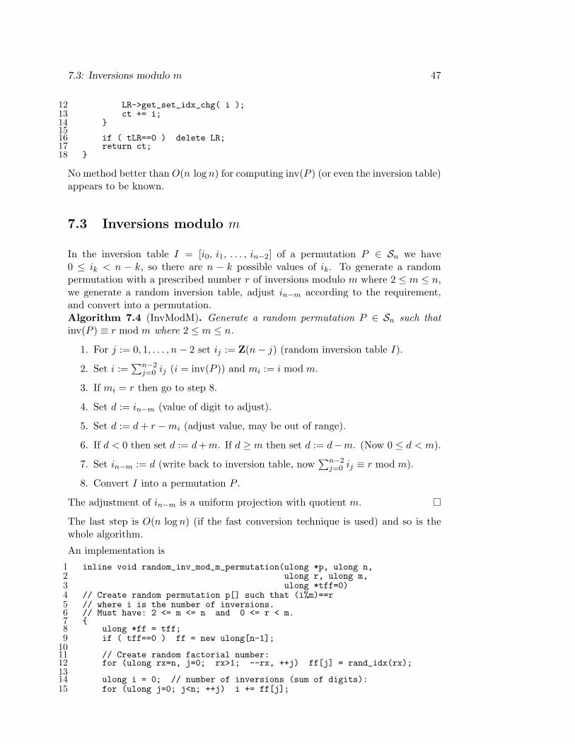
7.3: Inversions modulo m 47
12 LR->get_set_idx_chg( i );13 ct += i;14 }1516 if ( tLR==0 ) delete LR;17 return ct;18 }
No method better than O(n log n) for computing inv(P ) (or even the inversion table)appears to be known.
7.3 Inversions modulo m
In the inversion table I = [i0, i1, . . . , in−2] of a permutation P ∈ Sn we have0 ≤ ik < n − k, so there are n − k possible values of ik. To generate a randompermutation with a prescribed number r of inversions modulo m where 2 ≤ m ≤ n,we generate a random inversion table, adjust in−m according to the requirement,and convert into a permutation.Algorithm 7.4 (InvModM). Generate a random permutation P ∈ Sn such thatinv(P ) ≡ r mod m where 2 ≤ m ≤ n.
1. For j := 0, 1, . . . , n− 2 set ij := Z(n− j) (random inversion table I).
2. Set i :=∑n−2
j=0 ij (i = inv(P )) and mi := i mod m.
3. If mi = r then go to step 8.
4. Set d := in−m (value of digit to adjust).
5. Set d := d+ r −mi (adjust value, may be out of range).
6. If d < 0 then set d := d+m. If d ≥ m then set d := d−m. (Now 0 ≤ d < m).
7. Set in−m := d (write back to inversion table, now∑n−2
j=0 ij ≡ r mod m).
8. Convert I into a permutation P .
The adjustment of in−m is a uniform projection with quotient m.
The last step is O(n log n) (if the fast conversion technique is used) and so is thewhole algorithm.
An implementation is
1 inline void random_inv_mod_m_permutation(ulong *p, ulong n,2 ulong r, ulong m,3 ulong *tff=0)4 // Create random permutation p[] such that (i%m)==r5 // where i is the number of inversions.6 // Must have: 2 <= m <= n and 0 <= r < m.7 {8 ulong *ff = tff;9 if ( tff==0 ) ff = new ulong[n-1];
1011 // Create random factorial number:12 for (ulong rx=n, j=0; rx>1; --rx, ++j) ff[j] = rand_idx(rx);1314 ulong i = 0; // number of inversions (sum of digits):15 for (ulong j=0; j<n; ++j) i += ff[j];
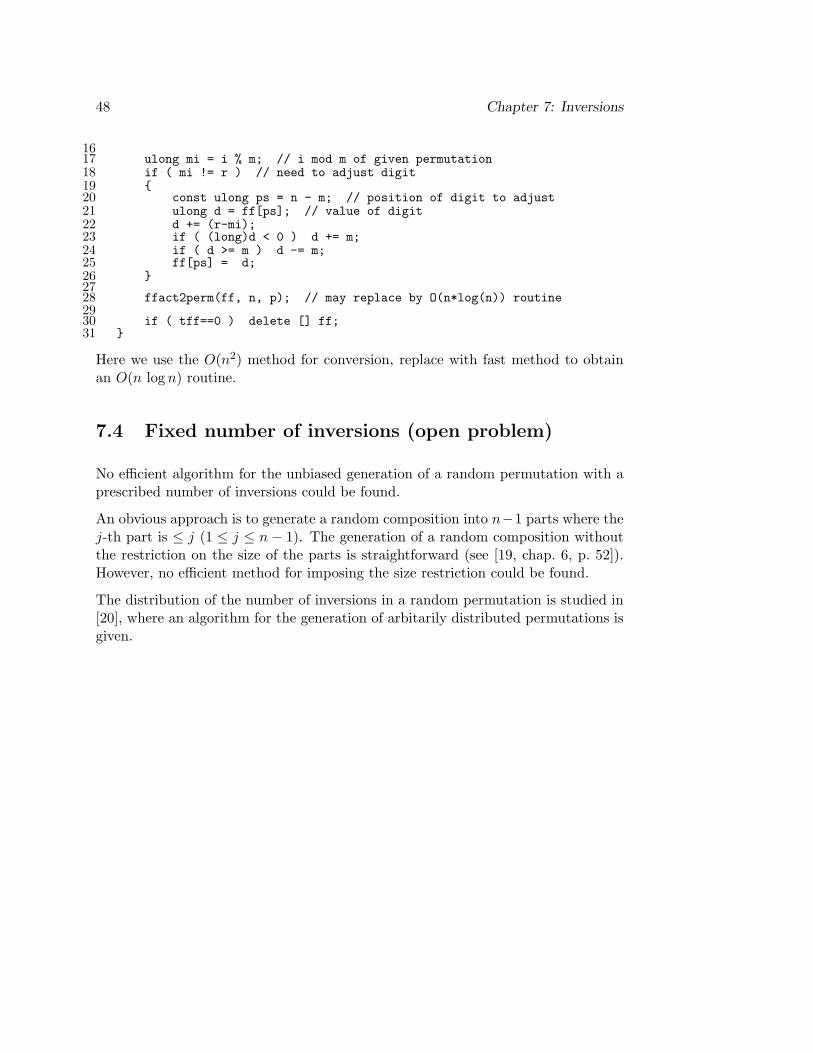
48 Chapter 7: Inversions
1617 ulong mi = i % m; // i mod m of given permutation18 if ( mi != r ) // need to adjust digit19 {20 const ulong ps = n - m; // position of digit to adjust21 ulong d = ff[ps]; // value of digit22 d += (r-mi);23 if ( (long)d < 0 ) d += m;24 if ( d >= m ) d -= m;25 ff[ps] = d;26 }2728 ffact2perm(ff, n, p); // may replace by O(n*log(n)) routine2930 if ( tff==0 ) delete [] ff;31 }
Here we use the O(n2) method for conversion, replace with fast method to obtainan O(n log n) routine.
7.4 Fixed number of inversions (open problem)
No efficient algorithm for the unbiased generation of a random permutation with aprescribed number of inversions could be found.
An obvious approach is to generate a random composition into n−1 parts where thej-th part is ≤ j (1 ≤ j ≤ n− 1). The generation of a random composition withoutthe restriction on the size of the parts is straightforward (see [19, chap. 6, p. 52]).However, no efficient method for imposing the size restriction could be found.
The distribution of the number of inversions in a random permutation is studied in[20], where an algorithm for the generation of arbitarily distributed permutations isgiven.
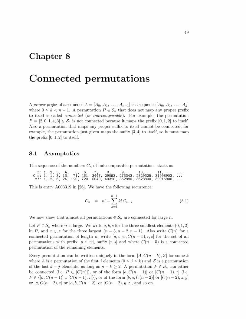
49
Chapter 8
Connected permutations
A proper prefix of a sequence A = [A0, A1, . . . , An−1] is a sequence [A0, A1, . . . , Ak]where 0 ≤ k < n − 1. A permutation P ∈ Sn that does not map any proper prefixto itself is called connected (or indecomposable). For example, the permutationP = [2, 0, 1, 4, 3] ∈ S5 is not connected because it maps the prefix [0, 1, 2] to itself.Also a permutation that maps any proper suffix to itself cannot be connected, forexample, the permutation just given maps the suffix [3, 4] to itself, so it must mapthe prefix [0, 1, 2] to itself.
8.1 Asymptotics
The sequence of the numbers Cn of indecomposable permutations starts asn: 1, 2, 3, 4, 5, 6, 7, 8, 9, 10, 11, ...
C_n: 1, 1, 3, 13, 71, 461, 3447, 29093, 273343, 2829325, 31998903, ...n!: 1, 2, 6, 24, 120, 720, 5040, 40320, 362880, 3628800, 39916800, ...
This is entry A003319 in [26]. We have the following recurrence:
Cn = n!−n−1∑k=1
k!Cn−k (8.1)
We now show that almost all permutations ∈ Sn are connected for large n.
Let P ∈ Sn where n is large. We write a, b, c for the three smallest elements (0, 1, 2)in P , and x, y, z for the three largest (n − 3, n − 2, n − 1). Also write C(n) for aconnected permutation of length n, write [u, v, w,C(n − 5), r, s] for the set of allpermutations with prefix [u, v, w], suffix [r, s] and where C(n − 5) is a connectedpermutation of the remaining elements.
Every permutation can be written uniquely in the form [A,C(n− k), Z] for some kwhere A is a permutation of the first j elements (0 ≤ j ≤ k) and Z is a permutationof the last k − j elements, as long as n − k ≥ 2: A permutation P ∈ Sn can eitherbe connected (i.e. P ∈ [C(n)]), or of the form [a,C(n − 1)] or [C(n − 1), z] (i.e.P ∈ {[a,C(n− 1)] ∪ [C(n− 1), z]}), or of the form [b, a, C(n− 2)] or [C(n− 2), z, y]or [a,C(n− 2), z] or [a, b, C(n− 2)] or [C(n− 2), y, z], and so on.
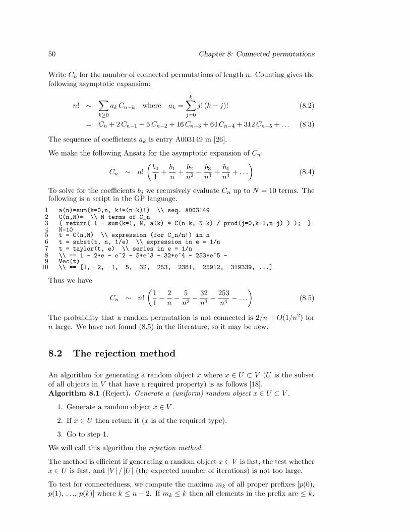
50 Chapter 8: Connected permutations
Write Cn for the number of connected permutations of length n. Counting gives thefollowing asymptotic expansion:
n! ∼∑k≥0
ak Cn−k where ak =k∑
j=0
j! (k − j)! (8.2)
= Cn + 2Cn−1 + 5Cn−2 + 16Cn−3 + 64Cn−4 + 312Cn−5 + . . . (8.3)
The sequence of coefficients ak is entry A003149 in [26].
We make the following Ansatz for the asymptotic expansion of Cn:
Cn ∼ n!(b01
+b1n
+b2n2
+b3n3
+b4n4
+ . . .
)(8.4)
To solve for the coefficients bj we recursively evaluate Cn up to N = 10 terms. Thefollowing is a script in the GP language.
1 a(n)=sum(k=0,n, k!*(n-k)!) \\ seq. A0031492 C(n,N)= \\ N terms of C_n3 { return( 1 - sum(k=1, N, a(k) * C(n-k, N-k) / prod(j=0,k-1,n-j) ) ); }4 N=105 t = C(n,N) \\ expression (for C_n/n!) in n6 t = subst(t, n, 1/e) \\ expression in e = 1/n7 t = taylor(t, e) \\ series in e = 1/n8 \\ == 1 - 2*e - e^2 - 5*e^3 - 32*e^4 - 253*e^5 -9 Vec(t)
10 \\ == [1, -2, -1, -5, -32, -253, -2381, -25912, -319339, ...]
Thus we have
Cn ∼ n!(
11− 2n− 5n2− 32n3− 253
n4− . . .
)(8.5)
The probability that a random permutation is not connected is 2/n + O(1/n2) forn large. We have not found (8.5) in the literature, so it may be new.
8.2 The rejection method
An algorithm for generating a random object x where x ∈ U ⊂ V (U is the subsetof all objects in V that have a required property) is as follows [18].Algorithm 8.1 (Reject). Generate a (uniform) random object x ∈ U ⊂ V .
1. Generate a random object x ∈ V .
2. If x ∈ U then return it (x is of the required type).
3. Go to step 1.
We will call this algorithm the rejection method.
The method is efficient if generating a random object x ∈ V is fast, the test whetherx ∈ U is fast, and |V | / |U | (the expected number of iterations) is not too large.
To test for connectedness, we compute the maxima mk of all proper prefixes [p(0),p(1), . . ., p(k)] where k ≤ n− 2. If mk ≤ k then all elements in the prefix are ≤ k,
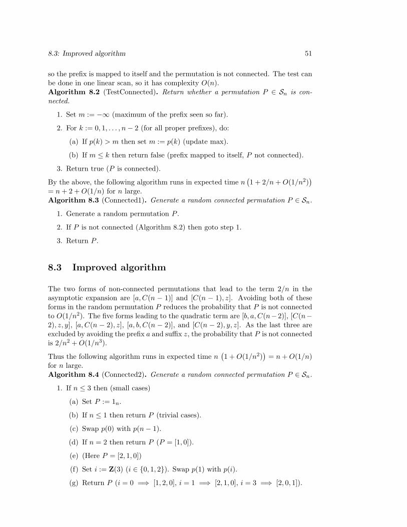
8.3: Improved algorithm 51
so the prefix is mapped to itself and the permutation is not connected. The test canbe done in one linear scan, so it has complexity O(n).Algorithm 8.2 (TestConnected). Return whether a permutation P ∈ Sn is con-nected.
1. Set m := −∞ (maximum of the prefix seen so far).
2. For k := 0, 1, . . . , n− 2 (for all proper prefixes), do:
(a) If p(k) > m then set m := p(k) (update max).
(b) If m ≤ k then return false (prefix mapped to itself, P not connected).
3. Return true (P is connected).
By the above, the following algorithm runs in expected time n(1 + 2/n+O(1/n2)
)= n+ 2 +O(1/n) for n large.Algorithm 8.3 (Connected1). Generate a random connected permutation P ∈ Sn.
1. Generate a random permutation P .
2. If P is not connected (Algorithm 8.2) then goto step 1.
3. Return P .
8.3 Improved algorithm
The two forms of non-connected permutations that lead to the term 2/n in theasymptotic expansion are [a,C(n − 1)] and [C(n − 1), z]. Avoiding both of theseforms in the random permutation P reduces the probability that P is not connectedto O(1/n2). The five forms leading to the quadratic term are [b, a, C(n−2)], [C(n−2), z, y], [a,C(n − 2), z], [a, b, C(n − 2)], and [C(n − 2), y, z]. As the last three areexcluded by avoiding the prefix a and suffix z, the probability that P is not connectedis 2/n2 +O(1/n3).
Thus the following algorithm runs in expected time n(1 +O(1/n2)
)= n+O(1/n)
for n large.Algorithm 8.4 (Connected2). Generate a random connected permutation P ∈ Sn.
1. If n ≤ 3 then (small cases)
(a) Set P := 1n.
(b) If n ≤ 1 then return P (trivial cases).
(c) Swap p(0) with p(n− 1).
(d) If n = 2 then return P (P = [1, 0]).
(e) (Here P = [2, 1, 0])
(f) Set i := Z(3) (i ∈ {0, 1, 2}). Swap p(1) with p(i).
(g) Return P (i = 0 =⇒ [1, 2, 0], i = 1 =⇒ [2, 1, 0], i = 3 =⇒ [2, 0, 1]).
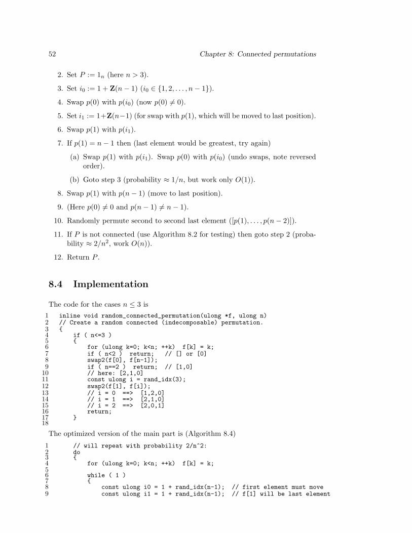
52 Chapter 8: Connected permutations
2. Set P := 1n (here n > 3).
3. Set i0 := 1 + Z(n− 1) (i0 ∈ {1, 2, . . . , n− 1}).
4. Swap p(0) with p(i0) (now p(0) 6= 0).
5. Set i1 := 1+Z(n−1) (for swap with p(1), which will be moved to last position).
6. Swap p(1) with p(i1).
7. If p(1) = n− 1 then (last element would be greatest, try again)
(a) Swap p(1) with p(i1). Swap p(0) with p(i0) (undo swaps, note reversedorder).
(b) Goto step 3 (probability ≈ 1/n, but work only O(1)).
8. Swap p(1) with p(n− 1) (move to last position).
9. (Here p(0) 6= 0 and p(n− 1) 6= n− 1).
10. Randomly permute second to second last element ([p(1), . . . , p(n− 2)]).
11. If P is not connected (use Algorithm 8.2 for testing) then goto step 2 (proba-bility ≈ 2/n2, work O(n)).
12. Return P .
8.4 Implementation
The code for the cases n ≤ 3 is1 inline void random_connected_permutation(ulong *f, ulong n)2 // Create a random connected (indecomposable) permutation.3 {4 if ( n<=3 )5 {6 for (ulong k=0; k<n; ++k) f[k] = k;7 if ( n<2 ) return; // [] or [0]8 swap2(f[0], f[n-1]);9 if ( n==2 ) return; // [1,0]
10 // here: [2,1,0]11 const ulong i = rand_idx(3);12 swap2(f[1], f[i]);13 // i = 0 ==> [1,2,0]14 // i = 1 ==> [2,1,0]15 // i = 2 ==> [2,0,1]16 return;17 }18
The optimized version of the main part is (Algorithm 8.4)
1 // will repeat with probability 2/n^2:2 do3 {4 for (ulong k=0; k<n; ++k) f[k] = k;56 while ( 1 )7 {8 const ulong i0 = 1 + rand_idx(n-1); // first element must move9 const ulong i1 = 1 + rand_idx(n-1); // f[1] will be last element
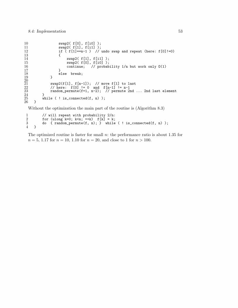
8.4: Implementation 53
10 swap2( f[0], f[i0] );11 swap2( f[1], f[i1] );12 if ( f[1]==n-1 ) // undo swap and repeat (here: f[0]!=0)13 {14 swap2( f[1], f[i1] );15 swap2( f[0], f[i0] );16 continue; // probability 1/n but work only O(1)17 }18 else break;19 }2021 swap2(f[1], f[n-1]); // move f[1] to last22 // here: f[0] != 0 and f[n-1] != n-123 random_permute(f+1, n-2); // permute 2nd ... 2nd last element24 }25 while ( ! is_connected(f, n) );26 }
Without the optimization the main part of the routine is (Algorithm 8.3)
1 // will repeat with probability 2/n:2 for (ulong k=0; k<n; ++k) f[k] = k;3 do { random_permute(f, n); } while ( ! is_connected(f, n) );4 }
The optimized routine is faster for small n: the performance ratio is about 1.35 forn = 5, 1.17 for n = 10, 1.10 for n = 20, and close to 1 for n > 100.

54 Chapter 8: Connected permutations
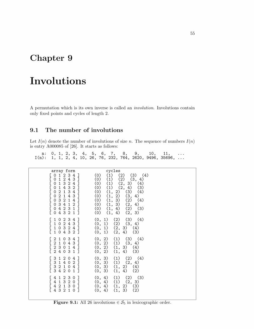
55
Chapter 9
Involutions
A permutation which is its own inverse is called an involution. Involutions containonly fixed points and cycles of length 2.
9.1 The number of involutions
Let I(n) denote the number of involutions of size n. The sequence of numbers I(n)is entry A000085 of [26]. It starts as follows:
n: 0, 1, 2, 3, 4, 5, 6, 7, 8, 9, 10, 11, ...I(n): 1, 1, 2, 4, 10, 26, 76, 232, 764, 2620, 9496, 35696, ...
array form cycles[ 0 1 2 3 4 ] (0) (1) (2) (3) (4)[ 0 1 2 4 3 ] (0) (1) (2) (3, 4)[ 0 1 3 2 4 ] (0) (1) (2, 3) (4)[ 0 1 4 3 2 ] (0) (1) (2, 4) (3)[ 0 2 1 3 4 ] (0) (1, 2) (3) (4)[ 0 2 1 4 3 ] (0) (1, 2) (3, 4)[ 0 3 2 1 4 ] (0) (1, 3) (2) (4)[ 0 3 4 1 2 ] (0) (1, 3) (2, 4)[ 0 4 2 3 1 ] (0) (1, 4) (2) (3)[ 0 4 3 2 1 ] (0) (1, 4) (2, 3)
[ 1 0 2 3 4 ] (0, 1) (2) (3) (4)[ 1 0 2 4 3 ] (0, 1) (2) (3, 4)[ 1 0 3 2 4 ] (0, 1) (2, 3) (4)[ 1 0 4 3 2 ] (0, 1) (2, 4) (3)
[ 2 1 0 3 4 ] (0, 2) (1) (3) (4)[ 2 1 0 4 3 ] (0, 2) (1) (3, 4)[ 2 3 0 1 4 ] (0, 2) (1, 3) (4)[ 2 4 0 3 1 ] (0, 2) (1, 4) (3)
[ 3 1 2 0 4 ] (0, 3) (1) (2) (4)[ 3 1 4 0 2 ] (0, 3) (1) (2, 4)[ 3 2 1 0 4 ] (0, 3) (1, 2) (4)[ 3 4 2 0 1 ] (0, 3) (1, 4) (2)
[ 4 1 2 3 0 ] (0, 4) (1) (2) (3)[ 4 1 3 2 0 ] (0, 4) (1) (2, 3)[ 4 2 1 3 0 ] (0, 4) (1, 2) (3)[ 4 3 2 1 0 ] (0, 4) (1, 3) (2)
Figure 9.1: All 26 involutions ∈ S5 in lexicographic order.
56 Chapter 9: Involutions
We have I(0) = 1, I(1) = 1, and, for n > 1, the recursion [24, pp. 85-86]
I(n) = I(n− 1) + (n− 1) I(n− 2) (9.1)
Pick any element x of an involution ∈ Sn. If it is a fixed point, the remainingelements are an involution ∈ Sn−1. If it lies in a 2-cycle with some other element y(there are n−1 choices for y), then remaining elements are an involution ∈ Sn−2.
Figure 9.1 illustrates this for the I(5) = 26 involutions of 5 elements. There areI(n − 1) = I(4) = 10 involutions that have x = 0 as a fixed point. The elements6= x form an involution in each of these. The remaining involutions contain a cycle(x, y) = (0, y) with (n− 1) = 4 choices for y. For each choice of y the elements 6= xand 6= y form an involution of size (n− 2) = 3, there are I(3) = 4 such involutions.
9.2 Branching probabilities
To generate a random involution, we put each element either into a fixed point orinto a 2-cycle. To obtain a uniform distribution, we need to compute (for every n)the probability that the element under consideration is a fixed point and branchaccordingly.
We can interpret relation (9.1) as follows. Among the I(n) involutions ∈ Sn thereare I(n − 1) such that the element x under consideration is a fixed point and theremaining (n − 1) I(n − 2) involutions have x in a 2-cycle. A first version of thealgorithm can now be given.Algorithm 9.1 (Involutions). Generate a random involution ∈ Sn.
1. Set P := 1n. Set S := {0, 1, . . . , n− 1}.
2. If n ≤ 1 exit.
3. Choose the smallest x ∈ S (cycle leader) and remove x from S.
4. Set t := Z(I(n)) and f := I(n− 1). Set n := n− 1.
5. If t < f then goto step 2 (fixed point, nothing to do).
6. Randomly choose y ∈ S (n− 1 choices) and remove y from S.
7. Set n := n− 1 and swap x with y (create a 2-cycle). Goto step 2.
In step 3 the word ‘smallest’ is used to make the choice well-defined. In fact anyelement ∈ S can be used.
The algorithm is obviously correct, but it is not practical. It has complexity O(n)only if the quantities I(n) can be computed in time O(1). Relation (9.1) allows toupdate a pair (I(n), I(n− 1)) 7→ (I(n+ 1), I(n)) with one multiplication and ad-dition. Using integer variables leads to large numbers requiring more than constanttime for these operations. With floating-point variables these operations are O(1)but an overflow will occur already for moderately large n. For example, with IEEEdouble precision floats I(295) ≈ 2.80309 · 10307 is the largest representable I(n).
9.3: Practical algorithm 57
We note that Algorithm 9.1 is a special case of a technique that uses unranking (seesection 2.8 on page 8). Let C(n) be the number of size-n combinatorial objects of acertain type satisfying a recurrence relation of the form
C(n) = u(n)C(n− 1) + v(n)C(n− 2) + w(n)C(n− 3) + . . . (9.2)
where the coefficient u(n), v(n), w(n), . . . are nonnegative. For example, relation9.1 is obtained by setting u(n) = 1, v(n) = (n − 1), and w(n) = . . . = 0. We callthe objects corresponding to the term u(n)C(n− 1) objects of the first type, thosecorresponding to v(n)C(n− 2) objects of the second type, and so on. An algorithmfor unranking can be given as follows.Algorithm 9.2 (Unrank). Generate the r-th (0 ≤ r < C(n)) combinatorial object.
1. Set U = u(n)C(n− 1), V = v(n)C(n− 2), W = W (n)C(n− 3), etc.
2. If r < U then return the r-th object of the first type of size n− 1 (recursion).
3. If r < U +V then return the (r−U)-th object of the second type of size n− 2(recursion).
4. If r < U + V +W then return the (r − U − V )-th object of the third type ofsize n− 3 (recursion).
5. (And so on).
A random unbiased object can be generated by calling this algorithm with parameterr := Z(C(n)) (0 ≤ r < C(n)).
9.3 Practical algorithm
The key to an efficient algorithm is to use normalized probabilities. Dividing relation(9.1) by I(n) gives
1 =I(n− 1)I(n)
+(n− 1) I(n− 2)
I(n)(9.3)
The terms on the right side are the probabilities for a fixed point and for a 2-cycle,respectively. We only need one quantity. Define b(n) = I(n − 1)/I(n), we have0 ≤ b(n) < 1. The update b(n) 7→ b(n+ 1) is
b(n+ 1) =1
1 + n b(n)(9.4)
In the algorithm we need the sequence b(n), b(n−1), b(n−2), etc., that is the otherdirection:
b(n) =1n
(1
b(n+ 1)− 1)
(9.5)
We could compute b(n) (via (9.4), in time O(n)) before the start of the algorithm,and use (9.5) in the course of the algorithm. However, (9.5) is numerically unstable.
58 Chapter 9: Involutions
Therefore we will use an array of precomputed values b(k) for 2 ≤ k ≤ n. If manyinvolutions need to be generated, this also has the advantage that the (usuallyexpensive) divisions in the computation are replaced by a simple read from memory.The recursion used in the following auxiliary algorithm is numerically stable.Algorithm 9.3 (AuxInvBranches). Precompute array B = [b(2), b(3), . . . , b(n)] ofprobabilities for a fixed point.
1. Set r := 0.5 (floating-point type).
2. For k := 2, 3, 4, . . . , n do:
(a) Set b(k) := r.
(b) Set r := 1/(1 + (k + 1) r) (update b(k) 7→ b(k + 1)).
The implementation uses an auxiliary routine for updating the probabilities:
1 inline void next_involution_branch_ratio(double &rat, double &n1)2 // R(n) = 1 / ( 1 + (n-1) * R(n-1) )3 // R(n+1) = 1 / ( 1 + n * R(n) )4 {5 n1 += 1.0;6 rat = 1.0/( 1.0 + n1*rat );7 }89 inline void init_involution_branch_ratios(double *b, ulong n)
10 {11 b[0] = 1.0;12 double rat = 0.5, n1 = 1.0;13 for (ulong k=1; k<n; ++k)14 {15 b[k] = rat;16 next_involution_branch_ratio(rat, n1);17 }18 }
In the main algorithm the set operations are to be done as described in section 5.1on page 25. The function R() returns an unbiased random real number 0 ≤ x < 1of floating-point type.Algorithm 9.4 (InvolutionsPrac). Generate a random involution ∈ Sn.
1. Precompute the array B = [b(2), b(3), . . . , b(n)] of branching probabilitieswith Algorithm 9.3.
2. Set P := 1n. Set S := {0, 1, . . . , n− 1}.
3. If n ≤ 1 exit.
4. Choose any x ∈ S (cycle leader) and remove x from S.
5. Set t := R() and f := b(n). Set n := n− 1.
6. If t < f then goto step 3 (fixed point, nothing to do).
7. Randomly choose y ∈ S (n− 1 choices) and remove y from S.
8. Set n := n− 1 and swap x with y (create a 2-cycle). Goto step 3.
The algorithm has complexity O(n) which is optimal.
9.4: Forward variant 59
The main routine can use preallocated workspaces for the set S (variable tr) andthe array of probabilities (variable tb). The first element chosen in each step is thelast (in the array representation) of the set S, with this choice the swap for removingthe element can be avoided.
1 template <typename Type>2 inline void random_permute_self_inverse(Type *f, ulong n,3 ulong *tr=0,4 double *tb=0, bool bi=false)5 // Permute the elements of f by a random involution.6 // Set bi:=true to signal that the branch probabilities in tb[]7 // have been precomputed (via init_involution_branch_ratios()).8 {9 ulong *r = tr;
10 if ( tr==0 ) r = new ulong[n];11 for (ulong k=0; k<n; ++k) r[k] = k;12 ulong nr = n; // number of elements available13 // available positions are r[0], ..., r[nr-1]1415 double *b = tb;16 if ( tb==0 ) { b = new double[n]; bi=false; }17 if ( !bi ) init_involution_branch_ratios(b, n);1819 while ( nr>=2 )20 {21 const ulong x1 = nr-1; // choose last element22 const ulong r1 = r[x1]; // available position23 // remove from set:24 --nr; // no swap needed if x1==last2526 const double rat = b[nr]; // probability to choose fixed point2728 const double t = rnd01(); // 0 <= t < 129 if ( t > rat ) // 2-cycle30 {31 const ulong x2 = rand_idx(nr);32 const ulong r2 = r[x2]; // random available position != r133 --nr; swap2(r[x2], r[nr]); // remove from set34 swap2( f[r1], f[r2] ); // create a 2-cycle35 }36 // else fixed point, nothing to do37 }3839 if ( tr==0 ) delete [] r;40 if ( tb==0 ) delete [] b;41 }
9.4 Forward variant
We give an algorithm which avoids the array of branch ratios. The sequence ofbranching probabilities has to be computed each time which can be a disadvantageif many involutions are to be generated.
Fix n and let Tj (0 ≤ j ≤ bn/2c) be the number of involutions ∈ Sn with j 2-cycles.We proceed in two steps. In the first step we randomly select 0 ≤ j ≤ bn/2c suchthat the probability for obtaining j is Tj/In where In =
∑bn/2cj=0 Tj is the number
of involutions ∈ Sn. In the second step we generate a random involution with j2-cycles.
In the following auxiliary algorithm the abbreviation NTC is used for “Number of
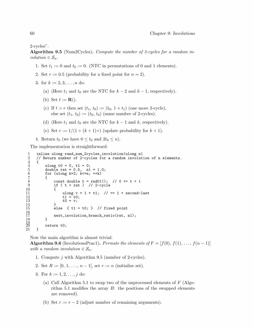
60 Chapter 9: Involutions
2-cycles”.Algorithm 9.5 (Num2Cycles). Compute the number of 2-cycles for a random in-volution ∈ Sn.
1. Set t1 := 0 and t0 := 0. (NTC in permutations of 0 and 1 elements).
2. Set r := 0.5 (probability for a fixed point for n = 2).
3. for k := 2, 3, . . . , n do:
(a) (Here t1 and t0 are the NTC for k − 2 and k − 1, respectively).
(b) Set t := R().
(c) If t > r then set (t1, t0) := (t0, 1 + t1) (one more 2-cycle),else set (t1, t0) := (t0, t0) (same number of 2-cycles).
(d) (Here t1 and t0 are the NTC for k − 1 and k, respectively).
(e) Set r := 1/(1 + (k + 1) r) (update probability for k + 1).
4. Return t0 (we have 0 ≤ t0 and 2t0 ≤ n).
The implementation is straightforward:
1 inline ulong rand_num_2cycles_involution(ulong n)2 // Return number of 2-cycles for a random involution of n elements.3 {4 ulong t0 = 0, t1 = 0;5 double rat = 0.5, n1 = 1.0;6 for (ulong k=2; k<=n; ++k)7 {8 const double t = rnd01(); // 0 <= t < 19 if ( t > rat ) // 2-cycle
10 {11 ulong v = 1 + t1; // == 1 + second-last12 t1 = t0;13 t0 = v;14 }15 else { t1 = t0; } // fixed point1617 next_involution_branch_ratio(rat, n1);18 }1920 return t0;21 }
Now the main algorithm is almost trivial:Algorithm 9.6 (InvolutionsPrac1). Permute the elements of F = [f(0), f(1), . . . , f(n− 1)]with a random involution ∈ Sn.
1. Compute j with Algorithm 9.5 (number of 2-cycles).
2. Set R := [0, 1, . . . , n− 1], set r := n (initialize set).
3. For k := 1, 2, . . . , j do:
(a) Call Algorithm 5.1 to swap two of the unprocessed elements of F (Algo-rithm 5.1 modifies the array B: the positions of the swapped elementsare removed).
(b) Set r := r − 2 (adjust number of remaining arguments).
9.4: Forward variant 61
The implementation uses the routine for creating a random cycle given as Algorithm5.1 on page 25:
1 template <typename Type>2 inline void random_permute_self_inverse1(Type *f, ulong n, ulong *tr=0)3 // Permute the elements of f by a random involution.4 // This routine avoids the array of branch probabilities.5 {6 ulong *r = tr;7 if ( tr==0 ) r = new ulong[n];8 for (ulong k=0; k<n; ++k) r[k] = k; // initialize set9 ulong nr = n; // number of elements available
10 // available positions are r[0], ..., r[nr-1]1112 ulong n2c = rand_num_2cycles_involution(n);13 while ( n2c-- ) nr = random_cycle(f, 2, r, nr);1415 if ( tr==0 ) delete [] r;16 }
A random involution is obtained with F = 1n:1 inline void random_self_inverse_permutation1(ulong *f, ulong n, ulong *tr=0)2 // Create a random involution.3 {4 for (ulong k=0; k<n; ++k) f[k] = k;5 random_permute_self_inverse1(f, n, tr);6 }
The routine implementing Algorithm 9.6 is slower than the routine for Algorithm9.4. Permuting 100,000 words (of 64 bits) 1,000 times takes (using an AMD64 CPUwith 2.2GHz) respectively 16.7 and 10.2 seconds.

62 Chapter 9: Involutions
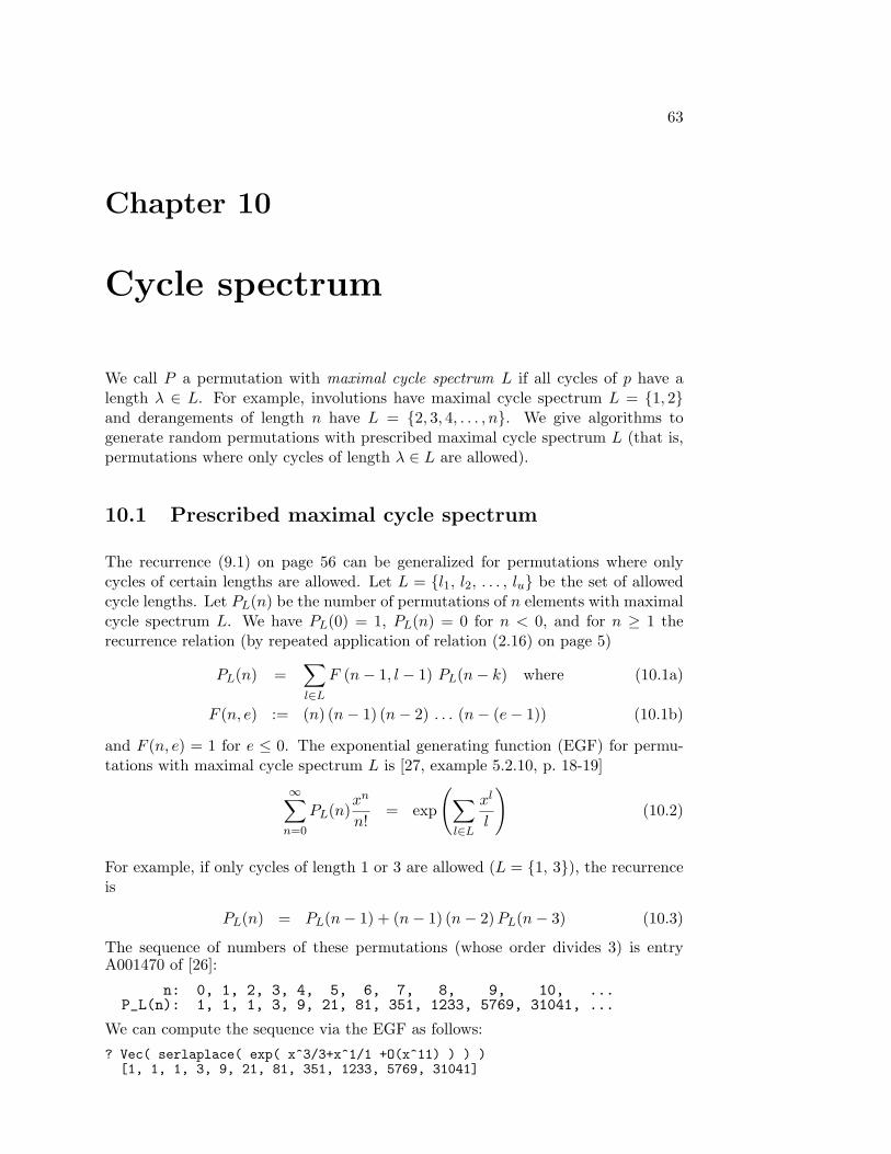
63
Chapter 10
Cycle spectrum
We call P a permutation with maximal cycle spectrum L if all cycles of p have alength λ ∈ L. For example, involutions have maximal cycle spectrum L = {1, 2}and derangements of length n have L = {2, 3, 4, . . . , n}. We give algorithms togenerate random permutations with prescribed maximal cycle spectrum L (that is,permutations where only cycles of length λ ∈ L are allowed).
10.1 Prescribed maximal cycle spectrum
The recurrence (9.1) on page 56 can be generalized for permutations where onlycycles of certain lengths are allowed. Let L = {l1, l2, . . . , lu} be the set of allowedcycle lengths. Let PL(n) be the number of permutations of n elements with maximalcycle spectrum L. We have PL(0) = 1, PL(n) = 0 for n < 0, and for n ≥ 1 therecurrence relation (by repeated application of relation (2.16) on page 5)
PL(n) =∑l∈L
F (n− 1, l − 1) PL(n− k) where (10.1a)
F (n, e) := (n) (n− 1) (n− 2) . . . (n− (e− 1)) (10.1b)
and F (n, e) = 1 for e ≤ 0. The exponential generating function (EGF) for permu-tations with maximal cycle spectrum L is [27, example 5.2.10, p. 18-19]
∞∑n=0
PL(n)xn
n!= exp
(∑l∈L
xl
l
)(10.2)
For example, if only cycles of length 1 or 3 are allowed (L = {1, 3}), the recurrenceis
PL(n) = PL(n− 1) + (n− 1) (n− 2)PL(n− 3) (10.3)
The sequence of numbers of these permutations (whose order divides 3) is entryA001470 of [26]:
n: 0, 1, 2, 3, 4, 5, 6, 7, 8, 9, 10, ...P_L(n): 1, 1, 1, 3, 9, 21, 81, 351, 1233, 5769, 31041, ...
We can compute the sequence via the EGF as follows:
? Vec( serlaplace( exp( x^3/3+x^1/1 +O(x^11) ) ) )[1, 1, 1, 3, 9, 21, 81, 351, 1233, 5769, 31041]
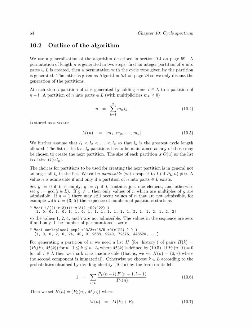
64 Chapter 10: Cycle spectrum
10.2 Outline of the algorithm
We use a generalization of the algorithm described in section 9.4 on page 59. Apermutation of length n is generated in two steps: first an integer partition of n intoparts ∈ L is created, then a permutation with the cycle type given by the partitionis generated. The latter is given as Algorithm 5.4 on page 28 so we only discuss thegeneration of the partitions.
At each step a partition of n is generated by adding some l ∈ L to a partition ofn− l. A partition of n into parts ∈ L (with multiplicities mk ≥ 0)
n =u∑
k=1
mk lk (10.4)
is stored as a vector
M(n) := [m1, m2, . . . , mu] (10.5)
We further assume that l1 < l2 < . . . < lu so that lu is the greatest cycle lengthallowed. The list of the last lu partitions has to be maintained as any of those maybe chosen to create the next partition. The size of each partition is O(u) so the listis of size O(u lu).
The choices for partitions to be used for creating the next partition is in general notamongst all lu in the list. We call n admissible (with respect to L) if PL(n) 6= 0. Avalue n is admissible if and only if a partition of n into parts ∈ L exists.
Set g := 0 if L is empty, g := l1 if L contains just one element, and otherwiseset g := gcd (l ∈ L). If g 6= 1 then only values of n which are multiples of g areadmissible. If g = 1 there may still occur values of n that are not admissible, forexample with L = {3, 5} the sequence of numbers of partitions starts as
? Vec( 1/((1-x^3)*(1-x^5)) +O(x^22) )[1, 0, 0, 1, 0, 1, 1, 0, 1, 1, 1, 1, 1, 1, 1, 2, 1, 1, 2, 1, 2, 2]
so the values 1, 2, 4, and 7 are not admissible. The values in the sequence are zeroif and only if the number of permutations is zero:
? Vec( serlaplace( exp( x^3/3+x^5/5 +O(x^22) ) ) )[1, 0, 0, 2, 0, 24, 40, 0, 2688, 2240, 72576, 443520, ...]
For generating a partition of n we need a list H (for ‘history’) of pairs H(k) =(PL(k), M(k)) for n−1 ≤ k ≤ n−lu where M(k) is defined by (10.5). If PL(n−l) = 0for all l ∈ L then we mark n as inadmissible (that is, we set H(n) = (0, ∗) wherethe second component is immaterial). Otherwise we choose k ∈ L according to theprobabilities obtained by dividing identity (10.1a) by the term on its left
1 =∑l∈L
PL(n− l)F (n− 1, l − 1)PL(n)
(10.6)
Then we set H(n) = (PL(n), M(n)) where
M(n) = M(k) + Ek (10.7)
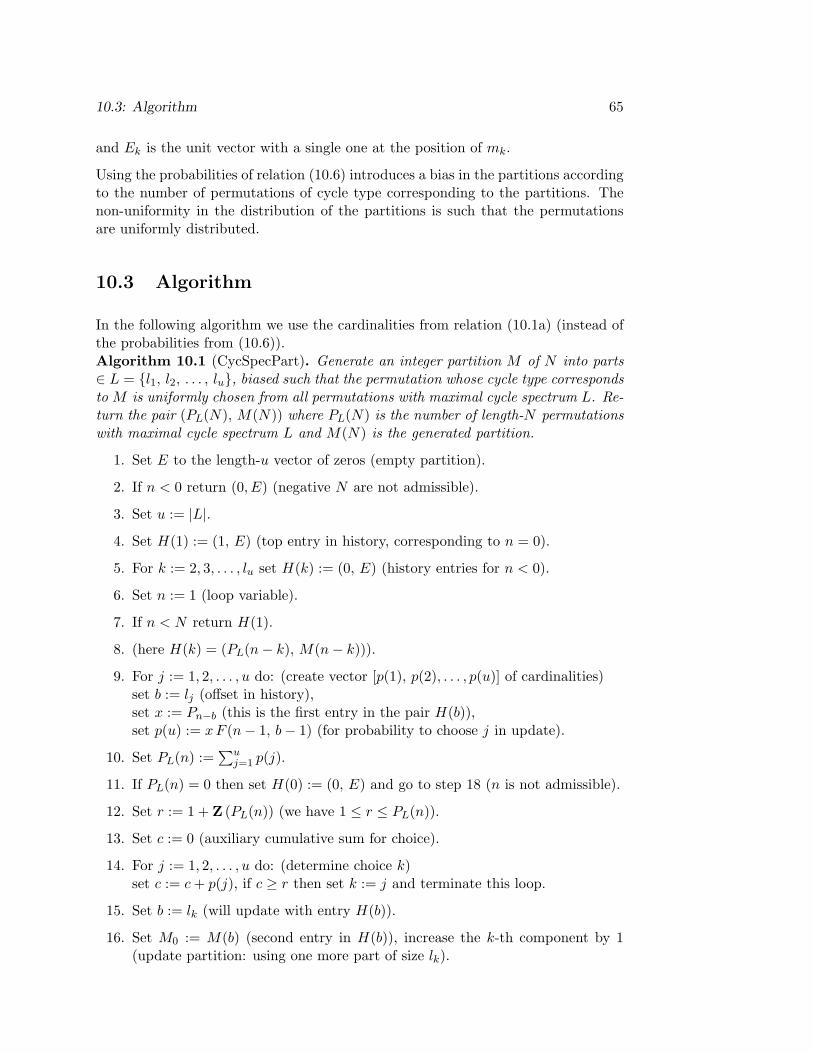
10.3: Algorithm 65
and Ek is the unit vector with a single one at the position of mk.
Using the probabilities of relation (10.6) introduces a bias in the partitions accordingto the number of permutations of cycle type corresponding to the partitions. Thenon-uniformity in the distribution of the partitions is such that the permutationsare uniformly distributed.
10.3 Algorithm
In the following algorithm we use the cardinalities from relation (10.1a) (instead ofthe probabilities from (10.6)).Algorithm 10.1 (CycSpecPart). Generate an integer partition M of N into parts∈ L = {l1, l2, . . . , lu}, biased such that the permutation whose cycle type correspondsto M is uniformly chosen from all permutations with maximal cycle spectrum L. Re-turn the pair (PL(N), M(N)) where PL(N) is the number of length-N permutationswith maximal cycle spectrum L and M(N) is the generated partition.
1. Set E to the length-u vector of zeros (empty partition).
2. If n < 0 return (0, E) (negative N are not admissible).
3. Set u := |L|.
4. Set H(1) := (1, E) (top entry in history, corresponding to n = 0).
5. For k := 2, 3, . . . , lu set H(k) := (0, E) (history entries for n < 0).
6. Set n := 1 (loop variable).
7. If n < N return H(1).
8. (here H(k) = (PL(n− k), M(n− k))).
9. For j := 1, 2, . . . , u do: (create vector [p(1), p(2), . . . , p(u)] of cardinalities)set b := lj (offset in history),set x := Pn−b (this is the first entry in the pair H(b)),set p(u) := xF (n− 1, b− 1) (for probability to choose j in update).
10. Set PL(n) :=∑u
j=1 p(j).
11. If PL(n) = 0 then set H(0) := (0, E) and go to step 18 (n is not admissible).
12. Set r := 1 + Z (PL(n)) (we have 1 ≤ r ≤ PL(n)).
13. Set c := 0 (auxiliary cumulative sum for choice).
14. For j := 1, 2, . . . , u do: (determine choice k)set c := c+ p(j), if c ≥ r then set k := j and terminate this loop.
15. Set b := lk (will update with entry H(b)).
16. Set M0 := M(b) (second entry in H(b)), increase the k-th component by 1(update partition: using one more part of size lk).
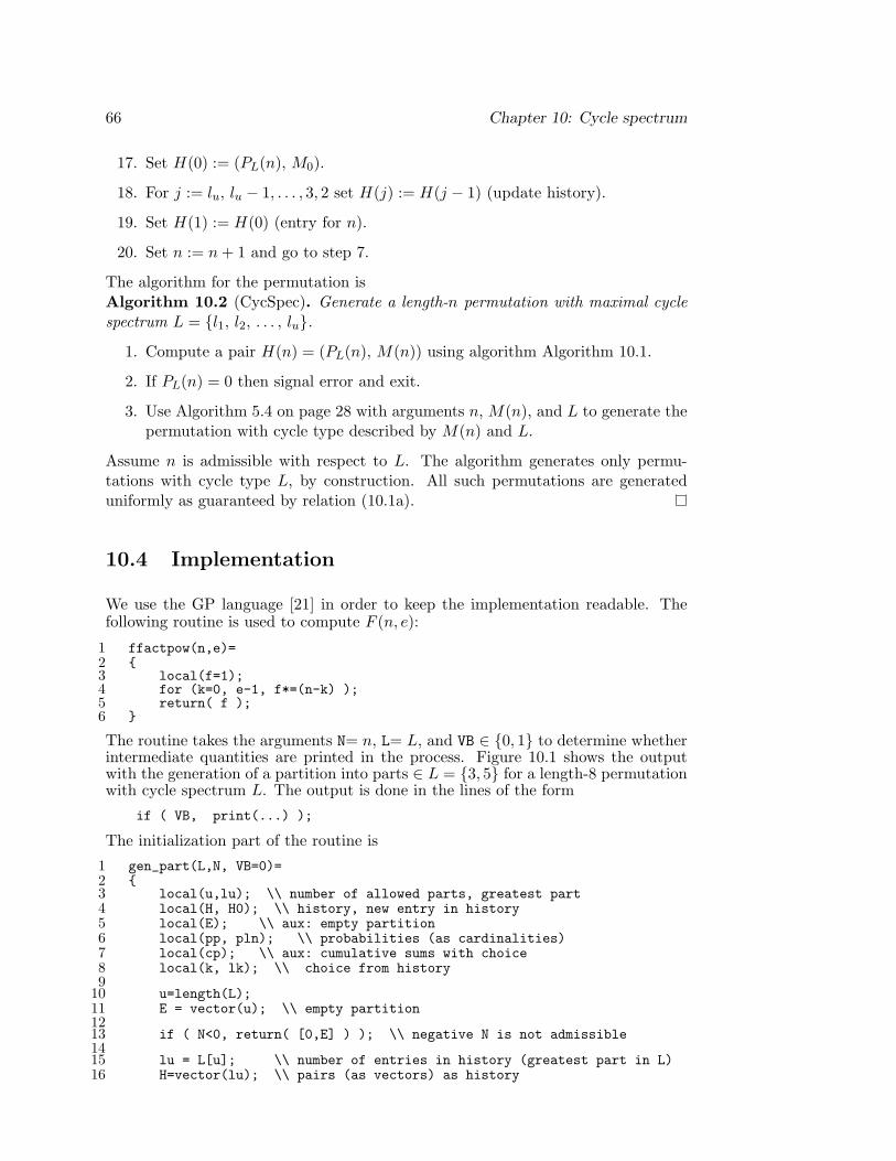
66 Chapter 10: Cycle spectrum
17. Set H(0) := (PL(n), M0).
18. For j := lu, lu − 1, . . . , 3, 2 set H(j) := H(j − 1) (update history).
19. Set H(1) := H(0) (entry for n).
20. Set n := n+ 1 and go to step 7.
The algorithm for the permutation isAlgorithm 10.2 (CycSpec). Generate a length-n permutation with maximal cyclespectrum L = {l1, l2, . . . , lu}.
1. Compute a pair H(n) = (PL(n), M(n)) using algorithm Algorithm 10.1.
2. If PL(n) = 0 then signal error and exit.
3. Use Algorithm 5.4 on page 28 with arguments n, M(n), and L to generate thepermutation with cycle type described by M(n) and L.
Assume n is admissible with respect to L. The algorithm generates only permu-tations with cycle type L, by construction. All such permutations are generateduniformly as guaranteed by relation (10.1a).
10.4 Implementation
We use the GP language [21] in order to keep the implementation readable. Thefollowing routine is used to compute F (n, e):
1 ffactpow(n,e)=2 {3 local(f=1);4 for (k=0, e-1, f*=(n-k) );5 return( f );6 }
The routine takes the arguments N= n, L= L, and VB ∈ {0, 1} to determine whetherintermediate quantities are printed in the process. Figure 10.1 shows the outputwith the generation of a partition into parts ∈ L = {3, 5} for a length-8 permutationwith cycle spectrum L. The output is done in the lines of the form
if ( VB, print(...) );
The initialization part of the routine is
1 gen_part(L,N, VB=0)=2 {3 local(u,lu); \\ number of allowed parts, greatest part4 local(H, H0); \\ history, new entry in history5 local(E); \\ aux: empty partition6 local(pp, pln); \\ probabilities (as cardinalities)7 local(cp); \\ aux: cumulative sums with choice8 local(k, lk); \\ choice from history9
10 u=length(L);11 E = vector(u); \\ empty partition1213 if ( N<0, return( [0,E] ) ); \\ negative N is not admissible1415 lu = L[u]; \\ number of entries in history (greatest part in L)16 H=vector(lu); \\ pairs (as vectors) as history
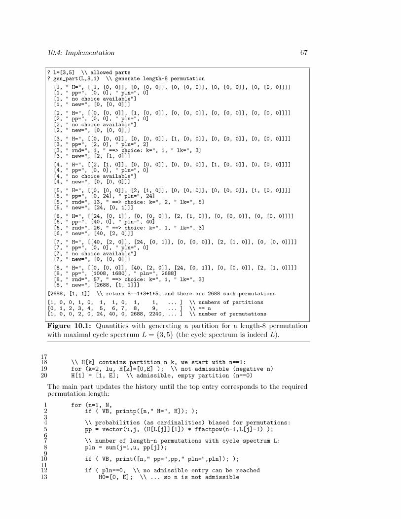
10.4: Implementation 67
? L=[3,5] \\ allowed parts? gen_part(L,8,1) \\ generate length-8 permutation
[1, " H=", [[1, [0, 0]], [0, [0, 0]], [0, [0, 0]], [0, [0, 0]], [0, [0, 0]]]][1, " pp=", [0, 0], " pln=", 0][1, " no choice available"][1, " new=", [0, [0, 0]]]
[2, " H=", [[0, [0, 0]], [1, [0, 0]], [0, [0, 0]], [0, [0, 0]], [0, [0, 0]]]][2, " pp=", [0, 0], " pln=", 0][2, " no choice available"][2, " new=", [0, [0, 0]]]
[3, " H=", [[0, [0, 0]], [0, [0, 0]], [1, [0, 0]], [0, [0, 0]], [0, [0, 0]]]][3, " pp=", [2, 0], " pln=", 2][3, " rnd=", 1, " ==> choice: k=", 1, " lk=", 3][3, " new=", [2, [1, 0]]]
[4, " H=", [[2, [1, 0]], [0, [0, 0]], [0, [0, 0]], [1, [0, 0]], [0, [0, 0]]]][4, " pp=", [0, 0], " pln=", 0][4, " no choice available"][4, " new=", [0, [0, 0]]]
[5, " H=", [[0, [0, 0]], [2, [1, 0]], [0, [0, 0]], [0, [0, 0]], [1, [0, 0]]]][5, " pp=", [0, 24], " pln=", 24][5, " rnd=", 13, " ==> choice: k=", 2, " lk=", 5][5, " new=", [24, [0, 1]]]
[6, " H=", [[24, [0, 1]], [0, [0, 0]], [2, [1, 0]], [0, [0, 0]], [0, [0, 0]]]][6, " pp=", [40, 0], " pln=", 40][6, " rnd=", 26, " ==> choice: k=", 1, " lk=", 3][6, " new=", [40, [2, 0]]]
[7, " H=", [[40, [2, 0]], [24, [0, 1]], [0, [0, 0]], [2, [1, 0]], [0, [0, 0]]]][7, " pp=", [0, 0], " pln=", 0][7, " no choice available"][7, " new=", [0, [0, 0]]]
[8, " H=", [[0, [0, 0]], [40, [2, 0]], [24, [0, 1]], [0, [0, 0]], [2, [1, 0]]]][8, " pp=", [1008, 1680], " pln=", 2688][8, " rnd=", 57, " ==> choice: k=", 1, " lk=", 3][8, " new=", [2688, [1, 1]]]
[2688, [1, 1]] \\ return 8==1*3+1*5, and there are 2688 such permutations
[1, 0, 0, 1, 0, 1, 1, 0, 1, 1, ... ] \\ numbers of partitions[0, 1, 2, 3, 4, 5, 6, 7, 8, 9, ... ] \\ == n[1, 0, 0, 2, 0, 24, 40, 0, 2688, 2240, ... ] \\ number of permutations
Figure 10.1: Quantities with generating a partition for a length-8 permutationwith maximal cycle spectrum L = {3, 5} (the cycle spectrum is indeed L).
1718 \\ H[k] contains partition n-k, we start with n==1:19 for (k=2, lu, H[k]=[0,E] ); \\ not admissible (negative n)20 H[1] = [1, E]; \\ admissible, empty partition (n==0)
The main part updates the history until the top entry corresponds to the requiredpermutation length:
1 for (n=1, N,2 if ( VB, printp([n," H=", H]); );34 \\ probabilities (as cardinalities) biased for permutations:5 pp = vector(u,j, (H[L[j]][1]) * ffactpow(n-1,L[j]-1) );67 \\ number of length-n permutations with cycle spectrum L:8 pln = sum(j=1,u, pp[j]);9
10 if ( VB, print([n," pp=",pp," pln=",pln]); );1112 if ( pln==0, \\ no admissible entry can be reached13 H0=[0, E]; \\ ... so n is not admissible
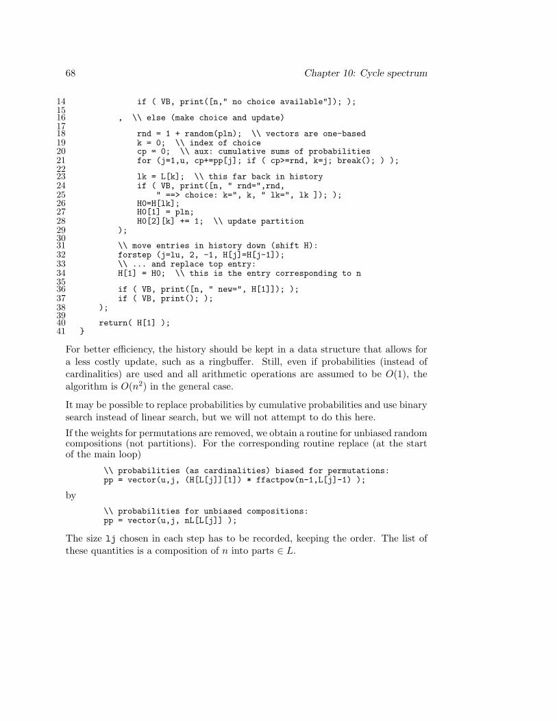
68 Chapter 10: Cycle spectrum
14 if ( VB, print([n," no choice available"]); );1516 , \\ else (make choice and update)1718 rnd = 1 + random(pln); \\ vectors are one-based19 k = 0; \\ index of choice20 cp = 0; \\ aux: cumulative sums of probabilities21 for (j=1,u, cp+=pp[j]; if ( cp>=rnd, k=j; break(); ) );2223 lk = L[k]; \\ this far back in history24 if ( VB, print([n, " rnd=",rnd,25 " ==> choice: k=", k, " lk=", lk ]); );26 H0=H[lk];27 H0[1] = pln;28 H0[2][k] += 1; \\ update partition29 );3031 \\ move entries in history down (shift H):32 forstep (j=lu, 2, -1, H[j]=H[j-1]);33 \\ ... and replace top entry:34 H[1] = H0; \\ this is the entry corresponding to n3536 if ( VB, print([n, " new=", H[1]]); );37 if ( VB, print(); );38 );3940 return( H[1] );41 }
For better efficiency, the history should be kept in a data structure that allows fora less costly update, such as a ringbuffer. Still, even if probabilities (instead ofcardinalities) are used and all arithmetic operations are assumed to be O(1), thealgorithm is O(n2) in the general case.
It may be possible to replace probabilities by cumulative probabilities and use binarysearch instead of linear search, but we will not attempt to do this here.
If the weights for permutations are removed, we obtain a routine for unbiased randomcompositions (not partitions). For the corresponding routine replace (at the startof the main loop)
\\ probabilities (as cardinalities) biased for permutations:pp = vector(u,j, (H[L[j]][1]) * ffactpow(n-1,L[j]-1) );
by
\\ probabilities for unbiased compositions:pp = vector(u,j, nL[L[j]] );
The size lj chosen in each step has to be recorded, keeping the order. The list ofthese quantities is a composition of n into parts ∈ L.
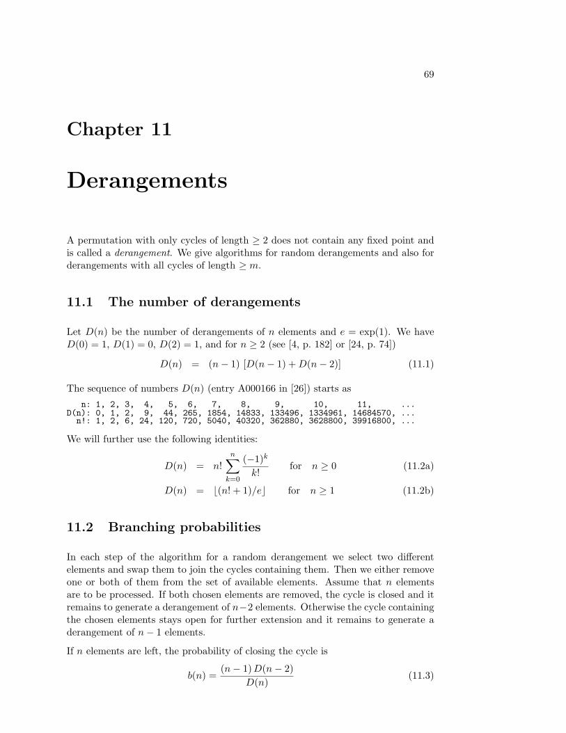
69
Chapter 11
Derangements
A permutation with only cycles of length ≥ 2 does not contain any fixed point andis called a derangement. We give algorithms for random derangements and also forderangements with all cycles of length ≥ m.
11.1 The number of derangements
Let D(n) be the number of derangements of n elements and e = exp(1). We haveD(0) = 1, D(1) = 0, D(2) = 1, and for n ≥ 2 (see [4, p. 182] or [24, p. 74])
D(n) = (n− 1) [D(n− 1) +D(n− 2)] (11.1)
The sequence of numbers D(n) (entry A000166 in [26]) starts asn: 1, 2, 3, 4, 5, 6, 7, 8, 9, 10, 11, ...
D(n): 0, 1, 2, 9, 44, 265, 1854, 14833, 133496, 1334961, 14684570, ...n!: 1, 2, 6, 24, 120, 720, 5040, 40320, 362880, 3628800, 39916800, ...
We will further use the following identities:
D(n) = n!n∑
k=0
(−1)k
k!for n ≥ 0 (11.2a)
D(n) = b(n! + 1)/ec for n ≥ 1 (11.2b)
11.2 Branching probabilities
In each step of the algorithm for a random derangement we select two differentelements and swap them to join the cycles containing them. Then we either removeone or both of them from the set of available elements. Assume that n elementsare to be processed. If both chosen elements are removed, the cycle is closed and itremains to generate a derangement of n−2 elements. Otherwise the cycle containingthe chosen elements stays open for further extension and it remains to generate aderangement of n− 1 elements.
If n elements are left, the probability of closing the cycle is
b(n) =(n− 1)D(n− 2)
D(n)(11.3)
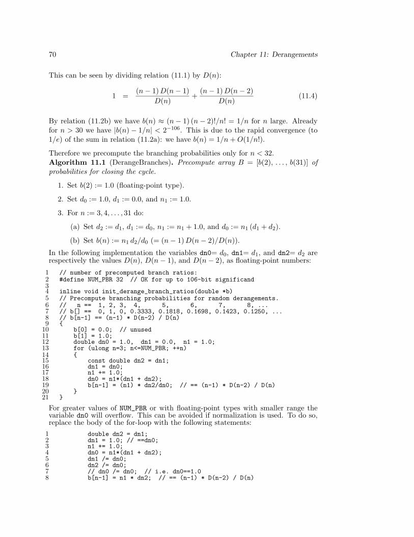
70 Chapter 11: Derangements
This can be seen by dividing relation (11.1) by D(n):
1 =(n− 1)D(n− 1)
D(n)+
(n− 1)D(n− 2)D(n)
(11.4)
By relation (11.2b) we have b(n) ≈ (n− 1) (n− 2)!/n! = 1/n for n large. Alreadyfor n > 30 we have |b(n)− 1/n| < 2−106. This is due to the rapid convergence (to1/e) of the sum in relation (11.2a): we have b(n) = 1/n+O(1/n!).
Therefore we precompute the branching probabilities only for n < 32.Algorithm 11.1 (DerangeBranches). Precompute array B = [b(2), . . . , b(31)] ofprobabilities for closing the cycle.
1. Set b(2) := 1.0 (floating-point type).
2. Set d0 := 1.0, d1 := 0.0, and n1 := 1.0.
3. For n := 3, 4, . . . , 31 do:
(a) Set d2 := d1, d1 := d0, n1 := n1 + 1.0, and d0 := n1 (d1 + d2).
(b) Set b(n) := n1 d2/d0 (= (n− 1)D(n− 2)/D(n)).
In the following implementation the variables dn0= d0, dn1= d1, and dn2= d2 arerespectively the values D(n), D(n− 1), and D(n− 2), as floating-point numbers:
1 // number of precomputed branch ratios:2 #define NUM_PBR 32 // OK for up to 106-bit significand34 inline void init_derange_branch_ratios(double *b)5 // Precompute branching probabilities for random derangements.6 // n == 1, 2, 3, 4, 5, 6, 7, 8, ...7 // b[] == 0, 1, 0, 0.3333, 0.1818, 0.1698, 0.1423, 0.1250, ...8 // b[n-1] == (n-1) * D(n-2) / D(n)9 {
10 b[0] = 0.0; // unused11 b[1] = 1.0;12 double dn0 = 1.0, dn1 = 0.0, n1 = 1.0;13 for (ulong n=3; n<=NUM_PBR; ++n)14 {15 const double dn2 = dn1;16 dn1 = dn0;17 n1 += 1.0;18 dn0 = n1*(dn1 + dn2);19 b[n-1] = (n1) * dn2/dn0; // == (n-1) * D(n-2) / D(n)20 }21 }
For greater values of NUM_PBR or with floating-point types with smaller range thevariable dn0 will overflow. This can be avoided if normalization is used. To do so,replace the body of the for-loop with the following statements:
1 double dn2 = dn1;2 dn1 = 1.0; // ==dn0;3 n1 += 1.0;4 dn0 = n1*(dn1 + dn2);5 dn1 /= dn0;6 dn2 /= dn0;7 // dn0 /= dn0; // i.e. dn0==1.08 b[n-1] = n1 * dn2; // == (n-1) * D(n-2) / D(n)
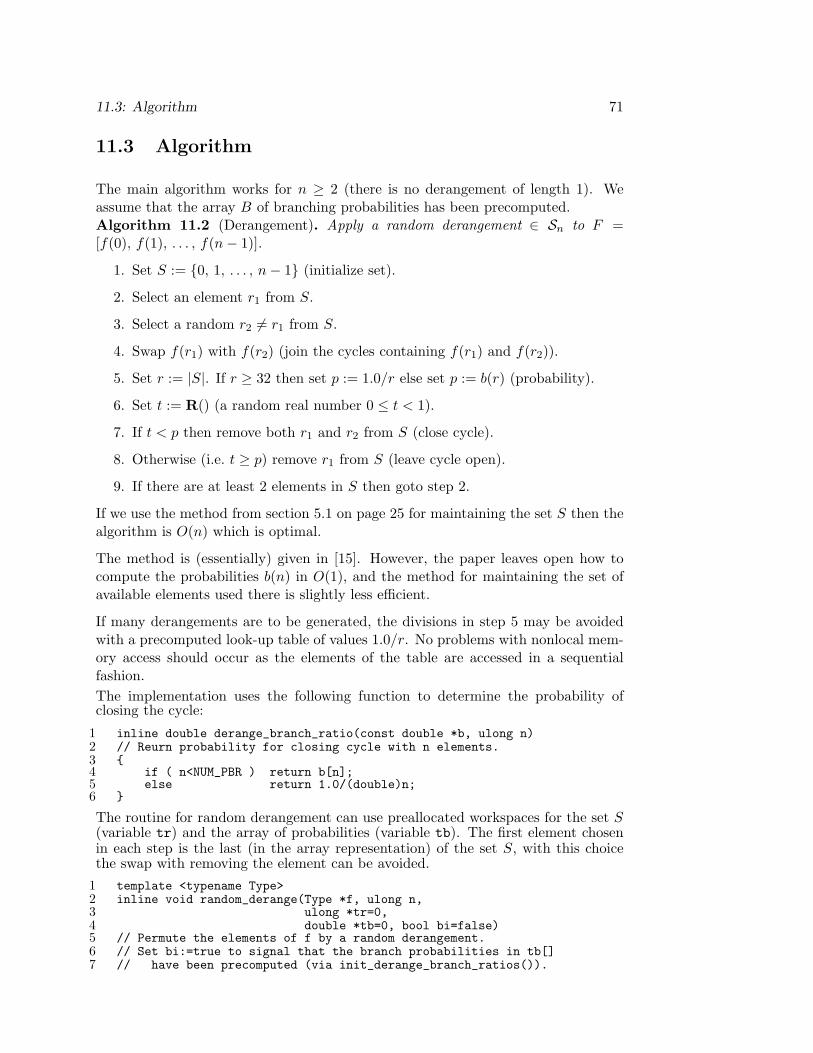
11.3: Algorithm 71
11.3 Algorithm
The main algorithm works for n ≥ 2 (there is no derangement of length 1). Weassume that the array B of branching probabilities has been precomputed.Algorithm 11.2 (Derangement). Apply a random derangement ∈ Sn to F =[f(0), f(1), . . . , f(n− 1)].
1. Set S := {0, 1, . . . , n− 1} (initialize set).
2. Select an element r1 from S.
3. Select a random r2 6= r1 from S.
4. Swap f(r1) with f(r2) (join the cycles containing f(r1) and f(r2)).
5. Set r := |S|. If r ≥ 32 then set p := 1.0/r else set p := b(r) (probability).
6. Set t := R() (a random real number 0 ≤ t < 1).
7. If t < p then remove both r1 and r2 from S (close cycle).
8. Otherwise (i.e. t ≥ p) remove r1 from S (leave cycle open).
9. If there are at least 2 elements in S then goto step 2.
If we use the method from section 5.1 on page 25 for maintaining the set S then thealgorithm is O(n) which is optimal.
The method is (essentially) given in [15]. However, the paper leaves open how tocompute the probabilities b(n) in O(1), and the method for maintaining the set ofavailable elements used there is slightly less efficient.
If many derangements are to be generated, the divisions in step 5 may be avoidedwith a precomputed look-up table of values 1.0/r. No problems with nonlocal mem-ory access should occur as the elements of the table are accessed in a sequentialfashion.The implementation uses the following function to determine the probability ofclosing the cycle:
1 inline double derange_branch_ratio(const double *b, ulong n)2 // Reurn probability for closing cycle with n elements.3 {4 if ( n<NUM_PBR ) return b[n];5 else return 1.0/(double)n;6 }
The routine for random derangement can use preallocated workspaces for the set S(variable tr) and the array of probabilities (variable tb). The first element chosenin each step is the last (in the array representation) of the set S, with this choicethe swap with removing the element can be avoided.
1 template <typename Type>2 inline void random_derange(Type *f, ulong n,3 ulong *tr=0,4 double *tb=0, bool bi=false)5 // Permute the elements of f by a random derangement.6 // Set bi:=true to signal that the branch probabilities in tb[]7 // have been precomputed (via init_derange_branch_ratios()).
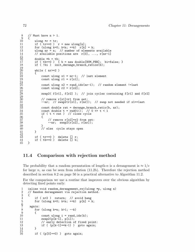
72 Chapter 11: Derangements
8 // Must have n > 1.9 {
10 ulong *r = tr;11 if ( tr==0 ) r = new ulong[n];12 for (ulong k=0; k<n; ++k) r[k] = k;13 ulong nr = n; // number of elements available14 // available positions are r[0], ..., r[nr-1]1516 double *b = tb;17 if ( tb==0 ) { b = new double[NUM_PBR]; bi=false; }18 if ( !bi ) init_derange_branch_ratios(b);1920 while ( nr>=2 )21 {22 const ulong x1 = nr-1; // last element23 const ulong r1 = r[x1];2425 const ulong x2 = rand_idx(nr-1); // random element !=last26 const ulong r2 = r[x2];2728 swap2( f[r1], f[r2] ); // join cycles containing f[r1] and f[r2]2930 // remove r[x1]=r1 from set:31 --nr; // swap2(r[x1], r[nr]); // swap not needed if x1==last3233 const double rat = derange_branch_ratio(b, nr);34 const double t = rnd01(); // 0 <= t < 135 if ( t < rat ) // close cycle36 {37 // remove r[x2]=r2 from set:38 --nr; swap2(r[x2], r[nr]);39 }40 // else cycle stays open41 }4243 if ( tr==0 ) delete [] r;44 if ( tb==0 ) delete [] b;45 }
11.4 Comparison with rejection method
The probability that a random permutation of length-n is a derangement is ≈ 1/efor large n, as can be seen from relation (11.2b). Therefore the rejection methoddescribed in section 8.2 on page 50 is a practical alternative to Algorithm 11.2.
For the comparison we use a routine that improves over the obvious algorithm bydetecting fixed points early:
1 inline void random_derangement_rej(ulong *p, ulong n)2 // Random derangement via rejection method.3 {4 if ( n<2 ) return; // avoid hang5 for (ulong k=0; k<n; ++k) p[k] = k;67 again:8 for (ulong k=n; k>1; --k)9 {
10 const ulong i = rand_idx(k);11 swap2(p[k-1], p[i]);12 // early detection of fixed point:13 if ( (p[k-1]==k-1) ) goto again;14 }1516 if ( (p[0]==0) ) goto again;
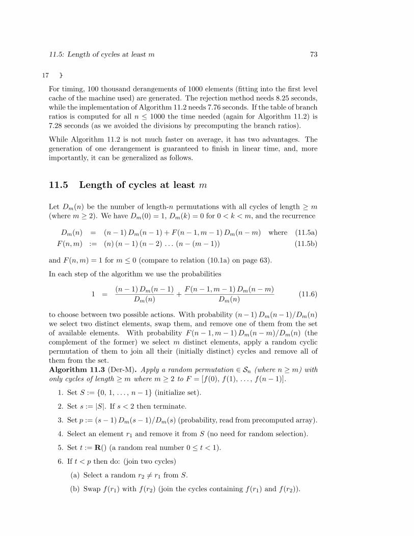
11.5: Length of cycles at least m 73
17 }
For timing, 100 thousand derangements of 1000 elements (fitting into the first levelcache of the machine used) are generated. The rejection method needs 8.25 seconds,while the implementation of Algorithm 11.2 needs 7.76 seconds. If the table of branchratios is computed for all n ≤ 1000 the time needed (again for Algorithm 11.2) is7.28 seconds (as we avoided the divisions by precomputing the branch ratios).
While Algorithm 11.2 is not much faster on average, it has two advantages. Thegeneration of one derangement is guaranteed to finish in linear time, and, moreimportantly, it can be generalized as follows.
11.5 Length of cycles at least m
Let Dm(n) be the number of length-n permutations with all cycles of length ≥ m(where m ≥ 2). We have Dm(0) = 1, Dm(k) = 0 for 0 < k < m, and the recurrence
Dm(n) = (n− 1)Dm(n− 1) + F (n− 1,m− 1)Dm(n−m) where (11.5a)F (n,m) := (n) (n− 1) (n− 2) . . . (n− (m− 1)) (11.5b)
and F (n,m) = 1 for m ≤ 0 (compare to relation (10.1a) on page 63).
In each step of the algorithm we use the probabilities
1 =(n− 1)Dm(n− 1)
Dm(n)+F (n− 1,m− 1)Dm(n−m)
Dm(n)(11.6)
to choose between two possible actions. With probability (n− 1)Dm(n− 1)/Dm(n)we select two distinct elements, swap them, and remove one of them from the setof available elements. With probability F (n− 1,m− 1)Dm(n−m)/Dm(n) (thecomplement of the former) we select m distinct elements, apply a random cyclicpermutation of them to join all their (initially distinct) cycles and remove all ofthem from the set.Algorithm 11.3 (Der-M). Apply a random permutation ∈ Sn (where n ≥ m) withonly cycles of length ≥ m where m ≥ 2 to F = [f(0), f(1), . . . , f(n− 1)].
1. Set S := {0, 1, . . . , n− 1} (initialize set).
2. Set s := |S|. If s < 2 then terminate.
3. Set p := (s− 1)Dm(s− 1)/Dm(s) (probability, read from precomputed array).
4. Select an element r1 and remove it from S (no need for random selection).
5. Set t := R() (a random real number 0 ≤ t < 1).
6. If t < p then do: (join two cycles)
(a) Select a random r2 6= r1 from S.
(b) Swap f(r1) with f(r2) (join the cycles containing f(r1) and f(r2)).
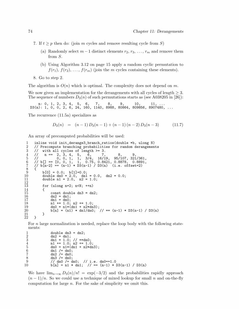
74 Chapter 11: Derangements
7. If t ≥ p then do: (join m cycles and remove resulting cycle from S)
(a) Randomly select m−1 distinct elements r2, r3, . . . , rm and remove themfrom S.
(b) Using Algorithm 3.12 on page 15 apply a random cyclic permutation tof(r1), f(r2), . . . , f(rm) (join the m cycles containing these elements).
8. Go to step 2.
The algorithm is O(n) which is optimal. The complexity does not depend on m.
We now given an implementation for the derangements with all cycles of length ≥ 3.The sequence of numbers D3(n) of such permutations starts as (see A038205 in [26]):
n: 0, 1, 2, 3, 4, 5, 6, 7, 8, 9, 10, 11, ...D3(n): 1, 0, 0, 2, 6, 24, 160, 1140, 8988, 80864, 809856, 8907480, ...
The recurrence (11.5a) specializes as
D3(n) = (n− 1)D3(n− 1) + (n− 1) (n− 2)D3(n− 3) (11.7)
An array of precomputed probabilities will be used:
1 inline void init_derange3_branch_ratios(double *b, ulong N)2 // Precompute branching probabilities for random derangements3 // with all cycles of length >= 3.4 // n == 2, 3, 4, 5, 6, 7, 8, 9,5 // 0, 0, 1, 1, 3/4, 16/19, 95/107, 321/361,6 // b[] == [0, 0, 1, 1, 0.75, 0.8421, 0.8878, 0.8891,7 // b[n-2] == (n-1) * D3(n-1) / D3(n) (i.e. offset=2)8 {9 b[0] = 0.0; b[1]=0.0;
10 double dn0 = 2.0, dn1 = 0.0, dn2 = 0.0;11 double n1 = 2.0, n2 = 1.0;1213 for (ulong n=2; n<N; ++n)14 {15 const double dn3 = dn2;16 dn2 = dn1;17 dn1 = dn0;18 n1 += 1.0; n2 += 1.0;19 dn0 = n1*(dn1 + n2*dn3);20 b[n] = (n1) * dn1/dn0; // == (n-1) * D3(n-1) / D3(n)21 }22 }
For n large normalization is needed, replace the loop body with the following state-ments:
1 double dn3 = dn2;2 dn2 = dn1;3 dn1 = 1.0; // ==dn0;4 n1 += 1.0; n2 += 1.0;5 dn0 = n1*(dn1 + n2*dn3);6 dn1 /= dn0;7 dn2 /= dn0;8 dn3 /= dn0;9 // dn0 /= dn0; // i.e. dn0==1.0
10 b[n] = n1 * dn1; // == (n-1) * D3(n-1) / D3(n)
We have limn→∞D3(n)/n! = exp(−3/2) and the probabilities rapidly approach(n− 1)/n. So we could use a technique of mixed lookup for small n and on-the-flycomputation for large n. For the sake of simplicity we omit this.
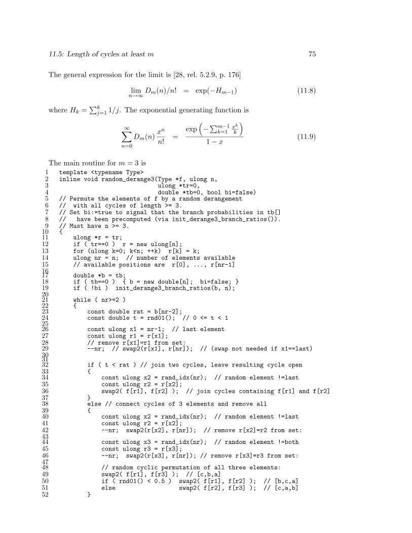
11.5: Length of cycles at least m 75
The general expression for the limit is [28, rel. 5.2.9, p. 176]
limn→∞
Dm(n)/n! = exp(−Hm−1) (11.8)
where Hk =∑k
j=1 1/j. The exponential generating function is
∞∑n=0
Dm(n)xn
n!=
exp(−∑m−1
k=1xk
k
)1− x
(11.9)
The main routine for m = 3 is1 template <typename Type>2 inline void random_derange3(Type *f, ulong n,3 ulong *tr=0,4 double *tb=0, bool bi=false)5 // Permute the elements of f by a random derangement6 // with all cycles of length >= 3.7 // Set bi:=true to signal that the branch probabilities in tb[]8 // have been precomputed (via init_derange3_branch_ratios()).9 // Must have n >= 3.
10 {11 ulong *r = tr;12 if ( tr==0 ) r = new ulong[n];13 for (ulong k=0; k<n; ++k) r[k] = k;14 ulong nr = n; // number of elements available15 // available positions are r[0], ..., r[nr-1]1617 double *b = tb;18 if ( tb==0 ) { b = new double[n]; bi=false; }19 if ( !bi ) init_derange3_branch_ratios(b, n);2021 while ( nr>=2 )22 {23 const double rat = b[nr-2];24 const double t = rnd01(); // 0 <= t < 12526 const ulong x1 = nr-1; // last element27 const ulong r1 = r[x1];28 // remove r[x1]=r1 from set:29 --nr; // swap2(r[x1], r[nr]); // (swap not needed if x1==last)303132 if ( t < rat ) // join two cycles, leave resulting cycle open33 {34 const ulong x2 = rand_idx(nr); // random element !=last35 const ulong r2 = r[x2];36 swap2( f[r1], f[r2] ); // join cycles containing f[r1] and f[r2]37 }38 else // connect cycles of 3 elements and remove all39 {40 const ulong x2 = rand_idx(nr); // random element !=last41 const ulong r2 = r[x2];42 --nr; swap2(r[x2], r[nr]); // remove r[x2]=r2 from set:4344 const ulong x3 = rand_idx(nr); // random element !=both45 const ulong r3 = r[x3];46 --nr; swap2(r[x3], r[nr]); // remove r[x3]=r3 from set:4748 // random cyclic permutation of all three elements:49 swap2( f[r1], f[r3] ); // [c,b,a]50 if ( rnd01() < 0.5 ) swap2( f[r1], f[r2] ); // [b,c,a]51 else swap2( f[r2], f[r3] ); // [c,a,b]52 }
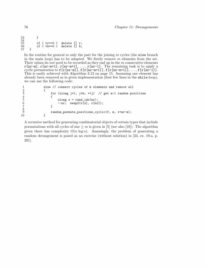
76 Chapter 11: Derangements
53 }5455 if ( tr==0 ) delete [] r;56 if ( tb==0 ) delete [] b;57 }
In the routine for general m only the part for the joining m cycles (the else branchin the main loop) has to be adapted. We firstly remove m elements from the set.Their values do not need to be recorded as they end up in the m consecutive elementsr[nr-m], r[nr-m+1], r[nr-m+1], . . . , r[nr-1]. The remaining task is to apply acyclic permutation to f[r[nr-m]], f[r[nr-m+1]], f[r[nr-m+1]], . . . , f[r[nr-1]].This is easily achieved with Algorithm 3.12 on page 15. Assuming one element hasalready been removed as in given implementation (first few lines in the while-loop),we can use the following code:
1 else // connect cycles of m elements and remove all2 {3 for (ulong j=1; j<m; ++j) // get m-1 random positions4 {5 ulong x = rand_idx(nr);6 --nr; swap2(r[x], r[nr]);7 }89 random_permute_positions_cyclic(f, m, r+nr-m);
10 }
A recursive method for generating combinatorial objects of certain types that includepermutations with all cycles of size ≥ m is given in [5] (see also [10]). The algorithmgiven there has complexity O(n log n). Amusingly, the problem of generating arandom derangement is posed as an exercise (without solution) in [23, ex. 19.a, p.201].
77
Appendix A
Bit-array
We give the implementation of the bit-array used in chapter 4 on page 19. Thedescribed class offers several convenient methods that do no exist for the bit-fieldsof the C-language, such as the search for the next set bit. The routines here are alsoa guide for implementing the corresponding mechanisms in languages that do nothave built-in Boolean arrays.
The value BITS_PER_LONG has to be set to the number of bits in a word of typeunsigned long (abbreviated as ulong).
1 class bitarray2 // Bit-array class mostly for use as memory saving array of Boolean values.3 // Valid index is 0...nb_-1 (as usual in C arrays).4 {5 public:6 ulong *f_; // bit bucket7 ulong n_; // number of bits8 ulong nfw_; // number of words where all bits are used, may be zero9 ulong mp_; // mask for partially used word if there is one, else zero
10 // (ones are at the positions of the _unused_ bits)11 bool myfq_; // whether f[] was allocated by class
We keep the data public to avoid the necessity for various get and set methods. Thenames of the class variables end in an underscore, making them easily identifiablein the class methods.
1 private:2 ulong ctor_core(ulong nbits)3 {4 n_ = nbits;56 // nw: number of words (incl. partially used), nw>=17 ulong nw = n_ / BITS_PER_LONG; // number of words89 // nbl: number of bits used in last (partially used) word, 0 if mw==mfw
10 ulong nbl = n_ - nw*BITS_PER_LONG; // number of bits used in last word11 nfw_ = nw; // number of fully used words1213 if ( 0!=nbl ) // there is a partially used word14 {15 ++nw; // increase total number of words16 mp_ = (~0UL) >> (BITS_PER_LONG-nbl); // correct mask for last word17 }18 else mp_ = 0UL;1920 return nw;21 }22
The constructor allocates memory by default. If the second argument is nonzero, itmust point to an accessible memory range of sufficient size:
78 Chapter A: Bit-array
1 public:2 bitarray(ulong nbits, ulong *f=0)3 // nbits must be nonzero4 {5 ulong nw = ctor_core(nbits);6 if ( f!=0 )7 {8 f_ = f;9 myfq_ = false;
10 }11 else12 {13 f_ = new ulong[nw];14 myfq_ = true;15 }16 }1718 ~bitarray() { if ( myfq_ ) delete [] f_; }
The following auxiliary definitions are used to access the n-th bit in the array f_:
1 #define DIVMOD(n, d, bm) \2 ulong d = n / BITS_PER_LONG; \3 ulong bm = 1UL << (n % BITS_PER_LONG);45 #define DIVMOD_TEST(n, d, bm) \6 ulong d = n / BITS_PER_LONG; \7 ulong bm = 1UL << (n % BITS_PER_LONG); \8 ulong t = bm & f_[d];
The division and remnant computations will respectively be optimized to shifts andbit-wise ANDs by the compiler.
The methods for testing, setting, clearing, and changing one bit are
1 ulong test(ulong n) const2 // Test whether n-th bit set.3 {4 DIVMOD_TEST(n, d, bm);5 return t;6 }78 void set(ulong n)9 // Set n-th bit.
10 {11 DIVMOD(n, d, bm);12 f_[d] |= bm;13 }1415 void clear(ulong n)16 // Clear n-th bit.17 {18 DIVMOD(n, d, bm);19 f_[d] &= ~bm;20 }2122 void change(ulong n)23 // Toggle n-th bit.24 {25 DIVMOD(n, d, bm);26 f_[d] ^= bm;27 }2829 ulong test_set(ulong n)30 // Test whether n-th bit is set and set it.31 {32 DIVMOD_TEST(n, d, bm);33 f_[d] |= bm;34 return t;
79
35 }3637 ulong test_clear(ulong n)38 // Test whether n-th bit is set and clear it.39 {40 DIVMOD_TEST(n, d, bm);41 f_[d] &= ~bm;42 return t;43 }4445 ulong test_change(ulong n)46 // Test whether n-th bit is set and toggle it.47 {48 DIVMOD_TEST(n, d, bm);49 f_[d] ^= bm;50 return t;51 }52
The methods for setting, clearing, or testing all bits in the array are
1 void clear_all()2 // Clear all bits.3 {4 for (ulong k=0; k<nfw_; ++k) f_[k] = 0;5 if ( mp_ ) f_[nfw_] = 0;6 }78 void set_all()9 // Set all bits.
10 {11 for (ulong k=0; k<nfw_; ++k) f_[k] = ~0UL;12 if ( mp_ ) f_[nfw_] = ~0UL;13 }1415 bool all_set_q() const16 // Return whether all bits are set.17 {18 for (ulong k=0; k<nfw_; ++k) if ( ~f_[k] ) return false;19 if ( mp_ )20 {21 ulong z = f_[nfw_] & mp_;22 if ( z!=mp_ ) return false;23 }24 return true;25 }2627 ulong all_clear_q() const28 // Return whether all bits are clear.29 {30 for (ulong k=0; k<nfw_; ++k) if ( f_[k] ) return false;31 if ( mp_ )32 {33 ulong z = f_[nfw_] & mp_;34 if ( z!=0 ) return false;35 }36 return true;37 }38
Methods for finding the next set or clear bit from a given index on are
1 ulong next_set(ulong n) const2 // Return index of next set or value beyond end.3 // Note: the given index n is included in the search4 {5 while ( (n<n_) && (!test(n)) ) ++n;6 return n;7 }8
80 Chapter A: Bit-array
9 ulong next_clear(ulong n) const10 // Return index of next clear or value beyond end.11 // Note: the given index n is included in the search12 {13 while ( (n<n_) && (test(n)) ) ++n;14 return n;15 }16 };
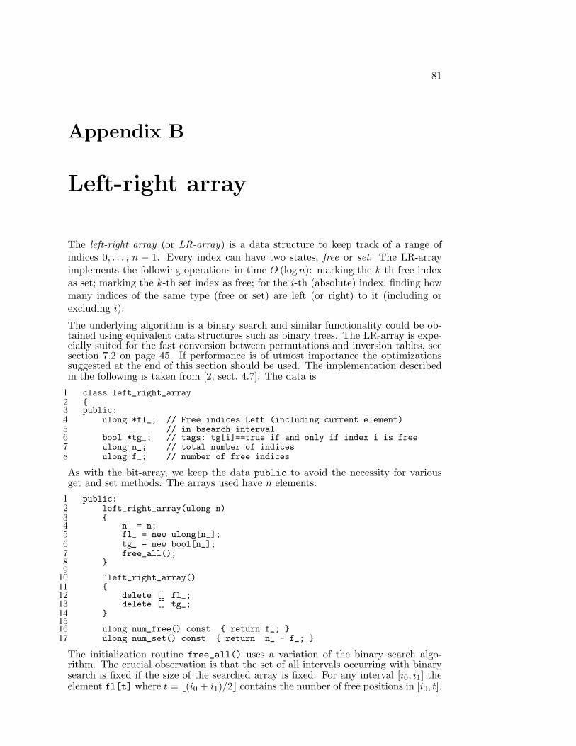
81
Appendix B
Left-right array
The left-right array (or LR-array) is a data structure to keep track of a range ofindices 0, . . . , n − 1. Every index can have two states, free or set. The LR-arrayimplements the following operations in time O (log n): marking the k-th free indexas set; marking the k-th set index as free; for the i-th (absolute) index, finding howmany indices of the same type (free or set) are left (or right) to it (including orexcluding i).
The underlying algorithm is a binary search and similar functionality could be ob-tained using equivalent data structures such as binary trees. The LR-array is expe-cially suited for the fast conversion between permutations and inversion tables, seesection 7.2 on page 45. If performance is of utmost importance the optimizationssuggested at the end of this section should be used. The implementation describedin the following is taken from [2, sect. 4.7]. The data is
1 class left_right_array2 {3 public:4 ulong *fl_; // Free indices Left (including current element)5 // in bsearch interval6 bool *tg_; // tags: tg[i]==true if and only if index i is free7 ulong n_; // total number of indices8 ulong f_; // number of free indices
As with the bit-array, we keep the data public to avoid the necessity for variousget and set methods. The arrays used have n elements:
1 public:2 left_right_array(ulong n)3 {4 n_ = n;5 fl_ = new ulong[n_];6 tg_ = new bool[n_];7 free_all();8 }9
10 ~left_right_array()11 {12 delete [] fl_;13 delete [] tg_;14 }1516 ulong num_free() const { return f_; }17 ulong num_set() const { return n_ - f_; }
The initialization routine free_all() uses a variation of the binary search algo-rithm. The crucial observation is that the set of all intervals occurring with binarysearch is fixed if the size of the searched array is fixed. For any interval [i0, i1] theelement fl[t] where t = b(i0 + i1)/2c contains the number of free positions in [i0, t].
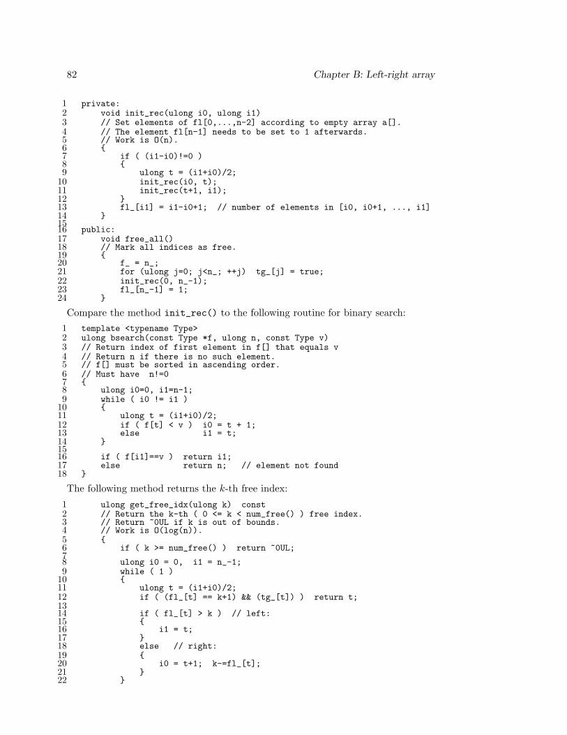
82 Chapter B: Left-right array
1 private:2 void init_rec(ulong i0, ulong i1)3 // Set elements of fl[0,...,n-2] according to empty array a[].4 // The element fl[n-1] needs to be set to 1 afterwards.5 // Work is O(n).6 {7 if ( (i1-i0)!=0 )8 {9 ulong t = (i1+i0)/2;
10 init_rec(i0, t);11 init_rec(t+1, i1);12 }13 fl_[i1] = i1-i0+1; // number of elements in [i0, i0+1, ..., i1]14 }1516 public:17 void free_all()18 // Mark all indices as free.19 {20 f_ = n_;21 for (ulong j=0; j<n_; ++j) tg_[j] = true;22 init_rec(0, n_-1);23 fl_[n_-1] = 1;24 }
Compare the method init_rec() to the following routine for binary search:1 template <typename Type>2 ulong bsearch(const Type *f, ulong n, const Type v)3 // Return index of first element in f[] that equals v4 // Return n if there is no such element.5 // f[] must be sorted in ascending order.6 // Must have n!=07 {8 ulong i0=0, i1=n-1;9 while ( i0 != i1 )
10 {11 ulong t = (i1+i0)/2;12 if ( f[t] < v ) i0 = t + 1;13 else i1 = t;14 }1516 if ( f[i1]==v ) return i1;17 else return n; // element not found18 }
The following method returns the k-th free index:
1 ulong get_free_idx(ulong k) const2 // Return the k-th ( 0 <= k < num_free() ) free index.3 // Return ~0UL if k is out of bounds.4 // Work is O(log(n)).5 {6 if ( k >= num_free() ) return ~0UL;78 ulong i0 = 0, i1 = n_-1;9 while ( 1 )
10 {11 ulong t = (i1+i0)/2;12 if ( (fl_[t] == k+1) && (tg_[t]) ) return t;1314 if ( fl_[t] > k ) // left:15 {16 i1 = t;17 }18 else // right:19 {20 i0 = t+1; k-=fl_[t];21 }22 }
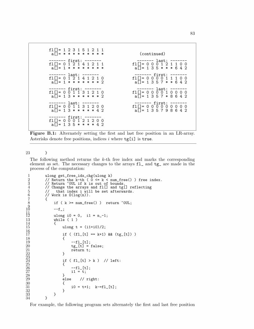
83
fl[]= 1 2 3 1 5 1 2 1 1a[]= * * * * * * * * * (continued)
------- first: ------- ------- last: -------fl[]= 0 1 2 1 4 1 2 1 1 fl[]= 0 0 0 1 2 1 1 0 0a[]= 1 * * * * * * * * a[]= 1 3 5 * * * 6 4 2
------- last: ------- ------- first: -------fl[]= 0 1 2 1 4 1 2 1 0 fl[]= 0 0 0 0 1 1 1 0 0a[]= 1 * * * * * * * 2 a[]= 1 3 5 7 * * 6 4 2
------- first: ------- ------- last: -------fl[]= 0 0 1 1 3 1 2 1 0 fl[]= 0 0 0 0 1 0 0 0 0a[]= 1 3 * * * * * * 2 a[]= 1 3 5 7 * 8 6 4 2
------- last: ------- ------- first: -------fl[]= 0 0 1 1 3 1 2 0 0 fl[]= 0 0 0 0 0 0 0 0 0a[]= 1 3 * * * * * 4 2 a[]= 1 3 5 7 9 8 6 4 2
------- first: -------fl[]= 0 0 0 1 2 1 2 0 0a[]= 1 3 5 * * * * 4 2
Figure B.1: Alternately setting the first and last free position in an LR-array.Asterisks denote free positions, indices i where tg[i] is true.
23 }
The following method returns the k-th free index and marks the correspondingelement as set. The necessary changes to the arrays fl_ and tg_ are made in theprocess of the computation:
1 ulong get_free_idx_chg(ulong k)2 // Return the k-th ( 0 <= k < num_free() ) free index.3 // Return ~0UL if k is out of bounds.4 // Change the arrays and fl[] and tg[] reflecting5 // that index i will be set afterwards.6 // Work is O(log(n)).7 {8 if ( k >= num_free() ) return ~0UL;9
10 --f_;1112 ulong i0 = 0, i1 = n_-1;13 while ( 1 )14 {15 ulong t = (i1+i0)/2;1617 if ( (fl_[t] == k+1) && (tg_[t]) )18 {19 --fl_[t];20 tg_[t] = false;21 return t;22 }2324 if ( fl_[t] > k ) // left:25 {26 --fl_[t];27 i1 = t;28 }29 else // right:30 {31 i0 = t+1; k-=fl_[t];32 }33 }34 }
For example, the following program sets alternately the first and last free position
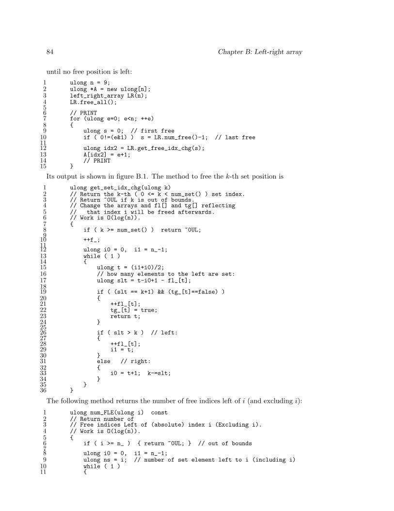
84 Chapter B: Left-right array
until no free position is left:1 ulong n = 9;2 ulong *A = new ulong[n];3 left_right_array LR(n);4 LR.free_all();56 // PRINT7 for (ulong e=0; e<n; ++e)8 {9 ulong s = 0; // first free
10 if ( 0!=(e&1) ) s = LR.num_free()-1; // last free1112 ulong idx2 = LR.get_free_idx_chg(s);13 A[idx2] = e+1;14 // PRINT15 }
Its output is shown in figure B.1. The method to free the k-th set position is
1 ulong get_set_idx_chg(ulong k)2 // Return the k-th ( 0 <= k < num_set() ) set index.3 // Return ~0UL if k is out of bounds.4 // Change the arrays and fl[] and tg[] reflecting5 // that index i will be freed afterwards.6 // Work is O(log(n)).7 {8 if ( k >= num_set() ) return ~0UL;9
10 ++f_;1112 ulong i0 = 0, i1 = n_-1;13 while ( 1 )14 {15 ulong t = (i1+i0)/2;16 // how many elements to the left are set:17 ulong slt = t-i0+1 - fl_[t];1819 if ( (slt == k+1) && (tg_[t]==false) )20 {21 ++fl_[t];22 tg_[t] = true;23 return t;24 }2526 if ( slt > k ) // left:27 {28 ++fl_[t];29 i1 = t;30 }31 else // right:32 {33 i0 = t+1; k-=slt;34 }35 }36 }
The following method returns the number of free indices left of i (and excluding i):
1 ulong num_FLE(ulong i) const2 // Return number of3 // Free indices Left of (absolute) index i (Excluding i).4 // Work is O(log(n)).5 {6 if ( i >= n_ ) { return ~0UL; } // out of bounds78 ulong i0 = 0, i1 = n_-1;9 ulong ns = i; // number of set element left to i (including i)
10 while ( 1 )11 {
85
12 if ( i0==i1 ) break;1314 ulong t = (i1+i0)/2;15 if ( i<=t ) // left:16 {17 i1 = t;18 }19 else // right:20 {21 ns -= fl_[t];22 i0 = t+1;23 }24 }2526 return i-ns;27 }
Based on this method are methods to determine the number of free/set indices to theleft/right, including/excluding the given index. We omit the out-of-bounds clausesin the following:
1 ulong num_FLI(ulong i) const2 // Return number of3 // Free indices Left of (absolute) index i (Including i).4 { return num_FLE(i) + tg_[i]; }56 ulong num_FRE(ulong i) const7 // Return number of8 // Free indices Right of (absolute) index i (Excluding i).9 { return num_free() - num_FLI(i); }
1011 ulong num_FRI(ulong i) const12 // Return number of13 // Free indices Right of (absolute) index i (Including i).14 { return num_free() - num_FLE(i); }1516 ulong num_SLE(ulong i) const17 // Return number of18 // Set indices Left of (absolute) index i (Excluding i).19 { return i - num_FLE(i); }2021 ulong num_SLI(ulong i) const22 // Return number of23 // Set indices Left of (absolute) index i (Including i).24 { return i - num_FLE(i) + !tg_[i]; }2526 ulong num_SRE(ulong i) const27 // Return number of28 // Set indices Right of (absolute) index i (Excluding i).29 { return num_set() - num_SLI(i); }3031 ulong num_SRI(ulong i) const32 // Return number of33 // Set indices Right of (absolute) index i (Including i).34 { return num_set() - i + num_FLE(i); }
Optimizations
With large sizes (say, well beyond the size of the second-level memory cache) muchof the time is spent waiting for the memory access. Using a structure correspondingto an m-ary tree (instead of the binary tree structure we used here) can drasticallyimprove the performance. The data on each node should fill at least one cache lineand be correspondingly aligned in memory.
86 Chapter B: Left-right array
LetB be the number of bits in a computer word (usually the C type unsigned long).At the terminals, a word can be used as a bit-array to indicate which of the B entriesare occupied. A fast routine for determining the index of the i-th set bit of the wordshould be used [2, sect. 1.10].
To further improve memory locality, the tags (indicating whether a position is occu-pied, tg_ in the class) should not be separated from the counts of the free positionsto the left (fl_ in the class). One way to do this is using one array where the leastsignificant bit in each word represents the tag and all higher bits are used for thecount.
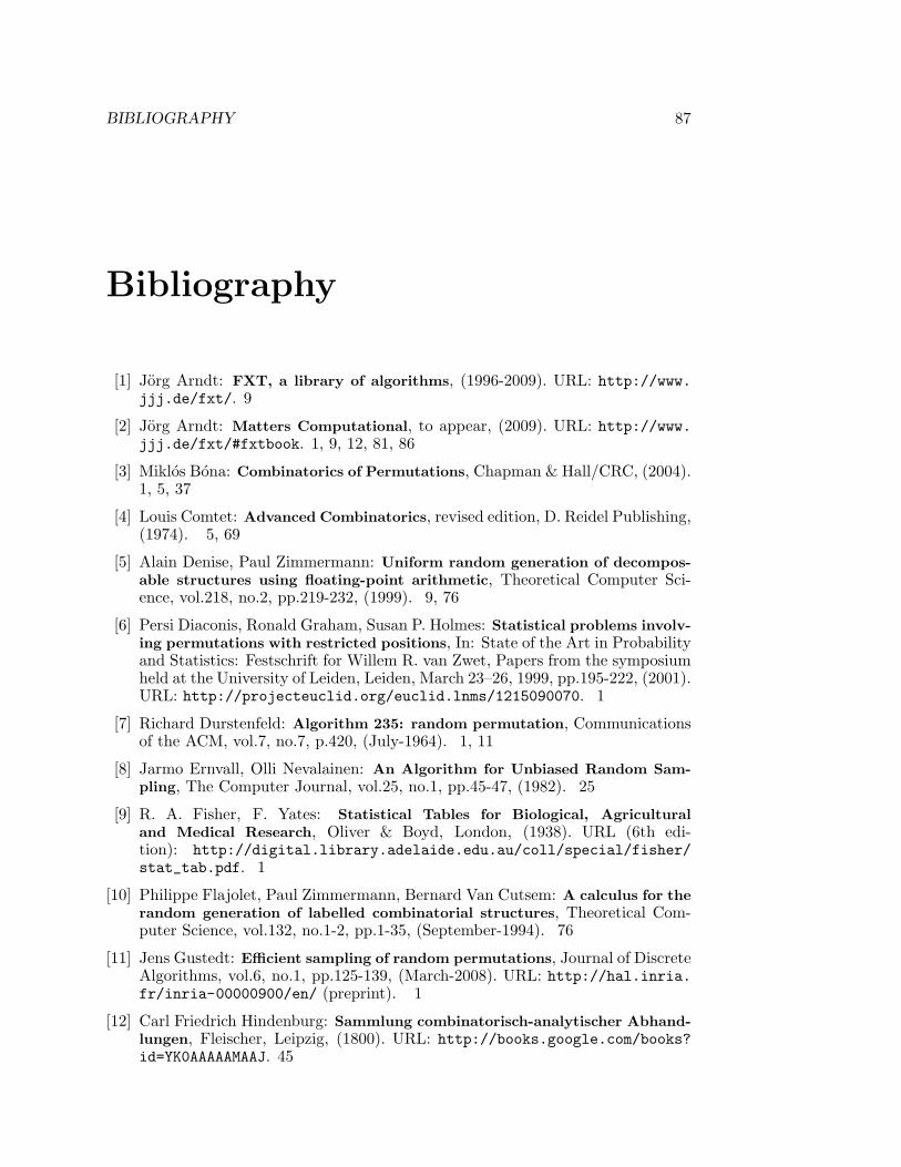
BIBLIOGRAPHY 87
Bibliography
[1] Jorg Arndt: FXT, a library of algorithms, (1996-2009). URL: http://www.jjj.de/fxt/. 9
[2] Jorg Arndt: Matters Computational, to appear, (2009). URL: http://www.jjj.de/fxt/#fxtbook. 1, 9, 12, 81, 86
[3] Miklos Bona: Combinatorics of Permutations, Chapman & Hall/CRC, (2004).1, 5, 37
[4] Louis Comtet: Advanced Combinatorics, revised edition, D. Reidel Publishing,(1974). 5, 69
[5] Alain Denise, Paul Zimmermann: Uniform random generation of decompos-able structures using floating-point arithmetic, Theoretical Computer Sci-ence, vol.218, no.2, pp.219-232, (1999). 9, 76
[6] Persi Diaconis, Ronald Graham, Susan P. Holmes: Statistical problems involv-ing permutations with restricted positions, In: State of the Art in Probabilityand Statistics: Festschrift for Willem R. van Zwet, Papers from the symposiumheld at the University of Leiden, Leiden, March 23–26, 1999, pp.195-222, (2001).URL: http://projecteuclid.org/euclid.lnms/1215090070. 1
[7] Richard Durstenfeld: Algorithm 235: random permutation, Communicationsof the ACM, vol.7, no.7, p.420, (July-1964). 1, 11
[8] Jarmo Ernvall, Olli Nevalainen: An Algorithm for Unbiased Random Sam-pling, The Computer Journal, vol.25, no.1, pp.45-47, (1982). 25
[9] R. A. Fisher, F. Yates: Statistical Tables for Biological, Agriculturaland Medical Research, Oliver & Boyd, London, (1938). URL (6th edi-tion): http://digital.library.adelaide.edu.au/coll/special/fisher/stat_tab.pdf. 1
[10] Philippe Flajolet, Paul Zimmermann, Bernard Van Cutsem: A calculus for therandom generation of labelled combinatorial structures, Theoretical Com-puter Science, vol.132, no.1-2, pp.1-35, (September-1994). 76
[11] Jens Gustedt: Efficient sampling of random permutations, Journal of DiscreteAlgorithms, vol.6, no.1, pp.125-139, (March-2008). URL: http://hal.inria.fr/inria-00000900/en/ (preprint). 1
[12] Carl Friedrich Hindenburg: Sammlung combinatorisch-analytischer Abhand-lungen, Fleischer, Leipzig, (1800). URL: http://books.google.com/books?id=YK0AAAAAMAAJ. 45
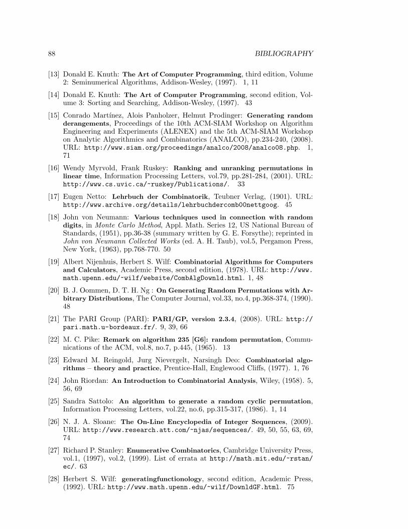
88 BIBLIOGRAPHY
[13] Donald E. Knuth: The Art of Computer Programming, third edition, Volume2: Seminumerical Algorithms, Addison-Wesley, (1997). 1, 11
[14] Donald E. Knuth: The Art of Computer Programming, second edition, Vol-ume 3: Sorting and Searching, Addison-Wesley, (1997). 43
[15] Conrado Martınez, Alois Panholzer, Helmut Prodinger: Generating randomderangements, Proceedings of the 10th ACM-SIAM Workshop on AlgorithmEngineering and Experiments (ALENEX) and the 5th ACM-SIAM Workshopon Analytic Algorithmics and Combinatorics (ANALCO), pp.234-240, (2008).URL: http://www.siam.org/proceedings/analco/2008/analco08.php. 1,71
[16] Wendy Myrvold, Frank Ruskey: Ranking and unranking permutations inlinear time, Information Processing Letters, vol.79, pp.281-284, (2001). URL:http://www.cs.uvic.ca/~ruskey/Publications/. 33
[17] Eugen Netto: Lehrbuch der Combinatorik, Teubner Verlag, (1901). URL:http://www.archive.org/details/lehrbuchdercomb00nettgoog. 45
[18] John von Neumann: Various techniques used in connection with randomdigits, in Monte Carlo Method, Appl. Math. Series 12, US National Bureau ofStandards, (1951), pp.36-38 (summary written by G. E. Forsythe); reprinted inJohn von Neumann Collected Works (ed. A. H. Taub), vol.5, Pergamon Press,New York, (1963), pp.768-770. 50
[19] Albert Nijenhuis, Herbert S. Wilf: Combinatorial Algorithms for Computersand Calculators, Academic Press, second edition, (1978). URL: http://www.math.upenn.edu/~wilf/website/CombAlgDownld.html. 1, 48
[20] B. J. Oommen, D. T. H. Ng : On Generating Random Permutations with Ar-bitrary Distributions, The Computer Journal, vol.33, no.4, pp.368-374, (1990).48
[21] The PARI Group (PARI): PARI/GP, version 2.3.4, (2008). URL: http://pari.math.u-bordeaux.fr/. 9, 39, 66
[22] M. C. Pike: Remark on algorithm 235 [G6]: random permutation, Commu-nications of the ACM, vol.8, no.7, p.445, (1965). 13
[23] Edward M. Reingold, Jurg Nievergelt, Narsingh Deo: Combinatorial algo-rithms – theory and practice, Prentice-Hall, Englewood Cliffs, (1977). 1, 76
[24] John Riordan: An Introduction to Combinatorial Analysis, Wiley, (1958). 5,56, 69
[25] Sandra Sattolo: An algorithm to generate a random cyclic permutation,Information Processing Letters, vol.22, no.6, pp.315-317, (1986). 1, 14
[26] N. J. A. Sloane: The On-Line Encyclopedia of Integer Sequences, (2009).URL: http://www.research.att.com/~njas/sequences/. 49, 50, 55, 63, 69,74
[27] Richard P. Stanley: Enumerative Combinatorics, Cambridge University Press,vol.1, (1997), vol.2, (1999). List of errata at http://math.mit.edu/~rstan/ec/. 63
[28] Herbert S. Wilf: generatingfunctionology, second edition, Academic Press,(1992). URL: http://www.math.upenn.edu/~wilf/DownldGF.html. 75