Introduction

Texture mapping was introduced in [Catmull 74] as a method ofadding to the visual richness of a computer generated image withoutadding geometry. There are three fundamental issues that must beaddressed to render textures. First, a texture must be acquired.Possibilities include creating a texture procedurally, painting atexture, or digitally scanning a texture from a photograph. Next, weneed to define a mapping from the texture space to the space of themodel to be textured. Defining this mapping should not require agreat deal of a user’s time. This mapping should not noticeablydistort the texture. Finally, we require a method of sampling thetexture during rendering so that the final image contains no artifactsdue to aliasing or resulting from the underlying texture representation[Heckbert 89]. These three issues are often interrelated, and this istrue of the techniques in this paper.

This paper explores a procedural method for texture synthesis andalso introduces a new method for fitting a texture to a surface. Eitherof these techniques can be used separately, but the examples givenhere shows the strength of using them together to produce naturaltextures on complex models. After a discussion of previous texturingmethods, the majority of the paper is divided into two parts, one foreach of these topics.

The first part of this paper describes a chemical mechanism forpattern formation know as reaction-diffusion. This mechanism, firstdescribed in [Turing 52], shows how two or more chemicals thatdiffuse across a surface and react with one another can form stablepatterns. A number of researchers have shown how simple patternsof spots and stripes can be created by reaction-diffusion systems[Bard 81; Murray 81; Meinhardt 82]. We begin by introducing thebasics of how a reaction-diffusion system can form simple patterns.We then introduce new results that show how more complex patternscan be generated by having an initial pattern set down by onechemical system and further refined by later chemical systems. Thiswidens the range of patterns that can be generated by reaction-diffusion to include such patterns as the rosettes found on leopardsand the multiple-width stripes found on some fish and snakes. Thesepatterns could be generated on a square grid and then mapped ontoan object’s surface using traditional techniques, but there areadvantages to synthesizing the pattern directly on the surface to betextured in a manner that will be described next.

The second part of this paper presents a method of generating a meshover the surface of a polyhedral model that can be used for texturesynthesis. The approach uses relaxation to evenly distribute pointsacross the model’s surface and then divides the surface into cellscentered at these points. We can simulate reaction-diffusion systemsdirectly on this mesh to create textures. Because there is no mappingfrom texture space to the object, there is no need to assign texture

Abstract

This paper describes a biologically motivated method of texturesynthesis called reaction-diffusion and demonstrates how thesetextures can be generated in a manner that directly matches thegeometry of a given surface. Reaction-diffusion is a process in whichtwo or more chemicals diffuse at unequal rates over a surface andreact with one another to form stable patterns such as spots andstripes. Biologists and mathematicians have explored the patternsmade by several reaction-diffusion systems. We extend the range oftextures that have previously been generated by using a cascade ofmultiple reaction-diffusion systems in which one system lays downan initial pattern and then one or more later systems refine the pattern.Examples of patterns generated by such a cascade process include theclusters of spots on leopards known as rosettes and the web-likepatterns found on giraffes. In addition, this paper introduces amethod by which reaction-diffusion textures are created to match thegeometry of an arbitrary polyhedral surface. This is accomplished bycreating a mesh over a given surface and then simulating the reaction-diffusion process directly on this mesh. This avoids the often difficulttask of assigning texture coordinates to a complex surface. A meshis generated by evenly distributing points over the model usingrelaxation and then determining which points are adjacent byconstructing their Voronoi regions. Textures are rendered directlyfrom the mesh by using a weighted sum of mesh values to computesurface color at a given position. Such textures can also be used asbump maps.

CR Categories and Subject Descriptors: I.3.3 [Computer Graphics]:Picture/Image Generation; I.3.5 [Computer Graphics]: Three-Dimensional Graphics and Realism - Color, shading, shadowing andtexture; J.3 [Life and Medical Sciences]: Biology.

Additional Keywords and Phrases: Reaction-diffusion, biologicalmodels, texture mapping.

Generating Textures on Arbitrary Surfaces Using Reaction-Diffusion

Greg TurkUniversity of North Carolina at Chapel Hill

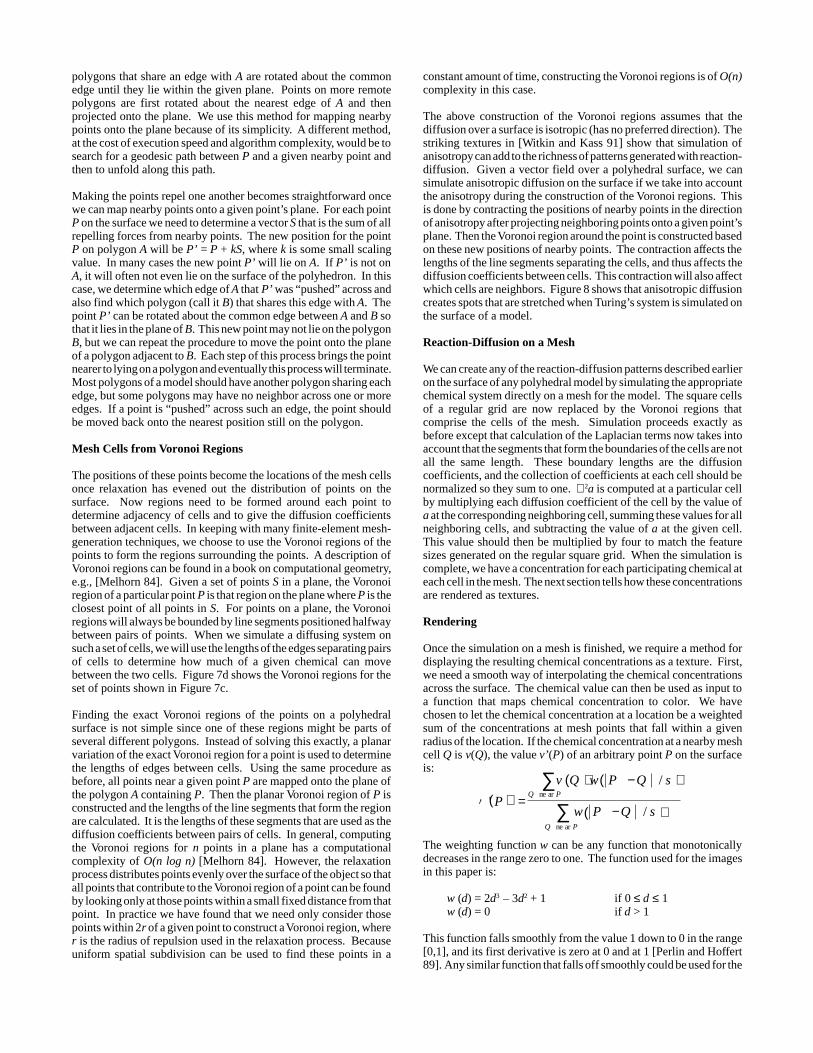
coordinates to polygons and there is no distortion of the textures. Atno time is the texture stored in some regular m × n grid, as are mosttextures. It is likely that other texture generation methods in additionto reaction-diffusion could also make use of such a mesh. Images ofsurfaces that have been textured using a mesh do not show aliasingartifacts or visual indication of the underlying mesh structure. Thesetextures can also be used for bump mapping, a technique introducedin [Blinn 78] to give the appearance of a rough or wrinkled surface.The three steps involved in texturing a model as in Figures 4, 5 and6 are: (1) generate a mesh that fits the polyhedral model, (2) simulatea reaction-diffusion system on the mesh (solve a partial differentialequation) and (3) use the final values from the simulation to specifysurface color while rendering the polygons of the model.

Artificial Texture Synthesis

A great strength of procedurally generating textures is that each newmethod can be used in conjunction with already existing functions.Several methods have been demonstrated that use composition ofvarious functions to generate textures. Gardner introduced the ideaof summing a small number of sine waves of different periods, phasesand amplitudes to create a texture [Gardner 85]. Pure sine wavesgenerate fairly bland textures, so Gardner uses the values of the lowperiod waves to alter the shape of the higher period waves. Thismethod gives textures that are evocative of patterns found in naturesuch as those of clouds and trees. Perlin uses band-limited noise asthe basic function from which to construct textures [Perlin 85]. Hehas shown that a wide variety of textures (stucco, wrinkles, marble,fire) can be created by manipulating such a noise function in variousways. [Lewis 89] describes several methods for generating isotropicnoise functions to be used for texture synthesis. A stunning exampleof using physical simulation for texture creation is the dynamic cloudpatterns of Jupiter in the movie 2010 [Yaeger and Upson 86].

Recent work on texture synthesis using reaction-diffusion is describedin [Witkin and Kass 91]. They show the importance of anisotropy byintroducing a rich set of new patterns that are generated by anisotropicreaction-diffusion. In addition, they demonstrate how reaction-diffusion systems can be simulated rapidly using fast approximationsto Gaussian convolution.

A texture can be created by painting an image, and the kinds oftextures that may be created this way are limitless. An unusualvariant of this is to paint an “image” in the frequency domain and thentake the inverse transform to create the final texture [Lewis 84].Lewis demonstrates how textures such as canvas and wood grain canbe created by this method. An extension to digital painting, describedin [Hanrahan and Haeberli 90], shows how use of a hardware z-buffercan allow a user to paint interactively onto the image of a three-dimensional surface.

Mapping Textures onto Surfaces

Once a texture has been created, a method is needed to map it ontothe surface to be textured. This is commonly cast into the problemof assigning texture coordinates (u,v) from a rectangle to the verticesof the polygons in a model. Mapping texture coordinates onto acomplex surface is not easy, and several methods have been proposedto accomplish this. A common approach is to define a mapping fromthe rectangle to the natural coordinate system of the target object’ssurface. For example, latitude and longitude can be used to define amapping onto a sphere, and parametric coordinates can be used whenmapping a texture onto a cubic patch [Catmull 74]. In some cases anobject might be covered by multiple patches, and in these instancescare must be taken to make the edges of the patches match. Asuccessful example of this is found in the bark texture for a model ofa maple tree in [Bloomenthal 85].

Another approach to texture mapping is to project the texture onto thesurface of the object. One example of this is to orient the texturesquare in R3 (Euclidean three-space) and perform a projection fromthis square onto the surface [Peachey 85]. Related to this is a two-steptexture mapping method given by [Bier and Sloan 86]. The first stepmaps the texture onto a simple intermediate surface in R3, such as abox or cylinder. The second step projects the texture from this surfaceonto the target object. A different method of texture mapping is tomake use of the polygonal nature of many graphical models. In thisapproach, taken by [Samek 86], the surface of a polyhedral object isunfolded onto the plane one or more times and the average of theunfolded positions of each vertex is used to determine textureplacement. A user can adjust the mapping by specifying where tobegin the unfolding of the polyhedral object.

Each of the above methods has been used with success for somemodels and textures. There are pitfalls to these methods, however.Each of the methods can cause a texture to be distorted because thereis often no natural map from the texture space to the surface of theobject. This is a fundamental problem that comes from defining thetexture pattern over a geometry that is different than that of the objectto be textured. Some of these techniques also require a good deal ofuser intervention. One solution to these problems for some imagesis the use of solid textures. A solid texture is a color function definedover a portion of R3, and such a texture is easily mapped onto thesurfaces of objects [Peachey 85; Perlin 85]. A point (x,y,z) on thesurface of an object is colored by the value of the solid texturefunction at this point in space. This method is well suited forsimulating objects that are formed from a solid piece of material suchas a block of wood or a slab of marble. Solid texturing is a successfultechnique because the texture function matches the geometry of thematerial being simulated, namely the geometry of R3. No assignmentof texture coordinates is necessary.

Quite a different approach to matching texture to surface geometryis given in [Ma and Gagalowicz 85]. They describe several methodsfor creating a local coordinate system at each point on the surface ofa given model. Statistical properties of a texture are then used tosynthesize texture on the surface so that it is oriented to the localcoordinate system.

Part One: Reaction-Diffusion

This section describes a class of patterns that are formed by reaction-diffusion systems. These patterns are an addition to the texturesynthesist’s toolbox, a collection of tools that include such proceduralmethods as Perlin’s noise function and Gardner’s sum-of-sine waves.The reaction-diffusion patterns can either be used alone or they canbe used as an initial pattern that can be built on using other procedures.This section begins by discussing reaction-diffusion as it relates todevelopmental biology and then gives specific examples of patternsthat can be generated using reaction-diffusion.

A central issue in developmental biology is how the cells of anembryo arrange themselves into particular patterns. For example,how is it that the cells in the embryo of a worm become organized intosegments? Undoubtedly there are many organizing mechanismsworking together throughout the development of an animal. Onepossible mechanism, first described by Turing, is that two or morechemicals can diffuse through an embryo and react with each otheruntil a stable pattern of chemical concentrations is reached [Turing52]. These chemical pre-patterns can then act as a trigger for cells ofdifferent types to develop in different positions in the embryo. Suchchemical systems are known as reaction-diffusion systems, and thehypothetical chemical agents are called morphogens. Since theintroduction of these ideas, several mathematical models of suchsystems have been studied to see what patterns can be formed and tosee how these matched actual animal patterns such as coat spotting

These equations are given for a discrete model, where each ai is one

“cell” in a line of cells and where the neighbors of this cell are ai-1

anda

i+1. The values for β

i are the sources of slight irregularities in

chemical concentration across the line of cells. Figure 1 illustratesthe progress of the chemical concentration of b across a line of 60cells as its concentration varies over time. Initially the values of a

iand b

i were set to 4 for all cells along the line. The values of β

i were

clustered around 12, with the values varying randomly by ± 0.05. Thediffusion constants were set to D

a = .25 and D

b = .0625, which means

that a diffuses more rapidly than b, and s = 0.03125. Notice how afterabout 2000 iterations the concentration of b has settled down into apattern of peaks and valleys. The simulation results look different indetail to this when a different random seed is used for β

i, but such

simulations have the same characteristic peaks and valleys withroughly the same scale to these features.

Reaction-Diffusion on a Grid

The reaction-diffusion system given above can also be simulated ona two-dimensional field of cells. The most common form for such asimulation is to have each cell be a square in a regular grid, and havea cell diffuse to each of its four neighbors on the grid. The discreteform of the equations is:

∆ai,j = s (16 – a

i,j b

i,j) + D

a (a

i+1,j + a

i-1,j + a

i,j +1 + a

i,j-1 – 4a

i,j)

∆bi,j = s (a

i,j b

i,j – b

i,j – β

i,j) + D

b (b

i+1,j + b

i-1,j + b

i,j+1 + b

i,j-1 – 4b

i,j)

In this form, the value of ∇2a at a cell is found by summing each ofthe four neighboring values of a and subtracting four times the valueof a at the cell. Each of the neighboring values for a are given thesame weight in this computation because the length of the sharededge between any two cells is always the same on a square grid. Thiswill not be the case when we perform a similar computation on a lessregular grid, where different neighbors will be weighted differentlywhen calculating ∇2a.

Figure 2 (upper left) shows the result of a simulation of theseequations on a 64 × 64 grid of cells. Notice that the valleys ofconcentration in b take the form of spots in two dimensions. It is thenature of this system to have high concentrations for a in these spotregions where b is low. Sometimes chemical a is called an inhibitorbecause high values for a in a spot region prevent other spots fromforming nearby. In two-chemical reaction-diffusion systems theinhibitor is always the chemical that diffuses more rapidly.

We can create spots of different sizes by changing the value of theconstant s for this system. Small values for s (s = 0.05 in Figure 2,upper left) cause the reaction part of the system to proceed moreslowly relative to the diffusion and this creates larger spots. Largervalues for s produce smaller spots (s = 0.2 in Figure 2, upper right).The spot patterns at the top of Figure 2 were generated with β

i,j = 12

± 0.1. If the random variation of βi,j is increased to 12 ± 3, the spots

become more irregular in shape (Figure 3, upper left). The patternsthat can be generated by this reaction-diffusion system wereextensively studied in [Bard and Lauder 74] and [Bard 81].

Reaction-diffusion need not be restricted to two-chemical systems.For the generation of striped patterns, Meinhardt has proposed asystem involving five chemicals that react with one another [Meinhardt82]. See the appendix of this paper for details of Meinhardts’ssystem. The result of simulating such a system on a two-dimensionalgrid can be seen in Figure 3 (lower left). Notice that the systemgenerates random stripes that tend to fork and sometimes formislands of one color or the other. This pattern is like random stripesfound on some tropical fish and is also similar to the pattern of righteye and left eye regions of the ocular dominance columns found inmammals [Hubel and Wiesel 79].

Figure 1: One-dimensional example of reaction-diffusion.Chemical concentration is shown in intervals of 400 time steps.

The first equation says that the change of the concentration of a at agiven time depends on the sum of a function F of the localconcentrations of a and b and the diffusion of a from places nearby.The constant D

a says how fast a is diffusing, and the Laplacian ∇2 a

is a measure of how high the concentration of a is at one location withrespect to the concentration of a nearby. If nearby places have ahigher concentration of a, then ∇2 a will be positive and a diffusestoward this position. If nearby places have lower concentrations,then ∇2 a will be negative and a will diffuse away from this position.

The key to pattern formation based on reaction-diffusion is that aninitial small amount of variation in the chemical concentrations cancause the system to be unstable initially and to be driven to a stablestate in which the concentrations of a and b vary across the surface.A set of equations that Turing proposed for generating patterns in onedimension provides a specific example of reaction-diffusion:

∆ai = s (16 – a

i b

i) + D

a (a

i+1 + a

i-1 – 2a

i)

∆bi = s (a

i b

i – b

i – β

i) + D

b (b

i+1 + b

i-1 – 2b

i)

and stripes on mammals [Bard 81; Murray 81]. Only recently has anactual reaction-diffusion system been observed in the laboratory[Lengyel and Epstein 91]. So far no direct evidence has been foundto show that reaction-diffusion is the operating mechanism in thedevelopment of any particular embryo pattern. This should not betaken as a refutation of the model, however, because the field ofdevelopmental biology is still young and very few mechanisms havebeen verified to be the agents of pattern formation in embryodevelopment.

The basic form of a simple reaction-diffusion system is to have twochemicals (call them a and b) that diffuse through the embryo atdifferent rates and that react with each other to either build up or breakdown a and b. These systems can be explored in any dimension. Forexample, we might use a one-dimensional system to look at segmentformation in worms, or we could look at reaction-diffusion on asurface for spot-pattern formation. Here are the equations showingthe general form of a two-chemical reaction-diffusion system:

∂t

∂a = F(a,b) + D

a ∇ 2

a

∂t

∂b = G(a,b) + D

b ∇ 2

b

Complex Patterns

This section shows how we can generate more complex patternsusing reaction-diffusion by allowing one chemical system to setdown an initial pattern and then having this pattern refined bysimulating a second system. One model of embryogenesis of the fruitfly shows how several reaction-diffusion systems might lay downincreasingly refined stripes to give a final pattern that matches thesegmentation pattern in the embryo [Hunding 90]. Bard has suggestedthat such a cascade process might be responsible for some of the lessregular coat patterns of some mammals [Bard 81], but he gives nodetails about how two chemical systems might interact. The patternsshown in this section are new results that are inspired by Bard’s ideaof cascade processes.

The upper portion of Figure 2 shows how we can change the spot sizeof a pattern by changing the size parameter s of Turing’s reaction-diffusion system from 0.05 to 0.2. The lower left portion of Figure2 demonstrates that these two systems can be combined to create thelarge-and-small spot pattern found on cheetahs. We can make thispattern by running the large spot simulation, “freezing” part of thispattern, and then running the small spot simulation in the unfrozenportion of the computation mesh. Specifically, once the large spotsare made (using s = 0.05) we set a boolean flag frozen to TRUE foreach cell that has a concentration for chemical b between 0 and 4.These marked cells are precisely those that form the dark spots in theupper left of Figure 2. Then we run the spot forming mechanismagain using s = 0.2 to form the smaller spots. During this secondphase all of the cells marked as frozen retain their old values for theconcentrations of a and b. These marked cells must still participatein the calculation of the values of the Laplacian for a and b forneighboring cells. This allows the inhibitory nature of chemical a toprevent the smaller spots from forming too near the larger spots. Thisfinal image is more natural than the image we would get if we simplysuperimposed the top two images of Figure 2.

We can create the leopard spot pattern of Figure 2 (lower right) inmuch the same way as we created the cheetah spots. We lay down theoverall plan for this pattern by creating the large spots as in the upperleft of Figure 2 (s = 0.05). Now, in addition to marking as frozen thosecells that form the large spots, we also change the values of chemicalsa and b to be 4 at these marked cells. When we run the second system

Figure 3: Irregular spots, reticulation, random stripes and mixed large-and-small stripes.

Figure 2: Reaction-diffusion on a square grid. Large spots, small spots, cheetah and leopard patterns.

to form smaller spots (s = 0.2) the small spots tend to form in the areasadjacent to the large spots. The smaller spots can form near the largespots because the inhibitor a is not high at the marked cells. Thistexture can also be seen on the horse model in Figure 4.

In a manner analogous to the large-and-small spots of Figure 2 (lowerleft) we can create a pattern with small stripes running between largerstripes. The stripe pattern of Figure 3 (lower right) is such a patternand is modelled after the stripes found on fish such as the lionfish. Wecan make the large stripes that set the overall structure of the patternby running Meinhardt’s stripe-formation system with diffusion ratesof D

g = 0.1 and D

s = 0.06 (see Appendix). Then we mark those cells

in the white stripe regions as frozen and run a second stripe-formingsystem with D

g = 0.008 and D

s = 0.06. The slower diffusion of

chemicals g1 and g

2 (a smaller value for D

g) causes thinner stripes to

form between the larger stripes.

We can use both the spot and stripe formation systems together toform the web-like pattern called reticulation that is found on giraffes.Figure 3 (upper right) shows the result of first creating slightlyirregular spots as in Figure 3 (upper left) and then using the stripe-formation system to make stripes between the spots. Once again wemark as frozen those cells that comprise the spots. We also set theconcentrations of the five chemicals at the frozen cells to the valuesfound in the white regions of the patterns made by the stripe-formation system. This causes black stripes to form between themarked cells when the stripe-formation system is run as the secondstep in the cascade process. Figure 5 is an example of how such atexture looks on a polyhedral model.

Regular Stripe Patterns

The chemical system that produces random stripes like those inFigure 3 (lower left) can also be used to produce more regular stripepatterns. The random stripes are a result of the slight randomperturbations in the “substrate” for the chemical system. If theserandom perturbations are removed so the system starts with acompletely homogeneous substrate, then no stripes will formanywhere. Regular stripes will form on a mesh that is homogeneouseverywhere except at a few “stripe initiator” cells, and the stripes will

radiate from these special cells. One way to create an initiator cell isto slightly raise or lower the substrate value at that cell. Another wayis to mark the cell as frozen and set the value of one of the chemicalsto be higher or lower than at other cells. The pseudo-zebra in Figure6 was created in this manner. Its stripes were initiated by choosingseveral cells on the head and one cell on each of the hooves, markingthese cells as frozen and setting the initial value of chemical g

1 at

these cells to be slightly higher than at other cells.

Varying Parameters Across a Surface

On many animals the size of the spots or stripes varies across the coat.For example, the stripes on a zebra are more broad on the hindquarters than the stripes on the neck and legs. Bard has suggestedthat, after the striped pattern is set, the rate of tissue growth may varyat different locations on the embryo [Bard 77]. This effect can beapproximated by varying the diffusion rates of the chemicals acrossthe computation mesh. The pseudo-zebra of Figure 6 has widerstripes near the hind quarters than elsewhere on the model. This wasaccomplished by allowing the chemicals to diffuse more rapidly atthe places where wider stripes were desired.

Part Two: Mesh Generation and Rendering

This section describes how to generate a mesh over a polyhedralmodel that can be used for texture synthesis and that will lend itselfto high-quality image generation. The strength of this technique isthat no explicit mapping from texture space to an object’s surface isrequired. There is no texture distortion. There is no need for a userto manually assign texture coordinates to the vertices of polygons.Portions of this section will describe how such a mesh can be used tosimulate a reaction-diffusion system for an arbitrary polyhedralmodel. This mesh will serve as a replacement to the regular squaregrids used to generate Figures 2 and 3. We will create textures bysimulating a reaction-diffusion system directly on the mesh. It islikely that these meshes can also be used for other forms of texturesynthesis. Such a mesh can be used for texture generation wherevera texture creation method only requires the passing of informationbetween neighboring texture elements (mesh cells).

There are a wide variety of sources for polyhedral models in computergraphics. Models generated by special-effects houses are oftendigitized by hand from a scale model. Models taken from CAD mightbe created by conversion from constructive solid geometry to apolygonal boundary representation. Some models are generatedprocedurally, such as fractals used to create mountain ranges andtrees. Often these methods will give us few guarantees about theshapes of the polygons, the density of vertices across the surface orthe range of sizes of the polygons. Sometimes such models willcontain very skinny polygons or vertices where dozens of polygonsmeet. For these reasons it is unwise to use the original polygons asthe mesh to be used for creating textures. Instead, a new mesh needsto be generated that closely matches the original model but that hasproperties that make it suitable for texture synthesis. This mesh-generation method must be robust in order to handle the wide varietyof polyhedral models used in computer graphics.

Mesh generation is a common problem in finite-element analysis,and a wide variety of methods have been proposed to create meshes[Ho-Le 88]. Automatic mesh generation is a difficult problem ingeneral, but the requirements of texture synthesis will serve tosimplify the problem. We only require that the model be divided upinto relatively evenly-spaced regions. The mesh-generation techniquedescribed below divides a polyhedral surface into cells that abut oneanother and fully tile the polyhedral model. The actual descriptionof a cell consists of a position in R3, a list of adjacent cells and a listof scalar values that tell how much diffusion occurs between this celland each of its neighbors. No explicit geometric representation of the Figure 6: Pseudo-Zebra

Figure 4: Leopard-Horse

Figure 5: Giraffe

loop k timesfor each point P on surface

determine nearby points to Pmap these nearby points onto the plane containing the polygon of Pcompute and store the repulsive forces that the mapped points exert on P

for each point P on surfacecompute the new position of P based on the repulsive forces

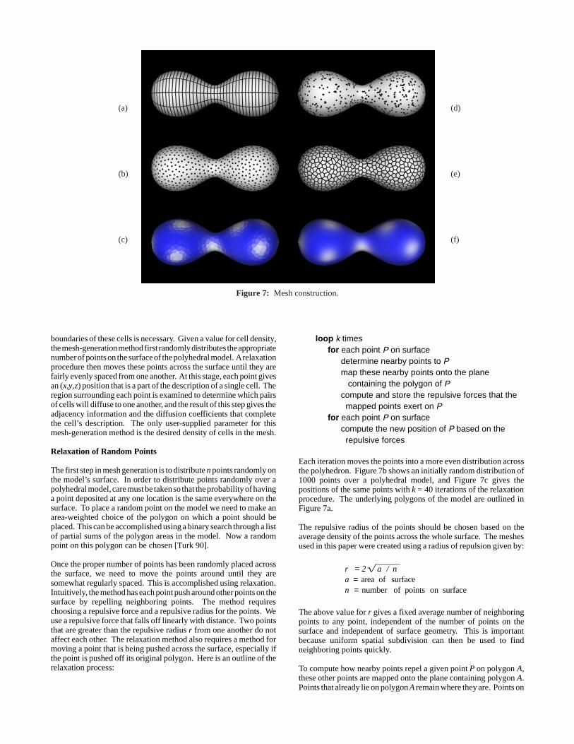
Each iteration moves the points into a more even distribution acrossthe polyhedron. Figure 7b shows an initially random distribution of1000 points over a polyhedral model, and Figure 7c gives thepositions of the same points with k = 40 iterations of the relaxationprocedure. The underlying polygons of the model are outlined inFigure 7a.

The repulsive radius of the points should be chosen based on theaverage density of the points across the whole surface. The meshesused in this paper were created using a radius of repulsion given by:

The above value for r gives a fixed average number of neighboringpoints to any point, independent of the number of points on thesurface and independent of surface geometry. This is importantbecause uniform spatial subdivision can then be used to findneighboring points quickly.

To compute how nearby points repel a given point P on polygon A,these other points are mapped onto the plane containing polygon A.Points that already lie on polygon A remain where they are. Points on

(a)

(b)

(c)

(d)

(e)

(f)

boundaries of these cells is necessary. Given a value for cell density,the mesh-generation method first randomly distributes the appropriatenumber of points on the surface of the polyhedral model. A relaxationprocedure then moves these points across the surface until they arefairly evenly spaced from one another. At this stage, each point givesan (x,y,z) position that is a part of the description of a single cell. Theregion surrounding each point is examined to determine which pairsof cells will diffuse to one another, and the result of this step gives theadjacency information and the diffusion coefficients that completethe cell’s description. The only user-supplied parameter for thismesh-generation method is the desired density of cells in the mesh.

Relaxation of Random Points

The first step in mesh generation is to distribute n points randomly onthe model’s surface. In order to distribute points randomly over apolyhedral model, care must be taken so that the probability of havinga point deposited at any one location is the same everywhere on thesurface. To place a random point on the model we need to make anarea-weighted choice of the polygon on which a point should beplaced. This can be accomplished using a binary search through a listof partial sums of the polygon areas in the model. Now a randompoint on this polygon can be chosen [Turk 90].

Once the proper number of points has been randomly placed acrossthe surface, we need to move the points around until they aresomewhat regularly spaced. This is accomplished using relaxation.Intuitively, the method has each point push around other points on thesurface by repelling neighboring points. The method requireschoosing a repulsive force and a repulsive radius for the points. Weuse a repulsive force that falls off linearly with distance. Two pointsthat are greater than the repulsive radius r from one another do notaffect each other. The relaxation method also requires a method formoving a point that is being pushed across the surface, especially ifthe point is pushed off its original polygon. Here is an outline of therelaxation process:

r = 2 a / na = area of surfacen = number of points on surface

Figure 7: Mesh construction.

polygons that share an edge with A are rotated about the commonedge until they lie within the given plane. Points on more remotepolygons are first rotated about the nearest edge of A and thenprojected onto the plane. We use this method for mapping nearbypoints onto the plane because of its simplicity. A different method,at the cost of execution speed and algorithm complexity, would be tosearch for a geodesic path between P and a given nearby point andthen to unfold along this path.

Making the points repel one another becomes straightforward oncewe can map nearby points onto a given point’s plane. For each pointP on the surface we need to determine a vector S that is the sum of allrepelling forces from nearby points. The new position for the pointP on polygon A will be P’ = P + kS, where k is some small scalingvalue. In many cases the new point P’ will lie on A. If P’ is not onA, it will often not even lie on the surface of the polyhedron. In thiscase, we determine which edge of A that P’ was “pushed” across andalso find which polygon (call it B) that shares this edge with A. Thepoint P’ can be rotated about the common edge between A and B sothat it lies in the plane of B. This new point may not lie on the polygonB, but we can repeat the procedure to move the point onto the planeof a polygon adjacent to B. Each step of this process brings the pointnearer to lying on a polygon and eventually this process will terminate.Most polygons of a model should have another polygon sharing eachedge, but some polygons may have no neighbor across one or moreedges. If a point is “pushed” across such an edge, the point shouldbe moved back onto the nearest position still on the polygon.

Mesh Cells from Voronoi Regions

The positions of these points become the locations of the mesh cellsonce relaxation has evened out the distribution of points on thesurface. Now regions need to be formed around each point todetermine adjacency of cells and to give the diffusion coefficientsbetween adjacent cells. In keeping with many finite-element mesh-generation techniques, we choose to use the Voronoi regions of thepoints to form the regions surrounding the points. A description ofVoronoi regions can be found in a book on computational geometry,e.g., [Melhorn 84]. Given a set of points S in a plane, the Voronoiregion of a particular point P is that region on the plane where P is theclosest point of all points in S. For points on a plane, the Voronoiregions will always be bounded by line segments positioned halfwaybetween pairs of points. When we simulate a diffusing system onsuch a set of cells, we will use the lengths of the edges separating pairsof cells to determine how much of a given chemical can movebetween the two cells. Figure 7d shows the Voronoi regions for theset of points shown in Figure 7c.

Finding the exact Voronoi regions of the points on a polyhedralsurface is not simple since one of these regions might be parts ofseveral different polygons. Instead of solving this exactly, a planarvariation of the exact Voronoi region for a point is used to determinethe lengths of edges between cells. Using the same procedure asbefore, all points near a given point P are mapped onto the plane ofthe polygon A containing P. Then the planar Voronoi region of P isconstructed and the lengths of the line segments that form the regionare calculated. It is the lengths of these segments that are used as thediffusion coefficients between pairs of cells. In general, computingthe Voronoi regions for n points in a plane has a computationalcomplexity of O(n log n) [Melhorn 84]. However, the relaxationprocess distributes points evenly over the surface of the object so thatall points that contribute to the Voronoi region of a point can be foundby looking only at those points within a small fixed distance from thatpoint. In practice we have found that we need only consider thosepoints within 2r of a given point to construct a Voronoi region, wherer is the radius of repulsion used in the relaxation process. Becauseuniform spatial subdivision can be used to find these points in a

The weighting function w can be any function that monotonicallydecreases in the range zero to one. The function used for the imagesin this paper is:

w (d) = 2d3 – 3d2 + 1 if 0 ≤ d ≤ 1w (d) = 0 if d > 1

This function falls smoothly from the value 1 down to 0 in the range[0,1], and its first derivative is zero at 0 and at 1 [Perlin and Hoffert89]. Any similar function that falls off smoothly could be used for the

constant amount of time, constructing the Voronoi regions is of O(n)complexity in this case.

The above construction of the Voronoi regions assumes that thediffusion over a surface is isotropic (has no preferred direction). Thestriking textures in [Witkin and Kass 91] show that simulation ofanisotropy can add to the richness of patterns generated with reaction-diffusion. Given a vector field over a polyhedral surface, we cansimulate anisotropic diffusion on the surface if we take into accountthe anisotropy during the construction of the Voronoi regions. Thisis done by contracting the positions of nearby points in the directionof anisotropy after projecting neighboring points onto a given point’splane. Then the Voronoi region around the point is constructed basedon these new positions of nearby points. The contraction affects thelengths of the line segments separating the cells, and thus affects thediffusion coefficients between cells. This contraction will also affectwhich cells are neighbors. Figure 8 shows that anisotropic diffusioncreates spots that are stretched when Turing’s system is simulated onthe surface of a model.

Reaction-Diffusion on a Mesh

We can create any of the reaction-diffusion patterns described earlieron the surface of any polyhedral model by simulating the appropriatechemical system directly on a mesh for the model. The square cellsof a regular grid are now replaced by the Voronoi regions thatcomprise the cells of the mesh. Simulation proceeds exactly asbefore except that calculation of the Laplacian terms now takes intoaccount that the segments that form the boundaries of the cells are notall the same length. These boundary lengths are the diffusioncoefficients, and the collection of coefficients at each cell should benormalized so they sum to one. ∇2a is computed at a particular cellby multiplying each diffusion coefficient of the cell by the value ofa at the corresponding neighboring cell, summing these values for allneighboring cells, and subtracting the value of a at the given cell.This value should then be multiplied by four to match the featuresizes generated on the regular square grid. When the simulation iscomplete, we have a concentration for each participating chemical ateach cell in the mesh. The next section tells how these concentrationsare rendered as textures.

Rendering

Once the simulation on a mesh is finished, we require a method fordisplaying the resulting chemical concentrations as a texture. First,we need a smooth way of interpolating the chemical concentrationsacross the surface. The chemical value can then be used as input toa function that maps chemical concentration to color. We havechosen to let the chemical concentration at a location be a weightedsum of the concentrations at mesh points that fall within a givenradius of the location. If the chemical concentration at a nearby meshcell Q is v(Q), the value v’(P) of an arbitrary point P on the surfaceis:

v ' P( ) =v Q( )w P −Q / s( )

Q ne arP∑

w P −Q / s( )Q ne arP

∑

weighting function. The images in this paper have been made usinga value of s = 2r, where r is the repulsive radius from the relaxationmethod. Much smaller values for s make the individual mesh pointsnoticeable, and values much larger than this will blur together thevalues of more nearby mesh points. Uniform spatial subdivisionmakes finding nearby mesh points a fast operation because onlythose mesh points within a distance s contribute to a point’s value.Figure 7e shows the individual cell values from a pattern generatedby reaction-diffusion, where the chemical concentrations have beenmapped to a color gradation from blue to white. Figure 7f shows thesurface colors given by the weighted average for v’(P) describedabove.

The method described above gives smooth changes of chemicalconcentration across the surface of the model, and rendered imagesdo not show evidence of the underlying mesh used to create thetexture. Aliasing of the texture can occur, however, when a texturedobject is scaled down small enough that the texture features, saystripes, are about the same width as the pixels of the image. Super-sampling of the texture is one possible way to lessen this problem, butcomputing the texture value many times to find the color at one pixelis costly. A better approach is to extend the notion of levels ofincreasingly blurred textures [Williams 83] to those textures definedby the simulation mesh.

The blurred versions of the texture are generated using the simulationmesh, and each mesh point has associated with it an RGB (red, green,blue) color triple for each blur level. Level 0 is an unblurred versionof the texture and is created by evaluating the concentration-to-colorfunction at the mesh points for each concentration value and storingthe color as an RGB triple at each mesh point. Blur levels 1 and higherare created by allowing these initial color values to diffuse across thesurface. When the values of a two-dimensional gray-scale image areallowed to diffuse across the image, the result is the same asconvolving the original image with a Gaussian filter. Larger amountsof blurring (wider Gaussian filters) are obtained by diffusing forlonger periods of time. Similarly, allowing the RGB values at themesh points to diffuse across the mesh results in increasingly blurredversions of the texture given on the mesh. The relationship betweendiffusion for a time t and convolution with a Gaussian kernel ofstandard deviation σ is t = σ2 / 2 [Koenderink 84]. The blur levels ofFigure 9 were generated so that each level’s Gaussian kernel has astandard deviation twice that of the preceding blur level.

The texture color at a point is given by a weighted average betweenthe colors from two blur levels. The choice of blur levels and theweighting between the levels at a pixel is derived from anapproximation to the amount of textured surface that is covered bythe pixel. This estimate of surface area can be computed from thedistance to the surface and the angle the surface normal makes withthe direction to the eye. The natural unit of length for this area is r,the repulsion radius for mesh building. The proper blur level at apixel is the base two logarithm of the square root of a, where a is thearea of the surface covered by the pixel in square units of r. We haveproduced short animated sequences using this anti-aliasing techniqueand they show no aliasing of the textures.

Bump mapping is a technique used to make a surface appear roughor wrinkled without explicitly altering the surface geometry [Blinn78]. The rough appearance is created from a gray-scale texture byadding a perturbation vector to the surface normal and then evaluatingthe lighting model based on this new surface normal. Perlin showedthat the gradient of a scalar-valued function in R3 can be used as aperturbation vector to produce convincing surface roughness [Perlin85]. We can use the gradient of the values v’(P) of a reaction-diffusion simulation to give a perturbation vector at a given point P:

Figure 8: Anisotropic diffusion

Figure 10: Bump mapping

Figure 9: Blur levels for anti-aliasing

d = r / 100gx = (v’(P) – v’(P + [d,0,0])) / dgy = (v’(P) – v’(P + [0,d,0])) / dgz = (v’(P) – v’(P + [0,0,d])) / dperturbation vector = [k * gx, k * gy, k * gz]

The above method for computing the gradient of v’ evaluates thefunction at P and at three nearby points in each of the x, y and zdirections. The value d is taken to be a small fraction of the repulsiveradius r to make sure we stay close enough to P that we get an accurateestimate for the gradient. The gradient can also be computed directlyfrom the definition of v’ by calculating exactly the partial derivativesin x, y and z. The scalar parameter k is used to scale the bump features,and changing k’s sign causes bumps to become indentations and viceversa. Figure 10 shows bumps created in this manner based theresults of a reaction-diffusion system.

Implementation and Performance

Creating a texture using reaction-diffusion for a given model can bea CPU-intensive task. Each of the textures in Figures 4, 5 and 6 tookseveral hours to generate on a DEC 3100 workstation. These meshescontained 64,000 points. Perhaps there is some consolation in thethought that nature requires the same order of magnitude in time tolay down such a pattern in an embryo. Such texture synthesis timeswould seem to prohibit much experimenting with reaction-diffusiontextures. It is fortunate that a given reaction-diffusion system with aparticular set of parameters produces the same texture features onsmall square grids as the features from a simulation on much largermeshes. The patterns in this paper were first simulated on a 64 × 64grid of cells where the simulations required less than a minute tofinish. These simulations were run on a Maspar MP-I, which is aSIMD computer with 4096 processing elements connected in a two-dimensional grid. A workstation such as a DEC 3100 can performsimilar simulations on a 32 × 32 grid in about two minutes, which isfast enough to explore new textures. Once a texture is generated byreaction-diffusion, the time to render the model with a texture isreasonably fast. The image in Figure 4 required 70 seconds to renderat 512 × 512 resolution without anti-aliasing on a DEC 3100. Thesame horse without texture takes 16 seconds to render.

Future Work

The cascade processes that formed the textures in this paper are justa few of the patterns that can be generated by reaction-diffusion.More exploration should be made on how one chemical system canleave a pattern for later systems. For example, one chemical systemcould affect the random substrate of a second system. What patternscan be formed if one system causes different rates of diffusion indifferent locations in a second system?

Other methods of pattern creation could be performed on the meshesused for texture synthesis. Examples that might be adapted fromcellular automata [Toffoli and Margolus 87] include two-dimensionalannealing, diffusion-limited aggregation and the Belousov-Zhabotinskii reaction.

Acknowledgments

I would like to thank those people who have offered ideas andencouragement for this work. These people include David Banks,Henry Fuchs, Albert Harris, Steve Molnar, Brice Tebbs, and TurnerWhitted. Thanks also for the suggestions provided by the anonymousreviewers. Linda Houseman helped clean up my writing and DavidEllsworth provided valuable photographic assistance. Thanks toRhythm & Hues for the horse, Steve Speer for the giraffe and AppleComputer’s Vivarium Program for the sea-slug.

In this system, the chemicals g1 and g

2 indicate the presence of one

or the other stripe color (white or black, for instance). Theconcentration of r is used to make sure that only one of g

1 and g

2 are

present at any one location. Chemicals s1 and s

2 assure that the

regions of g1 and g

2 are limited in width. A program written in

FORTRAN to simulate this system can be found in [Meinhardt 82].

References

[Bard 77] Bard, Jonathan, “A Unity Underlying the Different ZebraStriping Patterns,” Journal of Zoology, Vol. 183, No. 4, pp. 527–539 (December 1977).

[Bard 81] Bard, Jonathan B. L., “A Model for Generating Aspects ofZebra and Other Mammalian Coat Patterns,” Journal of TheoreticalBiology, Vol. 93, No. 2, pp. 363–385 (November 1981).

[Bard and Lauder 74] Bard, Jonathan and Ian Lauder, “How WellDoes Turing’s Theory of Morphogenesis Work?,” Journal ofTheoretical Biology, Vol. 45, No. 2, pp. 501–531 (June 1974).

[Bier and Sloan 86] Bier, Eric A. and Kenneth R. Sloan, Jr., “Two-Part Texture Mapping,” IEEE Computer Graphics andApplications, Vol. 6, No. 9, pp. 40–53 (September 1986).

[Blinn 78] Blinn, James F., “Simulation of Wrinkled Surfaces,”Computer Graphics, Vol. 12, No. 3 (SIGGRAPH ’78), pp. 286–292 (August 1978).

[Bloomenthal 85] Bloomenthal, Jules, “Modeling the Mighty Maple,”Computer Graphics, Vol. 19, No. 3 (SIGGRAPH ’85), pp. 305–311 (July 1985).

[Catmull 74] Catmull, Edwin E., “A Subdivision Algorithm forComputer Display of Curved Surfaces,” Ph.D. Thesis, Departmentof Computer Science, University of Utah (December 1974).

This work was supported by a Graduate Fellowship from IBM and bythe Pixel-Planes project. Pixel-Planes is supported by the NationalScience Foundation (MIP-9000894) and the Defense AdvancedResearch Projects Agency, Information Science and TechnologyOffice (Order No. 7510).

Appendix: Meinhardt’s Stripe-Formation System

The stripes of Figure 3 (lower images) and Figure 6 were created witha five-chemical reaction-diffusion system given in [Meinhardt 82].The equations of Meinhardt’s system are as follows:

∂g1

∂t=

cs2g

12

r − αg1

+ D g

∂ 2g

1

∂x 2+ρ

0

∂g2

∂t=

cs1g

22

r − αg2

+ D g

∂ 2g

2

∂x 2+ρ

0

∂r∂t =cs

2g

12 +cs

1g

22 − βr

∂s1

∂t= γ g

1−s

1( ) + D s

∂ 2s

1

∂x 2+ρ

1

∂s2

∂t = γ g2

−s2( ) + D s

∂ 2s

2

∂x 2 +ρ1

[Gardner 85] Gardner, Geoffrey Y., “Visual Simulation of Clouds,”Computer Graphics, Vol. 19, No. 3 (SIGGRAPH ’85), pp. 297–303 (July 1985).

[Hanrahan and Haeberli 90] Hanrahan, Pat and Paul Haeberli,“Direct WYSIWYG Painting and Texturing on 3D Shapes,”Computer Graphics, Vol. 24, No. 4 (SIGGRAPH ’90), pp. 215–223 (August 1990).

[Heckbert 89] Heckbert, Paul S., “Fundamentals of Texture Mappingand Image Warping,” M.S. Thesis, Department of ElectricalEngineering and Computer Science, University of California atBerkeley (June 1989).

[Ho-Le 88] Ho-Le, K., “Finite Element Mesh Generation Methods:A Review and Classification,” Computer Aided Design, Vol. 20,No. 1, pp. 27–38 (January/February 1988).

[Hubel and Wiesel 79] Hubel, David H. and Torsten N. Wiesel,“Brain Mechanisms of Vision,” Scientific American, Vol. 241, No.3, pp. 150–162 (September 1979).

[Hunding 90] Hunding, Axel, Stuart A. Kauffman, and Brian C.Goodwin, “Drosophila Segmentation: Supercomputer Simulationof Prepattern Hierarchy,” Journal of Theoretical Biology, Vol. 145,pp. 369–384 (1990).

[Koenderink 84] Koenderink, Jan J., “The Structure of Images,”Biological Cybernetics, Vol. 50, No. 5, pp. 363–370 (August1984).

[Lengyel and Epstein 91] Lengyel, István and Irving R. Epstein,“Modeling of Turing Structures in the Chlorite–Iodide–MalonicAcid–Starch Reaction System,” Science, Vol. 251, No. 4994, pp.650–652 (February 8, 1991).

[Lewis 84] Lewis, John-Peter, “Texture Synthesis for DigitalPainting,” Computer Graphics, Vol. 18, No. 3 (SIGGRAPH ’84),pp. 245–252 (July 1984).

[Lewis 89] Lewis, J. P., “Algorithms for Solid Noise Synthesis,”Computer Graphics, Vol. 23, No. 3 (SIGGRAPH ’89), pp. 263–270 (July 1989).

[Ma and Gagalowicz 85] Ma, Song De and Andre Gagalowicz,“Determination of Local Coordinate Systems for Texture Synthesison 3-D Surfaces,” Eurographics ‘85, edited by C. E. Vandoni.

[Meinhardt 82] Meinhardt, Hans, Models of Biological PatternFormation, Academic Press, London, 1982.

[Melhorn 84] Melhorn, Kurt, Multi-dimensional Searching andComputational Geometry, Springer-Verlag, 1984.

[Murray 81] Murray, J. D., “On Pattern Formation Mechanisms forLepidopteran Wing Patterns and Mammalian Coat Markings,”Philosophical Transactions of the Royal Society B, Vol. 295, pp.473–496.

[Peachey 85] Peachey, Darwyn R., “Solid Texturing of ComplexSurfaces,” Computer Graphics, Vol. 19, No. 3 (SIGGRAPH ’85),pp. 279–286 (July 1985).

[Perlin 85] Perlin, Ken, “An Image Synthesizer,” Computer Graphics,Vol. 19, No. 3 (SIGGRAPH ’85), pp. 287–296 (July 1985).

[Perlin and Hoffert 89] Perlin, Ken and Eric M. Hoffert,“Hypertexture,” Computer Graphics, Vol. 23, No. 3 (SIGGRAPH’89), pp. 253–262 (July 1989).

[Samek 86] Samek, Marcel, Cheryl Slean and Hank Weghorst,“Texture Mapping and Distortion in Digital Graphics,” The VisualComputer, Vol. 2, No. 5, pp. 313–320 (September 1986).

[Toffoli and Margolus 87] Toffoli, Tommaso and Norman Margolus,Cellular Automata Machines, MIT Press, 1987.

[Turing 52] Turing, Alan, “The Chemical Basis of Morphogenesis,”Philosophical Transactions of the Royal Society B, Vol. 237, pp.37–72 (August 14, 1952).

[Turk 90] Turk, Greg, “Generating Random Points in Triangles,” inGraphics Gems, edited by Andrew Glassner, Academic Press,1990.

[Williams 83] Williams, Lance, “Pyramidal Parametrics,” ComputerGraphics, Vol. 17, No. 3 (SIGGRAPH ’83), pp. 1–11 (July 1983).

[Witkin and Kass 91] Witkin, Andrew and Michael Kass, “Reaction-Diffusion Textures,” Computer Graphics, Vol. 25 (SIGGRAPH’91).

[Yeager and Upson] Yeager, Larry and Craig Upson, “CombiningPhysical and Visual Simulation — Creation of the Planet Jupiterfor the Film 2010,” Computer Graphics, Vol. 20, No. 4 (SIGGRAPH’86), pp. 85–93 (August 1986).