Embed Size (px)
Citation preview
NASA
Contractor Report 195306
/ --
. ! f
Army Research Laborat0_ z_?
Contractor Report ARL-CR-145
Generation of Gear Tooth Surfaces
by Application of CNC Machines
EL. Litvin and N.X. Chen
University of Illinois at Chicago
Chicago, Illinois
April 1994
(NASA-CR-195306) GENERATION OF
GEA_ TOOTH SURFACES BY APPLICATION
OF CNC MACHINES Final Report
(I11inois Univ.) 84 p
G3/3_
N94-30205
Unclas
0004777
Prepared for
Lewis Research Center
Under Grant NAG3-1263
National Aeronautics and
Space Administration
U.S. ARMY
RESEARCH LABORATORY
https://ntrs.nasa.gov/search.jsp?R=19940025700 2018-05-27T18:05:16+00:00Z

_ t
Generation of Gear Tooth Surfaces by Application of CNC Machines
F.L. Litvin and N.X. Chen
The University of Illinois at Chicago
Chicago, Illinois 60680
Summary
This study will demonstrate the importance of application of CNC machines in generation
of gear tooth surfaces with new topology. This topology decreases gear vibration and will
extend the gear capacity and service life. A preliminary investigation by a tooth contact
analysis(TCA) program has shown that gear tooth surfaces in line contact (for instance,
involute helical gears with parallel axes, worm-gear drives with cylindrical worms etc.) are
very sensitive to angular errors of misalignment that cause edge contact and an unfavorable
shape of transmission errors and vibration.
The new topology of gear tooth surfaces is based on the localization of bearing contact,
and the synthesis of a predesigned parabolic function of transmission errors that is able to
absorb a piecewise linear function of transmission errors caused by gear misalignment.
The report will describe the following topics: (1) Description of kinematics of CNC
machines with 6 degrees-of-freedom that can be applied for generation of gear tooth surfaces
with new topology. (2) A new method for grinding of gear tooth surfaces by a cone surface
or surface of revolution based on application of CNC machines. This method provides an
optimal approximation of the ground surfaceto the given one. This method is especially
beneficial when undevelopedruled surfacesare to be ground. (3) Execution of motions of
the CNC machine. The solution to this problem can be applied aswell for the transfer of
machine-tool settings from a conventional generator to the CNC machine.
The developed theory required the derivation of a modified equation of meshing based
on application of the concept of space curves, space curves represented on surfaces, geodesic
curvature, surface torsion etc. Condensed information on these topics of differential geometry
is provided as well.
Introduction
The design and manufacture of gears with new topology of gear tooth surfaces are prob-
lems of great importance for helicopter transmissions. The existing technology of gears is
restricted with the necessity to use cutting and grinding machines whose kinematics is based
on linear relations between the motions of the tool and the workpiece.
The need of low-noise gears with increased load capacity and service life can be satisfied
with a new topology of gear tooth surfaces that is able to provide: (i) a reduced sensitivity to
misalignment and avoidance of edge contact, (ii) a parabolic type of function of transmission
errors to reduce the level of possible vibration, (iii) a localized bearing contact with controlled
dimensions of the instantaneous contact ellipse.
The application of CNC (Computer Numerically Controlled) machines overcomes the
obstacles presented for generation of gears with a new surface topology by using the existing
equipment. The CNC machines are able to provide computer controlled nonlinear relations
between the motions of the tool and the gear being generated. Although such machines are
used at present mainly for the installment of machine-tool settings with higher precision,
their prosperous future is in their application for generation of gears with new topology. The
CNC machinesarea uniqueopportunity for researchersto modify the geometry of traditional
gear drives and benefit industry with gear drives with substantially improved parameters.
The modification of geometry of gear tooth surfaces requires from researchers a new
approach for the development of principles of conjugation of gear tooth surfaces. Application
of conjugate gear tooth surfaces being in instantaneous line contact is in the authors' opinion
an anachronism. Such gear tooth surfaces are very sensitive to misalignment that causes the
shift of the bearing contact to the edge and transmission errors of such a type that cause
a jerk at the transfer from one cycle of meshing to the next. The considerations above are
true for spur gears, involute helical gears with parallel axes, and worm-gear drives.
It is necessary as well to change the attitude to some finishing processes such as honing
and shaving applied for helical and spur gears. It is not reasonable to require that such
finishing processes would provide the exact screw involute surfaces knowing ahead that only
modified tooth surfaces are to be applied.
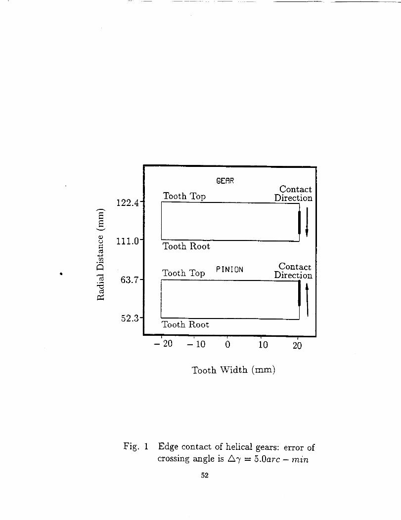
The statements mentioned above are illustrated with the following drawings.
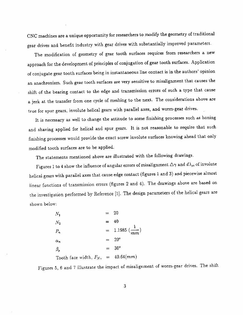
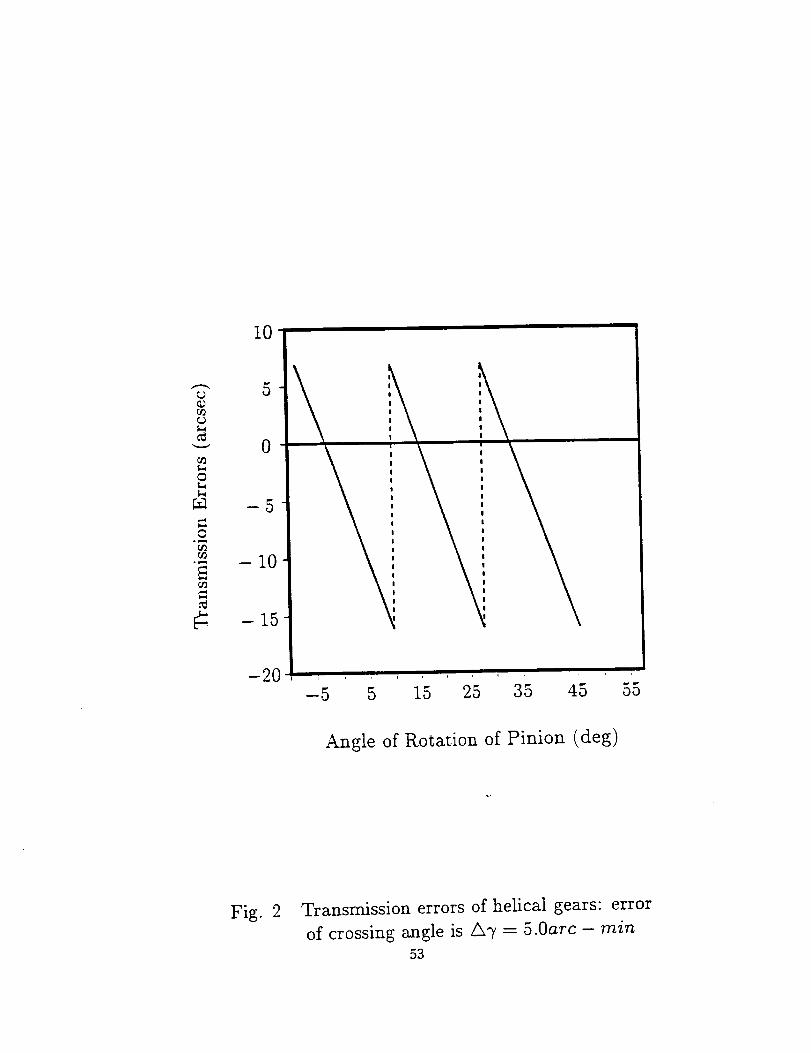
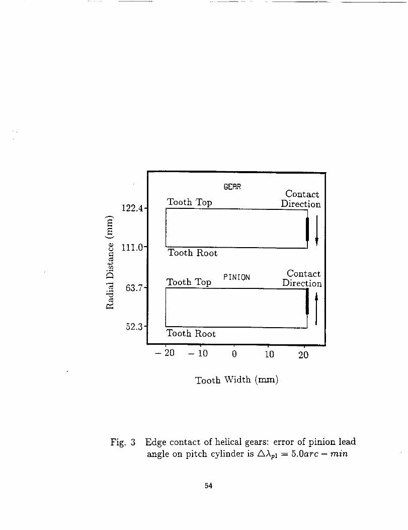
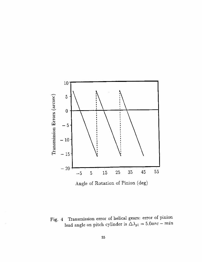
Figures 1 to 4 show the influence of angular errors of misalignment/k-y and dApi of involute
helical gears with parallel axes that cause edge contact (figures 1 and 3) and piecewise almost
linear functions of transmission errors (figures 2 and 4). The drawings above are based on
the investigation performed by Reference [1]. The design parameters of the helical gears are
shown below:
N1
N2
_n
Figures
= 20
= 40
= 1.1985(--1 )mm
.__ 20 °
3p = 30°
Tooth face width, IN, = 40.64(mm)
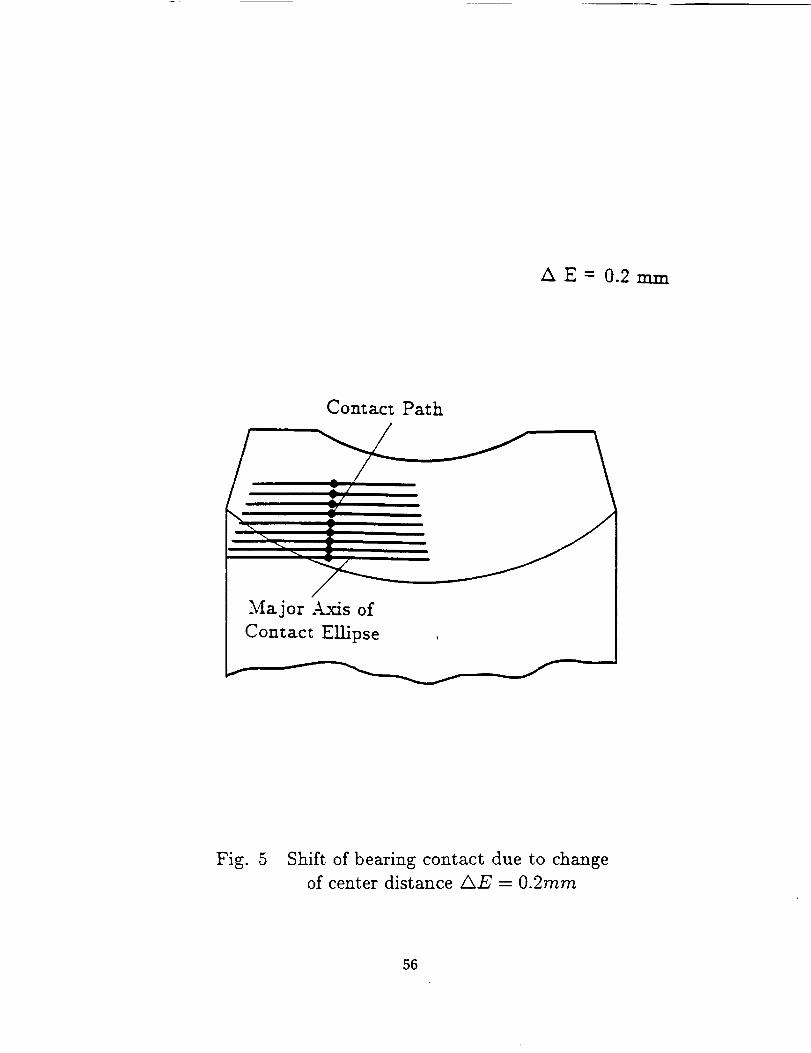
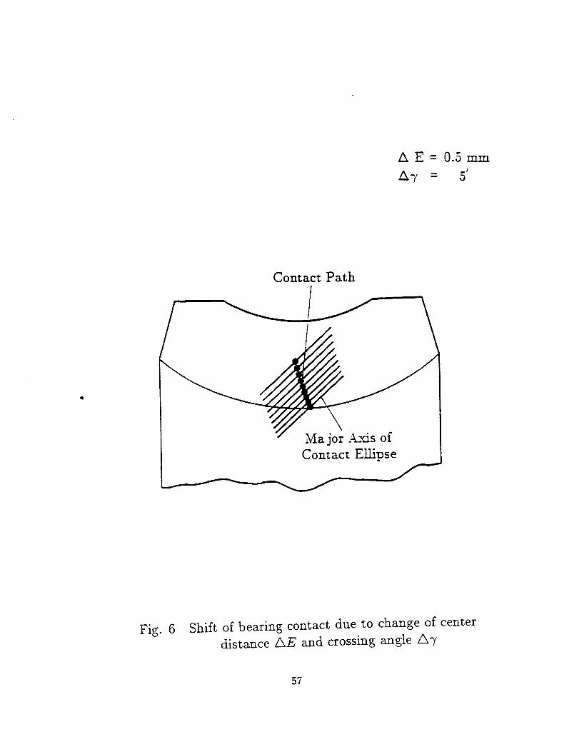
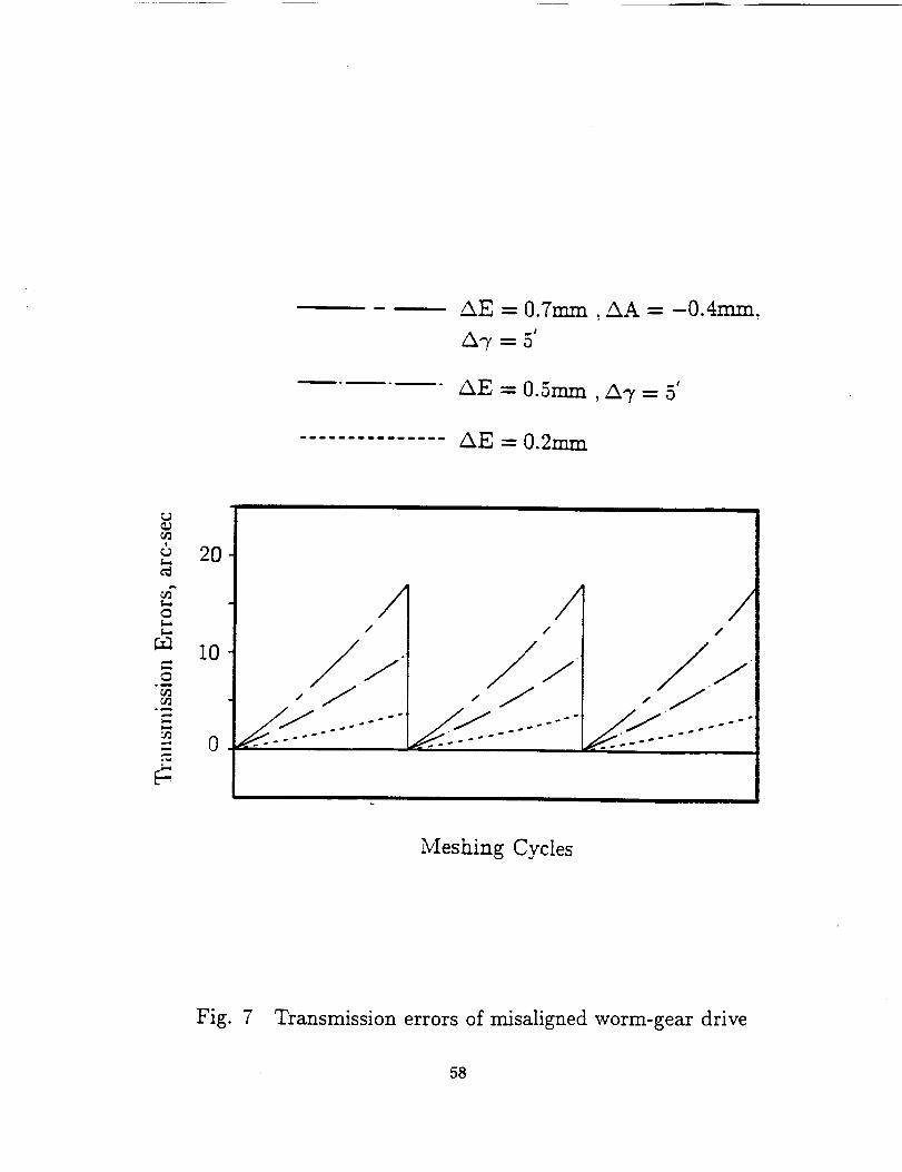
5, 6 and 7 illustrate the impact of misalignment of worm-gear drives. The shift
of the bearing contact is shownin figures5 and 6, and the undesirableshift of transmission
errors is shown in figure 7 that will inevitable cause vibration. The drawings are based on
the research accomplished by Reference [2].
The design parameters of the worm-gear drive are shown below:
N1 = 2
N2 = 30
Axial module, m = 8(mm)
7 = 90°
Shortest distance, E, = 176(ram)
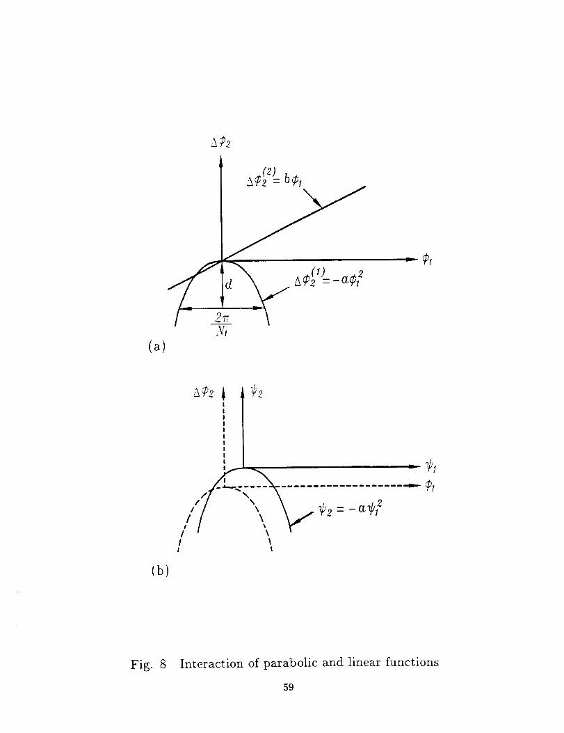
Figure 8 illustrates why a predesigned parabolic type of transmission errors is beneficial
for the gears with the new topology (Ref. [3]). This figure illustrates the interaction of
a parabolic function of transmission errors(provided at the stage of synthesis of the gear
tooth surfaces) with a linear function of transmission errors(caused by misalignment). The
combination of these functions is again a parabolic function, with the same slope as the
predesigned one that is translated with respect to the initial parabolic function. This means
that the predesigned parabolic function absorbs the linear function and keeps the shape of
a parabolic function.
There are three cases of generation of the workpiece surface Ep by the given tool surface
Et by CNC machines:
(1) Surfaces Et and E v are in continuous tangency, however they contact each other at
every instant at a point not a line.
(2) Surfaces Et and Ep are in continuous tangency and they contact each other at every
instant at a line. Surface Ep is generated in this case as the envelope to the family of
surfaces Et. The family of surfaces is generated in relative motion of Et to Ep.
(3) An approximate method for generation of a surface Eg (ground or cut) with an optimal
approximation to the ideal surface Z v.
An example of case 1 is the generation, for instance, of a die designed for forging of a gear.
Generation of conventional spiral bevel gears and hypoid gears by the "Phoenix" machine
is the example of case 2 generation. Case 3 is the basic idea for a new method for surface
generation discussed in section 4. Only cases 2 and 3 of surface generation are discussed in
this report.
The contents of the report covers the following topics:
(i) Description of "Phoenix" and "Star" CNC machines, that are suitable for generation
of gear tooth surfaces with new topology.
(ii) Execution of motions of CNC machines.
(iii) Generation of a surface with optimal approximation to the ideal surface.
(iv) Concept of curvatures that are required for computations for the proposed approach
for generation.
1. "Phoenix" and "Star" CNC Machines
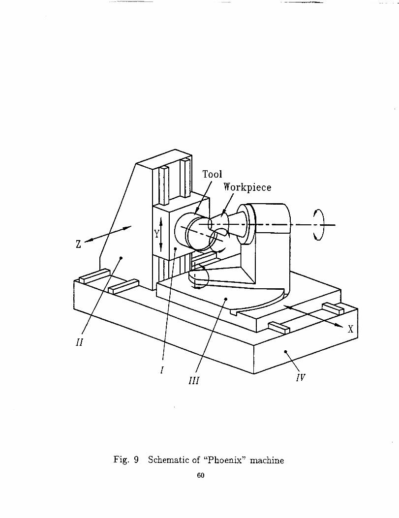
"Phoenix" CNC Machine
The "Phoenix" CNC machine (figure 9) is designed by the Gleason Works for generation
of spiral bevel and hypoid gears. The machine is provided with a total of six degrees-of-
freedom. Three rotational motions, and three translational motions are used. The transla-
tional motions are performed in three mutually perpendicular directions. Two of rotational
motions are provided as rotation of the workpiece and the rotation that enables to change
the angle between the axes of the workpiece and the tool. The sixth rotational motion is
provided as rotation of the tool about its axis, and generally is not related with the pro-
cessfor generation. The motions with other five degrees-of-freedomare provided asrelated
motions in the processfor surfacegeneration.
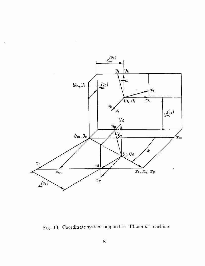
Coordinate Systems Applied for "Phoenix"
Coordinate systemsSt (zt, yt, zt) and Sp (xp, yp, zp) are rigidly connected to the tool
and the workpiece, respectively (figure 10). For further discussions we will distinguish four
reference frames designated in figure 9 as I, II, III and IV. The reference frame IV is the
fixed one to the housing of the machine. Reference frames I, II and III perform translations
in three mutually perpendicular directions, respectively. We designate coordinate systems Sh
and S,_ that represent reference frames I and III, respectively(figures 9 and 10). Coordinate
axes of Sh and S,_ are parallel to each other and the location of ,.,Ohwith respect to S,_ is
(oh)). Coordinate system St performs rotational motionrepresented by (x_ h}, ytOh), and z,_
with respect to Sh about the Zh-axis. To describe the coordinate transformation from S,_ to
Sp, we use coordinate systems S', and Sd(figure 10). Coordinate system S, performs rotation
with respect to S_ about the y,_-axis. Coordinate axes of system Sd are parallel to the
respective axes of S,; the location of origin Od with respect to O, is determined with the
parameter x_ °') = const. Coordinate system Sp performs rotational motion with respect to
Sd about the Xg-axis.
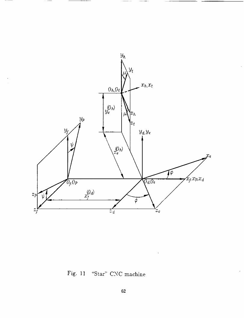
"Star" CNC Machine
A version of the "Star" CNC machine that is provided with 6 degrees-of-freedom is shown
in figure 11. Coordinate systems St (xt, yt, zt), St, (xp, yp, zp) and S f (x], Yl, z]) are rigidly
connected to the tool, workpiece and frame, respectively. Coordinate system Sd is parallel
to system S.f and the location of Sd with respect to S! is represented inS/ by (x_°_), 0,
0). Coordinate system S, performs rotational motion with respect to Sd about the yd-axis.
Coordinate system Sh is parallel to S_ and the location of Sh with respect to S, is represented
6
in S, by (0, (oh) .(oh)3 Coordinate system St performs rotational motion with respect toY_ ' J"(_ /.
Sh about the zh-axis. Coordinate system Sp performs rotational motion with respect to
the fixed coordinate system 5'I about the zs-axis. Altogether there are three translational
motions along axes z/, y, and z, and three rotational motions about axes z s, yd, and zh.
2. Basic Principle of Execution of Motions on CNC Machine
Consider that the location and orientation of the tool with respect to the workpiece are
given in coordinate systems that are represented for a conventional generator or for an ab-
stract(mathematical) model of the process for generation. We will consider for the following
derivations the example of application of the "Phoenix" machine. A similar approach can be
applied for other types of CNC machines, for instance, for the "Star" machine. Our goal is
to develop the algorithm for the execution of motions of the CNC machine using the initial
information mentioned above. Reference [4] has used for this purpose the existence of a
common trihedron for the two couples of coordinate systems (S_ c), S_ c)) and (S} c), Sp(el)
that are applied for the CNC machine and for the generating process, respectively. The
approach used in this report is as follows:
(i) Consider that 4 x 4 matrices M_kt ) and 3 × 3 matrices _ptrCk)(k = C, G) have been
derived. The superscripts "C" and "G" indicate the CNC machine and the abstract
generating process, respectively.
(ii) The matrix equality
L(C) r(a) (1)pt = J'Jpt
will provide the same orientation of St(k) with respect to Sp(k) (k = C,
reference frames.
G) in both
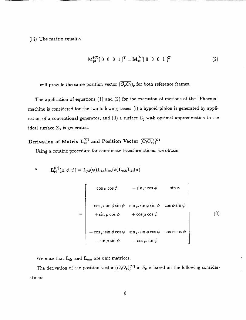
(iii) The matrix equality
M c)r 0 0 0 1 ]T I_AI'(G)[ 0 0 0 1 ]Tp,t = '--.'.p, L (2)
will provide the same position vector (O_O-_,)p for both reference frames.
The application of equations (1) and (2) for the execution of motions of the "Phoenix"
machine is considered for the two following cases: (i) a hypoid pinion is generated by appli-
cation of a conventional generator, and (ii) a surface Eg with optimal approximation to the
ideal surface Ep is generated.
Derivation of Matrix r(c) and Position Vector (0,0_)_ c)a-Jpt
Using a routine procedure for coordinate transformations, we obtain
L_C)(/_, ¢, '4') = L,d(¢)Ld,L,,_(¢)L_hLh,(_)
cos # cos ¢ - sin # cos $ sin
- cos # sin ¢ sin _3
+ sin # cos _b
- cos # sin ¢ cos O
- sin/_ sin ¢
sin # sin ¢ sin ¢
+ cos _ cos ¢
sin # sin ¢ cos _b
- cos # sin _b
cos Q sin ¢
cos Ocos ¢
(3)
We note that Ld, and Lmh are unit matrices.
The derivation of the position vector (OtOp)(p c) in Sp is based on the following consider-
ations:
8
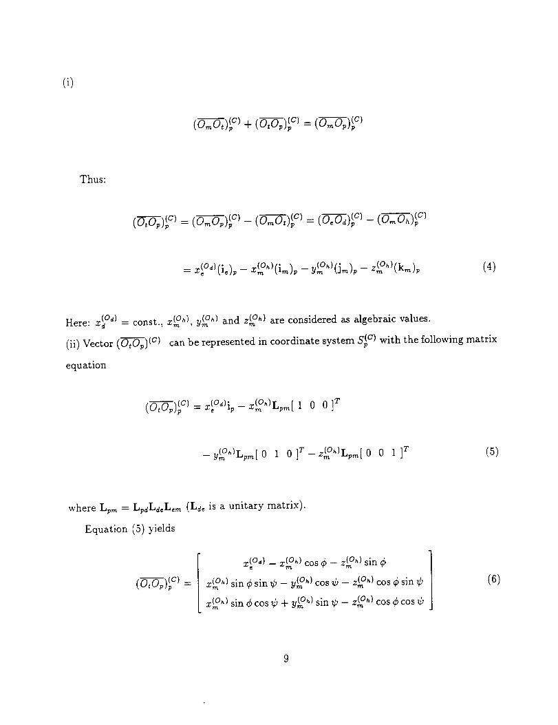
(i)
(o,,,o,)p+ (o,G)ff) = (o,,,o,,)p
Thus:
(o,o,)p = (omG)p -(o-joT,)p= (o,o_)p - (o,,,o_)p
_(o,)(i,)p _ z_,,)(i,.,,)p _ y_h)(j,.,,)p __ z(Oh)(k,,)p (4)
(oh) . (on) and (oh) are considered as algebraic values.Here: z_ °a) = const., z m , y,,_ Zm
(ii) Vector (0,0_) (c) can be represented in coordinate system S(pc) with the following matrix
equation
(O,Op)g c) = z_°d)iv- z_h)gp_[1 0 0 ]T
--y_h)Lpm[0 1 0]T--zf_)Lpm[0 0 1 ]T (5)
where Lpm = LpdLd,L,m (Ld¢ is a unitary matrix).
Equation (5) yields
(o--_)__)=x!Od) _ "_,_-(°h)cos ¢ -- --(°h) sin ¢
-(oh) cos ¢ sin _'-(oh) sin ¢ sin ¢ y_h) cos _b - z_:.Urn "
. (oh) sin _ z(,_°h} cos ¢ cos _b(oh) sin ¢ cos _ + _,_Xr n
(6)
9
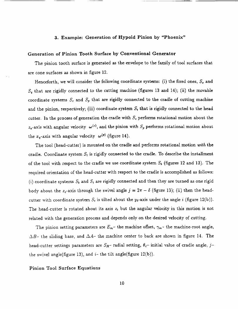
3. Example: Generation of Hypoid Pinion by "Phoenix"
Generation of Pinion Tooth Surface by Conventional Generator
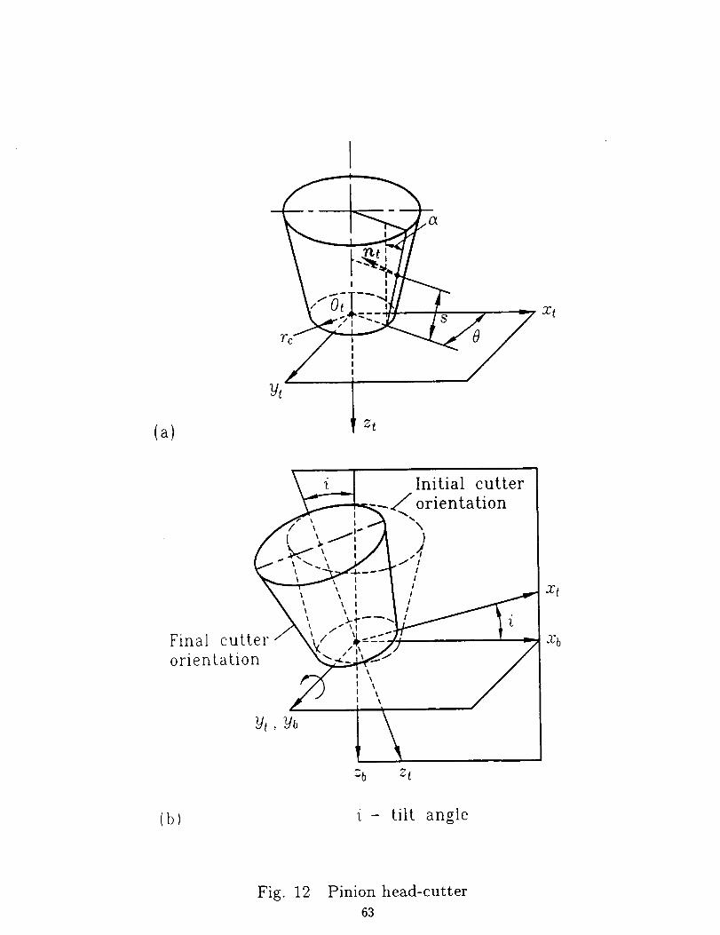
The pinion tooth surface is generated as the envelope to the family of tool surfaces that
are cone surfaces as shown in figure 12.
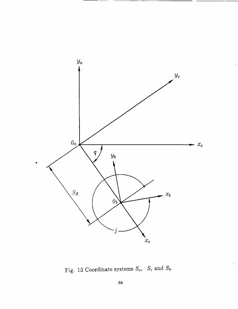
Henceforth, we will consider the following coordinate systems: (i) the fixed ones, So and
Sq that are rigidly connected to the cutting machine (figures 13 and 14); (ii) the movable
coordinate systems Sc and Sp that are rigidly connected to the cradle of cutting machine
and the pinion, respectively; (iii) coordinate system S_ that is rigidly connected to the head
cutter. In the process of generation the cradle with Sc performs rotational motion about the
Zo-aXis with angular velocity w (c), and the pinion with Sp performs rotational motion about
the zq-axis with angular velocity w (p) (figure 14).
The tool (head-cutter) is mounted on the cradle and performs rotational motion with the
cradle. Coordinate system St is rigidly connected to the cradle. To describe the installment
of the tool with respect to the cradle we use coordinate system Sb (figures 12 and 13). The
required orientation of the head-cutter with respect to the cradle is accomplished as follows:
(i) coordinate systems Sb and St are rigidly connected and then they are turned as one rigid
body about the z_-axis through the swivel angle j = 27r - _ (figure 13); (ii) then the head-
cutter with coordinate system St is tilted about the yb-axis under the angle i (figure 12(5)).
The head-cutter is rotated about its axis zt but the angular velocity in this motion is not
related with the generation process and depends only on the desired velocity of cutting.
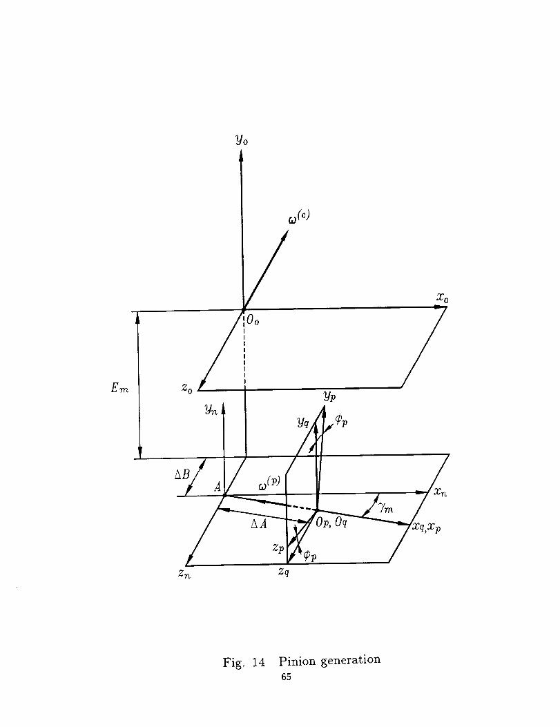
The pinion setting parameters are Era- the machine offset, "r,_- the machine-root angle,
AB- the sliding base, and AA- the machine center to back are shown in figure 14. The
head-cutter settings parameters are SR- radial setting, 8c- initial value of cradle angle, j-
the swivel angle(figure 13), and i- the tilt angle(figure 12(b)).
Pinion Tool Surface Equations
10
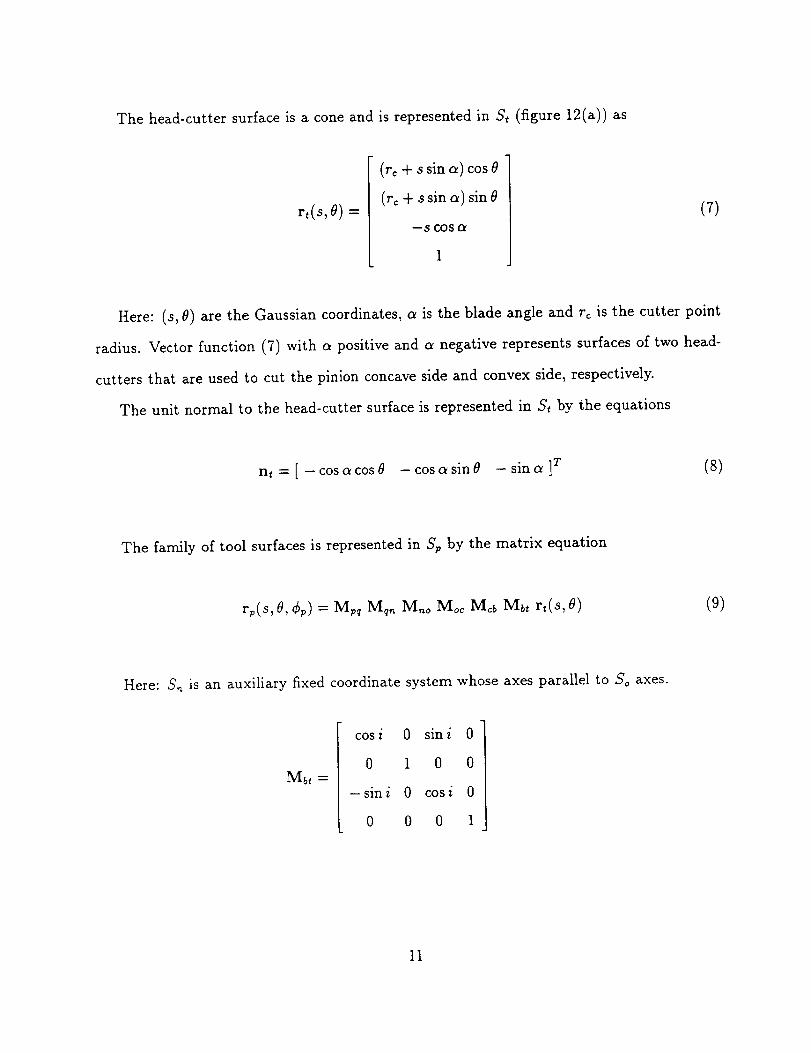
The head-cutter surface is a cone and is represented in St (figure 12(a)) as
rt(s, _) =
(re + s sin or) cos 8
(re + s sin a) sin 8
--3 COS O_
(7)
Here: (s, 8) are the Gaussian coordinates, a is the blade angle and r, is the cutter point
radius. Vector function (7) with a positive and a negative represents surfaces of two head-
cutters that are used to cut the pinion concave side and convex side, respectively.
The unit normal to the head-cutter surface is represented in St by the equations
nt=[-cosc_cosO -cosasine --sina]T (8)
The family of tool surfaces is represented in Sp by the matrix equation
rp(s, e, ¢p)= Mpq Mq_ M_o Mo, M,b Mb, rt(s,O) (9)
Here: S_ is an auxiliary fixed coordinate system whose axes parallel to So axes.
Mbt =
cosi 0 sini 0
0 1 0 0
-sini 0 cos/ 0
0 0 0 1
11
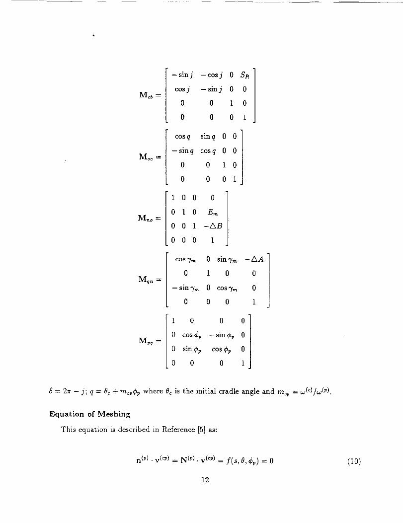
Meb
-sinj -cosj 0 SR
cosj -sinj 0 0
0 0 I 0
0 0 0 1
Moc
cos q sin q 0 0
-sinq cos q 0 0
0 0 1 0
0 0 0 1
M_o
1 0 0 0
010 E_
001 -AB
000 1
Mqn
cos 7= 0 sinT,_ -AA
0 1 0 0
-sinT,_ 0 cos 7.: 0
0 0 0 1
Mpq
1 0 0 0
0 cos_p -sin_p 0
0 sin_p cos6p 0
0 0 0 1
6 = 2r - j; q = 8c + mcp¢p where 8c is the initial cradle angle and m_ = w(c)/w (p).
Equation of Meshing
This equation is described in Reference [5] as:
n (p). v (_v) = N (p). v (cp) = f(s, O, _p) = 0 (10)
12
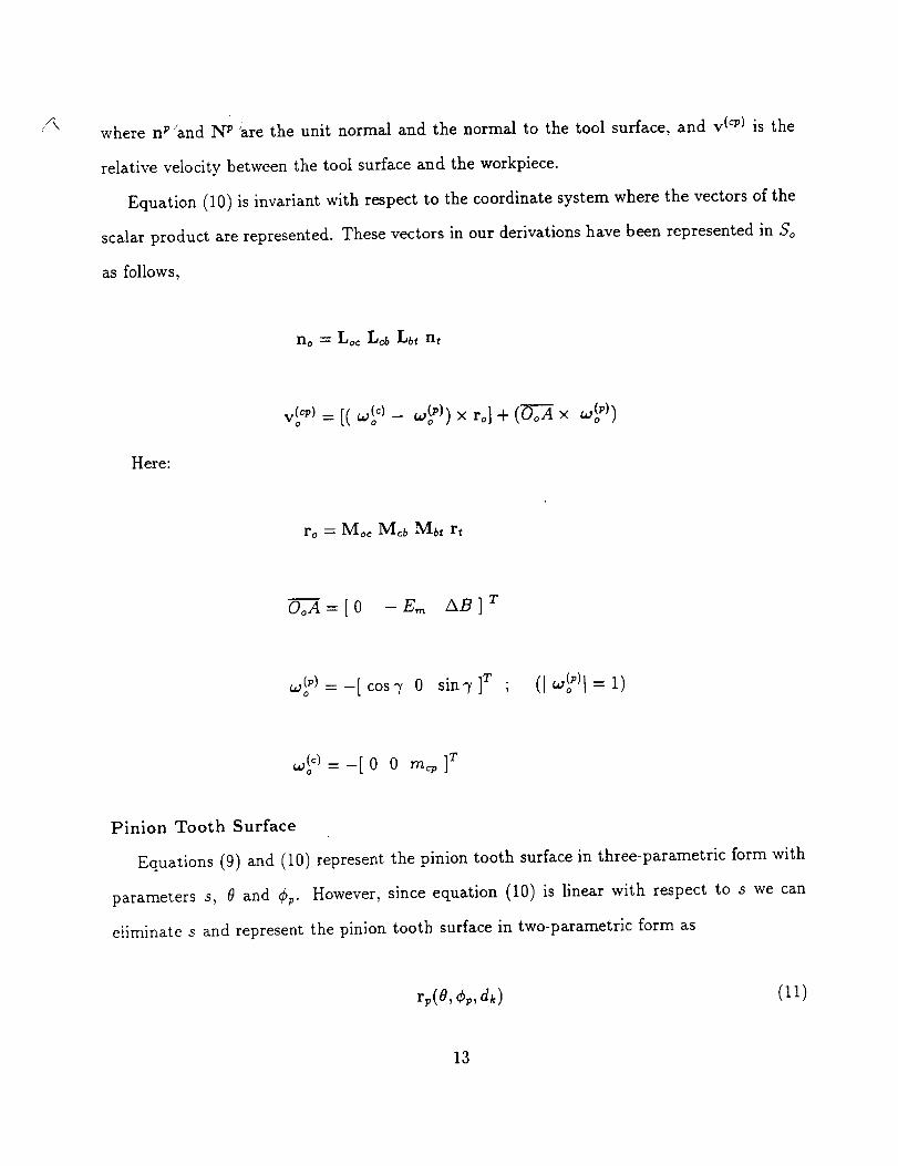
where n p !and N p are the unit normal and the normal to the tool surface, and v (_) is the
relative velocity between the tool surface and the workpiece.
Equation (10) is invariant with respect to the coordinate system where the vectors of the
scalar product are represented. These vectors in our derivations have been represented in So
as follows,
no = Loc L_b Lbt nt
Here:
v_) = [(w_=) - w(f)) x ro] + (OoA x w(P))
ro = Moc M_b Mbt rt
OoA=[O -E,_ AB] T
w_ p)=-[cos'/ 0 sin 3'1T ; (1"?)]=1)
Pinion Tooth Surface
Equations (9) and (10) represent the pinion tooth surface in three-parametric form with
parameters s, 0 and Cv- However, since equation (10) is linear with respect to s we can
eliminate s and represent the pinion tooth surface in two-parametric form as
rp(O,¢v, dk ) (11)
13
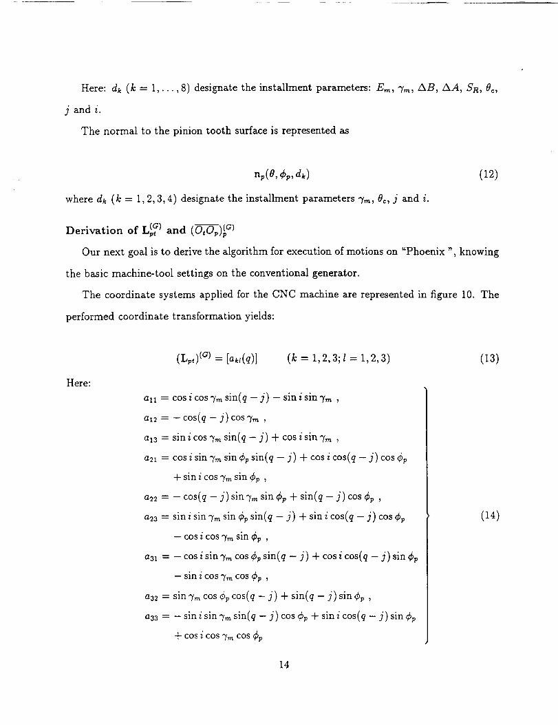
Here: dk (k = 1,..., 8) designate the installment parameters: E,_, 7,_, AB, AA, Sn, 8c,
j and i.
The normal to the pinion tooth surface is represented as
n,,(o, ¢,,, (12)
where dk (k = I,2,3,4) designate the installmentparameters 3',_,#c,j and i.
Derivation of L_? ) and (O---_p)$c)
Our next goal isto derivethe algorithm for execution ofmotions on "Phoenix ",knowing
the basic machine-tool settingson the conventional generator.
The coordinate systems applied for the CNC machine are represented in figureI0. The
performed coordinate transformation yields:
Here:
(Lpt) (a) = [ak,(q)] (k = 1,2,3;l = 1,2,3)
alt = cos i cosT_ sin(q -j) - sini sinT_ ,
a12 = - cos(q - j) cos 7,_ ,
a13 = sin i cos 7m sin(q - j) + cos i sin 7m ,
a2_ = cos i sin 7-, sin Cp sin(q -- j) + cos i cos(q - j) cos ¢_
+ sin i cos 7_ sin Cp ,
a22 = - cos(q - j) sin 7_ sin Cp + sin(q - j) cos Cp,
a23 = sin i sin 3',,, sin Cp sin(q - j) + sin i cos(q - j) cos Cp
-- cos i cos 7,_ sin Cp ,
a3_ = - cos i sin 7_ cos dp sin(q -- j) + cos i cos(q - j) sin Cp
- sin i cos 7,_ cos Cp ,
a3: = sin 7,,, cos ¢p cos(q - j) + sin(q - j) sin Cp,
azz = - sin i sin 3'_ sin(q - j) cos dr, + sin i cos(q - j) sin Cp
+ cos i cos 7m cos Cp
(13)
(14)
14
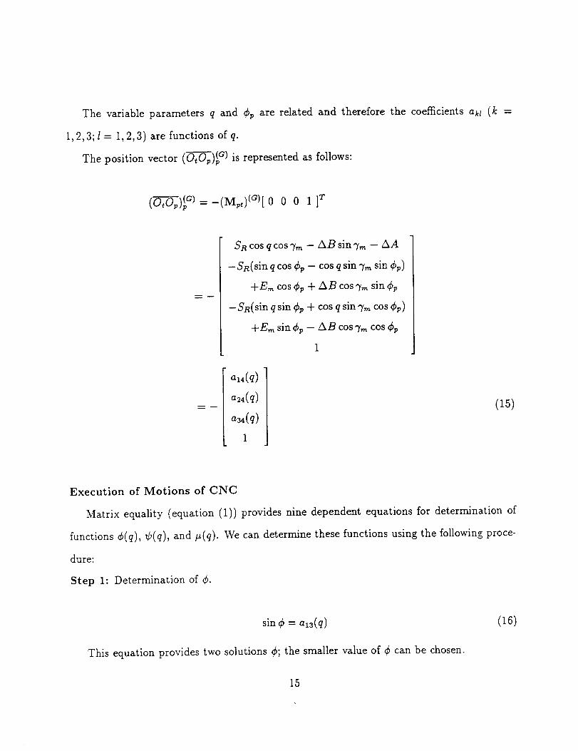
The variable parameters q and Cp are related and therefore the coefficients akl (k =
1,2,3;l = 1,2,3) are functions of q.
The position vector (OtO-_)(p G) is represented as follows:
(o-;_)_) =-(M,,,)_°)[ o 0 o 11_"
Sn cos q cos 7-_ - AB sin 7-, - AA
-Sn(sin q cos Cv - cos q sin 7-, sin Cv)
+E,_ cos Cv + AB cos %,, sin Cp
-Sn(sin q sin Cp + cos q sin "r,_ cos Cp)
+E_ sin Cp - AB cos 7-, cos Cp
1
a_(q)
a2_(q)
a_(q)
I
(15)
Execution of Motions of CNC
Matrix equality (equation (1)) provides nine dependent equations for determination of
functions ¢(q), ¢(q), and #(q). We can determine these functions using the following proce-
dure:
Step 1: Determination of ¢.
sin ¢ = al3(q )
This equation provides two solutions ¢; the smaller value of ¢ can be chosen.
(16)
15
Step 2: Determination of ¢.
cosCsin¢ = a 3(q), cos¢cos¢ = a.(q)
These equations provide a unique solution for _p, considering ¢ as given.
Step 3: Determination of #.
(17)
cos #cos¢ = atl(q) , - sin# cos ¢ = a12(q) (lS)
These equations provide a unique solution for #, considering ¢ as given.
For the generation a face-milled hypoid pinion, a tool with a cone surface is applied. The
tool surface is a surface of revolution and the rotation of the tool about its axis is not related
with ¢. Functions (17) must be applied and executed only for the generation of face-hobbed
hypoid pinion, that is cut by a blade.
Vector equality
(o,o )g = (19)
permits the determination of functions x_h)(q), y(OD(q), and z_°h)(q). Equations (6), (15)
and (19) considered simultaneously, represent a system of three linear equations in the un-
knowns: z,_(°h), y(Oh), z_Oh). The solution to these equations enables to determine the trans-
lational motions on the CNC machine.
4. Generation of a Surface with Optimal Approximation To the Ideal Surface
Introduction
This section is based on the research accomplished by Reference [2] that was directed at
generation of a surface (Eg) that must be in optimal approximation to the theoretical (ideal)
surface Ep.
16
The method for generationof Eg is basedon following ideas:
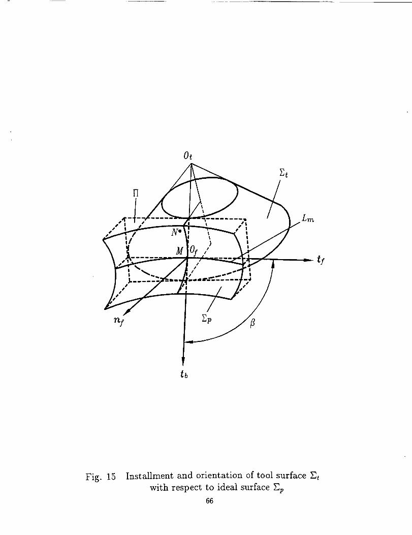
(1) A mean line Lm on the ideal surface Ep is chosen as shown in figure 15.
(2) The tool surface Et is a properly designed surface of revolution (in particular cases Et
is a circular cone as shown in figure 15) that moves along L,,,. Surfaces Et and Ep are
in continuous tangency along L,_; M is the current point of tangency (figure 15). The
orientation of Et with respect to Ep (determined with angle 8) is continuously varying.
Angle _ at current point M of tangency is formed by the tangents tf and tb to L_ and
the tool generatrix, respectively (figure 15). Tangents t I and tb form plane H that is
tangent to Et and Zp at point M.
(3) The tool surface Et in its motion with respect to Ep swept out a region of space as a
family of surfaces Et. The envelope to the family of Et is surface Eg, the ground or
cut surface, that is in tangency with the theoretical surface Zp at any point M of L,,
and must be in optimal approximation to Zp in any direction that differs from L_.
(4) The optimal approximation of Eg to E v is obtained by variation of angle 3 (figure 15).
(5) The continuous tangency of tool surface Et with Ep and properly varied orientation
of Et can be obtained by the execution of required motions of the tool by a computer
controlled multi-degree-of-freedom machine. One of these degrees of freedom, rotation
of the tool about its axis, provides the desired velocity of grinding (cutting) and is not
related with the process for generation of Eg.
The contents of this section cover the following topics:
(I) Determination of equation of meshing between the tool surface E, and the generated
surface Eg. The equation of meshing provides the necessary condition of envelope
existence to the family of surfaces.
17
(2) Determination of generatedsurface_g as the envelope to the family of surfaces _'t
swept out by the tool. Surface _,g coincides with the theoretical (ideal) surface E_
along the mean line L,_ and deviates from _p out of L,_.
(3) Determination of deviations of Eg from I;p (in regions that differ from L._) and mini-
mizations of I;g deviations for optimal approximation of Eg to Ep.
(4) Determination of curvatures of Eg that are required when the simulation of meshing
and contact of two mating surfaces are considered.
(5) Execution of required motions of Et with respect to E_ by application of a multi-degree-
freedom, computer numerically controlled machine.
An effective approach for the derivation of the necessary condition of the envelope _g
existence is discussed. This method is based on the idea of motion of the Darboux-Frenet
trihedron along L,_, the chosen mean line of _p.
An additional effective approach for determination of curvatures of generated surface _g
is discussed as well. This approach is based on the fact that the normal curvatures and
surface torsions (geodesic torsions) of Eg are: (i) equal to the normal curvatures and surface
torsions of Ep along L,_; and (5) equal to the normal curvatures and surface torsions of tool
surface E, along the characteristic Lg (the instantaneous line of tangency of E, and Eg).
Mean Line on Ideal Surface _p
The ideal surface Ep is considered as a regular one and is represented as
rp(up, 0p) E C 2 0rp 0rp
where (up, 0p) are the Gaussian coordinates of _p.
The unit normal to Ep is represented as
0, E (20)
18
Np Np 0rp 0rp (21)np- INpl' - Ou--'_x 00----_
The determination of mean line on Lm is based on the following procedure:
(i) Initially, we determine numerically n points on surface Ep that will belong approxi-
mately to the desired mean line L,_.
(ii) Then, we can derive a polynomial function
v--, ,_(n-j)Upi(Opi ) = _ aJ%i ,
j--1
(i = 1,...,,) (22)
that will relate surface parameters (up, Op) for the n points of the mean line on Ep.
The mean line L,_, tangent Tp and unit tangent tp to the mean line are represented as
followsQ
0rp 0rp dup tp Tp (23)rp(up(Op),Op), Tp- _ + Oup dOp ' = iTpl
The constraint for tp is that it must be of the same sign and differ from zero at the same
intervals of interpolation.
Tool Surface
The tool surface Et is represented in coordinate system St rigidly connected to the tool
by the following equations
x, = zt(u,)cosO, , y,=xt(u,)sinOt , z,= z,(u,) (24)
19
The axial sectionof Et obtained by taking 0t = 0 represents a circular arc, or a straight
line in the case when Et is a circular cone. Surface as shown in equations(24) of the tool is
formed by rotation of the axial section of Et about the zt-axis.
The surface unit normal is determined as
N, Or, Or,n, = [Nt----[' N, = x Ou, (25)
Equation of Meshing Between Et and Eg
Equation of meshing represents the necessary condition of existence of envelope Eg to
the family of surfaces Et that is swept out by the tool surface Et.
The equation of meshing can be derived by using the equation
N}') • = 0 (26)
Here: i indicates the coordinate system E_ where the vectors of the scalar product are
represented; N (t) is the normal to surface Et; v (tg) is the relative velocity in the motion of
Et with respect to Eg.
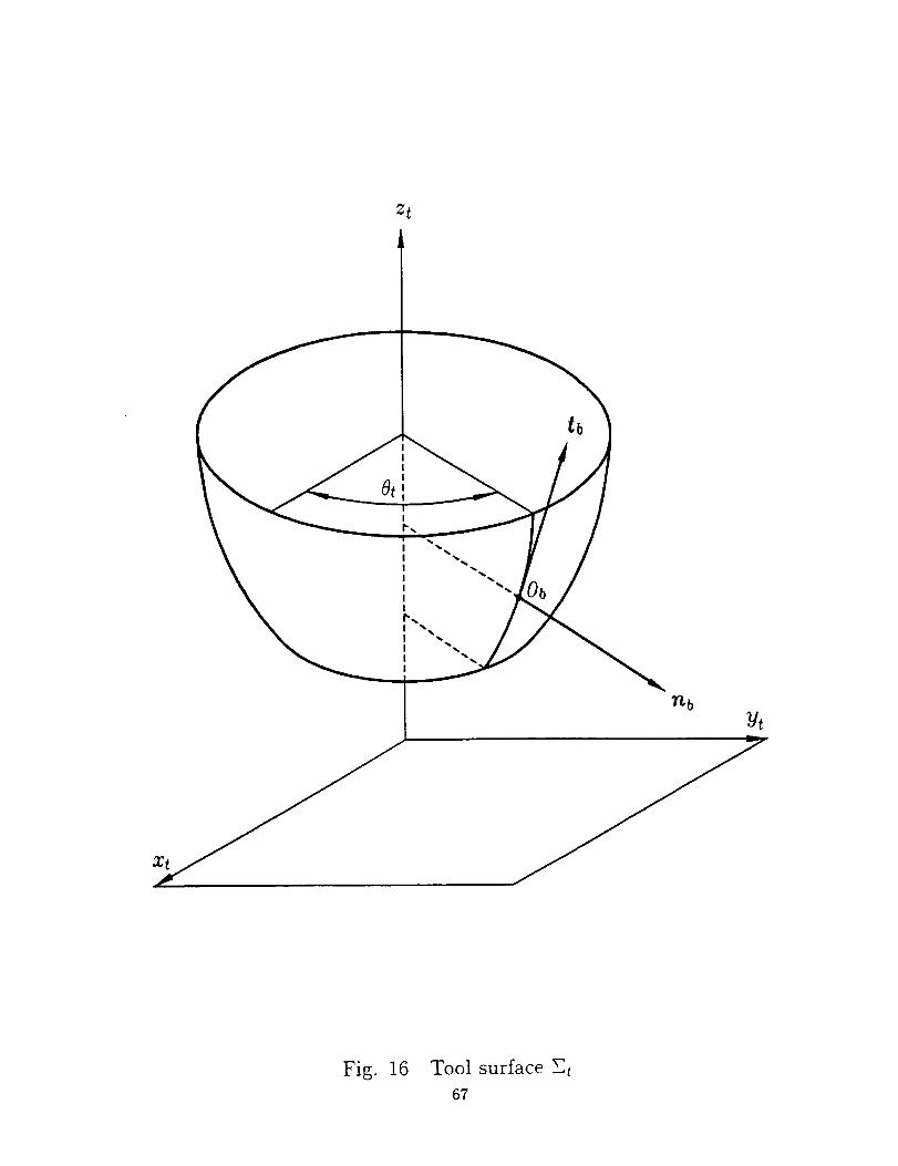
Henceforth, we will consider two basic coordinate systems, St and Sp, that are rigidly
connected to the tool surface Et and the ideal surface Ep. In addition to Et, we will consider
two trihedrons: Sb(tb, db, nb) and S](tl, dr, n]). Trihedron Sb is rigidly connected to Et and
coordinate system St (figure 16). Here: Ob is the point of the chosen generatrix of Et where
the trihedron is located; tb is the tangent to the generatrix at Oh; nb is the surface unit
normal of Et at Oh; db = nb x tb; vectors tb and ds form the tangent plane to E_ at Oh.
Trihedron S! moves along the mean line L_ (figure 17); tl is the tangent to the mean line L,_
at current point M (figure 17); n I is the surface unit normal to Ep at point M; d I = nf x t f;
vectors t! and df form the tangent plane to Ep at point M.
The tool with surface Et and trihedron St moves along mean line L,,, of Ep and Ob
2O
coincideswith current point M of meanline L_. Surfaces Et and Ep are in tangency at any
current point M of mean line L,_. The orientation of Sb with respect to St is determined
with angle fl that is varied in the process for generation.
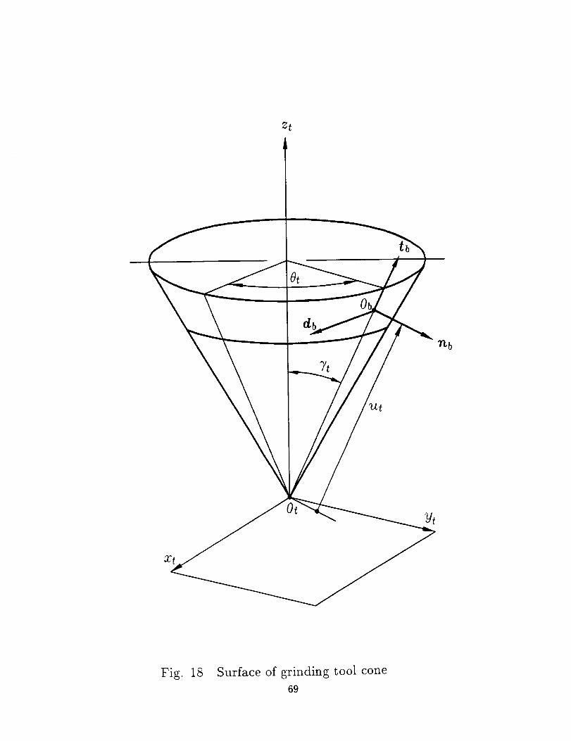
We start the derivations with the case when Et is a circular cone(figure 18). The angular
velocity wy of rotation of Sy with respect to Sp is represented as
ds
wy = (tty - k_d] + kgny)_- _ (27)
Here: t is the surface torsion (geodesic torsion), kn and kg are the normal and geodesic cur-
vatures of surface Ep at current point M of mean line L,_, ds is the infinitesimal displacement
along L_.
The angular velocity _2y of trihedron Sb is represented in Sy as
d_ [ dE IT ds (28)Oy = _vy + -_-ny = t -k,, kg + -_s d'-t"
The orientation of cone Et is determined by function B(O,_) and
dj3 d/3 dOp dE, 1(29)
where "r_ is the tangent to the mean line L= at current point M.
The transformations of vector components in transition from St to Sb and Sb to Sf are
represented by 3 x 3 matrix operators Lbt and Lyb. Here:
Lfb =
cosB --sin_ 0
sin_ cos/3 0
0 0 1
(30)
21
Lbt _--
sin 7t cos Ot sin 7t sin 0, cos _',
sin 8t - cos Ot 0
cos 7t cos Ot cos 7_ sin Ot - sin 7t
(31)
The cone surface Et is represented in S, as follows (fig. 18)
[r, = u, sin 7, cos 0, sin 7* sin 0, cos 7t
where (ut, 0,) are the surface parameters, 7* is the cone apex angle.
The unit normal to the cone surface is
(32)
[n, = cos "Ytcos 8, cos 7* sin 8t - sin 7t (33)
The sought-for equation of meshing, necessary condition of existence of envelope Eg, is
represented in the form:
where
n_). v_ tg) =0 (34)
n(yt) -- Ly, n, (35)
The derivation of expression v_tg) is simplified while taking into account the following
considerations:
(a) The relative velocity vector v_ *g) can be represented as
ds
v_tg)= ,Q_)r_ *) + _-_t! (36)
22
Here, /2) s) is the skew-symmetric matrix represented as
Vector _! is represented by
0 --¢aJ 3 L02
O-)3 0 --LOl
-- LO2 LO1 0
['2f -- wit/+ w2d/+ w3n/ - [ t -kn
(37)
d_ ]r dskg+ _ J d-_ (3S)
(b) Consider that point N on surface Et(fig. 15) is the point of the characteristic (the
line of tangency of Et and the generated surface Eg). Certainly, the equation of meshing
must be satisfied for point N.
The position vector OIN can be represented as(figs. 15 and 18)
OyN = O,N - 0,0! (39)
Here, OtN is the position vector of point N that is drawn from the origin Ot of St to N;
vector OtN is represented in St as
OtW = utet = ut(sinTt cos0t it + sinTtsinOt jt + cosT, kt)
where
0Out (rt)
et- O__t(rt) '
is the unit vector of cone generatrix OtN.
Vector OtO] (figure 18) is represented in Sb as
(40)
(41)
23
OtO! = It ib
wh rel,-Vector O/N is represented in S/using the matrix equation
r_t) = utL:tet - ItL/bib
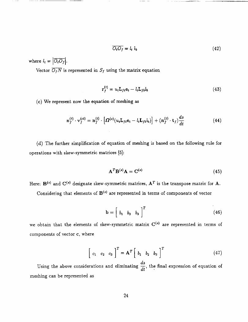
(c) We represent now the equation of meshing as
n_ t). v_a)= n(/)" [O(S)(utLltet- ltL:bib)] + (n_ t)- t:) _-_
(42)
(43)
(44)
(d) The further simplification of equation of meshing is based on the following rule for
operations with skew-symmetric matrices [5]:
ATB(')A = C (s) (45)
Here: B {s) and C (_) designate skew-symmetric matrices, A T is the transpose matrix for A.
Considering that elements of B (_) are represented in terms of components of vector
lT
b=/ bl b_ b3 (46)
we obtain that the elements of skew-symmetric matrix C (_) are represented in terms of
components of vector c, where
T
ds
Using the above considerations and eliminating _-_, the final expression of equation of
meshing can be represented as
24
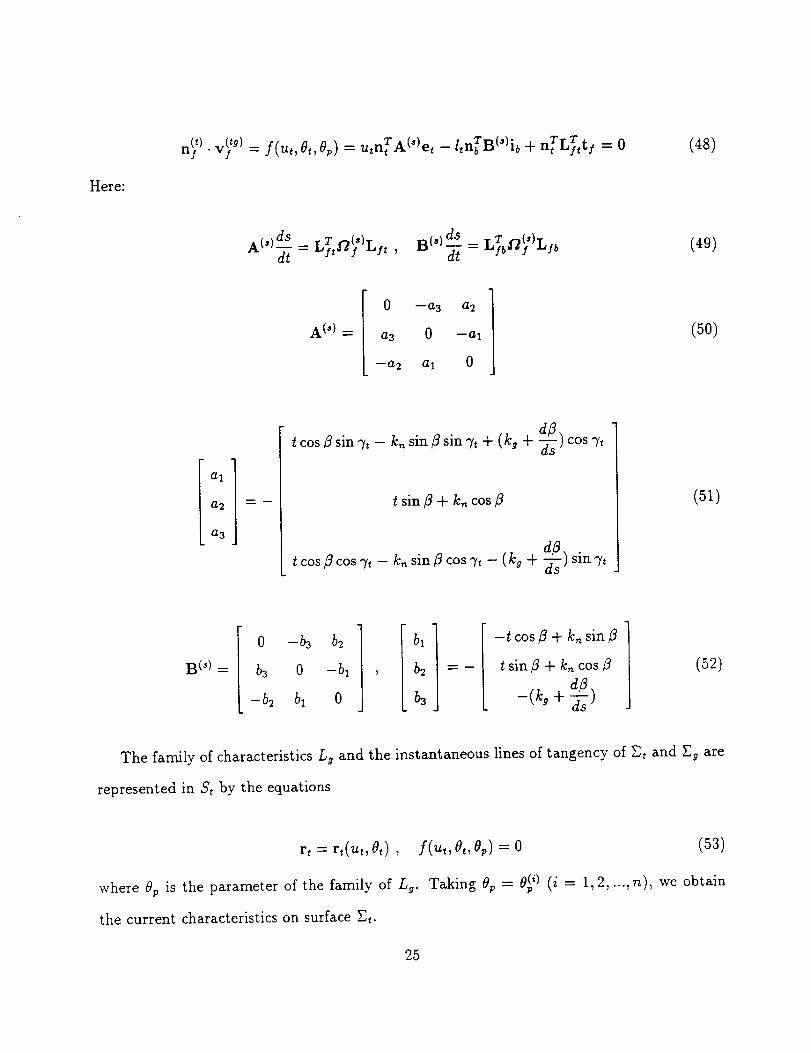
Here:
n_ t) • v_ tg) : f(ut, O,,Op) = utnTA0)e,- /,nTB0)ib + nTL_t! = 0 (48)
A(,) ds .z ,-,(,)r B(,) ____ L_'b.O_')Ljbd---[= JUftJ" f "ltaft ' =(49)
A (') =
0 -- a3 a2
a 3 0 --al
--a2 at 0
(50)
al
a2
a3
t cos fl sin 7t - k,_ sin fl sin 7t + (kg + _s ) cos 7_
t sin fl + k,_ cos fl
t cos fl cos 7, - k,_ sin fl cos 7t - (kg + _s ) sin 7t
(51)
B(,) =
q
0 -b3 b2 i
1b3 0 -bl
-b2 bt 0
bl
, b2
b3;-I
q
-t cos fl + k,_ sin fl /
t sin fl + k,_ cos fl
-(kg +
(52)
The family of characteristics Lg and the instantaneous lines of tangency of Et and Eg are
represented in S, by the equations
r, = r,(ut,0t) , f(u,,0t, Sp) = 0 (53)
where 0p is the parameter of the family of Lg. Taking 0p = 0(p_) (i = 1,2, ...,n), we obtain
the current characteristics on surface Et.
25
It is easy to verify that the equation of meshing between _t and Eg is satisfied the current
point M of mean line L,,_ on the ideal surface Ep. This means that the characteristic Lg
intersects L,_ at point M, for which we can take 0t = 0 since _t is a surface of revolution. In
the case when _t is a circular cone (figure 18), we can take for point M that ut = _ = lt.
The approach discussed above for the derivation of the equation of meshing can be easily
extended for application in the more general case when the tool surface is a general surface
of revolution.
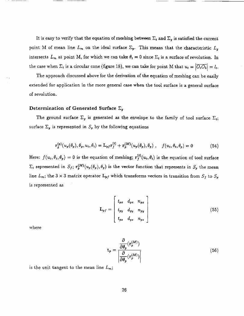
Determination of Generated Surface Eg
The ground surface Eg is generated as the envelope to the family of tool surface IEt;
surface lEg is represented in Sp by the following equations
= L 1r ')+ f(u,,e,,e,,)= o (54)
Here: f(u. St,Or, ) = 0 is the equation of meshing; r_0(u,, St) is the equation of tool surface
lEt represented in $I; r_M)(up(0p),ap) is the vector function that represents in Sp the mean
line L,,,; the 3 x 3 matrix operator Lp._ which transforms vectors in transition from S/ to Sp
is represented as
ip]
where
tp--
is the unit tangent to the mean line L,_;
tp_ dp_ npx
tp_ d_ npy
tpz dpz 7Zpz
(55)
(56)
26
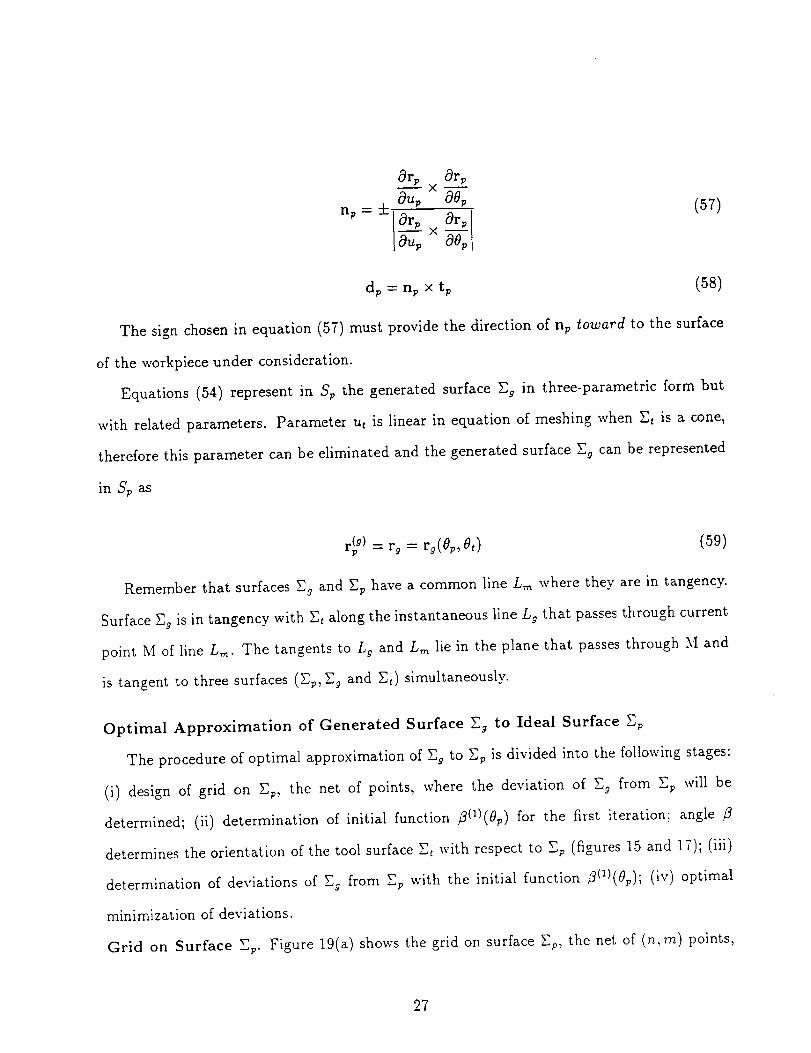
(_Fp _rp
np- -1- _u--_ x aS_- (57)
a,.,0up × 00p
dp =np x tp (58)
The sign chosen in equation (57) must provide the direction of n v toward to the surface
of the workpiece under consideration.
Equations (54) represent in Sp the generated surface Eg in three-parametric form but
with related parameters. Parameter ut is linear in equation of meshing when Et is a cone,
therefore this parameter can be eliminated and the generated surface Eg can be represented
in Sp as
r_ g) = r 9 : rg(Op, Ot) (59)
Remember that surfaces _9 and _p have a common line Lm where they are in tangency.
Surface Eg is in tangency with Et along the instantaneous line Lg that passes through current
point M of line Lm. The tangents to Lg and Lm lie in the plane that passes through M and
is tangent to three surfaces (E;, P,g and Et) simultaneously.
Optimal Approximation of Generated Surface Eg to Ideal Surface Ep
The procedure of optimal approximation of Eg to Ep is divided into the following stages:
(i) design of grid on Ep, the net of points, where the deviation of Eg from Ep will be
determined; (ii) determination of initial function 13(1)(0p) for the first iteration; angle /3
determines the orientation of the tool surface Et with respect to Ep (figures 15 and 17); (iii)
determination of deviations of Eg from Ep with the initial function 3(1)(0p); (iv) optimal
minimization of deviations.
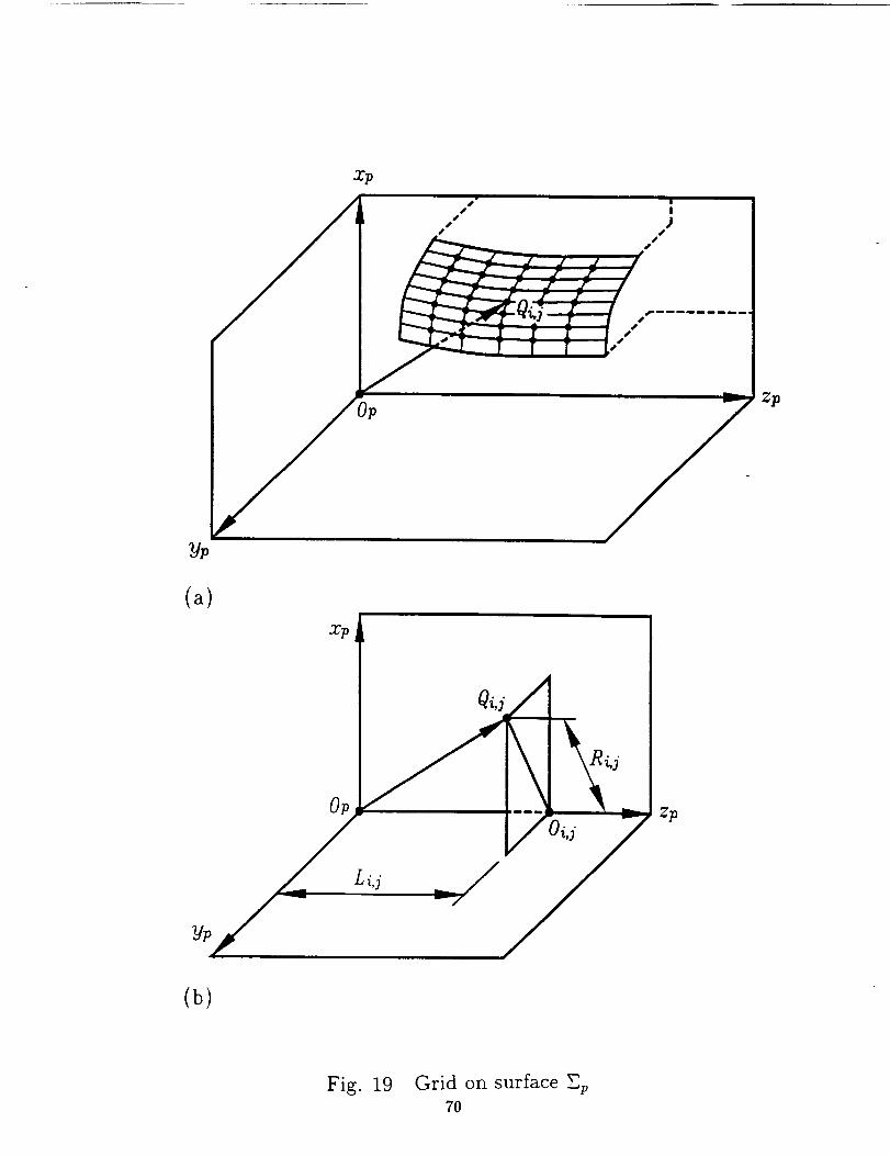
Grid on Surface Ep. Figure 19(a) shows the grid on surface Ep, the net of (n, rn) points,
27
where the deviations of Eg from Ep are considered. The position vector is OpQi,j = r__'j)
(figure 19(b)). The computation is based on the following procedure:
(i) The desired components L w and R/,j of the position vector r(pi,j) are considered as
known.
(ii) Taking into account that
L,,j=z_',_), R?,,,= [x_"J)(up,e,)]2+ [y_"J)(up,0_)]2 (60)
we will obtain the surface Ep parameters (u(p_'j), 0p(_'j)) for each grid point.
Determination of Initial Function /9(1) (0p). The determination of/9(1)(0p) is based on
the following idea: the instantaneous direction of tb (the tool generatrix) with respect to
tangent t/to the mean line L,,_ (figure 17) must provide the minimal value [k(r). Here: k if)
is the relative normal curvature determined as
kl")= ki')- kl") (61)
where k!') and kiP) are the normal curvatures of surfaces _t and _p along tb. In the case of
nondevelopable ruled surface _p, vector tb can be directed along the asymptote of Ep.
The requirement that ki T) is minimal, enables to determine function _(1)(8,,) numerically.
dESince we need for further computations the derivative _--_p, function/9(1)(8v) is represented
as a polynomial function that must satisfy the numerical data obtained for the chosen points
of mean line L,_.
Determination of Deviations of Zg from Ep. We are able at this stage of investigation to
determine the equation of meshing between surfaces Y,, and Eg, and surface Eg as discussed
above. The computation of deviations of Eg from Ep at the grid points is based on the
following considerations:
28
(i) SurfacesEp and Eg are representedin the samecoordinatesystem (Sp) by the following
vector functions:
r.(0g,0,) (s2)
(ii) The position vector r(pi'j) and surface coordinates (u_i'J),O_ i'j)) are known for each point
Q(vi,j) of the grid on surface Ep.
(iii) Point Q(gi,j) on surface Eg corresponds to point Q(pi'J) on surface E_. The surface Eg
_a(_,J) n(id)_ be determined by using the following two equationsparameters _,,g ,vt j can
= /(63)
',j)) .(',J)r,,(',J)o[,J))
(iv) Due to deviations of Eg from Ep, we have that x(gi'i) # x_ iJ). The deviation of Eg from
Ep at the grid point Q(pi,i) is determined by the equation
_',J = n_ i'j)" ( r(iS)a - -pr(iJ)) (64)
where n(pi'j) is the unit normal to surface E v at the grid point Q_'J).
The deviation _i,j can be positive or negative. We designate as positive such a deviation
when 6i,j > 0 considering that n(p_'j) is directed into the "body" of surface Ep. Positive devi-
ations of Eg with respect to Ep provide that Eg is inside of Ep and surface Eg is "crowned".
It is not excluded that initially the inequality $_,j > 0 is not observed yet for all points
of the grid. Positive deviations _;,j can be provided choosing the following options:
(1) choosing a surface of revolution with a circular arc in the axial section instead of a circular
cone; a proper radius of the circular arc must be determined.
(2) changing parameter It = O----t_ I (figures 17 and 18); this means that the grinding cone
will be displaced along ts with respect to the mean line Lm.
29
(3) varying the initially chosen function _(1)(0p).
Minimization of Deviations 6ij. Consider that deviations 6i,j (i - 1, ..., n; j = 1, ...,m)
of Eg with respect to Ep have been determined at the (n, m) grid points. The minimization
of deviations can be obtained by corrections of previously obtained function _3(1)(0p). The
correction of angle/3 is equivalent to the correction of the angle that is formed by the principal
directions on surfaces Et and Eg. The correction of angle fl can be achieved by turning of
the tool about the common normal to surfaces ]Et and _p at their instantaneous point of
tangency M_.
The minimization of deviations 6i,j is based on the following procedure:
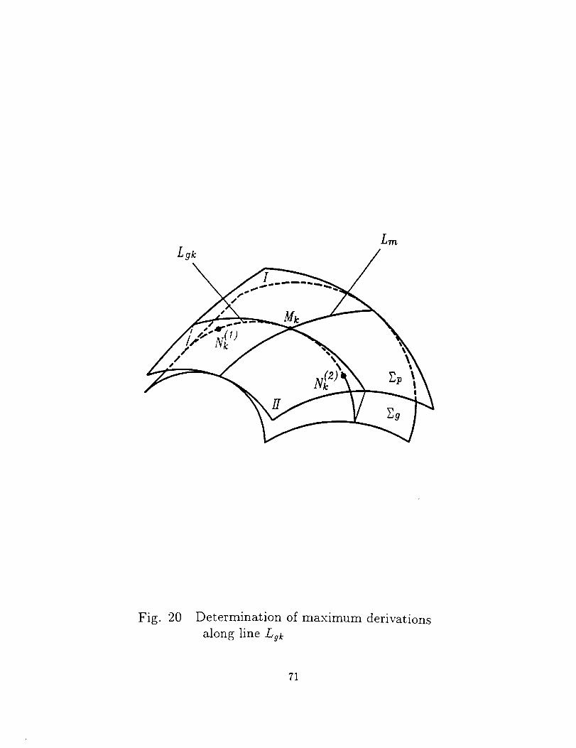
Step 1: Consider the characteristic Lg_, the line of contact between surfaces Et and Eg,
that passes through current point Mk of mean line L,_ on surface Ep (figure 20). Determine
the deviations _k between Et and Ep along line Lgk and find out the maximum deviations
x(1) and x(2) Points of where the deviations are a maximum aredesignated as _k,_x _k._=. Lgk
designated as Nk (1) and N_ _). These points are determined in regions I and II of surface _9
with line L,_ as the border. The simultaneous consideration of the maximum deviations in
both regions permits the minimization of the deviations for the whole surface Eg.
Note: The deviations of Et from _p along Lgk are simultaneously the deviations of 29
from Ep along Lgk since Lgk is the line of tangency of Et and Eg.
Step 2: The minimization of deviations is accomplished by correction of angle flk that is
determined at point Mk (figure 20). The minimization of deviations is performed locally,
for a piece k of surface E 9 with the characteristic Lgk. The process of minimization is a
computerized iterative process based on the following considerations:
(i) The objective function is represented as
with the constraint _i,j >_ 0.
= + (65)
30
(ii) The variableof the object function is A_/k. Then, consideringthe angle
(66)
andusingthe equation of meshingwith _k,wecandeterminethe new characteristic,the piece
of envelopeE__) and the new deviations. Iterations are required to provide the sought-for
objective function. The final correction of angle j3kwedesignateas _3_°pt).
Note 1: The new contact line L_ ) (determined with /3_2)) slightly differs from the real
contact line since the derivative _ but not _ is used for determination L_2k). However,
L_ ) is very close to the real contact line.
Step 3: The procedure discussed must be performed for the set of pieces of surfaces Eg with
the characteristic Lgk for each surface piece. Remember that the deviations for the whole
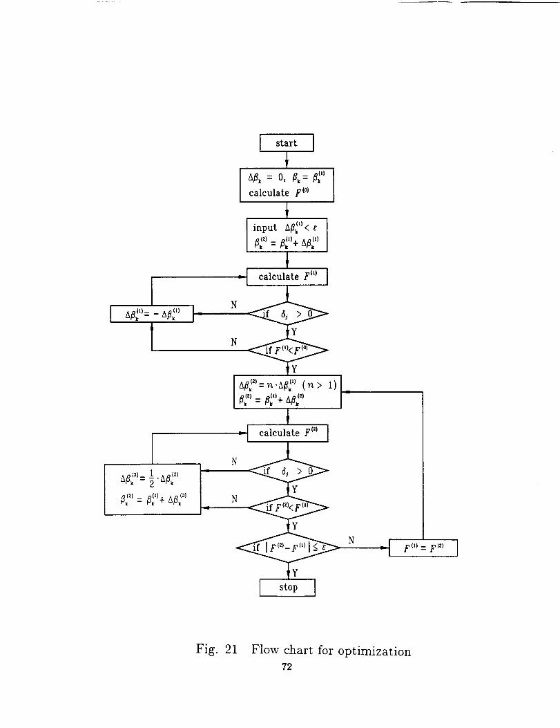
surface must satisfy the inequality _;,j >_ 0. The procedure of optimization is illustrated with
the flowchart shown in figure 21.
C_jrvatures of Ground Surface Eg
The direct determination of curvatures of Eg by using surface Zg equations is a com-
plicated problem. The solution to this problem can be substantially simplified using the
following approach proposed by the authors: (i) the normal curvatures and surface torsions
(geodesic torsions) of surfaces Ep and Eg are equal along line Lm, respectively; (ii) the nor-
mal curvatures and surface torsions of surfaces Et and Zg are equal along line Lg. This
permits the derivation of four equations that represent the principal curvatures of surface
Eg in terms of normal curvatures and surface torsions of Ep and Et. However, only three of
these equations are independent (see below).
Further derivations are based on the following equations:
1 1 (kz - kH) cos 2qk,_ = kz cos 2 q + kzz sin 2 q = _(kz + kz_) +
(67)
31
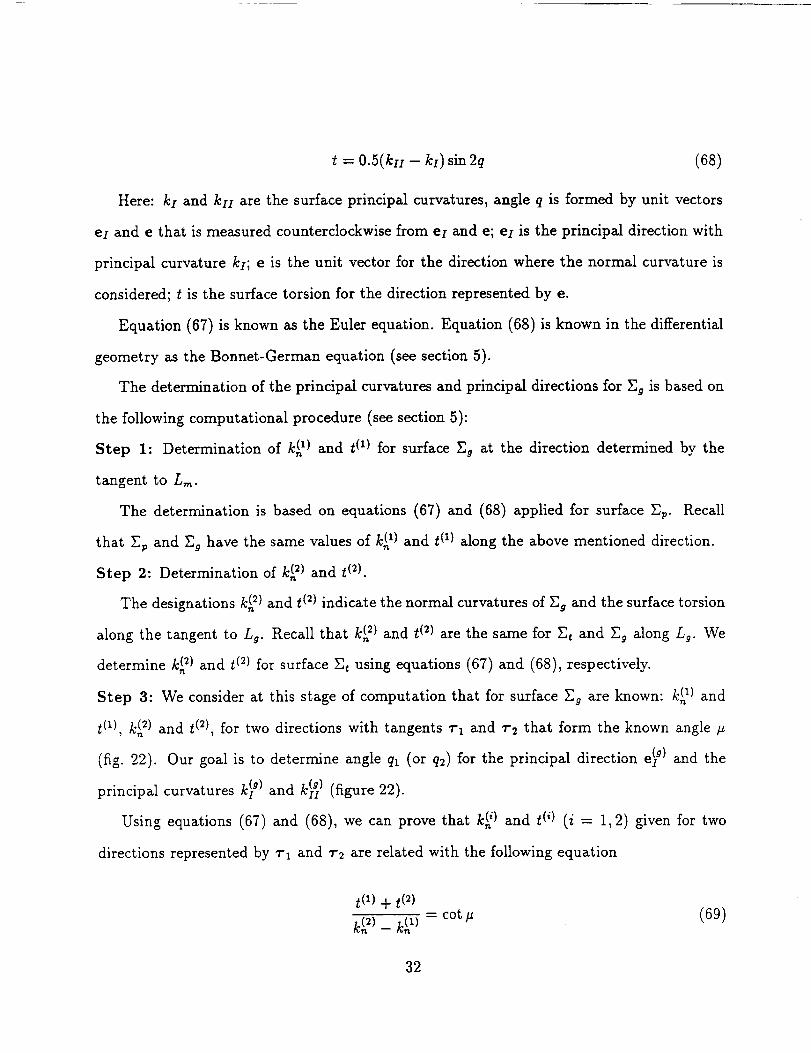
t = 0.5(kii - kz) sin 2q (68)
Here: kx and kIi are the surface principal curvatures, angle q is formed by unit vectors
ei and e that is measured counterclockwise from el and e; ei is the principal direction with
principal curvature ki; e is the unit vector for the direction where the normal curvature is
considered; t is the surface torsion for the direction represented by e.
Equation (67) is known as the Euler equation. Equation (68) is known in the differential
geometry as the Bonnet-German equation (see section 5).
The determination of the principal curvatures and principal directions for Eg is based on
the following computational procedure (see section 5):
Step 1: Determination of k(n 1) and t (1) for surface Eg at the direction determined by the
tangent to L_.
The determination is based on equations (67) and (68) applied for surface Ep. Recall
that Ep and Eg have the same values of k(1) and t (1) along the above mentioned direction.
Step 2: Determination of k(__) and t (2).
The designations k(_2) and t (2) indicate the normal curvatures of Eg and the surface torsion
along the tangent to Lg. Recall that k(_2) and t (2) are the same for Et and Eg along L 9. We
determine k(n2) and t (2) for surface Et using equations (67) and (68), respectively.
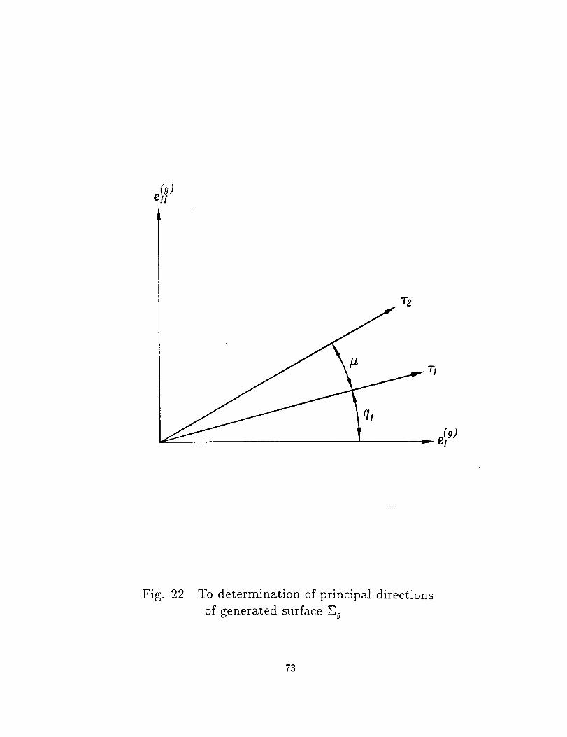
Step 3: We consider at this stage of computation that for surface Eg are known: kO) and
t (1), k(_2) and t (2), for two directions with tangents 1"1 and v2 that form the known angle #
(fig. 22). Our goal is to determine angle ql (or q2) for the principal direction e(xg) and the
principal curvatures k? ) and k(1_) (figure 22).
Using equations (67) and (68), we can prove that k(__) and t (0 (i = 1,2) given for two
directions represented by _'1 and 7"2 are related with the following equation
tO) + t (2)
k_) _ k_) - cot _ (69)
32
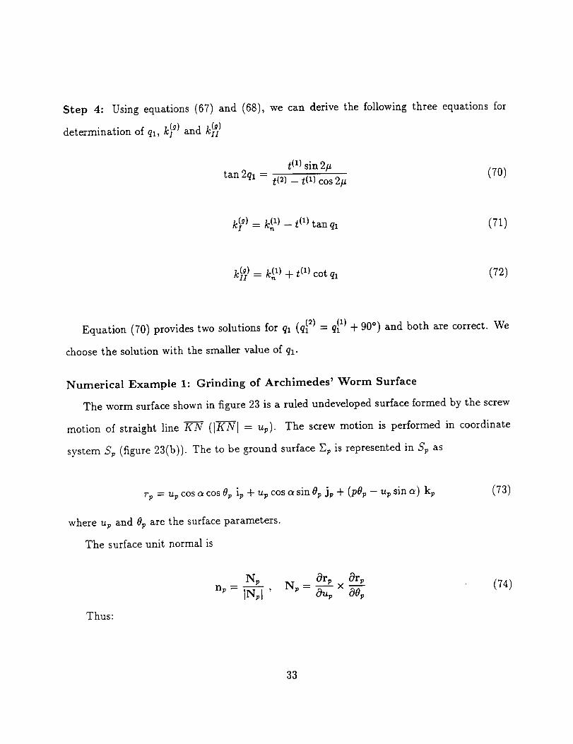
Step 4: Using equations (67) and (68), we can derive the following three equations for
determination of ql, k_g) and k_ }
t (1) sin 2_ (70)tan 2ql = t(2) _ t(1) cos 2_
k (g) -- k (1) - t 0) tan ql (71)
k(i_) = k(_x) + t (1) cot qx (72)
Equation (70) provides two solutions for ql (q_2)
choose the solution with the smaller value of qx.
= q_l) + 90 o) and both are correct. We
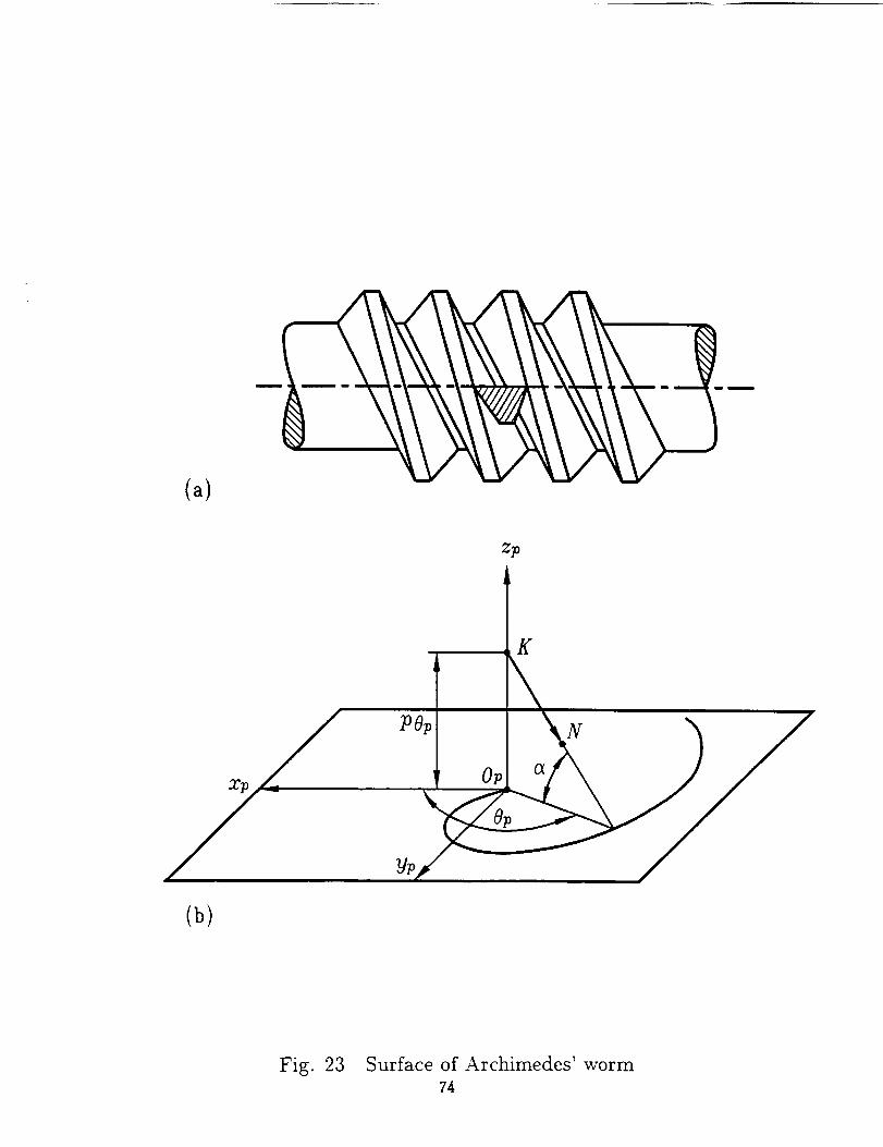
Numerical Example 1: Grinding of Archimedes' Worm Surface
The worm surface shown in figure 23 is a ruled undeveloped surface formed by the screw
motion of straight line _ (I/-_--NI = up). The screw motion is performed in coordinate
system Sp (figure 23(b)). The to be ground surface Ep is represented in Sp as
rp = up cos a cos 8p ip + up cos a sin 8p jp + (pOp - up sin a) kp
where up and 8p are the surface parameters.
The surface unit normal is
Thus:
(73)
(74)
33
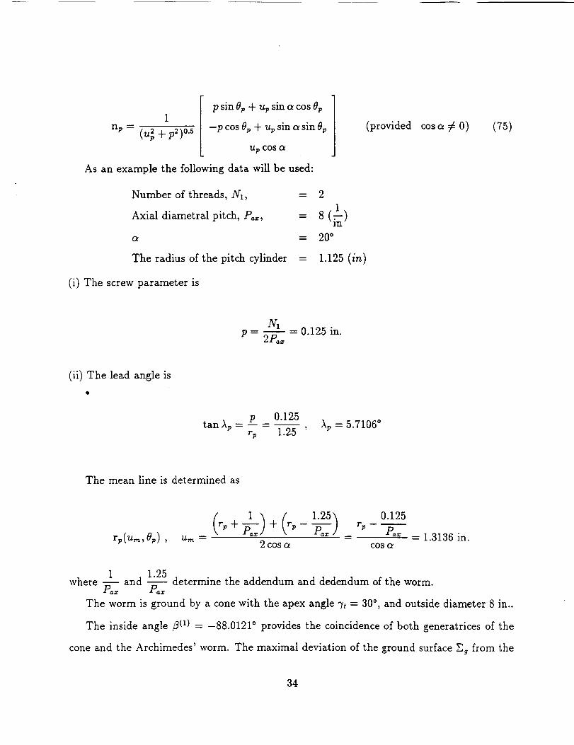
p sin 0p + up sin a cos 0p1
np - (u_ + p_)°'s -p cos 0v + up sin a sin 6p
Up COS ¢_
As an example the following data will be used:
Number of threads, N1,
Axial diametral pitch, P_,,
Ot
= 2
= 8= 20 °
The radius of the pitch cylinder = 1.125 (in)
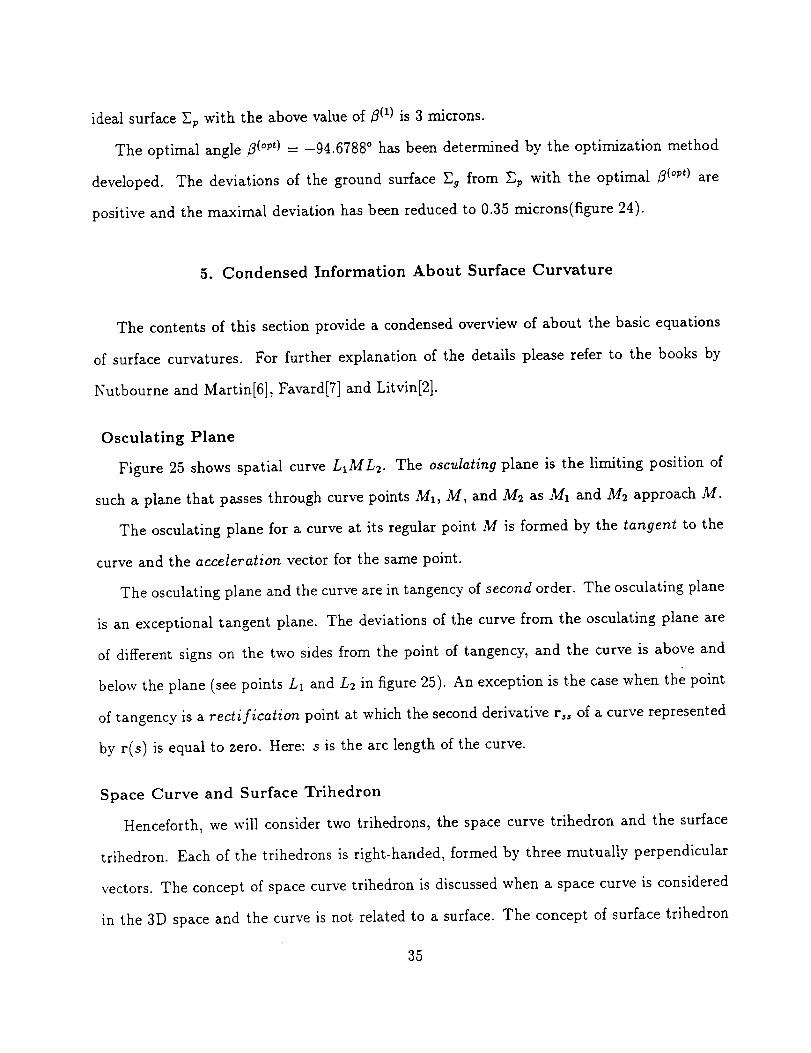
(i) The screw parameter is
(provided cosa # O) (75)
-- 0.125 in.
(ii) The lead angle is
tan Ap - p - 0.125 Ap = 5.7106 °rp 1.25 '
The mean line is determined as
(____) ( 1.25'_ 0.125rp + + rp -p-_ ] rp P_ - 1.3136 in.
rp(u,_, Op) , u,,_ = 2 cos a -- cos cr
1 1.25
where _ and _ determine the addendum and dedendum of the worm.
The worm is ground by a cone with the apex angle 7t = 30 °, and outside diameter 8 in..
The inside angle ;3(1) = -88.0121 ° provides the coincidence of both generatrices of the
cone and the Archimedes' worm. The maximal deviation of the ground surface Zg from the
34
ideal surfaceEpwith the abovevalueof B(1)is 3 microns.
The optimal angle 3 (°pt) = -94.6788 ° has been determined by the optimization method
developed. The deviations of the ground surface E 9 from Ep with the optimal 3(opt) are
positive and the maximal deviation has been reduced to 0.35 microns(figure 24).
5. Condensed Information About Surface Curvature
The contents of this section provide a condensed overview of about the basic equations
of surface curvatures. For further explanation of the details please refer to the books by
Nutbourne and Martin[6], Favard[7] and Litvin[2].
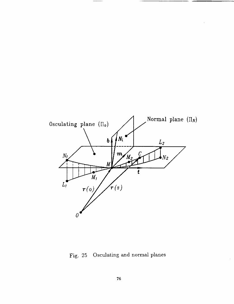
Osculating Plane
Figure 25 shows spatial curve L1ML2. The osculating plane is the limiting position of
such a plane that passes through curve points M1, M, and M2 as M1 and M2 approach M.
The osculating plane for a curve at its regular point M is formed by the tangent to the
curve and the acceleration vector for the same point.
The osculating plane and the curve are in tangency of second order. The osculating plane
is an exceptional tangent plane. The deviations of the curve from the osculating plane are
of different signs on the two sides from the point of tangency, and the curve is above and
below the plane (see points L1 and L2 in figure 25). An exception is the case when the point
of tangency is a rectification point at which the second derivative r_s of a curve represented
by r(s) is equal to zero. Here: s is the arc length of the curve.
Space Curve and Surface Trihedron
Henceforth, we will consider two trihedrons, the space curve trihedron and the surface
trihedron. Each of the trihedrons is right-handed, formed by three mutually perpendicular
vectors. The concept of space curve trihedron is discussed when a space curve is considered
in the 3D space and the curve is not related to a surface. The concept of surface trihedron
35
and spacecurve trihedron are consideredsimultaneouslywhen the spacecurve belongsto
a certain surfaceand the curve inherits someof the properties of the surface to which it
belongs.
Space Curve Trihedron
We consider a coordinate system that is rigidly connected to the curve. Position vector
OC = r(s) determines the current point C of the curve (figure 25); s =MC is the length of
the curve arc; M is the starting point.
Consider that a small piece of curve L1ML2 is located in the osculating plane IIo(figure
25). Plane IIlv is perpendicular to plane 1-Io and passes through point M of the curve.
We define the normal N to the curve as a vector that is perpendicular to the tangent
to the curve. There is an infinite number of normals N to the curve at its point M. All of
normals N belong to plane 1-IN since the unit tangent t is perpendicular to KIN. For instance,
vector Ni is one of the set of curve normals(figure 25). Two normals of the set of normals
must be specified:
(i) the principal normal with the unit vector m that lies in the osculating plane I-Io and is
the line of intersection of planes lIo and IIlv (figure 25) and
(ii) the binormal b that is perpendicular to t and m simultaneously.
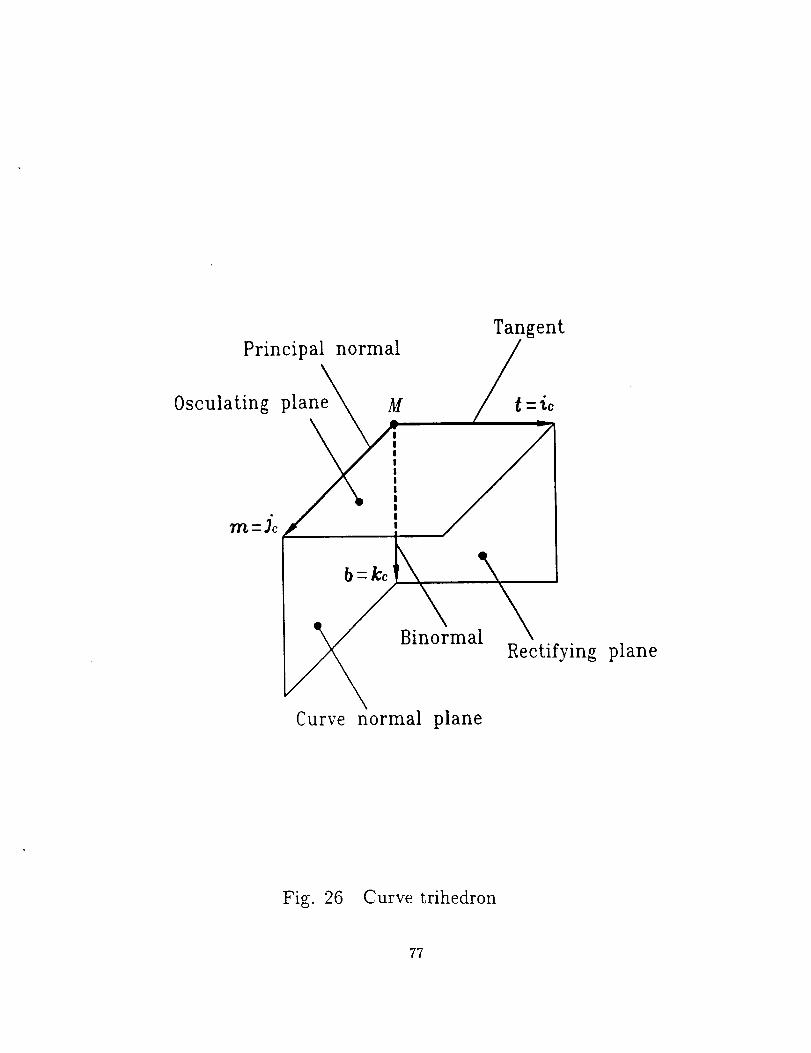
We may identify at each current point of the curve three mutually orthogonal vectors
(figure 25): the tangent vector t, the principal normal m, and the binormal b. The ori-
entation of these vectors in a fixed coordinate system is varied, depending on the location
of the point on the curve. We may consider now a trihedron Sc as a rigid body with three
mutually perpendicular vectors ec(i,, jc, kc) that form a right trihedron (figure 26). The
origin of the trihedron moves along the curve, and the unit vectors ic, j_, kc represent t, m,
b, respectively. Unit vectors t, m, b are taken at the current point of the curve where the
origin of trihedron Sc is located at this instant.
The representation of unit vectors t, m, and b in terms of derivatives of vector function
36
r(s) is basedon the following consideration:
(i) Unit vectors t, m, and b form a right-hand trihedron (figures25 and 26). Thus
t=mxb, m=bxt, b=txm
(ii) Unit vector t is directed along the tangent to the curveand therefore
(76)
Vector r, is a unit vector since I dr I= ds.
(iii) The principal normal to the curve is perpendicular to the curve tangent t = r,. The
d
derivative rs, = _ss(r,) is perpendicular to r_, lies in the osculating plane and therefore the
unit vector rn of the principal normal is represented as
(iv) Taking into account the expression for b in equations (76), we obtain the following
equation for the binormal
b(s)=t xrn--r, x rs_
I r,, I
Frenet-Serret Equations
The motion of the trihedren along a spatial curve can be represented in two components:
(i) as a translational motion along the curve (the origin of the trihedron moves along the curve
37
and the unit vectors of the trihedron keeptheir original orientation), (ii) and asa rotational
motion (the trihedron is rotated as a rigid body (to be coincidedwith the principal normal
m¢ and the tangent tc to the curveat the curve neighboring point).
Consider that the origin of curve trihedron coincides with point M of the curve and the
unit vectors to, me and bc determine the instantaneous orientation of the trihedron(figure
26). The neighboring point of the curve is N and IM--N I = ds,where s is the arc length of
the curve. The unit vectors of the trihedron at N are determined as (t_, m_ and b_), where
t'_ = tc + t,¢ds, m'_ = m_ + m,cds, b: = b_ + b,cds (77)
Here:
dt_ dm_ dbc
ts_= d'--s-' m,,- ds ' bs_= d-'_- (78)
that are taken at point M.
Frenet-Serret equations define ts,, ms_ and b,c as follows (see References [6], [7] and [2]):
t$c
m$c
b$c
_omc
: Tbc - _:otc
--Tin c
0
_o
0
_o 0
0 T
-r 0
tc
m_ (79)
bC
where _o and 7"are the curvature and torsion of the space curve at point M. It is evident
that in the case of a planar curve, the unit vector b¢ is perpendicular to the plane where the
38
curve is located, b,: is equal to zero and the curve torsion _"of a planar curve is equal to
zero.
Equations of _o and 7 for a Parametric Spatial Curve
Consider that the spatial curve is represented by vector function r(0). After derivations
we obtain (see References [2], [6], and [7])
_o
re0.m Ire ×reel- Ire 13
[(zeyee - zeeye) 2 + (zezeo - zeozo) 2 + (yozoe - yooze)2]in
(8O)
The curvature _:o obtained from equation (80) is always positive because the principal
normal m: is located in the osculating plane and is directed to the center of curve curvature.
The curve curvature _o can be also represented in the form
a_-m (81)_;o-- 2
V r
Here: v_ and a_ are the velocity and acceleration of a point in its motion along the curve
and are represented as follows
dO (82)v_ = re d-_
a_--ree(_t)2 + re(d_) (83)
Obviously, the curvature no can be also represented as
39
roo• m
_° -- r_ (84)
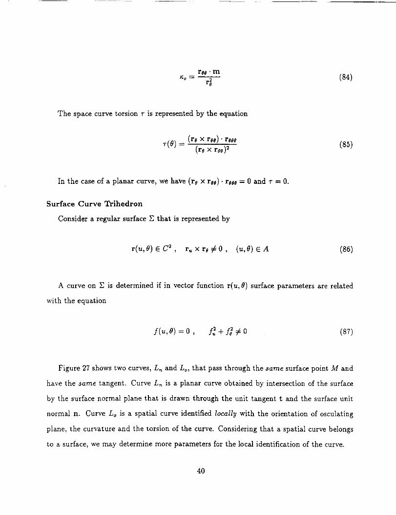
The space curve torsion v is represented by the equation
r(0) = (r0 x roo)'rooo(r0× too) (ss)
In the case of a planar curve, we have (r0 x roo)" rooo = 0 and r = 0.
Surface Curve Trihedron
Consider a regular surface E that is represented by
r(u, 0) eC 2, r,,xr0_0, (u,0) eA (86)
A curve on E is determined if in vector function r(u, 0) surface parameters are related
with the equation
f(u,O) = O, f2 + f_ _ 0 (s7)
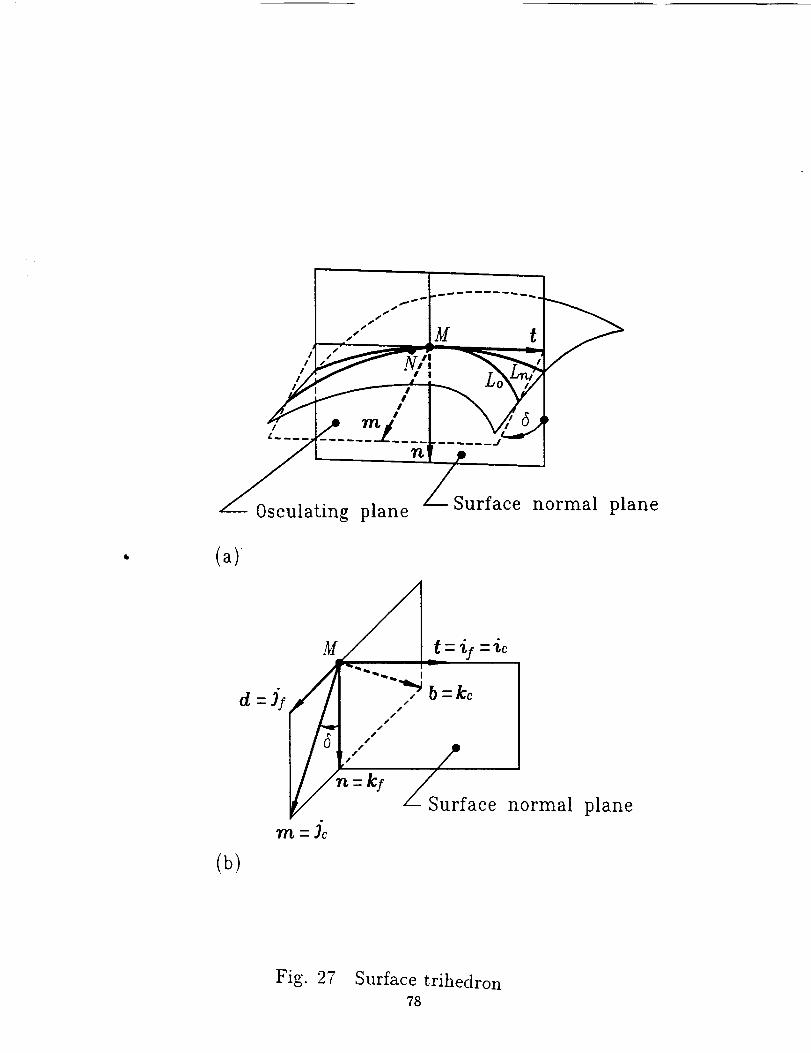
Figure 27 shows two curves, L,_ and Lo, that pass through the same surface point M and
have the same tangent. Curve L,_ is a planar curve obtained by intersection of the surface
by the surface normal plane that is drawn through the unit tangent t and the surface unit
normal n. Curve Lo is a spatial curve identified locally with the orientation of osculating
plane, the curvature and the torsion of the curve. Considering that a spatial curve belongs
to a surface, we may determine more parameters for the local identification of the curve.
40
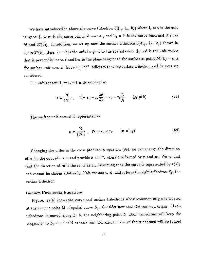
We have introduced in above the curve trihedron So(it, jc, k,) where ic = t is the unit
tangent, j, = m is the curve principal normal, and k, = b is the curve binormal (figures
26 and 27(b)). In addition, we set up now the surface trihedron Sf(if, jr, ky) shown in
figure 27(b). Here: i] = t is the unit tangent to the spatial curve, jf = d is the unit vector
that is perpendicular to t and lies in the plane tangent to the surface at point M; kf = n is
the surface unit normal. Subscript "f" indicates that the surface trihedron and its axes are
considered.
The unit tangent if = ic = t is determined as
do AT T r_+ =r_ (f0 # 0) (88)
t - IT I , = rO_uu - ro_o
The surface unit normal is represented as
N (n kj) (89)n - i = ru x re =INl'
Changing the order in the cross product in equation (89), we can change the direction
of n for the opposite one, and provide 5 < 90 °, where 5 is formed by n and m. We remind
that the direction of m is the same as rss (assuming that the curve is represented by r(s))
and cannot be chosen arbitrarily. Unit vectors t, d, and n form the right trihedron Sf, the
surface trihedron.
Bonnet-Kovalevski Equations
Figure. 27(b) shows the curve and surface trihedrons whose common origin is located
at the current point M of spatial curve Lo. Consider now that the common origin of both
trihedrons is moved along Lo to the neighboring point N. Both trihedrons will keep the
tangent t* to Lo at point N as their common axis, but one of the trihedrons will be turned
41
with respect to the other one since the motion along Lo will be accompanied with the change
of angle 5 formed by vector m and n. Obviously, the unit vectors of the surface trihedron
will change at N their orientation with respect to the orientation at M. Designating the unit
vectors at N by t*, d" and n*, we have
t'=t(s)+tsds, d'=d(s)+d,ds, n'=n(s)+nsds (90)
where
t_= d(t(s)), ds-d(d(s)), n,= d(n(s)) (91)
Bonnet-Kovalevski equations express the derivatives ts, d, and ns in terms of t¢9, t¢,_ and
t as follows (see References [6] and [2]).
t, = agd + a,_n = agJl + tc,',kl
d_ : -tcgt + tn = -t¢9i ] + tkf
n_ = -_t - td = -_ij - tjl
/(92)
Here: _, _g and t are the surface normal curvature, geodesic curvature, and the surface
torsion, respectively. The concept of surface normal and principal curvatures is discussed in
many books on differential geometry, but the determination and concept of _g and t requires
additional explanation that is presented next in this report.
Geodesic Curvature
Frenet-Serret equations (92) yield that
42
t s ----_o m(93)
where _o is the curvature of a spatial curve; the curvature center lies in the osculating
plane. Equations (92) and (93) yield that
_om = _gd + _n (94)
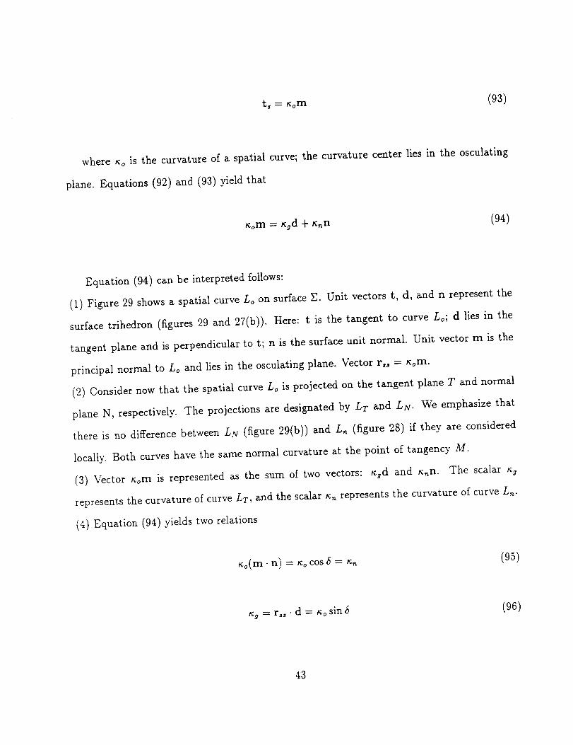
Equation (94) can be interpreted follows:
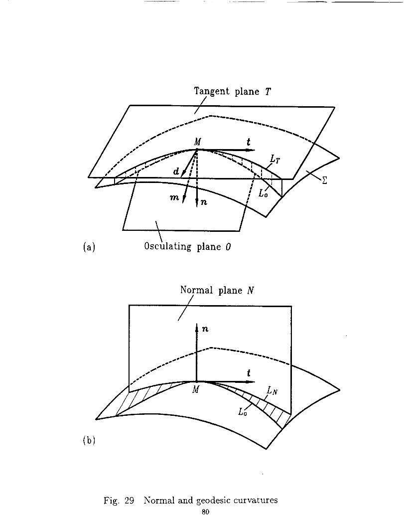
(1) Figure 29 shows a spatial curve Lo on surface E. Unit vectors t, d, and n represent the
surface trihedron (figures 29 and 27(b)). Here: t is the tangent to curve Lo; d lies in the
tangent plane and is perpendicular to t; n is the surface unit normal. Unit vector m is the
principal normal to Lo and lies in the osculating plane. Vector r, - horn.
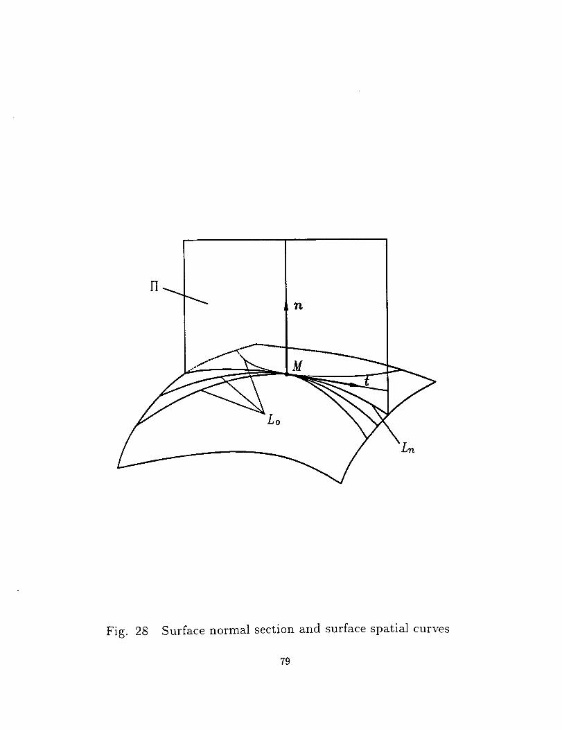
(2) Consider now that the spatial curve Lo is projected on the tangent plane T and normal
plane N, respectively. The projections are designated by LT and LN. We emphasize that
there is no difference between L_v (figure 29(b)) and Ln (figure 28) if they are considered
locally. Both curves have the same normal curvature at the point of tangency M.
(3) Vector _om is represented as the sum of two vectors: ngd and n,n. The scalar ng
represents the curvature of curve LT, and the scalar n, represents the curvature of curve L,.
(4) Equation (94) yields two relations
no(m- n) = _oCOS8 = a_(95)
_g = rs, • d = _osint_(96)
43
where 6 is the angle formed by vectors m and n that determines the orientation of osculating
plane with respect to the normal plane. Equations (95) and (96) relate curvatures _o and
_ and angle 6.
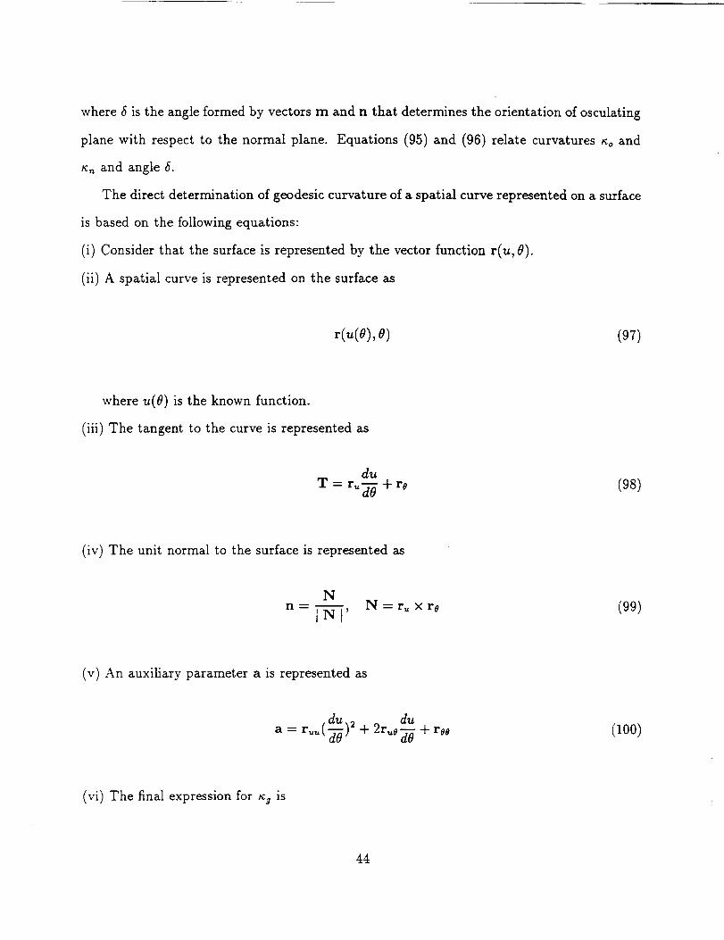
The direct determination of geodesic curvature of a spatial curve represented on a surface
is based on the following equations:
(i) Consider that the surface is represented by the vector function r(u, 8).
(ii) A spatial curve is represented on the surface as
r(u(0),0) (97)
where u(O) is the known function.
(iii) The tangent to the curve is represented as
d_
T = r_-_ + re (98)
(iv) The unit normal to the surface is represented as
N
n-INl' N=r_xro (99)
(v) An auxiliary parameter a is represented as
dlz
a = 2+ + reo (loo)
(vi) The final expression for _g is
44
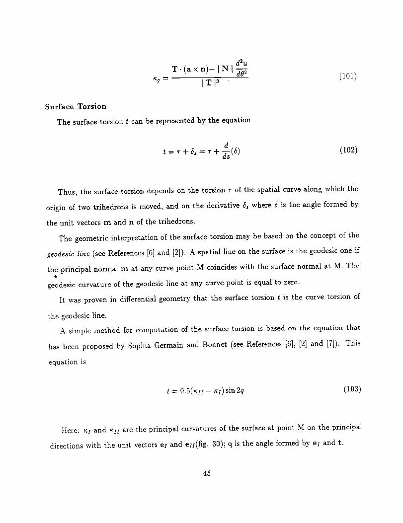
t_ g
d2u
T.(ax n)- I N I _-_
ITI 3
Surface Torsion
The surface torsion t can be represented by the equation
(lOl)
t = + = + (102)
Thus, the surface torsion depends on the torsion r of the spatial curve along which the
origin of two trihedrons is moved, and on the derivative *_ where 6 is the angle formed by
the unit vectors m and n of the trihedrons.
The geometric interpretation of the surface torsion may be based on the concept of the
geodesic line (see References [6] and [2]). h spatial line on the surface is the geodesic one if
the principal normal m at any curve point M coincides with the surface normal at M. The
geodesic curvature of the geodesic line at any curve point is equal to zero.
It was proven in differential geometry that the surface torsion t is the curve torsion of
the geodesic line.
A simple method for computation of the surface torsion is based on the equation that
has been proposed by Sophia Germain and Bonnet (see References [6], [2] and [7]). This
equation is
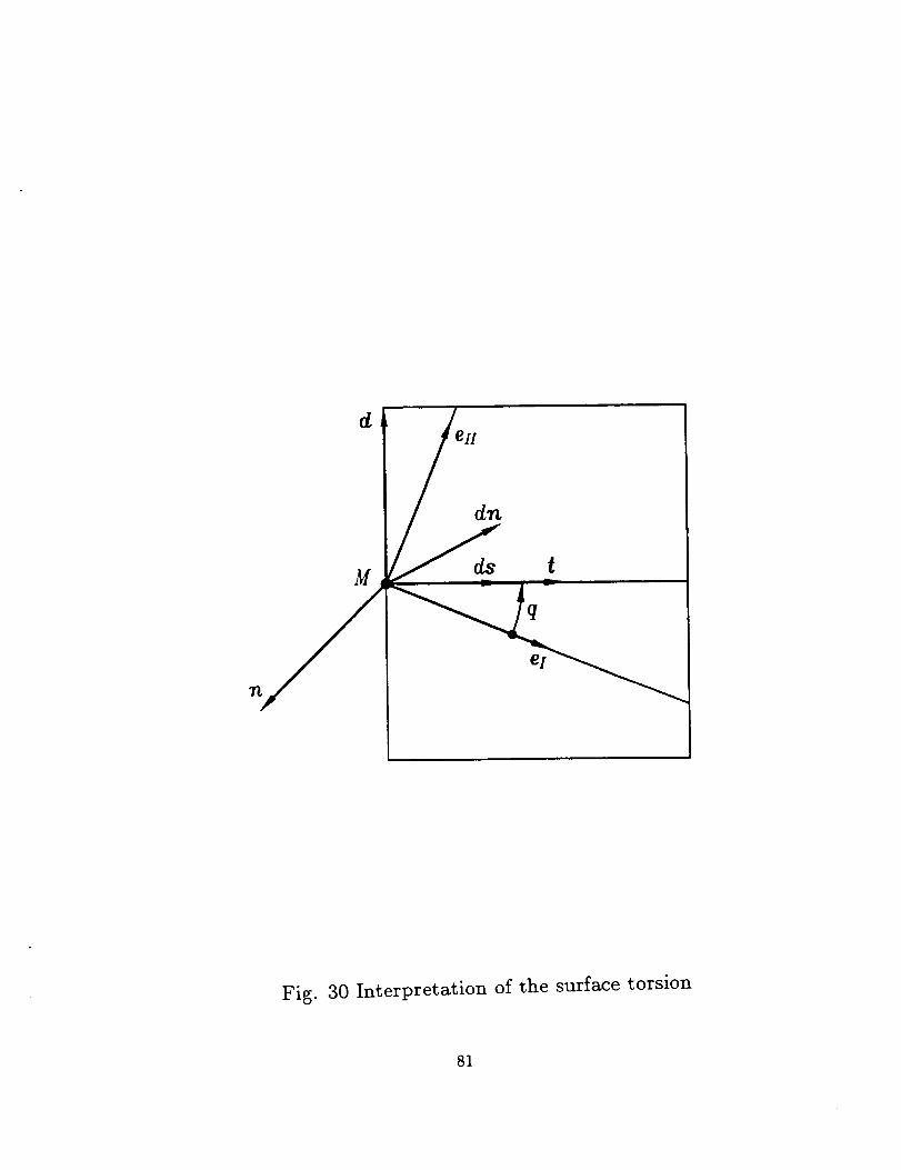
t = 0.5(an- _I)sin2q (103)
Here: _I and an are the principal curvatures of the surface at point M on the principal
directions with the unit vectors eI and en(fig. 30); q is the angle formed by ez and t.
45
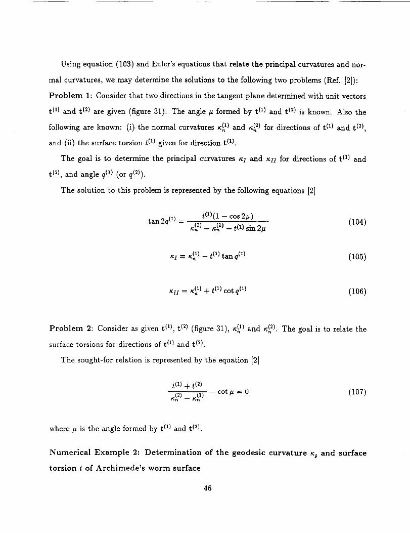
Using equation (103) and Euler's equations that relate the principal curvatures and nor-
mal curvatures, we may determine the solutions to the following two problems (Ref. [2]):
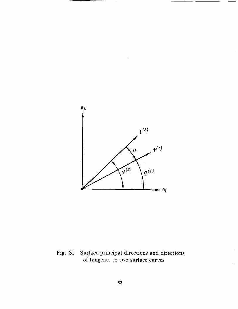
Problem 1: Consider that two directions in the tangent plane determined with unit vectors
t (1} and t (2) are given (figure 31). The angle/z formed by t (1) and t (2) is known. Also the
following are known: (i) the normal curvatures _(1) and _) for directions of t (1) and t (_),
and (ii) the surface torsion t (1) given for direction t (1).
The goal is to determine the principal curvatures _: and _H for directions of t (1) and
t (2), and angle q(1) (or q(2)).
The solution to this problem is represented by the following equations [2]
tan2q(1) = t(1)(1 - cos 2#)K(n2) -- K_ 1) -- t (1) sin 2/z
(104)
KI = t_(n1) -- t (1) tan q(1) (1o8)
_I: = _;(i)+ t(x)cotq(X) (106)
Problem 2: Consider as given t (1), t (2) (figure 31), n(1) and _;(2). The goal is to relate the
surface torsions for directions of t (x} and t (2).
The sought-for relation is represented by the equation [2]
t(1)+ t(2)cot ju = 0 (107)
where # is the angle formed by t (I) and t (2).
Numerical Example 2: Determination of the geodesic curvature n9 and surface
torsion t of Archimede's worm surface
46
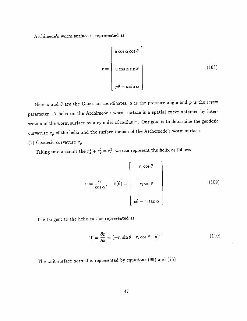
Archimede'sworm surfaceis representedas
r
COS _ COS
u cos a sin 0
pa - u sin a
(10s)
Here u and 0 are the Gaussian coordinates, a is the pressure angle and p is the screw
parameter. A helix on the Archimede's worm surface is a spatial curve obtained by inter-
section of the worm surface by a cylinder of radius rl. Our goal is to determine the geodesic
curvature ng of the helix and the surface torsion of the Archemede's worm surface.
(1) Geodesic curvature _g
2 2 = r_ we can represent the helix as followsTaking into account the r x + rv
riu - , r[v)
COS (2
r i COS
r_ sin #
pO - r_ tan a
(109)
The tangent to the helix can be represented as
Or_(-r_sinO r_cos0 p)Z (110)T - 0O
The unit surface normal is represented by equations (99) and (75)
47
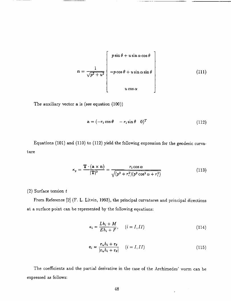
n
p sin 0 + u sin a cos 0
-p cos 0 + u sin a sin 0
U COS (3_
(III)
The auxiliary vector a is (see equation (100))
a=(-ricos0 -risin0 0) T (112)
Equations (101) and (110) to (112) yield the following expression for the geodesic curva-
ture
T. (a x n) ricos_- - (113)
_ ITI3 _(p2 + r?)(p2 cos2_ + r?)
(2) Surface torsion t
From Reference [2] (F. L. Litvin, 1993), the principal curvatures and principal directions
at a surface point can be represented by the following equations:
Lh_ + M
x_ = Ehi + F' (i = I, II) (114)
r_,hi + re
ei = [r_,hi + to[ (i = I, II) (115)
The coefficients and the partial derivative in the case of the Archimedes' worm can be
expressed as follows:
48
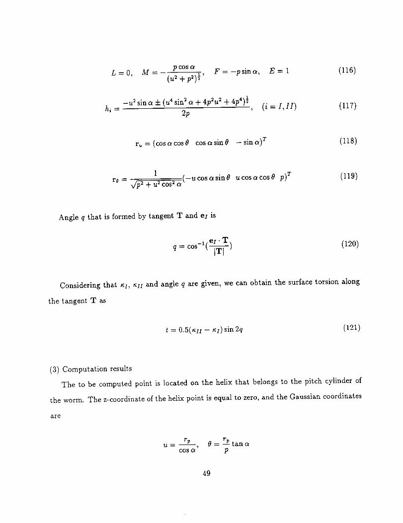
pcosa F = -psina, E = 1 (116)L=O, M= (u 2+p2)_'
-u2sina+(u4sin2a+4p2u2 + 4p4)½ (i= I, II)hi = 2p '
(i17)
r_ = (cos a cos 0 cos a sin 0 - sin a)r (118)
1
= _/p2 + u 2 cos 2 a(-u, cos a sin 0 u cos a cos 0 p)Tr0(ii9)
Angle q that is formed by tangent T and ez is
_l,ei • T
q=cos t _-_-_-)(12o)
Considering that _I, _u and angle q are given, we can obtain the surface torsion along
the tangent T as
t = 0.5(K;II -- _;I) sin 2q (12i)
(3) Computation results
The to be computed point is located on the helix that belongs to the pitch cylinder of
the worm. The z-coordinate of the helix point is equal to zero, and the Gaussian coordinates
are
rp 0 = __rPtan c_
cos a p
49
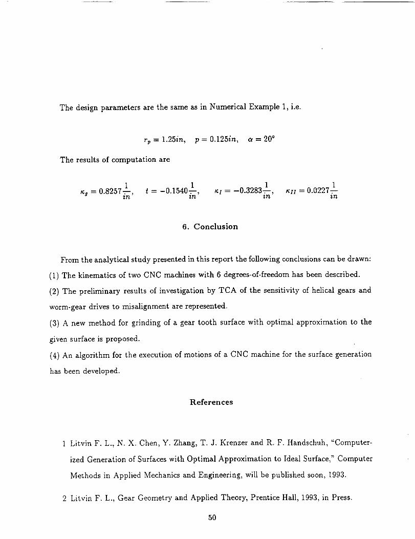
The designparametersare the sameasin Numerical Example 1, i.e.
rp=l.25in, p=0.125in, a=20 °
The results of computation are
1 1 1 1t% = 0.8257v-, t = -0.1540 .--, xI = --0.3283v-, t¢II= 0.0227.--
6. Conclusion
From the analytical study presented in this report the following conclusions can be drawn:
(1) The kinematics of two CNC machines with 6 degrees-of-freedom has been described.
(2) The preliminary results of investigation by TCA of the sensitivity of helical gears and
worm-gear drives to misalignment are represented.
(3) A new method for grinding of a gear tooth surface with optimal approximation to the
given surface is proposed.
(4) An algorithm for the execution of motions of a CNC machine for the surface generation
has been developed.
References
Litvin F. L., N. X. Chen, Y. Zhang, T. J. Krenzer and R. F. Handschuh, "Computer-
ized Generation of Surfaces with Optimal Approximation to Ideal Surface," Computer
Methods in Applied Mechanics and Engineering, will be published soon, 1993.
2 Litvin F. L., Gear Geometry and Applied Theory, Prentice Hall, 1993, in Press.
5O
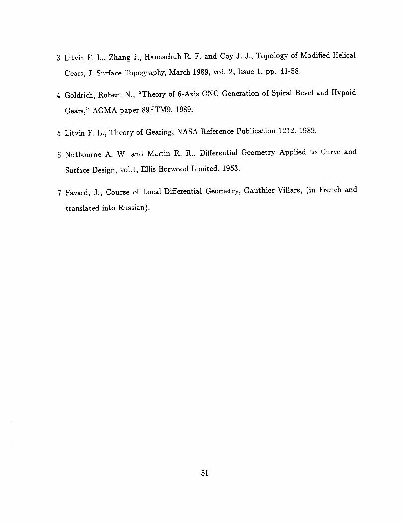
3 Litvin F. L., Zhang J., HandschuhR. F. and Coy J. J., Topology of Modified Helical
Gears,J. SurfaceTopography,March 1989,vol. 2, Issue1, pp. 41-58.
4 Goldrich, Robert N., "Theory of 6-Axis CNC Generationof Spiral Bevel and Hypoid
Gears," AGMA paper 89FTM9, 1989.
5 Litvin F. L., Theory of Gearing, NASA ReferencePublication 1212,1989.
6 Nutboume A. W. and Martin R. R., Differential Geometry Applied to Curve and
Surface Design, vol.1, Ellis Horwood Limited, 1953.
7 Favard, J., Course of Local Differential Geometry, Gauthier-Villars, (in French and
translated into Russian).
51
122.4
III.0c_
. ,""4
63.7-
52.3-
Tooth Top
GERRContact
Direction
Tooth Root
Tooth TopP I NI ON Contact
Direction
Tooth Root
i 1
- 20 - I0 0 I0 20
Tooth Width (mm)
Fig. 1 Edge contact of helical gears: error of
crossing angle is /k 7 = 5.0arc - rain
52
10
b
-5 5 15 25 35 45 55
Angle of Rotation of Pinion (deg)
Fig. Transmission errors of helical gears: error
of crossing angle is A7 = 5.0arc - rain53
_9_9
¢4
° .,,.q
°_.,q
122.4-
111.0-
63.7-
52.3
Tooth Top
GESR
Tooth Root
Tooth Top
Contact
Direction
Tooth Root
| 1
-- 20 - I0
P I NI ON ContactDirection
0 I0 20
Tooth Width (ram)
Fig. 3 Edge contact of helical gears: error of pinion lead
angle on pitch cylinder is/X,kpl = 5.0arc - rain
54
10
-5 5 15 25 35 45 55
Angle of Rotation of Pinion (deg)
Fig. 4 Transmission error of helical gears: error of pinion
lead angle on pitch cylinder is/XApl = 5.0arc - rain
55
AE= 0.2 n:u:n
Contact Path
Major Axis of
ontact Ellipse
Fig. 5 Shift of bearing contact due to change
of center distance AE = 0.2rnm
56
0.5 mm
0
Contact Path
i
Contact Ellipse
Fig. 6 Shift of bearing contact due to change of center
distance/XE and crossing angle /X-y
57
AE --0.7ram, AA -- -0.4ram,
A-),= o
AE = 0.5ram, A7 = o
AE = 0.2ram
L_
!
O°_
°_
20
I0
0
//
Meshing Cycles
Fig. 7 Transmission errors of misaligned worm-gear drive
58
(a)
(b)
/ \
,,_ ,_\j _--_7I_ \ r! I1 I
Fig. 8 Interaction of parabolic and linear functions
59
Tool
Workpieee
Z
II
H
X
IIII IV
Fig. 9 Schematic of "Phoenix" machine
60
/
x_(Oh)
z_) _
zh/Zt
Yd
_i(°h)
Fig. 10 Coordinate systems applied to "Phoenix" machine
61
Oh,Or
Yh
_t
Zp
Zf 2 d Ze
Fig. 11 "Star" CNC machine
62
(a)
a
Xt
Yt
Zt
\ i _ [ Initial cutter
__ _rientation
C. ,._.:',,/[.4__---_ i
\" ',,i I!Final cutter / X_"" )_'---=7' =orientation _' /
2b Zt
Xt
Xb
(b) i- tilt angle
Fig. 12 Pinion head-cutter63
YO
O0
YC
--- X o
Fig. 13 Coordinate systems So, Sc and Sb.
64
_0
Em
r
X o
O0
½
ZT_ zq
Fig. 14 Pinion generation
65
I
I
Ot
M
_b
Fig. 15 Installment and orientation of tool surface Et
with respect to ideal surface _p
66
Z
Fig. 16 Tool surface Et
67
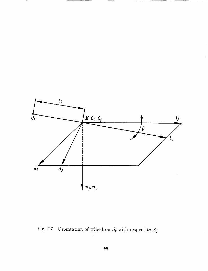
Fig. 17 Orientation of trihedron Sb with respect to Sf
68
Zt
Xt
Fig. 18 Surface of grinding tool cone
69
(a)
S f
SS
Xp
_p
½
OpZp
(b)
Fig. 19 Grid on surface __-_p
70
LIT1,
Fig. 20 Determination of maximum derivations
along line Lgk
71
start I
calculate F {°)
i
input 5p_1)<
I
t
I
^(_)_I (2) [=_p_- _"A_
ij-
[ AR(2)-n.AR (_) In> 1)[[r'k -- r'k x
8(2) R")+ AR(z) =rk "- I'M r'k
1=I calculate F ('' I
N
N =l F(') : F (2)
Fig. 21 Flow chart for optimization
72
(9)ell
Fig. 22 To determination of principal directions
of generated surface __-.g
73
(a)
km
zp
K
pop /o, _I\ J /
(b)
Fig. 23 Surface of Archimedes' worm74
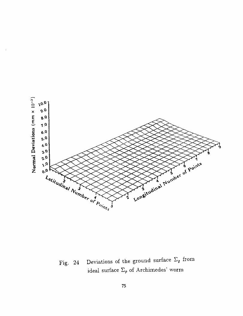
Fig. 24Deviations of the ground surface Eg from
ideal surface Ep of Archimedes' worm
75
Osculating plane (No)Normal plane (tiN)
N1
gt
LI,-(o) (_)
0
Fig. 25 Osculating and normal planes
76
Principal normalTangent
Osculating plane M
Binormal_
Rectifying plane
Curve normal plane
Fig. 26 Curve trihedron
77
(a)
iiii;: __,//
_/ 4_ Surface normal planem-Jc
(b)
Fig. 27 Surface trihedron
78
n
oO_
Fig. 28 Surface normal section and surface spatial curves
79
Tangent plane T
.°/" M t '
d|
|
m
I
II
' L_III
(a) Os, ing plane 0
Normal plane N
//n
(b}
Fig. 29 Normal and geodesic curvatures8O
d
n
H
Fig. 30 Interpretation of the surface torsion
81
eiI
t (2)
I _, t(O
ei
Fig. 31 Surface principal directions and directions
of tangents to two surface curves
82

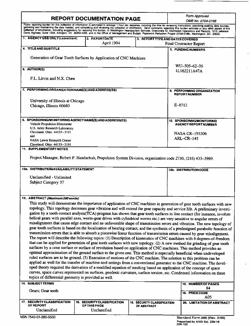
Form ApprovedREPORT DOCUMENTATION PAGE OMBNo. 0704-0188
Public reporting burden for this collection of information is estimated to average 1 hour per response, including the time for reviewing instructio*as, searching existing data sources,gathering and maintaining the data needed, and completing and reviewing the co_lestion of information. Send comments regarding this burden estimate or any other aspect of thiscollection of information, including suggestions for reducing this burden, to Washington Headquarters Services, Directorate for Inf0cmation Operations and Reports, 1215 JeffersonDavis Highway, Suite 1204, Arlington. VA 22202-4302, and to the Office of Management and Budget, Paporwod( Reduction Project (0704-0188), Washington, DC 20503.
1. AGENCYUSEONLY(Leaveb/ank) 2. REPORTDATE 3. REPORTTYPEANDDATESCOVERED
: 4. TITLEANDSUBTITLE
April 1994
Generation of Gear Tooth Surfaces by Application of CNC Machines
6. AUTHOR(S)
F.L. Litvin and N.X. Chen
7. PERFORMING ORGANIZATION NAME(S) AND ADDRESSEES)
University of Illinois at Chicago
Chicago, Illinois 60680
9. SPONSORING/MONITORING AGENCY NAME(S) AND ADDRESS(ES)Vehicle Propulsion Directorate
U.S. Army Research LaboratoryCleveland, Ohio 44135-3191and
NASA Lewis Research Center
Cleveland, Ohio 44135-3191
Final Contractor Report
5. FUNDING NUMBERS
WU-505-62-36
1L162211A47A
8. PERFORMING ORGANIZATION
REPORT NUMBER
E-8712
10. SPONSORING/MONITORING
AGENCYREPORTNUMBER
NASA CR-195306
ARL--CR-145
11. SUPPLEMENTARY NOTES
Project Manager, Robert F. Handschuh, Propulsion System Division, organization code 2730, (216) 433-3969.
12a. DISTRIBUTION/AVAILABILITY STATEMENT
Unclassified - Unlimited
Subject Category 37
12b. DISTRIBUTION CODE
13. ABSTRACT (Maximum 2OO words)
This study will demonstrate the importance of application of CNC machines in generation of gear tooth surfaces with new
topology. This topology decreases gear vibration and will extend the gear capacity and service life. A preliminary investi-
gation by a tooth contact analysis(TCA) program has shown that gear tooth surfaces in line contact (for instance, involute
helical gears with parallel axes, worm-gear drives with cylindrical worms etc.) are very sensitive to angular errors of
misalignment that cause edge contact and an unfavorable shape of transmission errors and vibration. The new topology of
gear tooth surfaces is based on the localization of bearing contact, and the synthesis of a predesigned parabolic function of
transmission errors that is able to absorb a piecewise linear function of transmission errors caused by gear misalignment.
The report will describe the following topics: (1) Description of kinematics of CNC machines with 6 degrees-of-freedom
that can be applied for generation of gear tooth surfaces with new topology. (2) A new method for grinding of gear tooth
surfaces by a cone surface or surface of revolution based on application of CNC machines. This method provides an
optimal approximation of the ground surface to the given one. This method is especially beneficial when undeveloped
ruled surfaces are to be ground. (3) Execution of motions of the CNC machine. The solution to this problem can be
applied as well for the transfer of machine-tool settings from a conventional generator to the CNC machine. The devel-
oped theory required the derivation of a modified equation of meshing based on application of the concept of space
curves, space curves represented on surfaces, geodesic curvature, surface torsion, etc. Condensed information on these
topics of differential geometry is provided as well.
14. SUBJECT TERMS
Gears; Gear teeth
17. SECURITY CLASSIFICATION
OF REPORT
Unclassified
NSN 7540-01-280-5500
18. SECURITY CLASSIFICATION
OFTHIS PAGE
Unclassified
19. SECURITY CLASSIRCATION
OF ABSTRACT
15. NUMBER OF PAGES
84
16. PRICE CODE
A05
20. LIMITATION OF ABSTRACT
Standard Form 298 (Rev. 2-89)
Prescribed by ANSI Std. Z39-18298-102

o_.r mz_" <o _.-,p_
.. -
C
3
-- °