Generation of Length Distribution, Length Diagram, Fibrogram, and

Hindawi Publishing CorporationModelling and Simulation in EngineeringVolume 2007, Article ID 27521, 13 pagesdoi:10.1155/2007/27521

Research ArticleGeneration of Length Distribution, Length Diagram,Fibrogram, and Statistical Characteristics by Weightof Cotton Blends

B. Azzouz, M. Ben Hassen, and F. Sakli

Received 1 August 2007; Accepted 12 December 2007

Recommended by F. Gao

The textile fibre mixture as a multicomponent blend of variable fibres imposes regarding the proper method to predict the charac-teristics of the final blend. The length diagram and the fibrogram of cotton are generated. Then the length distribution, the lengthdiagram, and the fibrogram of a blend of different categories of cotton are determined. The length distributions by weight of fivedifferent categories of cotton (Egyptian, USA (Pima), Brazilian, USA (Upland), and Uzbekistani) are measured by AFIS. Fromthese distributions, the length distribution, the length diagram, and the fibrogram by weight of four binary blends are expressed.The length parameters of these cotton blends are calculated and their variations are plotted against the mass fraction x of onecomponent in the blend .These calculated parameters are compared to those of real blends. Finally, the selection of the optimalblends using the linear programming method, based on the hypothesis that the cotton blend parameters vary linearly in functionof the components rations, is proved insufficient.

Copyright © 2007 B. Azzouz et al. This is an open access article distributed under the Creative Commons Attribution License,which permits unrestricted use, distribution, and reproduction in any medium, provided the original work is properly cited.

1. INTRODUCTION

Fibre length is a very important physical measure in cottonspinning industry. In common with most of cotton proper-ties, it varies greatly between varieties and within the samevariety due to growth environment. Length is related to othercotton fibre characteristics. Longer fibres are generally moreuniform, finer, and stronger than shorter ones. Cotton lengthaffects many parameters during the spinning process such asproduction efficiency, amount of waste, and cleaning degree.Yarn quality parameters such as strength, elongation, hairi-ness, and evenness are strongly correlated to the length ofcotton fibres.

The fibre length of a cotton sample can only be fully de-scribed by its distribution, but fibre length distribution is anawkward way to compare cotton length. Therefore, certaincharacteristics (statistical parameters) of a fibre length distri-bution are often used to make comparison.

Several researches were interested in fibre-length analy-sis. Many of these researches studied the methods and theinstruments measuring the fibre length.

Hertel [1], the inventor of the fibrograph, gives an opticalmethod to plotting the fibrogram from a sample of parallelfibres. From this fibrogram, fibre length and fibre length uni-formity of raw fibre samples can be determined by a geomet-ric interpretation.

Landstreet [2] described the basic ideas of the fibrogramtheory starting from a frequency diagram and establishinggeometrical and probabilistic interpretations for single fibrelength, two fibre length, and multiple fibre length popula-tions.

Krowicki et al. [3, 4] applied a new approach to gener-ate the fibrogram from the length array data similar to Land-street method. They assumed a random catching and holdingof fibres within each of the length groups generating a trian-gular distribution by relative weight for each length group.

Krowicki and Duckett [5] showed that the mean lengthand the proportion of fibres can be obtained from the fibro-gram.

Zeidman et al. [6, 7] discussed the concept of short fibrescontent (SFC) and showed relationships between SFC andother fibre length parameters and functions. Later, they de-termined empirical relationships between SFC and the HVI(high volume instrument) length.

Other studies were conducted to generate fibre length pa-rameters and to study the relationships between these pa-rameters and their effects on the other fibre characteristicsand on the end product quality [8, 9].

To produce yarn with acceptable quality and reasonablecost, it should be a blend of different varieties and categoriesof cotton.

2 Modelling and Simulation in Engineering

In literature, numerous studies were interested to op-timise blends from different nature of fibre. However, fewstudies were dedicated to multicomponent cotton blends.These studies proved that an achievement of good qualityand economic blend of different categories of cotton becamemore to more important.

Elmoghazy [10, 11] proposed a number of fibre selectiontechniques for a uniform multicomponent cotton blend andconsistent output characteristics. Later, he studied sources ofvariability in a multicomponent cotton blend and critical fac-tors affecting it.

Zeidman et al. [6] present equations necessary to deter-mine the short fibre content (SFC) of a binary blend if theSFC and other fibre characteristics of each component areknown.

Elmoghazy [12] used the linear programming method tooptimise the cost of cotton fibre blends with respect to thequality criteria presented in linear equations. His work is in-teresting and deals with all cotton parameters, but it supposesthat the blend characteristics and particularly length param-eters are linear to the component ratios.

In this study, we expressed and studied the length distri-bution functions (the distribution f (x), the length diagramq(x), and the fibrogram p(x)) of cotton and of a multicom-ponent blend of cotton.

Then we studied the variation of length parameters interms of the component ratios in the blend. To reach this ob-ject, we measure the biased-weight length distribution by Ad-vanced Fibre Information System (AFIS) of each componentof the blend. From these distributions, the length parametersof any blend (with any ratio) can be calculated. Thus theirvariations (particularly for binary blends) versus the ratiosof the components can be known. Then the blend length pa-rameters determined from the established blend distributionfunctions are compared to real blend parameters and goodcorrelations are obtained.

The work presented in this paper is a part of number ofworks, in progress, that consist to use these length mathe-matical models with other nonlinear mathematical and sta-tistical models, established to estimate the other cotton blendparameters (fineness, maturity, strength, and elongation), tooptimise the selection of multicomponent cotton blends byusing multiobjectives optimisation techniques.

2. DEFINITIONS

The fibre length can be described by its distribution by num-ber that expresses the probability of occurrence fn(l) of a fi-bre within the length group [l − dl, l + dl], or it can be de-scribed by its distribution by weight fw(l) that expresses theweight of fibres in each length group [l − dl, l + dl].

In this study, we will be interested only in biased-weightlength and fw(l) will be noted by f (l).

A biased-weight diagram q(l) can be obtained from thedistribution by weight by summing f (l) from the longest tothe shortest length group defined by [l − dl, l + dl];

q(l) =∫∞lf (t)dt. (1)

Summing and normalising q(l) from the longest lengthgroup to the shortest give the fibogram p(l);

p(l) = 1ML

∫∞lq(t)dt, (2)

where ML is the mean length by weight expressed in the fol-lowing paragraph.

A family of parameters has been derived over the years.Mean length (ML), short fibre content (SFC%), upper quar-tile length (UQL), upper half mean length (UHML), upperquartile mean length (UQML), span lengths (SL), unifor-mity index (UI%), and uniformity ratio (UR%) are the mostlength distribution parameters.

2.1. Mean length by weight (ML)

The mean length by weight ML is obtained by summing theproduct of fibre length and its weight, then dividing by thetotal weight of the fibres, which can be described by

ML =∫∞

0t f (t)dt. (3)

2.2. Variance of fibre length by weight (Var)

The variance of fibre length by weight is obtained by sum-ming the product of the square of the difference betweenfibre length and the mean length by weight and its weight,then dividing by the total weight of the fibres, which can bedescribed by

Var =∫∞

0

(t −ML

)2f (t)dt. (4)

2.3. Standard deviation of fibre length by weight (σ)

The standard deviation of fibre length by weight σ is the rootsquare of the variance Var and it expresses the dispersion offibres length:

σ =√

Var. (5)

2.4. Coefficient of fibre length variation byweight (CV%)

The coefficient of variation of fibre length CV% is the ratioof σ divided by the mean length ML:

CV% = σ

ML× 100. (6)

2.5. Upper quartile length by weight (UQL)

The upper quartile length is defined as the length that is ex-ceeded by 25% of fibres by weight:

∫∞UQL

f (t)dt = q(UQL) = 0.25. (7)

B. Azzouz et al. 3

2.6. Upper half mean length by weight (UHML)

The UHML is the average length of the longest one-half ofthe fibres when they are divided on a weight basis:

UHML = 1q(ME)

∫∞MEt f (t) = 2

∫∞MEt f (t), (8)

where ME is the median length that exceeded by 50% of fi-bres by weight, then q(ME) = 0.5.

2.7. Upper quarter mean length by weight (UQML)

The UQML is the average length of the longest one-quarterof the fibres when they are divided on a weight basis. So it isthe mean length of the fibres longer than UQL:

UQML = 1q(UQL)

∫∞UQL

t f (t) = 4∫∞

UQLt f (t). (9)

2.8. Span length by weight (SLt%)

The percentage span length t% indicates the percentage offibres that extends a specified distance or longer. The 2.5%and 50% are the most commonly used by industry. It can becalculated from the fibrogram as

p(SLt%) = t

100. (10)

2.9. Uniformity index (UI%)

UI% is the ratio of the mean length divided by the upperhalf-mean length. It is a measure of the uniformity of fibrelengths in the sample expressed as a percent:

UI% = MLUHML

× 100. (11)

2.10. Uniformity ratio (UR%)

UR% is the ratio of the 50% span length to the 2.5% spanlength. It is a smaller value than the UI% by a factor close to1.8:

UR% = SL50%

SL2.5%× 100. (12)

2.11. Short fibre content (SFC%)

SFC% is the percentage by weight of fibres less than one halfinch (12.7 mm). Mathematically, it is described as follows:

SFC% = 100×∫ 12.7

0f (t)dt = 100× (1− q(12.7)). (13)

3. GENERATING THE LENGTH DISTRIBUTION,THE LENGTH DIAGRAM, AND THE FIBROGRAMOF COTTON FIBRE

The cotton length distribution by weight (obtained by mea-suring the weight of fibres in each length group) can be de-scribed by the following equation:

f (l) =

⎧⎪⎪⎪⎪⎪⎪⎪⎪⎪⎪⎪⎪⎪⎪⎪⎨⎪⎪⎪⎪⎪⎪⎪⎪⎪⎪⎪⎪⎪⎪⎪⎩

w1

cif l ∈ [0 , c]

...wi

cif l ∈ [(i− 1)c , ic]

...wn

cif l ∈ [(n− 1)c ,nc]

0 if l ≥ nc.

(14)

w1,w2, . . . ,wn are the weight proportions of fibres, respec-tively, on the length groups [0, c], [c, 2c], . . . , [(n − 1)c,nc].Such c is the length group width. For example, in the AFIScase c is 2 mm and it is 2.5 mm for the Almeter.

The corresponding length diagram by weight q can beobtained by summing f from the longest to the shortestlength by using (1):

q(l) =

⎧⎪⎪⎪⎪⎪⎪⎪⎪⎪⎪⎪⎪⎪⎪⎪⎪⎪⎪⎪⎪⎨⎪⎪⎪⎪⎪⎪⎪⎪⎪⎪⎪⎪⎪⎪⎪⎪⎪⎪⎪⎪⎩

w1c − lc

+n∑j=2

wj if l ∈ [0 , c]

...

wiic − lc

+n∑

j=i+1

wj if l ∈ [(i− 1)c , ic]

...

wnnc − lc

if l ∈ [(n− 1)c ,nc]

0 if l ≥ nc.

(15)

The fibrogram by weight is calculated by summing and nor-malising q from the longest to the shortest length. Equation(2) can be used to calculate the fibrogram, so

p(l) =

⎧⎪⎪⎪⎪⎪⎪⎪⎪⎪⎪⎪⎪⎪⎪⎪⎪⎪⎪⎪⎪⎪⎪⎪⎪⎪⎪⎪⎨⎪⎪⎪⎪⎪⎪⎪⎪⎪⎪⎪⎪⎪⎪⎪⎪⎪⎪⎪⎪⎪⎪⎪⎪⎪⎪⎪⎩

1ML

[(c − l)2

2c+

n∑j=2

wj

((2 j − 1)c

2− l

)]

if l ∈ [0 , c]...

1ML

[(ic − l)2

2c+

n∑j=i+1

wj

((2 j − 1)c

2− l

)]

if l ∈ [(i− 1)c , ic]...

1ML

[(c − l)2

2c

]if l ∈ [(n− 1)c ,nc]

0 if l ≥ nc.

(16)


4. GENERATING LENGTH DISTRIBUTION,LENGTH DIAGRAM, AND FIBROGRAM OFMULTICOMPONENT COTTON BLEND

In this part of study, the length distribution, the length di-agram, and the fibrogram of blend composed of k differ-ent cottons with the proportions x1, x2, . . . , xk will be gen-erated.

Considering k samples of different categories of fibreswith respective masses M1,M2, . . . ,Mk and with length dis-tributions by weight f1, f2, . . . , fk, their length diagrams byweight are q1, q2, . . . , qk and their fibrogram by weight arep1,p2, . . .,pk.

mi(l) and fi(l) are the weight and the proportion of thesample i in the length group [l − dl, l + dl], so

fi (l) = mi (l)Mi

. (17)

The weight of the total blend is

M =k∑i=1

Mi. (18)

The ratio of the sample i in the blend is

xi = Mi

M. (19)

The weight of the blend fibres that belong to the length group[l−dl, l+dl] ism(l) =∑k

j=1 mi and their percentage is f (l) =m(l)/M =∑k

i=1mi(l)/M =∑ki=1(mi(l)/Mi)(Mi/M).

So according to (3) and (5),

f (l) =k∑i=1

xi f i(l). (20)

The mean length of the blend is

ML =∫∞

0l f (l)dl=

∫∞0

[ k∑i=1

xi fi(l)

]dl=

k∑i=1

[xi

∫∞0l f i(l)dl

],

(21)

then

ML =k∑i=1

xi MLi. (22)

The length variance of the blend is (details of the derivationsare given in the appendix)

σ2 =k∑i=1

xiσ2i +

∑1≤i< j≤k

xixj(MLi −ML j

)2. (23)

The coefficient of the blend length variation is

CV% = 1∑ki=1xi MLi

[ k∑i=1

xi ML2i CV2

i

+∑

1≤i< j≤kxixj

(MLi −ML j

)2]1/2

.

(24)

The biased-weight diagram of the blend is

q(l) =∫∞lf (t)dt =

∫∞l

[ k∑i=1

xi fi (t)

]dt

=k∑i=1

[xi

∫∞lfi (t)dt

],

(25)

then

q(l) =k∑i=1

xiqi (l),

p(l) = 1ML

∫∞lq(t)dt = 1

ML

∫∞l

[ k∑i=1

xiqi(t)

]dt

= 1ML

k∑i=1

[xi

∫∞lqi(t)dt

]

=k∑i=1

[xiMLi

ML1

MLi

∫∞lqi(t)dt

],

(26)

then

p(l) =k∑i=1

xiMLiML

pi(l). (27)

The formulas (20), (26), and (27) showed the equations thatrelate ,respectively, the distribution f, the length diagram q,and the fibrogram p of the blend to, respectively, the distri-butions f1, f2, . . . , fk, the length diagrams q1,q2,. . .,qk, and thefibrograms p1,p2,. . .,pk of the k components. These equationsused with (14), (15), and (16) allow generating the equationsof the length distribution, length diagram, and fibrogram ofmulticomponent cotton blend.

Thus

f (l) =

⎧⎪⎪⎪⎪⎪⎪⎪⎪⎪⎪⎪⎪⎪⎪⎪⎪⎪⎪⎪⎪⎪⎪⎪⎨⎪⎪⎪⎪⎪⎪⎪⎪⎪⎪⎪⎪⎪⎪⎪⎪⎪⎪⎪⎪⎪⎪⎪⎩

k∑h=1

xhwh1

cif l ∈ [0 , c]

...k∑

h=1

xhwhi

cif l ∈ [(i− 1)c , ic]

...k∑

h=1

xhwhn

cif l ∈ [(n− 1)c ,nc]

0 if l ≥ nc,

(28)

B. Azzouz et al. 5

Table 1: Length characteristics of cottons.

Cotton category ML (mm) UQL (mm) UHML (mm) UQML (mm) SL50% (mm) SL2.5% (mm) CV(%) UI(%) UR(%) SFC(%)

Eg 31.2 37.4 38.5 42.7 15.9 39.9 30.1 81 39.9 3.1

Uz 26 30.6 32 35.5 13.2 33.8 30.5 81.4 39.1 4.5

USA1 30.2 35.4 36.7 40.5 15.3 38 28.1 82.2 40.3 2.5

USA2 24 28.9 29.9 32.9 12.4 31 31.6 80.5 39.9 7

Br 25.6 31.3 32.5 36 13.2 34.1 33.9 79 38.6 7.1

Whi is weight of fibres from cotton h in the length class [(i−1)c, ic],

q(l) =

⎧⎪⎪⎪⎪⎪⎪⎪⎪⎪⎪⎪⎪⎪⎪⎪⎪⎪⎪⎪⎪⎪⎪⎪⎪⎪⎪⎪⎪⎪⎪⎪⎪⎪⎪⎪⎨⎪⎪⎪⎪⎪⎪⎪⎪⎪⎪⎪⎪⎪⎪⎪⎪⎪⎪⎪⎪⎪⎪⎪⎪⎪⎪⎪⎪⎪⎪⎪⎪⎪⎪⎪⎩

k∑h=1

xhwh1c − lc

+n∑j=2

k∑h=1

xhwhj

if l ∈ [0, c]

...

k∑h=1

xhwhiic − lc

+n∑

j=i+1

k∑h=1

xhwhj

if l ∈ [(i− 1)c , ic]

...

k∑h=1

xhwhnnc − lc

if l ∈ [(n− 1)c,nc]

0 if l ≥ nc,

(29)

MLp(l) =

⎧⎪⎪⎪⎪⎪⎪⎪⎪⎪⎪⎪⎪⎪⎪⎪⎪⎪⎪⎪⎪⎪⎪⎪⎪⎪⎪⎪⎪⎪⎪⎨⎪⎪⎪⎪⎪⎪⎪⎪⎪⎪⎪⎪⎪⎪⎪⎪⎪⎪⎪⎪⎪⎪⎪⎪⎪⎪⎪⎪⎪⎪⎩

(c − l)2

2c+

n∑j=2

[(2 j − 1

2c − l

) k∑h=1

xhwhj

]

if l ∈ [0 , c]

...

(ic − l)2

2c+

n∑j=i+1

[(2 j − 1

2c − l

) k∑h=1

xhwhj

]

if l ∈ [(i− 1)c , ic]

...

(nc − l)2

2cif l ∈ [(n− 1)c,nc]

0 if l ≥ nc.

(30)

5. VARIATION OF STATISTICAL CHARACTERISTICS BYWEIGHT OF COTTON BINARY BLENDS

5.1. Materials and methods

The length distribution by weight of five categories of cot-ton, where two (Egyptian (Eg) and USA1) are long and three

(Brazilian (Br), USA2, and Uzbekistani (Uz)) are mediumlength, was measured by AFIS. Their length parameters aregiven in Table 1. AFIS allows measuring the weight of fibresin each 2 mm length group.

Four binary blends were studied (USA2/Brazilian; Egyp-tian/USA1, USA1/USA2, and Egyptian/Uzbekistani).

Particularly for binary blends, the following equations(31), (32), and (33) of the length distribution, the length dia-gram, and the fibrogram by weight can be derived from (28),(29), and (30):

f (l) =

⎧⎪⎪⎪⎪⎪⎪⎪⎪⎪⎪⎪⎪⎪⎪⎪⎪⎪⎪⎨⎪⎪⎪⎪⎪⎪⎪⎪⎪⎪⎪⎪⎪⎪⎪⎪⎪⎪⎩

xw11

c+ (1− x)

w21

cif l ∈ [0, c]

...

xw1i

c+ (1− x)

w2i

cif l ∈ [(i− 1)c, ic]

...

xw1n

c+ (1− x)

w2n

cif l ∈ [(n− 1)c,nc]

0 if l ≥ nc,

(31)

where w1i is the weight of fibres from cotton 1 in the lengthgroup [(i−1)c, ic] and w 2i is the weight of fibres from cotton2 in the length group [(i− 1)c, ic]:

q(l) =

⎧⎪⎪⎪⎪⎪⎪⎪⎪⎪⎪⎪⎪⎪⎪⎪⎪⎪⎪⎪⎪⎪⎪⎪⎪⎪⎪⎪⎪⎪⎨⎪⎪⎪⎪⎪⎪⎪⎪⎪⎪⎪⎪⎪⎪⎪⎪⎪⎪⎪⎪⎪⎪⎪⎪⎪⎪⎪⎪⎪⎩

(xw11 +(1− x)w21

) c − lc

+n∑j=2

(xw1 j+(1−x)w2 j

)

if l ∈ [0, c]...(xw1i+(1−x)w2i

) ic − lc

+n∑

j=i+1

(xw1 j+(1−x)w2 j

)

if l ∈ [(i− 1)c, ic]...

(xw1n + (1− x)w2n)nc − lc

if l ∈ [(n− 1)c,nc]

0 if l ≥ nc,(32)


0 0.2 0.4 0.6 0.8 1

x

24

25

26

27

28

29

30

31

32

ML

(mm

)

Egyptian/UzbekistaniUSA1/USA2

Egyptian/USA1USA2/Brazilian

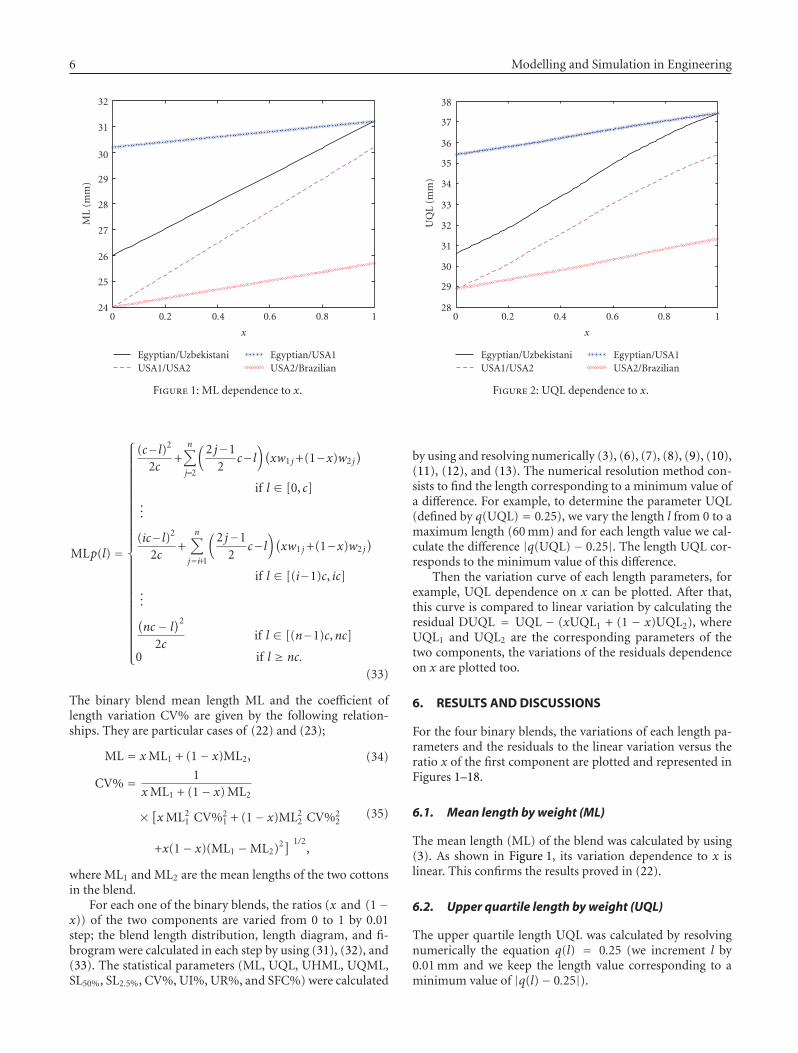
Figure 1: ML dependence to x.

MLp(l) =

⎧⎪⎪⎪⎪⎪⎪⎪⎪⎪⎪⎪⎪⎪⎪⎪⎪⎪⎪⎪⎪⎪⎪⎪⎪⎪⎪⎪⎪⎨⎪⎪⎪⎪⎪⎪⎪⎪⎪⎪⎪⎪⎪⎪⎪⎪⎪⎪⎪⎪⎪⎪⎪⎪⎪⎪⎪⎪⎩

(c−l)2

2c+

n∑j=2

(2 j−1

2c−l

)(xw1 j+(1−x)w2 j

)

if l ∈ [0, c]...

(ic−l)2

2c+

n∑j=i+1

(2 j−1

2c−l

)(xw1 j+(1−x)w2 j

)

if l ∈ [(i−1)c, ic]...(nc − l)2

2cif l ∈ [(n−1)c,nc]

0 if l ≥ nc.

(33)

The binary blend mean length ML and the coefficient oflength variation CV% are given by the following relation-ships. They are particular cases of (22) and (23);

ML = xML1 + (1− x)ML2, (34)

CV% = 1xML1 + (1− x) ML2

× [xML21 CV%2

1 + (1− x)ML22 CV%2

2

+x(1− x)(ML1 −ML2)2] 1/2,

(35)

where ML1 and ML2 are the mean lengths of the two cottonsin the blend.

For each one of the binary blends, the ratios (x and (1−x)) of the two components are varied from 0 to 1 by 0.01step; the blend length distribution, length diagram, and fi-brogram were calculated in each step by using (31), (32), and(33). The statistical parameters (ML, UQL, UHML, UQML,SL50%, SL2.5%, CV%, UI%, UR%, and SFC%) were calculated

0 0.2 0.4 0.6 0.8 1

x

28

29

30

31

32

33

34

35

36

37

38

UQ

L(m

m)



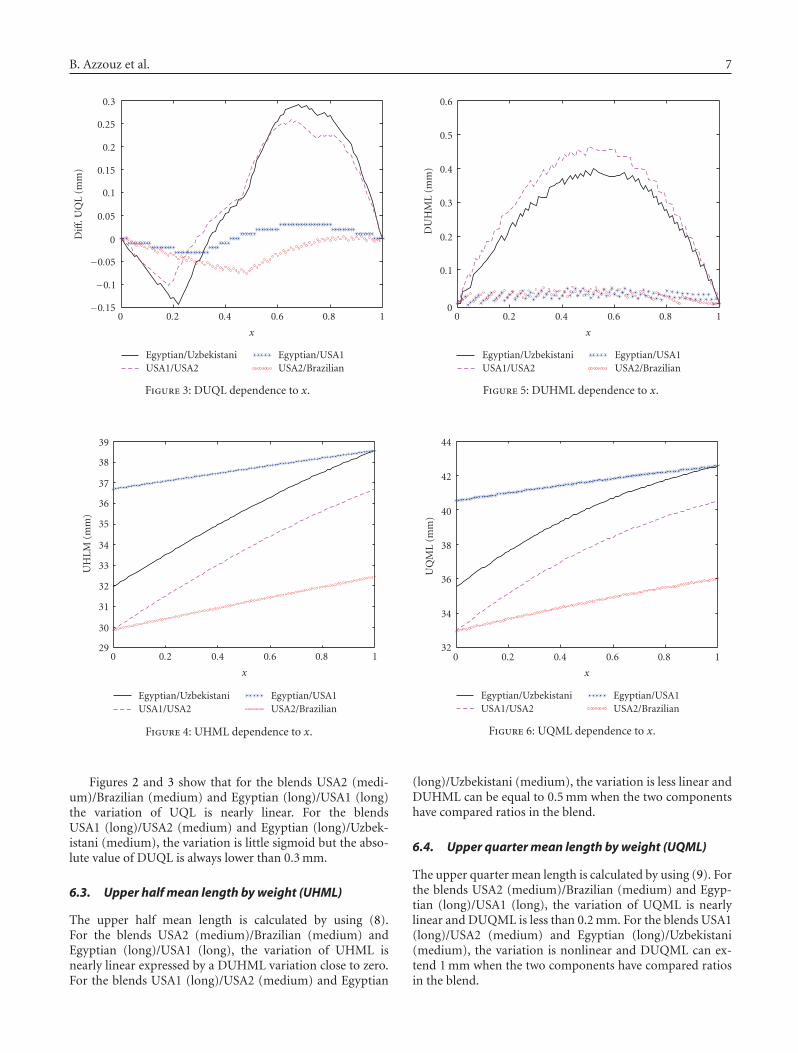
Figure 2: UQL dependence to x.

by using and resolving numerically (3), (6), (7), (8), (9), (10),(11), (12), and (13). The numerical resolution method con-sists to find the length corresponding to a minimum value ofa difference. For example, to determine the parameter UQL(defined by q(UQL) = 0.25), we vary the length l from 0 to amaximum length (60 mm) and for each length value we cal-culate the difference |q(UQL) − 0.25|. The length UQL cor-responds to the minimum value of this difference.

Then the variation curve of each length parameters, forexample, UQL dependence on x can be plotted. After that,this curve is compared to linear variation by calculating theresidual DUQL = UQL − (xUQL1 + (1 − x)UQL2), whereUQL1 and UQL2 are the corresponding parameters of thetwo components, the variations of the residuals dependenceon x are plotted too.

6. RESULTS AND DISCUSSIONS

For the four binary blends, the variations of each length pa-rameters and the residuals to the linear variation versus theratio x of the first component are plotted and represented inFigures 1–18.

6.1. Mean length by weight (ML)

The mean length (ML) of the blend was calculated by using(3). As shown in Figure 1, its variation dependence to x islinear. This confirms the results proved in (22).

6.2. Upper quartile length by weight (UQL)

The upper quartile length UQL was calculated by resolvingnumerically the equation q(l) = 0.25 (we increment l by0.01 mm and we keep the length value corresponding to aminimum value of |q(l)− 0.25|).

B. Azzouz et al. 7

0 0.2 0.4 0.6 0.8 1

x

−0.15

−0.1

−0.05

0

0.05

0.1

0.15

0.2

0.25

0.3

Diff

.UQ

L(m

m)



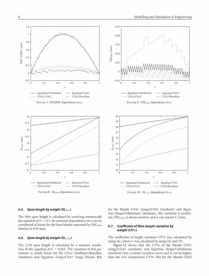
Figure 3: DUQL dependence to x.

0 0.2 0.4 0.6 0.8 1

x

29

30

31

32

33

34

35

36

37

38

39

UH

LM

(mm

)



Figure 4: UHML dependence to x.

Figures 2 and 3 show that for the blends USA2 (medi-um)/Brazilian (medium) and Egyptian (long)/USA1 (long)the variation of UQL is nearly linear. For the blendsUSA1 (long)/USA2 (medium) and Egyptian (long)/Uzbek-istani (medium), the variation is little sigmoid but the abso-lute value of DUQL is always lower than 0.3 mm.

6.3. Upper half mean length by weight (UHML)

The upper half mean length is calculated by using (8).For the blends USA2 (medium)/Brazilian (medium) andEgyptian (long)/USA1 (long), the variation of UHML isnearly linear expressed by a DUHML variation close to zero.For the blends USA1 (long)/USA2 (medium) and Egyptian

0 0.2 0.4 0.6 0.8 1

x

0

0.1

0.2

0.3

0.4

0.5

0.6

DU

HM

L(m

m)



Figure 5: DUHML dependence to x.

0 0.2 0.4 0.6 0.8 1

x

32

34

36

38

40

42

44U

QM

L(m

m)



Figure 6: UQML dependence to x.

(long)/Uzbekistani (medium), the variation is less linear andDUHML can be equal to 0.5 mm when the two componentshave compared ratios in the blend.

6.4. Upper quarter mean length by weight (UQML)

The upper quarter mean length is calculated by using (9). Forthe blends USA2 (medium)/Brazilian (medium) and Egyp-tian (long)/USA1 (long), the variation of UQML is nearlylinear and DUQML is less than 0.2 mm. For the blends USA1(long)/USA2 (medium) and Egyptian (long)/Uzbekistani(medium), the variation is nonlinear and DUQML can ex-tend 1 mm when the two components have compared ratiosin the blend.


0 0.2 0.4 0.6 0.8 1

x

−0.2

0

0.2

0.4

0.6

0.8

1

1.2

Diff

.UQ

ML

(mm

)



Figure 7: DUQML dependence to x.

0 0.2 0.4 0.6 0.8 1

x

12

12.5

13

13.5

14

14.5

15

15.5

16

SL50

%(m

m)



Figure 8: SL50% dependence to x.

6.5. Span length by weight (SL50%)

The 50% span length is calculated by resolving numericallythe equation p(l) = 0.5. Its variation dependence on x can beconsidered as linear for the four blends expressed by DSL50%

inferior to 0.05 mm.

6.6. Span length by weight (SL2.5%)

The 2.5% span length is calculated by a numeric resolu-tion of the equation p(l) = 0.025. The variation of this pa-rameter is nearly linear for the USA2 (medium)/Brazilian(medium) and Egyptian (long)/USA1 (long) blends. But

0 0.2 0.4 0.6 0.8 1

x

−0.01

0

0.01

0.02

0.03

0.04

0.05

DSL

50%

(mm

)



Figure 9: DSL50% dependence to x.

0 0.2 0.4 0.6 0.8 1

x

30

31

32

33

34

35

36

37

38

39

40

SL2.

5%(m

m)



Figure 10: SL2.5% dependence to x.

for the blends USA1 (long)/USA2 (medium) and Egyp-tian (long)/Uzbekistani (medium), the variation is nonlin-ear; DSL2.5% is always positive and it can extend 1.5 mm.

6.7. Coefficient of fibre length variation byweight (CV%)

The coefficient of length variation CV% was calculated byusing (6), where σ was calculated by using (4) and (5).

Figure 12 shows that the CV% of the blends USA1(long)/USA2 (medium) and Egyptian (long)/Uzbekistani(medium) has a convex variation curve and it can be higherthan the two components CV%. But for the blends USA2

B. Azzouz et al. 9

0 0.2 0.4 0.6 0.8 1

x

0

0.2

0.4

0.6

0.8

1

1.2

1.4

1.6

DSL

2.5%

(mm

)



Figure 11: DSL2.5% dependence to x.

0 0.2 0.4 0.6 0.8 1

x

28

29

30

31

32

33

34

35

CV

(%)



Figure 12: CV% dependence to x.

(medium)/Brazilian (medium) and Egyptian (long)/USA1(long), its variation is close to a right line. Equation (35)proves this result. When the two cottons have close meanlengths, the quadratic term (ML1 −ML2)2x (1 − x) is neg-ligible.

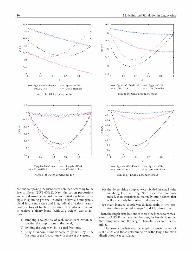
6.8. Uniformity index (UI%)

The uniformity index is calculated by using (11). DUI% isnegative and it is nearly zero for the USA2 (medium)/Brazil-ian (medium) and Egyptian (long)/USA1 (long) blends. Sothe variation of this parameter can be considered linear inthe case of these two blends, and it can reach −1% (more

0 0.2 0.4 0.6 0.8 1

x

0

0.5

1

1.5

2

2.5

DC

V(%

)



Figure 13: DCV% dependence to x.

than 50% of the difference between the UI% of the two com-ponents) in the two blends, USA1 (long)/USA2 (medium)and Egyptian (long)/Uzbekistani (medium).

6.9. Uniformity ratio (UR%)

The uniformity ratio is calculated by using (12). As DUI%and DUR% are negative, they are close to zero for the USA2(medium)/Brazilian (medium) and Egyptian (long)/USA1(long) blends. For the USA1 (long)/USA2 (medium) andEgyptian (long)/ Uzbekistani (medium) blends, the variationof UR% is nonlinear and the absolute value of DUR% can ex-tend 1.5%. This is more than 100% of the difference betweenthe UR% of the two components.

6.10. Short fibre content (SFC%)

The short fibre content was calculated by using (13). Asshown in Figure 18, the variation of this parameter is linear.That can be mathematically proved:

SFC =∫ 12.7

0f (l) dl =

∫ 12.7

0

[x f1(l) + (1− x) f2(l)

]dl

= x∫ 12.7

0f1(l)dl + (1− x)

∫ 12.7

0f2(l)dl

= xSFC1 + (1− x)SFC2.

(36)

7. COMPARISON TO REAL BLENDS

We tried to compare the variation of the statistical length pa-rameters determined from blend distribution functions ex-pressed previously from the ones of real blends.

The USA1/USA2 binary blend studied above was con-sidered. Nine binary blends (0.1/0.9, 0.2/0.8, 0.3/0.7, 0.4/0.6,0.5/0.5, 0.6/0.4, 0.7/0.3, 0.8/0.2, and 0.9/0.1) were achievedand homogenised with manual method. The two ratios of


0 0.2 0.4 0.6 0.8 1

x

79

79.5

80

80.5

81

81.5

82

82.5

UI

(%)



Figure 14: UI% dependence to x.

0 0.2 0.4 0.6 0.8 1

x

−1.2

−1

−0.8

−0.6

−0.4

−0.2

0

0.2

DU

I(%

)



Figure 15: DUI% dependence to x.

cottons composing the blend were obtained according to theFrench Norm (NFG 07062). Next, the cotton proportionsare mixed using a manual method based on blend prin-ciple in spinning process. In order to have a homogenousblend in the transverse and longitudinal directions, a ran-dom meeting of fractions was done. The adopted methodto achieve a binary blend (with 20 g weight) was as fol-lows:

(1) sampling a weight mi of each constituent cotton re-specting the proportions in the blend,

(2) dividing the weight mi in 16 equal fractions,

(3) using a random numbers table to gather 2 by 2 thefractions of the first cotton with those of the second,

0 0.2 0.4 0.6 0.8 1

x

37.5

38

38.5

39

39.5

40

40.5

UR

(%)



Figure 16: UR% dependence to x.

0 0.2 0.4 0.6 0.8 1

x

−1.8

−1.6

−1.4

−1.2

−1

−0.8

−0.6

−0.4

−0.2

0.2

0

DU

R(%

)



Figure 17: DUR% dependence to x.

(4) the 16 resulting couples were divided in small tuftsweighting less than 0.5 g. Next, they were randomlymixed, then transformed manually into 6 slivers thatwill successively be doubled and stretched,

(5) every blended couple was divided again in two por-tions then subjected to steps 3 and 4 for three times.

Then, the length distributions of these nine blends were mea-sured by AFIS. From these distributions, the length diagrams,the fibrograms, and the length characteristics were deter-mined.

The correlation between the length parameter values ofreal blends and those determined from the length functiondistributions was calculated.

B. Azzouz et al. 11

0 0.2 0.4 0.6 0.8 1

x

2.5

3

3.5

4

4.5

5

5.5

6

6.5

7

7.5

SFC

(%)



Figure 18: SFC% dependence to x.

0 0.1 0.2 0.3 0.4 0.5 0.6 0.7 0.8 0.9 1

x

30

31

32

33

34

35

36

37

38

39

SL2.

5%(m

m)

Predicted valuesMeasured values

R2 = 0.97

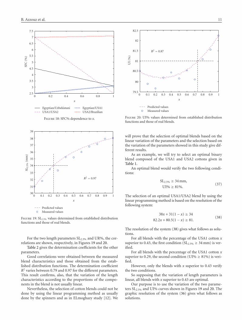
Figure 19: SL2.5% values determined from established distributionfunctions and those of real blends.

For the two length parameters SL2.5% and UR%, the cor-relations are shown, respectively, in Figures 19 and 20.

Table 2 gives the determination coefficients for the otherparameters.

Good correlations were obtained between the measuredblend characteristics and those obtained from the estab-lished distribution functions. The determination coefficientR2 varies between 0.79 and 0.97 for the different parameters.This result confirms, also, that the variation of the lengthcharacteristics according to the proportions of the compo-nents in the blend is not usually linear.

Nevertheless, the selection of cotton blends could not bedone by using the linear programming method as usuallydone by the spinners and as in ELmoghazy study [12]. We

0 0.1 0.2 0.3 0.4 0.5 0.6 0.7 0.8 0.9 1

x

79.5

80

80.5

81

81.5

82

82.5

UI

(%)

Predicted valuesMeasured values

R2 = 0.87

Figure 20: UI% values determined from established distributionfunctions and those of real blends.

will prove that the selection of optimal blends based on thelinear variation of the parameters and the selection based onthe variation of the parameters showed in this study give dif-ferent results.

As an example, we will try to select an optimal binaryblend composed of the USA1 and USA2 cottons given inTable 1.

An optimal blend would verify the two following condi-tions:

SL2.5% ≥ 34 mm,

UI% ≥ 81%.(37)

The selection of an optimal USA1/USA2 blend by using thelinear programming method is based on the resolution of thefollowing system:

38x + 31(1− x) ≥ 34

82.2x + 80.5(1− x) ≥ 81.(38)

The resolution of the system (38) gives what follows as solu-tions.

For all blends with the percentage of the USA1 cotton xsuperior to 0.43, the first condition (SL2.5% ≥ 34 mm) is ver-ified.

For all blends with the percentage of the USA1 cotton xsuperior to 0.29, the second condition (UI% ≥ 81%) is veri-fied.

However, only the blends with x superior to 0.43 verifythe two conditions.

So supposing that the variation of length parameters islinear, all blends with x superior to 0.43 are optimal.

Our purpose is to use the variation of the two parame-ters SL2.5% and UI% curves shown in Figures 19 and 20. Thegraphic resolution of the system (36) gives what follows assolutions.


Table 2: Determination coefficients between the parameters determined from the blends established models and the real ones.

Parameters ML (mm) UQL (mm) UHML (mm) UQML (mm) SL50%(mm) CV(%) UR(%) SFC(%)

Determination coefficient (R2) 0.83 0.89 0.93 0.94 0.84 0.86 0.79 0.86

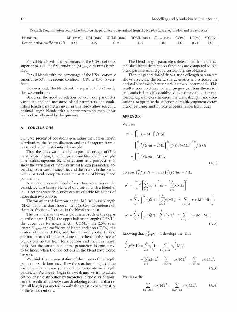
For all blends with the percentage of the USA1 cotton xsuperior to 0.24, the first condition (SL2.5% ≥ 34 mm) is ver-ified.

For all blends with the percentage of the USA1 cotton xsuperior to 0.74, the second condition (UI% ≥ 81%) is veri-fied.

However, only the blends with x superior to 0.74 verifythe two conditions.

Based on the good correlation between our parametervariations and the measured blend parameters, the estab-lished length parameters given in this study allow selectingoptimal length blends with a better precision than linearmethod usually used by the spinners.

8. CONCLUSIONS

First, we presented equations generating the cotton lengthdistribution, the length diagram, and the fibrogram from ameasured length distribution by weight.

Then the study was intended to put the concept of fibrelength distribution, length diagram, and fibrogram by weightof a multicomponent blend of cottons in a perspective toshow the variation of many statistical length parameters ac-cording to the cotton categories and their ratios in the blend,with a particular emphasis on the variation of binary blendparameters.

A multicomponents blend of n cotton categories can beconsidered as a binary blend of one cotton with a blend ofn − 1 cottons.So such a study can be valuable for blends ofmore than two cottons.

The variations of the mean length (ML 50%), span length(SL50%), and the short fibre content (SFC%) dependence onthe mass fraction of cottons in the blend are linear.

The variations of the other parameters such as the upperquartile length (UQL), the upper half mean length (UHML),the upper quarter mean length (UQML), the 2.5% spanlength SL2.5%, the coefficient of length variation (CV%), theuniformity index (UI%), and the uniformity ratio (UR%)are not linear and the curves are more bent in the case ofblends constituted from long cottons and medium lengthones. But the variation of these parameters is consideredto be linear when the two cottons in the blend have closedlengths.

We think that representation of the curves of the lengthparameter variations may allow the searcher to adjust thesevariation curves by analytic models that generate each lengthparameter. We already begin this work and we try to adjustcotton length distribution by theoretical blend distributions,from these distributions we are developing equations that re-late all length parameters to only the statistic characteristicsof these distributions.

The blend length parameters determined from the es-tablished blend distribution functions are compared to realblend parameters and good correlations are obtained.

Then the generation of the variation of length parametersallows predicting the blend characteristics and selecting theoptimal blends with better precision than linear models. Thisresult is now used, in a work in progress, with mathematicaland statistical models established to estimate the other cot-ton blend parameters (fineness, maturity, strength, and elon-gation), to optimise the selection of multicomponent cottonblends by using multiobjectives optimisation techniques.

APPENDIX

We have

σ2 =∫∞

0

[t −ML

]2f (t)dt

=∫∞

0t2 f (t)dt − 2ML

∫∞0t f (t)dt+ML2

∫∞0f (t)dt

=∫∞

0t2 f (t)dt −ML2,

(A.1)

because∫∞

0 f (t)dt = 1 and∫∞

0 t f (t)dt = ML,

σ2 =∫∞

0t2[ k∑i=1

xi fi(t)

]dt −

[ k∑i=1

xiMLi

]2

=k∑i=1

xi

∫∞0t2 fi(t)−

[ k∑i=1

x2i ML2

i +2∑

1≤i< j≤kxixjMLiML j

],

σ2 =k∑i=1

xi

∫∞0t2 fi(t)−

k∑i=1

x2i ML2

i −2∑

1≤i< j≤kxixjMLiML j .

(A.2)

Knowing that∑k

i=1xi = 1 develops the term

k∑i=1

x2i ML2

i =k∑i=1

xi

(1−

∑1≤ j /=i≤k

xj

)ML2

i

=k∑i=1

xiML2i −

∑1≤ j<i≤k

xixjML2i −

∑1≤ j>i≤k

xixjML2i .

(A.3)

We can write∑

1≤ j<i≤kxixjML2

i =∑

1≤i< j≤kxixjML2

j . (A.4)

B. Azzouz et al. 13

Thus

k∑i=1

x2i ML2

i =k∑i=1

xi

(1−

∑1≤ j /=i≤k

xj

)ML2

i

=k∑i=1

xi ML2i −

∑1≤i< j≤k

xixj(ML2

i + ML2j

),

(A.5)

then

σ2 =k∑i=1

xi

∫∞0t2 fi(t)−

k∑i=1

xiML2i −

∑1≤i< j≤k

xixj(ML2

i +ML2j

)

− 2∑

1≤i< j≤kxixjMLiML j ,

σ2 =k∑i=1

xi

[∫∞0t2 fi(t)dt −ML2

i

]

−∑

1≤i< j≤kxixj

(ML2

i + ML2j − 2MLi ML j

).

(A.6)

Finally,

σ2 =k∑i=1

xiσ2i +

∑1≤i< j≤k

xixj(MLi −ML j

)2. (A.7)

REFERENCES

[1] K. L. Hertel, “A method of fiber-length analysis using the fibro-graph,” Textile Research Journal, vol. 10, no. 12, pp. 510–525,1940.

[2] C. B. Landstreet, “The fibrogram: its concept and use in mea-suring cotton fiber length,” Textile Bulletin, vol. 87, no. 4, pp.54–57, 1961.

[3] R. S. Krowicki, J. M. Hemstreet, and K. E. Duckett, “Differ-ent approach to generating the fibrogram from fiber-length-array data—part I: theory,” Journal of the Textile Institute. Part1, vol. 88, no. 1, part 1, pp. 1–4, 1997.

[4] R. S. Krowicki, J. M. Hemstreet, and K. E. Duckett, “A differentapproach to generating the fibrogram from fiber-length-arraydata—part II: application,” Journal of the Textile Institute. Part1, vol. 89, no. 1, pp. 1–9, 1998.

[5] R. S. Krowicki and K. E. Duckett, “An examination of the fi-brogram,” Textile Research Journal, vol. 57, no. 4, pp. 200–204,1987.

[6] M. I. Zeidman, S. K. Batra, and P. E. Sasser, “Determiningshort fiber content in cotton—part I: some theoretical fun-damentals,” Textile Research Journal, vol. 61, no. 1, pp. 21–30,1991.

[7] M. I. Zeidman, S. K. Batra, and P. E. Sasser, “Determiningshort fiber content in cotton—part II: measures of SFC fromHVI data—statistical models,” Textile Research Journal, vol. 61,no. 2, pp. 106–113, 1991.

[8] M. Zeidman and P. S. Sawhney, “Influence of fiber length dis-tribution on strength efficiency of fibers in yarn,” Textile Re-search Journal, vol. 72, no. 3, pp. 216–220, 2002.

[9] X. Cui, T. A. Calamari Jr., and M. W. Suh, “Theoritical andpractical aspects of fiber length comparisons of various cot-tons,” Textile Research Journal, vol. 68, no. 7, pp. 467–472,1998.

[10] Y. E. Elmoghazy and Y. Gowayed, “Theory and practice of cot-ton fiber selection—part I: fiber selection techniques and balepicking algorithms,” Textile Research Journal, vol. 65, no. 1, pp.32–40, 1995.

[11] Y. E. El Mogahzy and Y. Gowayed, “Theory and practice ofcotton fiber selection—part II: sources of cotton mix variabil-ity and critical factors affecting it,” Textile Research Journal,vol. 65, no. 2, pp. 75–84, 1995.

[12] Y. E. El Mogahzy, “Optimizing cotton blend costs withrespect to quality using HVI fiber properties and linearprogramming—part 1: fundamentals and advanced tech-niques of linear programming,” Textile Research Journal,vol. 62, no. 1, pp. 1–8, 1992.

AUTHOR CONTACT INFORMATION

B. Azzouz: Textile Research Unit of ISET K-H, BP 68,Ksar Hellal 5070, Tunisia; [email protected]

M. Ben Hassen: Textile Research Unit of ISET K-H, BP 68,Ksar Hellal 5070, Tunisia; [email protected]

F. Sakli: Textile Research Unit of ISET K-H, BP 68,Ksar Hellal 5070, Tunisia; [email protected]

[email protected]

International Journal of

AerospaceEngineeringHindawi Publishing Corporationhttp://www.hindawi.com Volume 2010

RoboticsJournal of

Hindawi Publishing Corporationhttp://www.hindawi.com Volume 2014


Active and Passive Electronic Components

Control Scienceand Engineering

Journal of



RotatingMachinery


Hindawi Publishing Corporation http://www.hindawi.com

Journal ofEngineeringVolume 2014

Submit your manuscripts athttp://www.hindawi.com

VLSI Design



Shock and Vibration


Civil EngineeringAdvances in

Acoustics and VibrationAdvances in



Electrical and Computer Engineering

Journal of

Advances inOptoElectronics

Hindawi Publishing Corporation http://www.hindawi.com

Volume 2014

The Scientific World JournalHindawi Publishing Corporation http://www.hindawi.com Volume 2014

SensorsJournal of


Modelling & Simulation in EngineeringHindawi Publishing Corporation http://www.hindawi.com Volume 2014


Chemical EngineeringInternational Journal of Antennas and

Propagation




Navigation and Observation



DistributedSensor Networks


Documents

Generation of Length Distribution, Length Diagram, Fibrogram, and