Generic Distributed Exact Cover Solver

Jan Magne Tjensvold

December 21, 2007

Abstract

This report details the implementation of a distributed computing system whichcan be used to solve exact cover problems. This work is based on Donald E.Knuth’s recursive Dancing Links algorithm which is designed to efficiently solveexact cover problems. A variation of this algorithm is developed which enablesthe problems to be distributed to a global network of computers using theBOINC framework. The parallel nature of this distributed computing platformallows more complex problems to be solved. Exact cover problems includes,but is not limited to, n-queens, Latin Square puzzles, Sudoku, polyomino tiling,set packing and set partitioning. The details of the modified Dancing Linksalgorithm and the implementation is explained in detail. A Petri net model isdeveloped to examine the flow of data in the distributed system by running anumber of simulations.

Acknowledgements

I wish to thank Hein Meling for his detailed and insightful comments on thereport and his helpful ideas on the design and implementation of the software.

i

Contents

1 Introduction 11.1 Queens . . . . . . . . . . . . . . . . . . . . . . . . . . . . . . . . . 11.2 Related work . . . . . . . . . . . . . . . . . . . . . . . . . . . . . 31.3 Report organization . . . . . . . . . . . . . . . . . . . . . . . . . 3

2 Dancing Links 42.1 Exact cover . . . . . . . . . . . . . . . . . . . . . . . . . . . . . . 42.2 Generalized cover . . . . . . . . . . . . . . . . . . . . . . . . . . . 52.3 Algorithm X . . . . . . . . . . . . . . . . . . . . . . . . . . . . . 72.4 Dancing Links . . . . . . . . . . . . . . . . . . . . . . . . . . . . 9

2.4.1 Data structure . . . . . . . . . . . . . . . . . . . . . . . . 102.4.2 Algorithm . . . . . . . . . . . . . . . . . . . . . . . . . . . 11

2.5 Parallel Dancing Links . . . . . . . . . . . . . . . . . . . . . . . . 12

3 Implementation details 153.1 Architecture . . . . . . . . . . . . . . . . . . . . . . . . . . . . . . 153.2 Transforms . . . . . . . . . . . . . . . . . . . . . . . . . . . . . . 17

3.2.1 n-queens . . . . . . . . . . . . . . . . . . . . . . . . . . . . 173.3 File format . . . . . . . . . . . . . . . . . . . . . . . . . . . . . . 19

3.3.1 Byte ordering . . . . . . . . . . . . . . . . . . . . . . . . . 193.3.2 Storing sparse boolean matrices . . . . . . . . . . . . . . . 19

3.4 libdecs . . . . . . . . . . . . . . . . . . . . . . . . . . . . . . . . . 233.4.1 Modes of operation . . . . . . . . . . . . . . . . . . . . . . 233.4.2 Building the boolean matrix . . . . . . . . . . . . . . . . . 23

4 Testing and simulation 254.1 Simulation . . . . . . . . . . . . . . . . . . . . . . . . . . . . . . . 25

4.1.1 Model . . . . . . . . . . . . . . . . . . . . . . . . . . . . . 254.1.2 Simulation . . . . . . . . . . . . . . . . . . . . . . . . . . 304.1.3 Results . . . . . . . . . . . . . . . . . . . . . . . . . . . . 31

4.2 Testing . . . . . . . . . . . . . . . . . . . . . . . . . . . . . . . . 33

5 Conclusion 355.1 Future work . . . . . . . . . . . . . . . . . . . . . . . . . . . . . . 35

Bibliography 37

ii

List of Figures

1.1 Board configuration where the queens at B1 and H7 attack eachother . . . . . . . . . . . . . . . . . . . . . . . . . . . . . . . . . . 2

1.2 One possible solution to the 8-queens problem . . . . . . . . . . . 2

2.1 The two solutions S1 (left) and S2 (right) to the 4-queens problem 62.2 Algorithm X search tree for the example matrix . . . . . . . . . . 92.3 Doubly-linked list . . . . . . . . . . . . . . . . . . . . . . . . . . . 102.4 Doubly-linked list with element x removed . . . . . . . . . . . . . 102.5 Circular quad-linked list representation of the example matrix . . 11

3.1 Generic Distributed Exact Cover Solver system architecture . . . 163.2 Structure of the main file header . . . . . . . . . . . . . . . . . . 203.3 Structure of the matrix file header combined with the main header 213.4 Structure of the result file header combined with the main header 22

4.1 Petri net for the distributed computing server . . . . . . . . . . . 274.2 Petri net for the distributed computing network . . . . . . . . . . 274.3 Petri net for a single distributed computing client . . . . . . . . . 284.4 Petri net model of the DECS system with a single client connected 294.5 Work distribution during the first 10 seconds . . . . . . . . . . . 314.6 Complete simulation of the distribution and collection completed

in 63 minutes . . . . . . . . . . . . . . . . . . . . . . . . . . . . . 324.7 Another simulation of the distribution and collection completed

in 67 minutes . . . . . . . . . . . . . . . . . . . . . . . . . . . . . 324.8 Simulation of the distribution and collection with 48 clients . . . 324.9 Simulation of the distribution and collection with 48 clients and

1 token in pfree,i . . . . . . . . . . . . . . . . . . . . . . . . . . . 334.10 Number of updates with and without the S heuristic for 14-queens 344.11 Log plot of updates with the S heuristic for increasing values of

n in n-queens . . . . . . . . . . . . . . . . . . . . . . . . . . . . . 34

iii

Chapter 1

Introduction

This report details the design and implementation of a distributed computingsystem to solve exact cover problems. Donald Knuth’s Dancing Links (DLX)algorithm [15] is used to solve the exact cover problems. Exact cover is a generaltype of problem which can be applied to a wide range of problems. It can beused to solve problems like n-queens, polyomino tiling, Latin square puzzles,Sudoku, set packing and set partitioning. For more detailed information abouthow exact cover can be applied to n-queens, see Section 3.2.1.

Distributed computing with this algorithm is accomplished by exploiting therecursive nature of DLX to split the problem into smaller pieces. The GenericDistributed Exact Cover Solver (DECS) then takes advantage of a distributedcomputing middleware called BOINC [1] to handle the work distribution andresult collection process. The report explains in detail how the DLX algorithmworks and some concrete types of problems it can be applied to. It also looks atsome of the important aspects of the implementation as well as some simulationand test results.

1.1 Queens

The 8-queens problem asks how eight queens can be placed on an 8×8 chessboardso that no two queens attack each other. In chess a queen can attack horizontally,vertically and diagonally on the board. Figure 1.1 might appear to be a validsolution at first sight, but more careful study shows that the queens at B1 andH7 are attacking each other, thus rendering this configuration invalid. Figure1.2 shows a valid solution to the eight queens problem. Depending on thesymmetries in the solution up to seven other solutions can easily be found byrotating the board 90, 180 and 270 degrees. By turning the board upside downand applying the same rotations the other four solutions can be found. The 8-queens problem has a total of 92 configurations where none of the queens attackeach other.

n-queens is the generalized form of the 8-queens problem where n queensare placed on an n×n board. A number of different algorithms exist to find allthe solutions to a given n-queens problem. This report will show the details ofhow the DLX algorithm is able to solve the n-queens problem.

1

Figure 1.1: Board configuration where the queens at B1 and H7 attack eachother

Figure 1.2: One possible solution to the 8-queens problem

2

1.2 Related work

There are numerous implementations of the Dancing Links algorithm availablewith and without source code. In addition to Knuth’s own implementation inCWEB [16] a quick search found source code for Java, Python, C, C++, Ruby,Lisp, Haskell, MATLAB and Mathematica. Some of the implementations weregeneric while others aimed for a specific application (mostly Sudoku). Commonfor all these implementations is that none of them were designed for parallelprocessing.

Alfred Wassermann developed a parallel version of Knuth’s algorithm in[26] by using PVM [11] to solve a problem presented in Knuth’s original paper.Matthew Wolff also developed a parallel version and with the help of MPI[21] he used it to find solutions to the n + k queens problem [5]. However,Wassermann and Wolff only published the solutions to their respective problemsand not the actual implementations they used. The only available open sourceparallel version is written by Owen O’Malley for the Apache Hadoop project[3] in May 2007. O’Malley’s implementation uses the MapReduce framework[8] provided by Hadoop to do the computations in parallel. The details of thisimplementation and how it divides the problem into smaller pieces has, to theauthor’s knowledge, not been published.

1.3 Report organization

This report is organized into several chapters. Chapter 2 describes the DancingLinks algorithm. Chapter 3 discusses different aspects of the implementation.Chapter 4 describes the some simulation and test results and Chapter 5 con-cludes this report.

3

Chapter 2

Dancing Links

Dancing Links (DLX) is an algorithm invented by Donald Knuth to solve anyexact cover problem. It was first described in [15] where he looks at the detailsof the algorithm and uses it to solve some practical problems. Before we lookat the DLX algorithm in more detail we need to explain what an exact coverproblem is.

2.1 Exact cover

To represent an exact cover problem we use a matrix in which each element iseither zero or one (non-zero). This type of matrix is called a boolean, binary,logical or {0,1}-matrix. We use “matrix” in the rest of this report to mean aboolean matrix and to prevent ambiguity “non-zero” is used instead of “one”to identify the value of a matrix element1.

Definition Given a collection of subsets E of a set U , an exact cover is a subsetS of E such that each element of U appears once in S.

The set U is the set of columns U = {1, 2, . . . , n}. E is the collection of rowswhere each set contains the number of the columns which has non-zero values.The idea is that each column in the matrix represents a specific constraint andeach row is a way to satisfy some of the constraints. For the general m × nmatrix

A =

a1,1 a1,2 a1,3 · · · a1,n

a2,1 a2,2 a2,3 · · · a2,n

a3,1 a3,2 a3,3 · · · a3,n

......

.... . .

...am,1 am,2 am,3 · · · am,n

ai,j is an element in the matrix at row i, column j where ai,j ∈ {0, 1}. Thenumber of rows is m and the number of columns is n. A subset of rows froma matrix is an exact cover iff (if and only if) each column has exactly one non-zero (one) element. Let RA and RB be the set of rows in matrix A and B

1A non-zero value is effectively the same as one because a boolean matrix can only haveelements zero and one.

4

respectively. If RB ⊆ RA then B forms the following k × n matrix

B =

b1,1 b1,2 b1,3 · · · b1,n

b2,1 b2,2 b2,3 · · · b2,n

b3,1 b3,2 b3,3 · · · b3,n

......

.... . .

...bk,1 bk,2 bk,3 · · · bk,n

k ≤ m so that B is a reduced matrix of A or, in the case where k = m, the twomatrices are identical. The number of columns in A and B is always the same.The subset RB is an exact cover iff the following equation is satisfied

k∑i=1

bi,j = 1 ∀j ∈ {1, 2, . . . , n}

Example In practical applications we are usually given an initial matrix A andtasked with finding all the subsets of rows which are exact covers. For examplethe following matrix

1 0 0 00 1 1 01 0 0 10 0 1 10 1 0 00 0 1 0

(2.1)

represents a specific exact cover problem. In this matrix row 2 and 3 forma valid solution (exact cover) because the subset of rows {2, 3}, and thus thereduced matrix [

0 1 1 01 0 0 1

]has exactly one non-zero element in each column. By adopting a trial and errorapproach one can find that the full set of solutions for the matrix in (2.1) is{{1, 4, 5}, {2, 3}, {3, 5, 6}}.

2.2 Generalized cover

A generalized form of exact cover, called generalized cover, is sometimes bettersuited to solve certain types of problems. Any generalized cover problem can betranslated to an exact cover problem by adding additional rows. The generalizedcover problem divides the matrix into primary and secondary columns which aresubject to two different sets of constraints. Each primary column in the solutionmust have exactly one non-zero element, as before. However, each secondarycolumn in the solution can have either zero or one non-zero element, instead ofexactly one.

Let CP be the set of primary columns and CS the set of secondary columnsin matrix A and B. The subset of rows RB is an exact cover iff both of thefollowing equations are satisfied

k∑i=1

bi,j = 1 ∀j ∈ CP ∧k∑

i=1

bi,j ≤ 1 ∀j ∈ CS

5

n-queens (see Section 3.2.1) is one type of problem that generalized cover canbe applied to. Creating a secondary column for each diagonal on the chessboardwill reduce the number of rows in the final matrix. Given a smaller matrix theDLX algorithm will have to do less processing to find the solutions, which in turnresults in better performance. The DLX algorithm itself does not require anymodifications to solve generalized cover problems, but the matrix constructionprocedure requires some minor adjustments (see Section 3.4.2).

Example In the 4-queens problem each of the four ranks (rows) and four files(columns) on the chessboard corresponds to a primary column in the exactcover matrix. Each rank and file can only contain one queen, otherwise thequeens would attack each other either horizontally or vertically in that rankor file. Placing four queens on a 4 × 4 board means that each rank and filemust contain exactly one queen. Because queens also attack diagonally eachdiagonal is also assigned a column in the matrix. Some of the diagonals will beunoccupied because the number of diagonals is larger than eight. To accountfor this we have to relax the constraints placed on the columns by letting thecolumns representing the diagonals be secondary columns.

Primary columns 1 to 4 represents the ranks 1 through 4, and primarycolumns 5 to 8 represents the files A to D. On a 4 × 4 board there are tendiagonals if we ignore each of the four corners diagonals, which has only asingle square. The way each diagonal is numbered is unimportant as they areonly needed to represent the problem and are not required to interpret thefinal solutions. We assign each of the ten diagonals to the secondary columns9 to 18. Following the exact cover definition the set U is the set of columnsU = {1, 2, . . . , 18}. E is the collection of rows where each set contains thecolumn numbers with non-zero elements in that row.

E ={{1, 5, 16}, {1, 6, 9, 17}, {1, 7, 10, 18}, {1, 8, 11},{2, 5, 9, 15}, {2, 6, 10, 16}, {2, 7, 11, 17}, {2, 8, 12, 18},{3, 5, 10, 14}, {3, 6, 11, 15}, {3, 7, 12, 16}, {3, 8, 13, 17},{4, 5, 11}, {4, 6, 12, 14}, {4, 7, 13, 15}, {4, 8, 16}}

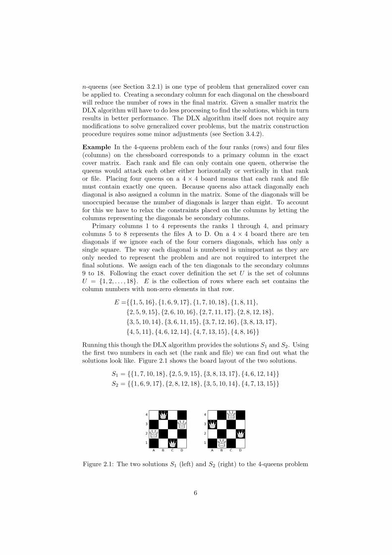
Running this though the DLX algorithm provides the solutions S1 and S2. Usingthe first two numbers in each set (the rank and file) we can find out what thesolutions look like. Figure 2.1 shows the board layout of the two solutions.

S1 = {{1, 7, 10, 18}, {2, 5, 9, 15}, {3, 8, 13, 17}, {4, 6, 12, 14}}S2 = {{1, 6, 9, 17}, {2, 8, 12, 18}, {3, 5, 10, 14}, {4, 7, 13, 15}}

Figure 2.1: The two solutions S1 (left) and S2 (right) to the 4-queens problem

6

Algorithm 1 Algorithm X recursive search procedure.1: procedure search(A,H)2: if H is empty then3: Print solution and return. {Base case for the recursion}4: Choose a column c.5: foreach row r such that ar,c = 1 do6: Add r to partial solution.7: Save state of matrix A and list H.8: foreach column j such that ar,j = 1 do9: foreach row i such that ai,j = 1, except i = r do

10: Delete row i from matrix A.11: Delete column j from matrix A and list H.12: Delete row r from matrix A.13: search(A,H)14: Restore state of matrix A and list H.15: Remove r from the partial solution.

2.3 Algorithm X

Exact cover is a type of problem known to be NP-complete [10]. Severalmethods exist to find all the solutions to an exact cover problem. The moststraight forward algorithm is to check all possible subsets of rows. Given asubset we then check to see if there is exactly one non-zero element in eachcolumn. However, as the size of the matrix increases we will experience a com-binatorial explosion on the number of possible subset to test. Given a matrixwith m unique rows the total number of subset to test would be 2m − 1 . The8-queens problem, which has a matrix consisting of 64 rows, gives an immense18 446 744 073 709 551 615 sets. Given that only 92 of these are valid solu-tions this simple algorithm can hardly be recommended. Surprisingly MihaiOltean and Oana Muntean has proposed a design for an optical device in [18]which might be able to solve some exact cover problems using this technique.Their idea is to harness the massive parallelism of light, but certain technicalchallenges remain before a working prototype can be constructed.

Another approach, which is presented in [15], is Algorithm X (for the lackof a better name). This backtrack algorithm uses a more intelligent eliminationmethod to “wriggle” its way through the matrix and find all the solutions.Looking at matrix (2.1) we can easily determine that row 1 and 3 can neverbe in the same set. They are in conflict with each other because both of themhave a non-zero element in the first column. Since there must be exactly onenon-zero element in each column we can rule out any set containing both row 1and 3.

Algorithm X uses similar logic to recursively traverse the search tree bybacktracking. Backtracking is the process of exploring all possible paths in asearch tree to locate solutions. When a path in the search does not yield anysolutions the algorithm backtracks and starts searching the next available pathin the tree. A modified version of Algorithm X is presented in Algorithm 1.Changes are made to improve the readability, logical consistency and to makeit easier to compare with the Dancing Links algorithm. Algorithm X is initiallycalled with the matrix A and the column header list H. H is initialized with

7

the numbers 1, 2, . . . , n, where n is the number of columns in A.If H is empty the partial solution is an exact cover and the algorithm returns.

Otherwise, the algorithm chooses a column c and loops through each row rwhich has a non-zero element in column c. Any conflict between row r andthe remaining rows are resolved at line 8 to 12. The algorithm then calls itselfrecursively with the reduced matrix and column list. This continues until allthe rows with non-zero elements in column c have been tested, in which case allthe branches in the search tree have been traversed.

Any rule for choosing column c will produce all the solutions, but there aresome rules that work better than others. In [15] Knuth uses what he refers toas the S heuristic, which is to always choose the column with the least amountof non-zero elements. This approach has proved to work well in a large numberof cases so it is a reasonable rule to make use of in practice.

Example Using matrix (2.1) we wish to demonstrate how Algorithm X works.The columns and rows have been numbered to make it easier to keep track ofthem when the matrix is modified.

123456

1 2 3 41 0 0 00 1 1 01 0 0 10 0 1 10 1 0 00 0 1 0

We begin by choosing column 1. Looking at this column we choose row 1 wherethere is a non-zero element. Our partial solution is now {1}. Row 1 only hasone conflicting row which is row 3, which has a conflict in column 1. We removecolumn 1, row 1 and row 3 which results in the following matrix

2456

2 3 41 1 00 1 11 0 00 1 0

(2.2)

This time we choose column 2 and then row 2 so that the partial solutionbecomes {1, 2}. Row 2 conflicts with all the remaining rows (row 5 in column2 and row 4 and 6 in column 3). After all the conflicts have been resolved thematrix itself is empty, but the column list H is not. Because there are no non-zero elements left in the matrix the recursive call will return immediately (theloop condition at line 5 is not satisfied) and matrix (2.2) is restored. This timewe choose row 5 which results in the partial solution {1, 5}. Row 5 conflictswith row 2 in column 2 and by eliminating the conflicts we get the followingmatrix

46

3 4[1 11 0

]We choose column 3 and then row 4 which gives us the partial solution {1, 5, 4}.After all the conflicts are resolved the matrix is completely empty along with

8

the column header list. This tells us that {1, 5, 4} is one of the solutions to thisproblem.

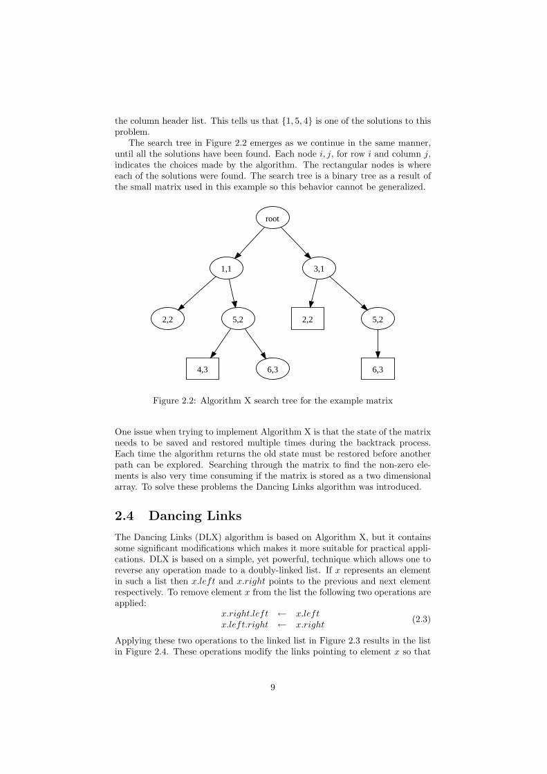
The search tree in Figure 2.2 emerges as we continue in the same manner,until all the solutions have been found. Each node i, j, for row i and column j,indicates the choices made by the algorithm. The rectangular nodes is whereeach of the solutions were found. The search tree is a binary tree as a result ofthe small matrix used in this example so this behavior cannot be generalized.

2,2 5,2 2,2 5,2

6,34,3 6,3

3,1

root

1,1

Figure 2.2: Algorithm X search tree for the example matrix

One issue when trying to implement Algorithm X is that the state of the matrixneeds to be saved and restored multiple times during the backtrack process.Each time the algorithm returns the old state must be restored before anotherpath can be explored. Searching through the matrix to find the non-zero ele-ments is also very time consuming if the matrix is stored as a two dimensionalarray. To solve these problems the Dancing Links algorithm was introduced.

2.4 Dancing Links

The Dancing Links (DLX) algorithm is based on Algorithm X, but it containssome significant modifications which makes it more suitable for practical appli-cations. DLX is based on a simple, yet powerful, technique which allows one toreverse any operation made to a doubly-linked list. If x represents an elementin such a list then x.left and x.right points to the previous and next elementrespectively. To remove element x from the list the following two operations areapplied:

x.right.left ← x.leftx.left.right ← x.right

(2.3)

Applying these two operations to the linked list in Figure 2.3 results in the listin Figure 2.4. These operations modify the links pointing to element x so that

9

an iteration through the list will no longer traverse through this element, butinstead skip right past it.

x

Figure 2.3: Doubly-linked list

x

Figure 2.4: Doubly-linked list with element x removed

When programming one might be tempted to set x.left and x.right to a nullvalue and delete the x object or let the garbage collector do its thing. However,smart as that might seem it would prevent one from applying a second set ofoperations. In [12] Hitotumatu and Noshita introduced a pair of operationswhich allows one to insert an element back into the list in exactly the sameplace it was removed from. The following two operations work as the inverse ofthe operations in (2.3) by adding x back into the list.

x.right.left ← xx.left.right ← x

(2.4)

To maintain the state information for the matrix the DLX algorithm uses theoperations in (2.3) and (2.4). The x element is preserved so that the algorithmcan reverse the remove operations, which are used to reduce the matrix.

2.4.1 Data structure

DLX stores the matrix as a collection of several circular doubly-linked lists whereeach non-zero value in the matrix is an element in the lists. Using this sparsematrix representation saves a lot of memory because the number of zero elementsusually outnumber the non-zero elements. This advantage will normally growwhen the size of the matrix increases. As an example the n-queens problem forn = 10 has 396 non-zero elements, but they only account for 7.33% of the totalnumber of elements.

Each row and column in the matrix is represented by a separate list. Inaddition the set of column headers is also stored in a list. Each element x inthe linked lists have six attributes: x.left, x.right, x.up, x.down, x.column andx.row. The x.row attribute is an addition to Knuth’s original algorithm to en-able detection of the row number. The first four attributes contains a pointerto an element in the respective list. x.left and x.right belongs to a row list andx.up and x.down belongs to a column list. x.column is a pointer to the columnheader and x.row is a non-negative integer storing the row number of the el-ement. A column header c has the additional c.name (column name/number)and c.size (number of elements in column) attributes. Secondary column head-ers used by the generalized cover problem have their c.left and c.right attributes

10

pointing to c (itself). The special column header element h acts as a root ele-ment for the rest of the data structure.

Figure 2.5 shows shows how the matrix in (2.1) can be represented usingthis data structure. To avoid clutter the x.column links pointing to the columnheaders are not displayed in the figure.

hA

2

B

2

C

3

D

2

Figure 2.5: Circular quad-linked list representation of the example matrix

2.4.2 Algorithm

The DLX algorithm is very similar in nature to Algorithm X and in essencethe two algorithms work exactly in the same way. Given the example matrix(2.1) the DLX algorithm will follow the same path as shown in Figure 2.2.The difference is that DLX uses a specialized data structure together with thelinked list remove and add operations to save and restore the state of the matrix.Comparing Algorithm 1 and Algorithm 2 reveals that they are very similar innature.

The DLX algorithm is initially called with k = 0 (recursion level 0) and apointer to the column header h of the matrix. Printing a solution using thex.row attribute is done by printing Oi.row for all i ∈ {1, 2, . . . , k}. Columnselection is done using the S heuristic, which picks the column with the lowestvalue for c.size. Algorithm 3 simply steps through each column header lookingfor the lowest size.

The cover(c) and uncover(c) algorithms are the main differences betweenDLX and Algorithm X. The purpose of cover(c) is to remove column c fromthe column header list and to resolve any conflicts in the column. It uses theoperations in (2.3) to remove the conflicting elements from the column lists.

11

The cover(c) algorithm also increments the value of updates which is used tomeasure how many operations the search algorithm requires to complete. Oneupdate equals four link modifications or one application of both the linked listremove and add operations. The size column header attribute is maintainedby both the cover(c) and uncover(c) algorithms so that the S heuristic worksproperly. Algorithm 4 contains the pseudo code for the cover procedure.

The uncover(c) algorithm restores the state of the matrix using the oper-ations in (2.4). Notice that Algorithm 5 walks up and left in the lists whileAlgorithm 4 walks down and right. This ensures that the elements are put backin the reverse order in which they were removed. This is the only way to makesure that all the links are restored to their original state.

2.5 Parallel Dancing Links

To be able to solve more complex exact cover problems the solution processmust be distributed to a larger number of computers. To accomplish this wemust first break the problem into smaller pieces. In [17] Maus and Aas inves-tigates recursive procedures as the unit for parallelizing. They introduce sometechniques on how to split the recursion tree which can be directly applied tothe search tree in DLX. The main idea is that the algorithm is first run in abreath-first mode so that the search tree is explored one level at a time. Whena certain number of nodes in the tree has been discovered the search stops andthe nodes are distributed to a set of computers and solved in parallel.

The search procedure of DLX is a backtrack algorithm which explores thesearch tree depth-first. Making this a breath-first algorithm can be achieved bynot allowing it to proceed deeper than a certain level in the search tree. Whenthe given level is reached the partial solution O is saved. O can then be used toinitialize a separate process by running DLX on a different computer (or anotherprocessor on the same computer). As long as the predefined depth d is not toodeep or shallow the partial solutions can be used to efficiently solve the exactcover problem in a distributed manner. If d is too deep (high) the algorithm willfind all solutions before the splitting happens, and if it is too shallow (low) thenumber of partial solutions might be too low to be of any use. Adding line 10 to12 in Algorithm 6 is the only changes required to make the original Algorithm2 support this scheme.

Each partial solution produced by psearch(k, d) can be used as an initial-ization vector for the modified search procedure search init(O) in Algorithm 7.O is the initialization vector and O.size is the length of the vector (number ofrows in the partial solution). The initialization vectors and the matrix can bedistributed and the modified search procedure can be run in parallel on eachcomputer. If required each computer can do further splitting locally to takeadvantage of multiple processors.

This approach does not guarantee that each initialization vector provides thesame amount of work. Unfortunately there is no straight forward method toestimate the complexity of the subtree given by a specific initialization vector.In [14] Knuth uses a Monte Carlo approach to estimate the running time ofa backtrack algorithm. By doing random walks in the subtree he is able toestimate the cost of backtracking. This approach would be worth investigatingfor a future version of DECS.

12

Algorithm 2 Dancing Links recursive search.1: procedure search(k)2: if h.right = h then3: Print solution and return. {Base case for the recursion}4: c← choose column()5: cover(c)6: foreach r ← c.down, c.down.down, . . . , while r 6= c do7: Ok ← r {Add r to partial solution}8: foreach j ← r.right, r.right.right, . . . , while j 6= r do9: cover(j.column)

10: search(k + 1)11: foreach j ← r.left, r.left.left, . . . , while j 6= r do12: uncover(j.column)13: uncover(c)

Algorithm 3 Column selection using the S heuristic.1: function choose column()2: s←∞3: foreach j ← h.right, h.right.right, . . . , while j 6= h do4: if j.size < s then5: c← j6: s← j.size7: return column c

Algorithm 4 Cover column c.1: procedure cover(c)2: c.right.left← c.left {Remove column c}3: c.left.right← c.right4: foreach i← c.down, c.down.down, . . . , while i 6= c do5: foreach j ← i.right, i.right.right, . . . , while j 6= i do6: j.down.up← j.up {Remove element j}7: j.up.down← j.down8: j.column.size← j.column.size− 19: updates← updates + 1

Algorithm 5 Uncover column c.1: procedure uncover(c)2: foreach i← c.up, c.up.up . . . , while i 6= c do3: foreach j ← i.left, i.left.lseft, . . . , while j 6= i do4: j.column.size← j.column.size + 15: j.down.up← j {Add element j}6: j.up.down← j7: c.right.left← c {Add column c}8: c.left.right← c

13

Algorithm 6 Dancing Links parallel recursive splitter.1: procedure psearch(k, d)2: if h.right = h then3: Print solution and return. {Base case for the recursion}4: c← choose column()5: cover(c)6: foreach r ← c.down, c.down.down, . . . , while r 6= c do7: Ok ← r {Add r to partial solution}8: foreach j ← r.right, r.right.right, . . . , while j 6= r do9: cover(j.column)

10: if k ≥ d and h.right 6= h then11: Print partial solution. {Prevent further recursion}12: else13: psearch(k + 1)14: foreach j ← r.left, r.left.left, . . . , while j 6= r do15: uncover(j.column)16: uncover(c)

Algorithm 7 Dancing Links search initialization.1: procedure search init(O)2: for k ← 0 to O.size− 1 do3: c← choose column()4: cover(c)5: r ← Ok

6: foreach j ← r.right, r.right.right, . . . , while j 6= r do7: cover(j.column)8: search(O.size) {Do actual search}

14

Chapter 3

Implementation details

DECS has been implemented in the C++ programming language and the sourcecode is available at http://decs.googlecode.com/ licensed under the GNUGeneral Public License version 2. The DECS software suite consists of severalparts:

libdecs This static library contains all the essential parts of DECS like theDLX algorithm, the sparse boolean matrix representation code and thefile input/output functionality.

dance The dance command line program can solve exact covers stored in theDECS file format. It can also display various information about the con-tent of a DECS file.

bdance The bdance program is integrated with the BOINC framework. Thisis the program that any BOINC client connected to the DECS project willdownload and use. It simply reads from the file in.decs, solves the exactcover and writes the solutions to the out.decs file.

degen The DECS matrix generator is a command line program which canbuild exact cover matrices and save them in the DECS file format. It canalso do reverse transforms and analyze DECS result files from previouscomputations. It relies on a set of libraries to do forward and reversetransforms on the specific type of problem. Currently the only libraryavailable is for the n-queens problem.

3.1 Architecture

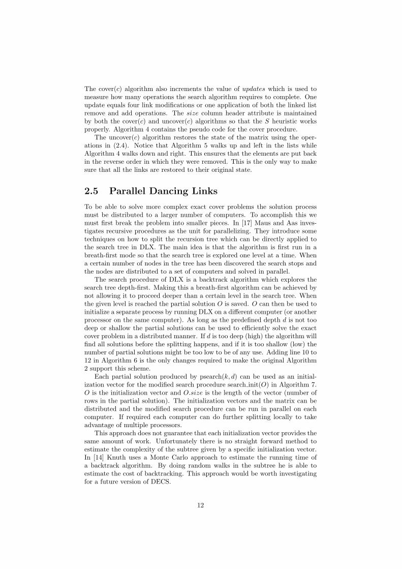
The DECS system architecture is layer based as shown in Figure 3.1. Theapplication layer is where external applications produce exact cover problemsand where the final solutions end up. The transformation layer is where thedegen program and its libraries operate. The generalization step is when degenreceives a problem, turns it into an exact cover problem and outputs the matrixin the DECS file format. This file is then handed to libdecs where the DLXparallel recursive splitter (Algorithm 6) produces a number of work units. Eachof the work units are handed to the BOINC system, which makes sure that theyare available for clients connected to the BOINC server provided by DECS.

15

TransformTransformation from

specific problem into a

generic DLX matrix

DivideDivide the problem

into multiple smaller

work units

DistributeDistribute the work units

to systems sharing their

computational power

CollectGet solutions from each

system until all work units

have been processed

MergePlace all the solutions

in a common place

ready to be transformed

Reverse TransformTransform the solutions

back into a form suitable

for the specific problem

ProblemPolyomino tiling, sudoku,

n queens, set packing,

set partitioning, etc.

SolutionApplication specific

presentation of the

solution.

ConquerProcess the work units

on each system to find

all available solutions

Generalize Specialize

Propagate Aggregate

Compute

Recurse Iterate

Application

Transformation

DECS

BOINC

Request Response

Computation

Figure 3.1: Generic Distributed Exact Cover Solver system architecture

16

When a client receives a work unit it runs the DLX algorithm (Algorithm 7) tofind all the solutions. The client then sends the solutions back the the BOINCserver where they are verified for correctness and stored until the solutions toall the related work units has been received. BOINC then hands the solutionsback to libdecs which reads and analyzes the solution files and merges them intoa single file. Finally it passes the resulting file to the degen program which runsa reverse transform on the solutions. It then writes the final results in whateverformat the application needs.

3.2 Transforms

To turn a specific problem into an exact cover problem an algorithm is neededthat understands that specific problem. This algorithm then turns the probleminto an exact cover matrix which can be solved by the DLX algorithm. Whenthe solutions to the matrix has been found they need to be translated back(reverse transform) into the domain of the original problem so that it is possibleto understand the end result. The degen program makes use of a set of librariesto accomplish these two task.

3.2.1 n-queens

The n-queens problem has been described in detail in Section 1.1 along withan example in Section 2.2. It was originally proposed by the chess player MaxBezzel in 1848. Since that time many people has made an effort to find thenumber of solutions for steadily increasing values of n. The next unsolved puzzleis for n = 26 which is expected to have somewhere around 2 × 1016 solutions.Trying to parallelize the n-queens problem is nothing new. As early as 1989Bruce Abramson and Moti Yung presented a divide and conquer algorithm in[2] which in principle could be used to do parallel processing. A Danish bachelorproject from the spring of 2007 [6] tried to solve the problem for n = 26 on theMiG [25] Grid computing platform. One of the most promising projects latelyis the BOINC based NQueens@Home [24] project. About 13 years of CPU timehas been registered by the project after running for only 3 months.

Algorithm 8 shows how the n-queens transform takes place. The parameterA is a matrix (or two dimmensional array) with all elements set to zero, i × jrows, 2n primary columns and 4n−6 secondary columns (for the two diagonals).The elements in A are accessed by A[i, j] where i is the row, j is the columnand both values start at zero. Each iteration through the inner loop generatesone row in the matrix for each file on the chessboard. The outer loop stepsthrough all the ranks on the board and by multiplying the number of ranks andfiles we get n2 rows in the final matrix. Each of these rows represents a uniqueplacement of a queen on the chessboard. The algorithm is made a bit complexby the calculation of each of the two diagonals. At the end of the algorithm thematrix A can be saved to file and made ready for further processing.

17

Algorithm 8 Transforming n-queens into the exact cover matrix A.1: procedure queens-tf(n, A)2: for i← 0 to n− 1 do3: for j ← 0 to n− 1 do4: row ← i× j5: A[row, i]← 1 {The rank}6: A[row, j + n]← 1 {The file}7: d1 ← i + j {The first diagonal}8: if d1 6= 0 and d1 6= 2n− 2 then9: if d1 < 2n− 2 then

10: A[row, d1 + 2n− 1]← 111: else12: A[row, d1 + 2n− 2]← 113: d2 ← n− i + j − 1 {The second diagonal}14: if d2 6= 0 and d2 6= 2n− 2 then15: if d2 < 2n− 2 then16: A[row, d2 + 4n− 4]← 117: else18: A[row, d2 + 4n− 5]← 1

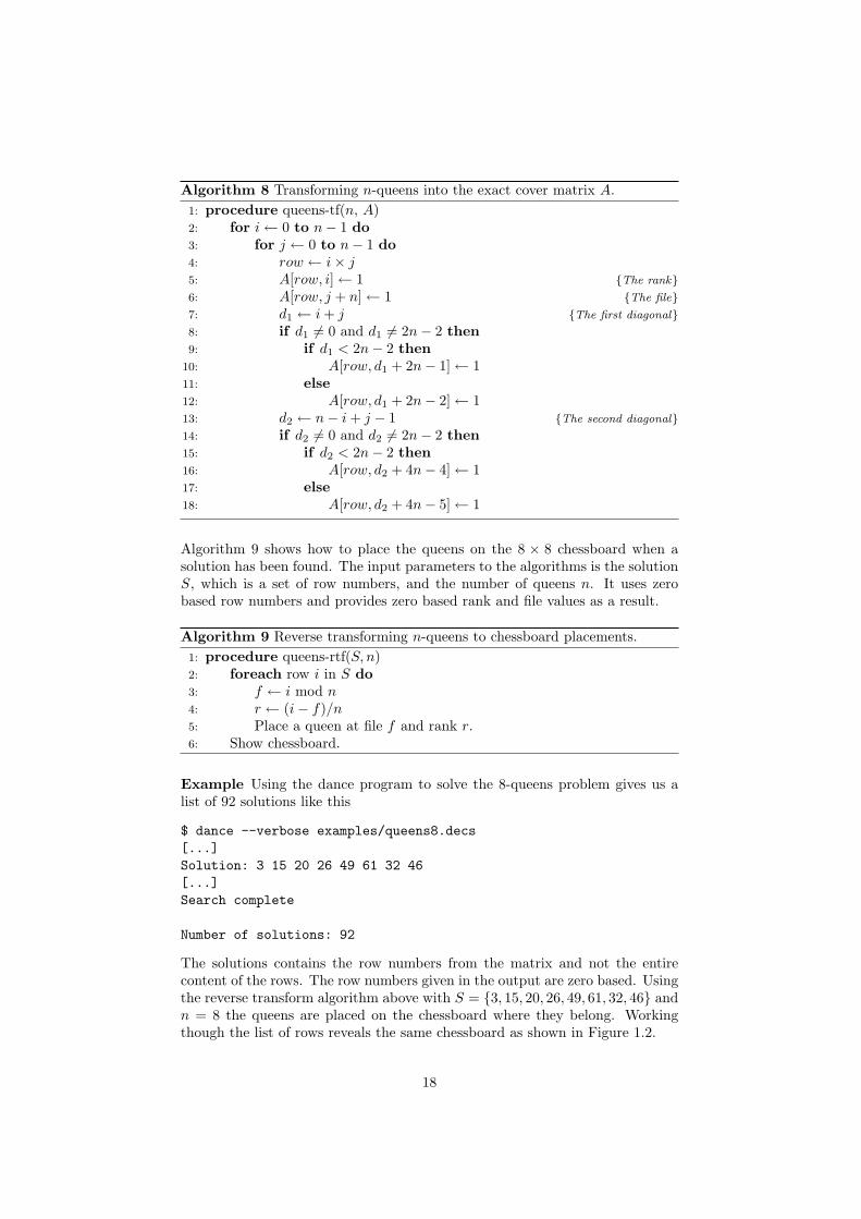
Algorithm 9 shows how to place the queens on the 8 × 8 chessboard when asolution has been found. The input parameters to the algorithms is the solutionS, which is a set of row numbers, and the number of queens n. It uses zerobased row numbers and provides zero based rank and file values as a result.

Algorithm 9 Reverse transforming n-queens to chessboard placements.1: procedure queens-rtf(S, n)2: foreach row i in S do3: f ← i mod n4: r ← (i− f)/n5: Place a queen at file f and rank r.6: Show chessboard.

Example Using the dance program to solve the 8-queens problem gives us alist of 92 solutions like this

$ dance --verbose examples/queens8.decs[...]Solution: 3 15 20 26 49 61 32 46[...]Search complete

Number of solutions: 92

The solutions contains the row numbers from the matrix and not the entirecontent of the rows. The row numbers given in the output are zero based. Usingthe reverse transform algorithm above with S = {3, 15, 20, 26, 49, 61, 32, 46} andn = 8 the queens are placed on the chessboard where they belong. Workingthough the list of rows reveals the same chessboard as shown in Figure 1.2.

18

3.3 File format

In order to store and transfer a DLX problem matrix efficiently a file formathad to be defined for this specific purpose.

3.3.1 Byte ordering

Several challenges arise when defining a file format, but one of the most commonis that of byte ordering. Different platforms use different byte ordering, meaningthat the order of the bytes in variables bigger than 1 byte may differ from onesystem to another.

Byte ordering deals with how the bytes for individual variables are orderedin memory. For a 1 byte large variable the byte ordering is irrelevant as it isonly possible to order that single byte one way. For variables larger that 1 bytethe order the bytes appear in when read from and written to memory follow oneof the two major conventions: big-endian or little-endian.

Big-endian stores the most significant byte (MSB) first and the least signifi-cant byte (LSB) last while little-endian does it the other way around. In Table3.1 we can see that the value 0x7E, when stored in a single byte of memory, isrepresented in the same way for both types of byte ordering. However, whenthe same value is stored in 2 bytes of memory the difference is clearly visible.

Byte order 1 byte 2 bytes 4 bytesBig-endian 7E 00 7E 12 34 56 78Little-endian 7E 7E 00 78 56 34 12

Table 3.1: Difference in representation between little and big endian when stor-ing the value 0x7E and 0x12345678.

In order to achieve portability between different processor and operating systemplatforms one has to choose either big-endian, little-endian or a bit to indicatethe byte ordering used in the file. It is also possible to use a endian-neutralformat like ASCII text or the External Data Representation (XDR) [9] standard.To make the file format consistent across platforms little-endian was chosen.Following the recommendations of Intel’s Endianness White Paper [7] the properbyte swapping methods for big-endian systems has been implemented.

3.3.2 Storing sparse boolean matrices

The storage format for the sparse boolean problem matrix has been designedfor fast and efficient reading. All values are unsigned integers unless explicitlystated otherwise. For more information on how the matrix data structure isconstructed when it is read from file, see Section 3.4.2.

The main file header format is made as simple as possible to allow futureextensions to be made without breaking backwards compatibility. In everyDECS formatted file the 8 first bytes of the file are occupied by the main headeras shown in Table 3.2 and Figure 3.2. Currently only the first byte of the versionfield is used. In a future versions both bytes in the version field are plannedto be ASCII characters so that a separate ASCII format can be defined. Thetype field indicates how the data following the header will look like. When the

19

Offset Length Description0 4 fileid - File type ID: “DECS”4 2 version - File format version.6 1 type - 0 for exact cover matrix and 1 for results.

Other values are currently unused.7 1 reserved - Reserved for future use.

Table 3.2: Main file header format. Offset and length in bytes.

Figure 3.2: Structure of the main file header

ASCII format is defined it will probably use the two ASCII characters “M” and“R” to indicate the type of file.

Matrix file format

When the type field in the main header is 0 then the file contains an exact covermatrix. It also means that the 40 bytes following the main header is part ofthe matrix file format header. The full structure of the matrix header is shownTable 3.3 and Figure 3.3.

The DLX algorithm does not use the column and row names that name offpoints to or the problem ID and the problem specific information. This in-formation can be used by the BOINC client to display graphical informationduring the computation. For example it can use the problem ID to identifythe correct transform, and when the DLX algorithm finds a solution it can runthe reverse transform and display the solution graphically. As an example then-queens problem could update the screen every 5 second with the last solutionfound along with the total number of solutions found at that point. BOINC hasbuilt-in support for OpenGL rendering and the solutions could be displayed aspart of a special BOINC screen saver. The structure of the problem informationis up to the developers of the problem specific library to determine. The onlyrequirement is that the first 4 bytes must contain the size of the data (includingthe value itself) as an unsigned 32-bit integer.

One special note should be made of the bit flags at offset 44. The leastsignificant bit (LSB) in the bit flag value is the “conserve bandwidth“ flag.When the conserve bandwidth flag is set only the number of solutions shouldbe stored in the DECS result file when the problem has been solved. If theconserve bandwidth flag is not set then every single solution is stored in theresult file. This setting can be overridden by the presence of a special commandline argument. The rest of the bits are yet to be assigned a value and meaning.

20

Offset Length Description8 4 cols num - Number of columns > 1.

12 4 rows num - Number of rows > 1.16 4 elems num - Number of non-zero values in the matrix

> 1.20 4 elems off - Byte offset to the matrix element entries.

Should never be 0.24 4 secol off - Byte offset to the secondary column list.

0 if unavailable.28 4 init off - Byte offset to the initialization vector. 0

if unavailable.32 4 name off - Byte offset to the column and row name

list. 0 if unavailable.36 4 prob id - Problem ID. Each problem type has a

unique ID so that the correct transform can be chosenand the problem specific information can be decoded.

40 4 prob off - Byte offset to problem specific informa-tion. 0 if unavailable.

44 4 flags - Bit flags for various purposes.

Table 3.3: Matrix file header format. Offset and length in bytes.

Figure 3.3: Structure of the matrix file header combined with the main header

21

Result file format

If the type field in the main header is 1 then the file contains the results of anexact cover problem. The size of the result header is 16 bytes as shown in Table3.4 and Figure 3.4.

When the DLX algorithm has solved an exact cover problem it stores theresults in a file using the result file format. If the conserve bandwidth flag isset in the matrix file then results off will be zero. This indicates that nosolutions are stored in the file.

The structure of the data pointed to by many of the byte offsets are simplelists that consists of unsigned 32-bit integers. This format is used by the so-lution list (results off), matrix element list (elems off), secondary columnlist (secol off) and the initialization vector list (init off). The first value nis the size of the list indicating how many unsigned 32-bit integers it contains.Reading the following n values (4n bytes) provides all the elements of the list.The solution list and matrix element list are actually a sequence of lists whereeach list represents one solution (set of rows) or one row in the matrix (set ofcolumns numbers for elements with non-zero values). By using the value readfrom the respective header fields results num or rows num the correct numberof lists can be obtained from the file.

Offset Length Description8 4 results num - Number of results.

12 4 results off - Byte offset to the list of solutions. 0 ifunavailable.

16 4 prob id - Problem type ID. Each problem type has aunique ID so that the correct transform can be chosenand the problem specific information can be decoded.

20 4 prob off - Byte offset to problem specific informa-tion. 0 if unavailable.

Table 3.4: Result file header format. Offset and length in bytes.

Figure 3.4: Structure of the result file header combined with the main header

22

3.4 libdecs

3.4.1 Modes of operation

DECS has two basic modes of operation regarding how it handles the returnvalues in the system. In the first mode each client will store and forward allthe solutions it finds back to the BOINC server. This provides the callingapplication with the full set of solutions so that it can run a detailed analysison them or save them for later use. For problems which generates a very largenumber of solutions this approach can cause a huge strain on the system. Thestorage and bandwidth capacities of the computing nodes and the BOINC serverwould quickly become a bottleneck if there are too many solutions. In extremecases it might even cause some of the solutions to never be returned becausethe system is unable to handle the load. A policy of not accepting overly largeproblem matrices could be implemented to prevent this problem.

The second mode of operation will discard the actual results, but insteadkeep a count on how many solutions has been found. When a matrix has beensolved it only returns the value holding the number of solutions to the server.This drastically reduces the bandwidth and storage requirements for the clientsand servers, but it also makes it impossible to analyze the final solutions. This isthe default mode used by the n-queens library because there we are usually notinterested individual solutions. Instead we only want to know the total numberof solutions.

A possible extension to this would be to add other return values than thenumber of solutions. Each solution the DLX algorithm finds could be furtheranalyzed so that other aspects of the solutions could be returned.

3.4.2 Building the boolean matrix

Before the DLX algorithm can be started the matrix needs to be read from afile and the data structures must be initialized. Each non-zero element in thematrix is a quad-linked node in a circular quad-linked structure.

To construct the matrix data structure we have some special column objects.Before the nodes are added a root node is created which is the basis for the entirestructure. To the right of the root node all the column header nodes are addedin the order of increasing column indices. Algorithm 10 shows how the circulardoubly-linked column list is created. It starts by creating the root node R ontowhich all the column nodes are attached. Take special note of how the secondarycolumn objects are linking to themselves on line 10 and 11.

To initialize the data structure the nodes must be added row by row byreading them from the left to the right side. The algorithm starts with the toprow and works its way down to the bottom. It also makes use of the columnheader array H which was initialized in Algorithm 10.

23

Algorithm 10 Create the circular doubly-linked list of columns.1: R← new column object2: T ← R3: for i← 1 to the value of the cols num field do4: C ← new column object with index i5: if column i is a primary column then6: C.left← T {Add primary column header}7: T.right← C8: T ← C9: else

10: C.left← C {Add secondary column header}11: C.right← C12: H[i]← C13: R.left← T14: T.right← R

Algorithm 11 Create the circular quad-linked node structure.1: for i← 1 to the value of the rows num field do2: foreach column index j in row i do3: N ← new node object with row index i4: C ← H[j]5: N.column← C6: C.size← C.size + 1 {Increment column size}7: N.up← C.up {Add element to column list}8: N.down← C9: C.up.down← N

10: C.up← N11: if T is set then12: N.left← T {Add element to row list}13: N.right← T.right14: T.right.left← N15: T.right← N16: else17: N.left← N {First node in a row}18: N.right← N19: T ← N20: Unset T

24

Chapter 4

Testing and simulation

4.1 Simulation

DECS mainly works by dividing a problem into smaller pieces and throughBOINC [1] it distributes these pieces to a collection of client systems. BOINCalso handles the result collection process. In BOINC the clients send HTTPGET and POST messages to a web server in order to download more work andupload the results. We wish to simulate this system by constructing a Petrinet model which represents a simplified version of DECS. Petri net, invented in1962 by Carl Adam Petri [19, 20], is used to model and simulate discrete-eventsystems.

4.1.1 Model

The Petri net model is based on the architecture as shown in Figure 3.1. Inorder for the simulation to be useful the complete request/response cycle hasbeen modeled. The firing times of the transitions have been determined byresearch and testing.

Assumptions

To begin with a few assumptions are made regarding the system being modeled.This is done in order to make the model simple and easy to understand. Becausewe are dealing with a distributed system we need to be aware of the mostcommon pitfalls we might encounter. From “The eight fallacies of distributedcomputing” [23] the following assumptions apply to our model:

• The network is reliable.

• Topology does not change.

We assume that all the hardware and the software in the distributed systemis reliable. Without this assumption we would have to take into account allsorts of failure scenarios which would cause the Petri net model to becomeoverly complex. The model also assumes that the network topology does notchange significantly. BOINC itself can deal with several different changes totopology, like disconnected clients and wireless roaming clients, etc., but to

25

make the model simple we assume that the clients are always reachable throughthe network. However, there are some of the eight fallacies we do NOT makeassumptions about or which do not apply to this project:

• Latency is zero.

• Bandwidth is infinite.

• The network is secure.

• There is one administrator.

• Transport cost is zero.

• The network is homogeneous.

Zero latency is not assumed because the latency of the distributed system ismodeled by the firing time of each of the transitions. In the cases where itcounts we do not assume infinite bandwidth. However, it is difficult to accuratelymodel both the bandwidth limitation and the latency between the clients andthe server without making the model significantly harder to understand. Thecurrent solution is a compromise between accuracy and readability. BOINChandles all the network communication and carries the burden of securing thedistributed system against attacks. These security mechanisms are not modeledbecause they have no direct impact on the performance of the system. The “oneadministrator” and “zero transport cost” assumptions fall outside the scope ofthis report. The way the system is administered and the infrastructure costsare not our concern. As far as BOINC goes it does not care what platformthe server or clients run because it is able to supports most major operatingsystems and hardware platforms. Some additional assumptions are presentedlater under the sections they belong to.

Server model

We begin by first modeling the server in this distributed computing system.It is assumed that there is only one server, even though BOINC in practicecan support more than one. The server has two “pipelines” so to speak: Therequest pipeline and the response pipeline. In Figure 4.1 shows the completeserver model.

The request pipeline begins with the place preq onto which an applicationmay submit a specific exact cover problem to be processed by DECS. The specificproblem is then transformed into a more generic form by the transition ttr beforeit is placed in pdiv. From there the problem is divided into several smallerproblems by tdiv and the resulting pieces1 are placed in pdist to be distributedto the clients. The weight, m, of the arc from tdiv to pdist is the number ofpieces the problem is divided into.

The response pipeline starts with the place pcol where the solutions from theclients are placed. When all the solutions have arrived they are merged togetherby tmrg and the resulting solution is placed in prtr. The weight of the arc frompcol to tmrg will also have to be m in order to ensure that the merging processdoes not take place before all the solutions has arrived. From prtr the generic

1BOINC uses the term “work units” instead of pieces, but it is essentially the same thing.

26

preq

pdiv

pdist

ttr

tdiv

pres

prtr

pcol

trtr

tmrg

m m

Figure 4.1: Petri net for the distributed computing server

ptx

ttx

prx

trx

Figure 4.2: Petri net for the distributed computing network

solution is transformed back into the domain of the specific problem by trtr andreturned to the application in pres.

Network model

In an attempt to model the bandwidth limitation on the server side the Petri netin Figure 4.2 has been designed. It is a primitive bandwidth throttling deviceand with the correct firing times it should be able to regulate the flow of datacoming from and going to the server. ttx and ptx model the transmit limit and trx

and prx model the receive limit. It is assumed that the network communicationchannel is full duplex2 and that the combined network bandwidth of all theconnected clients is equal to or larger than the bandwidth on the server side. Inother words we assume that the bottleneck is on the server side, which is truein most cases where the number of clients is high. The individual bandwidthlimitations for each client and the complete operation of the TCP/IP and HTTPprotocols are not modeled.

2Full duplex allows data to be sent and received at the same time.

27

pjobs,ipfree,i

tget,i

tcomp,i

psol,i

tput,i

Figure 4.3: Petri net for a single distributed computing client

Client model

Figure 4.3 shows the Petri net model of a single computing client. To model asystem with more than one client the client model is duplicated as many timesas there are clients. To identify each client they are given a number i from 1to n. When tget,i is fired the HTTP GET request is send to the server and apiece of the problem is returned to the client and placed in pjobs,i, which is a jobqueue. tcomp,i is the computing program which processes each job from pjobs,i

one at a time. This model assumes that the computing program is only able toprocess one problem at the same time, even on multi-processor systems. Whena computation is complete the resulting solution is placed in psol,i and then sentto the server by tput,i. pfree,i is used to control the number of simultaneouspieces that a client can work on at the same time. The get and put operationsare assumed to be running in a separate thread so that they do not significantlyimpact the running time of a computation.

Petri net definition

A Petri net graph is a weighted bipartite graph (P, T,A, w). P is the set ofplaces, T is the set of transitions, A is the set of arcs and w is the arc weightfunction. A Petri net model of the system with a single client is shown in Figure4.4. If additional clients are added the complexity steadily increases as the clientmodel is duplicated and each client is connected to ptx and prx. Below we havedefined the Petri net model as shown in the figure.

P = {preq, pres, prtr, pdiv, pdist, pcol, ptx, prx, pfree, pjobs, psol}T = {ttr, trtr, tdiv, tmrg, ttx, trx, tget,1, tcomp,1, tput,1}A = {(preq, ttr), (ttr, pdiv), (pdiv, tdiv), (tdiv, pdist), (pcol, tmrg), (tmrg, prtr),

(prtr, trtr), (trtr, pres), (pdist, ttx), (trx, pcol), (ptx, tget,1), (tput,1, prx),(tget,1, pjobs,1), (pjobs,1, tcomp,1), (tcomp,1, pfree,1), (pfree,1, tget,1),(tcomp,1, psol,1), (psol,1, tput,1)}

w(tdiv, pdist) = w(pcol, tmrg) = m

28

preq

pdiv

pdist

ttr

tdiv

pres

prtr

pcol

trtr

tmrg

m m

ptx

ttx

prx

trx

pjobs,1pfree,1

tget,1

tcomp,1

psol,1

tput,1Client

Network

Server

Figure 4.4: Petri net model of the DECS system with a single client connected

29

4.1.2 Simulation

GPenSIM [22] version 2.1 is used in the modeling and simulation of this dis-tributed computing system. GPenSIM is a software package for MATLAB whichenables one to use all the powerful facilities for statistics and plotting whichMATLAB is known for.

Simulation parameters

To fully define the model a set of different parameters has to be defined. Theseparameters are the firing times of the transitions, arc weights, number of clientsand the initial dynamics3.

To be able to find the correct parameters we need to specify what problem wewant DECS to solve. Lets say that we want to solve the 20-queens problem. Itshould take about 12 hours of CPU time to solve this problem according to theNQueens@Home project [24]. Although they are using a specialized algorithminstead of the DLX algorithm used by DECS, we assume that the running timeis about the same. In reality the DLX algorithm is significantly slower than thealgorithm used by the NQueens@Home project.

The number of clients is chosen to be n = 12, meaning that if this was anideal system the problem would be solved in 1 hour. Each client should usearound 10 minutes to solve each piece of the problem so the problem is dividedinto m = 72 pieces. The transformation of the specific 20-queens problem to theDLX matrix takes 160 milliseconds so the firing time for ttr is 0.160 seconds.The reverse transform, given that the number of solutions is about 39 billions,takes 39 seconds so that the firing time for trtr is 39. The system can also bemodeled so that only a value containing the number of solutions is returnedfrom the clients, instead of returning the complete set of solutions. Dividingthe problem into 72 pieces in DECS gives a firing time of 0.12 seconds for tdiv.Merging the solutions in tmrg results in a firing time of 7.2 seconds. Since wemodel the solution of only one problem we have to place one initial token inpreq.

Each of the problem pieces are 100 kilobit large and the server has a upstreambandwidth of 400 kbps (kilobit per second). This gives a throughput of 4 piecesper second which means that the firing time of ttx must be 0.25 second. ptx

should have a maximum number of tokens so that it better reflects the correctbandwidth when no more HTTP GET requests are being issued by the clients.We choose to set the maximum limit to 4, which is the maximum number ofpieces that can be send each second. The downstream bandwidth of the server is2000 kbps and each of the solutions has been compressed down to 8000 kilobit.The rate of packets downstream will be 0.25 per second, which results in a 4second firing time of trx.

Each of the clients has an average round trip time (RTT) to the server ofabout 100 milliseconds. For HTTP this gives a latency of 2×RTT+ the time ittakes to transfer the file. The file transfer times has already been accounted forby ttx and trx. Since the RTT will usually vary a bit we use a normal distributionwith a mean of 200 milliseconds (2 × RTT ) and a standard deviation of 20 togenerate random firing times for tget and tput. The firing time of tcomp is a

3The initial dynamics/markings is the number and location of tokens at the start of thesimulation.

30

uniform distribution with a minimum of 8 minutes and a maximum of 12. Wealso put two tokens in pfree to allow each client to retrieve two pieces of workfrom the server initially.

4.1.3 Results

From Figure 4.5 you can see that the primitive bandwidth throttling is doingits job. It takes about 7 seconds to distribute the initial 24 pieces4 from pdist

to the clients.

Figure 4.5: Work distribution during the first 10 seconds

A complete simulation in GPenSIM takes 364 steps and depending on the ran-dom timing it finishes around 67 minutes. Figure 4.6 shows a complete simula-tion which only took 63 minutes. You can clearly see the stages when each ofthe clients finish their work and request a new piece from the server. Anothersimulation shown in Figure 4.7 with the same parameters appears to have dis-tributed the distribute and collect operations more evenly in time. This wouldno doubt have caused less stress on the server and its bandwidth, but unfor-tunately it also hurts performance as it used 67 minutes in total to solve theproblem.

By multiplying the number of clients by 4 so that n = 48 one might expectthe total time to solve the problem would be reduced by 75%. However, asseen by Figure 4.8 it takes about 24 minutes, which is only a 64% reduction(relative to a 67 minute simulation with 12 clients). Ideally it should have taken15 minutes, but with the increased amount of clients the limited bandwidth onthe server is starting to become a bottleneck. The number of pieces is also aproblem as there are now 1.5 pieces for each client, and as a result about halfof the clients have no work to process during the last stage.

A slight optimization can be done by reducing the number of tokens in pfree,i

from 2 to 1. This will allow the clients who completes the first piece fastest torequest a second piece and start working on it. This adjustment will causethe 24 slowest clients to not get any work. Figure 4.9 shows the result of thissimulation which took about 22 1/2 minute.

4Each of the 12 clients requests 2 pieces each to begin with because they have two tokensin pfree.

31

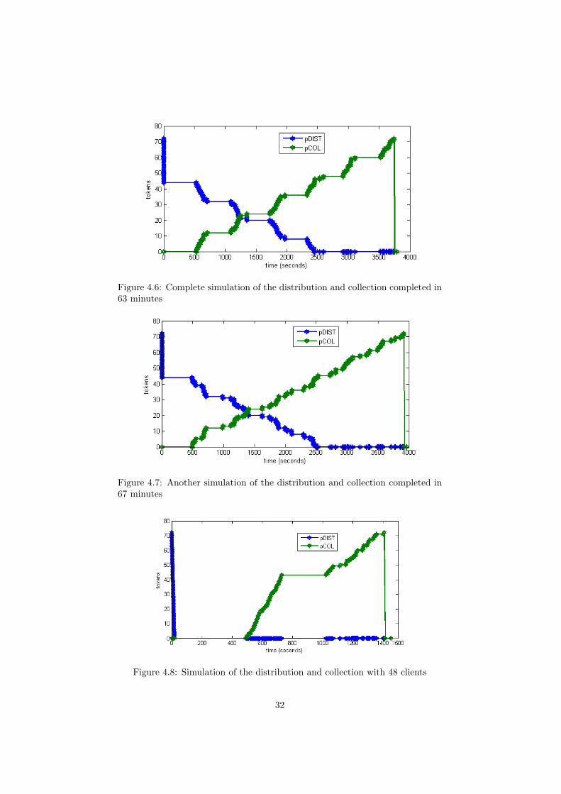
Figure 4.6: Complete simulation of the distribution and collection completed in63 minutes

Figure 4.7: Another simulation of the distribution and collection completed in67 minutes

Figure 4.8: Simulation of the distribution and collection with 48 clients

32

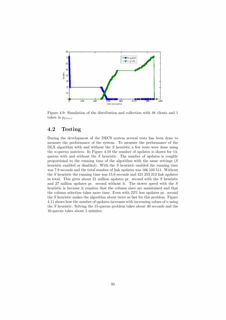
Figure 4.9: Simulation of the distribution and collection with 48 clients and 1token in pfree,i

4.2 Testing

During the development of the DECS system several tests has been done tomeasure the performance of the system. To measure the performance of theDLX algorithm with and without the S heuristic a few tests were done usingthe n-queens matrices. In Figure 4.10 the number of updates is shown for 14-queens with and without the S heuristic. The number of updates is roughlyproportional to the running time of the algorithm with the same settings (Sheuristic enabled or disabled). With the S heuristic enabled the running timewas 7.9 seconds and the total number of link updates was 166 103 511. Withoutthe S heuristic the running time was 15.6 seconds and 421 253 213 link updatesin total. This gives about 21 million updates pr. second with the S heuristicand 27 million updates pr. second without it. The slower speed with the Sheuristic is because it requires that the column sizes are maintained and thatthe column selection takes more time. Even with 22% less updates pr. secondthe S heuristic makes the algorithm about twice as fast for this problem. Figure4.11 shows how the number of updates increases with increasing values of n usingthe S heuristic. Solving the 15-queens problem takes about 40 seconds and the16-queens takes about 5 minutes.

33

0

1e+007

2e+007

3e+007

4e+007

5e+007

6e+007

7e+007

8e+007

9e+007

1e+008

0 1 2 3 4 5 6 7 8 9 10 11 12 13

Upd

ates

Recursion level

Updates with S heuristicUpdates without S heuristic

Figure 4.10: Number of updates with and without the S heuristic for 14-queens

101

102

103

104

105

106

107

108

109

1010

2 3 4 5 6 7 8 9 10 11 12 13 14 15 16

Upd

ates

Queens

Figure 4.11: Log plot of updates with the S heuristic for increasing values of nin n-queens

34

Chapter 5

Conclusion

The goal of this project was to develop a distributed system for solving ex-act cover problems. By using the BOINC framework a working system hasbeen implemented and is now ready to be used. Many challenging exact coverproblems can now be processed by the DECS system if enough users choose toparticipate. Hopefully this project will be able to shed new light on previouslyunsolved problems.

Learning a new programming language and solving new problems has re-sulted in an interesting and useful learning experience. The DECS system hasmany areas where it can be improved and made better. By releasing the sourcecode under an open source license the project will hopefully attract a group ofusers who might be willing to contribute with more than raw CPU power.

5.1 Future work

Implement a compression scheme

To ease the file format explanation and implementation no compression tech-nique was implemented. In cases where an exact cover problem has a very largenumber of solutions it would be an advantage to have some sort of compression.A technique called bit packing described in [4, 13] provides a way to do somesimple compression with a very low performance overhead. By applying thistechnique we can exploit the otherwise unused bits. The bit packing schemecan also be generalized to pack the data even more densely by doing sub-bitprecision packing. The trade off between processing overhead and file size canbe beneficial in cases where the number of solutions is large and where storageand bandwidth resources are scarce. It might also be worth looking into othercompression schemes which are easy to implement.

Implement more transforms

Currently only the n-queens transform has been implemented. The other trans-forms explained in the report could be implemented as well making DECS moreuseful.

35

Improve the Petri net simulation model

The Petri net model could be made more complete by incorporating other as-pects of distributed computing as well. Simulating client failure or maliciousclients submitting incorrect data could be a possible extension. That would re-quire a certain piece of the problem to be sent to multiple clients for redundancyand verification. It would also be a good idea to try to eliminate some of as-sumptions currently present in the simulation. This would make the simulationresults more accurate and true to the actual system.

36

Bibliography

[1] BOINC - Berkeley Open Infrastructure for Network Computing. A softwareplatform for volunteer computing and desktop Grid computing used byprojects such as SETI@home., URL http://boinc.berkeley.edu/.

[2] Bruce Abramson and Moti Yung. Divide and Conquer under Global Con-straints: A Solution to the N -Queens Problem. Journal of Parallel andDistributed Computing, 6:649–662, 1989.

[3] Apache. Hadoop. Hadoop is an open source Java software framework forrunning parallel computation on large clusters of commodity computers.,URL http://lucene.apache.org/hadoop/.

[4] Jonathan Blow. Packing Integers. Game Developer Magazine, pages 16–19,May 2002.

[5] R. D. Chatham. The N+k Queens Problem Page. URL http://people.moreheadstate.edu/fs/d.chatham/n+kqueens.html.

[6] Thomas Clement Mogensen, Frej Soyam, and Alex Esmann. N-dronningproblemet i MiG. URL http://code.google.com/p/queens/.

[7] Intel Corporation. Endianness White Paper, May 2004. URL http://www.intel.com/design/intarch/papers/endian.htm.

[8] Jeffrey Dean and Sanjay Ghemawat. MapReduce: Simplified Data Pro-cessing on Large Clusters. In OSDI’04, 6th Symposium on Operating Sys-tems Design and Implementation, Sponsored by USENIX, in cooperationwith ACM SIGOPS, pages 137–150. 2004. URL http://labs.google.com/papers/mapreduce.html.

[9] Mike Eisler. XDR: External Data Representation Standard. RFC 4506(Standards Track), May 2006. URL http://www.ietf.org/rfc/rfc4506.txt.

[10] M.R. Garey and D.S. Johnson. Computers and Intractability: A Guide tothe Theory of NP-Completeness. W.H. Freeman & Co Ltd, 1979. ISBN0-7167-1045-5.

[11] Al Geist, Adam Beguelin, Jack Dongarra, Weicheng Jiang, RobertManchek, and Vaidy Sunderam. PVM: Parallel Virtual Machine - A Users’Guide and Tutorial for Networked Parallel Computing. MIT Press, Scien-tific and Engineering Computation, 1994. URL http://www.csm.ornl.gov/pvm/.

37

[12] Hirosi Hitotumatu and Kohei Noshita. A Technique for ImplementingBacktrack Algorithms and its Application. Information Processing Letters,8(4):174–175, April 1979.

[13] Pete Isensee. Bit Packing: A Network Compression Technique. GameProgramming Gems 4, pages 571–578, March 2004.

[14] Donald E. Knuth. Estimating the Efficiency of Backtrack Programs. Math-emathics of Computation, 29(129):121–136, January 1975.

[15] Donald E. Knuth. Dancing Links. In Jim Davies, Bill Roscoe, and JimWoodcock, editors, Millenial Perspectives in Computer Science, pages 187–214. Palgrave, Houndmills, Basingstoke, Hampshire, 2000. URL http://www-cs-faculty.stanford.edu/~knuth/preprints.html.

[16] Donald E. Knuth and Silvio Levy. The CWEB System of Structured Doc-umentation. Addison Wesley, 1993. ISBN 0-201-57569-8. CWEB is asoftware system that facilitates the creation of readable programs in C,C++, and Java., URL http://www-cs-faculty.stanford.edu/~knuth/cweb.html.

[17] Arne Maus and Torfinn Aas. PRP - Parallel Recursive Procedures, October1995. URL http://heim.ifi.uio.no/~arnem/PRP/.

[18] Mihai Oltean and Oana Muntean. Exact Cover with light, 2007. URLhttp://arxiv.org/PS_cache/arxiv/pdf/0708/0708.1962v1.pdf.

[19] Carl Adam Petri. Kommunikation mit Automaten. Bonn: Institut fr In-strumentelle Mathematik, Schriften des IIM Nr. 2, 1962.

[20] Carl Adam Petri. Kommunikation mit Automaten. New York: GriffissAir Force Base, Technical Report RADC-TR-65–377, 1:1–Suppl. 1, 1966.English translation.

[21] Michael J. Quinn. Parallel Programming in C with MPI and OpenMP.McGraw-Hill, 2004.

[22] Reggie Davidrajuh. GPenSIM. A general purpose Petri net simulator formathematical modeling and simulation of discrete-event systems in MAT-LAB., URL http://www.davidrajuh.net/gpensim/.

[23] Arnon Rotem-Gal-Oz. Fallacies of Distributed Computing Explained. URLhttp://www.rgoarchitects.com/Files/fallacies.pdf.

[24] Universidad de Concepcin. NQueens@Home. URL http://nqueens.ing.udec.cl/.

[25] Brian Vinter. The Architecture of the Minimum intrusion Grid, MiG.Communicating Process Architectures, 2005.

[26] Alfred Wassermann. Covering the Aztec Diamond with One-sided Tetra-sticks – Extended Version, December 1999. URL http://did.mat.uni-bayreuth.de/wassermann/.

38