Generic Programming

Jesse Perla, Thomas J. Sargent and John Stachurski

July 23, 2020

1 Contents

• Overview 2• Exploring Type Trees 3• Distributions 4• Numbers and Algebraic Structures 5• Reals and Algebraic Structures 6• Functions, and Function-Like Types 7• Limitations of Dispatching on Abstract Types 8• Exercises 9

I find OOP methodologically wrong. It starts with classes. It is as if mathemati-cians would start with axioms. You do not start with axioms - you start withproofs. Only when you have found a bunch of related proofs, can you come upwith axioms. You end with axioms. The same thing is true in programming: youhave to start with interesting algorithms. Only when you understand them well,can you come up with an interface that will let them work. – Alexander Stepanov

2 Overview

In this lecture we delve more deeply into the structure of Julia, and in particular into

• abstract and concrete types• the type tree• designing and using generic interfaces• the role of generic interfaces in Julia performance

Understanding them will help you

• form a “mental model” of the Julia language• design code that matches the “white-board” mathematics• create code that can use (and be used by) a variety of other packages• write “well organized” Julia code that’s easy to read, modify, maintain and debug• improve the speed at which your code runs

(Special thank you to Jeffrey Sarnoff)

1

2.1 Generic Programming is an Attitude

From Mathematics to Generic Programming [1]

Generic programming is an approach to programming that focuses on designingalgorithms and data structures so that they work in the most general setting with-out loss of efficiency… Generic programming is more of an attitude toward pro-gramming than a particular set of tools.

In that sense, it is important to think of generic programming as an interactive approach touncover generality without compromising performance rather than as a set of rules.

As we will see, the core approach is to treat data structures and algorithms as loosely cou-pled, and is in direct contrast to the is-a approach of object-oriented programming.

This lecture has the dual role of giving an introduction into the design of generic algorithmsand describing how Julia helps make that possible.

2.2 Setup

In [1]: using InstantiateFromURL# optionally add arguments to force installation: instantiate = true,�

↪precompile = truegithub_project("QuantEcon/quantecon-notebooks-julia", version = "0.8.0")

In [2]: using LinearAlgebra, Statisticsusing Distributions, Plots, QuadGK, Polynomials, Interpolationsgr(fmt = :png);

3 Exploring Type Trees

The connection between data structures and the algorithms which operate on them is handledby the type system.

Concrete types (i.e., Float64 or Array{Float64, 2}) are the data structures we applyan algorithm to, and the abstract types (e.g. the corresponding Number and AbstractAr-ray) provide the mapping between a set of related data structures and algorithms.

In [3]: using Distributionsx = 1y = Normal()z = "foo"@show x, y, z@show typeof(x), typeof(y), typeof(z)@show supertype(typeof(x))

# pipe operator, |>, is is equivalent@show typeof(x) |> supertype@show supertype(typeof(y))@show typeof(z) |> supertype@show typeof(x) <: Any;

2

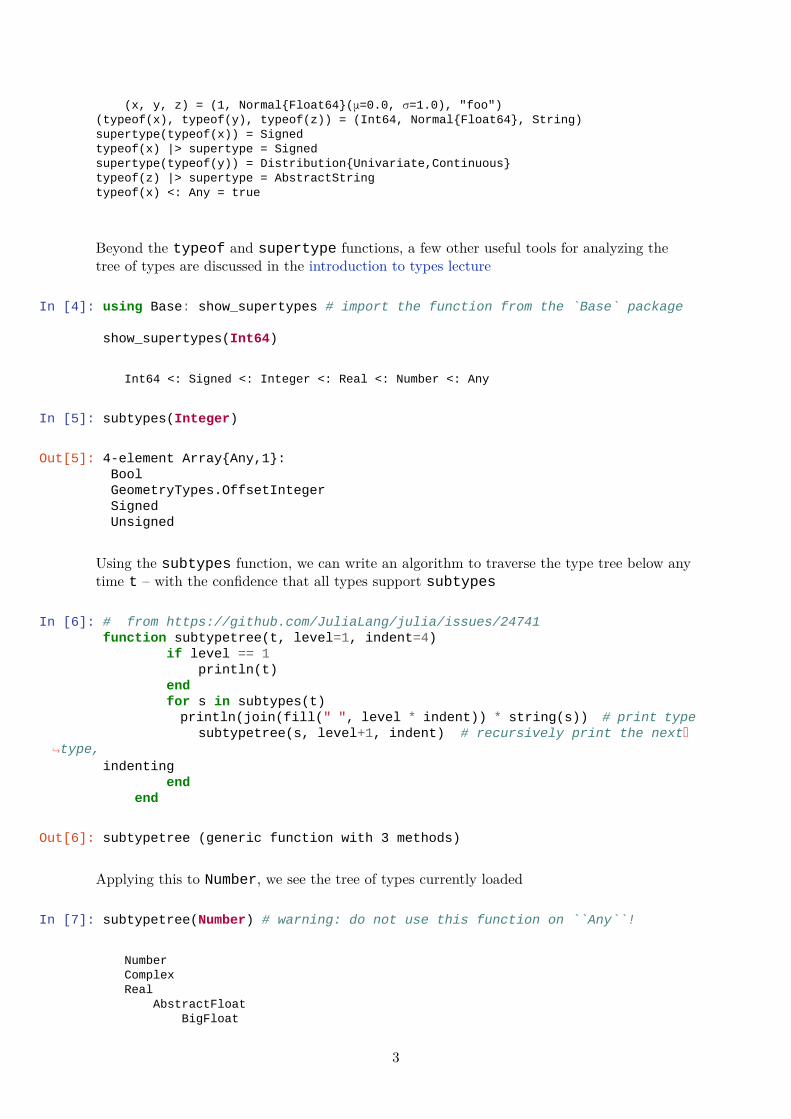
(x, y, z) = (1, Normal{Float64}(μ=0.0, σ=1.0), "foo")(typeof(x), typeof(y), typeof(z)) = (Int64, Normal{Float64}, String)supertype(typeof(x)) = Signedtypeof(x) |> supertype = Signedsupertype(typeof(y)) = Distribution{Univariate,Continuous}typeof(z) |> supertype = AbstractStringtypeof(x) <: Any = true

Beyond the typeof and supertype functions, a few other useful tools for analyzing thetree of types are discussed in the introduction to types lecture

In [4]: using Base: show_supertypes # import the function from the `Base` package

show_supertypes(Int64)

Int64 <: Signed <: Integer <: Real <: Number <: Any

In [5]: subtypes(Integer)

Out[5]: 4-element Array{Any,1}:BoolGeometryTypes.OffsetIntegerSignedUnsigned

Using the subtypes function, we can write an algorithm to traverse the type tree below anytime t – with the confidence that all types support subtypes

In [6]: # from https://github.com/JuliaLang/julia/issues/24741function subtypetree(t, level=1, indent=4)

if level == 1println(t)

endfor s in subtypes(t)println(join(fill(" ", level * indent)) * string(s)) # print type

subtypetree(s, level+1, indent) # recursively print the next�↪type,

indentingend

end

Out[6]: subtypetree (generic function with 3 methods)

Applying this to Number, we see the tree of types currently loaded

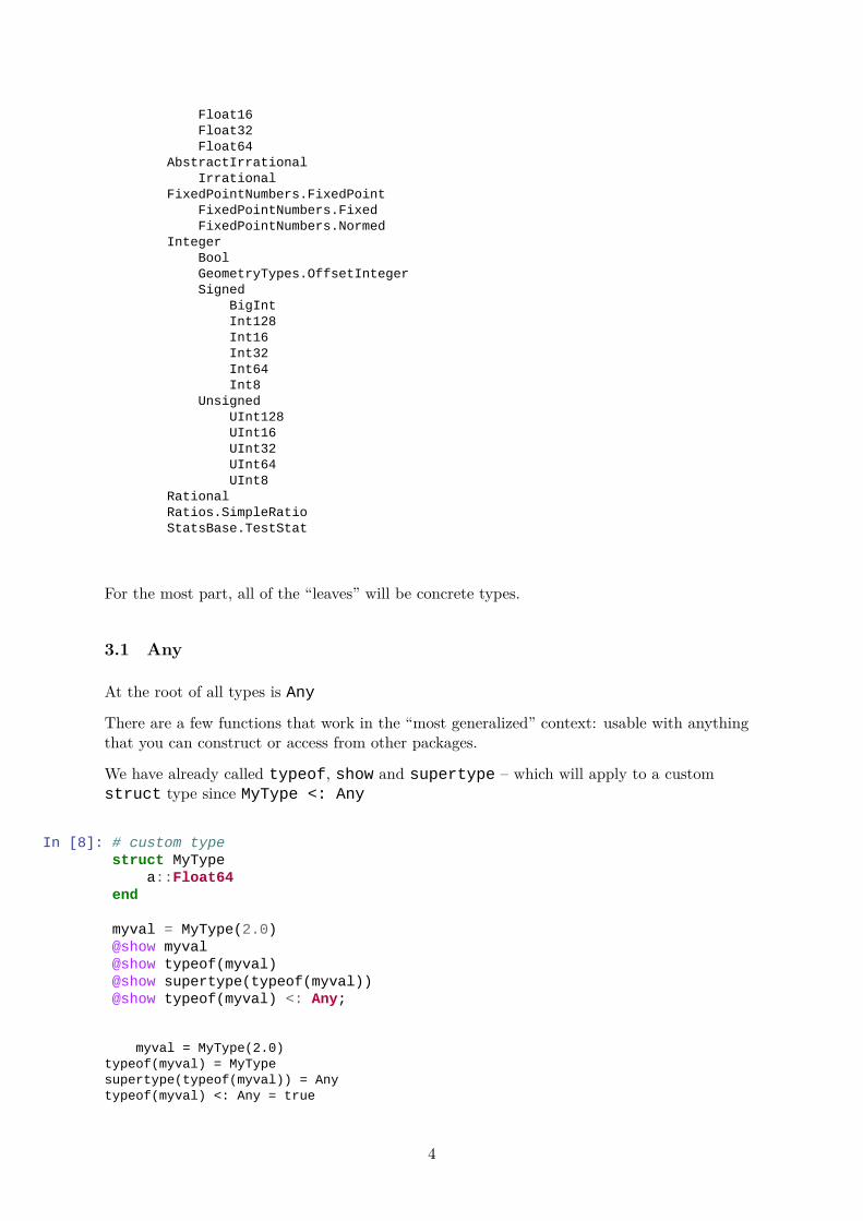
In [7]: subtypetree(Number) # warning: do not use this function on ``Any``!

NumberComplexReal

AbstractFloatBigFloat

3

Float16Float32Float64

AbstractIrrationalIrrational

FixedPointNumbers.FixedPointFixedPointNumbers.FixedFixedPointNumbers.Normed

IntegerBoolGeometryTypes.OffsetIntegerSigned

BigIntInt128Int16Int32Int64Int8

UnsignedUInt128UInt16UInt32UInt64UInt8

RationalRatios.SimpleRatioStatsBase.TestStat

For the most part, all of the “leaves” will be concrete types.

3.1 Any

At the root of all types is Any

There are a few functions that work in the “most generalized” context: usable with anythingthat you can construct or access from other packages.

We have already called typeof, show and supertype – which will apply to a customstruct type since MyType <: Any

In [8]: # custom typestruct MyType

a::Float64end

myval = MyType(2.0)@show myval@show typeof(myval)@show supertype(typeof(myval))@show typeof(myval) <: Any;

myval = MyType(2.0)typeof(myval) = MyTypesupertype(typeof(myval)) = Anytypeof(myval) <: Any = true

4

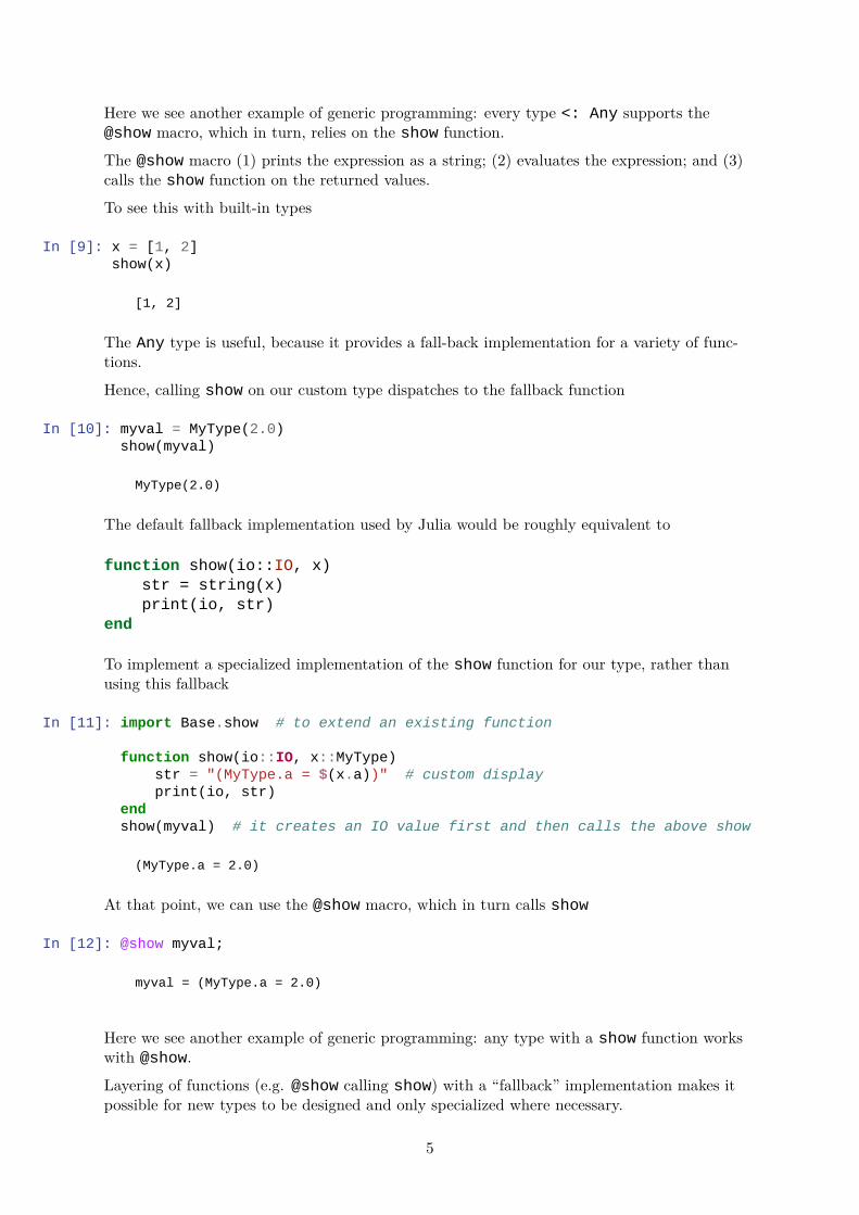
Here we see another example of generic programming: every type <: Any supports the@show macro, which in turn, relies on the show function.

The @show macro (1) prints the expression as a string; (2) evaluates the expression; and (3)calls the show function on the returned values.

To see this with built-in types

In [9]: x = [1, 2]show(x)

[1, 2]

The Any type is useful, because it provides a fall-back implementation for a variety of func-tions.

Hence, calling show on our custom type dispatches to the fallback function

In [10]: myval = MyType(2.0)show(myval)

MyType(2.0)

The default fallback implementation used by Julia would be roughly equivalent to

function show(io::IO, x)str = string(x)print(io, str)

end

To implement a specialized implementation of the show function for our type, rather thanusing this fallback

In [11]: import Base.show # to extend an existing function

function show(io::IO, x::MyType)str = "(MyType.a = $(x.a))" # custom displayprint(io, str)

endshow(myval) # it creates an IO value first and then calls the above show

(MyType.a = 2.0)

At that point, we can use the @show macro, which in turn calls show

In [12]: @show myval;

myval = (MyType.a = 2.0)

Here we see another example of generic programming: any type with a show function workswith @show.

Layering of functions (e.g. @show calling show) with a “fallback” implementation makes itpossible for new types to be designed and only specialized where necessary.

5

3.2 Unlearning Object Oriented (OO) Programming (Advanced)

See Types for more on OO vs. generic types.

If you have never used programming languages such as C++, Java, and Python, then thetype hierarchies above may seem unfamiliar and abstract.

In that case, keep an open mind that this discussion of abstract concepts will have practicalconsequences, but there is no need to read this section.

Otherwise, if you have used object-oriented programming (OOP) in those languages, thensome of the concepts in these lecture notes will appear familiar.

Don’t be fooled!

The superficial similarity can lead to misuse: types are not classes with poor encapsula-tion, and methods are not the equivalent to member functions with the order of argumentsswapped.

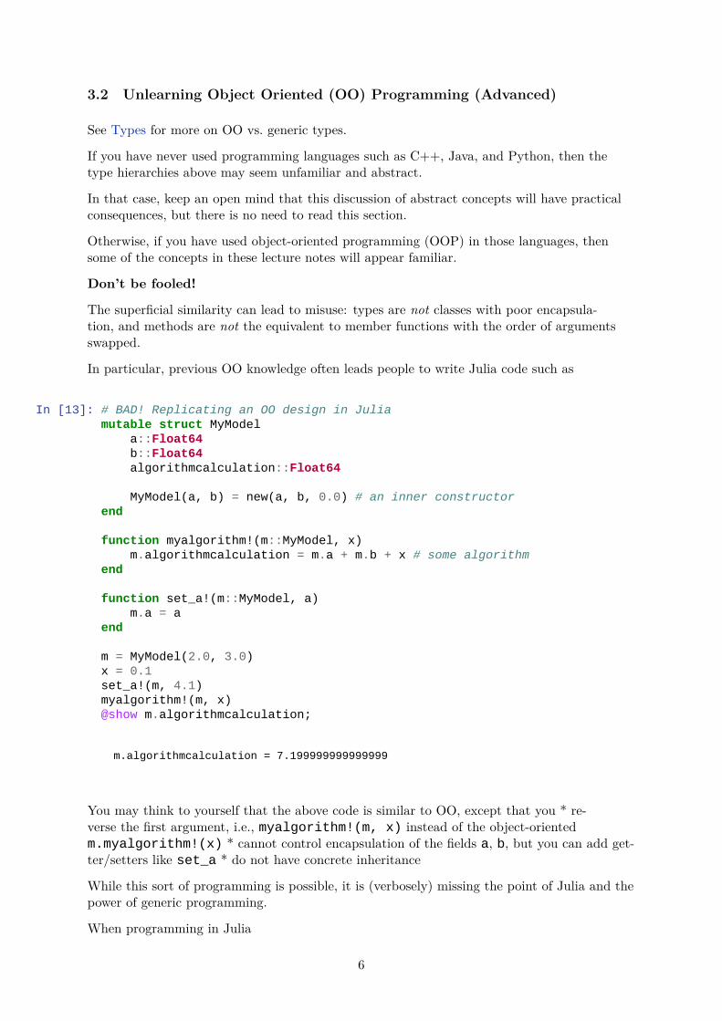
In particular, previous OO knowledge often leads people to write Julia code such as

In [13]: # BAD! Replicating an OO design in Juliamutable struct MyModel

a::Float64b::Float64algorithmcalculation::Float64

MyModel(a, b) = new(a, b, 0.0) # an inner constructorend

function myalgorithm!(m::MyModel, x)m.algorithmcalculation = m.a + m.b + x # some algorithm

end

function set_a!(m::MyModel, a)m.a = a

end

m = MyModel(2.0, 3.0)x = 0.1set_a!(m, 4.1)myalgorithm!(m, x)@show m.algorithmcalculation;

m.algorithmcalculation = 7.199999999999999

You may think to yourself that the above code is similar to OO, except that you * re-verse the first argument, i.e., myalgorithm!(m, x) instead of the object-orientedm.myalgorithm!(x) * cannot control encapsulation of the fields a, b, but you can add get-ter/setters like set_a * do not have concrete inheritance

While this sort of programming is possible, it is (verbosely) missing the point of Julia and thepower of generic programming.

When programming in Julia

6

• there is no encapsulation and most custom types you create will be im-mutable.

• Polymorphism is achieved without anything resembling OOP inheritance.• Abstraction is implemented by keeping the data and algorithms that operate on them

as orthogonal as possible – in direct contrast to OOP’s association of algorithms andmethods directly with a type in a tree.

• The supertypes in Julia are simply used for selecting which specialized algorithm to use(i.e., part of generic polymorphism) and have nothing to do with OO inheritance.

• The looseness that accompanies keeping algorithms and data structures as orthogonal aspossible makes it easier to discover commonality in the design.

3.2.1 Iterative Design of Abstractions

As its essence, the design of generic software is that you will start with creating algorithmswhich are largely orthogonal to concrete types.

In the process, you will discover commonality which leads to abstract types with informallydefined functions operating on them.

Given the abstract types and commonality, you then refine the algorithms as they are morelimited or more general than you initially thought.

This approach is in direct contrast to object-oriented design and analysis (OOAD).

With that, where you specify a taxonomies of types, add operations to those types, and thenmove down to various levels of specialization (where algorithms are embedded at pointswithin the taxonomy, and potentially specialized with inheritance).

In the examples that follow, we will show for exposition the hierarchy of types and the algo-rithms operating on them, but the reality is that the algorithms are often designed first, andthe abstact types came later.

4 Distributions

First, consider working with “distributions”.

Algorithms using distributions might (1) draw random numbers for Monte-Carlo methods;and (2) calculate the pdf or cdf – if it is defined.

The process of using concrete distributions in these sorts of applications led to the creation ofthe Distributions.jl package.

Let’s examine the tree of types for a Normal distribution

In [14]: using Distributionsd1 = Normal(1.0, 2.0) # an example type to explore@show d1show_supertypes(typeof(d1))

d1 = Normal{Float64}(μ=1.0, σ=2.0)Normal{Float64} <: Distribution{Univariate,Continuous} <:Sampleable{Univariate,Continuous} <: Any

7

The Sampleable{Univariate,Continuous} type has a limited number of functions,chiefly the ability to draw a random number

In [15]: @show rand(d1);

rand(d1) = 0.39874233573413165

The purpose of that abstract type is to provide an interface for drawing from a variety of dis-tributions, some of which may not have a well-defined predefined pdf.

If you were writing a function to simulate a stochastic process with arbitrary iid shocks,where you did not need to assume an existing pdf etc., this is a natural candidate.

For example, to simulate 𝑥𝑡+1 = 𝑎𝑥𝑡 + 𝑏𝜖𝑡+1 where 𝜖 ∼ 𝐷 for some 𝐷, which allows drawingrandom values.

In [16]: function simulateprocess(x�; a = 1.0, b = 1.0, N = 5,d::Sampleable{Univariate,Continuous})

x = zeros(typeof(x�), N+1) # preallocate vector, careful on the typex[1] = x�for t in 2:N+1

x[t] = a * x[t-1] + b * rand(d) # drawendreturn x

end@show simulateprocess(0.0, d=Normal(0.2, 2.0));

simulateprocess(0.0, d = Normal(0.2, 2.0)) = [0.0, 1.3280876101452868,4.723250702951301, 6.733054883502428, 6.562190243882545, 8.452982642957956]

The Sampleable{Univariate,Continuous} and, especially, the Sam-pleable{Multivariate,Continuous} abstract types are useful generic interfaces forMonte-Carlo and Bayesian methods.

Moving down the tree, the Distributions{Univariate, Continuous} abstract typehas other functions we can use for generic algorithms operating on distributions.

These match the mathematics, such as pdf, cdf, quantile, support, minimum, maxi-mum, etc.

In [17]: d1 = Normal(1.0, 2.0)d2 = Exponential(0.1)@show d1@show d2@show supertype(typeof(d1))@show supertype(typeof(d2))

@show pdf(d1, 0.1)@show pdf(d2, 0.1)@show cdf(d1, 0.1)@show cdf(d2, 0.1)@show support(d1)@show support(d2)

8

@show minimum(d1)@show minimum(d2)@show maximum(d1)@show maximum(d2);

d1 = Normal{Float64}(μ=1.0, σ=2.0)d2 = Exponential{Float64}(θ=0.1)supertype(typeof(d1)) = Distribution{Univariate,Continuous}supertype(typeof(d2)) = Distribution{Univariate,Continuous}pdf(d1, 0.1) = 0.18026348123082397pdf(d2, 0.1) = 3.6787944117144233cdf(d1, 0.1) = 0.32635522028792cdf(d2, 0.1) = 0.6321205588285577support(d1) = RealInterval(-Inf, Inf)support(d2) = RealInterval(0.0, Inf)minimum(d1) = -Infminimum(d2) = 0.0maximum(d1) = Infmaximum(d2) = Inf

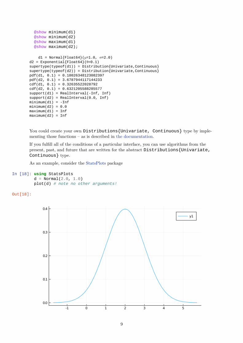
You could create your own Distributions{Univariate, Continuous} type by imple-menting those functions – as is described in the documentation.If you fulfill all of the conditions of a particular interface, you can use algorithms from thepresent, past, and future that are written for the abstract Distributions{Univariate,Continuous} type.As an example, consider the StatsPlots package

In [18]: using StatsPlotsd = Normal(2.0, 1.0)plot(d) # note no other arguments!

Out[18]:

9

Calling plot on any subtype of Distributions{Univariate, Continuous} displaysthe pdf and uses minimum and maximum to determine the range.

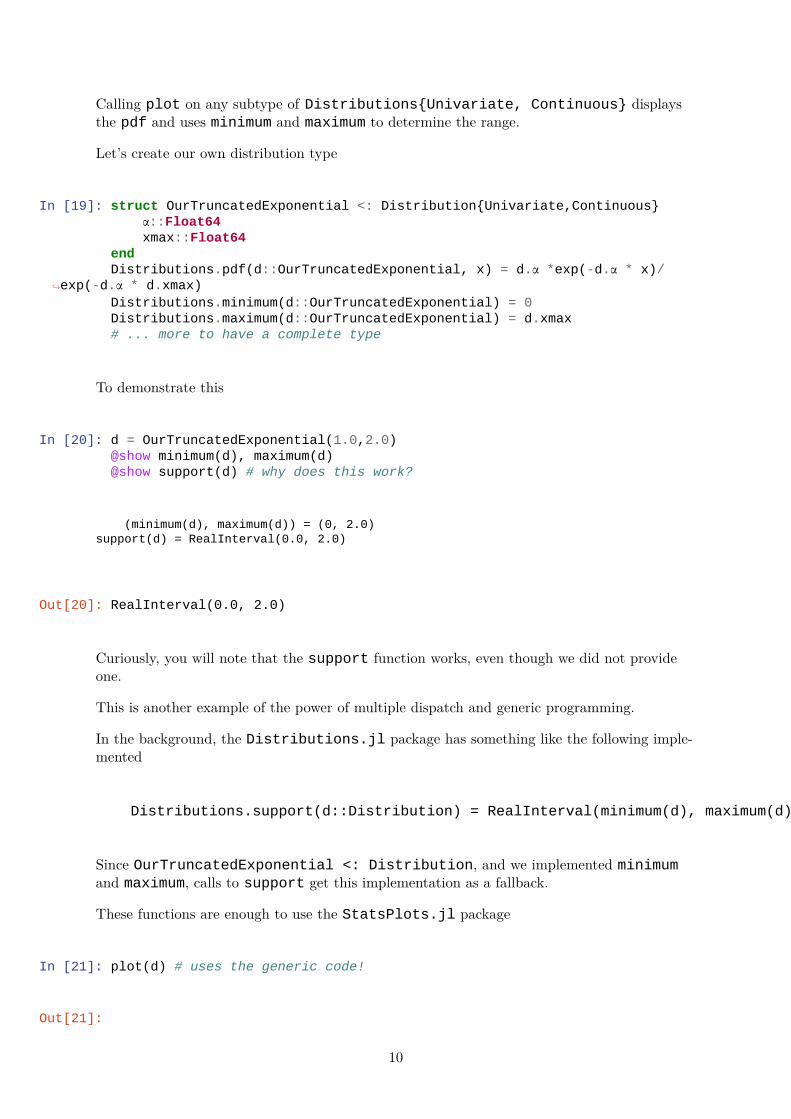
Let’s create our own distribution type

In [19]: struct OurTruncatedExponential <: Distribution{Univariate,Continuous}α::Float64xmax::Float64

endDistributions.pdf(d::OurTruncatedExponential, x) = d.α *exp(-d.α * x)/

↪exp(-d.α * d.xmax)Distributions.minimum(d::OurTruncatedExponential) = 0Distributions.maximum(d::OurTruncatedExponential) = d.xmax# ... more to have a complete type

To demonstrate this

In [20]: d = OurTruncatedExponential(1.0,2.0)@show minimum(d), maximum(d)@show support(d) # why does this work?

(minimum(d), maximum(d)) = (0, 2.0)support(d) = RealInterval(0.0, 2.0)

Out[20]: RealInterval(0.0, 2.0)

Curiously, you will note that the support function works, even though we did not provideone.

This is another example of the power of multiple dispatch and generic programming.

In the background, the Distributions.jl package has something like the following imple-mented

Distributions.support(d::Distribution) = RealInterval(minimum(d), maximum(d))

Since OurTruncatedExponential <: Distribution, and we implemented minimumand maximum, calls to support get this implementation as a fallback.

These functions are enough to use the StatsPlots.jl package

In [21]: plot(d) # uses the generic code!

Out[21]:

10

A few things to point out

• Even if it worked for StatsPlots, our implementation is incomplete, as we haven’tfulfilled all of the requirements of a Distribution.

• We also did not implement the rand function, which means we are breaking the im-plicit contract of the Sampleable abstract type.

• It turns out that there is a better way to do this precise thing already built into Dis-tributions.

In [22]: d = Truncated(Exponential(0.1), 0.0, 2.0)@show typeof(d)plot(d)

typeof(d) = Truncated{Exponential{Float64},Continuous,Float64}

Out[22]:

11

This is the power of generic programming in general, and Julia in particular: you can com-bine and compose completely separate packages and code, as long as there is an agreement onabstract types and functions.

5 Numbers and Algebraic Structures

Define two binary functions, + and ⋅, called addition and multiplication – although the opera-tors can be applied to data structures much more abstract than a Real.

In mathematics, a ring is a set with associated additive and multiplicative operators where

• the additive operator is associative and commutative

• the multiplicative operator is associative and distributive with respect to the additiveoperator

• there is an additive identity element, denoted 0, such that 𝑎 + 0 = 𝑎 for any 𝑎 in the set• there is an additive inverse of each element, denoted −𝑎, such that 𝑎 + (−𝑎) = 0• there is a multiplicative identity element, denoted 1, such that 𝑎 ⋅ 1 = 𝑎 = 1 ⋅ 𝑎• a total or partial ordering is not required (i.e., there does not need to be any meaning-

ful < operator defined)• a multiplicative inverse is not required

While this skips over some parts of the mathematical definition, this algebraic structure pro-vides motivation for the abstract Number type in Julia

• Remark: We use the term “motivation” because they are not formally con-nected and the mapping is imperfect.

• The main difficulty when dealing with numbers that can be concretely created on acomputer is that the requirement that the operators are closed in the set are difficultto ensure (e.g. floating points have finite numbers of bits of information).

12

Let typeof(a) = typeof(b) = T <: Number, then under an informal definition of thegeneric interface for Number, the following must be defined

• the additive operator: a + b

• the multiplicative operator: a * b• an additive inverse operator: -a• an inverse operation for addition a - b = a + (-b)• an additive identity: zero(T) or zero(a) for convenience• a multiplicative identity: one(T) or one(a) for convenience

The core of generic programming is that, given the knowledge that a value is of type Number,we can design algorithms using any of these functions and not concern ourselves with the par-ticular concrete type.

Furthermore, that generality in designing algorithms comes with no compromises on perfor-mance compared to carefully designed algorithms written for that particular type.

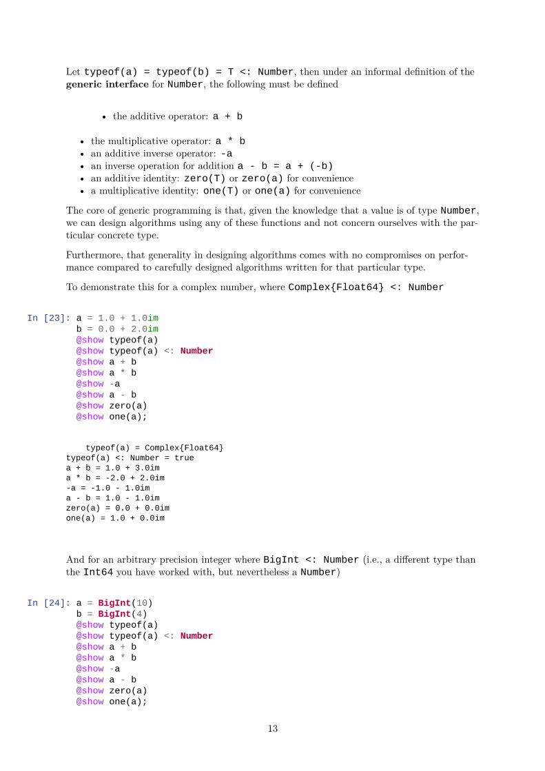
To demonstrate this for a complex number, where Complex{Float64} <: Number

In [23]: a = 1.0 + 1.0imb = 0.0 + 2.0im@show typeof(a)@show typeof(a) <: Number@show a + b@show a * b@show -a@show a - b@show zero(a)@show one(a);

typeof(a) = Complex{Float64}typeof(a) <: Number = truea + b = 1.0 + 3.0ima * b = -2.0 + 2.0im-a = -1.0 - 1.0ima - b = 1.0 - 1.0imzero(a) = 0.0 + 0.0imone(a) = 1.0 + 0.0im

And for an arbitrary precision integer where BigInt <: Number (i.e., a different type thanthe Int64 you have worked with, but nevertheless a Number)

In [24]: a = BigInt(10)b = BigInt(4)@show typeof(a)@show typeof(a) <: Number@show a + b@show a * b@show -a@show a - b@show zero(a)@show one(a);

13

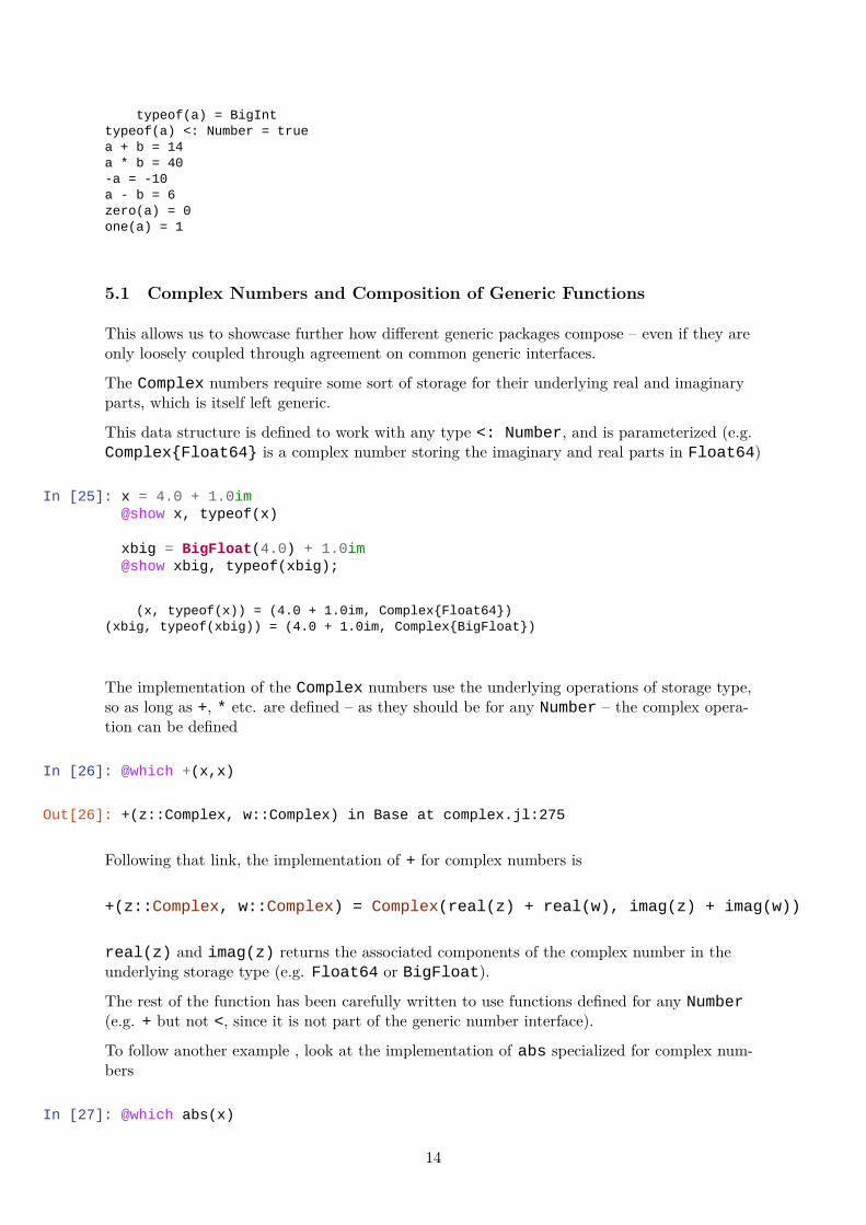
typeof(a) = BigInttypeof(a) <: Number = truea + b = 14a * b = 40-a = -10a - b = 6zero(a) = 0one(a) = 1

5.1 Complex Numbers and Composition of Generic Functions

This allows us to showcase further how different generic packages compose – even if they areonly loosely coupled through agreement on common generic interfaces.

The Complex numbers require some sort of storage for their underlying real and imaginaryparts, which is itself left generic.

This data structure is defined to work with any type <: Number, and is parameterized (e.g.Complex{Float64} is a complex number storing the imaginary and real parts in Float64)

In [25]: x = 4.0 + 1.0im@show x, typeof(x)

xbig = BigFloat(4.0) + 1.0im@show xbig, typeof(xbig);

(x, typeof(x)) = (4.0 + 1.0im, Complex{Float64})(xbig, typeof(xbig)) = (4.0 + 1.0im, Complex{BigFloat})

The implementation of the Complex numbers use the underlying operations of storage type,so as long as +, * etc. are defined – as they should be for any Number – the complex opera-tion can be defined

In [26]: @which +(x,x)

Out[26]: +(z::Complex, w::Complex) in Base at complex.jl:275

Following that link, the implementation of + for complex numbers is

+(z::Complex, w::Complex) = Complex(real(z) + real(w), imag(z) + imag(w))

real(z) and imag(z) returns the associated components of the complex number in theunderlying storage type (e.g. Float64 or BigFloat).

The rest of the function has been carefully written to use functions defined for any Number(e.g. + but not <, since it is not part of the generic number interface).

To follow another example , look at the implementation of abs specialized for complex num-bers

In [27]: @which abs(x)

14

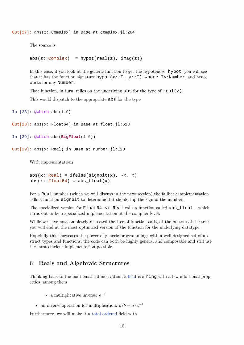
Out[27]: abs(z::Complex) in Base at complex.jl:264

The source is

abs(z::Complex) = hypot(real(z), imag(z))

In this case, if you look at the generic function to get the hypotenuse, hypot, you will seethat it has the function signature hypot(x::T, y::T) where T<:Number, and henceworks for any Number.

That function, in turn, relies on the underlying abs for the type of real(z).

This would dispatch to the appropriate abs for the type

In [28]: @which abs(1.0)

Out[28]: abs(x::Float64) in Base at float.jl:528

In [29]: @which abs(BigFloat(1.0))

Out[29]: abs(x::Real) in Base at number.jl:120

With implementations

abs(x::Real) = ifelse(signbit(x), -x, x)abs(x::Float64) = abs_float(x)

For a Real number (which we will discuss in the next section) the fallback implementationcalls a function signbit to determine if it should flip the sign of the number.

The specialized version for Float64 <: Real calls a function called abs_float – whichturns out to be a specialized implementation at the compiler level.

While we have not completely dissected the tree of function calls, at the bottom of the treeyou will end at the most optimized version of the function for the underlying datatype.

Hopefully this showcases the power of generic programming: with a well-designed set of ab-stract types and functions, the code can both be highly general and composable and still usethe most efficient implementation possible.

6 Reals and Algebraic Structures

Thinking back to the mathematical motivation, a field is a ring with a few additional prop-erties, among them

• a multiplicative inverse: 𝑎−1

• an inverse operation for multiplication: 𝑎/𝑏 = 𝑎 ⋅ 𝑏−1

Furthermore, we will make it a total ordered field with

15

• a total ordering binary operator: 𝑎 < 𝑏

This type gives some motivation for the operations and properties of the Real type.

Of course, Complex{Float64} <: Number but not Real – since the ordering is not de-fined for complex numbers in mathematics.

These operations are implemented in any subtype of Real through

• the multiplicative inverse: inv(a)

• the multiplicative inverse operation: a / b = a * inv(b)• an ordering a < b

We have already shown these with the Float64 and BigFloat.

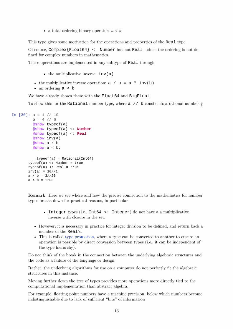
To show this for the Rational number type, where a // b constructs a rational number 𝑎𝑏

In [30]: a = 1 // 10b = 4 // 6@show typeof(a)@show typeof(a) <: Number@show typeof(a) <: Real@show inv(a)@show a / b@show a < b;

typeof(a) = Rational{Int64}typeof(a) <: Number = truetypeof(a) <: Real = trueinv(a) = 10//1a / b = 3//20a < b = true

Remark: Here we see where and how the precise connection to the mathematics for numbertypes breaks down for practical reasons, in particular

• Integer types (i.e., Int64 <: Integer) do not have a a multiplicativeinverse with closure in the set.

• However, it is necessary in practice for integer division to be defined, and return back amember of the Real’s.

• This is called type promotion, where a type can be converted to another to ensure anoperation is possible by direct conversion between types (i.e., it can be independent ofthe type hierarchy).

Do not think of the break in the connection between the underlying algebraic structures andthe code as a failure of the language or design.

Rather, the underlying algorithms for use on a computer do not perfectly fit the algebraicstructures in this instance.

Moving further down the tree of types provides more operations more directly tied to thecomputational implementation than abstract algebra.

For example, floating point numbers have a machine precision, below which numbers becomeindistinguishable due to lack of sufficient “bits” of information

16

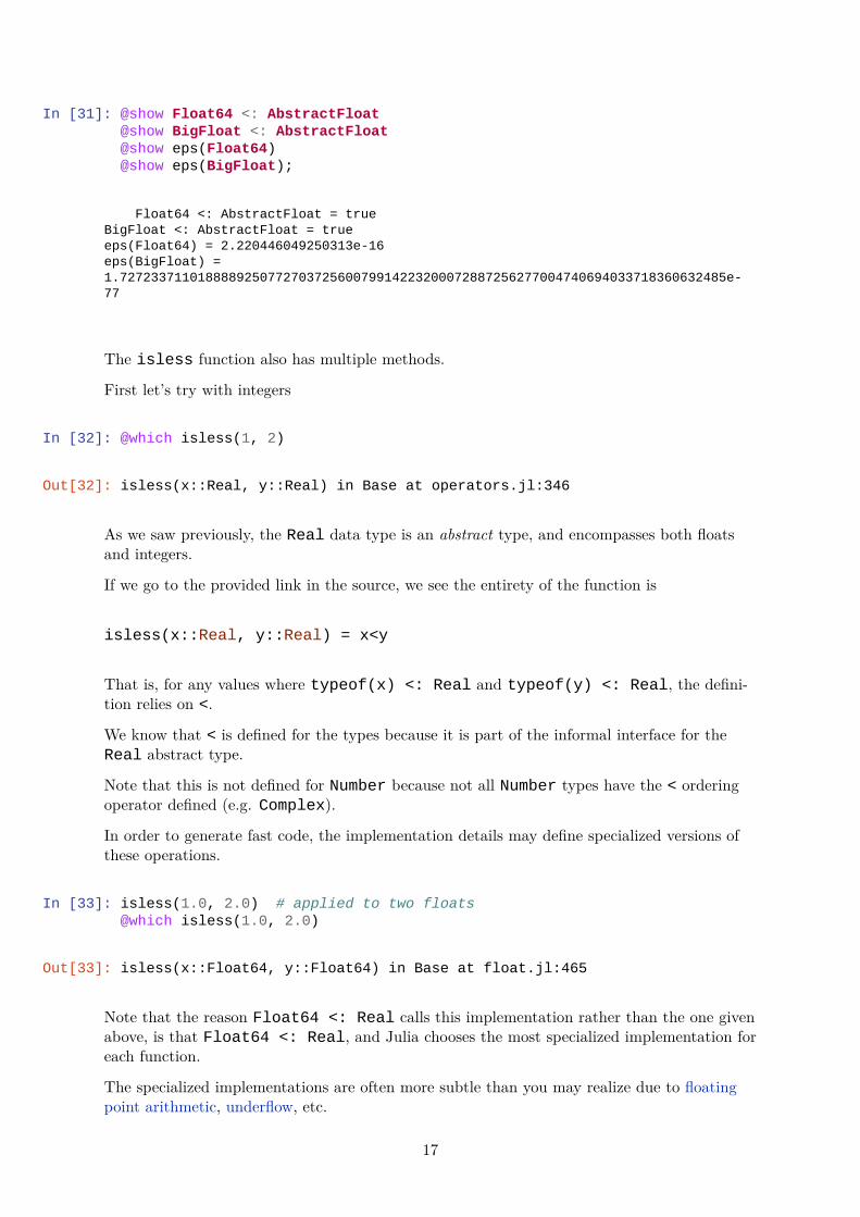
In [31]: @show Float64 <: AbstractFloat@show BigFloat <: AbstractFloat@show eps(Float64)@show eps(BigFloat);

Float64 <: AbstractFloat = trueBigFloat <: AbstractFloat = trueeps(Float64) = 2.220446049250313e-16eps(BigFloat) =1.727233711018888925077270372560079914223200072887256277004740694033718360632485e-77

The isless function also has multiple methods.

First let’s try with integers

In [32]: @which isless(1, 2)

Out[32]: isless(x::Real, y::Real) in Base at operators.jl:346

As we saw previously, the Real data type is an abstract type, and encompasses both floatsand integers.

If we go to the provided link in the source, we see the entirety of the function is

isless(x::Real, y::Real) = x<y

That is, for any values where typeof(x) <: Real and typeof(y) <: Real, the defini-tion relies on <.

We know that < is defined for the types because it is part of the informal interface for theReal abstract type.

Note that this is not defined for Number because not all Number types have the < orderingoperator defined (e.g. Complex).

In order to generate fast code, the implementation details may define specialized versions ofthese operations.

In [33]: isless(1.0, 2.0) # applied to two floats@which isless(1.0, 2.0)

Out[33]: isless(x::Float64, y::Float64) in Base at float.jl:465

Note that the reason Float64 <: Real calls this implementation rather than the one givenabove, is that Float64 <: Real, and Julia chooses the most specialized implementation foreach function.

The specialized implementations are often more subtle than you may realize due to floatingpoint arithmetic, underflow, etc.

17

7 Functions, and Function-Like Types

Another common example of the separation between data structures and algorithms is theuse of functions.

Syntactically, a univariate “function” is any f that can call an argument x as f(x).

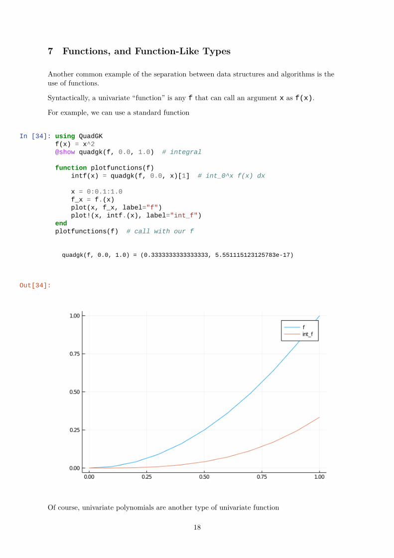
For example, we can use a standard function

In [34]: using QuadGKf(x) = x^2@show quadgk(f, 0.0, 1.0) # integral

function plotfunctions(f)intf(x) = quadgk(f, 0.0, x)[1] # int_0^x f(x) dx

x = 0:0.1:1.0f_x = f.(x)plot(x, f_x, label="f")plot!(x, intf.(x), label="int_f")

endplotfunctions(f) # call with our f

quadgk(f, 0.0, 1.0) = (0.3333333333333333, 5.551115123125783e-17)

Out[34]:

Of course, univariate polynomials are another type of univariate function

18

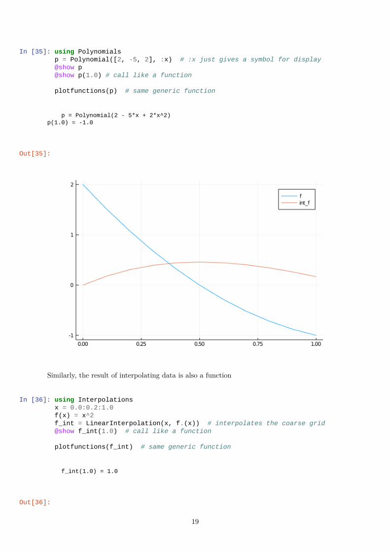
In [35]: using Polynomialsp = Polynomial([2, -5, 2], :x) # :x just gives a symbol for display@show p@show p(1.0) # call like a function

plotfunctions(p) # same generic function

p = Polynomial(2 - 5*x + 2*x^2)p(1.0) = -1.0

Out[35]:

Similarly, the result of interpolating data is also a function

In [36]: using Interpolationsx = 0.0:0.2:1.0f(x) = x^2f_int = LinearInterpolation(x, f.(x)) # interpolates the coarse grid@show f_int(1.0) # call like a function

plotfunctions(f_int) # same generic function

f_int(1.0) = 1.0

Out[36]:

19

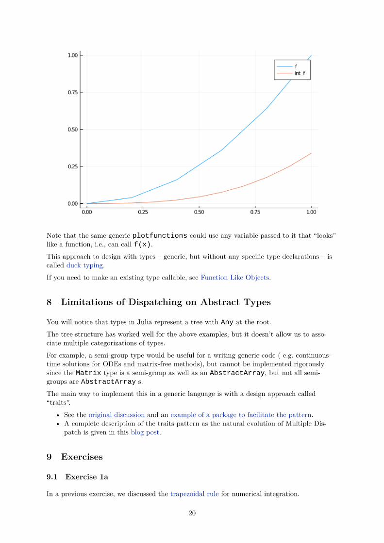
Note that the same generic plotfunctions could use any variable passed to it that “looks”like a function, i.e., can call f(x).This approach to design with types – generic, but without any specific type declarations – iscalled duck typing.If you need to make an existing type callable, see Function Like Objects.

8 Limitations of Dispatching on Abstract Types

You will notice that types in Julia represent a tree with Any at the root.The tree structure has worked well for the above examples, but it doesn’t allow us to asso-ciate multiple categorizations of types.For example, a semi-group type would be useful for a writing generic code ( e.g. continuous-time solutions for ODEs and matrix-free methods), but cannot be implemented rigorouslysince the Matrix type is a semi-group as well as an AbstractArray, but not all semi-groups are AbstractArray s.The main way to implement this in a generic language is with a design approach called“traits”.

• See the original discussion and an example of a package to facilitate the pattern.• A complete description of the traits pattern as the natural evolution of Multiple Dis-

patch is given in this blog post.

9 Exercises

9.1 Exercise 1a

In a previous exercise, we discussed the trapezoidal rule for numerical integration.

20

To summarize, the vector

∫�̄�

𝑥𝑓(𝑥) 𝑑𝑥 ≈ 𝜔 ⋅ ⃗𝑓

where ⃗𝑓 ≡ [𝑓(𝑥1) … 𝑓(𝑥𝑁)] ∈ 𝑅𝑁 and, for a uniform grid spacing of Δ,

𝜔 ≡ Δ [12 1 … 1 1

2] ∈ 𝑅𝑁

The quadrature rule can be implemented easily as

In [37]: using LinearAlgebrafunction trap_weights(x)

return step(x) * [0.5; ones(length(x) - 2); 0.5]endx = range(0.0, 1.0, length = 100)ω = trap_weights(x)f(x) = x^2dot(f.(x), ω)

Out[37]: 0.3333503384008434

However, in this case the creation of the ω temporary is inefficient as there are no rea-sons to allocate an entire vector just to iterate through it with the dot. Instead, createan iterable by following the interface definition for Iteration, and implement the modifiedtrap_weights and integration.

Hint: create a type such as

In [38]: struct UniformTrapezoidalcount::IntΔ::Float64

end

and then implement the function Base.iterate(S::UniformTrapezoidal,state=1).

9.2 Exercise 1b (Advanced)

Make the UniformTrapezoidal type operate as an array with interface definition for Ab-stractArray. With this, you should be able it go ω[2] or length(ω) to access the quadra-ture weights.

9.3 Exercise 2 (Advanced)

Implement the same features as Exercise 1a and 1b, but for the non-uniform trapezoidal rule.

References[1] Alexander A. Stepanov and Daniel E. Rose. From mathematics to generic programming.

Addison-Wesley, 2014.

21