Knowledge-Based Systems 54 (2013) 86–102

Contents lists available at ScienceDirect

Knowledge-Based Systems

journal homepage: www.elsevier .com/locate /knosys

GeneSIS: A GA-based fuzzy segmentation algorithm for remote sensingimages

0950-7051/$ - see front matter � 2013 Elsevier B.V. All rights reserved.http://dx.doi.org/10.1016/j.knosys.2013.07.018

⇑ Corresponding author. Tel.: +30 2310 996343; fax: +30 2310 996447.E-mail address: theochar@eng.auth.gr (J.B. Theocharis).

Stelios K. Mylonas, Dimitris G. Stavrakoudis, John B. Theocharis ⇑Aristotle University of Thessaloniki, Department of Electrical and Computer Engineering, Division of Electronics and Computer Eng., 54124 Thessaloniki, Greece

a r t i c l e i n f o

Article history:Available online 16 August 2013

Keywords:Genetic algorithm (GA)-based imagesegmentationSequential object extractionSpectral-spatial classificationFuzzy output SVMHyperspectral images

a b s t r a c t

This paper proposes an object-based classification scheme for handling remotely sensed images. Themethod combines the results of a supervised pixel-based classifier with spatial information extractedfrom image segmentation. First, pixel-wise classification is implemented by a fuzzy output SVM classifierusing spectral and textural features of pixels. This classification results to a set of fuzzy membershipmaps. Operating on this transformed space, a Genetic Sequential Image Segmentation (GeneSIS) algo-rithm is next developed to partition the image into homogeneous regions. GeneSIS follows a sequentialobject extraction approach, whereby at each iteration a single object is extracted by invoking a GA-basedobject extraction algorithm. This module evaluates the fuzzy content of candidate regions, and throughan effective fitness function design provides objects with optimal balance between three fuzzy compo-nents: coverage, consistency and smoothness. The final classification map is obtained automatically viasegmentation, since each segment is extracted with its own class label. The validity of the proposedmethod is shown on the land cover classification of three different remote sensing images, with varyingnumber of spectral bands (multispectral/hyperspectral), different spatial resolutions and ground truthcover types. The accuracy results of our approach are favorably compared with the ones obtained byother segmentation-based classification techniques.

� 2013 Elsevier B.V. All rights reserved.

1. Introduction

The rich amount of information currently available from satel-lite images with high spectral and spatial resolution (HSSR) posesnew challenges in the field of land cover classification from remo-tely sensed imagery. An attractive method, recently receiving con-siderable attention, is to incorporate spatial information toimprove the classification results obtained by traditional pixel-based classifiers. One way to achieve this goal is to extract contex-tual information from fixed-window neighborhoods around pixelsand incorporate it to their feature vector of spectral values. Thedrawback of this method is that it raises the issue of scale selection,due to the existence of structures of different sizes within the im-age. A more effective alternative for integrating spatial informationis to perform image segmentation. Segmentation is the partitioningof the image into disjoint regions so that each region is connectedand homogeneous with respect to some homogeneity criterion ofinterest. More formally, if I denotes the image, segmentation isthe partition of I into Ns homogeneous segments Si such that:

[Ns

i¼1

Si ¼ I ; Si \ Sj ¼ ;; i – j: ð1Þ

According to Fu and Mui [14], most of the existing image seg-mentation techniques can be distinguished into one of the follow-ing three categories: clustering/feature thresholding, edgedetection and region extraction. Clustering techniques operate inthe spectral space, searching for significant modes in the patternsdistribution. The created clusters are then mapped back to the spa-tial domain to form the segmentation map [18,25,34]. Importantissues to be addressed with cluster methods is the determinationof the proper number of clusters and the consideration of the spa-tial association of pixels which is usually ignored. On the otherhand, edge detection and region extraction techniques operate onthe spatial space of the image. Edge-based methods search for dis-continuities in the image by examining the existence of local edges.The extracted edges finally enclose the created objects. The wa-tershed transformation is the most commonly used method of thiscategory and different variants have been proposed in the litera-ture [4,10,26]. The main limitation of these approaches is theirsensitivity to local variations, which typically results inover-segmentation of the image. For this reason, watershed is oftenincorporated into more sophisticated methods as a preliminarysegmentation step [19].

S.K. Mylonas et al. / Knowledge-Based Systems 54 (2013) 86–102 87

Region growing is the most commonly employed methodologyin the domain of region-based segmentation. Region growing seg-mentation algorithms usually start from a pixel level and evaluatea homogeneity criterion in order to decide which neighboring pix-els and/or objects should be merged next. The process is repeatedin a sequential order, until a termination condition is satisfied.Proper selection of the termination conditions has been always achallenging task in these methods, since the definition of a mean-ingful stopping criterion is not straightforward. Some algorithms,like the fractal net evolution approach (FNEA) [2], the hierarchicalstep-wise optimization (HSWO) [3] and its extension HierarchicalSegmentation (HSEG) [31], take advantage of the hierarchy exist-ing in the continuous merges. So, instead of having a single seg-mentation, they create multiple ones by stopping the mergingprocess at different phases, using a set of user-defined stoppingthresholds. The end result is a hierarchy of segmentations, eachwith a different scale, from coarser to finer ones. The demerit hereis that a range of thresholds—usually with no physical meaning—must be chosen and the resulting hierarchy must be examinedby an expert in order to obtain the most suitable segmentation. Re-cently, many methods have been proposed that cope with thisproblem, attempting to automatically obtain a single segmentationmap from a hierarchy. In [28–30] this is achieved by incorporatingknowledge from a supervised pixel-based classifier, whereas in[33] the segmentation hierarchy is represented as a binary parti-tion tree, which is next pruned according to a properly defined cri-terion. Finally, another category of region growing methods is themarker-based or seeded techniques [11,12,27,32]. Here, the merg-ing starts from previously selected pixels (markers or seeds), whichcan be chosen either automatically or by human intervention. Eachof these seeds creates a unique object and the created objects ex-pand until the entire image is covered.

The main drawback of all region growing methods is the lowobservation scale, since the possible merges are limited betweenneighbors without any knowledge of what lies beyond this neigh-borhood. In this paper, we present a novel version of the GeneticSequential Image Segmentation (GeneSIS), a region-based segmen-tation technique which tries to overcome the above problem. Oneof GeneSIS’ merits is the region-based search instead of a pixel-based one. This allows the algorithm to have a global view of a cer-tain image region, without being restricted only to adjacent neigh-bors. Specifically, a set (population) of rectangle windows withvariable size are placed on the image and a genetic algorithm(GA) continuously relocates them over the image, trying to findthe best object for extraction. The evaluation of each candidate ob-ject is carried out by considering it as a unique entity. In this waywe ignore possible local dissimilarities existing in its interior,which can lead to erroneous merges in classical region growingalgorithms. Moreover, the flexibility in window sizes results inthe extraction and recognition of multi-scaled objects. This isachieved in a single segmentation, avoiding the need to create ahierarchy of segmentations. Finally, GeneSIS manipulates the can-didate regions in a fuzzy manner, thus exploiting all the informa-tion existing in the terrain in a more efficient way.

Various GA-based segmentation methods have been suggestedin the past which can be separated into two categories, accordingto the application of the GA. In the first one, the GA is used to opti-mize a set of parameters that control a common segmentationalgorithm [6,10,13]. The asset of these methods lies on the simplic-ity of the representation (encoding a small number of parameters),but on the other hand they have severe computational require-ments, since an entire image segmentation should be completedfor each chromosome’s evaluation. The second category includesthose methods adopting the global encoding approach, where eachchromosome encodes a segmentation of the whole image[5,7,15,20]. These methods suffer from high computational costs,

since their representation increases the search space complexityof the GA exponentially. Therefore, optimal solutions can only beattained at the expense of large population sizes and after a largenumber of generations. On the contrary, GeneSIS decomposes theglobal segmentation problem into a sequence of simpler tasks, thatis, the extraction of unique objects, which are performed itera-tively. The GA is now devoted to the extraction of a single objectat a time, allowing the adoption of a simpler encoding for the solu-tions, which reduces considerably the search space complexity.

The rest of the paper is organized as follows. In Section 2, weprovide a general description of the proposed scheme, whereasSection 3 focuses on the GeneSIS approach. The GA part of GeneSISis detailed thoroughly in Section 4. Experimental results on threedifferent images are presented in Section 5, and the paper con-cludes in Section 6 with some final remarks.

2. General configuration

The architecture of the proposed classification scheme is de-picted in Fig. 1. The method can be divided into two principalstages. The first stage performs a pixel-based classification via asupervised classifier. Our intention with this step is to assign fuzzydegrees for each image pixel to each class label. To achieve thistask, we employ the fuzzy output SVM (FO-SVM) classifier sug-gested by Moustakidis and Theocharis [22]. As a result, fuzzy clas-sification provides a set of fuzzy membership maps (FMM) whichcontain the membership values of image pixels to every class. Sub-sequently, we apply a connected component (CC) labeling upon theinitial classification map, thus obtaining a preliminary segmenta-tion map. The initial CCs are mainly used to estimate the averagesize of spatial structures encountered in the terrain. Finally, weuse the fuzzy output of the classifier and the created CCs to selectmarkers. The markers are highly confident pixels associated withlarge structures, used to avoid possible under-segmentation ofthe image.

At the second stage—which constitutes our major contribu-tion—GeneSIS, a novel segmentation algorithm is developed. Ouraim is to reduce the over-segmentation of the initial segmentationmap, that is, partition the image into larger and more homoge-neous regions. GeneSIS follows an iterative object learning ap-proach, whereby objects are extracted in an iterative fashion.This was inspired by the principal philosophy of the so-called Iter-ative Rule Learning (IRL) approach, employed for the developmentof genetic fuzzy rule-based classification systems (GFRBCSs) [8,16].Under the IRL, fuzzy rules are produced independently and the fi-nal rule base is constructed through repeated calls to a rule extrac-tion algorithm. Each time a new rule is extracted, all trainingpatterns sufficiently covered by the rule are extracted, permittingthe algorithm to subsequently concentrate on uncovered regionsof the feature space. Nevertheless, there exist significant differ-ences between the IRL and the iterative procedure employed bythe herein proposed GeneSIS. In IRL, the extraction of the fuzzyrules is performed in the spectral space, whereas GeneSIS extractscrisp rules in the spatial space of the image. The boundaries of theextracted objects are crisp, but their content is fuzzy, since the im-age pixels are evaluated through their fuzzy degrees.

A preliminary version of GeneSIS has been proposed in [23]. Inaddition to the herein thorough experimental analysis on differentimages, the present methodology incorporates significant modifi-cations and extensions which are briefly the following: (a) In theaforementioned scheme, an unsupervised clustering algorithmwas used during the first stage to generate the FMMs. Contrarily,here we employ a supervised classifier (SVM) in order to createmore confident connected components and markers. Further, inthe former case, a majority voting was applied at the final stage

Remotely Sensed Image(Bands, Textural Features)

Generation of Fuzzy Membership Map (FMM)

from Classifier’s output scores

Initial Image Segmentation via Connected Component Labeling

Selection of Reliable Marker Pixels

Pixel-based Classification by SVM

Fuzzy Image Segmentation

byGeneSIS

Final Spectral/Spatial Classification Map

Fig. 1. Flowchart of the proposed scheme.

88 S.K. Mylonas et al. / Knowledge-Based Systems 54 (2013) 86–102

to classify the obtained segments while in the current scheme, thisis not necessary since the segments are extracted with their ownclass label. (b) To reduce the computational demands, at eachextraction iteration of GeneSIS, the search for the best object isnow restricted to a specially selected image region, instead of usingthe entire image as search space. (c) A third fitness criterion,namely smoothness, is added to the existing coverage and consis-tency, in order to assist the extraction of smoothly shaped objects.(d) The iterative object extraction procedure is now terminated be-fore the entire image is covered and the remaining part is assignedto the already extracted objects through a suitably designed rou-tine. (e) In the genetic algorithm part, a specially designed localtuning operator is included to accelerate convergence of the to-wards fruitful sites of the image.

2.1. Pixel-based classification by SVM

Support Vector Machine (SVM) [9] is a commonly applied clas-sifier for the classification of remotely sensed imagery. SVM is abinary classifier which tries to find an optimal separating hyper-plane that maximizes the margin between the two classes. Severaltechniques have been developed to handle multi-class problems.One of them is one-versus-all (OVA) strategy, whereby the multi-class classification problem is decomposed to K binary problems,where K is the number of information classes. Therefore, K binarySVMs are constructed {Cl1, . . . , Clq, . . . , ClK}, where the Clq modelis trained to separate patterns of class Lq from the remaining pat-terns, and is represented by the discriminative function fq(x). Posi-tive values of fq(x) indicate that pattern x belongs to class Lq (theclass on which it is constructed) to a stronger or weaker degree,whereas negative ones suggest that the pattern belongs to a com-peting class.

In order to fuzzify the results of SVM, we use the Fuzzy OutputSVM (FO-SVM) [22], which combines the SVM scores of OVA to de-rive fuzzy membership degrees of every pattern to the classes. Spe-cifically, the membership degree lj(x) of a pattern x to class Lj isdetermined as follows:

ljðxÞ ¼1

1þ eðln 0:25ÞðfjðxÞ�mjðxÞÞ; ð2Þ

where mjðxÞ ¼maxi ¼ 1 . . . Ki–j

ffiðxÞg is the maximum decision value

of the remaining K � 1 classifiers if we exclude classifier Clj. Thecalculation of the membership values is based on the difference{fj(x) �mj(x)}, which represents the uncertainty in the decisionbetween the different voters.

2.2. Initial segmentation

After obtaining the pixel-wise classification map throughFO-SVM, each pixel of the image x 2 I obtains a vector with theassociated fuzzy membership degrees:

lðxÞ ¼ ½l1ðxÞ; . . . ;ljðxÞ; . . . ;lKðxÞ� ð3Þ

and as a result K fuzzy membership maps (FMMs) are created.These maps contain all the important information required for thedifferent stages of our method. In this respect, the fuzzy classifica-tion procedure can be regarded as an image transformation fromthe feature space to a space of membership values. Based on thesevalues, each pixel is assigned to a class label, following the maxargument principle:

LðxÞ ¼ arg maxj¼1;...;KfljðxÞg ð4Þ

where Lð�Þ is the class label assignment function andLðxÞ 2 fL1; . . . ; Lj; . . . ; LKg. Adjacent pixels of the same label can

S.K. Mylonas et al. / Knowledge-Based Systems 54 (2013) 86–102 89

now be connected to form the initial segments of the image. This isachieved by applying a connected-component (CC) labeling algo-rithm, in which spatially connected pixels that belong to the sameclass are merged into a single object. As a result, we obtain a pri-mary segmentation map containing the set of initial CCs:C ¼ fCi=i ¼ 1; . . . ;XðCÞg, where X(�) denotes the crisp cardinalityoperator. Further, each CC shares the same label with its pixels:LðCiÞ 2 fL1; . . . ; Lj; . . . ; LKg.

2.3. Marker selection

Having delineated the initial CCs, we proceed to the markerselection. Marking is performed according to the size of the CCsand the level of confidence of the allocated pixels. The most reli-able regions of these structures will be marked, in order to retaintheir label after segmentation by GeneSIS and, hence, prevent un-der-segmentation. To this end, we choose those CCs from C, whosearea is larger than a specified threshold XC

min. Then, a percentage P%of pixels contained in these CCs with the highest membership de-grees are marked. The markers are not necessarily connected,appearing as spatially disjoint subsets of pixels. Spatial regionsnot including markers are regarded of uncertain label and their la-bel might change after GeneSIS. The value of XC

min depends uponthe content of spatial structures existing in the terrain for a specificapplication. It represents, approximately, the area of the smallestregion of interest we want to recognize. In the sequel, a markedinitial object will be denoted as CðmÞi .

3. Segmentation by GeneSIS

In this section we elaborate on the different parts of the seg-mentation stage, the GeneSIS algorithm. An outline of the proposedapproach is depicted in Fig. 2. Due to the iterative nature of Gene-SIS, one segment St is extracted at each iteration t. Therefore, thecovered part of the image gradually increases after each iteration.Henceforth, the covered part of the image up to iteration t will bedenoted as SðtÞ. Initially, S(0) = £. Also, for reasons that will be ex-plained in the following, we need to define the set of uncoveredinitial segments after iteration t, which is denoted as RC(t). Thisset is initialized to the one of the initial CCs, RCð0Þ ¼ C.

3.1. Iterative object extraction

This is the iterative part of the algorithm which is repeated fort = 1, 2, ... , until the termination condition is satisfied. Henceforth,when referring to the term ‘‘iteration’’ we will mean an extraction

Fig. 2. Outline of Gen

iteration of GeneSIS, namely, an algorithmic round devoted to thegeneration of a new object from the uncovered area. Each iterationt encompasses five distinct stages, which are detailed in the follow-ing subsections.

3.1.1. Size estimation of uncovered areaGiven RC(t � 1) and prior to the object search at this iteration,

we compute the mean and standard deviation of the area of all spa-tial structures existing in the uncovered part of the image:

AavgðtÞ ¼X

Cj2RCðt�1ÞXðCjÞ=XðRCðt � 1ÞÞ ð5Þ

AstdðtÞ ¼X

Cj2RCðt�1ÞðXðCjÞ � AavgðtÞÞ2=XðRCðt � 1ÞÞ: ð6Þ

The above quantities give an approximate view of the distribu-tion of the remaining structures’ area, thus providing an estimationof the spatial scale to be searched in the sequel. These values willbe used by the Object Extraction Algorithm (OEA), in order to ad-just the region growing capabilities of the GA individuals and adaptthe object search to the spatial characteristics of the currentlyuncovered area. In that respect, they have a remarkable impacton the size of St generated at each iteration. Since the classifier-based segmentation usually creates a large number of very smallcomponents (mainly due to salt and pepper effect), in the calcula-tion of (5) and (6) we exclude insignificant CCs with an area smal-ler than a prescribed threshold Amin. Finally, the update of Aavg(t)and Astd(t) is performed after a fixed number of iterations (e.g.20), so as to reduce computational demands.

3.1.2. Determination of spatial search domainAt each iteration our method tries to find the best possible ob-

ject to be extracted from the uncovered area. One search strategy isto consider all possible solutions around the entire image. How-ever, this might lead to the unnecessary evaluation of worthlesssolutions, which are located either in already extracted parts orin highly mixed regions of the image. Therefore, in order to boostthe search process and thereby reduce the computational cost,for each iteration t we localize the search at a specific rectangularregion, called the Spatial Search Domain (SSD(t)).SSD(t) is deter-mined by exploiting the information contained in RC(t � 1). In par-ticular, we want to focus the search on a promising region that canlead to the extraction of as large and as pure (homogeneous) ob-jects as possible. Accordingly, we choose the component Cj withthe largest area and delineate its bounding box, i.e. the smallestrectangle that contains Cj:

eSIS procedure.

90 S.K. Mylonas et al. / Knowledge-Based Systems 54 (2013) 86–102

xðjÞm ; yðjÞm ; x

ðjÞM ; y

ðjÞM

� �¼ BBðCjÞ; Cj 2 RCðt � 1Þ ð7Þ

BB(�) denotes the bounding box operator, while ðxðjÞm ; yðjÞm Þ and

ðxðjÞM ; yðjÞM Þ represent the upper-left and the lower-right corners of

the rectangle, respectively. Finally, these bounds are extended alongall directions to create the SSD at iteration t:

SSDðtÞ ¼ xðjÞm � Dx; yðjÞm � Dy; xðjÞM þ Dx; yðjÞM þ Dy� �

; ð8Þ

where Dx ¼ xðjÞm þ xðjÞM

� �=2 and Dy ¼ yðjÞm þ yðjÞM

� �=2.

3.1.3. Object extraction algorithmThe Object Extraction Algorithm (OEA) is actually a GA-based

routine. Each individual in the population represents a differentobject and the evolutionary process tries to find the best possibleobject, evaluating the carefully crafted fitness function. At theend of the GA the elite individual contains the extracted objectSt, i.e.:

St OEAðRCðt � 1Þ; AavgðtÞ; AstdðtÞ; SSDðtÞÞ ð9Þ

This object receives its own class label and this label is assignedto each pixel of this object in the classification map. A detaileddescription of the OEA is provided in Section 4.

3.1.4. Adaptation of covered and uncovered areaAfter the extraction of the new segment St, the set of extracted

segments is updated as:

SðtÞ ¼ Sðt � 1Þ [ St ð10Þ

At the same time, we need to update the remaining part of theimage, before proceeding to the next iteration (extraction). To thisend, we remove the pixels of St from the set of uncovered initialsegments RC(t � 1), and hence, each Cj e RC(t � 1)is rearranged asfollows:

Cj Cj n ðCj \ StÞ; ð11Þ

where A n B ¼ fxjx 2 A; x R Bg, in order to create the RC(t).

3.1.5. Termination conditionOne possibility in terminating the algorithm is to continue the

object extraction until the entire image is segmented. The draw-back of this approach lies in the fact that the unsegmented partof the image during the last iterations will be composed of smallpatches of pixels dispersed around the image. This leads to thecompulsory extraction of small and probably meaningless seg-ments, which incurs unnecessary complexity to our algorithm.For this reason, we chose to terminate the iterative extractions

Fig. 3. Brief description of OE

when all the remaining CCs become insignificant, i.e.XðCjÞ < Amin; 8Cj 2 RCðtÞ.

3.2. Assignment of remaining parts

After terminating the extraction iteration of OEA, the image hasbeen segmented into a certain number of meaningful objects, withthe exception of those small patches mentioned before which areyet left unassigned. To complete the segmentation task, we chooseto apportion these areas to the neighboring already extracted ob-jects. This is accomplished via an iterative merging process thatfollows the principles of region growing. In our context, the possi-ble merges are limited only between the neighboring pairs of aremaining Cj and the previously extracted St. The merge is con-ducted according to a similarity criterion which is defined as:

SIMðCj; StÞ ¼X

x2Cj ;LðStÞ¼Lk

lkðxÞ=XðCjÞ: ð12Þ

With this criterion we actually find the fuzzy content of object Cj tothe classes of its extracted neighbors. Whenever Cj has multipleneighbors St of the same label, one of these neighbors is selectedrandomly. The assignment of the remaining small parts is executediteratively. At each iteration, among all possible pairs (Cj, St) wechoose the pair that exhibits the maximum similarity degree andmerge the participating neighbors. The class of the selected St is fi-nally assigned to the pixels of Cj in the classification map. The pro-cedure continues until all the remaining Cj have been absorbed.

4. Object extraction algorithm

Genetic algorithms (GAs) [17] are universal optimization meth-ods, inspired from the genetic adaptation of natural evolution. AGA maintains a population of trial solutions, called chromosomes,which evolve over generations by means of genetic operators suchas mutation, crossover and selection. At each generation, the can-didate solutions are evaluated using an objective function, alsoknown as fitness function. Fittest individuals, as defined by theobjective function, have a higher probability to survive, whereasweak individuals are eventually removed from the population.GA is an effective search algorithm capable of avoiding local min-ima, compared to traditional supervised optimization methods.The Object Extraction Algorithm (OEA) is implemented via a GAthe basic parts of which are outlined in Fig. 3. Over the nextsub-sections, we discuss the main issues of OEA, including the indi-vidual’s encoding, the population initialization and the fitnessfunction used.

A in pseudo-code form.

S.K. Mylonas et al. / Knowledge-Based Systems 54 (2013) 86–102 91

4.1. Chromosome encoding and initialization

Each chromosome represents a candidate object for extraction.For computational efficiency, we use a simple representation,where each object is encoded as an axis-aligned rectangle. Specif-ically, an individual Ok of the population is described as a sequenceof four integer-coded genes:

Ok ¼ xðkÞ1 ; yðkÞ1 ; xðkÞ2 ; yðkÞ2

� �; ð13Þ

where xðkÞ1 ; yðkÞ1

� �and xðkÞ2 ; yðkÞ2

� �represent the upper-left and the

lower-right corners of the rectangle, respectively. As mentioned inSection 3, the search for a new segment, and hence the populationevolution, is confined to a spatial search domain around the largestinitial CC of the uncovered area. For this reason, the individuals areinitialized randomly within SSD(t).

4.2. Active region of a chromosome

When evaluating candidate solutions, we are particularly inter-ested in obtaining objects the major part of which is homogeneous,i.e. they contain pixels achieving high fuzzy degrees for the sameclass label. Nevertheless, owing to the genetic evolution, an en-coded object may be spatially located in such a way that some partof the chromosome rectangle has already been extracted at previ-ous invocations of the OEA, whereas some other part containsmarked regions of a different label. To cope with this situation,an object Ok is evaluated in terms of the so called active area, de-noted as AR(Ok).

1S1C

3C

2C

(a) (b)

2S

1S1C

2C

3C

(d) (e)Fig. 4. Illustration of an object extraction (considering the second iteration): (a) set of extof the elite chromosome, (d) modified set of extracted segments Sð2Þ, and (e) modified

The determination of the active area is accomplished along thefollowing steps (Fig. 4). In the first step, we remove from Ok allareas extracted from previous calls of OEA, since our main objec-tive is to segment currently uncovered regions of the image. Letus define the overlapping region between Ok and the already ex-tracted segments St:

OVEðOkÞ ¼ Ok \ Sðt � 1Þ: ð14Þ

The remaining area O0k obtained by excluding OVE(Ok) from Ok isdetermined by:

O0k ¼ Ok n OVEðOkÞ: ð15Þ

Next, we determine the dominant class label of the individual. Thisis decided on the basis of the fuzzy coverage of O0k for the differentclass labels:eXjðOkÞ ¼

Xx 2 O0kLðxÞ ¼ Lj

ljðxÞ: ð16Þ

eXjðOkÞ indicates the fuzzy degree to which pixels of label j exist inO0k. Finally, the dominant label of Ok is determined via the max argu-ment rule:

LðOkÞ ¼ arg maxj¼1;...;K

feXjðOkÞg: ð17Þ

Generally, the sub-area O0k includes pixels of the object’s classlabel, as well as pixels assigned to different labels. The formerare regarded as positive examples (PEs) whereas the latter onesare considered as negative examples (NEs). The homogeneity prop-

4C

OVE

(O )kAR

OVM

(c)

4C

5C

Class 1

Class 2

Class 3

Extracted

racted segments Sð1Þ, (b) set of uncovered connected components RC(1), (c) internalset of uncovered connected components RC(2).

92 S.K. Mylonas et al. / Knowledge-Based Systems 54 (2013) 86–102

erty of a region dictates that O0k should contain as many PEs as pos-sible with strong fuzzy degrees, and a smaller portion of NEs, pref-erably with lower degrees to other labels. A special occasion ofinterest occurs when O0k includes connected areas of NEs withmarkers inside. Let us define these sections as a set comprisingthe marked overlapping regions of O0k with the uncovered CCs ofdifferent labels:

OVMðOkÞ ¼[

j ¼ 1LðCjÞ–LðOkÞ

XðRCðt�1ÞÞ

ðO0k \ CjÞðmÞ: ð18Þ

We choose to exclude OVM(Ok) from O0k, on the basis of the follow-ing rationale. According to the marker selection scheme (Sec-tion 2.3), marked sections belong to large and homogeneous CCs,as drawn from the pixel-wise classifier’s evidence. Thus, it seemsreasonable to allow them to be absorbed by a different object at asubsequent invocation of OEA. Most importantly, with this removal,we avoid under-segmentation, since the object is prevented fromexpanding into regions of possibly different label. The active areaAR(Ok) of a candidate solution is now formulated as follows:

ARðOkÞ ¼ Ok n ðOVEðOkÞ [ OVMðOkÞÞ: ð19Þ

Finally, an important requirement of our method is that the ac-tive area should be a connected component. This constraint is im-posed in order to avoid the extraction of spatially disjoint segmentsof the same label from a single call of the OEA. The connectednesscondition is satisfied by applying a CC labeling algorithm to AR(Ok).In case that the active area is not connected, we find the compo-nent with the largest area ARCðkÞmax, and consider this componentas the new active region, i.e. ARðOkÞ ¼ ARCðkÞmax. After the removalof smaller components (if they exist) and the modification of activeregion, there is a possibility that the dominant label of the chromo-some might have changed. Therefore, the label is recalculatedusing again (16) and (17).

After the previous readjustments, the AR(Ok) is a subset of Ok

and its location in the image may differ significantly from the cor-responding rectangular area. For this reason, the chromosome isrepaired and limited to the bounding box of its active region, i.e.:

Orepk ¼ BB ARðOkÞð Þ: ð20Þ

From now on, we will consider that chromosomes have been re-paired and that their active region is connected. The active arearepresents the useful region of an individual. Its boundaries delin-eate the shape of the object extracted from Ok. Furthermore, in thefitness function calculations we employ exclusively the fuzzy de-grees of pixels belonging to AR(Ok) , as discussed in the sequel,while those pixels lying in the remaining area of Ok aredisregarded.

An illustration of the chromosome evaluation process and clar-ification of the relevant notation is given in Fig. 4 through an arti-ficial example. Suppose we are in the second iteration of GeneSISand that object S1 has previously been extracted (Fig. 4(a)). Theset RC(1) of the uncovered connected components after the firstiteration is presented in Fig. 4(b) and includes four CCs from theSVM map, with the three of them being large enough to have mark-ers. Assume that the rectangle appearing in the same figure repre-sents the best chromosome attained after termination of geneticevolution. The internal of this chromosome is demonstrated inmore detail in Fig. 4(c). As a first step, the section OVE (overlapwith the previous extracted segment) is excluded. Next, theremaining part is used to determine the dominant class of the ob-ject. The resulting label is Class 2, as assumed from Fig. 4(c). In thefollowing, we check if the chromosome is intersected with markedregions of other labels. Indeed, the section OVM is such a case and,as discussed previously, this region is undesired and should be ex-

cluded. The remaining part of the chromosome constitutes the ac-tive region (AR). This is the part of the chromosome which isevaluated by the fitness function and is finally extracted as seg-ment S2 (Fig. 4(d)). After the extraction of S2, the uncovered partof the image is rearranged and the new set of remaining CCs(RC(2)) is shown in Fig. 4(e). Portions of C1 and C4 were removed,C3 remained the same, while C2 was split into two connectedcomponents.

4.3. Fitness function

The determination of fitness function is of particular impor-tance for the GA and hence the OEA. In the context of image seg-mentation, the suggested fitness function design aims at fulfillingthree goals simultaneously: the extracted objects should be large,homogeneous (that is, they should not contain mixed regions ofdifferent labels), and smoothly shaped. The first two objectivesare attained by means of the coverage and consistency criteria,respectively, whereas for the third one we devise a proper smooth-ness criterion. All fitness components are computed in a fuzzymanner by manipulating the fuzzy degrees of the pixels for therespective class labels. Given the dominant label of Ok, we definethe fuzzy coverage of the PEs and NEs, respectively, covered bythe active area of Ok as follows:

eXpðOkÞ ¼X

x 2 ARðOkÞLðxÞ ¼ Lj;LðxÞ ¼ LðOkÞ

ljðxÞ ð21Þ

eXnðOkÞ ¼X

x 2 ARðOkÞLðxÞ ¼ Lj;LðxÞ–LðOkÞ

ljðxÞ: ð22Þ

The coverage criterion promotes the extraction of large objectsby maximizing the fuzzy coverage of PEs. The notion of a large ob-ject is strongly related to the size of existing components in theuncovered part of the image, and therefore differs along the vari-ous rounds of extraction. In order to match the GA search to thecurrently available components size, we need to define a thresholdvalue Athr(t), considered as an estimate of a large object’s area. Tothis aim we use the statistic measures Aavg(t), Astd(t) and defineAthr(t)as follows:

AthrðtÞ ¼ AavgðtÞ þ 3 � AstdðtÞ: ð23Þ

The coverage fitness is now defined by passing eXpðOkÞ throughthe following monotonically increasing sigmoid function, in orderto obtain values within the range [0,1]:

fCOV ¼1

1þ e�bðeXpðOkÞ�Aavg ðtÞÞ: ð24Þ

Parameter b controls the slope of the sigmoid; it is defined sothat for the threshold value Athr(t) we obtain a large coveragevalue d (for example, d = 0.99). Notice that objects with eXpðOkÞ ¼AavgðtÞ are assigned a fitness value fCOV = 0.5, thereby being re-garded as solutions of moderate quality. In addition, highly quali-fied solutions with fCOV ffi 1.0 are obtained for objects whoseactive areas fulfill the condition eXpðOkÞP AthrðtÞ. In this way, theGA search is properly adapted to the scale of the uncovered areaof the image, while at the same time promotes the extraction oflarge objects, thus avoiding over-segmentation.

On the other hand, consistency serves as a measure of the re-gion’s homogeneity, acting along an opposite direction to the cov-erage criterion. It prevents the continuous growing of an object andits expansion into highly mixed regions, thereby avoiding under-segmentation. Consistency encourages the formation of objectscovering a large number of confident PEs and fewer NEs:

S.K. Mylonas et al. / Knowledge-Based Systems 54 (2013) 86–102 93

fCONS ¼0; eXpðOkÞ 6 eXnðOkÞeXpðOkÞ�eXnðOkÞeXpðOkÞ

; otherwise;

8><>: ð25Þ

with fCONS e [0, 1]. A zero consistency value is assigned to those ob-jects that cover more NEs than PEs. The fitness value then increaseslinearly to 1 when the number of NEs diminishes.

The third fitness component quantifies the smoothness of theobject and serves as a measure of textural homogeneity, since itevaluates the shape of the object. Objects with irregular shapeare penalized, to avoid the simultaneous extraction of spatially re-mote regions of the same label. Initially, we compute the ratio be-tween the fuzzy coverage of the inactive area and the fuzzycoverage of the active area as follows:

k ¼X

x R ARðOkÞLðxÞ ¼ Lj

ljðxÞX

x 2 ARðOkÞLðxÞ ¼ Lj

ljðxÞ,

: ð26Þ

The shape of an object with small k is nearly rectangular (ideallyrectangular for k ¼ 0) which is considered as the ideal shape of anobject. To obtain normalized fitness values inside the range [0,1],the smoothness fitness is defined through the following function:

fSMO ¼1

1þ ak: ð27Þ

Parameter a controls the slope of the function. It is defined so thatthe smoothness fitness takes a large value (e.g. fSMOðkaccÞ ¼ 0:9) foran acceptable value of kacc (e.g. kacc ¼ 0:3).

The overall fitness function is obtained by combining the abovethree criteria:

f ¼ fCOV � fCONS � fSMO: ð28Þ

During the initial iterations where the image is mostly uncov-ered, the OEA extracts large and pure objects, which fulfill bothcoverage and consistency criteria to a high degree. As the imageis progressively segmented, the OEA spatially achieves an optimalbalance between coverage (region growing) and consistency(homogeneity), while maintaining the shape of the object intoacceptable limits.

4.4. Genetic operators

The crossover operator is implemented using the well-knownone-point crossover, applied with a probability pc. In the mutation,each gene is chosen with a probability pm and assigned to a randomvalue from its domain. The mutation probability rate is chosen be-tween a small value (e.g. 0.01) and an upper limit defined as the

Fig. 5. Description of local tuning oper

inverse of the number of genes in the solution encoding (0.25here). Tournament selection is used for selecting individuals tobe recombined for the next generation, while elitism ensures thatthe fitness of the best solution will not decrease during evolution.The above operators comprise the main mechanism of the searchprocedure. Starting from the initial population of rectangles andthrough crossover and mutation operators, new rectangles are cre-ated at each generation of the GA. Thus the search space is ex-plored and via the survival of the fittest individuals the GA leadsto a desirable solution. The algorithm terminates after a maximumnumber of iterations, or when the fitness value of the best individ-ual does not increase after a fixed number of generations.

At the end of each generation, a specially designed local tuningoperator is applied on the best individual, as described in Fig. 5.This operator adjusts locally the size of the rectangle, along a se-quence of successive (four) trials, striving to improve further its fit-ness value. After the first generations, the population usuallyconverges to a specific region, so this operator boosts the evolu-tionary search and assists in finding faster the best solution,spatially.

5. Experimental analysis

The proposed methodology was tested on the land cover classi-fication of three different study areas, with varying spectral andspatial characteristics. The corresponding remotely sensed imageshave been acquired by three different sensors, one multispectral(Koronia dataset) and two hyperspectral (Indiana and Pavia data-sets), each with different spatial resolution. Moreover, the contextof the images differs, since two of the study areas are agricultural,while the third one includes urban cover types. This diverse exper-imental setup serves as a means to investigate the method’s qual-ities in various circumstances. Table 1 shows the GA parametersused in all experiments for the OEA. The mutation rate is set to0.01 for the Koronia image experiments and 0.25 for the othertwo images. Owing to the stochastic nature of GeneSIS, for eachcase study we performed 30 independent runs with random initialseeds, in order to obtain a robust evaluation of the method’sbehavior.

In the comparative analysis, apart from the pixel-based SVMclassification, we have also included the results from other recentlyproposed segmentation-based methods in the domain of remotesensing classification. Specifically, the Classification and Hierarchi-cal Optimization (CaHO) [28], Hierarchical Segmentation withintegrated Classification (HSwC) [29], and Marker-based HSEG(M-HSEGop) [30] are all extensions of HSEG [31], attempting toautomatically obtain a unique segmentation map from the hierar-chy produced by HSEG. The first two start from an SVM map,

ator applied to the elite solutions.

Table 1Parameters used in the OEA.

Parameter Value

Maximum number of generations 1000Number of generations allowed without change 40Population size 20Tournament size 2Crossover probability 0.8Mutation probability [0.01–0.25]

94 S.K. Mylonas et al. / Knowledge-Based Systems 54 (2013) 86–102

whereas the third one utilizes the SVM to select markers. We havechosen Swght = 0.0 in order to prevent merging of non-adjacent re-gions. In this case HSEG is equivalent to HSWO [3]. Finally, theminimum spanning forest (MSF) [27] is a marker-based seededmethod, which only needs a set of labeled markers. In all thesemethods, for fair comparison we used the same SVM classifierlearnt by a common dataset of training instances. In addition, thesame set of markers is employed as the one used by GeneSIS.The dissimilarity criteria (DC) utilized by each method are thosereported in the original works. In the following Tables, the termMV refers to majority voting, used optionally in MSF method toperform reclassification of the resulting CCs after termination ofthe region growing stage.

5.1. Koronia Image

5.1.1. Study area and feature setsThe Koronia Image refers to an IKONOS bundle image, over a cul-

tivated area surrounding Lake Koronia, northern Greece. The image

Fig. 6. Three-band false color composite of the Koronia image.

Table 2Information classes, number of labeled data, and classification accuracies in percentage ooverall accuracy (OA), average accuracies (AA) and kappa coefficient (j). SAM and MSE denoobtained after majority voting.

DC No. of test samples SVM SVM + GeneSIS CaHO

SAM MSE

OA – 77.37 83.26 (82.93) 82.30 81.4AA – 78.94 85.41 82.71 81.9k – 64.19 72.94 71.31 70.0Alfalfa 150,666 64.78 71.54 68.58 67.9Cereals 106,533 81.17 85.21 85.07 83.6Maize 310,851 81.94 88.01 88.00 87.1Orchards 2301 80.61 89.21 93.40 88.9Urban 6965 86.19 93.09 78.47 81.9

has 4 spectral bands (3 visible and one near-infrared) with a spatialresolution of 4 m/pixel. Our experiments were conducted on a sub-image of 1000 � 1000 pixels, extracted from the agricultural zonenearby the lake. A three-band false color composite of the exam-ined image is presented in Fig. 6. Five classes of interest were iden-tified: alfalfa, cereals, maize, orchards and urban areas, with thefirst three being the major ones. The training set was selected ran-domly from the reference data and comprises 300 samples for thefirst three classes and 150 for the remaining two. The rest of thereference data comprised the test set. The exact number of testingsamples per class is shown in Table 2.

The gray-level values of the four bands are usually employed forthe classification of multispectral images. However, in order to de-crease the overlapping between the spectral signatures of the clas-ses, and thus enhance the classification accuracies, we havederived advanced textural and spectral features from the imagebands. The procedure employed here is similar to the one followedby Mitrakis et al. [21]. The spectral features comprise two alterna-tive color spaces: the IHS transformation, which uses intensity (I),hue (H) and saturation (S) as the three positioned parameters, andthe Tasseled Cap transformation, which produces three data struc-tures representing vegetation information. The IHS transformationprovided a very low standard deviation for the saturation channeland, therefore, only intensity and hue were finally used. Overall,the spectral features set comprise a total of five features, collec-tively referred to as Transformed Spectral Features (TSF) in thefollowing. The textural features considered are the Gray LevelCo-occurrence Matrix (GLCM) and the Wavelet Features (WF).The former set consists of 16 textural features (four features foreach band), representing the frequency with which different graylevels occur in sliding windows of pre-specified size. The latter fea-tures measure the energy distribution in windows of the originalimage, providing detailed description of the frequency content ofan image. The WF set comprises a total of 28 features (7 energyfeatures pertaining to each of the 4 bands). A more detailed discus-sion for the extraction of the aforementioned features can be foundin Mitrakis et al. [21]. The aggregated set of the 53 features(bands + WF + GLCM + TSF) will be used for SVM learning, the for-mation of FMM maps and the selection of markers, three prerequi-site stages of the GeneSIS segmentation.

5.1.2. Obtained segmentation resultsFor clarity in the presentations, the obtained maps will be de-

picted on a portion of 450 � 450 pixels of the whole study area.The three-band false color image and the reference data of this por-tion are shown in Fig. 7(a) and (b), respectively. As a first step, thepixel-based classification was performed using the multiclassFO-SVM, considering a radial basis function (RBF) kernel. Theoptimal parameters C and c were chosen through 5-fold cross val-idation: C = 512and c = 2�11. The classification map obtained is

f the different methods for the Koronia image. Performance is evaluated in terms ofte the dissimilarity criteria used by region growing methods. MV stands for the results

HSwC M-HSEGop MSF

SAM SAM SAM SAM + MV L1 L1 + MV

6 82.49 80.52 80.25 80.41 81.44 82.023 81.57 84.00 78.85 78.81 78.54 78.847 71.36 68.43 67.95 68.12 69.78 70.637 66.09 63.95 65.17 64.95 66.47 66.614 85.88 84.78 83.04 82.41 83.40 83.808 89.38 86.76 86.47 87.09 87.96 88.824 91.82 92.93 70.90 70.90 65.09 65.092 74.69 91.58 88.66 88.72 89.80 89.88

S.K. Mylonas et al. / Knowledge-Based Systems 54 (2013) 86–102 95

shown in Fig. 7(c). The visual assessment of the map shows thatthe majority of fields are correctly classified. However, withinsome large physical structures, i.e. crop fields, there exist smallpatches being classified erroneously. For instance, some compo-nents within certain maize fields are wrongly assigned to the alfal-fa class. As it can be easily verified from Fig. 7(a), these patchesdiffer spectrally from the main field. However, since the pixel-wise

(a)

(c)

(e)Alfalfa Cereals Ma

Fig. 7. Portion of the study area: (a) three-band false color composite, (b) reference sites,(f) final classification map.

classifier ignores the large scale spatial information, this kind ofmisclassifications is reasonable.

In the next step, labeling of connected components on the clas-sification map was performed using four-neighborhood connectiv-ity. The resulting segmentation map contains 54,414 initial objects.The large number of initial components is explained by the pres-ence of many very small regions (up to a few pixels), due to the salt

(b)

(d)

(f)ize Orchards Urban

(c) classification map by SVM, (d) markers, (e) segmentation map after GeneSIS, and

0

0.5

1

Cov

erag

e

0

0.5

1

Con

sist

ency

0

0.5

1

Smoo

thne

ss

0 500 1000 1500 2000 25000

0.5

1

Ove

rall

Fitn

ess

Fig. 8. Fitness components and overall fitness of the elite chromosome at the end of each iteration.

96 S.K. Mylonas et al. / Knowledge-Based Systems 54 (2013) 86–102

and pepper effect. Having obtained these objects, we proceed tothe marker selection step. Since the great majority of referencefields in the study area comprise more than 100 pixels, the sizeof the significant structures to be marked is set to XC

min ¼ 100. Asa result, 744 initial CCs are marked. Further, by choosing a percent-age of P = 10% of their most reliable pixels, we obtain a set of61,511 markers of different labels, spread throughout the image.The marked pixels are shown in Fig. 7(d).

Subsequently, image segmentation is performed throughGeneSIS. In order to decide the termination of the objects extrac-tion procedure, the size of the insignificant objects was chosen toAmin = 20. Among the 30 different maps obtained by GeneSIS, a typ-ical segmentation result is shown in Fig. 7(e), where the small-sized not extracted regions are presented in black color. Comparedto the initial segmentation, GeneSIS generated on average aconsiderably smaller number of 2639 segments, which mostly cor-respond to compact and well-shaped regions. The final classifica-tion map after the absorption of the remaining small objects isshown in Fig. 7(f). Visual inspection of the maps shows that allsmaller ‘noisy’ objects in Fig. 7(c) have been absorbed from largerones in Fig. 7(f), which indicates that GeneSIS avoids over-segmen-tation to a substantial degree. On the other hand, due to the utili-zation of markers, the large objects retain their shapes, hencecircumventing under-segmentation. At the same time, they alsoimprove their matching with the reference fields. In the initialsegmentation there were some large objects that extended overvarious reference fields of the same label. Now, owing to the effectof the coverage and smoothness criteria, these objects have beensplit into smaller ones, which match better with the real fields. Fur-thermore, it should be stressed that despite the fact that chromo-somes are encoded as rectangles, the created segments appear invariable shapes. This flexibility emanates from the incorporationof the active area of a chromosome, an issue discussed thoroughlyin Section 4.3.

5.1.3. Segmentation characteristicsIn order to highlight the principles of GeneSIS, we present in

this section the basic attributes of the extracted objects. Fig. 8shows the fitness components of the best solutions obtained by atypical run of the GeneSIS algorithm, as a function of the extractioniterations, i.e. the successive invocations of OEA. It can be seen thatconsistency and smoothness components always achieve high val-ues which indicates that the extracted objects are homogeneousand well-shaped. As regards the coverage fitness, it also receiveshigh values for the majority of iterations, which implies that thecreated objects have a size similar to or higher to the currentthreshold value Athr(t). Nevertheless, for some of the latest itera-tions where the major part of the image has been covered, the cov-erage criterion achieves occasionally lower values. Under theseconditions, the OEA has difficulties in identifying both large andpure objects to extract, therefore being forced to balance betweenthe three fitness components, and particularly, between coverageand consistency. As can be seen, in most of the cases it prefers toreduce the size of the objects, in favor of consistency andsmoothness.

Continuing the elaboration of the segmentation results, Fig. 9(a)shows the actual size of the extracted objects versus the number ofextraction iterations. Larger segments are created from homoge-neous regions of the SVM map during the initial invocations ofthe OEA (t < 500), whereas smaller ones are generated at lateriterations, when the uncovered space is reduced. This demon-strates the capability of GeneSIS in recognizing and extractingsuitable objects at different search scales, as can be also seenfrom Fig. 7(e). Finally, Fig. 9(b) presents the coverage percentageof the image after each extraction. It can be noticed that thegreatest portion of the image is extracted during the first itera-tions. Specifically, after the first 500 iterations where the largestobjects are extracted, about the 70% of the image has been alreadycovered. Subsequently, the coverage rate decreases gradually,

0 500 1000 1500 2000 25000

1000

2000

3000

4000

5000

6000

7000

8000

9000

Iterations

Size

of e

xtra

cted

seg

men

ts

0 500 1000 1500 2000 25000

1020304050

60708090

100

Iterations

Cov

ered

are

a of

imag

e(%

)

(a) (b)Fig. 9. (a) Size of the extracted segments per iteration and (b) Percentage of covered image after each iteration.

Fig. 10. Population’s evolution during first iteration: (a) initial population, (b) intermediate population, (c) final population, and (d) elite individual on SVM map.

S.K. Mylonas et al. / Knowledge-Based Systems 54 (2013) 86–102 97

since the subsequently extracted objects have considerably smallersize.

5.1.4. Extracted object shapesAt this point, we present some experimental cases with the goal

to highlight the following issues: examine the population evolu-tion along the GA generations pertaining to a single call of OEA,highlight the shapes of the objects extracted at different invoca-tions of OEA, and demonstrate the influence of the smoothness fit-ness component.

In regard to the first issue, Fig. 10 shows the evolution of popu-lation during the first extraction of GeneSIS, where the whole im-age is yet uncovered. The outer border lines of all the subplotsincluded in the above figure delineate the spatial search domain(SSD) at this iteration. Fig. 10(a) shows the randomly selected ini-tial population of chromosomes within the SSD, where the blackbolded rectangle corresponds to the elite individual. As expected,the population comprises rectangles of varying size and locationspread over the entire region covered by the SSD. Further,Fig. 10(b) and (c) show the population at an intermediate genera-tion of the evolutionary process and the final generation, respec-tively. With the aid of genetic operators, the search space isexplored by creating new individuals at each generation. As theGA proceeds, only the fittest solutions survive and the populationfinally converges around the elite individual. This can be clearlynoticed in Fig. 10(b) and (c), since the spatial range of the popula-tion is continuously reduced while individuals are focalized at aspecific region where the fittest solutions exist. The final elite chro-mosome is depicted in Fig. 10(d) on the initial SVM map. It can benoticed that the final population was concentrated on the largemaize fields of the SSD area. The selected solution is the one whichsatisfies best all fitness criteria, namely, it covers a large (coverage)and homogeneous (consistency) maize field with a perfect rectan-gular shape (smoothness). In that case, the whole interior of the

elite rectangle is extracted (AR(Oe) � Oe), since there is no overlap-ping with either previously extracted objects or marked connectedregions of different labels. Finally, we should stress the influence ofthe local tuning operator which is verified by the fact that the bestsolution managed to fit optimally in respect to its surroundingcomponents. Any relocation of rectangle’s sides would lead to fit-ness decrease.

Fig. 11 depicts the extraction of an object at a further invocationof OEA where several segments have been already derived from theimage. For ease in the presentation, in this example, we are focus-ing on the area around the currently determined SSD. The previ-ously extracted segments are depicted in Fig. 11(a), whileFig. 11(b) shows the uncovered area of this region. The large rect-angle in boldface defines the SSD at this iteration whereas thesmaller one corresponds to the elite chromosome obtained aftertermination of the genetic search by OEA. A significant part ofthe SSD has been covered from previous iterations, and especiallythe largest and purest regions in its interior. Therefore, since thepossible fruitful solutions are now limited, the best solution islocalized on a partially mixed maize field. As can be seen fromFig. 11(c), the extracted object (active area) is a connected subsetof the chromosome’s rectangular area (AR(Oe) � Oe), since the eliteindividual overlaps both with an already extracted region andmarked regions of different label. Specifically, two small cerealsparts and the internal orchards field (hole) contain markers andconsequently, they are excluded from the chromosome’s evalua-tion. As a result, we are led to the extraction of an object withnon-rectangular shape. Arbitrary shaped objects of this type areusually obtained at later iterations whereby OEA strives to extractlarge and yet pure objects in search areas of the SVM map withmixed components. While coverage and consistency criteria areused continuously to evaluate the size and homogeneity of thesolutions, the smoothness component participates now activelyin the final fitness balance, to provide the smoothest objects.

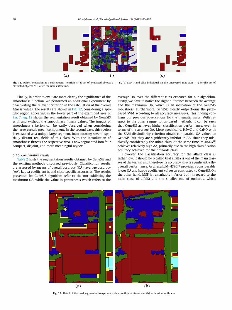
Fig. 11. Object extraction at a subsequent iteration t: (a) set of extracted objects Sðt � 1Þ, (b) SSD(t) and elite individual on the uncovered map RC(t � 1), (c) the set ofextracted objects SðtÞ after the new extraction.

98 S.K. Mylonas et al. / Knowledge-Based Systems 54 (2013) 86–102

Finally, in order to evaluate more clearly the significance of thesmoothness function, we performed an additional experiment bydeactivating the relevant criterion in the calculation of the overallfitness values. The results are shown in Fig. 12, considering a spe-cific region appearing in the lower part of the examined area ofFig. 7. Fig. 12 shows the segmentation result obtained by GeneSISwith and without the smoothness fitness values. The impact ofsmoothness criterion can be easily observed when consideringthe large cereals green component. In the second case, this regionis extracted as a unique large segment, incorporating several spa-tially distant real fields of this class. With the introduction ofsmoothness fitness, the respective area is now segmented into fourcompact, disjoint, and more meaningful objects.

5.1.5. Comparative resultsTable 2 hosts the segmentation results obtained by GeneSIS and

the existing methods discussed previously. Classification resultsare assessed by means of overall accuracy (OA), average accuracy(AA), kappa coefficient k, and class-specific accuracies. The resultspresented for GeneSIS algorithm refer to the run exhibiting themaximum OA, while the value in parenthesis which refers to the

Fig. 12. Detail of the final segmented image: (a) with

average OA over the different runs executed for our algorithm.Firstly, we have to notice the slight difference between the averageand the maximum OA, which is an indication of the GeneSISrobustness. Furthermore, GeneSIS clearly outperforms the pixel-based SVM according to all accuracy measures. This finding con-firms our previous observations for the thematic maps. With re-spect to the other segmentation-based methods, it can be seenthat GeneSIS achieves higher classification performance, even interms of the average OA. More specifically, HSwC and CaHO withthe SAM dissimilarity criterion obtain comparable OA values toGeneSIS, but they are significantly inferior in AA, since they mis-classify considerably the urban class. At the same time, M-HSEGop

achieves relatively high AA, primarily due to the high classificationaccuracy achieved for the orchards class.

However, the classification accuracy for the alfalfa class israther low. It should be recalled that alfalfa is one of the main clas-ses of the terrain and therefore its accuracy affects significantly theoverall performance. As a result, M-HSEGop provides a considerablylower OA and kappa coefficient values as contrasted to GeneSIS. Onthe other hand, MSF is remarkably inferior both in regard to themain class of alfalfa and the smaller one of orchards, which

smoothness fitness and (b) without smoothness.

Table 3Information classes, number of labeled data, and classification accuracies in percentage of the different methods for the Indiana image. Performance is evaluated in terms ofoverall accuracy (OA), average accuracies (AA) and kappa coefficient (j). SAM and MSE denote the dissimilarity criteria used by region growing methods. MV stands for the resultsobtained after majority voting.

DC No. of Samples SVM SVM + GeneSIS CaHO HSwC M-HSEGop MSF

SAM MSE SAM SAM SAM SAM + MV L1 L1 + MV

OA – 76.22 94.51 (93.61) 93.48 89.57 92.56 93.18 93.01 93.01 93.27 93.28AA – 84.03 97.02 96.05 94.56 95.71 89.24 88.91 88.91 89.20 89.21k – 73.09 93.71 92.55 88.11 91.49 92.17 91.98 91.98 92.28 92.30Alfalfa 54 87.18 100 89.74 89.74 89.74 89.74 89.74 89.74 89.74 89.74Corn-notill 1434 72.62 94.80 93.21 87.50 88.95 93.64 92.63 92.63 92.85 92.77Corn-min 834 67.35 81.89 85.08 77.55 85.59 88.90 89.03 89.03 90.18 90.43Corn 234 76.09 99.46 100 100 100 100 97.83 97.83 100 100Grass/Pasture 497 92.39 95.97 96.42 93.96 96.20 96.20 94.18 94.18 94.18 94.18Grass/Trees 747 95.41 99.86 99 99.57 99.14 96.84 97.70 97.70 100 100Grass/pasture-mowed 26 100 100 100 100 100 100 100 100 100 100Hay-windrowed 489 97.04 99.77 99.77 99.77 99.77 99.77 100 100 99.77 99.77Oats 20 80 100 100 100 100 0 0 0 0 0Soybeans-notill 968 77.12 96.73 98.80 95.21 99.02 82.03 82.35 82.35 82.24 82.24Soybeans-min 2468 58.35 92.60 90.28 79.82 88.75 94.38 94.71 94.71 94.25 94.25Soybean-clean 614 84.40 96.81 95.21 96.10 95.74 96.28 95.57 95.57 96.45 96.45Wheat 212 99.38 100 100 99.38 99.38 99.38 99.38 99.38 100 100Woods 1294 88.91 94.45 90.84 94.37 90.84 91 91 91 91 91Bldg-grass-tree-drive 380 72.73 100 98.48 100 98.18 99.70 98.48 98.48 98.79 98.79Stone-steel towers 95 95.56 100 100 100 100 100 100 100 97.78 97.78

S.K. Mylonas et al. / Knowledge-Based Systems 54 (2013) 86–102 99

explains the low observed values for OA and AA. The poor resultsobtained for alfalfa are attributed to the high spectral similarity be-tween this class and the maize one. This is also clearly verified bothfrom the low performances achieved for these classes by SVM andtheir mixed appearance in the SVM map of Fig. 7(c). GeneSIS man-ages to handle this spectral ambiguity effectively and increase thealfalfa accuracy nearly by a percentage of 7%, considerably betterthan all the other methods. At the same time, GeneSIS achieveshigh classification results for all other classes, thus avoiding under-estimation for any specific class.

5.2. Indiana image

The Indiana Image was recorded by the AVIRIS sensor over avegetation area in Northwestern Indiana [1]. The spatial dimensionof the image is 145 � 145 and its spatial resolution is 20 m/pixel.From the total set of 220 bands, twenty water absorption bandshave been removed [24], and the remaining 200 were used inour experiments. Table 3 shows the sixteen classes of interest iden-tified in this application and the exact number of reference sam-ples per class. A three band false color composite and thereference sites are shown in Fig. 13(a) and (b), respectively. Thetraining set was selected randomly from reference data and in-cludes 15 samples for the three smaller classes (namely alfalfa,grass/pasture-mowed and oats) and 50 for the remaining classes.The rest of the reference data comprised the test set.

Initially, pixel-wise classification by FO-SVM was performedconsidering again the RBF kernel. The optimal parameters werechosen by 5-fold cross validation: C = 512 and c = 2�9. The classifi-cation map obtained is shown in Fig. 13(c). As we can see, themajority of the fields are correctly classified. Nevertheless, thereexists a strong confusion between the spectrally similar corn andsoybeans types, which produces many misclassifications withincertain fields of the corresponding classes. The consequence of thisis that the resulting map is very noisy and highly fragmented. Toconfront with this situation, we chose a large marking percentageof P = 35%, much greater than the one selected for the KoroniaImage. The size of the significant structures to be marked was setto XC

min ¼ 20, since the smaller reference field in the study area isthat of oats with 20 pixels. The resulting 3396 markers are de-picted in Fig. 13(d).

Subsequently, image segmentation is performed through Gene-SIS. The size of the insignificant objects used for the extraction ter-mination was set here to Amin = 10. From the different runs of ouralgorithm, a typical segmentation map obtained is shown inFig. 13(e). GeneSIS generated, on average, a considerably smallernumber of 199 segments, compared to the number of 4246 of ini-tial connected components. These segments cover mostly the largeand homogeneous areas of the image, achieving also a nice match-ing with the respective reference fields. In this experiment, we cannotice the ability of GeneSIS to recognize fields even if these com-ponents are not marked in the initial map. A typical example is theoats field, which was not large enough in SVM map in order to bemarked. However, GeneSIS evaluated the fuzzy content of this re-gion, recognized the dominant class and extracted a correctly la-beled segment that resembles highly the corresponding referencefield. Due to the aforementioned fragmented result of SVM, anappreciable portion of the image remained uncovered after Gene-SIS (black colored regions in Fig. 13(e)), despite the small valueof Amin. These regions were finally absorbed by the already ex-tracted objects using the approach described in Section 3.2. The fi-nally created classification map is shown in Fig. 13(f). Theimprovement of this result compared to the SVM map is evident.Particularly, all ambiguities have been removed, with the resultingmap being much more homogeneous than the initial one.

Table 3 shows the classification results for the different meth-ods on the Indiana image. It can be seen again that the differencebetween the average and the best OA is quite small which mani-fests the robustness of the segmentation/classification resultsyielded by GeneSIS. There is also a substantial enhancement incomparison with the pixel-based SVM classification in regard toall accuracy measures. Especially, we should note the large in-crease in soybeans-min accuracy, which is obvious by observingthe corresponding maps. With respect to other segmentation-based methods, we can see that GeneSIS achieves higher classifica-tion performance even in terms of average OA. All the competingmethods achieve similar OA values, with the only exception ofCaHO when operating under the MSE criterion, which exhibitsthe lowest performance, mainly due to misclassifications in thecorn-min and soybeans-min classes. Moreover, GeneSIS alsoachieves the highest AAs, managing thus to classify sufficientlyall the classes without underestimating any of them. On the

Fig. 13. Indiana image: (a) three-band false color composite, (b) reference sites, (c) classification map by SVM, (d) markers, (e) segmentation map after GeneSIS, and (f) finalclassification map.

Table 4Information classes, number of labeled data, and classification accuracies in percentage of the different methods for the University of Pavia. Performance is evaluated in terms ofoverall accuracy (OA), average accuracies (AA) and kappa coefficient (j). SAM and MSE denote the dissimilarity criteria used by region growing methods. MV stands for the resultsobtained after majority voting.

DC No. of Samples SVM SVM + GeneSIS CaHO HSwC M-HSEGop MSF

Train Test SAM MSE SAM SAM SAM SAM + MV L1 L1 + MV

OA – 81 88.96 (88.41) 88.45 85.52 87.51 89.96 88.48 88.52 87.50 87.99AA – 88.15 93.86 94.45 92.65 93.21 95.39 93.30 93.36 94.57 94.71k – 75.74 85.67 85.07 81.42 83.87 86.97 85.11 85.16 83.81 84.41Asphalt 548 6304 76.51 94.18 93.51 85.58 90.75 97.73 97.26 97.26 90.82 90.80

Meadows 540 18146 73.59 81.08 79.22 76.36 78.81 80.80 78.76 78.81 78.12 79.17Gravel 392 1815 71.35 79.83 86.39 82.48 85.40 92.29 89.48 89.48 91.18 91.18Trees 524 2912 98.70 97.87 98.73 98.59 98.52 96.91 95.54 95.60 93.61 93.78Metal sheets 265 1113 99.01 99.37 99.82 98.92 99.82 99.91 99.91 99.91 99.91 99.91Bare soil 532 4572 91.80 98.27 98.21 96.78 97.05 97.88 97.73 97.77 98.23 98.23Bitumen 375 981 91.54 96.43 97.35 96.33 98.17 98.88 99.18 99.18 100 100Bricks 514 3364 91.14 98.07 99.20 98.90 98.81 99.79 99.85 99.85 99.29 99.29Shadows 231 795 99.75 99.62 97.61 99.87 91.57 94.34 82.01 82.39 100 100

100 S.K. Mylonas et al. / Knowledge-Based Systems 54 (2013) 86–102

contrary, the marker-based methods MSF and M-HSEGop attainquite lower average accuracies, since they misclassify completelythe oats class. This occurs because owing to its size the oats fieldis unmarked and these methods utilize the markers as seeds tostart growing. In such a case, a marker of different label isexpanded over this field, which is deterministically misclassifiedat the end. Finally, note that the classification results of MSFremained intact after the majority voting step (MV).

5.3. University of Pavia image

The University of Pavia image is of an urban area that was ac-quired by the ROSIS-03 sensor over the University of Pavia, north-ern Italy. The spatial dimension of the image is 610 � 340, itsspatial resolution is 1.3 m/pixel. The full spectral range of the ini-tially recorded image contains 115 bands (ranging from 0.43 to0.86 lm). The 12 most noisy data channels have been removed,and the remaining 103 spectral bands were used in our experi-ments. The nine classes of interest existing in this hyperspectralimage along with the corresponding number of samples are

detailed in Table 4. A three band true color composite and the ref-erence sites are shown in Fig. 14(a) and (b), respectively.

First, pixel-wise classification by FO-SVM was performed con-sidering the RBF kernel. The optimal parameters were chosen by5-fold cross validation: C = 8 and c = 2�5. The obtained classifica-tion map is shown in Fig. 14(c). As can be seen, most of the classareas are correctly classified, except mainly from a large meadowsregion in the lower part of the image. As can be viewed inFig. 14(a), this region is spectrally heterogeneous although it be-longs to the same class. As a result, SVM confuses this meadowspart with trees and bare soil. The size of large structures to bemarked was set here to XC

min ¼ 20, in order for the GeneSIS to beable to recognize some small components of trees and shadows.In this experiment, we selected the marking percentage parameteras P = 20% which yielded a set of 25,112 markers, shown inFig. 14(d). Next, image segmentation was performed using Gene-SIS. The size of the insignificant objects used for the terminationof object extractions, was chosen to be Amin = 10.

One of the segmentation maps obtained is shown in Fig. 14(e).Overall, GeneSIS generated on average 2305 segments, much fewer

Fig. 14. University of Pavia image: (a) three-band color composite, (b) reference sites, (c) classification map by SVM, (d) markers, (e) segmentation map after GeneSIS, and (f)final classification map.

S.K. Mylonas et al. / Knowledge-Based Systems 54 (2013) 86–102 101

than the number of 24,670 of initial connected components con-tained in the SVM map. However, compared to our previous exper-iments and considering the size of the image, this resulting numberof segments is considerably larger than the expected one. This out-come is explained from Fig. 14(a) by observing that the entire im-age along with all its class components is rotated in respect to thevertical axis. The direct consequence is that as can be seen fromFig. 14(e), the rotated structures, like roads, bricks and meadows,are over-segmented. Structures that could be extracted as a singlesegment, are now covered by many repeatedly extracted objects ofvarying size, yielding a highly fragmented segmentation map. It isevident that the lack of rotation in the chromosome’s rectanglerepresentation used in the present version of GeneSIS, reduces itsflexibility, rendering it unable to avoid over-segmentation for thistype of images.

The final classification map obtained after the absorption of thesmall remaining regions is presented in Fig. 14(f). Despite the over-segmentation noticed before, the resulting map is clearly morehomogeneous than the SVM map. However, the misclassification

in the aforementioned meadows region remains after GeneSIS, be-cause this component was large enough to receive markers of thebare soil class, as assigned erroneously by SVM.

Table 4 hosts the classification results of the different methodsfor the Pavia image. From statistical point of view, we have a pic-ture similar to the one noticed in our previous experiments. Par-ticularly, the average OA value is slightly lower to the best OAwhich implies that the repeated runs of GeneSIS produce classifi-cation results consistently similar to the best ones. When con-trasted to the pixel-based SVM, the increase of all accuracies isobvious, especially in the classes of asphalt, meadows and gravel,where SVM provided the poorest performance. This indicates thatthe observed over-segmentation in GeneSIS does not affect signif-icantly the final performance. The competitive methods achievesimilar results to GeneSIS with small variations, and onlyM-HSEGop is distinguished with a higher performance. In themixed and largest class of meadows, GeneSIS performs slightlybetter than the other methods, while on the other it achievesthe lowest accuracy in gravel.

102 S.K. Mylonas et al. / Knowledge-Based Systems 54 (2013) 86–102

6. Conclusions

A novel image segmentation approach has been presented inthis paper, the GeneSIS algorithm, for automated segmentationand classification of remote sensing imagery. GeneSIS partitionsthe image sequentially into compact and homogeneous regionsby invoking a GA-based object extraction algorithm. The extractedobjects achieve an optimal balance between the three fuzzy crite-ria, namely, coverage, consistency and smoothness, calculated onthe spatial domain. The final classification map is obtained directlyafter image segmentation since each image object has its own classlabel. Our method is validated on the classification of three studyareas with different spectral and spatial characteristics. The com-parative results with other segmentation-based classifiers provethe robustness of the GeneSIS algorithm and its effectiveness inobtaining competitive classification accuracies for all classes. Adrawback of the proposed method is that it produces occasionallyover-segmentation results when dealing with images containingrotated ground truth structures, such as the University of Pavia im-age. To confront with this problem, we are planning to enhance theflexibility in the chromosomes representation, by incorporatingrotating rectangles and/or considering other more descriptive geo-metric shapes such as polygonal search objects.

Acknowledgment

The authors would like to thank P. Gamba from the Universityof Pavia, Italy, for providing the hyperspectral data.

References

[1] AVIRIS NW Indiana’s Indian Pines 1992. Data Set. ftp://ftp.ecn.purdue.edu/biehl/Multispec/92AV3C (original files) and ftp://ftp.ecn.purdue.edu/biehl/PC_Multispec/ThyFiles.zip (ground truth).

[2] M. Baatz, A. Schäpe, Multiresolution Segmentation – An OptimizationApproach for High Quality Multi-Scale Image Segmentation. AngewandteGeographische Informationsverarbeitung XII, Wichmann-Verlag, Heidelberg,2000. pp. 12–23.

[3] J. Beaulieu, M. Goldberg, Hierarchy in picture segmentation: a stepwiseoptimal approach, IEEE Transactions on Pattern Analysis and MachineIntelligence 11 (1989) 150–163.

[4] S. Beucher, F. Meyer, The morphological approach to segmentation: thewatershed transformation, Mathematical Morphology in Image Processing 10(1993) 433–481.

[5] S. Bhandarkar, H. Zhang, Image segmentation using evolutionary computation,IEEE Transactions on Evolutionary Computation 3 (1) (1999) 1–21.

[6] B. Bhanu, S. Lee, J. Ming, Adaptive image segmentation using a geneticalgorithm, IEEE Transactions on Systems, Man, and Cybernetics 25 (12) (1995)1543–1567.

[7] D.N. Chun, H.S. Yang, Robust image segmentation using genetic algorithm witha fuzzy measure, Pattern Recognition 29 (7) (1996) 1195–1211.

[8] O. Cordón, F. Herrera, F. Hoffmann, L. Magdalena, Genetic Fuzzy Systems:Evolutionary Tuning and Learning of Fuzzy Knowledge Bases, World Scientific,Singapore, 2001.

[9] C. Cortes, V. Vapnik, Support-vector networks, Machine Learning 20 (1995)273–297.

[10] S. Derivaux, G. Forestier, C. Wemmert, S. Lefevre, Supervised imagesegmentation using watershed transform, fuzzy classification andevolutionary computation, Pattern Recognition Letters 31 (15) (2010) 2364–2374.

[11] A. Falcão, J. Stolfi, R. Lotufo, The image foresting transform: theory, algorithms,and applications, IEEE Transactions on Pattern Analysis and MachineIntelligence 26 (1) (2004) 19–29.

[12] J. Fan, G. Zeng, M. Body, M.-S. Hacid, Seeded region growing: an extensive andcomparative study, Pattern Recognition Letters 26 (8) (2005) 1139–1156.

[13] Feitosa, R.Q., Costa, G.A., Cazes, T.B., Feijo, B., 2006. A genetic approach for theautomatic adaptation of segmentation parameters. In: InternationalConference on Object-based Image Analysis.

[14] K.S. Fu, J.K. Mui, A survey on image segmentation, Pattern Recognition 13(1981) 3–16.

[15] M. Gong, Y.H. Yang, Quadtree-based genetic algorithm and its applications tocomputer vision, Pattern Recognition 37 (8) (2004) 1723–1733.

[16] A. González, F. Herrera, Multi-stage genetic fuzzy systems based on theiterative rule learning approach, Mathware and Soft Computing 4 (3) (1997)233–249.

[17] J.H. Holland, Adaptation in Natural and Artificial Systems, University ofMichigan Press, Ann Arbor, MI, 1975.

[18] X. Huang, L. Zhang, An adaptive mean-shift analysis approach for objectextraction and classification from urban hyperspectral imagery, IEEETransactions on Geoscience and Remote Sensing 46 (12) (2008) 4173–4185.

[19] S. Makrogiannis, G. Economou, S. Fotopoulos, Region dissimilarity relation thatcombines feature-space and spatial information for color image segmentation,IEEE Transactions on Systems, Man, and Cybernetics, Part B: Cybernetics 35 (1)(2005) 44–53.

[20] K. Melkemi, M. Batouche, S. Foufou, A multiagent system approach for imagesegmentation using genetic algorithms and external optimization heuristics,Pattern Recognition Letters 27 (2006) 1230–1238.

[21] N. Mitrakis, C. Topaloglou, T. Alexandridis, J. Theocharis, G. Zalidis, Decisionfusion of GA self-organizing neuro-fuzzy multilayered classifiers for land coverclassification using textural and spectral features, IEEE Transactions onGeoscience and Remote Sensing 46 (7) (2008) 2137–2152.

[22] S. Moustakidis, J. Theocharis, A fast SVM-based wrapper feature selectionmethod driven by a fuzzy complementary criterion, Pattern Analysis andApplications 15 (4) (2012) 379–397.

[23] S. Mylonas, D. Stavrakoudis, J. Theocharis, A GA-based sequential fuzzysegmentation approach for classification of remote sensing images, IEEEInternational Conference on Fuzzy Systems (2012) 707–714.

[24] S. Tadjudin, D.A. Landgrebe, Covariance estimation with limited trainingsamples, IEEE Transactions on Geoscience and Remote Sensing 37 (4) (1999)2113–2118.

[25] Y. Tarabalka, J.A. Benediktsson, J. Chanussot, Spectral-spatial classification ofhyperspectral imagery based on partitional clustering techniques, IEEETransactions on Geoscience and Remote Sensing 47 (8) (2009) 2973–2987.

[26] Y. Tarabalka, J. Chanussot, J.A. Benediktsson, Segmentation and classification ofhyperspectral images using watershed transformation, Pattern Recognition 43(7) (2010) 2367–2379.

[27] Y. Tarabalka, J. Chanussot, J.A. Benediktsson, Segmentation and classification ofhyperspectral images using minimum spanning forest grown fromautomaticallyselected markers, IEEE Transactions on Systems, Man, andCybernetics 40 (5) (2010) 1267–1279.

[28] Y. Tarabalka, J.C. Tilton, Spectral-spatial classification of hyperspectral imagesusing hierarchical optimization, Workshop on Hyperspectral Image and SignalProcessing: Evolution in Remote Sensing, 2011a, pp. 1–4.

[29] Y. Tarabalka, J.C. Tilton, Best merge region growing with integratedprobabilistic classification for hyperspectral imagery, InternationalGeoscience and Remote Sensing, Symposium, 2011b, pp. 3724–3727.

[30] Y. Tarabalka, J.C. Tilton, J.A. Benediktsson, J. Chanussot, A marker-basedapproach for the automated selection of a single segmentation from ahierarchical set of image segmentations, IEEE Journal of Selected Topics inApplied Earth Observations and Remote Sensing 5 (1) (2012) 262–272.

[31] J.C. Tilton, Analysis of hierarchically related image segmentations, in: IEEEWorkshop on Advances in Techniques for Analysis of Remotely Sensed Data,2003, pp. 60–69.

[32] J. Udupa, S. Samarasekera, Fuzzy connectedness and object definition: theory,algorithms, and applications in image segmentation, Graphical Models andImage Processing 58 (3) (1996) 246–261.

[33] S. Valero, P. Salembier, J. Chanussot, Comparison of merging orders andpruning strategies for binary partition tree in hyperspectral data, IEEEInternational Conference on Image Processing, 2010, pp. 2565–2568.

[34] H. Yang, Q. Du, Decision fusion on supervised and unsupervised classifiers forhyperspectral imagery, IEEE Geoscience and Remote Sensing Letters 7 (4)(2010) 875–879.