PERPUSTAKAAN UMP

11111111111111111111111 0000080274

Genetic Algorithm to Optimize Routing Problem

Modelled As the Travelling Salesman Problem

MUHAMMAD AZRUL FAIZ BIN NOR ADZMI

A project report submitted in partial fulfilment

Of the requirements for the award of the degree of

Bachelor of Mechatronic Engineering

Faculty of Manufacturing Engineering

University Malaysia Pahang

JUNE 2013

ABSTRACT

This study presents genetic algorithm (GA) to solve routing problem modelled as the

travelling salesman problem (TSP). Genetic algorithm conceptually follows steps

inspired by the biological process of evolution. GA is following the ideas of "survival

of the fittest" which meant better and better solution evolves from previous generations

until a near optimal solution is obtained. In TSP, There are cities and distance given

between the cities. The salesman needs to visit all the cities, but does not to travel so

much. This study will use PCB component placement which is modelled as TSP. The

objective is to find the sequence of the routing in order to minimize travelling distance.

The GA with Roulette wheel selection, linear order crossover and inversion mutation

is used in the study. The computational experiment was done using several randomly

generated data with different GA parameter setting. The optimal distance obtains for

40 component placements is 8.9861 mm within 6.751 seconds The results from the

experiments show that GA used in this study is effective to solve PCB component

placement which is modelled as TSP.

VI

ABSTRAK

Kajian mi membentangkan algoritma genetik (GA) untuk menyelesaikan masalah

laluan dimodelkan sebagai masalah jurujual kembara (TSP). Konsep algoritma genetic

berikut adalah mengikut langkah-langkah yang diilhamkan oleh proses perkembangan

biologi. GA men gikut idea-idea "yang kuat terus hidup" bermakna yang lebih baik dan

penyelesaian yang lebih baik akan berkembang dari generasi yang sebelumnya

sehingga memperolehi penyelesaian yang optimum atau hampir optimum. Dalam TSP,

terdapat bandar-bandar dan juga jarak di antara bandar-bandar. Jurujual dikehendaki

melawat semua bandar-bandar dengan perjalanan yang sedikit. Kajian mi akan

menggunakan penempatan komponen pada PCB yang dimodelkan sebagai TSP.

Tujuannya adalah untuk mencari urutan laluan dalam usaha untuk mengurangkanjarak

perjalanan. Algoritma genetic dengan pemilihan roda Roulette, penyilangan perintah

linear dan penyongsangan mutasi telah digunakan dalam kajian mi. Kajian mi

dijalankan dengan menggunakan beberapa data yang dijanakan secara rawak dengan

penetapan parameter GA yang berbeza. Jarak optimum yang diperolehi bagi 40

penempatan komponen adalah 8.9861 mm dalam masa 6.751 saat. Keputusan daripada

eksperimen menunjukkan bahawa GA yang digunakan dalam kajian mi adalah

berkesan untuk menyelesaikan penempatan komponen pada PCB yang dimodelkan

sebagai TSP.

am

TABLE OF CONTENTS

CHAPTER TITLE PAGE

SUPERVISOR'S DECLARATION

STUDENT DECLARATION

DEDICATED iv

ACKNOLEDGEMENTS v

ABSTRACT vi

ABSTRAK vii

TABLE OF CONTENTS viii

LIST OF TABLES xi

LIST OF FIGURES xii

CHAPTER 1 INTRODUCTION

1.1 BACKGROUND OF STUDY 1

1.2 PROBLEM STATEMENT 2

1.3 OBJECTIVES 2

1.4 SCOPE OF STUDY 2

1.5 METHODOLOGY OF STUDY 2

1.6 SUMMARY 3

CHAPTER 2 LITERATURE REVIEW

2.1 INTRODUCTION 4

2.2 GENETIC ALGORTIHM 4

2.2.1 Encoding 5

2.2.2 Evolution 5

VIII

IA

2.2.3 Crossover 5

2.2.4 Mutation 5

2.2.5 Decoding 6

2.3 CHROMOSOME REPRESENTATION IN GA 6

2.3.1 Binary Representation 6

2.3.2 Path Representation 8

2.4 CHROMOSOME EVOLUTION & SELECTION 9

2.4.1 Evolution Process 9

2.4.2 Roulette Wheel Selection 10

2.4.3 Tournament Selection 11

2.5 CROSSOVER MECHANISM 12

2.5.1 Order Crossover (OX) 12

2.5.2 Linear Order Crossover (LOX) 13

2.5.3 Partially Mapped Crossover (PMIX) 14

2.5.4 Cycle Crossover (CX) 14

2.6 MUTATION MECHANISM 15

2.6.1 Inversion Mutation 15

2.6.2 Insertion Mutation 15

2.6.3 Displacement Mutation 16

2.6.4 Exchange Mutation 16

2.7 TRAVELLING SALESMAN PROBLEM 16

2.8 SIMPLE PROBLEM 17

2.9 GA IN SEQUENCING ROUTING IN TSP 20

2.10 SUMMARY 21

CHAPTER 3 METHODOLOGY

3.1 INTRODUCTION 22

3.2 PROJECT FLOW CHART 23

3.3 GA PARAMETER 24

3.4 GA METHOD 24

3.4.1 Initialization and Representation 24

3.4.2 Selection 25

3.4.3 GA Operators 25

x

3.4.4 Termination 26

3.5 GENERAL PROCESS OF GA 26

3.6 PROCESS FLOW OF GA FOR TSP 27

3.7 COMPANY VISIT 28

3.8 TOOL 28

3.9 SUMMARY 28

CHAPTER 4 RESULTS AND DISCUSSION

4.1 INTRODUCTION 29

4.2 CASE STUDY: K. E. MANUFACTURING SDN. BHD. 29

4.2.1 SMT Machine 29

4.2.2 Component Placement Process 30

4.3 EXPERIMENT SETUP 33

4.3.1 Control Parameters 34

4.3.2 Computational Experiments 35

4.4 RESULT AND DISCUSSION 35

4.4.1 lst Ran ofGAProgram 36

4.4.2 2'' Run of GA Program (variable rate of crossover) 37

4.4.3 3rd Run of GA Program (variable rate of mutation) 38

4•44 4h Run of GA Program (variable rate of pop_size) 39

44•5 5h Run of GA Program (variable rate of max gene) 40

CHAPTER 5 CONCLUSION AND RECOMMENDATION

5.1 INTRODUCTION 41

5.2 SUMMARY AND CONCLUSION 41

5.3 RECOMMENDATION 42

REFERENCES 43

APPENDIX

A Gantt Chart of The Project 44

B Example of Programming Code 45

Ea

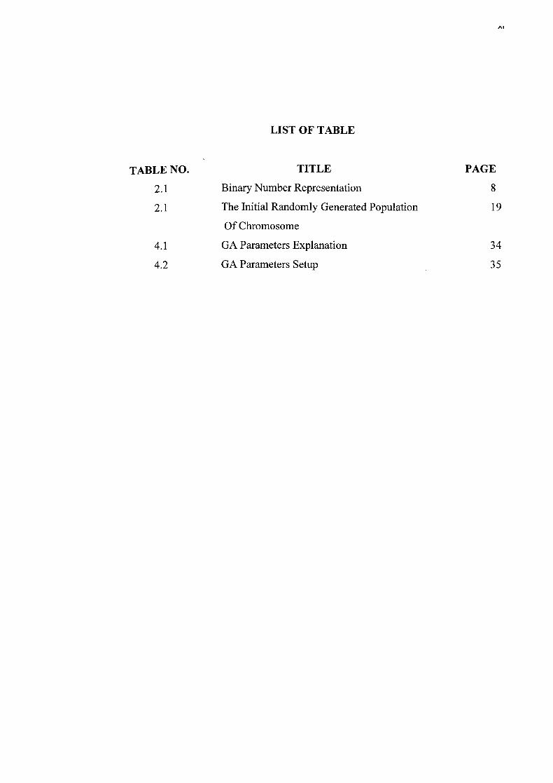
LIST OF TABLE

TABLE NO. TITLE PAGE

2.1 Binary Number Representation 8

2.1 The Initial Randomly Generated Population 19

Of Chromosome

4.1 GA Parameters Explanation

34

4.2 GA Parameters Setup 35

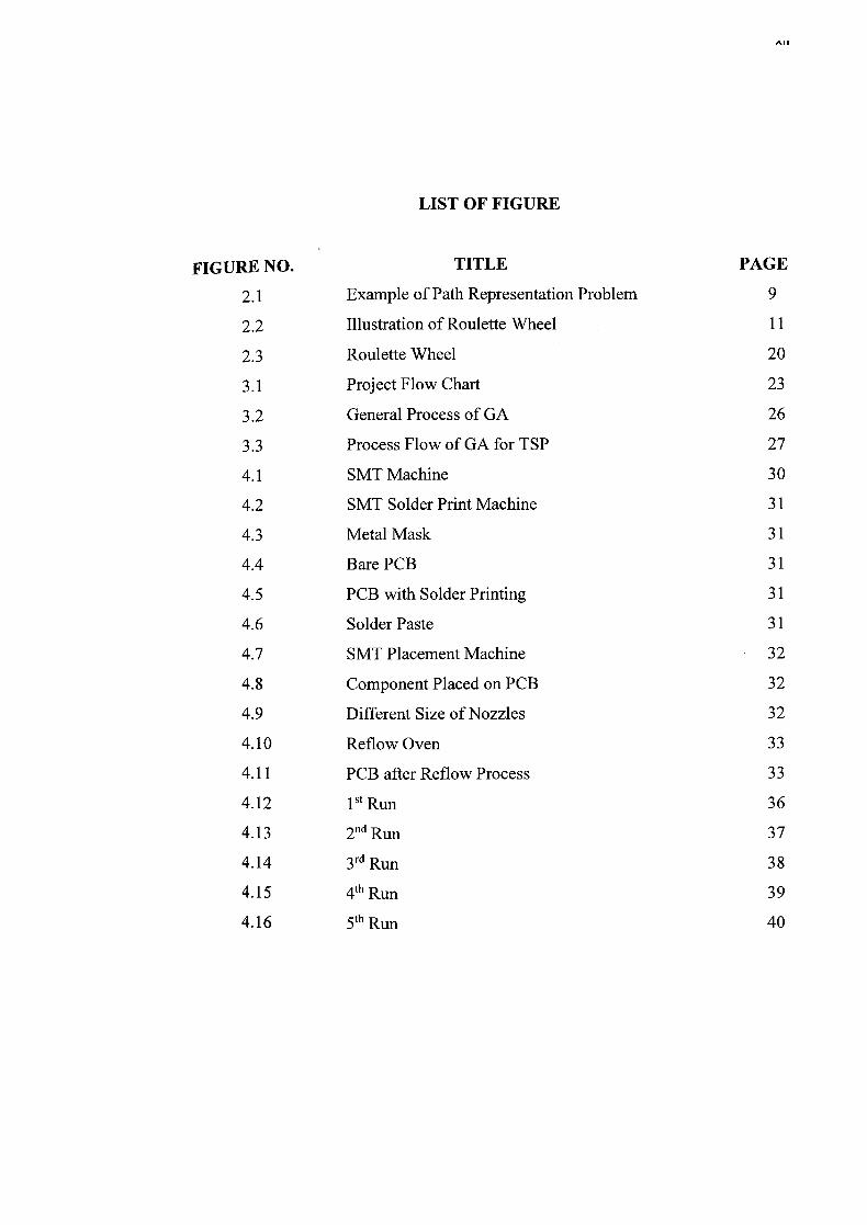
LIST OF FIGURE

FIGURE NO. TITLE PAGE

2.1 Example of Path Representation Problem 9

2.2 Illustration of Roulette Wheel 11

2.3 Roulette Wheel 20

3.1 Project Flow Chart 23

3.2 General Process of GA 26

3.3 Process Flow of GA for TSP 27

4.1 SMT Machine 30

4.2 SMT Solder Print Machine 31

4.3 Metal Mask 31

4.4 Bare PCB 31

4.5 PCB with Solder Printing 31

4.6 Solder Paste 31

4.7 SMT Placement Machine 32

4.8 Component Placed on PCB 32

4.9 Different Size of Nozzles 32

4.10 Reflow Oven 33

4.11 PCB after Reflow Process 33

4.12 1st Run 36

4.13 2nd Run 37

4.14 3rdRun 38

4.15 4th Run 39

4.16 5th Run 40

lilE

CHAPTER 1

INTRODUCTION

1.1 BACKGROUND OF STUDY

The Traveling salesman problems (TSP) is one of the most widely studied

problems in combinatorial optimization (Chatterjee et. a!, 1995). The TSP idea is to

find a tour of a given number of cities, visiting each city exactly once and returning to

the starting city where the length of this tour is minimized. The travelling salesman

problem (TSP) is an NP-hard problem in combinatorial optimization studied in

operations research and theoretical computer science. This complexity can solve by

given n is the number of cities to be visited, the total number of possible routes

covering all cities can be given as a set of feasible solutions of the TSP and is given as

(n-l)!12.

The Genetic algorithms are relatively new optimization technique which can

be applied to various problems, including those that are NP-hard. This genetic

algorithms technique does not ensure an optimal solution, however it usually gives

good come up in a reasonable amount of time. This, therefore, would be a good

algorithm to try on the traveling salesman problem, one of the most famous NP-hard

problems. Genetic algorithms are loosely based on natural evolution and use a

"survival of the fittest" technique, where the best solutions survive and are varied until

we get a good result.

The MATLAB is a tool which is used to develop a program for GAs which

will be used to solve TSP. MATLAB is a special-purpose computer program optimized

to perform engineering and scientific calculations. It is high-performance language for

technical computing. MATLAB combine the computation, visualization, and

programming in an easy-to-use environment where problems and solution are

expressed in familiar mathematical notation.

1.2 PROBLEM STATEMENTS

Modern production factories, which want to obtain high profits, usually

maximize their productivity. The latter goal can be achieved, among others, by optimal

or almost optimal scheduling of jobs in the production process. The problem is to get

the optimum result for routing distances same like TSP. This includes getting the

shortest distance and time taken to visit all the cities and return back to original

position. The constraint is there is no shorter way to solve the problem. Travelling

salesman has to visit each city with different sequence and compare the result and

choose the most optimum result. The genetic algorithm method is a one of the tools

used to solve optimization problems. Remember in mind that the longer the distance

taken will cause the more time taken to complete.

1.3 OBJECTIVES

The objectives are:

• To find the optimum route that minimizes the travelling distance / cost / time.

• To develop TSP fitness function and to use GA programming to solve TSP.

1.4 SCOPES OF STUDY

• To apply TSP concept using GA to one of the case study (real application in

industry case).

• To use MATLAB to simulate and to solve problem.

1.5 METHODOLOGY OF STUDY

This study is conducted under three main steps. The first step is the literature

review. In literature review, the previous method that used to solve routing problem

J

modelled as the travelling salesman problem and simulated to ensure the algorithm are

working as reported in scientific literatures. Then, the existing algorithms limitations

are identified.

From the previous limitations method, a new sequencing problem is developed

as the purpose solution to optimize the routing problem. In order to prove that genetic

algorithm was one of the methods that could solve routing distance problem, various

kind of problem will be perform. The results of the performance will be analyst as the

final step of this study.

1.7 SUMMARY

This chapter discussed about the project background such as the important of

this routing distance optimization and study in other to know which type of algorithm

that can be applied to a wide variety problem. It is also described the problem statement

of this project, the important to the study, the objective, the scope of the project and

the methodology of study.

CHAPTER 2

LITERATURE REVIEW

2.1 INTRODUCTION

This chapter explains the study and methods that used to solve optimization

problem such as Travelling Salesman Problems (TSP). There was also an explanation

of the genetic algorithm (GA) method and the steps that need to follow to solve the

problem using the GA method. At the end of this chapter, it is shown how the GA

method can be used to get the optimum or near the optimum result for TSP.

2.2 GENETIC ALGORITHM

Genetic Algorithm (GA) is an optimization technique, based on natural

evolution. It was introduced by John Holland in 1975 (Othman 2002). This technique

copied the biological theory, where the concept of "survival of the fittest" exits. GA

provides a method of searching which does not need to explore every possible solution

in the feasible region to obtain a good result (Othman 2002).

In nature, the fittest individuals are most likely to survive and mate. Therefore

the next generation should be fitter and healthier because they were raised from healthy

parents. This same idea is applied to a problem by first "guessing" solution and then

combining the fittest solutions to create a new generation. The genetic algorithm

consist five steps, that is:

1. Encoding

2. Evaluation

3. Crossover

1

4. Mutation

5. Decoding

2.2.1 Encoding

A suitable encoding is found for the solution to a problem so that each possible

solution has a unique encoding and the encoding is some form of string. Many possible

solution need to be encoded to create a population. The traditional way to represent a

solution is with a string of zeroes (0) and ones (1). However genetic algorithms are not

restricted to this encoding (Chatterjee et.al 1996).

2.2.2 Evaluation

The fitness of each individual in the population is then computed; this is how

well the individual fits the problem and whether it is near the optimum compared to

other individuals in the population. This fitness is used to find the individual's

probability of crossover. Evaluation function is used to decide how good a

chromosome is. This function is also known as objective function (Bryant 2001).

2.2.3 Crossover

Crossover is where the two individuals are recombined to create new

individuals which are copied into the new generation. Not every chromosome is used

in crossover. The evaluation function gives each chromosome a 'score' which is used

to decide the chromosome's probability of crossover. The crossover operator randomly

chooses a crossover point where two parent chromosomes 'break' and then exchanges

the chromosome parts after that point (Negnevitsky 2002).

2.2.4 Mutation

Mutation, which is rare in nature, represents a change in gene. It may lead to a

significant improvement in fitness, but more often has rather more harmful results.

Mutation is used to avoid getting trapped in a local optimum. The chromosome is

ci

naturally near the local optimum and very far from the global optimum (possible

solution) due to the randomness process. Some individuals are chosen randomly to be

mutated and then a mutation point is randomly chosen. Mutation causes the character

in the corresponding position of the string changed (Negnevitsky 2002).

2.2.5 Decoding

On all the four processes are done, a new generation has been formed and the

process is repeated until some stopping criteria have been reached. At this point the

individual who is closest to the optimum is decoded and the process is complete

(Bryant 2000).

2.3 CHROMOSOME REPRESENTATION IN GA

In genetic algorithms, each individual that is a member of the population

represents a potential solution to the problem. This solution information is coded in

the associated chromosome of that individual. A chromosome is a string of gene

positions, where each gene position holds an allele value that constitutes a part of the

solution to the problem. Allele value at a gene position represents an element from a

finite alphabet. This alphabet depends on the nature of the problem. There are number

of possible chromosome representations, due to vast variety of problem types.

However there are two representation types which are most commonly used: binary

representation and path/permutation representation (Bryant 2000).

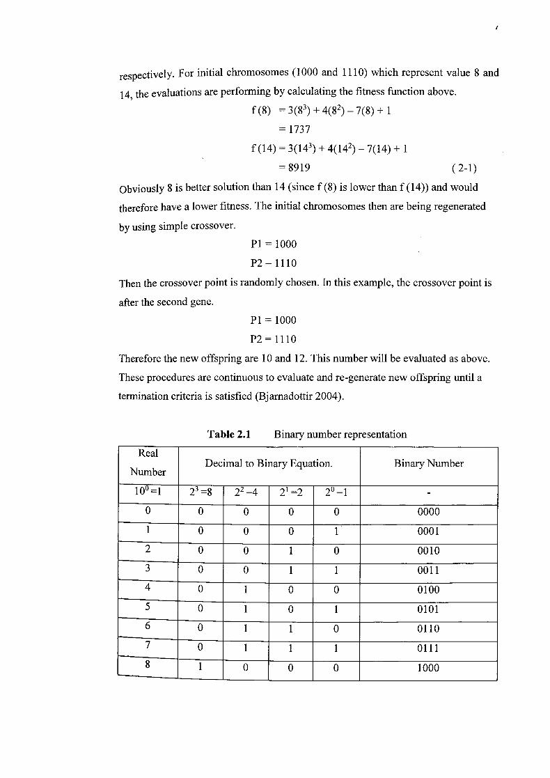
2.3.1 Binary Representation

In binary representation, the finite alphabet domain which allele at each gene

Position takes its value from is the set 10, l}. An example of problem to minimize the

function of, f(x) = 3x 3 + 4x2 - 7x +1 over the integers in set 10, 1, ..., 15}. The binary

number for the integer set was represented in table 2.1. The possible solution for the

problem are obviously just numbers, so the representation is simple the binary form of

each number. For example, the binary representation of 8 and 14 are 1000 and 1110

I

respectively. For initial chromosomes (1000 and 1110) which represent value 8 and

14, the evaluations are performing by calculating the fitness function above.

f(8) =3(83)+4(82)_7(8)+ 1

= 1737

f(14) = 3(14) + 4(142) -7(14)+l

=8919 (2-1)

Obviously 8 is better solution than 14 (since f (8) is lower than f (14)) and would

therefore have a lower fitness. The initial chromosomes then are being regenerated

by using simple crossover.

P1 = 1000

P2=1110

Then the crossover point is randomly chosen. In this example, the crossover point is

after the second gene.

P1 = 1000

P2=1110

Therefore the new offspring are 10 and 12. This number will be evaluated as above.

These procedures are continuous to evaluate and re-generate new offspring until a

termination criteria is satisfied (Bjamadottir 2004).

Table 2.1 Binary number representation

Real

NumberDecimal to Binary Equation. Binary Number

100 =1 2' =8 22=4 2'=2 20 =1 -

0

-

0 0 0 0 0000

1 0 0

0

0

1

1

0

0001

0010 2 0

3 0 0 1 1 0011

4 0 1 0 0 0100

0 1 0 1 0101

0 1 1 0 0110

Th 1 1 1 0111

Iii!iiiii 1 0 0 0 1000

8

0 0 1 1 . 001

10

E

9

EF, 1

0 1 0 1010

0 1 1 1011

12 i 1 0 0 1100

-i-______ -1 1 0 1 1101

1 1 1 0 1110

Th- 1 1 1 1 1111

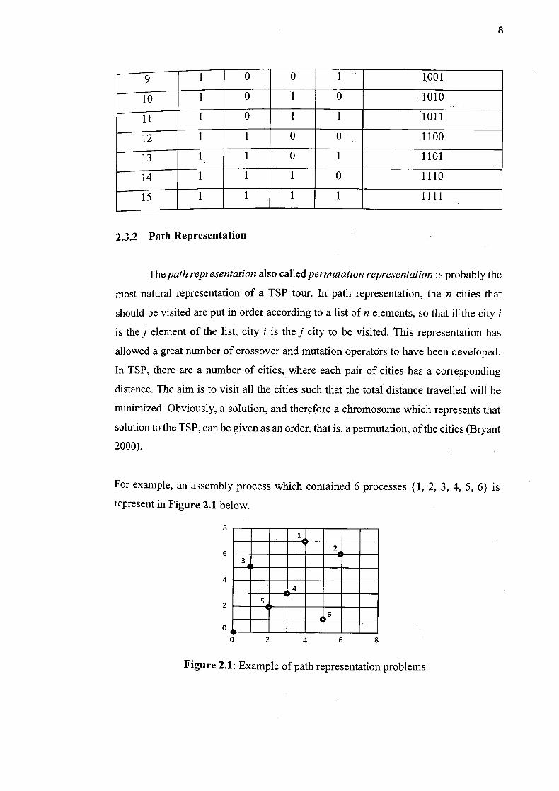
2.3.2 Path Representation

The path representation also called permutation representation is probably the

most natural representation of a TSP tour. In path representation, the n cities that

should be visited are put in order according to a list of n elements, so that if the city I

is the] element of the list, city i is the j city to be visited. This representation has

allowed a great number of crossover and mutation operators to have been developed.

In TSP, there are a number of cities, where each pair of cities has a corresponding

distance. The aim is to visit all the cities such that the total distance travelled will be

minimized. Obviously, a solution, and therefore a chromosome which represents that

solution to the TSP, can be given as an order, that is, a permutation, of the cities (Bryant

2000).

For example, an assembly process which contained 6 processes 11, 2, 3, 4, 5, 6} is

represent in Figure 2.1 below.

8

6

4

2

0

MMMMMMMM

WMMMMMMM MMMMMMMM MMWMMMMM MW^MMMM^

0 2 4 6 8

Figure 2.1: Example of path representation problems

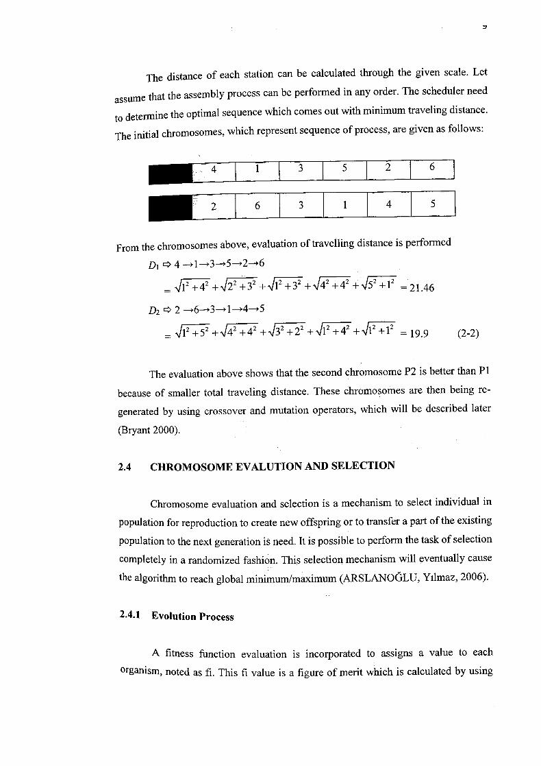
The distance of each station can be calculated through the given scale. Let

assume that the assembly process can be performed in any order. The scheduler need

to determine the optimal sequence which comes out with minimum traveling distance.

The initial chromosomes, which represent sequence of process, are given as follows:

From the chromosomes above, evaluation of travelling distance is performed

Di 4

452 +=21.46

D2 2 —6----3--+1-4---5

= j 5 2 4242 +32 +22 +12 +42 +V12+12 = 19.9 (2-2)

The evaluation above shows that the second chromosome P2 is better than P1

because of smaller total traveling distance. These chromosomes are then being re-

generated by using crossover and mutation operators, which will be described later

(Bryant 2000).

2.4 CHROMOSOME EVALUTION AND SELECTION

Chromosome evaluation and selection is a mechanism to select individual in

population for reproduction to create new offspring or to transfer a part of the existing

population to the next generation is need. It is possible to perform the task of selection

completely in a randomized fashion. This selection mechanism will eventually cause

the algorithm to reach global minimum/maximum (ARSLANOOLU, Yilmaz, 2006).

2.4.1 Evolution Process

A fitness function evaluation is incorporated to assigns a value to each

organism, noted as fi. This fi value is a figure of merit which is calculated by using

LU

any domain knowledge that applies. In principle, this is the only point in the algorithm

that domain knowledge is necessary. Organisms are chosen using the fitness value as

a guide, where those with higher fitness values are chosen more often.

Selecting organisms based on fitness value is a major factor in the strength of

GAs as search algorithms. The method employed here was to calculate the total

Euclidean distance Di for each organism first, then compute fi by using the following

equation

fiDmax — DI (2.3)

where Dmax is the longest Euclidean distance over organisms in the population (M.

Melanie, 1996).

2.4.2 Roulette Wheel Selection

In keeping with the ideas of natural selection, we assume that stronger

individuals, that is, those with higher fitness values, are more likely to mate than the

weaker ones. One way to simulate this is to select parents with a probability that is

directly proportional to their fitness values. This method is called the roulette wheel

method (ARSLANOOLU, Yilmaz, 2006).

Pi=Fi/>1Fj(2.4)

The idea behind the roulette wheel selection technique is that each individual

is given a chance to become a parent in proportion to its fitness. The chances of

selecting a parent can be seen as spinning a roulette wheel with the size of the slot for

each parent being proportional to its fitness. Obviously, those with the largest fitness

(slot sizes) have more chance of being chosen. Consider a roulette wheel with a

number of slices on it, each of which has an associated width as shown in Figure 2.2.

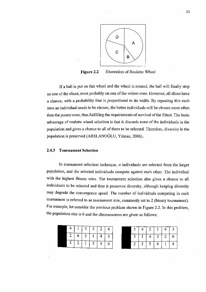
11

Figure 2.2 Illustration of Roulette Wheel

If a ball is put on this wheel and the wheel is rotated, the ball will finally stop

on one of the slices, most probably on one of the widest ones. However, all slices have

a chance, with a probability that is proportional to its width. By repeating this each

time an individual needs to be chosen, the better individuals will be chosen more often

than the poorer ones, thus fulfilling the requirements of survival of the fittest. The basic

advantage of roulette wheel selection is that it discards none of the individuals in the

population and gives a chance to all of them to be selected. Therefore, diversity in the

population is preserved (ARSLANOLU, Yilmaz, 2006)..

2.4.3 Tournament Selection

In tournament selection technique, n individuals are selected from the larger

population, and the selected individuals compete against each other. The individual

with the highest fitness wins. The tournament selection also gives a chance to all

individuals to be selected and thus it preserves diversity, although keeping diversity

may degrade the convergence speed. The number of individuals competing in each

tournament is referred to as tournament size, commonly set to 2 (binary tournament).

For example, let consider the previous problem shown in Figure 2.2. In this problem,

the population size is 6 and the chromosomes are given as follows:

MENNEN muumuu muumuu MENNEN

-_UUUUuU1 MENNEN

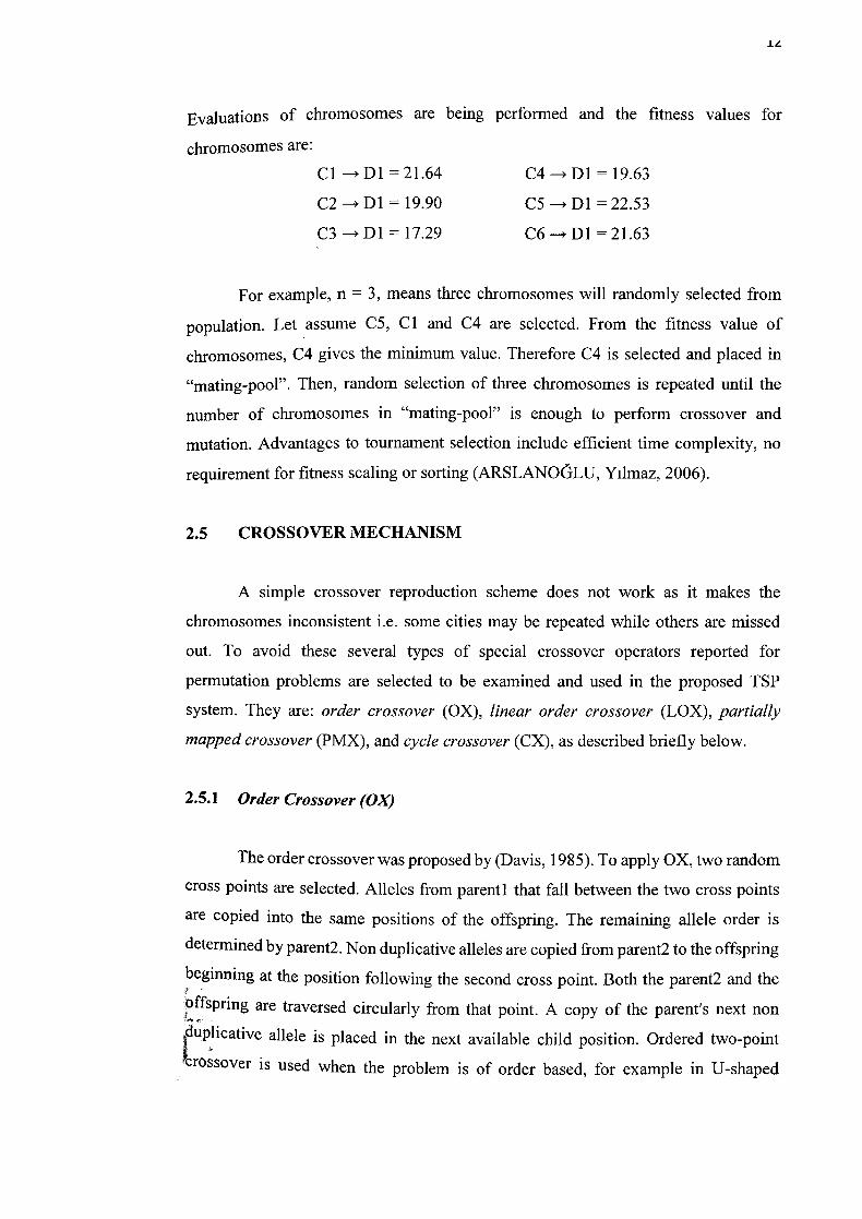
Evaluations of chromosomes are being performed and the fitness values for

chromosomes are:

Cl - Dl =21.64 C4 -* Dl = 19.63

C2 -* Dl = 19.90 C5—*D1 =22.53

C3 —* D1 = 17.29 C6 -+ Dl =21.63

For example, n = 3, means three chromosomes will randomly selected from

population. Let assume C5, Cl and C4 are selected. From the fitness value of

chromosomes, C4 gives the minimum value. Therefore C4 is selected and placed in

"mating-pool". Then, random selection of three chromosomes is repeated until the

number of chromosomes in "mating-pool" is enough to perform crossover and

mutation. Advantages to tournament selection include efficient time complexity, no

requirement for fitness scaling or sorting (ARSLANOLU, Yilmaz, 2006).

2.5 CROSSOVER MECHANISM

A simple crossover reproduction scheme does not work as it makes the

chromosomes inconsistent i.e. some cities may be repeated while others are missed

out. To avoid these several types of special crossover operators reported for

permutation problems are selected to be examined and used in the proposed TSP

system. They are: order crossover (OX), linear order crossover (LOX), partially

mapped crossover (PMX), and cycle crossover (CX), as described briefly below.

2.5.1 Order Crossover (OX)

The order crossover was proposed by (Davis, 1985). To apply OX, two random

cross points are selected. Alleles from parenti that fall between the two cross points

are copied into the same positions of the offspring. The remaining allele order is

detenTnined by parent2. Non duplicative alleles are copied from parent2 to the offspring

beginning at the position following the second cross point. Both the parent2 and the

offspring are traversed circularly from that point. A copy of the parent's next non

r

duplicative allele is placed in the next available child position. Ordered two-point cro, ssover is used when the problem is of order based, for example in U-shaped

assembly line balancing etc. given two parent chromosomes, two random crossover

points are selected partitioning them into a left, middle and right portion. The ordered

two-point crossover behaves in a following way: Child 1 inherits its left and right

section from parent l and its middle section is determined by the genes in the middle

section of parent 1 in the order in which the values appear in parent 2. A similar process

is applied to child 2. This is shown in example below.

Example:

LParentl:42113165 j i-'\.

Child 1:42131165 I Parent2:23114156 I Child 2:23141156

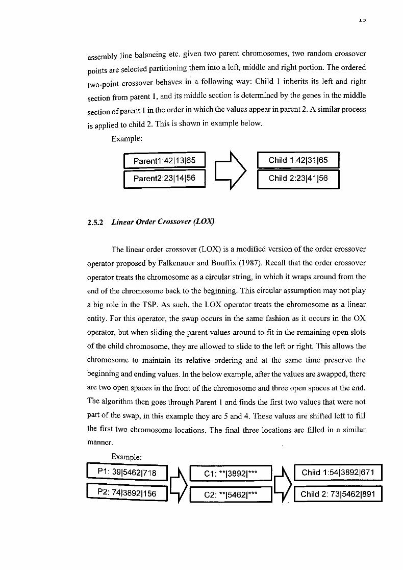
2.5.2 Linear Order Crossover (LOX)

The linear order crossover (LOX) is a modified version of the order crossover

operator proposed by Falkenauer and Bouffix (1987). Recall that the order crossover

operator treats the chromosome as a circular string, in which it wraps around from the

end of the chromosome back to the beginning. This circular assumption may not play

a big role in the TSP. As such, the LOX operator treats the chromosome as a linear

entity. For this operator, the swap occurs in the same fashion as it occurs in the OX

operator, but when sliding the parent values around to fit in the remaining open slots

of the child chromosome, they are allowed to slide to the left or right. This allows the

chromosome to maintain its relative ordering and at the same time preserve the

beginning and ending values. In the below example, after the values are swapped, there

are two open spaces in the front of the chromosome and three open spaces at the end.

The algorithm then goes through Parent 1 and finds the first two values that were not

part of the swap, in this example they are 5 and 4. These values are shifted left to fill

the first two chromosome locations. The final three locations are filled in a similar

manner.

Example:

1 Cl: **138921*** Child 1:54138921671 I EIP2: 74138921156 I I C2: **154621*** FChild 2: 73154621891 I

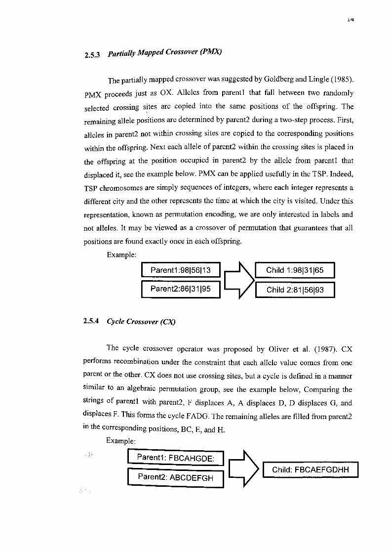
2.5.3 Partially Mapped Crossover (PMX)

The partially mapped crossover was suggested by Goldberg and Lingle (1985).

PMX proceeds just as OX. Alleles from parenti that fall between two randomly

selected crossing sites are copied into the same positions of the offspring. The

remaining allele positions are determined by parent2 during a two-step process. First,

alleles in parent2 not within crossing sites are copied to the corresponding positions

within the offspring. Next each allele of parent2 within the crossing sites is placed in

the offspring at the position occupied in parent2 by the allele from parenti that

displaced it, see the example below. PMX can be applied usefully in the TSP. Indeed,

TSP chromosomes are simply sequences of integers, where each integer represents a

different city and the other represents the time at which the city is visited. Under this

representation, known as permutation encoding, we are only interested in labels and

not alleles. It may be viewed as a crossover of permutation that guarantees that all

positions are found exactly once in each offspring.

Example:

I Parentl:98156113 I Child 1:98131165 I

I Parent2:86131195 I Child 2:81156193 I

2.5.4 Cycle Crossover (CX)

The cycle crossover operator was proposed by Oliver et al. (1987). CX

performs recombination under the constraint that each allele value comes from one

parent or the other. CX does not use crossing sites, but a cycle is defined in a manner

Similar to an algebraic permutation group, see the example below, Comparing the

strings of parentl with parent2, F displaces A, A displaces D, D displaces G, and

displaces F. This forms the cycle FADG. The remaining alleles are filled from parent2 in the corresponding positions, BC, E, and H.

Example:

EParenti: FBCAHGDE: I [Parent2: ABCDEFGH I

LI Child: FBCAEFGDHH I

FAM

2.6 MUTATION MECHANISM

In order to avoid from getting stuck onto a local minimum, population diversity

is required to be kept up to some extent. In genetic algorithms, this is achieved by the

help of a mutation mechanism, which causes some sudden changes on the traits of

individuals according to a predefined mutation probability parameter (Negnevitsky,

2011). A new offspring can be achieved by different ways either by flipping, inserting,

swapping or sliding the allele values at two randomly chosen gene positions.

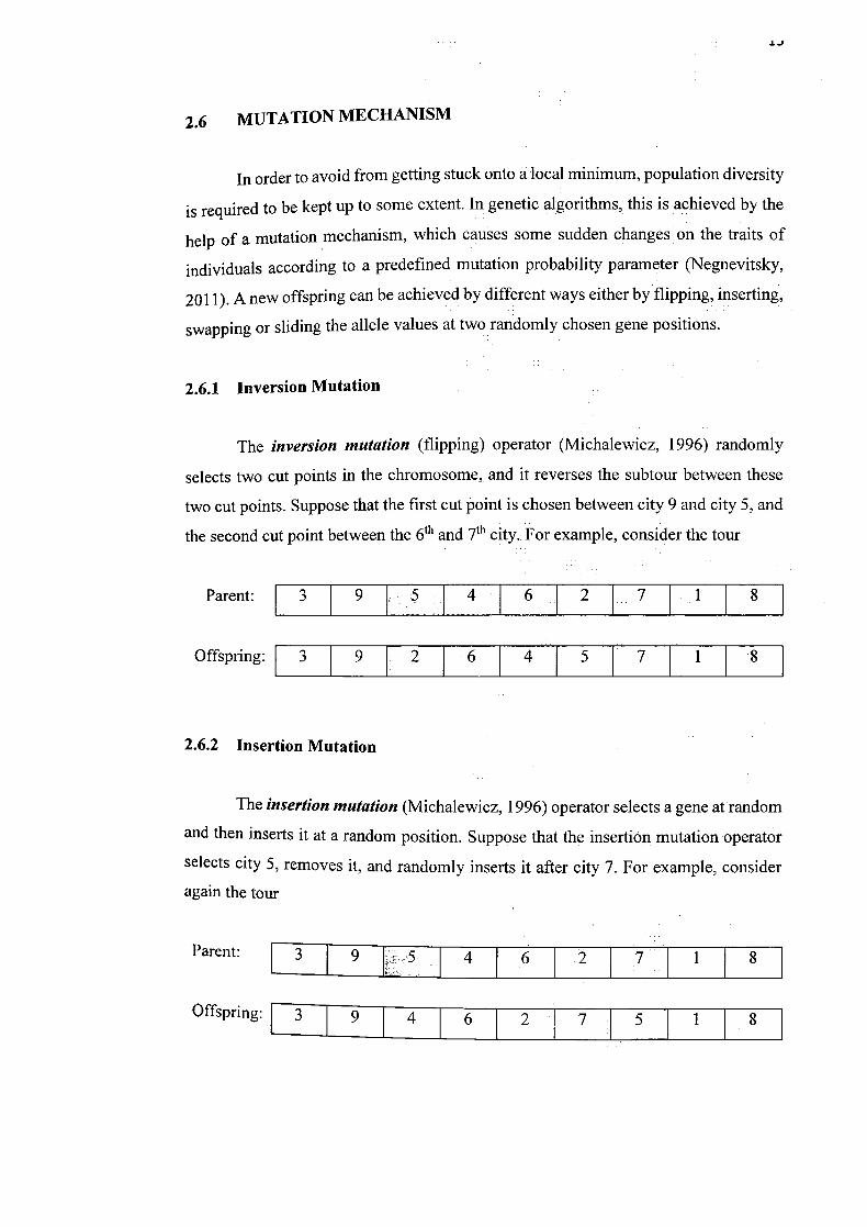
2.6.1 Inversion Mutation

The inversion mutation (flipping) operator (Michalewicz, 1996) randomly

selects two cut points in the chromosome, and it reverses the subtour between these

two cut points. Suppose that the first cut point is chosen between city 9 and city 5, and

the second cut point between the 6th and 7th city. For example, consider the tour

Parent: I 3 1 9 5 1 4 1 6 1 2 7 1 1 8

Offspring: 1 3 1 9 1. 2 1 6 4 1 5 1 7 1 1 8

2.6.2 Insertion Mutation

The insertion mutation (Michalewicz, 1996) operator selects a gene at random

and then inserts it at a random position. Suppose that the insertion mutation operator

selects city 5, removes it, and randomly inserts it after city 7. For example, consider

again the tour

Parent: [_3 9 4 •6 2 7 1 8

Offspring: [j 9 4 I 6 I 2 I 7 I 5 1 I 8

PIM

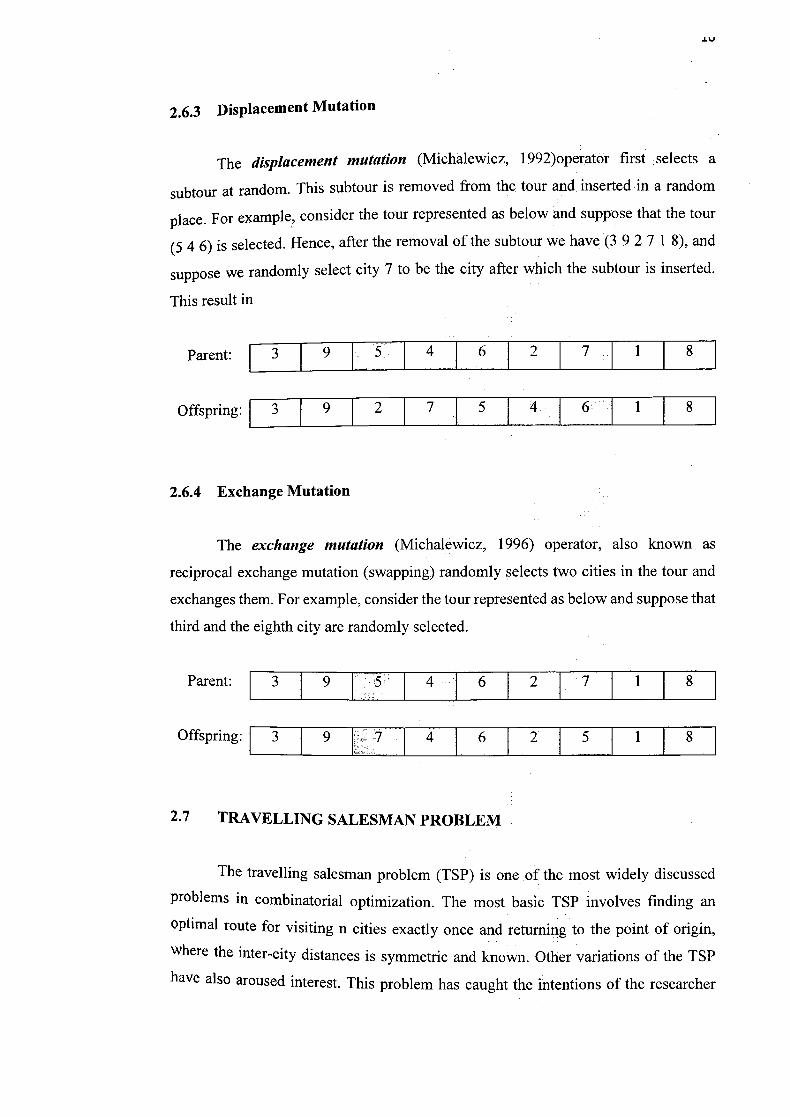
2.6.3 Displacement Mutation

The displacement mutation (Michalewicz, 1992)operator first selects a

subtour at random. This subtour is removed from the tour and inserted in a random

place. For example, consider the tour represented as below and suppose that the tour

(5 4 6) is selected. Hence, after the removal of the subtour we have (3 9 2 7 1 8), and

suppose we randomly select city 7 to be the city after which the subtour is inserted.

This result in

Parent: rm I 9 5 1 4 1 6 1 2 1 7 1 1 8

Offspring:[ 7 1 5 1 4 6: 1 8

2.6.4 Exchange Mutation

The exchange mutation (Michalewicz, 1996) operator, also known as

reciprocal exchange mutation (swapping) randomly selects two cities in the tour and

exchanges them. For example, consider the tour represented as below and suppose that

third and the eighth city are randomly selected.

Parent:l3 9ll 41612171118

Offspring: L

3 1 9 7 4 62 5 1 8

2.7 TRAVELLING SALESMAN PROBLEM

The travelling salesman problem (TSP) is one Of the most widely discussed

problems in combinatorial optimization. The most basic TSP involves finding an

Optimal route for visiting n cities exactly once and returning to the point of origin,

where the inter-city distances is symmetric and known. Other variations of the TSP

have also aroused interest. This problem has caught the intentions of the researcher