Tallinn University of Technology

Institute of Cybernetics

Genetic Inference of

Finite State MachinesMaster thesis

Margarita Spichakova

Supervisor:

Professor Jaan Penjam

Tallinn 2007

Declaration

Herewith I declare that this thesis is based on my own work. All ideas, majorviews and data from different sources by other authors are used only with areference to the source. The thesis has not been submitted for any degree orexamination in any other university.

. . . . . . . . . . . . . . . . . . . . . . . . . . . . . . . . . . . .

(Date) (Author)

Abstract

This thesis proposes a methodology based on genetic algorithms for infer-ring finite state machines. It defines basic parameters like fitness functionsand chromosomal representation that can be used with canonical genetic al-gorithm. Different types of finite state machines can be infered. Severalimprovements were introduced: inner decimal representation has been usedto improve the speed of initialization stage, post–processing stage has beenused to remove unaccessible states.

The experimental implementaion has also been presented, together with someexperiments.

1

Contents

1 Introduction 81.1 Motivation and goal . . . . . . . . . . . . . . . . . . . . . . . 81.2 Historical background . . . . . . . . . . . . . . . . . . . . . . . 91.3 Organization of the work . . . . . . . . . . . . . . . . . . . . . 10

2 Finite State Machines 112.1 Alphabets, strings, language . . . . . . . . . . . . . . . . . . . 122.2 Finite acceptor . . . . . . . . . . . . . . . . . . . . . . . . . . 13

2.2.1 Basic definitions . . . . . . . . . . . . . . . . . . . . . . 132.2.2 Minimal automata . . . . . . . . . . . . . . . . . . . . 15

2.3 Mealy and Moore machines . . . . . . . . . . . . . . . . . . . 162.3.1 Basic definitions . . . . . . . . . . . . . . . . . . . . . . 162.3.2 Equivalence of Moore and Mealy machines . . . . . . . 172.3.3 FSM minimization . . . . . . . . . . . . . . . . . . . . 172.3.4 FA as FSM with output . . . . . . . . . . . . . . . . . 19

3 Genetic Algorithms 213.1 Evolutionary algorithm . . . . . . . . . . . . . . . . . . . . . . 213.2 Canonical genetic algorithm . . . . . . . . . . . . . . . . . . . 22

3.2.1 Characteristics of canonical GA . . . . . . . . . . . . . 223.2.2 Genetic representation . . . . . . . . . . . . . . . . . . 223.2.3 Formal description of canonical GA . . . . . . . . . . . 23

3.3 Genetic operators . . . . . . . . . . . . . . . . . . . . . . . . . 233.3.1 Mutation . . . . . . . . . . . . . . . . . . . . . . . . . 233.3.2 Crossover . . . . . . . . . . . . . . . . . . . . . . . . . 243.3.3 Selection . . . . . . . . . . . . . . . . . . . . . . . . . . 25

4 Genetic Identification of Finite State Machines 274.1 Fitness functions . . . . . . . . . . . . . . . . . . . . . . . . . 27

4.1.1 Distance between strings . . . . . . . . . . . . . . . . . 274.1.2 Fitness value evaluation . . . . . . . . . . . . . . . . . 28

2

4.2 Chromosomal encoding. Genetic operators . . . . . . . . . . . 294.2.1 Restrictions . . . . . . . . . . . . . . . . . . . . . . . . 304.2.2 Moore machines . . . . . . . . . . . . . . . . . . . . . . 304.2.3 Mealy machines . . . . . . . . . . . . . . . . . . . . . . 35

4.3 Initialization. Reduction of invalid individuals . . . . . . . . . 37

5 Implementation 395.1 Experimental software description . . . . . . . . . . . . . . . . 39

5.1.1 FSM package . . . . . . . . . . . . . . . . . . . . . . . 405.1.2 Beings package . . . . . . . . . . . . . . . . . . . . . . 415.1.3 Evolution package . . . . . . . . . . . . . . . . . . . . . 42

5.2 Evolutionary trace . . . . . . . . . . . . . . . . . . . . . . . . 445.3 Post processing . . . . . . . . . . . . . . . . . . . . . . . . . . 44

6 Experiments 466.1 Learning Random Finite State Machines . . . . . . . . . . . . 46

6.1.1 Getting the training data . . . . . . . . . . . . . . . . . 466.1.2 Equivalence of Mealy and Moore machines . . . . . . . 466.1.3 Adjusting the parameter ’number of states’ . . . . . . . 486.1.4 Moore machine with unknown number of states . . . . 52

6.2 Learning Mealy machine. Parity checker . . . . . . . . . . . . 546.3 Learning Mealy machine. Two unit delay . . . . . . . . . . . . 546.4 Learning Moore machine. Pattern recognizer . . . . . . . . . . 566.5 Learning Moore machine. Up–down counter . . . . . . . . . . 58

7 Conclusions and future work 617.1 Conclusions . . . . . . . . . . . . . . . . . . . . . . . . . . . . 617.2 Future work . . . . . . . . . . . . . . . . . . . . . . . . . . . . 62

3

List of Tables

2.1 The example of transition table for FA . . . . . . . . . . . . . 142.2 Moore machine minimization. Step 1 . . . . . . . . . . . . . . 182.3 Moore machine minimization. Step 2 . . . . . . . . . . . . . . 18

3.1 Roulette–wheel selection . . . . . . . . . . . . . . . . . . . . . 26

4.1 String distance functions . . . . . . . . . . . . . . . . . . . . . 284.2 Measuring fitness value . . . . . . . . . . . . . . . . . . . . . . 294.3 One section of chromosome for storing the Moore machine

with fixed number of states . . . . . . . . . . . . . . . . . . . 314.4 Chromosomal representation of the Moore machine with fixed

number of states . . . . . . . . . . . . . . . . . . . . . . . . . 314.5 Chromosomal representation of a Moore machine with fixed

number of states . . . . . . . . . . . . . . . . . . . . . . . . . 324.6 One section of chromosome for storing the Moore machine

with unknown number of states . . . . . . . . . . . . . . . . . 334.7 Chromosomal representation of the Moore machine. Adopting

the number of states . . . . . . . . . . . . . . . . . . . . . . . 334.8 Example. Chromosomal representation of the Moore machine.

Adopting the number of states . . . . . . . . . . . . . . . . . . 344.9 One section of chromosome for storing the Mealy machine with

fixed number of states . . . . . . . . . . . . . . . . . . . . . . 354.10 Chromosomal representation of the Mealy machine with fixed

number of states . . . . . . . . . . . . . . . . . . . . . . . . . 364.11 Example. Chromosomal representation of the Mealy machine

with fixed number of states . . . . . . . . . . . . . . . . . . . 364.12 Error in decoding process . . . . . . . . . . . . . . . . . . . . 38

5.1 Removing unreachable states. Example . . . . . . . . . . . . . 45

6.1 Training data. Equivalence of Mealy and Moore machines . . 476.2 Equivalence of Mealy and Moore machine. Results . . . . . . . 48

4

6.3 Training data. Number of states . . . . . . . . . . . . . . . . . 496.4 Choice of number of states. Results . . . . . . . . . . . . . . . 506.5 Choice of number of states. Frequencies . . . . . . . . . . . . . 516.6 Generating a Moore machine with unknown number of states.

Results . . . . . . . . . . . . . . . . . . . . . . . . . . . . . . . 536.7 Parity checker. Training data . . . . . . . . . . . . . . . . . . 546.8 Two unit delay. Training data . . . . . . . . . . . . . . . . . . 556.9 Pattern recognizer. Training data . . . . . . . . . . . . . . . . 566.10 Up–down counter. Training data . . . . . . . . . . . . . . . . 59

5

List of Figures

1.1 Problem of system identification . . . . . . . . . . . . . . . . . 9

2.1 FSM classification . . . . . . . . . . . . . . . . . . . . . . . . . 112.2 Finite Acceptor . . . . . . . . . . . . . . . . . . . . . . . . . . 132.3 FA. Transition diagram . . . . . . . . . . . . . . . . . . . . . . 142.4 FSM . . . . . . . . . . . . . . . . . . . . . . . . . . . . . . . . 162.5 Moore machine minimization . . . . . . . . . . . . . . . . . . . 192.6 Converting FA to FSM. FA . . . . . . . . . . . . . . . . . . . 202.7 Converting FA to FSM. FSM . . . . . . . . . . . . . . . . . . 20

3.1 Mutation . . . . . . . . . . . . . . . . . . . . . . . . . . . . . . 243.2 Inversion . . . . . . . . . . . . . . . . . . . . . . . . . . . . . . 243.3 One point crossover . . . . . . . . . . . . . . . . . . . . . . . . 243.4 Roulette–wheel selection . . . . . . . . . . . . . . . . . . . . . 26

4.1 A Moore machine represented as transition diagram . . . . . . 314.2 A Moore machine with an unreachable state . . . . . . . . . . 334.3 A Mealy machine represented as transition diagram . . . . . . 364.4 Coding/decoding process from binary genotype to FSM . . . . 374.5 Coding/decoding process from binary genotype to FSM using

decimal representation . . . . . . . . . . . . . . . . . . . . . . 38

5.1 Packages . . . . . . . . . . . . . . . . . . . . . . . . . . . . . . 405.2 FSM package . . . . . . . . . . . . . . . . . . . . . . . . . . . 415.3 Beings package . . . . . . . . . . . . . . . . . . . . . . . . . . 425.4 Evolution package . . . . . . . . . . . . . . . . . . . . . . . . . 435.5 Evolutionary trace . . . . . . . . . . . . . . . . . . . . . . . . 44

6.1 Choice of number of states. Frequencies . . . . . . . . . . . . . 526.2 Parity checker. Transition diagram . . . . . . . . . . . . . . . 556.3 Two unit delay. Evolutionary trace . . . . . . . . . . . . . . . 566.4 Two unit delay. Transition diagram . . . . . . . . . . . . . . . 566.5 Pattern recognizer for ”abb”. Evolutionary trace . . . . . . . . 57

6

6.6 Pattern recognizer for ”abb”, incorrect. Transition diagram . . 576.7 Pattern recognizer for ”abb”. Transition diagram . . . . . . . 586.8 Up–down counter. Original machine. Transition diagram . . . 586.9 Up–down counter. Generated machine. Transition diagram . . 596.10 Up–down counter. Evolutionary trace . . . . . . . . . . . . . . 60

7

Chapter 1

Introduction

1.1 Motivation and goal

Identification has been defined as an inference process, which deduces aninternal representation of the system (named internal model, usually a statemachine) from samples of it’s functioning (named external model, usuallygiven by several input/output sequences) [18]. There are many possibilitiesto a represent system, one of them is to use a finite state machine (FSM).

There are many applications for identification in different fields such as logicaldesign, verification or test, sequential learning. For example finite automata(FA) are useful models for many important kind of hardware and softwaresystems (lexical analysis, system for verifying the correctness).

The modeling problem consists of researching the ’best’ FSM (in practice,one of those that best describe the process behavior), which respects the dy-namics of the external model. The process is indeed considered a black box.

Finding a FSM consistent with the given input/output sequences is a prob-lem in the field of grammatical inference [18].

Finding a minimum size deterministic FA consistent with the set of givensamples is NP–complete [7]. The genetic simulation approach is an alterna-tive that reduces the complexity of the preceding methods.

Our goal is to create methods based on Genetic Algorithm (GA), which allowto find FSM using only external behavior.

8

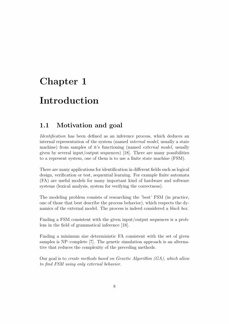
The task is to find a FSM M that is consistent with all elements in theset given input/output sequence set ζ, that is composed of a number of in-put/output sequences (external behavior).

External behavior

((RRRRRRRRRRRRRR

Number of states // GeneticAlgorithm

// FSM

Type of the machine

66mmmmmmmmmmmmmm

Figure 1.1: Problem of system identification

There are two types of solutions that can be found during the process ofidentification:

• Complete solution is a solution that operated correctly for all giveninput/output sequences

• Incomplete solution is a solution that operated correctly for some in-put/output sequences.

1.2 Historical background

In the early 1960s Fogel introduced Evolutionary Programming (EP) [5]. Thesimulated evolution was performed by modifying a population of FSM. Otherauthors also used EP for solving the problem of FSM identification. KumarChellapilla and David Czarnecki proposed the variation of EP to solve theproblem of modular FSM synthesis [4]. Karl Benson presented a model com-prising FSM with embedded genetic programs which co–evolve to performthe task of Automatic Target Detection [3].

Another approach to solve the problem of FSM identification is based on GA.This method has been researched by several authors. Tongchim and Chongis-titvatana investigated parallel implementation of GA to solve the problem ofFSM synthesis [23]. Chongistitvatana and Niparnan improved GA by evolv-ing only the state transition function [20]. Chongistitvatana also presented a

9

method of FSM synthesis from multiple partial input/output sequences [21].Jason W. Horihan and Yung–Hsiang Lu paid more attention to improvingthe FSM evolution by using progressive fitness functions [10].

Different types of machines can be inferred using GA: Lamine Ngome usedgenetic simulation for Moore machine identification [19], Pushmeet Kohliused GA to synthesize FA accepting particular language using accept/rejectdata [11], Philip Hingston showed in [8] how GA can be used for the inferenceof regular language from a set of positive examples, Xiaojun Geng appliedGA for solving identification problem for asynchronous FSM [6]. The algo-rithm for Automated Negotiations presented by Tu, Wolff and Lamersdorfis based on GA synthesis of FSM [24]. Simon M. Lucas paid more attentionto finite state transducers [16] and compares his method to ”Heuristic StateMerging” [17].

GA has also been used for solving other similar problems: for solving StateAssignment Problem [1], for identification of nondeterministic pushdown au-tomata [12], for inferring regular and context-free grammars [15], for protect-ing resources [22].

1.3 Organization of the work

The thesis is organized in the following way: in chapter 2 we give theoreticaloverview of FSM. Chapter 3 contains the basic theory of GA. In chapter 4we present a method for genetic inference of FSM. The implementation ofthat method is presented in chapter 5. Experiments required to show theefficiency of the presented method are described in chapter 6.

10

Chapter 2

Finite State Machines

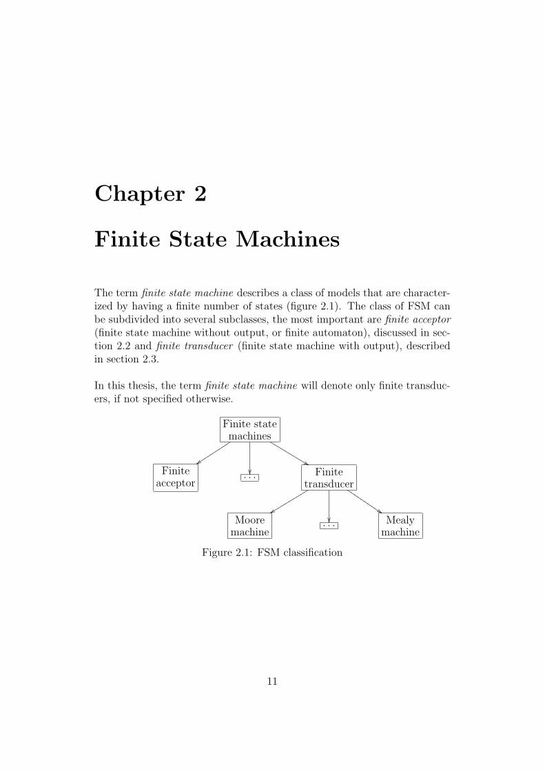
The term finite state machine describes a class of models that are character-ized by having a finite number of states (figure 2.1). The class of FSM canbe subdivided into several subclasses, the most important are finite acceptor(finite state machine without output, or finite automaton), discussed in sec-tion 2.2 and finite transducer (finite state machine with output), describedin section 2.3.

In this thesis, the term finite state machine will denote only finite transduc-ers, if not specified otherwise.

Finite statemachines

yyttttttttt

��%%LLLLLLLLLL

Finiteacceptor

. . . Finitetransducer

yyrrrrrrrrrr

��$$III

IIIIII

I

Mooremachine

. . . Mealymachine

Figure 2.1: FSM classification

11

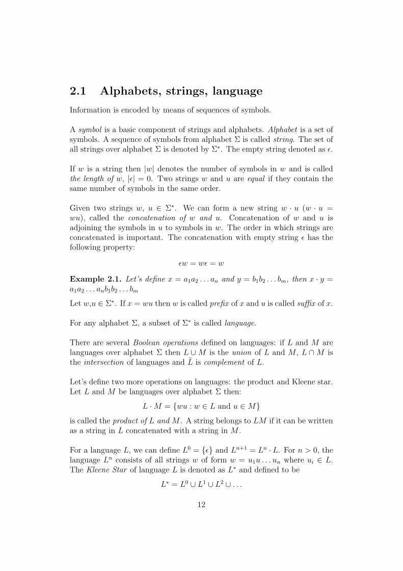
2.1 Alphabets, strings, language

Information is encoded by means of sequences of symbols.

A symbol is a basic component of strings and alphabets. Alphabet is a set ofsymbols. A sequence of symbols from alphabet Σ is called string. The set ofall strings over alphabet Σ is denoted by Σ∗. The empty string denoted as ε.

If w is a string then |w| denotes the number of symbols in w and is calledthe length of w, |ε| = 0. Two strings w and u are equal if they contain thesame number of symbols in the same order.

Given two strings w, u ∈ Σ∗. We can form a new string w · u (w · u =wu), called the concatenation of w and u. Concatenation of w and u isadjoining the symbols in u to symbols in w. The order in which strings areconcatenated is important. The concatenation with empty string ε has thefollowing property:

εw = wε = w

Example 2.1. Let’s define x = a1a2 . . . an and y = b1b2 . . . bm, then x · y =a1a2 . . . anb1b2 . . . bm

Let w,u ∈ Σ∗. If x = wu then w is called prefix of x and u is called suffix of x.

For any alphabet Σ, a subset of Σ∗ is called language.

There are several Boolean operations defined on languages: if L and M arelanguages over alphabet Σ then L ∪M is the union of L and M , L ∩M isthe intersection of languages and L is complement of L.

Let’s define two more operations on languages: the product and Kleene star.Let L and M be languages over alphabet Σ then:

L ·M = {wu : w ∈ L and u ∈M}

is called the product of L and M . A string belongs to LM if it can be writtenas a string in L concatenated with a string in M .

For a language L, we can define L0 = {ε} and Ln+1 = Ln ·L. For n > 0, thelanguage Ln consists of all strings w of form w = u1u . . . un where ui ∈ L.The Kleene Star of language L is denoted as L∗ and defined to be

L∗ = L0 ∪ L1 ∪ L2 ∪ . . .

12

2.2 Finite acceptor

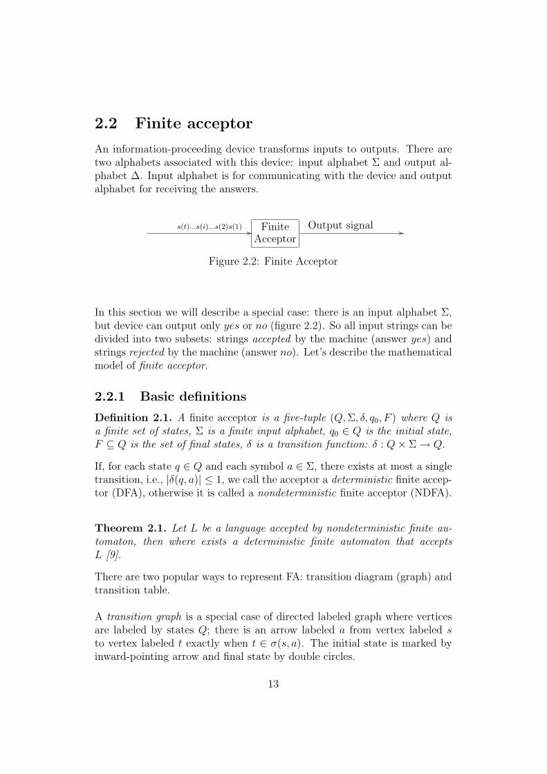
An information-proceeding device transforms inputs to outputs. There aretwo alphabets associated with this device: input alphabet Σ and output al-phabet ∆. Input alphabet is for communicating with the device and outputalphabet for receiving the answers.

s(t)...s(i)...s(2)s(1) // FiniteAcceptor

Output signal //

Figure 2.2: Finite Acceptor

In this section we will describe a special case: there is an input alphabet Σ,but device can output only yes or no (figure 2.2). So all input strings can bedivided into two subsets: strings accepted by the machine (answer yes) andstrings rejected by the machine (answer no). Let’s describe the mathematicalmodel of finite acceptor.

2.2.1 Basic definitions

Definition 2.1. A finite acceptor is a five-tuple (Q, Σ, δ, q0, F ) where Q isa finite set of states, Σ is a finite input alphabet, q0 ∈ Q is the initial state,F ⊆ Q is the set of final states, δ is a transition function: δ : Q× Σ→ Q.

If, for each state q ∈ Q and each symbol a ∈ Σ, there exists at most a singletransition, i.e., |δ(q, a)| ≤ 1, we call the acceptor a deterministic finite accep-tor (DFA), otherwise it is called a nondeterministic finite acceptor (NDFA).

Theorem 2.1. Let L be a language accepted by nondeterministic finite au-tomaton, then where exists a deterministic finite automaton that acceptsL [9].

There are two popular ways to represent FA: transition diagram (graph) andtransition table.

A transition graph is a special case of directed labeled graph where verticesare labeled by states Q; there is an arrow labeled a from vertex labeled sto vertex labeled t exactly when t ∈ σ(s, a). The initial state is marked byinward-pointing arrow and final state by double circles.

13

Example 2.2. Here is an example of simple FA represented as transitiondiagram (figure 2.3) and as transition table 2.1.

GFED@ABCq0a22 ??

b // GFED@ABC?>=<89:;f1a

oo bll

Figure 2.3: FA. Transition diagram

Five ingredients of FA:

• Set of states {q0, f1}

• The input alphabet Σ = {a, b}

• The initial state q0

• The set of final states F = {f1}

• The transition function δ : Q× Σ→ Q is defined as

δ(q0, a) = q0, δ(q0, b) = f1, δ(f1, a) = q0, δ(f1, b) = f1

The transition table for this acceptor is represented in table 2.1.

Table 2.1: The example of transition table for FAa b

→ q0 q0 f1

← f1 q0 f1

Let’s define the language accepted by FA.

Definition 2.2. If M = (Q, Σ, δ, q0, F ) is FA, a ∈ Σ ∪ ε, we say (q, aw) `M

(p, w), iff p ∈ δ(q, a). `M is called yield operator.

Definition 2.3. A string w is said to be accepted by an acceptor M iff(q0, w) `∗M (p, ε) for some p ∈ F , i.e., there exists a finite sequence of tran-sitions, corresponding to the input string w, from the initial state to somefinal state.The language accepted by M , is denoted as L(M) and defines as:

L(M) = {w | ∃p ∈ F : (q0, w) `∗M (p, ε)}.

14

2.2.2 Minimal automata

An acceptor can be reduced in size without changing the language recognized.There are two methods of doing this:

• removing the states that cannot play any role in deciding whether astring is accepted;

• merging the states that ’do the same work’.

Let A = (Q, Σ, i, q0, F ) be a FA.

Definition 2.4. We can say that state q ∈ Q is accessible if there is a stringx ∈ Σ∗ such that q0 ·x = q, where q0 ·x = q means that state q can be reachedfrom state q0 by making transitions according to corresponding symbols of x.

q0x0−→ q1

x1−→ . . .xn−→ q

A state that is not accessible is inaccessible. An acceptor is accessible if it’severy state is accessible. The inaccessible states of an automaton play norole in accepting strings, so they can be removed without the language beingchanged.

Definition 2.5. Two states qi ∈ Q an qj ∈ Q are distinguishable if thereexists X ∈ Σ∗ such that

(qi · x, qj · x) ∈ (F × F ′) ∪ (F ′ × F ),

where F ′ ∈ Q \ F .

In other words, for the same string x, one of states qi · x, qj · x is final andthe other is not final.

If states qi an qj are indistinguishable thus means that for each x ∈ Σ∗

qi · x ∈ F ⇔ qj · x ∈ F .

Define the relation 'A on the set of states Q by

qi 'A qj ⇔ qi and qj are indistinguishable.

Definition 2.6. An acceptor is reduced if each pair of states in an acceptoris distinguishable.

Theorem 2.2. Let A be a FA. There is an algorithm that constructs anaccessible acceptor, Aa, such that L(A) = L(Aa) [14].

15

Theorem 2.3. Let A be a FA. There is an algorithm that constructs a reducedacceptor , Ar, such that L(A) = L(Ar) [14].

Those two theorems can be applied to any acceptor A in turn yielding anacceptor Aar = (Aa)r that is both accessible and reduced.

Definition 2.7. Let L be a language accepted by FA. A finite acceptor Ais said to be minimal (for L) if L(A) = L, and if B is any FA such thatL(B) = L, then the number of states of A is less than or equal to number ofstates of B.

If A is minimal acceptor then it is reduced and accessible. An algorithm forFA minimization can be found in [13].

2.3 Mealy and Moore machines

2.3.1 Basic definitions

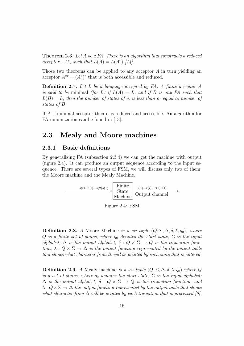
By generalizing FA (subsection 2.3.4) we can get the machine with output(figure 2.4). It can produce an output sequence according to the input se-quence. There are several types of FSM, we will discuss only two of them:the Moore machine and the Mealy Machine.

s(t)...s(i)...s(2)s(1) //FiniteState

Machine

r(n)...r(i)...r(2)r(1)

Output channel//

Figure 2.4: FSM

Definition 2.8. A Moore Machine is a six-tuple (Q, Σ, ∆, δ, λ, q0), whereQ is a finite set of states, where q0 denotes the start state; Σ is the inputalphabet; ∆ is the output alphabet; δ : Q × Σ → Q is the transition func-tion; λ : Q × Σ → ∆ is the output function represented by the output tablethat shows what character from ∆ will be printed by each state that is entered.

Definition 2.9. A Mealy machine is a six-tuple (Q, Σ, ∆, δ, λ, q0) where Qis a set of states, where q0 denotes the start state; Σ is the input alphabet;∆ is the output alphabet; δ : Q × Σ → Q is the transition function, andλ : Q×Σ→ ∆ the output function represented by the output table that showswhat character from ∆ will be printed by each transition that is processed [9].

16

The key difference between Moore and Mealy machines:

• Moore machines print a character when entering the state;

• Mealy machines print a character when traversing an arc.

Definition 2.10. An input/output sequence S of length n is a set of pairs{(i0, o0), (i1, o1), . . . , (in, on)} where (ii, oi) ∈ Σ × ∆. An input/output se-quence set ζ is a set of S.

A FSM M = (Q, Σ, ∆, δ, λ, q0) is said to be consistent with an input/outputsequence S iff oj = λ(qj, ij) for all 0 ≤ j ≤ n.

2.3.2 Equivalence of Moore and Mealy machines

Given a Mealy machine Me and a Moore machine Mo, which automaticallyprints the character x in the start state, we say that these two machines areequivalent if for every input string the output string from Mo is exactly xconcatenated with output from Me.

Theorem 2.4. If Mo is a Moore machine, then there is a Mealy machineMe that is equivalent to it.

Theorem 2.5. For every Mealy machine Me, there is an equivalent Mooremachine Mo.

2.3.3 FSM minimization

Both Moore and Mealy machines can be minimized in a way that directlygeneralizes the minimization of FA described in subsection 2.2.2.

Definition 2.11. Two FSMs are equivalent iff for any given input sequence,identical output sequences are produced.

Definition 2.12. Two states q0 and q1 in a given FSM are equivalent iffeach input sequence beginning from q0 yields an output sequence identical tothat obtained by starting from q1.

To minimize Moore machine we need to find and remove equivalent states.First, we need to find all pairs of states which have the same output. Second,we need to check all pairs of states with the same output: if target states oftransitions marked by each input symbol are equal for two states, whetherthis is a pair of equivalent states (algorithm 2.1).

17

Algorithm 2.1. Minimization of Moore machine

for (each pair of states (qi, qj)){

if (qi and qj have different output){

mark qi and qj as not equivalent;

}

}

{

for (each unmarked pair){

for (each input symbol, qi and qj are transferred to

states which are not equivalent) {

Mark qi and qj as not equivalent;

}

}

} while (marking is possible);

Unmarked pairs are equivalent;

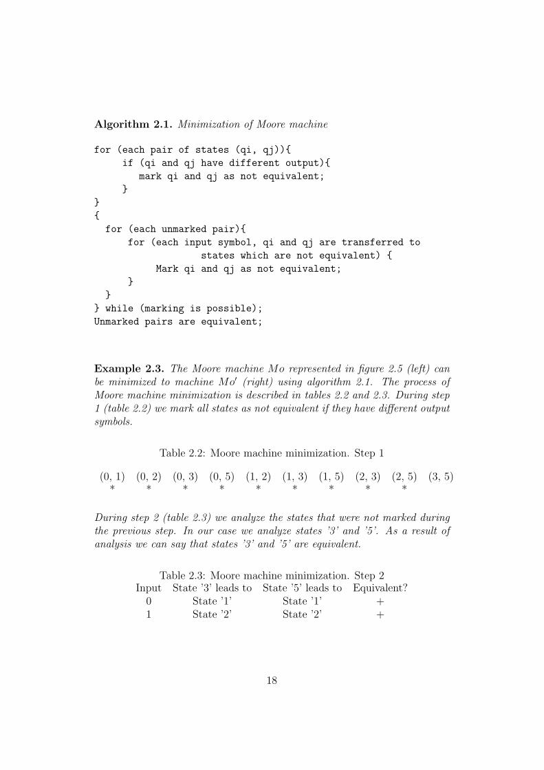
Example 2.3. The Moore machine Mo represented in figure 2.5 (left) canbe minimized to machine Mo′ (right) using algorithm 2.1. The process ofMoore machine minimization is described in tables 2.2 and 2.3. During step1 (table 2.2) we mark all states as not equivalent if they have different outputsymbols.

Table 2.2: Moore machine minimization. Step 1

(0, 1) (0, 2) (0, 3) (0, 5) (1, 2) (1, 3) (1, 5) (2, 3) (2, 5) (3, 5)* * * * * * * * *

During step 2 (table 2.3) we analyze the states that were not marked duringthe previous step. In our case we analyze states ’3’ and ’5’. As a result ofanalysis we can say that states ’3’ and ’5’ are equivalent.

Table 2.3: Moore machine minimization. Step 2Input State ’3’ leads to State ’5’ leads to Equivalent?

0 State ’1’ State ’1’ +1 State ’2’ State ’2’ +

18

ONMLHIJK0/0

0

��

1 // ONMLHIJK1/1

1

��

0oo ONMLHIJK0/0

0

��

1 // ONMLHIJK1/1

1

��

0oo

ONMLHIJK3/2

1}}||

||||

||||

0

==||||||||||

ONMLHIJK2/3

1

OO

0

==||||||||||ONMLHIJK5/2

0

OO

1oo ONMLHIJK2/3

1

OO

0 // ONMLHIJK5/2

0

OO

1oo

Figure 2.5: Moore machine minimization

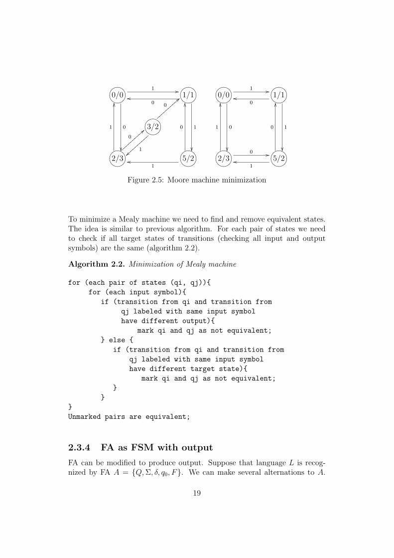
To minimize a Mealy machine we need to find and remove equivalent states.The idea is similar to previous algorithm. For each pair of states we needto check if all target states of transitions (checking all input and outputsymbols) are the same (algorithm 2.2).

Algorithm 2.2. Minimization of Mealy machine

for (each pair of states (qi, qj)){

for (each input symbol){

if (transition from qi and transition from

qj labeled with same input symbol

have different output){

mark qi and qj as not equivalent;

} else {

if (transition from qi and transition from

qj labeled with same input symbol

have different target state){

mark qi and qj as not equivalent;

}

}

}

Unmarked pairs are equivalent;

2.3.4 FA as FSM with output

FA can be modified to produce output. Suppose that language L is recog-nized by FA A = {Q, Σ, δ, q0, F}. We can make several alternations to A.

19

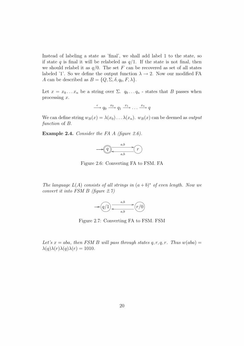
Instead of labeling a state as ’final’, we shall add label 1 to the state, soif state q is final it will be relabeled as q/1. If the state is not final, thenwe should relabel it as q/0. The set F can be recovered as set of all stateslabeled ’1’. So we define the output function λ → 2. Now our modified FAA can be described as B = {Q, Σ, δ, q0, F, λ}.

Let x = x0 . . . xn be a string over Σ. q0 . . . qn - states that B passes whenprocessing x.

ε−→ q0x0−→ q1

x1−→ . . .xn−→ q

We can define string wB(x) = λ(x0) . . . λ(xn). wB(x) can be deemed as outputfunction of B.

Example 2.4. Consider the FA A (figure 2.6).

GFED@ABC?>=<89:;q//a,b //GFED@ABCra,b

oo

Figure 2.6: Converting FA to FSM. FA

The language L(A) consists of all strings in (a + b)∗ of even length. Now weconvert it into FSM B (figure 2.7)

ONMLHIJKq/1//a,b // ONMLHIJKr/0a,b

oo

Figure 2.7: Converting FA to FSM. FSM

Let’s x = aba, then FSM B will pass through states q, r, q, r. Thus w(aba) =λ(q)λ(r)λ(q)λ(r) = 1010.

20

Chapter 3

Genetic Algorithms

3.1 Evolutionary algorithm

Evolutionary Algorithm (EA) is a search algorithm based on simulationof biological evolution. In EA some mechanisms inspired by evolution areused: reproduction, mutation, recombination, selection. Candidate solutionpresents the individuals of the evolution.

All basic instances of EA share a number of common properties which cancharacterize a general EA:

• EA implements the process of collective learning of population of indi-viduals. Each individual presents a search point in the space of potentialsolutions to the problem.

• New individuals are randomly generated from previous population us-ing processes that model mutation and recombination. Mutation usu-ally represents a self–replication, but reproduction require two or moreindividuals.

• A measure of the quality can be assigned to all individuals (fitnessfunction).

Some differences in implementation of those principles characterize the in-stances of EA (Thomas Back [2]):

• Genetic algorithms (originally described by Holland (1962, 1975)) —the solution represented as an array of numbers (usually binary num-bers). A recombination operator is also used to produce new solutions.

21

• Evolutionary strategies (developed by Rechenberg (1965,1973) and Schwe-fel (1965, 1977)) — uses the real number vectors for representing so-lution. Mutation and crossover are essential operators for searching insearch space.

• Evolutionary programming (developed by Lawrence J Fogel (1962)) —the algorithm was originally developed to evolve FSM, but most ap-plications are for search spaces involving real-valued vectors. Does notincorporate the recombination of individuals and emphasizes the mu-tation.

In this work we will discuss only GA.

3.2 Canonical genetic algorithm

GAs are a class of evolutionary algorithms first proposed and analyzed byJohn Holland (1975).

3.2.1 Characteristics of canonical GA

According to Larry J Eshelman [2] there are three features which distinguishGAs, as first proposed by Holland from other evolutionary algorithms:

• the representation used — bi strings ;

• the method of selection — proportional selection;

• the primary method of producing variations — crossover ;

Many subsequent alternations of GA have adopted different kinds of selec-tions, and also some of them use different representations (not binary) ofsolutions. But all those methods are inspired by the original algorithm.

3.2.2 Genetic representation

Genetic representation is a way of representing solutions/individuals. In GAthe binary representation of fixed size is used (chromosome). The main prop-erty that makes this representation convenient is that their parts are easilyaligned due to their fixed size.

The genotype of the individual is manipulated by the GA. To evaluate theindividual we need to decode the genotype to phenotype and assign the fitness

22

value. The process of mapping from genotype to phenotype is called decoding.The process of mapping from phenotype to genotype is called coding.

3.2.3 Formal description of canonical GA

First step is to generate (randomly) the initial population P (0). Each indi-vidual must be evaluated by the fitness function. Then some individuals willbe selected for reproduction and copied to C(t). Next the genetic operators(mutation and crossover) are applied to C(t) producing C ′(t). After newoffsprings are generated a new population must be created from C ′(t) andP (t−1). If the size of population is M , then M individuals must be selectedfrom C ′(t) and P (t− 1) to produce P (t).

Algorithm 3.1. (Canonical GA)

t=0;

initialize P(t);

evaluate structures in P(t);

while (termination condition is not satisfied){

t++;

selectReproduction C(t) from P(t-1);

recombine and mutate structures in C(t) forming C’(t);

evaluate structures in C’(t);

selectReplace P(t) from C’(t) and P(t-1);

}

3.3 Genetic operators

3.3.1 Mutation

One of the best known mechanisms for producing variations is mutation,where new trial solutions are created by making small, random changes inrepresentation of prior trial solutions. If binary representation is used, themutation is achieved by randomly flipping one bit (figure 3.1).

Another option is called inversion. In this case the segment of the chromo-some after random mutation point (suffix) is reversed (figure 3.2).

23

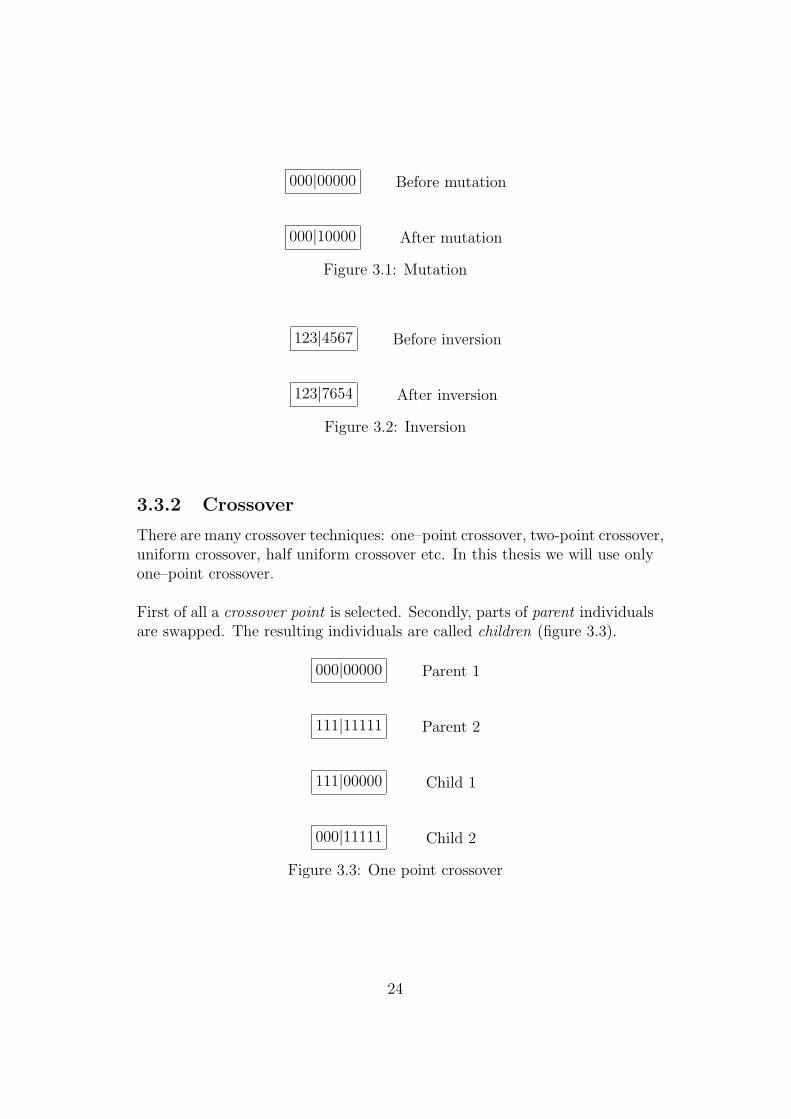
000|00000 Before mutation

000|10000 After mutation

Figure 3.1: Mutation

123|4567 Before inversion

123|7654 After inversion

Figure 3.2: Inversion

3.3.2 Crossover

There are many crossover techniques: one–point crossover, two-point crossover,uniform crossover, half uniform crossover etc. In this thesis we will use onlyone–point crossover.

First of all a crossover point is selected. Secondly, parts of parent individualsare swapped. The resulting individuals are called children (figure 3.3).

000|00000 Parent 1

111|11111 Parent 2

111|00000 Child 1

000|11111 Child 2

Figure 3.3: One point crossover

24

3.3.3 Selection

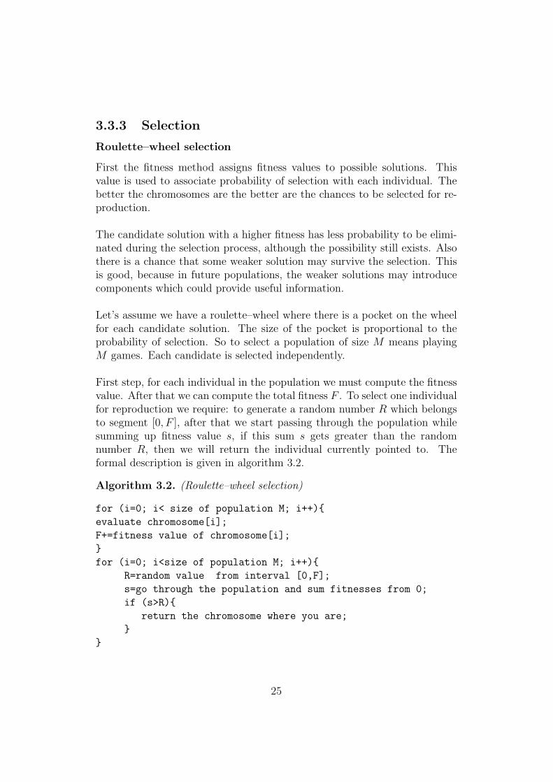
Roulette–wheel selection

First the fitness method assigns fitness values to possible solutions. Thisvalue is used to associate probability of selection with each individual. Thebetter the chromosomes are the better are the chances to be selected for re-production.

The candidate solution with a higher fitness has less probability to be elimi-nated during the selection process, although the possibility still exists. Alsothere is a chance that some weaker solution may survive the selection. Thisis good, because in future populations, the weaker solutions may introducecomponents which could provide useful information.

Let’s assume we have a roulette–wheel where there is a pocket on the wheelfor each candidate solution. The size of the pocket is proportional to theprobability of selection. So to select a population of size M means playingM games. Each candidate is selected independently.

First step, for each individual in the population we must compute the fitnessvalue. After that we can compute the total fitness F . To select one individualfor reproduction we require: to generate a random number R which belongsto segment [0, F ], after that we start passing through the population whilesumming up fitness value s, if this sum s gets greater than the randomnumber R, then we will return the individual currently pointed to. Theformal description is given in algorithm 3.2.

Algorithm 3.2. (Roulette–wheel selection)

for (i=0; i< size of population M; i++){

evaluate chromosome[i];

F+=fitness value of chromosome[i];

}

for (i=0; i<size of population M; i++){

R=random value from interval [0,F];

s=go through the population and sum fitnesses from 0;

if (s>R){

return the chromosome where you are;

}

}

25

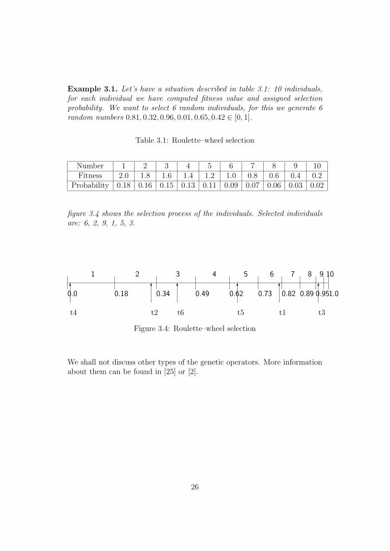
Example 3.1. Let’s have a situation described in table 3.1: 10 individuals,for each individual we have computed fitness value and assigned selectionprobability. We want to select 6 random individuals, for this we generate 6random numbers 0.81, 0.32, 0.96, 0.01, 0.65, 0.42 ∈ [0, 1].

Table 3.1: Roulette–wheel selection

Number 1 2 3 4 5 6 7 8 9 10Fitness 2.0 1.8 1.6 1.4 1.2 1.0 0.8 0.6 0.4 0.2

Probability 0.18 0.16 0.15 0.13 0.11 0.09 0.07 0.06 0.03 0.02

figure 3.4 shows the selection process of the individuals. Selected individualsare: 6, 2, 9, 1, 5, 3.

0.0

1

0.18

2

0.34

3

0.49

4

0.62

5

0.73

6

0.82

7

0.89

8

0.95

9 10

1.06

t1

6

t2

6

t3

6

t4

6

t5

6

t6

Figure 3.4: Roulette–wheel selection

We shall not discuss other types of the genetic operators. More informationabout them can be found in [25] or [2].

26

Chapter 4

Genetic Identification of FiniteState Machines

In this chapter we will apply the GA to the problem of FSM identification.The major difficulty lies in the efficient coding of the information and choiceof adaptation function of the members of population.

4.1 Fitness functions

We choose a fitness function defined as a calculus performed on all I/O se-quences (couples {input, output}). The idea is to estimate the proximitybetween the evaluated individual and searched FSM.

4.1.1 Distance between strings

We can specify several functions for computing distance between strings.

The simplest one is strict distance. It can be measured as

dstrict(x, y) =

{0 : x = y1 : x 6= y

(4.1)

Strict distance returns 0 if strings are equal, otherwise it returns 1.

Given two strings x, y. The computing of strict distance has the worst casetime complexity O(|x|), when |x| = |y|, otherwise it is constant in time (if

27

|x| 6= |y|, then function will return 1).

We can specify a function ∆(a, b), where a, b are symbols in some alphabet:

∆(a, b) =

{0 : a = b1 : a 6= b

(4.2)

that returns 1 if chars are not equal.

To compute Hamming distance dHam between two strings we need to countthe number of different bits in the same positions.

dHam(x, y) = ΣMin(|x|,|y|)i=1 ∆(xi, yi) (4.3)

Computing Hamming distance has a complexity of O(Min(|x|, |y|)).

The distance between two strings can be also evaluated by the length ofmaximal equal prefix dLP (the analysis will be stopped at the first differencebetween strings).

dLP (x, y) = Σx=yi=1 ∆(xi, yi) (4.4)

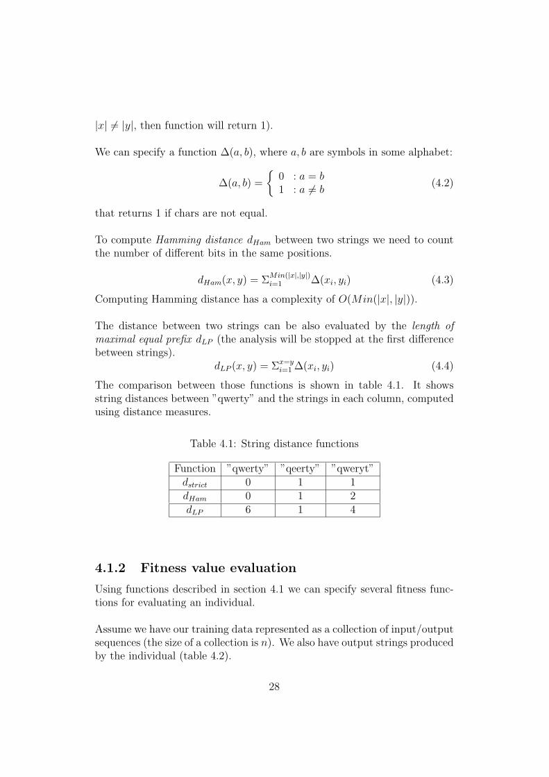
The comparison between those functions is shown in table 4.1. It showsstring distances between ”qwerty” and the strings in each column, computedusing distance measures.

Table 4.1: String distance functions

Function ”qwerty” ”qeerty” ”qweryt”dstrict 0 1 1dHam 0 1 2dLP 6 1 4

4.1.2 Fitness value evaluation

Using functions described in section 4.1 we can specify several fitness func-tions for evaluating an individual.

Assume we have our training data represented as a collection of input/outputsequences (the size of a collection is n). We also have output strings producedby the individual (table 4.2).

28

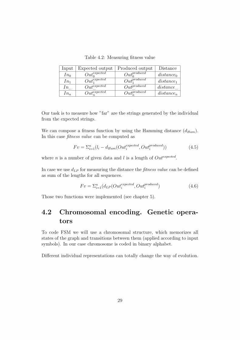
Table 4.2: Measuring fitness value

Input Expected output Produced output Distance

In0 Outexpected0 Outproduced

0 distance0

In1 Outexpected1 Outproduced

1 distance1

In... Outexpected... Outproduced

... distance...

Inn Outexpectedn Outproduced

n distancen

Our task is to measure how ”far” are the strings generated by the individualfrom the expected strings.

We can compose a fitness function by using the Hamming distance (dHam).In this case fitness value can be computed as

Fv = Σni=1(li − dHam(Outexpected

i , Outproducedi )) (4.5)

where n is a number of given data and l is a length of Outexpected.

In case we use dLP for measuring the distance the fitness value can be definedas sum of the lengths for all sequences.

Fv = Σni=1(dLP (Outexpected

i , Outproducedi ) (4.6)

Those two functions were implemented (see chapter 5).

4.2 Chromosomal encoding. Genetic opera-

tors

To code FSM we will use a chromosomal structure, which memorizes allstates of the graph and transitions between them (applied according to inputsymbols). In our case chromosome is coded in binary alphabet.

Different individual representations can totally change the way of evolution.

29

4.2.1 Restrictions

To be able to represent FSM as a binary chromosome several restrictions arerequired.

No final state. According to definition 2.8 and definition 2.9 FSM doesnot have a final state. FSM finishes it’s work then proceeds the input stringto the end.

Initial state. FSM must have only one initial state and this state is alwayslabeled as ’0’.

Deterministic. FSM has only one initial state and only one possible tran-sition for each input value. (For example, a situation, where there exist bothtransitions ’a/1’ and ’a/0’ is not allowed).

Complete. For each state and each input symbol, there must be one edge.

4.2.2 Moore machines

Moore machine with fixed number of states

Let’s have a target machine Mo with the number of states in the target ma-chine known in advance (n states).

Input alphabet: Σ = {i0, . . . , ik−1}.

Output alphabet: ∆ = {o0, . . . , om−1}. To code one symbol of output alpha-bet requires dlog2me bits.

Set of states: Q = {q0, . . . , qn−1 }. To code one state requires dlog2ne bits.

To store information about one state requires one section of the chromosome(presented in table 4.3).

To store the information about state qj we need to store the value associatedwith that state (output value) oj and for all transitions by reading symbol i0we save the target state qi... .

The number of bits required for storing one section can be counted usingequation 4.7.

30

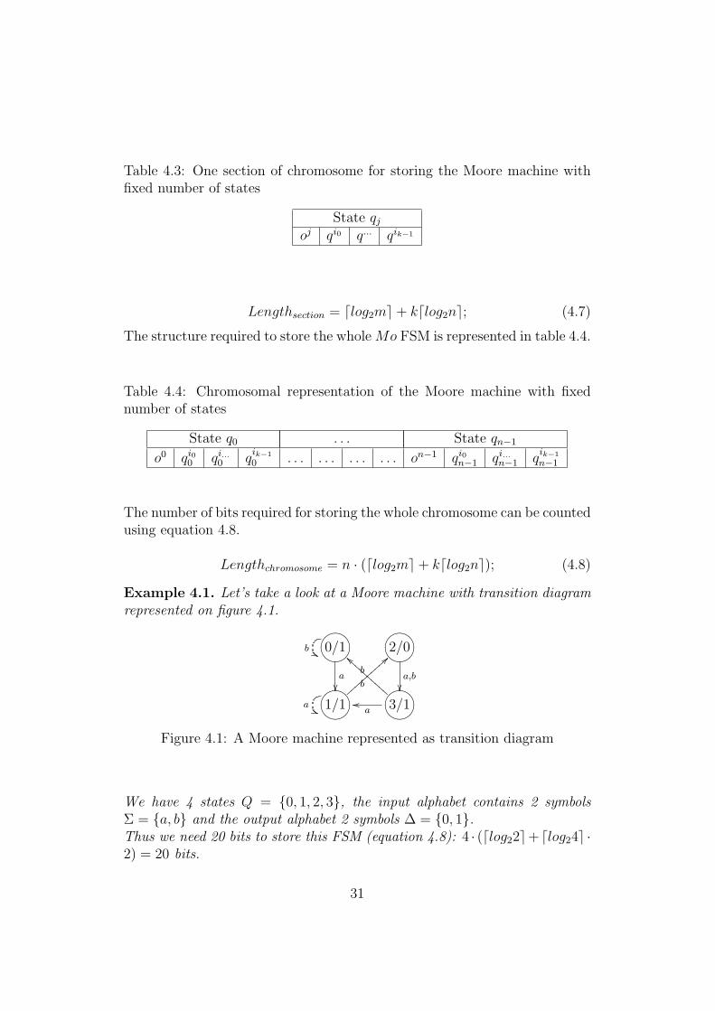
Table 4.3: One section of chromosome for storing the Moore machine withfixed number of states

State qj

oj qi0 q... qik−1

Lengthsection = dlog2me+ kdlog2ne; (4.7)

The structure required to store the whole Mo FSM is represented in table 4.4.

Table 4.4: Chromosomal representation of the Moore machine with fixednumber of states

State q0 . . . State qn−1

o0 qi00 qi...

0 qik−1

0 . . . . . . . . . . . . on−1 qi0n−1 qi...

n−1 qik−1

n−1

The number of bits required for storing the whole chromosome can be countedusing equation 4.8.

Lengthchromosome = n · (dlog2me+ kdlog2ne); (4.8)

Example 4.1. Let’s take a look at a Moore machine with transition diagramrepresented on figure 4.1.

ONMLHIJK0/1b ))

a

��

ONMLHIJK2/0

a,b��ONMLHIJK1/1a ))

b

==|||||||||| ONMLHIJK3/1aoo

b

aaBBBBBBBBBB

Figure 4.1: A Moore machine represented as transition diagram

We have 4 states Q = {0, 1, 2, 3}, the input alphabet contains 2 symbolsΣ = {a, b} and the output alphabet 2 symbols ∆ = {0, 1}.Thus we need 20 bits to store this FSM (equation 4.8): 4 · (dlog22e+ dlog24e ·2) = 20 bits.

31

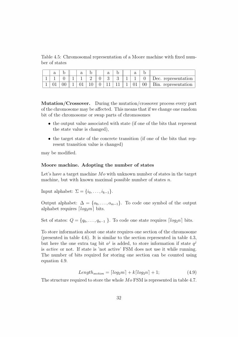
Table 4.5: Chromosomal representation of a Moore machine with fixed num-ber of states

a b a b a b a b1 1 0 1 1 2 0 3 3 1 1 0 Dec. representation1 01 00 1 01 10 0 11 11 1 01 00 Bin. representation

Mutation/Crossover. During the mutation/crossover process every partof the chromosome may be affected. This means that if we change one randombit of the chromosome or swap parts of chromosomes

• the output value associated with state (if one of the bits that representthe state value is changed),

• the target state of the concrete transition (if one of the bits that rep-resent transition value is changed)

may be modified.

Moore machine. Adopting the number of states

Let’s have a target machine Mo with unknown number of states in the targetmachine, but with known maximal possible number of states n.

Input alphabet: Σ = {i0, . . . , ik−1}.

Output alphabet: ∆ = {o0, . . . , om−1}. To code one symbol of the outputalphabet requires dlog2me bits.

Set of states: Q = {q0, . . . , qn−1 }. To code one state requires dlog2ne bits.

To store information about one state requires one section of the chromosome(presented in table 4.6). It is similar to the section represented in table 4.3,but here the one extra tag bit aj is added, to store information if state qj

is active or not. If state is ’not active’ FSM does not use it while running.The number of bits required for storing one section can be counted usingequation 4.9.

Lengthsection = dlog2me+ kdlog2ne+ 1; (4.9)

The structure required to store the whole Mo FSM is represented in table 4.7.

32

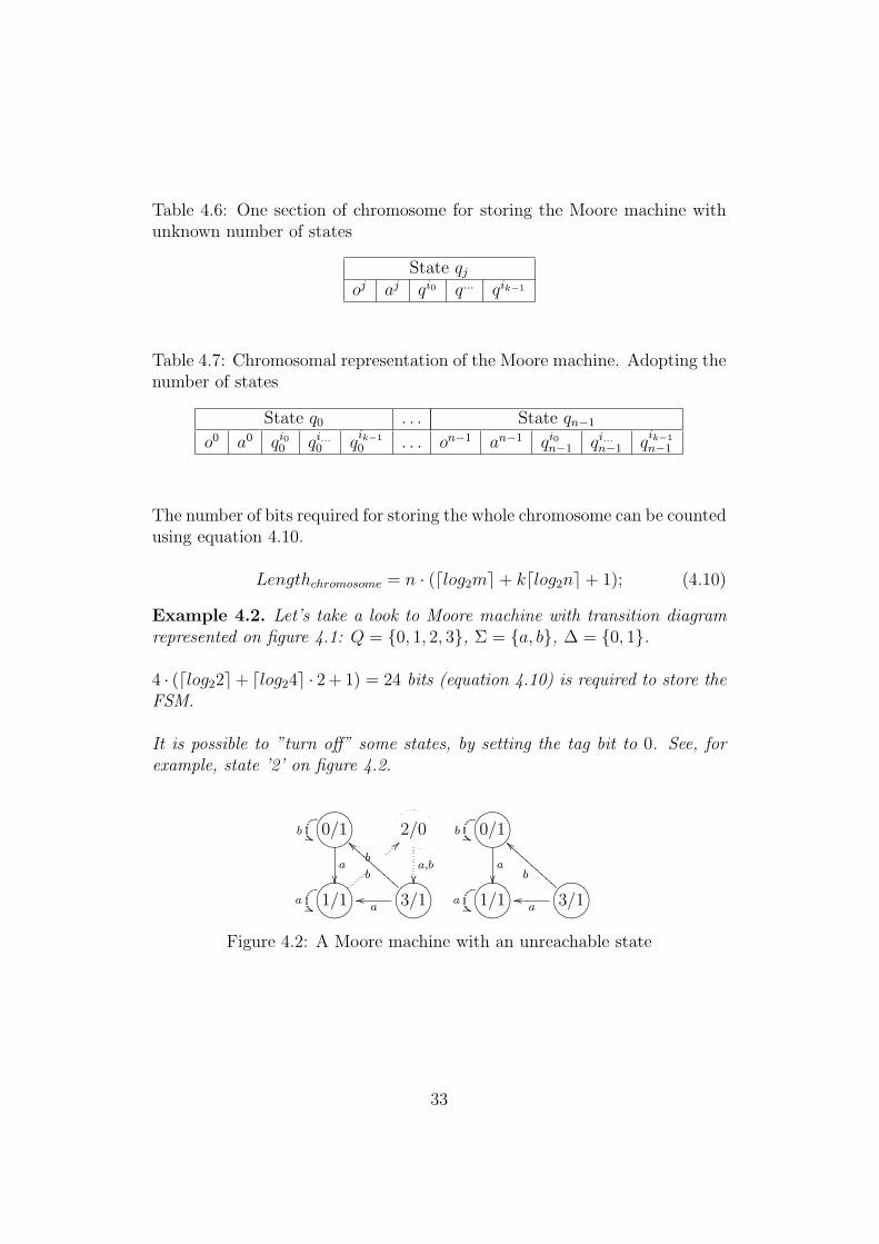
Table 4.6: One section of chromosome for storing the Moore machine withunknown number of states

State qj

oj aj qi0 q... qik−1

Table 4.7: Chromosomal representation of the Moore machine. Adopting thenumber of states

State q0 . . . State qn−1

o0 a0 qi00 qi...

0 qik−1

0 . . . on−1 an−1 qi0n−1 qi...

n−1 qik−1

n−1

The number of bits required for storing the whole chromosome can be countedusing equation 4.10.

Lengthchromosome = n · (dlog2me+ kdlog2ne+ 1); (4.10)

Example 4.2. Let’s take a look to Moore machine with transition diagramrepresented on figure 4.1: Q = {0, 1, 2, 3}, Σ = {a, b}, ∆ = {0, 1}.

4 · (dlog22e+ dlog24e · 2 + 1) = 24 bits (equation 4.10) is required to store theFSM.

It is possible to ”turn off” some states, by setting the tag bit to 0. See, forexample, state ’2’ on figure 4.2.

ONMLHIJK0/1b ))

a

��

2/0

a,b��

ONMLHIJK0/1b ))

a

��ONMLHIJK1/1a ))

b

==

ONMLHIJK3/1aoo

b

aaBBBBBBBBBBONMLHIJK1/1a ))

ONMLHIJK3/1aoo

b

aaBBBBBBBBBB

Figure 4.2: A Moore machine with an unreachable state

33

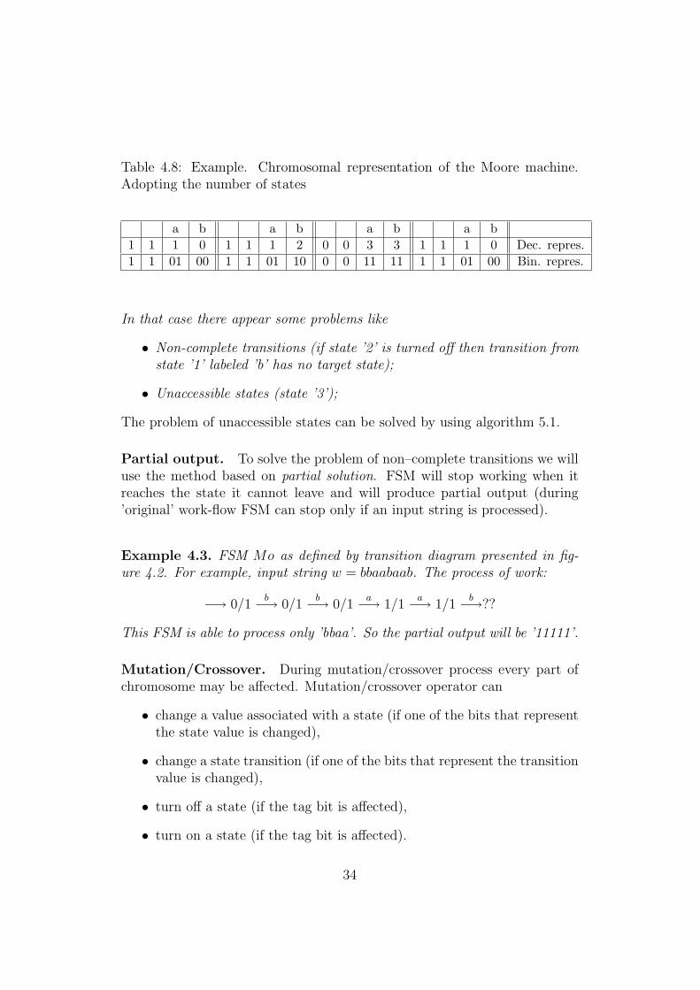
Table 4.8: Example. Chromosomal representation of the Moore machine.Adopting the number of states

a b a b a b a b1 1 1 0 1 1 1 2 0 0 3 3 1 1 1 0 Dec. repres.1 1 01 00 1 1 01 10 0 0 11 11 1 1 01 00 Bin. repres.

In that case there appear some problems like

• Non-complete transitions (if state ’2’ is turned off then transition fromstate ’1’ labeled ’b’ has no target state);

• Unaccessible states (state ’3’);

The problem of unaccessible states can be solved by using algorithm 5.1.

Partial output. To solve the problem of non–complete transitions we willuse the method based on partial solution. FSM will stop working when itreaches the state it cannot leave and will produce partial output (during’original’ work-flow FSM can stop only if an input string is processed).

Example 4.3. FSM Mo as defined by transition diagram presented in fig-ure 4.2. For example, input string w = bbaabaab. The process of work:

−→ 0/1b−→ 0/1

b−→ 0/1a−→ 1/1

a−→ 1/1b−→??

This FSM is able to process only ’bbaa’. So the partial output will be ’11111’.

Mutation/Crossover. During mutation/crossover process every part ofchromosome may be affected. Mutation/crossover operator can

• change a value associated with a state (if one of the bits that representthe state value is changed),

• change a state transition (if one of the bits that represent the transitionvalue is changed),

• turn off a state (if the tag bit is affected),

• turn on a state (if the tag bit is affected).

34

Finite Acceptor

In section 2.3.4 is shown how it is possible to represent FA as a FSM withoutput (Moore machine). This gives a possibility to use methods describedabove to infer FA.

4.2.3 Mealy machines

Mealy machine with fixed number of states

Let’s have a target machine Me with exactly n states in the target machine.Input and output alphabets are observed from input/output sequences.

Input alphabet: Σ = {i0, . . . , ik−1}.

Output alphabet: ∆ = {o0, . . . , om−1}. To code one symbol of the outputalphabet requires dlog2me bits.

Set of states: Q = {q0, . . . , qn−1 }. To code one state requires dlog2ne bits.

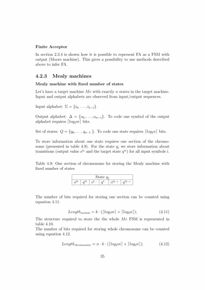
To store information about one state requires one section of the chromo-some (presented in table 4.9). For the state qj we store information abouttransitions (output value oi0 and the target state qi0) for all input symbols i.

Table 4.9: One section of chromosome for storing the Mealy machine withfixed number of states

State qj

oi0 qi0 oi... qi... oik−1 qik−1

The number of bits required for storing one section can be counted usingequation 4.11.

Lengthsection = k · (dlog2me+ dlog2ne); (4.11)

The structure required to store the the whole Me FSM is represented intable 4.10.The number of bits required for storing whole chromosome can be countedusing equation 4.12.

Lengthchromosome = n · k · (dlog2me+ dlog2ne); (4.12)

35

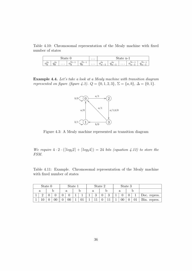
Table 4.10: Chromosomal representation of the Mealy machine with fixednumber of states

State 0 . . . State n-1oi00 qi0

0 . . . oik−1

0 qik−1

0 . . . oi0n−1 qi0

n−1 . . . oik−1

n−1 qik−1

n−1

Example 4.4. Let’s take a look at a Mealy machine with transition diagramrepresented on figure (figure 4.3). Q = {0, 1, 2, 3}, Σ = {a, b}, ∆ = {0, 1}.

?>=<89:;0b/0 55a/1 // ?>=<89:;2

a/1,b/0

��?>=<89:;1b/1 55

a/0

OO

?>=<89:;3b/0

oo

a/1

__>>>>>>>>>>>>>>>>>

Figure 4.3: A Mealy machine represented as transition diagram

We require 4 · 2 · (dlog22e + dlog24e) = 24 bits (equation 4.12) to store theFSM.

Table 4.11: Example. Chromosomal representation of the Mealy machinewith fixed number of states

State 0 State 1 State 2 State 3a b a b a b a b

1 2 0 0 0 0 1 1 1 3 0 3 1 0 0 1 Dec. repres.1 10 0 00 0 00 1 01 1 11 0 11 1 00 0 01 Bin. repres.

36

Mutation/Crossover. During mutation/crossover process every part ofthe chromosome may be affected. This means that if we change one randombit of the chromosome or swap parts of chromosomes

• the value associated with transition (if one of the bits that representthe output value is changed),

• the target state of the concrete transition (if one one of bits that rep-resent the transition value is changed)

may be modified.

4.3 Initialization. Reduction of invalid indi-

viduals

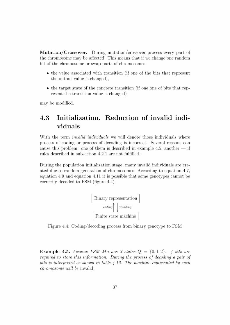
With the term invalid individuals we will denote those individuals whereprocess of coding or process of decoding is incorrect. Several reasons cancause this problem: one of them is described in example 4.5, another — ifrules described in subsection 4.2.1 are not fulfilled.

During the population initialization stage, many invalid individuals are cre-ated due to random generation of chromosomes. According to equation 4.7,equation 4.9 and equation 4.11 it is possible that some genotypes cannot becorrectly decoded to FSM (figure 4.4).

Binary representation

decoding

��

Finite state machine

coding

OO

Figure 4.4: Coding/decoding process from binary genotype to FSM

Example 4.5. Assume FSM Mo has 3 states Q = {0, 1, 2}. 4 bits arerequired to store this information. During the process of decoding a pair ofbits is interpreted as shown in table 4.12. The machine represented by suchchromosome will be invalid.

37

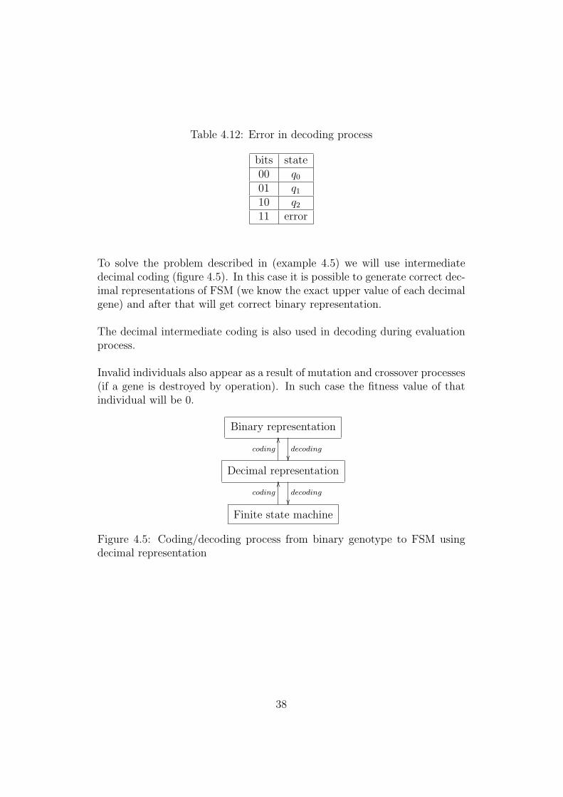
Table 4.12: Error in decoding process

bits state00 q0

01 q1

10 q2

11 error

To solve the problem described in (example 4.5) we will use intermediatedecimal coding (figure 4.5). In this case it is possible to generate correct dec-imal representations of FSM (we know the exact upper value of each decimalgene) and after that will get correct binary representation.

The decimal intermediate coding is also used in decoding during evaluationprocess.

Invalid individuals also appear as a result of mutation and crossover processes(if a gene is destroyed by operation). In such case the fitness value of thatindividual will be 0.

Binary representation

decoding��

Decimal representation

decoding

��

coding

OO

Finite state machine

coding

OO

Figure 4.5: Coding/decoding process from binary genotype to FSM usingdecimal representation

38

Chapter 5

Implementation

5.1 Experimental software description

The methods described in chapter 4 were implemented in a tool GeSM, whichis written in Java SE 2.0. This tool allows to generate form input/outputdata:

• a Moore machine with fixed number of states;

• a Moore machine with unknown number of states (the maximal numberof states is given);

• a Mealy machine with fixed number of states;

It also allows to:

• change parameters of evolution (like size of population, number of gen-erations, mutation probability etc);

• rerun the program for statictical purposes;

• generate random FSM and random input data (required for some tests);

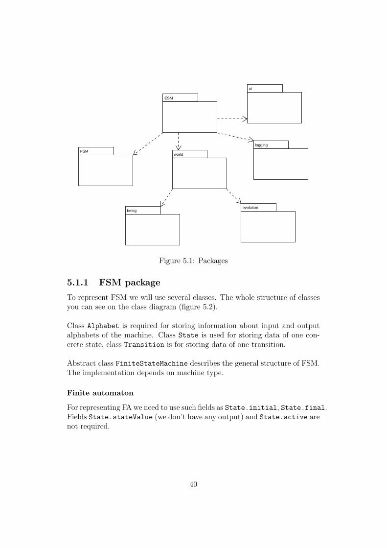
The program contains several packages (figure 5.1):

• fsm decsribes the structure of FSM (subsection 5.1.1).

• world contains two packages: evolution and beings. evolution

contains the implementation of evolution process (subsection 5.1.3).beings describes the process of coding/decoding of FSM (subsection 5.1.2).

• ui contains user interface.

• logging is required for logging and output formatting.

39

ESM

FSM

logging

ui

world

beingevolution

Figure 5.1: Packages

5.1.1 FSM package

To represent FSM we will use several classes. The whole structure of classesyou can see on the class diagram (figure 5.2).

Class Alphabet is required for storing information about input and outputalphabets of the machine. Class State is used for storing data of one con-crete state, class Transition is for storing data of one transition.

Abstract class FiniteStateMachine describes the general structure of FSM.The implementation depends on machine type.

Finite automaton

For representing FA we need to use such fields as State.initial, State.final.Fields State.stateValue (we don’t have any output) and State.active arenot required.

40

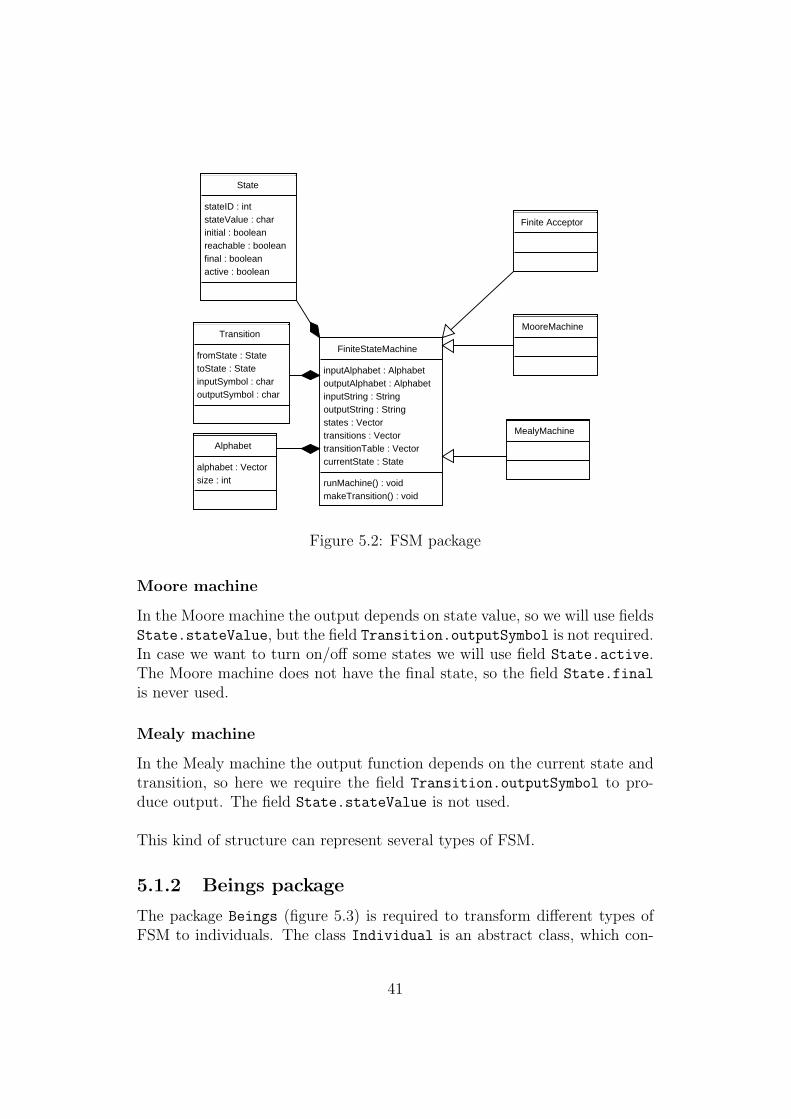
FiniteStateMachine

runMachine() : voidmakeTransition() : void

inputAlphabet : AlphabetoutputAlphabet : AlphabetinputString : StringoutputString : Stringstates : Vectortransitions : VectortransitionTable : VectorcurrentState : State

State

stateID : intstateValue : charinitial : booleanreachable : booleanfinal : booleanactive : boolean

Transition

fromState : StatetoState : StateinputSymbol : charoutputSymbol : char

Alphabet

alphabet : Vectorsize : int

Finite Acceptor

MooreMachine

MealyMachine

Figure 5.2: FSM package

Moore machine

In the Moore machine the output depends on state value, so we will use fieldsState.stateValue, but the field Transition.outputSymbol is not required.In case we want to turn on/off some states we will use field State.active.The Moore machine does not have the final state, so the field State.final

is never used.

Mealy machine

In the Mealy machine the output function depends on the current state andtransition, so here we require the field Transition.outputSymbol to pro-duce output. The field State.stateValue is not used.

This kind of structure can represent several types of FSM.

5.1.2 Beings package

The package Beings (figure 5.3) is required to transform different types ofFSM to individuals. The class Individual is an abstract class, which con-

41

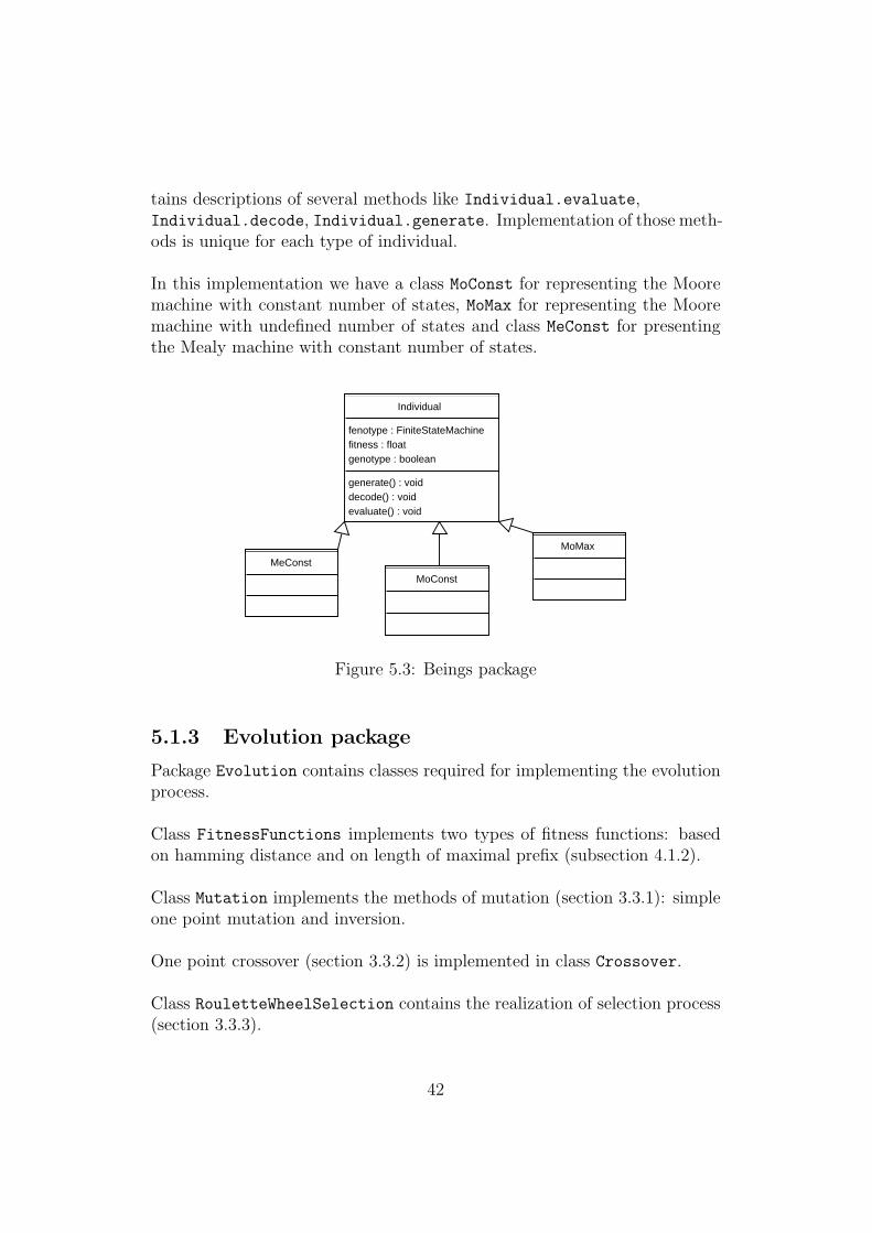
tains descriptions of several methods like Individual.evaluate,Individual.decode, Individual.generate. Implementation of those meth-ods is unique for each type of individual.

In this implementation we have a class MoConst for representing the Mooremachine with constant number of states, MoMax for representing the Mooremachine with undefined number of states and class MeConst for presentingthe Mealy machine with constant number of states.

Individual

generate() : voiddecode() : voidevaluate() : void

fenotype : FiniteStateMachinefitness : floatgenotype : boolean

MeConst

MoConst

MoMax

Figure 5.3: Beings package

5.1.3 Evolution package

Package Evolution contains classes required for implementing the evolutionprocess.

Class FitnessFunctions implements two types of fitness functions: basedon hamming distance and on length of maximal prefix (subsection 4.1.2).

Class Mutation implements the methods of mutation (section 3.3.1): simpleone point mutation and inversion.

One point crossover (section 3.3.2) is implemented in class Crossover.

Class RouletteWheelSelection contains the realization of selection process(section 3.3.3).

42

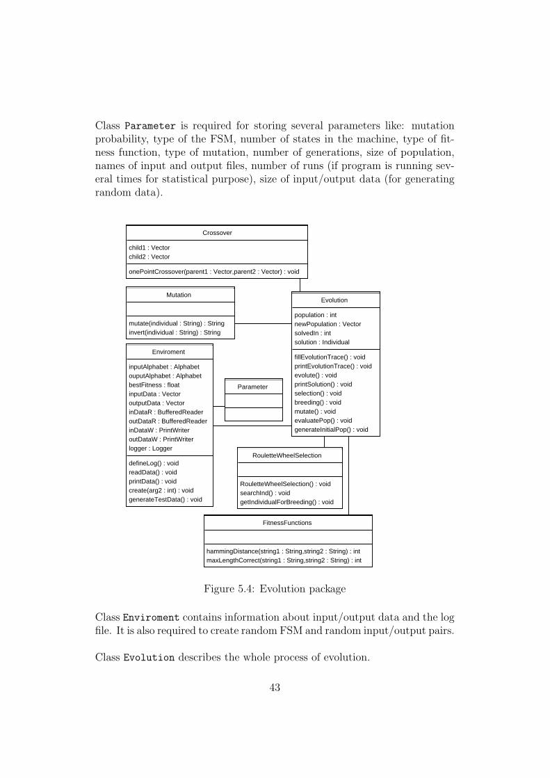
Class Parameter is required for storing several parameters like: mutationprobability, type of the FSM, number of states in the machine, type of fit-ness function, type of mutation, number of generations, size of population,names of input and output files, number of runs (if program is running sev-eral times for statistical purpose), size of input/output data (for generatingrandom data).

Crossover

onePointCrossover(parent1 : Vector,parent2 : Vector) : void

child1 : Vectorchild2 : Vector

FitnessFunctions

hammingDistance(string1 : String,string2 : String) : intmaxLengthCorrect(string1 : String,string2 : String) : int

Mutation

mutate(individual : String) : Stringinvert(individual : String) : String

Enviroment

defineLog() : voidreadData() : voidprintData() : voidcreate(arg2 : int) : voidgenerateTestData() : void

inputAlphabet : AlphabetouputAlphabet : AlphabetbestFitness : floatinputData : VectoroutputData : VectorinDataR : BufferedReaderoutDataR : BufferedReaderinDataW : PrintWriteroutDataW : PrintWriterlogger : Logger

Evolution

fillEvolutionTrace() : voidprintEvolutionTrace() : voidevolute() : voidprintSolution() : voidselection() : voidbreeding() : voidmutate() : voidevaluatePop() : voidgenerateInitialPop() : void

population : intnewPopulation : VectorsolvedIn : intsolution : Individual

RouletteWheelSelection

RouletteWheelSelection() : voidsearchInd() : voidgetIndividualForBreeding() : void

Parameter

Figure 5.4: Evolution package

Class Enviroment contains information about input/output data and the logfile. It is also required to create random FSM and random input/output pairs.

Class Evolution describes the whole process of evolution.

43

5.2 Evolutionary trace

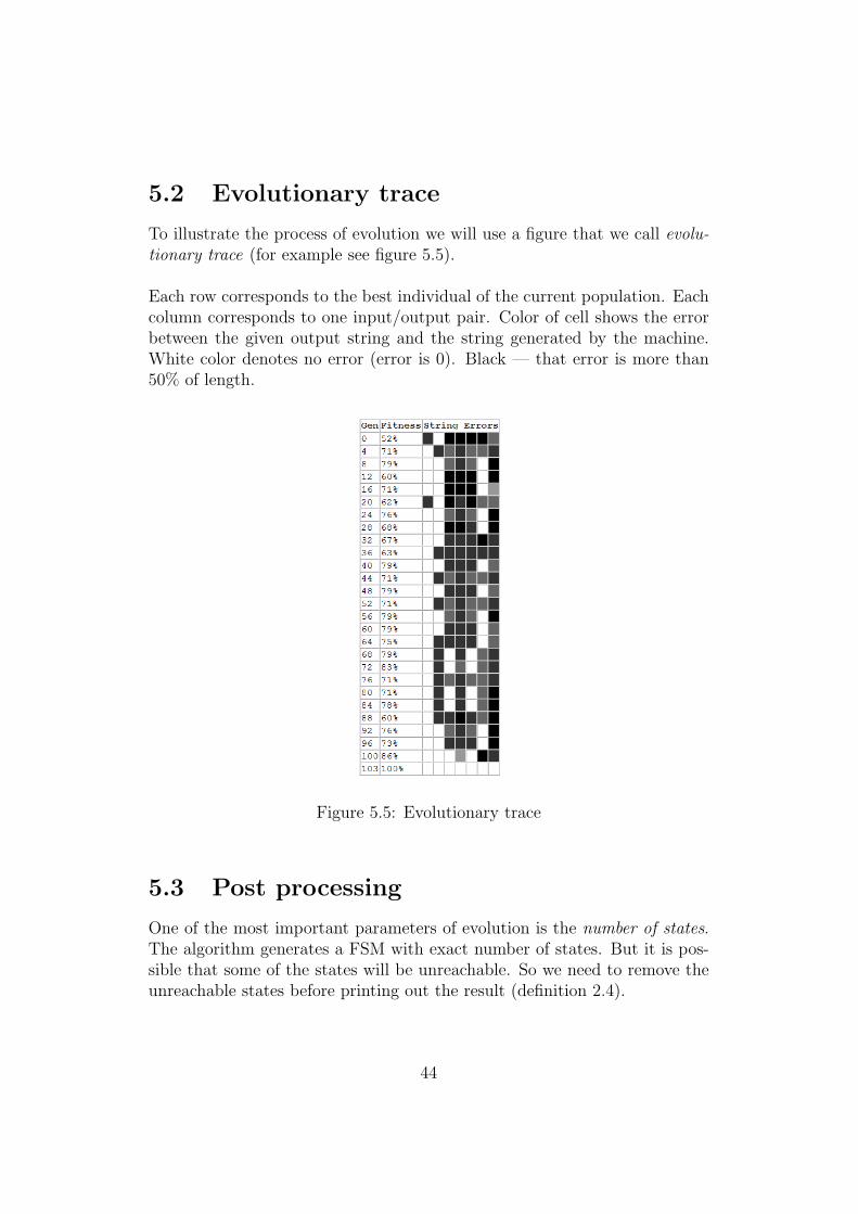
To illustrate the process of evolution we will use a figure that we call evolu-tionary trace (for example see figure 5.5).

Each row corresponds to the best individual of the current population. Eachcolumn corresponds to one input/output pair. Color of cell shows the errorbetween the given output string and the string generated by the machine.White color denotes no error (error is 0). Black — that error is more than50% of length.

Figure 5.5: Evolutionary trace

5.3 Post processing

One of the most important parameters of evolution is the number of states.The algorithm generates a FSM with exact number of states. But it is pos-sible that some of the states will be unreachable. So we need to remove theunreachable states before printing out the result (definition 2.4).

44

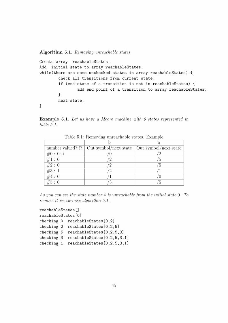
Algorithm 5.1. Removing unreachable states

Create array reachableStates;

Add initial state to array reachableStates;

while(there are some unchecked states in array reachableStates) {

check all transitions from current state;

if (end state of a transition is not in reachableStates) {

add end point of a transition to array reachableStates;

}

next state;

}

Example 5.1. Let us have a Moore machine with 6 states represented intable 5.1.

Table 5.1: Removing unreachable states. Exampleb a

number:value:i?:f? Out symbol/next state Out symbol/next state#0 : 0: i /0 /2#1 : 0 /2 /5#2 : 0 /2 /5#3 : 1 /2 /1#4 : 0 /1 /0#5 : 0 /3 /5

As you can see the state number 4 is unreachable from the initial state 0. Toremove it we can use algorithm 5.1.

reachableStates[]

reachableStates[0]

checking 0 reachableStates[0,2]

checking 2 reachableStates[0,2,5]

checking 5 reachableStates[0,2,5,3]

checking 3 reachableStates[0,2,5,3,1]

checking 1 reachableStates[0,2,5,3,1]

45

Chapter 6

Experiments

6.1 Learning Random Finite State Machines

6.1.1 Getting the training data

To show how this approach works we need training data. One way would beto generate random data for experiments.

Algorithm 6.1. (The process of getting training data)

Generate random FSM of t type with n states;

Reset the FSM to start state;

Produce a random input sequence;

Feed the input sequence to the FSM and collect

the corresponding output sequence;

Store input/output sequences;

Store number of states n;

Store type of the machine t;

The stored input/output sequences, number of states and type of the machineare used for experiments.

6.1.2 Equivalence of Mealy and Moore machines

The equivalence of Mealy and Moore machines (subsection 2.3.2) allows usto use both methods described in subsection 4.2.2 and subsection 4.2.3.

Task Generate Moore and Mealy machines for given training data.

46

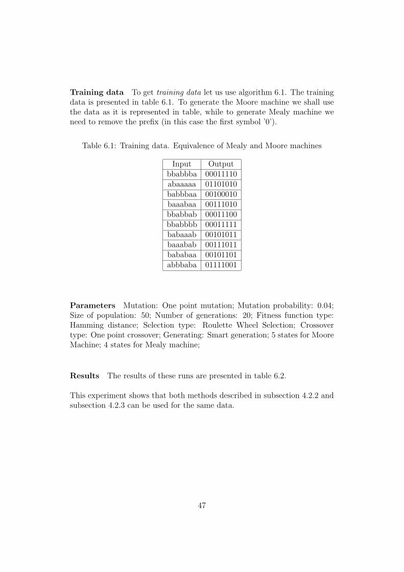
Training data To get training data let us use algorithm 6.1. The trainingdata is presented in table 6.1. To generate the Moore machine we shall usethe data as it is represented in table, while to generate Mealy machine weneed to remove the prefix (in this case the first symbol ’0’).

Table 6.1: Training data. Equivalence of Mealy and Moore machines

Input Outputbbabbba 00011110abaaaaa 01101010babbbaa 00100010baaabaa 00111010bbabbab 00011100bbabbbb 00011111babaaab 00101011baaabab 00111011bababaa 00101101abbbaba 01111001

Parameters Mutation: One point mutation; Mutation probability: 0.04;Size of population: 50; Number of generations: 20; Fitness function type:Hamming distance; Selection type: Roulette Wheel Selection; Crossovertype: One point crossover; Generating: Smart generation; 5 states for MooreMachine; 4 states for Mealy machine;

Results The results of these runs are presented in table 6.2.

This experiment shows that both methods described in subsection 4.2.2 andsubsection 4.2.3 can be used for the same data.

47

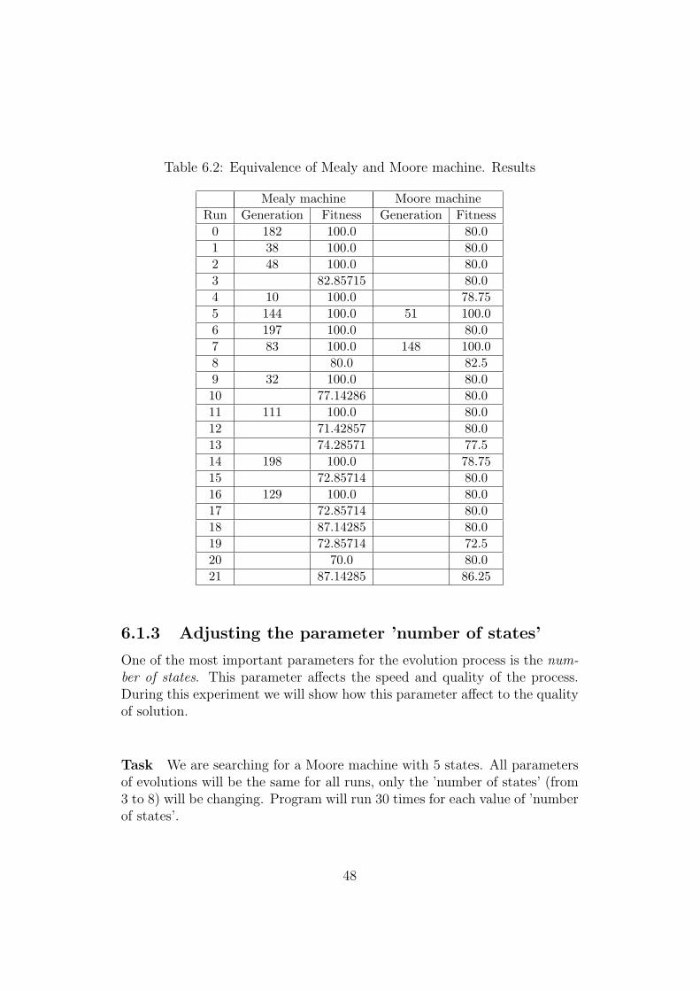
Table 6.2: Equivalence of Mealy and Moore machine. Results

Mealy machine Moore machineRun Generation Fitness Generation Fitness

0 182 100.0 80.01 38 100.0 80.02 48 100.0 80.03 82.85715 80.04 10 100.0 78.755 144 100.0 51 100.06 197 100.0 80.07 83 100.0 148 100.08 80.0 82.59 32 100.0 80.010 77.14286 80.011 111 100.0 80.012 71.42857 80.013 74.28571 77.514 198 100.0 78.7515 72.85714 80.016 129 100.0 80.017 72.85714 80.018 87.14285 80.019 72.85714 72.520 70.0 80.021 87.14285 86.25

6.1.3 Adjusting the parameter ’number of states’

One of the most important parameters for the evolution process is the num-ber of states. This parameter affects the speed and quality of the process.During this experiment we will show how this parameter affect to the qualityof solution.

Task We are searching for a Moore machine with 5 states. All parametersof evolutions will be the same for all runs, only the ’number of states’ (from3 to 8) will be changing. Program will run 30 times for each value of ’numberof states’.

48

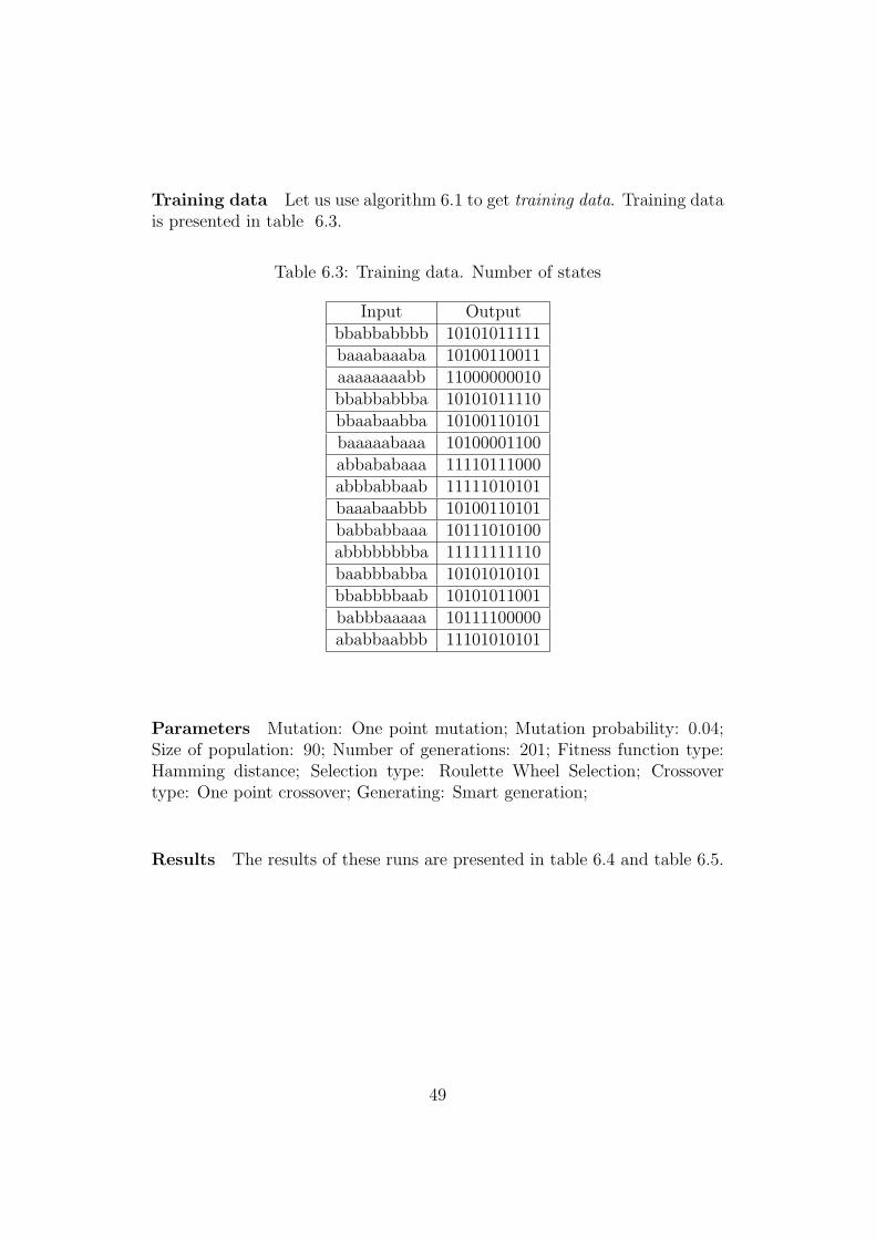
Training data Let us use algorithm 6.1 to get training data. Training datais presented in table 6.3.

Table 6.3: Training data. Number of states

Input Outputbbabbabbbb 10101011111baaabaaaba 10100110011aaaaaaaabb 11000000010bbabbabbba 10101011110bbaabaabba 10100110101baaaaabaaa 10100001100abbababaaa 11110111000abbbabbaab 11111010101baaabaabbb 10100110101babbabbaaa 10111010100abbbbbbbba 11111111110baabbbabba 10101010101bbabbbbaab 10101011001babbbaaaaa 10111100000ababbaabbb 11101010101

Parameters Mutation: One point mutation; Mutation probability: 0.04;Size of population: 90; Number of generations: 201; Fitness function type:Hamming distance; Selection type: Roulette Wheel Selection; Crossovertype: One point crossover; Generating: Smart generation;

Results The results of these runs are presented in table 6.4 and table 6.5.

49

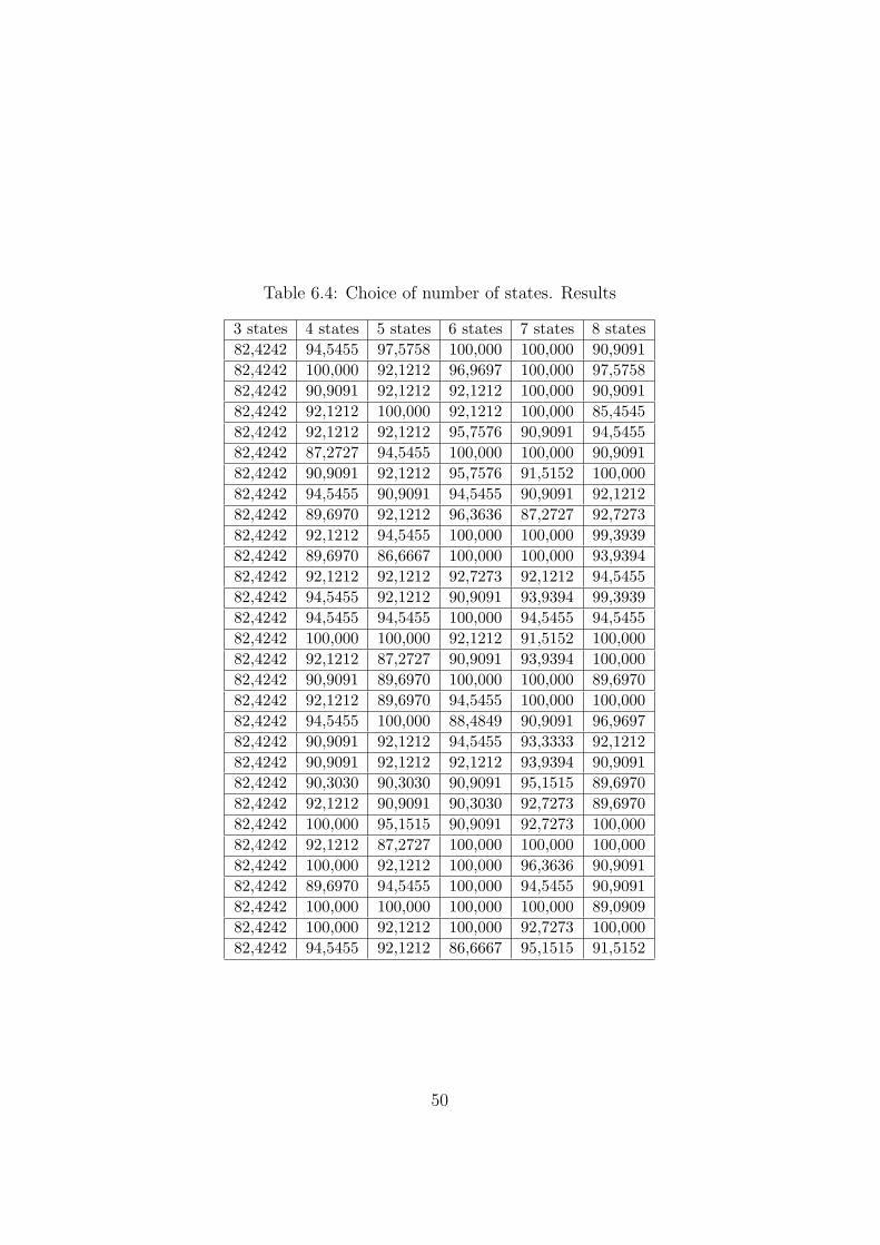
Table 6.4: Choice of number of states. Results

3 states 4 states 5 states 6 states 7 states 8 states82,4242 94,5455 97,5758 100,000 100,000 90,909182,4242 100,000 92,1212 96,9697 100,000 97,575882,4242 90,9091 92,1212 92,1212 100,000 90,909182,4242 92,1212 100,000 92,1212 100,000 85,454582,4242 92,1212 92,1212 95,7576 90,9091 94,545582,4242 87,2727 94,5455 100,000 100,000 90,909182,4242 90,9091 92,1212 95,7576 91,5152 100,00082,4242 94,5455 90,9091 94,5455 90,9091 92,121282,4242 89,6970 92,1212 96,3636 87,2727 92,727382,4242 92,1212 94,5455 100,000 100,000 99,393982,4242 89,6970 86,6667 100,000 100,000 93,939482,4242 92,1212 92,1212 92,7273 92,1212 94,545582,4242 94,5455 92,1212 90,9091 93,9394 99,393982,4242 94,5455 94,5455 100,000 94,5455 94,545582,4242 100,000 100,000 92,1212 91,5152 100,00082,4242 92,1212 87,2727 90,9091 93,9394 100,00082,4242 90,9091 89,6970 100,000 100,000 89,697082,4242 92,1212 89,6970 94,5455 100,000 100,00082,4242 94,5455 100,000 88,4849 90,9091 96,969782,4242 90,9091 92,1212 94,5455 93,3333 92,121282,4242 90,9091 92,1212 92,1212 93,9394 90,909182,4242 90,3030 90,3030 90,9091 95,1515 89,697082,4242 92,1212 90,9091 90,3030 92,7273 89,697082,4242 100,000 95,1515 90,9091 92,7273 100,00082,4242 92,1212 87,2727 100,000 100,000 100,00082,4242 100,000 92,1212 100,000 96,3636 90,909182,4242 89,6970 94,5455 100,000 94,5455 90,909182,4242 100,000 100,000 100,000 100,000 89,090982,4242 100,000 92,1212 100,000 92,7273 100,00082,4242 94,5455 92,1212 86,6667 95,1515 91,5152

50

In table 6.4 each cell shows the fitness value (in %) of the found solution forthat run of program.

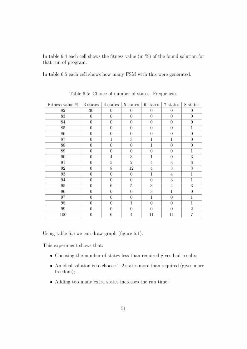
In table 6.5 each cell shows how many FSM with this were generated.

Table 6.5: Choice of number of states. Frequencies

Fitness value % 3 states 4 states 5 states 6 states 7 states 8 states82 30 0 0 0 0 083 0 0 0 0 0 084 0 0 0 0 0 085 0 0 0 0 0 186 0 0 0 0 0 087 0 1 3 1 1 088 0 0 0 1 0 089 0 0 0 0 0 190 0 4 3 1 0 391 0 5 2 4 3 692 0 8 12 4 3 393 0 0 0 1 4 194 0 0 0 0 3 195 0 6 5 3 4 396 0 0 0 3 1 097 0 0 0 1 0 198 0 0 1 0 0 199 0 0 0 0 0 2100 0 6 4 11 11 7

Using table 6.5 we can draw graph (figure 6.1).

This experiment shows that:

• Choosing the number of states less than required gives bad results;

• An ideal solution is to choose 1–2 states more than required (gives morefreedom);

• Adding too many extra states increases the run time;

51

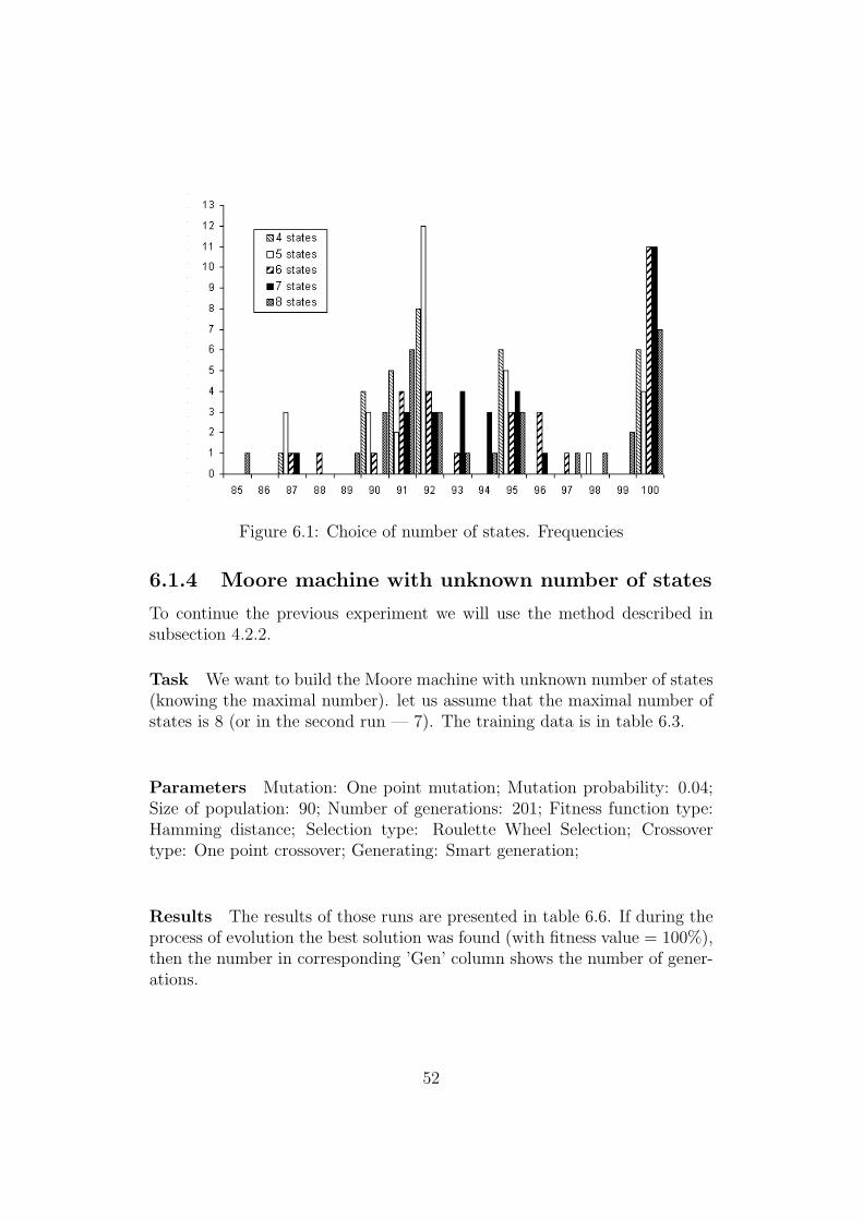
Figure 6.1: Choice of number of states. Frequencies

6.1.4 Moore machine with unknown number of states

To continue the previous experiment we will use the method described insubsection 4.2.2.

Task We want to build the Moore machine with unknown number of states(knowing the maximal number). let us assume that the maximal number ofstates is 8 (or in the second run — 7). The training data is in table 6.3.

Parameters Mutation: One point mutation; Mutation probability: 0.04;Size of population: 90; Number of generations: 201; Fitness function type:Hamming distance; Selection type: Roulette Wheel Selection; Crossovertype: One point crossover; Generating: Smart generation;

Results The results of those runs are presented in table 6.6. If during theprocess of evolution the best solution was found (with fitness value = 100%),then the number in corresponding ’Gen’ column shows the number of gener-ations.

52

Table 6.6: Generating a Moore machine with unknown number of states.Results

Maximal number of states 7 Maximal number of states 8Run Gen Fitness number of states Gen Fitness number of states

0 201 87,2727 6 74 100,0000 71 201 95,1515 6 84 100,0000 72 201 90,9091 6 201 88,4849 83 201 87,8788 6 201 88,4849 74 201 89,0909 7 201 97,5758 85 201 92,1212 7 55 100,0000 86 201 87,2727 5 87 100,0000 87 201 94,5455 6 201 88,4849 88 201 95,7576 7 55 100,0000 79 201 92,1212 7 81 100,0000 710 201 94,5455 7 142 100,0000 711 181 100,0000 6 201 90,9091 812 201 89,6970 7 201 90,9091 713 201 95,7576 6 120 100,0000 714 201 83,6364 7 133 100,0000 815 201 90,9091 6 201 90,9091 816 201 92,1212 7 201 91,5152 817 201 87,2727 7 201 89,6970 718 201 87,2727 6 102 100,0000 719 201 86,0606 6 201 87,2727 820 201 87,8788 6 201 99,3939 721 201 88,4849 5 201 87,2727 722 201 89,6970 7 201 96,9697 823 69 100,0000 7 201 87,8788 624 201 89,0909 7 201 87,2727 525 201 94,5455 7 17 100,0000 726 53 100,0000 6 201 85,4545 727 201 86,6667 7 201 92,1212 628 201 89,0909 7 201 84,8485 829 201 86,0606 6 57 100,0000 8

53

During the experiment where maximal possible number of states was 7 only3 maximal solutions were found: 2 solutions with 6 states and 1 with 7 states.

During the experiment where maximal possible number of states was 8, 12maximal solutions were found: 8 solutions with 7 states and 4 with 8 states.

6.2 Learning Mealy machine. Parity checker

Task To design a Mealy Machine which takes binary input and producesoutput 0 when the current string (so far) has odd parity.

Training data Training data is presented in table 6.7.

Table 6.7: Parity checker. Training data

Input Output01010101 1001100110101010 0011001100110011 1101110100111100 1101011101001100 1000100010011001 0001000111001001 01110001

Parameters Mutation: One point mutation; Mutation probability: 0.04;Size of population: 30; Number of generations: 100; Fitness function type:Hamming distance; Selection type: Roulette Wheel Selection; Crossovertype: One point crossover; Generating: Smart generation; Number of states 2;

Results Solution was found in 3 generations.

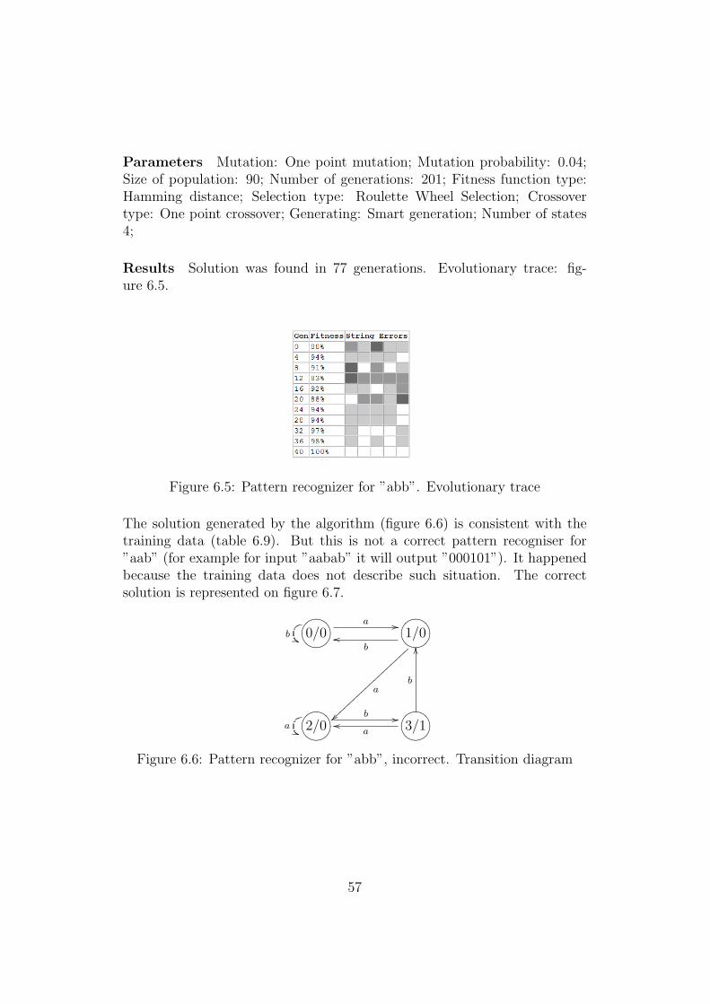
6.3 Learning Mealy machine. Two unit delay

Task To construct a Mealy machine that behaves as a two–unit delay.

r(t) =

{s(t− 2) : t > 2

0 : otherwise

54

?>=<89:;00/1 55

1/0 // ?>=<89:;11/1

oo 0/0ii

Figure 6.2: Parity checker. Transition diagram

Sample input/output session:

time 123456789stimulus 000110100response 000001101

Training data The training data is presented in table 6.8.

Table 6.8: Two unit delay. Training data

Input Output01010101 0001010110101010 0010101000110011 0000110000111100 0000111101001100 0001001110011001 0010011011001001 00110010

Parameters Mutation: One point mutation; Mutation probability: 0.04;Size of population: 90; Number of generations: 500; Fitness function type:Hamming distance; Selection type: Roulette Wheel Selection; Crossovertype: One point crossover; Generating: Smart generation; Number of states 6;

Results Solution was found in 79 generations. Evolutionary trace: fig-ure 6.3.

55

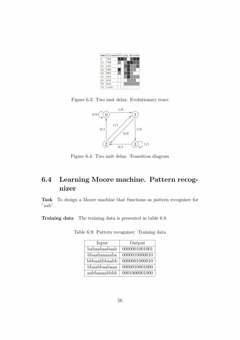
Figure 6.3: Two unit delay. Evolutionary trace

?>=<89:;00/0 55

1/0 // ?>=<89:;1

0/0

������

����

����

����

�

1/0

��?>=<89:;2

0/1

OO

1/1

??����������������� ?>=<89:;30/1

oo 1/1ii

Figure 6.4: Two unit delay. Transition diagram

6.4 Learning Moore machine. Pattern recog-

nizer

Task To design a Moore machine that functions as pattern recogniser for”aab”.

Training data The training data is presented in table 6.9.

Table 6.9: Pattern recognizer. Training data

Input Outputbabaabaabaab 0000001001001bbaabaaaaaba 0000010000010bbbaabbbaabb 0000001000010bbaabbaabaaa 0000010001000aabbaaaabbbb 0001000001000

56

Parameters Mutation: One point mutation; Mutation probability: 0.04;Size of population: 90; Number of generations: 201; Fitness function type:Hamming distance; Selection type: Roulette Wheel Selection; Crossovertype: One point crossover; Generating: Smart generation; Number of states4;

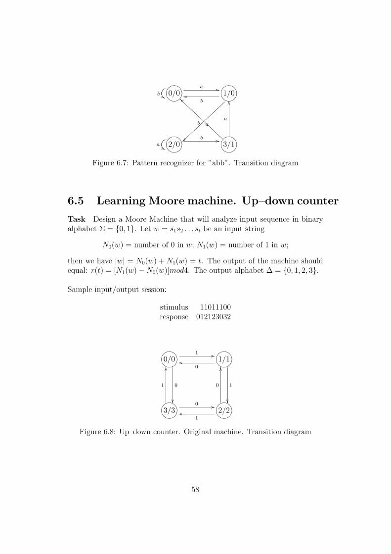
Results Solution was found in 77 generations. Evolutionary trace: fig-ure 6.5.

Figure 6.5: Pattern recognizer for ”abb”. Evolutionary trace

The solution generated by the algorithm (figure 6.6) is consistent with thetraining data (table 6.9). But this is not a correct pattern recogniser for”aab” (for example for input ”aabab” it will output ”000101”). It happenedbecause the training data does not describe such situation. The correctsolution is represented on figure 6.7.

ONMLHIJK0/0b ))

a // ONMLHIJK1/0

a

~~}}}}

}}}}

}}}}

}}}}

}}b

oo

ONMLHIJK2/0a ))

b // ONMLHIJK3/1aoo

b

OO

Figure 6.6: Pattern recognizer for ”abb”, incorrect. Transition diagram

57

ONMLHIJK0/0b ))

a // ONMLHIJK1/0

a

~~}}}}

}}}}

}}}}

}}}}

}}b

oo

ONMLHIJK2/0a ))

b // ONMLHIJK3/1

b

`AAAAAAAAAAAAAAAAAA

a

OO

Figure 6.7: Pattern recognizer for ”abb”. Transition diagram

6.5 Learning Moore machine. Up–down counter

Task Design a Moore Machine that will analyze input sequence in binaryalphabet Σ = {0, 1}. Let w = s1s2 . . . st be an input string

N0(w) = number of 0 in w; N1(w) = number of 1 in w;

then we have |w| = N0(w) + N1(w) = t. The output of the machine shouldequal: r(t) = [N1(w)−N0(w)]mod4. The output alphabet ∆ = {0, 1, 2, 3}.

Sample input/output session:

stimulus 11011100response 012123032

ONMLHIJK0/0

0

��

1 // ONMLHIJK1/1

1

��

0oo

ONMLHIJK3/3

1

OO

0 // ONMLHIJK2/2

0

OO

1oo

Figure 6.8: Up–down counter. Original machine. Transition diagram

58

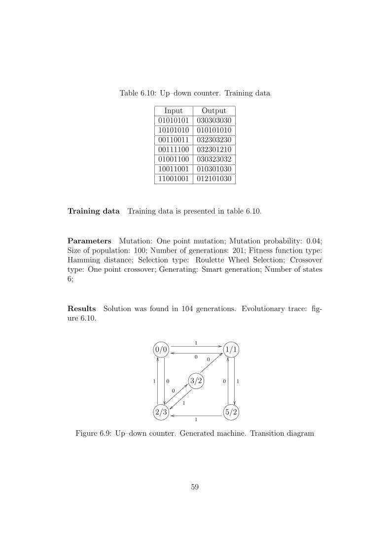
Table 6.10: Up–down counter. Training data

Input Output01010101 03030303010101010 01010101000110011 03230323000111100 03230121001001100 03032303210011001 01030103011001001 012101030

Training data Training data is presented in table 6.10.

Parameters Mutation: One point mutation; Mutation probability: 0.04;Size of population: 100; Number of generations: 201; Fitness function type:Hamming distance; Selection type: Roulette Wheel Selection; Crossovertype: One point crossover; Generating: Smart generation; Number of states6;

Results Solution was found in 104 generations. Evolutionary trace: fig-ure 6.10.

ONMLHIJK0/0

0

��

1 // ONMLHIJK1/1

1

��

0oo

ONMLHIJK3/2

1}}||

||||

||||

0

==||||||||||

ONMLHIJK2/3

1

OO

0

==||||||||||ONMLHIJK5/2

0

OO

1oo

Figure 6.9: Up–down counter. Generated machine. Transition diagram

59

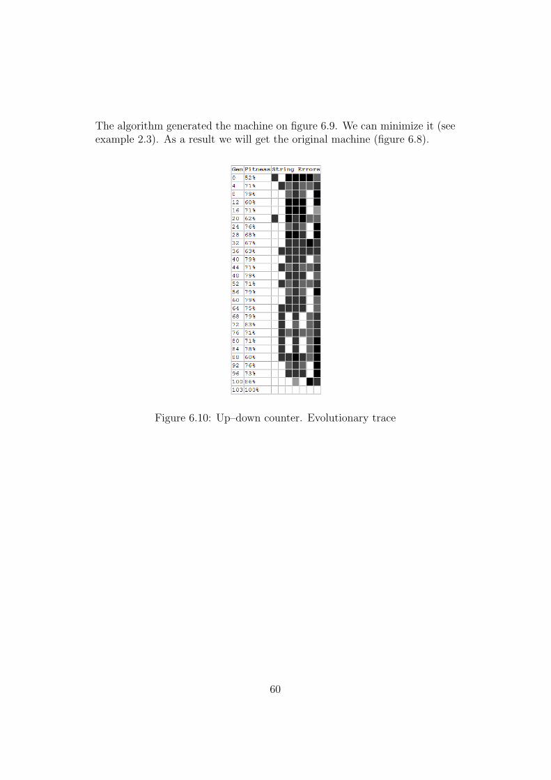
The algorithm generated the machine on figure 6.9. We can minimize it (seeexample 2.3). As a result we will get the original machine (figure 6.8).

Figure 6.10: Up–down counter. Evolutionary trace

60

Chapter 7

Conclusions and future work

7.1 Conclusions

In this thesis we have introduced methods for FSM inference based on GA.

First, we presented the basic theory of FSM (chapter 2) and GA (chapter 3).The main definitions and algorithms were described.

Second, we defined several methods for inference of different kinds of FSM:inference of Moore machine with constant number of states, inference ofMealy machines with constant number of states, also a method for adjustingthe number of states for the Moore machine was introduced. Different fitnessfunctions were used.

Also several improvements to the algorithms were made: to solve the prob-lem of invalid individuals during initialization stage we used the inner deci-mal coding (section 4.3), problem of unaccessible states was solved at post–processing stage (section 5.3), for problem of non–complete transitions (ap-pears if we use the method for adjusting number of states for the Mooremachine) the method based on partial solution was introduced (section 4.2.2).

An essential part of this work is the implementation of the described methods(chapter 5) using Java. The process of evolution has been illustrated withthe evolutionary trace diagram.

The tool GeSM was used for experiments (chapter 6). Several experiment onrandom data were made to show how this method works for different kindsof FSM, also how the number of states affects the process of evolution. To

61

show how this tool works with actual tasks from the real world we madeexperiments with several FSM like parity checker, two unit delay machine,pattern recognizer, up–down counter. During those experiments we tried toreconstruct the FSM having only external description.

The results of the work are the following:

• Method for Mealy and Moore machine inference based on GA. Individ-ual representations and fitness functions were introduced.

• Improvement of initialization process — use of inner decimal represen-tation to reduce invalid individuals.

• Method for solving problem of non–complete transitions based on par-tial solution.

• Post–processing stage which allows to solve problem of unaccessiblestates.

• Implementation of presented method in Java.

• Successful testing of method using random data and real–world exam-ples.

7.2 Future work

More work needs to be done to improve the quality of the process. Futureresearch should continue to improve the implementation. Parameters of theevolution and their affect on the presented methods must be explored. Alsosome other genetic operators should be implemented. The effect of usingdifferent operators must be investigated.

To improve the process of adjusting the number of states in case of Mooremachines the fitness functions must be modified to take into account thenumber of states.

The post–processing stage can be improved by adding implementation of theminimization process.

Future work should also include experiments with more sophisticated exam-ples.

62

Loplike olekumasinate geneetiline tuletamineMargarita Spitsakova

Resumee

Mudeli identifitseerimine on protsess, mis voimaldab tuletada susteemi sisemisekirjelduse tema valise kaitumise pohjal. Susteemi kirjeldamiseks kasutataksetihti loplikku olekumasinat.

Probleemiks on asjaolu, et lopliku olekumasina tuletamine on NP–keerulineulesanne. Keerukuse vahendamiseks voib kasutada geneetiliste algoritmidebaasil loodud meetodeid.

Kaesoleva too ulesandeks oli valja tootada algoritm lopliku olekumasina lei-dmiseks kasutades geneetilisi meetodeid, keskenduses kahele loplikule oleku-masina pohituubile: Moore ja Mealy masinale. Nende jaoks leidsime ge-neetilised meetodid mis voimaldavad tuletada etteantud olekute arvuga masinasisendi–valjundi kirjeldusest. Moore masina genereerimiseks on koostatud kaalgoritm, mis ei kasuta tapset olekute arvu, vaid lahtub maksimaalsest.Need meetodid on realiseeritud Java keeles. Programmi testimiseks on tehtudrida eksperimente.

Kaesolev too koosneb viiest peatukist.

Esimeses peatukis antakse luhike ulevaade loplike olekumasinate teooriast.Selle peatuki esimeses ja teises osas esitatakse formaalsete keelte ja loplikeautomaatide teoreetilised alused. Kolmandas osas kirjeldatakse valjundigaloplikke olekumasinaid — Mealy ja Moore masinaid — ja nende minimiseer-imist.

Teises peatukis kirjeldatakse geneetiliste algoritmide pohiprintsiipe.

Kolmas peatukk on too pohiosa. Selles peatukis kasitletakse geneetiliste al-goritmide modifitseerimist, selleks et tuletada loplikke olekumasinaid ainultnende sisendi–valjundi paaride ja masina tuubi pohjal. Esimeses osas kir-jeldatakse funktsioone, mis voimaldavad hinnata konkretse olekumasina so-bivust mudeliks. Teises ja kolmas osas vaadeldakse olekumasina kodderimistbitijadana ja sellega kaasnevaid probleeme (vigased inviviidid, saavutamatudolekud ja vigased uleminekud).

Neljandas peatukkis esitatakse loplike olekumasinate genereerimise prototuupi.

63

Nimetatud programm on kirjutatud Javas, ning tema kirjeldamiseks on ka-sutatud UML diagramme.

Viimases peatukis antakse ulevaade teostatud eksperimentidest: iga ulesandekorral kirjeldatakse selle pustitust ja tulemusi. Esimeses osas kasitletatakseeksperimente juhuslike andmetega, teises — reaalse maailma naiteid.

64

Bibliography

[1] J. Amaral, K. Turner, and J. Ghosh. Designing genetic algorithms forthe state assignment problem, 1995.

[2] Thomas Back, David B. Fogel, and Zbigniew Michalewicz, editors.Handbook of Evolutionary Computation. IOP Publishing Ltd., 1997.

[3] Karl A Benson. Evolving finite state machines with embedded geneticprogramming for automatic target detection within SAR imagery. InProceedings of the 2000 Congress on Evolutionary Computation CEC00,pages 1543–1549. IEEE Press, 6-9 July 2000.

[4] Kumar Chellapilla and David Czarnecki. A preliminary investigationinto evolving modular finite state machines, 1999.

[5] L. J. Fogel, A. J. Owens, and M. J. Walsh. Artificial Intelligence throughSimulated Evolution. John Wiley, 1966.

[6] Xiaojun Geng. Solving identification problem for asynchronous finitestate machines using genetic algorithms. In GECCO ’06: Proceedingsof the 8th annual conference on Genetic and evolutionary computation,pages 1413–1414, New York, NY, USA, 2006. ACM Press.

[7] E.M. Gold. Complexity of automaton identification from given data.Information and Control, 37:302–320, 1978.

[8] Philip Hingston. A genetic algorithm for regular inference. In Lee Spec-tor, Erik D. Goodman, Annie Wu, W. B. Langdon, Hans-Michael Voigt,Mitsuo Gen, Sandip Sen, Marco Dorigo, Shahram Pezeshk, Max H. Gar-zon, and Edmund Burke, editors, Proceedings of the Genetic and Evolu-tionary Computation Conference (GECCO-2001), pages 1299–1306, SanFrancisco, California, USA, 7-11 2001. Morgan Kaufmann.

[9] JE Hopcroft and JD Ullman. Introduction to Automata Theory, Lan-guages, and Computation. Addison-Wesley, Reading, Massachusetts,1979.

65

[10] Jason W. Horihan and Yung-Hsiang Lu. Improving fsm evolution withprogressive fitness functions. In GLSVLSI ’04: Proceedings of the 14thACM Great Lakes symposium on VLSI, pages 123–126. ACM Press,2004.

[11] Pushmeet Kohli. A new genetic algorithm based scheme for inferringfinite state machines from accept/reject data samples. In IICAI, pages632–645, 2003.

[12] M. Lankhorst. A genetic algorithm for induction of nondeterministicpushdown automata.

[13] Mark V. Lawson. Finite Automata. Chapman and Hall/CRC, 2003.

[14] Mark V. Lawson. Finite automata. In Handbook of Networked andEmbedded Control Systems, pages 117–144. 2005.

[15] Simon Lucas. Structuring chromosomes for context-free grammar evo-lution. In Proceedings of The IEEE Conference on Evolutionary Com-putation, IEEE World Congress on Computational Intelligence, 1994.

[16] Simon M. Lucas. Evolving finite state transducers: Some initial explo-rations. In EuroGP, pages 130–141, 2003.

[17] Simon M. Lucas and T. Jeff reynolds. Learning finite state transducers:Evolution versus heuristic state merging, 2007.

[18] Lamine Ngom, Claude Baron, and Jean-Claude Geffroy. Genetic simula-tion for finite state machine identification. In SS ’99: Proceedings of theThirty-Second Annual Simulation Symposium, page 118, Washington,DC, USA, 1999. IEEE Computer Society.

[19] Lamine Ngom, Claude Baron, and Jean-Claude Geffroy. Genetic simula-tion for finite state machine identification. In SS ’99: Proceedings of theThirty-Second Annual Simulation Symposium, page 118, Washington,DC, USA, 1999. IEEE Computer Society.

[20] Nattee Niparnan and Prabhas Chongstitvatana. An improved geneticalgorithm for the inference of finite state machine. In GECCO ’02:Proceedings of the Genetic and Evolutionary Computation Conference,page 189, San Francisco, CA, USA, 2002. Morgan Kaufmann PublishersInc.

66

[21] Chatchawit Aporntewan Prabhas Chongstitvatana. Improving correct-ness of finite-state machine synthesis from multiple partial input/outputsequences.

[22] William M. Spears and Diana F. Gordon. Evolving finite-state ma-chine strategies for protecting resources. In International Syposium onMethodologies for Intelligent Systems, pages 166–175, 2000.

[23] Shisanu Tongchim and Prabhas Chongstitvatana. Parallel genetic algo-rithm for finite state machine synthesis from input/output sequences.In Erick Cantu-Paz and Bill Punch, editors, Evolutionary Computationand Parallel Processing, pages 20–25, Las Vegas, Nevada, USA, 8 2000.

[24] M. T. Tu, E. Wolff, and W. Lamersdorf. Genetic algorithms for auto-mated negotiations: A fsm-based application approach. In DEXA ’00:Proceedings of the 11th International Workshop on Database and ExpertSystems Applications, page 1029, Washington, DC, USA, 2000. IEEEComputer Society.

[25] Darrell Whitley. A genetic algorithm tutorial. Statistics and Computing,4:65–85, 1994.

67