Genetic polymorphisms between altruism and selfishness close to the Hamilton threshold rb = c Article 

Published Version 

Creative Commons: Attribution 4.0 (CC­BY) 

Open Access 

Sibly, R. M. and Curnow, R. N. (2017) Genetic polymorphisms between altruism and selfishness close to the Hamilton threshold rb = c. Royal Society Open Science, 4 (2). 160649. ISSN 2054­5703 doi: https://doi.org/10.1098/rsos.160649 Available at http://centaur.reading.ac.uk/69107/ 

It is advisable to refer to the publisher’s version if you intend to cite from the work. Published version at: http://dx.doi.org/10.1098/rsos.160649 

To link to this article DOI: http://dx.doi.org/10.1098/rsos.160649 

Publisher: The Royal Society 

All outputs in CentAUR are protected by Intellectual Property Rights law, including copyright law. Copyright and IPR is retained by the creators or other copyright holders. Terms and conditions for use of this material are defined in the End User Agreement  . 

www.reading.ac.uk/centaur   

CentAUR 

Central Archive at the University of Reading 

Reading’s research outputs online

rsos.royalsocietypublishing.org

ResearchCite this article: Sibly RM, Curnow RN. 2017Genetic polymorphisms between altruism andselfishness close to the Hamilton thresholdrb= c. R. Soc. open sci. 4: 160649.http://dx.doi.org/10.1098/rsos.160649

Received: 30 August 2016Accepted: 11 January 2017

Subject Category:Biology (whole organism)

Subject Areas:behaviour/evolution/theoretical biology

Keywords:Hamilton’s rule, population genetics,stable polymorphisms

Author for correspondence:Richard M. Siblye-mail: r.m.sibly@reading.ac.uk

Electronic supplementary material is availableonline at https://dx.doi.org/10.6084/m9.figshare.c.3677068.

Genetic polymorphismsbetween altruism andselfishness close to theHamilton threshold rb= cRichard M. Sibly1 and Robert N. Curnow21School of Biological Sciences, University of Reading, Whiteknights,Reading RG6 6AS, UK2Department of Mathematics and Statistics, University of Reading,Whiteknights, Reading RG6 6AX, UK

RMS, 0000-0001-6828-3543

Genes that in certain conditions make their carriers altruisticare being identified, and altruism and selfishness have shownto be heritable in man. This raises the possibility that geneticpolymorphisms for altruism/selfishness exist in man andother animals. Here we characterize some of the conditionsin which genetic polymorphisms may occur. We show fordominant or recessive alleles how the positions of stableequilibria depend on the benefit to the recipient, b, and thecost to the altruist, c, for diploid altruists helping half orfull sibs, and haplodiploid altruists helping sisters. Stablepolymorphisms always occur close to the Hamilton thresholdrb = c. The position of the stable equilibrium moves away 0or 1 with both increases in c, the cost paid by the altruist,and increasing divergence from the Hamilton threshold, andalleles for selfishness can reach frequencies around 50%. Weevaluate quantitative estimates of b, c and r from field studiesin the light of these predictions, but the values do not fallin the regions where genetic polymorphisms are expected.Nevertheless, it will be interesting to see as genes for altruismare discovered whether they are accompanied by alternatealleles for selfishness.

1. IntroductionGenes that in certain conditions make their carriers altruistichave recently been identified [1,2]. At the same time, in man,some 30–50% of the variation in willingness to help others isheritable [3–10] (but cf. [11]). This raises the possibility thatgenetic polymorphisms for altruism/selfishness exist in man andother animals.

The theoretical study of genetic polymorphisms betweenaltruism and selfishness relies on single locus two-allele models

2017 The Authors. Published by the Royal Society under the terms of the Creative CommonsAttribution License http://creativecommons.org/licenses/by/4.0/, which permits unrestricteduse, provided the original author and source are credited.

on February 8, 2017http://rsos.royalsocietypublishing.org/Downloaded from

2

rsos.royalsocietypublishing.orgR.Soc.opensci.4:160649

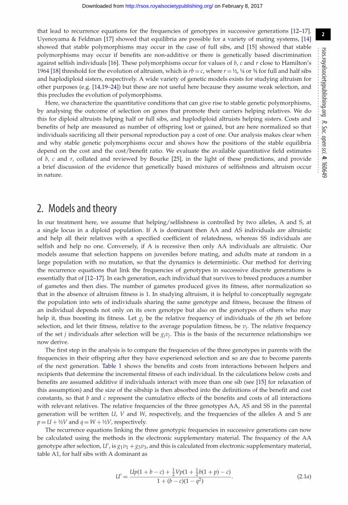
................................................that lead to recurrence equations for the frequencies of genotypes in successive generations [12–17].Uyenoyama & Feldman [17] showed that equilibria are possible for a variety of mating systems, [14]showed that stable polymorphisms may occur in the case of full sibs, and [15] showed that stablepolymorphisms may occur if benefits are non-additive or there is genetically based discriminationagainst selfish individuals [16]. These polymorphisms occur for values of b, c and r close to Hamilton’s1964 [18] threshold for the evolution of altruism, which is rb = c, where r = ½, ¼ or ¾ for full and half sibsand haplodiploid sisters, respectively. A wide variety of genetic models exists for studying altruism forother purposes (e.g. [14,19–24]) but these are not useful here because they assume weak selection, andthis precludes the evolution of polymorphisms.

Here, we characterize the quantitative conditions that can give rise to stable genetic polymorphisms,by analysing the outcome of selection on genes that promote their carriers helping relatives. We dothis for diploid altruists helping half or full sibs, and haplodiploid altruists helping sisters. Costs andbenefits of help are measured as number of offspring lost or gained, but are here normalized so thatindividuals sacrificing all their personal reproduction pay a cost of one. Our analysis makes clear whenand why stable genetic polymorphisms occur and shows how the positions of the stable equilibriadepend on the cost and the cost/benefit ratio. We evaluate the available quantitative field estimatesof b, c and r, collated and reviewed by Bourke [25], in the light of these predictions, and providea brief discussion of the evidence that genetically based mixtures of selfishness and altruism occurin nature.

2. Models and theoryIn our treatment here, we assume that helping/selfishness is controlled by two alleles, A and S, ata single locus in a diploid population. If A is dominant then AA and AS individuals are altruisticand help all their relatives with a specified coefficient of relatedness, whereas SS individuals areselfish and help no one. Conversely, if A is recessive then only AA individuals are altruistic. Ourmodels assume that selection happens on juveniles before mating, and adults mate at random in alarge population with no mutation, so that the dynamics is deterministic. Our method for derivingthe recurrence equations that link the frequencies of genotypes in successive discrete generations isessentially that of [12–17]. In each generation, each individual that survives to breed produces a numberof gametes and then dies. The number of gametes produced gives its fitness, after normalization sothat in the absence of altruism fitness is 1. In studying altruism, it is helpful to conceptually segregatethe population into sets of individuals sharing the same genotype and fitness, because the fitness ofan individual depends not only on its own genotype but also on the genotypes of others who mayhelp it, thus boosting its fitness. Let gj be the relative frequency of individuals of the jth set beforeselection, and let their fitness, relative to the average population fitness, be vj. The relative frequencyof the set j individuals after selection will be gjvj. This is the basis of the recurrence relationships wenow derive.

The first step in the analysis is to compare the frequencies of the three genotypes in parents with thefrequencies in their offspring after they have experienced selection and so are due to become parentsof the next generation. Table 1 shows the benefits and costs from interactions between helpers andrecipients that determine the incremental fitness of each individual. In the calculations below costs andbenefits are assumed additive if individuals interact with more than one sib (see [15] for relaxation ofthis assumption) and the size of the sibship is then absorbed into the definitions of the benefit and costconstants, so that b and c represent the cumulative effects of the benefits and costs of all interactionswith relevant relatives. The relative frequencies of the three genotypes AA, AS and SS in the parentalgeneration will be written U, V and W, respectively, and the frequencies of the alleles A and S arep = U + ½V and q = W + ½V, respectively.

The recurrence equations linking the three genotypic frequencies in successive generations can nowbe calculated using the methods in the electronic supplementary material. The frequency of the AAgenotype after selection, U′, is g1v1 + g3v3, and this is calculated from electronic supplementary material,table A1, for half sibs with A dominant as

U′ = Up(1 + b − c) + 12 Vp(1 + 1

2 b(1 + p) − c)1 + (b − c)(1 − q2)

. (2.1a)

on February 8, 2017http://rsos.royalsocietypublishing.org/Downloaded from

3

rsos.royalsocietypublishing.orgR.Soc.opensci.4:160649

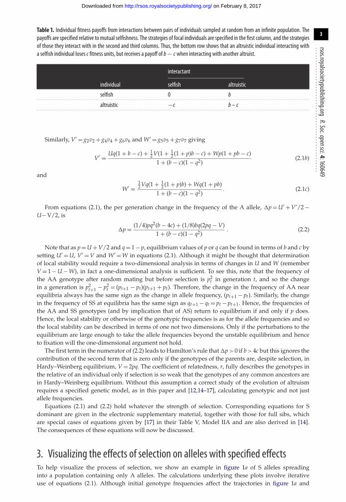
................................................Table 1. Individual fitness payoffs from interactions between pairs of individuals sampled at random from an infinite population. Thepayoffs are specified relative to mutual selfishness. The strategies of focal individuals are specified in the first column, and the strategiesof those they interact with in the second and third columns. Thus, the bottom row shows that an altruistic individual interacting witha selfish individual loses c fitness units, but receives a payoff of b− c when interacting with another altruist.

interactant

individual selfish altruistic

selfish 0 b. . . . . . . . . . . . . . . . . . . . . . . . . . . . . . . . . . . . . . . . . . . . . . . . . . . . . . . . . . . . . . . . . . . . . . . . . . . . . . . . . . . . . . . . . . . . . . . . . . . . . . . . . . . . . . . . . . . . . . . . . . . . . . . . . . . . . . . . . . . . . . . . . . . . . . . . . . . . . . . . . . . . . . . . . . . . . . . . . . . . . . . . . . . . . . . . . . . . . . . . . . . . . . . . . . . . . . . . .

altruistic −c b – c. . . . . . . . . . . . . . . . . . . . . . . . . . . . . . . . . . . . . . . . . . . . . . . . . . . . . . . . . . . . . . . . . . . . . . . . . . . . . . . . . . . . . . . . . . . . . . . . . . . . . . . . . . . . . . . . . . . . . . . . . . . . . . . . . . . . . . . . . . . . . . . . . . . . . . . . . . . . . . . . . . . . . . . . . . . . . . . . . . . . . . . . . . . . . . . . . . . . . . . . . . . . . . . . . . . . . . . . .

Similarly, V′ = g2v2 + g4v4 + g6v6 and W′ = g5v5 + g7v7 giving

V′ = Uq(1 + b − c) + 12 V(1 + 1

2 (1 + p)b − c) + Wp(1 + pb − c)1 + (b − c)(1 − q2)

(2.1b)

and

W′ =12 Vq(1 + 1

2 (1 + p)b) + Wq(1 + pb)1 + (b − c)(1 − q2)

. (2.1c)

From equations (2.1), the per generation change in the frequency of the A allele, �p = U′ + V′/2 −U− V/2, is

�p = (1/4)pq2(b − 4c) + (1/8)bq(2pq − V)1 + (b − c)(1 − q2)

. (2.2)

Note that as p = U + V/2 and q = 1 − p, equilibrium values of p or q can be found in terms of b and c bysetting U′ = U, V′ = V and W′ = W in equations (2.1). Although it might be thought that determinationof local stability would require a two-dimensional analysis in terms of changes in U and W (rememberV = 1 − U − W), in fact a one-dimensional analysis is sufficient. To see this, note that the frequency ofthe AA genotype after random mating but before selection is p2

t in generation t, and so the changein a generation is p2

t+1 − p2t = (pt+1 − pt)(pt+1 + pt). Therefore, the change in the frequency of AA near

equilibria always has the same sign as the change in allele frequency, (pt+1 − pt). Similarly, the changein the frequency of SS at equilibria has the same sign as qt+1 − qt = pt − pt+1. Hence, the frequencies ofthe AA and SS genotypes (and by implication that of AS) return to equilibrium if and only if p does.Hence, the local stability or otherwise of the genotypic frequencies is as for the allele frequencies and sothe local stability can be described in terms of one not two dimensions. Only if the perturbations to theequilibrium are large enough to take the allele frequencies beyond the unstable equilibrium and henceto fixation will the one-dimensional argument not hold.

The first term in the numerator of (2.2) leads to Hamilton’s rule that �p > 0 if b > 4c but this ignores thecontribution of the second term that is zero only if the genotypes of the parents are, despite selection, inHardy–Weinberg equilibrium, V = 2pq. The coefficient of relatedness, r, fully describes the genotypes inthe relative of an individual only if selection is so weak that the genotypes of any common ancestors arein Hardy–Weinberg equilibrium. Without this assumption a correct study of the evolution of altruismrequires a specified genetic model, as in this paper and [12,14–17], calculating genotypic and not justallele frequencies.

Equations (2.1) and (2.2) hold whatever the strength of selection. Corresponding equations for Sdominant are given in the electronic supplementary material, together with those for full sibs, whichare special cases of equations given by [17] in their Table V, Model IIA and are also derived in [14].The consequences of these equations will now be discussed.

3. Visualizing the effects of selection on alleles with specified effectsTo help visualize the process of selection, we show an example in figure 1a of S alleles spreadinginto a population containing only A alleles. The calculations underlying these plots involve iterativeuse of equations (2.1). Although initial genotype frequencies affect the trajectories in figure 1a and

on February 8, 2017http://rsos.royalsocietypublishing.org/Downloaded from

4

rsos.royalsocietypublishing.orgR.Soc.opensci.4:160649

................................................

1.00.80.60.40.20

0.0015

0.0010

0.0005

0

–0.0005

Dq

q

q

(a) (b)

10

0.2

0.4

0.6

0.8

1.0

2000 4000 6000generation

8000 10 000

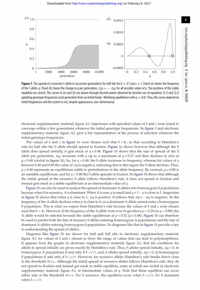
Figure 1. The spread of a recessive S allele in successive generations for half sibs for b= 3.7 and c= 1. Panel (a) shows the frequencyof the S allele, q. Panel (b) shows the change in q per generation,�q= − �p, for all possible values of q. The positions of the stableequilibria are circled. The curves in (a) and (b) are drawn through discrete points obtained by iterative use of equations (2.1) and (2.2)updating genotype frequencies each generation from an initial Hardy–Weinberg equilibriumwith q= 0.01. Thus, the curves depend oninitial frequencies and the system is not, despite appearances, one-dimensional.

electronic supplementary material, figure A1, trajectories with specified values of b and c were found toconverge within a few generations whatever the initial genotype frequencies. So figure 1 and electronicsupplementary material, figure A1, give a fair representation of the process of selection whatever theinitial genotype frequencies.

The values of b and c in figure 1a were chosen such that b < 4c, so that according to Hamilton’srule for half sibs the S allele should spread to fixation. Figure 1a shows however that although the Sallele does spread initially, it gets stuck at q = 0.48. Figure 1b shows that the rate of spread of the Sallele per generation, �q, increases with q up to a maximum at q = 0.27 and then declines to zero atq = 0.48 (circled in figure 1b). So, for q < 0.48, the S allele increases in frequency, whereas for values of qbetween 0.48 and 0.80 the value of �q is negative, indicating that in this region the S allele declines. Thus,q = 0.48 represents an equilibrium stable to perturbations in the allele frequency. By contrast, q = 0.80 isan unstable equilibrium, and for q > 0.80 the S allele spreads to fixation. So figure 1b shows that althoughthe initial spread of the recessive S allele follows Hamilton’s rule, it does not spread to fixation andinstead gets stuck in a stable equilibrium at an intermediate value of q.

Figure 1b can also be used to analyse the spread of dominant A alleles into homozygous S populationsbecause when S is recessive, A is dominant. When A is rare, p is small and q = 1 − p is close to 1. Inspectionof figure 1b shows that when q is close to 1, �q is positive. It follows that �p= −�q is negative. So thefrequency of the A allele declines when p is close to 0, so a dominant A allele cannot enter a homozygousS population. This is what we expect from Hamilton’s rule because the values of b and c were chosensuch that b < 4c. However, if the frequency of the A allele were ever to get above p = 0.20 (so q < 0.80), theA allele would be selected towards the stable equilibrium at p = 0.52 (q = 0.48). Figure 1b can thereforebe used to predict both the fate of recessive S alleles entering homozygous A populations and the fate ofdominant A alleles entering homozygous S populations. So diagrams like that in figure 1b provide a keyto understanding the spread of alleles.

Diagrams like figure 1b are shown for half and full sibs in electronic supplementary material,figure A1, for values of b and c chosen to show the range of values that can lead to polymorphisms.It appears from the graphs in electronic supplementary material, figure A1, that the conditions foralleles to spread initially are given exactly by Hamilton’s rule. Thus, S alleles spread initially, �q > 0, inhomozygous A populations if and only if b < c/r, and A alleles spread initially, �p > 0, in homozygousS populations if and only if b > c/r. However, for recessive alleles Hamilton’s rule breaks down closeto the threshold rb = c. Although the initial spread of recessive alleles follows Hamilton’s rule, they donot spread to fixation and instead get stuck in stable equilibria, some of which are circled in electronicsupplementary material, figure A1, at intermediate values of q. Note that these equilibria can occureither side of the threshold rb = c. For S recessive, the equilibria occur when b < c/r, for S dominantwhen b > c/r.

on February 8, 2017http://rsos.royalsocietypublishing.org/Downloaded from

5

rsos.royalsocietypublishing.orgR.Soc.opensci.4:160649

................................................4. Mapping the positions of the stable equilibriaIn this section, we explore the relationship between stable gene frequencies and the values of b and cthat produce them. We start with the derivation in [17] for full sibs, from the recurrence equations for thegenotypic frequencies, of quadratic equations (their eqn 51) that show how equilibrium values of p or qvary with the values of b and c. Writing x = b/c − 2, the quadratic equation for the equilibrium values ofp for S dominant, A recessive is

c(1 + x)2p2 − c(1 + x)p + x = 0, (4.1)

and for A dominant and S recessive

c(1 + x)2p2 − c(1 + 2x)(1 + x)p − x = 0. (4.2)

Uyenoyama & Feldman [17] did not distinguish stable from unstable equilibria, but these can bedistinguished because the first equilibrium encountered by a favoured allele entering a population isbound to be stable. Thus if there are two internal equilibria, the one with lower p is stable for A allelesand the one with lower q is stable for S alleles.

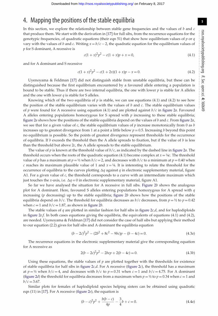
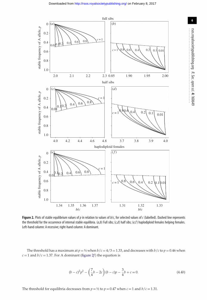
Knowing which of the two equilibria of p is stable, we can use equations (4.1) and (4.2) to see howthe position of the stable equilibrium varies with the values of b and c. The stable equilibrium valuesof p were found for A recessive using equation (4.1) and are plotted against b/c in figure 2a. FavouredA alleles entering populations homozygous for S spread with p increasing to these stable equilibria;figure 2a shows how the positions of the stable equilibria depend on the values of b and c. From figure 2a,we see that for a given value of c, the stable equilibrium values of p increase monotonically from 0 as bincreases up to greatest divergence from 1 at a point a little below p = 0.5. Increasing b beyond this pointno equilibrium is possible. So the points of greatest divergence represent thresholds for the occurrenceof equilibria. If b exceeds the threshold then the A allele spreads to fixation, but if the value of b is lessthan the threshold but above 2c, the A allele spreads to the stable equilibrium.

The value of p is known at the threshold value of b/c, as indicated by the dashed line in figure 2a. Thethreshold occurs when the roots of the quadratic equation (4.1) become complex at x = ¼c. The thresholdvalue of p has a maximum at p = ½ when b/c = 2, and decreases with b/c to a minimum at p = 0.40 whenc reaches its maximum plausible value of 1 and x = ¼. It is interesting to relate the threshold for theoccurrence of equilibria to the curves plotting �q against q in electronic supplementary material, figureA1. For a given value of c, the threshold corresponds to a curve with an intermediate maximum whichjust touches the x-axis, i.e. �q = 0 in electronic supplementary material, figure A1.

So far we have analysed the situation for A recessive in full sibs. Figure 2b shows the analogousplot for A dominant. Here, favoured S alleles entering populations homozygous for A spread with qincreasing (p decreasing) up to the stable equilibria; figure 2b shows how the positions of the stableequilibria depend on b/c. The threshold for equilibria decreases as b/c decreases, from p = ½ to p = 0.42when c = 1 and b/c = 1.87, as shown in figure 2b.

The stable values of q are plotted in similar fashion for half sibs in figure 2c,d, and for haplodiploidsin figure 2e,f. In both cases equations giving the equilibria, the equivalents of equations (4.1) and (4.2),are needed. Uyenoyama & Feldman [17] did not consider the case of half sibs but applying their methodto our equation (2.2) gives for half sibs and A dominant the equilibria equation

(b − 2c)2p2 − (2b2 + 8c2 − 9bc)p − (b − 4c) = 0. (4.3a)

The recurrence equations in the electronic supplementary material give the corresponding equationfor A recessive as

2(b − 2c)2p2 − 2bcp + 2(b − 4c) = 0. (4.3b)

Using these equations, the stable values of p are plotted together with the thresholds for existenceof stable equilibria for half sibs in figure 2c,d. For A recessive (figure 2c), the threshold has a maximumat p = ½ when b/c = 4, and decreases with b/c to p = 0.31 when c = 1 and b/c = 4.75. For A dominant(figure 2d) the threshold for equilibria decreases from a maximum when p = ½ to p = 0.34 when c = 1 andb/c = 3.67.

Similar plots for females of haplodiploid species helping sisters can be obtained using quadraticeqn (11) in [17]. For A recessive (figure 2e), the equation is

(b − c)2p2 + b(b − c)4p

− 34

b + c = 0. (4.4a)

on February 8, 2017http://rsos.royalsocietypublishing.org/Downloaded from

6

rsos.royalsocietypublishing.orgR.Soc.opensci.4:160649

................................................

b/c b/c

haplodiploid females

half sibs

full sibs

stab

le f

requ

ency

of

A a

llele

, p

stab

le f

requ

ency

of

A a

llele

, p

stab

le f

requ

ency

of

A a

llele

, p

0

0.2

0.4

0.6

0.8

1.0

0

0.2

0.4

0.6

0.8

1.0

0

0.2

0.4

0.6

0.8

1.0

c = 1

c = 1

0.8

0.80.60.40.20.10.01

c = 1

c = 1

0.80.60.40.20.10.01

0.6 0.4 0.2 0.1 0.01

0.8 0.6 0.4 0.2 0.1 0.01

c = 1

c = 1

0.80.60.40.20.10.010.8 0.6 0.4 0.2 0.1 0.01

1.34

4.0 4.2 4.4 4.6 4.8 3.7 3.8 3.9 4.0

2.0 2.1 2.2 2.3 0.85 1.90 1.95 2.00

1.35 1.36 1.37 1.31 1.32 1.33

(b)(a)

(d)(c)

( f )(e)

Figure 2. Plots of stable equilibrium values of p in relation to values of b/c, for selected values of c (labelled). Dashed line representsthe threshold for the occurrence of internal stable equilibria. (a,b) Full sibs; (c,d) half sibs; (e,f ) haplodiploid females helping females.Left-hand column: A recessive; right-hand column: A dominant.

The threshold has a maximum at p = ½ when b/c = 4/3 = 1.33, and decreases with b/c to p = 0.46 whenc = 1 and b/c = 1.37. For A dominant (figure 2f ) the equation is

(b − c)2p2 −(

74

b − 2c)

(b − c)p − 34

b + c = 0. (4.4b)

The threshold for equilibria decreases from p = ½ to p = 0.47 when c = 1 and b/c = 1.31.

on February 8, 2017http://rsos.royalsocietypublishing.org/Downloaded from

7

rsos.royalsocietypublishing.orgR.Soc.opensci.4:160649

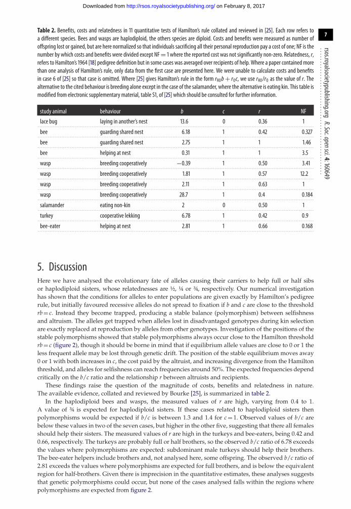
................................................Table 2. Benefits, costs and relatedness in 11 quantitative tests of Hamilton’s rule collated and reviewed in [25]. Each row refers toa different species. Bees and wasps are haplodiploid, the others species are diploid. Costs and benefits were measured as number ofoffspring lost or gained, but are here normalized so that individuals sacrificing all their personal reproduction pay a cost of one; NF is thenumber by which costs and benefits were divided except NF= 1 where the reported cost was not significantly non-zero. Relatedness, r,refers to Hamilton’s 1964 [18] pedigree definition but in some cases was averaged over recipients of help. Where a paper contained morethan one analysis of Hamilton’s rule, only data from the first case are presented here. We were unable to calculate costs and benefitsin case 6 of [25] so that case is omitted. Where [25] gives Hamilton’s rule in the form rROb+ rOc, we use rRO/rO as the value of r. Thealternative to the cited behaviour is breeding alone except in the case of the salamander, where the alternative is eating kin. This table ismodified from electronic supplementary material, table S1, of [25] which should be consulted for further information.

study animal behaviour b c r NF

lace bug laying in another’s nest 13.6 0 0.36 1. . . . . . . . . . . . . . . . . . . . . . . . . . . . . . . . . . . . . . . . . . . . . . . . . . . . . . . . . . . . . . . . . . . . . . . . . . . . . . . . . . . . . . . . . . . . . . . . . . . . . . . . . . . . . . . . . . . . . . . . . . . . . . . . . . . . . . . . . . . . . . . . . . . . . . . . . . . . . . . . . . . . . . . . . . . . . . . . . . . . . . . . . . . . . . . . . . . . . . . . . . . . . . . . . . . . . . . . .

bee guarding shared nest 6.18 1 0.42 0.327. . . . . . . . . . . . . . . . . . . . . . . . . . . . . . . . . . . . . . . . . . . . . . . . . . . . . . . . . . . . . . . . . . . . . . . . . . . . . . . . . . . . . . . . . . . . . . . . . . . . . . . . . . . . . . . . . . . . . . . . . . . . . . . . . . . . . . . . . . . . . . . . . . . . . . . . . . . . . . . . . . . . . . . . . . . . . . . . . . . . . . . . . . . . . . . . . . . . . . . . . . . . . . . . . . . . . . . . .

bee guarding shared nest 2.75 1 1 1.46. . . . . . . . . . . . . . . . . . . . . . . . . . . . . . . . . . . . . . . . . . . . . . . . . . . . . . . . . . . . . . . . . . . . . . . . . . . . . . . . . . . . . . . . . . . . . . . . . . . . . . . . . . . . . . . . . . . . . . . . . . . . . . . . . . . . . . . . . . . . . . . . . . . . . . . . . . . . . . . . . . . . . . . . . . . . . . . . . . . . . . . . . . . . . . . . . . . . . . . . . . . . . . . . . . . . . . . . .

bee helping at nest 0.31 1 1 3.5. . . . . . . . . . . . . . . . . . . . . . . . . . . . . . . . . . . . . . . . . . . . . . . . . . . . . . . . . . . . . . . . . . . . . . . . . . . . . . . . . . . . . . . . . . . . . . . . . . . . . . . . . . . . . . . . . . . . . . . . . . . . . . . . . . . . . . . . . . . . . . . . . . . . . . . . . . . . . . . . . . . . . . . . . . . . . . . . . . . . . . . . . . . . . . . . . . . . . . . . . . . . . . . . . . . . . . . . .

wasp breeding cooperatively −0.39 1 0.50 3.41. . . . . . . . . . . . . . . . . . . . . . . . . . . . . . . . . . . . . . . . . . . . . . . . . . . . . . . . . . . . . . . . . . . . . . . . . . . . . . . . . . . . . . . . . . . . . . . . . . . . . . . . . . . . . . . . . . . . . . . . . . . . . . . . . . . . . . . . . . . . . . . . . . . . . . . . . . . . . . . . . . . . . . . . . . . . . . . . . . . . . . . . . . . . . . . . . . . . . . . . . . . . . . . . . . . . . . . . .

wasp breeding cooperatively 1.81 1 0.57 12.2. . . . . . . . . . . . . . . . . . . . . . . . . . . . . . . . . . . . . . . . . . . . . . . . . . . . . . . . . . . . . . . . . . . . . . . . . . . . . . . . . . . . . . . . . . . . . . . . . . . . . . . . . . . . . . . . . . . . . . . . . . . . . . . . . . . . . . . . . . . . . . . . . . . . . . . . . . . . . . . . . . . . . . . . . . . . . . . . . . . . . . . . . . . . . . . . . . . . . . . . . . . . . . . . . . . . . . . . .

wasp breeding cooperatively 2.11 1 0.63 1. . . . . . . . . . . . . . . . . . . . . . . . . . . . . . . . . . . . . . . . . . . . . . . . . . . . . . . . . . . . . . . . . . . . . . . . . . . . . . . . . . . . . . . . . . . . . . . . . . . . . . . . . . . . . . . . . . . . . . . . . . . . . . . . . . . . . . . . . . . . . . . . . . . . . . . . . . . . . . . . . . . . . . . . . . . . . . . . . . . . . . . . . . . . . . . . . . . . . . . . . . . . . . . . . . . . . . . . .

wasp breeding cooperatively 28.7 1 0.4 0.184. . . . . . . . . . . . . . . . . . . . . . . . . . . . . . . . . . . . . . . . . . . . . . . . . . . . . . . . . . . . . . . . . . . . . . . . . . . . . . . . . . . . . . . . . . . . . . . . . . . . . . . . . . . . . . . . . . . . . . . . . . . . . . . . . . . . . . . . . . . . . . . . . . . . . . . . . . . . . . . . . . . . . . . . . . . . . . . . . . . . . . . . . . . . . . . . . . . . . . . . . . . . . . . . . . . . . . . . .

salamander eating non-kin 2 0 0.50 1. . . . . . . . . . . . . . . . . . . . . . . . . . . . . . . . . . . . . . . . . . . . . . . . . . . . . . . . . . . . . . . . . . . . . . . . . . . . . . . . . . . . . . . . . . . . . . . . . . . . . . . . . . . . . . . . . . . . . . . . . . . . . . . . . . . . . . . . . . . . . . . . . . . . . . . . . . . . . . . . . . . . . . . . . . . . . . . . . . . . . . . . . . . . . . . . . . . . . . . . . . . . . . . . . . . . . . . . .

turkey cooperative lekking 6.78 1 0.42 0.9. . . . . . . . . . . . . . . . . . . . . . . . . . . . . . . . . . . . . . . . . . . . . . . . . . . . . . . . . . . . . . . . . . . . . . . . . . . . . . . . . . . . . . . . . . . . . . . . . . . . . . . . . . . . . . . . . . . . . . . . . . . . . . . . . . . . . . . . . . . . . . . . . . . . . . . . . . . . . . . . . . . . . . . . . . . . . . . . . . . . . . . . . . . . . . . . . . . . . . . . . . . . . . . . . . . . . . . . .

bee-eater helping at nest 2.81 1 0.66 0.168. . . . . . . . . . . . . . . . . . . . . . . . . . . . . . . . . . . . . . . . . . . . . . . . . . . . . . . . . . . . . . . . . . . . . . . . . . . . . . . . . . . . . . . . . . . . . . . . . . . . . . . . . . . . . . . . . . . . . . . . . . . . . . . . . . . . . . . . . . . . . . . . . . . . . . . . . . . . . . . . . . . . . . . . . . . . . . . . . . . . . . . . . . . . . . . . . . . . . . . . . . . . . . . . . . . . . . . . .

5. DiscussionHere we have analysed the evolutionary fate of alleles causing their carriers to help full or half sibsor haplodiploid sisters, whose relatednesses are ½, ¼ or ¾, respectively. Our numerical investigationhas shown that the conditions for alleles to enter populations are given exactly by Hamilton’s pedigreerule, but initially favoured recessive alleles do not spread to fixation if b and c are close to the thresholdrb = c. Instead they become trapped, producing a stable balance (polymorphism) between selfishnessand altruism. The alleles get trapped when alleles lost in disadvantaged genotypes during kin selectionare exactly replaced at reproduction by alleles from other genotypes. Investigation of the positions of thestable polymorphisms showed that stable polymorphisms always occur close to the Hamilton thresholdrb = c (figure 2), though it should be borne in mind that if equilibrium allele values are close to 0 or 1 theless frequent allele may be lost through genetic drift. The position of the stable equilibrium moves away0 or 1 with both increases in c, the cost paid by the altruist, and increasing divergence from the Hamiltonthreshold, and alleles for selfishness can reach frequencies around 50%. The expected frequencies dependcritically on the b/c ratio and the relationship r between altruists and recipients.

These findings raise the question of the magnitude of costs, benefits and relatedness in nature.The available evidence, collated and reviewed by Bourke [25], is summarized in table 2.

In the haplodiploid bees and wasps, the measured values of r are high, varying from 0.4 to 1.A value of ¾ is expected for haplodiploid sisters. If these cases related to haplodiploid sisters thenpolymorphisms would be expected if b/c is between 1.3 and 1.4 for c = 1. Observed values of b/c arebelow these values in two of the seven cases, but higher in the other five, suggesting that there all femalesshould help their sisters. The measured values of r are high in the turkeys and bee-eaters, being 0.42 and0.66, respectively. The turkeys are probably full or half brothers, so the observed b/c ratio of 6.78 exceedsthe values where polymorphisms are expected: subdominant male turkeys should help their brothers.The bee-eater helpers include brothers and, not analysed here, some offspring. The observed b/c ratio of2.81 exceeds the values where polymorphisms are expected for full brothers, and is below the equivalentregion for half-brothers. Given there is imprecision in the quantitative estimates, these analyses suggeststhat genetic polymorphisms could occur, but none of the cases analysed falls within the regions wherepolymorphisms are expected from figure 2.

on February 8, 2017http://rsos.royalsocietypublishing.org/Downloaded from

8

rsos.royalsocietypublishing.orgR.Soc.opensci.4:160649

................................................Using the simplest of genetic models, we have identified regions where genetic polymorphisms

between selfishness and altruism are expected, but other models also can give rise to geneticpolymorphisms. Using methods as here, based on recurrence equations for genotype frequencies, ithas been shown that under certain conditions non-additivity of costs and benefits can lead to stablegenetic polymorphisms [15], as can discrimination against selfish individuals [16], sexual antagonismacting under balancing selection [26] and heterozygous advantage [14]. Genetic polymorphisms couldalso arise through selection–mutation balance [27], temporal environmental variation causing selectionto act in different directions over time (e.g. [25]), or if altruism was a mixed not a pure strategy [28].The intermediate degrees of dominance discussed in [12] and [17] could also be studied numerically.A restriction on our method is that the recurrence equations used in our analyses are exact only when thepopulation is large in the sense that there are an infinite number of sibships of each type as defined, forexample, in electronic supplementary material, table A1. The evolutionary process is then deterministic.Those limitations have been to some extent overcome in individual-based simulations which showedthat Hamilton’s 1964 [18] rule accurately predicted the minimum relatedness necessary for altruismto evolve [29]. The individuals evolved in a population of size 1600 and were equipped with haploidgenetic systems characterized by mutation, recombination and pleiotropic and epistatic effects. It wouldbe helpful to repeat these experiments with diploidy to replicate the conditions investigated here.

To carry out a test of Hamilton’s rule in nature, it is necessary that there exist both selfish and altruisticindividuals, whose relative costs and benefits can be compared. But how can such a polymorphism ofselfishness and altruism come about? One possibility is that the polymorphism has a genetic basis, so thatselfishness and altruism are heritable, as in the cases analysed here. Alternatively, some individuals maybe prevented from acting selfishly. This occurs in bee-eaters which choose altruism when the ‘selfish’option of breeding alone is blocked when their nests are destroyed by close kin [30]; in female insectsrendered small by strategic food deprivation whose best option is helping sibs; and in male turkeysunable to achieve dominance within their sibship whose best option is altruistic support of the dominantmale [31].

Our results and the experimental work reviewed by Bourke [25] raise the question of whether weshould expect to find examples of the coexistence of selfishness and altruism in nature. To answer this,we need to consider how helping evolves over evolutionary time. Suppose genes arise through mutation,which cause their carriers to provide food, protection or support to relatives when needed. At the start ofthe evolutionary process it may be that this help confers benefits at a cost to helpers such that rb − c > 0,but rb − c may not be in the region where polymorphisms are expected to occur. In this case, the genesresponsible would be selected and spread through the population to fixation. However, there may stillbe further benefits available at some additional cost to the helper. Eventually further benefits are onlyavailable by pushing the benefits into the region at which stable polymorphisms are expected to occur.Recessive genes that cause their carriers to provide/withhold help are then expected to spread initiallybut to get trapped, as we have shown using the simplest of genetic models. The expected outcome is astable balance between selfishness and altruism. This together with non-additivity [15], discriminationagainst selfish individuals [16] and other factors mentioned above may contribute to the substantialheritability of selfishness/altruism found in man. As further genes for altruism are identified, it will beinteresting to see whether they are accompanied by alternate alleles for selfishness.

Data accessibility. Working needed to derive the recurrence equations (equations (2.1a–c)) together with an additionalfigure showing how the effects of selection can be visualized are available in the electronic supplementary material.Authors’ contributions. R.M.S. and R.N.C. designed and carried out the modelling and wrote the manuscript. Both authorsread and approved the manuscript before submission.Competing interests. We declare we have no competing interests.Funding. R.M.S. is employed by the University of Reading, R.N.C. is retired.Acknowledgements. We are very grateful to Andrew Bourke, Louise Johnson, Mark Pagel and two referees for helpfulcomments.

References1. Jiang Y, Chew SH, Ebstein RP. 2013 The role of D4

receptor gene exon III polymorphisms in shapinghuman altruism and prosocial behavior. Front. Hum.Neurosci. 7, 195. (doi:10.3389/fnhum.2013.00195)

2. Simola DF, et al. 2016 Epigenetic (re)programmingof caste-specific behavior in the ant Camponotus

floridanus. Science 351, U42–U69. (doi:10.1126/science.aac6633)

3. Cesarini D, Dawes CT, Johannesson M, LichtensteinP, Wallace B. 2009 Genetic variation in preferencesfor giving and risk taking. Quart. J. Econ. 124,809–842. (doi:10.1162/qjec.2009.124.2.809)

4. Gregory AM, Light-Hausermann JH, Rijsdijk F, EleyTC. 2009 Behavioral genetic analyses of prosocialbehavior in adolescents. Dev. Sci. 12, 165–174.(doi:10.1111/j.1467-7687.2008.00739.x)

5. Hur YM, Rushton JP. 2007 Genetic andenvironmental contributions to prosocial behaviour

on February 8, 2017http://rsos.royalsocietypublishing.org/Downloaded from

9

rsos.royalsocietypublishing.orgR.Soc.opensci.4:160649

................................................in 2-to 9-year-old South Korean twins. Biol. Lett. 3,664–666. (doi:10.1098/rsbl.2007.0365)

6. Israel S, Hasenfratz L, Knafo-Noam A. 2015 Thegenetics of morality and prosociality. Curr. Opin.Psychol. 6, 55–59. (doi:10.1016/j.copsyc.2015.03.027)

7. Knafo A, Plomin R. 2006 Prosocial behavior fromearly to middle childhood: genetic andenvironmental influences on stability and change.Dev. Psychol. 42, 771–786. (doi:10.1037/0012-1649.42.5.771)

8. Rushton JP. 2004 Genetic and environmentalcontributions to pro-social attitudes: a twin studyof social responsibility. Proc. R. Soc. Lond. B 271,2583–2585. (doi:10.1098/rspb.2004.2941)

9. Rushton JP, Fulker DW, Neale MC, Nias DKB,Eysenck HJ. 1986 Altruism and aggression—theheritability of individual differences. J. Pers. Soc.Psychol. 50, 1192–1198. (doi:10.1037/0022-3514.50.6.1192)

10. Scourfield J, John B, Martin N, McGuffin P. 2004 Thedevelopment of prosocial behaviour in children andadolescents: a twin study. J. Child Psychol. Psych. 45,927–935. (doi:10.1111/j.1469-7610.2004.t01-1-00286.x)

11. Krueger RF, Hicks BM, McGue M. 2001 Altruism andantisocial behavior: independent tendencies,unique personality correlates, distinct etiologies.Psychol. Sci. 12, 397–402. (doi:10.1111/1467-9280.00373)

12. Cavalli-Sforza LL, Feldman MW. 1978 Darwinianselection and altruism. Theor. Popul. Biol. 14,268–280. (doi:10.1016/0040-5809(78)90028-X)

13. Levitt PR. 1975 General kin selection modelsfor genetic evolution of sib altruism in diploid

and haplodiploid species. Proc. Natl Acad. Sci.USA 72, 4531–4535. (doi:10.1073/pnas.72.11.4531)

14. Rowthorn R. 2006 The evolution of altruismbetween siblings: Hamilton’s rule revisited. J. Theor.Biol. 241, 774–790. (doi:10.1016/j.jtbi.2006.01.014)

15. Sibly RM, Curnow RN. 2011 Selfishness and altruismcan coexist when help is subject to diminishingreturns. Heredity 107, 167–173. (doi:10.1038/hdy.2011.2)

16. Sibly RM, Curnow RN. 2012 Evolution ofdiscrimination in populations at equilibriumbetween selfishness and altruism. J. Theor. Biol. 313,162–171. (doi:10.1016/j.jtbi.2012.08.014)

17. Uyenoyama MK, Feldman MW. 1981 On relatednessand adaptive topography in kin selection. Theor.Popul. Biol. 19, 87–123. (doi:10.1016/0040-5809(81)90036-8)

18. Hamilton WD. 1964 The genetical evolution of socialbehaviour (I & II). J. Theor. Biol. 12, 1–16.(doi:10.1016/0022-5193(64)90038-4)

19. Fletcher JA, Doebeli M. 2006 How altruism evolves:assortment and synergy. J. Evol. Biol. 19, 1389–1393.(doi:10.1111/j.1420-9101.2006.01146.x)

20. Frank SA. 1998 Foundations of social evolution.Princeton, NJ: Princeton University Press.

21. Queller DC. 1985 Kinship, reciprocity and synergismin the evolution of social behaviour. Nature 318,366–367. (doi:10.1038/318366a0)

22. Queller DC. 1992 A general-model for kin selection.Evolution 46, 376–380. (doi:10.2307/2409858)

23. Roze D, Rousset F. 2004 The robustness ofHamilton’s rule with inbreeding and dominance: kinselection and fixation probabilities under partial sib

mating. Am. Nat. 164, 214–231.(doi:10.1086/422202)

24. van Veelen M, Garcia J, Sabelis MW, Egas M. 2012Group selection and inclusive fitness are notequivalent; the Price equation vs. models andstatistics. J. Theor. Biol. 299, 64–80. (doi:10.1016/j.jtbi.2011.07.025)

25. Bourke AFG. 2014 Hamilton’s rule and the causes ofsocial evolution. Phil. Trans. R. Soc. B 369, 20130362.(doi:10.1098/rstb.2013.0362)

26. Mullon C, Pomiankowski A, Reuter M. 2012 Theeffects of selection and genetic drift on the genomicdistribution of sexually antagonistic alleles.Evolution 66, 3743–3753. (doi:10.1111/j.1558-5646.2012.01728.x)

27. Van Dyken JD, Linksvayer TA, Wade MJ. 2011 Kinselection-mutation balance: a model for theorigin, maintenance, and consequences of socialcheating. Am. Nat. 177, 288–300. (doi:10.1086/658365)

28. Charlesworth B. 1978 Somemodels of evolution ofaltruistic behavior between siblings. J. Theor. Biol.72, 297–319. (doi:10.1016/0022-5193(78)90095-4)

29. Waibel M, Floreano D, Keller L. 2011 A quantitativetest of Hamilton’s rule for the evolution of altruism.PLoS Biol. 9, e1000615. (doi:10.1371/journal.pbio.1000615)

30. Emlen ST, Wrege PH. 1992 Parent offspring conflictand the recruitment of helpers among bee-eaters.Nature 356, 331–333. (doi:10.1038/356331a0)

31. Krakauer AH. 2005 Kin selection and cooperativecourtship in wild turkeys. Nature 434, 69–72.(doi:10.1038/nature03325)

on February 8, 2017http://rsos.royalsocietypublishing.org/Downloaded from