Embed Size (px)
Citation preview
Genotyping Console 4.0
User Manual
For research use only.
Not for use in diagnostic procedures.
Trademarks
Affymetrix®, GeneChip®, NetAffx®, Command Console®, Powered by Affymetrix™, GeneChip-compatible™, Genotyping Console™, DMET™, GeneTitan™, Axiom™, and GeneAtlas™ are trademarks or registered trademarks of Affymetrix, Inc. All other trademarks are the property of their respective owners.
All other trademarks are the property of their respective owners.
This database/product contains information from the Online Mendelian Inheritance in Man® (OMIM®) database, which has been obtained under a license from the Johns Hopkins University. This database/product does not represent the entire, unmodified OMIM® database, which is available in its entirety at www.ncbi.nlm.nih.gov/omim/.
Limited License Notice
Limited License. Subject to the Affymetrix terms and conditions that govern your use of Affymetrix products, Affymetrix grants you a non-exclusive, non-transferable, non-sublicensable license to use this Affymetrix product only in accordance with the manual and written instructions provided by Affymetrix. You understand and agree that except as expressly set forth in the Affymetrix terms and conditions, that no right or license to any patent or other intellectual property owned or licensable by Affymetrix is conveyed or implied by this Affymetrix product. In particular, no right or license is conveyed or implied to use this Affymetrix product in combination with a product not provided, licensed or specifically recommended by Affymetrix for such use.
Patents
Software products may be covered by one or more of the following patents: U.S. Patent Nos. 5,733,729; 5,795,716; 5,974,164; 6,066,454; 6,090,555; 6,185,561; 6,188,783; 6,223,127; 6,228,593; 6,229,911; 6,242,180; 6,308,170; 6,361,937; 6,420,108; 6,484,183; 6,505,125; 6510,391; 6,532,462; 6,546,340; 6,687,692; 6,607,887; 7,062,092 and other U.S. or foreign patents.
Copyright
© 2009 Affymetrix, Inc. All Rights Reserved.
Contents
CHAPTER 1: INTRODUCTION .............................................................................................................................................. 1
ABOUT THIS MANUAL .................................................................................................................................................................. 2
TECHNICAL SUPPORT .................................................................................................................................................................. 3
CHAPTER 2: WORKING WITH GENOTYPING CONSOLE .................................................................................................. 5
INSTALLATION INSTRUCTIONS ....................................................................................................................................................... 6
UPDATES & GENERAL INFORMATION ............................................................................................................................................. 6
NOTES FOR USERS OF EARLIER VERSIONS OF GENOTYPING CONSOLE ............................................................................................ 7
STARTING GENOTYPING CONSOLE ................................................................................................................................................ 7
Affymetrix® Genotyping Console User Manual
PARTS OF THE CONSOLE ........................................................................................................................................................... 10
FILE TYPES & DATA ORGANIZATION IN GTC ................................................................................................................................ 12
BASIC WORKFLOWS IN GENOTYPING CONSOLE ............................................................................................................................ 18
WORKING WITH COMMANDS IN GENOTYPING CONSOLE ................................................................................................................. 23
WINDOW LAYOUT OPTIONS ........................................................................................................................................................ 24
CHAPTER 3: USER PROFILES ........................................................................................................................................... 27
CREATE/SELECT A USER PROFILE .............................................................................................................................................. 27
DELETE A USER PROFILE ........................................................................................................................................................... 29
CHAPTER 4: LIBRARY & ANNOTATION FILES ................................................................................................................ 31
SETTING THE LIBRARY PATH ...................................................................................................................................................... 31
OBTAINING LIBRARY & ANNOTATION FILES .................................................................................................................................. 34
CHAPTER 5: WORKSPACES & DATA SETS .................................................................................................................... 42
CREATE A NEW WORKSPACE & ADD DATA .................................................................................................................................. 43
CREATE A DATA SET ................................................................................................................................................................. 47
ADD DATA ................................................................................................................................................................................ 48
SAMPLE ATTRIBUTES TABLE ....................................................................................................................................................... 55
REMOVING DATA FROM A DATA SET ............................................................................................................................................ 56
EDIT SAMPLE ATTRIBUTES ......................................................................................................................................................... 58
MISSING DATA .......................................................................................................................................................................... 60
SHARING DATA ......................................................................................................................................................................... 63
CHAPTER 6: QUALITY CONTROL FOR GENOTYPING ANALYSIS ................................................................................. 67
MODIFY QC THRESHOLDS ......................................................................................................................................................... 67
CONTRAST QC ......................................................................................................................................................................... 69
DISH QC ................................................................................................................................................................................ 69
QC CALL RATE ......................................................................................................................................................................... 70
INTENSITY QC TABLE FOR AXIOM™ DATA (DEFAULT VIEW) ........................................................................................................... 74
INTENSITY QC TABLE FOR SNP 6.0 DATA (DEFAULT VIEW) ........................................................................................................... 75
INTENSITY QC TABLE FOR HUMAN MAPPING 100K/500K & SNP 5.0 DATA (DEFAULT VIEW) ............................................................ 76
CUSTOM GROUPS OF INTENSITY QC FILES .................................................................................................................................. 76
Affymetrix® Genotyping Console User Manual
GRAPHING QC RESULTS ........................................................................................................................................................... 78
SIGNATURE SNPS .................................................................................................................................................................... 80
CHAPTER 7: GENOTYPING ANALYSIS ............................................................................................................................ 83
NEW ANALYSIS CONFIGURATIONS ............................................................................................................................................... 83
PERFORM GENOTYPING ANALYSIS .............................................................................................................................................. 87
REVIEW THE GENOTYPING RESULTS ........................................................................................................................................... 95
CONCORDANCE CHECKS .......................................................................................................................................................... 121
EXPORTING GENOTYPE RESULTS ............................................................................................................................................. 131
CHAPTER 8: TABLE & GRAPH FEATURES .................................................................................................................... 146
GENOTYPING DATA TABLES ..................................................................................................................................................... 146
TABLE FEATURES .................................................................................................................................................................... 146
GRAPH FEATURES ................................................................................................................................................................... 151
CHAPTER 9: COPY NUMBER & LOH ANALYSIS FOR HUMAN MAPPING 100K/500K ARRAYS ................................ 153
INTRODUCTION TO 100K/500K ANALYSIS .................................................................................................................................. 154
COPY NUMBER/LOH ANALYSIS FOR HUMAN MAPPING 100K/500K ARRAYS ................................................................................ 155
COPY NUMBER QC SUMMARY TABLE FOR 100K/500K ............................................................................................................... 178
CHANGING ALGORITHM CONFIGURATIONS FOR HUMAN MAPPING 100K/500K ANALYSIS................................................................ 179
CHAPTER 10: COPY NUMBER & LOH ANALYSIS FOR GENOME-WIDE HUMAN SNP 6.0 ARRAYS ........................... 189
COPY NUMBER/LOH ANALYSIS FOR SNP 6.0 ARRAYS ............................................................................................................... 192
COPY NUMBER QC SUMMARY TABLE FOR THE GENOME-WIDE HUMAN SNP ARRAY 6.0 ............................................................... 207
CHANGING ALGORITHM CONFIGURATIONS FOR SNP 6.0 ANALYSIS .............................................................................................. 210
CHAPTER 11: COMMON FUNCTIONS FOR COPY NUMBER/LOH ANALYSES .............................................................. 227
USING THE SEGMENT REPORTING TOOL & CUSTOM REGIONS ..................................................................................................... 227
LOADING DATA INTO THE GTC BROWSER .................................................................................................................................. 249
EXPORT COPY NUMBER/LOH DATA .......................................................................................................................................... 251
SETTING QC THRESHOLDS ...................................................................................................................................................... 257
CHAPTER 12: COPY NUMBER VARIATION ANALYSIS ................................................................................................... 260
PERFORMING COPY NUMBER VARIATION ANALYSIS .................................................................................................................... 260
CNV TABLE DISPLAY .............................................................................................................................................................. 262
Affymetrix® Genotyping Console User Manual
EXPORTING CNV DATA ........................................................................................................................................................... 264
CHAPTER 13: HEAT MAP VIEWER .................................................................................................................................... 269
OPENING THE HEAT MAP ......................................................................................................................................................... 270
OVERVIEW OF THE HEAT MAP DISPLAY ..................................................................................................................................... 276
CNV MAP .............................................................................................................................................................................. 279
HEAT MAP .............................................................................................................................................................................. 280
NAVIGATING THE HEAT MAP ..................................................................................................................................................... 283
SORTING DATA IN THE HEAT MAP ............................................................................................................................................. 287
EXPORTING VIEWER IMAGES .................................................................................................................................................... 290
VIEWING REGIONS IN OTHER SITES .......................................................................................................................................... 291
APPENDIX A: ALGORITHMS ............................................................................................................................................. 292
GENOTYPING .......................................................................................................................................................................... 292
COPY NUMBER/LOH ............................................................................................................................................................... 293
APPENDIX B: FORWARD STRAND TRANSLATION ........................................................................................................ 295
APPENDIX C: ADVANCED WORKFLOWS ........................................................................................................................ 296
ANALYZING GENOTYPING RESULTS OF SPECIFIC GENE LISTS ...................................................................................................... 296
VIEW SNP CLUSTER GRAPHS OF CASE VERSUS CONTROL SAMPLES ........................................................................................... 299
APPENDIX D: ANNOTATION DEFINITIONS ...................................................................................................................... 304
APPENDIX E: GENDER CALLING IN GTC ........................................................................................................................ 307
GENDER CALLS IN INTENSITY QC ............................................................................................................................................. 307
GENDER CALLS IN INTENSITY QC AND GENOTYPING ANALYSIS .................................................................................................... 307
GENDER CALLS (FEMALE OR MALE) IN COPY NUMBER ANALYSIS (SNP 6.0 ONLY) ........................................................................ 310
CN SEGMENT REPORT (SNP 6.0 ONLY) ................................................................................................................................... 310
Affymetrix® Genotyping Console User Manual
APPENDIX F: CONTRAST QC FOR SNP 6.0 INTENSITY DATA ...................................................................................... 312
APPENDIX G: BEST PRACTICES SNP 6.0 ANALYSIS WORKFLOW .............................................................................. 314
APPENDIX H: BEST PRACTICES AXIOM ANALYSIS WORKFLOW ................................................................................ 316
APPENDIX I: COPY NUMBER VARIATION ANALYSIS ................................................................................................... 318
APPENDIX J: HARD DISK REQUIREMENTS .................................................................................................................... 319
APPENDIX K: TROUBLESHOOTING ................................................................................................................................. 320
Affymetrix® Genotyping Console User Manual 1
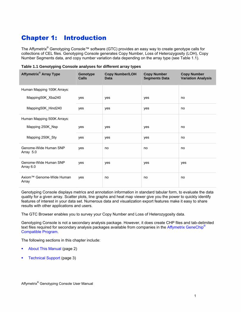
Chapter 1: Introduction The Affymetrix® Genotyping Console™ software (GTC) provides an easy way to create genotype calls for collections of CEL files. Genotyping Console generates Copy Number, Loss of Heterozygosity (LOH), Copy Number Segments data, and copy number variation data depending on the array type (see Table 1.1).
Table 1.1 Genotyping Console analyses for different array types
Affymetrix® Array Type Genotype Calls
Copy Number/LOH Data
Copy Number Segments Data
Copy Number Variation Analysis
Human Mapping 100K Arrays:
Mapping50K_Xba240
yes
yes
yes
no
Mapping50K_Hind240 yes yes yes no
Human Mapping 500K Arrays:
Mapping 250K_Nsp
yes
yes
yes
no
Mapping 250K_Sty yes yes yes no
Genome-Wide Human SNP Array 5.0
yes no no no
Genome-Wide Human SNP Array 6.0
yes yes yes yes
Axiom™ Genome-Wide Human Array
yes no no no
Genotyping Console displays metrics and annotation information in standard tabular form, to evaluate the data quality for a given array. Scatter plots, line graphs and heat map viewer give you the power to quickly identify features of interest in your data set. Numerous data and visualization export features make it easy to share results with other applications and users.
The GTC Browser enables you to survey your Copy Number and Loss of Heterozygosity data.
Genotyping Console is not a secondary analysis package. However, it does create CHP files and tab-delimited text files required for secondary analysis packages available from companies in the Affymetrix GeneChip® Compatible Program.
The following sections in this chapter include:
About This Manual (page 2)
Technical Support (page 3)
Affymetrix® Genotyping Console User Manual 2
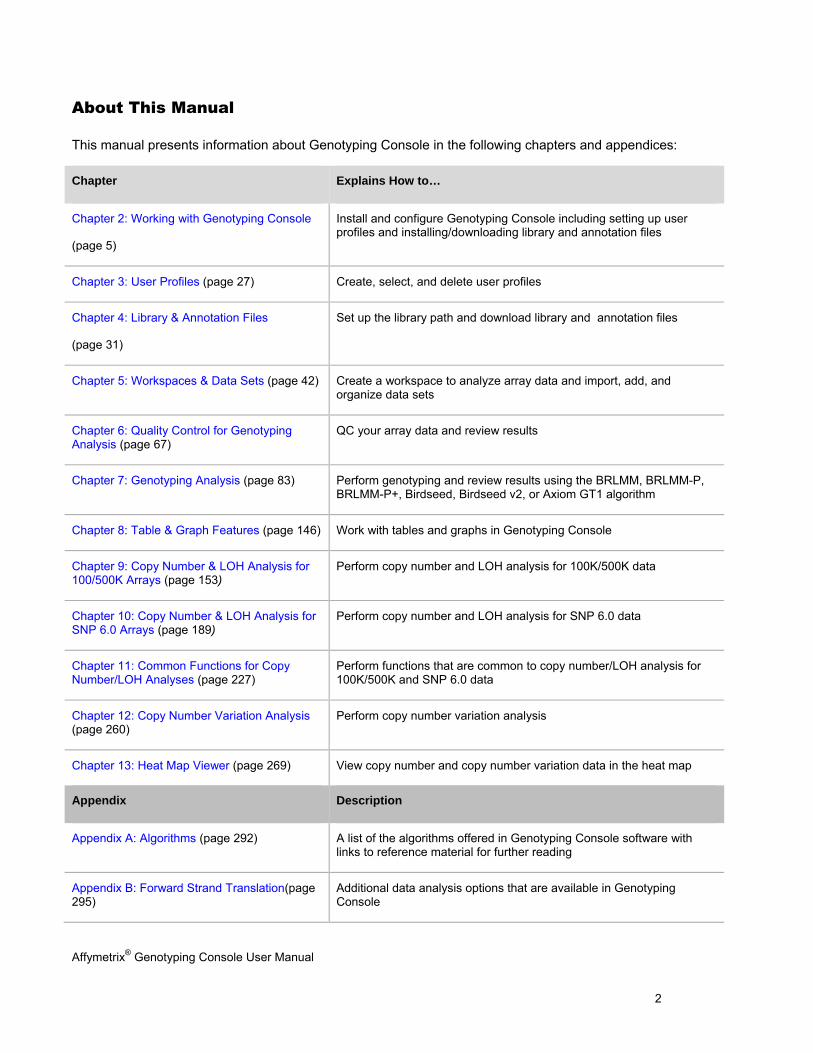
About This Manual
This manual presents information about Genotyping Console in the following chapters and appendices:
Chapter Explains How to…
Chapter 2: Working with Genotyping Console
(page 5)
Install and configure Genotyping Console including setting up user profiles and installing/downloading library and annotation files
Chapter 3: User Profiles (page 27) Create, select, and delete user profiles
Chapter 4: Library & Annotation Files
(page 31)
Set up the library path and download library and annotation files
Chapter 5: Workspaces & Data Sets (page 42) Create a workspace to analyze array data and import, add, and organize data sets
Chapter 6: Quality Control for Genotyping Analysis (page 67)
QC your array data and review results
Chapter 7: Genotyping Analysis (page 83) Perform genotyping and review results using the BRLMM, BRLMM-P, BRLMM-P+, Birdseed, Birdseed v2, or Axiom GT1 algorithm
Chapter 8: Table & Graph Features (page 146) Work with tables and graphs in Genotyping Console
Chapter 9: Copy Number & LOH Analysis for 100/500K Arrays (page 153)
Perform copy number and LOH analysis for 100K/500K data
Chapter 10: Copy Number & LOH Analysis for SNP 6.0 Arrays (page 189)
Perform copy number and LOH analysis for SNP 6.0 data
Chapter 11: Common Functions for Copy Number/LOH Analyses (page 227)
Perform functions that are common to copy number/LOH analysis for 100K/500K and SNP 6.0 data
Chapter 12: Copy Number Variation Analysis (page 260)
Perform copy number variation analysis
Chapter 13: Heat Map Viewer (page 269) View copy number and copy number variation data in the heat map
Appendix Description
Appendix A: Algorithms (page 292) A list of the algorithms offered in Genotyping Console software with links to reference material for further reading
Appendix B: Forward Strand Translation(page 295)
Additional data analysis options that are available in Genotyping Console
Affymetrix® Genotyping Console User Manual 3
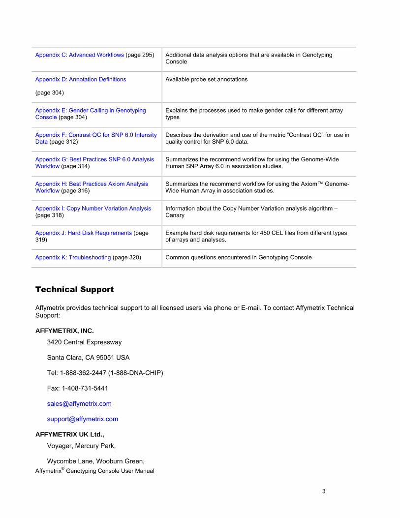
Appendix C: Advanced Workflows (page 295) Additional data analysis options that are available in Genotyping Console
Appendix D: Annotation Definitions
(page 304)
Available probe set annotations
Appendix E: Gender Calling in Genotyping Console (page 304)
Explains the processes used to make gender calls for different array types
Appendix F: Contrast QC for SNP 6.0 Intensity Data (page 312)
Describes the derivation and use of the metric “Contrast QC” for use in quality control for SNP 6.0 data.
Appendix G: Best Practices SNP 6.0 Analysis Workflow (page 314)
Summarizes the recommend workflow for using the Genome-Wide Human SNP Array 6.0 in association studies.
Appendix H: Best Practices Axiom Analysis Workflow (page 316)
Summarizes the recommend workflow for using the Axiom™ Genome-Wide Human Array in association studies.
Appendix I: Copy Number Variation Analysis (page 318)
Information about the Copy Number Variation analysis algorithm – Canary
Appendix J: Hard Disk Requirements (page 319)
Example hard disk requirements for 450 CEL files from different types of arrays and analyses.
Appendix K: Troubleshooting (page 320) Common questions encountered in Genotyping Console
Technical Support
Affymetrix provides technical support to all licensed users via phone or E-mail. To contact Affymetrix Technical Support:
AFFYMETRIX, INC.
3420 Central Expressway
Santa Clara, CA 95051 USA
Tel: 1-888-362-2447 (1-888-DNA-CHIP)
Fax: 1-408-731-5441
AFFYMETRIX UK Ltd.,
Voyager, Mercury Park,
Wycombe Lane, Wooburn Green,

Affymetrix® Genotyping Console User Manual 4
High Wycombe HP10 0HH
United Kingdom
UK and Others Tel: +44 (0) 1628 552550
France Tel: 0800919505
Germany Tel: 01803001334
Fax: +44 (0) 1628 552585
AFFYMETRIX JAPAN K.K.
Mita NN Bldg. 16F
4-1-23 Shiba Minato-ku,
Tokyo 108-0014 Japan
Tel. 03-5730-8200
Fax: 03-5730-8201
Affymetrix® Genotyping Console User Manual 5
Chapter 2: Working with Genotyping Console Genotyping Console is a stand-alone application. It can be installed on computers that have GeneChip® Operating System (GCOS) software, Affymetrix GeneChip® Command Console™ (AGCC) software, or either.
Note: If you are using GCOS files, Affymetrix recommends that you transfer data out of GCOS using the Data Transfer Tool (available at Affymetrix.com) and use the Flat File option in order to retain sample attributes.
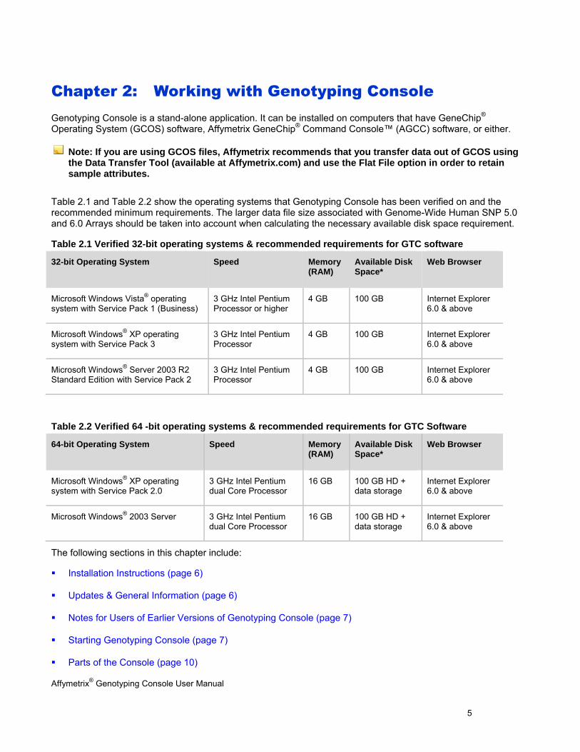
Table 2.1 and Table 2.2 show the operating systems that Genotyping Console has been verified on and the recommended minimum requirements. The larger data file size associated with Genome-Wide Human SNP 5.0 and 6.0 Arrays should be taken into account when calculating the necessary available disk space requirement.
Table 2.1 Verified 32-bit operating systems & recommended requirements for GTC software
32-bit Operating System Speed Memory (RAM)
Available Disk Space*
Web Browser
Microsoft Windows Vista® operating system with Service Pack 1 (Business)
3 GHz Intel Pentium Processor or higher
4 GB 100 GB Internet Explorer 6.0 & above
Microsoft Windows® XP operating system with Service Pack 3
3 GHz Intel Pentium Processor
4 GB 100 GB Internet Explorer 6.0 & above
Microsoft Windows® Server 2003 R2 Standard Edition with Service Pack 2
3 GHz Intel Pentium Processor
4 GB 100 GB Internet Explorer 6.0 & above
Table 2.2 Verified 64 -bit operating systems & recommended requirements for GTC Software
64-bit Operating System Speed Memory (RAM)
Available Disk Space*
Web Browser
Microsoft Windows® XP operating system with Service Pack 2.0
3 GHz Intel Pentium dual Core Processor
16 GB 100 GB HD + data storage
Internet Explorer 6.0 & above
Microsoft Windows® 2003 Server 3 GHz Intel Pentium dual Core Processor
16 GB 100 GB HD + data storage
Internet Explorer 6.0 & above
The following sections in this chapter include:
Installation Instructions (page 6)
Updates & General Information (page 6)
Notes for Users of Earlier Versions of Genotyping Console (page 7)
Starting Genotyping Console (page 7)
Parts of the Console (page 10)
Affymetrix® Genotyping Console User Manual 6
File Types & Data Organization in GTC (page 12)
To use Genotyping Console, you must:
1. Install the GTC software (page 6).
2. Create a user profile (page 27 ).
3. Download or copy the necessary library and annotation files (page 31).
4. Set up a workspace and data set(s) (page 43).
Installation Instructions
1. Download the software from Affymetrix.com: http://www.affymetrix.com/products/software/index.affx, follow the Genotyping Console link. You will need to download the 32-bit or 64-bit installer, depending on your computer operating system. If you download the 32-bit installer for a 64 bit Windows operating system, it won’t work and vice versa.
2. Unzip the downloaded software package. This includes the installation program and release notes.
3. Review the release notes and installation instructions before proceeding with the installation.
4. Double-click GenotypingConsoleSetup.exe or GenotypingConsoleSetup32.exe to install the software (the exe file names are different, depending on whether it is a 32-bit or 64-bit installer).
5. Follow the directions provided by the installer.
Note: The setup process installs the required Microsoft components, which includes the .NET 3.5 framework and Java components and Visual C++ runtime libraries.
Updates & General Information
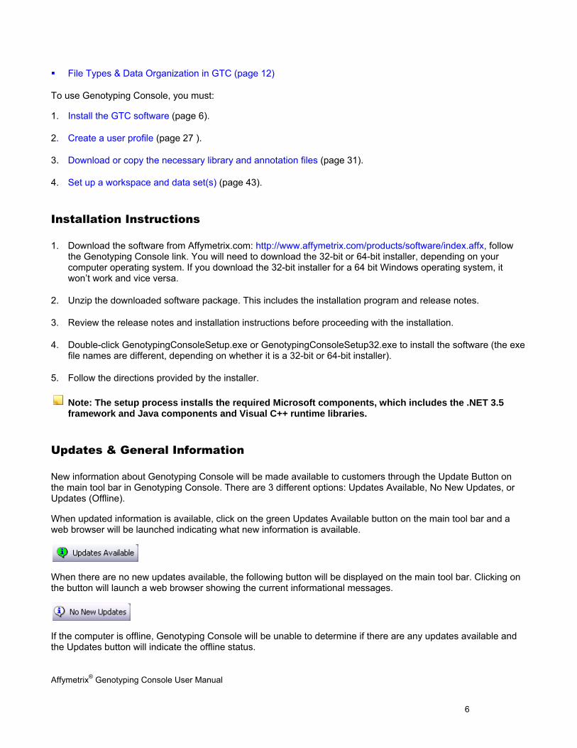
New information about Genotyping Console will be made available to customers through the Update Button on the main tool bar in Genotyping Console. There are 3 different options: Updates Available, No New Updates, or Updates (Offline).
When updated information is available, click on the green Updates Available button on the main tool bar and a web browser will be launched indicating what new information is available.
When there are no new updates available, the following button will be displayed on the main tool bar. Clicking on the button will launch a web browser showing the current informational messages.
If the computer is offline, Genotyping Console will be unable to determine if there are any updates available and the Updates button will indicate the offline status.
Affymetrix® Genotyping Console User Manual 7
Notes for Users of Earlier Versions of Genotyping Console
GTC 4.0 and earlier versions of GTC cannot be run on the same computer. The GTC 4.0 library and annotation files are not compatible with earlier versions of GTC. You can use GTC 4.0 and an earlier version of GTC on two different computers; however, you will need to separately maintain two sets of library and annotation files on the appropriate computer. To do this:
1. Create a new GTC 4.0 library folder on your computer.
2. Download or copy the new GTC 4.0 library and annotation files to this folder. See Obtaining Library & Annotation Files (page 34) for more information.
3. Set the library path for GTC to the new library folder. See Setting the Library Path (page 31).
Note: GTC 4.0 workspaces cannot be opened in earlier versions of GTC. Workspaces created in earlier versions of GTC can be opened in GTC 4.0, but then cannot be used in earlier versions of GTC.
Note: Custom analysis configurations for GTC 3.x will be updated to work with GTC 4.0. Once they have been updated they will not work with older versions of GTC.
Starting Genotyping Console
1. Double-click the Genotyping Console shortcut on the desktop. Alternately, from the Windows Start Menu, select Programs > Affymetrix > Genotyping Console.
The Genotyping Console opens with the User Profile window displayed.
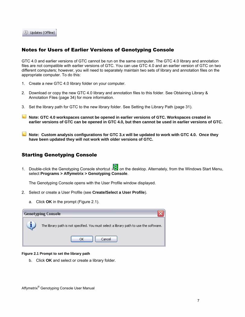
2. Select or create a User Profile (see Create/Select a User Profile).
a. Click OK in the prompt (Figure 2.1).
Figure 2.1 Prompt to set the library path
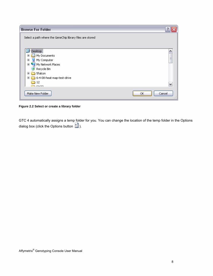
b. Click OK and select or create a library folder.
Affymetrix® Genotyping Console User Manual 8
Figure 2.2 Select or create a library folder
GTC 4 automatically assigns a temp folder for you. You can change the location of the temp folder in the Options
dialog box (click the Options button ).
Affymetrix® Genotyping Console User Manual 9
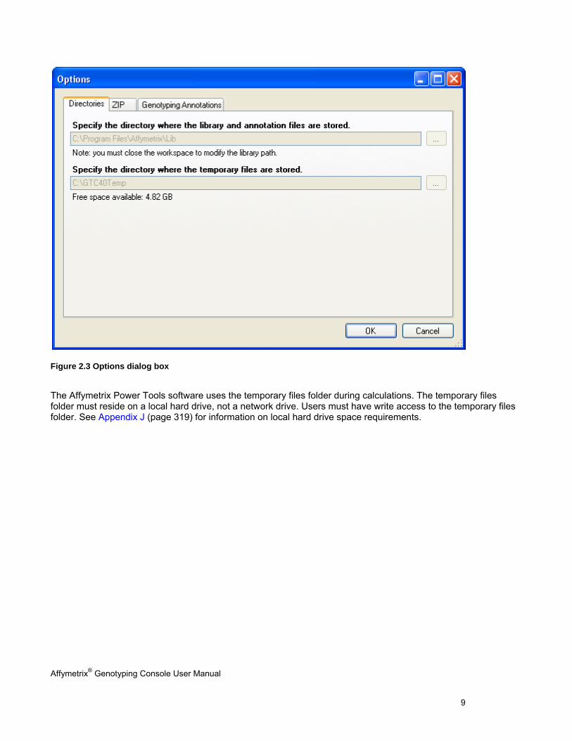
Figure 2.3 Options dialog box .
The Affymetrix Power Tools software uses the temporary files folder during calculations. The temporary files folder must reside on a local hard drive, not a network drive. Users must have write access to the temporary files folder. See Appendix J (page 319) for information on local hard drive space requirements.
Affymetrix® Genotyping Console User Manual 10
Parts of the Console
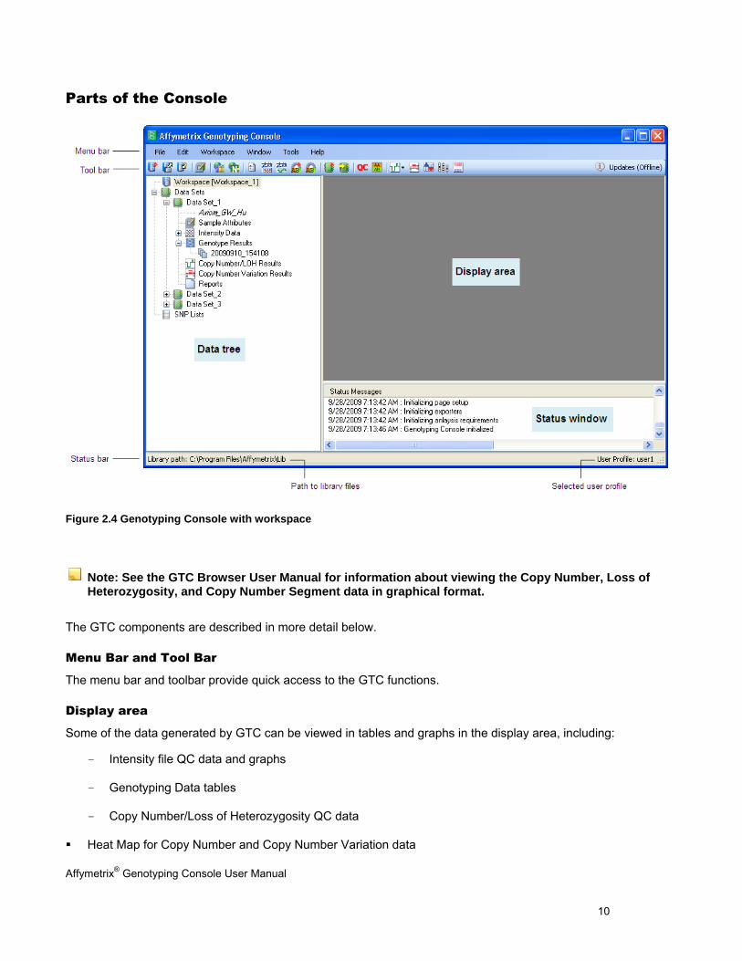
Figure 2.4 Genotyping Console with workspace
Note: See the GTC Browser User Manual for information about viewing the Copy Number, Loss of Heterozygosity, and Copy Number Segment data in graphical format.
The GTC components are described in more detail below.
Menu Bar and Tool Bar
The menu bar and toolbar provide quick access to the GTC functions.
Display area
Some of the data generated by GTC can be viewed in tables and graphs in the display area, including:
- Intensity file QC data and graphs
- Genotyping Data tables
- Copy Number/Loss of Heterozygosity QC data
Heat Map for Copy Number and Copy Number Variation data
Affymetrix® Genotyping Console User Manual 11
Note: The Copy Number, Loss of Heterozygosity, and Copy Number Segment data generated by GTC is displayed in the GTC Browser. See the Affymetrix GTC Browser User Manual for more information.
Tree
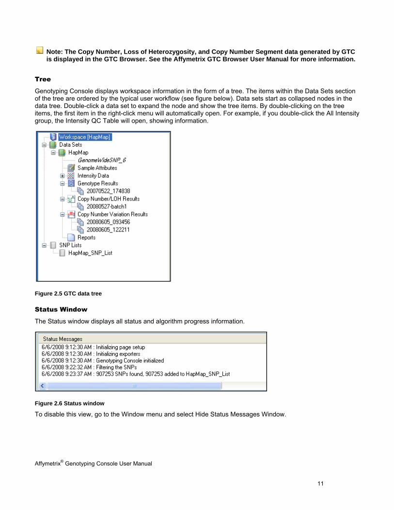
Genotyping Console displays workspace information in the form of a tree. The items within the Data Sets section of the tree are ordered by the typical user workflow (see figure below). Data sets start as collapsed nodes in the data tree. Double-click a data set to expand the node and show the tree items. By double-clicking on the tree items, the first item in the right-click menu will automatically open. For example, if you double-click the All Intensity group, the Intensity QC Table will open, showing information.
Figure 2.5 GTC data tree
Status Window
The Status window displays all status and algorithm progress information.
Figure 2.6 Status window
To disable this view, go to the Window menu and select Hide Status Messages Window.
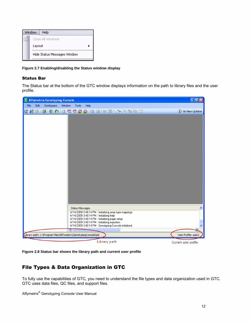
Affymetrix® Genotyping Console User Manual 12
Figure 2.7 Enabling/disabling the Status window display
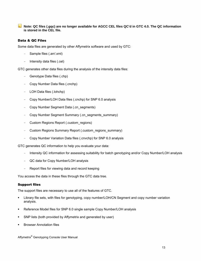
Status Bar
The Status bar at the bottom of the GTC window displays information on the path to library files and the user profile.
Figure 2.8 Status bar shows the library path and current user profile
File Types & Data Organization in GTC
To fully use the capabilities of GTC, you need to understand the file types and data organization used in GTC. GTC uses data files, QC files, and support files.
Affymetrix® Genotyping Console User Manual 13
Note: QC files (.gqc) are no longer available for AGCC CEL files QC’d in GTC 4.0. The QC information is stored in the CEL file.
Data & QC Files
Some data files are generated by other Affymetrix software and used by GTC:
- Sample files (.arr/.xml)
- Intensity data files (.cel)
GTC generates other data files during the analysis of the intensity data files:
- Genotype Data files (.chp)
- Copy Number Data files (.cnchp)
- LOH Data files (.lohchp)
- Copy Number/LOH Data files (.cnchp) for SNP 6.0 analysis
- Copy Number Segment Data (.cn_segments)
- Copy Number Segment Summary (.cn_segments_summary)
- Custom Regions Report (.custom_regions)
- Custom Regions Summary Report (.custom_regions_summary)
- Copy Number Variation Data files (.cnvchp) for SNP 6.0 analysis
GTC generates QC information to help you evaluate your data:
- Intensity QC information for assessing suitability for batch genotyping and/or Copy Number/LOH analysis
- QC data for Copy Number/LOH analysis
- Report files for viewing data and record keeping
You access the data in these files through the GTC data tree.
Support files
The support files are necessary to use all of the features of GTC.
Library file sets, with files for genotyping, copy number/LOH/CN Segment and copy number variation analysis.
Reference Model files for SNP 6.0 single sample Copy Number/LOH analysis
SNP lists (both provided by Affymetrix and generated by user)
Browser Annotation files
Affymetrix® Genotyping Console User Manual 14
Data Organization in Genotyping Console
The data used in GTC is organized by:
Workspace
Data sets
SNP lists
User Profiles allow you to keep your information about algorithm parameters, table and graph viewing options, and other application settings.
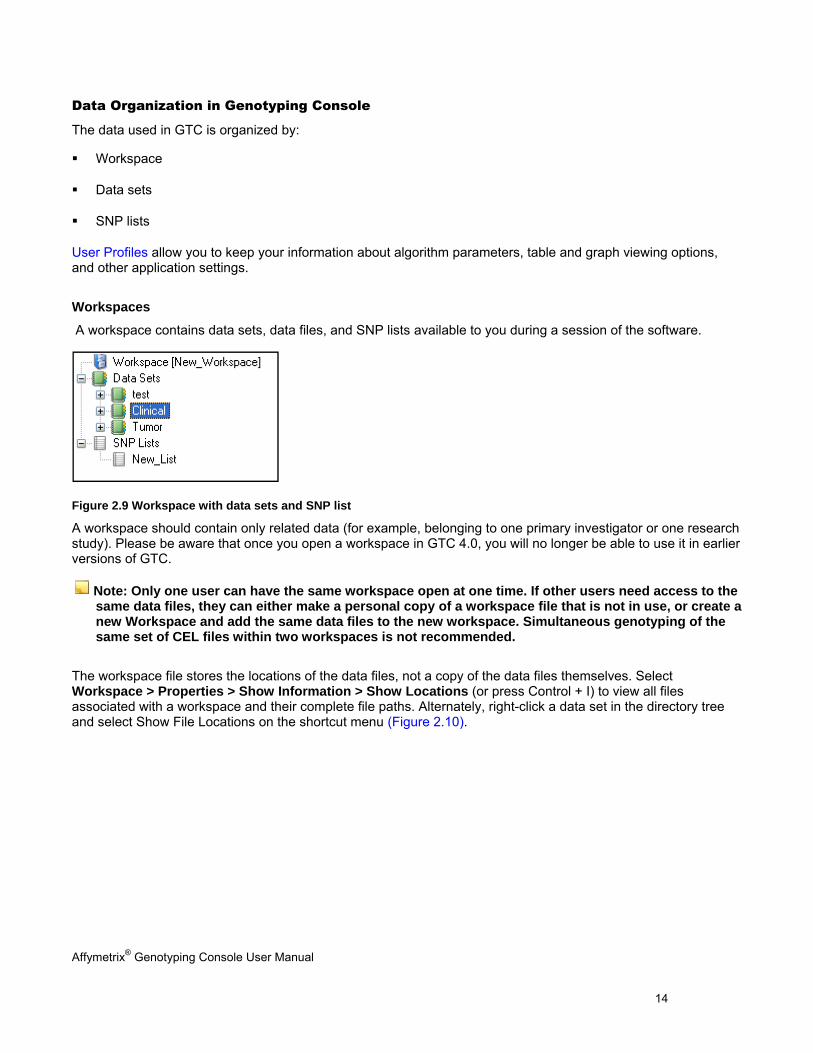
Workspaces
A workspace contains data sets, data files, and SNP lists available to you during a session of the software.
Figure 2.9 Workspace with data sets and SNP list
A workspace should contain only related data (for example, belonging to one primary investigator or one research study). Please be aware that once you open a workspace in GTC 4.0, you will no longer be able to use it in earlier versions of GTC.
Note: Only one user can have the same workspace open at one time. If other users need access to the same data files, they can either make a personal copy of a workspace file that is not in use, or create a new Workspace and add the same data files to the new workspace. Simultaneous genotyping of the same set of CEL files within two workspaces is not recommended.
The workspace file stores the locations of the data files, not a copy of the data files themselves. Select Workspace > Properties > Show Information > Show Locations (or press Control + I) to view all files associated with a workspace and their complete file paths. Alternately, right-click a data set in the directory tree and select Show File Locations on the shortcut menu (Figure 2.10).
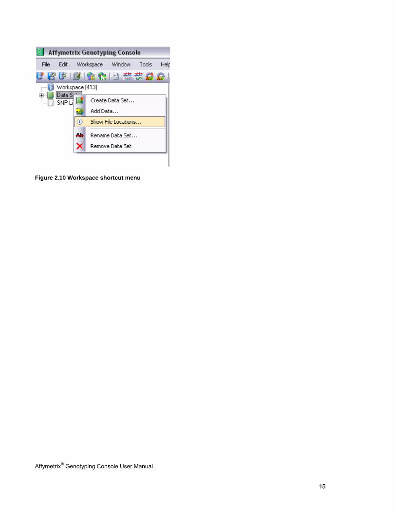
Affymetrix® Genotyping Console User Manual 15
Figure 2.10 Workspace shortcut menu
Affymetrix® Genotyping Console User Manual 16
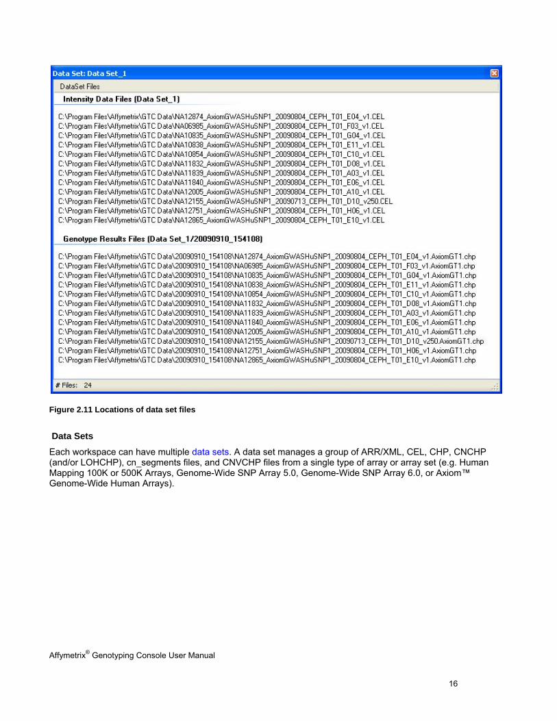
Figure 2.11 Locations of data set files
Data Sets
Each workspace can have multiple data sets. A data set manages a group of ARR/XML, CEL, CHP, CNCHP (and/or LOHCHP), cn_segments files, and CNVCHP files from a single type of array or array set (e.g. Human Mapping 100K or 500K Arrays, Genome-Wide SNP Array 5.0, Genome-Wide SNP Array 6.0, or Axiom™ Genome-Wide Human Arrays).
Affymetrix® Genotyping Console User Manual 17
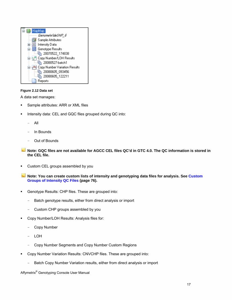
Figure 2.12 Data set
A data set manages:
Sample attributes: ARR or XML files
Intensity data: CEL and GQC files grouped during QC into:
- All
- In Bounds
- Out of Bounds
Note: GQC files are not available for AGCC CEL files QC’d in GTC 4.0. The QC information is stored in the CEL file.
Custom CEL groups assembled by you
Note: You can create custom lists of intensity and genotyping data files for analysis. See Custom Groups of Intensity QC Files (page 76).
Genotype Results: CHP files. These are grouped into:
- Batch genotype results, either from direct analysis or import
- Custom CHP groups assembled by you
Copy Number/LOH Results: Analysis files for:
- Copy Number
- LOH
- Copy Number Segments and Copy Number Custom Regions
Copy Number Variation Results: CNVCHP files. These are grouped into:
- Batch Copy Number Variation results, either from direct analysis or import
Affymetrix® Genotyping Console User Manual 18
Reports
- Concordance reports
Within a data set, information can be displayed in tables and graphs for viewing and exporting:
Sample attribute information
QC metrics
Signature SNP genotypes
CHP and SNP summary data
SNP cluster graphs
Copy Number/LOH QC information, copy number segment and custom region data (not for Genome-Wide Human SNP Array 5.0 or Axiom™ Genome-Wide Human Array)
Copy Number Variation results data
Note: Copy Number/LOH data can be displayed in the GTC Browser. See the GTC Browser manual for more information.
Note: Copy Number and Copy Number Variation data for SNP 6.0 is also displayed in the Heat Map Viewer together with copy number data. In order to view Copy Number Variation data in the Heat Map Viewer, you must have copy number data that originates from same CEL files. See Chapter 13: Heat Map Viewer on page 269 for more information.
SNP Lists
SNP lists allow you to manage markers of interest. You can generate SNP lists or import custom SNP lists.
Basic Workflows in Genotyping Console
You can use GTC 4.0 with the following types of arrays:
Human Mapping 100K arrays:
- Mapping50K_Xba240 arrays
- Mapping50K_Hind240 arrays
Human Mapping 500K arrays:
- Mapping 250K_Nsp arrays
- Mapping250K_Sty arrays
Genome-Wide Human SNP Array 5.0
Genome-Wide Human SNP Array 6.0
Affymetrix® Genotyping Console User Manual 19
Axiom™ Genome-Wide Human Array
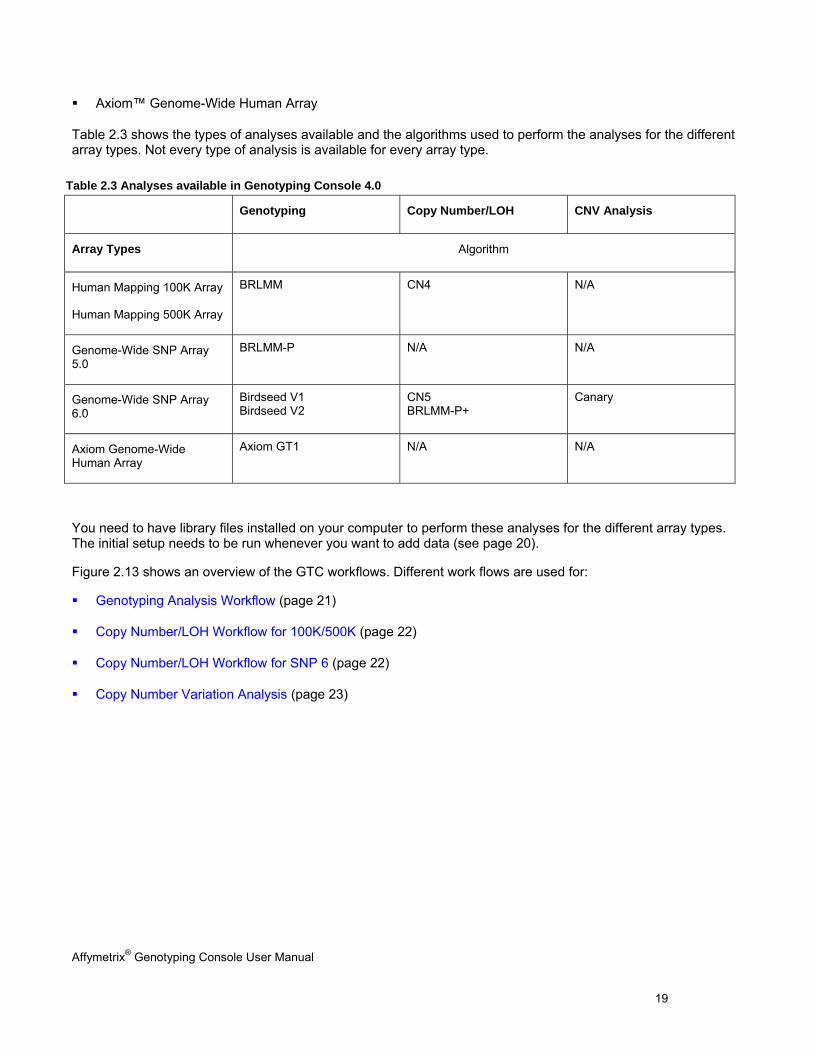
Table 2.3 shows the types of analyses available and the algorithms used to perform the analyses for the different array types. Not every type of analysis is available for every array type.
Table 2.3 Analyses available in Genotyping Console 4.0
Genotyping Copy Number/LOH CNV Analysis
Array Types Algorithm
Human Mapping 100K Array
Human Mapping 500K Array
BRLMM CN4 N/A
Genome-Wide SNP Array 5.0
BRLMM-P N/A N/A
Genome-Wide SNP Array 6.0
Birdseed V1 Birdseed V2
CN5 BRLMM-P+
Canary
Axiom Genome-Wide Human Array
Axiom GT1 N/A N/A
You need to have library files installed on your computer to perform these analyses for the different array types. The initial setup needs to be run whenever you want to add data (see page 20).
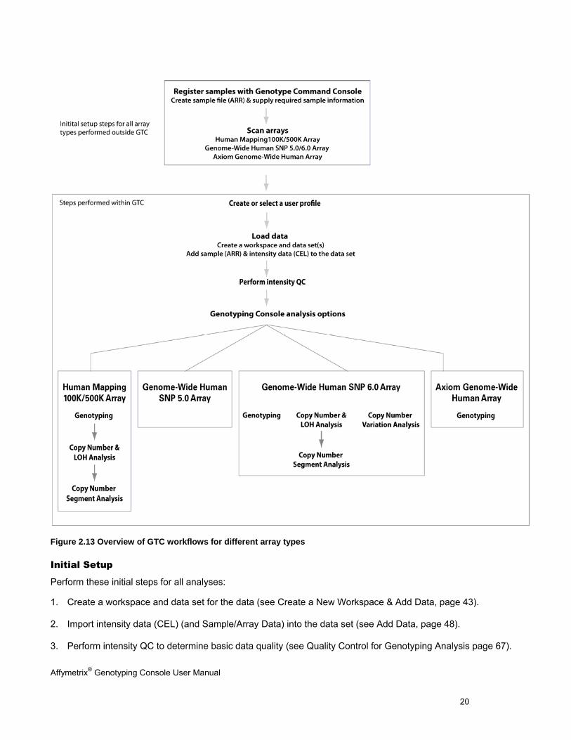
Figure 2.13 shows an overview of the GTC workflows. Different work flows are used for:
Genotyping Analysis Workflow (page 21)
Copy Number/LOH Workflow for 100K/500K (page 22)
Copy Number/LOH Workflow for SNP 6 (page 22)
Copy Number Variation Analysis (page 23)
Affymetrix® Genotyping Console User Manual 20
Figure 2.13 Overview of GTC workflows for different array types
Initial Setup
Perform these initial steps for all analyses:
1. Create a workspace and data set for the data (see Create a New Workspace & Add Data, page 43).
2. Import intensity data (CEL) (and Sample/Array Data) into the data set (see Add Data, page 48).
3. Perform intensity QC to determine basic data quality (see Quality Control for Genotyping Analysis page 67).
Affymetrix® Genotyping Console User Manual 21
The intensity quality control check:
- Can be performed on a selected set of CEL files or all CEL files. QC can also be automatically performed upon import of CEL files to the data set.
- Automatically groups CEL files into All, In Bounds, and Out of Bounds groups based on the QC threshold(s). Additional custom groupings of CEL files can also be made. The resulting QC Call Rates and other metrics are displayed in tables and graphs, and can be exported. Removing poor quality CEL files from the set can improve the quality of the genotypes of the remaining CEL files.
Note: GTC looks for existing QC information in the CEL file first, then a QC file (.gqc). If available, GTC uses this QC information and does not execute the QC algorithm. If the information is not available, GTC performs intensity QC and stores the information in the CEL file if it is an AGCC CEL file or in the gqc file, if it is a GCOS CEL file. However, it is requried to perform intensity QC again for SNP 6.0 arrays with QC information generated in GTC 2.0 due to a QC algorithm update since GTC 2.1.
After performing the initial steps, you can proceed with the different analyses.
Genotyping Analysis Workflow
Genotyping analysis provides SNP calls for the following array types:
Human Mapping 100K Arrays: Mapping50K_Xba240 and Mapping50K_Hind240 arrays
Human Mapping 500K Arrays: Mapping 250K_Nsp and Mapping250K_Sty arrays
Genome-Wide Human SNP Array 5.0
Genome-Wide Human SNP Array 6.0
Axiom™ Genome-Wide Human Array
To perform genotyping analysis:
1. Select a group or set of intensity data files (CEL) in a data set.
2. Perform genotyping analysis on the group of files.
3. Review the initial genotyping analysis QC data in the CHP Summary Results table Call Rate and other metrics that are displayed in tables and graphs.
4. View the SNP results in the SNP Summary Results table that provides the following information and other metrics:
- SNP Call Rate
- Hardy-Weinberg p-value
- Minor Allele Frequency
- SNP Call (AA, AB, BB)
SNP Lists can be generated by filtering on any of these values.
Affymetrix® Genotyping Console User Manual 22
Note: You need a SNP list to view genotype result data.
5. The SNP Cluster graphs can also be displayed based on a SNP List and group of CHP files. Genotypes can be exported in tab-delimited text format for all SNPs or a sub-set based on a SNP List. See Genotyping Analysis (page 83) for more information.
Copy Number/LOH Workflow for 100K/500K Arrays
To perform a CN/LOH analysis for 100K/500K arrays, you must have both the CEL intensity data files and the genotyping CHP files for the arrays you wish to analyze.
To perform a CN/LOH Analysis for 100K/500K arrays:
1. Need CEL and genotyping CHP files for the arrays.
2. Perform Copy Number and/or LOH analysis in GTC, producing:
- Copy Number Data Files
- LOH Data Files
See Copy Number & LOH Analysis for Human Mapping 100K/500K Arrays (page 153).
3. Run the Segment Reporting Tool on the CN files to generate:
- Segment Data Files
- Segment Summary file
- Custom Region Data files
- Custom Region Summary File
See Using the Segment Reporting Tool & Custom Regions (page 227).
4. Review data in the GTC Browser, using:
- Whole Genome View
- Chromosome View
- Segment Report table
5. Export data for further analysis.
Copy Number/LOH Workflow for SNP 6.0 Arrays
To perform Copy Number/LOH analysis on SNP 6 data:
1. Need intensity files (CEL) for the arrays.
2. Perform Copy Number and/or LOH analysis in GTC to generate Copy Number/LOH data files. See Copy Number & LOH Analysis for Genome-Wide Human SNP 6.0 Arrays (page 189).
3. Run the Segment Reporting Tool on the CNCHP files to generate:
Affymetrix® Genotyping Console User Manual 23
- Segment Data files
- Segment Summary file
- Custom Region Data files
- Custom Region Summary file
See Using the Segment Reporting Tool & Custom Regions (page 227).
4. Review the data in the GTC Browser:
- Whole Genome view
- Chromosome view
- Segment Report table
5. View the log2ratio values in the Heat Map Viewer
6. Export the data for further analysis.
Copy Number Variation Analysis
Copy Number Variation (CNV) analysis is for the Genome-Wide Human SNP Array 6.0 only. For CNV analysis, the Canary algorithm makes CN state calls (0, 1, 2, 3, 4) for regions with known copy number variants (CNV) or copy number polymorphisms (CNP). The region within known copy number variants can contain one or more CN/SNP probe sets.
To perform CNV analysis:
1. Start with intensity data (CEL).
2. Perform the Copy Number Variation analysis. See Copy Number Variation Analysis (page 260).
3. View the results in the Heat Map viewer with copy number results. See Heat Map Viewer (page 269).
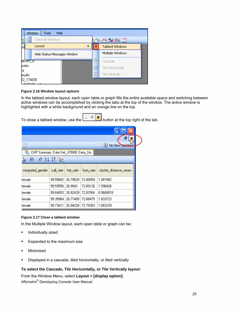
Working with Commands in Genotyping Console
Commands in Genotyping Console can be accessed from:
Main menus
Toolbar shortcuts
Right-clicks on tree items
Right clicks on table rows
Right-clicks on graphs or from the graph toolbar
The tree items serve dual functions, organizing the data and results as well as guiding you through the workflow. The file menus are context sensitive, which means that some commands will be hidden until you’ve selected the items in the tree or table to which the command applies.
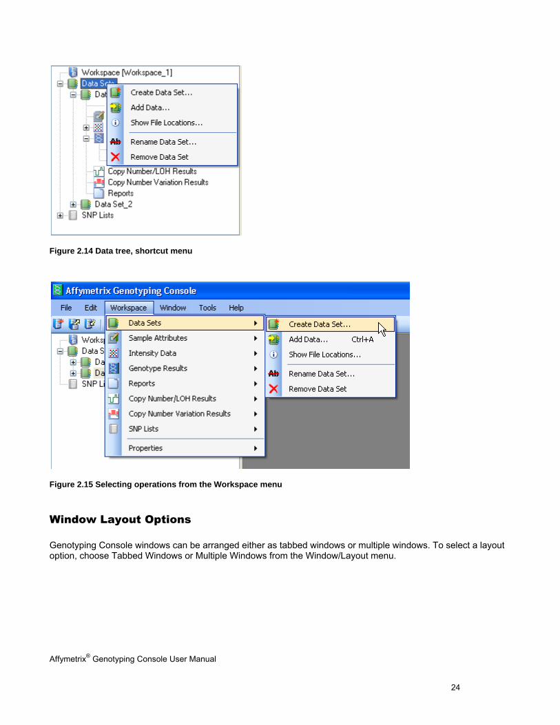
Affymetrix® Genotyping Console User Manual 24
Figure 2.14 Data tree, shortcut menu
Figure 2.15 Selecting operations from the Workspace menu
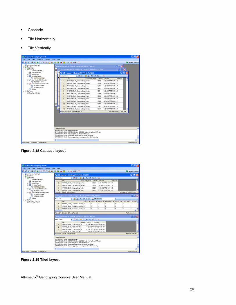
Window Layout Options
Genotyping Console windows can be arranged either as tabbed windows or multiple windows. To select a layout option, choose Tabbed Windows or Multiple Windows from the Window/Layout menu.
Affymetrix® Genotyping Console User Manual 25
Figure 2.16 Window layout options
In the tabbed window layout, each open table or graph fills the entire available space and switching between active windows can be accomplished by clicking the tabs at the top of the window. The active window is highlighted with a white background and an orange line on the top.
To close a tabbed window, use the button at the top right of the tab.
Figure 2.17 Close a tabbed window
In the Multiple Window layout, each open table or graph can be:
Individually sized
Expanded to the maximum size
Minimized
Displayed in a cascade, tiled horizontally, or tiled vertically
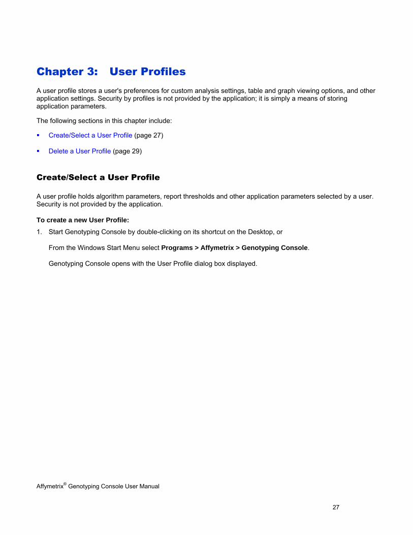
To select the Cascade, Tile Horizontally, or Tile Vertically layout:
From the Window Menu, select Layout > [display option]:
Affymetrix® Genotyping Console User Manual 26
Cascade
Tile Horizontally
Tile Vertically
Figure 2.18 Cascade layout
Figure 2.19 Tiled layout
Affymetrix® Genotyping Console User Manual 27
Chapter 3: User Profiles A user profile stores a user's preferences for custom analysis settings, table and graph viewing options, and other application settings. Security by profiles is not provided by the application; it is simply a means of storing application parameters.
The following sections in this chapter include:
Create/Select a User Profile (page 27)
Delete a User Profile (page 29)
Create/Select a User Profile
A user profile holds algorithm parameters, report thresholds and other application parameters selected by a user. Security is not provided by the application.
To create a new User Profile:
1. Start Genotyping Console by double-clicking on its shortcut on the Desktop, or
From the Windows Start Menu select Programs > Affymetrix > Genotyping Console.
Genotyping Console opens with the User Profile dialog box displayed.
Affymetrix® Genotyping Console User Manual 28
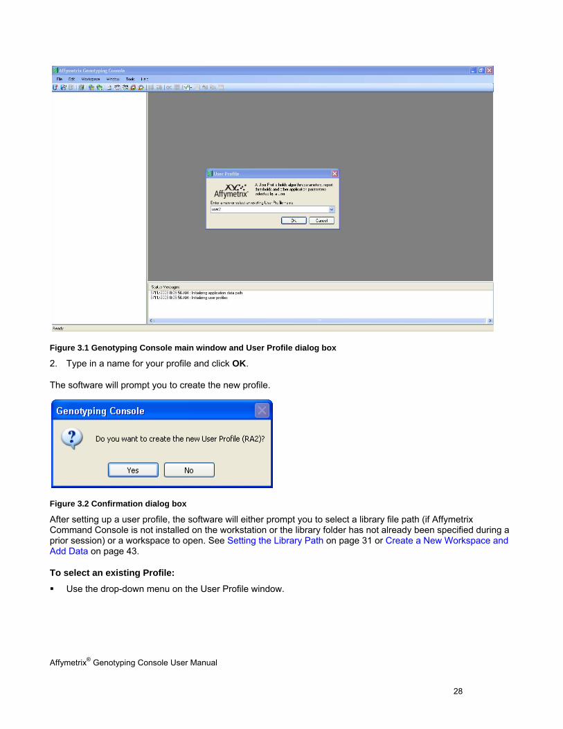
Figure 3.1 Genotyping Console main window and User Profile dialog box
2. Type in a name for your profile and click OK.
The software will prompt you to create the new profile.
Figure 3.2 Confirmation dialog box
After setting up a user profile, the software will either prompt you to select a library file path (if Affymetrix Command Console is not installed on the workstation or the library folder has not already been specified during a prior session) or a workspace to open. See Setting the Library Path on page 31 or Create a New Workspace and Add Data on page 43.
To select an existing Profile:
Use the drop-down menu on the User Profile window.
Affymetrix® Genotyping Console User Manual 29
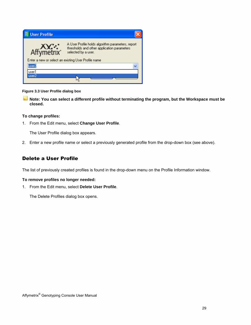
Figure 3.3 User Profile dialog box
Note: You can select a different profile without terminating the program, but the Workspace must be closed.
To change profiles:
1. From the Edit menu, select Change User Profile.
The User Profile dialog box appears.
2. Enter a new profile name or select a previously generated profile from the drop-down box (see above).
Delete a User Profile
The list of previously created profiles is found in the drop-down menu on the Profile Information window.
To remove profiles no longer needed:
1. From the Edit menu, select Delete User Profile.
The Delete Profiles dialog box opens.
Affymetrix® Genotyping Console User Manual 30
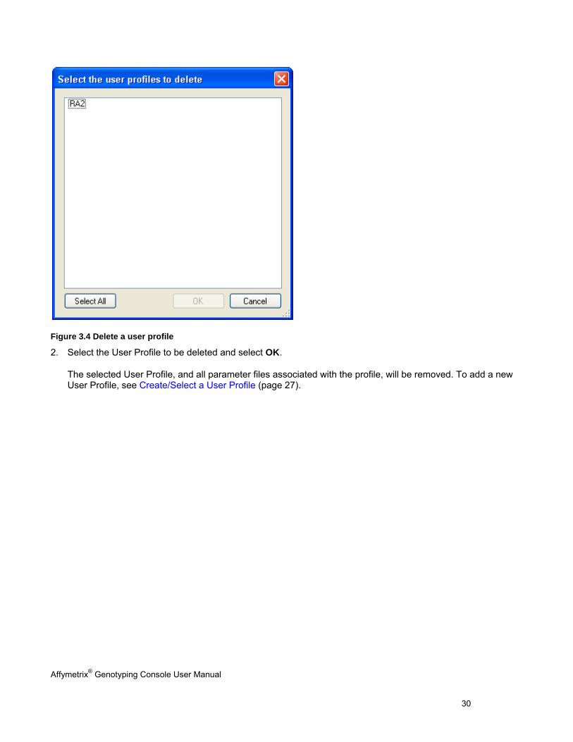
Figure 3.4 Delete a user profile
2. Select the User Profile to be deleted and select OK.
The selected User Profile, and all parameter files associated with the profile, will be removed. To add a new User Profile, see Create/Select a User Profile (page 27).
Affymetrix® Genotyping Console User Manual 31
Chapter 4: Library & Annotation Files Genotyping Console requires information stored in library files to analyze the CEL files generated by GCOS or Affymetrix GeneChip® Command Console™ (AGCC) software. These files are available from NetAffx and can be downloaded within Genotyping Console. Genotyping Console downloads only those library files it requires from NetAffx for analysis, but these are not registered with GCOS or Command Console and are not sufficient to scan arrays.
Genotyping Console uses SQLite annotation files (*.annot.db) to display and export additional information about the SNP and CN probe sets (such as Chromosome, Physical Position, dbSNP RS ID, etc.) as well as for certain analysis and filtering steps. You can use custom annotation files in GTC 4.0, but the files must be in SQLite format.
The following sections in this chapter include:
Setting the Library Path
Obtaining Library & Annotation Files (page 34)
Setting the Library Path
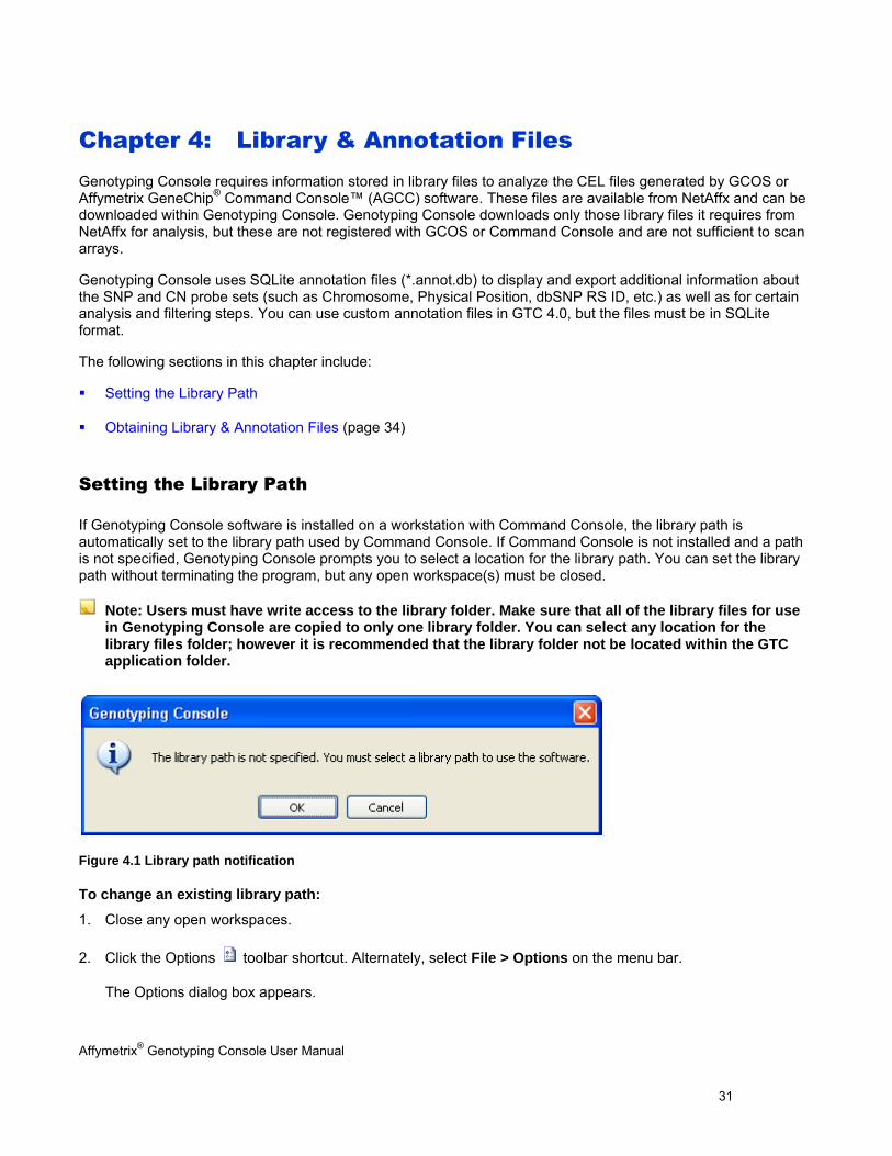
If Genotyping Console software is installed on a workstation with Command Console, the library path is automatically set to the library path used by Command Console. If Command Console is not installed and a path is not specified, Genotyping Console prompts you to select a location for the library path. You can set the library path without terminating the program, but any open workspace(s) must be closed.
Note: Users must have write access to the library folder. Make sure that all of the library files for use in Genotyping Console are copied to only one library folder. You can select any location for the library files folder; however it is recommended that the library folder not be located within the GTC application folder.
Figure 4.1 Library path notification
To change an existing library path:
1. Close any open workspaces.
2. Click the Options toolbar shortcut. Alternately, select File > Options on the menu bar.
The Options dialog box appears.
Affymetrix® Genotyping Console User Manual 32
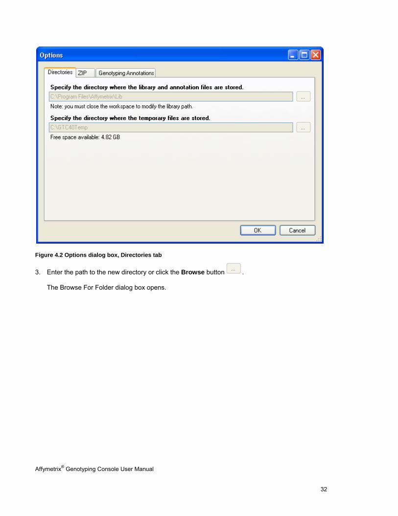
Figure 4.2 Options dialog box, Directories tab
3. Enter the path to the new directory or click the Browse button .
The Browse For Folder dialog box opens.
Affymetrix® Genotyping Console User Manual 33
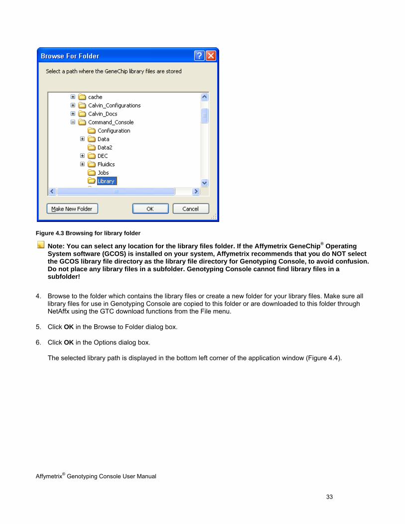
Figure 4.3 Browsing for library folder
Note: You can select any location for the library files folder. If the Affymetrix GeneChip® Operating System software (GCOS) is installed on your system, Affymetrix recommends that you do NOT select the GCOS library file directory as the library file directory for Genotyping Console, to avoid confusion. Do not place any library files in a subfolder. Genotyping Console cannot find library files in a subfolder!
4. Browse to the folder which contains the library files or create a new folder for your library files. Make sure all library files for use in Genotyping Console are copied to this folder or are downloaded to this folder through NetAffx using the GTC download functions from the File menu.
5. Click OK in the Browse to Folder dialog box.
6. Click OK in the Options dialog box.
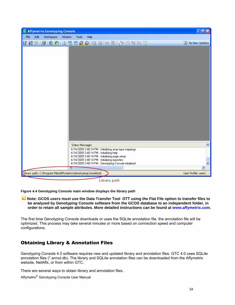
The selected library path is displayed in the bottom left corner of the application window (Figure 4.4).
Affymetrix® Genotyping Console User Manual 34
Figure 4.4 Genotyping Console main window displays the library path
Note: GCOS users must use the Data Transfer Tool DTT using the Flat File option to transfer files to be analyzed by Genotyping Console software from the GCOS database to an independent folder, in order to retain all sample attributes. More detailed instructions can be found at www.affymetrix.com.
The first time Genotyping Console downloads or uses the SQLite annotation file, the annotation file will be optimized. This process may take several minutes or more based on connection speed and computer configurations.
Obtaining Library & Annotation Files
Genotyping Console 4.0 software requires new and updated library and annotation files. GTC 4.0 uses SQLite annotation files (*.annot.db). The library and SQLite annotation files can be downloaded from the Affymetrix website, NetAffx, or from within GTC.
There are several ways to obtain library and annotation files.
Affymetrix® Genotyping Console User Manual 35
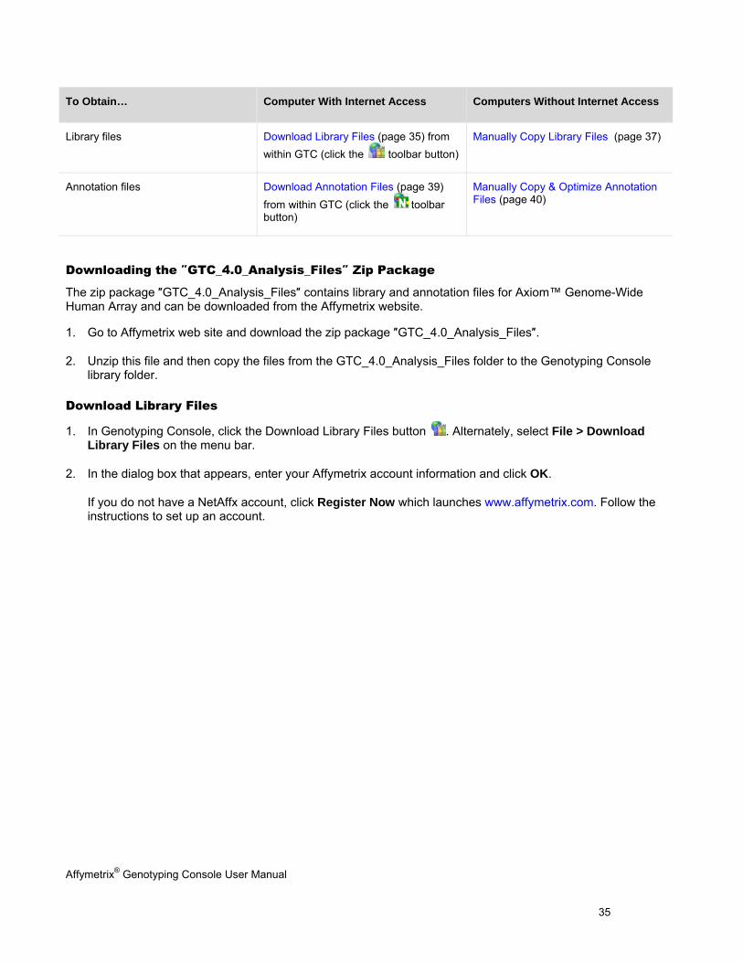
To Obtain… Computer With Internet Access Computers Without Internet Access
Library files Download Library Files (page 35) from within GTC (click the toolbar button)
Manually Copy Library Files (page 37)
Annotation files Download Annotation Files (page 39) from within GTC (click the toolbar button)
Manually Copy & Optimize Annotation Files (page 40)
Downloading the ″GTC_4.0_Analysis_Files″ Zip Package
The zip package ″GTC_4.0_Analysis_Files″ contains library and annotation files for Axiom™ Genome-Wide Human Array and can be downloaded from the Affymetrix website.
1. Go to Affymetrix web site and download the zip package ″GTC_4.0_Analysis_Files″.
2. Unzip this file and then copy the files from the GTC_4.0_Analysis_Files folder to the Genotyping Console library folder.
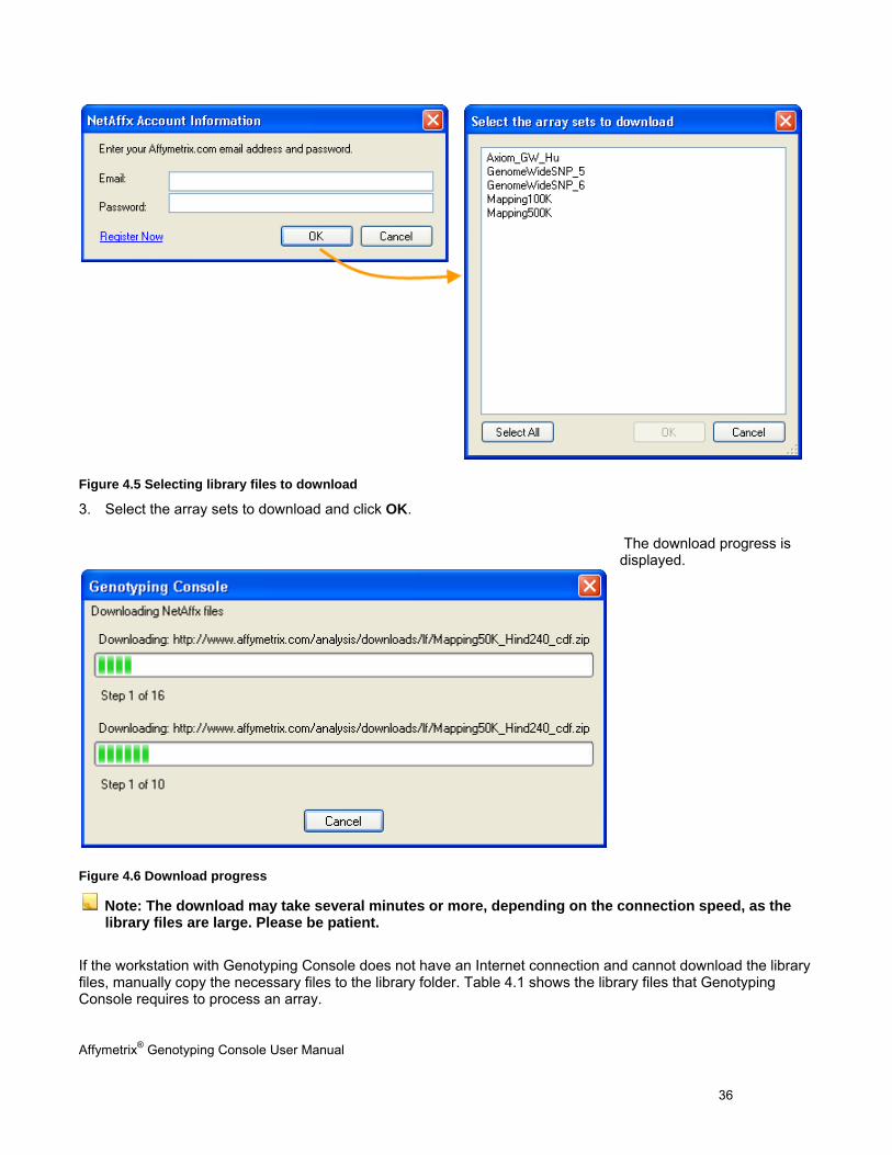
Download Library Files
1. In Genotyping Console, click the Download Library Files button . Alternately, select File > Download Library Files on the menu bar.
2. In the dialog box that appears, enter your Affymetrix account information and click OK.
If you do not have a NetAffx account, click Register Now which launches www.affymetrix.com. Follow the instructions to set up an account.
Affymetrix® Genotyping Console User Manual 36
Figure 4.5 Selecting library files to download
3. Select the array sets to download and click OK.
The download progress is displayed.
Figure 4.6 Download progress
Note: The download may take several minutes or more, depending on the connection speed, as the library files are large. Please be patient.
If the workstation with Genotyping Console does not have an Internet connection and cannot download the library files, manually copy the necessary files to the library folder. Table 4.1 shows the library files that Genotyping Console requires to process an array.
Affymetrix® Genotyping Console User Manual 37
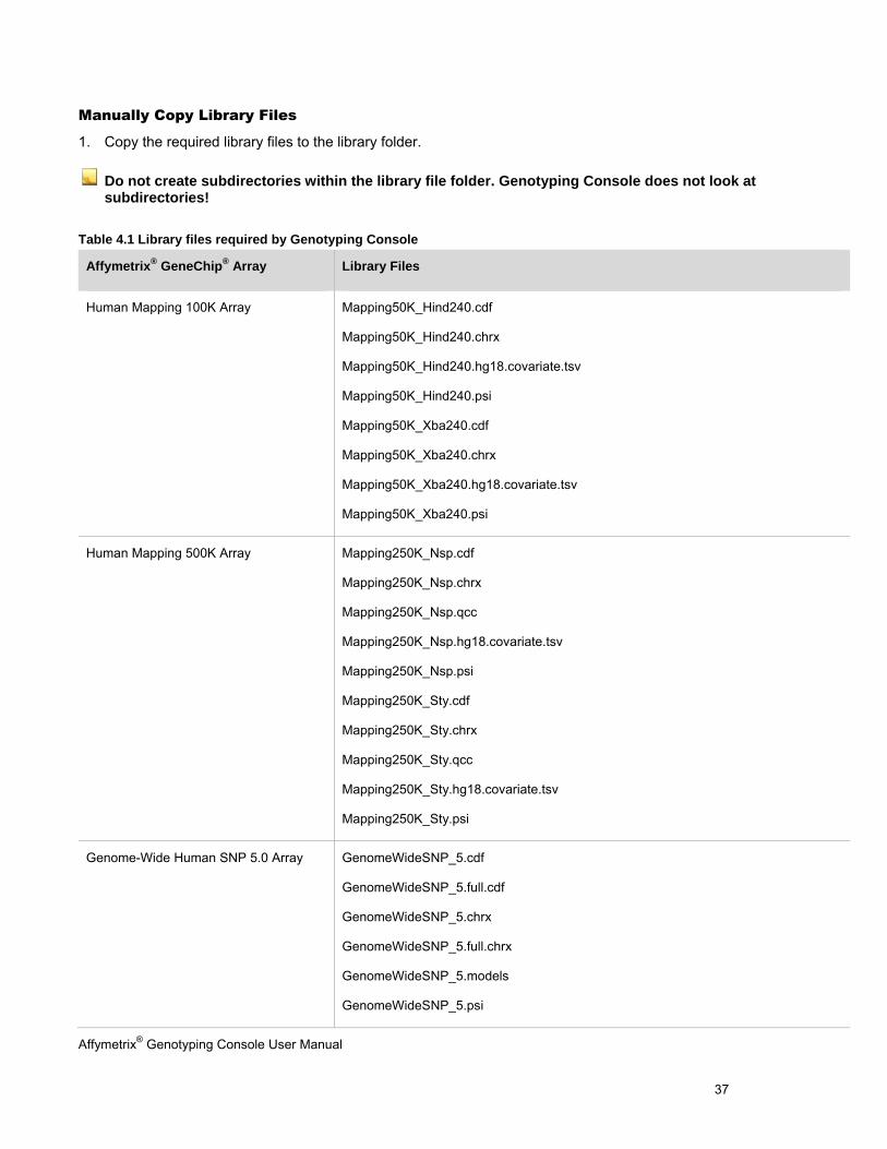
Manually Copy Library Files
1. Copy the required library files to the library folder.
Do not create subdirectories within the library file folder. Genotyping Console does not look at subdirectories!
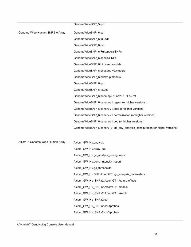
Table 4.1 Library files required by Genotyping Console
Affymetrix® GeneChip® Array Library Files
Human Mapping 100K Array
Mapping50K_Hind240.cdf
Mapping50K_Hind240.chrx
Mapping50K_Hind240.hg18.covariate.tsv
Mapping50K_Hind240.psi
Mapping50K_Xba240.cdf
Mapping50K_Xba240.chrx
Mapping50K_Xba240.hg18.covariate.tsv
Mapping50K_Xba240.psi
Human Mapping 500K Array
Mapping250K_Nsp.cdf
Mapping250K_Nsp.chrx
Mapping250K_Nsp.qcc
Mapping250K_Nsp.hg18.covariate.tsv
Mapping250K_Nsp.psi
Mapping250K_Sty.cdf
Mapping250K_Sty.chrx
Mapping250K_Sty.qcc
Mapping250K_Sty.hg18.covariate.tsv
Mapping250K_Sty.psi
Genome-Wide Human SNP 5.0 Array
GenomeWideSNP_5.cdf
GenomeWideSNP_5.full.cdf
GenomeWideSNP_5.chrx
GenomeWideSNP_5.full.chrx
GenomeWideSNP_5.models
GenomeWideSNP_5.psi
Affymetrix® Genotyping Console User Manual 38
GenomeWideSNP_5.qcc
Genome-Wide Human SNP 6.0 Array
GenomeWideSNP_6.cdf
GenomeWideSNP_6.full.cdf
GenomeWideSNP_6.psi
GenomeWideSNP_6.Full.specialSNPs
GenomeWideSNP_6.specialSNPs
GenomeWideSNP_6.birdseed.models
GenomeWideSNP_6.birdseed-v2.models
GenomeWideSNP_6.brlmm-p.models
GenomeWideSNP_6.qcc
GenomeWideSNP_6.r2.qcc
GenomeWideSNP_6.hapmap270.na29.1.r1.a5.ref
GenomeWideSNP_6.canary-v1.region (or higher versions)
GenomeWideSNP_6.canary-v1.prior (or higher versions)
GenomeWideSNP_6.canary-v1.normalization (or higher versions)
GenomeWideSNP_6.canary-v1.bed (or higher versions)
GenomeWideSNP_6.canary_v1.gc_cnv_analysis_configuration (or higher versions)
Axiom™ Genome-Wide Human Array
Axiom_GW_Hu.analysis
Axiom_GW_Hu.array_set
Axiom_GW_Hu.gc_analysis_configuration
Axiom_GW_Hu.geno_intensity_report
Axiom_GW_Hu.gc_thresholds
Axiom_GW_Hu.SNP.AxiomGT1.gc_analysis_parameters
Axiom_GW_Hu_SNP.r2.AxiomGT1.feature-effects
Axiom_GW_Hu_SNP.r2.AxiomGT1.models
Axiom_GW_Hu_SNP.r2.AxiomGT1.sketch
Axiom_GW_Hu_SNP.r2.cdf
Axiom_GW_Hu_SNP.r2.chrXprobes
Axiom_GW_Hu_SNP.r2.chrYprobes
Affymetrix® Genotyping Console User Manual 39
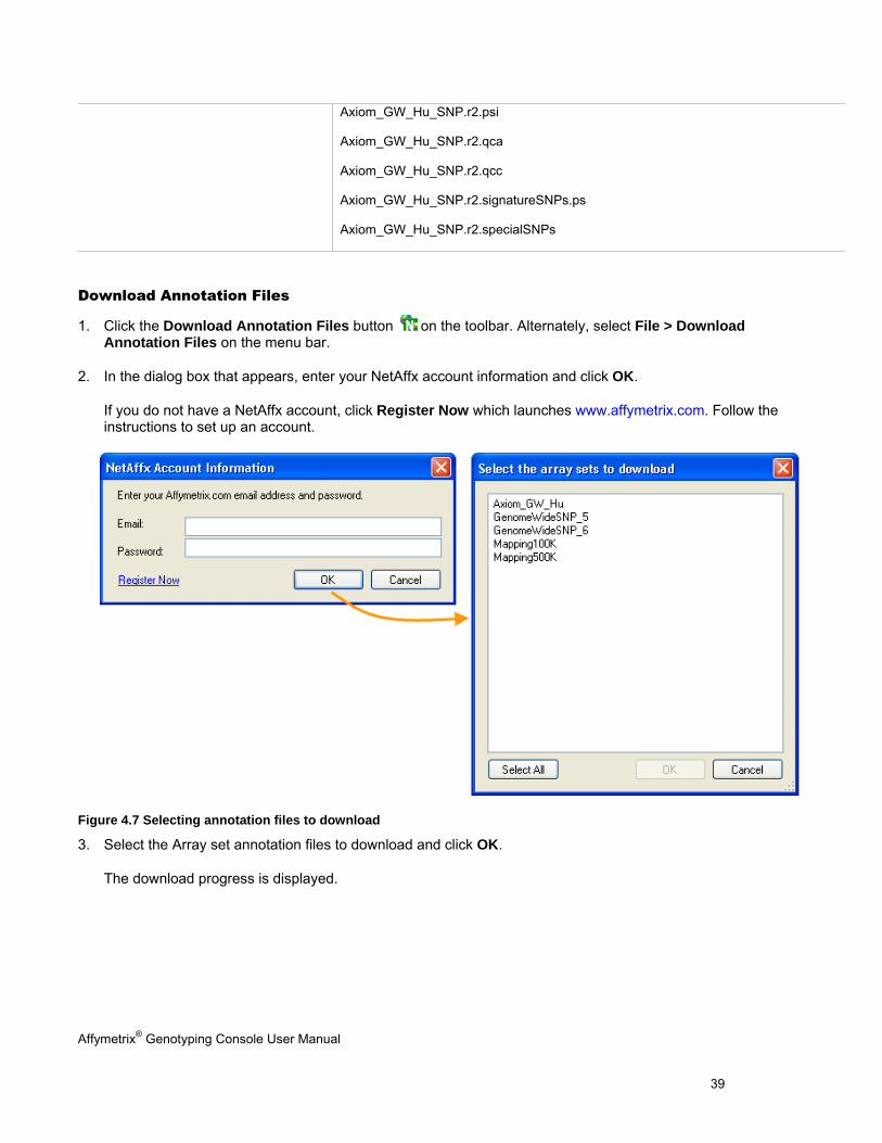
Download Annotation Files
1. Click the Download Annotation Files button on the toolbar. Alternately, select File > Download Annotation Files on the menu bar.
2. In the dialog box that appears, enter your NetAffx account information and click OK.
If you do not have a NetAffx account, click Register Now which launches www.affymetrix.com. Follow the instructions to set up an account.
Figure 4.7 Selecting annotation files to download
3. Select the Array set annotation files to download and click OK.
The download progress is displayed.
Axiom_GW_Hu_SNP.r2.psi
Axiom_GW_Hu_SNP.r2.qca
Axiom_GW_Hu_SNP.r2.qcc
Axiom_GW_Hu_SNP.r2.signatureSNPs.ps
Axiom_GW_Hu_SNP.r2.specialSNPs
Affymetrix® Genotyping Console User Manual 40
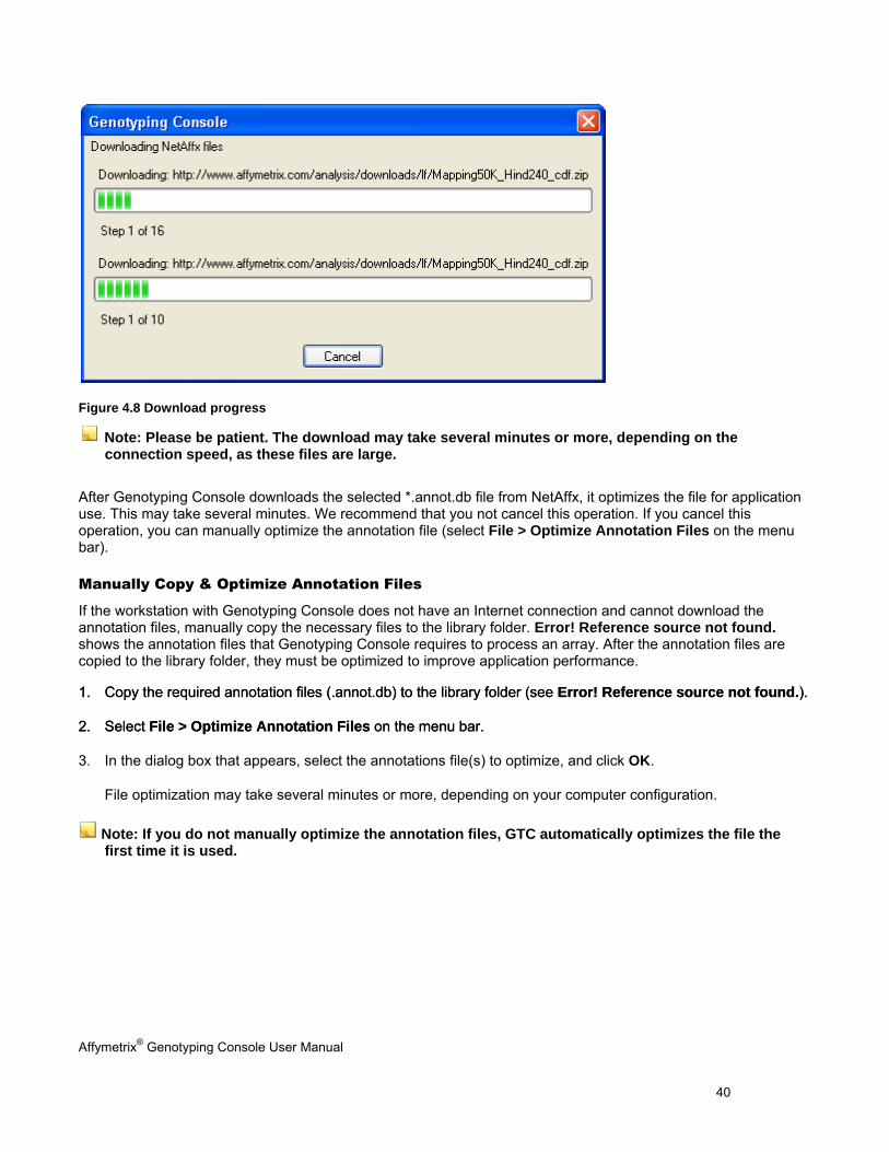
Figure 4.8 Download progress
Note: Please be patient. The download may take several minutes or more, depending on the connection speed, as these files are large.
After Genotyping Console downloads the selected *.annot.db file from NetAffx, it optimizes the file for application use. This may take several minutes. We recommend that you not cancel this operation. If you cancel this operation, you can manually optimize the annotation file (select File > Optimize Annotation Files on the menu bar).
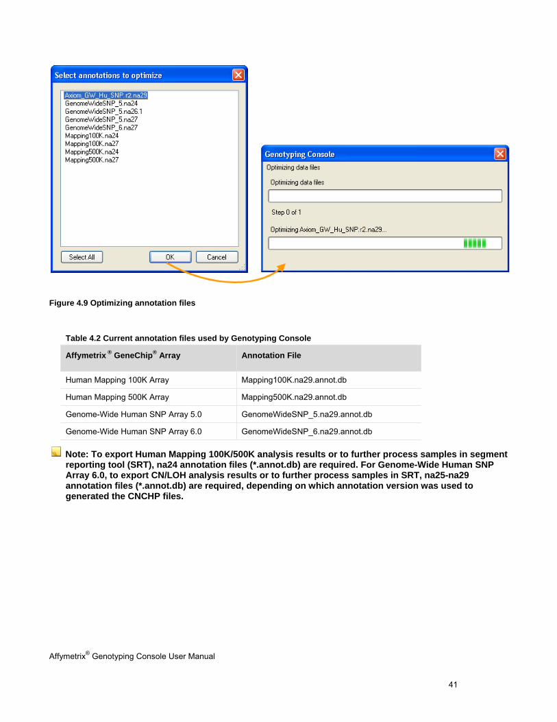
Manually Copy & Optimize Annotation Files
If the workstation with Genotyping Console does not have an Internet connection and cannot download the annotation files, manually copy the necessary files to the library folder. Error! Reference source not found. shows the annotation files that Genotyping Console requires to process an array. After the annotation files are copied to the library folder, they must be optimized to improve application performance.
1. Copy the required annotation files (.annot.db) to the library folder (see Error! Reference source not found.). 1. Copy the required annotation files (.annot.db) to the library folder (see Error! Reference source not found.).
2. Select File > Optimize Annotation Files on the menu bar. 2. Select File > Optimize Annotation Files on the menu bar.
3. In the dialog box that appears, select the annotations file(s) to optimize, and click OK.
File optimization may take several minutes or more, depending on your computer configuration.
Note: If you do not manually optimize the annotation files, GTC automatically optimizes the file the first time it is used.
Affymetrix® Genotyping Console User Manual 41
Figure 4.9 Optimizing annotation files
Table 4.2 Current annotation files used by Genotyping Console
Affymetrix ® GeneChip® Array Annotation File
Human Mapping 100K Array Mapping100K.na29.annot.db
Human Mapping 500K Array Mapping500K.na29.annot.db
Genome-Wide Human SNP Array 5.0 GenomeWideSNP_5.na29.annot.db
Genome-Wide Human SNP Array 6.0 GenomeWideSNP_6.na29.annot.db
Note: To export Human Mapping 100K/500K analysis results or to further process samples in segment reporting tool (SRT), na24 annotation files (*.annot.db) are required. For Genome-Wide Human SNP Array 6.0, to export CN/LOH analysis results or to further process samples in SRT, na25-na29 annotation files (*.annot.db) are required, depending on which annotation version was used to generated the CNCHP files.
Affymetrix® Genotyping Console User Manual 42
Chapter 5: Workspaces & Data Sets To get started using Genotyping Console, you will create a workspace and add a data set(s) consisting of a collection of the following types of files for analysis and examination:
Sample files (ARR/XML)
Intensity files (CEL)
Genotyping files (CHP)
Copy number (CNCHP), LOH (LOHCHP), and/or copy number segment files (cn_segments)/copy number custom region files (custom_regions)
Copy number variation files (CNVCHP)
The workspace file stores the locations of the data files, not a copy of the data files themselves. Only one user can have a workspace open at one time. If other users need to have access to the same data files, they can either make a personal copy of a Workspace file that is not in use, or create a new workspace and add the same data files to the new workspace. Simultaneous genotyping of the same set of CEL files within two workspaces is not recommended.
The following sections in this chapter include:
Create a New Workspace (page 43)
Open an Existing Workspace (page 45)
Create a Data Set (page 47)
Add Data (page 48)
Sample Attributes Table (page 55)
Remove Data from a Data Set (page 56)
Edit Sample Attributes (page 58)
Missing Data (page 60)
Sharing Data (page 63)
Note: GCOS users must use DTT v1.1, using the Flat File option, to transfer files to be analyzed by Genotyping Console from the GCOS database to an independent folder, in order to retain all sample attributes. More detailed instructions can be found at www.affymetrix.com; then go to Support/Technical/Tutorial/GCOS.
Note: Affymetrix recommends that you do not use long file names for the .CEL and .CHP files, since these long names can cause display problems in the Heat Map Viewer. The status bar in the Heat Map Viewer will not be able to display all the information if the CNCHP and CNVCHP file names (derived from the .CEL file names) are too long.
Affymetrix® Genotyping Console User Manual 43
Note: GTC 4.0 workspaces cannot be opened in earlier version of GTC. Workspaces from earlier versions of GTC can be opened in GTC 4.0, but then cannot be opened again in earlier versions of GTC.
Create a New Workspace & Add Data
If you create a new workspace, Genotyping Console will also prompt you to 1) create a new Data Set, and 2) select the data to add to the data set.
To create a new workspace and add data:
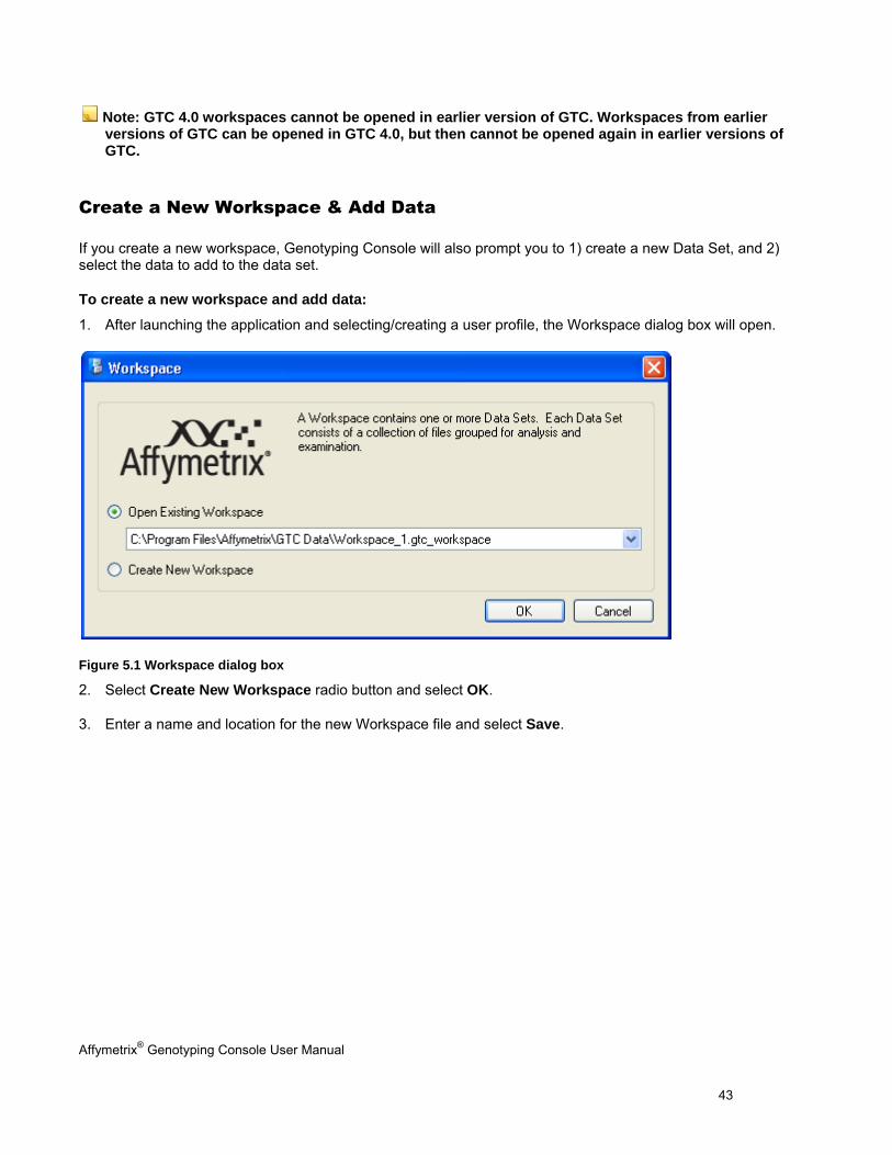
1. After launching the application and selecting/creating a user profile, the Workspace dialog box will open.
Figure 5.1 Workspace dialog box
2. Select Create New Workspace radio button and select OK.
3. Enter a name and location for the new Workspace file and select Save.
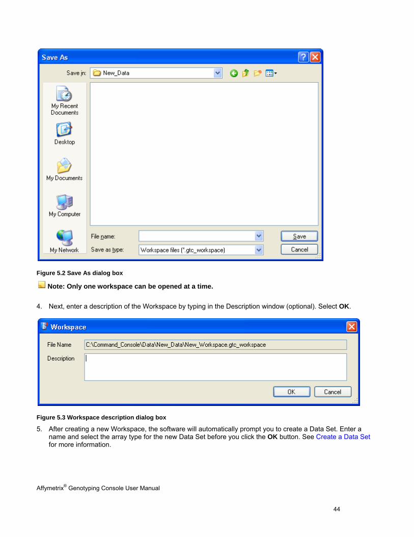
Affymetrix® Genotyping Console User Manual 44
Figure 5.2 Save As dialog box
Note: Only one workspace can be opened at a time.
4. Next, enter a description of the Workspace by typing in the Description window (optional). Select OK.
Figure 5.3 Workspace description dialog box
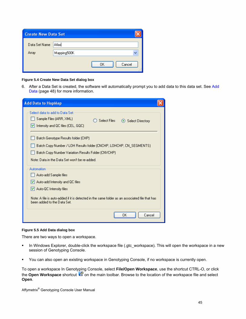
5. After creating a new Workspace, the software will automatically prompt you to create a Data Set. Enter a name and select the array type for the new Data Set before you click the OK button. See Create a Data Set for more information.
Affymetrix® Genotyping Console User Manual 45
Figure 5.4 Create New Data Set dialog box
6. After a Data Set is created, the software will automatically prompt you to add data to this data set. See Add Data (page 48) for more information.
Figure 5.5 Add Data dialog box
There are two ways to open a workspace.
In Windows Explorer, double-click the workspace file (.gtc_workspace). This will open the workspace in a new session of Genotyping Console.
You can also open an existing workspace in Genotyping Console, if no workspace is currently open.
To open a workspace In Genotyping Console, select File/Open Workspace, use the shortcut CTRL-O, or click the Open Workspace shortcut on the main toolbar. Browse to the location of the workspace file and select Open.
Affymetrix® Genotyping Console User Manual 46
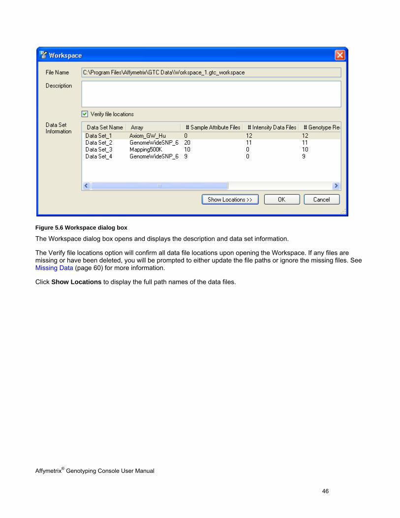
Figure 5.6 Workspace dialog box
The Workspace dialog box opens and displays the description and data set information.
The Verify file locations option will confirm all data file locations upon opening the Workspace. If any files are missing or have been deleted, you will be prompted to either update the file paths or ignore the missing files. See Missing Data (page 60) for more information.
Click Show Locations to display the full path names of the data files.
Affymetrix® Genotyping Console User Manual 47
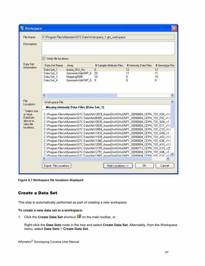
Figure 5.7 Workspace file locations displayed
Create a Data Set
This step is automatically performed as part of creating a new workspace.
To create a new data set in a workspace:
1. Click the Create Data Set shortcut on the main toolbar, or
Right-click the Data Sets node in the tree and select Create Data Set. Alternately, from the Workspace menu, select Data Sets > Create Data Set.
Affymetrix® Genotyping Console User Manual 48
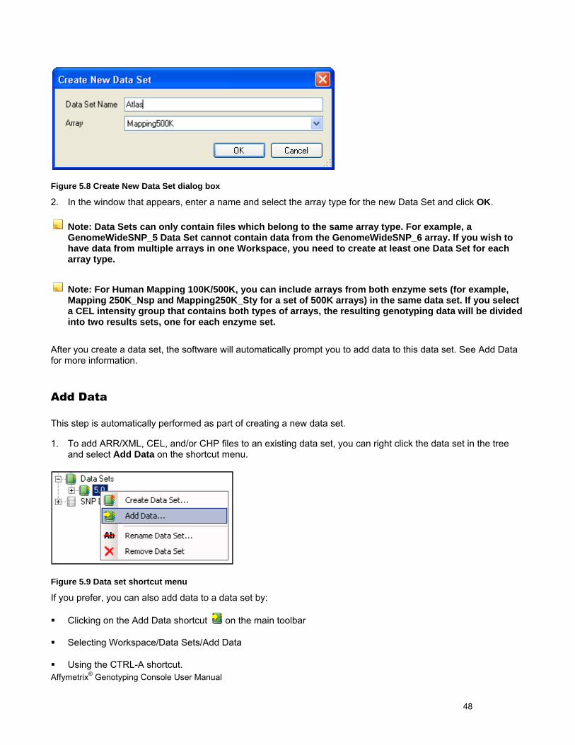
Figure 5.8 Create New Data Set dialog box
2. In the window that appears, enter a name and select the array type for the new Data Set and click OK.
Note: Data Sets can only contain files which belong to the same array type. For example, a GenomeWideSNP_5 Data Set cannot contain data from the GenomeWideSNP_6 array. If you wish to have data from multiple arrays in one Workspace, you need to create at least one Data Set for each array type.
Note: For Human Mapping 100K/500K, you can include arrays from both enzyme sets (for example, Mapping 250K_Nsp and Mapping250K_Sty for a set of 500K arrays) in the same data set. If you select a CEL intensity group that contains both types of arrays, the resulting genotyping data will be divided into two results sets, one for each enzyme set.
After you create a data set, the software will automatically prompt you to add data to this data set. See Add Data for more information.
Add Data
This step is automatically performed as part of creating a new data set.
1. To add ARR/XML, CEL, and/or CHP files to an existing data set, you can right click the data set in the tree and select Add Data on the shortcut menu.
Figure 5.9 Data set shortcut menu
If you prefer, you can also add data to a data set by:
Clicking on the Add Data shortcut on the main toolbar
Selecting Workspace/Data Sets/Add Data
Using the CTRL-A shortcut.

Affymetrix® Genotyping Console User Manual 49
Genotyping Console will detect which data set that you want to add data to based on the highlighted tree item. If the software cannot determine the data set that you want to add data to, you will be prompted to select a data set.
Note: Only data files (ARR/XML, CEL, or CHP) generated by Affymetrix software or GeneChip compatible software partners can be imported into Genotyping Console. Any supported data files that are edited outside of these software packages may cause import to fail or Genotyping Console software to crash.
Note: Affymetrix recommends using data files in AGCC format, as there is only limited support for GCOS files. For example, editing of XML sample attributes is not supported. Also, CHP files that are generated by Genotype Console and then imported into another workspace will not include sample attribute information if the CHP files were generated from GCOS-format CEL files. Affymetrix recommends using the Data Transfer Tool (DTT v1.1.1, provided with GCOS) Flat File transfer out option to create a copy of the XML and CEL files for use by Genotyping Console. For more information, go to: http://www.affymetrix.com/support/downloads/manuals/data_transfer_tool_user_guide.pdf or www.affymetrix.com; then to Support/Technical/Tutorial/GCOS.
2. Select the data type (ARR/XML, CEL, GQC, and/or CHP) to add to the newly created Data Set and check-mark any automated steps that should also occur, such as auto-add data or auto-QC intensity files. If you want to select an entire directory, click the Select Directory radio button. Then click OK.

Affymetrix® Genotyping Console User Manual 50
Figure 5.10 Add Data dialog box
Note: You must have write access to the folder in which the CEL files are located for GTC to be able to write QC information. If you only have read access, you must first copy the data to a folder where you have write access.
Table 5.1 Add data options
Select data to add to Data Set Description
Select Files radio buttons Add files selected from a directory to the data set.
Select Directory radio button Add all files in a selected directory to the data set.
Sample Files (ARR, XML) If selected, Genotyping Console will add user-selected sample files to the Data Set. These files can be in either AGCC format (ARR, preferred) or GCOS format (XML).
Intensity and QC Files (CEL,GQC)
If selected, Genotyping Console will add user-selected Intensity (CEL) and associated Genotyping Console QC files (GQC) to the Data Set.
Batch Genotype Results folder (CHP)
If selected, Genotyping Console software will add CHP files in the user-selected folder. If the CHP files are not from the same batch genotyping operation, they will be separated into multiple Genotype Result groups.
Batch Copy Number/LOH Results folder (CNCHP, If selected, Genotyping Console software will add CNCHP and/or LOHCHP and
Affymetrix® Genotyping Console User Manual 51
LOHCHP, CN_SEGMENTS, CUSTOM_REGIONS)
CN_SEGMENTS and CUSTOM_REGIONS files in the user-selected folder.
Batch Copy Number Variation Results folder (CNVCHP)
If selected, Genotyping Console software will add CNVCHP files in the user-selected folder.
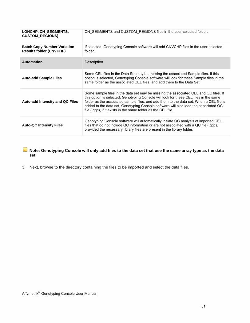
Automation Description
Auto-add Sample Files Some CEL files in the Data Set may be missing the associated Sample files. If this option is selected, Genotyping Console software will look for these Sample files in the same folder as the associated CEL files, and add them to the Data Set.
Auto-add Intensity and QC Files
Some sample files in the data set may be missing the associated CEL and QC files. If this option is selected, Genotyping Console will look for these CEL files in the same folder as the associated sample files, and add them to the data set. When a CEL file is added to the data set, Genotyping Console software will also load the associated QC file (.gqc), if it exists in the same folder as the CEL file.
Auto-QC Intensity Files Genotyping Console software will automatically initiate QC analysis of imported CEL files that do not include QC information or are not associated with a QC file (.gqc), provided the necessary library files are present in the library folder.
Note: Genotyping Console will only add files to the data set that use the same array type as the data set.
3. Next, browse to the directory containing the files to be imported and select the data files.
Affymetrix® Genotyping Console User Manual 52
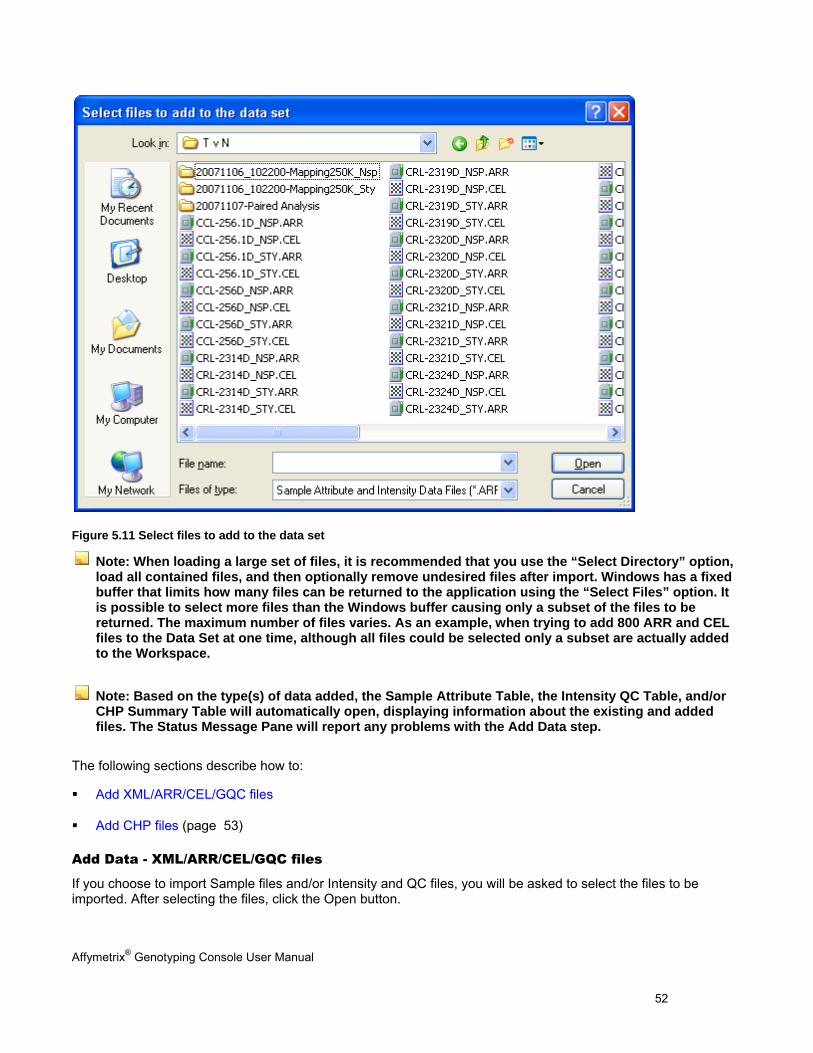
Figure 5.11 Select files to add to the data set
Note: When loading a large set of files, it is recommended that you use the “Select Directory” option, load all contained files, and then optionally remove undesired files after import. Windows has a fixed buffer that limits how many files can be returned to the application using the “Select Files” option. It is possible to select more files than the Windows buffer causing only a subset of the files to be returned. The maximum number of files varies. As an example, when trying to add 800 ARR and CEL files to the Data Set at one time, although all files could be selected only a subset are actually added to the Workspace.
Note: Based on the type(s) of data added, the Sample Attribute Table, the Intensity QC Table, and/or CHP Summary Table will automatically open, displaying information about the existing and added files. The Status Message Pane will report any problems with the Add Data step.
The following sections describe how to:
Add XML/ARR/CEL/GQC files
Add CHP files (page 53)
Add Data - XML/ARR/CEL/GQC files
If you choose to import Sample files and/or Intensity and QC files, you will be asked to select the files to be imported. After selecting the files, click the Open button.
Affymetrix® Genotyping Console User Manual 53
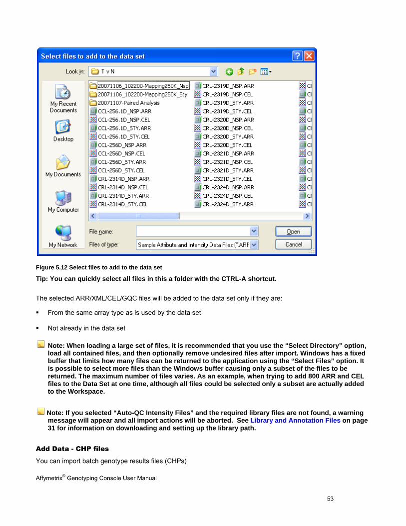
Figure 5.12 Select files to add to the data set
Tip: You can quickly select all files in this a folder with the CTRL-A shortcut.
The selected ARR/XML/CEL/GQC files will be added to the data set only if they are:
From the same array type as is used by the data set
Not already in the data set
Note: When loading a large set of files, it is recommended that you use the “Select Directory” option, load all contained files, and then optionally remove undesired files after import. Windows has a fixed buffer that limits how many files can be returned to the application using the “Select Files” option. It is possible to select more files than the Windows buffer causing only a subset of the files to be returned. The maximum number of files varies. As an example, when trying to add 800 ARR and CEL files to the Data Set at one time, although all files could be selected only a subset are actually added to the Workspace.
Note: If you selected “Auto-QC Intensity Files” and the required library files are not found, a warning message will appear and all import actions will be aborted. See Library and Annotation Files on page 31 for information on downloading and setting up the library path.
Add Data - CHP files
You can import batch genotype results files (CHPs)
Affymetrix® Genotyping Console User Manual 54
Genotype analysis results files (.CHP)
Copy Number/Loss of Heterozygosity (CN/LOH) analysis results files (.CNCHP and .LOHCHP)
Copy Number Variation (CNV) analysis results files (.CNVCHP)
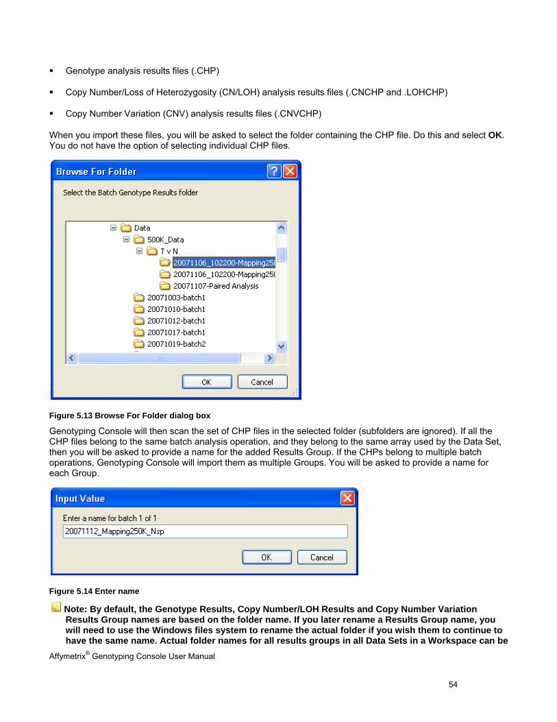
When you import these files, you will be asked to select the folder containing the CHP file. Do this and select OK. You do not have the option of selecting individual CHP files.
Figure 5.13 Browse For Folder dialog box
Genotyping Console will then scan the set of CHP files in the selected folder (subfolders are ignored). If all the CHP files belong to the same batch analysis operation, and they belong to the same array used by the Data Set, then you will be asked to provide a name for the added Results Group. If the CHPs belong to multiple batch operations, Genotyping Console will import them as multiple Groups. You will be asked to provide a name for each Group.
Figure 5.14 Enter name
Note: By default, the Genotype Results, Copy Number/LOH Results and Copy Number Variation Results Group names are based on the folder name. If you later rename a Results Group name, you will need to use the Windows files system to rename the actual folder if you wish them to continue to have the same name. Actual folder names for all results groups in all Data Sets in a Workspace can be
Affymetrix® Genotyping Console User Manual 55
found by the command Ctrl+I and clicking the “Show Locations button, or from the menu: Workspace>Properties>Show Information, and clicking the Show Locations button.
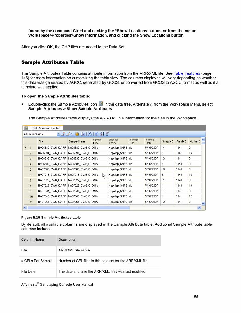
After you click OK, the CHP files are added to the Data Set.
Sample Attributes Table
The Sample Attributes Table contains attribute information from the ARR/XML file. See Table Features (page 146) for more information on customizing the table view. The columns displayed will vary depending on whether this data was generated by AGCC, generated by GCOS, or converted from GCOS to AGCC format as well as if a template was applied.
To open the Sample Attributes table:
Double-click the Sample Attributes icon in the data tree. Alternately, from the Workspace Menu, select Sample Attributes > Show Sample Attributes.
The Sample Attributes table displays the ARR/XML file information for the files in the Workspace.
Figure 5.15 Sample Attributes table
By default, all available columns are displayed in the Sample Attribute table. Additional Sample Attribute table columns include:
Column Name Description
File ARR/XML file name
# CELs Per Sample Number of CEL files in this data set for the ARR/XML file
File Date The date and time the ARR/XML files was last modified.
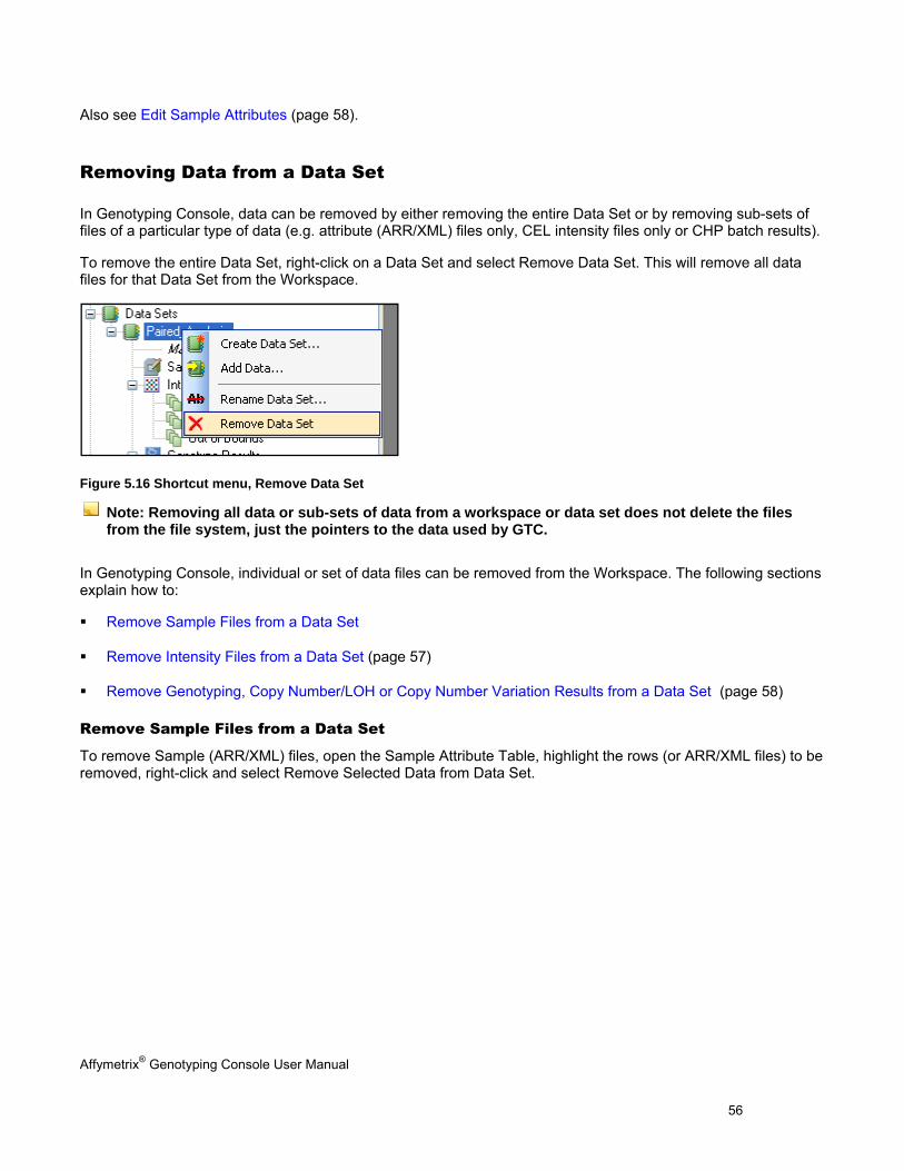
Affymetrix® Genotyping Console User Manual 56
Also see Edit Sample Attributes (page 58).
Removing Data from a Data Set
In Genotyping Console, data can be removed by either removing the entire Data Set or by removing sub-sets of files of a particular type of data (e.g. attribute (ARR/XML) files only, CEL intensity files only or CHP batch results).
To remove the entire Data Set, right-click on a Data Set and select Remove Data Set. This will remove all data files for that Data Set from the Workspace.
Figure 5.16 Shortcut menu, Remove Data Set
Note: Removing all data or sub-sets of data from a workspace or data set does not delete the files from the file system, just the pointers to the data used by GTC.
In Genotyping Console, individual or set of data files can be removed from the Workspace. The following sections explain how to:
Remove Sample Files from a Data Set
Remove Intensity Files from a Data Set (page 57)
Remove Genotyping, Copy Number/LOH or Copy Number Variation Results from a Data Set (page 58)
Remove Sample Files from a Data Set
To remove Sample (ARR/XML) files, open the Sample Attribute Table, highlight the rows (or ARR/XML files) to be removed, right-click and select Remove Selected Data from Data Set.
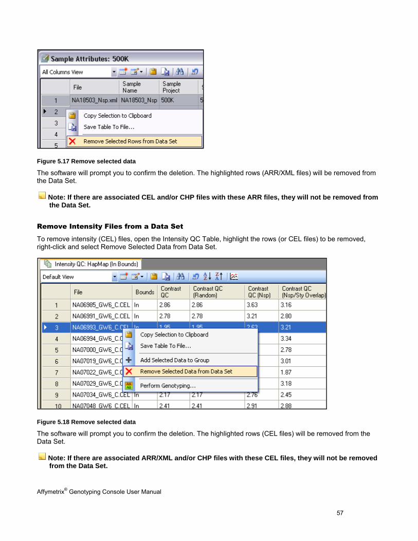
Affymetrix® Genotyping Console User Manual 57
Figure 5.17 Remove selected data
The software will prompt you to confirm the deletion. The highlighted rows (ARR/XML files) will be removed from the Data Set.
Note: If there are associated CEL and/or CHP files with these ARR files, they will not be removed from the Data Set.
Remove Intensity Files from a Data Set
To remove intensity (CEL) files, open the Intensity QC Table, highlight the rows (or CEL files) to be removed, right-click and select Remove Selected Data from Data Set.
Figure 5.18 Remove selected data
The software will prompt you to confirm the deletion. The highlighted rows (CEL files) will be removed from the Data Set.
Note: If there are associated ARR/XML and/or CHP files with these CEL files, they will not be removed from the Data Set.
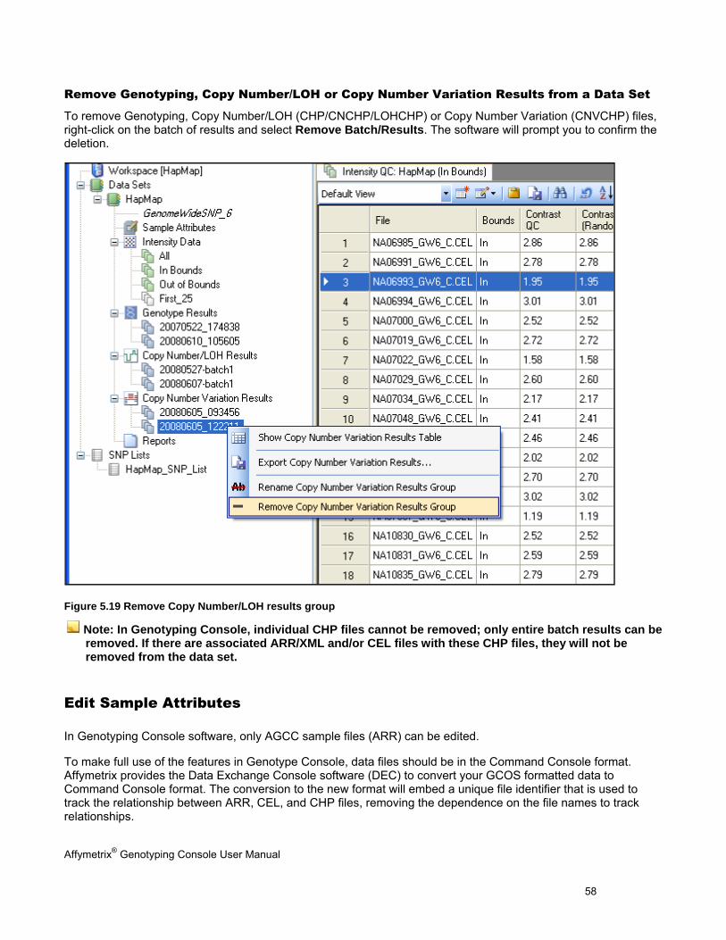
Affymetrix® Genotyping Console User Manual 58
Remove Genotyping, Copy Number/LOH or Copy Number Variation Results from a Data Set
To remove Genotyping, Copy Number/LOH (CHP/CNCHP/LOHCHP) or Copy Number Variation (CNVCHP) files, right-click on the batch of results and select Remove Batch/Results. The software will prompt you to confirm the deletion.
Figure 5.19 Remove Copy Number/LOH results group
Note: In Genotyping Console, individual CHP files cannot be removed; only entire batch results can be removed. If there are associated ARR/XML and/or CEL files with these CHP files, they will not be removed from the data set.
Edit Sample Attributes
In Genotyping Console software, only AGCC sample files (ARR) can be edited.
To make full use of the features in Genotype Console, data files should be in the Command Console format. Affymetrix provides the Data Exchange Console software (DEC) to convert your GCOS formatted data to Command Console format. The conversion to the new format will embed a unique file identifier that is used to track the relationship between ARR, CEL, and CHP files, removing the dependence on the file names to track relationships.
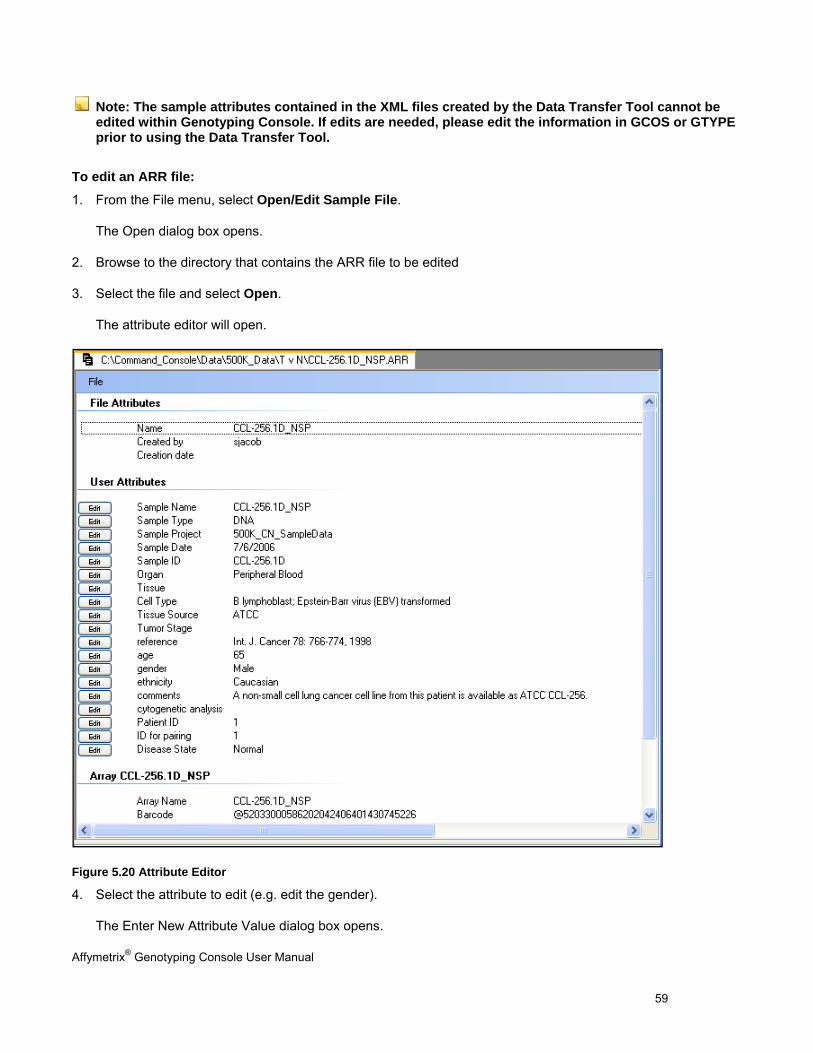
Affymetrix® Genotyping Console User Manual 59
Note: The sample attributes contained in the XML files created by the Data Transfer Tool cannot be edited within Genotyping Console. If edits are needed, please edit the information in GCOS or GTYPE prior to using the Data Transfer Tool.
To edit an ARR file:
1. From the File menu, select Open/Edit Sample File.
The Open dialog box opens.
2. Browse to the directory that contains the ARR file to be edited
3. Select the file and select Open.
The attribute editor will open.
Figure 5.20 Attribute Editor
4. Select the attribute to edit (e.g. edit the gender).
The Enter New Attribute Value dialog box opens.
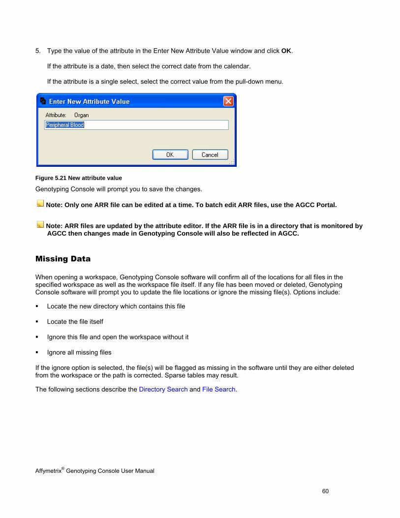
Affymetrix® Genotyping Console User Manual 60
5. Type the value of the attribute in the Enter New Attribute Value window and click OK.
If the attribute is a date, then select the correct date from the calendar.
If the attribute is a single select, select the correct value from the pull-down menu.
Figure 5.21 New attribute value
Genotyping Console will prompt you to save the changes.
Note: Only one ARR file can be edited at a time. To batch edit ARR files, use the AGCC Portal.
Note: ARR files are updated by the attribute editor. If the ARR file is in a directory that is monitored by AGCC then changes made in Genotyping Console will also be reflected in AGCC.
Missing Data
When opening a workspace, Genotyping Console software will confirm all of the locations for all files in the specified workspace as well as the workspace file itself. If any file has been moved or deleted, Genotyping Console software will prompt you to update the file locations or ignore the missing file(s). Options include:
Locate the new directory which contains this file
Locate the file itself
Ignore this file and open the workspace without it
Ignore all missing files
If the ignore option is selected, the file(s) will be flagged as missing in the software until they are either deleted from the workspace or the path is corrected. Sparse tables may result.
The following sections describe the Directory Search and File Search.
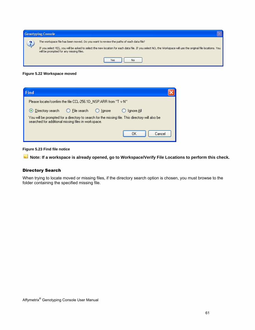
Affymetrix® Genotyping Console User Manual 61
Figure 5.22 Workspace moved
Figure 5.23 Find file notice
Note: If a workspace is already opened, go to Workspace/Verify File Locations to perform this check.
Directory Search
When trying to locate moved or missing files, if the directory search option is chosen, you must browse to the folder containing the specified missing file.
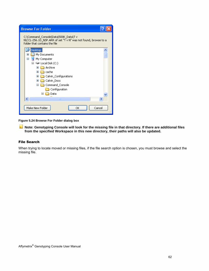
Affymetrix® Genotyping Console User Manual 62
Figure 5.24 Browse For Folder dialog box
Note: Genotyping Console will look for the missing file in that directory. If there are additional files from the specified Workspace in this new directory, their paths will also be updated.
File Search
When trying to locate moved or missing files, if the file search option is chosen, you must browse and select the missing file.
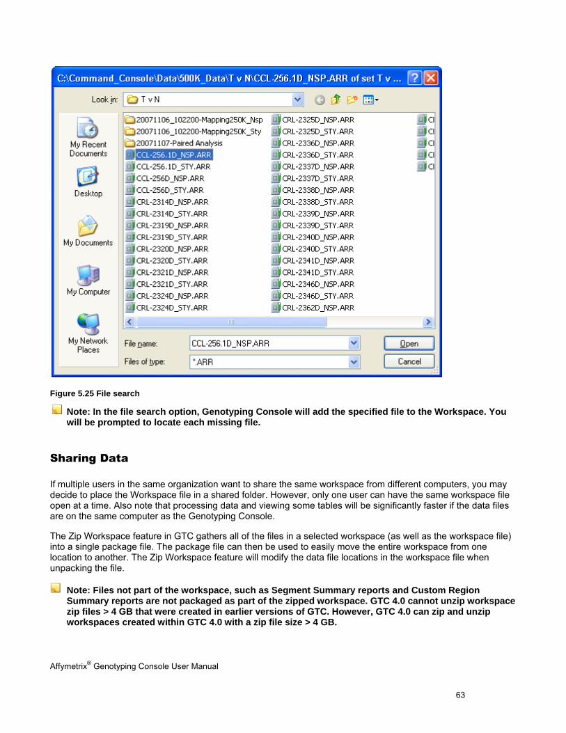
Affymetrix® Genotyping Console User Manual 63
Figure 5.25 File search
Note: In the file search option, Genotyping Console will add the specified file to the Workspace. You will be prompted to locate each missing file.
Sharing Data
If multiple users in the same organization want to share the same workspace from different computers, you may decide to place the Workspace file in a shared folder. However, only one user can have the same workspace file open at a time. Also note that processing data and viewing some tables will be significantly faster if the data files are on the same computer as the Genotyping Console.
The Zip Workspace feature in GTC gathers all of the files in a selected workspace (as well as the workspace file) into a single package file. The package file can then be used to easily move the entire workspace from one location to another. The Zip Workspace feature will modify the data file locations in the workspace file when unpacking the file.
Note: Files not part of the workspace, such as Segment Summary reports and Custom Region Summary reports are not packaged as part of the zipped workspace. GTC 4.0 cannot unzip workspace zip files > 4 GB that were created in earlier versions of GTC. However, GTC 4.0 can zip and unzip workspaces created within GTC 4.0 with a zip file size > 4 GB.
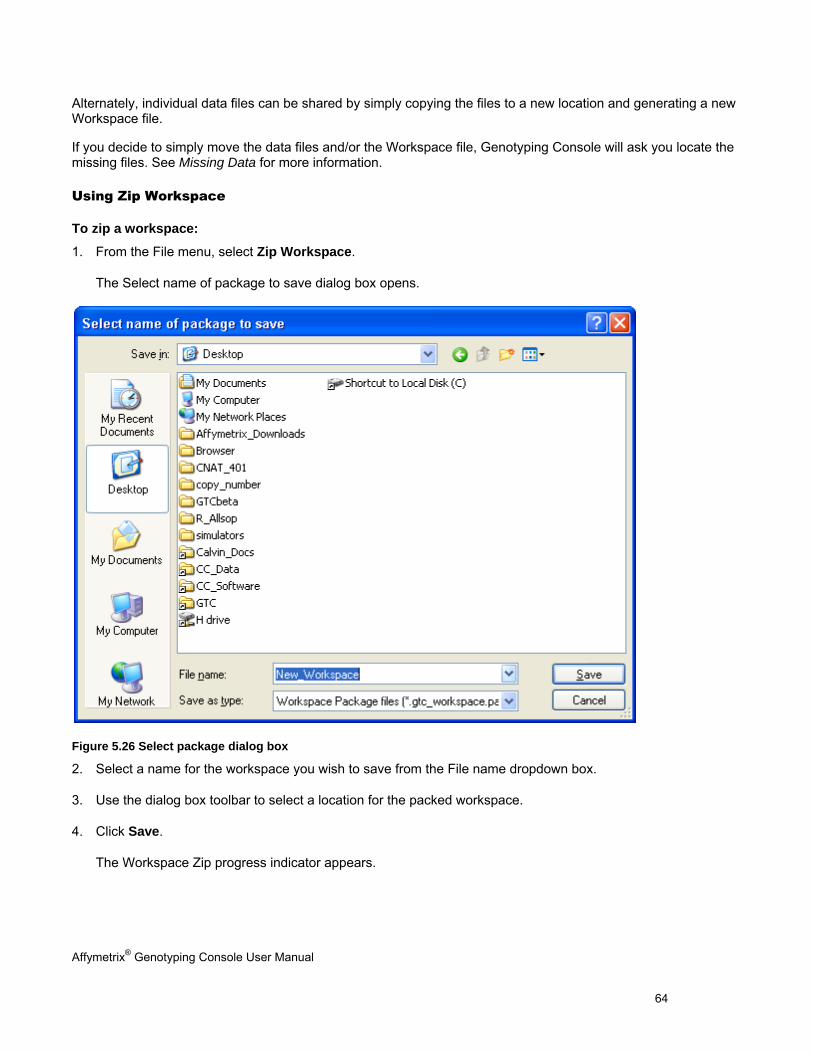
Affymetrix® Genotyping Console User Manual 64
Alternately, individual data files can be shared by simply copying the files to a new location and generating a new Workspace file.
If you decide to simply move the data files and/or the Workspace file, Genotyping Console will ask you locate the missing files. See Missing Data for more information.
Using Zip Workspace
To zip a workspace:
1. From the File menu, select Zip Workspace.
The Select name of package to save dialog box opens.
Figure 5.26 Select package dialog box
2. Select a name for the workspace you wish to save from the File name dropdown box.
3. Use the dialog box toolbar to select a location for the packed workspace.
4. Click Save.
The Workspace Zip progress indicator appears.
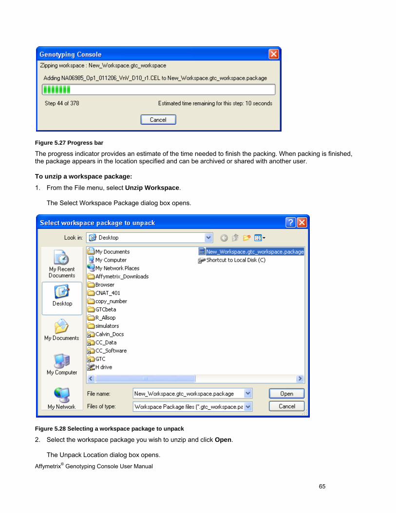
Affymetrix® Genotyping Console User Manual 65
Figure 5.27 Progress bar
The progress indicator provides an estimate of the time needed to finish the packing. When packing is finished, the package appears in the location specified and can be archived or shared with another user.
To unzip a workspace package:
1. From the File menu, select Unzip Workspace.
The Select Workspace Package dialog box opens.
Figure 5.28 Selecting a workspace package to unpack
2. Select the workspace package you wish to unzip and click Open.
The Unpack Location dialog box opens.
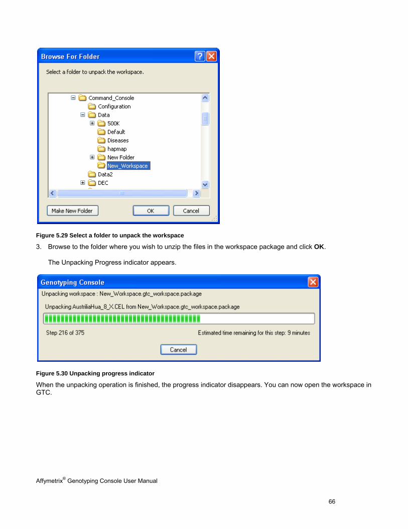
Affymetrix® Genotyping Console User Manual 66
Figure 5.29 Select a folder to unpack the workspace
3. Browse to the folder where you wish to unzip the files in the workspace package and click OK.
The Unpacking Progress indicator appears.
Figure 5.30 Unpacking progress indicator
When the unpacking operation is finished, the progress indicator disappears. You can now open the workspace in GTC.
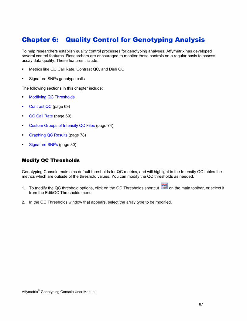
Affymetrix® Genotyping Console User Manual 67
Chapter 6: Quality Control for Genotyping Analysis To help researchers establish quality control processes for genotyping analyses, Affymetrix has developed several control features. Researchers are encouraged to monitor these controls on a regular basis to assess assay data quality. These features include:
Metrics like QC Call Rate, Contrast QC, and Dish QC
Signature SNPs genotype calls
The following sections in this chapter include:
Modifying QC Thresholds
Contrast QC (page 69)
QC Call Rate (page 69)
Custom Groups of Intensity QC Files (page 74)
Graphing QC Results (page 78)
Signature SNPs (page 80)
Modify QC Thresholds
Genotyping Console maintains default thresholds for QC metrics, and will highlight in the Intensity QC tables the metrics which are outside of the threshold values. You can modify the QC thresholds as needed.
1. To modify the QC threshold options, click on the QC Thresholds shortcut on the main toolbar, or select it from the Edit/QC Thresholds menu.
2. In the QC Thresholds window that appears, select the array type to be modified.
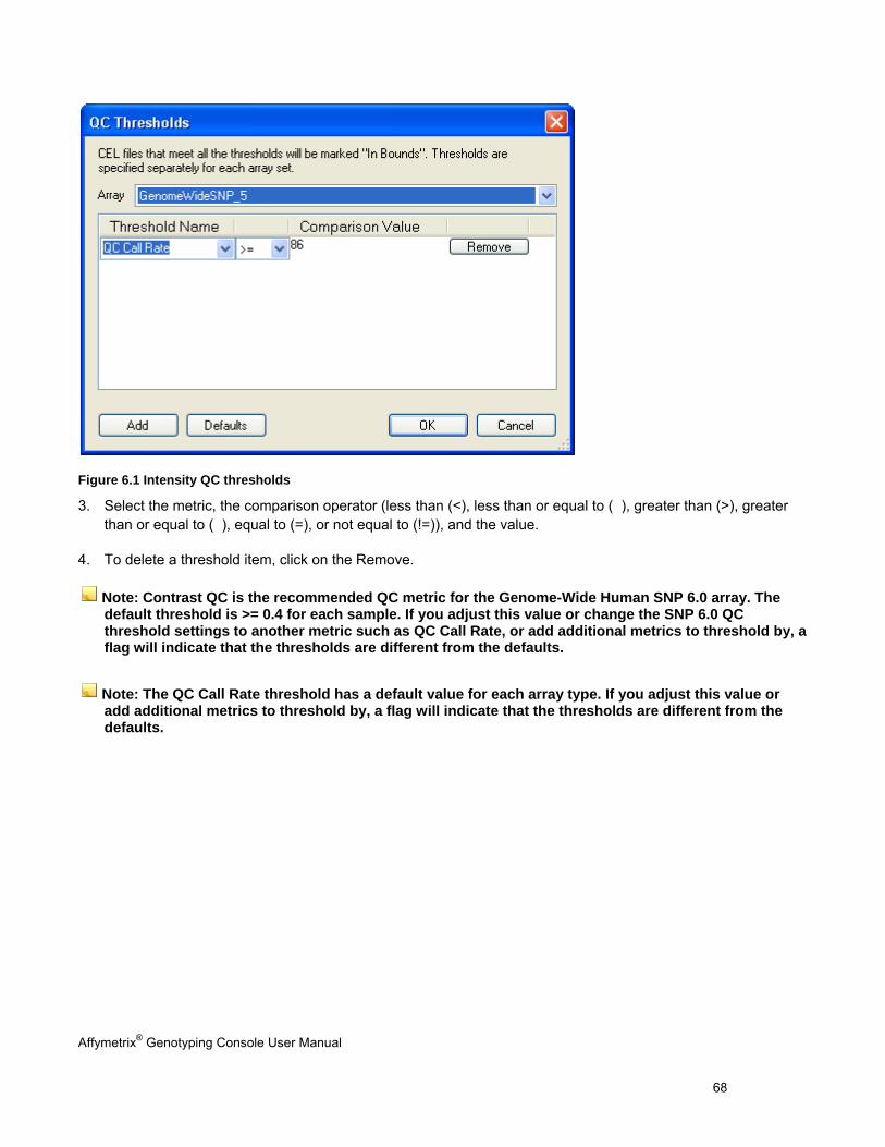
Affymetrix® Genotyping Console User Manual 68
Figure 6.1 Intensity QC thresholds
3. Select the metric, the comparison operator (less than (<), less than or equal to ( ), greater than (>), greater than or equal to ( ), equal to (=), or not equal to (!=)), and the value.
4. To delete a threshold item, click on the Remove.
Note: Contrast QC is the recommended QC metric for the Genome-Wide Human SNP 6.0 array. The default threshold is >= 0.4 for each sample. If you adjust this value or change the SNP 6.0 QC threshold settings to another metric such as QC Call Rate, or add additional metrics to threshold by, a flag will indicate that the thresholds are different from the defaults.
Note: The QC Call Rate threshold has a default value for each array type. If you adjust this value or add additional metrics to threshold by, a flag will indicate that the thresholds are different from the defaults.
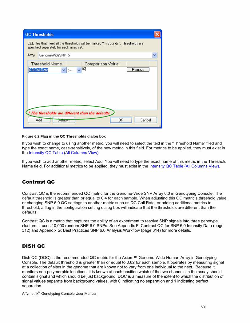
Affymetrix® Genotyping Console User Manual 69
Figure 6.2 Flag in the QC Thresholds dialog box
If you wish to change to using another metric, you will need to select the text in the “Threshold Name” filed and type the exact name, case-sensitively, of the new metric in this field. For metrics to be applied, they must exist in the Intensity QC Table (All Columns View).
If you wish to add another metric, select Add. You will need to type the exact name of this metric in the Threshold Name field. For additional metrics to be applied, they must exist in the Intensity QC Table (All Columns View).
Contrast QC
Contrast QC is the recommended QC metric for the Genome-Wide SNP Array 6.0 in Genotyping Console. The default threshold is greater than or equal to 0.4 for each sample. When adjusting this QC metric’s threshold value, or changing SNP 6.0 QC settings to another metric such as QC Call Rate, or adding additional metrics to threshold, a flag in the configuration setting dialog box will indicate that the thresholds are different than the defaults.
Contrast QC is a metric that captures the ability of an experiment to resolve SNP signals into three genotype clusters. It uses 10,000 random SNP 6.0 SNPs. See Appendix F: Contrast QC for SNP 6.0 Intensity Data (page 312) and Appendix G: Best Practices SNP 6.0 Analysis Workflow (page 314) for more details.
DISH QC
Dish QC (DQC) is the recommended QC metric for the Axiom™ Genome-Wide Human Array in Genotyping Console. The default threshold is greater than or equal to 0.82 for each sample. It operates by measuring signal at a collection of sites in the genome that are known not to vary from one individual to the next. Because it monitors non-polymorphic locations, it is known at each position which of the two channels in the assay should contain signal and which should be just background. DQC is a measure of the extent to which the distribution of signal values separate from background values, with 0 indicating no separation and 1 indicating perfect separation.
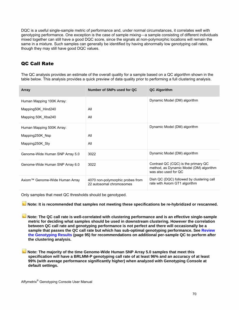
Affymetrix® Genotyping Console User Manual 70
DQC is a useful single-sample metric of performance and, under normal circumstances, it correlates well with genotyping performance. One exception is the case of sample mixing―a sample consisting of different individuals mixed together can still have a good DQC score, since the signals at non-polymorphic locations will remain the same in a mixture. Such samples can generally be identified by having abnormally low genotyping call rates, though they may still have good DQC values.
QC Call Rate
The QC analysis provides an estimate of the overall quality for a sample based on a QC algorithm shown in the table below. This analysis provides a quick preview of data quality prior to performing a full clustering analysis.
Array Number of SNPs used for QC QC Algorithm
Human Mapping 100K Array:
Mapping50K_Hind240
Mapping 50K_Xba240
All
All
Dynamic Model (DM) algorithm
Human Mapping 500K Array:
Mapping250K_Nsp
Mapping250K_Sty
All
All
Dynamic Model (DM) algorithm
Genome-Wide Human SNP Array 5.0 3022 Dynamic Model (DM) algorithm
Genome-Wide Human SNP Array 6.0 3022 Contrast QC (CQC) is the primary QC method, as Dynamic Model (DM) algorithm was also used for QC
Axiom™ Genome-Wide Human Array 4070 non-polymorphic probes from 22 autosomal chromosomes
Dish QC (DQC) followed by clustering call rate with Axiom GT1 algorithm
Only samples that meet QC thresholds should be genotyped.
Note: It is recommended that samples not meeting these specifications be re-hybridized or rescanned.
Note: The QC call rate is well-correlated with clustering performance and is an effective single-sample metric for deciding what samples should be used in downstream clustering. However the correlation between QC call rate and genotyping performance is not perfect and there will occasionally be a sample that passes the QC call rate but which has sub-optimal genotyping performance. See Review the Genotyping Results (page 95) for recommendations on additional per-sample QC to perform after the clustering analysis.
Note: The majority of the time Genome-Wide Human SNP Array 5.0 samples that meet this specification will have a BRLMM-P genotyping call rate of at least 96% and an accuracy of at least 99% (with average performance significantly higher) when analyzed with Genotyping Console at default settings.
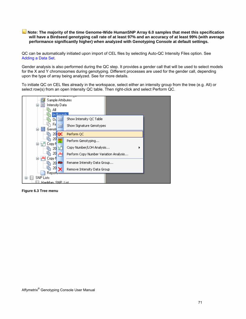
Affymetrix® Genotyping Console User Manual 71
Note: The majority of the time Genome-Wide HumanSNP Array 6.0 samples that meet this specification will have a Birdseed genotyping call rate of at least 97% and an accuracy of at least 99% (with average performance significantly higher) when analyzed with Genotyping Console at default settings.
QC can be automatically initiated upon import of CEL files by selecting Auto-QC Intensity Files option. See Adding a Data Set.
Gender analysis is also performed during the QC step. It provides a gender call that will be used to select models for the X and Y chromosomes during genotyping. Different processes are used for the gender call, depending upon the type of array being analyzed. See for more details.
To initiate QC on CEL files already in the workspace, select either an intensity group from the tree (e.g. All) or select row(s) from an open Intensity QC table. Then right-click and select Perform QC.
Figure 6.3 Tree menu
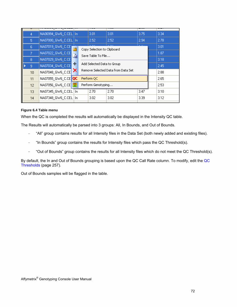
Affymetrix® Genotyping Console User Manual 72
Figure 6.4 Table menu
When the QC is completed the results will automatically be displayed in the Intensity QC table.
The Results will automatically be parsed into 3 groups: All, In Bounds, and Out of Bounds.
- “All” group contains results for all Intensity files in the Data Set (both newly added and existing files).
- “In Bounds” group contains the results for Intensity files which pass the QC Threshold(s).
- “Out of Bounds” group contains the results for all Intensity files which do not meet the QC Threshold(s).
By default, the In and Out of Bounds grouping is based upon the QC Call Rate column. To modify, edit the QC Thresholds (page 257).
Out of Bounds samples will be flagged in the table.
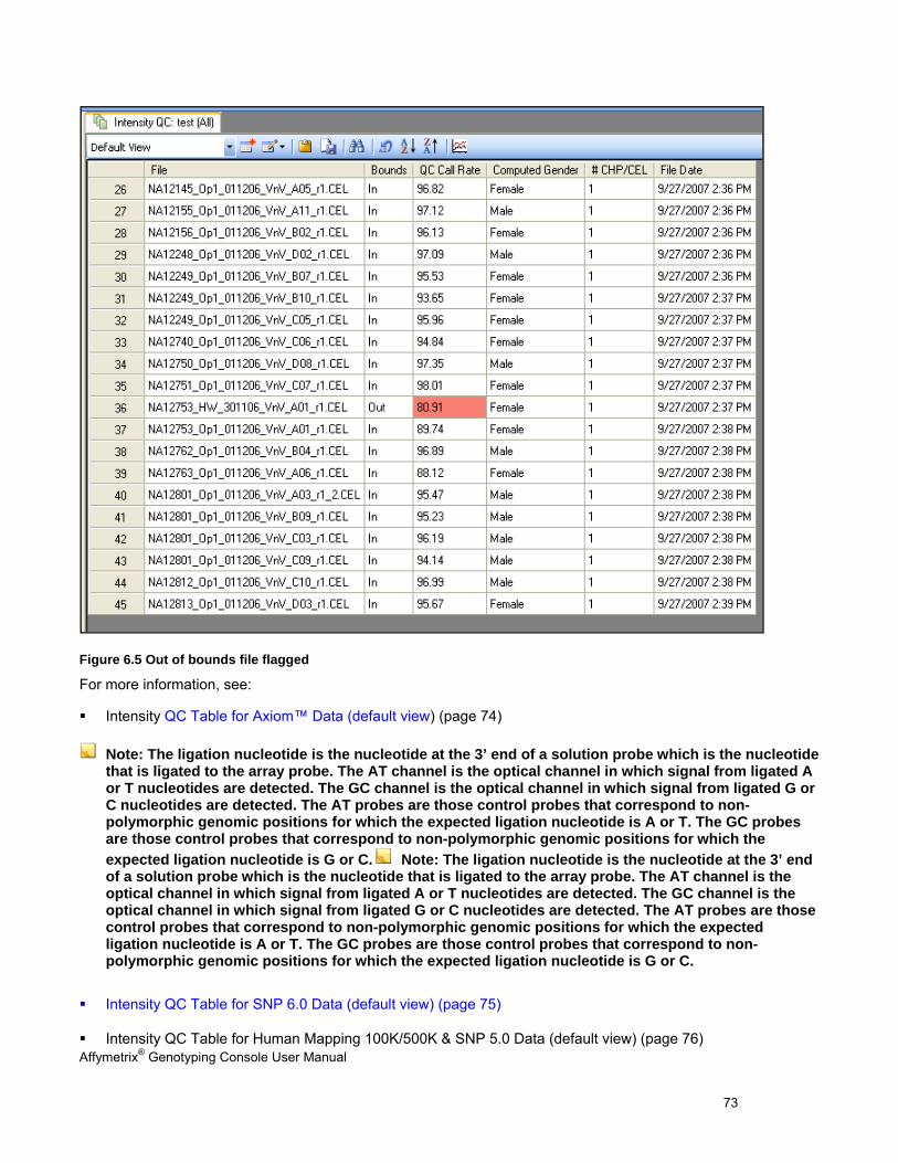
Affymetrix® Genotyping Console User Manual 73
Figure 6.5 Out of bounds file flagged
For more information, see:
Intensity QC Table for Axiom™ Data (default view) (page 74)
Note: The ligation nucleotide is the nucleotide at the 3’ end of a solution probe which is the nucleotide that is ligated to the array probe. The AT channel is the optical channel in which signal from ligated A or T nucleotides are detected. The GC channel is the optical channel in which signal from ligated G or C nucleotides are detected. The AT probes are those control probes that correspond to non-polymorphic genomic positions for which the expected ligation nucleotide is A or T. The GC probes are those control probes that correspond to non-polymorphic genomic positions for which the expected ligation nucleotide is G or C. Note: The ligation nucleotide is the nucleotide at the 3’ end of a solution probe which is the nucleotide that is ligated to the array probe. The AT channel is the optical channel in which signal from ligated A or T nucleotides are detected. The GC channel is the optical channel in which signal from ligated G or C nucleotides are detected. The AT probes are those control probes that correspond to non-polymorphic genomic positions for which the expected ligation nucleotide is A or T. The GC probes are those control probes that correspond to non-polymorphic genomic positions for which the expected ligation nucleotide is G or C.
Intensity QC Table for SNP 6.0 Data (default view) (page 75)
Intensity QC Table for Human Mapping 100K/500K & SNP 5.0 Data (default view) (page 76)
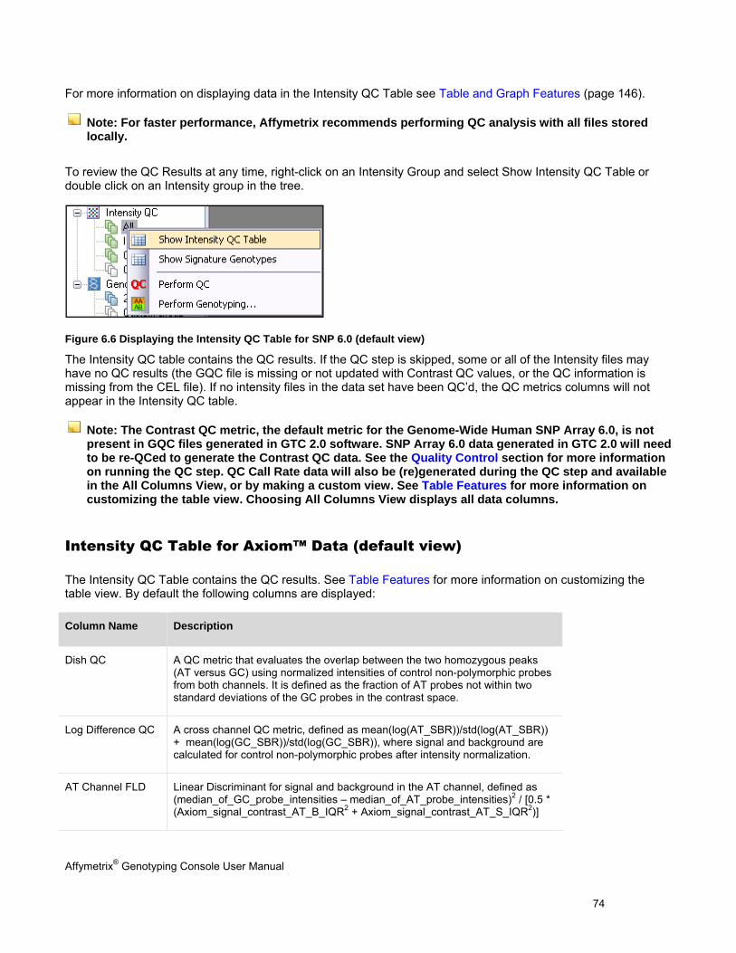
Affymetrix® Genotyping Console User Manual 74
For more information on displaying data in the Intensity QC Table see Table and Graph Features (page 146).
Note: For faster performance, Affymetrix recommends performing QC analysis with all files stored locally.
To review the QC Results at any time, right-click on an Intensity Group and select Show Intensity QC Table or double click on an Intensity group in the tree.
Figure 6.6 Displaying the Intensity QC Table for SNP 6.0 (default view)
The Intensity QC table contains the QC results. If the QC step is skipped, some or all of the Intensity files may have no QC results (the GQC file is missing or not updated with Contrast QC values, or the QC information is missing from the CEL file). If no intensity files in the data set have been QC’d, the QC metrics columns will not appear in the Intensity QC table.
Note: The Contrast QC metric, the default metric for the Genome-Wide Human SNP Array 6.0, is not present in GQC files generated in GTC 2.0 software. SNP Array 6.0 data generated in GTC 2.0 will need to be re-QCed to generate the Contrast QC data. See the Quality Control section for more information on running the QC step. QC Call Rate data will also be (re)generated during the QC step and available in the All Columns View, or by making a custom view. See Table Features for more information on customizing the table view. Choosing All Columns View displays all data columns.
Intensity QC Table for Axiom™ Data (default view)
The Intensity QC Table contains the QC results. See Table Features for more information on customizing the table view. By default the following columns are displayed:
Column Name Description
Dish QC A QC metric that evaluates the overlap between the two homozygous peaks (AT versus GC) using normalized intensities of control non-polymorphic probes from both channels. It is defined as the fraction of AT probes not within two standard deviations of the GC probes in the contrast space.
Log Difference QC A cross channel QC metric, defined as mean(log(AT_SBR))/std(log(AT_SBR)) + mean(log(GC_SBR))/std(log(GC_SBR)), where signal and background are calculated for control non-polymorphic probes after intensity normalization.
AT Channel FLD Linear Discriminant for signal and background in the AT channel, defined as (median_of_GC_probe_intensities – median_of_AT_probe_intensities)2 / [0.5 * (Axiom_signal_contrast_AT_B_IQR2 + Axiom_signal_contrast_AT_S_IQR2)]
Affymetrix® Genotyping Console User Manual 75
GC Channel FLD Linear Discriminant for signal and background in the GC channel, defined as (median_of_GC_probe_intensities – median_of_AT_probe_intensities)2 / [0.5 * (Axiom_signal_contrast_GC_B_IQR2 + Axiom_signal_contrast_GC_S_IQR2)]
Computed Gender Sample gender
#CHP/CEL Number of CHP files in this data set for the specified CEL file
File Date The date and time the CEL file was last modified
Note: The ligation nucleotide is the nucleotide at the 3’ end of a solution probe which is the nucleotide that is ligated to the array probe. The AT channel is the optical channel in which signal from ligated A or T nucleotides are detected. The GC channel is the optical channel in which signal from ligated G or C nucleotides are detected. The AT probes are those control probes that correspond to non-polymorphic genomic positions for which the expected ligation nucleotide is A or T. The GC probes are those control probes that correspond to non-polymorphic genomic positions for which the expected ligation nucleotide is G or C.
Intensity QC Table for SNP 6.0 Data (default view)
The following columns can be displayed for SNP 6.0 data after running QC in Genotyping Console:
Column Name Description
File CEL file name
Bounds In Bounds/Out of Bounds indicates whether the CEL file met the specified QC threshold(s)
Contrast QC Computed Contrast QC for all QC SNPs
Contrast QC (Random) Contrast QC for 10K random autosomal SNPs (SNP 6.0 only)
Contrast QC (Nsp) Contrast QC for QC 20K SNPs on Nsp fragments (SNP 6.0 only)
Contrast QC (Nsp/Sty Overlap)
Contrast QC for QC 20K SNPs on Sty fragments (SNP 6.0 only)
Contrast QC (Sty) Contrast QC for QC 20K SNPs on Sty fragments (SNP 6.0 only)
QC Call Rate Computed QC Call Rate for all QC SNPs
Computed Gender Computed gender. For more details, see Appendix E: Gender Calling, page 307.
# CHP/CEL Number of CHP files in this data set for the specified CEL file
File Date The date and time the CEL file was last modified
Affymetrix® Genotyping Console User Manual 76
The Genome-Wide Human SNP Array 6.0 contains SNPs and CN probe sets from two enzyme sets (Nsp and Sty). Some SNPs and CN probe sets are only present on fragments generated by one of the enzymes, while other SNPs and CN probe sets are present on fragments generated from either enzyme’s reaction.
There are situations where a sample may work properly with one enzyme set, but not with the other.
Contrast QC is broken down by enzyme set for these arrays to help you evaluate the data for these issues.
Intensity QC Table for Human Mapping 100K/500K & SNP 5.0 Data (default
view)
The Intensity QC Table contains the QC results. See Table Features for more information on customizing the table view. By default the following columns will be displayed:
Column Name Description
File CEL file name
Bounds In Bounds/Out of Bounds indicates whether the CEL file met the specified QC threshold(s)
QC Call Rate Computed QC Call Rate for all QC SNPs
Computed Gender Computed gender
For more details, see Appendix E: Gender Calling, page 307.
# CHP/CEL Number of CHP files in this Data Set for the specified CEL file
File Date The date and time the CEL file was last modified
The Genome-Wide Human SNP Array 5.0 contains SNPs and CN probe sets from two enzyme sets (Nsp and Sty). Some SNPs and CN probe sets only work with one of the enzyme sets, while other SNPs work with both.
There are situations where a sample may work properly with one enzyme set, but not with the other.
The QC Call rate is broken down by enzyme set for these arrays to help you evaluate the data for these issues.
Custom Groups of Intensity QC Files
Genotyping Console allows for custom grouping of intensity QC Files.
To make a custom group of intensity QC Files:
1. Select the row(s) from an open Intensity QC table to be added to the new group
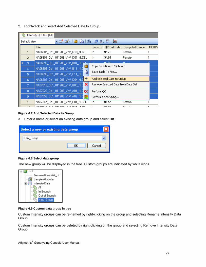
Affymetrix® Genotyping Console User Manual 77
2. Right-click and select Add Selected Data to Group.
Figure 6.7 Add Selected Data to Group
3. Enter a name or select an existing data group and select OK.
Figure 6.8 Select data group
The new group will be displayed in the tree. Custom groups are indicated by white icons.
Figure 6.9 Custom data group in tree
Custom Intensity groups can be re-named by right-clicking on the group and selecting Rename Intensity Data Group.
Custom Intensity groups can be deleted by right-clicking on the group and selecting Remove Intensity Data Group.
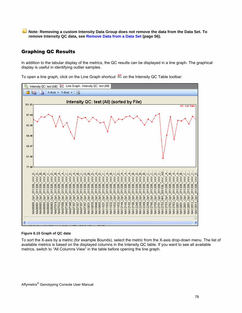
Affymetrix® Genotyping Console User Manual 78
Note: Removing a custom Intensity Data Group does not remove the data from the Data Set. To remove Intensity QC data, see Remove Data from a Data Set (page 56).
Graphing QC Results
In addition to the tabular display of the metrics, the QC results can be displayed in a line graph. The graphical display is useful in identifying outlier samples.
To open a line graph, click on the Line Graph shortcut on the Intensity QC Table toolbar:
Figure 6.10 Graph of QC data
To sort the X-axis by a metric (for example Bounds), select the metric from the X-axis drop-down menu. The list of available metrics is based on the displayed columns in the Intensity QC table. If you want to see all available metrics, switch to “All Columns View” in the table before opening the line graph.
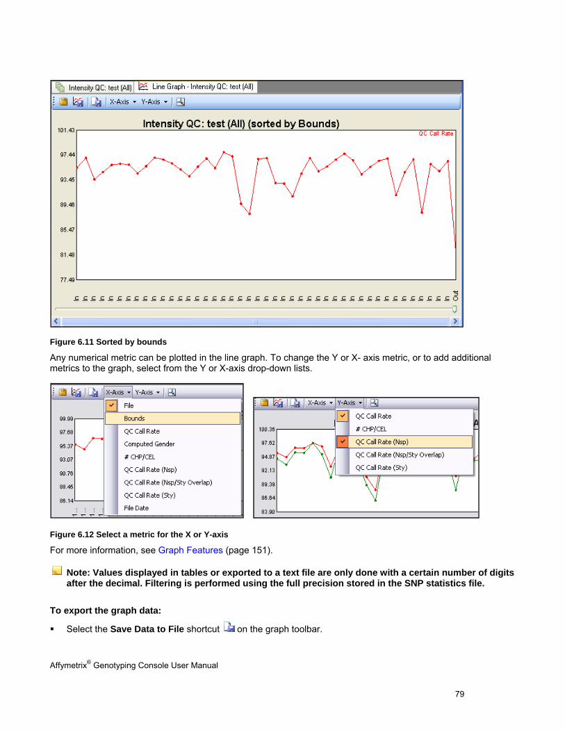
Affymetrix® Genotyping Console User Manual 79
Figure 6.11 Sorted by bounds
Any numerical metric can be plotted in the line graph. To change the Y or X- axis metric, or to add additional metrics to the graph, select from the Y or X-axis drop-down lists.
Figure 6.12 Select a metric for the X or Y-axis
For more information, see Graph Features (page 151).
Note: Values displayed in tables or exported to a text file are only done with a certain number of digits after the decimal. Filtering is performed using the full precision stored in the SNP statistics file.
To export the graph data:
Select the Save Data to File shortcut on the graph toolbar.
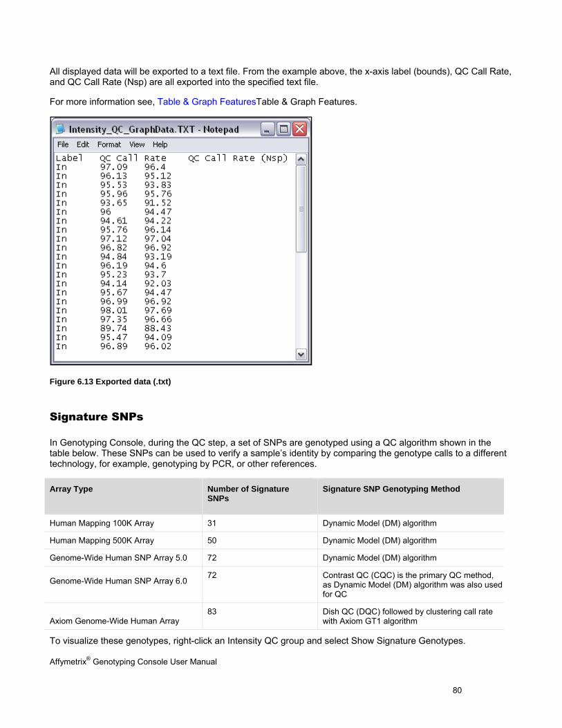
Affymetrix® Genotyping Console User Manual 80
All displayed data will be exported to a text file. From the example above, the x-axis label (bounds), QC Call Rate, and QC Call Rate (Nsp) are all exported into the specified text file.
For more information see, Table & Graph FeaturesTable & Graph Features.
Figure 6.13 Exported data (.txt)
Signature SNPs
In Genotyping Console, during the QC step, a set of SNPs are genotyped using a QC algorithm shown in the table below. These SNPs can be used to verify a sample’s identity by comparing the genotype calls to a different technology, for example, genotyping by PCR, or other references.
Array Type Number of Signature SNPs
Signature SNP Genotyping Method
Human Mapping 100K Array 31 Dynamic Model (DM) algorithm
Human Mapping 500K Array 50 Dynamic Model (DM) algorithm
Genome-Wide Human SNP Array 5.0 72 Dynamic Model (DM) algorithm
Genome-Wide Human SNP Array 6.0
72 Contrast QC (CQC) is the primary QC method, as Dynamic Model (DM) algorithm was also used for QC
Axiom Genome-Wide Human Array 83 Dish QC (DQC) followed by clustering call rate
with Axiom GT1 algorithm
To visualize these genotypes, right-click an Intensity QC group and select Show Signature Genotypes.
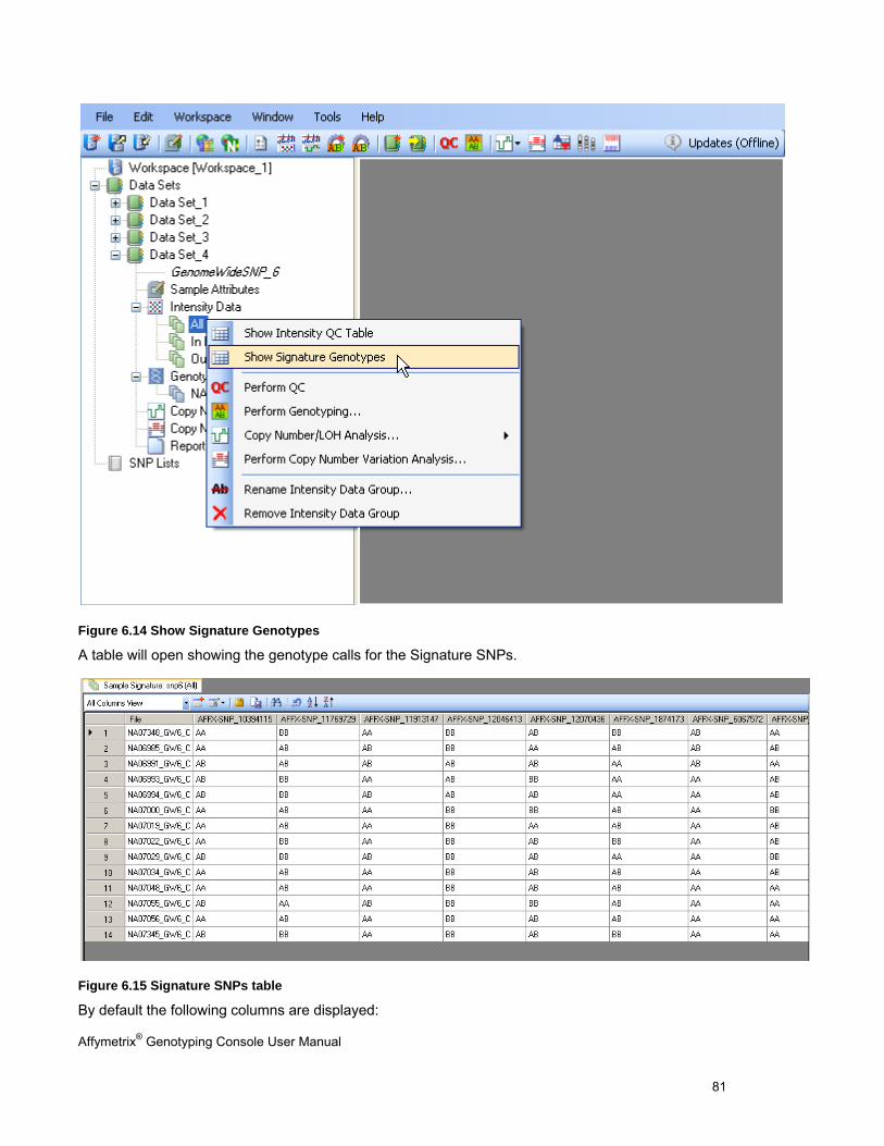
Affymetrix® Genotyping Console User Manual 81
Figure 6.14 Show Signature Genotypes
A table will open showing the genotype calls for the Signature SNPs.
Figure 6.15 Signature SNPs table
By default the following columns are displayed:

Affymetrix® Genotyping Console User Manual 82
File - file name
AFFX-SNP_# - Probe set ID for signature SNP
Annotations for these signature SNPs can be obtained either from NetAffx, or by first importing a custom SNP list containing the listed Probe Set IDs. For more information on displaying data in the Signature Genotypes Table see Table and Graph Features (page 144).
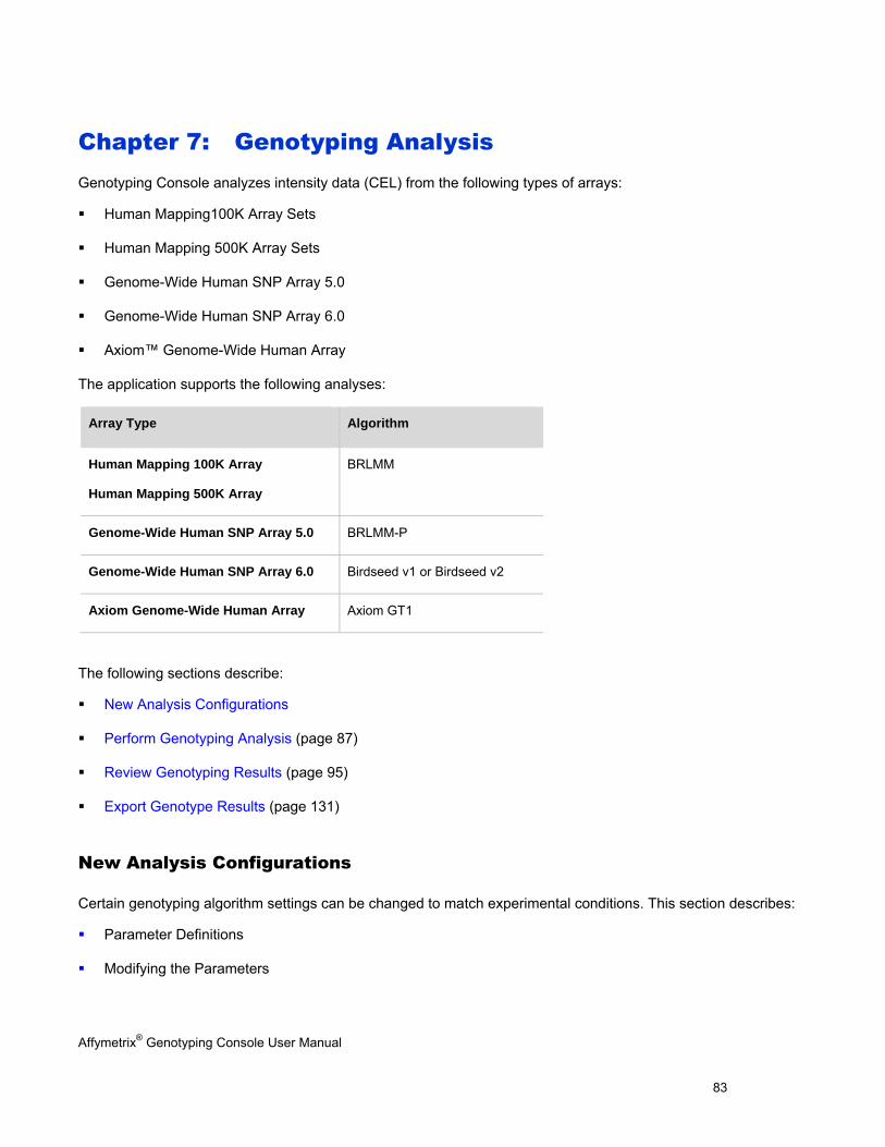
Affymetrix® Genotyping Console User Manual 83
Chapter 7: Genotyping Analysis Genotyping Console analyzes intensity data (CEL) from the following types of arrays:
Human Mapping100K Array Sets
Human Mapping 500K Array Sets
Genome-Wide Human SNP Array 5.0
Genome-Wide Human SNP Array 6.0
Axiom™ Genome-Wide Human Array
The application supports the following analyses:
The following sections describe:
New Analysis Configurations
Perform Genotyping Analysis (page 87)
Review Genotyping Results (page 95)
Export Genotype Results (page 131)
New Analysis Configurations
Certain genotyping algorithm settings can be changed to match experimental conditions. This section describes:
Parameter Definitions
Modifying the Parameters
Array Type Algorithm
Human Mapping 100K Array
Human Mapping 500K Array
BRLMM
Genome-Wide Human SNP Array 5.0 BRLMM-P
Genome-Wide Human SNP Array 6.0 Birdseed v1 or Birdseed v2
Axiom Genome-Wide Human Array Axiom GT1
Affymetrix® Genotyping Console User Manual 84
Parameter Definitions
Parameters for Human Mapping 100K/500K Arrays, Genome-Wide Human SNP Array 5.0/6.0, & Axiom™ Genome-Wide Human Array
Score/Confidence Threshold – The maximum value of confidence for which the algorithm will make a genotype call. Calls with confidence scores less than the threshold are assigned a call. For example, if the threshold is 0.15, then any SNP with confidence < 0.15 is called, and any SNP with confidence > 0.15 is not called. If the threshold is increased (maximum = 1), then additional SNPs in which there is less confidence (higher confidence score) will be called.
Parameters for Human Mapping 100K/500K Arrays only
In addition to the parameters above, the following parameters can be set for 100K/500K array data:
Prior Size – How many probe sets to use for determining prior.
DM Threshold – DM confidence threshold used for seeding clusters.
Modifying the Parameters
To modify the default algorithm settings:
1. Select the New Genotyping Configuration shortcut on the main toolbar, or
From the Edit menu, select Genotyping Configurations > New Configuration.
The Select Probe Array Type dialog box opens.
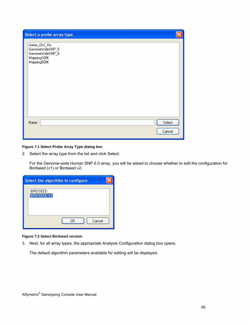
Affymetrix® Genotyping Console User Manual 85
Figure 7.1 Select Probe Array Type dialog box
2. Select the array type from the list and click Select.
For the Genome-wide Human SNP 6.0 array, you will be asked to choose whether to edit the configuration for Birdseed (v1) or Birdseed v2.
Figure 7.2 Select Birdseed version
3. Next, for all array types, the appropriate Analysis Configuration dialog box opens.
The default algorithm parameters available for editing will be displayed.
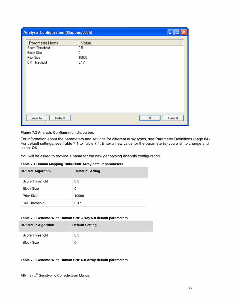
Affymetrix® Genotyping Console User Manual 86
Figure 7.3 Analysis Configuration dialog box
For information about the parameters and settings for different array types, see Parameter Definitions (page 84). For default settings, see Table 7.1 to Table 7.4. Enter a new value for the parameter(s) you wish to change and select OK.
You will be asked to provide a name for the new genotyping analysis configuration.
Table 7.1 Human Mapping 100K/500K Array default parameters
BRLMM Algorithm Default Setting
Table 7.2 Genome-Wide Human SNP Array 5.0 default parameters
BRLMM-P Algorithm Default Setting
Table 7.3 Genome-Wide Human SNP 6.0 Array default parameters
Score Threshold 0.5
Block Size 0
Prior Size 10000
DM Threshold 0.17
Score Threshold 0.5
Block Size 0
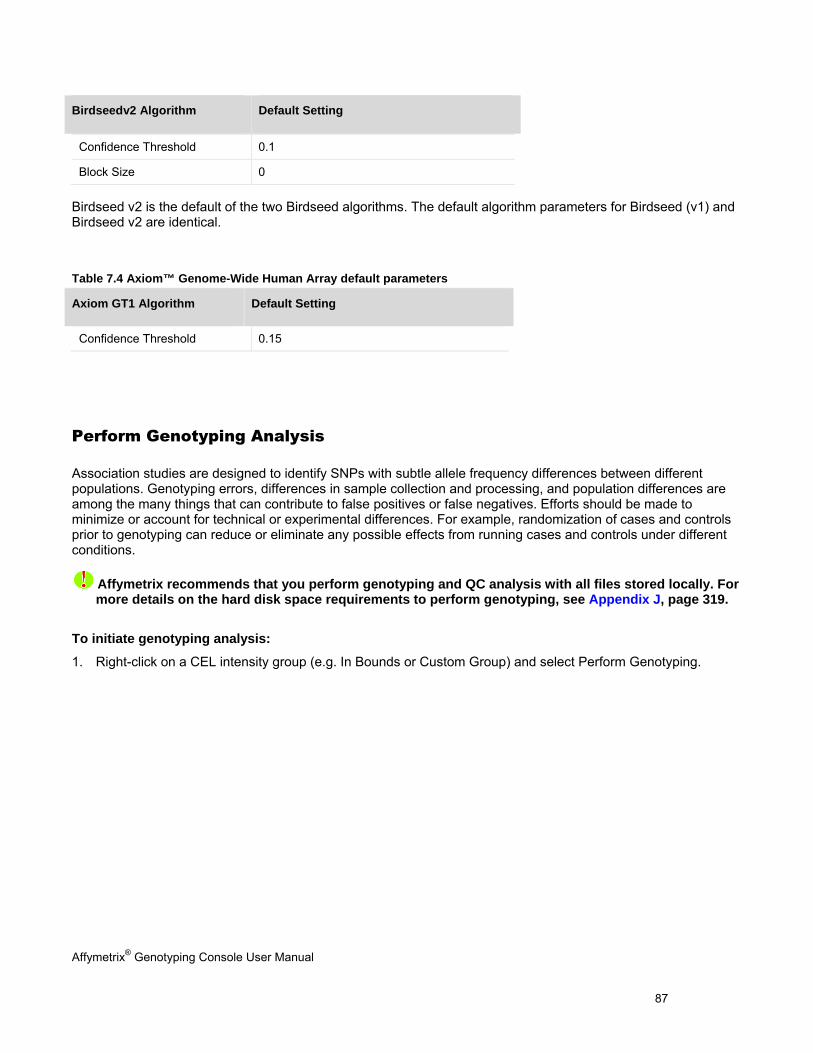
Affymetrix® Genotyping Console User Manual 87
Birdseedv2 Algorithm Default Setting
Birdseed v2 is the default of the two Birdseed algorithms. The default algorithm parameters for Birdseed (v1) and Birdseed v2 are identical.
Table 7.4 Axiom™ Genome-Wide Human Array default parameters
Axiom GT1 Algorithm Default Setting
Perform Genotyping Analysis
Association studies are designed to identify SNPs with subtle allele frequency differences between different populations. Genotyping errors, differences in sample collection and processing, and population differences are among the many things that can contribute to false positives or false negatives. Efforts should be made to minimize or account for technical or experimental differences. For example, randomization of cases and controls prior to genotyping can reduce or eliminate any possible effects from running cases and controls under different conditions.
Affymetrix recommends that you perform genotyping and QC analysis with all files stored locally. For more details on the hard disk space requirements to perform genotyping, see Appendix J, page 319.
To initiate genotyping analysis:
1. Right-click on a CEL intensity group (e.g. In Bounds or Custom Group) and select Perform Genotyping.
Confidence Threshold 0.1
Block Size 0
Confidence Threshold 0.15
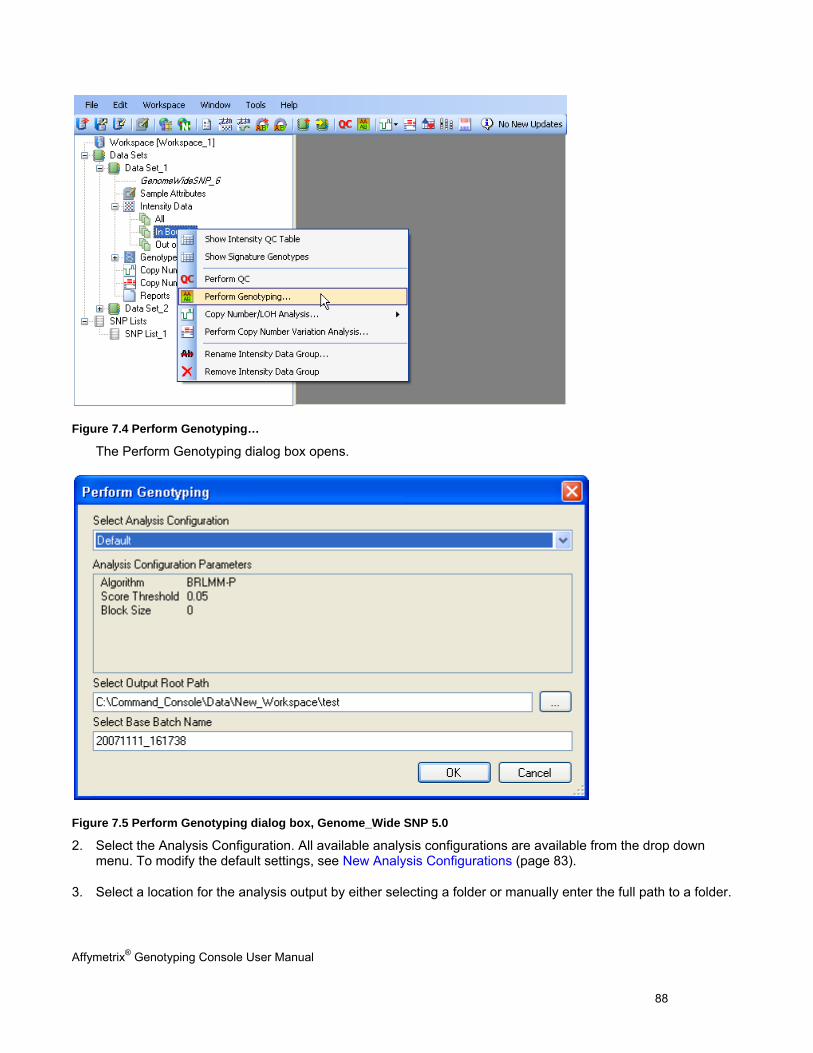
Affymetrix® Genotyping Console User Manual 88
Figure 7.4 Perform Genotyping…
The Perform Genotyping dialog box opens.
Figure 7.5 Perform Genotyping dialog box, Genome_Wide SNP 5.0
2. Select the Analysis Configuration. All available analysis configurations are available from the drop down menu. To modify the default settings, see New Analysis Configurations (page 83).
3. Select a location for the analysis output by either selecting a folder or manually enter the full path to a folder.
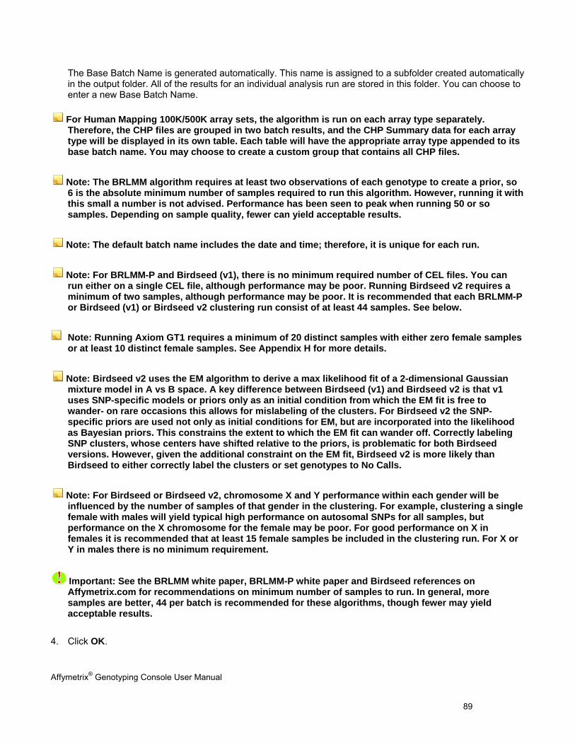
Affymetrix® Genotyping Console User Manual 89
The Base Batch Name is generated automatically. This name is assigned to a subfolder created automatically in the output folder. All of the results for an individual analysis run are stored in this folder. You can choose to enter a new Base Batch Name.
For Human Mapping 100K/500K array sets, the algorithm is run on each array type separately. Therefore, the CHP files are grouped in two batch results, and the CHP Summary data for each array type will be displayed in its own table. Each table will have the appropriate array type appended to its base batch name. You may choose to create a custom group that contains all CHP files.
Note: The BRLMM algorithm requires at least two observations of each genotype to create a prior, so 6 is the absolute minimum number of samples required to run this algorithm. However, running it with this small a number is not advised. Performance has been seen to peak when running 50 or so samples. Depending on sample quality, fewer can yield acceptable results.
Note: The default batch name includes the date and time; therefore, it is unique for each run.
Note: For BRLMM-P and Birdseed (v1), there is no minimum required number of CEL files. You can run either on a single CEL file, although performance may be poor. Running Birdseed v2 requires a minimum of two samples, although performance may be poor. It is recommended that each BRLMM-P or Birdseed (v1) or Birdseed v2 clustering run consist of at least 44 samples. See below.
Note: Running Axiom GT1 requires a minimum of 20 distinct samples with either zero female samples or at least 10 distinct female samples. See Appendix H for more details.
Note: Birdseed v2 uses the EM algorithm to derive a max likelihood fit of a 2-dimensional Gaussian mixture model in A vs B space. A key difference between Birdseed (v1) and Birdseed v2 is that v1 uses SNP-specific models or priors only as an initial condition from which the EM fit is free to wander- on rare occasions this allows for mislabeling of the clusters. For Birdseed v2 the SNP-specific priors are used not only as initial conditions for EM, but are incorporated into the likelihood as Bayesian priors. This constrains the extent to which the EM fit can wander off. Correctly labeling SNP clusters, whose centers have shifted relative to the priors, is problematic for both Birdseed versions. However, given the additional constraint on the EM fit, Birdseed v2 is more likely than Birdseed to either correctly label the clusters or set genotypes to No Calls.
Note: For Birdseed or Birdseed v2, chromosome X and Y performance within each gender will be influenced by the number of samples of that gender in the clustering. For example, clustering a single female with males will yield typical high performance on autosomal SNPs for all samples, but performance on the X chromosome for the female may be poor. For good performance on X in females it is recommended that at least 15 female samples be included in the clustering run. For X or Y in males there is no minimum requirement.
Important: See the BRLMM white paper, BRLMM-P white paper and Birdseed references on Affymetrix.com for recommendations on minimum number of samples to run. In general, more samples are better, 44 per batch is recommended for these algorithms, though fewer may yield acceptable results.
4. Click OK.
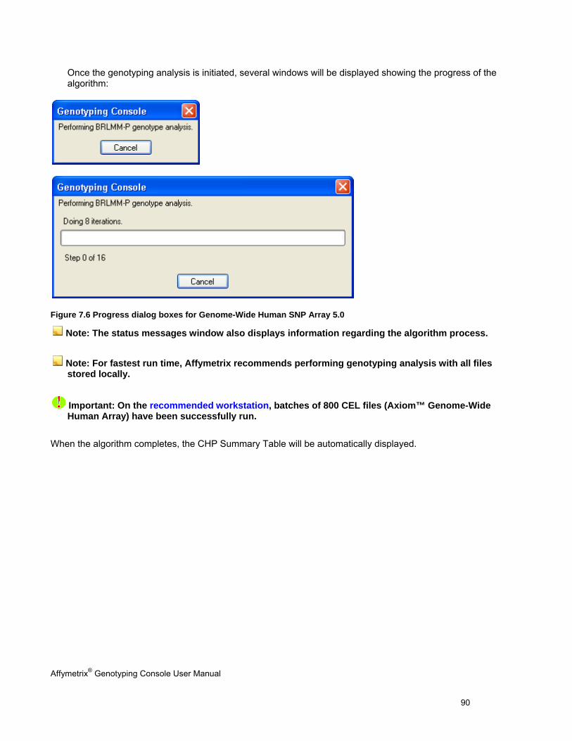
Affymetrix® Genotyping Console User Manual 90
Once the genotyping analysis is initiated, several windows will be displayed showing the progress of the algorithm:
Figure 7.6 Progress dialog boxes for Genome-Wide Human SNP Array 5.0
Note: The status messages window also displays information regarding the algorithm process.
Note: For fastest run time, Affymetrix recommends performing genotyping analysis with all files stored locally.
Important: On the recommended workstation, batches of 800 CEL files (Axiom™ Genome-Wide Human Array) have been successfully run.
When the algorithm completes, the CHP Summary Table will be automatically displayed.
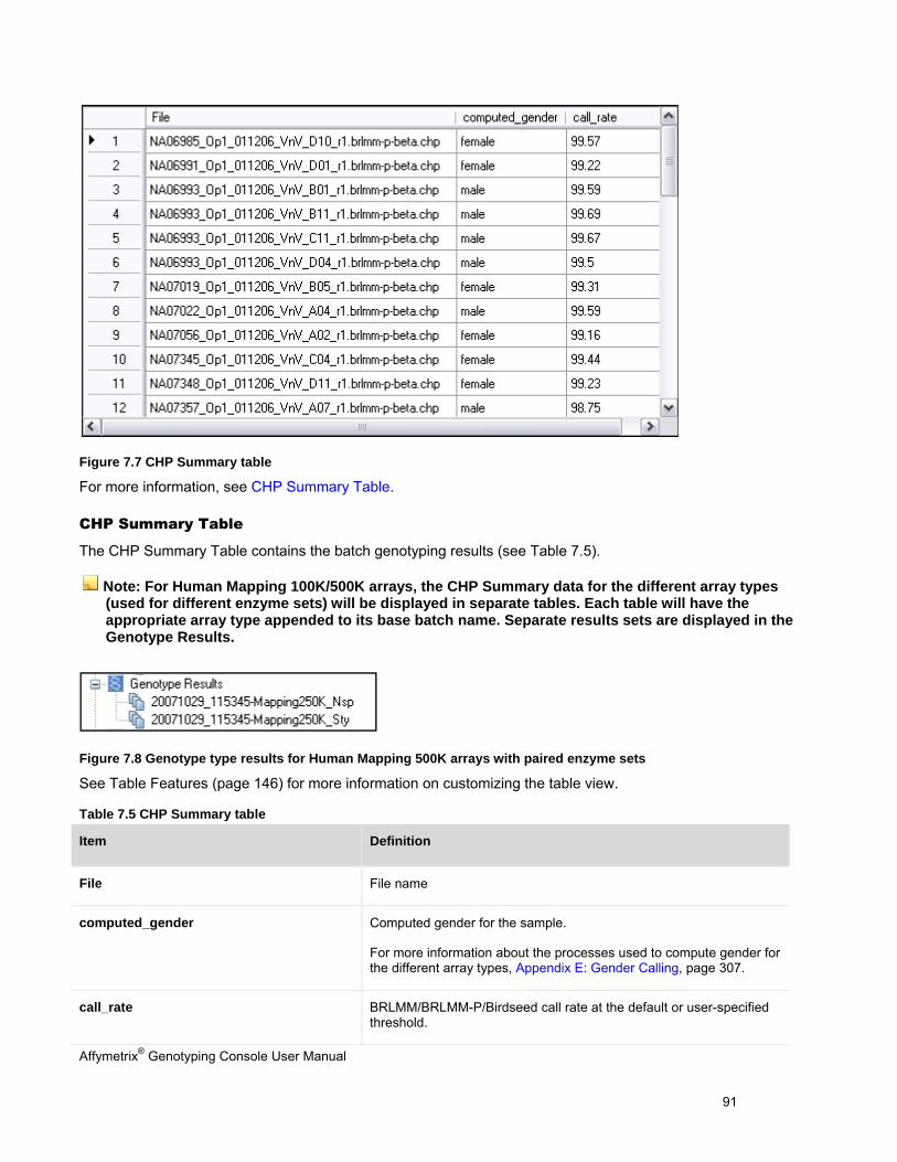
Affymetrix® Genotyping Console User Manual 91
Figure 7.7 CHP Summary table
For more information, see CHP Summary Table.
CHP Summary Table
The CHP Summary Table contains the batch genotyping results (see Table 7.5).
Note: For Human Mapping 100K/500K arrays, the CHP Summary data for the different array types (used for different enzyme sets) will be displayed in separate tables. Each table will have the appropriate array type appended to its base batch name. Separate results sets are displayed in the Genotype Results.
Figure 7.8 Genotype type results for Human Mapping 500K arrays with paired enzyme sets
See Table Features (page 146) for more information on customizing the table view.
Table 7.5 CHP Summary table
Item Definition
File File name
computed_gender Computed gender for the sample.
For more information about the processes used to compute gender for the different array types, Appendix E: Gender Calling, page 307.
call_rate BRLMM/BRLMM-P/Birdseed call rate at the default or user-specified threshold.
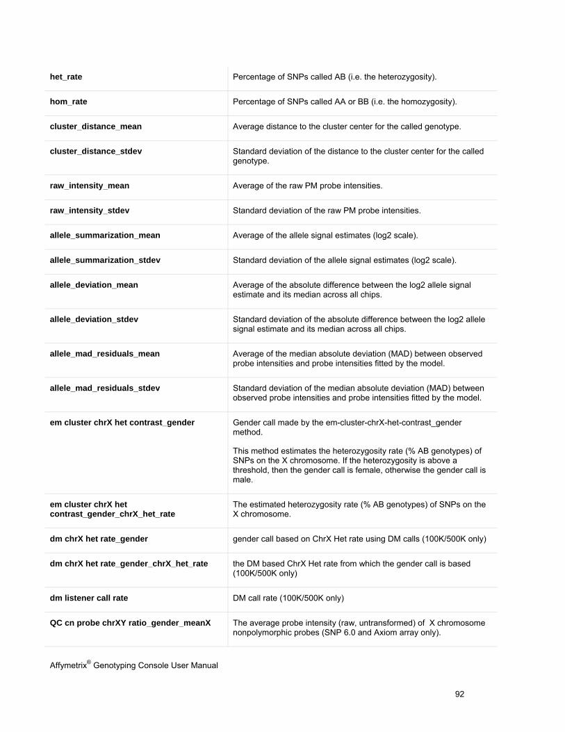
Affymetrix® Genotyping Console User Manual 92
het_rate Percentage of SNPs called AB (i.e. the heterozygosity).
hom_rate Percentage of SNPs called AA or BB (i.e. the homozygosity).
cluster_distance_mean Average distance to the cluster center for the called genotype.
cluster_distance_stdev Standard deviation of the distance to the cluster center for the called genotype.
raw_intensity_mean Average of the raw PM probe intensities.
raw_intensity_stdev Standard deviation of the raw PM probe intensities.
allele_summarization_mean Average of the allele signal estimates (log2 scale).
allele_summarization_stdev Standard deviation of the allele signal estimates (log2 scale).
allele_deviation_mean Average of the absolute difference between the log2 allele signal estimate and its median across all chips.
allele_deviation_stdev Standard deviation of the absolute difference between the log2 allele signal estimate and its median across all chips.
allele_mad_residuals_mean Average of the median absolute deviation (MAD) between observed probe intensities and probe intensities fitted by the model.
allele_mad_residuals_stdev Standard deviation of the median absolute deviation (MAD) between observed probe intensities and probe intensities fitted by the model.
em cluster chrX het contrast_gender Gender call made by the em-cluster-chrX-het-contrast_gender method.
This method estimates the heterozygosity rate (% AB genotypes) of SNPs on the X chromosome. If the heterozygosity is above a threshold, then the gender call is female, otherwise the gender call is male.
em cluster chrX het contrast_gender_chrX_het_rate
The estimated heterozygosity rate (% AB genotypes) of SNPs on the X chromosome.
dm chrX het rate_gender gender call based on ChrX Het rate using DM calls (100K/500K only)
dm chrX het rate_gender_chrX_het_rate the DM based ChrX Het rate from which the gender call is based (100K/500K only)
dm listener call rate DM call rate (100K/500K only)
QC cn probe chrXY ratio_gender_meanX The average probe intensity (raw, untransformed) of X chromosome nonpolymorphic probes (SNP 6.0 and Axiom array only).
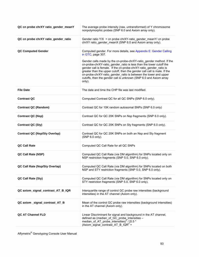
Affymetrix® Genotyping Console User Manual 93
QC cn probe chrXY ratio_gender_meanY The average probe intensity (raw, untransformed) of Y chromosome nonpolymorphic probes (SNP 6.0 and Axiom array only).
QC cn probe chrXY ratio_gender_ratio Gender ratio Y/X = cn probe chrXY-ratio_gender_meanY/ cn probe chrXY ratio_gender_meanX (SNP 6.0 and Axiom array only).
QC Computed Gender Computed gender. For more details, see Appendix E: Gender Calling in GTC, page 307.
Gender calls made by the cn-probe-chrXY-ratio_gender method. If the cn-probe-chrXY-ratio_gender_ratio is less than the lower cutoff the gender call is female. If the cn-probe-chrXY-ratio_gender_ratio is greater than the upper cutoff, then the gender call call is male. If the cn-probe-chrXY-ratio_gender_ratio is between the lower and upper cutoffs, then the gender call is unknown (SNP 6.0 and Axiom array only).
File Date The date and time the CHP file was last modified.
Contrast QC Computed Contrast QC for all QC SNPs (SNP 6.0 only).
Contrast QC (Random) Contrast QC for 10K random autosomal SNPs (SNP 6.0 only)
Contrast QC (Nsp) Contrast QC for QC 20K SNPs on Nsp fragments (SNP 6.0 only).
Contrast QC (Sty) Contrast QC for QC 20K SNPs on Sty fragments (SNP 6.0 only).
Contrast QC (Nsp/Sty Overlap) Contrast QC for QC 20K SNPs on both an Nsp and Sty fragment (SNP 6.0 only).
QC Call Rate Computed QC Call Rate for all QC SNPs
QC Call Rate (NSP) Computed QC Call Rate (via DM algorithm) for SNPs located only on NSP restriction fragments (SNP 5.0, SNP 6.0 only).
QC Call Rate (Nsp/Sty Overlap) Computed QC Call Rate (via DM algorithm) for SNPs located on both NSP and STY restriction fragments (SNP 5.0, SNP 6.0 only).
QC Call Rate (Sty) Computed QC Call Rate (via DM algorithm) for SNPs located only on STY restriction fragments (SNP 5.0, SNP 6.0 only).
QC axiom_signal_contrast_AT_B_IQR Interquartile range of control GC probe raw intensities (background intensities) in the AT channel (Axiom only).
QC axiom _signal_contrast_AT_B Mean of the control GC probe raw intensities (background intensities) in the AT channel (Axiom only).
QC AT Channel FLD Linear Discriminant for signal and background in the AT channel, defined as (median_of_GC_probe_intensities – median_of_AT_probe_intensities)2 / [0.5 * (Axiom_signal_contrast_AT_B_IQR2 +
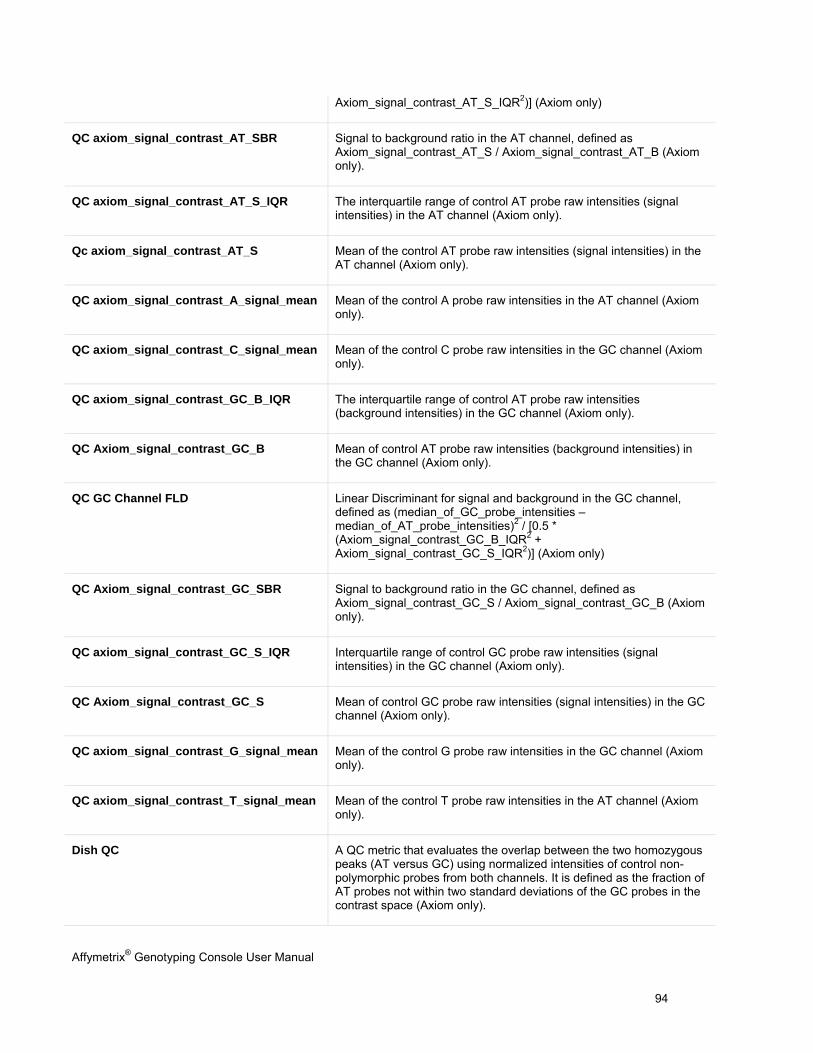
Affymetrix® Genotyping Console User Manual 94
Axiom_signal_contrast_AT_S_IQR2)] (Axiom only)
QC axiom_signal_contrast_AT_SBR Signal to background ratio in the AT channel, defined as Axiom_signal_contrast_AT_S / Axiom_signal_contrast_AT_B (Axiom only).
QC axiom_signal_contrast_AT_S_IQR The interquartile range of control AT probe raw intensities (signal intensities) in the AT channel (Axiom only).
Qc axiom_signal_contrast_AT_S Mean of the control AT probe raw intensities (signal intensities) in the AT channel (Axiom only).
QC axiom_signal_contrast_A_signal_mean Mean of the control A probe raw intensities in the AT channel (Axiom only).
QC axiom_signal_contrast_C_signal_mean Mean of the control C probe raw intensities in the GC channel (Axiom only).
QC axiom_signal_contrast_GC_B_IQR The interquartile range of control AT probe raw intensities (background intensities) in the GC channel (Axiom only).
QC Axiom_signal_contrast_GC_B Mean of control AT probe raw intensities (background intensities) in the GC channel (Axiom only).
QC GC Channel FLD Linear Discriminant for signal and background in the GC channel, defined as (median_of_GC_probe_intensities – median_of_AT_probe_intensities)2 / [0.5 * (Axiom_signal_contrast_GC_B_IQR2 + Axiom_signal_contrast_GC_S_IQR2)] (Axiom only)
QC Axiom_signal_contrast_GC_SBR Signal to background ratio in the GC channel, defined as Axiom_signal_contrast_GC_S / Axiom_signal_contrast_GC_B (Axiom only).
QC axiom_signal_contrast_GC_S_IQR Interquartile range of control GC probe raw intensities (signal intensities) in the GC channel (Axiom only).
QC Axiom_signal_contrast_GC_S Mean of control GC probe raw intensities (signal intensities) in the GC channel (Axiom only).
QC axiom_signal_contrast_G_signal_mean Mean of the control G probe raw intensities in the GC channel (Axiom only).
QC axiom_signal_contrast_T_signal_mean Mean of the control T probe raw intensities in the AT channel (Axiom only).
Dish QC A QC metric that evaluates the overlap between the two homozygous peaks (AT versus GC) using normalized intensities of control non-polymorphic probes from both channels. It is defined as the fraction of AT probes not within two standard deviations of the GC probes in the contrast space (Axiom only).
Affymetrix® Genotyping Console User Manual 95
Log Difference QC A cross channel QC metric, defined as mean(log(AT_SBR))/std(log(AT_SBR)) + mean(log(GC_SBR))/std(log(GC_SBR)), where signal and background are calculated for control non-polymorphic probes after intensity normalization (Axiom only)
QC axiom_varscore_CV_GC Median of the coefficient of variation for each control GC probe set in the GC channel (Axiom only).
QC axiom_varscore_CV_AT Median of the coefficient of variation for each control AT probe set in the AT channel (Axiom only).
For more information on displaying data in the CHP Summary Table see Table and Graph Features (page 146).
In addition to the tabular display of the metrics, the CHP results can be displayed in a line graph.
To open a line graph:
Click the line graph shortcut on the CHP Summary table toolbar.
The available features for this line graph are the same as in the Graphing QC Results section (page 78).
Review the Genotyping Results
Before conducting downstream analysis of genotyping results it is essential to perform thorough QC of both SNPs and samples. There is no single ‘best’ way to do the QC, but some steps that are generally helpful in a broad range of circumstances are outlined below.
1. Per-sample QC filtering
Pre-clustering
- Samples failing the per-chip QC metric should be excluded prior to clustering, as described in Chapter 6: Quality Control for Genotyping Analysis (page 67).
- Sample swaps which may have occurred during handling should be identified and resolved or removed. One way to do this is to generate a ‘fingerprint’ by typing all samples on a subset of a dozen or more SNPs which intersect with the SNPs reported in the Signature SNPs (page 80). Another is to use known pedigree information (where appropriate) to confirm expected relatedness patterns.
Post-clustering
- Remove samples with outlier clustering call rates or heterozygosity (which will tend to be low-performing samples that escaped the QC call rate filter).
- Depending on the downstream analysis to be applied, consider identifying any cryptic relatedness and removing related samples.
- Depending on the downstream analysis to be applied, consider controlling for population structure possibly be removing samples that are clearly from different populations from the bulk of the collection.
2. Per-SNP QC filtering
Affymetrix® Genotyping Console User Manual 96
Remove SNPs with per-SNP call rates (sometimes referred to as completeness) less than some threshold. Commonly-used values for the per-SNP call rate threshold range from 90% to 95%.
Consider removing SNPs with minor allele frequency (MAF) below a certain threshold (for example, 1%).
Depending on circumstances, consider removing SNPs significantly out of Hardy Weinberg equilibrium in cases and/or controls. A p-value threshold in the range of 10-7 is sometimes used.
Once the genotyping results are generated, you can:
Display SNP Summary Table (page 96)
Display Custom Groups of Genotyping Results (page 101)
Create SNP Lists (page 103)
Import SNP Lists (page 107)
Display SNP Cluster Graph (page 109)
Save All SNP Cluster Graphs to PDF File (page 118)
SNP Summary Table
Important: you cannot display the SNP Summary Table until you have created a SNP list. See Create a SNP List (page 103) for more information.
The SNP Summary Table contains SNP level statistics based on the batch of CHP files.
To open, right-click on a batch and select Show SNP Summary Table.
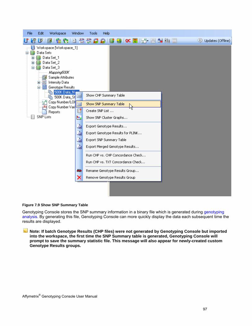
Affymetrix® Genotyping Console User Manual 97
Figure 7.9 Show SNP Summary Table
Genotyping Console stores the SNP summary information in a binary file which is generated during genotyping analysis. By generating this file, Genotyping Console can more quickly display the data each subsequent time the results are displayed.
Note: If batch Genotype Results (CHP files) were not generated by Genotyping Console but imported into the workspace, the first time the SNP Summary table is generated, Genotyping Console will prompt to save the summary statistic file. This message will also appear for newly-created custom Genotype Results groups.
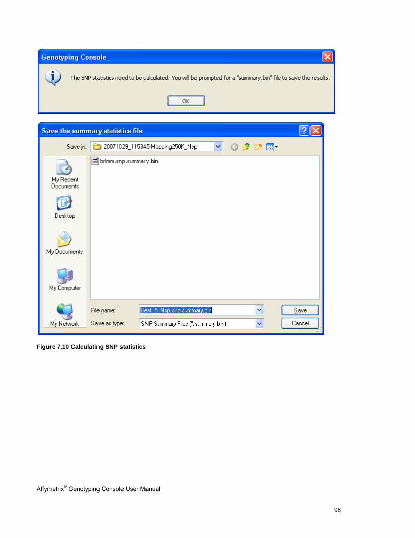
Affymetrix® Genotyping Console User Manual 98
Figure 7.10 Calculating SNP statistics
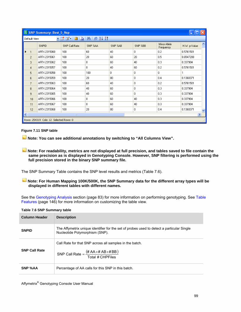
Affymetrix® Genotyping Console User Manual 99
Figure 7.11 SNP table
Note: You can see additional annotations by switching to “All Columns View”.
Note: For readability, metrics are not displayed at full precision, and tables saved to file contain the same precision as is displayed in Genotyping Console. However, SNP filtering is performed using the full precision stored in the binary SNP summary file.
The SNP Summary Table contains the SNP level results and metrics (Table 7.6).
Note: For Human Mapping 100K/500K, the SNP Summary data for the different array types will be displayed in different tables with different names.
See the Genotyping Analysis section (page 83) for more information on performing genotyping. See Table Features (page 146) for more information on customizing the table view.
Table 7.6 SNP Summary table
Column Header Description
SNPID The Affymetrix unique identifier for the set of probes used to detect a particular Single Nucleotide Polymorphism (SNP).
SNP Call Rate
Call Rate for that SNP across all samples in the batch.
( )CHPFiles #Total
BB#AB#AA# Rate Call SNP ++=
SNP %AA Percentage of AA calls for this SNP in this batch.
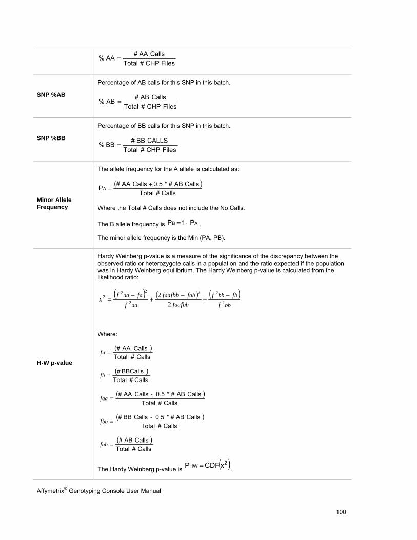
Affymetrix® Genotyping Console User Manual 100
Files CHP #TotalCalls AA # AA% =
SNP %AB
Percentage of AB calls for this SNP in this batch.
Files CHP #TotalCalls AB# AB% =
SNP %BB
Percentage of BB calls for this SNP in this batch.
Files CHP #TotalCALLS BB #BB % =
Minor Allele Frequency
The allele frequency for the A allele is calculated as:
( )Calls #Total
Calls AB #* 0.5Calls AA #PA+=
Where the Total # Calls does not include the No Calls.
The B allele frequency is AB P1P −= .
The minor allele frequency is the Min (PA, PB).
H-W p-value
Hardy Weinberg p-value is a measure of the significance of the discrepancy between the observed ratio or heterozygote calls in a population and the ratio expected if the population was in Hardy Weinberg equilibrium. The Hardy Weinberg p-value is calculated from the likelihood ratio:
( ) ( ) ( )bb
bbbbbaa
abaa
aa
aaa
fff
ffffbbf
fffx 2
22
2
222
22 −+−+−=
Where:
( )Calls #Total
Calls AA #=af
( )Calls #Total
BBCalls#=bf
( )Calls #Total
Calls AB #* 0.5Calls AA # +=aaf
( )Calls #Total
Calls AB #* 0.5Calls BB # +=bbf
( )Calls #Total
Calls AB#=abf
The Hardy Weinberg p-value is ( )2HW xCDFP = .
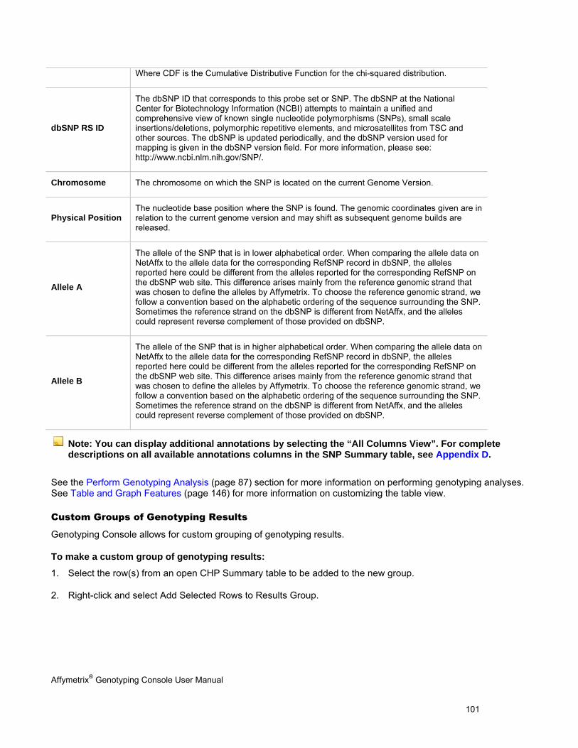
Affymetrix® Genotyping Console User Manual 101
Where CDF is the Cumulative Distributive Function for the chi-squared distribution.
dbSNP RS ID
The dbSNP ID that corresponds to this probe set or SNP. The dbSNP at the National Center for Biotechnology Information (NCBI) attempts to maintain a unified and comprehensive view of known single nucleotide polymorphisms (SNPs), small scale insertions/deletions, polymorphic repetitive elements, and microsatellites from TSC and other sources. The dbSNP is updated periodically, and the dbSNP version used for mapping is given in the dbSNP version field. For more information, please see: http://www.ncbi.nlm.nih.gov/SNP/.
Chromosome The chromosome on which the SNP is located on the current Genome Version.
Physical Position The nucleotide base position where the SNP is found. The genomic coordinates given are in relation to the current genome version and may shift as subsequent genome builds are released.
Allele A
The allele of the SNP that is in lower alphabetical order. When comparing the allele data on NetAffx to the allele data for the corresponding RefSNP record in dbSNP, the alleles reported here could be different from the alleles reported for the corresponding RefSNP on the dbSNP web site. This difference arises mainly from the reference genomic strand that was chosen to define the alleles by Affymetrix. To choose the reference genomic strand, we follow a convention based on the alphabetic ordering of the sequence surrounding the SNP. Sometimes the reference strand on the dbSNP is different from NetAffx, and the alleles could represent reverse complement of those provided on dbSNP.
Allele B
The allele of the SNP that is in higher alphabetical order. When comparing the allele data on NetAffx to the allele data for the corresponding RefSNP record in dbSNP, the alleles reported here could be different from the alleles reported for the corresponding RefSNP on the dbSNP web site. This difference arises mainly from the reference genomic strand that was chosen to define the alleles by Affymetrix. To choose the reference genomic strand, we follow a convention based on the alphabetic ordering of the sequence surrounding the SNP. Sometimes the reference strand on the dbSNP is different from NetAffx, and the alleles could represent reverse complement of those provided on dbSNP.
Note: You can display additional annotations by selecting the “All Columns View”. For complete descriptions on all available annotations columns in the SNP Summary table, see Appendix D.
See the Perform Genotyping Analysis (page 87) section for more information on performing genotyping analyses. See Table and Graph Features (page 146) for more information on customizing the table view.
Custom Groups of Genotyping Results
Genotyping Console allows for custom grouping of genotyping results.
To make a custom group of genotyping results:
1. Select the row(s) from an open CHP Summary table to be added to the new group.
2. Right-click and select Add Selected Rows to Results Group.
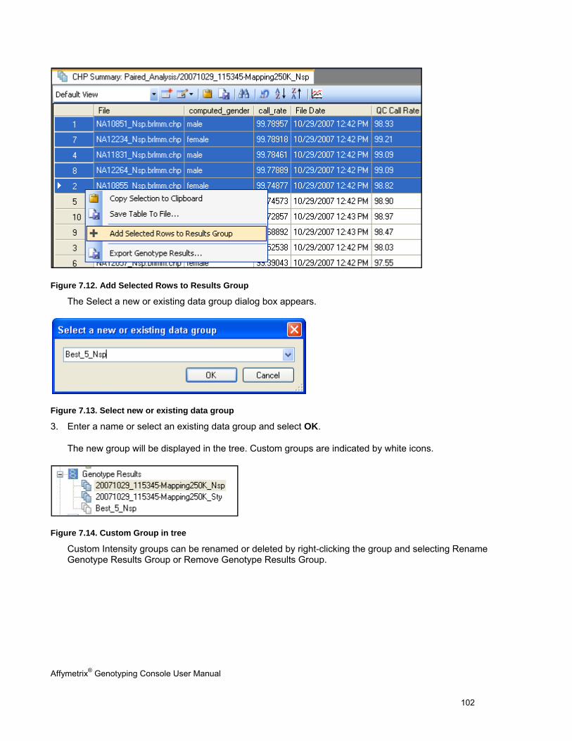
Affymetrix® Genotyping Console User Manual 102
Figure 7.12. Add Selected Rows to Results Group
The Select a new or existing data group dialog box appears.
Figure 7.13. Select new or existing data group
3. Enter a name or select an existing data group and select OK.
The new group will be displayed in the tree. Custom groups are indicated by white icons.
Figure 7.14. Custom Group in tree
Custom Intensity groups can be renamed or deleted by right-clicking the group and selecting Rename Genotype Results Group or Remove Genotype Results Group.
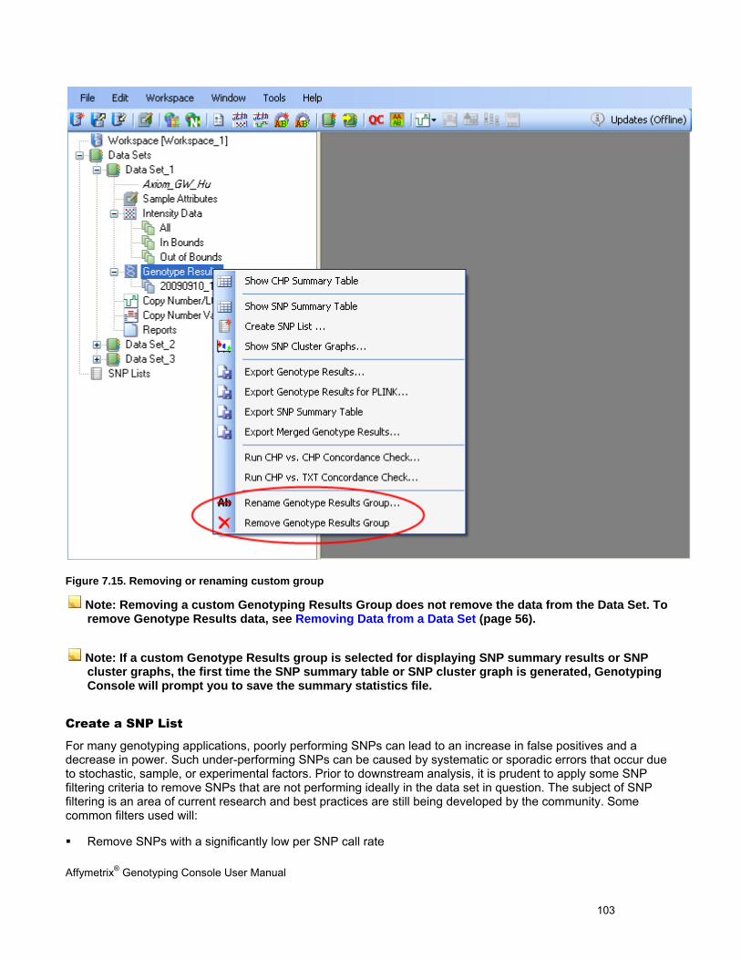
Affymetrix® Genotyping Console User Manual 103
Figure 7.15. Removing or renaming custom group
Note: Removing a custom Genotyping Results Group does not remove the data from the Data Set. To remove Genotype Results data, see Removing Data from a Data Set (page 56).
Note: If a custom Genotype Results group is selected for displaying SNP summary results or SNP cluster graphs, the first time the SNP summary table or SNP cluster graph is generated, Genotyping Console will prompt you to save the summary statistics file.
Create a SNP List
For many genotyping applications, poorly performing SNPs can lead to an increase in false positives and a decrease in power. Such under-performing SNPs can be caused by systematic or sporadic errors that occur due to stochastic, sample, or experimental factors. Prior to downstream analysis, it is prudent to apply some SNP filtering criteria to remove SNPs that are not performing ideally in the data set in question. The subject of SNP filtering is an area of current research and best practices are still being developed by the community. Some common filters used will:
Remove SNPs with a significantly low per SNP call rate
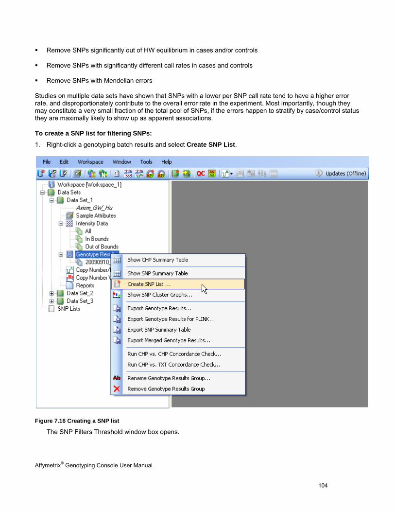
Affymetrix® Genotyping Console User Manual 104
Remove SNPs significantly out of HW equilibrium in cases and/or controls
Remove SNPs with significantly different call rates in cases and controls
Remove SNPs with Mendelian errors
Studies on multiple data sets have shown that SNPs with a lower per SNP call rate tend to have a higher error rate, and disproportionately contribute to the overall error rate in the experiment. Most importantly, though they may constitute a very small fraction of the total pool of SNPs, if the errors happen to stratify by case/control status they are maximally likely to show up as apparent associations.
To create a SNP list for filtering SNPs:
1. Right-click a genotyping batch results and select Create SNP List.
Figure 7.16 Creating a SNP list
The SNP Filters Threshold window box opens.
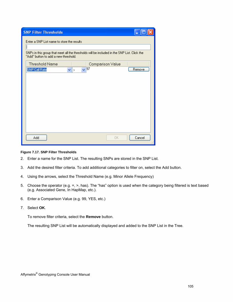
Affymetrix® Genotyping Console User Manual 105
Figure 7.17. SNP Filter Thresholds
2. Enter a name for the SNP List. The resulting SNPs are stored in the SNP List.
3. Add the desired filter criteria. To add additional categories to filter on, select the Add button.
4. Using the arrows, select the Threshold Name (e.g. Minor Allele Frequency)
5. Choose the operator (e.g. =, >, has). The “has” option is used when the category being filtered is text based (e.g. Associated Gene, In HapMap, etc.).
6. Enter a Comparison Value (e.g. 99, YES, etc.)
7. Select OK.
To remove filter criteria, select the Remove button.
The resulting SNP List will be automatically displayed and added to the SNP List in the Tree.
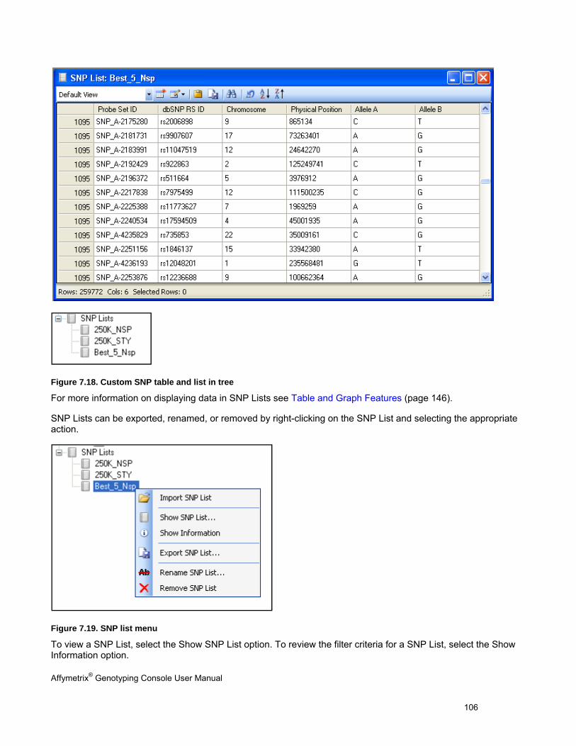
Affymetrix® Genotyping Console User Manual 106
Figure 7.18. Custom SNP table and list in tree
For more information on displaying data in SNP Lists see Table and Graph Features (page 146).
SNP Lists can be exported, renamed, or removed by right-clicking on the SNP List and selecting the appropriate action.
Figure 7.19. SNP list menu
To view a SNP List, select the Show SNP List option. To review the filter criteria for a SNP List, select the Show Information option.
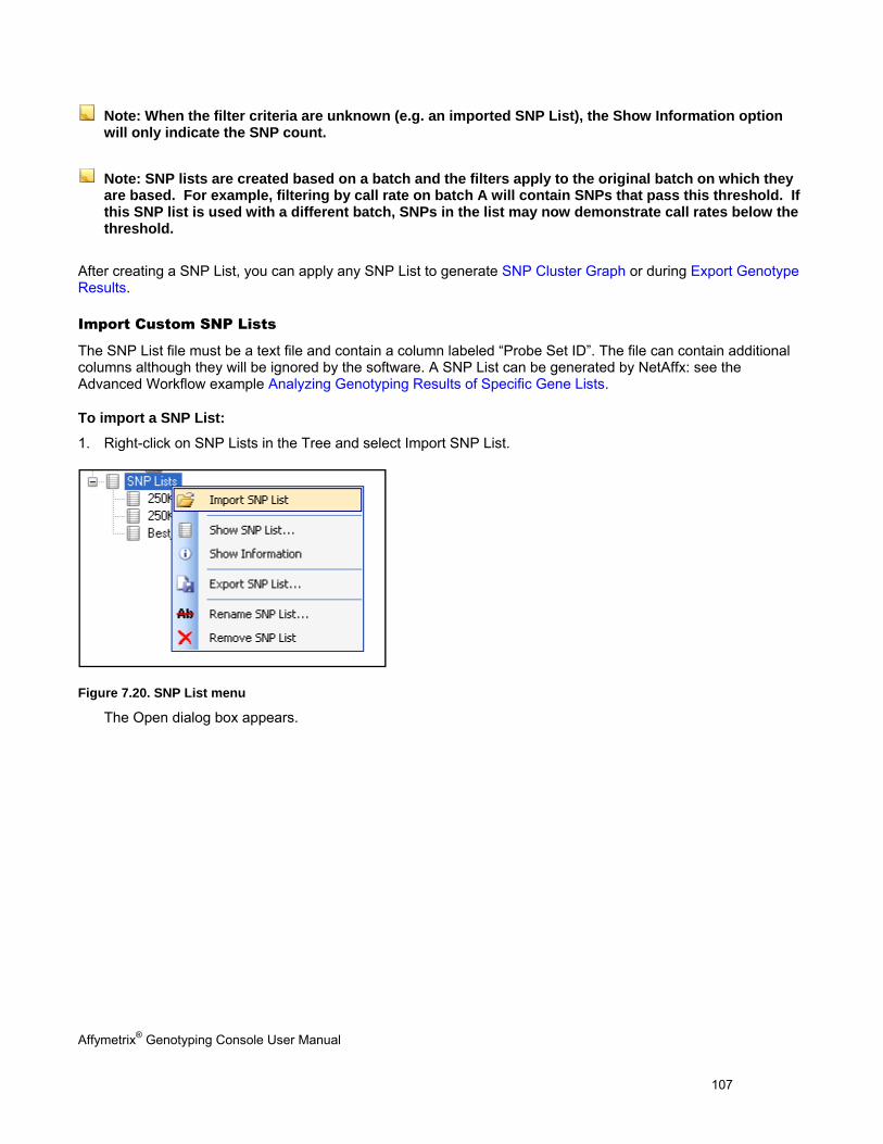
Affymetrix® Genotyping Console User Manual 107
Note: When the filter criteria are unknown (e.g. an imported SNP List), the Show Information option will only indicate the SNP count.
Note: SNP lists are created based on a batch and the filters apply to the original batch on which they are based. For example, filtering by call rate on batch A will contain SNPs that pass this threshold. If this SNP list is used with a different batch, SNPs in the list may now demonstrate call rates below the threshold.
After creating a SNP List, you can apply any SNP List to generate SNP Cluster Graph or during Export Genotype Results.
Import Custom SNP Lists
The SNP List file must be a text file and contain a column labeled “Probe Set ID”. The file can contain additional columns although they will be ignored by the software. A SNP List can be generated by NetAffx: see the Advanced Workflow example Analyzing Genotyping Results of Specific Gene Lists.
To import a SNP List:
1. Right-click on SNP Lists in the Tree and select Import SNP List.
Figure 7.20. SNP List menu
The Open dialog box appears.
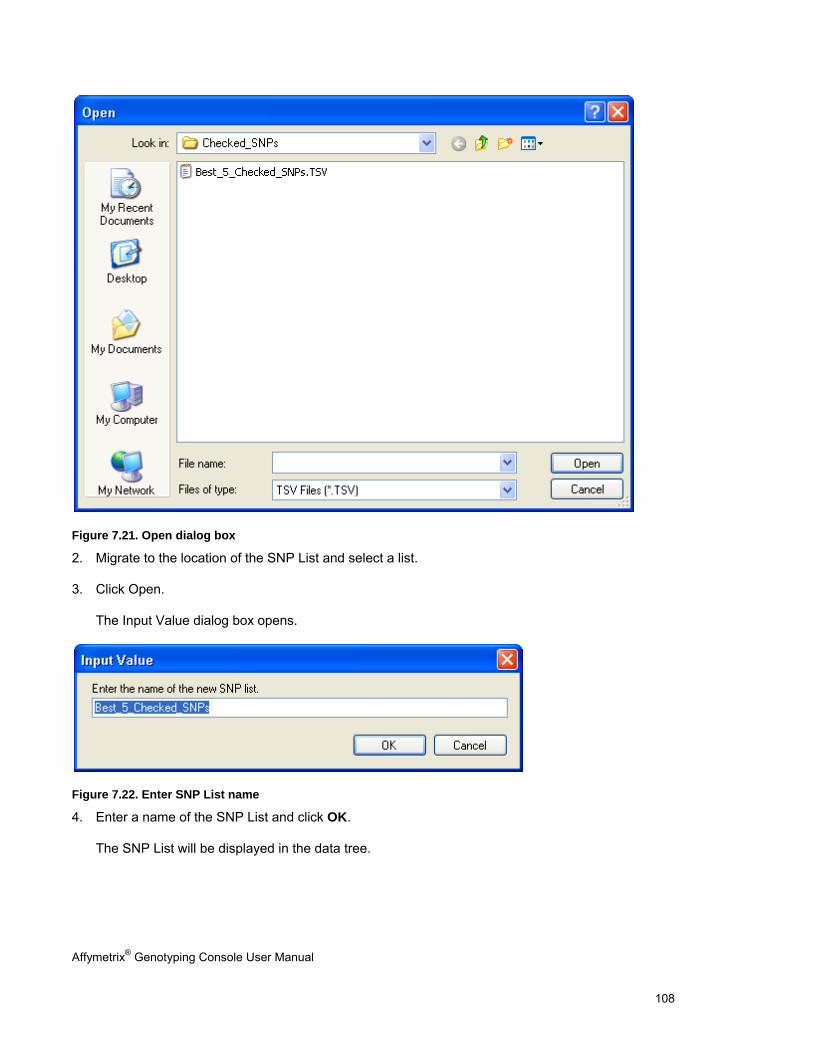
Affymetrix® Genotyping Console User Manual 108
Figure 7.21. Open dialog box
2. Migrate to the location of the SNP List and select a list.
3. Click Open.
The Input Value dialog box opens.
Figure 7.22. Enter SNP List name
4. Enter a name of the SNP List and click OK.
The SNP List will be displayed in the data tree.
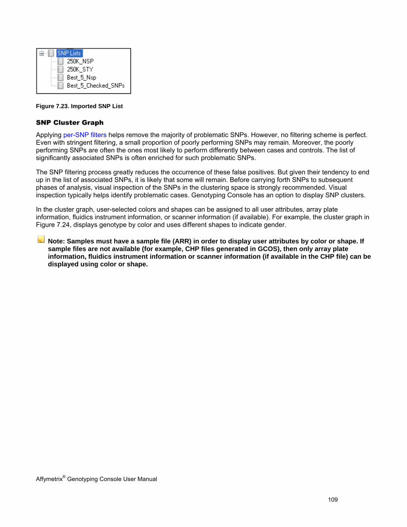
Affymetrix® Genotyping Console User Manual 109
Figure 7.23. Imported SNP List
SNP Cluster Graph
Applying per-SNP filters helps remove the majority of problematic SNPs. However, no filtering scheme is perfect. Even with stringent filtering, a small proportion of poorly performing SNPs may remain. Moreover, the poorly performing SNPs are often the ones most likely to perform differently between cases and controls. The list of significantly associated SNPs is often enriched for such problematic SNPs.
The SNP filtering process greatly reduces the occurrence of these false positives. But given their tendency to end up in the list of associated SNPs, it is likely that some will remain. Before carrying forth SNPs to subsequent phases of analysis, visual inspection of the SNPs in the clustering space is strongly recommended. Visual inspection typically helps identify problematic cases. Genotyping Console has an option to display SNP clusters.
In the cluster graph, user-selected colors and shapes can be assigned to all user attributes, array plate information, fluidics instrument information, or scanner information (if available). For example, the cluster graph in Figure 7.24, displays genotype by color and uses different shapes to indicate gender.
Note: Samples must have a sample file (ARR) in order to display user attributes by color or shape. If sample files are not available (for example, CHP files generated in GCOS), then only array plate information, fluidics instrument information or scanner information (if available in the CHP file) can be displayed using color or shape.
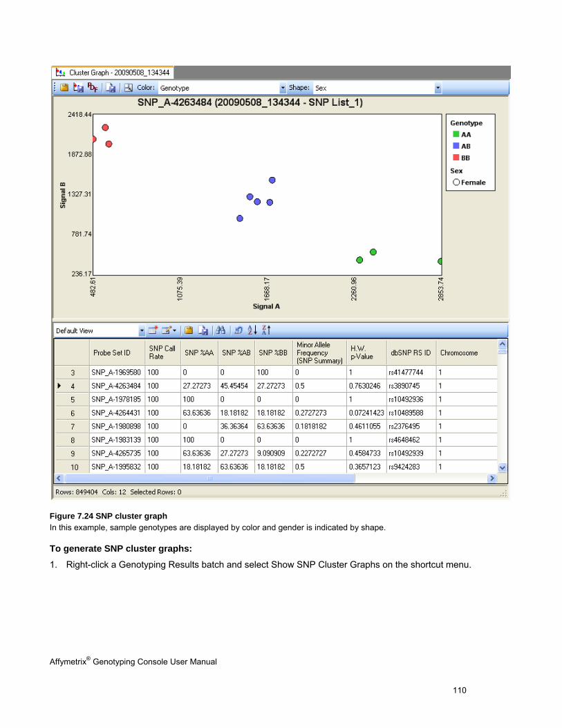
Affymetrix® Genotyping Console User Manual 110
Figure 7.24 SNP cluster graph In this example, sample genotypes are displayed by color and gender is indicated by shape.
To generate SNP cluster graphs:
1. Right-click a Genotyping Results batch and select Show SNP Cluster Graphs on the shortcut menu.
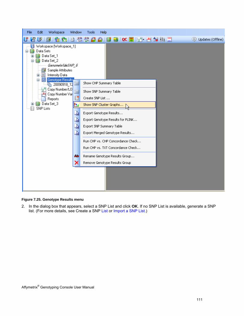
Affymetrix® Genotyping Console User Manual 111
Figure 7.25. Genotype Results menu
2. In the dialog box that appears, select a SNP List and click OK. If no SNP List is available, generate a SNP list. (For more details, see Create a SNP List or Import a SNP List.)
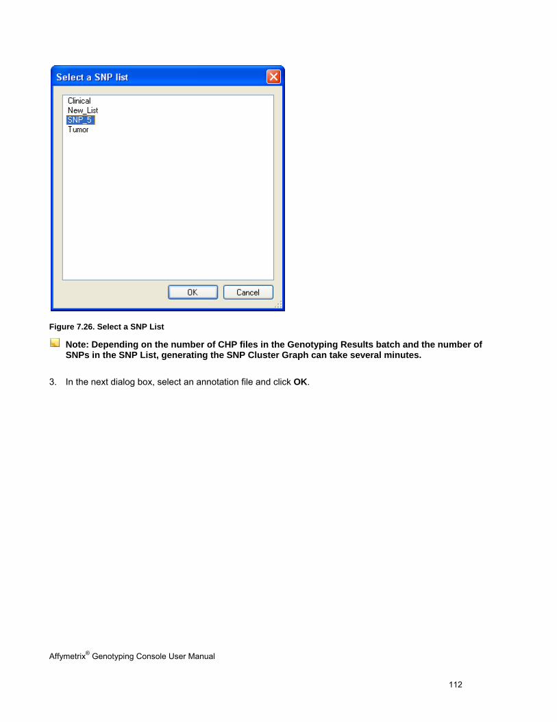
Affymetrix® Genotyping Console User Manual 112
Figure 7.26. Select a SNP List
Note: Depending on the number of CHP files in the Genotyping Results batch and the number of SNPs in the SNP List, generating the SNP Cluster Graph can take several minutes.
3. In the next dialog box, select an annotation file and click OK.
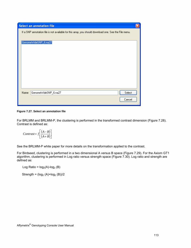
Affymetrix® Genotyping Console User Manual 113
Figure 7.27. Select an annotation file
For BRLMM and BRLMM-P, the clustering is performed in the transformed contrast dimension (Figure 7.28). Contrast is defined as:
( )( )⎥⎦
⎤⎢⎣
⎡+−=
BABAfContrast
See the BRLMM-P white paper for more details on the transformation applied to the contrast.
For Birdseed, clustering is performed in a two dimensional A versus B space (Figure 7.29). For the Axiom GT1 algorithm, clustering is performed in Log ratio versus strength space (Figure 7.30). Log ratio and strength are defined as:
Log Ratio = log2(A)-log2 (B)
Strength = (log2 (A)+log2 (B))/2
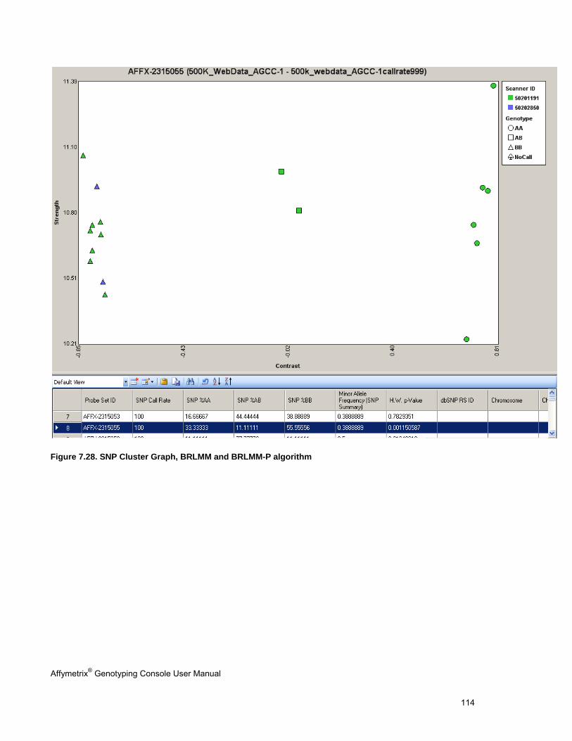
Affymetrix® Genotyping Console User Manual 114
Figure 7.28. SNP Cluster Graph, BRLMM and BRLMM-P algorithm
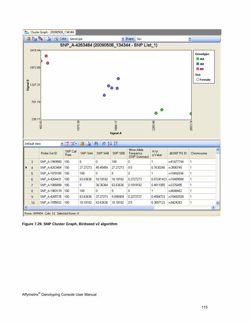
Affymetrix® Genotyping Console User Manual 115
Figure 7.29. SNP Cluster Graph, Birdseed v2 algorithm
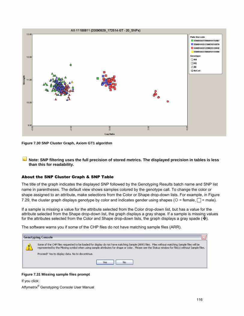
Affymetrix® Genotyping Console User Manual 116
Figure 7.30 SNP Cluster Graph, Axiom GT1 algorithm
Note: SNP filtering uses the full precision of stored metrics. The displayed precision in tables is less than this for readability.
About the SNP Cluster Graph & SNP Table
The title of the graph indicates the displayed SNP followed by the Genotyping Results batch name and SNP list name in parentheses. The default view shows samples colored by the genotype call. To change the color or shape assigned to an attribute, make selections from the Color or Shape drop-down lists. For example, in Figure 7.29, the cluster graph displays genotype by color and indicates gender using shapes ( = female, = male).
If a sample is missing a value for the attribute selected from the Color drop-down list, but has a value for the attribute selected from the Shape drop-down list, the graph displays a gray shape. If a sample is missing values for the attributes selected from the Color and Shape drop-down lists, the graph displays a gray spade ( ).
The software warns you if some of the CHP files do not have matching sample files (ARR).
Figure 7.31 Missing sample files prompt
If you click:
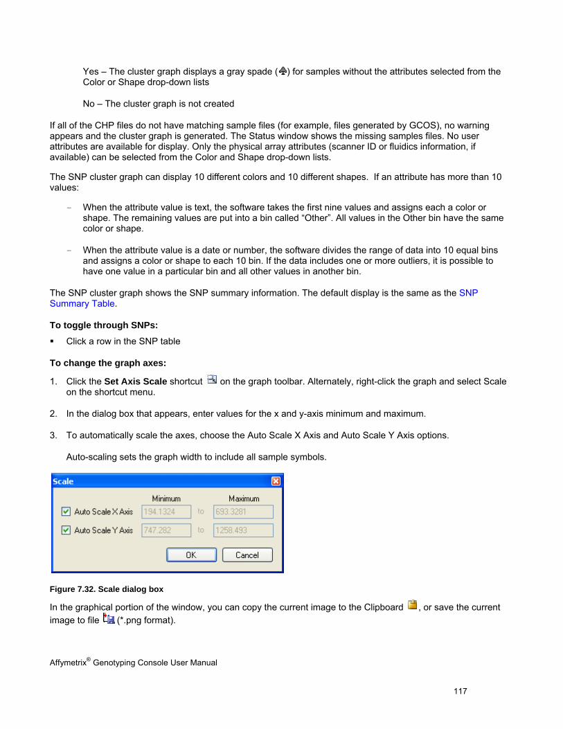
Affymetrix® Genotyping Console User Manual 117
Yes – The cluster graph displays a gray spade ( ) for samples without the attributes selected from the Color or Shape drop-down lists
No – The cluster graph is not created
If all of the CHP files do not have matching sample files (for example, files generated by GCOS), no warning appears and the cluster graph is generated. The Status window shows the missing samples files. No user attributes are available for display. Only the physical array attributes (scanner ID or fluidics information, if available) can be selected from the Color and Shape drop-down lists.
The SNP cluster graph can display 10 different colors and 10 different shapes. If an attribute has more than 10 values:
- When the attribute value is text, the software takes the first nine values and assigns each a color or shape. The remaining values are put into a bin called “Other”. All values in the Other bin have the same color or shape.
- When the attribute value is a date or number, the software divides the range of data into 10 equal bins and assigns a color or shape to each 10 bin. If the data includes one or more outliers, it is possible to have one value in a particular bin and all other values in another bin.
The SNP cluster graph shows the SNP summary information. The default display is the same as the SNP Summary Table.
To toggle through SNPs:
Click a row in the SNP table
To change the graph axes:
1. Click the Set Axis Scale shortcut on the graph toolbar. Alternately, right-click the graph and select Scale on the shortcut menu.
2. In the dialog box that appears, enter values for the x and y-axis minimum and maximum.
3. To automatically scale the axes, choose the Auto Scale X Axis and Auto Scale Y Axis options.
Auto-scaling sets the graph width to include all sample symbols.
Figure 7.32. Scale dialog box
In the graphical portion of the window, you can copy the current image to the Clipboard , or save the current image to file (*.png format).
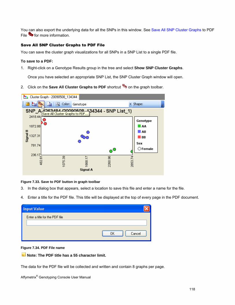
Affymetrix® Genotyping Console User Manual 118
You can also export the underlying data for all the SNPs in this window. See Save All SNP Cluster Graphs to PDF File for more information.
Save All SNP Cluster Graphs to PDF File
You can save the cluster graph visualizations for all SNPs in a SNP List to a single PDF file.
To save to a PDF:
1. Right-click on a Genotype Results group in the tree and select Show SNP Cluster Graphs.
Once you have selected an appropriate SNP List, the SNP Cluster Graph window will open.
2. Click on the Save All Cluster Graphs to PDF shortcut on the graph toolbar.
Figure 7.33. Save to PDF button in graph toolbar
3. In the dialog box that appears, select a location to save this file and enter a name for the file.
4. Enter a title for the PDF file. This title will be displayed at the top of every page in the PDF document.
Figure 7.34. PDF File name
Note: The PDF title has a 55 character limit.
The data for the PDF file will be collected and written and contain 8 graphs per page.
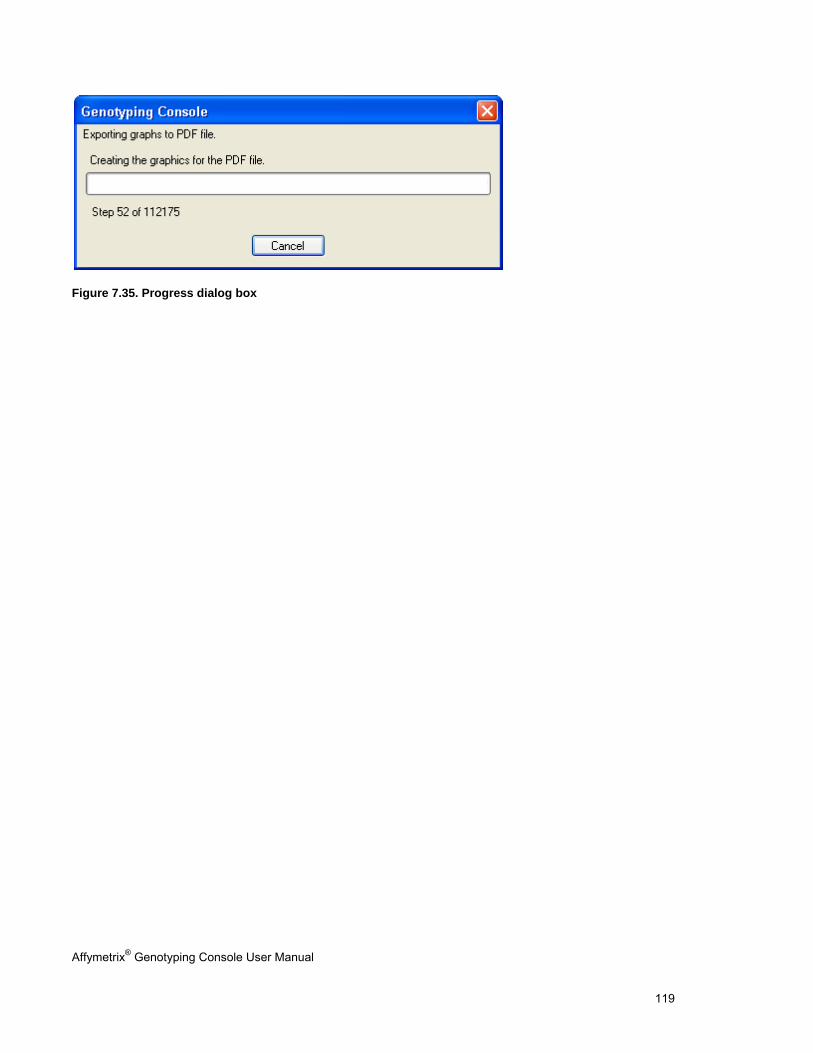
Affymetrix® Genotyping Console User Manual 119
Figure 7.35. Progress dialog box
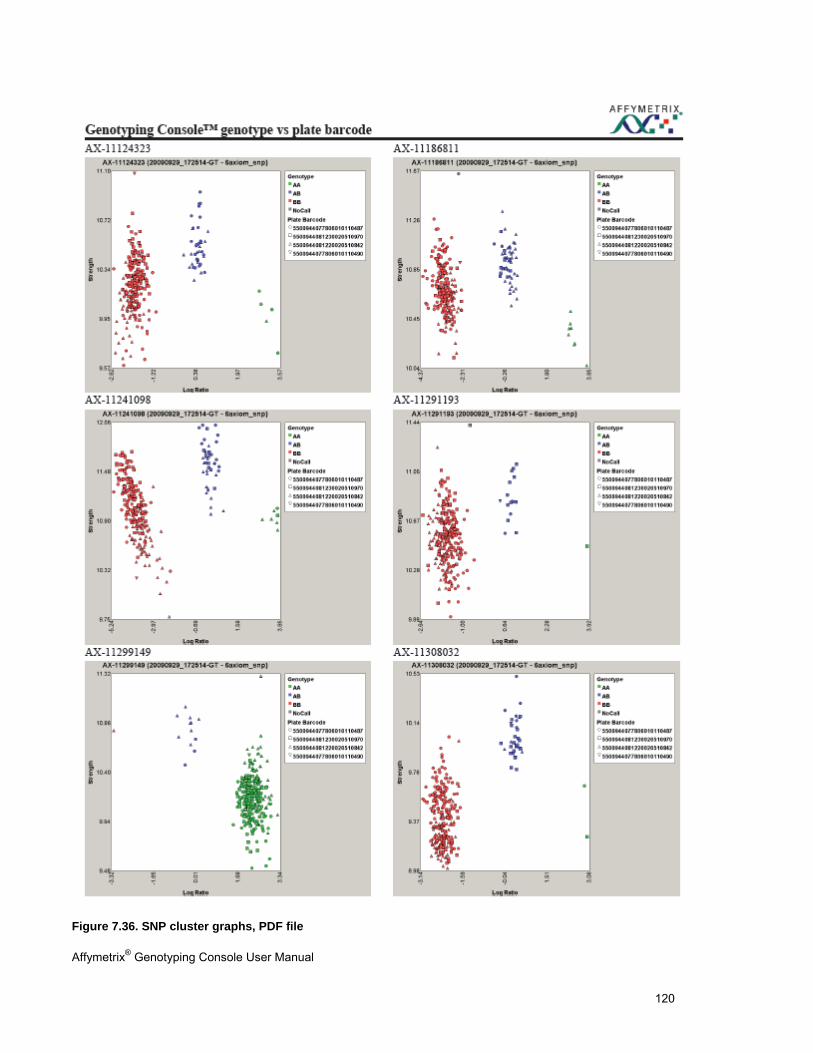
Affymetrix® Genotyping Console User Manual 120
Figure 7.36. SNP cluster graphs, PDF file
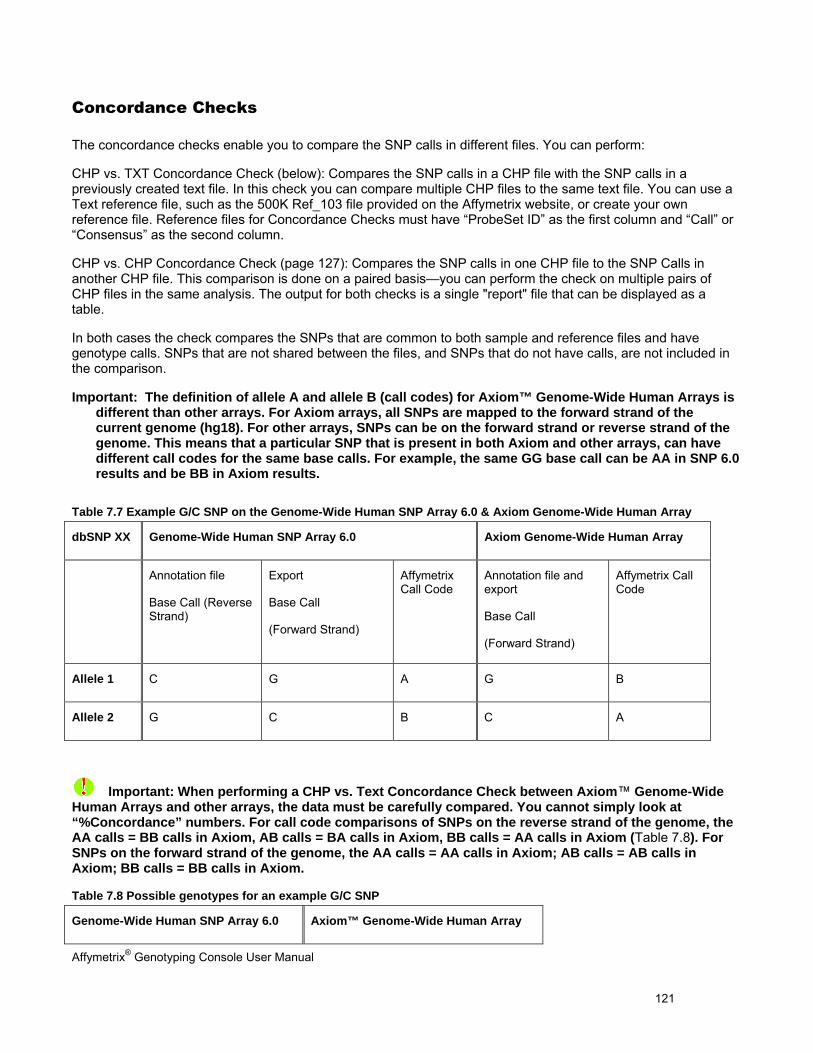
Affymetrix® Genotyping Console User Manual 121
Concordance Checks
The concordance checks enable you to compare the SNP calls in different files. You can perform:
CHP vs. TXT Concordance Check (below): Compares the SNP calls in a CHP file with the SNP calls in a previously created text file. In this check you can compare multiple CHP files to the same text file. You can use a Text reference file, such as the 500K Ref_103 file provided on the Affymetrix website, or create your own reference file. Reference files for Concordance Checks must have “ProbeSet ID” as the first column and “Call” or “Consensus” as the second column.
CHP vs. CHP Concordance Check (page 127): Compares the SNP calls in one CHP file to the SNP Calls in another CHP file. This comparison is done on a paired basis—you can perform the check on multiple pairs of CHP files in the same analysis. The output for both checks is a single "report" file that can be displayed as a table.
In both cases the check compares the SNPs that are common to both sample and reference files and have genotype calls. SNPs that are not shared between the files, and SNPs that do not have calls, are not included in the comparison.
Important: The definition of allele A and allele B (call codes) for Axiom™ Genome-Wide Human Arrays is different than other arrays. For Axiom arrays, all SNPs are mapped to the forward strand of the current genome (hg18). For other arrays, SNPs can be on the forward strand or reverse strand of the genome. This means that a particular SNP that is present in both Axiom and other arrays, can have different call codes for the same base calls. For example, the same GG base call can be AA in SNP 6.0 results and be BB in Axiom results.
Table 7.7 Example G/C SNP on the Genome-Wide Human SNP Array 6.0 & Axiom Genome-Wide Human Array
dbSNP XX Genome-Wide Human SNP Array 6.0 Axiom Genome-Wide Human Array
Annotation file
Base Call (Reverse Strand)
Export
Base Call
(Forward Strand)
Affymetrix Call Code
Annotation file and export
Base Call
(Forward Strand)
Affymetrix Call Code
Allele 1 C G A G B
Allele 2 G C B C A
Important: When performing a CHP vs. Text Concordance Check between Axiom™ Genome-Wide Human Arrays and other arrays, the data must be carefully compared. You cannot simply look at “%Concordance” numbers. For call code comparisons of SNPs on the reverse strand of the genome, the AA calls = BB calls in Axiom, AB calls = BA calls in Axiom, BB calls = AA calls in Axiom (Table 7.8). For SNPs on the forward strand of the genome, the AA calls = AA calls in Axiom; AB calls = AB calls in Axiom; BB calls = BB calls in Axiom.
Table 7.8 Possible genotypes for an example G/C SNP
Genome-Wide Human SNP Array 6.0 Axiom™ Genome-Wide Human Array
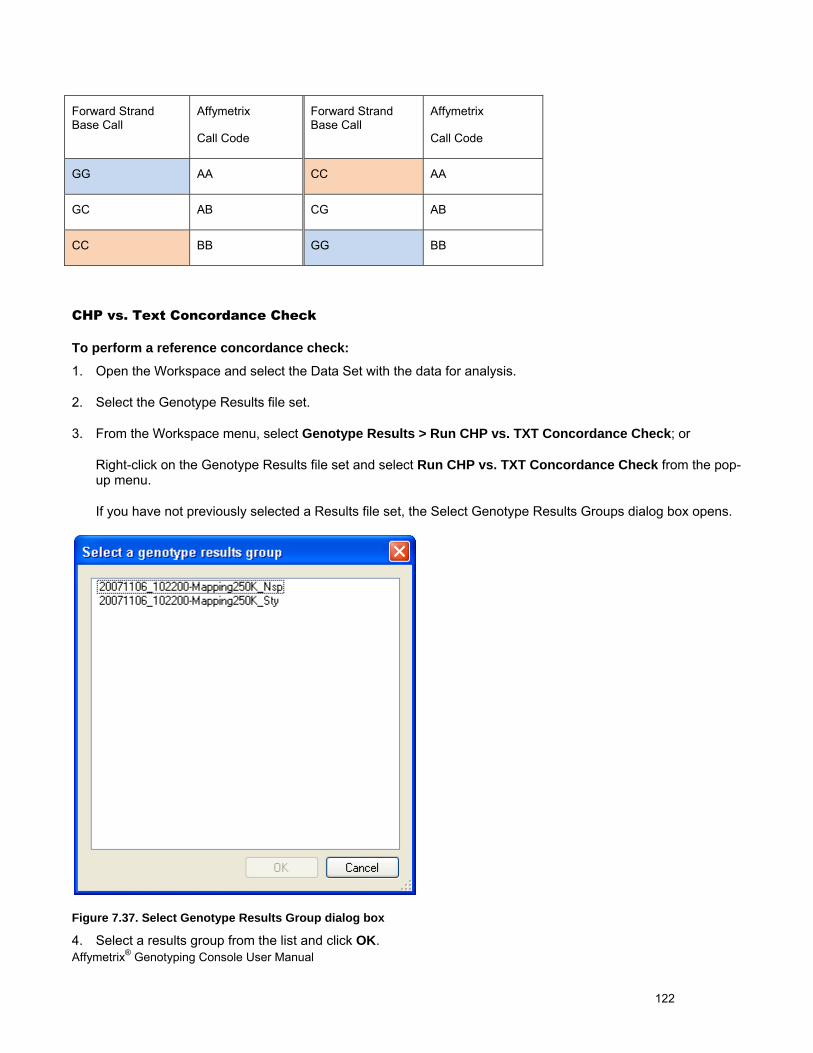
Affymetrix® Genotyping Console User Manual 122
Forward Strand Base Call
Affymetrix
Call Code
Forward Strand Base Call
Affymetrix
Call Code
GG AA CC AA
GC AB CG AB
CC BB GG BB
CHP vs. Text Concordance Check
To perform a reference concordance check:
1. Open the Workspace and select the Data Set with the data for analysis.
2. Select the Genotype Results file set.
3. From the Workspace menu, select Genotype Results > Run CHP vs. TXT Concordance Check; or
Right-click on the Genotype Results file set and select Run CHP vs. TXT Concordance Check from the pop-up menu.
If you have not previously selected a Results file set, the Select Genotype Results Groups dialog box opens.
Figure 7.37. Select Genotype Results Group dialog box
4. Select a results group from the list and click OK.
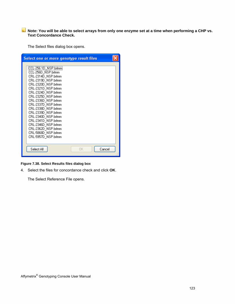
Affymetrix® Genotyping Console User Manual 123
Note: You will be able to select arrays from only one enzyme set at a time when performing a CHP vs. Text Concordance Check.
The Select files dialog box opens.
Figure 7.38. Select Results files dialog box
4. Select the files for concordance check and click OK.
The Select Reference File opens.
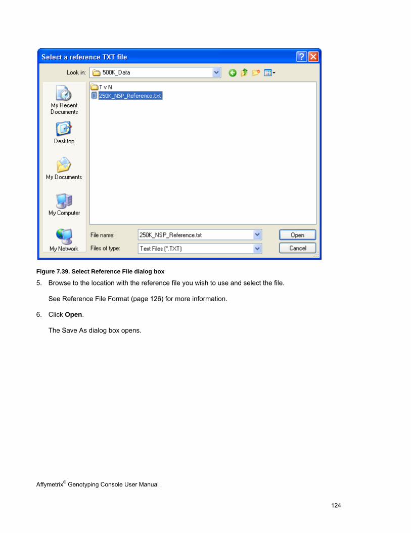
Affymetrix® Genotyping Console User Manual 124
Figure 7.39. Select Reference File dialog box
5. Browse to the location with the reference file you wish to use and select the file.
See Reference File Format (page 126) for more information.
6. Click Open.
The Save As dialog box opens.
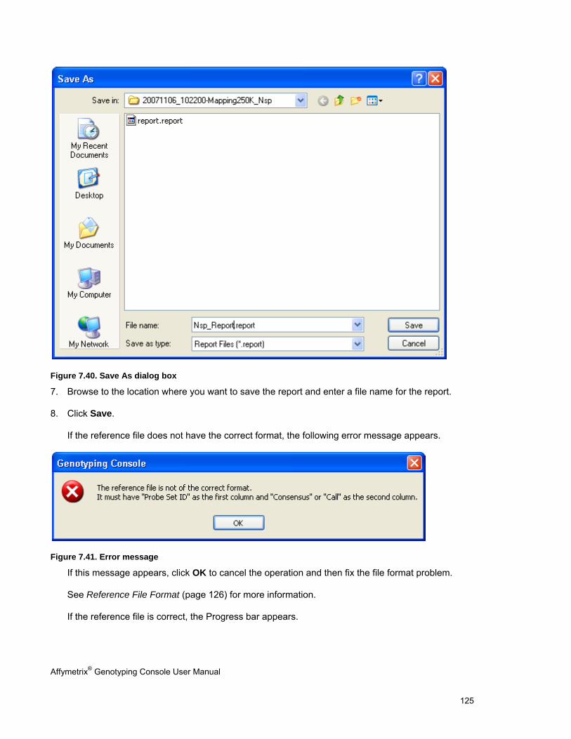
Affymetrix® Genotyping Console User Manual 125
Figure 7.40. Save As dialog box
7. Browse to the location where you want to save the report and enter a file name for the report.
8. Click Save.
If the reference file does not have the correct format, the following error message appears.
Figure 7.41. Error message
If this message appears, click OK to cancel the operation and then fix the file format problem.
See Reference File Format (page 126) for more information.
If the reference file is correct, the Progress bar appears.
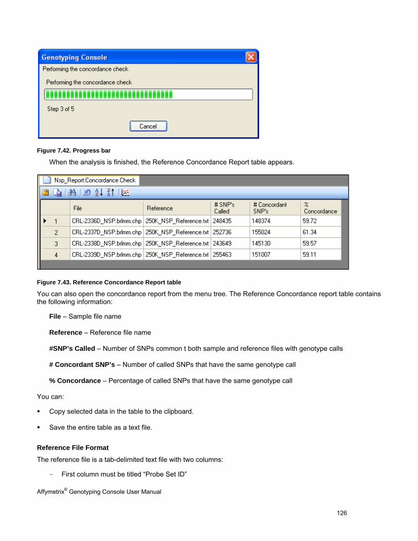
Affymetrix® Genotyping Console User Manual 126
Figure 7.42. Progress bar
When the analysis is finished, the Reference Concordance Report table appears.
Figure 7.43. Reference Concordance Report table
You can also open the concordance report from the menu tree. The Reference Concordance report table contains the following information:
File – Sample file name
Reference – Reference file name
#SNP’s Called – Number of SNPs common t both sample and reference files with genotype calls
# Concordant SNP’s – Number of called SNPs that have the same genotype call
% Concordance – Percentage of called SNPs that have the same genotype call
You can:
Copy selected data in the table to the clipboard.
Save the entire table as a text file.
Reference File Format
The reference file is a tab-delimited text file with two columns:
- First column must be titled “Probe Set ID”
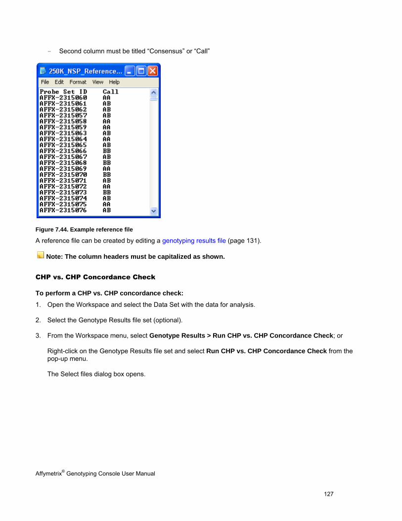
Affymetrix® Genotyping Console User Manual 127
- Second column must be titled “Consensus” or “Call”
Figure 7.44. Example reference file
A reference file can be created by editing a genotyping results file (page 131).
Note: The column headers must be capitalized as shown.
CHP vs. CHP Concordance Check
To perform a CHP vs. CHP concordance check:
1. Open the Workspace and select the Data Set with the data for analysis.
2. Select the Genotype Results file set (optional).
3. From the Workspace menu, select Genotype Results > Run CHP vs. CHP Concordance Check; or
Right-click on the Genotype Results file set and select Run CHP vs. CHP Concordance Check from the pop-up menu.
The Select files dialog box opens.
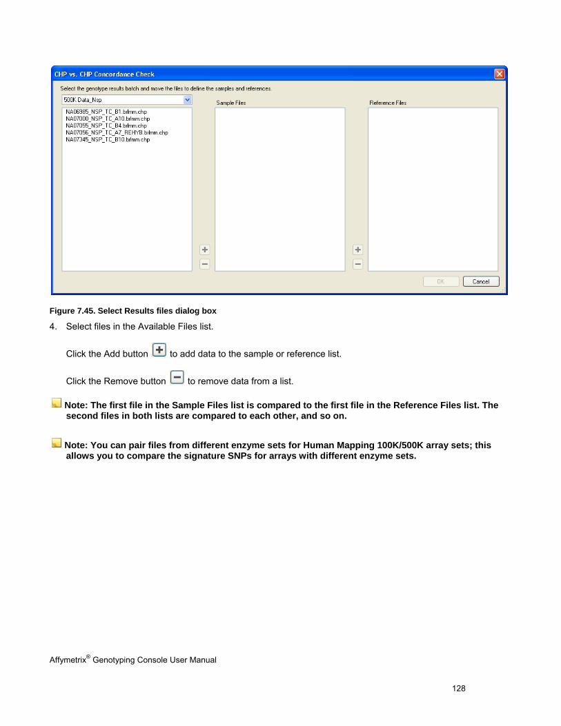
Affymetrix® Genotyping Console User Manual 128
Figure 7.45. Select Results files dialog box
4. Select files in the Available Files list.
Click the Add button to add data to the sample or reference list.
Click the Remove button to remove data from a list.
Note: The first file in the Sample Files list is compared to the first file in the Reference Files list. The second files in both lists are compared to each other, and so on.
Note: You can pair files from different enzyme sets for Human Mapping 100K/500K array sets; this allows you to compare the signature SNPs for arrays with different enzyme sets.
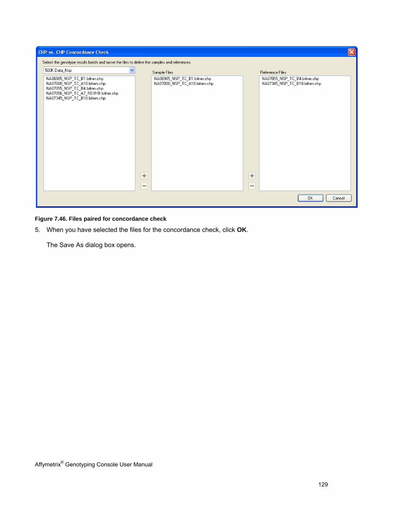
Affymetrix® Genotyping Console User Manual 129
Figure 7.46. Files paired for concordance check
5. When you have selected the files for the concordance check, click OK.
The Save As dialog box opens.
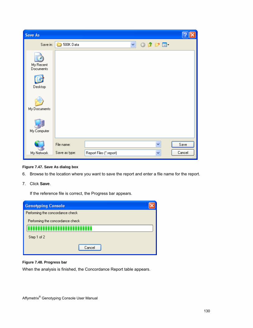
Affymetrix® Genotyping Console User Manual 130
Figure 7.47. Save As dialog box
6. Browse to the location where you want to save the report and enter a file name for the report.
7. Click Save.
If the reference file is correct, the Progress bar appears.
Figure 7.48. Progress bar
When the analysis is finished, the Concordance Report table appears.
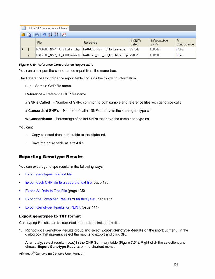
Affymetrix® Genotyping Console User Manual 131
Figure 7.49. Reference Concordance Report table
You can also open the concordance report from the menu tree.
The Reference Concordance report table contains the following information:
File – Sample CHP file name
Reference – Reference CHP file name
# SNP’s Called – Number of SNPs common to both sample and reference files with genotype calls
# Concordant SNP’s – Number of called SNPs that have the same genotype call
% Concordance – Percentage of called SNPs that have the same genotype call
You can:
- Copy selected data in the table to the clipboard.
- Save the entire table as a text file.
Exporting Genotype Results
You can export genotype results in the following ways:
Export genotypes to a text file
Export each CHP file to a separate text file (page 135)
Export All Data to One File (page 135)
Export the Combined Results of an Array Set (page 137)
Export Genotype Results for PLINK (page 141)
Export genotypes to TXT format
Genotyping Results can be exported into a tab-delimited text file.
1. Right-click a Genotype Results group and select Export Genotype Results on the shortcut menu. In the dialog box that appears, select the results to export and click OK.
Alternately, select results (rows) in the CHP Summary table (Figure 7.51). Right-click the selection, and choose Export Genotype Results on the shortcut menu.
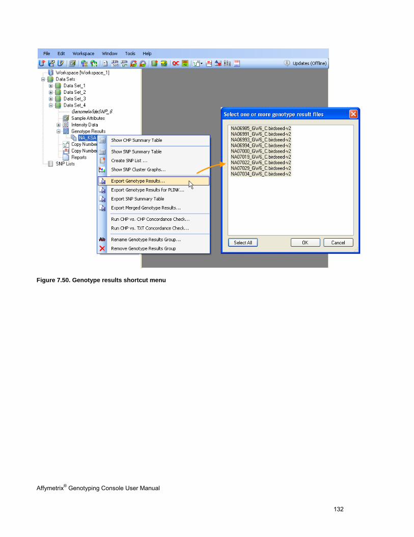
Affymetrix® Genotyping Console User Manual 132
Figure 7.50. Genotype results shortcut menu
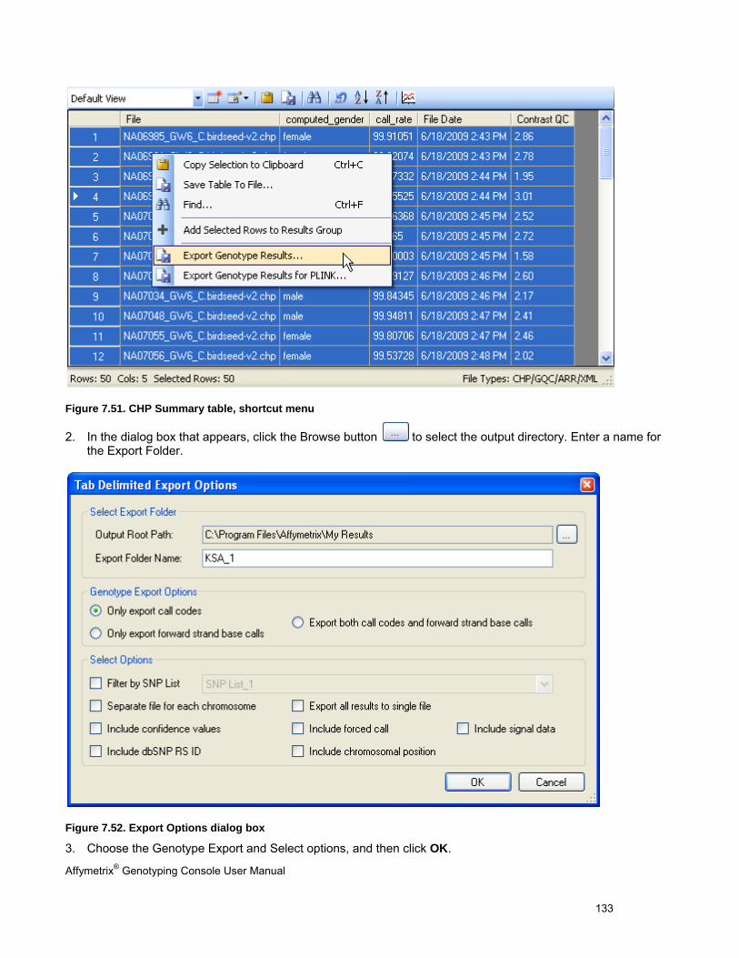
Affymetrix® Genotyping Console User Manual 133
Figure 7.51. CHP Summary table, shortcut menu
2. In the dialog box that appears, click the Browse button to select the output directory. Enter a name for the Export Folder.
Figure 7.52. Export Options dialog box
3. Choose the Genotype Export and Select options, and then click OK.
Affymetrix® Genotyping Console User Manual 134
The data is exported to a one or more text files, depending upon the options selected.
Note: An export that generates “NoChromosome.txt” indicates an invalid SNP list (for example, retired SNPs that are no longer annotated.)
Table 7.9 Tab Delimited Export Options
Genotype Export Options Description
Only export call codes Choose this option to include only the allele call codes (AA, AB, or BB) in the text file.
Only export forward strand base calls Choose this option to include only the forward strand base calls (AT, CG, AG, TC, --, etc) in the text file.
Export both call codes and forward strand base calls Choose this option to include both the allele call codes and the forward strand base calls in the text file. For more details on forward strand base call translation, see Appendix B: Forward Strand Translation, page 295.
Select Options Description
Filter by SNP List Exports only the SNPs in a user-specified SNP list.
Separate file for each chromosome Generates 26 text files (one for each chromosome, plus files containing SNPs on chromosome X, Y, or MT and a file containing SNPs that do not have chromosome information) instead of one text file for each CHP file. This option is not available if you select the “Export all results to single file” option.
Include confidence values Choose this option to include the confidence value for each call in the exported results.
Include dbSNP RS ID Choose this option to include the dbSNP RS ID that corresponds to the SNP probe set. The dbSNP at the National Center for Biotechnology Information (NCBI) attempts to maintain a unified and comprehensive view of known SNPs, small scale insertions/deletions, polymorphic repetitive elements, and microsatellites from the SNP consortium (TSC) and other sources. The dbSNP database is updated periodically, and the dbSNP version used for mapping is given in the dbSNP version field. For more information, please see http://www.ncbi.nlm.nih.gov/SNP/.
Export all results to single file Generates a single text file. If this option is not chosen, one text file is generated for each CHP file.
Include forced call Calls that do not meet the confidence score threshold specified by the configuration file are normally reported as “No Call”. If the “Include forced call” option is selected, the genotype results include what the call would be if “No Calls” are not allowed.
Include chromosomal position The chromosome and chromosomal position for the probe set
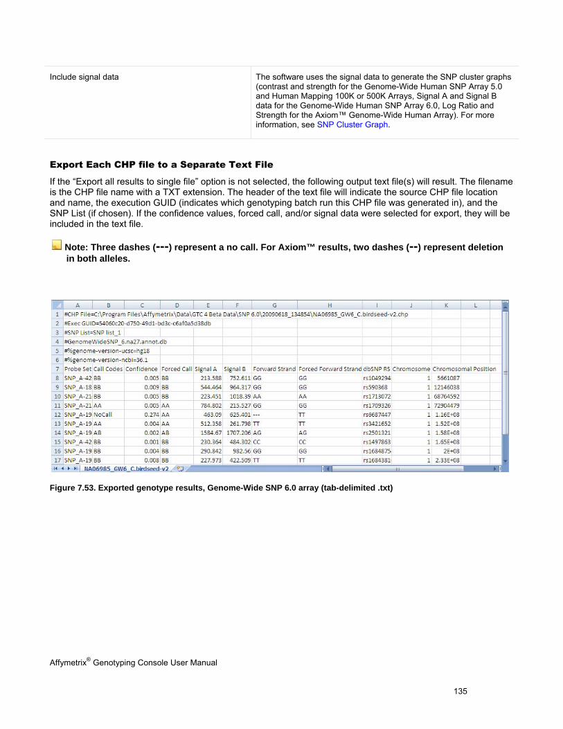
Affymetrix® Genotyping Console User Manual 135
Include signal data The software uses the signal data to generate the SNP cluster graphs (contrast and strength for the Genome-Wide Human SNP Array 5.0 and Human Mapping 100K or 500K Arrays, Signal A and Signal B data for the Genome-Wide Human SNP Array 6.0, Log Ratio and Strength for the Axiom™ Genome-Wide Human Array). For more information, see SNP Cluster Graph.
Export Each CHP file to a Separate Text File
If the “Export all results to single file” option is not selected, the following output text file(s) will result. The filename is the CHP file name with a TXT extension. The header of the text file will indicate the source CHP file location and name, the execution GUID (indicates which genotyping batch run this CHP file was generated in), and the SNP List (if chosen). If the confidence values, forced call, and/or signal data were selected for export, they will be included in the text file.
Note: Three dashes (---) represent a no call. For Axiom™ results, two dashes (--) represent deletion in both alleles.
Figure 7.53. Exported genotype results, Genome-Wide SNP 6.0 array (tab-delimited .txt)
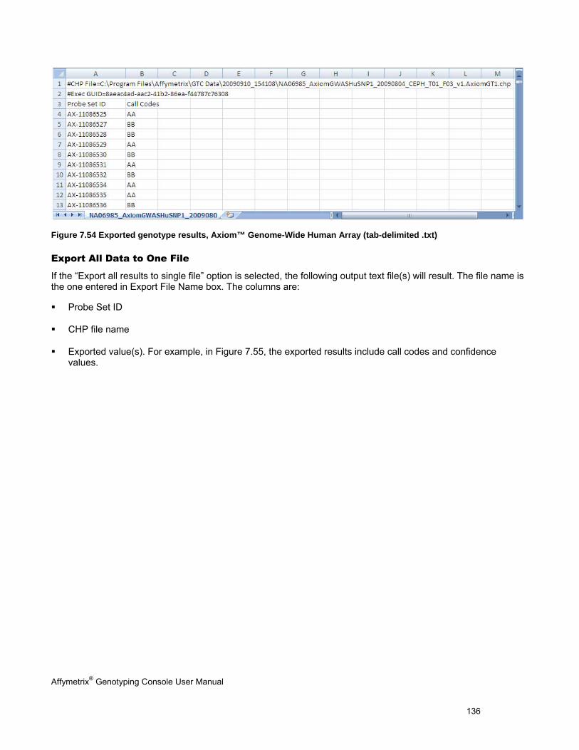
Affymetrix® Genotyping Console User Manual 136
Figure 7.54 Exported genotype results, Axiom™ Genome-Wide Human Array (tab-delimited .txt)
Export All Data to One File
If the “Export all results to single file” option is selected, the following output text file(s) will result. The file name is the one entered in Export File Name box. The columns are:
Probe Set ID
CHP file name
Exported value(s). For example, in Figure 7.55, the exported results include call codes and confidence values.
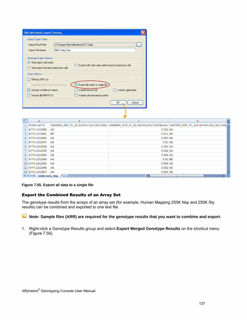
Affymetrix® Genotyping Console User Manual 137
Figure 7.55. Export all data to a single file
Export the Combined Results of an Array Set
The genotype results from the arrays of an array set (for example, Human Mapping 250K Nsp and 250K Sty results) can be combined and exported to one text file.
Note: Sample files (ARR) are required for the genotype results that you want to combine and export.
1. Right-click a Genotype Results group and select Export Merged Genotype Results on the shortcut menu (Figure 7.56).
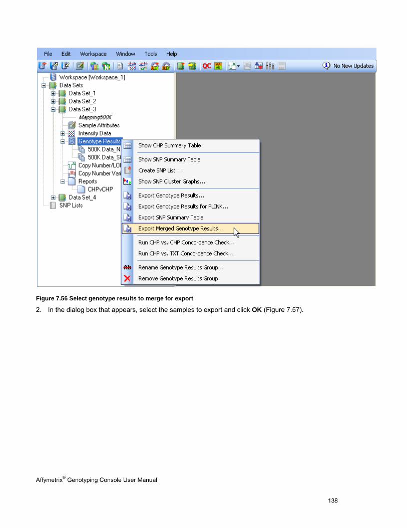
Affymetrix® Genotyping Console User Manual 138
Figure 7.56 Select genotype results to merge for export
2. In the dialog box that appears, select the samples to export and click OK (Figure 7.57).
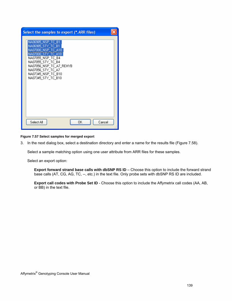
Affymetrix® Genotyping Console User Manual 139
Figure 7.57 Select samples for merged export
3. In the next dialog box, select a destination directory and enter a name for the results file (Figure 7.58).
Select a sample matching option using one user attribute from ARR files for these samples.
Select an export option:
Export forward strand base calls with dbSNP RS ID – Choose this option to include the forward strand base calls (AT, CG, AG, TC, --, etc.) in the text file. Only probe sets with dbSNP RS ID are included.
Export call codes with Probe Set ID - Choose this option to include the Affymetrix call codes (AA, AB, or BB) in the text file.
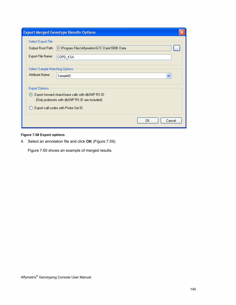
Affymetrix® Genotyping Console User Manual 140
Figure 7.58 Export options
4. Select an annotation file and click OK (Figure 7.59).
Figure 7.60 shows an example of merged results.
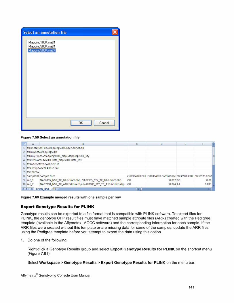
Affymetrix® Genotyping Console User Manual 141
Figure 7.59 Select an annotation file
Figure 7.60 Example merged results with one sample per row
Export Genotype Results for PLINK
Genotype results can be exported to a file format that is compatible with PLINK software. To export files for PLINK, the genotype CHP result files must have matched sample attribute files (ARR) created with the Pedigree template (available in the Affymetrix AGCC software) and the corresponding information for each sample. If the ARR files were created without this template or are missing data for some of the samples, update the ARR files using the Pedigree template before you attempt to export the data using this option.
1. Do one of the following:
Right-click a Genotype Results group and select Export Genotype Results for PLINK on the shortcut menu (Figure 7.61).
Select Workspace > Genotype Results > Export Genotype Results for PLINK on the menu bar.
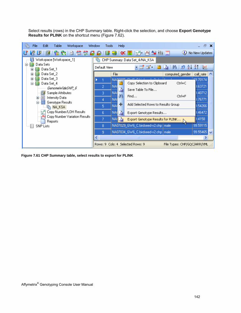
Affymetrix® Genotyping Console User Manual 142
Select results (rows) in the CHP Summary table. Right-click the selection, and choose Export Genotype Results for PLINK on the shortcut menu (Figure 7.62).
Figure 7.61 CHP Summary table, select results to export for PLINK
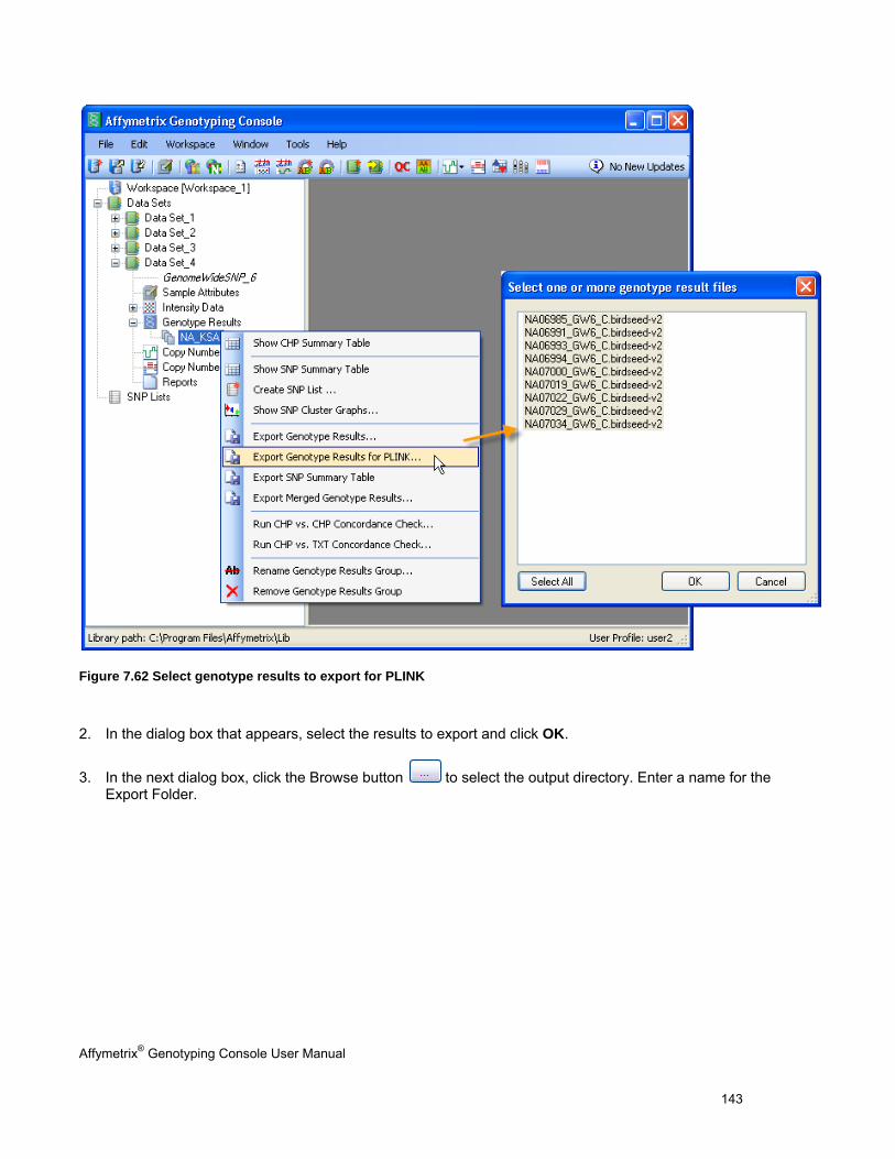
Affymetrix® Genotyping Console User Manual 143
Figure 7.62 Select genotype results to export for PLINK
2. In the dialog box that appears, select the results to export and click OK.
3. In the next dialog box, click the Browse button to select the output directory. Enter a name for the Export Folder.
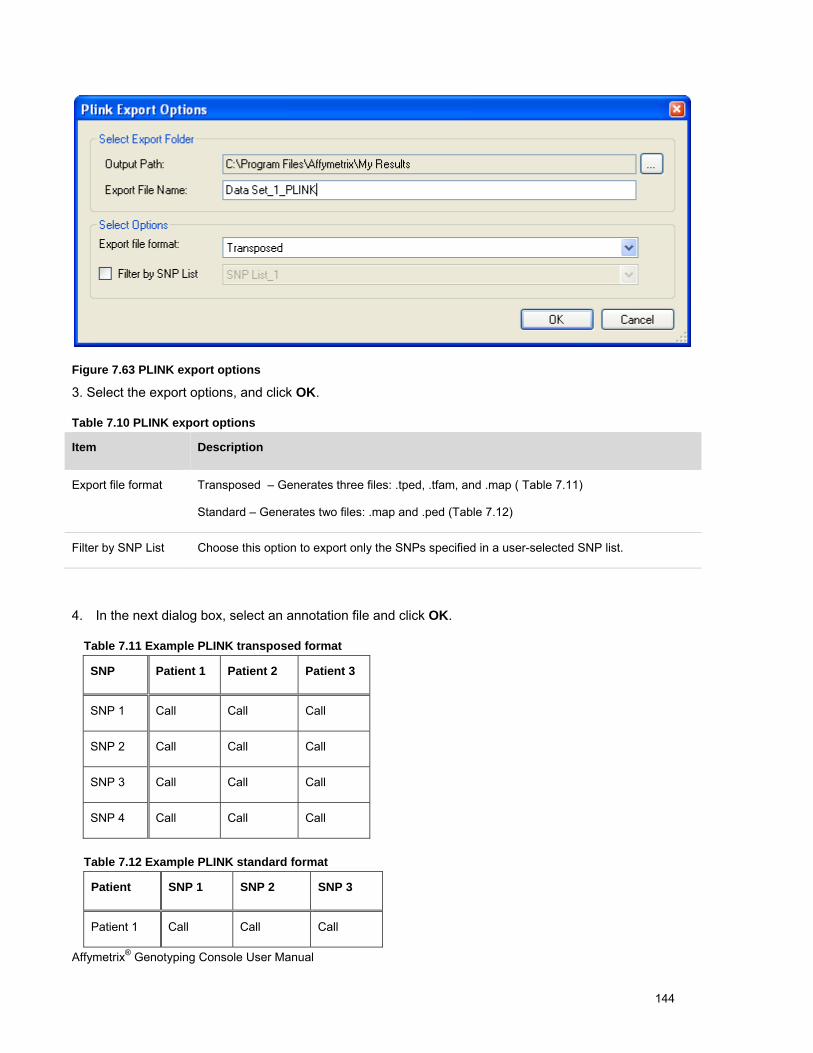
Affymetrix® Genotyping Console User Manual 144
Figure 7.63 PLINK export options
3. Select the export options, and click OK.
Table 7.10 PLINK export options
Item Description
Export file format Transposed – Generates three files: .tped, .tfam, and .map ( Table 7.11)
Standard – Generates two files: .map and .ped (Table 7.12)
Filter by SNP List Choose this option to export only the SNPs specified in a user-selected SNP list.
4. In the next dialog box, select an annotation file and click OK.
Table 7.11 Example PLINK transposed format
Table 7.12 Example PLINK standard format
Patient SNP 1 SNP 2 SNP 3
Patient 1 Call Call Call
SNP Patient 1 Patient 2 Patient 3
SNP 1 Call Call Call
SNP 2 Call Call Call
SNP 3 Call Call Call
SNP 4 Call Call Call

Affymetrix® Genotyping Console User Manual 145
Patient 2 Call Call Call
Patient 3 Call Call Call
Patient 4 Call Call Call
Affymetrix® Genotyping Console User Manual 146
Chapter 8: Table & Graph Features In Genotyping Console, there are several properties which are common to all tables and graphs. The following sections describe:
Genotyping Data Tables (146)
Table Features (page 146)
Graph Features (page 151)
Note: The use of the GTC Copy Number to view Copy Number/LOH data is described in the GTC Browser Manual.
Genotyping Data Tables
In Genotyping Console, there are several tables which display data:
Sample Attribute Table (page 55)
Intensity QC Table (page 76)
CHP Summary Table (page 91)
SNP Summary Table (page 96)
Note: For Human Mapping 100K/500K or Axiom™ Genome-Wide Human arrays, the CHP Summary and SNP Summary data for the different array types will be displayed in different tables with different names.
Table Features
All common table functions are accessible through the shortcuts on the table toolbar.
Figure 8.1 Table toolbar
Table 8.1 Table Toolbar functions
Table Function Description
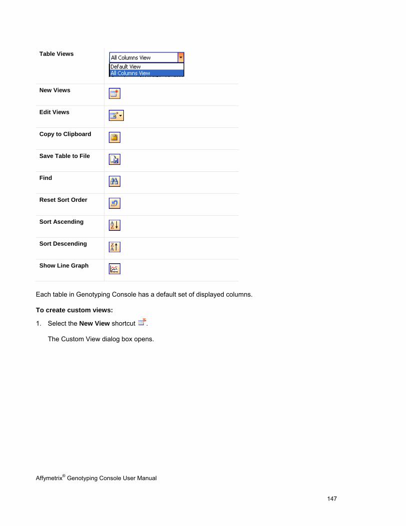
Affymetrix® Genotyping Console User Manual 147
Each table in Genotyping Console has a default set of displayed columns.
To create custom views:
1. Select the New View shortcut .
The Custom View dialog box opens.
Table Views
New Views
Edit Views
Copy to Clipboard
Save Table to File
Find
Reset Sort Order
Sort Ascending
Sort Descending
Show Line Graph
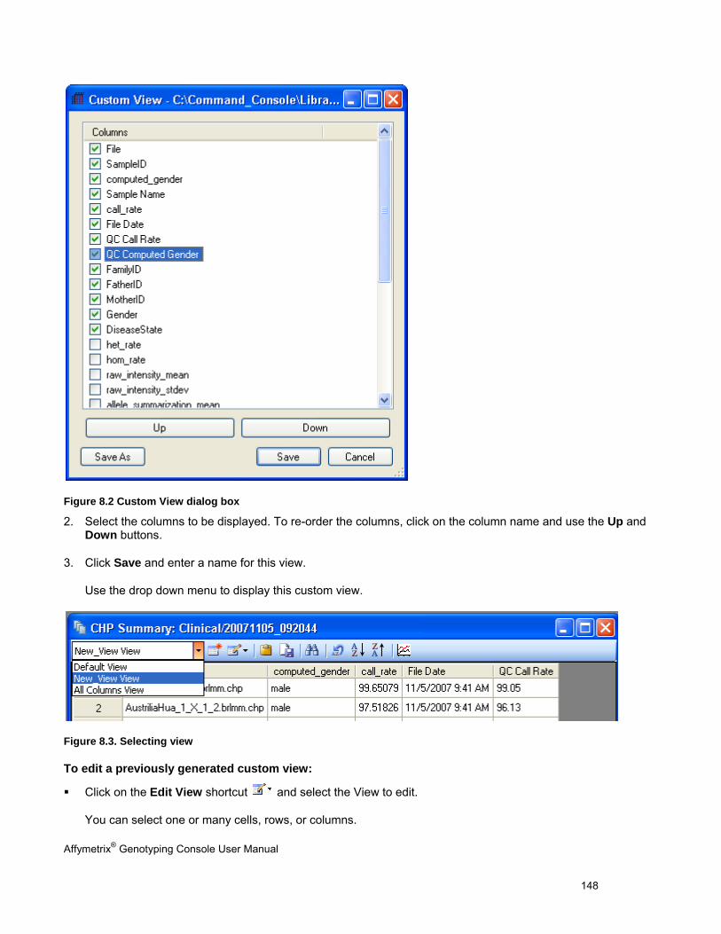
Affymetrix® Genotyping Console User Manual 148
Figure 8.2 Custom View dialog box
2. Select the columns to be displayed. To re-order the columns, click on the column name and use the Up and Down buttons.
3. Click Save and enter a name for this view.
Use the drop down menu to display this custom view.
Figure 8.3. Selecting view
To edit a previously generated custom view:
Click on the Edit View shortcut and select the View to edit.
You can select one or many cells, rows, or columns.
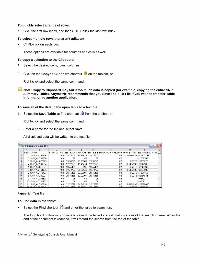
Affymetrix® Genotyping Console User Manual 149
To quickly select a range of rows:
Click the first row index, and then SHIFT-click the last row index.
To select multiple rows that aren’t adjacent
CTRL-click on each row.
These options are available for columns and cells as well.
To copy a selection to the Clipboard:
1. Select the desired cells, rows, columns.
2. Click on the Copy to Clipboard shortcut on the toolbar, or
Right-click and select the same command.
Note: Copy to Clipboard may fail if too much data is copied (for example, copying the entire SNP Summary Table). Affymetrix recommends that you Save Table To File if you wish to transfer Table information to another application.
To save all of the data in the open table to a text file:
1. Select the Save Table to File shortcut from the toolbar, or
Right-click and select the same command.
2. Enter a name for the file and select Save.
All displayed data will be written to the text file.
Figure 8.4. Text file
To Find data in the table:
Select the Find shortcut and enter the value to search on.
The Find Next button will continue to search the table for additional instances of the search criteria. When the end of the document is reached, it will restart the search from the top of the table.
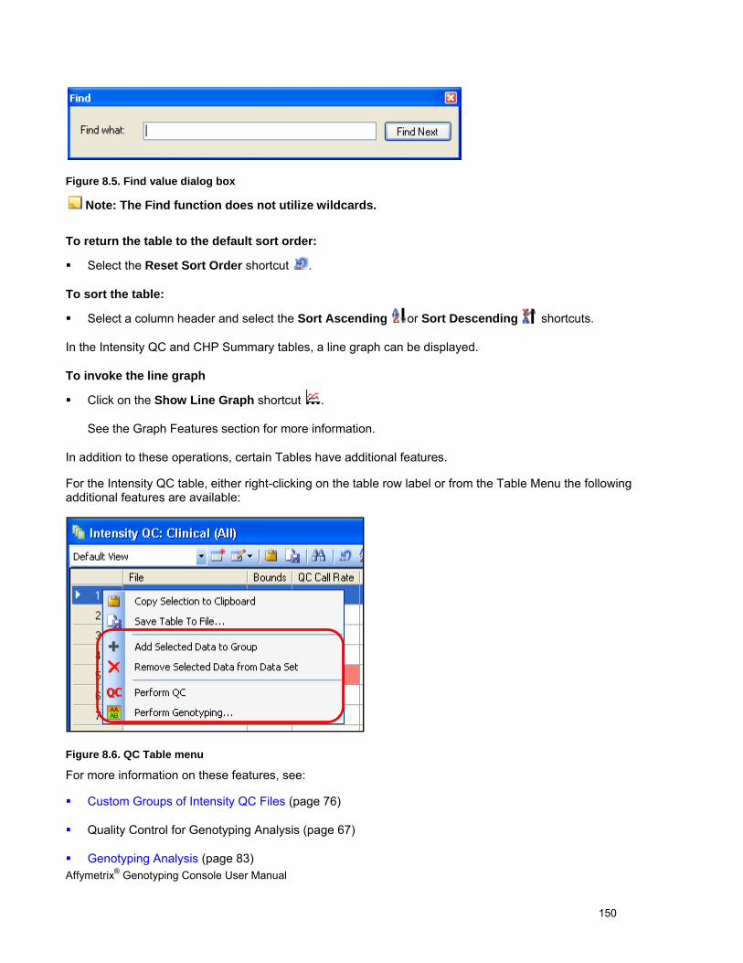
Affymetrix® Genotyping Console User Manual 150
Figure 8.5. Find value dialog box
Note: The Find function does not utilize wildcards.
To return the table to the default sort order:
Select the Reset Sort Order shortcut .
To sort the table:
Select a column header and select the Sort Ascending or Sort Descending shortcuts.
In the Intensity QC and CHP Summary tables, a line graph can be displayed.
To invoke the line graph
Click on the Show Line Graph shortcut .
See the Graph Features section for more information.
In addition to these operations, certain Tables have additional features.
For the Intensity QC table, either right-clicking on the table row label or from the Table Menu the following additional features are available:
Figure 8.6. QC Table menu
For more information on these features, see:
Custom Groups of Intensity QC Files (page 76)
Quality Control for Genotyping Analysis (page 67)
Genotyping Analysis (page 83)
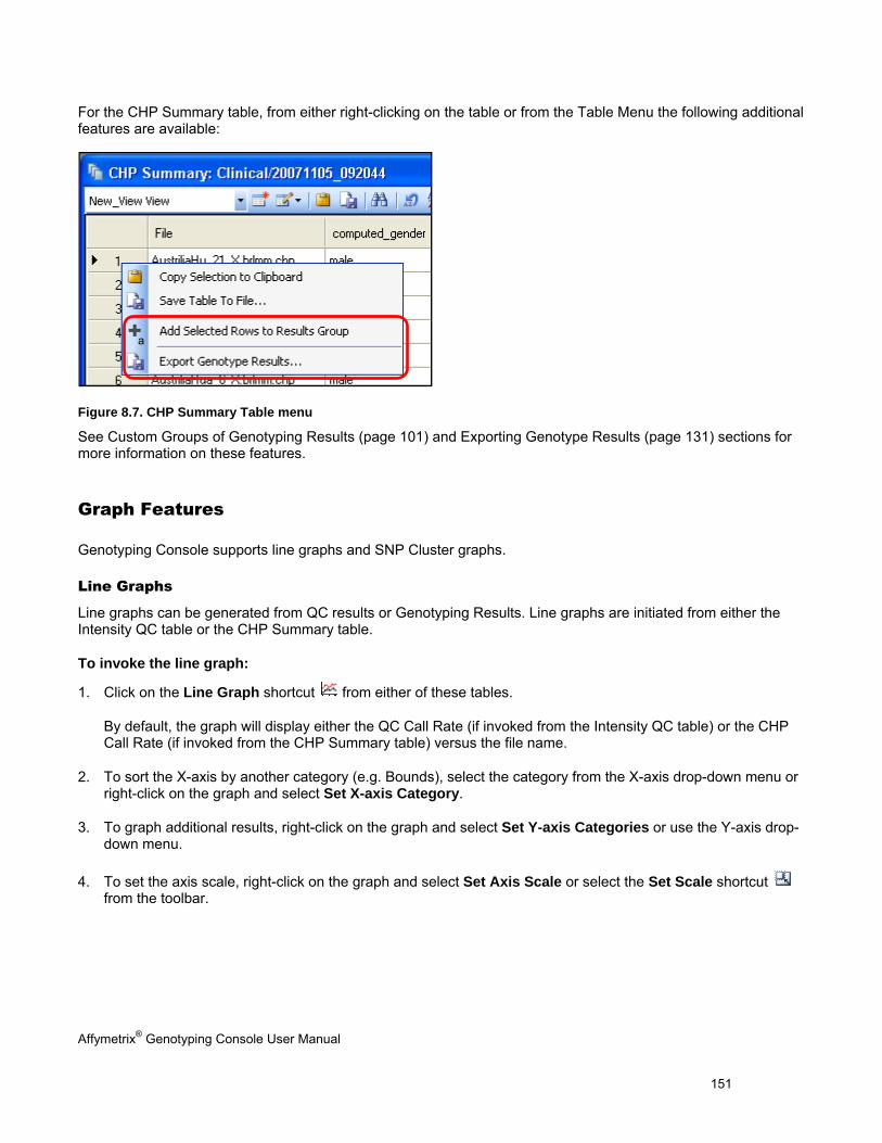
Affymetrix® Genotyping Console User Manual 151
For the CHP Summary table, from either right-clicking on the table or from the Table Menu the following additional features are available:
Figure 8.7. CHP Summary Table menu
See Custom Groups of Genotyping Results (page 101) and Exporting Genotype Results (page 131) sections for more information on these features.
Graph Features
Genotyping Console supports line graphs and SNP Cluster graphs.
Line Graphs
Line graphs can be generated from QC results or Genotyping Results. Line graphs are initiated from either the Intensity QC table or the CHP Summary table.
To invoke the line graph:
1. Click on the Line Graph shortcut from either of these tables.
By default, the graph will display either the QC Call Rate (if invoked from the Intensity QC table) or the CHP Call Rate (if invoked from the CHP Summary table) versus the file name.
2. To sort the X-axis by another category (e.g. Bounds), select the category from the X-axis drop-down menu or right-click on the graph and select Set X-axis Category.
3. To graph additional results, right-click on the graph and select Set Y-axis Categories or use the Y-axis drop-down menu.
4. To set the axis scale, right-click on the graph and select Set Axis Scale or select the Set Scale shortcut from the toolbar.
a
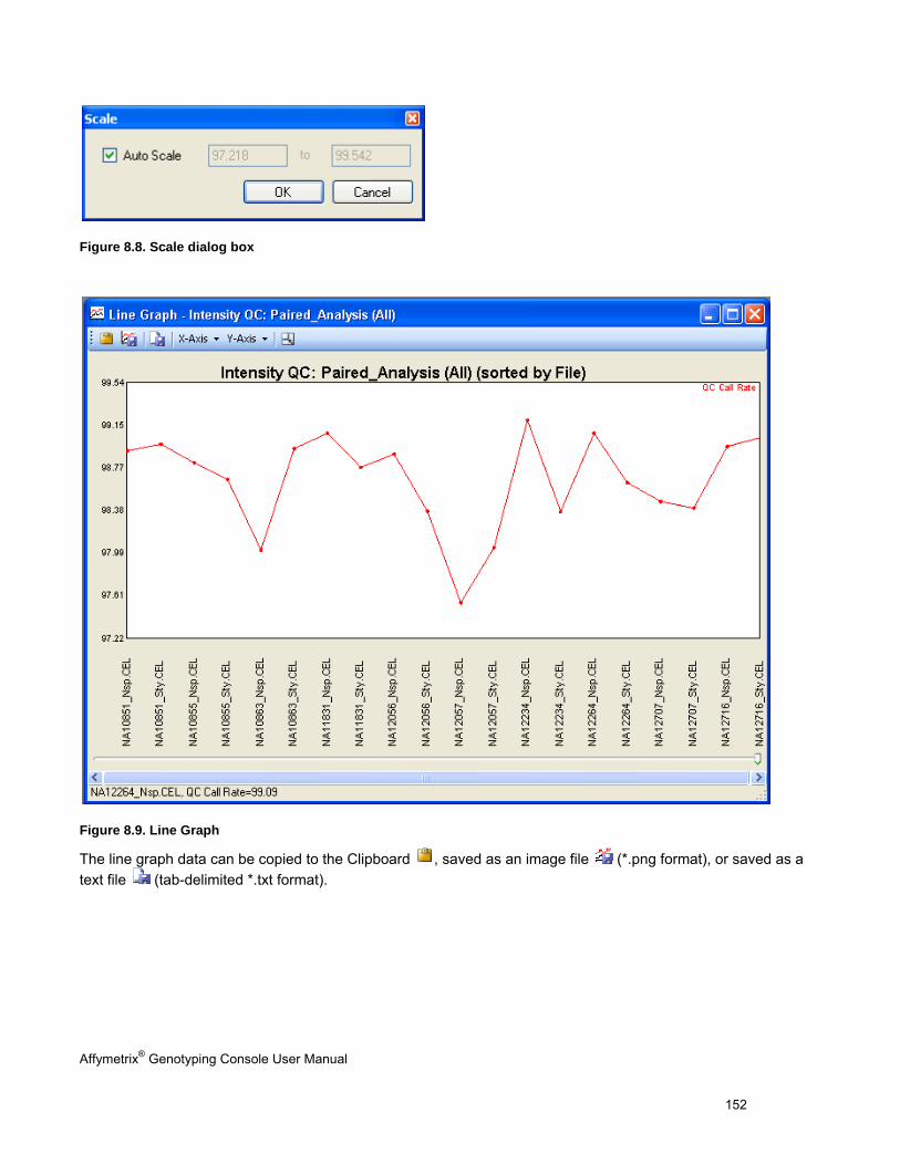
Affymetrix® Genotyping Console User Manual 152
Figure 8.8. Scale dialog box
Figure 8.9. Line Graph
The line graph data can be copied to the Clipboard , saved as an image file (*.png format), or saved as a text file (tab-delimited *.txt format).
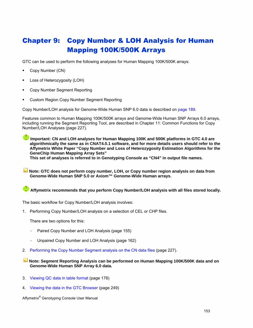
Affymetrix® Genotyping Console User Manual 153
Chapter 9: Copy Number & LOH Analysis for Human Mapping 100K/500K Arrays
GTC can be used to perform the following analyses for Human Mapping 100K/500K arrays:
Copy Number (CN)
Loss of Heterozygosity (LOH)
Copy Number Segment Reporting
Custom Region Copy Number Segment Reporting
Copy Number/LOH analysis for Genome-Wide Human SNP 6.0 data is described on page 189.
Features common to Human Mapping 100K/500K arrays and Genome-Wide Human SNP Arrays 6.0 arrays, including running the Segment Reporting Tool, are described in Chapter 11: Common Functions for Copy Number/LOH Analyses (page 227).
Important: CN and LOH analyses for Human Mapping 100K and 500K platforms in GTC 4.0 are algorithmically the same as in CNAT4.0.1 software, and for more details users should refer to the Affymetrix White Paper “Copy Number and Loss of Heterozygosity Estimation Algorithms for the GeneChip Human Mapping Array Sets” This set of analyses is referred to in Genotyping Console as “CN4” in output file names.
Note: GTC does not perform copy number, LOH, or Copy number region analysis on data from Genome-Wide Human SNP 5.0 or Axiom™ Genome-Wide Human arrays.
Affymetrix recommends that you perform Copy Number/LOH analysis with all files stored locally.
The basic workflow for Copy Number/LOH analysis involves:
1. Performing Copy Number/LOH analysis on a selection of CEL or CHP files.
There are two options for this:
- Paired Copy Number and LOH Analysis (page 155)
- Unpaired Copy Number and LOH Analysis (page 162)
2. Performing the Copy Number Segment analysis on the CN data files (page 227).
Note: Segment Reporting Analysis can be performed on Human Mapping 100K/500K data and on Genome-Wide Human SNP Array 6.0 data.
3. Viewing QC data in table format (page 178)
4. Viewing the data in the GTC Browser (page 249)
Affymetrix® Genotyping Console User Manual 154
5. Exporting data into formats that can be used by secondary analysis software (page 251)
You can also:
Change the QC threshold settings (page 257)
Change the algorithm parameters for 100K/500K analysis (page 179)
Introduction to 100K/500K Analysis
This section covers:
Array design
Algorithm
Array Design
Human Mapping 100K/500K analyses use two arrays to provide full coverage of the genome. 50K or 250K arrays can be run individually, as well.
Human Mapping 100K (combination of Xba240 and Hind 240 below)
- Mapping50K_Xba240
- Mapping50K_Hind240
Human Mapping 500K (combination of Nsp and Sty below)
- Mapping250K_Nsp
- Mapping250K_Sty
The Segment Report Tool is run after Copy Number analysis.
If you wish to run CN number and/or LOH analysis on both array types at the same time, you need to have Enzyme Set attributes set up for the files. You can use Enzyme Set and Sample + Reference attributes to make sorting and pairing up the files easier.
Algorithm
CN4 performs paired and unpaired CN analysis
Paired CN Analysis
Paired CN Analysis is used to compare, for example, two samples from the same individual to look for copy number differences in different types of tissues (examples would be Tumor/Normal or Treated/Untreated).
Paired analysis requires that genotyping batch analysis be performed on the data to be analyzed first.
Unpaired CN Analysis
Unpaired CN Analysis is used to compare sample files to a set of reference files.
Affymetrix® Genotyping Console User Manual 155
Unpaired analysis requires that genotyping batch analysis be performed on the data to be analyzed first.
Copy number data is output in files with the suffix .CN4.cnchp).
LOH analysis can be run at the same time as copy number analysis or in a separate step without running the copy number analysis.
Human Mapping 100K/500K copy number and LOH data is output in separate files (CN4.cnchp files and CN4.lohchp files)
Copy number segment reports can be run on Human Mapping 100K/500K array CN data, but no gender calls are made by the Segment Reporting Tool.
Copy Number/LOH Analysis for Human Mapping 100K/500K Arrays
Affymetrix recommends that you perform Copy Number/LOH analysis with all files stored locally.
This section describes the different Copy Number/LOH workflows for Human Mapping 100K/500K arrays.
Paired Copy Number and LOH Analysis (below)
Unpaired Copy Number and LOH Analysis (page 162)
Copy Number/LOH File Format for Human Mapping 100K/500K Array Data (page 167)
Selecting Results Groups (page 169)
Using Shared Attributes to Group Samples (page 172)
Copy Number data files for Human Mapping 100K/500K arrays have the extension CN4.cnchp. Loss of heterozygosity data files for Human Mapping 100K/500K arrays have the extension CN4.lohchp.
Paired Copy Number and LOH Analysis
Paired CN Analysis is used to compare two samples from the same individual to look for copy number differences in different types of tissues (Normal/Tumor, for example).
To perform Paired CN/LOH analysis:
Genotyping batch analysis must be performed on the data to be analyzed, first.
Enzyme Set attributes are required to have been assigned to the arrays to match array sets originating with the same sample. For example, you could use the “Patient ID” attribute as the Enzyme Set identifier.
It will also be helpful if another sample attribute field exists to help group arrays into either the Sample or Reference category. For example, you could use “Disease State” or “Tissue Type” attributes
The Copy Number and LOH files resulting from combined Enzyme Set data will be named using the Enzyme Set attribute for the array set. Output files can be given a suffix.
For more information about using shared attributes to pair files by enzyme set or sample/reference group, see Using Shared Attributes to Group Samples.
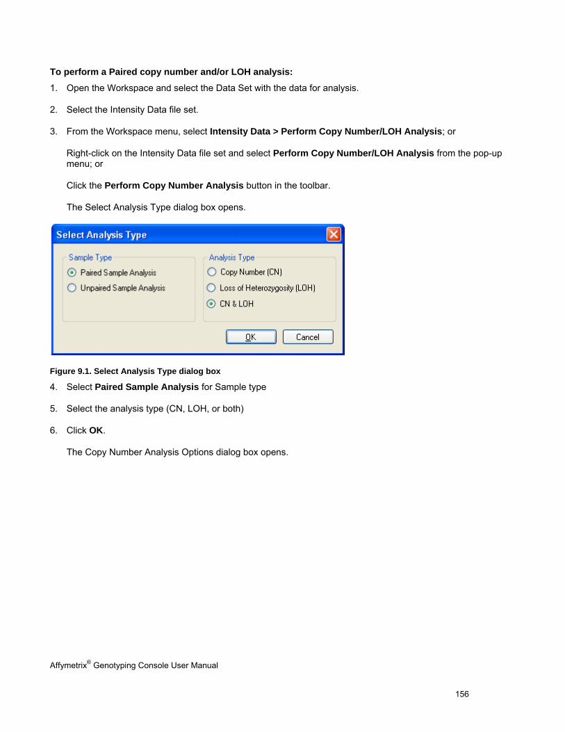
Affymetrix® Genotyping Console User Manual 156
To perform a Paired copy number and/or LOH analysis:
1. Open the Workspace and select the Data Set with the data for analysis.
2. Select the Intensity Data file set.
3. From the Workspace menu, select Intensity Data > Perform Copy Number/LOH Analysis; or
Right-click on the Intensity Data file set and select Perform Copy Number/LOH Analysis from the pop-up menu; or
Click the Perform Copy Number Analysis button in the toolbar.
The Select Analysis Type dialog box opens.
Figure 9.1. Select Analysis Type dialog box
4. Select Paired Sample Analysis for Sample type
5. Select the analysis type (CN, LOH, or both)
6. Click OK.
The Copy Number Analysis Options dialog box opens.
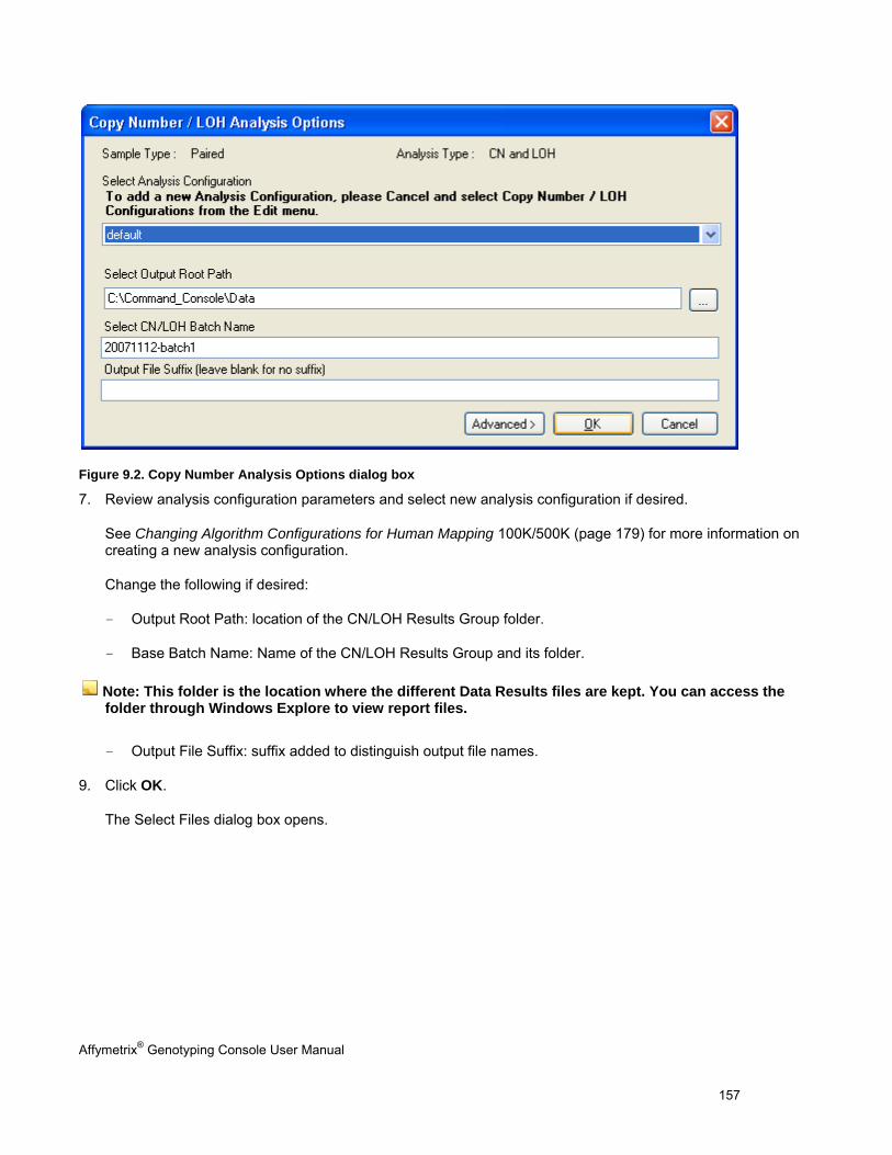
Affymetrix® Genotyping Console User Manual 157
Figure 9.2. Copy Number Analysis Options dialog box
7. Review analysis configuration parameters and select new analysis configuration if desired.
See Changing Algorithm Configurations for Human Mapping 100K/500K (page 179) for more information on creating a new analysis configuration.
Change the following if desired:
- Output Root Path: location of the CN/LOH Results Group folder.
- Base Batch Name: Name of the CN/LOH Results Group and its folder.
Note: This folder is the location where the different Data Results files are kept. You can access the folder through Windows Explore to view report files.
- Output File Suffix: suffix added to distinguish output file names.
9. Click OK.
The Select Files dialog box opens.

Affymetrix® Genotyping Console User Manual 158
Figure 9.3. Select Files for Paired sample
10. Select the Enzyme Set shared attribute from the Enzyme Set Shared Attribute drop-down list.
The files are sorted by Enzyme Set Attribute.
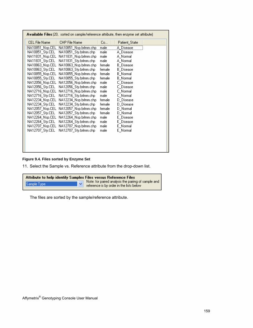
Affymetrix® Genotyping Console User Manual 159
Figure 9.4. Files sorted by Enzyme Set
11. Select the Sample vs. Reference attribute from the drop-down list.
The files are sorted by the sample/reference attribute.
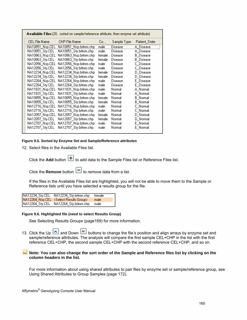
Affymetrix® Genotyping Console User Manual 160
Figure 9.5. Sorted by Enzyme Set and Sample/Reference attributes
12. Select files in the Available Files list.
Click the Add button to add data to the Sample Files list or Reference Files list.
Click the Remove button to remove data from a list.
If the files in the Available Files list are highlighted, you will not be able to move them to the Sample or Reference lists until you have selected a results group for the file.
Figure 9.6. Highlighted file (need to select Results Group)
See Selecting Results Groups (page169) for more information.
13. Click the Up and Down buttons to change the file’s position and align arrays by enzyme set and sample/reference attributes. The analysis will compare the first sample CEL+CHP in the list with the first reference CEL+CHP, the second sample CEL+CHP with the second reference CEL+CHP, and so on.
Note: You can also change the sort order of the Sample and Reference files list by clicking on the column headers in the list.
For more information about using shared attributes to pair files by enzyme set or sample/reference group, see Using Shared Attributes to Group Samples (page 172).
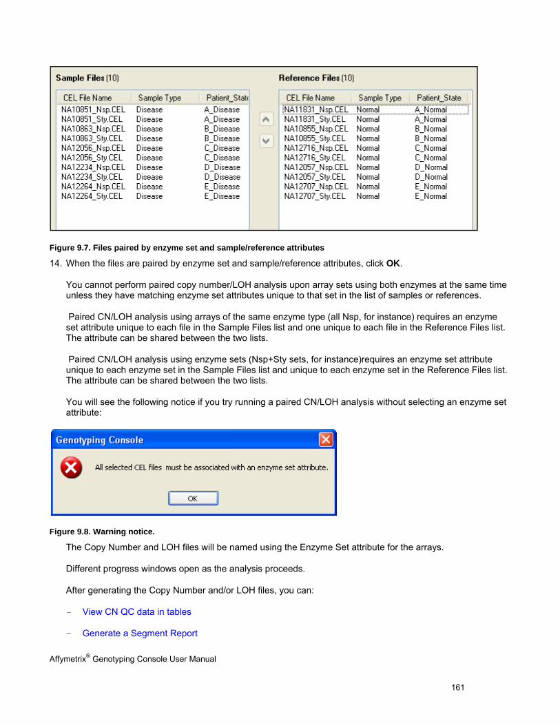
Affymetrix® Genotyping Console User Manual 161
Figure 9.7. Files paired by enzyme set and sample/reference attributes
14. When the files are paired by enzyme set and sample/reference attributes, click OK.
You cannot perform paired copy number/LOH analysis upon array sets using both enzymes at the same time unless they have matching enzyme set attributes unique to that set in the list of samples or references.
Paired CN/LOH analysis using arrays of the same enzyme type (all Nsp, for instance) requires an enzyme set attribute unique to each file in the Sample Files list and one unique to each file in the Reference Files list. The attribute can be shared between the two lists.
Paired CN/LOH analysis using enzyme sets (Nsp+Sty sets, for instance)requires an enzyme set attribute unique to each enzyme set in the Sample Files list and unique to each enzyme set in the Reference Files list. The attribute can be shared between the two lists.
You will see the following notice if you try running a paired CN/LOH analysis without selecting an enzyme set attribute:
Figure 9.8. Warning notice.
The Copy Number and LOH files will be named using the Enzyme Set attribute for the arrays.
Different progress windows open as the analysis proceeds.
After generating the Copy Number and/or LOH files, you can:
- View CN QC data in tables
- Generate a Segment Report
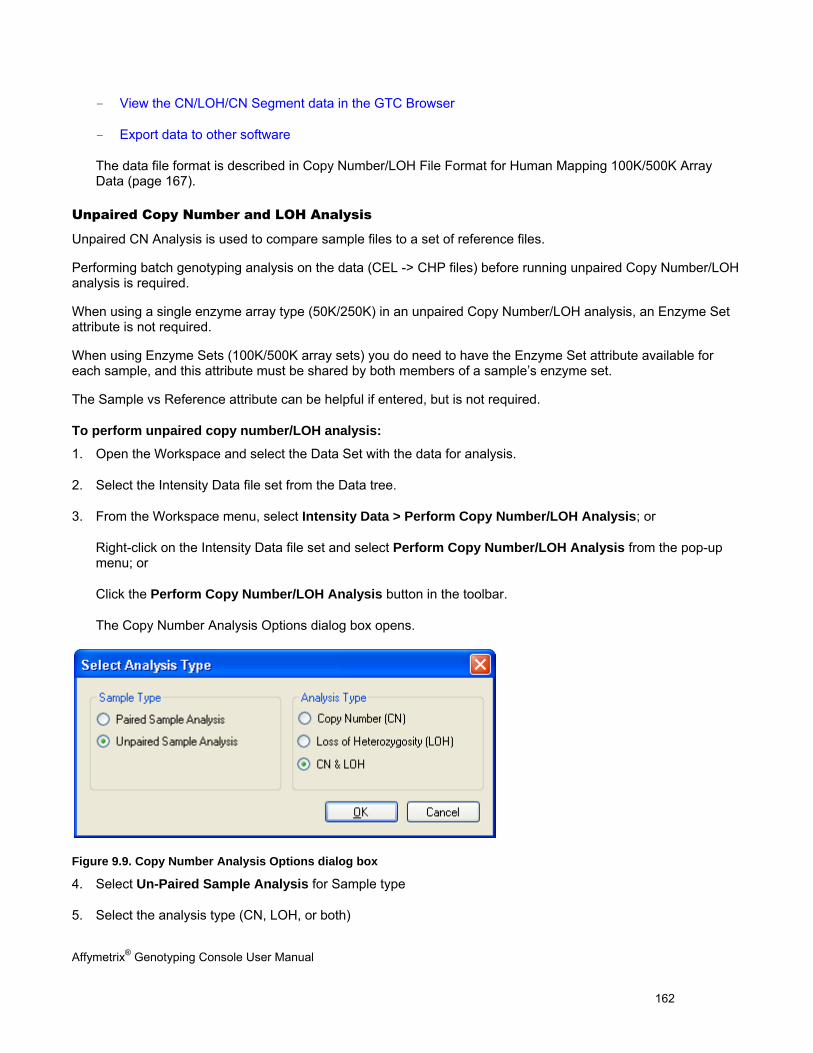
Affymetrix® Genotyping Console User Manual 162
- View the CN/LOH/CN Segment data in the GTC Browser
- Export data to other software
The data file format is described in Copy Number/LOH File Format for Human Mapping 100K/500K Array Data (page 167).
Unpaired Copy Number and LOH Analysis
Unpaired CN Analysis is used to compare sample files to a set of reference files.
Performing batch genotyping analysis on the data (CEL -> CHP files) before running unpaired Copy Number/LOH analysis is required.
When using a single enzyme array type (50K/250K) in an unpaired Copy Number/LOH analysis, an Enzyme Set attribute is not required.
When using Enzyme Sets (100K/500K array sets) you do need to have the Enzyme Set attribute available for each sample, and this attribute must be shared by both members of a sample’s enzyme set.
The Sample vs Reference attribute can be helpful if entered, but is not required.
To perform unpaired copy number/LOH analysis:
1. Open the Workspace and select the Data Set with the data for analysis.
2. Select the Intensity Data file set from the Data tree.
3. From the Workspace menu, select Intensity Data > Perform Copy Number/LOH Analysis; or
Right-click on the Intensity Data file set and select Perform Copy Number/LOH Analysis from the pop-up menu; or
Click the Perform Copy Number/LOH Analysis button in the toolbar.
The Copy Number Analysis Options dialog box opens.
Figure 9.9. Copy Number Analysis Options dialog box
4. Select Un-Paired Sample Analysis for Sample type
5. Select the analysis type (CN, LOH, or both)
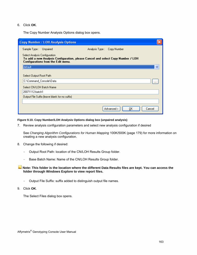
Affymetrix® Genotyping Console User Manual 163
6. Click OK.
The Copy Number Analysis Options dialog box opens.
Figure 9.10. Copy Number/LOH Analysis Options dialog box (unpaired analysis)
7. Review analysis configuration parameters and select new analysis configuration if desired
See Changing Algorithm Configurations for Human Mapping 100K/500K (page 179) for more information on creating a new analysis configuration.
8. Change the following if desired:
- Output Root Path: location of the CN/LOH Results Group folder.
- Base Batch Name: Name of the CN/LOH Results Group folder.
Note: This folder is the location where the different Data Results files are kept. You can access the folder through Windows Explore to view report files.
- Output File Suffix: suffix added to distinguish output file names.
9. Click OK.
The Select Files dialog box opens.
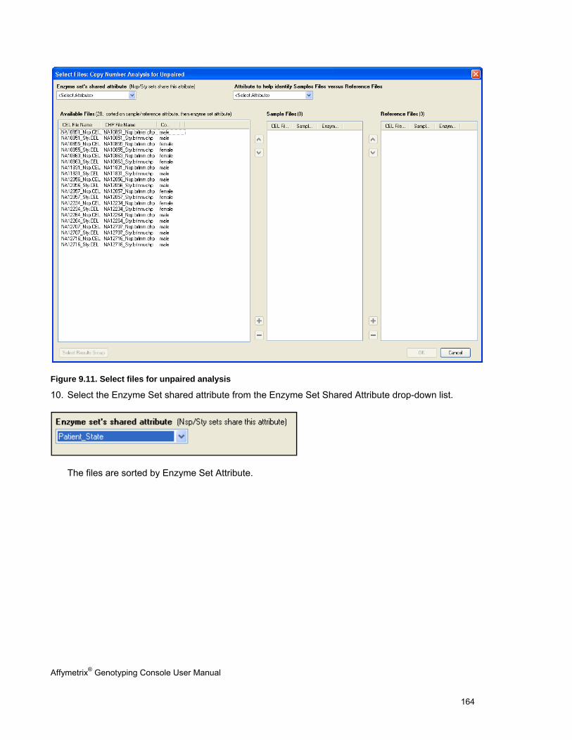
Affymetrix® Genotyping Console User Manual 164
Figure 9.11. Select files for unpaired analysis
10. Select the Enzyme Set shared attribute from the Enzyme Set Shared Attribute drop-down list.
The files are sorted by Enzyme Set Attribute.
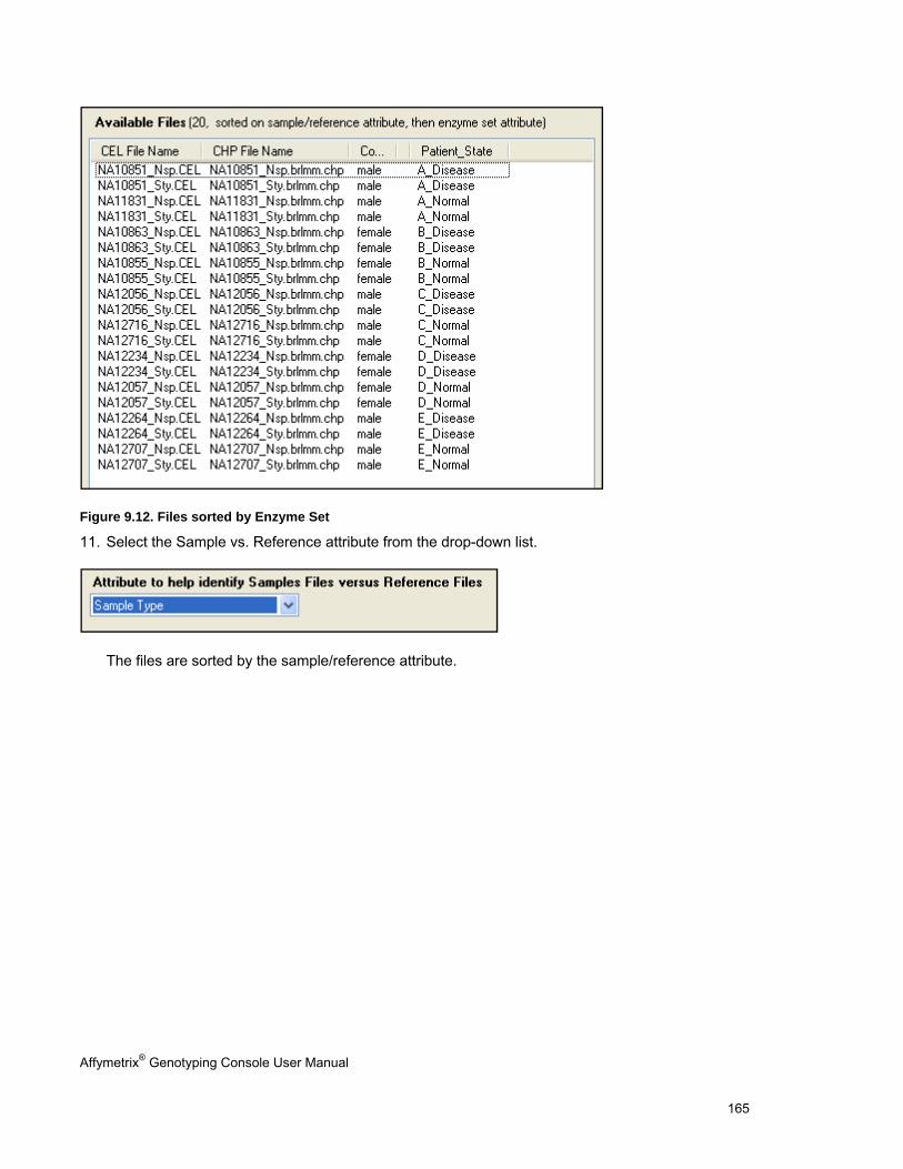
Affymetrix® Genotyping Console User Manual 165
Figure 9.12. Files sorted by Enzyme Set
11. Select the Sample vs. Reference attribute from the drop-down list.
The files are sorted by the sample/reference attribute.
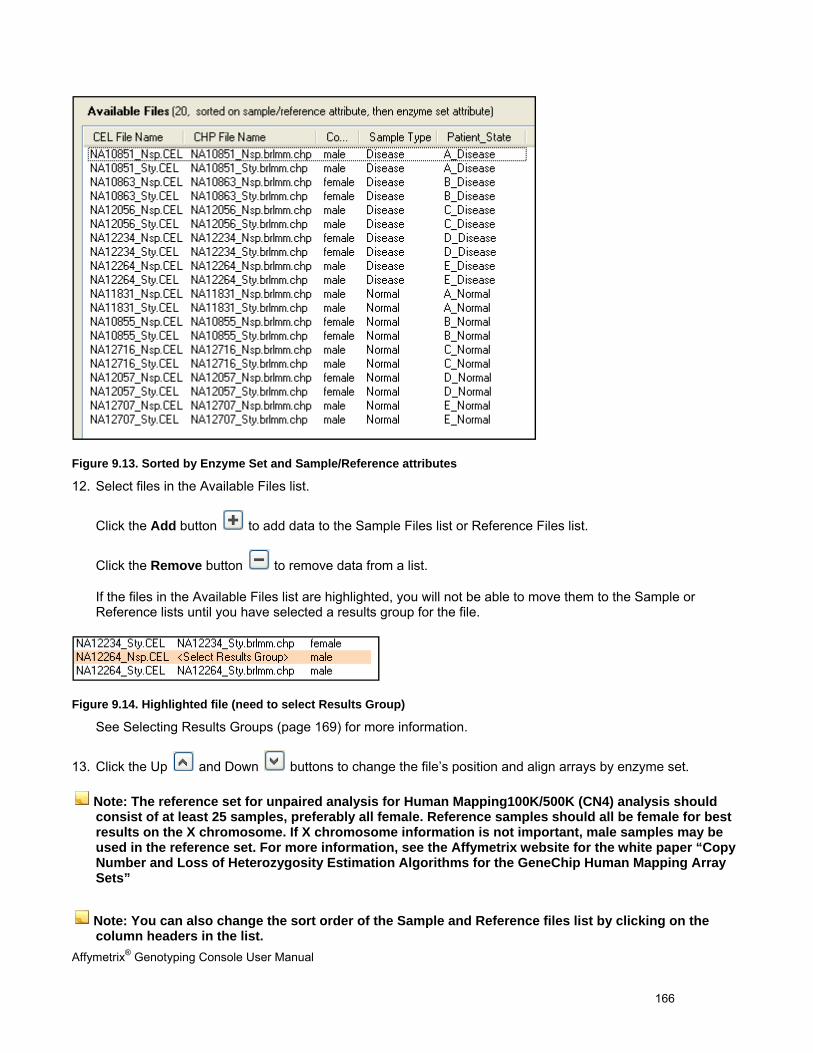
Affymetrix® Genotyping Console User Manual 166
Figure 9.13. Sorted by Enzyme Set and Sample/Reference attributes
12. Select files in the Available Files list.
Click the Add button to add data to the Sample Files list or Reference Files list.
Click the Remove button to remove data from a list.
If the files in the Available Files list are highlighted, you will not be able to move them to the Sample or Reference lists until you have selected a results group for the file.
Figure 9.14. Highlighted file (need to select Results Group)
See Selecting Results Groups (page 169) for more information.
13. Click the Up and Down buttons to change the file’s position and align arrays by enzyme set.
Note: The reference set for unpaired analysis for Human Mapping100K/500K (CN4) analysis should consist of at least 25 samples, preferably all female. Reference samples should all be female for best results on the X chromosome. If X chromosome information is not important, male samples may be used in the reference set. For more information, see the Affymetrix website for the white paper “Copy Number and Loss of Heterozygosity Estimation Algorithms for the GeneChip Human Mapping Array Sets”
Note: You can also change the sort order of the Sample and Reference files list by clicking on the column headers in the list.
Affymetrix® Genotyping Console User Manual 167
For more information about using shared attributes to pair files by enzyme set or sample/reference group, see Using Shared Attributes to Group Samples (page 172).
14. Click OK.
IMPORTANT: The Copy Number and LOH output files will be named using the Enzyme Set attribute for the arrays.
Different progress windows open as the analysis proceeds.
After generating the Copy Number and/or LOH files, you can:
- View CN QC data in tables.
- Generate Segment Report.
- View the CN/LOH/CN Segment data in the GTC Browser.
- Export data to other software.
The data file format is described in Copy Number/LOH File Format for Human Mapping 100K/500K Array Data.
Copy Number/LOH File Format for Human Mapping 100K/500K Array Data
The copy number and LOH data are in separate files for Human Mapping 100K/500K array data.
Header Section
The resulting CN4.cnchp and CN4.lohchp data files contain the following information in the header:
Information about the array (# SNPs, probe array type, library file)
Algorithm parameters and command line that was executed (e.g. all advanced parameters that were used)
Workflow (e.g. paired copy number)
Sample Name
Reference file(s) used
Data Section – For *.CN4.cnchp (Copy Number) Files
The resulting data files contain the following data:
Note: Those values that are labeled “paired analysis only” require that the Generate Allele-Specific Copy Number check box is selected in the Advanced Analysis options.
Item Description
ProbeSet SNP ID
Affymetrix® Genotyping Console User Manual 168
Chromosome Chromosome number
Position Physical position of the SNP
Log2Ratio Smoothed Log2 ratio value
HmmMedianLog2Ratio Median Log2 ratio value of all contiguous SNPs in the given HMM copy number state segment
CNState HMM copy number state
NegLog10PValue Negative Log10 p-value indicating how different the median Log2 ratio of the HMM state is from the normal state (CN State 2) for that particular sample
Log2RatioMin Smoothed Log2 ratio value for the allele with the lower signal intensity (paired analysis only)
HmmMedianLog2RatioMin Median Log2 ratio value of all the contiguous SNPs in the given HMM copy number state segment of the allele with the lower signal intensity (paired analysis only)
CNStateMin HMM copy number state of the allele with the lower signal intensity (paired analysis only)
NegLog10PValueMin Negative Log10 p-value indicating how different the median Log2 ratio of the HMM state of the allele with the lower signal intensity is from the CN 2 State for that particular sample (paired analysis only)
Log2RatioMax Smoothed Log2 ratio value for the allele with the higher signal intensity (paired analysis only)
HmmMedianLog2RatioMax Median Log2 ratio value of all the contiguous SNPs in the given HMM copy number state segment of the allele with the higher signal intensity (paired analysis only)
CNStateMax HMM copy number state of the allele with the higher signal intensity (paired analysis only)
NegLog10PValueMax Negative Log10 p-value indicating how different the median Log2 ratio of the HMM state of the allele with the higher signal intensity is from the CN 2 State for that particular sample (paired analysis only)
Chip# The Array ID (1 or 2) where the SNP resides:
1 = The first array in the virtual set as displayed in the Sample List box.
2 = The second array in the virtual set as displayed in the Sample List box.
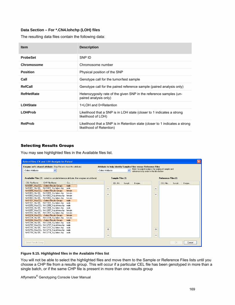
Affymetrix® Genotyping Console User Manual 169
Data Section – For *.CN4.lohchp (LOH) files
The resulting data files contain the following data:
Item Description
ProbeSet SNP ID
Chromosome Chromosome number
Position Physical position of the SNP
Call Genotype call for the tumor/test sample
RefCall Genotype call for the paired reference sample (paired analysis only)
RefHetRate Heterozygosity rate of the given SNP in the reference samples (un-paired analysis only)
LOHState 1=LOH and 0=Retention
LOHProb Likelihood that a SNP is in LOH state (closer to 1 indicates a strong likelihood of LOH)
RetProb Likelihood that a SNP is in Retention state (closer to 1 indicates a strong likelihood of Retention)
Selecting Results Groups
You may see highlighted files in the Available files list.
Figure 9.15. Highlighted files in the Available Files list
You will not be able to select the highlighted files and move them to the Sample or Reference Files lists until you choose a CHP file from a results group. This will occur if a particular CEL file has been genotyped in more than a single batch, or if the same CHP file is present in more than one results group
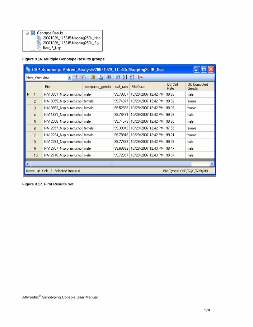
Affymetrix® Genotyping Console User Manual 170
Figure 9.16. Multiple Genotype Results groups
Figure 9.17. First Results Set
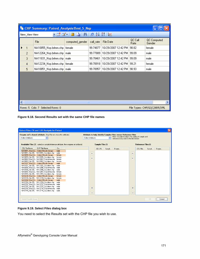
Affymetrix® Genotyping Console User Manual 171
Figure 9.18. Second Results set with the same CHP file names
Figure 9.19. Select Files dialog box
You need to select the Results set with the CHP file you wish to use.
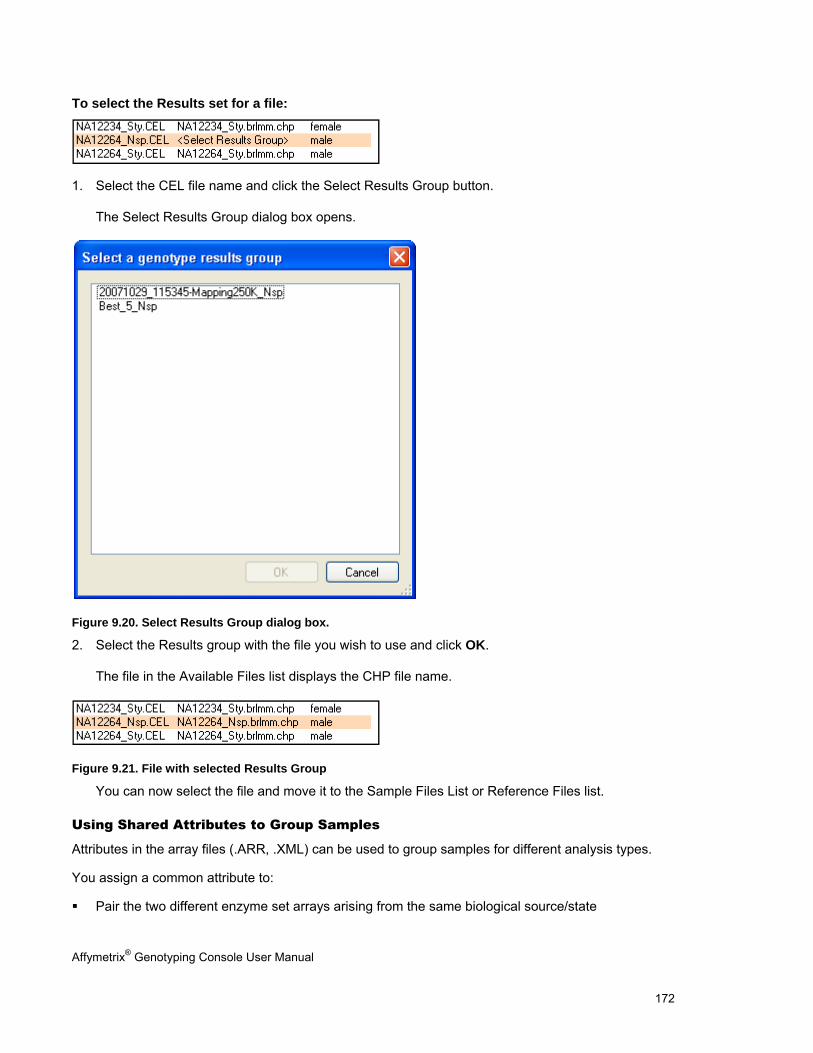
Affymetrix® Genotyping Console User Manual 172
To select the Results set for a file:
1. Select the CEL file name and click the Select Results Group button.
The Select Results Group dialog box opens.
Figure 9.20. Select Results Group dialog box.
2. Select the Results group with the file you wish to use and click OK.
The file in the Available Files list displays the CHP file name.
Figure 9.21. File with selected Results Group
You can now select the file and move it to the Sample Files List or Reference Files list.
Using Shared Attributes to Group Samples
Attributes in the array files (.ARR, .XML) can be used to group samples for different analysis types.
You assign a common attribute to:
Pair the two different enzyme set arrays arising from the same biological source/state
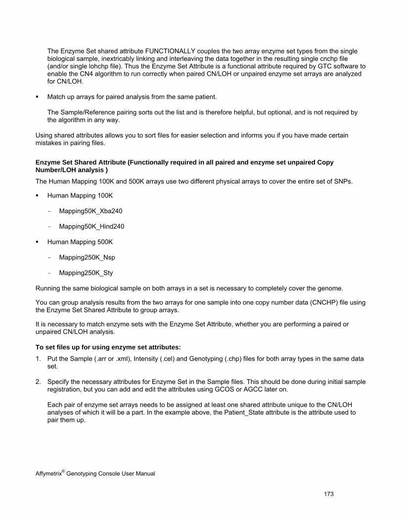
Affymetrix® Genotyping Console User Manual 173
The Enzyme Set shared attribute FUNCTIONALLY couples the two array enzyme set types from the single biological sample, inextricably linking and interleaving the data together in the resulting single cnchp file (and/or single lohchp file). Thus the Enzyme Set Attribute is a functional attribute required by GTC software to enable the CN4 algorithm to run correctly when paired CN/LOH or unpaired enzyme set arrays are analyzed for CN/LOH.
Match up arrays for paired analysis from the same patient.
The Sample/Reference pairing sorts out the list and is therefore helpful, but optional, and is not required by the algorithm in any way.
Using shared attributes allows you to sort files for easier selection and informs you if you have made certain mistakes in pairing files.
Enzyme Set Shared Attribute (Functionally required in all paired and enzyme set unpaired Copy Number/LOH analysis )
The Human Mapping 100K and 500K arrays use two different physical arrays to cover the entire set of SNPs.
Human Mapping 100K
- Mapping50K_Xba240
- Mapping50K_Hind240
Human Mapping 500K
- Mapping250K_Nsp
- Mapping250K_Sty
Running the same biological sample on both arrays in a set is necessary to completely cover the genome.
You can group analysis results from the two arrays for one sample into one copy number data (CNCHP) file using the Enzyme Set Shared Attribute to group arrays.
It is necessary to match enzyme sets with the Enzyme Set Attribute, whether you are performing a paired or unpaired CN/LOH analysis.
To set files up for using enzyme set attributes:
1. Put the Sample (.arr or .xml), Intensity (.cel) and Genotyping (.chp) files for both array types in the same data set.
2. Specify the necessary attributes for Enzyme Set in the Sample files. This should be done during initial sample registration, but you can add and edit the attributes using GCOS or AGCC later on.
Each pair of enzyme set arrays needs to be assigned at least one shared attribute unique to the CN/LOH analyses of which it will be a part. In the example above, the Patient_State attribute is the attribute used to pair them up.
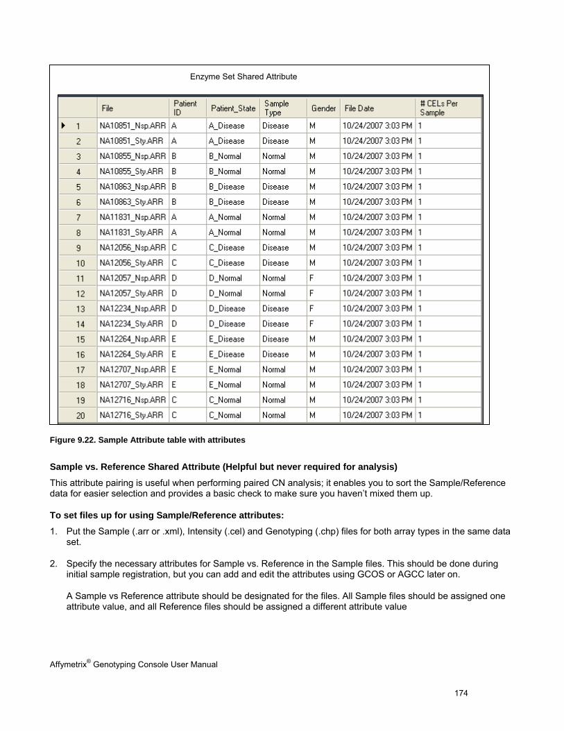
Affymetrix® Genotyping Console User Manual 174
Figure 9.22. Sample Attribute table with attributes
Sample vs. Reference Shared Attribute (Helpful but never required for analysis)
This attribute pairing is useful when performing paired CN analysis; it enables you to sort the Sample/Reference data for easier selection and provides a basic check to make sure you haven’t mixed them up.
To set files up for using Sample/Reference attributes:
1. Put the Sample (.arr or .xml), Intensity (.cel) and Genotyping (.chp) files for both array types in the same data set.
2. Specify the necessary attributes for Sample vs. Reference in the Sample files. This should be done during initial sample registration, but you can add and edit the attributes using GCOS or AGCC later on.
A Sample vs Reference attribute should be designated for the files. All Sample files should be assigned one attribute value, and all Reference files should be assigned a different attribute value
Enzyme Set Shared Attribute
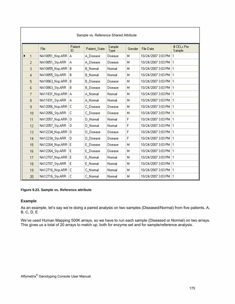
Affymetrix® Genotyping Console User Manual 175
Figure 9.23. Sample vs. Reference attribute
Example
As an example, let’s say we’re doing a paired analysis on two samples (Diseased/Normal) from five patients, A, B, C, D, E
We’ve used Human Mapping 500K arrays, so we have to run each sample (Diseased or Normal) on two arrays. This gives us a total of 20 arrays to match up, both for enzyme set and for sample/reference analysis.
Sample vs. Reference Shared Attribute
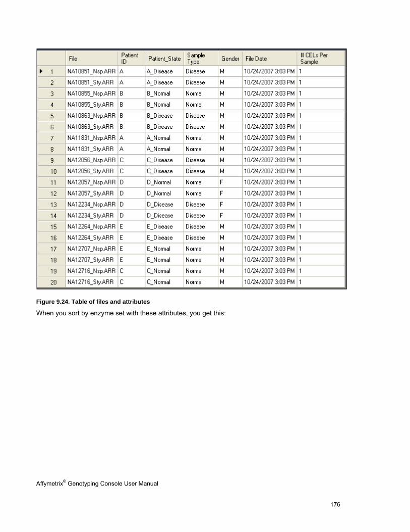
Affymetrix® Genotyping Console User Manual 176
Figure 9.24. Table of files and attributes
When you sort by enzyme set with these attributes, you get this:
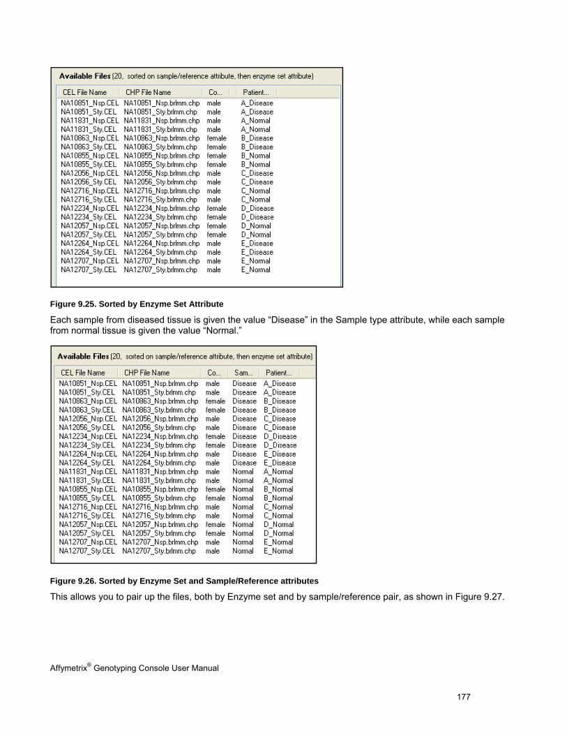
Affymetrix® Genotyping Console User Manual 177
Figure 9.25. Sorted by Enzyme Set Attribute
Each sample from diseased tissue is given the value “Disease” in the Sample type attribute, while each sample from normal tissue is given the value “Normal.”
Figure 9.26. Sorted by Enzyme Set and Sample/Reference attributes
This allows you to pair up the files, both by Enzyme set and by sample/reference pair, as shown in Figure 9.27.
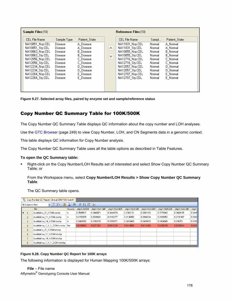
Affymetrix® Genotyping Console User Manual 178
Figure 9.27. Selected array files, paired by enzyme set and sample/reference status
Copy Number QC Summary Table for 100K/500K
The Copy Number QC Summary Table displays QC information about the copy number and LOH analyses.
Use the GTC Browser (page 249) to view Copy Number, LOH, and CN Segments data in a genomic context.
This table displays QC information for Copy Number analysis.
The Copy Number QC Summary Table uses all the table options as described in Table Features.
To open the QC Summary table:
Right-click on the Copy Number/LOH Results set of interested and select Show Copy Number QC Summary Table; or
From the Workspace menu, select Copy Number/LOH Results > Show Copy Number QC Summary Table.
The QC Summary table opens.
Figure 9.28. Copy Number QC Report for 100K arrays
The following information is displayed for Human Mapping 100K/500K arrays:
File – File name
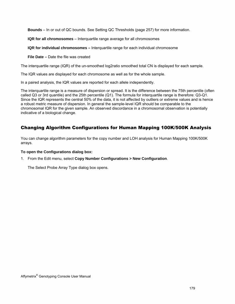
Affymetrix® Genotyping Console User Manual 179
Bounds – In or out of QC bounds. See Setting QC Thresholds (page 257) for more information.
IQR for all chromosomes – Interquartile range average for all chromosomes
IQR for individual chromosomes – Interquartile range for each individual chromosome
File Date – Date the file was created
The interquartile range (IQR) of the un-smoothed log2ratio smoothed total CN is displayed for each sample.
The IQR values are displayed for each chromosome as well as for the whole sample.
In a paired analysis, the IQR values are reported for each allele independently.
The interquartile range is a measure of dispersion or spread. It is the difference between the 75th percentile (often called Q3 or 3rd quantile) and the 25th percentile (Q1). The formula for interquartile range is therefore: Q3-Q1. Since the IQR represents the central 50% of the data, it is not affected by outliers or extreme values and is hence a robust metric measure of dispersion. In general the sample-level IQR should be comparable to the chromosomal IQR for the given sample. An observed discordance in a chromosomal observation is potentially indicative of a biological change.
Changing Algorithm Configurations for Human Mapping 100K/500K Analysis
You can change algorithm parameters for the copy number and LOH analysis for Human Mapping 100K/500K arrays.
To open the Configurations dialog box:
1. From the Edit menu, select Copy Number Configurations > New Configuration.
The Select Probe Array Type dialog box opens.
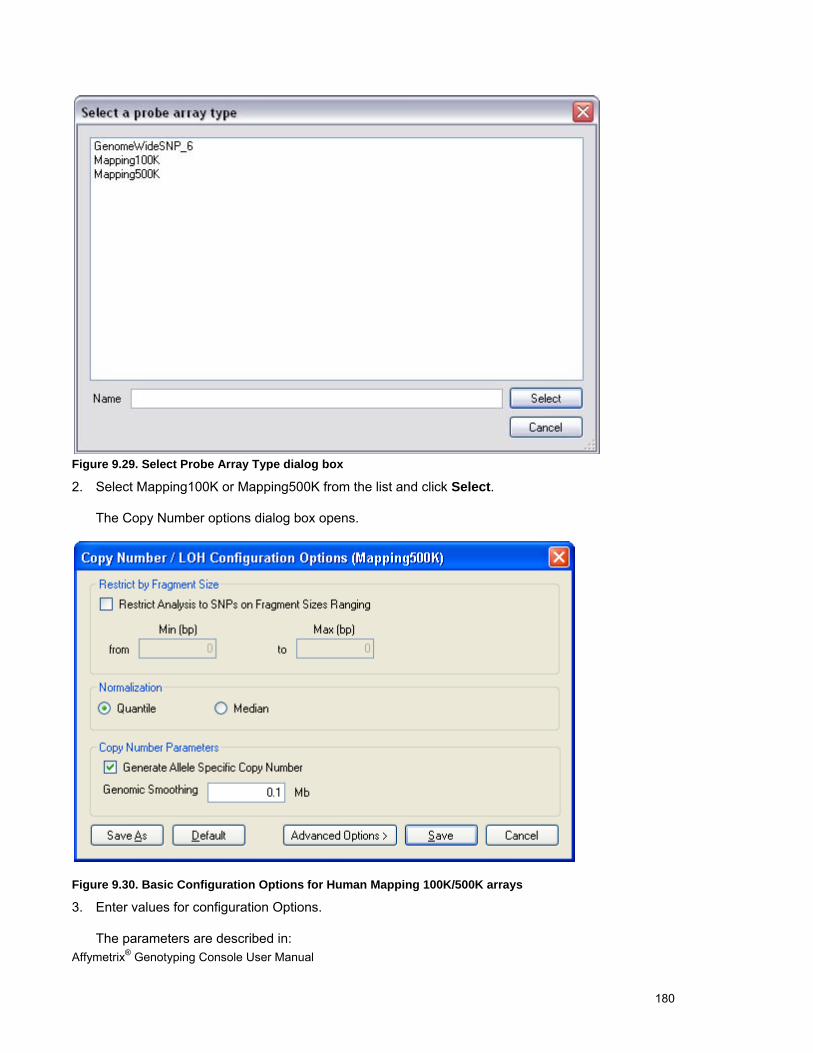
Affymetrix® Genotyping Console User Manual 180
Figure 9.29. Select Probe Array Type dialog box
2. Select Mapping100K or Mapping500K from the list and click Select.
The Copy Number options dialog box opens.
Figure 9.30. Basic Configuration Options for Human Mapping 100K/500K arrays
3. Enter values for configuration Options.
The parameters are described in:
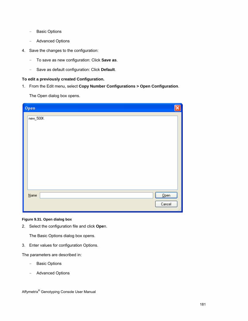
Affymetrix® Genotyping Console User Manual 181
- Basic Options
- Advanced Options
4. Save the changes to the configuration:
- To save as new configuration: Click Save as.
- Save as default configuration: Click Default.
To edit a previously created Configuration.
1. From the Edit menu, select Copy Number Configurations > Open Configuration.
The Open dialog box opens.
Figure 9.31. Open dialog box
2. Select the configuration file and click Open.
The Basic Options dialog box opens.
3. Enter values for configuration Options.
The parameters are described in:
- Basic Options
- Advanced Options
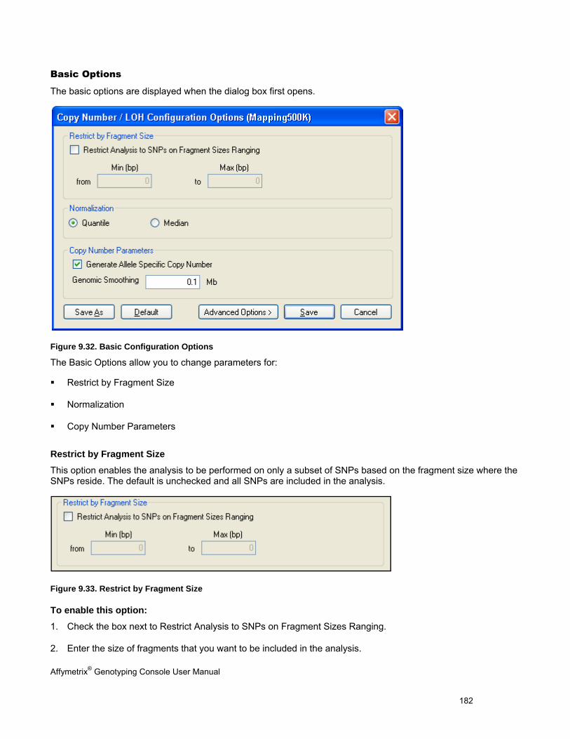
Affymetrix® Genotyping Console User Manual 182
Basic Options
The basic options are displayed when the dialog box first opens.
Figure 9.32. Basic Configuration Options
The Basic Options allow you to change parameters for:
Restrict by Fragment Size
Normalization
Copy Number Parameters
Restrict by Fragment Size
This option enables the analysis to be performed on only a subset of SNPs based on the fragment size where the SNPs reside. The default is unchecked and all SNPs are included in the analysis.
Figure 9.33. Restrict by Fragment Size
To enable this option:
1. Check the box next to Restrict Analysis to SNPs on Fragment Sizes Ranging.
2. Enter the size of fragments that you want to be included in the analysis.
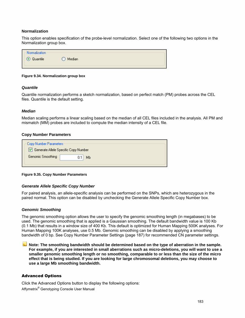
Affymetrix® Genotyping Console User Manual 183
Normalization
This option enables specification of the probe-level normalization. Select one of the following two options in the Normalization group box.
Figure 9.34. Normalization group box
Quantile
Quantile normalization performs a sketch normalization, based on perfect match (PM) probes across the CEL files. Quantile is the default setting.
Median
Median scaling performs a linear scaling based on the median of all CEL files included in the analysis. All PM and mismatch (MM) probes are included to compute the median intensity of a CEL file.
Copy Number Parameters
Figure 9.35. Copy Number Parameters
Generate Allele Specific Copy Number
For paired analysis, an allele-specific analysis can be performed on the SNPs, which are heterozygous in the paired normal. This option can be disabled by unchecking the Generate Allele Specific Copy Number box.
Genomic Smoothing
The genomic smoothing option allows the user to specify the genomic smoothing length (in megabases) to be used. The genomic smoothing that is applied is a Gaussian smoothing. The default bandwidth value is 100 Kb (0.1 Mb) that results in a window size of 400 Kb. This default is optimized for Human Mapping 500K analyses. For Human Mapping 100K analyses, use 0.5 Mb. Genomic smoothing can be disabled by applying a smoothing bandwidth of 0 bp. See Copy Number Parameter Settings (page 187) for recommended CN parameter settings.
Note: The smoothing bandwidth should be determined based on the type of aberration in the sample. For example, if you are interested in small aberrations such as micro-deletions, you will want to use a smaller genomic smoothing length or no smoothing, comparable to or less than the size of the micro effect that is being studied. If you are looking for large chromosomal deletions, you may choose to use a large Mb smoothing bandwidth.
Advanced Options
Click the Advanced Options button to display the following options:
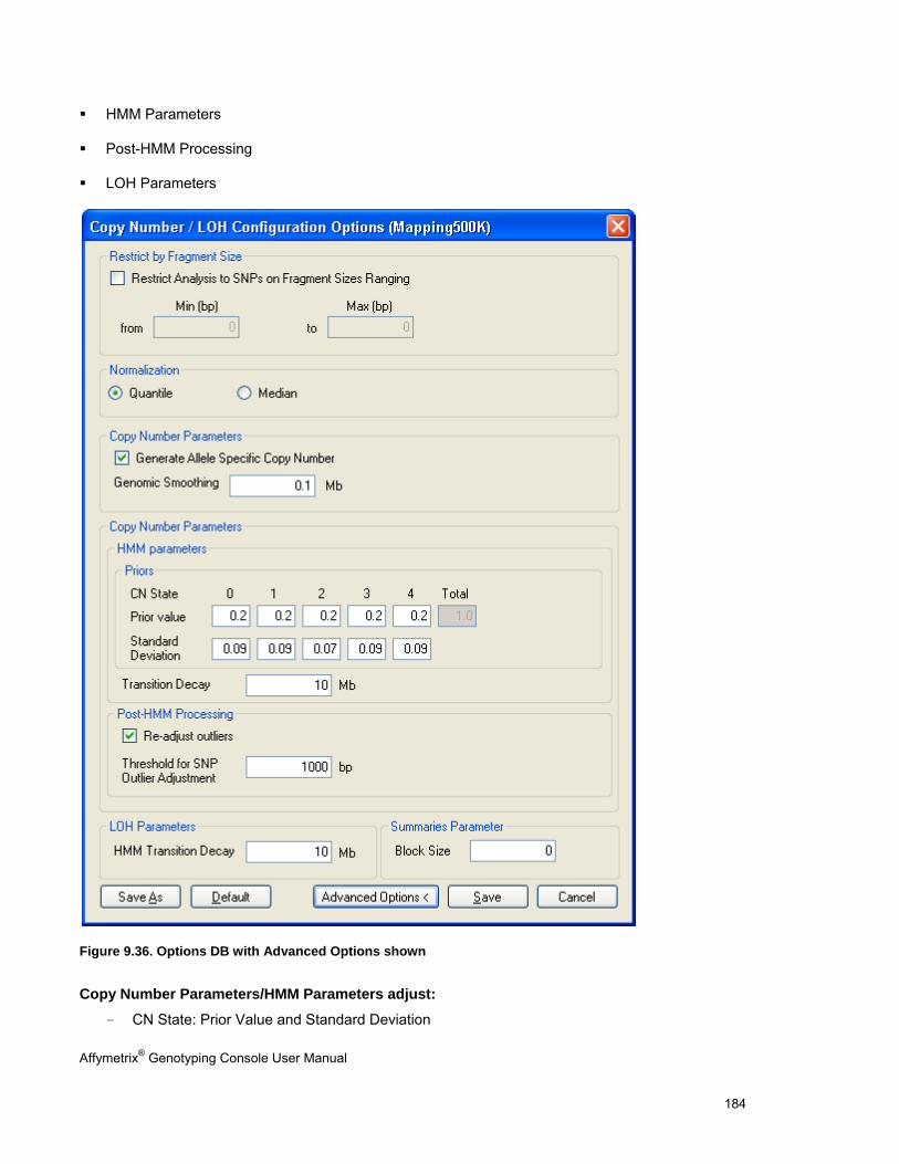
Affymetrix® Genotyping Console User Manual 184
HMM Parameters
Post-HMM Processing
LOH Parameters
Figure 9.36. Options DB with Advanced Options shown
Copy Number Parameters/HMM Parameters adjust:
- CN State: Prior Value and Standard Deviation
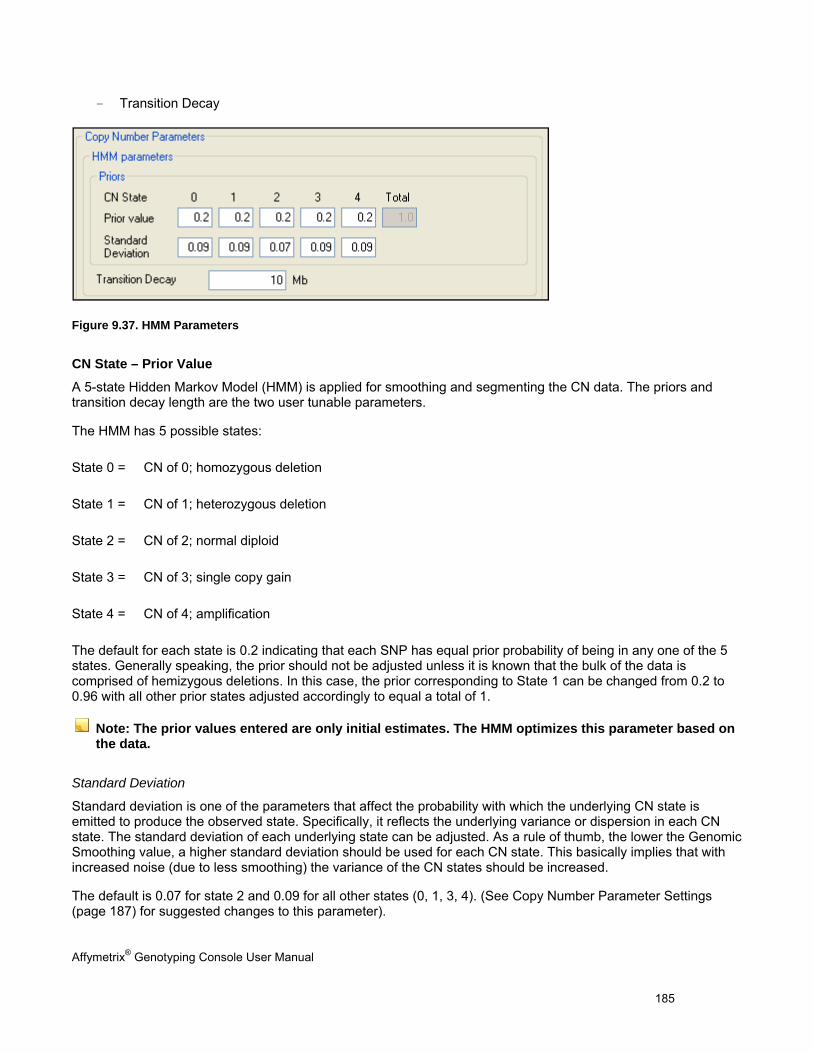
Affymetrix® Genotyping Console User Manual 185
- Transition Decay
Figure 9.37. HMM Parameters
CN State – Prior Value
A 5-state Hidden Markov Model (HMM) is applied for smoothing and segmenting the CN data. The priors and transition decay length are the two user tunable parameters.
The HMM has 5 possible states:
State 0 = CN of 0; homozygous deletion
State 1 = CN of 1; heterozygous deletion
State 2 = CN of 2; normal diploid
State 3 = CN of 3; single copy gain
State 4 = CN of 4; amplification
The default for each state is 0.2 indicating that each SNP has equal prior probability of being in any one of the 5 states. Generally speaking, the prior should not be adjusted unless it is known that the bulk of the data is comprised of hemizygous deletions. In this case, the prior corresponding to State 1 can be changed from 0.2 to 0.96 with all other prior states adjusted accordingly to equal a total of 1.
Note: The prior values entered are only initial estimates. The HMM optimizes this parameter based on the data.
Standard Deviation
Standard deviation is one of the parameters that affect the probability with which the underlying CN state is emitted to produce the observed state. Specifically, it reflects the underlying variance or dispersion in each CN state. The standard deviation of each underlying state can be adjusted. As a rule of thumb, the lower the Genomic Smoothing value, a higher standard deviation should be used for each CN state. This basically implies that with increased noise (due to less smoothing) the variance of the CN states should be increased.
The default is 0.07 for state 2 and 0.09 for all other states (0, 1, 3, 4). (See Copy Number Parameter Settings (page 187) for suggested changes to this parameter).
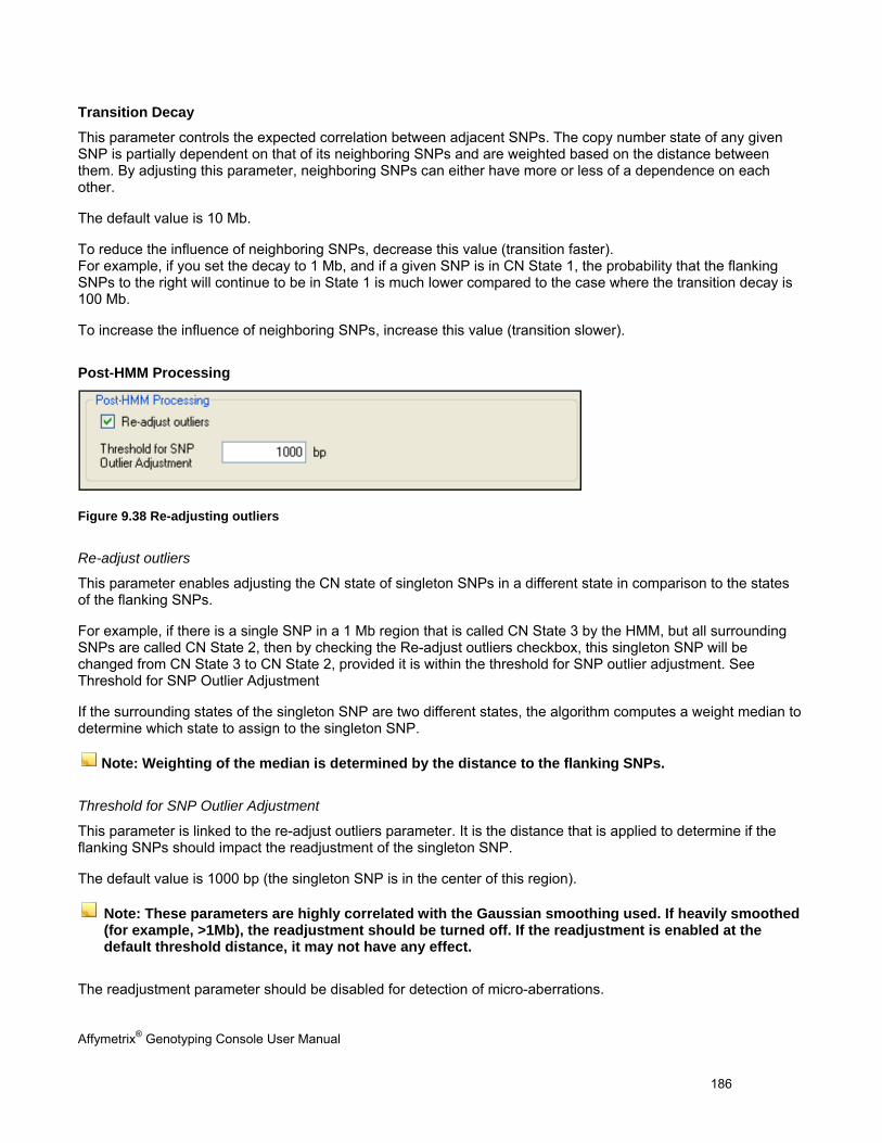
Affymetrix® Genotyping Console User Manual 186
Transition Decay
This parameter controls the expected correlation between adjacent SNPs. The copy number state of any given SNP is partially dependent on that of its neighboring SNPs and are weighted based on the distance between them. By adjusting this parameter, neighboring SNPs can either have more or less of a dependence on each other.
The default value is 10 Mb.
To reduce the influence of neighboring SNPs, decrease this value (transition faster). For example, if you set the decay to 1 Mb, and if a given SNP is in CN State 1, the probability that the flanking SNPs to the right will continue to be in State 1 is much lower compared to the case where the transition decay is 100 Mb.
To increase the influence of neighboring SNPs, increase this value (transition slower).
Post-HMM Processing
Figure 9.38 Re-adjusting outliers
Re-adjust outliers
This parameter enables adjusting the CN state of singleton SNPs in a different state in comparison to the states of the flanking SNPs.
For example, if there is a single SNP in a 1 Mb region that is called CN State 3 by the HMM, but all surrounding SNPs are called CN State 2, then by checking the Re-adjust outliers checkbox, this singleton SNP will be changed from CN State 3 to CN State 2, provided it is within the threshold for SNP outlier adjustment. See Threshold for SNP Outlier Adjustment
If the surrounding states of the singleton SNP are two different states, the algorithm computes a weight median to determine which state to assign to the singleton SNP.
Note: Weighting of the median is determined by the distance to the flanking SNPs.
Threshold for SNP Outlier Adjustment
This parameter is linked to the re-adjust outliers parameter. It is the distance that is applied to determine if the flanking SNPs should impact the readjustment of the singleton SNP.
The default value is 1000 bp (the singleton SNP is in the center of this region).
Note: These parameters are highly correlated with the Gaussian smoothing used. If heavily smoothed (for example, >1Mb), the readjustment should be turned off. If the readjustment is enabled at the default threshold distance, it may not have any effect.
The readjustment parameter should be disabled for detection of micro-aberrations.
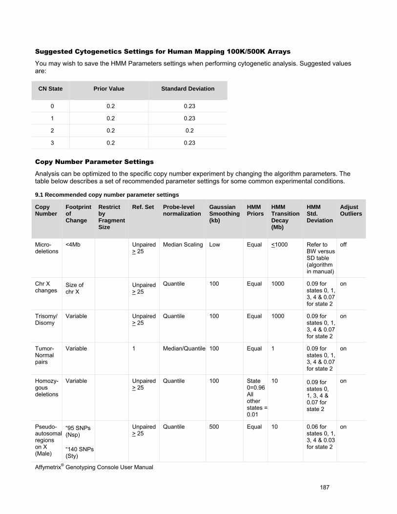
Affymetrix® Genotyping Console User Manual 187
Suggested Cytogenetics Settings for Human Mapping 100K/500K Arrays
You may wish to save the HMM Parameters settings when performing cytogenetic analysis. Suggested values are:
CN State Prior Value Standard Deviation
0 0.2 0.23
1 0.2 0.23
2 0.2 0.2
3 0.2 0.23
Copy Number Parameter Settings
Analysis can be optimized to the specific copy number experiment by changing the algorithm parameters. The table below describes a set of recommended parameter settings for some common experimental conditions.
9.1 Recommended copy number parameter settings
Copy Number
Footprint of Change
Restrict by Fragment Size
Ref. Set Probe-level normalization
Gaussian Smoothing (kb)
HMM Priors
HMM Transition Decay (Mb)
HMM Std. Deviation
Adjust Outliers
Micro-deletions
<4Mb Unpaired > 25
Median Scaling Low Equal <1000 Refer to BW versus SD table (algorithm in manual)
off
Chr X changes
Size of chr X
Unpaired > 25
Quantile 100 Equal 1000 0.09 for states 0, 1, 3, 4 & 0.07 for state 2
on
Trisomy/ Disomy
Variable Unpaired > 25
Quantile 100 Equal 1000 0.09 for states 0, 1, 3, 4 & 0.07 for state 2
on
Tumor-Normal pairs
Variable 1 Median/Quantile 100 Equal 1 0.09 for states 0, 1, 3, 4 & 0.07 for state 2
on
Homozy-gous deletions
Variable Unpaired > 25
Quantile 100 State 0=0.96 All other states = 0.01
10 0.09 for states 0, 1, 3, 4 & 0.07 for state 2
on
Pseudo-autosomalregions on X (Male)
“95 SNPs (Nsp)
“140 SNPs (Sty)
Unpaired > 25
Quantile 500 Equal 10 0.06 for states 0, 1, 3, 4 & 0.03 for state 2
on
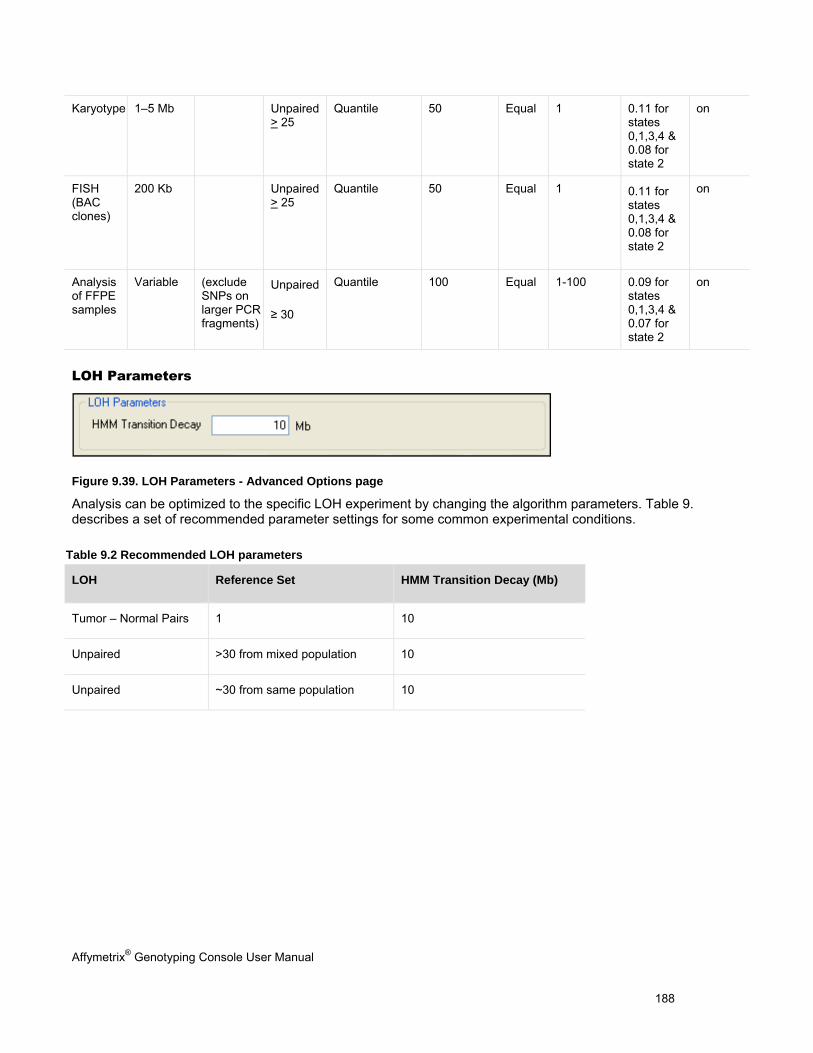
Affymetrix® Genotyping Console User Manual 188
Karyotype 1–5 Mb Unpaired > 25
Quantile 50 Equal 1 0.11 for states 0,1,3,4 & 0.08 for state 2
on
FISH (BAC clones)
200 Kb Unpaired > 25
Quantile 50 Equal 1 0.11 for states 0,1,3,4 & 0.08 for state 2
on
Analysis of FFPE samples
Variable (exclude SNPs on larger PCR fragments)
Unpaired
≥ 30
Quantile 100 Equal 1-100 0.09 for states 0,1,3,4 & 0.07 for state 2
on
LOH Parameters
Figure 9.39. LOH Parameters - Advanced Options page
Analysis can be optimized to the specific LOH experiment by changing the algorithm parameters. Table 9. describes a set of recommended parameter settings for some common experimental conditions.
Table 9.2 Recommended LOH parameters
LOH Reference Set HMM Transition Decay (Mb)
Tumor – Normal Pairs 1 10
Unpaired >30 from mixed population 10
Unpaired ~30 from same population 10
Affymetrix® Genotyping Console User Manual 189
Chapter 10: Copy Number & LOH Analysis for Genome-Wide Human SNP 6.0 Arrays
GTC 4.0 can be used to perform the following analyses for the Genome-Wide Human SNP Array 6.0:
Copy Number (CN)
Loss of Heterozygosity (LOH)
The following analyses are performed on the CN data generated during CN/LOH analysis.
Copy Number Segment Reporting
Custom Region Copy Number Segment Reporting
Note: Copy Number Variation (CNV) analysis is performed in a separate step from CN/LOH analysis. The CNV data can be viewed in the Heat Map with the CN data. See Chapter 12: Copy Number Variation Analysis (page 260) for more information.
GTC 4.0 provides an updated default CN configuration file to accommodate updates in CN analysis. For the configuration type CN/LOH Analysis, the Marker-level Normalization option is set to Median Autosome in the default configuration file. You can manually change the Marker-level Normalization option by editing the configuration file (for more details, see Changing Algorithm Configurations for SNP 6.0 Analysis, page 210). CN configuration files from GTC 3.0, 3.0.1, and 3.0.2 are automatically updated when GTC 4.0 launches, or when a new user profile is selected, or when the library path is changed. Configuration files from GTC 2.0 or 2.1 are not updated.
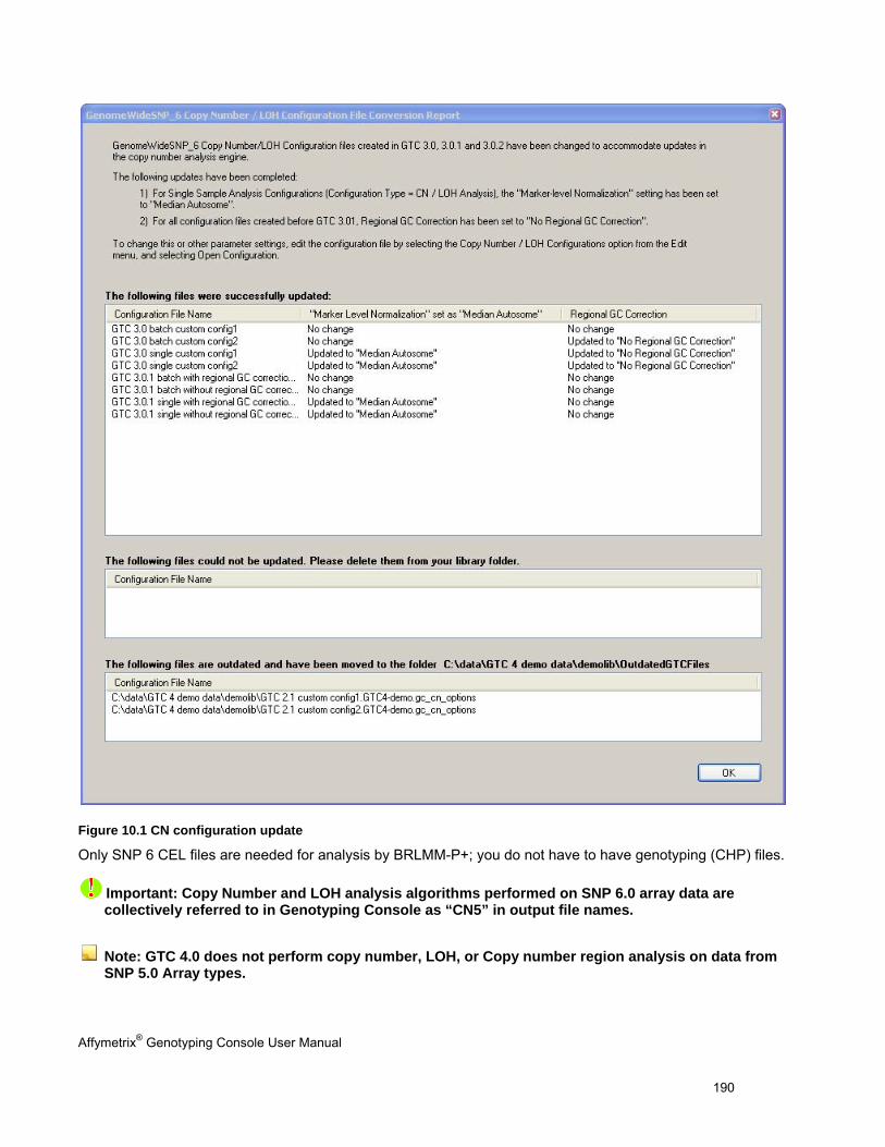
Affymetrix® Genotyping Console User Manual 190
Figure 10.1 CN configuration update
Only SNP 6 CEL files are needed for analysis by BRLMM-P+; you do not have to have genotyping (CHP) files.
Important: Copy Number and LOH analysis algorithms performed on SNP 6.0 array data are collectively referred to in Genotyping Console as “CN5” in output file names.
Note: GTC 4.0 does not perform copy number, LOH, or Copy number region analysis on data from SNP 5.0 Array types.
Affymetrix® Genotyping Console User Manual 191
Affymetrix recommends that you perform Copy Number/LOH analysis with all files stored locally. For more details on hard disk space requirements, see Appendix J, page 319.
Affymetrix recommends that you perform Copy Number/LOH analysis with regional GC correction configuration.
The basic workflow for Copy Number/LOH analysis for SNP 6.0 arrays involves:
1. Performing Copy Number/LOH analysis on a selection of CEL files (page 192).
There are two options for this analysis:
- CN/LOH Reference Model File Creation and Analysis (Batch Sample Mode) (page 193)
- CN/LOH Analysis with a Previously Created Reference Model File (Single Sample Mode) (page 200)
2. Performing the Copy Number Segment analysis on the CN data files (page 227).
Note: Segment Reporting Analysis can also be performed on 100K/500K data.
3. Running the Segment Reporting Tool on the SNP 6.0 CN data (page 227).
For SNP 6.0 data, the Segment Report also provides gender calls, including reports for samples with Unknown (or ambiguous) genders.
4. Viewing QC data in table format (page 207)
5. Viewing the CN/LOH data in the GTC Browser (page 249)
6. Viewing the Copy Number and Copy Number Variation (CNV) data in the Heat Map Viewer (page 269).
Note: CNV analysis is performed in a separate step from CN/LOH analysis. The CNV data can be viewed in the Heat Map with the CN data. See Chapter 12: Copy Number Variation Analysis (page 260) for more information.
7. Exporting data into formats that can be used by secondary analysis software (page 251)
You can also:
Change the QC threshold settings (page 257)
Change the algorithm parameters for SNP 6.0 analysis (page 210)
Note: Small numerical differences may occur between different runs even with the same inputs due to an interaction between rounding from double to single precision and the way the application handles memory management.
Affymetrix® Genotyping Console User Manual 192
Copy Number/LOH Analysis for SNP 6.0 Arrays
Important: Affymetrix recommends that you perform Copy Number/LOH analysis with all files stored locally.
The CN/LOH analysis outputs files with the extension CN5.cnchp, and these files contain both copy number and LOH data.
The following types of analysis can be performed:
CN/LOH Reference Model File Creation and Analysis (Batch Sample Mode), below
This analysis first creates a Reference Model file using the CEL files for the selected samples. Then each CEL file that went into making this Reference Model file is analyzed against this Reference Model file. From this comparison, the sample's Copy Number and LOH data are generated. The genotype calls made on the fly by the BRLMM-P+ algorithm are used for the LOH analysis.
The analysis provides Gender Calls — Female or Male.
CN/LOH Analysis with a Previously Created Reference Model File (Single Sample Mode) (page 200)
In this analysis you compare the selected sample CEL files to a previously created Reference Model file, either the HapMap270 file supplied by Affymetrix or a Reference Model file you have created using the CN/LOH Reference Model File Creation and Analysis process described above. In this “Single sample” workflow, there are no CHP files generated and the LOH analysis is done with the genotype calls made on the fly by the BRLMM-P+ algorithm using the Reference Model data.
The analysis provides Gender Calls — Female or Male.
Note: Small numerical differences may occur between different runs even with the same inputs due to an interaction between rounding from double to single precision and the way the application handles memory management.
Note: CN/LOH analysis can be run with configuration with regional GC correction or with configuration without regional GC correction in both batch sample mode and single sample mode.
Note: Previous GTC 3.0 configuration files will automatically be updated by GTC 4.0 and run as configuration without GC correction with updated score threshold (1.0) and configurable Marker-level Normalization.
Note: Configuration with regional GC correction will need NetAffx NA26.1 or higher version of annotation files. Configuration without regional GC correction will need NetAffx NA25 or higher version of annotation files.
Copy Number and LOH analyses are done during the same analysis run and the data are kept in the same CN5.cnchp file.
Affymetrix® Genotyping Console User Manual 193
CN/LOH Reference Model File Creation and Analysis (Batch Sample Mode)
Important: Affymetrix recommends that you perform Copy Number/LOH analysis with regional GC correction configuration.
Important: Affymetrix recommends that you run Copy Number/LOH analysis with batch sample mode and regional GC correction using chips run at the same lab using the same reagent lots to reduce general variability and to correct GC waviness. See Appendix J, page 319 for more details on hard disk space requirements.
This analysis first creates a Reference Model File (.REF) using the CEL files for the selected samples. Then each CEL file that went into making this Reference Model File is analyzed against this Reference Model File and the sample's Copy Number and LOH data are generated. Note that the genotype calls on the fly from the BRLMM-P+ are used for the LOH analysis. The Reference Model Files end in the filename extension .ref.
To create a Reference Model File for SNP 6.0 analysis and perform CN/LOH analysis:
1. Open the Workspace and select the Data Set with the data for analysis.
2. Select the Intensity Data file set from the Data tree.
3. From the Workspace menu, select Intensity Data > Create Copy Number/LOH Reference Model File and Perform Analysis; or
Right-click on the Intensity Data file set and select Create Copy Number/LOH Reference Model File and Perform Analysis from the pop-up menu; or
Click the Create Copy Number/LOH Analysis button in the toolbar and select Create Copy Number/LOH Reference Model File and Perform Analysis… from the menu.
The Copy Number/LOH Analysis Options for Reference Model File Creation and analysis dialog box opens.
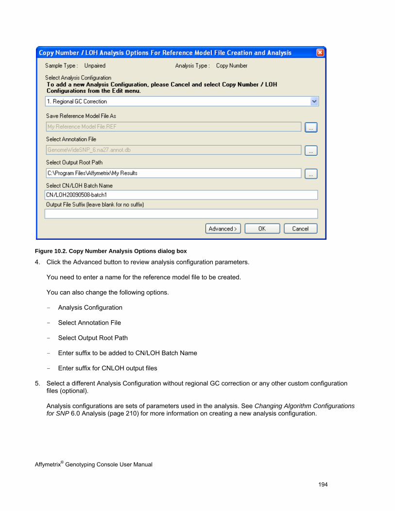
Affymetrix® Genotyping Console User Manual 194
Figure 10.2. Copy Number Analysis Options dialog box
4. Click the Advanced button to review analysis configuration parameters.
You need to enter a name for the reference model file to be created.
You can also change the following options.
- Analysis Configuration
- Select Annotation File
- Select Output Root Path
- Enter suffix to be added to CN/LOH Batch Name
- Enter suffix for CNLOH output files
5. Select a different Analysis Configuration without regional GC correction or any other custom configuration files (optional).
Analysis configurations are sets of parameters used in the analysis. See Changing Algorithm Configurations for SNP 6.0 Analysis (page 210) for more information on creating a new analysis configuration.
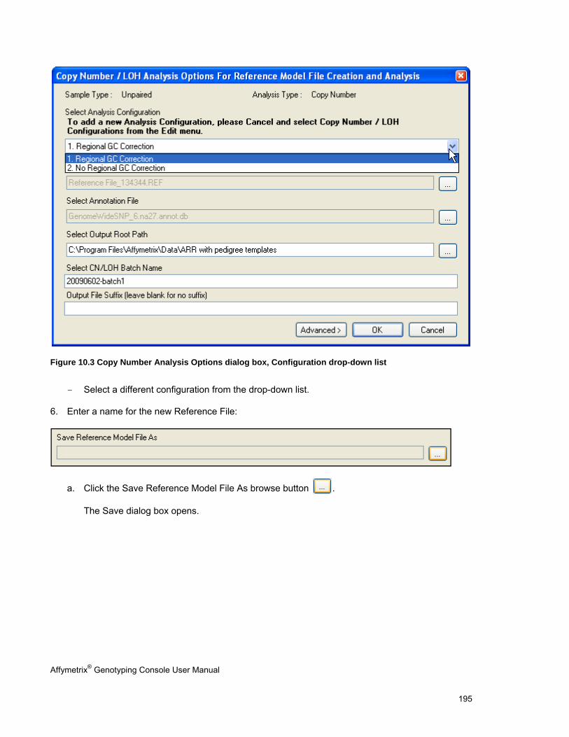
Affymetrix® Genotyping Console User Manual 195
Figure 10.3 Copy Number Analysis Options dialog box, Configuration drop-down list
- Select a different configuration from the drop-down list.
6. Enter a name for the new Reference File:
a. Click the Save Reference Model File As browse button .
The Save dialog box opens.
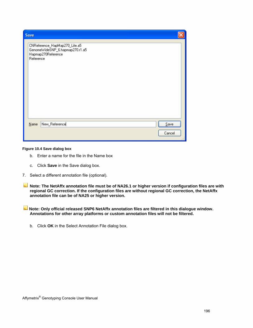
Affymetrix® Genotyping Console User Manual 196
Figure 10.4 Save dialog box
b. Enter a name for the file in the Name box
c. Click Save in the Save dialog box.
7. Select a different annotation file (optional).
Note: The NetAffx annotation file must be of NA26.1 or higher version if configuration files are with regional GC correction. If the configuration files are without regional GC correction, the NetAffx annotation file can be of NA25 or higher version.
Note: Only official released SNP6 NetAffx annotation files are filtered in this dialogue window. Annotations for other array platforms or custom annotation files will not be filtered.
b. Click OK in the Select Annotation File dialog box.
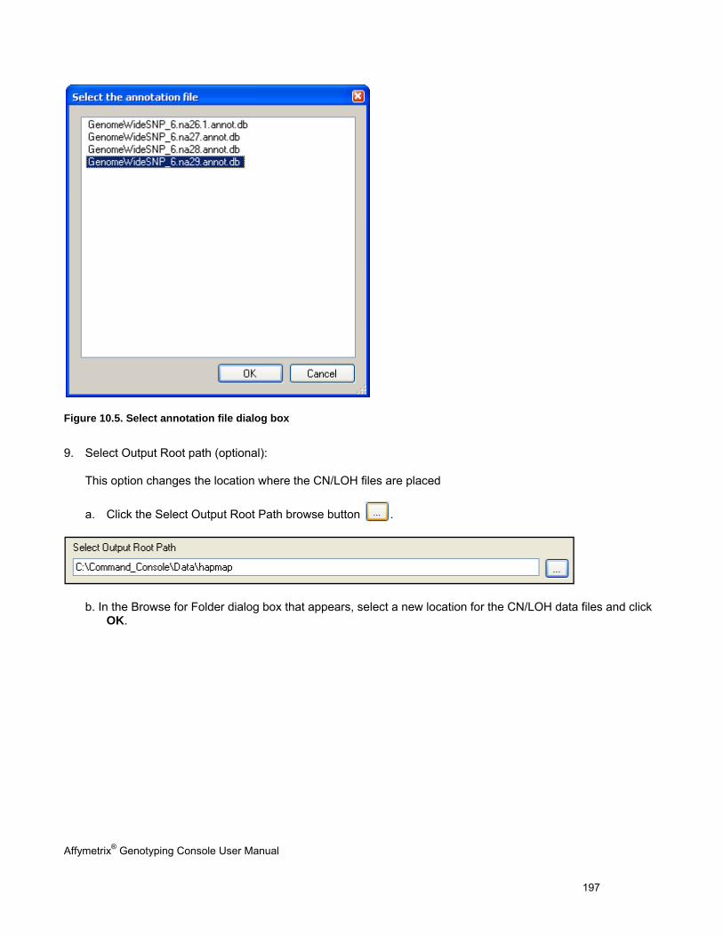
Affymetrix® Genotyping Console User Manual 197
Figure 10.5. Select annotation file dialog box
9. Select Output Root path (optional):
This option changes the location where the CN/LOH files are placed
a. Click the Select Output Root Path browse button .
b. In the Browse for Folder dialog box that appears, select a new location for the CN/LOH data files and click OK.
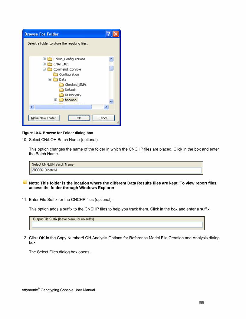
Affymetrix® Genotyping Console User Manual 198
Figure 10.6. Browse for Folder dialog box
10. Select CN/LOH Batch Name (optional):
This option changes the name of the folder in which the CNCHP files are placed. Click in the box and enter the Batch Name.
Note: This folder is the location where the different Data Results files are kept. To view report files, access the folder through Windows Explorer.
11. Enter File Suffix for the CNCHP files (optional):
This option adds a suffix to the CNCHP files to help you track them. Click in the box and enter a suffix.
12. Click OK in the Copy Number/LOH Analysis Options for Reference Model File Creation and Analysis dialog box.
The Select Files dialog box opens.
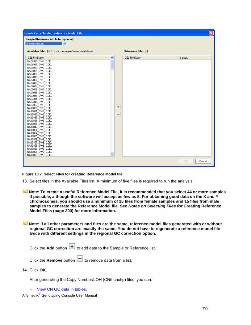
Affymetrix® Genotyping Console User Manual 199
Figure 10.7. Select Files for creating Reference Model file
13. Select files in the Available Files list. A minimum of five files is required to run the analysis.
Note: To create a useful Reference Model File, it is recommended that you select 44 or more samples if possible, although the software will accept as few as 5. For obtaining good data on the X and Y chromosomes, you should use a minimum of 15 files from female samples and 15 files from male samples to generate the Reference Model file. See Notes on Selecting Files for Creating Reference Model Files (page 200) for more information.
Note: If all other parameters and files are the same, reference model files generated with or without regional GC correction are exactly the same. You do not have to regenerate a reference model file twice with different settings in the regional GC correction option.
Click the Add button to add data to the Sample or Reference list.
Click the Remove button to remove data from a list.
14. Click OK.
After generating the Copy Number/LOH (CN5.cnchp) files, you can:
- View CN QC data in tables.
Affymetrix® Genotyping Console User Manual 200
- Use the new Reference Model file to perform additional single-sample CN/LOH analysis (below).
- Generate Copy Number Segment Reports.
- View the CN data in the Heat Map viewer
- Export data to other software.
Notes on Selecting Files for Creating Reference Model Files
Affymetrix recommends using a minimum of 44 samples when creating a Reference Model File. A minimum of five files is required to run the analysis.
For Chromosome X female samples are the reference. Affymetrix recommends using at least 15 female samples when creating a Reference Model File for analysis of the X chromosome.
For Chromosome Y male samples are the reference. Affymetrix recommends using at least 15 male samples when creating a Reference Model File for analysis of the Y chromosome.
Affymetrix recommends using a mixed gender samples when creating a Reference Model File for analysis.
CN/LOH Analysis with a Previously Created Reference Model File (Single Sample Mode)
Important: Affymetrix recommends that you perform Copy Number/LOH analysis with regional GC correction configuration.
Important: Affymetrix recommends that you run Copy Number/LOH analysis with batch sample mode and regional GC correction using chips run at the same lab using the same reagent lots to reduce general variability and to correct GC waviness. See Appendix J, page 319 for more details on hard disk space requirements.
In this analysis you compare the selected sample CEL files to a previously created Reference Model file, either the HapMap270 one supplied by Affymetrix or a reference you have created using the CN/LOH Reference Model File Creation and Analysis process described above. In this workflow no CHP files are required; instead the LOH analysis is done with the genotype calls made on the fly by the BRLMM-P+ algorithm.
Note: You can perform a single sample analysis on more than one CEL file at a time; single sample means that each CEL file is compared to a reference model file.
Notes on Selecting Files against a Previously Created Reference Model File
Affymetrix recommends not using only female samples against a Reference Model File previously created with only male samples when running CN/LOH analysis.
See Appendix A: Algorithms (page 292) for references to the BRLMM-P+ algorithm.
To perform CN/LOH analysis with a previously created Reference Model File:
1. Open the Workspace and select the Data Set with the data for analysis.
2. Select the Intensity Data file set.
3. From the Workspace menu, select Intensity Data > Perform Copy Number/LOH Analysis; or
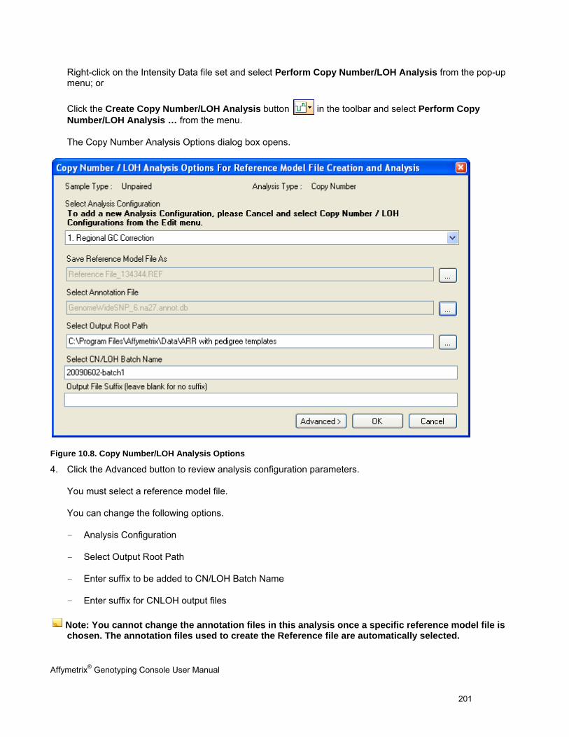
Affymetrix® Genotyping Console User Manual 201
Right-click on the Intensity Data file set and select Perform Copy Number/LOH Analysis from the pop-up menu; or
Click the Create Copy Number/LOH Analysis button in the toolbar and select Perform Copy Number/LOH Analysis … from the menu.
The Copy Number Analysis Options dialog box opens.
Figure 10.8. Copy Number/LOH Analysis Options
4. Click the Advanced button to review analysis configuration parameters.
You must select a reference model file.
You can change the following options.
- Analysis Configuration
- Select Output Root Path
- Enter suffix to be added to CN/LOH Batch Name
- Enter suffix for CNLOH output files
Note: You cannot change the annotation files in this analysis once a specific reference model file is chosen. The annotation files used to create the Reference file are automatically selected.
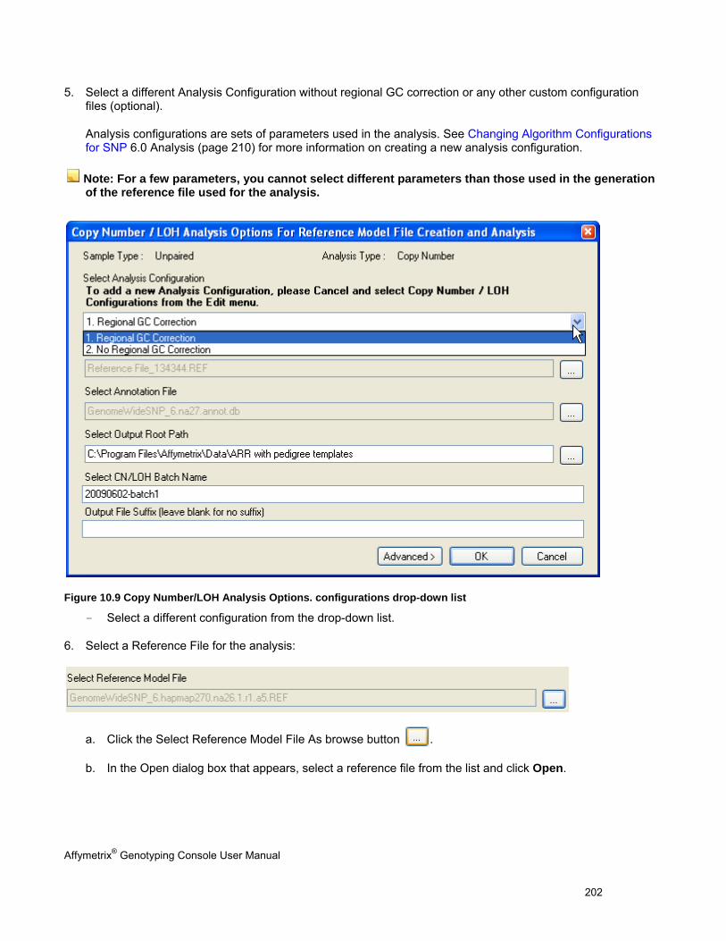
Affymetrix® Genotyping Console User Manual 202
5. Select a different Analysis Configuration without regional GC correction or any other custom configuration files (optional).
Analysis configurations are sets of parameters used in the analysis. See Changing Algorithm Configurations for SNP 6.0 Analysis (page 210) for more information on creating a new analysis configuration.
Note: For a few parameters, you cannot select different parameters than those used in the generation of the reference file used for the analysis.
Figure 10.9 Copy Number/LOH Analysis Options. configurations drop-down list
- Select a different configuration from the drop-down list.
6. Select a Reference File for the analysis:
a. Click the Select Reference Model File As browse button .
b. In the Open dialog box that appears, select a reference file from the list and click Open.
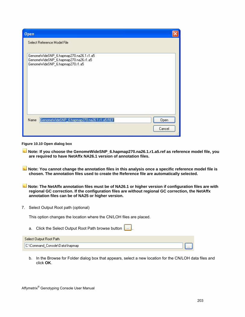
Affymetrix® Genotyping Console User Manual 203
Figure 10.10 Open dialog box
Note: If you choose the GenomeWideSNP_6.hapmap270.na26.1.r1.a5.ref as reference model file, you are required to have NetAffx NA26.1 version of annotation files.
Note: You cannot change the annotation files in this analysis once a specific reference model file is chosen. The annotation files used to create the Reference file are automatically selected.
Note: The NetAffx annotation files must be of NA26.1 or higher version if configuration files are with regional GC correction. If the configuration files are without regional GC correction, the NetAffx annotation files can be of NA25 or higher version.
7. Select Output Root path (optional)
This option changes the location where the CN/LOH files are placed.
a. Click the Select Output Root Path browse button .
b. In the Browse for Folder dialog box that appears, select a new location for the CN/LOH data files and click OK.
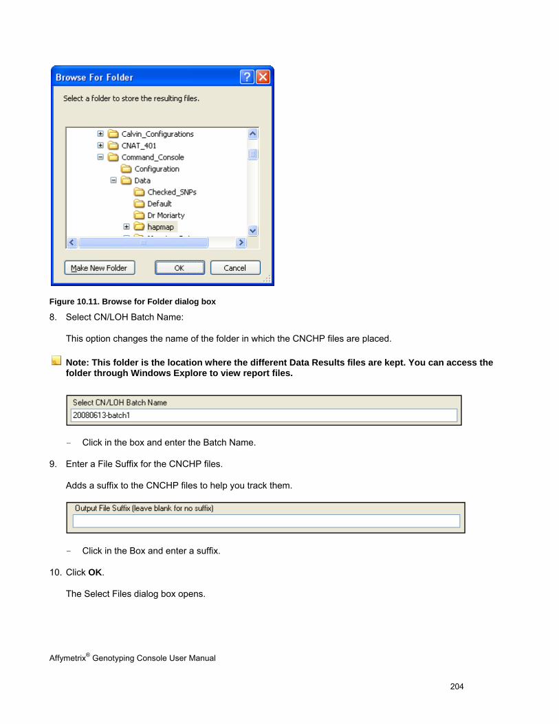
Affymetrix® Genotyping Console User Manual 204
Figure 10.11. Browse for Folder dialog box
8. Select CN/LOH Batch Name:
This option changes the name of the folder in which the CNCHP files are placed.
Note: This folder is the location where the different Data Results files are kept. You can access the folder through Windows Explore to view report files.
- Click in the box and enter the Batch Name.
9. Enter a File Suffix for the CNCHP files.
Adds a suffix to the CNCHP files to help you track them.
- Click in the Box and enter a suffix.
10. Click OK.
The Select Files dialog box opens.
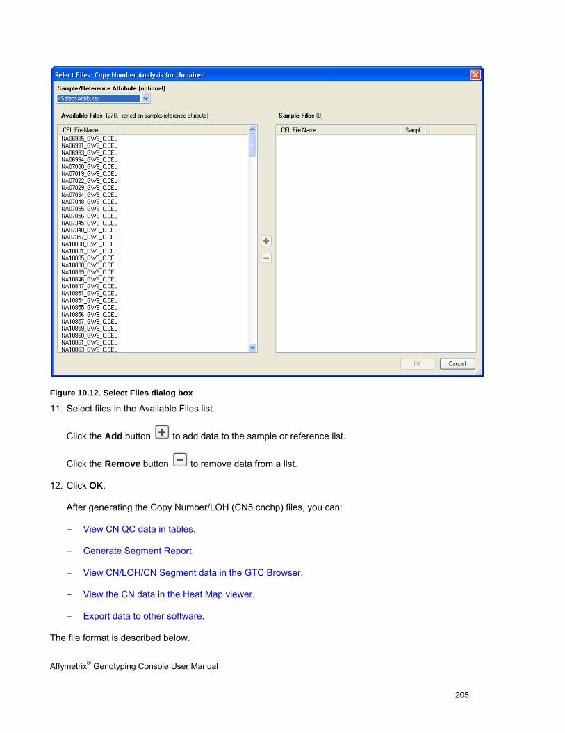
Affymetrix® Genotyping Console User Manual 205
Figure 10.12. Select Files dialog box
11. Select files in the Available Files list.
Click the Add button to add data to the sample or reference list.
Click the Remove button to remove data from a list.
12. Click OK.
After generating the Copy Number/LOH (CN5.cnchp) files, you can:
- View CN QC data in tables.
- Generate Segment Report.
- View CN/LOH/CN Segment data in the GTC Browser.
- View the CN data in the Heat Map viewer.
- Export data to other software.
The file format is described below.
Affymetrix® Genotyping Console User Manual 206
Copy Number/LOH Data File Format for Genome-Wide Human SNP Array 6.0 Data
For Genome-Wide Human SNP Array 6.0 analysis, the Copy Number and LOH data are kept in the same file.
Header Section
The header section contains the following information:
Information about the Software and Algorithm version used to generate the data
File name, creation and modification times, and unique identifier
Array type
Genome version and library information
CN/LOH Algorithm parameters
Reference Model File used
Number of Markers for each chromosome
X and Y chromosome information
Data Section – for *.CN5.cnchp files
The data section contains the following information:
allele difference
Difference of A signal and B signal each standardized with respect to their median values in the reference
cnstate HMM copy number state
smoothsignal Smoothed log2 ratios or smoothed log2 ratios calibrated to Copy Number and anti-logged (depending on the options setting)
loh Loss of Heterozygosity, 1=LOH, and 0=retention
log2ratio Log2 ratio value
Adjusting Normalization and Background Parameters for Reference Model File and Sample Files
The Copy Number algorithms depend on comparing signal for each marker in each sample against a reference formed from a group of samples. The underlying assumption is that for each marker the reference state in the group will be CN=2 (except for the Y chromosome, where the reference state is CN=1), and hence deviations from the reference can be seen by forming the log ratio of each marker's signal compared to its reference value. For the autosomes, the reference value for each probe set is formed by taking the median of summarized probe set signals across all samples in the reference. For each SNP probe set, summary signal is calculated after normalizing intensities by using probe logarithmic intensity error (PLIER) with non-standard options for each of the SNP allele probe sets and summing the result of both alleles. For each CN probe set, summary signal is the normalized intensity only. For chromosome X, the reference value is formed using only the samples determined
Affymetrix® Genotyping Console User Manual 207
not to have a single X and assumes the majority of such samples are diploid. For chromosome Y, the reference value is formed using only the samples determined to have a Y present.
Note: Forming a reference where a large fraction of the samples have one or more chromosomal aneuploidies in common will give you weird results for the affected chromosomes.
In the process of calculating signal various normalization steps are made so that signal from each sample can be meaningfully compared with each other. If these normalization steps are not the same, then the comparison is no longer meaningful. In particular, in single sample workflow, new samples are normalized in the same way as the reference.
For information about changing the algorithm parameters, see Changing Algorithm Configurations for SNP 6.0 Analysis (page 210).
For information about the algorithm description, see Appendix A: Algorithms (page 292).
Copy Number QC Summary Table for the Genome-Wide Human SNP Array 6.0
Use the GTC Browser (page 249) to view Copy Number, LOH, and CN Segments data in a genomic context.
Use the Heat Map Viewer (page 269) to view Copy Number data along with Copy Number Variation data, if available.
The Copy Number QC Summary Table displays QC information about the copy number and LOH analyses.
The Copy Number QC Summary Table uses all the table options as described in Table Features.
To open the QC Summary table:
Right-click on the Copy Number/LOH Results set of interested and select Show Copy Number QC Summary Table; or
From the Workspace menu, select Copy Number/LOH Results > Show Copy Number QC Summary Table.
The QC Summary table opens.
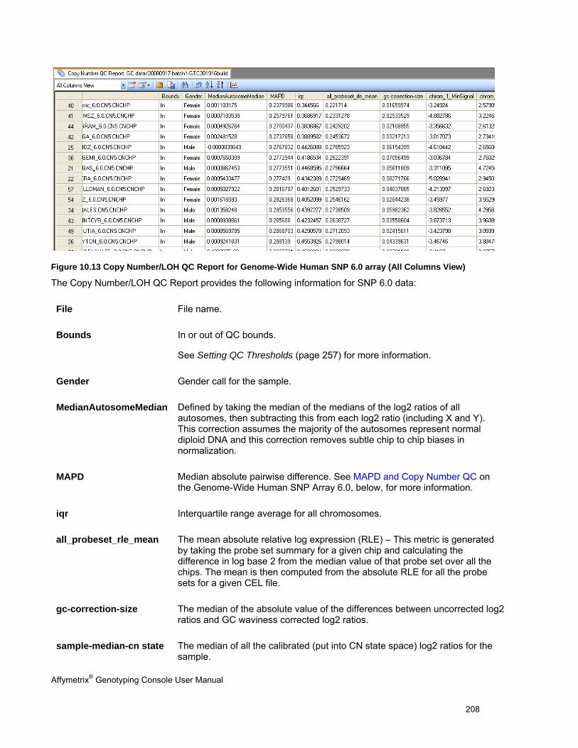
Affymetrix® Genotyping Console User Manual 208
Figure 10.13 Copy Number/LOH QC Report for Genome-Wide Human SNP 6.0 array (All Columns View)
The Copy Number/LOH QC Report provides the following information for SNP 6.0 data:
File File name.
Bounds In or out of QC bounds.
See Setting QC Thresholds (page 257) for more information.
Gender Gender call for the sample.
MedianAutosomeMedian Defined by taking the median of the medians of the log2 ratios of all autosomes, then subtracting this from each log2 ratio (including X and Y). This correction assumes the majority of the autosomes represent normal diploid DNA and this correction removes subtle chip to chip biases in normalization.
MAPD Median absolute pairwise difference. See MAPD and Copy Number QC on the Genome-Wide Human SNP Array 6.0, below, for more information.
iqr Interquartile range average for all chromosomes.
all_probeset_rle_mean The mean absolute relative log expression (RLE) – This metric is generated by taking the probe set summary for a given chip and calculating the difference in log base 2 from the median value of that probe set over all the chips. The mean is then computed from the absolute RLE for all the probe sets for a given CEL file.
gc-correction-size The median of the absolute value of the differences between uncorrected log2 ratios and GC waviness corrected log2 ratios.
sample-median-cn state The median of all the calibrated (put into CN state space) log2 ratios for the sample.
Affymetrix® Genotyping Console User Manual 209
sample-hom-frequency The frequency (homozygous calls / all SNP calls) of SNP homozygous calls for the sample.
sample-het-frequency The frequency (heterozygous calls / all SNP calls) of SNP heterozygous calls for the sample.
waviness-sd The residual standard deviation (SD) after correcting for adjacent probe set to probe set SD based on autosomal log2 ratios. The waviness-sd is a measure of the signal variability in longer range waviness.
chrom_MinSignal (one for each chromosome)
Minimum Log2Ratio for a given chromosome and sample.
Chrom_MaxSignal (one for each chromosome
Maximum Log2Ratio for a given chromosome and sample.
File Date Date file was created.
MAPD and Copy Number QC on the Genome-Wide Human SNP Array 6.0
MAPD is defined as the Median of the Absolute values of all Pairwise Differences between log2 ratios for a given chip. Each pair is defined as adjacent in terms of genomic distance, with SNP markers and CN markers being treated equally. Hence any two markers that are adjacent in the genomic coordinates are a pair. Except at the beginning and the end of a chromosome every marker belongs to 2 pairs as it is adjacent to a marker preceding it and a marker following it on the genome.
MAPD is a per chip estimate of variability, like Standard Deviation (SD). If the log2 ratios are distributed normal with a constant SD then MAPD/0.96 is equal to SD. However, using MAPD is robust against high biological variability in log2 ratios induced by conditions such as cancer.
Variability in log2 ratios in a chip arises from two distinct sources:
- Intrinsic variability in the starting material, hyb cocktail preparation, the chip, the scanner
- Apparent variability induced by the fact that the reference may have systematic differences from this chip.
Regardless of the source of the variability, increased variability decreases the quality of CN calls.Very high MAPD is a failure. Variability in general will be reduced by using a reference set generated from chips run at the same lab using the same reagent lots.
As in genotyping, there can be substantial batch effects or lab-to-lab systematic effects. If a reference is generated from chips run in another lab such systematic differences inflate apparent variability. Affymetrix has observed that using the supplied Affymetrix reference with chips run in different labs will inflate MAPD by around 50%, but a factor of 2 is possible.
If a chip with MAPD generated from the Affymetrix reference is greater than 0.35, then we recommend against using that chip in an analysis.
When using a Reference Model File made up of arrays NOT generated in the same lab using the same reagent lots: CNCHP files with a MAPD value greater than 0.35 should not be used for further analysis.
When using a Reference Model File made up of arrays that WERE generated in the same lab using the same reagent lots: CNCHP files with a MAPD value greater than 0.3 should not be used for further analysis.
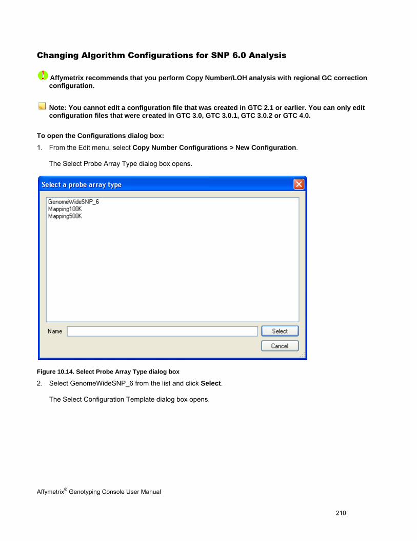
Affymetrix® Genotyping Console User Manual 210
Changing Algorithm Configurations for SNP 6.0 Analysis
Affymetrix recommends that you perform Copy Number/LOH analysis with regional GC correction configuration.
Note: You cannot edit a configuration file that was created in GTC 2.1 or earlier. You can only edit configuration files that were created in GTC 3.0, GTC 3.0.1, GTC 3.0.2 or GTC 4.0.
To open the Configurations dialog box:
1. From the Edit menu, select Copy Number Configurations > New Configuration.
The Select Probe Array Type dialog box opens.
Figure 10.14. Select Probe Array Type dialog box
2. Select GenomeWideSNP_6 from the list and click Select.
The Select Configuration Template dialog box opens.
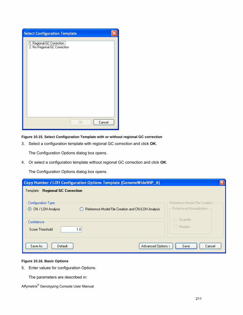
Affymetrix® Genotyping Console User Manual 211
Figure 10.15. Select Configuration Template with or without regional GC correction
3. Select a configuration template with regional GC correction and click OK.
The Configuration Options dialog box opens.
4. Or select a configuration template without regional GC correction and click OK.
The Configuration Options dialog box opens.
Figure 10.16. Basic Options
5. Enter values for configuration Options.
The parameters are described in:
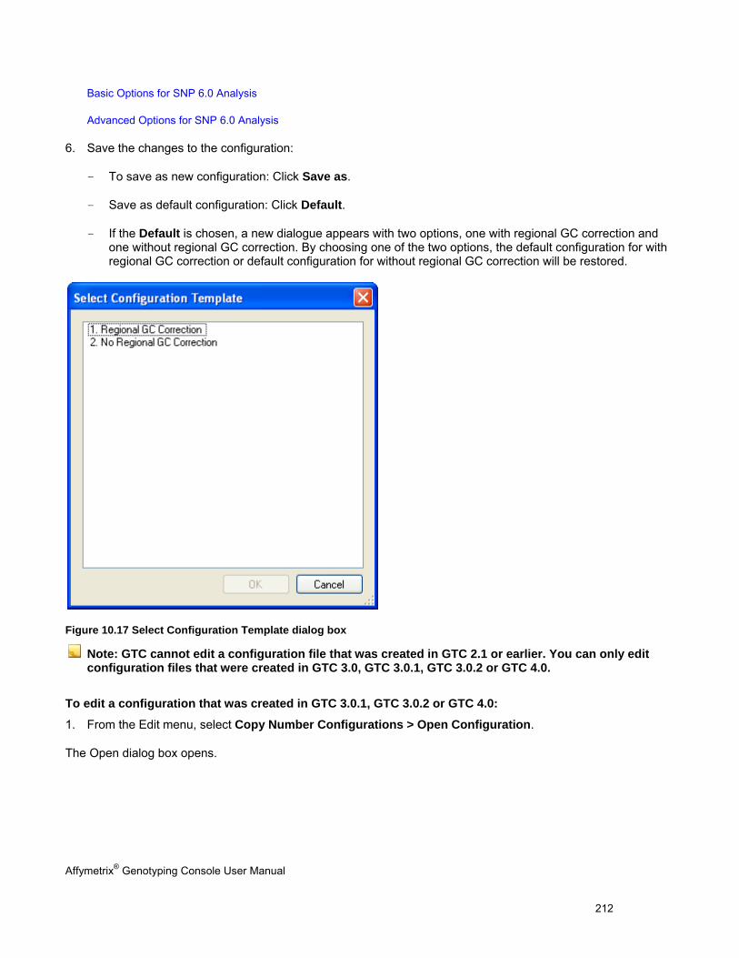
Affymetrix® Genotyping Console User Manual 212
Basic Options for SNP 6.0 Analysis
Advanced Options for SNP 6.0 Analysis
6. Save the changes to the configuration:
- To save as new configuration: Click Save as.
- Save as default configuration: Click Default.
- If the Default is chosen, a new dialogue appears with two options, one with regional GC correction and one without regional GC correction. By choosing one of the two options, the default configuration for with regional GC correction or default configuration for without regional GC correction will be restored.
Figure 10.17 Select Configuration Template dialog box
Note: GTC cannot edit a configuration file that was created in GTC 2.1 or earlier. You can only edit configuration files that were created in GTC 3.0, GTC 3.0.1, GTC 3.0.2 or GTC 4.0.
To edit a configuration that was created in GTC 3.0.1, GTC 3.0.2 or GTC 4.0:
1. From the Edit menu, select Copy Number Configurations > Open Configuration.
The Open dialog box opens.
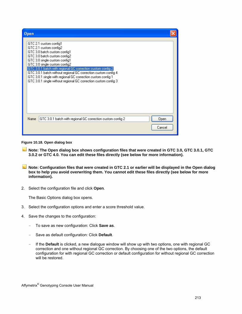
Affymetrix® Genotyping Console User Manual 213
Figure 10.18. Open dialog box
Note: The Open dialog box shows configuration files that were created in GTC 3.0, GTC 3.0.1, GTC 3.0.2 or GTC 4.0. You can edit these files directly (see below for more information).
Note: Configuration files that were created in GTC 2.1 or earlier will be displayed in the Open dialog box to help you avoid overwriting them. You cannot edit these files directly (see below for more information).
2. Select the configuration file and click Open.
The Basic Options dialog box opens.
3. Select the configuration options and enter a score threshold value.
4. Save the changes to the configuration:
- To save as new configuration: Click Save as.
- Save as default configuration: Click Default.
- If the Default is clicked, a new dialogue window will show up with two options, one with regional GC correction and one without regional GC correction. By choosing one of the two options, the default configuration for with regional GC correction or default configuration for without regional GC correction will be restored.
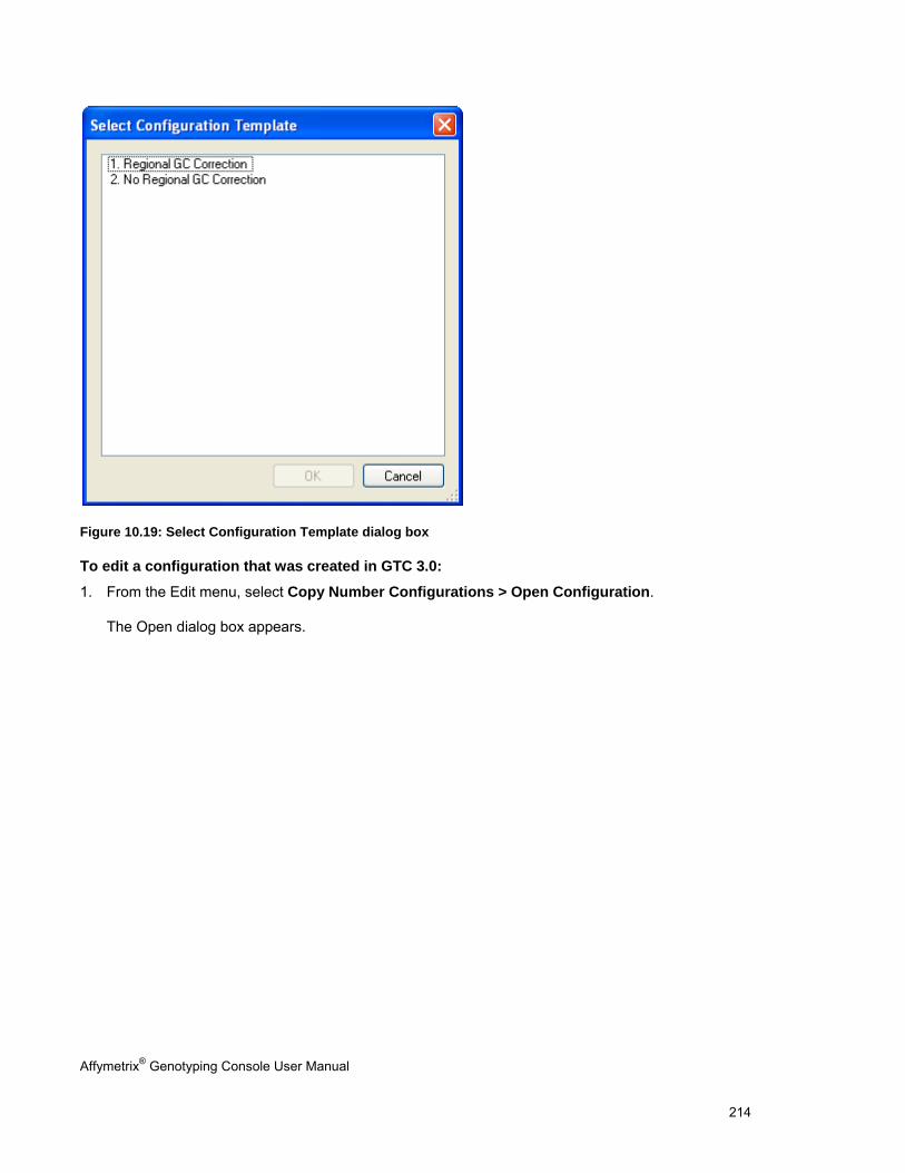
Affymetrix® Genotyping Console User Manual 214
Figure 10.19: Select Configuration Template dialog box
To edit a configuration that was created in GTC 3.0:
1. From the Edit menu, select Copy Number Configurations > Open Configuration.
The Open dialog box appears.
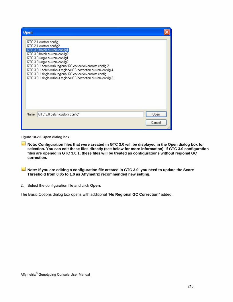
Affymetrix® Genotyping Console User Manual 215
Figure 10.20. Open dialog box
Note: Configuration files that were created in GTC 3.0 will be displayed in the Open dialog box for selection. You can edit these files directly (see below for more information). If GTC 3.0 configuration files are opened in GTC 3.0.1, these files will be treated as configurations without regional GC correction.
Note: If you are editing a configuration file created in GTC 3.0, you need to update the Score Threshold from 0.05 to 1.0 as Affymetrix recommended new setting.
2. Select the configuration file and click Open.
The Basic Options dialog box opens with additional “No Regional GC Correction” added.
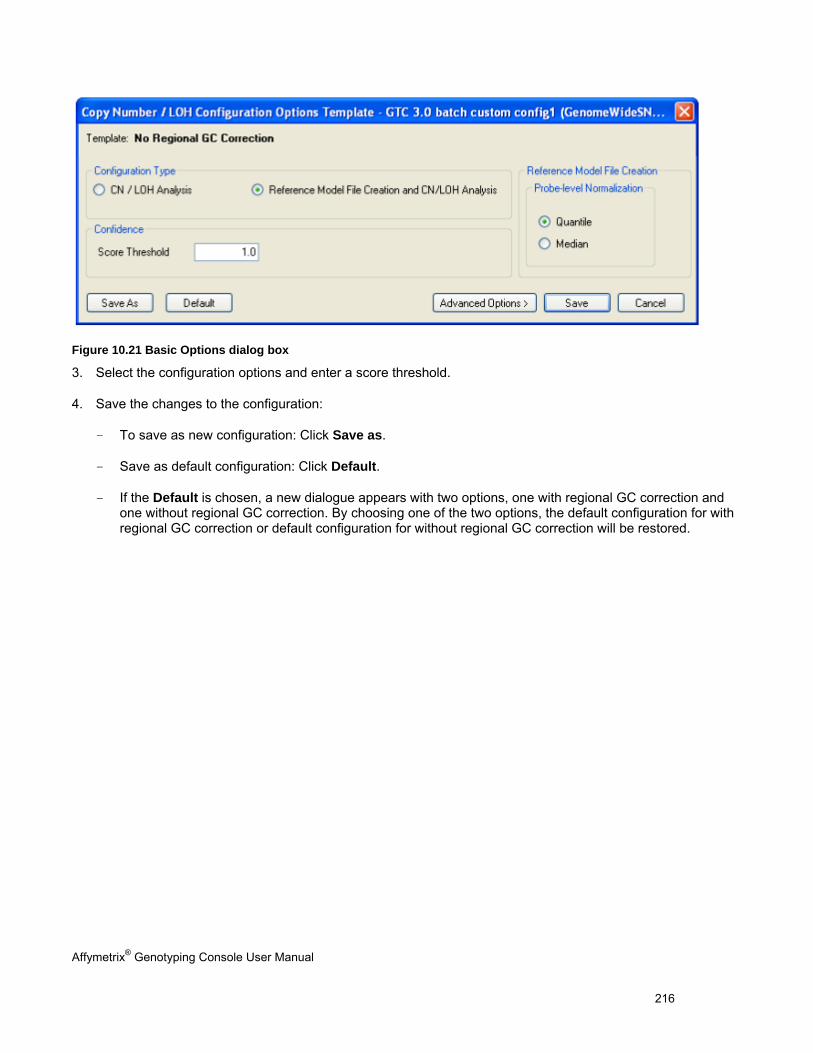
Affymetrix® Genotyping Console User Manual 216
Figure 10.21 Basic Options dialog box
3. Select the configuration options and enter a score threshold.
4. Save the changes to the configuration:
- To save as new configuration: Click Save as.
- Save as default configuration: Click Default.
- If the Default is chosen, a new dialogue appears with two options, one with regional GC correction and one without regional GC correction. By choosing one of the two options, the default configuration for with regional GC correction or default configuration for without regional GC correction will be restored.
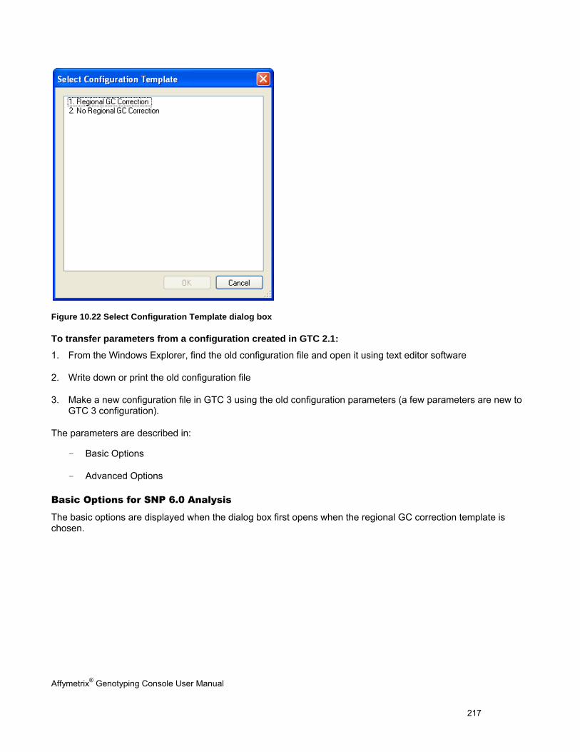
Affymetrix® Genotyping Console User Manual 217
Figure 10.22 Select Configuration Template dialog box
To transfer parameters from a configuration created in GTC 2.1:
1. From the Windows Explorer, find the old configuration file and open it using text editor software
2. Write down or print the old configuration file
3. Make a new configuration file in GTC 3 using the old configuration parameters (a few parameters are new to GTC 3 configuration).
The parameters are described in:
- Basic Options
- Advanced Options
Basic Options for SNP 6.0 Analysis
The basic options are displayed when the dialog box first opens when the regional GC correction template is chosen.
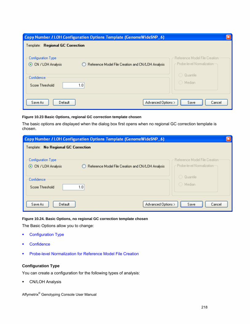
Affymetrix® Genotyping Console User Manual 218
Figure 10.23 Basic Options, regional GC correction template chosen
The basic options are displayed when the dialog box first opens when no regional GC correction template is chosen.
Figure 10.24. Basic Options, no regional GC correction template chosen
The Basic Options allow you to change:
Configuration Type
Confidence
Probe-level Normalization for Reference Model File Creation
Configuration Type
You can create a configuration for the following types of analysis:
CN/LOH Analysis
Affymetrix® Genotyping Console User Manual 219
Reference Model File Creation and CN/LOH Analysis
Certain options are available only when the Reference Model File Creation and CN/LOH Analysis option is selected.
Confidence/Score Threshold
Score/Confidence Threshold is the maximum score at which the algorithm will make a genotype call. Larger values of the score/confidence threshold indicate less certain calls. Calls with confidence scores above the threshold are assigned a no-call.
Probe-level Normalization for Reference Model File Creation
Quantile normalization is recommended for copy number analysis of association and cytogenetics samples. Quantile normalization is most appropriate for samples where most of the chromosomes are relatively normal.
In contrast, many cancer samples contain significant abnormalities that impact much of the genome; therefore, median normalization is recommended.
Important: For any single sample Copy Number/LOH Analysis run, the Probe-level Normalization and Probe-level Background Correction parameters must be and will be set the same for the Analysis as these parameters were set during the generation of the Reference Model File used in the Analysis.
Advanced Options for SNP 6.0 Analysis
Click Advanced Options to display the following options:
Reference Model File Creation: Advanced Options
Copy Number Parameters: HMM Parameters with regional GC correction
Copy Number Parameters: HMM Parameters without regional GC correction
Copy Number Parameters: Post-HMM Processing Parameters
LOH Parameters
Smoothing Signal Graph Output
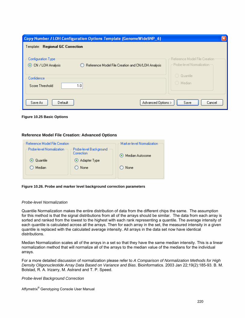
Affymetrix® Genotyping Console User Manual 220
Figure 10.25 Basic Options
Reference Model File Creation: Advanced Options
\
Figure 10.26. Probe and marker level background correction parameters
Probe-level Normalization
Quantile Normalization makes the entire distribution of data from the different chips the same. The assumption for this method is that the signal distributions from all of the arrays should be similar. The data from each array is sorted and ranked from the lowest to the highest with each rank representing a quantile. The average intensity of each quantile is calculated across all the arrays. Then for each array in the set, the measured intensity in a given quantile is replaced with the calculated average intensity. All arrays in the data set now have identical distributions.
Median Normalization scales all of the arrays in a set so that they have the same median intensity. This is a linear normalization method that will normalize all of the arrays to the median value of the medians for the individual arrays.
For a more detailed discussion of normalization please refer to A Comparison of Normalization Methods for High Density Oligonucleotide Array Data Based on Variance and Bias. Bioinformatics. 2003 Jan 22;19(2):185-93. B. M. Bolstad, R. A. Irizarry, M. Astrand and T. P. Speed.
Probe-level Background Correction
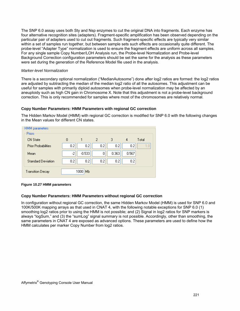
Affymetrix® Genotyping Console User Manual 221
The SNP 6.0 assay uses both Sty and Nsp enzymes to cut the original DNA into fragments. Each enzyme has four alternative recognition sites (adapters). Fragment-specific amplification has been observed depending on the particular pair of adapters used to cut out fragments. Such fragment-specific effects are typically very similar within a set of samples run together, but between sample sets such effects are occasionally quite different. The probe-level “Adapter Type” normalization is used to ensure the fragment effects are uniform across all samples. For any single sample Copy Number/LOH Analysis run, the Probe-level Normalization and Probe-level Background Correction configuration parameters should be set the same for the analysis as these parameters were set during the generation of the Reference Model file used in the analysis.
Marker-level Normalization
There is a secondary optional normalization (“MedianAutosome”) done after log2 ratios are formed: the log2 ratios are adjusted by subtracting the median of the median log2 ratio of all the autosomes. This adjustment can be useful for samples with primarily diploid autosomes when probe-level normalization may be affected by an aneuploidy such as high CN gain in Chromosome X. Note that this adjustment is not a probe-level background correction. This is only recommended for samples where most of the chromosomes are relatively normal.
Copy Number Parameters: HMM Parameters with regional GC correction
The Hidden Markov Model (HMM) with regional GC correction is modified for SNP 6.0 with the following changes in the Mean values for different CN states.
Figure 10.27 HMM parameters
Copy Number Parameters: HMM Parameters without regional GC correction
In configuration without regional GC correction, the same Hidden Markov Model (HMM) is used for SNP 6.0 and 100K/500K mapping arrays as that used in CNAT 4, with the following notable exceptions for SNP 6.0 (1) smoothing log2 ratios prior to using the HMM is not possible; and (2) Signal in log2 ratios for SNP markers is always “logSum,” and (3) the “sumLog” signal summary is not possible. Accordingly, other than smoothing, the same parameters in CNAT 4 are exposed as advanced options. These parameters are used to define how the HMM calculates per marker Copy Number from log2 ratios.
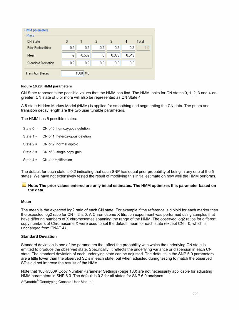
Affymetrix® Genotyping Console User Manual 222
Figure 10.28. HMM parameters
CN State represents the possible values that the HMM can find. The HMM looks for CN states 0, 1, 2, 3 and 4-or-greater. CN state of 5 or more will also be represented as CN State 4
A 5-state Hidden Markov Model (HMM) is applied for smoothing and segmenting the CN data. The priors and transition decay length are the two user tunable parameters.
The HMM has 5 possible states:
The default for each state is 0.2 indicating that each SNP has equal prior probability of being in any one of the 5 states. We have not extensively tested the result of modifying this initial estimate on how well the HMM performs.
Note: The prior values entered are only initial estimates. The HMM optimizes this parameter based on the data.
Mean
The mean is the expected log2 ratio of each CN state. For example if the reference is diploid for each marker then the expected log2 ratio for CN = 2 is 0. A Chromosome X titration experiment was performed using samples that have differing numbers of X chromosomes spanning the range of the HMM. The observed log2 ratios for different copy numbers of Chromosome X were used to set the default mean for each state (except CN = 0, which is unchanged from CNAT 4).
Standard Deviation
Standard deviation is one of the parameters that affect the probability with which the underlying CN state is emitted to produce the observed state. Specifically, it reflects the underlying variance or dispersion in each CN state. The standard deviation of each underlying state can be adjusted. The defaults in the SNP 6.0 parameters are a little lower than the observed SD’s in each state, but when adjusted during testing to match the observed SD’s did not improve the results of the HMM.
Note that 100K/500K Copy Number Parameter Settings (page 183) are not necessarily applicable for adjusting HMM parameters in SNP 6.0. The default is 0.2 for all states for SNP 6.0 analyses.
State 0 = CN of 0; homozygous deletion
State 1 = CN of 1; heterozygous deletion
State 2 = CN of 2; normal diploid
State 3 = CN of 3; single copy gain
State 4 = CN 4; amplification
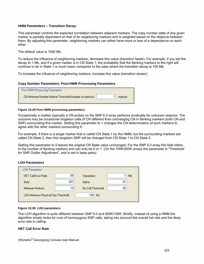
Affymetrix® Genotyping Console User Manual 223
HMM Parameters – Transition Decay:
This parameter controls the expected correlation between adjacent markers. The copy number state of any given marker is partially dependent on that of its neighboring markers and is weighted based on the distance between them. By adjusting this parameter, neighboring markers can either have more or less of a dependence on each other.
The default value is 1000 Mb.
To reduce the influence of neighboring markers, decrease this value (transition faster). For example, if you set the decay to 1 Mb, and if a given marker is in CN State 1, the probability that the flanking markers to the right will continue to be in State 1 is much lower compared to the case where the transition decay is 100 Mb.
To increase the influence of neighboring markers, increase this value (transition slower).
Copy Number Parameters: Post-HMM Processing Parameters
Figure 10.29 Post HMM processing parameters
Occasionally a marker (typically a CN probe) on the SNP 6.0 array performs erratically for unknown reasons. The outcome may be occasional singleton calls of CN different from unchanging CN in flanking markers (both CN and SNP) surrounding this marker. Setting this parameter to 1 changes the CN determination of such markers to agree with the other markers surrounding it.
For example, if there is a single marker that is called CN State 1 by the HMM, but the surrounding markers are called CN State 2, then this singleton SNP will be changed from CN State 1 to CN State 2.
Setting this parameter to 0 leaves the original CN State value unchanged. For the SNP 6.0 array this field refers to the number of flanking markers and can only be 0 or 1. (On the 100K/500K arrays the parameter is “Threshold for SNP Outlier Adjustment”, and is set in base pairs)
LOH Parameters
Figure 10.30. LOH parameters
The LOH algorithm is quite different between SNP 6.0 and 500K/100K. Briefly, instead of using a HMM the algorithm simply looks for runs of homozygous SNP calls, taking into account the overall het rate and the likely error rate in calling.
HET Call Error Rate
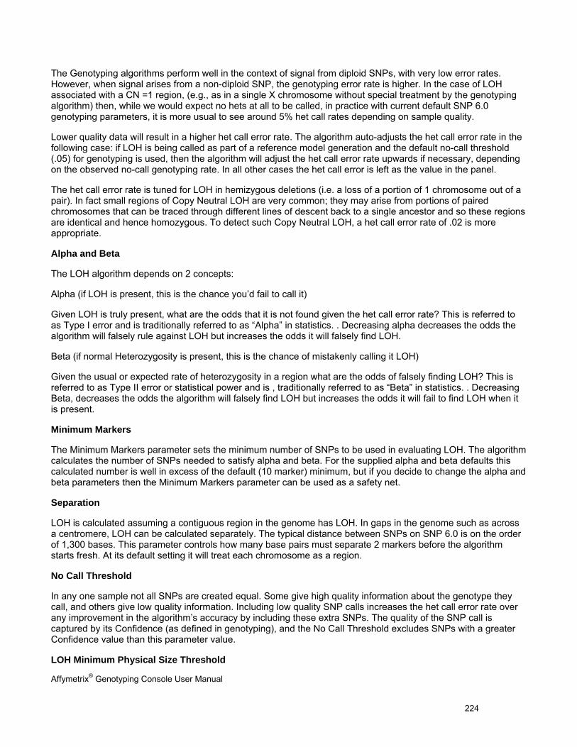
Affymetrix® Genotyping Console User Manual 224
The Genotyping algorithms perform well in the context of signal from diploid SNPs, with very low error rates. However, when signal arises from a non-diploid SNP, the genotyping error rate is higher. In the case of LOH associated with a CN =1 region, (e.g., as in a single X chromosome without special treatment by the genotyping algorithm) then, while we would expect no hets at all to be called, in practice with current default SNP 6.0 genotyping parameters, it is more usual to see around 5% het call rates depending on sample quality.
Lower quality data will result in a higher het call error rate. The algorithm auto-adjusts the het call error rate in the following case: if LOH is being called as part of a reference model generation and the default no-call threshold (.05) for genotyping is used, then the algorithm will adjust the het call error rate upwards if necessary, depending on the observed no-call genotyping rate. In all other cases the het call error is left as the value in the panel.
The het call error rate is tuned for LOH in hemizygous deletions (i.e. a loss of a portion of 1 chromosome out of a pair). In fact small regions of Copy Neutral LOH are very common; they may arise from portions of paired chromosomes that can be traced through different lines of descent back to a single ancestor and so these regions are identical and hence homozygous. To detect such Copy Neutral LOH, a het call error rate of .02 is more appropriate.
Alpha and Beta
The LOH algorithm depends on 2 concepts:
Alpha (if LOH is present, this is the chance you’d fail to call it)
Given LOH is truly present, what are the odds that it is not found given the het call error rate? This is referred to as Type I error and is traditionally referred to as “Alpha” in statistics. . Decreasing alpha decreases the odds the algorithm will falsely rule against LOH but increases the odds it will falsely find LOH.
Beta (if normal Heterozygosity is present, this is the chance of mistakenly calling it LOH)
Given the usual or expected rate of heterozygosity in a region what are the odds of falsely finding LOH? This is referred to as Type II error or statistical power and is , traditionally referred to as “Beta” in statistics. . Decreasing Beta, decreases the odds the algorithm will falsely find LOH but increases the odds it will fail to find LOH when it is present.
Minimum Markers
The Minimum Markers parameter sets the minimum number of SNPs to be used in evaluating LOH. The algorithm calculates the number of SNPs needed to satisfy alpha and beta. For the supplied alpha and beta defaults this calculated number is well in excess of the default (10 marker) minimum, but if you decide to change the alpha and beta parameters then the Minimum Markers parameter can be used as a safety net.
Separation
LOH is calculated assuming a contiguous region in the genome has LOH. In gaps in the genome such as across a centromere, LOH can be calculated separately. The typical distance between SNPs on SNP 6.0 is on the order of 1,300 bases. This parameter controls how many base pairs must separate 2 markers before the algorithm starts fresh. At its default setting it will treat each chromosome as a region.
No Call Threshold
In any one sample not all SNPs are created equal. Some give high quality information about the genotype they call, and others give low quality information. Including low quality SNP calls increases the het call error rate over any improvement in the algorithm’s accuracy by including these extra SNPs. The quality of the SNP call is captured by its Confidence (as defined in genotyping), and the No Call Threshold excludes SNPs with a greater Confidence value than this parameter value.
LOH Minimum Physical Size Threshold
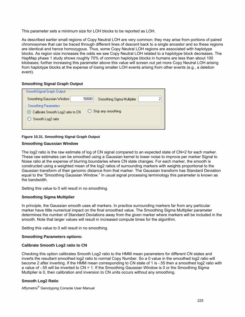
Affymetrix® Genotyping Console User Manual 225
This parameter sets a minimum size for LOH blocks to be reported as LOH.
As described earlier small regions of Copy Neutral LOH are very common; they may arise from portions of paired chromosomes that can be traced through different lines of descent back to a single ancestor and so these regions are identical and hence homozygous. Thus, some Copy Neutral LOH regions are associated with haplotype blocks. As region size increases the odds we see Copy Neutral LOH related to a haplotype block decreases. The HapMap phase 1 study shows roughly 70% of common haplotype blocks in humans are less than about 100 kilobases; further increasing this parameter above this value will screen out yet more Copy Neutral LOH arising from haplotype blocks at the expense of losing smaller LOH events arising from other events (e.g., a deletion event).
Smoothing Signal Graph Output
Figure 10.31. Smoothing Signal Graph Output
Smoothing Gaussian Window
The log2 ratio is the raw estimate of log of CN signal compared to an expected state of CN=2 for each marker. These raw estimates can be smoothed using a Gaussian kernel to lower noise to improve per marker Signal to Noise ratio at the expense of blurring boundaries where CN state changes. For each marker, the smooth is constructed using a weighted mean of the log2 ratios of surrounding markers with weights proportional to the Gaussian transform of their genomic distance from that marker. The Gaussian transform has Standard Deviation equal to the “Smoothing Gaussian Window.” In usual signal processing terminology this parameter is known as the bandwidth.
Setting this value to 0 will result in no smoothing.
Smoothing Sigma Multiplier
In principle, the Gaussian smooth uses all markers. In practice surrounding markers far from any particular marker have little numerical impact on the final smoothed value. The Smoothing Sigma Multiplier parameter determines the number of Standard Deviations away from the given marker where markers will be included in the smooth. Note that larger values will result in increased compute times for the algorithm.
Setting this value to 0 will result in no smoothing.
Smoothing Parameters options:
Calibrate Smooth Log2 ratio to CN
Checking this option calibrates Smooth Log2 ratio to the HMM mean parameters for different CN states and inverts the resultant smoothed log2 ratio to normal Copy Number. So a 0 value in the smoothed log2 ratio will become 2 after inverting. If the HMM mean corresponding to CN state of 1 is -.55 then a smoothed log2 ratio with a value of -.55 will be inverted to CN = 1. If the Smoothing Gaussian Window is 0 or the Smoothing Sigma Multiplier is 0, then calibration and inversion to CN units occurs without any smoothing.
Smooth Log2 Ratio

Affymetrix® Genotyping Console User Manual 226
Checking this option results in the smoothed log2 ratios only.
Skip any smoothing
Checking this option will prevent smoothed log2 ratios from being calculated and included in the CNCHP file output.
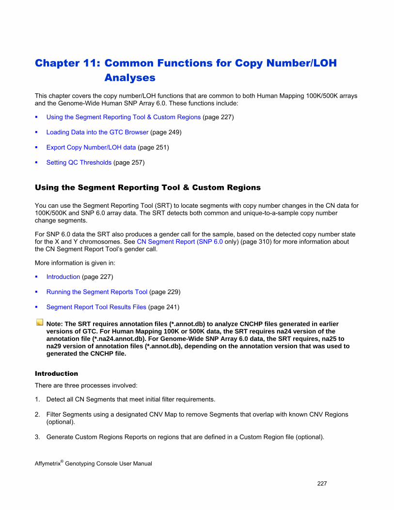
Affymetrix® Genotyping Console User Manual 227
Chapter 11: Common Functions for Copy Number/LOH Analyses
This chapter covers the copy number/LOH functions that are common to both Human Mapping 100K/500K arrays and the Genome-Wide Human SNP Array 6.0. These functions include:
Using the Segment Reporting Tool & Custom Regions (page 227)
Loading Data into the GTC Browser (page 249)
Export Copy Number/LOH data (page 251)
Setting QC Thresholds (page 257)
Using the Segment Reporting Tool & Custom Regions
You can use the Segment Reporting Tool (SRT) to locate segments with copy number changes in the CN data for 100K/500K and SNP 6.0 array data. The SRT detects both common and unique-to-a-sample copy number change segments.
For SNP 6.0 data the SRT also produces a gender call for the sample, based on the detected copy number state for the X and Y chromosomes. See CN Segment Report (SNP 6.0 only) (page 310) for more information about the CN Segment Report Tool’s gender call.
More information is given in:
Introduction (page 227)
Running the Segment Reports Tool (page 229)
Segment Report Tool Results Files (page 241)
Note: The SRT requires annotation files (*.annot.db) to analyze CNCHP files generated in earlier versions of GTC. For Human Mapping 100K or 500K data, the SRT requires na24 version of the annotation file (*.na24.annot.db). For Genome-Wide SNP Array 6.0 data, the SRT requires, na25 to na29 version of annotation files (*.annot.db), depending on the annotation version that was used to generated the CNCHP file.
Introduction
There are three processes involved:
1. Detect all CN Segments that meet initial filter requirements.
2. Filter Segments using a designated CNV Map to remove Segments that overlap with known CNV Regions (optional).
3. Generate Custom Regions Reports on regions that are defined in a Custom Region file (optional).
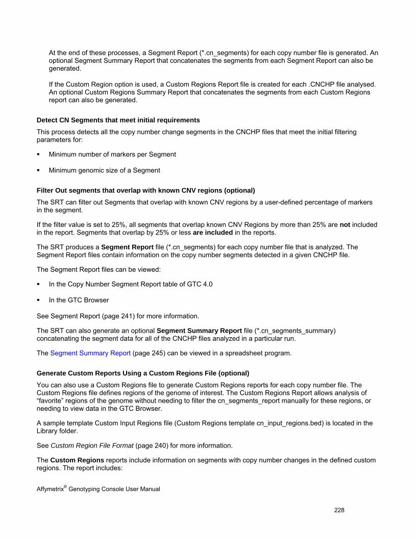
Affymetrix® Genotyping Console User Manual 228
At the end of these processes, a Segment Report (*.cn_segments) for each copy number file is generated. An optional Segment Summary Report that concatenates the segments from each Segment Report can also be generated.
If the Custom Region option is used, a Custom Regions Report file is created for each .CNCHP file analysed. An optional Custom Regions Summary Report that concatenates the segments from each Custom Regions report can also be generated.
Detect CN Segments that meet initial requirements
This process detects all the copy number change segments in the CNCHP files that meet the initial filtering parameters for:
Minimum number of markers per Segment
Minimum genomic size of a Segment
Filter Out segments that overlap with known CNV regions (optional)
The SRT can filter out Segments that overlap with known CNV regions by a user-defined percentage of markers in the segment.
If the filter value is set to 25%, all segments that overlap known CNV Regions by more than 25% are not included in the report. Segments that overlap by 25% or less are included in the reports.
The SRT produces a Segment Report file (*.cn_segments) for each copy number file that is analyzed. The Segment Report files contain information on the copy number segments detected in a given CNCHP file.
The Segment Report files can be viewed:
In the Copy Number Segment Report table of GTC 4.0
In the GTC Browser
See Segment Report (page 241) for more information.
The SRT can also generate an optional Segment Summary Report file (*.cn_segments_summary) concatenating the segment data for all of the CNCHP files analyzed in a particular run.
The Segment Summary Report (page 245) can be viewed in a spreadsheet program.
Generate Custom Reports Using a Custom Regions File (optional)
You can also use a Custom Regions file to generate Custom Regions reports for each copy number file. The Custom Regions file defines regions of the genome of interest. The Custom Regions Report allows analysis of “favorite” regions of the genome without needing to filter the cn_segments_report manually for these regions, or needing to view data in the GTC Browser.
A sample template Custom Input Regions file (Custom Regions template cn_input_regions.bed) is located in the Library folder.
See Custom Region File Format (page 240) for more information.
The Custom Regions reports include information on segments with copy number changes in the defined custom regions. The report includes:
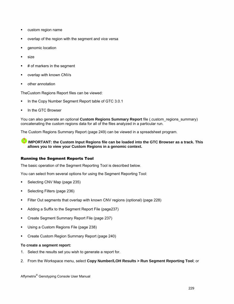
Affymetrix® Genotyping Console User Manual 229
custom region name
overlap of the region with the segment and vice versa
genomic location
size
# of markers in the segment
overlap with known CNVs
other annotation
TheCustom Regions Report files can be viewed:
In the Copy Number Segment Report table of GTC 3.0.1
In the GTC Browser
You can also generate an optional Custom Regions Summary Report file (.custom_regions_summary) concatenating the custom regions data for all of the files analyzed in a particular run.
The Custom Regions Summary Report (page 249) can be viewed in a spreadsheet program.
IMPORTANT: the Custom Input Regions file can be loaded into the GTC Browser as a track. This allows you to view your Custom Regions in a genomic context.
Running the Segment Reports Tool
The basic operation of the Segment Reporting Tool is described below.
You can select from several options for using the Segment Reporting Tool:
Selecting CNV Map (page 235)
Selecting Filters (page 236)
Filter Out segments that overlap with known CNV regions (optional) (page 228)
Adding a Suffix to the Segment Report File (page237)
Create Segment Summary Report File (page 237)
Using a Custom Regions File (page 238)
Create Custom Region Summary Report (page 240)
To create a segment report:
1. Select the results set you wish to generate a report for.
2. From the Workspace menu, select Copy Number/LOH Results > Run Segment Reporting Tool; or
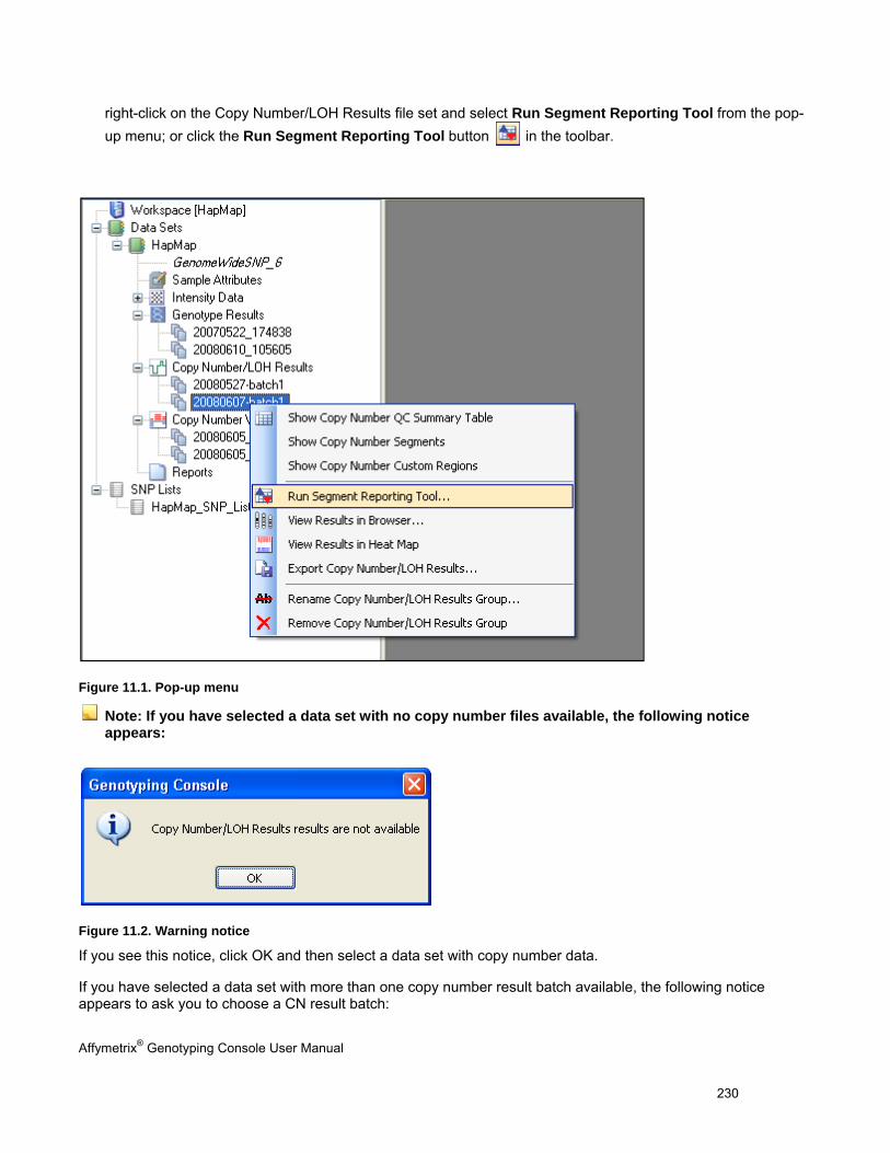
Affymetrix® Genotyping Console User Manual 230
right-click on the Copy Number/LOH Results file set and select Run Segment Reporting Tool from the pop-up menu; or click the Run Segment Reporting Tool button in the toolbar.
Figure 11.1. Pop-up menu
Note: If you have selected a data set with no copy number files available, the following notice appears:
Figure 11.2. Warning notice
If you see this notice, click OK and then select a data set with copy number data.
If you have selected a data set with more than one copy number result batch available, the following notice appears to ask you to choose a CN result batch:
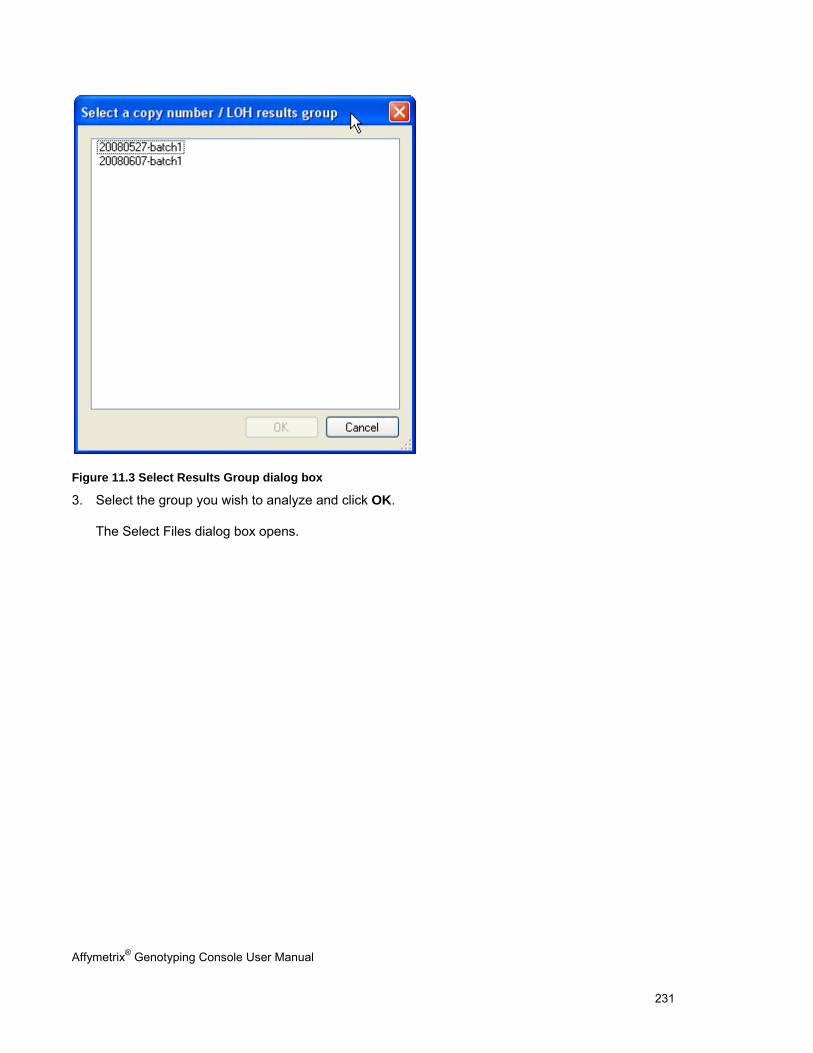
Affymetrix® Genotyping Console User Manual 231
Figure 11.3 Select Results Group dialog box
3. Select the group you wish to analyze and click OK.
The Select Files dialog box opens.
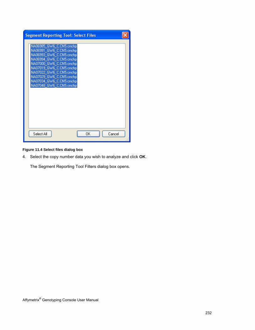
Affymetrix® Genotyping Console User Manual 232
Figure 11.4 Select files dialog box
4. Select the copy number data you wish to analyze and click OK.
The Segment Reporting Tool Filters dialog box opens.
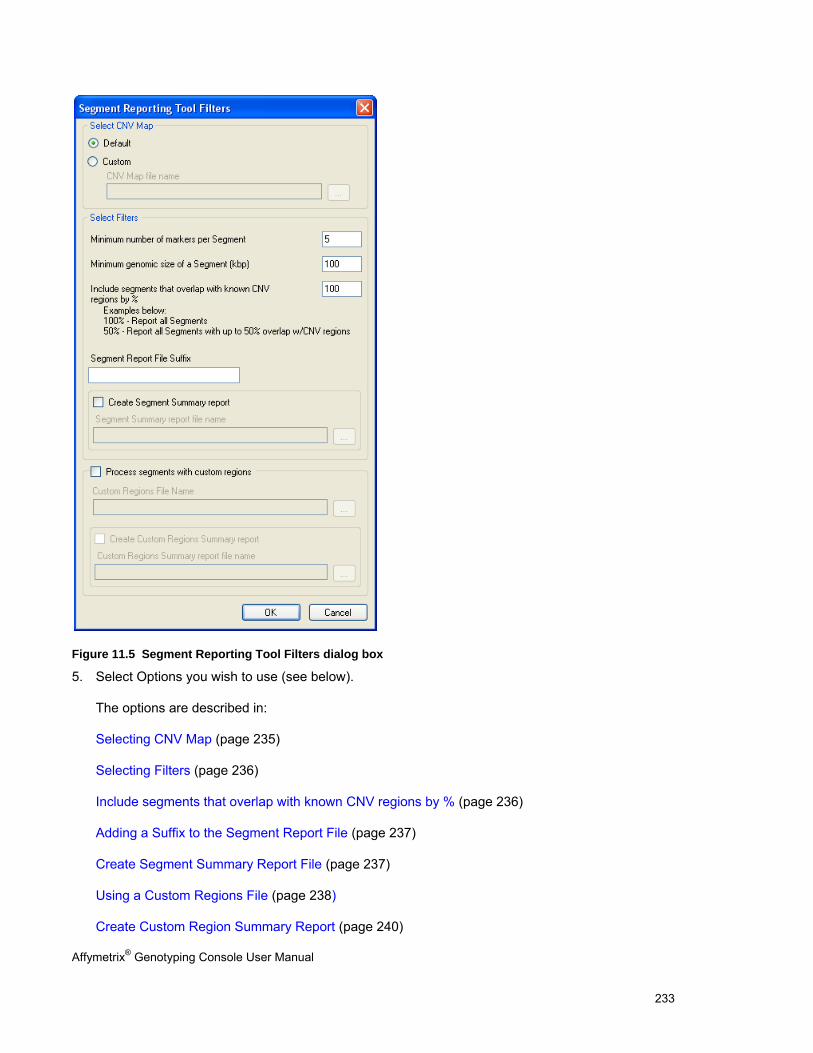
Affymetrix® Genotyping Console User Manual 233
Figure 11.5 Segment Reporting Tool Filters dialog box
5. Select Options you wish to use (see below).
The options are described in:
Selecting CNV Map (page 235)
Selecting Filters (page 236)
Include segments that overlap with known CNV regions by % (page 236)
Adding a Suffix to the Segment Report File (page 237)
Create Segment Summary Report File (page 237)
Using a Custom Regions File (page 238)
Create Custom Region Summary Report (page 240)
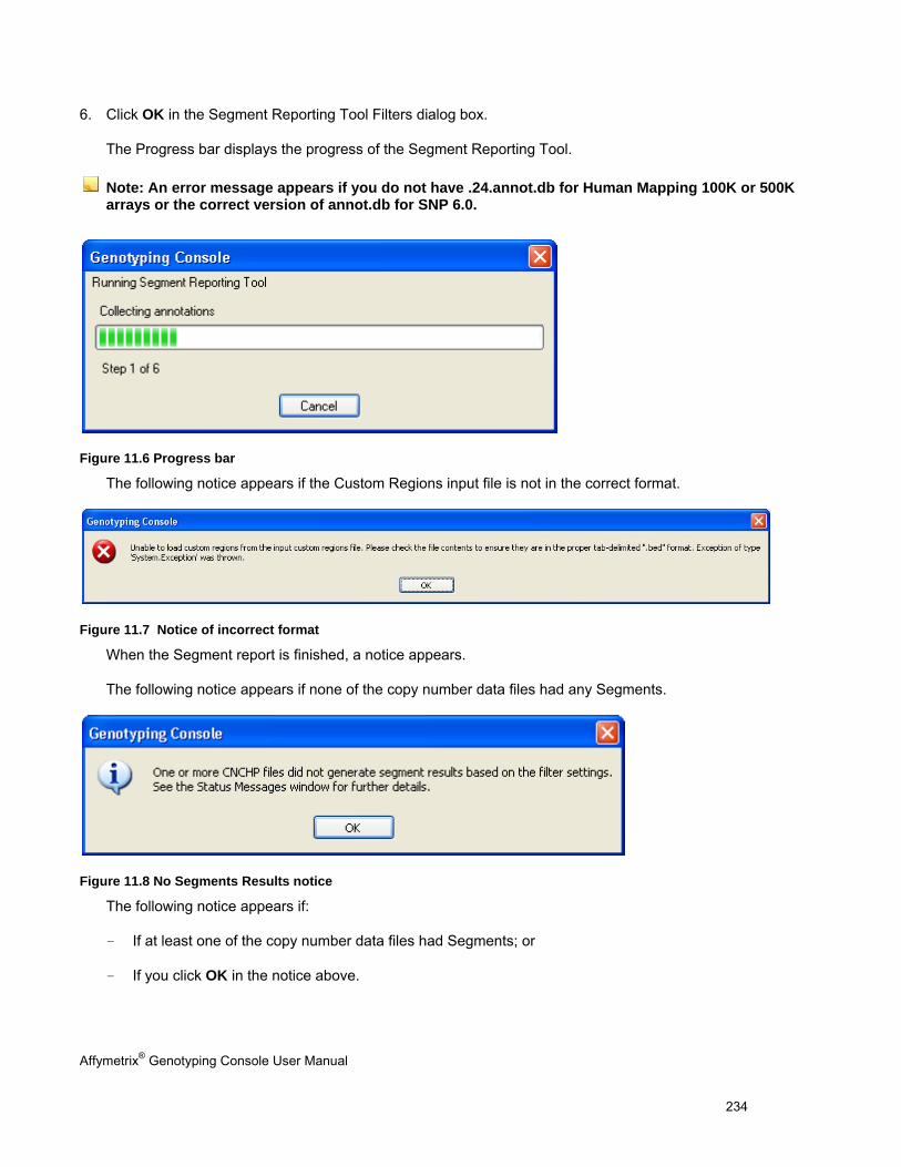
Affymetrix® Genotyping Console User Manual 234
6. Click OK in the Segment Reporting Tool Filters dialog box.
The Progress bar displays the progress of the Segment Reporting Tool.
Note: An error message appears if you do not have .24.annot.db for Human Mapping 100K or 500K arrays or the correct version of annot.db for SNP 6.0.
Figure 11.6 Progress bar
The following notice appears if the Custom Regions input file is not in the correct format.
Figure 11.7 Notice of incorrect format
When the Segment report is finished, a notice appears.
The following notice appears if none of the copy number data files had any Segments.
Figure 11.8 No Segments Results notice
The following notice appears if:
- If at least one of the copy number data files had Segments; or
- If you click OK in the notice above.
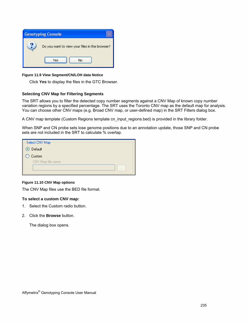
Affymetrix® Genotyping Console User Manual 235
Figure 11.9 View Segment/CN/LOH data Notice
Click Yes to display the files in the GTC Browser.
Selecting CNV Map for Filtering Segments
The SRT allows you to filter the detected copy number segments against a CNV Map of known copy number variation regions by a specified percentage. The SRT uses the Toronto CNV map as the default map for analysis. You can choose other CNV maps (e.g. Broad CNV map, or user-defined map) in the SRT Filters dialog box.
A CNV map template (Custom Regions template cn_input_regions.bed) is provided in the library folder.
When SNP and CN probe sets lose genome positions due to an annotation update, those SNP and CN probe sets are not included in the SRT to calculate % overlap.
Figure 11.10 CNV Map options
The CNV Map files use the BED file format.
To select a custom CNV map:
1. Select the Custom radio button.
2. Click the Browse button.
The dialog box opens.
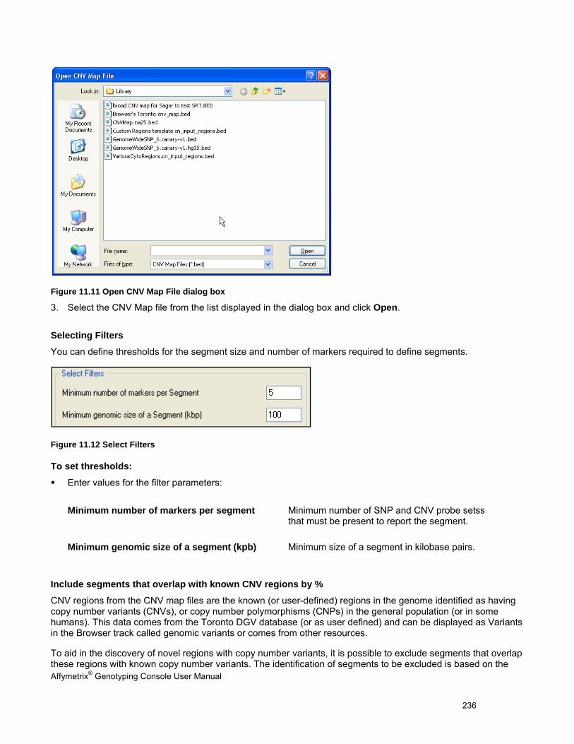
Affymetrix® Genotyping Console User Manual 236
Figure 11.11 Open CNV Map File dialog box
3. Select the CNV Map file from the list displayed in the dialog box and click Open.
Selecting Filters
You can define thresholds for the segment size and number of markers required to define segments.
Figure 11.12 Select Filters
To set thresholds:
Enter values for the filter parameters:
Minimum number of markers per segment Minimum number of SNP and CNV probe setss that must be present to report the segment.
Minimum genomic size of a segment (kpb) Minimum size of a segment in kilobase pairs.
Include segments that overlap with known CNV regions by %
CNV regions from the CNV map files are the known (or user-defined) regions in the genome identified as having copy number variants (CNVs), or copy number polymorphisms (CNPs) in the general population (or in some humans). This data comes from the Toronto DGV database (or as user defined) and can be displayed as Variants in the Browser track called genomic variants or comes from other resources.
To aid in the discovery of novel regions with copy number variants, it is possible to exclude segments that overlap these regions with known copy number variants. The identification of segments to be excluded is based on the
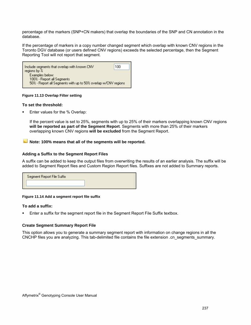
Affymetrix® Genotyping Console User Manual 237
percentage of the markers (SNP+CN makers) that overlap the boundaries of the SNP and CN annotation in the database.
If the percentage of markers in a copy number changed segment which overlap with known CNV regions in the Toronto DGV database (or users defined CNV regions) exceeds the selected percentage, then the Segment Reporting Tool will not report that segment.
Figure 11.13 Overlap Filter setting
To set the threshold:
Enter values for the % Overlap:
If the percent value is set to 25%, segments with up to 25% of their markers overlapping known CNV regions will be reported as part of the Segment Report. Segments with more than 25% of their markers overlapping known CNV regions will be excluded from the Segment Report.
Note: 100% means that all of the segments will be reported.
Adding a Suffix to the Segment Report Files
A suffix can be added to keep the output files from overwriting the results of an earlier analysis. The suffix will be added to Segment Report files and Custom Region Report files. Suffixes are not added to Summary reports.
Figure 11.14 Add a segment report file suffix
To add a suffix:
Enter a suffix for the segment report file in the Segment Report File Suffix textbox.
Create Segment Summary Report File
This option allows you to generate a summary segment report with information on change regions in all the CNCHP files you are analyzing. This tab-delimited file contains the file extension .cn_segments_summary.
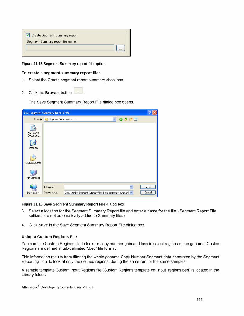
Affymetrix® Genotyping Console User Manual 238
Figure 11.15 Segment Summary report file option
To create a segment summary report file:
1. Select the Create segment report summary checkbox.
2. Click the Browse button .
The Save Segment Summary Report File dialog box opens.
Figure 11.16 Save Segment Summary Report File dialog box
3. Select a location for the Segment Summary Report file and enter a name for the file. (Segment Report File suffixes are not automatically added to Summary files)
4. Click Save in the Save Segment Summary Report File dialog box.
Using a Custom Regions File
You can use Custom Regions file to look for copy number gain and loss in select regions of the genome. Custom Regions are defined in tab-delimited “.bed” file format
This information results from filtering the whole genome Copy Number Segment data generated by the Segment Reporting Tool to look at only the defined regions, during the same run for the same samples.
A sample template Custom Input Regions file (Custom Regions template cn_input_regions.bed) is located in the Library folder.
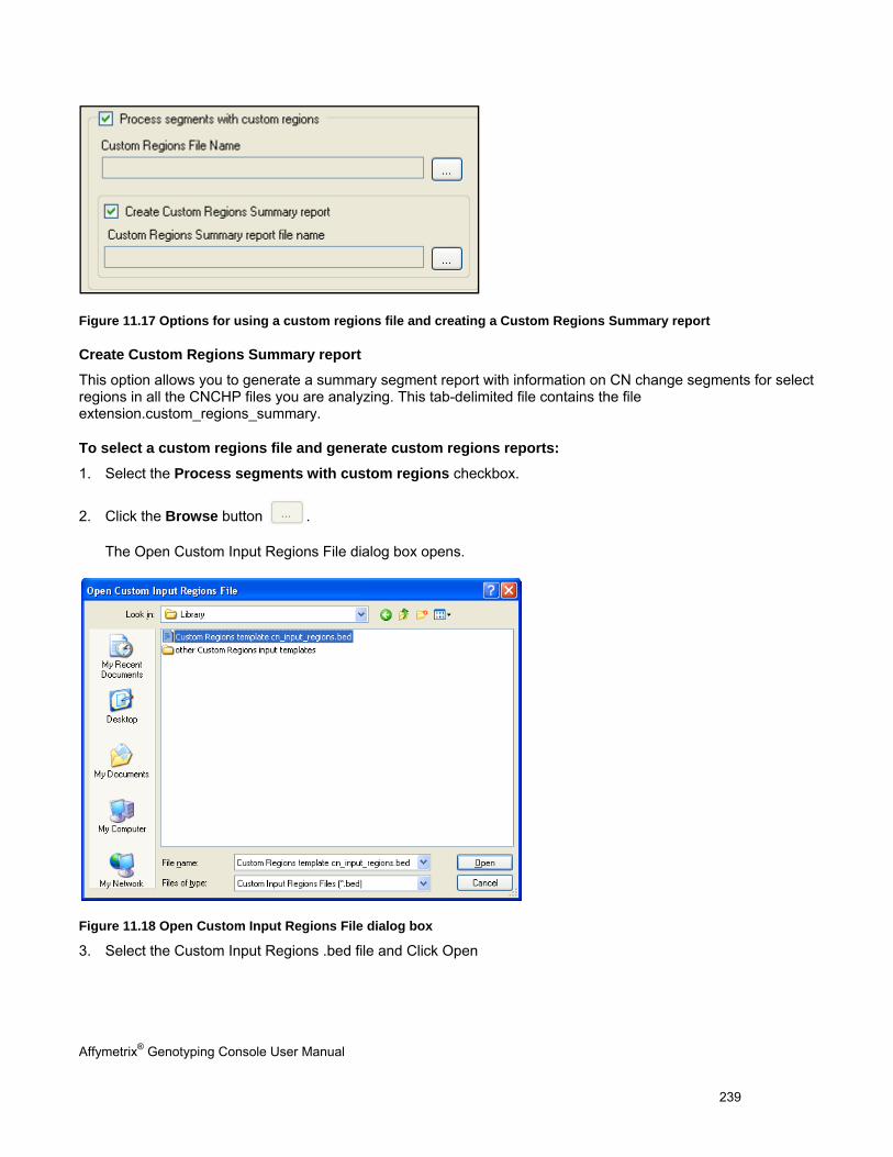
Affymetrix® Genotyping Console User Manual 239
Figure 11.17 Options for using a custom regions file and creating a Custom Regions Summary report
Create Custom Regions Summary report
This option allows you to generate a summary segment report with information on CN change segments for select regions in all the CNCHP files you are analyzing. This tab-delimited file contains the file extension.custom_regions_summary.
To select a custom regions file and generate custom regions reports:
1. Select the Process segments with custom regions checkbox.
2. Click the Browse button .
The Open Custom Input Regions File dialog box opens.
Figure 11.18 Open Custom Input Regions File dialog box
3. Select the Custom Input Regions .bed file and Click Open
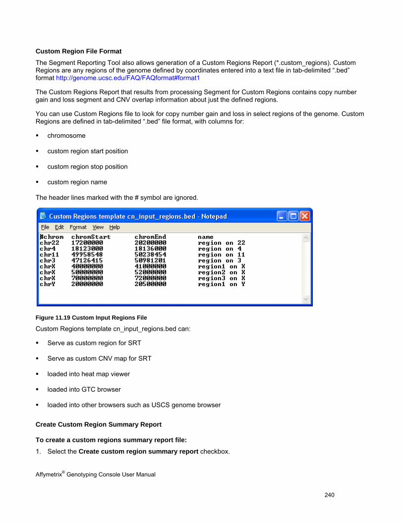
Affymetrix® Genotyping Console User Manual 240
Custom Region File Format
The Segment Reporting Tool also allows generation of a Custom Regions Report (*.custom_regions). Custom Regions are any regions of the genome defined by coordinates entered into a text file in tab-delimited “.bed” format http://genome.ucsc.edu/FAQ/FAQformat#format1
The Custom Regions Report that results from processing Segment for Custom Regions contains copy number gain and loss segment and CNV overlap information about just the defined regions.
You can use Custom Regions file to look for copy number gain and loss in select regions of the genome. Custom Regions are defined in tab-delimited “.bed” file format, with columns for:
chromosome
custom region start position
custom region stop position
custom region name
The header lines marked with the # symbol are ignored.
Figure 11.19 Custom Input Regions File
Custom Regions template cn_input_regions.bed can:
Serve as custom region for SRT
Serve as custom CNV map for SRT
loaded into heat map viewer
loaded into GTC browser
loaded into other browsers such as USCS genome browser
Create Custom Region Summary Report
To create a custom regions summary report file:
1. Select the Create custom region summary report checkbox.
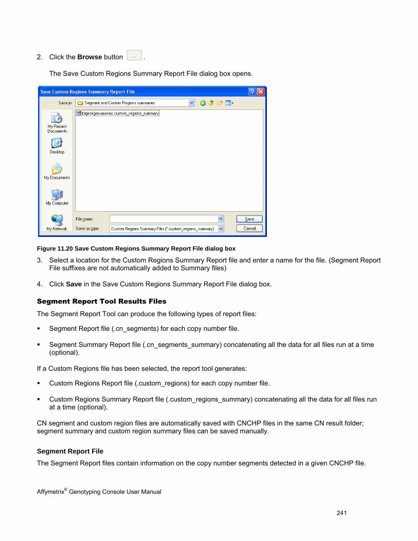
Affymetrix® Genotyping Console User Manual 241
2. Click the Browse button .
The Save Custom Regions Summary Report File dialog box opens.
Figure 11.20 Save Custom Regions Summary Report File dialog box
3. Select a location for the Custom Regions Summary Report file and enter a name for the file. (Segment Report File suffixes are not automatically added to Summary files)
4. Click Save in the Save Custom Regions Summary Report File dialog box.
Segment Report Tool Results Files
The Segment Report Tool can produce the following types of report files:
Segment Report file (.cn_segments) for each copy number file.
Segment Summary Report file (.cn_segments_summary) concatenating all the data for all files run at a time (optional).
If a Custom Regions file has been selected, the report tool generates:
Custom Regions Report file (.custom_regions) for each copy number file.
Custom Regions Summary Report file (.custom_regions_summary) concatenating all the data for all files run at a time (optional).
CN segment and custom region files are automatically saved with CNCHP files in the same CN result folder; segment summary and custom region summary files can be saved manually.
Segment Report File
The Segment Report files contain information on the copy number segments detected in a given CNCHP file.
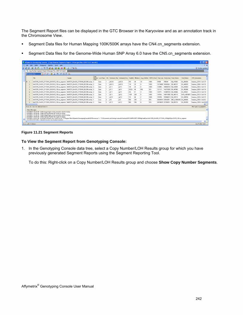
Affymetrix® Genotyping Console User Manual 242
The Segment Report files can be displayed in the GTC Browser in the Karyoview and as an annotation track in the Chromosome View.
Segment Data files for Human Mapping 100K/500K arrays have the CN4.cn_segments extension.
Segment Data files for the Genome-Wide Human SNP Array 6.0 have the CN5.cn_segments extension.
Figure 11.21 Segment Reports
To View the Segment Report from Genotyping Console:
1. In the Genotyping Console data tree, select a Copy Number/LOH Results group for which you have previously generated Segment Reports using the Segment Reporting Tool.
To do this: Right-click on a Copy Number/LOH Results group and choose Show Copy Number Segments.
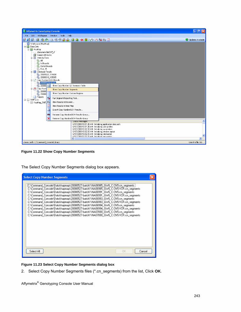
Affymetrix® Genotyping Console User Manual 243
Figure 11.22 Show Copy Number Segments
The Select Copy Number Segments dialog box appears.
Figure 11.23 Select Copy Number Segments dialog box
2. Select Copy Number Segments files (*.cn_segments) from the list, Click OK.
Affymetrix® Genotyping Console User Manual 244
The Segment Reports for all chosen files open in a single list in the display area.
Segment report information can also be viewed in the GTC Browser. See Loading Data into the GTC Browser (page 249).
The Copy Number Segments Report table content changes if you are using a custom map in the “Copy Number Segments Report” table. Starting from GTC 3.0.1, “%CNV_Overlap” is replaced with the %CNV_Overlap numbers calculated from the custom map and “CNV_Annotation” is replaced with variations names from the custom map.
File Name of the segment data file (seen in GTC table view only).
Sample CNCHP File name.
Copy Number State per marker CN as estimated by the HMM.
Loss/Gain Whether the Copy number change is a decrease or increase from the expected normal value.
Chr Chromosome where the segment is located.
Cytoband_Start_Pos The Chromosome’s cytoband within which a Copy Number change segment begins.
Cytoband_End_Pos The Chromosome’s cytoband within which a Copy Number change segment ends.
Size (kb) Size of the segment of Copy Number change.
#Markers Number of SNPs+CNV markers within the segment.
Avg_DistBetweenMarkers(kb) Length of segment divided by number of markers encompassed by that segment.
%CNV_Overlap Percentage of markers in a segment which overlap the boundaries of a known CNV.
Start_Linear_Pos base pair position on the Chromosome at which the first marker in the segment begins (going from top of the p-arm to the bottom of the q-arm of the chromosome).
End_Linear_Position base pair position on the Chromosome at which the last marker in the segment begins (going from top of the p-arm to the bottom of the q-arm of the chromosome).
Start_Marker Name of the first SNP or CN marker of a Copy Number change segment.
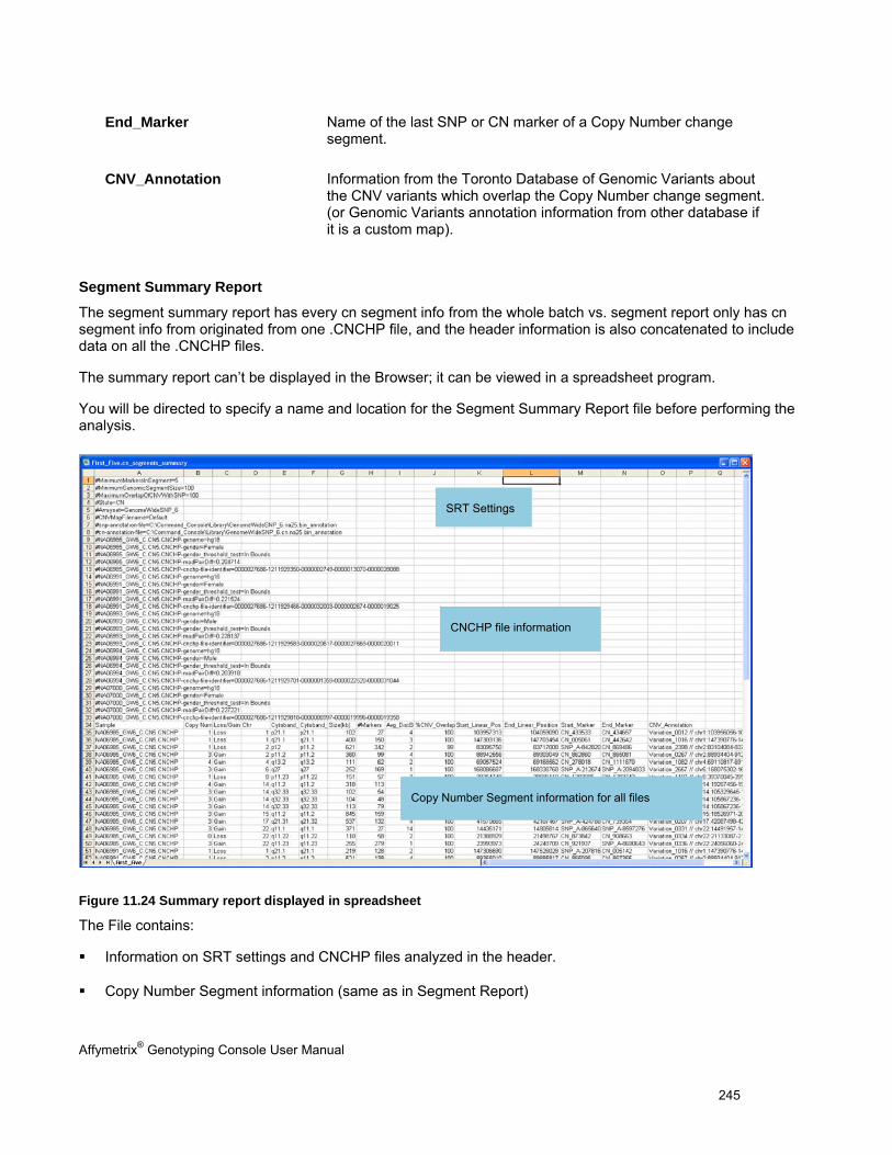
Affymetrix® Genotyping Console User Manual 245
End_Marker Name of the last SNP or CN marker of a Copy Number change segment.
CNV_Annotation Information from the Toronto Database of Genomic Variants about the CNV variants which overlap the Copy Number change segment. (or Genomic Variants annotation information from other database if it is a custom map).
Segment Summary Report
The segment summary report has every cn segment info from the whole batch vs. segment report only has cn segment info from originated from one .CNCHP file, and the header information is also concatenated to include data on all the .CNCHP files.
The summary report can’t be displayed in the Browser; it can be viewed in a spreadsheet program.
You will be directed to specify a name and location for the Segment Summary Report file before performing the analysis.
Figure 11.24 Summary report displayed in spreadsheet
The File contains:
Information on SRT settings and CNCHP files analyzed in the header.
Copy Number Segment information (same as in Segment Report)
SRT Settings
CNCHP file information
Copy Number Segment information for all files
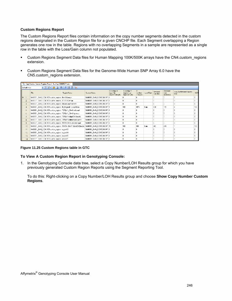
Affymetrix® Genotyping Console User Manual 246
Custom Regions Report
The Custom Regions Report files contain information on the copy number segments detected in the custom regions designated in the Custom Region file for a given CNCHP file. Each Segment overlapping a Region generates one row in the table. Regions with no overlapping Segments in a sample are represented as a single row in the table with the Loss/Gain column not populated.
Custom Regions Segment Data files for Human Mapping 100K/500K arrays have the CN4.custom_regions extension.
Custom Regions Segment Data files for the Genome-Wide Human SNP Array 6.0 have the CN5.custom_regions extension.
Figure 11.25 Custom Regions table in GTC
To View A Custom Region Report in Genotyping Console:
1. In the Genotyping Console data tree, select a Copy Number/LOH Results group for which you have previously generated Custom Region Reports using the Segment Reporting Tool.
To do this: Right-clicking on a Copy Number/LOH Results group and choose Show Copy Number Custom Regions.
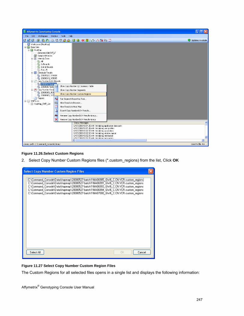
Affymetrix® Genotyping Console User Manual 247
Figure 11.26.Select Custom Regions
2. Select Copy Number Custom Regions files (*.custom_regions) from the list, Click OK
Figure 11.27 Select Copy Number Custom Region Files
The Custom Regions for all selected files opens in a single list and displays the following information:
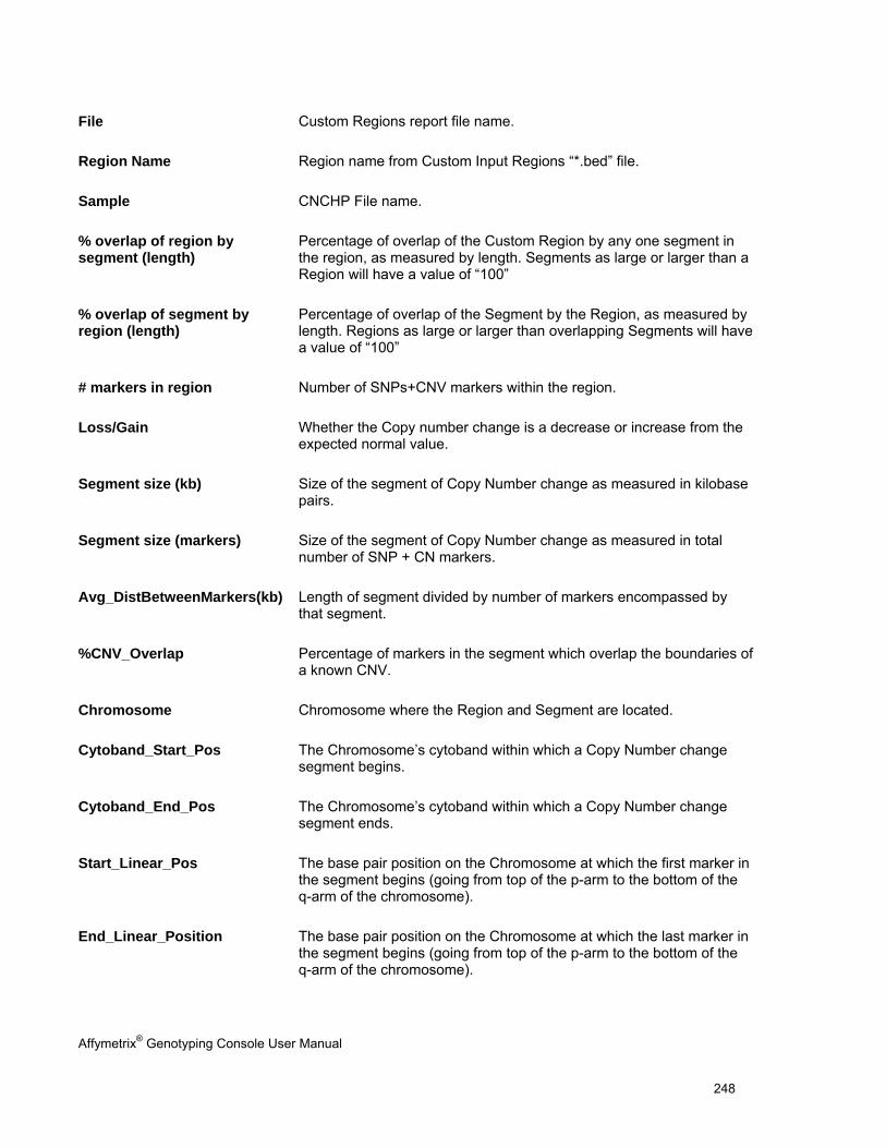
Affymetrix® Genotyping Console User Manual 248
File Custom Regions report file name.
Region Name Region name from Custom Input Regions “*.bed” file.
Sample CNCHP File name.
% overlap of region by segment (length)
Percentage of overlap of the Custom Region by any one segment in the region, as measured by length. Segments as large or larger than a Region will have a value of “100”
% overlap of segment by region (length)
Percentage of overlap of the Segment by the Region, as measured by length. Regions as large or larger than overlapping Segments will have a value of “100”
# markers in region Number of SNPs+CNV markers within the region.
Loss/Gain Whether the Copy number change is a decrease or increase from the expected normal value.
Segment size (kb) Size of the segment of Copy Number change as measured in kilobase pairs.
Segment size (markers) Size of the segment of Copy Number change as measured in total number of SNP + CN markers.
Avg_DistBetweenMarkers(kb) Length of segment divided by number of markers encompassed by that segment.
%CNV_Overlap Percentage of markers in the segment which overlap the boundaries of a known CNV.
Chromosome Chromosome where the Region and Segment are located.
Cytoband_Start_Pos The Chromosome’s cytoband within which a Copy Number change segment begins.
Cytoband_End_Pos The Chromosome’s cytoband within which a Copy Number change segment ends.
Start_Linear_Pos The base pair position on the Chromosome at which the first marker in the segment begins (going from top of the p-arm to the bottom of the q-arm of the chromosome).
End_Linear_Position The base pair position on the Chromosome at which the last marker in the segment begins (going from top of the p-arm to the bottom of the q-arm of the chromosome).
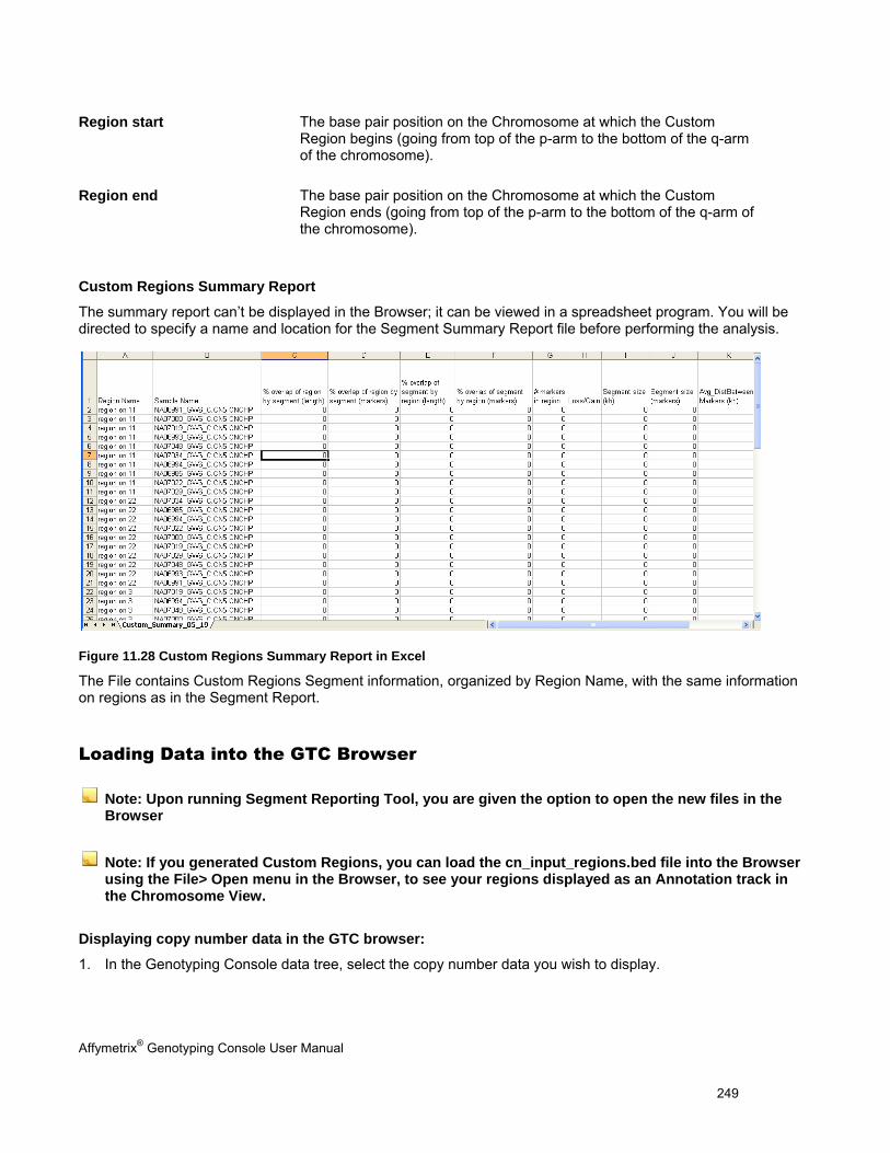
Affymetrix® Genotyping Console User Manual 249
Region start The base pair position on the Chromosome at which the Custom Region begins (going from top of the p-arm to the bottom of the q-arm of the chromosome).
Region end The base pair position on the Chromosome at which the Custom Region ends (going from top of the p-arm to the bottom of the q-arm of the chromosome).
Custom Regions Summary Report
The summary report can’t be displayed in the Browser; it can be viewed in a spreadsheet program. You will be directed to specify a name and location for the Segment Summary Report file before performing the analysis.
Figure 11.28 Custom Regions Summary Report in Excel
The File contains Custom Regions Segment information, organized by Region Name, with the same information on regions as in the Segment Report.
Loading Data into the GTC Browser
Note: Upon running Segment Reporting Tool, you are given the option to open the new files in the Browser
Note: If you generated Custom Regions, you can load the cn_input_regions.bed file into the Browser using the File> Open menu in the Browser, to see your regions displayed as an Annotation track in the Chromosome View.
Displaying copy number data in the GTC browser:
1. In the Genotyping Console data tree, select the copy number data you wish to display.
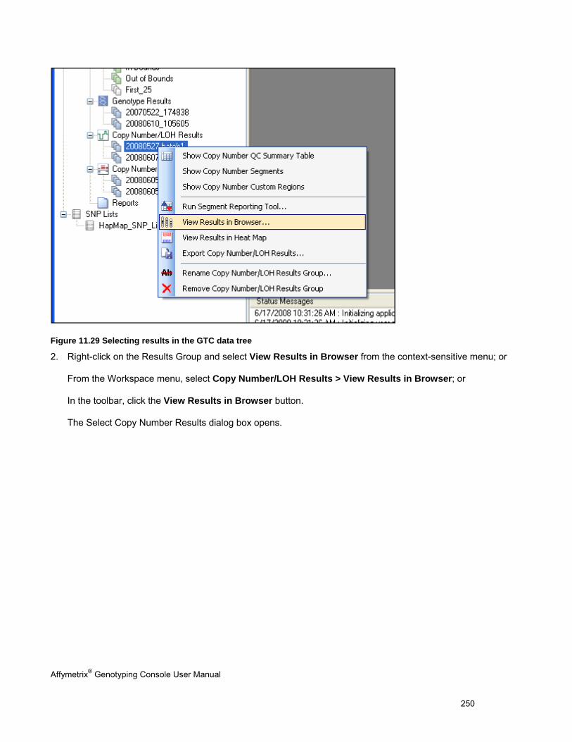
Affymetrix® Genotyping Console User Manual 250
Figure 11.29 Selecting results in the GTC data tree
2. Right-click on the Results Group and select View Results in Browser from the context-sensitive menu; or
From the Workspace menu, select Copy Number/LOH Results > View Results in Browser; or
In the toolbar, click the View Results in Browser button.
The Select Copy Number Results dialog box opens.
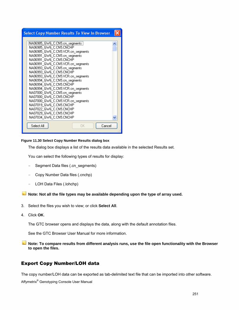
Affymetrix® Genotyping Console User Manual 251
Figure 11.30 Select Copy Number Results dialog box
The dialog box displays a list of the results data available in the selected Results set.
You can select the following types of results for display:
- Segment Data files (.cn_segments)
- Copy Number Data files (.cnchp)
- LOH Data Files (.lohchp)
Note: Not all the file types may be available depending upon the type of array used.
3. Select the files you wish to view; or click Select All.
4. Click OK.
The GTC browser opens and displays the data, along with the default annotation files.
See the GTC Browser User Manual for more information.
Note: To compare results from different analysis runs, use the file open functionality with the Browser to open the files.
Export Copy Number/LOH data
The copy number/LOH data can be exported as tab-delimited text file that can be imported into other software.
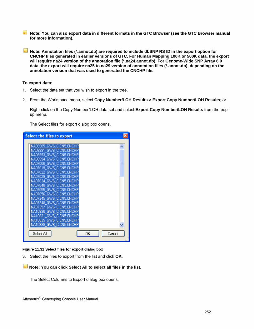
Affymetrix® Genotyping Console User Manual 252
Note: You can also export data in different formats in the GTC Browser (see the GTC Browser manual for more information).
Note: Annotation files (*.annot.db) are required to include dbSNP RS ID in the export option for CNCHP files generated in earlier versions of GTC. For Human Mapping 100K or 500K data, the export will require na24 version of the annotation file (*.na24.annot.db). For Genome-Wide SNP Array 6.0 data, the export will require na25 to na29 version of annotation files (*.annot.db), depending on the annotation version that was used to generated the CNCHP file.
To export data:
1. Select the data set that you wish to export in the tree.
2. From the Workspace menu, select Copy Number/LOH Results > Export Copy Number/LOH Results; or
Right-click on the Copy Number/LOH data set and select Export Copy Number/LOH Results from the pop-up menu.
The Select files for export dialog box opens.
Figure 11.31 Select files for export dialog box
3. Select the files to export from the list and click OK.
Note: You can click Select All to select all files in the list.
The Select Columns to Export dialog box opens.
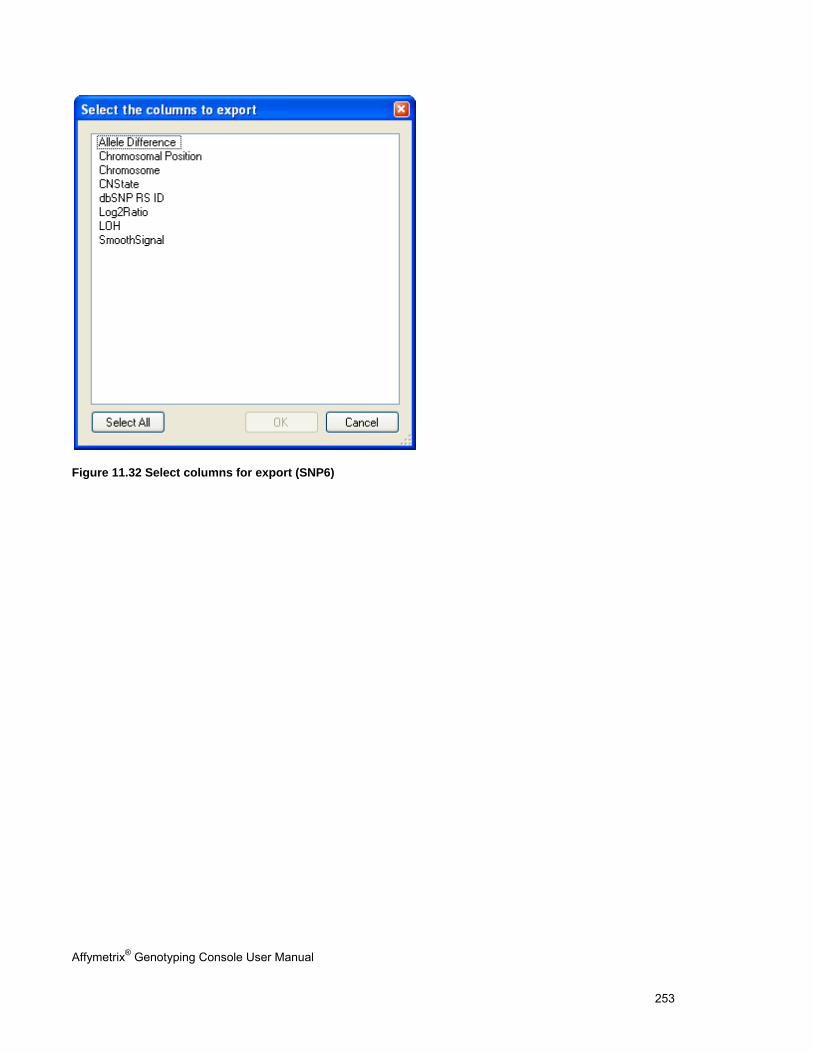
Affymetrix® Genotyping Console User Manual 253
Figure 11.32 Select columns for export (SNP6)
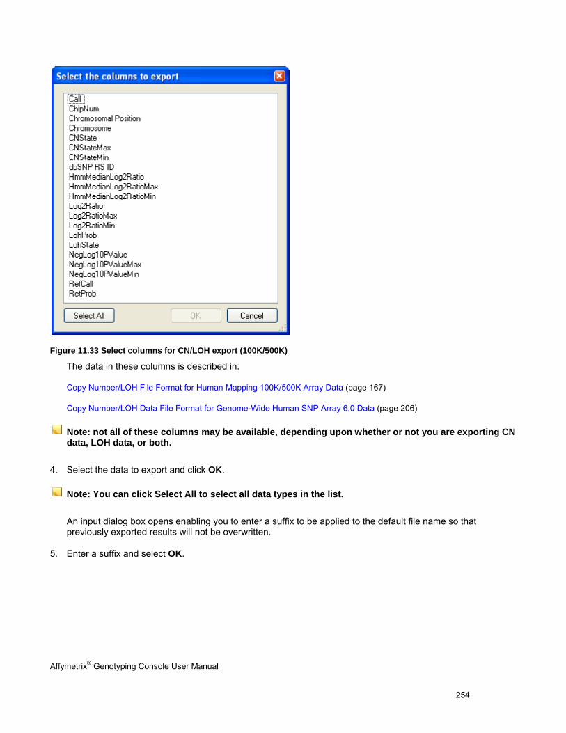
Affymetrix® Genotyping Console User Manual 254
Figure 11.33 Select columns for CN/LOH export (100K/500K)
The data in these columns is described in:
Copy Number/LOH File Format for Human Mapping 100K/500K Array Data (page 167)
Copy Number/LOH Data File Format for Genome-Wide Human SNP Array 6.0 Data (page 206)
Note: not all of these columns may be available, depending upon whether or not you are exporting CN data, LOH data, or both.
4. Select the data to export and click OK.
Note: You can click Select All to select all data types in the list.
An input dialog box opens enabling you to enter a suffix to be applied to the default file name so that previously exported results will not be overwritten.
5. Enter a suffix and select OK.
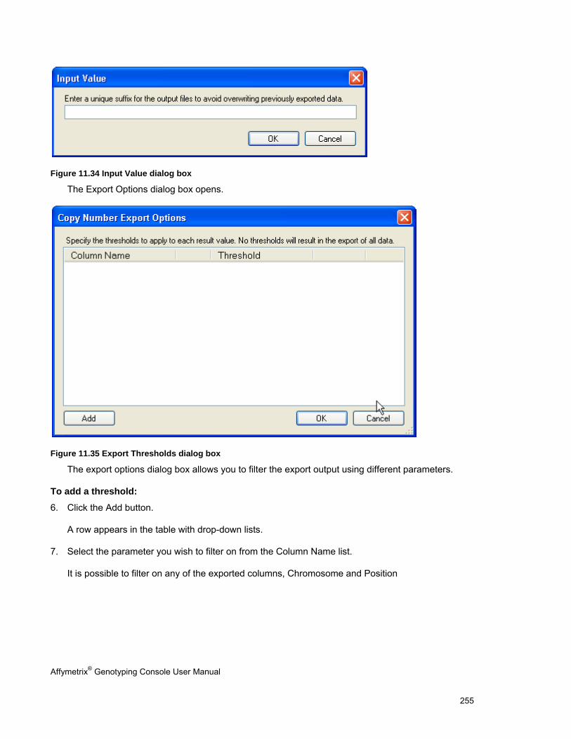
Affymetrix® Genotyping Console User Manual 255
Figure 11.34 Input Value dialog box
The Export Options dialog box opens.
Figure 11.35 Export Thresholds dialog box
The export options dialog box allows you to filter the export output using different parameters.
To add a threshold:
6. Click the Add button.
A row appears in the table with drop-down lists.
7. Select the parameter you wish to filter on from the Column Name list.
It is possible to filter on any of the exported columns, Chromosome and Position
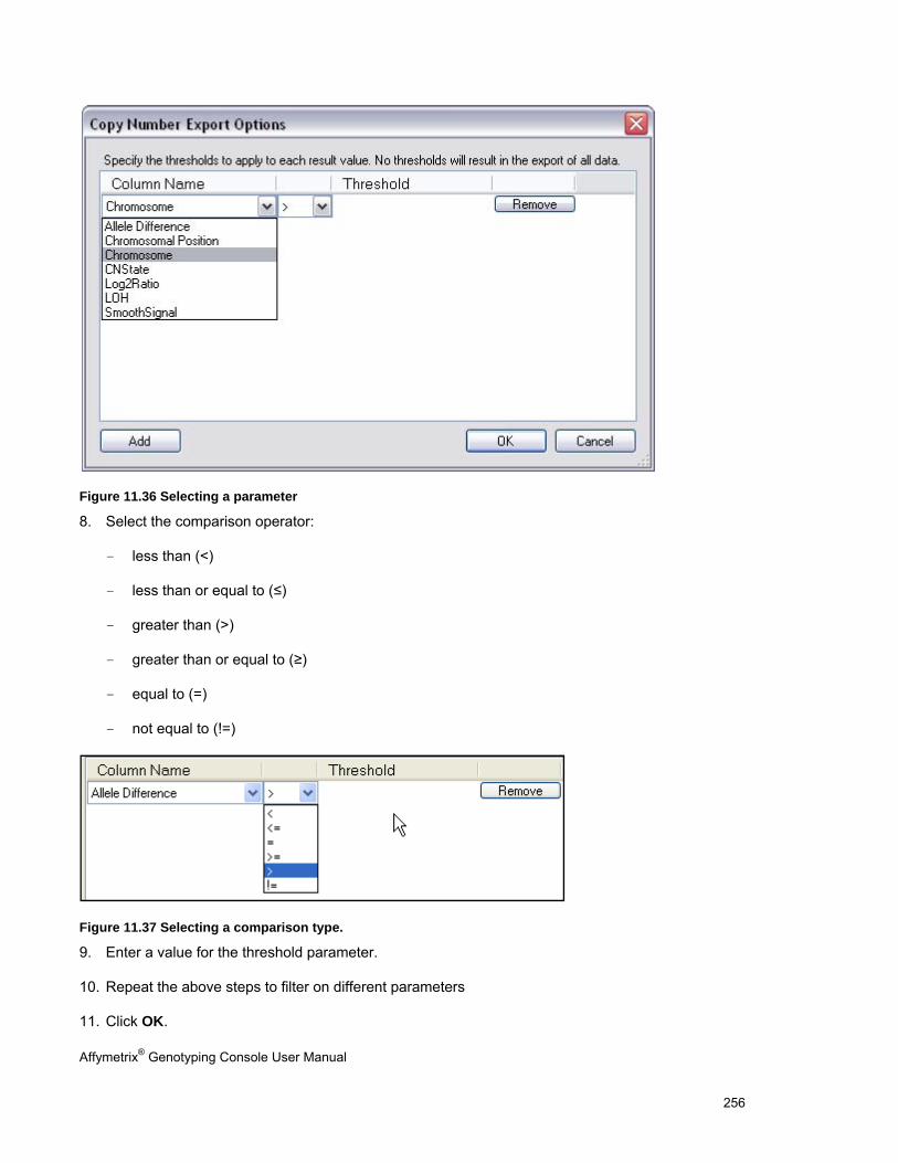
Affymetrix® Genotyping Console User Manual 256
Figure 11.36 Selecting a parameter
8. Select the comparison operator:
- less than (<)
- less than or equal to (≤)
- greater than (>)
- greater than or equal to (≥)
- equal to (=)
- not equal to (!=)
Figure 11.37 Selecting a comparison type.
9. Enter a value for the threshold parameter.
10. Repeat the above steps to filter on different parameters
11. Click OK.
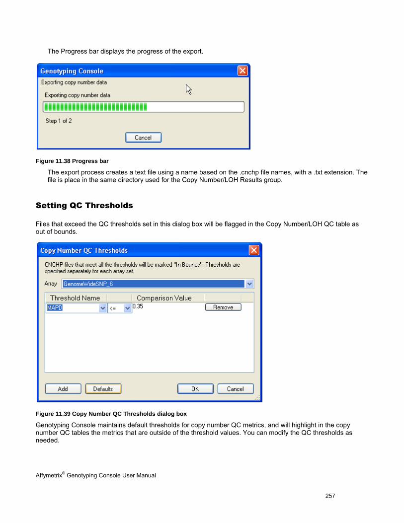
Affymetrix® Genotyping Console User Manual 257
The Progress bar displays the progress of the export.
Figure 11.38 Progress bar
The export process creates a text file using a name based on the .cnchp file names, with a .txt extension. The file is place in the same directory used for the Copy Number/LOH Results group.
Setting QC Thresholds
Files that exceed the QC thresholds set in this dialog box will be flagged in the Copy Number/LOH QC table as out of bounds.
Figure 11.39 Copy Number QC Thresholds dialog box
Genotyping Console maintains default thresholds for copy number QC metrics, and will highlight in the copy number QC tables the metrics that are outside of the threshold values. You can modify the QC thresholds as needed.
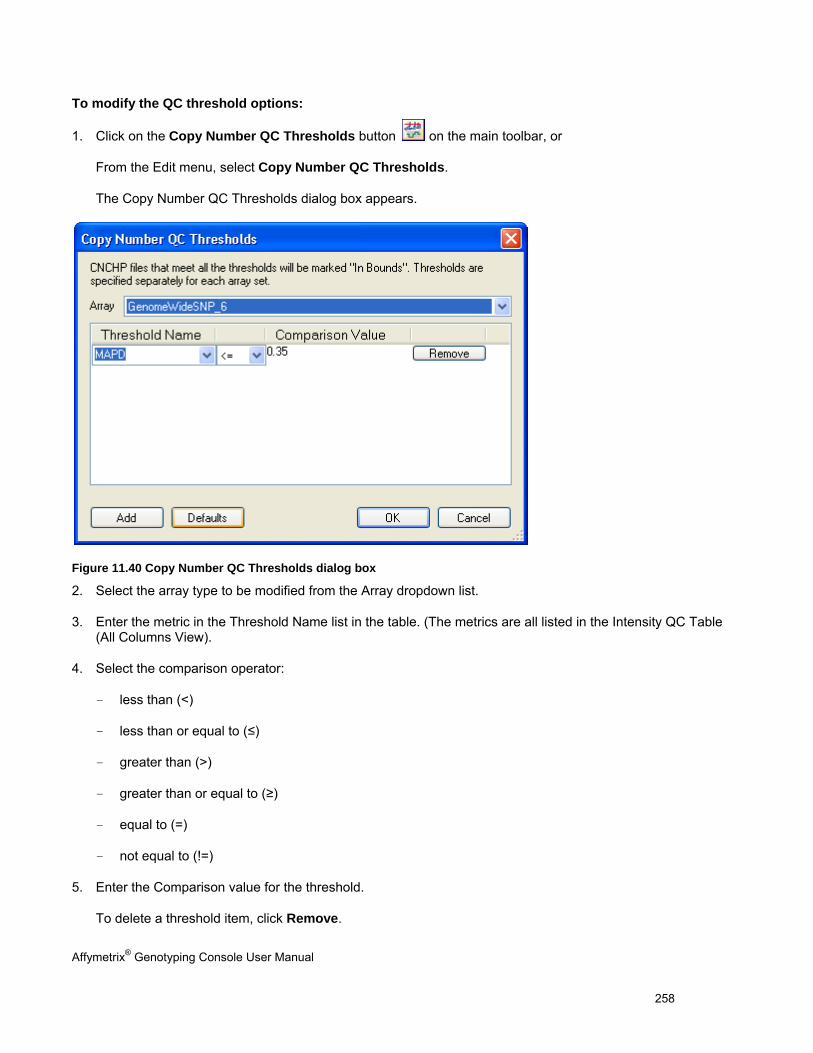
Affymetrix® Genotyping Console User Manual 258
To modify the QC threshold options:
1. Click on the Copy Number QC Thresholds button on the main toolbar, or
From the Edit menu, select Copy Number QC Thresholds.
The Copy Number QC Thresholds dialog box appears.
Figure 11.40 Copy Number QC Thresholds dialog box
2. Select the array type to be modified from the Array dropdown list.
3. Enter the metric in the Threshold Name list in the table. (The metrics are all listed in the Intensity QC Table (All Columns View).
4. Select the comparison operator:
- less than (<)
- less than or equal to (≤)
- greater than (>)
- greater than or equal to (≥)
- equal to (=)
- not equal to (!=)
5. Enter the Comparison value for the threshold.
To delete a threshold item, click Remove.
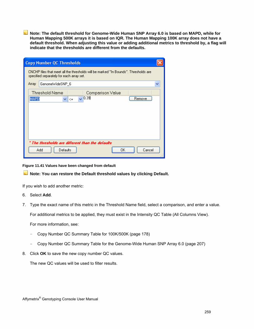
Affymetrix® Genotyping Console User Manual 259
Note: The default threshold for Genome-Wide Human SNP Array 6.0 is based on MAPD, while for Human Mapping 500K arrays it is based on IQR. The Human Mapping 100K array does not have a default threshold. When adjusting this value or adding additional metrics to threshold by, a flag will indicate that the thresholds are different from the defaults.
Figure 11.41 Values have been changed from default
Note: You can restore the Default threshold values by clicking Default.
If you wish to add another metric:
6. Select Add.
7. Type the exact name of this metric in the Threshold Name field, select a comparison, and enter a value.
For additional metrics to be applied, they must exist in the Intensity QC Table (All Columns View).
For more information, see:
- Copy Number QC Summary Table for 100K/500K (page 178)
- Copy Number QC Summary Table for the Genome-Wide Human SNP Array 6.0 (page 207)
8. Click OK to save the new copy number QC values.
The new QC values will be used to filter results.
Affymetrix® Genotyping Console User Manual 260
Chapter 12: Copy Number Variation Analysis Copy Number Variation (CNV) Analysis uses the Canary algorithm to make a CN state call (0, 1, 2, 3, 4) for previously identified regions with known copy number variations in the genome. It uses a region file with a region ID and a list of the CN/SNP probe setss in the region (a region with common copy number variation can contain a few too many CN/SNP probe sets).
Note: CNV is only available for Genome-Wide Human SNP Array 6.0 data; it does not work with other arrays.
Performing Copy Number Variation Analysis
Important: Always save your results folders with a different batch name and location to make sure you can find your data later on. If you don't change the output root path, GTC will use the previous file path, which can belong to another data set or another hard disk. For more details on hard disk space requirements, see Appendix J, page 319.
To perform CNV analysis:
1. Open the workspace and select the data set with the data for analysis.
2. Select the intensity data file set from the data tree.
3. From the workspace menu, select Intensity Data > Perform Copy Number Variation Analysis…; or
Right-click the intensity data file set and select Perform Copy Number Variation Analysis… from the pop-up menu; or
Click the Perform Copy Number Variation Analysis… button in the toolbar.
The Copy Number Analysis Options dialog box opens.
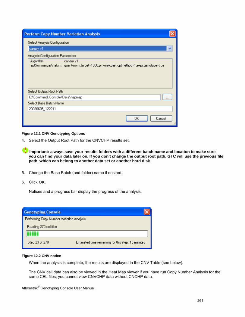
Affymetrix® Genotyping Console User Manual 261
Figure 12.1 CNV Genotyping Options
4. Select the Output Root Path for the CNVCHP results set.
Important: always save your results folders with a different batch name and location to make sure you can find your data later on. If you don't change the output root path, GTC will use the previous file path, which can belong to another data set or another hard disk.
5. Change the Base Batch (and folder) name if desired.
6. Click OK.
Notices and a progress bar display the progress of the analysis.
Figure 12.2 CNV notice
When the analysis is complete, the results are displayed in the CNV Table (see below).
The CNV call data can also be viewed in the Heat Map viewer if you have run Copy Number Analysis for the same CEL files; you cannot view CNVCHP data without CNCHP data.
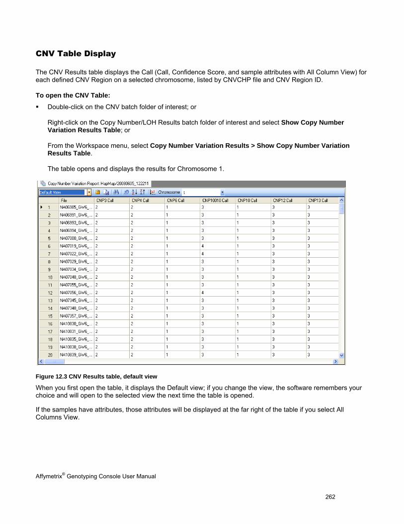
Affymetrix® Genotyping Console User Manual 262
CNV Table Display
The CNV Results table displays the Call (Call, Confidence Score, and sample attributes with All Column View) for each defined CNV Region on a selected chromosome, listed by CNVCHP file and CNV Region ID.
To open the CNV Table:
Double-click on the CNV batch folder of interest; or
Right-click on the Copy Number/LOH Results batch folder of interest and select Show Copy Number Variation Results Table; or
From the Workspace menu, select Copy Number Variation Results > Show Copy Number Variation Results Table.
The table opens and displays the results for Chromosome 1.
Figure 12.3 CNV Results table, default view
When you first open the table, it displays the Default view; if you change the view, the software remembers your choice and will open to the selected view the next time the table is opened.
If the samples have attributes, those attributes will be displayed at the far right of the table if you select All Columns View.
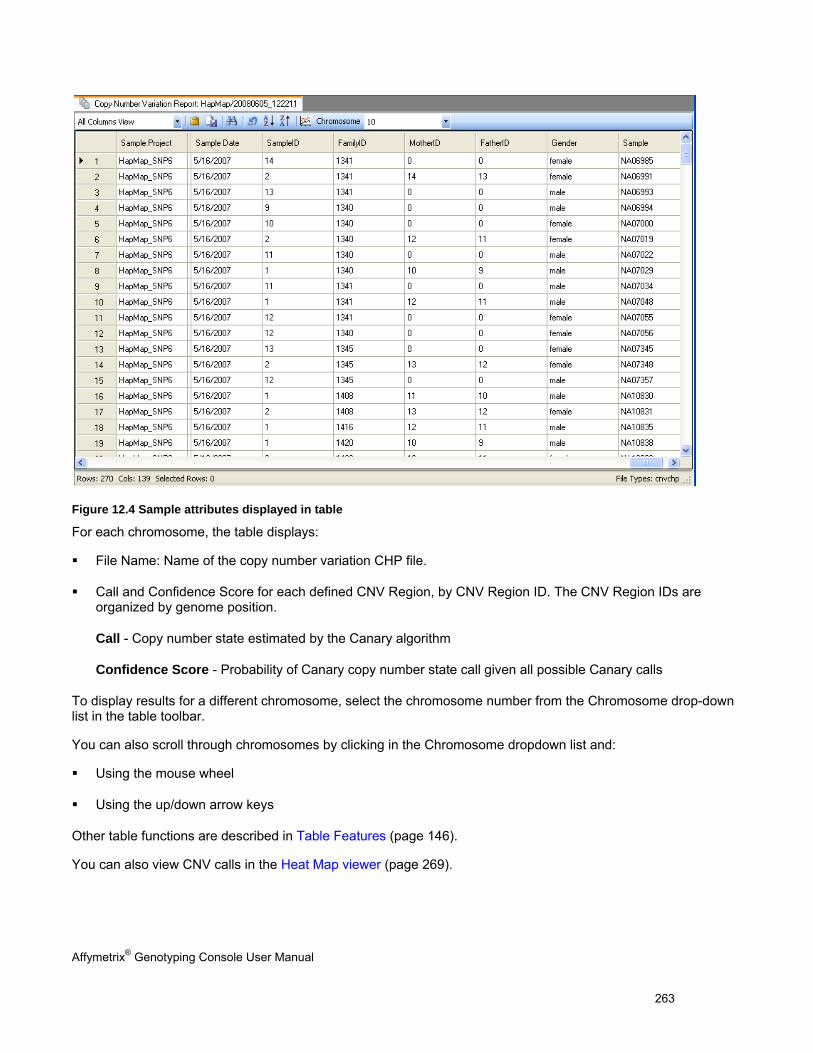
Affymetrix® Genotyping Console User Manual 263
Figure 12.4 Sample attributes displayed in table
For each chromosome, the table displays:
File Name: Name of the copy number variation CHP file.
Call and Confidence Score for each defined CNV Region, by CNV Region ID. The CNV Region IDs are organized by genome position.
Call - Copy number state estimated by the Canary algorithm
Confidence Score - Probability of Canary copy number state call given all possible Canary calls
To display results for a different chromosome, select the chromosome number from the Chromosome drop-down list in the table toolbar.
You can also scroll through chromosomes by clicking in the Chromosome dropdown list and:
Using the mouse wheel
Using the up/down arrow keys
Other table functions are described in Table Features (page 146).
You can also view CNV calls in the Heat Map viewer (page 269).
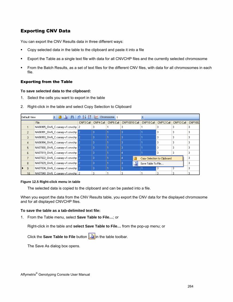
Affymetrix® Genotyping Console User Manual 264
Exporting CNV Data
You can export the CNV Results data in three different ways:
Copy selected data in the table to the clipboard and paste it into a file
Export the Table as a single text file with data for all CNVCHP files and the currently selected chromosome
From the Batch Results, as a set of text files for the different CNV files, with data for all chromosomes in each file.
Exporting from the Table
To save selected data to the clipboard:
1. Select the cells you want to export in the table
2. Right-click in the table and select Copy Selection to Clipboard
Figure 12.5 Right-click menu in table
The selected data is copied to the clipboard and can be pasted into a file.
When you export the data from the CNV Results table, you export the CNV data for the displayed chromosome and for all displayed CNVCHP files.
To save the table as a tab-delimited text file:
1. From the Table menu, select Save Table to File…; or
Right-click in the table and select Save Table to File… from the pop-up menu; or
Click the Save Table to File button in the table toolbar.
The Save As dialog box opens.
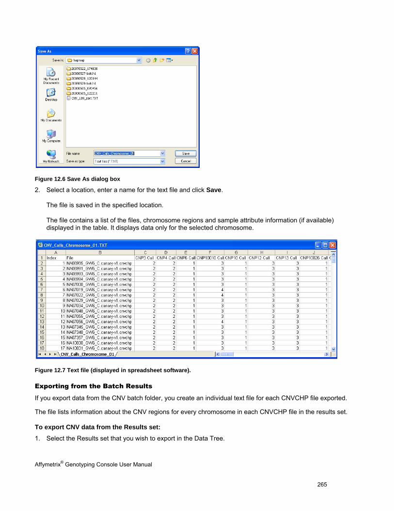
Affymetrix® Genotyping Console User Manual 265
Figure 12.6 Save As dialog box
2. Select a location, enter a name for the text file and click Save.
The file is saved in the specified location.
The file contains a list of the files, chromosome regions and sample attribute information (if available) displayed in the table. It displays data only for the selected chromosome.
Figure 12.7 Text file (displayed in spreadsheet software).
Exporting from the Batch Results
If you export data from the CNV batch folder, you create an individual text file for each CNVCHP file exported.
The file lists information about the CNV regions for every chromosome in each CNVCHP file in the results set.
To export CNV data from the Results set:
1. Select the Results set that you wish to export in the Data Tree.
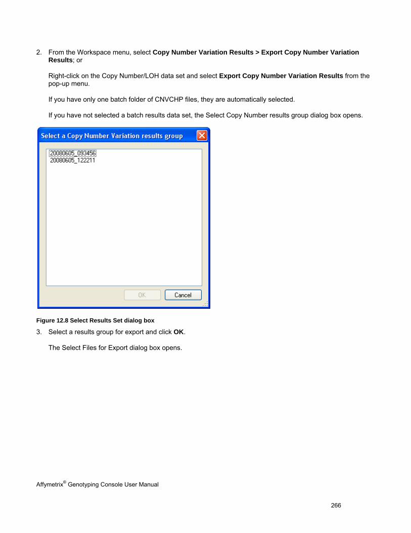
Affymetrix® Genotyping Console User Manual 266
2. From the Workspace menu, select Copy Number Variation Results > Export Copy Number Variation Results; or
Right-click on the Copy Number/LOH data set and select Export Copy Number Variation Results from the pop-up menu.
If you have only one batch folder of CNVCHP files, they are automatically selected.
If you have not selected a batch results data set, the Select Copy Number results group dialog box opens.
Figure 12.8 Select Results Set dialog box
3. Select a results group for export and click OK.
The Select Files for Export dialog box opens.
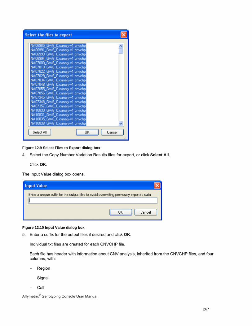
Affymetrix® Genotyping Console User Manual 267
Figure 12.9 Select Files to Export dialog box
4. Select the Copy Number Variation Results files for export, or click Select All.
Click OK.
The Input Value dialog box opens.
Figure 12.10 Input Value dialog box
5. Enter a suffix for the output files if desired and click OK.
Individual txt files are created for each CNVCHP file.
Each file has header with information about CNV analysis, inherited from the CNVCHP files, and four columns, with:
- Region
- Signal
- Call

Affymetrix® Genotyping Console User Manual 268
- Confidence
Affymetrix® Genotyping Console User Manual 269
Chapter 13: Heat Map Viewer The Heat Map viewer displays:
Copy Number (CN) intensity values (~log2 ratios) from probe sets in the CNCHP files
Copy number state calls for the copy number variations (CNV) in corresponding CNVCHP files, if available
Note: You can view CN data with or without matching CNV data. If you change the default CNV map after data is loaded in the Heat Map viewer, all the associated CNVCNP files will be removed (CNVCHP files are map-specific). You must have CNCHP data available to load CNVCHP data.
It allows you to:
Compare the CNV calls from CNVCHP files using raw intensity values from individual probe sets within the CNV regions from CNCHP files.
Survey large quantities of genomic data to detect de novo CNV regions.
The Heat Map viewer displays:
CNV regions if you load CNVCHP files (the default CNV map file with BED format will automatically follow)
Genomic positions of the current viewing window
Log2ratio value data from CNCHP files (intensity value) for each SNP or CN as a color value representing the converted log2 ratios in a heat map with a pre-defined scale.
Summary histogram to indicate the frequencies of probe sets with certain color values
In the status bar, it shows:
Sample names: CNCHP file name, and CNVCHP file name (if available)
SNP or CN probe set ID,
log2 ratio of a SNP or CN probe set; or
With additional CNV region ID, copy number call for the CNV region and confidence score for the copy number call from CNVCHP files (if available) if you mouse over a CNV region contains CNV calls.
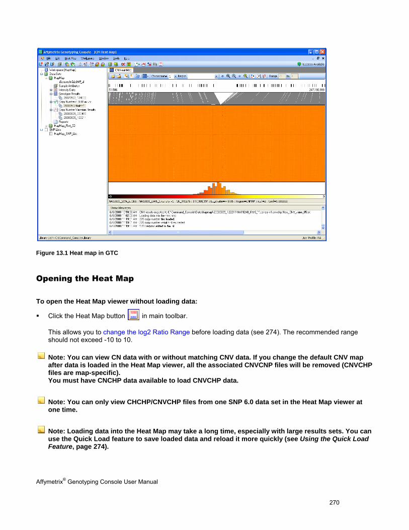
Affymetrix® Genotyping Console User Manual 270
Figure 13.1 Heat map in GTC
Opening the Heat Map
To open the Heat Map viewer without loading data:
Click the Heat Map button in main toolbar.
This allows you to change the log2 Ratio Range before loading data (see 274). The recommended range should not exceed -10 to 10.
Note: You can view CN data with or without matching CNV data. If you change the default CNV map after data is loaded in the Heat Map viewer, all the associated CNVCNP files will be removed (CNVCHP files are map-specific). You must have CNCHP data available to load CNVCHP data.
Note: You can only view CHCHP/CNVCHP files from one SNP 6.0 data set in the Heat Map viewer at one time.
Note: Loading data into the Heat Map may take a long time, especially with large results sets. You can use the Quick Load feature to save loaded data and reload it more quickly (see Using the Quick Load Feature, page 274).
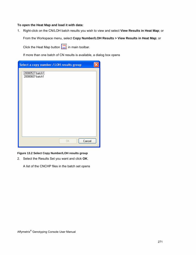
Affymetrix® Genotyping Console User Manual 271
To open the Heat Map and load it with data:
1. Right-click on the CN/LOH batch results you wish to view and select View Results in Heat Map; or
From the Workspace menu, select Copy Number/LOH Results > View Results in Heat Map; or
Click the Heat Map button in main toolbar.
If more than one batch of CN results is available, a dialog box opens
Figure 13.2 Select Copy Number/LOH results group
2. Select the Results Set you want and click OK.
A list of the CNCHP files in the batch set opens
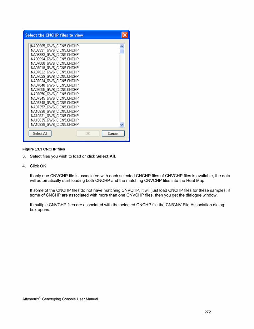
Affymetrix® Genotyping Console User Manual 272
Figure 13.3 CNCHP files
3. Select files you wish to load or click Select All.
4. Click OK.
If only one CNVCHP file is associated with each selected CNCHP files of CNVCHP files is available, the data will automatically start loading both CNCHP and the matching CNVCHP files into the Heat Map.
If some of the CNCHP files do not have matching CNVCHP, it will just load CNCHP files for these samples; if some of CNCHP are associated with more than one CNVCHP files, then you get the dialogue window.
If multiple CNVCHP files are associated with the selected CNCHP file the CN/CNV File Association dialog box opens.
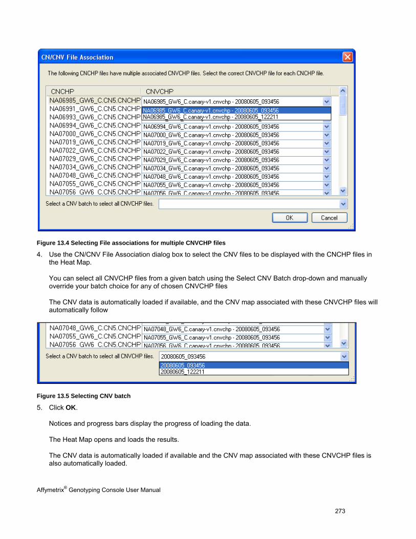
Affymetrix® Genotyping Console User Manual 273
Figure 13.4 Selecting File associations for multiple CNVCHP files
4. Use the CN/CNV File Association dialog box to select the CNV files to be displayed with the CNCHP files in the Heat Map.
You can select all CNVCHP files from a given batch using the Select CNV Batch drop-down and manually override your batch choice for any of chosen CNVCHP files
The CNV data is automatically loaded if available, and the CNV map associated with these CNVCHP files will automatically follow
Figure 13.5 Selecting CNV batch
5. Click OK.
Notices and progress bars display the progress of loading the data.
The Heat Map opens and loads the results.
The CNV data is automatically loaded if available and the CNV map associated with these CNVCHP files is also automatically loaded.
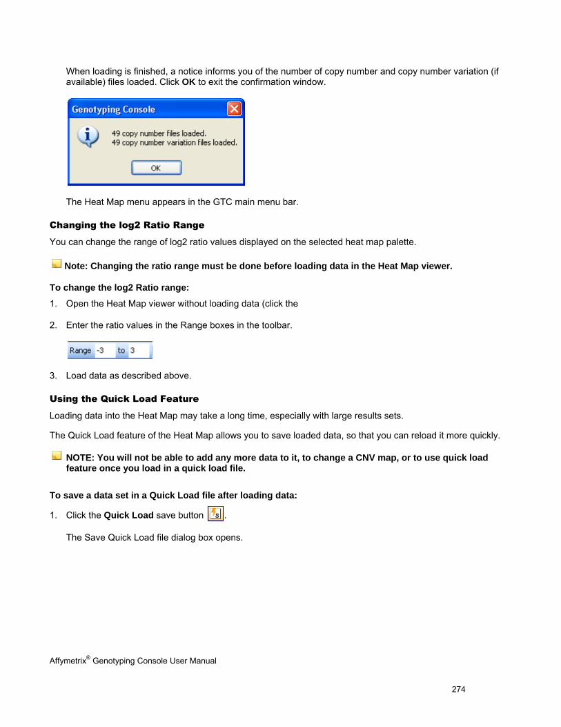
Affymetrix® Genotyping Console User Manual 274
When loading is finished, a notice informs you of the number of copy number and copy number variation (if available) files loaded. Click OK to exit the confirmation window.
The Heat Map menu appears in the GTC main menu bar.
Changing the log2 Ratio Range
You can change the range of log2 ratio values displayed on the selected heat map palette.
Note: Changing the ratio range must be done before loading data in the Heat Map viewer.
To change the log2 Ratio range:
1. Open the Heat Map viewer without loading data (click the
2. Enter the ratio values in the Range boxes in the toolbar.
3. Load data as described above.
Using the Quick Load Feature
Loading data into the Heat Map may take a long time, especially with large results sets.
The Quick Load feature of the Heat Map allows you to save loaded data, so that you can reload it more quickly.
NOTE: You will not be able to add any more data to it, to change a CNV map, or to use quick load feature once you load in a quick load file.
To save a data set in a Quick Load file after loading data:
1. Click the Quick Load save button .
The Save Quick Load file dialog box opens.
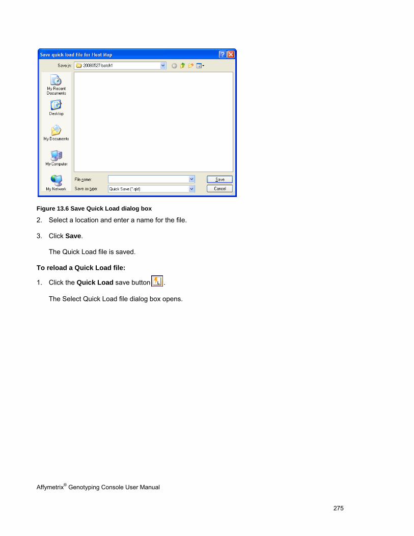
Affymetrix® Genotyping Console User Manual 275
Figure 13.6 Save Quick Load dialog box
2. Select a location and enter a name for the file.
3. Click Save.
The Quick Load file is saved.
To reload a Quick Load file:
1. Click the Quick Load save button .
The Select Quick Load file dialog box opens.
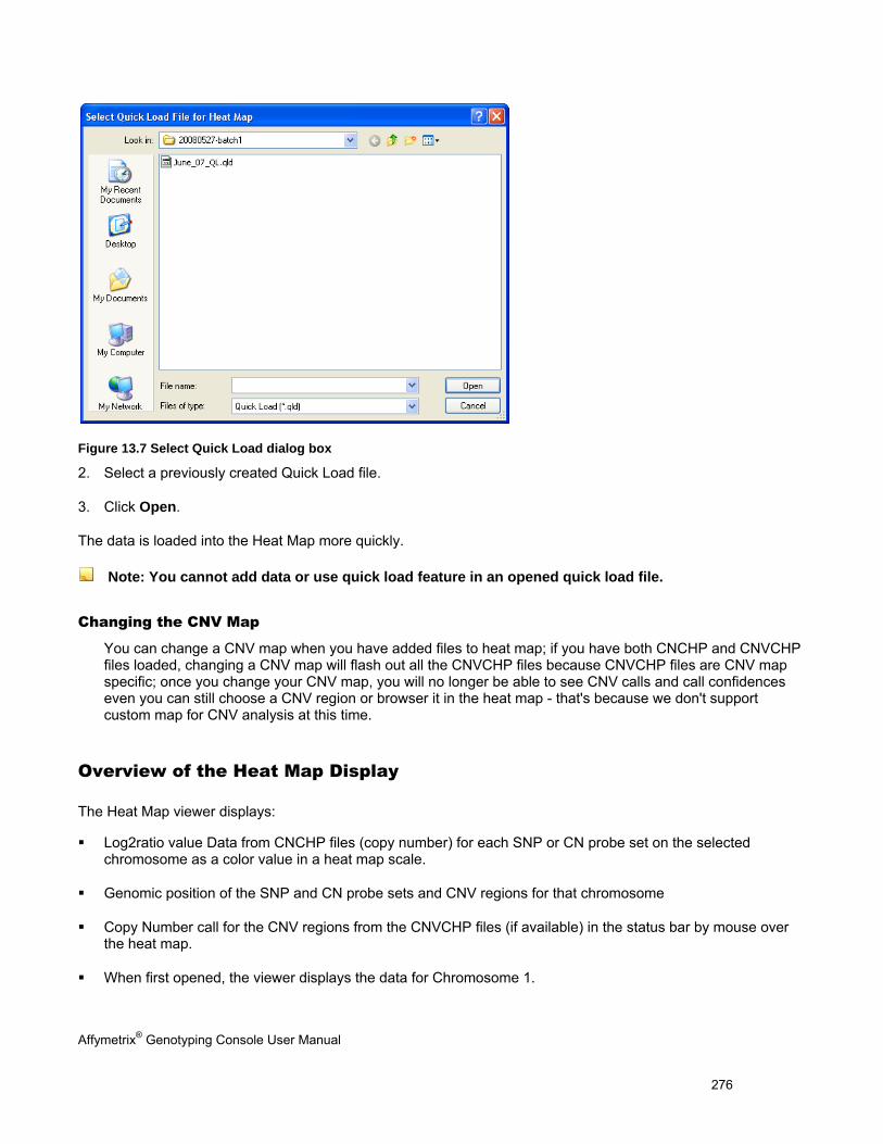
Affymetrix® Genotyping Console User Manual 276
Figure 13.7 Select Quick Load dialog box
2. Select a previously created Quick Load file.
3. Click Open.
The data is loaded into the Heat Map more quickly.
Note: You cannot add data or use quick load feature in an opened quick load file.
Changing the CNV Map
You can change a CNV map when you have added files to heat map; if you have both CNCHP and CNVCHP files loaded, changing a CNV map will flash out all the CNVCHP files because CNVCHP files are CNV map specific; once you change your CNV map, you will no longer be able to see CNV calls and call confidences even you can still choose a CNV region or browser it in the heat map - that's because we don't support custom map for CNV analysis at this time.
Overview of the Heat Map Display
The Heat Map viewer displays:
Log2ratio value Data from CNCHP files (copy number) for each SNP or CN probe set on the selected chromosome as a color value in a heat map scale.
Genomic position of the SNP and CN probe sets and CNV regions for that chromosome
Copy Number call for the CNV regions from the CNVCHP files (if available) in the status bar by mouse over the heat map.
When first opened, the viewer displays the data for Chromosome 1.
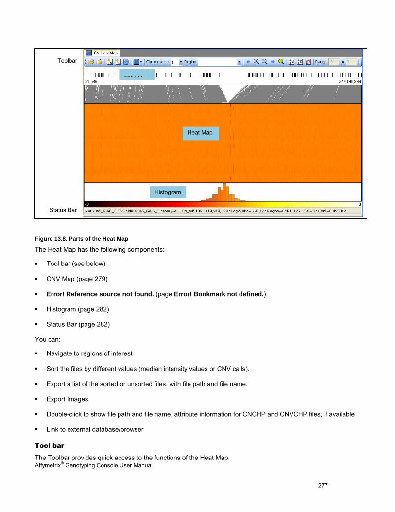
Affymetrix® Genotyping Console User Manual 277
Figure 13.8. Parts of the Heat Map
The Heat Map has the following components:
Tool bar (see below)
CNV Map (page 279)
Error! Reference source not found. (page Error! Bookmark not defined.)
Histogram (page 282)
Status Bar (page 282)
You can:
Navigate to regions of interest
Sort the files by different values (median intensity values or CNV calls).
Export a list of the sorted or unsorted files, with file path and file name.
Export Images
Double-click to show file path and file name, attribute information for CNCHP and CNVCHP files, if available
Link to external database/browser
Tool bar
The Toolbar provides quick access to the functions of the Heat Map.
CNV Map
Toolbar
Status Bar
Heat Map
Histogram
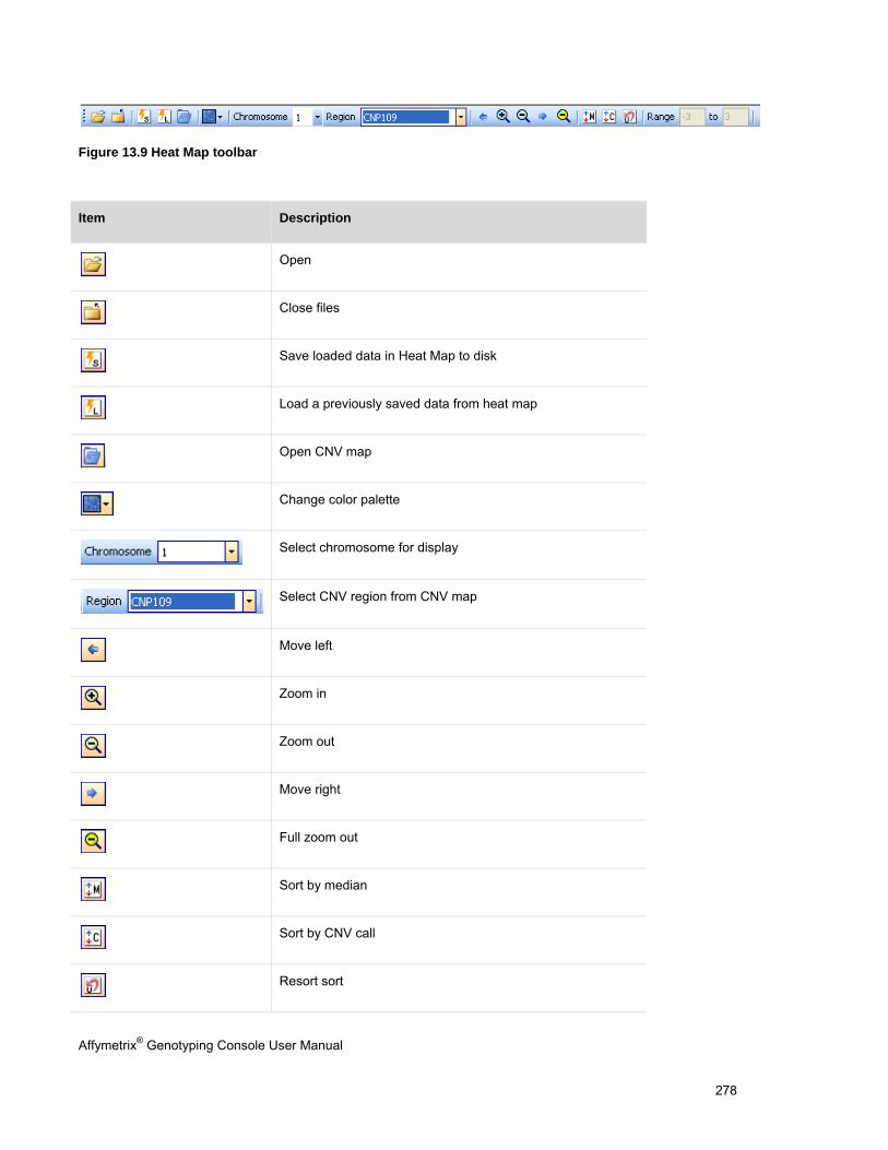
Affymetrix® Genotyping Console User Manual 278
Figure 13.9 Heat Map toolbar
Item Description
Open
Close files
Save loaded data in Heat Map to disk
Load a previously saved data from heat map
Open CNV map
Change color palette
Select chromosome for display
Select CNV region from CNV map
Move left
Zoom in
Zoom out
Move right
Full zoom out
Sort by median
Sort by CNV call
Resort sort
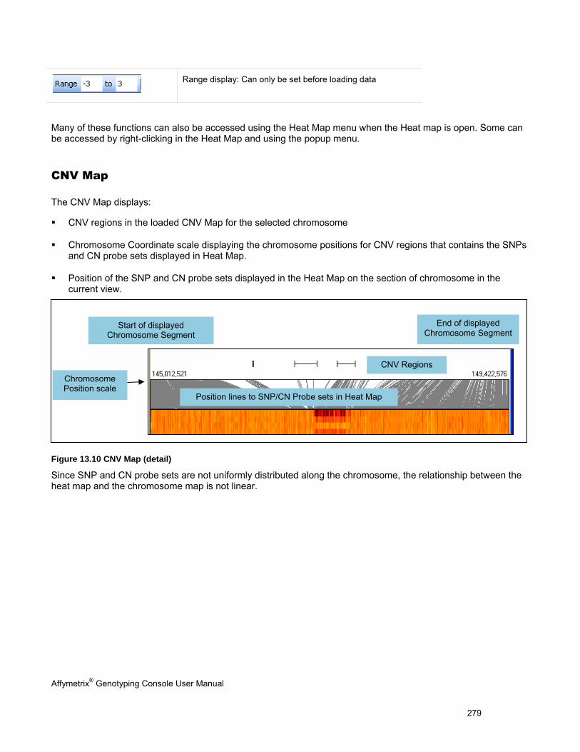
Affymetrix® Genotyping Console User Manual 279
Range display: Can only be set before loading data
Many of these functions can also be accessed using the Heat Map menu when the Heat map is open. Some can be accessed by right-clicking in the Heat Map and using the popup menu.
CNV Map
The CNV Map displays:
CNV regions in the loaded CNV Map for the selected chromosome
Chromosome Coordinate scale displaying the chromosome positions for CNV regions that contains the SNPs and CN probe sets displayed in Heat Map.
Position of the SNP and CN probe sets displayed in the Heat Map on the section of chromosome in the current view.
Figure 13.10 CNV Map (detail)
Since SNP and CN probe sets are not uniformly distributed along the chromosome, the relationship between the heat map and the chromosome map is not linear.
Start of displayed Chromosome Segment
Chromosome Position scale
Position lines to SNP/CN Probe sets in Heat Map
CNV Regions
End of displayed Chromosome Segment
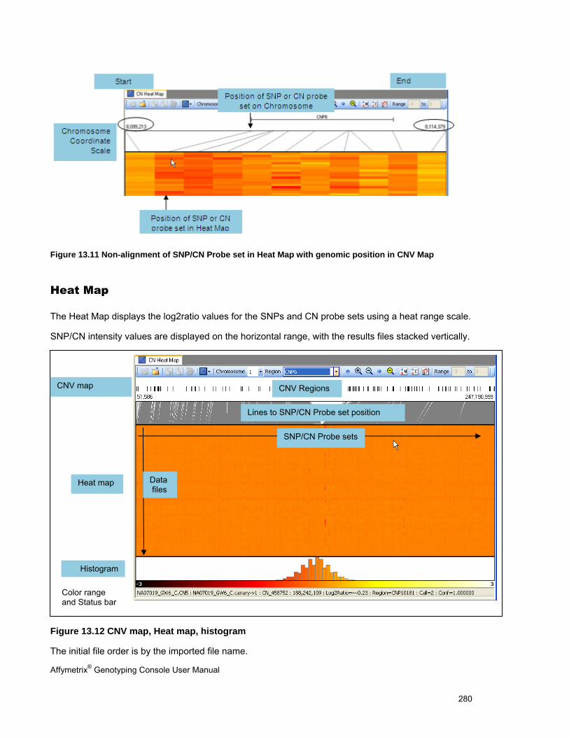
Affymetrix® Genotyping Console User Manual 280
Figure 13.11 Non-alignment of SNP/CN Probe set in Heat Map with genomic position in CNV Map
Heat Map
The Heat Map displays the log2ratio values for the SNPs and CN probe sets using a heat range scale.
SNP/CN intensity values are displayed on the horizontal range, with the results files stacked vertically.
Figure 13.12 CNV map, Heat map, histogram
The initial file order is by the imported file name.
Heat map
Histogram
Color range and Status bar
CNV map CNV Regions
Lines to SNP/CN Probe set position
Data files
SNP/CN Probe sets
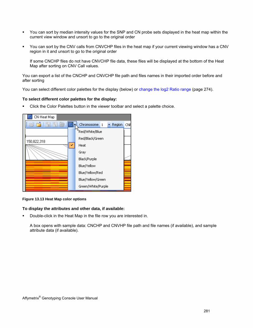
Affymetrix® Genotyping Console User Manual 281
You can sort by median intensity values for the SNP and CN probe sets displayed in the heat map within the current view window and unsort to go to the original order
You can sort by the CNV calls from CNVCHP files in the heat map if your current viewing window has a CNV region in it and unsort to go to the original order
If some CNCHP files do not have CNVCHP file data, these files will be displayed at the bottom of the Heat Map after sorting on CNV Call values.
You can export a list of the CNCHP and CNVCHP file path and files names in their imported order before and after sorting
You can select different color palettes for the display (below) or change the log2 Ratio range (page 274).
To select different color palettes for the display:
Click the Color Palettes button in the viewer toolbar and select a palette choice.
Figure 13.13 Heat Map color options
To display the attributes and other data, if available:
Double-click in the Heat Map in the file row you are interested in.
A box opens with sample data: CNCHP and CNVHP file path and file names (if available), and sample attribute data (if available).
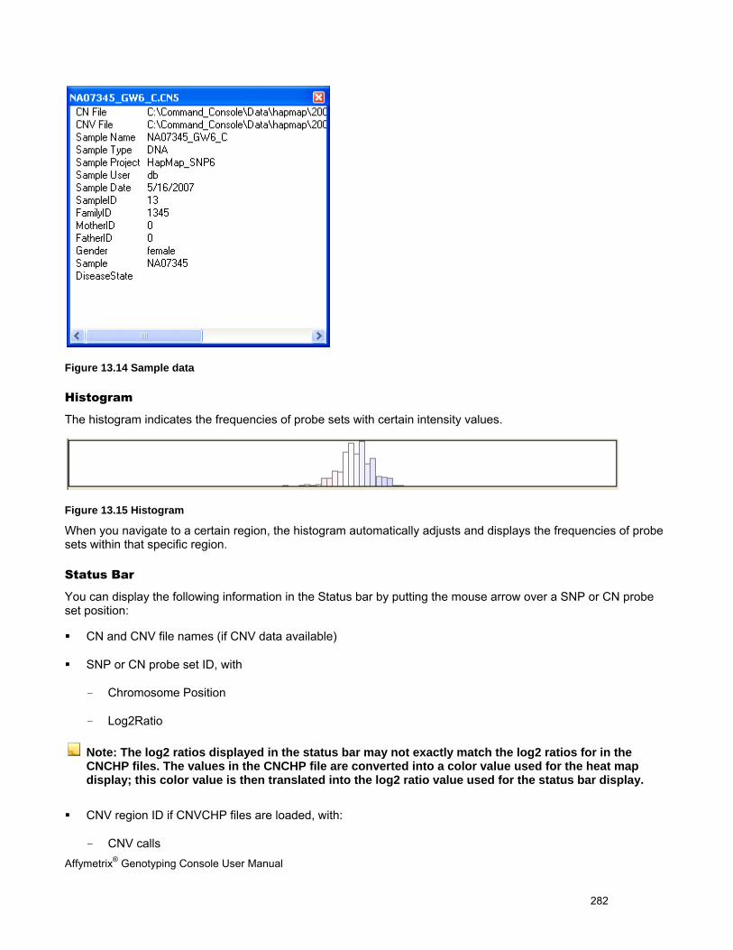
Affymetrix® Genotyping Console User Manual 282
Figure 13.14 Sample data
Histogram
The histogram indicates the frequencies of probe sets with certain intensity values.
Figure 13.15 Histogram
When you navigate to a certain region, the histogram automatically adjusts and displays the frequencies of probe sets within that specific region.
Status Bar
You can display the following information in the Status bar by putting the mouse arrow over a SNP or CN probe set position:
CN and CNV file names (if CNV data available)
SNP or CN probe set ID, with
- Chromosome Position
- Log2Ratio
Note: The log2 ratios displayed in the status bar may not exactly match the log2 ratios for in the CNCHP files. The values in the CNCHP file are converted into a color value used for the heat map display; this color value is then translated into the log2 ratio value used for the status bar display.
CNV region ID if CNVCHP files are loaded, with:
- CNV calls
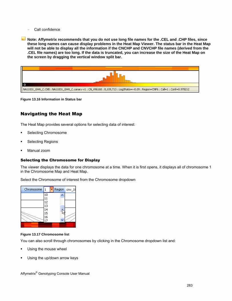
Affymetrix® Genotyping Console User Manual 283
- Call confidence
Note: Affymetrix recommends that you do not use long file names for the .CEL and .CHP files, since these long names can cause display problems in the Heat Map Viewer. The status bar in the Heat Map will not be able to display all the information if the CNCHP and CNVCHP file names (derived from the .CEL file names) are too long. If the data is truncated, you can increase the size of the Heat Map on the screen by dragging the vertical window split bar.
Figure 13.16 Information in Status bar
Navigating the Heat Map
The Heat Map provides several options for selecting data of interest:
Selecting Chromosome
Selecting Regions
Manual zoom
Selecting the Chromosome for Display
The viewer displays the data for one chromosome at a time. When it is first opens, it displays all of chromosome 1 in the Chromosome Map and Heat Map.
Select the Chromosome of interest from the Chromosome dropdown
Figure 13.17 Chromosome list
You can also scroll through chromosomes by clicking in the Chromosome dropdown list and:
Using the mouse wheel
Using the up/down arrow keys
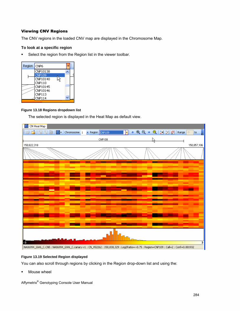
Affymetrix® Genotyping Console User Manual 284
Viewing CNV Regions
The CNV regions in the loaded CNV map are displayed in the Chromosome Map.
To look at a specific region
Select the region from the Region list in the viewer toolbar.
Figure 13.18 Regions dropdown list
The selected region is displayed in the Heat Map as default view.
Figure 13.19 Selected Region displayed
You can also scroll through regions by clicking in the Region drop-down list and using the:
Mouse wheel
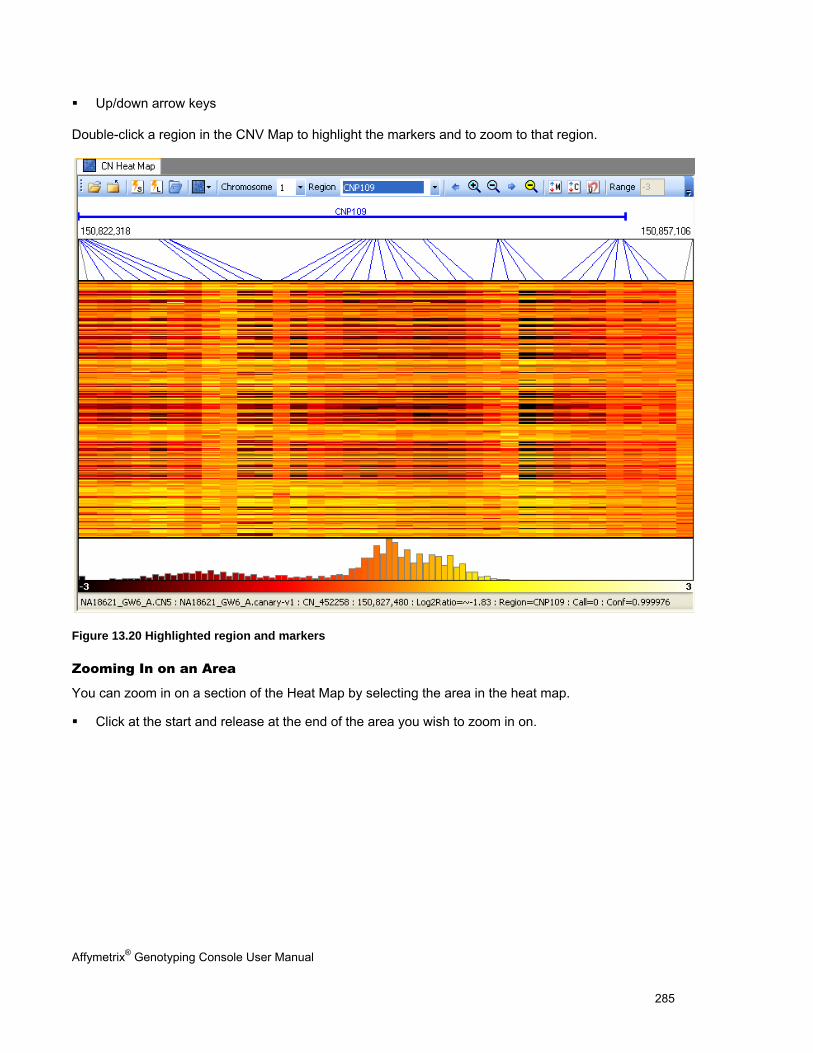
Affymetrix® Genotyping Console User Manual 285
Up/down arrow keys
Double-click a region in the CNV Map to highlight the markers and to zoom to that region.
Figure 13.20 Highlighted region and markers
Zooming In on an Area
You can zoom in on a section of the Heat Map by selecting the area in the heat map.
Click at the start and release at the end of the area you wish to zoom in on.
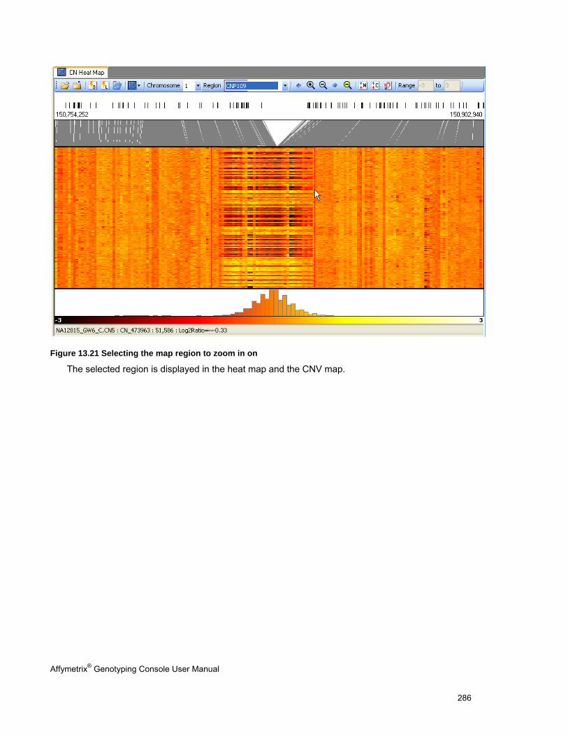
Affymetrix® Genotyping Console User Manual 286
Figure 13.21 Selecting the map region to zoom in on
The selected region is displayed in the heat map and the CNV map.
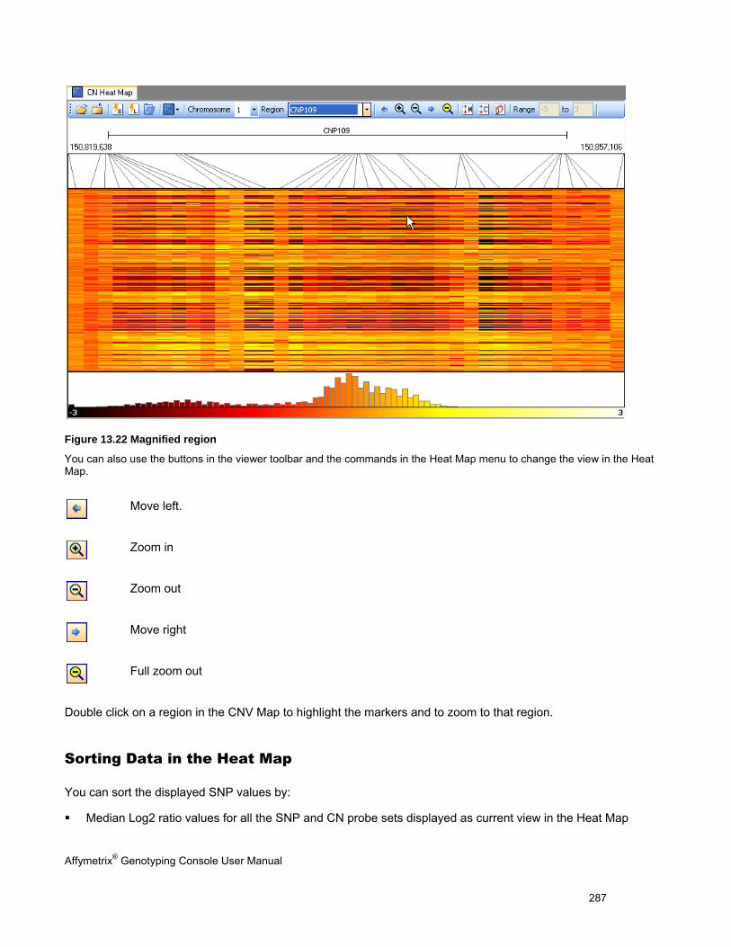
Affymetrix® Genotyping Console User Manual 287
Figure 13.22 Magnified region
You can also use the buttons in the viewer toolbar and the commands in the Heat Map menu to change the view in the Heat Map.
Move left.
Zoom in
Zoom out
Move right
Full zoom out
Double click on a region in the CNV Map to highlight the markers and to zoom to that region.
Sorting Data in the Heat Map
You can sort the displayed SNP values by:
Median Log2 ratio values for all the SNP and CN probe sets displayed as current view in the Heat Map
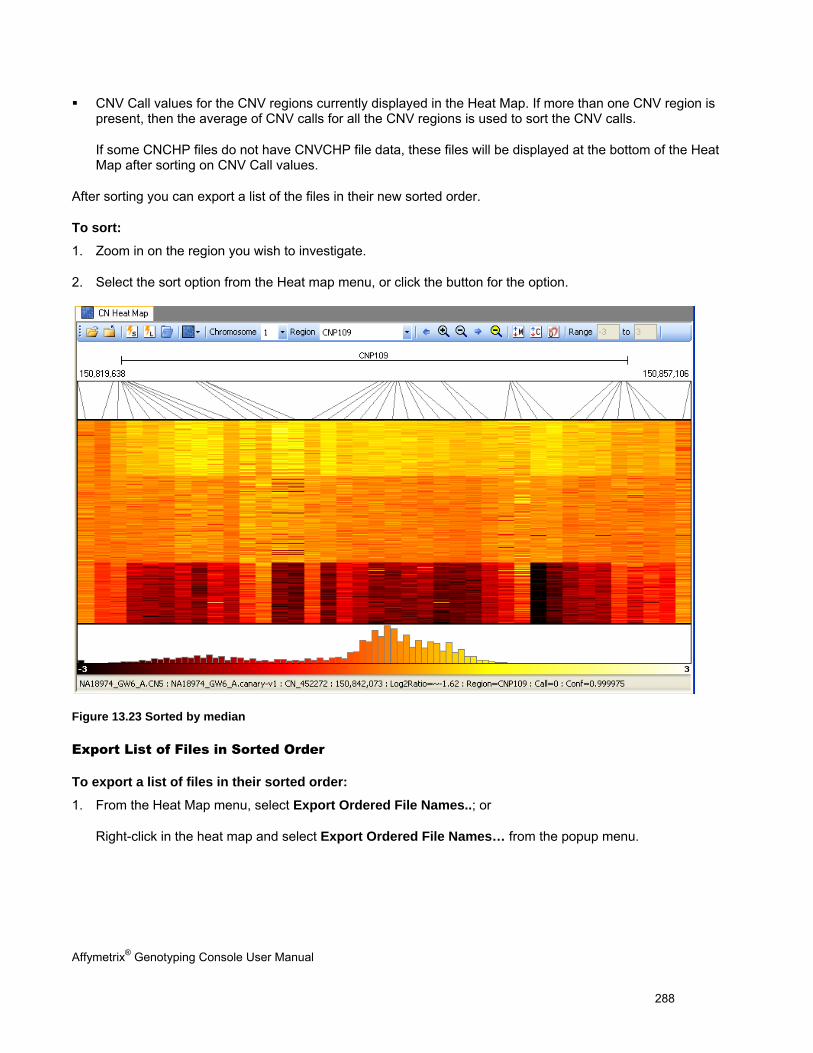
Affymetrix® Genotyping Console User Manual 288
CNV Call values for the CNV regions currently displayed in the Heat Map. If more than one CNV region is present, then the average of CNV calls for all the CNV regions is used to sort the CNV calls.
If some CNCHP files do not have CNVCHP file data, these files will be displayed at the bottom of the Heat Map after sorting on CNV Call values.
After sorting you can export a list of the files in their new sorted order.
To sort:
1. Zoom in on the region you wish to investigate.
2. Select the sort option from the Heat map menu, or click the button for the option.
Figure 13.23 Sorted by median
Export List of Files in Sorted Order
To export a list of files in their sorted order:
1. From the Heat Map menu, select Export Ordered File Names..; or
Right-click in the heat map and select Export Ordered File Names… from the popup menu.
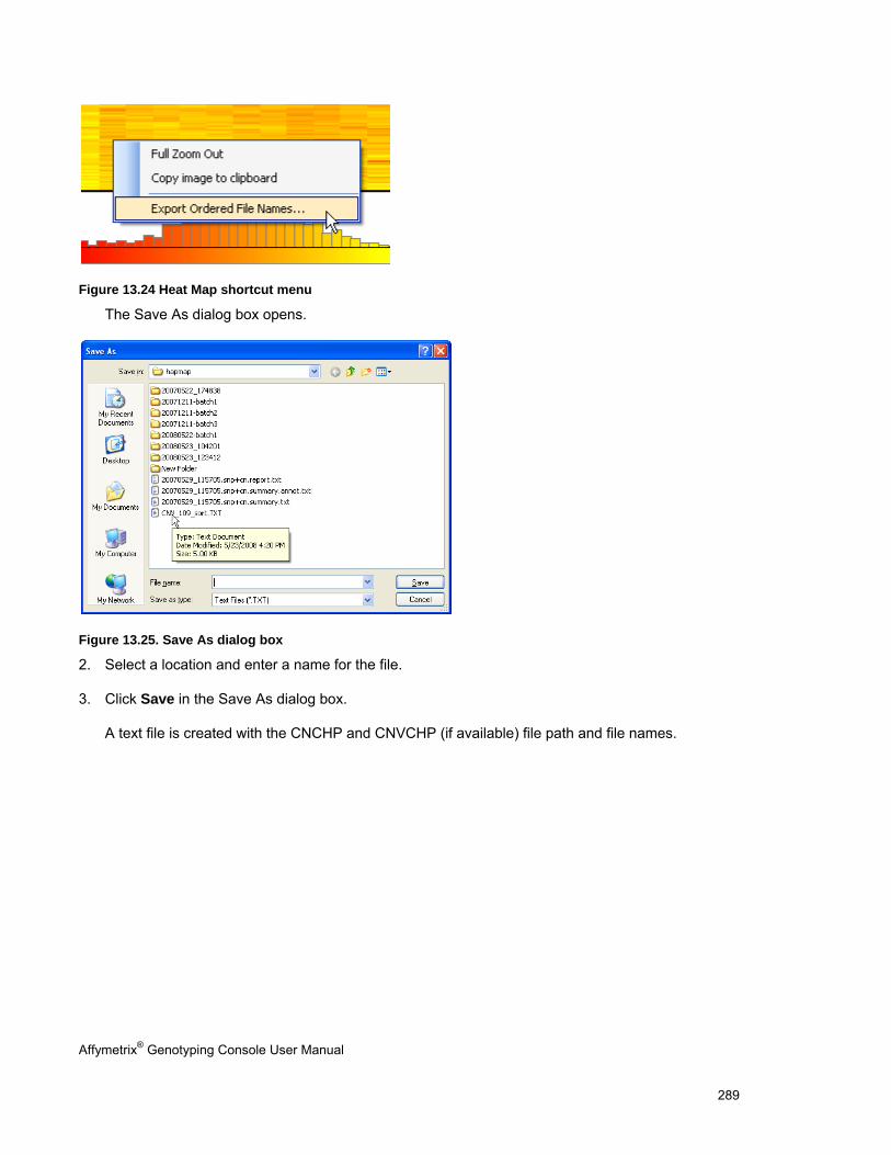
Affymetrix® Genotyping Console User Manual 289
Figure 13.24 Heat Map shortcut menu
The Save As dialog box opens.
Figure 13.25. Save As dialog box
2. Select a location and enter a name for the file.
3. Click Save in the Save As dialog box.
A text file is created with the CNCHP and CNVCHP (if available) file path and file names.
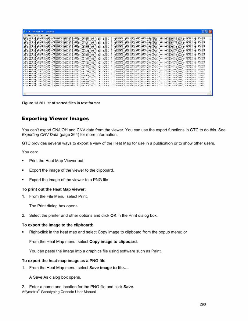
Affymetrix® Genotyping Console User Manual 290
Figure 13.26 List of sorted files in text format
Exporting Viewer Images
You can’t export CN/LOH and CNV data from the viewer. You can use the export functions in GTC to do this. See Exporting CNV Data (page 264) for more information.
GTC provides several ways to export a view of the Heat Map for use in a publication or to show other users.
You can:
Print the Heat Map Viewer out.
Export the image of the viewer to the clipboard.
Export the image of the viewer to a PNG file
To print out the Heat Map viewer:
1. From the File Menu, select Print.
The Print dialog box opens.
2. Select the printer and other options and click OK in the Print dialog box.
To export the image to the clipboard:
Right-click in the heat map and select Copy image to clipboard from the popup menu; or
From the Heat Map menu, select Copy image to clipboard.
You can paste the image into a graphics file using software such as Paint.
To export the heat map image as a PNG file
1. From the Heat Map menu, select Save image to file….
A Save As dialog box opens.
2. Enter a name and location for the PNG file and click Save.
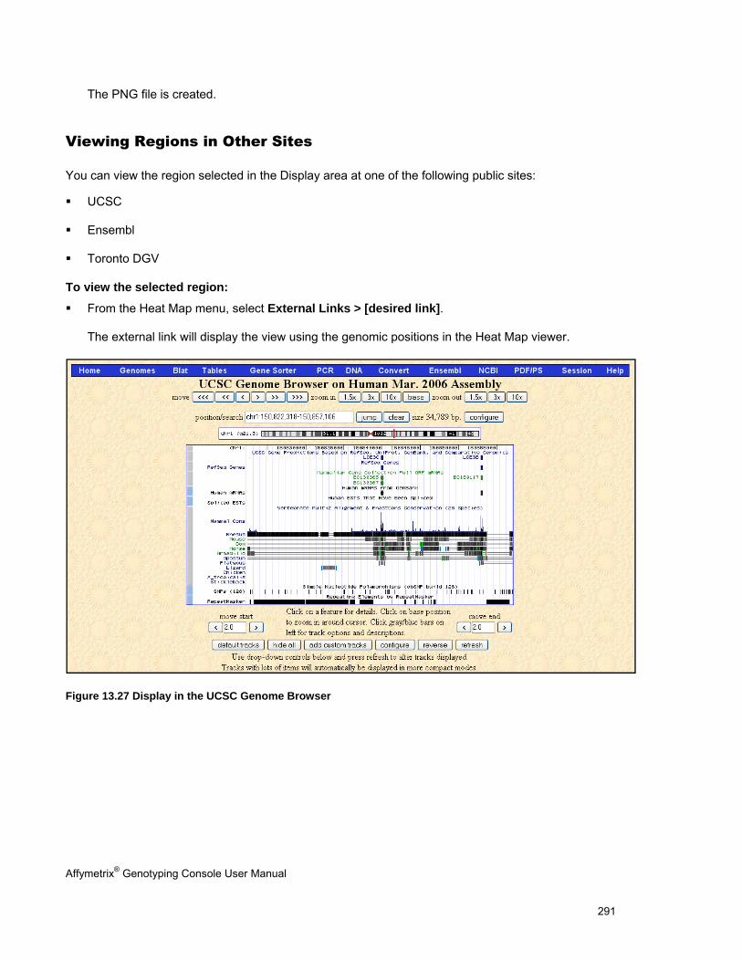
Affymetrix® Genotyping Console User Manual 291
The PNG file is created.
Viewing Regions in Other Sites
You can view the region selected in the Display area at one of the following public sites:
UCSC
Ensembl
Toronto DGV
To view the selected region:
From the Heat Map menu, select External Links > [desired link].
The external link will display the view using the genomic positions in the Heat Map viewer.
Figure 13.27 Display in the UCSC Genome Browser
Affymetrix® Genotyping Console User Manual 292
Appendix A: Algorithms The details of the algorithms used by GTC 4.0 and their typical performance are described in various white papers.
Genotyping
100K/500K BRLMM algorithm
http://www.affymetrix.com/support/technical/whitepapers/brlmm_whitepaper.pdf
SNP 5.0 arrays BRLMM-P algorithm
http://www.affymetrix.com/support/technical/whitepapers/brlmmp_whitepaper.pdf
SNP 6.0 Birdseed (v1) and Birdseed v2 genotyping algorithms
Genotyping Console 4.0 allows users to choose between genotyping SNP 6.0 array data with the Birdseed (v1) and the Birdseed v2 algorithms. Birdseed v2 uses EM to derive a maximum likelihood fit of a 2-dimensional Gaussian mixture model in A vs B space.
A key difference between Birdseed (v1) and Birdseed v2 is that v1 uses SNP-specific models or priors only as an initial condition from which the EM fit is free to wander- on rare occasions this allows for mislabeling of the clusters. For Birdseed v2 the SNP-specific priors are used not only as initial conditions for EM, but are incorporated into the likelihood as Bayesian priors. This constrains the extent to which the EM fit can wander off. Correctly labeling SNP clusters, whose centers have shifted relative to the priors, is problematic for both Birdseed versions. However, given the additional constraint on the EM fit, Birdseed v2 is more likely than Birdseed to either correctly label the clusters or set genotypes to No Calls.
Birdseed v2 is usually more robust than Birdseed in the face of poor quality experiments, and increases accuracy with a small decrease in call rate in these cases. In high quality datasets, little performance difference between v1 and v2 is seen, while in low quality datasets large increases in concordance are seen with v2
Birdseed v2 clustering by plate is equivalent to clustering all samples, unlike Birdseed (v1) where clustering by plate increases False Discovery Rate. Because of this, use of Birdseed v2 allows clustering-by-plate or clustering all samples at once, which ever best fits with the laboratory’s workflow.
See the Affymetrix.com website for information on Birdseed algorithms.
Axiom GT1 Algorithm
The Axiom GT1 method is a new genotyping procedure delivered in Genotyping Console 4.0 for use with the Axiom Genome-Wide Human array. The primary methodological change has been to incorporate multichannel processing into the APT workflow, supporting the ligation-based assay. In addition, Axiom GT1 incorporates substantial improvements and features in the areas of preprocessing and genotype calling over BRLMM-P which was used for the Genome-Wide SNP Array 5.0 (see SNP 5.0 arrays BRLMM-P algorithm). Many of the improvements in genotype calling were developed for the DMET Plus product, including 2-dimensional cluster modeling and outlier detection. Preprocessing has been improved by an artifact reduction layer which reduces the impact of spatially localized artifacts on genotyping performance. Together these changes allow for good genotyping performance on the ligation-based assay platform.
Affymetrix® Genotyping Console User Manual 293
Multichannel processing allows the use of both traditional allelelic differences, in which two different probes respond to the same region of sequence and distinguish alleles, as well as dye-based allele detection, in which the same probe is imaged in more than one channel to distinguish alleles. Both these workflows are handled in Genotyping Console 4.0 transparently to the user, and both types of probe strategy are used on the Axiom product.
The second area of improvement is in the genotype clustering and calling. Many of the improvements were developed in the course of the DMET Plus product and can be found described in the DMET Plus algorithm white paper:
http://www.affymetrix.com/support/technical/whitepapers/dmet_plus_algorithm_whitepaperv1.pdf
Briefly, clusters are now represented as 2-dimensional gaussians and resistance to non-gaussian cluster behavior has been improved. As usual, training data has been used to generate SNP-specific models which represent the cluster properties learned for each marker. Unlike DMET Plus which is designed to call in a single sample mode without adapting to the data, the default behavior is to use dynamic clustering to adapt the clusters to the observed data. Although a single sample can be run by itself, more samples allow more learning of any shifts from the training data.
Finally, the key advance in preprocessing is an "artifact reduction" layer that is designed to use information obtained from replicated probes to reduce the impact of small localized artifacts which sometimes occur. This method operates on the raw probe data using spatially distributed replicate probes to detect unusual differences between replicate intensities. Standard image processing operations (morphological transformations) are used to detect regions of the array where deviations occurring in both channels cluster, indicating a potential localized artifact. Once regions are marked as untrusted due to a potential artifact, intensities from trusted replicates are used to replace untrusted features for genotyping purposes. In the case where all replicates are marked untrusted for a given probe, the failsafe behavior is to leave the intensities unmodified and allow the genotyping method to evaluate whether the data is compatible with the clusters. This preprocessing layer improves the genotyping performance in the relatively rare case where localized artifacts occur on the image, while leaving typical arrays without artifacts unaffected.
Summarizing, Axiom GT1 handles multichannel data, incorporates improvements in genotype clustering and calling that have occurred in the development of other products, and introduces an artifact-reduction stage in preprocessing. These changes have been tuned to provide high performance on the ligation assay based genotyping platform and allow for flexible adaption of the method to future genotyping products.
Copy Number/LOH
100K/500K CN/LOH Algorithm
http://www.affymetrix.com/support/technical/whitepapers/cnat_4_algorithm_whitepaper.pdf
SNP 6.0 CN/LOH Algorithm
SNP 6.0 CN/LOH analysis uses the BRLMM-P+ algorithm, which is similar to BRLMM-P with some different parameters. See the existing documentation for BRLMM-P associated with SNP5 for more information.
SNP 6.0 CN GC waviness algorithm implemented into APT and since GTC 3.0.1
The summary of the algorithm correction is: for each sample, markers are divided into 25 different bins based on the equally spaced percentiles of the average GC count (GC content) in the upstream/downstream 250kb for a particular marker (500kb total). Within each of the 25 bins, the markers are sub-divided based on their type: CN/SNP marker type, enzyme fragment type (Nsp, Sty, Nsp+Sty), which gives 5 sub-bins per major bin as there is no CN probes in Sty-only fragments, for a total of 5x25=125 bins. For the autosomal markers in each bin, the median log2 ratio of each bin is adjusted to zero and interquartile ranges (IQRs) are equalized across all the bins.
Affymetrix® Genotyping Console User Manual 294
Then the log2 ratios of all markers (including X and Y markers) in that bin are adjusted using the adjustment based on the autosomal markers on that bin. Finally, the IQRs of all the adjusted log2 ratios (including the X and Y chromosomes) is multiplied by a factor that makes the IQRs of the adjusted log2 ratios equal to the IQRs of the original log2 ratios.
SNP 6.0 Canary Algorithm
The Canary Algorithm is a clustering algorithm developed by the Broad Institute used to provide copy number state calls of a pre-determined set of genomic regions with copy number variation (CNV regions). The copy number state call is reported by an integer call of copy number. Each call is paired with a confidence score between 0 and 1 with 1 reflecting a high level of confidence that the call is correct. The CNV regions are polymorphic in the sense that their copy number is atypically variable in relation to the genome as a whole. The terms copy number variation (CNV) and copy number polymorphism (CNP) are each used to describe the same attribute of copy number variability of genomic regions.
Inputs to the Canary algorithm are:
1. A region file containing region names and sets of SNP and CN probe sets for each region
2. A prior file containing clustering information empirically derived from external training data
3. A normalization file containing a list of names of probe sets used for normalizing the data
4. A set of CEL files, one for each sample to be genotyped.
A CDF file is needed by the software running Canary in order to retrieve probe sets intensities recorded in the CEL files.
Output consists of a set of CHP files, one for each CEL file, with the suffix CNVCHP. Each CHP file contains region names, intensities, calls and confidences.
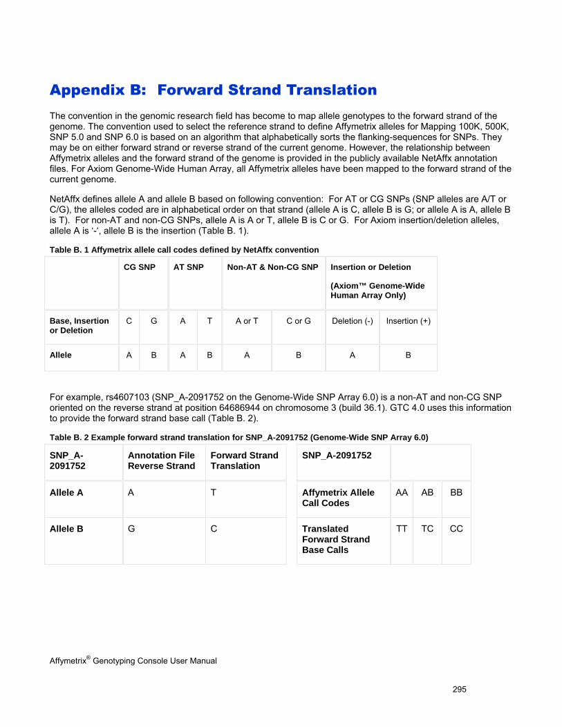
Affymetrix® Genotyping Console User Manual 295
Appendix B: Forward Strand Translation The convention in the genomic research field has become to map allele genotypes to the forward strand of the genome. The convention used to select the reference strand to define Affymetrix alleles for Mapping 100K, 500K, SNP 5.0 and SNP 6.0 is based on an algorithm that alphabetically sorts the flanking-sequences for SNPs. They may be on either forward strand or reverse strand of the current genome. However, the relationship between Affymetrix alleles and the forward strand of the genome is provided in the publicly available NetAffx annotation files. For Axiom Genome-Wide Human Array, all Affymetrix alleles have been mapped to the forward strand of the current genome.
NetAffx defines allele A and allele B based on following convention: For AT or CG SNPs (SNP alleles are A/T or C/G), the alleles coded are in alphabetical order on that strand (allele A is C, allele B is G; or allele A is A, allele B is T). For non-AT and non-CG SNPs, allele A is A or T, allele B is C or G. For Axiom insertion/deletion alleles, allele A is ‘-‘, allele B is the insertion (Table B. 1).
Table B. 1 Affymetrix allele call codes defined by NetAffx convention
CG SNP AT SNP Non-AT & Non-CG SNP Insertion or Deletion
(Axiom™ Genome-Wide Human Array Only)
Base, Insertion or Deletion
C G A T A or T C or G Deletion (-) Insertion (+)
Allele A B A B A B A B
For example, rs4607103 (SNP_A-2091752 on the Genome-Wide SNP Array 6.0) is a non-AT and non-CG SNP oriented on the reverse strand at position 64686944 on chromosome 3 (build 36.1). GTC 4.0 uses this information to provide the forward strand base call (Table B. 2).
Table B. 2 Example forward strand translation for SNP_A-2091752 (Genome-Wide SNP Array 6.0)
SNP_A-2091752
Annotation File Reverse Strand
Forward Strand Translation
SNP_A-2091752
Allele A A T Affymetrix Allele Call Codes
AA AB BB
Allele B G C Translated Forward Strand Base Calls
TT TC CC
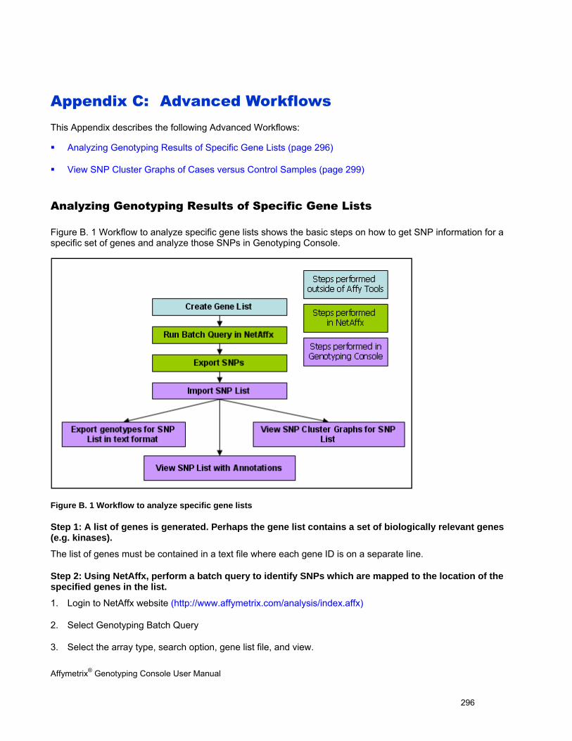
Affymetrix® Genotyping Console User Manual 296
Appendix C: Advanced Workflows This Appendix describes the following Advanced Workflows:
Analyzing Genotyping Results of Specific Gene Lists (page 296)
View SNP Cluster Graphs of Cases versus Control Samples (page 299)
Analyzing Genotyping Results of Specific Gene Lists
Figure B. 1 Workflow to analyze specific gene lists shows the basic steps on how to get SNP information for a specific set of genes and analyze those SNPs in Genotyping Console.
Figure B. 1 Workflow to analyze specific gene lists
Step 1: A list of genes is generated. Perhaps the gene list contains a set of biologically relevant genes (e.g. kinases).
The list of genes must be contained in a text file where each gene ID is on a separate line.
Step 2: Using NetAffx, perform a batch query to identify SNPs which are mapped to the location of the specified genes in the list.
1. Login to NetAffx website (http://www.affymetrix.com/analysis/index.affx)
2. Select Genotyping Batch Query
3. Select the array type, search option, gene list file, and view.
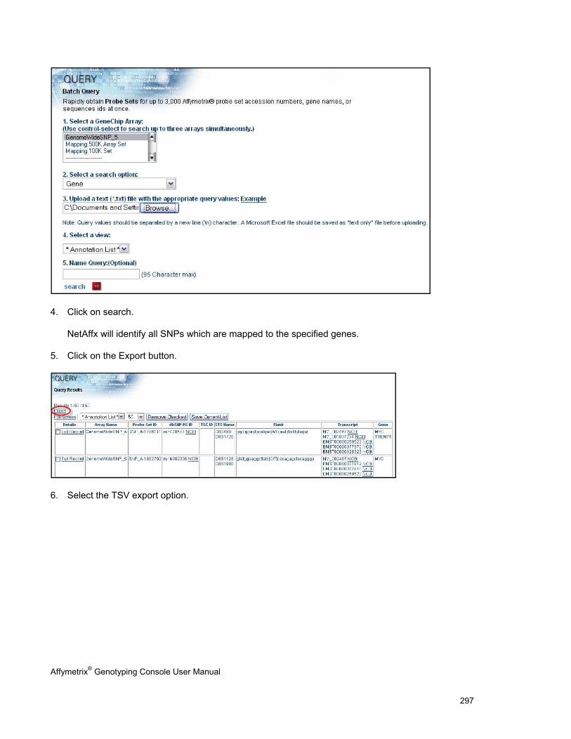
Affymetrix® Genotyping Console User Manual 297
4. Click on search.
NetAffx will identify all SNPs which are mapped to the specified genes.
5. Click on the Export button.
6. Select the TSV export option.
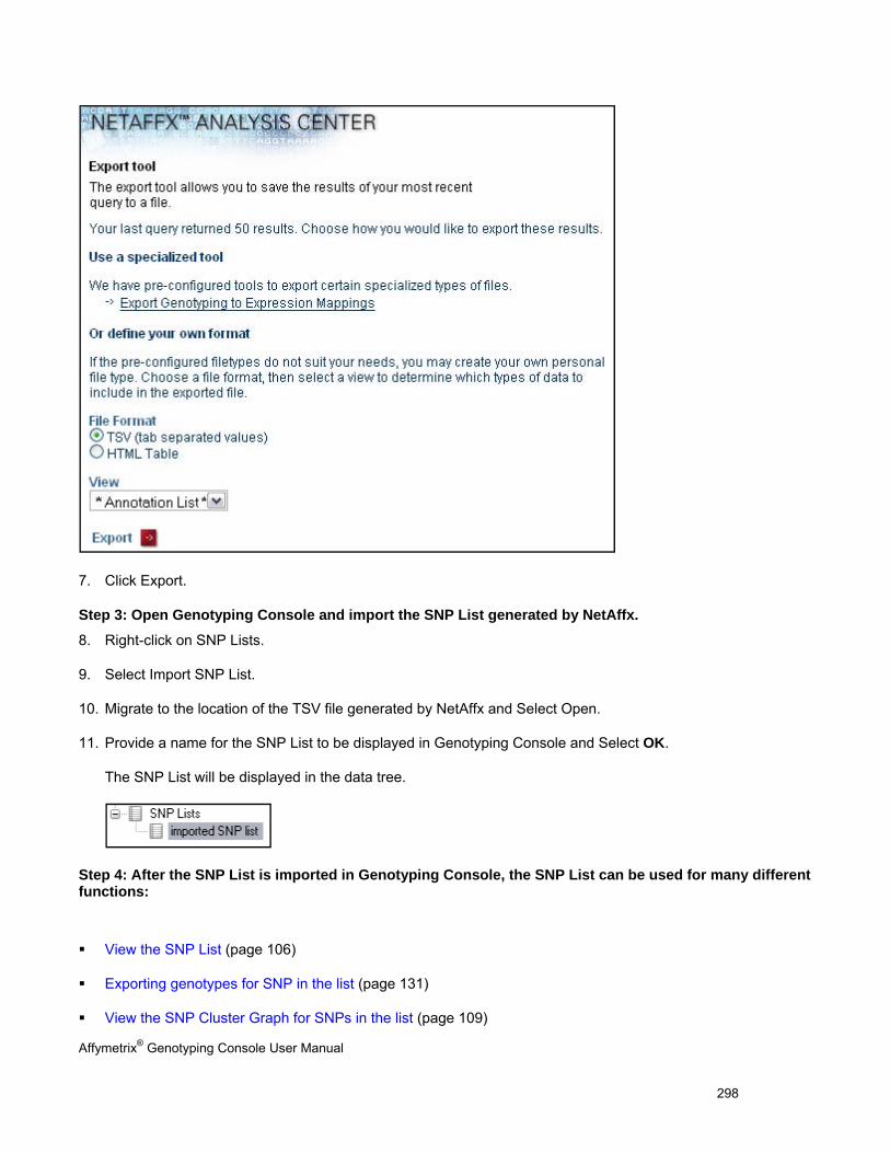
Affymetrix® Genotyping Console User Manual 298
7. Click Export.
Step 3: Open Genotyping Console and import the SNP List generated by NetAffx.
8. Right-click on SNP Lists.
9. Select Import SNP List.
10. Migrate to the location of the TSV file generated by NetAffx and Select Open.
11. Provide a name for the SNP List to be displayed in Genotyping Console and Select OK.
The SNP List will be displayed in the data tree.
Step 4: After the SNP List is imported in Genotyping Console, the SNP List can be used for many different functions:
View the SNP List (page 106)
Exporting genotypes for SNP in the list (page 131)
View the SNP Cluster Graph for SNPs in the list (page 109)
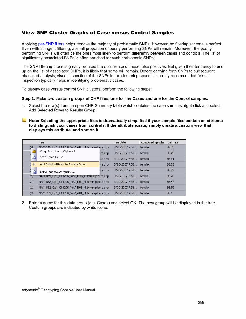
Affymetrix® Genotyping Console User Manual 299
View SNP Cluster Graphs of Case versus Control Samples
Applying per-SNP filters helps remove the majority of problematic SNPs. However, no filtering scheme is perfect. Even with stringent filtering, a small proportion of poorly performing SNPs will remain. Moreover, the poorly performing SNPs will often be the ones most likely to perform differently between cases and controls. The list of significantly associated SNPs is often enriched for such problematic SNPs.
The SNP filtering process greatly reduced the occurrence of these false positives. But given their tendency to end up on the list of associated SNPs, it is likely that some will remain. Before carrying forth SNPs to subsequent phases of analysis, visual inspection of the SNPs in the clustering space is strongly recommended. Visual inspection typically helps in identifying problematic cases.
To display case versus control SNP clusters, perform the following steps:
Step 1: Make two custom groups of CHP files, one for the Cases and one for the Control samples.
1. Select the row(s) from an open CHP Summary table which contains the case samples, right-click and select Add Selected Rows to Results Group.
Note: Selecting the appropriate files is dramatically simplified if your sample files contain an attribute to distinguish your cases from controls. If the attribute exists, simply create a custom view that displays this attribute, and sort on it.
2. Enter a name for this data group (e.g. Cases) and select OK. The new group will be displayed in the tree. Custom groups are indicated by white icons.
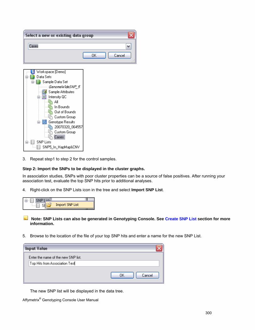
Affymetrix® Genotyping Console User Manual 300
3. Repeat step1 to step 2 for the control samples.
Step 2: Import the SNPs to be displayed in the cluster graphs.
In association studies, SNPs with poor cluster properties can be a source of false positives. After running your association test, evaluate the top SNP hits prior to additional analyses.
4. Right-click on the SNP Lists icon in the tree and select Import SNP List.
Note: SNP Lists can also be generated in Genotyping Console. See Create SNP List section for more information.
5. Browse to the location of the file of your top SNP hits and enter a name for the new SNP List.
The new SNP list will be displayed in the data tree.
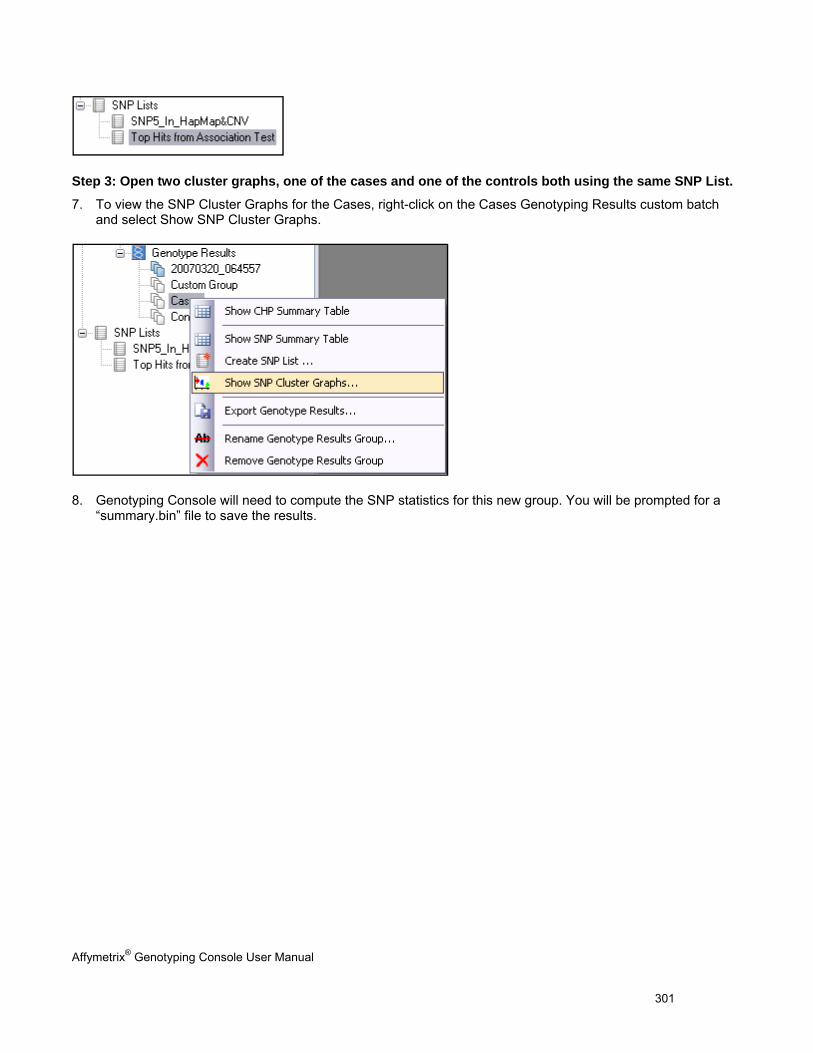
Affymetrix® Genotyping Console User Manual 301
Step 3: Open two cluster graphs, one of the cases and one of the controls both using the same SNP List.
7. To view the SNP Cluster Graphs for the Cases, right-click on the Cases Genotyping Results custom batch and select Show SNP Cluster Graphs.
8. Genotyping Console will need to compute the SNP statistics for this new group. You will be prompted for a “summary.bin” file to save the results.
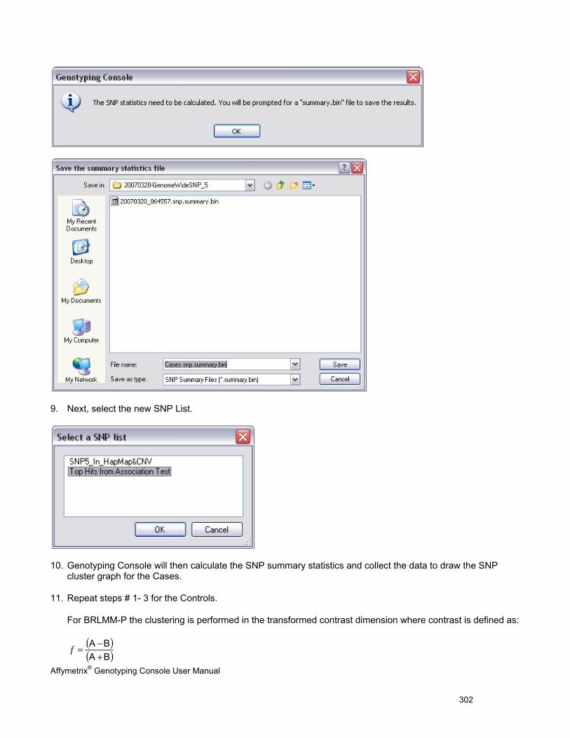
Affymetrix® Genotyping Console User Manual 302
9. Next, select the new SNP List.
10. Genotyping Console will then calculate the SNP summary statistics and collect the data to draw the SNP cluster graph for the Cases.
11. Repeat steps # 1- 3 for the Controls.
For BRLMM-P the clustering is performed in the transformed contrast dimension where contrast is defined as:
( )( )BA
BA+−=f
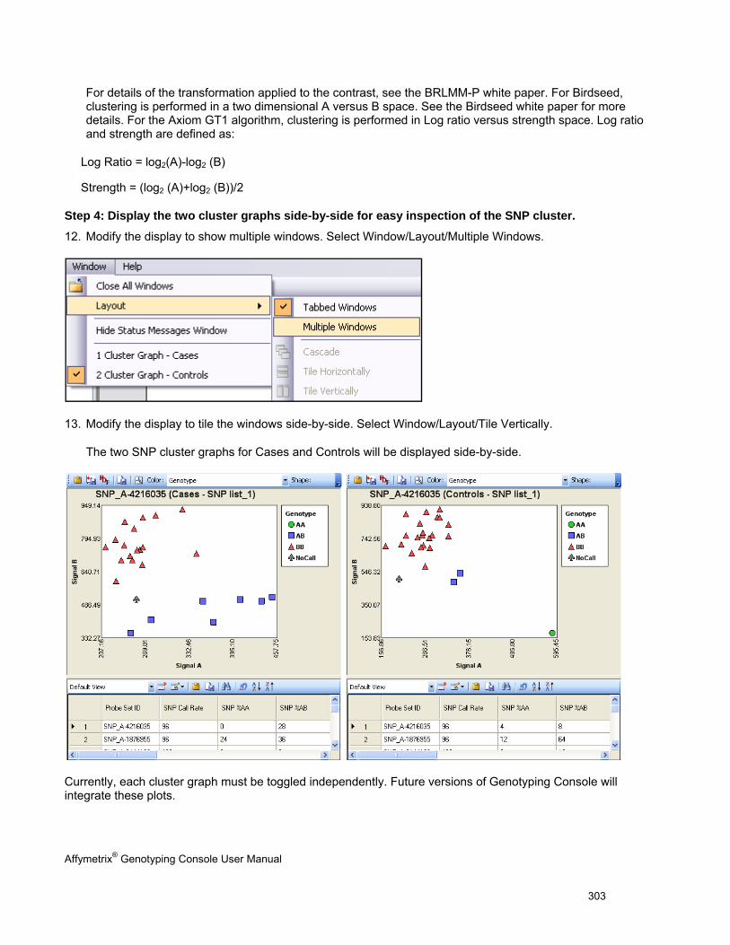
Affymetrix® Genotyping Console User Manual 303
For details of the transformation applied to the contrast, see the BRLMM-P white paper. For Birdseed, clustering is performed in a two dimensional A versus B space. See the Birdseed white paper for more details. For the Axiom GT1 algorithm, clustering is performed in Log ratio versus strength space. Log ratio and strength are defined as:
Log Ratio = log2(A)-log2 (B)
Strength = (log2 (A)+log2 (B))/2
Step 4: Display the two cluster graphs side-by-side for easy inspection of the SNP cluster.
12. Modify the display to show multiple windows. Select Window/Layout/Multiple Windows.
13. Modify the display to tile the windows side-by-side. Select Window/Layout/Tile Vertically.
The two SNP cluster graphs for Cases and Controls will be displayed side-by-side.
Currently, each cluster graph must be toggled independently. Future versions of Genotyping Console will integrate these plots.
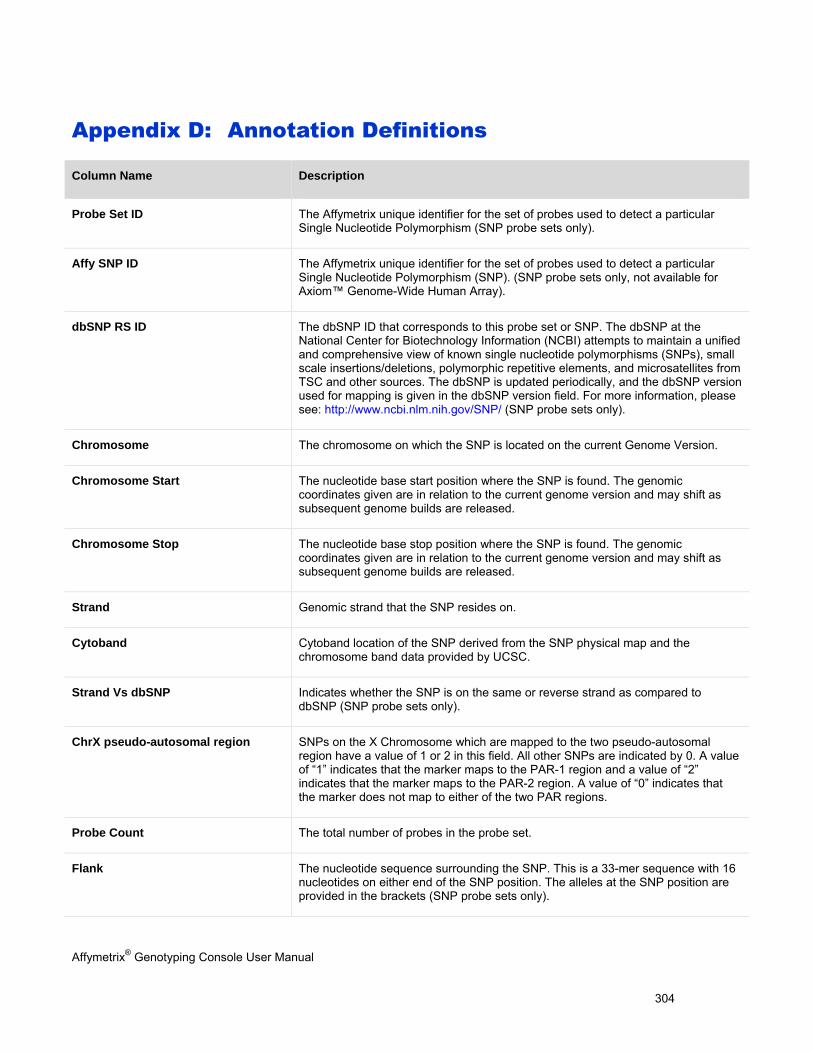
Affymetrix® Genotyping Console User Manual 304
Appendix D: Annotation Definitions
Column Name Description
Probe Set ID The Affymetrix unique identifier for the set of probes used to detect a particular Single Nucleotide Polymorphism (SNP probe sets only).
Affy SNP ID The Affymetrix unique identifier for the set of probes used to detect a particular Single Nucleotide Polymorphism (SNP). (SNP probe sets only, not available for Axiom™ Genome-Wide Human Array).
dbSNP RS ID The dbSNP ID that corresponds to this probe set or SNP. The dbSNP at the National Center for Biotechnology Information (NCBI) attempts to maintain a unified and comprehensive view of known single nucleotide polymorphisms (SNPs), small scale insertions/deletions, polymorphic repetitive elements, and microsatellites from TSC and other sources. The dbSNP is updated periodically, and the dbSNP version used for mapping is given in the dbSNP version field. For more information, please see: http://www.ncbi.nlm.nih.gov/SNP/ (SNP probe sets only).
Chromosome The chromosome on which the SNP is located on the current Genome Version.
Chromosome Start The nucleotide base start position where the SNP is found. The genomic coordinates given are in relation to the current genome version and may shift as subsequent genome builds are released.
Chromosome Stop The nucleotide base stop position where the SNP is found. The genomic coordinates given are in relation to the current genome version and may shift as subsequent genome builds are released.
Strand Genomic strand that the SNP resides on.
Cytoband Cytoband location of the SNP derived from the SNP physical map and the chromosome band data provided by UCSC.
Strand Vs dbSNP Indicates whether the SNP is on the same or reverse strand as compared to dbSNP (SNP probe sets only).
ChrX pseudo-autosomal region SNPs on the X Chromosome which are mapped to the two pseudo-autosomal region have a value of 1 or 2 in this field. All other SNPs are indicated by 0. A value of “1” indicates that the marker maps to the PAR-1 region and a value of “2” indicates that the marker maps to the PAR-2 region. A value of “0” indicates that the marker does not map to either of the two PAR regions.
Probe Count The total number of probes in the probe set.
Flank The nucleotide sequence surrounding the SNP. This is a 33-mer sequence with 16 nucleotides on either end of the SNP position. The alleles at the SNP position are provided in the brackets (SNP probe sets only).
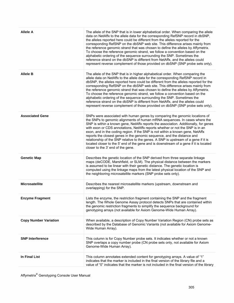
Affymetrix® Genotyping Console User Manual 305
Allele A The allele of the SNP that is in lower alphabetical order. When comparing the allele data on NetAffx to the allele data for the corresponding RefSNP record in dbSNP, the alleles reported here could be different from the alleles reported for the corresponding RefSNP on the dbSNP web site. This difference arises mainly from the reference genomic strand that was chosen to define the alleles by Affymetrix. To choose the reference genomic strand, we follow a convention based on the alphabetic ordering of the sequence surrounding the SNP. Sometimes the reference strand on the dbSNP is different from NetAffx, and the alleles could represent reverse complement of those provided on dbSNP (SNP probe sets only).
Allele B The allele of the SNP that is in higher alphabetical order. When comparing the allele data on NetAffx to the allele data for the corresponding RefSNP record in dbSNP, the alleles reported here could be different from the alleles reported for the corresponding RefSNP on the dbSNP web site. This difference arises mainly from the reference genomic strand that was chosen to define the alleles by Affymetrix. To choose the reference genomic strand, we follow a convention based on the alphabetic ordering of the sequence surrounding the SNP. Sometimes the reference strand on the dbSNP is different from NetAffx, and the alleles could represent reverse complement of those provided on dbSNP (SNP probe sets only).
Associated Gene SNPs were associated with human genes by comparing the genomic locations of the SNPs to genomic alignments of human mRNA sequences. In cases where the SNP is within a known gene, NetAffx reports the association. Additionally, for genes with exon or CDS annotations, NetAffx reports whether or not the SNP is in an exon, and in the coding region. If the SNP is not within a known gene, NetAffx reports the closest genes in the genomic sequence, and the distance and relationship of the SNP relative to the genes. A SNP is upstream of a gene if it is located closer to the 5' end of the gene and is downstream of a gene if it is located closer to the 3' end of the gene.
Genetic Map Describes the genetic location of the SNP derived from three separate linkage maps (deCODE, Marshfield, or SLM). The physical distance between the markers is assumed to be linear with their genetic distance. The genetic location is computed using the linkage maps from the latest physical location of the SNP and the neighboring microsatellite markers (SNP probe sets only).
Microsatellite Describes the nearest microsatellite markers (upstream, downstream and overlapping) for the SNP.
Enzyme Fragment Lists the enzyme, the restriction fragment containing the SNP and the fragment length. The Whole Genome Assay protocol detects SNPs that are contained within the genomic restriction fragments to simplify the sequence background for genotyping arrays (not available for Axiom Genome-Wide Human Array).
Copy Number Variation When available, a description of Copy Number Variation Region (CN) probe sets as described by the Database of Genomic Variants (not available for Axiom Genome-Wide Human Array).
SNP Interference This column is for Copy Number probe sets. It indicates whether or not a known SNP overlaps a copy number probe (CN probe sets only, not available for Axiom Genome-Wide Human Array).
In Final List This column annotates extended content for genotyping arrays. A value of “1” indicates that the marker is included in the final version of the library file and a value of “0” indicates that the marker is not included in the final version of the library
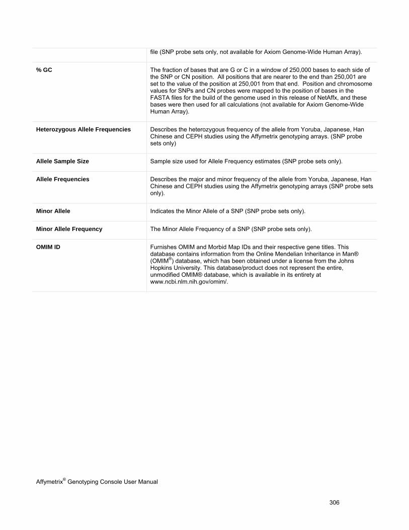
Affymetrix® Genotyping Console User Manual 306
file (SNP probe sets only, not available for Axiom Genome-Wide Human Array).
% GC The fraction of bases that are G or C in a window of 250,000 bases to each side of the SNP or CN position. All positions that are nearer to the end than 250,001 are set to the value of the position at 250,001 from that end. Position and chromosome values for SNPs and CN probes were mapped to the position of bases in the FASTA files for the build of the genome used in this release of NetAffx, and these bases were then used for all calculations (not available for Axiom Genome-Wide Human Array).
Heterozygous Allele Frequencies Describes the heterozygous frequency of the allele from Yoruba, Japanese, Han Chinese and CEPH studies using the Affymetrix genotyping arrays. (SNP probe sets only)
Allele Sample Size Sample size used for Allele Frequency estimates (SNP probe sets only).
Allele Frequencies Describes the major and minor frequency of the allele from Yoruba, Japanese, Han Chinese and CEPH studies using the Affymetrix genotyping arrays (SNP probe sets only).
Minor Allele Indicates the Minor Allele of a SNP (SNP probe sets only).
Minor Allele Frequency The Minor Allele Frequency of a SNP (SNP probe sets only).
OMIM ID Furnishes OMIM and Morbid Map IDs and their respective gene titles. This database contains information from the Online Mendelian Inheritance in Man® (OMIM®) database, which has been obtained under a license from the Johns Hopkins University. This database/product does not represent the entire, unmodified OMIM® database, which is available in its entirety at www.ncbi.nlm.nih.gov/omim/.
Affymetrix® Genotyping Console User Manual 307
Appendix E: Gender Calling in GTC GTC 4.0 can generate gender calls from:
Intensity QC
Genotyping Analysis
CN Segment Report (for SNP 6.0 only)
Copy number analysis for SNP 6.0 arrays provides information about calls for the X chromosomes and about calls for the Y chromosome based on signal intensity and allelic ratio, and provide a gender call (Female or Male) in the output table.
The processes used for gender calling differ depending upon:
The type of array being analyzed.
Step in the workflow being performed
Gender Calls in Intensity QC
See Contrast QC (page 69) for information on the algorithm used for the Intensity QC step.
QC analysis for genotyping uses DM algorithm to make SNP calls for Intensity QC purposes. It uses the following processes for making the gender call during this step.
Contrast QC is the recommended QC metric for the SNP 6.0 array in Genotyping Console 3.0.1. The default threshold is “greater than or equal to 0.4” for each sample. When adjusting this QC metric’s threshold value, or changing SNP 6.0 QC settings to another metric such as QC Call Rate, or adding additional metrics to threshold, a flag in the configuration setting dialog box will indicate that the thresholds are different than the defaults.
Contrast QC is a metric that captures the ability of an experiment to resolve SNP signals into three genotype clusters. It uses 10,000 random SNP 6.0 SNPs. See Appendix F: Contrast QC for SNP 6.0 Intensity Data (page 312) for more details.
Gender Calls in Intensity QC and Genotyping Analysis
Table D. 1 summarizes the methods used for gender calls during Intensity QC and genotyping analysis.
Table D. 1 Gender calling methods
Array Type Gender Call Algorithm
Genotyping Algorithm Gender Call
Reference
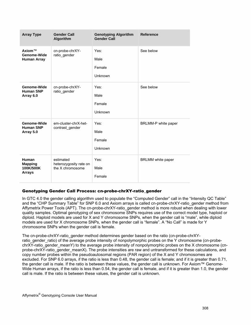
Affymetrix® Genotyping Console User Manual 308
Array Type Gender Call Algorithm
Genotyping Algorithm Gender Call
Reference
Axiom™ Genome-Wide Human Array
cn-probe-chrXY-ratio_gender
Yes:
Male
Female
Unknown
See below
Genome-Wide Human SNP Array 6.0
cn-probe-chrXY-ratio_gender
Yes:
Male
Female
Unknown
See below
Genome-Wide Human SNP Array 5.0
em-cluster-chrX-het-contrast_gender
Yes:
Male
Female
Unknown
BRLMM-P white paper
Human Mapping 100K/500K Arrays
estimated heterozygosity rate on the X chromosome
Yes:
Male
Female
BRLMM white paper
Genotyping Gender Call Process: cn-probe-chrXY-ratio_gender
In GTC 4.0 the gender calling algorithm used to populate the “Computed Gender” call in the “Intensity QC Table” and the “CHP Summary Table” for SNP 6.0 and Axiom arrays is called cn-probe-chrXY-ratio_gender method from Affymetrix Power Tools (APT). The cn-probe-chrXY-ratio_gender method is more robust when dealing with lower quality samples. Optimal genotyping of sex chromosome SNPs requires use of the correct model type, haploid or diploid. Haploid models are used for X and Y chromosome SNPs, when the gender call is “male”, while diploid models are used for X chromosome SNPs, when the gender call is “female”. A “No Call” is made for Y chromosome SNPs when the gender call is female.
The cn-probe-chrXY-ratio_gender method determines gender based on the ratio (cn-probe-chrXY-ratio_gender_ratio) of the average probe intensity of nonpolymorphic probes on the Y chromosome (cn-probe-chrXY-ratio_gender_meanY) to the average probe intensity of nonpolymorphic probes on the X chromosome (cn-probe-chrXY-ratio_gender_meanX). The probe intensities are raw and untransformed for these calculations, and copy number probes within the pseudoautosomal regions (PAR region) of the X and Y chromosomes are excluded. For SNP 6.0 arrays, if the ratio is less than 0.48, the gender call is female; and if it is greater than 0.71, the gender call is male. If the ratio is between these values, the gender call is unknown. For Axiom™ Genome-Wide Human arrays, if the ratio is less than 0.54, the gender call is female, and if it is greater than 1.0, the gender call is male. If the ratio is between these values, the gender call is unknown.
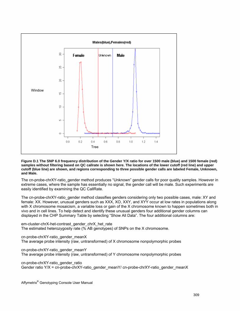
Affymetrix® Genotyping Console User Manual 309
Figure D.1 The SNP 6.0 frequency distribution of the Gender Y/X ratio for over 1500 male (blue) and 1500 female (red) samples without filtering based on QC callrate is shown here. The locations of the lower cutoff (red line) and upper cutoff (blue line) are shown, and regions corresponding to three possible gender calls are labeled Female, Unknown, and Male.
The cn-probe-chrXY-ratio_gender method produces “Unknown” gender calls for poor quality samples. However in extreme cases, where the sample has essentially no signal, the gender call will be male. Such experiments are easily identified by examining the QC CallRate.
The cn-probe-chrXY-ratio_gender method classifies genders considering only two possible cases, male: XY and female: XX. However, unusual genders such as XXX, XO, XXY, and XYY occur at low rates in populations along with X chromosome mosaicism, a variable loss or gain of the X chromosome known to happen sometimes both in vivo and in cell lines. To help detect and identify these unusual genders four additional gender columns can displayed in the CHP Summary Table by selecting “Show All Data”. The four additional columns are:
em-cluster-chrX-het-contrast_gender_chrX_het_rate The estimated heterozygosity rate (% AB genotypes) of SNPs on the X chromosome.
cn-probe-chrXY-ratio_gender_meanX The average probe intensity (raw, untransformed) of X chromosome nonpolymorphic probes
cn-probe-chrXY-ratio_gender_meanY The average probe intensity (raw, untransformed) of Y chromosome nonpolymorphic probes
cn-probe-chrXY-ratio_gender_ratio Gender ratio Y/X = cn-probe-chrXY-ratio_gender_meanY/ cn-probe-chrXY-ratio_gender_meanX
Window
Tree
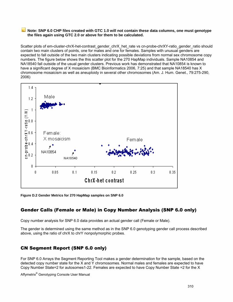
Affymetrix® Genotyping Console User Manual 310
Note: SNP 6.0 CHP files created with GTC 1.0 will not contain these data columns, one must genotype the files again using GTC 2.0 or above for them to be calculated.
Scatter plots of em-cluster-chrX-het-contrast_gender_chrX_het_rate vs cn-probe-chrXY-ratio_gender_ratio should contain two main clusters of points, one for males and one for females. Samples with unusual genders are expected to fall outside of the two main clusters indicating possible deviations from normal sex chromosome copy numbers. The figure below shows the this scatter plot for the 270 HapMap individuals. Sample NA10854 and NA18540 fall outside of the usual gender clusters. Previous work has demonstrated that NA10854 is known to have a significant degree of X mosaicism (BMC Bioinformatics 2006, 7:25) and that sample NA18540 has X chromosome mosaicism as well as aneuploidy in several other chromosomes (Am. J. Hum. Genet., 79:275-290, 2006)
Figure D.2 Gender Metrics for 270 HapMap samples on SNP 6.0
Gender Calls (Female or Male) in Copy Number Analysis (SNP 6.0 only)
Copy number analysis for SNP 6.0 data provides an actual gender call (Female or Male).
The gender is determined using the same method as in the SNP 6.0 genotyping gender call process described above, using the ratio of chrX to chrY nonpolymorphic probes.
CN Segment Report (SNP 6.0 only)
For SNP 6.0 Arrays the Segment Reporting Tool makes a gender determination for the sample, based on the detected copy number state for the X and Y chromosomes. Normal males and females are expected to have Copy Number State=2 for autosomes1-22. Females are expected to have Copy Number State =2 for the X

Affymetrix® Genotyping Console User Manual 311
chromosome, while normal males are expected to have Copy Number State=1 for the X chromosome and =1 for Y chromosome.
First the algorithm checks that the Copy Number QC metric MAPD is less than 0.5 to ensure the data is of sufficient quality. Next the mean copy number for the non-pseudo autosomal portion of the X chromosome and Y chromosome are used to assign gender. If the mean copy number for the X chromosome is between 0.8 to 1.3 and the mean copy number for Y is between 0.8 to 1.2, then a "male" is assigned. If the mean copy number for X is from 1.9 to 2.1 and Y is from 0 to 0.4, then a "female" is assigned. Finally, if neither of the above cases are true, then "Unknown" is assigned. Samples flagged “Unknown ” by the software and are assessed for Copy Number change as if they were female (CN State for X=2, and Y=0).
Affymetrix® Genotyping Console User Manual 312
Appendix F: Contrast QC for SNP 6.0 Intensity Data Contrast QC is the per sample Quality Control test metric for SNP 6.0 intensity data (CEL files). When all steps of the assay are working as expected, the Contrast QC is typically greater than 0.4. As an added flag for potentially problem data sets, check that the proportion of samples that fall below the 0.4 threshold are less than 10%, and the average of the samples that pass this 0.4 test are greater than or equal to 1.7. If the proportion falling below 0.4 is greater than 10%,or the average of the passing samples is at or below 1.7, then sample quality and process should be closely examined for possible issues.
The Contrast QC is a metric that captures the ability of an experiment to resolve SNP signals into three genotype clusters. It uses a static set of 10,000 randomly chosen SNP 6.0 SNPs, measuring the difference between peaks in “Contrast” distributions (Fig 217) produced by homozygote genotypes, and the valleys they share with the heterozygote peak, and takes the smaller of the two values. In poor quality experiments the homozygote peaks are not well-resolved from the heterozygote peak and the difference values approach zero. Contrast QC values are also computed for Contrast distributions produced by a static set of 20K randomly chosen SNPs on Nsp fragments only and a static set of 20K randomly chosen SNPs on Sty fragments only. These are called Contrast QC (Nsp) and Contrast QC (Sty); respectively. If the absolute difference between these two values is greater than two, this is evidence that that a sample may have worked properly with one enzyme set, but not with the other, and the Contrast QC value is adjusted to zero to reflect this problem. These Contrast QC values are well correlated with the higher Call Rates and concordance achieved when calls are subsequently made with Birdseed (versions 1 or 2). The correlation between Birdseed accuracy and Birdseed Call Rate is also very high. As an extra guard against the inclusion of any outlier samples that pass through the Contrast QC filter, it is a good idea to reject samples that are notable outliers in terms of their Birdseed Call Rate. When using Birdseed (v1), clustering larger batches of samples will improve the performance of the algorithm. The algorithm improvements in Birdseed v2 allow you to cluster by plate with the same performance as clustering larger batches of samples.
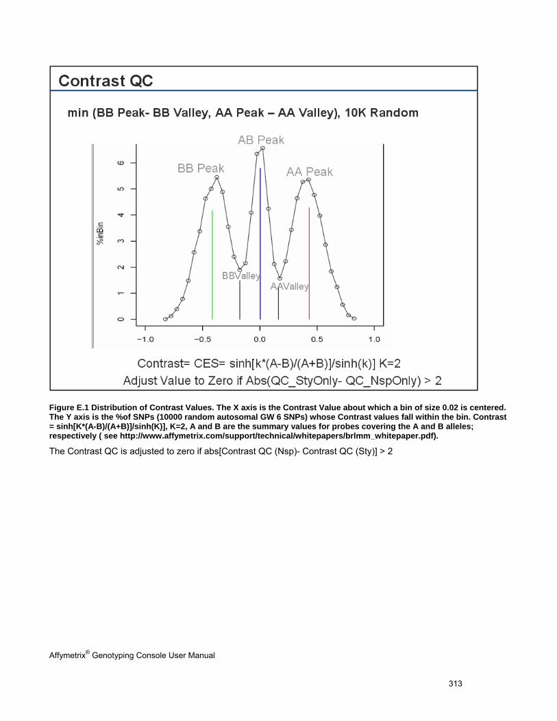
Affymetrix® Genotyping Console User Manual 313
Figure E.1 Distribution of Contrast Values. The X axis is the Contrast Value about which a bin of size 0.02 is centered. The Y axis is the %of SNPs (10000 random autosomal GW 6 SNPs) whose Contrast values fall within the bin. Contrast = sinh[K*(A-B)/(A+B)]/sinh(K)], K=2, A and B are the summary values for probes covering the A and B alleles; respectively ( see http://www.affymetrix.com/support/technical/whitepapers/brlmm_whitepaper.pdf).
The Contrast QC is adjusted to zero if abs[Contrast QC (Nsp)- Contrast QC (Sty)] > 2
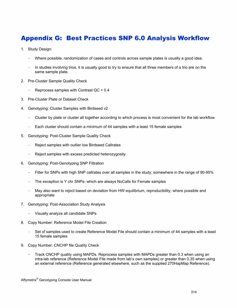
Affymetrix® Genotyping Console User Manual 314
Appendix G: Best Practices SNP 6.0 Analysis Workflow 1. Study Design:
- Where possible, randomization of cases and controls across sample plates is usually a good idea.
- In studies involving trios, it is usually good to try to ensure that all three members of a trio are on the same sample plate.
2. Pre-Cluster Sample Quality Check
- Reprocess samples with Contrast QC < 0.4
3. Pre-Cluster Plate or Dataset Check
4. Genotyping: Cluster Samples with Birdseed v2
- Cluster by plate or cluster all together according to which process is most convenient for the lab workflow
- Each cluster should contain a minimum of 44 samples with a least 15 female samples
5. Genotyping: Post-Cluster Sample Quality Check
- Reject samples with outlier low Birdseed Callrates
- Reject samples with excess predicted heterozygosity
6. Genotyping: Post-Genotyping SNP Filtration
- Filter for SNPs with high SNP callrates over all samples in the study; somewhere in the range of 90-95%
- The exception is Y chr SNPs- which are always NoCalls for Female samples
- May also want to reject based on deviation from HW equilibrium, reproducibility, where possible and appropriate
7. Genotyping: Post-Association Study Analysis
- Visually analyze all candidate SNPs
8. Copy Number: Reference Model File Creation
- Set of samples used to create Reference Model File should contain a minimum of 44 samples with a least 15 female samples
9. Copy Number: CNCHP file Quality Check
- Track CNCHP quality using MAPDs. Reprocess samples with MAPDs greater than 0.3 when using an intra-lab reference (Reference Model File made from lab’s own samples) or greater than 0.35 when using an external reference (Reference generated elsewhere, such as the supplied 270HapMap Reference).

Affymetrix® Genotyping Console User Manual 315
- If MAPDs are consistently high when using an external reference, recalculate MAPDs with an intra-lab reference. If the MAPDs all drop significantly, then the high MAPD is an artifact introduced by a systematic difference between current samples and the samples that made up the reference rather than a quality issue.
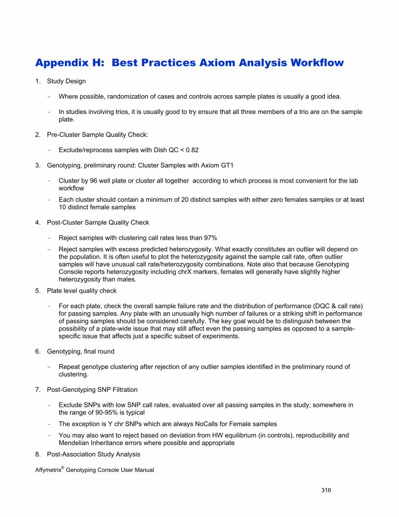
Affymetrix® Genotyping Console User Manual 316
Appendix H: Best Practices Axiom Analysis Workflow 1. Study Design
- Where possible, randomization of cases and controls across sample plates is usually a good idea.
- In studies involving trios, it is usually good to try ensure that all three members of a trio are on the sample plate.
2. Pre-Cluster Sample Quality Check:
- Exclude/reprocess samples with Dish QC < 0.82
3. Genotyping, preliminary round: Cluster Samples with Axiom GT1
- Cluster by 96 well plate or cluster all together according to which process is most convenient for the lab workflow
- Each cluster should contain a minimum of 20 distinct samples with either zero females samples or at least 10 distinct female samples
4. Post-Cluster Sample Quality Check
- Reject samples with clustering call rates less than 97%
- Reject samples with excess predicted heterozygosity. What exactly constitutes an outlier will depend on the population. It is often useful to plot the heterozygosity against the sample call rate, often outlier samples will have unusual call rate/heterozygosity combinations. Note also that because Genotyping Console reports heterozygosity including chrX markers, females will generally have slightly higher heterozygosity than males.
5. Plate level quality check
- For each plate, check the overall sample failure rate and the distribution of performance (DQC & call rate) for passing samples. Any plate with an unusually high number of failures or a striking shift in performance of passing samples should be considered carefully. The key goal would be to distinguish between the possibility of a plate-wide issue that may still affect even the passing samples as opposed to a sample-specific issue that affects just a specific subset of experiments.
6. Genotyping, final round
- Repeat genotype clustering after rejection of any outlier samples identified in the preliminary round of clustering.
7. Post-Genotyping SNP Filtration
- Exclude SNPs with low SNP call rates, evaluated over all passing samples in the study; somewhere in the range of 90-95% is typical
- The exception is Y chr SNPs which are always NoCalls for Female samples
- You may also want to reject based on deviation from HW equilibrium (in controls), reproducibility and Mendelian Inheritance errors where possible and appropriate
8. Post-Association Study Analysis

Affymetrix® Genotyping Console User Manual 317
- Visually inspect cluster plots for all candidate SNPs to ensure that there is nothing unusual about the clustering
Affymetrix® Genotyping Console User Manual 318
Appendix I: Copy Number Variation Analysis Copy Number Variation Analysis is performed using the Canary algorithm which was developed by the Broad Institute for the purpose of making copy number state calls for genomic regions with copy number variations. These genomic regions can be called regions with copy number variation (CNV regions) or regions with copy number polymorphism (CNP). These CNV regions are observed to be more variable in regard to copy number states than is typical of the genome as a whole. The specialized algorithm, Canary, was developed for these CNV regions because other copy number analysis methods assume a copy number of 2 to be the predominant copy number state in a sample of individuals. This frequency assumption is not reliable in the CNV regions and can lead to misled copy number state calls in the set of samples as a whole.
The Broad Institute first identified and made copy number state calls for the CNV regions in the population of HapMap samples. For each of these regions a set of probe sets, deemed to be “smart”, was assigned. Fidelity and robust response are two criteria attributed to smart probe sets. Within each CNV region selected by the Broad Institute, summaries of smart probe sets resulted in a clustering pattern consistent with copy number state. The frequency of HapMap individuals with a certain copy number state as well as cluster centers and means was recorded as empirical prior clustering estimates used by Canary. In GTC 4.0, the sets of smart probe sets mapping to CNV regions are stored a region file and the prior cluster information is stored in a prior file. All smart probe sets in the region file correspond to NCBI build 36.1 of the human genome. The CNV regions with their corresponding chromosomal positions are recorded in the CNV map file. This CNV map file is required for CNV result table display and also for the heat map viewer display.
GTC 4.0 uses a set of 1141 CNV regions derived from those identified by the Broad. To reduce sample-to-sample variability, these 1141 CNV regions are a subset filtered to ensure that each CNV region is mapped to by more than one smart probe set, reduced by restriction enzymes into more than one fragment and produces clustering results consistent in two full sets of HapMap samples independently processed at separate sites.
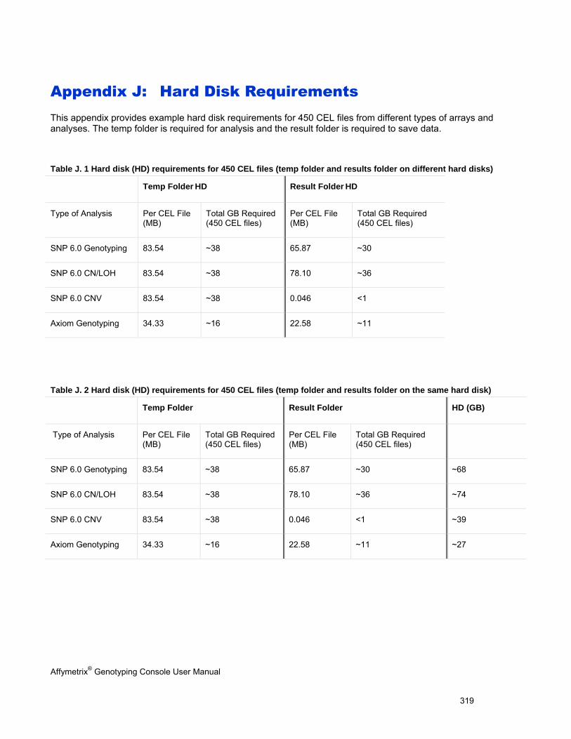
Affymetrix® Genotyping Console User Manual 319
Appendix J: Hard Disk Requirements This appendix provides example hard disk requirements for 450 CEL files from different types of arrays and analyses. The temp folder is required for analysis and the result folder is required to save data.
Table J. 1 Hard disk (HD) requirements for 450 CEL files (temp folder and results folder on different hard disks)
Temp Folder HD Result Folder HD
Type of Analysis Per CEL File (MB)
Total GB Required (450 CEL files)
Per CEL File (MB)
Total GB Required (450 CEL files)
SNP 6.0 Genotyping 83.54 ~38 65.87 ~30
SNP 6.0 CN/LOH 83.54 ~38 78.10 ~36
SNP 6.0 CNV 83.54 ~38 0.046 <1
Axiom Genotyping 34.33 ~16 22.58 ~11
Table J. 2 Hard disk (HD) requirements for 450 CEL files (temp folder and results folder on the same hard disk)
Temp Folder Result Folder HD (GB)
Type of Analysis Per CEL File (MB)
Total GB Required (450 CEL files)
Per CEL File (MB)
Total GB Required (450 CEL files)
SNP 6.0 Genotyping 83.54 ~38 65.87 ~30 ~68
SNP 6.0 CN/LOH 83.54 ~38 78.10 ~36 ~74
SNP 6.0 CNV 83.54 ~38 0.046 <1 ~39
Axiom Genotyping 34.33 ~16 22.58 ~11 ~27
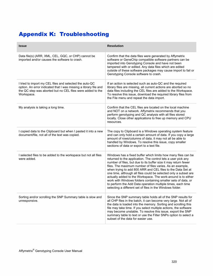
Affymetrix® Genotyping Console User Manual 320
Appendix K: Troubleshooting
Issue Resolution
Data file(s) (ARR, XML, CEL, GQC, or CHP) cannot be imported and/or causes the software to crash.
Confirm that the data files were generated by Affymetrix software or GeneChip compatible software partners can be imported into Genotyping Console and have not been tampered with or edited. Any data files which are edited outside of these software packages may cause import to fail or Genotyping Console software to crash.
I tried to import my CEL files and selected the auto-QC option. An error indicated that I was missing a library file and the QC step was aborted but no CEL files were added to the Workspace.
If an action is selected such as auto-QC and the required library files are missing, all current actions are aborted so no data files including the CEL files are added to the Workspace. To resolve this issue, download the required library files from the File menu and repeat the data import.
My analysis is taking a long time. Confirm that the CEL files are located on the local machine and NOT on a network. Affymetrix recommends that you perform genotyping and QC analysis with all files stored locally. Close other applications to free up memory and CPU resources.
I copied data to the Clipboard but when I pasted it into a new document/file, not all of the text was copied.
The copy to Clipboard is a Windows operating system feature and can only hold a certain amount of data. If you copy a large amount of rows/columns of data, it may not all be able to handled by Windows. To resolve this issue, copy smaller sections of data or export to a text file.
I selected files to be added to the workspace but not all files were added.
Windows has a fixed buffer which limits how many files can be returned to the application. The control lets a user pick any number of files, but due to its buffer size it may return fewer files. The maximum number of files varies. As an example, when trying to add 800 ARR and CEL files to the Data Set at one time, although all files could be selected only a subset are actually added to the Workspace. The work-around is to either work with Windows folders containing smaller sets of data, or to perform the Add Data operation multiple times, each time selecting a different set of files in the Windows folder.
Sorting and/or scrolling the SNP Summary table is slow and unresponsive.
Since the SNP summary table holds all of the SNP results for all CHP files in the batch, it can become very large. Not all of the data is loaded into the memory. Sorting and scrolling this file may take time. If you select multiple actions, the software may become unstable. To resolve this issue, export the SNP summary table to text or use the Filter SNPs option to select a subset of the data for easier use.
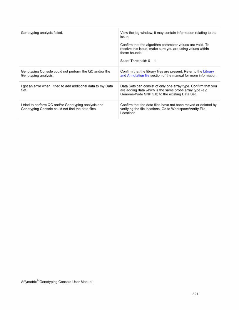
Affymetrix® Genotyping Console User Manual 321
Genotyping analysis failed. View the log window; it may contain information relating to the issue.
Confirm that the algorithm parameter values are valid. To resolve this issue, make sure you are using values within these bounds:
Score Threshold: 0 – 1
Genotyping Console could not perform the QC and/or the Genotyping analysis.
Confirm that the library files are present. Refer to the Library and Annotation file section of the manual for more information.
I got an error when I tried to add additional data to my Data Set.
Data Sets can consist of only one array type. Confirm that you are adding data which is the same probe array type (e.g. Genome-Wide SNP 5.0) to the existing Data Set.
I tried to perform QC and/or Genotyping analysis and Genotyping Console could not find the data files.
Confirm that the data files have not been moved or deleted by verifying the file locations. Go to Workspace/Verify File Locations.