Embed Size (px)
Citation preview
GTB Tailings Basins I – Final Report
Geochemical Tracer Based (GTB) Sulfate Balance Models for Active Tailings Basins on Minnesota’s Iron Range (I) Process Waters
Michael Berndt, Travis Bavin, and Megan Kelly
November 10, 2016
Minnesota Department of Natural Resources Lands and Minerals Division
500 Lafayette Rd., St. Paul, MN 55155
Page 1 of 64
GTB Tailings Basins I – Final Report
Abstract Minnesota’s taconite industry produces sulfate in a number of ways that include the burning of fuel, the grinding and processing of ore, and the oxidation of sulfides in tailings basins and stockpiles. This study is the first of a three part series evaluating sulfate release and transport associated with tailings basins using geochemical tracer based (GTB) methods. Focus here is placed on the chemistry of process waters that circulate between the processing plant and tailings basins. Part two evaluates sulfate in tailings pore waters and part three focuses on the chemistry of water in seeps, wells, and surface waters located outside the basins.
Four to five sets of water samples in this study were collected from each of five taconite processing operations over a two year period in 2014 and 2015 and analyzed for sulfate and several geochemical tracers. Key sampling locations included sites where water enters or leaves the taconite processing plants and tailings basins. Geochemical tracers included the concentrations of chloride and bromide; isotope ratios for hydrogen and oxygen in water (δ2HH2O and δ18OH2O); and isotope ratios for sulfur and oxygen in dissolved sulfate (δ34SSO4 and δ18OSO4). Chloride and bromide concentrations are used for quantifying impacts of dilution and for constraining water balance calculations. δ18OH2O and δ2HH2O are used to help quantify the amounts of evaporation and dilution occurring at each operation. δ34SSO4 and δ18OSO4 are used for qualitatively identifying sulfate sources and for quantifying process related to sulfide oxidation and sulfate reduction. These geochemical parameters are combined here with available hydrologic information into steady state GTB models to provide objective estimates for the sulfate and water fluxes for each of the five operations studied.
The relative amounts of sulfate generated and released into process waters at each operation depends on the reactivity of the tailings and the manner in which water is routed. In some cases the mass of sulfate that fills the pore spaces in tailings is similar to the mass of sulfate generated during mineral processing. In one case, Hibbing Taconite, the process plant and basin appear to be a net sink for dissolved sulfate since the mass of sulfate brought into the plant with makeup waters is less than the mass released to the environment. Makeup water and plant-generated sulfate are the most important sources of sulfate in process waters at U.S. Steel Keetac, Hibbing Taconite, United Taconite, and ArcelorMittal while tailings oxidation appears to be the major source at U.S. Steel Minntac. The reason for this difference is that water reacting with sulfide-bearing coarse and fine tailings is returned to the processing loop at U.S. Steel Minntac. Tailings from the other operations are either less reactive than those at U.S. Steel Minntac or are placed in a manner that prevents released sulfate from joining the process water loop.
Page 2 of 64
GTB Tailings Basins I – Final Report
Table of Contents Abstract ......................................................................................................................................................... 2
Introduction .................................................................................................................................................. 4
Purpose of This Report .................................................................................................................................. 5
Approach ....................................................................................................................................................... 6
Sample Locations and Dates ....................................................................................................................... 11
Chemical Methods ...................................................................................................................................... 12
Results and Discussion ................................................................................................................................ 13
General Statement .................................................................................................................................. 13
U.S. Steel - Keewatin Taconite ................................................................................................................ 14
Hibbing Taconite ..................................................................................................................................... 16
U. S. Steel- Minntac ................................................................................................................................. 17
United Taconite ....................................................................................................................................... 19
ArcelorMittal ........................................................................................................................................... 22
Closing Remarks .......................................................................................................................................... 23
Tables .......................................................................................................................................................... 25
Figures ......................................................................................................................................................... 36
References .................................................................................................................................................. 46
Appendix 1: Surface Area Calculations ...................................................................................................... 48
Appendix 2. A Water Isotope-Based Evaporation Model for US Steel’s Minntac Tailings Basin ............... 52
Isotope Model Background ..................................................................................................................... 52
Minntac Study ......................................................................................................................................... 55
References .............................................................................................................................................. 57
Page 3 of 64
GTB Tailings Basins I – Final Report
Introduction The Biwabik Iron Formation contains small amounts of iron sulfide minerals that oxidize and release sulfate when mined and placed in contact with air and water. Pyrite (FeS2) is the dominant iron sulfide mineral in the western part of the Iron Range while pyrrhotite (FeS) becomes more common in metamorphosed portions of the deposit close to the Duluth Complex. Although sulfide minerals are usually minor components in the ore, even small amounts can produce problematic sulfate levels in situations where the volume of rock exposed to oxidation and rinsing cycles is large.
The current wild rice standard, which is under review by the state of Minnesota, requires that waters used for the production of wild rice have no more than 10 mg/L when wild rice is growing. Sulfate concentrations greater than 10 mg/L are regularly encountered in waters sampled near mining operations throughout the world, including on the Iron Range where wild rice is commonly found. Other potential applicable standards include a secondary 250 mg/L standard for drinking water consumed by humans and 1000 mg/L in water that serves as a drinking water source for wildlife. Concentrations at these levels are less common on the Iron Range, found only occasionally in undiluted process and pit waters. Alkalinity, conductivity, and hardness may be elevated to levels that are close to or even above applicable standards in some settings on the Iron Range and these, too, are associated with waters containing elevated sulfate. Thus, this study on taconite tailings basins was conducted to provide a better understanding of sulfate sources and sinks associated with taconite processing and tailings deposition.
There are many pathways for sulfate to enter waters moving through taconite processing operations and this can make identification and quantification of sources difficult. Taconite operations mine and grind vast masses of iron ore which has non-uniform sulfide content. Grinding is accomplished in stages that also include separation of the primary ore mineral magnetite (Fe3O4) from non-ore minerals that include carbonates, silicates, and iron oxides in addition to iron sulfides. Grinding and mineral separation are water intensive operations that also vary from site to site across the Iron Range. Although much water is reused during mineral processing, continued pumping of water from sources outside the operation are needed to replace that which is evaporated or seeps from the basins. The water pumped into the operation generally contains some sulfate and is referred to as make-up water. Make-up water can contribute a substantial amount of sulfate to the operation if the sulfate concentration in the water is elevated.
Additionally, the grinding of iron ore exposes and damages pyrite mineral surfaces, promoting oxidative weathering that can release additional sulfate to process waters both within the process plant and in the tailings basin. Induration, the process required to harden the magnetite powder into a form suitable for shipping and conversion to steel, generates gaseous SO2 and SO3 that is captured by wet scrubbers and may be converted to sulfate in process waters. Waters use for mineral processing and for the scrubbing of process gases may be sent with tailings out to tailings basins, where the freshly ground solids containing small amounts of sulfide may be exposed to air and water and release sulfate. Depending on where this type of sulfate is released, it may add sulfate to circulating water that returns to the processing plant or to waters seeping into surrounding surface and ground waters.
Page 4 of 64
GTB Tailings Basins I – Final Report
Long-term management strategies to control sulfate require an understanding of how and where sulfate enters an operation and eventually leaks into the environment. This study is the first of a three-part series directed at modeling sulfate behavior in taconite tailings basins and associated processing facilities:
1. Part I (this report) focuses on process waters circulating between the processing plants and their associated tailings basins.
2. Part II (Berndt et al., 2016) reports sulfate concentrations in pore waters sampled in coarse and fine tailings of various ages from four taconite operations and calculates field-based release rates for sulfate into water that infiltrate and percolate through tailings.
3. Part III (Kelly et al., 2016a) focuses on processes affecting sulfate concentrations in wells and surface waters sampled outside the basin. The impacts of dilution are quantified using dissolved chloride and bromide concentrations, while changes in sulfate concentration and isotope ratios are used to quantify the addition of sulfate from oxidation of sulfide minerals and the reduction and conversion of sulfate to sulfide as waters flow through the tailings impoundment and into the glacial tills or other sediments.
Additional supporting studies include evaluation of tailings hydrology in 2014 and 2015 (Bavin et al., 2016), sulfur concentration and pyrite weathering characteristics in tailings (Jacobs et al., 2016), measurement of O2 consumption in tailings (Berndt and Koski, 2016), and evaluation of sulfate and other geochemical tracers sampled from three deep cores from fine and coarse tailings at Minntac (Kelly et al., 2016b)
The present study uses geochemical tracer based (GTB) methods that were developed and tested previously at U.S. Steel Minntac in 2012 and 2013. These methods rely on collection of samples from a carefully selected set of flux points at each operation and analyzing them for sulfate concentrations, halide tracers (Br and Cl), the isotopic ratios of hydrogen and oxygen in water, δ2HH2O and δ18OH2O, and sulfur and oxygen isotopic ratios in dissolved sulfate, δ18OSO4 and δ34SSO4. Participation, in this case, was expanded beyond U.S. Steel’s Minntac operation (near Mountain Iron) to include processing plants at Keewatin Taconite, near Keewatin; Hibbing Taconite, located between Chisholm and Hibbing; United Taconite, with tailings basin located near Forbes; and ArcelorMittal located near Virginia (Figure 1).
Purpose of This Report The purpose of this report is to couple hydrologic and chemical data together to construct generalized or simplified, steady state sulfate and water mass balance models for five taconite processing facilities. The models calculate the specific loading of sulfate to process water from make-up water drawn into the plant, generated by taconite processing within each plant, or from the oxidation of pyrite stored in the tailings basin.
A secondary objective for this report is to test the utility of using chemical measurements to assist in construction of hydrologic balance models for each of the taconite processing facilities. For example, the amount by which bromide or chloride concentrations decrease from the time water is pumped to the basin and returned to the plant can be used to quantify the net amounts of precipitation and evaporation in the basin. Moreover, δ2HH2O and δ18OH2O can be used to determine the degree to which water drawn
Page 5 of 64
GTB Tailings Basins I – Final Report
into the operation or falling as precipitation on the basin evaporates before it seeps or is discharged from the operation. While precipitation and evaporation can be estimated in other ways, the methods provided here provides a relatively objective means to help constrain the hydrologic balance.
While considerable effort was made to interact with mining companies during the development of the spreadsheet models that are included in this document, there was a downturn in the industry that occurred near the end of the current study and which continued as the models were being developed. Not all companies were able to continue to participate in the study during the downturn owing to layoffs and staffing shortages.
Thus, rather than considering the balances provided in this report to be finalized chemical and mass balances, they should be considered as starting points to be used to help quantify if and how changes made to the taconite processing facilities could lead to decreases or increases in sulfate released to the environment. Spread-sheet model results are presented that describe simplified hydrologic and chemical balances existing at the operations in 2014 and 2015. The spreadsheet models provide herein will be retained at the Minnesota DNR and can be modified if and when additional information becomes available.
Approach The GTB methods developed and used here for each operation are steady-state models that represent the average conditions observed for the period of time spanning the sampling visits to each site: Spring 2014 to autumn 2015 for companies that remained open during the full study period and less for companies that closed during the 2015 industry slowdown. The GTB approach involves simultaneously solving a series of mass balance equations for sulfate, chloride, water, and isotope ratios for components of water and sulfate. The equations use averaged measured values made at each of the operations (e.g., chloride concentration, sulfate concentration and isotope ratios, water flow rates and isotopic composition). Where more than one solution exists, results are compared to other field observations or measurements, as available, to help refine the estimates.
An implied constraint of a steady-state model is that masses and concentrations remain approximately fixed over the long term. While short-term seasonal variations in chemistry and volume are certain to occur, a steady-state approximation of fluxes over time can be made by averaging concentrations in samples collected over a range of conditions (wet, dry, warm, and cold). Steady-state models do not provide information on the fluxes at any one specific point in time but they provide a generalized average rate of flow. While transient models could be constructed from the data collected, they would likely require a greater level of sampling effort and interaction with the mining companies than was available at this time.
Mass balance calculations are conducted simultaneously for each of three parts of an operation (Figure 2): processing plant, pond, and tailing pile pore spaces. If no new storage occurs, then the amount leaving one part must exactly equal the amounts arriving in the other. In this way, the balances for each part of the operation are interlinked and mass balance equations for the entire operation can be superimposed on other constraints involving the fractionation of hydrogen and oxygen isotopes that occurs as a result
Page 6 of 64
GTB Tailings Basins I – Final Report
of evaporation. The calculations were typically first completed separately and independently for the processing plant, pond, and tailings pile. An iterative approach was then used to complete the balance for all three sections simultaneously while ensuring consistency with water isotope data, precipitation estimates, and other available geographical, hydrologic, and geochemical information.
Taconite processing plant balance: The primary source of water to the processing plant is tailings basin “return water”, however, some “make-up water” is inevitably added to the processing plant to balance net water lost elsewhere in the operation. Records were usually available for the flow rates of water to the plant which consisted of make-up water pumped from off-property sources or water returning from the tailings basin. In some cases, however, the flow rate for “raw water” was reported, comprising of mixed make-up and return water sources. Flow rates were not always available for water exiting the plant and so the mass of water exiting the plant was set equal to the mass of water entering the plant minus an estimated amount that was lost during taconite processing (evaporation or pumped elsewhere). By measuring concentration and flow rates for the water entering the plant and the concentration in water exiting the plant, a full plant balance for water and dissolved chloride and sulfate could be obtained.
The taconite processing plant was assumed not to gain or lose water over time, but was considered a potential source for both sulfate and chloride. Thus, once the water balance was obtained for the plant, any excess of sulfate and chloride found for water exiting the plant compared to that entering the plant was assumed to have been produced within the plant.
One complication occurring at some operations involved the plant-site settling basins which receive water from and return it to the plant. Plant site settling basins were assumed to be a part of the plant – and thus have net-zero impact on the balance calculations. This assumption was tested and found, ultimately, to impact the balance in the tailing basin. For example, if there actually was net leakage of water from the settling basin, then assuming a net-zero balance for this source ultimately leads to an over-estimation of leakage from the basin. Thus, for plants that have on-site settling basins, some of the leakage estimated for the tailings basin may occur as seepage from the plant site settling basin. Provision was included in the spreadsheet models for the plant site settling basin if additional information becomes available.
Some processing plants send floor wash and agglomeration water to the tailings basins rather than to an on-site settling basin. This impacts the exchange of water and elements between the plant and the basin, and so was explicitly included in the calculations for both parts of the operation, plant and basin. For U.S. Steel Minntac, the flow-rate could not be measured individually for agglomerator water, floor wash, and tailing water sent to the basin. In these cases, the ratio of water exiting to the plants as process and agglomerator waters was estimated and all of the concentrations for each stream were measured independently.
As the study progressed it was found that evaporation of water in the plant was a major unknown variable. Some plants provided estimates for the amount of evaporative loss (stack gases, dust collectors, other evaporation), while others did not. For companies that did not provide estimates we assumed an average of 400 gpm was lost by evaporation for each production line. Higher evaporation leads to concentration
Page 7 of 64
GTB Tailings Basins I – Final Report
of elements circulating through the plant and decreases the calculated loads of sulfate and chloride sent to the basin, and this can ultimate affect the mass of water seeping from the basin.
Finally, it was found that transfer of water between the plant and the basin involved large flow rates and that even small errors in the measurement of one or the other flow rates could have large consequences in the mass balance constraints for chloride and sulfate. To minimize errors related to this effect, we accepted either the inlet or the outlet flow values and calculated the other flow rate based on water balance constraints for the plant. An increase in chloride or sulfate observed in the outlet compared to that for combined inlet waters could then be applied to all of the water that cycled through the plant. This is much more precise method than accepting an error in the measurement of flow rates and carrying that error through the rest of the calculation. An obvious advantage of this approach is that it also facilitates calculation in cases where one of the large parts of the water balance equation cannot be measured or are poorly known. This is typically true for tailings slurry which contains a composited and variable solid content whose flow rates for the water component can be difficult to measure.
Pond water balance: In each case studied, the processing plant balance was used as both an input for the basin and as a point where water was sent back to the plant. Because the pond shares these points with the plant, the plant’s balance results could be used directly for the pond’s balances for water, sulfate, and chloride balances.
Precipitation dilutes and evaporation increases the concentrations of dissolved constituents and, thus, simply observing the changes in chloride concentration and water isotope ratios that occurred within the facility provide strong quantitative information on precipitation and evaporation.
Another important constraint involves using the chloride flux for the pond and plant to calculate the rate of water lost from the tailings basin pond. Typically, the chloride (or bromide) load in water returning to a plant is less than that in water sent to the basin from the plant. Assuming steady-state conditions apply, then the lost chloride load can be attributed to loss of process water from the pond (for a model with no change in basin storage). Because the chloride concentrations are measured in process waters within the basin, this chloride loss can be used directly to calculate the flux of process water (and also sulfate) seeping into or trapped within tailings.
Process water lost from the pond can either fill newly formed void spaces in freshly deposited fine tailings or it can seep from the basin into surrounding groundwater or surface waters. Void spaces for coarse tailings were ignored in the models since they usually only hold a nominal amount of water compared to in fine tailings, and are easily rinsed by precipitation (Bavin et al., 2016). Fine tailings, however, may hold process water for long periods of time or may be subjected to rinsing by fresh precipitation (Bavin et al., 2016; Berndt et al., 2016a; Kelly et al., 2016b). The degree to which fine tailings are filled with process water, precipitation, and air, are left as adjustable parameters in the models and are estimated using information on their chloride concentrations for waters seeping from the basins.
An important component of any water and mass balance study for a system that is open to the atmosphere involves accounting for precipitation and evaporation (net precipitation). Net precipitation was calculated here using information on total precipitation and infiltration rates for tailings (Bavin et al.,
Page 8 of 64
GTB Tailings Basins I – Final Report
2016) and using changes in the water isotopic compositions to compute evaporation (Gammons, et al., 2006; Kelly, 2013, Appendix A). For the present model, water falling on unsaturated tailings within the basin was treated separately from water falling on saturated land. Water falling on unsaturated tailings evaporates partially and with almost no impact on its isotopic composition (Bavin et al., 2016). Evaporation of water falling on saturated land or directly on the pond, however, does impact the isotopic composition of the water remaining in the basin. Water falling on tailings but then draining back into the pond will evaporate partially without impact on isotopic ratios as it infiltrates until it rejoins the circulating process waters, at which point any further evaporation will impact the isotopic ratio of the water remaining in the pond. All three types of processes were accounted for within the model as follows.
According to Bavin et al. (2016) precipitation at the Hibbing airport averaged 21.98 inches per year in 2014 and 2015. Observations and modeling using a computer program designed for this purpose (Hydrus 1D) indicated that approximately 10.5 inches of the water falling on unsaturated fine tailings with a fine sand texture evaporated, which was consistent with field observations for infiltration at Minntac. Thus, water falling on unsaturated tailings was modeled as losing 10.5 inches of precipitation/year without impact to its isotopic composition. Infiltrating water that rejoined the processing loop was treated like water entering along any other pathway (agglomerator, tailings, pump backs). Water falling directly on saturated tailings or onto the pond directly was assumed to mix into existing waters in the pond and affect both its volume and chemistry (dilution of chloride and sulfate with water having averaged local meteoric water isotope ratios). The total evaporation from the process loop was calculated, finally, by comparing the isotopic composition of properly composited water from operational inputs (from precipitation, return of freshwater to the pond following infiltration, make-up water) with that measured in the pond water. Both the fraction of the surface composed of unsaturated tailings and the fraction of the precipitation that infiltrates into unsaturated tailings and returns to the pond were included as adjustable parameters in the model.
An important parameter relates to the concentration of water falling on land that returns to the processing loop which can be calculated by dividing the sulfate load added in the basin by the net flow rate of water falling on the land to the process loop. If this concentration becomes too small or too large compared to measured values for pore waters (e.g., Berndt et al., 2016), then the percent of precipitation falling on the land and returning to the pool must be re-estimated.
Initially, evaporation in the processing plants was ignored in the calculations of isotope estimates related to net evaporation for the tailing basin. However, it was found eventually that for at least one of the processing plants (United Taconite) which has a relatively small basin size compared to the plant, this procedure likely over-estimated evaporation for the basin. The difficulty that arises in modeling plant evaporation relates to the ineffectiveness in this process to impact water isotope ratios compared to evaporation from the basin. For example, if an aliquot of water is sent to an internal process into the plant that evaporates the water completely, no water returns to impact the isotopic ratios for water still circulating in the processing loop. This compares to evaporation taking place directly from the clear water pool in the tailings basins where 100% of the water left behind following evaporation is retained in the process loop. Moreover, evaporation in the processing plant takes place under conditions different from those taking place in the basin (e.g., near 100 C during induration and re-condensation in wet-scrubbers).
Page 9 of 64
GTB Tailings Basins I – Final Report
Fractionation at high temperatures has less impact on isotopic ratios compared to that at low temperatures.
Ultimately, an empirical relationship was developed to differentiate but still account for the impact of in-plant evaporation compared to evaporation in the basin at United Taconite where independent plant evaporation estimates were provided by plant personnel. Based on this and other available information, plant evaporation was estimated to have approximately 20% of an impact on the isotopic ratios compared to evaporation in the basin such that:
TotEvap% = BasinEvap% + PEC x PlantEvap%
where TotEvap% is the total evaporation estimated from the change in water isotopic ratios for sources (make up water and precipitation) compared to process waters circulating in the basin; BasinEvap% is the percentage of water entering the from other sources (makeup water plus precipitation) that evaporates from the basin prior to being lost from the processing loop; and PlantEvap% is the percentage of the process water that is lost by evaporation in the plant prior to being lost from the operation. PEC refers to a “plant evaporation constant” which was set at 0.20 for this study based on information and modeling conducted in communication with personnel at United Taconite.
Plant evaporation is relatively poorly constrained in the models, although estimates were provided by several of the companies. Generally, however, apparent acceptable fits could be achieved for plant balances using this equation and assuming approximately 400 gpm evaporated per line. If evaporation from the plant became too large, then it resulted in less acceptable values for the percentages of land that were considered unsaturated for the tailings basins.
Tailings basin pore waters: Pore waters in tailings basins were balanced separately from pond water owing to the complexities associated with exchange between precipitation, tailings, and pond water. Water falling as precipitation directly on tailings may rejoin the process water loop, or join process waters that either seep from or remain locked up within pore spaces within the basin. Meanwhile, new pore spaces are continuously generated within the basin and need to be filled either with process water, water that falls on the basin, or with air. This model assumes that new void space is created in proportion to the mass of composited (coarse + fine) or fine tailings produced by the operation (Bavin et al., 2016). Adjustable parameters are then used to control the fraction of the newly produced tailings that are filled by fresh precipitation, process water, and air. The remainder of the water may seep into surrounding groundwater and surface waters. These parameters can be adjusted to fit other existing field data or measurements as available (e.g., percentage of basin covered by saturated land and pond water, chloride concentration in well waters and seeps, basin construction that dictates likely flow paths in tailings).
Tailing porosity is an important consideration for estimates of water locked up in pore spaces. Less water is likely to be locked up in coarse tailings than it is in composited or fine tailings. Bavin et al. (2016) reported porosity values for cores collected from four of the operations in this study. The average porosity of cored fine tailings was 53 percent at United Taconite and Arcelor Mittal. Cored Minntac fine tailings averaged 55 percent porosity. The cored unsegregated tailings at Hibbing Taconite that were sampled in their East Basin averaged 51 percent porosity while cored coarse tailings at Minntac, United Taconite, and
Page 10 of 64
GTB Tailings Basins I – Final Report
Arcelor Mittal averaged 40, 41, and 42 percent porosity respectively. No cores were collected at Keetac so it was assumed that their tailings had an averaged porosity of cored unsegregated tailings similar to those at Hibbing Taconite (51 percent).
An important constraint for the models involved comparing the chloride concentrations in wells and seepage at the toe of the basin with chloride concentrations in process waters. This parameter could be used to adjust the relative amounts of process water and direct precipitation (to land) that seep from the basin. Additionally, some information was collected on the total chloride and bromide concentrations and water flow rates at points located well downstream from the basins. This information can help to constrain the total surface seepage rates of undiluted process waters from the basins. Generally, however, the frequency of sampling was insufficient to provide quantification of surface fluxes. An exception is U.S. Steel Minntac where sampling and flow measurements were made monthly. Those data are presented and discussed by Kelly et al. 2016a and used to help constrain the basin balances in this report.
Iteration: Models were constructed on a series of spreadsheets that link the data to appropriate mass balance equations. In practice, however, it was found that some of the adjustable parameters were not entirely independent from each other when all of the mass and chemical balance constraints were added into the model. In these cases an iterative approach was used such that dependent parameters were consistent with the overall model.
If the results of the model appeared inconsistent with other field information, such as air photos from the basins or with information from drill core samples, then adjusted parameters were manipulated until a full balance was achieved consistent with a reasonably local geography and hydrology. In some cases, the available hydrologic information was very limited (e.g., a range of flow values provided without an average value, or no flow value at all). In most of these cases, solutions to the model could still be achieved owing to redundancies in the calculation. More detailed discussion of the site specific constraints is provided in the results and discussion sections for each operation.
Sample Locations and Dates Sample sites were chosen based on availability, access, and likely utility for the GTB geochemical model. At a bare minimum, samples were always collected from sites where water is brought into the plant or tailings basin from the outside (e.g., make-up water) and where water was exchanged between the plant and the basin (agglomerator, tailings, and basin return water). Several sites had additional discharges from the plant or from seepage pump-back systems to the basins. When access was available, these sites were also sampled. Finally, there were numerous samples collected from internal sites within plants and tailings basins. Although the data collected from these sites may or may not be used directly in the GTB model, they provided qualitative insight on the processes taking place in the plant or basin that could be used to support or improve the calculations. Specific locations at each basin are discussed in the results section.
One shortcoming of the present models is the lack of estimates for water loss related to production of gaseous water in the processing plants. This process potentially impacts our water balances for the plant
Page 11 of 64
GTB Tailings Basins I – Final Report
and is effectively similar to evaporation. A small nominal value (200 to 300 gpm) was selected as a place holder to account for water gained from ore and water lost from stacks. This potentially impacts our evaporation calculations, but will not be considered further until more information on specific masses becomes available. Several scrubber waters were collected and analyzed isotopically to facilitate possible future inclusion of wet scrubbers on the overall model.
Five sampling rounds were conducted between May 2014 and October 2015. The objective was to sample for a range of conditions, including wet to dry and warm to cold (freezing). Keewatin Taconite and United Taconite experienced temporary shutdowns during the study and so we were only able to access those sites three and four times, respectively. Additionally, we were unable to collect tailings from Keetac during one of our site visits because the plant was open, but not producing tailings at the time the samples were collected. The rest of the basin was functioning normally, so the other samples were collected.
Chemical Methods Grab samples were collected for major cation and anion analysis and filtered on site using 0.45 µm cartridge syringe filters. Samples analyzed for cations were preserved with ultra-pure nitric acid and shipped on ice along with the samples used for anion analysis (University of Minnesota – Geochemistry Laboratory, Minneapolis, Minnesota). Cations were analyzed by ICP–AES (Thermo Scientific iCAP 6500) and anions were measured by ion-chromatography (Dionex ICS 2000). The list of cations analyzed includes Al, Ba, Ca, Fe, K, Li, Mg, Mn, Na, P, Si, and Sr. The list of anions includes F, acetate, formate, chloride, nitrite, bromide, nitrate, sulfate, oxalate, thiosulfate, and phosphate. Here we report only bromide, chloride, and sulfate concentrations that were used in the model. Concentrations for other elements are available upon request. Detection limits for bromide, chloride, and sulfate are approximately 0.01, 0.01, and 0.02 mg/L on undiluted samples. Samples were diluted by 1 to 10x, depending on the expected and measured concentrations. Any samples that were found to exceed the concentrations measured in the highest standard were diluted to lower concentrations and reanalyzed.
All water isotope samples were filtered using a 0.45 µm PES membrane filters at the field site and were stored unpreserved in 30 mL HDPE bottles until shipped for analysis to the University of Waterloo Environmental Isotope Lab. Bottles were tightly sealed with limited headspace to minimize evaporative loss. Ratios for 18O/16O were determined via gas equilibration and head space injection into an IsoPrime Continuous Flow Isotope Ratio Mass Spectrometer (CF-IRMS). Ratios for 2H/1H were determined using chromium reduction on a EuroVector Elemental Analyzer coupled with an IsoPrime CF-IRMS. Internal laboratory standards are calibrated and tested against international standards from the International Atomic Energy Agency (IAEA), including Standard Light Antarctic Precipitation (SLAP), Greenland Ice Sheet Precipitation (GISP), and Vienna Standard Mean Ocean Water (VSMOW). Values for δ18OH2O and δ2HH2O are reported in ‰ relative to the international standard Vienna Standard Mean Ocean Water (VSMOW), which approximates the composition of the global ocean. Sample replicates are run approximately every 8 samples. Analytical uncertainties are ±0.2‰ and ±0.8‰ for δ18O and δ2H, respectively.
Approximately 250 mL to 1 L water was collected for S and O isotope analysis of sulfate-. Samples were filtered after collection at the Hibbing laboratory using 0.7 µm glass fiber filter paper. All samples collected in 2012 for sulfate isotope analysis were prepared at the DNR’s Hibbing Laboratory. The method
Page 12 of 64
GTB Tailings Basins I – Final Report
involves the quantitative conversion of dissolved sulfate to solid BaSO4 using procedures modified from Carmody et al. (1998). Water samples were first filtered through a 0.45 µm PES membrane filters. The filtrate was acidified with 1M HCl to a pH of 3-4 and heated at 90°C for approximately 1 hour so that any carbonate present would be degassed as CO2. Approximately 6 ml of 6 percent H2O2 was also added to each sample prior to heating to oxidize and degas any dissolved organic matter. These measures reduce contamination of the BaSO4 precipitate. After heating, ~5 ml of 20 percent BaCl2 was added (in excess) and the samples were allowed to cool for several hours or overnight. The BaSO4 precipitate was collected on preweighed 0.45 µm PES membrane filters, and was dried overnight at 90°C. Once dry, the BaSO4 powder was weighed, scraped into glass vials, and stored until shipment to the University of Waterloo Environmental Isotope Laboratory in Ontario, Canada for isotopic analysis.
The University of Waterloo Environmental Isotope Laboratory analyzed each BaSO4 sample for δ34SSO4 and δ18OSO4. Relative 34S and 32S abundances for the precipitates were determined using an Isochrom Continuous Flow Stable Isotope Ratio Mass Spectrometer (GV Instruments, Micromass, UK) coupled to a Costech Elemental Analyzer (CNSO 2010, UK). Relative 18O and 16O abundances for the precipitate were determined using a GVI Isoprime Mass Spectrometer coupled to a Hekatech High Temperature Furnace and a Euro Vector Elemental Analyzer. Values for δ34SSO4 are reported in ‰ units against the primary reference scale of Vienna-Canyon Diablo Troilite meteorite (VCDT), with an analytical precision of 0.3‰. δ18OSO4 is reported relative to VSMOW, with analytical precision of 0.5‰.
Results and Discussion General Statement Sulfate and chloride concentrations for the basins were relatively stable during the study period, except in the winter when concentrations were elevated at all operations (Figure 3). The elevated winter concentrations were almost certainly due to formation of ice, which removes water from the ponds in the basin but leaves the dissolved salts to accumulate and reach higher concentrations in the unfrozen basin water fraction. Although the ice formation may cause water seeping from the pond to have higher concentrations, it should minimally impacts the total mass of water and dissolved constituents stored in the basin. The steady state model provides for this effect by including the concentrations measured in the winter in the averaged concentrations used in the models. In this study, however, we made no attempt to weight winter versus summer values according to the relative lengths of the seasons. It was thought that to do so would minimally improve the overall accuracy of the models compared to other aspects of the model discussed in each section.
In addition, there appears to be a slight increase in the concentration of sulfate and chloride over time for each of the basins. This is likely because the study began immediately following a relatively wet spring, when concentrations of water in the basin would be expected to be low, and concluded in the autumn, when evaporation was likely higher than average. It is possible, if not likely, that tailing ponds were at elevated water levels throughout the Iron Range when the study began compared to at the end, which would obviate a need for including a changing water storage term in the balance equations used at some or all of the operations. A negative storage term for water in the basin would require greater leakage from the basin. Allowing for increasing concentrations of sulfate or chloride over time, while keeping the
Page 13 of 64
GTB Tailings Basins I – Final Report
pond volume fixed, would result in slightly lower leakage volumes of process water than were calculated in the models.
U.S. Steel - Keewatin Taconite Ten sampling sites were selected for Keewatin Taconite. These include Reservoir-2, the outer basin/stage 2 weir, the inner tailings basin’s decant tower, tailings slurry as it emerged from the plant or entered the basin, scrubber water input and output streams, and water brought into the operation from Carlz, Section 18 and Russell Pits. The 48-inch line that extends from the plant to Bennett Pit was also sampled, as was water at the Reservoir 6 pump house that pumps water to the plant. Results for water and sulfate isotopes and for dissolved chloride, bromide, and sulfate, are presented in Table 1 and Figures 4 to 6.
The most important sites for constraining balances at the plant include the Carlz Pit, which serves as source water to the processing plant; the 48-inch waste line, which outputs water to Bennett Pit; and the tailing slurry and basin return water from Reservoir 6. The Section 18 and Bennett Pit waters are pumped to the Russell Pit, which in turn provides water to the Carlz Pit (makeup source for the plant). For the basin, the most important points were the tailings slurry and water returning to the plant from the Reservoir 6 Pump House since virtually all transfer between plant and basin occurs at those sites. Scrubber water input and output samples could be used to evaluate the qualitative impacts of the scrubber on changes taking place within the plant. Samples at the internal basin decant tower provide qualitative insight on the changes that take place within the pond following deposition of tailings, but prior to being transferred to Reservoir 6.
Very limited water balance data was available for this study and so an assumption was made that flows during the study period were similar to those reported for an August 2011 to August 2013 water balance (Leisch, 2014). This balance reported that approximately 11743 gpm was returned from Reservoir 6 to the plant, 3421 gpm was used for additional makeup (Carlz pit presently, Res. 5, previously), 2227 gpm was pumped from the plant through the 48-inch line, and there was a net loss of 818 gpm to evaporation, pellet cooling, indurator exhaust, and other processes within the plant. The report indicated that 10,496 gpm of water was pumped from the plant with tailings, but using this value leaves an excess of water in the plant. In the present study, we assumed that this value was the least certain of those measured. Thus, the water leaving the plant with tailings was calculated by difference (12,119 gpm). Approximately 1440 gpm were pumped to Reservoir 6 from the Reservoir 2 within the basin.
For chemical balances, we note that the sulfate/chloride ratios stay relatively constant at the key sampling locations (Figure 4). This alone suggests that a large fraction of the sulfate and cholride present in the operation’s process waters is either brought into the plant with makeup water or is introduced within the mineral processing loop (fuel, grinding up of mineral fluid inclusions, grinding related oxidation of freshly exposed iron sulfides) because a large amount of sulfide oxidation in the tailings basin would impact the sulfate concentration without impacting chloride concentration. If this happened, then water returning to the plant from the basin would have sulfate/chloride ratios that are elevated compared to those in waters sent to the basin from the plant.
Page 14 of 64
GTB Tailings Basins I – Final Report
Values for δ2HH2O and δ18OH2O are close to the evaporation line, indicating the reasonability of using evaporation as a constraint for water balance purposes in the basin (Figure 5). The makeup water from Carlz Pit has already evaporated by about 15 percent before it is drawn into the plant, but water falling on the basin as precipitation is assumed to have zero percent initial evaporation. Ultimately, the basin return water averages a total of approximately 13.1 percent more evaporated than that for a representative mix of makeup water and precipitation.
Measured δ34SSO4 and δ18OSO4 for Carlz Pit waters are distinctly lower than those measured for tailings or basin return waters (Figure 6), which are, in turn, lower than those measured for scrubber waters. This is an additional indication that sulfate is being added primarily within the plant at this site, most likely from the wet scrubber. This confirms that both scrubber and makeup water are important sources of sulfate at this operation.
The surface area for the basin was measured at 8.81 square miles (Appendix 1). The company reported that they deposited 13 million metric tons of fine tailings in the basin in 2014 in their annual mine report to the DNR.
Model results (Table 2) reveal an average of about 2.1 metric tons of sulfate are brought into the operation per day from Carlz Pit and an average of 1.32 metric tons per day are pumped out to Bennet Pit. Approximately 0.8 metric tons are produced in the processing plant, either by oxidation of freshly crushed tailings or from the scrubber water input and another 0.5 metric tons per day are added by the rinsing of sulfate from sulfide minerals that are oxidizing in the tailings basin.
This basin is unusually constructed compared to most basins because much of the water that precipitates and infiltrates within the basin eventually returns to the process loop. The current water balance estimates that water falling on the land and returning to the process loop would have an average sulfate concentrations of approximately 44 mg/L. This relatively low concentration helps to explain why the mass of sulfate added in the basin is low compared to that from the other sources.
If we assume that newly formed tailings remain saturated with water following deposition, then we calculate that 2.81 tons/day of sulfate are locked up in tailings and another 1.72 tons/day sulfate is lost in water seeping from or discharged from the basin. No tailings were cored at this basin, however, the porosity for composited tailings measured at Hibbing Taconite (0.51) were used in this calculation to facilitate the calculations.
Interestingly, the mass of water “locked up” in the present model (2541 gpm) is significantly larger than that calculated in Leisch’s model (1531 gpm). Leisch’s model assumed that tailings water content within the tailings that is locked-up and not available for transport is 27%. The present model assumes that the all of the pore spaces are filled with water, which is based on a conceptual model that the phreatic surface in the tailing pile rises at a rate equal to that of the surface of the tailings.
However, net precipitation added to the process loop in the present model was calculated at 2338 gpm which included water precipitated directly on or that runs across saturated land surface to the reservoirs and that which lands on dry land but eventually re-emerges in the reservoirs after allowing for some
Page 15 of 64
GTB Tailings Basins I – Final Report
surface evaporation. This amount is substantially higher than the 1458 gpm net precipitation amounts estimated by Leisch (2014; Table 5). These two differences, in effect, cancel each other out in the overall models.
Various improvements could be made in the model with more refined selection of pumping inputs, changes to levels for the existing basin (e.g., building pond storage into the model), or by constructing the model to include transient (measured) changes to flow and climate events. These results indicate, however, that the relative concentrations measured in the present study can be accounted for using the previously modeled flow rates from Leisch (2014), although significant differences in masses locked up and added by precipitation need to be evaluated.
Hibbing Taconite Hibbing Taconite’s processing plant pumps most of its makeup water from the Scranton Pit but occasionally also pumps makeup water from the Morton Pit. According to plant personnel, water is pumped to the plant at a rate of approximately 6000 gpm. Additional water is brought into the process loop by pumping water from the Group 5 pits directly into the tailings basin pond (1301 gpm according to water appropriationrecords on MPARS). Also according to plant personnel, approximately 120,000 gallons of water are exchanged between the plant and the basin each minute and agglomerator water is also pumped out to the basin at a rate of approximately 7500 gpm. All of these sites were sampled during our study along with an additional site at an internal weir in the basin (Table 3).
Makeup water from Scranton and Morton pits have much lower sulfate and chloride concentrations than water sampled from the other sites, indicating that this is a relative small source of sulfate compared to other sources in the operation (Figure 7). The agglomerator has the highest concentration for each, indicating this is an important source of sulfate. Tailing slurry and basin return waters have similar sulfate and chloride concentrations to each other, owing likely to the rapid rates of exchange between the basin and plant. This rapid circulation rate makes it difficult to determine definitively the relative contributions from the plant and the basin by simply observing the differences in sulfate to chloride ratios in the basin and the plant.
δ2HH2O and δ18OH2O values in the sampled waters all fall relatively close to a meteoric water evaporation trend (Figure 8). The water that is drawn into the plant or basin from the Scranton, Morton, and Group 5 Pits is already approximately 10 percent evaporated, while that circulating in the process loop ranges from 20 to 40 percent evaporated, ranging seasonally. The average return water is 23 % more evaporated than water derived from a representative mixture of makeup water and precipitation.
δ18OSO4 and δ34SSO4 values for the water in the process loop are relatively distinct from those measured in the makeup waters (Figure 9). This supports the idea that most of the sulfate is generated in the processing loop or basin and not brought into the plant from other sources. Waters sampled outside the basin (from Kelly et al., 2016) have highly elevated δ18OSO4 and δ34SSO4 values indicating that there is widespread reduction of sulfate in water seeping from the basin.
Page 16 of 64
GTB Tailings Basins I – Final Report
The Hibbing Taconite basin has an area of 9.69 square miles (Appendix 1). In 2014, the plant reported depositing 19.8 million long tons of tailing into their basin. No specific flow data were reported so the general values were used in our model (117500 gpm for tailing, 7500 gpm for agglomerator). For the model results provided in Table 4, we assumed that the Scranton Pit was pumped full time at 4000 gpm and that the Morton was pumped half time at that rate (e.g., average of 2000 gpm). Assuming a nominal value for water brought into the plant or lost from the stack of 1200 gpm, this meant that return water was brought back into the plant at a rate of 120,200 gpm.
The model results displayed in Table 4 assume that 73% of the basin area was unsaturated and none of the water falling on the unsaturated land was returning to the basin (Table 4). Similar acceptable solutions were found by increasing the unsaturated land percentages and allowing a fraction of that water to return to the process loop.
According to the model shown, approximately 3.2 metric tons of sulfate are produced in the plant per day while 2.3 metric tons are brought into the operation from the Scranton and Morton Pits and another 1.2 metric tons per day are brought in from the Group 5 pits. Little or no sulfate appears to be produced by oxidation of sulfide minerals in the tailings. Approximately 6.56 metric tons of sulfate are lost from the process water loop per day, 2.86 tons of which are locked up in the tailings and 3.7 tons are returned to the environment. However, Kelly et al. (2016a) found that little sulfate is added and the majority of the sulfate is removed from process waters that are entering surface waters around the basin. Overall, the calculations provided here and by Kelly et al. (2016a) suggest that this operation may be a net sulfate sink since 3.5 metric tons per day are brought into the plant and only a fraction of the sulfate is returned to surface waters.
Improvements could be made in the model with more refined selection of input rates for makeup water, allowing for changes to water levels in the existing basin (e.g., building pond storage into the model), or by constructing the model to include transient (measured) changes to flow and climate events.
U. S. Steel- Minntac U.S. Steel Minntac has the largest basin in Minnesota and also has the highest sulfate concentrations in its process waters. Selected sampling sites (Table 5) include the Mountain Iron Pit, composited tailings and agglomerator waters, concentrator sewer discharge waters, and water returning to the plant from the basin. During the later sampling events, makeup water was transferred from the West Pit into the plant, and Mountain Iron Pit water became a less important source. The calculations relied instead on “raw water”, also referred to as “scrubber makeup water” which consists of pre-mixed plant makeup and return water. The operation also has two large catch basins on its east side that pump seepage water back into the basin and those sites were sampled and treated in the model as any other outside source would be. Cell 2, which is inside the basin was also sampled, but its chemistry was not used in construction of the GTB model for this plant.
Chemical data from Kelly et al. (2016a) for the Dark and Sand Rivers were also included in this study for comparison purposes. The Dark and Sand River sites are located downstream from the tailings basin and collect all of the sulfate and chloride loads for waters seeping from the west and east sides of the basin,
Page 17 of 64
GTB Tailings Basins I – Final Report
respectively. Chemistry for scrubber water blow down samples collected previously by the DNR are reported in Table 3, also for comparison purposes. These samples were collected from Line 3, which is a recirculating scrubber, and provide insight on the relative influence that scrubbers have on the isotopic composition of water and dissolved sulfate.
Considerable variation occurs in sulfate and chloride concentrations around the Minntac site (Figure 10). Waters circulating within the plant and between the plant and basin have higher sulfate and chloride concentrations than makeup water showing that most of the chloride and sulfate are generated at the site rather than being brought in from outside water sources. The sulfate/chloride ratios are higher in water returning to the plant from the basin than they are in agglomerator water or in water discharged to the basin with tailings. This indicates that tailing oxidation must be a considerable source at Minntac. The catch basins both have higher sulfate/chloride ratios than the return water, indicating that the seepage draining from these sites has additional sulfate added compared to that found in the process water ponds. However, the chloride concentrations in the catch basin waters are lower than in the pond, indicating that there has also been considerable dilution. The processes adding sulfate to and diluting waters during seepage from this basin are discussed further by Berndt et al. (2016) and Kelly et al. (2016a).
Water isotope values (δ2HH2O and δ18OH2O) plot close to the local evaporation trend, and in a similar range to those measured at the other operations (Figure 11). For this site, makeup water is less than 5 percent evaporated before it is brought into the plant. Water circulating in the processing loop has been evaporated by between 15 and 30 percent, depending on the season. Our model used 20% evaporation which was computed using averaged measured values for sources, meteoric water, and basin waters and with consideration for the relative amounts of source water derived from precipitation (0% evaporated) or pumped to the site (approximately 5% evaporated).
The measured values for δ18OSO4 and δ34SSO4 were quite distinct in the makeup water sources compared to that circulating in the basin, generated in wet scrubbers, or found outside the basin in the catch basins or local surface waters (Figure 12). It is likely that a mixture of sulfate sources and sinks are found in the plant and basin and the mixture of these processes produces a relatively fixed isotopic composition for the process waters with values intermediate to all of the potential sources. Von Korff and Bavin (2014) examined the isotopic composition of sulfate generated by the oxidation of tailing samples collected and reacted in the laboratory. Tailings exposed to oxygen and rinsed in the laboratory initially had δ18OSO4 values between -6 and 4 ‰. After about 10 weeks of oxidation and weekly rinsing, the values were close to that of the water that was being used to rinse the tailings. The δ18OH2O values for process and meteoric waters range from -6 to -12 ‰, well below the δ18OSO4 values found in the basin. Although a significant fraction of the sulfate molecules in the basin were derived by sulfide oxidation outside the plant, a considerable amount must also be either provided by the scrubber process or, at least, have its isotopic composition modified by induration processes.
The U.S. Steel Minntac basin has an area of 11.7 square miles (Appendix 1). In 2014, the plant reported depositing 22 million long tons of tailing into their basin. Flow rates were collected from many of the sites during each of the visits and the five values measured during those visits were averaged to generate the model presented in Table 6. An important constraint involved the relative amounts of agglomerator and
Page 18 of 64
GTB Tailings Basins I – Final Report
fine tailings water that was sent to the basin. A value of 0.67 was used for this factor (e.g., water transferred to the tailings basin from the plant is 67 percent of the flow and agglomerator water is 33 percent), based on conversation with plant personnel.
Minntac estimates that approximately 1140 gpm of water are lost in the processing plant. Other constraints used to constrain the model included the following: that water falling on land and returning to the pond has approximately 3000 mg/L of added sulfate and water leaving from the basin consists of 79% process water and 21 % precipitation that never contacted the process water loop. These estimates are based on composition of pore fluids collected from deep cores of the inner dike (Kelly et al., 2016b) and on the Cl-based estimates of the amount of dilution found in wells and seeps reported by Kelly et al. (2016a). An assumption is that much of the sulfate added to the pond is derived from waters that seeped through the inner dike and into Cells 1 and 2.
The model shown estimates that 17.1 metric tons of sulfate per day are generated by sulfide oxidation in the basin and added to the process water’s inventory. This compares to approximately 16 metric tons per day that are brought into the plant with makeup water. An additional 2.04 metric tons/day of sulfate is generated in the processing plant.
The total amount of process water that is locked up, according to this model, is 4453 gpm and an additional 5434 gpm of process water is leaked into the environment carrying 26.5 metric tons of sulfate per day. The modeled amount is larger than estimated from Sand and Dark River chloride loads (3030 gpm; Kelly et al., 2016a) but come into closer agreement by considering that 700 gpm of water that seeps out is pumped back into the basin and that additional water seeping from the basin could be directed downward and, thus, displace low-Cl groundwater beneath the surface. The model estimates that the total amount of diluted process water escaping from the basin is 6896 gpm.
It is important to note that these estimates assume steady state conditions exist and that no net storage occurred over the study period. Modifying these assumptions could change the results of the model. As mentioned for the other basins, confidence in the model could be improved with more refined selection of input rates for makeup water and allowing for changes to water levels in the existing basin (e.g., building or losing pond storage) or by constructing the model to include transient (measured) changes to flow and climate events. In addition, owing to the relatively large amounts of sulfate involved in this water balance compared to that in the other operations, the Minnesota DNR contracted for independent third party development of a much more detailed reactive transport model for water seeping from the basin. Results from that model are presented in Ng et. al. (2016).
United Taconite Eight sampling sites were selected for United Taconite during discussions with plant personnel (Table 7). For modeling process waters the most pertinent sites included the makeup water which is drawn from the St. Louis River and the water sent out to and returning from the tailings basin. The other sites were outside the basin and are discussed by Kelly et al. (2016a). The basin currently has two sections, Basin 1 and Basin 2; only the second of which is active. Although water seeps from both basins, it appears that Basin 1 does not contribute to Basin 2’s pond chemistry, and thus its hydrologic inputs and seeps were
Page 19 of 64

GTB Tailings Basins I – Final Report
not considered in the GTB model presented here. The plant has an on-site settling pond (Hammer Lake) which, according to plant personnel, is kept at near-neutral hydrologic conditions and so does not drain to the environment. However, it appears, based on location next to the basin, that it could accept seepage water from Basin 1. This site’s contribution to the plant balance is likely small compared to other contributions and was ignored in this model. However, its contribution to the plant balances for water and possibly sulfate should be considered in future discussions concerning this plant’s water and chemical balances.
Only four sampling rounds were completed at United Taconite because the plant was temporarily shut down during the final sampling round. The makeup water from the St. Louis River has much lower sulfate and chloride concentrations than tailings or basin water (Figure 13) indicating that the plant is the major source of both sulfate and chloride to process waters. If the basin were the primary source, then its concentration would be elevated compared to that of water exiting the plant with tailings. The relatively large seasonal variations observed for sulfate and chloride and the fact that composition of water sent to the basin was similar to that of water returning from the basin during each visit indicates that (1) the basin’s storage volume must be (1) too small to buffer chemistry during seasonal fluctuations such as ice formation and changes in precipitation and evaporation rates and (2) residence times of water in the tailings basin pond must be too short to permit large differences to develop in chemistry of water’s sent to and received from the basin.
Water brought into the plant, in tailings, and in the basin have δ2HH2O and δ18OH2O values close to the evaporation line (Figure 14). St. Louis River inputs were variously evaporated from near zero percent to about 13 percent, depending on the season. These were averaged to estimate the isotopic composition of intake waters for the plant. Basin return waters were, on average, slightly more evaporated than water in the tailings slurry. This implies that the precipitation into the basin may be net negative, however the large amount of scatter and the short residence times for water in the pond make it difficult to determine this with confidence. Changes in water isotopic ratios suggest that approximately 14% of the water brought into the plant is evaporated before the water is lost from the process loops.
Values for δ18OSO4 ranged between 1.8 and 4.0 ‰ for the basin and plant sites and δ34SSO4 values clustered tightly between 7.5 and 8.5 ‰ (Figure 15). These values are consistent with a major contribution by water from scrubbers within the plant. Water sampled from Little Tony Lake at the toe of the basin had distinctly lower δ18OSO4 and elevated δ34SSO4, suggesting that both sulfide oxidation and reduction are taking place as waters seep from the basin into surrounding surface waters (Kelly et al., 2016a).
Basin 2 has an area of 1.0 square miles, much smaller than the other basins in the study (Appendix 1). The plant reported depositing 10.6 million long tons of tailings in Basin 2 in their 2014 mining report submitted to the Minnesota DNR. According to DNR water appropriation records stored in MPARS, water was drawn in from the St. Louis River during the study period at an average rate of 4177 gpm. Plant personnel supplied addition information for the plant balance estimating that approximately 1016 gpm of water was evaporated during induration and dust collection and that approximately 5725 gpm was returned from the basin to the plant. Assuming that Hammer Lake has a net zero discharge results in 9358 gpm that must be sent to the basin.
Page 20 of 64
GTB Tailings Basins I – Final Report
If we assumed that none of the water that falls on unsaturated land returns to the basin at this site, but rather mixes with process water locked up or seeping from the basin then the model requires that 47 % of the land, on average, is unsaturated and the rest is saturated and accepts precipitation. Interestingly, the results indicate net negative precipitation to the pond 118 gpm. This is again attributed to the relatively small pond volume which contributed to large seasonal scatter of data points and difficulty in distinguishing what processes occur in the plant versus what processes occur in the basin. Model results indicate that water brings an average of approximately 1.5 metric tons of sulfate into the plant per day, and the plant and tailing basin combine produce approximately 3.44 metric tons of sulfate per day.
If we assume that all of the newly created fine tailings void spaces produced during tailing deposition are filled with process water, then we calculate that this would remove 2.4 metric tons of sulfate per day from the potential total sulfate lost when water seeps from the pond. This leaves 1.9 metric tons of sulfate per day that leaks out from the basin, or about 0.2 metric tons per day more than that derived from the St. Louis River. Thus, most of the additional sulfate generated in the plant is locked up in tailings. Reducing the amount of void space filled with process water would resultin less sulfate locked up and more sent to seepage. Kelly et al. (2016a) show that considerable dilution occurs to water seeping from the basin and that additional sulfate is added as well.
Much discussion was held with plant personnel concerning the balance shown in Table 7. In the 2015/2016 winter period, when the plant was not operating and the basin was covered with ice, the water level dropped in the basin consistent with 648 gpm leaking from the basin. It was assumed that winter precipitation to the basin blew off the ice. Even it was assumed that all of this precipitation contributed to the weight of the ice, it would increase the seepage to 850 gpm.
This compares to the value of 1544 gpm calculated in the current model (e.g., process water not locked up in the fine tailings). The company further indicated that the model presented here does not take into account the potential rise in the phreatic surface that they have observed in the sloped portion of the basin (e.g., within the coarse tails dike), a value which they estimated to be approximately 407 gpm (e.g., locked up in coarse tailings used to build the dike). Accepting this value would increase the 1971 gpm void loss calculated in the current model to 2378 gpm and reduce the 1544 gpm seepage down to 1137 gpm. Whatever the true leakage rate is, the composition of waters seeping from the toe of this basin (Kelly et al., 2016a) indicates that even though tailings oxidation is not an important source of sulfate in United Taconite’s process waters, it is an important source for waters during transport from the pond to the toe of the basin.
Improvements could be made in the model with more refined information on exchange of water between the plant and Hammer Lake, allowing for changes to water levels in the existing basin (e.g., building pond storage into the model), or by constructing the model to include transient (measured) changes to flow and climate events. More specific seasonally relevant information on the transfer of water between the plant and the basin would be required to facilitate development of a transient model.
Page 21 of 64
GTB Tailings Basins I – Final Report
ArcelorMittal Sample sites selected for ArcelorMittal included its raw water and each of the components (plant site settling basin, upland basin return, and Enterprise Pit makeup water). The fine tailing slurry water was also sampled as were several wells and surface waters outside the basin. Chemistry for waters in the wetland sampled just outside of the basin are provided for comparison purposes in this report, but are presented and interpreted in more detail by Kelly et al (2016a). ArcelorMittal has two tailings deposition facilities: an upland basin and an in-pit tailings deposition facility that operated continuously in the past but only infrequently during the present study.
Sulfate concentrations were found to be lower in ArcelorMittal’s basin than they were at any of the other basins in our study (Figure 16). However, the sulfate concentrations in both the plant and the basin are elevated compared to those in the Enterprise makeup water, indicating that sulfate is produced during mineral processing and interaction with tailings in the basin. Chloride concentrations in water returning to the plant are lower than waters sent to the basin from the plant indicating that there is considerable dilution from precipitation within the basin. However, sulfate/chloride ratios are elevated in water coming from the basin compared to waters sent to the basin from the plant. This is a sign that there is at least some sulfate production from Fe-sulfide oxidation occurring in the basin.
Values for δ2HH2O and δ18OH2O in samples collected all fall close to the local evaporation line (Figure 17). Makeup water from the Enterprise Pit had already been evaporated by about 10 percent before it was drawn into the plant while water returning from the tailings basin was evaporated by approximately 20 percent, slightly higher than the evaporation percentages for the water in the tailing slurry. Modeling suggested that the water entering the operation’s process water loop as combined precipitation and makeup water evaporates a combined 17% before exiting the operation as discharge or seepage.
Values for δ18OSO4 in the Enterprise Pit source water (Figure 18) are higher than found in many other pits throughout the Iron Range, which tend to have distinctly negative δ18OSO4 values. The reason for this is unclear, but it suggests that biologic processes within the pit have modified the δ18OSO4 values. This only tends to happen in pit waters with relatively low sulfate concentrations (Kelly et al., 2014). δ18OSO4 is even higher in the operation, possibly the result of the waters having passed through the scrubbing process within the plant. The water returning from the basin tends to have slightly elevated δ18OSO4 and δ34SSO4
values compared to the tailing slurry water. This suggests that exchange between the pond and tailings within the basin results in some sulfate reduction although the percentages are relatively small. Water seeping from the northern edge of the basin (plotted in Figure 17 for comparison) has very high δ18OSO4 and δ34SSO4 values. This is consistent with considerable sulfate loss during seepage from the basin, which is described and interpreted in greater detail by Kelly et al. (2016a).
The upland basin at ArcelorMittal contains two cells, 2 and 2a (Appendix 1). Water from either cell migrates northward through an inner dike into the “clear water” pond, from which tailings suspended in the slurry from the plant have largely settled out of the water. Thus, unlike the case at United Taconite, which has an inactive basin that contributes little water to the process loop, water seeping from
Page 22 of 64
GTB Tailings Basins I – Final Report
ArcelorMittal’s inactive basin clearly can still contribute to process water volumes in the active basin. The entire basin, including the inactive cell, has an area of approximately 3.38 square miles (Appendix 1).
It was estimated from the company’s annual reports that the operation produced fine tailings at an average rate of 3.81 million cu yards/year during the study period with Cell 2 receiving 93% of this and the Minorca Pit receiving the rest. For the GTB calculation, it was assumed that any water pumped with tailings to the Minorca facility was not returned to the plant, although this was never confirmed by plant personnel. Also, due to wet spring conditions, water was being directly discharged at a rate of approximately 6000 gallons per minute from the basin when samples were collected in June 2014. Rather than include a term for this directly, mass balance constraints were used to account for this loss over the long term and it was assumed that this could be part of the net seepage rate.
According to the DNR’s water appropriation records, the plant drew water into the plant from the Enterprise Pit at an average rate of 947 gpm during the study period. This was used as a direct input for our model. To facilitate an initial model calculation, the average for a range of values provided by the plant was used to constrain return water flow from the basin at 2513 gpm. The plant site settling basin was considered to be part of the plant itself with the mass of water pumped to the basin approximately matching the mass pumped back to the plant. The model assumed that the raw water input was constant, but that water was drawn either from the enterprise or return water to make up the total mass required to run the plant. Tailing flow rate was calculated then from the plant balance after assuming a 400 gpm loss from evaporation within the plant.
The model result displayed in Table 10 provides a reasonable fit to the geographical, geochemical, and hydrological information collected for this plant and basin. Generally, a small amount of sulfate appears to be generated in either the plant (0.13 metric tons per day) or the basin (0.27 metric tons per day). This compares to 0.27 metric tons per day brought into the plant with makeup water from the Enterprise Pit. The modeled calculations include approximately 0.23 metric tons of sulfate per day that is stored in newly created pore spaces and 0.33 metric metric tons of sulfate lost per day to the environment from the Upland Basin. This amount is only slightly higher than the amount drawn into the processing plant from the Enterprise Pit.
Confidence in the modeled values is relatively low for this operation owing to limited availability of flow information. The balances could likely be improved substantially with better information regarding the averaged inputs to the plant from the upland basin and Minorca Pit. Also, no gains or losses were modeled for the plant-site settling basin owing to lack of information regarding net flow or leakage. Finally, it is unknown whether water was drawn in from the Minorca Pit during the study period. Even without this information, however, the relatively low sulfate concentrations in samples collected throughout the processing loop imply that taconite processing at Arcelor Mittal is a relatively small source of sulfate for Minnesota’s Iron Range.
Closing Remarks Geochemical tracers potentially have widespread application for assisting with water and chemical mass balances at taconite processing facilities. The chemical methods used here to supplement the water
Page 23 of 64
GTB Tailings Basins I – Final Report
balance information are not new, but previous use on the Iron Range has been relatively limited. Four to five sets of samples were collected from key flow points at five taconite processing plants and analyzed for bromide and chloride, δ2HH2O, δ18OH2O, δ18OSO4 and δ34SSO4. What were referred to as geochemical tracer based (GTB) models were then constructed to account for the observed chemistry and flow information as available.
Taconite processing facilities are large complex plants that use much water and cover relatively large areas of land in northeastern Minnesota. Objective information on water and chemical balances provide the industry and the state and federal agencies with the ability to identify and prevent or limit impacts to the environment. However, the size and complexity of the mining operations and seasonal variations make it necessary to rely on models that can fill in gaps in the frequency and availability of samples.
Isotopic and tracer methods have become widespread in environmental applications and the costs associated with analysis and interpretation has correspondingly decreased. It is hoped that as familiarity with the methods increases that the utility of the models will become recognized and more widely used for water and chemical balance purposes by taconite processing facilities as well as the agencies that regulate them. When the present study began, relatively little information was available on the source and fate of sulfate balances at taconite processing plants.
The present study advances the understanding of the sulfate sources in taconite processing plants in the western part of the Iron Range, however, it is clear that additional information is still needed to improve the balances. In particular, relatively little information was available on the amount of evaporation associated with the taconite processing plants and on the effect that this process has on the isotopic composition of sulfate and water molecules circulating in the process loops. It is also likely that additional flow information, if it becomes available, could be incorporated into the present models. Finally, out of necessity, the models all assumed that steady state conditions prevailed and that there was no change in the volume of water within the processing loop over the period of the study. Transient models could be constructed with the present data, but this would likely require a much greater effort than was possible for the present study.
Page 24 of 64
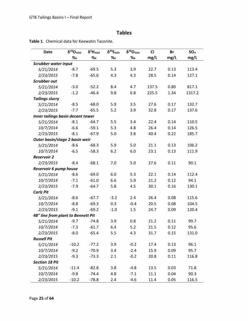
GTB Tailings Basins I – Final Report
Tables Table 1. Chemical data for Keewatin Taconite.
Date δ18OH2O δ2HH2O δ34SSO4 δ18OSO4 Cl Br SO4 ‰ ‰ ‰ ‰ mg/L mg/L mg/L
Scrubber water input
5/21/2014 -8.7 -69.5 5.3 3.9 22.7 0.13 113.4 2/23/2015 -7.8 -65.6 4.3 4.3 28.5 0.14 127.1
Scrubber out 5/21/2014 -3.0 -52.2 8.4 4.7 137.5 0.80 817.1 2/23/2015 -1.2 -46.4 9.8 6.8 225.5 1.34 1317.2
Tailings slurry 5/21/2014 -8.5 -68.0 5.9 3.5 27.6 0.17 132.7 2/23/2015 -7.7 -65.5 5.2 3.9 32.8 0.17 137.6
Inner tailings basin decant tower 5/21/2014 -8.1 -64.7 5.5 3.4 22.4 0.14 110.5 10/7/2014 -6.6 -59.1 5.3 4.8 26.4 0.14 126.5 2/23/2015 -8.1 -67.9 5.0 3.8 40.4 0.22 185.7
Outer basin/stage 2 basin weir 5/21/2014 -8.6 -68.3 5.9 5.0 21.1 0.13 106.2 10/7/2014 -6.5 -58.3 6.2 6.0 23.1 0.13 111.9
Reservoir 2
2/23/2015 -8.4 -68.1 7.0 5.0 27.6 0.11 90.1 Reservoir 6 pump house
5/21/2014 -8.6 -69.0 6.0 5.3 22.1 0.14 112.4 10/7/2014 -7.1 -61.0 6.6 5.9 21.2 0.12 94.1 2/23/2015 -7.9 -64.7 5.8 4.5 30.1 0.16 130.1
Carlz Pit 5/21/2014 -8.6 -67.7 -3.2 2.4 26.4 0.08 115.6 10/7/2014 -8.8 -69.3 0.3 -0.4 20.5 0.08 104.5 2/23/2015 -9.1 -69.2 -1.0 1.5 24.7 0.09 120.4
48" line from plant to Bennett Pit 5/21/2014 -9.7 -74.8 3.9 0.8 21.2 0.11 99.7 10/7/2014 -7.3 -61.7 6.4 5.2 21.5 0.12 95.6 2/23/2015 -8.0 -65.4 5.5 4.3 31.7 0.15 131.0
Russell Pit 5/21/2014 -10.2 -77.2 3.9 -0.2 17.4 0.13 96.1 10/7/2014 -9.2 -70.9 3.4 -2.4 15.9 0.09 95.7 2/23/2015 -9.3 -73.3 2.1 -0.2 20.8 0.11 116.8
Section 18 Pit 5/21/2014 -11.4 -82.8 3.8 -4.8 13.5 0.03 71.8 10/7/2014 -9.8 -74.4 4.8 -7.1 11.1 0.04 90.3 2/23/2015 -10.2 -78.8 2.4 -4.6 11.4 0.05 116.5
Page 25 of 64
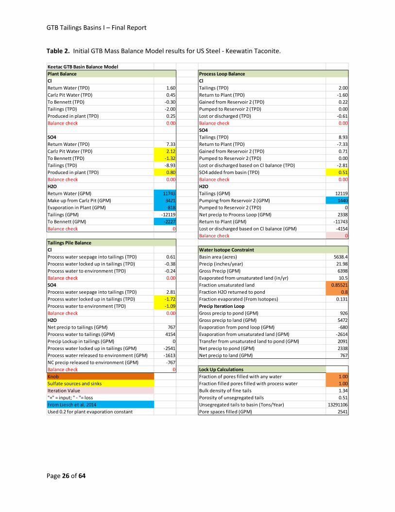
GTB Tailings Basins I – Final Report
Table 2. Initial GTB Mass Balance Model results for US Steel - Keewatin Taconite.
Keetac GTB Basin Balance ModelPlant Balance Process Loop BalanceCl ClReturn Water (TPD) 1.60 Tailings (TPD) 2.00Carlz Pit Water (TPD) 0.45 Return to Plant (TPD) -1.60To Bennett (TPD) -0.30 Gained from Reservoir 2 (TPD) 0.22Tailings (TPD) -2.00 Pumped to Reservoir 2 (TPD) 0.00Produced in plant (TPD) 0.25 Lost or discharged (TPD) -0.61Balance check 0.00 Balance check 0.00
SO4SO4 Tailings (TPD) 8.93Return Water (TPD) 7.33 Return to Plant (TPD) -7.33Carlz Pit Water (TPD) 2.12 Gained from Reservoir 2 (TPD) 0.71To Bennett (TPD) -1.32 Pumped to Reservoir 2 (TPD) 0.00Tailings (TPD) -8.93 Lost or discharged based on Cl balance (TPD) -2.81Produced in plant (TPD) 0.80 SO4 added from basin (TPD) 0.51Balance check 0.00 Balance check 0.00H2O H2OReturn Water (GPM) 11743 Tailings (GPM) 12119Make up from Carlz Pit (GPM) 3421 Pumping from Reservoir 2 (GPM) 1440Evaporation in Plant (GPM) -818 Pumped to Reservoir 2 (TPD) 0Tailings (GPM) -12119 Net precip to Process Loop (GPM) 2338To Bennett (GPM) -2227 Return to Plant (GPM) -11743Balance check 0 Lost or discharged based on Cl balance (GPM) -4154
Balance check 0Tailings Pile BalanceCl Water Isotope ConstraintProcess water seepage into tailings (TPD) 0.61 Basin area (acres) 5638.4Process water locked up in tailings (TPD) -0.38 Precip (inches/year) 21.98Process water to environment (TPD) -0.24 Gross Precip (GPM) 6398Balance check 0.00 Evaporated from unsaturated land (in/yr) 10.5SO4 Fraction unsaturated land 0.85521Process water seepage into tailings (TPD) 2.81 Fraction H2O returned to pond 0.8Process water locked up in tailings (TPD) -1.72 Fraction evaporated (From Isotopes) 0.131Process water to environment (TPD) -1.09 Precip Iteration LoopBalance check 0.00 Gross precip to pond (GPM) 926H2O Gross precip to land (GPM) 5472Net precip to tailings (GPM) 767 Evaporation from pond loop (GPM) -680Process water to tailings (GPM) 4154 Evaporation from unsaturated land (GPM) -2614Precip Lockup in tailings (GPM) 0 Transfer from unsaturated land to pond (GPM) 2091Process water locked up in tailings (GPM) -2541 Net precip to pond (GPM) 2338Process water released to environment (GPM) -1613 Net precip to land (GPM) 767NC precip released to environment (GPM) -767Balance check 0 Lock Up CalculationsKnob Fraction of pores filled with any water 1.00Sulfate sources and sinks Fraction filled pores filled with process water 1.00Iteration Value Bulk density of fine tails 1.34"+" = input; " - "= loss Porosity of unsegregated tails 0.51From Liesch et al, 2014 Unsegregated tails to basin (Tons/Year) 13291106Used 0.2 for plant evaporation constant Pore spaces filled (GPM) 2541
Page 26 of 64
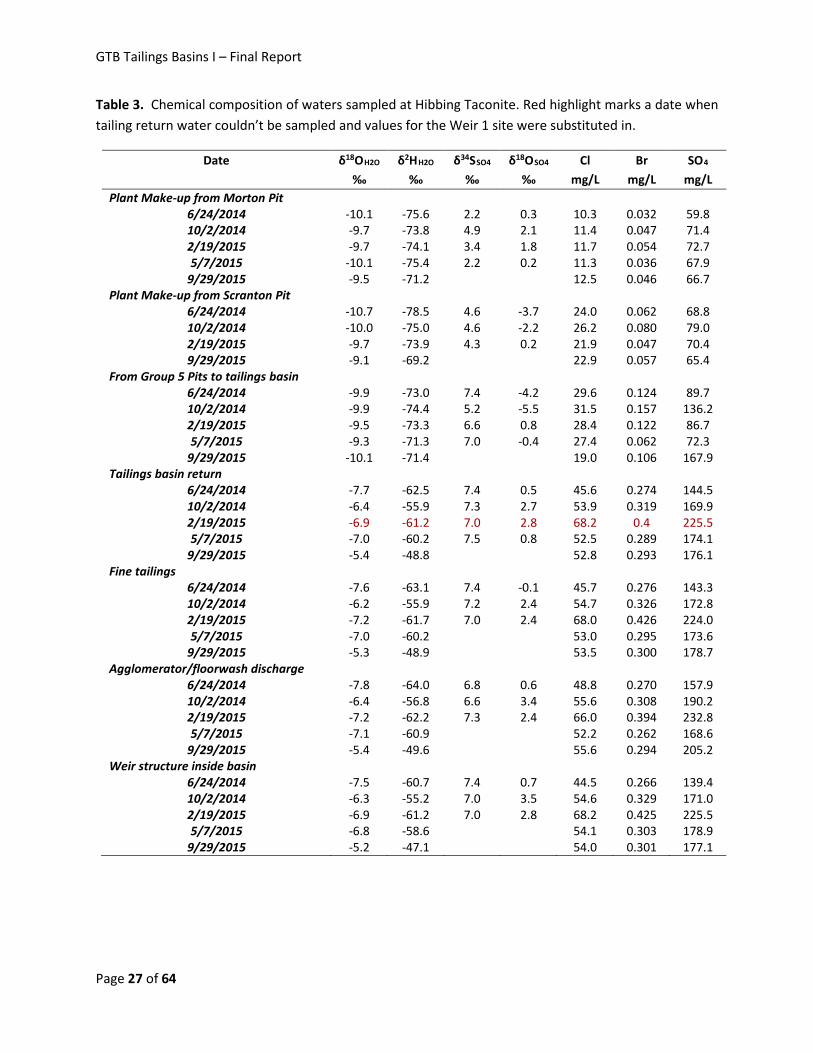
GTB Tailings Basins I – Final Report
Table 3. Chemical composition of waters sampled at Hibbing Taconite. Red highlight marks a date when tailing return water couldn’t be sampled and values for the Weir 1 site were substituted in.
Date δ18OH2O δ2HH2O δ34SSO4 δ18OSO4 Cl Br SO4 ‰ ‰ ‰ ‰ mg/L mg/L mg/L
Plant Make-up from Morton Pit 6/24/2014 -10.1 -75.6 2.2 0.3 10.3 0.032 59.8 10/2/2014 -9.7 -73.8 4.9 2.1 11.4 0.047 71.4 2/19/2015 -9.7 -74.1 3.4 1.8 11.7 0.054 72.7 5/7/2015 -10.1 -75.4 2.2 0.2 11.3 0.036 67.9
9/29/2015 -9.5 -71.2 12.5 0.046 66.7 Plant Make-up from Scranton Pit
6/24/2014 -10.7 -78.5 4.6 -3.7 24.0 0.062 68.8 10/2/2014 -10.0 -75.0 4.6 -2.2 26.2 0.080 79.0 2/19/2015 -9.7 -73.9 4.3 0.2 21.9 0.047 70.4 9/29/2015 -9.1 -69.2 22.9 0.057 65.4
From Group 5 Pits to tailings basin 6/24/2014 -9.9 -73.0 7.4 -4.2 29.6 0.124 89.7 10/2/2014 -9.9 -74.4 5.2 -5.5 31.5 0.157 136.2 2/19/2015 -9.5 -73.3 6.6 0.8 28.4 0.122 86.7 5/7/2015 -9.3 -71.3 7.0 -0.4 27.4 0.062 72.3
9/29/2015 -10.1 -71.4 19.0 0.106 167.9 Tailings basin return
6/24/2014 -7.7 -62.5 7.4 0.5 45.6 0.274 144.5 10/2/2014 -6.4 -55.9 7.3 2.7 53.9 0.319 169.9 2/19/2015 -6.9 -61.2 7.0 2.8 68.2 0.4 225.5 5/7/2015 -7.0 -60.2 7.5 0.8 52.5 0.289 174.1
9/29/2015 -5.4 -48.8 52.8 0.293 176.1 Fine tailings
6/24/2014 -7.6 -63.1 7.4 -0.1 45.7 0.276 143.3 10/2/2014 -6.2 -55.9 7.2 2.4 54.7 0.326 172.8 2/19/2015 -7.2 -61.7 7.0 2.4 68.0 0.426 224.0 5/7/2015 -7.0 -60.2 53.0 0.295 173.6
9/29/2015 -5.3 -48.9 53.5 0.300 178.7 Agglomerator/floorwash discharge
6/24/2014 -7.8 -64.0 6.8 0.6 48.8 0.270 157.9 10/2/2014 -6.4 -56.8 6.6 3.4 55.6 0.308 190.2 2/19/2015 -7.2 -62.2 7.3 2.4 66.0 0.394 232.8 5/7/2015 -7.1 -60.9 52.2 0.262 168.6
9/29/2015 -5.4 -49.6 55.6 0.294 205.2 Weir structure inside basin
6/24/2014 -7.5 -60.7 7.4 0.7 44.5 0.266 139.4 10/2/2014 -6.3 -55.2 7.0 3.5 54.6 0.329 171.0 2/19/2015 -6.9 -61.2 7.0 2.8 68.2 0.425 225.5 5/7/2015 -6.8 -58.6 54.1 0.303 178.9
9/29/2015 -5.2 -47.1 54.0 0.301 177.1
Page 27 of 64
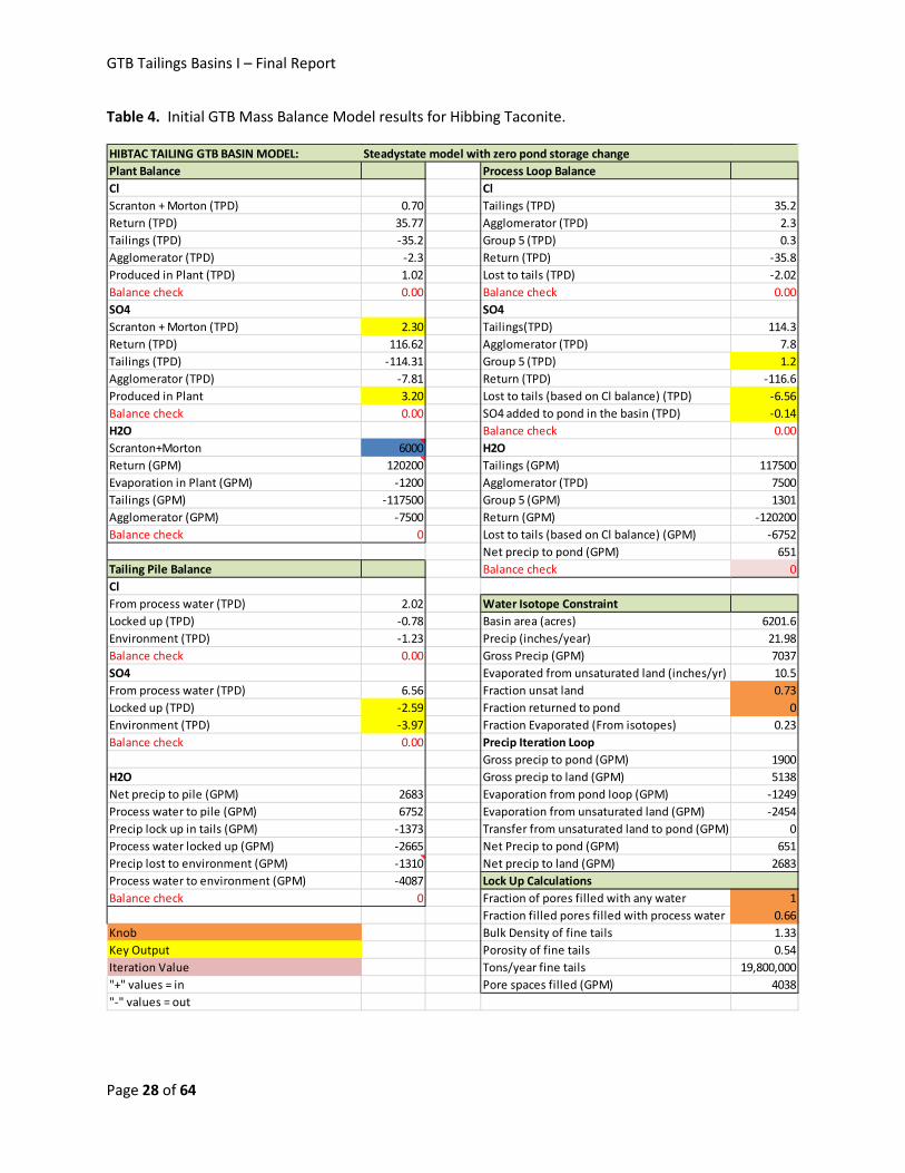
GTB Tailings Basins I – Final Report
Table 4. Initial GTB Mass Balance Model results for Hibbing Taconite.
HIBTAC TAILING GTB BASIN MODEL: Steadystate model with zero pond storage changePlant Balance Process Loop BalanceCl ClScranton + Morton (TPD) 0.70 Tailings (TPD) 35.2Return (TPD) 35.77 Agglomerator (TPD) 2.3Tailings (TPD) -35.2 Group 5 (TPD) 0.3Agglomerator (TPD) -2.3 Return (TPD) -35.8Produced in Plant (TPD) 1.02 Lost to tails (TPD) -2.02Balance check 0.00 Balance check 0.00SO4 SO4Scranton + Morton (TPD) 2.30 Tailings(TPD) 114.3Return (TPD) 116.62 Agglomerator (TPD) 7.8Tailings (TPD) -114.31 Group 5 (TPD) 1.2Agglomerator (TPD) -7.81 Return (TPD) -116.6Produced in Plant 3.20 Lost to tails (based on Cl balance) (TPD) -6.56Balance check 0.00 SO4 added to pond in the basin (TPD) -0.14H2O Balance check 0.00Scranton+Morton 6000 H2OReturn (GPM) 120200 Tailings (GPM) 117500Evaporation in Plant (GPM) -1200 Agglomerator (TPD) 7500Tailings (GPM) -117500 Group 5 (GPM) 1301Agglomerator (GPM) -7500 Return (GPM) -120200Balance check 0 Lost to tails (based on Cl balance) (GPM) -6752
Net precip to pond (GPM) 651Tailing Pile Balance Balance check 0ClFrom process water (TPD) 2.02 Water Isotope ConstraintLocked up (TPD) -0.78 Basin area (acres) 6201.6Environment (TPD) -1.23 Precip (inches/year) 21.98Balance check 0.00 Gross Precip (GPM) 7037SO4 Evaporated from unsaturated land (inches/yr) 10.5From process water (TPD) 6.56 Fraction unsat land 0.73Locked up (TPD) -2.59 Fraction returned to pond 0Environment (TPD) -3.97 Fraction Evaporated (From isotopes) 0.23Balance check 0.00 Precip Iteration Loop
Gross precip to pond (GPM) 1900H2O Gross precip to land (GPM) 5138Net precip to pile (GPM) 2683 Evaporation from pond loop (GPM) -1249Process water to pile (GPM) 6752 Evaporation from unsaturated land (GPM) -2454Precip lock up in tails (GPM) -1373 Transfer from unsaturated land to pond (GPM) 0Process water locked up (GPM) -2665 Net Precip to pond (GPM) 651Precip lost to environment (GPM) -1310 Net precip to land (GPM) 2683Process water to environment (GPM) -4087 Lock Up CalculationsBalance check 0 Fraction of pores filled with any water 1
Fraction filled pores filled with process water 0.66Knob Bulk Density of fine tails 1.33Key Output Porosity of fine tails 0.54Iteration Value Tons/year fine tails 19,800,000"+" values = in Pore spaces filled (GPM) 4038"-" values = out
Page 28 of 64

GTB Tailings Basins I – Final Report
Table 5. Chemical composition of waters sampled at U. S. Steel Minntac.
Date δ18OH2O δ2HH2O δ34SSO4 δ18OSO4 Cl Br SO4 ‰ ‰ ‰ ‰ mg/L mg/L mg/L
Mt. Iron Pit
5/28/2014 -10.2 -76.6 4.9 -6.9 29.5 0.11 365 10/8/2014 -10.7 -79.1 5.6 -6.8 28.6 0.11 343 2/24/2015 -10.5 -79.6 6.7 -7.3 32.0 0.14 411 5/13/2015 -10.8 -79.9 5.6 -8.7 31.1 0.10 401 10/7/2015 -10.6 -78.9 29.9 0.11 408 Scrubber makeup; raw water
5/28/2014 -8.5 -69.9 7.5 -1.6 119 0.90 740 2/24/2015 -7.9 -68.7 8.7 0.1 137 1.22 904 5/13/2015 -7.6 -66.2 139 1.07 862 10/7/2015 -7.2 -62.4 111 0.87 764 Composite tailings steps 1, 2, and 3
5/28/2014 -8.2 -69.0 7.3 -1.4 152 1.17 786 10/8/2014 -7.6 -66.3 8.5 -1.0 154 1.21 799 2/24/2015 -7.6 -67.9 8.7 0.1 170 1.58 949 5/13/2015 -7.4 -65.4 143 1.10 863 10/7/2015 -6.8 -61.4 137 1.12 797 Composite agglomerator steps 1/2 and 3
5/28/2014 -8.1 -68.9 7.1 -0.4 149 1.16 839 10/8/2014 -7.1 -65.2 9.2 -0.4 154 1.19 849 2/24/2015 -7.4 -66.9 8.8 0.4 165 1.51 990 5/13/2015 -6.8 -64.2 160 1.26 925 10/7/2015 -6.7 -60.7 138 1.13 848 Tailings basin Cell 2 5/28/2014 -8.2 -68.7 8.4 -1.2 129 1.00 844 10/8/2014 -6.8 -62.4 8.3 0.0 135 1.05 885 2/24/2015 -7.3 -65.2 8.9 2.1 164 1.50 1087 5/13/2015 -7.4 -64.7 8.5 -1.4 138 1.07 886 10/7/2015 -6.0 -56.2 145 1.14 933 Basin return water (Cell 1) 5/28/2014 -8.1 -68.1 7.7 -0.5 142 1.09 835 10/8/2014 -6.9 -62.9 8.5 -0.8 142 1.10 850 2/24/2015 -7.3 -65.8 8.7 0.5 163 1.49 1038 5/13/2015 -7.3 -64.4 8.5 -0.9 143 1.11 905 10/7/2015 -6.2 -57.4 147 1.15 923
Page 29 of 64
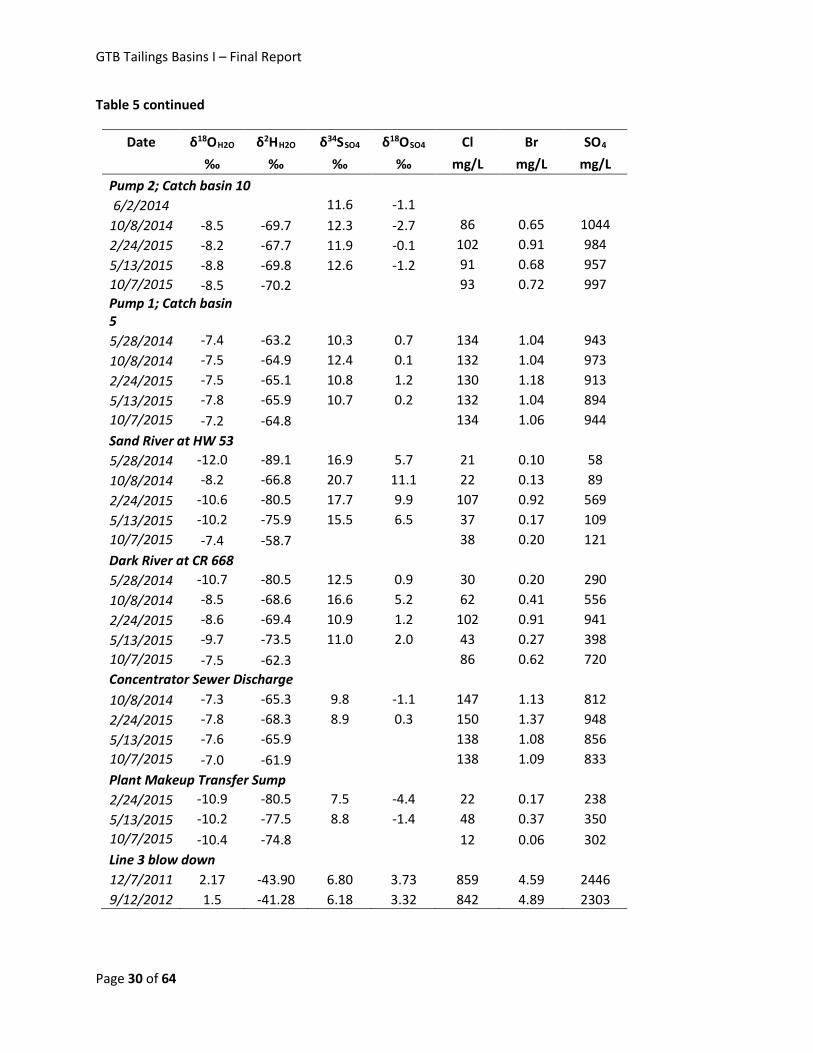
GTB Tailings Basins I – Final Report
Table 5 continued
Date δ18OH2O δ2HH2O δ34SSO4 δ18OSO4 Cl Br SO4 ‰ ‰ ‰ ‰ mg/L mg/L mg/L
Pump 2; Catch basin 10 6/2/2014 11.6 -1.1
10/8/2014 -8.5 -69.7 12.3 -2.7 86 0.65 1044 2/24/2015 -8.2 -67.7 11.9 -0.1 102 0.91 984 5/13/2015 -8.8 -69.8 12.6 -1.2 91 0.68 957 10/7/2015 -8.5 -70.2 93 0.72 997 Pump 1; Catch basin 5
5/28/2014 -7.4 -63.2 10.3 0.7 134 1.04 943 10/8/2014 -7.5 -64.9 12.4 0.1 132 1.04 973 2/24/2015 -7.5 -65.1 10.8 1.2 130 1.18 913 5/13/2015 -7.8 -65.9 10.7 0.2 132 1.04 894 10/7/2015 -7.2 -64.8 134 1.06 944 Sand River at HW 53
5/28/2014 -12.0 -89.1 16.9 5.7 21 0.10 58 10/8/2014 -8.2 -66.8 20.7 11.1 22 0.13 89 2/24/2015 -10.6 -80.5 17.7 9.9 107 0.92 569 5/13/2015 -10.2 -75.9 15.5 6.5 37 0.17 109 10/7/2015 -7.4 -58.7 38 0.20 121 Dark River at CR 668 5/28/2014 -10.7 -80.5 12.5 0.9 30 0.20 290 10/8/2014 -8.5 -68.6 16.6 5.2 62 0.41 556 2/24/2015 -8.6 -69.4 10.9 1.2 102 0.91 941 5/13/2015 -9.7 -73.5 11.0 2.0 43 0.27 398 10/7/2015 -7.5 -62.3 86 0.62 720 Concentrator Sewer Discharge 10/8/2014 -7.3 -65.3 9.8 -1.1 147 1.13 812 2/24/2015 -7.8 -68.3 8.9 0.3 150 1.37 948 5/13/2015 -7.6 -65.9 138 1.08 856 10/7/2015 -7.0 -61.9 138 1.09 833 Plant Makeup Transfer Sump
2/24/2015 -10.9 -80.5 7.5 -4.4 22 0.17 238 5/13/2015 -10.2 -77.5 8.8 -1.4 48 0.37 350 10/7/2015 -10.4 -74.8 12 0.06 302 Line 3 blow down 12/7/2011 2.17 -43.90 6.80 3.73 859 4.59 2446 9/12/2012 1.5 -41.28 6.18 3.32 842 4.89 2303
Page 30 of 64

GTB Tailings Basins I – Final Report
Table 6. Initial GTB Mass Balance Model results for U. S. Steel-Minntac.
Page 31 of 64
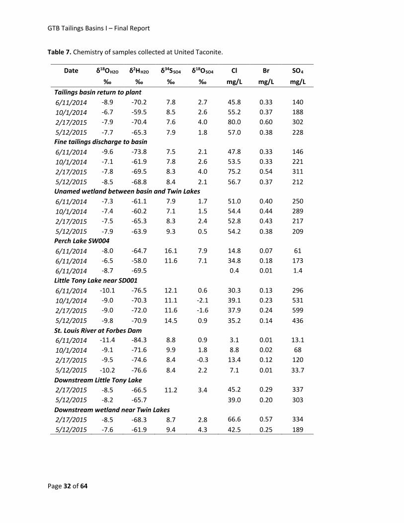
GTB Tailings Basins I – Final Report
Table 7. Chemistry of samples collected at United Taconite.
Date δ18OH2O δ2HH2O δ34SSO4 δ18OSO4 Cl Br SO4 ‰ ‰ ‰ ‰ mg/L mg/L mg/L
Tailings basin return to plant
6/11/2014 -8.9 -70.2 7.8 2.7 45.8 0.33 140 10/1/2014 -6.7 -59.5 8.5 2.6 55.2 0.37 188 2/17/2015 -7.9 -70.4 7.6 4.0 80.0 0.60 302 5/12/2015 -7.7 -65.3 7.9 1.8 57.0 0.38 228 Fine tailings discharge to basin 6/11/2014 -9.6 -73.8 7.5 2.1 47.8 0.33 146 10/1/2014 -7.1 -61.9 7.8 2.6 53.5 0.33 221 2/17/2015 -7.8 -69.5 8.3 4.0 75.2 0.54 311 5/12/2015 -8.5 -68.8 8.4 2.1 56.7 0.37 212 Unamed wetland between basin and Twin Lakes 6/11/2014 -7.3 -61.1 7.9 1.7 51.0 0.40 250 10/1/2014 -7.4 -60.2 7.1 1.5 54.4 0.44 289 2/17/2015 -7.5 -65.3 8.3 2.4 52.8 0.43 217 5/12/2015 -7.9 -63.9 9.3 0.5 54.2 0.38 209 Perch Lake SW004 6/11/2014 -8.0 -64.7 16.1 7.9 14.8 0.07 61 6/11/2014 -6.5 -58.0 11.6 7.1 34.8 0.18 173 6/11/2014 -8.7 -69.5 0.4 0.01 1.4 Little Tony Lake near SD001 6/11/2014 -10.1 -76.5 12.1 0.6 30.3 0.13 296 10/1/2014 -9.0 -70.3 11.1 -2.1 39.1 0.23 531 2/17/2015 -9.0 -72.0 11.6 -1.6 37.9 0.24 599 5/12/2015 -9.8 -70.9 14.5 0.9 35.2 0.14 436 St. Louis River at Forbes Dam 6/11/2014 -11.4 -84.3 8.8 0.9 3.1 0.01 13.1 10/1/2014 -9.1 -71.6 9.9 1.8 8.8 0.02 68 2/17/2015 -9.5 -74.6 8.4 -0.3 13.4 0.12 120 5/12/2015 -10.2 -76.6 8.4 2.2 7.1 0.01 33.7 Downstream Little Tony Lake 2/17/2015 -8.5 -66.5 11.2 3.4 45.2 0.29 337 5/12/2015 -8.2 -65.7 39.0 0.20 303 Downstream wetland near Twin Lakes 2/17/2015 -8.5 -68.3 8.7 2.8 66.6 0.57 334 5/12/2015 -7.6 -61.9 9.4 4.3 42.5 0.25 189
Page 32 of 64
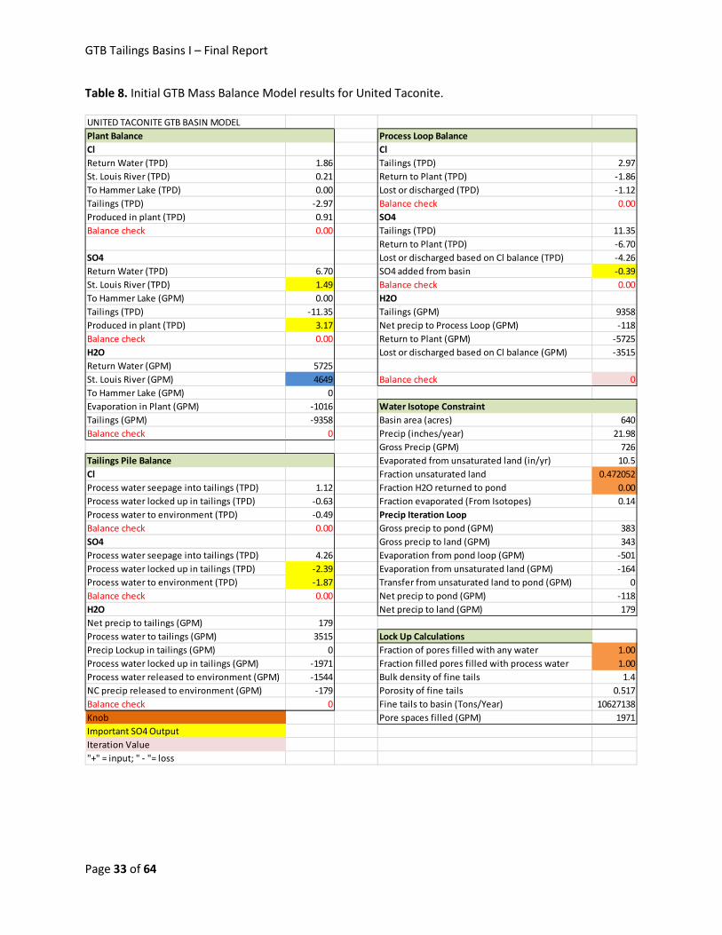
GTB Tailings Basins I – Final Report
Table 8. Initial GTB Mass Balance Model results for United Taconite.
UNITED TACONITE GTB BASIN MODELPlant Balance Process Loop BalanceCl ClReturn Water (TPD) 1.86 Tailings (TPD) 2.97St. Louis River (TPD) 0.21 Return to Plant (TPD) -1.86To Hammer Lake (TPD) 0.00 Lost or discharged (TPD) -1.12Tailings (TPD) -2.97 Balance check 0.00Produced in plant (TPD) 0.91 SO4Balance check 0.00 Tailings (TPD) 11.35
Return to Plant (TPD) -6.70SO4 Lost or discharged based on Cl balance (TPD) -4.26Return Water (TPD) 6.70 SO4 added from basin -0.39St. Louis River (TPD) 1.49 Balance check 0.00To Hammer Lake (GPM) 0.00 H2OTailings (TPD) -11.35 Tailings (GPM) 9358Produced in plant (TPD) 3.17 Net precip to Process Loop (GPM) -118Balance check 0.00 Return to Plant (GPM) -5725H2O Lost or discharged based on Cl balance (GPM) -3515Return Water (GPM) 5725St. Louis River (GPM) 4649 Balance check 0To Hammer Lake (GPM) 0Evaporation in Plant (GPM) -1016 Water Isotope ConstraintTailings (GPM) -9358 Basin area (acres) 640Balance check 0 Precip (inches/year) 21.98
Gross Precip (GPM) 726Tailings Pile Balance Evaporated from unsaturated land (in/yr) 10.5Cl Fraction unsaturated land 0.472052Process water seepage into tailings (TPD) 1.12 Fraction H2O returned to pond 0.00Process water locked up in tailings (TPD) -0.63 Fraction evaporated (From Isotopes) 0.14Process water to environment (TPD) -0.49 Precip Iteration LoopBalance check 0.00 Gross precip to pond (GPM) 383SO4 Gross precip to land (GPM) 343Process water seepage into tailings (TPD) 4.26 Evaporation from pond loop (GPM) -501Process water locked up in tailings (TPD) -2.39 Evaporation from unsaturated land (GPM) -164Process water to environment (TPD) -1.87 Transfer from unsaturated land to pond (GPM) 0Balance check 0.00 Net precip to pond (GPM) -118H2O Net precip to land (GPM) 179Net precip to tailings (GPM) 179Process water to tailings (GPM) 3515 Lock Up CalculationsPrecip Lockup in tailings (GPM) 0 Fraction of pores filled with any water 1.00Process water locked up in tailings (GPM) -1971 Fraction filled pores filled with process water 1.00Process water released to environment (GPM) -1544 Bulk density of fine tails 1.4NC precip released to environment (GPM) -179 Porosity of fine tails 0.517Balance check 0 Fine tails to basin (Tons/Year) 10627138Knob Pore spaces filled (GPM) 1971Important SO4 OutputIteration Value"+" = input; " - "= loss
Page 33 of 64
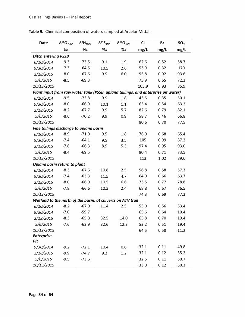
GTB Tailings Basins I – Final Report
Table 9. Chemical composition of waters sampled at Arcelor Mittal.
Date δ18OH2O δ2HH2O δ34SSO4 δ18OSO4 Cl Br SO4 ‰ ‰ ‰ ‰ mg/L mg/L mg/L
Ditch entering PSSB
6/10/2014 -9.3 -73.5 9.1 1.9 62.6 0.52 58.7 9/30/2014 -7.3 -64.5 10.5 2.6 53.9 0.32 170 2/18/2015 -8.0 -67.6 9.9 6.0 95.8 0.92 93.6 5/6/2015 -8.5 -69.3 75.9 0.65 72.2
10/13/2015 105.9 0.93 85.9 Plant input from raw water tank (PSSB, upland tailings, and enterprise pit water) 6/10/2014 -9.5 -73.8 9.9 1.8 43.5 0.35 50.1 9/30/2014 -8.0 -66.9 10.1 1.1 63.4 0.54 63.2 2/18/2015 -8.2 -67.7 9.9 5.7 82.6 0.79 82.1 5/6/2015 -8.6 -70.2 9.9 0.9 58.7 0.46 66.8
10/13/2015 80.6 0.70 77.5 Fine tailings discharge to upland basin 6/10/2014 -8.9 -71.0 9.5 1.8 76.0 0.68 65.4 9/30/2014 -7.4 -64.1 9.5 3.5 105 0.99 87.2 2/18/2015 -7.8 -66.3 8.9 5.3 97.4 0.95 93.0 5/6/2015 -8.4 -69.5 80.4 0.71 73.5
10/13/2015 113 1.02 89.6 Upland basin return to plant 6/10/2014 -8.3 -67.6 10.8 2.5 56.8 0.58 57.3 9/30/2014 -7.4 -63.3 11.5 4.7 64.0 0.66 63.7 2/18/2015 -8.0 -66.0 10.5 6.6 73.5 0.77 78.8 5/6/2015 -7.8 -66.6 10.3 2.4 68.8 0.67 76.5
10/13/2015 74.3 0.69 77.2 Wetland to the north of the basin; at culverts on ATV trail 6/10/2014 -8.2 -67.0 11.4 2.5 55.0 0.56 53.4 9/30/2014 -7.0 -59.7 65.6 0.64 10.4 2/18/2015 -8.3 -65.8 32.5 14.0 65.8 0.70 19.4 5/6/2015 -7.6 -63.9 32.6 12.3 53.2 0.51 19.4
10/13/2015 64.5 0.58 11.2 Enterprise Pit 9/30/2014 -9.2 -72.1 10.4 0.6 32.1 0.11 49.8 2/18/2015 -9.9 -74.7 9.2 1.2 32.1 0.12 55.2 5/6/2015 -9.5 -73.6 32.5 0.11 50.7
10/13/2015 33.0 0.12 50.3
Page 34 of 64
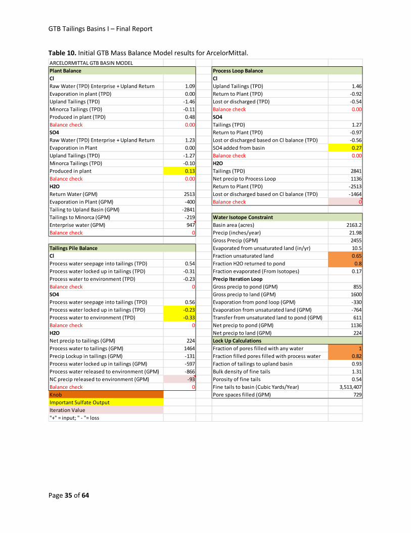
GTB Tailings Basins I – Final Report
Table 10. Initial GTB Mass Balance Model results for ArcelorMittal.
ARCELORMITTAL GTB BASIN MODELPlant Balance Process Loop BalanceCl ClRaw Water (TPD) Enterprise + Upland Return 1.09 Upland Tailings (TPD) 1.46Evaporation in plant (TPD) 0.00 Return to Plant (TPD) -0.92Upland Tailings (TPD) -1.46 Lost or discharged (TPD) -0.54Minorca Tailings (TPD) -0.11 Balance check 0.00Produced in plant (TPD) 0.48 SO4Balance check 0.00 Tailings (TPD) 1.27SO4 Return to Plant (TPD) -0.97Raw Water (TPD) Enterprise + Upland Return 1.23 Lost or discharged based on Cl balance (TPD) -0.56Evaporation in Plant 0.00 SO4 added from basin 0.27Upland Tailings (TPD) -1.27 Balance check 0.00Minorca Tailings (TPD) -0.10 H2OProduced in plant 0.13 Tailings (TPD) 2841Balance check 0.00 Net precip to Process Loop 1136H2O Return to Plant (TPD) -2513Return Water (GPM) 2513 Lost or discharged based on Cl balance (TPD) -1464Evaporation in Plant (GPM) -400 Balance check 0Tailing to Upland Basin (GPM) -2841Tailings to Minorca (GPM) -219 Water Isotope ConstraintEnterprise water (GPM) 947 Basin area (acres) 2163.2Balance check 0 Precip (inches/year) 21.98
Gross Precip (GPM) 2455Tailings Pile Balance Evaporated from unsaturated land (in/yr) 10.5Cl Fraction unsaturated land 0.65Process water seepage into tailings (TPD) 0.54 Fraction H2O returned to pond 0.8Process water locked up in tailings (TPD) -0.31 Fraction evaporated (From Isotopes) 0.17Process water to environment (TPD) -0.23 Precip Iteration LoopBalance check 0 Gross precip to pond (GPM) 855SO4 Gross precip to land (GPM) 1600Process water seepage into tailings (TPD) 0.56 Evaporation from pond loop (GPM) -330Process water locked up in tailings (TPD) -0.23 Evaporation from unsaturated land (GPM) -764Process water to environment (TPD) -0.33 Transfer from unsaturated land to pond (GPM) 611Balance check 0 Net precip to pond (GPM) 1136H2O Net precip to land (GPM) 224Net precip to tailings (GPM) 224 Lock Up CalculationsProcess water to tailings (GPM) 1464 Fraction of pores filled with any water 1Precip Lockup in tailings (GPM) -131 Fraction filled pores filled with process water 0.82Process water locked up in tailings (GPM) -597 Faction of tailings to upland basin 0.93Process water released to environment (GPM) -866 Bulk density of fine tails 1.31NC precip released to environment (GPM) -93 Porosity of fine tails 0.54Balance check 0 Fine tails to basin (Cubic Yards/Year) 3,513,407Knob Pore spaces filled (GPM) 729Important Sulfate OutputIteration Value"+" = input; " - "= loss
Page 35 of 64
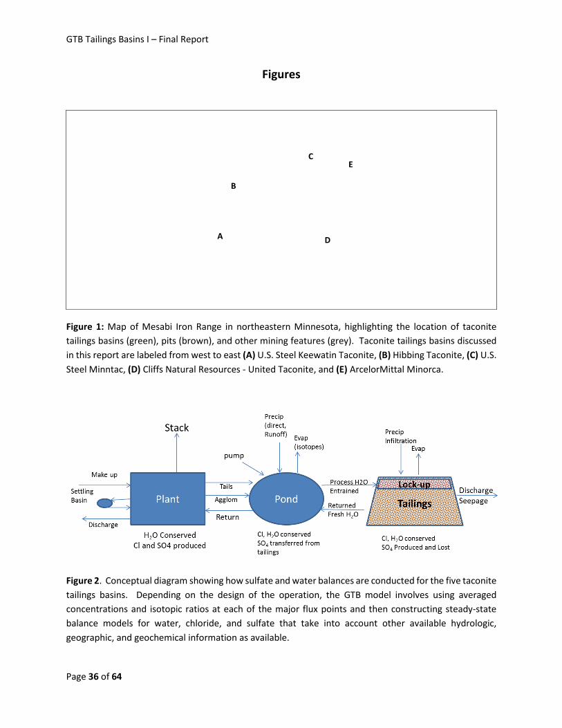
GTB Tailings Basins I – Final Report
Figures
Figure 1: Map of Mesabi Iron Range in northeastern Minnesota, highlighting the location of taconite tailings basins (green), pits (brown), and other mining features (grey). Taconite tailings basins discussed in this report are labeled from west to east (A) U.S. Steel Keewatin Taconite, (B) Hibbing Taconite, (C) U.S. Steel Minntac, (D) Cliffs Natural Resources - United Taconite, and (E) ArcelorMittal Minorca.
Figure 2. Conceptual diagram showing how sulfate and water balances are conducted for the five taconite tailings basins. Depending on the design of the operation, the GTB model involves using averaged concentrations and isotopic ratios at each of the major flux points and then constructing steady-state balance models for water, chloride, and sulfate that take into account other available hydrologic, geographic, and geochemical information as available.
A
B
C
D
E
Page 36 of 64
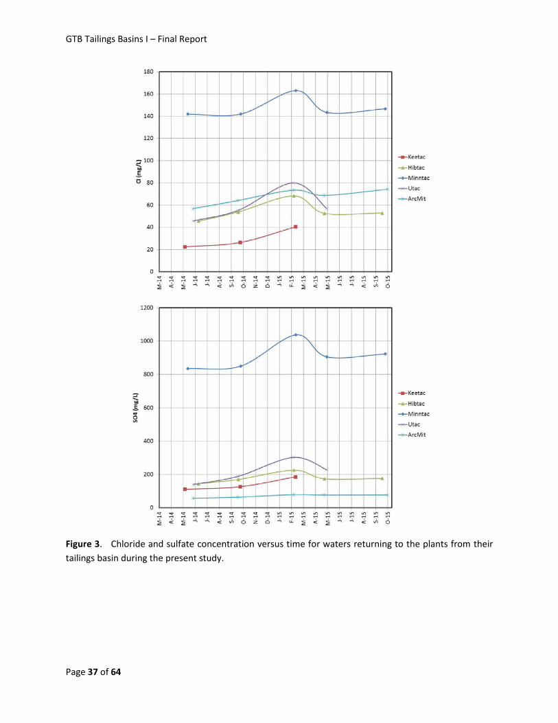
GTB Tailings Basins I – Final Report
Figure 3. Chloride and sulfate concentration versus time for waters returning to the plants from their tailings basin during the present study.
Page 37 of 64
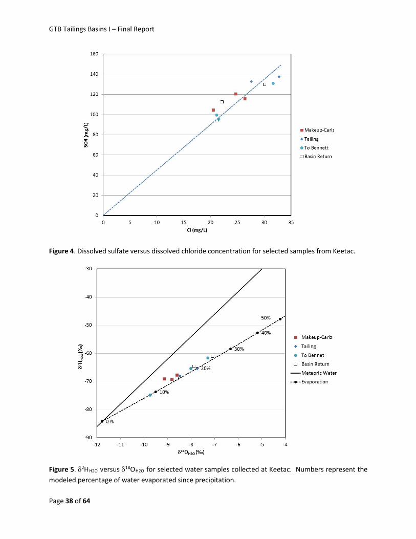
GTB Tailings Basins I – Final Report
Figure 4. Dissolved sulfate versus dissolved chloride concentration for selected samples from Keetac.
Figure 5. δ2HH2O versus δ18OH2O for selected water samples collected at Keetac. Numbers represent the modeled percentage of water evaporated since precipitation.
Page 38 of 64
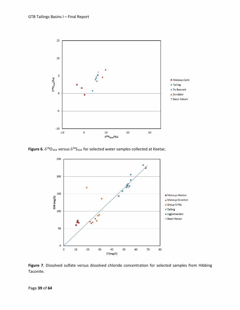
GTB Tailings Basins I – Final Report
Figure 6. δ18OSO4 versus δ34SSO4 for selected water samples collected at Keetac.
Figure 7. Dissolved sulfate versus dissolved chloride concentration for selected samples from Hibbing Taconite.
Page 39 of 64
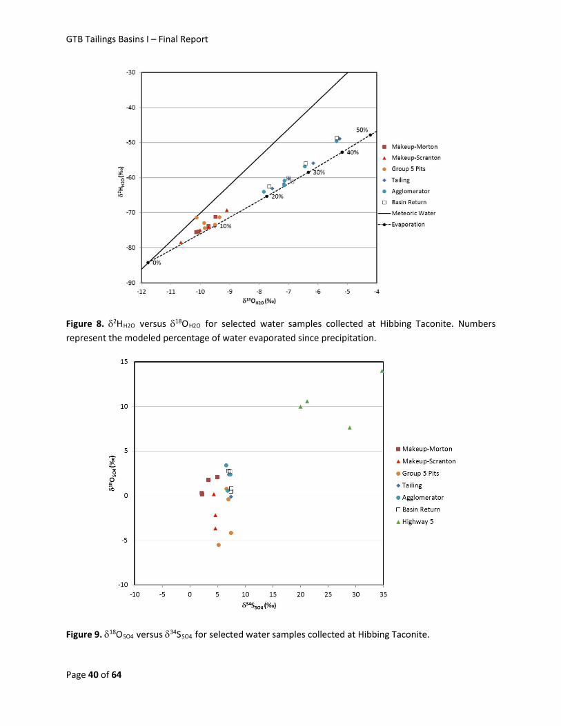
GTB Tailings Basins I – Final Report
Figure 8. δ2HH2O versus δ18OH2O for selected water samples collected at Hibbing Taconite. Numbers represent the modeled percentage of water evaporated since precipitation.
Figure 9. δ18OSO4 versus δ34SSO4 for selected water samples collected at Hibbing Taconite.
Page 40 of 64
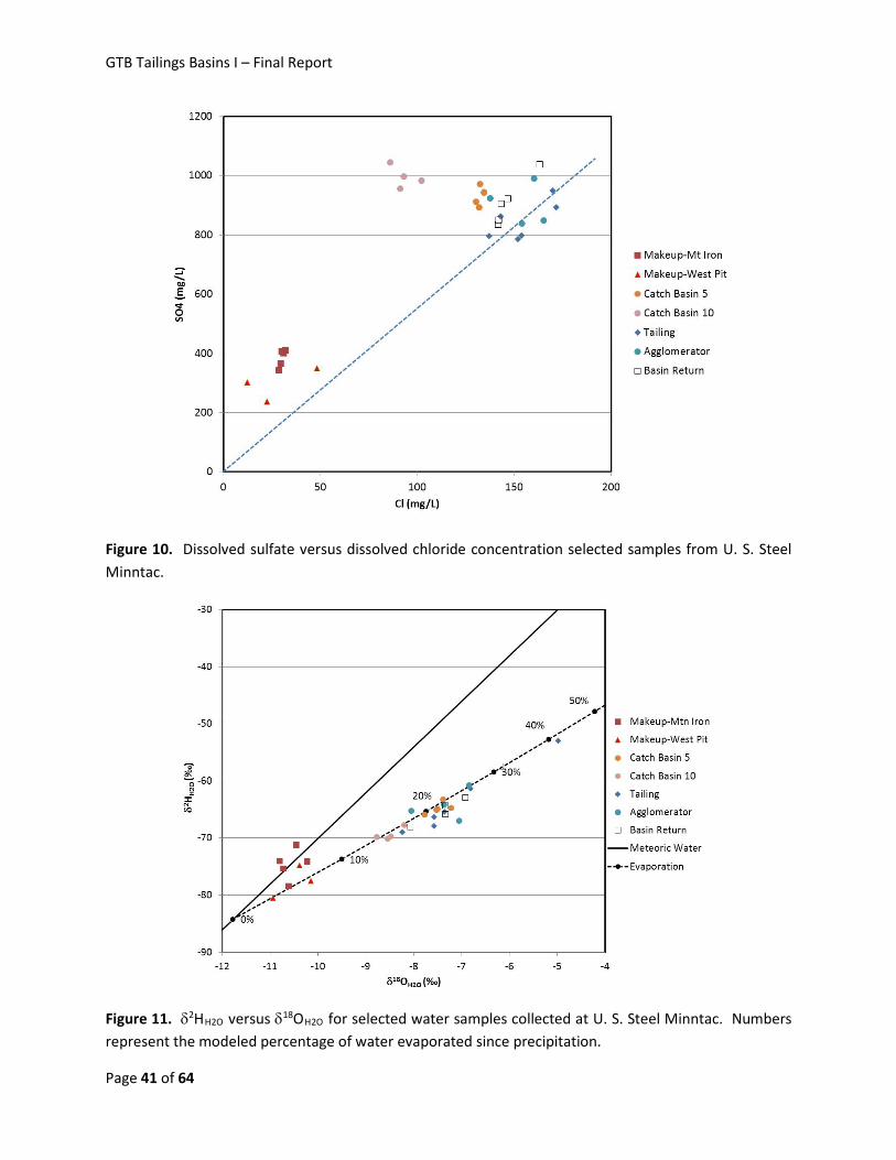
GTB Tailings Basins I – Final Report
Figure 10. Dissolved sulfate versus dissolved chloride concentration selected samples from U. S. Steel Minntac.
Figure 11. δ2HH2O versus δ18OH2O for selected water samples collected at U. S. Steel Minntac. Numbers represent the modeled percentage of water evaporated since precipitation.
Page 41 of 64
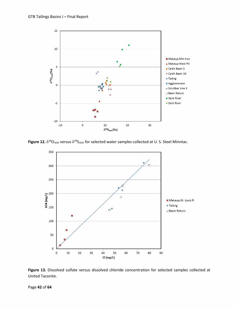
GTB Tailings Basins I – Final Report
Figure 12. δ18OSO4 versus δ34SSO4 for selected water samples collected at U. S. Steel Minntac.
Figure 13. Dissolved sulfate versus dissolved chloride concentration for selected samples collected at United Taconite.
Page 42 of 64

GTB Tailings Basins I – Final Report
Figure 14. δ2HH2O versus δ18OH2O for selected water samples collected at United Taconite. Numbers represent the modeled percentage of water evaporated since precipitation.
Figure 15. δ18OSO4 versus δ34SSO4 for selected water samples collected at United Taconite.
Page 43 of 64
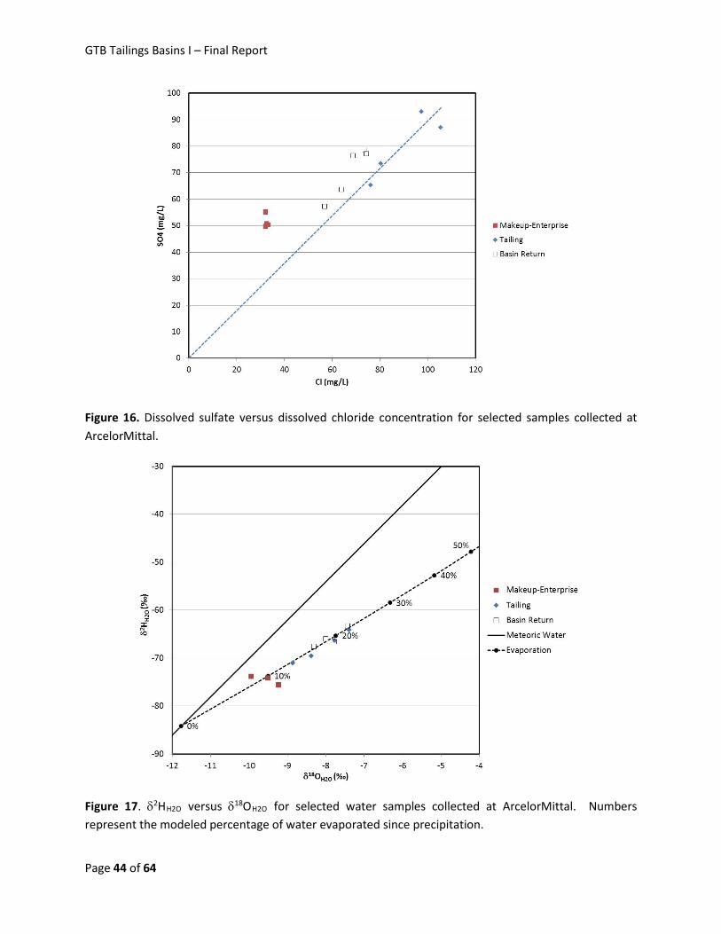
GTB Tailings Basins I – Final Report
Figure 16. Dissolved sulfate versus dissolved chloride concentration for selected samples collected at ArcelorMittal.
Figure 17. δ2HH2O versus δ18OH2O for selected water samples collected at ArcelorMittal. Numbers represent the modeled percentage of water evaporated since precipitation.
Page 44 of 64
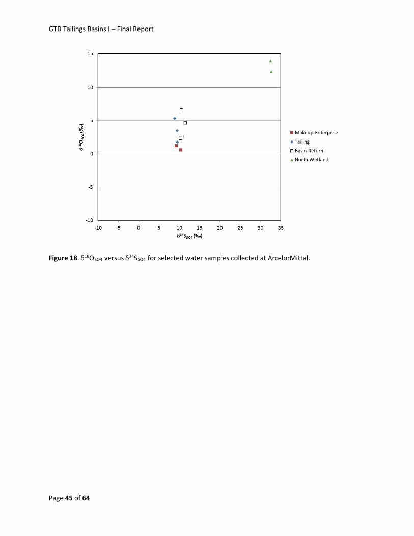
GTB Tailings Basins I – Final Report
Figure 18. δ18OSO4 versus δ34SSO4 for selected water samples collected at ArcelorMittal.
Page 45 of 64
GTB Tailings Basins I – Final Report
References Bavin, T., Koski, S., Jacobs, C., Berndt, M., and Kelly, M. (2016). Physical and Hydrologic Properties of Taconite Tailings. Minnesota Department of Natural Resources Research Report. 50 p.
Berndt, M. E., and Koski, S. (2016). Pore-Gas Oxygen Concentrations in Taconite Tailings: Initial Test Results. A Minnesota Department of Natural Resources Research Memo. 7 pages.
Berndt, M., Bavin, T., Koski, S., Jacobs, C., and Kelly, M. (2016). Geochemical Tracer Based (GTB) Models for Active Tailings basins on Minnesota’s Iron Range (II) Field Based Sulfate Release Rates for Coarse and Fine Tailings. Minnesota Department of Natural Resources Report. 51 p.
Carmody, R. W., Plummer, L. N., Busenberg, E., Coplen, T. B., (1998). Methods for collection of dissolved sulfate and sulfide and analysis of their sulfur isotopic composition. U.S. Geological Survey Open-File Report 97-234.
Gammons, C. H., Poulson, S. R., Pellicori, D. A., Reed, P. J., Roesler, A. J., Petrescu, E. M. (2006). The hydrogen and oxygen isotopic composition of precipitation, evaporated mine water, and river water in Montana, USA. Journal of Hydrology 328, 319-330.
Jacobs, C., Koski, S., Bavin, T., and Berndt, M. (2016) Sulfur concentrations and pyrite textures in coarse and fine taconite tailings exposed to the elements for 0 to 30 years, 2016. A Minnesota Department of Natural Resources Research Report. 90 pages.
Kelly, M. J. (2013). A water isotope-based evaporation model for US Steel’s Minntac Tailings Basin. A Minnesota Department of Natural Resources Memo. 12 pages. (Attached in Appendix 2).
Kelly, M., Berndt, M., and Bavin, T. (2014) Use of sulfate and water isotopes to improve water and chemical balance estimates for water seeping from tailings basins (Focus on U.S. Steel’s Minntac Basin). A Minnesota DNR Research Report. 31. p. Available at: http://files.dnr.state.mn.us/lands_minerals/reclamation/kelly_et_al_2014.pdf
Kelly, M. J, Berndt M. E., Bavin, T. K. and Koski, S. R. (2016a). Geochemical Tracer Based (GTB) Sulfate Balance Models (III) Well Waters, Seeps, and Downstream Surface Waters. Minnesota Department of Natural Resources Research Report. _ Pages.
Kelly, M., Koski, S., Jacobs, and Berndt, M. (2016b). Sonic Drilling at the Minntac Tailings Basin: Project Status. 20 Pages.
Liesch Associates, Inc. (2014). Keetac Water Balance Report August 2011-August 2013. 25 p. Plus Tables and Figures.
Ng, G.-H. Crystal, O’Hara, P., and Yourd, A. (2016). Development of a Reactive Sulfate Transport Model for a Minnesota Taconite Tailings Basin (Minntac). University of Minnesota Report to the Minnesota Department of Natural Resources. 28 Pages.
Page 46 of 64

GTB Tailings Basins I – Final Report
Von Korff, B. and Bavin, T. (2014). Short Term Sulfate Release Rates and Sulfide Oxidation Mechanisms for Taconite Tailings from the Minntac and Keetac Mining Facilities. Minnesota Department of Natural Resources Report, 48 pages.
Page 47 of 64
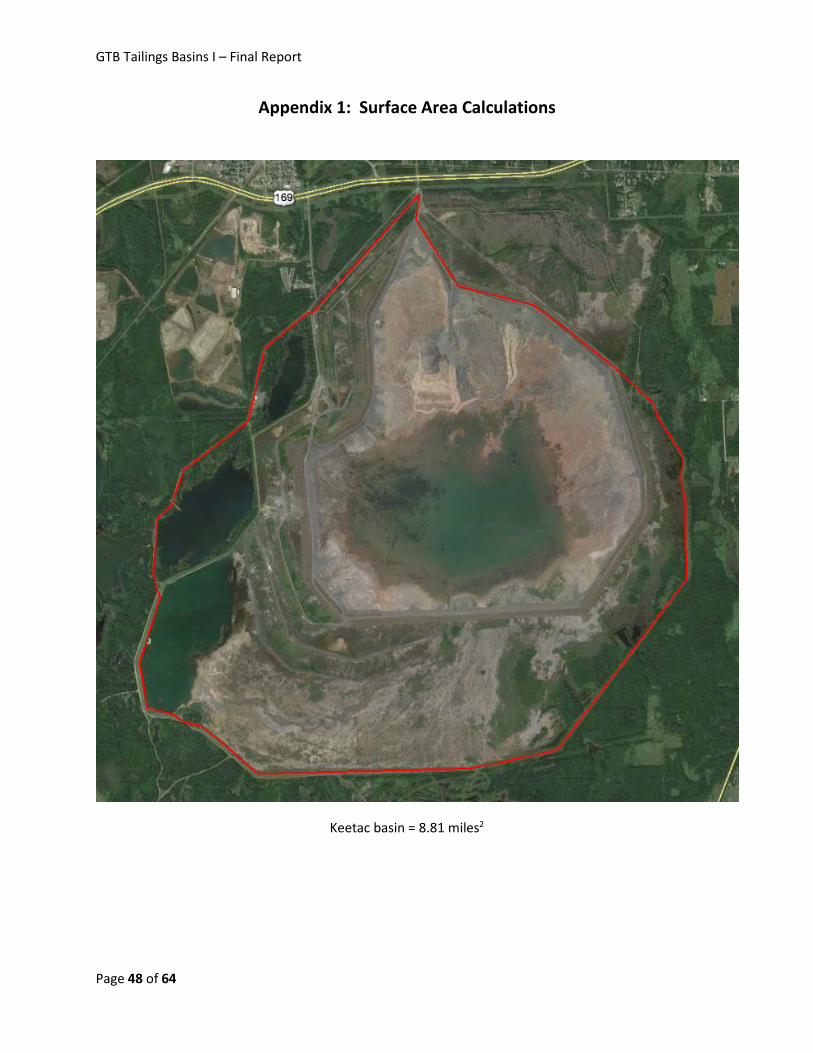
GTB Tailings Basins I – Final Report
Appendix 1: Surface Area Calculations
Keetac basin = 8.81 miles2
Page 48 of 64
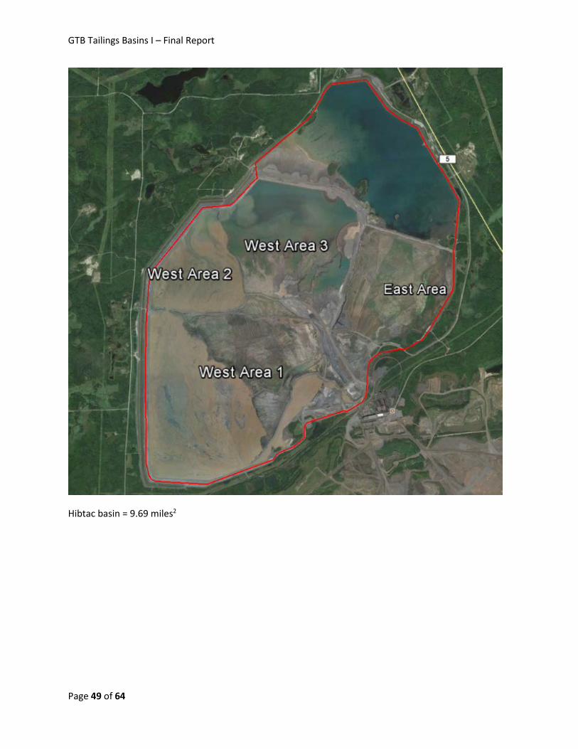
GTB Tailings Basins I – Final Report
Hibtac basin = 9.69 miles2
Page 49 of 64
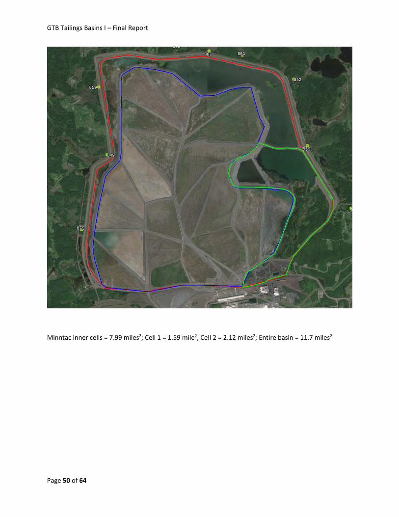
GTB Tailings Basins I – Final Report
Minntac inner cells = 7.99 miles2; Cell 1 = 1.59 mile2, Cell 2 = 2.12 miles2; Entire basin = 11.7 miles2
Page 50 of 64
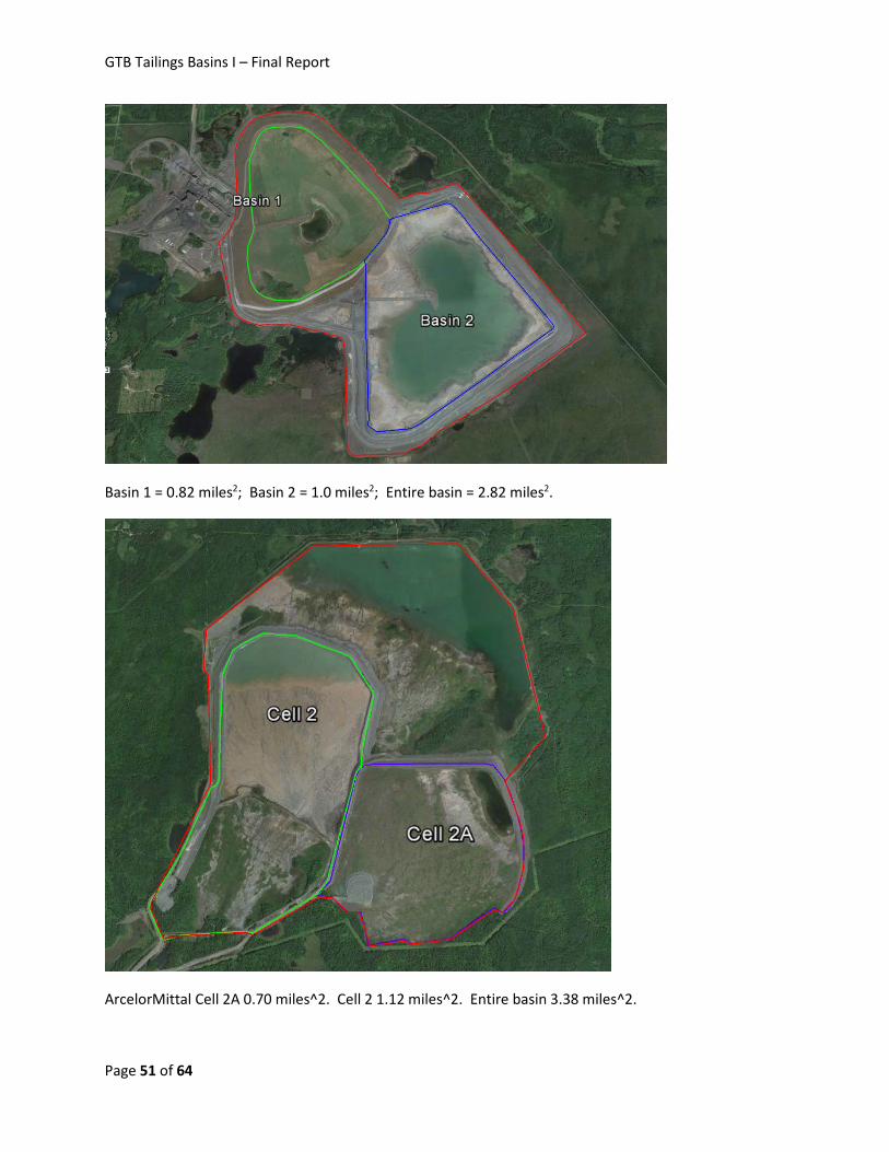
GTB Tailings Basins I – Final Report
Basin 1 = 0.82 miles2; Basin 2 = 1.0 miles2; Entire basin = 2.82 miles2.
ArcelorMittal Cell 2A 0.70 miles^2. Cell 2 1.12 miles^2. Entire basin 3.38 miles^2.
Page 51 of 64
GTB Tailings Basins I – Final Report
Appendix 2. A Water Isotope-Based Evaporation Model for US Steel’s Minntac Tailings Basin
Megan J. Kelly
A Minnesota Department of Natural Resources Memo
December 3, 2013
An accurate estimate of evaporative loss is critical for any mine water balance calculation. This component, however, is often difficult to determine directly. The Minnesota Department of Natural Resources is addressing this difficulty by using a water isotope mass balance model to quantify the evaporation/inflow ratio (E/I) for tailings basin water. This type of model is based on experimentally and theoretically derived relationships between the liquid and vapor phase during evaporation, and requires relatively few measurements to gain an important piece of information. This memo describes the scientific basis for use of the isotope-based evaporation model, along with a case study from US Steel’s Minntac Tailings Basin.
Isotope Model Background
Hydrogen and oxygen isotopes of water are extremely valuable in hydrological studies, as they can be used to define water sources, evaluate mixing of different water sources, and determine the impact of evaporation on a water body. The fractionation, or partitioning, of heavy and light isotopes between different phases or reservoirs can impart distinct and characteristic isotopic signatures, allowing us to trace movement and processes that have affected a water body over time. Fractionation between the liquid phase and the vapor phase of water is described by the fractionation factor, α, where
α = [18O/16O]L/[18O/16O]V (1)
The isotopic values themselves are reported as delta (δ) values, in per mil (‰) units relative to a standard.
δ18O (‰) = [(18O/16Osample)/(18O/16O)standard - 1] x1000 (2)
Comparable equations apply for 2H/1H as well. Under equilibrium conditions, the fractionation effect is a function of temperature. We can calculate the fractionation factor between liquid water and vapor at any given temperature between 0 and 100°C using the following, experimentally derived equations (Majoube, 1971):
For oxygen (where T is in Kelvin): ln αl-v = (1137/T2) – (0.4156/T) – 0.00207 (3)
Page 52 of 64
GTB Tailings Basins I – Final Report
For hydrogen: ln αl-v = (24844/T2) – (76.248/T) + 0.052612 (4)
Isotope fractionation is typically very small. A related term, the isotope separation factor (ε), describes fractionation effects in terms of the deviation from 1, and is multiplied by 1000 to put the value in more convenient per mil (‰) units.
ε = 1000 (α l-v-1) ≈ δL - δV (5) This value also approximates the difference in delta (δ) values between the two phases. A global survey of the isotopic composition of meteoric waters by Craig (1961) demonstrated that the values fall on a tight line in δ2H vs. δ18O space with a slope of ~8 (see Figure 1). This line is referred to as the Global Meteoric Water Line (GMWL) and serves as a reference for numerous and varied studies of the global water cycle. Condensation of water vapor from an air mass as precipitation is an equilibrium process, where heavy isotopes are preferentially rained out due to their lower saturation vapor pressure. Latitude and elevation affect where the δ2H and δ18O of precipitation plots along the GMWL, as well as seasonal conditions and air mass history. Mean annual precipitation (MAP) at any particular location, however, tends to be relatively stable.
Fractionation during evaporation is also partially controlled by equilibrium effects due to the mass-related differences in vapor pressure; heavy molecules with lower vapor pressure are less likely to enter the vapor phase during evaporation. Therefore, water bodies that have undergone evaporation are enriched in the heavy isotopes of both hydrogen and oxygen relative to the source water. Furthermore, the isotopic signature of an evaporated source will generally plot below the GMWL on a trend with a shallower slope, referred to as the Local Evaporation Line (LEL, Figure 1). Evaporation imparts an additional kinetic fractionation effect due to molecular diffusion and turbulent transport of evaporated moisture across the water/air interface. Kinetic fractionation effects are dependent on local climate conditions, particularly the ambient relative humidity. For evaporation from small bodies of water, the kinetic effect can be described by the following relationships (Merlivat, 1978; Gonfiantini, 1986).
εk = 14.2 (1-h) (6) εk = 12.5(1-h) (7)
With decreasing relative humidity, the kinetic fractionation between liquid and vapor increases and the slope LEL decreases. Typically, LEL slopes range between ~4 and 7 (Gat, 1971). The intersection of the LEL trend with the GMWL represents the composition of average recharge water, usually close to the annual average composition of local precipitation. As the impact of evaporation increases, the isotopic signature of the water body is pulled along the evaporation trend, further away from the intersection point. The total fractionation (εtot) during evaporation is equivalent to the sum of ε and εk.
Page 53 of 64
GTB Tailings Basins I – Final Report
Various aspects of a lake’s water balance can be examined using a combined water and isotope mass balance approach (i.e. Gibson et al., 1993; Gibson et al., 2002; Gammons et al., 2006), including the amount of vapor outflow (i.e. evaporative flux). The balance can be represented as follows:
d(VδL)/dt = IδI – QδQ – EδE (8)
Where V is lake volume, t is time, I=inflow, and δI is typically close to the isotopic composition of mean annual precipitation, Q=outflow, with δQ equivalent to the composition of lake water (δL), and E=vapor outflow, where δE represents the composition of moisture evaporated from the lake. Under hydrological steady state conditions, volume remains relatively constant and thus dV/dt is approximately 0. By substituting and rearranging equation 8, it is possible to solve for the fraction of input water lost to evaporation,
E/I = (δI - δL)/(δE - δL) (9) According to mass balance requirements, the initial water composition, the evaporated moisture, and the residual water must all plot along the same line (Figure 1). The composition of residual lake water in response to evaporation will depend on the composition of the evaporated moisture, which in turn is affected by climate variables and ambient vapor composition. However, it is difficult to determine the isotopic composition of evaporated moisture directly. To address this complication, Craig and Gordon (1965) developed a theoretical model for the isotopic composition of evaporated moisture:
δE = (α*δL - hδA – εtot)/(1 - h + εk/1000) (10) δA represents the isotopic composition of atmospheric moisture in equilibrium with precipitation, which can be estimated using the relationship
δA = δp – ε (11) The relationship between δA and δp is often not a purely equilibrium process (see Clark and Fritz, 1997), but the above approximation is considered reasonable for long term averages (Jacob and Sonntag, 1991). Using equations 9 and 10, we can solve for E/I using information that is relatively easy to obtain. The equations can be modified for various desired outcomes as follows:
E/I = (δL – δI) /m(δ* – δL) (12) or
δL = (δI + Xmδ*)/(1 + Xm) (13) where m is the enrichment slope,
m = (h – 10-3ε)/(1 – h + 10-3εk) (14)
Page 54 of 64
GTB Tailings Basins I – Final Report
and δ* is the limiting isotope enrichment,
δ* = (hδA + ε)/(h-10-3ε) (15) representing the isotopic composition of a water body as is evaporates to dryness.
Minntac Study The MN DNR applied the above model to a study of the Minntac tailings basin. A total of 35 water samples from plant processing, tailings basin, pit source, monitoring wells, and two downstream sites were collected on three occasions during 2011-2012. The first sampling trip took place in December, 2011, and included Mountain Iron Pit, a number of plant process waters (scrubber, blowdown, thickener, agglomerator process water, fine tails), Cell 1 basin return water, two seepage collection sites on the east side of the basin, and downstream on the Sand River. A similar set of samples was collected on September 12, 2012, with the addition of Cell 2 water, two monitoring wells on the east side of the basin, and a downstream site on the Dark River, which runs from the west side of the basin. We returned in late October to sample an additional suite of 8 monitoring wells surrounding the basin (see Figure 2)
All water isotope samples collected in 2012 were filtered using a 0.45 µm membrane filter and stored unpreserved in 30 mL HDPE bottles until shipped to University of Waterloo Environmental Isotope Lab for analysis. Bottles were tightly sealed with limited headspace to minimize further evaporative loss. Samples obtained in 2011 were collected in 1L bottles for both water and sulfate isotope analysis. The 1L samples were filtered in the Hibbing laboratory using 0.7 µm glass fiber filters and sent to the University of Waterloo for analysis. Water isotope samples were analyzed using standard isotope ratio mass spectrometry methods. 18O/16O abundance is determined via gas equilibration and head space injection into an IsoPrime Continuous Flow Isotope Ratio Mass Spectrometer (CF-IRMS). 2H/1H is determined via chromium reduction on a EuroVector Elemental analyzer coupled with an IsoPrime CF-IRMS. Internal laboratory standards are calibrated and tested against international standards from the International Atomic Energy Agency (IAEA), including Standard Light Antarctic Precipitation (SLAP), Greenland Ice Sheet Precipitation (GISP), and Vienna Standard Mean Ocean Water (VSMOW). All Results are reported as δ18O and δ2H in per mil relative to VSMOW. Sample replicates are run approximately every 8 samples. Analytical uncertainties are ±0.2‰ and ±0.8‰ for δ18O and δ2H, respectively.
In a seasonal climate like Minnesota’s, the temperature and relative humidity can vary quite a bit during a typical year. For the purposes of this study, we assume that most evaporation occurs during the ice-free, warmer months between May and October. Climate averages during only these months were used to eliminate some issues that arise when dealing with seasonal variability. Average temperature in Mountain Iron, MN during May through October is ~13.5°C, and the equilibrium fractionation factors for oxygen and hydrogen are calculated accordingly using equations 2 and 3. Values used in our calculations are listed in Table 2. The average relative
Page 55 of 64
GTB Tailings Basins I – Final Report
humidity for May-October in Mountain Iron, MN, is approximately 0.6. This value was used in most of the final calculations, but a range of possibilities was also explored as discussed below.
The isotopic signature of precipitation also varies widely over the course of a year in seasonal climates, in part due to the temperature dependent saturation vapor pressures of the water molecules. The composition of monthly local precipitation in Mountain Iron, MN, was estimated using the online isotopes in precipitation calculator (OIPC) website (Bowen, 2013; Bowen et al., 2005; Bowen and Revenaugh, 2003), which provides interpolated amount-weighted data between existing Global Network of Isotopes in Precipitation (GNIP) monitoring stations (IAEA). The nearest GNIP stations to Minntac’s facilities are in Chicago, IL (annual average -6.2‰, -44.7‰), and Atikokan, ON (annual average -12.6‰, -91.5‰). The interpolated annual amount weighted average values for Mountain Iron, MN are -10.7‰ (δ18O, VSMOW) and -77.0‰ (δ2H, V SMOW). The amount weighted isotopic averages for precipitation during the months when most evaporation takes place, May through October, is -9.7‰ (δ18O, VSMOW) and -67.4‰ (δ2H, VSMOW). All modeled monthly isotopic values for Mountain Iron precipitation are shown in Figure 1. The composition of ambient atmospheric vapor in equilibrium with average May-October precipitation was calculated assuming equilibrium between the liquid and vapor phase, using the equation 11. These values and all other parameters used in the evaporation model are listed in Table 2.
Water isotope results are listed in Table 1 and shown in Figure 3. The majority of the data points plot well off of the GMWL, along a trend with a slope of ~4.5. The intersection of this LEL trend with the GMWL likely represents the composition of average natural recharge water. Input water in this case, however, needs to be modified slightly because plant process water is also drawn from Mountain Iron Pit, which is itself slightly affected by evaporation. We account for this using a 60:40 mix of the natural recharge water source and Mountain Iron Pit water source to represent the actual composition of input water (δI, see Tables 1 and 2).
Tailings basin waters are relatively enriched in the heavy isotopes as they have been subject to a larger degree of evaporation than precipitation or fresh groundwater recharge sources. The average δ18OH2O of Minntac’s Tailings Basin Cell 1, which is returned to the plant for process water, is -4.9‰, compared to average precipitation in the area, -10.7‰. Background wells #9 in the Slow Creek watershed and #10 in the Sand River watershed both plot close to the GMWL itself, with isotopic values that suggest they are recharged mainly by warm season (May-Oct) precipitation. The isotopic composition of seepage pumpback water, mine-impacted wells, and downstream locations fall along the evaporative trend in between the evaporation-impacted basin water and the recharge water. Relative contributions of the two end members can be determined for each site using isotope mass balance calculations. Mixing relationships for the different wells are described further in Kelly et al. (2013).
We predicted δL values for this system for different values of E/I, using equation 13 and the parameters listed in Table 2. The modeled LEL trend fits the data well, suggesting appropriate values were used for the aforementioned parameters (Figure 3). The evaporative flux for the
Page 56 of 64
GTB Tailings Basins I – Final Report
“lake,” in this case Tailings Basin Cell 1, was determined with equation 10 using both oxygen and hydrogen isotopes. The two estimates are very close, differing by less than 2 percent, but we ultimately rely on the more precise oxygen isotope measurements in our final analysis. Oxygen isotope-calculated E/I is 0.351, meaning that approximately 35 percent of the water that has made it to the tailings basin pool has been lost to evaporation.
The sensitivity of this evaporation estimate to the choice of input variables was tested by varying each by ±10 percent. The resulting suite of evaporation estimates range between 28.7 percent and 42.4 percent (see Table 3). Evaporation appears to be most sensitive to changes in the humidity (h) and the isotopic composition of atmospheric moisture (δ18OA), which can in turn affect “δ*” (both h and δ18OA), and “m” (h only). We therefore focus on the sensitivity to h and δA, as well as changes in the composition of input water (δ18OI). Coincidentally, a ±10 percent change in δ18OI results in values similar to the either composition of average natural recharge water or the composition of average May-October precipitation. The modeled δL trend using the 60:40 mix of recharge water and Mountain Iron Pit water input variable, however, fits the Minntac data trend much better than either of the alternative input estimates. Thus, we are confident with our original input estimate. As mentioned previously, δ18OA is estimated using the composition of precipitation and the assumption of equilibrium between the two phases. Long term climate averages for h and T during the evaporative season were used to calculate equilibrium and kinetic fractionation effects. Additional departures from equilibrium may impact the true value of δA for both hydrogen and oxygen. When direct measurements of δA are not available (as is typically the case), previous studies have addressed this uncertainty by scaling ε* for both 2H and 18O to best fit the LEL trend (i.e. Bennett et al., 2008). Again, as the slope of the modeled δL line approximates the slope of the Minntac data trend better using the originally chosen δA value, we are confident in that value. The selected humidity value of 0.6 is based on atmospheric averages for May-October in Mountain Iron, MN. If the water temperature is higher than air temperature above the “lake,” humidity would decrease, which would result in a slightly lower estimate for percent evaporation. The evaporation estimate using a humidity value of 0.5 (lower than the value used in the -10 percent sensitivity test) is 30.9 percent. Additional monitoring of lake composition and climate parameters will improve these estimates in the future. However, at this time we believe the values selected for the variables listed in Table 2 are valid and represent the closest fit for the Minntac data.
References
Bennett, K. E., Gibson, J. J., and McEachern, P. M., 2008. Water-yield estimates for critical loadings assessment: comparisons of gauging methods versus and isotopic approach. Canadian Journal of Fisheries and Aquatic Sciences 65, 83-99.
Bowen, G. J., 2013. The Online Isotopes in Precipitation Calculator, version 2.2.
http://www.waterisotopes.org.
Page 57 of 64
GTB Tailings Basins I – Final Report
Bowen G. J. and Revenaugh J., 2003. Interpolating the isotopic composition of modern meteoric
precipitation. Water Resources Research 39(10), 1299, doi:10.129/2003WR002086. (for annual average values)
Bowen G. J., Wassenaar L. I. and Hobson K. A., 2005. Global application of stable hydrogen and
oxygen isotopes to wildlife forensics. Oecologia 143, 337-348, doi:10.1007/s00442-004-1813-y. (for monthly average values)
Clark, I.D., and Fritz, P., 1997. Environmental isotopes in hydrogeology. CRC Press/Lewis
Publishers, Boca Raton, FL. Craig, H., 1961. Isotopic variations in meteoric waters. Science 133, 1702-1703.
Craig, H., and Gordon, L. I., 1965. Deuterium and oxygen 18 variations in the ocean and marine atmosphere. In proc. Stable Isotopes in Oceanographic Studies and Paleotemperatures, 1965, Spoleto, Italy. edited by E. Tongiogi, pp 9-130, V. Lishi e F., Pisa.
Gammons, C. H., Poulson, S. R., Pellicori, D. A., Reed, P. J., Roesler, A. J., Petrescu, E. M., 2006. The hydrogen and oxygen isotopic composition of precipitation, evaporated mine water, and river water in Montana, USA. Journal of Hydrology 328, 319-330.
Gat, J. R., 1971. Comments on the stable isotope method in regional groundwater investigations. Water Resources Research 7, 980-993.
Gibson, J. J., Edwards, T. W. D., Bursey, G. G., Prowse, T. D., 1993. Estimating Evaporation using
stable isotopes: Quantitative results and sensitivity analysis for two catchments in northern Canada. Nordic Hydrology 24, 79-94.
Gibson, J. J., Prepas, E. E., McEachern, P., 2002. Quantitative comparison of lake throughflow,
residency, and catchment runoff using stable isotopes: modeling and results from a regional survey of Boreal lakes. Journal of Hydrology 262, 128-144.
Gonfiantini, R., 1986. Environmental isotopes in lake studies. Handbook of Environmental
Isotope Geochemistry (P. Fritz, J.-Ch. Fontes, Eds) Elsevier, Amsterdam, 113-168. Jacob, H. and Sonntag, C., 1991. An 8-year record of the seasonal variation of 2H and 18O in
atmospheric water vapor and precipitation at Heidelber, Germany. Tellus 43B, 291-300. Kelly, M. J., 2013. Using sulfate and water isotopes to improve water and chemical balance
estimates for water seeping from tailings basins (focus on Minntac Basin) Minnesota Department of Natural Resources, Division of Lands and Minerals, St. Paul, MN,
Page 58 of 64

GTB Tailings Basins I – Final Report
Majoube, M., 197 1. Fractionnement en oxyg;ne 18 et en deutkrium entre l’eau et sa vapeur. J. Chim. Phys. 68, 1423-1436.
Merlivat, L., 1978. Molecular diffusivities of H218O, H2H16O, and H216O in gases. Journal de Chimie Physique 58, 17531766.
Page 59 of 64
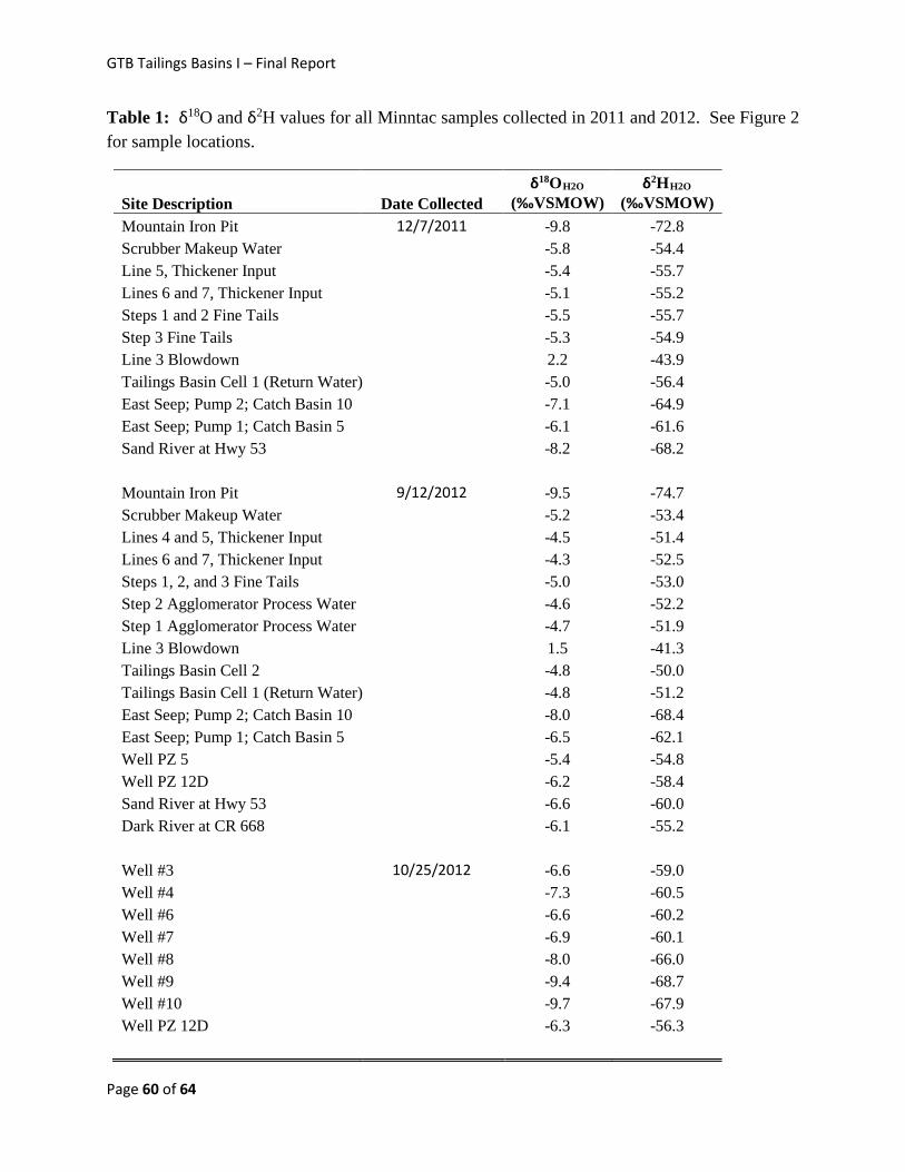
GTB Tailings Basins I – Final Report
Table 1: δ18O and δ2H values for all Minntac samples collected in 2011 and 2012. See Figure 2 for sample locations.
Site Description Date Collected δ18OH2O
(‰VSMOW) δ2HH2O
(‰VSMOW) Mountain Iron Pit 12/7/2011 -9.8 -72.8 Scrubber Makeup Water -5.8 -54.4 Line 5, Thickener Input -5.4 -55.7 Lines 6 and 7, Thickener Input -5.1 -55.2 Steps 1 and 2 Fine Tails -5.5 -55.7 Step 3 Fine Tails -5.3 -54.9 Line 3 Blowdown 2.2 -43.9 Tailings Basin Cell 1 (Return Water) -5.0 -56.4 East Seep; Pump 2; Catch Basin 10 -7.1 -64.9 East Seep; Pump 1; Catch Basin 5 -6.1 -61.6 Sand River at Hwy 53 -8.2 -68.2 Mountain Iron Pit 9/12/2012 -9.5 -74.7 Scrubber Makeup Water -5.2 -53.4 Lines 4 and 5, Thickener Input -4.5 -51.4 Lines 6 and 7, Thickener Input -4.3 -52.5 Steps 1, 2, and 3 Fine Tails -5.0 -53.0 Step 2 Agglomerator Process Water -4.6 -52.2 Step 1 Agglomerator Process Water -4.7 -51.9 Line 3 Blowdown 1.5 -41.3 Tailings Basin Cell 2 -4.8 -50.0 Tailings Basin Cell 1 (Return Water) -4.8 -51.2 East Seep; Pump 2; Catch Basin 10 -8.0 -68.4 East Seep; Pump 1; Catch Basin 5 -6.5 -62.1 Well PZ 5 -5.4 -54.8 Well PZ 12D -6.2 -58.4 Sand River at Hwy 53 -6.6 -60.0 Dark River at CR 668 -6.1 -55.2 Well #3 10/25/2012 -6.6 -59.0 Well #4 -7.3 -60.5 Well #6 -6.6 -60.2 Well #7 -6.9 -60.1 Well #8 -8.0 -66.0 Well #9 -9.4 -68.7 Well #10 -9.7 -67.9 Well PZ 12D -6.3 -56.3
Page 60 of 64
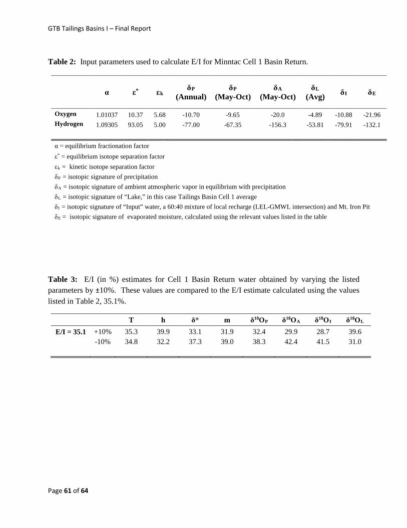
GTB Tailings Basins I – Final Report
Table 2: Input parameters used to calculate E/I for Minntac Cell 1 Basin Return.
α ε* εk δP
(Annual) δP
(May-Oct) δA
(May-Oct) δL
(Avg) δI δE
Oxygen 1.01037 10.37 5.68 -10.70 -9.65 -20.0 -4.89 -10.88 -21.96 Hydrogen 1.09305 93.05 5.00 -77.00 -67.35 -156.3 -53.81 -79.91 -132.1 α = equilibrium fractionation factor ε* = equilibrium isotope separation factor εk = kinetic isotope separation factor δP = isotopic signature of precipitation δA = isotopic signature of ambient atmospheric vapor in equilibrium with precipitation δL = isotopic signature of “Lake,” in this case Tailings Basin Cell 1 average δI = isotopic signature of “Input” water, a 60:40 mixture of local recharge (LEL-GMWL intersection) and Mt. Iron Pit δE = isotopic signature of evaporated moisture, calculated using the relevant values listed in the table
Table 3: E/I (in %) estimates for Cell 1 Basin Return water obtained by varying the listed parameters by ±10%. These values are compared to the E/I estimate calculated using the values listed in Table 2, 35.1%.
T h δ* m δ18OP δ18OA δ18OI δ18OL E/I = 35.1 +10% 35.3 39.9 33.1 31.9 32.4 29.9 28.7 39.6
-10% 34.8 32.2 37.3 39.0 38.3 42.4 41.5 31.0
Page 61 of 64
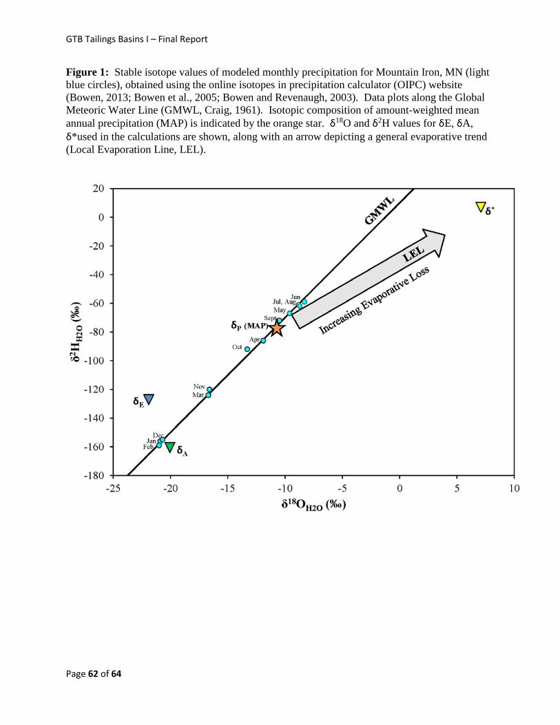
GTB Tailings Basins I – Final Report
Figure 1: Stable isotope values of modeled monthly precipitation for Mountain Iron, MN (light blue circles), obtained using the online isotopes in precipitation calculator (OIPC) website (Bowen, 2013; Bowen et al., 2005; Bowen and Revenaugh, 2003). Data plots along the Global Meteoric Water Line (GMWL, Craig, 1961). Isotopic composition of amount-weighted mean annual precipitation (MAP) is indicated by the orange star. δ18O and δ2H values for δE, δA, δ*used in the calculations are shown, along with an arrow depicting a general evaporative trend (Local Evaporation Line, LEL).
Page 62 of 64
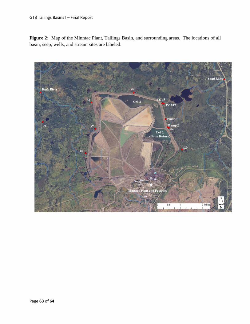
GTB Tailings Basins I – Final Report
Figure 2: Map of the Minntac Plant, Tailings Basin, and surrounding areas. The locations of all basin, seep, wells, and stream sites are labeled.
Page 63 of 64
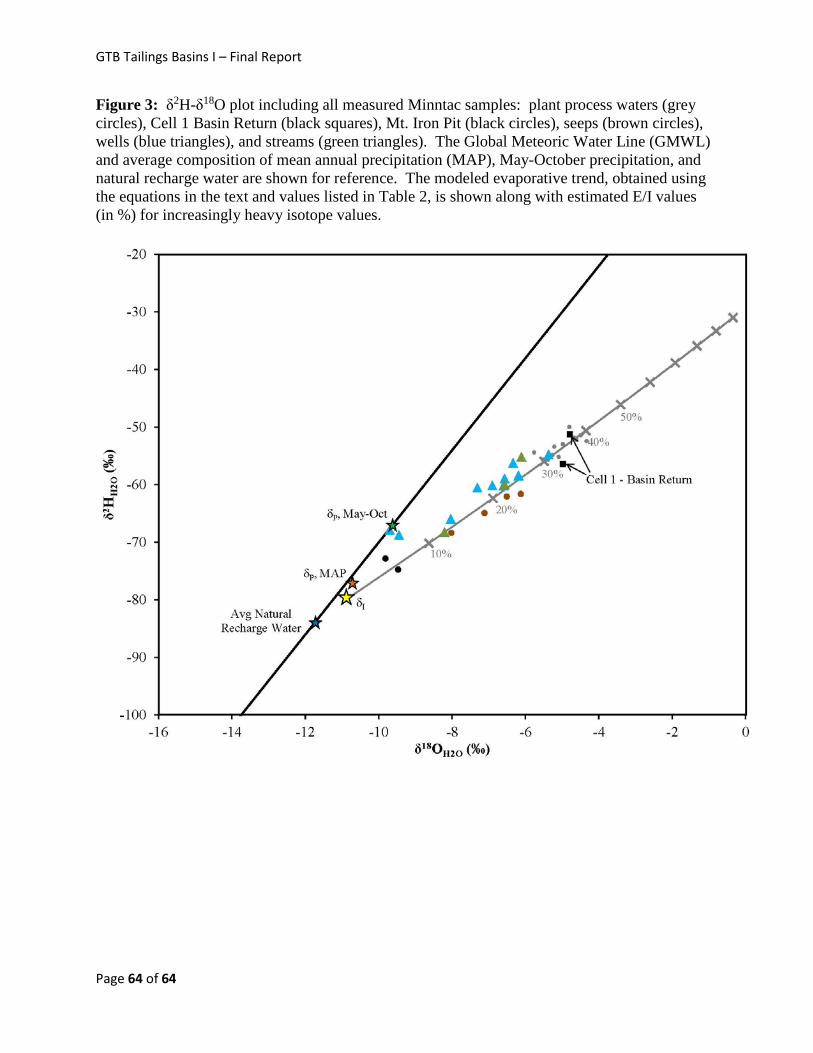
GTB Tailings Basins I – Final Report
Figure 3: δ2H-δ18O plot including all measured Minntac samples: plant process waters (grey circles), Cell 1 Basin Return (black squares), Mt. Iron Pit (black circles), seeps (brown circles), wells (blue triangles), and streams (green triangles). The Global Meteoric Water Line (GMWL) and average composition of mean annual precipitation (MAP), May-October precipitation, and natural recharge water are shown for reference. The modeled evaporative trend, obtained using the equations in the text and values listed in Table 2, is shown along with estimated E/I values (in %) for increasingly heavy isotope values.
Page 64 of 64