Seismic Imaging of the Alaska Subduction Zone: Implicationsfor Slab Geometry and VolcanismRobert Martin-Short1 , Richard Allen1 , Ian D. Bastow2 , Robert W. Porritt3 ,and Meghan S. Miller4

1Berkeley Seismological Laboratory, University of California, Berkeley, CA, USA, 2Department of Earth Science andEngineering, Imperial College London, London, UK, 3Institute for Geophysics, Jackson School of Geosciences, University ofTexas at Austin, Austin, TX, USA, 4Research School of Earth Sciences, Australian National University, Canberra, ACT, Australia

Abstract Alaska has been a site of subduction and terrane accretion since the mid-Jurassic. The areafeatures abundant seismicity, active volcanism, rapid uplift, and broad intraplate deformation, allassociated with subduction of the Pacific plate beneath North America. The juxtaposition of a slab edge withsubducted, overthickened crust of the Yakutat terrane beneath central Alaska is associated with manyenigmatic volcanic features. The causes of the Denali Volcanic Gap, a 400-km-long zone of volcanicquiescence west of the slab edge, are debated. Furthermore, the Wrangell Volcanic Field, southeast of thevolcanic gap, also has an unexplained relationship with subduction. To address these issues, we present ajoint ambient noise, earthquake-based surface wave, and P-S receiver function tomography model of Alaska,along with a teleseismic S wave velocity model. We compare the crust and mantle structure between thevolcanic and nonvolcanic regions, across the eastern edge of the slab and between models. Low crustalvelocities correspond to sedimentary basins, and several terrane boundaries are marked by changes in Mohodepth. The continental lithosphere directly beneath the Denali Volcanic Gap is thicker than in the adjacentvolcanic region. We suggest that shallow subduction here has cooled the mantle wedge, allowing theformation of thick lithosphere by the prevention of hot asthenosphere from reaching depths where it caninteract with fluids released from the slab and promote volcanism. There is no evidence for subductedmaterial east of the edge of the Yakutat terrane, implying the Wrangell Volcanic Field formed directly above aslab edge.

Plain Language Summary We present new images of the Alaskan subduction zone that reveal thethree-dimensional structure of the upper mantle and crust. Our study leverages data from a new array ofhigh-quality seismometers, the Transportable Array, which has been deployed across the entire state. Wecombine multiple geophysical techniques with complementary strengths to examine the upper 150 km overa wider geographic area than has previously been imaged. This enables us to observe major changes incrustal thickness across Alaska, map the eastern edge of the subducted Yakutat-Pacific plate, and note thatthe enigmatic Wrangell Volcanoes lie directly above this edge, which may help to explain their unusualfeatures. We also observe significant differences in the mantle structure beneath a volcanic region, theAleutian Arc, and an adjacent zone of volcanic quiescence. We infer that shallow-angle subduction beneaththis region has cooled the mantle here and thus limits the production of magma for volcanoes.

1. Introduction

Alaska exhibits a broad range of tectonic processes, the study of which can be used to address broader ques-tions surrounding subduction, arc accretion, continental crust growth, and magmatism. Much of the Alaskancrust comprises rocks associated with the northern Cordilleran Orogen, which represents westward growth ofthe North American continent by accretion of terranes to the margin of Laurentia since the Late Triassic(Nelson & Colpron, 2007; Plafker & Berg, 1994). This process continues today with the convergence and partialsubduction of the Yakutat terrane with the southern margin of Alaska, at the northeastern corner of thePacific plate (e.g., Eberhart-Phillips et al., 2006; O’Driscoll & Miller, 2015; Plafker & Berg, 1994). This uniquegeometry chronicles a transition from subduction of the Pacific plate beneath North America in the west intoright-lateral strike-slip motion in the east. Furthermore, the region exhibits a myriad of interesting tectonicand geodynamic processes within a relatively small area: abundant seismicity, shallow subduction, broadintraplate deformation and uplift, mantle flow around a slab edge, unusual magmatic activity in the

MARTIN-SHORT ET AL. 4541

Geochemistry, Geophysics, Geosystems

RESEARCH ARTICLE10.1029/2018GC007962

Key Points:• We use receiver functions, ambient

noise, earthquake-based surfacewave, and teleseismic body wavetomography to image the Alaskansubsurface

• Shallow subduction below the DenaliVolcanic Gap preventsasthenospheric flow into zones ofslab fluid release, suppressingvolcanism here

• The edge of the subducted Yakutatterrane delineates the easternmostextent of subduction; the WrangellVolcanic Field lies above this edge

Supporting Information:• Supporting Information S1

Correspondence to:R. Martin-Short,rmartin-short@berkeley.edu

Citation:Martin-Short, R., Allen, R., Bastow, I. D.,Porritt, R. W., & Miller, M. S. (2018).Seismic imaging of the Alaskasubduction zone: Implications for slabgeometry and volcanism. Geochemistry,Geophysics, Geosystems, 19, 4541–4560.https://doi.org/10.1029/2018GC007962

Received 14 SEP 2018Accepted 11 OCT 2018Accepted article online 27 OCT 2018Published online 21 NOV 2018

©2018. American Geophysical Union.All Rights Reserved.

Wrangell Volcanic Field (WVF), and a zone of volcanic quiescence known as the Denali Volcanic Gap (DVG;Eberhart-Phillips et al., 2006; Jadamec & Billen, 2010; Martin-Short et al., 2016; Plafker & Berg, 1994; Preece& Hart, 2004; Rondenay et al., 2010; Wang & Tape, 2014).

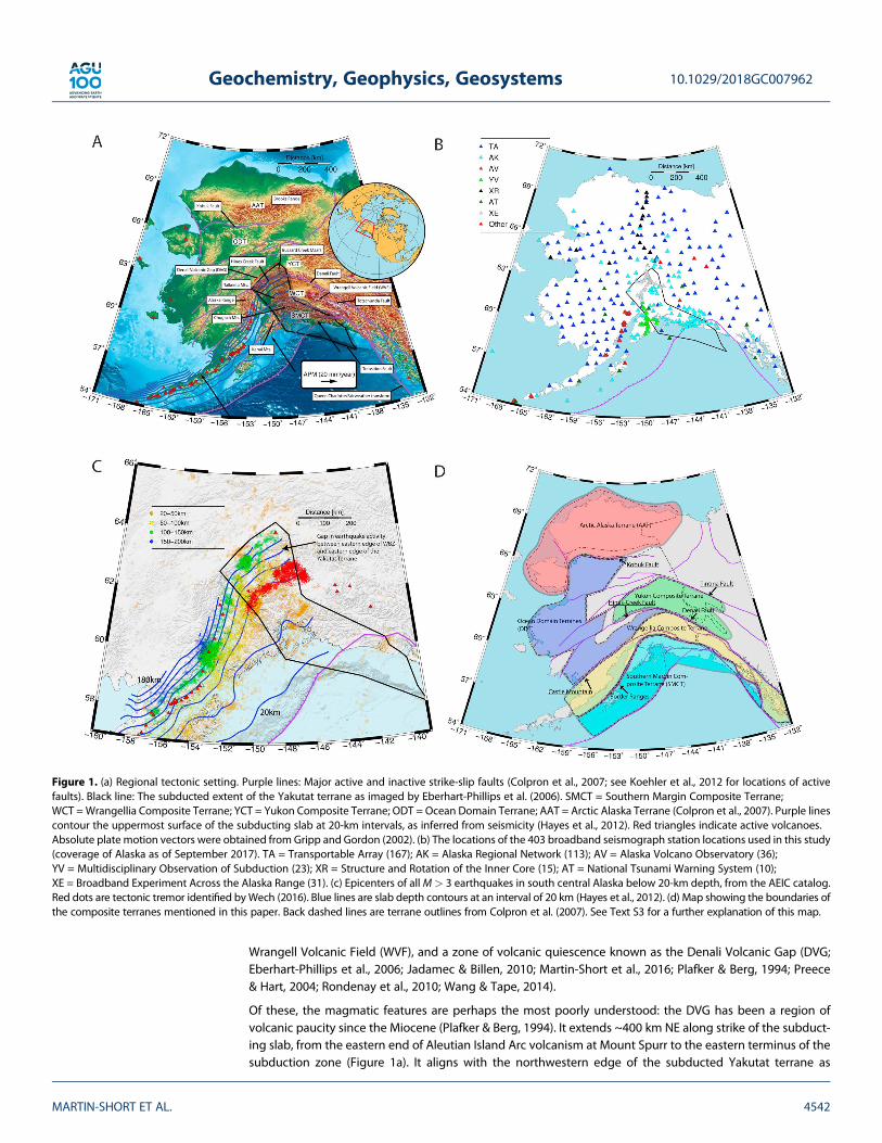
Of these, the magmatic features are perhaps the most poorly understood: the DVG has been a region ofvolcanic paucity since the Miocene (Plafker & Berg, 1994). It extends ~400 km NE along strike of the subduct-ing slab, from the eastern end of Aleutian Island Arc volcanism at Mount Spurr to the eastern terminus of thesubduction zone (Figure 1a). It aligns with the northwestern edge of the subducted Yakutat terrane as

Figure 1. (a) Regional tectonic setting. Purple lines: Major active and inactive strike-slip faults (Colpron et al., 2007; see Koehler et al., 2012 for locations of activefaults). Black line: The subducted extent of the Yakutat terrane as imaged by Eberhart-Phillips et al. (2006). SMCT = Southern Margin Composite Terrane;WCT =Wrangellia Composite Terrane; YCT = Yukon Composite Terrane; ODT = Ocean Domain Terrane; AAT = Arctic Alaska Terrane (Colpron et al., 2007). Purple linescontour the uppermost surface of the subducting slab at 20-km intervals, as inferred from seismicity (Hayes et al., 2012). Red triangles indicate active volcanoes.Absolute plate motion vectors were obtained from Gripp and Gordon (2002). (b) The locations of the 403 broadband seismograph station locations used in this study(coverage of Alaska as of September 2017). TA = Transportable Array (167); AK = Alaska Regional Network (113); AV = Alaska Volcano Observatory (36);YV = Multidisciplinary Observation of Subduction (23); XR = Structure and Rotation of the Inner Core (15); AT = National Tsunami Warning System (10);XE = Broadband Experiment Across the Alaska Range (31). (c) Epicenters of allM> 3 earthquakes in south central Alaska below 20-km depth, from the AEIC catalog.Red dots are tectonic tremor identified byWech (2016). Blue lines are slab depth contours at an interval of 20 km (Hayes et al., 2012). (d) Map showing the boundaries ofthe composite terranes mentioned in this paper. Back dashed lines are terrane outlines from Colpron et al. (2007). See Text S3 for a further explanation of this map.

10.1029/2018GC007962Geochemistry, Geophysics, Geosystems

MARTIN-SHORT ET AL. 4542

determined by Eberhart-Phillips et al. (2006). The Yakutat terrane is a portion of buoyant, overthickened(>20 km) oceanic crust, thought to have formed as an oceanic plateau (Christeson et al., 2010). Yakutatsubduction is believed to have caused shallowing of the slab beneath south central Alaska (Plafker & Berg,1994). Globally, subduction zones of overthickened crust are known to be associated with slab-flatteningand volcanic gaps (e.g., Gutscher et al., 2000).

The DVG features a well-defined Wadati-Benioff Zone to ~120-km depth, likely associated with seismicitygenerated by the expulsion of water from hydrous minerals (Rondenay et al., 2008). The subduction stylebeneath the DVG differs from archetypal regions of flat-slab subduction (e.g., Nankai, Peru, and Chile)because its Wadati-Benioff Zone does not become horizontal (Chuang et al., 2017; Gutscher et al., 2000).Furthermore, several studies have argued that the sub-DVG mantle wedge may feature conditions suitablefor melt production but suggest that this melt is unable to reach the surface (e.g., McNamara & Pasayanos,2002; Rondenay et al., 2010).

The WVF lies just east of the eastern edge of the subducted Yakutat terrane (Figure 1a); it is dominated bylarge, andesitic shield volcanoes and calc-alkaline affinity lavas that are typical of continental volcanic arcs(Richter et al., 1990). However, the WVF also features some unusual characteristics: the presence of adakiticand tholeiitic lavas at some locations (e.g., Preece & Hart, 2004), a northwestward progression in activity overtime (Richter et al., 1990) and limited seismic or tomographic evidence for an underlying slab (Martin-Shortet al., 2016). These findings raise questions about the source of magma for the WFV and how it is connectedto the history of Yakutat subduction, which is thought to be associated with the onset of volcanism here (e.g.,Finzel et al., 2011).

Any explanation of the causes of volcanism in the WVF requires consideration of the eastern edge of the sub-ducted Pacific-Yakutat plate, the location of which is also a subject of debate (e.g., Wech, 2016). Although theWadati-Benioff zone terminates abruptly at ~148°W, there are multiple lines of evidence that suggest that theslab extends further east. This includes the location of the eastern edge of the Yakutat terrane as inferredfrom local tomography (Eberhart-Phillips et al., 2006) and the eastern limit of slab-related high-velocityanomalies seen in teleseismic surface wave (Wang & Tape, 2014) and teleseismic body wave (Martin-Shortet al., 2016) tomography. Furthermore, Wech (2016) identified a zone of tectonic tremor extending 85 kmeast of the eastern edge of the Wadati-Benioff zone, suggesting the presence of an aseismically deformingslab (Figure 1c). It has been suggested that the slab extends further east of the tremor zone, below theWVF, but deforms by continuous slip there (Wech, 2016). This interpretation has important implications forthe potential causes of volcanism here, and, given the lack of seismicity, high-resolution imaging of the uppermantle is required to locate the eastern edge of the subducting material.

The Alaskan subduction zone has been the subject of numerous seismic imaging studies. However, most uti-lize linear or small-aperture seismometer networks, whose resulting models do not fully map the geometry ofthe subducting material beneath Alaska. Recent deployment of the EarthScope Transportable Array (TA)offers an unprecedented opportunity to expand these models.

This study uses data from 405 broadband seismograph stations, including TA deployments up to September2017 (Figure 1b). We construct an absolute S wave velocity model using a joint inversion of Rayleigh wavephase velocity maps from ambient noise and earthquake-based surface wave tomography in combinationwith P-S receiver functions calculated at each station. This joint model complements an updated version ofthe finite frequency, earthquake-based S wave relative arrival time model of Martin-Short et al. (2016), whichuses data from the TA and AK networks from January 2014 to September 2017. All models presented are iso-tropic. Our ambient noise workflow constructs phase velocity maps for periods of 10–35 s, which are sensitiveprimarily to crustal velocity structure. Our earthquake-based surface wave tomography workflow generatesphase velocity maps for periods 25–130 s, which are sensitive primarily to velocity structure at lower-crustalto middle-upper-mantle depths. To improve the resolution of velocity discontinuities, we use P-to-S receiverfunctions (Miller et al., 2018) calculated using the FuncLab software package (Eager & Fouch, 2012; Porritt &Miller, 2018).

Numerous recent studies have used joint inversion of phase velocities from ambient noise and teleseismicsurface waves in regional tomography (the central Andean plateau, Ward et al., 2016; Madagascar, Prattet al., 2017; and the Malawi rift, Accardo et al., 2017). Receiver functions have also been incorporated into

10.1029/2018GC007962Geochemistry, Geophysics, Geosystems

MARTIN-SHORT ET AL. 4543

such inversions (e.g., Porritt et al., 2015). However, few studies have marshaled a combination of ambientnoise, surface wave tomography, receiver functions, and body wave tomography to investigate a singleregion as we do here.

This paper presents the most comprehensive velocity models of the Alaskan crust and mantle to date, usingthem to reconcile the interpretations of previous, more geographically restricted, studies of the area. Ourjoint imaging approach is powerful because it harnesses the complementary strengths of each technique.However, one caveat is that it becomes difficult to accurately assess the resolution of the models becausethey are constructed from the inversion of multiple data sets, the uncertainties associated with which com-bine in a nontrivial fashion. Throughout this paper we acknowledge that confidence in our interpretationmay be limited by this constraint.

Our images reveal large variations in crustal thickness across Alaska (Figures S4 and S7 in the supportinginformation). Furthermore, they reveal significant differences between the velocity structure of the mantlewedge beneath the volcanic region and the DVG and provide important new constraints on the eastern edgeof the subducted slab.

2. Tectonic Setting

Alaska comprises a collection of terranes (Figure 1d), most of which have accreted to the western margin ofNorth America via a combination of subduction and translation along major strike-slip faults over the past200 Ma (Plafker & Berg, 1994; Text S1). Throughout much of the Proterozoic, Alaska lay at a passive marginat the edge of Laurentia (Colpron et al., 2007). Continental growth began with the onset of subduction inthe Devonian, which brought the Yukon Composite Terrane (YCT), whose basement material had previouslyrifted from the margin of Laurentia, back into contact with cratonic North America by the early Triassic. Sincethe Cretaceous, this terrane has undergone extension and migration via right-lateral motion on the Tintinafault, which bounds it to the north (Figure 1d; Pavlis et al., 1993).

The Arctic Alaska Terrane and Ocean Domain Terrane (ODT) are located to the northwest of the YCT(Figures 1a and 1d). The former contains continental-affinity rocks of the Alaska-Arctic microplate that col-lided with the northern margin of Laurentia in late Jurassic time, forming the Brooks Range (Cole et al.,1997). The latter are a complex assembly of ocean-affinity terranes accreted during the Mesozoic(Nockleberg et al., 2000).

South of the Denali Fault, the Wrangellia Composite Terrane (WCT) comprises three major allochthonous ter-ranes: Wrangellia, Alexander and Peninsular, which consist of various island arc assemblages, flood basalts,and volcanoclastic rocks (Trop & Ridgway, 2007). By the early Cretaceous, the WCT had accreted to the YCTvia northward verging subduction. Subduction and consumption of the Kula plate, followed by subductionof the Pacific plate, then brought the Southern Margin Composite Terrane (SMCT; Figure 1d) into contact withNorth America (Colpron et al., 2007; Trop & Ridgway, 2007). This composite terrane contains mélange,scraped-off sediments, and near-trench intrusive material that form an accretionary prism. The SMCT alsoincludes the allochthonous Yakutat terrane. Thought to have been formed as an oceanic plateau off the westcoast of North America ~50 Ma, the Yakutat terrane was subsequently rafted north by dextral motion on theQueen Charlotte/Fairweather transform. It came into contact with and began subducting beneath the south-ern margin of Alaska as early as 35 Ma (Christeson et al., 2010; Finzel et al., 2011).

Offshore seismic reflection surveys reveal that the Yakutat crust is uniform and wedge shaped, thickeningfrom 15 to 30 km in a west-east profile and overlain by ~8 km of sedimentary cover (Worthington et al.,2012). The Yakutat terrane is bounded to the south by the Transition fault (Figure 1a), across which there isa sharp Moho offset between ~20 Ma-old, 6 km-thick Pacific crust to ~50 Ma-old, 30 km-thick Yakutat crust(Christeson et al., 2010). The outline of the subducted Yakuat terrane, as inferred from the local tomographyof Eberhart-Phillips et al. (2006), is highlighted in Figure 1a.

It is generally accepted that subduction of the thick, buoyant, downgoing Yakutat crust has reduced the dipof the downgoing plate, which in turn has led to rapid uplift of the Chugach and Alaska ranges, large-scalecrustal shortening and a cessation of magmatism in the DVG. Geological and thermochronological data sug-gest significant uplift in south central Alaska began in late Eocene time and advanced northeastward (Finzelet al., 2011). Furthermore, magmatism above the Yakutat subduction region ceased ~32 Ma. This implies that

10.1029/2018GC007962Geochemistry, Geophysics, Geosystems

MARTIN-SHORT ET AL. 4544

south central Alaska experienced steep subduction and volcanism similar to that operating in the modernAleutian island arc before the onset of interaction with the Yakutat terrane at ~35 Ma (Finzel et al., 2011).Additionally, there is evidence that volcanism in the WVF is connected to the history of Yakutat subduction.Geochronological evidence suggests a northwestward progression of volcanic activity in the WFV, starting~26 Ma and ceasing ~0.2 Ma (Richter et al., 1990). This led Finzel et al. (2011) to suggest that the northwest-ward insertion of Yakutat lithosphere beneath Alaska is responsible for WVF volcanism at the slab edge.

WVF volcanism is atypical for a subduction zone. Preece and Hart (1994) identify three geochemical trends inWVF lavas that may illuminate their origins. The first is a dominant, arc-wide suite of calc-alkaline lavasderived from a mantle wedge MORB source that experienced relatively high degree partial melting due tointeraction with slab-derived fluids. A second suite of calc-alkaline lavas is restricted to front side volcanoesalong the southeastern edge of the field. This also has a mantle wedge source, but contains adakites sugges-tive of slab melting (Preece & Hart, 2004). Third, a collection of tholeiitic lavas erupted from a chain of cindercones along the central axis of the WVF are inferred to derive from low degree partial melting of anhydrousmantle wedge material in a localized extensional setting (Preece & Hart, 2004).

In contrast to the WVF, the geochemistry and physiography of the Aleutian arc are more typical of a subduc-tion setting: calc-alkaline lava-erupting stratovolcanoes overlie the 100-km depth contour of a well-defined,steeply dipping Wadati-Benioff zone (e.g., Plafker & Berg, 1994). The position of the present-day Aleutian arcwas established by ~55 Ma (Plafker & Berg, 1994), and, given the modern Pacific plate convergence rate of~50 mm/year, several thousand kilometers of lithosphere has been subducted beneath the Aleutian arc sinceits formation.

3. Previous Imaging Studies

Martin-Short et al. (2016) used teleseismic P and Swave body wave tomography to image the Pacific-Yakutatslab beneath Alaska as a continuous feature. At >150-km depth, slab structure beneath the DVG is similar tothat beneath the Aleutian Island arc. A high-velocity anomaly in the mantle wedge beneath the DVG, absentbeneath the Aleutian arc, is only tentatively interpreted due to poor resolution in the upper 100 km of themodel. Limited resolution also hampers the ability of Martin-Short et al. (2016) to interpret shallow mantlestructure beneath the Wrangell Volcanoes: despite recognizing the absence of deep subduction beneaththe WVF, their model cannot preclude the presence of a flat-lying or truncated slab in the upper 100 km.The surface wave tomography study of Wang and Tape (2014) reaches similar conclusions: a weak high-velocity anomaly underlies the WVF, but its relationship to the subducting Yakutat lithosphere is unresolveddue to sparse instrument coverage northeast of the volcanoes. Additionally, Wang and Tape (2014) note thepresence of an aseismic portion of the slab close to its eastern edge, an observation corroborated by Martin-Short et al. (2016).

Local earthquake tomography reveals the shallow structure of the Yakutat subduction zone (Eberhart-Phillipset al., 2006). The downgoing Yakutat crust is imaged as a low-velocity, high Vp/Vs layer above relatively flat-lying high-velocity lithosphere. This double layer structure is seen only beneath the DVG, where it extends to~150-km depth, coincident with the termination of seismicity. The receiver function study of Ferris et al.(2003) and images from 2-D multichannel inversion of scattered teleseismic body waves (Rondenay et al.,2008) confirm the presence of a low-velocity zone atop the downgoing Yakutat lithosphere. This is readilyinterpreted as the basaltic Yakutat crust, which undergoes dehydration and transformation to eclogite, result-ing in a thinning of the low-velocity zone down to 150 km, where it vanishes (Rondenay et al., 2008). Wadati-Benioff zone seismicity beneath the DVG follows a single plane, confined to the low velocity Yakutat crust. Incontrast, intermediate depth seismicity within the downgoing Pacific slab to the west exhibits a thickerWadati-Benioff zone with two planes of seismicity (Cole et al., 1997). This observation has been interpretedas differences in the hydration state of the Yakutat crust beneath the DVG and the Pacific crust beneaththe volcanic arc, which may be an important step toward explaining the link between Yakutat subductionand volcanic quiescence (Chuang et al., 2017).

Stachnik et al. (2004) produce a 2-D model of the seismic attenuation structure beneath the DVG, which exhi-bits three distinctive regions. First, a low attenuation zone in the nose of the mantle wedge trenchward of theDenali Fault, is interpreted as cool, serpentinized material, isolated frommantle wedge convection. Second, ahigher attenuation zone in the uppermost layer of the subducting lithosphere directly below the mantle

10.1029/2018GC007962Geochemistry, Geophysics, Geosystems

MARTIN-SHORT ET AL. 4545

wedge nose is interpreted as fluids escaping the Yakutat crust. Finally, a high attenuation zone in the mantlewedge northwest of the Denali Fault is interpreted as hot, convecting mantle material. However, themaximum attenuation values in this region are roughly half those of the central Andes and northern Japansubduction zones, suggesting a wedge that is 100–150 °C cooler than normal (Stachnik et al., 2004). Thisobservation has been suggested as an explanation for the DVG and is consistent with the high-velocityanomaly in the DVG mantle wedge imaged by Martin-Short et al. (2016). Eberhart-Phillips et al. (2006) alsosee a high-velocity anomaly here but interpret it as a residual slab segment from partial subduction of theWCT beneath the YCT. Such a feature could inhibit the passage of fluids and magma toward the surface,but its continuity beneath the DVG is poorly constrained.

Other studies assert that melt is present within the DVG mantle wedge but cannot reach the surface: localtomography-derived Poisson’s ratios are similarly high beneath the DVG and arc volcanoes to the west(McNamara & Pasayanos, 2002), suggesting suitable melting conditions in the DVG wedge, but with meltmigration arrested by increased compression in the overlying crust as a result of Yakutat collision(McNamara & Pasayanos, 2002). Rondenay et al. (2010) propose a model in which shallowing of the slab dipdue to Yakutat subduction has cooled the DVG mantle wedge and prevented the accumulation of melt pro-duced in a pinch zone fromwhich it can erupt. This explains the presence of a flat-lying low-velocity zone at 60-km depth in the images of Rondenay et al. (2008), interpreted as pooling melt beneath the LAB. Rondenayet al. (2010) support their interpretation via geodynamicmodeling of the evolution of themantle wedge tem-perate field in the case of steady state subduction and slab advance. Given an approximation to the shallowslab geometry beneath the DVG and in the presence of temperature-dependent viscosity, slab advance actsto cool the mantle wedge and limits the focused accumulation of melt, extinguishing volcanism (Rondenayet al., 2010); slab advance associated with Yakutat subduction has thus led to a cessation of DVG volcanics.

A similar argument pertains to the eastern edge of the subducted slab beneath south central Alaska.Geodynamic modeling of mantle flow and comparison to constraints from seismic anisotropy supports theexistence of deep subduction west of ~148°E, but only a short (reaching <115 km depth) slab beneath theWVF (Jadamec & Billen, 2010). Whether the edge of the subducted Yakutat terrane corresponds to the slabedge, or non-Yakutat lithosphere exists further to the east or beneath the WVF is unclear, with importantimplications for potential magma sources here.

However, the Wadati-Benioff zone terminates west of the edge of the tomographically imaged Yakutat ter-rane (Eberhart-Phillips et al., 2006; Martin-Short et al., 2016; Wang & Tape, 2014) and the extent of the slabas inferred by tectonic tremor (Wech, 2016). Indeed, a transition in tremor frequency from low in the westto high in the east led Wech (2016) to assert that deformation continues by continuous aseismic slip furthereast, connecting the seismic Pacific-Yakutat slab to an aseismic Wrangell slab. The causes of intermediatedepth seismicity, or lack thereof (e.g., in Cascadia), are debated but are thought to be related to the structureand hydration state of the downgoing plate (e.g., Hacker et al., 2003). The presence of a slab edge and closeproximity of hot asthenospheric material may influence the transition from seismic to aseismic deformationhere, but the geometry of this boundary must be mapped to address such issues.

The receiver function studies of O’Driscoll and Miller (2015) and Bauer et al. (2014) have attempted to con-strain the subduction geometry beneath Alaska by imaging velocity discontinuity structures. The S-P receiverfunction model of O’Driscoll and Miller (2015) does not resolve moderate-to-steeply dipping structures butreveals a flat Yakutat LAB at ~100-km depth beneath south central Alaska and hints at the existence of a shal-low slab beneath the WVF. The plane wave migration technique employed by Bauer et al. (2014) imaged dip-ping features and Yakutat crust ~80 km below the WVF; the extent of the slab north of the volcanoes wasunconstrained, however.

Ward (2015) used ambient noise tomography to study south central Alaska. At short periods (8–12 s), lowphase velocities are associated with thick sedimentary basins such as the Cook Inlet, Kodiak Shelf andTanana basins (Figure 4a). An elongate region of low phase velocities underlies the WVF at intermediate per-iods (14–25 s). The shape of this region mirrors that of a relatively low Bouguer gravity anomaly, implyingcompositional heterogeneity between the WVF and the surrounding crust (Ward, 2015). At 20- to 25-s period,across the Denali Fault, low velocities beneath the WCT in the south contrast with higher velocities in thenorth, beneath the YCT. This is interpreted as a change in crustal thickness between the terranes. A Moho off-set of ~10 km near the Denali Fault has been reported by receiver function studies (e.g., Brennan et al., 2011;

10.1029/2018GC007962Geochemistry, Geophysics, Geosystems

MARTIN-SHORT ET AL. 4546

Miller et al., 2018; Veenstra et al., 2006) and local tomography (Allam et al., 2017), which demonstrates theoffset occurs across the Hines Creek Fault in central Alaska and the Totschunda Fault to the east. The crustthickens again further north beneath the Brooks Range (Fuis et al., 2008).

4. Data Sets and Methodology

Rayleigh wave phase velocity maps are produced using independent workflows for the ambient noise andearthquake surface wave datasets. Receiver functions were then generated for all stations (Miller et al.,2018), before being inverted jointly with the phase velocity data for absolute shear wave speed below eachstation. Finally, a 3-D S velocity map is generated by interpolation between station locations.

4.1. Ambient Noise Tomography

Continuous, daylong, long-period, vertical component seismograms from broadband stations in the region52–73°N, 171–123°W were analyzed for the period January 2014 to September 2017 (Figure 1b). FollowingBensen et al. (2008) and Ward (2015), time domain normalization with an absolute mean method and a128-s window was applied to these data after filtering in a 5- to 150-s passband. Spectral whitening was thenapplied to reduce spectral imbalance and the real and imaginary components of each daylong time serieswere output. Station spectra were grouped into monthlong segments and cross-correlograms determinedfor each station-station pair. These were subsequently stacked over the maximum available timeframe. Theresulting two-sided, stacked cross-correlograms are dominated by Rayleigh wave energy traveling betweenthe stations in two directions. They can then be averaged to create a symmetric signal, which is an estimationof the Empirical Greens Function of the station-station path (Bensen et al., 2007). The dispersion characteris-tics of Empirical Greens Functions were determined using the FTAN method with a phase-matched filter(Levshin et al., 1992), yielding group and phase velocity dispersion curves for each station-station path at per-iods of 8–40 s. Dispersion curves corresponding to station pairs where one station is far outside the region ofinterest (Figure 2) were removed, as were dispersion measurements with a signal-to-noise ratio < 15 and aninterstation distance<3 wavelengths. These criteria followWard (2015), but we found that varying them hadlittle impact on the final model. The remaining dispersion measurements were then inverted for 2-D maps ofphase velocity for periods of 10–35 s using the ray theoretical surface wave inversion method of Barmin et al.(2001). Resolution testing indicates that our ray coverage yields phase velocity maps able to resolve featuresof length scale ≥100 km (Figures S1–S3).

Our inversions are regularized via three user-defined parameters: The damping (α), the smoothing in regionsof poor path coverage (β), and the Gaussian smoothing width (σ). Systematic variation of these parametersand inversion on a 0.1 × 0.1° grid reveals that their values do not significantly affect the results within theregion of interest. Thus, we follow Ward (2015) and use α = 600 and β = 100; σ is roughly equal to one wave-length of the inversion period. Our results are similar to those of Ward (2015) where they overlap spatially butspan a larger area due to our expanded station coverage (Figure 2). Resolution tests of the ambient noisetomography are shown in Figures S1–S3.

4.2. Earthquake-Based Surface Wave Tomography

To investigate deeper velocity structure, we follow Jin and Gaherty (2015) and use the Automated SurfaceWave Measuring System (ASWMS) software package to produce 25- to 130-s period fundamental modeRayleigh wave phase velocity maps from the seismograms of teleseismic earthquakes. We analyze waveformsrecorded at all stations for earthquakes of mb > 6 from January 2014 to September 2017 within a distancerange of 20–160° (Figure S4). For each station-event pair, the Rayleigh wave and most of its coda are wind-owed and a cross correlation between this packet and waveforms recorded for the same earthquake at allstations within 500 km is performed. The peak of each cross-correlogram is further windowed and the peri-ods of interest are isolated by application of narrow band-pass filters. Each filtered cross-correlogram can berepresented by a five-parameter wavelet, two of whose parameters are the time-dependent group and phasedelays between the two stations whose waveforms were cross correlated. For each frequency the results areinverted for the phase traveltime gradient, which is then used by the Eikonal and Helmholtz equations to pro-duce phase velocity maps (Jin & Gaherty, 2015). Smoothing and quality control parameters in the ASWMSworkflow are chosen to minimize the difference in appearance between phase velocity maps in the 25- to35-s period range and those produced for the same period range by the ambient noise tomography

10.1029/2018GC007962Geochemistry, Geophysics, Geosystems

MARTIN-SHORT ET AL. 4547

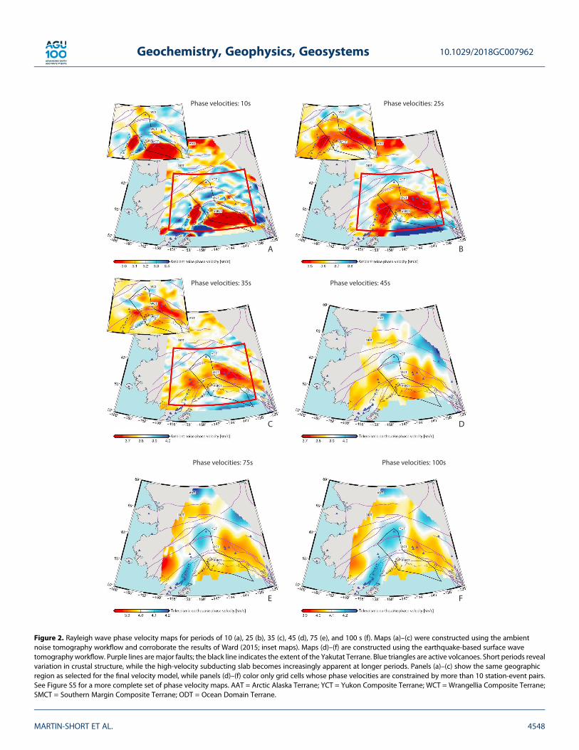
Figure 2. Rayleigh wave phase velocity maps for periods of 10 (a), 25 (b), 35 (c), 45 (d), 75 (e), and 100 s (f). Maps (a)–(c) were constructed using the ambientnoise tomography workflow and corroborate the results of Ward (2015; inset maps). Maps (d)–(f) are constructed using the earthquake-based surface wavetomography workflow. Purple lines are major faults; the black line indicates the extent of the Yakutat Terrane. Blue triangles are active volcanoes. Short periods revealvariation in crustal structure, while the high-velocity subducting slab becomes increasingly apparent at longer periods. Panels (a)–(c) show the same geographicregion as selected for the final velocity model, while panels (d)–(f) color only grid cells whose phase velocities are constrained by more than 10 station-event pairs.See Figure S5 for a more complete set of phase velocity maps. AAT = Arctic Alaska Terrane; YCT = Yukon Composite Terrane; WCT = Wrangellia Composite Terrane;SMCT = Southern Margin Composite Terrane; ODT = Ocean Domain Terrane.

10.1029/2018GC007962Geochemistry, Geophysics, Geosystems

MARTIN-SHORT ET AL. 4548

workflow (Figures S5–S6). Phase velocity maps produced by the ASWMS workflow are sensitive to the lowercrust and upper mantle at short periods; longer periods image the subducting Pacific-Yakutat plate. See TextS2 for a more complete description of the parameters used and Figure S7 for estimates of uncertainty in thephase velocity maps produced by this workflow.

4.3. Receiver Functions

Receiver functions are estimations of the Earth response function beneath a seismometer (e.g., Langston,1979). We utilize a large database of P-S receiver functions determined at 468 stations in Alaska and theYukon by Miller et al. (2018). An upgraded version of the Funclab software package (Eager & Fouch, 2012;Porritt & Miller, 2018) is used to calculate and trace edit the receiver functions. The first step involves timedomain iterative deconvolution to estimate the radial Earth response, which is then multiplied by the trans-form of a 2.5-s-wide Gaussian pulse in the frequency domain to limit the inclusion of high-frequency signalsnot warranted by the observations (Langston, 1979). We supplement this data set with receiver functions forTA and AK network stations, calculated from waveforms recorded between January 2014 and September2017. A Gaussian pulse of 1-s width damps high-frequency signals in the receiver functions, leaving themwith only the direct arrival and signals from the most significant discontinuities.

In preparation for the joint inversion workflow, we follow Porritt et al. (2015) by binning the receiver functionsat each station in ray parameter increments of 0.01 and back azimuth increments of 45° and stack the resultsin each bin.

4.4. Joint Inversion

We use the Joint96 program from the Computer Programs in Seismology software suite (Herrmann, 2013) tojointly invert the stacked P-S receiver functions and phase velocities from the ambient noise and earthquake-based surface wave processing workflows (Julià et al., 2000). These data sets are theoretically sensitive to thedensity, P and S velocity structure of the subsurface, but in practice the S velocity structure has the dominantinfluence and is hence inverted for here (e.g., Julià et al., 2000).

In the period range 25–35 s, we have phase velocities from both the ambient noise and event-based tomo-graphy. These are combined using a simple linear weighting scheme that places 100% weight on the ambi-ent noise tomography at 25 s and 0% at 35 s. Overlap between the ambient noise and event-based phasevelocity maps is imperfect (Figure 2). At the model edges some stations lack sufficient event-based phasemeasurements to construct a full 1-D profile; mean velocities corresponding to that period are used instead.Figures S5 and S6 show examples of the phase velocity maps included in the inversion.

Given an 82-layer initial S velocity model (the 1-D starting velocity model of Eberhart-Phillips et al., 2006, witha constant velocity of 4.48 km/s from the surface to 60-km depth), Joint96 conducts a series of forward cal-culations and linearized inversions to iterate toward a final model. Our simple starting model contains no apriori assumptions about crustal thickness, meaning the final result is entirely data driven.

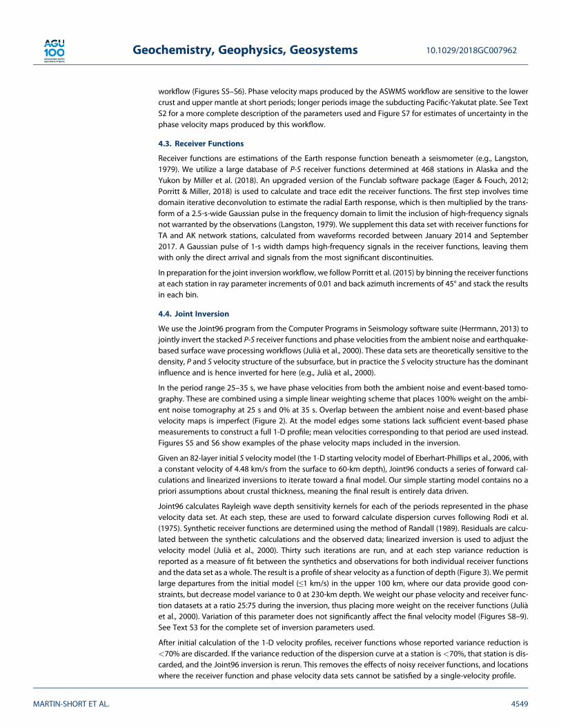
Joint96 calculates Rayleigh wave depth sensitivity kernels for each of the periods represented in the phasevelocity data set. At each step, these are used to forward calculate dispersion curves following Rodi et al.(1975). Synthetic receiver functions are determined using the method of Randall (1989). Residuals are calcu-lated between the synthetic calculations and the observed data; linearized inversion is used to adjust thevelocity model (Julià et al., 2000). Thirty such iterations are run, and at each step variance reduction isreported as a measure of fit between the synthetics and observations for both individual receiver functionsand the data set as a whole. The result is a profile of shear velocity as a function of depth (Figure 3). We permitlarge departures from the initial model (≤1 km/s) in the upper 100 km, where our data provide good con-straints, but decrease model variance to 0 at 230-km depth. We weight our phase velocity and receiver func-tion datasets at a ratio 25:75 during the inversion, thus placing more weight on the receiver functions (Juliàet al., 2000). Variation of this parameter does not significantly affect the final velocity model (Figures S8–9).See Text S3 for the complete set of inversion parameters used.

After initial calculation of the 1-D velocity profiles, receiver functions whose reported variance reduction is<70% are discarded. If the variance reduction of the dispersion curve at a station is<70%, that station is dis-carded, and the Joint96 inversion is rerun. This removes the effects of noisy receiver functions, and locationswhere the receiver function and phase velocity data sets cannot be satisfied by a single-velocity profile.

10.1029/2018GC007962Geochemistry, Geophysics, Geosystems

MARTIN-SHORT ET AL. 4549

In some locations (e.g., offshore) receiver function data are unavailable, but velocity structure can still be con-strained by the phase velocity data sets. In offshore regions, we construct a 1 × 1° grid of ghost stations atwhich the phase velocity dataset alone is used to construct 1-D velocity profiles (see Figures S1–S3 for the

Figure 3. Example of the joint inversion workflow for station M19K, which lies above the subducting Pacific plate. (a) The fitto the phase velocity data. (b) Final velocity models constructed using just the phase velocity data (model 1) and with theaddition of the receiver functions (models 2 and 3). The joint model is the preferred model because it reveals a clearerdiscontinuity structure. (c) The fits to the observed receiver function stacks. See Text S2 for more detailed explanation of thejoint inversion procedure. TA = Transportable Array.

10.1029/2018GC007962Geochemistry, Geophysics, Geosystems

MARTIN-SHORT ET AL. 4550

offshore resolution). The same is true for a small number of onshore station locations where all the of thereceiver function data is removed by the QC workflow. A map of all locations at which 1-D velocity profileswere extracted is shown in Figure S10.

The surface waves most sensitive to velocity structure >100-km depth have long periods (>100 s) and thuslong wavelengths (>300 km). This causes a reduction in the lateral resolution of our joint model with depth.Consequently, we truncate our profiles at 200 km and use a relative S velocity model derived from finite fre-quency, relative arrival time body wave tomography to investigate the mantle below.

A three-dimensional (3-D) model of shear velocity to 200-km depth is constructed by linear interpolationbetween the 1-D profiles determined at the station locations (hereafter known as the joint model). We alsoconstruct a 3-D model using constraints from the phase velocities alone using the same station locationsas in the joint inversion (hereafter known as model 2) and by linear interpolation between profiles determinedon a regular grid with a spacing of 0.5° (hereafter known as model 3). There is little difference between modelsgenerated by the two interpolation strategies. However, at shallow depths, the grid-interpolation modelscontain more structure (Figures S11–12). Comparison of the joint model with the phase velocity-only modelreveals that addition of receiver functions greatly improves our ability to identify the Moho and LAB (FiguresS13 and S14).

4.5. Teleseismic Body Wave Tomography

We extend the finite frequency, relative arrival time S wave velocity model of Martin-Short et al. (2016) byincorporating traveltime picks for mb > 6.0 earthquakes recorded on AK and TA instruments betweenJune 2016 and September 2017, at epicentral distances of 30–120°. Caution should be exercised when com-paring the relative and absolute velocities (Bastow, 2012). However, the locations of these anomalies can beused to inform and support interpretations of the joint model above 200-km depth and extend our knowl-edge of the mantle structure below. Resolution tests of our teleseismic S wave model are shown in FiguresS15 and S16.

5. Results

We present a series of depth slices and cross sections through the joint model and teleseismic body wavemodels (Figures 4–6). We color the depth slices by absolute velocity, with the color scale centered on themean velocity at each depth. Absolute velocities in the crust and mantle are colored separately in cross sec-tions though the joint model (Figures 5 and 6).

We identify four core observations: The pattern of velocity anomalies in the crust, variations in Mohodepth across Alaska, differences in mantle wedge anomalies between the DVG and Aleutian arc, andthe geometry of the subducting slab, which is inferred from the extent of a prominent high-velocityfeature (Figure 4).

At shallow depths (10–20 km) we observe several regions of very low S wave velocity (< 3.1 km/s at 10 km),which roughly correspond to the locations of the deep Cook Inlet, Kodiak Shelf, and Colville sedimentarybasins (Figure 4). Relatively high velocities are seen beneath regions of high topography, including theAlaska and Chugach ranges, the mountains of the Aleutian Arc and the eastern YCT. The central YCT containsthe lowland Tanana valley region, where relatively low velocities are likely associated with the Nenana andYukon Flats basins (Figures 4 and S12). Model 3, which comprises profiles interpolated over short distanceson a regular grid, yields themost detailed images of structure at these shallow depths (Figure S12). In the caseof model 2 (Figure S11) and the joint model, interpolation between velocity profiles determined at stationlocations tends to smooth short wavelength structure that is present in the ambient noise dataset and resol-vable on the 0.5° grid.

At lower-crustal depths (30–45 km) we see several long wavelength anomalies (Figures 4, S11, and 12).There is a dramatic contrast between low velocities south of the central part of the Denali Fault and highvelocities to the north. Onshore velocities are highest below the lowlands of the Tanana basin anddecrease again below the high topography of the Brooks Range. The lowest velocities are seen beneaththe Aleutian Island arc, Chugach Mountains, and WVF, corroborating phase velocity maps at intermediateperiods (14–25 s) constrained by Ward (2015). The highest velocities are found offshore, beneath thePacific plate.

10.1029/2018GC007962Geochemistry, Geophysics, Geosystems

MARTIN-SHORT ET AL. 4551

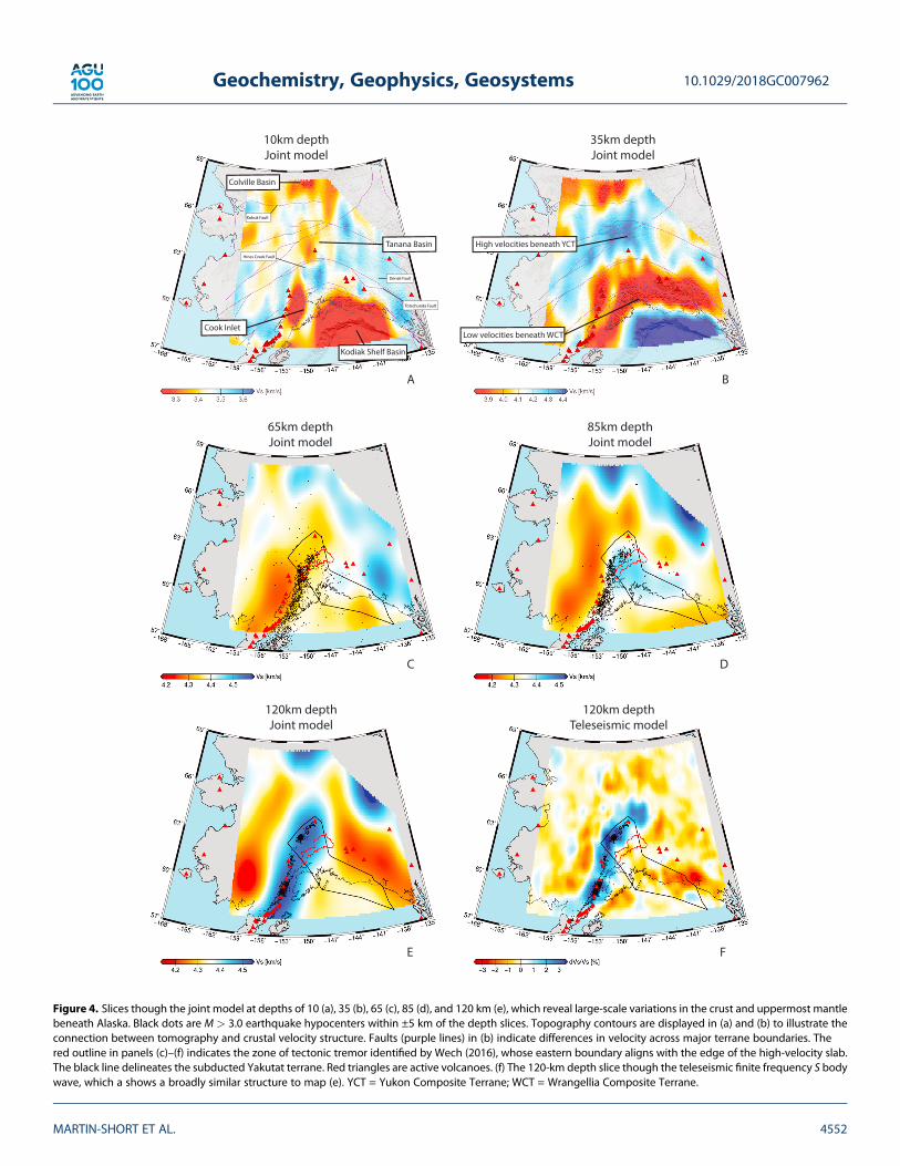
Figure 4. Slices though the joint model at depths of 10 (a), 35 (b), 65 (c), 85 (d), and 120 km (e), which reveal large-scale variations in the crust and uppermost mantlebeneath Alaska. Black dots are M > 3.0 earthquake hypocenters within ±5 km of the depth slices. Topography contours are displayed in (a) and (b) to illustrate theconnection between tomography and crustal velocity structure. Faults (purple lines) in (b) indicate differences in velocity across major terrane boundaries. Thered outline in panels (c)–(f) indicates the zone of tectonic tremor identified by Wech (2016), whose eastern boundary aligns with the edge of the high-velocity slab.The black line delineates the subducted Yakutat terrane. Red triangles are active volcanoes. (f) The 120-km depth slice though the teleseismic finite frequency S bodywave, which a shows a broadly similar structure to map (e). YCT = Yukon Composite Terrane; WCT = Wrangellia Composite Terrane.

10.1029/2018GC007962Geochemistry, Geophysics, Geosystems

MARTIN-SHORT ET AL. 4552

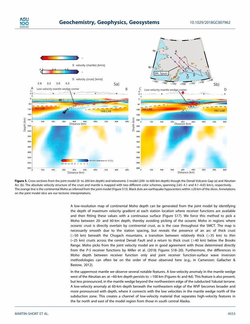
A low-resolution map of continental Moho depth can be generated from the joint model by identifyingthe depth of maximum velocity gradient at each station location where receiver functions are availableand then fitting these values with a continuous surface (Figure S17). We force this method to pick aMoho between 20- and 60-km depth, thereby avoiding picking of the oceanic Moho in regions whereoceanic crust is directly overlain by continental crust, as is the case throughout the SMCT. The map isnecessarily smooth due to the station spacing, but reveals the presence of an arc of thick crust(>50 km) beneath the Chugach mountains, a transition between relatively thick (>35 km) to thin(~25 km) crusts across the central Denali Fault and a return to thick crust (>40 km) below the BrooksRange. Moho picks from the joint velocity model are in good agreement with those determined directlyfrom the P-S receiver functions by Miller et al. (2018; Figures S18–20). Furthermore, the differences inMoho depth between receiver function only and joint receiver function-surface wave inversionmethodologies can often be on the order of those observed here (e.g., in Cameroon: Gallacher &Bastow, 2012).

In the uppermost mantle we observe several notable features. A low-velocity anomaly in the mantle wedgewest of the Aleutian arc at ~60-km depth persists to>100 km (Figures 4c and 4d). This feature is also present,but less pronounced, in the mantle wedge beyond the northwestern edge of the subducted Yakutat terrane.A low-velocity anomaly at 60-km depth beneath the northeastern edge of the WVF becomes broader andmore pronounced with depth, where it connects with the low velocities in the mantle wedge north of thesubduction zone. This creates a channel of low-velocity material that separates high-velocity features inthe far north and east of the model region from those in south central Alaska.

Low velocity mantle wedge corner5b)

Distance (km) Distance (km)

Distance (km)Distance (km)

5a)D

D

A

A

B

B

C

C

Dep

th (k

m)

Dep

th (k

m)

NA-LABNA-LABPAC-LABYAK-LAB

Low velocity mantle wedge corner

2.8 3.2 3.6 4.0

S velocity (crust) [km/s]

4.2 4.4 4.6

S velocity (mantle) [km/s]

Mt. Spurr

Figure 5. Cross sections from the joint model (0- to 200-km depth) and teleseismic Smodel (200- to 600-km depth) though the Denali Volcanic Gap (a) and AleutianArc (b). The absolute velocity structure of the crust and mantle is mapped with two different color schemes, spanning 2.65–4.1 and 4.1–4.65 km/s, respectively.The orange line is the continental Moho as inferred from the joint model (Figure S15). Black dots are earthquake hypocenters within ±20 km of the slices. Annotationson the joint model slice are our tectonic interpretations.

10.1029/2018GC007962Geochemistry, Geophysics, Geosystems

MARTIN-SHORT ET AL. 4553

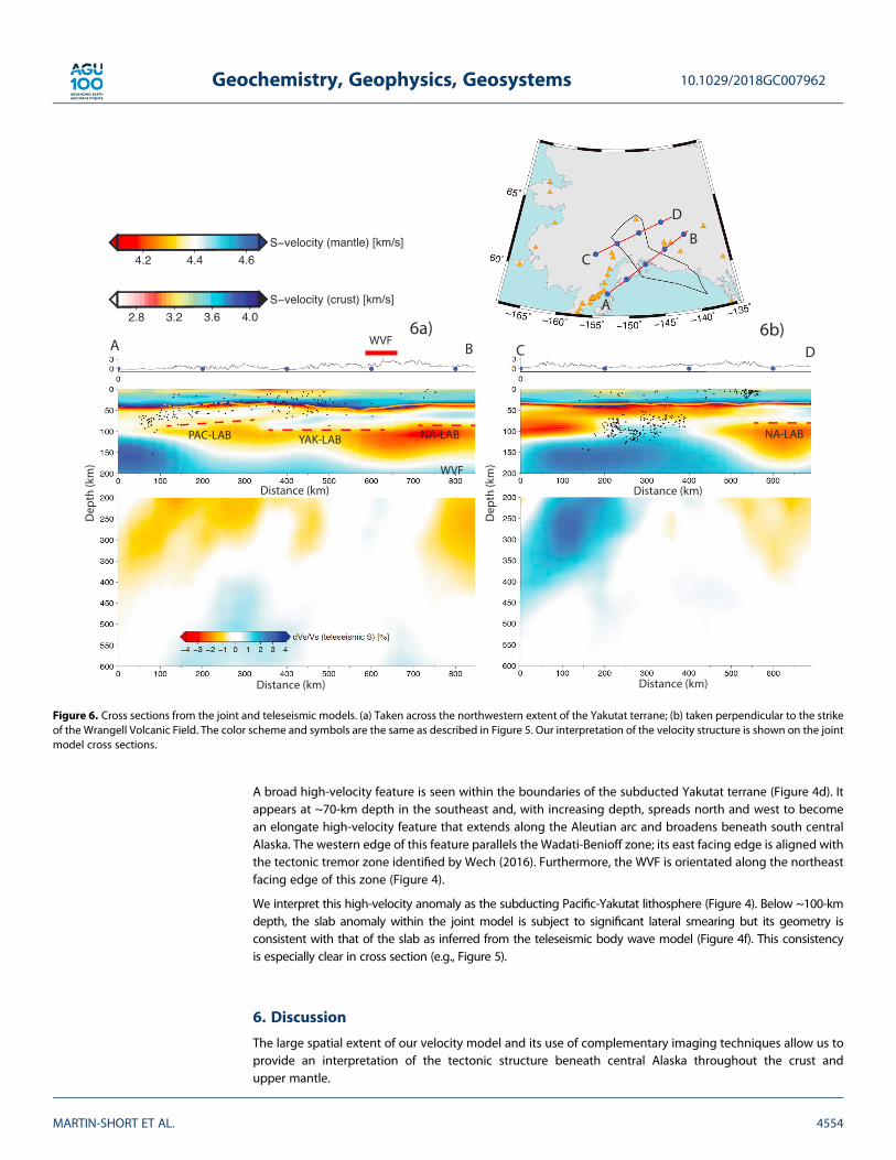
A broad high-velocity feature is seen within the boundaries of the subducted Yakutat terrane (Figure 4d). Itappears at ~70-km depth in the southeast and, with increasing depth, spreads north and west to becomean elongate high-velocity feature that extends along the Aleutian arc and broadens beneath south centralAlaska. The western edge of this feature parallels the Wadati-Benioff zone; its east facing edge is aligned withthe tectonic tremor zone identified by Wech (2016). Furthermore, the WVF is orientated along the northeastfacing edge of this zone (Figure 4).

We interpret this high-velocity anomaly as the subducting Pacific-Yakutat lithosphere (Figure 4). Below ~100-kmdepth, the slab anomaly within the joint model is subject to significant lateral smearing but its geometry isconsistent with that of the slab as inferred from the teleseismic body wave model (Figure 4f). This consistencyis especially clear in cross section (e.g., Figure 5).

6. Discussion

The large spatial extent of our velocity model and its use of complementary imaging techniques allow us toprovide an interpretation of the tectonic structure beneath central Alaska throughout the crust andupper mantle.

Figure 6. Cross sections from the joint and teleseismic models. (a) Taken across the northwestern extent of the Yakutat terrane; (b) taken perpendicular to the strikeof the Wrangell Volcanic Field. The color scheme and symbols are the same as described in Figure 5. Our interpretation of the velocity structure is shown on the jointmodel cross sections.

10.1029/2018GC007962Geochemistry, Geophysics, Geosystems

MARTIN-SHORT ET AL. 4554

6.1. Crustal Structure and Moho Depth Variations

At shallow depths, the lowest velocities are located within the ≥8-km-deep Cook Inlet and Kodiak shelf sedi-mentary basins (Christeson et al., 2010; Shellenbaum et al., 2010). Moderately low velocities characterizeother major Cenozoic sedimentary basins (Figures 4a, S11, and S12). The highest velocities are seen beneaththe Chugach, Kenai and Talkeetna Mountains, which comprise layers of intermediate to ultramafic material,thought to be accreted slivers of oceanic crust (Ferris et al., 2003). High velocities also characterize theAleutian arc and western Yukon-Tanana uplands, where they likely indicate the high-grade metamorphicor igneous cores of these elevated regions.

In most locations, our model lacks the necessary resolution to map potentially abrupt steps in crustal thick-ness across terrane boundaries (e.g., Allam et al., 2017; Miller et al., 2018). However, our maps, cross sectionsandMoho depth calculations confirm that significant crustal thickness variations exist from terrane to terrane(Figures 3, S11, 12, S17, and S21). Despite not being constrained by receiver functions, the Pacific-Yakutatcrust offshore is observed to be relatively thin compared to that of North America, hence explaining the pre-sence of mantle velocities offshore in the 35-km depth slice (Figure 4b). The continental crust beneath theWCT and SMCT is relatively thick, especially beneath the Chugach Mountains and south of the WVF, whereit exceeds 50 km (Figure S17). This is consistent with previous observations of Moho depth in this region(Christeson et al., 2010; Eberhart-Phillips et al., 2006; Miller et al., 2018) and is probably the result ofYakutat underplating of the WCT (Christeson et al., 2010).

The sharp velocity contrast between the WCT and YCT across the Denali Fault in central and eastern Alaska at35-km depth (Figure 4b) is interpreted as a Moho step. This is consistent with previous studies, which consis-tently report that crust below the Tanana Basin is some of the thinnest in Alaska (e.g., Miller et al., 2018;Veenstra et al., 2006) and is offset from the thick crust to the south along the Hines Creek Fault (Allamet al., 2017). This offset is most dramatic close to where the Broadband Experiment Across the AlaskaRange array crosses the terrane boundary, but continues west along the Hines Creek Fault and then southon the landward side of the Aleutian arc (Figure 4). There is no abrupt change in velocity between the YCTand ODT, but the sharp decrease in velocity seen across the Kobuk fault zone (Figure 4), which bounds theArctic Alaska and ODT, indicates crustal thickening beneath the Brooks Range, consistent with the findingsof Miller et al. (2018).

6.2. Mantle Wedge and DVG

Figures 5 and S19 show cross sections through the velocity structure of the DVG (Figure 5a) and the Aleutianisland arc near Mount Spurr (Figure 5b). These indicate the slab and continental LAB locations, which areinferred from velocity discontinuities and agree with LAB picks from O’Driscoll and Miller (2015) where themodels overlap (Figure S21).

The slab is imaged as a dipping, high-velocity (4.4–4.6 km/s) structure whose uppermost surface is deli-neated by a Wadati-Benioff zone. The slab geometry and velocity values are consistent with the modelsof Wang and Tape (2014) and Eberhart-Phillips et al. (2006). The latter study has higher resolution but ismore restricted spatially. Velocities in the mantle wedge are relatively low (4.2–4.3 km/s) and overlainby a zone of higher velocities (4.3–4.5 km/s), interpreted as continental lithosphere. In both cases thereis a region of very low velocities (4.1–4.2 km/s) at the nose of the mantle wedge at depths of40–60 km (corresponding to ~1.2–1.8GPa), directly above a high seismicity zone that likely marks theonset of eclogitization (Chuang et al., 2017; Rondenay et al., 2008). The large volume change that accom-panies eclogitization of the downgoing oceanic crust is thought to promote fluid release into the mantlewedge (Audet et al., 2009). At the cool (< 600 °C) mantle wedge nose, hydration of peridotite leads to theformation of the serpentine mineral antigorite, the presence of which can depress seismic velocities (e.g.,Christensen, 1996). We interpret the low velocity mantle forearc in Figures 5a and 5b to indicate thepresence of fluids and the formation of antigorite. Evidently, the degree of serpentinization is low in com-parison to Cascadia, because the receiver functions do not indicate an inverted Moho as is there (Bostocket al., 2002). These findings support the interpretation of Stachnik et al. (2004), who attribute a high-Qregion in the DVG mantle forearc to serpentinization. The Vp/Vs model of Rossi et al. (2006) also indicates≤30% serpetinization within the nose of the DVG mantle wedge. Our models indicate that this serpenti-nized nose is present in both the volcanic and nonvolcanic zones.

10.1029/2018GC007962Geochemistry, Geophysics, Geosystems

MARTIN-SHORT ET AL. 4555

In both cross sections, a continental LAB caps the low velocity mantle wedge asthenosphere. Below the vol-canogenic region, the LAB dips northward in such a way that it disappears beneath the Aleutian arc volca-noes (Figure 5b). In contrast, the continental LAB beneath the DVG is horizontal at ~70-km depth, thusseparating the low-velocity mantle wedge asthenosphere from the serpentinized forearc mantle at shallowerdepths (Figure 5a). The location of this horizontal LAB is similar to that of the horizontal low velocity anomalyseen below the DVG in the images of Rondenay et al. (2008), which they interpret as pooled melt below animpermeable mantle layer. This supports the suggestion of Chuang et al. (2017) that the Rondenay et al.(2008) low-velocity anomaly is an expression of the continental LAB, where dry lithosphere overlies hydratedasthenosphere. Our model resolution is insufficient to rule out the melt-pocket interpretation, however, andit remains compatible with our discussion.

In the Aleutian Arc cross section (Figure 5b), the dipping LAB allows low velocity mantle wedge materialmuch closer to the surface than the horizontal LAB beneath the DVG. We interpret this low velocity regionas convecting, hot asthenosphere. In the volcanogenic zone, it is present in the mantle directly below the vol-canoes, above the 100-km depth contour of the downgoing slab. Fluids being released from eclogitizingoceanic crust thus enter this zone and contribute to melt production and volcanism. In contrast, the paucityof low-velocity mantle wedge material above the 100-km slab depth contour within the DVG suggests thatthe mantle wedge there is relatively isolated from asthenospheric circulation and may not be warm enoughto generate sufficient melt to cause volcanism, even if slab-derived fluids are present. This is consistent withthe Q tomography of Stachnik et al. (2004), which suggests that the DVG mantle wedge is anomalously cool.Cooling of the wedge and isolation from circulation can be attributed to shallowing of the slab dip angle dueto subduction of the thick Yakutat crust, as indicated by the geodynamic modeling of Rondenay et al. (2010).Localized melt production must still occur in this region as evidenced by the presence of the Buzzard CreekMaars cinder cones (Figure 1a).

The DVGmantle wedgemay also be deprived of slab-derived fluids relative to the Aleutian arc mantle wedge,which could further help to explain the observed pattern of anomalies.

Chuang et al. (2017) propose the Yakutat water budget is confined to the uppermost oceanic crust, renderingthe Yakutat terrane relatively anhydrous compared to the adjacent Pacific plate. Thus, most fluid is releasedover a relatively small depth range (60–80 km), where P-T conditions prevent it from catalyzing melt produc-tion. If the catalyzing fluids are restricted to shallow depths, metagabbros in themid-Yakutat crust can remainmetastable to>100 km depth, below which they experience accelerated eclogitization at pressures far aboveequilibrium (Chuang et al., 2017).

Our model does not constrain the relative hydration states of Yakutat and Pacific crust nor does it allow us todistinguish between low-velocity zones resulting from fluid or melt. Nevertheless, the Chuang et al. (2017)interpretation, which elucidates previously unexplained characteristics of DVG seismicity, is compatible withour observations. Consequently, we suggest that a combination of low mantle wedge temperatures due torelative isolation from asthenosphere circulation, and low-fluid content due to shallow dehydration of theYakutat crust, explain the lack of volcanism in the DVG and its association with the Yakutat terrane.

6.3. Eastern Slab Edge and WVF

The teleseismic tomography model indicates that the deep (>150 km) slab terminates abruptly and does notextend past 148°W. This likely has important implications for asthenospheric flow (e.g., Jadamec & Billen,2010). The eastern edge of the subducted material above 150-km depth corresponds to the eastern edgeof the Yakutat terrane as imaged by Eberhart-Phillips et al. (2006; Figures 4 and 6). We interpret the broadhigh-velocity zone that appears within the boundaries of the Yakutat terrane to be the subducted Yakutatlithosphere, which is connected to the subducted Pacific lithosphere in a continuous arc. Given approximateages of 50 Ma for the Yakutat terrane and 20 Ma for the adjacent Pacific plate, a simple conductive coolingcalculation reveals that the Yakutat lithosphere should be ~25 km thicker than Pacific lithosphere. Thismay explain why the Yakutat lithosphere is more prominent in our models (Figures 4 and 5).

Although the Wadati-Benioff zone terminates ~85 km west of the eastern edge of the subducted material,the end of tectonic tremor zone identified by Wech (2016) is well aligned with this edge (Figure 4d). The tre-mor zone occurs at depths of 50–80 km, and the interevent time increases from ~10 days in the west to ~3 hrin the east. Wech (2016) suggests that this increase in tremor frequency documents a transition from periodic

10.1029/2018GC007962Geochemistry, Geophysics, Geosystems

MARTIN-SHORT ET AL. 4556

slip to continuous aseismic slip. However, we see no evidence for subductedmaterial east of the eastern edgeof the tremor zone and thus conclude this is the true slab edge. The lack of a Wadati-Benioff zone andincrease in tremor frequency could thus be explained by heating of the slab edge by the adjacenthot asthenosphere.

Figures 4d and 6 suggest that the southeast to northwest trending WVF lies directly above the truncatededge of the subducted Yakutat Terrane. This is compatible with the observations of previous studies (e.g.,Bauer et al., 2014; O’Driscoll & Miller, 2015), which also note the presence of subducted lithosphere beneaththe WVF. However, these studies infer that the subducting material also extends northeast of the WVF, aswould be the case in a typical subduction zone. We see no evidence for a Wrangell slab that extends north-east of the WVF in our models. Instead, we observe a horizontal Yakutat LAB that terminates directly belowthe WVF (Figure 6a). This is consistent with the SKS splitting observations of Witt (2016), which reveal a dra-matic change in fast axis orientation across the axis of the WVF. This could be interpreted as a transitionbetween subslab flow to flow in the asthenosphere beyond the slab edge, which parallels North Americanabsolute plate motion. However, we acknowledge that our inability to conduct resolution tests on the jointmodel must limit our confidence in these interpretations.

Northeast of the edge of the Yakutat terrane, which is interpreted as the edge of the subducted material, liesa zone of low-velocity (4.1–4.3 km/s) asthenosphere. This is capped by relatively fast (4.4–4.5 km/s) material at~70-km depth, interpreted as continental lithosphere (Figure 6). Geodynamic modeling predicts quasi-toroidal mantle flow around the sharp edge of the Pacific-Yakutat slab should lead to upwelling beneaththe WVF, explaining volcanism there (Jadamec & Billen, 2010, 2012). The presence of a low-velocity zone justnorthwest of the volcanoes supports this idea. We assert that the unusual geochemical and physiographicalcharacteristics of the WVF, in addition to its northwestward advance over the past 23 Ma, can be explained byprocesses occurring at the truncated edge of the Yakutat terrane and their interaction with hot, upwellingasthenosphere. The arc-wide suite of calc-alkaline lavas identified by Preece and Hart (2004) could beexplained by interaction between fluids derived from the Yakutat crust, and this high-temperature astheno-sphere. Melting of the slab edge itself would also explain the presence of adakites along the south facingedge of the WVF (Preece & Hart, 2004). The northwestward insertion of the Yakutat terrane beneath NorthAmerica may have been associated with the formation of transtensional basins within the WVF (Finzelet al., 2011), which in turn provide a suitable environment for the eruption of the tholeiitic lavas reportedby Preece and Hart (2004).

7. Conclusions

We have presented a new absolute velocity model of the Alaskan subduction zone by jointly inverting recei-ver functions and phase velocities from ambient noise tomography and earthquake-based surface wavetomography. This complements an updated version of the finite frequency, teleseismic Swave relative arrivaltime tomography model of Martin-Short et al. (2016). Recent deployment of the TA in Alaska permits theconstruction of tomography models of sufficient geographic extent to investigate differences between man-tle wedge structure below the DVG and adjacent Aleutian arc, and to map the geometry of the eastern edgeof the slab. We draw three fundamental conclusions:

1. There is a significant difference in crustal thickness between the Southern Composite Terranes (SMCT andWCT) and YCT, which lies to the north of the Denali Fault. The largest offset occurs in central Alaska, wherethe Tanana Basin lies adjacent to the Alaska Range. This has been noted by previous localized studies (e.g.,Allam et al., 2017; Miller et al., 2018; Veenstra et al., 2006; Ward, 2015), but we are the first to observe it in alarge-scale velocity model. The thickest crust in Alaska (50–55 km) is found beneath the Chugach range,where crustal thickening may be the result of underplating of material from the subducting Yakutat ter-rane (e.g., Christeson et al., 2010).

2. A reduction in slab dip caused by the introduction of thick, buoyant Yakutat crust to the subduction zonehas cooled the mantle wedge below the DVG, thickening the continental lithosphere here and thuspreventing hot, convecting asthenosphere mixing with slab-derived fluids at depths where they couldpromote extensive melting. This contrasts with the steeper dip of the subducting Pacific plate to the west.Our interpretation is similar to that made by Rondenay et al. (2010) and supported by their geodynamicmodeling.

10.1029/2018GC007962Geochemistry, Geophysics, Geosystems

MARTIN-SHORT ET AL. 4557

3. We provide new constraints on the geometry of the eastern edge of the subducting slab, although ourconfidence is limited by an inability to conduct resolution tests on the joint model. The edge of theYakutat terrane, as inferred from the crustal model of Eberhart-Phillips et al. (2006), closely aligns withthe edge of the high-velocity slab, and with the eastern limit of the tectonic tremor region (Wech,2016). We see no evidence for subducted material east of the Yakutat terrane, implying the WVF liesdirectly above the truncated, northeastward facing edge of the Yakutat terrane. Adjacent to this edge isa low-velocity (4.2–4.3 km/s) zone, interpreted as hot, potentially upwelling, asthenosphere. Melting ofthe slab edge by this material, interaction with fluids derived from the Yakutat crust, and extension ofthe overlying crust within transtensional basins, may explain the unusual geochemistry and age progres-sion of the WVF.

Finally, our model provides a platform on which further imaging studies of this region can build. Suchwork could, for example, seek to quantify the uncertainties in our joint model though a Monte-Carloinversion approach (e.g., Shen et al., 2013). The resolution of our models might also be improvedthrough the joint inversion of Rayleigh wave group, Love wave phase, and group velocities along withthe Rayleigh phase observations made here. Future studies might also seek to jointly invert body andsurface wave observations to produce a single model capable of resolving features from the crust tothe mantle transition zone in order to gain a more self-consistent picture of the subduction zone at alarge scale.

ReferencesAccardo, N. J., Gaherty, J. B., Shillington, D. J., Ebinger, C. J., Nyblade, A. A., Mbogoni, G. J., et al. (2017). Surface wave imaging of the weakly

extended Malawi rift from ambient-noise and teleseismic Rayleigh waves from onshore and lake-bottom seismometers. GeophysicalJournal International, 209(3), 1892–1905. https://doi.org/10.1093/gji/ggx133

Allam, A. A., Schulte-Pelkum, V., Ben-Zion, Y., Tape, C., Ruppert, N., & Ross, Z. E. (2017). Ten kilometer vertical Moho offset and shallow velocitycontrast along the Denali fault zone from double-difference tomography, receiver functions, and fault zone head waves. Tectonophysics,721, 56–69. https://doi.org/10.1016/j.tecto.2017.09.003

Audet, P., Bostock, M. G., Christensen, N. I., & Peacock, S. M. (2009). Seismic evidence for overpressured subducted oceanic crust andmegathrust fault sealing. Nature, 457(7225), 76–78. https://doi.org/10.1038/nature07650

Barmin, M. P., Ritzwoller, M. H., & Levshin, A. L. (2001). A fast and reliable method for surface wave tomography. Pure and Applied Geophysics,158(8), 1351–1375. https://doi.org/10.1007/PL00001225

Bastow, I. D. (2012). Relative arrival-time upper-mantle tomography and the elusive background mean. Geophysical Journal International,190(2), 1271–1278. https://doi.org/10.1111/j.1365-246X.2012.05559.x

Bauer, M. A., Pavlis, G. L., & Landes, M. (2014). Subduction geometry of the Yakutat terrane, southeastern Alaska. Geosphere, 10(6), 1161–1176.https://doi.org/10.1130/GES00852.1

Bensen, G. D., Ritzwoller, M. H., Barmin, M. P., Levshin, A. L., Lin, F., Moschetti, M. P., et al. (2007). Processing seismic ambient noise data toobtain reliable broad-band surface wave dispersion measurements. Geophysical Journal International, 169(3), 1239–1260. https://doi.org/10.1111/j.1365-246X.2007.03374.x

Bensen, G. D., Ritzwoller, M. H., & Shapiro, N. M. (2008). Broadband ambient noise surface wave tomography across the United States. Journalof Geophysical Research, 113, B05306. https://doi.org/10.1029/2007JB005248

Bostock, M. G., Hyndman, R. D., Rondenay, S., & Peacock, S. M. (2002). An inverted continental moho and serpentinization of the forearcmantle. Nature, 417(6888), 536–538. https://doi.org/10.1038/417536a

Brennan, P. R. K., Gilbert, H., & Ridgway, K. D. (2011). Crustal structure across the central Alaska Range: Anatomy of a Mesozoic collisional zone.Geochemistry, Geophysics, Geosystems, 12, Q04010. https://doi.org/10.1029/2011GC003519

Christensen, N. I. (1996). Poisson’s ratio and crustal seismology. Journal of Geophysical Research, 101(B2), 3139–3156. https://doi.org/10.1029/95JB03446

Christeson, G. L., Gulick, S. P. S., van Avendonk, H. J. A., Worthington, L. L., Reece, R. S., & Pavlis, T. L. (2010). The Yakutat terrane: Dramaticchange in crustal thickness across the transition fault, Alaska. Geology, 38(10), 895–898. https://doi.org/10.1130/G31170.1

Chuang, L., Bostock, M., Wech, A., & Plourde, A. (2017). Plateau subduction, intraslab seismicity, and the Denali (Alaska) volcanic gap. Geology,45(7), 647–650. https://doi.org/10.1130/G38867.1

Cole, F., Bird, K. J., Toro, J., Roure, F., O’Sullivan, P. B., Pawlewicz, M., & Howelll, D. G. (1997). An integratedmodel for the tectonic developmentof the frontal Brooks Range and Colville Basin 250 km west of the Trans-Alaska Crustal Transect. Journal of Geophysical Research, 102(B9),20,685–20,708. https://doi.org/10.1029/96JB03670

Colpron, M., Nelson, J. A. L., & Murphy, D. C. (2007). Northern cordilleran terranes and their interactions through time. GSA Today, 17(4), 4–10.https://doi.org/10.1130/GSAT01704-5A.1

Eager, K. C., & Fouch, M. J. (2012). FuncLab: A MATLAB interactive toolbox for handling receiver function datasets. Seismological ResearchLetters, 83(3), 596–603. https://doi.org/10.1785/gssrl.83.3.596

Eberhart-Phillips, D., Christensen, D. H., Brocher, T. M., Dutta, U., Hansen, R., & Ratchkovski, N. A. (2006). Imaging the transition from Aleutiansubduction to Yakutat collision in central Alaska, with local earthquakes and active source data. Journal of Geophysical Research, 111,B11303. https://doi.org/10.1029/2005JB004240

Ferris, A., Abers, G. A., Christensen, D. H., & Veenstra, E. (2003). High resolution image of the subducted Pacific (?) plate beneathCentral Alaska, 50-150 km depth. Earth and Planetary Science Letters, 214(3–4), 575–588. https://doi.org/10.1016/S0012-821X(03)00403-5

Finzel, E. S., Trop, J. M., Ridgway, K. D., & Enkelmann, E. (2011). Upper plate proxies for flat-slab subduction processes in southern Alaska. Earthand Planetary Science Letters, 303(3–4), 348–360. https://doi.org/10.1016/j.epsl.2011.01.014

10.1029/2018GC007962Geochemistry, Geophysics, Geosystems

MARTIN-SHORT ET AL. 4558

AcknowledgmentsWe thank C. Tape and one anonymousreviewer for helpful comments. Allseismograms come from theIncorporated Research Institutions forSeismology (IRIS) Data ManagementCenter, which is funded through theSeismological Facilities for theAdvancement of Geoscience andEarthScope (SAGE) Proposal of theNational Science Foundation underCooperative Agreement EAR-126168.TA network data were made freelyavailable as part of the EarthScopeUSArray facility, operated by IRIS andsupported by the National ScienceFoundation, under CooperativeAgreements EAR-1261681. Ambientnoise phase velocities were constructedusing CU-Boulder software (http://ciei.colorado.edu/Products/). Earthquake-derived phase velocities weredetermined using the ASWMS software(https://ds.iris.edu/ds/products/aswms).Figures were created using the GenericMapping Tools (Wessel & Smith, 1998).

Fuis, G. S., Moore, T. E., Plafker, G., Brocher, T. M., Fisher, M. A., Mooney, W. D., et al. (2008). Trans-Alaska crustal transect and continentalevolution involving subduction underplating and synchronous foreland thrusting. Geology, 36(3), 267–270. https://doi.org/10.1130/G24257A.1

Gallacher, R., & Bastow, I. (2012). The development of magmatism along the Cameroon Volcanic Line: Evidence from teleseismic receiverfunctions. Tectonics, 31, TC3018. https://doi.org/10.1029/2011TC003028

Gripp, A. E., & Gordon, R. G. (2002). Young tracks of hotspots and current plate velocities. Geophysical Journal International, 150(2), 321–361.https://doi.org/10.1046/j.1365-246X.2002.01627.x

Gutscher, M. A., Maury, R., Eissen, J. P., & Bourdon, E. (2000). Can slab melting be caused by flat subduction? Geology, 28(6), 535–538. https://doi.org/10.1130/0091-7613(2000)28<535:CSMBCB>2.0.CO;2

Hacker, B. R., Peacock, S. M., Abers, G. A., & Holloway, S. D. (2003). Subduction factory 2. Are intermediate-depth earthquakes in subductingslabs linked to metamorphic dehydration reactions? Journal of Geophysical Research, 108(B1), 2030. https://doi.org/10.1029/2001JB001129

Hayes, G. P., Wald, D. J., & Johnson, R. L. (2012). Slab1.0: A three-dimensional model of global subduction zone geometries. Journal ofGeophysical Research, 117, B01302. https://doi.org/10.1029/2011JB008524

Herrmann, R. B. (2013). Computer Programs in Seismology: An evolving tool for instruction and research. Seismological Research Letters, 84(6),1081–1088. https://doi.org/10.1785/0220110096

Jadamec, M., & Billen, M. I. (2012). The role of rheology and slab shape on rapid mantle flow: Three-dimensional numerical models of theAlaska slab edge. Journal of Geophysical Research, 117, B02304. https://doi.org/10.1029/2011JB008563

Jadamec, M. A., & Billen, M. I. (2010). Reconciling surface plate motions with rapid three-dimensional mantle flow around a slab edge. Nature,465(7296), 338–341. https://doi.org/10.1038/nature09053

Jin, G., & Gaherty, J. B. (2015). Surface wave phase-velocity tomography based on multichannel cross-correlation. Geophysical JournalInternational, 201(3), 1383–1398. https://doi.org/10.1093/gji/ggv079

Julià, J., Ammon, C. J., Herrmann, R. B., & Correig, A. M. (2000). Joint inversion of receiver function and surface wave dispersion observations.Geophysical Journal International, 143(1), 99–112. https://doi.org/10.1046/j.1365-246x.2000.00217.x

Koehler, R. D., Rebecca-Ellen, F., Burns, P. A. C., & Combellick, R. A. (2012). Quaternary faults and folds in Alaska: A digital database. AlaskaDivision of Geological & Geophysical Surveys, 141(July).

Langston, C. A. (1979). Structure under Mount Rainier, Washington, inferred from teleseismic body waves. Journal of Geophysical Research,84(B9), 4749–4762. https://doi.org/10.1029/JB084iB09p04749

Levshin, A. L., Ratnikova, L. I., & Berger, J. O. N. (1992). Peculiarities of surface wave propagation across central Eurasia. Bulletin of theSeismological Society of America, 82(6), 2464–2493.

Martin-Short, R., Allen, R. M., & Bastow, I. D. (2016). Subduction geometry beneath south-central Alaska and its relationship to volcanism.Geophysical Research Letters, 43, 9509–9517. https://doi.org/10.1002/2016GL070580

McNamara, D. E., & Pasayanos, M. E. (2002). Seismological evidence for a sub-volcanic arc mantle wedge beneath the Denali volcanic gap,Alaska. Geophysical Research Letters, 29(16), 1814. https://doi.org/10.1029/2001GL014088

Miller, M. S., O’Driscoll, L. J., Porritt, R. W., & Roeske, S. M. (2018). Multiscale crustal architecture of Alaska inferred from P receiver functions.Lithopshere, 10(2), 267–278.

Nelson, J., & Colpron, M. (2007). Tectonics and metallogeny of the British Columbia, Yukon and Alaskan Cordillera, 1.8 Ga to the present.Mineral Deposits of Canada: A Synthesis of Major Deposit-Types, District Metallogeny, the Evolution of Geological Provinces, and ExplorationMethods, 2703(5), 755–791.

Nockleberg, W. J., Parfenov, L. M., Monger, J. W. H., Norton, I. O., Khanchuk, A. I., Stone, D. B., et al. (2000). Phanerozoic tectonic evolution ofthe Circum-North Pacific. USGS Professional Paper, 1626 (pp. 1–122).

O’Driscoll, L. J., & Miller, M. S. (2015). Lithospheric discontinuity structure in Alaska, thickness variations determined by Sp receiver functions.Tectonics, 34, 694–714. https://doi.org/10.1002/2014TC003669

Pavlis, T. L., Sisson, V. B., Foster, H. L., Nokleberg, W. J., & Plafker, G. (1993). Mid-Cretaceous extensional tectonics of the Yukon-Tanana Terrane,Trans-Alaska Crustal Transect (TACT), east-central Alaska. Tectonics, 12(1), 103–122. https://doi.org/10.1029/92TC00860

Plafker, G., & Berg, H. (Eds.) (1994). The Geology of AlaskaOverview of the geology and tectonic evolution of Alaska, The Geology of NorthAmerica series (Vol. G-1, pp. 989–1021). America: Geological Society.

Porritt, R. W., & Miller, M. S. (2018). Updates to FuncLab, a Matlab based GUI for handling receiver functions. Computers and Geosciences, 111,260–271. https://doi.org/10.1016/j.cageo.2017.11.022

Porritt, R. W., Miller, M. S., & Darbyshire, F. A. (2015). Lithospheric architecture beneath Hudson Bay. Geochemistry, Geophysics, Geosystems, 18,1541–1576. https://doi.org/10.1002/2015GC005845

Pratt, M. J., Wysession, M. E., Aleqabi, G., Wiens, D. A., Nyblade, A. A., Shore, P., et al. (2017). Shear velocity structure of the crust and uppermantle of Madagascar derived from surface wave tomography. Earth and Planetary Science Letters, 458, 405–417. https://doi.org/10.1016/j.epsl.2016.10.041

Preece, S. J., & Hart, W. K. (2004). Geochemical variations in the < 5Ma Wrangell Volcanic Field, Alaska: Implications for the magmatic andtectonic deveopment of a complex continental arc system. Tectonophysics, 392(1-4), 165–191. https://doi.org/10.1016/j.tecto.2004.04.011

Randall, G. E. (1989). Efficient calculation of differential seismograms for lithospheric receiver functions. Geophysical Journal International,99(3), 469–481. https://doi.org/10.1111/j.1365-246X.1989.tb02033.x

Richter, D. H., Smith, J. G., Lanphere, M. A., Dalrymple, G. B., Reed, B. L., & Shew, N. (1990). Age progression of volcanism, Wrangell volcanicfield, Alaska. Bulletin of Volcanology, 53(1), 29–44. https://doi.org/10.1007/BF00680318

Rodi, W. L., Glover, P., Li, T. M. C., & Alexander, S. S. (1975). A fast, accurate method for computing group-velocity partial derivatives forRayleigh and Love modes. Bulletin of the Seismological Society of America, 65(5), 1105–1114.

Rondenay, S., Abers, G. A., & van Keken, P. E. (2008). Seismic imaging of subduction zonemetamorphism. Geology, 36(4), 275–278. https://doi.org/10.1130/G24112A.1

Rondenay, S., Montési, L. G. J., & Abers, G. a. (2010). New geophysical insight into the origin of the Denali volcanic gap. Geophysical JournalInternational, 182(2), 613–630. https://doi.org/10.1111/j.1365-246X.2010.04659.x

Rossi, G., Abers, G. A., Rondenay, S., & Christensen, D. H. (2006). Unusual mantle Poisson’s ratio, subduction, and crustal structure in CentralAlaska. Journal of Geophysical Research, 111, B09311. https://doi.org/10.1029/2005JB003956

Shellenbaum, D. P., Gregerson, L., & Delaney, P. (2010). Top Mesozoic unconformity depth map of the Cook Inlet Basin, Alaska. Division ofGeological & Geophysical Surveys Report of Investigation 2010–2, 1 sheet (scale 1:500,000).

Shen, W., Ritzwoller, M. H., Schulte-Pelkum, V., & Lin, F. C. (2013). Joint inversion of surface wave dispersion and receiver functions: ABayesianmonte-Carlo approach. Geophysical Journal International, 192(2), 807–836. https://doi.org/10.1093/gji/ggs050

10.1029/2018GC007962Geochemistry, Geophysics, Geosystems

MARTIN-SHORT ET AL. 4559

Stachnik, J. C., Abers, G. A., & Christensen, D. H. (2004). Seismic attenuation and mantle wedge temperatures in the Alaska subduction zone.Journal of Geophysical Research, 109, B10304. https://doi.org/10.1029/2004JB003018

Trop, J. M., & Ridgway, K. D. (2007). Mesozoic and Cenozoic tectonic growth of southern Alaska: A sedimentary basin perspective. In K. D.Ridgway, J. M. Trop, J. M. G. Glen, & J. M. O’Neil (Eds.), Tectonic growth of a collisional continental margin: Crustal evolution of south-centralAlaska (Vol. 2431, pp. 55–94). America: Geological Society.

Veenstra, E., Christensen, D. H., Abers, G. A., & Ferris, A. (2006). Crustal thickness variation in south-central Alaska. Geology, 34(9), 781–784.https://doi.org/10.1130/G22615.1

Wang, Y., & Tape, C. (2014). Seismic velocity structure and anisotropy of the Alaska subduction zone based on surface wave tomography.Journal of Geophysical Research: Solid Earth, 119, 8845–8865. https://doi.org/10.1002/2014JB011438

Ward, K. M. (2015). Ambient noise tomography across the southern Alaskan cordillera. Geophysical Research Letters, 42, 3218–3227. https://doi.org/10.1002/2015GL063613

Ward, K. M., Zandt, G., Beck, S. L., Wagner, L. S., & Tavera, H. (2016). Lithospheric structure beneath the northern Central Andean Plateau fromthe joint inversion of ambient noise and earthquake-generated surface waves. Journal of Geophysical Research: Solid Earth, 121,8217–8238. https://doi.org/10.1002/2016JB013237

Wech, A. G. (2016). Extending Alaska’s plate boundary: Tectonic tremor generated by Yakutat subduction. Geology, 44(7), 587–590. https://doi.org/10.1130/G37817.1

Wessel, P., & Smith, W. H. F. (1998). New, improved version of generic mapping tools released. Eos, Transactions American Geophysical Union,79(47), 579–579. https://doi.org/10.1029/98EO00426

Witt, D. R. (2016). Seismic anisotropy in Northwestern Canada and Eastern Alaska from shear wave splitting measurements. Doctoral dis-sertation, Colorado State University Libraries.

Worthington, L. L., Van Avendonk, H. J. A., Gulick, S. P. S., Christeson, G. L., & Pavlis, T. L. (2012). Crustal structure of the Yakutat terrane and theevolution of subduction and collision in southern Alaska. Journal of Geophysical Research, 117, B01102. https://doi.org/10.1029/2011JB008493

10.1029/2018GC007962Geochemistry, Geophysics, Geosystems

MARTIN-SHORT ET AL. 4560