Geodesic-based Modeling on Manifold Triangulationsw3.impa.br/~dimasmm/papers/thesis.pdf · Geodesic-based Modeling on Manifold Triangulations author: Dimas Mart· nez Morera advisors:

Instituto Nacional de Matematica Pura e Aplicada

Geodesic-based Modeling on ManifoldTriangulations

author: Dimas Martınez Morera

advisors: Paulo Cezar CarvalhoLuiz Velho

August, 2006

Abstract

We present a new algorithm to compute a geodesic path over a triangulated surface. Based on Sethian’sFast Marching Method and Polthier’s Straightest Geodesics theory, we are able to generate an iterativeprocess to obtain a good discrete geodesic approximation. It can handle both convex and non-convexsurfaces.

We define a new class of curves, called geodesic Bezier curves, that are suitable for modeling on manifoldtriangulations. As a natural generalization of Bezier curves, the new curves are as smooth as possible.We discuss the construction of C0 and C1 piecewise Bezier splines. We also describe how to performediting operations, such as trimming, using these curves. Special care is taken to achieve interactive ratesfor modeling tasks.

After giving an appropriated definition of convex sets on triangulations, we use it to study the conver-gence of the geodesic algorithm, as well as the convex hull property of geodesic Bezier curves. We provesome results concerning convex sets.

Keywords: Discrete Geodesic, Geodesic Bezier Curve, Manifold Triangulation, de Casteljau Algo-rithm, Discrete Differential Geometry, Spline Curves, Free-Form Design, Convex Setson Triangulations.

i

Resumo

Neste trabalho apresentamos um novo algoritmo para calcular geodesicas em triangulacoes. Baseado no“Fast Marching Method” desenvolvido por Sethian e na teoria de “Straightest Geodesics” de Polthier,geramos um processo iterativo que permite obter uma boa aproximacao da geodesica discreta. Nossoalgoritmo funciona tanto em superfıcies convexas quanto nao convexas.

Definimos uma nova classe de curvas, chamadas de curvas de Bezier geodesicas, que sao adequadaspara modelagem em triangulacoes. Sendo uma generalizacao das curvas de Bezier planas, as novascurvas sao tao suaves quanto possıvel. Discutimos a construcao de splines de Bezier C0 e C1. Tambemdescrevemos um modo de realizar operacoes de edicao, como “trimming”, usando estas curvas.

Damos uma definicao alternativa de conjuntos convexos em triangulacoes, a qual e mais adequada aoestudo da convergencia do algoritmo para calcular geodesicas. Esta definicao tambem permite provara propriedade do fecho convexo das curvas de Bezier geodesicas. Alem disso provamos algumas pro-priedades relativas aos conjuntos convexos em triangulacoes.

Keywords: Geodesica Discreta, Curva de Bezier Geodesica, Algoritmo de de Casteljau, ConjuntosConvexos em Triangulacoes, Geometria Diferencial Discreta.

iii

Acknowledgements

I would like to express my gratitude to those who contributed to the development of this thesis.

I am grateful to professors Paulo Cezar Carvalho and Luiz Velho by their guidance and encouragementduring this research work. The suggestions of professor Luiz Henrique de Figueiredo were very help-ful, especially in the subject of chapter 3. Discussions with professor Adan Corcho about convex setsimproved the exposition of the results of chapter 4, as well as their mathematical formalism.

Without the financial support from CNPQ and UMALCA, it would not be possible the development ofthis thesis. So I am very grateful to these institutions.

The wonderful research environment of IMPA and the excellence of its staff contributed much to bringthis work to a good end. In particular, the people from the VISGRAF Laboratory were of great im-portance. The implementation of the algorithms described here was possible thanks to their valuablehelp, particularly Ives Macedo and Adelailson Peixoto. The help of Margareth Catoia Varela in discov-ering the insights of FLTK was fundamental. Every color in the figures of this work was selected byGeisa Faustino. I wish also to express my gratitude to other friends from IMPA: Freddy, Javier, Sofıa,Juan Carlos, Ze, Lourena, Perfilino, Nair, Ary, Esdras, Emilio, Nelma, Sergio, Daniel, William, Aryana,Francisco, Duilio, LG, Andre.

Even being geographically distant, the colleagues of the Geometry Group of ICIMAF were very impor-tant during these years. We had some useful discussions about this work and I had the opportunity ofpresent parts of it in the group’s seminary. ICIMAF stands for Instituto de Cibernetica, Matematica yFısica; it is located in Havana, Cuba.

Finally, I wish to express my enormous gratitude to my wife Alessandra by her fondness, love, encour-agement and especially by her patience. I wish also thank my parents who guided me through the liveand encourage me to study, showing me its importance since I was still a child.

v

Contents

1 Introduction 11.1 Notations and Preliminary Definitions . . . . . . . . . . . . . . . . . . . . . . . . . . . 1

1.1.1 Discrete Surfaces . . . . . . . . . . . . . . . . . . . . . . . . . . . . . . . . . . 11.1.2 Curve Notations . . . . . . . . . . . . . . . . . . . . . . . . . . . . . . . . . . 21.1.3 Length Functional . . . . . . . . . . . . . . . . . . . . . . . . . . . . . . . . . 21.1.4 Continuity . . . . . . . . . . . . . . . . . . . . . . . . . . . . . . . . . . . . . 2

1.2 Overview . . . . . . . . . . . . . . . . . . . . . . . . . . . . . . . . . . . . . . . . . . 2

2 Discrete Geodesic Curves 32.1 Geodesic Curves . . . . . . . . . . . . . . . . . . . . . . . . . . . . . . . . . . . . . . 4

2.1.1 Geodesic curves on smooth surfaces . . . . . . . . . . . . . . . . . . . . . . . . 42.1.2 Discrete geodesics . . . . . . . . . . . . . . . . . . . . . . . . . . . . . . . . . 5

2.2 Geodesic Computation . . . . . . . . . . . . . . . . . . . . . . . . . . . . . . . . . . . 72.2.1 Getting an initial approximation . . . . . . . . . . . . . . . . . . . . . . . . . . 72.2.2 Correcting a path . . . . . . . . . . . . . . . . . . . . . . . . . . . . . . . . . . 82.2.3 Implementation issues . . . . . . . . . . . . . . . . . . . . . . . . . . . . . . . 112.2.4 Convergence . . . . . . . . . . . . . . . . . . . . . . . . . . . . . . . . . . . . 13

2.3 Experiments . . . . . . . . . . . . . . . . . . . . . . . . . . . . . . . . . . . . . . . . . 132.3.1 Single source problem . . . . . . . . . . . . . . . . . . . . . . . . . . . . . . . 13

3 Geodesic Bezier Curves 173.1 Related Work . . . . . . . . . . . . . . . . . . . . . . . . . . . . . . . . . . . . . . . . 183.2 Geodesic Bezier Curves . . . . . . . . . . . . . . . . . . . . . . . . . . . . . . . . . . . 19

3.2.1 Classical Bezier Curves . . . . . . . . . . . . . . . . . . . . . . . . . . . . . . 193.2.2 Bezier Curves on Manifold Triangulations . . . . . . . . . . . . . . . . . . . . . 203.2.3 Properties of Geodesic Bezier Curves . . . . . . . . . . . . . . . . . . . . . . . 21

3.3 Modeling . . . . . . . . . . . . . . . . . . . . . . . . . . . . . . . . . . . . . . . . . . 223.3.1 User Interaction . . . . . . . . . . . . . . . . . . . . . . . . . . . . . . . . . . . 223.3.2 Region Fill and Trimming . . . . . . . . . . . . . . . . . . . . . . . . . . . . . 23

3.4 Piecewise Bezier Spline Curves . . . . . . . . . . . . . . . . . . . . . . . . . . . . . . 24

4 Convex Sets on Discrete Surfaces 274.1 Discrete Geodesic Curvature . . . . . . . . . . . . . . . . . . . . . . . . . . . . . . . . 274.2 Convex Sets . . . . . . . . . . . . . . . . . . . . . . . . . . . . . . . . . . . . . . . . . 284.3 Convex Hull . . . . . . . . . . . . . . . . . . . . . . . . . . . . . . . . . . . . . . . . . 294.4 On the Metric of Discrete Surfaces . . . . . . . . . . . . . . . . . . . . . . . . . . . . . 304.5 Applications . . . . . . . . . . . . . . . . . . . . . . . . . . . . . . . . . . . . . . . . . 314.6 Non-Polygonal Curves . . . . . . . . . . . . . . . . . . . . . . . . . . . . . . . . . . . 32

vii

viii

5 Conclusion 335.1 Further Research . . . . . . . . . . . . . . . . . . . . . . . . . . . . . . . . . . . . . . 33

Bibliography 35

1 Introduction

Discrete surfaces, especially triangulations, are present in many applications ranging from simple 3Dobjects to sophisticated mechanical engines or complex scanning models. Consequently, a wide range ofmodeling techniques have been developed [3, 4, 6, 20, 22, 36] to create or modify them. Most of thesetechniques rely on the use of parameterizations, carrying the difficulties associated to their use.

A great amount of effort has been devoted to obtaining good parameterizations for discrete surfaces. Avery good reference for this subject can be found on the tutorials of Floater and Hormann [12, 13] and thereferences therein. However, the selection of the parameterization appropriated for certain applicationdepends both on the surface and the application itself.

In this thesis we develop an algorithm to compute geodesic curves on triangulations. Since it does notdepend on a parameterization, any modeling operation depending on geodesics will also be parame-terization independent. That property permitted us to develop a simple geodesic-based toolbox to domodeling operations directly on the mesh without facing the problems associated to parameterizations.The definition and study of geodesic Bezier curves, as well as the construction of C0 and C1 splines, helpus to design complicated curves on the surface, or to determine and select a region that can be trimmed,have a texture mapped to it, or even be painted with a color different from the rest of the surface. Thosebasic operations are, several times, the starting point for more sophisticated applications.

1.1 Notations and Preliminary Definitions

1.1.1 Discrete Surfaces

We restrict this work to the study of curves defined on manifold triangulations. Thus, we will use thefollowing definition of discrete surfaces.

Definition 1.1 A discrete surface S is a finite set F of (triangular) faces such that:

1. Any point in S lies in at least one triangle in F .

2. The intersection of two different triangles in F is either empty, or consists of a common vertex, orof a common edge.

3. Each point in S has a neighborhood which is either homeomorphic to a disc, or homeomorphic toa semi-disc.

Let P be a vertex of the discrete surface S, and θ be the sum of all its incident angles. The discreteGaussian curvature of S at P is given by κ(P ) = 2π − θ [26]. The vertices of discrete surfaces areclassified according to Gaussian curvature:

1

2 CHAPTER 1. INTRODUCTION

Definition 1.2 A mesh vertex is classified according to the sum θ of its incident angles as:

1. Euclidean if 2π − θ = 0,

2. Spherical if 2π − θ > 0, or

3. Hyperbolic if 2π − θ < 0.

1.1.2 Curve Notations

We denote by a greek letter (α, β, γ, . . .) a curve over a smooth surface, and use capital greek letters (A,B, Γ, . . .) to denote curves over discrete surfaces.

A polygonal line Γ on a triangle mesh S is defined as a sequence of nodes {P0, P1, . . . , Pn} ⊂ S suchthat every line segment PiPi+1 is also contained in S. We refer to polygonal vertices as nodes, in orderto differentiate them from mesh vertices.

1.1.3 Length Functional

The length functional L(γ) = length(γ) defined on the set of curves over a smooth surface G can beextended to S as:

L(Γ) =∑

f∈F

L(Γ|f ),

where L(Γ|f ) is measured according to the Euclidean metric in face f .

1.1.4 Continuity

Curves defined over a triangulation S cannot be smooth, the only exception being when they are com-pletely defined on a planar part of S, which is usually not the case. However, as continuity is a localproperty we can analyze the intrinsic behavior of a curve C on S by looking at the intersection of theneighborhoods of each curve point with S.

We define Ck continuity at points having a neighborhood isometric to a plane as the usual Ck continuityin the unfolding of that neighborhood. In particular, this applies to points lying in the interior of meshedges and faces. In the case of mesh vertices, continuity is not well defined.

1.2 Overview

Chapter 2 describes an iterative algorithm to compute geodesic paths on triangulations. Two differentiteration strategies to reach the geodesic curve are presented. This algorithm is very suitable for themodeling tasks discussed later in this work.

Geodesic Bezier curves, which are suitable for modeling on manifold triangulations, are defined in chap-ter 3. Some results about their smoothness and their similarity with classical Bezier curves are proved.It is also presented a discussion on the construction of C0 and C1 piecewise Bezier splines, and it isdescribed how to perform editing operations, such as trimming, using these curves. Special care is takento achieve interactive rates for modeling tasks.

After giving an appropriated definition of convex sets on triangulations, in chapter 4, we use it to studythe convergence of the geodesic algorithm, as well as the convex hull property of geodesic Bezier curves.Some results concerning convex sets are proved. Finally in section 5 we give concluding remarks andindicate potential further research.

2 Discrete Geodesic Curves

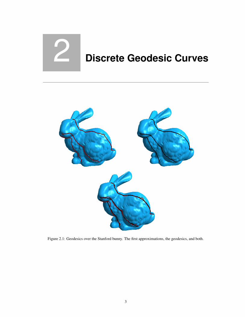
Figure 2.1: Geodesics over the Stanford bunny. The first approximations, the geodesics, and both.

3

4 CHAPTER 2. DISCRETE GEODESIC CURVES

Geodesic curves are useful in many areas of science and engineering, such as robot motion planning,terrain navigation, surface parameterization [12], remeshing [31] and front propagation over surfaces[27]. The increasing development of discrete surface models, as well as the use of smooth surfaces dis-cretization to study their geometry, demanded the definition of Geodesic Curves for polyhedral surfaces[2, 26], and hence the study of efficient algorithms to compute them.

Such curves are called Discrete Geodesics and there exist some different definitions for them, mostlydepending on the application in which they are used. Considering a geodesic as a shortest path betweentwo points on the surface is perhaps the more widely used definition.

In this chapter we are concerned with the problem of computing a locally shortest geodesic joining twopoints over the surface. There are some slightly different formulations for this problem. The simplestversion is the single source shortest path problem, in which one wishes to find a shortest path betweena source point and any other point on the surface. Another, more complex, version of the problem asksfor a subdivision on the surface such that a shortest path between any pair of points in the surface can befound quickly; this is known as the all pairs shortest path problem.

Most of the algorithms use front propagation or some other kind of Dijkstra’s-like algorithm. In 1987Mitchell, Mount and Papadimitriou [24] proposed the Continuous Dijkstra technique to build a datastructure from which we can find a shortest path between the source and any point in time O(k +log m), where k is the number of faces crossed by the path and m is the number of mesh edges. Thisalgorithm runs in O(m2 log m) time and requires O(m2) space. In 1999 Kapoor [15] also used wavepropagation techniques, very similar to Continuous Dijkstra, but with more efficient data structures, toget an O(n log2 n) algorithm, n being the number of mesh vertices. Sethian’s Fast Marching Method(FMM from now on) was used by Kimmel and Sethian [18] to define a distance function from a sourcepoint to the rest of the surface in O(n log n), and integrate back a differential equation to get the geodesicpath. Unlike the others, the last algorithm does not give the exact geodesic paths but an approximationto it; this approximation could be improved using the iterative process we propose in this paper. Thealgorithm of Chen and Han [5] builds a data structure based on surface unfoldings. In contrast to theother algorithms, it does not follow the wave front propagation paradigm and runs in O(n2) time withO(n) space. There are many other algorithms to compute shortest geodesics; for more information, werefer the reader to [5, 15, 18, 24, 32] and the references therein.

Chapter overview: In section 2.1 we do a quick review of the definitions for smooth and discretesurfaces. Section 2.2 presents the geodesic algorithm, which is the main contribution of this chapter. Webegin with an approximate path and use an iterative process to approach the true geodesic path. Finallyin section 2.3 we show some experimental results and adapt our algorithm to the single source shortestpath problem.

2.1 Geodesic Curves

Geodesic curves generalize the concept of straight lines for smooth surfaces. Therefore, they have several“good” properties, discussed on section 2.1.1. Unfortunately it is not possible to find such a class ofcurves over meshes sharing all these properties; as a consequence there are some different definitions forgeodesic curves on discrete surfaces, discussed in section 2.1.2, that depend on their proposed use. Therest of this section was mainly extracted from references [10, 26].

2.1.1 Geodesic curves on smooth surfaces

Consider a smooth two-dimensional surface G and a differential tangent vector field w : U ⊂ G → TPG.

Definition 2.1 Let y ∈ TPG, and consider a parameterized curve α : (−ε, ε) → U , with α(0) = P ,α′(0) = y and let w(t), t ∈ (−ε, ε) be the restriction of the vector field w to the curve α. The vector

2.1. GEODESIC CURVES 5

obtained by the projection of (dw/dt)(0) onto the plane TPG is called the covariant derivative at P ofthe vector field w relative to the vector y. This covariant derivative is denoted by (Dw/dt)(0).

The definition of the covariant derivative depends only on the field w and the vector y and not onthe curve α. This concept can be extended to a vector field which is defined only at the points of aparameterized curve. We denote the covariant derivative of a vector field w(t), defined along a curve α,by (Dw/dt)(t). For details on this subject see [10].

Consider a curve γ : I → G parameterized by arc length, i.e, |γ ′(t)| = 1 for all t in I . An example of adifferential vector field along γ is given by the field w(t) = γ ′(t) of the tangent vectors of γ.

Definition 2.2 γ is said to be geodesic at t ∈ I if the covariant derivative of γ ′ at t is zero, i.e.,

Dγ′(t)

dt= 0;

γ is a geodesic if it is a geodesic for all t ∈ I .

The following prop characterizes geodesic curves.

Proposition 2.1 The following properties are equivalent:

1. γ is a geodesic.

2. γ is a locally shortest curve; i.e, it is a critical point of the length functional L(γ) = length(γ).

3. γ′′ is parallel to the surface normal.

4. γ has vanishing geodesic curvature κg = 0 1.

From item 4 of Proposition 2.1 above, it can be concluded that geodesic curves are as straight as they canbe, if we see them from an intrinsic point of view. As a matter of fact, the curve variation up to a secondorder takes place only in the direction of the surface normal if it has vanishing geodesic curvature. Onthe other hand, item 2 tells us that a shortest smooth curve joining two points a geodesic. The converseis not true in general: there are geodesic curves which are critical points of the length functional but arenot shortest. Nevertheless, the property of being shortest is desirable for curves in many applications andit is perhaps the characterization of geodesic curve more used in practice. Another interesting propertyof geodesics is that they may have self-intersections, which is impossible for shortest curves.

2.1.2 Discrete geodesics

A curve defined over a mesh will be regular only if it is completely contained in one face or on a setof connected coplanar faces. The existence of such set of connected and coplanar faces is very rare.Therefore, the existence of regular curves passing through more than one face is unlikely. This is thefirst obstacle that we encounter when trying to generalize geodesics to discrete surfaces. The second oneis the fact that it is not possible in general to find a large enough set of curves over discrete surfaces forwhich all items of Proposition 2.1 hold.

There are some different generalizations of geodesic curves to a discrete surface S, all of them calledof discrete geodesics. Quasi-geodesics were defined by Aleksandrov and Zalgaller [2] as limit curves ofgeodesics on a family of converging smooth surfaces. They also defined discrete geodesics as criticalpoints of the length functional over polyhedral surfaces; in other words, they define them as locally short-est curves over S. From now on we call them shortest discrete geodesics or simply shortest geodesics.In particular, the problem we address in this chapter is to find a shortest geodesic joining two points overa triangular mesh.

Polthier and Schmies [26] defined straightest geodesics inspired in the characterization of smooth ge-o-de-sics given by item 4 of proposition 2.1. They defined discrete geodesic curvature as a generalization

1The geodesic curvature κg generalizes to surfaces the concept of curvature of a plane curve. See reference [10].


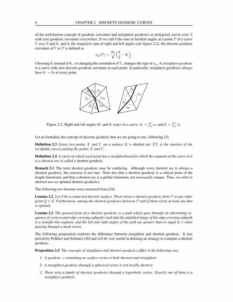
of the well-known concept of geodesic curvature and straightest geodesics as polygonal curves over Swith zero geodesic curvature everywhere. If we call θ the sum of incident angles at a point P of a curveΓ over S and θr and θl the respective sum of right and left angles (see figure 2.2), the discrete geodesiccurvature of Γ at P is defined as

κg(P ) =2π

θ

(θ

2− θr

).

Choosing θl instead of θr, or changing the orientation of Γ, changes the sign of κg. A straightest geodesicis a curve with zero discrete geodesic curvature at each point. In particular, straightest geodesics alwayshave θr = θl at every point.

α0

α1

α2α3β0

β1

β2 β3 α0

α1

β0

β1

Figure 2.2: Right and left angles (θr and θl resp.) in a curve. θr =∑

αi and θl =∑

βi.

Let us formalize the concept of discrete geodesic that we are going to use, following [2].

Definition 2.3 Given two points X and Y on a surface S, a shortest arc XY is the shortest of therectifiable curves joining the points X and Y .

Definition 2.4 A curve in which each point has a neighborhood for which the segment of the curve in itis a shortest arc is called a shortest geodesic.

Remark 2.1 The term shortest geodesic may be confusing. Although every shortest arc is always ashortest geodesic, the converse is not true. Note also that a shortest geodesic is a critical point of thelength functional, and that a shortest arc is a global minimum, not necessarily unique. Thus, we refer toshortest arcs as optimal shortest geodesics.

The following two lemmas were extracted from [24].

Lemma 2.2 Let S be a connected discrete surface. There exists a shortest geodesic from P to any otherpoint Q ∈ S. Furthermore, among the shortest geodesics between P and Q there exists at least one thatis optimal.

Lemma 2.3 The general form of a shortest geodesic is a path which goes through an alternating se-quence of vertices and edge-crossing subpaths such that the unfolded image of the edge-crossing subpathis a straight line segment, and the left and right angles of the path are greater than or equal to π whenpassing through a mesh vertex.

The following proposition explores the difference between straightest and shortest geodesic. It wasproved by Polthier and Schmies [26] and will be very useful in defining an strategy to compute a shortestgeodesic.

Proposition 2.4 The concepts of straightest and shortest geodesics differ in the following way:

1. A geodesic γ containing no surface vertex is both shortest and straightest.

2. A straightest geodesic through a spherical vertex is not locally shortest.

3. There exist a family of shortest geodesics through a hyperbolic vertex. Exactly one of them is astraightest geodesic.

2.2. GEODESIC COMPUTATION 7

2.2 Geodesic Computation

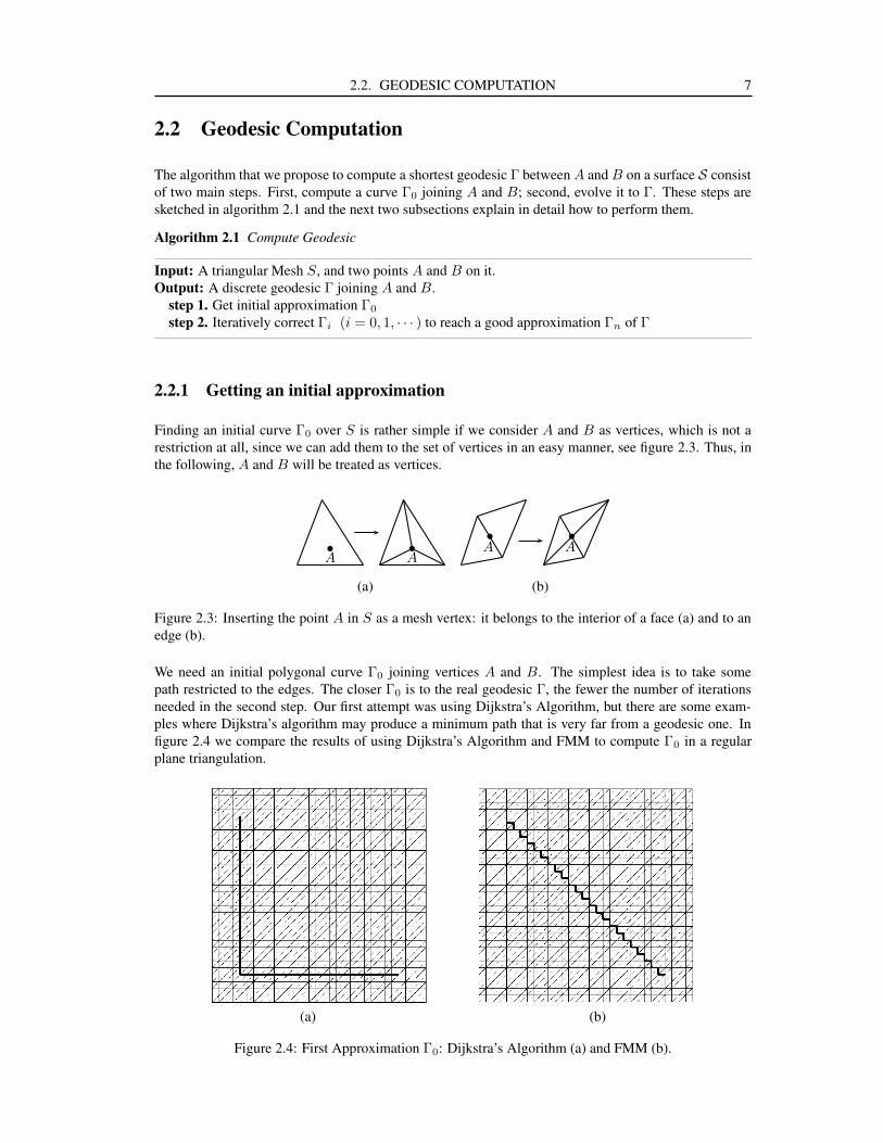
The algorithm that we propose to compute a shortest geodesic Γ between A and B on a surface S consistof two main steps. First, compute a curve Γ0 joining A and B; second, evolve it to Γ. These steps aresketched in algorithm 2.1 and the next two subsections explain in detail how to perform them.

Algorithm 2.1 Compute Geodesic

Input: A triangular Mesh S, and two points A and B on it.Output: A discrete geodesic Γ joining A and B.

step 1. Get initial approximation Γ0

step 2. Iteratively correct Γi (i = 0, 1, · · · ) to reach a good approximation Γn of Γ

2.2.1 Getting an initial approximation

Finding an initial curve Γ0 over S is rather simple if we consider A and B as vertices, which is not arestriction at all, since we can add them to the set of vertices in an easy manner, see figure 2.3. Thus, inthe following, A and B will be treated as vertices.

•A

•A

•A

•A

(a) (b)

Figure 2.3: Inserting the point A in S as a mesh vertex: it belongs to the interior of a face (a) and to anedge (b).

We need an initial polygonal curve Γ0 joining vertices A and B. The simplest idea is to take somepath restricted to the edges. The closer Γ0 is to the real geodesic Γ, the fewer the number of iterationsneeded in the second step. Our first attempt was using Dijkstra’s Algorithm, but there are some exam-ples where Dijkstra’s algorithm may produce a minimum path that is very far from a geodesic one. Infigure 2.4 we compare the results of using Dijkstra’s Algorithm and FMM to compute Γ0 in a regularplane triangulation.

(a) (b)

Figure 2.4: First Approximation Γ0: Dijkstra’s Algorithm (a) and FMM (b).


We decided to use FMM to define a distance function in the vertices of the mesh, as done by Kimmeland Sethian [18]. They solve the Eikonal equation

|∇D| = 1,

where D(P ) is the (geodesic) distance from A to any point P on S (see references [18, 30] for details).The efficiency of this process relies on the propagation of D over S maintaining a narrow band of verticesclose to the front. Once D is computed for every vertex, they must solve the ordinary differential equation

dχ(s)

ds= −∇D

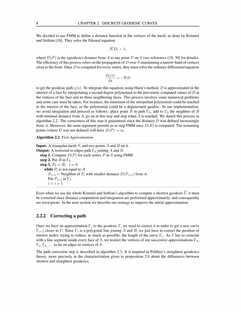
to get the geodesic path χ(s). To integrate this equation, using Huen’s method, D is approximated in theinterior of a face by interpolating a second degree polynomial to the previously computed values of D atthe vertices of the face and its three neighboring faces. This process involves some numerical problemsand some care must be taken. For instance, the minimum of the interpolant polynomial could be reachedin the interior of the face, or the polynomial could be a degenerated quadric. In our implementation,we avoid integration and proceed as follows: place point B in path Γ0, add to Γ0 the neighbor of Bwith minimal distance from A, go on in this way and stop when A is reached. We sketch this process inalgorithm 2.2. The correctness of this step is guaranteed since the distance D was defined increasinglyfrom A. Moreover, the same argument permits us to stop FMM once D(B) is computed. The remainingpoints (where D was not defined) will have D(P ) = ∞.

Algorithm 2.2 First Approximation

Input: A triangular mesh S, and two points A and B on it.Output: A restricted to edges path Γ0 joining A and B.

step 1. Compute D(P ) for each vertex P in S using FMMstep 2. Put B in Γ0

step 3. P0 = B, i = 0while Pi is not equal to A

Pi+1 = Neighbor of Pi with smaller distance D(Pi+1) from A.Put Pi+1 in Γ0

i = i + 1

Even when we use the whole Kimmel and Sethian’s algorithm to compute a shortest geodesic Γ, it mustbe corrected since distance computation and integration are performed approximately, and consequentlyare error-prone. In the next section we describe our strategy to improve the initial approximation.

2.2.2 Correcting a path

Once we have an approximation Γi to the geodesic Γ, we need to correct it in order to get a new curveΓi+1 closer to Γ. Since Γi is a polygonal line joining A and B, we just have to correct the position ofinterior nodes, trying to reduce, as much as possible, the length of the curve Γi. As Γ has to coincidewith a line segment inside every face of S, we restrict the vertices of our successive approximations Γ0,Γ1, Γ2 . . . to lie on edges or vertices of S.

The path correction step is described in algorithm 2.3. It is inspired in Polthier’s straightest geodesicstheory, more precisely in the characterization given in proposition 2.4 about the differences betweenshortest and straightest geodesics.


Algorithm 2.3 Path Correction

Input: A triangular mesh S, and a polygonal curve Γi joining A and B.Output: A shorter path Γi+1 joining A and B.

Pi+1,0 = Pi0 = B and Pi+1,n′ = Pin = Afor j = 1, 2, · · · , n − 1

correct the position of node Pij

Each node Pij is corrected to the new position Pi+1,j′ such that the curve segment between nodesPi+1,j′−1 and Pi,j+1 goes to the geodesic joining them, restricted to the set of faces that are neighborsto Pij .

Note that we use Pi+1,j′−1, the last corrected node, instead of Pi,j−1. Doing that, we do not need extraspace to store the new curve, since it is enough to substitute Pij’s position by its new position Pi+1,j′ .We will also get a better correction Pi+1,j′ since, to compute its position, we use a node whose positionwas previously corrected. Finally, we are able to prove that our algorithm actually reduces the lengthof Γi at each step, what cannot be guaranteed using the old neighbor Pi,j−1.

In some cases (when Pij coincides with a mesh vertex) it is necessary to replace node Pij by more than anode when correcting Γi. Also, some nodes may be eliminated when approaching a mesh vertex. Thesefacts justify the notation Pi+1,j′ used above for the corrected node in curve Γi+1.

We will use different procedures to correct the positions of the nodes of the polygonal Γi which belongto the interior of mesh edges and of those coinciding with mesh vertices, since they do not behave in thesame way. For instance, a point belonging to an edge has only two adjacent triangles while a vertex mayhave any number of them.

Correction of a node in the interior of an edge.

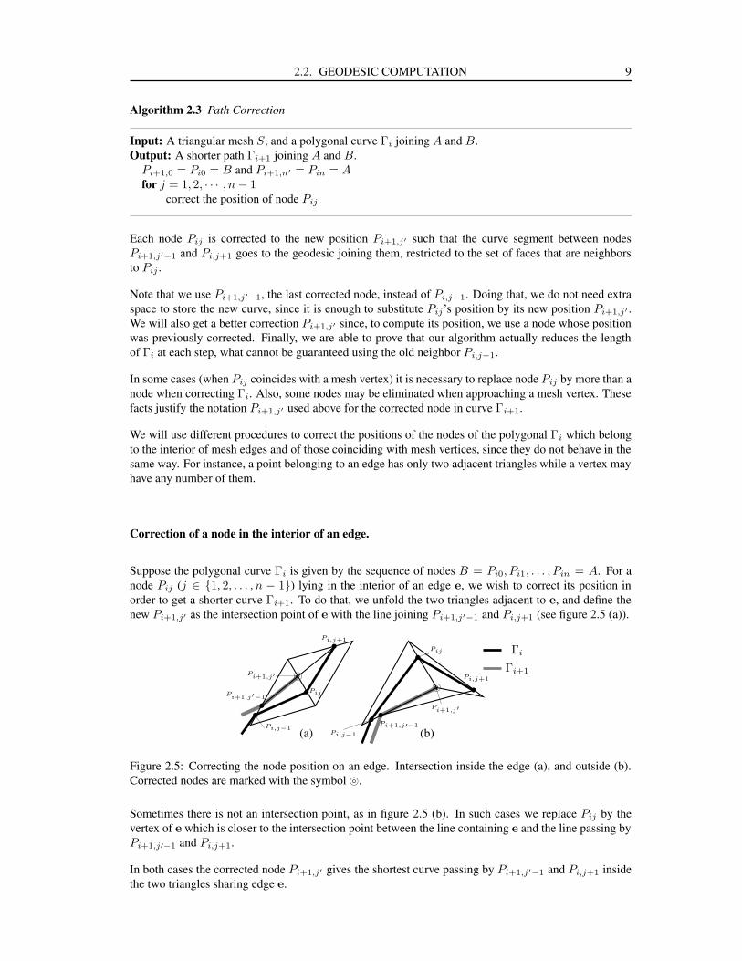
Suppose the polygonal curve Γi is given by the sequence of nodes B = Pi0, Pi1, . . . , Pin = A. For anode Pij (j ∈ {1, 2, . . . , n − 1}) lying in the interior of an edge e, we wish to correct its position inorder to get a shorter curve Γi+1. To do that, we unfold the two triangles adjacent to e, and define thenew Pi+1,j′ as the intersection point of e with the line joining Pi+1,j′−1 and Pi,j+1 (see figure 2.5 (a)).

••

•

•

}

Pi,j−1

Pij

Pi,j+1

Pi+1,j′

Pi+1,j′−1

(a)•

•

•

•

}

Pi,j−1

Pi+1,j′−1

Pij

Pi,j+1

Pi+1,j′

(b)

Γi

Γi+1

Figure 2.5: Correcting the node position on an edge. Intersection inside the edge (a), and outside (b).Corrected nodes are marked with the symbol }.

Sometimes there is not an intersection point, as in figure 2.5 (b). In such cases we replace Pij by thevertex of e which is closer to the intersection point between the line containing e and the line passing byPi+1,j′−1 and Pi,j+1.

In both cases the corrected node Pi+1,j′ gives the shortest curve passing by Pi+1,j′−1 and Pi,j+1 insidethe two triangles sharing edge e.


Correction of a node coinciding with a mesh vertex.

When Pij coincides with a mesh vertex, the correction is not so simple as in the previous case. Noticethat, now, Pij usually belongs to more than two triangles. We need to find a shortest path betweenPi+1,j′−1 and Pi,j+1 in the union of all triangles containing Pij as vertex. Suppose Pij correspondsto the kth vertex of S; then, such union of triangular faces, the star of vertex k, will be denoted by Sk.For simplicity Pi+1,j′−1 and Pi,j+1 are supposed to be on the boundary of Sk; otherwise one of thembelongs to the interior of Sk and in that case we can eliminate it from Γi without any loss of information.In fact, this node elimination will result in a shorter curve (see figure 2.6).

•

•

•

•

Pi,j−1

Pij Pi,j+1

Pi,j+2

•

•

•

•

Pi,j−1

Pij

Pi,j+1

Figure 2.6: Elimination of a node inside Sk.

We first classify node Pij as in definition 1.2 by computing left and right angles θl and θr, and then weshorten the curve by taking into account proposition 2.4. If Pij is euclidean then Sk can be isometricallyunfolded to be part of a plane and we just have to join the images of Pi+1,j′−1 and Pi,j+1 in the unfoldingof Sk. If Pij is spherical then no shortest curve may pass through it; in this case choose the part of Sk

with smaller angle, flatten it up, and join Pi+1,j′−1 to Pi,j+1. Finally, when Pij is hyperbolic we havetwo cases. The first one occurs when θr and θl are both larger than π. In this case no correction isneeded, since the curve cannot be shortened by moving Pij (see proof of proposition 2.4 [26]). If one ofthe angles, say θr, is smaller than π then the geodesic must pass through the corresponding side of Sk;we then proceed to flatten it up an compute the line joining Pi+1,j′−1 and Pi,j+1.

In all cases we have to compute the intersections of the computed line with the edges of the correspondingflattened part of Sk and we have to insert them in the polygonal curve in the correct order. Like inprevious case, it could happen that the intersection point is outside of some edge (see figure 2.7); in thatcase we insert the vertex of the edge in the path as we did before. Doing that, we usually obtain a pathwhich is not the shortest one inside the star of Pij . It can be improved performing a new node correctionon the extreme of the corresponding edge, obtaining the shortest path between the neighbors of Pij

2.

•

•

•

•

••

(a) (b)

Γn

Γn+1

Figure 2.7: Correcting a node coinciding with a mesh vertex. Convex star (a) and non-convex star (b).The resulting path before the additional correction in the non-convex star is shown as a dotted line.

Remark 2.2 Note that, in all cases, it is sufficient to trace the geodesic line in the side of Sk with smallerangle. At hyperbolic vertices, the geodesic can only be traced on the smaller angle’s side since the otherside has angle bigger than π and the curve cannot be shortened in it. On the other hand, it is possible

2Note that in this case the correction has “gone” outside the star of Pij .


sometimes to shorten the curve in both sides of an spherical vertex, but the law of the cosines ensuresthat the shortest one is obtained in the side with smaller angle. Although the problem of selecting theright side of Sk to look for Pi+1,j′ seems not to be necessary at euclidean vertices, the shortest pathshould also pass through the side with the smaller angle. In order to be convinced of this fact, supposethat Sk is part of a plane (otherwise we can flatten it isometrically), and consider the triangle formed byPi+1,j′−1, Pij and Pi,j+1; the angle in Pij , which is an interior angle of a triangle, must be less than π,hence the smallest between θr and θl, since their sum is 2π.

2.2.3 Implementation issues

Is it necessary to add new vertices to S?

To simplify the exposition, we supposed that both extremes of a geodesic are vertices of the mesh S. Wesuggested to add, if necessary, new vertices to S. However, this is not necessary at all. In fact, we canperform all computations without adding any new vertex to S; lets see:

Defining the initial curve Γ0: The definition of the distance function D begins by setting D(A) = 0,and them propagating a wave until D(B) is set. If A lies in the interior of a face f , we begin setting D atthe vertices of f as the euclidean distance D(V ) = ‖V −A‖2 from A to V , and then propagate the wave.If A lies in the interior of an edge e, we begin setting D at all the vertices of the two neighboring facesof e. The propagation stops when the distance function D have been set at one of the vertices which areneighbors of B. As for point A, there are three neighbors if B lies inside a face, or four if B lies insidean edge. Finally, the first approximation is computed as in algorithm 2.2, but beginning at the neighborof B with smaller value of the distance function D, and stopping when a neighbor of A was reached.After that we add B and A to Γ0 as first and last point respectively.

Correcting points inside a face: Although the nodes of geodesics curves are restricted to the edgesand vertices of the mesh, some times may be interesting to consider curves having nodes in the interiorof faces. This happens, for instance, in the computation of geodesic Bezier curves in chapter 3 wherenodes in the interior of faces are obtained due to a subdivision process. To avoid adding new vertices tothe mesh we must provide a rule to correct nodes in the interior of faces. Fortunately, this rule is verysimple: as a geodesic must be a straight line in the interior of faces, whenever we need to correct a nodeinside a face we just eliminate it from the curve.

Stopping criterion

An iterative process should always be controlled by a stop criterion, usually based on some error measure.Perhaps the most natural error measure for geodesic computation is given by curve length. However,the difference between the lengths of two successive approximations could be very small even whenthe curve is far from a shortest geodesic. This behavior is due to the fact that the evolution of thecurve has small variation close to mesh vertices, what is usually solved in a second iteration step. Inour implementation, we define a measure of error for each curve node based on proposition 2.4, andthen define a curve error measure as the maximum node error. For nodes lying in the interior of meshedges and nodes coinciding with euclidean mesh vertices, we define the error as the discrete geodesiccurvature κg, since in those cases shortest and straightest geodesics coincide. For nodes coinciding withspherical mesh vertices we define the error as a huge value, since no shortest geodesic can pass throughit. For nodes coinciding with hyperbolic mesh vertices we define the error as zero if both θl and θr aregreater than π and as a huge value otherwise, because only in the first case a shortest geodesic can passthrough it.


Boundary handling

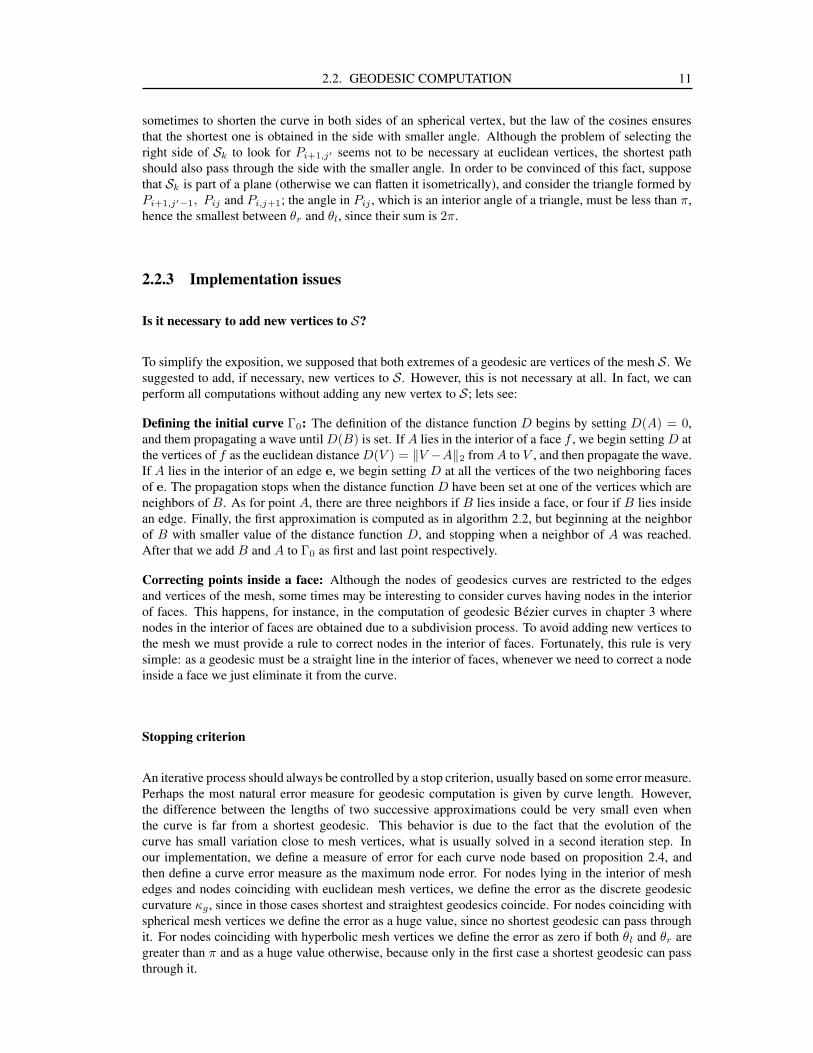
In some cases a geodesic path can touch a boundary or even coincide in part with it. For example ina plane with a hole or a non convex polygon as boundary, see figure 2.8. In order to correctly handle

Figure 2.8: Geodesics touching the boundary.

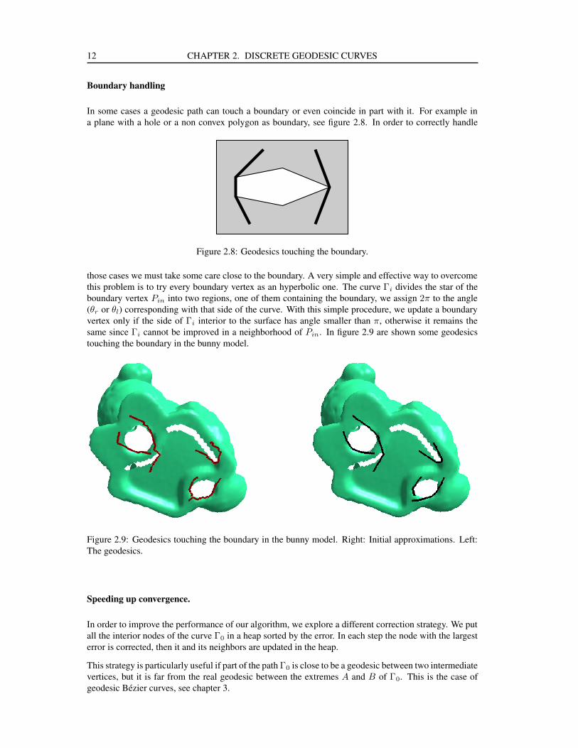
those cases we must take some care close to the boundary. A very simple and effective way to overcomethis problem is to try every boundary vertex as an hyperbolic one. The curve Γi divides the star of theboundary vertex Pin into two regions, one of them containing the boundary, we assign 2π to the angle(θr or θl) corresponding with that side of the curve. With this simple procedure, we update a boundaryvertex only if the side of Γi interior to the surface has angle smaller than π, otherwise it remains thesame since Γi cannot be improved in a neighborhood of Pin. In figure 2.9 are shown some geodesicstouching the boundary in the bunny model.

Figure 2.9: Geodesics touching the boundary in the bunny model. Right: Initial approximations. Left:The geodesics.

Speeding up convergence.

In order to improve the performance of our algorithm, we explore a different correction strategy. We putall the interior nodes of the curve Γ0 in a heap sorted by the error. In each step the node with the largesterror is corrected, then it and its neighbors are updated in the heap.

This strategy is particularly useful if part of the path Γ0 is close to be a geodesic between two intermediatevertices, but it is far from the real geodesic between the extremes A and B of Γ0. This is the case ofgeodesic Bezier curves, see chapter 3.

2.3. EXPERIMENTS 13

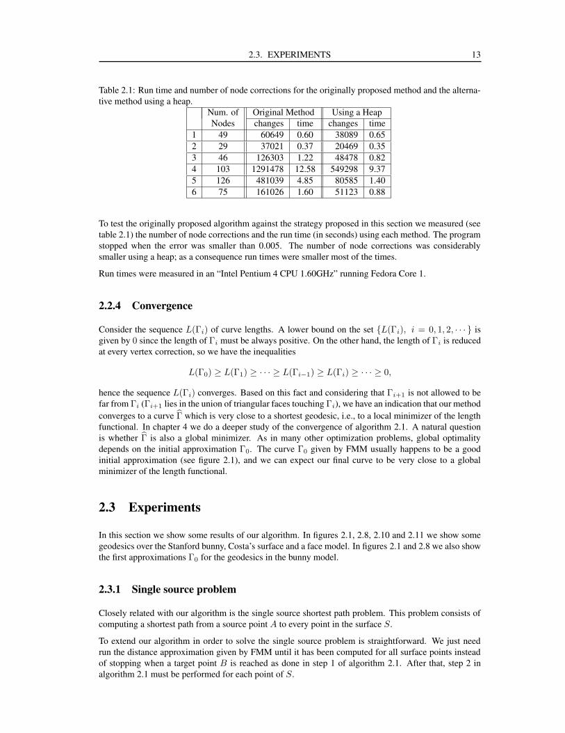
Table 2.1: Run time and number of node corrections for the originally proposed method and the alterna-tive method using a heap.

Num. of Original Method Using a HeapNodes changes time changes time

1 49 60649 0.60 38089 0.652 29 37021 0.37 20469 0.353 46 126303 1.22 48478 0.824 103 1291478 12.58 549298 9.375 126 481039 4.85 80585 1.406 75 161026 1.60 51123 0.88

To test the originally proposed algorithm against the strategy proposed in this section we measured (seetable 2.1) the number of node corrections and the run time (in seconds) using each method. The programstopped when the error was smaller than 0.005. The number of node corrections was considerablysmaller using a heap; as a consequence run times were smaller most of the times.

Run times were measured in an “Intel Pentium 4 CPU 1.60GHz” running Fedora Core 1.

2.2.4 Convergence

Consider the sequence L(Γi) of curve lengths. A lower bound on the set {L(Γi), i = 0, 1, 2, · · · } isgiven by 0 since the length of Γi must be always positive. On the other hand, the length of Γi is reducedat every vertex correction, so we have the inequalities

L(Γ0) ≥ L(Γ1) ≥ · · · ≥ L(Γi−1) ≥ L(Γi) ≥ · · · ≥ 0,

hence the sequence L(Γi) converges. Based on this fact and considering that Γi+1 is not allowed to befar from Γi (Γi+1 lies in the union of triangular faces touching Γi), we have an indication that our methodconverges to a curve Γ which is very close to a shortest geodesic, i.e., to a local minimizer of the lengthfunctional. In chapter 4 we do a deeper study of the convergence of algorithm 2.1. A natural questionis whether Γ is also a global minimizer. As in many other optimization problems, global optimalitydepends on the initial approximation Γ0. The curve Γ0 given by FMM usually happens to be a goodinitial approximation (see figure 2.1), and we can expect our final curve to be very close to a globalminimizer of the length functional.

2.3 Experiments

In this section we show some results of our algorithm. In figures 2.1, 2.8, 2.10 and 2.11 we show somegeodesics over the Stanford bunny, Costa’s surface and a face model. In figures 2.1 and 2.8 we also showthe first approximations Γ0 for the geodesics in the bunny model.

2.3.1 Single source problem

Closely related with our algorithm is the single source shortest path problem. This problem consists ofcomputing a shortest path from a source point A to every point in the surface S.

To extend our algorithm in order to solve the single source problem is straightforward. We just needrun the distance approximation given by FMM until it has been computed for all surface points insteadof stopping when a target point B is reached as done in step 1 of algorithm 2.1. After that, step 2 inalgorithm 2.1 must be performed for each point of S.


(a) (b)

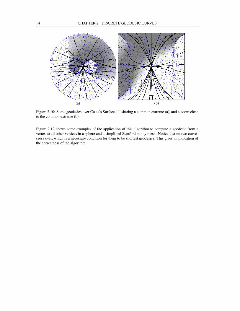
Figure 2.10: Some geodesics over Costa’s Surface, all sharing a common extreme (a), and a zoom closeto the common extreme (b).

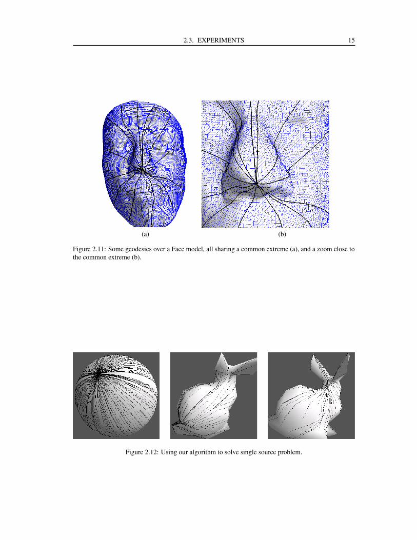
Figure 2.12 shows some examples of the application of this algorithm to compute a geodesic from avertex to all other vertices in a sphere and a simplified Stanford bunny mesh. Notice that no two curvescross over, which is a necessary condition for them to be shortest geodesics. This gives an indication ofthe correctness of the algorithm.

2.3. EXPERIMENTS 15

(a) (b)

Figure 2.11: Some geodesics over a Face model, all sharing a common extreme (a), and a zoom close tothe common extreme (b).

Figure 2.12: Using our algorithm to solve single source problem.

3 Geodesic Bezier Curves

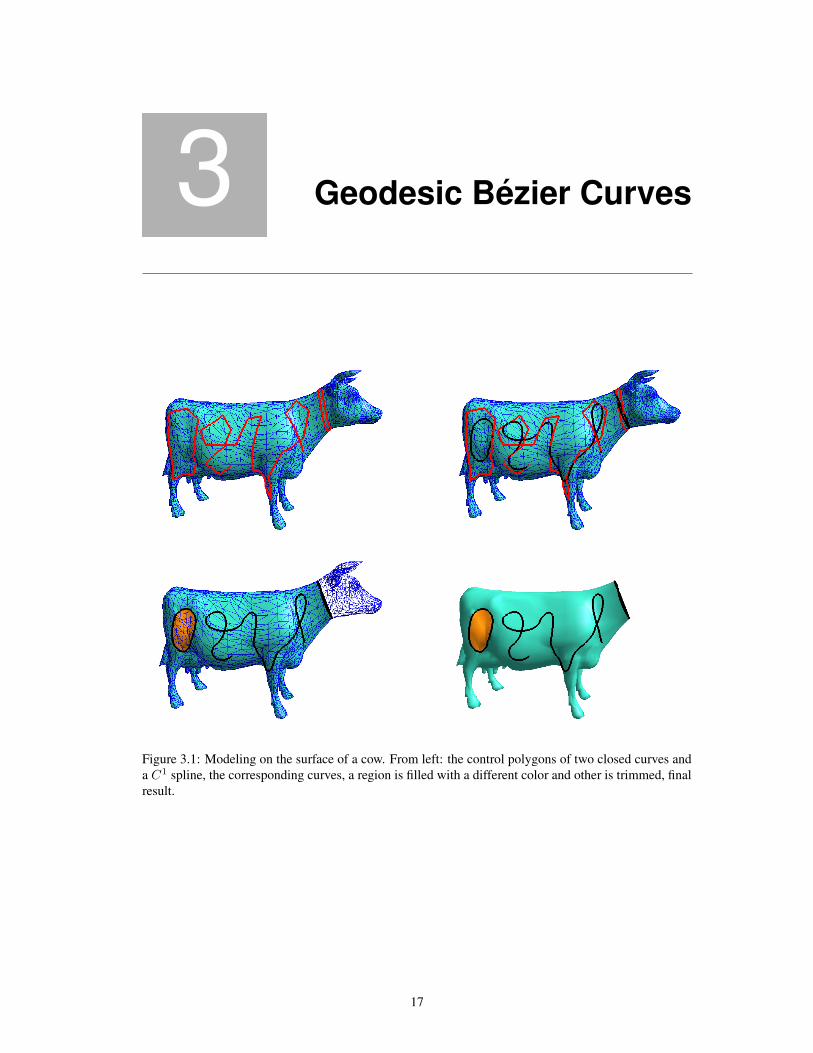
Figure 3.1: Modeling on the surface of a cow. From left: the control polygons of two closed curves anda C1 spline, the corresponding curves, a region is filled with a different color and other is trimmed, finalresult.

17

18 CHAPTER 3. GEODESIC BEZIER CURVES

Designing free-form curves is a basic operation in Geometric Modeling. Doing so in Euclidean spaceis a widely studied problem; see [7, 11] and many others. The problem becomes harder, however, if wewish to design on a curved geometry, such as triangulated surfaces. Most existing work for the later task,relies on imposing a suitable parameterization, which is usually an unintuitive approach that leads to aseries of “trial and error” operations. We pursue instead a direct design in the geometry of the surface,an approach that has received much less attention.

In this chapter we introduce a new class of curves that are suitable for free-form modeling directly onthe geometry of a manifold mesh. Defined by means of the de Casteljau Algorithm, they are a naturalgeneralization of Bezier curves. Thus, we call them “Intrinsic Bezier Curves”.

Chapter overview: This chapter begins, in section 3.1, with a summary of related work. After summa-rizing classical Bezier curves theory, we define in section 3.2 the new class of curves and compare themto the classical ones. A study of their use in modeling operations is done in section 3.3. Section 3.4describes the construction of piecewise Bezier spline curves on triangulations.

3.1 Related Work

The de Casteljau algorithm has been adapted to Riemannian manifolds using geodesic interpolation [25].However, it has been applied only to some surfaces where geodesic computation is relatively easy, suchas spheres or Lie groups; see [8, 29] and the references therein for details. The only modeling operationstudied in those works is the construction of cubic splines. Furthermore, trimming seems to be very hardto perform in this setting. We define curves using the same idea as in [25], but we consider manifoldtriangulations.

Another generalization of cubic splines to smooth manifolds is given in [14, 28]. The curves are definedby interpolating a set of knot points on the surface, minimizing an energy functional. These results arealso applicable to triangulations, but they require the computation of local smooth approximations. If theposition of a knot is changed, the whole curve must be recomputed since there is no local control of itsshape. On the other hand, the interpolation of tangent vectors or higher derivatives has not been studied.Using geodesic Bezier curves we can overcome these difficulties, and it becomes possible to prescribederivatives at knot points and to have local control of the segments of the Bezier spline curve.

Trimming is a very important application in CAGD. This operation is usually done by means of a param-eterization. One has to figure out which curve in the parameter space corresponds to the desired curveon the surface, which is generally a difficult problem. Most of the time these curves are obtained as theresult of CSG operations, or more general surface intersections [20, 6]. An approach for subdivisionsurfaces is to modify the original (coarse) mesh in order to obtain a trimmed limit surface [4, 22]. Ourtrimming operations are done directly on the mesh and no parameterization is needed.

Recent works [35, 34, 33] define a general framework for curve subdivision schemes. Geodesic Beziercurves fits into this framework. However, smoothness of limit curves is only studied – and proved – inthe case of smooth manifolds, considering meshes as an approximation of smooth surfaces, what is notalways the case. For example, a potential user may be interested in modeling on a coarse mesh instead ofa refined one. Besides, models with sharp features are best approximated with non-smooth surfaces. Inthis thesis we analyze the smoothness of geodesic Bezier curves in the context of triangular meshes, andalso how to handle modifications in the position of control points at interactive rates, what is not done inthose works. Our results are also applicable to the other geodesic-based subdivision schemes fitting intothis framework.

3.2. GEODESIC BEZIER CURVES 19

3.2 Geodesic Bezier Curves

Bezier curves are of great importance when modeling on Rn. A natural question is how to generalize

them to curved geometries. In this section we propose a class of curves that generalize Bezier curves tomanifold triangulations.

3.2.1 Classical Bezier Curves

Given n+1 control points P0, P1, . . . , Pn in Rd, they define a curve given by the following parametric

expression:

P (u) =

n∑

i=0

(n

i

)(1 − u)n−iuiPi, 0 ≤ u ≤ 1, (3.1)

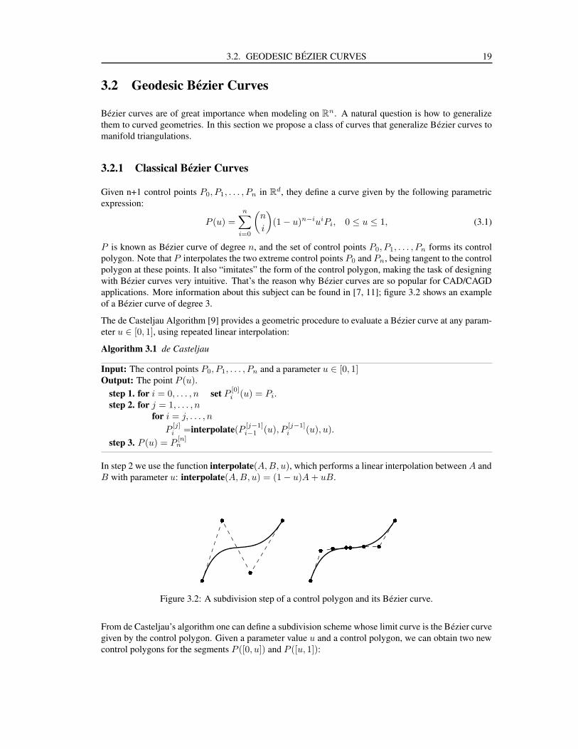
P is known as Bezier curve of degree n, and the set of control points P0, P1, . . . , Pn forms its controlpolygon. Note that P interpolates the two extreme control points P0 and Pn, being tangent to the controlpolygon at these points. It also “imitates” the form of the control polygon, making the task of designingwith Bezier curves very intuitive. That’s the reason why Bezier curves are so popular for CAD/CAGDapplications. More information about this subject can be found in [7, 11]; figure 3.2 shows an exampleof a Bezier curve of degree 3.

The de Casteljau Algorithm [9] provides a geometric procedure to evaluate a Bezier curve at any param-eter u ∈ [0, 1], using repeated linear interpolation:

Algorithm 3.1 de Casteljau

Input: The control points P0, P1, . . . , Pn and a parameter u ∈ [0, 1]Output: The point P (u).

step 1. for i = 0, . . . , n set P[0]i (u) = Pi.

step 2. for j = 1, . . . , nfor i = j, . . . , n

P[j]i =interpolate(P [j−1]

i−1 (u), P[j−1]i (u), u).

step 3. P (u) = P[n]n

In step 2 we use the function interpolate(A,B, u), which performs a linear interpolation between A andB with parameter u: interpolate(A,B, u) = (1 − u)A + uB.

�

�

�

�

�

��

�

Figure 3.2: A subdivision step of a control polygon and its Bezier curve.

From de Casteljau’s algorithm one can define a subdivision scheme whose limit curve is the Bezier curvegiven by the control polygon. Given a parameter value u and a control polygon, we can obtain two newcontrol polygons for the segments P ([0, u]) and P ([u, 1]):


Algorithm 3.2 Subdivision of a control polygon

Input: The control points P0, P1, . . . , Pn and a parameter u ∈ [0, 1]Output: Two sets of control points defining P ([0, u]) and P ([u, 1]).

step 1. deCasteljau((P0, P1, . . . , Pn), u).step 2.

P ([0, u]) =bezier(P [0]0 , P

[1]1 , . . . , P

[n]n )

P ([u, 1]) =bezier(P [n]n , P

[n−1]n , . . . , P

[0]n )

Evaluating the curve at u, using de Casteljau’s algorithm, provides the intermediary interpolated pointsP

[j]i . The output (step 2) are the control polygons defining both (Bezier) segments of the curve. Fig-

ure 3.2 shows a subdivision step of the control polygon of a degree 3 Bezier curve.

Algorithm 3.2 provides the rule for the subdivision scheme converging to the curve. Additionally, thisscheme can be made adaptive by stopping the subdivision whenever a control polygon can be consideredas “almost straight”.

3.2.2 Bezier Curves on Manifold Triangulations

Intrinsic Bezier curves are defined by means of the subdivision algorithm for classical Bezier curves.Given a control polygon P0, P1, . . . , Pn on a surface S, we want to compute a curve C on S interpolatingP0 and Pn, whose shape is controlled by the position of the interior points P1, P2, . . . , Pn−1.

The curve C is defined as the limit of the subdivision scheme given in algorithm 3.2 of section 3.2.1.The main difference is that the sides of the control polygon are no longer line segments, but geodesicsconnecting the control points. This imposes the necessity of modifying the interpolation step on algo-rithm 3.1. The equivalent to linear interpolation in the geometry of the surface is the interpolation alonggeodesic lines. Algorithm 3.3 describes the interpolation step in the case of manifold triangulations:

Algorithm 3.3 Interpolation on Manifold Triangulations

Input: A manifold triangulation S, two points Q1 and Q2 on it and a parameter u ∈ [0, 1]Output: A point Q on S interpolating Q1 and Q2.

step 1. Γ =ComputeGeodesic(Q1, Q2).step 2. Q = the point of Γ such that

dΓ(Q1, Q) = udΓ(Q1, Q2)

In algorithm 3.3, dΓ(A,B) computes the distance between A and B along Γ. Note that since Γ is apolygonal line, it is very simple to perform step 2.

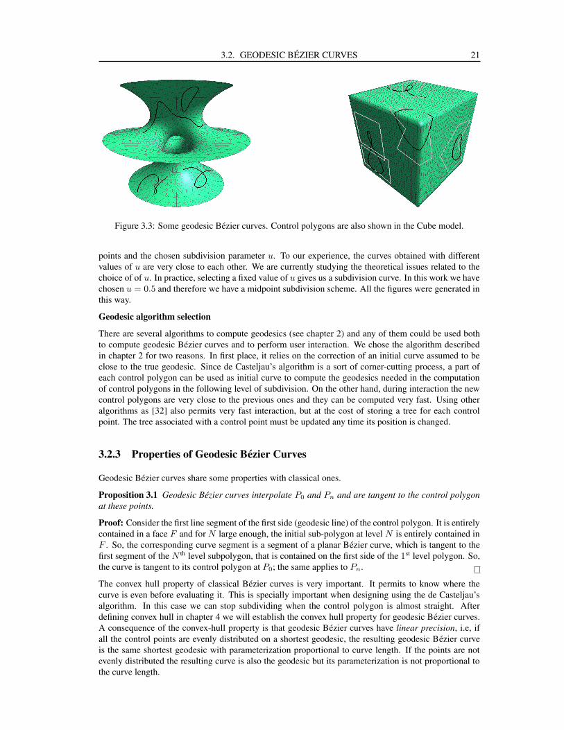
To compute an approximation of C, we can use the subdivision adaptive algorithm. It stops at someprescribed level of subdivision or when the control polygon can be considered as a geodesic segment;i.e., when all of its control vertices have error smaller than a prescribed tolerance. Figure 3.3 shows somegeodesic Bezier curves along with their control polygons.

The use of de Casteljau’s algorithm in the definition of geodesic Bezier curves makes them a general-ization of planar Bezier curves. Note that a geodesic on a plane is a straight line. Therefore, when thetriangulation is planar both concepts coincide; see for example the curves designed on the (planar) facesof the cube in figure 3.3. As in the case of classical Bezier curves, we have a parameterization of ourcurves with parameter u ∈ [0, 1]. Evaluation at any particular parameter value can be performed easilyby subdividing the corresponding control polygon at each level of subdivision, imitating the bisectionalgorithm used to compute roots of polynomials. Previous calculations can be used to evaluate at newparameter values, this can be useful when performing many evaluations.

It is known that shortest geodesics are not unique on triangulations. Consequently, the use of a differentsubdivision parameter may lead to a different curve. So geodesic Bezier curves depends on the control

3.2. GEODESIC BEZIER CURVES 21

Figure 3.3: Some geodesic Bezier curves. Control polygons are also shown in the Cube model.

points and the chosen subdivision parameter u. To our experience, the curves obtained with differentvalues of u are very close to each other. We are currently studying the theoretical issues related to thechoice of of u. In practice, selecting a fixed value of u gives us a subdivision curve. In this work we havechosen u = 0.5 and therefore we have a midpoint subdivision scheme. All the figures were generated inthis way.

Geodesic algorithm selectionThere are several algorithms to compute geodesics (see chapter 2) and any of them could be used bothto compute geodesic Bezier curves and to perform user interaction. We chose the algorithm describedin chapter 2 for two reasons. In first place, it relies on the correction of an initial curve assumed to beclose to the true geodesic. Since de Casteljau’s algorithm is a sort of corner-cutting process, a part ofeach control polygon can be used as initial curve to compute the geodesics needed in the computationof control polygons in the following level of subdivision. On the other hand, during interaction the newcontrol polygons are very close to the previous ones and they can be computed very fast. Using otheralgorithms as [32] also permits very fast interaction, but at the cost of storing a tree for each controlpoint. The tree associated with a control point must be updated any time its position is changed.

3.2.3 Properties of Geodesic Bezier Curves

Geodesic Bezier curves share some properties with classical ones.

Proposition 3.1 Geodesic Bezier curves interpolate P0 and Pn and are tangent to the control polygonat these points.

Proof: Consider the first line segment of the first side (geodesic line) of the control polygon. It is entirelycontained in a face F and for N large enough, the initial sub-polygon at level N is entirely contained inF . So, the corresponding curve segment is a segment of a planar Bezier curve, which is tangent to thefirst segment of the N th level subpolygon, that is contained on the first side of the 1st level polygon. So,the curve is tangent to its control polygon at P0; the same applies to Pn.

The convex hull property of classical Bezier curves is very important. It permits to know where thecurve is even before evaluating it. This is specially important when designing using the de Casteljau’salgorithm. In this case we can stop subdividing when the control polygon is almost straight. Afterdefining convex hull in chapter 4 we will establish the convex hull property for geodesic Bezier curves.A consequence of the convex-hull property is that geodesic Bezier curves have linear precision, i.e, ifall the control points are evenly distributed on a shortest geodesic, the resulting geodesic Bezier curveis the same shortest geodesic with parameterization proportional to curve length. If the points are notevenly distributed the resulting curve is also the geodesic but its parameterization is not proportional tothe curve length.


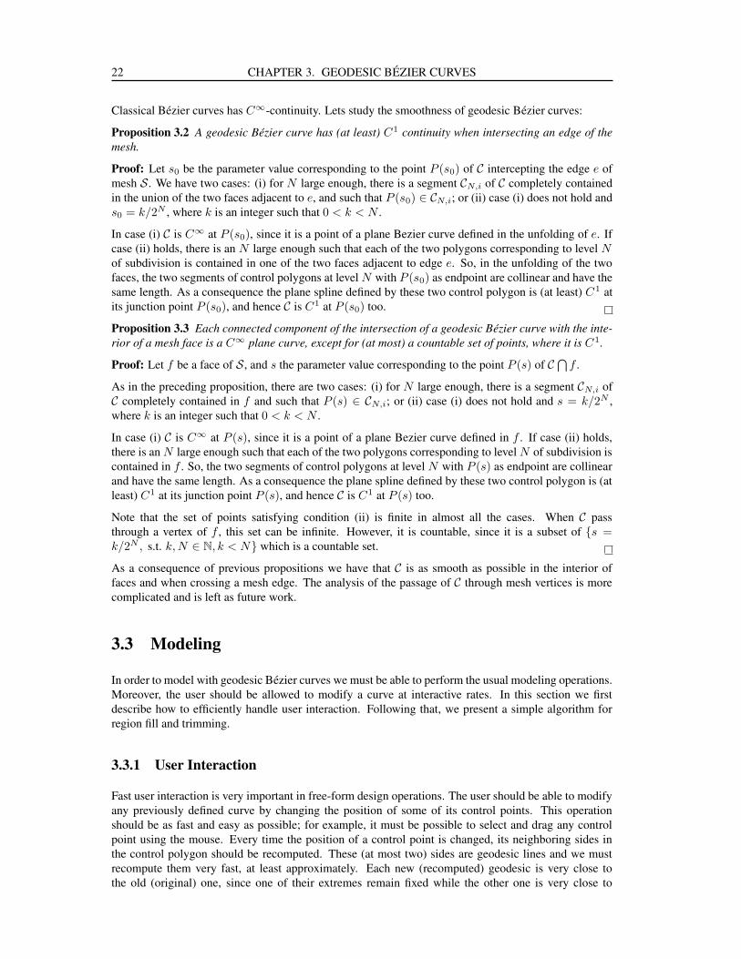
Classical Bezier curves has C∞-continuity. Lets study the smoothness of geodesic Bezier curves:

Proposition 3.2 A geodesic Bezier curve has (at least) C1 continuity when intersecting an edge of themesh.

Proof: Let s0 be the parameter value corresponding to the point P (s0) of C intercepting the edge e ofmesh S. We have two cases: (i) for N large enough, there is a segment CN,i of C completely containedin the union of the two faces adjacent to e, and such that P (s0) ∈ CN,i; or (ii) case (i) does not hold ands0 = k/2N , where k is an integer such that 0 < k < N .

In case (i) C is C∞ at P (s0), since it is a point of a plane Bezier curve defined in the unfolding of e. Ifcase (ii) holds, there is an N large enough such that each of the two polygons corresponding to level Nof subdivision is contained in one of the two faces adjacent to edge e. So, in the unfolding of the twofaces, the two segments of control polygons at level N with P (s0) as endpoint are collinear and have thesame length. As a consequence the plane spline defined by these two control polygon is (at least) C1 atits junction point P (s0), and hence C is C1 at P (s0) too.

Proposition 3.3 Each connected component of the intersection of a geodesic Bezier curve with the inte-rior of a mesh face is a C∞ plane curve, except for (at most) a countable set of points, where it is C1.

Proof: Let f be a face of S, and s the parameter value corresponding to the point P (s) of C⋂

f .

As in the preceding proposition, there are two cases: (i) for N large enough, there is a segment CN,i ofC completely contained in f and such that P (s) ∈ CN,i; or (ii) case (i) does not hold and s = k/2N ,where k is an integer such that 0 < k < N .

In case (i) C is C∞ at P (s), since it is a point of a plane Bezier curve defined in f . If case (ii) holds,there is an N large enough such that each of the two polygons corresponding to level N of subdivision iscontained in f . So, the two segments of control polygons at level N with P (s) as endpoint are collinearand have the same length. As a consequence the plane spline defined by these two control polygon is (atleast) C1 at its junction point P (s), and hence C is C1 at P (s) too.

Note that the set of points satisfying condition (ii) is finite in almost all the cases. When C passthrough a vertex of f , this set can be infinite. However, it is countable, since it is a subset of {s =k/2N , s.t. k,N ∈ N, k < N} which is a countable set.

As a consequence of previous propositions we have that C is as smooth as possible in the interior offaces and when crossing a mesh edge. The analysis of the passage of C through mesh vertices is morecomplicated and is left as future work.

3.3 Modeling

In order to model with geodesic Bezier curves we must be able to perform the usual modeling operations.Moreover, the user should be allowed to modify a curve at interactive rates. In this section we firstdescribe how to efficiently handle user interaction. Following that, we present a simple algorithm forregion fill and trimming.

3.3.1 User Interaction

Fast user interaction is very important in free-form design operations. The user should be able to modifyany previously defined curve by changing the position of some of its control points. This operationshould be as fast and easy as possible; for example, it must be possible to select and drag any controlpoint using the mouse. Every time the position of a control point is changed, its neighboring sides inthe control polygon should be recomputed. These (at most two) sides are geodesic lines and we mustrecompute them very fast, at least approximately. Each new (recomputed) geodesic is very close tothe old (original) one, since one of their extremes remain fixed while the other one is very close to

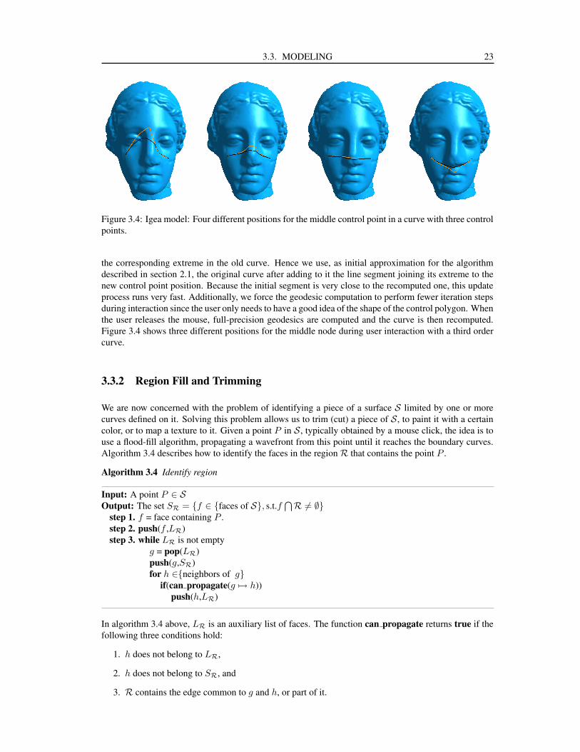
3.3. MODELING 23

Figure 3.4: Igea model: Four different positions for the middle control point in a curve with three controlpoints.

the corresponding extreme in the old curve. Hence we use, as initial approximation for the algorithmdescribed in section 2.1, the original curve after adding to it the line segment joining its extreme to thenew control point position. Because the initial segment is very close to the recomputed one, this updateprocess runs very fast. Additionally, we force the geodesic computation to perform fewer iteration stepsduring interaction since the user only needs to have a good idea of the shape of the control polygon. Whenthe user releases the mouse, full-precision geodesics are computed and the curve is then recomputed.Figure 3.4 shows three different positions for the middle node during user interaction with a third ordercurve.

3.3.2 Region Fill and Trimming

We are now concerned with the problem of identifying a piece of a surface S limited by one or morecurves defined on it. Solving this problem allows us to trim (cut) a piece of S, to paint it with a certaincolor, or to map a texture to it. Given a point P in S, typically obtained by a mouse click, the idea is touse a flood-fill algorithm, propagating a wavefront from this point until it reaches the boundary curves.Algorithm 3.4 describes how to identify the faces in the region R that contains the point P .

Algorithm 3.4 Identify region

Input: A point P ∈ SOutput: The set SR = {f ∈ {faces of S}, s.t.f

⋂R 6= ∅}

step 1. f = face containing P .step 2. push(f ,LR)step 3. while LR is not empty

g = pop(LR)push(g,SR)for h ∈{neighbors of g}

if(can propagate(g 7→ h))push(h,LR)

In algorithm 3.4 above, LR is an auxiliary list of faces. The function can propagate returns true if thefollowing three conditions hold:

1. h does not belong to LR,

2. h does not belong to SR, and

3. R contains the edge common to g and h, or part of it.


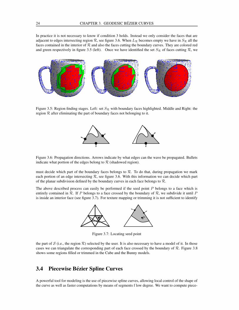
In practice it is not necessary to know if condition 3 holds. Instead we only consider the faces that areadjacent to edges intersecting region R, see figure 3.6. When LR becomes empty we have in SR all thefaces contained in the interior of R and also the faces cutting the boundary curves. They are colored redand green respectively in figure 3.5 (left). Once we have identified the set SR of faces cutting R, we

Figure 3.5: Region finding stages. Left: set SR with boundary faces highlighted. Middle and Right: theregion R after eliminating the part of boundary faces not belonging to it.

•••

••

Figure 3.6: Propagation directions. Arrows indicate by what edges can the wave be propagated. Bulletsindicate what portion of the edges belong to R (shadowed region).

must decide which part of the boundary faces belongs to R. To do that, during propagation we markeach portion of an edge intersecting R, see figure 3.6. With this information we can decide which partof the planar subdivision defined by the boundary curves in each face belongs to R.

The above described process can easily be performed if the seed point P belongs to a face which isentirely contained in R. If P belongs to a face crossed by the boundary of R, we subdivide it until Pis inside an interior face (see figure 3.7). For texture mapping or trimming it is not sufficient to identify

•P •P

••

Figure 3.7: Locating seed point

the part of S (i.e., the region R) selected by the user. It is also necessary to have a model of it. In thosecases we can triangulate the corresponding part of each face crossed by the boundary of R. Figure 3.8shows some regions filled or trimmed in the Cube and the Bunny models.

3.4 Piecewise Bezier Spline Curves

A powerful tool for modeling is the use of piecewise spline curves, allowing local control of the shape ofthe curve as well as faster computations by means of segments f low degree. We want to compute piece-

3.4. PIECEWISE BEZIER SPLINE CURVES 25

Figure 3.8: Filled and trimmed regions: Trimmed Cube and Stanford’s bunny with two trimmed regionsand one filled.

wise spline curves of geodesic Bezier curves, so next we investigate how to guarantee some continuityat junction points.

As usual, C0 continuity is reached by defining the first control point of a segment Ci+1 to be the same asthe last control point of its previous segment Ci. To guarantee C1 continuity is harder because we musthave the last side of the control polygon of Ci aligned with the first side of the control polygon of Ci+1.Moreover, the length of these two sides must be the same. This means that we need to locate threecontrol points in the same geodesic line. In other words, the position of the two first control vertices ofthe segment Ci+1 are determined by the position of the control vertices of the previous segment Ci.

Given the control polygon of the ith segment Ci of a spline curve C, how to compute the two first controlpoints P i+1

0 and P i+11 of Ci+1? Its first control point P i+1

0 is the same as the last control point P im

of Ci. The second one, P i+11 , is hard to find because we do not know how to continue the geodesic line

between P im−1 and P i

m. For smooth surfaces we can compute the unique geodesic passing by a point ina direction. This is not the case for shortest geodesics on meshes. Nevertheless the straightest geodesicsdefined by [26] have this nice property. For that reason we define the first side of the control polygonof Ci+1 as the straightest geodesic continuing the last side of the control polygon of Ci. It is known [26]that if a straightest geodesic does not pass by a spherical vertex, it is also a shortest geodesic. So wecan expect that most of the times our control polygon will be defined by means of shortest geodesics. Itis important to note that all the properties of section 3.2.3 are also satisfied if we replace one or moreof the shortest geodesics by straightest ones. Thus, the relaxation we did to the definition of the controlpolygon, in order to have C1 continuity, is more than justified.

Finally note that modifying the position of P im−1 modifies the position of P i+1

1 and vice versa. In thelast case, the last side of the control polygon of Ci will be a straightest geodesic. Modifying the positionof the junction point conduce us to modify at least the position of one of the control points P i

m−1 andP i+1

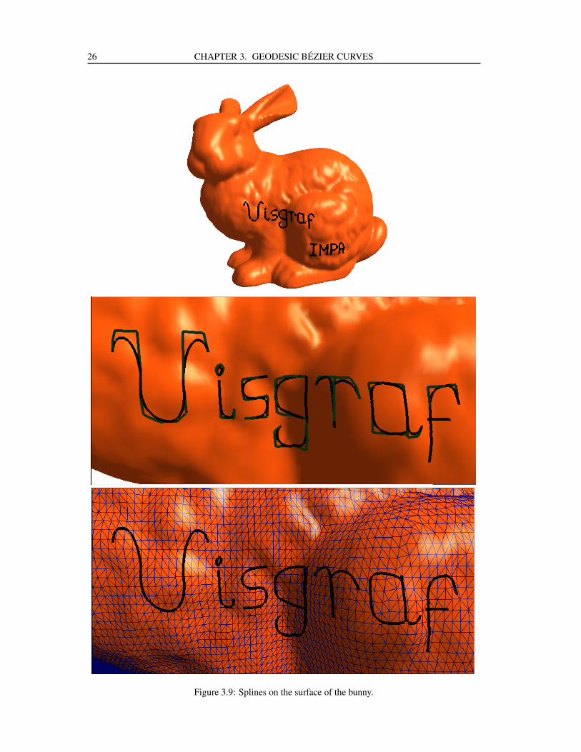
1 . Figure 3.9 show the use of C1 splines to write in the surface of the Stanford’s bunny model. Themiddle curve in figure 3.1 is a C1 spline, composed by 8 Bezier segments.


Figure 3.9: Splines on the surface of the bunny.

4 Convex Sets on DiscreteSurfaces

To define convex sets in triangulations requires some care. A naive definition, as the intersection of thesurface with a convex set, will not work because it ignores the intrinsic geometry of the surface. As inthe case of geodesics, there are different definitions obtained by imitating the behavior of plane convexsets [2], but they are too restrictive. For example, non-optimal shortest geodesics are not convex in theusual sense. Our definition allow them to be convex.

In this chapter we define convex sets based on the geodesic curvature of the boundary curves, and derivethe concept of convex hull in manifolds. Those definitions are very useful to prove the convergence ofthe geodesic algorithm of chapter 2, and the convex hull property of geodesic Bezier curves defined inchapter 3.

4.1 Discrete Geodesic Curvature

Polthier and Schmies [26] defined straightest geodesics as curves with zero geodesic curvature κg(P ),where

κg(P ) =2π

θ

(θ

2− θr

).

In order to obtain a similar characterization for shortest geodesics, we must employ an alternative defi-nition of discrete geodesic curvature:

Definition 4.1 The discrete geodesic curvature of a polygonal curve at a given point P is given by thefollowing expression.

κs(P ) =

0, if θ(P ) > 2π, θr(P ) ≥ π and θl(P ) ≥ π∞, if θ(P ) < 2π and θr(P ) = θl(P )κg(P ), otherwise

Remark 4.1 We use the notation κs to distinguish this new definition of discrete geodesic curvaturefrom Polthier’s one. The subindex s stands for shortest.

Remark 4.2 Boundary points are treated as hyperbolic, as done in section 2.2.3.

With this alternative definition of geodesic curvature at hand, we can characterize discrete shortestgeodesics on triangulations:

Proposition 4.1 A polygonal curve Γ contained in a manifold triangulation S is a shortest geodesic ifand only if its geodesic curvature κs is identically zero.

Proof: Let Γ be a shortest geodesic on S and P a node of Γ. If P does not coincide with a mesh vertex,or coincides with an euclidean one, then θr and θl are equals; consequently κs(P ) = κg(P ) = 0. If P

27

28 CHAPTER 4. CONVEX SETS ON DISCRETE SURFACES

coincides with a hyperbolic vertex then both θr and θl must be greater than π, hence κs(P ) = 0. Finally,P cannot coincide with a spherical vertex.

On the other hand, suppose that Γ have zero geodesic curvature everywhere. That means –see defini-tion 4.1 and proposition 2.4– that a small perturbation in the position of any vertex will increase thelength of Γ. Thus, it is a local minimum of the length functional and consequently a shortest geodesic.

4.2 Convex Sets

It is known that if the boundary of a plane convex set is a smooth curve, then its curvature does notchange its sign [10]. If the boundary is a polygonal line, then at each vertex the angle correspondingto the interior of the set is smaller that the exterior one. Based on these facts, we define convex sets ontriangulations.

Definition 4.2 Let C be a connected subset of a surface S. C is convex if its boundary ∂C can beparametrized by a closed curve Γ : I −→ ∂C such that:

1. ∀t ∈ I κs(Γ(t)) ≤ 0, and

2. the interior of set C is always situated in the left side of Γ.

Remark 4.3 If we replace’≤’ by ’≥’ and ’left’ by ’right’ in definition 4.2, we get an equivalent definitionof convex set.

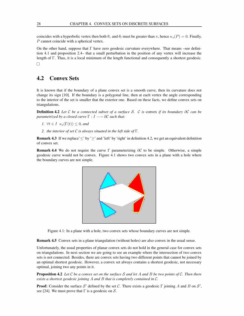
Remark 4.4 We do not require the curve Γ parameterizing ∂C to be simple. Otherwise, a simplegeodesic curve would not be convex. Figure 4.1 shows two convex sets in a plane with a hole wherethe boundary curves are not simple.

Figure 4.1: In a plane with a hole, two convex sets whose boundary curves are not simple.

Remark 4.5 Convex sets in a plane triangulation (without holes) are also convex in the usual sense.

Unfortunately, the usual properties of planar convex sets do not hold in the general case for convex setson triangulations. In next section we are going to see an example where the intersection of two convexsets is not connected. Besides, there are convex sets having two different points that cannot be joined byan optimal shortest geodesic. However, a convex set always contains a shortest geodesic, not necessaryoptimal, joining two any points in it.

Proposition 4.2 Let C be a convex set on the surface S and let A and B be two points of C. Then thereexists a shortest geodesic joining A and B that is completely contained in C.

Proof: Consider the surface S ′ defined by the set C. There exists a geodesic Γ joining A and B on S ′,see [24]. We must prove that Γ is a geodesic on S.

4.3. CONVEX HULL 29

If Γ does not touch the boundary of S ′ then it is also a geodesic on S. Suppose now that the point P ∈ Γbelongs to the boundary of S ′. If we choose an orientation of Γ such that the angle θl of Γ at P is theone in the interior of S ′, then θl must be greater than or equal to π, because boundary points are treatedas hyperbolic vertices. This means that the angle θl of ∂C at P is also greater than or equal to π, but asC is a convex set then, looking to ∂C as a curve on S, the angle θr of ∂C at P must also be greater thanor equal to π. Hence, P is a hyperbolic or euclidean point on S and the geodesic curvature κs(P ) of Γat P is also zero when looking to Γ as a curve on S. This means that Γ is a geodesic on S.

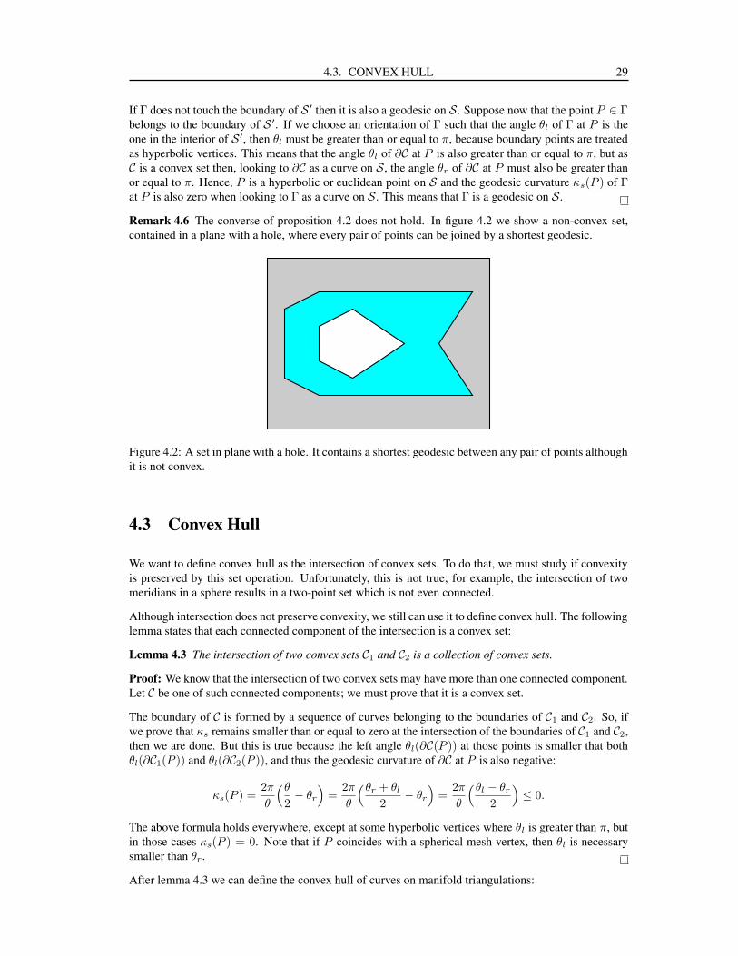
Remark 4.6 The converse of proposition 4.2 does not hold. In figure 4.2 we show a non-convex set,contained in a plane with a hole, where every pair of points can be joined by a shortest geodesic.

Figure 4.2: A set in plane with a hole. It contains a shortest geodesic between any pair of points althoughit is not convex.

4.3 Convex Hull

We want to define convex hull as the intersection of convex sets. To do that, we must study if convexityis preserved by this set operation. Unfortunately, this is not true; for example, the intersection of twomeridians in a sphere results in a two-point set which is not even connected.

Although intersection does not preserve convexity, we still can use it to define convex hull. The followinglemma states that each connected component of the intersection is a convex set:

Lemma 4.3 The intersection of two convex sets C1 and C2 is a collection of convex sets.

Proof: We know that the intersection of two convex sets may have more than one connected component.Let C be one of such connected components; we must prove that it is a convex set.

The boundary of C is formed by a sequence of curves belonging to the boundaries of C1 and C2. So, ifwe prove that κs remains smaller than or equal to zero at the intersection of the boundaries of C1 and C2,then we are done. But this is true because the left angle θl(∂C(P )) at those points is smaller that bothθl(∂C1(P )) and θl(∂C2(P )), and thus the geodesic curvature of ∂C at P is also negative:

κs(P ) =2π

θ

(θ

2− θr

)=

2π

θ

(θr + θl

2− θr

)=

2π

θ

(θl − θr

2

)≤ 0.

The above formula holds everywhere, except at some hyperbolic vertices where θl is greater than π, butin those cases κs(P ) = 0. Note that if P coincides with a spherical mesh vertex, then θl is necessarysmaller than θr.

After lemma 4.3 we can define the convex hull of curves on manifold triangulations:


Definition 4.3 Let Γ be a curve defined on a surface S. The convex hull Γ of Γ is the intersection of allconvex sets containing Γ.

Γ =⋃

Γ⊂Ci

Ci.

Remark 4.7 Note that we cannot extend the concept of convex hull in manifolds to arbitrary sets. Forinstance, the convex hull of two poles of a sphere would be the two points, which is not a connected set.However, this concept is well defined for curves, for which the convex hull is always a convex connectedset.

The following proposition will be useful in section 4.5.

Proposition 4.4 Given a simple polygonal curve Γ, joining two different points A and B, the area of itsconvex hull A(Γ) is equal to zero if and only if Γ is a simple shortest geodesic.

Proof: If Γ is a simple shortest geodesic, then it is a convex set and consequently Γ = Γ, so A(Γ) = 0.

Now assume that A(Γ) = 0, and suppose it is not a shortest geodesic. There exists an interior nodePi ∈ Γ where κs(P ) 6= 0. Hence, the set bounded by the geodesic joining Pi−1 and Pi+1, and thesegment of Γ between Pi−1 and Pi+1 belongs to Γ. But the area of that set, which is a subset of Γ, is notzero, which is a contradiction.

After defining convex hull, it is interesting to know how its shape depends on the curve. Next lemmaanswer this question for polygonal curves.

Lemma 4.5 The boundary of the convex hull Γ of a polygonal curve Γ is composed of a sequence ofgeodesic segments whose extremes are nodes of Γ.

Proof: We know that κs(∂Γ(.)) ≤ 0, suppose that κs(P ) < 0 at a point P ∈ ∂Γ. If P /∈ Γ, then we canjoin two points of its neighboring sides in ∂Γ by a geodesic segment Γ0 not crossed by Γ. Substituingthe portion of ∂Γ between those points by Γ0 we obtain a convex set C0 ⊂ Γ containing Γ, but then Γwould not be the convex hull of Γ.

If the boundary ∂C of a convex set is a polygonal curve, we can distinguish two type of nodes in it, thosewhere the geodesic curvature κs is zero, and those with non-null geodesic curvature. From now on, werefer to the last ones as vertices. Doing this, we can look at ∂C as a polygon whose sides are geodesics.

4.4 On the Metric of Discrete Surfaces

Until now, the definition of the length functional was the only metric property of triangulations neededfor our exposition. In next section we will need other metric properties as distance and limit.

Given a connected discrete surface, as defined in chapter 1, a distance between its points can be defined.

Definition 4.4 The distance between two points P and Q on a connected discrete surface S is definedas the length of an optimal shortest arc joining P and Q.

ρ(P,Q) = infΓP Q⊂S

{L(ΓPQ)}

As stated in lemma 2.2, if S is connected there always exists a shortest arc joining P and Q. Hence thedistance ρ is well defined. The surface S, provided with ρ, becomes a metric space [1, 2]. A metric likethis one, where the distance between two points is the same as the length of the shortest arcs joining them,is called intrinsic. Note that on the interior of each face the metric of S coincides with the euclideanmetric and then the length of curves, as defined in section 1.1.3, is the same as the length of curves onthe intrinsic metric of S.

A metric space M is complete if every Cauchy sequence converges to a point of M . For a space providedwith an intrinsic metric we can give an equivalent definition of completeness, see [1].

4.5. APPLICATIONS 31

Definition 4.5 A metric of a space M is called complete if the Weierstrass theorem holds for M , i.e, ifeach infinite bounded set in M has an accumulation point.

The following lemma is rather obvious and is probably proved somewhere else. However, we have notseen it proved and will give a proof here.

Lemma 4.6 A discrete surface S, provided with its intrinsic metric, is a complete metric space.

Proof: From definition 4.5, it is enough to prove that every infinite set has an accumulation point.1Suppose that the set A ∈ S is infinite. Since S has a finite number of faces, there is a face f ∈ S whichhas infinite points of A. As in f the euclidean and intrinsic metric coincide, A has an accumulation pointon f , and so it has an accumulation point on S.

The following proposition will be useful in next section.

Proposition 4.7 Let {Cn}∞n=0 be a sequence of closed sets in a discrete surface S such that Cn+1 ⊂ Cn

and Cn 6= ∅. There exists a closet set C 6= ∅ such that C =⋂∞

n=0 Cn and for all ε > 0 there exists ann ∈ N such that if N ≥ n then ρ(P, C) < ε for all P ∈ CN .

Proof: The closed set C exists and is non-empty, see [21]. Lets prove the second part. Suppose that itdoes not hold, i.e, there is an ε > 0 such that ∀n ∈ N there exists a point Pn ∈ Cn such that ρ(Pn, C) ≥ ε.Consider the sequence {Pn}, from lemma 4.6 it has a subsequence {Pkn

} convergent to a point P andρ(P, C) ≥ ε. Given a k ∈ N, Pkn

∈ Ck for all kn ≥ k and hence P ∈ Ck, so P ∈ C and ρ(Pn, C) = 0.But this is a contradiction with ρ(P, C) ≥ ε.

4.5 Applications

The definition of convex hull of curves on triangulations help us to study the convergence of the geodesicalgorithm presented in chapter 2.

In the rest of this chapter, {Γn}n∈N denotes the sequence generated by algorithm 2.1. The followinglemma will be used later:

Lemma 4.8 In a triangulation S, Γn+1 belongs to the convex hull of Γn.

Proof: At each vertex correction, for example at Pnj , the sequence Pn,j−1PnjPn,j+1 goes to thegeodesic segment joining the points Pn,j−1 and Pn,j+1, which is entirely contained in the convex hullof the current curve Γn. So, each vertex of Γn+1 belongs to the convex hull of Γn and so does Γn+1.

Proposition 4.9 If every Γn is simple, then the sequence converges to a geodesic line.

Proof: Let Cn be the convex hull of Γn. Consider the set

C =∞⋂

n=0

Cn.

From lemma 4.8 we know that Cn

⋂Cn+1 = Cn+1. From proposition 4.7 we know that C exists and is

closed. Each Cn is convex and so does C.

We must prove that A(C) = 0 since, by proposition 4.4, only simple geodesic lines have convex hullwith area equal to zero.

By proposition 4.7, for an arbitrary ε > 0 we can find a natural number n such that all the vertices in theboundary ∂Cn of Cn are at distance smaller than ε from the boundary ∂C of C.

Suppose that A(C) 6= 0. Each vertex of ∂Cn is also a node of Γn, see lemma 4.5. There is an n largeenough such that the vertices of ∂Cn are very close to ∂C and such that for each node Pnj ∈ Γn ∩ ∂Cn

the geodesic line joining its neighbors Pn,j−1 and Pn,j+1 in Γn intersects C. When we compute the1Since we are considering the case of discrete surfaces, which are bounded, every infinite set on them is also bounded.


A B

C

Cn

Γn

Figure 4.3: The convex hull of Γn is very close to C.

next curve Γn+1, it will pass through C, and as Pin belongs to the boundary of the convex hull of Γn,there will be points of C outside of Cn+1, but this is impossible since ∀n C ⊂ Cn ⇒ C ⊂ Cn+1. As aconsequence A(C) must be zero and hence Γn

−→n→∞Γ which is a geodesic.

Proposition 4.9 looks very restrictive, since we require that every curve Γn be simple. However, thisseems to be the general case. When we look for an initial approximation, using FMM, the resultingcurve Γ0 is certainly simple. After that, each correction is performed in a neighborhood of a curve nodeand it us unlikely that self-intersection will occur.

To finish this section, we present another application of convex hulls:

Proposition 4.10 Geodesic Bezier curves satisfy the convex hull property. This is, a geodesic Beziercurve is completely inside the convex hull of its control polygon.

Proof: This proposition is a direct consequence of lemma 4.8.

4.6 Non-Polygonal Curves

Up to now, all the material in this chapter was mainly dedicated to polygonal curves. In fact, as faras this work is concerned, polygonal curves are enough. Nevertheless, we can extend our study aboutconvexity to sets with non-polygonal boundaries. We can also extend it to smooth manifolds. For thesake of completeness, we consider them here.

Consider a piecewise smooth curve Γ on a triangulation S2. At points where the curve is smooth, it hasneighborhoods which are isometric to a piece of plane, so we define the geodesic curvature κs of Γ atthose points as the corresponding curvature in the unfolding. At non-smooth points, we define κs as thecurvature corresponding to the polygonal line defined by the left and right tangent on these points, whenit exists. Otherwise κs is not defined.

On smooth manifolds, the geodesic curvature is always defined for smooth curves. Consider a piece-wise smooth curve γ, which is simple and closed. In points where γ is not smooth, we can look at thecorresponding left and right tangent lines in the plane tangent to the manifold. If the angle3 betweenthem is smaller than π, and the geodesic curvature at smooth points does not change its sign, then the setbounded by γ is convex.

2Note that polygonal curves are special cases of piecewise smooth curves.3This angle is measured in the same direction of the curve.

5 Conclusion

We have presented an iterative algorithm to compute a shortest geodesic between two points over adiscrete surface. At each step it computes a new curve with smaller length. This is done by reducinglocally the curve length at each vertex. It explores the fact that the intersection of a mesh face with ashortest geodesic is a line segment, and hence its vertices lie on mesh vertices or edges. The proposediterative process allows also to improve an approximation given by any other (non-exact) algorithm. Asfar as the author knows, there is not other algorithm which improves discrete geodesic approximations.We have also given an strategy to speed up the convergence, it is specially useful when part of the initialcurve is close to be a geodesic as in the case of geodesic Bezier curves.

Using the geodesic algorithm, we defined geodesic Bezier curves, which are a generalization of Eu-clidean Bezier curves to manifold triangulations, and studied some properties of them. They have theadvantage of being defined intrinsically, which makes them independent of any parameterization. Wehave shown how to use them to define pieces or regions of a surface, allowing trimming, local texturemapping, and region coloring. Fast user interaction joined with the possibility of constructing C0 andC1 splines make of them a powerful tool for free-form modeling on manifold triangulations.

Convex sets on discrete surfaces were defined by imitating the property of plane convex sets of havingboundary curves that do not change the sign of the curvature. There were studied some properties ofconvex sets on triangulation and it was defined convex hull of curves in this context. As applicationswe get the convex hull property of geodesic Bezier curves and studied the convergence of the geodesicalgorithm.

5.1 Further Research

Although using a heap in the geodesic algorithm diminishes the amount of node corrections, we have notgreat improvement in performance because at each correction the neighboring nodes must be updatedin the heap. It is interesting to study other correction strategies as the multiple choice approach, wherewe randomly select few nodes and correct the one with largest error. It is very important to study theorder of convergence of the geodesic algorithm. It is also useful to compare the result with differenttriangulations of simple surfaces as the cylinder, where it is trivial to compute the geodesics.

An interesting application of the geodesic algorithm would be to parameterize a triangulation using theexponential map, what can lead to well-shaped charts.

There remain some theoretical issues associated with geodesic Bezier curves; it will be very interestingto see which other properties of classical Bezier curves hold for the new curves and also which conceptscan be generalized to the geometry of manifold triangulations. For example, it is not clear how to definethe control polygons if we want C2 continuity or higher. The continuity of the curves at mesh verticeshas to be studied. One should also investigate whether there is something equivalent to affine invariance

33

34 CHAPTER 5. CONCLUSION

of Bezier curves in the case of geodesic Bezier curves. It would be interesting to compare the propertiesof the limit curves defined by the de Casteljau’s subdivision algorithm with those of the well-knownsubdivision schemes for curves and surfaces.

There are some works about geodesic computation in geometries other than manifold triangulations. So,we can define geodesic Bezier curves for point clouds [23], for Riemannian manifolds [19], and forsmooth surfaces [17, 16]. The next step is to study how to handle user interaction in a fast way andwhat properties of classical Bezier curves are inherited by geodesic Bezier curves on those geometries.A good point to start could be subdivision surfaces where the extension of the ideas in this thesis seemsto be straightforward, with the nice property that user interaction could be handled at low resolution,making it faster.

The extension of these results to other subdivision schemes, as well as the definition of interpolant splineswill certainly result in a design toolkit with wider capabilities.

Bibliography

[1] A. D. Aleksandrov. A. D. Aleksandrov selected works. Intrinsic Geometry of Convex Surfaces.Chapman & Hall/CRC, 2006.

[2] A. D. Aleksandrov and V. A. Zalgaller. Intrinsic Geometry of Surfaces, volume 15 of Translationof Mathematical Monographs. AMS, 1967.

[3] H. Biermann, I. Martin, F. Bernardini, and D. Zorin. Cut-and-paste editing of multiresolutionsurfaces. In SIGGRAPH ’02: Proceedings of the 29th annual conference on Computer graphicsand interactive techniques, pages 312–321, New York, NY, USA, 2002. ACM Press.

[4] H. Biermann, I. M. Martin, D. Zorin, and F. Bernardini. Sharp features on multiresolution subdivi-sion surfaces. Graph. Models, 64(2):61–77, 2002.

[5] J. Chen and Y. Han. Shortest paths on a polyhedron. In Proceedings of 6th Annu. ACM Sympos.Comput. Geom, pages 360–369, 1990.

[6] L. C. G. Coelho, M. Gattass, and L. H. de Figueiredo. Intersecting and trimming parametric mesheson finite-element shells. International Journal for Numerical Methods in Engineering, 47(4):777–800, 2000.

[7] E. Cohen, R. F. Riesenfeld, and G. Elber. Geometric Modeling with Splines: An introduction. A KPeters, Ltd., 63 South Avenue, Natick, MA 01760, 2001.

[8] P. Crouch, G. Kun, and F. S. Leite. The de Casteljau algorithm on Lie groups and spheres. Journalof Dynamical and Control Systems, 5(3):397–429, July 1999.

[9] P. de Casteljau. Outillage Methodes Calcul. Internes Dokument P2108, SA Andre Citroen, Paris,Feb. 1959.

[10] M. P. Do Carmo. Differential Geometry of Curves and Surfaces. Prentice-Hall, 1976.

[11] G. Farin. Curves and surfaces for CAGD: a practical guide. Morgan Kaufmann Publishers Inc.,San Francisco, 2002.

[12] M. S. Floater and K. Hormann. Parameterization of triangulations and unorganized points. InA. Iske, E. Quak, and M. S. Floater, editors, Tutorials on Multiresolution in Geometric Modelling,Mathematics and Visualization, pages 287–316. Springer, 2002.

[13] M. S. Floater and K. Hormann. Surface Parameterization: a Tutorial and Survey, pages 157–186.Springer-Verlag, Heidelberg, 2005.

[14] M. Hofer and H. Pottmann. Energy-minimizing splines in manifolds. ACM Trans. Graph.,23(3):284–293, 2004.

[15] S. Kapoor. Efficient computation of geodesic shortest paths. In Proceedings of 31st Annu. ACMSympos. Theory Comput., pages 770–779, 1999.

35

36 BIBLIOGRAPHY

[16] E. Kasap, M. Yapici, and F. T. Akyildiz. A numerical study for computation of geodesic curves.Applied Mathematics and Computation, 171(2):1206–1213, 2005.

[17] R. Kimmel and G. Sapiro. Shortening three-dimensional curves via two-dimensional flows. Com-puters and Mathematics with Applications, 29(3):49–62, 1995.

[18] R. Kimmel and J. Sethian. Computing geodesic paths on manifolds. In Proceedings of the NationalAcademy of Sciences of the USA, 95(15):8431–8435, July 1998.

[19] E. Klassen, A. Srivastava, W. Mio, and S. Joshi. Analysis of planar shapes using geodesic paths onshape manifolds. IEEE Trans. Pattern Analysis and Machine Intelligence, 26(3):372–384, 2004.

[20] S. Krishnan and D. Manocha. An efficient surface intersection algorithm based on lower dimen-sional formulation. ACM Trans. on Computer Graphics, 16(1):74–106, 1997.

[21] E. Lages. Curso de analise, volume 2. Projeto Euclides, 5 edition, 1999.

[22] N. Litke, A. Levin, and P. Schroder. Trimming for subdivision surfaces. Computer Aided GeometricDesign, 18(5):463–481, June 2001.

[23] F. Memoli and G. Sapiro. Distance functions and geodesics on submanifolds of Rd and point

clouds. SIAM Journal on Applied Mathematics, 65(4):1227–1260, 2005.

[24] J. S. B. Mitchell, D. M. Mount, and C. H. Papadimitriou. The discrete geodesic problem. SIAM J.Comput., 16:647–668, 1987.

[25] F. C. Park and B. Ravani. Bezier curves on Riemannian manifolds and Lie groups with kinematicapplications. ASME Journal of Mechanical Design, 117:36–40, 1995.

[26] K. Polthier and M. Schmies. Straightest geodesics on polyhedral surfaces. In H.-C. Hege andK. Polthier, editors, Visualization and Mathematics, pages 135–150. Springer Verlag, Heidelberg,1998.

[27] K. Polthier and M. Schmies. Geodesic flow on polyhedral surfaces. In Data Visualization, Pro-ceedings of Eurographics Workshop on Scientific Visualization, Vienna, 1999. Springer Verlag.

[28] H. Pottmann and M. Hofer. A variational aproach to spline curves on surfaces. Computer AidedGeometric Design, 22(7):693–709, October 2005.

[29] R. C. Rodriguez, F. S. Leite, and J. Jacubiak. A new geometric algorithm to generate smoothinterpolating curves on riemannian manifolds. LMS Journal of Computation and Mathematics,(8):251–266, 2005.

[30] J. A. Sethian. A fast marching level set method for monotonically advancing fronts. In Proceedingsof the National Academy of Sciences of the USA, 93(4):1591–1595, February 1996.

[31] O. Sifri, A. Sheffer, and C. Gotsman. Geodesic-based surface remeshing. In Proceedings of 12th

International Meshing Roundtable, 2003.

[32] V. Surazhsky, T. Surazhsky, D. Kirsanov, S. Gortler, and H. Hoppe. Fast exact and approximategeodesics on meshes. In Proceedings of ACM SIGGRAPH 2005, pages 553–560, 2005.

[33] J. Wallner. Smoothness analysis of subdivision schemes by proximity. Constr. Approx., 24(3):289–318, 2006.

[34] J. Wallner and N. Dyn. Convergence and C1 analysis of subdivision schemes on manifolds byproximity. Comput. Aided Geom. Design, 22(7):593–622, 2005.

[35] J. Wallner and H. Pottmann. Intrinsic subdivision with smooth limits for graphics and animation.ACM Trans. Graphics, 25(2):356–374, 2006.

[36] Y. Yu, K. Zhou, D. Xu, X. Shi, H. Bao, B. Guo, and H.-Y. Shum. Mesh editing with poisson-basedgradient field manipulation. ACM Trans. Graph., 23(3):644–651, 2004.

Documents

Geodesic-based Modeling on Manifold Triangulationsw3.impa.br/~dimasmm/papers/thesis.pdf · Geodesic-based Modeling on Manifold Triangulations author: Dimas Mart· nez Morera advisors: