Embed Size (px)
Citation preview
GeoFrame Basic Petrophysical Interpretation using PrePlus and PetroView Plus
Training and Exercise Guide
Schlumberger Information Solutions July 9, 2002
Copyright Notice © 2002 Schlumberger. All rights reserved. No part of this manual may be reproduced, stored in a retrieval system, or translated in any form or by any means, electronic or mechanical, including photocopying and recording, without the prior written permission of GeoQuest, 5599 San Felipe, Suite 1700, Houston, TX 77056-2722.
Disclaimer The License Agreement governs use of this product. Schlumberger makes no warranties, exclick, implied, or statutory, with respect to the product described herein and disclaims without limitation any warranties of merchantability or fitness for a particular purpose. Schlumberger reserves the right to revise the information in this manual at any time without notice.
Trademark Information GeoFrame™, StratLog™ WellPix™, WellEdit™, WellSketch™, and CPS-3™ are trademarks of Schlumberger.
SPARCstation ™, Solaris™, Ultra™ and SunOS™ are trademarks of Sun Microsystems, Inc. UNIX® is a registered trademark of X/Open Company Limited. All other products and product names are trademarks or registered trademarks of their respective companies or organizations.
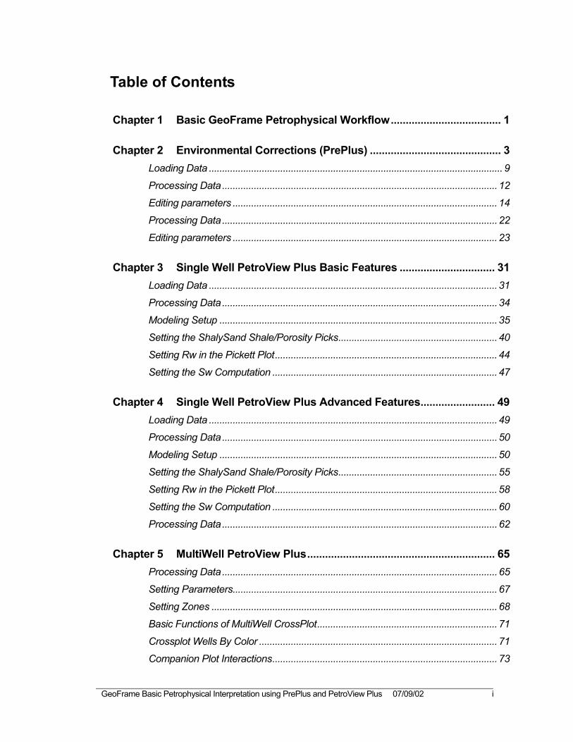
Table of Contents
Chapter 1 Basic GeoFrame Petrophysical Workflow..................................... 1
Chapter 2 Environmental Corrections (PrePlus) ............................................ 3 Loading Data ............................................................................................................... 9 Processing Data........................................................................................................ 12 Editing parameters .................................................................................................... 14 Processing Data........................................................................................................ 22 Editing parameters .................................................................................................... 23
Chapter 3 Single Well PetroView Plus Basic Features ................................ 31 Loading Data ............................................................................................................. 31 Processing Data........................................................................................................ 34 Modeling Setup ......................................................................................................... 35 Setting the ShalySand Shale/Porosity Picks............................................................ 40 Setting Rw in the Pickett Plot.................................................................................... 44 Setting the Sw Computation ..................................................................................... 47
Chapter 4 Single Well PetroView Plus Advanced Features......................... 49 Loading Data ............................................................................................................. 49 Processing Data........................................................................................................ 50 Modeling Setup ......................................................................................................... 50 Setting the ShalySand Shale/Porosity Picks............................................................ 55 Setting Rw in the Pickett Plot.................................................................................... 58 Setting the Sw Computation ..................................................................................... 60 Processing Data........................................................................................................ 62
Chapter 5 MultiWell PetroView Plus............................................................... 65 Processing Data........................................................................................................ 65 Setting Parameters.................................................................................................... 67 Setting Zones ............................................................................................................ 68 Basic Functions of MultiWell CrossPlot.................................................................... 71 Crossplot Wells By Color .......................................................................................... 71 Companion Plot Interactions..................................................................................... 73
GeoFrame Basic Petrophysical Interpretation using PrePlus and PetroView Plus 07/09/02 i
MultiWell Data Normalization Using MultiWell CrossPlot/Histogram...................... 74 Using MultiWell Data Functioning ............................................................................ 76 Building a Template .................................................................................................. 78 Building a presentation file for MultiWell .................................................................. 85 Processing Data........................................................................................................ 89
Chapter 6 Reservoir Property Summation and Mapping (ResSum & Basemap Plus)...................................................................................................... 93
Creating a LithoZone ................................................................................................ 93 Running BaseMapPlus on Your Secondary Screen ............................................... 97 Running ResSum On Your Primary Screen ............................................................ 98
ii GeoFrame Basic Petrophysical Interpretation using PrePlus and PetroView Plus 07/09/02
Basic GeoFrame Petrophysical Workflow Schlumberger
Chapter 1 Basic GeoFrame Petrophysical Workflow
Overview
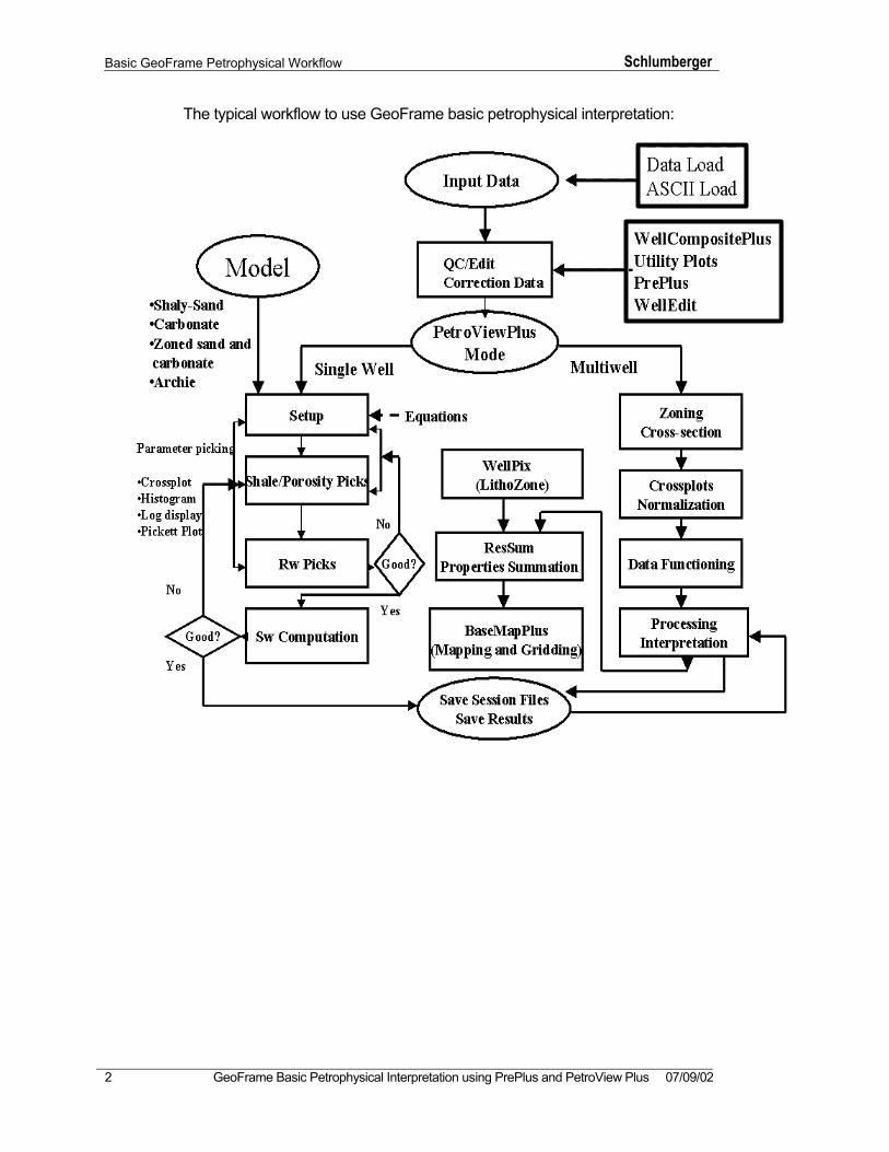
It is highly recommended to edit and environmentally correct logs before using them as input to a computer processed interpretation. Log editing is performed in the WellEdit module of GeoFrame and is the subject of another course. PrePlus is a GeoFrame petrophysics application that applies environmental corrections to logs acquired by the major acquisition vendors and is covered in chapter 2. PetroView Plus provides a guided-log analysis for the generalist or specialist. The PetroView Plus program has two modes that are covered in chapters 3 through 5: Single Well and MultiWell. The Single Well PetroView Plus program guides the user through the minimum number of operations required to do a simple petrophysical evaluation of Well log data. It offers three simple evaluation models for processing, plus user-defined functioning capabilities. It also offers interactive parameter selection in the crossplots, histograms and log displays and provides graphic presentations of input and output data. The MultiWell PetroView Plus program provides the ability to do MultiWell zonation, MultiWell cross-section display, MultiWell crossplot display, MultiWell data normalization, MultiWell data functioning and MultiWell data Processing and interpretation based on the Single Well PetroView Plus model and session file. The output of PetroView Plus (porosity, volume of shale, water saturation, etc.) coupled with zones created in MultiWell PetroView Plus or WellPix can be input to ResSum for average thickness and zone property calculations. The ResSum outputs can then be gridded and visualized with Basemap Plus, which is covered in chapter 6.
GeoFrame Basic Petrophysical Interpretation using PrePlus and PetroView Plus 07/09/02 1
Basic GeoFrame Petrophysical Workflow Schlumberger
The typical workflow to use GeoFrame basic petrophysical interpretation:
2 GeoFrame Basic Petrophysical Interpretation using PrePlus and PetroView Plus 07/09/02
Environmental Corrections (PrePlus) Schlumberger
Chapter 2 Environmental Corrections (PrePlus)
Overview
PrePlus applies environmental corrections and converts the information to logs for most wireline and LWD log tools. It will accept Schlumberger data asWell as data from the logging tools of the other major service companies, such as Halliburton and Atlas Wireline Service. Each environmental correction is associated with a specific wireline or LWD tool or measurement type, except GEN EC, which computes temperature, pressure, differential caliper and hole rugosity data. The transforms are used to prepare environmentally corrected acquisition data for use in advanced interpretation programs. The transforms can combine different corrected, measured data to produce values for formation properties (porosity, resistivity, conductivity, etc.) Addition to PrePlus, GeoFrame provides another application Hisorical EC which is a product for correcting older Schlumberger logs that are not included in the PrePlus application. The tools that are corrected by this module include: Compensated Formation Density (FDC), Sidewall Neutron Porosity (SNP), Micro-Laterolog (MLL), Short Normal Resistivity (SN), Laterolog 7 (LL7) and Laterolog 8 (LL8). The PrePlus can correct for these environmental effects:
• Hole size
• Mudcake thickness
• Mud weight
• Borehole salinity
• Standoff
• Formation pressure
• Formation temperature
• Formation salinity
• Formation thickness
• Shoulder effects
• Casing inside diameter
• Casing and cement thickness
• Special corrections for resistivity tool (Groningen effect for LLD Sleeve effect, etc…)
In order to perform accurate environmental corrections, the following data will be needed:
GeoFrame Basic Petrophysical Interpretation using PrePlus and PetroView Plus 07/09/02 3
Environmental Corrections (PrePlus) Schlumberger
• Raw digital data plus field prints
• Mud reports so the mud properties can be verified
• Deviation data for deviated Wells for making pressure corrections
• Surface temperature and temperature gradient for Well with no temperature log
• Formation salinity data/Formation water resistivity and temperature The PrePlus program offers two interactive modes: Express mode and Expert mode. Express mode allows you to run the program directly from the Session Builder for normal jobs, which don’t require recalibration or other expert features. The PrePlus is run after the data are loaded and before an interpretation package (such as ELANPLus, PetroView Plus, RockCell etc.) is run. It can be run interactively or in batch operation with the session file you saved from the interactive processing. For a detailed explanation of the features mentioned above and algorithms used in PrePlus, please refer to the online help documentation in the GeoFrame Bookshelf.
Schlumberger Tools Corrections
The supported Schlumberger tools corrections include:
• AIT: Array Induction Tool
• ALAT: DIT-D and DIT-E:Dual Induction Tool
• DLT
• EPT
• HALS (Platform Express)
• MCFL (Platform Express)
• MSFL
• SFL
• Phasor Reconstruct
• HRDD (Platform Express)
• LDT
• LDS (IPLT)
• SLDT: Slim Litho Density Tool
• CNT-A/H/G and HNGS
• CNT-C/D and SCNT: Slimhole Compensated Neutron Tool
• APS/HAPS: Accelerated Porosity /Hostile Accelerated Porosity Sonde
4 GeoFrame Basic Petrophysical Interpretation using PrePlus and PetroView Plus 07/09/02
Environmental Corrections (PrePlus) Schlumberger
• NGT
• SGT
• STGC
• RST
Schlumberger LWD Tools Corrections
The Supported Schlumberger LWD Tools Corrections include:
• AND
• ARC
• CDN
• CDR
• RAB
Atlas Wireline Service Tools Corrections
• GR
• CDL
• CN
• DLL
• MLL
• DIFL
• PROX
Halliburton Logging Service Tools Corrections
• GR
• SGR
• CNT_K
• DSNT_A
• DIL
• DILT_A
• DG
• DLL
• FORXO Trasform:Rt/Rxo
• MSFL
GeoFrame Basic Petrophysical Interpretation using PrePlus and PetroView Plus 07/09/02 5
Environmental Corrections (PrePlus) Schlumberger
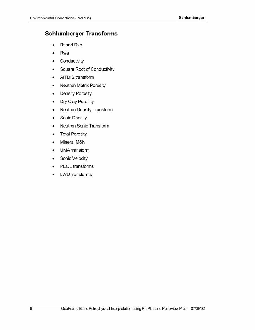
Schlumberger Transforms
• Rt and Rxo
• Rwa
• Conductivity
• Square Root of Conductivity
• AITDIS transform
• Neutron Matrix Porosity
• Density Porosity
• Dry Clay Porosity
• Neutron Density Transform
• Sonic Density
• Neutron Sonic Transform
• Total Porosity
• Mineral M&N
• UMA transform
• Sonic Velocity
• PEQL transforms
• LWD transforms
6 GeoFrame Basic Petrophysical Interpretation using PrePlus and PetroView Plus 07/09/02
Environmental Corrections (PrePlus) Schlumberger
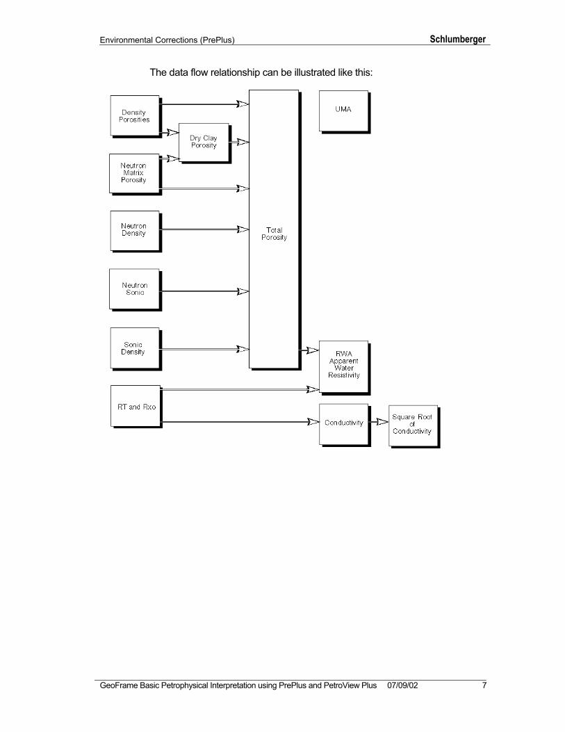
The data flow relationship can be illustrated like this:
GeoFrame Basic Petrophysical Interpretation using PrePlus and PetroView Plus 07/09/02 7
Environmental Corrections (PrePlus) Schlumberger
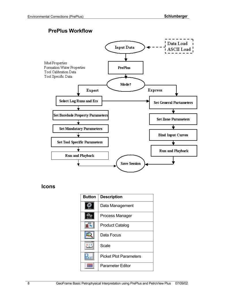
PrePlus Workflow
Icons
Button Description
Data Management
Process Manager
Product Catalog
Data Focus
Scale
Picket Plot Parameters
Parameter Editor
8 GeoFrame Basic Petrophysical Interpretation using PrePlus and PetroView Plus 07/09/02
Environmental Corrections (PrePlus) Schlumberger
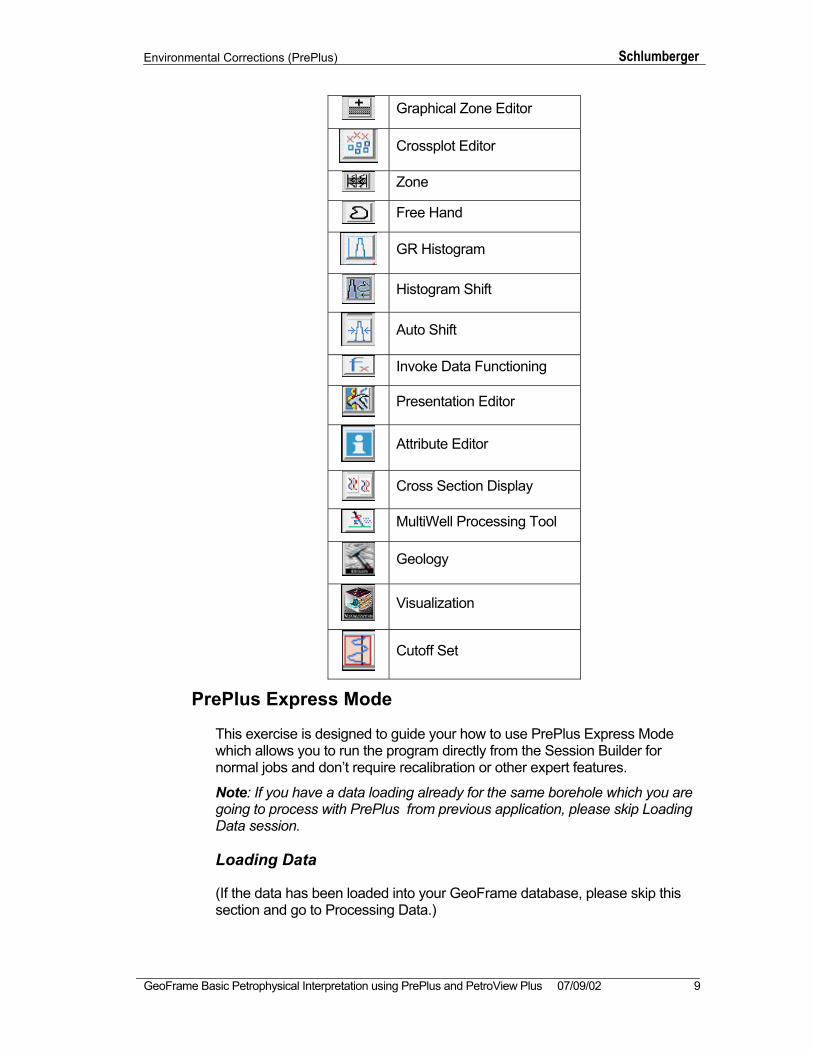
Graphical Zone Editor
Crossplot Editor
Zone
Free Hand
GR Histogram
Histogram Shift
Auto Shift
Invoke Data Functioning
Presentation Editor
Attribute Editor
Cross Section Display
MultiWell Processing Tool
Geology
Visualization
Cutoff Set
PrePlus Express Mode
This exercise is designed to guide your how to use PrePlus Express Mode which allows you to run the program directly from the Session Builder for normal jobs and don’t require recalibration or other expert features.
Note: If you have a data loading already for the same borehole which you are going to process with PrePlus from previous application, please skip Loading Data session.
Loading Data
(If the data has been loaded into your GeoFrame database, please skip this section and go to Processing Data.)
GeoFrame Basic Petrophysical Interpretation using PrePlus and PetroView Plus 07/09/02 9
Environmental Corrections (PrePlus) Schlumberger
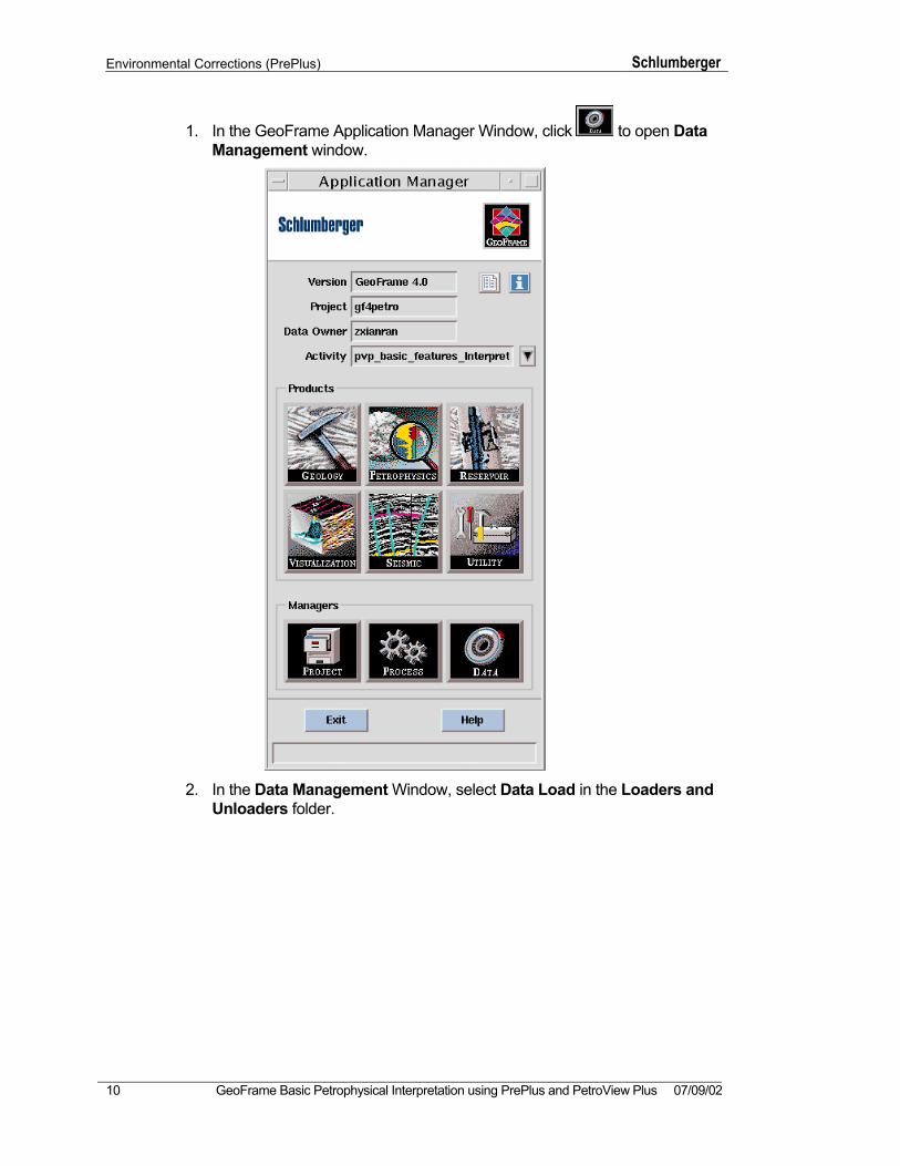
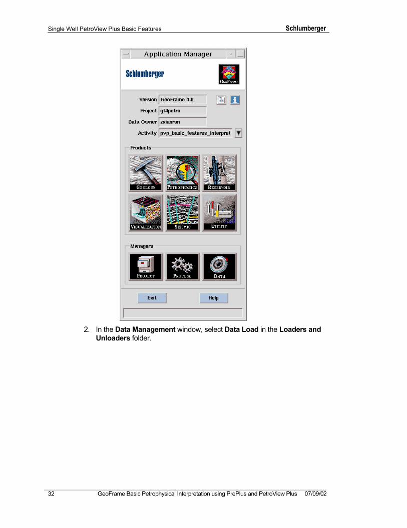
1. In the GeoFrame Application Manager Window, click to open Data Management window.
2. In the Data Management Window, select Data Load in the Loaders and
Unloaders folder.
10 GeoFrame Basic Petrophysical Interpretation using PrePlus and PetroView Plus 07/09/02
Environmental Corrections (PrePlus) Schlumberger
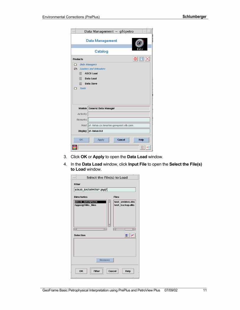
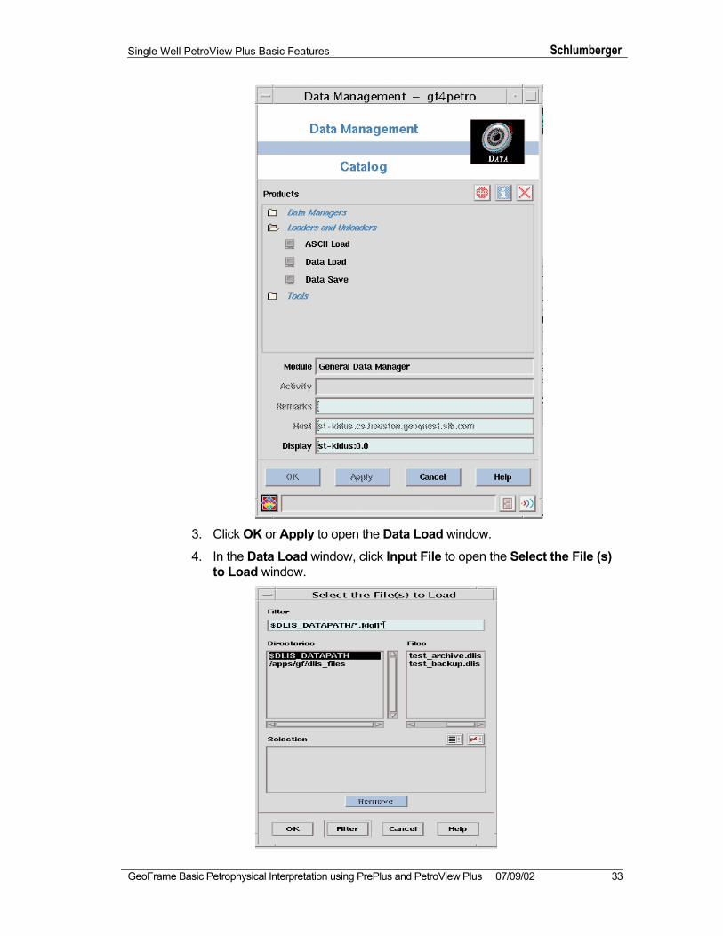
3. Click OK or Apply to open the Data Load window.
4. In the Data Load window, click Input File to open the Select the File(s) to Load window.
GeoFrame Basic Petrophysical Interpretation using PrePlus and PetroView Plus 07/09/02 11
Environmental Corrections (PrePlus) Schlumberger
5. In the Filter field, enter the directory path given by the instructor.
6. Click Filter button to display files from the selected directory and select sfe4_dite.dlis, sfe4_ldt_cnt.dlis, and sfe4_msfl.dlis. Then click OK to close the window
7. From the Data Load window, set the Target: a. Field = Frontier b. Well UWI = SFE#4 c. Borehole UWI = SFE#4
8. Click Run in the Data Load window to start loading data.
9. Click Exit to close the Data Load window.
10. Click OK in all pop-up message windows that appear.
Processing Data
1. In the GeoFrame Application Manager window, click to open the Process Manager.
2. In the Process Manager window, select File>New Activity.
3. Click to open the Product Catalog.
4. In the Product Catalog window, click the Petrophysics folder and select PrePlus.
5. Click OK to close the Product Catalog window.
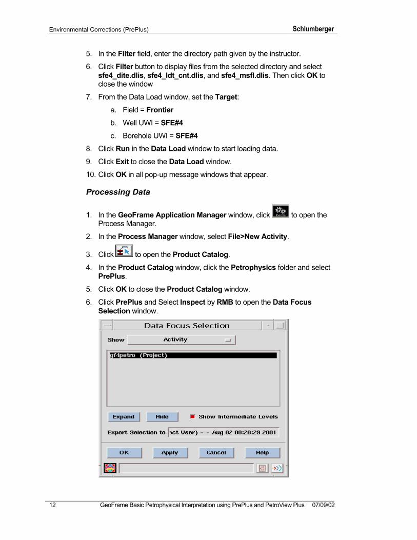
6. Click PrePlus and Select Inspect by RMB to open the Data Focus Selection window.
12 GeoFrame Basic Petrophysical Interpretation using PrePlus and PetroView Plus 07/09/02
Environmental Corrections (PrePlus) Schlumberger
7. In the Data Focus Selection window, click Activity to change the Show type to Borehole and select Borehole SFE#4.
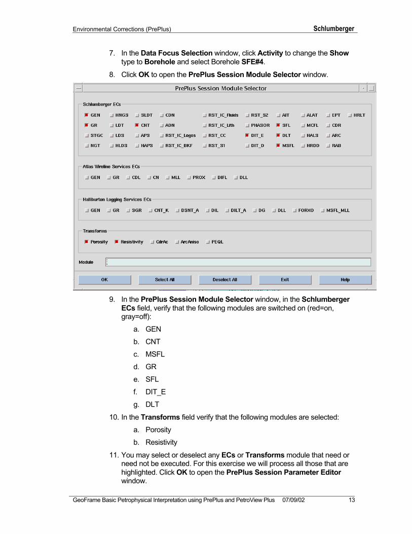
8. Click OK to open the PrePlus Session Module Selector window.
9. In the PrePlus Session Module Selector window, in the Schlumberger
ECs field, verify that the following modules are switched on (red=on, gray=off):
a. GEN b. CNT c. MSFL d. GR e. SFL f. DIT_E g. DLT
10. In the Transforms field verify that the following modules are selected: a. Porosity b. Resistivity
11. You may select or deselect any ECs or Transforms module that need or need not be executed. For this exercise we will process all those that are highlighted. Click OK to open the PrePlus Session Parameter Editor window.
GeoFrame Basic Petrophysical Interpretation using PrePlus and PetroView Plus 07/09/02 13
Environmental Corrections (PrePlus) Schlumberger
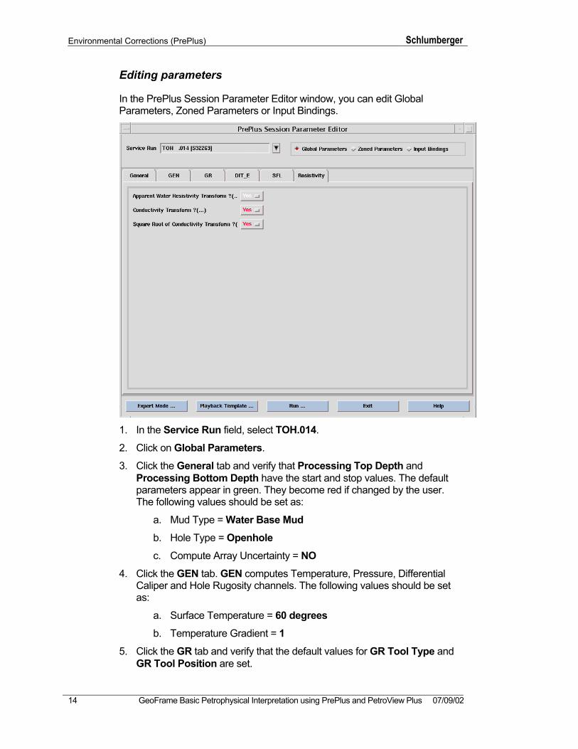
Editing parameters
In the PrePlus Session Parameter Editor window, you can edit Global Parameters, Zoned Parameters or Input Bindings.
1. In the Service Run field, select TOH.014.
2. Click on Global Parameters.
3. Click the General tab and verify that Processing Top Depth and Processing Bottom Depth have the start and stop values. The default parameters appear in green. They become red if changed by the user. The following values should be set as:
a. Mud Type = Water Base Mud
b. Hole Type = Openhole
c. Compute Array Uncertainty = NO
4. Click the GEN tab. GEN computes Temperature, Pressure, Differential Caliper and Hole Rugosity channels. The following values should be set as:
a. Surface Temperature = 60 degrees
b. Temperature Gradient = 1
5. Click the GR tab and verify that the default values for GR Tool Type and GR Tool Position are set.
14 GeoFrame Basic Petrophysical Interpretation using PrePlus and PetroView Plus 07/09/02
Environmental Corrections (PrePlus) Schlumberger
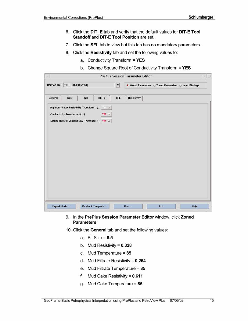
6. Click the DIT_E tab and verify that the default values for DIT-E Tool Standoff and DIT-E Tool Position are set.
7. Click the SFL tab to view but this tab has no mandatory parameters.
8. Click the Resistivity tab and set the following values to:
a. Conductivity Transform = YES
b. Change Square Root of Conductivity Transform = YES
9. In the PrePlus Session Parameter Editor window, click Zoned
Parameters.
10. Click the General tab and set the following values:
a. Bit Size = 8.5
b. Mud Resistivity = 0.328
c. Mud Temperature = 85
d. Mud Filtrate Resistivity = 0.264
e. Mud Filtrate Temperature = 85
f. Mud Cake Resistivity = 0.611
g. Mud Cake Temperature = 85
GeoFrame Basic Petrophysical Interpretation using PrePlus and PetroView Plus 07/09/02 15
Environmental Corrections (PrePlus) Schlumberger
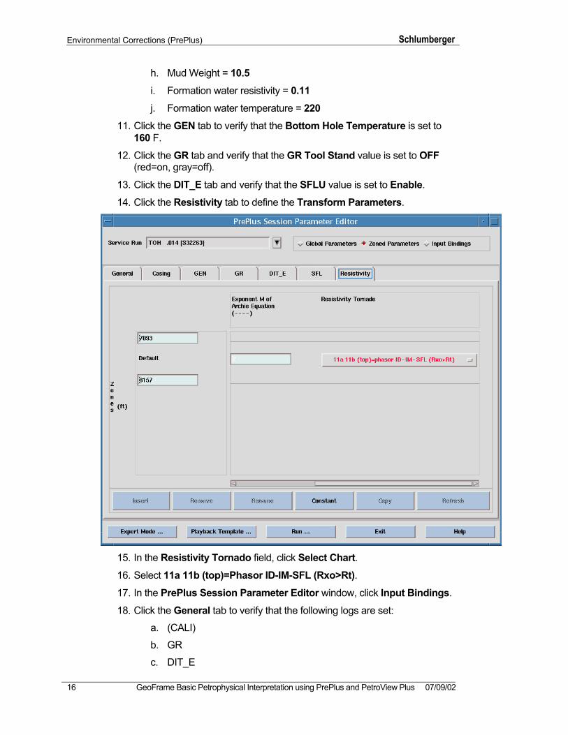
h. Mud Weight = 10.5
i. Formation water resistivity = 0.11
j. Formation water temperature = 220 11. Click the GEN tab to verify that the Bottom Hole Temperature is set to
160 F.
12. Click the GR tab and verify that the GR Tool Stand value is set to OFF (red=on, gray=off).
13. Click the DIT_E tab and verify that the SFLU value is set to Enable.
14. Click the Resistivity tab to define the Transform Parameters.
15. In the Resistivity Tornado field, click Select Chart. 16. Select 11a 11b (top)=Phasor ID-IM-SFL (Rxo>Rt). 17. In the PrePlus Session Parameter Editor window, click Input Bindings.
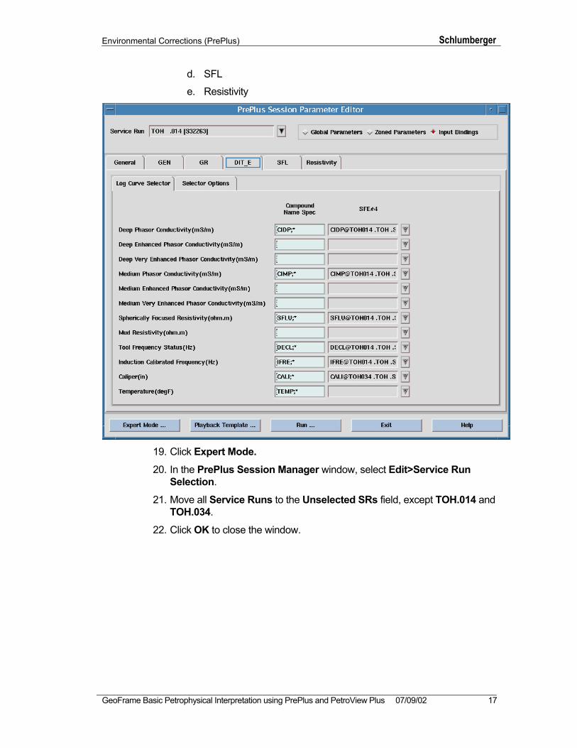
18. Click the General tab to verify that the following logs are set: a. (CALI) b. GR c. DIT_E
16 GeoFrame Basic Petrophysical Interpretation using PrePlus and PetroView Plus 07/09/02
Environmental Corrections (PrePlus) Schlumberger
d. SFL e. Resistivity
19. Click Expert Mode. 20. In the PrePlus Session Manager window, select Edit>Service Run
Selection.
21. Move all Service Runs to the Unselected SRs field, except TOH.014 and TOH.034.
22. Click OK to close the window.
GeoFrame Basic Petrophysical Interpretation using PrePlus and PetroView Plus 07/09/02 17
Environmental Corrections (PrePlus) Schlumberger
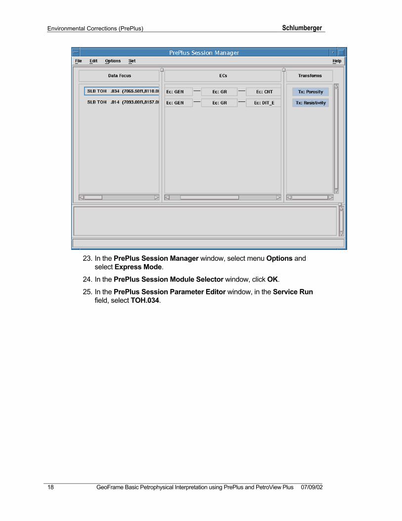
23. In the PrePlus Session Manager window, select menu Options and
select Express Mode.
24. In the PrePlus Session Module Selector window, click OK.
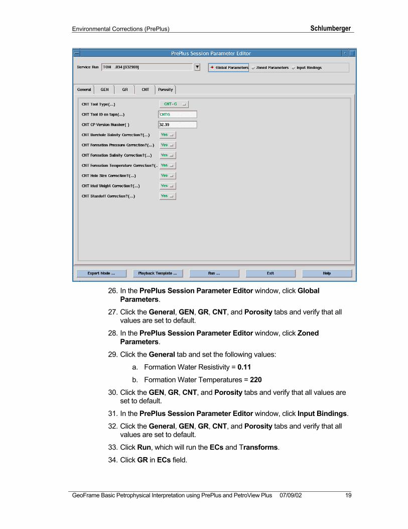
25. In the PrePlus Session Parameter Editor window, in the Service Run field, select TOH.034.
18 GeoFrame Basic Petrophysical Interpretation using PrePlus and PetroView Plus 07/09/02
Environmental Corrections (PrePlus) Schlumberger
26. In the PrePlus Session Parameter Editor window, click Global
Parameters.
27. Click the General, GEN, GR, CNT, and Porosity tabs and verify that all values are set to default.
28. In the PrePlus Session Parameter Editor window, click Zoned Parameters.
29. Click the General tab and set the following values:
a. Formation Water Resistivity = 0.11
b. Formation Water Temperatures = 220
30. Click the GEN, GR, CNT, and Porosity tabs and verify that all values are set to default.
31. In the PrePlus Session Parameter Editor window, click Input Bindings.
32. Click the General, GEN, GR, CNT, and Porosity tabs and verify that all values are set to default.
33. Click Run, which will run the ECs and Transforms.
34. Click GR in ECs field.
GeoFrame Basic Petrophysical Interpretation using PrePlus and PetroView Plus 07/09/02 19
Environmental Corrections (PrePlus) Schlumberger
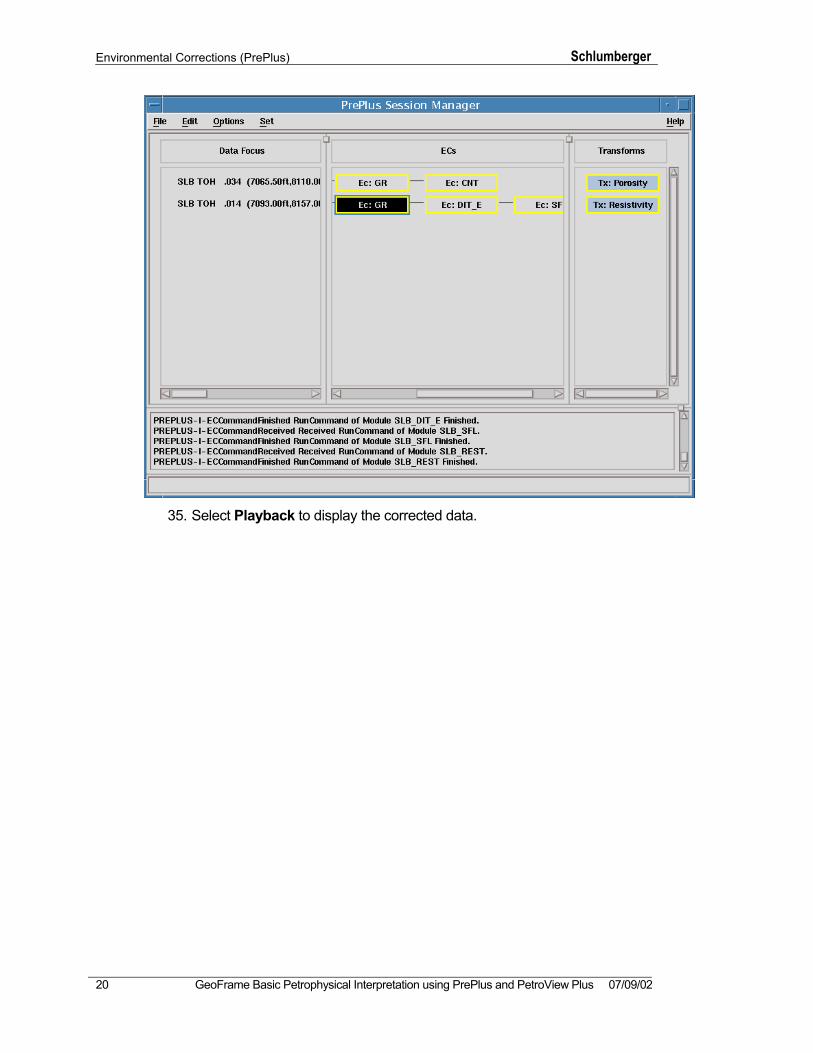
35. Select Playback to display the corrected data.
20 GeoFrame Basic Petrophysical Interpretation using PrePlus and PetroView Plus 07/09/02
Environmental Corrections (PrePlus) Schlumberger
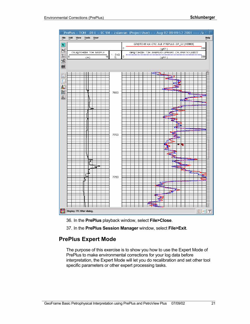
36. In the PrePlus playback window, select File>Close.
37. In the PrePlus Session Manager window, select File>Exit.
PrePlus Expert Mode
The purpose of this exercise is to show you how to use the Expert Mode of PrePlus to make environmental corrections for your log data before interpretation, the Expert Mode will let you do recalibration and set other tool specific parameters or other expert processing tasks.
GeoFrame Basic Petrophysical Interpretation using PrePlus and PetroView Plus 07/09/02 21
Environmental Corrections (PrePlus) Schlumberger
Processing Data
1. In the GeoFrame Application Manager window, click to open the Process Manager.
2. In the Process Manager window, select File>New Activity.
3. Click to open the Product Catalog.
4. In the Product Catalog window, click the Petrophysics folder and select PrePlus.
5. Click OK to close the Product Catalog window.
6. Click PrePlus and Select Inspect by RMB to open the Data Focus Selection Window.
7. In the Data Focus Selection window, click Activity to change the Show type to Borehole and select Borehole SFE#4.
8. Click OK to open the PrePlus Session Module Selector window.
9. In the PrePlus Session Module Selector window, click OK to open the PrePlus Session Parameter Editor window
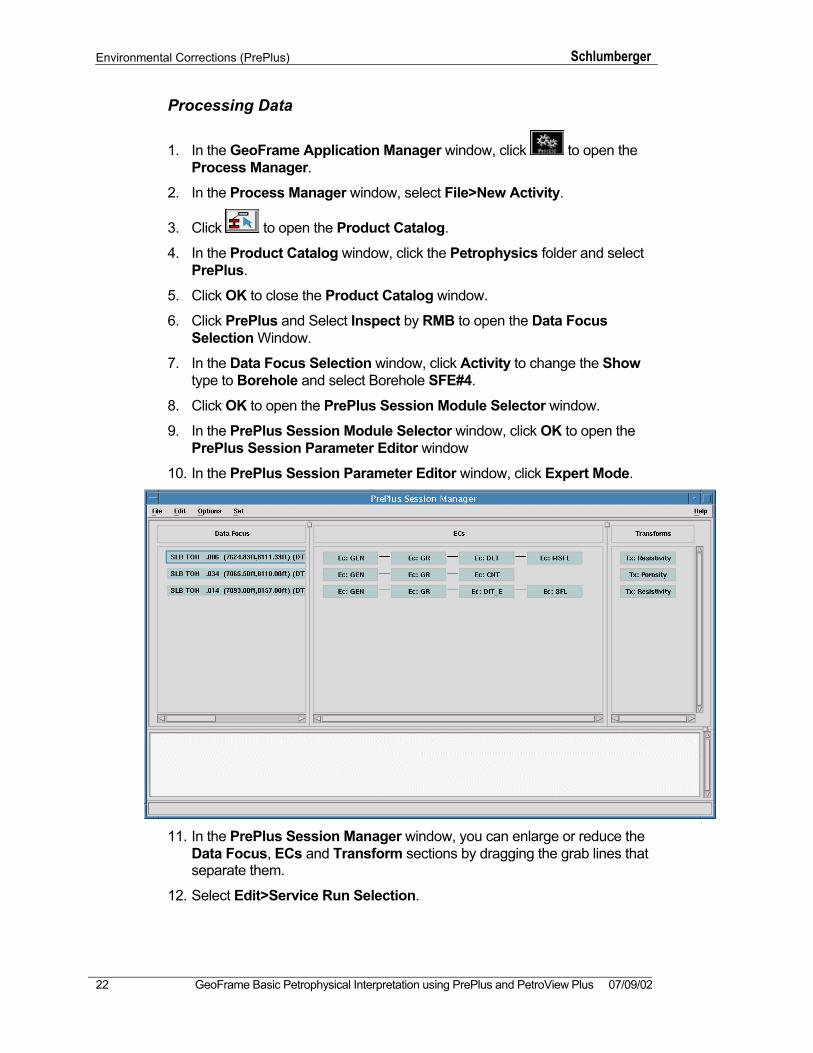
10. In the PrePlus Session Parameter Editor window, click Expert Mode.
11. In the PrePlus Session Manager window, you can enlarge or reduce the
Data Focus, ECs and Transform sections by dragging the grab lines that separate them.
12. Select Edit>Service Run Selection.
22 GeoFrame Basic Petrophysical Interpretation using PrePlus and PetroView Plus 07/09/02
Environmental Corrections (PrePlus) Schlumberger
13. Select files TOH.014 and TOH.034. GeoFrame selects EC modules automatically for each service run in a way that preserves continuity of input data (i.e., certain modules must run before others).
14. Select Edit>EC Selection to edit the Selected ECs list or to create a new list if preferred. Unselected ECs list shows all available modules for the selected service company.
Editing parameters
In the PrePlus Session Parameter Editor window, you can edit Global Parameters, Zoned Parameters or Input Bindings.
Borehole Properties: Associated with the physical borehole and subdivided into Global and Zoned Parameters. The Borehole Properties Editor must be opened before any processing can be done.
Mandatory Parameters: The minimum parameters that must be inspected or set to run all the modules for a given Service Run. To set these a Service Run must be selected.
Tool Specific Parameters: Are parameters that affect a given tool module. To set these an EC Module must be selected. 1. Access Editing parameters by selecting Options>Editing parameters. 2. Selecting Service Run (in the Data Focus panel). 3. Selecting Tool EC (in ECs and Transforms panel) and pressing the right
mouse button (MB3).
GeoFrame Basic Petrophysical Interpretation using PrePlus and PetroView Plus 07/09/02 23
Environmental Corrections (PrePlus) Schlumberger
4. Select Options>Borehole Properties.
Note: Once a task is completed in PrePlus a * symbol is associated with it, to inform you that this menu has been viewed before. The program first searches the database to find the start/stop extent of the Service Run, and if it finds an extent, the color-coding for the depth interval is black. If it cannot find the
24 GeoFrame Basic Petrophysical Interpretation using PrePlus and PetroView Plus 07/09/02
Environmental Corrections (PrePlus) Schlumberger
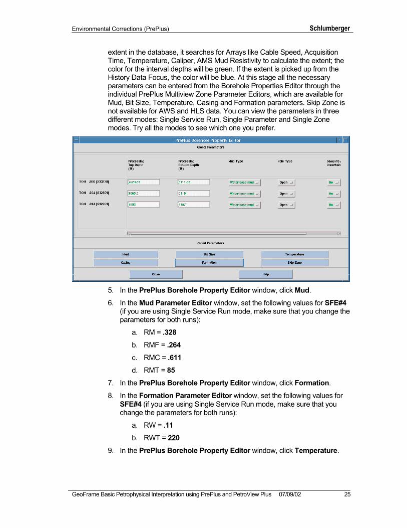
extent in the database, it searches for Arrays like Cable Speed, Acquisition Time, Temperature, Caliper, AMS Mud Resistivity to calculate the extent; the color for the interval depths will be green. If the extent is picked up from the History Data Focus, the color will be blue. At this stage all the necessary parameters can be entered from the Borehole Properties Editor through the individual PrePlus Multiview Zone Parameter Editors, which are available for Mud, Bit Size, Temperature, Casing and Formation parameters. Skip Zone is not available for AWS and HLS data. You can view the parameters in three different modes: Single Service Run, Single Parameter and Single Zone modes. Try all the modes to see which one you prefer.
5. In the PrePlus Borehole Property Editor window, click Mud.
6. In the Mud Parameter Editor window, set the following values for SFE#4 (if you are using Single Service Run mode, make sure that you change the parameters for both runs):
a. RM = .328
b. RMF = .264
c. RMC = .611
d. RMT = 85
7. In the PrePlus Borehole Property Editor window, click Formation.
8. In the Formation Parameter Editor window, set the following values for SFE#4 (if you are using Single Service Run mode, make sure that you change the parameters for both runs):
a. RW = .11
b. RWT = 220
9. In the PrePlus Borehole Property Editor window, click Temperature.
GeoFrame Basic Petrophysical Interpretation using PrePlus and PetroView Plus 07/09/02 25
Environmental Corrections (PrePlus) Schlumberger
10. In the Temperature Parameter Editor window, set the following values for SFE#4 (if you are using Single Service Run mode, make sure that you change the parameters for both runs):
c. BHT = 220
11. Click OK to close the PrePlus Borehole Property Editor window
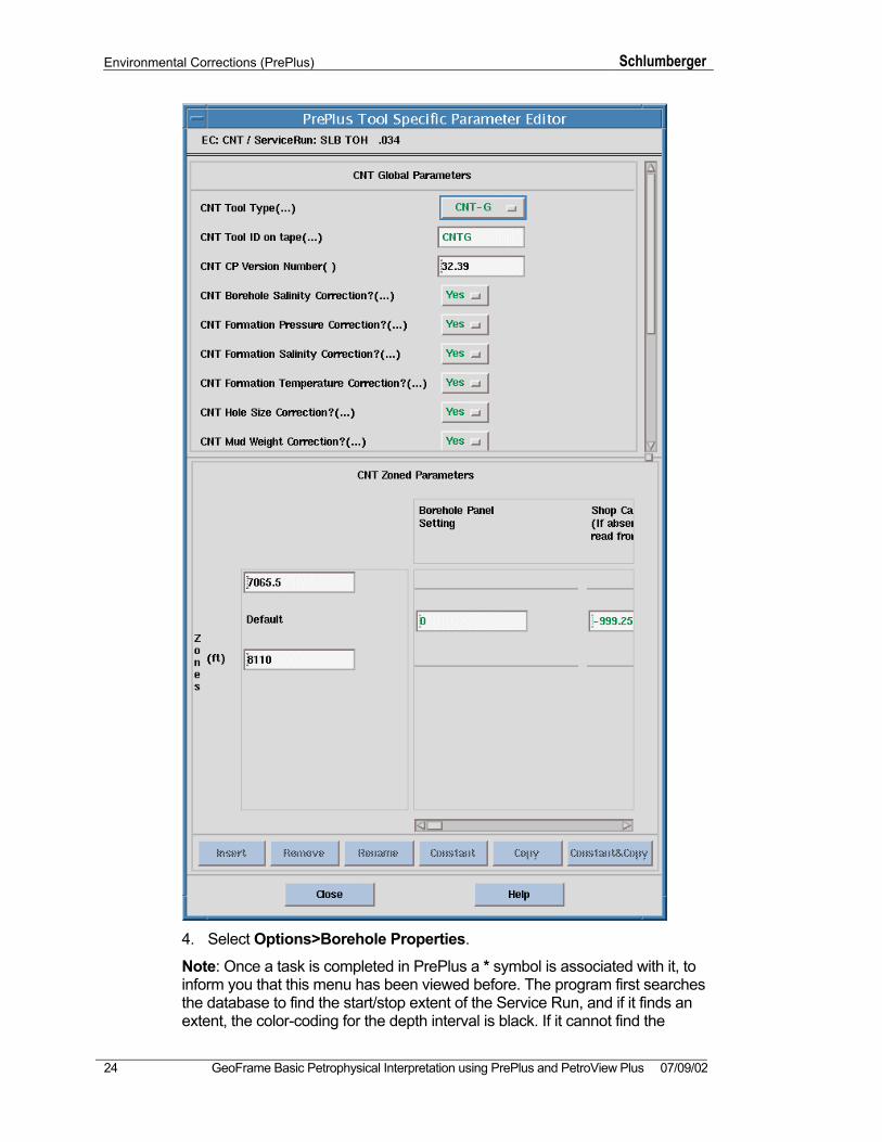
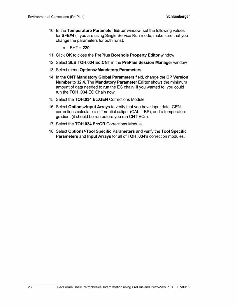
12. Select SLB TOH.034 Ec:CNT in the PrePlus Session Manager window
13. Select menu Options>Mandatory Parameters.
14. In the CNT Mandatory Global Parameters field, change the CP Version Number to 32.4. The Mandatory Parameter Editor shows the minimum amount of data needed to run the EC chain. If you wanted to, you could run the TOH .034 EC Chain now.
15. Select the TOH.034 Ec:GEN Corrections Module.
16. Select Options>Input Arrays to verify that you have input data. GEN corrections calculate a differential caliper (CALI - BS), and a temperature gradient (it should be run before you run CNT ECs).
17. Select the TOH.034 Ec:GR Corrections Module.
18. Select Options>Tool Specific Parameters and verify the Tool Specific Parameters and Input Arrays for all of TOH .034’s correction modules.
26 GeoFrame Basic Petrophysical Interpretation using PrePlus and PetroView Plus 07/09/02
Environmental Corrections (PrePlus) Schlumberger
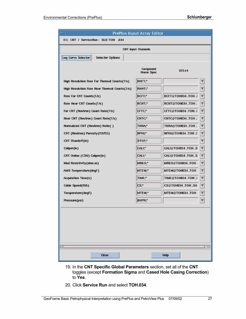
19. In the CNT Specific Global Parameters section, set all of the CNT
toggles (except Formation Sigma and Cased Hole Casing Correction) to Yes.
20. Click Service Run and select TOH.034.
GeoFrame Basic Petrophysical Interpretation using PrePlus and PetroView Plus 07/09/02 27
Environmental Corrections (PrePlus) Schlumberger
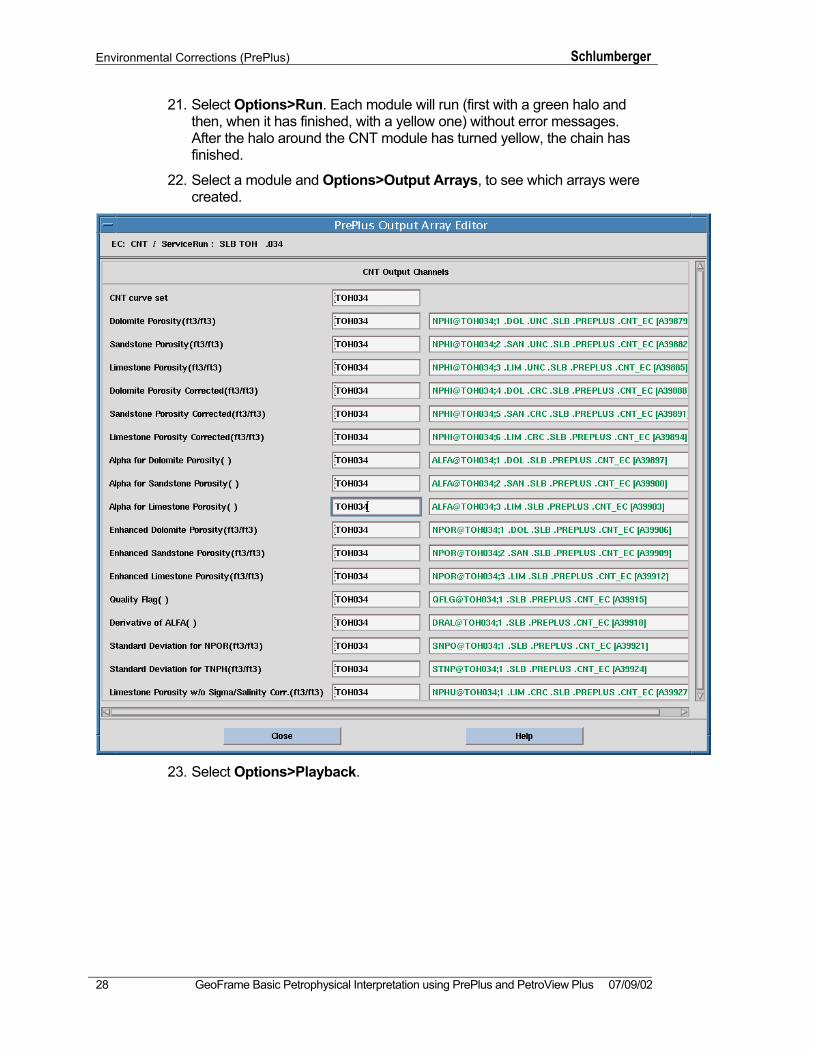
21. Select Options>Run. Each module will run (first with a green halo and then, when it has finished, with a yellow one) without error messages. After the halo around the CNT module has turned yellow, the chain has finished.
22. Select a module and Options>Output Arrays, to see which arrays were created.
23. Select Options>Playback.
28 GeoFrame Basic Petrophysical Interpretation using PrePlus and PetroView Plus 07/09/02
Environmental Corrections (PrePlus) Schlumberger
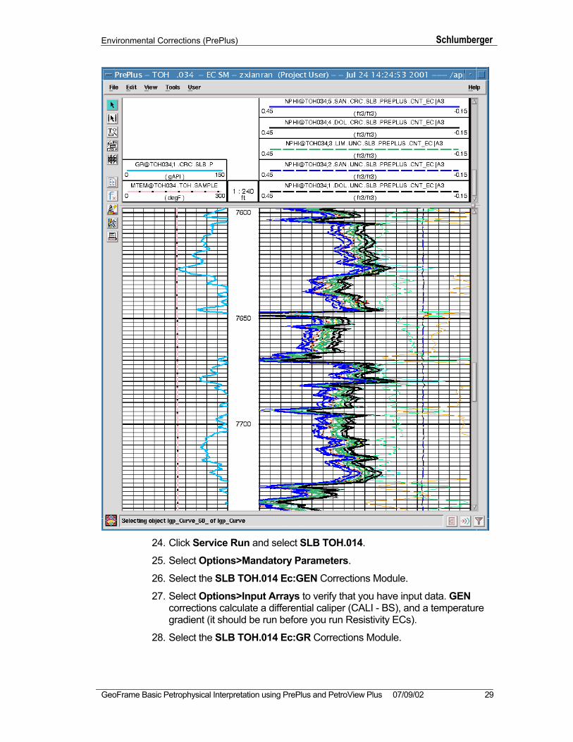
24. Click Service Run and select SLB TOH.014.
25. Select Options>Mandatory Parameters.
26. Select the SLB TOH.014 Ec:GEN Corrections Module.
27. Select Options>Input Arrays to verify that you have input data. GEN corrections calculate a differential caliper (CALI - BS), and a temperature gradient (it should be run before you run Resistivity ECs).
28. Select the SLB TOH.014 Ec:GR Corrections Module.
GeoFrame Basic Petrophysical Interpretation using PrePlus and PetroView Plus 07/09/02 29
Environmental Corrections (PrePlus) Schlumberger
29. Select Options>Tool Specific Parameters and verify the Tool Specific Parameters and Input Arrays for all of SLB TOH.014’s correction modules.
30. Click Service Run and select SLB TOH.014.
31. Select Options>Run. Each module will run (first with a green halo and then, when it has finished, with a yellow one) without error messages.
32. Select a module and Options>Output Arrays, to see which arrays were created.
33. Select Options>Playback, to view these arrays. Traditionally, GeoFrame distinguishes between those corrections made by applying borehole conditions to the raw arrays (EC Modules), and those that compute new arrays (such as Rt or Rxo) from other sources (Transform Modules). The distinction is no longer as solid as it once was, but the basic structure is retained.
34. Click the Resistivity tab.
35. Select menu Options>Transform Specific Parameters.
36. In the Transform Parameter window, set Compute RT? to Compute Rt. 37. Set Use Std. Off Chart Logic For RT? to Use Chart. 38. In the Resistivity Tornado Chart Selection field, select 11a 11b
(top)=Phasor ID-IM-SFL (Rxo>Rt). 39. Click the Porosity tab.
40. Select Options>Run. The output from the Transforms can be viewed in the same way as that from the EC Modules. The Playback can be run from each EC module.
30 GeoFrame Basic Petrophysical Interpretation using PrePlus and PetroView Plus 07/09/02
Single Well PetroView Plus Basic Features Schlumberger
Chapter 3 Single Well PetroView Plus Basic Features
Overview
The following are some of the major features in PetroView Plus:
• Model Zonation: Shaly-Sand, carbonate, simple Archie and Zoned Sand/Carbonate Models are available
• Porosity Option: Density-Neutron, density, sonic, Neutron, external Porosity or User-defined equation
• Water Saturation Equation: Archie, dual water, Waxman-Smiths, indonesia, Nigeria, simandoux, user-defined equation
• Interactive parameter selection in the: Log Curve, crossplot, histogram
• Linear or non-linear shale volume calculation
• Bad borehole detection
• Wyllie Sonic Porosity or Hunt-Raymer equation
• Session file save and recall (Exclick mode) For a detailed explanation of the features mentioned above and algorithms used in PetroView Plus, please refer to the online help documentation in the GeoFrame Bookshelf.
Basic Single Well Petrophysical Interpretation
Note: If you have a data loading already for the same borehole which you are going to process with PetroView Plus from previous application, please skip Loading Data session.
Loading Data
(If the data has been loaded into your GeoFrame database, please skip this section and go to Processing Data.)
1. In the GeoFrame Application Manager Window, click to open the Data Management window.
GeoFrame Basic Petrophysical Interpretation using PrePlus and PetroView Plus 07/09/02 31
Single Well PetroView Plus Basic Features Schlumberger
2. In the Data Management window, select Data Load in the Loaders and
Unloaders folder.
32 GeoFrame Basic Petrophysical Interpretation using PrePlus and PetroView Plus 07/09/02
Single Well PetroView Plus Basic Features Schlumberger
3. Click OK or Apply to open the Data Load window.
4. In the Data Load window, click Input File to open the Select the File (s) to Load window.
GeoFrame Basic Petrophysical Interpretation using PrePlus and PetroView Plus 07/09/02 33
Single Well PetroView Plus Basic Features Schlumberger
5. In the Filter text field, enter the directory path given by the instructor.
6. Click button Filter to display files from the selected directory and select petro_updates.dlis.
7. Click OK to close the Select the File(s) to Load window.
8. Do not assign a Field, Well, Borehole, or Producer name to the Data Load window.
9. Click Run in the Data Load window to start loading data.
10. Click Exit to close the Data Load window.
11. Click OK in all pop-up message windows that appear.
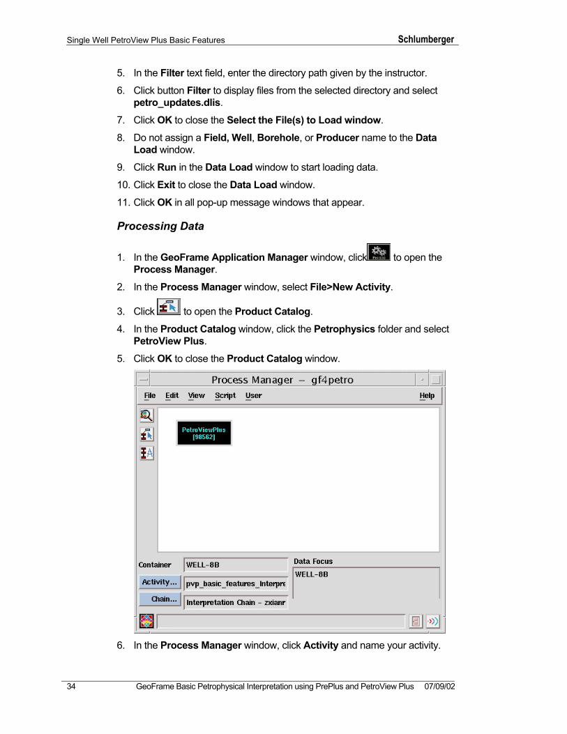
Processing Data
1. In the GeoFrame Application Manager window, click to open the Process Manager.
2. In the Process Manager window, select File>New Activity.
3. Click to open the Product Catalog.
4. In the Product Catalog window, click the Petrophysics folder and select PetroView Plus.
5. Click OK to close the Product Catalog window.
6. In the Process Manager window, click Activity and name your activity.
34 GeoFrame Basic Petrophysical Interpretation using PrePlus and PetroView Plus 07/09/02
Single Well PetroView Plus Basic Features Schlumberger
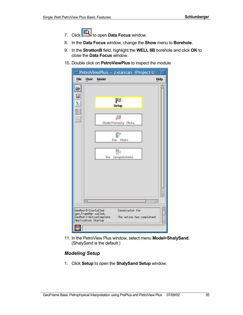
7. Click to open Data Focus window.
8. In the Data Focus window, change the Show menu to Borehole.
9. In the StrattonB field, highlight the WELL 8B borehole and click OK to close the Data Focus window.
10. Double click on PetroViewPlus to inspect the module
11. In the PetroView Plus window, select menu Model>ShalySand.
(ShalySand is the default.)
Modeling Setup
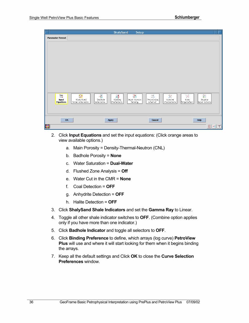
1. Click Setup to open the ShalySand Setup window.
GeoFrame Basic Petrophysical Interpretation using PrePlus and PetroView Plus 07/09/02 35
Single Well PetroView Plus Basic Features Schlumberger
2. Click Input Equations and set the input equations: (Click orange areas to
view available options.) a. Main Porosity = Density-Thermal-Neutron (CNL)
b. Badhole Porosity = None
c. Water Saturation = Dual-Water d. Flushed Zone Analysis = Off e. Water Cut in the CMR = None
f. Coal Detection = OFF
g. Anhydrite Detection = OFF
h. Halite Detection = OFF
3. Click ShalySand Shale Indicators and set the Gamma Ray to Linear.
4. Toggle all other shale indicator switches to OFF. (Combine option applies only if you have more than one indicator.)
5. Click Badhole Indicator and toggle all selectors to OFF.
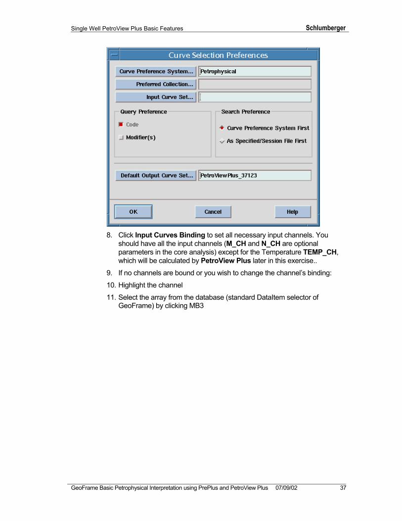
6. Click Binding Preference to define, which arrays (log curve) PetroView Plus will use and where it will start looking for them when it begins binding the arrays.
7. Keep all the default settings and Click OK to close the Curve Selection Preferences window.
36 GeoFrame Basic Petrophysical Interpretation using PrePlus and PetroView Plus 07/09/02
Single Well PetroView Plus Basic Features Schlumberger
8. Click Input Curves Binding to set all necessary input channels. You
should have all the input channels (M_CH and N_CH are optional parameters in the core analysis) except for the Temperature TEMP_CH, which will be calculated by PetroView Plus later in this exercise..
9. If no channels are bound or you wish to change the channel’s binding: 10. Highlight the channel 11. Select the array from the database (standard DataItem selector of
GeoFrame) by clicking MB3
GeoFrame Basic Petrophysical Interpretation using PrePlus and PetroView Plus 07/09/02 37
Single Well PetroView Plus Basic Features Schlumberger
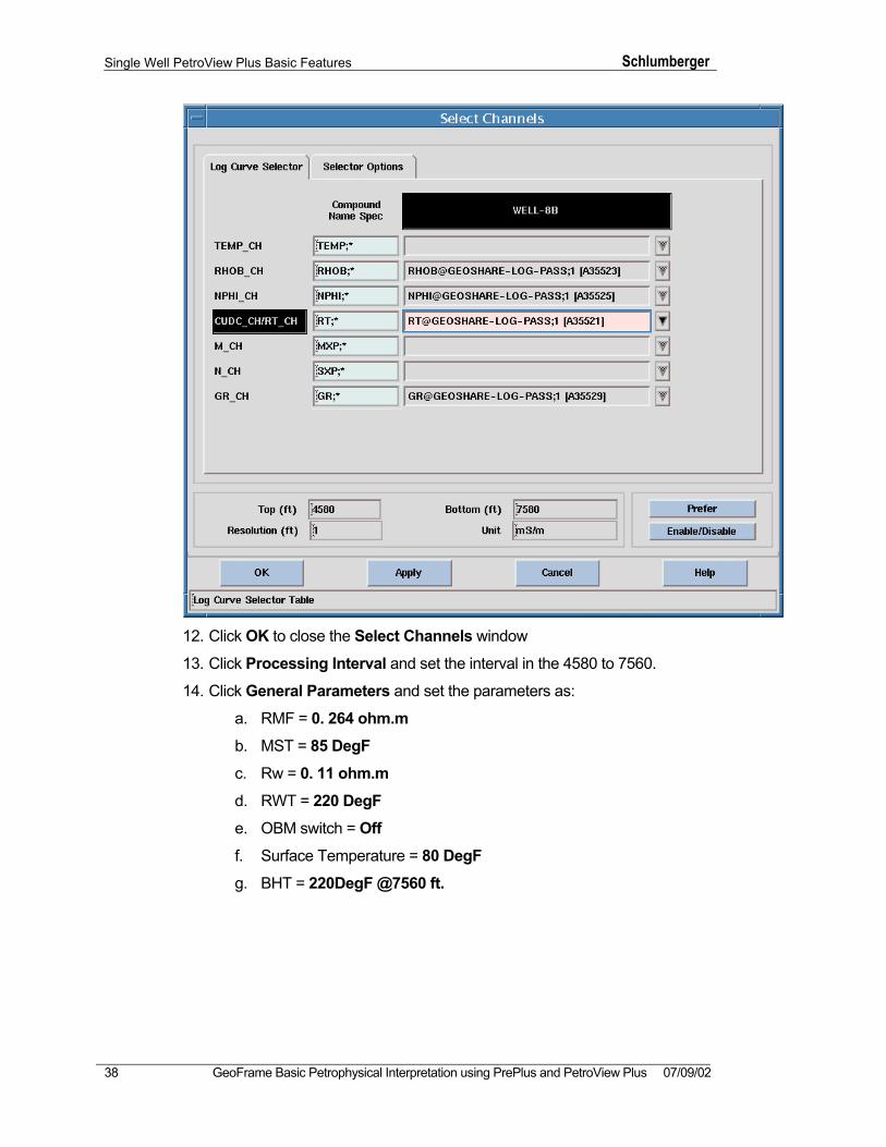
12. Click OK to close the Select Channels window
13. Click Processing Interval and set the interval in the 4580 to 7560.
14. Click General Parameters and set the parameters as:
a. RMF = 0. 264 ohm.m
b. MST = 85 DegF
c. Rw = 0. 11 ohm.m
d. RWT = 220 DegF
e. OBM switch = Off f. Surface Temperature = 80 DegF
g. BHT = 220DegF @7560 ft.
38 GeoFrame Basic Petrophysical Interpretation using PrePlus and PetroView Plus 07/09/02
Single Well PetroView Plus Basic Features Schlumberger
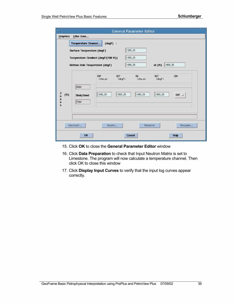
15. Click OK to close the General Parameter Editor window
16. Click Data Preparation to check that Input Neutron Matrix is set to Limestone. The program will now calculate a temperature channel. Then click OK to close this window
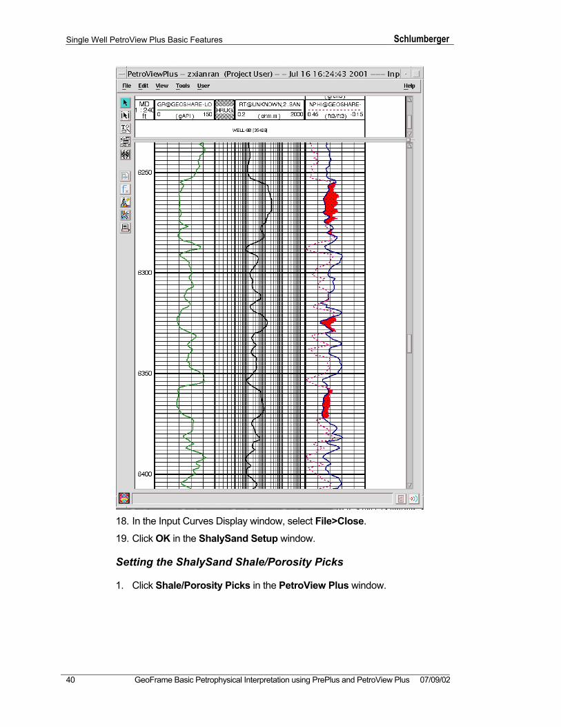
17. Click Display Input Curves to verify that the input log curves appear correctly.
GeoFrame Basic Petrophysical Interpretation using PrePlus and PetroView Plus 07/09/02 39
Single Well PetroView Plus Basic Features Schlumberger
18. In the Input Curves Display window, select File>Close.
19. Click OK in the ShalySand Setup window.
Setting the ShalySand Shale/Porosity Picks
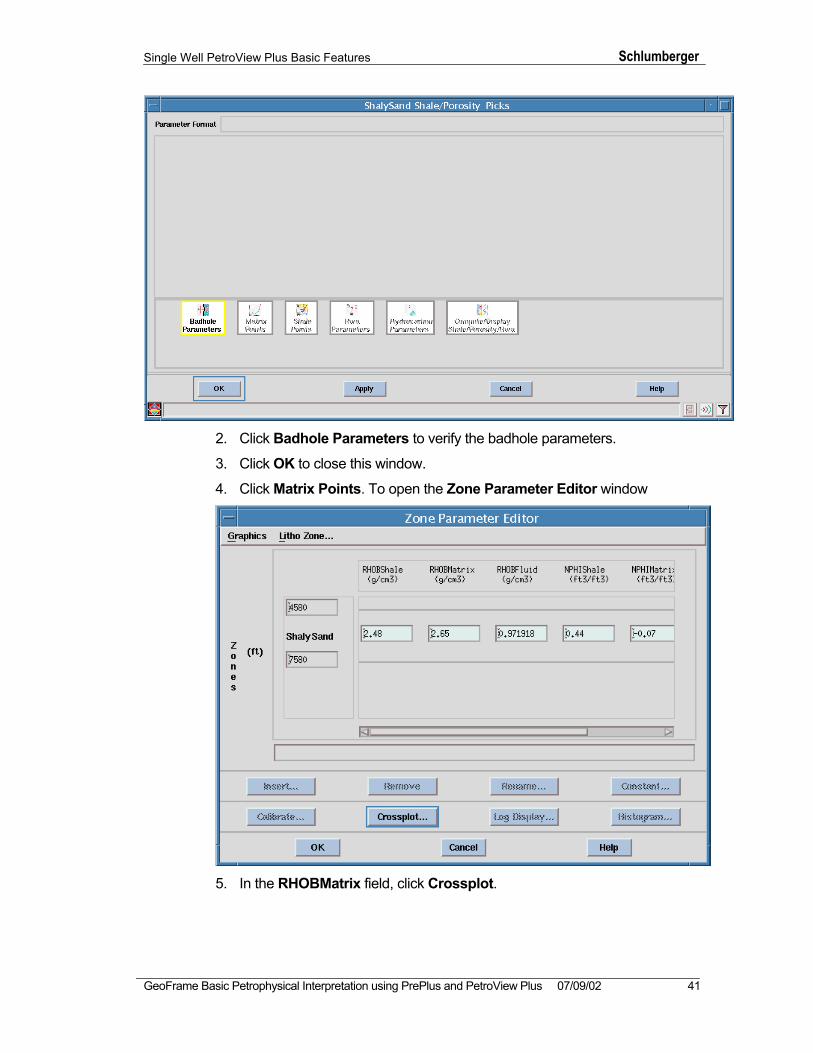
1. Click Shale/Porosity Picks in the PetroView Plus window.
40 GeoFrame Basic Petrophysical Interpretation using PrePlus and PetroView Plus 07/09/02
Single Well PetroView Plus Basic Features Schlumberger
2. Click Badhole Parameters to verify the badhole parameters.
3. Click OK to close this window.
4. Click Matrix Points. To open the Zone Parameter Editor window
5. In the RHOBMatrix field, click Crossplot.
GeoFrame Basic Petrophysical Interpretation using PrePlus and PetroView Plus 07/09/02 41
Single Well PetroView Plus Basic Features Schlumberger
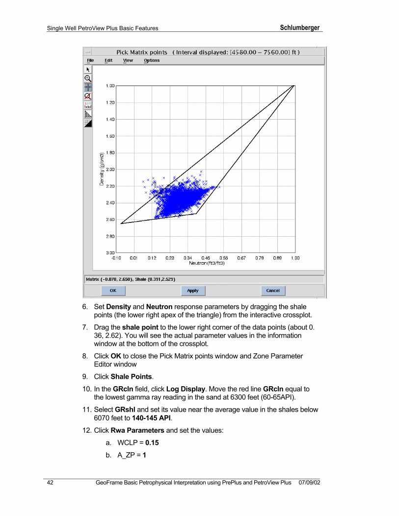
6. Set Density and Neutron response parameters by dragging the shale
points (the lower right apex of the triangle) from the interactive crossplot.
7. Drag the shale point to the lower right corner of the data points (about 0. 36, 2.62). You will see the actual parameter values in the information window at the bottom of the crossplot.
8. Click OK to close the Pick Matrix points window and Zone Parameter Editor window
9. Click Shale Points.
10. In the GRcln field, click Log Display. Move the red line GRcln equal to the lowest gamma ray reading in the sand at 6300 feet (60-65API).
11. Select GRshl and set its value near the average value in the shales below 6070 feet to 140-145 API.
12. Click Rwa Parameters and set the values:
a. WCLP = 0.15
b. A_ZP = 1
42 GeoFrame Basic Petrophysical Interpretation using PrePlus and PetroView Plus 07/09/02
Single Well PetroView Plus Basic Features Schlumberger
c. C_DWA = 0
d. M_MWA = 2
13. Select Hydrocarbon Parameters and set the values:
a. RHOHYD = 0.2
b. LH_CORR = Off c. HTYP = Gas
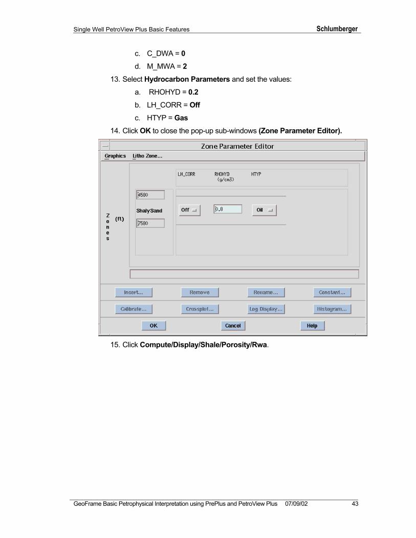
14. Click OK to close the pop-up sub-windows (Zone Parameter Editor).
15. Click Compute/Display/Shale/Porosity/Rwa.
GeoFrame Basic Petrophysical Interpretation using PrePlus and PetroView Plus 07/09/02 43
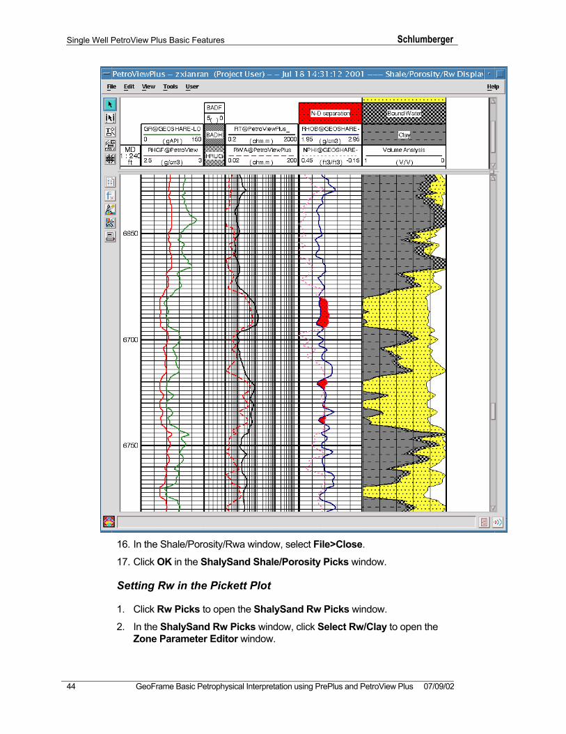
Single Well PetroView Plus Basic Features Schlumberger
16. In the Shale/Porosity/Rwa window, select File>Close.
17. Click OK in the ShalySand Shale/Porosity Picks window.
Setting Rw in the Pickett Plot
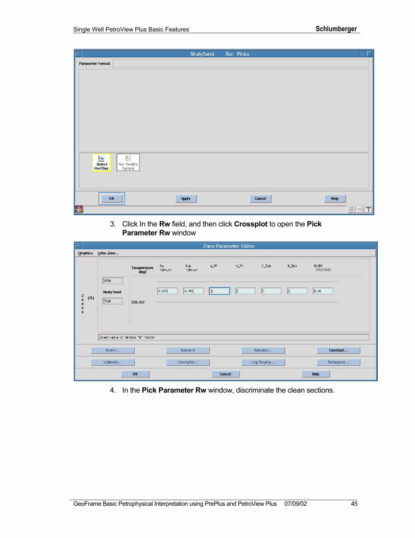
1. Click Rw Picks to open the ShalySand Rw Picks window.
2. In the ShalySand Rw Picks window, click Select Rw/Clay to open the Zone Parameter Editor window.
44 GeoFrame Basic Petrophysical Interpretation using PrePlus and PetroView Plus 07/09/02
Single Well PetroView Plus Basic Features Schlumberger
3. Click In the Rw field, and then click Crossplot to open the Pick
Parameter Rw window
4. In the Pick Parameter Rw window, discriminate the clean sections.
GeoFrame Basic Petrophysical Interpretation using PrePlus and PetroView Plus 07/09/02 45
Single Well PetroView Plus Basic Features Schlumberger
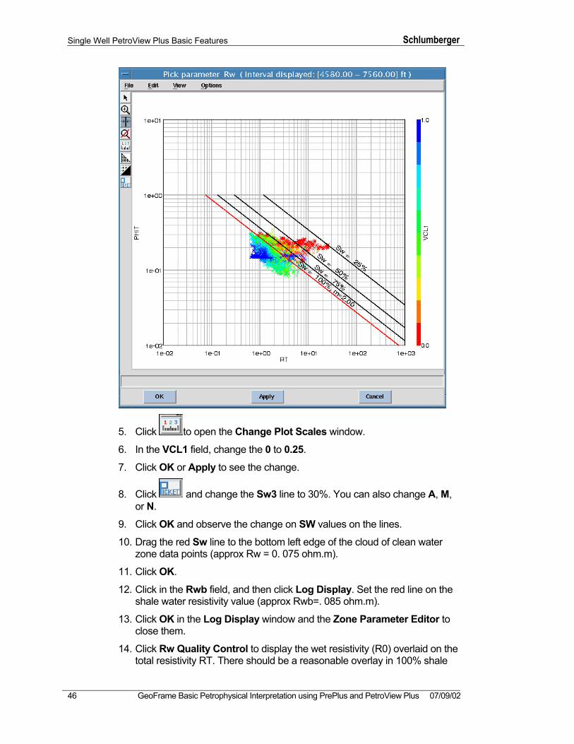
5. Click to open the Change Plot Scales window.
6. In the VCL1 field, change the 0 to 0.25.
7. Click OK or Apply to see the change.
8. Click and change the Sw3 line to 30%. You can also change A, M, or N.
9. Click OK and observe the change on SW values on the lines.
10. Drag the red Sw line to the bottom left edge of the cloud of clean water zone data points (approx Rw = 0. 075 ohm.m).
11. Click OK.
12. Click in the Rwb field, and then click Log Display. Set the red line on the shale water resistivity value (approx Rwb=. 085 ohm.m).
13. Click OK in the Log Display window and the Zone Parameter Editor to close them.
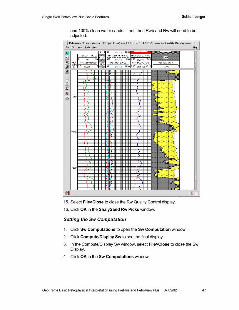
14. Click Rw Quality Control to display the wet resistivity (R0) overlaid on the total resistivity RT. There should be a reasonable overlay in 100% shale
46 GeoFrame Basic Petrophysical Interpretation using PrePlus and PetroView Plus 07/09/02
Single Well PetroView Plus Basic Features Schlumberger
and 100% clean water sands. If not, then Rwb and Rw will need to be adjusted.
15. Select File>Close to close the Rw Quality Control display.
16. Click OK in the ShalySand Rw Picks window.
Setting the Sw Computation
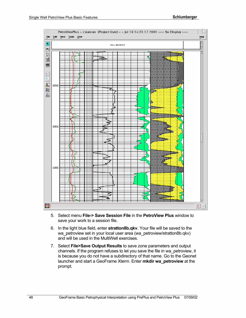
1. Click Sw Computations to open the Sw Computation window.
2. Click Compute/Display Sw to see the final display.
3. In the Compute/Display Sw window, select File>Close to close the Sw Display.
4. Click OK in the Sw Computations window.
GeoFrame Basic Petrophysical Interpretation using PrePlus and PetroView Plus 07/09/02 47
Single Well PetroView Plus Basic Features Schlumberger
5. Select menu File-> Save Session File in the PetroView Plus window to
save your work to a session file.
6. In the light blue field, enter stratton8b.qkv. Your file will be saved to the wa_petroview set in your local user area (wa_petroview/stratton8b.qkv) and will be used in the MultiWell exercises.
7. Select File>Save Output Results to save zone parameters and output channels. If the program refuses to let you save the file in wa_petroview, it is because you do not have a subdirectory of that name. Go to the Geonet launcher and start a GeoFrame Xterm. Enter mkdir wa_petroview at the prompt.
48 GeoFrame Basic Petrophysical Interpretation using PrePlus and PetroView Plus 07/09/02
Single Well PetroView Plus Advanced Features Schlumberger
Chapter 4 Single Well PetroView Plus Advanced Features
Overview
The following are some of the major features in PetroView Plus Advanced
• Model Zonation: Allows you to switch between the “ShalySand” and “Carbonate” models
• Computation of Sxo Saturation: Allows you to compute Sxo (flushed zone) saturation needed for a light hydrocarbon correction or to produce a “moved-oil” plot that might be indicative of productive intervals
• Coal, Anhydrite and Halite Detection: Allows you to detect special minerals and flag these minerals for geological correlation
• Light Hydrocarbon correction: Allows you to compute a correction to porosity based on the density of the hydrocarbon in the flushed zone and get a more accurate porosity
• User-defined Sw lines on Pickett Plots: Allows you to define the Sw lines and cutoff on the data that is used in the Pickett plot and then get a good Rw determination
• Non-linear shale volume calculation
• Support for Oil-Based Mud For a detailed explanation of the features mentioned above and algorithms used in PetroView Plus, please refer to the online help documentation in the GeoFrame Bookshelf.
Advanced Single Well Petrophysical Interpretation
Loading Data
If the data has been loaded into your GeoFrame database, please skip this section and go to Processing Data.
1. In the GeoFrame Application Manager Window, click to open Data Management. In the Data Management window, select a data load module in the Loaders and Unloaders folder.
2. Click OK or Apply to open the Data Load window.
3. Click Input File to open the Select the File (s) to Load window.
4. In the Filter text field, enter the directory path given to you by the instructor.
GeoFrame Basic Petrophysical Interpretation using PrePlus and PetroView Plus 07/09/02 49
Single Well PetroView Plus Advanced Features Schlumberger
5. Click Filter button to display files of the selected directory and select petro_updates.dlis.
6. Click OK to close the Select the File (s) to Load window. Do not assign a Field, Well, Borehole, or Producer name to the Data Load window.
7. Click Run in the Data Load window to start loading data.
8. Click Exit to close the Data Load window.
Processing Data
1. In the GeoFrame Application Manager window, click to open Process Manager.
2. In the Process Manager window, select File>New Activity.
3. Click to open the Product Catalog.
4. In the Product Catalog window, click the Petrophysics folder and select PetroView Plus.
5. Click OK to close the Product Catalog window. 6. Click Activity and name your activity.
7. Click to open the Data Focus window.
8. In the Data Focus window, change the Show menu to Borehole.
9. In the Complex-Sand-Carb field, highlight the Complex-Sand-Carb borehole and click OK.
10. In the PetroView Plus window, select Model>Zoned Sand/Carbonate.
Modeling Setup
Note: Before you open a new sub-window, please close the sub-window you opened by the previous clicking.
1. Click Setup to open the Zoned ShalySand Setup/Carbonate window.
2. Click Input Equations and set the input equations: (Click orange areas to view available options.)
a. Main Porosity = Density-Thermal-Neutron (CNL) b. Badhole Porosity = Sonic-Wyllie
c. Water Saturation = Dual-Water d. Flushed Zone Analysis = Using-Flushed-Zone-Resistivity
e. Wet<>Dry Clay = WCLP
f. Water Cut in the CMR = None
g. Coal Detection = OFF
h. Anhydrite Detection = ON
50 GeoFrame Basic Petrophysical Interpretation using PrePlus and PetroView Plus 07/09/02
Single Well PetroView Plus Advanced Features Schlumberger
i. Halite Detection = ON
3. Click ShalySand Shale Indicators and set the Density-Thermal Neutron as Linear and Gamma Ray to Clavier.
4. Click Carbonate Shale Indicators and set Gamma Ray to Linear. 5. Click Badhole Indicator and set Differential Caliper and Hole Rugosity
to ON and all other selectors to OFF.
6. Click OK.
7. Click Special Mineral Indicators. Set the following indicators to ON and all others to OFF:
a. ANHYDRITE: Density = ON
b. ANHYDRITE: Thermal Neutron = ON
c. HALITE: Density = ON
d. HALITE: Thermal Neutron = ObN
8. Click Binding Preference to define which enters of arrays (log curve) PetroView Plus will use and where it will start looking for them when it begins binding the arrays. Keep all the default settings and close the sub-window in this exercise.
9. Click Input Curves Binding to toggle all necessary input channels. You should have all necessary input channels (M_CH and N_CH are optional parameters in the core analysis) except for the Temperature TEMP_CH, which will be calculated by PetroView Plus. ( If your data set has the temperature data, it will be bound automatically)
10. Click OK. 11. If no channels are bound or you wish to change the channel’s binding,
highlight the array
12. Click MB3
13. Click Log Curve Selector
GeoFrame Basic Petrophysical Interpretation using PrePlus and PetroView Plus 07/09/02 51
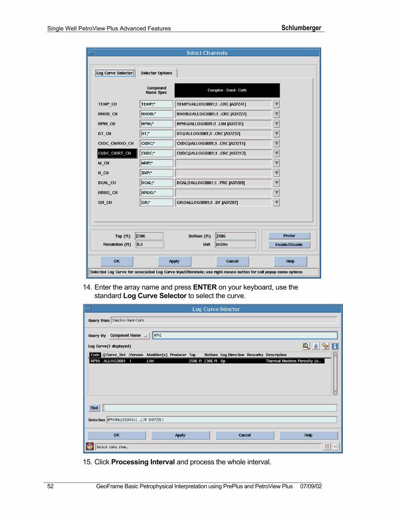
Single Well PetroView Plus Advanced Features Schlumberger
14. Enter the array name and press ENTER on your keyboard, use the
standard Log Curve Selector to select the curve.
15. Click Processing Interval and process the whole interval.
52 GeoFrame Basic Petrophysical Interpretation using PrePlus and PetroView Plus 07/09/02
Single Well PetroView Plus Advanced Features Schlumberger
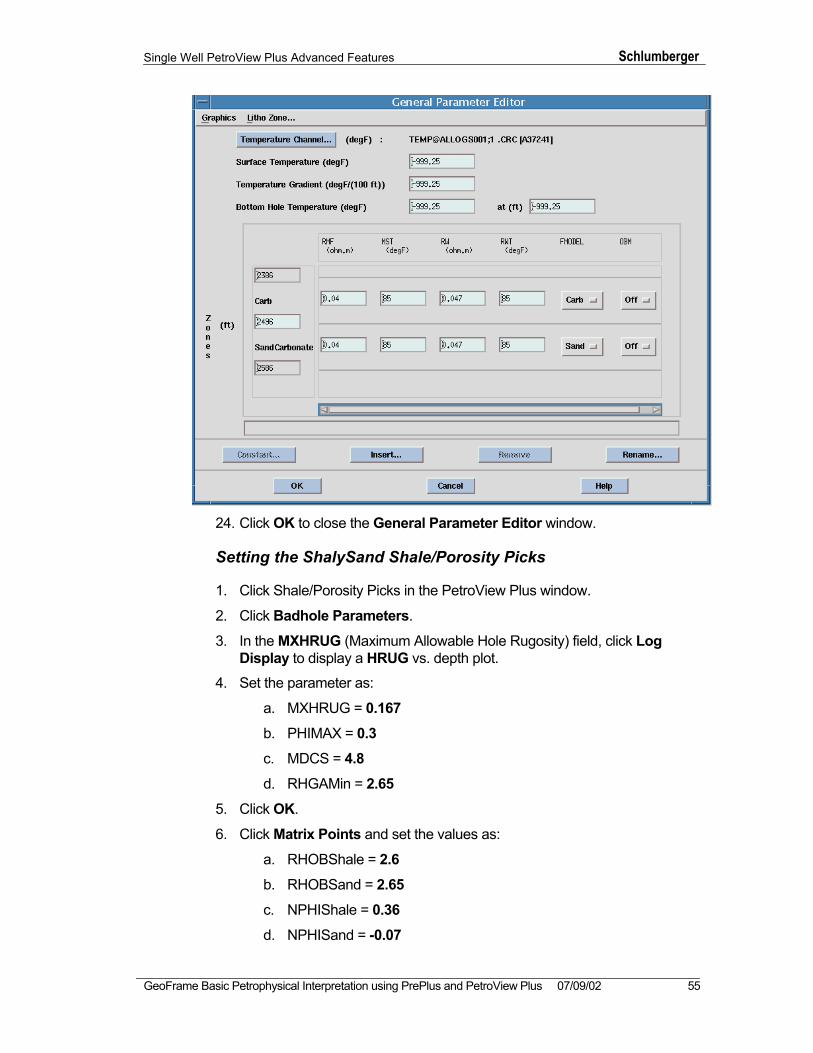
16. Click General Parameters and set the parameters as:
a. RMF = 0.04 ohm.m
b. MST = 85 DegF
c. Rw = 0.047 ohm.m
d. RWT = 85 DegF
e. OBM switch = Off f. Surface Temperature = 75 DegF
g. BHT = 85 DegF @ 2586 ft. 17. Click Data Preparation and change Caliper to HRUG to YES. The
program will calculate hole rugosity.
18. Click Display Input Curves to view the input log curves and the newly calculated HRUG.
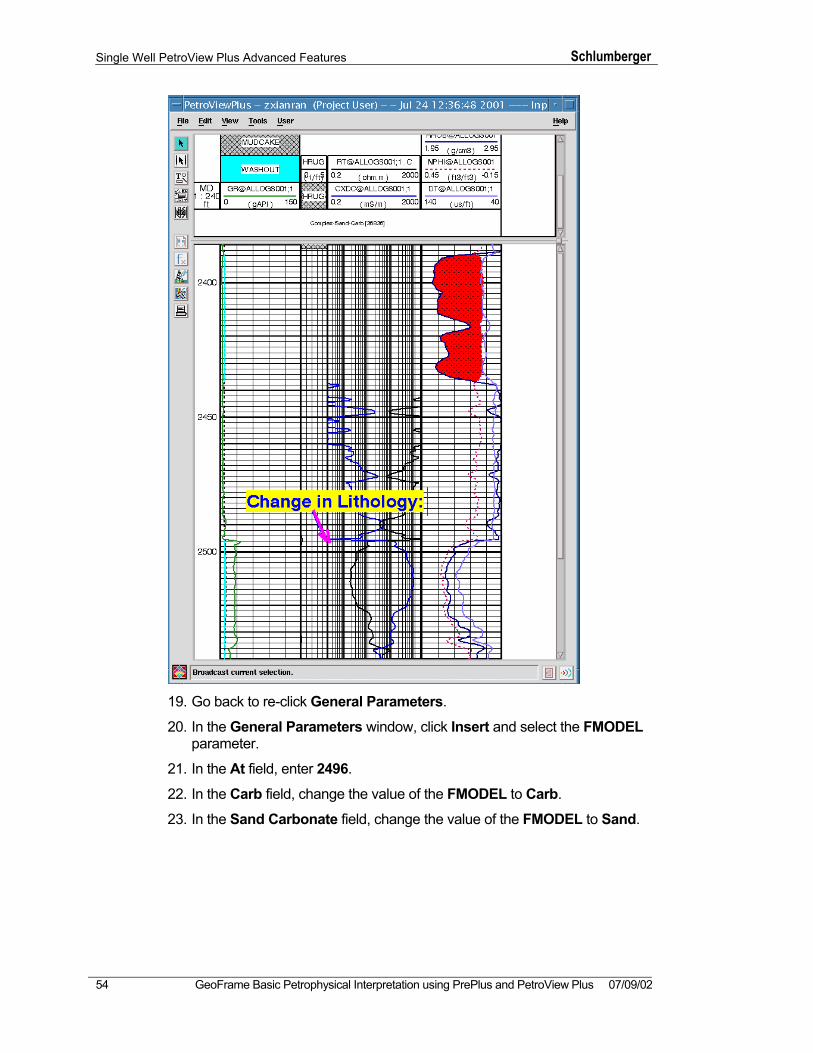
Note: When you view the plot, notice that there is an abrupt change in lithology at 2496 ft. This is the boundary between sand-shale and carbonate-evaporite. You can now go back to the General Parameters task to put in this zoning. Keep this display for future reference.
GeoFrame Basic Petrophysical Interpretation using PrePlus and PetroView Plus 07/09/02 53
Single Well PetroView Plus Advanced Features Schlumberger
19. Go back to re-click General Parameters.
20. In the General Parameters window, click Insert and select the FMODEL parameter.
21. In the At field, enter 2496.
22. In the Carb field, change the value of the FMODEL to Carb.
23. In the Sand Carbonate field, change the value of the FMODEL to Sand.
54 GeoFrame Basic Petrophysical Interpretation using PrePlus and PetroView Plus 07/09/02
Single Well PetroView Plus Advanced Features Schlumberger
24. Click OK to close the General Parameter Editor window.
Setting the ShalySand Shale/Porosity Picks
1. Click Shale/Porosity Picks in the PetroView Plus window.
2. Click Badhole Parameters.
3. In the MXHRUG (Maximum Allowable Hole Rugosity) field, click Log Display to display a HRUG vs. depth plot.
4. Set the parameter as:
a. MXHRUG = 0.167
b. PHIMAX = 0.3
c. MDCS = 4.8
d. RHGAMin = 2.65
5. Click OK.
6. Click Matrix Points and set the values as:
a. RHOBShale = 2.6
b. RHOBSand = 2.65
c. NPHIShale = 0.36
d. NPHISand = -0.07
GeoFrame Basic Petrophysical Interpretation using PrePlus and PetroView Plus 07/09/02 55
Single Well PetroView Plus Advanced Features Schlumberger
7. Use the crossplot to determine the endpoints for the zones in which the model enter has been set to Sand.
8. Click Shale Points.
9. In the GRcln field, click Log Display.
10. Move the red line to make GRcln to the lower part of the GR readings (about 6 Gapi).
11. Select GRshl and set it to 100 Gapi. 12. Click Badhole Porosity.
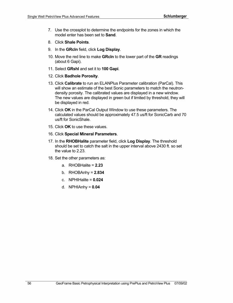
13. Click Calibrate to run an ELANPlus Parameter calibration (ParCal). This will show an estimate of the best Sonic parameters to match the neutron-density porosity. The calibrated values are displayed in a new window. The new values are displayed in green but if limited by threshold, they will be displayed in red.
14. Click OK in the ParCal Output Window to use these parameters. The calculated values should be approximately 47.5 us/ft for SonicCarb and 70 us/ft for SonicShale.
15. Click OK to use these values.
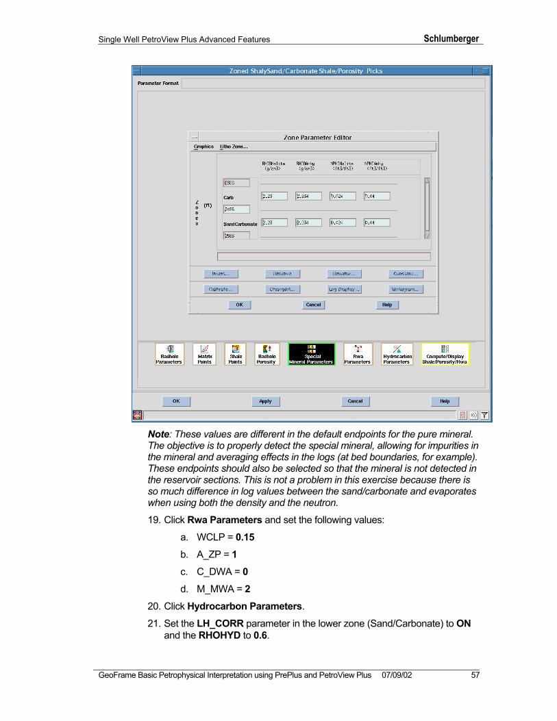
16. Click Special Mineral Parameters.
17. In the RHOBHalite parameter field, click Log Display. The threshold should be set to catch the salt in the upper interval above 2430 ft. so set the value to 2.23.
18. Set the other parameters as:
a. RHOBHalite = 2.23
b. RHOBAnhy = 2.834
c. NPHIHalite = 0.024
d. NPHIAnhy = 0.04
56 GeoFrame Basic Petrophysical Interpretation using PrePlus and PetroView Plus 07/09/02
Single Well PetroView Plus Advanced Features Schlumberger
Note: These values are different in the default endpoints for the pure mineral. The objective is to properly detect the special mineral, allowing for impurities in the mineral and averaging effects in the logs (at bed boundaries, for example). These endpoints should also be selected so that the mineral is not detected in the reservoir sections. This is not a problem in this exercise because there is so much difference in log values between the sand/carbonate and evaporates when using both the density and the neutron.
19. Click Rwa Parameters and set the following values:
a. WCLP = 0.15
b. A_ZP = 1
c. C_DWA = 0
d. M_MWA = 2
20. Click Hydrocarbon Parameters.
21. Set the LH_CORR parameter in the lower zone (Sand/Carbonate) to ON and the RHOHYD to 0.6.
GeoFrame Basic Petrophysical Interpretation using PrePlus and PetroView Plus 07/09/02 57
Single Well PetroView Plus Advanced Features Schlumberger
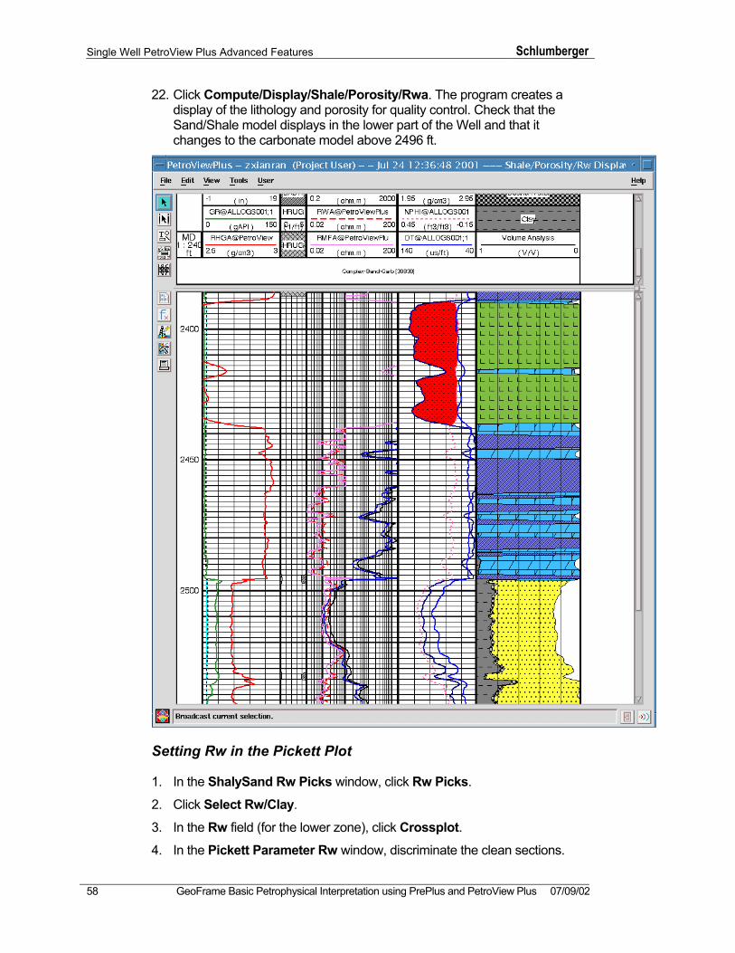
22. Click Compute/Display/Shale/Porosity/Rwa. The program creates a display of the lithology and porosity for quality control. Check that the Sand/Shale model displays in the lower part of the Well and that it changes to the carbonate model above 2496 ft.
Setting Rw in the Pickett Plot
1. In the ShalySand Rw Picks window, click Rw Picks.
2. Click Select Rw/Clay.
3. In the Rw field (for the lower zone), click Crossplot. 4. In the Pickett Parameter Rw window, discriminate the clean sections.
58 GeoFrame Basic Petrophysical Interpretation using PrePlus and PetroView Plus 07/09/02
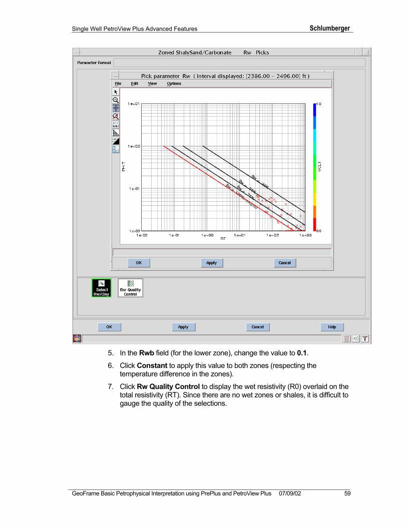
Single Well PetroView Plus Advanced Features Schlumberger
5. In the Rwb field (for the lower zone), change the value to 0.1.
6. Click Constant to apply this value to both zones (respecting the temperature difference in the zones).
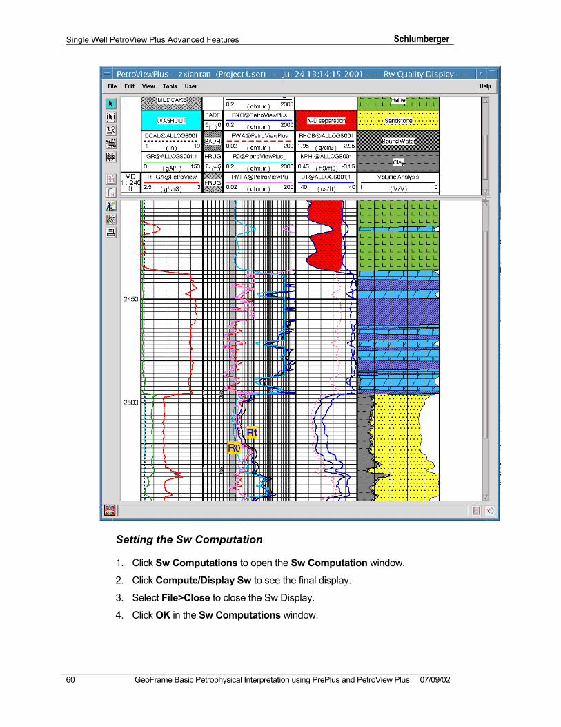
7. Click Rw Quality Control to display the wet resistivity (R0) overlaid on the total resistivity (RT). Since there are no wet zones or shales, it is difficult to gauge the quality of the selections.
GeoFrame Basic Petrophysical Interpretation using PrePlus and PetroView Plus 07/09/02 59
Single Well PetroView Plus Advanced Features Schlumberger
Setting the Sw Computation
1. Click Sw Computations to open the Sw Computation window.
2. Click Compute/Display Sw to see the final display.
3. Select File>Close to close the Sw Display.
4. Click OK in the Sw Computations window.
60 GeoFrame Basic Petrophysical Interpretation using PrePlus and PetroView Plus 07/09/02
Single Well PetroView Plus Advanced Features Schlumberger
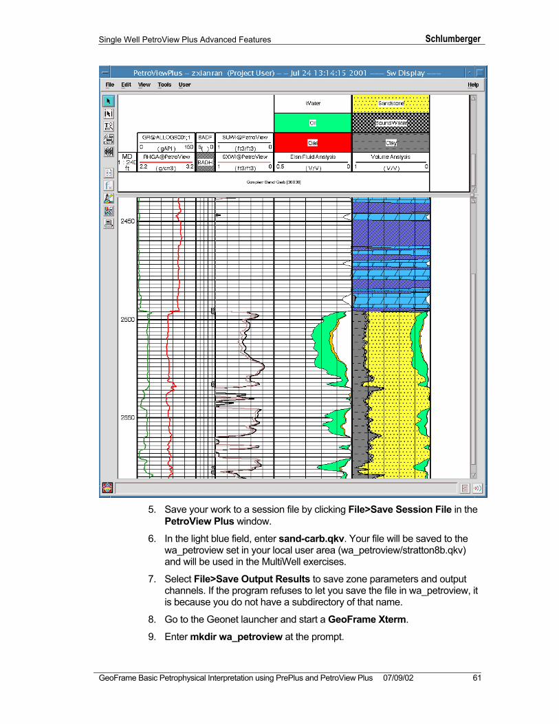
5. Save your work to a session file by clicking File>Save Session File in the
PetroView Plus window.
6. In the light blue field, enter sand-carb.qkv. Your file will be saved to the wa_petroview set in your local user area (wa_petroview/stratton8b.qkv) and will be used in the MultiWell exercises.
7. Select File>Save Output Results to save zone parameters and output channels. If the program refuses to let you save the file in wa_petroview, it is because you do not have a subdirectory of that name.
8. Go to the Geonet launcher and start a GeoFrame Xterm.
9. Enter mkdir wa_petroview at the prompt.
GeoFrame Basic Petrophysical Interpretation using PrePlus and PetroView Plus 07/09/02 61
Single Well PetroView Plus Advanced Features Schlumberger
10. Now go back to PVP and File>Save Output Results.
11. Re-run PetroView Plus with new parameters. Now that you have been through all the parameters once, it is not necessary to follow the full sequence of parameter setting.
12. Click Shale/Porosity Picks.
13. In the Special Mineral Parameters field, change RHOBHalite to 2.5 in the upper zone.
14. Click Sw Computations.
15. Click Compute/Display Sw. The display should now show more salt in the upper zone.
Single Well Petrophysical Interpretation Using Exclick Mode & Iterations
Processing Data
1. In the GeoFrame Application Manager window, click to open the Process Manager.
2. In the Process Manager window, select File>New Activity.
3. Click to open the Product Catalog.
4. Click the Petrophysics folder and select PetroView Plus.
5. Click OK to close the Product Catalog window.
6. Click Activity and name your activity.
7. Click to open the Data Focus.
8. In the Data Focus window, change the Show menu to Borehole.
9. In the StrattonB field, highlight the Well 20B borehole and click OK.
10. In the PetroView Plus window, click Open File and select stratton8.qkv.
11. Click Compute/Display Sw.
12. In the General Parameter Editor window, set the Bottom Hole Temperature (BHT) to 220 DegF @7400 ft.
13. Click OK and the final display will appear when the computation is completed.
14. Click Shale/Porosity Picks.
15. Click Shale Points.
16. In the GRshl field, click Log Display.
17. Set the GRsh value to 98 and the GRcln value to 60.
18. Click OK
62 GeoFrame Basic Petrophysical Interpretation using PrePlus and PetroView Plus 07/09/02
Single Well PetroView Plus Advanced Features Schlumberger
19. Click Compute/Display Sw. Adjust the other parameters and re-run the computation as required.
20. Click Shale/Porosity Picks to add a zone to the model.
21. Click Shale Points. 22. Click Insert and change the zone from 7400 to 6225.
23. In the upper zone field, enter Top.
24. Click OK to insert the boundary.
25. In the GRsh field of the Top zone, set the parameter to 115 and click OK.
26. Click Compute/Display Sw.
27. Select View>Scale and adjust the vertical display scale to 1:1000 to see the results.
28. Select User>Save Output Results to set the controls to overwrite previous outputs or save as a different file.
29. Select File>Save Session File to save the session file.
30. In the Selection field, enter wa_petroview/stratton20B.qkv.
31. Click OK.
GeoFrame Basic Petrophysical Interpretation using PrePlus and PetroView Plus 07/09/02 63

MultiWell PetroView Plus Schlumberger
Chapter 5 MultiWell PetroView Plus
Overview
The functions of MultiWell PetroView Plus:
• MultiWell Parameter Management
• MultiWell Graphical Zonation
• MultiWell Normalization
• MultiWell Crossplots/Histograms/Regression Analysis
• MultiWell Data Function
• MultiWell Data Processing
• MultiWell Cross-Section
• Interactive Well Normalization For a detailed explanation of the features mentioned above and algorithms used in PetroView Plus, please refer to the online help documentation in the GeoFrame Bookshelf.
Setting Parameters and Zones
The Zone Parameter Editor allows you to perform graphical zonation. The editor also allows creation of MultiWell parameters and provides user-controlled, multi-spreadsheet views of parameter.
Processing Data
1. In the GeoFrame Application Manager window, click to open the Process Manager.
2. In the Process Manager window, select File>New Activity.
3. Click to open the Product Catalog.
4. Click the Petrophysics folder and select PetroView Plus.
5. Click OK.
6. Click Activity and name your activity.
7. Click to open the Data Focus and change the Show menu to Field.
8. In the Data Focus window, highlight the StrattonB field.
9. Click OK.
10. Double click on the PetroView Plus module to open the PetroView Plus window.
GeoFrame Basic Petrophysical Interpretation using PrePlus and PetroView Plus 07/09/02 65
MultiWell PetroView Plus Schlumberger
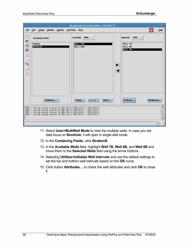
11. Select User>MultiWell Mode to view the multiple wells. In case you set
data focus on Borehole, it will open in single well mode.
12. In the Containing Fields, click StrattonB.
13. In the Available Wells field, highlight Well 7B, Well 8B, and Well 9B and move them to the Selected Wells field using the arrow buttons.
14. Selecting Utilities>Initialize Well Intervals and use the default settings to set the top and bottom well intervals based on the GR curve.
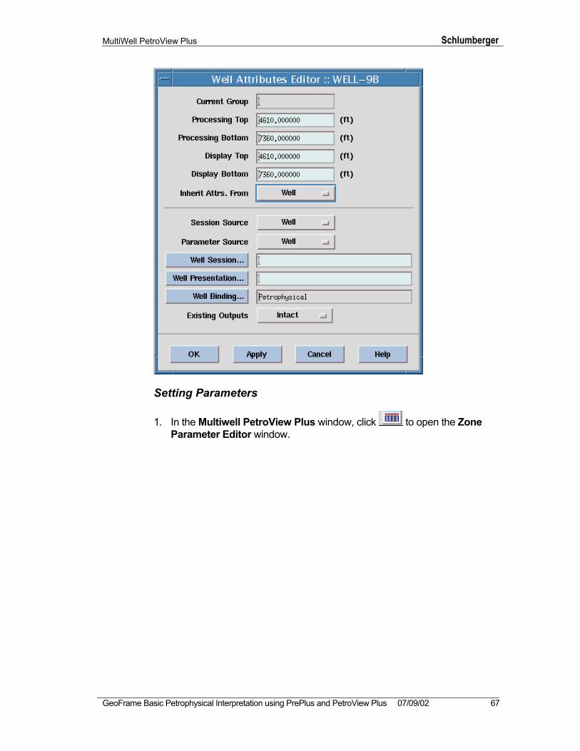
15. Click button Attributes… to check the well attributes and click OK to close it.
66 GeoFrame Basic Petrophysical Interpretation using PrePlus and PetroView Plus 07/09/02
MultiWell PetroView Plus Schlumberger
Setting Parameters
1. In the Multiwell PetroView Plus window, click to open the Zone Parameter Editor window.
GeoFrame Basic Petrophysical Interpretation using PrePlus and PetroView Plus 07/09/02 67
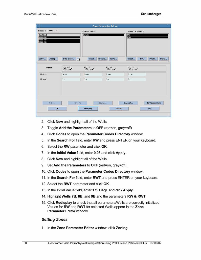
MultiWell PetroView Plus Schlumberger
2. Click New and highlight all of the Wells.
3. Toggle Add the Parameters to OFF (red=on, gray=off).
4. Click Codes to open the Parameter Codes Directory window.
5. In the Search For field, enter RW and press ENTER on your keyboard.
6. Select the RW parameter and click OK.
7. In the Initial Value field, enter 0.03 and click Apply.
8. Click New and highlight all of the Wells.
9. Set Add the Parameters to OFF (red=on, gray=off).
10. Click Codes to open the Parameter Codes Directory window.
11. In the Search For field, enter RWT and press ENTER on your keyboard.
12. Select the RWT parameter and click OK.
13. In the Initial Value field, enter 175 DegF and click Apply.
14. Highlight Wells 7B, 8B, and 9B and the parameters RW & RWT. 15. Click Redisplay to check that all parameters/Wells are correctly initialized.
Values for RW and RWT for selected Wells appear in the Zone Parameter Editor window.
Setting Zones
1. In the Zone Parameter Editor window, click Zoning.
68 GeoFrame Basic Petrophysical Interpretation using PrePlus and PetroView Plus 07/09/02
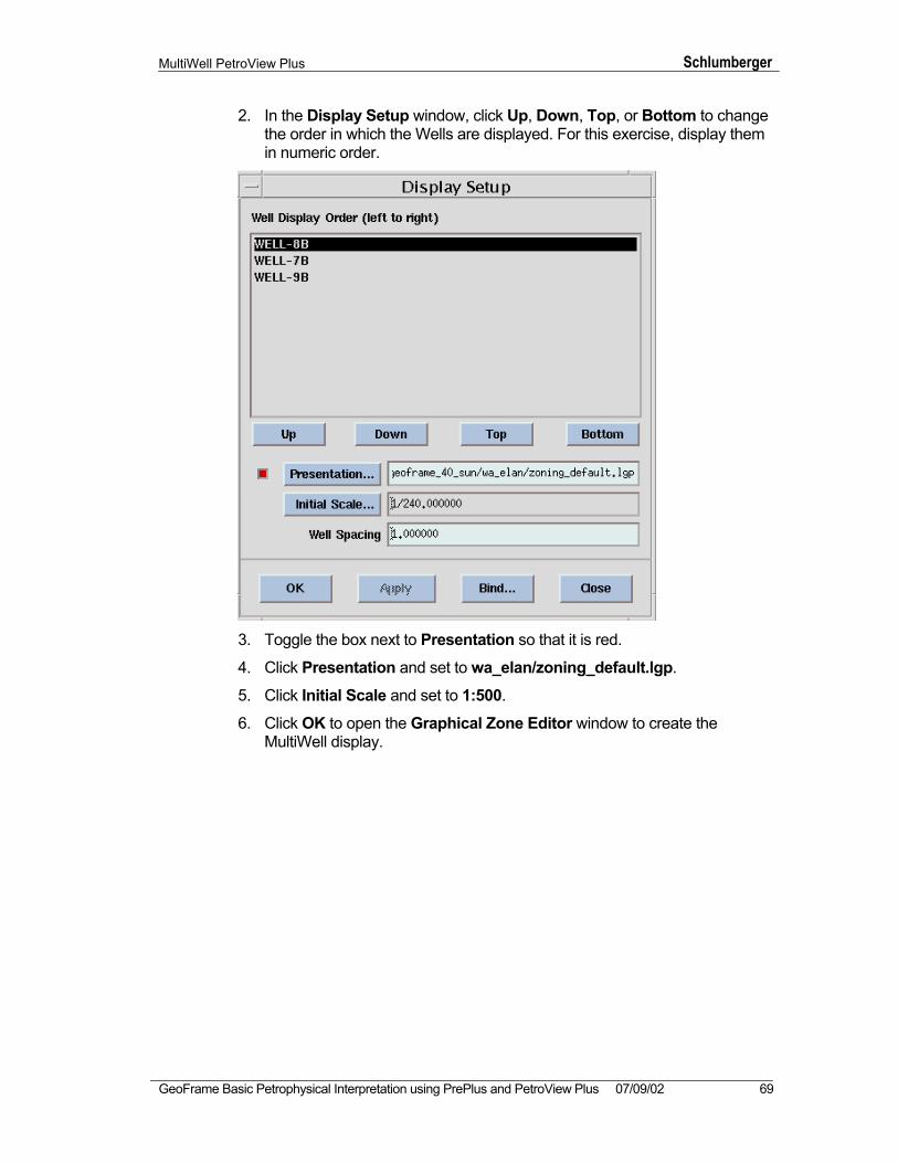
MultiWell PetroView Plus Schlumberger
2. In the Display Setup window, click Up, Down, Top, or Bottom to change the order in which the Wells are displayed. For this exercise, display them in numeric order.
3. Toggle the box next to Presentation so that it is red.
4. Click Presentation and set to wa_elan/zoning_default.lgp.
5. Click Initial Scale and set to 1:500.
6. Click OK to open the Graphical Zone Editor window to create the MultiWell display.
GeoFrame Basic Petrophysical Interpretation using PrePlus and PetroView Plus 07/09/02 69
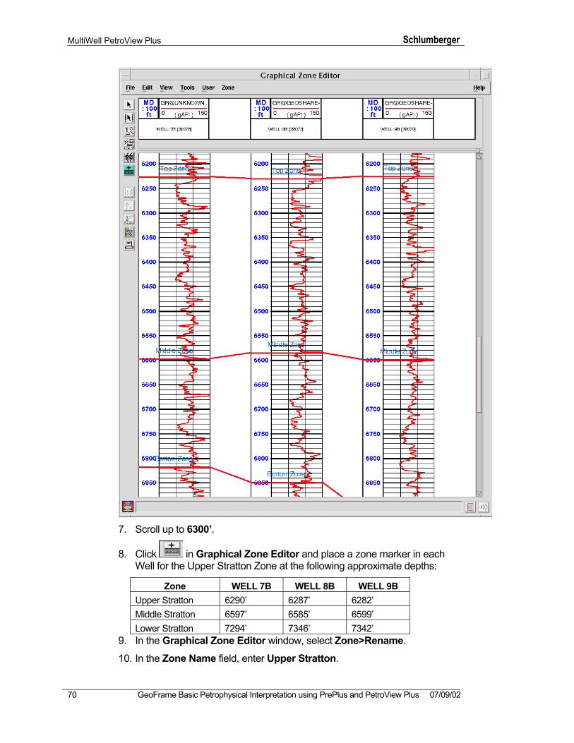
MultiWell PetroView Plus Schlumberger
7. Scroll up to 6300’.
8. Click in Graphical Zone Editor and place a zone marker in each Well for the Upper Stratton Zone at the following approximate depths:
Zone WELL 7B WELL 8B WELL 9B Upper Stratton 6290’ 6287’ 6282’ Middle Stratton 6597’ 6585’ 6599’ Lower Stratton 7294’ 7346’ 7342’
9. In the Graphical Zone Editor window, select Zone>Rename.
10. In the Zone Name field, enter Upper Stratton.
70 GeoFrame Basic Petrophysical Interpretation using PrePlus and PetroView Plus 07/09/02
MultiWell PetroView Plus Schlumberger
11. In the Zone Name field, enter Middle Stratton.
12. In the Zone Name field, enter Lower Stratton.
13. Select File>Close. 14. Highlight all the Wells in the Upper Stratton Zone, all the zones in the
middle panel, and the parameter RW in the right panel.
15. Change the RW to 0.035 and click Redisplay.
16. Click OK to exit the Zone Parameter Editor.
MultiWell Crossplot (Normalization)
The MultiWell crossplot allows you to crossplot single or multiple Wells and histogram multiple Wells, you can also use this Window to define “Key Wells” vs. “Target Well” and normalize the Target Well in the histogram or crossplot Window.
Basic Functions of MultiWell CrossPlot
Continue with the same activity of previous exercise (Setting Parameters and Zones). If you forget the activity name, go to the Process Manager to select the activity you named by selecting File>Open Activity.
1. In the MultiWell PetroView Plus window, set the displays for cross-section and crossplot.
2. Select Utilities>Set Module Displays.
3. Change CrossSection to hostname: 0.1 or hostname: 0.0 (whichever is the opposite of what PetroView Plus started on).
4. Click OK.
5. In the Containing Fields section, select StrattonB.
6. In the Available Wells field, highlight Well 7B, Well 8B, Well 9B and move them to the Selected Wells section.
Crossplot Wells By Color
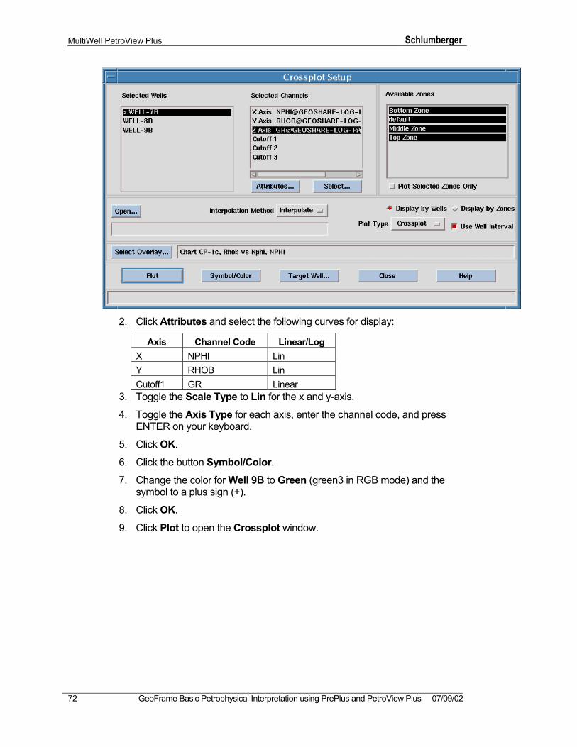
1. Click to open the Crossplot Setup window.
GeoFrame Basic Petrophysical Interpretation using PrePlus and PetroView Plus 07/09/02 71
MultiWell PetroView Plus Schlumberger
2. Click Attributes and select the following curves for display:
Axis Channel Code Linear/Log X NPHI Lin Y RHOB Lin Cutoff1 GR Linear
3. Toggle the Scale Type to Lin for the x and y-axis.
4. Toggle the Axis Type for each axis, enter the channel code, and press ENTER on your keyboard.
5. Click OK.
6. Click the button Symbol/Color. 7. Change the color for Well 9B to Green (green3 in RGB mode) and the
symbol to a plus sign (+).
8. Click OK.
9. Click Plot to open the Crossplot window.
72 GeoFrame Basic Petrophysical Interpretation using PrePlus and PetroView Plus 07/09/02
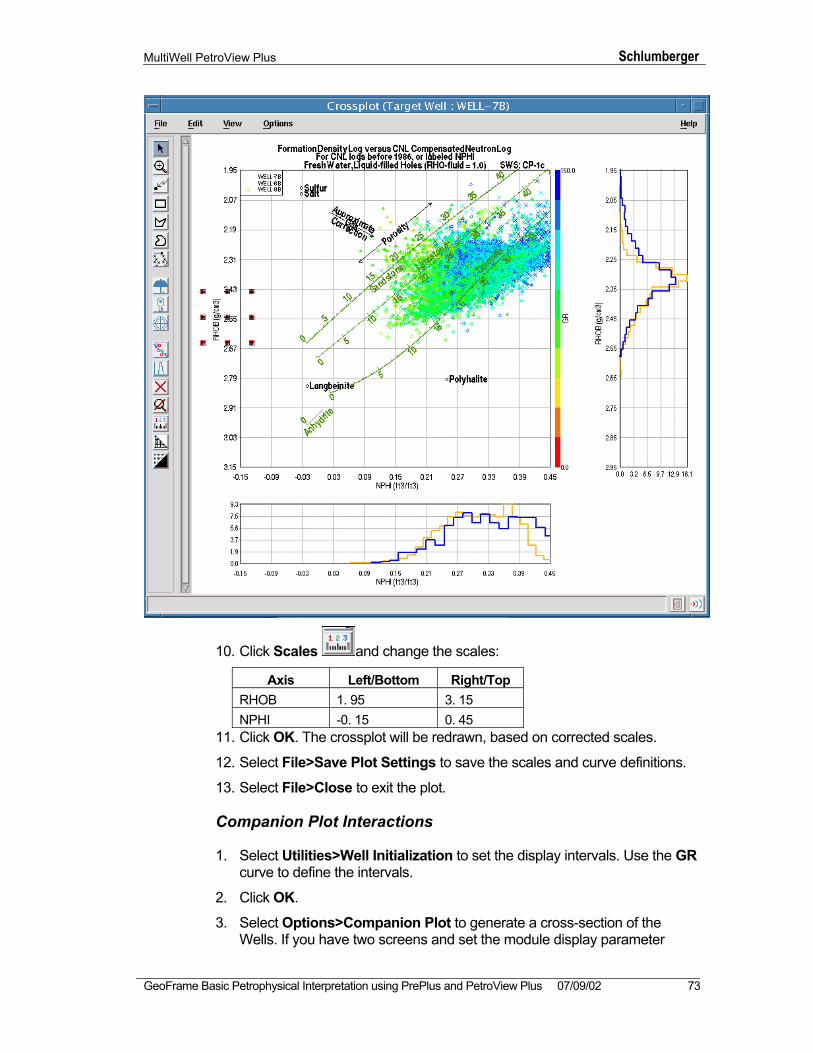
MultiWell PetroView Plus Schlumberger
10. Click Scales and change the scales:
Axis Left/Bottom Right/Top RHOB 1. 95 3. 15 NPHI -0. 15 0. 45
11. Click OK. The crossplot will be redrawn, based on corrected scales.
12. Select File>Save Plot Settings to save the scales and curve definitions.
13. Select File>Close to exit the plot.
Companion Plot Interactions
1. Select Utilities>Well Initialization to set the display intervals. Use the GR curve to define the intervals.
2. Click OK.
3. Select Options>Companion Plot to generate a cross-section of the Wells. If you have two screens and set the module display parameter
GeoFrame Basic Petrophysical Interpretation using PrePlus and PetroView Plus 07/09/02 73
MultiWell PetroView Plus Schlumberger
correctly, the cross-section should appear on the opposite screen. The RT curve is scaled linearly. Clicking on the curve and changing Scale Type to Logarithmic.
4. In the Companion Plot window, click Zone to activate the zone selection.
5. Scroll to approximately 6250 ft and select 6240 - 6250 ft in Well 7B. The relevant points will highlight in red on the crossplot.
6. In the Crossplot window, click Free Hand and select points in the crossplot by drawing a small circle around selected points. These selections will show up in the Cross-Section window.
7. Select View>Scale to change the vertical scale in the Cross-Section window.
8. Set the Vertical Scale to 1/1000 or a similar scale to see more of the data.
MultiWell Data Normalization Using MultiWell CrossPlot/Histogram
Continue with the same activity of previous exercise (MultiWell Crossplot). If you forget the activity name, go to the Process Manager to select the activity you named by selecting File>Open Activity.
1. In the Containing Fields field, click StrattonB.
2. Move Well 7B, Well 8B, and Well 9B into the Selected Wells panel.
3. If you have started a new session, select Utilities>Well Initialization.
4. Click to open MultiWell Crossplot Editor. 5. In the Selected Channels field, select X Axis.
6. Click Attributes.
7. Click Channel Code and select GR.
8. Click OK.
9. Click Apply.
10. Change the Axis Type to Y.
11. Set the Channel Code to RHOB.
12. Set the Cutoff1 to NPHI. 13. Click High Cut Point to adjust the NPHI cutoff interactively. 14. Move the red line to eliminate some of the more suspect data points
(approximately 0.50).
15. Click OK.
16. Click Close.
74 GeoFrame Basic Petrophysical Interpretation using PrePlus and PetroView Plus 07/09/02
MultiWell PetroView Plus Schlumberger
17. Click Target Well to verify that Well 7B is selected. (If the Well is selected, it will have a >to the left of it.)
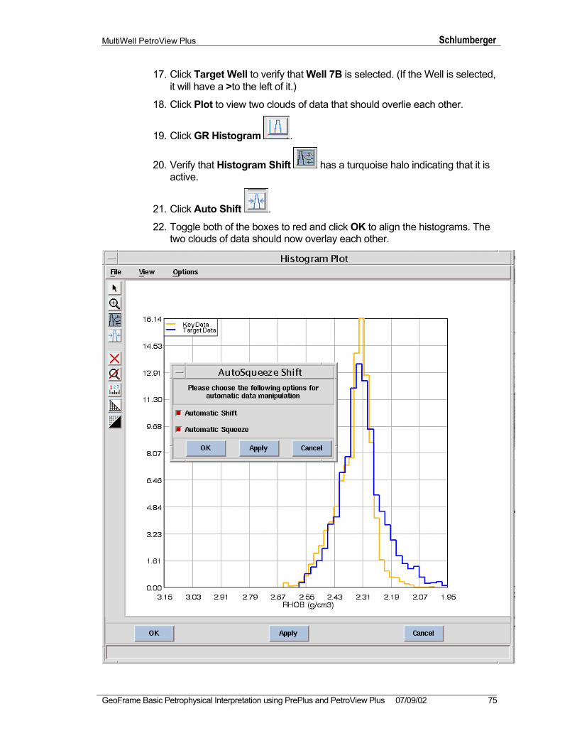
18. Click Plot to view two clouds of data that should overlie each other.
19. Click GR Histogram .
20. Verify that Histogram Shift has a turquoise halo indicating that it is active.
21. Click Auto Shift .
22. Toggle both of the boxes to red and click OK to align the histograms. The two clouds of data should now overlay each other.
GeoFrame Basic Petrophysical Interpretation using PrePlus and PetroView Plus 07/09/02 75
MultiWell PetroView Plus Schlumberger
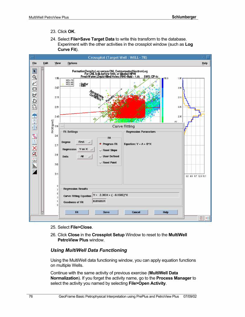
23. Click OK.
24. Select File>Save Target Data to write this transform to the database. Experiment with the other activities in the crossplot window (such as Log Curve Fit).
25. Select File>Close.
26. Click Close in the Crossplot Setup Window to reset to the MultiWell PetroView Plus window.
Using MultiWell Data Functioning
Using the MultiWell data functioning window, you can apply equation functions on multiple Wells.
Continue with the same activity of previous exercise (MultiWell Data Normalization). If you forget the activity name, go to the Process Manager to select the activity you named by selecting File>Open Activity.
76 GeoFrame Basic Petrophysical Interpretation using PrePlus and PetroView Plus 07/09/02
MultiWell PetroView Plus Schlumberger
1. In the Containing Fields field, click StrattonB.
2. Move Well 7B, Well 8B, and Well 9B into the Selected Wells panel.
3. If you have started a new session, select Utilities>Well Initialization.
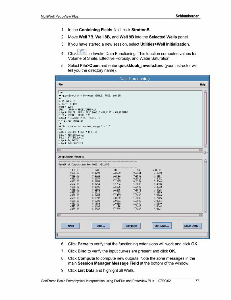
4. Click to Invoke Data Functioning. This function computes values for Volume of Shale, Effective Porosity, and Water Saturation.
5. Select File>Open and enter quickklook_mwelp.func (your instructor will tell you the directory name).
6. Click Parse to verify that the functioning extensions will work and click OK.
7. Click Bind to verify the input curves are present and click OK.
8. Click Compute to compute new outputs. Note the zone messages in the main Session Manager Message Field at the bottom of the window.
9. Click List Data and highlight all Wells.
GeoFrame Basic Petrophysical Interpretation using PrePlus and PetroView Plus 07/09/02 77
MultiWell PetroView Plus Schlumberger
10. Click Apply to view the outputs. They will appear in the Computation Results section of the Data Functioning Window.
11. Click Save Data in the Data Functioning window.
12. Click Save in the Save Data window to output the results to the database. The saved items will be displayed in the Data Functioning window.
13. Click Close.
14. Select File>Close.
15. Click General Data Manager to query for the results computed above or uses Log Curve Data Manager to check in the database.
16. Use the template presentation file built in the exercise, MultiWell Cross-section, to display all Wells’ computed results
Question: There is no RW parameter setting for the quicklook_mwelp.func, how can this exercise get the correct computation?
MultiWell Display
Using the WellCompositePlus Presentation Builder, you can generate user customized template files and make MultiWell cross section displays.
Continue with the same activity of previous exercise (MultiWell Data Functioning). If you forget the activity name, go to the Process Manager to select the activity you named by selecting File>Open Activity.
Building a Template
1. In the GeoFrame Application Manager window, click to open the Process Manager.
2. In the Process Manager window, select File>New Activity.
3. Click to open the Product Catalog.
4. Click the Petrophysics folder and select WellCompositePlus.
5. Click OK.
6. Click Activity and name your activity.
7. Click to set up Data Focus.
8. Change Show to Field.
9. In the StrattonB field, highlight the Well 8B borehole and click OK.
10. Double click on the WellCompositePlus module, open the WellcompositePlus window.
11. Change the template file to blank.lgp.
12. Click Run to open the main graphics window.
78 GeoFrame Basic Petrophysical Interpretation using PrePlus and PetroView Plus 07/09/02
MultiWell PetroView Plus Schlumberger
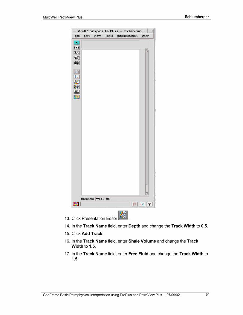
13. Click Presentation Editor .
14. In the Track Name field, enter Depth and change the Track Width to 0.5.
15. Click Add Track.
16. In the Track Name field, enter Shale Volume and change the Track Width to 1.5.
17. In the Track Name field, enter Free Fluid and change the Track Width to 1.5.
GeoFrame Basic Petrophysical Interpretation using PrePlus and PetroView Plus 07/09/02 79
MultiWell PetroView Plus Schlumberger
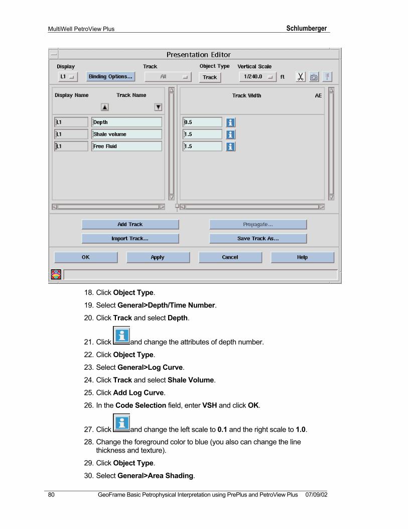
18. Click Object Type.
19. Select General>Depth/Time Number. 20. Click Track and select Depth.
21. Click and change the attributes of depth number.
22. Click Object Type.
23. Select General>Log Curve.
24. Click Track and select Shale Volume.
25. Click Add Log Curve.
26. In the Code Selection field, enter VSH and click OK.
27. Click and change the left scale to 0.1 and the right scale to 1.0. 28. Change the foreground color to blue (you also can change the line
thickness and texture).
29. Click Object Type.
30. Select General>Area Shading.
80 GeoFrame Basic Petrophysical Interpretation using PrePlus and PetroView Plus 07/09/02
MultiWell PetroView Plus Schlumberger
31. Click Track and select Shale Volume.
32. Click Add Area Shading.
33. Click and change the filling mode as Fill In the To.
34. Click Boundary 1 and select Left. 35. Click Boundary 2 and select VSH.
36. Select shale pattern with a gray background and click OK.
37. Click Object Type.
38. Select General>Log Curve.
39. Click Track and select Free Fluid.
40. Click Add Log Curve.
41. In the Query by Code field, enter PHIE and click OK.
42. Click and change the left scale to 0.5 and the right scale to 0. 43. Change the foreground color to red (you can also change the line
thickness and texture).
GeoFrame Basic Petrophysical Interpretation using PrePlus and PetroView Plus 07/09/02 81
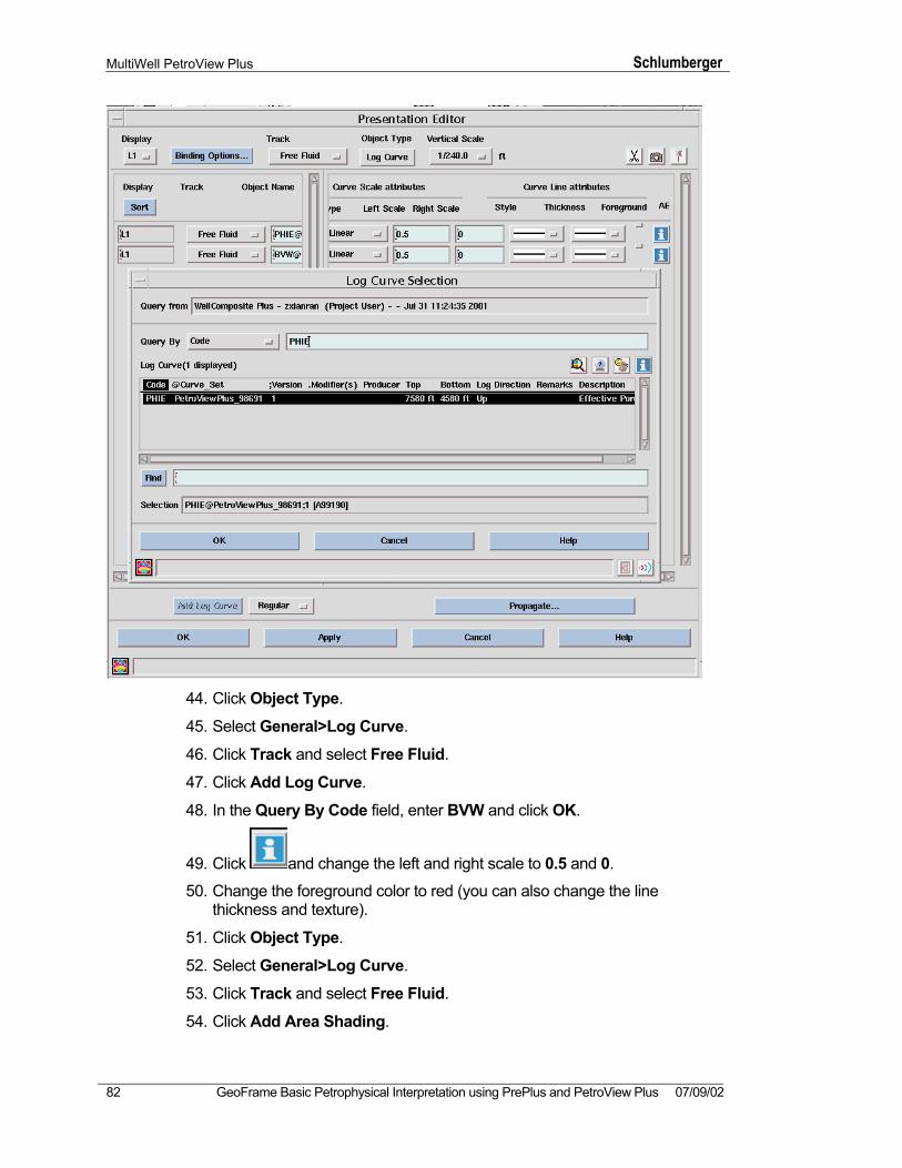
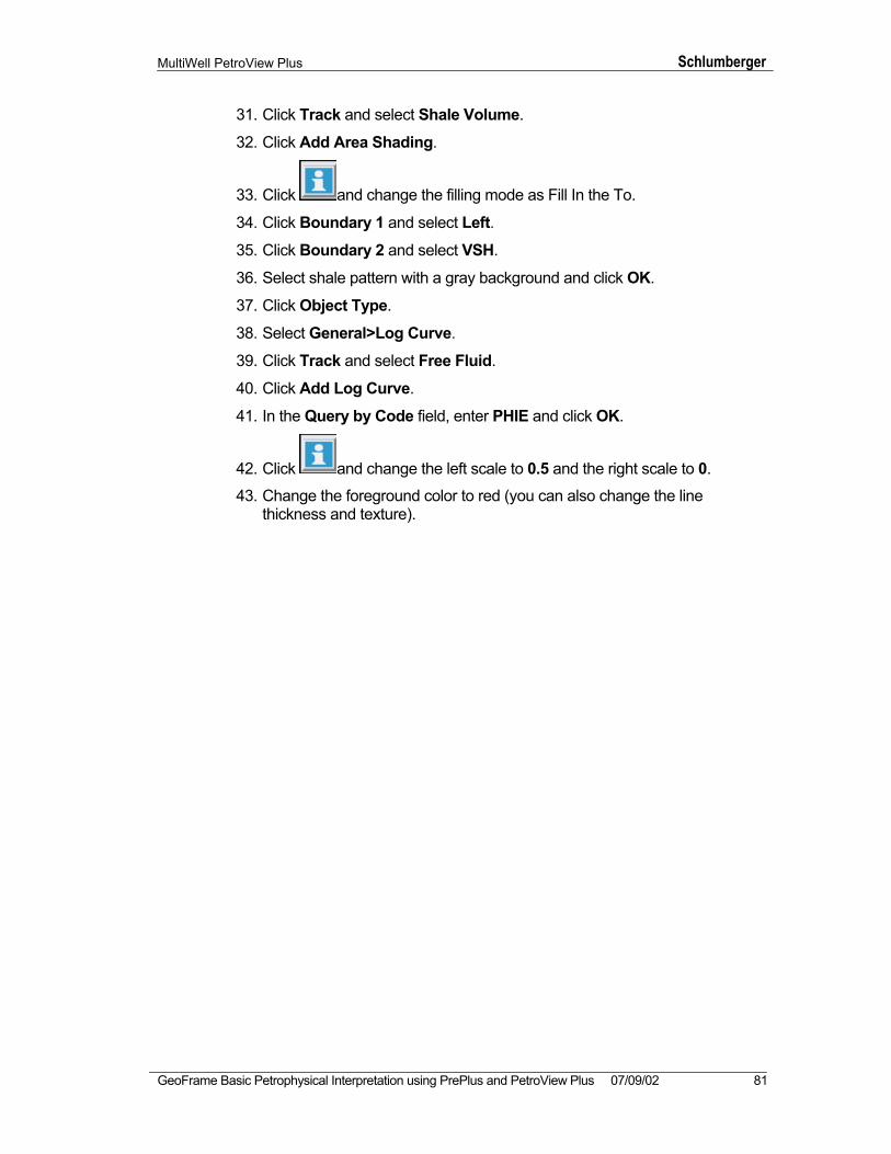
MultiWell PetroView Plus Schlumberger
44. Click Object Type.
45. Select General>Log Curve.
46. Click Track and select Free Fluid.
47. Click Add Log Curve.
48. In the Query By Code field, enter BVW and click OK.
49. Click and change the left and right scale to 0.5 and 0. 50. Change the foreground color to red (you can also change the line
thickness and texture).
51. Click Object Type.
52. Select General>Log Curve.
53. Click Track and select Free Fluid.
54. Click Add Area Shading.
82 GeoFrame Basic Petrophysical Interpretation using PrePlus and PetroView Plus 07/09/02
MultiWell PetroView Plus Schlumberger
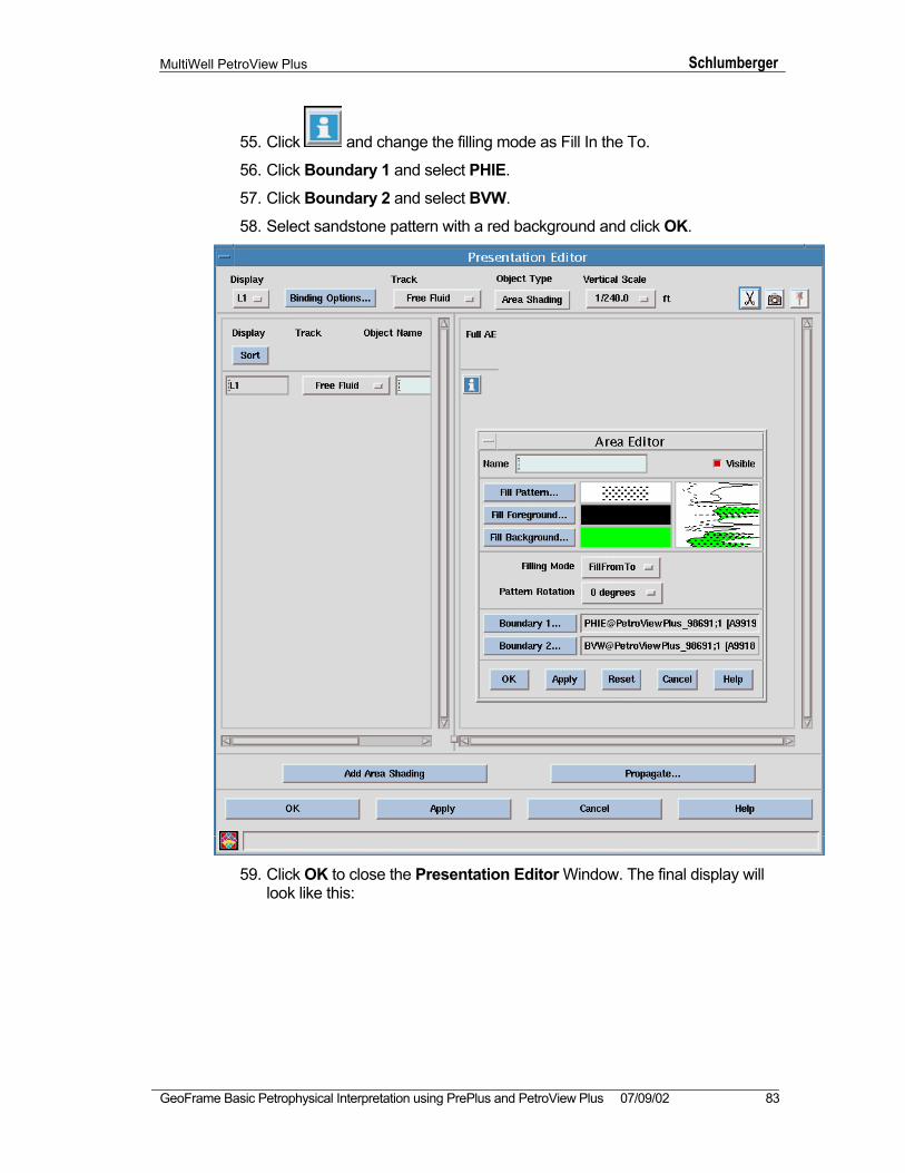
55. Click and change the filling mode as Fill In the To.
56. Click Boundary 1 and select PHIE.
57. Click Boundary 2 and select BVW.
58. Select sandstone pattern with a red background and click OK.
59. Click OK to close the Presentation Editor Window. The final display will
look like this:
GeoFrame Basic Petrophysical Interpretation using PrePlus and PetroView Plus 07/09/02 83
MultiWell PetroView Plus Schlumberger
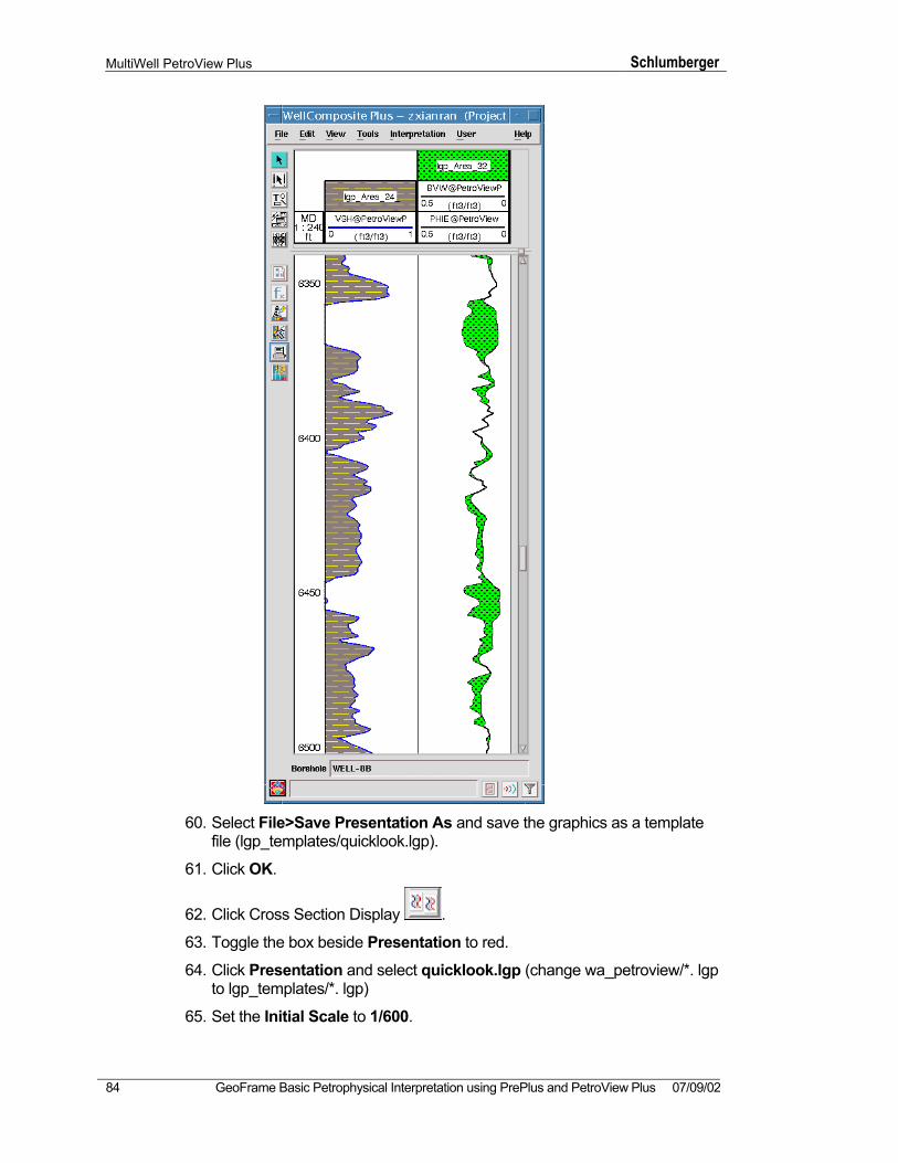
60. Select File>Save Presentation As and save the graphics as a template
file (lgp_templates/quicklook.lgp).
61. Click OK.
62. Click Cross Section Display .
63. Toggle the box beside Presentation to red.
64. Click Presentation and select quicklook.lgp (change wa_petroview/*. lgp to lgp_templates/*. lgp)
65. Set the Initial Scale to 1/600.
84 GeoFrame Basic Petrophysical Interpretation using PrePlus and PetroView Plus 07/09/02
MultiWell PetroView Plus Schlumberger
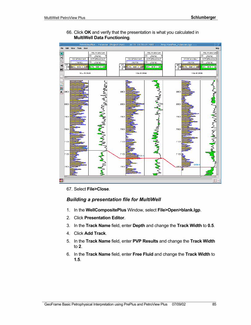
66. Click OK and verify that the presentation is what you calculated in MultiWell Data Functioning.
67. Select File>Close.
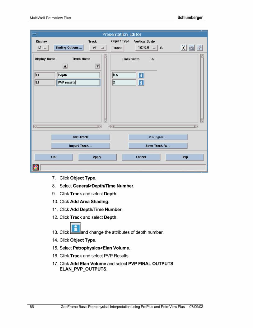
Building a presentation file for MultiWell
1. In the WellCompositePlus Window, select File>Open>blank.lgp.
2. Click Presentation Editor. 3. In the Track Name field, enter Depth and change the Track Width to 0.5.
4. Click Add Track.
5. In the Track Name field, enter PVP Results and change the Track Width to 2.
6. In the Track Name field, enter Free Fluid and change the Track Width to 1.5.
GeoFrame Basic Petrophysical Interpretation using PrePlus and PetroView Plus 07/09/02 85
MultiWell PetroView Plus Schlumberger
7. Click Object Type.
8. Select General>Depth/Time Number. 9. Click Track and select Depth.
10. Click Add Area Shading.
11. Click Add Depth/Time Number. 12. Click Track and select Depth.
13. Click and change the attributes of depth number.
14. Click Object Type.
15. Select Petrophysics>Elan Volume.
16. Click Track and select PVP Results.
17. Click Add Elan Volume and select PVP FINAL OUTPUTS ELAN_PVP_OUTPUTS.
86 GeoFrame Basic Petrophysical Interpretation using PrePlus and PetroView Plus 07/09/02
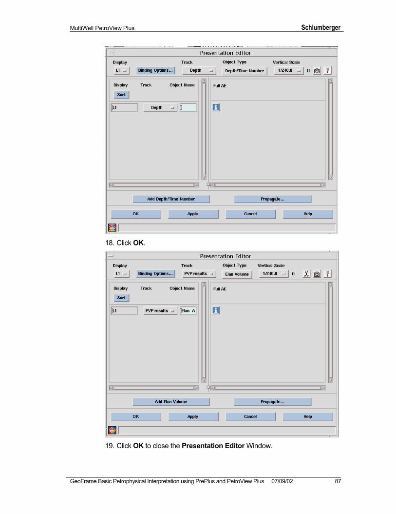
MultiWell PetroView Plus Schlumberger
18. Click OK.
19. Click OK to close the Presentation Editor Window.
GeoFrame Basic Petrophysical Interpretation using PrePlus and PetroView Plus 07/09/02 87
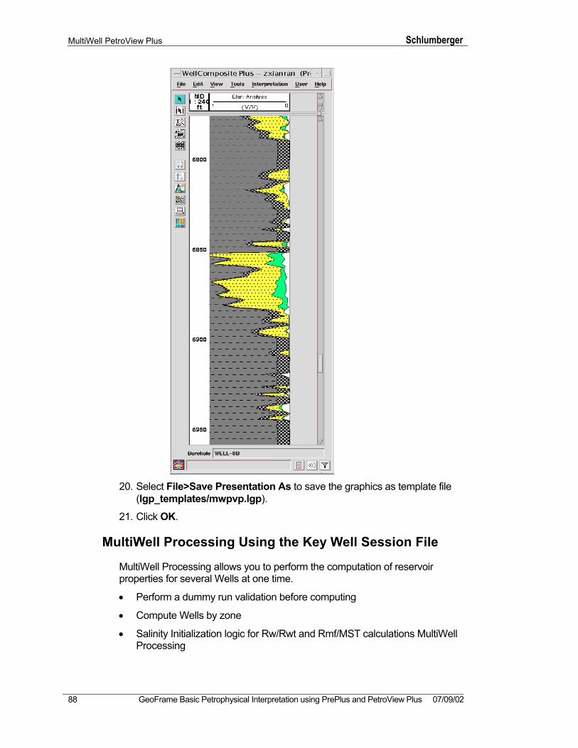
MultiWell PetroView Plus Schlumberger
20. Select File>Save Presentation As to save the graphics as template file
(lgp_templates/mwpvp.lgp).
21. Click OK.
MultiWell Processing Using the Key Well Session File
MultiWell Processing allows you to perform the computation of reservoir properties for several Wells at one time.
• Perform a dummy run validation before computing
• Compute Wells by zone
• Salinity Initialization logic for Rw/Rwt and Rmf/MST calculations MultiWell Processing
88 GeoFrame Basic Petrophysical Interpretation using PrePlus and PetroView Plus 07/09/02
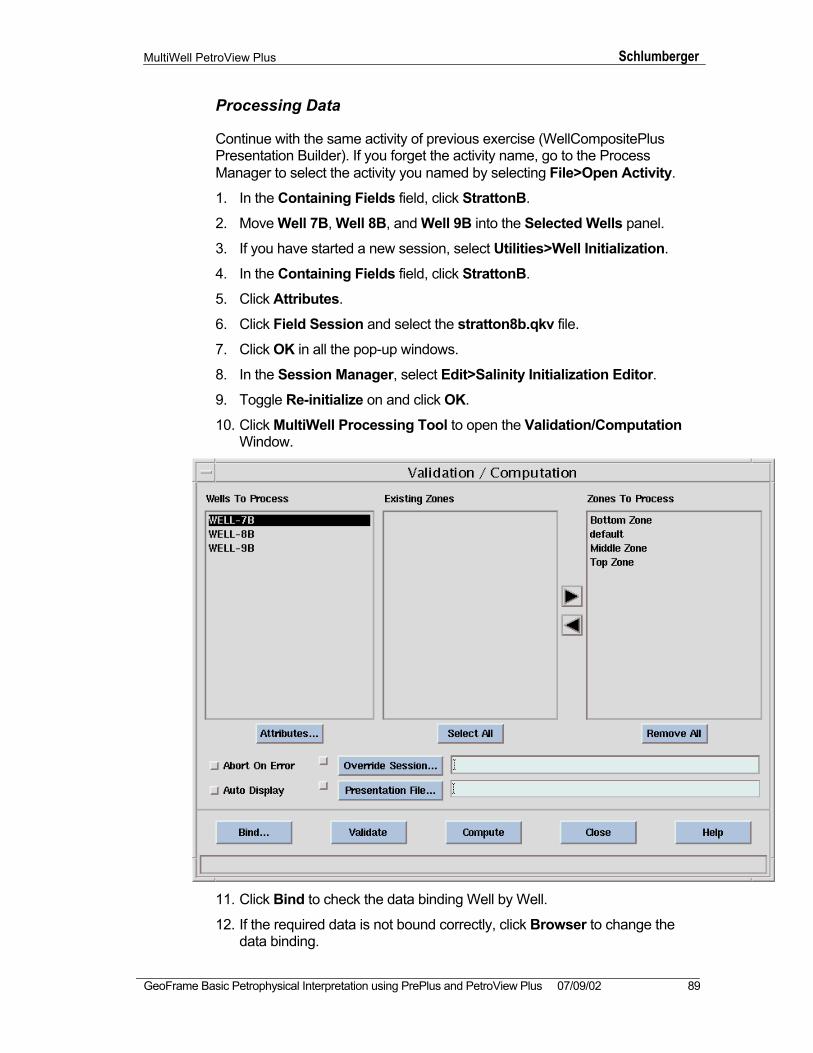
MultiWell PetroView Plus Schlumberger
Processing Data
Continue with the same activity of previous exercise (WellCompositePlus Presentation Builder). If you forget the activity name, go to the Process Manager to select the activity you named by selecting File>Open Activity.
1. In the Containing Fields field, click StrattonB.
2. Move Well 7B, Well 8B, and Well 9B into the Selected Wells panel.
3. If you have started a new session, select Utilities>Well Initialization.
4. In the Containing Fields field, click StrattonB.
5. Click Attributes.
6. Click Field Session and select the stratton8b.qkv file.
7. Click OK in all the pop-up windows.
8. In the Session Manager, select Edit>Salinity Initialization Editor. 9. Toggle Re-initialize on and click OK.
10. Click MultiWell Processing Tool to open the Validation/Computation Window.
11. Click Bind to check the data binding Well by Well.
12. If the required data is not bound correctly, click Browser to change the data binding.
GeoFrame Basic Petrophysical Interpretation using PrePlus and PetroView Plus 07/09/02 89
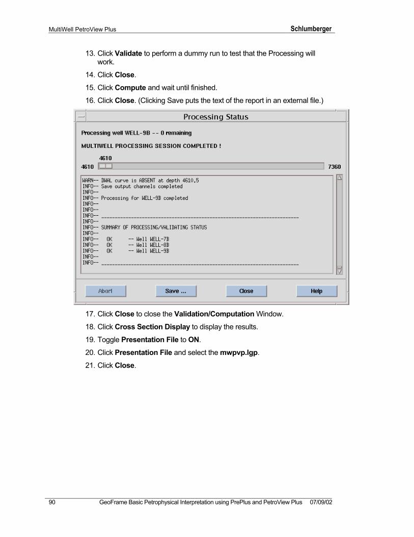
MultiWell PetroView Plus Schlumberger
13. Click Validate to perform a dummy run to test that the Processing will work.
14. Click Close.
15. Click Compute and wait until finished.
16. Click Close. (Clicking Save puts the text of the report in an external file.)
17. Click Close to close the Validation/Computation Window.
18. Click Cross Section Display to display the results.
19. Toggle Presentation File to ON.
20. Click Presentation File and select the mwpvp.lgp.
21. Click Close.
90 GeoFrame Basic Petrophysical Interpretation using PrePlus and PetroView Plus 07/09/02
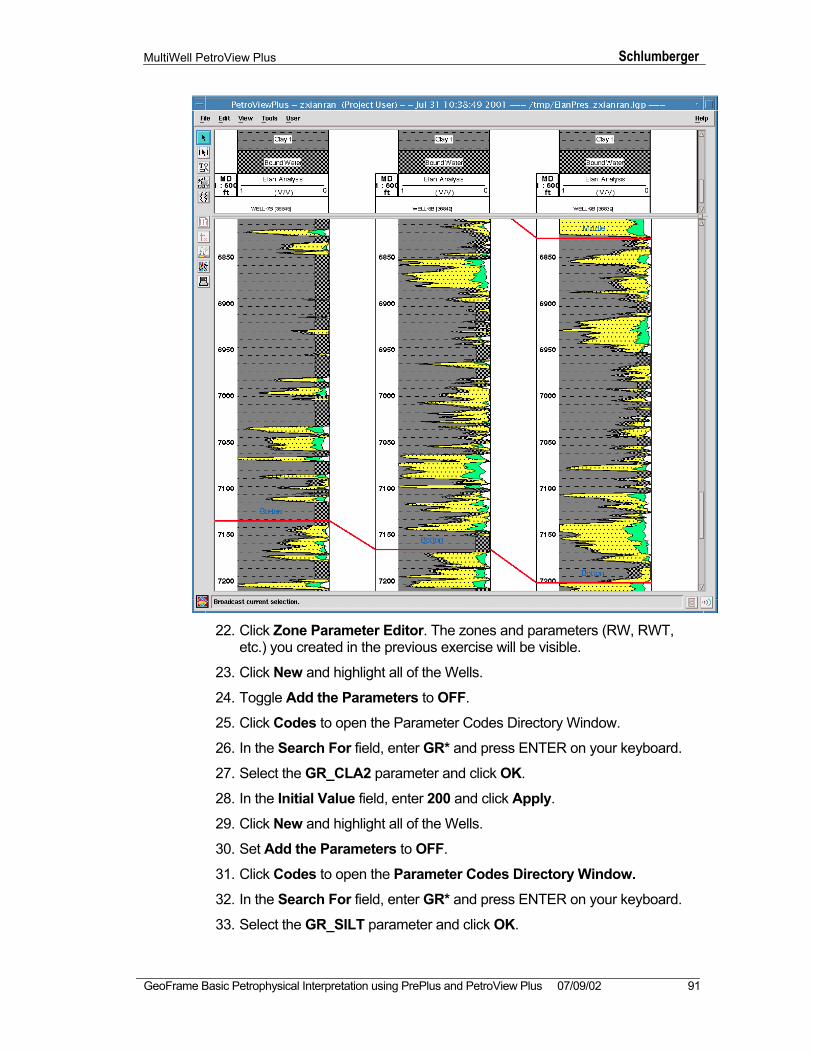
MultiWell PetroView Plus Schlumberger
22. Click Zone Parameter Editor. The zones and parameters (RW, RWT,
etc.) you created in the previous exercise will be visible.
23. Click New and highlight all of the Wells.
24. Toggle Add the Parameters to OFF.
25. Click Codes to open the Parameter Codes Directory Window.
26. In the Search For field, enter GR* and press ENTER on your keyboard.
27. Select the GR_CLA2 parameter and click OK.
28. In the Initial Value field, enter 200 and click Apply.
29. Click New and highlight all of the Wells.
30. Set Add the Parameters to OFF.
31. Click Codes to open the Parameter Codes Directory Window. 32. In the Search For field, enter GR* and press ENTER on your keyboard.
33. Select the GR_SILT parameter and click OK.
GeoFrame Basic Petrophysical Interpretation using PrePlus and PetroView Plus 07/09/02 91
MultiWell PetroView Plus Schlumberger
34. In the Initial Value field, enter 20 and click Apply.
35. Click OK.
36. Highlight WELLS 7B, 8B, and 9B and the parameters GR_CLA2 and GR_SILT together with one of the zones (Middle Stratton).
37. Click Redisplay to check that all parameters/Wells are correctly initialized. Values for RW and RWT for selected Wells appear in the Zone Parameter Editor Window.
38. Click Constant to set GR_CLA2=140 to all the zones in WELL 7B.
39. Click OK to exit the Zone Parameter Editor.
40. Click Attributes.
41. In the Select for Existing Outputs field, change Intact to Overwrite.
42. Click to re-run the PetroView Plus computation (repeat steps 11-18) for all three Wells, you will see that the new results for WELL 7B are more reasonable, but the Clay Computation for WELL 8B and WELL 9B maybe need to be adjusted. Use Zone Parameter Editor and Zoning to adjust new parameters for all Wells.
43. Select File>Save As and save the multiple Well sessions as stratton.mw.
44. Select File>Save Data.
45. Click on the Zone Sets and Zone Parameters to be saved.
46. Click OK.
Note: Saving the session file actually saves the zone sets and Well attributes to an ASCII file that can later be loaded to restore the status of the MultiWell session. The data save step saves the zone sets and parameters to the database so that the reservoir summation program can pick up the proper zone boundaries.
The next step is to create MultiWell LithoZone in the WellPix Lump. The MultiWell properties are in the ResSum and make a 2D distribution (contour/gridding) map for MultiWell properties in the BaseMapPlus.
92 GeoFrame Basic Petrophysical Interpretation using PrePlus and PetroView Plus 07/09/02
Reservoir Property Summation and Mapping (ResSum & Basemap Plus) Schlumberger
Chapter 6 Reservoir Property Summation and Mapping (ResSum & Basemap Plus)
Overview
This chapter will describe a workflow for calculating and mapping reservoir properties based on the petrophysical logs and formation markers. This workflow will use the WellPix and ResSum to create LithoZones and compute reservoir properties and averages for the zones. ResSum create sums and averages of log petrophysical properties by zone for one or multiple boreholes, these properties can then be output to a report, and they are also saved to the database as part of the zones associated with layers, these properties can then be gridded and mapped in Basemap or CPS3 products. For a detailed explanation of WellPix, ResSum and Basemap, please refer to the online help documentation in the GeoFrame Bookshelf. Data Requirements (Log Curve data and petrophysical analysis data):
• LithoZone for specific Zone Version: Created in the WellPix
• Petrophysical analysis data (Porosity, Volume of shale/clay, Water Saturation, permeability etc.): Output in the petrophysical analysis products (GeoFrame PetroView Plus, GeoFrame, ELANPlus or third party applications)
Creating a LithoZone
1. In the Application Manager, click .
GeoFrame Basic Petrophysical Interpretation using PrePlus and PetroView Plus 07/09/02 93
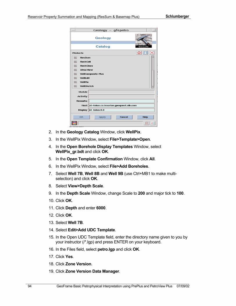
Reservoir Property Summation and Mapping (ResSum & Basemap Plus) Schlumberger
2. In the Geology Catalog Window, click WellPix.
3. In the WellPix Window, select File>Template>Open.
4. In the Open Borehole Display Templates Window, select WellPix_gr.bdt and click OK.
5. In the Open Template Confirmation Window, click All. 6. In the WellPix Window, select File>Add Boreholes.
7. Select Well 7B, Well 8B and Well 9B (use Ctrl+MB1 to make multi-selection) and click OK.
8. Select View>Depth Scale.
9. In the Depth Scale Window, change Scale to 200 and major tick to 100.
10. Click OK.
11. Click Depth and enter 6000.
12. Click OK.
13. Select Well 7B.
14. Select Edit>Add UDC Template. 15. In the Open UDC Template field, enter the directory name given to you by
your instructor (/*.lgp) and press ENTER on your keyboard.
16. In the Files field, select petro.lgp and click OK.
17. Click Yes.
18. Click Zone Version.
19. Click Zone Version Data Manager.
94 GeoFrame Basic Petrophysical Interpretation using PrePlus and PetroView Plus 07/09/02
Reservoir Property Summation and Mapping (ResSum & Basemap Plus) Schlumberger
20. In the Name field, enter stratton_sands_zv.
21. Click OK to create a new Zone Version and store the LithoZone, which will be created in WellPix.
22. Click OK to close the Select Zone Version Window.
23. Select Well 7B and click Create Single Litho Zone.
GeoFrame Basic Petrophysical Interpretation using PrePlus and PetroView Plus 07/09/02 95
Reservoir Property Summation and Mapping (ResSum & Basemap Plus) Schlumberger
24. Click Create Layer. 25. In the Layer name field, enter stratton_sands.
26. Click Upper Surface and select the Stratton Sands. 27. Click OK.
28. Click Lower Surface and select the Base Stratton Sands. 29. Click OK.
30. Click Layer Pattern and select the sand pattern (column 6 row 3).
31. Click OK.
32. Click Layer Color and select gold.
33. Click OK.
34. Click OK to close the Layer Creation Window
35. In the Single Litho Zone Interpretation Window, click Boreholes.
36. Select Well 8B and Well 9B and click OK.
37. Toggle the Propagate zero-length zones option to ON.
38. Click OK to create the Litho Zone stratton_sands.
96 GeoFrame Basic Petrophysical Interpretation using PrePlus and PetroView Plus 07/09/02
Reservoir Property Summation and Mapping (ResSum & Basemap Plus) Schlumberger
39. Select File>Exit.
Running BaseMapPlus on Your Secondary Screen
1. In the Application Manager Window, click .
GeoFrame Basic Petrophysical Interpretation using PrePlus and PetroView Plus 07/09/02 97
Reservoir Property Summation and Mapping (ResSum & Basemap Plus) Schlumberger
2. In the Visualization Window, select Basemap.
3. In the Display field, change the last 0 to 1.
4. Click OK to run the Basemap Plus on your secondary screen
5. Select Create Default Geological Map and click OK. Manage the Basemap graphics appearance based on what you have learned about how to use Basemap.
Running ResSum On Your Primary Screen
1. In the Geology Catalog Window, click ResSum.
98 GeoFrame Basic Petrophysical Interpretation using PrePlus and PetroView Plus 07/09/02
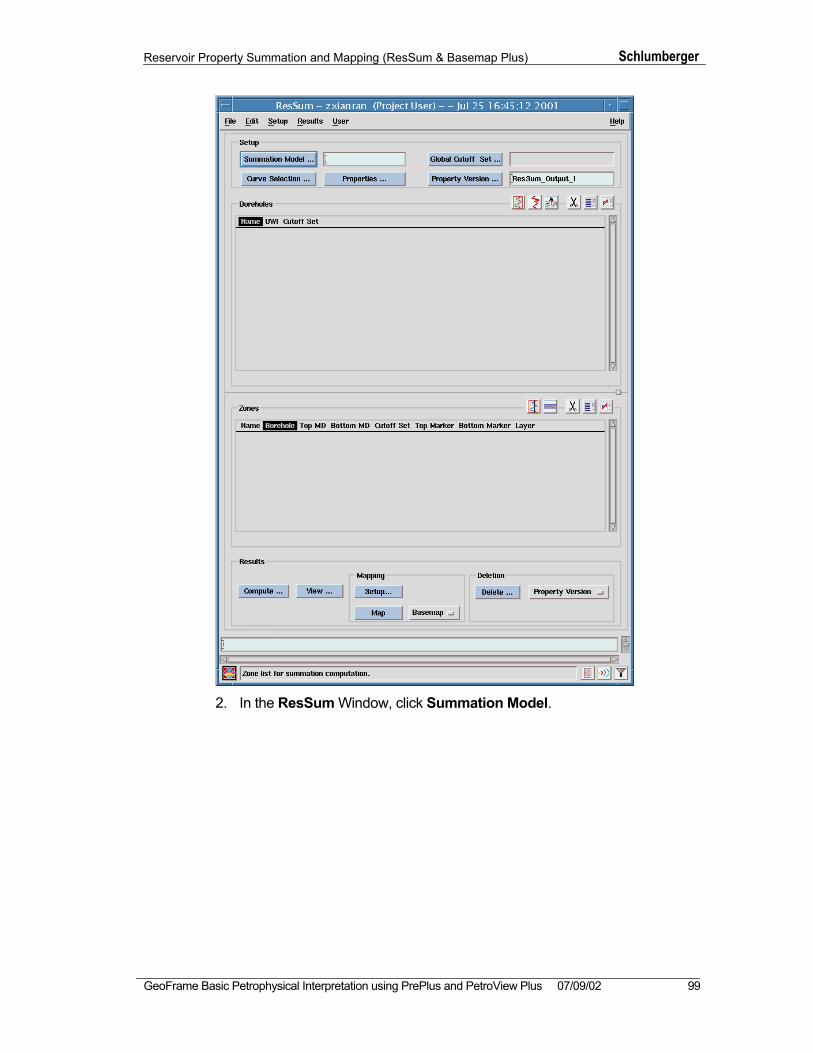
Reservoir Property Summation and Mapping (ResSum & Basemap Plus) Schlumberger
2. In the ResSum Window, click Summation Model.
GeoFrame Basic Petrophysical Interpretation using PrePlus and PetroView Plus 07/09/02 99
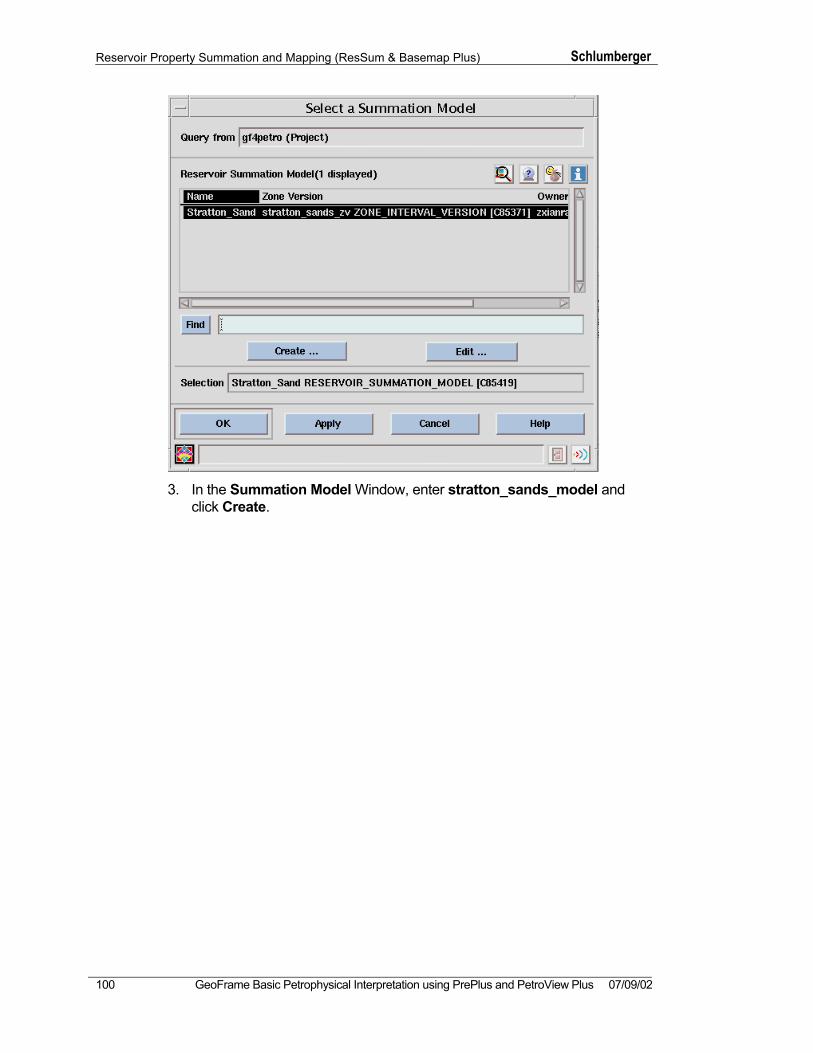
Reservoir Property Summation and Mapping (ResSum & Basemap Plus) Schlumberger
3. In the Summation Model Window, enter stratton_sands_model and
click Create.
100 GeoFrame Basic Petrophysical Interpretation using PrePlus and PetroView Plus 07/09/02
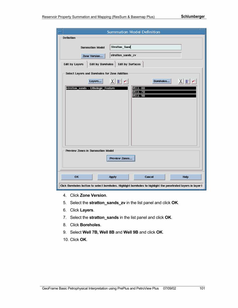
Reservoir Property Summation and Mapping (ResSum & Basemap Plus) Schlumberger
4. Click Zone Version.
5. Select the stratton_sands_zv in the list panel and click OK.
6. Click Layers.
7. Select the stratton_sands in the list panel and click OK.
8. Click Boreholes.
9. Select Well 7B, Well 8B and Well 9B and click OK.
10. Click OK.
GeoFrame Basic Petrophysical Interpretation using PrePlus and PetroView Plus 07/09/02 101
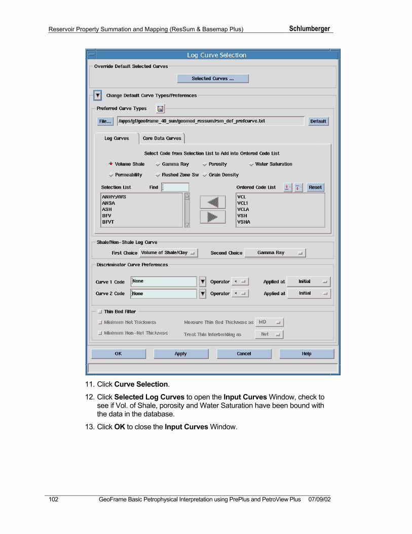
Reservoir Property Summation and Mapping (ResSum & Basemap Plus) Schlumberger
11. Click Curve Selection.
12. Click Selected Log Curves to open the Input Curves Window, check to see if Vol. of Shale, porosity and Water Saturation have been bound with the data in the database.
13. Click OK to close the Input Curves Window.
102 GeoFrame Basic Petrophysical Interpretation using PrePlus and PetroView Plus 07/09/02
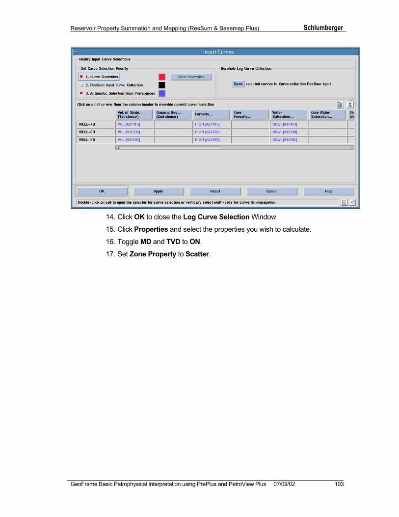
Reservoir Property Summation and Mapping (ResSum & Basemap Plus) Schlumberger
14. Click OK to close the Log Curve Selection Window
15. Click Properties and select the properties you wish to calculate.
16. Toggle MD and TVD to ON.
17. Set Zone Property to Scatter.
GeoFrame Basic Petrophysical Interpretation using PrePlus and PetroView Plus 07/09/02 103
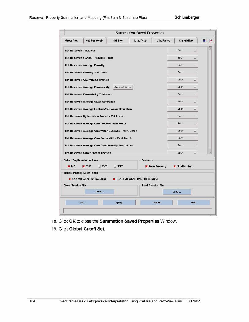
Reservoir Property Summation and Mapping (ResSum & Basemap Plus) Schlumberger
18. Click OK to close the Summation Saved Properties Window.
19. Click Global Cutoff Set.
104 GeoFrame Basic Petrophysical Interpretation using PrePlus and PetroView Plus 07/09/02
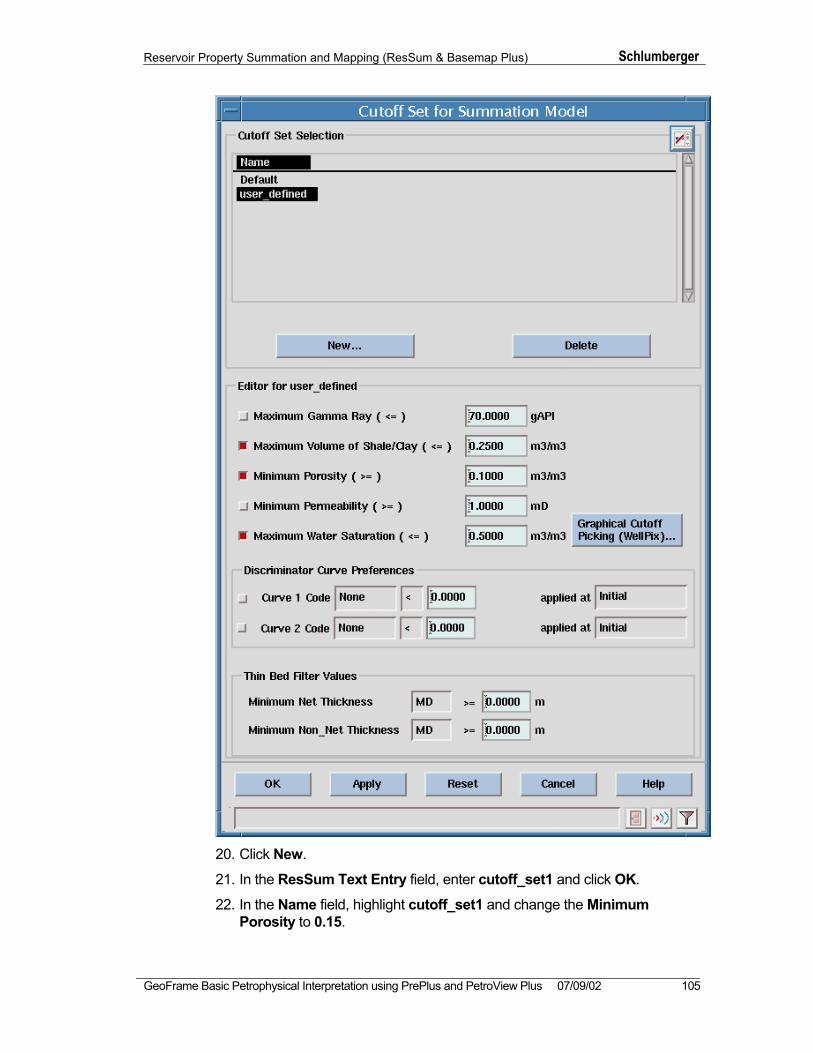
Reservoir Property Summation and Mapping (ResSum & Basemap Plus) Schlumberger
20. Click New.
21. In the ResSum Text Entry field, enter cutoff_set1 and click OK.
22. In the Name field, highlight cutoff_set1 and change the Minimum Porosity to 0.15.
GeoFrame Basic Petrophysical Interpretation using PrePlus and PetroView Plus 07/09/02 105
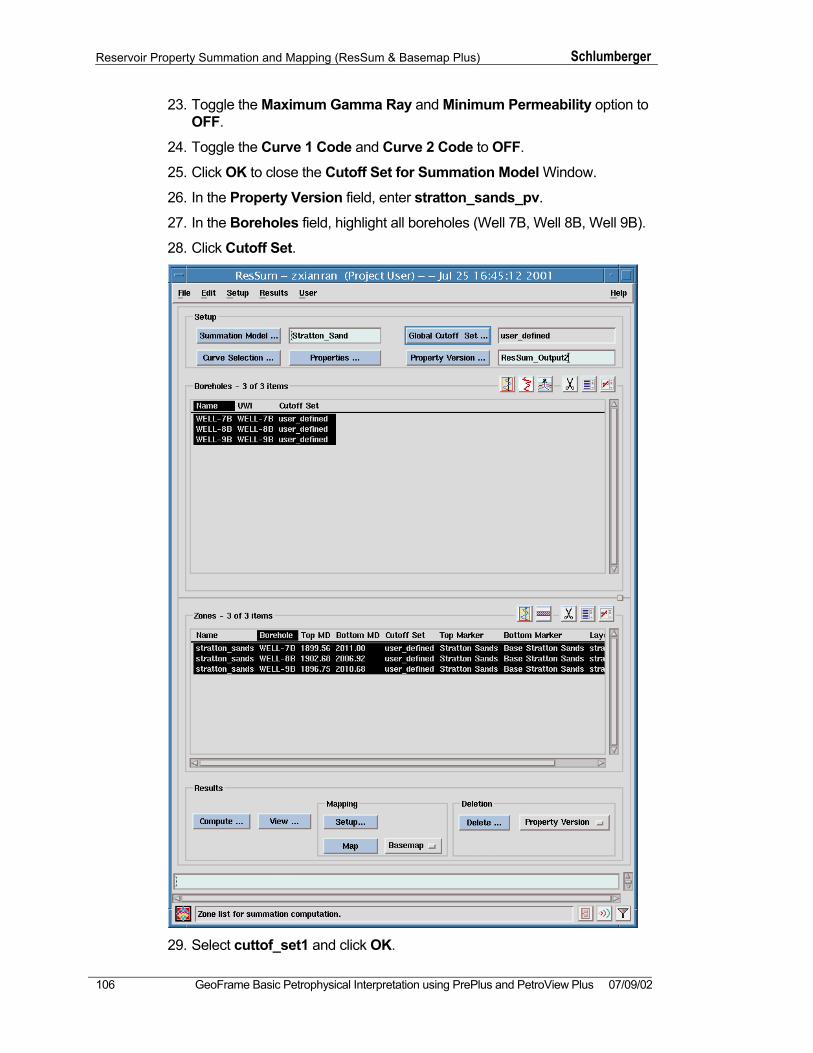
Reservoir Property Summation and Mapping (ResSum & Basemap Plus) Schlumberger
23. Toggle the Maximum Gamma Ray and Minimum Permeability option to OFF.
24. Toggle the Curve 1 Code and Curve 2 Code to OFF.
25. Click OK to close the Cutoff Set for Summation Model Window.
26. In the Property Version field, enter stratton_sands_pv.
27. In the Boreholes field, highlight all boreholes (Well 7B, Well 8B, Well 9B).
28. Click Cutoff Set.
29. Select cuttof_set1 and click OK.
106 GeoFrame Basic Petrophysical Interpretation using PrePlus and PetroView Plus 07/09/02
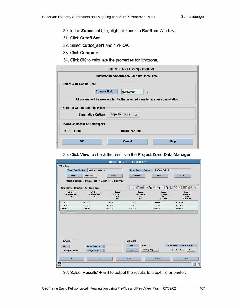
Reservoir Property Summation and Mapping (ResSum & Basemap Plus) Schlumberger
30. In the Zones field, highlight all zones in ResSum Window.
31. Click Cutoff Set. 32. Select cuttof_set1 and click OK.
33. Click Compute.
34. Click OK to calculate the properties for lithozone.
35. Click View to check the results in the Project Zone Data Manager.
36. Select Results>Print to output the results to a text file or printer.
GeoFrame Basic Petrophysical Interpretation using PrePlus and PetroView Plus 07/09/02 107
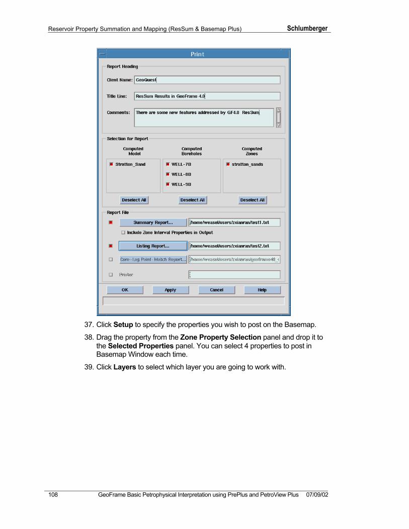
Reservoir Property Summation and Mapping (ResSum & Basemap Plus) Schlumberger
37. Click Setup to specify the properties you wish to post on the Basemap.
38. Drag the property from the Zone Property Selection panel and drop it to the Selected Properties panel. You can select 4 properties to post in Basemap Window each time.
39. Click Layers to select which layer you are going to work with.
108 GeoFrame Basic Petrophysical Interpretation using PrePlus and PetroView Plus 07/09/02
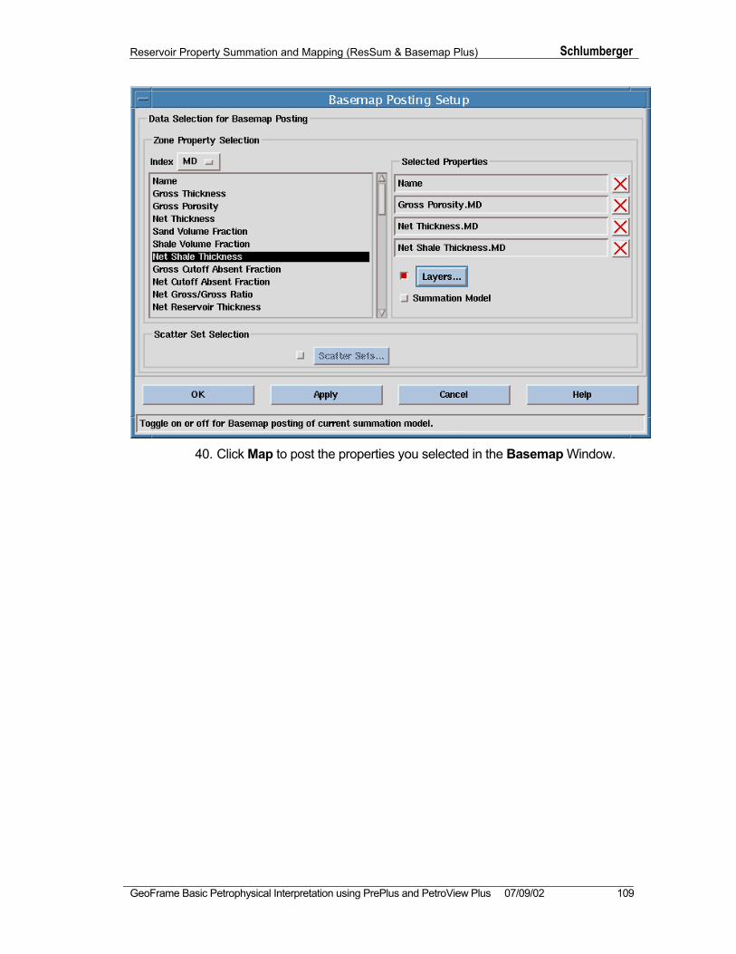
Reservoir Property Summation and Mapping (ResSum & Basemap Plus) Schlumberger
40. Click Map to post the properties you selected in the Basemap Window.
GeoFrame Basic Petrophysical Interpretation using PrePlus and PetroView Plus 07/09/02 109
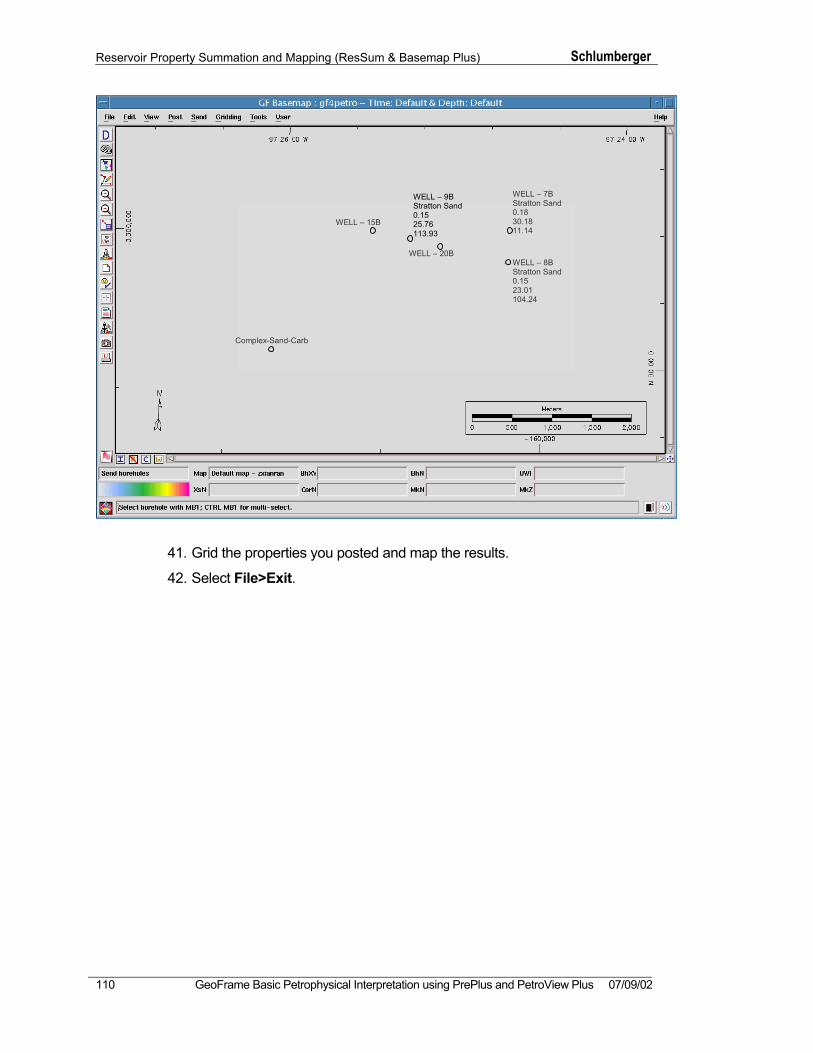
Reservoir Property Summation and Mapping (ResSum & Basemap Plus) Schlumberger
110 GeoFrame Basic Petrophysical Interpretation using PrePlus and PetroView Plus 07/09/02
WELL – 15B
WELL – 20B
WELL – 7B Stratton Sand0.18 30.18 11.14
WELL – 8B Stratton Sand0.15 23.01 104.24
WELL – 9B Stratton Sand0.15 25.76 113.93
Complex-Sand-Carb
41. Grid the properties you posted and map the results.
42. Select File>Exit.