Geographic Routing Made Practical

Young-Jin Kim† Ramesh Govindan† Brad Karp∗ Scott Shenker‡

†University of Southern California ∗Intel Research/CMU ‡UCB/ICSILos Angeles, CA 90089 Pittsburgh, PA 15213 Berkeley, CA 94704

{youngjki, ramesh}@usc.edu bkarp@cs.cmu.edu shenker@icsi.berkeley.edu

AbstractGeographic routing has been widely hailed as the mostpromising approach to generally scalable wireless rout-ing. However, the correctness of all currently proposedgeographic routing algorithms relies on idealized as-sumptions about radios and their resulting connectivitygraphs. We use testbed measurements to show that theseidealized assumptions are grossly violated by real radios,and that these violations cause persistent failures in geo-graphic routing, even on static topologies. Having identi-fied this problem, we then fix it by proposing the Cross-Link Detection Protocol (CLDP), which enables prov-ably correct geographic routing onarbitrary connectiv-ity graphs. We confirm in simulation and further testbedmeasurements that CLDP is not only correct but practi-cal: it incurs low overhead, exhibits low path stretch, al-ways succeeds in real, static wireless networks, and con-verges quickly after topology changes.

1 IntroductionThere is a very broad literature on geographic routingalgorithms, particularly on the sub-class that uses facerouting on a planar subgraph [2, 7, 13, 17, 18, 24]. Thesealgorithms are attractive for wireless ad hoc networks be-cause they have been shown to scale better than otheralternatives: they require per-node state independent ofnetwork size, dependent only on network density. Morerecently, geographic routing algorithms have been pro-posed for use as a routing primitive for static sensor net-works, as building blocks for data storage and flexiblequery processing in sensor networks [20, 23], and evenas a fallback routing mechanism for reduced state rout-ing in the Internet [9].

Despite research activity on geographic routing span-ning half a decade, we know of no work in which re-searchers haveimplementedand deployedgeographicrouting protocols in realistic environments. Using ourimplementation of the GPSR geographic routing algo-rithm [13]—which we believe to be the first of its kind—

we first show that GPSR incurs permanent packet deliv-ery failures between node pairs on two different sensornetwork testbeds where we had no control over nodeplacement. To wit, GPSR leaves over 30% of nodepairs permanently disconnected in one testbed experi-ment, and over 10% disconnected in another. The signifi-cant incidence of these delivery failures and their perma-nent nature suggest that known geographic routing tech-niques are impractical for use in real deployments.

GPSR is built upon graph planarization algorithmsthat are amenable to distributed implementation [2, 13].These planarization algorithms rely purely on neigh-bor location information to determine whether or notlinks to neighbors belong in the planarized subgraph.When greedy forwarding is impossible, GPSR deliversa packet by successively traversing the faces of the pla-nar subgraph cut by the line between the packet’s sourceand destination. A body of subsequent work (includingGOAFR+ [17] and its many variants) has extended thisface routing technique to offer shorter worst-case pathsthan GPSR. A common assumption made by the pla-narization algorithms used by all these geographic rout-ing protocols is that connectivity between nodes can bedescribed byunit graphs. In such graphs, a node is al-ways connected to all nodes within its fixed, “nominal”radio range, and never connected to nodes outside thisrange.

We show that our implementation of GPSR incurs per-manent delivery failures precisely because real radiosroutinely violate the unit graph assumption. Such vio-lations can cause three kinds of pathologies in the pla-narization process: a link in the planar subgraph is re-moved when it should not be (partitioned planar sub-graph); the nodes at the two ends of a link disagree onwhether or not the link belongs in the planar graph (uni-directional links); or a pair of crossed links remain inthe supposedly planar subgraph (crossing links). Thesepathologies, in turn, can result in persistent routing fail-ures in the network, where geographic routing fails to

find a path for at least one source-destination pair. A pre-viously proposed “fix” to these planarization techniques,the mutual-witness procedure [11, 12, 24], fails to elimi-nate many instances of routing failure on our testbeds.

We remedy this problem by proposing a distributedCross-Link Detection Protocol (CLDP) that, given an ar-bitrary connected graph, produces a subgraph on whichface traversal cannot cause a routing failure, regardlessof radio irregularities and localization errors. In CLDP,each node probes the faces on which each of its linkssits to determine if there exists a crossing link. Crossinglinks are eliminated only when doing so would not dis-connect the resulting subgraph. This algorithm isquali-tativelydifferent from the planarization algorithms usedby earlier face routing protocols, in both its approachand its correctness. The unmodified GPSR algorithmconducts perimeter-mode forwarding using the subgraphproduced by CLDP.1 CLDP retains geographic routing’sdesirable scaling properties. Moreover, we have proventhat CLDP prevents routing failures in an arbitrary con-nected graph.2

Finally, we present measurements from simulationsand experiments on two different wireless sensor net-work testbeds that validate CLDP’s correctness, andshow that CLDP incurs moderate overhead, convergesquickly, and picks low-loss paths. Because CLDP ren-ders geographic routing correct on real radio networks,we believe it represents the first generally scalable andpractical approach for any-to-any routing in large-scalewireless settings.

2 Preliminaries and Related WorkWe now review prior work in geographic routing proto-cols and describe the essentials of the workings of geo-graphic routing that provide the context for our work.

There is a very broad literature on geographic rout-ing: from initial sketches suggesting routing using po-sition information [4, 15]; to the first detailed proposals,including GFG [2], GPSR [13], and the GOAFR+ fam-ily of algorithms [17]; to refinements of these propos-als for efficiency [7], robustness under real network con-ditions [18, 24], and even routing geographically whennode location information is unavailable [21,22].

We now describe the shared characteristics of theGFG, GPSR, and GOAFR+ algorithms, and hereafterrefer to this family of algorithms simply as geographicrouting.3

Geographic routing schemes usegreedy routingwherepossible. In greedy routing, packets are stamped with thepositions of their destinations; all nodes know their ownpositions; and a node forwards a packet to its neighborthat is geographically closest to the destination,so longas that neighbor is closer to the destination. Local max-imamay exist where no neighbor is closer to the destina-

tion. In such cases, greedy forwarding fails, and anotherstrategy must be used to continue making progress to-ward the destination. In particular, the packet must onlyfind its way to a node closer to the destination than thelocal maximum; at that point, greedy routing may onceagain make progress.

In the case where a network graph has no crossingedges4—that is, the graph isplanar— geographic rout-ing schemes recover similarly byface routing. Note thata planar graph consists offaces,enclosed polygonal re-gions bounded by edges. Geographic routing uses twoprimitives to traverse planar graphs: theright-hand rule,andface changes. The right-hand rule tours a face end-lessly in a cycle, and can thus be used to walk a face.Figure 1 shows an example of the rule, which dictatesthat upon receiving a packet on a link, the receiving nodeforwards that packet on the first link it finds after sweep-ing counter-clockwise about itself from the ingress link.

Consider the planar graph in Figure 2, in which thesource nodeSand destination nodeD are indicated. Ob-serve that the line segmentSD mustcut a series of facesin the planar graph; these faces are numbered and bor-dered in bold. Geographic routing algorithms exploitthis property by successively walking the faces cut bythis line. That is, they use the right-hand rule to tour aface. While walking a face, upon encountering an edgethat crosses the line segmentSD at a point closer toDthan the point at which the current face was entered, ge-ographic routing algorithms perform aface change:theybegin walking the bordering face that is next along theline segmentSD.5 The numbering of faces in Figure 2shows the order in which faces are traversed fromS to Don that planar graph. Should a face be toured in its en-tirety without discovering an edge that crosses line seg-mentSD at a point closer toD than the point at whichthe current face was entered, face routing fails. On a pla-nar graph, such a loop on a face only occurs when thedestination is disconnected.

Note that if the graph is not planar, face routing mayfail. Figure 3 shows an example graph on which thispathology occurs. In this example,D is located physi-cally in the interior of a face, but is only connected tothe rest of the network graph by an edge that crosses thisenclosing face. Face routing walks successive faces cutby the line fromS to D, until it reaches the face enclos-ing D, whose first edge crosses line segmentSDat pointp. The right-hand rule then tours this face in its entirety,but fails to find an edge that crosses line segmentSDat apoint closer toD thanp. Thus, face routing fails.

Wireless networks’ connectivity graphs typically con-tain many crossing edges. A method for obtaining a pla-nar subgraph of a wireless network graph is thus needed;greedy routing operates on the full network graph, butto work correctly, face routing must operate on a planar

4D C

BA 2

1 3

Figure 1: Right-hand rule.Asweeps counterclockwise fromlink 1 to find link 2, forwardsto B, &c.

5

S D1

23

4

Figure 2: The faces progressively closerfrom S to D along line segmentSD,numbered in the order visited. Faces cutby SDare bordered in bold.

p

S

D

Figure 3: Example of face routing fail-ure on non-planar graphs. There is nopoint closer toD thanp on the face en-closingD.

A

B

RNG

A

B

GG

WW

Figure 4: Definitions of the GG and RNG. A witnessmust fall within the shaded circle (GG) or lune (RNG)for edge(A,B) to be eliminated in the planar graph.

A

B

VW

Figure 5: The RNG partitions a non-unit graph; edge(A,B) is eliminated.

subgraph of the full network graph. What is required isa planarizationtechnique that is simply implementablewith an asynchronous distributed algorithm.

Geographic routing algorithms planarize graphs usingtwo planar graph constructs that meet that requirement:the Relative Neighborhood Graph (RNG) [26] and theGabriel Graph (GG) [5]. The RNG and GG give rulesfor how to connect vertices placed in a plane with edgesbased purely on the positions of each vertex’s single-hopneighbors. Both the RNG and GG provably yield a con-nected, planar graph so long as the connectivity betweennodes obeys theunit graph assumption:for any two ver-ticesA andB, those two verticesmustbe connected by anedge if they are less or equal to some threshold distanced apart, butmust notbe connected by an edge if they aregreater thand apart. We shall refer tod as thenominalradio rangein a wireless network; the notion is that allnodes have perfectly circular radio ranges of radiusd,centered at their own positions.

The unit graph assumption is quite intuitive for wire-less networks. The simplest ideal radio model is onewhere all transmitters radiate fixed transmission powerperfectly omnidirectionally; receivers can discern alltransmissions properly when they are received withabove some threshold signal-to-noise ratio; and radiotransmissions propagate in free space, such that their en-ergy dissipates as the square of distance. Under that ide-alized model, there indeed exists a nominal radio range.

We briefly state the definitions of the GG and RNG, aswe shall refer to them repeatedly in Section 3. The pla-narization process runs on afull graph, which includesall links in the radio network, and produces aplanar sub-graphof the full graph. We assume that each node in thenetwork knows its single-hop neighbors’ positions; suchneighbor information is trivially obtained if each nodeperiodically transmits broadcast packets containing itsown position. Consider an edge in the full graph between

two nodesA andB. Both A andB must decide whetherto keep the edge between them in the planar graph, oreliminate it in the planar graph. Without loss of general-ity, consider nodeA. Both for the GG and RNG, nodeAsearches its single-hop neighbor list for anywitnessnodeW that lies within a particular geometric region. If one ormore witnesses are found, the edge(A,B) is eliminatedin the planar graph. If no witnesses are found, the edge(A,B) is kept in the planar graph. For the GG, the regionwhere a witness must exist to eliminate the edge is thecircle whose diameter is line segmentAB. For the RNG,this region is thelune defined by the intersection of thetwo circles centered atA andB, each with radius|AB|.We show these two regions in Figure 4.

Under the unit graph assumption, it is known that fora clustering of points in the plane, the set of edges in theEuclidean minimum spanning tree over those points is asubset of the set of edges in the RNG [26]. The edges inthe RNG are in turn a subset of those in the GG; the in-tuition for this relationship lies in the relative sizes of thelune and circle regions. Finally, the set of edges in theGG is a subset of that in the Delaunay triangulation overthe set of points [25]. These relationships dictate that theGG and RNG are both connected (so eliminating cross-ing edges cannot disconnect the network!) and planar, asdesired. Note that if the network graphviolatesthe unitgraph assumption, the RNG and GG can produce aparti-tionedplanarized graph [11], one that contains unidirec-tional links, and even one that is not planar. An exampleof a partitioning for the RNG appears in Figure 5. Here,there is no link betweenA andV, and none betweenBandW, though these links are shorter than the nominalradio range. NodesA and B see witnessesW andV,respectively, though neither witness provides transitiveconnectivity. BothA andB conclude they should removeedge(A,B) in the planarized graph, and a partition re-sults. Similar cases are possible in the GG.

We observe that whether radio graphs conform to theunit-graph assumption is a question of great importance,as partitioning the planarized graph used in face routingwill cause routing failures. In the next section, we ex-plore in detail the many reasons real radios violate theunit graph assumption, and give detailed examples of thepathologies these violations create in the GG and RNG.

Recently, Kuhnet al. have investigated relaxing theunit-graph assumption to improve the robustness of theGG planarization [18]. In theQuasi-Unit Disk Graphthey propose, the nominal radio range is normalized to1. Links may notexist between nodes greater than dis-tance 1 apart, and linksmustexist between nodes lessthan a parameterd apart. For nodes betweend and 1 dis-tance apart, links may or may not exist; it’s in this regionwhere Quasi-Unit Disk Graphs are a more general classthan unit graphs. Kuhnet al. provide an algorithm forreplacing “missing” links betweend and 1 in length withvirtual links, that are essentially tunnels through multi-ple existing links. They show that the GG planarizationsucceeds on this augmented graph without partitioningit. Their analysis shows that this technique is only scal-able whend ≥ 1/

√2; for lesser values ofd (for which

the unit-graph assumption is progressively relaxed fur-ther) virtual links may be comprised of increasingly longpaths of physical hops.

3 Pathologies in Real DeploymentsIn the previous section, we demonstrated two situationswhere GPSR’s perimeter-mode routing may fail: whencrossing links remain after planarization is applied, andwhen planarization partitions the network graph. It isnatural to ask how prevalent these pathologies are in realdeployments of GPSR: are they so rare as to be of purelytheoretical interest, or do they significantly negatively af-fect reachability between pairs of nodes? We confirm inthis section that the latter is the case, using measurementstaken on real wireless networks.

GPSR Implementation and Testbeds

We implemented GPSR for Mica-2 sensor motes. Ourfull-fledged nesC [8] implementation includes the GGand the RNG planarization algorithms (chosen via a con-figuration parameter), as well as greedy- and perimeter-mode packet forwarding. It also includes a hop-by-hopretransmission mechanism, as the default Mica-2 MAClayer does not implement link-layer retransmission. Fi-nally, our implementation rejects wireless links whosequality—measured by probing link loss rate—is belowa configurable threshold. This mechanism incorporateshysteresis to avoid oscillatory behavior on links whosequality is near the threshold. Our complete implementa-tion is over 4500 lines of nesC code.

We measured this implementation’s behavior on twotestbeds. Each consists of Mica-2 motes that span a floor

of an office building: one with 75 motes in Berkeley’sSoda Hall, where offices are separated by floor-to-ceilingwalls, and one with 51 motes at Intel Research Berkeley,where cubicles are separated by low dividers. We reportonly the Soda Hall results in the interest of brevity.6

Motes instrument most offices and some of the hall-ways in Soda Hall. Because the testbed is shared, wewere able to use only a 50-node subset of it. As wecould not control the placement of these devices, theGPSR failures discussed below are not contrived by care-ful node placement. We did, however, have one tool forcontrolling network topology: radio transmit power. Atthe default power setting on the testbed, all nodes werewithin two hops of each other. To generate an interest-ing multi-hop topology, we reduced the radio transmitpower from 15 to 2. In the resulting topology, the aver-age path length was around 5 hops, and the average nodedegree was 5.2. Note that controlling transmit poweris roughly equivalent to appropriately scaling the geo-graphic dimensions of the testbed. Finally, we staticallyconfigured nodes with their locations.

Pathologies

Figure 6 depicts the full network topology on the 50-node Soda Hall testbed, as is used by GPSR’s greedy-mode forwarding. Our GPSR implementation does notforward on links with packet loss rates in excess of 30%;those links are not shown in the figure. Many links crossone another, particularly in the dense region of the net-work toward the left. It is the job of GPSR’s planariza-tion to eliminate these crossing links, to produce a planargraph for use by GPSR’s perimeter-mode forwarding.

We measure the fraction of all pairs of nodes on thisnetwork that can reach one another with GPSR routing.In these measurements, we iterate over all nodes in thenetwork, allowing one node at a time to send traffic toeach other node in the network. We send 10 packets, andretransmit at the link level. If one or more packets reachthe destination, we count that directed pair of nodes asconnected, and in this way, measure routing algorithmsuccess rather than short-term packet loss characteristics.We find that only 68.2% of directed node pairs can com-municate successfully in the testbed—a significant frac-tion of node pairs experiencepermanent partition!

To help elucidate the reasons for these routing failures,we present in Figure 7 the network subgraph that resultsafter our GPSR implementation distributedly applies theGG planarization to the full topology. There are threeclasses of pathology present in this network subgraph:

Network partitions: While the full network is con-nected, there are two connected components in Figure 7;the majority of the network comprises one connectedcomponent, and the nodes at the lower left of the fig-ure the other. Such cases arise in situations such as those

Figure 6: 50-node testbed. Linkswith packet loss rates over 30% arenot shown.

Figure 7: GPSR’s GG subgraph onthe 50-node testbed.

Figure 8: GPSR’s GG/MW sub-graph on the 50-node testbed.

previously described in Figure 5.Asymmetric links: Links denoted with an arrow ex-

ist in the planar subgraphonly in the direction indi-cated. Such links may give rise to unidirectional parti-tions in the planar subgraph, where an asymmetric linkrepresents the only connectivity between two connectedcomponents. The GG and RNG planarizations produceasymmetric links in cases similar to that depicted in Fig-ure 5; consider the case whereW is not present in thegraph. On that topology,A→ B will remain, butB→ Awill not.

Crossing links: There are a few instances of crossinglinks that remain in Figure 7. For example, consider thelong horizontal link that spans the hallway, and crossesa far shorter link. The GG and RNG planarizations mayproduce such pathologies when there are highly irregularradio ranges, as is the case here: the node at the right endof the long link cannot see any witnesses, and thus willnot remove the long link; nor do the nodes at either endof the short, vertical link see any witnesses.

Radio range irregularities, which may be exacerbatedby elimination of high-loss links, thus cause significantrouting failures for GPSR in a real deployment. We ex-pect other variants of GPSR to behave similarly, sincethey all use planarization methods based on unit-diskgraphs. For context, we note that several measurementstudies [1, 6, 27] have documented non-ideal radio be-havior; however, ours is the first to quantify their impacton existing geographic routing protocols.

We have also implemented and experimented with apreviously proposed fix to the GG’s and RNG’s tendencyto partition graphs when radio ranges are irregular. Thefix in question is themutual witness(MW) extension toGPSR [11, 12, 24]. When nodeA considers whether tokeep link(A,B) from the full graph in the RNG or GGplanar graph, mutual witness dictates thatA only elimi-nate link(A,B) if there exists at least one witness in theRNG or GG region that is visibleboth to A andB. Thisfact may be directly verified with local communication:if all nodes broadcast their neighbor lists (only a sin-gle hop), then all nodes may verify whether a particular

neighbor shares a particular other neighbor. The intuitionfor this mutual witness is that it preserves connectivity:links are only eliminated in the planar graph if a transi-tive path through a witness is explicitly verified, ratherthan relying on the location of the witness to assure sucha transitive path’s existence. Unfortunately, MW suffersfrom another ill; on some non-unit graphs, it willleavecrossing linksin the graph produced by the RNG andGG. Indeed, in our experiments with MW, we observedthis behavior: GPSR augmented with MW enables con-nectivity between only 87.8% node pairs in one experi-ment, leaving more than 10% of node pairs persistentlydisconnected. Figure 8 shows the subgraph the MW ex-tension generates in this experiment; note the crossingedges that remain that give rise to routing failures.

In sum, these results suggest that current geographicrouting protocols are impractical. Although we havedemonstrated this only using relatively unsophisticatedMica-2 radios, we believe our conclusions hold for otherkinds of wireless devices as well, since the failure of theunit-disk assumption as a result of obstacles or multi-pathing is fairly fundamental. We spend the rest of thepaper discussing a qualitatively different and practicableapproach to geographic routing. As an aside, we notethat while many of the pathologies we describe aboveare caused by radio range irregularities, localization er-rors can also cause the same pathologies [14, 24]. Weleave measurement of the effects of localization errors intestbed deployments to future work.

4 Cross-Link Detection Protocol

We have established that existing planarization tech-niques frequently cause face routing to fail on real wire-less networks, where the unit-graph assumption is vio-lated. We now proceed to describe the Cross-Link De-tection Protocol (CLDP), a planarization technique thatcannot cause face routing to fail on any connected graph.As such, CLDP is also robust to arbitrary localization er-rors [14]; we omit a detailed discussion herein for lackof space.

A

D

B

C

Figure 9: CLDP Probing us-ing right-hand-rule, Case 1.

A B

C D

Figure 10:. . ., Case 2.

A B

C D

Figure 11:. . ., Case 3.

A B

C D

Figure 12:. . ., Case 4.

4.1 CLDP Overview

To describe the essential ideas behind CLDP, we firstconsider a static graph consisting of several nodes andlinks. We make no assumptions about the connectivity ofthis graph (i.e.,to which other nodes a given node may beconnected). However, we assume that nodes in the graphare assigned positions in some 2-dimensional coordinatesystem, that the graph is connected, and that all the linksare bi-directional. Initially, we also make several otheridealized assumptions (like link-serialized execution ofthe protocol) to simplify exposition. We will return abit later to consider the applicability of CLDP to morerealistic wireless networks: in particular, we will con-sider the impact of node and link dynamics, and presenta truly distributed, parallel realization of CLDP. We donot explicitly consider node mobility in our evaluation ofCLDP, and leave that to future work.7

The high-level idea behind CLDP is simple: eachnode, in an entirely distributed fashion,probeseach ofits links to see if it iscrossed(in a geographic sense) byone or more other links. A probe initially contains thelocations of the endpoints of the link being probed, andtraverses the graph using the right-hand rule. For exam-ple, in Figure 9, consider a probe originated by nodeDfor the link(D,A). It contains the geographic coordinatesof D andA, and traverses the graph using the right-handrule, as shown by the dashed arrows. When the probe isabout to traverse the link(B,C), nodeB “notices” thatthis traversal would cross(D,A); B records this fact inthe probe so that when the probe returns toD, D no-tices a cross-link and “removes” either the(A,D) linkor the(B,C) link (after a message exchange withB). Bysymmetry, the cross-links would have been detected bya probe of(A,D) originated byA or a probe of(B,C)originated either byB or C.

Care must be taken in dealing with degenerate cross-ings caused by exactly colinear links. A correct way todeal with these is to randomly, but slightly, perturb thereported location of each node to make the likelihood ofsuch links vanishingly small. To simplify our discussion,we ignore such degeneracies in the rest of this paper.

We have described CLDP in a decentralized fashion,but to understand CLDP’s properties, it helps to envisionthe results of applying CLDP on all links of a static (i.e.,unchanging), arbitrary (i.e., no specific connectivity as-sumptions), connected graph. Initially, assume that allthe links in this graph are markedroutable. Then, sup-

pose that each link is probed repeatedly and in some or-der with the constraint that only one probe is active at anygiven time (this is an idealization we relax later). As wehave described above, a probe may cause a link to be re-moved. When we say CLDP “removes” a link, we meanthat the link is markednon-routable. The set of routablelinks forms aroutable subgraph. Furthermore,all CLDPprobes traverse the current snapshot of the routable sub-graph. Cross-links are not always marked non-routable;we show later how CLDP preserves cross-links the dele-tion of which would render the routable subgraph dis-connected. This property implies that if the graph is con-nected to start with, CLDP does not partition it. Theprobing stops when subsequent probing of links wouldnot cause any link to be marked non-routable.

We say a graph issafeif face routing between all pairsof nodes in the graph is guaranteed not to fail. As we dis-cuss in Section 4.5 (and our simulations and experimentsSection 5 bear this out as well), CLDP always producesa safe routable subgraph from any arbitrary input con-nected graph. This result is surprising for the followingreason. It is easy to see that CLDP attempts to planarizethe routable subgraph by removing cross-links, and facerouting is known not to fail on a planarized graph. How-ever, there is noa priori reason to believe (and no priorliterature that suggests) that using the right-hand rule re-peatedly to detect and remove cross-links will always re-sult in a planarization (modulo the cross-links that needto be preserved to avoid disconnections) on an arbitrarygraph.

As a practical matter, other forwarding strategies alsowork perfectly on the CLDP-derived routable subgraphs,such as GPSR’s combination of greedy- and perimeter-mode traversals [13], and GOAFR’s improvement thatuses ellipses to bound face traversals when possible [17].Note further that greedy forwarding uses the full graph(including links marked “non-routable” by CLDP); onlyface routing uses the CLDP-derived routable subgraphduring recovery from local maxima.

In describing CLDP, we have made two simplifyingassumptions: strictly sequential probing of links, and nonode or link dynamics. In the following sub-sections werelax these two assumptions. Before doing so, however,we consider two other problems: how CLDP deals withcross-links whose removal would partition the routablesubgraph, and how CLDP detects multiple cross-links.

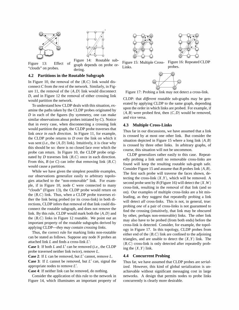
Figure 13: Effect of“clouds” on probes.

AB

C

D

Figure 14: Routable sub-graph depends on probe or-dering.

A

X

Z

Y

W

B

Figure 15: Multiple Cross-Links.

A

X

Z

Y

W

B

Figure 16: Repeated CLDPprobes.

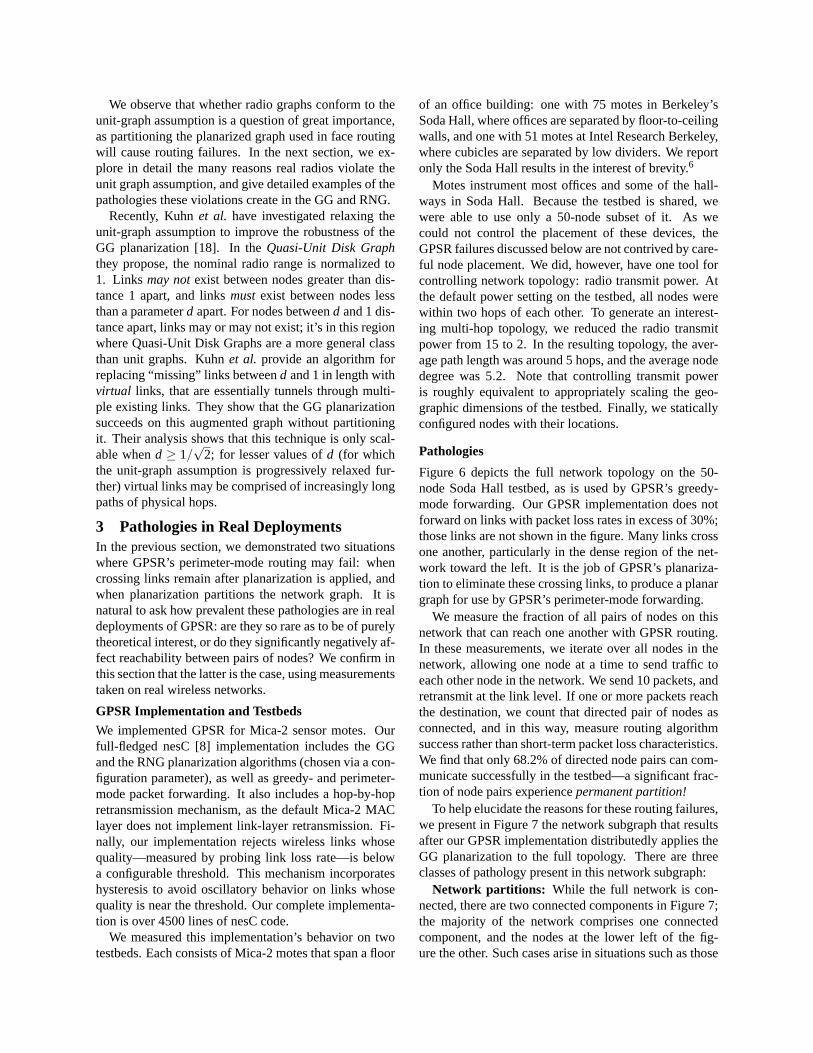
4.2 Partitions in the Routable SubgraphIn Figure 10, the removal of the(B,C) link would dis-connectC from the rest of the network. Similarly, in Fig-ure 11, the removal of the(A,D) link would disconnectD, and in Figure 12 the removal of either crossing linkwould partition the network.

To understand how CLDP deals with this situation, ex-amine the paths taken by the CLDP probes originated byD in each of the figures (by symmetry, one can makesimilar observations about probes initiated byC). Noticethat in every case, when disconnecting a crossing linkwould partition the graph, the CLDP probe traverses thatlink once in each direction. In Figure 11, for example,the CLDP probe returns toD over the link on which itwas sent (i.e., the(A,D) link). Intuitively, it is clear whythis should be so: there is no closed face over which theprobe can return. In Figure 10, the CLDP probe origi-nated byD traverses link(B,C) once in each direction.From this,B (or C) can infer that removing link(B,C)would cause a partition.

While we have given the simplest possible examples,our observations generalize easily to arbitrary topolo-gies attached to the “non-removable” link. For exam-ple, if in Figure 10, nodeC were connected to many“clouds” (Figure 13), the CLDP probe would return onthe (B,C) link. Thus, when a CLDP probe traverses ei-ther the link being probed (or its cross-link) in both di-rections, CLDP infers that removal of that link could dis-connect the routable subgraph, and does not remove thelink. By this rule, CLDP would mark both the(A,D) andthe (B,C) links in Figure 12 routable. We point out animportant property of the routable subgraphs derived byapplying CLDP—they may contain crossing links.

Thus, the correct rule for marking links non-routablecan be stated as follows. Suppose any nodeN probes anattached linkL and finds a cross-linkL′:Case 1: If both L andL′ can be removed (i.e., the CLDPprobe traversed neither link twice), removeL.Case 2: If L can be removed, butL′ cannot, removeL.Case 3: If L cannot be removed, butL′ can, signal theappropriate nodes to removeL′.Case 4: If neither link can be removed, do nothing.

Consider the application of this rule to the network inFigure 14, which illuminates an important property of

A

DC

B

X Y

Figure 17: Probing a link may not detect a cross-link.

CLDP: thatdifferent routable sub-graphs may be gen-erated by applying CLDP to the same graph, dependingupon the order in which links are probed. For example, if(A,B) were probed first, then(C,D) would be removed,and vice versa.

4.3 Multiple Cross-LinksThus far in our discussions, we have assumed that a linkis crossed by at most one other link. But consider thesituation depicted in Figure 15 where a long link(A,B)is crossed by three other links. In arbitrary graphs, ofcourse, this situation will not be uncommon.

CLDP generalizes rather easily to this case. Repeat-edly probing a link until no removable cross-links arefound will keep the resulting routable sub-graph safe.Consider Figure 15 and assume thatB probes link(A,B).The first such probe will traverse the faces shown, de-tecting the cross-link(X,Y), which will be removed. Asecond probe sent byB (Figure 16) will detect the(X,W)cross-link, resulting in the removal of that link (and soon). Our examples of multiple cross-links are a bit mis-leading, as they suggest that repeatedly probing a linkwill detect all cross-links. This is not, in general, true:probingoneof a pair of cross-links is not guaranteed tofind the crossing (intuitively, that link may be obscuredby other, perhaps non-removable) links. The other linkmay also have to be probed (from both ends) before thecross-link is detected. Consider, for example, the topol-ogy in Figure 17. In this topology, CLDP probes fromeither end of the(B,C) link are confined to the adjoiningtriangles, and are unable to detect the(X,Y) link. The(B,C) cross-link is only detected after repeatedly prob-ing the(X,Y) link.

4.4 Concurrent ProbingThus far, we have assumed that CLDP probes areserial-ized. However, this kind of global serialization is un-achievable without significant messaging cost in largenetworks. A design that permits nodes to probe linksconcurrently is clearly more desirable.

Unfortunately, concurrent probing can render the rout-ing subgraph disconnected. Consider Figure 9 and as-sume that whileD probes link(A,D), C concurrentlyprobes link(B,C). When each probe returns,C andD each detect a cross-link, and mark their directly at-tached links non-routable (assume that either link can beremoved), leaving the routable subgraph disconnected.Such a race condition can be prevented using a simpletie-breakrule that deterministically decides which cross-link should be deleted. However, the tie-break rule doesnot guarantee correctness in the general case.

A simple approach would be tolock a link while itis being probed. CLDP drops probes that encounter alocked link in either direction, and retries them later.This approach effectively ensures that the faces adjoin-ing the locked link are not altered while the link is locked(modulo changes caused by node failures or additions,which we discuss later).

CLDP uses this basic strategy, but takes care to avoidrace conditions in cases where the cross-link (and notthe probed link) must be removed. Furthermore, it re-duces convergence time using a few simple optimiza-tions, since the basic strategy can cause many droppedprobes. Finally, it also reduces probing overhead byavoiding probes on links which have already been deter-mined to be routable, unless one of the adjoining faceshas changed. We now describe these modifications.

First, CLDP useslazy locking. That is, when CLDPneeds to probe a link, itfirst sends a probe without lock-ing the link. If this probe returns indicating either thatthere are no cross-links or that this link and its cross-linkcannot be removed (Case 4, Figure 12), CLDP marks thelink to be routable. Thus, in this case (which one expectsto be common for small faces on dense networks), CLDPconverges quickly without locking links. Routable linksare markeddormantand not subsequently probed unlesswoken up; we later describe how this happens.

There are two other possible outcomes of a probe mes-sage; either the probed link needs to be removed fromthe CLDP-derived graph (e.g.,Case 2, Figure 10), or itscross link needs to be removed (e.g.,Case 3, Figure 11).In the former case, CLDP enters acommitphase, whereit locks the probed link, and re-probes the link but us-ing a specially marked “commit” message. All probestraversing a locked link in either direction are dropped.However, when a commit message traverses a lockedlink, a deterministic tie-break is applied which ensuresthat if two links on the same face are being “commit”-edsimultaneously, only one of the commit messages suc-ceeds in traversing the face. When the “commit” probesucceeds, CLDP unlocks the probed link, and marks itasnon-routable. The act of marking a link non-routablechanges the faces adjacent to the link. As Figures 15and 16 show, removal of a link can reveal cross-links

(e.g., the (X,W) link does not see the(A,B) cross-linkuntil the (X,Y) link is removed from the graph). Ac-cordingly, the changed faces must be re-probed. To ac-complish this, when CLDP removes a link (i.e.,marks itnon-routable), it awakens the two adjacentdormant(seeabove) links (i.e., those obtained by applying the right-hand rule and the left-hand rule from this link).

The last case to consider is when a probe indicates thatthe cross-link (e.g., link (B,C), Figure 11) must be re-moved. Recall (Figure 17) that, in general, a probe ofthe cross-link might not reveal the crossing. For this rea-son, when a probe indicates the cross-link needs to beremoved, CLDP walks the corresponding face again us-ing a “commit” probe, and locks the cross-link after theprobe reaches it. When that probe succeeds, the nodenotifies both ends of the cross-link to mark the link non-routable.

Finally, we describe CLDP’s behavior when a linkis added to or deleted from the underlying connectivitygraph. When a link is added to the underlying graph,CLDP awakens the adjacent dormant links. This causeslinks on the corresponding faces to be probed again,eliminating cross-links when necessary. Link deletionpresents a more subtle problem. Consider Figure 15, andsuppose that links(Z,W) and(X,Y) have been markednon-routable. Now, suppose that link(A,B) fails. Thesimplest way to restore the links(Z,W) and (X,Y) tothe routable sub-graph would be to periodically re-probethese links. This is what CLDP does. It is possibleto design optimizations that can reduce the overhead ofperiodic probing. For example, nodeA could remem-ber which cross-links were removed when(A,B) wasprobed, and notify the ends of those cross links when(A,B) fails. We have left the design of these optimiza-tions for future work.

CLDP implements its probing actions using a simplestate machine and a protocol consisting of several mes-sage types. In the interest of brevity, we refer the in-terested reader to [14] for a detailed specification of theCLDP protocol.

4.5 Statement of CorrectnessSpace constraints limit us only to state the theorems thatprove CLDP’s correctness. In this formal analysis, weassume that the full network graphs are static and haveno degeneracies: no vertices are coincident, and no pairsof edges at a single node have the same incident bearing;there is a provably correct way to handle the latter de-generacy, elided because of space constraints. Thus, thenotion of a “crossing” is well-defined. For each graph de-fine a (perhaps empty) set of crossingsC; each elementof C is a pair of edges that intersect in the plane.

Our results are based on the fact that all face walkseventually return to their starting points. We use the

following terminology to describe how a face walk re-turns to its starting point. An edge issingly-walkedifa face walk starting on that edge does not return via thatsame edge (in the opposite direction). An edge isdoubly-walkedif it returns via the same edge in the opposite di-rection. The general rule in CLDP is that when a cross-ing is detected, no doubly-walked edge can be removed,but if one of the crossing edges is singly-walked, then anedge is removed. Our first result is a general observationabout crossings in connected graphs.

Theorem 4.1 If a connected graph G has at least onecrossing, then there is at least one face with a crossing.

This result shows that if we had used a version ofCLDP that eliminatedall crossings then we would endup with a set of connected planar components. To helpstate our next result, we term a graphCLDP-stableifCLDP would not eliminate any edge in the graph, werethe edges probed in serial fashion. We then have:

Theorem 4.2 Geographic routing never fails on a con-nected CLDP-stable graph.

This says that if we use CLDP’s rules about when toeliminate crossings, then we end up with a connectedgraph on which one can reliably use geographic routing.

5 Simulation ResultsThe above theorems assert CLDP’s correctness on staticgraphs. However, to show that CLDP is practical onreal wireless networks, we examine the performance ofCLDP through simulation in this section, and throughexperimentation in the next.

Methodology and Metrics We implemented CLDP(and other geographic routing protocols, described be-low) in TinyOS [10], the event-driven operating systemused on the Mica-2 motes. TinyOS code can be directlyexecuted on TOSSIM [19], a process-level simulator thatcan be used to directly debug and evaluate sensor net-work applications and protocols. Our implementation ofCLDP in TinyOS is 750 lines of nesC code. In this sec-tion, we report simulation results obtained from runningCLDP and other protocols using TOSSIM’s support forpacket-level simulation.

In this section, we compare (whenever appropriate)CLDP’s performance against three alternatives,GPSRdenotes the full implementation of GPSR using theGabriel Graph for planarization, greedy forwarding,and perimeter traversal for routing around voids. WeuseGPSRto provide context for CLDP’s performance.GPSR′NOPLANdenotes a protocol that forwards pack-ets using GPSR on the full connectivity graph (i.e., with-out planarization).GPSR′NOPLANdelineates the base-line performance of face walking on the networks westudy. GPSR′GG/MW includes, in addition to GPSR

and planarization, an implementation of the “mutual wit-ness” procedure for avoiding unidirectional links and dis-connections in the planarized graph when the unit-graphassumptions are violated (Section 3).GPSR′GG/MWquantifies the inadequacy of that proposed fix for pla-narization failures, thereby highlighting the need forCLDP. GPSR′CLDP denotes our proposed protocol us-ing CLDP, greedy forwarding, and perimeter traversal.

In each of our simulations, we use a 200-node topol-ogy in which nodes are randomly positioned on a fixed-size two-dimensional surface. We conducted simulationson two types of networks: wireless networks with an ide-alized radio model with circular radio ranges (we intro-duce reality in the form of obstacles), and Bernoulli ran-dom graphs which have a fixed connection probabilityfor any pair of nodes, regardless of Euclidean distancebetween the nodes. For our wireless network simula-tions, we evaluate the performance of various geographicrouting protocols as a function of node density. Our mea-sure of density is the average number of neighbors of anode. We scale the area of the surface in order to varynode density; for our highest density we use an area of1300 x 1300 units, while for our lowest, we use an areaof 2000 x 2000 units. The radio range is 180 units.

In our simulations with obstacles, the number of ob-stacles is indicated by a parameterf , such thatf N is thetotal number of obstacles (N is the number of nodes).Each obstacle is of fixed length (45 units) in each of oursimulations. The mid-point of the obstacle is randomlypositioned on the two-dimensional surface, and the ori-entation of the obstacle is equally likely to be either ver-tical or horizontal. This obstacle model helps us stressCLDP and other protocols to varying extents in order tomeasure their performance.

Our Bernoulli random graphs are generated in the ob-vious way: we flip a weighted coin for each pair of nodes,assigning a link between them with the desired connec-tion probability.

For each simulation we first generate a network topol-ogy. We then ensure that the topology is connected.At the beginning of the simulation, TOSSIM enforcesa boot-up time during which nodes are started randomly.In our simulations, 200 nodes are started randomly in thefirst 30 seconds. Following the boot phase, each simula-tion consists of two phases. In the first phase, we let theappropriate routability determination protocol (CLDP, orGPSR’s planarization and/or mutual witness procedure)execute at each node long enough for the network to con-verge. In the second phase, we send packets pairwisebidirectionally between nodes in a staggered manner tominimize wireless collisions. This latter phase tests forrouting failures. For each data point in the graphs below,we run 50 random topologies. We have verified that thisis sufficient to produce negligible 95% confidence inter-

0.65

0.70

0.75

0.80

0.85

0.90

0.95

1.00

8.8 8.1 7.5 7.0 6.6 6.1 5.7 5.3 5.0Node density (no. obstacle = N)

GPSRGPSR'NOPLANGPSR'GG/MWGPSR'CLDP

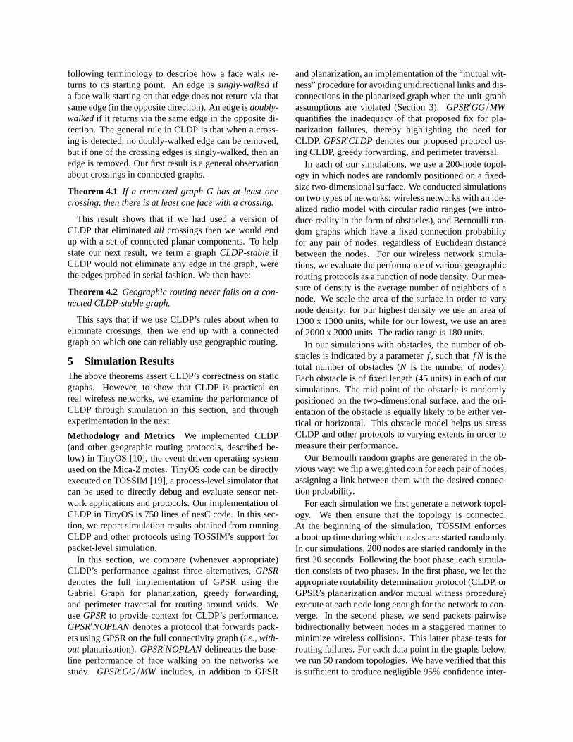
Figure 18: Success rate for 1.0N obstacles.

0.00

0.20

0.40

0.60

0.80

1.00

1 2 4 8 16 32 64 102Stretch

8.8 density7.0 density5.7 density4.7 density

Figure 19: CDF of stretch (1.0N obstacles).

0

1

2

3

4

5

6

7

8

8.8 8.1 7.5 7.0 6.6 6.1 5.7 5.3 5.0Node density (no. obstacles = N)

GPSR'NOPLANGPSR'GG/MWGPSR'CLDP

Figure 20: Average stretch forN obstacles.

0.40

0.50

0.60

0.70

0.80

0.90

1.00

10 8 6 4Probability of link connectivity (%)

GPSRGPSR'NOPLANGPSR'GG/MWGPSR'CLDP

Figure 21: Random graph success rate.

vals for the mean values of our metrics.We do not simulate packet losses due to interference or

buffer overrun in either phase. Our simulations do droppackets, however, when face routing fails. Packet losseswould increase the convergence time of CLDP, or wouldalter the level of concurrent probing in CLDP. Our simu-lation methodology already introduces significant con-currency by ensuring that all nodes start at nearly thesame time. (Note that our testbed measurements includeinterference and buffer overrun effects, of course.)

We use two primary measures of performance. Thesuccess ratemeasures the fraction of sender/receiverpairs for which packet transmissions from the sender aresuccessfully received. Theaverage stretchmeasures theaverage of path stretch for all sender/receiver pairs. Thestretch of a path is the ratio of the number of hops usingthe routing scheme in question to the number of hops inthe shortest path. We also evaluate the overhead and con-vergence time of CLDP; we define these metrics below.

Given space constraints, we only present a samplingof simulation results extensively described in [14]. Inparticular, we omit results validating CLDP’s correctnesson networks with localization errors as well as a detaileddiscussion of CLDP’s performance on random graphs.

Wireless Networks with Obstacles Figure 18 showsthe success rate as a function of node density for our var-ious protocols, in the presence ofN obstacles. Note thatthis is an extremely harsh environment, with as many ob-stacles as nodes. As expected, CLDP allows perfect de-livery success across all node densities we evaluated. In-terestingly, GPSR’s planarization procedure fails ratherdramatically in the presence of even a moderate num-

ber of obstacles. In these circumstances, it appears to bemore advantageous simply to use GPSR on the connec-tivity graph without planarization. The mutual-witnessprocedure fixes many of GPSR’s shortcomings and isclose to perfect in some cases. At most densities it canestablish paths between 99% or more node pairs, but it isnever perfect. In a real deployment, however, MW failsfar more dramatically, as discussed in Section 3.

Figure 20 plots the average stretch as a function ofnode density for our various protocols, in the presence ofN obstacles. CLDP exhibits an average stretch between 2and slightly above 4, with a higher stretch at lower densi-ties. CLDP outperforms GPSR’GG/MW in this respect;CLDP removes only cross links, but GPSR’GG/MW re-moves all links that are witnessed by planarization andhence incurs higher stretch. However, CLDP may exhibitlong paths. This is evident from the CDF of stretch forCLDP (Figure 19, withN obstacles). Notice the long tailof the distribution, in which some paths have a stretchof over 100! Across the range of densities we explore,though, 60-95% of the paths have a stretch less than 2.

Random Graphs To stress CLDP, we also simulatedit on Bernoulli random graphs with various connectiv-ity probabilities. As Figure 21 shows, CLDP exhibits norouting failures, even on random graphs. By contrast,all other variants exhibit significant routing failures onsparse random graphs (low connection probabilities). Inparticular, MWP exhibits more systematic routing fail-ures than on wireless networks. Clearly, none of theseother protocols is practical for routing on random graphs.

Overhead We measured how many CLDP messagesare needed to add a link to a wireless network withN ob-

0.6

0.65

0.7

0.75

0.8

0.85

0.9

0.95

1

0 50 100 150 200 250 300 350 400

Fra

ctio

n of

link

s w

ith o

verh

ead

<=

x

Overhead

8.8 density7.0 density5.7 density4.7 density

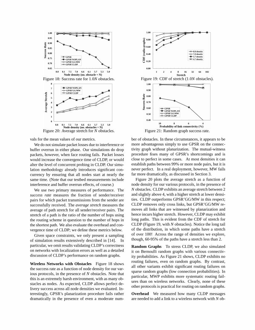
Figure 22: Overhead for wireless network withN obsta-cles.

0.6

0.65

0.7

0.75

0.8

0.85

0.9

0.95

1

0 2 4 6 8 10

Fra

ctio

n of

link

s w

ith c

onve

rgen

ce ti

me

<=

x

Convergence time (in units of probing intervals)

8.8 density7.0 density5.7 density4.7 density

Figure 23: Convergence time distribution for wirelessnetwork withN obstacles.

stacles. This gives us some idea of the overhead incurredby CLDP. In our experiments for measuring overhead,after a network has reached steady state, two nodes notdirectly connected to each other are randomly selectedand an additional link between them is activated.

The overheadis the total number of CLDP controlmessages (probe and commit) traversing a link in eitherdirection until the network has converged. Figure 22plots the distribution of link overheads averaged over20 link additions on each of 200 wireless topologies.It shows that about 85%-90% of links see fewer than4 messages, but a very small fraction of links see up-wards of 100 messages. This latter phenomenon can beexplained as follows. Assume that a new link is addedwhich crosses existing edges. When CLDP removesthese crossing edges, it needs to wake up all links on thefaces adjacent to the removed link in order to detect suc-cessively hidden cross-edges. These links generate probemessages to see if they are crossed by others. Hence, thenumber of messages observed on a link depends on thesize of the face. Clearly, in our wireless topologies (par-ticular in the ones with lower density), there exist longfaces.

Network Convergence Time We measured howquickly CLDP converges both on wireless networks withN obstacles and on Bernoulli random graphs. In ex-periments of convergence time, 200 nodes are initiallystarted roughly simultaneously. In our CLDP implemen-tation, nodes periodically probe their attached links be-fore the links become dormant. Thus, the convergencetime of CLDP is a function of this periodic timer. Theconvergence timeof a link is defined as the number ofCLDP probing intervals before a link becomes dormantand remains thus (Section 4.4). Notice that our exper-iments measure link convergence atstartup; one wouldexpect that in steady-state, the time for convergence af-ter a single link failure and recovery can be expected tobe considerably lower. Figure 23 shows the convergencetime distribution for wireless networks withN obstacles.In Figure 23, about 95% of links converge within 4 probe

intervals and all links converge within 9. In practice(Section 6), convergence times are slightly longer.

Network Dynamics Finally, we conducted simula-tions to evaluate CLDP’s resilience to network dynam-ics. These experiments were done on 200 wireless net-works withN obstacles as well as 200 Bernoulli randomgraphs. In all experiments, we took each given topology,randomly selected some links, and marked them non-routable in order to force those links to be re-probed byCLDP. Then we let CLDP execute at each node. Initially,these non-routable links are not used for CLDP probing.Over time, however, these links are woken up and areCLDP-probed. After all links had reached a dormantstate, we determined whether packets could be routedbetween all pairs. In every case, CLDP converged to anetwork with 100% pairwise connectivity. Note that if alink flaps, CLDP will continuously attempt to probe thelink. It might be possible to dampen this activity, but wehave not investigated such mechanisms.

Summary In every simulation experiment, CLDP es-tablishes routing paths between all node pairs. It exhibitsreasonable stretch, overhead, and convergence times.Moreover, it works well under network dynamics. Wenext measure how CLDP performs on actual wirelesstestbeds.

6 Experimental ResultsIn this section, we describe CLDP’s performance in de-ployment on wireless sensor network testbeds.

Testbeds and Experiments

We deployed CLDP on two different sensor nodetestbeds; as geographic routing’s behavior is sensitive tothe detailed placement of nodes and obstacles, we soughtto demonstrate CLDP’s behavior for multiple node andobstacle placements, to the extent possible using testbedresources at our disposal. The first testbed we shall la-bel R, and consists of 75 Mica-2 “dots” with 433 MHzradios, deployed roughly one per room on one floor ofBerkeley’s Soda Hall. As described in Section 3, thiswas a shared testbed infrastructure, so we had no control

Figure 24: Node layout forRs. Figure 25: . . . forC.

over node layout and were able to use only a subset ofthe nodes for our experiments. We report performancemeasurements obtained on two different subsets of thistestbed: Rs (Figure 24) which contains 23 nodes, andRm(Figure 6) which contains 50 nodes.

The second testbed, which we shall callC, consistsof 51 Mica-2 “dots” deployed across a floor of IntelResearch Berkeley, of which we were able to use 36.In addition to environmental differences (cubicles inCvs. rooms in R), the testbeds differ in thatC’s nodesare suspected to have poorer quality radios. Further-more,C’s radios operate at 916 Mhz, and incur interfer-ence from other nearby devices in that unlicensed band.Again, onC we had no control over node layout.

As described in Section 3, in these testbeds we ad-justed node transmit power to obtain a multi-hop topol-ogy. ForRmandC, notice that the topologies stress geo-graphic routing protocols significantly–they contain twoor more “clusters” of sensor nodes linked by one or twolinks, a configuration that triggers perimeter-mode rout-ing frequently. Of course, such topologies aren’t verypractical since their capacity would be constrained by thebottleneck links. However, they can give some idea ofworst-case CLDP performance, as we discuss below.

We thus conducted three sets of experiments:Rm, Rs,andC. In each experiment, nodes were configured withtheir locations. We started all nodes roughly simultane-ously and let CLDP probing converge. We logged everypacket (all devices in both testbeds had console accessthrough a serial port), and we also recorded pair-wiselink quality. In addition, forRs, we conducted an exper-iment in which we sent 50 packets between each pair ofnodes in order to measure packet delivery performance.Our packet forwarding implementation tries up to threelink-layer retransmissions per hop.

Results

In this section, we report on the performance of CLDPaccording to a variety of metrics. At the outset, we pointout that in all three experiments, CLDP was immuneto the pathologies described in Section 3 and establishedpairwise connectivity between 100% of node pairs.

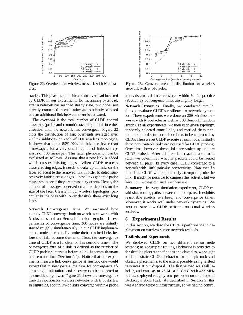
Path Performance One aspect of a routing protocol’spath performance is stretch. For most node pairs (Fig-ure 26), CLDP’s stretch is reasonable (2 or 3). How-ever, CLDP does exhibit fairly significant stretch (up to

20 in some cases) for a small fraction of node pairs. Highstretch arises from long paths between pairs of nodes.Often, such long paths arise during traversal of the outerperimeter of the network.

One might argue that comparing CLDP paths withshortest paths is unrealistic, since shortest-path routingis known to offer low throughput [3] over a wirelessnetwork whose links span a wide range of packet de-livery rates. For this reason, we measure the qualityof CLDP’s path selection. Figure 27 computes the dis-tribution of pairwise packet delivery rates (the fractionof delivered packets) for both CLDP (measured onRs)and ETX (computed from link quality estimates onRs).8

CLDP’s packet delivery performance is comparable to,but slightly worse than this “idealized” ETX. A compar-ison with a real implementation of ETX might lessen thediscrepancy between the two considerably. Finally, wenote that ETX (when implemented on a proactive proto-col like DSR, on a network with a dynamic topology) islikely to incur higher overhead than CLDP.

Convergence Time Figure 28 shows that most linksconverge within 15–20 probe intervals; with a 15 sec-ond probe timer, this corresponds to about 4.0 min-utes. However, some links exhibit very long conver-gence times (up to 70 intervals). Our experiment mea-suresstartupconvergence, since all the nodes are startedroughly simultaneously. For CLDP, this is the worstcase: when all links are simultaneously probed, linklocking will delay convergence significantly. This alsoexplains whyRm and C show a qualitatively differentbehavior; the bottleneck links between clusters inducesignificant probe contention.

A more realistic measure of link convergence time isthe time it takes for a single link to converge when therest of the network is in steady state. Even for a moder-ate size network, we couldn’t automate this experimenteasily, so we estimate this interval. We obtained oures-timated steady-state convergence timeby counting onlythose CLDP probes that do not encounter locked links.By this measure, CLDP converges very fast (Figure 29);more than 99% of the links converge within 6 intervalsin all three experiments.

In addition, we also conducted an experiment wherewe started with a converged network, and manually dis-abled and then re-enabled an arbitrary link chosen fromten arbitrarily selected nodes. We then measured the time

0.55

0.6

0.65

0.7

0.75

0.8

0.85

0.9

0.95

1

0 5 10 15 20Fra

ctio

n of

nod

e pa

irs w

ith s

tret

ch <

= x

Stretch

RsRm

C

Figure 26: CDF of stretch.

0

0.1

0.2

0.3

0.4

0.5

0.6

0.7

0.8

0.9

1

0 0.2 0.4 0.6 0.8 1

Fra

ctio

n of

nod

e pa

irs w

ith d

eliv

ery

rate

<=

x

packet delivery rate

Rs(CLDP)Rs(ETX)

Figure 27: CDF of pairwise packet delivery rate.

0

0.1

0.2

0.3

0.4

0.5

0.6

0.7

0.8

0.9

1

0 10 20 30 40 50 60 70 80 90

Fra

ctio

n of

link

s w

ith c

onve

rgen

ce ti

me

<=

x

Convergence time (in units of probing intervals)

RsRm

C

Figure 28: CDF of convergence time.

0

0.2

0.4

0.6

0.8

1

0 1 2 3 4 5 6 7 8

Fra

ctio

n of

link

s w

ith e

stim

ates

con

verg

ence

Convergence time (in units of probing intervals)

RsRm

C

Figure 29: CDF of estimated steady-state convergence.

for CLDP to converge after each transition. After dis-abling a link, CLDP converged on average within 1.86probing intervals; after enabling a link, CLDP convergedon average within 0.59 probing intervals.9

Overhead Finally, we quantify the overhead of CLDPfrom our measurements. The primary metric we study isthe distribution of probing overhead on individual links.However, rather than merely count the number of CLDPprobe messages on each link for the entire duration ofthe experiment, we compute the average number of mes-sages on each link10 per probing interval. Normalizingthe overhead this way helps us compare different experi-ments whose convergence times are different. Figure 30shows that the overhead of CLDP is quite low; even onthe busiest link, CLDP incurs less than one packet persecond (if we assume a probe interval of 15 seconds),and on most links the overhead is significantly less.

0

0.1

0.2

0.3

0.4

0.5

0.6

0.7

0.8

0.9

1

0 2 4 6 8 10 12

Fra

ctio

n of

link

s w

ith o

verh

ead

<=

x

Overhead

RsRm

C

Figure 30: CDF of overhead.

7 ConclusionWe have motivated, described, and evaluated CLDP,which, to our knowledge, is the first distributed pla-narization protocol that renders geographic routing cor-rect on arbitrary graphs. Simulations and measurementson real testbeds indicate that CLDP is quite practical: itoffers high delivery rates, low overhead, and fast conver-gence. In future, we plan to investigate CLDP’s overheadand robustness on more dynamic topologies, as well asthe effect of localization errors on CLDP’s path stretchin deployment.

AcknowledgmentsWe thank the anonymous reviewers for their comments,and Ellen Zegura for her thoughtful shepherding of thispaper. We are further indebted to Om Gnawali for thecomparison with ETX, and Jerry Zhao, Xin Li, and WeiHong for helping us to use the UC Berkeley and IntelResearch Berkeley sensor network testbeds.

Notes1Other face routing techniques [17] can be used as well; CLDP pre-

serves their correctness, but may affect their performance.2For lack of space, we only present the resulting theorems, not their

proofs, which may be found in [14].3We note that there exist other routing algorithms that make use of

position information, such as LAR [16], but we restrict the scope of ourwork to the family of face-routing algorithms in which a node forwardsto a single neighbor on the basis of geographic information.

4We refer to links and edges interchangeably throughout the paper.5Other face-change rules are possible, including changing faces at

the edge whose crossing ofSD is theclosestsuch crossing toD on the

current face. We use the first crossing, not best crossing, throughoutthis paper; this choice is known to be average-case efficient, and hasbeen refined [17] to be worst-case optimal.

6While pathologies in geographic routing are sensitive to the partic-ular placement of nodes and the obstacles between them, we observedsimilar results on the two testbeds, and thus expect similar behavior inother real deployments.

7In principle, CLDP wouldn’t need additional mechanisms to func-tion under mobility, and would work well when link disconnections dueto mobility occur on much longer timescales than the time required tocomplete CLDP probes.

8While CLDP uses only “good” links, our simulation of ETX is notsimilarly constrained.

9If a link is probed exactly once before it becomes dormant, thatcounts as a convergence time of zero.

10Although we count the number of messages on a link, recall thatin our implementation, each message on a “link” constitutes a radiobroadcast. Interpreted thus, our measure of overhead indicates the num-ber of data packets that CLDP probing displaces in our deployment. Amore general measure, and one that we have not investigated since itdepends on deployment density and other environmental factors, is thefraction of transmission capacity that CLDP probing overhead occu-pies.

References[1] S. Biswas and R. Morris. Opportunistic routing in multi-

hop wireless networks. InProc. ACM HotNets Workshop,Boston, MA, USA, Nov. 2003.

[2] P. Bose, P. Morin, I. Stojmenovic, and J. Urrutia. Routingwith guaranteed delivery in ad hoc wireless networks. InProc. ACM DIALM Workshop, pages 48–55, Seattle, WA,USA, Aug. 1999. ACM.

[3] D. De Couto, D. Aguayo, B. Chambers, and R. Mor-ris. Performance of multihop wireless networks: Shortestpath is not enough. InProc. ACM HotNets Workshop,New Jersey, USA, Oct. 2002.

[4] G. Finn. Routing and addressing problems inlarge metropolitan-scale internetworks. Technical Re-port ISI/RR-87-180, USC/Information Sciences Institute,Mar. 1987.

[5] K. Gabriel and R. Sokal. A new statistical approach to ge-ographic variation analysis.Systematic Zoology, 18:259–278, 1969.

[6] D. Ganesan, D. Estrin, A. Woo, D. Culler, B. Krish-namachari, and S. Wicker. Complex behavior at scale:An experimental study of low-power wireless sensor net-works. Technical Report UCLA/CSD-TR-02-0013, Uni-versity of California, Los Angeles, Computer Science De-partment, 2002.

[7] J. Gao, L. Guibas, J. Hershberger, L. Zhang, and A. Zhu.Geometric spanner for routing in mobile networks. InProc. ACM MobiHoc, pages 45–55, Oct. 2001.

[8] D. Gay, P. Levis, R. von Behren, M. Welsh, E. Brewer,and D. Culler. The nesC language: A holistic approach tonetworked embedded systems. InProc. ACM SIGPLANPLDI, San Diego, CA, June 2003.

[9] R. Gummadi, N. Kothari, Y.-J. Kim, R. Govindan,B. Karp, and S. Shenker. Reduced state routing in theInternet. InProc. ACM HotNets Workshop, San Diego,USA, Nov. 2004.

[10] J. Hill, R. Szewczyk, A. Woo, S. Hollar, D. Culler, andK. Pister. System architecture directions for networkedsensors. InProc. 9th ACM ASPLOS, pages 93–104, Cam-bridge, MA, USA, Nov. 2000. ACM.

[11] B. Karp.Geographic Routing for Wireless Networks. PhDthesis, Harvard University, 2000.

[12] B. Karp. Challenges in geographic routing: Sparse net-works, obstacles, and traffic provisioning. Presentation atthe DIMACS Workshop on Pervasive Networking, May2001.

[13] B. Karp and H. T. Kung. GPSR: Greedy perimeter state-less routing for wireless networks. InProc. ACM/IEEEMobiCom, pages 243–254, Boston, Mass., USA, Aug.2000. ACM.

[14] Y.-J. Kim, R. Govindan, B. Karp, and S. Shenker. Prac-tical and robust geographic routing in wireless networks.Technical Report 04-832, Department of Computer Sci-ence, University of Southern California, 2004.

[15] L. Kleinrock and H. Takagi. Optimal transmission rangesfor randomly distributed packet radio terminals.IEEETrans. Comm., 32(3):246–257, 1984.

[16] Y.-B. Ko and N. Vaidya. Location-aided routing in mobilead hoc networks. InProc. ACM/IEEE MobiCom, Aug.1998.

[17] F. Kuhn, R. Wattenhofer, Y. Zhang, and A. Zollinger.Geometric ad-hoc routing: Of theory and practice. InProc. ACM PODC, Boston, MA, USA, July 2003.

[18] F. Kuhn, R. Wattenhofer, and A. Zollinger. Ad-hoc net-works beyond unit disk graphs. InProc. ACM DIALMPOMC Workshop, Sept. 2003.

[19] P. Levis, N. Lee, M. Welsh, and D. Culler. TOSSIM: ac-curate and scalable simulation of entire tinyOS applica-tions. InProc. ACM Sensys, pages 126–137. ACM Press,2003.

[20] X. Li, Y. J. Kim, R. Govindan, and W. Hong. Multi-dimensional range queries in sensor networks. InProc. ACM Sensys, Los Angeles, CA, USA, Nov. 2003.

[21] J. Newsome and D. Song. GEM: Graph embedding forrouting and data-centric stroage in sensor networks withgeographic information. InProc. ACM Sensys, Nov.2003.

[22] A. Rao, S. Ratnasamy, S. Shenker, and I. Stoica.Geographic routing without location information. InProc. ACM/IEEE MobiCom, pages 96–108, Oct. 2003.

[23] S. Ratnasamy, B. Karp, L. Yin, F. Yu, D. Estrin, R. Govin-dan, and S. Shenker. GHT: A geographic hash table fordata-centric storage. InProc. ACM WSNA Workshop,pages 78–87, Atlanta, Georgia, USA, Sept. 2002. ACM.

[24] K. Seada, A. Helmy, and R. Govindan. Localization er-rors on geographic face routing in sensor networks. InProc. IEEE IPSN Workshop, Berkeley, CA, USA, Apr.2004.

[25] R. Sokal and D. Matula. Properties of Gabriel graphs rel-evant to geographic variation research and the clusteringof points in the plane.Geographical Analysis, 12:205–222, 1980.

[26] G. Toussaint. The relative neighborhood graph of a finiteplanar set.Pattern Recognition, 12(4):261–268, 1980.

[27] J. Zhao and R. Govindan. Understanding packet deliv-ery performance in dense wireless sensor networks. InProc. ACM Sensys, Los Angeles, CA, November 2003.