Geography and Income Convergence 13

8/13/2019 Geography and Income Convergence 13

http://slidepdf.com/reader/full/geography-and-income-convergence-13 1/30

Inter-American Development BankBanco Interamericano de Desarrol l o

Latin American Research Networ kRed de Centros de Investigación

Research networ k Wor king paper #R-395

Geogr aphy and Income Convergenceamong Brazil ian States

ByCar l os R. Azzoni*

Naercio Menezes-Fil ho* Tatiane A. de Menezes*

Raul Sil veira-Neto*

*University of São Paulo

May 2000



2

Cataloging-in-Publication data provided by the

Inter-American Development Bank

Felipe Herrera Library

Geography and income convergence among Brazilian states / by Carlos R. Azzoni … [et al.].

p. cm. (Research Network Working papers ; R-395)Includes bibliographical references.

1. Income--Brazil--Mathematical models. 2. Income--Brazil--Effect of Human services on--

Mathematical models. 3. Income--Brazil--Effect of Human geography on--Mathematicalmodels. 4. Income distribution--Brazil--Mathematical models. I. Azzoni, Carlos

Roberto. II. Inter-American Development Bank. Research Dept. III. Series.

339.3 G385--dc21

82000

Inter-American Development Bank 1300 New York Avenue, N.W.

Washington, D.C. 20577

The views and interpretations in this document are those of the authors and should not be

attributed to the Inter-American Development Bank, or to any individual acting on its behalf.

The Research Department (RES) publishes the Latin American Economic Policies Newsletter , aswell as working papers and books, on diverse economic issues. To obtain a complete list of RES

publications and read or download them, please visit our web site at: www.iadb.org/res/32.htm.



3

Abstract

The objective of the study is to identify the role of geographical variables in explainingdifferences in per capita income among Brazilian states. It also aims at ascertaining thedegree to which such variables affect convergence or divergence trends in per capita incomeamong these states. In order to investigate these issues it uses micro-data, instead of themore traditional aggregate data, averaged up from household to birth cohort level. Both thelevel and the change in average household income per capita across Brazilian states arecorrelated to geographical and household variables. The aim is to capture not only theinfluence of household human capital and wealth variables on the convergence of per capitaincome (along the lines of the neoclassical model), but also that of spatial or geographicalcharacteristics, such as public infrastructure, health and education services. Therefore, thispaper simultaneously considers data on geographical variables and repeated cross-sections of household surveys. The use of cohort level data means that we can constructcohort/ state/year means for all variables of interest and control for state, life cycle andcomposition effects for the first time in this literature. The results indicate that thegeographical variables seem to be important determinants of income levels and growth.

Altogether, the results indicate that human capital and infrastructure variables are importantareas for government intervention, as these are some of the main factors behind thedifferences in steady-state rate of income growth in Brazil.

Acknowledgments

This paper is part of the Inter-American Development Bank research program on theeffects of geography on development. Support from NEMESIS - Núcleo de Estudos eModelos Espaciais Sistêmicos, FUJB No. 7077-7, FINEP/ PRONEX No. 41.96.0405.00is also acknowledged. We are very grateful to audience members of the IDB seminar atCuernavaca, to Fabiana del Felicio at FEA-RP for excellent research assistance, toDenisard Alves for the climate data and to seminar participants at UFMG, IPEA/RJ,FVG-RJ, and at the European Meeting of the Regional Science Association International.



4

CONTENTS

1. Introduction 52. Regional Inequalities in Brazil 5

3. Theory 64. Econometric Methodology 84.1. The Construction of Cohorts 9

5. Data and Data Sources 106. Econometric Results 157. Conclusions and Policy Implications 19References 21

TABLES

Table 1 – Description of the main variables 23 Table 2 – Correlation coefficients among variables 24 Table 3 – Regression results for income levels–Dependent Variable ln(y) 25 Table 4 – Regression results for income growth – Dependent Variable∆ln(y) 26 Table 5 – Convergence results 27 Table 6 – Decomposition of income differentials among regions 27 Table 7 – Interstate Gini coefficients 28 Table 8 – Variables averages and standard deviations by state 29

FIGURES

Figure 1 – Per capita income for Brazilian macro regions 10Figure 2 – Per capita income and age of household head across cohorts 11Figure 3 – Education and household age across cohorts 12Figure 4 – Education across Brazilian macro regions 12Figure 5 – Geographical variables for Brazilian states 13Figure 6 – Urban/ rural situation and density across Brazilian states 13Figure 7 – Infrastructure variables for Brazilian states 14Figure 8 – Human development variables for Brazilian states 14



5

1. Introduction

In mainstream economics, the starting point for understanding the existence of poor regions is theneoclassical exogenous growth model developed by Solow and Swan in 1956. According to thismodel, per capita income differentials among regions are determined by their respective initialendowments of resources, so that it is not so much that there are poor regions, as given areas that

have a greater concentration of poor families. Such models are presented in greater detail in Barroand Sala-i-Martin (1995).

Recent studies, such as Hall and Jones (1996), Chang (1994), Ravallion and Jalan (1996) and Jalan and Ravaillon (1998b) have highlighted the importance of geographical, institutional andpolitical variables in determining regional income differentials. According to these authors, in certaincircumstances the presence of poor families is determined endogenously, and not by the morewidespread exogenous variables assumed in growth models. Differing levels of “geographicalcapital,” such as climate, local infrastructure, access to public services and knowledge about the localphysical reality and adequate technologies, would influence the use of private capital. That is,geographical variables would affect the marginal return of private capital. The imperfect mobility of

factors, usually assumed in this sort of model, would create the conditions for the persistency of inequalities. The coexistence of increasing returns to geographical capital with non-increasing returnsto private capital is conceivable in this line of reasoning. Poor people tend to live in poorly suppliedregions. With the same personal characteristics, they would be better off if living in a richer region.

This difference in diagnosis is reflected in the important issue of policy recommendations.According to the first class of models, regional inequality is to be solved by allowing free mobility of factors that should in turn result in long-term convergence of growth rates. The second strand of the literature, on the other hand, can be used to justify regional policies aiming at reducing regionalinequality, such as public investments in “geographical capital.”

The objective of this paper is to offer evidence on this controversy in the case of stateincome inequalities in Brazil over the period 1981-1996. In Section 2 some general information onregional inequalities in Brazil is provided as well as a review of the some existing empirical studies,creating the background for the study to be performed in the paper. Section 3 presents amethodological discussion of the model to be estimated. Section 4 presents the data used in theresearch and discusses the advantages and limitations of using micro-data. Section 5 presents anddiscusses the econometric results, which are commented on in the concluding section.

2. Regional Inequalities in Brazil

Brazil is well known for its high levels of regional income inequalities. In 1960, Brazil had a GDPper capita of US$1,449. Thirty-five years later, in 1995, this figure had risen to US$3,556,corresponding to an average growth rate of 2.6% per year. Data on per capita GDP for Brazilianstates indicate that only three Brazilian states had figures above the national average, namely, SãoPaulo, Rio de Janeiro and Rio Grande do Sul. The state of São Paulo was notable for a GDP percapita that was almost 2 times the national average. The poorest state was Piauí, with a GDP percapita that was 4.5 times less than the Brazilian average, and 8.9 times less than that of the state of São Paulo. It is notable that nine of the ten poorest states in Brazil were in the Northeast, and threeof the four states of the Southeast were among the five richest states in Brazil.



6

In 1995 a larger number of states were above the national average. Of these, the first two,São Paulo and Rio de Janeiro, are in the Southeast region, while the next three, Rio Grande do Sul,Paraná and Santa Catarina, belong to the South. The other Southeastern states achieved visibleimprovements with regard to the national average (e.g., the state of Mato Grosso). Of the tenpoorest states, eight are in the Northeast, and two in the North, Amazonas and Pará, were notablefor having declined in relative terms since 1960 to a standing among the ten states with the lowestGDP per capita. São Paulo was still the richest state in 1995, with a GDP per capita that was 1.7times the national average, with an average growth rate of 2.1% per year between 1960 and 1995,0.5% below the national growth average. Piauí, on the other hand, was still the poorest state inBrazil. It is nevertheless interesting to note that while, in absolute terms, the state’s position wasconsiderably worse than the rest of the country, in relative terms it had improved, with a GDP percapita that was 3.7 times smaller than the national average, and 6.1 times smaller than that of therichest state. Another interesting point is that in the state of Piauí GDP per capita grew 3.1% peryear, one percentage point above that of the state of São Paulo for the same period. Theseobservations raise the question of whether there is an income convergence trend among Brazilianstates.

Taking the neoclassical growth model as a basis, Ferreira and Diniz (1995), Schwartsman(1996) and Zini (1998), analyzing the period initiated in 1970, could not reject the hypothesis of absolute convergence. They estimated speeds of convergence among Brazilian states that wereabove the levels predicted by the model. Azzoni (1999), working with a longer series (1939-1996),also found indications of absolute convergence of income, but at a much lower speed. I t remains tobe investigated whether there are spatial externalities that condition regional growth. That is to say,geographical characteristics such as climate, public and private infrastructure (which could beunderstood as reflecting “geographical capital”) may be affecting the growth rates of states orregions by influencing the productivity of individual or family capital. This would have decisiveimplications for public sector policies designed to combat poverty and to improve incomes atregional and state levels, since differences in living standards would result not only from the initial

conditions of families, as assumed by neoclassical growth models, but also from differences in the“geographical capital” between regions.

Since the previous models used for calculating convergence did not consider the effect of geographical variables, and these would tend to be positively correlated with initial income, theirresults could, in fact, be reflecting conditional instead of absolute convergence, and they could beunderestimating the true velocity to this convergence. We thus propose to estimate the variation inhousehold income per capita for Brazilian states as a function of geographical, state and householdvariables, in order to capture not only the influence of the individual characteristics of householdson the convergence or divergence of per capita income (along the lines of the neoclassical model),but also that of spatial or geographical characteristics.

3. Theory

This section aims at presenting the neoclassical growth model with exogenous savings, geographicalvariables and fixed effects, as in Islam (1992), to be taken to the data. Consider the productionfunction, with labor augmenting technical progress:



7

where Y = product, K = capital, L = labor and G = geographical capital (fixed in the economy). The public input is thus complementary to private inputs, and we have:

where n and g are the (exogenously determined) population and technology rates of growth.Capital accumulation per effective worker in the steady state will be given by:

k g n y sdt

dk ˆ)( δ++−= )

where s = savings rate, δ = depreciation rate and:

)()(

)(ˆ,)()(

)(ˆ

t Lt A

t K k

t Lt A

t Y y ==

This equation implies steady state levels of capital and product (per effective worker), which aredescribed by:

α

α

δ−

++= 1)(*ˆ

g n

sGk

αα

α

δ

−−

++=

1

1

1)(*ˆ G g n

sG y

With the product per effective worker given by Gt k t y )(ˆ)(ˆ α= , we can approximate its timevariation around the steady state to get (in logs):

))](ˆln(*)ˆ[ln())(ˆln(

t y ydt

t yd −= λ

whereλ = (n+g+δ)(1-α).

The growth of per-capita product during the periodτ = t2 - t1 around the steady-state will be:where we have used the fact that gt At yt y −−= ))0(ln())(ln())(ˆln(

( ) ( )( ) Gt Lt At K t Y αα −

=1

)()(

( ) ( )

( ) ( ) gt

nt

e At A

e Lt L

0

0

=

=

( ) ( ) ( ) ( ) ( ) ( )

( ) ( ) ( ) ( ) )0(ln)1(121ln1ln11

ln1

1ln1

11ln2ln

Aet et g t yeGe

g ne set yt y

λτλτλτλτ

λτλτ

α

α

δα

α

α

α

−−−−

−−

−+−+−+−−

+++−

−−−

−=−



8

One can include human capital in the production function:

and around the steady state we will then have:

where h* = human capital investment as a fraction of income in the steady state.

4. Econometric Methodology

This section aims at representing the last equation in a form that can be estimated with the data athand. As the main aim of this research is to investigate the roles of geographical and human capitalvariables on growth, we propose:

Where:

whereG andH are human capital and geographical variables.

( ) ( ) ( ) ( )[ ] ( )Gt H t Lt At K t Y φφαα −−=

1

( ) ( ) ( ) ( ) ( ) ( ) ( )

( ) ( ) ( ) ( ) ( )λτλτλτλτ

λτλτλ

βα

α

βα

β

δβα

βα

βα

α

−−−−

−−−

−+−+−−

−+−−

−

+++−−

+−−

−−−+−−=−

et g AeGehe

g ne set yet yt y t

2)0(ln11

1ln1

1

ln1

1ln1

11ln11ln2ln

*

( )

( ) ( )

( )

( )

( )12

]1

1/)0(ln)ln()(ln[

1

11

1

1ln2ln

1ln1

t et g

A g n seS

e

t yt y y

t y y

t

i

it

it

λτ−

λτ−

λτ−

−

−=η

β−α−+δ++β+α−α

β−α−−=

−=γ

−=∆

=

it t it it iit it G H S y y ε+η+β+β++γ =∆ − 211



9

4.1The Construction of Cohorts

The data we use come from repeated cross-sections of very rich household surveys, carried out bythe Brazilian Census Bureau (see below). The use of micro-data to examine issues of convergence

has not, as far as we know, been done in the literature before. It is well known in the consumptionand labor supply literature (see Browninget al ., 1985 and Attanasio and Browning, 1994) that withrepeated cross-sections it is possible to construct demographic cohorts based on date of birth, andcalculate cohort-year means for all variables of interest, including income, education, labor forceparticipation and living conditions. We propose to extend this methodology to include the state of residence as another grouping variable and derive state-cohort-year means for the variables of interest. The value attributed to each cohort in state s in year t is

cst

n

i

i

cst n

y

y

cst

∑=

ln

where: ncst is the proportion of household heads born in an interval of determined years (e.g., 1940to 1945), living in state s in period t . Ten cohorts were constructed for each state in each year. Thesame procedure was applied for all other variables included in the analysis, so that we have, forexample, the average number of years of education for people included in each cohort; the sameholds for all other variables.

The advantages of such a procedure are many-fold. Firstly and most importantly, the use of micro-data allows us to control for changes in the composition of the population in each state thatcannot be controlled for with the use of aggregate data. Secondly, we can control for life-cycle andgeneration effects, which means that we are, in effect, considering the effect of geographicalvariables on income growth and convergence within a generation or for a population with the same

age. Thirdly, one can identify state fixed effects without having to rely only on the time componentof the series, since we have obtained various (10 in our case) observations for a given state in a givenyear. Finally, one can rely on differences across generations within a state-year group to identify theeffects of human capital on growth, for example, that are not readily identified using aggregate data(Islam, 1994). The main disadvantage of using cohort level data is that if there are measurementerrors at the household level they are likely to be carried out to the cohort means unless the cell sizesare large.

In effect, we will be estimating an equation of the form:

Where the subscript c means that the variables are now cohort-state-year means,X = household

controls andLF = life cycle variables.

it t cit cit ict ict iict ict LF X G H S y y εηββββγ +++++++=∆ − 43211



10

5. Data and Data Sources

The implementation of the model described above requires panel data, not easily available in general.In the case of Brazil we have repeated cross-sections of a yearly household survey (PNAD -

Pesquisa Nacional por Amostra de Domicílios), conducted by IBGE, the Brazilian Census Bureau,that can be used as a pseudo-panel, by constructing a model that looks like an individual-level modelbut is for cohorts (see Ravallion, 1998). Due to data limitations, only 19 out of 27 states wereconsidered in the study; the excluded states belong to the almost uninhabited northern region(including the Amazon region). The total number of households considered in different years rangedfrom 49,514 to 90,776, with an average of 58,328.1 The average number of households per cohort is269. Due to the small number of observations in some cohorts, only 2,166 were considered in theanalysis.

The main variables in the analysis are as shown in Table 1. The dependent variable usedthroughout (y) is per capita monthly labor income from the main job. We have also made some

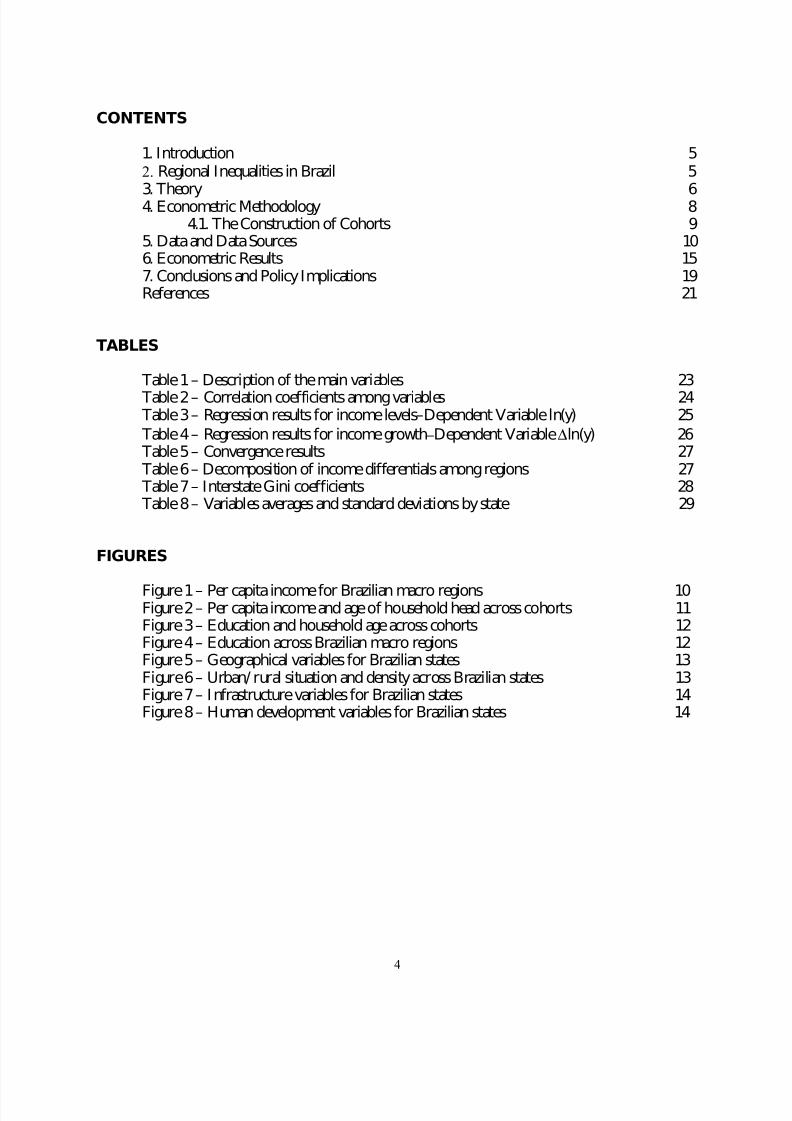
experiments with two other variables, hourly labor income and total income, with no apparentchange in the results.2 In Figure 1 the evolution of per capita income over the period 1981-1996 forfour macro-regions of Brazil is displayed. The first observation relates to the level of income: theaverage for all states in Brazil over the 16 year period is of US$45 per month, or US$540 per year,indicating the low average level of income in the country. Secondly, a slight declining trend isobserved for all states and regions, showing that the average income fell in Brazil during the periodconsidered.

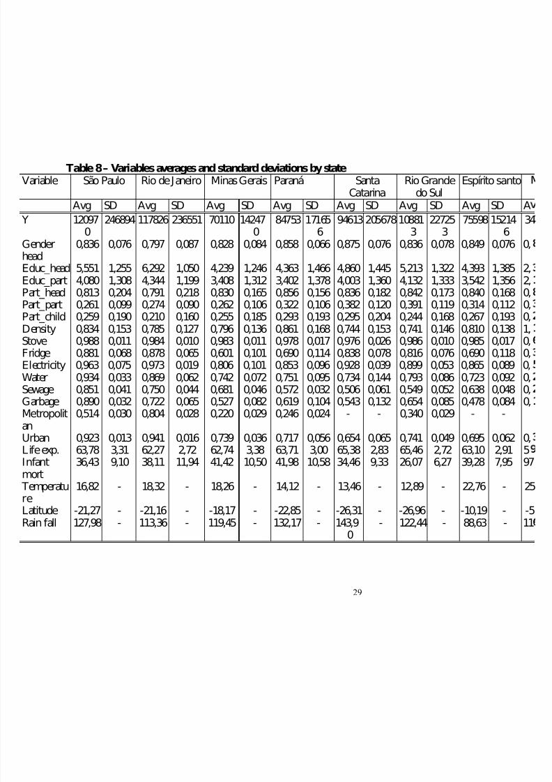
1 Table 8 presents averages and standard deviations for all variables for each state2 Instead of the 3,040 possible cases (10 cohorts x 19 states x 16 years). The small cohorts are located among the youngest in the first years of theperiod and among the oldest in the more recent years. Only cohorts with at least 30 households were included in the sample.

Figure 1 - Per capita income for Brazilian macro regions

Northeast

3.0

3.3

3.5

3.8

4.0

4.3

4.5

81 82 83 84 85 86 87 88 89 90 91 92 93 94 95 96

L o g o

f p .

c .

i n c o m e

( R $ / m o n

t h )

South

Center-West



11

It is interesting to point out the peak for all regions in the year 1986, related to the Cruzadomacroeconomic stabilization plan, which included heavy price controls and brought inflation down. The plan was preceded by a sharp depression in 1983, and even before 1986 some growth in incomecould be observed. Income levels fell after 1986 and began to recover only in 1994, with theimplementation of the Real macroeconomic stabilization plan. It was applied in July of 1994 andsucceeded in reducing inflation gradually during the following month, producing the peak observedin 1995. Finally worth mentioning is the difference between the Northeast region and the otherthree regions in terms of income levels, with that region presenting lower levels of income and theother three presenting similar higher levels. The average annual figures for the South, Southeast andCenter-West are close to US$800, and for the Northeast they are around US$360. Over time, thereis no indication that this difference is falling.

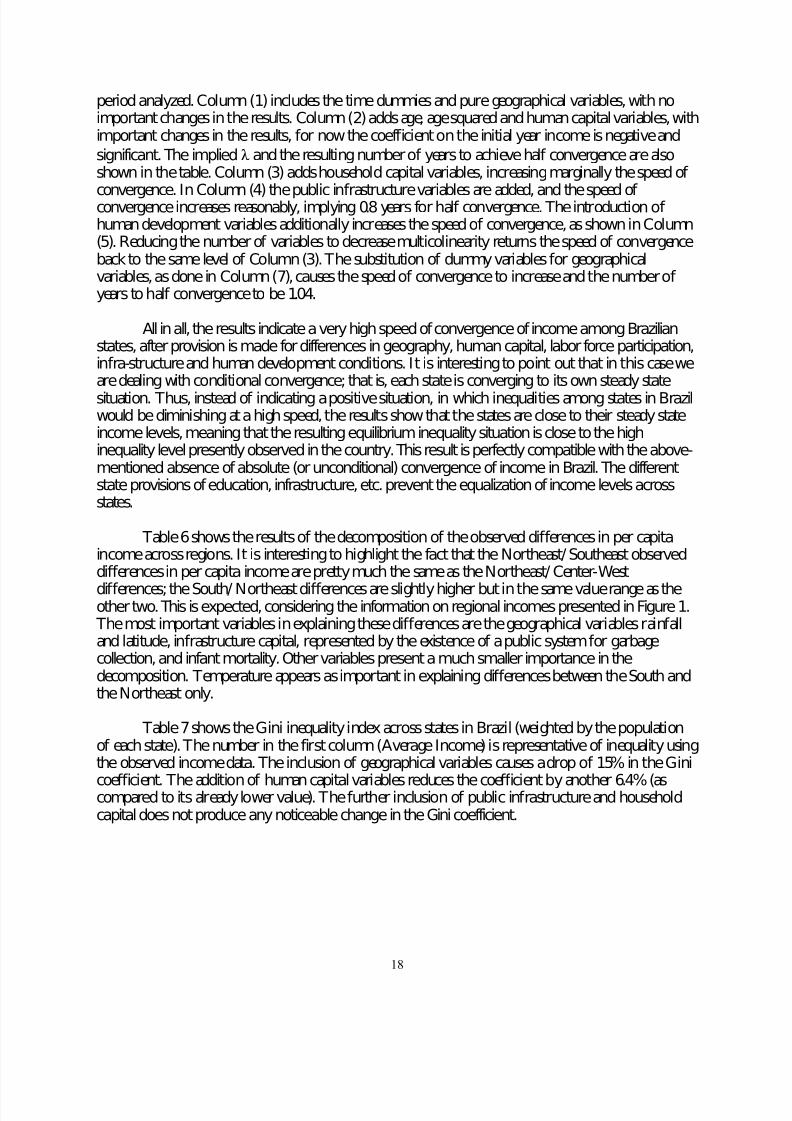
In Figure 2 the per capita income per household by cohort (or age) is presented. Eachcohort is represented by a line, the set of lines indicating the general trend. The traditional life cyclebehavior of income is present, although not as clear as if individual data were used. Income grows as

individuals grow older but, up to a certain age, so does the number of children, preventing growth inaverage income. For people over 40, the average income falls as expected. For each cohort (eachline) the traditional life cycle behavior of income is also present.

Figure 2 - Per capita income and age of household head across cohorts

2.0

2.5

3.0

3.5

4.0

4.5

5.0

2 2

2 4

2 6

2 8

3 0

3 2

3 4

3 6

3 8

4 0

4 2

4 4

4 6

4 8

5 0

5 2

5 4

5 6

5 8

6 0

6 2

6 4

6 6

6 8

Household head age

L o g o f i n c o m e ( R $ / m o n t h )

Each line represents a Cohort

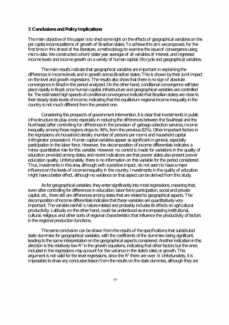
The same cohort disposition is utilized in Figure 3 for the household head’s education. Ingeneral, the number of years of education is very low, with an overall average of 3.8 years for thecountry as a whole. The positive slopes of the cohort curves indicate that the number of years of study grows in each cohort as the household head grows older, but only up to a certain age range(mid-40s); after that the curves are flat, indicating that household heads do not invest in educationany more. The overall declining disposition of the curves show that the younger generations presenthigher levels of education, as compared to older generations, as a result of the improvements madein the Brazilian education system over time.



Figure 3 - Education and household age across cohorts

1.5

2.5

3.5

4.5

5.5

6.5

2 2

2 5

2 8

3 1

3 4

3 7

4 0

4 3

4 6

4 9

5 2

5 5

5 8

6 1

6 4

6 7

Y e a r s o f e d

u c a t i o n

This can be seen also in Figure 4, in which the total number of years of education for eachmacro region is displayed. An increasing trend is observed for every region, but differences in levelsare important: the differences between the South and the Southeast are small, with the Center-West

falling behind and the Northeast with a much lower level. The average number of years of educationfor the regions are: Southeast, 5.4; South, 4.8; Center-West, 4.0, and Northeast, 2.9

Figure 4 - Education across Brazilian macro regions

Southeast

South

Center West

Northeast

2.0

2.5

3.0

3.5

4.0

4.5

5.0

5.5

6.0

1981 1982 1983 1984 1985 1986 1987 1988 1989 1990 1991 1992 1993 1994 1995 1996

Y e a r s o f e d u c a t i o n

The pure geographical variables are rainfall, (the negative of) latitude3 and temperature in June (the month with the highest variation across states in Brazil). These are displayed in Figure 5, inwhich the states are positioned in the horizontal axis in decreasing order of per capita income levels.It is clear from the figure that there is a positive correlation between income level and the variablesrainfall and latitude and a negative correlation between income and temperature.

3 Throughout the paper the negative of latitude will be utilized in order to facilitate the interpretation of the coefficients. Thus, Southern (richer)

states will show a higher value and Northern (poorer) states a lower value for this variable.



13

Figure 5 - Geographical variables for Brazilian states

1

2

3

4

5

SP MS RJ RS MT SC PR GO MG ES SE BA PE AL RN CE PB MA PI

L o g

Rainfall (cm3/year)

Latitude (negative of degrees)

Temperature (Degrees C)

Two control variables are displayed in Figure 6: urban(1)/ rural(0) situation and density(persons per room in the household). The former is positively correlated with income, meaning thatpoor states have a higher percentage of people living in rural areas. Density, on the other hand, isnegatively related to income, for poorer states tend to have more persons per room in thehousehold.

0

0.2

0.4

0.6

0.8

1

1.2

1.4

SP RJ MT PR MG SE PE RN PB PI

urban

density

Figure 6 – Urban/Rural situation and density

The infrastructure variables include access to public sewage, electricity and garbage systems. The average levels for states are shown in Figure 7, in which states are also displayed in decreasingorder of income levels (household connected to the service = 1; not connected = 0). As can be seen,there is a positive correlation between the percentage of households connected and income for allthree variables.



Figure 7 - Infrastructure variables for Brazilian states

0

0.2

0.4

0.6

0.8

1


C o n n e c

t i o n

t o p u

b l i c s e r v

i c e =

1

n o c o n n e c

t i o n =

0

Electricity

Garbage

Sewage

Finally, Figure 8 displays two proxies for the efficiency of public services: infant mortalityand life expectancy. It is clear that life expectancy increases with the state’s income level and thatinfant mortality decreases with income. It is also clear that there is a big difference between theNortheast region states and the others, for the former present much higher levels of infant mortality.

Figure 8 - Human development variables across Brazilian states

0

20

40

60

80

100

120


I n f a n t m o r t a l i t y

50

55

60

65

70

Y e a r s

Life expectancyInfant mortality

Other human capital variables are education of the household head’s partner and a measureof children’s delay in education (number of years of schooling effectively attended by the childdivided by the expected number of years of attendance, given the child’s age). The life cycle variablesinclude age and participation of household head, partner and children in the labor force. Other

controls variables include the gender of household head and measures of household wealth, such aswhether the household possesses a stove and refrigerator (“fridge” in tables). Time and cohortdummies were also included. The simple correlations among the main variables used in the analysisare presented in Table 2.



15

6. Econometric Results

We have estimated the main equation of interest in two different forms for the dependent variable:the logarithm of per capita income and the first differences of the logarithm of per capita income foreach state.4 Most right-hand side variables vary across cohorts, years and states; the exceptions areinfant mortality and life expectancy, which vary across years and states but are invariant acrosscohorts, and geographical variables, which vary only across states. The standard errors have beencorrected by the fact that data may come from a population with a grouped structure, according togeographic location (state). The presence of intra-group error correlation and the fact that theregressors include variables with repeated values within states (e.g., climate variables) mean that theOLS estimated standard errors may be invalid for statistical inference. Therefore, we adopted theapproach described by Moulton (1986) and adjusted the OLS standard errors accordingly; thestandard errors are also heteroskedasticity robust. Dummy variables for each year were included inall regressions.

Table 3 presents the results of the estimations using the levels of income as the dependentvariable. Column (1) presents results for the regression including only time dummies and

geographical variables. Only (the negative of) latitude is statistically significant, its sign indicating thatthe farther South, the higher the state’s income. In Column (2) human capital controls are included.As expected, the coefficients of the household head’s education and labor force participation enterpositively while, conditional on this result, the coefficient of the partner’s participation in the laborforce enters negatively. Education of the partner is not significant but whether or not the childrenparticipate in the labor force is significant and the coefficient is positive. It is interesting to point outthat in this column latitude remains positive and significant, but temperature also becomessignificantly positive.

These alternating signs for the two variables pose a problem, for states farther South (highervalues for latitude) are also cooler (smaller values for temperature). We ran some experiments with

the variable distance from the state’s capital city to the sea, to control for the fact that coastal citiespresent higher temperature, regardless of latitude, and that most capital cities in the Northeast aresea cities. On the other hand, the rich and fast growing states in the Center-West present hightemperatures, are in the middle range of latitude and very distant from the sea. An interactiondummy for temperature and distance to the sea was tested, which appeared not significantly, butcaused the coefficient on temperature to become non-significant too. From these experiments, it isclear that latitude is the most stable of the geographical variables, with the others being moresensitive to the inclusion of additional variables, as will become clear below.

With respect to the wealth variables included in Column (3), only refrigerator possessionmakes a significant and positive difference on the level of household income. All the other variables

present similar results as in Column (2). Variables indicating the rural/ urban situation andinfrastructure capital for households are included in Column (4). In this case, refrigerator possessionis no longer significant,5 but density becomes significant, keeping its negative sign as before. Thisindicates that states with a higher coverage of public garbage collection and with fewer persons perroom tend to present higher levels of income. Gender of the household head becomes significant,indicating that household headed by males tend to present higher per capita income (the sign is the

4 Given that the income levels are expressed in logarithms, the first differences indicate the rates of growth.

5 Multicolinearity among the regressors turns the t test inefficient but the coefficients are non-biased.



16

same as in the previous columns, but the coefficients were not statistically significant in those). Asfor the geographical variables, rainfall appears as significant, the sign indicating higher incomes forstates with higher rainfall levels; the other two geographical variables remain significant and with thesame signs as before. The proxies for the efficiency of public services (children’s education, lifeexpectancy and infant mortality) included in Column (5) are not significant; refrigerator possessionreappears as significant.

Column (6) drops some of the variables to avoid multicolinearity and some minor changes inthe results occur. The household head’s education becomes insignificant, as does temperature. Thelife cycle variables now appear as significant and with the expected sign; metropolitan status issignificant and positive. Only a small drop in the R2 is observed from Column (5) to Column (6).Finally, Column (7) drops the geographical variables and includes the state dummies,6 with somechanges in the coefficients resulting: education of the household head is again significant; the lifecycle variables remain significant and with the right signs. The biggest change is the inclusion of infant mortality as significant and with a negative sign, indicating that infant mortality is negativelyassociated with the state’s income level. Therefore, the substitution of dummy variables forgeographical variables does not provoke large changes in the results and in some cases they become

more reasonable, as in the signs for the life cycle variables.

Of the results as a whole, latitude seems to be the most stable of the geographical variables,appearing in all regressions with the expected sign and significantly in five out of six specifications;the other two appear only in some specifications and temperature always with contradicting sign.Participation of the household members in the labor force is the most robust of the human capitalvariables, with positive signs for the head and the children and negative signs for the partner. Thisindicates that partners tend to participate more in the labor force when the household per capitaincome is lower; as income grows, partners tend to participate less. Education of the household headwas not significant in only one case. As far as the other variables, the number of persons per room(density) appears always with a negative sign and is significant in four out of five specifications.

Household capital, indicated by refrigerator possession, appear as significant and positive only intwo out of five specifications, although always with a positive sign. The existence of garbagecollection service is also important, for this variable was significant in all cases in which it wasincluded.

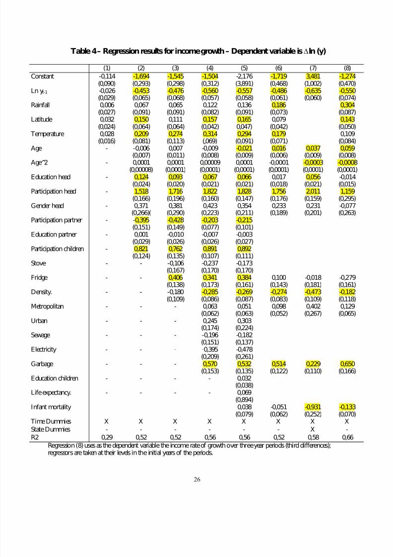
Table 4 reports the results of the first-differences specifications, with the inclusion of theinitial level of income as a regressor. In the first column, one can see that there is no significantunconditional relationship between changes in income and the “pure” geographical variables; thesame holds for the initial income level. The results become a bit more interesting when controls forhuman capital and labor force participation are included (Column 2). It can be seen that the initiallevel of income presents a significant negative sign, indicating the states with lower initial income

levels tend to grow faster than states with higher income levels. Latitude and temperature appear assignificant, with the same conflict of signs as in the results of Table 3.7 The signs for education andlabor force participation are the same as in the regressions with income levels presented before: themore educated the household head and the children, the higher the labor force participation and thelower the partner’s participation in the labor force, the higher the income growth.

6 Notice that the geographical variables as well as the state dummy variables are time invariant. As such, they are substitutes for each other and

cannot enter simultaneously in the regression.7 The same experiments for the equations in levels of income presented similar results in this case, indicating that latitude is the most stable of the

geographical variables considered in the study.



17

The inclusion of household capital and density information (Column 3) causes latitude to benon-significant but does not change the sign and significance of the initial level of income and of temperature. Only refrigerator possession is (positively) associated with income growth. All theeducation and labor force participation variables keep their status as in the previous column. Theinclusion of the metropolitan/urban/ rural situation and public infrastructure made in Column (4)makes latitude and density significant, as compared to the previous column. Of the newly includedvariables, only connection to public garbage collection is (positively) associated with income growthand density becomes significant. In Column (5) all variables are included, the last being childreneducation and human development variables, which turned out to be insignificant. No importantchanges with respect to the results of Column (4) are observed.

Column (6) drops some of the variables to deal with multicolinearity among the regressors.Comparing Columns (5) and (6), there is a substitution of rainfall for latitude. Education of thehousehold head and refrigerator possession both become insignificant; there is also a small decreasein R2. Equation (7) substitutes state dummies for the geographical variables, with a small gain in R2

and some minor changes in results: now life cycle variables and education of the household headbecome significant, while refrigerator possession becomes insignificant. As in the regression in

income levels, infant mortality appears as negative and significant, indicating that states with higherinfant mortality tend to grow less than states with lower infant mortality levels.

Finally, in Column (8) income growth was measured in third-differences and all right hand-side variables at their levels in the initial year of the three-year periods to address causality concerns.As can be seen, the initial income remains as significant as in the other specifications. Rainfall andlatitude appear as significant, with the same sign contradiction; life cycle indicators are significantand with the expected signs; education of the household head, however, appears as insignificant, andwith a wrong sign. Labor force participation, density, garbage and infant mortality present the sameresults as before. Thus, even taking into account possible causality problems, the main results seemto hold.

Considering these results on income growth, it is clear that the initial level of income is animportant variable, being present in all specifications. The same holds for the participation of thehousehold head and children (positive sign) and partner (negative sign) in the labor force. Density isalways negative, but significant in only three out of six specifications. Education of the householdhead is significant in six out of eight specifications; household capital (refrigerator possession) ispositive and significant in four out of six specifications. Public infrastructure, represented by garbagecollection, was positive and significant in all cases it was included in the regressions. Among thegeographical variables, temperature is significant in five out of seven specifications and latitude infour, with the contradictory signs commented on before.

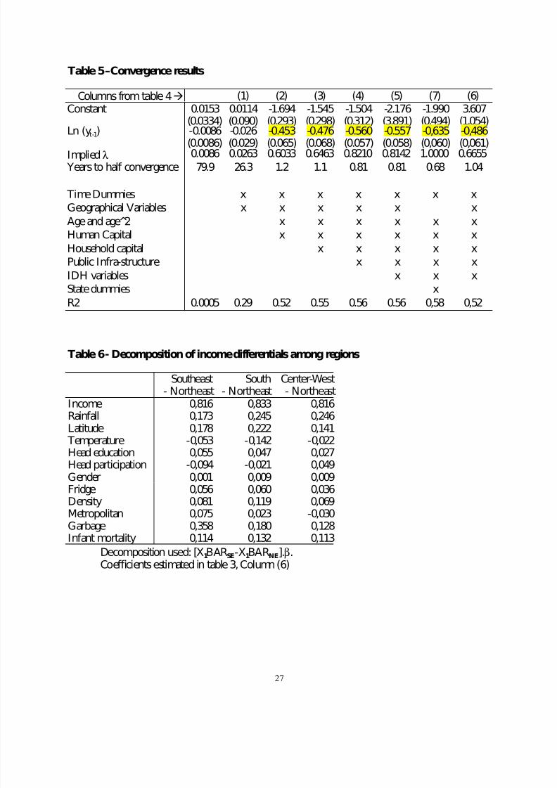
As mentioned before, in all specifications but the first, the coefficient for the lagged incomeis negative and significant, indicating that states with smaller levels of initial income tend to havefaster income growth. In Table 5 the coefficients on the lagged dependent variable for the differentspecifications of Table 4 are presented again, together with the implied λ and the estimated velocityto half convergence (column numbers are the same as in Table 4). In the first column there are noother variables apart from the lagged dependent variable. The estimated coefficient is very small andnot significantly different from zero, which basically implies persistence in income differencesamong states. That is, there is no evidence of absolute convergence among states in Brazil in the



18

period analyzed. Column (1) includes the time dummies and pure geographical variables, with noimportant changes in the results. Column (2) adds age, age squared and human capital variables, withimportant changes in the results, for now the coefficient on the initial year income is negative andsignificant. The impliedλ and the resulting number of years to achieve half convergence are alsoshown in the table. Column (3) adds household capital variables, increasing marginally the speed of

convergence. In Column (4) the public infrastructure variables are added, and the speed of convergence increases reasonably, implying 0.8 years for half convergence. The introduction of human development variables additionally increases the speed of convergence, as shown in Column(5). Reducing the number of variables to decrease multicolinearity returns the speed of convergenceback to the same level of Column (3). The substitution of dummy variables for geographicalvariables, as done in Column (7), causes the speed of convergence to increase and the number of years to half convergence to be 1.04.

All in all, the results indicate a very high speed of convergence of income among Brazilianstates, after provision is made for differences in geography, human capital, labor force participation,infra-structure and human development conditions. It is interesting to point out that in this case weare dealing with conditional convergence; that is, each state is converging to its own steady statesituation. Thus, instead of indicating a positive situation, in which inequalities among states in Brazilwould be diminishing at a high speed, the results show that the states are close to their steady stateincome levels, meaning that the resulting equilibrium inequality situation is close to the highinequality level presently observed in the country. This result is perfectly compatible with the above-mentioned absence of absolute (or unconditional) convergence of income in Brazil. The differentstate provisions of education, infrastructure, etc. prevent the equalization of income levels acrossstates.

Table 6 shows the results of the decomposition of the observed differences in per capitaincome across regions. It is interesting to highlight the fact that the Northeast/Southeast observeddifferences in per capita income are pretty much the same as the Northeast/ Center-West

differences; the South/ Northeast differences are slightly higher but in the same value range as theother two. This is expected, considering the information on regional incomes presented in Figure 1. The most important variables in explaining these differences are the geographical variables rainfalland latitude, infrastructure capital, represented by the existence of a public system for garbagecollection, and infant mortality. Other variables present a much smaller importance in thedecomposition. Temperature appears as important in explaining differences between the South andthe Northeast only.

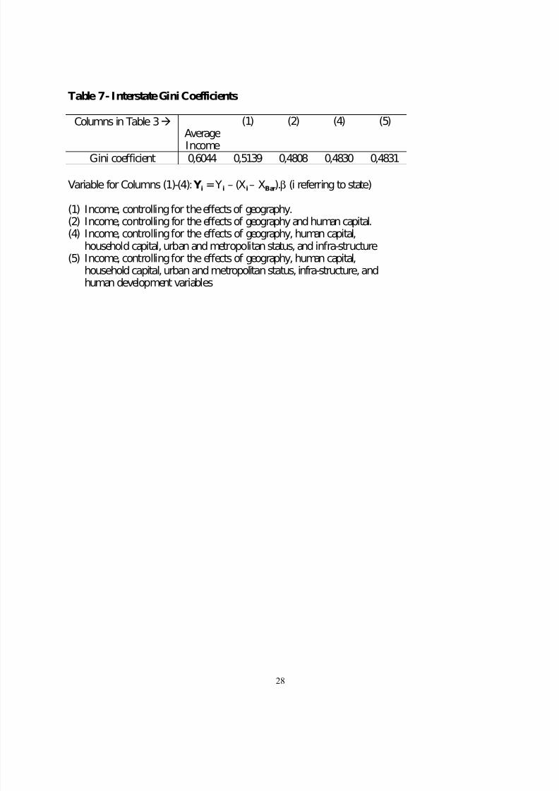
Table 7 shows the Gini inequality index across states in Brazil (weighted by the populationof each state). The number in the first column (Average Income) is representative of inequality usingthe observed income data. The inclusion of geographical variables causes a drop of 15% in the Gini

coefficient. The addition of human capital variables reduces the coefficient by another 6.4% (ascompared to its already lower value). The further inclusion of public infrastructure and householdcapital does not produce any noticeable change in the Gini coefficient.



19

7. Conclusions and Policy Implications

The main objective of this paper is to shed some light on the effects of geographical variables on theper capita income patterns of growth of Brazilian states. To achieve this aim, we proposed, for thefirst time in this strand of the literature, a methodology to examine the issue of convergence usingmicro-data. We constructed cohort/ state/year averages of all variables of interest, and regressedincome levels and income growth on a variety of human capital, life cycle and geographical variables.

The main results indicate that geographical variables are important in explaining thedifferences in income levels and in growth across Brazilian states. This is shown by their joint impacton the level and growth regressions. The results also show that there is no sign of absoluteconvergence in Brazil in the period analyzed. On the other hand, conditional convergence will takeplace rapidly in Brazil, once human capital, infrastructure and geographical variables are controlledfor. The estimated high speeds of conditional convergence indicate that Brazilian states are close totheir steady state levels of income, indicating that the equilibrium regional income inequality in thecountry is not much different from the present one.

Considering the prospects of government intervention, it is clear that investments in publicinfra-structure do play a role, especially in reducing the differences between the Southeast and theNortheast (after controlling for differences in the provision of garbage collection services, incomeinequality among those regions drops to 36%, from the previous 82%). Other important factors inthe regressions are household density (number of persons per room) and household capital(refrigerator possession). Human capital variables appear as significant in general, especiallyparticipation in the labor force. However, the decomposition of income differentials indicates aminor quantitative role for this variable. However, no control is made for variations in the quality of education provided among states, and recent indications are that poorer states also present poorereducation quality. Unfortunately, there is no information on this variable for the period considered. Thus, investments in this area, although with a positive impact, do not seem to have a major

influence on the levels of income inequality in the country. Investments in the quality of educationmight have a better effect, although no evidence on that aspect can be derived from this study.

As for geographical variables, they enter significantly into most regressions, meaning that,even after controlling for differences in education, labor force participation, social and privatecapital, etc., there still are differences among states that are related to geographical aspects. Thedecomposition of income differentials indicates that these variables are quantitatively veryimportant. The variable rainfall is nature-related and probably includes its effects on agriculturalproductivity. Latitude, on the other hand, could be understood as encompassing institutional,cultural, religious and other sorts of regional characteristics that influence the productivity of factorsin the regional production functions.

The same conclusion can be drawn from the results of the specifications that substitutedstate dummies for geographical variables, with the coefficients of the dummies being significant,leading to the same interpretation on the geographical aspects considered. Another indication in thisdirection is the relatively low R2 in the growth equations, indicating that other factors but the onesincluded in the regressions may account for the variance in the state’s rates or growth. Thisargument is not valid for the level regressions, since the R2 there are over .9. Unfortunately, it isimpossible to draw any conclusive lesson from the results on the state dummies, although they are



20

interesting enough to suggest that institutional differences may have an important role in shapingregional inequality in Brazil.

In general, the results of this study indicate that investments in public infrastructure and ineducation may help reducing regional inequality in Brazil. Another important aspect is participationin the labor force, for this variable appeared almost always as an important factor in the definition of income levels and income growth. Thus, provision of job opportunities seems to be a relevantfactor.

Even after considering the positive expected effects of public investments, there is someindication that income inequality is self-fulfilling, for wealthier states and states with dynamic labormarkets tend to have higher income levels and to growth faster. Moreover, the importance of geographical variables indicates that probably a good deal of government intervention should bedirected towards institution building, government efficiency improvement, etc. Even aftercontrolling for variables related to human, household and social capital, there still is a great deal tobe explained in terms of differences in income growth between Brazilian states.



21

References

Attanasio, O. and Browning, M. 1995. “Consumption over the Life Cycle and the Business Cycle.”American Economic Review . 85 (5): 1118-1136.

Azzoni, C. 1999. “Economic Growth and Regional Income Inequalities in Brazil.” Annals of Regional Science . Forthcoming.

Barro, R. and Sala-i-Martin, X. 1995.Economic Growth . New York, United States: McGraw Hill.

---- 1997. “Technological Diffusion, Convergence, and Growth.” Journal of Economic Growth . 2 (1): 1-26

Barro, R., Mankiw, G. and Sala-I-Martin, X. 1995. “Capital Mobility in Neoclassical Models of Growth.” NBER Working Paper 4206. Cambridge, United States: National Bureau of EconomicResearch.

Blundell, R., Browning, M and Meghir, C. 1994. “Consumer Demand and the Life-Cycle Allocationof Household Expenditures.”Review of Economic Studies . 61 (1): 57-80.

Browning, M., Deaton, A. and Irish, M. 1985. “A Profitable Approach to Labor Supply andCommodity Demands Over the Life Cycle.”Econometrica . 53 (3): 503-544.

Chang, R. 1994. “Income Inequality and Economic Growth: Evidence and Recent Theories.”Economic Review, Federal Reserve Bank of A tlanta . 79: 1-9.

Deaton, A. 1985. “Panel Data from Time Series of Cross-Sections.” Journal of Econometrics .30: 109-126.

Ferreira, A. H. and Diniz, C C. 1995 “Convergencia entre las rentas per capita estaduales en Brasil.”EURE-Revista Latioamericana de Estudios Urbano Regionales. 21 (62): 17-31.

Hall,R. and Jones, C. 1996. “The Productivity of Nations.” NBER Working Paper 5812.Cambridge, United States: National Bureau of Economic Research

Helliwell, John, 1996. “Do Borders Matter for Social Capital? Economic Growth and Civic Culturein U.S. States and Canadian Provinces.” NBER Working Paper 5863. Cambridge, United States:National Bureau of Economic Research.

Islam, N. 1995. “Growth Empirics: A Panel Data Approach.”Quarterly Journal of Economics .110 (4): 1127-1170.

Jalan, J. and Ravallion, M. 1998a. “Are There Dynamic Gains from a Poor-Area DevelopmentProgram?”Journal of Public Economics . 67 (1): 65 - 85.

---- 1998b. “Geographic Poverty Traps?” Discussion Paper No. 86. Boston, United States: BostonUniversity, Institute for Economic Development.



22

Jones, C. 1995a. “Times Series Tests of Endogenous Growth Models.”Quarterly Journal of Economics.110 (2): 495-525.

----. 1995b. “R & D Based Models of Economic Growth.” Journal of Political Economy . 101 (4): 759-784.

---- 1997. “On the Evolution of the World Income Distribution.” NBER Working Paper 5812.Cambridge, United States: National Bureau of Economic Research.

Moffitt, R. 1993. “Identification and Estimation of Dynamic Models with a Time Series of Repeated Cross-Sections.” Journal of Econometrics. 59: 99-123.

Moulton, B. 1986. “Random Group Effects and the Precision of Regression Estimates.” Journal

of Econometrics. 32: 385-397.

Ravallion, M. 1998a. “Poor Areas.” In: A. Ullah and D. Giles, editors. Handbook of Applied

Economic Statistics. New York, United States: Marcel Dekker, Inc.

----. 1998b. “Reaching Poor Areas in a Federal System.” Policy Research Group Working Paper

1901. Washington, DC, United States: World Bank.

Ravallion, M. and Jalan, J. 1996. “Growth Divergence Due to Spatial Externalities.” Economic Letters. 53 (2): 227-232.

Ravallion, M.and Wodon, Q. 1998. “Poor Areas or Just Poor People?” Policy Research Working

Paper 1798. Washington, DC, United States: World Bank.

Romer, P. 1986. “Increasing Returns and Long Run Growth.” Journal of Political Economy.94: 1002-37.

Solow, R.W. 1956. “ A Contribution to the Theory of Economic Growth.” Quarterly Journal of

Economics. 70: 65-94.

Schwartsman, A. 1996. “Convergence Across Brazilian States.” Discussion Paper, nº 02/96. SãoPaulo, Brazil: Universidade de São Paulo, IPE.

Swan, T.W. 1956. “Economic Growth and Capital Accumulation.” Economic Record. 32: 334-

61.

Zini, A. A., Jr. 1998. “Regional Income Convergence in Brazil and its Socio-EconomicDeterminants.” Economia Aplicada. 2 (2): 383-411.



23

Table 1: Description of the main variables

Code Brazil NE and CO South and SE

Avg SD Avg SD Avg SDDependent Variable:

Monthly per capita household income y 71103 156911 56522 121330 96097 201583

Family:

Gender of the household head (male = 1; female = 0) Gender_head 0,835 0,079 0,832 0,077 0,840 0,081

Education : years of education of household head Educ_head 3,858 1,654 3,199 1,367 4,987 1,486

Education of partner Educ_part 3,151 1,429 2,747 1,305 3,845 1,366

Participation in the labor market (hh head previous week) Part_head 0,847 0,161 0,857 0,145 0,830 0,183

Participation of partner Part_part 0,304 0,115 0,298 0,111 0,315 0,119

Participation of children (average) Part_child 0,246 0,171 0,238 0,161 0,260 0,187

Household:

Density – occupants per room HH dens. 0,913 0,206 0,982 0,203 0,796 0,152

Availability of stove (yes = 1; no = 0) Stove 0,915 0,110 0,876 0,121 0,983 0,016

Availability of refrigerator (yes = 1; no = 0) Fridge 0,572 0,208 0,457 0,147 0,771 0,136

Electricity (supplied with electricity = 1; not supplied = 0) Electricity 0,769 0,166 0,694 0,152 0,898 0,092

Water (supplied by the public system = 1; not supplied = 0) Water 0,621 0,185 0,522 0,140 0,792 0,116

Sewage (served by the public system = 1; not served = 0) Sewage 0,484 0,170 0,387 0,108 0,650 0,122

Garbage (served by the public system = 1; not served = 0) Garbage 0,497 0,191 0,418 0,163 0,633 0,157

Geographical:

Urban/rural (urban = 1; rural = 0) Metrop. 0,164 0,227 0,082 0,149 0,303 0,266

Metropolitan region (metropolitan = 1; non-metropolitan=0) Urban 0,675 0,140 0,618 0,121 0,773 0,114

Life Expectancy (IDH) Life exp. 61,199 4,001 59,694 3,640 63,778 3,196

Infant Mortality (IDH) Infant mort 65,473 35,407 82,187 34,048 36,821 10,758

Average temperature in the Winter - Celsius degrees Temp 19,892 4,334 21,778 3,738 16,661 3,241

Latitude – degrees Latitude -13,315 7,094 -8,839 3,049 -20,987 5,240

Rainfall – mm/year Rain fall 103,039 24,553 92,485 22,393 121,133 16,079



24

Table 2 – Correlation coefficient among variables

Ln(y) ∆ln(y) Educ_ head

Gender head

Part_ head

Educ_ part

Part_ ch

Stove Fridge HHdens

Metrop Urban Water Electricity

Sewage Garbage Rainfa

Ln(y) 1

∆ ln(y) 0.378* 1

Educ_head 0.710* 0.134* 1

Gender_head 0.541* 0.178* 0.497* 1

Part_head 0.208* 0.110* 0.418* 0.321* 1

Educ_part 0.664* 0.153* 0.946* 0.656* 0.517* 1

Part_children -0.266* -0.095* -0.594* -0.677* -0.233* -0.710* 1

Stove 0.433* 0.033 0.476* -0.012 0.043* 0.385* 0.048* 1

Fridge 0.558* 0.036 0.658* -0.051* 0.252* 0.495* 0.107* 0.666* 1

HH Density 0.002 0.077* -0.187* 0.488* 0.159* -0.011 -0.255* -0.492* -0.561* 1

Metrop 0.296* 0.008 0.414* -0.078* -0.013 0.255* -0.063* 0.316* 0.419* -0.174* 1

Urban 0.508* 0.063* 0.652* -0.039* 0.039* 0.494* -0.072* 0.711* 0.773* -0.485* 0.605* 1

Water 0.554* 0.053* 0.617* -0.019 0.004 0.467* 0.031 0.698* 0.838* -0.506* 0.448* 0.785* 1

Electricity 0.455* 0.039* 0.662* -0.074* 0.264* 0.531* -0.019 0.743* 0.881* -0.612* 0.376* 0.805* 0.818* 1

Sewage 0.536* 0.029 0.605* -0.059* -0.03 0.429* 0.054* 0.690* 0.821* -0.508* 0.535* 0.839* 0.853* 0.792* 1

Garbage 0.505* 0.03 0.609* -0.071* 0.093* 0.460* 0.011 0.672* 0.818* -0.527* 0.447* 0.864* 0.800* 0.834* 0.830* 1

Rainfall0.419* 0.002 0.314* 0.144* 0.050* 0.221* 0.086* 0.105* 0.490* -0.191* 0.073* 0.165* 0.327* 0.231* 0.364* 0.270* 1

Latitude 0.607* 0.033 0.548* 0.067* -0.002 0.384* 0.063* 0.581* 0.788* -0.495* 0.377* 0.602* 0.749* 0.630* 0.704* 0.645* 0.645*

Temp -0.546* -0.033 -0.450* -0.099* -0.040* -0.333* -0.062* -0.547* -0.664* 0.451* -0.228* 0.498* -0.592* -0.535* -0.510* -0.541* -0.454*

life expec. 0.251* 0 0.473* -0.157* 0.449* 0.362* 0.119* 0.419* 0.738* -0.620* 0.158* 0.463* 0.485* 0.681* 0.505* 0.539* 0.429*

infant mort. -0.455* -0.01 -0.530* 0.018 -0.189* -0.391* -0.103* -0.519* -0.775* 0.563* -0.214* 0.536* -0.624* -0.6175* -0.642* -0.539* -0.605*



25

Table 3 - Regression results for income levels – dependent variable is ln (y)(1) (2) (3) (4) (5) (6) (7)

Constant -0,064(0,692)

-2,942(0,494)

-2,734(0,421)

-2,369(0,459)

-0,436(5,552)

-2,894(0,720)

3,697(0,770)

Rainfall 0,424(0,222)

0,236(0,195)

0,219(0,198)

0,301(0,136)

0,303(0,151)

0,443(0,153)

Latitude 0,563(0,113)

0,327(0,108)

0,236(0,107)

0,284(0,056)

0,281(0,063)

0,163(0,081)

Temperature 0,206(0,155)

0,351(0,159)

0,470(0,199)

0,4640,129)

0,455(0,170)

0,316(0,170)

Age - 0,009(0,012)

0,008(0,019)

0,003(0,013)

-0,003(0,013)

0,041(0,009)

0,063(0,011)

Age 2 - -0,0008(0,0001

-0,0001(0,0002)

-0,0001(0,0001)

-0,00004(0,0001)

-0,0004(0,0001)

-0,001(0,0001)

Education head - 0,241(0,051)

0,168(0,035)

0,093(0,029)

0,089(0,028)

-0,002(0,035)

0,060(0,024)

Participation head - 2,390(0,227)

2,726(0,257)

2,656(0,206)

2.637(0,193)

2,775(0,156)

2,713(0,127)

Gender head - 0,621(0,400)(

0,636(0,418)

0,689(0,299)

0,617(0,284)

0,290(0,261)

0,209(0,200)

Participation partner - -0,855(0,304)

-0,885(0,289)

-0,451(0,131)

-0,439(0,166)

Education partner - -0,024(0,057)

-0,047(0,044)

-0,019(0,035)

-0,017(0,037)

Participation children - -1,442(0,230) 1,225(0,230)- 1,326(0,161) 1,320(0,164)Stove - - -0,204

(0,251)-0,408(0,243)

-0,374(0,238)

Fridge - - 0,821(0,280)-

0,529(0,278)

0,528(0,224)

0,184(0,249)

-0,061(0,230)

Density. - - -0,365(0,188)

-0,504(0,135)

-0,457(0,128)

-0,585(0,138)

-0,781(0,137)

Metropolitan - - - 0,180(0,118)

0,191(0,120)

0,275(0,131)

0,469(0,351)

Urban - - - 0,422(0,247)

0,401(0,302)

Sewage - - - -0,392(0,256)

-0,381(0,255)

Electricity - - - -0,521(0,303)

-0,523(0,348)

Garbage - - - 0,896

(0,231)

0,894

(0,190)

0,949

(0,214)

0,320

(0,134)Education children - - - - 0,138(0,071)

Life Expectancy - - - - -0,401(1,297)

Infant Mortality -0,030(0,130)

-0,125(0,123)

-1,101(0,239)

Time Dummies x X X X X X X

State Dummies - - - - - - x

R2 0,48 0,88 0,89 0,91 0,91 0,89 0,92



26

Table 4 – Regression results for income growth – Dependent variable is∆ln (y)

(1) (2) (3) (4) (5) (6) (7) (8)Constant -0,114

(0,090)-1,694(0,293)

-1,545(0,298)

-1,504(0,312)

-2,176(3,891)

-1,719(0,468)

3,481(1,002)

-1,274(0,470)

Ln yt-1 -0,026

(0,029)

-0,453

(0,065)

-0,476

(0,068)

-0,560

(0,057)

-0,557

(0,058)

-0,486

(0,061)

-0,635

(0,060)

-0,550

(0,074)Rainfall 0,006

(0,027)0,067(0,091)

0,065(0,091)

0,122(0,082)

0,136(0,091)

0,186(0,073)

0,304(0,087)

Latitude 0,032(0,024)

0,150(0,064)

0,111(0,064)

0,157(0,042)

0,1650,047)

0,079(0,042)

0,143(0,050)

Temperature 0,028(0,016)

0,209(0,081)

0,274(0,113)

0,314(,069)

0,294(0,091)

0,179(0,071)

0,109(0,084)

Age - -0,006(0,007)

0,007(0,011)

-0,009(0,008)

-0,021(0,009)

0,016(0,006)

0,037(0,009)

0,059(0,008)

Age 2 - 0,0001(0,00008)

0,0001(0,0001)

0,00009(0,0001)

0,0001(0,0001)

-0,0001(0,0001)

-0,0003(0,0001)

-0,0008(0,0001)

Education head - 0,124(0,024)

0,093(0,020)

0,067(0,021)

0,066(0,021)

0,017(0,018)

0,056(0,021)

-0,014(0,015)

Participation head - 1,518(0,166)

1,716(0,196)

1,822(0,160)

1,828(0,147)

1,756(0,176)

2,011(0,159)

1,159(0,295)

Gender head - 0,371(0,266)(

0,381(0,290)

0,423(0,223)

0,354(0,211)

0,233(0,189)

0,231(0,201)

-0,077(0,263)

Participation partner - -0,395(0,151)

-0,428(0,149)

-0,203(0,077)

-0,215(0,101)

Education partner - 0,001(0,029)

-0,010(0,026)

-0,007(0,026)

-0,003(0,027)

Participation children - 0,821(0,124)

0,762(0,135)

0,891(0,107)

0,892(0,111)

Stove - - -0,106(0,167)

-0,237(0,170)

-0,173(0,170)

Fridge - - 0,406(0,138)

0,341(0,173)

0,384(0,161)

0,100(0,143)

-0,018(0,181)

-0,279(0,161)

Density. - - -0,180(0,109)

-0,285(0,086)

-0,269(0,087)

-0,274(0,083)

-0,473(0,109)

-0,182(0,118)

Metropolitan - - - 0,063(0,062)

0,051(0,063)

0,098(0,052)

0,402(0,267)

0,129(0,065)

Urban - - - 0,245(0,174)

0,303(0,224)

Sewage - - - -0,196(0,151)

-0,182(0,137)

Electricity - - - -0,395(0,209)

-0,478(0,261)

Garbage - - - 0,570(0,153)

0,532(0,135)

0,514(0,122)

0,229(0,110)

0,650(0,166)

Education children - - - - 0,032(0,038)

Life expectancy. - - - - 0,069(0,894)

Infant mortality 0,038(0,079)

-0,051(0,062)

-0,931(0,252)

-0,133(0,070)

Time Dummies X X X X X X X XState Dummies - - - - - - X -R2 0,29 0,52 0,52 0,56 0,56 0,52 0,58 0,66

Regression (8) uses as the dependent variable the income rate of growth over three year periods (third differences);regressors are taken at their levels in the initial years of the periods.



27

Table 5 –Convergence results

Columns from table 4à (1) (2) (3) (4) (5) (7) (6)Constant 0.0153

(0.0334)0.0114(0.090)

-1.694(0.293)

-1.545(0.298)

-1.504(0.312)

-2.176(3.891)

-1.990(0.494)

3.607(1.054)

Ln (yt-1

) -0.0086(0.0086)

-0.026(0.029)

-0.453(0.065)

-0.476(0.068)

-0.560(0.057)

-0.557(0.058)

-0,635(0,060)

-0,486(0,061)

Impliedλ 0.0086 0.0263 0.6033 0.6463 0.8210 0.8142 1.0000 0.6655 Years to half convergence 79.9 26.3 1.2 1.1 0.81 0.81 0.68 1.04

Time Dummies x x x x x x xGeographical Variables x x x x x xAge and age 2 x x x x x xHuman Capital x x x x x xHousehold capital x x x x xPublic Infra-structure x x x x

IDH variables x x xState dummies xR2 0.0005 0.29 0.52 0.55 0.56 0.56 0,58 0,52

Table 6 - Decomposition of income differentials among regions

Southeast- Northeast

South- Northeast

Center-West- Northeast

Income 0,816 0,833 0,816

Rainfall 0,173 0,245 0,246Latitude 0,178 0,222 0,141 Temperature -0,053 -0,142 -0,022Head education 0,055 0,047 0,027Head participation -0,094 -0,021 0,049Gender 0,001 0,009 0,009Fridge 0,056 0,060 0,036Density 0,081 0,119 0,069Metropolitan 0,075 0,023 -0,030Garbage 0,358 0,180 0,128Infant mortality 0,114 0,132 0,113

Decomposition used: [X1BARSE-X1BARNE].β.Coefficients estimated in table 3, Column (6)



28

Table 7 - Interstate Gini Coefficients

Columns in Table 3à

AverageIncome

(1) (2) (4) (5)

Gini coefficient 0,6044 0,5139 0,4808 0,4830 0,4831

Variable for Columns (1)-(4): Y i = Yi – (Xi– XBar).β (i referring to state)

(1) Income, controlling for the effects of geography.(2) Income, controlling for the effects of geography and human capital.(4) Income, controlling for the effects of geography, human capital,

household capital, urban and metropolitan status, and infra-structure(5) Income, controlling for the effects of geography, human capital,

household capital, urban and metropolitan status, infra-structure, andhuman development variables



29

Table 8 – Variables averages and standard deviations by stateVariable São Paulo Rio de Janeiro Minas Gerais Paraná Santa

CatarinaRio Grande

do SulEspírito santo

Avg SD Avg SD Avg SD Avg SD Avg SD Avg SD Avg SD

Y 120970

246894117826 236551 70110 142470

84753 171656

94613205678108813

227253

75598152146

Genderhead

0,836 0,076 0,797 0,087 0,828 0,084 0,858 0,066 0,875 0,076 0,836 0,078 0,849 0,076

Educ_head 5,551 1,255 6,292 1,050 4,239 1,246 4,363 1,466 4,860 1,445 5,213 1,322 4,393 1,385Educ_part 4,080 1,308 4,344 1,199 3,408 1,312 3,402 1,378 4,003 1,360 4,132 1,333 3,542 1,356Part_head 0,813 0,204 0,791 0,218 0,830 0,165 0,856 0,156 0,836 0,182 0,842 0,173 0,840 0,168Part_part 0,261 0,099 0,274 0,090 0,262 0,106 0,322 0,106 0,382 0,120 0,391 0,119 0,314 0,112Part_child 0,259 0,190 0,210 0,160 0,255 0,185 0,293 0,193 0,295 0,204 0,244 0,168 0,267 0,193Density 0,834 0,153 0,785 0,127 0,796 0,136 0,861 0,168 0,744 0,153 0,741 0,146 0,810 0,138Stove 0,988 0,011 0,984 0,010 0,983 0,011 0,978 0,017 0,976 0,026 0,986 0,010 0,985 0,017Fridge 0,881 0,068 0,878 0,065 0,601 0,101 0,690 0,114 0,838 0,078 0,816 0,076 0,690 0,118Electricity 0,963 0,075 0,973 0,019 0,806 0,101 0,853 0,096 0,928 0,039 0,899 0,053 0,865 0,089Water 0,934 0,033 0,869 0,062 0,742 0,072 0,751 0,095 0,734 0,144 0,793 0,086 0,723 0,092Sewage 0,851 0,041 0,750 0,044 0,681 0,046 0,572 0,032 0,506 0,061 0,549 0,052 0,638 0,048Garbage 0,890 0,032 0,722 0,065 0,527 0,082 0,619 0,104 0,543 0,132 0,654 0,085 0,478 0,084

Metropolitan

0,514 0,030 0,804 0,028 0,220 0,029 0,246 0,024 - - 0,340 0,029 - -

Urban 0,923 0,013 0,941 0,016 0,739 0,036 0,717 0,056 0,654 0,065 0,741 0,049 0,695 0,062Life exp. 63,78 3,31 62,27 2,72 62,74 3,38 63,71 3,00 65,38 2,83 65,46 2,72 63,10 2,91Infantmort

36,43 9,10 38,11 11,94 41,42 10,50 41,98 10,58 34,46 9,33 26,07 6,27 39,28 7,95

Temperature

16,82 - 18,32 - 18,26 - 14,12 - 13,46 - 12,89 - 22,76 -

Latitude -21,27 - -21,16 - -18,17 - -22,85 - -26,31 - -26,96 - -10,19 -Rain fall 127,98 - 113,36 - 119,45 - 132,17 - 143,9

0- 122,44 - 88,63 -



30

Table 8 – Variables averages and standard deviations by state (continued)Variable Rio Grande do

NortePariba Pernambuco Alagoas Sergipe Bahia Mato

dAvg SD Avg SD Avg SD Avg SD Avg SD Avg SD Avg

Y 50877 104970 43305 88464 55808108992

50889 111278 53628 109881

57743 114035

9009

Genderhead

0,833 0,085 0,814 0,083 0,808 0,077 0,824 0,090 0,805 0,091 0,823 0,072 0,861

Educ_head 3,276 1,196 3,236 1,279 3,479 1,031 2,780 1,132 3,084 1,199 3,071 1,088 4,284

Educ_part 3,044 1,328 3,050 1,398 2,879 1,170 2,239 1,135 2,666 1,217 2,467 1,050 3,420Part_head 0,838 0,160 0,831 0,146 0,824 0,159 0,821 0,178 0,843 0,160 0,869 0,129 0,874Part_part 0,290 0,105 0,286 0,113 0,288 0,087 0,271 0,100 0,313 0,109 0,304 0,090 0,273Part_child 0,218 0,158 0,217 0,146 0,230 0,154 0,236 0,156 0,236 0,165 0,229 0,157 0,247Density 0,977 0,173 0,946 0,179 0,938 0,159 0,994 0,180 0,962 0,186 0,952 0,159 0,842Stove 0,867 0,063 0,940 0,027 0,938 0,024 0,845 0,070 0,923 0,035 0,892 0,037 0,967Fridge 0,457 0,110 0,403 0,101 0,468 0,091 0,442 0,112 0,497 0,130 0,417 0,074 0,669Electricity 0,784 0,108 0,734 0,106 0,785 0,079 0,735 0,111 0,751 0,119 0,669 0,085 0,820Water 0,578 0,066 0,600 0,067 0,595 0,077 0,500 0,078 0,593 0,091 0,510 0,057 0,691Sewage 0,418 0,068 0,428 0,053 0,452 0,056 0,352 0,062 0,407 0,066 0,372 0,053 0,505Garbage 0,560 0,090 0,492 0,079 0,461 0,075 0,455 0,110 0,473 0,098 0,357 0,058 0,600

Metropolitan - - - - 0,410 0,038 - - - - 0,224 0,040 -

Urban 0,665 0,047 0,651 0,050 0,720 0,041 0,588 0,070 0,613 0,101 0,579 0,054 0,766Life exp. 58,45 4,07 57,53 3,55 58,84 2,76 56,71 2,76 59,07 3,41 60,52 2,92 63,06nfant

mort107,19 27,67 113,48 25,94 100,7

722,36 122,99 17,54 79,95 14,49 70,91 11,61 37,02

Temperature

- - 22,84 - 21,97 - 23,63 - 22,76 - 18,69 - 13,04

Latitude - - -6,83 - -8,05 - -8,67 - -10,19 - -10,84 - -14,2Rain fall - - 67,76 - 63,46 - 91,10 - 88,63 - 76,33 - 84,08

Documents

Geography and Income Convergence 13