No. 04 [v. 05]

2012

GEOGRAPHYENVIRONMENTSUSTAINABILITY

RUSSIAN GEOGRAPHICAL SOCIETY

FACULTY OF GEOGRAPHY,

M.V. LOMONOSOV MOSCOW STATE UNIVERSITY

INSTITUTE OF GEOGRAPHY,

RUSSIAN ACADEMY OF SCIENCES

gi412.indd 1gi412.indd 1 24.12.2012 9:10:3424.12.2012 9:10:34

2

GES

04|

2012

EDITORIAL BOARD

EDITORSINCHIEF:Kasimov Nikolay S.Lomonosov Moscow State University, Faculty of GeographyRussia

Kotlyakov Vladimir M.Russian Academy of SciencesInstitute of GeographyRussia

Vandermotten ChristianUniversité Libre de BruxellesBelgique

Tikunov Vladimir S. (Secretary-General)Lomonosov Moscow State University,Faculty of Geography, RussiaBabaev Agadzhan G.Turkmenistan Academy of Sciences,Institute of deserts, TurkmenistanBaklanov Petr Ya.Russian Academy of Sciences,Pacific Institute of Geography, RussiaBaume Otfried,Ludwig Maximilians Universitat Munchen,Institut fur Geographie, GermanyChalkley BrianUniversity of Plymouth, UKDmitriev Vasily V.St-Petersburg State University, Faculty ofGeography and Geoecology, RussiaDobrolubov Sergey A.Lomonosov Moscow State University,Faculty of Geography, RussiaD’yakonov Kirill N.Lomonosov Moscow State University,Faculty of Geography, RussiaGritsay Olga V.Russian Academy of Sciences,Institute of Geography, RussiaGunin Petr D.Russian Academy of Sciences,Institute of Ecology and Evolution, RussiaGuo Hua TongChinese Academy of Sciences, ChinaHayder AdnaneAssociation of Tunisian Geographers, TunisiaHimiyama YukioHokkaido University of Education,Institute of Geography, JapanKolosov Vladimir A.Russian Academy of Sciences,Institute of Geography, RussiaKonečný MilanMasaryk University,Faculty of Science, Czech RepublicKroonenberg Salomon,Delft University of TechnologyDepartment of Applied Earth Sciences,The Netherlands

O’Loughlin JohnUniversity of Colorado at Boulder,Institute of Behavioral Sciences, USAMalkhazova Svetlana M.Lomonosov Moscow State University,Faculty of Geography, RussiaMamedov RamizBaku State University,Faculty of Geography, AzerbaijanMironenko Nikolay S.Lomonosov Moscow State University,Faculty of Geography, RussiaNefedova Tatyana G.Russian Academy of Sciences,Institute of Geography, RussiaPalacio-Prieto JoseNational Autonomous University of Mexico,Institute of Geography, MexicoPalagiano CosimoUniversita degli Studi di Roma “La Sapienza”,Instituto di Geografia, ItalyRadovanovic MilanSerbian Academy of Sciences and Arts,Geographical Institute “Jovan Cvijić”, SerbiaRichling AndrzejUniversity Warsaw, Faculty of Geography and Regional Studies, PolandRudenko Leonid G.National Ukrainian Academyof Sciences, Institute of GeographyUkraineSolomina Olga N.Russian Academy of Sciences,Institute of Geography, RussiaTishkov Arkady A.Russian Academy of Sciences,Institute of Geography, RussiaThorez PierreUniversité du Havre – UFR “Lettreset Sciences Humaines” FranceVargas Rodrigo BarrigaMilitary Geographic Institute, ChileViktorov Alexey S.Russian Academy of Sciences,Institute of Environmental Geosciences, RussiaZilitinkevich Sergey S.Finnish Meteorological Institute, Finland

gi412.indd 2gi412.indd 2 24.12.2012 9:10:3424.12.2012 9:10:34

3

GES

04|

2012

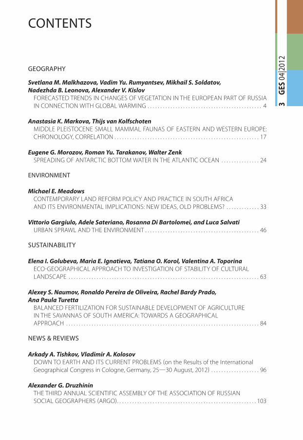
CONTENTS

GEOGRAPHY

Svetlana M. Malkhazova, Vadim Yu. Rumyantsev, Mikhail S. Soldatov,

Nadezhda B. Leonova, Alexander V. Kislov

FORECASTED TRENDS IN CHANGES OF VEGETATION IN THE EUROPEAN PART OF RUSSIA

IN CONNECTION WITH GLOBAL WARMING . . . . . . . . . . . . . . . . . . . . . . . . . . . . . . . . . . . . . . . . . . . . . 4

Anastasia K. Markova, Thijs van Kolfschoten

MIDDLE PLEISTOCENE SMALL MAMMAL FAUNAS OF EASTERN AND WESTERN EUROPE:

CHRONOLOGY, CORRELATION . . . . . . . . . . . . . . . . . . . . . . . . . . . . . . . . . . . . . . . . . . . . . . . . . . . . . . . . . 17

Eugene G. Morozov, Roman Yu. Tarakanov, Walter Zenk

SPREADING OF ANTARCTIC BOTTOM WATER IN THE ATLANTIC OCEAN . . . . . . . . . . . . . . . 24

ENVIRONMENT

Michael E. Meadows

CONTEMPORARY LAND REFORM POLICY AND PRACTICE IN SOUTH AFRICA

AND ITS ENVIRONMENTAL IMPLICATIONS: NEW IDEAS, OLD PROBLEMS? . . . . . . . . . . . . . 33

Vittorio Gargiulo, Adele Sateriano, Rosanna Di Bartolomei, and Luca Salvati

URBAN SPRAWL AND THE ENVIRONMENT . . . . . . . . . . . . . . . . . . . . . . . . . . . . . . . . . . . . . . . . . . . . . 46

SUSTAINABILITY

Elena I. Golubeva, Maria E. Ignatieva, Tatiana O. Korol, Valentina A. Toporina

ECOGEOGRAPHICAL APPROACH TO INVESTIGATION OF STABILITY OF CULTURAL

LANDSCAPE . . . . . . . . . . . . . . . . . . . . . . . . . . . . . . . . . . . . . . . . . . . . . . . . . . . . . . . . . . . . . . . . . . . . . . . . . . . 63

Alexey S. Naumov, Ronaldo Pereira de Oliveira, Rachel Bardy Prado,

Ana Paula Turetta

BALANCED FERTILIZATION FOR SUSTAINABLE DEVELOPMENT OF AGRICULTURE

IN THE SAVANNAS OF SOUTH AMERICA: TOWARDS A GEOGRAPHICAL

APPROACH . . . . . . . . . . . . . . . . . . . . . . . . . . . . . . . . . . . . . . . . . . . . . . . . . . . . . . . . . . . . . . . . . . . . . . . . . . . . 84

NEWS & REVIEWS

Arkady A. Tishkov, Vladimir A. Kolosov

DOWN TO EARTH AND ITS CURRENT PROBLEMS on the Results of the International

Geographical Congress in Cologne, Germany, 2530 August, 2012 . . . . . . . . . . . . . . . . . . . 96

Alexander G. Druzhinin

THE THIRD ANNUAL SCIENTIFIC ASSEMBLY OF THE ASSOCIATION OF RUSSIAN

SOCIAL GEOGRAPHERS ARGO . . . . . . . . . . . . . . . . . . . . . . . . . . . . . . . . . . . . . . . . . . . . . . . . . . . . . . . 103

gi412.indd 3gi412.indd 3 24.12.2012 9:10:3424.12.2012 9:10:34

4

GEO

GRA

PHY

ABSTRACT. The paper discusses connections

between zonal boundaries of vegetation

and productivity of forest stands and

some climatic parameters. It also suggests

mathematical-cartographic models of these

connections. The models are used to forecast

changes in the boundaries of the vegetation

sub-zones and of forest stands productivity

in the European Part of Russia and on the

adjacent areas for 2046–2065 under one of

the scenarios of global warming.

KEY WORDS: Zoning of vegetation, growth

of timber, global warming, climatic

parameters, forecasts, mathematical-

cartographic model.

INTRODUCTION AND BACKGROUND

The most important feature of the modern

climate is global warming. It can be traced

as a background process throughout the

XXth century and it has become most

prominent beginning in the 1970s. Climate

warming is detected from meteorological

observations (for a rigorous analysis, only

data of the measurements of non-urbanized

areas are used) and is supported by indirect

evidence, of which the principal one is the

rise in the oceans’ level and melting of

mountain glaciers. The major challenge for

the modern science is the question of the

climate forecast and identification of the

environmental response to these changes.

This paper discusses some issues related

to changes in the vegetation cover (VC)

occurring under the influence of current

trends of climate change and a projection of

its dynamics in the European Part of Russia.

It is best to consider feedbacks of VC to

climatic changes under an integrated

approach. This approach involves, first of

all, ideas of the planetary homeostasis

(i.e., the tendency of the natural system to

reproduce itself, to restore the lost balance,

and to overcome resistance of the external

environment) that have been best reflected

in the Gaia hypothesis [Lovelock, 1982].

However, with all its elegance, this concept

of the biological control over the global

climate must, apparently, be rejected –

empirical and theoretical results show

that the dynamics of the Earth’s history

for the global biota depended heavily on

geophysical phenomena occurring on the

planet [Budyko, et al., 1985].

The interaction between VC and climate

can be assessed with varying level of

detail. The VC properties (morphological,

physical, and psychological) are considered

Svetlana M. Malkhazova1, Vadim Yu. Rumyantsev1*, Mikhail S. Soldatov1, Nadezhda B. Leonova1, Alexander V. Kislov2

1 Department of Biogeography, Faculty of Geography, Lomonosov Moscow State University; Leninskiye Gory, 1, 119234, Moscow, Russia; tel.: 8(495)9394717, fax: 8(495)9328836* Corresponding author; e-mail: vyurum@biogeo.ru2 Department of Meteorology and Climatology, Faculty of Geography, Lomonosov Moscow State University; Leninskiye Gory, 1, 119234, Moscow, Russia; tel.: 8(495)9393043, fax: 8(495)9328836, e-mail: avkislov@mail.ru

FORECASTED TRENDS IN CHANGES OF VEGETATION IN THE EUROPEAN PART OF RUSSIA IN CONNECTION WITH GLOBAL WARMING

gi412.indd 4gi412.indd 4 24.12.2012 9:10:3424.12.2012 9:10:34

5

GEO

GRA

PHY

together with soil parameters in current

climate models in the calculations of

various flows (heat, moisture, and carbon

dioxide) between the atmosphere and

the underlying surface. These are the so-

called SVAT (“Soil-Vegetation-Atmosphere-

Transfer”) models that can be integrated

or used individually. The resulting climate

change calculations determine changes of

the biophysical and biochemical processes

in plants and soils, defining changes in

species composition, length of the growing

period, and the vegetation structure. The

process of transition from inputs of climatic

models to the VC parameters may occur

at different levels of complexity. This may

involve very simple regression relations and

much more sophisticated models, such as

EFIMOD (http://ecobas.org/www-server/

rem/mdb/efimod.html; http://prezi.com/

tprjzowtnuj3/2), BIOME 6000, etc. A common

feature is a unidirectional approach; i.e., the

information about the changes in VC is

not interactively fed back to the climate

model. At the same time, changes in the

properties of VC influence the exchange of

heat, H2O, and CO2 with the atmosphere,

and these changes can effectively impact

the thermodynamic field of the atmosphere.

Thus, the so-called dynamic models of

vegetation were developed. These include,

for example, ORCHIDEE [Krinner, et al.,

2005], JSBACH [Bathiany, et al., 2010], etc.,

that are interactively connected with the

atmosphere component of climatic models.

Such systems are already able to reflect

feedback-based transient changes.

This paper treats changes in VC through static

relations, i.e., regression equations. The use

of the simplest approach is quite reasonable

since the use of complex models does not

often produce reasonable results due to

requirements for very precise information

of the VC parameters. VC is characterized

through its zonal boundaries and productivity

parameters of woody plants.

Shifts in zonal boundaries of vegetation are

found in different regions of the world.

With sufficient moisture, they are most

likely where the temperature is the limiting

factor [Turmanina, 1976]. Therefore, the most

noticeable changes can be observed at the

northern limit of the distribution of woody

vegetation: with global warming, the forest

boundary at high latitudes is expected to

shift north [Turmanina, 1976; Velichko, 1992;

Malkhazova, et al., 2011]. Modern research in

the polar regions of Siberia has identified the

spread of woody vegetation to the north.

Thus, for the world’s northernmost forests

in Khatanga (Taimyr) over the last 30 years,

a 65% increase of larch canopy closure and

their shift into the tundra area at 3–20 m/yr

have been detected [Kharuk, et al., 2006].

Unfortunately, similar data are not available

for the southern regions of Russia.

Establishing the quantitative relationship

between the zonal boundaries of VC and

climatic parameters is associated frequently

with an array of problems that relate to

complex relations between VC and climate

change, to uncertainty in dependencies

between VC boundaries and climate, to

vegetation system inertia, to multi-factorial

nature of climatic impacts, and to uncertainty

of the definition of the notion of “zonal

boundaries” itself [Malkhazova, et al., 2011].

Quantitative analysis of the effect of climate

on the productivity of forest stands is of

particular importance for the assessment

of resource-biosphere relationships. Growth

of timber is an integral indicator of stand

productivity. Growth of timber is defined by

biological characteristics of the species and

by the entire array of abiotic factors, among

which, climate is of paramount importance.

Warming, in conditions of the shortage of

heat supply, leads, apparently, to an increase

in productivity of forest stands in Russia and

some European countries (0.5% per year

from 1961 to 1998) [Alekseev and Markov,

2003].

The goals of this work included identification

of climate indicators that are most associated

with vegetation, establishment of forms

of these relationships, and assessment of

forecasted values of selected vegetation

gi412.indd 5gi412.indd 5 24.12.2012 9:10:3424.12.2012 9:10:34

6

GEO

GRA

PHY

characteristics based on climatic models

for the mid XXIth century [Kislov, et al.,

2008; Kislov, 2011]. As a result, mathematical

and cartographic models of relationships

between vegetation zoning and productivity

for the European Part of Russia (EPR) and

some climatic parameters were built. These

models were used to forecast possible

changes in the boundaries of the vegetation

sub-zones and in stand productivity in the

EPR in the middle of the XXIth century

caused by global warming.

MATERIALS AND METHODS

Climatic data. Information about the spatial

distribution of climatic parameters used in

the above-mentioned models characterizes

the EPR and the adjacent areas. The territory is

broken into a grid with a 2 Ѕ 2 deg. cell size.

The data for the period from 1961 to 1989

inclusively (that are called a «period of the

modern climate» on the recommendation of

the World Meteorological Organization) are the

results of the NCAP/NCEP re-analysis [Kislov,

2011; Kislov, et al., 2011] interpolated to the

nodes (the geometric centers of the cells) of the

degree grid. For each node, a range of climate

parameters was calculated. It was assumed,

that their values for the node (point) can be

extrapolated to the whole cell (polygon).

Structurally similar projections for 2046–

2065 are based on the data of numerical

experiments carried out with climatic

models under the project CMIP3 (Coupled

Model Intercomparison Project) of the WCRP

(World Climate Research Program). For the

characteristics of the future anthropogenic

impacts, “A2” scenario (i.e., one of the most

“harsh” scenarios of the IPCC (Intergovernmental

Panel on Climate Change)) was adopted [Kislov,

2011; Kislov, et al., 2011].

Of a variety of available climatic parameter,

the parameters selected for the analysis are

as follows:

1) Effective air temperature (T > 10°C). The

analysis considered a number of days with

effective temperature and the annual sum

of such temperatures. These indicators are

considered the major climatic characteristics

of plants growing season.

2) The hydrothermal coefficient (HTC ) by

Selyaninov:

HTC = Sum_R/0.1 Sum_T (1)

where: Sum_R is the total precipitation for

the year; Sum_T is the sum of effective

temperatures for the year.

Zoning of vegetation. Possible changes

in the vegetation zones boundaries were

assessed based on the map “Zones and types

of vegetation belts of Russia and adjacent

territories” [Zones and types..., 1992]. This

map represents the most common

understanding of the modern zoning of

vegetation, while satisfying the fullest the

requirements to scale and detail. It was

assumed that the map represents the

equilibrium of the zonal boundaries of

vegetation and of the conditions for the

“period of the modern climate”.

Within the EPR, the following categories of

the classification of flatland vegetation are

used (zones and sub-zones, in accordance

with the legend of the map (Fig. 1A)

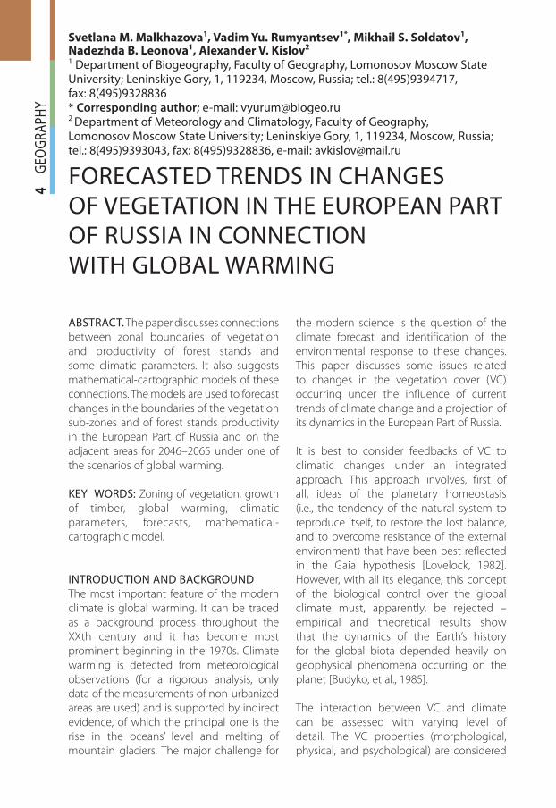
A. Tundra zone. Sub-zones: A2 – arctic tundra

(only on some islands of the EPR, however, is

considered in the numbering system); A3 –

northern hypoarctic (typical) tundra; A4 –

southern hypoarctic (shrub) tundra.

B. Taiga zone. Sub-zones: B1 – forest tundra;

B2 – northern taiga; B3 – middle taiga;

B4 – southern taiga; B5 – sub-taiga (mixed

forest).

C. Deciduous forest zone. Sub-zones: C1 –

broadleaved forest; C2 – forest-steppe.

D. Steppe zone. Sub-zones: D1 – northern

(bunch-grass-turf ) steppe; D2 – middle (dry)

steppe; D3 – southern (desert) steppe.

gi412.indd 6gi412.indd 6 24.12.2012 9:10:3524.12.2012 9:10:35

7

GEO

GRA

PHY

E. Desert zone. Sub-zones: E1 – northern

desert; E2 – middle desert; E3 – southern

desert (not present in the study area under

modern conditions, however, is present in the

forecast – see below).

The analysis was performed at the level of

the vegetation sub-zones. Within the study

area, they were numbered from north to

south from “1” (A2) to “16” (E3).

Fig. 1A shows the distribution of the nodes and

degree grid cells over the map of the modern

zoning vegetation [Zones and types..., 1992].

The analysis was performed separately for the

nodes and cells, as their spatial association with

the vegetation sub-zones boundaries differed

somewhat. Exclu ded from the analysis were

the nodes and cells that were outside the

boundaries of the vegetation units identified

on the map, as well as the islands (except for

the largest), mountain areas, and seas. Each

node or cell was assigned a number of the sub-

zone. It was assumed:

for the nodes – the node is within the –

sub-zone;

for the cells – more than 50% of the area –

of the cell is within the sub-zone, even

if its geometric center (node) is located

outside the sub-zone.

The analysis of the map (Fig. 1A) showed

that a significant number of the nodes (at

least 20%) are almost on the boundaries

of the sub-zones. Approximately the same

number of the cells is divided by these

boundaries practically in half. If we consider

that the accuracy of the zonal boundaries

on the map is, to some extent, relative, it

can be concluded that the assignment of

specific nodes or cells to a particular sub-

zone, in some cases, is rather arbitrarily,

particularly in the northern areas where

the latitudinal extent of the sub-zones is

minimal. However, all the nodes and cells,

with some assumptions, have been confined

to specific sub-zones (Fig. 1B).

Growth of timber. The analysis was based

on the data on stocks and growth of forests

from the statistical materials of the State

Accounting of the Forest Fund (SAFF) for

1963–1990. Of a large number of forest

Fig. 1. A – the cells (polygons) and the nodes (points) of the degree grid used as the locations of the

climatic data when superimposed with the map of the current zoning of vegetation.

B – sub-zonal locations of the grid cells.

A2-E2 – vegetation sub-zones (see text). Gray color indicates mountain areas

gi412.indd 7gi412.indd 7 24.12.2012 9:10:3524.12.2012 9:10:35

8

GEO

GRA

PHY

taxation parameters in the data of SAFF

for all groups of tree species, the following

parameters were selected for the analysis:

The total stock of timber is the amount of raw

stem wood of all the trees of the forest stand.

It depends on many factors, including, the

forested area, the average age of the stand, etc.

The total average annual growth of timber is

the parameter that characterizes the annual

increase of the stem stock of the forest

on average for the entire period of its life.

This is an integral stand productivity index

that reflects conditions of its development,

including climatic.

To analyze the relationships between

climate and productivity parameters,

36 administrative regions of the Russian

Federation within the EPR were selected.

Most of them are located entirely within the

forest area, but there are others where the

forested land occupies a relatively small area

(Belgorod, Orel, Kursk Oblast, etc.). Therefore,

the analysis was carried out for all the regions

and separately for those fully located within

the forest areas.

The data of SAFF were recalculated to arrive

at the units of “m3/ha of forested area.” Thus,

the parameters for the “average stock” and

“average growth” of trees were obtained;

then they were used to calculate the average

long-term values for 1961–1988 for each of

the selected Russian administrative regions.

The map of the administrative regions was

superimposed with the degree grid (see

above). The multi-year weighted average

(for the area) climatic parameters were

calculated for each administrative region of

the Russian Federation; the calculations were

made considering the set of the grid cells

that cover each region and the proportion

of the cells’ area for the region.

Then, the relationships were assessed

(Pearson correlation coefficients of the pairs)

between:

the values of climatic parameters and the –

sub-zonal locations of the nodes and cells

(numbers of sub-zones); the results are

shown in Table 1;

the values of climatic and productivity –

parameters; the results are shown in Table 2.

The linear regression equations calculated for

these indicators were then used to support

and build the forecast models.

Data processing and calculations were carried

out with MS Visual FoxPro and STATISTIKA

software. Cartographic work was carried out

in the MapInfo Professional GIS environment.

RESULTS AND DISCUSSION

Zoning of vegetation

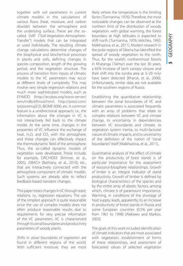
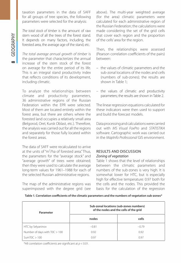
Table 1 shows that the level of relationships

between the climatic parameters and

numbers of the sub-zones is very high. It is

somewhat lower for HTC, but is especially

high for effective temperature: 0.97 both for

the cells and the nodes. This provided the

basis for the calculation of the regression

Table 1. Correlation coeffi cients of the climatic parameters and the numbers of vegetation sub-zones*

Parameter

Sub-zonal locations (sub-zones numbers)

of the nodes and the cells of the grid

nodes cells

HTC by Selyaninov –0.81 –0.79

Number of days with Т0С > 100 0.92 0.92

SumТ0С > 100 0.97 0.97

*All correlation coeffi cients are signifi cant at p < 0.01.

gi412.indd 8gi412.indd 8 24.12.2012 9:10:3524.12.2012 9:10:35

9

GEO

GRA

PHY

relationships between the sub-zonal

locations of the grid’s nodes and cells and

the climatic parameters (Fig. 2).

Fig. 2 shows nonlinear relationships for the

HTC parameter; however, these relationships

were not analyzed at the current stage;

therefore, HTC was not used in the forecast.

We can also see that the sum of effective

temperatures actually shows a linear

relationship with the vegetation zoning.

A similar pattern was obtained for the

number of days with effective temperature,

although in this case, the strength of

the relationship was somewhat lower

(Table 1), so the graphs for the last case are

not given.

Thus, the sum of effective temperatures

appeared to be the best parameter of

all climatic parameters considered for

the forecast of possible changes of the

vegetation sub-zone boundaries in the EPR

in the middle of the XXIth century; this

parameter had the tightest connection with

the vegetation zoning (Fig. 2, Table 1).

The relationships betweens the sub-zonal

locations of the nodes and cells of the

grid and the values of the sum of effective

temperatures parameter are described by two

regression equations (Fig. 2). Modification of

some of these formulas (averaging the values

of the coefficients for the nodes and cells)

allowed arriving at the following equation

applicable both to the cells and the nodes.

Zon_ID = 1 + 0.0034 Sum_T, (2)

where: Zon_ID is the serial number of the

sub-zone (1–15),

Sum_T is the sum of effective temperatures.

Using the existing forecast values Sum_T in

equation (2) made it possible to determine

the potential location of each cell of the

degree grid for 2046–2065 in the zoning

system, defined by the sum of effective

Fig. 2. The relationships between the order numbers of the vegetation sub-zones (Zon_ID),

HTC by Selyaninov (HTC), and the sum of effective temperatures (Sum_T).

A, B – HTC (A – for the cells, B – for the nodes), C, D – the sum of effective temperatures

(C – for the cells, D – for sthe nodes)

gi412.indd 9gi412.indd 9 24.12.2012 9:10:3524.12.2012 9:10:35

10

G

EOG

RAPH

Y

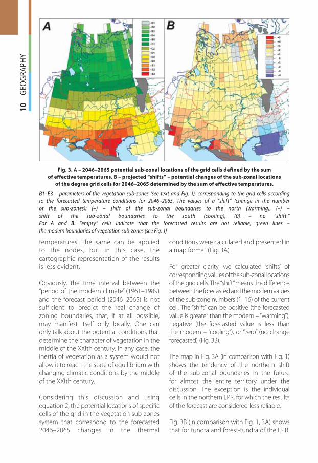
temperatures. The same can be applied

to the nodes, but in this case, the

cartographic representation of the results

is less evident.

Obviously, the time interval between the

“period of the modern climate” (1961–1989)

and the forecast period (2046–2065) is not

sufficient to predict the real change of

zoning boundaries, that, if at all possible,

may manifest itself only locally. One can

only talk about the potential conditions that

determine the character of vegetation in the

middle of the XXIth century. In any case, the

inertia of vegetation as a system would not

allow it to reach the state of equilibrium with

changing climatic conditions by the middle

of the XXIth century.

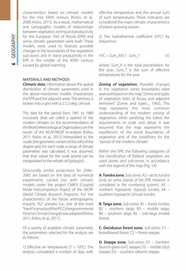
Considering this discussion and using

equation 2, the potential locations of specific

cells of the grid in the vegetation sub-zones

system that correspond to the forecasted

2046–2065 changes in the thermal

conditions were calculated and presented in

a map format (Fig. 3A).

For greater clarity, we calculated “shifts” of

corresponding values of the sub-zonal locations

of the grid cells. The “shift” means the difference

between the forecasted and the modern values

of the sub-zone numbers (1–16) of the current

cell. The “shift” can be positive (the forecasted

value is greater than the modern – “warming”),

negative (the forecasted value is less than

the modern – “cooling”), or “zero” (no change

forecasted) (Fig. 3B).

The map in Fig. 3A (in comparison with Fig. 1)

shows the tendency of the northern shift

of the sub-zonal boundaries in the future

for almost the entire territory under the

discussion. The exception is the individual

cells in the northern EPR, for which the results

of the forecast are considered less reliable.

Fig. 3B (in comparison with Fig. 1, 3A) shows

that for tundra and forest-tundra of the EPR,

Fig. 3. A – 2046–2065 potential sub-zonal locations of the grid cells defined by the sum

of effective temperatures. B – projected “shifts” – potential changes of the sub-zonal locations

of the degree grid cells for 2046–2065 determined by the sum of effective temperatures.

B1–E3 – parameters of the vegetation sub-zones (see text and Fig. 1), corresponding to the grid cells according

to the forecasted temperature conditions for 2046–2065. The values of a “shift” (change in the number

of the sub-zones): (+) – shift of the sub-zonal boundaries to the north (warming), (–) –

shift of the sub-zonal boundaries to the south (cooling), (0) – no “shift.”

For A and B: “empty” cells indicate that the forecasted results are not reliable; green lines –

the modern boundaries of vegetation sub-zones (see Fig. 1)

gi412.indd 10gi412.indd 10 24.12.2012 9:10:3624.12.2012 9:10:36

11

G

EOG

RAPH

Y

the forecasted trends in the “shifts” of the

sub-zonal boundaries correspond to the

established ideas. The development of

favorable, for forest vegetation, conditions

is expected. In this case, in the north of

the territory for individual cells, there

are very significant “shifts” leading to a

situation where, for example, on the Kola

Peninsula, the forecasted temperature

conditions in some places will support

the growth of southern taiga or mixed

forests (Fig. 3A).

Negative “shifts” within the study area are

forecasted primarily outside of Russia, for the

northwest of Kazakhstan; within Russia – for

the southern Urals (Fig. 3B).

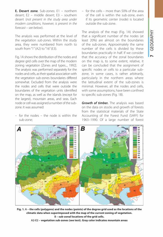
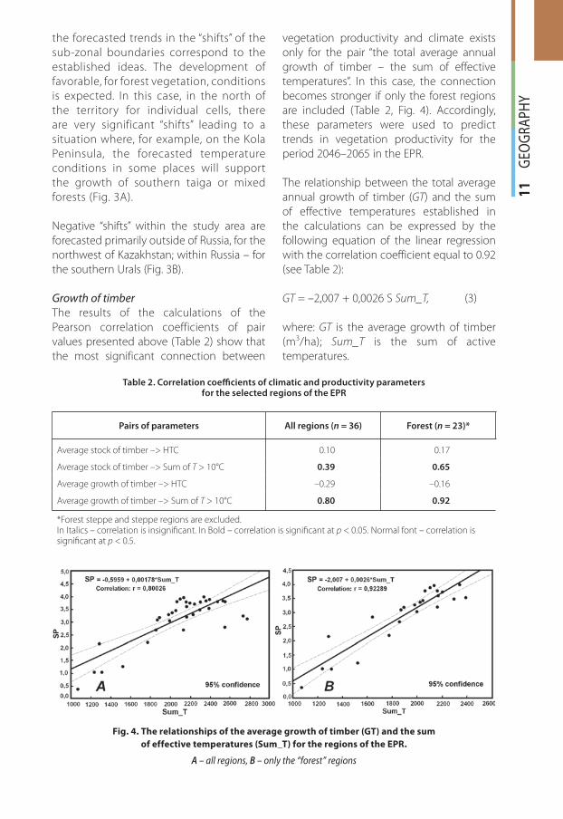
Growth of timber

The results of the calculations of the

Pearson correlation coefficients of pair

values presented above (Table 2) show that

the most significant connection between

vegetation productivity and climate exists

only for the pair “the total average annual

growth of timber – the sum of effective

temperatures”. In this case, the connection

becomes stronger if only the forest regions

are included (Table 2, Fig. 4). Accordingly,

these parameters were used to predict

trends in vegetation productivity for the

period 2046–2065 in the EPR.

The relationship between the total average

annual growth of timber (GT) and the sum

of effective temperatures established in

the calculations can be expressed by the

following equation of the linear regression

with the correlation coefficient equal to 0.92

(see Table 2):

GT = –2,007 + 0,0026 Ѕ Sum_T, (3)

where: GT is the average growth of timber

(m3/ha); Sum_T is the sum of active

temperatures.

Table 2. Correlation coeffi cients of climatic and productivity parameters for the selected regions of the EPR

Pairs of parameters All regions (n = 36) Forest (n = 23)*

Average stock of timber –> HTC 0.10 0.17

Average stock of timber –> Sum of Т > 10°C 0.39 0.65

Average growth of timber –> HTC –0.29 –0.16

Average growth of timber –> Sum of Т > 10°C 0.80 0.92

*Forest steppe and steppe regions are excluded. In Italics – correlation is insignifi cant. In Bold – correlation is signifi cant at p < 0.05. Normal font – correlation is signifi cant at p < 0.5.

Fig. 4. The relationships of the average growth of timber (GT) and the sum

of effective temperatures (Sum_T) for the regions of the EPR.

A – all regions, B – only the “forest” regions

gi412.indd 11gi412.indd 11 24.12.2012 9:10:3624.12.2012 9:10:36

12

G

EOG

RAPH

Y

Using forecasted values of Sum_T for the

EPR for 2045–2065 in equation (3), we

can calculate the potential value of the

average annual growth of timber for each

analyzed point in the territory. Additionally,

we calculated the “shifts” in the values of the

average annual growth of timber defined

both for the forecasted and the modern

periods (Table 3, Fig. 5).

The results show a general trend in the

productivity growth of the stands, resulting

in higher values of the forecasted average

growth of timber for 2046–2065 compared

with the current climate. Particularly

significant increase in the growth and thus

its maximum values are forecasted for the

southern and eastern parts of the territory.

Thus, the greatest “shifts” in the productivity

are expected for the Middle Volga region

(Republic of Mari El – 1.62 m3/ha, Republic of

Chuvash – 1.65 m3/ha) and the Middle Urals

(Perm Oblast – 1.66 m3/ha).

It should be noted that this forecast is

possible only in conditions of sufficient

moisture supply in these areas, that is, if an

increase in annual precipitation occurs. The

Table 3. The forecasted for 2046-2065 changes in the timber annual growth

for the “forest” regions of the EPR

Administrative regions

of the Russian Federation

Average annual growth

of timber (m3/ha)“Shift”*

1961–1990 2045–2065

Arkhangelsk Oblast 1.03 2.51 1.48

Bryanks Oblast 4 5.54 1.54

Vladimir Oblast 3.7 4.98 1.21

Vologda Oblast 2.2 3.72 1.52

Ivanovo Oblast 3.8 4.68 0.88

Kaluga Oblast 3.97 5.12 1.15

Kirov Oblast 2.7 4.07 1.37

Kostroma Oblast 3.11 4.14 1.03

Leningrad Oblast 2.85 3.81 0.96

Moscow Oblast 3.73 4.96 1.23

Murmansk Oblast 0.38 1.91 1.53

Nizhnyi Novgorod Oblast 3.6 4.82 1.22

Novgorod Oblast 3.2 4.17 0.97

Perm Oblast 2.16 3.82 1.66

Pskov Oblast 3.05 4.43 1.38

Smolensk Oblast 3.9 4.78 0.88

Tver Oblast 3.3 4.4 1.1

Yaroslavl Oblast 3.43 4.46 1.03

Republic of Karelia 1.25 2.55 1.3

Republic of Komi 1.04 2.42 1.38

Republic of Mari El 3.2 4.82 1.62

Republic of Udmurt 3.38 4.54 1.16

Republic of Chuvash 3.49 5.14 1.65

* “Shift” means the change between the forecasted and the current values of the growth of timber parameter, m3/ha .

gi412.indd 12gi412.indd 12 24.12.2012 9:10:3724.12.2012 9:10:37

13

G

EOG

RAPH

Y

noticeable “shifts” are also projected for the

most northern regions – the Murmansk and

Arkhangelsk regions. If, at the present time,

the average increase is small and is 0.38,

and 1.03 m3/ha, respectively, in 2046–2065,

the growth is forecasted to increase by

1.5 m3/ha, i.e., 2.5–3 times (Table 3). This is

consistent with the established current ideas

that the most significant changes in forest

vegetation will occur at the northern limit

of its distribution, where the conditions for

the existence of forest are extreme, and that

specifically temperature is a limiting factor

in the development of trees and in their

productivity.

CONCLUSION

The results of the analysis show that the

forecasted “shifts” of the sub-zonal boundaries

of vegetation associated with the thermal

conditions of the growing season can have

both positive (“warming” – “shift” in the

conditions determining the northern shift

of the existing sub-zonal boundaries: almost

the entire EPR) and zero (there is no “shift”:

the individual cells in the EPR) trends. In

some regions of the south part of the study

area, the “shifts,” according to the forecasted

changes in the temperature conditions, can

have even a negative trend.

For the growth of timber parameter for the

entire territory under the discussion, only

positive “shifts” are forecasted. However, it

should be kept in mind that this parameter

is not tightly connected with the climatic

conditions. It is known, that growth of timber

for each forest species increases along with

better climatic conditions only to some

point after which the growth slows down

[Romanovsky and Schekalev, 2009].

The results obtained demonstrate the

relationships between the vegetation parameters

and the sum of effective temperatures only.

It can be assumed that the results are reliable

only if current, for the area, conditions of sufficient

moisture supply are preserved. The analysis

performed earlier [Kislov, et al., 2008; Kislov,

2011] shows that in the EPR (except for its

southern border), warming occurring

simultaneously with the growth of precipitation

maintains moisture supply that is close to

the modern conditions. This confirms the

representativeness of the results.

Fig. 5. A – 2046–2065 forecasted average growth of timber (m3/ha). B – Forecasted “shifts” of the

average values of growth of timber in comparison with the period of “the modern climate” (only for

“forest” regions of the EPR). Explanations are in the text.

There are no data for the Komi-Permyak AO (the “white spot” on the map).

Vegetation zones and sub-zones (boundaries and parameters) – see above

gi412.indd 13gi412.indd 13 24.12.2012 9:10:3724.12.2012 9:10:37

14

G

EOG

RAPH

YIt must be stressed that the forecast

considers, especially with respect to the

zonal boundaries, trends of changes and

not the changes themselves. It is possible

that the real “shifts” of these boundaries

in the EPR by the middle of the XXIth

century will be manifested only locally

because of insufficient succession rates.

This, however, does not mean that the

impacts of climate change on the discussed

territory are small. In fact, it means that

most of the plant communities in the area

will exist in temperature conditions not

characteristic to the area, for indefinitely

long period. In the short term, it is highly

desirable to attempt to assess the possible

consequences of such non-equilibrium

state of the ecosystems. �

REFERENCES

1. Alekseev V.A., Markov M.V. (2003). The Forest Fund statistics and the change of forest

productivity in Russia in the second half of the twentieth century. St-Pb.: Saint-Petersburg

Forest Ecology Center. 272 p. (In Russian).

2. Bathiany S., Claussen M., Brovkin V., Raddatz T., Gayler V. (2010). Combined biogeophysi-

cal and biogeochemical effects of large-scale forest cover changes in MPI earth system

model. Biogeosciences Discuss., 7, pp. 387–428. (http://www.biogeosciences-discuss.

net/7/387/2010/).

3. Budyko M.I., Ronov A.B., Yanshin A.L. (1985). The history of the atmosphere. L., 365 p. (In

Russian).

4. Kharuk V.I., Ranson K.J., Im S.T., Naurzbaev M.M. (2006). Larch forests of forest tundra and

climatic trends. Ecology, № 5, pp. 323–331. (In Russian).

5. Kislov A.V. (2011). Dynamics of the climate in the XX and XXI century // Environmental

and geographical consequences of global climate warming in the XXI century in the

East-European plain and in the Western Siberia (Eds. N.S. Kasimov and A.V. Kislov). M.: MAX

Press, pp. 14–49 (In Russian).

6. Kislov A.V., Evstigneev V.M., Malkhazova S.M., Sokolikhina N.N., Surkova G.V., Toropov P.A.,

Chernyshev A.V., Chumachenko A.N. (2008). Forecast of climate resources of the East-

European plain under condition of global warming in the XXI century. M.: MAX Press, 290

p. (In Russian).

7. Kislov A., Grebenets V., Evstigneev V., Malkhazova S., Rumiantsev V., Sidorova M., Soldatov

M., Surkova G., Shartova N. (2011). Estimation systemique des consequences du rechauf-

fement climatique au XXI siecle dans le Nord Eurasien // Le Changement Climatique. Eu-

rope, Asie Septentrionale, Amerique du Nord. Quatriemes Dialogues Europeens d’Evian /

Edite par M. Tabeaud et A. Kislov. – Eurcasia: Copy-Media, pp. 75–88 (In French).

8. Krinner G., Viovy N., Noblet-Ducoudre N., Ogee J., Polcher J., Friedlingstein P., Ciais P., Sitch

S., Prentice I.C. (2005). A dynamic global vegetation model for studies of the coupled

atmosphere-biosphere system. Global Biogeochem. Cycles, 19, GB1015.

9. Lavorel S., Diaz S., Cornelissen J.H.C., Garnier E., Harrison S.P., McIntyre S., Pausa J.G., Perez-

Harguindeguy N., Roumet C., Urcelay C. (2007). Plant Functional Types: Are We Getting

Any Closer to the Holy Grail? In: Canadell J.G., Pataki D.E. and Pitelka L.F. (Eds.), Terrestrial

Ecosystems in a Changing World, Springer, pp. 149–160.

gi412.indd 14gi412.indd 14 24.12.2012 9:10:3724.12.2012 9:10:37

15

G

EOG

RAPH

Y

10. Lovelock J.E. Gaia (1982). A new look at life on Earth. New York: Oxford University Press.

11. Malkhazova S.M., Minin A.A., Leonova N.B., Rumiantsev V.Yu., Soldatov M.S. (2011). Trends

of possible changes of the vegetation in the European part of Russia and in Western

Siberia // Environmental and geographical consequences of global climate warming in

the XXI century in the East-European plain and in the Western Siberia / Ed. N.S. Kasimov

and A.V. Kislov. M.: MAX Press, pp. 342–388 (In Russian).

12. Olchev A.V., Novenko E.Yu. (2012). Evaporation of forest ecosystems of the central regions

of European Russia in the Holocene. Mathematical Biology and Bioinformatics. V. 7. Num-

ber 1. pp. 284–298 (In Russian).

13. Romanovsky M.G., Schekalev R.V. (2009). The forest and climate of the Central part of Rus-

sia. M.: Inst. of Forestry RAS, 68 p. (In Russian).

14. Turmanina V.I. (1976). Phytoindication of climate oscillations // Landscape indication of

natural processes. Proc. of Moscow Naturalists Society. V. 15, pp. 64–70 (In Russian).

15. Vegetatioon zones and types of vegetation belts in Russia and adjacent territories (1992).

Map, 1: 8000000 / Ed. G.N. Ogureeva. M.: Izd-vo LLP “Ecor” (In Russian).

16. Velichko A.A. (1992). Zonal and macroregional changes of landscape and climatic

conditions caused by the “greenhouse effect”. Izvestiya RAS, Phys. Geography, N 2.

Pp. 89–101. (In Russian).

Svetlana M. Malkhazova has a degree of Doctor of Geographical

Sciences. She is Professor, Head of the Department of

Biogeography, Faculty of Geography, Lomonosov Moscow State

University. The main research interests relate to the problems

of biogeography, ecology, and medical geography. She is the

author of over 250 scientific publications, including 10 books,

several textbooks, and medical and environmental atlases.

Vadim Yu. Rumiantsev has a Ph.D. in Geography. He is Senior

Researcher at the Department of Biogeography, Faculty of

Geography, Lomonosov Moscow State University. His main

research interests include mammalian environmental geography,

biogeographic mapping, and the use of GIS technology in

biogeography. His current main scientific activities are in the field

of theoretical, methodological, and practical aspects of

geoinformation mapping of the distribution of terrestrial

vertebrates. He is the author and a co-author of 230 scientific

publications, including more than 80 thematic map-sheets in

complex national and regional atlases.

gi412.indd 15gi412.indd 15 24.12.2012 9:10:3824.12.2012 9:10:38

16

G

EOG

RAPH

Y

Mikhail S. Soldatov has a Ph.D. in Geography. He is Scientific

Reseacher at the Department of Biogeography, Faculty of

Geography, Lomonosov Moscow State University. His scientific

interests include a broad range of aspects of botanical geography,

biogeographic mapping, and medical geography. He published

80 scientific papers.

Nadezhda B. Leonova has a Ph.D. in Geography. She is Leading

Scientific Researcher at the Department of Biogeography, Faculty

of Geography, Lomonosov Moscow State University. Her main

scientific interests include problems of botanical geography and

assessment, monitoring, and conservation of boreal forests

biodiversity under global changes of the environment. The main

scientific works are associated with taiga ecosystems of European

Russia. She is the author of more than 40 publications, including

9 monographs, many research papers, teaching curricula and

textbooks, and popular science books.

Alexander V. Kislov has a degree of Doctor of Geographical

Sciences. He is Professor, Head of the Department of Meteorology

and Climatology, Faculty of Geography, Lomonosov Moscow

State University. His main research interests are in the theory of

climate, paleoclimate, and climate forecast and modeling. He is

the author of more than 100 papers, several monographs, and

teaching manuals.

gi412.indd 16gi412.indd 16 24.12.2012 9:10:3824.12.2012 9:10:38

17

G

EOG

RAPH

Y

ABSTRACT. Many new very important

Middle Pleistocene small mammal localities

of Europe were discovered during the last

decades. These new data permit to divide

the Middle Pleistocene geological sequences

of Eastern and Western Europe and carried

out the correlation between them. However,

there are some difficulties connected with

the incongruity of mammal appearance in

different parts of Europe. In this paper we

would like to discuss all these problems using

Middle Pleistocene small mammal data and

to present the possible biostratigraphical

scheme for the whole Europe.

KEY WORDS: small mammals, Middle

Pleistocene, Europe, correlation

MATERIALS AND METHODS

In this article we use the Western European

stratigraphical scheme. According this

scheme the beginning of the Middle

Pleistocene corresponding to the boundary of

palaeomagnetic epochs Matuyama–Brunhes

(~0.8 mln. yrs. BP) and the end of Middle

Pleistocene falls to the beginning of Eemian

(=Mikulian) Interglacial (about 0,135 mln. BP).

The Early and Middle Neopleistocene of the

Russian stratigraphical scheme correspond to

the Middle Pleistocene of Western European

stratigraphical scheme.

Eastern Europe

Dniester, Danube and Prut basins. One of

the most complete sections of the Middle

Pleistocene is the Kolkotova Balka section

near the Tiraspol town (Moldova, Dniester

basin). The deposits corresponding to the

whole Middle Pleistocene are opened up

in this outcrop. The several layers with

mammal faunas were discovered here:

the lowest 3 layers with small and large

mammal fauna were found in the fluvial

deposits of different facies. The fauna of

these fluvial layers describe as the stratotype

of Tiraspolian mammalian complex

[Alexandrova, 1976; Pleistocene of Tiraspol,

1971] which correspond to the Il’inkian

Horizon of Russian stratigraphical scheme

with Mimomys savini, Prolagurus posterius –

Lagurus transiens, Microtus (Stenocranius)

hintoni-gregaloides, Microtus arvaloides,

Microtus ratticepoides (=oeconomus) and

others; 2) above the fluvial deposits of

the Dniester River underlies the horizon of

the Vorona fossil soil with small mammal

fauna which is correlated with the Muchkap

Interglacial. Fauna includes Lagurus transiens

(archaic morphotype), Microtus gregalis and

others; 3) uppermost the loess deposits lie

covered the horizon of the Inzhava fossil

soil, synchronous to Likhvin Interglacial

with Lagurus transiens – L. lagurus, Microtus

(S.) gregalis, Microtus ex gr. agrestis и др.

Anastasia K. Markova1*, Thijs van Kolfschoten2

1* Leading scientist, Institute of Geography of the Russian Academy of Sciences; Staromonetny per., 29, 119017 Moscow, Russia; Tel.: +7-495-9590016, Fax: +7-495-9590033E-mail: amarkova@list.ru (Corresponding author)2 Faculty of Archaeology, Leiden University; P.O. Box 9515, 2300 RA Leiden, The Netherlands, Reuvensplaats 3-4, 2311 BE Leiden; Tel.: + 31 (0)71 527 2640, Fax: + 31 (0)71 527 2429,e-mail: t.van.kolfschoten@arch.leidenuniv.nl

MIDDLE PLEISTOCENE SMALL MAMMAL FAUNAS OF EASTERN AND WESTERN EUROPE: CHRONOLOGY, CORRELATION

gi412.indd 17gi412.indd 17 24.12.2012 9:10:3924.12.2012 9:10:39

18

G

EOG

RAPH

Y[Mikhailesku, Markova, 1992; Markova,

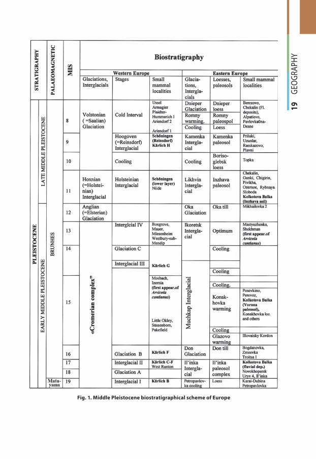
2007]. So the faunas of this key section

reflected the natural events of the most

part of the Middle Pleistocene (Fig. 1). These

faunas expressed the significant evolutional

changes in different phylogenetic lines of

Arvicolidae: Prolagurus – Lagurus, Microtus

(Stenocranius) hintoni-gregaloides – M. (S).

gregalis and others. The different taphonomy

of Kolkotova Balka main horizons (fluvial

deposits and fossil soils) didn’t permit to reveal

the transition between the rooted voles of

Mimomys genus (the ancestral form of water

vole Arvicola) and the un-rooted voles of

Arvicola genus. All localities with Mimomys were

found in fluvial older deposits. The different

fossil soils overlying the fluvial deposits didn’t

include the remains of water voles Arvicola

(or its ancestor form Mimomys intermedius)

what could be explained by their taphonomy.

There are several other very principal Middle

Pleistocene small mammal localities situated

on the south-west of the Russian Plain in Prut

and Danube River basins. The faunas were

described in Nagornoe, Suvorovo, Ozernoe,

Plavni and many others localities. These

localities as a rule characterize only one stage

of Middle Pleistocene: Il’inka Interglacial,

Muchkap Interglacial, Likhvin Interglacial and

Kamenka Interglacial. Most of them include

the fauna of the Likhvin Interglacial. The

significance of these materials for stratigraphy

also is very high. All of these localities were

found in the liman and lake deposits and

include not only mammal remains but also

brackish-water mollusks what permits to

carry out the straight correlation between

the continental and marine deposits of the

Russian Plain and the Black Sea [Mikhailesku,

Markova, 1992].

Dnieper basin. There are several Middle

Pleistocene localities of small mammals are

known from the Dnieper basin, mostly from

the middle part of basin. They are connected

with the fluvial deposits of IV terrace of

Dnieper. The localities Gunki and Pivikha

are situated on the left bank of Dnieper; the

Chigirin locality is situated on the right bank

[Markova, 1982] (Fig.1).

Gunki locality was studied by the several

methods (geological, pedological, palyno-

logical, malacological methods). Also the

palaeomagnetic investigation of deposits had

been done [Velichko et al., 1982]. This outcrop

includes the deposits of second part of the

Middle Pleistocene and the Upper Pleistocene.

The Dnieper (=Zaalian) till is registered here. The

Romny and Kamenka paleosols were described

below the Dnieper till. Fluvial thickness occurred

below the loess-paleosol sequence. The fluvial

deposits of IV terrace are correlated with

the Likhvin Interglacial by the palynological

and mammalian data. The small mammal

remains were discovered in the 3 facieses of

alluvium close by age. The rich fauna didn’t

include the teeth of rooted voles Mimomys

and Borsodia. There are no also remains of

archaic voles (with “pitymys” triangles) such

as Microtus (Terricola) arvaloides and Microtus

(Stenocranius) gregaloides. Steppe lemmings are

presented by the remains of Lagurus genus

with Lagurus transiens morphotypes (which

are more abundant) and Lagurus lagurus ones.

The Microtus genus includes the voles Microtus

arvalis, M. oeconomus and M. (S.) gregalis. The

palynological data indicate the Likhvin age of

the deposits [Gubonina, 1982]. Malacological

materials show on Early Euksinian age of

mollusk fauna. Gunki section is a unique one

by the completeness of the palaeontological

data [Markova, 1982]. The localities Pivikha and

Chigirin include similar small mammal faunas

by the species composition [Markova, 2006].

Don and Desna basins. The complicated

mammalian succession was described by the

materials of Middle Pleistocene small mammal

faunas from Don and Desna basins. The earliest

of them are correlated with the beginning of

Middle Pleistocene, the latest is referred to the

Dnieper (=Saalian) Glaciation [Agadjanian et

al., 2008; Markova, 2007]. The small mammal

materials related as well as to the interglacials

so to the glaciations (Don Glaciation, Oka

Glaciation and Dnieper Glaciation).

In last years the small mammal faunas with

archaic Arvicola were found in the deposits

related to interval, which follows Muchkap

interglacial and cooling which is next after

gi412.indd 18gi412.indd 18 24.12.2012 9:10:3924.12.2012 9:10:39

19

G

EOG

RAPH

Y

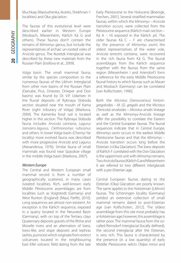
Fig. 1. Middle Pleistocene biostratigraphical scheme of Europe

gi412.indd 19gi412.indd 19 24.12.2012 9:10:3924.12.2012 9:10:39

20

G

EOG

RAPH

YMuchkap (Mastuzhenka, Ikorets, Shekhnan-1

localities) and Oka glaciation.

The faunas of this evolutional level were

described earlier in Western Europe

(Mosbach, Miesenheim, Kärlich Kä G and

others). These faunas don’t’ contain the

remains of Mimomys genus, but include the

representatives of archaic un-rooted voles of

Arvicola genus. The Ikoretzk Interglacial was

described by these new materials from the

Russian Plain [Iosifova et al., 2009].

Volga basin. The small mammal fauna,

similar by the species composition to the

numerous faunas of the Likhvin Interglacial

from other river basins of the Russian Plain

(Danube, Prut, Dniester, Dnieper and Don

basins) was found by Dr. V.P. Udartsev in

the fluvial deposits of Rybnaya Sloboda

section situated near the mouth of Kama

River (right tributary of Volga) [Markova,

2004]. The Kamenka fossil soil is located

higher in this section. The Rybnaya Sloboda

fauna includes Arvicola сantiana, Lagurus

transiens-lagurus, Clethrionomys rufocanus

and others. In lower Volga basin (Chernyi Yar

locality) more evolved fauna was described

with more progressive Arvicola and Lagurus

[Alexandrova, 1976]. Similar fauna of small

mammals was found near Spasskoe village

in the middle Volga basin [Markova, 2007].

Western Europe

The Central and Western European small

mammal record is from a number of

geographically scattered, in many cases

isolated localities. Rich, well-known early

Middle Pleistocene assemblages are from

localities such as Voigtstedt (Gemany) and

West Runton (England) [Maul, Parfitt, 2010].

Long sequences are almost non-existent. An

exception is the Kärlich sequence, exposed

in a quarry located in the Neuwied Basin

(Germany), with on top of the Tertiary clays

Quaternary deposits gravels of the Rhine and

Moselle rivers and an alternation of loess,

loess-like, and slope deposits and tephras

(ashes, pumices) which originate from extinct

volcanoes located in the neighbouring

East Eifel volcanic field dating from the late

Early Pleistocene to the Holocene [Boenigk,

Frechen, 2001]. Several stratified mammalian

faunas, within which the Mimomys – Arvicola

transition occurs, were collected from the

Pleistocene sequence (Kärlich main section –

Kä A – H) exposed in the Kärlich pit. The

older faunas Kä C – F are characterised

by the presence of Mimomys savini; the

oldest representatives of the water vole,

Arvicola terrestris cantiana, were recovered

in the rich fauna from Kä G. The faunal

assemblages from the Kärlich sequence

together with the faunas from the same

region (Miesenheim I and Ariendorf ) form

a reference for the early Middle Pleistocene

faunal history to which faunas such as Mauer

and Mosbach (Germany) can be correlated

[van Kolfschoten, 1990].

Both the Microtus (Stenocranius) hintoni-

gregaloides – M. (S). gregalis and the Microtus

(Terricola) arvaloides – Microtus arvalis lineage

as well as the Mimomys-Arvicola lineage

offer the possibility to correlate the Eastern

and the Central European faunas. The faunal

sequences indicate that in Central Europe,

Mimomys savini occurs in the earliest Middle

Pleistocene faunas and that the Mimomys –

Arvicola transition occurs long before the

Elsterian (=Oka Glaciation). The loess deposits

of Kärlich F correlated with the Don Glaciation

is the uppermost unit with Mimomys remains.

Two Arvicola faunas (Kärlich G and Miesenheim

I) are referred to two different interglacials

with a pre-Elsterian age.

Central European faunas dating to the

Elsterian (Oka) Glaciation are poorly known.

The same applies to the Holsteinian (Likhvin)

faunas. The Schöningen locality (Germany)

yielded an extensive collection of small

mammal remains dated to post-Elsterian

age [van Kolfschoten, 2012]. The oldest

assemblage from this site most probably has

a Holsteinian age; however, this assemblage is

rather poor. The mammal fauna from the so-

called Reinsdorf Interglacial (locally defined),

the second interglacial after the Elsterian,

is very rich. This fauna is characterised by

the presence (in a low quantity) of early

Middle Pleistocene relicts (Talpa minor and

gi412.indd 20gi412.indd 20 24.12.2012 9:10:3924.12.2012 9:10:39

21

G

EOG

RAPH

Y

Drepanosorex) as well as rather primitive

water vole Arvicola molars indicating that

the age of the fauna predates many well-

known late Middle Pleistocene faunas such

as Weimar-Ehringsdorf (Germany) and

Maastricht-Belvédère (The Netherlands) [van

Kolfschoten, 1985] with a more advanced

Arvicola record and with relicts.

DISCUSSION

The phylogenetic lines Microtus (Stenocra-

ni us) hintoni-gregaloides – M. (S). gregalis,

Microtus (Terricola) arvaloides – Microtus arva-

lis and Mimomys – Arvicola are the base for the

correlation of Eastern and Western Pleisto-

cene small mammal faunas. The analysis

of the Middle Pleistocene mammalian se-

qu en ce of Central and Western Europe

indicates that Mimomys savini was disco-

vered in ear liest Middle Pleistocene faunas.

The Mimomys – Arvicola transition was found

in Western Europe long before the Elsterian

(=Oka) Glaciation. The loess deposits

of Kärlich F are correlated with the Don

Glaciation of Eastern Europe and are the latest

sediments with Mimomys remains (Fig. 1).

Two localities with archaic Arvicola (Kärlich G

and Miesenheim I) are referred to two different

interglacials. Both of them are related to

pre-Elsterian time. The faunas, synchronous

to the Elsterian Glaciation, are practically

unknown in Western Europe. The faunas of

the Holsteinian (=Likhvin) Interglacial are

very rare in this part of Europe.

Schöningen locality (Germany) includes the

rich collection of small mammal remains

corresponding to post-Elsterian deposits. The

earliest layer with small mammal remains in

Schöningen, possibly related to Holsteinian

Interglacial. Unfortunately this locality

contains only few small mammal bones.

The rich strata with small mammals in

Schöningen is synchronous to the Reinsdorf

Interglacial (this Interglacil was distinguished

only in this region). This fauna corresponds

to the younger Interglacial then Holsteinian

warm phase. Possibly it could be synchronous

to the Kamenka Interglacial of Eastern Europe.

The Reinsdorf fauna includes few relics of the

first half of Middle Pleistocene – Talpa minor

and Drepanosorex and also archaic Arvicola

cantianus. That permits to conclude that this

fauna are earlier then late Middle Pleistocene

faunas of Weimar-Eringsdorf (Germany) and

Maastricht-Belv@édère (the Netherlands)

with more progressive water voles [van

Kolfschoten, 1990].

Thus, we can reveal the evolutional succession

of small mammal faunas in Western and Eastern

Europe during Middle Pleistocene based on

the morphological changes in the different

phylogenetic lines. These transformations

have the similar trends in the different parts

of Europe. The revealed succession of small

mammal faunas indicates significant similarities

of the Middle Pleistocene faunas belonged to

the large stratigraphical divisions in different

European regions. Unfortunately now only

few full Middle Pleistocene sections with

the significant succession of heterochronous

mammalian faunas are known both on the

Russian Plain and in Western Europe. The

fullest picture was revealed to the Dniester

and Don River basins of the Russian Plain and

also for the Neuwied and Rhine River basins

of Central Europe.

Unfortunately the mammals of the one

of the most important phylogenetic line

Prolagurus – Lagurus, which gives a lot of

information about the stratigraphical

position of the Eastern European faunas,

are absent in Western Europe. So, we need

to base only on Mimomys – Arvicola and

Microtus members.

We need to mention some differences in the

first appearance of new small mammal taxa

in Western and Eastern Europe. So, there are

un-known Central European faunas with

Mimomys remains which correspond to the

complicated interval between the cold stage

synchronous to the Don Glaciation and the

Elster Glaciation. Only archaic water voles

Arvicola cantianus were discovered in these

faunas. On the contrary there are several

important well-known mammal localities

gi412.indd 21gi412.indd 21 24.12.2012 9:10:3924.12.2012 9:10:39

22

G

EOG

RAPH

Yin Eastern Europe (in the Dniester and Don

basins) with evolved Mimomus (M. savini)

which related to the Muchkap Interglacial.

This Interglacial took place between the

Don and Oka Glaciations. The first un-rooted

water voles Arvicola cantianus appeared only

in the very end of this complicated interval

during the Ikoretsk Interglacial. Till now this

phase was revealed only in the Don basin.

The future studies of small mammal faunas

from the different regions of Europe and also

the correlation of main stratigraphical horizons

with mammal localities permit to establish most

reliable correlations of Middle Pleistocene small

mammal faunas of Eastern and Western Europe.

Described analysis of the Middle Pleistocene

small mammal faunas could help to

reconstruct and to date the natural events

of Middle Pleistocene for the territory of

whole Europe and to reveal the similarities

and un-similarities in Arvicolidae evolution

in the different parts of Europe. �

REFERENCES

1. Agadjanian A.K., Iosifova Yu.I., Shik S.M. (2008). Mastyuzhenka section /Upper Don/ and its significance for regional stratigraphy. Actual problems of Neogene and Quaternary strati-graphy and its discussion on the 33 International Geological Congress, Norway, Materials of Russian scientific conference. Moscow. P. 20–24 (In Russan).

2. Alexandrova L.P. (1976). Anthropogene rodents of European part of USSR. Moscow, Nauka. 98 pp. (In Russian).

3. Boenigk W., Frechen, M. 2001. Zur Geologie der Kärlich Hauptwand. Mainzer geowissen-schaftliche Mitteilungen. 30. P. 123–194.

4. Gubonina Z.P. (1982). Palynological studies of principal horizons of loess and paleosols southern part of the Russian Plain. Regional and general paleogeography of loess and periglacial regions. Moscow, Nauka (In Russian).

5. Iosifova Yu. I., Agadjanian A.K., Ratnikov V.Yu., Sycheva S.A. (2009). About Ikoretsk suite and horizon in the upper part of the Lower Neopleistocene in the Mastyuzhenka sec-tion (Voronezh region). Bulletin of Regional inter-institutions commission on Center and Southern arts of the Russian Plain. Moscow, RAEN, V. 4. P. 89–104 (In Russian).

6. Markova A.K. (1982). Pleistocene Rodents of the Russian Plain. Moscow, Nauka. 182 pp. (In Russian).

7. Markova A.K. (2006). Likhvin fauna of small mammals from the Rybnaya Sloboda locality (the mouth of Kama River) and its position in Middle Pleistocene sequence of European mammal faunas. Anthropogene and modern ecology. Nature and Man. S-Petersburg. Gumanistika. P. 137–141 (In Russian).

8. Markova A.K. (2006). Likhvin Interglacial small mammal faunas of Eastern Europe. Quater-nary International, Volume 149, Issue 1: 67–79.

9. Markova A.K. (2007). Pleistocene mammal faunas of Eastern Europe. Quaternary Interna-tional. V.160. Issue 1. P. 100–111.

10. Maul L.C., Parfitt, S.A. (2010). Micromammals from the 1995 Mammoth Excavation at West Runton, Norfolk, UK: Morphometric data, biostratigraphy and taxonomic reappraisal. Quaternary International. V. 228, N 1–2. P.91–115.

11. Maul L.C., Parfitt, S.A. (2010). Micromammals from the 1995 Mammoth Excavation at West Runton, Norfolk, UK: Morphometric data, biostratigraphy and taxonomic reappraisal. Quaternary International. V. 228, N 1–2. P. 91–115.

gi412.indd 22gi412.indd 22 24.12.2012 9:10:4024.12.2012 9:10:40

23

G

EOG

RAPH

Y

12. Mikhailesku C.D., Markova A.K. (1992). Paleogeographical stages of Anthropogene fauna development in the south of Moldova. Kishinev, Shtiintsa. 311 pp. (In Russian).

13. Pleistocene of Tiraspol. 1971. Kishinev, Shtiintsa. 187 pp. (In Russian).

14. van Kolfschoten T. (1985). The Middle Pleistocene (Saalian) and Late Pleistocene (Weich-selian) mammal faunas from Maastricht–Belvédère, Southern Limburg, The Netherlands. Meded. Rijks Geol. Dienst. V. 39. N 1. P. 45–74.

15. van Kolfschoten T. (1990). The evolution of the mammal fauna in the Netherlands and the middle Rhine Area (Western Germany) during the late Middle Pleistocene. Meded. Rijks Geol.Dienst. 43/ 3. P. 1–69.

16. van Kolfschoten T. (2012). The Palaeolithic record from the locality Sch@öningen (Germany) in a biostratigraphical and archaeozoological perspective. Abstract to International confe-rence “European Middle Palaeolithic during MIS 8–MIS 3”. Wolbrom, Poland. P. 49.

17. Velichko A.A., Gribchenko Yu.N., Gubonina Z.P., Markova A.K., Morozova T.D., Pevzner M.A., Chepalyga A.L. (1997). Gunki section. Loess-paleosol formation of the Eastern European Plain. Paleogeography and stratigraphy. Moscow, Institute of Geography RAS. P. 60–79 (In Russian).

Anastasia K. Markova is specialist in Quaternary palaeontology

and historical biogeography and works in the Laboratory of

Biogeography of the Institute of Geography RAS. Her main fields

of interests focused on evolutional peculiarities of Pleistocene

small mammals, their geographical distribution in the past and

their palaeoecology. She leaded the intra-institutional scientific

collective, which study the species composition, biodiversity and

distribution of Late Pleistocene and Holocene mammal faunas of

Northern Eurasia. She is the member of INQUA-Subcommission

on European Stratigraphy, the member of Russian Quaternary Commission and the

member of editorial board of the journal “Stratigraphy. Geological correlation”. A.K. Markova

published more than 200 scientific papers including 4 monographs; chapters in 8 collective

monographs and the chapters in 4 palaeogeographical atlases.

Thijs van Kolfschoten is professor in mammalian palaeo- and

archaeozoology and Quaternary biostratigraphy and has research

position at the Faculty of Archaeology, Leiden University (The

Netherlands). His main fields of interest are Quaternary mammals,

biostratigraphy and palaeoecology. His palaeontological research

focuses on continental deposits ranging from the Early

Pleistocene until the early Holocene. Changes in Late Pleistocene

and early Holocene ecosystems in Europe north of the Alps are

investigated in close collaboration with Russian colleagues. The

results of these and previous research projects he published in

more than 120 scientific papers. Prof. Kolfschoten was President of the INQUA-Subcommission

on European Stratigraphy (SEQS) 1995–2003 and since 2003 is Vice-president of the INQUA

Commission on Stratigraphy and Chronology and since 2001 is secretary of the ICS/IUGS

Subcommision of Quaternary Stratigraphy. He is President of INQUA-The Netherlands since

2003. Thijs van Kolfschoten is founder of the European Quaternary Mammal Research

Association (EuroMam) and its secretary since 1994. He is regional editor (Europe) of

Quaternary International, the Journal of the International Union for Quaternary Research,

and member of the editorial board of the French-language journal Quaternaire

gi412.indd 23gi412.indd 23 24.12.2012 9:10:4024.12.2012 9:10:40

24

G

EOG

RAPH

Y

ABSTRACT. This paper describes the

transport of bottom water from its source

region in the Weddell Sea through the abyssal

channels of the Atlantic Ocean. The research

brings together the recent observations and

historical data. A strong flow of Antarctic

Bottom Water through the Vema Channel

is analyzed. The mean speed of the flow

is 30 cm/s. A temperature increase was

found in the deep Vema Channel, which

has been observed for 30 years already. The

flow of bottom water in the northern part

of the Brazil Basin splits. Part of the water

flows through the Romanche and Chain

fracture zones. The other part flows to the

North American Basin. Part of the latter flow

propagates through the Vema Fracture Zone

into the Northeast Atlantic. The properties of

bottom water in the Kane Gap and Discovery

Gap are also analyzed.

KEY WORDS: Abyssal channels, Vema,

Romanche, Chain, Kane, bottom water

INTRODUCTION

Antarctic Bottom Water (AABW) is formed

over the Antarctic slope as a result of mixing

of the cold and heavy Antarctic Shelf Water

with the lighter, warmer, and more saline

Circumpolar Deep Water [Orsi et al., 1999].

In the region of origin, Antarctic Shelf Water

is formed in the autumn-winter season

over the Antarctic shelf due to cooling of

the relatively fresh Antarctic Surface Water

to nearly freezing point temperature and

increased salinity caused by ice formation.

The resulting water mass with increased

density descends and reaches the ocean

floor. In the Atlantic Ocean the regions

of dominating Antarctic Bottom Water

formation are in the southern and western

parts of the Weddell Sea.

Antarctic Bottom Water represents the

coldest and deepest layer of the South

Atlantic. A commonly accepted definition

describes AABW as water with potential

temperature cooler than 2°C [Wüst, 1936].

This layer can occupy a layer 1000 m thick

and even more at the bottom of the Atlantic

Ocean. The thickness decreases in the

northern direction up to complete wedging-

out at the bottom in the North Atlantic.

Generally, propagation of Antarctic waters

in the bottom layer of the Atlantic Ocean

is confined to depressions in the bottom

topography. The pathways of AABW in

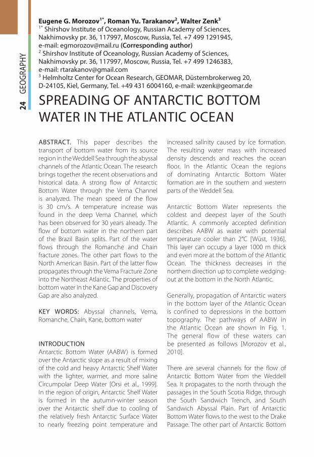
the Atlantic Ocean are shown in Fig. 1.

The general flow of these waters can

be presented as follows [Morozov et al.,

2010].

There are several channels for the flow of

Antarctic Bottom Water from the Weddell

Sea. It propagates to the north through the

passages in the South Scotia Ridge, through

the South Sandwich Trench, and South

Sandwich Abyssal Plain. Part of Antarctic

Bottom Water flows to the west to the Drake

Passage. The other part of Antarctic Bottom

Eugene G. Morozov1*, Roman Yu. Tarakanov2, Walter Zenk3

1* Shirshov Institute of Oceanology, Russian Academy of Sciences, Nakhimovsky pr. 36, 117997, Moscow, Russia, Tel. +7 499 1291945, e-mail: egmorozov@mail.ru (Corresponding author)2 Shirshov Institute of Oceanology, Russian Academy of Sciences, Nakhimovsky pr. 36, 117997, Moscow, Russia, Tel. +7 499 1246383, e-mail: rtarakanov@gmail.com3 Helmholtz Center for Ocean Research, GEOMAR, Düsternbrokerweg 20, D-24105, Kiel, Germany, Tel. +49 431 6004160, e-mail: wzenk@geomar.de

SPREADING OF ANTARCTIC BOTTOM WATER IN THE ATLANTIC OCEAN

gi412.indd 24gi412.indd 24 24.12.2012 9:10:4024.12.2012 9:10:40

25

G

EOG

RAPH

Y

Water propagates through the Georgia and

Northeast Georgia passages to the Georgia

Basin. Then, Antarctic Bottom Water flows

to the Argentine Basin through the Falkland

Gap in the Falkland Ridge.

It is commonly accepted that AABW

propagates from the Argentine Basin to

the Brazil Basin in three places: through the

Vema Channel, Hunter Channel, and over the

Santos Plateau. In the northern part of the

Brazil Basin, the flow of AABW splits. A part of

the flow is transported to the eastern basin

through the Romanche and Chain fracture

zones, influencing the waters of the bottom

layer in the Southeast Atlantic. The other

part flows through the Equatorial Channel,

propagating further to the Northeast Atlantic

through the Vema Fracture Zone and to the

North American Basin in the west, where it

is entrained into the cyclonic gyre within

its northward spreading zone, reaching the

Newfoundland Bank.

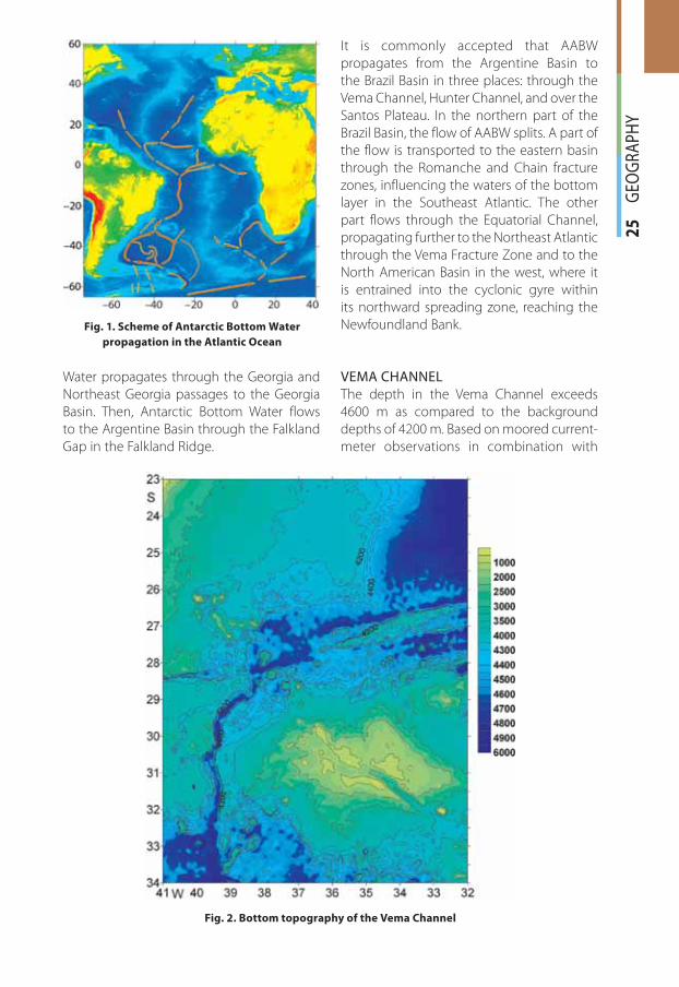
VEMA CHANNEL

The depth in the Vema Channel exceeds

4600 m as compared to the background

depths of 4200 m. Based on moored current-

meter observations in combination with

Fig. 1. Scheme of Antarctic Bottom Water

propagation in the Atlantic Ocean

Fig. 2. Bottom topography of the Vema Channel

gi412.indd 25gi412.indd 25 24.12.2012 9:10:4024.12.2012 9:10:40

26

G

EOG

RAPH

Ygeostrophic velocity computations from

hydrographic stations, the total Antarctic

Bottom Water transport across the Rio Grande

Rise and Santos Plateau is estimated at 6.9 Sv

[Hogg et al., 1999]. On the average, two thirds

of this volume passes through the Vema

Channel. The rest part flows over the Santos

Plateau and through the Hunter Channel.

The bottom topography around the Vema

Channel is shown in Fig. 2. The Vema

Channel is the deepest one among the

passages existing for Antarctic Bottom Water.

Therefore, the coldest water (Weddell Sea

Deep Water) can exit the Argentine Basin in

the equatorward direction only through this

channel [Zenk et al., 1993].

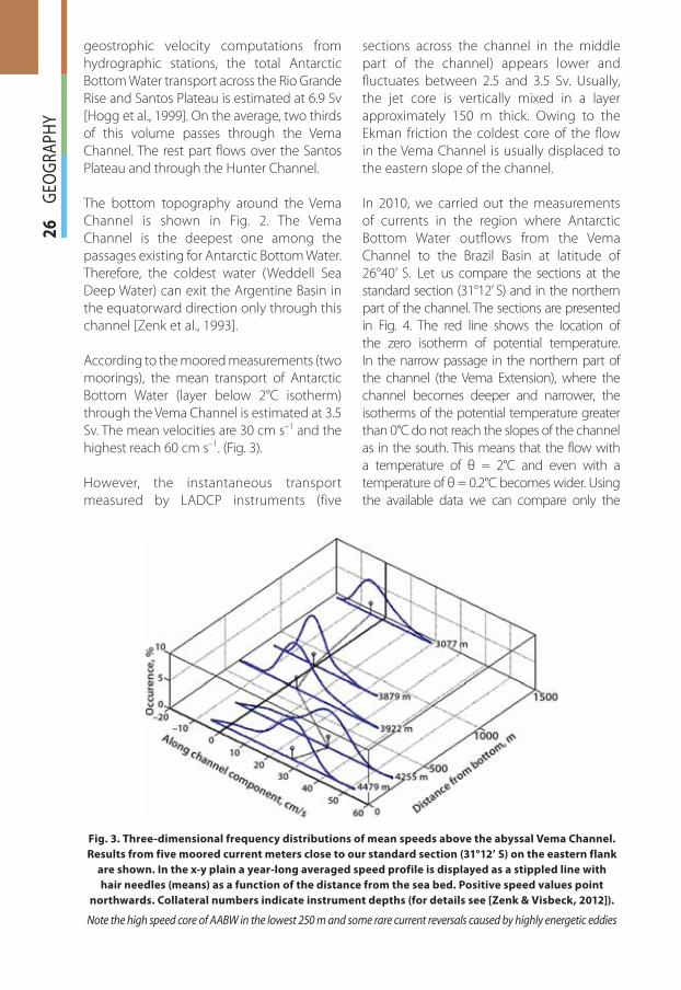
According to the moored measurements (two

moorings), the mean transport of Antarctic

Bottom Water (layer below 2°C isotherm)

through the Vema Channel is estimated at 3.5

Sv. The mean velocities are 30 cm s–1 and the

highest reach 60 cm s–1. (Fig. 3).

However, the instantaneous transport

measured by LADCP instruments (five

sections across the channel in the middle

part of the channel) appears lower and

fluctuates between 2.5 and 3.5 Sv. Usually,

the jet core is vertically mixed in a layer

approximately 150 m thick. Owing to the

Ekman friction the coldest core of the flow

in the Vema Channel is usually displaced to

the eastern slope of the channel.

In 2010, we carried out the measurements

of currents in the region where Antarctic

Bottom Water outflows from the Vema

Channel to the Brazil Basin at latitude of

26°40’ S. Let us compare the sections at the

standard section (31°12’ S) and in the northern

part of the channel. The sections are presented

in Fig. 4. The red line shows the location of

the zero isotherm of potential temperature.

In the narrow passage in the northern part of

the channel (the Vema Extension), where the

channel becomes deeper and narrower, the

isotherms of the potential temperature greater

than 0°C do not reach the slopes of the channel

as in the south. This means that the flow with

a temperature of θ = 2°С and even with a

temperature of θ = 0.2°С becomes wider. Using

the available data we can compare only the

Fig. 3. Three-dimensional frequency distributions of mean speeds above the abyssal Vema Channel.

Results from five moored current meters close to our standard section (31°12’ S) on the eastern flank

are shown. In the x-y plain a year-long averaged speed profile is displayed as a stippled line with

hair needles (means) as a function of the distance from the sea bed. Positive speed values point

northwards. Collateral numbers indicate instrument depths (for details see [Zenk & Visbeck, 2012]).

Note the high speed core of AABW in the lowest 250 m and some rare current reversals caused by highly energetic eddies

gi412.indd 26gi412.indd 26 24.12.2012 9:10:4124.12.2012 9:10:41

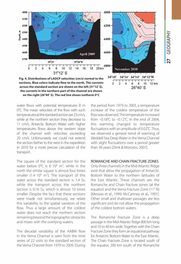
27

G

EOG

RAPH

Y

water flows with potential temperatures θ m

0°C. The mean velocities of the flow with such

temperatures at the standard section are 23 cm/s,

while at the northern section they decrease to

11 cm/s. Antarctic Bottom Water with higher

temperatures flows above the western slope

of the channel with velocities exceeding

20 cm/s. Unfortunately we could not extend

the section farther to the west in the expedition

in 2010 for a more precise calculation of the

transport.

The square of the standard section for the

water below 0°C is 6 106 m2, while in the

north the similar square is almost four times

smaller (1.4 106 m2). The transport of this

water across the standard section is 1.4 Sv,

while the transport across the northern

section is 0.16 Sv, which is almost 10 times

smaller. Despite the fact that these sections

were made not simultaneously, we relate

this variability to the spatial variation of the

flow. Thus a large amount of the coldest

water does not reach the northern section

remaining beyond the topographic obstacles

and mixes with the overlying waters.

The decadal variability of the AABW flow

in the Vema Channel is seen from the time

series of 22 visits to the standard section of

the Vema Channel from 1979 to 2009. During

the period from 1979 to 2003, a temperature

increase of the coldest temperature of the

flow was observed. The temperature increased

from –0.18°C to –0.12°C. In the end of 2004,

this warming changed to temperature

fluctuations with an amplitude of 0.02°C. Thus,

we observed a general trend of warming of

Weddell Sea Deep Water in the Vema Channel

with slight fluctuations over a period greater

than 30 years [Zenk & Morozov, 2007].

ROMANCHE AND CHAIN FRACTURE ZONES

Only three channels in the Mid-Atlantic Ridge

exist that allow the propagation of Antarctic

Bottom Water to the northern latitudes of

the East Atlantic. These channels are: the

Romanche and Chain fracture zones (at the

equator) and the Vema Fracture Zone (11° N)

[Messias et al., 1999; McCartney et al., 1991].

Other small and shallower passages are less

significant and do not allow the propagation

of the coldest bottom waters.

The Romanche Fracture Zone is a deep

passage in the Mid-Atlantic Ridge 800 km long

and 10 to 40 km wide. Together with the Chain

Fracture Zone they form an equatorial pathway

for Antarctic Bottom Water to the East Atlantic.

The Chain Fracture Zone is located south of

the equator, 200 km south of the Romanche

Fig. 4. Distributions of LADCP velocities (cm/s) normal to the

sections. Blue colors indicate flow to the north. The currents

across the standard section are shown on the left (31°12’ S),

the currents in the northern part of the channel are shown

on the right (26°40’ S). The red line shows isotherm 0°C

gi412.indd 27gi412.indd 27 24.12.2012 9:10:4224.12.2012 9:10:42

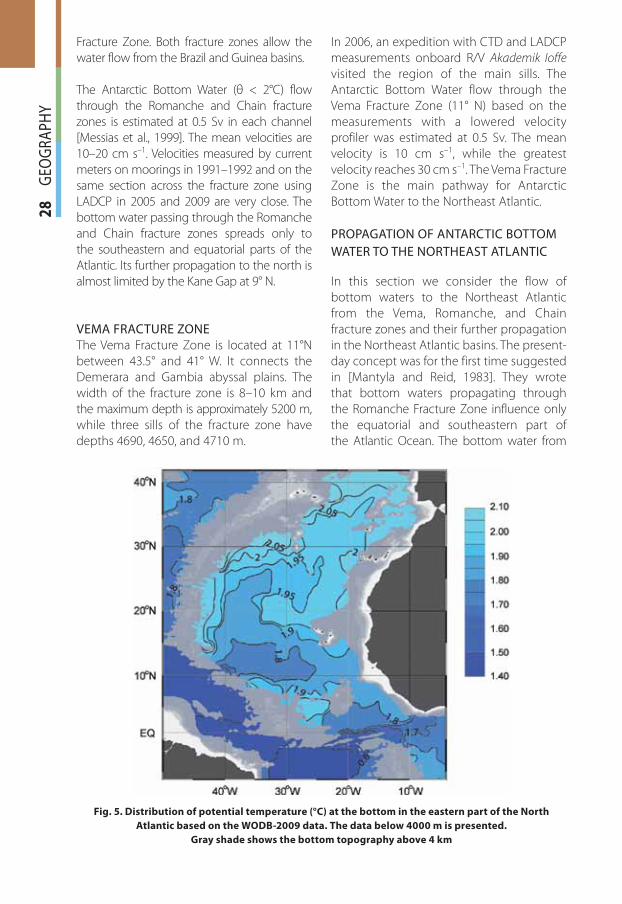
28

G

EOG

RAPH

YFracture Zone. Both fracture zones allow the

water flow from the Brazil and Guinea basins.

The Antarctic Bottom Water (θ < 2°C) flow

through the Romanche and Chain fracture

zones is estimated at 0.5 Sv in each channel

[Messias et al., 1999]. The mean velocities are

10–20 cm s–1. Velocities measured by current

meters on moorings in 1991–1992 and on the

same section across the fracture zone using

LADCP in 2005 and 2009 are very close. The

bottom water passing through the Romanche

and Chain fracture zones spreads only to

the southeastern and equatorial parts of the

Atlantic. Its further propagation to the north is

almost limited by the Kane Gap at 9° N.

VEMA FRACTURE ZONE

The Vema Fracture Zone is located at 11°N

between 43.5° and 41° W. It connects the

Demerara and Gambia abyssal plains. The

width of the fracture zone is 8–10 km and

the maximum depth is approximately 5200 m,

while three sills of the fracture zone have

depths 4690, 4650, and 4710 m.

In 2006, an expedition with CTD and LADCP

measurements onboard R/V Akademik Ioffe

visited the region of the main sills. The

Antarctic Bottom Water flow through the

Vema Fracture Zone (11° N) based on the

measurements with a lowered velocity

profiler was estimated at 0.5 Sv. The mean

velocity is 10 cm s–1, while the greatest

velocity reaches 30 cm s–1. The Vema Fracture

Zone is the main pathway for Antarctic

Bottom Water to the Northeast Atlantic.

PROPAGATION OF ANTARCTIC BOTTOM

WATER TO THE NORTHEAST ATLANTIC

In this section we consider the flow of

bottom waters to the Northeast Atlantic

from the Vema, Romanche, and Chain

fracture zones and their further propagation

in the Northeast Atlantic basins. The present-

day concept was for the first time suggested

in [Mantyla and Reid, 1983]. They wrote

that bottom waters propagating through

the Romanche Fracture Zone influence only

the equatorial and southeastern part of

the Atlantic Ocean. The bottom water from

Fig. 5. Distribution of potential temperature (°C) at the bottom in the eastern part of the North

Atlantic based on the WODB-2009 data. The data below 4000 m is presented.

Gray shade shows the bottom topography above 4 km

gi412.indd 28gi412.indd 28 24.12.2012 9:10:4224.12.2012 9:10:42

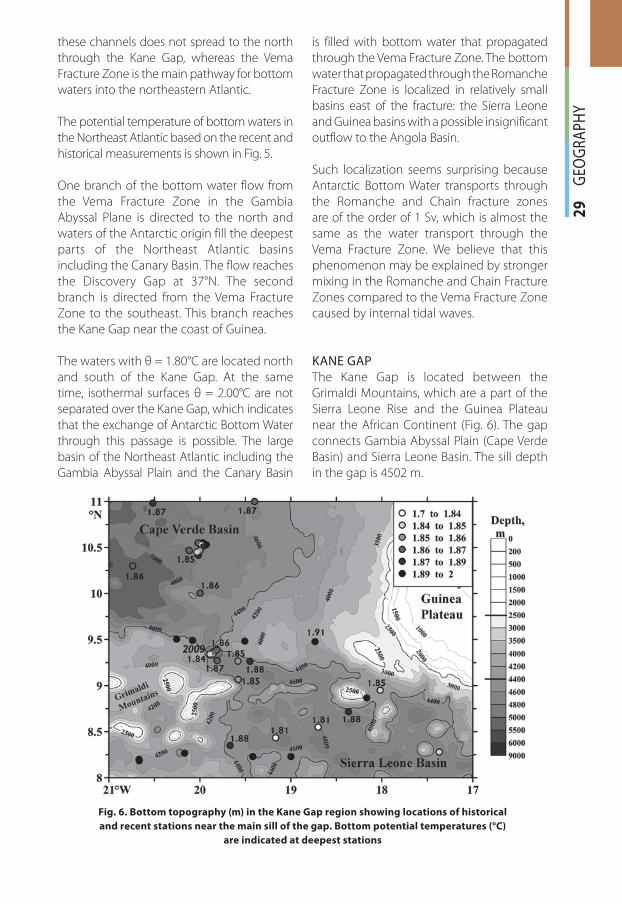
29

G

EOG

RAPH

Y

these channels does not spread to the north

through the Kane Gap, whereas the Vema

Fracture Zone is the main pathway for bottom

waters into the northeastern Atlantic.

The potential temperature of bottom waters in

the Northeast Atlantic based on the recent and

historical measurements is shown in Fig. 5.

One branch of the bottom water flow from

the Vema Fracture Zone in the Gambia

Abyssal Plane is directed to the north and

waters of the Antarctic origin fill the deepest

parts of the Northeast Atlantic basins

including the Canary Basin. The flow reaches

the Discovery Gap at 37°N. The second

branch is directed from the Vema Fracture

Zone to the southeast. This branch reaches

the Kane Gap near the coast of Guinea.

The waters with θ = 1.80°C are located north

and south of the Kane Gap. At the same

time, isothermal surfaces θ = 2.00°C are not

separated over the Kane Gap, which indicates

that the exchange of Antarctic Bottom Water

through this passage is possible. The large

basin of the Northeast Atlantic including the

Gambia Abyssal Plain and the Canary Basin

is filled with bottom water that propagated

through the Vema Fracture Zone. The bottom

water that propagated through the Romanche

Fracture Zone is localized in relatively small

basins east of the fracture: the Sierra Leone

and Guinea basins with a possible insignificant

outflow to the Angola Basin.

Such localization seems surprising because

Antarctic Bottom Water transports through

the Romanche and Chain fracture zones

are of the order of 1 Sv, which is almost the

same as the water transport through the

Vema Fracture Zone. We believe that this

phenomenon may be explained by stronger

mixing in the Romanche and Chain Fracture

Zones compared to the Vema Fracture Zone

caused by internal tidal waves.

KANE GAP

The Kane Gap is located between the

Grimaldi Mountains, which are a part of the

Sierra Leone Rise and the Guinea Plateau

near the African Continent (Fig. 6). The gap

connects Gambia Abyssal Plain (Cape Verde

Basin) and Sierra Leone Basin. The sill depth

in the gap is 4502 m.

Fig. 6. Bottom topography (m) in the Kane Gap region showing locations of historical

and recent stations near the main sill of the gap. Bottom potential temperatures (°C)

are indicated at deepest stations

gi412.indd 29gi412.indd 29 24.12.2012 9:10:4224.12.2012 9:10:42

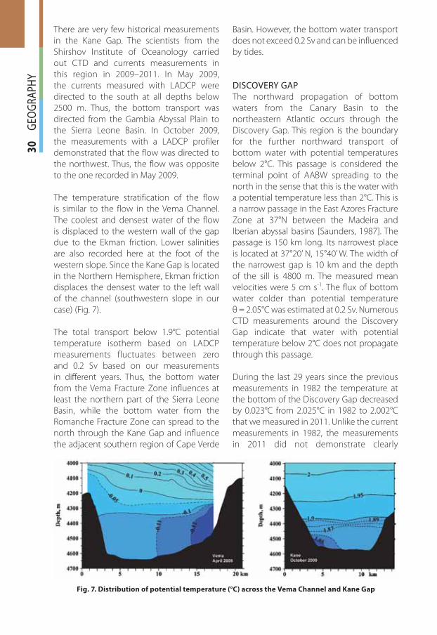
30

G

EOG

RAPH

YThere are very few historical measurements

in the Kane Gap. The scientists from the

Shirshov Institute of Oceanology carried

out CTD and currents measurements in

this region in 2009–2011. In May 2009,

the currents measured with LADCP were

directed to the south at all depths below

2500 m. Thus, the bottom transport was

directed from the Gambia Abyssal Plain to

the Sierra Leone Basin. In October 2009,

the measurements with a LADCP profiler

demonstrated that the flow was directed to

the northwest. Thus, the flow was opposite

to the one recorded in May 2009.

The temperature stratification of the flow

is similar to the flow in the Vema Channel.

The coolest and densest water of the flow

is displaced to the western wall of the gap

due to the Ekman friction. Lower salinities

are also recorded here at the foot of the

western slope. Since the Kane Gap is located

in the Northern Hemisphere, Ekman friction

displaces the densest water to the left wall

of the channel (southwestern slope in our

case) (Fig. 7).

The total transport below 1.9°C potential

temperature isotherm based on LADCP

measurements fluctuates between zero

and 0.2 Sv based on our measurements

in different years. Thus, the bottom water

from the Vema Fracture Zone influences at

least the northern part of the Sierra Leone

Basin, while the bottom water from the

Romanche Fracture Zone can spread to the

north through the Kane Gap and influence

the adjacent southern region of Cape Verde

Basin. However, the bottom water transport

does not exceed 0.2 Sv and can be influenced

by tides.

DISCOVERY GAP

The northward propagation of bottom

waters from the Canary Basin to the

northeastern Atlantic occurs through the

Discovery Gap. This region is the boundary

for the further northward transport of

bottom water with potential temperatures

below 2°C. This passage is considered the

terminal point of AABW spreading to the

north in the sense that this is the water with

a potential temperature less than 2°C. This is

a narrow passage in the East Azores Fracture

Zone at 37°N between the Madeira and

Iberian abyssal basins [Saunders, 1987]. The

passage is 150 km long. Its narrowest place

is located at 37°20’ N, 15°40’ W. The width of

the narrowest gap is 10 km and the depth

of the sill is 4800 m. The measured mean

velocities were 5 cm s-1. The flux of bottom

water colder than potential temperature

θ = 2.05°C was estimated at 0.2 Sv. Numerous

CTD measurements around the Discovery

Gap indicate that water with potential

temperature below 2°C does not propagate

through this passage.

During the last 29 years since the previous

measurements in 1982 the temperature at

the bottom of the Discovery Gap decreased

by 0.023°C from 2.025°С in 1982 to 2.002°С

that we measured in 2011. Unlike the current

measurements in 1982, the measurements

in 2011 did not demonstrate clearly

Fig. 7. Distribution of potential temperature (°C) across the Vema Channel and Kane Gap

gi412.indd 30gi412.indd 30 24.12.2012 9:10:4324.12.2012 9:10:43

31

G

EOG

RAPH

Y

manifested northerly flow of the bottom

water. A fluctuating flow was observed in

2011. One core displaced to the eastern

slope was directed to the northeast with

velocities of approximately 5 cm/s and the

second core with slightly greater velocities

was directed to the southwest and displaced

to the western slope.

CONCLUSIONS

We summarized the characteristics of the

transport of bottom water from its source

region in the Weddell Sea through the main

abyssal channels of the Atlantic Ocean. The

analysis is based on the recent CTD-sections

and moored current meters as well as on the

historical data. The main properties of the

bottom flow in the Vema Channel include

a flow with a mean speed of 30 cm/s. The

measurements in the Vema Channel that

have been continuing for 30 years already

revealed a temperature increase and recent

fluctuations in the temperature of the coldest

water. After the flow of Antarctic Bottom

Water passes the Brazil Basin it splits into two

flows. Part of the water flows through the

Romanche and Chain fracture zones to the

east. The other part flows to the northwest

to the North American Basin. Part of the

latter flow propagates through the Vema

Fracture Zone into the Northeast Atlantic.

We analyze an unsteady flow of bottom

water in the Kane Gap. The terminal point

for the Antarctic Bottom Water flow is the

Discovery Gap.

ACKNOWLEDGEMENTS

The expeditions onboard Russian research

vessels were carried out as a part of

projects “Southern Ocean” and “Meridian”.

The study was supported by the Russian

Foundation for Basic Research and Programs

of the Presidium of the Russian Academy

of Sciences. The German expeditions were

supported by funds of the German Research

Foundation (Bonn) and the German Federal

Ministry of Education and Research, Berlin

(CLIVAR Marin-2). �

REFERENCES

1. Hogg N.G., Owens W.B. (1999). Direct measurement of the deep circulation within the Brazil Basin, Deep-Sea Res. II, Vol. 46, pp. 335–353.

2. Mantyla A.W., Reid J.L. (1983). Abyssal characteristics of the World Ocean waters, Deep-Sea Res., Vol. 30, N 8, pp. 805–833.

3. McCartney M.S., Bennet S.L., Woodgate-Jones M.E. (1991). Eastward flow through the Mid-Atlantic ridge at 11° N and its influence on the abyss of the Eastern basin, J. Phys. Oceanogr., Vol. 21, N 8, pp. 1089–1121.

4. Messias M.-J., Andrie C., Memery L., Mercier H. (1999). Tracing the North Atlantic Deep Water through the Romanche and Chain fracture zones with chlorofluoromethanes, Deep-Sea Res. Vol. 46, pp. 1247–1278.

5. Morozov E.G., Demidov A.N., Tarakanov R.Y., Zenk W. (2010). Abyssal Channels of the At-lantic Ocean: Water Structure and Flows, Springer, 266 p.

6. Orsi A.H., Johnsson G.C., Bullister J.L. (1999). Circulation, mixing, and production of Antarc-tic Bottom Water, Progress in Oceanography, Vol. 43, pp. 55–109.

7. Saunders P.M. (1987). Flow through Discovery Gap, J. Phys. Oceanogr., Vol. 17, N. 5, pp. 631–643.

8. Wüst G. (1936). Schichtung und Zirkulation des Atlantischen Ozeans, Das Bodenwasser und die Stratosphäre. In: A. Defant (Ed.), Wissenschaftliche Ergebnisse, Deutsche Atlantische Expedition auf dem Forschungs – und Vermessungsschiff „Meteor“ 1925–1927, 6 (1), Walter de Gruyter & Co, Berlin, 411 pg.

gi412.indd 31gi412.indd 31 24.12.2012 9:10:4324.12.2012 9:10:43

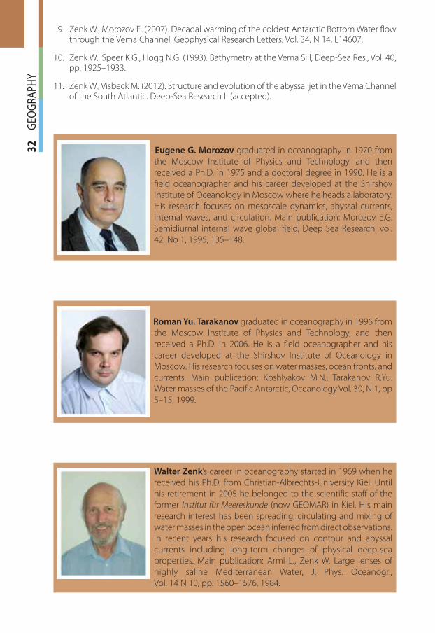
32

G

EOG

RAPH

Y 9. Zenk W., Morozov E. (2007). Decadal warming of the coldest Antarctic Bottom Water flow

through the Vema Channel, Geophysical Research Letters, Vol. 34, N 14, L14607.

10. Zenk W., Speer K.G., Hogg N.G. (1993). Bathymetry at the Vema Sill, Deep-Sea Res., Vol. 40, pp. 1925–1933.

11. Zenk W., Visbeck M. (2012). Structure and evolution of the abyssal jet in the Vema Channel of the South Atlantic. Deep-Sea Research II (accepted).

Eugene G. Morozov graduated in oceanography in 1970 from

the Moscow Institute of Physics and Technology, and then

received a Ph.D. in 1975 and a doctoral degree in 1990. He is a

field oceanographer and his career developed at the Shirshov

Institute of Oceanology in Moscow where he heads a laboratory.

His research focuses on mesoscale dynamics, abyssal currents,

internal waves, and circulation. Main publication: Morozov E.G.

Semidiurnal internal wave global field, Deep Sea Research, vol.

42, No 1, 1995, 135–148.

Roman Yu. Tarakanov graduated in oceanography in 1996 from

the Moscow Institute of Physics and Technology, and then

received a Ph.D. in 2006. He is a field oceanographer and his

career developed at the Shirshov Institute of Oceanology in

Moscow. His research focuses on water masses, ocean fronts, and

currents. Main publication: Koshlyakov M.N., Tarakanov R.Yu.

Water masses of the Pacific Antarctic, Oceanology Vol. 39, N 1, pp

5–15, 1999.

Walter Zenk’s career in oceanography started in 1969 when he

received his Ph.D. from Christian-Albrechts-University Kiel. Until

his retirement in 2005 he belonged to the scientific staff of the

former Institut für Meereskunde (now GEOMAR) in Kiel. His main

research interest has been spreading, circulating and mixing of

water masses in the open ocean inferred from direct observations.

In recent years his research focused on contour and abyssal

currents including long-term changes of physical deep-sea

properties. Main publication: Armi L., Zenk W. Large lenses of

highly saline Mediterranean Water, J. Phys. Oceanogr.,

Vol. 14 N 10, pp. 1560–1576, 1984.

gi412.indd 32gi412.indd 32 24.12.2012 9:10:4324.12.2012 9:10:43

33

EN

VIR

ON

MEN

T

ABSTRACT. An extensive land reform

programme is underway, which faces many

challenges unique to the socio-political

context of post-apartheid South Africa. The

aim of this paper is to review the extent to

which agrarian land reform policy, more

particularly in respect to its land distribution

element, incorporates environmental

sustainability principles into resultant

practice and whether or not this may lead to

exacerbation of land degradation problems

in the country. The paper briefly outlines the

key land reform role-players, the policy and

implementation process of land reform, and

considers these in relation to the problem

of land degradation. Ongoing problems of

implementation with the land redistribution

programme are discussed in relation to a

number of significant challenges. The

paper illustrates the lack of integration

of environmental planning in the land

reform process generally and points to the

potentially deleterious impact of land reform

on land degradation.

KEY WORDS: Land reform, land degradation,

apartheid, environmental impact, agricultural

policy, rural livelihoods

INTRODUCTION AND CONTEXT

LAND REFORM IN SOUTH AFRICA

Land reform is a highly topical and emotionally

charged issue that has received particular

attention in southern Africa but one that

resonates across the continent as a whole

[Cousins, 2009]. South Africa, as an emerging

democracy with a well known history of

conquest and dispossession of land in the

colonial and apartheid eras, has embarked

on a systematic land reform programme

in order to redress previous political and

economic imbalances. Since the demise of

the apartheid system in the early 1990s, land

reform has been a part of the restructuring

process in South Africa, and was one of the

cornerstones of African National Congress

(ANC) policy when they formed the new

democratic government in 1994 [Ibsen, 2000;

Lemon, 2004]. The ANC’s Reconstruction and

Development Programme (RDP) envisaged a

land reform programme that was integral to

rural development:

A national land reform programme is the

central and driving force of a programme of

rural development [African National Congress,

1993, section 2.4.2].

Through a government programme of land

reform since 1994, efforts are being made to

redress the past inequity of access to land

and resources, although it remains a hotly

debated, emotive and contested issue and

one that is further complicated by other

social and health problems in the region

[Drimie, 2003]. There has been much debate

in both official government circles and in the

media (see, for example, Financial Mail, 28th

February 2012, in which progress is described

as proceeding “...at a snail’s pace”). There

are, in addition, other concerns, particularly

Michael E. MeadowsDepartment of Environmental & Geographical Science, University of Cape TownRondebosch 7701, South Africa; Tel: +27 21 650 2873, Fax: +27 21 65- 3456;e-mail: mmeadows@mweb.co.za

CONTEMPORARY LAND REFORM POLICY AND PRACTICE IN SOUTH AFRICA AND ITS ENVIRONMENTAL IMPLICATIONS: NEW IDEAS, OLD PROBLEMS?

gi412.indd 33gi412.indd 33 24.12.2012 9:10:4424.12.2012 9:10:44

34

EN

VIR

ON

MEN

Tover the potential environmental impact of

agrarian land reform if sustainability issues

are not systematically incorporated into

policy and practice [Wynberg and Sowman,

2007]. Thus, while there are clear political

and economic imperatives to land reform,

the fact that much of rural South Africa

experiences a semi-arid climate and is highly

susceptible to land degradation [Hoffman

et al., 1999; Kakembo and Rowntree, 2003],

strongly suggests that such environmental

concerns need to be taken very seriously.

The model of land reform developed and

adopted by the post-1994 democratic

government has three elements: land

restitution (the return to the previous

owners of land taken away under racially

discriminatory laws, limited to those

removals that took place after the 1913 Land

Act), land tenure reform (administration and

legislation to improve tenure security and to

accommodate diverse forms of land tenure,

including communal tenure) and a market-

led, demand-driven land redistribution

programme that intends to achieve both

political goals and economic growth in

the agricultural sector [DLA, 1997; Turner

and Ibsen, 2000]. The land redistribution

programme initially aimed to obtain the

transfer of 30% of historically white-owned

agricultural land (including both private

commercial and State agricultural land) by

2014 [ANC 1993]. This paper explores agrarian

land reform in South Africa, in particular its

land redistribution component, and assesses

the policy, process and practice of land

reform together with its possible impacts on

the environment. In reviewing progress – or

lack of it – in regard to land reform, it is argued

that any process that lacks integrity in terms

of the environment will ultimately fail to

solve the social and economic problems it is

aimed at addressing. The argument is made

that, while land reform per se is absolutely

key to rural development in the country,

its implementation without significant

consideration of the natural environmental

constraints of the country, cannot resolve

the serious inequities associated with the

marginalisation South Africa’s rural poor.

While land reform has been a cornerstone

of national policy since the installation

of the first democratic government in

1994, the proposed future trajectory for

the programme is set out in the recent

Green Paper on Land Reform issued by the

Department of Rural Development and Land

Reform [DRDLR, 2011]. The basic tenets of the

policy are underpinned by the recognition that

agrarian transformation is fundamental to future

social cohesion and development in general as

well as improved food sovereignty and food

security in particular; such goals depend on

more equitable access to and ownership of

land. The strategy involves government support

(subsidies and technical support) for people

of so-called designated population groups,

wishing to purchase agricultural land for farming

purposes (each described as a “land reform

project”). The extent to which the revised land

reform policy, as set out in this Green Paper,

redresses some of the shortcomings of the

original, post-apartheid intentions provides an

important focus for this paper.

Rural livelihoods in South Africa are

acknowledged to be complex and dynamic

systems and that ‘…undoing the social,

economic and cultural effects of centuries

of discrimination and exclusion on the basis

of race, class and gender, will take time and

an enduring national political effort [DRDLR,

2011]. However, the fact that agrarian

livelihoods and, indeed, the livelihoods of

the rural population in general, are directly

dependent on natural resources highlights

the significance of the environment to

the process. This clearly has important

implications for the conceptualisation,

design and implementation of land reform

policy and practice [Shackleton et al. 1999].

It is, therefore, essential that the planning

of land reform, including restitution,

redistribution and tenure reform, should

systematically embrace an evaluation of the

land and the available natural resources, and

an assessment of the suitability of land for

the envisaged land uses (the impacts of the

land uses on the natural environment). Such

evaluation should incorporate an inventory

and assessment of the existing situation

gi412.indd 34gi412.indd 34 24.12.2012 9:10:4424.12.2012 9:10:44

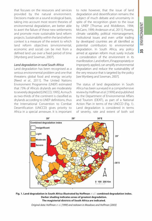
35

EN

VIR

ON

MEN

T

that focuses on the resources and services

provided by the natural environment.

Decisions made on a sound ecological basis,

taking into account most recent theories of

environmental degradation, are better able

to avert the failure of these new settlements

and promote more sustainable land reform

projects. Sustainability within the land reform

context is a measure of the extent to which

land reform objectives (environmental,

economic and social) can be met from a

defined land use over a fixed period of time

[Wynberg and Sowman, 2007].

Land degradation in rural South Africa

Land degradation has been recognised as a

serious environmental problem and one that

threatens global food and energy security

[Reed et al., 2011]. The United Nations

Environment Programme (UNEP) estimated

that 73% of Africa’s drylands are moderately

to severely degraded [UNCCD, 1995]. As much

as two-thirds of the continent is classified as

drylands according to UNEP definitions, thus

the International Convention to Combat

Desertification (UNCCD) gives priority to

Africa in a special annexure. It is important

to note however, that the issue of land

degradation and desertification remains the

subject of much debate and uncertainty in

spite of the recognition given to the issue

by UNEP [Thomas and Middleton, 1994;

McCann, 1999; Andersson et al., 2011]. Poverty,

climate variability, political mismanagement,

institutional issues and even unfair trading

by developed countries are all identified as

potential contributors to environmental

degradation. In South Africa, any policy

aimed at agrarian reform must surely include

a consideration of the environment in its

manifestation. Land reform, if inappropriately or

improperly applied, can amplify environmental

degradation and reduce the sustainability of

the very resource that is targeted by the policy

[see Wynberg and Sowman, 2007].

The status of land degradation in South

Africa has been surveyed in a comprehensive

review by Hoffman et al. [1999] and published

by the Department of Environmental Affairs

and Tourism (DEAT), as part of a National

Action Plan in terms of the UNCCD (Fig. 1).

Land degradation is considered in terms

of severity, rate and extent of both soil

Fig. 1. Land degradation in South Africa illustrated by Hoffman et al.’s combined degradation index.

Darker shading indicates areas of greatest degradation.

The magisterial districts of South Africa are indicated.

Original data: Hoffman et al. [1999] and redrawn in Meadows and Hoffman [2003]

gi412.indd 35gi412.indd 35 24.12.2012 9:10:4424.12.2012 9:10:44

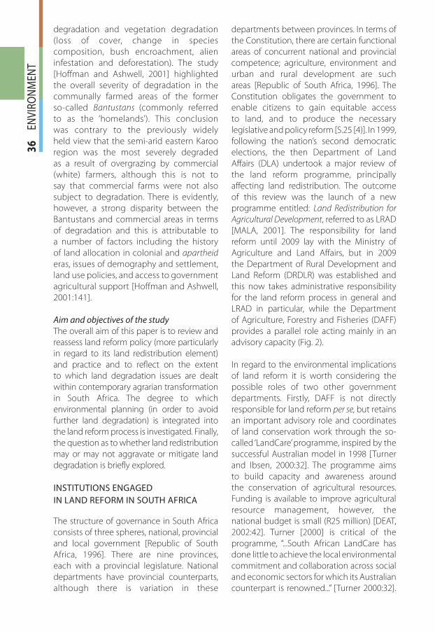
36

EN

VIR

ON

MEN

Tdegradation and vegetation degradation

(loss of cover, change in species

composition, bush encroachment, alien

infestation and deforestation). The study

[Hoffman and Ashwell, 2001] highlighted

the overall severity of degradation in the

communally farmed areas of the former

so-called Bantustans (commonly referred

to as the ‘homelands’). This conclusion

was contrary to the previously widely

held view that the semi-arid eastern Karoo

region was the most severely degraded

as a result of overgrazing by commercial

(white) farmers, although this is not to

say that commercial farms were not also

subject to degradation. There is evidently,

however, a strong disparity between the

Bantustans and commercial areas in terms

of degradation and this is attributable to

a number of factors including the history

of land allocation in colonial and apartheid

eras, issues of demography and settlement,

land use policies, and access to government

agricultural support [Hoffman and Ashwell,

2001:141].

Aim and objectives of the study

The overall aim of this paper is to review and

reassess land reform policy (more particularly

in regard to its land redistribution element)

and practice and to reflect on the extent

to which land degradation issues are dealt

within contemporary agrarian transformation

in South Africa. The degree to which

environmental planning (in order to avoid

further land degradation) is integrated into

the land reform process is investigated. Finally,

the question as to whether land redistribution

may or may not aggravate or mitigate land

degradation is briefly explored.

INSTITUTIONS ENGAGED

IN LAND REFORM IN SOUTH AFRICA

The structure of governance in South Africa

consists of three spheres, national, provincial

and local government [Republic of South

Africa, 1996]. There are nine provinces,

each with a provincial legislature. National

departments have provincial counterparts,

although there is variation in these

departments between provinces. In terms of

the Constitution, there are certain functional

areas of concurrent national and provincial

competence; agriculture, environment and

urban and rural development are such

areas [Republic of South Africa, 1996]. The

Constitution obligates the government to

enable citizens to gain equitable access

to land, and to produce the necessary

legislative and policy reform [S.25 [4)]. In 1999,

following the nation’s second democratic

elections, the then Department of Land

Affairs (DLA) undertook a major review of

the land reform programme, principally

affecting land redistribution. The outcome

of this review was the launch of a new

programme entitled: Land Redistribution for

Agricultural Development, referred to as LRAD

[MALA, 2001]. The responsibility for land

reform until 2009 lay with the Ministry of

Agriculture and Land Affairs, but in 2009

the Department of Rural Development and

Land Reform (DRDLR) was established and

this now takes administrative responsibility

for the land reform process in general and

LRAD in particular, while the Department

of Agriculture, Forestry and Fisheries (DAFF)

provides a parallel role acting mainly in an

advisory capacity (Fig. 2).

In regard to the environmental implications

of land reform it is worth considering the

possible roles of two other government

departments. Firstly, DAFF is not directly

responsible for land reform per se, but retains

an important advisory role and coordinates

of land conservation work through the so-

called ‘LandCare’ programme, inspired by the

successful Australian model in 1998 [Turner

and Ibsen, 2000:32]. The programme aims

to build capacity and awareness around

the conservation of agricultural resources.

Funding is available to improve agricultural

resource management, however, the

national budget is small (R25 million) [DEAT,

2002:42]. Turner [2000] is critical of the

programme, “...South African LandCare has

done little to achieve the local environmental

commitment and collaboration across social

and economic sectors for which its Australian

counterpart is renowned...” [Turner 2000:32].

gi412.indd 36gi412.indd 36 24.12.2012 9:10:4524.12.2012 9:10:45

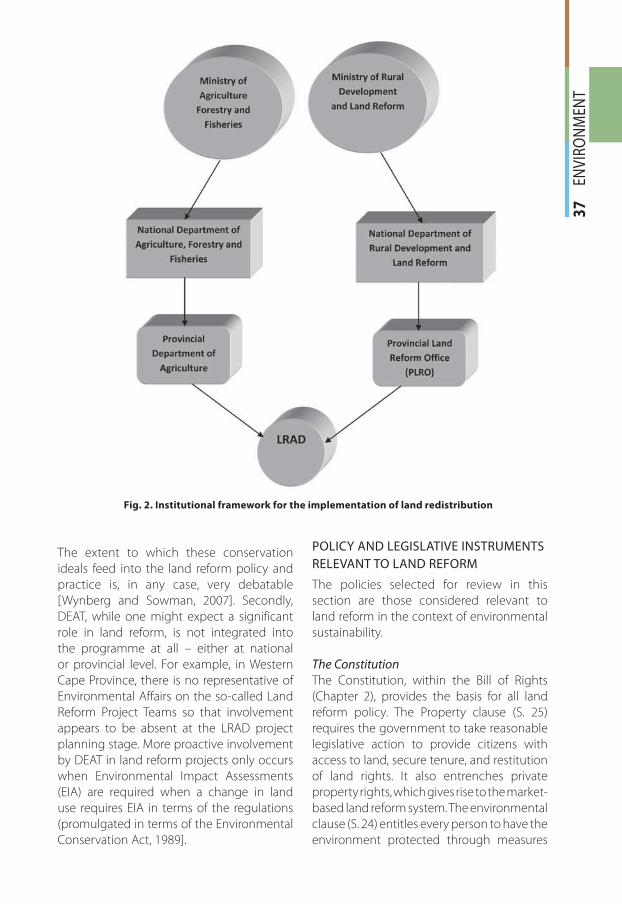
37

EN

VIR

ON

MEN

T

The extent to which these conservation

ideals feed into the land reform policy and

practice is, in any case, very debatable

[Wynberg and Sowman, 2007]. Secondly,

DEAT, while one might expect a significant

role in land reform, is not integrated into

the programme at all – either at national

or provincial level. For example, in Western

Cape Province, there is no representative of

Environmental Affairs on the so-called Land

Reform Project Teams so that involvement

appears to be absent at the LRAD project

planning stage. More proactive involvement

by DEAT in land reform projects only occurs

when Environmental Impact Assessments

(EIA) are required when a change in land

use requires EIA in terms of the regulations

(promulgated in terms of the Environmental

Conservation Act, 1989].

POLICY AND LEGISLATIVE INSTRUMENTS

RELEVANT TO LAND REFORM

The policies selected for review in this

section are those considered relevant to

land reform in the context of environmental

sustainability.

The Constitution

The Constitution, within the Bill of Rights

(Chapter 2), provides the basis for all land

reform policy. The Property clause (S. 25)

requires the government to take reasonable

legislative action to provide citizens with

access to land, secure tenure, and restitution

of land rights. It also entrenches private

property rights, which gives rise to the market-

based land reform system. The environmental

clause (S. 24) entitles every person to have the

environment protected through measures

Fig. 2. Institutional framework for the implementation of land redistribution

gi412.indd 37gi412.indd 37 24.12.2012 9:10:4524.12.2012 9:10:45

38

EN

VIR

ON

MEN

Twhich prevent “...ecological degradation”

and “...secure ecologically sustainable

development and use of natural resources

while promoting justifiable economic and

social development” (S. 24(b)). In terms of

this clause, land reform administrators and

participants are therefore required by the

constitution to develop and implement land

reform projects in a manner that will promote

ecologically sustainable development and

avoid ecological degradation.

White Paper on Land Policy, Department

of Land Affairs, 1997

The framework policy for land reform is still

the White Paper on Land Policy, 1997 [DLA,

1997]. The principles of the land reform

programme stated in the White Paper, set

out in Table 1 are such that planning of land

reform projects must ensure “...economic

viability and environmental sustainability”

[DLA, 1997:12].

The White Paper on Land Policy acknowledges

the existence of “...severe land degradation

and soil erosion” which it attributes to

landlessness, overcrowding in Bantustans,

and inappropriate farming methods on

commercial farms [DLA, 1997:23]. It identifies

the potential of the land reform programme

to result in land degradation:

One of the challenges of land reform is

to relieve land pressure without extending

environmental degradation over a wider

area. Unless projects are properly planned

and necessary measures are put in place to

govern zoning, planning and the ultimate

land use, the programme could result in land

being used unsustainably [DLA White Paper

on Land Policy, 1997:25].

The policy requires a 43feasibility study to

be prepared, with the assistance of DLA

planners, which includes an “...assessment

of environmental consequences of the

proposed undertaking” [DLA, 1997:25]. This

requires the consideration of the suitability

of the natural resources for the proposed

farming [DLA, 1997:25].

Land Redistribution for Agricultural

Development (LRAD) – Ministry of Agriculture

and Land Affairs, (Version 4, 2002)

The then Minister of Agriculture and Land

Affairs undertook a review of land reform

policy and programmes resulting in the

LRAD programme, launched in August

2001. LRAD deals with both the transfer of

agricultural land to individuals or groups,

and with commonage projects aimed at

improving access to municipal and tribal

land primarily for grazing purposes. LRAD

provides technical support and grants to

historically disadvantaged South African

citizens, regardless of income, to access land

specifically for agricultural purposes. The

Table 1. Land reform principles

Social justice Government must deal with landlessness and to remedy the unequal distribution of land in South Africa

Poverty focus Priority is given to the poor who need land to contribute to income and food security

Needs-based Land reform should respond to the expressed needs of people

Government as facilitator Government should facilitate the expression of demand and inform people of their optionas

Flexibility Provincial and local variations require fl exible application of policy within a frame-work of national norms.

Participation The participation of communities and individuals as partners with government. Deci-sions at local level.

Gender equity Priority should be given to women applicants

Economic and environ-mental sustainability

Planning of land reform projects must ensure these are economically and environ-mentally sustainable

Source: DLA, 1997. White Paper on South African Land Policy, Department of Land Aff airs.

gi412.indd 38gi412.indd 38 24.12.2012 9:10:4524.12.2012 9:10:45

39

EN

VIR

ON

MEN

T

aim of the LRAD programme was explicitly

stated as the transfer of 30% of the country’s

commercial agricultural land by 2014 in

order to improve food sovereignty for the

rural poor; decongest overcrowded former

homeland areas; expand opportunities for

women and young people in rural areas; and

promote environmental sustainability of land

and other natural resources [MALA, 2001:6].

LRAD may be considered as demand-led,

meaning beneficiaries must define the type

of project and must identify their own land

and acquisition of land continues to be on

the basis of the ‘willing-buyer, willing seller’

approach.

In the LRAD programme, all ‘beneficiaries’

must make a contribution in cash, kind or

labour of a minimum of ZAR1 5000.

1Beneficiaries can access a range of grants

along a sliding scale from ZAR 20 000 –

R100 000 per individual, depending on the

amount of their own contribution. The grant

and the contribution are calculated on an

individual adult basis; if people apply as a

group, the total amount of the grant and

own contribution are both scaled up by

the number of individuals represented in

the group. The programme is unclear and

conflicting with regard to the requirement

for environmental assessment of projects.

Version 4 of 2002 states that the ‘Business

Plan’ should include “...environmental impact

assessments” but only “...if applicable to the

project”, without any explanation of when

this would be the case.

Green Paper on Land Reform,

September 2011 [DRD&LR, 2011]

The release of the Green Paper (a document

issued for public comment and indicating a

policy framework) on Land Reform by DRDLR

in September 2011 [DRDLR, 2011] heralds

a fundamentally different approach to the

issue of agrarian transformation. It is implicit,

although not explicitly acknowledged, that

the need for a new structure lies in the failure

of the LRAD programme. The vision for land

1 Note, ZAR = South African Rand. At time of going to press,

1.0 US$ is approximately ZAR 8.7.

reform as set out in the Green Paper is:

reasonable access to land with secure rights

in order to fulfil basic needs for housing

and productive livelihoods [DRDLR, 2011].

Administratively, the most important

difference between the proposed system

and the existing LRAD is the adoption of a

proposed Land Management Commission

with extensive powers and which, working

with a Land Valuer-General, will oversee

the identification and purchase of land for

redistribution and restitution. The message

is that market principles have been an

impediment to land reform and that, de

facto, the ‘willing seller, willing buyer’

principle is no longer deemed central to

the transaction process. It is envisaged

that more properties would become

State-owned and that there would be

less emphasis on private ownership of

agricultural land. The concept of ‘land

ceilings’ is also alluded to, implying that

there should be a maximum amount of

land owned by any particular individual;

this is also a new, and highly controversial,

development, although there are no

specific recommendations as to what

such a ceiling should be. The much

anticipated Green Paper has received

generally highly critical reviews – from

frustration that the proposed policy

framework fails to give clear guidance as

to how agrarian transformation can be

achieved (for example, AgriSA, 2011], to

outright rejection on the grounds that the

proposals on land tenure violate the South

African Constitution [Afriforum, 2012].

Crucially, in relation to the theme of this

paper, there is no specific consideration of

environmental sustainability in the vision

(further discussed below).

LAND REFORM IN SOUTH AFRICA:

STATUS AND CHALLENGES

The strategic objective of the land

redistribution component of land reform was

to ensure the transfer of 30% of all agricultural

land by 2014 to the historically disadvantaged.

What progress has been made and how

realistic is it that the target will be met?

gi412.indd 39gi412.indd 39 24.12.2012 9:10:4524.12.2012 9:10:45

40

EN

VIR

ON

MEN

TWhat of the environmental sustainability of

the programme? Certainly there have been

significant problems regarding delivery due

to the enormous scale of this objective, to

lack of budget, lack of capacity and skills and

to constraints embedded in the actual land

reform policy instruments. In this section,

some of the problems experienced with

the implementation of land reform are

explored.

The challenge of delivery

The scale of redistribution of land envisaged in

the land reform programme is enormous and

way beyond the levels of delivery achieved

thus far. The land reform programme has

been constrained by shortfalls in budget,

with potential expenditure being double or

more the amount available from the national

treasury as well as underspending [DLA, 1999].

Slow implementation of land redistribution

projects has been a consistently alarming

feature of the programme, as indicated by

statistics for particular years. For example,

in 2006–2007, the then Department of

Land Affairs reported land transferred at

258 890 ha, which was barely 10% of the

targeted figure of 2.5 million ha [Lahiff, 2008].

Indeed, by 2007 the programme was so

far behind the land redistribution target

that approximately 2 million ha of land a

year would have to be acquired to reach

the target of 30% by the end of the year

2014 and that “...this is the equivalent of an

area the size of the Kruger National Park

every year for the next seven years” [De

Villiers 2007:7]. However, the introduction

of the Proactive Land Acquisition Strategy

(PLAS) and the Land and Agrarian Reform

Project (LARP), “...together with a greater

political emphasis on expropriation, raises

the possibility of at least some increase in

the rate of land transfer” [Lahiff, 2008: 2].

The most recent statistics are, accordingly,

somewhat more encouraging and suggest

an increasing pace of acquisition. During

2011–12, the Department actually over-

performed in transferring ownership of

some 392,850 ha (cf 239,990 ha in 2009) of

land against an annual target of 303,612 ha

[DRDLR, 2012], albeit this still falls woefully

short of what would be required if the figure

of 30% of total land were to be reached

by 2014.

Quantity or quality?

In its early years, the land reform programme

prioritised speed of delivery of land rather

than sustainability and quality of land reform

[DLA, 2000:36]. DLA’s internal performance

management systems have rewarded

officials in terms of quantity, measured in

hectares and households and in spending

their budget. The latest report [DRDLR,

2012] hints at the transfer of ‘strategically

located’ land and perhaps points to a greater

emphasis on effective land planning as a

key performance area. Davis [2011] argues

that there focus has now shifted from simple

land acquisition and transfer to ensuring

that systems are in place to make productive

use of the land, although it is difficult to see

exactly what such systems are in perusing

the policy instruments.

Lack of capacity

The lack of capacity within land reform offices,

affects the ability to deliver both quantity

and quality. Jacobs [2003] reported that

understaffing throughout the ranks of DLA

imposes constraints on the ability to meet

the needs of land reform beneficiaries and

the department itself notes that more than

11% of posts remain vacant [DRDLR, 2012].

Both implementation and effectiveness are

clearly constrained by a lack of capacity and,

in reviewing the programme, the department

indicates that more successful land reform

projects are those where the individual or

group beneficiaries are adequately trained.

The current programme, however, does not

provide for the inclusion of environmental

considerations either in the business plan or

in the development of capacity for the land

redistribution beneficiaries.

Accessing suitable land

A market-based model of land reform

has thus far meant that land had to be

obtained on a ‘willing-seller, willing-buyer’

basis. The high demand for land, coupled

with the fact that no incentive exists for

gi412.indd 40gi412.indd 40 24.12.2012 9:10:4624.12.2012 9:10:46

41

EN

VIR

ON

MEN

T

landowners to sell or subdivide their land

for redistribution purposes, means that

land available for land redistribution may

often be of poor quality and/or high price.

Landowners are also reluctant to sell land

through a slow, bureaucratic process,

which involves waiting for land grants to

be approved before the sale transaction

can be completed [Jacobs, 2003; Heibinck

and Shackleton, 2010]. The problem may

therefore manifest itself in terms of land

degradation because the LRAD system

is silent on the issue as to where land

reform takes place, such as in or near the

overcrowded former homeland areas. It

remains to be seen if the new procedures

proposed in the 2011 Green Paper will

address some of these shortcomings, but

the lack of any attention to land quality in

the documentation remains a concern.

DISCUSSION

It is clear that South African land reform,

particularly in the context of land

redistribution, has thus far failed to deliver

on its lofty aims. The goal of “30% by 2014”

will not be met (the current figure stands at

somewhat less than 10%) and has even been

referred to as trying to put out a fire with a

broken teacup [Moseley and McCusker, 2008].

The ‘two cycles’ of policy [Hall, 2007] that saw

an earlier, more populist policy aimed at very

poor farmers has been replaced by one that

focuses more on emerging black commercial

farmers, yet neither has been able to keep

pace with demand. This is a policy shift that

arguably ‘...reflects a desire on the part of

the government to support the expansion

of black commercial farmers ...rather than

radically restructure the agriculture sector in

South Africa’ [Boudreaux, 2010] and misses

the opportunity to improve social justice.

The policy set out in the 2011 Green Paper

aims to redress some of these shortcomings

but it proposes to do so by placing more

land in the hands of the State – a highly

controversial and, as yet, untested strategy.

Although environmental sustainability in

general, and land degradation in particular,

are to some extent reflected in the land reform

policies and instruments, it is clear that they

remain secondary or minor considerations.

Thurs, the White Paper on Land Policy 1997

acknowledges the existence of severe land

degradation and the risk of increased land

degradation as a result of the land reform

programme but the LRAD policy documents

do not provide sufficient detail to ensure

that adequate attention to environmental

planning occurs in the design stages of

projects. There is insufficient guidance on

the issue of environment as it relates to

land reform for private sector consultants,

agricultural officers or planners to ensure

sustainability. Any future policy needs to be

translated into simple tools that can be used

by planners, consultants and agricultural

officers to achieve both quantity and quality

in terms of land reform projects. Regrettably,

the new dispensation promised in the Green

Paper is silent on such matters. The only,

tangential, reference to sustainability in this

policy document are those comments that

refer to ‘livelihood security’ or ‘sustainable

rural production systems’ but these terms

are more likely used in the context of the

economic, rather than environmental or

ecological, context.

Poorly planned and managed land

redistribution may easily lead to more

intensive production, resulting in over-

cultivation or overgrazing. Exceeding the

carrying capacity of land (humans and

livestock) therefore has the potential to

increase land degradation. The viability of

farming enterprises will be threatened if

farmers have unrealistic expectations of

the supply of natural resources and the

productive potential of their land. Detailed

resource assessments and land evaluations

prior to project implementation, can avoid

potential risks associated with pressure from

overcrowding, both humans and livestock.

Review of land reform projects post-

implementation clearly reveals some of the

negative environmental impacts of land

reform [see DLA, 2000]. These impacts need

to be minimised through more thorough

gi412.indd 41gi412.indd 41 24.12.2012 9:10:4624.12.2012 9:10:46

42

EN

VIR

ON

MEN

Tenvironmental planning if intensified land

degradation is to be avoided. The effect

of land degradation goes beyond the

physical impacts and the issue of agricultural

production. The social impacts of land

degradation are increasing urbanisation,

as farming becomes less productive.

[Hoffman and Ashwell 2001]. As Hebinck

and Shackleton [2010: p xx] note: “...

resources and their use can and should

not be treated as disconnected from the

social actors that access and use them”

and there is a distinct risk in the current

and likely future implementation of the

land reform programme in South Africa

that such a disconnection can result in

significant environmental deterioration.

An environmentally unsustainable solution

cannot resolve the crisis of rural poverty and

inequity [see Giller et al., 2008, for a possible

approach to addressing this problem].

Returning to the key elements of this paper,

it is clear that environmental sustainability

and land degradation have not yet been

adequately addressed in South Africa’s land

reform programme. Initially, it appears that

there was recognition of the potential

risk of environmental deterioration but

the policy in practice has fallen short of

providing adequate, sufficiently detailed

and user-friendly guidelines to avoid further

degradation. Environmental planning is not

integrated into the land reform process

in a consistent and coherent manner. The

potential impact of land reform on land

degradation is problematic and could result

in the failure of land reform projects. The

impact of land reform on land use and

land degradation has thus far not been

monitored. It is a lesson that we need

to learn fast if the land reform process,

controversial and complex as it already is,

is not to result in further environmental

degradation and the exposure of South

Africa’s historically disadvantaged rural

poor to even greater levels of risk and

vulnerability. Land reform experience

elsewhere suggests that ecological and

environmental factors can be incorporated

successfully into the system. In Brazil, for

example, where historically agrarian reform

had been associated with deforestation

and environmental degradation, the

government introduced a scheme in 2003

that actively encouraged citizens to adopt

an ecologically sustainable attitude to land

[Wittman, 2010]. Successive governments

in that country have successfully integrated

food production and environmental

management into the land reform

programme [Davis, 2011]; South Africa

would surely do well to implement such

a model.

CONCLUSION

Although it is important not to delay

the process of land reform even further,

incorporation of environmental guidelines

and proper follow-up to individual land

reform projects in the form of sound

ecological monitoring and advice is

essential if land degradation is not to

be accelerated as a result. The South

African environment has been termed

a ‘neglected dimension’ in agrarian

transformation [Wynberg and Sowman,

2007] and, unfortunately, newly proposed

policy interventions appear unlikely to

be any more sustainable than existing

ones. Given the semi-arid nature of much

of South Africa, the words of Geist and

Lambin [2004: 828] are highly pertinent

where they note that “...a detailed

understanding of the complex set of

proximal causes and underlying driving

forces affecting dryland-cover change

is required before any assessment or policy

intervention”. Furthermore, as Seekings

and Nattrass [2004] argue, several

post-1994 government policies have

accentuated rather than alleviated poverty

so that, without proper environmental

planning, land reform is at risk of doing

the same.

ACKNOWLEDGEMENTS

I am grateful to Ms Sandra Rippon for her

contributions to an earlier version of this

manuscript. �

gi412.indd 42gi412.indd 42 24.12.2012 9:10:4624.12.2012 9:10:46

43

EN

VIR

ON

MEN

T

REFERENCES

1. African National Congress, (1993). The Reconstruction and Development Programme. ANC, Johannesburg.

2. Afriforum, (2012). Stop the Green Paper. www.stopthegreenpaper.co.za (accessed 7th October, 2012).

3. Agri SA, (2011). Agri SA comments on the Green Paper on Land Reform, (2011) http://www.agrisa.co.za/Dokumente/Green%20Paper.pdf (accessed 7th October, 2012).

4. Andersson, E., Brogaard S. and Olsson L. (2011). The political ecology of land degradation. Annual Review of Environment and Resources 36: 295–319.

5. Boudreaux, K. (2010). Land reform as social justice: the case of South Africa. Journal of the Institute of Economic Affairs.

6. Cousins, B. (2009). Land reform in South Africa. Journal of Agrarian Change 9 (3): 421–431.

7. Davis, J.S. (2011). Policy and implementation: land and agrarian reform in South Africa. International Business and Economics Research Journal 10 (11): 37–46.

8. De Villiers, B. (2007). Land reform: a commentary. Policy Paper, Konrad-Adenauer Founda-tion, Johannesburg.

9. DEAT (Department of Environmental Affairs and Tourism), (2002). First draft National Action Programme: combating land degradation to alleviate rural poverty. DEAT, Pretoria.

10. DLA (Department of Land Affairs), (1997). White Paper on South African land policy. Pre-toria: DLA, Pretoria.

11. DLA (Department of Land Affairs), (1999). Annual report. Pretoria: DLA.

12. DLA (Department of Land Affairs), (2000). Consolidated environmental implementation and management plan. DLA, Pretoria.

13. DRDLR, (2011). Green Paper on Land Reform. Department of Rural Development and Land Reform, Pretoria.

14. DRDLR, (2012). Annual Report. Department of Rural Development and Land Reform, Pretoria.

15. Drimie, S. (2003). HIV/Aids and land: case studies from Kenya, Lesotho and South Africa. Development Southern Africa 20 (5): 647–658.

16. Financial Mail, (2012). Progress still lacking. Financial Mail, 28th February 2011.

17. Geist, J.Y. and Lambin E.F. (2004). Dynamic causes of desertification. BioScience 54 (9): 817–829.

18. Giller, K.E., Leeuwis C., Andersson J.A., Andriesse W., Brouwer A., Frost P., Hebinck P., Heitkö-nig I., van Ittersum M.K., Koning N., Ruben R., Slingerland M., Udo H., Veldkamp C., van de Vijver T., van Wijk M.T. and Windmeijer P. (2008). Competing claims on natural resources: what role for science? Ecology and Society 13 (2): 34.

gi412.indd 43gi412.indd 43 24.12.2012 9:10:4624.12.2012 9:10:46

44

EN

VIR

ON

MEN

T 19. Hall, R. (2010). Two cycles of land policy in South Africa: tracing the contours. In: Anseeuw,

W. and Alden, C. (eds). The Struggle over Land in Africa Conflicts, Politics and Change. HSRC Press, Pretoria, pp xx-xx.

20. Hebinck, H. and Shackleton C. (2010). Reforming Land and Resource Use in South Africa. Routledge, London and New York.

21. Hoffman, M.T. and Ashwell A. (2000). Nature divided: land degradation in South Africa. University of Cape Town Press, Cape Town.

22. Hoffman, M.T., Todd S., Ntshona Z. and Turner S. (1999). Land Degradation in South Africa. DEAT, Pretoria.

23. Ibsen, H. (2000). Visions of equity: land reform, environment and gender in post-apartheid South Africa. In: Benjaminsen T.A., Cousins B. and Thompson L. (eds.) Contested Resour-ces: Challenges to the Governance of Natural Resources in South Africa. University of the Western Cape, Bellville: Programme for Land and Agrarian Studies.

24. Jacobs, P. (2003). Support for agricultural development. Programme for Land and Agra-rian Studies, School of Government, University of the Western Cape, Bellville.

25. Kakembo, V. and Rowntree K.M. (2003). The relationship between land use and soil ero-sion in the communal lands near Peddie Town, Eastern Cape, South Africa. Land Degra-dation and Development 14: 39–49.

26. Lahiff, E. (2008). Land reform in South Africa: a status report 2008. PLAAS Research Report 38, 49pp. Programme for Land and Agrarian Studies, Bellville.

27. Lemon, A. (2004). Apartheid and capitalism revisited. South African Geographical Journal 86 (2): 1–10.

28. MALA (Ministry of Agriculture and Land Affairs) (2001). Land redistribution for agricultural development: a sub-programme of the land redistribution programme, Pretoria: Ministry of Agriculture and Land Affairs.

29. McCann, J.C. (1999). Green Land, Brown Land, Black Land: an Environmental History of Africa, 1800–1990. Oxford: James Currey.

30. Meadows, M.E. and Hoffman M.T. (2003). Land degradation and climate change in South Africa. The Geographical Journal 169 (2): 168–177.

31. Moseley, W.G. and McCusker B. (2008). Fighting fire with a broken teacup: a compara-tive analysis of South Africa’s land redistribution program. Geographical Review 98 (3): 322–3338.

32 Reed, M.S. (and 30 co-authors) (2011). Cross-scale monitoring and assessment of land degradation and sustainable land management: a methodological framework for know-ledge management. Land Degradation and Development 22: 261–271.

33. Republic of South Africa, (1996). Constitution of the Republic of South Africa, Act 108 of 1996: Government Printer, Pretoria.

34. Seekings, J. and Nattrass N. (2004). The post-apartheid distributional regime. Cape Town: Centre for Social Science Research Working Paper no. 76, University of Cape Town.

gi412.indd 44gi412.indd 44 24.12.2012 9:10:4624.12.2012 9:10:46

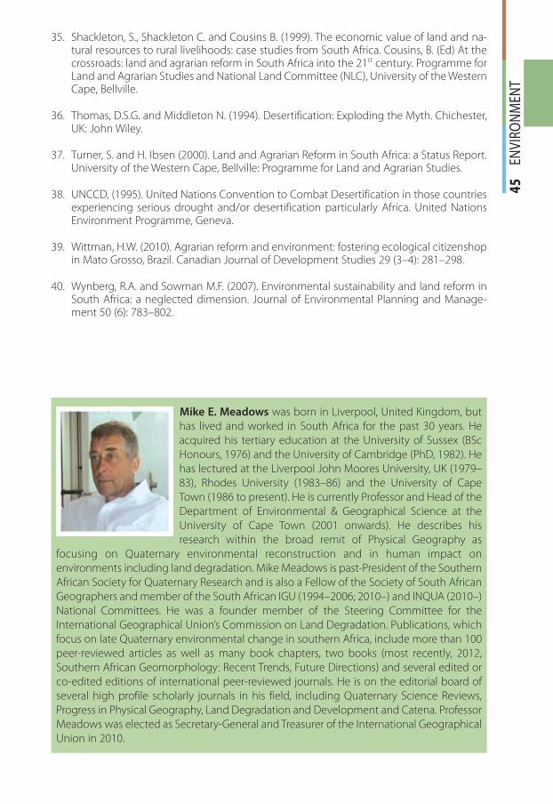
45

EN

VIR

ON

MEN

T

35. Shackleton, S., Shackleton C. and Cousins B. (1999). The economic value of land and na-tural resources to rural livelihoods: case studies from South Africa. Cousins, B. (Ed) At the crossroads: land and agrarian reform in South Africa into the 21st century. Programme for Land and Agrarian Studies and National Land Committee (NLC), University of the Western Cape, Bellville.

36. Thomas, D.S.G. and Middleton N. (1994). Desertification: Exploding the Myth. Chichester, UK: John Wiley.

37. Turner, S. and H. Ibsen (2000). Land and Agrarian Reform in South Africa: a Status Report. University of the Western Cape, Bellville: Programme for Land and Agrarian Studies.

38. UNCCD, (1995). United Nations Convention to Combat Desertification in those countries experiencing serious drought and/or desertification particularly Africa. United Nations Environment Programme, Geneva.

39. Wittman, H.W. (2010). Agrarian reform and environment: fostering ecological citizenshop in Mato Grosso, Brazil. Canadian Journal of Development Studies 29 (3–4): 281–298.

40. Wynberg, R.A. and Sowman M.F. (2007). Environmental sustainability and land reform in South Africa: a neglected dimension. Journal of Environmental Planning and Manage-ment 50 (6): 783–802.

Mike E. Meadows was born in Liverpool, United Kingdom, but

has lived and worked in South Africa for the past 30 years. He

acquired his tertiary education at the University of Sussex (BSc

Honours, 1976) and the University of Cambridge (PhD, 1982). He

has lectured at the Liverpool John Moores University, UK (1979–

83), Rhodes University (1983–86) and the University of Cape

Town (1986 to present). He is currently Professor and Head of the

Department of Environmental & Geographical Science at the

University of Cape Town (2001 onwards). He describes his

research within the broad remit of Physical Geography as

focusing on Quaternary environmental reconstruction and in human impact on

environments including land degradation. Mike Meadows is past-President of the Southern

African Society for Quaternary Research and is also a Fellow of the Society of South African

Geographers and member of the South African IGU (1994–2006; 2010–) and INQUA (2010–)

National Committees. He was a founder member of the Steering Committee for the

International Geographical Union’s Commission on Land Degradation. Publications, which

focus on late Quaternary environmental change in southern Africa, include more than 100

peer-reviewed articles as well as many book chapters, two books (most recently, 2012,

Southern African Geomorphology: Recent Trends, Future Directions) and several edited or

co-edited editions of international peer-reviewed journals. He is on the editorial board of

several high profile scholarly journals in his field, including Quaternary Science Reviews,

Progress in Physical Geography, Land Degradation and Development and Catena. Professor

Meadows was elected as Secretary-General and Treasurer of the International Geographical

Union in 2010.

gi412.indd 45gi412.indd 45 24.12.2012 9:10:4624.12.2012 9:10:46

46

EN

VIR

ON

MEN

T

ABSTRACT. Urban sprawl is among the most

debated topics in the field of urbanism,

environmental sciences, ecology, economics,

and geography. As urban sprawl involves

different subjects of study, this phenomenon

is extremely fascinating on the one side,

but very complex and difficult to analyze

on the other side. For this reason, sprawl

has and is attracting the interest of many

researchers from all over the world, having the

objective to define the nature, dynamics and

consequences that the process of low-density

urban expansion is having on the biophysical

and socioeconomic environment. The aim

of this review is to provide a brief picture

on the nature of the relationship existing

between sprawl and the environment with

special attention to Europe. The growing

environmental vulnerability of the European

urban regions was discussed according

to a bibliographic survey based on quali-

quantitative studies. Evidence support the

idea that environmental policy and regional

planning should cope more effectively with

the increasing vulnerability of ‘shrinking’

urban regions to natural hazards.

KEY WORDS: Urban Sprawl, Regional

Geography, Land consumption, Indicators,

Europe

INTRODUCTION

Compactness and dispersion were and are

the two main schemes with which cities

have evolved. There has always been an

intellectual debate regarding the positive

and negative traits of these two patterns of

urbanization. But only since the beginning

of the 20th century, as the world population

rapidly increased and concerns regarding

the preservation of the natural environment

from the effects of urbanization grew, the

debate on compact versus sprawl trajectories

of urban development has become a matter

of intense research [Bruegmann, 2005].

Urban sprawl, that is the phenomenon of

low-density settlement diffusion over large

peri-urban regions, is amongst the most

debated topics in the fields of urbanism,

environmental sciences, ecology, economics,

geography, and sociology. As sprawl involves

different subjects of study, the phenomenon

is extremely fascinating on the one side, but

very complex and difficult to analyze on the

other [Davoudi 2003]. For these reasons, sprawl

has and is attracting the interest of many

researchers from all over the world, having

the objective to define the nature, dynamics

and consequences that the phenomenon

of low-density urban expansion is having

on the natural environment [Chin 2002,

Hasse 2004, 2008, Classically, sprawl is a

phenomenon associated with the rapid low-

density outward expansion of United States

cities, steaming back to the early part of the

20th century, fueled by the rapid growth of

private car ownership and the preference for

detached houses with gardens [European

Environment Agency 2006]. Therefore, the

first studies on the sprawl process of cities

have been conducted in North America,

Vittorio Gargiulo1, Adele Sateriano2, Rosanna Di Bartolomei3, and Luca Salvati4*

1 Undergraduate student at Delft University, The Netherlands; e-mail: vittorio.gargiulo@yahoo.it2 Via C. Facchinetti 85, I-00161 Rome, Italy; e-mail: adsateri@tin.it3 Sapienza’ University of Rome, Department of Social and Economics Sciences, Piazzale A. Moro 5, I-00185 Rome, Italy, e-mail address: rosanna.dibartolomei@gmail.com4 Italian Agricultural Research Council – Centre for the Study of Soil-Plant Interactions,Via della Navicella 2-4, I-00161 Rome, Italy; e-mail: luca.salvati@entecra.it* Corresponding author

URBAN SPRAWL AND THE ENVIRONMENT

gi412.indd 46gi412.indd 46 24.12.2012 9:10:4724.12.2012 9:10:47

47

EN

VIR

ON

MEN

T

where the phenomenon initially appeared

with greatest intensity [Downs 1999]. Today,

the sprawl process is amongst the major

concerns in developed and developing

countries of the world for its adverse

environmental impact [Frenkel and Askenazi

2007]. Nevertheless, the vast majority of

secondary sources regarding the urban

phenomenon are still of North American

origin [Johnson 2001].

The aim of this contribution is to discuss

about sprawl dynamics at various

geographical scales and to comment on

its relationships with environmental quality

and natural resource depletion [Kahn 2000].

After having given a general overview on the

phenomenon, the first paragraph illustrates

the typical spatial morphological forms

and other features with which the process

manifests itself [Hall 1997]. Single-use

zoning, low-density development, ribbon

and leapfrog development, land-sealing of

agricultural and natural areas, infrastructure-

driven development and car-dependent

communities have been described and

interpreted as different forms of urban sprawl

[Jaret et al. 2009].

In the subsequent paragraphs, the impact

and environmental consequences of

sprawl are explored both qualitatively

and quantitatively. The latter analysis has

revealed particularly difficult as the effects of

deteriorating ecosystems and consumption

of natural resource due to low-density

urbanization are not easy to quantify

[Craglia et al. 2004]. Nevertheless, for a better

understanding of the environmental impact

of sprawl, the paragraph has focused on the

energy and natural resources consumption

differentials between compact and diffused

patterns of urbanization [Frenkel and

Askenazi 2008].

In the present contribution, the analysis of

sprawl and its environmental consequences

was concentrated on Europe. In order to

give a picture on the diffusion of urban

sprawl in Europe, four categories of urban

development trends have been provided.

The very general picture is that Atlantic,

Central, Eastern and Southern European

regions present mixed patterns of growth and

decline combined with sprawl, the Western

region is growing with sprawl and Northern

Europe is growing with containment [Hasse

and Lathrop 2003]. Through data provided

by the European Environment Agency, the

impacts of urban sprawl in Europe have

been studied and quantified where possible.

Land consumption (mainly to the expense

of agricultural areas), water consumption

(the interferences of soil sealing on the

recharge of groundwater basins, especially

in the mountain ranges of Europe where the

main water tanks are located), raw materials

growing demand (especially for concrete)

and energy consumption (mainly fossil fuels

for transport) related to the sprawl process

in Europe have been discussed [e.g. Haase

and Nuissl 2010]. Furthermore, this study

has shown the connection between sprawl,

climate changes and increasing vulnerability

of urban zones to extreme weather events.

By extending urbanized areas over greater

portions of land, probability and frequency

of disasters related to extreme weather

events raises.

DISCUSSING THE MORPHOLOGICAL

TRAITS OF SPRAWL

According to the location where the

phenomenon has been studied, researchers

have arrived to different definitions of

urban sprawl since the phenomenon

greatly varies over the cities of the globe.

It has different characteristics, dynamics,

effects and consequences according to the

nature of human societies that determine

it. Consequently, searching for a unique

definition of sprawl is made even more

difficult when the differences in patterns

and processes of urbanisation in various

countries and regions are considered

[Longhi and Musolesi 2007]. Traditionally,

urban sprawl was defined as a low density,

inefficient suburban development around

the periphery of cities, characterised by

auto-dependent development on rural

land. This definition emphasises sprawl as

gi412.indd 47gi412.indd 47 24.12.2012 9:10:4724.12.2012 9:10:47

48

EN

VIR

ON

MEN

Ta spatial pattern of urbanisation associated

with design features that encourage car

dependency. Nonetheless, other definitions

of sprawl emphasise different characteristics

of the phenomenon, as we can see from the

following quotations:

“Urban sprawl refers to a gluttonous use of

land, uninterrupted monotonous development,

leapfrog discontinuous development and

inefficient land use”. [Peiser, 2001].

“Urban Sprawl is a pattern of urban and

metropolitan growth that reflects low density,

automobile-dependent, exclusionary new

development on the fringe of settled areas often

surrounding a deteriorating city”. [Squires, 2002].

“Urban Sprawl is random unplanned growth

characterized by inadequate accessibility to

essential land uses such as housing, jobs, and

public services like schools, hospitals, and mass

transit”. [Bullard et al., 2000].

It is possible to state that the term “sprawl”

has a negative connotation in most writings;

social scientists usually depict sprawl as a

problem. Some do it explicitly by definition,

others link it to negative consequences such

as the decline of central cities or worsening

public health. Neutral terms (such as urban

deconcentration, suburban expansion,

counter-urbanisation) have not caught

on, in part, because these terms do not

suggest any distinction between sprawl and

suburbanisation in general. In other words,

many scholars studying sprawl view it as “a

particular form of suburbanisation with several

characteristics that differentiate it from other

conceivable forms of suburbanisation”.

From the above definitions, it is possible to

notice that even if there is still no consensus

on the exact meaning of sprawl, experts

seem to agree on the key components of

the concept. It seems clear that sprawl refers

to spread out low-density development

beyond the edge of a city’s boundaries,

where people depend on the automobile

for transportation because they live far

from where they work, shop, go to school,

worship, or pursue leisure activities. Downs

[1997] stressed six features of sprawl, some

of which distinguish it from other forms of

suburbanisation: (i) no limits placed on the

outward suburban expansion; (ii) legal control

over land-use, local services, transportation,

property taxes, and fiscal policy divided

among many small entities or jurisdictions,

with no central agency responsible for the

planning or control of these issues regionally;

(iii) extensive “leapfrog” development; (iv)

fragmented land ownership; (v) different

types of land-use, spatially separated or

zoned into distinct areas; and, finally, (vi)

extensive strip commercial and residential

development along larger suburban roads.

Downs’ formulation of sprawl is valuable

because it suggests the need to think of

and measure sprawl in terms of multiple

indicators or dimensions rather than simply

in terms of low-density settlement patterns.

A recent report by Ewing et al. [2002] provides

a summary of some of the indicators that

can be used to measure sprawl. In general,

these reflect the characteristics outlined

above and include: (i) low-density residential

developments; (ii) a rigid separation of homes,

services and workplaces; (iii) a network of

roads marked by large blocks and poor access;

and (iv) a lack of well-defined activity centers,

such as ‘downtowns’ and town centers. Finally,

Ewing et al. [2002] suggests that sprawl might

be regarded as a “process in which the spread of

development across the landscape far outpaces

population growth”.

In this sense, the definition given by Glaster

[2001] is the one that best allows sprawl to

be considered as a process and not merely

a spatial pattern. This process is initiated

by social, economic and environmental

pressures that cause a fall in demand for

land development in the centre of the

city whilst increasing it in the peripheral

areas. The city spreads over a larger surface

(while the volume remains approximately

constant). With this definition of sprawl, we

must be very careful in distinguishing the

(compact) growing process of the city with

the spreading one.

gi412.indd 48gi412.indd 48 24.12.2012 9:10:4724.12.2012 9:10:47

49

EN

VIR

ON

MEN

T

ENVIRONMENTAL IMPLICATIONS

OF URBAN SPRAWL

Low-density urban patterns of development

have several costs and implications. Most

of these concern the degradation of the

natural and social environment, besides

direct financial costs. In this section,

a research on the impact of sprawl will

help us understanding whether anti-

sprawl crusaders correctly boycott low-

density urbanization in favor of compact

growth. Sprawl not only results in direct

habitat loss [McInnes, 2010], but also has

a considerable impact on ecosystems and

natural resources. The essential biological

and physical systems include:

wetlands, useful for flood control and –

wastewater renovation;

forests, and grasslands that allows climate –

regulation;

biodiversity factors that provide to healthy, –

well-functioning ecosystems;

goods such as solar energy, wind energy, –

aesthetics, clean air, clean water, and

potential resources.

Environmental resources to help maintain

the ecosystem until the goods, services,

and the space required to generate

them remain unchanged. The excessive

pollution, ecosystem destruction, and

other forms of abuse, degrade or destroy

the environmental resources in the

long term. The environmental impact of

sprawl stretches of geographical scales

local, regional and global [Barnes et al.

2002]. An unintended consequence of

low-density suburban growth is greater

resource consumption leading to greater

environmental damage if compared with a

compact development pattern. Here below

is presented a comparison between the

energy and natural resources consumption

(which is directly related to impacts on the

environment) of compact and low-density

patterns of urbanisation.

Compact vs sprawl: energy consumption

differentials

According to Kahn [2000] the environmental

costs of increased suburbanisation are a

function of how much extra resources new

households and inhabitants of suburbia

consume. These resources are mainly fossil

fuels (related to home energy consumption

and the increasing vehicle mileage) and rural-

agricultural land. Newman and Kenworthy

[1989] clearly evidenced the relation

between low-density urban development

and the energy consumption per capita.

Sprawl inevitably brings to higher demands

and consumption of energy mainly in the

transport sector, which fundamentally relies

on non-renewable forms of energy, such as

fossil fuels. In contrast, travelling distances are

kept relatively small in compact cities, thus

favouring other forms of transport (mainly

walking and bicycling) and a reduced use

of automobiles. Furthermore, as dwelling

units in suburban areas are larger than the

usual apartments of the compact city, home

energy consumption is also scaled up by low-

density patterns of urbanisation. Even if new

constructions are more likely to incorporate

energy-conservation technologies and

materials, thus increasing their efficiency,

in the overall suburbanite’s household-level

energy consumption is greater than the one

of compact cities.

The most immediate consequence of

growing rates of combustion processes of

fossil fuels due to higher consumption rates

of low-density urban centres is air pollution.

The carbon dioxide in vehicular emissions

and power stations is a major greenhouse

gas that has been linked to global warming.

Traffic-generated air pollution threatens

human health, agricultural production, and

ecological systems. This is illustrated by

ground-level ozone, a major air pollutant

linked to the patterns and volumes of traffic

stimulated by sprawl development. Ozone

impairs respiratory functions in healthy

individuals and aggravates the ill health of

those suffering from heart and respiratory

diseases. Other health problems arising from

gi412.indd 49gi412.indd 49 24.12.2012 9:10:4724.12.2012 9:10:47

50

EN

VIR

ON

MEN

Tozone exposure include chest pains, nausea,

and throat irritation. Ozone also damages

foliage, interferes with the physiological

operations of plants, and is responsible for

important annual losses in crop production.

On the other hand, long-term effects of

fossil fuel combustion are at the current

moment subjected to a certain degree of

uncertainties. Nevertheless, according to the

Intergovernmental Panel on Climate Change

(IPCC) there is a general agreement amongst

scientist on the rationale that human activities

are significantly contributing to the rise in

Green House Gas in the atmosphere, which

are believed to be responsible of climate

changes. If the rationale that urban sprawl

leads to higher energy consumption and

land-use per capita is accepted, then its role

in contributing to climate changes must be

considered. Consequently, one of the major

objectives of planning will be to promote

and develop efficient urban forms that rely

always less on the consumption of fossil

fuels and agricultural/forest land. If the list

of countries that signed the Kyoto Protocol

intend to decrease their GHG emissions by

the amounts that they have promised, then

sprawl needs to be controlled in the future.

Natural resource depletion

Suburbs “are now the dominant residential,

retail, and commercial centres of growth and

political muscle” and the continuation and

replication of this trend “place(s) enormous

pressure on land, water, and other resources”.

Amongst the major concerns regarding the

sprawl process is that it “eats into open space”

[Kahn 2000]. Low-density suburban and

exurban development not only degrades

environmental resources such as water

quality, air quality, and wildlife habitats,

but also limits or eliminates accessibility to

natural resources such as agricultural lands,

timberland, minerals, and water. The U.S.

Environmental Protection Agency (EPA) has

created a sprawl index based on per capita

consumption. According to these studies, a

home owner whose year income is $50,000

and who lives in a central area of the city has

an average lot size of 7.8 thousand square

feet (less than a quarter of an acre), while the

average home owner in the suburbs with the

same income has an average lot size of 12.3

thousand square feet. Even if city-suburb

land consumption differential varies among

cities, the general trend is that suburbanites

consume more land per capita.

As suburban land grows, farmland is likely

to decline. The idea of sprawl conjures up

images of concrete roads and parking lots

replacing agricultural land. As the population

of metropolitan areas grows, it is likely that

land at the fringe of such areas will be

converted for urban use. As forest cover

and agricultural land is cleared for urban

development, both the quantity and quality

of water supply are threatened: as impervious

land is built over larger areas, rainfall is

less effectively absorbed and returned to

groundwater aquifers. Instead, relatively

more stormwater flows to streams and rivers

and is carried downstream. Frumkin [2002]

shows that, in USA, about 4% of rainfall

on undeveloped grassland, compared with

15% of rainfall on suburban land, was lost as

runoff. This phenomenon also applies to the

snow-melt, especially early in the melting

process. With less groundwater recharge,

communities that depend on groundwater

for their drinking water may face shortages.

Agricultural production depends on a mix of

environmental services such as soil fertility,

soil moisture, solar energy, and climate;

inputs of human, animal, and fossil fuel

energy via labour and machinery; and an

array of other inputs, practices, and programs

such as fertilisers, pesticides, irrigation, soil

conservation, research, and agricultural

support programs. Although sprawl may

not threaten overall agricultural production,

it does result in alterations and declines in

local agricultural activities and to the loss

of prime farmland. Many cities were sited,

and subsequently developed, due to the

rich agricultural soils of their hinterlands.

The metropolitan areas grow spatially, entire

zones previously dedicated to agriculture

have been replaced by apartment blocks.

This phenomenon is facilitated by the main

characteristics of agricultural soils make

gi412.indd 50gi412.indd 50 24.12.2012 9:10:4724.12.2012 9:10:47

51

EN

VIR

ON

MEN

T

them suitable for commercial and residential

development. Therefore, competition for use

of these lands is often intense, with conversion

typically uses to those that provide more

immediate economic returns. To compete

with alternative uses, farmers in urbanising

areas must work remaining agricultural lands

more intensively, change to more profitable

crops, or shift to operations that require less

investment in infrastructure.

Many authors showed that since the mid-

twentieth century, American farmers have

been producing more crops on fewer acres;

also they measured that crop production

increased from the use of hybrids, fertilisers,

and pesticides with a major loss of farmland

[Furuseth and Pierce, 1982, Buelt 1996].

The forest resources have made significant

contributions to the economic development

and industrial growth of many regions.

The harvesting of timber can be severely

reduced in order to preserve habitat needed

for endangered and threatened species, or

to support economically important, non-

extractive uses of forests, such as recreation

or can be threatened by sprawl. In fact,

with expanding residential land-use, forests

become more valuable for development

than for timber production. Urbanization

alters landscapes and fragments prior

patterns of land-use and land cover,

dramatically reducing the amount of habitat,

the size of remaining patches of habitat,

and the degree of connection amongst the

remaining patches [Barlow et al, 1998].

Sprawl not only dramatically reduces

the amount of habitat’s wildlife, but also

degrades adjacent habitats with light and

noise pollution emanating from developed

areas. According to the National Wildlife

Federation, “artificial lighting may also

fragment the landscape and habitat for wildlife,

even if there are connecting corridors”.

Another consequence of the suburban

and exurban development is closure and/

or re-locate aloof since urban centre the

quarries extraction of mineral resources.

This can be problematic for several reasons.

First, industrial minerals such as the limes,

sands, and gravels used to make cement

and required in large amounts for building,

are commodities sensitive to transportation

costs. If these must be “transported any

appreciable distance from the originating pit

to the building site, then transport costs can

readily come to be even higher than the original

purchase price” [Legget, 1973].

Second, shifting operations to other sites

can compromise and destroy the ecological

and aesthetic integrity of remaining open

spaces.

In summary, resource consumption

differentials in compact and diffused cities

range from +31% in vehicle mileage, to

+58% in lot size and to +49% in household

energy consumption.

Results of this comparison indicate that

urban sprawl leads to higher consumptions

of fossil fuels and natural resources such as

agricultural land and forest areas. This brings

to higher levels of air pollution, declining

farmland activities, less natural and forest

land, loss of natural habitats and problems

related to water supply [e.g. Attorre et al.

1998, Alphan 2003, Aguilar 2008]. Other

environmental impacts related to natural

resource consumption by spreading

urban centres include poor water quality

stemming from urban “non-point” sources of

pollution; destabilisation of stream channels

and flooding due to stormwater runoff from

developed areas; alterations of micro-climates

and local climates, including the urban

heat island effect and increases in extreme

summer heat hazard; loss and fragmentation

of wildlife habitats; degradation of landscape

aesthetics; and noise and light pollution.

In order to understand the future pressure

on urbanization and, possibly, urban

diffusion, data from the World Urbanization

Prospects have been considered. The overall

picture provided by such data suggested

that in developed countries, but above all

in less developed countries, the percentage

of urban population is expected to grow

gi412.indd 51gi412.indd 51 24.12.2012 9:10:4824.12.2012 9:10:48

52

EN

VIR

ON

MEN

Tin the following years [Kasanko et al.

2006]. This further evidences the necessity

of planned growth (for less developed

countries) and containment (for industrial

countries) strategies in order to tackle the

pressure on sprawl, especially if sustainable

development is really an objective that the

world is committed to achieve [Brouwer et

al. 1991, Balchin 1996, Camagni et al. 1998,

Burchell et al. 2005].

THE IGNORED CHALLENGE?

AN OUTLOOK ON EUROPEAN URBAN

TRENDS

Urban dispersion is advancing in many

metropolitan areas of the world, and it is

becoming a common feature also in all the

cities of the European Union, regardless of their

geographical, economic or administrative

characteristics. The rising interest amongst

European countries in mapping and

exploring this particular pattern of growth is

testified by the increasing number of studies

and EU research projects [e.g. Couch et al.

2007] which aim at providing the debate

with vivid arguments and satellite images

of cities undergoing explosive changes,

scattering over ever-greater areas.

By the late 1980s the first environmental

concerns regarding urban sprawl began to

appear throughout the European Union.

By then, the control of sprawl had become

a major consideration of urban policy in

most European countries. According to

the Brundtland Commission, “uncontrolled

development makes provision of housing,

roads, water supply, sewers and public services

prohibitively expensive. Cities are often built

on the most productive agricultural land, and

unguided growth results in the unnecessary

loss of this land. The UN Agenda 21 asked all

states to promote sustainable patterns of urban

development and land use that should aim for

compact growth”. The European Commission

also stated that: “uncontrolled growth results in

increased levels of private transport, increased

energy consumption, makes infrastructures

and services more costly and has negative

effects on the quality of the countryside and

the environment. (...) It is therefore necessary

to work together to find sustainable solutions

for planning and managing urban growth”

[European Environment Agency 2006].

In this period, the European Commission

began to work on town planning strategies

that would consider as a priority mixed

land-use and denser urban development

in order to reduce the impact of sprawl on

the natural and social environment. With

this objective, the European Environmental

Agency stated that “it is clear according to

the good governance criteria that the EU has

specific obligations and a mandate to act

and take a lead role in developing the right

frameworks for intervention at all levels, and to

pave the way for local action. Policies at all levels

including local, national and European need

to have an urban dimension to tackle urban

sprawl and help to redress the market failures

that drive urban sprawl. The provision of new

visions for the spatial development of Europe’s

cities and regions is vital for the creation of a

range of integrated mutually reinforcing policy

responses” [European Environment Agency

2006].

To sum up, as in North America and other

parts of the world, throughout Europe urban

sprawl is becoming a consolidated threat. The

environmental, social and economic impacts

of the phenomenon for both cities and the

countryside of Europe are becoming always

more evident and require immediate action,

especially now that the global challenge for

climate change is putting more pressure on

governments. For this reason, modern town

planning was developed, with the objective

of controlling urban expansion.

Nevertheless, in its early stages urban

planning did not manage to accomplish

its objective and is still struggling today.

For example, between 1922 and 1939 over

340,000 hectares of rural land in England

and Wales were converted to urban uses (a

40% increase in the total urban area of the

country). In the aftermath of World War II,

many European countries invested heavily

in planned urban expansions schemes.

gi412.indd 52gi412.indd 52 24.12.2012 9:10:4824.12.2012 9:10:48

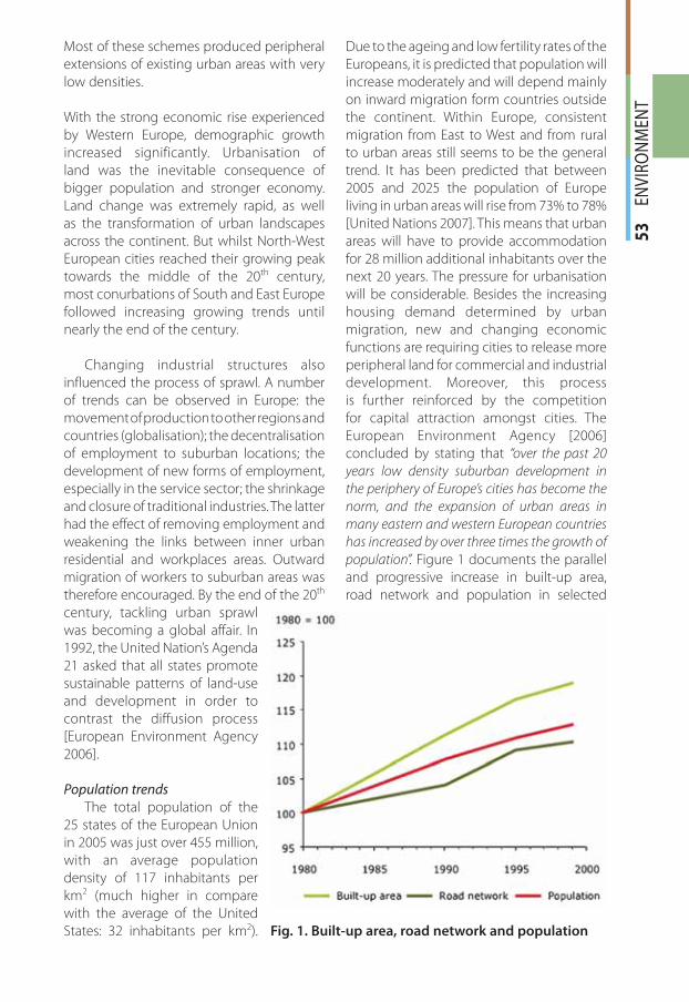
53

EN

VIR

ON

MEN

T

Most of these schemes produced peripheral

extensions of existing urban areas with very

low densities.

With the strong economic rise experienced

by Western Europe, demographic growth

increased significantly. Urbanisation of

land was the inevitable consequence of

bigger population and stronger economy.

Land change was extremely rapid, as well

as the transformation of urban landscapes

across the continent. But whilst North-West

European cities reached their growing peak

towards the middle of the 20th century,

most conurbations of South and East Europe

followed increasing growing trends until

nearly the end of the century.

Changing industrial structures also

influenced the process of sprawl. A number

of trends can be observed in Europe: the

movement of production to other regions and

countries (globalisation); the decentralisation

of employment to suburban locations; the

development of new forms of employment,

especially in the service sector; the shrinkage

and closure of traditional industries. The latter

had the effect of removing employment and

weakening the links between inner urban

residential and workplaces areas. Outward

migration of workers to suburban areas was

therefore encouraged. By the end of the 20th

century, tackling urban sprawl

was becoming a global affair. In

1992, the United Nation’s Agenda

21 asked that all states promote

sustainable patterns of land-use

and development in order to

contrast the diffusion process

[European Environment Agency

2006].

Population trends

The total population of the

25 states of the European Union

in 2005 was just over 455 million,

with an average population

density of 117 inhabitants per

km2 (much higher in compare

with the average of the United

States: 32 inhabitants per km2).

Due to the ageing and low fertility rates of the

Europeans, it is predicted that population will

increase moderately and will depend mainly

on inward migration form countries outside

the continent. Within Europe, consistent

migration from East to West and from rural

to urban areas still seems to be the general

trend. It has been predicted that between

2005 and 2025 the population of Europe

living in urban areas will rise from 73% to 78%

[United Nations 2007]. This means that urban

areas will have to provide accommodation

for 28 million additional inhabitants over the

next 20 years. The pressure for urbanisation

will be considerable. Besides the increasing

housing demand determined by urban

migration, new and changing economic

functions are requiring cities to release more

peripheral land for commercial and industrial

development. Moreover, this process

is further reinforced by the competition

for capital attraction amongst cities. The

European Environment Agency [2006]

concluded by stating that “over the past 20

years low density suburban development in

the periphery of Europe’s cities has become the

norm, and the expansion of urban areas in

many eastern and western European countries

has increased by over three times the growth of

population”. Figure 1 documents the parallel

and progressive increase in built-up area,

road network and population in selected

Fig. 1. Built-up area, road network and population

gi412.indd 53gi412.indd 53 24.12.2012 9:10:4824.12.2012 9:10:48

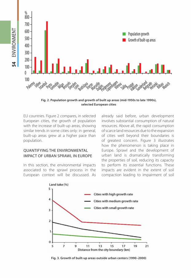
54

EN

VIR

ON

MEN

T

EU countries. Figure 2 compares, in selected

European cities, the growth of population

with the increase of built-up areas, showing

similar trends in some cities only: in general,

built-up areas grew at a higher pace than

population.

QUANTIFYING THE ENVIRONMENTAL

IMPACT OF URBAN SPRAWL IN EUROPE

In this section, the environmental impacts

associated to the sprawl process in the

European context will be discussed. As

already said before, urban development

involves substantial consumption of natural

resources. Above all, the rapid consumption

of scarce land resources due to the expansion

of cities well beyond their boundaries is

of greatest concern. Figure 3 illustrates

how the phenomenon is taking place in

Europe. Sprawl and the development of

urban land is dramatically transforming

the properties of soil, reducing its capacity

to perform its essential functions. These

impacts are evident in the extent of soil

compaction leading to impairment of soil

Fig. 2. Population growth and growth of built up areas (mid-1950s to late 1990s),

selected European cities

Fig. 3. Growth of built-up areas outside urban centers (1990–2000)

%800 –

700 –

600 –

500 –

400 –

300 –

200 –

100 –0

100

MunichBilbao

Helsinki

Belgrade

Sunderland

IraklionPrague

TallinVienna

Copenhagen

Pordenone

DublinMarseilleTrie

steBratisla

vaLyon

DresdenBrussels

MilanGrenoble

PortoIstanbul

UdinePalermo

Population growth

Growth of built-up areas

gi412.indd 54gi412.indd 54 24.12.2012 9:10:4824.12.2012 9:10:48

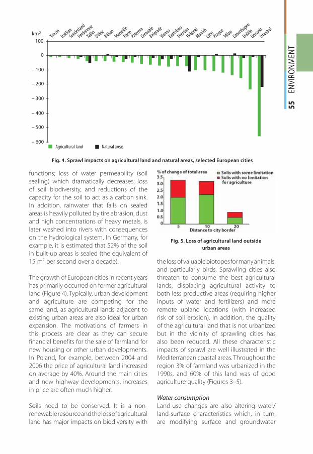
55

EN

VIR

ON

MEN

T

functions; loss of water permeability (soil

sealing) which dramatically decreases; loss

of soil biodiversity, and reductions of the

capacity for the soil to act as a carbon sink.

In addition, rainwater that falls on sealed

areas is heavily polluted by tire abrasion, dust

and high concentrations of heavy metals, is

later washed into rivers with consequences

on the hydrological system. In Germany, for

example, it is estimated that 52% of the soil

in built-up areas is sealed (the equivalent of

15 m2 per second over a decade).

The growth of European cities in recent years

has primarily occurred on former agricultural

land (Figure 4). Typically, urban development

and agriculture are competing for the

same land, as agricultural lands adjacent to

existing urban areas are also ideal for urban

expansion. The motivations of farmers in

this process are clear as they can secure

financial benefits for the sale of farmland for

new housing or other urban developments.

In Poland, for example, between 2004 and

2006 the price of agricultural land increased

on average by 40%. Around the main cities

and new highway developments, increases

in price are often much higher.

Soils need to be conserved. It is a non-

renewable resource and the loss of agricultural

land has major impacts on biodiversity with

the loss of valuable biotopes for many animals,

and particularly birds. Sprawling cities also

threaten to consume the best agricultural

lands, displacing agricultural activity to

both less productive areas (requiring higher

inputs of water and fertilizers) and more

remote upland locations (with increased

risk of soil erosion). In addition, the quality

of the agricultural land that is not urbanized

but in the vicinity of sprawling cities has

also been reduced. All these characteristic

impacts of sprawl are well illustrated in the

Mediterranean coastal areas. Throughout the

region 3% of farmland was urbanized in the

1990s, and 60% of this land was of good

agriculture quality (Figures 3–5).

Water consumption

Land-use changes are also altering water/

land-surface characteristics which, in turn,

are modifying surface and groundwater

Fig. 4. Sprawl impacts on agricultural land and natural areas, selected European cities

Fig. 5. Loss of agricultural land outside

urban areas

km2

100 –

0 –

– 100 –

– 200 –

– 300 –

– 400 –

– 500 –

– 600 –

Munich

Bilbao

Helsinki

Belgrade

Sunderland

Iraklio

n

PragueTallin Vienna

Copenhagen

Pordenone

DublinMarse

ille

Trieste

Bratislava

LyonDresden

Brussels

MilanGrenoble

PortoIsta

nbul

UdinePalerm

o

Agricultural land Natural areas

/ / / / / / / / / / / / / / / / / / / / / / / /

gi412.indd 55gi412.indd 55 24.12.2012 9:10:4924.12.2012 9:10:49

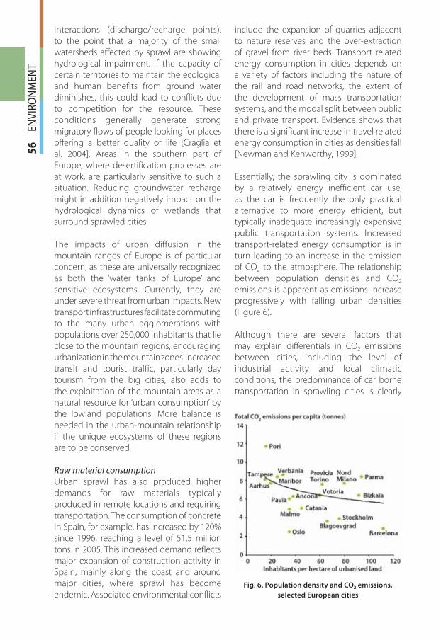
56

EN

VIR

ON

MEN

Tinteractions (discharge/recharge points),

to the point that a majority of the small

watersheds affected by sprawl are showing

hydrological impairment. If the capacity of

certain territories to maintain the ecological

and human benefits from ground water

diminishes, this could lead to conflicts due

to competition for the resource. These

conditions generally generate strong

migratory flows of people looking for places

offering a better quality of life [Craglia et

al. 2004]. Areas in the southern part of

Europe, where desertification processes are

at work, are particularly sensitive to such a

situation. Reducing groundwater recharge

might in addition negatively impact on the

hydrological dynamics of wetlands that

surround sprawled cities.

The impacts of urban diffusion in the

mountain ranges of Europe is of particular

concern, as these are universally recognized

as both the ‘water tanks of Europe’ and

sensitive ecosystems. Currently, they are

under severe threat from urban impacts. New

transport infrastructures facilitate commuting

to the many urban agglomerations with

populations over 250,000 inhabitants that lie

close to the mountain regions, encouraging

urbanization in the mountain zones. Increased

transit and tourist traffic, particularly day

tourism from the big cities, also adds to

the exploitation of the mountain areas as a

natural resource for ‘urban consumption’ by

the lowland populations. More balance is

needed in the urban-mountain relationship

if the unique ecosystems of these regions

are to be conserved.

Raw material consumption

Urban sprawl has also produced higher

demands for raw materials typically

produced in remote locations and requiring

transportation. The consumption of concrete

in Spain, for example, has increased by 120%

since 1996, reaching a level of 51.5 million

tons in 2005. This increased demand reflects

major expansion of construction activity in

Spain, mainly along the coast and around

major cities, where sprawl has become

endemic. Associated environmental conflicts

include the expansion of quarries adjacent

to nature reserves and the over-extraction

of gravel from river beds. Transport related

energy consumption in cities depends on

a variety of factors including the nature of

the rail and road networks, the extent of

the development of mass transportation

systems, and the modal split between public

and private transport. Evidence shows that

there is a significant increase in travel related

energy consumption in cities as densities fall

[Newman and Kenworthy, 1999].

Essentially, the sprawling city is dominated

by a relatively energy inefficient car use,

as the car is frequently the only practical

alternative to more energy efficient, but

typically inadequate increasingly expensive

public transportation systems. Increased

transport-related energy consumption is in

turn leading to an increase in the emission

of CO2 to the atmosphere. The relationship

between population densities and CO2

emissions is apparent as emissions increase

progressively with falling urban densities

(Figure 6).

Although there are several factors that

may explain differentials in CO2 emissions

between cities, including the level of

industrial activity and local climatic

conditions, the predominance of car borne

transportation in sprawling cities is clearly

Fig. 6. Population density and CO2 emissions,

selected European cities

gi412.indd 56gi412.indd 56 24.12.2012 9:10:5024.12.2012 9:10:50

57

EN

VIR

ON

MEN

T

a major factor in the growth of urban green

house gas emissions. Urban sprawl therefore

poses significant threats to the EU Kyoto

commitments to reduce greenhouse gas

emissions by 2020. Sprawl also increases the

length of trips required to collect municipal

waste for processing at increasingly distant

waste treatment plants and this is expected

to continue as household waste grows 3–4%

annually. The material cycle is becoming

geographically decoupled with increasing

transport demands, impacting on transport

related energy consumption and pollution

emissions.

Climate changes

Sprawl related growth of urban transport

and greenhouse gas emissions have major

implications for global warming and climate

change, with the expectation of increasingly

severe weather events in the coming years

and increased incidences of river and coastal

flooding. The risks from the continuous

development of these areas in the context

of a changing climate is evident in the

recent major floods in Europe that have

affected large urban populations. The floods

in central Europe occurred in august 2002

caused 112 casualties and over 400,000

people were evacuated from their homes.

These expected transformations pose major

challenges for urban planning that are

clearly focused on the growth of urban

sprawl along the coastal fringes throughout

Europe, as well as development of sprawling

extensions across greenfield sites in the river

valleys and lowlands of Europe.

The flooding of the coastal regions of Europe

due to rising sea levels and climate change

is particularly worrying considering the

concentration of urban populations along

the coasts and the importance of these

areas for tourism. The countries of Europe

most vulnerable to coastal flooding include

the Netherlands and Belgium, where more

than 85% of the coast is under 5m elevation.

Other countries at risk include Germany

and Romania where 50% of the coastline

is below 5m, Poland (30%) and Denmark

(22%), as well as France, the United Kingdom

and Estonia where lowlands cover 10–15%

of the country. Overall, 9% of all European

coastal zones lie below 5m elevation. Even

with conservative estimates of predictions

for sea level rise, a substantial part of the

population of Europe living in the coastal

regions are highly vulnerable to sea level

rise and flooding. It is clear that this is

not a specific issue generated by sprawl,

however, the management of these risks and

planning for adaptation will be made more

complicated if sprawl is not controlled. By

extending urban areas over greater portions

of lands, the probability and frequency of

disasters related to extreme weather events

will grow in the future.

Impact on society and urban quality

Changes in lifestyle associated with sprawl

contribute to increases the demand of natural

resources. People are living increasingly in

individual households, which tend to be

less efficient, requiring more resources per

capita than larger households. For instance,

a two-person household uses 300 liters of

water per day, two single households use

210 liters each. A two-person household will

use 20% less energy than two single person

households. The number of households

grew by 11% between 1990 and 2000, a

trend that increases land-use and acts as

a driver for expansion of urban areas. The

general trend is for greater consumption

of resources per capita with an associated

growth in environmental impact. This adds

pressure to the fact that about 60% of large

European cities are already over-exploiting

their groundwater resources and water

availability.

Moreover, market oriented land-use

allocations driving urban expansion and

the transformation of economic activity

often result in the abandonment of former

industrial areas. As a result, there are many

derelict or underused former industrial zones

throughout Europe that have moved to

peripheral areas or less developed countries.

For example, in Spain about 50% of sites

contaminated from past industrial activities

are located in urban areas (1999), and in Austria

gi412.indd 57gi412.indd 57 24.12.2012 9:10:5024.12.2012 9:10:50

58

EN

VIR

ON

MEN

Tit is estimated that abandoned industrial sites

cover about 2% of all urban areas (2004).

Generally, the efficiency savings of more

compact city development as compared with

market driven suburbanization can be as high

as 20–45% in land resources, 15–25% in the

construction of local roads and 7–15% savings

in the provision of water and sewage facilities.

Finally, urban sprawl produces many adverse

environmental impacts that have direct

effects on the quality of life and human health

in cities, such as poor air quality (worsened by

the increased use of cars in sprawled areas)

and high noise levels that often exceed the

established safety limits. In the period 1996–

2002 significant proportions of the urban

population were exposed to air pollutant

concentrations exceeding the EU limit values

(25–50% of the urban population for different

pollutants). It is estimated that approximately

20 million Europeans suffer from respiratory

problems linked to air pollution.

CONCLUSION

What is urban sprawl and how does it adapt

to the different territorial contexts in which

it is taking place? These are the principal

questions that have been tackled with the

analysis of a vast body of literature mostly

originating from North America. Formal and

informal definitions of the phenomenon

have been investigated. The former have

illustrated various different features of sprawl,

but at the same time they have evidenced

the lack of a global and unique definition

of the urban process being discussed

[Tsai 2005]. This goes in the direction of

the initial hypothesis of this research, that

is the necessity of studying sprawl with

comparative analysis, as the phenomenon

presents different features and consequences

according to the territorial context being

considered [Newman and Thornely 1996].

Informal definitions have been also discussed,

as these result useful in giving a solid

comprehension on the concept of exurban

development. The sand-castle metaphor

has been illustrated in order to stress the

main feature of sprawling spatial patterns of

urbanisation: the “volume” of the city remains

approximately constant, but it is spread over

a larger surface. Therefore, the concept of

sprawl has been associated to the process of

transformation of the density gradient line

of urban and residential activities, which will

result always less steep as the phenomenon

takes place. To emphasise the importance of

the process of transformation rather than the

final urban configuration of sprawling cities,

the necessity of treating the phenomenon as

a verb more than a noun, and to differentiate

it forms the process of urban growth has been

underlined [Couch et al. 2007]. In the early

1980s, the European Commission officially

manifested its concerns for the diffusion of

the sprawl process within the continent,

as this is negatively contributing to the

achievement of a sustainable development

imposed by the United Nations. Pressure

on modern town planning for reaching this

objective has not produced positive effects,

with urban uncontrolled expansion still

being the norm in many European countries

since the aftermath of World War II. But

as concerns regarding low-density urban

diffusion grow, the need for an accurate

analysis of the phenomenon in the European

context is becoming increasingly urgent for

the formulation of efficient territorial policies

[Prud’homme and Lee 1999]. In the second

half of the 20th century, Europe, and especially

southern Europe, experienced a period of

rapid population growth and urbanisation. In

these last years, the former has significantly

slowed down and stabilised while the latter

is still increasing. All this indicates that the

sprawl process is at work in the region since

several years. Furthermore, the EEA report

entitled “Urban sprawl in Europe” [2006] also

evidences this trend, stating that 6 out of

10 of the European cities with the highest

sprawl rates are located in the Northern

Mediterranean region, and more in general,

in economically disadvantaged regions

[Richardson and Chang-Hee 2004].

Besides the general impact of sprawl,

coastalisation along the European shores,

taken as a paradigmatic example of

gi412.indd 58gi412.indd 58 24.12.2012 9:10:5024.12.2012 9:10:50

59

EN

VIR

ON

MEN

T

(sometimes uncontrolled) urban diffusion,

brings to a loss of farming and natural land

(which is amongst the richest and most

productive of the region), the destruction

of highly valuable natural habitats, the

degradation and pollution of the shores

and sea, the reduction of small scale

fishing and the increasing vulnerability of

the area to extreme weather and natural

events. With regards to this last point (the

increasing vulnerability towards extreme

weather and natural events) this study

dedicates further attention [Turok and

Mykhnenko 2007]. Research shows that

the growing pressure on the environment

due to human-induced demand factors

(urbanisation and natural resources

consumption), is increasing the disaster

potential of cities and megacities [Scott

2001]. Cities are expanding over more

and more area [Schneider and Woodcock

2008], thus increasing their exposure to

natural disasters (such as earthquakes and

floods). This situation is raising concerns

as extreme weather events are likely to

increase both in frequency and intensity

due to climate changes [APFM, 2012].

The growing vulnerability of urban centres

is testified by the increasing damages

related to natural hazards [Salvati 2010].

A survey on natural disasters shows that

the region is more vulnerable to extreme

seasons, short-duration hazards (such as

floods and earthquakes) and slow long-

term changes, including sea-level rise and

coastal squeeze. These evidence support the

idea that environmental policy and regional

planning should cope more effectively with

the increasing vulnerability of large urban

regions to natural hazards. �

REFERENCES 1. Aguilar, A.G. (2008). Peri-urbanization, illegal settlements and environmental impact in

Mexico City, Cities, 25, 133–145.

2. Alphan, H. (2003). Land use change and urbanisation of Adana, Turkey, Land Degr. Deve-lop., 14, 575–586.

3. Associated Programme on Flood Management (APFM), “Urban Flood Management in a Changing Climate” (2012) Integrated Flood Management Tools Series, APFM Technical Document No. 19, ©World Meteorological Organization, p. 1–56.

4. Attorre, F., Rossetti, A., Sbrega, B., Bruno, F. (1998). Landscape changes in Rome, Italy, Coe-nosis, 13, 578–564.

5. Balchin, P. (1996). Housing Policy in Europe, London and New York: Routledge.

6. Barlow, S.A., Munn, I.A., Cleaves, D.A., and Evans, D.L. (1998). The effects of urban sprawl on timber harvest. Journal of Forestry (December]: 10–14.

7. Barnes, K.B., Morgan, J.M., Roberge, M.C., and Lowe, S. (2002). Sprawl development: its patterns, consequences, and measurement, Center for Geographic Information Sciences, Towson University, p. 1–24.

8. Brouwer, F.B., Thomas, A.J., Chadwick, M.J. (1991). Land use changes in Europe. Processes of change, environmental transformations and future patterns, Dordrecht: Kluwer Acade-mic Publishers.

9. Bruegmann, R. (2005). Sprawl: a compact history, Chicago: University of Chicago Press.

10. Buelt, K. (1996) “Land use planning: A farmer’s perspective”. In Land Use In America, ed. H. L. Diamond and P.F. Noonan, 237–243. Washington, D.C.: Island Press.

11. Bullard, R.D., Glenn, S.J., and Torres, A.O. (2000). Sprawl City. Washington DC: Island Press.

gi412.indd 59gi412.indd 59 24.12.2012 9:10:5124.12.2012 9:10:51

60

EN

VIR

ON

MEN

T 12. Burchell, R.W., Downs, A., McCann, B., Mukherji, S. (2005). Sprawl Costs – Economic Im-

pacts of Unchecked Development, Washington: Island Press.

13. Camagni, R., Capello, R., Nijkamp, P. (1998). Toward Sustainable City Policy: an Economy-Environment-Technology Nexus, Ecol. Econ., 24, 103–118.

14. Chin, N. (2002). Unearthing the Roots of Urban Sprawl: A Critical Analysis of Form, Func-tion and Methodology, Centre for Advanced Spatial Analysis of the University College London, Working Paper, Series 47.

15. Couch, C., Leontidou, L., Petschel-Held, G. (2007). Urban Sprawl in Europe – Landscapes, Land-Use Change & Policy, Oxford, UK: Blackwell Publishing.

16. Craglia, M., Leontidou, L., Nuvolati, G., Schweikart, J. (2004). Towards the Development of Quality Indicators in the ‘Digital’ City, Environ. Plan. B, 31, 51–64.

17. Davoudi, S., 2003, Polycentricity in European Spatial Planning: From an Analytical Tool to a Normative Agenda, Eur. Plan. Stud., 11 (8), 979–999.

18. Downs, A. (1999). Some Realities about Sprawl and Urban Decline, Hous. Pol. Deb., 10 (4), 955–974.

19. Downs, A. (1997). The Challenge of Our Declining Big Cities. Housing Policy Debate 8: 359–408.

20. European Environmental Agency (2006). Urban sprawl in Europe – The ignored chal-lenge, Copenhagen: EEA Report no. 10.

21. Ewing, R., Pendall, R., Chen, D. (2002). Measuring Sprawl and Its Impact, Washington, DC: Smart Growth America.

22. Frenkel, A., Ashkenazi, M. (2007). The integrated sprawl index: measuring the urban land-scape in Israel, Ann. Reg. Sci., 42 (1), 99–121.

23. Frenkel, A., Ashkenazi, M. (2008). Measuring Urban Sprawl: How can We Deal With It? Environ. Plan. B, 35, 56–79.

24. Frumkin, H. (2002). Urban Sprawl and Public Health. Public Health Reports, Association of Schools of Public Health. Pp. 117–216.

25. Furuseth, O.J., and Pierce, J.T. (1982). Agricultural Land In An Urban Society. Washington, D.C.: Association of American Geographers.

26. Glaster, G., Hanson, R., Ratcliffe, M.R., Wolman, H., Coleman, S., Freihage, J. (2001). Wrestling Sprawl to the Ground: Defining and Measuring an Elusive Concept, Hous. Pol. Deb., 12 (4), 681–717.

27. Haase, D., and Nuissl, H. (2010). The urban-to-rural gradient of land use change and imper-vious cover: a long-term trajectory for the city of Leipzig, Land Use Sci., 5 (2), 123–142.

28. Hall, P. (1997). The Future of Metropolis and Its Form, Reg. Stud., 31 (3), 211–220.

29. Hasse, J.E. (2004). A Geospatial Approach to Measuring New Development for Characteristics of Sprawl, Landscape Journal: Design, Planning and Management of the Land, 23 p. 52–67.

30. Hasse, J.E., and Lathrop, R.G. (2003). Land Resource Impact Indicators of Urban Sprawl, Appl. Geogr., 23, 159–175.

31. Hasse, J.E. (2008). Using remote sensing and GIS integration to identify spatial characteris-tics of sprawl at the building-unit level, book chapter in Integrating Remote Sensing and GIS, edited by Victor Mesev, John Wiley & Sons, London.

gi412.indd 60gi412.indd 60 24.12.2012 9:10:5124.12.2012 9:10:51

61

EN

VIR

ON

MEN

T

32. Jaret, C., Ghadge, R., Reid, L.W., Adelman, R.M. (2009). The Measurement of Suburban Sprawl: An Evaluation, City & Community, 8 (1), 65–84.

33. Johnson, M.P. (2001). Environmental Impacts of Urban Sprawl: A Survey of the Literature and Proposed Research Agenda, Environ. Plan. B, 33, 717–735.

34. Kahn, M.E. (2000). The environmental impact of suburbanization. Journal of Policy Analy-sis and Management 19 (4): 569–586.

35. Legget, R.F. (1973). Cities and Geology. New York: McGraw-Hill, Inc.

36. Longhi, C., Musolesi, A. (2007). European cities in the process of economic integration: towards structural convergence, Ann. Reg. Sci., 41, 333–351.

37. McInnes, R. (2010). Urban Development, Biodiversity and Wetland Management, export workshop 16 to 17 november 2009, Oxoford Unhabitat, p. 1–57.

38. Newman, P. & Kenworthy, J. (1999). Sustainability and Cities: Overcoming automobile.

39. Newman, P. & Kenworthy, J. (1989). Cities and Automobile Dependence: An International Sourcebook Gower, England.

40. Newman, P. and Thornley, A. (1996). Urban planning in Europe – International competi-tion, national systems and planning projects, London, Routledge.

41. Peiser, R. (2001). Decomposing urban sprawl. Town Planning Review. 3 (72), 96–108.

42. Prud’homme, R., Lee, G. (1999). Sprawl, Speed and the Efficiency of Cities, Urban Stud., 36, 1849–1858.

43. Richardson, H.W., Chang-Hee, C.B. (2004). Urban Sprawl in Western Europe and the United States, London: Ashgate.

44. Salvati, L. (2010). Economic Causes and Consequences of Land Degradation and Deserti-fication Risk in Southern Europe. Integrating Micro-Macro Approaches Into a Geographi-cal Perspective, Int. J. Ecol. Econ. Stat., (March- April).

45. Schneider, A., Woodcock, C.E. (2008). Compact, dispersed, fragmented, extensive? A com-parison of urban growth in 25 global cities using remotely sensed data, pattern metrics and census information, Urban Stud., 45, 659–692.

46. Scott, A.J. (2001). Global City-Regions – Trends, Theory, Policy, New York: Oxford Unversity Press.

47. Squires, G.D. (2002). Urban Sprawl: Causes, Consequences, and Policy Decisions. Washing-ton DC: Urban Institute Press.

48. Tsai, Y. (2005). Quantifying Urban Form: Compactness versus Sprawl, Urban Stud., 42 (1), 141–161.

49. Turok, I., Mykhnenko, V. (2007). The trajectories of European cities, 1960–2005. Cities, 24 (3), 165–182.

50. United Nations (2007). World urbanization prospects: the 2006 revision, New York: UN.

51. Xiaojun Y. (2011). Urban Remote Sensing: Monitoring, Synthesis and Modeling in the Urban Environment, (Ed.). Chichester: John Wiley & Sons.

gi412.indd 61gi412.indd 61 24.12.2012 9:10:5124.12.2012 9:10:51

62

EN

VIR

ON

MEN

T Vittorio Gargiulo Morelli achieved his Bachelor in Science

degree in Environmental Engineering at the University of Rome

‘La Sapienza’, specializing in the fields of Urban Planning and

Ecological Spatial Planning in Mediterranean cities. Successively,

he obtained his Master in Science degree in Engineering and

Policy Analysis at Delft University of Technology, where he

focused on subjects of Systems Modeling and Policy Analysis of

Multi-Actor Systems, and completed his final thesis on Sustainable

and Intelligent Cities. He has participated to several research

projects concerning land-use change, urban sprawl and polycentric

development, sustainable and intelligent cities and is author of

one book and more than 10 scientific articles in English.

Rosanna Di Bartolomei has graduated in Economic in University

of Rome “La Sapienza” with a specialization in Environmental

Indicators. Successively, Rosanna obtained Master in Science in

Data Intelligence and Decision-making Strategies at University of

Rome “La Sapienza”. Rosanna’s collaborates with Council for

Research and Experimentation in Agriculture (CRA]. The main

research issues include: human settlements, urban form,

adaptation to climate change, sustainable agriculture and

planning for sustainable development. She is the author of eight

scientific articles in English, and one article in Italian.

Luca Salvati is a geographer holding two bachelor’s degrees

(ecology: 2000; demography and social sciences: 2004), a master’s

degree in economic statistics, a specialization degree in

Geography and Environment, and a PhD in Economic Geography.

He is Associate Professor of Cartography and GIS, Multivariate

Statistics, and Strategic Environmental Assessment at Third

University of Rome and collaborates with University of Rome “La

Sapienza” on projects pertaining to the field of urban and rural

geography. After working with various national and European

research institutions on projects concerning desertification,

sustainable agriculture, land-use, climate change, urban sprawl

and polycentric development at the regional scale, he now holds a chair at the Italian

Council for Research and Experimentation in Agriculture (CRA). He is author of more than

70 scientific articles in English, ten books, essays and cartographical atlases.

Adele Sateriano has graduated in Law at the University of Rome

‘La Sapienza’ with a specialization in Environmental Law. Adele’s

main research issues include: human settlements, urban form,

adaptation to climate change, sustainable agriculture and

planning for sustainable development. She is author of five

scientific articles in English, and one book in Italian.

gi412.indd 62gi412.indd 62 24.12.2012 9:10:5124.12.2012 9:10:51

63

SU

STA

INA

BILI

TY

ABSTRACT. Today in Russia, much attention is

given to research and practical identification

of the cultural landscape (CL) stability

parameters that define its dependency on

the character of the territorial land use.

As a rule, these are projects of territorial

and landscape planning (LP) aimed at

assessment of stability of the CL depending

on the conditions of the social and natural

environment, on the level of changes of its

components, and on the direct relation with

the nature and the type of natural resources

management. This approach defines most

fully conditions and the level of impact on

the landscape.

The paper discusses the main types of

natural resource management of the CL.

Residential areas are the most complex and

multifunctional types of natural resource

management. They are of the greatest

interest to the research as an object of “co-

creation of man and nature” [Sochava, 1978].

This is determined by an important role

of residential areas with their infrastructure

as a landscape reshaping element that

influences the functioning and structure of

the CL. Cities, suburbs and towns, as human

environment, require a special attention in

order to achieve an environmentally friendly

and sustainable landscape.

In the concept of LP, much attention is given

to assessment of the natural components

of the CL. As a rule, assessment of soil,

climate (atmosphere), water, and landscape

sensitivity and significance is conducted

[Drozdov, 2006]. The selection of assessment

criteria varies depending on the natural

resource management type. Obtained results

are compared with parameters that are

indicative for or specific to naturally occurring

landscape. The crisis of environmental

components makes LP the vitally necessary

management instrument. The goals of

landscape planning are broadly formulated –

landscape planning should cover the entire

territory of the country, should consider both

natural and socio-economic factors, and

should develop measures to prevent and

control impacts on the landscape.

KEY WORDS: cultural landscape, stability

of cultural landscape, landscape planning,

landscape stability criteria, environmental

management, sustainable development

INTRODUCTION

The concept of LP is connected with the

concept of CL and specifically emphasizes

sustainable development of these systems.

In summary, this concept (LP) means such

a development (change), which allows the

present generation to meet their needs

without threatening the existence of such

landscapes for future generations. This

development is based on sustainable use of

CLs to the extent that will not damage their

Elena I. Golubeva1*, Maria E. Ignatieva2, Tatiana O. Korol1, Valentina A. Toporina1

1 Lomonosov Moscow State University, Faculty of Geography, Moscow, Russia* Corresponding author2 Division of Landscape Architecture, Department of Urban and Rural Development at Swedish University of Agricultural Sciences; PO Box 7012, SE-750 77 Uppsala, Sweden; Tel +46-18-672508; fax +46-18-673512; e-mail maria.ignatiea@slu.se; webpage www.slu.se

ECO-GEOGRAPHICAL APPROACH TO INVESTIGATION OF STABILITY OF CULTURAL LANDSCAPE

gi412.indd 63gi412.indd 63 24.12.2012 9:10:5224.12.2012 9:10:52

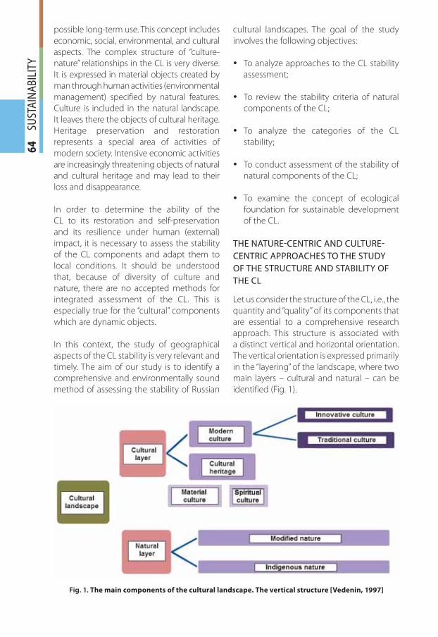
64

SU

STA

INA

BILI

TYpossible long-term use. This concept includes

economic, social, environmental, and cultural

aspects. The complex structure of “culture-

nature” relationships in the CL is very diverse.

It is expressed in material objects created by

man through human activities (environmental

management) specified by natural features.

Culture is included in the natural landscape.

It leaves there the objects of cultural heritage.

Heritage preservation and restoration

represents a special area of activities of

modern society. Intensive economic activities

are increasingly threatening objects of natural

and cultural heritage and may lead to their

loss and disappearance.

In order to determine the ability of the

CL to its restoration and self-preservation

and its resilience under human (external)

impact, it is necessary to assess the stability

of the CL components and adapt them to

local conditions. It should be understood

that, because of diversity of culture and

nature, there are no accepted methods for

integrated assessment of the CL. This is

especially true for the “cultural” components

which are dynamic objects.

In this context, the study of geographical

aspects of the CL stability is very relevant and

timely. The aim of our study is to identify a

comprehensive and environmentally sound

method of assessing the stability of Russian

cultural landscapes. The goal of the study

involves the following objectives:

To analyze approaches to the CL stability �assessment;

To review the stability criteria of natural �components of the CL;

To analyze the categories of the CL �stability;

To conduct assessment of the stability of �natural components of the CL;

To examine the concept of ecological �foundation for sustainable development

of the CL.

THE NATURE-CENTRIC AND CULTURE-

CENTRIC APPROACHES TO THE STUDY

OF THE STRUCTURE AND STABILITY OF

THE CL

Let us consider the structure of the CL, i.e., the

quantity and “quality” of its components that

are essential to a comprehensive research

approach. This structure is associated with

a distinct vertical and horizontal orientation.

The vertical orientation is expressed primarily

in the “layering” of the landscape, where two

main layers – cultural and natural – can be

identified (Fig. 1).

Fig. 1. The main components of the cultural landscape. The vertical structure [Vedenin, 1997]

gi412.indd 64gi412.indd 64 24.12.2012 9:10:5224.12.2012 9:10:52

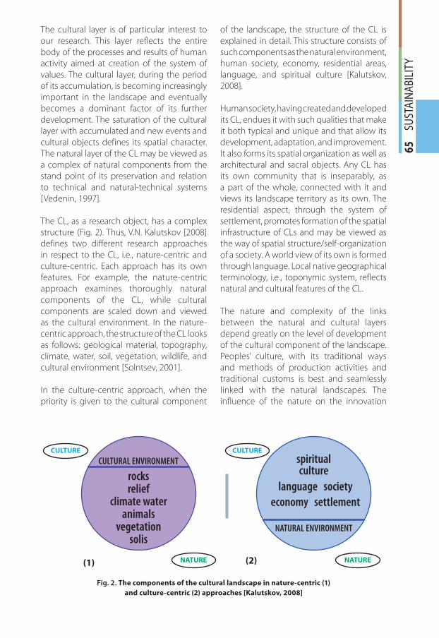
65

SU

STA

INA

BILI

TY

The cultural layer is of particular interest to

our research. This layer reflects the entire

body of the processes and results of human

activity aimed at creation of the system of

values. The cultural layer, during the period

of its accumulation, is becoming increasingly

important in the landscape and eventually

becomes a dominant factor of its further

development. The saturation of the cultural

layer with accumulated and new events and

cultural objects defines its spatial character.

The natural layer of the CL may be viewed as

a complex of natural components from the

stand point of its preservation and relation

to technical and natural-technical systems

[Vedenin, 1997].

The CL, as a research object, has a complex

structure (Fig. 2). Thus, V.N. Kalutskov [2008]

defines two different research approaches

in respect to the CL, i.e., nature-centric and

culture-centric. Each approach has its own

features. For example, the nature-centric

approach examines thoroughly natural

components of the CL, while cultural

components are scaled down and viewed

as the cultural environment. In the nature-

centric approach, the structure of the CL looks

as follows: geological material, topography,

climate, water, soil, vegetation, wildlife, and

cultural environment [Solntsev, 2001].

In the culture-centric approach, when the

priority is given to the cultural component

of the landscape, the structure of the CL is

explained in detail. This structure consists of

such components as the natural environment,

human society, economy, residential areas,

language, and spiritual culture [Kalutskov,

2008].

Human society, having created and developed

its CL, endues it with such qualities that make

it both typical and unique and that allow its

development, adaptation, and improvement.

It also forms its spatial organization as well as

architectural and sacral objects. Any CL has

its own community that is inseparably, as

a part of the whole, connected with it and

views its landscape territory as its own. The

residential aspect, through the system of

settlement, promotes formation of the spatial

infrastructure of CLs and may be viewed as

the way of spatial structure/self-organization

of a society. A world view of its own is formed

through language. Local native geographical

terminology, i.e., toponymic system, reflects

natural and cultural features of the CL.

The nature and complexity of the links

between the natural and cultural layers

depend greatly on the level of development

of the cultural component of the landscape.

Peoples’ culture, with its traditional ways

and methods of production activities and

traditional customs is best and seamlessly

linked with the natural landscapes. The

influence of the nature on the innovation

CULTURE

NATURE(1) (2)

spiritualculture

language societyeconomy settlement

NATURAL ENVIRONMENT

CULTURAL ENVIRONMENT

rocksrelief

climate wateranimals

vegetationsolis

CULTURE

NATURE

Fig. 2. The components of the cultural landscape in nature-centric (1)

and culture-centric (2) approaches [Kalutskov, 2008]

gi412.indd 65gi412.indd 65 24.12.2012 9:10:5224.12.2012 9:10:52

66

SU

STA

INA

BILI

TYculture and on the production of higher

cultural values (science, professional art) is

much weaker. The reason for it, first of all, is that,

contrary to the traditional culture that leans

towards weakly urbanized landscapes, the

innovation culture associated with activities

of professional specialized institutions often

adopts international standards and modern

technologies. Activities of artists who work in

the area of innovative culture are often take

place in urban landscapes where the nature

has already been greatly modified, where

a human is surrounded by structures from

artificial materials, and where, instead of the

natural environment, there are geometricized

residential areas, artificial water bodies,

orderly designed and specially created green

areas, etc. Therefore, the development of the

landscape cultural layer is also occurring with

a relatively high degree of independence

from the natural factors. At that, under the

influence of different innovative and specific

cultures and often on the same natural base,

there form different elements of culture and,

therefore, different CLs.

Under the influence of specific characteristics

of the nature, the degree of its transformation

and the level of development of society,

regional and national features, a territorial

cultural-natural system is formed. This system

is defined by many mutually complementing

cultural and natural communities, by

pronounced vertical morphological structure,

by existence of close links between different

layers, and by territorial and genetic unity.

The territorial cultural-natural systems differ

depending on relations between heritage

and contemporary culture and the level of

development of traditional and innovative

elements and cultural and natural layers of

landscape.

The most noticeable differences are between

urban and rural cultural-natural systems. They

are associated, first of all, with the dominance

of primarily innovative culture in cities. In the

rural culture and in its associated territorial

systems, the presence of traditional values

is higher compared to cities. Significant

differences in these two types of systems are

also manifested in the level of expression of

their links with the natural components. It is

weak in cities, but it is the leading factor in

rural systems. Urban cultural-natural systems

are characterized primarily by a high density

of built-up areas, noticeable dominancy of

hard surfaces on the earth surface (asphalt,

pavement), developed network of artificial

elements in the landscape, almost complete

absence of undisturbed natural systems, and

by the high saturation of urban space with

artistic and cultural-intellectual processes

(that have, primarily, innovative character).

The rural system represents a collection

of small built-up sites inside agricultural

areas (fields, meadows, hay lands) and different

natural elements (forests, river valleys, lakes,

etc.). Here, the traditional culture dominates

and innovative processes are manifested less

compared with cities. At the same time, in the

most part of the systems, the elements of urban

and rural cultures are blending and, therefore,

their specific properties are manifested not

so clearly, which is reflected not only in the

character of processes that take place here, but

also in the morphology of the landscape.

The CL is composed of a set of territorial

cultural-natural systems comprising an

interconnected system that provide for

development, regeneration, and preservation

of objects and phenomena of both the

innovative and traditional cultures. This

predefines the original diversity of the CL,

the basis of its hierarchical structure, and

a specific interdependency of its internal

elements.

Stability is the ability of a system to maintain

its parameters under impact or to return to its

original state after disturbance of its structure.

The CL has its own limits of stability that have

not yet been well studied. Now it is possible

to state the following: stability is not a static

state of a system, but fluctuations around

some medial state. The wider the natural

span of the landscape states, the lower the

probability of an irreversible transformation

after disturbance impacts [Golovanov, et al.

2006; Sochava, 1978; Isachenko, 1974, 1980].

gi412.indd 66gi412.indd 66 24.12.2012 9:10:5324.12.2012 9:10:53

67

SU

STA

INA

BILI

TY

STABILITY CRITERIA

OF THE CL NATURAL COMPONENTS

Under the nature-centric approach to

research on stability of the CL, it is necessary

to discuss the natural basis of the landscape

and regard as a system that consists of

natural components.

The main stabilizing natural element is the

biota, as the easily adapting and the most

rapidly regenerating landscape element.

Intense biological cycles and biological

productivity are the main prerequisites

of the landscape stability. The vegetation

cover maintains gravitational balance of the

landscape and prevents its denudation. The

biota plays the leading role in the landscape

self-regulation process.

The lithosphere is the most stable element

of the landscape. However, if it is disturbed,

it is not capable to regenerate. Its stability is

an important prerequisite of the landscape

stability. Three categories of stability can be

identified in terms of impacts on geological-

morphological basis of the landscape;

these impacts are the results of abrupt

disturbances of the surface at different types

of construction, mining of mineral deposits,

movement of track equipment in permafrost

conditions, of violations of erosion- and

filtration-preventive measures in agricultural

and forestry sectors, and of other types of

impacts [Vorontsov, et al., 1989]:

relatively stable (in the absence of massive �deformations of the morphological-

lithogenic basis and with possibility of a

complete regeneration of the landscape

after disturbances);

fragile (geological-geomorphological basis �has substantial deformations as a result of

active erosion, cryogenic-eolian, and other

exogenic processes, with possibility of a

partial natural or artificial regeneration of

the landscape after disturbances);

unstable (large and massive deformations �of the morphological basis with intense

formation of landslides and gullies,

thermokarst, thermoerosion, mudslides,

etc., that lead to irreversible changes or to

the degradation of the landscape).

For the first two types, there is a possibility of

preservation or regeneration of the landscape

through its recultivation and landscape

planning activities. Landscapes with

significantly modified morpho-lithogenic

basis have little chance of resembling the

original ones, however, there are ways of

creation of artificial landscapes (for example,

technoparks) with intensive recultivation.

In the process of development, any landscape

undergoes impacts and its stability is limited.

The threshold of stability, expressed through

resistance of the landscape and of its

parameters and properties, as well as the

critical parameters of impacts are defined in

each particular case.

Thus, it is possible to formulate the general

criteria of landscape stability [Isachenko,

1974, 1980]. First of all, it is a high level of

organization and intense performance and

balance of its functions, including biological

productivity and ability to regeneration of

the vegetation cover. These properties are

defined by the optimal ratios of heat and

moisture and are manifested by the level of

development of the soil cover and, eventually,

by soil fertility. The natural stability is one

of the prerequisites for sustainable natural

resource management [Sochava, 1978].

Resistance of landscape depends on the

internal heterogeneity of its elements. For

example, a diverse composition of meadow

herbs makes the meadow more stable under

different weather conditions compared with

the artificial hay land with lesser species

diversity (as well as in the case of lawns, for

example). A well-defined micro-topography

and variations in water-physical properties

of soils also increase stability of both the

soil and the vegetation covers: during dry

periods of the year, the biomass productivity

is higher in low parts; during wet periods it is

better at micro-elevations.

gi412.indd 67gi412.indd 67 24.12.2012 9:10:5324.12.2012 9:10:53

68

SU

STA

INA

BILI

TYLandscape stability grows with the increase

in its ranking in the landscape classification

system. In this sense, the least stable is

the facies, i.e., the smallest unit. It is

characterized by homogenous conditions of

its location, environment, and biocoenosis.

Facies have strongest response to both

changes in external natural conditions and

human activity. They are radically altered

through natural resource use. Larger units of

landscapes are less susceptible to change. In

general, in defining static stability, there are

the following determining relations between

properties of natural elements and resistance

to anthropogenic pressure [Kazakov, 2008]:

gravitational, or denudational, potential �of the area (relative elevations and

differentiation) – the greater it is, the

lesser is resistance to denudation, erosion,

mechanical loads, and even to toxicants;

surface slopes – the steeper they are, �the lesser is the stability, however, at

the slopes of lesser than 1°, stability may

decrease due to possible water logging

and low self-purification of landscapes

from pollutants;

mechanical composition of soils – is usually �associated with natural territorial systems

(landscapes) composed of light loams

and fine sands, however, the maximum

may shift somewhat depending on

types of impacts (under the impact of

acid precipitation, the graph of natural

territorial system stability is sharply

asymmetric; at the soil depth of 1.2 m,

the natural territorial system stability falls

with decreasing depth;

hydrotopes (moisture content) – in meso �moisture condition resistance is high; in

dry and wet habitats it is decreased;

climatic characteristics – high-resistant �landscape enjoys the optimal ratio of heat

and moisture (hydrothermal coefficient

and humidity factor are close to one); the

low-resistant corresponds to areas with

distinct limiting thermal and moisture

factors and large amplitudes of their

fluctuations; temperate winds of 2.5–4

m/sec also promote increase in landscape

stability;

soils – the greater the thickness of humus �horizon, the humus content, and the

base-saturation and capacity of the soil

absorbing complex, the greater the

natural territorial systems stability;

biota – the greater the capacity and �intensity of biogeochemical cycle and

the density of the projective cover of the

surface, the higher the natural territorial

system stability.

The landscapes are resistant if they are:

characterized by increased diversity and �overlapping (doubling) of structures;

located in the centers of their zonal and �regional typology;

trans-accumulative (more stable than �trans-alluvial);

larger in scale and matter; �

higher in hierarchal ranks. �

THE CHARACTER OF NATURAL

RESOURCE MANAGEMENT

AS A CATEGORY OF THE CL STABILITY

After isolation of the main criteria of the

natural landscape components, it is now

necessary to identify categories of the

CL stability. The connection between the

natural and cultural elements is rather

complex and the best correspondence is

manifested through the character of the

territorial natural resource management. The

character reflects the natural structure of the

CL and also the social-economic specifics of

the territorial use.

The natural stability is one of the prerequisites

of sustainable natural resource management.

It is based on unaltered characteristics of

gi412.indd 68gi412.indd 68 24.12.2012 9:10:5324.12.2012 9:10:53

69

SU

STA

INA

BILI

TY

the natural components. With increasing

economic activity, the natural stability of

the natural landscape decreases and there

appears a new acquired stability of, now,

the CL A new criterion is formed from given

natural factors under the impact of the type

of land use in the process of landscape

evolution. The sense of the acquired stability

is in the adaptive variability of the landscape

structure and functions that undergo human

impact.

Considering the main natural resource

management function of the landscape, it

is possible to suggest the typology of the

CL in terms of their functional-economic

classification [Basalikas, 1977; Fedotov and

Dvurechenskyi, 1977; Runova, et al., 1993].

There are the following main functions of

the isolated parts of the territory: agricultural,

forestry, recreational, industrial-urbanistic,

and reservational [Basalikas, 1977]. The further

division occurs within the types that include

distinct, in terms of functions, subtypes.

The following types of natural resource

management can be isolated: forestry-

industrial, forestry-agricultural, agricultural,

agro-recreational-forestry-industrial,

industrial, transportation, urban, traditional,

reservational, and environmental disasters

[Runova, et al., 1993].

From the works of classic landscape science,

the correspondence of these classifications

of the types of natural resource management

to the classification of the CL in terms of its

content, becomes apparent – agricultural,

forest, water, industrial, residential; in terms of

genesis – technogenic, shifting-agricultural,

arable, pyrogenic, pastoral-digressive [Milkov,

1973].

It is known that any territory is used in

many ways, and its landscapes can be

multifunctional. During isolation of types

and subtypes of territorial use, researchers

identify the main (background) landscape

use that makes the main impact on the

nature, Thus, in the agricultural, such impact

is represented by soil management; in the

forestry – by industrial logging. Significant

changes of the natural landscape are

associated with the industrial and urban

types of natural resource management.

These types contain all the most significantly

altered landscapes and they, at the same

time, reveal the main structure of the socio-

economic subsystem – of the main carrier of

stationary and mobile sources of the natural

environment pollutants.

Thus, the industrial and urban types may

be considered the most unstable natural-

anthropogenic formations due to the intense

economic activity and a relatively “young

age” of these formations – all this promotes

weakening of the internal links and prevents

gradual restoration and regeneration of the

natural stability of the industrial and urban

territories. In order to optimize conditions

of landscape rehabilitation, it is necessary to

apply modern methods of reclamation and

to use principles of sustainable territorial and

landscape planning.

The agricultural and forestry-industrial types

of territorial use differ qualitatively from the

industrial and urban, whose identification

principles are close to economic-geographic.

They are characterized by the type of direct

natural resource management – resource

use, i.e., use of the nature as the means

of the production of products of natural

origin [Runova, 1985]. In this case, the nature

stability is organically linked with its use

and requires the support for sustainable

economic activity.

These types of the territorial use encompass

the largest ranges of native landscapes

transformations. They create the main natural

and anthropogenic-natural background for

natural resource management.

The traditional natural resource management

should be isolated into a special type that

predetermines sustainable use of resources

with the minimal impact on the natural

environment. Such traditional types include

reindeer husbandry, fishing, farming, stock-

breeding, and economic activity of private

gi412.indd 69gi412.indd 69 24.12.2012 9:10:5324.12.2012 9:10:53

70

SU

STA

INA

BILI

TYhouseholds that provide for the greatest

stability of all CL components.

The other types of natural resource

management are associated with the

extensive character of the use of resource,

thus, influencing the native landscapes

to the smallest extent. Such types are

the reservational and recreational types

that maintain the function of landscape

preservation. However, the number of

such islands of natural environment is so

small that they can not, without external

support, provide stability and preservation

of the entire CL saturated with industrial and

residential areas.

Considering the information presented

above, it is possible to conclude that the CL

stability is strictly linked with the character

of natural resource management. This allows

us to suggest three types of stability that

depend on the territorial use type:

stable, including extensive type – �traditional, recreational, and nature

reservational;

moderately stable vast territories under �forest-economic and agricultural use;

fragile urban and industrial zones with �significant differentiation and changes of

the structure of the native landscapes.

ASSESSMENT OF STABILITY

OF THE NATURAL ELEMENTS IN THE CL

The CL can be defined as a single system that

consists of components whose number and

characteristics are not always determined to

the fullest extent. It is especially true for the

“cultural” elements, for which it is not always

possible to assess stability and to define

significance in the common system. For some

non-material elements, it is quite difficult as

well. Therefore, in the identification of the

landscape stability criteria, it is feasible to

identify the main criteria of the assessment

for the natural elements. They should satisfy

the following requirements [Drozdov, 2006]:

be directed towards achieving the main �goals of the territorial use in conditions

of equal priorities of maintenance of the

ecological balance and sustainable socio-

economic development;

reflect to the fullest extent the current �conditions of the natural environment

of both natural and altered by economic

activity ecosystems;

give an idea about possible changes in �the state of isolated natural elements in

achieving the main goals of the territorial

use and under the allowable level of such

use.

Landscape planning may serve as the main

methodological instrument in identifiaction

of criteria of the landscape stability. It provides

integrated assessment of the CL, its state,

significance, and possible changes. The method

is based on the assessment of natural elements,

for which a set of criteria is developed; the

criteria reflect the nature of the CL.

In order to provide a comprehensive

approach to the landscape state, A.V. Drozdov

(2006) isolates the main element for the

assessment, i.e., the biotope that reflects all

natural landscape elements and defines its

two criteria – sensitivity and significance.

The sensitivity criterion means the ability

of a given natural element to change its

properties and dynamic characteristics under

the impact of human economic activity. In a

general case, an object’s sensitivity is:

ability to react to change; �

strength of reaction; in this context, it is the �thresholds of sensitivity – low, high, etc.;

tolerance threshold; in this case, it is the �range of a factor impact where an object

is preserved (an organism survives, a state

of something does not change, etc.).

Sensitivity of biotopes, depending on the true

state of the environment of the biocoenosis,

gi412.indd 70gi412.indd 70 24.12.2012 9:10:5324.12.2012 9:10:53

71

SU

STA

INA

BILI

TY

should be defined considering possible

consequences of impacts that may include

fires, harvest, herd grazing, summer grazing

and free-range animal husbandry, aerosols

inputs, etc. The biotopes’ assessment, in

terms of sensitivity, is conducted based

on the species composition of vegetation

communities, their dynamic state,

disintegration, and structural parameters. For

forests, the latter includes structure, crown

density, height, presence or absence of thick

under-storey and undergrowth, character

of grass cover, presence of rare species,

forms of plants dissemination, presence of

constraints, etc.

Highly sensitive systems may include

biotopes where:

part of species composition of the �biocoenosis may be lost irreversibly

due to large breaks between the area of

distribution;

specific life forms of the inhabitants �may disappear for a long time due to

the absence of conditions of secondary

dissemination or to the elimination of the

dissemination promoters;

quality and of fodder grasses stocks attract �herd animals and it increases the danger

of overgrazing.

Moderately sensitive systems may include

biotopes where:

composition and structure of biocoenosis �regenerate due to migrants or to the

supply of seed material (germs) from the

outside;

soil is preserved or changes following �the age-regeneration succession of

biocoenosis.

Low sensitive systems include biotopes where

conditions for emergence and expansion of

fires are not favorable and consequences

of other impacts (stock grazing, agricultural

activities, etc.) are insignificant. Sensitivity of

soils is usually defined in terms of potential

ability of water and wind erosion under the

impact of different types of anthropogenic

pressure [Isachenko, 1980]. The main soil

sensitivity criterion is the degree of impact of

the natural modern exogenic soil-destructive

processes. The level of soil sensitivity is

within, as a rule, three qualitative grades

and is associated with the following cases or

conditions:

high sensitivity level – exogenic processes �may completely disturb the natural soil

structure or to completely destroy it;

moderate soil sensitivity – partial changes of �soil structure or of its elements are possible;

low soil sensitivity – under anthropogenic �impact, soils maintain their natural

structure and functions, and soil fertility

and other properties are preserved.

Soil sensitivity for territories affected

by anthropogenic pollution should be

assessed by using well-established methods

[Glazovskaya, 1981].

Sensitivity of territories to changes in

hydrological situation should be defined

based on the assessment of runoff

properties. Sensitivity of areas on the slopes

of watersheds and sensitivity of alluvial-valley

systems should be assessed individually.

Atmospheric sensitivity to pollution should

be assessed using natural ability of air for

self-purification from hazardous pollutants.

The following criteria may be used in the

assessment:

annual amplitude of air temperature; �

mean annual wind speed; �

annual frequency of zero-wind; �

annual sum of atmospheric precipitation; �

number of days per year with the relative �air humidity of 80% or greater;

gi412.indd 71gi412.indd 71 24.12.2012 9:10:5324.12.2012 9:10:53

72

SU

STA

INA

BILI

TYqualitative characteristics of conditions of �formation of air temperature inversions in

the surface atmospheric layer.

The assessment of landscape sensitivity

under technical and recreational use is

based on specifics of its reaction to changes

in the morphological-lithogenic foundation

(intensity and reversibility) in response to

anthropogenic impacts. The following grades

of landscape sensitivity can be suggested:

stable, i.e., safe and favorable surfaces where �activity of exogenic processes is insignificant;

they are suitable for intense use;

relatively stable, where the intensity of �exogenic processes is not significant;

they are suitable for extensive use under

conditions of preservation of soil and

ground cover;

unstable, i.e., dangerous surfaces whose �use may lead to landscape degradation

and irreversible processes;

extremely unstable, i.e., very dangerous �surfaces whose use is not feasible; in

this case, economic activity and even

human lives are threatened by possibility

of emergency disastrous situations.

Significance is the second criterion in the

landscape assessment and for developing

recommendations for further use. It defines

the priority goals and objects for LP. In terms

of significance, biotopes can be divided into

three groups:

highly significant – biotopes where �original (potential) and existing conditions

of the environment are almost identical

(locations of rare endemic and relict

species of flora and fauna; rare biotopes;

biotopes that are relatively wide spread

but only in specific conditions);

moderately significant – biotopes where �existing conditions (or those that can be

restored) of the environment are close to the

potential;

insignificant – the current state is not the �same as the original.

The criteria for the landscape significance

assessment may be:

diversity and uniqueness that are �expressed through the quantity of different

landscape types or their morphological

parts that exist within a specific area;

contrast that is defined by a combination �of diverse landscapes and the level of

topography differentiation;

esthetic attractiveness that allows �identifying landscapes with a unique

appearance and the best distinctiveness;

uniqueness that accounts for the �distribution of rare and relict landscapes

and of nature monuments of educational

and scientific values;

recreational and commercial potential �(berries and mushroom picking, etc.); it

also considers comfort that define types

of recreation and its specialization.

As it can be seen, the methodology of LP has

developed rather distinct recommendations

for assessment of sensitivity and significance

of the natural landscape elements, which

cannot be said in respect to the CL that

requires specific and individual approach in

each case.

As we have already mentioned above, two

approaches are possible in assessment of

stability of the CL: the nature-centric and

the culture-centric. First of all, let us review

the nature-centric approach because the CL

is developing within the limits of a specific

natural territorial system.

We evaluated this approach using an example

of such category of the CL as a country estate.

Thus, the works of T.E. Isachenko (2004)

give a detailed analysis of changes of the

natural components, landscape structure,

and fragmentation of the territory during

gi412.indd 72gi412.indd 72 24.12.2012 9:10:5424.12.2012 9:10:54

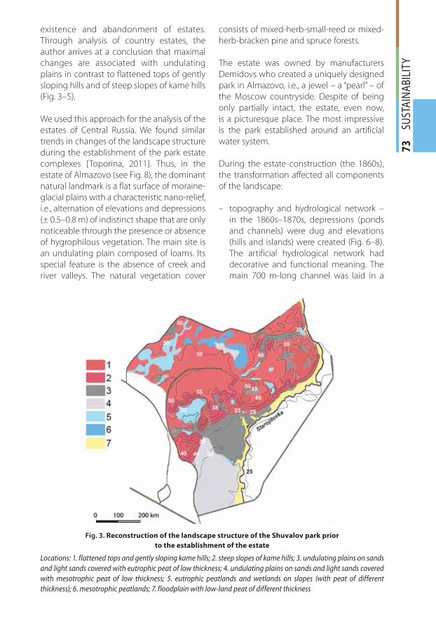
73

SU

STA

INA

BILI

TY

existence and abandonment of estates.

Through analysis of country estates, the

author arrives at a conclusion that maximal

changes are associated with undulating

plains in contrast to flattened tops of gently

sloping hills and of steep slopes of kame hills

(Fig. 3–5).

We used this approach for the analysis of the

estates of Central Russia. We found similar

trends in changes of the landscape structure

during the establishment of the park estate

complexes [Toporina, 2011]. Thus, in the

estate of Almazovo (see Fig. 8), the dominant

natural landmark is a flat surface of moraine-

glacial plains with a characteristic nano-relief,

i.e., alternation of elevations and depressions

(± 0.5–0.8 m) of indistinct shape that are only

noticeable through the presence or absence

of hygrophilous vegetation. The main site is

an undulating plain composed of loams. Its

special feature is the absence of creek and

river valleys. The natural vegetation cover

consists of mixed-herb-small-reed or mixed-

herb-bracken pine and spruce forests.

The estate was owned by manufacturers

Demidovs who created a uniquely designed

park in Almazovo, i.e., a jewel – a “pearl” – of

the Moscow countryside. Despite of being

only partially intact, the estate, even now,

is a picturesque place. The most impressive

is the park established around an artificial

water system.

During the estate construction (the 1860s),

the transformation affected all components

of the landscape:

topography and hydrological network – –

in the 1860s–1870s, depressions (ponds

and channels) were dug and elevations

(hills and islands) were created (Fig. 6–8).

The artificial hydrological network had

decorative and functional meaning. The

main 700 m-long channel was laid in a

Fig. 3. Reconstruction of the landscape structure of the Shuvalov park prior

to the establishment of the estate

Locations: 1. flattened tops and gently sloping kame hills; 2. steep slopes of kame hills; 3. undulating plains on sands

and light sands covered with eutrophic peat of low thickness; 4. undulating plains on sands and light sands covered

with mesotrophic peat of low thickness; 5. eutrophic peatlands and wetlands on slopes (with peat of different

thickness); 6. mesotrophic peatlands; 7. floodplain with low-land peat of different thickness

gi412.indd 73gi412.indd 73 24.12.2012 9:10:5424.12.2012 9:10:54

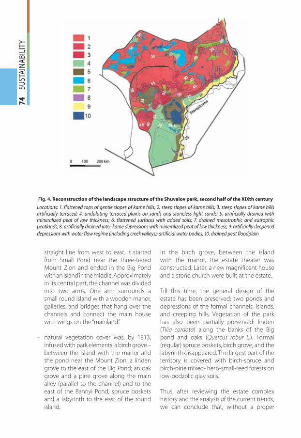
74

SU

STA

INA

BILI

TY

Fig. 4. Reconstruction of the landscape structure of the Shuvalov park, second half of the XIXth century

Locations: 1. flattened tops of gentle slopes of kame hills; 2. steep slopes of kame hills; 3. steep slopes of kame hills artificially terraced; 4. undulating terraced plains on sands and stoneless light sands; 5. artificially drained with mineralized peat of low thickness; 6. flattened surfaces with added soils; 7. drained mesotrophic and eutrophic peatlands; 8. artificially drained inter-kame depressions with mineralized peat of low thickness; 9. artificially deepened

depressions with water flow regime (including creek valleys); artificial water bodies; 10. drained peat floodplain

straight line from west to east. It started

from Small Pond near the three-tiered

Mount Zion and ended in the Big Pond

with an island in the middle. Approximately

in its central part, the channel was divided

into two arms. One arm surrounds a

small round island with a wooden manor,

galleries, and bridges that hang over the

channels and connect the main house

with wings on the “mainland.”

natural vegetation cover was, by 1813, –

infused with park elements: a birch grove –

between the island with the manor and

the pond near the Mount Zion; a linden

grove to the east of the Big Pond; an oak

grove and a pine grove along the main

alley (parallel to the channel) and to the

east of the Bannyi Pond; spruce boskets

and a labyrinth to the east of the round

island.

In the birch grove, between the island

with the manor, the estate theater was

constructed. Later, a new magnificent house

and a stone church were built at the estate.

Till this time, the general design of the

estate has been preserved: two ponds and

depressions of the formal channels, islands,

and creeping hills. Vegetation of the park

has also been partially preserved: linden

(Tilia cordata) along the banks of the Big

pond and oaks (Quercus robur L.). Formal

(regular) spruce boskets, birch grove, and the

labyrinth disappeared. The largest part of the

territory is covered with birch-spruce and

birch-pine mixed- herb-small-reed forests on

low-podzolic glay soils.

Thus, after reviewing the estate complex

history and the analysis of the current trends,

we can conclude that, without a proper

gi412.indd 74gi412.indd 74 24.12.2012 9:10:5424.12.2012 9:10:54

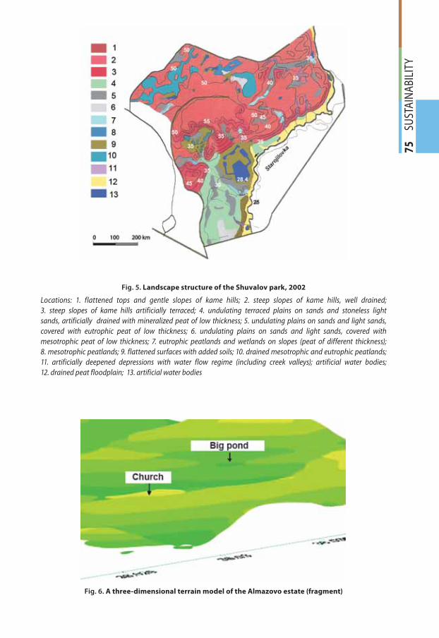
75

SU

STA

INA

BILI

TY

Fig. 5. Landscape structure of the Shuvalov park, 2002

Locations: 1. flattened tops and gentle slopes of kame hills; 2. steep slopes of kame hills, well drained;

3. steep slopes of kame hills artificially terraced; 4. undulating terraced plains on sands and stoneless light

sands, artificially drained with mineralized peat of low thickness; 5. undulating plains on sands and light sands,

covered with eutrophic peat of low thickness; 6. undulating plains on sands and light sands, covered with

mesotrophic peat of low thickness; 7. eutrophic peatlands and wetlands on slopes (peat of different thickness);

8. mesotrophic peatlands; 9. flattened surfaces with added soils; 10. drained mesotrophic and eutrophic peatlands;

11. artificially deepened depressions with water flow regime (including creek valleys); artificial water bodies;

12. drained peat floodplain; 13. artificial water bodies

Fig. 6. A three-dimensional terrain model of the Almazovo estate (fragment)

gi412.indd 75gi412.indd 75 24.12.2012 9:10:5424.12.2012 9:10:54

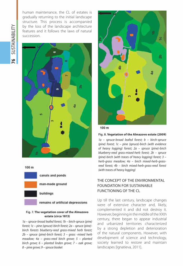
76

SU

STA

INA

BILI

TYhuman maintenance, the CL of estates is

gradually returning to the initial landscape

structure. This process is accompanied

by the loss of the landscape architecture

features and it follows the laws of natural

succession.

THE CONCEPT OF THE ENVIRONMENTAL

FOUNDATION FOR SUSTAINABLE

FUNCTIONING OF THE CL

Up till the last century, landscape changes

were of extensive character and, likely,

complemented it and did not destroy it.

However, beginning in the middle of the XXth

century, there began to appear industrial

and urbanized territories characterized

by a strong depletion and deterioration

of the natural components. However, with

development of science and technology,

society learned to restore and maintain

landscapes [Ignatieva, 2011].

Fig. 7. The vegetation cover of the Almazovo

estate (circa 1813)

1a – spruce-broad leafed forest; 1b – birch-spruce (pine)

forest; 1c – pine (spruce)-birch forest; 2a – spruce (pine)-

birch forests blueberry-reed grass-mixed herb forest;

2b – spruce (pine)-birch forest; 3 – grass -mixed herb

meadow; 4a – grass-reed birch grove; 5 – planted

birch grove; 6 – planted linden grove; 7 – oak grove;

8 – pine grove; 9 – spruce bosket

Fig. 8. Vegetation of the Almazovo estate (2009)

1a – spruce-broad leafed forest; b – birch-spruce

(pine) forest; 1c – pine (spruce)-birch (with evidence

of heavy logging) forest; 2a – spruce (pine)-birch

blueberry-reed grass-mixed-herb forest; 2b – spruce

(pine)-birch (with traces of heavy logging) forest; 3 –

herb-grass meadow; 4a – birch mixed-herb-grass-

reed forest; 4b – birch mixed-herb-grass-reed forest

(with traces of heavy logging)

gi412.indd 76gi412.indd 76 24.12.2012 9:10:5524.12.2012 9:10:55

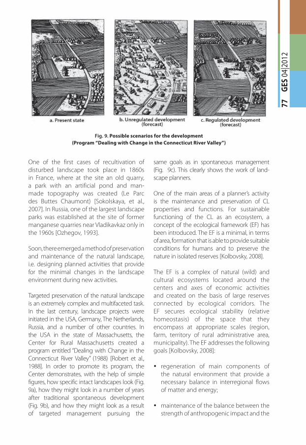
77

G

ES 0

4|20

12

One of the first cases of recultivation of

disturbed landscape took place in 1860s

in France, where at the site an old quarry,

a park with an artificial pond and man-

made topography was created (Le Parc

des Buttes Chaumont) [Sokolskaya, et al.,

2007]. In Russia, one of the largest landscape

parks was established at the site of former

manganese quarries near Vladikavkaz only in

the 1960s [Ozhegov, 1993].

Soon, there emerged a method of preservation

and maintenance of the natural landscape,

i.e. designing planned activities that provide

for the minimal changes in the landscape

environment during new activities.

Targeted preservation of the natural landscape

is an extremely complex and multifaceted task.

In the last century, landscape projects were

initiated in the USA, Germany, The Netherlands,

Russia, and a number of other countries. In

the USA in the state of Massachusetts, the

Center for Rural Massachusetts created a

program entitled “Dealing with Change in the

Connecticut River Valley” (1988) [Robert et al.,

1988]. In order to promote its program, the

Center demonstrates, with the help of simple

figures, how specific intact landscapes look (Fig.

9a), how they might look in a number of years

after traditional spontaneous development

(Fig. 9b), and how they might look as a result

of targeted management pursuing the

same goals as in spontaneous management

(Fig. 9c). This clearly shows the work of land-

scape planners.

One of the main areas of a planner’s activity

is the maintenance and preservation of CL

properties and functions. For sustainable

functioning of the CL as an ecosystem, a

concept of the ecological framework (EF) has

been introduced. The EF is a minimal, in terms

of area, formation that is able to provide suitable

conditions for humans and to preserve the

nature in isolated reserves [Kolbovsky, 2008].

The EF is a complex of natural (wild) and

cultural ecosystems located around the

centers and axes of economic activities

and created on the basis of large reserves

connected by ecological corridors. The

EF secures ecological stability (relative

homeostasis) of the space that they

encompass at appropriate scales (region,

farm, territory of rural administrative area,

municipality). The EF addresses the following

goals [Kolbovsky, 2008]:

regeneration of main components of �the natural environment that provide a

necessary balance in interregional flows

of matter and energy;

maintenance of the balance between the �strength of anthropogenic impact and the

Fig. 9. Possible scenarios for the development

(Program “Dealing with Change in the Connecticut River Valley”)

gi412.indd 77gi412.indd 77 24.12.2012 9:10:5524.12.2012 9:10:55

78

SU

STA

INA

BILI

TYlevel of biochemical activity and physical

stability of the natural environment

including the existence of conditions for

sufficiently high rates of pollution, their

biological processing, and stabilization

of impact of transportation, engineering,

and recreational loads on the landscape;

maintenance of the biological mass �balance in intact or lightly disturbed areas

that are affected by economic activity in

main landscapes of the region;

provision of maximal possible, in given �conditions, diversity and complexity of

environmental systems in the region.

In reality, the EF is formed among given

structural lines and ranges, i.e. a city with

its suburbs and industrial areas, large

transportation centers and arterials, agricultural

areas and forests, river network, sources and

range of pollution, interregional transit flows of

pollution, etc. The main blocks (components)

of such foundation are forests of different

size, river network, wetlands (that represent

hydrographic centers), reserves and national

parks, and different natural monuments.

As it was mentioned above, the main unstable

territories are the industrial-urbanized areas.

In order to improve conditions of settlement

areas, the principles of creation of the urban

EF have been developed. The urban EF is an

environment territorial system designed for

enhancement of the environmental situation

of urbanized areas through [Yang, et al. 2004]:

isolation of the most hazardous centers of �technogenic impact;

protection of historical elements of the CL; �

restoration of valuable components of �natural ecosystems;

enhancement of comfort level in �residential environment.

The urban EF should consist of different

elements of the CL (parks, gardens,

boulevards, street trees) and elements

of the remaining nature (suburb forests,

parks, valley forest-meadow areas). The EF

includes blocks of different size (large inter-

arterial wedges and spots of vegetation of

residential gardens and of different functional

purposes – green, recreational, sanitary-

protective, and engineering-protective).

Finally, and the most importantly, the EF is

characterized by integrity – all components

and blocks should be spatially connected

in a single live network of centers (areal

blocks of the EF) and corridors (linear blocks

of the EF). From the positions of zoning

law, the EF achieves urban nature-protective

and recreational goals, forming special legal

zones: recreational, specially protected

natural territories, protected historical and

cultural monuments, and their landscape

space. Development of the EF assumes

regeneration of its natural elements and the

formation of new green spaces that restore

continuity of the urban natural landscape

structure; preservation, identification, and

visual realization and accentuation of

historically characteristic landscape views,

garden-park complexes, and urban scenic

views [Gobster, et al., 2007].

Restoration of spatial continuity of the natural

and semi-natural elements of the urban EF is

achieved through the creation of a well-

developed system of green connectors that

unite isolated territories and the natural

complexes. It assumes:

formation of a system of specially protected �suburb territories by identification of

the most valuable, typical, and unique

ecosystems and landscapes (or their

elements) of both the natural and the

cultural origin;

preservation of existing and restoration �of lost landscapes of valleys of large and

small rivers as environmental corridors;

identification and preservation, in each �sector, of the urban rosette of free arterial

wedges and territories-connectors that

include existing and reserve areas of the

gi412.indd 78gi412.indd 78 24.12.2012 9:10:5524.12.2012 9:10:55

79

SU

STA

INA

BILI

TY

EF and that provide interconnection of

its main areas and between them and

suburb landscapes;

restoration and design of new large urban �parks (as spatial intercity areas of the EF)

instead of old and lost, especially in the

new housing development areas;

formation, in the contact zones of the EF �and in the urbanized territories of buffer

zones, of low-density and heavily green

areas that are able to decrease pressure

on the natural complex;

development of a system of inter-block �greening and of greening of pedestrian

zones, streets, industrial zones, and

engineering network;

preservation and creation of new green �areas of common use (boulevards, gardens)

and areas of special purposes (protective

belts along railways, engineering-technical

zones, and networks);

recultivation and rehabilitation of �wastelands, industrial areas, storehouse and

public utilities zones, protected zones of

different purposes, developed depositing

sites, watersheds, slurry reservoirs, ash

disposal areas, and tailing dumps;

establishment of environmental corridors �along major roadways and railways.

The urban EF is, at the same time, a

recreational foundation. In urban conditions,

these two concepts practically blend

together because it is difficult to rely here

on the creation of protected elements of

the EF that are closed for the public and for

the recreational use (it may only be possible

within botanical gardens, protected private

areas, or areas with regulated schedule

of operation). Therefore, the formation of

the EF assumes a simultaneous creation

of recreational areas. Park is seen as the

main urban recreational type. In the urban

environment, large parks (exceeding 5 ha)

are especially important since they maintain

complex layered structure of the biota

(ground layer, several shrub layers, low-trees

layer, groundfloor, and layer of developed

species different in height). Specifically such

parks exhibit the maximal biodiversity and

are able to regulate and form microclimate.

Parks may be artificially created or created on

the basis of natural vegetation.

Parks and urban cultivated green areas are,

of course, the main remnants of the nature

at any urbanized territory with a set of

environmental niches [Alvey, 2006]. Their

species diversity depends on the age and the

storey-structure of plantings, frequency of

mowing, soil and fertilizing regime, intensity

of trampling, and existence of water bodies.

These factors, in turn, determine the number

of nesting sites and shelters for birds that nest

in hollows of trunks or in branches of trees.

Parks are the refuges for disappearing local

species and for archaeophytes and neophytes;

besides, they are the islands for lichens in

urban conditions. In parks, there are also edge

communities and communities of grazing

areas; locally, there are thickets of shrubs similar

to natural [Goroshyna and Ignatyeva, 2000]

Urban parks are a vivid example of the island

environment under significant anthropogenic

impact (disturbance by people, dogs,

automobile pollutants, chlorides, dust,

pesticides, mechanical disturbances,

altered microclimatic parameters). As any

island, a park, depending on its size and

configuration, consists of an internal center

and an edge. The edge zone carries an

especially strong anthropogenic load. The

smaller the park, the greater a relative area

of the edge zone where the influence of

the surrounding environment of the urban

territory is spread through the entire island

and the central zone disappears; after that,

its functional zoning is obsolete.

Today, urban and other planners have a

sufficient number of ways to maintain

environmental situation in residential areas by

forming the EF that includes blocks different in

size, i.e., inter wedges, green belts and urban

nature-protective and recreational zones.

gi412.indd 79gi412.indd 79 24.12.2012 9:10:5524.12.2012 9:10:55

80

SU

STA

INA

BILI

TYCONCLUSION

1. The CL is less stable compared with its

original natural landscape. Stability of the

natural landscape is defined by its intrinsic

diversity. As a rule, the following potentially

more stable geoecosystems can be isolated:

with increased diversity and overlapping

(doubling) components of structure; in the

centers of their zonal and regional typicality;

trans-accumulative are more stable than

trans-alluvial; larger in area and matter;

and of higher hierarchal ranks. The main

methodological instrument of assessment of

landscape stability is LP that defines stability

criteria of the natural landscape components.

The main element of assessment is the

biotope. It reflects all natural components

of the landscape. Its two criteria, i.e.,

sensitivity and significance, are identified.

The sensitivity criterion assumes an ability

of a given natural complex to change its

properties and dynamic characteristic under

the impact of human economic activity. The

second criterion is significance that helps to

identify priority goals and objects for LP.

2. Identification of the stability categories

of the CL is associated with a number of

difficulties. The methodology of LP has

developed rather clear recommendations

for assessment of sensitivity and significance

of the natural landscape, which cannot be

stated in respect to the CL that requires a

specific and individual approach in each

particular case. In contemporary scientific

research, only basic and general assessment

criteria of natural components are used for

the identification of the CL stability criteria.

3. The link between the natural and cultural

components is rather complex and the

maximal correspondence is manifested

through the character of territorial natural

resource management. It reflects the

natural structure of the CL and it also

considers the socio-economic features of

the territorial use. The natural stability is

one of the prerequisites for sustainable

resource use. With the increase in human

economic activity, the natural stability of

the natural landscape decreases and there

emerges new acquired stability, but in this

case, already of the CL. The essence of the

acquired stability is in the adaptive variability

of structures and functions of the landscape

under anthropogenic impact.

4. Stability of the CL is closely associated

with the character of natural resource

management. This allows identifying three

groups of stability that depend on the

types of territorial use: stable (they include

extensive types – traditional, recreational,

nature protective), moderately stable

(vast territories of forest management

and agricultural purposes), and unstable

(urbanized and industrial zones with strong

differentiation and changes in the structure

of the native landscapes).

5. For the sustainable functioning of the

CL as an ecosystem, a concept of the EF

has been introduced; the EF is the minimal,

in area, formation that is able to provide

for suitable environmental conditions for

humans, to preserve the nature at least in

the form of isolated reserves, to identify

the most hazardous centers of technogenic

impact, to preserve historical elements of the

CL, to restore valuable fragments of natural

ecosystems, and to enhance comfort of the

residential area. The urban EF consists of

different elements of the CL (parks, gardens,

boulevards, and street plantings) and of

fragments of the remaining nature (suburb

forest, parks, and valley forest-meadow

spaces).

6. The EF achieves the nature protective

and recreational goals of urban territories,

forming special legal zones: recreational,

specially protected natural areas, and

protected historical and cultural monuments

together with space around them.

7. Development of EFs assumes restoration

of the natural urban elements, formation of

new green spaces (a system of inter-block

green areas and greening of pedestrian

zones, streets, industrial areas, storehouse

and public utilities zones, protected

zones of different purposes, developed

gi412.indd 80gi412.indd 80 24.12.2012 9:10:5524.12.2012 9:10:55

81

SU

STA

INA

BILI

TY

depositing sites, watersheds, slurry

reservoirs, ash disposal areas, and tailing

dumps) that restore continuity of the urban

natural-landscape structure; preservation,

identification, visual realization, and

accentuation of characteristic historical

landscape views, park-garden complexes,

and urban scenic views.

Thus, we can reach a conclusion on

the incomplete and insufficient level of

development of criteria for assessment of

stability of the CL in modern science. This

results from great diversity of both the CLs

themselves and their natural conditions of

formation, as well as of the types of natural

resource management. All discussed research

approaches on CL stability were developed

with the obvious domination of the nature-

centric approach that is based on assessment

of the natural component of the landscape. This

is explained by the difficulty of identification

of the structure of the CL, its components,

and assessment of their stability. Today, the

methodology of the EF for urbanized areas

may be considered the best developed

methodology of the CL stability assessment.

Modern methods of assessment and formation

of the EFs in cities promote preservation of

properties and functions of the CL. �

REFERENCES

1. Alvey, A.A. (2006). Promoting and preserving biodiversity in the urban forest. Urban Fores-try and Urban Greening. 5 (4). pp. 195–201.

2. Basalikas, A.B. (1977). Reflection of socio-economic and natural factors in functionally-oriented anthropogenization of landscapes (using an example of Lithuania) // Procee-dings of the USSR Academy of Sci., Ser. Geogr. № 1. pp. 108–115 (in Russian).

3. Dramstad, W., Olson, J., Forman, R. (1996). Landscape. Ecology Principles. In: Landscape Ar-chitecture and Land-use Planning. “Island Press”, Harvard University. 80 p.

4. Drozdov, A.V. (2006). Landscape planning with elements of engineering biology. M.: “Association of Scientific Publications KMK”, 239 p. (in Russian).

5. Fedotov, V.I., Dvurechenskyi, V.N. (1977). Technogenic landscape, its content and structure // Issues of Geography. № 106. pp. 65–73 (in Russian).

6. Glazovskaya, M.A. (1981). General soil science and soil geography. M.: “Vyshaya Shkola”, 400 p. (in Russian).

7. Gobster, P.H., Nassauer, J.I., Daniel, T.C., Fry, G. (2007). The shared landscape: What does aesthetics have to do with ecology? Landscape Ecology. 22 (7). pp. 959–972.

8. Golovanov, A.I. Kozhanov, E.S., Sukharev, Yu. I. (2006). Landscape science. M.: “Kolos”. 215 p. (in Russian).

9. Goroshina, T.K., Ignatieva, M.E. (2000). Botanical urban tours “State Scientific and Technical Publishing House of Chemical Literature”, 160 p. (in Russian).

10. Ignatieva, M.E. (2011). The Gardens of the Old and the New Worlds. Tours of Landscape Architecht. – SPB. “Iskusstvo”, (in Russian).

11. Isachenko, A.G. (1974). On the so-called anthropogenic landscapes. Proceedings of the All-Union Geographical Society. Vol. 106, Issue 1, pp. 70–77 (in Russian).

12. Isachenko, A.G. (1980). Optimization of the natural environment (geographical aspect). – M.: “Mysl”, 284 p. (in Russian).

13. Isachenko, T.E. (2003). Manors of the nobility and landscape: three centuries of interaction. Herald of the SPB State University. Ser. Geogr. Issue 4 (№ 31). pp. 88–101 (in Russian).

gi412.indd 81gi412.indd 81 24.12.2012 9:10:5624.12.2012 9:10:56

82

SU

STA

INA

BILI

TY 14. Kalutskov, V.N. (2008). Landscape in cultural geography. M.: “Novyi Chronograph”, 320 p.

(in Russian).

15. Kazakov, L.K. (2008). Landscape science with the elements of landscape planning. M.: “Academia”, 336 p. (in Russian).

16. Kolbovsky Eu.Yu. (2008). Landscape planning. M.: Publishing Center: “Academia”, 336 p. (in Russian).

17. Ozhegov, S.S. (1993). The history of landscape architecture. M.: “Stroiizdat”, 234 p. (in Russian).

18. Runova, T.G. (1985). Sustainable resource use as an object of economic-geographic stu-dies, Proceedings of the USSR Academy of Sci. Ser. Geogr. № 2. pp. 46-58 (in Russian).

19. Runova, T.G., Volkova, I.N., Nefedova, T.G. (1993). Territorial organization of resource use. M.: “Nauka”, 206 p. (in Russian).

20. Sochava, V.B. (1978). Basics of geosystem science. Novosibirsk, 320 p.

21. Sokolskaya, O.B. Teodoronsky, V.S., Vergunov, A.P. (2007). Landscape architecture: speciali-zed object. M.: Publishing Center: “Academia”, 224 p. (in Russian).

22. Solntsev, N.A. (2001). The science of landscape. Selected papers. M.: “MSU Press”, 383 p. (in Russian).

23. Toporina, V.A. (2011). Landscape location typology of estates of Central Russia. Environ-ment of urbanized territories. № 1. pp. 60–66 (in Russian).

24. Vedenin, Yu. A., Kuleshova, M.E. (2004). Cultural landscapes as categories of heritage // Cultural landscape as an object of heritage. M.- SPB., pp. 13–36 (in Russian).

25. Vedenin, Yu.A. (1997). Sketches on geography of art. SPB.: Dmitryi Bulanin, 224 p. (in Rus-sian).

26. Vorontsov, A.I., Schetinsky, E.A., Nikodimov, I.D. (1989). Protection of the nature. M: “Agropromizdat”, 303 p. (in Russian).

27. Yang, J., McBride, J., Zhou, J., Sun, Z. (2004). The urban forest in Beijing and its role in air pollution reduction. Urban Forestry and Urban Greening. 3 (2). pp. 65–78.

28. Yaro Robert, Arendt Randall, Dodson Harry, Brabec Elizabeth (1988). Dealing with Change in the Connecticut River Valley: A Design Manual for Conservation and Development.

Lincoln Institute of Land Policy, Cambridge, MA, 441 pp.

Elena I. Golubeva is Professor of Environmental Science

Department and Head of Education Program “Landscape Planning

& Design” at the Faculty of Geography, Lomonosov Moscow State

University. 1974 – M.Sc. in Biogeography, 1982 – Ph.D. in Biogeography

and Bioproduction, 1999 – D. Sc. in Biology. Member of the Russian

Academy of Nature Science. Laureate of Russian Governmental

Award in Science and Technology (1997). Her primary research

interests are in diagnostics of ecosystem health under nature and

anthropogenic pressure. Main publications: Methods of diagnostics

of transformed ecosystems (1999); Change of structure and function

of vegetation under pollution impact in the North (2007, with co-

authors); Urban Cultural Landscape: Traditions and Modern Trends

(2012, with co-authors).

gi412.indd 82gi412.indd 82 24.12.2012 9:10:5624.12.2012 9:10:56

83

SU

STA

INA

BILI

TY

Valentina A. Toporina graduated from the Lomonosov Moscow

State University in 2003. She is a Scientific Researcher at the

Environmental Management Department, MSU Faculty of

Geography. She received her PhD degree in Geography from the

Lomonosov Moscow State University in 2012. Her primary

research interests are in cultural geography, cultural landscapes,

and mapping of cultural landscapes, attributes and categories of

landscape sustainability. Main publications: Contribution of

manorial estates to cultural landscapes in Russia (2010); Landscape conditionality types of

manorial estates: case study for European Russia (2011); Challenges of cultural heritage

conservation: case study for estates’ parks in European Russia (2012).

Tatiana O. Korol graduated with a MSc from the Department of Social and Economic Geography of Russia, Lomonosov Moscow State University, in 1999, and with a PhD in Geography in 2003. Since 2010 she is a Senior Researcher at the Environmental Science Department and Supervisor of Distance Education Program “Landscape Planning & Design” at the MSU Faculty of Geography. Her primary research interests are in land-use planning, urban and landscape design, sustainability of cultural landscapes. Main publications: Art and design landscape. Textbook (2010, editor with E.I. Golubeva); Experience in the use of tools of landscape planning in the project landscaping of private land ownership (2010); Landscape research with

application to land-use planning of building zones: a case of study for Skolkovo, Moscow region (2012, with E.I.Golubeva).

Maria E. Ignatieva is Professor in Landscape Architecture,

Division of Landscape Architecture, Department of Urban and

Rural Development at Swedish University of Agricultural Sciences.

MSc.: Leningrad Forest Technical Academy (1982). PhD: Moscow

State University in 1987. Honorary doctor at St. Petersburg State

Forest Technical Academy (2012). Main research is urban

biodiversity and design and history of landscape architecture.

Main publications: Gardens of Old and New World. Journey of a

Landscape Architect (2011); Design and future of urban

biodiversity (2010). Maria has realised several landscape

architecture projects in the USA and New Zealand.

gi412.indd 83gi412.indd 83 24.12.2012 9:10:5624.12.2012 9:10:56

84

SU

STA

INA

BILI

TY

ABSTRACT. South American countries

still possess considerable land reserves for

agricultural development. Huge areas of

virgin lands and natural pastures have been

converted to agricultural crops and suffer

increasing pressure. Growing demand

for food in the world and attractiveness for

capital investment drive this colonization

further deep into the regions that cannot be

converted to commercial agriculture without

serious negative environmental consequen ces.

Agricultural development in these areas neither

can be considered economically sustainable,

as high production costs sometimes surpass

revenues from the harvest. Most of the

recently colonized regions in South America

are those under savanna landscapes, where

low nutrient availability in the soil restricts

agricultural use. Understanding the problem

of sustainability of agricultural development in

savannas is impossible without geographical

analysis. Spatial approach at different scales

enables precise vision of weak points of recently

established agricultural systems and helps to

draw solutions to diminish their instability. The

objective of this paper was to develop, with GIS

tools, a geographically based analysis that could

identify the spatial variation and magnitude of

soil potassium, potassium uptake, potassium

fertilization, and potassium balance in order to

improve the efficiency of mineral fertilizers use.

KEY WORDS: Sustainable development

of agriculture, mineral fertilizers, savannas,

cerrado, South America, Brazil

INTRODUCTION

South America, perhaps, is one of the

last agricultural frontiers of the humanity.

Since its conquest by Spain, Portugal

and other European powers, agricultural

development on this continent is going

along with colonization of virgin lands.

After the colonial period, the late 19th –

early 20th centuries were marked by

colonization of the Argentinean Pampa

and the southern states of Brazil. The last

large-scale colonization campaign started

in the 1980s, with colonization of the

Center-West region in Brazil. Later on, it

also affected the fringe of the Amazon

region and the inner parts of the North-

East region of this country [Naumov, 2005].

From Brazil, colonization has spread to the

neighboring areas of Paraguay and Bolivia.

In Colombia and Venezuela, the agricultural

frontier also started moving towards the

peripheral regions [Naumov, 2010]. These

areas, together with some Argentinean

provinces, became the ground for the recent

soybean production boom in Latin America

[International Potash Institute, 2011].

Alexey S. Naumov1*, Ronaldo Pereira de Oliveira2, Rachel Bardy Prado2, Ana Paula Turetta2

1 Faculty of Geography, Lomonosov Moscow State University, Leninskie Gory 119991 Moscow, Russia; e-mail: alnaumov@mail.ru* Corresponding author2 Brazilian Agricultural Research Corporation (EMBRAPA), National Soils Research Center (Embrapa Solos), Rua Jardim Bot@ânico,1024, Rio de Janeiro, Brazil

BALANCED FERTILIZATION FOR SUSTAINABLE DEVELOPMENT OF AGRICULTURE IN THE SAVANNAS OF SOUTH AMERICA: TOWARDS A GEOGRAPHICAL APPROACH

gi412.indd 84gi412.indd 84 24.12.2012 9:10:5624.12.2012 9:10:56

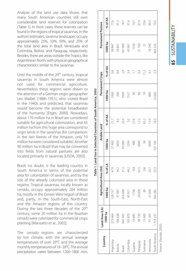
85

SU

STA

INA

BILI

TY

Analysis of the land use data shows that

many South American countries still own

considerable land reserves for colonization

(Table 1). In most cases, these reserves can be

found in the regions of tropical savannas. In the

authors’ estimates, savanna landscapes occupy

approximately 25%, 33%, 50%, and 25% of

the total land area in Brazil, Venezuela and

Colombia, Bolivia, and Paraguay, respectively.

Besides, there are areas outside the Tropics, like

Argentinean North, with physical-geographical

characteristics similar to the savannas.

Until the middle of the 20th century, tropical

savannas in South America were almost

not used for commercial agriculture.

Nevertheless these regions were drawn to

the attention of a German origin geographer

Leo Waibel (1888–1951), who visited Brazil

in the 1940s and predicted, that savannas

would become the potential breadbasket

of the humanity [Etges, 2000]. Nowadays,

about 170 million ha in Brazil are considered

suitable for agricultural colonization, and 65

million ha from this huge area correspond to

virgin lands in the savannas (for comparison:

in the rain forests of the Amazon, only 10

million ha were considered suitable). Another

90 million ha in Brazil that may be converted

into fields from natural pastures are also

located primarily in savannas [USDA, 2003].

Brazil, no doubt, is the leading country in

South America in terms of the potential

area for colonization of savannas, and by the

size of the already colonized area in these

regions. Tropical savannas, locally known as

cerrado, occupy approximately 204 million

ha, mostly in the Center-West region of Brazil

and, partly, in the South-East, North-East

and the Amazon regions of this country.

During the last three decades of the 20th

century, some 20 million ha in the Brazilian

cerrado were colonized for commercial crops

planting [Manzatto et al., 2002].

The cerrado regions are characterized

by hot climate, with the annual average

temperatures of over 20°C and the average

monthly temperatures of 18–28°C. The annual

precipitation varies between 1200–1800 mm,

Tab

le 1

. La

nd

Use

in S

ele

cte

d C

ou

ntr

ies

of

So

uth

Am

eri

ca, 2

00

3

Co

un

try

La

nd

Are

a (

LA

)

10

00

ha

Ag

ricu

ltu

ral A

rea

(A

A)

Ara

ble

La

nd

Pe

rma

ne

nt

Cro

ps

Pe

rma

ne

nt

Pa

stu

re

10

00

ha

% o

f L

A1

00

0 h

a%

of

AA

10

00

ha

% o

f A

A1

00

0 h

a%

of

AA

Arg

en

tin

a2

73

66

91

28

74

74

7.0

27

90

02

1.7

10

00

0.8

99

84

77

7.6

Bo

livia

10

8 4

38

37

08

73

4.2

30

50

8.2

20

60

.63

3 8

31

91

.2

Bra

zil

84

5 9

42

26

3 6

00

31

.25

9 0

00

22

.47

60

02

.91

97

00

07

4.7

Co

lom

bia

10

3 8

70

45

91

14

4.2

22

93

5.0

15

57

3.4

42

06

19

1.6

Gu

yan

a1

9 6

85

17

40

8.8

48

02

7.6

30

1.7

12

30

70

.7

Para

gu

ay3

9 7

30

24

83

66

2.5

30

40

12

.29

60

.42

1 7

00

87

.4

Suri

nam

e1

5 6

00

89

0.6

58

65

.21

01

1.2

21

23

.6

Ve

ne

zue

la9

1 2

05

21

64

02

3.7

26

00

12

.08

00

3.7

18

24

08

4.3

Sou

th A

me

rica

1 7

53

23

75

84

28

53

3.3

10

7 1

05

18

.31

3 6

45

2.3

46

3 5

35

79

.3

Sou

rce

: [Fa

ost

at, 2

00

5].

gi412.indd 85gi412.indd 85 24.12.2012 9:10:5624.12.2012 9:10:56

86

SU

STA

INA

BILI

TYwith strongly pronounced wet (October–March

in the Southern hemisphere) and dry seasons.

Abundant heat and moisture permit planting

without irrigation of maize, soybean, sorghum,

sunflower, cotton, and harvesting commercial

crops twice a year from the same field.

The soil properties, which predominate in

the cerrado1, 1such as high acidity (pH 4–5),

low cation-exchange capacity (CEC), low

base saturation, and high levels of Al3+, limit

their agricultural use. Only after liming and

application of mineral fertilizers, these soils

become suitable for continuous planting

of grains, oilseeds, and other crops. No-till

practices on these soils became popular

for preventing soil erosion, maintaining

stable temperature and moisture regime in

the upper soil horizons, and improving low

organic matter contents. According to the

Brazilian Federation of Direct Planting into

the Straw, the area under no-till systems in

Brazil in 2005/2006 agricultural year equaled

25.5 million ha; 38% of this area corresponded

to the cerrado regions [Andrade et al., 2010]

Along with agricultural colonization of the

Brazilian cerrado, the consumption of mineral

fertilizers in this country has been increasing.

Potassium is one of the macronutrients highly

demanded by crops such as soybean, maize,

and sugarcane. For example, for each 1 t of

yield of soybeans, 20 kg of K2O are extracted

from the soil. Assuming that the average

soybean yield in Brazil approaches 3 t ha-1,

this is just enough to maintain the “zero”

balance of potassium in the soil; farmers

need to apply 100 kg ha–1 of KCl, the most

widespread potassium fertilizer, containing

60% of K2O. In 2010/2011 agricultural year,

Brazilian farmers harvested 69 million t of

soybeans from 24 million ha [Companhia

Nacional de Abastecimento, 2011]. For this,

they have used 25% of the nearly 7 million

t of potassium fertilizers, imported in 2010

to Brazil, making this country the 3rd in the

world after USA and China by the volume of

their imports [Potash Statistics, 2011].

1 Ferralsols by the FAO soil classification, or latossolos by the

Brazilian soil classification [Sistema brasileiro de classificação

de solos, 1999].

OBJECTS AND METHODS OF RESEARCH

In 2001, after establishing of a formal

agreement between the International

Potash Institute (IPI) and the Brazilian

Corporation for Agricultural Research

(EMBRAPA), a joint research project “Fertilize

Brazil”, aiming to develop and disseminate

balanced fertilization practices for Brazilian

agriculture, was initiated. In 2004, at the

first stage of the project implementation,

potassium balance in agricultural systems

was estimated at the level of 26 states and

for more than 4000 municipios (counties)

of Brazil.

During 2006-2007, data from 3000 soil

profiles, collected by the EMBRAPA National

Soils Research Center, were used for

mapping potassium contents in the soil.

Spatial interpretation of these data proved

to be technically difficult, because of

complicated linking of the data to the soil

types, landscape contours, and the network

of administrative units [Prado et al, 2008].

Soil profiles, described by EMBRAPA, are

unequally distributed by Brazilian territory.

They are very sparse in regions, where the

cerrado landscapes predominate. However,

as soil profiles data comparison showed,

soils of the Brazilian cerrado and similar

savanna landscapes are not uniform and

vary in physical and chemical properties.

For example, potassium availability in the

upper layers of the soil may differ from 15 to

150 mg kg–1 [Naumov and Prado, 2008].

The potassium export calculation was done

with the crop yield data on agricultural

production (for harvestable parts of the

crop) from the municipal statistical database

of the Brazilian Institute for Geography and

Statistics (IBGE). The estimates were based

on such indicators as the annual volume of

production (t) of 19 main commercial crops:

soybean, maize, sugar cane, coffee, cocoa,

oranges, beans, etc., including planted

eucalyptus, and the average uptake of the

nutrient with 1 t of their yields. The estimates

of the potassium input in the soil were

less precise. The only data source available

was statistics on the volume of potassium

gi412.indd 86gi412.indd 86 24.12.2012 9:10:5724.12.2012 9:10:57

87

SU

STA

INA

BILI

TY

fertilizers sales by state (t), provided by the

National Association of Mineral Fertilizers

Dissemination [ANDA, 2004].

From many points of view, those Brazilian

agricultural regions that were formed after

clearing of the cerrado natural vegetation,

deserve special attention for evaluation

of sustainability of agricultural systems

regarding balanced fertilization. Initially,

the cerrado regions with more fertile soils

were colonized, but now agricultural

frontier has shifted towards marginal

areas with poorer soils. Data on these

soils are scarce; farmers, who moved

there are mostly from the southern states

of Brazil and they often neglect local

natural conditions. Until recently, there

was a lack of scientific knowledge about

how to adopt agricultural practices in

these areas. From the technical point

of view, extrapolation of the EMBRAPA

data on soil profiles to all areas under

the cerrado vegetation for purposes of

further evaluation of potassium balance

in the soil and for the development of

recommendations for farmers could result

in significant discrepancies.

On the next stage of the project

implementation, we decided to carry out

a more detailed research and to create a

GIS-based spatial description of potassium

balance in agricultural systems in one of the

main grain and oilseed producing regions

of the Brazilian cerrado – South West of the

Goias state (Fig. 1). Large-scale commercial

agriculture began to develop in this state

in the late 1970s, and nowadays, Goias

is one of the main maize and soybean

producing regions (8.1 million Mt, or 15%

of the total national annual harvest of maize

grain in Brazil in 2010, and 7.5 million Mt, or

11% of soybeans). Cotton and sugarcane

planting is also spreading in this region, and

cattle ranching and poultry industry are

developing fast in association with forage

production [Projecções do agronegócio,

2010].

In 2005–2006, potassium availability in

soil was estimated from the data of soil

Fig. 1. Research polygon in the South West of the Goias state, Brazil

gi412.indd 87gi412.indd 87 24.12.2012 9:10:5724.12.2012 9:10:57

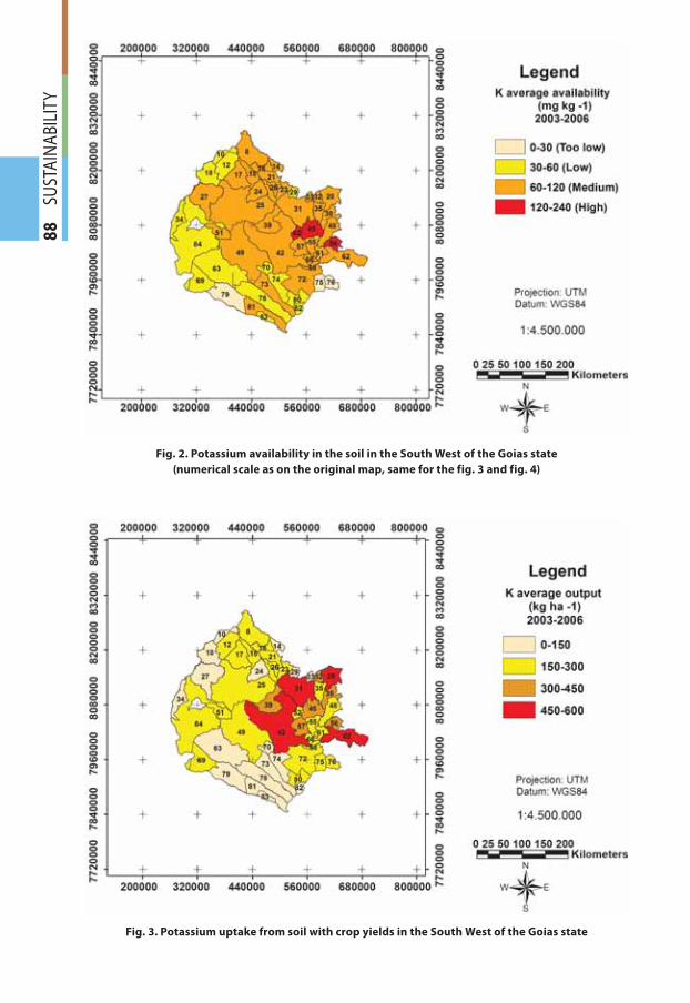
88

SU

STA

INA

BILI

TY

Fig. 2. Potassium availability in the soil in the South West of the Goias state

(numerical scale as on the original map, same for the fig. 3 and fig. 4)

Fig. 3. Potassium uptake from soil with crop yields in the South West of the Goias state

gi412.indd 88gi412.indd 88 24.12.2012 9:10:5724.12.2012 9:10:57

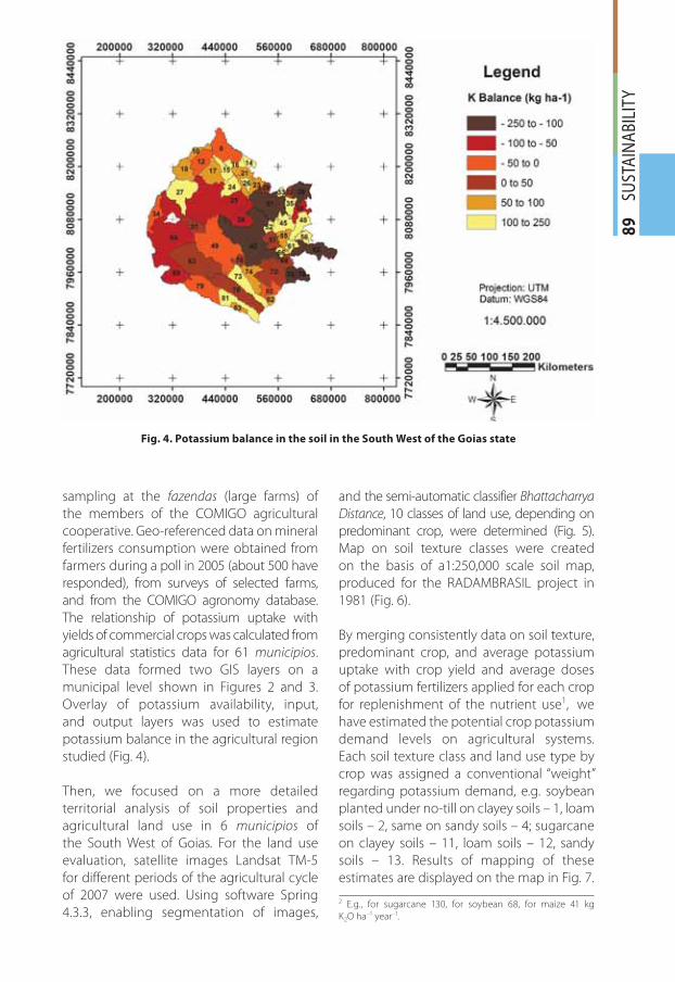
89

SU

STA

INA

BILI

TY

sampling at the fazendas (large farms) of

the members of the COMIGO agricultural

cooperative. Geo-referenced data on mineral

fertilizers consumption were obtained from

farmers during a poll in 2005 (about 500 have

responded), from surveys of selected farms,

and from the COMIGO agronomy database.

The relationship of potassium uptake with

yields of commercial crops was calculated from

agricultural statistics data for 61 municipios.

These data formed two GIS layers on a

municipal level shown in Figures 2 and 3.

Overlay of potassium availability, input,

and output layers was used to estimate

potassium balance in the agricultural region

studied (Fig. 4).

Then, we focused on a more detailed

territorial analysis of soil properties and

agricultural land use in 6 municipios of

the South West of Goias. For the land use

evaluation, satellite images Landsat TM-5

for different periods of the agricultural cycle

of 2007 were used. Using software Spring

4.3.3, enabling segmentation of images,

and the semi-automatic classifier Bhattacharrya

Distance, 10 classes of land use, depending on

predominant crop, were determined (Fig. 5).

Map on soil texture classes were created

on the basis of a1:250,000 scale soil map,

produced for the RADAMBRASIL project in

1981 (Fig. 6).

By merging consistently data on soil texture,

predominant crop, and average potassium

uptake with crop yield and average doses

of potassium fertilizers applied for each crop

for replenishment of the nutrient use1, 2we

have estimated the potential crop potassium

demand levels on agricultural systems.

Each soil texture class and land use type by

crop was assigned a conventional “weight”

regarding potassium demand, e.g. soybean

planted under no-till on clayey soils – 1, loam

soils – 2, same on sandy soils – 4; sugarcane

on clayey soils – 11, loam soils – 12, sandy

soils – 13. Results of mapping of these

estimates are displayed on the map in Fig. 7.

2 E.g., for sugarcane 130, for soybean 68, for maize 41 kg

K2O ha–1 year–1.

Fig. 4. Potassium balance in the soil in the South West of the Goias state

gi412.indd 89gi412.indd 89 24.12.2012 9:10:5824.12.2012 9:10:58

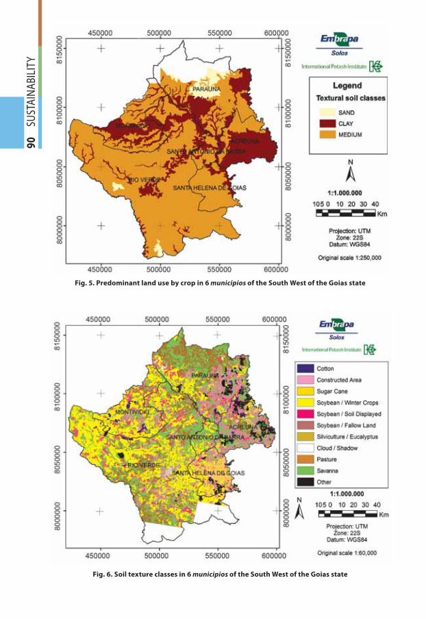
90

SU

STA

INA

BILI

TY

Fig. 5. Predominant land use by crop in 6 municipios of the South West of the Goias state

Fig. 6. Soil texture classes in 6 municipios of the South West of the Goias state

gi412.indd 90gi412.indd 90 24.12.2012 9:10:5824.12.2012 9:10:58

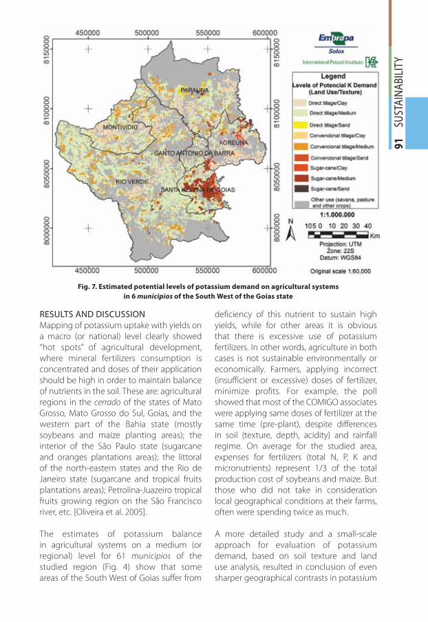
91

SU

STA

INA

BILI

TY

RESULTS AND DISCUSSION

Mapping of potassium uptake with yields on

a macro (or national) level clearly showed

“hot spots” of agricultural development,

where mineral fertilizers consumption is

concentrated and doses of their application

should be high in order to maintain balance

of nutrients in the soil. These are: agricultural

regions in the cerrado of the states of Mato

Grosso, Mato Grosso do Sul, Goias, and the

western part of the Bahia state (mostly

soybeans and maize planting areas); the

interior of the São Paulo state (sugarcane

and oranges plantations areas); the littoral

of the north-eastern states and the Rio de

Janeiro state (sugarcane and tropical fruits

plantations areas); Petrolina-Juazeiro tropical

fruits growing region on the São Francisco

river, etc. [Oliveira et al. 2005].

The estimates of potassium balance

in agricultural systems on a medium (or

regional) level for 61 municipios of the

studied region (Fig. 4) show that some

areas of the South West of Goias suffer from

deficiency of this nutrient to sustain high

yields, while for other areas it is obvious

that there is excessive use of potassium

fertilizers. In other words, agriculture in both

cases is not sustainable environmentally or

economically. Farmers, applying incorrect

(insufficient or excessive) doses of fertilizer,

minimize profits. For example, the poll

showed that most of the COMIGO associates

were applying same doses of fertilizer at the

same time (pre-plant), despite differences

in soil (texture, depth, acidity) and rainfall

regime. On average for the studied area,

expenses for fertilizers (total N, P, K and

micronutrients) represent 1/3 of the total

production cost of soybeans and maize. But

those who did not take in consideration

local geographical conditions at their farms,

often were spending twice as much.

A more detailed study and a small-scale

approach for evaluation of potassium

demand, based on soil texture and land

use analysis, resulted in conclusion of even

sharper geographical contrasts in potassium

Fig. 7. Estimated potential levels of potassium demand on agricultural systems

in 6 municipios of the South West of the Goias state

gi412.indd 91gi412.indd 91 24.12.2012 9:10:5924.12.2012 9:10:59

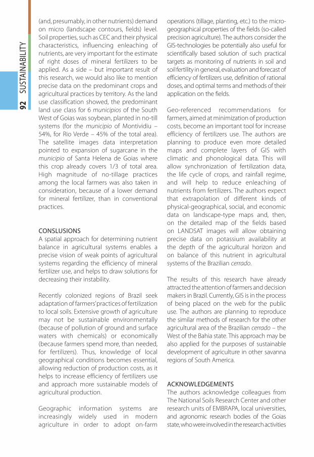
92

SU

STA

INA

BILI

TY(and, presumably, in other nutrients) demand

on micro (landscape contours, fields) level.

Soil properties, such as CEC and their physical

characteristics, influencing enleaching of

nutrients, are very important for the estimate

of right doses of mineral fertilizers to be

applied. As a side – but important result of

this research, we would also like to mention

precise data on the predominant crops and

agricultural practices by territory. As the land

use classification showed, the predominant

land use class for 6 municipios of the South

West of Goias was soybean, planted in no-till

systems (for the municipio of Montividiu –

54%, for Rio Verde – 45% of the total area).

The satellite images data interpretation

pointed to expansion of sugarcane in the

municipio of Santa Helena de Goias where

this crop already covers 1/3 of total area.

High magnitude of no-tillage practices

among the local farmers was also taken in

consideration, because of a lower demand

for mineral fertilizer, than in conventional

practices.

CONSLUSIONS

A spatial approach for determining nutrient

balance in agricultural systems enables a

precise vision of weak points of agricultural

systems regarding the efficiency of mineral

fertilizer use, and helps to draw solutions for

decreasing their instability.

Recently colonized regions of Brazil seek

adaptation of farmers’ practices of fertilization

to local soils. Extensive growth of agriculture

may not be sustainable environmentally

(because of pollution of ground and surface

waters with chemicals) or economically

(because farmers spend more, than needed,

for fertilizers). Thus, knowledge of local

geographical conditions becomes essential,

allowing reduction of production costs, as it

helps to increase efficiency of fertilizers use

and approach more sustainable models of

agricultural production.

Geographic information systems are

increasingly widely used in modern

agriculture in order to adopt on-farm

operations (tillage, planting, etc.) to the micro-

geographical properties of the fields (so-called

precision agriculture). The authors consider the

GIS-technologies be potentially also useful for

scientifically based solution of such practical

targets as monitoring of nutrients in soil and

soil fertility in general, evaluation and forecast of

efficiency of fertilizers use, definition of rational

doses, and optimal terms and methods of their

application on the fields.

Geo-referenced recommendations for

farmers, aimed at minimization of production

costs, become an important tool for increase

efficiency of fertilizers use. The authors are

planning to produce even more detailed

maps and complete layers of GIS with

climatic and phonological data. This will

allow synchronization of fertilization data,

the life cycle of crops, and rainfall regime,

and will help to reduce enleaching of

nutrients from fertilizers. The authors expect

that extrapolation of different kinds of

physical-geographical, social, and economic

data on landscape-type maps and, then,

on the detailed map of the fields based

on LANDSAT images will allow obtaining

precise data on potassium availability at

the depth of the agricultural horizon and

on balance of this nutrient in agricultural

systems of the Brazilian cerrado.

The results of this research have already

attracted the attention of farmers and decision

makers in Brazil. Currently, GIS is in the process

of being placed on the web for the public

use. The authors are planning to reproduce

the similar methods of research for the other

agricultural area of the Brazilian cerrado – the

West of the Bahia state. This approach may be

also applied for the purposes of sustainable

development of agriculture in other savanna

regions of South America.

ACKNOWLEDGEMENTS

The authors acknowledge colleagues from

The National Soils Research Center and other

research units of EMBRAPA, local universities,

and agronomic research bodies of the Goias

state, who were involved in the research activities

gi412.indd 92gi412.indd 92 24.12.2012 9:10:5924.12.2012 9:10:59

93

SU

STA

INA

BILI

TY

during 2001–2011. Our research also greatly

benefited from the support of field workers –

agronomists and farmers, who strive to achieve

sustainability of agriculture and provided us

with useful data on their practices.

The research was supported by the

International Potash Institute (IPI) and

the Brazilian Corporation for Agricultural

Research (EMBRAPA) that cooperate in the

Project “Fertilize Brazil”. �

REFERENCES

1. Andrade A.G., Freitas P.L., Landers, J. (2010). Aspectos gerais do manejo e conservação do solo e da água e as mudanças ambientais. In: Prado, R.B. Turetta A.P.D., Andrade A.G. Manejo e conservação do solo e da água no contexto das mudanças ambientais. Rio de Janeiro: Embrapa Solos, p. 25–52. /in Portuguese/

2. Anuário estatístico do setor de fertilizantes (2004). São Paulo: ANDA, 165 p. /in Portuguese/

3. Brasil Projecções do agronegócio, 2010/2011 a 2020/2021 (2011). Brasilia: Ministério da agricultura, pecuária e abastecimento, 59 p. /in Portuguese/

4. Companhia Nacional de Abastecimento (2011). Acompanhamento de safra brasileira: grãos, sexto levantamento, março 2011. Brasília: Conab, 40 p. /in Portuguese/

5. Etges V.E. (2000). Geografía Agrária: a contibuicão de Leo Waibel. EDUNISC, Santa Cruz do Sul, 224 p. /in Portuguese/

6. Faostat – the statistical database of the Food and Agriculture Organization of the United Nations (http://faostat.fao.org/default.aspx).

7. International Potash Instutute (2011). IPI Boletín 20. Soja en Latinoamérica. Buenos Aires: Agroeditorial, 180 p. /in Spanish/

8. Manzatto C.V., Freitas Junior, E., Perez, J.R. (2002). Uso Agricola dos Solos Brasileiros. Rio de Janeiro: Embrapa, 174 p. /in Portuguese/

9. Naumov A. (2005). Land Use in Brazil: Major Contemporary Changes and Their Driving Forces. In: Understanding Land-Use and Land-Cover Change in Global and Regional Context. Science Publishers, Inc., 208–223.

10. Naumov A., Prado R.B. (2008). Mapping spatial and temporal potassium balances in Brazilian soils of south-west Goias. Electronic International Fertilizer Correspondent. No. 15, March. P. 5–12. http://www.ipipotash.org/en/eifc/2008/15/3

11. Naumov A.S. (2010). Spatial scenarios of development of agriculture in the world: con-temporary agricultural colonization in South America. In: Geography of Global Develop-ment. Vol. 2. Moscow: KMK Publishers, p. 407–422 /in Russian/

12. Oliveira R.P., Machado P.L.O.A., Bernardi A.C de C., and A. Naumov (2005). Considerações sobre o uso de solo e regionalização do balanço de potássio na agricultura brasileira. In: Potássio na agricultura brasileira. Anais do Simpósio «Potássio na agricultura brasileira». Piracicaba: POTAFOS, p. 119–164 /in Portuguese/.

13. Potash Statistics 2011 (2012). International fertilizers Association. Paris: IFA.

14. Prado R.B., Benites V.M., Machado P.L.O.A., Polidoro J.C., Dart R.O. and Naumov A. (2008). Mapping potassium availability from limited soil profile data in Brazil. In: Digital Soil Map-ping with Limited Data. Springer Science+Business Media. p. 91–101.

15. Prado R.B., Ferreira C.E., Benites V.M., Naumov A. (2009). Mapeamento e descrição do padrão de uso e cobertura da terra em municipios so sudoeste goiano a partir de ima-

gi412.indd 93gi412.indd 93 24.12.2012 9:10:5924.12.2012 9:10:59

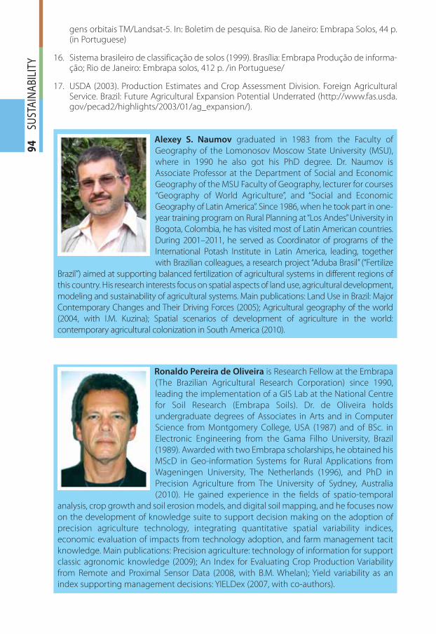
94

SU

STA

INA

BILI

TYgens orbitais TM/Landsat-5. In: Boletim de pesquisa. Rio de Janeiro: Embrapa Solos, 44 p. (in Portuguese)

16. Sistema brasileiro de classificação de solos (1999). Brasília: Embrapa Produção de informa-ção; Rio de Janeiro: Embrapa solos, 412 p. /in Portuguese/

17. USDA (2003). Production Estimates and Crop Assessment Division. Foreign Agricultural Service. Brazil: Future Agricultural Expansion Potential Underrated (http://www.fas.usda.gov/pecad2/highlights/2003/01/ag_expansion/).

Alexey S. Naumov graduated in 1983 from the Faculty of

Geography of the Lomonosov Moscow State University (MSU),

where in 1990 he also got his PhD degree. Dr. Naumov is

Associate Professor at the Department of Social and Economic

Geography of the MSU Faculty of Geography, lecturer for courses

“Geography of World Agriculture”, and “Social and Economic

Geography of Latin America”. Since 1986, when he took part in one-

year training program on Rural Planning at “Los Andes” University in

Bogota, Colombia, he has visited most of Latin American countries.

During 2001–2011, he served as Coordinator of programs of the

International Potash Institute in Latin America, leading, together

with Brazilian colleagues, a research project “Aduba Brasil” (“Fertilize

Brazil”) aimed at supporting balanced fertilization of agricultural systems in different regions of

this country. His research interests focus on spatial aspects of land use, agricultural development,

modeling and sustainability of agricultural systems. Main publications: Land Use in Brazil: Major

Contemporary Changes and Their Driving Forces (2005); Agricultural geography of the world

(2004, with I.M. Kuzina); Spatial scenarios of development of agriculture in the world:

contemporary agricultural colonization in South America (2010).

Ronaldo Pereira de Oliveira is Research Fellow at the Embrapa

(The Brazilian Agricultural Research Corporation) since 1990,

leading the implementation of a GIS Lab at the National Centre

for Soil Research (Embrapa Soils). Dr. de Oliveira holds

undergraduate degrees of Associates in Arts and in Computer

Science from Montgomery College, USA (1987) and of BSc. in

Electronic Engineering from the Gama Filho University, Brazil

(1989). Awarded with two Embrapa scholarships, he obtained his

MScD in Geo-information Systems for Rural Applications from

Wageningen University, The Netherlands (1996), and PhD in

Precision Agriculture from The University of Sydney, Australia

(2010). He gained experience in the fields of spatio-temporal

analysis, crop growth and soil erosion models, and digital soil mapping, and he focuses now

on the development of knowledge suite to support decision making on the adoption of

precision agriculture technology, integrating quantitative spatial variability indices,

economic evaluation of impacts from technology adoption, and farm management tacit

knowledge. Main publications: Precision agriculture: technology of information for support

classic agronomic knowledge (2009); An Index for Evaluating Crop Production Variability

from Remote and Proximal Sensor Data (2008, with B.M. Whelan); Yield variability as an

index supporting management decisions: YIELDex (2007, with co-authors).

gi412.indd 94gi412.indd 94 24.12.2012 9:11:0024.12.2012 9:11:00

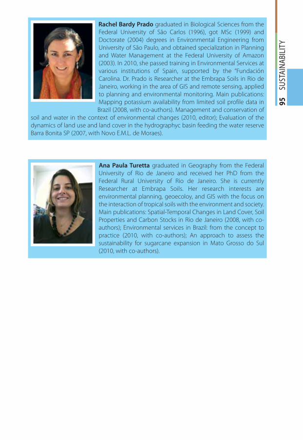
95

SU

STA

INA

BILI

TY

Rachel Bardy Prado graduated in Biological Sciences from the

Federal University of São Carlos (1996), got MSc (1999) and

Doctorate (2004) degrees in Environmental Engineering from

University of São Paulo, and obtained specialization in Planning

and Water Management at the Federal University of Amazon

(2003). In 2010, she passed training in Environmental Services at

various institutions of Spain, supported by the “Fundación

Carolina. Dr. Prado is Researcher at the Embrapa Soils in Rio de

Janeiro, working in the area of GIS and remote sensing, applied

to planning and environmental monitoring. Main publications:

Mapping potassium availability from limited soil profile data in

Brazil (2008, with co-authors). Management and conservation of

soil and water in the context of environmental changes (2010, editor); Evaluation of the

dynamics of land use and land cover in the hydrographyc basin feeding the water reserve

Barra Bonita SP (2007, with Novo E.M.L. de Moraes).

Ana Paula Turetta graduated in Geography from the Federal

University of Rio de Janeiro and received her PhD from the

Federal Rural University of Rio de Janeiro. She is currently

Researcher at Embrapa Soils. Her research interests are

environmental planning, geoecoloy, and GIS with the focus on

the interaction of tropical soils with the environment and society.

Main publications: Spatial-Temporal Changes in Land Cover, Soil

Properties and Carbon Stocks in Rio de Janeiro (2008, with co-

authors); Environmental services in Brazil: from the concept to

practice (2010, with co-authors); An approach to assess the

sustainability for sugarcane expansion in Mato Grosso do Sul

(2010, with co-authors).

gi412.indd 95gi412.indd 95 24.12.2012 9:11:0024.12.2012 9:11:00

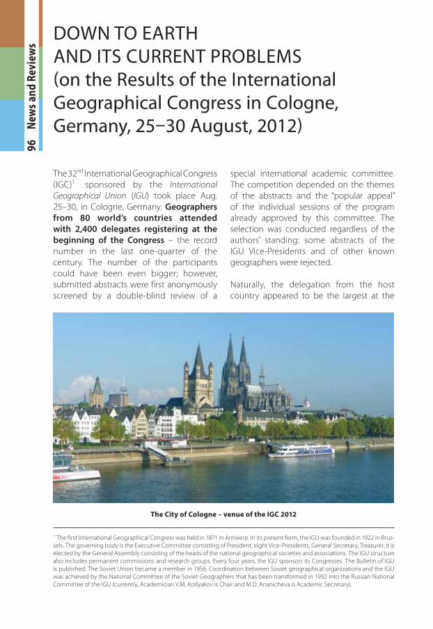
96

N

ews

and

Rev

iew

s

The 32nd International Geographical Congress

(IGC)1 sponsored by the International

Geographical Union (IGU) took place Aug.

25–30, in Cologne, Germany. Geographers

from 80 world’s countries attended

with 2,400 delegates registering at the

beginning of the Congress – the record

number in the last one-quarter of the

century. The number of the participants

could have been even bigger; however,

submitted abstracts were first anonymously

screened by a double-blind review of a

special international academic committee.

The competition depended on the themes

of the abstracts and the “popular appeal”

of the individual sessions of the program

already approved by this committee. The

selection was conducted regardless of the

authors’ standing: some abstracts of the

IGU Vice-Presidents and of other known

geographers were rejected.

Naturally, the delegation from the host

country appeared to be the largest at the

DOWN TO EARTH AND ITS CURRENT PROBLEMS(on the Results of the International Geographical Congress in Cologne, Germany, 25–30 August, 2012)

The City of Cologne – venue of the IGC 2012

1 The first International Geographical Congress was held in 1871 in Antwerp. In its present form, the IGU was founded in 1922 in Brus-

sels. The governing body is the Executive Committee consisting of President, eight Vice-Presidents, General Secretary, Treasurer; it is

elected by the General Assembly consisting of the heads of the national geographical societies and associations. The IGU structure

also includes permanent commissions and research groups. Every four years, the IGU sponsors its Congresses. The Bulletin of IGU

is published. The Soviet Union became a member in 1956. Coordination between Soviet geographical organizations and the IGU

was achieved by the National Committee of the Soviet Geographers that has been transformed in 1992 into the Russian National

Committee of the IGU (currently, Academician V.M. Kotlyakov is Chair and M.D. Ananicheva is Academic Secretary).

gi412.indd 96gi412.indd 96 24.12.2012 9:11:0024.12.2012 9:11:00

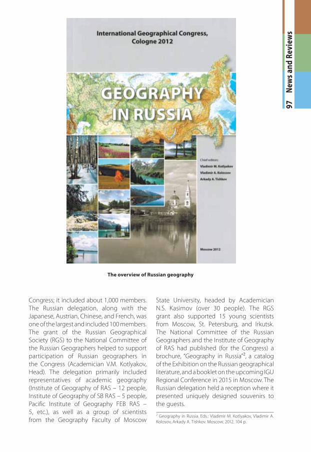
97

N

ews

and

Rev

iew

s

Congress; it included about 1,000 members.

The Russian delegation, along with the

Japanese, Austrian, Chinese, and French, was

one of the largest and included 100 members.

The grant of the Russian Geographical

Society (RGS) to the National Committee of

the Russian Geographers helped to support

participation of Russian geographers in

the Congress (Academician V.M. Kotlyakov,

Head). The delegation primarily included

representatives of academic geography

(Institute of Geography of RAS – 12 people,

Institute of Geography of SB RAS – 5 people,

Pacific Institute of Geography FEB RAS –

5, etc.), as well as a group of scientists

from the Geography Faculty of Moscow

State University, headed by Academician

N.S. Kasimov (over 30 people). The RGS

grant also supported 15 young scientists

from Moscow, St. Petersburg, and Irkutsk.

The National Committee of the Russian

Geographers and the Institute of Geography

of RAS had published (for the Congress) a

brochure, “Geography in Russia”2,1a catalog

of the Exhibition on the Russian geographical

literature, and a booklet on the upcoming IGU

Regional Conference in 2015 in Moscow. The

Russian delegation held a reception where it

presented uniquely designed souvenirs to

the guests.

2 Geography in Russia. Eds.: Vladimir M. Kotlyakov, Vladimir A.

Kolosov, Arkady A. Tishkov. Moscow, 2012. 104 p.

The overview of Russian geography

gi412.indd 97gi412.indd 97 24.12.2012 9:11:0124.12.2012 9:11:01

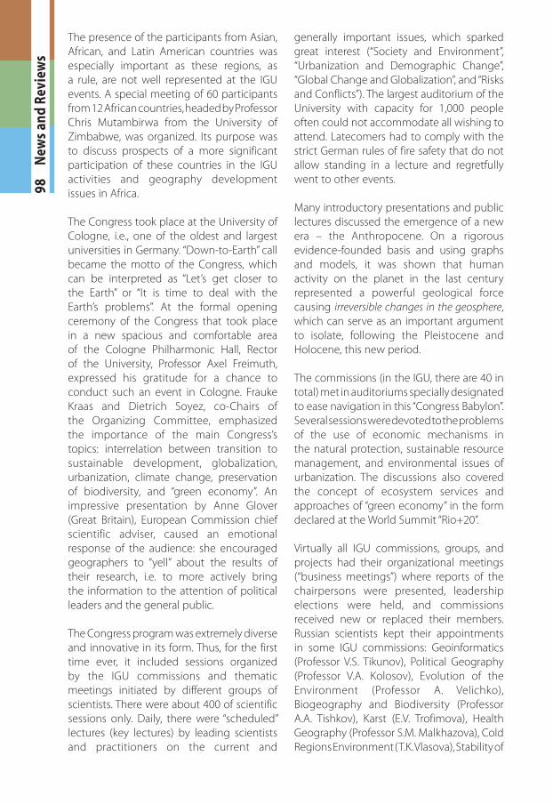
98

N

ews

and

Rev

iew

sThe presence of the participants from Asian,

African, and Latin American countries was

especially important as these regions, as

a rule, are not well represented at the IGU

events. A special meeting of 60 participants

from 12 African countries, headed by Professor

Chris Mutambirwa from the University of

Zimbabwe, was organized. Its purpose was

to discuss prospects of a more significant

participation of these countries in the IGU

activities and geography development

issues in Africa.

The Congress took place at the University of

Cologne, i.e., one of the oldest and largest

universities in Germany. “Down-to-Earth” call

became the motto of the Congress, which

can be interpreted as “Let’s get closer to

the Earth” or “It is time to deal with the

Earth’s problems”. At the formal opening

ceremony of the Congress that took place

in a new spacious and comfortable area

of the Cologne Philharmonic Hall, Rector

of the University, Professor Axel Freimuth,

expressed his gratitude for a chance to

conduct such an event in Cologne. Frauke

Kraas and Dietrich Soyez, co-Chairs of

the Organizing Committee, emphasized

the importance of the main Congress’s

topics: interrelation between transition to

sustainable development, globalization,

urbanization, climate change, preservation

of biodiversity, and “green economy”. An

impressive presentation by Anne Glover

(Great Britain), European Commission chief

scientific adviser, caused an emotional

response of the audience: she encouraged

geographers to “yell” about the results of

their research, i.e. to more actively bring

the information to the attention of political

leaders and the general public.

The Congress program was extremely diverse

and innovative in its form. Thus, for the first

time ever, it included sessions organized

by the IGU commissions and thematic

meetings initiated by different groups of

scientists. There were about 400 of scientific

sessions only. Daily, there were “scheduled”

lectures (key lectures) by leading scientists

and practitioners on the current and

generally important issues, which sparked

great interest (“Society and Environment”,

“Urbanization and Demographic Change”,

“Global Change and Globalization”, and “Risks

and Conflicts”). The largest auditorium of the

University with capacity for 1,000 people

often could not accommodate all wishing to

attend. Latecomers had to comply with the

strict German rules of fire safety that do not

allow standing in a lecture and regretfully

went to other events.

Many introductory presentations and public

lectures discussed the emergence of a new

era – the Anthropocene. On a rigorous

evidence-founded basis and using graphs

and models, it was shown that human

activity on the planet in the last century

represented a powerful geological force

causing irreversible changes in the geosphere,

which can serve as an important argument

to isolate, following the Pleistocene and

Holocene, this new period.

The commissions (in the IGU, there are 40 in

total) met in auditoriums specially designated

to ease navigation in this “Congress Babylon”.

Several sessions were devoted to the problems

of the use of economic mechanisms in

the natural protection, sustainable resource

management, and environmental issues of

urbanization. The discussions also covered

the concept of ecosystem services and

approaches of “green economy” in the form

declared at the World Summit “Rio+20”.

Virtually all IGU commissions, groups, and

projects had their organizational meetings

(“business meetings”) where reports of the

chairpersons were presented, leadership

elections were held, and commissions

received new or replaced their members.

Russian scientists kept their appointments

in some IGU commissions: Geoinformatics

(Professor V.S. Tikunov), Political Geography

(Professor V.A. Kolosov), Evolution of the

Environment (Professor A. Velichko),

Biogeography and Biodiversity (Professor

A.A. Tishkov), Karst (E.V. Trofimova), Health

Geography (Professor S.M. Malkhazova), Cold

Regions Environment (T.K. Vlasova), Stability of

gi412.indd 98gi412.indd 98 24.12.2012 9:11:0224.12.2012 9:11:02

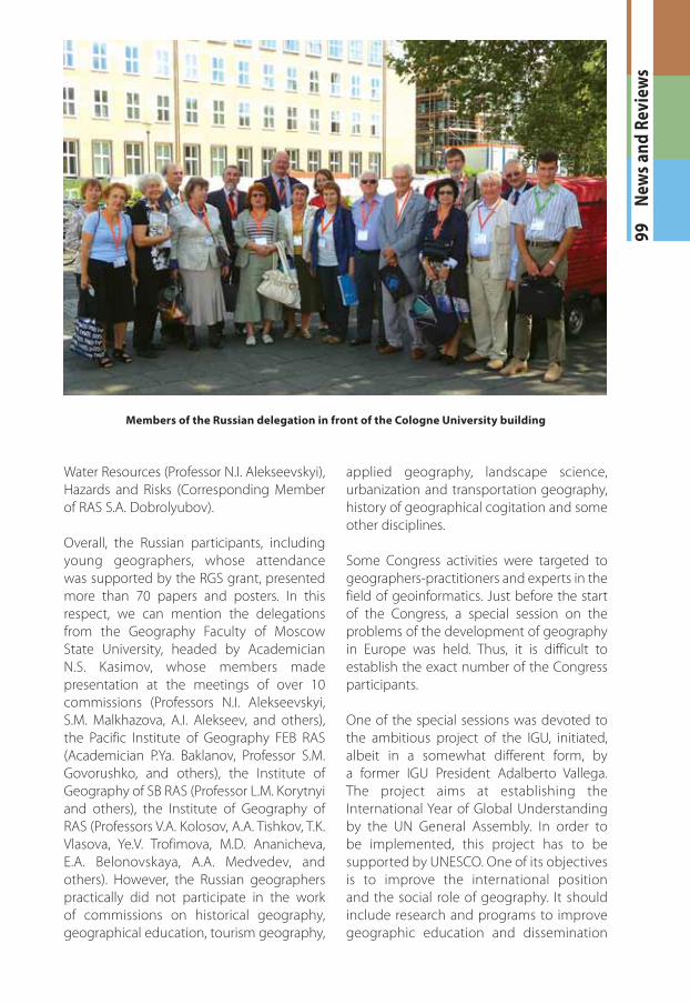
99

N

ews

and

Rev

iew

s

Water Resources (Professor N.I. Alekseevskyi),

Hazards and Risks (Corresponding Member

of RAS S.A. Dobrolyubov).

Overall, the Russian participants, including

young geographers, whose attendance

was supported by the RGS grant, presented

more than 70 papers and posters. In this

respect, we can mention the delegations

from the Geography Faculty of Moscow

State University, headed by Academician

N.S. Kasimov, whose members made

presentation at the meetings of over 10

commissions (Professors N.I. Alekseevskyi,

S.M. Malkhazova, A.I. Alekseev, and others),

the Pacific Institute of Geography FEB RAS

(Academician P.Ya. Baklanov, Professor S.M.

Govorushko, and others), the Institute of

Geography of SB RAS (Professor L.M. Korytnyi

and others), the Institute of Geography of

RAS (Professors V.A. Kolosov, A.A. Tishkov, T.K.

Vlasova, Ye.V. Trofimova, M.D. Ananicheva,

E.A. Belonovskaya, A.A. Medvedev, and

others). However, the Russian geographers

practically did not participate in the work

of commissions on historical geography,

geographical education, tourism geography,

applied geography, landscape science,

urbanization and transportation geography,

history of geographical cogitation and some

other disciplines.

Some Congress activities were targeted to

geographers-practitioners and experts in the

field of geoinformatics. Just before the start

of the Congress, a special session on the

problems of the development of geography

in Europe was held. Thus, it is difficult to

establish the exact number of the Congress

participants.

One of the special sessions was devoted to

the ambitious project of the IGU, initiated,

albeit in a somewhat different form, by

a former IGU President Adalberto Vallega.

The project aims at establishing the

International Year of Global Understanding

by the UN General Assembly. In order to

be implemented, this project has to be

supported by UNESCO. One of its objectives

is to improve the international position

and the social role of geography. It should

include research and programs to improve

geographic education and dissemination

Members of the Russian delegation in front of the Cologne University building

gi412.indd 99gi412.indd 99 24.12.2012 9:11:0224.12.2012 9:11:02

10

0

New

s an

d R

evie

ws

of geographical knowledge in a globalizing

world. The main idea is to promote

awareness of each person that their daily

activities impact the environment on a

global scale. The International Year of

Global Understanding is also aimed at

facilitating the integration of natural and

social sciences, at providing scientific and

social support for priority directions of UN

and UNESCO, and on using positive results

of the previous UN Years with the goals

of achieving sustainable development.

A booklet on this subject, including in

Russian, was distributed among the

participants. The project was presented

by its coordinator Professor Benno Werlen

(University of Jena), by a former President

of the IGU Professor Bruno Messerli

(Switzerland), and by Professor John Pickles

(University of North Carolina, USA).

The other two special sessions hosted

presentations of two IGU projects,

“Geographical Magazines of the World”

and “Sustainable Development of Cities”

(the research advisor for both – Professor

Ton Dietz from the Netherlands). The first

project has been completed in general

and its results include the creation of an

online global database and a search engine

on international and national geographic

magazines available at the IGU site (www.

igu-online.org). The second project,

implemented jointly by Dutch and Chinese

experts, on contrary, is just beginning. Its

mission is to create a website on sustainable

urban development, recognized by the

international scientific community and

practitioners of municipal government, and

then to create an IGU-sponsored center for

sustainable cities certification.

Special attention of the IGU Organizing

and Executive Committees was directed

toward youth. The Congress held the

traditional International Olympiad for high

school students on geography; as usual, it

was well attended: 128 participants from

32 countries participated. The Olympiad

program consisted of a written part, a

multimedia test, and a field part. In addition,

participants made poster presentations on

the theme “Water Resources and Water Use

Problems”. The group of winners, who took

the first twenty places by the total score,

was dominated by students from Eastern

and Central Europe, and the main prize was

won by a contestant from Singapore. The

winners were celebrated by high officials

and all the participants at the opening

ceremony of the Congress. The Russian

participants were also not without rewards.

The Russian team won two medals: “silver” by

Maria Samoletova from St. Petersburg and

“bronze” by Yegor Shustov from Slyudyanka

(Irkutsk region). But most importantly, at

the Olympiad, there was an atmosphere

of friendship and prestige of geographical

knowledge.

The Youth Forum was an important part

of the program and its poster session of

papers presented by young scientists

was, admittedly, extremely successful.

Usually, poster presentations remain on

the periphery of the major events, but this

time, the presentations were well attended

and were often complemented with

discussions in a relaxed atmosphere often

resulting in the establishment of possible

scientific cooperation. The Youth Forum also

included interactive classes, “Science Project

Management”, “Thesis Work Optimization”,

“Publications in English: Where, When, and

How”, “Academic Text Art”, “Collegiate Career

Steps”, “European Grants”, “International

Career Prospects for Bachelor-Students”, etc.

The success of the youth programs was

secured by special youth grants from the

IGU and the organizers of the Congress.

The program of the Congress, for the first

time ever, included a special session for

teachers of high school geography including

discussions of issues of connecting academic

research with training courses supported by

federal and state ministries of education.

The Organizing Committee has developed

and implemented a program “IGC School –

IGС in School», where a number of famous

geographers gave public lectures at

gi412.indd 100gi412.indd 100 24.12.2012 9:11:0324.12.2012 9:11:03

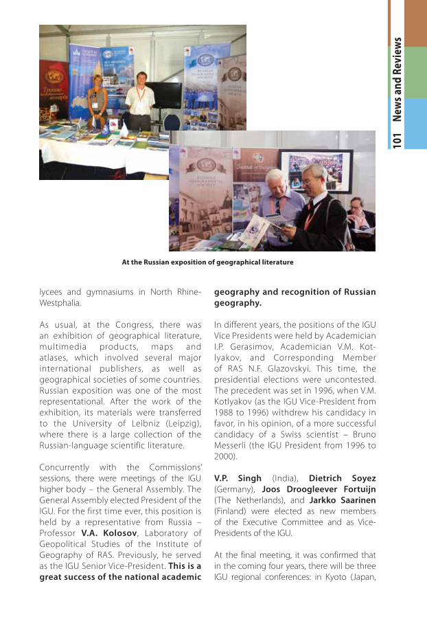
10

1

New

s an

d R

evie

ws

lycees and gymnasiums in North Rhine-

Westphalia.

As usual, at the Congress, there was

an exhibition of geographical literature,

multimedia products, maps and

atlases, which involved several major

international publishers, as well as

geographical societies of some countries.

Russian exposition was one of the most

representational. After the work of the

exhibition, its materials were transferred

to the University of Leibniz (Leipzig),

where there is a large collection of the

Russian-language scientific literature.

Concurrently with the Commissions’

sessions, there were meetings of the IGU

higher body – the General Assembly. The

General Assembly elected President of the

IGU. For the first time ever, this position is

held by a representative from Russia –

Professor V.A. Kolosov, Laboratory of

Geopolitical Studies of the Institute of

Geography of RAS. Previously, he served

as the IGU Senior Vice-President. This is a

great success of the national academic

geography and recognition of Russian

geography.

In different years, the positions of the IGU

Vice Presidents were held by Academician

I.P. Gerasimov, Academician V.M. Kot-

lyakov, and Corresponding Member

of RAS N.F. Glazovskyi. This time, the

presidential elections were uncontested.

The precedent was set in 1996, when V.M.

Kotlyakov (as the IGU Vice-President from

1988 to 1996) withdrew his candidacy in

favor, in his opinion, of a more successful

candidacy of a Swiss scientist – Bruno

Messerli (the IGU President from 1996 to

2000).

V.P. Singh (India), Dietrich Soyez

(Germany), Joos Droogleever Fortuijn

(The Netherlands), and Jarkko Saarinen

(Finland) were elected as new members

of the Executive Committee and as Vice-

Presidents of the IGU.

At the final meeting, it was confirmed that

in the coming four years, there will be three

IGU regional conferences: in Kyoto (Japan,

At the Russian exposition of geographical literature

gi412.indd 101gi412.indd 101 24.12.2012 9:11:0324.12.2012 9:11:03

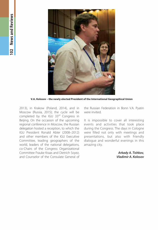
10

2

New

s an

d R

evie

ws

2013), in Krakow (Poland, 2014), and in

Moscow (Russia, 2015); the cycle will be

completed by the IGU 33rd Congress in

Beijing. On the occasion of the upcoming

regional conference in Moscow, the Russian

delegation hosted a reception, to which the

IGU President Ronald Abler (2008–2012)

and other members of the IGU Executive

Committee, leading geographers of the

world, leaders of the national delegations,

co-Chairs of the Congress Organizational

Committee Frauke Kraas and Dietrich Soyez,

and Counselor of the Consulate General of

the Russian Federation in Bonn V.A. Pyatin

were invited.

It is impossible to cover all interesting

events and activities that took place

during the Congress. The days in Cologne

were filled not only with meetings and

presentations, but also with friendly

dialogue and wonderful evenings in this

amazing city.

Arkady A. Tishkov,

Vladimir A. Kolosov

V.A. Kolosov – the newly elected President of the International Geographical Union

gi412.indd 102gi412.indd 102 24.12.2012 9:11:0424.12.2012 9:11:04

10

3

New

s an

d R

evie

ws

On 29–30 September, 2012, in St. Petersburg,

at St. Petersburg State University, a regular

session of the Annual Scientific Assembly of

the Association of Russian Social Geographers

(ARGO) was held.

Launched in May 2010, ARGO now bands

three quarters of the professional community

working in the field of socio-economic

geography and is represented by 28 regional

offices that together cover almost all Russia’s

space from Kaliningrad to Vladivostok.

During the Annual ARGO Assembly held

in St. Petersburg (the previous two were

held in Rostov-on-Don and Kaliningrad), the

international conference, “The Evolution of

the Socio-Geographical Cogitation” took

place, which was attended by leading

Russian social geographers (including

35 Doctors of Geographical Sciences), as well

as by colleagues from Belarus, the Netherlands,

Lithuania, Serbia, and Ukraine. The focus

of the conference were such issues as the

balance of continuity and modernization in

social geography, the transformation and

deformation of the Russian space, as well

as the prevailing variety of names of our

science. Presentations of S.S. Artobolevskyi,

V.L. Baburin, P.Ya. Baklanov, Yu.N. Gladkov,

N.V. Kaledin, K.V. Mezentsev, A.N. Pilyasov,

V.N. Streletskyi, A.I. Treyvish, G.M. Fedorov,

and numerous subsequent discussions in

the format of “round table” aroused lively

scientific debate.

A special discussion, “Ethnogenesis as a Factor

of Regional Development,” was devoted to the

100th anniversary of the birth of an outstanding

Russian historian, geographer, and ethnologist

L.N. Gumilev. His scientific heritage and the

potential of its application to understanding the

post-Soviet Russia’s ethnogeographical realities

were the subject of presentations by A.D.

Badov, D. Burneyka, N.I. Bykov, T.I. Gerasimenko,

A.G. Druzhinin, V.N. Streletskyi, A.I. Chistobaev,

N.A. Schitova, V.A. Shuper, etc.

At the Assembly, there was a presentation of

new scientific and educational developments

and publications, including the first edition of

the annual “Social and Economic Geography.

Bulletin of the Association of Russian Social

Geographers (ARGO )” as well as the collective

scientific ARGO-sponsored publication

“Space of Modern Russia: Opportunities and

Constraints of Development (Reflections by

Social Geographers)”1.1

An important component of the Assembly

was a joint meeting of the Coordination

and Advisory Councils of the ARGO, where

specific objectives and priorities for the future

of the Association were actively discussed

and identified.

Alexander G. Druzhinin

1 Space of Modern Russia: Opportunities and Constraints of De-

velopment (Reflections by Social Geographers). Eds.: A.G. Dru-

zhinin, V.A. Kolosov, and V.E. Shuvalov. M.: Vuzovskaya Kniga.

2012. – 336 p.

THE THIRD ANNUAL SCIENTIFIC ASSEMBLY OF THE ASSOCIATION OF RUSSIAN SOCIAL GEOGRAPHERS (ARGO)

gi412.indd 103gi412.indd 103 24.12.2012 9:11:0524.12.2012 9:11:05

10

4

GES

04|

2012

ISSN 2071-9388

SOCIALLY SCIENTIFIC MAGAZINE“GEOGRAPHY, ENVIRONMENT, SUSTAINABILITY”No. 04(v. 05) 2012

FOUNDERS OF THE MAGAZINE: Faculty of Geography, M.V. Lomonosov Moscow State

University and Institute of Geography of the Russian Academy of Sciences

The magazine is published with financial support of the Russian Geographical Society.

The magazine is registered in Federal service on supervision of observance of the legislation

in sphere of mass communications and protection of a cultural heritage. The certificate of

registration: ПИ МФС77-29285, 2007, August 30.

EDITORIAL OFFICE

M.V. Lomonosov Moscow State University

Moscow 119991 Russia

Leninskie Gory,

Faculty of Geography, 2108a

Phone 7-495-9392923

Fax 7-495-9328836

E-mail: GESJournal@yandex.ru

DESIGN & PRINTING

Advertising and Publishing Agency “Advanced Solutions”

Moscow 105120 Russia

Nizhnyaya Syromyatnicheskaya, 5/7, 2

Phone 7-495-9167574

Fax 7-495-9167673

E-mail: om@aov.ru

Sent into print 05.12.2012

Order N gi412

Format 70 ½ 100 cm/16

8.45 p. sh.

Digital print

Circulation 700 ex.

gi412.indd 104gi412.indd 104 24.12.2012 9:11:0524.12.2012 9:11:05