Embed Size (px)
Citation preview
Geological and Mineral Potential Mapping by Geoscience Data Integration
Sentayehu Zewdie Mekonnen
April, 2008

Geological and Mineral Potential Mapping by Geoscience Data Integration
by
Sentayehu Zewdie Mekonnen
Thesis submitted to the International Institute for Geo-information Science and Earth Observation in
partial fulfilment of the requirements for the degree of Master of Science in Geo-information Science
and Earth Observation, Specialisation: Earth Science Data Provision
Supervisors:
Dr. T. Woldai (1st Supervisor)
Dr. E. J. M. Carranza (2nd Supervisor)
Thesis Assessment Board
Prof. Dr.F. vander Meer (Chairman)
Dr. Ir. C. Mannaerts (External Examiner)
Dr. T. Woldai (1st Supervisor)
Dr. E. J. M. Carranza (2nd Supervisor)
Observer :
Drs T.M. Loran (Program Director, AES)
INTERNATIONAL INSTITUTE FOR GEO-INFORMATION SCIENCE AND EARTH OBSERVATION
ENSCHEDE, THE NETHERLANDS

Disclaimer This document describes work undertaken as part of a programme of study at the International Institute for Geo-information Science and Earth Observation. All views and opinions expressed therein remain the sole responsibility of the author, and do not necessarily represent those of the institute.

i
Abstract
Spatial data integration and analysis for updating geological map and predicting mineral potential
were carried out on the available analogue and digital remote sensing datasets of Magondi Belt,
Zimbabwe. In the search for mineral potential areas, accurate and up-to-date geological maps are
essential as it represents the most basic information for directing exploration activities. To this end,
the existing geological map of the study area, which was published in 1961, is too old to extract up-to-
date information for mineral exploration. However, Geological Survey of Zimbabwe (GSZ) has
acquired several exploration datasets from different exploration and mining companies. The problem
is there is no proper integration of the exploratory datasets in order to update the geological map and
prospect and delineate new exploration targets. Moreover, modern exploration techniques and new
tools like RS and GIS have not been applied in order to integrate the diverse geological datasets to
predict mineral potential map for certain types of mineral deposits in the Magondi Belt. The main
objective of this research was to integrate these datasets to update the geological map and produce
mineral potential map of the study area. In this research, the various datasets were processed,
integrated and modelled using GIS and remote sensing techniques. Landsat TM and ASTER images
were interpreted and classified to delineate major lithological units and structural features.
Lineaments were interpreted from DEM and vertical derivative total field magnetics. Lithological
interpretations made on analytical signal total field magnetics were compiled with results of
interpreted multispectral images to produce updated geological map. The map was validated and a
total accuracy of 76% was obtained.
Estimation and integration of spatial evidences were conducted in the southern portion of the study
area. Evidential belief functions (EBFs) were used to quantify the spatial association between Cu
deposit and geological features. Deposit recognition criteria were the basis for extracting spatial
evidences based on the characteristic features of strata-bound Cu-Ag-Au mineralization in the study
area. The geochemical copper anomaly map, which delineated the potential zone of mineralization,
was used as one spatial evidence. Among the lithological units, arkose and dolomite were important
spatial evidence. The linear structure, NW trending faults and magnetic anomalies have similar
spatial evidence to copper mineralization. The belief function maps were integrated and classified to
produce a binary predictive copper potential map. Validations conducted on the predictive map
without magnetic evidence indicates that the favourable potential zone correctly delineate 12% of the
Cu-anomaly, 58% of the ‘model’ and 60% of the ‘validation’ deposit. Validation conducted on
predictive map using magnetic evidences improved the spatial coverage of the favourability zone by
0.3% and delineated 19% of the Cu-anomaly. These indicate that integration of all spatial evidences
give satisfactory result for mapping mineral potential of the study area. The result implies the
usefulness of the model for further exploration of undiscovered strata-bound copper deposit in the
study area.

ii
Acknowledgements
I would like to thank the International Institute for Geo-information Science and Earth Observation
(ITC) for offering me the financial and academic support to follow the masters program. The
Geological Survey of Ethiopia (GSE) is equally thanked for endorsing my application for ITC grant. I
am very grateful to Dr T. Woldai, first supervisor, for his devoted guidance, constructive comments,
technical support and advice from the very stage of the research proposal to the final stage of
completing this thesis. His encouragement and help during my critical health problem is unforgettable.
I am indebted to Dr. E.J.M. Carranza, second supervisor for his critical comment, invaluable
suggestions, guidance and helpful technical support through out the thesis period.
I am indebted and grateful to Drs. Tom Loran, Program Director of AES for all his unreserved support
and help during my problem and extending my studies for the period I spent in hospital. Great thanks
and special appreciation goes to Drs. J. B. de Smeth, whose encouragement, help, kindness and
support during my heath problem and studies is invaluable. Great thanks go to all my instructors for
giving me enormous knowledge during my MSc. study. I also extend my sincere gratitude to all AES
MSc students especially my closest friends not listed her but known for their moral, social and
academic support and assistance during my stay in ITC.
I would like to forward my thanks to the administrative staff especially the Facility and ITC Hotel
management for providing me the necessary facility.
iii
Table of contents
1. Introduction ........................................................................................................................1
1.1. Research background ............................................................................................................1
1.2. Problem statements................................................................................................................2
1.3. Research objective..................................................................................................................3
1.4. Research Question..................................................................................................................3
1.5. Hypothesis ...............................................................................................................................3
1.6. Methodology ...........................................................................................................................4
1.7. Justification.............................................................................................................................5
1.8. Organization of the thesis......................................................................................................6
2. Study area ...........................................................................................................................7
2.1. Location and access................................................................................................................7
2.2. Previous work.........................................................................................................................8
2.3. Geological setting ...................................................................................................................8 2.3.1. Magondi Supergroup..................................................................................................................... 8 2.3.2. Basement Complex...................................................................................................................... 11 2.3.3. Deweras Group............................................................................................................................ 11 2.3.4. Lomagundi Group ....................................................................................................................... 13 2.3.5. Piriwiri Group.............................................................................................................................. 14
2.4. Metamorphism .....................................................................................................................15
2.5. Tectonic settings of Magondi Supergroup .........................................................................16
2.6. Mineralization ......................................................................................................................18 2.6.1. Deweras Group............................................................................................................................ 18 2.6.2. Lomagundi Group ....................................................................................................................... 18 2.6.3. Piriwiri Group.............................................................................................................................. 18
3. Datasets and Methodology ...............................................................................................19
3.1. Datasets used.........................................................................................................................19
3.2. General Methodology...........................................................................................................19 3.2.1. Updating geological map............................................................................................................. 20 3.2.2. Mineral potential map.................................................................................................................. 21
3.3. Processing and Interpretations of mapped and remotly sensed datasets .......................22 3.3.1. Analogue geological maps........................................................................................................... 22 3.3.2. Multispectral image processing and interpretations..................................................................... 23
3.3.2.1. Principal components transformation and interpretations ....................................................... 24 3.3.2.2. Band combination and lithological interpretations.................................................................. 29 3.3.2.3. Band ratio images and interpretations..................................................................................... 31
3.3.3. Digital Number for multispectral image ...................................................................................... 32
iv
3.3.4. Image classification .....................................................................................................................33 3.3.5. Processing and interpretation of Shuttle Radar Topography Mission (SRTM) and ASTER
DEM images .................................................................................................................................................34 3.3.6. Processing and interpretation of aeromagnetic data ....................................................................35
3.3.6.1. Aeromagnetic database and generation of grid .......................................................................36 3.3.6.2. Applying filters to enhance aeromagnetic images ...................................................................36 Vertical derivative ....................................................................................................................................37 Analytical signal .......................................................................................................................................37
3.3.7. Geochemical data processing and interpretations........................................................................39 3.3.7.1. Univariate statistics .................................................................................................................40 3.3.7.2. Bivariate statistics ...................................................................................................................53 3.3.7.3. Multivariate.............................................................................................................................55
4. Data integration for Geological mapping........................................................................60
4.1. Combining images with digital elevation model (DEM).................................................. 60
4.2. Combining with high resolution image ............................................................................. 61
4.3. Intensity-Hue-Saturation (IHS) transformation and fusion ........................................... 61
4.4. Compilation of interpreted images and lithological boundaries .................................... 62 4.4.1. Biotite and hornblend para gneiss (gn) ........................................................................................63 4.4.2. Meta-ultramafic rock (ul) ............................................................................................................63 4.4.3. Granite (gr) ..................................................................................................................................63 4.4.4. Doloritic dykes (dk).....................................................................................................................63 4.4.5. Basic igneous rocks (ig) ..............................................................................................................63 4.4.6. Arkose (ak) ..................................................................................................................................64 4.4.7. Dolomite (dl) ...............................................................................................................................64 4.4.8. Phyllite (ph) .................................................................................................................................64 4.4.9. Graphytic slate (gsl).....................................................................................................................64 4.4.10. Slate, phyllite and quartzite (sl, ph, qz) .......................................................................................65 4.4.11. Feldspar bearing Quartzite (qz) ...................................................................................................65
4.5. Geological structures interpreted from integrated images ............................................. 65
4.6. Updated geological map...................................................................................................... 67
4.7. Validation of updated geological map ............................................................................... 70
4.8. Comparison with the old geological map .......................................................................... 70
4.9. Summary of geological integration.................................................................................... 72
5. Spatial data integration for predictive modeling of mineral potential ...........................74
5.1. Evidential Belief for mapping mineral potential.............................................................. 74
5.2. Deposit recognition criteria and spatial datasets ............................................................. 78
5.3. Estimation and integration of EBFs .................................................................................. 80 5.3.1. Test of correctness of EBFS ........................................................................................................80
5.4. Classification and validation of mineral potential map................................................... 83
5.5. Summary of spatial data integration for predictive modeling of mineral potential..... 86
v
6. Conclusion and Recommendation...................................................................................88
6.1. Conclusion.............................................................................................................................88
6.2. Recommendation..................................................................................................................89
7. Reference ..........................................................................................................................90
Appendices ...............................................................................................................................93
Appendix A Frequency histograms and box-plots of elements in Magondi Belt (als=Alaska, umb=Umboe, mha=Mahangura and sha=Shamrock ) .................................................................93
Appendix B Field observation dataset ...........................................................................................95
vi
List of figures
Figure 2-1 Location map of the research area........................................................................................................7 Figure 2-2 Simplified geological map of Zimbabwe showing the mobile belts and cover surrounding the
Archaean craton (after Stagman, 1978). Box shows the Magondi mobile belt, study area, enlarged on Figure.
2.2. ...........................................................................................................................................................................9 Figure 2-3 Geological map of north-west Zimbabwe; showing the Magondi Supergroup, the basement gneisses,
granitoids of the Archaean craton and the surrounding cover (after Stagman, 1978)..........................................10 Figure 2-4 Generalized lithostratigraphy of northern part of Deweras Group (after Master, 1991). ..................12 Figure 2-5 Lithostratigraphic units of Lomagundi Group (after Master, 1991). See Figure 2.3 for legend.......14 Figure 2-6 Generalized lithostratigraphy of the Piriwiri Group (after Master 1991). See Figure 2.3 for legend.15 Figure 2-7 Schematic summary of the evolution of the Magondi Basin between 2.2 to 1.8 Ga, from the initiation
of back-arc rifting, and the deposition of the Deweras, Lomagundi and Priwiri groups, to the Magondi Orogeny
(after Master, 1991). .............................................................................................................................................17 Figure 3-1 Flow chart for updating geological map of the research area............................................................20 Figure 3-2 Flow chart for methodology of Mineral potential map .......................................................................21 Figure 3-3Geological map of Magondi Belt digitized from Geological map of Southern Rhodesia, Surveyor-
General (1985), UTM Zone 36S projection, WGS 84 Datum................................................................................22 Figure 3-4 Geological map covering south eastern parts of the study are, digitized from Carballo Lopez (1998),
UTM Zone 36S projection, WGS 84 Datum. .........................................................................................................23 Figure 3-5 Distribution of ASTER and Landsat channels with respect to the electromagnetic spectrum (after
Kalinowski and Oliver, 2004)................................................................................................................................25 Figure 3-6 PC bands of 234 (RGB) discriminating the lithology of the study area UTM Zone 36S projection,
WGS 84 Datum. .....................................................................................................................................................26 Figure 3-7 PC band images used for lithological interpretation. a) PC4 enhanced clay minerals or Al-OH; b)
PC3 enhanced ferrous oxide minerals; c) PC2 enhanced ferric oxides and d) Colour composite PC band image
234 RGB discriminate lithological units in the research area. (Bright pixels shows areas of strong reflectance)
(dl= dolomite, sl = slate, ph = phyllite, gsl = graphitic slate, gr = granite). .......................................................27 Figure 3-8 Generalized reflectance spectra of vegetation, iron oxides and clays (Fraser and Green, 1987) .....28 Figure 3-9 PC band images used for lithological interpretation a) PC3 image enhancing iron oxide/limonite b)
PC4 enhances clay rich zone (bright pixels shows areas of strong reflectance). UTM Zone 36S projection, WGS
84 Datum. ..............................................................................................................................................................29 Figure 3-10 Interpreted images of band combination a) ASTER 7, 4, 2 (RGB); b) ASTER 3, 6, 11 (RGB) ; and c)
Landsat TM 4, 5, 3 RGB UTM Zone 36S projection, WGS 84 Datum). (dl= dolomite, sl = slate, ph = phyllite,
gsl = graphitic slate, gr = granite, gn = gneiss). ..................................................................................................31 Figure 3-11 Showing different band ratio and band combinations of Landsat TM a) Band ratio 5/7 indicating
clay rich minerals; b) ratio 3/1 enhancing iron oxide rich rocks; c) ratio 5/4 enhances iron oxide and d) color
composite ratio images of combination of ratios 5/7, 3/1 and 5/4 RGB discriminating lithology(bright pixels
shows areas of strong reflectance) (dl= dolomite, sl = slate, ph = phyllite, gsl = graphitic slate, gr = granite,
gn = gneiss) ...........................................................................................................................................................32 Figure 3-12 Mean DN values of lithologic units in individual spectral bands of Landsat TM .............................32 Figure 3-13 Mean DN values of major lithologic unit in ASTER 11 bands VNIR, SWIR and TIR (Band 11) ......33 Figure 3-14 Classified images using supervised classification (Maximum likelihood classifications); a) Landsat
TM and b) ASTER, UTM Zone 36S projection, WGS 84 Datum. ..........................................................................34 Figure 3-15 Hill shaded DEM images a) ASTER b) SRTM c) interpreted lineaments, UTM Zone 36S projection,
WGS 84 Datum. .....................................................................................................................................................35 Figure 3-16 Magnetic total field image a) profile map showing the shape of the magnetic anomalies; and b)
unfiltered total magnetic grid of Magondi-Belt, Zimbabwe ..................................................................................37
vii
Figure 3-17 Color shaded relief image of the total magnetic field a) first vertical derivative indicating
interpreted lineaments and doloritic dykes b) analytic signal showing interpreted lithologic boundaries
(illumination inclination, I=45 and declination 315)............................................................................................ 38 Figure 3-18 Interpreted lithology and lineaments from aeromagnetic data ........................................................ 39 Figure 3-19 Geochemical soil sample location map of Magondi Belt .................................................................. 40 Figure 3-20 Indicating Box plot of an idealized population standardized to the anomaly threshold Fu and the
spread Measure (after Yusta et al. 1998). ............................................................................................................. 41 Figure 3-21 Frequency histogram and box-plot showing distribution of Cu on log transformed data Circles in
box plot represents outliers representing values above threshold. For a better representation see Appendix A.
als=Alaska, umb=Umboe, mha=Mahangura and sha=Shamrock. ...................................................................... 42 Figure 3-22 Frequency histogram and box-plot of Zn on log transformed data. Outliers and extreme values on
high end on both box plot and histogram show anomalous values. For a better representation see Appendix A.
als=Alaska, umb=Umboe, mha=Mahangura and sha=Shamrock. ...................................................................... 43 Figure 3-23 Geochemical anomaly map a) Copper (Cu); and b) Zinc (Zn). Magondi Belt, UTM Zone 36S
projection, WGS 84 Datum.................................................................................................................................... 44 Figure 3-24 Frequency histogram and box-plot of Pb on log transformed data. For a better representation see
Appendix A. als=Alaska, umb=Umboe, mha=Mahangura and sha=Shamrock................................................... 45 Figure 3-25 Frequency histogram and box-plot of Fe on log transformed data showing anomalous values of
Alaska on extreme end. For a better representation see Appendix A. als=Alaska, umb=Umboe,
mha=Mahangura and sha=Shamrock. ................................................................................................................. 46 Figure 3-26 Fe anomaly map of Alaska, Magondi Belt, UTM projection, WGS 84 Zone 36S. Bright area
indicates anomalous concentration. ...................................................................................................................... 46 Figure 3-27 Frequency histogram and box-plot of Co on log transformed data showing very little anomalous
concentration on high end. The box plot on Mhangura shows no anomaly. For a better representation see
Appendix A. als=Alaska, umb=Umboe, mha=Mahangura and sha=Shamrock................................................... 47 Figure 3-28 Frequency histogram and box-plot of Ni on log transformed data. Extreme values on high end
indicate anomalous concentration. For a better representation see Appendix A. als=Alaska, umb=Umboe,
mha=Mahangura and sha=Shamrock. ................................................................................................................. 48 Figure 3-29 Nickel anomaly map of Magondi Belt, UTM Zone 36S projection, WGS 84..................................... 49 Figure 3-30 Frequency histogram and box-plot of As on log transformed data showing no outliers on extreme
ends. als=Alaska, umb=Umboe, mha=Mahangura and sha=Shamrock .............................................................. 50 Figure 3-31 Frequency histogram and box-plot of Au.......................................................................................... 51 Figure 3-32 Frequency histogram and box-plot of Ag on log transformed data. Circles on box plot represent
values above the threshold. Plus signs in Mhangura indicate very high anomalous values. als=Alaska,
umb=Umboe, mha=Mahangura and sha=Shamrock ........................................................................................... 52 Figure 3-33 Geochemical anomaly map a) Gold (Au); and b) Silver (Ag) Magondi Belt, UTM Zone 36S
projection, WGS 84. .............................................................................................................................................. 53 Figure 3-34 Scatter plots of elements of Shamrock, Mhangura, Umboe and Alaska areas.................................. 54 Figure 3-35 Showing PC scores and accompanying box plots indicating anomalous concentration of copper in
Alaska, Umboe, Mhangura and Shamrock areas. Box plots show outliers in the high end corresponding to
anomalous values of Cu. (n=number of geochemical soil samples in the area). ................................................. 57 Figure 3-36 Copper anomaly map of Magondi Belt. Polygons represent copper anomaly zone.......................... 59 Figure 4-1 Integrated color composite normalized multispectral images a) DEM fused with Landsat TM 4, 5, 3
RGB b) DEM fused with ASTER 7, 4, 2 RGB; c) PC image 2, 3, 4 RGB fused with Landsat TM, high resolution
panchromatic image d) Landsat TM 4, 5, 3 RGB transformed to IHS and fused with high resolution
panchromatic image (band 8); (qz= quartzite, dl= dolomite, sl = slate, ph = phyllite, gsl = graphitic slate, gr =
granite, gn = gneiss).............................................................................................................................................. 62 Figure 4-2 Color composite 3 6 11 RGB ASTER, fused with DEM showing interpreted structural features; a)
tightly folded quartzite and dolomite; b) NE and NW trending foliations faults and folds. .................................. 66
viii
Figure 4-3 Color composite 453 RGB indicating interpreted folded igneous rocks and arkose in the northern
parts of the area.....................................................................................................................................................67 Figure 4-4 Interpreted images showing windows of southern portion of the study area a) Landsat 453 RGB fused
with DEM b) IHS image fused with high resolution panchromatic image c) PC bands 12 3 (RGB) fused with
high resolution panchromatic image d) interpreted geology e) analytical signal of total magnetic field;; f) SRTM
DEM. (ig = basic igneous rocks ak = arkose, ph = phylite, gsl = graphitic slate, sl = slate, gr = granite; qz =
quartzite)................................................................................................................................................................68 Figure 4-5 Geological maps of Magondi BeltCompiled updated geological map of the research area. (UTM
Zone 36S projection WGS 84 Datum)....................................................................................................................73 Figure 5-1 Schematic relationships of EBFs (adopted from Carranza and Hale, 2003). .....................................75 Figure 5-2 Spatial evidence maps a) lithological units, b) NW fault, c) magnetic anomaly map and d) PC4 score
representing concentration of Cu in Alaska and Umboe area; UTM Zone 36S projection, WGS 84 Datum.....79 Figure 5-3 Attribute map of EBFs for lithological unit classes A) belief map B) disbelief map and C) uncertainty map, UTM Zone 36S projection, WGS 84 Datum. ..........................................................................82 Figure 5-4 Attribute maps of EBFs for magnetic anomaly classes A) belief map B) disbelief map and C)
uncertainty map, UTM Zone 36S projection, WGS 84 Datum...............................................................................82 Figure 5-5 Attribute map of EBFs for pc scores classes A) belief map B) disbelief map and C) uncertainty map,
UTM Zone 36S projection, WGS 84 Datum. .........................................................................................................82 Figure 5-6 Attribute maps of EBFs for proximity to NW fault classes A) belief map B) disbelief map and C)
uncertainty map, UTM Zone 36S projection, WGS 84 Datum...............................................................................83 Figure 5-7 Integrated EBFs maps of strata-bound Cu potential showing A) belief map; B) disbelief map; C)
Uncertainty map and D) plausibility map, E) Test of correctness of estimation and integration of EBFs. UTM
Zone 36S projection, WGS 84 Datum. (bel=belief, dis=disbelief, unc=uncertainty)...........................................83 Figure 5-8 Predictive map of strata-bound copper deposit potential A) using spatial evidences lithology, PC4
and NW fault B) using all spatial evidences including magnetic anomaly. Small circles and triangles represent
locations of large and small scale known Cu deposits and occurrences used in training and validation data
respectively; polygons represent geochemical Cu-anomaly zones, Magondi Belt, UTM Zone 36S projection,
WGS 84 Datum ......................................................................................................................................................84
ix
List of tables
Table 3-1 Eigenvector loadings of principal components for ASTER VNIR and SWIR data and their variance.. 25 Table 3-2 Eigenvector loadings of principal components for Landsat TM data and their variance..................... 27 Table 3-3 Eigenvector loadings of principal components for Landsat TM bands 1, 3, 4 and 5 data and their
variance................................................................................................................................................................. 28 Table 3-4 Eigenvector loadings of principal components for Landsat TM bands 1, 4, 5 and 7 data ................... 28 Table 3-5 Summary statistics of Cu on box plots on log transformed data ........................................................... 42 Table 3-6 Summary statistics of zinc (Zn) on log transformed data...................................................................... 43 Table 3-7 Summary statistics of lead (Pb) on log transformed data ..................................................................... 45 Table 3-8 Summary statistics of iron (Fe) ............................................................................................................. 46 Table 3-9 Summary statistics of Cobalt (Co) computed based on equation [B] ................................................... 47 Table 3-10 Summary statistics of nickel (Ni)......................................................................................................... 48 Table 3-11 Summary statistics of arsenic (As) computed using equation [B]....................................................... 50 Table 3-12 Summary statistics of gold (Au)........................................................................................................... 51 Table 3-13 Summary statistics of arsenic (Ag) calculated .................................................................................... 52 Table 3-14 Pearson linear correlation coefficient of Shamrock, Mhangura, Umboe ........................................... 54 Table 3-15 Principal component analysis of elements in Shamrock, Mhangura, Umboe and Alaska .................. 55 Table 4-1 Interpreted lithology and their characteristic features ......................................................................... 69 Table 4-2 Confusion matrix results for updated geological map versus ground Control/field observation data . 71 Table 4-3 Cross table for old geological map and updated geological map of Magondi Belt (ig = basic igneous
rocks, ak = arkose, ph = phylite, gsl = graphitic slate, sl = slate, gr = granite, qz = quartzite, sst grits and
sandstone, al=alluvium) ........................................................................................................................................ 72 Table 5-1 Estimation of EBFs for class of values in maps of deposit recognition criteria for strata bound Cu-Ag
potential, Magondi Belt. (EBFs of PC scores are calculated in descending order. .............................................. 81 Table 5-2 Validation of predictive strata-bound copper potential map using Known Cu deposit, South Magondi-
Belt......................................................................................................................................................................... 85 Table 5-3 Validation of predictive strata-bound copper potential map using small scale Cu deposit/occurrences,
South Magondi-Belt............................................................................................................................................... 85 Table 5-4 Validation of predictive strata-bound copper potential map using geochemical soil Cu anomaly, South
Magondi-Belt......................................................................................................................................................... 86
GEOLOGICAL AND MINERAL POTENTIAL MAPPING BY GEOSCIENCE DATA INTEGRATION
1
1. Introduction
1.1. Research background
Reliable geoscience information in the form of geological and mineral potential maps is very
important for exploration and development of mineral resources. In countries like Zimbabwe for
example, mineral resource development has played an important role for sustainable economic
development. For many years now, the northern parts of Zimbabwe, especially the Magondi Belt,
have been a target for gold and base metal exploration. Alaska and Mhangura are the major copper
producing mines currently in operation. The Magondi Belt is situated in the Magondi district north-
west of the capital city Harare. It covers an area of 8,500 km2 between 16° 15’S and 17° 30’S latitude
and between 29° 50’E and 30° 15’E longitude.
Copper production and exploration in the Magondi Belt started in the 15th century, following the old
workings exploited by the local people. Proper exploration activities however, started as the early
1940s with employment of advanced exploration techniques by the Zimbabwean Government and
mining companies. During the period 1970 to 1978, the production of copper reached its peak and a
maximum of 55,000 tones of copper have been exploited (Kambewa, 1998). Since then, most mines
are either exhausted or closed. To substitute the old mines and sustain the country’s economy, the
Geological Survey of Zimbabwe (GSZ) has conducted a number of exploration surveys. In 1970,
ground and airborne geophysical surveys were conducted in the area. Between the years 1983-1995
the GSZ, in collaboration with the Japan International Co-operation Agency, Metal Mining Agency
(JICA), has carried out exploration work. The work concentrated on the collection of geochemical,
geophysical and geological data in the northern part of the Magondi basin (Kambewa, 1998).
Today, the GSZ has acquired large amounts of geological datasets from various conventional
exploration and mining companies. Most of the information is dispersed and kept in analogue format.
However, no attempt has been done to convert these data and integrate information to establish a
mineral potential map to attract investment in the region. Moreover, the existing geological map is
published in 1961, and does not convey detailed information for undertaking mineral potential
mapping. At present the area is covered by optical and microwave remote sensing digital datasets, but
these datasets have not been processed and integrated with the available geological data.
Conventional geological mapping and mineral exploration are labour intensive and require high
investment, and take long periods of investigation. On the contrary, modern exploration techniques
are cost effective and quick and can be achieved in less time. In this research, the various datasets
available for the Magondi Belt were processed, integrated and modelled using Geographic
Information System (GIS) and Remote Sensing (RS). The objective of this research was to integrate
the available geological datasets in order to update the geological map and to produce a mineral
GEOLOGICAL AND MINERAL POTENTIAL MAPPING BY GEOSCIENCE DATA INTEGRATION
2
potential map. In the research, optical and microwave remote sensing datasets and aeromagnetic
remote sensing data were processed, interpreted and integrated for both geological and mineral
potential mapping. Ground truth field observation datasets were used to further improve and validate
the geological map. Comparisons were made between the old and updated geological map.
Geochemical soil sample and aeromagnetic data were processed and analysed. The results of analysis
and interpretations were used in spatial data integration and predictive modelling for mineral potential
mapping.
The interpreted images were further integrated to produce an updated geological map. The new
geological map was used to extract spatial evidences for predicting mineral potential map. Estimation
and integration of spatial evidences were conducted using evidential belief functions (EBFs). The
belief function maps were integrated and the resulting map was classified to produce a binary
predictive mineral potential map. Validations conducted on the binary predictive map using Cu
anomaly and deposits indicated a satisfactory result which implies the usefulness of the model for
further exploration of undiscovered strata-bound copper deposit in the northern parts of the study
area.
1.2. Problem statements
The Magondi Belt of Zimbabwe contains several copper mines, which were discovered as a result of
follow up investigation of old workings exploited by local people. Currently, a number of mines are
closed and the present ones are depleted due to long period of exploitation (Kambewa, 1998). These
mines are considered to be favourable spatial indications for finding new potential areas. Exploration
of new potential locations for mineral development commonly takes place in and around areas where
mineral deposits have already been found (van Roij, 2006). For this reason, the study area attracts
exploration companies to conduct investigation to discover new deposits. However, investors require
organized datasets to decide and plan their exploration activity. This indicates that access to such
datasets is very important. Mineral potential maps are an important part of such datasets, which help
to focus the exploration activities over the most potential areas, thereby increasing the possibilities of
finding new deposits by optimizing the exploration expenditure (Andrada de Palomera, 2004).
In the search for mineral potential areas, accurate and up-to-date geological maps are essential as it
represents the most basic information for directing exploration activities. To this end, the published
geological map of the study area which was published in 1961 needs updating. To the knowledge of
the author, this map is too old, produced using conventional mapping techniques. However, GSZ has
acquired several exploration datasets from different exploration and mining companies. The challenge
is that there is no proper integration of the exploratory datasets such as aeromagnetic, optical and
microwave data in order to prospect and delineate new exploration targets. Moreover, modern
exploration techniques and new tools like RS and GIS have not been applied in order to integrate the
GEOLOGICAL AND MINERAL POTENTIAL MAPPING BY GEOSCIENCE DATA INTEGRATION
3
diverse geological datasets to predict mineral potential map for certain types of mineral deposits in the
Magondi Belt.
1.3. Research objective
The main objective of this research is to apply GIS and RS based techniques for interpretation and
integration of diverse geologic datasets such as, geological, geochemical, geophysical, and optical RS
and microwave datasets, to update the existing geological map and to produce a mineral potential map
of the Magondi Belt. The research aimed at testing the capability of the integration model to produce
mineral potential map.
In order to achieve the major objectives the following sub objectives were set:
• Interpret the remote sensing images and aeromagnetic data to update the existing geologic map of the area.
• To delineate the host rocks of strata-bound Cu-Ag-Au mineralization.
• To identify geologic features with spatial associations to Cu-Ag-Au mineralizations and extract these features from the available geological, geochemical, remote sensing, and aeromagnetic datasets.
• To quantify the spatial associations of known Cu-Ag-Au mineral deposits with the geological features of the study area and develop models capable of integrating and predicting areas with potential for Cu-Ag-Au mineralizations.
1.4. Research Question
1. How can remote sensing, geomagnetics, geochemical and geological datasets be used for updating geological map and modelling the mineral potential of the study area?
2. Which tectonic structures have spatial association with Cu-Ag-Au mineralization in the study area?
3. Which simple approaches are useful for integrating the geological datasets in order to predict the mineral potential of the area?
1.5. Hypothesis
It is possible to interpret and integrate various geological datasets such as geological, geochemical, geophysical, remote sensing and known mineral deposit data in order to update the geological map
and produce a mineral potential map of the research area using RS and GIS. There may be unidentified host rocks and tectonic structures which controlled mineralization in the study area. To predict where these mineral deposits of interest might occur, it is necessary to study spatial
association between known deposit occurrences and certain geological features that control their occurrence. GIS-based predictive modeling such as evidential belief functions (EBFs), involves analysis of spatial associations between multi-layered geological features and known deposit occurrences to predict where deposits of interest are likely to occur.
GEOLOGICAL AND MINERAL POTENTIAL MAPPING BY GEOSCIENCE DATA INTEGRATION
4
1.6. Methodology
Updating the geological map and producing a mineral potential map is the general purpose of this
research. In both methods, several steps were undertaken. In the first instance literature review was
done for extracting information concerning the general geology of the study area. Data preparation
and pre-processing of optical and microwave remotely sensed images, such as Landsat TM, ASTER,
SRTM and aeromagnetic data were conducted using ILWIS and ERDAS software. Various image
enhancement techniques were employed to clearly visualize the image. Radiometric and geometric
corrections were applied in order to remove the influence of the atmosphere and to get surface
reflectance. Images were georeferenced and subset into one projection system.
The existing 1:1,000,000 scale geological map of the research area was digitized from the existing
geological map of Zimbabwe at a scale of. Additional geological features in northeastern parts of the
study area were digitized from interpreted maps of Landsat TM and low resolution aeromagnetic data
at a scale of 1:500,000 (Carballo Lopez, 1998).
Mean values digital numbers (DN) of lithological units in individual Landsat TM and ASTER bands
were calculated and the values were plotted to see which band best discriminate the lithologies. Based
on the selected individual bands an image classification was carried out using maximum likelihood
classification.
Appropriate band combinations were chosen for lithological and structural interpretations. The band
combinations were variously fused with the SRTM data in order to further enhance lithological
boundaries. The shaded-relief image of the SRTM was used for interpretation of lineaments. Analysis
and extraction of lithology, lineament and faults were supported by sample datasets and information
obtained from the existing geological maps. Geological features extracted from the fused images were
integrated with the sample datasets into one digital format in GIS. The extracted geological features
were digitized in order to produce an updated geological map.
Four major steps were followed for creating a mineral potential map: 1) spatial data input, 2)
conceptual data development, 3) spatial data processes, and 4) integration and validation. The first
step consists of input of spatial data like, geological, geophysical, geochemical data and occurrences
of known mineral deposits in the study area. Development of conceptual exploration model was
based on literature review of strata-bound Cu-Ag-Au deposit of study area. Here, information
regarding the deposit model in sedimentary basin environment was referred from literature. Study of
general characteristics of sedimentary Cu deposits in the area and establishment of criteria for the
recognition of potential zones for the occurrence of these deposits was carried out. Based on the
conceptual exploration model, spatial data analyses were carried out. Extraction of geological features
that have spatial association with Cu-Ag-Au mineralization in the study area was the third step, which
results in evidential maps to be used in the predictive mapping of Cu-Ag-Au mineralization potential
GEOLOGICAL AND MINERAL POTENTIAL MAPPING BY GEOSCIENCE DATA INTEGRATION
5
of the study area. Integrating the evidential maps for Cu-Ag-Au mineralization and validation of the
predictive maps were the last step undertaken.
1.7. Justification
The Magondi Belt of Zimbabwe, which has a favourable geological setting for gold and base-metal
mineralization, there are adequate geological datasets obtained from past geological mapping and
exploration surveys. The datasets includes geological map, aeromagnetic and geochemical data;
remote sensing images and several mine data. These datasets and the favourable geological setting
attract mining companies to explore potential areas for development. In order to increase the chance
of mineral discoveries and optimize the exploration expenditure, mining companies require
geoscientific knowledge which indicates the type of mineralization and locations of potential areas
(Andrada de Palomera, 2004; Thurmond et al., 2006). However, the lack of up-to-date geological
maps and absence of mineral potential maps holds back the investment and development activities in
the region.
There may be unidentified host rocks and tectonic structures which controlled mineralization in the
study area. The challenge is how to map these features in order to know potential areas for
mineralization. At present, it is difficult for the GSZ to use the conventional methods of geological
mapping and mineral exploration to find target areas for mineral deposit along extensive area, since
these techniques are labour and capital intensive, and require long period of investigation.
Today, powerful tools of RS and GIS have contributed a lot in modern geological mapping and
mineral exploration by enhancing, interpreting and integrating of various geologic datasets.
Integration of remotely sensed data and airborne magnetic data with other geological datasets is a
promising and cost effective method to add new structural and lithological features to the geological
map in a diverse geological province like the present research area, Magondi Belt (Isabirye Mugaddu,
2005), (Le Thi Chau, 2001). Mineral potential mapping involves delineation of potentially
mineralized zones based on geological features that are characterized by a significant spatial
association with target mineral deposit (Porwal et al., 2006). A systematic exploration program for
geological and mineral potential mapping therefore involves the integration of geological,
geochemical and geophysical techniques (Carranza et al., 1999). All the geoscience information
together with pre-processed remotely sensed data can be used as evidence to delineate potential areas
for further investigation (Chang-Jo and Fabbri, 1993).
GIS together with traditional geoscience datasets are used to obtain effective predictors of mineral
potential (Harris et al., 2006). Different researches revealed that enhancing, integrating and analysis
of geoscience data together with interpretations of remotely sensed datasets could help in predicting
mineral potential. To this end, Evidential Belief Functions theory (EBFs), which has been widely used
in mineral potential mapping (Carranza and Hale, 2003), was used to predict the potential for Cu
mineralization in the Magondi Belt. It was chosen because the method uses both knowledge and data
driven approaches and requires a number of representative mineral deposits to compute the spatial
association between the deposits and the geological features. The Magondi area therefore fulfils all
GEOLOGICAL AND MINERAL POTENTIAL MAPPING BY GEOSCIENCE DATA INTEGRATION
6
these criteria. This is the first time that EBFs were applied for mineral potential mapping t therefore
this study would help support the previous prediction techniques, which were totally based on simple
overlay methods (Carballo Lopez, 1998; Kambewa, 1998).
1.8. Organization of the thesis
This thesis deals with integration of geological datasets for updating the geological map and mapping
of mineral potential of Magondi Belt. The first chapter introduces the research background, the
problem definition, the scope and objective, and the questions and hypothesis of the research.
Information about the study area, such as location, access, general geology and previous works are
given in chapter two. Part of chapter two introduces tectonic setting, metamorphic history and
mineralization of the rocks in the study area.
The detailed methodologies employed for the geological mapping and mineral potential mapping of
the belt are described with the help of flow charts in chapter three. Data inputs, organization and
processes, spatial analysis, validation of results are the main steps followed in this chapter. The
available input data and software used for processing and analysis are mentioned in the same chapter.
Data processing and interpretation of analogue, aeromagnetic, optical and microwave remote sensing
data are clearly mentioned in the chapter. The data processing techniques mainly focused on
multispectral images, high resolution aeromagnetic data and geochemical stream sediment analysis.
Pre-processing of Landsat TM, ASTER and SRTM images are part of this chapter. Chapter four deals
with data integration and analysis for lithological and lineament mapping. The geochemical and
geophysical anomaly maps are integrated together with multispectral processed images to produce an
updated geological map. In chapter five, the method of EBFs for mineral potential mapping is
described. Conceptual model of mineral deposit, the deposit recognition criteria and spatial evidence
extractions done based on the geo-exploration data are discussed in detail. In this chapter, the spatial
association analyses were done between the evidence maps and copper mineralization followed by
spatial data integration for predictive mineral potential modelling. Here, generation and combining of
the predictor patterns and validation of the predictive model were undertaken to produce a predictive
Cu-Ag-Au potential map. Finally, the results are discussed and conclusions are made on chapter six.
Recommendations are also made on the same chapter.
GEOLOGICAL AND MINERAL POTENTIAL MAPPING BY GEOSCIENCE DATA INTEGRATION
7
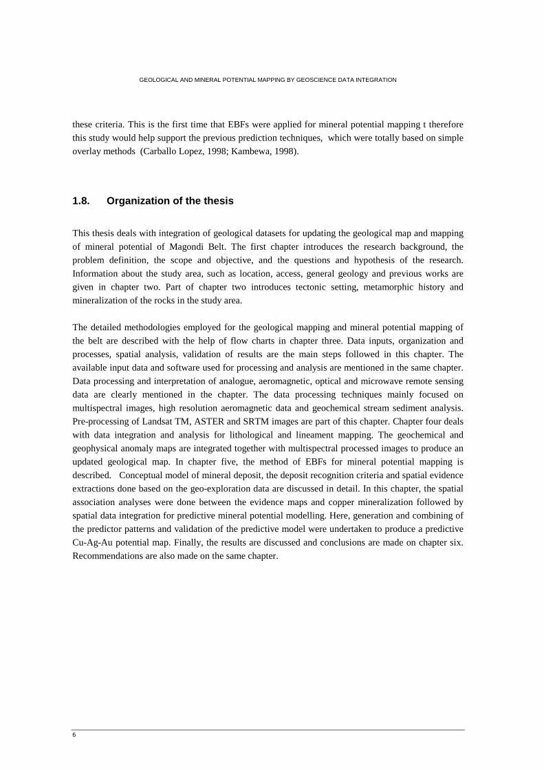
2. Study area
The northern part of Zimbabwe, especially the Magondi Belt, has been a target for gold and base
metal exploration for many years (Figure 2.1). Alaska and Mhangura, in the central part, and
Shamrock in northern parts of the country, are some of the explored base metal mines currently under
operation (Kambewa, 1998; Woldai et al., 2006). The Mhangura mine consists of two strata-bound,
sediment-hosted copper-silver deposits of Mangula and Norah. The main copper production of
Zimbabwe comes from these mines with by-products of gold and silver.
2.1. Location and access
The research area is situated in Zimbabwe about 187 km north-west of the capital city Harare. It is bounded by 160 15’S and 170 30’S latitudes and by 290 50’E and 30015’E longitudes with center at about interception of 170 00’S latitude and 300 00’ E longitude (Figure.2.1). The area extends 170 km north-south and 50 km east-west, covering a total area of 8,500 km2.
Access to the area is possible through the town Chinhoyi, about 130 km west of the capital city Harare. The two operating base metal mines, Mahngura and Shamrock are accessible from Chinhoyi. Mhangura mine is 70 km north of Chinhoyi (Figure 2.1).
Figure 2-1 Location map of the research area
GEOLOGICAL AND MINERAL POTENTIAL MAPPING BY GEOSCIENCE DATA INTEGRATION
8
2.2. Previous work
Magondi basin is a known Cu-Ag-Au mining province since 15th century. Copper metal was mined for production of ornamental and cutting objects by local smelters (Kambewa, 1998). Following the old workings by local people, a continuous exploration survey was conducted since late 1940’s to mid 1970’s. Stagman (1952) was among the first researchers to map the geology of the area around the Mangula Mine, Lomagundi and Guruve district (Stagman, 1978; Kambewa, 1998). Later on he tried to classify the geology of the area into basement and Magondi supergroup in 1978. The Magondi Belt had been studied by Master (Master et al., 1989; Master, 1991) from 1987-1991. In 1989, he studied the mineralization of copper and silver in red beds of early Proterozoic alluvial fans of the Mangula Mine, while in 1991, his research concentrated on the origin and controls on the distribution of copper and precious metal mineralization at Mhangura and Norah Mines.
During the year 1993 to 1995, the Geological Surveys of Zimbabwe and the Japan International Co-operation Agency, Metal Mining Agency, have conducted exploration work in northern part of Magondi Basin. Geological, geochemical and geophysical surveys were conducted during the joint exploration program (Kambewa, 1998).
Master et al. (1996) have integrated geological, geophysical, geochemical and Landsat TM data to identify the Highbury impact structure in the Magondi copper belt (Master et al., 1996). Kambewa (1998) and Carballo Lopez (1998) have conducted a research on the use of GIS and integration of remote sensing and geochemical data for mineral exploration in Magondi Basin. Both researchers were focused on integration of geological datasets with emphasis on geochemical data analysis in order to produce mineral potential map based on simple overlay techniques. Master (2003) has also explained the mineralization, host rock and tectonic structures of Norah Mine (Master, 2003). Validation and sensitivity analysis for mineral potential mapping were also done on the Magondi datasets (Woldai et al., 2006)
2.3. Geological setting
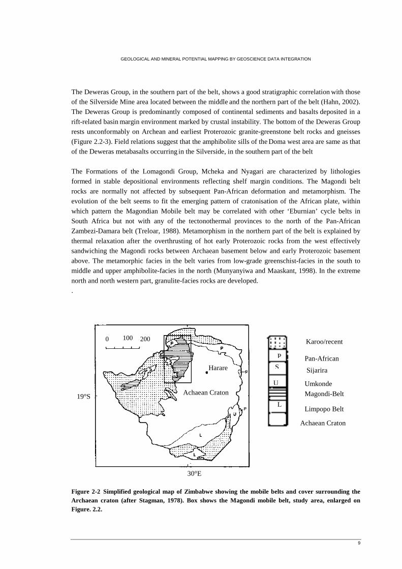
2.3.1. Magondi Supergroup
The Magondi Mobile Belt, which flanks the Zimbabwe Archaean craton to the NW, consists of
volcanics and sediments of the Magondi Supergroup deposited during the early Proterozoic 1850
Ma (Treloar, 1988). The Archean rocks, capping the basement beneath the Magondi Supergroup,
consist of the Midlands and Chinoyi Greenstone Belts, the Biri and Mangula granites and the
Hurungwe gneiss in the study area (Carballo Lopez, 1998). The rocks of Magondi Supergroup, which
were deposited in the Magondi Basin, extends under younger cover towards Botswana (Woldai et al.,
2006) The belt at the northwest rim of the Craton extends over a length of 250 km from the Munyati
River area in the south to the Shamrock Mine area in the north. The Magondi Supergroups subdivided
into the Deweras, Lomagondi and Piriwiri Groups (Hahn, 2002).
GEOLOGICAL AND MINERAL POTENTIAL MAPPING BY GEOSCIENCE DATA INTEGRATION
9
Harare
Achaean Craton
100 200 0
19°S
30°E
Sijarira
P
S
U
L
Karoo/recent
Pan-African
Umkonde
Magondi-Belt
Limpopo Belt
Achaean Craton
The Deweras Group, in the southern part of the belt, shows a good stratigraphic correlation with those
of the Silverside Mine area located between the middle and the northern part of the belt (Hahn, 2002).
The Deweras Group is predominantly composed of continental sediments and basalts deposited in a
rift-related basin margin environment marked by crustal instability. The bottom of the Deweras Group
rests unconformably on Archean and earliest Proterozoic granite-greenstone belt rocks and gneisses
(Figure 2.2-3). Field relations suggest that the amphibolite sills of the Doma west area are same as that
of the Deweras metabasalts occurring in the Silverside, in the southern part of the belt
The Formations of the Lomagondi Group, Mcheka and Nyagari are characterized by lithologies
formed in stable depositional environments reflecting shelf margin conditions. The Magondi belt
rocks are normally not affected by subsequent Pan-African deformation and metamorphism. The
evolution of the belt seems to fit the emerging pattern of cratonisation of the African plate, within
which pattern the Magondian Mobile belt may be correlated with other ‘Eburnian’ cycle belts in
South Africa but not with any of the tectonothermal provinces to the north of the Pan-African
Zambezi-Damara belt (Treloar, 1988). Metamorphism in the northern part of the belt is explained by
thermal relaxation after the overthrusting of hot early Proterozoic rocks from the west effectively
sandwiching the Magondi rocks between Archaean basement below and early Proterozoic basement
above. The metamorphic facies in the belt varies from low-grade greenschist-facies in the south to
middle and upper amphibolite-facies in the north (Munyanyiwa and Maaskant, 1998). In the extreme
north and north western part, granulite-facies rocks are developed.
.
Figure 2-2 Simplified geological map of Zimbabwe showing the mobile belts and cover surrounding the Archaean craton (after Stagman, 1978). Box shows the Magondi mobile belt, study area, enlarged on Figure. 2.2.
GEOLOGICAL AND MINERAL POTENTIAL MAPPING BY GEOSCIENCE DATA INTEGRATION
10
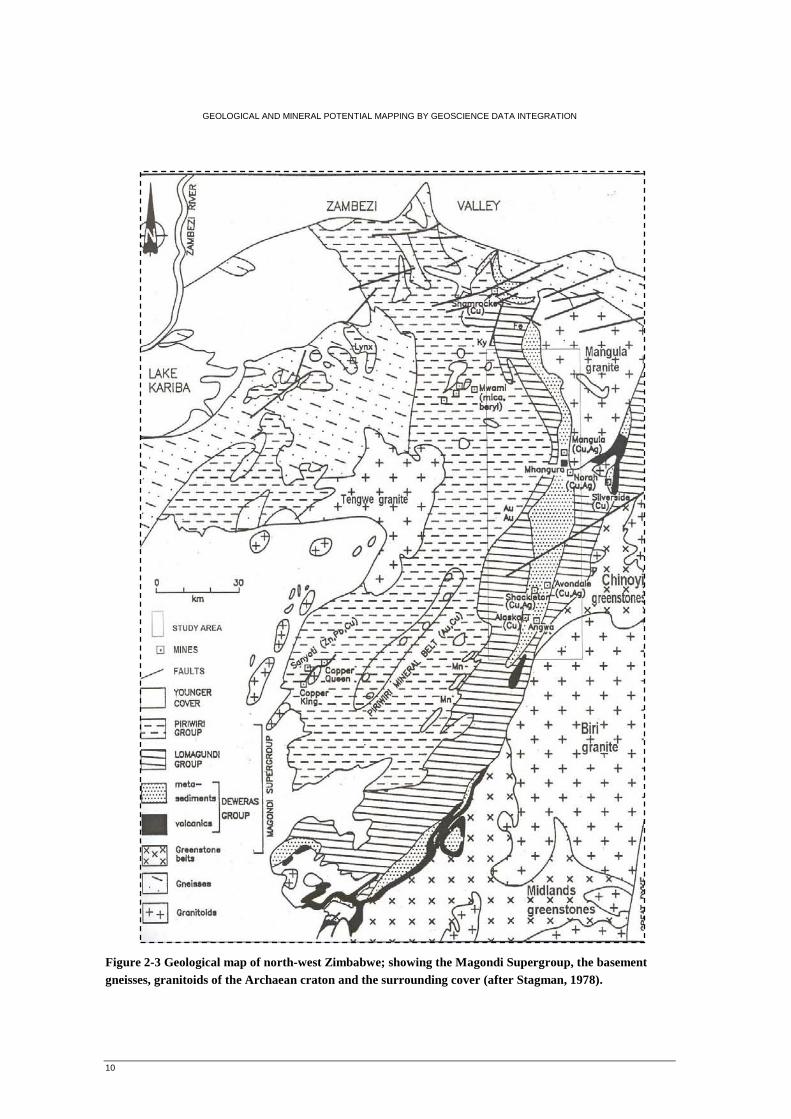
Figure 2-3 Geological map of north-west Zimbabwe; showing the Magondi Supergroup, the basement gneisses, granitoids of the Archaean craton and the surrounding cover (after Stagman, 1978).
GEOLOGICAL AND MINERAL POTENTIAL MAPPING BY GEOSCIENCE DATA INTEGRATION
11
2.3.2. Basement Complex
The Archean and earliest Proterozoic granite-greenstone belt rocks and gneisses of the Zimbabwe
Craton form the basement complex underlying the Magondi Supergroup. These rock units are exposed
in the south-eastern, north and north-eastern parts of the study area (Figure 2.3). The larger portion of
the basement consists of granite with relatively small greenstone rocks (Stagman, 1978). The
greenstone rocks comprise lavas of basaltic and andesitic composition. The gneissic rocks are rare and
mainly quartzo-feldspathic gneisses, which are predominantly medium to coarse-grained biotite
gneisses, locally migmatised during partial melting. The gnessic rocks are mainly composed of alkali
and plagioclase feldspars, biotite with less abundant hornblende, garnet, clino- and orthopyroxene.
Preliminary Rb-Sr and U-Pb radiometric data suggest that the gneisses are Paleoproterozoic to
NeoArchaean in age (Munyanyiwa and Maaskant, 1998). Single zircons analyzed for U-Pb isotope
from granite indicated that the intrusions took place during Paleoproterozoic Orogenesis (Majaule et
al., 2001).
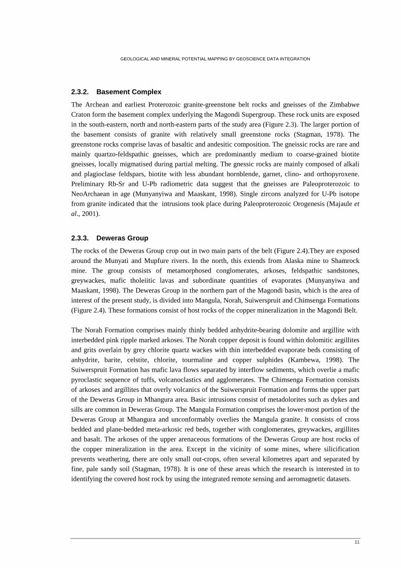
2.3.3. Deweras Group
The rocks of the Deweras Group crop out in two main parts of the belt (Figure 2.4).They are exposed
around the Munyati and Mupfure rivers. In the north, this extends from Alaska mine to Shamrock
mine. The group consists of metamorphosed conglomerates, arkoses, feldspathic sandstones,
greywackes, mafic tholeiitic lavas and subordinate quantities of evaporates (Munyanyiwa and
Maaskant, 1998). The Deweras Group in the northern part of the Magondi basin, which is the area of
interest of the present study, is divided into Mangula, Norah, Suiwerspruit and Chimsenga Formations
(Figure 2.4). These formations consist of host rocks of the copper mineralization in the Magondi Belt.
The Norah Formation comprises mainly thinly bedded anhydrite-bearing dolomite and argillite with
interbedded pink ripple marked arkoses. The Norah copper deposit is found within dolomitic argillites
and grits overlain by grey chlorite quartz wackes with thin interbedded evaporate beds consisting of
anhydrite, barite, celstite, chlorite, tourmaline and copper sulphides (Kambewa, 1998). The
Suiwerspruit Formation has mafic lava flows separated by interflow sediments, which overlie a mafic
pyroclastic sequence of tuffs, volcanoclastics and agglomerates. The Chimsenga Formation consists
of arkoses and argillites that overly volcanics of the Suiwerspruit Formation and forms the upper part
of the Deweras Group in Mhangura area. Basic intrusions consist of metadolorites such as dykes and
sills are common in Deweras Group. The Mangula Formation comprises the lower-most portion of the
Deweras Group at Mhangura and unconformably overlies the Mangula granite. It consists of cross
bedded and plane-bedded meta-arkosic red beds, together with conglomerates, greywackes, argillites
and basalt. The arkoses of the upper arenaceous formations of the Deweras Group are host rocks of
the copper mineralization in the area. Except in the vicinity of some mines, where silicification
prevents weathering, there are only small out-crops, often several kilometres apart and separated by
fine, pale sandy soil (Stagman, 1978). It is one of these areas which the research is interested in to
identifying the covered host rock by using the integrated remote sensing and aeromagnetic datasets.
GEOLOGICAL AND MINERAL POTENTIAL MAPPING BY GEOSCIENCE DATA INTEGRATION
12
Figure 2-4 Generalized lithostratigraphy of northern part of Deweras Group (after Master, 1991).
0
500m
1000m
GEOLOGICAL AND MINERAL POTENTIAL MAPPING BY GEOSCIENCE DATA INTEGRATION
13
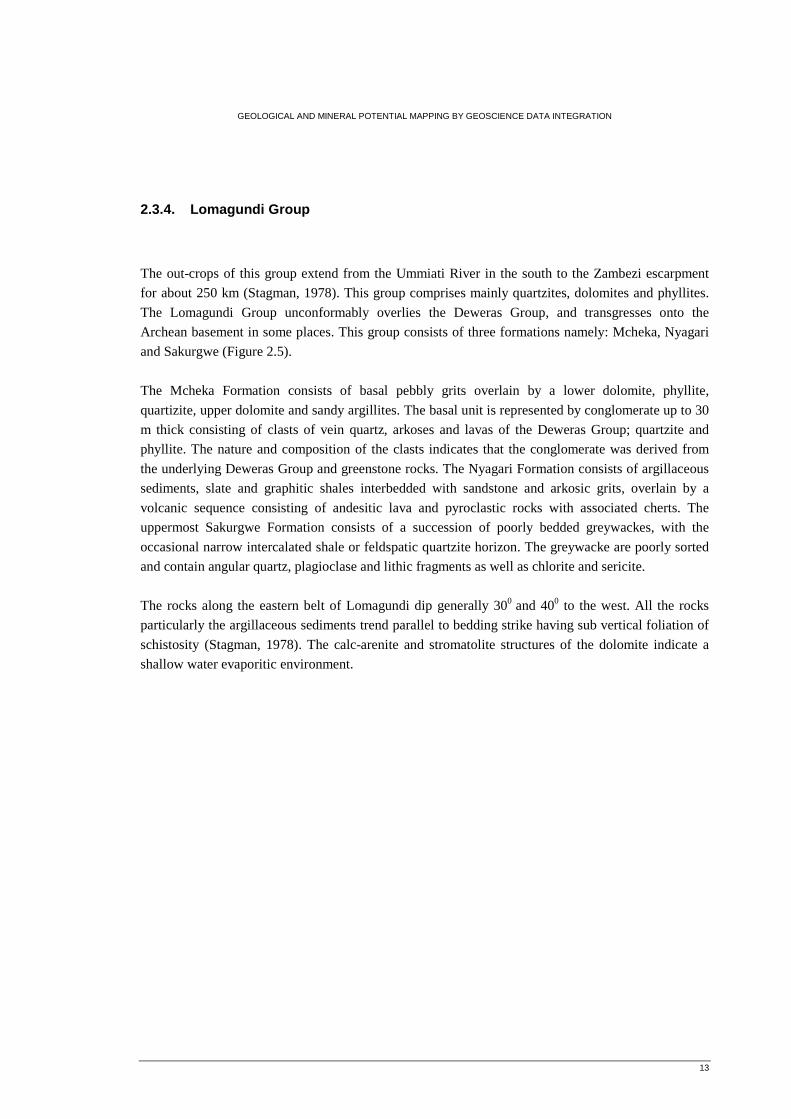
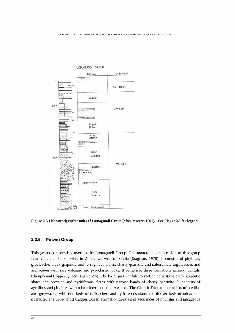
2.3.4. Lomagundi Group
The out-crops of this group extend from the Ummiati River in the south to the Zambezi escarpment
for about 250 km (Stagman, 1978). This group comprises mainly quartzites, dolomites and phyllites.
The Lomagundi Group unconformably overlies the Deweras Group, and transgresses onto the
Archean basement in some places. This group consists of three formations namely: Mcheka, Nyagari
and Sakurgwe (Figure 2.5).
The Mcheka Formation consists of basal pebbly grits overlain by a lower dolomite, phyllite,
quartizite, upper dolomite and sandy argillites. The basal unit is represented by conglomerate up to 30
m thick consisting of clasts of vein quartz, arkoses and lavas of the Deweras Group; quartzite and
phyllite. The nature and composition of the clasts indicates that the conglomerate was derived from
the underlying Deweras Group and greenstone rocks. The Nyagari Formation consists of argillaceous
sediments, slate and graphitic shales interbedded with sandstone and arkosic grits, overlain by a
volcanic sequence consisting of andesitic lava and pyroclastic rocks with associated cherts. The
uppermost Sakurgwe Formation consists of a succession of poorly bedded greywackes, with the
occasional narrow intercalated shale or feldspatic quartzite horizon. The greywacke are poorly sorted
and contain angular quartz, plagioclase and lithic fragments as well as chlorite and sericite.
The rocks along the eastern belt of Lomagundi dip generally 300 and 400 to the west. All the rocks
particularly the argillaceous sediments trend parallel to bedding strike having sub vertical foliation of
schistosity (Stagman, 1978). The calc-arenite and stromatolite structures of the dolomite indicate a
shallow water evaporitic environment.
GEOLOGICAL AND MINERAL POTENTIAL MAPPING BY GEOSCIENCE DATA INTEGRATION
14
Figure 2-5 Lithostratigraphic units of Lomagundi Group (after Master, 1991). See Figure 2.3 for legend.
2.3.5. Piriwiri Group
This group conformably overlies the Lomagundi Group. The monotonous succession of this group
form a belt of 50 km wide in Zimbabwe west of Sinoia (Stagman, 1978). It consists of phyllites,
greywacke, black graphitic and ferruginous slates, cherty quartzite and subordinate argillaceous and
arenaceous with rare volcanic and pyroclastic rocks. It comprises three formations namely: Umfuli,
Chenjiri and Copper Queen (Figure 2.6). The basal part Umfuli Formation consists of black graphitic
slates and breccias and pyritiferous slates with narrow bands of cherty quartzite. It consists of
agrillites and phyllites with minor interbedded greywacke. The Chenjir Formation consists of phyllite
and greywacke, with thin beds of tuffs, chert and pyritiferous slate, and thicker beds of micaceous
quartzite. The upper most Copper Queen Formation consists of sequences of phyllites and micaceous
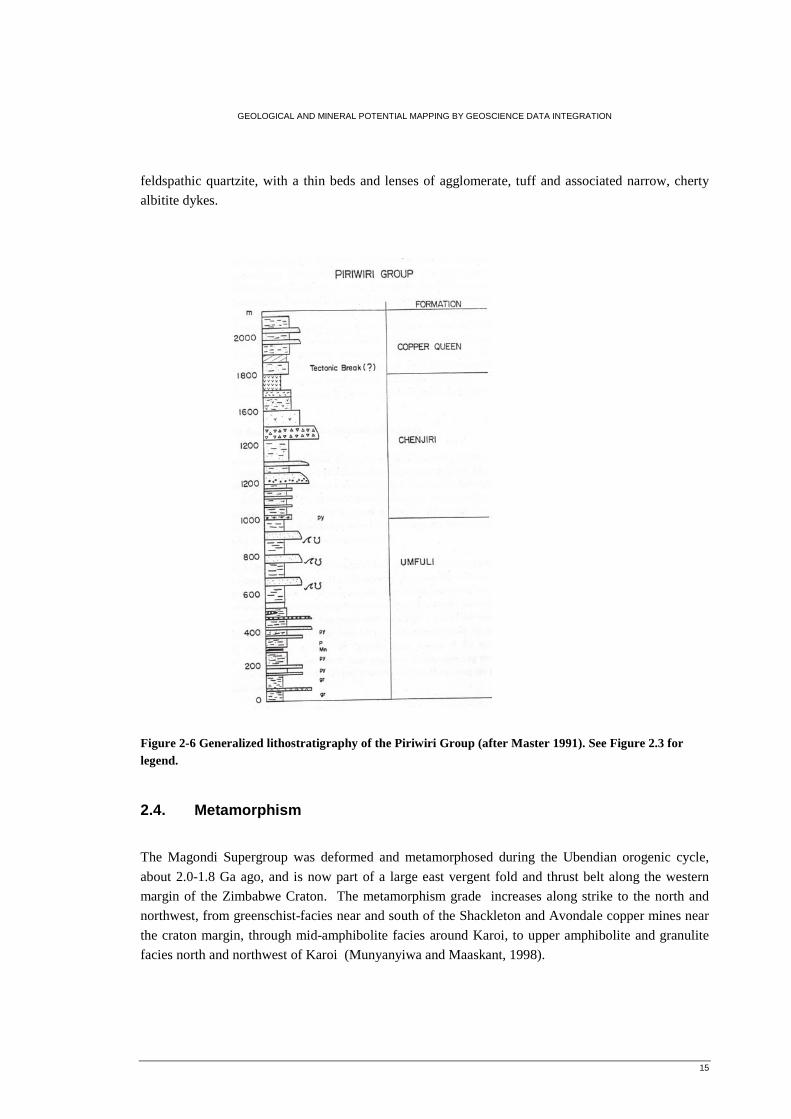
GEOLOGICAL AND MINERAL POTENTIAL MAPPING BY GEOSCIENCE DATA INTEGRATION
15
feldspathic quartzite, with a thin beds and lenses of agglomerate, tuff and associated narrow, cherty
albitite dykes.
Figure 2-6 Generalized lithostratigraphy of the Piriwiri Group (after Master 1991). See Figure 2.3 for legend.
2.4. Metamorphism
The Magondi Supergroup was deformed and metamorphosed during the Ubendian orogenic cycle,
about 2.0-1.8 Ga ago, and is now part of a large east vergent fold and thrust belt along the western
margin of the Zimbabwe Craton. The metamorphism grade increases along strike to the north and
northwest, from greenschist-facies near and south of the Shackleton and Avondale copper mines near
the craton margin, through mid-amphibolite facies around Karoi, to upper amphibolite and granulite
facies north and northwest of Karoi (Munyanyiwa and Maaskant, 1998).
GEOLOGICAL AND MINERAL POTENTIAL MAPPING BY GEOSCIENCE DATA INTEGRATION
16
2.5. Tectonic settings of Magondi Supergroup
The Magondi rocks were deposited in a back-arc continental basin developed in response to an
easterly directed subduction zone (Munyanyiwa and Maaskant, 1998). The subduction zone was
tectonically set in a rift related basin which formed on the continental side of an Andean-type
magmatic arc under the Zimbabwe Archean Craton (Figure 2.7). The distribution of the supracrustal
rocks of Magondi Belt was interpreted to record the transition of a passive-margin setting into
geosynclinal flysch-type deposits. The magmatic arc was part of a continental scale magmatic arc
produced during the “Ubendian” cycle (2.2-1.8 Ga), involving the collision of two Archaean age
continents, immediately after the consumption by subduction of the intervening oceanic crust (Master,
1991; Carballo Lopez, 1998). The sedimentary rock in the Magondi supergroup were formed within
the rift valley by sedimentation, which was later extended by left lateral fault parallel to Great Dyke.
A strike slip fault forms parallel faults and an anticline fold axis which cross obliquely to the rift
valley. These structures were formed before compaction of sediments and were pathways to metal
solution to the present strata-bound disseminated copper deposit (Kambewa, 1998). As a result of
compression and shortening during the second phases of deformation, N-S and NNE-SW trending
folds were developed. Folding of the Priwiri Group mainly on NN easterly axes curving N and
eventually NNW are common example (Stagman, 1978). Here, three phases of folding were
encountered. Tight folds with axial plane trending NE-SW, asymmetric folds trending NE and NNE
and open folds with NW trending axial plane are the first, second and third phases of folding
respectively (Kambewa, 1998). The first phase of folding, which has NE folds trending N65°E to
N55° in Deweras Group, was affected by cross folds trending S140° E. An axial plane and fracture
cleavages are manifested on early folds on argillaceous psammitic rocks. The rocks of the Lomagundi
Group were deformed by three phases of folding; the first phase has NE, eastward-verging folds,
refolded to N-W trending folds with NE trending cleavages indicating the third phases of deformation.
The Deweras group stratigraphy indicates that it was deposited in a continental rift basin, which was
faulted with the Archean basement to the east. It is an elongated fault bounded trough parallel to the
sinistral strike slip faults traversing the Archean craton of Zimbabwe in SSW-NNE direction. The
basin fill pattern was one of the transverse alluvial fans and transverse braded plains, within distal
playa lakes. In the Deweras Group, the amphibolite sills were folded together with the enclosing
sediments during the Magondi Orogeny (2000 and 1800 Ma). The refolding of these group rocks
occur around 530 Ma, in the Pan-African Orogeny. Deformed amphibolites are also observed in the
Lomagundi Group, in the northern most part of the belt (Shamrock and Makuti-East areas) (Hahn,
2002).
GEOLOGICAL AND MINERAL POTENTIAL MAPPING BY GEOSCIENCE DATA INTEGRATION
17
Figure 2-7 Schematic summary of the evolution of the Magondi Basin between 2.2 to 1.8 Ga, from the initiation of back-arc rifting, and the deposition of the Deweras, Lomagundi and Priwiri groups, to the
Magondi Orogeny (after Master, 1991).
2 3 4 5 1
z-c= Zimbabwe craton
c-c=Congo craton
Juvenile plutons
Continental crust
Juvenile magmatic arc
Oceanic crust
Lithospheric mantl
Asthenospheric mantle
Kariba Para gneisses
Deweras Group volcanics
1=ocean basin; 2=fore-arc; 3=magmatic-arc;
4= Magondi back-arc basin; 5=Zimbabwe
Achaean basin
a) 2.2 Ga. Initiation of subduction
b) 2.1 Ga. Early back-arc rifting. Deweras Group deposition
c) Later rifting. Deweras Group deposition
d) Thermal subsidence stage. Lomagundi and Piriwiri group deposition
e) Collisional stage, Magondi orogeneny
GEOLOGICAL AND MINERAL POTENTIAL MAPPING BY GEOSCIENCE DATA INTEGRATION
18
2.6. Mineralization
2.6.1. Deweras Group
The Magondi Belt is known by its base metal mineral potential sources. The two currently operating
mines, Alaska and Mhangura, produce copper with silver and gold as a by product. The Mangula
mine, the largest known deposit, with original deposit reserve of 60 million tons at an average grade
of 1.2% copper and 20 g/t silver with by products of gold, platinum and palladium. It is a strata-bound
copper silver deposit hosted in rocks of the Deweras Group (Kambewa, 1998; Master, 2003; Woldai
et al., 2006). Rocks such as arkoses, conglomerates and semipelitic schist, which have a total
stratigraphic thickness of about 200 m, are host rocks of the copper mineralization in Mangula Mine.
2.6.2. Lomagundi Group
Alaska and Shamrock mines are the major economic copper deposits found in highly sheared dolomite
and sandstone and siltstones intercalations in the Lomagundi Group. The mineralization mainly
consists of oxidized malachite ore, chalcocite and minor chalcopyrite. Malachite occurs as coatings
along the cleavages and fracture planes. The Lovel Gold Mine is the only gold mine found in the
Lomagundi Group. It is quartz vein type found in the lower dolomite of the Mcheka Formation and
contains abundant hematite, calcite, and red ochre and minor copper sulphide.
2.6.3. Piriwiri Group
The Sanyati massive sulphide deposit (Zn-Pb-Cu-Ag) in the Piriwiri Group is found 100 km south
west of Chinoyi. This deposit is characterized by malachite stains and ferruginous gossans extending
from the Copper King Dome to Copper Queen Dome, over a strike length of about 25 km. (Master,
1991). Besides the base metal sulphide mineralization, the rocks of Piriwiri group are known to
contain industrial minerals such as graphite, kyanite muscovite and beryl and gemstones like
tourmaline, aquamarine and topaz.
The massive sulphide deposits in the Piriwiri Group were probably “sedimentary exhalative” deposits,
which formed diagenetically during basin evolution (Woldai et al., 2006). Minor Cu-Au occurrences
of the “Piriwiri mineral belt” are related to the intermediate volcanics and pyroclastic rocks in the
Piriwiri Group. The ore-forming minerals are chalcocite, bornite, chalcopyrite and pyrite with minor
molybdnite and native silver. Traces of native gold, argentite, uraninite and wittichenite are also
common. The ore is characterized by a chalcocite core surrounded by bornite rich and disseminated
pyrite zones.
GEOLOGICAL AND MINERAL POTENTIAL MAPPING BY GEOSCIENCE DATA INTEGRATION
19
3. Datasets and Methodology
3.1. Datasets used
In this research various types of datasets were processed. ASTER, Landsat TM, SRTM and aeromagnetic geophysical data were used for identifying geological features like, lithology, lineaments, faults and folds. Deep seated structures and intrusions were easily identified using aeromagnetic geophysical data. The geochemical data were used to produce geochemical anomaly maps. The datasets of known mineral deposit was used for training in the prediction of mineral potential. Mineral occurrences and deposits of copper, which were not involved in the spatial analysis, were used to validate the predicted mineral potential map.
The geological feature in the research area were digitized from the Geological Maps of Zimbabwe
(after Surveyor-General, 1985) at a scale of 1:1,000,000 and a Geological Map of Magondi north
(after, Carballo Lopez, 1998) at scale of 1:500,000. These maps were used as input datasets in remote
sensing image interpretations and integration in order to identify major lithologic units in the study
area. Field observation data were used as cross-references during image interpretations and integration
of geological data. The dataset were also used in validating the updated geological map of the study
area.
The high resolution aeromagnetic data, total field magnetics, were used in interpreting subsurface
geology in the soil covered south central parts of the study area. Multispectral remote sensing images,
ASTER and Landsat TM, were used as input datasets in the interpretation of the lithology and
tectonic structure in the study area. During the interpretation of tectonic structures such as lineaments,
folds and faults, SRTM and ASTER digital elevation models (DEM) were used. In the image data
integration, both DEM images were alternately fused with Landsat and ASTER images to in order to
produce a lithological map. The updated maps and interpreted geochemical copper anomaly and
analytical signal total field magnetic maps were finally used as spatial evidence map for predicting
mineral potential.
3.2. General Methodology
Two methodologies were employed in updating the existing geological map and in producing map of
mineral potential of the study area. The updated geological map was used as one set of input data in
the methodology of mineral potential mapping. Flow charts indicating the general methodologies of
both groups are shown in figures 3.1 and 3.2.
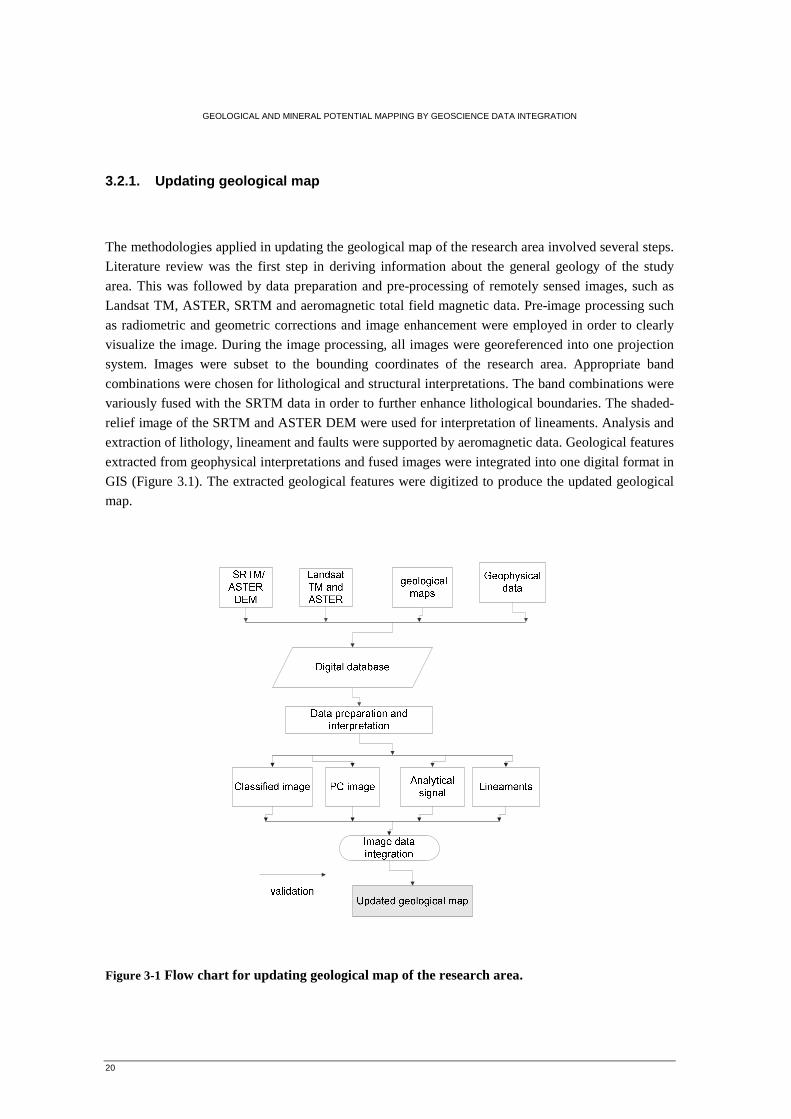
GEOLOGICAL AND MINERAL POTENTIAL MAPPING BY GEOSCIENCE DATA INTEGRATION
20
3.2.1. Updating geological map
The methodologies applied in updating the geological map of the research area involved several steps.
Literature review was the first step in deriving information about the general geology of the study
area. This was followed by data preparation and pre-processing of remotely sensed images, such as
Landsat TM, ASTER, SRTM and aeromagnetic total field magnetic data. Pre-image processing such
as radiometric and geometric corrections and image enhancement were employed in order to clearly
visualize the image. During the image processing, all images were georeferenced into one projection
system. Images were subset to the bounding coordinates of the research area. Appropriate band
combinations were chosen for lithological and structural interpretations. The band combinations were
variously fused with the SRTM data in order to further enhance lithological boundaries. The shaded-
relief image of the SRTM and ASTER DEM were used for interpretation of lineaments. Analysis and
extraction of lithology, lineament and faults were supported by aeromagnetic data. Geological features
extracted from geophysical interpretations and fused images were integrated into one digital format in
GIS (Figure 3.1). The extracted geological features were digitized to produce the updated geological
map.
Figure 3-1 Flow chart for updating geological map of the research area.
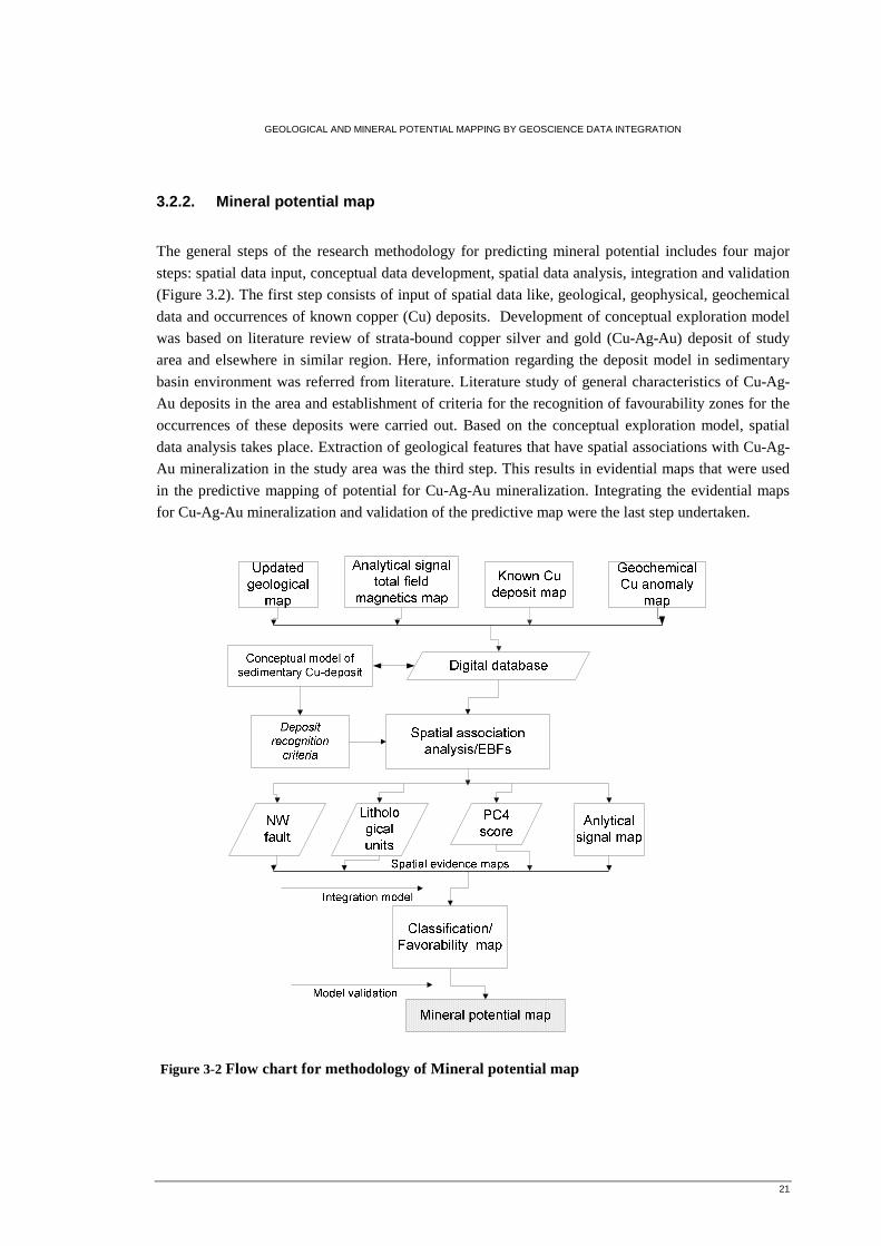
GEOLOGICAL AND MINERAL POTENTIAL MAPPING BY GEOSCIENCE DATA INTEGRATION
21
3.2.2. Mineral potential map
The general steps of the research methodology for predicting mineral potential includes four major
steps: spatial data input, conceptual data development, spatial data analysis, integration and validation
(Figure 3.2). The first step consists of input of spatial data like, geological, geophysical, geochemical
data and occurrences of known copper (Cu) deposits. Development of conceptual exploration model
was based on literature review of strata-bound copper silver and gold (Cu-Ag-Au) deposit of study
area and elsewhere in similar region. Here, information regarding the deposit model in sedimentary
basin environment was referred from literature. Literature study of general characteristics of Cu-Ag-
Au deposits in the area and establishment of criteria for the recognition of favourability zones for the
occurrences of these deposits were carried out. Based on the conceptual exploration model, spatial
data analysis takes place. Extraction of geological features that have spatial associations with Cu-Ag-
Au mineralization in the study area was the third step. This results in evidential maps that were used
in the predictive mapping of potential for Cu-Ag-Au mineralization. Integrating the evidential maps
for Cu-Ag-Au mineralization and validation of the predictive map were the last step undertaken.
Figure 3-2 Flow chart for methodology of Mineral potential map
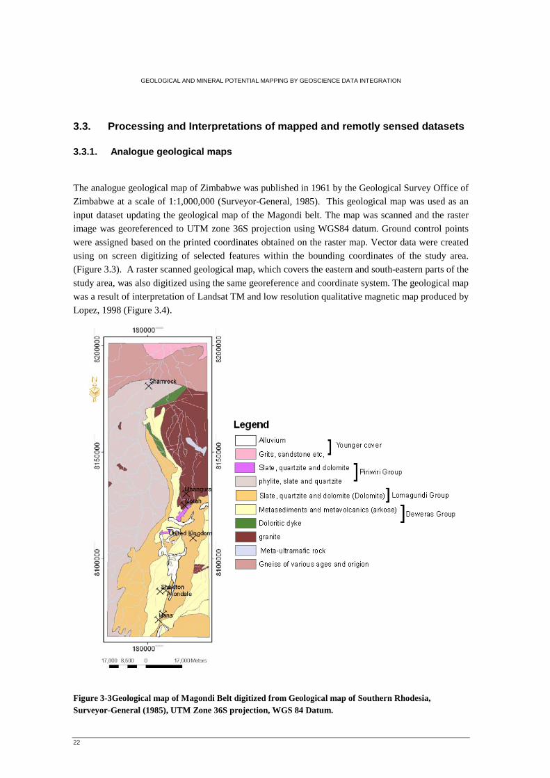
GEOLOGICAL AND MINERAL POTENTIAL MAPPING BY GEOSCIENCE DATA INTEGRATION
22
3.3. Processing and Interpretations of mapped and remotly sensed datasets
3.3.1. Analogue geological maps
The analogue geological map of Zimbabwe was published in 1961 by the Geological Survey Office of
Zimbabwe at a scale of 1:1,000,000 (Surveyor-General, 1985). This geological map was used as an
input dataset updating the geological map of the Magondi belt. The map was scanned and the raster
image was georeferenced to UTM zone 36S projection using WGS84 datum. Ground control points
were assigned based on the printed coordinates obtained on the raster map. Vector data were created
using on screen digitizing of selected features within the bounding coordinates of the study area.
(Figure 3.3). A raster scanned geological map, which covers the eastern and south-eastern parts of the
study area, was also digitized using the same georeference and coordinate system. The geological map
was a result of interpretation of Landsat TM and low resolution qualitative magnetic map produced by
Lopez, 1998 (Figure 3.4).
Figure 3-3Geological map of Magondi Belt digitized from Geological map of Southern Rhodesia, Surveyor-General (1985), UTM Zone 36S projection, WGS 84 Datum.
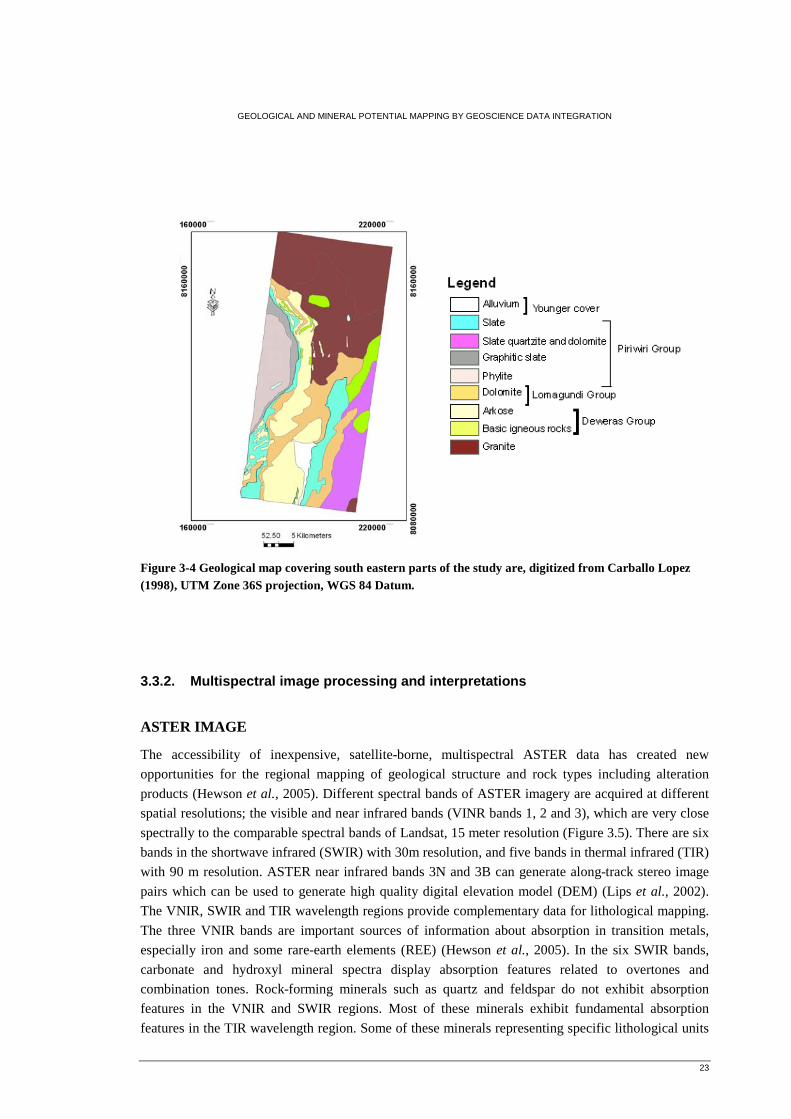
GEOLOGICAL AND MINERAL POTENTIAL MAPPING BY GEOSCIENCE DATA INTEGRATION
23
Figure 3-4 Geological map covering south eastern parts of the study are, digitized from Carballo Lopez (1998), UTM Zone 36S projection, WGS 84 Datum.
3.3.2. Multispectral image processing and interpretations
ASTER IMAGE
The accessibility of inexpensive, satellite-borne, multispectral ASTER data has created new
opportunities for the regional mapping of geological structure and rock types including alteration
products (Hewson et al., 2005). Different spectral bands of ASTER imagery are acquired at different
spatial resolutions; the visible and near infrared bands (VINR bands 1, 2 and 3), which are very close
spectrally to the comparable spectral bands of Landsat, 15 meter resolution (Figure 3.5). There are six
bands in the shortwave infrared (SWIR) with 30m resolution, and five bands in thermal infrared (TIR)
with 90 m resolution. ASTER near infrared bands 3N and 3B can generate along-track stereo image
pairs which can be used to generate high quality digital elevation model (DEM) (Lips et al., 2002).
The VNIR, SWIR and TIR wavelength regions provide complementary data for lithological mapping.
The three VNIR bands are important sources of information about absorption in transition metals,
especially iron and some rare-earth elements (REE) (Hewson et al., 2005). In the six SWIR bands,
carbonate and hydroxyl mineral spectra display absorption features related to overtones and
combination tones. Rock-forming minerals such as quartz and feldspar do not exhibit absorption
features in the VNIR and SWIR regions. Most of these minerals exhibit fundamental absorption
features in the TIR wavelength region. Some of these minerals representing specific lithological units
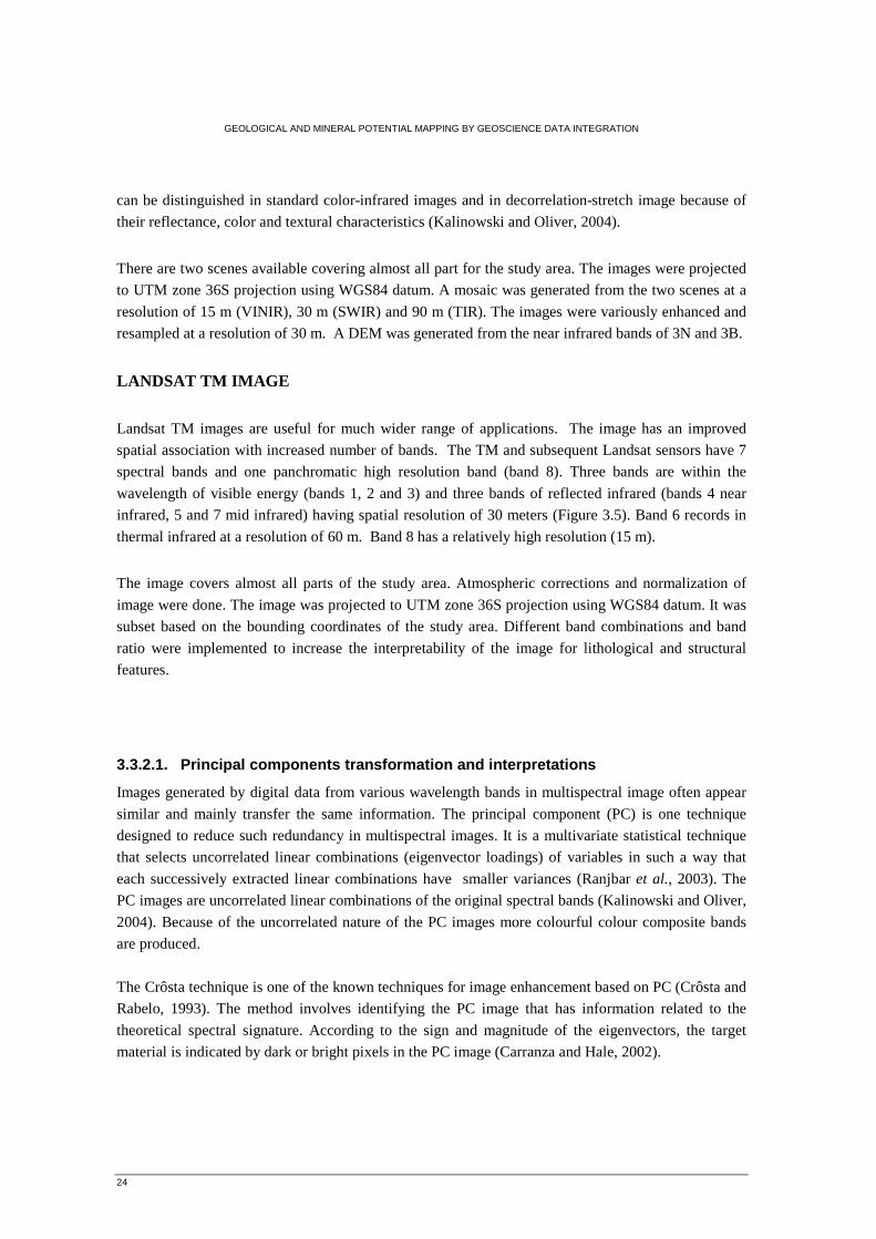
GEOLOGICAL AND MINERAL POTENTIAL MAPPING BY GEOSCIENCE DATA INTEGRATION
24
can be distinguished in standard color-infrared images and in decorrelation-stretch image because of
their reflectance, color and textural characteristics (Kalinowski and Oliver, 2004).
There are two scenes available covering almost all part for the study area. The images were projected
to UTM zone 36S projection using WGS84 datum. A mosaic was generated from the two scenes at a
resolution of 15 m (VINIR), 30 m (SWIR) and 90 m (TIR). The images were variously enhanced and
resampled at a resolution of 30 m. A DEM was generated from the near infrared bands of 3N and 3B.
LANDSAT TM IMAGE
Landsat TM images are useful for much wider range of applications. The image has an improved
spatial association with increased number of bands. The TM and subsequent Landsat sensors have 7
spectral bands and one panchromatic high resolution band (band 8). Three bands are within the
wavelength of visible energy (bands 1, 2 and 3) and three bands of reflected infrared (bands 4 near
infrared, 5 and 7 mid infrared) having spatial resolution of 30 meters (Figure 3.5). Band 6 records in
thermal infrared at a resolution of 60 m. Band 8 has a relatively high resolution (15 m).
The image covers almost all parts of the study area. Atmospheric corrections and normalization of
image were done. The image was projected to UTM zone 36S projection using WGS84 datum. It was
subset based on the bounding coordinates of the study area. Different band combinations and band
ratio were implemented to increase the interpretability of the image for lithological and structural
features.
3.3.2.1. Principal components transformation and interpretations
Images generated by digital data from various wavelength bands in multispectral image often appear
similar and mainly transfer the same information. The principal component (PC) is one technique
designed to reduce such redundancy in multispectral images. It is a multivariate statistical technique
that selects uncorrelated linear combinations (eigenvector loadings) of variables in such a way that
each successively extracted linear combinations have smaller variances (Ranjbar et al., 2003). The
PC images are uncorrelated linear combinations of the original spectral bands (Kalinowski and Oliver,
2004). Because of the uncorrelated nature of the PC images more colourful colour composite bands
are produced.
The Crôsta technique is one of the known techniques for image enhancement based on PC (Crôsta and
Rabelo, 1993). The method involves identifying the PC image that has information related to the
theoretical spectral signature. According to the sign and magnitude of the eigenvectors, the target
material is indicated by dark or bright pixels in the PC image (Carranza and Hale, 2002).
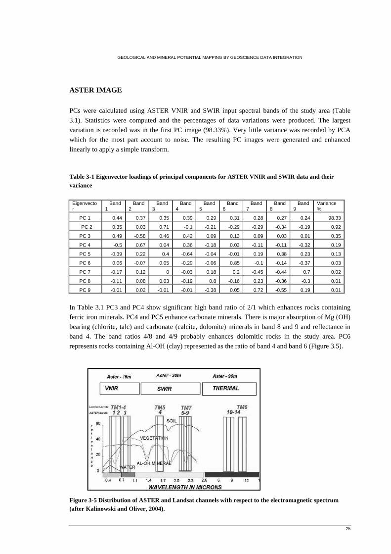
GEOLOGICAL AND MINERAL POTENTIAL MAPPING BY GEOSCIENCE DATA INTEGRATION
25
ASTER IMAGE PCs were calculated using ASTER VNIR and SWIR input spectral bands of the study area (Table
3.1). Statistics were computed and the percentages of data variations were produced. The largest
variation is recorded was in the first PC image (98.33%). Very little variance was recorded by PCA
which for the most part account to noise. The resulting PC images were generated and enhanced
linearly to apply a simple transform. Table 3-1 Eigenvector loadings of principal components for ASTER VNIR and SWIR data and their variance
Eigenvector
Band 1
Band 2
Band 3
Band 4
Band 5
Band 6
Band 7
Band 8
Band 9
Variance%
PC 1 0.44 0.37 0.35 0.39 0.29 0.31 0.28 0.27 0.24 98.33
PC 2 0.35 0.03 0.71 -0.1 -0.21 -0.29 -0.29 -0.34 -0.19 0.92
PC 3 0.49 -0.58 0.46 0.42 0.09 0.13 0.09 0.03 0.01 0.35
PC 4 -0.5 0.67 0.04 0.36 -0.18 0.03 -0.11 -0.11 -0.32 0.19
PC 5 -0.39 0.22 0.4 -0.64 -0.04 -0.01 0.19 0.38 0.23 0.13
PC 6 0.06 -0.07 0.05 -0.29 -0.06 0.85 -0.1 -0.14 -0.37 0.03
PC 7 -0.17 0.12 0 -0.03 0.18 0.2 -0.45 -0.44 0.7 0.02
PC 8 -0.11 0.08 0.03 -0.19 0.8 -0.16 0.23 -0.36 -0.3 0.01
PC 9 -0.01 0.02 -0.01 -0.01 -0.38 0.05 0.72 -0.55 0.19 0.01
In Table 3.1 PC3 and PC4 show significant high band ratio of 2/1 which enhances rocks containing
ferric iron minerals. PC4 and PC5 enhance carbonate minerals. There is major absorption of Mg (OH)
bearing (chlorite, talc) and carbonate (calcite, dolomite) minerals in band 8 and 9 and reflectance in
band 4. The band ratios 4/8 and 4/9 probably enhances dolomitic rocks in the study area. PC6
represents rocks containing Al-OH (clay) represented as the ratio of band 4 and band 6 (Figure 3.5). Figure 3-5 Distribution of ASTER and Landsat channels with respect to the electromagnetic spectrum (after Kalinowski and Oliver, 2004).
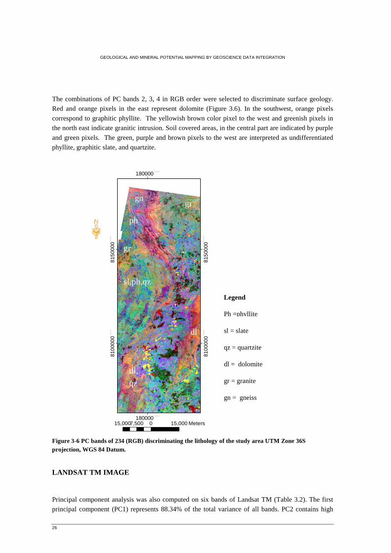
GEOLOGICAL AND MINERAL POTENTIAL MAPPING BY GEOSCIENCE DATA INTEGRATION
26
The combinations of PC bands 2, 3, 4 in RGB order were selected to discriminate surface geology.
Red and orange pixels in the east represent dolomite (Figure 3.6). In the southwest, orange pixels
correspond to graphitic phyllite. The yellowish brown color pixel to the west and greenish pixels in
the north east indicate granitic intrusion. Soil covered areas, in the central part are indicated by purple
and green pixels. The green, purple and brown pixels to the west are interpreted as undifferentiated
phyllite, graphitic slate, and quartzite. Figure 3-6 PC bands of 234 (RGB) discriminating the lithology of the study area UTM Zone 36S projection, WGS 84 Datum.
LANDSAT TM IMAGE
Principal component analysis was also computed on six bands of Landsat TM (Table 3.2). The first
principal component (PC1) represents 88.34% of the total variance of all bands. PC2 contains high
180000.000000
180000.000000
8100
000.0
000
00
8100
000.0
000
00
8150
000.0
0000
0
8150
000.0
0000
0·
15,000 0 15,0007,500 Meters
ph
dl,
qz
dl
gr
sl,ph,qz
gr
gn
gr = granite
Ph =phyllite
sl = slate
qz = quartzite
dl = dolomite
gn = gneiss
Legend
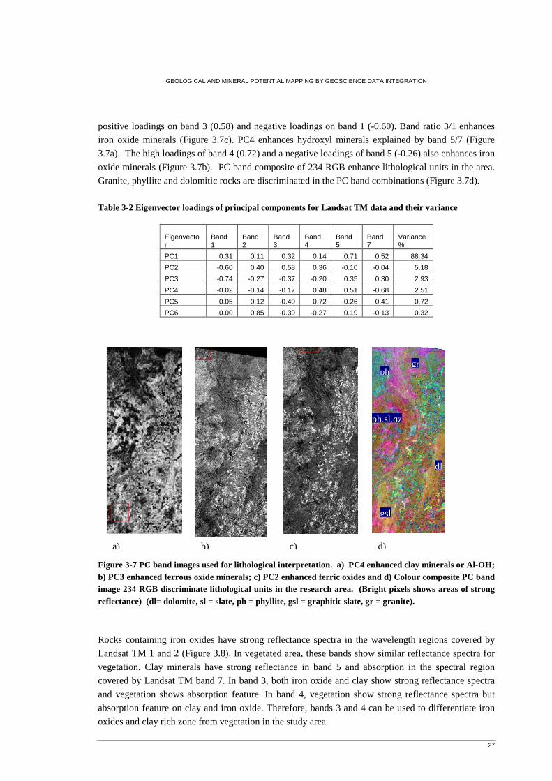
GEOLOGICAL AND MINERAL POTENTIAL MAPPING BY GEOSCIENCE DATA INTEGRATION
27
positive loadings on band 3 (0.58) and negative loadings on band 1 (-0.60). Band ratio 3/1 enhances
iron oxide minerals (Figure 3.7c). PC4 enhances hydroxyl minerals explained by band 5/7 (Figure
3.7a). The high loadings of band 4 (0.72) and a negative loadings of band 5 (-0.26) also enhances iron
oxide minerals (Figure 3.7b). PC band composite of 234 RGB enhance lithological units in the area.
Granite, phyllite and dolomitic rocks are discriminated in the PC band combinations (Figure 3.7d).
Table 3-2 Eigenvector loadings of principal components for Landsat TM data and their variance
Figure 3-7 PC band images used for lithological interpretation. a) PC4 enhanced clay minerals or Al-OH; b) PC3 enhanced ferrous oxide minerals; c) PC2 enhanced ferric oxides and d) Colour composite PC band image 234 RGB discriminate lithological units in the research area. (Bright pixels shows areas of strong reflectance) (dl= dolomite, sl = slate, ph = phyllite, gsl = graphitic slate, gr = granite).
Rocks containing iron oxides have strong reflectance spectra in the wavelength regions covered by
Landsat TM 1 and 2 (Figure 3.8). In vegetated area, these bands show similar reflectance spectra for
vegetation. Clay minerals have strong reflectance in band 5 and absorption in the spectral region
covered by Landsat TM band 7. In band 3, both iron oxide and clay show strong reflectance spectra
and vegetation shows absorption feature. In band 4, vegetation show strong reflectance spectra but
absorption feature on clay and iron oxide. Therefore, bands 3 and 4 can be used to differentiate iron
oxides and clay rich zone from vegetation in the study area.
Eigenvector
Band 1
Band 2
Band 3
Band 4
Band 5
Band 7
Variance %
PC1 0.31 0.11 0.32 0.14 0.71 0.52 88.34
PC2 -0.60 0.40 0.58 0.36 -0.10 -0.04 5.18
PC3 -0.74 -0.27 -0.37 -0.20 0.35 0.30 2.93
PC4 -0.02 -0.14 -0.17 0.48 0.51 -0.68 2.51
PC5 0.05 0.12 -0.49 0.72 -0.26 0.41 0.72
PC6 0.00 0.85 -0.39 -0.27 0.19 -0.13 0.32
a) b) c) d)
ph
ph,sl,qz
dl
gsl
gr
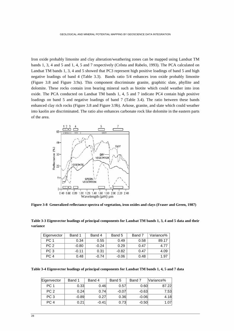
GEOLOGICAL AND MINERAL POTENTIAL MAPPING BY GEOSCIENCE DATA INTEGRATION
28
Iron oxide probably limonite and clay alteration/weathering zones can be mapped using Landsat TM
bands 1, 3, 4 and 5 and 1, 4, 5 and 7 respectively (Crôsta and Rabelo, 1993). The PCA calculated on
Landsat TM bands 1, 3, 4 and 5 showed that PC3 represent high positive loadings of band 5 and high
negative loadings of band 4 (Table 3.3). Bands ratio 5/4 enhances iron oxide probably limonite
(Figure 3.8 and Figure 3.9a). This component discriminate granite, graphitic slate, phyllite and
dolomite. These rocks contain iron bearing mineral such as biotite which could weather into iron
oxide. The PCA conducted on Landsat TM bands 1, 4, 5 and 7 indicate PC4 contain high positive
loadings on band 5 and negative loadings of band 7 (Table 3.4). The ratio between these bands
enhanced clay rich rocks (Figure 3.8 and Figure 3.9b). Arkose, granite, and slate which could weather
into kaolin are discriminated. The ratio also enhances carbonate rock like dolomite in the eastern parts
of the area.
Figure 3-8 Generalized reflectance spectra of vegetation, iron oxides and clays (Fraser and Green, 1987)
Table 3-3 Eigenvector loadings of principal components for Landsat TM bands 1, 3, 4 and 5 data and their variance
Table 3-4 Eigenvector loadings of principal components for Landsat TM bands 1, 4, 5 and 7 data
Eigenvector Band 1 Band 4 Band 5 Band 7 Variance%
PC 1 0.33 0.46 0.57 0.60 87.22
PC 2 0.24 0.74 -0.07 -0.63 7.53
PC 3 -0.89 0.27 0.36 -0.06 4.18
PC 4 0.21 -0.41 0.73 -0.50 1.07
Eigenvector Band 1 Band 4 Band 5 Band 7 Variance% PC 1 0.34 0.55 0.49 0.58 89.17 PC 2 -0.80 -0.24 0.29 0.47 4.77 PC 3 -0.11 0.31 -0.82 0.47 4.09 PC 4 0.48 -0.74 -0.06 0.48 1.97
Wavelength (µm) µm
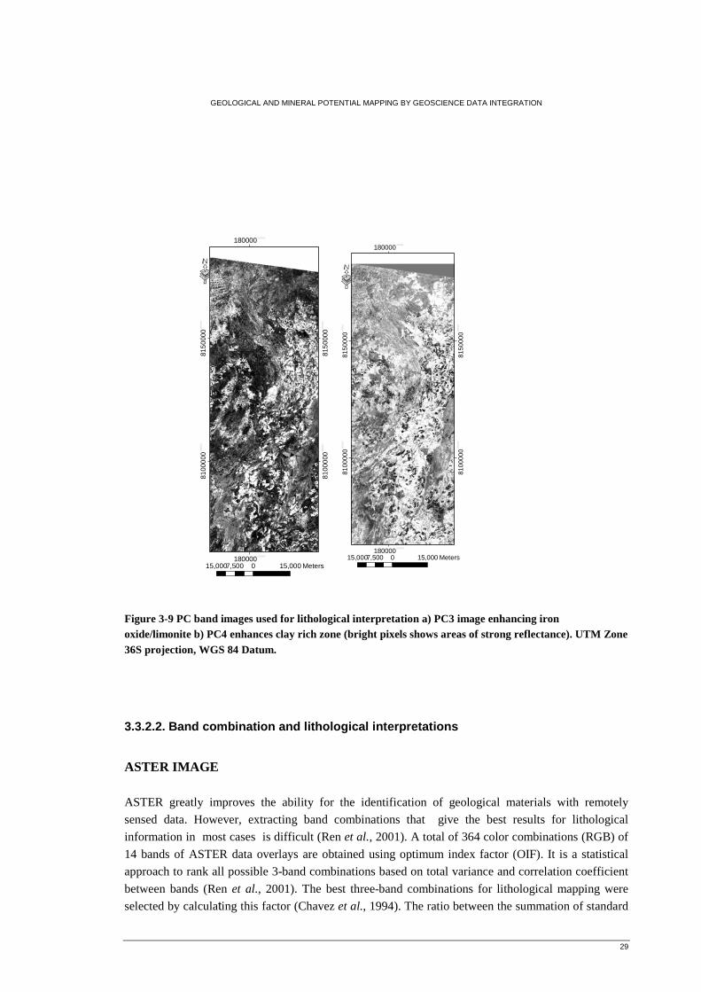
GEOLOGICAL AND MINERAL POTENTIAL MAPPING BY GEOSCIENCE DATA INTEGRATION
29
180000.000000
180000.000000
8100
000.0
00
00
0
8100
000.0
00
00
0
8150
000.0
00
00
0
8150
000.0
00
00
0
·
15,000 0 15,0007,500 Meters
180000.000000
180000.000000
8100
000.0
0000
0
8100
000.0
0000
0
8150
000.0
0000
0
8150
000.0
0000
0
·
15,000 0 15,0007,500 Meters
Figure 3-9 PC band images used for lithological interpretation a) PC3 image enhancing iron oxide/limonite b) PC4 enhances clay rich zone (bright pixels shows areas of strong reflectance). UTM Zone 36S projection, WGS 84 Datum.
3.3.2.2. Band combination and lithological interpretations
ASTER IMAGE ASTER greatly improves the ability for the identification of geological materials with remotely
sensed data. However, extracting band combinations that give the best results for lithological
information in most cases is difficult (Ren et al., 2001). A total of 364 color combinations (RGB) of
14 bands of ASTER data overlays are obtained using optimum index factor (OIF). It is a statistical
approach to rank all possible 3-band combinations based on total variance and correlation coefficient
between bands (Ren et al., 2001). The best three-band combinations for lithological mapping were
selected by calculating this factor (Chavez et al., 1994). The ratio between the summation of standard
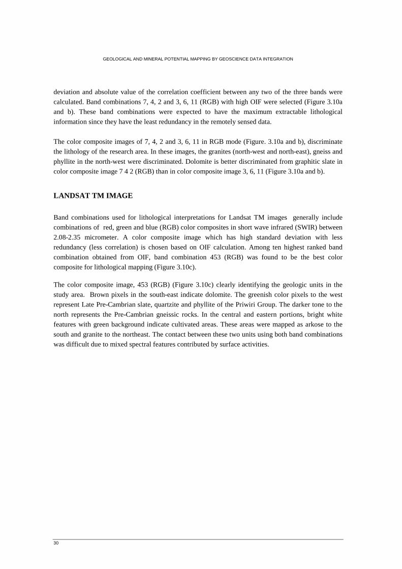
GEOLOGICAL AND MINERAL POTENTIAL MAPPING BY GEOSCIENCE DATA INTEGRATION
30
deviation and absolute value of the correlation coefficient between any two of the three bands were
calculated. Band combinations 7, 4, 2 and 3, 6, 11 (RGB) with high OIF were selected (Figure 3.10a
and b). These band combinations were expected to have the maximum extractable lithological
information since they have the least redundancy in the remotely sensed data.
The color composite images of 7, 4, 2 and 3, 6, 11 in RGB mode (Figure. 3.10a and b), discriminate
the lithology of the research area. In these images, the granites (north-west and north-east), gneiss and
phyllite in the north-west were discriminated. Dolomite is better discriminated from graphitic slate in
color composite image 7 4 2 (RGB) than in color composite image 3, 6, 11 (Figure 3.10a and b).
LANDSAT TM IMAGE
Band combinations used for lithological interpretations for Landsat TM images generally include
combinations of red, green and blue (RGB) color composites in short wave infrared (SWIR) between
2.08-2.35 micrometer. A color composite image which has high standard deviation with less
redundancy (less correlation) is chosen based on OIF calculation. Among ten highest ranked band
combination obtained from OIF, band combination 453 (RGB) was found to be the best color
composite for lithological mapping (Figure 3.10c).
The color composite image, 453 (RGB) (Figure 3.10c) clearly identifying the geologic units in the
study area. Brown pixels in the south-east indicate dolomite. The greenish color pixels to the west
represent Late Pre-Cambrian slate, quartzite and phyllite of the Priwiri Group. The darker tone to the
north represents the Pre-Cambrian gneissic rocks. In the central and eastern portions, bright white
features with green background indicate cultivated areas. These areas were mapped as arkose to the
south and granite to the northeast. The contact between these two units using both band combinations
was difficult due to mixed spectral features contributed by surface activities.
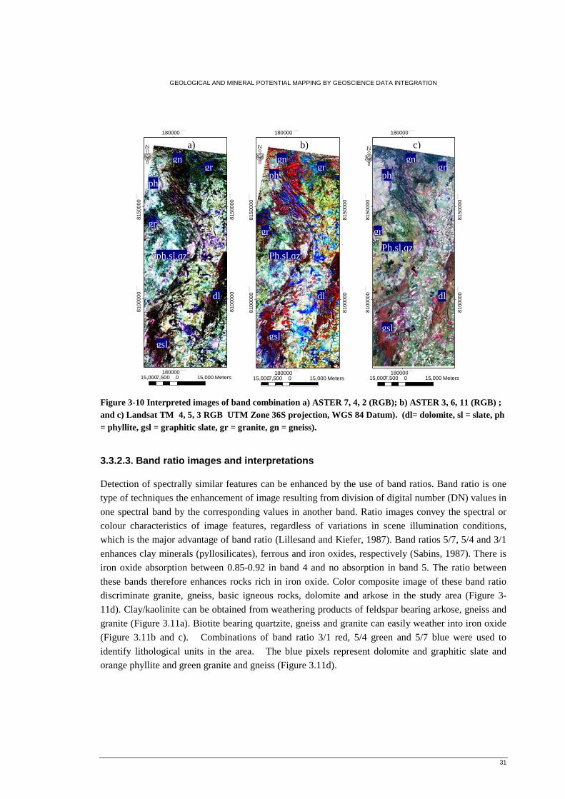
GEOLOGICAL AND MINERAL POTENTIAL MAPPING BY GEOSCIENCE DATA INTEGRATION
31
Figure 3-10 Interpreted images of band combination a) ASTER 7, 4, 2 (RGB); b) ASTER 3, 6, 11 (RGB) ; and c) Landsat TM 4, 5, 3 RGB UTM Zone 36S projection, WGS 84 Datum). (dl= dolomite, sl = slate, ph = phyllite, gsl = graphitic slate, gr = granite, gn = gneiss).
3.3.2.3. Band ratio images and interpretations
Detection of spectrally similar features can be enhanced by the use of band ratios. Band ratio is one
type of techniques the enhancement of image resulting from division of digital number (DN) values in
one spectral band by the corresponding values in another band. Ratio images convey the spectral or
colour characteristics of image features, regardless of variations in scene illumination conditions,
which is the major advantage of band ratio (Lillesand and Kiefer, 1987). Band ratios 5/7, 5/4 and 3/1
enhances clay minerals (pyllosilicates), ferrous and iron oxides, respectively (Sabins, 1987). There is
iron oxide absorption between 0.85-0.92 in band 4 and no absorption in band 5. The ratio between
these bands therefore enhances rocks rich in iron oxide. Color composite image of these band ratio
discriminate granite, gneiss, basic igneous rocks, dolomite and arkose in the study area (Figure 3-
11d). Clay/kaolinite can be obtained from weathering products of feldspar bearing arkose, gneiss and
granite (Figure 3.11a). Biotite bearing quartzite, gneiss and granite can easily weather into iron oxide
(Figure 3.11b and c). Combinations of band ratio 3/1 red, 5/4 green and 5/7 blue were used to
identify lithological units in the area. The blue pixels represent dolomite and graphitic slate and
orange phyllite and green granite and gneiss (Figure 3.11d).
180000.000000
180000.000000
8100
000.0
0000
0
8100
000.0
0000
0
8150
000.0
0000
0
8150
000.0
0000
0
·
15,000 0 15,0007,500 Meters
180000.000000
180000.000000
8100
000.0
000
00
8100
000.0
000
00
8150
000.0
0000
0
8150
000.0
0000
0
·
15,000 0 15,0007,500 Meters
180000.000000
180000.000000
8100
000.0
000
00
8100
000.0
000
00
8150
000.0
000
00
8150
000.0
000
00
·
15,000 0 15,0007,500 Meters
a) b) c)
ph ph ph
gr gr gr
gr gr gr
gsl gsl
gsl
dl dl dl
ph,sl,qz Ph,sl,qz Ph,sl,qz
gn gn gn
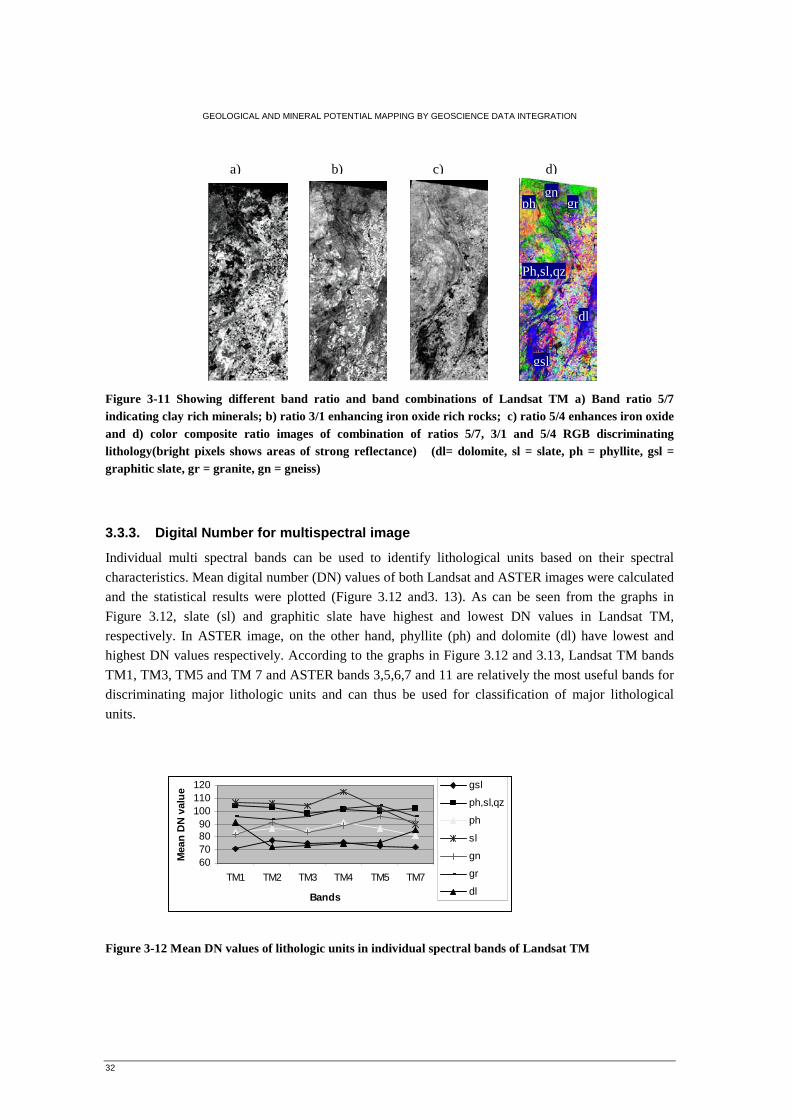
GEOLOGICAL AND MINERAL POTENTIAL MAPPING BY GEOSCIENCE DATA INTEGRATION
32
60708090
100110120
TM1 TM2 TM3 TM4 TM5 TM7
Bands
Mea
n D
N v
alu
e gsl
ph,sl,qz
ph
sl
gn
gr
dl
Figure 3-11 Showing different band ratio and band combinations of Landsat TM a) Band ratio 5/7 indicating clay rich minerals; b) ratio 3/1 enhancing iron oxide rich rocks; c) ratio 5/4 enhances iron oxide and d) color composite ratio images of combination of ratios 5/7, 3/1 and 5/4 RGB discriminating lithology(bright pixels shows areas of strong reflectance) (dl= dolomite, sl = slate, ph = phyllite, gsl = graphitic slate, gr = granite, gn = gneiss)
3.3.3. Digital Number for multispectral image
Individual multi spectral bands can be used to identify lithological units based on their spectral
characteristics. Mean digital number (DN) values of both Landsat and ASTER images were calculated
and the statistical results were plotted (Figure 3.12 and3. 13). As can be seen from the graphs in
Figure 3.12, slate (sl) and graphitic slate have highest and lowest DN values in Landsat TM,
respectively. In ASTER image, on the other hand, phyllite (ph) and dolomite (dl) have lowest and
highest DN values respectively. According to the graphs in Figure 3.12 and 3.13, Landsat TM bands
TM1, TM3, TM5 and TM 7 and ASTER bands 3,5,6,7 and 11 are relatively the most useful bands for
discriminating major lithologic units and can thus be used for classification of major lithological
units.
Figure 3-12 Mean DN values of lithologic units in individual spectral bands of Landsat TM
a) b) c) d)
ph
Ph,sl,qz
dl
gsl
gr gn
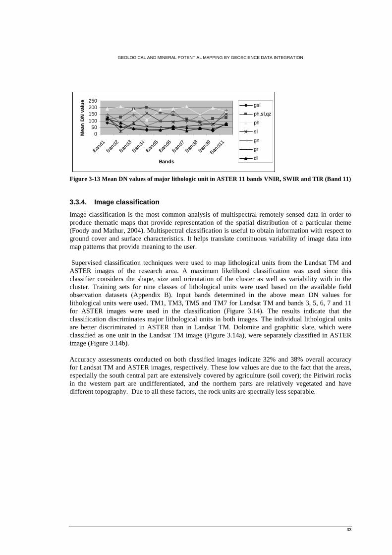
GEOLOGICAL AND MINERAL POTENTIAL MAPPING BY GEOSCIENCE DATA INTEGRATION
33
050
100150200250
Band1
Band2
Band3
Band4
Band5
Band6
Band7
Band8
Band9
Band1
1
Bands
Mea
n D
N v
alu
e
gsl
ph,sl,qz
ph
sl
gn
gr
dl
Figure 3-13 Mean DN values of major lithologic unit in ASTER 11 bands VNIR, SWIR and TIR (Band 11)
3.3.4. Image classification
Image classification is the most common analysis of multispectral remotely sensed data in order to produce thematic maps that provide representation of the spatial distribution of a particular theme (Foody and Mathur, 2004). Multispectral classification is useful to obtain information with respect to ground cover and surface characteristics. It helps translate continuous variability of image data into map patterns that provide meaning to the user. Supervised classification techniques were used to map lithological units from the Landsat TM and ASTER images of the research area. A maximum likelihood classification was used since this classifier considers the shape, size and orientation of the cluster as well as variability with in the cluster. Training sets for nine classes of lithological units were used based on the available field observation datasets (Appendix B). Input bands determined in the above mean DN values for lithological units were used. TM1, TM3, TM5 and TM7 for Landsat TM and bands 3, 5, 6, 7 and 11 for ASTER images were used in the classification (Figure 3.14). The results indicate that the classification discriminates major lithological units in both images. The individual lithological units are better discriminated in ASTER than in Landsat TM. Dolomite and graphitic slate, which were classified as one unit in the Landsat TM image (Figure 3.14a), were separately classified in ASTER image (Figure 3.14b). Accuracy assessments conducted on both classified images indicate 32% and 38% overall accuracy for Landsat TM and ASTER images, respectively. These low values are due to the fact that the areas, especially the south central part are extensively covered by agriculture (soil cover); the Piriwiri rocks in the western part are undifferentiated, and the northern parts are relatively vegetated and have different topography. Due to all these factors, the rock units are spectrally less separable.
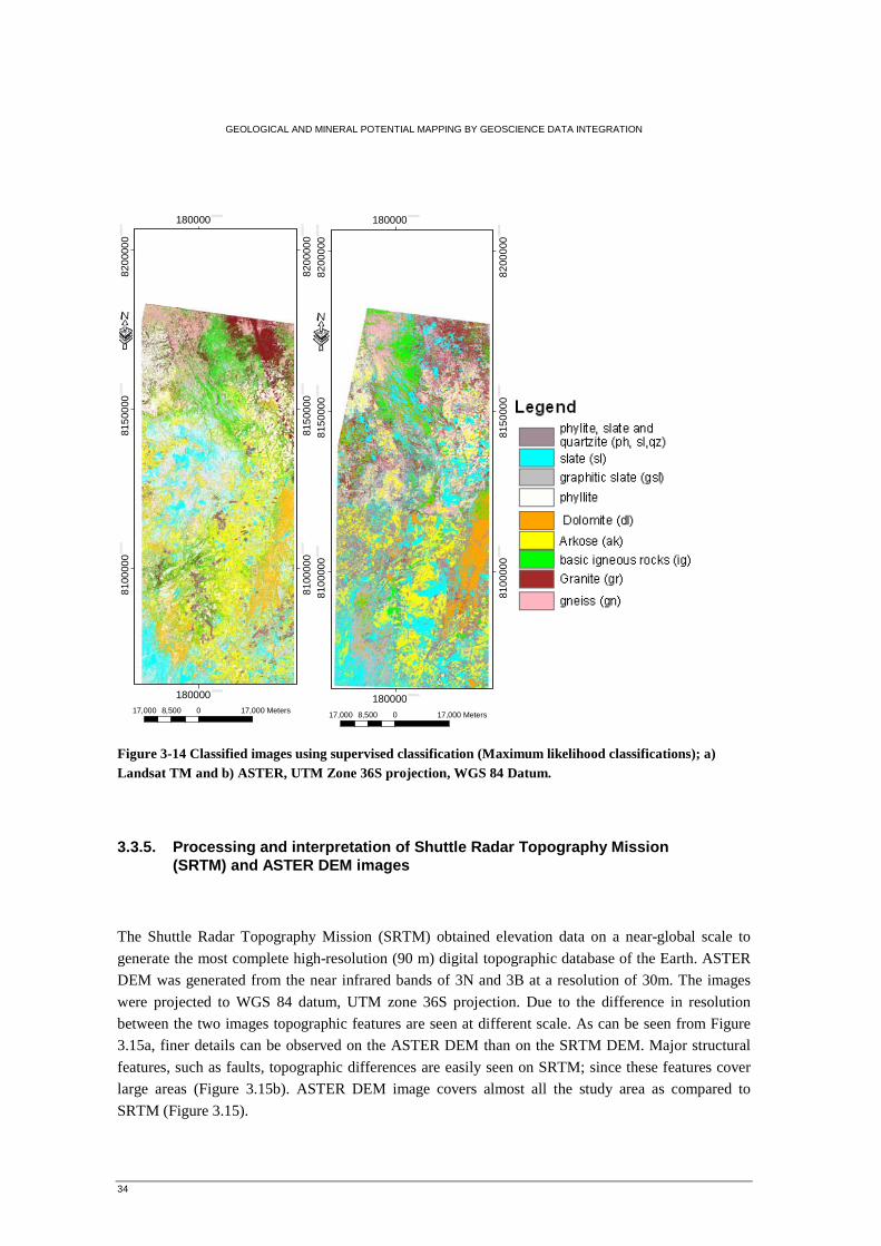
GEOLOGICAL AND MINERAL POTENTIAL MAPPING BY GEOSCIENCE DATA INTEGRATION
34
180000.000000
180000.000000
8100
000.0
00
000
8100
000.0
00
000
8150
000.0
0000
0
8150
000.0
0000
0
8200
000.0
000
00
8200
000.0
000
00
·
17,000 0 17,0008,500 Meters
180000.000000
180000.000000
8100
000.0
0000
0
8100
000.0
0000
0
8150
000.0
000
00
8150
000.0
000
00
8200
000.0
0000
0
8200
000.0
0000
0
·
17,000 0 17,0008,500 Meters
Figure 3-14 Classified images using supervised classification (Maximum likelihood classifications); a) Landsat TM and b) ASTER, UTM Zone 36S projection, WGS 84 Datum.
3.3.5. Processing and interpretation of Shuttle Radar Topography Mission (SRTM) and ASTER DEM images
The Shuttle Radar Topography Mission (SRTM) obtained elevation data on a near-global scale to
generate the most complete high-resolution (90 m) digital topographic database of the Earth. ASTER
DEM was generated from the near infrared bands of 3N and 3B at a resolution of 30m. The images
were projected to WGS 84 datum, UTM zone 36S projection. Due to the difference in resolution
between the two images topographic features are seen at different scale. As can be seen from Figure
3.15a, finer details can be observed on the ASTER DEM than on the SRTM DEM. Major structural
features, such as faults, topographic differences are easily seen on SRTM; since these features cover
large areas (Figure 3.15b). ASTER DEM image covers almost all the study area as compared to
SRTM (Figure 3.15).
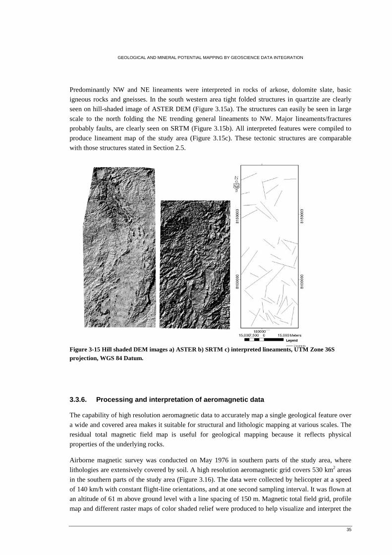
GEOLOGICAL AND MINERAL POTENTIAL MAPPING BY GEOSCIENCE DATA INTEGRATION
35
Predominantly NW and NE lineaments were interpreted in rocks of arkose, dolomite slate, basic
igneous rocks and gneisses. In the south western area tight folded structures in quartzite are clearly
seen on hill-shaded image of ASTER DEM (Figure 3.15a). The structures can easily be seen in large
scale to the north folding the NE trending general lineaments to NW. Major lineaments/fractures
probably faults, are clearly seen on SRTM (Figure 3.15b). All interpreted features were compiled to
produce lineament map of the study area (Figure 3.15c). These tectonic structures are comparable
with those structures stated in Section 2.5.
Figure 3-15 Hill shaded DEM images a) ASTER b) SRTM c) interpreted lineaments, UTM Zone 36S projection, WGS 84 Datum.
3.3.6. Processing and interpretation of aeromagnetic data
The capability of high resolution aeromagnetic data to accurately map a single geological feature over
a wide and covered area makes it suitable for structural and lithologic mapping at various scales. The
residual total magnetic field map is useful for geological mapping because it reflects physical
properties of the underlying rocks.
Airborne magnetic survey was conducted on May 1976 in southern parts of the study area, where
lithologies are extensively covered by soil. A high resolution aeromagnetic grid covers 530 km2 areas
in the southern parts of the study area (Figure 3.16). The data were collected by helicopter at a speed
of 140 km/h with constant flight-line orientations, and at one second sampling interval. It was flown at
an altitude of 61 m above ground level with a line spacing of 150 m. Magnetic total field grid, profile
map and different raster maps of color shaded relief were produced to help visualize and interpret the
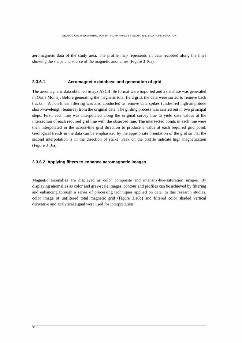
GEOLOGICAL AND MINERAL POTENTIAL MAPPING BY GEOSCIENCE DATA INTEGRATION
36
aeromagnetic data of the study area. The profile map represents all data recorded along the lines
showing the shape and source of the magnetic anomalies (Figure 3 16a).
3.3.6.1. Aeromagnetic database and generation of grid
The aeromagnetic data obtained in xyz ASCII file format were imported and a database was generated
in Oasis Montaj. Before generating the magnetic total field grid, the data were sorted to remove back
tracks. A non-linear filtering was also conducted to remove data spikes (undesired high-amplitude
short-wavelength features) from the original data. The girding process was carried out in two principal
steps. First, each line was interpolated along the original survey line to yield data values at the
intersection of each required grid line with the observed line. The intersected points in each line were
then interpolated in the across-line grid direction to produce a value at each required grid point.
Geological trends in the data can be emphasized by the appropriate orientation of the grid so that the
second interpolation is in the direction of strike. Peak on the profile indicate high magnetization
(Figure 3 16a).
3.3.6.2. Applying filters to enhance aeromagnetic images
Magnetic anomalies are displayed as color composite and intensity-hue-saturation images. By
displaying anomalies as color and grey-scale images, contour and profiles can be achieved by filtering
and enhancing through a series of processing techniques applied on data. In this research studies,
color image of unfiltered total magnetic grid (Figure 3.16b) and filtered color shaded vertical
derivative and analytical signal were used for interpretation.
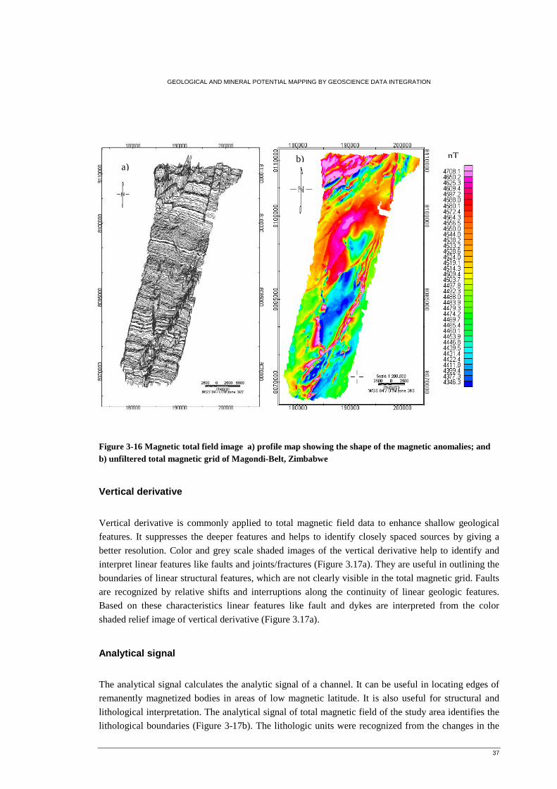
GEOLOGICAL AND MINERAL POTENTIAL MAPPING BY GEOSCIENCE DATA INTEGRATION
37
Figure 3-16 Magnetic total field image a) profile map showing the shape of the magnetic anomalies; and b) unfiltered total magnetic grid of Magondi-Belt, Zimbabwe
Vertical derivative
Vertical derivative is commonly applied to total magnetic field data to enhance shallow geological
features. It suppresses the deeper features and helps to identify closely spaced sources by giving a
better resolution. Color and grey scale shaded images of the vertical derivative help to identify and
interpret linear features like faults and joints/fractures (Figure 3.17a). They are useful in outlining the
boundaries of linear structural features, which are not clearly visible in the total magnetic grid. Faults
are recognized by relative shifts and interruptions along the continuity of linear geologic features.
Based on these characteristics linear features like fault and dykes are interpreted from the color
shaded relief image of vertical derivative (Figure 3.17a).
Analytical signal
The analytical signal calculates the analytic signal of a channel. It can be useful in locating edges of
remanently magnetized bodies in areas of low magnetic latitude. It is also useful for structural and
lithological interpretation. The analytical signal of total magnetic field of the study area identifies the
lithological boundaries (Figure 3-17b). The lithologic units were recognized from the changes in the
nT a)
b)
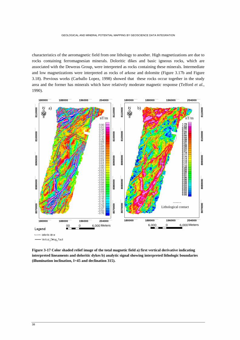
GEOLOGICAL AND MINERAL POTENTIAL MAPPING BY GEOSCIENCE DATA INTEGRATION
38
characteristics of the aeromagnetic field from one lithology to another. High magnetizations are due to
rocks containing ferromagnesian minerals. Doloritic dikes and basic igneous rocks, which are
associated with the Deweras Group, were interpreted as rocks containing these minerals. Intermediate
and low magnetizations were interpreted as rocks of arkose and dolomite (Figure 3.17b and Figure
3.18). Previous works (Carballo Lopez, 1998) showed that these rocks occur together in the study
area and the former has minerals which have relatively moderate magnetic response (Telford et al.,
1990).
Figure 3-17 Color shaded relief image of the total magnetic field a) first vertical derivative indicating interpreted lineaments and doloritic dykes b) analytic signal showing interpreted lithologic boundaries (illumination inclination, I=45 and declination 315).
180000.000000
180000.000000
188000.000000
188000.000000
196000.000000
196000.000000
204000.000000
204000.000000
8070
000.0
0000
0
8070
000.0
0000
0
8080
000.0
0000
0
8080
000.0
0000
0
8090
000.0
000
00
8090
000.0
000
00
8100
000.0
0000
0
8100
000.0
0000
0
8110
000.0
0000
0
8110
000.0
0000
0
·
Meters6,000 0 6,000
nT/m
180000.000000
180000.000000
188000.000000
188000.000000
196000.000000
196000.000000
204000.000000
204000.000000
8070
000.0
0000
0
8070
000.0
0000
0
8080
000.0
0000
0
8080
000.0
0000
0
8090
000.0
0000
0
8090
000.0
0000
0
8100
000.0
0000
0
8100
000.0
0000
0
8110
000.0
0000
0
8110
000.0
0000
0
·
Meters6,000 0 6,000
Lithological contact
a) b)
nT/m
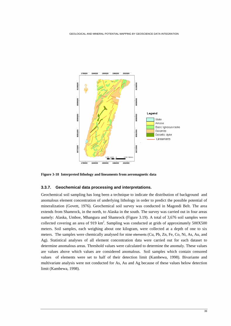
GEOLOGICAL AND MINERAL POTENTIAL MAPPING BY GEOSCIENCE DATA INTEGRATION
39
178000.000000
178000.000000
184000.000000
184000.000000
190000.000000
190000.000000
196000.000000
196000.000000
202000.000000
202000.000000
8072
000.0
0000
0
8072
000.0
0000
0
8081
000.0
0000
0
8081
000.0
0000
0
8090
000.0
0000
0
8090
000.0
0000
0
8099
000.0
000
00
8099
000.0
000
00
8108
000.0
0000
0
8108
000.0
0000
0
·
Meters5,250 0 5,2502,625
Figure 3-18 Interpreted lithology and lineaments from aeromagnetic data
3.3.7. Geochemical data processing and interpretations.
Geochemical soil sampling has long been a technique to indicate the distribution of background and
anomalous element concentration of underlying lithology in order to predict the possible potential of
mineralization (Govett, 1976). Geochemical soil survey was conducted in Magondi Belt. The area
extends from Shamrock, in the north, to Alaska in the south. The survey was carried out in four areas
namely: Alaska, Umboe, Mhangura and Shamrock (Figure 3.19). A total of 3,676 soil samples were
collected covering an area of 919 km2. Sampling was conducted at grids of approximately 500X500
meters. Soil samples, each weighing about one kilogram, were collected at a depth of one to six
meters. The samples were chemically analysed for nine elements (Cu, Pb, Zn, Fe, Co, Ni, As, Au, and
Ag). Statistical analyses of all element concentration data were carried out for each dataset to
determine anomalous areas. Threshold values were calculated to determine the anomaly. These values
are values above which values are considered anomalous. Soil samples which contain censored
values of elements were set to half of their detection limit (Kambewa, 1998). Bivariante and
multivariate analysis were not conducted for As, Au and Ag because of these values below detection
limit (Kambewa, 1998).
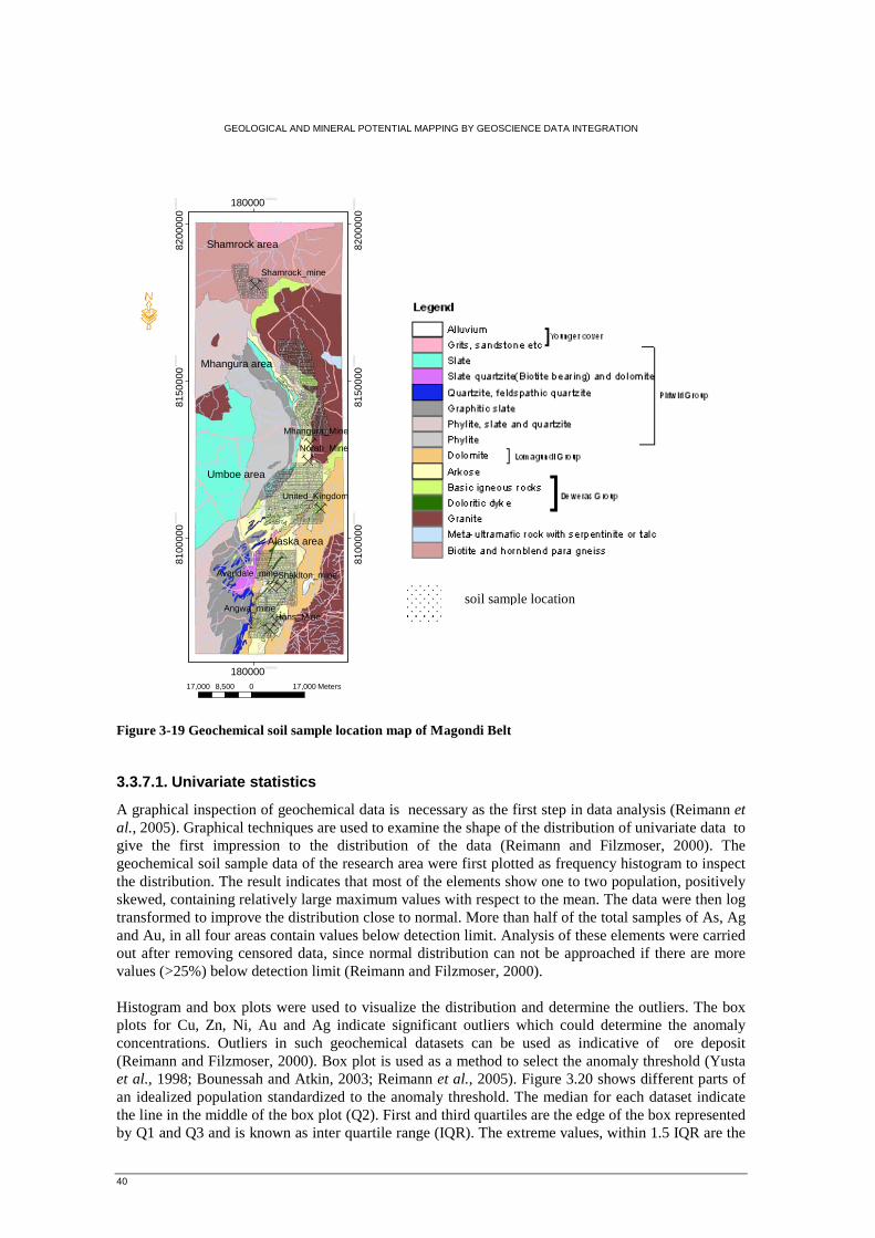
GEOLOGICAL AND MINERAL POTENTIAL MAPPING BY GEOSCIENCE DATA INTEGRATION
40
Ç
ÇÇÇÇ
Ç
Ç
Ç
Hans_Mine
Norah_Mine
Angwa_mine
Mhangura_Mine
Shaklton_mineAvondale_mine
Shamrock_mine
United_Kingdom
180000.000000
180000.000000
8100
000.0
0000
0
8100
000.0
0000
0
8150
000.0
000
00
8150
000.0
000
00
8200
000.0
000
00
8200
000.0
000
00
·
17,000 0 17,0008,500 Meters
Shamrock area
Mhangura area
Umboe area
Alaska area
Figure 3-19 Geochemical soil sample location map of Magondi Belt
3.3.7.1. Univariate statistics
A graphical inspection of geochemical data is necessary as the first step in data analysis (Reimann et al., 2005). Graphical techniques are used to examine the shape of the distribution of univariate data to give the first impression to the distribution of the data (Reimann and Filzmoser, 2000). The geochemical soil sample data of the research area were first plotted as frequency histogram to inspect the distribution. The result indicates that most of the elements show one to two population, positively skewed, containing relatively large maximum values with respect to the mean. The data were then log transformed to improve the distribution close to normal. More than half of the total samples of As, Ag and Au, in all four areas contain values below detection limit. Analysis of these elements were carried out after removing censored data, since normal distribution can not be approached if there are more values (>25%) below detection limit (Reimann and Filzmoser, 2000). Histogram and box plots were used to visualize the distribution and determine the outliers. The box plots for Cu, Zn, Ni, Au and Ag indicate significant outliers which could determine the anomaly concentrations. Outliers in such geochemical datasets can be used as indicative of ore deposit (Reimann and Filzmoser, 2000). Box plot is used as a method to select the anomaly threshold (Yusta et al., 1998; Bounessah and Atkin, 2003; Reimann et al., 2005). Figure 3.20 shows different parts of an idealized population standardized to the anomaly threshold. The median for each dataset indicate the line in the middle of the box plot (Q2). First and third quartiles are the edge of the box represented by Q1 and Q3 and is known as inter quartile range (IQR). The extreme values, within 1.5 IQR are the
soil sample location
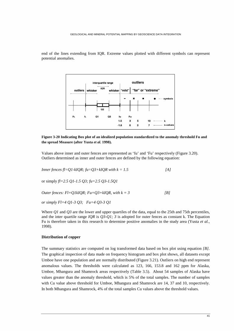
GEOLOGICAL AND MINERAL POTENTIAL MAPPING BY GEOSCIENCE DATA INTEGRATION
41
end of the lines extending from IQR. Extreme values plotted with different symbols can represent potential anomalies.
Figure 3-20 Indicating Box plot of an idealized population standardized to the anomaly threshold Fu and the spread Measure (after Yusta et al. 1998).
Values above inner and outer fences are represented as ‘fu’ and ‘Fu’ respectively (Figure 3.20). Outliers determined as inner and outer fences are defined by the following equation:
Inner fences fl=Q1-kIQR; fu=Q3+kIQR with k = 1.5 [A]
or simply fl=2.5 Q1-1.5 Q3; fu=2.5 Q3-1.5Q1
Outer fences: Fl=Q1kIQR; Fu=Q3+kIQR, with k = 3 [B] or simply Fl=4 Q1-3 Q3; Fu=4 Q3-3 Q1 Where Q1 and Q3 are the lower and upper quartiles of the data, equal to the 25th and 75th percentiles, and the inter quartile range IQR is Q3-Q1; 3 is adopted for outer fences as constant k. The Equation Fu is therefore taken in this research to determine positive anomalies in the study area (Yusta et al., 1998). Distribution of copper
The summary statistics are computed on log transformed data based on box plot using equation [B].
The graphical inspection of data made on frequency histogram and box plot shows, all datasets except
Umboe have one population and are normally distributed (Figure 3.21). Outliers on high end represent
anomalous values. The thresholds were calculated as 123, 166, 153.8 and 162 ppm for Alaska,
Umboe, Mhangura and Shamrock areas respectively (Table 3.5). About 54 samples of Alaska have
values greater than the anomaly threshold, which is 5% of the total samples. The number of samples
with Cu value above threshold for Umboe, Mhangura and Shamrock are 14, 37 and 10, respectively.
In both Mhangura and Shamrock, 4% of the total samples Cu values above the threshold values.
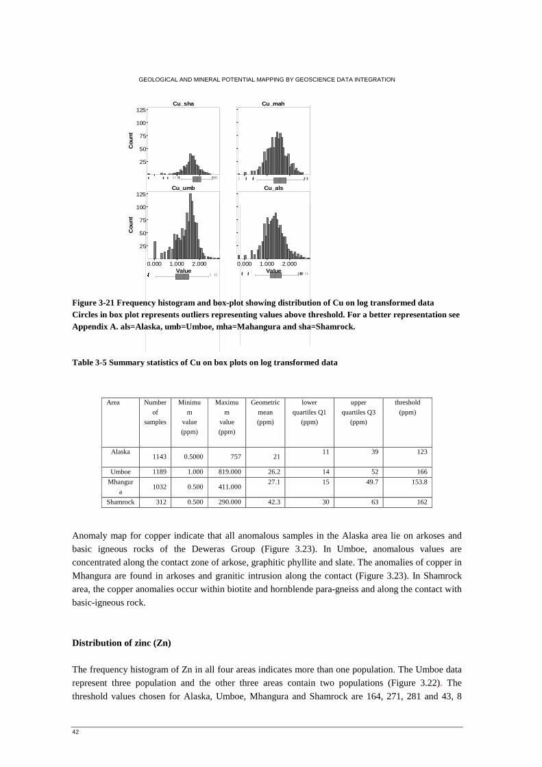
GEOLOGICAL AND MINERAL POTENTIAL MAPPING BY GEOSCIENCE DATA INTEGRATION
42
Figure 3-21 Frequency histogram and box-plot showing distribution of Cu on log transformed data Circles in box plot represents outliers representing values above threshold. For a better representation see Appendix A. als=Alaska, umb=Umboe, mha=Mahangura and sha=Shamrock. Table 3-5 Summary statistics of Cu on box plots on log transformed data
Anomaly map for copper indicate that all anomalous samples in the Alaska area lie on arkoses and
basic igneous rocks of the Deweras Group (Figure 3.23). In Umboe, anomalous values are
concentrated along the contact zone of arkose, graphitic phyllite and slate. The anomalies of copper in
Mhangura are found in arkoses and granitic intrusion along the contact (Figure 3.23). In Shamrock
area, the copper anomalies occur within biotite and hornblende para-gneiss and along the contact with
basic-igneous rock.
Distribution of zinc (Zn) The frequency histogram of Zn in all four areas indicates more than one population. The Umboe data
represent three population and the other three areas contain two populations (Figure 3.22). The
threshold values chosen for Alaska, Umboe, Mhangura and Shamrock are 164, 271, 281 and 43, 8
Area Number
of
samples
Minimu
m
value
(ppm)
Maximu
m
value
(ppm)
Geometric
mean
(ppm)
lower
quartiles Q1
(ppm)
upper
quartiles Q3
(ppm)
threshold
(ppm)
Alaska
1143 0.5000 757 21
11 39 123
Umboe 1189 1.000 819.000 26.2 14 52 166
Mhangur
a 1032 0.500 411.000
27.1 15 49.7 153.8
Shamrock 312 0.500 290.000 42.3 30 63 162
������������������������� ��������� ��
���� �� ���� �� �� �� ���� ���� ��� ����� � �
�� � � ���� ����� ���� ������� ���
25
50
75
100
125
Cou
nt
Cu_sha Cu_mah
Cu_umb Cu_als
0.000 1.000 2.000Value
25
50
75
100
125
Cou
nt
0.000 1.000 2.000Value
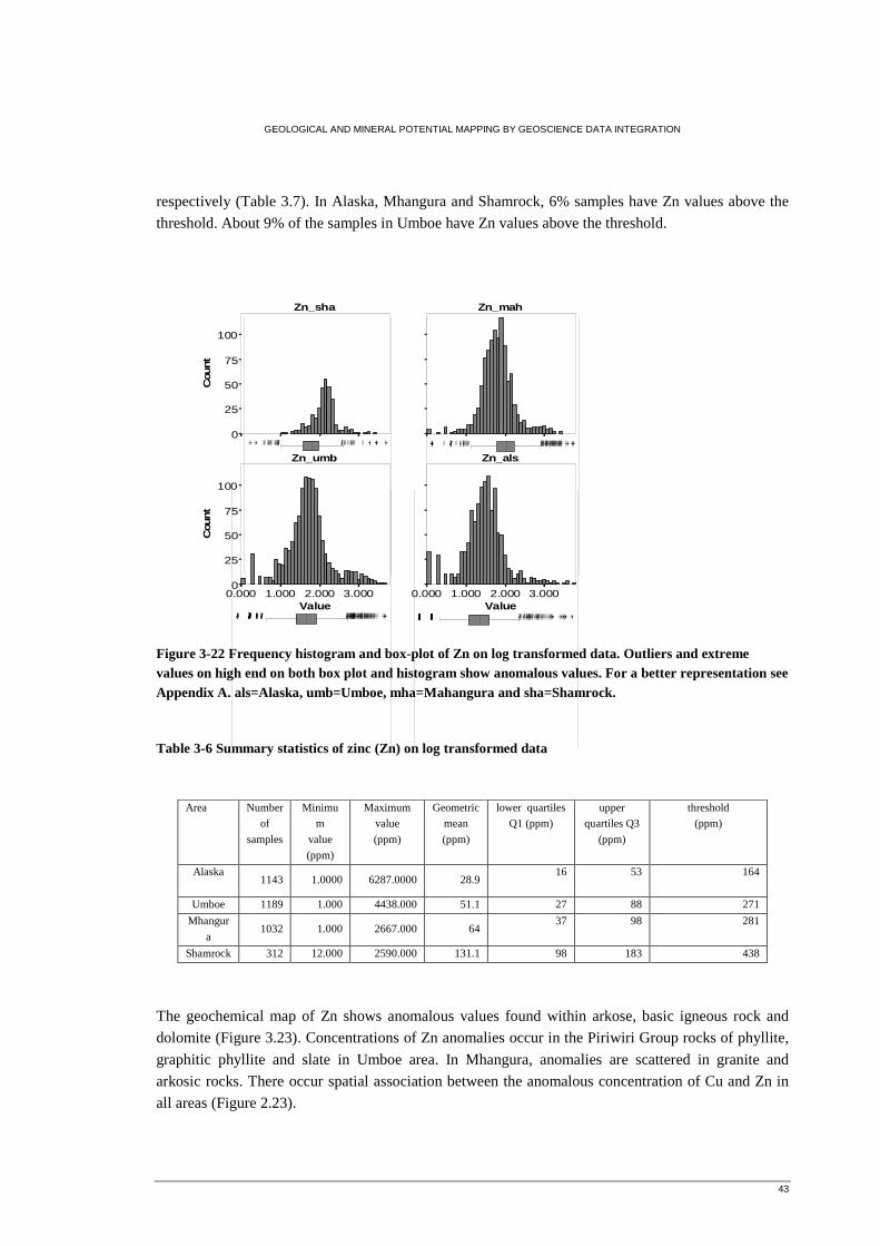
GEOLOGICAL AND MINERAL POTENTIAL MAPPING BY GEOSCIENCE DATA INTEGRATION
43
respectively (Table 3.7). In Alaska, Mhangura and Shamrock, 6% samples have Zn values above the
threshold. About 9% of the samples in Umboe have Zn values above the threshold.
Figure 3-22 Frequency histogram and box-plot of Zn on log transformed data. Outliers and extreme values on high end on both box plot and histogram show anomalous values. For a better representation see Appendix A. als=Alaska, umb=Umboe, mha=Mahangura and sha=Shamrock.
Table 3-6 Summary statistics of zinc (Zn) on log transformed data
The geochemical map of Zn shows anomalous values found within arkose, basic igneous rock and
dolomite (Figure 3.23). Concentrations of Zn anomalies occur in the Piriwiri Group rocks of phyllite,
graphitic phyllite and slate in Umboe area. In Mhangura, anomalies are scattered in granite and
arkosic rocks. There occur spatial association between the anomalous concentration of Cu and Zn in
all areas (Figure 2.23).
Area Number
of
samples
Minimu
m
value
(ppm)
Maximum
value
(ppm)
Geometric
mean
(ppm)
lower quartiles
Q1 (ppm)
upper
quartiles Q3
(ppm)
threshold
(ppm)
Alaska
1143 1.0000 6287.0000 28.9
16 53 164
Umboe 1189 1.000 4438.000 51.1 27 88 271
Mhangur
a 1032 1.000 2667.000 64
37 98 281
Shamrock 312 12.000 2590.000 131.1 98 183 438
��� � � ���� �� ���� �� ���� ���� ��� �� � �� � �������� ��� �� � ���� � ��� � ����� � �� ���� ���� �� ���� ������������ ������ ���� �� �
��� � ��� ����� � � ��� �� �� ����� �� �� �� ��� � ��� �� ��� �� ���� ��� ���� �� � ����� ��
0
25
50
75
100
Cou
nt
Zn_sha Zn_mah
Zn_umb Zn_als
0.000 1.000 2.000 3.000Value
0
25
50
75
100
Cou
nt
0.000 1.000 2.000 3.000Value
� ����� �� � � �� � ��� ������ ��� �������� �� ����� �� �� ���� ����� �� �� ��� �� � ��� �� �� ��� ��� �� � ��� � � ��� � ��� ���� � ���� � ��� ���� ��� � � � �� � � �� ��� � ��
�� � ��� �� ���� � � ��� � �� � �� �� �� ���� ��
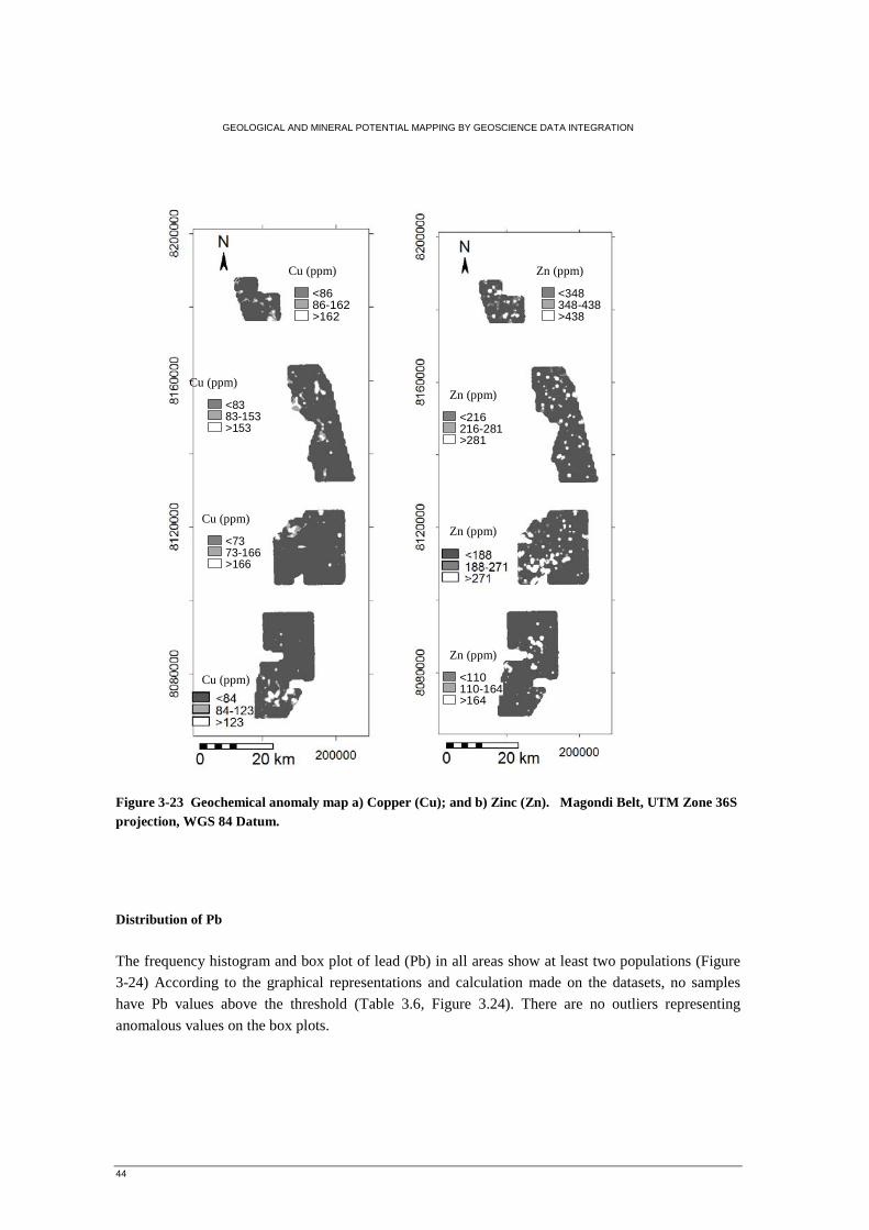
GEOLOGICAL AND MINERAL POTENTIAL MAPPING BY GEOSCIENCE DATA INTEGRATION
44
Figure 3-23 Geochemical anomaly map a) Copper (Cu); and b) Zinc (Zn). Magondi Belt, UTM Zone 36S projection, WGS 84 Datum.
Distribution of Pb
The frequency histogram and box plot of lead (Pb) in all areas show at least two populations (Figure
3-24) According to the graphical representations and calculation made on the datasets, no samples
have Pb values above the threshold (Table 3.6, Figure 3.24). There are no outliers representing
anomalous values on the box plots.
<8383-153>153
<7373-166>166
Cu (ppm)
<86 86-162 >162
Cu (ppm)
Cu (ppm)
Cu (ppm) <110110-164>164
<216216-281>281
<348348-438>438
Zn (ppm)
Zn (ppm)
Zn (ppm)
Zn (ppm)
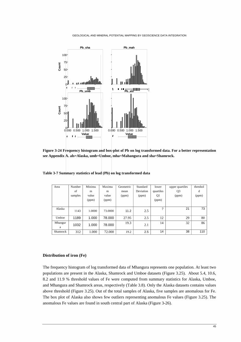
GEOLOGICAL AND MINERAL POTENTIAL MAPPING BY GEOSCIENCE DATA INTEGRATION
45
Figure 3-24 Frequency histogram and box-plot of Pb on log transformed data. For a better representation see Appendix A. als=Alaska, umb=Umboe, mha=Mahangura and sha=Shamrock.
Table 3-7 Summary statistics of lead (Pb) on log transformed data
Distribution of iron (Fe) The frequency histogram of log transformed data of Mhangura represents one population. At least two
populations are present in the Alaska, Shamrock and Umboe datasets (Figure 3.25). About 5.4, 10.6,
8.2 and 11.9 % threshold values of Fe were computed from summary statistics for Alaska, Umboe,
and Mhangura and Shamrock areas, respectively (Table 3.8). Only the Alaska datasets contains values
above threshold (Figure 3.25). Out of the total samples of Alaska, five samples are anomalous for Fe.
The box plot of Alaska also shows few outliers representing anomalous Fe values (Figure 3.25). The
anomalous Fe values are found in south central part of Alaska (Figure 3-26).
Area Number
of
samples
Minimu
m
value
(ppm)
Maximu
m
value
(ppm)
Geometric
mean
(ppm)
Standard
Deviation
(ppm)
lower
quartiles
Q1
(ppm)
upper quartiles
Q3
(ppm)
threshol
d
(ppm)
Alaska
1143 1.0000 73.0000 11.2 2.5 7 21 73
Umboe 1189 1.000 78.000 27.95 2.5 12 29 80 Mhangur
a 1032 1.000 78.000
19.3 2.1
14 32 86
Shamrock 312 1.000 72.000 19.2 2.5 14 38 110
0
25
50
75
100
Cou
nt
Pb_sha Pb_mah
Pb_umb Pb_als
0.000 0.500 1.000 1.500Value
0
25
50
75
100
Cou
nt
0.000 0.500 1.000 1.500Value
����������������������������������������������������������������������� ��� ������ ���� ���� �� ����� ��������� ����� ��� �������������������������������������������������������
������ ���� ��� ��� �� ��
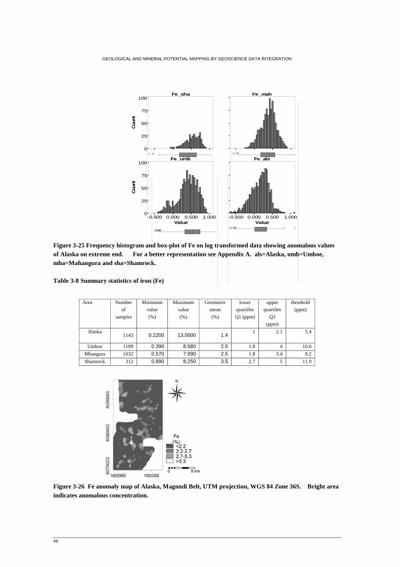
GEOLOGICAL AND MINERAL POTENTIAL MAPPING BY GEOSCIENCE DATA INTEGRATION
46
Figure 3-25 Frequency histogram and box-plot of Fe on log transformed data showing anomalous values of Alaska on extreme end. For a better representation see Appendix A. als=Alaska, umb=Umboe, mha=Mahangura and sha=Shamrock. Table 3-8 Summary statistics of iron (Fe)
Figure 3-26 Fe anomaly map of Alaska, Magondi Belt, UTM projection, WGS 84 Zone 36S. Bright area indicates anomalous concentration.
Area Number
of
samples
Minimum
value
(%)
Maximum
value
(%)
Geometric
mean
(%)
lower
quartiles
Q1 (ppm)
upper
quartiles
Q3
(ppm)
threshold
(ppm)
Alaska
1143 0.2200 13.0000 1.4
1 2.1 5.4
Umboe 1189 0.390 8.580 2.5 1.8 4 10.6
Mhangura 1032 0.570 7.990 2.5 1.8 3.4 8.2
Shamrock 312 0.890 8.250 3.5 2.7 5 11.9
� � � ��� � ��� ��
0
25
50
75
100
Cou
nt
Fe_sha Fe_mah
Fe_umb Fe_als
-0.500 0.000 0.500 1.000Value
0
25
50
75
100
Cou
nt
-0.500 0.000 0.500 1.000Value
�� �� �� �� ��� �� ��
�� ������ ���
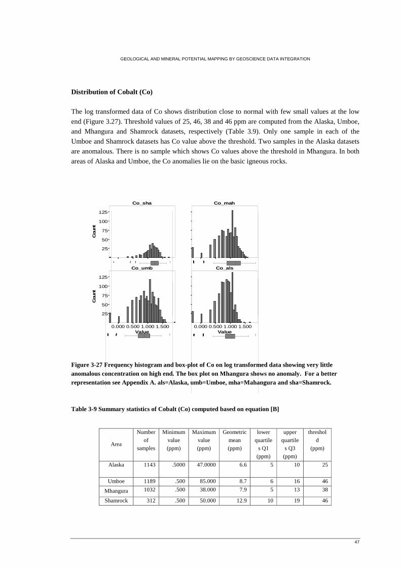
GEOLOGICAL AND MINERAL POTENTIAL MAPPING BY GEOSCIENCE DATA INTEGRATION
47
Distribution of Cobalt (Co)
The log transformed data of Co shows distribution close to normal with few small values at the low
end (Figure 3.27). Threshold values of 25, 46, 38 and 46 ppm are computed from the Alaska, Umboe,
and Mhangura and Shamrock datasets, respectively (Table 3.9). Only one sample in each of the
Umboe and Shamrock datasets has Co value above the threshold. Two samples in the Alaska datasets
are anomalous. There is no sample which shows Co values above the threshold in Mhangura. In both
areas of Alaska and Umboe, the Co anomalies lie on the basic igneous rocks.
Figure 3-27 Frequency histogram and box-plot of Co on log transformed data showing very little anomalous concentration on high end. The box plot on Mhangura shows no anomaly. For a better representation see Appendix A. als=Alaska, umb=Umboe, mha=Mahangura and sha=Shamrock. Table 3-9 Summary statistics of Cobalt (Co) computed based on equation [B]
Area
Number
of
samples
Minimum
value
(ppm)
Maximum
value
(ppm)
Geometric
mean
(ppm)
lower
quartile
s Q1
(ppm)
upper
quartile
s Q3
(ppm)
threshol
d
(ppm)
Alaska
1143 .5000 47.0000 6.6 5 10 25
Umboe 1189 .500 85.000 8.7 6 16 46
Mhangura 1032 .500 38.000 7.9 5 13 38
Shamrock 312 .500 50.000 12.9 10 19 46
�� ������������������������������������������������������ ��� ���������� ����� � ����� ��������� ���� ��� �� �
������ �������� ����� ���� ���� �� �� ����������� ��� ���
25
50
75
100
125
Cou
nt
Co_sha Co_mah
Co_umb Co_als
0.000 0.500 1.000 1.500Value
25
50
75
100
125
Cou
nt
0.000 0.500 1.000 1.500Value
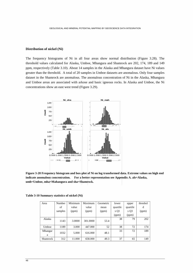
GEOLOGICAL AND MINERAL POTENTIAL MAPPING BY GEOSCIENCE DATA INTEGRATION
48
Distribution of nickel (Ni) The frequency histograms of Ni in all four areas show normal distribution (Figure 3.28). The
threshold values calculated for Alaska, Umboe, Mhangura and Shamrock are 202, 174, 189 and 149
ppm, respectively (Table 3.10). About 14 samples in the Alaska and Mhangura dataset have Ni values
greater than the threshold. A total of 20 samples in Umboe datasets are anomalous. Only four samples
dataset in the Shamrock are anomalous. The anomalous concentration of Ni in the Alaska, Mhangura
and Umboe areas are associated with arkose and basic igneous rocks. In Alaska and Umboe, the Ni
concentrations show an east west trend (Figure 3.29).
Figure 3-28 Frequency histogram and box-plot of Ni on log transformed data. Extreme values on high end indicate anomalous concentration. For a better representation see Appendix A. als=Alaska, umb=Umboe, mha=Mahangura and sha=Shamrock.
Table 3-10 Summary statistics of nickel (Ni)
Area Number
of
samples
Minimum
value
(ppm)
Maximum
value
(ppm)
Geometric
mean
(ppm)
lower
quartile
s Q1
(ppm)
upper
quartile
s Q3
(ppm)
threshol
d
(ppm)
Alaska
1143 3.0000 301.0000 53.4
38 79 202
Umboe 1189 3.000 447.000 52 38 72 174
Mhangur
a 1032 5.000 616.000 48.1
33 72 189
Shamrock 312 11.000 658.000 49.3 37 65 149
25
50
75
100
125
Cou
nt
Ni_sha Ni_mah
Ni_umb Ni_als
0.5001.0001.5002.0002.500Value
25
50
75
100
125
Cou
nt
0.5001.0001.5002.0002.500Value
��� ����� ����� �� � ��� � �� � ��� ��� ��������� �� ��� �� �� � ���� � ��� ���� � � ����
� � ��� �� �� �� � ���� �� � � ��� � ��� �� �� �
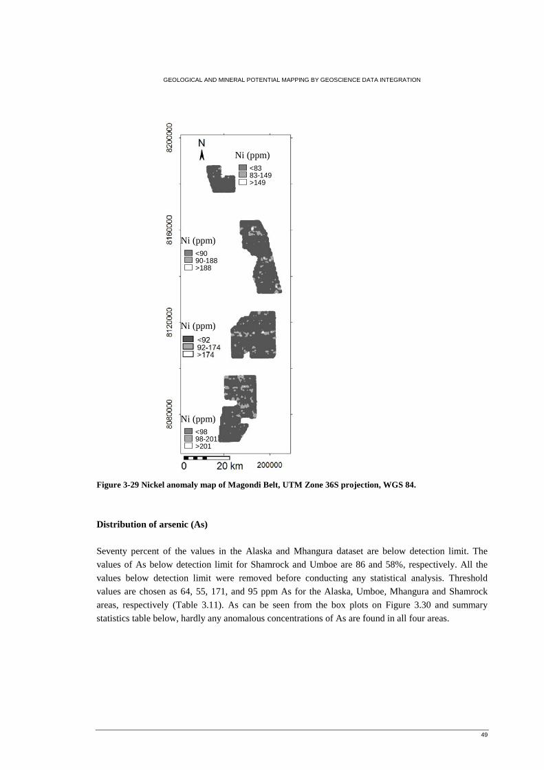
GEOLOGICAL AND MINERAL POTENTIAL MAPPING BY GEOSCIENCE DATA INTEGRATION
49
Figure 3-29 Nickel anomaly map of Magondi Belt, UTM Zone 36S projection, WGS 84.
Distribution of arsenic (As) Seventy percent of the values in the Alaska and Mhangura dataset are below detection limit. The
values of As below detection limit for Shamrock and Umboe are 86 and 58%, respectively. All the
values below detection limit were removed before conducting any statistical analysis. Threshold
values are chosen as 64, 55, 171, and 95 ppm As for the Alaska, Umboe, Mhangura and Shamrock
areas, respectively (Table 3.11). As can be seen from the box plots on Figure 3.30 and summary
statistics table below, hardly any anomalous concentrations of As are found in all four areas.
<9898-201>201
<9090-188>188
<8383-149>149
Ni (ppm)
Ni (ppm)
Ni (ppm)
Ni (ppm)
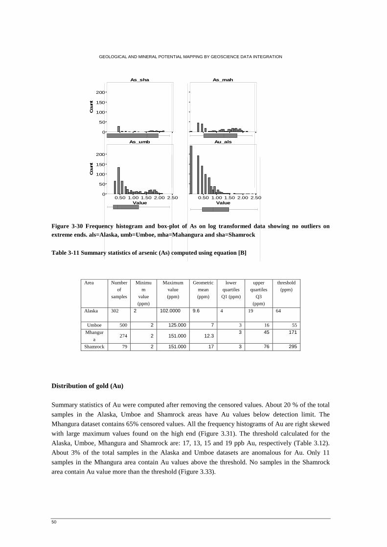
GEOLOGICAL AND MINERAL POTENTIAL MAPPING BY GEOSCIENCE DATA INTEGRATION
50
Figure 3-30 Frequency histogram and box-plot of As on log transformed data showing no outliers on extreme ends. als=Alaska, umb=Umboe, mha=Mahangura and sha=Shamrock
Table 3-11 Summary statistics of arsenic (As) computed using equation [B]
Distribution of gold (Au) Summary statistics of Au were computed after removing the censored values. About 20 % of the total
samples in the Alaska, Umboe and Shamrock areas have Au values below detection limit. The
Mhangura dataset contains 65% censored values. All the frequency histograms of Au are right skewed
with large maximum values found on the high end (Figure 3.31). The threshold calculated for the
Alaska, Umboe, Mhangura and Shamrock are: 17, 13, 15 and 19 ppb Au, respectively (Table 3.12).
About 3% of the total samples in the Alaska and Umboe datasets are anomalous for Au. Only 11
samples in the Mhangura area contain Au values above the threshold. No samples in the Shamrock
area contain Au value more than the threshold (Figure 3.33).
Area Number
of
samples
Minimu
m
value
(ppm)
Maximum
value
(ppm)
Geometric
mean
(ppm)
lower
quartiles
Q1 (ppm)
upper
quartiles
Q3
(ppm)
threshold
(ppm)
Alaska
302 2
102.0000 9.6 4 19 64
Umboe 500 2 125.000 7 3 16 55
Mhangur
a 274 2 151.000 12.3
3 45 171
Shamrock 79 2 151.000 17 3 76 295
0
50
100
150
200C
ount
As_sha As_mah
As_umb Au_als
0.50 1.00 1.50 2.00 2.50Value
0
50
100
150
200
Cou
nt
0.50 1.00 1.50 2.00 2.50Value
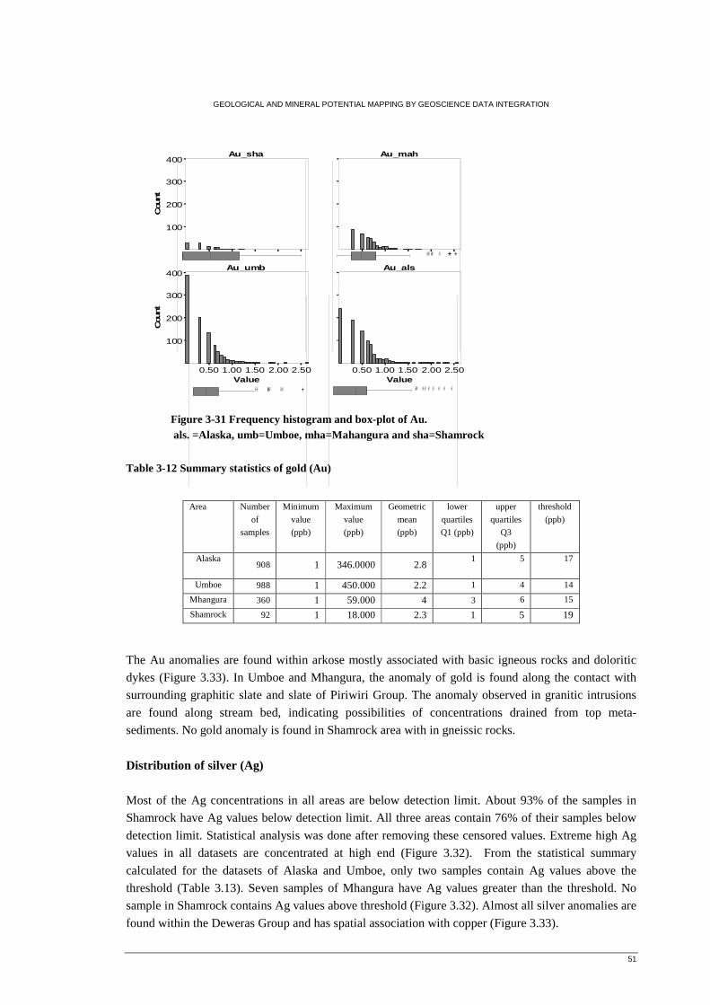
GEOLOGICAL AND MINERAL POTENTIAL MAPPING BY GEOSCIENCE DATA INTEGRATION
51
Figure 3-31 Frequency histogram and box-plot of Au. als. =Alaska, umb=Umboe, mha=Mahangura and sha=Shamrock
Table 3-12 Summary statistics of gold (Au)
The Au anomalies are found within arkose mostly associated with basic igneous rocks and doloritic
dykes (Figure 3.33). In Umboe and Mhangura, the anomaly of gold is found along the contact with
surrounding graphitic slate and slate of Piriwiri Group. The anomaly observed in granitic intrusions
are found along stream bed, indicating possibilities of concentrations drained from top meta-
sediments. No gold anomaly is found in Shamrock area with in gneissic rocks.
Distribution of silver (Ag)
Most of the Ag concentrations in all areas are below detection limit. About 93% of the samples in
Shamrock have Ag values below detection limit. All three areas contain 76% of their samples below
detection limit. Statistical analysis was done after removing these censored values. Extreme high Ag
values in all datasets are concentrated at high end (Figure 3.32). From the statistical summary
calculated for the datasets of Alaska and Umboe, only two samples contain Ag values above the
threshold (Table 3.13). Seven samples of Mhangura have Ag values greater than the threshold. No
sample in Shamrock contains Ag values above threshold (Figure 3.32). Almost all silver anomalies are
found within the Deweras Group and has spatial association with copper (Figure 3.33).
Area Number
of
samples
Minimum
value
(ppb)
Maximum
value
(ppb)
Geometric
mean
(ppb)
lower
quartiles
Q1 (ppb)
upper
quartiles
Q3
(ppb)
threshold
(ppb)
Alaska
908 1 346.0000 2.8
1 5 17
Umboe 988 1 450.000 2.2 1 4 14
Mhangura 360 1 59.000 4 3 6 15
Shamrock 92 1 18.000 2.3 1 5 19
100
200
300
400C
ount
Au_sha Au_mah
Au_umb Au_als
0.50 1.00 1.50 2.00 2.50Value
100
200
300
400
Cou
nt
0.50 1.00 1.50 2.00 2.50Value
�� �� � � � � ��� ���� �� �
���� � �� �
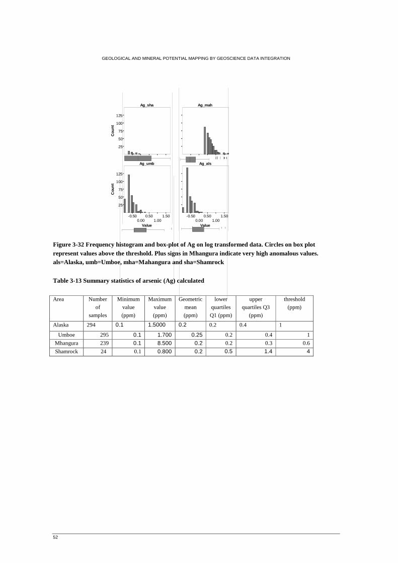
GEOLOGICAL AND MINERAL POTENTIAL MAPPING BY GEOSCIENCE DATA INTEGRATION
52
Figure 3-32 Frequency histogram and box-plot of Ag on log transformed data. Circles on box plot represent values above the threshold. Plus signs in Mhangura indicate very high anomalous values. als=Alaska, umb=Umboe, mha=Mahangura and sha=Shamrock
Table 3-13 Summary statistics of arsenic (Ag) calculated
Area Number
of
samples
Minimum
value
(ppm)
Maximum
value
(ppm)
Geometric
mean
(ppm)
lower
quartiles
Q1 (ppm)
upper
quartiles Q3
(ppm)
threshold
(ppm)
Alaska 294 0.1 1.5000 0.2 0.2 0.4 1
Umboe 295 0.1 1.700 0.25 0.2 0.4 1
Mhangura 239 0.1 8.500 0.2 0.2 0.3 0.6
Shamrock 24 0.1 0.800 0.2 0.5 1.4 4
25
50
75
100
125C
oun
t
Ag_sha Ag_mah
Ag_umb Ag_als
-0.500.00
0.501.00
1.50
Value
25
50
75
100
125
Cou
nt
-0.500.00
0.501.00
1.50
Value� ��
���� � �� �
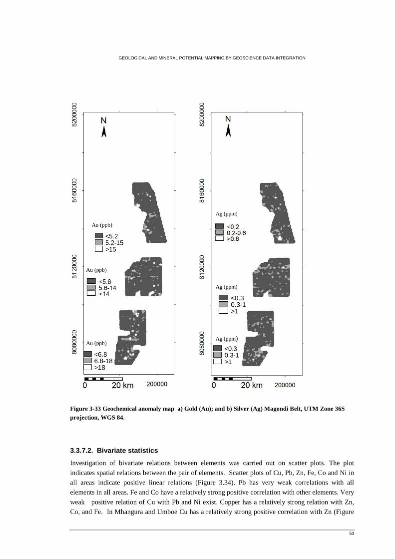
GEOLOGICAL AND MINERAL POTENTIAL MAPPING BY GEOSCIENCE DATA INTEGRATION
53
Figure 3-33 Geochemical anomaly map a) Gold (Au); and b) Silver (Ag) Magondi Belt, UTM Zone 36S projection, WGS 84.
3.3.7.2. Bivariate statistics
Investigation of bivariate relations between elements was carried out on scatter plots. The plot
indicates spatial relations between the pair of elements. Scatter plots of Cu, Pb, Zn, Fe, Co and Ni in
all areas indicate positive linear relations (Figure 3.34). Pb has very weak correlations with all
elements in all areas. Fe and Co have a relatively strong positive correlation with other elements. Very
weak positive relation of Cu with Pb and Ni exist. Copper has a relatively strong relation with Zn,
Co, and Fe. In Mhangura and Umboe Cu has a relatively strong positive correlation with Zn (Figure
<6.86.8-18>18
<5.25.2-15>15
Au (ppb)
Au (ppb)
Au (ppb)
Ag (ppm)
<0.30.3-1>1
<0.30.3-1>1
Ag (ppm)
Ag (ppm)
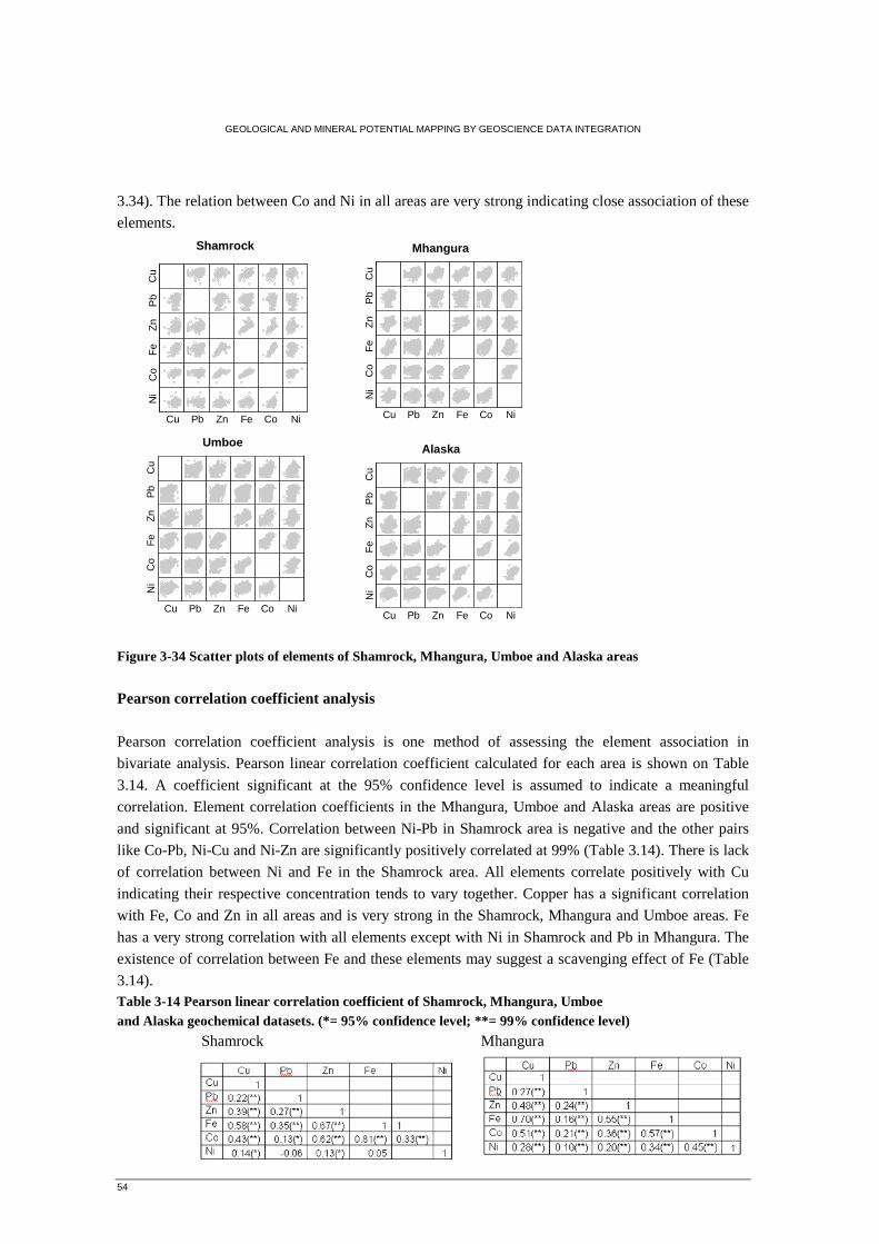
GEOLOGICAL AND MINERAL POTENTIAL MAPPING BY GEOSCIENCE DATA INTEGRATION
54
NiCoFeZnPbCu
Cu
Pb
Zn
Fe
Co
Ni
Mhangura
NiCoFeZnPbCu
Cu
Pb
Zn
Fe
Co
Ni
Shamrock
NiCoFeZnPbCu
Cu
Pb
Zn
Fe
Co
Ni
Umboe
NiCoFeZnPbCu
Cu
Pb
Zn
Fe
Co
Ni
Alaska
3.34). The relation between Co and Ni in all areas are very strong indicating close association of these
elements.
Figure 3-34 Scatter plots of elements of Shamrock, Mhangura, Umboe and Alaska areas
Pearson correlation coefficient analysis Pearson correlation coefficient analysis is one method of assessing the element association in
bivariate analysis. Pearson linear correlation coefficient calculated for each area is shown on Table
3.14. A coefficient significant at the 95% confidence level is assumed to indicate a meaningful
correlation. Element correlation coefficients in the Mhangura, Umboe and Alaska areas are positive
and significant at 95%. Correlation between Ni-Pb in Shamrock area is negative and the other pairs
like Co-Pb, Ni-Cu and Ni-Zn are significantly positively correlated at 99% (Table 3.14). There is lack
of correlation between Ni and Fe in the Shamrock area. All elements correlate positively with Cu
indicating their respective concentration tends to vary together. Copper has a significant correlation
with Fe, Co and Zn in all areas and is very strong in the Shamrock, Mhangura and Umboe areas. Fe
has a very strong correlation with all elements except with Ni in Shamrock and Pb in Mhangura. The
existence of correlation between Fe and these elements may suggest a scavenging effect of Fe (Table
3.14). Table 3-14 Pearson linear correlation coefficient of Shamrock, Mhangura, Umboe and Alaska geochemical datasets. (*= 95% confidence level; **= 99% confidence level)
Shamrock Mhangura
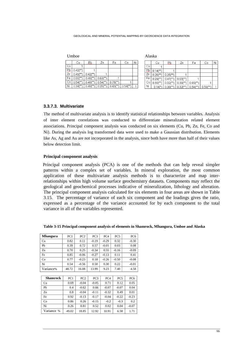
GEOLOGICAL AND MINERAL POTENTIAL MAPPING BY GEOSCIENCE DATA INTEGRATION
55
Umboe Alaska
3.3.7.3. Multivariate
The method of multivariate analysis is to identify statistical relationships between variables. Analysis
of inter element correlations was conducted to differentiate mineralization related element
associations. Principal component analysis was conducted on six elements (Cu, Pb, Zn, Fe, Co and
Ni). During the analysis log transformed data were used to make a Gaussian distribution. Elements
like As, Ag and Au are not incorporated in the analysis, since both have more than half of their values
below detection limit.
Principal component analysis
Principal component analysis (PCA) is one of the methods that can help reveal simpler patterns within a complex set of variables. In mineral exploration, the most common application of these multivariate analysis methods is to characterize and map inter-relationships within high volume surface geochemistry datasets. Components may reflect the geological and geochemical processes indicative of mineralization, lithology and alteration. The principal component analysis calculated for six elements in four areas are shown in Table 3.15. The percentage of variance of each six component and the loadings gives the ratio, expressed as a percentage of the variance accounted for by each component to the total variance in all of the variables represented.
Table 3-15 Principal component analysis of elements in Shamrock, Mhangura, Umboe and Alaska
Mhangura PC1 PC2 PC3 PC4 PC5 PC6
Cu 0.82 0.11 -0.19 -0.29 0.32 -0.30
Pb 0.39 0.72 0.57 -0.01 0.03 0.08
Zn 0.70 0.25 -0.34 0.55 -0.16 -0.09
Fe 0.85 -0.06 -0.27 -0.13 0.11 0.41
Co 0.77 -0.23 0.18 -0.26 -0.50 -0.08
Ni 0.54 -0.56 0.50 0.30 0.22 -0.01
Variance% 48.72 16.08 13.99 9.23 7.40 4.58
Shamrock PC1 PC2 PC3 PC4 PC5 PC6
Cu 0.69 -0.04 -0.05 0.71 0.12 0.05
Pb 0.4 -0.62 0.66 -0.07 -0.07 0.04
Zn 0.8 -0.04 -0.11 -0.32 0.49 0.01
Fe 0.92 -0.13 -0.17 -0.04 -0.22 -0.23
Co 0.86 0.26 -0.15 -0.2 -0.3 0.2
Ni 0.26 0.81 0.52 0.02 0.04 -0.07
Variance % 49.02 18.85 12.92 10.91 6.58 1.71
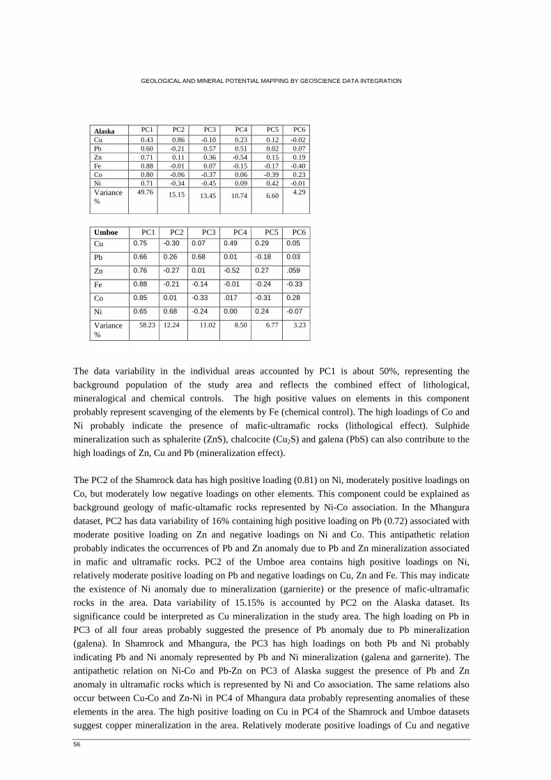
GEOLOGICAL AND MINERAL POTENTIAL MAPPING BY GEOSCIENCE DATA INTEGRATION
56
The data variability in the individual areas accounted by PC1 is about 50%, representing the
background population of the study area and reflects the combined effect of lithological,
mineralogical and chemical controls. The high positive values on elements in this component
probably represent scavenging of the elements by Fe (chemical control). The high loadings of Co and
Ni probably indicate the presence of mafic-ultramafic rocks (lithological effect). Sulphide
mineralization such as sphalerite (ZnS), chalcocite (Cu2S) and galena (PbS) can also contribute to the
high loadings of Zn, Cu and Pb (mineralization effect).
The PC2 of the Shamrock data has high positive loading (0.81) on Ni, moderately positive loadings on
Co, but moderately low negative loadings on other elements. This component could be explained as
background geology of mafic-ultamafic rocks represented by Ni-Co association. In the Mhangura
dataset, PC2 has data variability of 16% containing high positive loading on Pb (0.72) associated with
moderate positive loading on Zn and negative loadings on Ni and Co. This antipathetic relation
probably indicates the occurrences of Pb and Zn anomaly due to Pb and Zn mineralization associated
in mafic and ultramafic rocks. PC2 of the Umboe area contains high positive loadings on Ni,
relatively moderate positive loading on Pb and negative loadings on Cu, Zn and Fe. This may indicate
the existence of Ni anomaly due to mineralization (garnierite) or the presence of mafic-ultramafic
rocks in the area. Data variability of 15.15% is accounted by PC2 on the Alaska dataset. Its
significance could be interpreted as Cu mineralization in the study area. The high loading on Pb in
PC3 of all four areas probably suggested the presence of Pb anomaly due to Pb mineralization
(galena). In Shamrock and Mhangura, the PC3 has high loadings on both Pb and Ni probably
indicating Pb and Ni anomaly represented by Pb and Ni mineralization (galena and garnerite). The
antipathetic relation on Ni-Co and Pb-Zn on PC3 of Alaska suggest the presence of Pb and Zn
anomaly in ultramafic rocks which is represented by Ni and Co association. The same relations also
occur between Cu-Co and Zn-Ni in PC4 of Mhangura data probably representing anomalies of these
elements in the area. The high positive loading on Cu in PC4 of the Shamrock and Umboe datasets
suggest copper mineralization in the area. Relatively moderate positive loadings of Cu and negative
Alaska PC1 PC2 PC3 PC4 PC5 PC6
Cu 0.43 0.86 -0.10 0.23 0.12 -0.02 Pb 0.60 -0.21 0.57 0.51 0.02 0.07 Zn 0.71 0.11 0.36 -0.54 0.15 0.19 Fe 0.88 -0.01 0.07 -0.15 -0.17 -0.40 Co 0.80 -0.06 -0.37 0.06 -0.39 0.23 Ni 0.71 -0.34 -0.45 0.09 0.42 -0.01 Variance %
49.76 15.15
13.45
10.74
6.60
4.29
Umboe PC1 PC2 PC3 PC4 PC5 PC6
Cu 0.75 -0.30 0.07 0.49 0.29 0.05
Pb 0.66 0.26 0.68 0.01 -0.18 0.03
Zn 0.76 -0.27 0.01 -0.52 0.27 .059
Fe 0.88 -0.21 -0.14 -0.01 -0.24 -0.33
Co 0.85 0.01 -0.33 .017 -0.31 0.28
Ni 0.65 0.68 -0.24 0.00 0.24 -0.07
Variance%
58.23 12.24 11.02 8.50
6.77 3.23
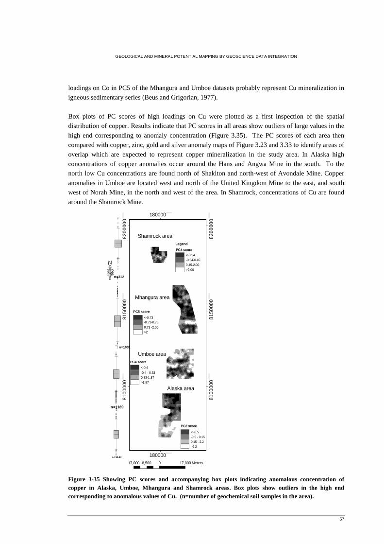
GEOLOGICAL AND MINERAL POTENTIAL MAPPING BY GEOSCIENCE DATA INTEGRATION
57
180000.000000
180000.000000
8100
000.0
000
00
8100
000.0
000
00
8150
000.0
0000
0
8150
000.0
0000
0
8200
000.0
0000
0
8200
000.0
0000
0
·
17,000 0 17,0008,500 Meters
Shamrock area
Mhangura area
Umboe area
Alaska area
PC2 score
< -0.5
-0.5 - 0.15
0.15 - 2.2
>2.2
PC4 score
<-0.4
-0.4 - 0.330.33-1.87>1.87
PC5 score
<-0.73-0.73-0.73
0.73 -2.00>2
Legend
PC4 score<-0.54-0.54-0.450.45-2.00>2.00
���
��
�
���
�
�
��
�
�
��
��
�
�
��
�
����
�
���
n=1143
�
�
�
�
�
�
�
��
�
�
�
�
�
�
�
�
�
�
�
�
�
�
�
���
���
�
�
�
�
�
��
��
�
�
��
���
�
��
��
�
�
�
��
�
�
�
�
�
�
�
�
��
��
�
�
�
���
n=1189
�
�
��
�
�
�
�
�
��
�
�
��
�
�
�
�
�
�
�
�
�
�
�
�
��
��
n=1032
�
�
��
�
��
�
�
���
�
�
n=312
loadings on Co in PC5 of the Mhangura and Umboe datasets probably represent Cu mineralization in
igneous sedimentary series (Beus and Grigorian, 1977).
Box plots of PC scores of high loadings on Cu were plotted as a first inspection of the spatial
distribution of copper. Results indicate that PC scores in all areas show outliers of large values in the
high end corresponding to anomaly concentration (Figure 3.35). The PC scores of each area then
compared with copper, zinc, gold and silver anomaly maps of Figure 3.23 and 3.33 to identify areas of
overlap which are expected to represent copper mineralization in the study area. In Alaska high
concentrations of copper anomalies occur around the Hans and Angwa Mine in the south. To the
north low Cu concentrations are found north of Shaklton and north-west of Avondale Mine. Copper
anomalies in Umboe are located west and north of the United Kingdom Mine to the east, and south
west of Norah Mine, in the north and west of the area. In Shamrock, concentrations of Cu are found
around the Shamrock Mine.
Figure 3-35 Showing PC scores and accompanying box plots indicating anomalous concentration of copper in Alaska, Umboe, Mhangura and Shamrock areas. Box plots show outliers in the high end corresponding to anomalous values of Cu. (n=number of geochemical soil samples in the area).
GEOLOGICAL AND MINERAL POTENTIAL MAPPING BY GEOSCIENCE DATA INTEGRATION
58
Geochemical interpretations
The spatial distributions of elements indicate that, most of the anomalies were found within the
arkoses of the Deweras Group. Some anomalies were also found along the surrounding boundaries of
arkoses with granite, slate and phyllite. The univariate analysis revealed that out of nine elements, six
elements, (Cu, Zn, Ni, Co, Au and Ag) show anomalous values in most of the datasets. Only Alaska
has anomaly of Fe. No anomaly of Co is encountered in Mhangura. The Absence of Au and Ag
anomalies in Shamrock area suggest no mineralization of these elements in gneissic rocks. Zn, Ni, Au
and Ag have a spatial relation with Cu indicating their close association. Copper has remarkable
strong positive relation with Zn, Co and Fe and weak relation with Ni and Pb. The positive linear
relations of copper in both areas might indicate same origin and type of mineralization hosted in
particular types of rocks, in this case arkose and basic igneous rocks of the Deweras Group.
The first component in the principal component analysis contains high loadings on all elements. The
relatively high loading of elements with Fe in this component probably indicates the possible
scavenging of elements with coprecipitation with iron hydroxide. High loadings of Ni and positive
loading on Co in PC2 of Shamrock could be due to the presence of mafic-ultamafic rocks represented
by Ni-Co association. Antipathetic relation between Pb-Zn and Ni-Co, in Mhangura and Ni-Pb and
Cu-Zn in Umboe, also corresponds to same rock containing Pb-Zn and Cu mineralization (Table
3.15). PC2 can therefore be used as one of the component to map ultramafic rocks of the study area.
The score of this component overlaps most of the basic igneous rocks and shows western extension of
meta-ultramafic rocks in Mhangura area. In Umboe, high PC2 scores coincide with anomalous
concentration of Ni. PC2 of the Alaska data, PC4 of the Umboe and Shamrock datasets and PC5 of
the Mhangura have high loadings on Cu probably representing the mineralization in the area. The
plots of scores of the components representing Cu anomalies show areas on Cu mineralization. These
components were overlapped with the copper anomaly map of Figure 3.23. The resulting map was
overlaid with the Au and Ag anomaly maps of Figure 3.33 to determine potential areas for
mineralization (Figure 3.36).
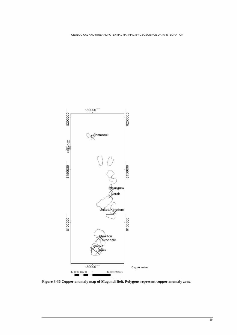
GEOLOGICAL AND MINERAL POTENTIAL MAPPING BY GEOSCIENCE DATA INTEGRATION
59
Figure 3-36 Copper anomaly map of Magondi Belt. Polygons represent copper anomaly zone.
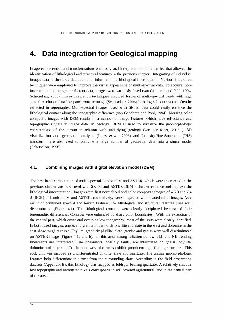
GEOLOGICAL AND MINERAL POTENTIAL MAPPING BY GEOSCIENCE DATA INTEGRATION
60
4. Data integration for Geological mapping
Image enhancement and transformations enabled visual interpretations to be carried that allowed the
identification of lithological and structural features in the previous chapter. Integrating of individual
images data further provided additional information to lthological interpretation. Various integration
techniques were employed to improve the visual appearance of multi-spectral data. To acquire more
information and integrate different data, images were variously fused (van Genderen and Pohl, 1994;
Schetselaar, 2006). Image integration techniques involved fusion of multi-spectral bands with high
spatial resolution data like panchromatic image (Schetselaar, 2006) Lithological contrast can often be
reflected in topography. Multi-spectral images fused with SRTM data could easily enhance the
lithological contact along the topographic difference (van Genderen and Pohl, 1994). Merging color
composite images with DEM results in a number of image features, which have reflectance and
topographic signals in image data. In geology, DEM is used to visualize the geomorphologic
characteristic of the terrain in relation with underlying geology (van der Meer, 2006 ). 3D
visualization and geospatial analysis (Jones et al., 2006) and Intensity-Hue-Saturation (IHS)
transform are also used to combine a large number of geospatial data into a single model
(Schetselaar, 1998).
4.1. Combining images with digital elevation model (DEM)
The best band combination of multi-spectral Landsat TM and ASTER, which were interpreted in the
previous chapter are now fused with SRTM and ASTER DEM to further enhance and improve the
lithological interpretation. Images were first normalized and color composite images of 4 5 3 and 7 4
2 (RGB) of Landsat TM and ASTER, respectively, were integrated with shaded relief images. As a
result of combined spectral and terrain features, the lithological and structural features were well
discriminated (Figure 4.1). The lithological contacts were clearly deciphered because of their
topographic differences. Contacts were enhanced by sharp color boundaries. With the exception of
the central part, which cover and occupies low topography, most of the units were clearly identified.
In both fused images, gneiss and granite in the north, phyllite and slate in the west and dolomite in the
east show rough textures. Phyllite, graphitic phyllite, slate, granite and gneiss were well discriminated
on ASTER image (Figure 4-1a and b). In this area, strong foliation trends, folds and NE trending
lineaments are interpreted. The lineaments, possibly faults, are interpreted on gneiss, phyllite,
dolomite and quartzite. To the southwest, the rocks exhibit prominent tight folding structures. This
rock unit was mapped as undifferentiated phyllite, slate and quartzite. The unique geomorphologic
features help differentiate this rock from the surrounding slate. According to the field observation
datasets (Appendix B), this lithology was mapped as feldspar-bearing quartzite. A relatively smooth,
low topography and variegated pixels corresponds to soil covered agricultural land in the central part
of the area.
GEOLOGICAL AND MINERAL POTENTIAL MAPPING BY GEOSCIENCE DATA INTEGRATION
61
4.2. Combining with high resolution image
The PCA analysis of Landsat TM conducted on previous chapter identifies lithologic features. Here,
in order to increase the spatial resolution of Landsat TM image the bands were resampled to the pixel
size of high resolution panchromatic image of Landsat band 8. Principal component analysis (PCA)
and intensity hue saturation (IHS) images can be used to merge Landsat spectral images to high
resolution panchromatic image (Rigol and Chica-Olmo, 1998; Owusu et al., 2006; Schetselaar, 2006).
Adding band 8 to PCA enhanced the resolution of the PC image and further increases the
interpretability (Figure 4.1c). The resulting image shows a clear structural features and lithologic
contacts.
To the southwest, a folded rock unit, which was not seen on enhanced images in the previous chapter,
is now clearly discriminated (Figure 4.3). This rock unit is classified as feldspar bearing quartzite
based on literature review and field observation dataset (Appendix B).
4.3. Intensity-Hue-Saturation (IHS) transformation and fusion
IHS images are well perceived by human eyes than RGB, since blue color is less sensitive to the
human eyes than red and green (van Roij, 2006). IHS color composite often adds more color to an
image and helps to discriminate lithological features.
Three steps are followed in IHS fusion and transformation in order to further enhance the color
composite image (Schetselaar, 1998). The first step is transforming the three bands to IHS. This is
followed by replacing the intensity component with the original band-image and finally transforms the
H; S using inverse IHS transforms which brings back the image to RGB. Color composite image of
Landsat TM 5 4 3 (RGB) was used for IHS transformation. The first band was replaced by high
resolution panchromatic image, band 8. The resulting image was enhanced and shows clear
lithological contacts and structural features. The western part of the area which was mapped as
undifferentiated quartzite, phyllite, graphitic slate and slate are now differentiated (Figure 4.1d). The
dark bluish pixel was one of the identified units. This rock unit according to field observation datasets
is described as feldspar bearing quartzite (Appendix B). Slate, graphitic slate and dolomite could also
be identified in the image.
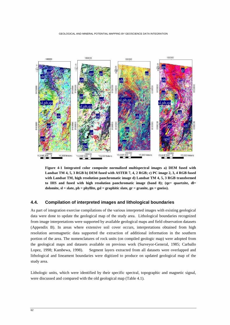
GEOLOGICAL AND MINERAL POTENTIAL MAPPING BY GEOSCIENCE DATA INTEGRATION
62
Figure 4-1 Integrated color composite normalized multispectral images a) DEM fused with Landsat TM 4, 5, 3 RGB b) DEM fused with ASTER 7, 4, 2 RGB; c) PC image 2, 3, 4 RGB fused with Landsat TM, high resolution panchromatic image d) Landsat TM 4, 5, 3 RGB transformed to IHS and fused with high resolution panchromatic image (band 8); (qz= quartzite, dl= dolomite, sl = slate, ph = phyllite, gsl = graphitic slate, gr = granite, gn = gneiss).
4.4. Compilation of interpreted images and lithological boundaries
As part of integration exercise compilations of the various interpreted images with existing geological
data were done to update the geological map of the study area. Lithological boundaries recognized
from image interpretations were supported by available geological maps and field observation datasets
(Appendix B). In areas where extensive soil cover occurs, interpretations obtained from high
resolution aeromagnetic data supported the extraction of additional information in the southern
portion of the area. The nomenclatures of rock units (on compiled geologic map) were adopted from
the geological maps and datasets available on previous work (Surveyor-General, 1985; Carballo
Lopez, 1998; Kambewa, 1998). Segment layers extracted from all datasets were overlapped and
lithological and lineament boundaries were digitized to produce on updated geological map of the
study area.
Lithologic units, which were identified by their specific spectral, topographic and magnetic signal,
were discussed and compared with the old geological map (Table 4.1).
ph gn gr
sl,ph,qz
gsl
qz dl
ak
ph
gr
qz
gsl
dl
sl
sl,ph,qz
gn gr
ak
sl
gr
qz
gsl
sl,ph,qz
gr
gn
ph
gsl
ak dl
ph
sl
sl,ph,qz
qz dl
gr
ak
gsl
GEOLOGICAL AND MINERAL POTENTIAL MAPPING BY GEOSCIENCE DATA INTEGRATION
63
4.4.1. Biotite and hornblend para gneiss (gn)
This rock unit was mapped as Precambrian gneiss of various age and origin in the existing published
geological map (Surveyor-General, 1985). On the various images used and interpreted, the unit was
recognized by its rough texture, parallel drainage pattern, relatively vegetated and occupying high
topography (Table 4.1). The boundary with phyllite is clearly identified throughout the interpreted
images. Interpretation of its contact with basic igneous rock is possible only in the fused images. PC
and band ratio images of Landsat TM bands 3/1 (iron oxide) and 5/7 (clay) show strong reflectance on
weathered surfaces due to iron bearing and kaolonized minerals (biotite and feldspar).
4.4.2. Meta-ultramafic rock (ul)
Meta ultramafic rocks reported as talc and serpentine-bearing are mapped in the eastern parts of the
area on the published geological map of Zimbabwe (Surveyor-General, 1985). Although not visible in
any of the interpreted images, the soil geochemistry revealed the presence of ultramafic rocks
interpreted by Co and Ni association in PC2 (Table 3.15).
4.4.3. Granite (gr)
Rocks of granitic intrusions occupy the northwestern, south-eastern and north-eastern parts of the
study area. Except in the south-east, which is mostly covered by soil, in most of the interpreted
images, the rocks exhibit rough texture, dendritic to sub-parallel drainage pattern, scarce vegetation
and occupy high terrain. PC and ratio images of 3/1 (iron) and 5/7 (clay) enhance the rock unit (Figure
3.7 and Figure 3.11). Strong reflectance in spectral region on band 5 and band 4 and major absorption
on band 7 and 6 of Landsat TM and ASTER, respectively, indicate the rock is highly kaolinized
(Table 4.1). The south-eastern granite was mapped partly as metasediment and metavolcanics, slates,
quartzite and dolomite (Figure 3.3). Although this unit is difficult to discriminate due to soil cover,
the field observation datasets show that the unit is entirely covered by granite (Appendix B).
4.4.4. Doloritic dykes (dk)
This unit was mapped as intrusive igneous rocks as dolorite and gabbro in the northern parts of the
study area (Figure 3.3). It was also reported to occur within the Deweras Group associated with basic
igneous rocks and arkose in the central part of the study area (Carballo Lopez, 1998). The unit was
also interpreted from analytical signal of total field magnetics (Figure 3.18).
4.4.5. Basic igneous rocks (ig)
Basic igneous rocks, like the doloritic dykes above, were interpreted from total field magnetic data.
(Figure 3.17 and 3.18) (Telford et al., 1990). Interpretation of this unit on multispectral Landsat TM
GEOLOGICAL AND MINERAL POTENTIAL MAPPING BY GEOSCIENCE DATA INTEGRATION
64
and ASTER images is possible in areas where there exist exposures. Discontinuous, NE trending,
some times folded and linear like features are seen in the central part (Figure 4.1c). The color
composite images of ASTER and fused images also enhanced the rock unit in the northern part of the
area (Figure 3.10a, and 4.1a). Here, the unit occupies high topography, rough texture and has sub-
parallel drainage pattern (Table 4.1).
4.4.6. Arkose (ak)
This unit occupies the central part of the study area where extensive agricultural activities takes place.
The unit was mapped as metasediment and metavolcanics (Figure 3.3) (Surveyor-General, 1985). Due
to thick soil cover, the interpretation in the southern area is only possible by using high resolution
aeromagnetic data. The analytical signal of total field magnetics reveal an intermediate magnetic
signal of the rock unit (Telford et al., 1990) (Figure 3.17b and 3.18). In the north central part, the unit
is well discriminated from all interpreted images.
4.4.7. Dolomite (dl)
The unit was mapped as slate, quartzite and dolomite (Figure 3.3) in the published geological map.
Except in the south central part, dolomite was well discriminated in all interpreted images. It shows
low reflectance in all bands except band 4 in Landsat TM and equivalent band 3 of ASTER. It has
rough texture, folded and faulted and occupies a relatively high topography (Figure 4.1 and 4.2). Clear
contact with the surrounding lithology is enhanced by sharp color boundaries. Interpretations of
analytical signal total field magnetics also confirms the occurrence of dolomite associated with
arkoses and basic igneous rocks (Figure 3.17b and 3.18). Its low magnetic signal (Telford et al., 1990)
makes it possible to discriminate from the other units. Image classification conducted on both Landsat
TM and ASTER image was well identified the unit (Figure 3.14).
4.4.8. Phyllite (ph)
This unit was mapped as part of undifferentiated slate, quartzite and phyllite (Figure 3.3) (Surveyor-
General, 1985). Its significant difference in topography and increased reflectance makes this unit
different from the undifferentiated rocks (Figure 4.1 and 4.2). It occupies the northwestern parts of the
area and is clearly discriminated in all interpreted and classified images. It has relatively smooth/fine
texture, characterized by parallel to sub-parallel drainage patterns and occupy high topography
(Figure 4.1 and 4.2).
4.4.9. Graphytic slate (gsl)
This unit is also mapped as part of undifferentiated rocks. Its relatively strong reflectance in spectral
region on Landsat TM band 3 and band ratio of 3/1 distinguishes the unit from the other
GEOLOGICAL AND MINERAL POTENTIAL MAPPING BY GEOSCIENCE DATA INTEGRATION
65
undifferentiated rocks (Table 4.1). This spectral characteristic of the rock indicates the composition of
iron oxide due to alteration or weathering of iron bearing minerals such as biotite. Rough texture,
significant relief and strongly developed foliation, folds and faults make it distinct from other rocks
(Figure 4.1a-d). According to previous works and the existing published map, this unit is associated
with dolomite and quartzite (Stagman, 1978; Surveyor-General, 1985). It has similar spectral
signature with dolomite in the southeastern part, suggesting that the unit consists of dolomite and
quartzite (Stagman, 1978; Surveyor-General, 1985) (Figure 4.2). Classification of ASTER image
discriminate the unit from dolomite (Figure 3.14).
4.4.10. Slate, phyllite and quartzite (sl, ph, qz)
This undifferentiated unit occurs in the western part of the area. In all interpreted images, the unit is
represented by variegated pixels, rough texture, contain strongly developed foliation and occupies a
relatively high topography (Figure 4.1 and 4.2). Due to similar relief, texture and mixed spectral
signature, it is difficult to distinguish between the rocks in this unit (Figure 3.14).
4.4.11. Feldspar bearing Quartzite (qz)
This rock unit, like the other Piriwiri Group rocks, was mapped as undifferentiated slate, phyllite and
quartzite. The boundaries of this can be delineated on the DEM. The fused images suggest that unit is
tightly folded (Figure 4.1a-d). Its low reflectance in all bands, rough texture, significant relief and
folding structure allow this unit to be distinguished from the other rock unit.
4.5. Geological structures interpreted from integrated images
Lineaments interpreted from the DEM are further supported by features extracted from the fused
images. A general NE trend of lineaments in the south, which turn to the NW, corresponds with
folded like structural features. This feature is clearly seen on graphitic phyllite, arkose and basic
igneous rocks (Figure 4.2). To the north, the rock units are highly fractured indicating NE and NW
trending regional lineaments, probably faults. Strong foliations, faults and folded structures are clearly
seen on quartzite, graphitic slate and dolomites (Figure 4.2). Here, tight, asymmetric folds with axial
plane trending NE-SW were interpreted. Similar folded structure in Piriwiri Group rocks with axial
plain trending NS and NNE were reported in the study area (Stagman, 1978).
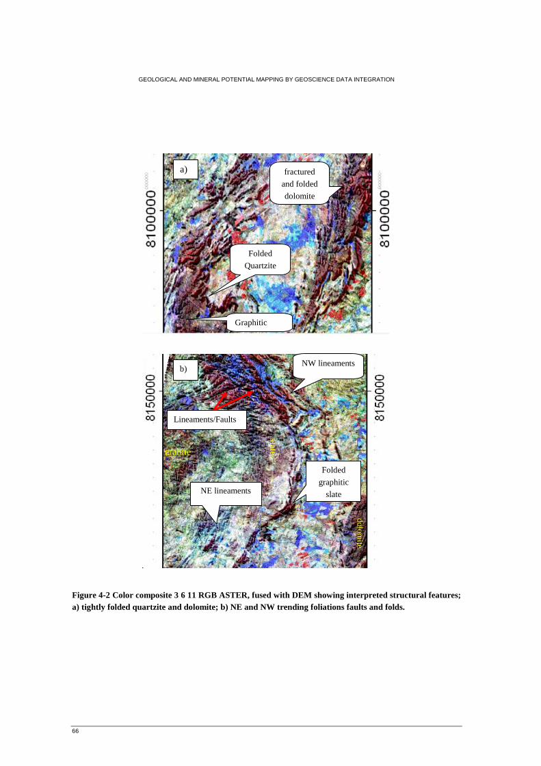
GEOLOGICAL AND MINERAL POTENTIAL MAPPING BY GEOSCIENCE DATA INTEGRATION
66
Figure 4-2 Color composite 3 6 11 RGB ASTER, fused with DEM showing interpreted structural features; a) tightly folded quartzite and dolomite; b) NE and NW trending foliations faults and folds.
Folded
Quartzite
fractured
and folded
dolomite
a)
Graphitic
Folded
graphitic
slate NE lineaments
dolomite
NW lineaments
Lineaments/Faults
b)
granite
slate
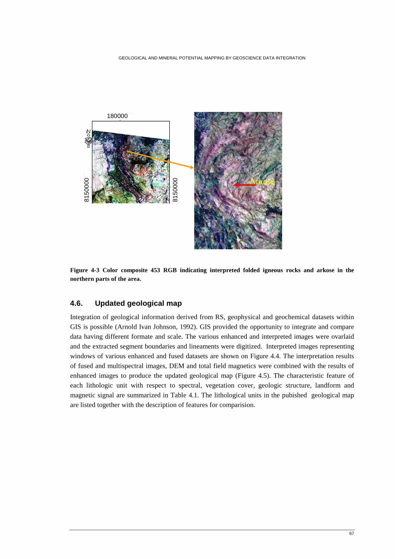
GEOLOGICAL AND MINERAL POTENTIAL MAPPING BY GEOSCIENCE DATA INTEGRATION
67
Figure 4-3 Color composite 453 RGB indicating interpreted folded igneous rocks and arkose in the northern parts of the area.
4.6. Updated geological map
Integration of geological information derived from RS, geophysical and geochemical datasets within
GIS is possible (Arnold Ivan Johnson, 1992). GIS provided the opportunity to integrate and compare
data having different formate and scale. The various enhanced and interpreted images were ovarlaid
and the extracted segment boundaries and lineaments were digitized. Interpreted images representing
windows of various enhanced and fused datasets are shown on Figure 4.4. The interpretation results
of fused and multispectral images, DEM and total field magnetics were combined with the results of
enhanced images to produce the updated geological map (Figure 4.5). The characteristic feature of
each lithologic unit with respect to spectral, vegetation cover, geologic structure, landform and
magnetic signal are summarized in Table 4.1. The lithological units in the pubished geological map
are listed together with the description of features for comparision.
180000.000000
8150
000.0
000
00
8150
000.0
000
00
·
Arkose
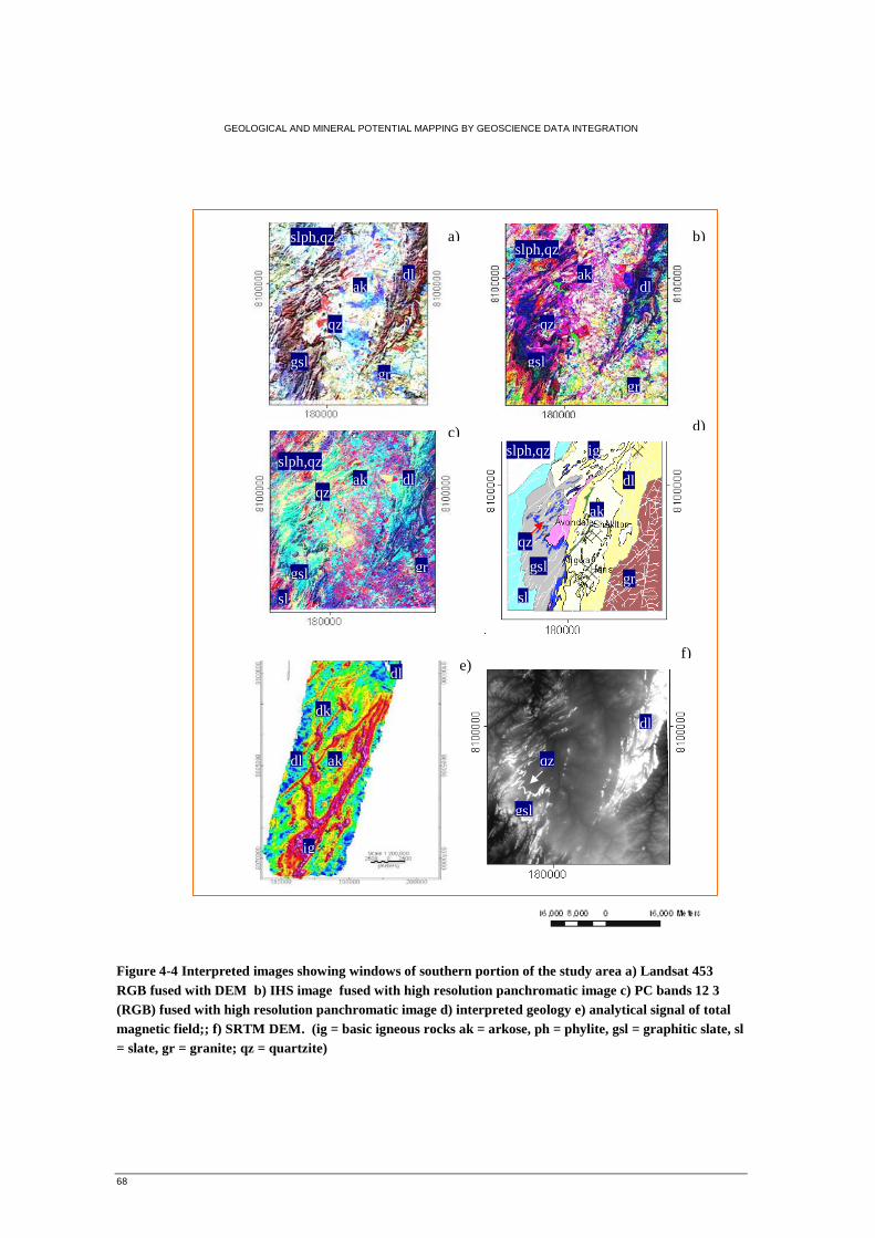
GEOLOGICAL AND MINERAL POTENTIAL MAPPING BY GEOSCIENCE DATA INTEGRATION
68
Figure 4-4 Interpreted images showing windows of southern portion of the study area a) Landsat 453 RGB fused with DEM b) IHS image fused with high resolution panchromatic image c) PC bands 12 3 (RGB) fused with high resolution panchromatic image d) interpreted geology e) analytical signal of total magnetic field;; f) SRTM DEM. (ig = basic igneous rocks ak = arkose, ph = phylite, gsl = graphitic slate, sl = slate, gr = granite; qz = quartzite)
a) b)
c) d)
e) f)
gsl
qz
gr
dl
slph,qz
ig
sl
gsl
gsl
ak qz
slph,qz
dl
gr
qz
dl
slph,qz
gr gsl
dl
slph,qz
qz
gr
ak
ak
ak
ig
dk
dl
dl
dl
gsl
qz
sl
ak
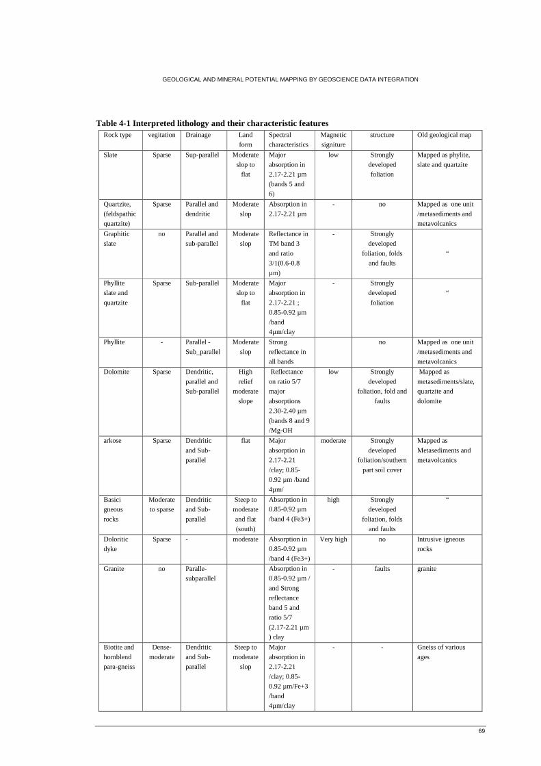
GEOLOGICAL AND MINERAL POTENTIAL MAPPING BY GEOSCIENCE DATA INTEGRATION
69
Table 4-1 Interpreted lithology and their characteristic features Rock type vegitation Drainage Land
form
Spectral
characteristics
Magnetic
signiture
structure Old geological map
Slate Sparse Sup-parallel Moderate
slop to
flat
Major
absorption in
2.17-2.21 µm
(bands 5 and
6)
low Strongly
developed
foliation
Mapped as phylite,
slate and quartzite
Quartzite,
(feldspathic
quartzite)
Sparse Parallel and
dendritic
Moderate
slop
Absorption in
2.17-2.21 µm
- no Mapped as one unit
/metasediments and
metavolcanics
Graphitic
slate
no Parallel and
sub-parallel
Moderate
slop
Reflectance in
TM band 3
and ratio
3/1(0.6-0.8
µm)
- Strongly
developed
foliation, folds
and faults
“
Phyllite
slate and
quartzite
Sparse Sub-parallel Moderate
slop to
flat
Major
absorption in
2.17-2.21 ;
0.85-0.92 µm
/band
4µm/clay
- Strongly
developed
foliation
“
Phyllite - Parallel -
Sub_parallel
Moderate
slop
Strong
reflectance in
all bands
no Mapped as one unit
/metasediments and
metavolcanics
Dolomite Sparse Dendritic,
parallel and
Sub-parallel
High
relief
moderate
slope
Reflectance
on ratio 5/7
major
absorptions
2.30-2.40 µm
(bands 8 and 9
/Mg-OH
low Strongly
developed
foliation, fold and
faults
Mapped as
metasediments/slate,
quartzite and
dolomite
arkose Sparse Dendritic
and Sub-
parallel
flat Major
absorption in
2.17-2.21
/clay; 0.85-
0.92 µm /band
4µm/
moderate Strongly
developed
foliation/southern
part soil cover
Mapped as
Metasediments and
metavolcanics
Basici
gneous
rocks
Moderate
to sparse
Dendritic
and Sub-
parallel
Steep to
moderate
and flat
(south)
Absorption in
0.85-0.92 µm
/band 4 (Fe3+)
high Strongly
developed
foliation, folds
and faults
“
Doloritic
dyke
Sparse - moderate Absorption in
0.85-0.92 µm
/band 4 (Fe3+)
Very high no Intrusive igneous
rocks
Granite no Paralle-
subparallel
Absorption in
0.85-0.92 µm /
and Strong
reflectance
band 5 and
ratio 5/7
(2.17-2.21 µm
) clay
- faults granite
Biotite and
hornblend
para-gneiss
Dense-
moderate
Dendritic
and Sub-
parallel
Steep to
moderate
slop
Major
absorption in
2.17-2.21
/clay; 0.85-
0.92 µm/Fe+3
/band
4µm/clay
- - Gneiss of various
ages
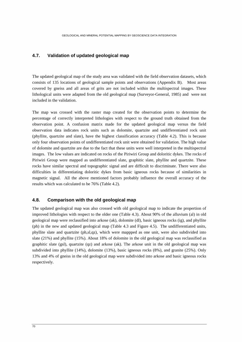
GEOLOGICAL AND MINERAL POTENTIAL MAPPING BY GEOSCIENCE DATA INTEGRATION
70
4.7. Validation of updated geological map
The updated geological map of the study area was validated with the field observation datasets, which
consists of 135 locations of geological sample points and observations (Appendix B). Most areas
covered by gneiss and all areas of grits are not included within the multispectral images. These
lithological units were adapted from the old geological map (Surveyor-General, 1985) and were not
included in the validation.
The map was crossed with the raster map created for the observation points to determine the
percentage of correctly interpreted lithologies with respect to the ground truth obtained from the
observation point. A confusion matrix made for the updated geological map versus the field
observation data indicates rock units such as dolomite, quartzite and undifferentiated rock unit
(phyllite, quartzite and slate), have the highest classification accuracy (Table 4.2). This is because
only four observation points of undifferentiated rock unit were obtained for validation. The high value
of dolomite and quartzite are due to the fact that these units were well interpreted in the multispectral
images. The low values are indicated on rocks of the Piriwiri Group and doloritic dykes. The rocks of
Piriwiri Group were mapped as undifferentiated slate, graphitic slate, phyllite and quartzite. These
rocks have similar spectral and topographic signal and are difficult to discriminate. There were also
difficulties in differentiating doloritic dykes from basic igneous rocks because of similarities in
magnetic signal. All the above mentioned factors probably influence the overall accuracy of the
results which was calculated to be 76% (Table 4.2).
4.8. Comparison with the old geological map
The updated geological map was also crossed with old geological map to indicate the propertion of
improved lithologies with respect to the older one (Table 4.3). About 90% of the alluvium (al) in old
geological map were reclassified into arkose (ak), dolomite (dl), basic igneous rocks (ig), and phyllite
(ph) in the new and updated geological map (Table 4.3 and Figure 4.5). The undifferentiated units,
phyllite slate and quartzite (ph,sl,qz), which were mappped as one unit, were also subdivided into
slate (21%) and phyllite (15%). About 18% of dolomite in the old geological map was reclassified as
graphitic slate (gsl), quartzite (qz) and arkose (ak). The arkose unit in the old geological map was
subdivided into phyllite (14%), dolomite (13%), basic igneous rocks (8%), and granite (25%). Only
13% and 4% of gneiss in the old geological map were subdivided into arkose and basic igneous rocks
respectively.
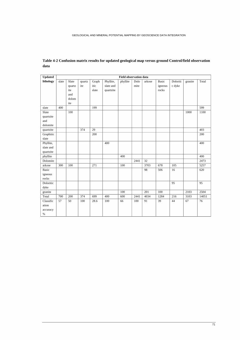
GEOLOGICAL AND MINERAL POTENTIAL MAPPING BY GEOSCIENCE DATA INTEGRATION
71
Table 4-2 Confusion matrix results for updated geological map versus ground Control/field observation data
Field observation data Updated lithology slate Slate
quartz
ite
and
dolom
ite
quartz
ite
Graph
itic
slate
Phyllite,
slate and
quartzite
phyllite Dolo
mite
arkose Basic
igneous
rocks
Doloriti
c dyke
granite Total
slate 400 199 599
Slate
quartzite
and
dolomite
100 1000 1100
quartzite 374 29 403
Graphitic
slate
200 200
Phyllite,
slate and
quartzite
400 400
phyllite 400 400
Dolomite 2441 32 2473
arkose 300 100 271 100 3703 678 105 5257
Basic
igneous
rocks
98 506 16 620
Doloritic
dyke
95 95
granite 100 201 100 2103 2504
Total 700 200 374 699 400 600 2441 4034 1284 216 3103 14051
Classific
ation
accuracy
%
57 50 100 28.6 100 66 100 91 39 44 67 76
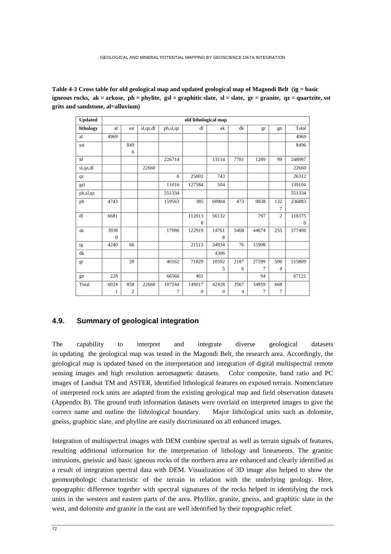
GEOLOGICAL AND MINERAL POTENTIAL MAPPING BY GEOSCIENCE DATA INTEGRATION
72
Table 4-3 Cross table for old geological map and updated geological map of Magondi Belt (ig = basic igneous rocks, ak = arkose, ph = phylite, gsl = graphitic slate, sl = slate, gr = granite, qz = quartzite, sst grits and sandstone, al=alluvium)
4.9. Summary of geological integration
The capability to interpret and integrate diverse geological datasets
in updating the geological map was tested in the Magondi Belt, the research area. Accordingly, the
geological map is updated based on the interpretation and integration of digital multispectral remote
sensing images and high resolution aeromagnetic datasets. Color composite, band ratio and PC
images of Landsat TM and ASTER, identified lithological features on exposed terrain. Nomenclature
of interpreted rock units are adapted from the existing geological map and field observation datasets
(Appendix B). The ground truth information datasets were overlaid on interpreted images to give the
correct name and outline the lithological boundary. Major lithological units such as dolomite,
gneiss, graphitic slate, and phyllite are easily discriminated on all enhanced images.
Integration of multispectral images with DEM combine spectral as well as terrain signals of features,
resulting additional information for the interpretation of lithology and lineaments. The granitic
intrusions, gneissic and basic igneous rocks of the northern area are enhanced and clearly identified as
a result of integration spectral data with DEM. Visualization of 3D image also helped to show the
geomorphologic characteristic of the terrain in relation with the underlying geology. Here,
topographic difference together with spectral signatures of the rocks helped in identifying the rock
units in the western and eastern parts of the area. Phyllite, granite, gneiss, and graphitic slate in the
west, and dolomite and granite in the east are well identified by their topographic relief.
Updated old lithological map
lithology al sst sl,qz,dl ph,sl,qz dl ak dk gr gn Total
al 4969 4969
sst 849
6
8496
sl 226714 13114 7781 1289 99 248997
sl,qz,dl 22660 22660
qz 6 25802 743 26312
gsl 11016 127584 504 139104
ph,sl,qz 551334 551334
ph 4743 159563 385 60904 473 9838 132
7
236883
dl 6681 112013
8
56132 797 2 118375
0
ak 3938
0
17086 122919 14761
8
5468 44674 255 377400
ig 4240 66 21513 34934 76 15908
dk 4306
gr 20 40162 71829 10592
5
2187
6
27599
7
500
4
515809
gn 228 66566 461 94 67121
Total 6024
1
858
2
22660 107244
7
149017
0
42418
0
3567
4
34859
7
668
7
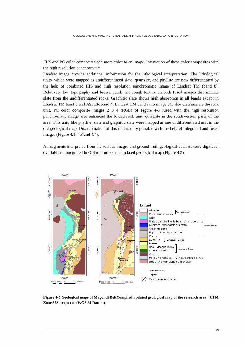
GEOLOGICAL AND MINERAL POTENTIAL MAPPING BY GEOSCIENCE DATA INTEGRATION
73
Ç
ÇÇÇÇ
Ç
Ç
Ç
Hans
Norah
Angwa
Mhangura
ShakltonAvondale
Shamrock
United Kingdom
180000.000000
180000.000000
8100
000.0
0000
0
8100
000.0
0000
0
8150
000.0
0000
0
8150
000.0
0000
0
8200
000.0
0000
0
8200
000.0
0000
0
·
16,000 0 16,0008,000 Meters
IHS and PC color composites add more color to an image. Integration of these color composites with
the high resolution panchromatic
Landsat image provide additional information for the lithological interpretation. The lithological
units, which were mapped as undifferentiated slate, quartzite, and phyllite are now differentiated by
the help of combined IHS and high resolution panchromatic image of Landsat TM (band 8).
Relatively low topography and brown pixels and rough texture on both fused images discriminate
slate from the undifferentiated rocks. Graphitic slate shows high absorption in all bands except in
Landsat TM band 3 and ASTER band 4. Landsat TM band ratio image 3/1 also discriminate the rock
unit. PC color composite images 2 3 4 (RGB) of Figure 4-3 fused with the high resolution
panchromatic image also enhanced the folded rock unit, quartzite in the southwestern parts of the
area. This unit, like phyllite, slate and graphitic slate were mapped as one undifferentiated unit in the
old geological map. Discrimination of this unit is only possible with the help of integrated and fused
images (Figure 4.1, 4.3 and 4.4).
All segments interpreted from the various images and ground truth geological datasets were digitized,
overlaid and integrated in GIS to produce the updated geological map (Figure 4.5).
Figure 4-5 Geological maps of Magondi BeltCompiled updated geological map of the research area. (UTM Zone 36S projection WGS 84 Datum).
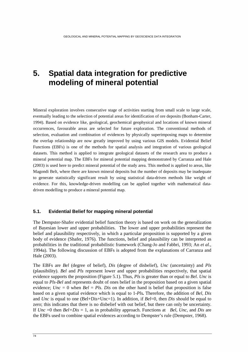
GEOLOGICAL AND MINERAL POTENTIAL MAPPING BY GEOSCIENCE DATA INTEGRATION
74
5. Spatial data integration for predictive modeling of mineral potential
Mineral exploration involves consecutive stage of activities starting from small scale to large scale,
eventually leading to the selection of potential areas for identification of ore deposits (Bonham-Carter,
1994). Based on evidence like, geological, geochemical geophysical and locations of known mineral
occurrences, favourable areas are selected for future exploration. The conventional methods of
selection, evaluation and combination of evidences by physically superimposing maps to determine
the overlap relationship are now greatly improved by using various GIS models. Evidential Belief
Functions (EBFs) is one of the methods for spatial analysis and integration of various geological
datasets. This method is applied to integrate geological datasets of the research area to produce a
mineral potential map. The EBFs for mineral potential mapping demonstrated by Carranza and Hale
(2003) is used here to predict mineral potential of the study area. This method is applied to areas, like
Magondi Belt, where there are known mineral deposits but the number of deposits may be inadequate
to generate statistically significant result by using statistical data-driven methods like weight of
evidence. For this, knowledge-driven modelling can be applied together with mathematical data-
driven modelling to produce a mineral potential map.
5.1. Evidential Belief for mapping mineral potential
The Dempster-Shafer evidential belief function theory is based on work on the generalization of Bayesian lower and upper probabilities. The lower and upper probabilities represent the belief and plausibility respectively, in which a particular proposition is supported by a given body of evidence (Shafer, 1976). The functions, belief and plausibility can be interpreted as probabilities in the traditional probabilistic framework (Chang-Jo and Fabbri, 1993; An et al., 1994a). The following discussion of EBFs is adopted from the explanations of Carranza and Hale (2003).
The EBFs are Bel (degree of belief), Dis (degree of disbelief), Unc (uncertainty) and Pls (plausibility). Bel and Pls represent lower and upper probabilities respectively, that spatial evidence supports the proposition (Figure 5.1). Thus, Pls is greater than or equal to Bel. Unc is equal to Pls-Bel and represents doubt of ones belief in the proposition based on a given spatial evidence; Unc = 0 when Bel = Pls. Dis on the other hand is belief that proposition is false based on a given spatial evidence which is equal to 1-Pls. Therefore, the addition of Bel, Dis and Unc is equal to one (Bel+Dis+Unc=1). In addition, if Bel=0, then Dis should be equal to zero; this indicates that there is no disbelief with out belief, but there can only be uncertainty. If Unc =0 then Bel+Dis = 1, as in probability approach. Functions at Bel, Unc, and Dis are the EBFs used to combine spatial evidences according to Dempster’s rule (Dempster, 1968).
GEOLOGICAL AND MINERAL POTENTIAL MAPPING BY GEOSCIENCE DATA INTEGRATION
75
Figure 5-1 Schematic relationships of EBFs (adopted from Carranza and Hale, 2003).
Estimation of EBFs can either be knowledge-driven or data driven. Knowledge-driven estimation of EBSs requires expert knowledge of the proposition being evaluated. When expert knowledge is lacking, EBFs can be estimated based on given spatial data described by Chung and Fabri (1993) and An and Bonham Carter (1994) (Chang-Jo and Fabbri, 1993; An et al., 1994a) When location of both mineralized and unmineralized zones are known data driven estimation procedures of Chung and Fabri, (1993) and An et al., (1994) are useful (Chang-Jo and Fabbri, 1993; Chung and Fabbri, 1993; An et al., 1994b). When locations of mineralized and unmineralized zones are only partially known, data-driven estimation procedures proposed by Carranza and Hale, 2003 is useful. This procedure is adopted for the study area.
Assume a spatial evidence map of an area T with N (T) total number of pixel. It is necessary to first determine the spatial coincidence between certain pixels in a map of training data (mineral occurrences) and certain pixel in a map of spatial evidence. To do this attributes of spatial evidence maps Xi(i=1,2,….,n) representing continuous variables must be first classified into Cij(j=1,2,…,m) classes of attribute. By overlaying binary map of training data on each multi-class spatial evidence map, the number of Cij pixel overlapping spatially with mineral deposit D pixels [i.e., N(Cij)∩N(D)] and number of Cij pixels not overlapping spatially with D pixels [ie., N(Cij)-N(Cij ∩D)] can be determined.
According to Carranza and Hale, (2003), EBF’s can be estimated as follows: The degree of belief, BelCij, that a mineral deposit exists, is
GEOLOGICAL AND MINERAL POTENTIAL MAPPING BY GEOSCIENCE DATA INTEGRATION
76
(Eq.1)
(Eq.1a)
Where the numerator is the conditional probability that a target mineral deposit exists given the presence Cij; that means a target mineral deposit occurs in Cij. The denominator is the conditional probability that a target mineral deposit exists given the absence of Cij; meaning a target mineral deposit occurs outside Cij. Thus, WcijD is the weight of Cij in terms of target mineral deposits being more present than absent in Cij as may be expected due to chance.
A weight WCij for Cij in data set D for the proposition Dis (disbelief that a mineral deposit exists based on D) is defined as:
(Eq.2)
(Eq.2a)
Where the numerator is the conditional probability that a target mineral deposit does not exist given the presence of Cij; it means simply that a target mineral deposit does not occur in Cij. The denominator is the conditional probability that a target mineral deposit does not exist given the absence of Cij; that is a target mineral deposit does not occur outside attribute Cij. Thus, WCij is the weight of Cij in terms of target mineral deposits being more absent than present in Cij as may be expected due to chance.
For data driven estimation of belief and disbelief (Equation 1 and 2), demonstrated by Carranza and Hale (2003), the spatial relationship between classes of layers of an evidential map should be taken into consideration besides the spatial relationship between evidential layer and target deposit.
GEOLOGICAL AND MINERAL POTENTIAL MAPPING BY GEOSCIENCE DATA INTEGRATION
77
Note that, if for Cij calculated WcijD=0, which means that Belcij = 0, then the corresponding calculated WCij should be re-set to zero so that the corresponding DisCij=0 according to (Figure 5-1).
Unccij=1-Belcij-Discij
(Eq.3)
Plscij= Belcij + Unccij or Plscij =1- Discij (Eq.4)
Maps of EBFs of spatial evidence Map X1 can be combined with maps of EBFs of spatial evidence mapX2 according to Dempster’s (1968) rule of combination in order to generate an integrated map of EBFs. The formula for combining maps of EBFs of two spatial evidence maps are the following ((Carranza and Hale, 2003), adopted from Wright and Bonham-Carter, 1996):
(Eq.5)
(Eq.6)
(Eq.7)
Where β=1-Belx1Disx2-Disx1Belx2, which is a normalizing factor to ensure that Bel+Unc+Dis=1.
Only maps of EBFs of two spatial evidence can be combined each time; other maps of EBFs
representing X2,….Xn are combined one after another by repeated applications of Eq.5-7. Final
combination of maps of EBFs results in integrated degree of belief, degree of disbelief, degree of
uncertainty and degree of plausibility for the proposition based on given spatial evidences
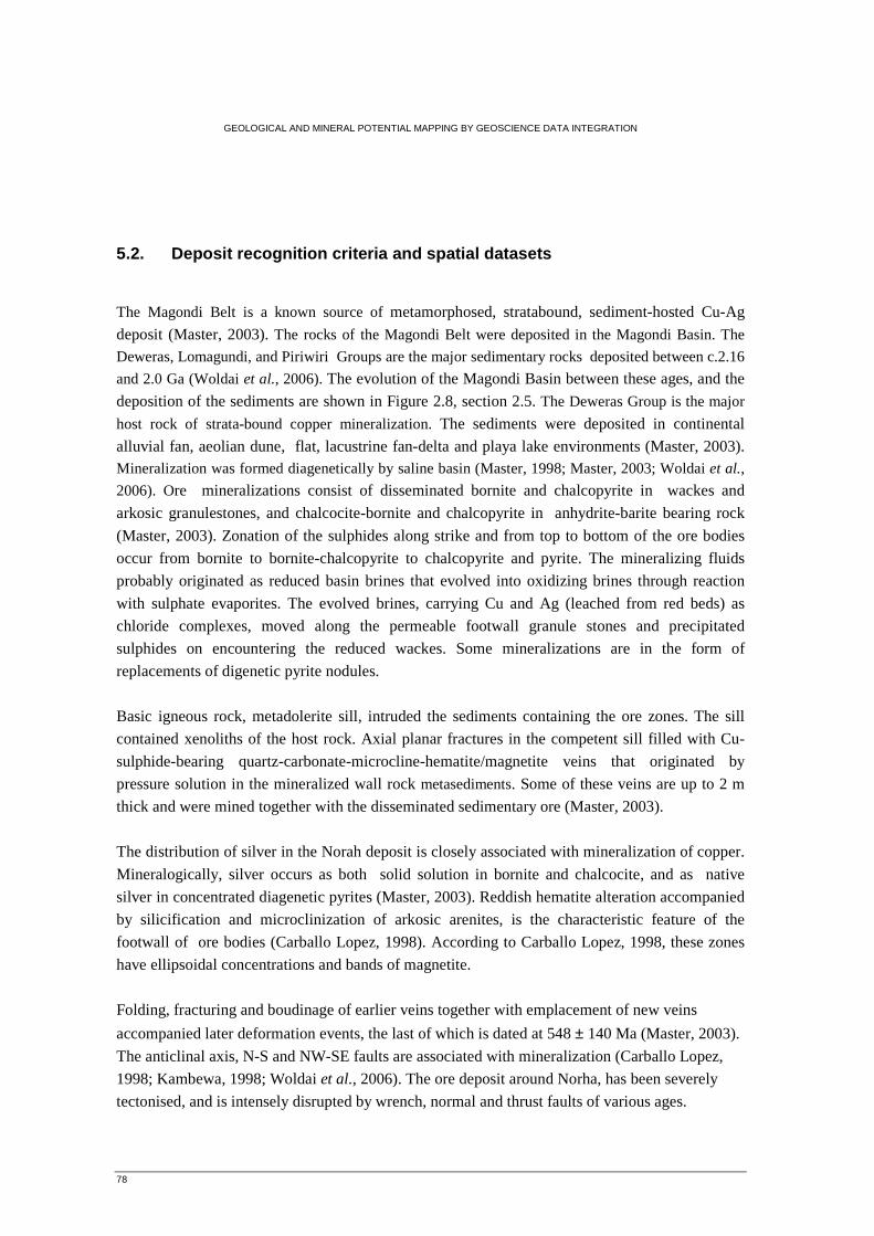
GEOLOGICAL AND MINERAL POTENTIAL MAPPING BY GEOSCIENCE DATA INTEGRATION
78
5.2. Deposit recognition criteria and spatial datasets
The Magondi Belt is a known source of metamorphosed, stratabound, sediment-hosted Cu-Ag
deposit (Master, 2003). The rocks of the Magondi Belt were deposited in the Magondi Basin. The
Deweras, Lomagundi, and Piriwiri Groups are the major sedimentary rocks deposited between c.2.16
and 2.0 Ga (Woldai et al., 2006). The evolution of the Magondi Basin between these ages, and the
deposition of the sediments are shown in Figure 2.8, section 2.5. The Deweras Group is the major
host rock of strata-bound copper mineralization. The sediments were deposited in continental
alluvial fan, aeolian dune, flat, lacustrine fan-delta and playa lake environments (Master, 2003). Mineralization was formed diagenetically by saline basin (Master, 1998; Master, 2003; Woldai et al.,
2006). Ore mineralizations consist of disseminated bornite and chalcopyrite in wackes and
arkosic granulestones, and chalcocite-bornite and chalcopyrite in anhydrite-barite bearing rock
(Master, 2003). Zonation of the sulphides along strike and from top to bottom of the ore bodies
occur from bornite to bornite-chalcopyrite to chalcopyrite and pyrite. The mineralizing fluids
probably originated as reduced basin brines that evolved into oxidizing brines through reaction
with sulphate evaporites. The evolved brines, carrying Cu and Ag (leached from red beds) as
chloride complexes, moved along the permeable footwall granule stones and precipitated
sulphides on encountering the reduced wackes. Some mineralizations are in the form of
replacements of digenetic pyrite nodules.
Basic igneous rock, metadolerite sill, intruded the sediments containing the ore zones. The sill
contained xenoliths of the host rock. Axial planar fractures in the competent sill filled with Cu-
sulphide-bearing quartz-carbonate-microcline-hematite/magnetite veins that originated by
pressure solution in the mineralized wall rock metasediments. Some of these veins are up to 2 m
thick and were mined together with the disseminated sedimentary ore (Master, 2003).
The distribution of silver in the Norah deposit is closely associated with mineralization of copper.
Mineralogically, silver occurs as both solid solution in bornite and chalcocite, and as native
silver in concentrated diagenetic pyrites (Master, 2003). Reddish hematite alteration accompanied
by silicification and microclinization of arkosic arenites, is the characteristic feature of the
footwall of ore bodies (Carballo Lopez, 1998). According to Carballo Lopez, 1998, these zones
have ellipsoidal concentrations and bands of magnetite.
Folding, fracturing and boudinage of earlier veins together with emplacement of new veins
accompanied later deformation events, the last of which is dated at 548 ± 140 Ma (Master, 2003).
The anticlinal axis, N-S and NW-SE faults are associated with mineralization (Carballo Lopez,
1998; Kambewa, 1998; Woldai et al., 2006). The ore deposit around Norha, has been severely
tectonised, and is intensely disrupted by wrench, normal and thrust faults of various ages.
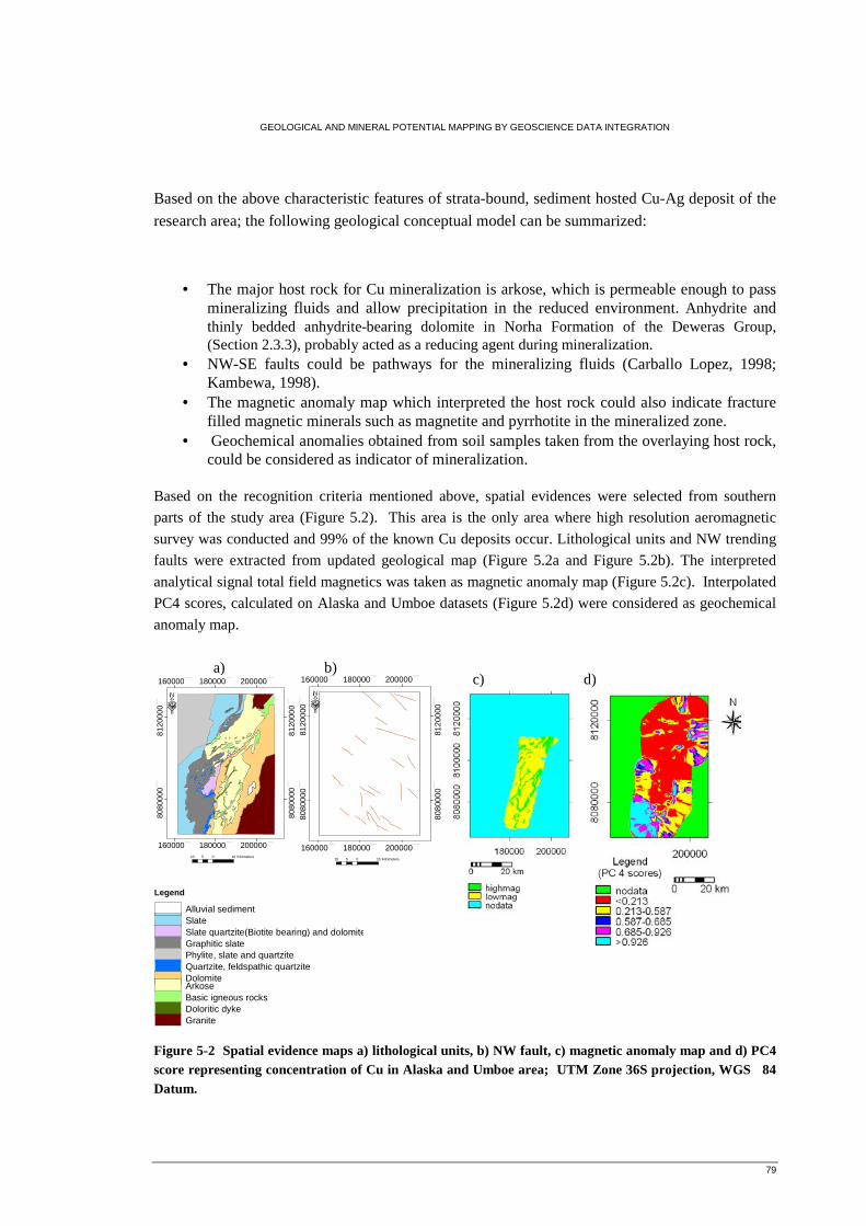
GEOLOGICAL AND MINERAL POTENTIAL MAPPING BY GEOSCIENCE DATA INTEGRATION
79
Legend
SlateSlate quartzite(Biotite bearing) and dolomiteGraphitic slatePhylite, slate and quartziteQuartzite, feldspathic quartziteDolomiteArkoseBasic igneous rocksDoloritic dykeGranite
Alluvial sediment
160000.000000
160000.000000
180000.000000
180000.000000
200000.000000
200000.000000
8080
000
.00
00
00
8080
000
.00
00
00
812
000
0.00
00
00
812
000
0.00
00
00
·
10 0 105 Kilometers
160000.000000
160000.000000
180000.000000
180000.000000
200000.000000
200000.000000
8080
000.0
0000
0
8080
000.0
0000
0
8120
000.0
0000
0
8120
000.0
0000
0
·
10 0 105 Kilometers
Based on the above characteristic features of strata-bound, sediment hosted Cu-Ag deposit of the
research area; the following geological conceptual model can be summarized:
• The major host rock for Cu mineralization is arkose, which is permeable enough to pass mineralizing fluids and allow precipitation in the reduced environment. Anhydrite and thinly bedded anhydrite-bearing dolomite in Norha Formation of the Deweras Group, (Section 2.3.3), probably acted as a reducing agent during mineralization.
• NW-SE faults could be pathways for the mineralizing fluids (Carballo Lopez, 1998; Kambewa, 1998).
• The magnetic anomaly map which interpreted the host rock could also indicate fracture filled magnetic minerals such as magnetite and pyrrhotite in the mineralized zone.
• Geochemical anomalies obtained from soil samples taken from the overlaying host rock, could be considered as indicator of mineralization.
Based on the recognition criteria mentioned above, spatial evidences were selected from southern
parts of the study area (Figure 5.2). This area is the only area where high resolution aeromagnetic
survey was conducted and 99% of the known Cu deposits occur. Lithological units and NW trending
faults were extracted from updated geological map (Figure 5.2a and Figure 5.2b). The interpreted
analytical signal total field magnetics was taken as magnetic anomaly map (Figure 5.2c). Interpolated
PC4 scores, calculated on Alaska and Umboe datasets (Figure 5.2d) were considered as geochemical
anomaly map.
Figure 5-2 Spatial evidence maps a) lithological units, b) NW fault, c) magnetic anomaly map and d) PC4 score representing concentration of Cu in Alaska and Umboe area; UTM Zone 36S projection, WGS 84 Datum.
a) b) c) d)
GEOLOGICAL AND MINERAL POTENTIAL MAPPING BY GEOSCIENCE DATA INTEGRATION
80
5.3. Estimation and integration of EBFs
Spatial evidence maps representing continuous variables were first classified using percentile
intervals of values. Areas which have no values were reclassified as “no data”. The resulting
multiclass spatial evidential maps were crossed with binary map of known copper deposit. The
number of class pixels N (Cij), sum of all class pixels N (T), number of class pixels that overlap with
deposit pixels (N (Cij∩D) and total number of deposit pixels N (D) were first calculated (Table 5.1).
EBFs estimation based on equations in section 5.1 (Equations 1-3) were performed to quantify the
spatial association between the deposit and spatial evidences (Table 5.1).
Based on the values calculated on Table 5.1, attribute maps of EBFs are created. The created belief
functions; belief, disbilief and uncertanity maps of lithological units, magnetic anomaly, PC4 scores
and proximity to NW faults are shown in Figure 5.3-6. Only arkose, dolomite and granite have spatial
association with Cu deposits. Zones of high degree of belief are mainly related to lithological units of
arkoses and dolomite. (Figure 5.3). These rocks have low degree of disbelief and uncertainty as
compared with the other units. This suggests that presence of these lithologic units can be used as
indicator of potential areas for copper mineralization. Zones of high degree of belief, low degree of
disbelieve and uncertainties are belonging to areas underlain by high magnetic anomalies (Table 5.1
and Figure 5.4). Areas occupied by high PC4 score (>0.926) corresponds to high degree of belief, low
degree of disbelief and uncertainty (Table 5.1 and Figure 5.5). This suggests geochemical anomalous
areas of copper are more prospective to find strata bound copper mineralization provided that the
other recognition criteria are fulfilled. High degree of belief is also related to proximity class of NW
fault between 0.00- 790m (Table 5.1 and Figure 5.6). This indicates the possible potential zone
within this distance.
The belief function maps of strata-bound copper mineralization were integrated by repeated use of
Equation 5.7, Section 5.1. The combined evidential belief function maps estimate new belief function
maps representing the degree of belief, disbelief, uncertainity and plausibility (Figure 5.7A-D). The
plausibility map was created by using Equation 4 (Figure 5.7). Spatial evidences representing, belief
functions of lithology, PC4 scores and NW fault were first integrated and the results were compared
with further integration with magnetic anomaly map. The belief and plausibility maps show
potentially favourable zones.
5.3.1. Test of correctness of EBFS
Test of correctness conducted on EBFs maps indicate that sum of bel+dis+unc for most pixels is 1.00.
The pixel values in the test map vary from 1.000 to 1.0001 for all four evidential maps. The test
conducted on the integrated EBFs map indicate values 0.9998 to 1.0001 (Figure 5.7E). This suggests
that error for the estimation and integration of EBFs is ± 0.0003 which can be considered as very low
and therefore, estimation and integration of EBFs can be considered to have been performed properly.
GEOLOGICAL AND MINERAL POTENTIAL MAPPING BY GEOSCIENCE DATA INTEGRATION
81
Table 5-1 Estimation of EBFs for class of values in maps of deposit recognition criteria for strata bound Cu-Ag potential, Magondi Belt. (EBFs of PC scores are calculated in descending order. Lithological units N(Cij) N(T) N(Cij∩D) N(D) Bel Dis Unc
Alluvial sediment 1228 330031 0 19 0 0 1 Arkose 71602 330031 10 19 0.53 0.33 0.1411 Basic igneous rocks 5814 330031 0 19 0 0 1 Dolomite 53113 330031 6 19 0.32 0.33 0.3526 Doloritic dyke 549 330031 0 19 0 0 1 Granite 45744 330031 3 19 0.15 0.33 0.5163 Graphitic slate 39161 330031 0 19 0 0 1 No data 10217 330031 0 19 0 0 1 Quartzite, feldspathic quartzite
6751 330031 0 19 0 0 1
Quartzite, phylite, slate 47980 330031 0 19 0 0 1 slate 41930 330031 0 19 0 0 1 Slate quartzite(Biotite bearing) and dolomite 5942 330031 0 19 0 0 1 Magnetic anomaly map N(Cij) N(T) N(Cij∩D) N(D) Bel Dis Unc
High magnetic anomaly 11737 330031 2 19 0.55 0.33 0.1158 Low magnetic anomaly 46042 330031 5 19 0.38 0.33 0.2874 No data 272252 330031 12 19 0.06 0.33 0.6068 Score of PCA/geochemical anomaly N(Cij) N(T) N(Cij∩D) N(D) Bel Dis Unc
No data 132045 330031 2 19 0.02 0.2 0.7789 <0.213 98972 330031 7 19 0.16 0.2 0.6368 0.213-0.587 49585 330031 5 19 0.24 0.2 0.5579 0.587-0.685 9861 330031 0 19 0 0 1 0.685-0.926 19808 330031 2 19 0.22 0.2 0.5792 >0.926 19760 330031 3 19 0.35 0.2 0.4472 Proximity to NW fault/fracture (km) N(Cij) N(T) N(Cij∩D) N(D) Bel Dis Unc
No data 1 330031 0 19 0 0 1 0.00-0.793 32708 330031 4 19 0.22 0.14 0.6395 0.793-1.529 32965 330031 2 19 0.1 0.14 0.7636 1.529-2.265 32386 330031 1 19 0.05 0.14 0.8136 2.265-3.020 33704 330031 3 19 0.15 0.14 0.7101 3.020-3.794 32509 330031 1 19 0.05 0.14 0.8138 3.794-4.627 33083 330031 3 19 0.15 0.14 0.7069 4.627-5.633 33514 330031 5 19 0.29 0.14 0.5726 5.633-6.969 32729 330031 0 19 0 0 1 6.969-9.389 33230 330031 0 19 0 0 1 9.389-21.799 33202 330031 0 19 0 0 1
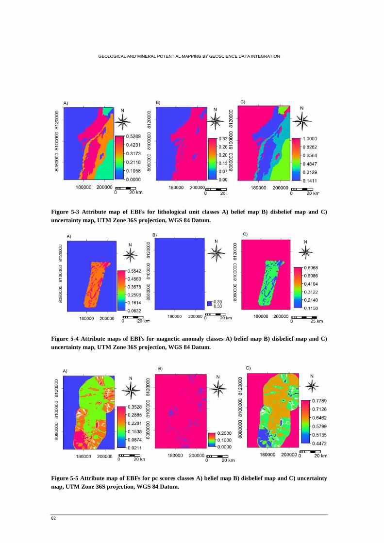
GEOLOGICAL AND MINERAL POTENTIAL MAPPING BY GEOSCIENCE DATA INTEGRATION
82
Figure 5-3 Attribute map of EBFs for lithological unit classes A) belief map B) disbelief map and C) uncertainty map, UTM Zone 36S projection, WGS 84 Datum. Figure 5-4 Attribute maps of EBFs for magnetic anomaly classes A) belief map B) disbelief map and C) uncertainty map, UTM Zone 36S projection, WGS 84 Datum.
Figure 5-5 Attribute map of EBFs for pc scores classes A) belief map B) disbelief map and C) uncertainty map, UTM Zone 36S projection, WGS 84 Datum.
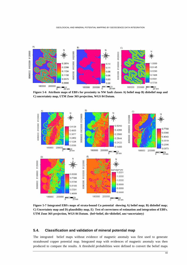
GEOLOGICAL AND MINERAL POTENTIAL MAPPING BY GEOSCIENCE DATA INTEGRATION
83
Figure 5-6 Attribute maps of EBFs for proximity to NW fault classes A) belief map B) disbelief map and C) uncertainty map, UTM Zone 36S projection, WGS 84 Datum.
Figure 5-7 Integrated EBFs maps of strata-bound Cu potential showing A) belief map; B) disbelief map; C) Uncertainty map and D) plausibility map, E) Test of correctness of estimation and integration of EBFs. UTM Zone 36S projection, WGS 84 Datum. (bel=belief, dis=disbelief, unc=uncertainty)
5.4. Classification and validation of mineral potential map
The integrated belief maps without evidence of magnetic anomaly was first used to generate
stratabound copper potential map. Integrated map with evidences of magnetic anomaly was then
produced to compare the results. A threshold probabilities were defined to convert the belief maps
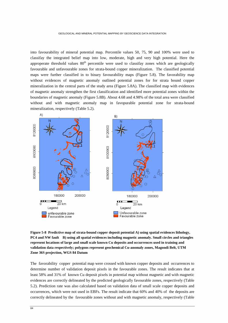
GEOLOGICAL AND MINERAL POTENTIAL MAPPING BY GEOSCIENCE DATA INTEGRATION
84
into favourability of mineral potential map. Percentile values 50, 75, 90 and 100% were used to
classifay the integrated belief map into low, moderate, high and very high potential. Here the
approperate threshold values 80th percentile were used to classifay zones which are geologically
favourable and unfavourable zones for strata-bound copper mineralization. The classified potential
maps were further classified in to binary favourability maps (Figure 5.8). The favorability map
without evidences of magnetic anomaly outlined potential zones for for strata bound copper
mineralization in the central parts of the study area (Figure 5.8A). The classified map with evidences
of magnetic anomaly strengthen the first classification and identified more potential zones within the
boundaries of magnetic anomaly (Figure 5.8B). About 4.68 and 4.98% of the total area were classified
without and with magnetic anomaly map in favopurable potential zone for strata-bound
mineralization, respectively (Table 5.2).
Figure 5-8 Predictive map of strata-bound copper deposit potential A) using spatial evidences lithology, PC4 and NW fault B) using all spatial evidences including magnetic anomaly. Small circles and triangles represent locations of large and small scale known Cu deposits and occurrences used in training and validation data respectively; polygons represent geochemical Cu-anomaly zones, Magondi Belt, UTM Zone 36S projection, WGS 84 Datum
The favorability copper potential map were crossed with known copper deposits and occurrences to
determine number of validation deposit pixels in the favourable zones. The result indicates that at
least 58% and 31% of known Cu deposit pixels in potential map without magnetic and with magnetic
evidences are correctly delineated by the predicted geologically favourable zones, respectively (Table
5.2). Prediction rate was also calculated based on validation data of small scale copper deposits and
occurrences, which were not used in EBFs. The result indicate that 60% and 40% of the deposits are
correctly delineated by the favourable zones without and with magnetic anomaly, respectively (Table
GEOLOGICAL AND MINERAL POTENTIAL MAPPING BY GEOSCIENCE DATA INTEGRATION
85
5.3). of the out of 10 small scale deposits of potential map without magnetics and 4 out ofcoincide
with the predicted potential zone. This implies, 60% Table 5-2 Validation of predictive strata-bound copper potential map using Known Cu deposit, South Magondi-Belt
Table 5-3 Validation of predictive strata-bound copper potential map using small scale Cu deposit/occurrences, South Magondi-Belt
The predictive map crossed with geochemical soil copper anomally indicates that at least 12% and
19% of the geochemical anomaly zones are overlapped with the favourable potential zones without
and with magnetic anomaly, respectively (Table 5.4).
Classified potential map
without magnetic anomaly
Proportion of
potential zone %
Number of
Known Cu-
deposit used
as training
data
Total =19
Success rate %
Unfavourable zone (without) 95.32 8 42
Favourable zone (without) 4.68 11 58
Unfavourable zone (with) 95.02 13 68.5
Favourable zone (with) 4.98 6 31.5
Classified potential map with
and with out magnetic
anomaly
Number of small scale deposit
used as validation data
Total =10
prediction rate
%
Unfavourable zone (without) 4 40
Favourable zone (without) 6 60
Unfavourable zone (with) 6 60
Favourable zone (with) 4 40
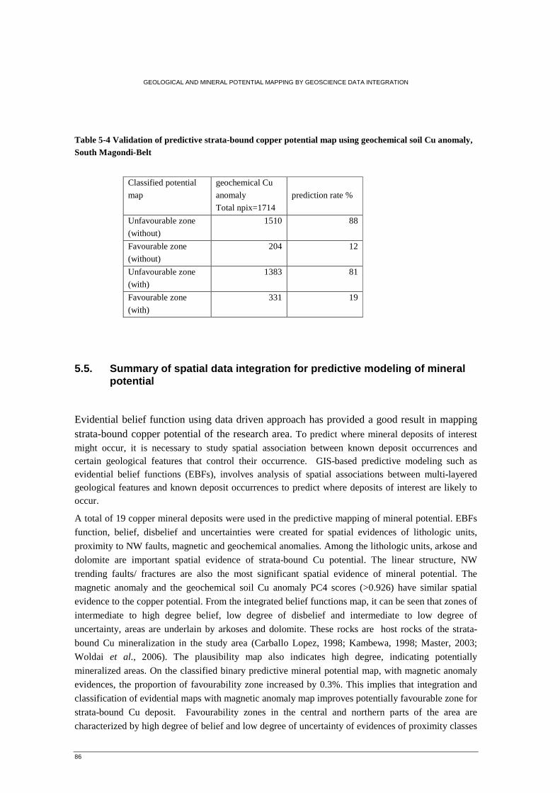
GEOLOGICAL AND MINERAL POTENTIAL MAPPING BY GEOSCIENCE DATA INTEGRATION
86
Table 5-4 Validation of predictive strata-bound copper potential map using geochemical soil Cu anomaly, South Magondi-Belt
5.5. Summary of spatial data integration for predictive modeling of mineral potential
Evidential belief function using data driven approach has provided a good result in mapping strata-bound copper potential of the research area. To predict where mineral deposits of interest
might occur, it is necessary to study spatial association between known deposit occurrences and certain geological features that control their occurrence. GIS-based predictive modeling such as evidential belief functions (EBFs), involves analysis of spatial associations between multi-layered geological features and known deposit occurrences to predict where deposits of interest are likely to occur.
A total of 19 copper mineral deposits were used in the predictive mapping of mineral potential. EBFs
function, belief, disbelief and uncertainties were created for spatial evidences of lithologic units,
proximity to NW faults, magnetic and geochemical anomalies. Among the lithologic units, arkose and
dolomite are important spatial evidence of strata-bound Cu potential. The linear structure, NW
trending faults/ fractures are also the most significant spatial evidence of mineral potential. The
magnetic anomaly and the geochemical soil Cu anomaly PC4 scores (>0.926) have similar spatial
evidence to the copper potential. From the integrated belief functions map, it can be seen that zones of
intermediate to high degree belief, low degree of disbelief and intermediate to low degree of
uncertainty, areas are underlain by arkoses and dolomite. These rocks are host rocks of the strata-
bound Cu mineralization in the study area (Carballo Lopez, 1998; Kambewa, 1998; Master, 2003;
Woldai et al., 2006). The plausibility map also indicates high degree, indicating potentially
mineralized areas. On the classified binary predictive mineral potential map, with magnetic anomaly
evidences, the proportion of favourability zone increased by 0.3%. This implies that integration and
classification of evidential maps with magnetic anomaly map improves potentially favourable zone for
strata-bound Cu deposit. Favourability zones in the central and northern parts of the area are
characterized by high degree of belief and low degree of uncertainty of evidences of proximity classes
Classified potential
map
geochemical Cu
anomaly
Total npix=1714
prediction rate %
Unfavourable zone
(without)
1510 88
Favourable zone
(without)
204 12
Unfavourable zone
(with)
1383 81
Favourable zone
(with)
331 19
GEOLOGICAL AND MINERAL POTENTIAL MAPPING BY GEOSCIENCE DATA INTEGRATION
87
of NW faults. One of the known large scale mine, Norah, in the north is situated on this fault line
probably indicating structurally controlled mineralization (Carballo Lopez, 1998; Kambewa, 1998;
Master, 2003). Zones of high degree of belief, low degree of disbelief and low degree of uncertainty
of evidences of anomalous geochemical signature provide a strong support to high favourable zone in
the southern parts of the area. This area is contact zone underlain by arkose, basic igneous rocks and
dolomite, which contain folds and faulted structures. Test conducted on integrated EBFs map
indicated that error for the estimation and integration of EBFs is ± 0.0003, which can be considered as
very low and, therefore, estimation and integration of EBFs can be considered to have performed
properly.
Validations conducted on the binary predictive map without magnetic anomaly evidence indicates that
the favourable potential zone correctly delineate 12% of the Cu-anomaly, 58% of the ‘model’ deposits
and 60% of the ‘validation’ deposit. Validations conducted on binary predictive map with magnetic
anomaly evidence indicates that the favourable potential zone correctly delineate 19% Cu anomaly
map, 31.5% of the ‘model’ deposits and 40% of the ‘validation’ deposit. The result implies that the
binary potential map with magnetic anomaly evidence map improves the proportion of favourability
zone as compared to the binary map without magnetic anomaly. This indicates a satisfactory result
which implies the usefulness of the model for further exploration of undiscovered strata-bound copper
deposit in the northern parts of the study area.
GEOLOGICAL AND MINERAL POTENTIAL MAPPING BY GEOSCIENCE DATA INTEGRATION
88
6. Conclusion and Recommendation
6.1. Conclusion
Spatial data processing, analysis and integration using remote sensing and GIS applications were
useful in updating the geological map and predicting mineral potential map of the study area. During
the processes of image interpretation, old geological maps were used as a base map to extract
information on major lithologic units. Multispectral image enhancement and interpretations were
important in identifying and delineating lithological units including host rocks for strata-bound
mineralization in the study area. Image classifications were also helped in mapping major lithologic
units. ASTER image better classified the lithologic units as compared with Landsat TM. The low
classification accuracy on both images were probably due to similarities in rock units, extensive soil
cover, vegetation and topography, which made the surface feature spectrally less separable. The high
resolution aeromagnetic data were help in identifying geologic features on areas where extensive soil
covers occur. Analytical signal and vertical derivatives of total field magnetics were helped in
extracting subsurface information to delineate host rocks and structural features, which are
responsible for mineralization. DEM generated from ASTER and SRTM images were used in
extracting major geological structures associated with mineralization. The NW-SE faults were found
an important spatial evidence for Cu mineralization. Images fused with DEM were helped in further
enhancing and increased interpretation of geological features. Integration of all interpreted images
helped in classifying lithologic units and updates the geological map of the study area. The geological
map was validated and a total accuracy of 76% was obtained.
Geochemical data processing and interpretation of principal component analysis were helpful in
identifying anomalous zones for strata-bound Cu-Ag-Au mineralization in the study area. Scores of
principal component (PC4) were used as one of evidential maps in predicting mineral potential of the
study area. Large scale known Cu deposit map were used in quantifying the spatial associations
between the deposit and geological features.
The theory of EBFs for mineral potential mapping was found to be the best method to predict mineral
potential map of the study area. Deposit recognition criteria were the basis for extracting spatial
evidences based on the characteristic features of strata-bound Cu-Ag-Au mineralization in the study
area and elsewhere in similar regions. Data driven approach were used to quantify the spatial
association between the known mineral deposit and geological features in Magondi Belt. A total of 19
copper mineral deposits were used in the predictive mapping of mineral potential. EBFs function,
belief, disbelief and uncertainties were created for spatial evidences of lithologic units, proximity to
NW faults, magnetic and geochemical anomalies. Among the lithologic units, arkose and dolomite
were found to be important spatial evidence of strata-bound Cu-Ag-Au potential. These rocks are
host rocks of the strata-bound Cu mineralization in the study area. EBFs maps containing spatial
evidence were integrated to produce favourability map. Test conducted on integrated EBFs map
indicated that error for estimation and integration of EBFs is ± 0.0003, which can be considered as
GEOLOGICAL AND MINERAL POTENTIAL MAPPING BY GEOSCIENCE DATA INTEGRATION
89
very low and, therefore, estimation and integration of EBFs can be considered to have performed
properly. The total area predicted under favourability zone in predictor maps with and without
magnetic anomaly is 4.98% and 4.68% respectively. This indicates that the binary potential map with
magnetic anomaly evidence could improve the proportion of favourability zone. Validations
conducted on the binary predictive map without magnetic anomaly evidence indicates that the
favourable potential zone correctly delineate 12% of the Cu-anomaly, 58% of the ‘model’ deposits
and 60% of the ‘validation’ deposit. Validations conducted on binary predictive map with magnetic
anomaly evidence also indicate that the favourable potential zone correctly delineate 19% the Cu
anomaly, 31.5% of the ‘model’ deposits and 40% of the ‘validation’ deposit. This indicates a
satisfactory result which implies the usefulness of the model for further exploration of undiscovered
strata-bound copper deposit in the northern parts of the study area where similar evidences occur.
6.2. Recommendation
• The predictive model has indicated potential areas in the southern parts of Magondi Belt.
Similar techniques are recommended for the northern area of the belt where same spatial
evidences occur.
• High resolution aeromagnetic data has found to map subsurface geological features and
improve the prediction of strata-bound Cu potential zone. This survey is recommended in the
northern parts of the area to map subsurface geology in soil covered area and predict potential
areas for strata-bound Cu mineralization.
• The Piriwiri Group rocks reported to host massive sulphide deposit. Application of theory of
Evidential Belief (EBFs) is recommended to predict such type of mineralization in the
research area.
GEOLOGICAL AND MINERAL POTENTIAL MAPPING BY GEOSCIENCE DATA INTEGRATION
90
7. Reference
An, P., Moon, W., and Bonham-Carter, G. (1994a) An object-oriented knowledge representation structure for exploration data integration. Natural Resources Research, 3, 132-45.
-. (1994b) Uncertainty management in integration of exploration data using the belief function. Natural Resources Research, 3, 60-71.
Andrada de Palomera, R.P. (2004) Application of remote sensing and geographic information systems for mineral predictive mapping, deseado massif, southern Argentina, p. 73. ITC, Enschede.
Arnold Ivan Johnson, C.B.P., James L. Fulton. (1992) Geographic information systems (GIS) and mapping- practices and standards. 348 p. ASTM International.
Beus, A.A., and Grigorian, S.V. (1977) Geochemical exploration methods for mineral deposits. 287 p. Applied Publishing, Wilmette.
Bonham-Carter, G.F. (1994) Geographic information systems for geoscientists: Modelling with GIS398 p. Pergamon, Kidlington etc.
Bounessah, M., and Atkin, B.P. (2003) An application of exploratory data analysis (eda) as a robust non-parametric technique for geochernical mapping in a semi-arid climate. Applied Geochemistry, 18, 1185-95.
Carballo Lopez, E. (1998) Integration of aeromagnetic thematic mapper and geochemical data for mineral exploration in the makonde district, Zimbabwe, p. 107. ITC, Delft.
Carranza, E.J.M., and Hale, M. (2002) Mineral imaging with landsat thematic mapper data for hydrothermal alteration mapping in heavily vegetated terrane. International Journal of Remote Sensing, 23.
-. (2003) Evidential belief functions for data - driven geologically constrained mapping of gold potential, Baguio district, Philippines. In: Ore Geology Reviews, 22(2003)1-2, pp. 117-132.
Carranza, E.J.M., Mangaoang, J.C., and Hale, M. (1999) Application of mineral exploration models and gis to generate mineral potential maps as input for optimum land use planning in the philippines. In: Natural Resources Research, 8(1999)2, pp. 165-173.
Chang-Jo, F.C., and Fabbri, A.G. (1993) Representation of geoscience information for data integration. In: Nonrenewable Resources, (1993), pp. 122-139.
Chavez, P.S.e., Marino, C.M.e., and Schowengerdt, R.A.e. (1994) Recent advances in remote sensing and hyperspectral remote sensing : 27 - 29 september 1994, rome. 238 p. The International Society for Optical Engineering (SPIE), Bellingham.
Chung, C.-J., and Fabbri, A. (1993) The representation of geoscience information for data integration. Natural Resources Research, 2, 122-39.
Crôsta, A.P., and Rabelo, A. (1993) Assessing of landsat tm for hydrothermal alteration mapping in central western brazil Proceedings of Ninth Thematic conference geologic remote sensing Pasadinea, p. 1053-61, California, USA.
Dempster, A.P. (1968) Generalization of bayesian inference. In: Journal of the royal statistical society, series B, 30(1968), pp. 205-247.
Foody, G.M., and Mathur, A. (2004) Toward intelligent training of supervised image classifications: Directing training data acquisition for svm classification. Remote Sensing of Environment, 93, 107-17.
Fraser, S.J., and Green, A.A. (1987) A software defoliant for geological analysis of band ratios. International Journal of Remote Sensing, 8.
Govett, G.J.S. (1976) Rock geochemistry in mineral exploration. 461 p. Elsevier, Amsterdam etc. Hahn, L. (2002) On the stratigraphy of the palaeoproterozoic deweras and lomagundi groups
(magondi supergroup) in zimbabwe. South African Journal of Geology, 105, 193-204.
GEOLOGICAL AND MINERAL POTENTIAL MAPPING BY GEOSCIENCE DATA INTEGRATION
91
Harris, J.R., Sanborn, M., Panagapko, D.A., Skulski, T., and Parker, J.R. (2006) Gold prospectivity maps of the red lake greenstone belt: Application of gis technology Source: Candaian Journal of Earth Science, 43 865-93.
Hewson, R.D., Cudahy, T.J., Mizuhiko, S., Ueda, K., and Mauger, A.J. (2005) Seamless geological map generation using aster in the broken hill-curnamona province of australia. Remote Sensing of Environment, 99, 159-72.
Isabirye Mugaddu, E. (2005) Integration of various remotely sensed data for geological mapping in the jinja area, uganda, p. 101. ITC, Enschede.
Jones, R.R., McCaffrey, K.J.W., Clegg, P., Wilson, R.W., Holliman, N.S., Holdsworth, R.E., Imber, J., and Waggott, S. (2006) Integration of regional to outcrop digital data: 3d visualisation of multi-scale geological models. Computers & Geosciences, In Press, Accepted Manuscript.
Kalinowski, A., and Oliver, a.S. (2004) Aster mineral index processing manual. Geoscience Australia. Kambewa, C. (1998) Use of gis in exploration for sediment hosted copper deposits in the makonde
basin, zimbabwe, p. 168. ITC, Delft. Le Thi Chau, H. (2001) Integrating landsat etm7, aerial photographs and field data for geological
mapping : The tabernas basin, southeast spain, p. 61. ITC, Enschede. Lillesand, T.M., and Kiefer, R.W. (1987) Remote sensing and image interpretation. 721 p. Wiley &
Sons, New York etc. Lips, A.L.W., Lawrence, C., Rowan, John, and Mars, C. (2002) Lithologic mapping in the mountain
pass, california area using advanced spaceborne thermal emission and reflection radiometer (aster) data
Majaule, T., Hanson, R.E., Key, R.M., Singletary, S.J., Martin, M.W., and Bowring, S.A. (2001) The
magondi belt in northeast botswana: Regional relations and new geochronological data from the sua pan area. Journal of African Earth Sciences, 32, 257-67.
Master, S. (1991) The origin and controls on the distribution of copper and precious metal mineralization at the mhangura and norah mines, Phd, p. 382. Witwatersrand university South Africa
-. (1998) Mineral deposits studies group meeting, university of greenwich, 5-6 january New
developments in understanding the origin of the Central African Copperbelt, University of Greenwich.
-. (2003) Norah mine, zimbabwe: A polydeformed and metamorphosed stratabound cu-ag deposit. In J.G. (RAU), H.H. (AARL), and C.M. (RAU), Eds. Mineralogy and Geochemistry of Base Metal Deposits in Southern Africa – Implications for Exploration and Beneficiation, p. 56, RAU, Auckland Park, South Africa.
Master, S., Ferraz, M.F.F., Woldai, T., and Zeil, P. (1996) Gis integration of data from the magondi copperbelt and the highbury meteorite impact structure in zimbabwe. In: Conf. on the application of remotely sensed data and GIS in environmetal and natural resources assessment in Africa, Harare, Zimbabwe, March 15-22, 1996, pp 151-154.
Master, S., Henry, G., and Borg, G. (1989) Geochemistry and mineralogy of banded iron-formation-hosted gold mineralization in the gwanda greenstone-belt, zimbabwe - a discussion. Economic Geology, 84, 194-7.
Munyanyiwa, H., and Maaskant, P. (1998) Metamorphism of the palaeoproterozoic magondi mobile belt north of karoi, zimbabwe. Journal of African Earth Sciences, 27, 223-40.
Owusu, E.A., Woldai, T., Barritt, S.D., Carranza, E.J.M., and Hale, M. (2006) Spatial association of gold deposits with remotely - sensed faults, south ashanti belt, ghana. In: AARSE 2006 : Proceeding of the 6th AARSE international conference on earth observation and geoinformation sciences in support of Africa's development, 30 October - 2 November 2006, Cairo, Egypt. Cairo : The National Authority for Remote Sensing and Space Science (NARSS), 2006. ISBN 1-920-01710-0. 8 p.
Porwal, A.K., Hale, M.p., and Carranza, E.J.M.p. (2006) Mineral potential mapping with mathematical geological models. ITC Dissertation;130, p. 289. ITC, Enschede.
GEOLOGICAL AND MINERAL POTENTIAL MAPPING BY GEOSCIENCE DATA INTEGRATION
92
Ranjbar, H., Shahriari, M., and Honarmand. (2003) Comparison of aster and etm+ data for exploration of porphyry copper mineralization: A case study of sar cheshmeh areas, kerman, iran.
Reimann, C., and Filzmoser, P. (2000) Normal and lognormal data distribution in geochemistry: Death of a myth. Consequences for the statistical treatment of geochemical and environmental data. Environmental Geology, 39, 1001-14.
Reimann, C., Filzmoser, P., and Garrett, R.G. (2005) Background and threshold: Critical comparison of methods of determination. Science of The Total Environment, 346, 1-16.
Ren, Dianwei, ABDELSALAM, and Mohamed, G. (2001) Optimum, index factor (oif) for aster data: Examples from the neoproterozoic allaqi suture. The Geological Society of America (GSA)
Rigol, J.P., and Chica-Olmo, M. (1998) Merging remote-sensing images for geological-environmental
mapping: Application to the cabo de gata-níjar natural park, spain. Environmental Geology, 34, 194-202.
Sabins, F.F. (1987) Remote sensing : Principles and interpretation. 449 p. W.H. Freeman, New York. Schetselaar, E.M. (1998) Fusion by the ihs transform : Should we use cylindrical or spherical
coordinates. International Journal of Remote Sensing, 19. -. (2006) Geological data integration. ILWIS application, Enschede, The Netherlands. Shafer. (1976) A mathematical theory of evidence. 297. Stagman, J.G. (1978) An outline of the geology of rodesia. 126 p. Salisbury, Kidlington etc. Surveyor-General. (1985) Provisional geological map of zimbabwe : 1:1.000.000 : Africa. Suryveyor-
General, Government of Zimbabwe, Salisbury. Telford, W.M., Geldart, L.P., and Sheriff, R.E. (1990) Applied geophysics. 770 p. Cambridge
University Press, Cambridge. Thurmond, A.K., Abdelsalam, M.G., and Thurmond, J.B. (2006) Optical-radar-dem remote sensing
data integration for geological mapping in the afar depression, ethiopia. Journal of African Earth Sciences, 44, 119-34.
Treloar, P.J. (1988) The geological evolution of the magondi mobile belt, zimbabwe. Precambrian Research, 38, 55-73.
van der Meer, F.D. (2006 ) Remote sensing and gis techniques applied to geological survey. ILWIS application, Enschede, The Netherlands.
van Genderen, J.L., and Pohl, C. (1994) Image fusion of optical and microwave satellite data for earth sciences applications. In: UN, CINA, ESA workshop on microwave remote sensing aplications, Beijing, China, 14-18 September 1994, pp. 1-7.
van Roij, A. (2006) Integration of airborne geophysical data and spaceborne multispectral data for geological mapping and mineral potential mapping in a poorly exposed region : A case study of the kibi area, ghana. 126 p. Utrecht University (UU), ITC, Utrecht,Enschede.
Woldai, T., Pistocchi, A., and Master, S. (2006) Validation and sensitivity analysis of a mineral potential model using favourability functions. In: Applied GIS, 2(2006)1, art.2 19 p.
Yusta, I., Velasco, F., and Herrero, J.M. (1998) Anomaly threshold estimation and data normalization using eda statistics: Application to lithogeochemical exploration in lower cretaceous zn-pb carbonate-hosted deposits, northern spain. Applied Geochemistry, 13, 421-39.
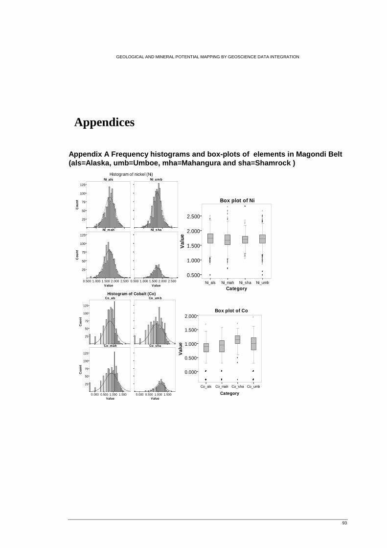
GEOLOGICAL AND MINERAL POTENTIAL MAPPING BY GEOSCIENCE DATA INTEGRATION
93
Co_als Co_mah Co_sha Co_umb
Category
0.000
0.500
1.000
1.500
2.000
Val
ue
��
�
���������������������� �
�����
�
�������
���
��
��
��
��
��
�
�
�
�
�
��������
�
�
�
�
�
�
�
�
��
�
�
���������
����
�
�
�
��
��
��
�������
��
��
�
��
�
�
�
������������������������������ �
Box plot of Co
25
50
75
100
125
Cou
nt
Co_als Co_um b
Co_mah Co_sha
0.000 0.500 1.000 1.500Value
25
50
75
100
125
Cou
nt
0.000 0.500 1.000 1.500Value
Histogram of Cobalt (Co)
25
50
75
100
125
Cou
nt
Ni_als Ni_umb
Ni_m ah Ni_sha
0.500 1.000 1.500 2.000 2.500Value
25
50
75
100
125
Cou
nt
0.500 1.000 1.500 2.000 2.500Value
Histogram of nickel (Ni)
Ni_als Ni_mah Ni_sha Ni_umb
Category
0.500
1.000
1.500
2.000
2.500
Val
ue
�
��
����
�
�
����
�
�
�
�
�
�
�
�
�
�
� ��
�
��
�
�
�
�
����
���
��
�
�
�
�
�
�
�
��
�
�
�
�
�
��
�
����
�
���
�
�
�
�
��
�
�
�
�
�
��
��
�
�
�
�
�
���
��
�
�
�
�
�
�
Box plot of Ni
Appendices
Appendix A Frequency histograms and box-plots of elements in Magondi Belt (als=Alaska, umb=Umboe, mha=Mahangura and sha=Shamrock )
GEOLOGICAL AND MINERAL POTENTIAL MAPPING BY GEOSCIENCE DATA INTEGRATION
94
Cu_als C u_umbCu_mahCu_sha
Category
0.000
1.000
2.000
3.000
Value
�
�
�
�
�
���
�
�
��
�
���
�
��
�����
�
��
��
��
�
�
���
�
�
�
��
�
�
��
�
�
���
�
�
�
�
�
��
�������������������������
�
��������
�
�
�
�
�
�
Box plot of Cu
25
50
75
100
125
Count
Cu_als
Cu_umb
Cu_mah
Cu_sha
0.000 1.000 2.000
Value
25
50
75
100
125
Count
0.000 1.000 2.000
Value
Histogram of copper (Cu)
0
25
50
75
100
Cou
nt
Pb_als Pb_m ah
Pb_sha Pb_um b
0.000 0.500 1.000 1.500Value
0
25
50
75
100
Cou
nt
0.000 0.500 1.000 1.500Value
Histogram of copper (Pb)
Pb_als Pb_mah Pb_sha Pb_umbCategory
0.000
0.500
1.000
1.500
2.000
Val
ue
��������������������������������������������������������������������
�
�
�
���
�
�
�
�
�
����
�
����
�
�
�������
�
�
�
�
��
�
������
�
���
�
�
�
�
�
�
�
�
�
�
�
��
��
�
���
���
�
���
�
���
�
�
�
����
�
��������
�
����
�
��
�
����������������� ������������������������������������������������������
Box plot of PbZn_als Zn_umb Zn_mah Zn_sha
Category
0.000
1.000
2.000
3.000
Val
ue
���
�
�
�
�
��
�
�
�
�
��
�
�
�
�
��
�
��
�
�
�
�
�
�
�
�
�
��
��
�����
�
�
�
�
�
�
�
�
��
�
�
��
�
��
���
�
�
�
�
���
����
�
�
�
���
�
�����������
�
�����
�
�
�
�
�
��
��
��
�
�
�
�
�
�
��
�
�
����
�
��
��
�
�
��
�
�
�
�
�
�
�
�
�
�
�
�
��
�����
�
���
�
�
�
��
�
�
�
�
�
�
���
�
�
�
��
�
�
�
�
�
�
�
�
�
�
�
�
��
�
��
�
�
�
�
�
�
�
�
�
�
�
�����
���
�
�
�����
�
�
�
�
�
���
��
�
�
�
���
�����
�
�
�
�
�
��
�
�
���
�
��
�
�
�
��
�
��
�
�
�
�
�
�
�
�
�
�
�
�
�
�
�
���
�
�
��
�
��
�
�
�
��
��
�
�
�
�
�
��
�
�
�
�
�
�
�
�
�
�
��
�
�
�
�
�
����
�
����
�
�
�
��
Box plot of Zn
0
25
50
75
100
Cou
nt
Zn_als Zn_um b
Zn_m ah Zn_s ha
0.000 1.000 2.000 3.000Value
0
25
50
75
100
Cou
nt
0.000 1.000 2.000 3.000Value
Histogram of copper (Zn)
0
25
50
75
100
Cou
nt
Fe_als Fe _um b
Fe_mah Fe _sha
-0.500 0.000 0.500 1.000Value
0
25
50
75
100
Cou
nt
-0.500 0.000 0.500 1.000Value
Histogram of Iron (Fe)
Fe_als Fe_umb Fe_mah Fe_sha
Category
-0.500
0.000
0.500
1.000
Val
ue
��
�
�
�
�
���
�
��
�
�
���
�
��
���
��
�
�
�
�
�
�
��
�����
Box plot of Fe
GEOLOGICAL AND MINERAL POTENTIAL MAPPING BY GEOSCIENCE DATA INTEGRATION
95
Appendix B Field observation dataset
observ_pt X_Coordinate Y_Coordinate Observation/ Rock_name
Strik_Dip of foliation
Geologic Structure Mine
200 177335.4852 8185241.602 Biotite and hornblend para gneiss 60w/40
221 178744.2261 8186024.568 Biotite and hornblend para gneiss 80/30
222 180037.6628 8186873.501 Biotite and hornblend para gneiss 52/74
223 180484.7084 8181004.988 Biotite and hornblende para gneiss Shamrock_mine
225 184879.8922 8168100.681 Granite
226 182178.411 8168246.988 Granite
227 188955.4083 8167835.872 Granite 64/52
228 186706.5774 8170036.25 Granite
229 183896.0571 8168110.938 Granite
230 189612.1949 8170026.858 Granite
231 192401.6793 8165177.266 Granite
232 191741.598 8163230.323 Granite
233 188469.0343 8171848.376 Basic igneous rocks 37/52
234 189575.8536 8172912.243 Granite
235 192255.7421 8176140.27 Granite 70/45
236 188492.9267 8161624.514 Granite
237 190407.8172 8162075.595 Granite 45w/50
238 189713.2375 8159321.502 granite 60w/48
239 187231.3514 8158548.216 phyllite 60w/78
240 190776.6774 8155073.936 Phylite 40w/45
241 192650.3858 8155141.833 Arkose 45w/75
241 194042.0354 8150303.978 arkose anticline
243 181287.298 8103085.204 Arkose 66/60
245 182154.0808 8104549.722 Arkose 48/58
665 183537.6245 8104717.376 basic igneous rocks syncline
754 183016.3142 8101804.315 Graphitic slate 15/83
976 186621.9559 8097946.381 Doloritic dyke 37/52
775 186621.9228 8097946.401 Doloritic dyke 543/87
887 188798.3015 8101714.186 Dolomite 75/18
932 192662.1893 8104690.554 Dolomite 24/10
512 188707.8236 8102447.654 Arkose 60/40
654 187141.922 8107095.637 Basic igneous rocks 57/53
110 188608.2312 8107091.802 Basic igneous rocks 52/72
731 190670.123 8107095.392 Arkose 72/28
553 192662.1963 8104690.519 Dolomite 24/10
676 191938.759 8108128.631 Basic igneous rocks 37/50
432 194217.0599 8109061.347 Arkose 80/44
188 194791.239 8110628.212 Arkose 83/17
1001 193008.052 8110334.711 arkose syncline
511 191870.3826 8090021.259 Arkose 28/58
988 191870.4042 8090021.298 Arkose 28/85
289 191701.5888 8089001.89 Basic igneous rocks 28/80
523 188689.0243 8085142.901 Arkose Avondale_mine
779 185882.3066 8084563.811 Arkose Shaklton_mine
659 194703.7194 8082156.876 Dolomite 45/75
96
239 183140.7584 8079497.75 Arkose anticline
712 183501.947 8078259.123 Arkose 38/82
899 182319.5141 8077757.359 Arkose 48w/33
550 181628.6593 8078064.634 Arkose
190 181589.916 8079149.352 Arkose 52/25
268 182887.7687 8082738.554 Doloritic dyke anticline
194 182714.1724 8083663.091 Arkose 42/22
366 194633.9609 8078957.419 Dolomite 45/80
1020 191434.9408 8077062.818 Dolomite anticline
656 193236.0785 8077492.866 Dolomite 45/85
440 190061.9432 8074671.538 Arkose 45/80
428 187257.7292 8074024.682 Arkose Angwa_mine
6280 185032.8833 8071282.588 Arkose Hans_Mine
773 184696.9334 8075528.248 arkose syncline
419 183597.9022 8074021.625 Basic igneous rocks 58/83
1002 192721.9104 8124492.716 Slate 38/45
122 192458.3745 8118634.855 Arkose 60
1030 197346.932 8124979.026 Arkose Norah_Mine
2825 203138.4184 8123059.882 Basic igneous rocks 25
1216 206580.3789 8124569.788 Dolomite syncline
1830 203898.8831 8117542.693 Dolomite syncline
2725 205304.1243 8116994.37 Dolomite syncline
335 201338.8978 8109748.25 Dolomite United_Kingdom
871 197190.8375 8111923.67 Basic igneous rocks 70/66
980 199827.0981 8096574.438 Dolomite syncline
621 198434.8294 8092895.428 Dolomite syncline
1200 196253.0636 8088415.278 Dolomite syncline
1919 196905.073 8087609.658 Dolomite syncline
634 197637.6448 8087596.21 Dolomite syncline
436 202290.8447 8078623.756 Granite Chinhoyi
774 198121.7973 8130458.429 Arkose Mhangura_Mine
284 195167.6377 8141204.321 Basic igneous rocks 31/84
659 194087.8378 8141304.124 Arkose 35/70
301 179200.1649 8089200.348 Slate quartzite(Biotite bearing) and dolomite
447 183112.0668 8087805.405 Arkose 32/60
987 188638.2248 8108222.451 Arkose 73
661 192587.4735 8115912.706 Arkose anticline
671 194619.6116 8118153.202 Arkose anticline
2003 195137.3635 8112124.321 Arkose anticline
805 183551.9954 8082702.078 Doloritic dyke
979 170524.4564 8090784.49 Quartzite, feldspathic quartzite
3054 177394.3731 8082641.187 Quartzite, feldspathic quartzite
2836 181784.3705 8105389.439 Quartzite, feldspathic quartzite
1040 182593.627 8102431.476 Quartzite, feldspathic quartzite
5459 177904.1661 8094396.676 Quartzite, feldspathic quartzite
4064 185668.9662 8107390.906 Arkose
551 170234.6583 8096647.043 Graphitic slate
2854 195425.9632 8103208.877 Dolomite
GEOLOGICAL AND MINERAL POTENTIAL MAPPING BY GEOSCIENCE DATA INTEGRATION
97
3300 197415.4367 8106461.234 Arkose
440 188056.4943 8113247.38 Arkose
117 192642.3067 8123734.719 Slate
752 182219.7194 8108112.247 Arkose
337 183295.0024 8157147.695 Slate
1028 190189.7925 8170425.154 Granite
1022 199059.0661 8169755.761 Granite
180 203695.5304 8191420.89 Biotite and hornblend para gneiss
999 203580.4129 8157973.13 Meta-ultramafic rock with serpentinite or talc
1016 175137.221 8163121.373 Phyllite
2823 197791.4365 8132865.952 Arkose
892 196240.998 8139133.608 Basic igneous rocks
541 197309.4312 8143733.964 Basic igneous rocks
3390 197309.4312 8143733.964 Basic igneous rocks
645 197309.4312 8143733.964 Basic igneous rocks
782 191704.5359 8153230.21 Arkose
893 193575.0597 8165282.556 Granite
566 186218.9276 8171941.241 Basic igneous rocks
671 172566.9818 8137241.898 Phylite, slate and quartzite
1101 168936.4625 8107134.232 Phylite, slate and quartzite
80 174033.5685 8155333.059 Slate
430 179696.4277 8163722.48 Arkose
54 185149.5513 8138344.481 Slate
870 187876.1131 8117993.216 Graphitic slate
7550 192280.5591 8130373.605 Graphitic slate
9870 181374.3119 8153234.777 Graphitic slate
32 163546.7924 8151137.422 Phylite
930 163756.5279 8173579.123 Phylite
81 167741.5028 8163302.082 Granite
900 186617.7 8123452.333 Graphitic slate
553 205703.6327 8066364.916 Granite
422 202977.0708 8091323.444 Granite
6650 207381.5169 8097825.245 Granite
6630 169419.387 8069114.522 Graphitic slate
554 165434.4121 8066597.696 Slate
5550 164385.7344 8088619.926 Slate
4300 193538.9723 8198962.558 Grits, sandstone etc
59 181793.7829 8198752.822 Grits, sandstone etc
71 185569.0224 8174627.677 Basic igneous rocks
2987 175501.7172 8126380.043 Phylite, slate and quartzite
5400 166692.8252 8126380.043 Phylite, slate and quartzite
19 166483.0897 8142949.149 Granite
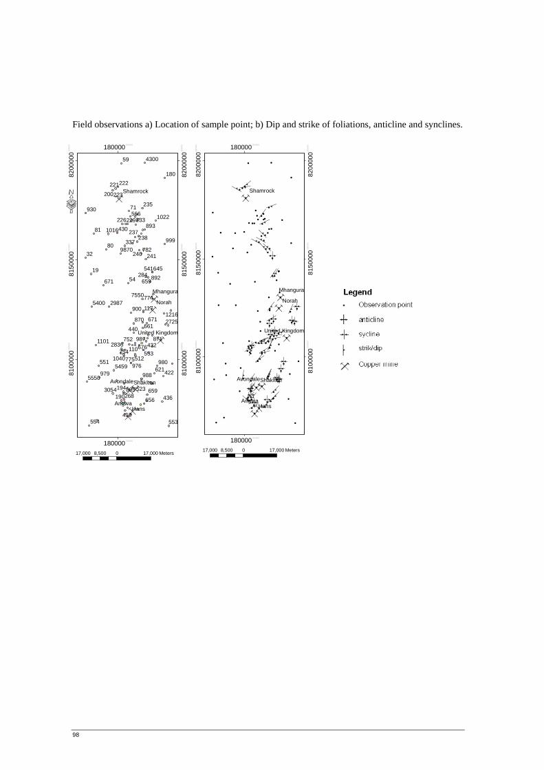
98
Ç
ÇÇÇÇ
Ç
Ç
Ç
¹¹¹
¹
¹¹
¹¹¹¹¹
¹¹¹ ¹¹¹
¹¹¹¹¹¹¹¹¹
¹¹¹
¹¹¹¹¹
¹ ¹¹¹¹
¹
¹
¹
¹
¹¹
¹ ¹
¹
¹Ï
ÑÑ
ÏÏ ÏÑ
ÑÑ Ñ
ÑÑÑ Ñ Ñ
Ï Ï Ï
!!
!
!
!!!
!
!
!
!
!
!
!
!
!!
!!
! !
!
!
! !
!
!!
!
!
!
! ! !
!
!!
!!
!!!
!!
!
!
!!!
!
!!
!
! !
!!
!
!
!
!
!
!
!
!
!!
!
!
!
!
!!!
!
!
!!
!
!
!
!
!
!
!
!
!
!
!
!
!
!
!
!
!
!
!
!
!!
!
!
!
!
!
!!!
!
!
!
!
!
!
!
!
!
!
!
!
!
!
!
!
!
!
!
!
!
!!
!
!!
!
Hans
Norah
Angwa
Mhangura
ShakltonAvondale
Shamrock
United Kingdom
180000.000000
180000.000000
8100
000.0
000
00
8100
000.0
000
00
8150
000.0
000
00
8150
000.0
000
00
8200
000.0
0000
0
8200
000.0
0000
0
17,000 0 17,0008,500 Meters
Ç
ÇÇÇÇ
Ç
Ç
Ç
Hans
Norah
Angwa
Mhangura
ShakltonAvondale
Shamrock
United Kingdom
19
71
59
81
32
54
80
554
422
553
900
930
870
430
671
566
893
782
645541
892
999
180
337
752
117
440
551
979
805
671661
987
659284
774
436
621980
871
419
656
194268190
659523
988
432676553
110
512775976
754
241240
238237
235
233229226
223
222221
200
5400 2987
4300
5550
9870
7550
1101
1016
1022
54591040
2836
3054
27251216
180000.000000
180000.000000
8100
000.0
000
00
8100
000.0
000
00
8150
000.0
0000
0
8150
000.0
0000
0
8200
000.0
000
00
8200
000.0
000
00
·
17,000 0 17,0008,500 Meters
Field observations a) Location of sample point; b) Dip and strike of foliations, anticline and synclines.