Geological Survey of Norway P.O.Box 6315 Torgarden NO-7491 TRONDHEIM Tel.: 47 73 90 40 00 REPORT

Report no.: 2019.004 ISSN: 0800-3416 (print) ISSN: 2387-3515 (online)

Grading: Open

Title:

Reprocessing of Refraction Seismic data from Åknes, Stranda Municipality, Møre & Romsdal County.

Authors:

Georgios Tassis & Jan Steinar Rønning Client:

NVE, Norwegian Water Resources and Energy Directorate

County:

Møre & Romsdal Commune:

Stranda

Map-sheet name (M=1:250.000)

Ålesund Map-sheet no. and -name (M=1:50.000)

1219 II Geiranger

Deposit name and grid-reference:

Åknes, UTM 32 395800 - 6895200 Number of pages: 29 Price (NOK): 100,- Map enclosures:

Fieldwork carried out:

2-12 July 2017 Date of report:

20.02.2019 Project no.:

329500 Person responsible:

Summary:

In continuation to the various ground geophysics data collected at the unstable rock slope area at Åknes during the past 15 years, NVE commissioned GeoExpert AG from Switzerland to perform additional seismic investigations. These investigations were aimed at helping to determine the thickness of the overburden material and of the fractured bedrock. It was also of interest to image tectonic faulting within the bedrock. The seismic acquisition was distributed in three profiles with a total length of 2.7 km. During the processing stage, GeoExpert AG implemented WET (Wave Eikonal Traveltime) inversion on these three profiles using Rayfract® software. Inversion utilized a starting model acquired by DeltatV method and a 50-iterations single run. Results were presented in a report delivered to NVE, together with the first break pickings of the raw data.

NGU has done extensive research and testing on the use of Rayfract® program and has

obtained specific knowledge via modeling of synthetic data and real data processing as to the optimized parameters a user should pick when vertical structures such as fracture zones in bedrock are investigated. NVE has provided the NGU with the refraction seismic data to undergo reprocessing in Rayfract® using a different approach than GeoExpert AG. Eventually, results would be delivered to NVE in a format compatible with the Åknes 3D model built in PETREL software by Schlumberger. This report presents the results obtained from reprocessing the three refraction seismic profiles in Åknes with the use of Rayfract®. We have produced starting models using two different approaches, Hagedoorn’s Plus-Minus using Midpoint Break and DeltatV methods and then implemented Multirun WET inversion using seven runs of maximum 50 iterations per run and minimal smoothing. The results are naturally close to the ones GeoExpert AG obtained but using parameter routines which highlight possible fracture zones have also induced some qualitative differences. All results were plotted in 3D using Geosoft Oasis Montaj together with older refraction seismic interpretations. Possible fracture zones were projected to the surface and plotted along similar interpretations obtained by ERT and structural mapping to check coherence between different methods and approaches.

Keywords: Geophysics

Refraction Seismic

Inversion

Reprocessing

Unstable Rock

Fracture Zones

Rock Quality

Scientific Report

CONTENTS

1. INTRODUCTION ................................................................................................. 7

2. MEASUREMENTS, INVERSION AND INTERPRATION BY GEOEXPERT AG .. 7

3. REPROCESSING: INITIAL MODELS AND MULTIRUN WET INVERSION ........ 9

4. REPROCESSING RESULTS ............................................................................. 10

4.1 Profile 17Åknes-1 ........................................................................................ 11

4.2 Profile 17Åknes-2 ........................................................................................ 13

4.3 Profile 17Åknes-3 ........................................................................................ 15

5. POINT CLOUD INTERPRETATION .................................................................. 17

5.1 Fractured / Water-Saturated Bedrock .......................................................... 17

5.2 Possible fracture zones ............................................................................... 18

5.3 Potential Rockslide Materials and Correlation with ERT interpretations ...... 21

6. DIGITIZING OF OLD REFREACTION SEISMIC & 3D PLOTTING.................... 24

6.1 Digitization of traditional Plus-Minus interpretations .................................... 24

6.2 3D Presentation ........................................................................................... 25

7. CONCLUSIONS ................................................................................................. 27

8. REFERENCES .................................................................................................. 29

7

1. INTRODUCTION

The Norwegian Water Resources and Energy Directorate (NVE) is putting together a multidisciplinary 3D model in PETREL software which accumulates all relevant information to the unstable rock slope at Åknes. NGU has previously performed a significant amount of ground geophysical measurements in the study area consisting of ERT, refraction seismic and GPR measurements (Rønning et al. 2006; Rønning et al. 2007). In association with the compilation of this 3D model, all old ERT profiles collected during various fieldwork seasons in Åknes and a new profile acquired in 2017, have been reprocessed and subsequently delivered to NVE in ASCII format to be plotted in 3D space (Tassis & Rønning 2018). This procedure is now repeated for the newest refraction seismic data collected in the area by the Swiss private company GeoExpert AG (GeoExpert 2017). NGU has spent a large effort in understanding and optimizing tomographic inversion of refraction seismic data done with Rayfract® software (Rayfract 2018a; Rayfract 2018b) by means of modeling but also by testing previously acquired knowledge on real data (Rønning et al. 2016, Tassis et al. 2017, Tassis et al. 2018). It has been concluded that when possible fracture zones are investigated, the best results are obtained by using a starting model constructed with the use of Hagedoorn’s Plus-Minus method (Hagedoorn 1959) and consequently by applying multirun Conjugate Gradient WET (Wave Eikonal Traveltime) inversion (Schuster & Quintus-Bosch 1993) with Cosine-Squared weighting and minimal smoothing. In this sense, the three refraction seismic profiles collected by GeoExpert AG in 2017 were reprocessed by NGU and delivered to NVE in ASCII format to be compatible with PETREL software (Schlumberger 2017). This report presents the reprocessing results of the refraction seismic data collected by GeoExpert AG and the digitization and conversion to vertical 3D grids of four additional refraction seismic profiles measured in the past by NGU (Rønning et al. 2006, Rønning et al. 2007) utilizing traditional Plus-Minus interpretation techniques (Hagedoorn 1959). The report also presents possible fracture zone interpretations on the newest WET inversion results using classed post (point cloud) visualization.

2. MEASUREMENTS, INVERSION AND INTERPRATION BY GEOEXPERT AG

Profiles 1, 2 and 3 (figure 2.1) were measured by GeoExpert AG between July 2nd and 12th 2017 using the SmartSystem acquisition system (260 channels, 24-bit A/D conversion). The seismic source consisted of two sets of 8 kg hammers with extended shaft and a metal plate, yielding a maximum attainable penetration depth of 100 m. Geophone spacing was set equal to 2 m while shots were conducted every 6 m, thus fulfilling the general prerequisites for WET inversion feasibility (shot spacing = 3 * geophone spacing). The Refraction Seismic processing sequence was compiled with the use of Rayfract® software and according to the technical report submitted by GeoExpert AG includes the following steps (GeoExpert 2017):

8

a. Refraction arrival picking b. CMP-sort of first break picks c. Derivation of the refraction seismic velocities for the initial model by using the

DeltatV method d. Refinement by iterative modeling of the velocity-depth profile by single-run

WET tomography (50 iterations) e. Display of velocity field

Interpretations were based on the assumption that 2,500 m/sec is to be regarded as the delimiter between loose rock / soil material and self-supporting rock. Material above this line was interpreted as either slope debris or a bedrock surface completely disintegrated by weathering or by jointing related to tectonic processes. Concerning possible fracture zones, several localities were marked by the authors of the technical report in text, but those interpretations are based on the reflection seismic data and no further quantitative information is given on these potential weak zones.

Figure 2.1: Positioning for all refraction seismic profiles conducted in Åknes in 2017 along with matching ERT profiles (white: 10 m electrode spacing, red: 5 m electrode spacing),

refraction seismic profiles from 2006 and borehole positions. LiDAR elevation relief.

9

3. REPROCESSING: INITIAL MODELS AND MULTIRUN WET INVERSION

The raw refraction seismic data from Åknes were delivered to NGU as the first break pickings performed by GeoExpert AG. All data were saved in the designated format immediately readable by Rayfract® (.asc and .cor files) while topographic information was already incorporated in these files. Essentially, this meant that no pre-processing was required from our part and that all three profiles were set and ready to be imported and subsequently inverted in Rayfract®. Our extensive modeling work on similar settings such as the one found in Åknes has shown that Hagedoorn’s Plus-Minus method with interactive branch point picking is our best option for producing starting models (Tassis et al. 2018). However, these datasets were produced with very dense shot points, starting from 260 for profile 1 and going up to 640 for profile 3. Due to Rayfract® not offering the possibility to zoom into individual traveltime curves in order to map traces to refractors in detail, such dense data make interactively picking branch points extremely time-consuming to almost impossible. Therefore, interactive branch point picking had to be replaced by our second go-to option which is the automatic Midpoint Breaks function (Tassis et al. 2018). The specialized parameters used for this procedure is shown in table 3.1.

Parameter Value / Option

No. of horizontal layers 2

Direct wave first breaks recorded Uncheck

Refractor Count 2

CMP Stack Width 15 or 20

Regression Receiver Count 2 or 3

Direct Wave Delta 2 or 3

Refracted Wave Offset Delta 3 or 5

Weathering Limit 300 m/sec

Refractor 1 Limit 1,500 m/sec

Overburden / Base Filter Both 15 or 20 Table 3.1: List of parameters utilized for Midpoint Breaks / Plus Minus method.

Such dense data have not allowed us to do individual branch point picking, but they gave us the opportunity to also implement DeltatV method like in the processing done by GeoExpert AG. In this way, we were able to test our strategy which incorporates Multirun Conjugate Gradient WET inversion with Cosine-Squared weighting and minimal smoothing on an initial model acquired by both Midpoint Breaks and DeltatV methods, in comparison to the simple single-run approach of the Swiss company. The parameters used to produce the DeltatV starting model are shown in table 3.2.

Parameter Value / Option

Suppress Velocity Artefacts Check

Smooth CMP Traveltime Curves Check

CMP curves stack width 10 or 20

Regression over offset stations 3 or 5

Weathering crossover 2 or 3

Surface Consistent Corrections Check Table 3.2: List of parameters utilized for DeltatV method.

10

After the construction of our initial models, implementing WET inversion was the next step. This procedure has been tested thoroughly at NGU (Tassis et al. 2017, 2018) and the choice of parameters follows a fixed course. Generally, relevant modeling has revealed that Conjugate Gradient inversion (CG iterations 10 or 15) is preferable over Steepest Descent while smoothing must be gradually decreased for lateral variations in seismic velocity to be highlighted. Parameters used for multirun WET inversion are presented in table 3.3.

Parameter Value / Option

Runs 7

Maximum no. of Iterations 50

Wavepath Frequency 50 Hz

Wavepath Width Decreasing from 30 to 8 %

Ricker differentiation -2 (Cosine)

Manual smoothing Check

Half smoothing filter width 3

Half smoothing filter height 1

Maximum velocity update 25 %

No. of Smooth nth iterations 10 Table 3.3: List of parameters utilized for multirun WET inversion.

NGU do not see that the reflection seismic interpretation performed by GeoExpert AG give reliable interpretations, and no attempt to reprocess these data have been tried.

4. REPROCESSING RESULTS

Geoexpert AG performed three refraction seismic lines in 2017. All these are reprocessed using the procedure described in section 3. Refraction seismic lines performed earlier by NGU (see Figure 2.1) do not have a shooting point spacing suitable for tomographic inversion. These data will be included in the 3D PETREL model as they are.

11

4.1 Profile 17Åknes-1

Figure 4.1 displays the results of the above described inversion procedure for profile 17Åknes-1. Top left shows the Midpoint Breaks / Hagedoorn’s Plus-Minus method initial model which presents a setting which is typical for such a model. Two low-velocity horizontal layers designated during Midpoint Breaks procedure overlay a highly fragmented bedrock even though relatively high overburden and base filters were used. The top layer follows an almost constant thickness of maximum 5 meters (~500 m/sec) throughout the profile while the underlying one (~1,300 m/sec) begins at a thickness of about 25 m in the west and decreasing to about 10 m in the east. These two layers represent most likely scree materials. Bedrock found below these overburden layers is fragmented in several columns that show an alternation of low and high velocity and vice versa. The Hagedoorn interpretation is negated by Multirun WET inversion as seen in the middle and left profile in figure 4.1. The qualitative and quantitative characteristics of the overburden layers are validated by inversion, but the bedrock appears to be continuously over 4,500 m/sec of seismic velocity except for an area at position 500 m, where a decrease in velocity is marked. In this area, a 50-m wide possible fracture zone can be registered presenting velocities of 3,500 – 3,600 m/sec while neighboring high-velocity blocks are up to 4,200 m/s west of the proposed zone and 5,000 m/sec east of it. It is also noteworthy to mention that after about 650 m, a wide low velocity area (~2,600 m/sec) can be seen which is continued all the way to the eastern end of the profile (about 150 m wide). The ray coverage plot seen at the bottom left of figure 4.1 indicates that there is a satisfactory number of wavepaths at full length of the profile yielding a depth coverage between 50 m at the edges and up to 90 m at the deepest part. The initial model constructed with the use of DeltatV method can be seen at the top right of figure 4.1. As expected, it is plagued by many high frequency artefacts and the change in velocity from top layer to supposed bedrock is smoother and more gradual. The exact same Multirun WET inversion scheme was applied here too, returning the result found at the middle right part of the figure. First, we may denote a number of artefact zone-looking features inherited by the starting model to the inversion result, seen as 1,500 m/sec vertical structures at multiple locations in the profile (at 60, 160, 320, 440 and 730 m). Furthermore, using a DeltatV starting model induces a transition zone between low-velocity top layers and possible bedrock which is thicker and more continuous than with Midpoint Breaks/Plus-Minus initial model. In the case of Hagedoorn’s starting model, the 2,500 – 3,000 m/sec transition zone was only apparent in the vicinity of the possible fracture zone at position 500 m with a maximum thickness of 30 meters. Using DeltatV as an initial model made the transition zone to be equally thick throughout the profile. As for the possible fracture zone described above, it is still evident and presents the same quantitative characteristics, although located about 40 m to the east compared to before. Ray coverage plotted at the bottom right part of figure 4.1, shows a larger but slightly unreasonable depth penetration of about 130 m which is comparable to the GeoExpert AG results. However, wavepaths here present a sparser and thus dubious distribution compared to the more compact allocation when Midpoint Breaks/Plus-Minus initial model is used. In any case, RMS errors for both inversion results are almost identical (3.8 against 3.9% respectively).

12

Figure 4.1: Profile 17Åknes-1 - Top: Initial models obtained by Midpoint Breaks and subsequent Hagedoorn’s Plus-Minus application (left) and DeltatV (right) method. Middle: Multirun WET Inversion results using Hagedoorn’s +/- (left) and DeltatV (right) starting models respectively. Bottom:

Ray coverage for respective WET Inversion.

13

4.2 Profile 17Åknes-2

Figure 4.2 follows the same setting as in figure 4.1 and demonstrates all steps of the inversion procedure using a Midpoint Breaks/Plus-Minus starting model on the left side and DeltatV on the right. The Midpoint Breaks/Plus-Minus starting model shown on the top left corner of the figure exhibits a low velocity regime in this area. The two top layers with velocities less than 1500 m/s specified during the implementation of Midpoint Breaks method present a constant collective thickness of about 20 meters throughout the length of the profile. Again, the space below these layers is mainly occupied by low-velocity fragments except for a location in the middle where a hint of the high-velocity bedrock is given. Considering the extremely high inclination of the ground along this profile, it is safe to assume that these low-velocities followed down in depth will be disproved during inversion. The Multirun WET inversion result for this profile shown in the middle left side of figure 4.2 validates the general low-velocity regime of the initial model, but also composes a more extensive low-velocity top-layer. On the northern half of the profile, this layer appears to be about 50 meters thick and presents a more homogeneous velocity between 1,000 and 1,500 m/sec while on the southern half, demonstrates a higher and more rapid increase in velocity over smaller depth i.e. from 500 m/sec superficially to 1,500 m/sec after 30 m. However, the most interesting feature in this profile is the vertical variation in velocity at about 220 m distance from possible bedrock (5,800 m/sec) to a rather wide low-velocity area (2,000 m/sec). This can be interpreted as an almost 130-m wide possible fracture zone and lies in proximity to the position of the back-scarp on the surface. How accurate this match is, will be shown later in this report. The DeltatV starting model on the other hand shown on the top right corner of figure 4.2 consists of a more realistic velocity distribution which again shows lots of high frequency artefacts. The subsequent implementation of WET inversion presented just below the initial model, returns a result which is quite similar to the Midpoint Breaks/Plus-Minus inversion result. Since RMS errors for both inversion results are again almost identical (3.0 % for DeltatV and 3.1 % for Plus-Minus), the main qualitative and quantitative difference refers to how the higher velocities are distributed in the profile. In DeltatV actuated inversion, which again shows a higher depth coverage than before (maximum 150 m meters vs. 130 m), possible bedrock occupies a larger area within the profile but with a lower velocity compared to the Plus-Minus inversion result (4,400 m/sec instead of 5,800m/sec). Regardless, the same low-velocity concentration can be found at the same location in the profile, with the same lateral change in velocity distribution, anomaly shape and total extension. Ray coverage for both approaches presents a similar wavepath pattern with lots of gaps in low-velocity areas and a higher concentration where bedrock is interpreted to be. Lastly, penetration depth for this case appears to be comparable between the two different starting models i.e. 130 m for Plus-Minus method and 140 m for DeltatV although the northern half of the former presents a noticeably smaller extent (80 m) than the latter (at least 100 m and increasing).

14

Figure 4.2: Profile 17Åknes-2 - Top: Starting models obtained by Midpoint Breaks and

subsequent Hagedoorn’s Plus-Minus application (left) and DeltatV (right) method. Middle: Multirun WET Inversion results using Hagedoorn’s +/- (left) and DeltatV (right) starting

models respectively. Bottom: Ray coverage for respective WET Inversion.

15

4.3 Profile 17Åknes-3

The third profile measured in Åknes by GeoExpert AG is covering almost the whole slope, all the way down to the fjord and was collected over very steep mountainside (see figure 2.1). This profile and the one presented in the previous section overlap near their edges, and profile 17Åknes-2 essentially is a continuation of 17Åknes-3 towards the north. In the technical report written by GeoExpert AG, these two profiles are merged, and we will be following this arrangement in the interpretation section. In this section, we focus on this profile separately shown in figure 4.3 and again displaying two Multirun WET inversion results together with respective starting models and ray coverage plots. Top left plot shows the Midpoint Breaks/Plus-Minus starting model which illustrates a low-velocity top layer decreasing in thickness towards the south from 20-25 meters to 5-10 near the fjord. Τhe bedrock block velocity beneath the top-layer presents interchanges between high and low values without any particular trend towards the south. In the same manner as in profile 17Åknes-2, steep topography is enabling blocks especially on the northern half of the profile to unrealistically extend in depth. This will be redeemed during WET inversion. Multirun WET inversion result is shown in the middle and left of figure 4.3. and is characterized by a low RMS error of 2.5 %. The qualitative characteristics of the low-velocity top layer (500 to 1500 m/sec) are verified by inversion, showing a larger thickness in the north (~30 m) than in the south (~10 m). This layer is almost continuous except at about 650 m where a small topographic ridge is interrupting it. This ridge relates to a high-velocity concentration almost continuous in depth which indicates outcropping solid bedrock at this location. Furthermore, high velocities which can be attributed to unfractured bedrock may be found deeper in the north than in the south, overlain by what we referred to in previous sections as transition zone (2,500 to 3,000 m/sec). This transition zone is becoming more apparent between positions 200 m and 600 m in the profile while being almost imperceptible at the southern edge where transition from top-layer to bedrock is very rapid. As for possible fracture zones, attention is immediately drawn towards the almost vertical velocity transition from almost 6,000 m/sec at the position of the above-mentioned ridge (650 m) to about 2,800 m/sec at about 800 m. Another possible weak zone locality can be marked at about 270 m where high-velocity concentrations (about 4,700 m/sec on both sides) are interrupted by a low-velocity breach which is about 2,500 m/sec just below the low-velocity top layer and gradually increases to 3,600 m/sec at the end of the coverage. Again, the DeltatV-built initial model shown on the top right of figure 4.3 presents many high-frequency artefacts but also a top-layer setting similar to the Plus-Minus method one. The multirun WET inversion result shown exactly below the initial model, presents a strong horizontal tendency to the velocity distribution which indicates that DeltatV combined with steep topography could lead to dubious structures. If we overlook the horizontal artefacts, the qualitative characteristics of this result are comparable to the Plus-Minus WET inversion one. Quantitatively, the possible fracture zone at 800 m is not as vertically formulated as before and presents a higher velocity (3,500 m/sec). The other marked locality is not interpretable due to heavy horizontal artefacts which mask any possible vertical weak zone hints. Lastly, we may once again notice on the bottom plots in figure 4.3 that DeltatV inversion offers a higher but sparser depth coverage which reaches locally 140 meters

16

as opposed to Plus-Minus where the maximum depth equals 95 m and the distribution is more close-knit. Generally, using DeltatV as a starting model pushes inversion to express the transition from top layer to bedrock more gradually and therefore offering faster routes through deeper layers. However, such penetration depths are doubtful especially for data produced with hammer strikes.

Figure 4.3: Profile 17Åknes-3 - Top: Initial models obtained by Midpoint Breaks and

subsequent Hagedoorn’s Plus-Minus application (left) and DeltatV (right) method. Middle: Multirun WET Inversion results using Hagedoorn’s +/- (left) and DeltatV (right) starting

models respectively. Bottom: Ray coverage for respective WET Inversion.

17

5. POINT CLOUD INTERPRETATION

By point cloud maps we refer to the plotting of individual point values in 2D or 3D space as dots that are colored according to the velocity group they fall into. In this way, velocities are divided into classes since we are not displaying the reprocessing results in gradually changing colored contours but as single-colored spans of values which represent different classes in bedrock. Therefore, we may classify the inversion results in a way that can highlight different bedrock classes in Åknes and help us interpret unstable masses and possible fracture zones in a pure numerical fashion. As mentioned in section 2, 2500 m/sec is the delimiter between fractured and massive bedrock in the technical report delivered by GeoExpert AG for interpreting the inverted seismic velocity. However, we will be categorizing bedrock in accordance with the classes we have assorted resistivity inversion results (Tassis & Rønning 2018). In this sense, we focus on two formations i.e. fractured bedrock that is drained and represents the potential rockslide material on the surface of the slope and fractured bedrock but this time water-saturated, which could contain gliding planes. For this purpose, we isolated inverted seismic velocities between 0 and 500 m/sec for scree materials (tallus), 500 to 2000 m/s highly fractured drained bedrock and between 2,000 and 3,500 m/sec for fractured / water-saturated bedrock in order to facilitate interpretation.

5.1 Fractured / Water-Saturated Bedrock

We employ point-cloud classification mode in order to make interpretations in relation with the water-saturated part of fractured bedrock in Åknes. Using the entire calculated value spectrum, we attempted to prompt clear limits within the velocity distribution to facilitate interpretation. The full classification utilized is shown in table 5.1.

Class color. Velocity (m/sec) Bedrock Description

Purple 500 or less Scree Materials - Tallus

Blue 500 – 2,000 Highly fractured / Drained

Green 2,000 – 3,500 Fractured / Water-Saturated

Yellow 3,500 – 5,000 Moderately Fractured, water saturated

Red 5,000 or more Unfractured Table 5.1: Proposed bedrock classification in Åknes based on inverted seismic velocity.

Using the above described bedrock allocation, we may utilize clear limits for two types of further interpretation, i.e. the top of the fractured / water-saturated bedrock and possible fracture zones. We consider the 2,000 m/sec contour as the top level of the water-saturated part of bedrock even though it is unclear whether it could operate as glide-plane for unstable masses or not and all vertical velocity concentrations below 3,500 m/sec as possible fracture zones. Firstly, figure 5.1 clearly displays the fractured / water-saturated bedrock by isolating this particular class and plotting its values in green color.

18

Figure 5.1: Classed post plotting of WET inversion acquired seismic velocities for all new seismic profiles in Åknes. Light blue lines: Interpreted top of fractured / water-saturated

bedrock. Black dotted lines: Interpreted possible fracture zones from seismic data. White dotted lines: Possible fracture zones from resistivity data.

5.2 Possible fracture zones

When it comes to interpreting possible fracture zones, it must be noted that the ERT classed post profiles shown on the right side of figure 5.3 (see next) are not the ones utilized to extract these interpretations. Those were done on the results with the use of Robust inversion and V/H filters 1 or 2 which favor vertical structures (Tassis & Rønning 2018). With refraction seismic and the specially designed WET inversion scheme applied to the data, we were enabled to make such interpretations on the same results shown in figure 5.1. In this figure, interpretations based on the inverted velocities are shown with black-dotted lines whereas possible fracture zones marked via resistivity are displayed with white-dotted lines. Concerning profile 17Åknes-1, one

19

possible fracture zone is marked based on the distribution of velocities and it can be seen at 500 m. ERT profile 4 on the other hand, revealed a possible weak zone at about 350 m which is not confirmed in refraction seismic. A combined interpretation could characterize this whole area as liable to fracture zones, framed by bedrock classed as unfractured (over 5,000 m/sec) both west of the ERT zone and east of the refraction seismic interpreted one. Combined profiles 17Åknes-2 and 3, present a velocity distribution which prompts the marking of several possible fracture zones. As can be seen at the bottom plot in figure 5.1, the total number of possible weak zones marked in this profile is five and they are marked with black-dotted lines. These five possible fracture zones may then be sub-categorized into two groups: the northern pair which is characterized by very low velocities continuous in depth (1,700 – 1,800 m/sec) and the mid and southern three which are described by low velocities still but at the same time higher than their counterparts in the north (2,800 – 3,400 m/sec). It should be highlighted here that the northernmost interpreted fracture zone matches the position of the back-scarp in the surface perfectly. As for the other potential zones, it is useful to approach them in context with those marked within ERT profile 2 (white-dotted lines). At first, we may notice that possible weak zones marked after WET inversion applied on refraction seismic data appear to be truly vertical as opposed to zones in ERT which are vertical in relation to topography. This is more easily observed with the first (at ~160 m) and last (at ~1000 m) possible weak zone found in 17Åknes-2 and 3 profile, which perfectly match the locations of two respective zones interpreted after inversion of profile 2 ERT data. This is due to the topographic inclination being attached to the data before WET inversion in refraction seismic and after Robust inversion (L1-norm) on ERT data. Regarding ERT data, robust inversion favors vertical features in relation to a flat plane but in areas with steep topography like in Åknes, the subsequent infusion of elevation causes this verticality to follow inclination and thus becoming very notable like in our case. Seismic WET inversion on the other hand treats data with topography instilled beforehand and therefore if vertical structures appear on the results, they are independent of steep inclinations. The second (at ~310 m) and third (at ~490 m) zone interpreted after WET inversion appear to be positioned norther compared to two zones marked on ERT and could be considered coherent. However, the fourth refraction seismic interpreted zone (at ~810 meters) which is also more dubious than the other and is marked with a question mark in figure 5.1, appears to be located a bit more to the south compared to a possibly corresponding zone extracted by ERT. Considering again that profiles 17-Åknes2 & -3 and ERT profile 2 are not coinciding, it is better to see how the projections of those zones on the surface are arranged on the Åknes slope map seen in figure 5.2. The same figure also contains the ERT interpreted zones to evaluate their coherence from a more generalized point of view along with structural mapping performed in the area by Ganerød et al. (2008) exactly as presented in report 2018.002 by Tassis & Rønning (2018).

20

Figure 5.2: Positioning for all refraction seismic and ERT profiles conducted in Åknes along

with interpreted fracture zones shown in colored boxes (red/violet and blue respectively). LiDAR elevation relief.

Figure 5.2 puts the possible fracture zones interpreted via seismic WET inversion into perspective for us and together with the ERT interpretations, old refraction seismic interpretations and structural mapping aids us in correlating our multiple insights. Before looking into the newest refraction seismic interpretations, we may pinpoint lineaments discerned from the LiDAR topography on the surface and mapping showed that they are also accompanied by either fracture, joints or foliation joints. First and foremost, we may note the prominent back-scarp fracture to the north (just south of ERT profile 6), another abrupt fall in elevation on the mid-east part of the slope (south of the eastern half of the 17Åknes-1 profile) and a V shaped topographic crack in the southernmost area covered by ground geophysics (along ERT profile 7). These areas were already associated with several ERT interpreted fracture zones but let’s fit the refraction seismic interpretations into the whole setting. The possible fracture zone marked on the eastern half of profile 17Åknes-1 appears that it could be associated with the second fracture area mentioned in the above paragraph. However, the lineament’s direction is east to west and then turning towards the northwest and the proposed weak zone lies to the north and at an area which shows a much milder elevation decrease. It is very interesting though that further to the north, traditional interpretation done more than ten years ago on the almost parallel refraction seismic profile 3 (Rønning et al., 2006), marked a possible weak zone which is similarly positioned within the profile and can be directly associated with the zone

21

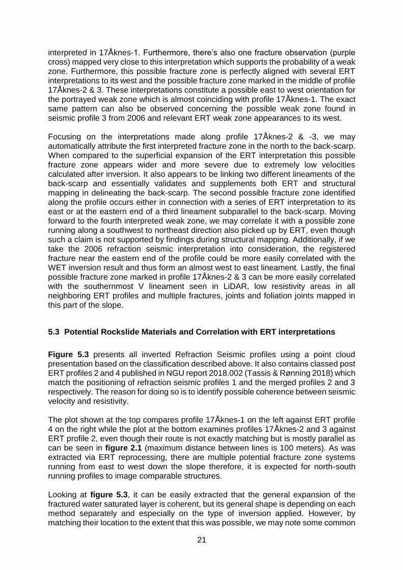
interpreted in 17Åknes-1. Furthermore, there’s also one fracture observation (purple cross) mapped very close to this interpretation which supports the probability of a weak zone. Furthermore, this possible fracture zone is perfectly aligned with several ERT interpretations to its west and the possible fracture zone marked in the middle of profile 17Åknes-2 & 3. These interpretations constitute a possible east to west orientation for the portrayed weak zone which is almost coinciding with profile 17Åknes-1. The exact same pattern can also be observed concerning the possible weak zone found in seismic profile 3 from 2006 and relevant ERT weak zone appearances to its west. Focusing on the interpretations made along profile 17Åknes-2 & -3, we may automatically attribute the first interpreted fracture zone in the north to the back-scarp. When compared to the superficial expansion of the ERT interpretation this possible fracture zone appears wider and more severe due to extremely low velocities calculated after inversion. It also appears to be linking two different lineaments of the back-scarp and essentially validates and supplements both ERT and structural mapping in delineating the back-scarp. The second possible fracture zone identified along the profile occurs either in connection with a series of ERT interpretation to its east or at the eastern end of a third lineament subparallel to the back-scarp. Moving forward to the fourth interpreted weak zone, we may correlate it with a possible zone running along a southwest to northeast direction also picked up by ERT, even though such a claim is not supported by findings during structural mapping. Additionally, if we take the 2006 refraction seismic interpretation into consideration, the registered fracture near the eastern end of the profile could be more easily correlated with the WET inversion result and thus form an almost west to east lineament. Lastly, the final possible fracture zone marked in profile 17Åknes-2 & 3 can be more easily correlated with the southernmost V lineament seen in LiDAR, low resistivity areas in all neighboring ERT profiles and multiple fractures, joints and foliation joints mapped in this part of the slope.

5.3 Potential Rockslide Materials and Correlation with ERT interpretations

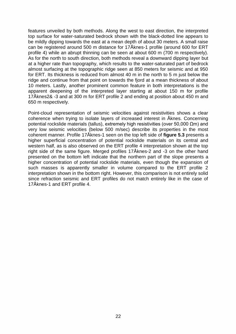
Figure 5.3 presents all inverted Refraction Seismic profiles using a point cloud presentation based on the classification described above. It also contains classed post ERT profiles 2 and 4 published in NGU report 2018.002 (Tassis & Rønning 2018) which match the positioning of refraction seismic profiles 1 and the merged profiles 2 and 3 respectively. The reason for doing so is to identify possible coherence between seismic velocity and resistivity. The plot shown at the top compares profile 17Åknes-1 on the left against ERT profile 4 on the right while the plot at the bottom examines profiles 17Åknes-2 and 3 against ERT profile 2, even though their route is not exactly matching but is mostly parallel as can be seen in figure 2.1 (maximum distance between lines is 100 meters). As was extracted via ERT reprocessing, there are multiple potential fracture zone systems running from east to west down the slope therefore, it is expected for north-south running profiles to image comparable structures. Looking at figure 5.3, it can be easily extracted that the general expansion of the fractured water saturated layer is coherent, but its general shape is depending on each method separately and especially on the type of inversion applied. However, by matching their location to the extent that this was possible, we may note some common

22

features unveiled by both methods. Along the west to east direction, the interpreted top surface for water-saturated bedrock shown with the black-dotted line appears to be mildly dipping towards the east at a mean depth of about 30 meters. A small raise can be registered around 500 m distance for 17Åknes-1 profile (around 600 for ERT profile 4) while an abrupt thinning can be seen at about 600 m (700 m respectively). As for the north to south direction, both methods reveal a downward dipping layer but at a higher rate than topography, which results to the water-saturated part of bedrock almost surfacing at the topographic ridge seen at 850 meters for seismic and at 950 for ERT. Its thickness is reduced from almost 40 m in the north to 5 m just below the ridge and continue from that point on towards the fjord at a mean thickness of about 10 meters. Lastly, another prominent common feature in both interpretations is the apparent deepening of the interpreted layer starting at about 150 m for profile 17Åknes2& -3 and at 300 m for ERT profile 2 and ending at position about 450 m and 650 m respectively. Point-cloud representation of seismic velocities against resistivities shows a clear coherence when trying to isolate layers of increased interest in Åknes. Concerning potential rockslide materials (tallus), extremely high resistivities (over 50,000 Ωm) and very low seismic velocities (below 500 m/sec) describe its properties in the most coherent manner. Profile 17Åknes-1 seen on the top left side of figure 5.3 presents a higher superficial concentration of potential rockslide materials on its central and western half, as is also observed on the ERT profile 4 interpretation shown at the top right side of the same figure. Merged profiles 17Åknes-2 and -3 on the other hand presented on the bottom left indicate that the northern part of the slope presents a higher concentration of potential rockslide materials, even though the expansion of such masses is apparently smaller in volume compared to the ERT profile 2 interpretation shown in the bottom right. However, this comparison is not entirely solid since refraction seismic and ERT profiles do not match entirely like in the case of 17Åknes-1 and ERT profile 4.

23

Figure 5.3: Point-cloud interpretation of WET inversion using Hagedoorn plus-minus starting model results (left) in relation with similar ERT interpretations in Åknes. Blue color (Green in fig. 5.1): fractured / water-

saturated bedrock (0 to 12,000 Ωm / 2,000 to 3,500 m/sec). Red color (Purple in fig. 5.1): scree materials (tallus) bedrock (over 50,000 Ωm / less than 500 m/sec).

24

6. DIGITIZING OF OLD REFREACTION SEISMIC & 3D PLOTTING

In the previous section, we have included the old refraction seismic interpretations in our attempt to frame the structural regime in Åknes. Furthermore, another goal for this project is to provide NVE with results that are plottable in PETREL software and therefore in 3D space. Having performed the same task with ERT, we have discerned that the best format in which to deliver results is ASCII containing dense point-clouds which are georeferenced and can be plotted in 3D with the use of color scales proposed by NGU (Tassis & Rønning 2018). We will be following the same procedure here which includes re-gridding of all WET inversion results using spacing equal to 1 m, but we will be doing the same for the old refraction seismic traditional Plus-Minus interpretations (Rønning et al., 2006; Rønning et al., 2007). The reason for that is to gather all refraction seismic profiles and results in Åknes in a unified format and by plotting them in 3D, to attain a better understanding of how WET inversion results correlate with traditional Plus-Minus interpretations from previous years. Lastly, we may note that contrary to the ERT results, there is no need for a specially designed logarithmic database for the seismic data. Seismic velocity in Åknes is a quantity that can be adequately described linearly with a top value equal to 6,000 m/sec for this case and a default rainbow color scale.

6.1 Digitization of traditional Plus-Minus interpretations

The digitization of the old refraction seismic results was executed in the same way as preparing models for Rayfract® in Surfer 16 (Golden Software 2019) i.e. by creating blocks, filling them with uniform velocity values, building a grid mosaic with all the different “puzzle” pieces that consist the old results and then blanking out every value outside of the depth coverage and above topography. We have therefore created grid files identical to the WET inversion and the result of plotting them using the same color scale can be seen in figure 6.1. Each respective grid file was then extracted to an ASCII point-cloud with 1-m spacing and georeferenced according to the positioning of the profiles. Thus, it was possible to plot old Plus-Minus outcomes along with the new WET inversion results in 3D using Oasis Montaj (version 9.5 – Geosoft 2018).

25

Figure 6.1: Digitized refraction seismic profiles S1, S2, S3 and S4 processed using

traditional Plus-Minus method (Rønning, et al., 2006; Rønning et al., 2007).

6.2 3D Presentation

Figure 6.2 shows the projection of both traditionally processed and WET inverted refraction seismic data in 3D space and seen from three different angles. The plot on the top shows the velocity grids isolated and floating in space (plot a. – view from above and SSW to NNE), the one on the bottom left shows the inclusion of LiDAR topography (plot b. – view from above and SSE to NNW) and the last on the bottom right presents a view from below to make the results visible in relation with topography (plot c. – view from below and NNE to SSW).

26

Figure 6.2: 3D presentation of the WET inversion and traditional Plus-Minus processed results from Åknes in Geosoft Oasis Montaj version 9.5.

Coordinates in UTM zone 32 North and x, y, z axes in meters. (Azimuth View: a. 33o - SSW, b. 305o- SE, c. 145o - NNE).

27

Focusing on the WET inversion results and the only cross-point where they meet, we deduce that they are matching quite well both in terms of the low-velocity overburden (below 2,000 m/sec) and the bedrock below (over 2,000 m/sec). This observation can also be extended to most of the cross-points between WET inversion and traditional Plus-Minus processing results if we acknowledge that the former display gradual changes in velocity and the latter single-valued blocks. Generally, all results seem to be fitting quite well with each other except for the obvious mismatch between the topography digitized from the old seismic interpretation figures and the LiDAR topography as can be seen on the bottom left plot in figure 6.2.

7. CONCLUSIONS

The goal for reprocessing refraction seismic data collected in Åknes by GeoExpert AG in 2017 was to use the NGU in-house experience with applying WET inversion using Rayfract® to get better velocity sections in general and to detect possible fracture zones in bedrock. Next step was to deliver these results to NVE in a format compatible with PETREL software so they could be part of a multidisciplinary 3D model. We have utilized both Midpoint Breaks / Plus-Minus and DeltatV outcomes as starting models and then applied the same type of multirun WET inversion on both to test how two essentially different initial models affect real data inversion results. We deduced that Midpoint Breaks / Plus-Minus starting models led to inversion results where vertical structures were more prominent and more easily interpreted. Furthermore, the high density of geophones (2 m) and shot points (6 m) utilized by GeoExpert AG in this study, enabled moderately intensive Plus-Minus and inversion schemes with controllable smoothing over the standard Conjugate Gradient inversion with Cosine-Squared weighting. This again supports the conclusion extracted by modelling that dense refraction seismic data collection simplifies WET inversion and utilized smoothing which in turn leads to more invariable / consistent results. Together with the actual inversion results, both used starting models and ray coverage plots were presented to give a complete outlook of how refraction seismic inversion works. It should be noted that Plus-Minus method within Rayfract® is not equivalent to the traditional interpretation using the same method as in the old seismic data results for example, but more a simplified version of it used to acquire a trustworthy starting model. Finally, unreasonable fragmentation in bedrock is usually negated during WET inversion. Again, data delivery to NVE was done in ASCII format exactly like with the respective ERT data. For these results to be easily plottable into PETREL software, we have extracted velocity point-clouds with a resolution of 1 m along both axes and had each point georeferenced. Due to the nature of seismic velocity, no specially designed color scale was necessary to create, and a linear rainbow scale was enough to present results adequately. Creating these dense point-clouds helped with our interpretations by classifying velocity values and assigning them to key features at play in Åknes i.e. potential rockslide materials (tallus) and fractured / water saturated bedrock. These two formations were already highlighted during the ERT reprocessing and by creating plots

28

only containing the velocity values representing those bedrock classes, gave us the opportunity to make direct comparisons with the ERT results. Our interpretational model is based on potential rockslide materials in Åknes are characterized by velocities below 500 m/sec, highly fractured and drained bedrock by velocities 500 to 2000 m/sec while the fractured / water-saturated bedrock could be pinpointed between 2,000 and 3,500 m/sec. It is simply noted that the respective ERT resistivity classes for these three formations were over 50,000 Ωm for the former, 12.000 to 50.000 for highly fractured drained bedrock and less than 12,000 Ωm for the latter. Results using the mentioned classification for both refraction seismic and ERT showed a high correlation for neighboring profiles. Interpretation of possible fracture zones with the use of WET inversion results utilized all velocity points lower than 3,500 m/sec and it was done in two dimensions. First vertically along each profile with the use of another classed-post plotting technique and then horizontally by plotting the projections of these findings on the surface of the Åknes map. In this way, several possible weak zones were identified across the three refraction seismic profiles and then they were associated with relevant ERT interpretations and the results of structural mapping. It has been shown via modeling on synthetic refraction seismic data that accurately defining the inclination of fracture zones is dubious with the use of WET inversion. Even though this is not the case with ERT, the effect of such steep topography on the calculated inclination with the use of either refraction seismic or ERT data needs to be investigated in the future. Finally, all results were plotted in 3D using Oasis Montaj version 9.5 along with newly digitized refraction seismic traditional Plus-Minus results in order to have all seismic profiling performed in Åknes over the years unified and presented in 3D space. In this way, we validated the correct positioning of all results, we checked the matching with the LiDAR topography and gained better insight on how our interpretations are arranged in 3D space.

29

8. REFERENCES

Ganerød, G.V. 2008: Structural mapping of the Åknes Rockslide, Møre and Romsdal

County, Western Norway. NGU Rapport. 2008.042. GeoExpert AG 2017: Hybrid Seismic Site Characterization on the Unstable Rock Mass

at Åknes. Technical Report, CH-8424 Embrach, 18th of August 2017. Geosoft, 2018: Oasis Montaj ver. 9.5. Geosoft Inc. copyright © 2018. Golden Software 2019: Surfer 16, ver. 16.2.375 - Powerful Contouring, Gridding & 3D

Surface Mapping Software. Golden Software, LLC, Colorado, USA. Hagedoorn, J.G. 1959: The Plus-Minus method of interpreting seismic refraction

sections. Geophysical Prospecting 7 (2), pp.158 – 182. Rayfract 2018a: Rayfract Seismic Refraction & Borehole Tomography- Subsurface

Seismic Velocity Models for Geotechnical Engineering and Exploration. Downloaded from http://rayfract.com

Rayfract 2018b: Rayfract help. Download from http://rayfract.com/help/rayfract.pdf Rønning, J.S., Dalsegg, E., Elvebakk, H., Ganerød, G. & Tønnesen, J.F. 2006:

Geofysiske målinger Åknes og Tafjord, Stranda og Nordal kommuner, Møre og Romsdal. NGU Rapport 2006.02.

Rønning, J.S., Dalsegg, E., Heincke, B.H. & Tønnesen, J.F. 2007: Geofysiske målinger

på bakken ved Åknes og ved Hegguraksla, Stranda og Nordal kommuner, Møre og Romsdal. NGU Rapport 2007.026.

Rønning, J.S., Tassis, G., Kirkeby, T. & Wåle, M. 2016: Retolkning av geofysiske data

og sammenligning med resultater fra tunneldriving, Knappetunnelen ved Ringveg Vest i Bergen. NGU Rapport 2016.048 (48s.).

Schlumberger 2017: PETREL software. © 2018 Schlumberger Limited. All rights

reserved. Schuster, G.T. & Quintus - Bosz, A. 1993: Wavepath Eikonal Traveltime Inversion:

Theory. Geophysics vol. 58, pp. 1314 – 1323. Tassis, G., Rohdewald, S. & Rønning, J.S. 2018: Tomographic Inversion of Synthetic

Refraction Seismic Data Using Various Starting Models in Rayfract® software. NGU Report 2018.015.

Tassis, G. & Rønning, J.S. 2018: Reprocessing of ERT data from Åknes, Stranda

Municipality, Møre & Romsdal County. NGU Report, 2018.002. Tassis, G., Rønning, J.S. & Rohdewald, S. 2017: Refraction seismic modeling and

inversion for the detection of fracture zones in bedrock with the use of Rayfract® software. NGU Report, 2017.025.