Embed Size (px)
Citation preview
8/7/2019 geomagnet 4
http://slidepdf.com/reader/full/geomagnet-4 1/17
Paleomagnetism: Chapter 4 64
SAMPLING, MEASUREMENT,
AND DISPLAY OF NRM
We now begin putting theories and observations of Chapters 1 through 3 to work. This chapter introduces
data acquisition procedures by presenting techniques for sample collection, and for measurement and dis-
play of NRM. A brief discussion of methods for identifying ferromagnetic minerals in a suite of paleomag-
netic samples is also included.
COLLECTION OF PALEOMAGNETIC SAMPLES
We understand from Chapter 1 that the surface geomagnetic field undergoes secular variation with periodicities
up to ~105 yr. The average direction is expected to be that of a geocentric axial dipole, and many paleomag-
netic investigations are designed to determine that average direction. Paleomagnetic samples are usually
collected to provide a set of quasi-instantaneous samplings of the geomagnetic field direction at the time of
rock formation. Because geomagnetic secular variation must be adequately averaged, the time interval
represented by the collection of paleomagnetic samples should be ≥105 yr. There is no clear upper limit for
the time interval, but this rarely exceeds 20 m.y.
Sample collection scheme
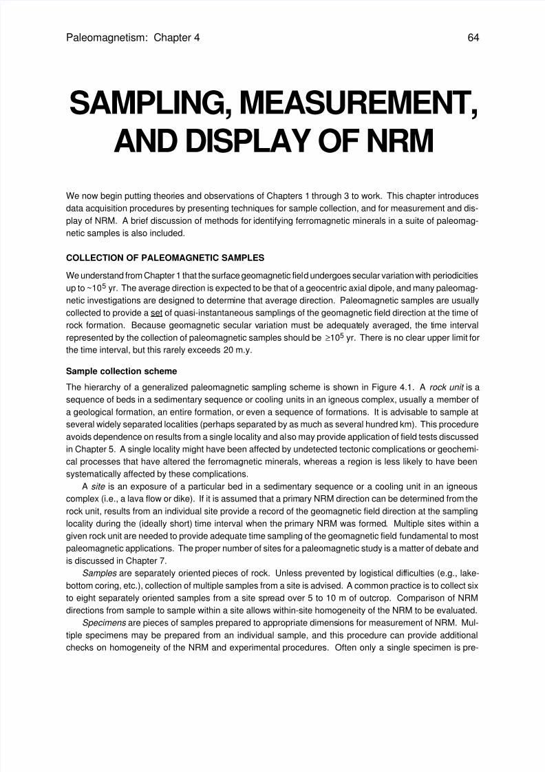
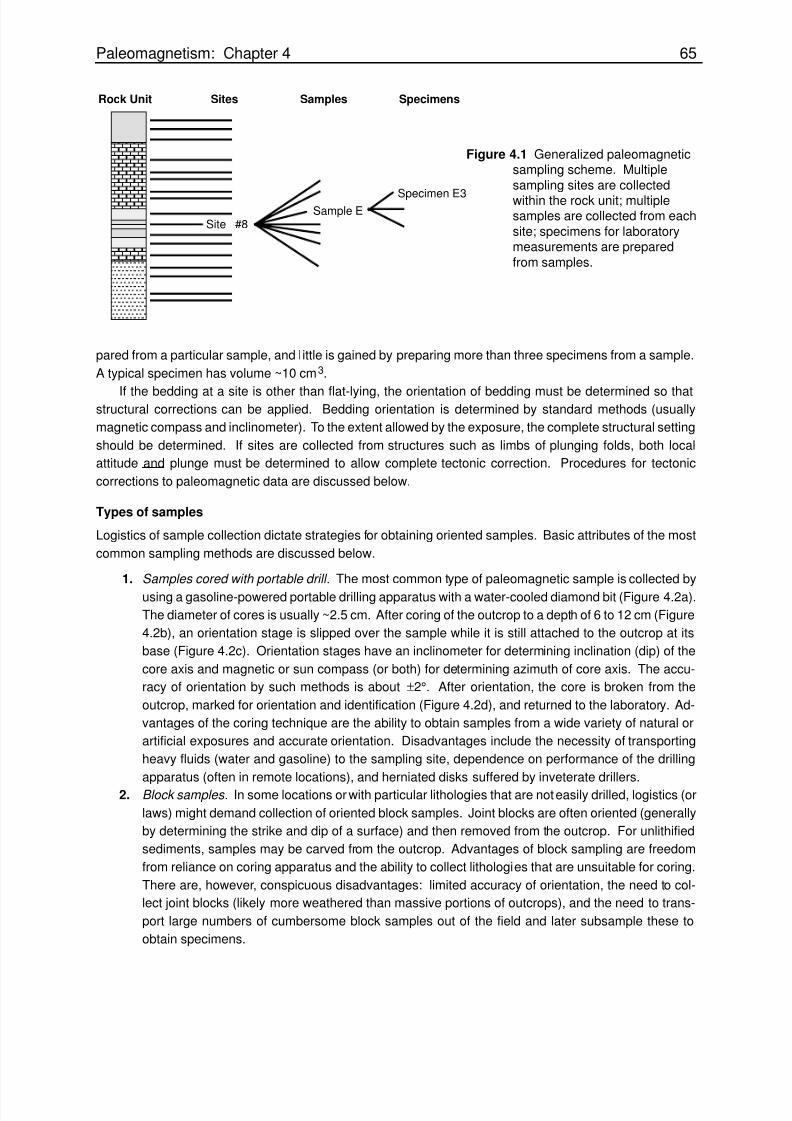
The hierarchy of a generalized paleomagnetic sampling scheme is shown in Figure 4.1. A rock unit is a
sequence of beds in a sedimentary sequence or cooling units in an igneous complex, usually a member of
a geological formation, an entire formation, or even a sequence of formations. It is advisable to sample at
several widely separated localities (perhaps separated by as much as several hundred km). This procedure
avoids dependence on results from a single locality and also may provide application of field tests discussed
in Chapter 5. A single locality might have been affected by undetected tectonic complications or geochemi-
cal processes that have altered the ferromagnetic minerals, whereas a region is less likely to have been
systematically affected by these complications.
A site is an exposure of a particular bed in a sedimentary sequence or a cooling unit in an igneous
complex (i.e., a lava flow or dike). If it is assumed that a primary NRM direction can be determined from the
rock unit, results from an individual site provide a record of the geomagnetic field direction at the sampling
locality during the (ideally short) time interval when the primary NRM was formed. Multiple sites within a
given rock unit are needed to provide adequate time sampling of the geomagnetic field fundamental to most
paleomagnetic applications. The proper number of sites for a paleomagnetic study is a matter of debate and
is discussed in Chapter 7.
Samples are separately oriented pieces of rock. Unless prevented by logistical difficulties (e.g., lake-
bottom coring, etc.), collection of multiple samples from a site is advised. A common practice is to collect six
to eight separately oriented samples from a site spread over 5 to 10 m of outcrop. Comparison of NRM
directions from sample to sample within a site allows within-site homogeneity of the NRM to be evaluated.
Specimens are pieces of samples prepared to appropriate dimensions for measurement of NRM. Mul-
tiple specimens may be prepared from an individual sample, and this procedure can provide additional
checks on homogeneity of the NRM and experimental procedures. Often only a single specimen is pre-
8/7/2019 geomagnet 4
http://slidepdf.com/reader/full/geomagnet-4 2/17
Paleomagnetism: Chapter 4 65
Rock Unit Sites Samples Specimens
Sample ESpecimen E3
#8Site
Figure 4.1 Generalized paleomagneticsampling scheme. Multiple
sampling sites are collected
within the rock unit; multiplesamples are collected from each
site; specimens for laboratorymeasurements are prepared
from samples.
pared from a particular sample, and little is gained by preparing more than three specimens from a sample.
A typical specimen has volume ~10 cm3.
If the bedding at a site is other than flat-lying, the orientation of bedding must be determined so thatstructural corrections can be applied. Bedding orientation is determined by standard methods (usually
magnetic compass and inclinometer). To the extent allowed by the exposure, the complete structural setting
should be determined. If sites are collected from structures such as limbs of plunging folds, both local
attitude and plunge must be determined to allow complete tectonic correction. Procedures for tectonic
corrections to paleomagnetic data are discussed below.
Types of samples
Logistics of sample collection dictate strategies for obtaining oriented samples. Basic attributes of the most
common sampling methods are discussed below.
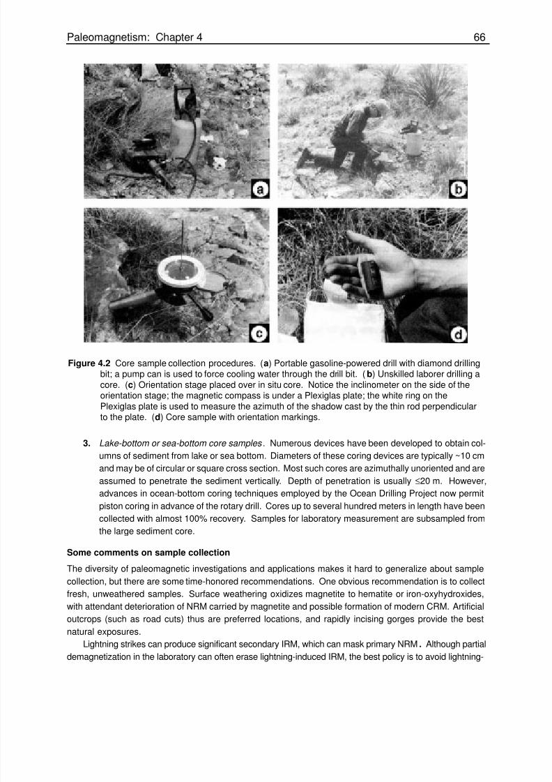
1. Samples cored with portable drill . The most common type of paleomagnetic sample is collected by
using a gasoline-powered portable drilling apparatus with a water-cooled diamond bit (Figure 4.2a).
The diameter of cores is usually ~2.5 cm. After coring of the outcrop to a depth of 6 to 12 cm (Figure
4.2b), an orientation stage is slipped over the sample while it is still attached to the outcrop at its
base (Figure 4.2c). Orientation stages have an inclinometer for determining inclination (dip) of the
core axis and magnetic or sun compass (or both) for determining azimuth of core axis. The accu-
racy of orientation by such methods is about ±2°. After orientation, the core is broken from the
outcrop, marked for orientation and identification (Figure 4.2d), and returned to the laboratory. Ad-
vantages of the coring technique are the ability to obtain samples from a wide variety of natural or
artificial exposures and accurate orientation. Disadvantages include the necessity of transporting
heavy fluids (water and gasoline) to the sampling site, dependence on performance of the drilling
apparatus (often in remote locations), and herniated disks suffered by inveterate drillers.
2. Block samples . In some locations or with particular lithologies that are not easily drilled, logistics (or
laws) might demand collection of oriented block samples. Joint blocks are often oriented (generally
by determining the strike and dip of a surface) and then removed from the outcrop. For unlithified
sediments, samples may be carved from the outcrop. Advantages of block sampling are freedom
from reliance on coring apparatus and the ability to collect lithologies that are unsuitable for coring.
There are, however, conspicuous disadvantages: limited accuracy of orientation, the need to col-
lect joint blocks (likely more weathered than massive portions of outcrops), and the need to trans-
port large numbers of cumbersome block samples out of the field and later subsample these to
obtain specimens.
8/7/2019 geomagnet 4
http://slidepdf.com/reader/full/geomagnet-4 3/17
Paleomagnetism: Chapter 4 66
Figure 4.2 Core sample collection procedures. (a) Portable gasoline-powered drill with diamond drillingbit; a pump can is used to force cooling water through the drill bit. (b) Unskilled laborer drilling a
core. (c) Orientation stage placed over in situ core. Notice the inclinometer on the side of theorientation stage; the magnetic compass is under a Plexiglas plate; the white ring on the
Plexiglas plate is used to measure the azimuth of the shadow cast by the thin rod perpendicularto the plate. (d) Core sample with orientation markings.
3. Lake-bottom or sea-bottom core samples . Numerous devices have been developed to obtain col-
umns of sediment from lake or sea bottom. Diameters of these coring devices are typically ~10 cm
and may be of circular or square cross section. Most such cores are azimuthally unoriented and are
assumed to penetrate the sediment vertically. Depth of penetration is usually ≤20 m. However,
advances in ocean-bottom coring techniques employed by the Ocean Drilling Project now permit
piston coring in advance of the rotary drill. Cores up to several hundred meters in length have been
collected with almost 100% recovery. Samples for laboratory measurement are subsampled from
the large sediment core.
Some comments on sample collection
The diversity of paleomagnetic investigations and applications makes it hard to generalize about sample
collection, but there are some time-honored recommendations. One obvious recommendation is to collect
fresh, unweathered samples. Surface weathering oxidizes magnetite to hematite or iron-oxyhydroxides,
with attendant deterioration of NRM carried by magnetite and possible formation of modern CRM. Artificial
outcrops (such as road cuts) thus are preferred locations, and rapidly incising gorges provide the best
natural exposures.
Lightning strikes can produce significant secondary IRM, which can mask primary NRM. Although partial
demagnetization in the laboratory can often erase lightning-induced IRM, the best policy is to avoid lightning-
8/7/2019 geomagnet 4
http://slidepdf.com/reader/full/geomagnet-4 4/17
Paleomagnetism: Chapter 4 67
prone areas. When possible, topographic highs should be avoided, especially in tropical regions. If samples
must be collected in lightning-prone areas, effects of lightning can be minimized by two procedures.
1. Outcrops of strongly magnetic rocks such as basalts can be surveyed prior to sample collection to
find areas that have probably been struck by lightning. This is done by “mapping” the areas where
significant (≥5°) deflections of the magnetic compass occur. If a magnetic compass is passed over
an outcrop at a distance of ~15 cm from the rock face while the compass is held in fixed azimuth, thestrong and inhomogeneous IRM produced by a lightning strike will cause detectable deflections of
the compass. These regions then can be avoided during sample collection.
2. Orientations of samples should be done by sun compass in lightning-prone regions. Procedures for
determining sample orientation by sun compass are straightforward, and the required calculations
can be done at the outcrop on a programmable pocket calculator. This is essential in basaltic
igneous complexes in which strength and inhomogeneity of outcrop magnetization can produce
significant deflections of the magnetic compass. Sun-compass orientations are also required at
high magnetic latitudes, where the horizontal component of the geomagnetic field is small. If cloudy
conditions prevent sun-compass orientation, it is possible to determine the local deflection of the
compass needle by sighting on a topographic feature at known azimuth from the collecting locality.
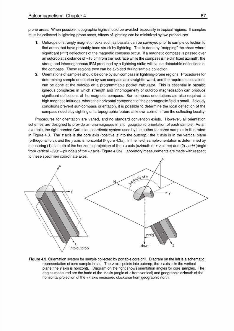
Procedures for orientation are varied, and no standard convention exists. However, all orientation
schemes are designed to provide an unambiguous in situ geographic orientation of each sample. As an
example, the right-handed Cartesian coordinate system used by the author for cored samples is illustrated
in Figure 4.3. The z axis is the core axis (positive z into the outcrop); the x axis is in the vertical plane
(orthogonal to z ); and the y axis is horizontal (Figure 4.3a). In the field, sample orientation is determined by
measuring (1) azimuth of the horizontal projection of the +x axis (azimuth of x -z plane) and (2) hade (angle
from vertical = [90° – plunge]) of the +z axis (Figure 4.3b). Laboratory measurements are made with respect
to these specimen coordinate axes.
Figure 4.3 Orientation system for sample collected by portable core drill. Diagram on the left is a schematic
representation of core sample in situ. The z axis points into outcrop; the x axis is in the verticalplane; the y axis is horizontal. Diagram on the right shows orientation angles for core samples. The
angles measured are the hade of the z axis (angle of z from vertical) and geographic azimuth of thehorizontal projection of the +x axis measured clockwise from geographic north.
z
y
down
hade
azim
uth of x
into outcrop
x
z
y
N
y
x
8/7/2019 geomagnet 4
http://slidepdf.com/reader/full/geomagnet-4 5/17
Paleomagnetism: Chapter 4 68
MEASUREMENT OF NRM
Meaningful paleomagnetic results have been obtained from rocks with NRM in the 10–8 G (10–5 A/m) range.
For a standard core specimen with volume of 10 cm3, the magnetic moment (M ) of such a sample would be
10–7 G cm3 (10–10 A m2), and there is genuine challenge in making reliable and rapid measurements of
specimens with M of this low magnitude. During the past three decades, sensitivity of rock magnetometers
has been improved by at least a factor of 1000. While early paleomagnetic studies were limited to stronglymagnetized basalts and red sediments, improvements in instrumentation have allowed paleomagnetic in-
vestigations to be extended to essentially all rock types. A detailed account of instrumentation is not pre-
sented here because Collinson (see Suggested Readings) has provided a detailed book on instruments
used in paleomagnetic research. Only the basics required to understand the logical development of paleo-
magnetic field and laboratory techniques are presented here.
During development of paleomagnetism (mostly in Britain) in the 1950s, the astatic magnetometer was
the primary instrument for measurement of NRM. Numerous varieties were developed, but all employed a
configuration of small sensing magnets suspended on a torsion fiber. The magnetic moment of the rock
specimen was detected by the rotation of the torsion fiber resulting from the magnetic field of the specimen
exerting torques on the sensing magnets. By clever and painstaking development, sensitive astatic magne-
tometers were constructed that could measure specimens with M ≤ 10–5 G cm3 (10–8 A m2). Significant
drawbacks were noise problems caused by acoustic vibrations and sensitivity to changes of the magnetic
field in the laboratory.
During the 1960s and early 1970s, the spinner magnetometer became the most commonly used mag-
netometer. Many varieties have been developed, but all involve a spinning shaft on which a rock specimen
is rotated and a magnetic field sensor to detect the oscillating magnetic field produced by the rotating
magnetic moment of the specimen. The signal from the sensor is passed to a phase-sensitive detector
designed to amplify signals at the rotation frequency of the spinning shaft. With the development of effective
phase-sensitive detectors and digital summing circuits, sensitivity of spinner magnetometers and speed of
measurement have been greatly improved. Modern spinner magnetometers can reliably measure NRM of
specimens with M ≈ 10–7 G.cm3 (10–10 A.m2). However, the measurement time increases with decreasing
intensity, and measurement of a specimen with such low intensity can require in excess of 30 minutes.
In the early 1970s, cryogenic magnetometers were developed that could measure weakly magnetized
specimens more quickly than spinner magnetometers. Cryogenic magnetometers use a magnetic field
sensor called a SQUID (Superconducting QUantum Interference Device) magnetometer, which is super-
conducting at liquid helium temperatures (4°K). The SQUID is placed in a dewar containing liquid helium. A
room-temperature access space is provided so that rock specimens can be placed near the SQUID, which
measures the magnetic moment of the specimen. Superconducting magnetometers can routinely measure
NRM of rock specimens with M ≤ 10–7 G cm3 (10–10 A m2). A major advantage is that measurement time is
only about 1 minute.
Regardless of the particular magnetometer employed, measurements are made of components (M x ,
M y , M z ) of magnetic moment of the specimen (in sample coordinates). This usually entails multiple mea-
surements of each component, allowing evaluation of homogeneity of NRM in the specimen and a measure
of signal-to-noise ratio. Data are usually fed into a computer that contains orientation data for the sample,
and calculation of the best-fit direction of NRM in sample coordinates and in geographic coordinates is
performed. With cryogenic magnetometers, this process of measurement and data reduction can be ac-
complished in about 1 minute per specimen.
Display of NRM directions
Vector directions in paleomagnetism are described in terms of inclination, I , (with respect to horizontal at the
collecting location) and declination, D , (with respect to geographic north) as shown in Figure 1.2. To display
8/7/2019 geomagnet 4
http://slidepdf.com/reader/full/geomagnet-4 6/17
Paleomagnetism: Chapter 4 69
such directions, a projection must be used to depict three-dimensional information on a two-dimensional
page. The usual procedure is to view the NRM direction as radiating from the center of a sphere and to
display the intersection of the NRM vector with this sphere. The sphere (and the points of intersection of the
vectors with it) are then projected onto the horizontal plane (the plane of the page). Various projection
techniques exist, and all have powers and limitations.
Two types of projections are commonly used in paleomagnetism. The equal-angle projection (the ste- reographic or Wulff projection) has the property that a cone defined by vectors that have a given angle from
a central vector plot as a circle about the central vector, regardless of where the central vector plots. How-
ever, the size of the circle changes with the direction of the central vector. (It is smaller if the central vector
has a steep inclination and thus plots near the center of the projection.)
The equal-area projection (the Lambert or Schmidt projection) has the property that the area of a cone
of vectors about a central vector will remain constant regardless of the direction of the central vector. How-
ever, the cone will plot as an ellipse on the equal-area projection, except when the central vector is vertical.
Because we are often concerned with the amount of directional scatter in distributions of paleomagnetic
directions, the equal-area projection is usually preferred. However, be warned that no strict convention
exists, and many research papers in paleomagnetism are published with paleomagnetic directions dis-
played using the equal-angle projection.Mineralogists often use projections of crystal faces (or poles to those faces) to display crystal symme-
tries, and structural geologists use projections to display mineral lineations or planes of bedding (or poles to
those planes). In both cases, the geometrical elements displayed are lines, and the upward-pointing or
downward-pointing end can be displayed with no loss of information (as long as the reader knows the
convention). Mineralogists generally use projections onto the upper hemisphere (they spend their lives
merrily staring into space), while structural geologists use projections onto the lower hemisphere (they
spend their lives on hands and knees examining mineral lineations, etc.). Paleomagnetists must be more
well rounded because paleomagnetic directions are true vector quantities and therefore plot in both upper
and lower hemispheres.
Projections onto the horizontal plane have the property that two vectors with equal declination but oppo-
site inclinations (e.g., I = 20°,D = 340°
and I = –20°, D = 340°) plot at the same point. Some convention
must be used to discriminate upwards-pointing directions from downward-pointing directions. The common
convention is to use solid data points for directions in the lower hemisphere and open data points for direc-
tions in the upper hemisphere.
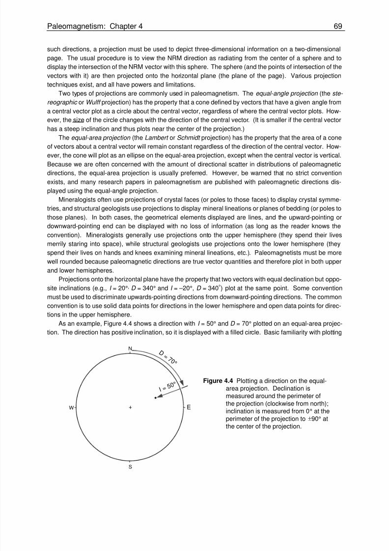
As an example, Figure 4.4 shows a direction with I = 50° and D = 70° plotted on an equal-area projec-
tion. The direction has positive inclination, so it is displayed with a filled circle. Basic familiarity with plotting
W
N
E
S
I = 50°
D = 7 0 °
Figure 4.4 Plotting a direction on the equal-
area projection. Declination ismeasured around the perimeter of
the projection (clockwise from north);inclination is measured from 0° at the
perimeter of the projection to ±90° atthe center of the projection.

8/7/2019 geomagnet 4
http://slidepdf.com/reader/full/geomagnet-4 7/17
Paleomagnetism: Chapter 4 70
and rotating vectors on an equal-area projection is assumed in many discussions that follow. If these
procedures are completely foreign to the reader, some time spent studying the relevant portions of Marshak
and Mitra (see Suggested Readings) or another introductory structural geology text would be wise.
Sample coordinates to geographic direction
The procedure for determining a geographic direction of NRM from the measured quantities is now pre-sented. Consider a cored sample for which orientation was determined by using the conventions of Figure
4.3. Sample orientation, volume (v ) of the specimen, and the components of magnetic moment (in sample
coordinates) are listed in Table 4.1.
Table 4.1 Data for Sample Coordinates to Geographic Coordinates Transformation
Sample orientation: Hade = 37°; Azimuth of +horizontal projection of +x = 25°Specimen volume: 10 cm3
Components of magnetic moment:
M x = 2.3 × 10⁻³ G cm3 (2.3 × 10⁻⁶ A m2)M y = –1.2 × 10⁻³ G cm3 (-1.2 × 10⁻⁶ A m2)
M z = 2.7 × 10⁻³
G cm3
(2.7 × 10⁻⁶
A m2
)Sample coordinates direction: I s = 46°; D s = 332°Geographic coordinates direction: I = 11°; D = 6°
Total magnetic moment, M , of the specimen is determined by
M = M x2+ M y
2+ M z
2(4.1)
From the data of Table 4.1, the result is M = 3.74 × 10⁻³ G cm3 (3.74 × 10⁻⁶ A m2). The intensity of NRM is
given by
NRM =M
v(4.2)
and is found to be 3.74 × 10⁻⁴ G (3.74 × 10⁻¹ A/m). The inclination, I s , and declination, D s , in sample coor-
dinates are given by
I s = tan−1 M z
M x2 + M y
2
(4.3)
and Ds = tan−1 M y
M x
Note that one must keep track of the proper quadrant for D s . With the data of Table 4.1, the resulting
direction in sample coordinates is I s = 46°, D s = –28° = 332°.To determine the direction of NRM in geographic coordinates (in situ), the sample axes (and NRM
direction determined within that coordinate system) are returned to the measured in situ orientation. In
practice, this is done by computing the coordinate transformations. But some insight is gained by examining
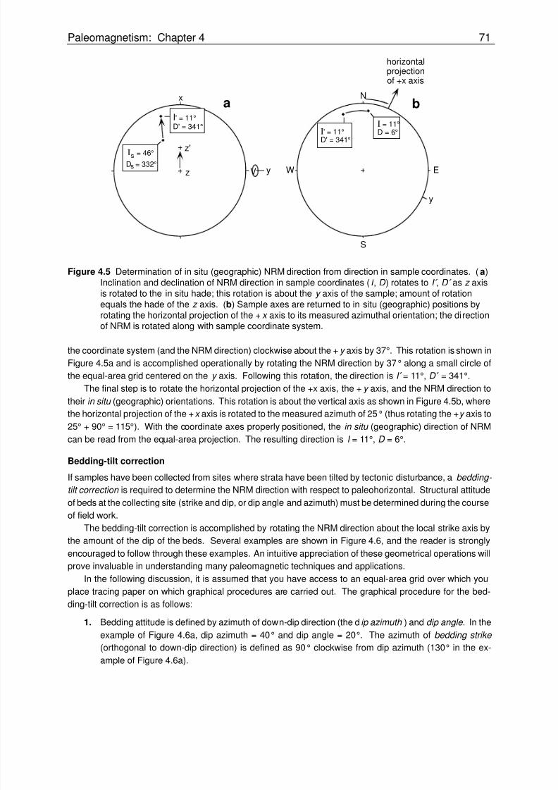
the graphical procedure illustrated in Figure 4.5.
The first step is to plot the direction in sample coordinates on the equal-area projection (Figure 4.5a).
The measured orientation of the +z axis of the sample was 37° (= hade). Remembering that the y axis is
horizontal (according to the convention of Figure 4.3), we return the z axis to its in situ orientation by rotating
8/7/2019 geomagnet 4
http://slidepdf.com/reader/full/geomagnet-4 8/17
Paleomagnetism: Chapter 4 71
N
E
S
W
b
I' = 11°D' = 341°
I = 11°D = 6°
V
x
yz
z'
a
D = 332°s
I = 46°s
I' = 11°D' = 341°
horizontalprojectionof +x axis
y
Figure 4.5 Determination of in situ (geographic) NRM direction from direction in sample coordinates. (a)
Inclination and declination of NRM direction in sample coordinates (I s
, D s
) rotates to I ′ , D ′ as z axisis rotated to the in situ hade; this rotation is about the y axis of the sample; amount of rotation
equals the hade of the z axis. (b) Sample axes are returned to in situ (geographic) positions byrotating the horizontal projection of the +x axis to its measured azimuthal orientation; the directionof NRM is rotated along with sample coordinate system.
the coordinate system (and the NRM direction) clockwise about the +y axis by 37°. This rotation is shown in
Figure 4.5a and is accomplished operationally by rotating the NRM direction by 37° along a small circle of
the equal-area grid centered on the y axis. Following this rotation, the direction is I ′= 11°, D ′ = 341°.The final step is to rotate the horizontal projection of the +x axis, the +y axis, and the NRM direction to
their in situ (geographic) orientations. This rotation is about the vertical axis as shown in Figure 4.5b, where
the horizontal projection of the +x axis is rotated to the measured azimuth of 25° (thus rotating the +y axis to25° + 90° = 115°). With the coordinate axes properly positioned, the in situ (geographic) direction of NRM
can be read from the equal-area projection. The resulting direction is I = 11°, D = 6°.
Bedding-tilt correction
If samples have been collected from sites where strata have been tilted by tectonic disturbance, a bedding-
tilt correction is required to determine the NRM direction with respect to paleohorizontal. Structural attitude
of beds at the collecting site (strike and dip, or dip angle and azimuth) must be determined during the course
of field work.
The bedding-tilt correction is accomplished by rotating the NRM direction about the local strike axis by
the amount of the dip of the beds. Several examples are shown in Figure 4.6, and the reader is strongly
encouraged to follow through these examples. An intuitive appreciation of these geometrical operations willprove invaluable in understanding many paleomagnetic techniques and applications.
In the following discussion, it is assumed that you have access to an equal-area grid over which you
place tracing paper on which graphical procedures are carried out. The graphical procedure for the bed-
ding-tilt correction is as follows:
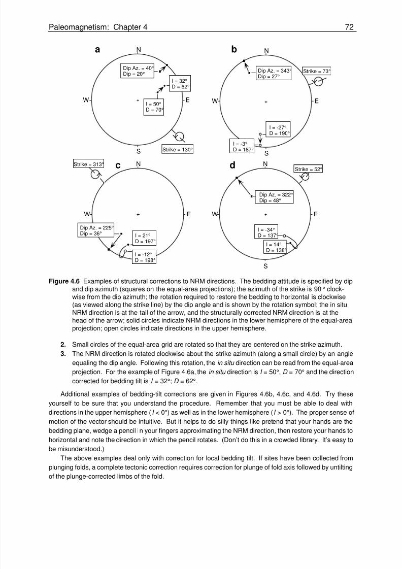
1. Bedding attitude is defined by azimuth of down-dip direction (the dip azimuth ) and dip angle . In the
example of Figure 4.6a, dip azimuth = 40° and dip angle = 20°. The azimuth of bedding strike
(orthogonal to down-dip direction) is defined as 90° clockwise from dip azimuth (130° in the ex-
ample of Figure 4.6a).
8/7/2019 geomagnet 4
http://slidepdf.com/reader/full/geomagnet-4 9/17
Paleomagnetism: Chapter 4 72
N
N
Dip Az. = 343°Dip = 27°
I = -27°D = 190°
I = -3°D = 187°
Strike = 73°
S
Strike = 52°
I = 14°D = 138°
I = -34°D = 137°
Dip Az. = 322°Dip = 48°
W E
E
S
W
b
dN
N
I = 50°D = 70°
I = 32°D = 62°
Dip Az. = 40°Dip = 20°
Strike = 130°S
EW
a
I = 21°D = 197°
Strike = 313°
Dip Az. = 225°Dip = 36°
I = -12°D = 198°
EW
c
Figure 4.6 Examples of structural corrections to NRM directions. The bedding attitude is specified by dipand dip azimuth (squares on the equal-area projections); the azimuth of the strike is 90° clock-
wise from the dip azimuth; the rotation required to restore the bedding to horizontal is clockwise(as viewed along the strike line) by the dip angle and is shown by the rotation symbol; the in situ
NRM direction is at the tail of the arrow, and the structurally corrected NRM direction is at thehead of the arrow; solid circles indicate NRM directions in the lower hemisphere of the equal-area
projection; open circles indicate directions in the upper hemisphere.
2. Small circles of the equal-area grid are rotated so that they are centered on the strike azimuth.
3. The NRM direction is rotated clockwise about the strike azimuth (along a small circle) by an angle
equaling the dip angle. Following this rotation, the in situ direction can be read from the equal-area
projection. For the example of Figure 4.6a, the in situ direction is I = 50°, D = 70° and the direction
corrected for bedding tilt is I = 32°; D = 62°.
Additional examples of bedding-tilt corrections are given in Figures 4.6b, 4.6c, and 4.6d. Try these
yourself to be sure that you understand the procedure. Remember that you must be able to deal with
directions in the upper hemisphere (I < 0°) as well as in the lower hemisphere (I > 0°). The proper sense of
motion of the vector should be intuitive. But it helps to do silly things like pretend that your hands are the
bedding plane, wedge a pencil in your fingers approximating the NRM direction, then restore your hands to
horizontal and note the direction in which the pencil rotates. (Don’t do this in a crowded library. It’s easy to
be misunderstood.)
The above examples deal only with correction for local bedding tilt. If sites have been collected from
plunging folds, a complete tectonic correction requires correction for plunge of fold axis followed by untilting
of the plunge-corrected limbs of the fold.
8/7/2019 geomagnet 4
http://slidepdf.com/reader/full/geomagnet-4 10/17
Paleomagnetism: Chapter 4 73
EVIDENCES OF SECONDARY NRM
The NRM of a rock (prior to any laboratory treatment) is generally composed of at least two components: a
primary NRM acquired during rock formation (TRM, CRM, or DRM) and secondary NRM components (e.g.,
VRM or lightning-induced IRM) acquired at some later time(s). Resultant NRM is the vector sum of primary
and secondary components (Equation (3.17)). In this section, we examine how distributions of NRM direc-
tions indicate the presence of secondary NRM components and begin examination of partial demagnetiza-tion procedures.
Characteristic NRM
There is some terminology applied to components of NRM that must be introduced at the outset. Partial
demagnetization procedures (discussed in Chapter 5) remove components of NRM. Components that are
easily removed are referred to as low-stability components . Removal of these low-stability components by
partial demagnetization will allow isolation of the more resistant high-stability components . In many cases,
the high-stability component can logically be inferred to be a primary NRM, while the low-stability compo-
nent is inferred to be a secondary NRM. However, this is not always the case, and a terminology has been
introduced to deal with this potential difficulty.
The highest-stability component of NRM that is isolated by partial demagnetization is generally referred
to as the characteristic component of NRM, abbreviated ChRM. Partial demagnetization usually can deter-
mine a ChRM direction but cannot directly determine whether it is primary; additional information is required
to infer whether the ChRM is primary. The purpose of the term characteristic component is that this term can
be applied to results of partial demagnetization experiments without the connotation of origin time attached
to the term primary NRM . This might seem an unnecessarily picky distinction, but it is useful to separate
inferences drawn from partial demagnetization experiments (determination of ChRM) from the less certain
inference that the ChRM is a primary NRM.
NRM distributions
Recognition and (hopefully) erasure of secondary NRM is the major goal of paleomagnetic laboratory work.
An initial step is recognition of secondary components of NRM. As the NRMs of specimens from a rock unit
are initially measured, the distribution of NRM often indicates the presence of secondary NRM.
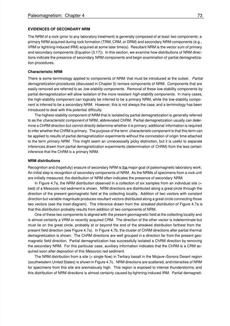
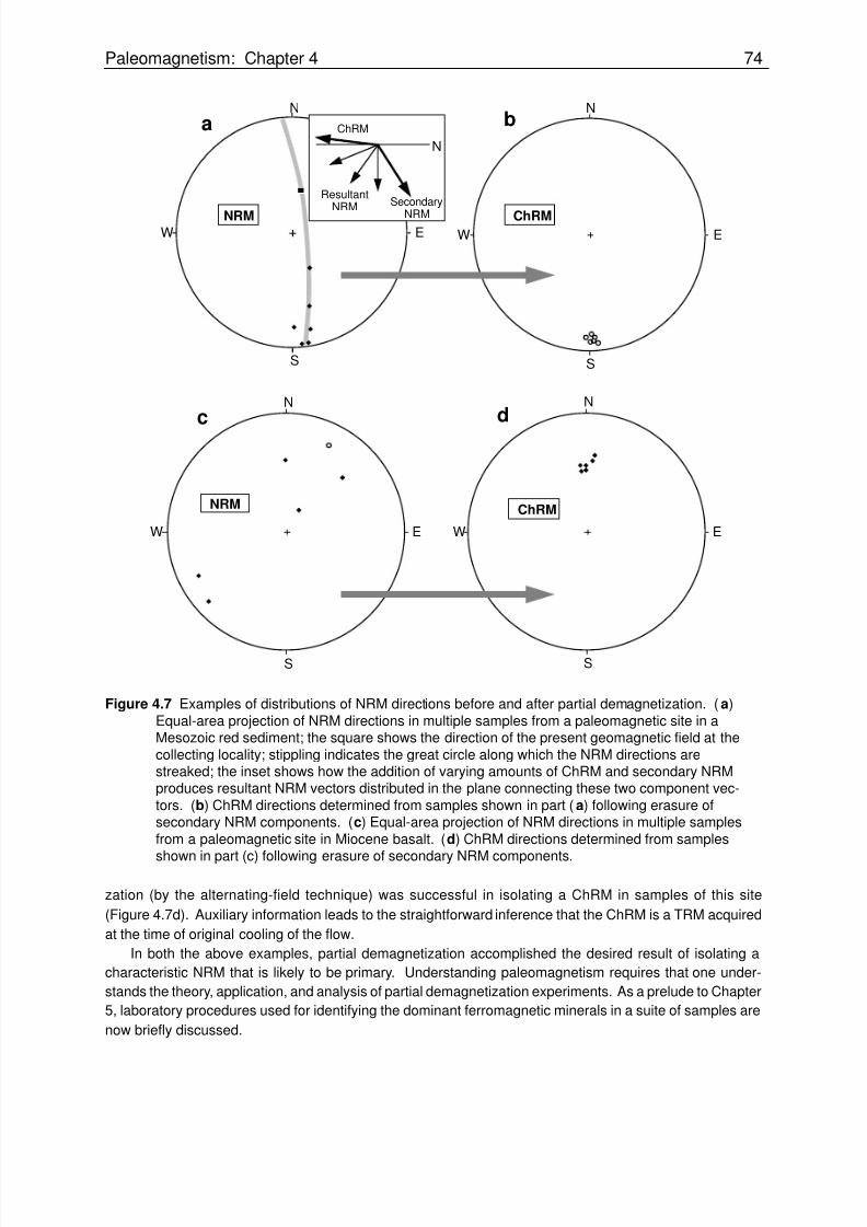
In Figure 4.7a, the NRM distribution observed in a collection of six samples from an individual site (=
bed) of a Mesozoic red sediment is shown. NRM directions are distributed along a great circle through the
direction of the present geomagnetic field at the collecting locality. Addition of two vectors with constant
direction but variable magnitude produces resultant vectors distributed along a great circle connecting those
two vectors (see the inset diagram). The inference drawn from the streaked distribution of Figure 4.7a is
that this distribution probably results from addition of two components of NRM.
One of these two components is aligned with the present geomagnetic field at the collecting locality and
is almost certainly a VRM or recently acquired CRM. The direction of the other vector is indeterminate but
must lie on the great circle, probably at or beyond the end of the streaked distribution farthest from the
present field direction (see Figure 4.7a). In Figure 4.7b, the cluster of ChRM directions after partial thermal
demagnetization is shown. The ChRM directions are well grouped in a direction far from the present geo-
magnetic field direction. Partial demagnetization has successfully isolated a ChRM direction by removing
the secondary NRM. For this particular case, auxiliary information indicates that the ChRM is a CRM ac-
quired soon after deposition of this Mesozoic red sediment.
The NRM distribution from a site (= single flow) in Tertiary basalt in the Mojave–Sonora Desert region
(southwestern United States) is shown in Figure 4.7c. NRM directions are scattered, and intensities of NRM
for specimens from this site are anomalously high. This region is exposed to intense thunderstorms, and
this distribution of NRM directions is almost certainly caused by lightning-induced IRM. Partial demagneti-
8/7/2019 geomagnet 4
http://slidepdf.com/reader/full/geomagnet-4 11/17
Paleomagnetism: Chapter 4 74
N
NN
N
EW W
S S
ENRM ChRM
a b
N
Secondary
NRM
ChRM
ResultantNRM
E EWW
S S
NRMChRM
c d
Figure 4.7 Examples of distributions of NRM directions before and after partial demagnetization. (a)
Equal-area projection of NRM directions in multiple samples from a paleomagnetic site in aMesozoic red sediment; the square shows the direction of the present geomagnetic field at the
collecting locality; stippling indicates the great circle along which the NRM directions arestreaked; the inset shows how the addition of varying amounts of ChRM and secondary NRMproduces resultant NRM vectors distributed in the plane connecting these two component vec-
tors. (b) ChRM directions determined from samples shown in part (a) following erasure ofsecondary NRM components. (c) Equal-area projection of NRM directions in multiple samples
from a paleomagnetic site in Miocene basalt. (d) ChRM directions determined from samples
shown in part (c) following erasure of secondary NRM components.
zation (by the alternating-field technique) was successful in isolating a ChRM in samples of this site
(Figure 4.7d). Auxiliary information leads to the straightforward inference that the ChRM is a TRM acquired
at the time of original cooling of the flow.
In both the above examples, partial demagnetization accomplished the desired result of isolating a
characteristic NRM that is likely to be primary. Understanding paleomagnetism requires that one under-
stands the theory, application, and analysis of partial demagnetization experiments. As a prelude to Chapter
5, laboratory procedures used for identifying the dominant ferromagnetic minerals in a suite of samples are
now briefly discussed.
8/7/2019 geomagnet 4
http://slidepdf.com/reader/full/geomagnet-4 12/17
Paleomagnetism: Chapter 4 75
IDENTIFICATION OF FERROMAGNETIC MINERALS
Identification of ferromagnetic minerals in a rock can help guide the design of partial demagnetization ex-
periments and the interpretation of results. The challenge is to associate a particular component of NRM
(identified from partial demagnetization) with a particular ferromagnetic mineral. This information can often
determine whether a characteristic NRM is primary or secondary. There are three families of techniques
used to identify ferromagnetic minerals: (1) microscopy techniques including optical microscopy, electronmicroprobe, and SEM; (2) determination of Curie temperature; and (3) coercivity spectrum analysis. In the
discussions below, attributes of these techniques are outlined, and some examples are provided.
Microscopy
Ferromagnetic minerals are opaque, and optical observations require reflected light microscopy. Optical
and SEM observations of textures allow sequences of mineral formation to be determined. This information
can sometimes determine whether minerals formed at the time of rock formation or by later chemical alter-
ation. Direct determination of elemental abundances through electron microprobe examination can facili-
tate identification of ferromagnetic minerals when more than one mineral could account for optical proper-
ties. Example photomicrographs are shown in Figure 2.11.
A major difficulty in applying optical and SEM observations is the low concentration of ferromagnetic
minerals and their small size (often ≤1 µ m in SD and PSD grains). Igneous rocks generally have sufficient
ferromagnetic minerals to allow optical examination of polished thin sections. However, optical examination
of ferromagnetic minerals in sedimentary rocks often requires extraction of ferromagnetic minerals, which
introduces uncertainties about the representative nature of the magnetic extract. For titanomagnetite, grain
sizes of SD and PSD grains (dominant carriers of remanent magnetization) are often below the limit of
optical resolution. It is often necessary to infer the mineralogy of SD and PSD grains from optical observa-
tions of larger MD grains. Although SEM examinations can provide pivotal information in particular cases,
such examinations cannot be done as a matter of course because of the cost and time required for sample
preparation.
Curie temperature determination
Curie temperatures of ferromagnetic minerals can be determined from strong-field thermomagnetic experi-
ments in which magnetization of a sample exposed to a strong magnetic field (≥1000 Oe = 100 mT) is
monitored while temperature is increased. For samples with magnetization dominated by the ferromagnetic
minerals (rather than paramagnetic and/or diamagnetic minerals), measured strong-field magnetization
approximates J s of the ferromagnetic mineral(s). Curie temperatures (T c ) are determined as the points of
major decrease in J s . If ferromagnetic minerals are sufficiently concentrated, the experiment can be performed
directly on a rock sample. However, for many rock types, determination of Curie temperature requires a mag-
netic concentrate, with attendant uncertainties about completeness of the extraction technique.
Figure 4.8 shows representative results of strong-field magnetization experiments. In Figure 4.8a, a
Curie temperature of ~575°C is observed, both on heating and cooling. Because this Curie temperature
could indicate either Ti-poor titanomagnetite or titanohematite of composition x ≈ 0.1, additional information
is required for complete identification. In this case, results of coercivity spectrum analysis (discussed below)
indicate that the ferromagnetic mineral is Ti-poor magnetite.
Figure 4.8b illustrates a strong-field thermomagnetic result that reveals T c ≈ 200°C. This Curie tempera-
ture could be due to either titanomagnetite or titanohematite (see Figures 2.8 and 2.10). Optical observa-
tions and electron microprobe data indicate that intermediate titanohematite is the dominant ferromagnetic
mineral in this magnetic extract.
Examples in Figures 4.8a and 4.8b are simple examples with single Curie temperatures and reversible
heating and cooling curves. However, irreversible chemical changes or complex combinations of ferromag-
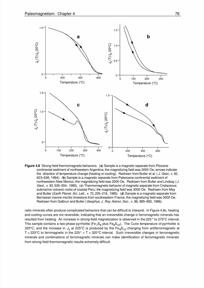
8/7/2019 geomagnet 4
http://slidepdf.com/reader/full/geomagnet-4 13/17
Paleomagnetism: Chapter 4 76
0 200 400 600
0
1.0
J (T)/J (20°C)
s
s
0
1.0
0.5
1.5
0 100 200 300
Temperature (°C)
Temperature (°C) Temperature (°C)
1.6
1.0
0
0 100 200 300 400
Temperature (°C)0 200 400 600
1.0
0
c d
ba
J (T)/J (2
0°C)
s
s
J (T)/J (20°C)
s
s
J (T)/J (20°C)
s
s
Figure 4.8 Strong-field thermomagnetic behaviors. (a) Sample is a magnetic separate from Pliocenecontinental sediment of northwestern Argentina; the magnetizing field was 3000 Oe; arrows indicate
the direction of temperature change (heating or cooling). Redrawn from Butler et al. (J. Geol ., v. 92,623–636, 1984). (b) Sample is a magnetic separate from Paleocene continental sediment ofnorthwestern New Mexico; the magnetizing field was 2000 Oe. Redrawn from Butler and Lindsay (J.
Geol ., v. 93, 535–554, 1985). (c) Thermomagnetic behavior of magnetic separate from Cretaceoussubmarine volcanic rocks of coastal Peru; the magnetizing field was 3000 Oe. Redrawn from May
and Butler (Earth Planet. Sci. Lett ., v. 72, 205–218, 1985). (d) Sample is a magnetic separate fromBerriasian marine micritic limestone from southeastern France; the magnetizing field was 3000 Oe.
Redrawn from Galbrun and Butler (Geophys. J. Roy. Astron. Soc ., v. 86, 885–892, 1986).
netic minerals often produce complicated behaviors that can be difficult to interpret. In Figure 4.8c, heating
and cooling curves are not reversible, indicating that an irreversible change in ferromagnetic minerals has
resulted from heating. An increase in strong-field magnetization is observed in the 225° to 275°C interval.
This sample contains a two-phase pyrrhotite (Fe7S8 plus Fe9S10). The Curie temperature of pyrrhotite is
320°C, and the increase in J s at 225°C is produced by the Fe9S10 changing from antiferromagnetic at
T < 225°C to ferrimagnetic in the 225° < T < 320°C interval. Such irreversible changes in ferromagnetic
minerals and combinations of ferromagnetic minerals can make identification of ferromagnetic minerals
from strong-field thermomagnetic results extremely difficult.
8/7/2019 geomagnet 4
http://slidepdf.com/reader/full/geomagnet-4 14/17
Paleomagnetism: Chapter 4 77
The final example of Figure 4.8d reveals Curie temperatures of 580°C and 680°C observed in a mag-
netic extract. Auxiliary information indicates that these Curie temperatures are due to magnetite and hema-
tite, respectively. This example is offered as illustration that a ferromagnetic mineral with low j s (like hema-
tite) can be observed in the presence of a coexisting ferromagnetic mineral with much stronger j s (like
magnetite). But this is an atypical example and highlights one of the major limitations of strong-field thermo-
magnetic analysis. Because measured J s of a sample is dominated by the mineral with high j s , coexistingferromagnetic minerals with low j s are often not apparent in results of strong-field thermomagnetic experi-
ments, even though these minerals may be major contributors to the NRM. In some cases, the coercivity
spectrum technique can overcome this limitation.
Coercivity spectrum analysis
Titanomagnetite has saturation magnetization, j s , up to 480 G (4.8 × 10⁵ A/m) and microscopic coercive
force, h c , < 3000 Oe (300 mT). (Similar h c is observed for titanohematite in the range of composition 0.5 ≤x ≤ 0.8 where it is ferrimagnetic above room temperature.) In contrast, hematite has j s of only 2–3 G (2–3 ×10³ A/m) but can have h c ≥ 10000 Oe (1 T). Similar high coercivity is observed for goethite. Coercivity
spectrum analysis uses the contrast in coercive force between titanomagnetite and hematite and goethite to
detect hematite (or goethite) coexisting with more strongly ferromagnetic minerals.
The usual procedure in coercivity spectrum analysis is to (1) induce isothermal remanent magnetization
(IRM) by exposing a sample to a magnetizing field, H , (2) measure resulting IRM, then (3) repeat the proce-
dure using a stronger magnetizing field. A sample containing only titanomagnetite (or ferrimagnetic
titanohematite) acquires IRM in H ≤ 3000 Oe (300 mT), but no additional IRM is acquired in higher H . If only
hematite (or goethite) is present, IRM is gradually acquired in H up to 30000 Oe (3 T). Samples containing
both titanomagnetite and hematite (or goethite) rapidly acquire IRM in H ≤ 3000 Oe (300 mT), followed by
gradual acquisition of additional IRM in stronger magnetizing fields. This procedure allows detection of
small amounts of hematite (or goethite) even when coexisting with more strongly ferromagnetic
titanomagnetite.
It is common to follow the IRM acquisition experiment with thermal demagnetization. IRM decreasesduring thermal demagnetization as blocking temperatures are reached. Major decreases in IRM during
thermal demagnetization allow estimation of Curie temperatures because maximum blocking temperatures
are always slightly less than the Curie temperature.
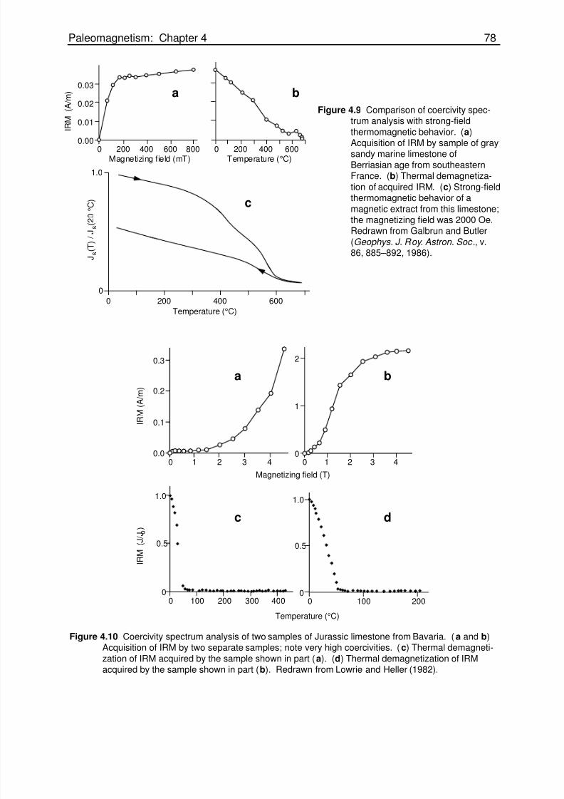
The utility of coercivity spectrum analysis is illustrated in Figure 4.9. Strong-field thermomagnetic
analysis of a magnetic separate from this Early Cretaceous limestone is shown in Figure 4.9c. A Curie
temperature of 580°C is evident, but there is no indication of a 680°C Curie temperature due to hema-
tite. However, IRM acquisition for a sample of this limestone (Figure 4.9a) shows a sharp rise in IRM
up to 3000 Oe (300 mT) due to magnetite, followed by increased IRM in higher magnetizing fields.
IRM acquired in H ≥ 3000 Oe (300 mT) is due to the presence of a high h c mineral (such as hematite or
goethite). Thermal demagnetization of acquired IRM for this rock is illustrated in Figure 4.9b. Most
IRM is removed by thermal demagnetization to the 580°C Curie temperature of magnetite. However,
the portion of IRM acquired in H ≥ 3000 Oe (300 mT) exhibits blocking temperatures up to 680°C, a
clear indication that the high h c component is hematite.
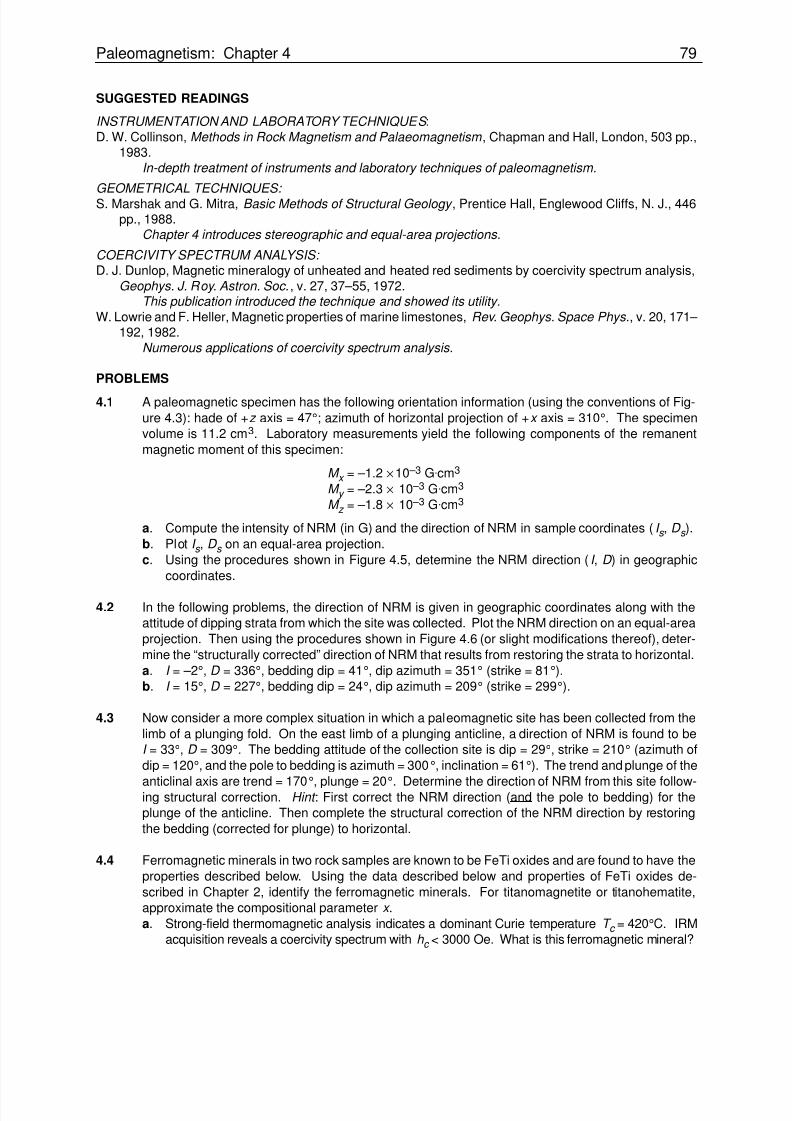
An additional example is provided in Figure 4.10. Although the shape of the IRM acquisition curves
(Figures 4.10a and 4.10b) is markedly different for these two samples of Jurassic limestone, IRM is
clearly dominated by a high coercivity mineral. IRM acquisition alone does not allow identification of
the mineral as hematite or goethite. But thermal demagnetization of acquired IRM (Figures 4.10c and
4.10d) reveals blocking temperatures ≤ 100°C, indicating that the dominant ferromagnetic mineral is
goethite (Curie temperature = 120°C).
8/7/2019 geomagnet 4
http://slidepdf.com/reader/full/geomagnet-4 15/17
Paleomagnetism: Chapter 4 78
Magnetizing field (mT) Temperature (°C)
IRM (A/m)
0.03
0.02
0.01
0.000 200 400 600 800 200 400 6000
Temperature (°C)
0 200 400 600
0
1.0
J (T) / J (20 °C)
s
s
c
ba
2
1
00.0
0.1
0.2
0.3
0 1 2 3 4 0 1 2 3 4
Magnetizing field (T)
IR
M (A/m)
1000 200 300 4000
0.5
1.0
1000 2000
0.5
1.0
Temperature (°C)
(J/J )o
IR
M
a b
c d
Figure 4.9 Comparison of coercivity spec-trum analysis with strong-field
thermomagnetic behavior. (a)
Acquisition of IRM by sample of graysandy marine limestone of
Berriasian age from southeasternFrance. (b) Thermal demagnetiza-
tion of acquired IRM. (c) Strong-fieldthermomagnetic behavior of a
magnetic extract from this limestone;the magnetizing field was 2000 Oe.Redrawn from Galbrun and Butler
(Geophys. J. Roy. Astron. Soc ., v.86, 885–892, 1986).
Figure 4.10 Coercivity spectrum analysis of two samples of Jurassic limestone from Bavaria. (a and b)Acquisition of IRM by two separate samples; note very high coercivities. (c) Thermal demagneti-
zation of IRM acquired by the sample shown in part (a). (d) Thermal demagnetization of IRMacquired by the sample shown in part (b). Redrawn from Lowrie and Heller (1982).
8/7/2019 geomagnet 4
http://slidepdf.com/reader/full/geomagnet-4 16/17
Paleomagnetism: Chapter 4 79
SUGGESTED READINGS
INSTRUMENTATION AND LABORATORY TECHNIQUES :
D. W. Collinson, Methods in Rock Magnetism and Palaeomagnetism , Chapman and Hall, London, 503 pp.,1983.
In-depth treatment of instruments and laboratory techniques of paleomagnetism.
GEOMETRICAL TECHNIQUES:
S. Marshak and G. Mitra, Basic Methods of Structural Geology , Prentice Hall, Englewood Cliffs, N. J., 446pp., 1988.
Chapter 4 introduces stereographic and equal-area projections.
COERCIVITY SPECTRUM ANALYSIS: D. J. Dunlop, Magnetic mineralogy of unheated and heated red sediments by coercivity spectrum analysis,
Geophys. J. Roy. Astron. Soc., v. 27, 37–55, 1972.This publication introduced the technique and showed its utility.
W. Lowrie and F. Heller, Magnetic properties of marine limestones, Rev. Geophys. Space Phys., v. 20, 171– 192, 1982.
Numerous applications of coercivity spectrum analysis.
PROBLEMS
4.1 A paleomagnetic specimen has the following orientation information (using the conventions of Fig-
ure 4.3): hade of +z axis = 47°; azimuth of horizontal projection of +x axis = 310°. The specimen
volume is 11.2 cm3. Laboratory measurements yield the following components of the remanent
magnetic moment of this specimen:
M x = –1.2 ×10⁻³ G.cm3
M y = –2.3 × 10⁻³ G.cm3
M z = –1.8 × 10⁻³ G.cm3
a. Compute the intensity of NRM (in G) and the direction of NRM in sample coordinates (I s , D s ).
b. Plot I s , D s on an equal-area projection.
c. Using the procedures shown in Figure 4.5, determine the NRM direction (I , D ) in geographic
coordinates.
4.2 In the following problems, the direction of NRM is given in geographic coordinates along with the
attitude of dipping strata from which the site was collected. Plot the NRM direction on an equal-area
projection. Then using the procedures shown in Figure 4.6 (or slight modifications thereof), deter-
mine the “structurally corrected” direction of NRM that results from restoring the strata to horizontal.
a. I = –2°, D = 336°, bedding dip = 41°, dip azimuth = 351° (strike = 81°).b. I = 15°, D = 227°, bedding dip = 24°, dip azimuth = 209° (strike = 299°).
4.3 Now consider a more complex situation in which a paleomagnetic site has been collected from the
limb of a plunging fold. On the east limb of a plunging anticline, a direction of NRM is found to be
I = 33°, D = 309°. The bedding attitude of the collection site is dip = 29°, strike = 210° (azimuth of
dip = 120°, and the pole to bedding is azimuth = 300°, inclination = 61°). The trend and plunge of the
anticlinal axis are trend = 170°, plunge = 20°. Determine the direction of NRM from this site follow-ing structural correction. Hint : First correct the NRM direction (and the pole to bedding) for the
plunge of the anticline. Then complete the structural correction of the NRM direction by restoring
the bedding (corrected for plunge) to horizontal.
4.4 Ferromagnetic minerals in two rock samples are known to be FeTi oxides and are found to have the
properties described below. Using the data described below and properties of FeTi oxides de-
scribed in Chapter 2, identify the ferromagnetic minerals. For titanomagnetite or titanohematite,
approximate the compositional parameter x .
a. Strong-field thermomagnetic analysis indicates a dominant Curie temperature T c = 420°C. IRM
acquisition reveals a coercivity spectrum with h c < 3000 Oe. What is this ferromagnetic mineral?
8/7/2019 geomagnet 4
http://slidepdf.com/reader/full/geomagnet-4 17/17
Paleomagnetism: Chapter 4 80
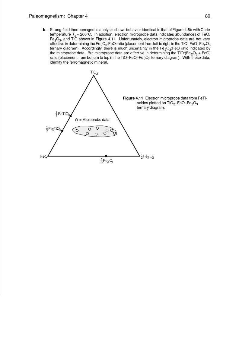
b. Strong-field thermomagnetic analysis shows behavior identical to that of Figure 4.8b with Curietemperature T c = 200°C. In addition, electron microprobe data indicates abundances of FeO,Fe2O3, and TiO shown in Figure 4.11. Unfortunately, electron microprobe data are not very
effective in determining the Fe2O3:FeO ratio (placement from left to right in the TiO–FeO–Fe2O3ternary diagram). Accordingly, there is much uncertainty in the Fe2O3:FeO ratio indicated by
the microprobe data. But microprobe data are effective in determining the TiO:(Fe2O3 + FeO)
ratio (placement from bottom to top in the TiO–FeO–Fe2O3 ternary diagram). With these data,identify the ferromagnetic mineral.
FeOFe O3 43
121Fe O2 3
2TiO
Fe TiO4213
FeTiO12 3
= Microprobe data
Figure 4.11 Electron microprobe data from FeTi-
oxides plotted on TiO2–FeO–Fe2O3ternary diagram.