GEOMETRIC CONSTRAINTS SOLVING: SOME TRACKS

Dominique Michelucci, Sebti Foufou, Loic Lamarque ∗

LE2I, UMR CNRS 5158, Univ. de Bourgogne, BP. 47870, 21078 Dijon, France

Pascal SchreckLSITT, Universite Louis Pasteur, Strasbourg, France†

Abstract

This paper presents some important issues and potential researchtracks for Geometric Constraint Solving: the use of the simplicialBernstein base to reduce the wrapping effect in interval methods,the computation of the dimension of the solution set with meth-ods used to measure the dimension of fractals, the pitfalls of graphbased decomposition methods, the alternative provided by linearalgebra, the witness configuration method, the use of randomizedprovers to detect dependences between constraints, the study of in-cidence constraints, the search for intrinsic (coordinate-free) for-mulations and the need for formal specifications.

CR Categories: J.6 [Computer Applications]: Computer AidedEngineering—CAD-CAM; I.3.5 [Computer Graphics]: Computa-tional Geometry and Object Modeling—Geometric algorithms, lan-guages, and systems

Keywords: Geometric Constraints Solving, decomposition, wit-ness configuration, Bernstein base, incidence constraint, random-ized prover, rigidity theory, projective geometry

1 Geometric constraints solving

This article intents to present some essential issues for GeometricConstraints Solving (GCS) and potential tracks for future research.For the sake of conciseness and homogeneity, it focuses on prob-lems related to the resolution, the decomposition, and the formula-tion of geometric constraints.

Today, all geometric modellers in CAD-CAM (Computer AidedDesign, Computer Aided Manufacturing) provide some GeometricConstraints Solver. The latter enables designers and engineers todescribe geometric entities (points, lines, planes, curves, surfaces)by specification of constraints: distances, angles, incidences, tan-gences between geometric entities. Constraints reduce to a systemof (typically algebraic) equations. Typically, an interactive 2D or3D editor permits the user to enter a so called approximate ”sketch”,and to specify geometric constraints (sometimes some constraintsare automatically guessed by the software). The solver must correctthe sketch, to make it satisfy the constraints.

Usually, the solver first performs a qualitative study of the con-straints system to detect under-, well- and over-constrained parts;when the system is correct, i.e. well-constrained, it is further de-composed into irreducible well-constrained subparts easier to solveand assemble. This qualitative study is mainly a Degree of Free-dom (DoF) analysis. It is typically performed on some kind ofgraphs [Owen 1991; Hoffmann et al. 2001; Gao and Zhang 2003;Hendrickson 1992; Ait-Aoudia et al. 1993; Lamure and Michelucci1998]. This article presents the pitfalls of graph based approaches,and suggests an alternative method. After this qualitative study,

∗e-mail: dmichel,sfoufou,loic.lamarque@u-bourgogne.fr†e-mail:schreck@dpt-info.u-strasbg.fr

if it is successful, irreducible subsystems are solved, either withsome formula in the simplest case (e.g. to compute the intersectionbetween two coplanar lines, or the third side length of a triangleknowing two other side lengths and an angle, etc), or with somenumerical method, e.g. a Newton-Raphson or an homotopy, whichtypically uses the sketch as a starting point for iterations, or with in-terval methods which can find all real solutions and enclose them inguaranteed boxes (a box is a vector of intervals). Computer algebrais not practicable because of the size of some irreducible systems,and it is not used by nowadays’ CAD-CAM modelers. In this ar-ticle, we will show that in some cases using computer algebra ispossible and relevant.

Depending on the context, either users expect only one solution, the”closest” one to an interactively provided sketch; or they expect thesolver to give all real roots, and interval methods are especially in-teresting in this case. For instance, in Robotics, problematic config-urations of flexible mechanisms are solutions of a set of geometricconstraints: engineers want to know all problematic situations or aguarantee that there is none.

The paper is organized as follow: Section 2 discusses GCS usinginterval arithmetic and Bernstein bases. Problems related to the de-composition of geometric constraints systems (degree of freedom,scaling, homography, pitfalls of graph based methods, etc.) are dis-cussed in Section 3. This section also provides some ideas on howprobabilistic tests such as NPM (Numerical Probabilistic Method)can be used as an efficient alternative for GCS and decompositionwhen they are used with a good initial configuration (which we referto as the witness configuration in Section 3.9). Section 4 considersGCS when there is a continuum of solutions and the use of curvetracing algorithms. Section 5 presents the expression of geometricconstraints in a coordinate free way and shows how kernel functionscan be used to provide intrinsic formulation of constraints. Section6 discusses the need for formal specifications of constraints and forspecification languages. The conclusion is given in Section 7.

2 Interval arithmetic and Bernstein bases

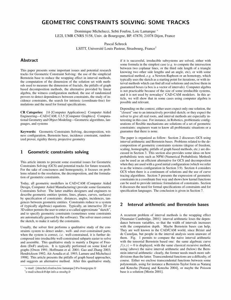
A recurrent problem of interval methods is the wrapping effect[Neumaier Cambridge, 2001]: interval arithmetic loses the depen-dance between variables, so that the width of intervals increaseswith the computation depth. Maybe Bernstein bases can help.They are well known in the CAD/CAM world, since Bezier andde Casteljau, but people in the interval analysis seem unaware ofthem. Fig. 1 permits to compare the naive interval arithmeticwith the tensorial Bernstein based one: the same algebraic curvef (x,y) = 0 is displayed, with the same classical recursive method,using (above) the naive interval arithmetic and (below) the Bern-stein interval arithmetic: clearly, the former needs much more sub-divisions than the latter. Transcendental functions are a difficulty, ofcourse. Either we enclose transcendental functions between somepolynomials, using for instance a Bernstein-Taylor form as Natarajand Kotecha [Nataraj and Kotecha 2004], or maybe the Poissonbase is a solution [Morin 2001].

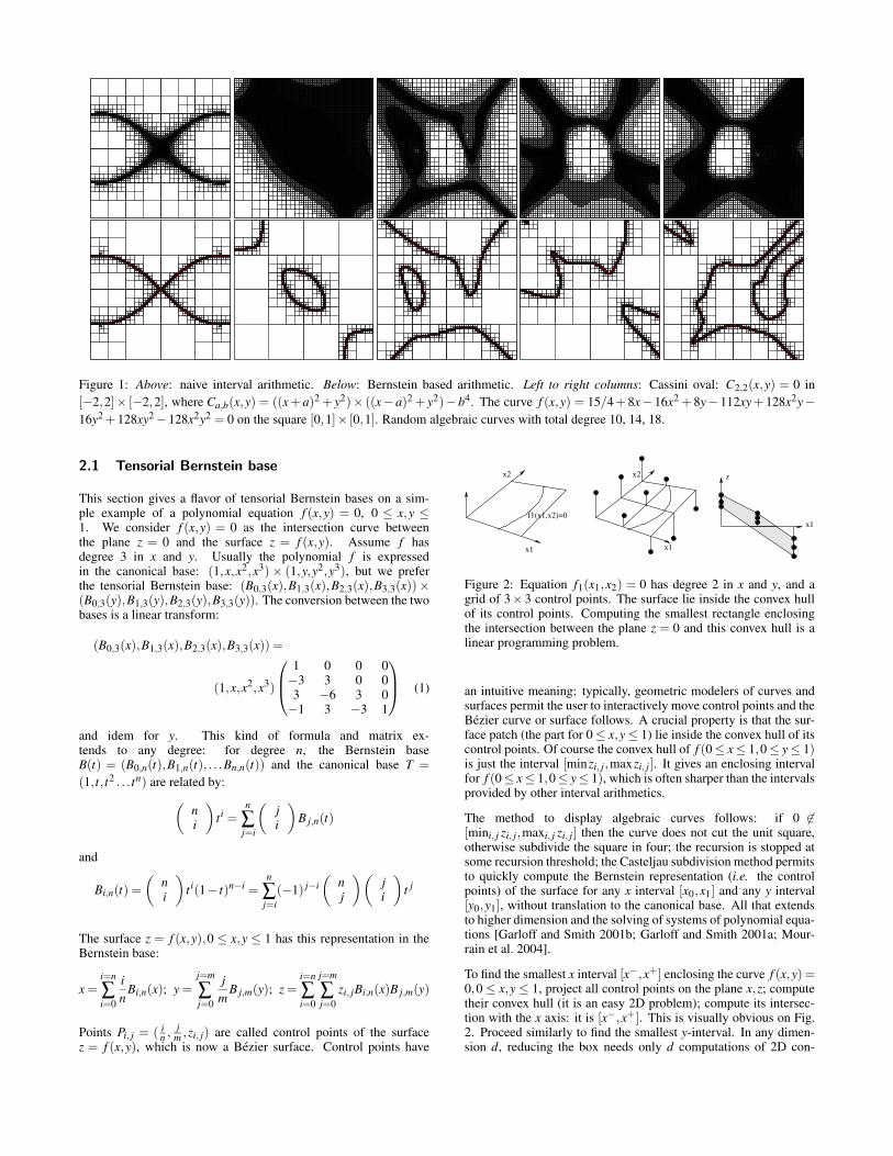
Figure 1: Above: naive interval arithmetic. Below: Bernstein based arithmetic. Left to right columns: Cassini oval: C2,2(x,y) = 0 in[−2,2]× [−2,2], where Ca,b(x,y) = ((x + a)2 + y2)× ((x− a)2 + y2)− b4. The curve f (x,y) = 15/4 + 8x− 16x2 + 8y− 112xy + 128x2y−16y2 +128xy2 −128x2y2 = 0 on the square [0,1]× [0,1]. Random algebraic curves with total degree 10, 14, 18.

2.1 Tensorial Bernstein base

This section gives a flavor of tensorial Bernstein bases on a sim-ple example of a polynomial equation f (x,y) = 0, 0 ≤ x,y ≤1. We consider f (x,y) = 0 as the intersection curve betweenthe plane z = 0 and the surface z = f (x,y). Assume f hasdegree 3 in x and y. Usually the polynomial f is expressedin the canonical base: (1,x,x2,x3)× (1,y,y2,y3), but we preferthe tensorial Bernstein base: (B0,3(x),B1,3(x),B2,3(x),B3,3(x))×(B0,3(y),B1,3(y),B2,3(y),B3,3(y)). The conversion between the twobases is a linear transform:

(B0,3(x),B1,3(x),B2,3(x),B3,3(x)) =

(1,x,x2,x3)

1 0 0 0−3 3 0 03 −6 3 0−1 3 −3 1

(1)

and idem for y. This kind of formula and matrix ex-tends to any degree: for degree n, the Bernstein baseB(t) = (B0,n(t),B1,n(t), . . .Bn,n(t)) and the canonical base T =

(1, t, t2 . . .tn) are related by:(

ni

)

t i =n

∑j=i

(

ji

)

B j,n(t)

and

Bi,n(t) =

(

ni

)

t i(1− t)n−i =n

∑j=i

(−1) j−i(

nj

)(

ji

)

t j

The surface z = f (x,y),0 ≤ x,y ≤ 1 has this representation in theBernstein base:

x =i=n

∑i=0

in

Bi,n(x); y =j=m

∑j=0

jm

B j,m(y); z =i=n

∑i=0

j=m

∑j=0

zi, jBi,n(x)B j,m(y)

Points Pi, j = ( in , j

m ,zi, j) are called control points of the surfacez = f (x,y), which is now a Bezier surface. Control points have

x2

x1 x1

x2

f1(x1,x2)=0x1

z

Figure 2: Equation f1(x1,x2) = 0 has degree 2 in x and y, and agrid of 3× 3 control points. The surface lie inside the convex hullof its control points. Computing the smallest rectangle enclosingthe intersection between the plane z = 0 and this convex hull is alinear programming problem.

an intuitive meaning: typically, geometric modelers of curves andsurfaces permit the user to interactively move control points and theBezier curve or surface follows. A crucial property is that the sur-face patch (the part for 0 ≤ x,y ≤ 1) lie inside the convex hull of itscontrol points. Of course the convex hull of f (0 ≤ x ≤ 1,0 ≤ y ≤ 1)is just the interval [minzi, j,maxzi, j]. It gives an enclosing intervalfor f (0≤ x≤ 1,0≤ y≤ 1), which is often sharper than the intervalsprovided by other interval arithmetics.

The method to display algebraic curves follows: if 0 6∈[mini, j zi, j,maxi, j zi, j] then the curve does not cut the unit square,otherwise subdivide the square in four; the recursion is stopped atsome recursion threshold; the Casteljau subdivision method permitsto quickly compute the Bernstein representation (i.e. the controlpoints) of the surface for any x interval [x0,x1] and any y interval[y0,y1], without translation to the canonical base. All that extendsto higher dimension and the solving of systems of polynomial equa-tions [Garloff and Smith 2001b; Garloff and Smith 2001a; Mour-rain et al. 2004].

To find the smallest x interval [x−,x+] enclosing the curve f (x,y) =0,0 ≤ x,y ≤ 1, project all control points on the plane x,z; computetheir convex hull (it is an easy 2D problem); compute its intersec-tion with the x axis: it is [x−,x+]. This is visually obvious on Fig.2. Proceed similarly to find the smallest y-interval. In any dimen-sion d, reducing the box needs only d computations of 2D con-

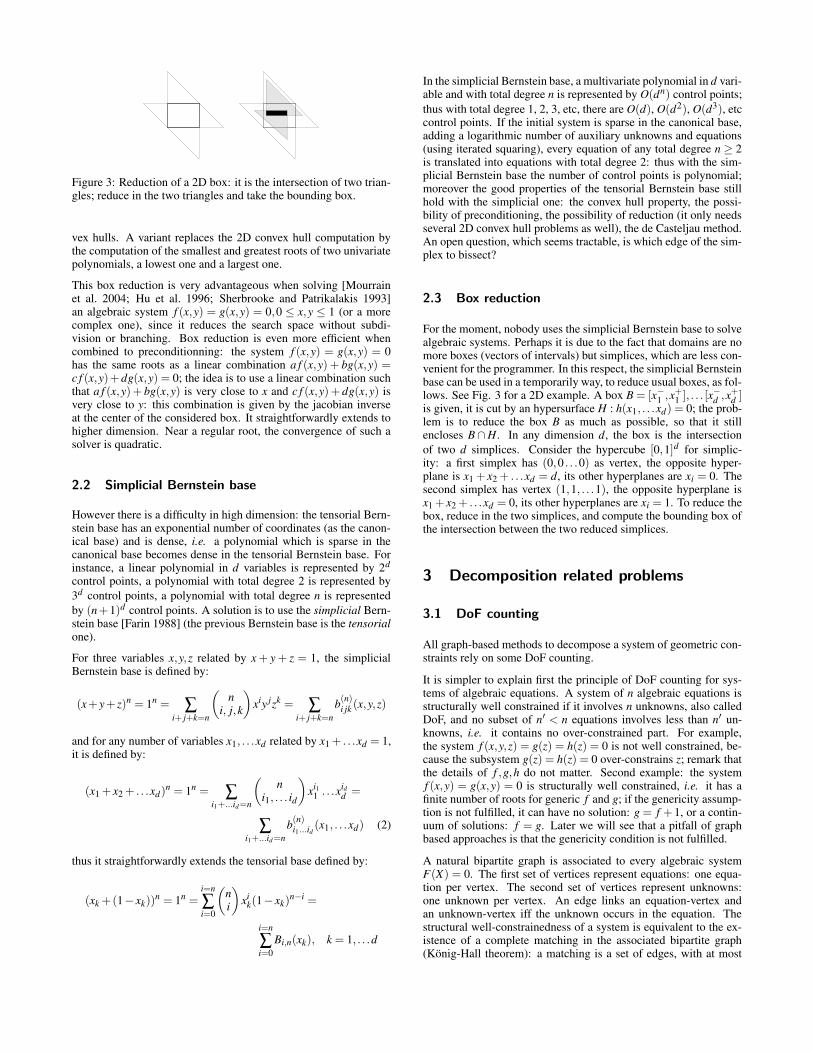
Figure 3: Reduction of a 2D box: it is the intersection of two trian-gles; reduce in the two triangles and take the bounding box.

vex hulls. A variant replaces the 2D convex hull computation bythe computation of the smallest and greatest roots of two univariatepolynomials, a lowest one and a largest one.

This box reduction is very advantageous when solving [Mourrainet al. 2004; Hu et al. 1996; Sherbrooke and Patrikalakis 1993]an algebraic system f (x,y) = g(x,y) = 0,0 ≤ x,y ≤ 1 (or a morecomplex one), since it reduces the search space without subdi-vision or branching. Box reduction is even more efficient whencombined to preconditionning: the system f (x,y) = g(x,y) = 0has the same roots as a linear combination a f (x,y) + bg(x,y) =c f (x,y)+dg(x,y) = 0; the idea is to use a linear combination suchthat a f (x,y)+ bg(x,y) is very close to x and c f (x,y)+ dg(x,y) isvery close to y: this combination is given by the jacobian inverseat the center of the considered box. It straightforwardly extends tohigher dimension. Near a regular root, the convergence of such asolver is quadratic.

2.2 Simplicial Bernstein base

However there is a difficulty in high dimension: the tensorial Bern-stein base has an exponential number of coordinates (as the canon-ical base) and is dense, i.e. a polynomial which is sparse in thecanonical base becomes dense in the tensorial Bernstein base. Forinstance, a linear polynomial in d variables is represented by 2d

control points, a polynomial with total degree 2 is represented by3d control points, a polynomial with total degree n is representedby (n+1)d control points. A solution is to use the simplicial Bern-stein base [Farin 1988] (the previous Bernstein base is the tensorialone).

For three variables x,y,z related by x + y + z = 1, the simplicialBernstein base is defined by:

(x+ y+ z)n = 1n = ∑i+ j+k=n

(

ni, j,k

)

xiy jzk = ∑i+ j+k=n

b(n)i jk (x,y,z)

and for any number of variables x1, . . .xd related by x1 + . . .xd = 1,it is defined by:

(x1 + x2 + . . .xd)n = 1n = ∑i1+...id=n

(

ni1, . . . id

)

xi11 . . .xid

d =

∑i1+...id=n

b(n)i1...id (x1, . . .xd) (2)

thus it straightforwardly extends the tensorial base defined by:

(xk +(1− xk))n = 1n =

i=n

∑i=0

(

ni

)

xik(1− xk)

n−i =

i=n

∑i=0

Bi,n(xk), k = 1, . . .d

In the simplicial Bernstein base, a multivariate polynomial in d vari-able and with total degree n is represented by O(dn) control points;thus with total degree 1, 2, 3, etc, there are O(d), O(d2), O(d3), etccontrol points. If the initial system is sparse in the canonical base,adding a logarithmic number of auxiliary unknowns and equations(using iterated squaring), every equation of any total degree n ≥ 2is translated into equations with total degree 2: thus with the sim-plicial Bernstein base the number of control points is polynomial;moreover the good properties of the tensorial Bernstein base stillhold with the simplicial one: the convex hull property, the possi-bility of preconditioning, the possibility of reduction (it only needsseveral 2D convex hull problems as well), the de Casteljau method.An open question, which seems tractable, is which edge of the sim-plex to bissect?

2.3 Box reduction

For the moment, nobody uses the simplicial Bernstein base to solvealgebraic systems. Perhaps it is due to the fact that domains are nomore boxes (vectors of intervals) but simplices, which are less con-venient for the programmer. In this respect, the simplicial Bernsteinbase can be used in a temporarily way, to reduce usual boxes, as fol-lows. See Fig. 3 for a 2D example. A box B = [x−1 ,x+

1 ], . . . [x−d ,x+d ]

is given, it is cut by an hypersurface H : h(x1, . . .xd) = 0; the prob-lem is to reduce the box B as much as possible, so that it stillencloses B∩ H. In any dimension d, the box is the intersectionof two d simplices. Consider the hypercube [0,1]d for simplic-ity: a first simplex has (0,0 . . .0) as vertex, the opposite hyper-plane is x1 + x2 + . . .xd = d, its other hyperplanes are xi = 0. Thesecond simplex has vertex (1,1, . . .1), the opposite hyperplane isx1 + x2 + . . .xd = 0, its other hyperplanes are xi = 1. To reduce thebox, reduce in the two simplices, and compute the bounding box ofthe intersection between the two reduced simplices.

3 Decomposition related problems

3.1 DoF counting

All graph-based methods to decompose a system of geometric con-straints rely on some DoF counting.

It is simpler to explain first the principle of DoF counting for sys-tems of algebraic equations. A system of n algebraic equations isstructurally well constrained if it involves n unknowns, also calledDoF, and no subset of n′ < n equations involves less than n′ un-knowns, i.e. it contains no over-constrained part. For example,the system f (x,y,z) = g(z) = h(z) = 0 is not well constrained, be-cause the subsystem g(z) = h(z) = 0 over-constrains z; remark thatthe details of f ,g,h do not matter. Second example: the systemf (x,y) = g(x,y) = 0 is structurally well constrained, i.e. it has afinite number of roots for generic f and g; if the genericity assump-tion is not fulfilled, it can have no solution: g = f +1, or a contin-uum of solutions: f = g. Later we will see that a pitfall of graphbased approaches is that the genericity condition is not fulfilled.

A natural bipartite graph is associated to every algebraic systemF(X) = 0. The first set of vertices represent equations: one equa-tion per vertex. The second set of vertices represent unknowns:one unknown per vertex. An edge links an equation-vertex andan unknown-vertex iff the unknown occurs in the equation. Thestructural well-constrainedness of a system is equivalent to the ex-istence of a complete matching in the associated bipartite graph(Konig-Hall theorem): a matching is a set of edges, with at most

one incident edge per vertex; vertices with an edge in the matchingare said to be covered or saturated by the matching; a matching ismaximum when it is maximum in cardinality; it is perfect iff allvertices are saturated. In intuitive words, one can find one equa-tion per unknown (the two vertices are linked in the bipartite graph)which determines this unknown. There are fast methods to computematchings in bipartite graph. Maximum matchings are equivalentto maximum flows (a lot of papers about graph based decomposi-tion refer to maximum flows rather than maximum matchings).

The decomposition of bipartite graphs due to Dulmage and Mendel-sohn also relies on maximum matchings. It partitions the systeminto a well-constrained part, an over-constrained part, an under-constrained part. The well-constrained part can be further decom-posed (in polynomial time also) into irreducible well-constrainedparts, which are partially ordered: for example f (x) = g(x,y) = 0is well constrained; it can be decomposed into f (x) = 0 which iswell constrained, and g(x,y) = 0 which is well constrained once xhas been replaced by the corresponding root.

Relatively to systems of equations, systems of geometric con-straints introduce two complications:

First geometric constraints are (classically...) assumed to be inde-pendent of the coordinate system, thus they can, for instance, de-termine the shape of a triangle in 2D (specifying either two lengthsand one angle, or one angle and two lengths, or three lengths) butthey can not fix the location and orientation of the triangle relativelyto the cartesian frame. This placement is defined by three param-eters (an x translation, an y translation, one angle). Thus in 2D,the DoF of a system is the number of unknowns (coordinates, radii,non geometric unknowns) minus 3. The same holds in 3D, wherethe placement needs six parameters; thus the DoF of a 3D systemis the number of unknowns minus 6 — the constant is d(d + 1)/2in dimension d. Numerous ways have been proposed for adaptingdecomposition methods for systems of equations to systems of ge-ometric constraints.

Second, the bipartite graph is visually cumbersome and not intu-itive. People prefer the ”natural” graph: each vertex represent a ge-ometric unknown (point, line, plane) or a non geometric unknown,and each edge represents a constraint. There is a difficulty for repre-senting constraints involving more than 2 entities; either hyper-arcsare used, or all constraints are binarized. Moreover vertices carryDoF, and edges (constraints) carry DoR: degree of restriction, i.e.the number of corresponding equations.

The differences between the bipartite and natural graphs are notessential. In passing, the matroid theory provides yet another for-malism to express the same things, but it is not used in the GCScommunity up to now.

In 2D, a point and a line have 2 DoF; in 3D, points and planeshave 3 DoF, lines have 4. In 3D, DoF counting (correctly) predictsthere is a finite number of lines which cut four given skew lines:the unknown line has 4 DoF and there are 4 constraints. Similarly,there is a finite number of lines tangent to 4 given spheres.

Decomposition methods are essential, since they permit to solve bigsystems of geometric constraints, which can not be otherwise.

3.2 Decomposition modulo scaling or homography

Decomposition methods are complex and do not always take intoaccount non geometric unknowns or geometric unknowns such asradii (which are independent on the cartesian frame, contrarily tounknowns). Decomposition methods should be simpler, more gen-eral, and decompose not only in subparts well constrained mod-

ulo displacements, but also modulo scaling [Schramm and Schreck2003]: so we can compute an angle, or a distance ratio, in one part,and propagate this information elsewhere, and modulo homogra-phy: so we can compute cross ratios in one part and propagate else-where.

3.3 Almost decomposition

Hoffmann, Gao and Yang [Gao et al. 2004] introduce almost de-compositions. They remark that a lot of irreducible systems in 3Dare easier to solve when one of the unknowns is considered as a pa-rameter, and when the system is solved for all (or some sampling)values of this parameter. In this artificial but simple example:

f1(x1,x2,x3,x4 = u) = 0f2(x1,x2,x3,x4 = u) = 0f3(x1,x2,x3,x4 = u) = 0f4(x1,x2,x3,x4,x5,x6,x7) = 0f5(x1,x2,x3,x4,x5,x6,x7) = 0f6(x1,x2,x3,x4,x5,x6,x7) = 0f7(x1,x2,x3,x4,x5,x6,x7) = 0

x4 is considered as a parameter u with a given value (we call it a keyunknown for convenience). The subsystem Su : f1(x1,x2,x3,u) =f2(x1,x2,x3,u) = f3(x1,x2,x3,u) = 0 is solved for all values of u,or in a more realistic way for some sampling of u. Then the restof the system Tu : f4(x) = f5(x) = f6(x) = 0 is solved, forgettingtemporarily one equation, say f7. f7 is then evaluated at all sam-pling points on the solution curve of f1(x) = . . . f6(x) = 0. Whenf7 almost vanishes, the possible root is polished with some New-ton iterations. For the class of basic 3D configurations studied byHoffmann, Gao and Yang [Gao et al. 2004], one key unknown issufficient most of the time, but some rare more difficult problemsneed two key unknowns. One may imagine several variants of thisapproach, for instance the use of marching curve methods to fol-low the curve parameterized with u, or methods to automaticallyproduce the best almost decomposition for irreducible systems: thebest is the one which minimizes the number of key unknowns.

Curve tracing [Michelucci and Faudot 2005] can also be used toexplore a finite set of solutions when no geometric symbolic so-lution is available (which is often the case in 3D). If the solutionproposed by the solver does not fit the user needs, the idea is toforget one constraint and to trace the corresponding curve. In thiscase the roots are the vertices of a graph the edges of which cor-respond to the curves where a constraint has been forgotten. If wehave d equations and d unknowns then each vertex is of degree d.One difficulty is that this graph can be disconnected, and there is noguarantee to reach every vertex starting from a given solution.

3.4 Some challenging problems

Some challenging problems resist this last attack of almost decom-position. Consider the graph of the regular icosahedron (20 trian-gles, 30 edges, 12 vertices). Labelling edges with lengths gives awell constrained system with 30 distance constraints between 12points in 3D (the regular pentagons of the icosahedron are not con-strained to stay coplanar). This kind of problems, with distanceconstraints only, is called the molecule [Hendrickson 1992; Portaet al. 2003; Laurent 2001] problem because of its applications inchemistry: find the configuration of a molecule given some dis-tances between its atoms. This last system has Bezout number230 ≈ 109.

A seemingly more difficult problem uses the graph of the regulardodecahedron (12 pentagonal faces, 20 vertices, 30 edges). Labeledges with lengths; this time, also impose to each of the 12 pen-tagonal faces to stay planar, for the problem to be well constrained.The dodecahedron problem is not a molecule one, because of thecoplanarity constraints. In the same family, the familiar cube givesa well constrained problem, with 8 unknown points, 12 distances,and 6 coplanarity relations.

Considering the regular octahedron gives a simpler molecule prob-lem, with 6 unknown points and 12 distances (no coplanarity con-dition). This problem was already solved by Durand and Hoffmann[Durand 1998; Durand and Hoffmann 2000] with homotopy. An-other solution is to use Cayley-Menger relations [Yang 2002; Portaet al. 2003; Michelucci and Foufou 2004].

3D

1 2

3

45

1

45

2

3

Figure 4: The double banana, and three other 3D configurationsdue to Auxkin Ortuzar, where DoF counting fails. No four pointsare coplanar.

3.5 Pitfalls of graph based methods

A pitfall of DoF counting is that geometric constraints can be de-pendent in subtle ways. In 2D, the simplest counter example to DoFcounting is given by the 3 angles of a triangle: they can not be fixedindependently (note they can in spherical geometry). Fig. 5 showsa more complex 2D counter example. In 3D, a simple counter ex-ample is: point A and B lie on line L, line L lie on plane H, pointA lie on plane H; the last constraint is implied by the others. Fig.4 shows other counter examples which make fail DoF counting in3D. It is possible to use some ad hoc tests in graph based methodsto account for some of these configurations. However every inci-dence theorem (Desargues, Pappus, Pascal, Beltrami, Cox... seeFig. 6) provide dependent constraints: just use its hypothesis andconclusion (or its negation) as constraints; moreover no generic-ity assumption (used in Rigidity theory) is violated since incidenceconstraints do not use parameters. Thus detecting a dependence isas hard as detecting or proving geometric theorems.

DoF counting is mathematically sound only in a very restrictedcase, the 2D molecule problem, i.e. when all constraints are genericdistance constraints between 2D points (thus points can not becollinear): it is Laman theorem [J. Graver 1993]. For the 3Dmolecule problem, no characterization is known; Fig. 4 leftmostshows the most famous counterexample to DoF counting: the dou-ble banana, which uses only distance constraints. Even in the sim-

L

A X

s

ab

BX’

s’

Figure 5: Left: be given 3 aligned points A,B,X ; for any points outside AB, for any L through X outside s, define: a = L∩As,b = L∩Bs, s′ = Ab∩ aB, X ′ = ss′ ∩AB; then X ′ is independent ofs and L. Right: Desargues theorem: if two triangles (in gray) areperspective, homologous sides cut in three collinear points.

p1

p2

q1

q2

q3

p3

q1

q2

q3

p3

p2

p1

Figure 6: Pappus, its dual, Pascal theorems.

ple case of distance constraints, a combinatorial (i.e. in terms ofgraph or matroids) characterization of well constrainedness seemsout of reach.

With the still increasing size of constraints systems, the probabilityfor a subtle dependence increases as well. J-C. Leon (personal com-munication), who uses geometric constraints to define constrainedsurfaces or curves, reports this typical behavior: the solver detectsno over-constrainedness but fails to find a solution; the failure per-sists when the user tries to modify the value of parameters (dis-tances, angles) – which is terribly frustrating. This independence toparameter values suggests that the dependence is due to some inci-dence theorems of projective geometry (such as Pappus, Desargues,Pascal, Beltrami, etc). For conciseness, the other hypothesis: sometriangular (or tetrahedral [Serre 2000]) inequality is violated, is notdetailed here.

Detecting such dependences -or solving in spite of them when it isa consistent dependence- is a key issue for GCS. Clearly, no graphbased method can detect all such dependences. It gives strong mo-tivation for investigating other methods.

3.6 Linear Algebra performs qualitative study

Today decomposition is graph based most of the time. Linear al-gebra seems a promising alternative. For conciseness, the idea isillustrated for 2D systems of distance constraints only between npoints. Assume also the distances are algebraically independent(thus no collinear points), and that points are represented by theircartesian coordinates: X = (x1,y1, . . .xn,yn). For clarity, we saythat p = (x,y) is a ”point”, and X is a ”configuration”. After Rigid-ity theory [J. Graver 1993; Lamure and Michelucci 1998], it is wellknown that it suffices to numerically study the jacobian at somerandom configuration X ∈ R2n. It is the essence of the so callednumerical probabilistic method (NPM).

By convention, the k th line of the jacobian J is the derivative ofthe k th equation of the system. Vectors m such that Jmt = 0 arecalled infinitesimal motions. The notation X = (x1, y1, . . . xn, yn) isalso used to denote the infinitesimal motion at configuration X .

First, if the rank of the jacobian (at the random, generic configu-ration) is equal to the number of equations, equations are indepen-dent; otherwise it is possible to extract a base of the equations. Sec-ond, the system is well-constrained (modulo displacement) if its ja-cobian has corank 3: actually it is even possible to give a base of thekernel of the jacobian (the kernel is the set of infinitesimal motions).This base is tx, ty,r, where tx = (1,0,1,0, . . .) is a translation in x,ty = (0,1,0,1, . . .) is a translation in y, and r is an instantaneous ro-tation around the origine: r = (−y1,x1,−y2,x2, . . .− yn,xn). These3 infinitesimal motions are displacements, also called isometries;they do not modify the relative location of points, contrarily to de-formations (also called flexions).

An infinitesimal motion m is a displacement iff for all couple ofpoints A,B, the difference A− B between A and B motions is or-

A B

O

23

4

7

516

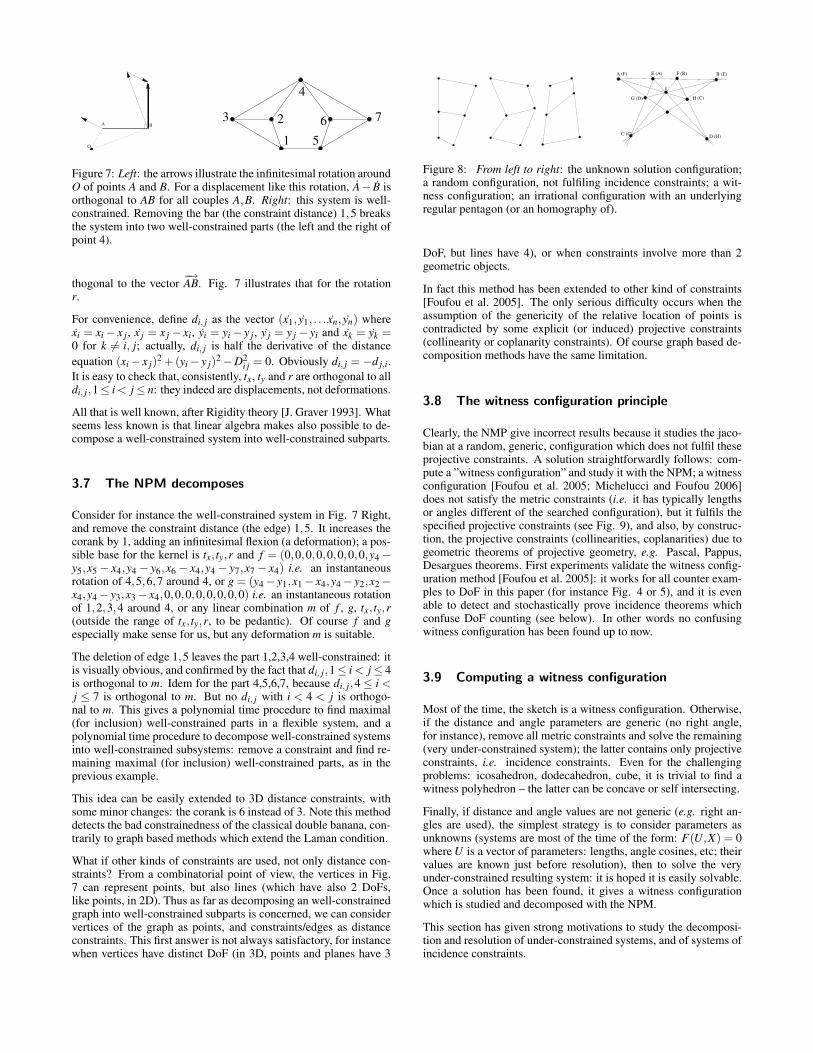
Figure 7: Left: the arrows illustrate the infinitesimal rotation aroundO of points A and B. For a displacement like this rotation, A− B isorthogonal to AB for all couples A,B. Right: this system is well-constrained. Removing the bar (the constraint distance) 1,5 breaksthe system into two well-constrained parts (the left and the right ofpoint 4).

thogonal to the vector−→AB. Fig. 7 illustrates that for the rotation

r.

For convenience, define di, j as the vector (x1, y1, . . . xn, yn) wherexi = xi − x j , x j = x j − xi, yi = yi − y j , y j = y j − yi and xk = yk =0 for k 6= i, j; actually, di, j is half the derivative of the distanceequation (xi − x j)

2 +(yi − y j)2 −D2

i j = 0. Obviously di, j = −d j,i.It is easy to check that, consistently, tx, ty and r are orthogonal to alldi, j,1≤ i < j ≤ n: they indeed are displacements, not deformations.

All that is well known, after Rigidity theory [J. Graver 1993]. Whatseems less known is that linear algebra makes also possible to de-compose a well-constrained system into well-constrained subparts.

3.7 The NPM decomposes

Consider for instance the well-constrained system in Fig. 7 Right,and remove the constraint distance (the edge) 1,5. It increases thecorank by 1, adding an infinitesimal flexion (a deformation); a pos-sible base for the kernel is tx, ty,r and f = (0,0,0,0,0,0,0,0,y4 −y5,x5 − x4,y4 − y6,x6 − x4,y4 − y7,x7 − x4) i.e. an instantaneousrotation of 4,5,6,7 around 4, or g = (y4 − y1,x1 − x4,y4 − y2,x2 −x4,y4 − y3,x3 − x4,0,0,0,0,0,0,0,0) i.e. an instantaneous rotationof 1,2,3,4 around 4, or any linear combination m of f , g, tx, ty,r(outside the range of tx, ty,r, to be pedantic). Of course f and gespecially make sense for us, but any deformation m is suitable.

The deletion of edge 1,5 leaves the part 1,2,3,4 well-constrained: itis visually obvious, and confirmed by the fact that di, j,1≤ i < j ≤ 4is orthogonal to m. Idem for the part 4,5,6,7, because di, j,4 ≤ i <j ≤ 7 is orthogonal to m. But no di, j with i < 4 < j is orthogo-nal to m. This gives a polynomial time procedure to find maximal(for inclusion) well-constrained parts in a flexible system, and apolynomial time procedure to decompose well-constrained systemsinto well-constrained subsystems: remove a constraint and find re-maining maximal (for inclusion) well-constrained parts, as in theprevious example.

This idea can be easily extended to 3D distance constraints, withsome minor changes: the corank is 6 instead of 3. Note this methoddetects the bad constrainedness of the classical double banana, con-trarily to graph based methods which extend the Laman condition.

What if other kinds of constraints are used, not only distance con-straints? From a combinatorial point of view, the vertices in Fig.7 can represent points, but also lines (which have also 2 DoFs,like points, in 2D). Thus as far as decomposing an well-constrainedgraph into well-constrained subparts is concerned, we can considervertices of the graph as points, and constraints/edges as distanceconstraints. This first answer is not always satisfactory, for instancewhen vertices have distinct DoF (in 3D, points and planes have 3

C (G) D (H)

H (C)

B (E)F (B)E (A)

G (D)

A (F)

I

Figure 8: From left to right: the unknown solution configuration;a random configuration, not fulfiling incidence constraints; a wit-ness configuration; an irrational configuration with an underlyingregular pentagon (or an homography of).

DoF, but lines have 4), or when constraints involve more than 2geometric objects.

In fact this method has been extended to other kind of constraints[Foufou et al. 2005]. The only serious difficulty occurs when theassumption of the genericity of the relative location of points iscontradicted by some explicit (or induced) projective constraints(collinearity or coplanarity constraints). Of course graph based de-composition methods have the same limitation.

3.8 The witness configuration principle

Clearly, the NMP give incorrect results because it studies the jaco-bian at a random, generic, configuration which does not fulfil theseprojective constraints. A solution straightforwardly follows: com-pute a ”witness configuration” and study it with the NPM; a witnessconfiguration [Foufou et al. 2005; Michelucci and Foufou 2006]does not satisfy the metric constraints (i.e. it has typically lengthsor angles different of the searched configuration), but it fulfils thespecified projective constraints (see Fig. 9), and also, by construc-tion, the projective constraints (collinearities, coplanarities) due togeometric theorems of projective geometry, e.g. Pascal, Pappus,Desargues theorems. First experiments validate the witness config-uration method [Foufou et al. 2005]: it works for all counter exam-ples to DoF in this paper (for instance Fig. 4 or 5), and it is evenable to detect and stochastically prove incidence theorems whichconfuse DoF counting (see below). In other words no confusingwitness configuration has been found up to now.

3.9 Computing a witness configuration

Most of the time, the sketch is a witness configuration. Otherwise,if the distance and angle parameters are generic (no right angle,for instance), remove all metric constraints and solve the remaining(very under-constrained system); the latter contains only projectiveconstraints, i.e. incidence constraints. Even for the challengingproblems: icosahedron, dodecahedron, cube, it is trivial to find awitness polyhedron – the latter can be concave or self intersecting.

Finally, if distance and angle values are not generic (e.g. right an-gles are used), the simplest strategy is to consider parameters asunknowns (systems are most of the time of the form: F(U,X) = 0where U is a vector of parameters: lengths, angle cosines, etc; theirvalues are known just before resolution), then to solve the veryunder-constrained resulting system: it is hoped it is easily solvable.Once a solution has been found, it gives a witness configurationwhich is studied and decomposed with the NPM.

This section has given strong motivations to study the decomposi-tion and resolution of under-constrained systems, and of systems ofincidence constraints.

3.10 Incidence constraints

The previous section has already given some motivations to studyincidence constraints, but these constraints also arise in photogram-metry, in computer vision, in automatic correction of hand madedrawings. We hope the systems of incidence constraints met in ourapplications to be trivial or almost trivial (defined below), howeverincidence constraints can be arbitrarily difficult even in 2D.

In 2D, a system of incidence constraints between points and linesreduce to a special 3D molecule problem [Hendrickson 1992; Portaet al. 2003; Laurent 2001]: represent unknown points and lines byunit 3D vectors; the incidence p ∈ L means that the correspondingvertices on the unit sphere have distance

√2. To avoid degeneracies

(either all points are equal, or all lines are equal), one can imposeto four generic points to lie on some arbitrary square on the unitsphere.

3.10.1 Trivial and almost trivial incidence systems

In 2D, a system of incidence constraints (point-line incidences) istrivial iff it contains only removable points and lines. A point pis removable when it is constrained to lie on two lines l1 and l2(or less): then its definition is stored in some data structure (eitherp = l1 ∩ l2, or p ∈ l1 is any point on line l1, or p is any point), it iserased from the incidence system, the rest of the system is solved,then the removed point is added using its definition. Symmetrically(or dually) for a line, when it is constrained to pass through twopoints (or less). Erasing a point or a line may make removableanother point or line. If all points and lines are removed, the graphis trivial. Trivial systems are easily solved, using the definitions ofremoved elements in reverse order.

The extension to 3D is straightforward. This method finds a witnessfor every Eulerian 3D polyhedra (a polyhedron is Eulerian iff itfulfils Euler formula). It is easily proved that every Eulerian 3Dpolyhedron contain a removable vertex or a removable face, andthus is trivial: assume there is a contradicting polyhedron, with Vvertices, E edges and F faces. Let v1,v2 . . .vV be the vertex degrees,all greater than 3, and f1, f2 . . . fF the number of vertices of the Ffaces, all greater than 3 as well; it is well known that ∑V

1 vi = 2E =

∑F1 f j , thus E ≥ 2V and E ≥ 2F . By Euler’ formula: V −E +F =

2. Thus E + 2 = V + F ≥ 2V + 2 and E + 2 = V + F ≥ 2F + 2.Add. We get 2E + 4 = 2V + 2F ≥ 4 + 2V + 2F : a contradiction.QED. Unfortunately, this simple method no more applies with nonEulerian polyhedra, say a faceted torus with quadrilateral faces andwhere every vertex has degree 4 (this last polyhedron has a rationalwitness too).

Another construction of a witness for Eulerian polyhedra first com-putes a 2D barycentric embedding (also called a Tutte embedding)of its vertices and edges: an arbitrary face is mapped to a convexpolygon and other vertices are barycenters of their neighbors – itsuffices to solve a linear system. Maxwell and Cremona alreadyknew that such a 2D embedding is the projection of a 3D convexpolyhedron; for instance, the three pairwise intersection edges ofthe three faces of a truncated tetrahedron concur. It is then easy tolift the Tutte embedding to a 3D convex polyhedron, using prop-agation and continuity between contiguous faces. In passing, thisconstruction proves Steinitz theorem: all 3D convex polyhedra arerealizable with rational coordinates only, and thus with integer co-ordinates only; this property is wrong for 4D convex polyhedra[Richter-Gebert 1996].

Configurations in incidence theorems are typically almost trivial(the word is chosen by analogy with almost decomposition). A

system is almost trivial iff, removing an incidence, the obtainedsystem is trivial: Desargues, Pappus, hexamy1 configurations arealmost trivial.

Almost triviality permits the witness configuration method to detectand prove incidence theorems in a probabilistic way: erase an inci-dence constraint to make the system trivial; for Pappus, Desargues,hexamy configurations to quote a few, due to the symmetry of thesystem, every incidence is convenient; solve the trivial system.

• If the obtained configuration fulfils the erased incidence con-straint, then this incidence is with high probability a conse-quence of the other incidences: a theorem has been detectedand (probabilistically) proved. A prototype [Foufou et al.2005], performing computations in a finite field Z/pZ (p aprime, near 109) for speed and exactness, probabilisticallyproves this way all theorems cited so far and some others,such as the Beltrami theorem2 in 3D in a fraction of a second.This shows that using some computer algebra is possible andrelevant.

• If the obtained configuration does not fulfil the erased inci-dence constraint, this constraint is not a consequence of theothers. This case occurs with the pentagonal configuration inFig. 8; the later is not realizable in Q: indeed a regular pen-tagon (or an homography of) is needed. This configuration isnot relevant for CAD-CAM (actually, we know none).

3.10.2 Universality of point line incidences

However, incidence constraints in 2D (and a fortiori in 3D) can bearbitrarily difficult; it is due to the following theorem which is arestatement3 of the fundamental theorem of projective geometry,known since von Staudt and Hilbert [Bonin 2002; Coxeter 1987;Hilbert 1971]:

Theorem 1 (Universality theorem) All algebraic systems ofequations with integer coefficients and unknowns in a field K

(typically K = R or C) reduce to a system of point-line incidenceconstraints in the projective plane P(K), with the same bit size.

The proof relies on the possibility to represent numbers by pointson a special arbitrary line, and on the geometric construction (withruler only) of the point representing the sum or the product of twonumbers (Fig. 9), from their point representation [Bonin 2002].Some consequences are:

• Alone, point-line incidences in the projective plane are suffi-cient to express all geometric constraints of today GCS.

• Programs solving point line incidence constraints (e.g. solv-ing the 3D molecule problem [Hendrickson 1992; Laurent2001; Porta et al. 2003]) can solve all systems of geometricconstraints.

• Programs detecting or proving incidence theorems in 2D (asthe hexamy prover [Michelucci and Schreck 2004]) addressall algebraic systems. Fascinating.

1An hexamy is an hexagon the opposite sides of which cut in threecollinear points; every permutation of an hexamy is also an hexamy; it isa desguise of Pascal theorem.

2Coxeter [Coxeter 1999; Coxeter 1987] credits Gallucci for this theo-rem, in his books.

3D. Michelucci and P. Schreck. Incidence constraints: a combinato-rial approach. Submitted to the special issue of IJCGA on Geometric Con-straints.

0 a b a+bb

0

aa+b

Infiniinfinity

1

0

ab

ba

a b ab10

Figure 9: left: affine and projective constructions of a+b; right: affine and projective constructions of a×b

• Algebra reduces to combinatorics: the bipartite graph of thepoint line incidences contains all the information of the al-gebraic system: no need for edge weights, no genericity as-sumption (contrarily to Rigidity theory).

• This bipartite graph is a fundamental data structure. What areits properties? its forbidden minors? Which link between itsgraph properties and properties of the algebraic system?

• Incidence constraints are definitively not a toy problem.

Practical consequences are unclear for the moment: for instance,does it make sense to reduce algebraic systems to a (highly degen-erate) 3D molecule problem? Probably not.

4 Solving with a continuum of solutions

Current solvers assume that the system to be solved has a finitenumber of solutions, and get into troubles or fail when there is acontinuum of solutions.

Arguably, computer algebra [Chou 1988; Chou et al. 1987], andgeometric solvers (typically ruler and compass) already deal withunder constrainedness; both are able to triangularize in some waygiven under-constrained systems F(X) = 0; for instance, severalelimination methods from computer algebra are (at least theoreti-cally) able to partition the set X of unknowns into T ∪Y , whereT is a set of parameters, and to compute a triangularized systemof equations: g1(T,y1) = g2(T,y1,y2) = . . .gn(T,y1,y2, . . .yn) = 0which define the unknowns in Y . In the 2D case, and when aruler and compass construction is possible, some geometric solversare able to produce a construction program (also named: straightline program, DAG, etc): y1 = h1(T ),y2 = h2(T,y1), . . .yn =hn(T,y1 . . .yn−1), where hi are multi-valued functions for comput-ing the intersection between two cercles, or between a line anda cercle, etc; dynamic geometry softwares [Bellemain 1992; Ko-rtenkamp 1999; Dufourd et al. 1997; Dufourd et al. 1998] havepopularized this last approach, which unfortunately does not scalewell in 3D.

Another approach, typically graph-based, considers that under-constrainedness are due to a mistake from the user or to an incom-plete specification; they try to detect and correct these mistakes, orto complete the system to make it well-constrained – and as simpleto solve as possible [Joan-Arinyo et al. 2003; Gao and Zhang 2003;Zhang and Gao 2006].

Some systems are intrinsically under-constrained: the specified setis continuous. This happens when designing mechanisms or artic-ulated bodies, when designing constrained curves or surfaces (forinstance for blends), when using an almost decomposition, whensearching a witness. Thus it makes sense to design more robustsolvers, able to deal with a continuum of solutions. Such a solvershould detect on the fly that there is a continuum of solutions,should compute the dimension of the solution set (0 for a finitesolution set, 1 for a curve, 2 for a surface, etc) and should be ableto segment solution curves and to triangulate solution surfaces, etc.

Methods for computing the dimension of a solution set already existin computer graphics (and elsewhere); roughly, cover the solutionset with a set of boxes (as in Fig. 1) with size length ε; if halving εmultiplies the number of boxes by about 1, 2, 4, 8, etc, induce thatthe solution set has dimension 0, 1, 2, 3, etc; this is the Bouliganddimension of fractals [Mandelbrot 1982; Barnsley 1998]. Insteadof boxes for the cover, it is possible to use balls or simplices. Thisultimate solver will unify the treatment of parameterized surfaces,implicit surfaces, blends, medial axis, and geometric constraints ingeometric modeling. C. Hoffmann calls that the ”dimensionalityparadigm”.

Fig. 10 illustrate such an ultimate solver with examples, mainly 2Dfor clarity. For the first picture, the input is the system:

(x− xc)2 +(y− yc)

2 = r2

(x1 − xc)2 +(y1 − yc)

2 = r2

(x2 − xc)2 +(y2 − yc)

2 = r2

(x3 − xc)2 +(y3 − yc)

2 = r2

with xn,yn the coordinates of the triangle vertices and x,y,xc,yc,rthe unknowns.

The second picture represents two circles with the radii defined byan equation; the input of the solver is the system:

x2 + y2 = r2

(r−1)(r−2) = 0

The third one shows the section of a Klein’s bottle; the input of thesolver is:

(x2 + y2 + z2 +2y−1)((x2 + y2 + z2 −2y−1)2 −8z2)+16xz(x2 + y2 + z2 −2y−1) = 0

x− z = 1

The latter is the intersection curve between an extruded folium anda sphere; the input of the solver is the system:

x2 + y2 + z2 = 1x3 + y3 −3xy = 0

The two last pictures illustrate also an adaptive subdivision in ac-cordance with the curvature of the solution set inside a box and adetection of the boxes containing singular points. In these exam-ples, the Bouligand dimension is used also to get rid of terminalboxes (at the lowest subdivision depth) without solutions.

5 Coordinates-free constraints

Recently several teams [Yang 2002; Lesage et al. 2000; Serre et al.1999; Serre et al. 2002; Serre et al. 2003; Michelucci and Foufou2004] propose coordinate-free formulations, which are sometimesadvantageous. For instance, the Cayley Menger determinant links

Figure 10: Some preliminary results of a solver based on centered interval arithmetic and Bouligand dimension; left: a triangle’s circumscribedcircle; middle-left: two circles with ”unknown” radius; middle-right: intersection between a plan and the Klein’s bottle; right: intersectionbetween an extruded folium and a sphere.

the distances between d + 2 points in dimension d and gives, forthe octahedron problem, a very simple system solvable with Com-puter Algebra. These intrinsic relations have been extended to otherconfigurations, e.g. with points and planes in 3D, points and linesin 2D. An intrinsic relation, due to Neil White, is given in Sturm-fels’s book [Sturmfels 1993], th. 3.4.7: it is the condition for fiveskew lines in 3D space to have a common transversal line. PhilippeSerre, in his PhD thesis [Serre 2000], gives the relation involvingdistances between two lines AB and CD and between points A, B,C, D. However, for 3D configurations involving not only lines butalso points or planes, intrinsic formulations (e.g. extending Cayley-Menger formulations) are missing most of the time. Even the in-trinsic condition for a set of points to lie on some algebraic curveor surface with given degree was unknown (it is given just below).Next sections suggest methods to find such relations. These issuesare foreseeable topics for GCS.

1

4

2

35

1

4

5

1 2

3

3

2

5

4

Figure 11: Isomorphic subgraphs of the same class monomials.

5.1 Finding new relations

To find relations linking invariants (distances, cosines, scalar prod-ucts, signed areas or volumes i.e. determinants) for a given config-uration of geometric elements, it suffices in theory to use a Grob-ner package which eliminates variables representing coordinates insome set of equations, for instance equations: (xi − x j)

2 + (yi −y j)

2 +(zi−z j)2−d2

i j = 0, i∈ [1;4] , j ∈ [i+1;5], to find the Cayley-Menger equation relating distances between 5 points in 3D. In prac-tice, computer algebra is not powerful enough. The polynomialconditions can be computed by interpolation: for instance, to guessthe Cayley-Menger equation in 3D, one can proceed in three steps:first, generate N random configurations of 5 points (xi,yi,zi) ∈ Z3,second compute square distances d(k)

i j , i ∈ [1;4] and j ∈ [i+1;5] foreach configuration k ∈ [1;N]; this gives N points with 15 coordi-nates; third, all these N points lie on the zero-set of an unknownpolynomial in the variables di j: search for this polynomial by try-ing increasing degrees.

This polynomial has an exponential number of monomials, thus anexponential number of unknown coefficients. Due to symmetry,

some monomials have the same coefficients; they are said to lie inthe same class. For instance, monomials d2

12d234, d2

13d224, etc lie in

the same class; monomials in the same class correspond to isomor-phic edge weighted subgraphs of K5, the complete graph with 5 ver-tices and with edges weighted by the degree of the correspondingmonomial (Fig. 11). To be feasible this interpolating method mustexploit this symmetry. The fast generation of these classes (and ofone instance per class) is an interesting and non trivial combinato-rial problem by itself, related to the Reed-Polya counting theory. Tovalidate this approach, we implemented a simple algorithm, whichsuccessfully computes Cayley-Menger relations, and distance rela-tions for six 2D (ten 3D) points to lie on the same conic (quadric). Alesson of this prototype is that another good reason to exploit sym-metry is to limit the size of the output interpolating polynomial.

5.2 Kernel functions provide intrinsic formulations

P2

P4P5 P3

P1 M

Figure 12: Vectorial condition for points to lie on a common conicor algebraic curve with degree d (two cases).

Given a set of non null vectors vi, i = 1 . . .n having a common ori-gin Ω, the set of lines li supported by these vectors and a planeπ not passing through Ω (Fig. 12), what is the condition on thescalar products between vectors vi for the intersection points be-tween lines li and plane π to lie on the same conic? This sectionshows that the matrix M with Mi, j = (vi · v j)

2 = M j,i must haverank 5 or less. If the n ≥ 6 intersection points do not lie on the sameconic, but are generic, the matrix M has rank 6 (assuming the vi liein 3D space). More generally:

Theorem 2 The intersection points between a plane π and thelines defined by supporting vectors vi through a common originΩ outside π lie on a degree d curve iff the matrix M(d), whereM(d)

i, j = (vi · v j)d = M(d)

j,i , has rank rd = d(d + 3)/2 or less (rd fordeficient rank). The generic rank gd = rd + 1 = (d + 1)(d + 2)/2(the rank of the matrix in the generic case) is given by the numberof monomials in the polynomial in 2 variables of degree d, sincethis curve is the zero set of such a polynomial.

The proof uses kernel functions [Cristianini and Shawe-Taylor2000]. Let pi = (xi,yi,hi), i = 1 . . .6 be six homogeneous points

in 2D and φ2 the function that maps each point pi to Pi = φ2(pi) =(x2

i ,y2i ,h

2i ,xiyi,xihi,yihi). By definition of conics, if points pi lie on

a common conic ax2i + by2

i + ch2i + dxiyi + exihi + f yihi = 0, then

points Pi lie on a common hyperplane, having equation: Pi · h = 0with h = (a,b,c,d,e, f ). Thus six generic (or random, i.e. not lyingon a common conic) 2D points pi give six lifted points Pi with rank6, and six 2D points pi lying on a common conic give six liftedpoints Pi with rank r2 = 5 or less.

If m vectors P1, . . .Pm have rank r, their Gram matrix Gi j = Pi ·Pj =G ji has also rank r. To compute Pi ·Pj, the naive method computePi = φ2(pi), and Pj = φ2(p j), then Pi ·Pj. Kernel functions avoid thecomputation of φ2(pi). A kernel function K is such that K(pi, p j) =φ2(pi) ·φ2(p j).

A first example of kernel function considers given p = (x,y,h) andhomogeneous φ2(p) = (x2,y2,h2,

√2xy,

√2xh,

√2yh). The cos-

metic√

2 constant does not modify rank but simplifies computa-tions: K(p, p′) = φ2(p) ·φ2(p′) = φ2(p) ·φ2(p′) = . . . = (p · p′)2 asthe reader will check. More generally, for an homogeneous kernelpolynomial of degree d, K(p, p′) = (p · p′)d : it suffices to adjust thecosmetic constants. Thus the Gram matrix for this homogeneouslift with degree d is: Gi, j = (pi · p j)

d . The proof of the previoustheorem follows straightforwardly.

A second example considers a non homogeneous lifting polyno-mial. Let p = (x,y) and φ(p) = (x2,y2,

√2xy,

√2x,

√2y,1). As

above, the√

2 does not modify rank but simplifies computations:K(p, p′) = φ(x,y) ·φ(x′,y′) = . . . = (p · p′ + 1)2 as the reader willcheck. More generally, for a non homogeneous lifting polynomialof degree d, K( p, p′) = (p · p′ +1)d . Thus the Gram matrix for thislift with degree d is Gi, j = (pi · p j + 1)d . We use the latter to an-swer the question: what is the coordinate-free condition for six 2Dpoints Pi, i = 0 . . .5 to lie on a common quadric, or on a commonalgebraic curve with degree d? We search a condition involvingscalar products between vectors P0Pj , thus independent on the co-ordinates of points Pi. Suppose that the plane π containing pointsPi is embedded in 3D space, let Ω be any one of the two points suchthat ΩP0 is orthogonal to π , and the distance ΩP0 equals 1. Usethe previous theorem: points Pi lie on the same conic iff the matrixM, where Mi, j = (

−→ΩPi ·

−−→ΩPj)

2, has rank five or less, and the Pi lieon the same algebraic curve with degree d iff the matrix M, whereMi, j = (

−→ΩPi ·

−−→ΩPj)

d has deficient rank rd = d(d +3)/2. We removeΩ:−→ΩPi ·

−−→ΩPj = (

−−→ΩP0 +

−−→P0Pi) · (

−−→ΩP0 +

−−→P0Pj)

=−−→ΩP0 ·

−−→ΩP0 +

−−→ΩP0 ·

−−→P0Pj +

−−→P0Pi ·

−−→ΩP0 +

−−→P0Pi ·

−−→P0Pj

= 1+0+0+−−→P0Pi ·

−−→P0Pj

Theorem 3 Coplanar points Pi lie on the same algebraic curvewith degree d iff the matrix M has deficient rank (i.e. rd = d(d +

3)/2) or less, where Mi, j = (1+−−→P0Pi ·

−−→P0Pj)

d .

These theorems nicely extends to surfaces and beyond. All relationsinvolving scalar products can be translated into relations involvingdistances only, using: −→u ·−→v = (−→u 2 +−→v 2 − (−→v −−→u )2)/2.

6 The need for formal specification

Constraints systems are sets of specification described using somespecification languages. Up to now, the community of constraintmodeling focused more on solvers than on the study of descriptionlanguages. However, the definition of such languages is of major

importance since it sets up the interface between the solver, themodeler and the user.

On this account, a language of constraints corresponds to the ex-ternal specifications of a solver: it makes the skeleton of the refer-ence manual of a given solver, or, conversely, it defines the techni-cal specifications for the solver to be realized. On the other hand,a language of constraints has to be clearly and fully described inorder to be able to define the conversion from a proprietary archi-tecture to an exchange format (which is itself described by such alanguage). CAD softwares are currently offering several exchangeformats, but, in our sense, they are very poorly related to the do-main of geometric constraints and they are unusable, for instance,for sharing benchmarks [Aut 2005].

It seems to us that a promising track in this domain consists inconsidering the meta-level. More clearly, we argue that we needa standard for the description of languages of geometric constraintsrather than (or in addition to) specific exchange formats. This isthe point of view adopted by the STEP consortium which is, as faras we know, not concerned by geometric constraints 4. Besides, ameta-level approach allows to consider a geometric universe as aparameter of an extensible solver.

A first attempt in this direction was presented in [Wintz et al. 2005].This work borrows the ideas and the terminology of the algebraicspecification theory [Wirsing 1990; Goguen 1987]: a constraintsystem is syntactically defined by a triple (C,X ,A) where X andA are some symbols respectively referring to unknowns and pa-rameters, and C is a set of predicative terms built on a heteroge-neous signature Σ. Recall that a heterogeneous signature is a triple< S,F,P > where

• S is a set of sorts which are symbols referring to types,

• F is a set of functional symbols typed by their profile f :s1 . . .sm → s,

• P is a set of predicative symbols typed by their profile p :s1 . . .sk

Functional symbols express the tools related to geometric construc-tion while the predicative symbols are used to describe geometricconstraints. The originality of the approach described in [Wintzet al. 2005] consists in the possibility of describing the semantic—or more precisely, several semantics like visualization, algebra,logic— within a single framework allowing to consider as manytool sets as provided semantic fields.

Since the main tools are based on syntactic analyzers, the supportlanguage considered is XML which is flexible enough to allow thedescription of geometric universes and which comes with a lot offacilities concerning the syntactic analysis.

The advantages of using formal specifications can be summarizedin the two following points: (i) Clarifying and expliciting the se-mantics, which helps to avoid the misunderstandings that com-monly occur between all the partners during data exchanges; and(ii) There are more and more software tools: parsers, but alsoprovers, code generators, compilers, which are able to use theseexplicited semantics; these tools make it easier to ensure the reli-ability and the consistence between distinct pieces of software, toextend the software and to document it.

There is, of course, a lot of works to do in this domain, let us enu-merate some crucial points:

4although some searchers are working on such a task (personal commu-nication of Dr. Mike Pratt)

• the definition of tools able to describe and handle the transla-tion between two languages of constraints (for instance usingthe notion of signature morphism).

• the automatic generation of tools from a given language ofconstraints.

• the possibility to take into account robustness consideration inthe framework (see, for instance, [Schreck 2001])

• ideally, it is possible to imagine that such languages would beable to fully describe geometric solvers from the input of theconstraints to the expression and visualization of the solutions

Tackling the problem from another point of view, the user, that isthe designer, should be allowed to enter his proper solutions of aconstraints system or his proper geometric constructions within theapplication. This should be made easier by considering a preciselanguage of constraints. This family of tools come with the abilityof compiling constructions and doing parametric design (see [Hoff-mann and Joan-Arinyo 2002]). This problem is naturally very closeto the generative modeling problem and the well known notion offeatures.

We think that the fields of geometric constraints solving and fea-tures modeling are mature enough for attempting to join themtogether (see for instance [Sitharam et al. 2006]). Indeed, thegeometric constraints solving field addresses routinely 3D prob-lems and takes more and more semantic aspects into consideration.This should give some hints to handle the problematic of under-constrained or over-constrained constraint systems. Indeed, up tonow, researchers in GCS field have considered this problem froma quite combinatorial point of view (see [Joan-Arinyo et al. 2003;Hoffmann et al. 2004]); maybe the user intentions should deservemore considerations.

7 Conclusion

This article posed several important problems for GCS and pro-posed several research tracks: the use of the simplicial Bernsteinbase to reduce the wrapping effect, the computation of the di-mension of the solution set, the pitfalls of graph based decom-position methods, the alternative provided by linear algebra, thewitness configuration method which overcomes the limitations ofDoF counting and which is even able to probabilistically detect andprove incidence theorems (Desargues, Pappus, Beltrami, hexamy,harmonic conjugate, etc and their duals), the study of incidenceconstraints, the search for intrinsic (coordinate-free) formulations.Maybe the more surprising conclusion concerns the importance ofincidence constraints.

Acknowledgements to our colleagues from the French Groupworking on geometric constraints and declarative modelling, partlyfunded by CNRS in 2003–2005.

References

AIT-AOUDIA, S., JEGOU, R., AND MICHELUCCI, D. 1993. Re-duction of constraint systems. In Compugraphic, 83–92.

AUTODESK. 2005. DXF reference, July.

BARNSLEY, M. 1998. Fractal everywhere. Academic Press.

BELLEMAIN, F. 1992. Conception, realisation et experimentationd’un logiciel d’aide a l’enseignement de la geometrie : Cabri-geometre. PhD thesis, Universite Joseph Fourier - Grenoble 1.

BONIN, J. 2002. Introduction to matroid theory. The GeorgeWashington University.

CHOU, S.-C., SCHELTER, W., AND YANG, J.-G. 1987. Charac-teristic sets and grobner bases in geometry theorem proving. InComputer-Aided geometric reasoning, INRIA Workshop, Vol. I,29–56.

CHOU, S.-C. 1988. Mechanical Geometry theorem Proving. D.Reidel Publishing Company.

COXETER, H. 1987. Projective geometry. Springer-Verlag, Hei-delberg.

COXETER, H. 1999. The beauty of geometry. 12 essays. Doverpublications.

CRISTIANINI, N., AND SHAWE-TAYLOR, J. 2000. An introduc-tion to support vector machines. Cambridge University Press.

DUFOURD, J.-F., MATHIS, P., AND SCHRECK, P. 1997. For-mal resolution of geometrical constraint systems by assembling.Proceedings of the 4th ACM Solid Modeling conf., 271–284.

DUFOURD, J.-F., MATHIS, P., AND SCHRECK, P. 1998. Geo-metric construction by assembling solved subfigures. ArtificialIntelligence Journal 99(1), 73–119.

DURAND, C., AND HOFFMANN, C. 2000. A systematic frame-work for solving geometric constraints analytically. Journal onSymbolic Computation 30, 493–520.

DURAND, C. B. 1998. Symbolic and Numerical Techniques forConstraint Solving. PhD thesis, Purdue University.

FARIN, G. 1988. Curves and Surfaces for Computer Aided Geo-metric Design — a Practical Guide. Academic Press, Boston,MA, ch. Bezier Triangles, 321–351.

FOUFOU, S., MICHELUCCI, D., AND JURZAK, J.-P. 2005. Nu-merical decomposition of constraints. In SPM ’05: Proceedingsof the 2005 ACM symposium on Solid and physical modeling,ACM Press, New York, USA, 143–151.

GAO, X.-S., AND ZHANG, G. 2003. Geometric constraint solvingvia c-tree decomposition. In ACM Solid Modelling, ACM Press,New York, 45–55.

GAO, X.-S., HOFFMANN, C., AND YANG, W. 2004. Solvingspatial basic geometric constraint configurations with locus in-tersection. Computer Aided Design 36, 2, 111–122.

GARLOFF, J., AND SMITH, A. 2001. Solution of systems of poly-nomial equations by using bernstein expansion. Symbolic Alge-braic Methods and Verification Methods, 87–97.

GARLOFF, J., AND SMITH, A. P. 2001. Investigation of a subdi-vision based algorithm for solving systems of polynomial equa-tions. Journal of nonlinear analysis : Series A Theory and Meth-ods 47, 1, 167–178.

GOGUEN, J. 1987. Modular specification of some basic geometricconstructions. In Artificial Intelligence, vol. 37 of Special Issueon Computational Computer Geometry, 123–153.

HENDRICKSON, B. 1992. Conditions for unique realizations.SIAM J. Computing 21, 1, 65–84.

HILBERT, D. 1971. Les fondements de la geometrie, a frenchtranslation of Grunlagen de Geometrie, with discussions by P.Rossier. Dunod.

HOFFMANN, C., AND JOAN-ARINYO, R. 2002. Handbook ofComputer Aided Geometric Design. North-Holland, Amster-dam, ch. Parametric Modeling, 519–542.

HOFFMANN, C., LOMONOSOV, A., AND SITHARAM, M. 2001.Decomposition plans for feometric constraint systems, part i :Performance measures for cad. J. Symbolic Computation 31,367–408.

HOFFMANN, C., SITHARAM, M., AND YUAN, B. 2004. Mak-ing constraint solvers more usable: overconstraint problem.Computer-Aided Design 36, 2, 377–399.

HU, C.-Y., PATRIKALAKIS, N., AND YE, X. 1996. Robust Inter-val Solid Modelling. Part 1: Representations. Part 2: BoundaryEvaluation. CAD 28, 10, 807–817, 819–830.

J. GRAVER, B. SERVATIUS, H. S. 1993. Combinatorial Rigid-ity. Graduate Studies in Mathematics. American MathematicalSociety.

JOAN-ARINYO, R., SOTO-RIERA, A., VILA-MARTA, S., ANDVILAPLANA, J. 2003. Transforming an unerconstrained geo-metric constraint problem into a wellconstrained one. In EightSymposium on Solid Modeling and Applications, ACM Press,Seattle (WA) USA, G. Elber and V.Shapiro, Eds., 33–44.

KORTENKAMP, U. 1999. Foundations of Dynamic Geometry. PhDthesis, Swiss Federal Institue of Technology, Zurich.

LAMURE, H., AND MICHELUCCI, D. 1998. Qualitative studyof geometric constraints. In Geometric Constraint Solving andApplications, Springer-Verlag.

LAURENT, M. 2001. Matrix completion problems. The Encyclo-pedia of Optimization 3, Interior - M, 221–229.

LESAGE, D., LEON, J.-C., AND SERRE, P. 2000. A declarativeapproach to a 2d variational modeler. In IDMME’00.

MANDELBROT, B. 1982. The Fractal Geometry of Nature. W.H.Freeman and Company, New York.

MICHELUCCI, D., AND FAUDOT, D. 2005. A reliable curvestracing method. IJCSNS 5, 10.

MICHELUCCI, D., AND FOUFOU, S. 2004. Using Cayley Mengerdeterminants. In Proceedings of the 2004 ACM symposium onSolid modeling, 285–290.

MICHELUCCI, D., AND FOUFOU, S. 2006. Geometric constraintsolving: the witness configuration method. To appear in Com-puter Aided Design, Elsevier.

MICHELUCCI, D., AND SCHRECK, P. 2004. Detecting inducedincidences in the projective plane. In isiCAD Workshop.

MORIN, G. 2001. Analytic functions in Computer Aided GeometricDesign. PhD thesis, Rice university, Houston, Texas.

MOURRAIN, B., ROUILLIER, F., AND ROY, M.-F. 2004. Bern-stein’s basis and real root isolation. Tech. Rep. 5149, INRIARocquencourt.

NATARAJ, P. S. V., AND KOTECHA, K. 2004. Global optimizationwith higher order inclusion function forms part 1: A combinedtaylor-bernstein form. Reliable Computing 10, 1, 27–44.

NEUMAIER, A. Cambridge, 2001. Introduction to Numerical Anal-ysis. Cambridge Univ. Press.

OWEN, J. 1991. Algebraic solution for geometry from dimensionalconstraints. In Proc. of the Symp. on Solid Modeling Foundationsand CAD/CAM Applications, 397–407.

PORTA, J. M., THOMAS, F., ROS, L., AND TORRAS, C. 2003.A branch and prune algorithm for solving systems of distanceconstraints. In Proceedings of the 2003 IEEE International Con-ference on Robotics & Automation.

RICHTER-GEBERT, J. 1996. Realization Spaces of Polytopes. Lec-ture Notes in Mathematics 1643, Springer.

SCHRAMM, E., AND SCHRECK, P. 2003. Solving geometricconstraints invariant modulo the similarity group. In Interna-tional Workshop on Computer Graphics and Geometric Model-ing, CGGM’2003, Springer-Verlag, Montreal, LNCS Series.

SCHRECK, P. 2001. Robustness in cad geometric constructions. InIEEE Computer Society Press, P. of the 5th International Con-ference IV in London, Ed., 111–116.

SERRE, P., CLEMENT, A., AND RIVIERE, A. 1999. Global con-sistency of dimensioning and tolerancing. ISBN 0-7923-5654-3.Kluwer Academic Publishers, March, 1–26.

SERRE, P., CLEMENT, A., AND RIVIERE, A. 2002. Formal defini-tion of tolerancing in CAD and metrology. In Integrated Designan Manufacturing in Mechanical Engineering. Proc. Third ID-MME Conference, Montreal, Canada, May 2000, Kluwer Aca-demic Publishers, 211–218.

SERRE, P., CLEMENT, A., AND RIVIERE, A. 2003. Analy-sis of functional geometrical specification. In Geometric Prod-uct Specification and Verification : Integration of functionality.Kluwer Academic Publishers, 115–125.

SERRE, P. 2000. Coherence de la specification d’un objet del’espace euclidien a n dimensions. PhD thesis, Ecole Centralede Paris.

SHERBROOKE, E. C., AND PATRIKALAKIS, N. 1993. Computa-tion of the solutions of nonlinear polynomial systems. ComputerAided Geometric Design 10, 5, 379–405.

SITHARAM, M., OUNG, J.-J., ZHOU, Y., AND ARBREE, A. 2006.Geometric constraints within feature hierarchies. Computer-Aided Design 38, 2, 22–38.

STURMFELS, B. 1993. Algorithms in Invariant Theory. Springer.

WINTZ, J., MATHIS, P., AND SCHRECK, P. 2005. Ametalanguage for geometric constraints description. InCAD Conference (presentation only, available at http://axis.u-strasbg.fr/~schreck/Publis/gcml.pdf).

WIRSING, M. 1990. Handbook of Theoretical Computer Science.Elsevier Science, ch. Algebraic specification, 677–780.

YANG, L. 2002. Distance coordinates used in geometric constraintsolving. In Proc. 4th Intl. Workshop on Automated Deduction inGeometry.

ZHANG, G., AND GAO, X.-S. 2006. Spatial geometric constraintsolving based on k-connected graph decomposition. To appearin Symposium on Applied Computing.