Geometric Level Set Methods in Imaging, Vision, and Graphics || Knowledge-Based Segmentation of Medical Images

21

Knowledge-Based Segmentation ofMedical Images

Michael Leventon, Eric Grimson, Olivier Faugeras,Ron Kikinis and William Wells III

Abstract

Knowledge-based medical image segmentation provides application-specific context by constructing prior models and incorporating them intothe segmentation process. In this chapter, we present recent work that inte-grates intensity, local curvature, and global shape information into level setbased segmentation of medical images. The object intensity distribution ismodeled as a function of signed distance from the object boundary, whichfits naturally into the level set framework. Curvature profiles act as bound-ary regularization terms specific to the shape being extracted, as opposed touniformly penalizing high curvature. We describe a representation for de-formable shapes and define a probability distribution over the variances ofa set of training shapes. The segmentation process embeds an initial curveas the zero level set of a higher dimensional surface, and evolves the surfacesuch that the zero level set converges on the boundary of the object to besegmented. At each step of the surface evolution, we estimate the pose andshape of the object in the image, based on the prior shape information andthe image information. We then evolve the surface globally, towards the es-timate, and locally, based on image information and curvature. Results aredemonstrated on magnetic resonance (MR) and computed tomography (CT)imagery.

21.1 Introduction

Medical image processing applications such as surgical planning, navigation,simulation, diagnosis, and therapy evaluation all benefit from segmentation ofanatomical structures from medical images. By segmentation, we refer to the pro-cess of labeling individual voxels in the volumetric scan by tissue type, based

402 Leventon, Grimson, Faugeras, Kikinis & Wells

on properties of the observed intensities as well as anatomical knowledge aboutnormal subjects.

Segmentation is typically performed using a mix of automated techniques andsemi-automated techniques. With CT data, segmentation of some structures canbe performed just using intensity thresholding. In general, however, segmentationis challenging and requires more sophisticated algorithms and significant humaninput. For example, the distribution of intensity values corresponding to one struc-ture may vary throughout the structure and also overlap those of another structure,defeating intensity-based segmentation techniques. The strength of an “edge” atthe boundary of the structure may vary or be weak relative to the texture insidethe object, creating difficulties for gradient-based boundary detection methods.

Boundary finding segmentation methods such as Snakes [263], are generallylocal algorithms that require some feature (such as an edge) to be present alongthe boundary of the object, and gravitate toward that feature. These methods maybe sensitive to the starting position and may “leak” through the boundary of theobject if the edge feature is not salient enough in a certain region in the image.

Level set segmentation involves solving the energy-based active contoursminimization problem by the computation of geodesics or minimal distancecurves [85, 270, 331]. In this approach, a curve is embedded as a zero level set of ahigher dimensional surface [401, 472]. The entire surface is evolved to minimizea metric defined by the curvature and image gradient.

In [593], segmentation is performed by evolving a curve to maximally sepa-rate predetermined statistics inside and outside the curve. Paragios and Derichein [409], build prior texture models and perform segmentation by combiningboundary and region information. These methods include both global and localinformation, adding robustness to noise and weak boundaries and are formulatedusing level set techniques providing the advantages of numerical stability andtopological flexibility.

Two common segmentation techniques, pixel classification [208, 261] andboundary localization [85, 263, 331, 593], typically include both an image termand a regularization term. In [236, 261], a regularization effect is included asa Markov prior expressing that structure labels should not vary sporadically ina local area (eliminating fragmentation). In [85, 263, 593], a smoothness termis added to penalize high curvature in the evolving curve. In [321], the regular-izer penalizes only the smaller of the two curvatures when segmenting curve-likestructures such as blood vessels. In most curve evolution methods, the amountof regularization required is a manually tuned parameter dependent on the shapeproperties of the object and noise in the image.

When segmenting or localizing an anatomical structure, having prior infor-mation about the expected shape of that structure can significantly aid in thesegmentation process. Both Cootes, et al. [133] and Wang and Staib [564] find aset of corresponding points across a set of training images and construct a statisti-cal model of shape variation that is then used in the localization of the boundary.Staib and Duncan [492] incorporate global shape information into the segmenta-

21. Knowledge-Based Segmentation of Medical Images 403

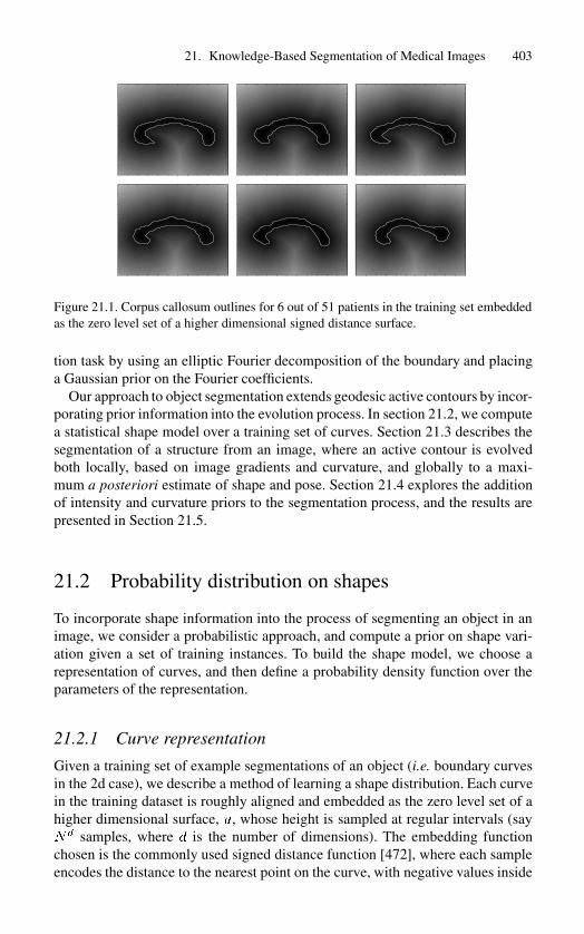
Figure 21.1. Corpus callosum outlines for 6 out of 51 patients in the training set embeddedas the zero level set of a higher dimensional signed distance surface.

tion task by using an elliptic Fourier decomposition of the boundary and placinga Gaussian prior on the Fourier coefficients.

Our approach to object segmentation extends geodesic active contours by incor-porating prior information into the evolution process. In section 21.2, we computea statistical shape model over a training set of curves. Section 21.3 describes thesegmentation of a structure from an image, where an active contour is evolvedboth locally, based on image gradients and curvature, and globally to a maxi-mum a posteriori estimate of shape and pose. Section 21.4 explores the additionof intensity and curvature priors to the segmentation process, and the results arepresented in Section 21.5.

21.2 Probability distribution on shapes

To incorporate shape information into the process of segmenting an object in animage, we consider a probabilistic approach, and compute a prior on shape vari-ation given a set of training instances. To build the shape model, we choose arepresentation of curves, and then define a probability density function over theparameters of the representation.

21.2.1 Curve representation

Given a training set of example segmentations of an object (i.e. boundary curvesin the 2d case), we describe a method of learning a shape distribution. Each curvein the training dataset is roughly aligned and embedded as the zero level set of ahigher dimensional surface, �, whose height is sampled at regular intervals (say�

� samples, where � is the number of dimensions). The embedding functionchosen is the commonly used signed distance function [472], where each sampleencodes the distance to the nearest point on the curve, with negative values inside


�� Mean ��

Mode 1

Mode 2

Mode 3

Figure 21.2. The three primary modes of variance of the corpus callosum training dataset.

the curve. Each such surface (distance map) can be considered a point in a highdimensional space (� � �

��

). The training set, � , consists of a set of surfaces� � �� . Our goal is to build a shape model over this distributionof surfaces. Since a signed distance map is uniquely determined from the zerolevel set, each distance map has a large amount of redundancy. Furthermore, thecollection of curves in the training set presumably has some dependence, as theyare shapes of the same class of object, introducing more redundancy in the trainingset. The cloud of points corresponding to the training set is approximated to havea Gaussian distribution, where most of the dimensions of the Gaussian collapse,leaving the principal modes of shape variation.

The mean surface, �, is computed by taking the mean of the signed distancefunctions, � � �

�

��. The variance in shape is computed using Principal Com-

ponent Analysis (PCA). The mean shape, �, is subtracted from each �� to createan mean-offset map, ��. Each such map, ��, is placed as a column vector inan �� -dimensional matrix � . Using Singular Value Decomposition, thecovariance matrix �

�� T is decomposed as:

�� T ��

�� T (21.1)

where � is a matrix whose column vectors represent the set of orthogonal modesof shape variation and � is a diagonal matrix of corresponding singular values.An estimate of a novel shape, �, can be represented by principal components ina -dimensional vector of coefficients, .

� � T�� (21.2)

where �� is a matrix consisting of the first columns of � that is used to projecta surface into the eigen-space. Given the coefficients , an estimate of the shape�, namely ��, is reconstructed from �� and �.


T3 T4 T5 T6 T7 T8 T9

�� Mean �� Mean ��

Figure 21.3. Top: Three-dimensional models of seven thoracic vertebrae (T3-T9) used astraining data. Bottom left and right: Extracted zero level set of first and second largestmode of variation respectively.

�� (21.3)

Note that in general �� will not be a true distance function, since convex lin-ear combinations of distance maps do not produce distance maps. However,the surfaces generally still have advantageous properties of smoothness, localdependence, and zero level sets consistent with the combination of originalcurves.

Under the assumption of a Gaussian distribution of shape represented by �, wecan compute the probability of a certain curve as:

� ��

��

�

��

��T��

��

�(21.4)

where �� contains the first � rows and columns of �. We also have consideredmodeling the distribution of shapes as a mixture of Gaussians or using a Parzenwindow density estimator, but keep to a Gaussian prior in this work.

Figure 21.1 shows a few of the 51 training curves used to define the shape mod-els of the corpus callosum. The original segmentations of the images are shownas white curves. The outlines are overlaid on the signed-distance map. Beforecomputing and combining the distance maps of these training shapes, the curveswere aligned using centroids and second moments to approximate the correspon-dence. Figure 21.2 illustrates zero level sets corresponding to the means and threeprimary modes of variance of the shape distribution of the corpus callosum. Fig-ure 21.3 shows the zero level set (as a triangle surface model) of seven rigidlyaligned vertebrae of one patient used as training data. The zero level sets of thetwo primary modes are shown as well. Note that for both the corpus and the verte-brae, the mean shapes and primary modes appear to be reasonable representativeshapes of the classes of objects being learned. In the case of the corpus callosum,the first mode seems to capture size, while the second mode roughly captures thedegree of curvature of the corpus. The third mode appears to represent the shiftingof the bulk of the corpus from front to back.


A B C

Figure 21.4. (a) The curve expected to be found in the image. (b) The image containing theshape to be segmented. (c) The same solid curve appears in three different locations, andthe direction of evolution depends on the position of the evolving curve with respect to theobject. The dotted lines show a later step in evolution given the curve’s position and shape.

21.2.2 The correspondence problem

When measuring shape variance of a certain part of an object across a population,it is important to compare like parts of the object. For example, when looking atvariances in the shape of the vertebrae, if two training examples are misalignedand a process of one is overlapping a notch of the other, then the model will notbe capturing the appropriate anatomical shape variance seen across vertebrae.

One solution to the correspondence problem is to explicitly generate all point-wise correspondences to ensure that comparisons are done consistently. Findingcorrespondences in general is a difficult problem. Manually localizing corre-sponding landmarks is tedious, while automatic landmark detection is prone toerrors, especially when dealing with 3D objects. In [133], Cootes requires the la-beling of 123 corresponding landmarks on each of 72 training instances whenbuilding a 2D model of the region of the brain around the ventricles. Whilethis method does an excellent job of performing the model-based matching, inmany applications, especially in 3D, careful labeling of such a large training setis infeasible.

Another approach to correspondence is to roughly align the training data be-fore performing the comparison and variance calculation. A rough alignment willnot match every part of each training instance perfectly, so one must consider therobustness of the representation to misalignment. Turk and Pentland [537] intro-duced Eigenfaces as a method of building models for recognition. Each imagein a set of face images (� � � array of intensities) is considered as a point inan ��-dimensional space, from which the principal components are computed.The Eigenface method is similar to our method of combining signed distancemaps of binary images, with an important distinction. Any slight misalignmentin the faces compares the intensity variance between independent objects, whileslightly misaligned pixels in a distance map are generally very highly correlated.Smoothing a grayscale or binary image propagates information spatially as well,increasing the correlation between neighboring pixels, but results in loss of infor-


Figure 21.5. Three steps in the evolution process. The evolving curve is shown solid, su-perimposed on the image (top row). The curve is matched to the expected curve to obtain aPDF over pose (bottom row). The next evolution step (based on pose and shape) is shownas the dotted line.

mation, whereas no information about the binary image is lost by computing itssigned distance function.

Using the signed distance map as the representation of shape provides toleranceto slight misalignment of object features, in the attempt to avoid having to solvethe general correspondence problem. In the examples presented here, the roughrigid alignment of the training instances resulted in the model capturing the shapevariances inherent in the population due to the dependence of nearby pixels in theshape representation.

21.3 Shape priors and geodesic active contours

Given a curve representation (the �-dimensional vector �) and a probability dis-tribution on �, the prior shape information can be folded into the segmentationprocess. This section describes adding a term to the level set evolution equationto pull the surface in the direction of the maximum a posteriori shape and positionof the final segmentation.

21.3.1 Geodesic active contours for segmentation

The snake methodology defines an energy function �� over a curve � as thesum of an internal and external energy of the curve, and evolves the curve tominimize the energy [263].

��

��

�� (21.5)

In [85], Caselles, et al. derive the equivalence of geodesic active contours to thetraditional energy-based active contours (snakes) framework by first reducing the


minimization problem to the following form:

��

�� (21.6)

where � is a function of the image gradient (usually of the form �� ). Using

Euler-Lagrange, the following curve evolution equation is derived [85]

��

�� (21.7)

where � is the curvature and � is the unit normal. By defining an embeddingfunction � of the curve �, the update equation for a higher dimensional surface iscomputed.

��

�� (21.8)

where � is an image-dependent balloon force added to force the contour to flowoutward [85, 127]. In this level set framework, the surface, �, evolves at everypoint perpendicular to the level sets as a function of the curvature at that point andthe image gradient.

21.3.2 Estimation of pose and shape

In addition to evolving the level set based on the curvature and the image term, weinclude a term that incorporates information about the shape of the object beingsegmented. To add such a global shape force to the evolution, the pose of theevolving curve with respect to the shape model must be known (see Figures 21.4and 21.5). Without an estimate of the pose, the shape model cannot adequatelyconstrain or direct the evolution. Therefore, at each step of the curve evolution,we seek to estimate the shape parameters, , and the rigid pose parameters, , ofthe final curve using a maximum a posteriori approach.

�MAP � MAP� � ��

� �� (21.9)

In this equation, � is the evolving surface at some point in time, whose zero levelset is the curve that is segmenting the object. The term �� is the gradient of theimage containing the object to be segmented. By our definition of shape and pose,the final segmentation curve is completely determined by and . Let �� be theestimated final curve, which can be computed from and . Therefore, we alsohave

��MAP � ��

� �� (21.10)


tn

q

^^

−3 −2 −1 0 1 2 30

0.25

0.5

0.75

1

u*

∇ I

Figure 21.6. The relationship between the distance map and the image gradient.

To compute the maximum a posteriori final curve, we expand the terms fromEq. 21.9 using Bayes’ Rule.

� ��

� ��(21.11)

��

� ��

Note that the preceding step assumes that shape is independent from pose. Sinceour current model does not attempt to capture the relationships between these twoquantities, this is reasonable. Future work may incorporate positional priors (andrelative positional priors between objects) into our shape model. We proceed bydefining each term of Eq. 21.11 in turn. We discard the normalization term in thedenominator as it does not depend on shape or pose.

Inside Term.

The first term in Eq. 21.11 computes the probability of a certain evolving curve,�, given the shape and pose of the final curve, �� (or �� ). Notice that thisterm does not include any image information whatsoever. Given our method ofinitializing the curve with a point inside the object, it is reasonable to assume thatthe curve should remain inside the object throughout the evolution. Therefore, ifthe evolving curve lies completely inside the final curve, then it is more likelythan a curve that lies partially or fully outside the final curve. We model this termas a Laplacian density function over �outside, the volume of the curve � that liesoutside the curve ��.

� �� outside� (21.12)

This term assumes that any curve � lying inside �� is equally likely. Since theinitial curve can be located at any point inside the object and the curve can evolvealong any path, we do not favor any such curve.

Gradient Term.

The second term in Eq. 21.11 computes the probability of seeing certain imagegradients given the current and final curves. Consider the relationship between ��

and �� when �� correctly outlines the boundary of the object (see Figure 21.6).Notice that the distance map �� is linear along the normal direction of the curve at


(u*-u)2λ

λ1v

λ1v (u*-u)2λNext Step inthe Evolution

u

Shape Prior(u*-u)

u*

v

u newCurrent Shape,

Gradient + Curvature Term

= +

MAP Final Shape

Figure 21.7. Illustration of the various terms in the evolution of the surface, �. The surface��, is the maximum a posteriori final shape. To update �, we combine the standard gradient

and curvature update term, �, and the direction of the MAP final shape, �� .

any boundary point, �, and �� . Furthermore, under the assumption that theobject boundary is a smoothed step edge, �� approximates a Gaussian along thenormal at �. Therefore, we’d expect the relationship between �� and �� to beGaussian in nature. Figure 21.6 shows an example scatter plot of these quantitieswhen �� is aligned with the object boundary. Let �� be the best fit Gaussianto the samples �� . We model the gradient probability term as a Laplacianof the goodness of fit of the Gaussian.

� ��

�(21.13)

Shape and pose priors.

The last two terms in Eq. 21.11 are based on our prior models, as described inSection 21.2. Our shape prior is a Gaussian model over the shape parameters, �,with shape variance ��.

� ��

��

��

�T��

��

�(21.14)

In our current framework, we seek to segment one object from an image, and donot retain prior information on the likelihood of the object appearing in a certainlocation. Thus, we simply assume a uniform distribution over pose parameters,which can include any type of transformation, depending on application.

� �� (21.15)

Currently we are modeling translation and rotation. We feel, however, that posi-tional priors could provide a rich source of information to explore in the future,especially when segmenting multiple objects from a single image that may haveclear prior relative poses, or when a distribution over pose in a fixed image-basedcoordinate system is known.

These terms define the maximum a posteriori estimator of shape and pose,which estimates the final curve or segmentation of the object. For efficiency, thesequantities are computed only in a narrow band around the zero level set of theevolving surface, and the MAP pose and shape are re-estimated at each evolution


step using simple gradient ascent on the log probability function in Eq. 21.11.While each ascent may yield a local maximum, the continuous re-estimation ofthese parameters as the surface evolves generally results in convergence on thedesired maximum. Next, we incorporate this information into the update equationcommonly used in level set segmentation.

21.3.3 Evolving the surface

Initially, the surface, �, is assumed to be defined by at least one point that liesinside the object to be segmented. Given the surface at time �, we seek to computean evolution step that brings the curve closer to the correct final segmentationbased on local gradient and global shape information.

The level set update expression shown in Eq. 21.8 provides a means of evolvingthe surface � over time towards the solution to the original curve-minimizationproblem stated in Eq. 21.6. Therefore, the shape of the surface at time �� can becomputed from �� by:

�� g ��

�(21.16)

where �� is a parameter defining the update step size.By estimating the final surface �� at a given time �, (Section 21.3.2), we can

also evolve the surface in the direction of the maximum a posteriori final surface:

��

�(21.17)

where �� is the linear coefficient that determines how much to trustthe maximum a posteriori estimate. Combining these equations yields the finalexpression for computing the surface at the next step.

��

�

��

�(21.18)

Figure 21.7 illustrates this evolution. The two parameters �� and �� are used tobalance the influence of the shape model and the gradient-curvature model. Theparameters also determine the overall step size of the evolution. The tradeoff be-tween shape and image depends on how much faith one has in the shape modeland the imagery for a given application. Currently, we set these parameters em-pirically for a particular segmentation task, given the general image quality andshape properties.

21.4 Statistical Image-Surface Relationship

This section describes a method of incorporating prior intensity and curvaturemodels into the segmentation process. We define now the surface � as the signeddistance function to the boundary curve �. Therefore, �� is both the height ofthe surface � at the position � and the signed distance from � to the nearest point


Ux

Ix

Surface

Image

I

I

I I

Uc

U

U

Ua

c

b

b

d

d

a tn

xUaU

bU

cU

dU

a b

Figure 21.8. (a) Statistical dependency of node samples of the surface � and pixels ofimage � . (b) The directions of the normal and tangent of � are shown at the position �.The contour curve of height �� is drawn.

on the curve �. Instead of estimating the position of � directly, we estimate thevalue of � at every position � in the image. Once � is computed, the boundaryof the object is found by extracting the zero level set of � .

We define a statistical dependency network over the surface � and the image � .To estimate the value �� of � at a certain position � in the image, we maximize� �� , namely the probability of the height of the surface at that point,given the entire image and the rest of the surface. This expression is difficult tomodel, given all the dependencies. We therefore simplify the problem to a Markovnetwork with only local dependencies. The links of the nodes in Figure 21.8arepresent the dependencies considered. We assume the height of the surface at acertain point depends only on the intensity value of the image at that point, andthe neighboring heights of the surface. This assumption can be expressed as:

� ��

�(21.19)

where � (x) is the neighborhood of �.Using properties of our network, we derive an expression for the above

probability consisting of terms we will estimate from a set of training data.

� ��

� �� (21.20)

��

� ��

� ��

� �� (21.21)

��

� �� (21.22)

��

� �� (21.23)

The definition of conditional probability is used in Equations 21.20 and 21.22,and we are multiplying by the identity in Equation 21.21. In the final expression,we note that when conditioned on ��, the heights of the surface at neighboringlocations do not depend on ��.


TrainingExample

� ��

Distance

Inte

nsity

−10 0 10 200

0.2

0.4

0.6

0.8

1

0.5

1

1.5

2

2.5

3

3.5

4x 10

−3

Distance

Inte

nsity

−10 0 10 200

0.2

0.4

0.6

0.8

1

0.5

1

1.5

2

2.5x 10

−3

Distance

Inte

nsity

−10 0 10 200

0.2

0.4

0.6

0.8

1

1

2

3

4

5

6

7

8

9

x 10−4

(A) (B) (C)

Figure 21.9. Top: One example of three training sets of random ellipses under differentimaging conditions The dotted contour shows the boundary of the object. Bottom: Thejoint intensity/distance-to-boundary PDF derived from the training set. Left and right ofthe black vertical line indicate the intensity profile inside and outside the object.

The first term in Equation 21.23 is the image term, that relates the intensity andthe surface at �. The next term relates the neighborhood of � about � to ��, andwill act as a regularization term. The following two sections describe a meansof estimating these functions based on prior training data. The denominator ofEquation 21.23 does not depend on ��, and thus is ignored during the estimationprocess.

21.4.1 Intensity Model

We define a joint distribution model, � �� , that relates intensity values, �, tosigned distances �, based on a set of training images and training segmentations.Let �� be a set of images of the same modality containing the sameanatomical structure of various subjects and �� be the set of corre-sponding segmented boundary curves of the anatomical structure. Let �� be thesigned distance map to the closed curve �� . The training set � , is a set of image-surface pairs, � � �� . We use a Parzen window densityestimator with a Gaussian windowing function to model the joint distribution. ThePDF is the mean of many 2D Gaussians centered at the positions �� for every pixel in every training image:

� ��

�

��

��

�

��

��

��

�

��

��

��

�(21.24)

where � is the set of all positions in the image, �� and �� are the variances of theParzen kernel, and the normalization factor � � �� .

Figure 21.9 illustrates the estimated joint probability density functions for ran-dom ellipses with various contrast scenarios. Notice that Ellipse A can be easilysegmented using a gradient based method, but cannot be thresholded, as the inten-


sity distribution inside and outside the object overlap significantly. On the otherhand, simple gradient methods would fail to extract Ellipse B due to high texture,while a single intensity threshold isolates the object. Neither scheme would workfor Ellipse C, as higher level knowledge is required to know which edge is thecorrect boundary.

Figure 21.10 illustrates the estimated joint PDFs for the corpus callosum andslices of two acquisitions of the femur. In the sagittal scan of the femur (Figure21.10d), the dark layer around the brighter, textured region is cortical bone, whichgives essentially no MR signal. Without prior knowledge of the intensity distribu-tion of the entire femur, the cortical bone could easily be missed in a segmentation.However, by training a joint distribution over intensity and signed distance, wegenerate a PDF that encodes the fact that the dark region is a part of the object.This example is similar to the synthetic ellipse in Figure 21.10a.

21.4.2 Curvature Model

Boundary detection methods commonly use a regularization term to uniformlypenalize regions of high curvature, independent of the structure being segmented[263, 85, 593]. Our goal is to use the term � �� as a local regularizer,but one that can be estimated from a set of training data, and thereby tuned to theappropriate application. One method of modeling this function is to create a 5DParzen joint PDF over �� and its four neighbors. A drawback of this approachis that a 5D space is difficult to fill and thus requires many training samples.Furthermore, the neighborhood depends on the embedded coordinate system, andwould give different results based on the pose of the object in the image (considera square aligned with the axes versus one rotated by ��Æ). Therefore, instead ofconsidering the four neighbors (two horizontal and two vertical) in the “arbitrary”embedded coordinate system, we use four (interpolated) neighbors in the directionof the local normal (��) and tangent (��) to the embedded curve (see Figure 21.8b).In other words, we reparameterize to an intrinsic coordinate system based on thesurface:

� �� (21.25)

� � �� (21.26)

� � �� (21.27)

The last step makes the assumption that the neighbors in the normal direction andthose in the tangent direction are conditionally independent given ��.

We now model the terms in Eq. 21.27 based on properties of the surface �

and prior knowledge of the boundary to be segmented. While � is consideredto be a finite network of nodes and �� a particular node, we define �� to bethe analogous continuous surface over �. We derive the relationship between ��and its neighbors by considering the first and second derivatives of �� in thedirections of the normal and tangent to the level set at �. The unit normal and unit


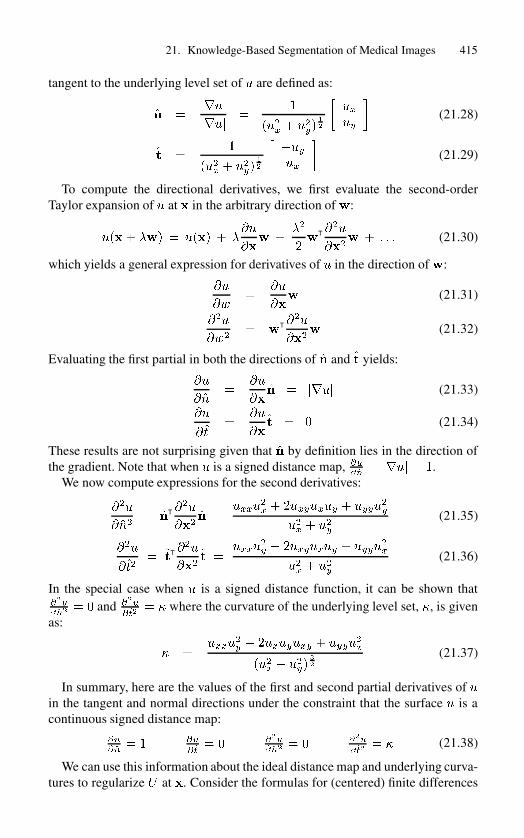
tangent to the underlying level set of � are defined as:

��

��

�

��

�

�

��

��

�(21.28)

��

��

�

�

��

�(21.29)

To compute the directional derivatives, we first evaluate the second-orderTaylor expansion of � at � in the arbitrary direction of �:

��

��

��

��

T ��

�� (21.30)

which yields a general expression for derivatives of � in the direction of �:

��

��

��

�� (21.31)

��

��

T ��

�� (21.32)

Evaluating the first partial in both the directions of �� and �� yields:

��

��

��

�� (21.33)

��

��

��

�� (21.34)

These results are not surprising given that �� by definition lies in the direction ofthe gradient. Note that when � is a signed distance map, ��

�� .

We now compute expressions for the second derivatives:

��

�� T �

��

��

��

� � ��

�

��

(21.35)

��

�� T �

��

��

��

� � ��

�

��

(21.36)

In the special case when � is a signed distance function, it can be shown that��

� � and ��

�� where the curvature of the underlying level set, �, is given

as:

� ��

�

� � ��

�

��

�

(21.37)

In summary, here are the values of the first and second partial derivatives of �in the tangent and normal directions under the constraint that the surface � is acontinuous signed distance map:

��

� � ��

��

��

�� (21.38)

We can use this information about the ideal distance map and underlying curva-tures to regularize � at �. Consider the formulas for (centered) finite differences


TrainingExample

� ��

Distance

Inte

nsity

−10 0 10 200

0.2

0.4

0.6

0.8

1

1

2

3

4

5

6

7

8

9

x 10−4

Distance

Inte

nsity

−10 0 10 200

0.2

0.4

0.6

0.8

1

0.2

0.4

0.6

0.8

1

1.2

1.4

1.6

1.8

x 10−3

Distance

Inte

nsity

−10 0 10 200

0.2

0.4

0.6

0.8

1

0.2

0.4

0.6

0.8

1

1.2

1.4

1.6

1.8

x 10−3

Distance

Inte

nsity

−10 0 10 200

0.2

0.4

0.6

0.8

1

0

1

2

3

4

5

6

7

8x 10

−4

� ��

−0.2 −0.1 0 0.1 0.20

0.05

0.1

0.15

κ

P(κ

)

−0.2 −0.1 0 0.1 0.20

0.005

0.01

0.015

0.02

0.025

0.03

0.035

κ

P(κ

)

−0.2 −0.1 0 0.1 0.20

0.01

0.02

0.03

0.04

κ

P(κ

)

−0.2 −0.1 0 0.1 0.20

0.01

0.02

0.03

0.04

0.05

0.06

κ

P(κ

)

(a) (b) (c) (d)

Figure 21.10. Top: One example of each of four training sets of objects. Middle: The jointintensity/distance-to-boundary PDF derived from the training set. Bottom: The curvatureprofile of each object class. Notice that the ellipse class has only positive curvature.

of an arbitrary 1D function.

��

��

��

��(21.39)

��

��

��

��(21.40)

Notice that �� does not appear in ��

, indicating that changing � only at oneposition at a time cannot change the local slope. However, changing �� doesdirectly affect the second derivative, so we model the relationship between ��and its neighbors to adhere to the second derivative constraints.

We define the likelihood of the neighbors in the normal direction to be:

� ��

��

��

�

��

�(21.41)

where � is a normalization factor and � determines the strength of the constant-normal-direction constraint. This has the effect of keeping the gradient magnitudeof the surface constant (however not necessarily 1), preventing the surface fromevolving arbitrarily. Typically one needs to extract the zero level set and reinitial-ize the distance function from time to time during the evolution. This direction ofregularization reduces the need to reinitialize the surface.

As for the likelihood of the neighbors in the tangent direction, we seek an ex-pression that takes into account the curvature profile of the training data. A convexshape, for example, has non-negative curvature everywhere, so if the training setconsists of all convex shapes, the level sets of the surface should stay convexthroughout the estimation. The fact that a polygon has bi-modal curvature ( and


Figure 21.11. Initial, middle, and final steps in the evolution process of segmenting twoslices of the femur. The training set consisted of 18 slices of the same femur, leaving outthe slice being segmented and its neighbors.

Figure 21.12. Four steps in the segmentation of two different corpora callosa. The lastimage in each case shows the final segmentation in black. The dotted contour is the standardevolution without the shape influence.

�) could be used to define a polygon-finder, if the surface can be constrainedto match the distribution of curvatures of the training set. For each training sur-face, �� , we compute a curvature map �� using Equation 21.37. We then definea PDF which encourages the curvature as reflected in the discrete differences�� to be consistent with curvatures observed in the training data(��). The PDF is derived using Parzen windowing, similar to the intensity PDFdefined in Section 21.4.1.

� �� (21.42)

�

��

��

��

�

��

��

��

�

��

�

The third row of Figure 21.10 shows the curvature profile of training sets ofvarious objects.


In summary, the regularization of the surface is broken down into a regular-ization in the local normal and tangent directions. The second derivative in thenormal direction is modeled as a zero mean, low variance Gaussian to keep thesurface linear in that direction. A distribution over the second derivative in thetangent direction (e.g. the curvature of the level sets) is derived from the trainingdata and used as an object-specific curvature regularization term.

21.4.3 Surface Estimation

In the previous section, we defined a model of the embedding surface of theboundary that we wish to estimate given a novel image. Starting with an initialclosed curve, we build the higher dimensional surface by computing the signeddistance to the curve at every point. Given the prior model and the image, theheight of the surface at location � is related to the image intensity at � and thelocal neighborhood of the surface by the following equation:

��

�� (21.43)

� �� Image Term

� �� Curvature Term

� �� Linearity Term

We use this equation to re-estimate each surface point independently, maximizingits log probability while assuming the rest of the surface is constant.

��

�� (21.44)

Instead of finding the global maximum of the PDF for each ��, we adjust�� in the direction of increasing probability towards the local maximum bydifferentiating the log probability in Equation 21.43.

��

��

��

�(21.45)

This update is repeated until there is little change in the surface. While small,local oscillations in the surface can occur if the step size � is too high, in prac-tice, an empirical value of � can easily be found such that the surface evolves inreasonable time without oscillations.

The linearity regularization term that acts on the surface in the direction nor-mal to the level set keeps the gradient magnitude locally constant, but in generalthe surface does not remain a true distance function. We therefore extract theboundary and reinitialize the distance map when the gradient magnitudes strayfrom 1. The regularization term greatly reduces the need to reinitialize, but itdoes not eliminate it. Typically reinitialization occurs once or twice during thesegmentation, or about every 50 iterations.


Figure 21.13. Early, middle, and final steps in the segmentation of the vertebra T7. Threeorthogonal slices and the 3D reconstruction are shown for each step. The black contour isa slice through the evolving surface. The white contour is a slice through the inside of theMAP final surface.

K Corpus 1 Corpus 2 Vertebra�� 1.3 mm 1.5 mm 2.7 mm�� 1.6 mm 2.0 mm 4.4 mm

Table 21.1. Partial Hausdorff distance between our segmentation and the manu-ally-segmented ground truth.

21.5 Results

Segmentation experiments were performed on 2D slices of MR images of the fe-mur and corpus callosum (Figures 21.11 and 21.12). For the femur experiments,the training set consisted of 18 nearby slices of the same femur, leaving out theslice being segmented and its neighbors. In both femur examples, the same ini-tialization point was used to seed the evolution. As the curve evolves, the MAPestimator of shape and pose locks into the shape of the femur slice.

The corpus callosum training set consisted of 49 examples like those in Fig-ure 21.1. The segmentations of two corpora callosa are shown in Figure 21.12.Notice that while the MAP shape estimator is initially incorrect, as the curveevolves, the pose and shape parameters converge on the boundary.

The vertebrae example illustrates the extension of the algorithm to 3D datasets.Figure 21.13 illustrates a few steps in the segmentation of vertebra T7. The train-ing set in this case consisted of vertebrae T3-T9, with the exception of T7. Theinitial surface was a small sphere placed in the body of the vertebra. The blackcontour is a slice through the zero level set of the evolving hyper-surface. Thewhite contour is the MAP pose and shape estimate. Segmenting the vertebra tookapproximately six minutes.

To validate the segmentation results, we compute the undirected partial Haus-dorff distance [249] between the boundary of the computed segmentation and theboundary of the manually-segmented ground truth. The directed partial Hausdorff


distance over two point sets � and � is defined as

��

��

��

where K is a quantile of the maximum distance. The undirected partial Hausdorffdistance is defined as �� . The resultsfor the corpora and vertebrae shown in Table 21.1 indicate that virtually all theboundary points lie within one or two voxels of the manual segmentation.

21.6 Conclusions

This work presents a means of incorporating prior knowledge into the geodesicactive contour method of medical image segmentation. The shape representa-tion of using PCA on the signed distance map was chosen with the intentionof being robust to slight misalignments without requiring exact point-wise corre-spondences. Our extension to active contours that estimates the model parametersand then evolves the curve based on that estimation provides a method of ro-bustly converging on the boundary even with noisy inputs. The representationand the curve evolution technique merge well together since the evolution re-quires a distance map of the evolving curve, which is inherent in the shape model.The intensity and curvature models provide a means of representing the object’sappearance and shape to further direct the segmentation process.

Documents

Geometric Level Set Methods in Imaging, Vision, and Graphics || Knowledge-Based Segmentation of Medical Images