Embed Size (px)
Citation preview
Scuola Internazionale Superiore di Studi Avanzati - Trieste
Area of MathematicsPh.D. in Mathematical Physics
Thesis
Geometric phases in graphene andtopological insulators
CandidateDomenico Monaco
Supervisorprof. Gianluca Panati
(“La Sapienza” Università di Roma)
Internal co-Supervisorprof. Ludwik Dabrowski
Thesis submitted in partial fulfillment of the requirements for thedegree of Philosophiæ Doctor
academic year 2014-15
SISSA - Via Bonomea 265 - 34136 TRIESTE - ITALY
Thesis defended in front of a Board of Examiners composed by
prof. Ludwik Dabrowski, dr. Alessandro Michelangeli, and prof. Cesare Reina as in-ternal members, and
prof. Gianluca Panati (“La Sapienza” Università di Roma), prof. Stefan Teufel (Eber-hard Karls Universität Tübingen) as external members
on September 15th, 2015

Abstract
This thesis collects three of the publications that the candidate produced during hisPh.D. studies. They all focus on geometric phases in solid state physics.
We first study topological phases of 2-dimensional periodic quantum systems, inabsence of a spectral gap, like e. g. (multilayer) graphene. A topological invariant nv ∈Z, baptized eigenspace vorticity, is attached to any intersection of the energy bands,and characterizes the local topology of the eigenprojectors around that intersection.With the help of explicit models, each associated to a value of nv ∈ Z, we are ableto extract the decay at infinity of the single-band Wannier function w in mono- andbilayer graphene, obtaining |w(x)| ≤ const · |x|−2 as |x|→∞.
Next, we investigate gapped periodic quantum systems, in presence of time-reversal symmetry. When the time-reversal operator Θ is of bosonic type, i. e. it sat-isfies Θ2 = 1l, we provide an explicit algorithm to construct a frame of smooth, pe-riodic and time-reversal symmetric (quasi-)Bloch functions, or equivalently a frameof almost-exponentially localized, real-valued (composite) Wannier functions, in di-mension d ≤ 3. In the case instead of a fermionic time-reversal operator, satisfyingΘ2 =−1l, we show that the existence of such a Bloch frame is in general topologicallyobstructed in dimension d = 2 and d = 3. This obstruction is encoded in Z2-valuedtopological invariants, which agree with the ones proposed in the solid state litera-ture by Fu, Kane and Mele.
iii


Acknowledgements
First and foremost, I want to thank my supervisor, Gianluca Panati, who lured meinto Quantum Mechanics and Solid State Physics when I was already hooked onTopology and Differential Geometry, and then showed me that there isn’t really thatmuch of a difference if you know where to look.
During the years of my Ph.D. studies, I have had the occasion to discuss withseveral experts in Mathematics and Physics, who guided my train of thoughts intonew and fascinating directions, and to whom I am definitely obliged. Big thanks toJean Bellissard, Raffaello Bianco, Horia Cornean, Ludwik Dabrowski, Giuseppe DeNittis, Gianfausto dell’Antonio, Domenico Fiorenza, Gian Michele Graf, Peter Kuch-ment, Alessandro Michelangeli, Adriano Pisante, Marcello Porta, Emil Prodan, Raf-faele Resta, Shinsei Ryu, Hermann Schulz-Baldes, Clément Tauber, Stefan Teufel,and Andrea Trombettoni.
I am also extremely grateful to Riccardo Adami, Claudio Cacciapuoti, RaffaeleCarlone, Michele Correggi, Pavel Exner, Luca Fanelli, Rodolfo Figari, AlessandroGiuliani, Ennio Gozzi, Gianni Landi, Mathieu Lewin, Gherardo Piacitelli, AlexanderSobolev, Jan Philip Solovej, Alessandro Teta, and Martin Zirnbauer, for inviting me tothe events they organized and granting me the opportunity to meet many amusingand impressive people.
v


Contents
Introduction . . . . . . . . . . . . . . . . . . . . . . . . . . . . . . . . . . . . . . . . . . . . . . . . . . . . . . . . . . . . . . ix1 Geometric phases of quantum matter . . . . . . . . . . . . . . . . . . . . . . . . . . . . . . ix
1.1 Quantum Hall effect . . . . . . . . . . . . . . . . . . . . . . . . . . . . . . . . . . . . . . . ix1.2 Quantum spin Hall effect and topological insulators . . . . . . . . . . xii
2 Analysis, geometry and physics of periodic Schrödinger operators . . . xv2.1 Analysis: Bloch-Floquet-Zak transform . . . . . . . . . . . . . . . . . . . . . . xv2.2 Geometry: Bloch bundle . . . . . . . . . . . . . . . . . . . . . . . . . . . . . . . . . . . xxi2.3 Physics: Wannier functions and their localization . . . . . . . . . . . . xxvi
3 Structure of the thesis . . . . . . . . . . . . . . . . . . . . . . . . . . . . . . . . . . . . . . . . . . . . . xxviiReferences . . . . . . . . . . . . . . . . . . . . . . . . . . . . . . . . . . . . . . . . . . . . . . . . . . . . . . . . . . . . xxix
Part I Graphene
Topological invariants of eigenvalue intersections and decrease of Wannierfunctions in graphene . . . . . . . . . . . . . . . . . . . . . . . . . . . . . . . . . . . . . . . . . . . . . . . . . . . . . 3Domenico Monaco and Gianluca Panati
1 Introduction . . . . . . . . . . . . . . . . . . . . . . . . . . . . . . . . . . . . . . . . . . . . . . . . . . . . . 32 Basic concepts . . . . . . . . . . . . . . . . . . . . . . . . . . . . . . . . . . . . . . . . . . . . . . . . . . . 5
2.1 Bloch Hamiltonians . . . . . . . . . . . . . . . . . . . . . . . . . . . . . . . . . . . . . . . . 52.2 From insulators to semimetals . . . . . . . . . . . . . . . . . . . . . . . . . . . . . . 72.3 Tight-binding Hamiltonians in graphene . . . . . . . . . . . . . . . . . . . . 72.4 Singular families of projectors . . . . . . . . . . . . . . . . . . . . . . . . . . . . . . 9
3 Topology of a singular 2-dimensional family of projectors . . . . . . . . . . . 93.1 A geometric Z-invariant: eigenspace vorticity . . . . . . . . . . . . . . . . 103.2 The canonical models for an intersection of eigenvalues . . . . . . 143.3 Comparison with the pseudospin winding number . . . . . . . . . . . 19
4 Universality of the canonical models . . . . . . . . . . . . . . . . . . . . . . . . . . . . . . . 265 Decrease of Wannier functions in graphene. . . . . . . . . . . . . . . . . . . . . . . . . 29
5.1 Reduction to a local problem around the intersection points . . 315.2 Asymptotic decrease of the n-canonical Wannier function . . . . 325.3 Asymptotic decrease of the true Wannier function. . . . . . . . . . . . 37
A Distributional Berry curvature for eigenvalue intersections . . . . . . . . . . 47References . . . . . . . . . . . . . . . . . . . . . . . . . . . . . . . . . . . . . . . . . . . . . . . . . . . . . . . . . . . . 49
Part II Topological Insulators
vii
viii Contents
Construction of real-valued localized composite Wannier functions forinsulators . . . . . . . . . . . . . . . . . . . . . . . . . . . . . . . . . . . . . . . . . . . . . . . . . . . . . . . . . . . . . . . . . 55Domenico Fiorenza, Domenico Monaco, and Gianluca Panati
1 Introduction . . . . . . . . . . . . . . . . . . . . . . . . . . . . . . . . . . . . . . . . . . . . . . . . . . . . . 552 From Schrödinger operators to covariant families of projectors . . . . . . 583 Assumptions and main results . . . . . . . . . . . . . . . . . . . . . . . . . . . . . . . . . . . . . 624 Proof: Construction of a smooth symmetric Bloch frame . . . . . . . . . . . . . 65
4.1 The relevant group action . . . . . . . . . . . . . . . . . . . . . . . . . . . . . . . . . . 664.2 Solving the vertex conditions . . . . . . . . . . . . . . . . . . . . . . . . . . . . . . . 674.3 Construction in the 1-dimensional case . . . . . . . . . . . . . . . . . . . . . 694.4 Construction in the 2-dimensional case . . . . . . . . . . . . . . . . . . . . . 694.5 Interlude: abstracting from the 1- and 2-dimensional case . . . . 754.6 Construction in the 3-dimensional case . . . . . . . . . . . . . . . . . . . . . 774.7 A glimpse to the higher-dimensional cases . . . . . . . . . . . . . . . . . . 82
5 A symmetry-preserving smoothing procedure . . . . . . . . . . . . . . . . . . . . . . 83References . . . . . . . . . . . . . . . . . . . . . . . . . . . . . . . . . . . . . . . . . . . . . . . . . . . . . . . . . . . . 87
Z2 invariants of topological insulators as geometric obstructions . . . . . . . . . . . . 89Domenico Fiorenza, Domenico Monaco, and Gianluca Panati
1 Introduction . . . . . . . . . . . . . . . . . . . . . . . . . . . . . . . . . . . . . . . . . . . . . . . . . . . . . 892 Setting and main results . . . . . . . . . . . . . . . . . . . . . . . . . . . . . . . . . . . . . . . . . . 92
2.1 Statement of the problem and main results . . . . . . . . . . . . . . . . . . 922.2 Properties of the reshuffling matrix ε . . . . . . . . . . . . . . . . . . . . . . . . 94
3 Construction of a symmetric Bloch frame in 2d . . . . . . . . . . . . . . . . . . . . . 963.1 Effective unit cell, vertices and edges . . . . . . . . . . . . . . . . . . . . . . . . 973.2 Solving the vertex conditions . . . . . . . . . . . . . . . . . . . . . . . . . . . . . . . 993.3 Extending to the edges . . . . . . . . . . . . . . . . . . . . . . . . . . . . . . . . . . . . . 1013.4 Extending to the face: a Z2 obstruction . . . . . . . . . . . . . . . . . . . . . . 1023.5 Well-posedness of the definition of δ . . . . . . . . . . . . . . . . . . . . . . . . 1063.6 Topological invariance of δ . . . . . . . . . . . . . . . . . . . . . . . . . . . . . . . . . 107
4 Comparison with the Fu-Kane index . . . . . . . . . . . . . . . . . . . . . . . . . . . . . . . 1095 A simpler formula for the Z2 invariant . . . . . . . . . . . . . . . . . . . . . . . . . . . . . . 1146 Construction of a symmetric Bloch frame in 3d . . . . . . . . . . . . . . . . . . . . . 116
6.1 Vertex conditions and edge extension . . . . . . . . . . . . . . . . . . . . . . . 1166.2 Extension to the faces: four Z2 obstructions . . . . . . . . . . . . . . . . . . 1176.3 Proof of Theorem 2.3 . . . . . . . . . . . . . . . . . . . . . . . . . . . . . . . . . . . . . . . 1196.4 Comparison with the Fu-Kane-Mele indices . . . . . . . . . . . . . . . . . 122
A Smoothing procedure . . . . . . . . . . . . . . . . . . . . . . . . . . . . . . . . . . . . . . . . . . . . . 124References . . . . . . . . . . . . . . . . . . . . . . . . . . . . . . . . . . . . . . . . . . . . . . . . . . . . . . . . . . . . 126
Conclusions
Open problems and perspectives . . . . . . . . . . . . . . . . . . . . . . . . . . . . . . . . . . . . . . . . . . . 1311 Disordered topological insulators . . . . . . . . . . . . . . . . . . . . . . . . . . . . . . . . . . 1312 Topological invariants for other symmetry classes . . . . . . . . . . . . . . . . . . . 1323 Magnetic Wannier functions . . . . . . . . . . . . . . . . . . . . . . . . . . . . . . . . . . . . . . 132References . . . . . . . . . . . . . . . . . . . . . . . . . . . . . . . . . . . . . . . . . . . . . . . . . . . . . . . . . . . . 133

Introduction
1 Geometric phases of quantum matter
In the last 30 years, the origin of many interesting phenomena which were discov-ered in quantum mechanical systems was established to lie in geometric phases [45].The archetype of such phases is named after sir Michael V. Berry [8], and was earlyrelated by Barry Simon [46] to the holonomy of a certain U (1)-bundle over the Bril-louin torus (see Section 2.1). Berry’s phase is a dynamical phase factor that is ac-quired by a quantum state on top of the standard energy phase, when the evolutionis driven through a loop in some parameter space. In applications to condensed mat-ter systems, this parameter space is usually the Brillouin zone. As an example, one ofthe most prominent incarnations of Berry’s phase effects in solid state physics canbe found in the modern theory of polarization [47], in which changes of the elec-tronic terms in the polarization vector, ∆Pel, through an adiabatic cycle are indeedexpressed as differences of geometric phases. This result, first obtained by R.D. King-Smith and David Vanderbilt [26], was later elaborated by Raffaele Resta [42]. In morerecent years, the Altland-Zirnbauer classification of random Hamiltonians in pres-ence of discrete simmetries [1] sparked the interest in geometric labels attached toquantum phases of matter, and paved the way for the advent of topological insula-tors (see Section 1.2).
After being confined to the realm of high-energy physics and gauge theories,topology and geometry made their entrance, through Berry’s phase, in the low-energy world of condensed matter systems. This Section is devoted to giving an in-formal overview on two instances of such geometric effects in solid state physics,namely the quantum Hall effect and the quantum spin Hall effect, which are of rele-vance also for the candidate’s works presented in this thesis in Parts I and II.
1.1 Quantum Hall effect
One of the first and most striking occurrences of a topological index attached to aquantum phase of matter is that of the quantum Hall effect [50, 17].
The experimental setup for the Hall effect consists in putting a very thin slab of acrystal (making it effectively 2-dimensional) into a constant magnetic field, whosedirection z is orthogonal to the plane Ox y in which the sample lies. If an electriccurrent is induced, say, in direction x, the charge carriers will experience a Lorentz
ix

x Introduction
force, which will make them accumulate along the edges in the transverse direction.If these edges are short-circuited, this will result in a transverse current flow j , calledHall current (see Figure 1).
jx
v
F
B
z
x
y
Hall effect
00
L
εF
Fig. 1 The experimental setup for the (quantum) Hall effect.
The relation between this induced current and the applied electric field E is ex-pressed by means of a 2×2 skew-symmetric tensor σ:
j =σE , σ=(
0 σx y−σx y 0
).
The quantity σx y is called the Hall conductivity; since the setting is 2-dimensional1,its inverse ρx y = 1/σx y coincides with the Hall resistivity. The expected behaviour ofthis quantity as a function of the applied magnetic field B is linear, i. e. ρx y ∝ B . In1980, Klaus von Klitzing and his collaborators [49] performed the same experimentbut at very low temperatures, so that quantum effects became relevant. What theyobserved was striking: the Hall resistivity displays plateaus, in which it stays constantas a function of the magnetic field, with sudden jumps between different plateaus(see Figure 2); moreover, the value of these plateaus comes exactly at inverses of inte-ger numbers, in units of a fundamental quantum h/e2 (where h is Planck’s constantand e the charge of a carrier):
(1.1) σx y = ne2
h, n ∈Z.
1 Also the resistivity ρ is a skew-symmetric tensor, defined as the inverse of the conductivity tensorσ.In 2-dimensions, however, the resistivity tensor is characterized just by one non-zero entry ρx y .

1. Geometric phases of quantum matter xi
This quantization phenomenon came to be known as the quantum Hall effect. Theexperimental precision of these measurements was incredible (in recent experi-ments this quantization rule can be measured up to an absolute error of 10−10 ∼10−11), which lead also to applications in metrology, setting a new precision stan-dard in the measurement of electric resistivity.
1-G
~o'-LIW=O~
Klaus vp~ K)itzig e quantized Ha(i effect 525
10-L
&0'
)Q3
L
10-
5-I,
Rx
(Kll) O-
R„
(KQ)
IQ)0-1 tpO )01 iO3
&xy = tane
)04,
FIG Calculations of theresistance measurem
e correction term 6rements due to the fini
/8' f h d (1/L=0 5)~ ~
o-06 04 0
VG(v)
-0,6 04 Og
VG(v)
FIG. 13. Measured cre curves for thegitudinal resistance R
Hall resistance Rance R of Q A-Al Q s heterostru-
ie ds.e vo tage at diffi erent magnetic
The Hall plateaus are much more p
h 11 ffes, since
ltt' b t L dquahty of th GaA -ASUrf
ya s-Al„oa& As ie ig
e condition 8c elec-
e a ready at relativet ' f lfilld 1 g
i ibl fo h' a rea y at a magnetic field
strength of 4 tesla. S'a. ince a finite c
V, mo
s tys ructures, even at a
is usually
, mo t fthi out applied gate volta
ase on mea-
e magnetic field. A typical result isall resistance RH ——
is shown in Fig. 14.3' m es
c 1e region where the long-
12-
RH
(xy 65.
L/W=1
L/i =0.2-0.3
Rx
Pxx
10-
8-hC
O)
-0.2
64.
.010..
1000—
3 2i 2t
63.
60 650
200-
00 2
MAGNET I C F )ELD (T)
I a
6
FIG. 12. Com a 'omparison between the m
respectivel've y.spon ing resistivity corn ponents p„and
i ies H and
xy n pxx s
FIG. 1 Experimentantal curves for the
o age V ——OV. Thensity correspondi
e temperatur re is a out 8 mK.on ing to a
Rev. Mod. Phys. , Vol. 58 N0. 3, July 1986 Fig. 2 The Hall resistivity ρx y as a function of the magnetic field B . The figure is taken from [50].
This peculiar quantization phenomenon rapidly attracted the attention of theo-retical and mathematical physicists, seeking for its explanation: we refer to the re-view of Gian Michele Graf [17] where the author presents the three main intepre-tations that where proposed in the 1980’s and 1990’s in the mathematical physicscommunity. The quantum Hall effect was put on mathematically rigorous groundsmainly by the group of Yosi Avron, Rudi Seiler, and Barry Simon [4, 5], as well as theone of Jean Bellissard and Hermann Schulz-Baldes [6, 23], with mutual exchangesof ideas. Elaborating on the pioneering work of Thouless, Kohmoto, Nightingale andden Nijs [48], both groups were able to interpret the integer appearing in the expres-sion (1.1) for the Hall conductivity as a Chern number (see Section 2.2), explainingits topological origin and its quantization at the same time. The methods used bythe two groups, however, are extremely different: Avron and his collaborators ex-ploited techniques from differential geometry and gauge theory to formalize the so-called Laughlin argument, while Bellissard and his collaborators made use of resultsfrom noncommutative geometry and K -theory, establishing also a bulk-edge corre-
xii Introduction
spondence, which makes their theory applicable also to disordered media. Having aframework that allows to include disorder is also convenient to qualify the quantiza-tion phenomenon as “topological”: it should be robust against (small) perturbationsof the system, among which one can include also randomly distributed impurities.
1.2 Quantum spin Hall effect and topological insulators
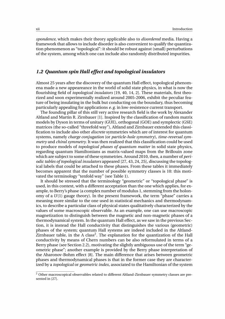
Almost 25 years after the discovery of the quantum Hall effect, topological phenom-ena made a new appeareance in the world of solid state physics, in what is now theflourishing field of topological insulators [19, 40, 14, 2]. These materials, first theo-rized and soon experimentally realized around 2005-2006, exhibit the peculiar fea-ture of being insulating in the bulk but conducting on the boundary, thus becomingparticularly appealing for applications e. g. in low-resistence current transport.
The founding pillar of this still very active research field is the work by AlexanderAltland and Martin R. Zirnbauer [1]. Inspired by the classification of random matrixmodels by Dyson in terms of unitary (GUE), orthogonal (GOE) and symplectic (GSE)matrices (the so-called “threefold way”), Altland and Zirnbauer extended this classi-fication to include also other discrete symmetries which are of interest for quantumsystems, namely charge conjugation (or particle-hole symmetry), time-reversal sym-metry and chiral symmetry. It was then realized that this classification could be usedto produce models of topological phases of quantum matter in solid state physics,regarding quantum Hamiltonians as matrix-valued maps from the Brillouin zonewhich are subject to some of these symmetries. Around 2010, then, a number of peri-odic tables of topological insulators appeared [27, 43, 24, 25], discussing the topolog-ical labels that could be attached to these phases. From these tables it immediatelybecomes apparent that the number of possible symmetry classes is 10: this moti-vated the terminology “tenfold way” (see Table 1).
It should be stressed that the terminology “geometric” or “topological phase” isused, in this context, with a different acceptation than the one which applies, for ex-ample, to Berry’s phase (a complex number of modulus 1, stemming from the holon-omy of a U (1) gauge theory). In the present framework, the term “phase” carries ameaning more similar to the one used in statistical mechanics and thermodynam-ics, to describe a particular class of physical states qualitatively characterized by thevalues of some macroscopic observable. As an example, one can use macroscopicmagnetization to distinguish between the magnetic and non-magnetic phases of athermodynamical system. In the quantum Hall effect, as we saw in the previous Sec-tion, it is instead the Hall conductivity that distinguishes the various (geometric)phases of the system; quantum Hall systems are indeed included in the Altland-Zirnbauer table, in the A class2. The explanation for the quantization of the Hallconductivity by means of Chern numbers can be also reformulated in terms of aBerry phase (see Section 2.2), motivating the slightly ambiguous use of the term “ge-ometric phase”; another example is provided by the Berry phase interpretation ofthe Aharonov-Bohm effect [8]. The main difference that arises between geometricphases and thermodynamical phases is that in the former case they are character-ized by a topological or geometric index, associated to the Hamiltonian of the system
2 Other macroscopical observables related to different Altland-Zirnbauer symmetry classes are pre-sented in [27].

1. Geometric phases of quantum matter xiii
Symmetry Dimension
AZ T C S 1 2 3 4 5 6 7 8
A 0 0 0 0 Z 0 Z 0 Z 0 Z
AIII 0 0 1 Z 0 Z 0 Z 0 Z 0
AI 1 0 0 0 0 0 Z 0 Z2 Z2 Z
BDI 1 1 1 Z 0 0 0 Z 0 Z2 Z2
D 0 1 0 Z2 Z 0 0 0 Z 0 Z2
DIII -1 1 1 Z2 Z2 Z 0 0 0 Z 0
AII -1 0 0 0 Z2 Z2 Z 0 0 0 Z
CII -1 -1 1 Z 0 Z2 Z2 Z 0 0 0
C 0 -1 0 0 Z 0 Z2 Z2 Z 0 0
CI 1 -1 1 0 0 Z 0 Z2 Z2 Z 0
Table 1 The periodic table of topological insulators. In the first column, “AZ” stands for the Altland-Zirnbauer (sometimes called Cartan) label [1]. The labels for the symmetries are: T (time-reversal),C (charge-conjugation), S (chirality). Time-reversal symmetry and charge conjugation are Z2-symmetries implemented antiunitarily, and hence can square to plus or minus the identity: this isthe sign appearing in the respective columns (0 stands for a broken symmetry). Chirality is insteadimplemented unitarily: 0 and 1 stand for absent or present chiral symmetry, respectively. Notice thatthe composition of a time-reversal and a charge conjugation symmetry is of chiral type. The tablerepeats periodically after dimension 8 (i. e. for example the column corresponding to d = 9 would beequal to the one corresponding to d = 1, and so on).
or to its ground state manifold, and persist moreover in being distinct also at zerotemperature.
Another strong motivation for the creation of these periodic tables came from theadvent of spintronics [39], namely the observation that in certain materials spin-orbit interactions and time-reversal symmetry combine to generate a separationof robust spin (rather than charge) currents, located on the edge of the sample(see Figure 3), that could also be exploited in principle for applications to quan-tum computing. This framework resembles very much, as long as current genera-tion is concerned, the situation described in the previous Section: indeed, this phe-nomenon was dubbed quantum spin Hall effect. The main difference between thelatter and the quantum Hall effect is the fact that the quantity that stays quantizedin the “quantum” regime is the parity of the number of (spin-filtered) stable edgemodes[30]. From a theoretical viewpoint, the seminal works in the field of the quan-tum spin Hall effect and of quantum spin pumping are the ones by Eugene Mele,Charles Kane and Liang Fu [20, 21, 15, 16]; the first experimental confirmation ofquantum spin Hall phenomena (in HgTe quantum wells) where obtained by thegroup of Shou-Cheng Zhang [7], see also [2] for a comprehensive list of experimen-tally realized topological insulators. The works by Fu, Kane and Mele were also thefirst to propose aZ2 classification for quantum spin Hall states, namely the presenceof just two distinct classes (the usual insulator and the “topological” one).
As was already remarked, quantum spin Hall systems fall in the row that displaystime-reversal symmetry (labelled by “AII” in Table 1) in periodic tables for topologicalinsulators. The latter is a Z2-symmetry of some quantum systems, implemented byan antiunitary operator T acting on the Hilbert space H of the system. The time-

xiv Introduction
jx
v Fv
F
m
m
z
x
y
Spin Hall effect
0
L
0 L
εF
V
Fig. 3 The experimental setup for the (quantum) spin Hall effect, leading to the formation of spinedge currents.
reversal symmetry operator T is called bosonic or fermionic depending on whetherT 2 =+1lH or T 2 =−1lH, respectively3. This terminology is motivated by the fact thatthere are “canonical” time-reversal operators when H = L2(Rd )⊗C2s+1, with s = 0and s = 1/2, is the Hilbert space of a spin-s particle: in the former case, T is justcomplex conjugation C on L2(Rd ) (and hence squares to the identity), while in thelatter T is implemented as C ⊗ eiπSy on H = L2(Rd )⊗C2 (squaring to −1lH), where
Sy = 12σ2 and σ2 =
(0 −ii 0
)is the second Pauli matrix. Quantum spin Hall systems fall
in the “fermionic” framework, because spin-orbit interactions are needed to play arôle analogous to that of the external magnetic field in the quantum Hall effect.
Given the stringent analogy between quantum Hall and quantum spin Hall sys-tems, and given also the geometric interpretation, in terms of Chern numbers, thatwas provided by the mathematical physics community for the labels attached to dif-ferent quantum phases in the former, it is very tempting to conjecture a topologi-cal origin also for the Z2-valued labels that distinguish different quantum spin Hallphases. Although a heuristic argument for the interpretation of these quantum num-bers in terms of topological data was already provided in the original Fu-Kane works[15], from a mathematically rigorous viewpoint the problem remained pretty muchopen, with the exclusion of pioneering works by Emil Prodan [38], Gian MicheleGraf and Marcello Porta [18], Hermann Schulz-Baldes [44], and Giuseppe De Nit-tis and Kiyonori Gomi [10]. Among the aims of this dissertation is indeed the oneto answer the above conjecture, and achieve a purely topological and obstruction-theoretic classification of quantum spin Hall systems in 2 and 3 dimensions (see PartII).
3 Since time-reversal symmetry flips the arrow of time, it must not change the physical description ofthe system if it is applied twice. Hence T gives a projective unitary representation of the group Z2 onthe Hilbert space H, and as such T 2 = eiθ1lH. By antiunitarity, it follows that
eiθT = T 2T = T 3 = T T 2 = T eiθ1lH = e−iθT
and consequently eiθ =±1.

2. Analysis, geometry and physics of periodic Schrödinger operators xv
Before moving to the outline of the dissertation, in the next Section we recall themathematical tools needed for the modeling of periodic gapped quantum systems,and the geometric classification of their quantum phases.
2 Analysis, geometry and physics of periodic Schrödinger operators
The aim of this Section is to present the main tools coming from analysis and geom-etry to describe crystalline systems from a mathematical point of view.
2.1 Analysis: Bloch-Floquet-Zak transform
Most of the solids which appear to be homogeneous at the macroscopic scale aremodeled by a Hamiltonian operator which is invariant with respect to translationsby vectors in a Bravais lattice Γ = SpanZ a1, . . . , ad ' Zd ⊂ Rd (see Figure 4). Moreprecisely, the one-particle Hamiltonian HΓ of the system is required to commutewith these translation operators Tγ:
(2.1) [HΓ,Tγ] = 0 for all γ ∈ Γ.
This feature can be exploited to simplify the spectral analysis of HΓ, and leads to theso-called Bloch-Floquet-Zak transform, that we review in this Section.
•
•
••
•
•
•
•
••
••
•a1 a2
Y
Fig. 4 The Bravais lattice Γ, encoding the periodicity of the crystal, should not be confused with thelattice of ionic cores of the medium. Indeed, also materials like graphene (see Part I of this disser-tation), whose atoms are arranged to form a honeycomb (hexagonal) structure, are described by aBravais lattice Γ= SpanZ a1, a2 'Z2. The lightly shaded part of the picture is a unit cell Y for Γ.

xvi Introduction
As an analogy, consider the free Hamiltonian H0 = −12∆ on L2(Rd ), which com-
mutes with all translation operators (Taψ)(x) := ψ(x − a), a ∈ Rd . Then, harmonicanalysis provides a unitary operator F : L2(Rd ) → L2(Rd ), namely the Fourier trans-form, which decomposes functions along the characters eik·x of the representationT : Rd → U(L2(Rd )) and hence reduces H0 to a multiplication operator in the mo-mentum representation:
(Fψ)(k) = (2π)−d∫Rd
dx eik·xψ(x) =⇒ FH0F−1 = |k|2.
We interpret this transformation to a multiplication operator as a “full diagonaliza-tion” of H0. As we will now detail, the Bloch-Floquet-Zak transform operates in a sim-ilar way, but exploiting just the translations along vectors in the lattice Γ. It followsthat only a “partial diagonalization” can be achieved, and in the Bloch-Floquet-Zakrepresentation there will still remain a part of HΓ which is in the form of a differentialoperator and accounts for the portion of the Hilbert space containing the degrees offreedom of a unit cell for Γ.
For the sake of concreteness we will mainly refer to the paradigmatic case of aperiodic real Schrödinger operator, acting in appropriate (Hartree) units as
(2.2) (HΓψ)(x) :=−1
2∆ψ(x)+VΓ(x)ψ(x), ψ ∈ L2(Rd ),
where VΓ is a real-valued Γ-periodic function. The latter condition implies immedi-ately that HΓ satisfies the commutation relation (2.1), where the translation opera-tors are implemented on L2(Rd ) according to the natural definition
(Tγψ)(x) :=ψ(x −γ), γ ∈ Γ, ψ ∈ L2(Rd ).
Notice that T : Γ→U(L2(Rd )), γ 7→ Tγ, provides a unitary representation of the latticetranslation group Γ on the Hilbert space L2(Rd ). More general Hamiltonians can betreated by the same methods, like for example the magnetic Bloch Hamiltonian
(HMBψ)(x) = 1
2(−i∇x + AΓ(x))2ψ(x)+VΓ(x)ψ(x), ψ ∈ L2(Rd )
and the periodic Pauli Hamiltonian
(HPauliψ)(x) = 1
2
((−i∇x + AΓ(x)) ·σ)2
ψ(x)+VΓ(x)ψ(x), ψ ∈ L2(R3)⊗C2,
where AΓ : Rd → Rd is Γ-periodic and σ = (σ1,σ2,σ3) is the vector consisting of thethree Pauli matrices. Another relevant case is that of Hamiltonians including a linearmagnetic potential (thus inducing a constant magnetic field), whose magnetic fluxper unit cell is a rational multiple of 2π (in appropriate units); in this case, the com-mutation relation (2.1) is satisfied, if one considers magnetic translation operatorsTγ [51].
In view of the commutation relation (2.1), one may look for simultaneous eigen-functions of HΓ and the translations
Tγ
γ∈Γ, i. e. for a solution to the problem

2. Analysis, geometry and physics of periodic Schrödinger operators xvii
(2.3)
(HΓψ)(x) = Eψ(x) E ∈R,(Tγψ
)(x) =ωγψ(x) ωγ ∈U (1).
The eigenvalues of the unitary operators Tγ provide an irreducible representationω : Γ→ U (1), γ 7→ ωγ, of the abelian group Γ ' Zd : it follows that ωγ is a character,i. e.
ωγ =ωγ(k) = eik·γ, for some k ∈Td∗ :=Rd /Γ∗.
Here Γ∗ denotes the dual lattice of Γ, given by those λ ∈ Rd such that λ ·γ ∈ 2πZ forall γ ∈ Γ. The quantum number k ∈ Td
∗ is called crystal (or Bloch) momentum, andthe quotient Td
∗ =Rd /Γ∗ is often called Brillouin torus.Thus, the eigenvalue problem (2.3) reads
(2.4)
(−12∆+VΓ
)ψ(k, x) = Eψ(k, x) E ∈R,
ψ(k, x −γ) = eik·γψ(k, x) k ∈Td∗ .
The above should be regarded as a PDE with k-dependent boundary conditions. Thepseudo-periodicity dictated by the second equation prohibits the existence of non-zero solutions in L2(Rd ). One then looks for generalized eigenfunctions ψ(k, ·), nor-malized by imposing ∫
Ydy |ψ(k, y)|2 = 1,
where Y is a fundamental unit cell for the lattice Γ.Existence of solutions to (2.4) as above is guaranteed by Bloch’s theorem [3], and
are hence called Bloch functions. Bloch’s theorem also gives that each solution ψ to(2.4) decomposes as
(2.5) ψ(k, x) = eik·xu(k, x)
where u(k, ·) is, for any fixed k, a Γ-periodic function of x, thus living in the Hilbertspace Hf := L2(Td ), with Td =Rd /Γ.
A more elegant and useful approach to obtain such Bloch functions (or rather theirΓ-periodic part) is provided by adapting ideas from harmonic analysis, as was men-tioned above. One introduces the so-called Bloch-Floquet-Zak transform,4 acting onfunctions w ∈C0(Rd ) ⊂ L2(Rd ) by
(2.6) (UBFZ w)(k, x) := 1
|B|1/2
∑γ∈Γ
e−ik·(x−γ) w(x −γ), x ∈Rd , k ∈Rd .
Here B denotes the fundamental unit cell for Γ∗, namely
B :=
k =d∑
j=1k j b j ∈Rd : −1
2≤ k j ≤
1
2
4 A comparison with the classical Bloch-Floquet transform, appearing in physics textbooks, is pro-vided in Remark 2.1.

xviii Introduction
where the dual basis b1, . . . ,bd ⊂Rd , spanning Γ∗, is defined by bi ·a j = 2πδi , j .Notice that from the definition (2.6) it follows at once that the function ϕ(k, x) =
(UBFZ w)(k, x) is Γ-periodic in y and Γ∗-pseudoperiodic in k, i. e.
ϕ(k +λ, x) = (τ(λ)ϕ
)(k, x) := e−iλ·xϕ(k, x), λ ∈ Γ∗.
The operators τ(λ) ∈U(Hf) defined above provide a unitary representation on Hf ofthe group of translations by vectors in the dual lattice Γ∗.
The properties of the Bloch-Floquet-Zak transform are summarized in the follow-ing theorem, whose proof can be found in [29] or verified by direct inspection (seealso [37]).
Theorem 2.1 (Properties of UBFZ). 1. The definition (2.6) extends to give a unitaryoperator
UBFZ : L2(Rd ) →Hτ,
also called the Bloch-Floquet-Zak transform, where the Hilbert space of τ-equivariantL2
loc-functions Hτ is defined as
Hτ :=ϕ ∈ L2
loc(Rd ;Hf) : ϕ(k +λ) = τ(λ)ϕ(k) for all λ ∈ Γ∗, for a.e. k ∈Rd
.
Its inverse is then given by
(U−1
BFZϕ)
(x) = 1
|B|1/2
∫B
dk eik·xϕ(k, x).
2. One can identify Hτ with the constant fiber direct integral [41, Sec. XIII.16]
Hτ ' L2(B;Hf) '∫ ⊕
Bdk Hf, Hf = L2(Td ).
Upon this identification, the following hold:
UBFZ TγU−1BFZ =
∫ ⊕
Bdk
(eik·γ1lHf
),
UBFZ
(−i
∂
∂x j
)U−1
BFZ =∫ ⊕
Bdk
(−i
∂
∂y j+k j
), j ∈ 1, . . . ,d ,
UBFZ fΓ(x)U−1BFZ =
∫ ⊕
Bdk fΓ(y), if fΓ is Γ-periodic.
In particular, if HΓ =−12∆+VΓ is as in (2.2) then
(2.7) UBFZ HΓU−1BFZ =
∫ ⊕
Bdk H(k), where H(k) = 1
2
(− i∇y +k)2 +VΓ(y).
3. Let ϕ=UBFZw and r ∈N. Then the following are equivalent:
(i) ϕ ∈ H rloc(Rd ;Hf)∩Hτ;
(ii) ⟨x⟩r w ∈ L2(Rd ), where ⟨x⟩ := (1+|x|2)1/2.

2. Analysis, geometry and physics of periodic Schrödinger operators xix
In particular, ϕ ∈C∞(Rd ;Hf)∩Hτ if and only if ⟨x⟩r w ∈ L2(Rd ) for all r ∈N.4. Let ϕ=UBFZw and α> 0. Then the following are equivalent:
(i) ϕ admits an analytic extension Φ in the strip
(2.8) Ωα :=κ= (κ1, . . . ,κd ) ∈Cd : |ℑκ j | <
α
2πp
dfor all j ∈ 1, . . . ,d
,
such that, if κ = k + ih ∈Ωα with k,h ∈ Rd , then k 7→ φh(k) := Φ(k + ih) is anelement of Hτ with Hτ-norm uniformly bounded in h;
(ii) eβ|x|w ∈ L2(Rd ) for all 0 ≤β<α.
Whenever the operator VΓ is Kato-small with respect to the Laplacian (i. e. in-finitesimally ∆-bounded), e. g. if
VΓ ∈ L2loc(Rd ) for d ≤ 3, or VΓ ∈ Lp
loc(Rd ) with p > d/2 for d ≥ 4,
then the operator H(k) appearing in (2.7), called the fiber Hamiltonian, is self-adjoint on the k-independent domain D= H 2(Td ) ⊂Hf. The k-independence of thedomain of self-adjointness, which considerably simplifies the mathematical analy-sis, is the main motivation to use the Bloch-Floquet-Zak transform (2.6) instead ofthe classical Bloch-Floquet transform (compare the following Remark). Notice in ad-dition that the fiber Hamiltonians enjoy the τ-covariance relation
H(k +λ) = τ(λ)H(k)τ(λ)−1, k ∈Rd , λ ∈ Γ∗,
and that moreover, since VΓ is real-valued,
H(−k) =C H(k)C−1, k ∈Rd
where C : Hf →Hf acts as complex conjugation. A similar relation holds also in thecase of the periodic Pauli Hamiltonian HPauli = 1
2 ((−i∇x + AΓ) ·σ)2 +VΓ, whose fiberHamiltonian HPauli(k) satisfies
HPauli(−k) =Cs HPauli(k)C−1s
with Cs = (1l⊗e−iπSy )C on L2(R3)⊗C2, and Sy the y-component of the spin operator.Since both C and Cs are antiunitary operators, these are instances of a time-reversalsymmetry (in Bloch momentum space), as mentioned in the previous Section; in thefirst case it is of bosonic type, since C 2 = 1l, while the second one is of fermionic type,since C 2
s =−1l.
Remark 2.1 (Comparison with classical Bloch-Floquet theory). In most solid statephysics textbooks [3], the classical Bloch-Floquet transform is defined as
(2.9) (UBF w)(k, x) := 1
|B|1/2
∑γ∈Γ
eik·γw(x −γ), x ∈Rd , k ∈Rd ,
for w ∈C0(Rd ) ⊂ L2(Rd ). The close relation with a discrete Fourier transform is thusmore explicit in this formulation, and indeed the function ψ(k, x) := (UBF w)(k, x)will be Γ∗-periodic in k and Γ-pseudoperiodic in y :
xx Introduction
ψ(k +λ, x) =ψ(k, x), λ ∈ Γ∗,
ψ(k, x +γ) = eik·γψ(k, x), γ ∈ Γ.
As is the case for the modified Bloch-Floquet transform (2.6), the definition (2.9)extends to a unitary operator
UBF : L2(Rd ) →∫ ⊕
BHk dk
where
Hk :=ψ ∈ L2
loc(Rd ) :ψ(x +γ) = eik·γψ(x) ∀γ ∈ Γ, for a.e. x ∈Rd
(compare (2.4)). Moreover, a periodic Schrödinger operator of the form HΓ =−12∆+
VΓ becomes, in the classical Bloch-Floquet representation,
UBF HΓU−1BF =
∫ ⊕
BHBF(k)dk, where HBF(k) =−1
2∆y +VΓ(y).
Although the form of the operator HBF(k), whose eigenfunctions ψ(k, ·) appear in(2.7), looks simpler than the one of the fiber Hamiltonian H(k) appearing in (2.11),one should observe that HBF(k) acts on a k-dependent domain in the k-dependentHilbert space Hk . This constitutes the main disadvantage of working with the classi-cal Bloch-Floquet transform (2.9), thus explaining why the modified definition (2.6)is preferred in the mathematical literature.
The two Bloch-Floquet representations (classical and modified) are nonethelessequivalent, since they are unitarily related by the operator
J=∫ ⊕
Bdk Jk , where Jk : Hf →Hk ,
(Jkϕ
)(y) = eik·yϕ(y), k ∈Rd ,
see (2.5), so that in particular Jk H(k)J−1k = HBF(k). As a consequence, the spectrum
of the fiber Hamiltonian is independent of the chosen definition. ♦
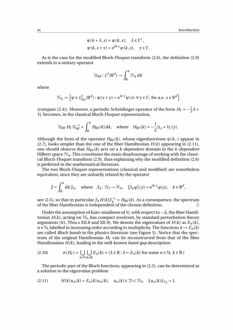
Under the assumption of Kato-smallness of VΓ with respect to−∆, the fiber Hamil-tonian H(k), acting on Hf, has compact resolvent, by standard perturbation theoryarguments [41, Thm.s XII.8 and XII.9]. We denote the eigenvalues of H(k) as En(k),n ∈N, labelled in increasing order according to multiplicity. The functions k 7→ En(k)are called Bloch bands in the physics literature (see Figure 5). Notice that the spec-trum of the original Hamiltonian HΓ can be reconstructed from that of the fiberHamiltonians H(k), leading to the well-known band-gap description:
(2.10) σ(HΓ) =⋃
n∈N
⋃k∈B
En(k) = λ ∈R :λ= En(k) for some n ∈N, k ∈B.
The periodic part of the Bloch functions, appearing in (2.5), can be determined asa solution to the eigenvalue problem
(2.11) H(k)un(k) = En(k)un(k), un(k) ∈D⊂Hf, ‖un(k)‖Hf= 1.
2. Analysis, geometry and physics of periodic Schrödinger operators xxi
k1k2
σ(H
(k))
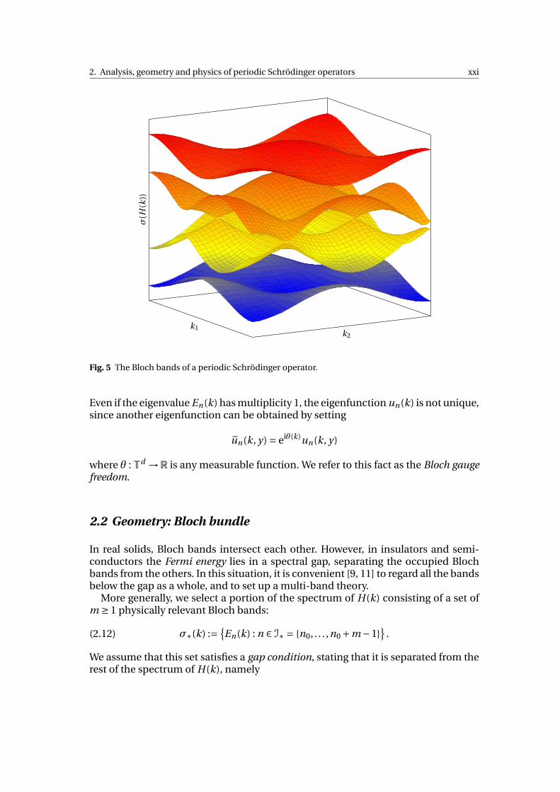
Fig. 5 The Bloch bands of a periodic Schrödinger operator.
Even if the eigenvalue En(k) has multiplicity 1, the eigenfunction un(k) is not unique,since another eigenfunction can be obtained by setting
un(k, y) = eiθ(k)un(k, y)
where θ :Td →R is any measurable function. We refer to this fact as the Bloch gaugefreedom.
2.2 Geometry: Bloch bundle
In real solids, Bloch bands intersect each other. However, in insulators and semi-conductors the Fermi energy lies in a spectral gap, separating the occupied Blochbands from the others. In this situation, it is convenient [9, 11] to regard all the bandsbelow the gap as a whole, and to set up a multi-band theory.
More generally, we select a portion of the spectrum of H(k) consisting of a set ofm ≥ 1 physically relevant Bloch bands:
(2.12) σ∗(k) := En(k) : n ∈ I∗ = n0, . . . ,n0 +m −1
.
We assume that this set satisfies a gap condition, stating that it is separated from therest of the spectrum of H(k), namely
xxii Introduction
(2.13) infk∈B
dist(σ∗(k),σ(H(k)) \σ∗(k)
)> 0
(consider e. g. the collection of the yellow and orange bands in Figure 5). Under thisassumption, one can define the spectral eigenprojector on σ∗(k) as
P∗(k) :=χσ∗(k)(H(k)) =∑
n∈I∗|un(k, ·)⟩⟨un(k, ·)| .
The family of spectral projectors P∗(k)k∈Rd is the main character in the investi-gation of geometric effects in insulators, as will become clear in what follows. Theequivalent expression for P∗(k), given by the Riesz formula
(2.14) P∗(k) = 1
2πi
∮C
(H(k)− z1l)−1 dz,
where C is any contour in the complex plane winding once around the set σ∗(k) andenclosing no other point in σ(H(k)), allows one to prove [36, Prop. 2.1] the following
Proposition 2.1. Let P∗(k) ∈B(Hf) be the spectral projector of H(k) correspondingto the set σ∗(k) ⊂R. Assume that σ∗ satisfies the gap condition (2.13). Then the familyP∗(k)k∈Rd has the following properties:
(p1) the map k 7→ P∗(k) is analytic5 from Rd to B(Hf) (equipped with the operatornorm);
(p2) the map k 7→ P∗(k) is τ-covariant, i. e.
P∗(k +λ) = τ(λ)P∗(k)τ(λ)−1, k ∈Rd , λ ∈ Γ∗.
(p3) the map k 7→ P∗(k) is time-reversal symmetric, i. e. there exists a antiunitary op-erator T : Hf →Hf such that
T 2 =±1l and P∗(−k) = T P∗(k)T −1, k ∈Rd .
Moreover, one has the following
(p4) compatibility property: T τ(λ) = τ(−λ)T for all λ ∈Λ.
In this multi-band case, the notion of Bloch function is relaxed to that of a quasi-Bloch function, which is a normalized eigenstate of the spectral projector rather thanof the fiber Hamiltonian:
(2.15) P∗(k)φ(k) =φ(k), φ(k) ∈Hf,∥∥φ(k)
∥∥Hf
= 1.
Abstracting from the specific case of periodic, time-reversal symmetric Schrödingeroperators, we consider a family of orthogonal projectors acting on a separable Hilbertspace H, satisfying the following
Assumption 2.1. The family of orthogonal projectors P (k)k∈Rd ⊂B(H) enjoys thefollowing properties:
5 Here and in the following, “analyticity” is meant in the sense of admitting an analytic extension to astrip in the complex domain as in (2.8).
2. Analysis, geometry and physics of periodic Schrödinger operators xxiii
(P1) regularity: the map Rd 3 k 7→ P (k) ∈B(H) is analytic (respectively continuous,C∞-smooth); in particular, the rank m := dimRanP (k) is constant in k;
(P2) τ-covariance: the map k 7→ P (k) is covariant with respect to a unitary represen-tation τ : Λ→ U(H) of a maximal lattice Λ ' Zd ⊂ Rd on the Hilbert space H,i. e.
P (k +λ) = τ(λ)P (k)τ(λ)−1, for all k ∈Rd ,λ ∈Λ;
(P3) time-reversal symmetry: the map k 7→ P (k) is time-reversal symmetric, i. e. thereexists an antiunitary operator Θ : H → H, called the time-reversal operator,such that
Θ2 =±1lH and P (−k) =ΘP (k)Θ−1, for all k ∈Rd .
Moreover, the unitary representation τ : Λ→U(H) and the time-reversal operatorΘ : H→H satisfy the following
(P4) compatibility condition:
Θτ(λ) = τ(λ)−1Θ for all λ ∈Λ. ♦
The previous Assumptions retain only the fundamentalZd - andZ2-symmetries ofthe family of eigenprojectors of a time-reversal symmetric periodic gapped Hamil-tonian, as in Proposition 2.1.
Following [35], one can construct a Hermitian vector bundle EP =(EP
π−→Td∗),
with Td∗ := Rd /Λ, called the Bloch bundle, starting from a family of projectors P :=
P (k)k∈Rd satisfying properties (P1) and (P2) (see Figure 6). One proceeds as follows:Introduce the following equivalence relation on the set Rd ×H:
(k,φ) ∼τ (k ′,φ′) if and only if there exists λ ∈Λ such that k ′ = k−λ and φ′ = τ(λ)φ.
The total space of the Bloch bundle is then
EP :=
[k,φ]τ ∈ (Rd ×H)/ ∼τ : φ ∈ RanP (k)
with projection π([k,φ]τ) = k (mod Λ) ∈Td∗ . The condition φ ∈ RanP (k), or equiva-
lently P (k)φ = φ, is independent of the representative [k,φ]τ in the ∼τ-equivalenceclass, in view of (P2).
By using the Kato-Nagy formula [22, Sec. I.4.6], one shows that the previous def-inition yields an analytic vector bundle, which moreover inherits from H a naturalHermitian structure given by⟨
[k,φ]τ, [k,φ′]τ⟩
:= ⟨φ,φ′⟩
H .
Indeed, pick k0 ∈Td∗ , and let U ⊂Td
∗ be a neighbourhood of k0 such that
‖P (k)−P (k0)‖B(H) < 1 for all k ∈U .
The Kato-Nagy formula then provides a unitary operator W (k;k0) ∈U(H), depend-ing analytically on k, such that
xxiv Introduction
k
RanP (k)
T2∗T2∗
k
RanP (k)
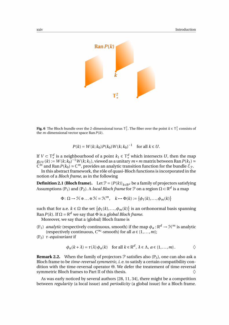
Fig. 6 The Bloch bundle over the 2-dimensional torus T2∗. The fiber over the point k ∈T2
∗ consists ofthe m-dimensional vector space RanP (k).
P (k) =W (k;k0)P (k0)W (k;k0)−1 for all k ∈U .
If V ⊂ Td∗ is a neighbourhood of a point k1 ∈ Td
∗ which intersects U , then the mapgUV (k) :=W (k;k0)−1W (k;k1), viewed as a unitary m×m matrix between RanP (k1) 'Cm and RanP (k0) 'Cm , provides an analytic transition function for the bundle EP.
In this abstract framework, the rôle of quasi-Bloch functions is incorporated in thenotion of a Bloch frame, as in the following
Definition 2.1 (Bloch frame). LetP= P (k)k∈Rd be a family of projectors satisfyingAssumptions (P1) and (P2). A local Bloch frame for P on a region Ω⊂Rd is a map
Φ : Ω→H⊕ . . .⊕H=Hm , k 7→Φ(k) := φ1(k), . . . ,φm(k)
such that for a.e. k ∈Ω the set
φ1(k), . . . ,φm(k)
is an orthonormal basis spanning
RanP (k). If Ω=Rd we say that Φ is a global Bloch frame.Moreover, we say that a (global) Bloch frame is
(F1) analytic (respectively continuous, smooth) if the map φa : Rd →Hm is analytic(respectively continuous, C∞-smooth) for all a ∈ 1, . . . ,m;
(F2) τ-equivariant if
φa(k +λ) = τ(λ)φa(k) for all k ∈Rd , λ ∈Λ, a ∈ 1, . . . ,m . ♦
Remark 2.2. When the family of projectors P satisfies also (P3), one can also ask aBloch frame to be time-reversal symmetric, i. e. to satisfy a certain compatibility con-dition with the time-reversal operator Θ. We defer the treatement of time-reversalsymmetric Bloch frames to Part II of this thesis. ♦
As was early noticed by several authors [28, 11, 34], there might be a competitionbetween regularity (a local issue) and periodicity (a global issue) for a Bloch frame.
2. Analysis, geometry and physics of periodic Schrödinger operators xxv
The existence of an analytic, τ-equivariant global Bloch frame for a family of projec-tors P = P (k)k∈Rd satisfying assumptions (P1) and (P2), which is equivalent to theexistence of a basis of localized Wannier functions (see Section 2.3), is, in general,topologically obstructed. The main advantage of the geometric picture and the use-fulness of the language of Bloch bundles is that it gives a way to measure and quan-tify this topological obstruction, and to look for sufficient conditions which guaran-tee its absence.
Indeed, the existence of a Bloch frame for P which satisfies (F1) and (F2) is equiv-alent to the triviality6 of the associated Bloch bundle EP. In fact, if the Bloch bundleEP is trivial, then an analytic Bloch frame
φa
a=1,...,m can be constructed by means
of an analytic isomorphism F : Td∗ ×Cm ∼−→ EP by setting φa(k) := F (k,ea), where
eaa=1,...,m is any orthonormal basis in Cm . Viceversa, a global analytic Bloch frameφa
a=1,...,m provides an analytic isomorphism G :Td
∗ ×Cm ∼−→ EP by setting
G (k, (v1, . . . , vm)) = [k, v1φ1(k)+·· ·+ vmφm(k)]τ.
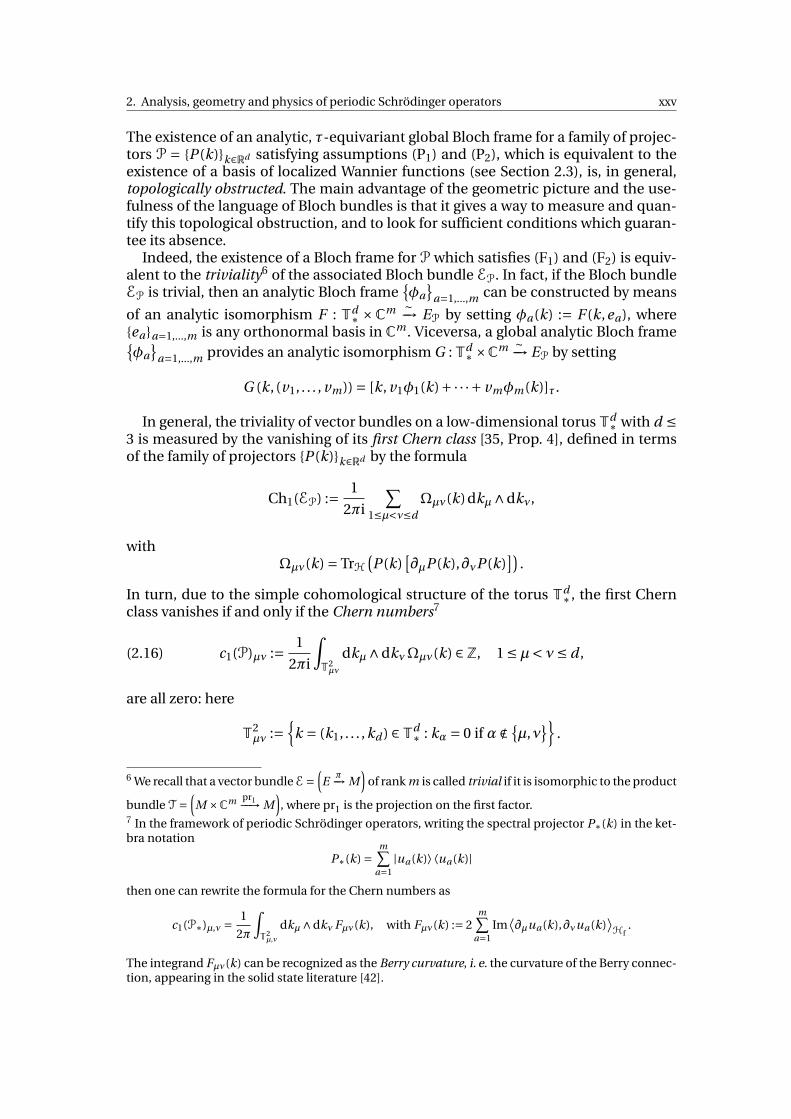
In general, the triviality of vector bundles on a low-dimensional torusTd∗ with d ≤
3 is measured by the vanishing of its first Chern class [35, Prop. 4], defined in termsof the family of projectors P (k)k∈Rd by the formula
Ch1(EP) := 1
2πi
∑1≤µ<ν≤d
Ωµν(k)dkµ∧dkν,
withΩµν(k) = TrH
(P (k)
[∂µP (k),∂νP (k)
]).
In turn, due to the simple cohomological structure of the torus Td∗ , the first Chern
class vanishes if and only if the Chern numbers7
(2.16) c1(P)µν := 1
2πi
∫T2µν
dkµ∧dkνΩµν(k) ∈Z, 1 ≤µ< ν≤ d ,
are all zero: here
T2µν :=
k = (k1, . . . ,kd ) ∈Td
∗ : kα = 0 if α ∉ µ,ν
.
6 We recall that a vector bundleE=(E
π−→ M)
of rank m is called trivial if it is isomorphic to the product
bundle T =(M ×Cm pr1−−→ M
), where pr1 is the projection on the first factor.
7 In the framework of periodic Schrödinger operators, writing the spectral projector P∗(k) in the ket-bra notation
P∗(k) =m∑
a=1|ua(k)⟩⟨ua(k)|
then one can rewrite the formula for the Chern numbers as
c1(P∗)µ,ν =1
2π
∫T2µ,ν
dkµ∧dkνFµν(k), with Fµν(k) := 2m∑
a=1Im
⟨∂µua(k),∂νua(k)
⟩Hf
.
The integrand Fµν(k) can be recognized as the Berry curvature, i. e. the curvature of the Berry connec-tion, appearing in the solid state literature [42].

xxvi Introduction
The main result of [35], later generalized in [33] to the case of a fermionic time-reversal symmetry, is the following.
Theorem 2.2 ([35, Thm. 1], [33, Thm. 1]). Let d ≤ 3, and let P = P (k)k∈Rd be afamily of projectors satisfying Assumption 2.1 (in particular, it is time-reversal sym-
metric). Then the Bloch bundle EP =(EP
π−→Td∗)
is trivial in the category of analytic
Hermitian vector bundles.
The above result then establishes the existence of analytic, τ-equivariant globalBloch frames in dimension d ≤ 3, whenever time-reversal symmetry is present.
2.3 Physics: Wannier functions and their localization
Coming back to periodic Schrödinger operators, we deduce some important phys-ical consequences of the above geometric results. Recall that Bloch functions aredefined as eigenfunctions of the fiber Hamiltonian H(k) for a fixed crystal mo-mentum k ∈ Rd . One can use them to mimic eigenfunctions of the original peri-odic Schrödinger operator HΓ, which strictly speaking do not exist since its spec-trum (2.10) is in general purely absolutely continuous (unless there is a flat bandEn(k) ≡ const). In order to do so, one uses the Bloch-Floquet-Zak antitransform tobring Bloch functions back to the position-space representation.
More precisely, assume that σ∗ in (2.12) consist of a single isolated Bloch band En(i. e. m = 1); the Wannier function wn associated to a choice of the Bloch functionun(k, ·) for the band En , as in (2.11), is defined by setting
(2.17) wn(x) := (U−1
BFZun)
(x) = 1
|B|1/2
∫B
dk eik·xun(k, x).
In the multiband case (m > 1), the rôle of Bloch functions is played by quasi-Blochfunctions, as in (2.15). The notion corresponding in position space to that of a Blochframe
φa
a=1,...,m is given by composite Wannier functions w1, . . . , wm ⊂ L2(Rd ),
which are defined in analogy with (2.17) as
wa(x) := (U−1
BFZφa)
(x) = 1
|B|1/2
∫B
eik·xφa(k, x)dk.
If we denote by
P∗ :=U−1BFZ
(∫ ⊕
Bdk P∗(k)
)UBFZ
the spectral projection of HΓ corresponding to the relevant set of bandsσ∗ =⋃
k∈Bσ∗(k),then it is not hard to prove [3] the following
Proposition 2.2. Let Φ = φa
a=1,...,m be a global Bloch frame for P∗(k)k∈Rd , and
denote by waa=1,...,m the set of the corresponding composite Wannier functions. Thenthe set
Tγwa
γ∈Γ;a=1,...,m gives an orthonormal basis of RanP∗.
Localization (that is, decay at infinity) of Wannier functions plays a fundamen-tal rôle in the transport theory of electrons [3, 31]. One says that a set of composite
3. Structure of the thesis xxvii
Wannier functions is almost-exponentially localized if it decays faster than any poly-nomial in the L2-sense, i. e. if∫
Rd
(1+|x|2)r |wa(x)|2 dx <∞ for all r ∈N, a ∈ 1, . . . ,m .
One says instead that composite Wannier functions are exponentially localized ifthey decay exponentially in the L2-sense, i. e. if∫
Rde2β|x||wa(x)|2 dx <∞ for some β> 0, for all a ∈ 1, . . . ,m .
Due to the properties of the Bloch-Floquet-Zak transform listed in Theorem 2.1,one has that a set of almost-exponentially (respectively exponentially) localizedcomposite Wannier functions exists if and only if there exists a smooth (respectivelyanalytic), τ-equivariant Bloch frame for the family of spectral projectors P∗(k)k∈Rd .In view of the results of Proposition 2.1, we can rephrase the abstract result of Theo-rem 2.2 as
Corollary 2.1. Let HΓ be a periodic, time-reversal symmetric Schrödinger operator,acting on L2(Rd )⊗CN with d ≤ 3. Denote by σ∗ a portion of the spectrum which satis-fies the gap condition (2.13), and denote by P∗ the associated spectral projector. Then,there exists an orthonormal basis
Tγwa
γ∈Γ;a=1,...,m consisting of exponentially lo-
calized composite Wannier functions for RanP∗.
Thus, we see that time-reversal symmetry is the crucial hypothesis to prove theexistence of localized Wannier functions in insulators.
3 Structure of the thesis
After the above review on geometric phases and topological invariants of crystallineinsulators, we are able to state the purpose of this dissertation. This thesis collectsthree of the publications that the candidate produced during his Ph.D. studies.
Part I contains the reproduction of [32]. The scope of this paper is to understandwheter geometric information can still be extracted from the datum of the spectralprojector in the case when the gap condition (2.13) is not satisfied. We consider thus2-dimensional crystals whose Fermi surface is first of all non-empty and degeneratesto a discrete set of points, that is, semimetallic materials, whose prototypical modelis (multilayer) graphene.
In these models, the associated family of eigenprojectors fails to be continuousat those points where eigenvalue bands touch. By adding a deformation parame-ter, which opens a gap between these bands (thus making the family of eigenpro-jectors smooth), one is able to recover a vector bundle, defined on a sphere (or apointed cylinder) in the now 3-dimensional parameter space, surrounding a degen-erate point. The first Chern number of this bundle, which characterizes completelyits isomorphism class by the same arguments contained in [35], is then the integer-valued topological invariant, baptized eigenspace vorticity, which is associated to theeigenvalue intersection. It is proved that this definition provides a stronger notionthan that of pseudospin winding number (at least in 2-band systems, where the lat-
xxviii Introduction
ter is defined), which appeared in the literature of solid state physics and was alsoaimed at quantifying a geometric phase in presence of eigenvalue intersections.
With the help of explicit models for the local geometry around eigenvalue cross-ings, the authors of [32] were also able to establish the decay rate of Wannier func-tions in mono- and bilayer graphene. More precisely, if w ∈ L2(R2) is the Wannierfunction associated to, say, the valence band of such materials, then∫
R2dx |x|2α|w(x)|2 <+∞ for all 0 ≤α< 1.
Part II contains instead the reproduction of [12] and [13]. In both these papers,the starting datum is that of a family of projectors as in Assumption 2.1 with d ≤ 3;in [12] the time-reversal operator is assumed to be of bosonic type, while in [13] it isof fermionic type, squaring respectively to +1l or −1l. The aim is to give an explicit al-gorithmic construction of smooth and τ-equivariant Bloch frames, whose existencewas proved by abstract geometric methods in [35] and [33] (compare Theorem 2.2),investigating moreover if a certain compatibility condition with time-reversal sym-metry can be enforced. The results depend crucially on the bosonic or fermionic na-ture of the time-reversal symmetry operator. Indeed, contrary to the bosonic case,in the fermionic framework there may be topological obstructions to the existenceof smooth, τ-equivariant and time-reversal symmetric Bloch frames in dimensionsd = 2 and d = 3. More explicitly, the results of [12] and [13] can be summarized asfollows.
The thesis closes illustrating some perspectives and reporting some recent devel-opments on the line of research initiated during the Ph.D. studies of the candidate.
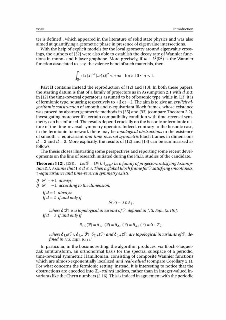
Theorem ([12], [13]). Let P= P (k)k∈Rd be a family of projectors satisfying Assump-tion 2.1. Assume that 1 ≤ d ≤ 3. Then a global Bloch frame forP satisfying smoothness,τ-equivariance and time-reversal symmetry exists:
If Θ2 =+1l always;If Θ2 =−1l according to the dimension:
If d = 1 always;If d = 2 if and only if
δ(P) = 0 ∈Z2,
where δ(P) is a topological invariant of P, defined in [13, Eqn. (3.16)];If d = 3 if and only if
δ1,0(P) = δ1,+(P) = δ2,+(P) = δ3,+(P) = 0 ∈Z2,
where δ1,0(P), δ1,+(P), δ2,+(P) and δ3,+(P) are topological invariants of P, de-fined in [13, Eqn. (6.1)].
In particular, in the bosonic setting, the algorithm produces, via Bloch-Floquet-Zak antitransform, an orthonormal basis for the spectral subspace of a periodic,time-reversal symmetric Hamiltonian, consisting of composite Wannier functionswhich are almost-exponentially localized and real-valued (compare Corollary 2.1).For what concerns the fermionic setting, instead, it is interesting to notice that theobstructions are encoded into Z2-valued indices, rather than in integer-valued in-variants like the Chern numbers (2.16). This is indeed in agreement with the periodic
References xxix
tables of topological insulators, and provides a geometric origin for these invariantsin the periodic framework. In particular, in [13] the authors show that such invari-ants δ,δ j ,s ∈ Z2, which are the mod 2 reduction of the degree of the determinant ofa unitary-valued map suitably defined on the boundary of half the Brillouin zone,coincide numerically with the ones proposed by L. Fu, C. Kane and E. Mele in theliterature on time-reversal symmetric topological insulators [15, 16].
References
1. ALTLAND, A.; ZIRNBAUER, M. : Non-standard symmetry classes in mesoscopic normal-superconducting hybrid structures, Phys. Rev. B 55, 1142–1161 (1997).
2. ANDO, Y. : Topological insulator materials, J. Phys. Soc. Jpn. 82, 102001 (2013).3. ASHCROFT, N.W.; MERMIN, N.D. : Solid State Physics. Harcourt (1976).4. AVRON, J.E.; SEILER, R.; YAFFE, L.G. : Adiabatic theorems and applications to the quantum Hall
effect, Commun. Math. Phys. 110, 33–49 (1987).5. AVRON, J.E.; SEILER, R.; SIMON, B. : Charge deficiency, charge transport and comparison of di-
mensions, Commun. Math. Phys. 159, 399–422 (1994).6. BELLISSARD, J.; VAN ELST, A.; SCHULZ-BALDES, H. : The noncommutative geometry of the quan-
tum Hall effect, J. Math. Phys 35, 5373–5451 (1994).7. BERNEVIG, B.A.; HUGHES, T.L.; ZHANG, SH.-CH. : Quantum Spin Hall Effect and Topological
Phase Transition in HgTe Quantum Wells, Science 15, 1757–1761 (2006).8. BERRY, M.V. : Quantal phase factors accompanying adiabatic changes, Proc. R. Lond. A392, 45–
57 (1984).9. BLOUNT, E.I. : Formalism of Band Theory, in: SEITZ, F.; TURNBULL, D. (eds.) : Solid State Physics,
vol. 13, 305–373. Academic Press (1962).10. DE NITTIS, G.; GOMI, K. : Classification of “Quaternionic” Bloch-bundles, Commun. Math. Phys.
339 (2015), 1–55.11. DES CLOIZEAUX, J. : Analytical properties of n-dimensional energy bands and Wannier functions,
Phys. Rev. 135, A698–A707 (1964).12. FIORENZA, D.; MONACO, D.; PANATI, G. : Construction of real-valued localized composite Wan-
nier functions for insulators, Ann. Henri Poincaré (2015), DOI 10.1007/s00023-015-0400-6.13. FIORENZA, D.; MONACO, D.; PANATI, G. : Z2 invariants of topological insulators as geometric
obstructions, available at arXiv:1408.1030.14. FRUCHART, M. ; CARPENTIER, D. : An introduction to topological insulators, Comptes Rendus
Phys. 14, 779–815 (2013).15. FU, L.; KANE, C.L. : Time reversal polarization and a Z2 adiabatic spin pump, Phys. Rev. B 74,
195312 (2006).16. FU, L.; KANE, C.L.; MELE, E.J. : Topological insulators in three dimensions, Phys. Rev. Lett. 98,
106803 (2007).17. GRAF, G.M. : Aspects of the Integer Quantum Hall Effect, P. Symp. Pure Math. 76, 429–442 (2007).18. GRAF, G.M.; PORTA, M. : Bulk-edge correspondence for two-dimensional topological insulators,
Commun. Math. Phys. 324, 851–895 (2013).19. HASAN, M.Z.; KANE, C.L. : Colloquium: Topological Insulators, Rev. Mod. Phys. 82, 3045–3067
(2010).20. KANE, C.L.; MELE, E.J. : Z2 Topological Order and the Quantum Spin Hall Effect, Phys. Rev. Lett.
95, 146802 (2005).21. KANE, C.L.; MELE, E.J. : Quantum Spin Hall Effect in graphene, Phys. Rev. Lett. 95, 226801 (2005).22. KATO, T. : Perturbation theory for linear operators. Springer, Berlin (1966).23. KELLENDONK, J.; RICHTER, T.; SCHULZ-BALDES, H. : Edge current channels and Chern numbers
in the integer quantum Hall effect, Rev. Math. Phys. 14, 87–119 (2002).24. KENNEDY, R.; GUGGENHEIM, C. : Homotopy theory of strong and weak topological insulators,
available at arXiv:1409.2529.25. KENNEDY, R.; ZIRNBAUER, M.R. : Bott periodicity forZ2 symmetric ground states of free fermion
systems, available at arXiv:1409.2537.
xxx Introduction
26. KING-SMITH, R.D.; VANDERBILT, D. : Theory of polarization of crystalline solids, Phys. Rev. B 47,1651 (1993).
27. KITAEV, A. : Periodic table for topological insulators and superconductors, AIP Conf. Proc. 1134,22 (2009).
28. KOHN, W. : Analytic properties of Bloch waves and Wannier functions, Phys. Rev. 115, 809 (1959).29. KUCHMENT, P. : Floquet Theory for Partial Differential Equations. Vol. 60 of Operator Theory
Advances and Applications. Birkhäuser Verlag (1993).30. MACIEJKO, J.; HUGHES, T.L.; ZHANG, SH.-CH. : The quantum spin Hall effect, Annu. Rev. Con-
dens. Matter Phys. 2, 31–53 (2011).31. MARZARI, N.; MOSTOFI, A.A.; YATES, J.R.; SOUZA I.; VANDERBILT, D. : Maximally localized Wan-
nier functions: Theory and applications, Rev. Mod. Phys. 84, 1419 (2012).32. MONACO, D.; PANATI, G. : Topological invariants of eigenvalue intersections and decrease of
Wannier functions in graphene, J. Stat. Phys. 155, Issue 6, 1027–1071 (2014).33. MONACO, D.; PANATI, G. : Symmetry and localization in periodic crystals: triviality of Bloch bun-
dles with a fermionic time-reversal symmetry, Acta Appl. Math. 137, Issue 1, 185–203 (2015).34. NENCIU, G. : Dynamics of band electrons in electric and magnetic fields: Rigorous justification
of the effective Hamiltonians, Rev. Mod. Phys. 63, 91–127 (1991).35. PANATI, G. : Triviality of Bloch and Bloch-Dirac bundles, Ann. Henri Poincaré 8, 995–1011 (2007).36. PANATI, G.; PISANTE, A. : Bloch bundles, Marzari-Vanderbilt functional and maximally localized
Wannier functions, Commun. Math. Phys. 322, 835–875 (2013).37. PANATI, G.; SPARBER, C.; TEUFEL, S. : Effective dynamics for Bloch electrons: Peierls substitution
and beyond, Commun. Math. Phys. 242, 547–578 (2003).38. PRODAN, E. : Robustness of the Spin-Chern number, Phys. Rev. B 80, 125327 (2009).39. QI, X.-L.; ZHANG, SH.-CH. : The quantum spin Hall effect and topological insulators, Phys. To-
day 63, 33 (2010).40. QI, X.-L.; ZHANG, SH.-CH. : Topological insulators and superconductors, Rev. Mod. Phys. 83,
1057 (2011).41. REED, M.; SIMON, B. : Methods of Modern Mathematical Physics, vol. IV: Analysis of Operators.
Academic Press (1978).42. RESTA, R. : Macroscopic polarization in crystalline dielectrics: the geometric phase approach,
Rev. Mod. Phys. 66, Issue 3, 899–915 (1994).43. RYU, S.; SCHNYDER, A.P.; FURUSAKI, A.; LUDWIG, A.W.W. : Topological insulators and supercon-
ductors: Tenfold way and dimensional hierarchy, New J. Phys. 12, 065010 (2010).44. SCHULZ-BALDES, H. : Persistence of spin edge currents in disordered Quantum Spin Hall sys-
tems, Commun. Math. Phys. 324, 589–600 (2013).45. SHAPERE, A.; WILCZEK, F. (eds.) : Geometric Phases in Physics. Vol. 5 of Advanced Series in Math-
ematical Physics. World Scientific, Singapore (1989).46. SIMON, B. : Holonomy, the quantum adiabatic theorem, and Berry’s phase, Phys. Rev. Lett. 51,
2167–2170 (1983).47. SPALDIN, N.A. : A beginner’s guide to the modern theory of polarization, J. Solid State Chem. 195,
2–10 (2012).48. THOULESS, D.J.; KOHMOTO, M.; NIGHTINGALE, M.P.; DEN NIJS, M. : Quantized Hall conduc-
tance in a two-dimensional periodic potential, Phys. Rev. Lett. 49, 405–408 (1982).49. VON KLITZING, K.; DORDA, G.; PEPPER, M. : New method for high-accuracy determination of
the fine-structure constant based on quantized Hall resistance, Phys. Rev. Lett. 45, 494 (1980).50. VON KLITZING, K. : The quantized Hall effect, Rev. Mod. Phys. 58, Issue no. 3, 519–531 (1986).51. ZAK, J. : Magnetic translation group, Phys. Review 134, A1602 (1964).
Part IGraphene

We reproduce here the content of the paper
MONACO, D.; PANATI, G. : Topological invariants of eigenvalue intersections and de-crease of Wannier functions in graphene, J. Stat. Phys. 155, Issue 6, 1027–1071 (2014).
Topological invariants of eigenvalue intersections anddecrease of Wannier functions in graphene
Domenico Monaco and Gianluca Panati
Dedicated to Herbert Spohn, with admiration
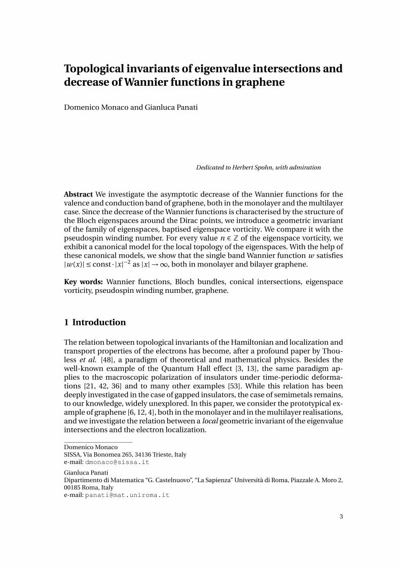
Abstract We investigate the asymptotic decrease of the Wannier functions for thevalence and conduction band of graphene, both in the monolayer and the multilayercase. Since the decrease of the Wannier functions is characterised by the structure ofthe Bloch eigenspaces around the Dirac points, we introduce a geometric invariantof the family of eigenspaces, baptised eigenspace vorticity. We compare it with thepseudospin winding number. For every value n ∈ Z of the eigenspace vorticity, weexhibit a canonical model for the local topology of the eigenspaces. With the help ofthese canonical models, we show that the single band Wannier function w satisfies|w(x)| ≤ const · |x|−2 as |x|→∞, both in monolayer and bilayer graphene.
Key words: Wannier functions, Bloch bundles, conical intersections, eigenspacevorticity, pseudospin winding number, graphene.
1 Introduction
The relation between topological invariants of the Hamiltonian and localization andtransport properties of the electrons has become, after a profound paper by Thou-less et al. [48], a paradigm of theoretical and mathematical physics. Besides thewell-known example of the Quantum Hall effect [3, 13], the same paradigm ap-plies to the macroscopic polarization of insulators under time-periodic deforma-tions [21, 42, 36] and to many other examples [53]. While this relation has beendeeply investigated in the case of gapped insulators, the case of semimetals remains,to our knowledge, widely unexplored. In this paper, we consider the prototypical ex-ample of graphene [6, 12, 4], both in the monolayer and in the multilayer realisations,and we investigate the relation between a local geometric invariant of the eigenvalueintersections and the electron localization.
Domenico MonacoSISSA, Via Bonomea 265, 34136 Trieste, Italye-mail: [email protected]
Gianluca PanatiDipartimento di Matematica “G. Castelnuovo”, “La Sapienza” Università di Roma, Piazzale A. Moro 2,00185 Roma, Italye-mail: [email protected]
3

4 Domenico Monaco, Gianluca Panati
A fundamental tool to study the localization of the electrons in periodic andalmost-periodic systems is provided by Wannier functions [52, 28]. In the case ofa single Bloch band isolated from the rest of the spectrum, the existence of an expo-nentially localized Wannier function was proved in dimension d = 1 by W. Kohn forcentrosymmetric crystals [22]. The latter hypothesis has been later removed by J. deCloizeaux [8]. A proof of existence for d ≤ 3 has been obtained by J. de Cloizeaux forcentrosymmetric crystals [7, 8], and by G. Nenciu [32] in the general case.
Whenever the Bloch bands intersect each other, there are two possible approaches.On the one hand, following de Cloizeaux [8], one considers a relevant family of Blochbands which are separated by a gap from the rest of the spectrum (e. g. the bandsbelow the Fermi energy in an insulator). Then the notion of Bloch function is re-laxed to the weaker notion of quasi-Bloch function, and one investigates whetherthe corresponding composite Wannier functions are exponentially localized. An af-firmative answer was provided by G. Nenciu for d = 1 [33], and only recently ford ≤ 3 [5, 38]. On the other hand, one may focus on a single non-isolated band andestimate the asymptotic decrease of the corresponding single-band Wannier func-tion, as |x| →∞. The rate of decrease depends, roughly speaking, on the regularityof the Bloch function at the intersection points.
In this paper we follow the second approach. We consider the case of graphene(both monolayer and bilayer) [6, 12] and we explicitly compute the rate of decreaseof the Wannier functions corresponding to the conduction and valence band. Sincethe rate of decrease crucially depends on the behaviour of the Bloch functions at theDirac points, we preliminarily study the topology of the Bloch eigenspaces aroundthose points.
More precisely, we introduce a geometric invariant of the eigenvalue intersection,which encodes the behaviour of the Bloch eigenspaces at the singular point (Sec-tion 3.1). We show that our invariant, baptised eigenspace vorticity, equals the pseu-dospin winding number [39, 34, 27] whenever the latter is well-defined (Section 3.3).We prove, under suitable assumptions, that if the value of the eigenspace vorticityis nv ∈ Z, then the local behaviour of the Bloch eigenspaces is described by the nv-canonical model, explicitly described in Section 3.2. For example, monolayer andbilayer graphene correspond to the cases nv = 1 and nv = 2, respectively. The coreof our topological analysis is Theorem 4.1, which shows that, in the relevant situa-tions, the family of canonical models provides a complete classification of the localbehaviour of the eigenspaces.
As a consequence of the previous geometric analysis, in Section 5 we are able tocompute the rate of decrease of Wannier functions corresponding to the valence andconduction bands of monolayer and bilayer graphene. For both bands, we essen-tially obtain that
(1.1) |w(x)| ≤ const · |x|−2 as |x|→∞,
see Theorems 5.1 and 5.3 for precise statements.The power-law decay in (1.1) suggests that electrons in the conduction or valence
band are delocalized. The absence of localization and the finite metallic conductiv-ity in monolayer graphene are usually explained as a consequence of the Dirac-like(conical) energy spectrum. Since bilayer graphene has the usual parabolic spectrum,“the observation of the maximum resistivity ≈ h/4e2 [...] is most unexpected” [34],thus challenging theoreticians to provide an explanation of the absence of localiza-
Reproduction of J. Stat. Phys. 155, Issue 6, 1027–1071 (2014)

Wannier functions in graphene 5
tion in bilayer graphene.In this paper, we show that the absence of localization is not a direct consequenceof the conical spectrum, but it is rather a consequence of the non-smoothness ofthe Bloch functions at the intersection points, which is in turn a consequence of anon-zero eigenspace vorticity, a condition which is verified by both mono- and mul-tilayer graphene. While the existence of a local geometric invariant distinguishingmonolayer graphene from bilayer graphene has been foreseen by several authors, ase. g. [34, 27, 39], our paper first demonstrates the relation between non-trivial localtopology and absence of localization in position space.
While the Wannier functions in graphene are the motivating example, the impor-tance of our topological analysis goes far beyond the specific case: we see a widevariety of possible applications, ranging from the topological phase transition in theHaldane model [17], to the analysis of the conical intersections arising in systemsof ultracold atoms in optical lattices [54, 25, 47], to a deeper understanding of theinvariants in 3-dimensional topological insulators [18, 19, 44]. As for the latter item,the applicability of our results is better understood in terms of edge states, follow-ing [18, Sec. IV]. Indeed, in a 3d crystal occupying the half-space, the edge statesare decomposed with respect to a 2d crystal momentum; on the corresponding 2dBrillouin zone, there are four points invariant under time-reversal symmetry wheresurface Bloch bands may be doubly degenerate, yielding an intersection of eigenval-ues. Although a detailed analysis is postponed to future work, we are confident thatmethods and techniques developed in this paper will contribute to a deeper under-standing of the invariants of topological insulators.
Acknowledgments. We are indebted with D. Fiorenza and A. Pisante for manyinspiring discussions, and with R. Bianco, R. Resta and A. Trombettoni for inter-esting comments and remarks. We are also grateful to the anonymous reviewersfor their useful observations and suggestions. Financial support from the INdAM-GNFM project “Giovane Ricercatore 2011”, and from the AST Project 2009 “Wannierfunctions” is gratefully acknowledged.
2 Basic concepts
In this Section, we briefly introduce the basic concepts and the notation, referring to[35, Section 2] for details.
2.1 Bloch Hamiltonians
To motivate our definition, we initially consider a periodic Hamiltonian HΓ =−∆+VΓwhere VΓ(x +γ) = VΓ(x) for every γ in the periodicity lattice Γ = SpanZ a1, . . . , ad (here a1, . . . , ad is a linear basis of Rd ). We assume that the potential VΓ defines anoperator which is relatively bounded with respect to ∆ with relative bound zero, inorder to guarantee that HΓ is self-adjoint on the domain W 2,2(Rd ): when d = 2 (therelevant dimension for our subsequent analysis), for example, this holds wheneverVΓ ∈ L2
loc(R2) [41, Thm. XIII.96]. To study such Bloch Hamiltonians, one introduces
the (modified) Bloch-Floquet transform UBF, acting on a function w ∈ S(Rd ) as
Reproduction of J. Stat. Phys. 155, Issue 6, 1027–1071 (2014)
6 Domenico Monaco, Gianluca Panati
(UBFw) (k, y) := 1
|B|1/2
∑γ∈Γ
e−ik·(y+γ)w(y +γ), k ∈Rd , y ∈Rd .
Here B is the fundamental unit cell for the dual lattice Γ∗, i. e. the lattice generatedover the integers by the dual basis
a∗
1 , . . . , a∗d
defined by the relations a∗
i ·a j = 2πδi , j .As can be readily verified, the function UBFw is Γ∗-pseudoperiodic and Γ-periodic,meaning that
(UBFw) (k +λ, y) = e−iλ·y (UBFw) (k, y) for λ ∈ Γ∗,
(UBFw) (k, y +γ) = (UBFw) (k, y) for γ ∈ Γ.
Consequently, the function (UBFw) (k, ·), for fixed k ∈ Rd , can be interpreted as anelement of the k-independent Hilbert space Hf = L2(Td
Y ), where TdY = Rd /Γ is a d-
dimensional torus in position space.The Bloch-Floquet transform UBF, as defined above, extends to a unitary operator
UBF : L2(Rd ) →∫ ⊕
BdkHf
whose inverse is given by
(U−1
BFu)
(x) = 1
|B|1/2
∫B
dk eik·xu(k, [x]), x ∈Rd ,
where [x] := x mod Γ. With the hypotheses on the potential VΓ mentioned above,one verifies that HΓ becomes a fibred operator in Bloch-Floquet representation,namely
(2.1) UBFHΓU−1BF =
∫ ⊕
Bdk H(k) where H(k) = (−i∇y +k)2 +VΓ.
Each H(k) acts on the k-independent domain D := W 2,2(TdY ) ⊂Hf, where it defines
a self-adjoint operator. Since for any κ0 ∈Cd one has
H(κ) = H(κ0)+2(κ−κ0) · (−i∇y )+ (κ2 −κ20)1l
and (−i∇y ) is relatively bounded with respect to H(κ0), the assignment κ 7→ H(κ)defines an entire family of type (A), and hence an entire analytic family in the senseof Kato [41, Thm. XII.9].
Moreover, all the operators H(k), k ∈ Rd , have compact resolvent, and conse-quently they only have pure point spectrum accumulating at infinity. We label theeigenvalues in increasing order, i. e. E0(k) ≤ ·· · ≤ En(k) ≤ En+1(k) ≤ ·· · , repeated ac-cording to their multiplicity; the function k 7→ En(k) is usually called the n-th Blochband. We denote by un(k) the solution to the eigenvalue problem
(2.2) H(k)un(k) = En(k)un(k), un(k, ·) ∈D⊂Hf.
The function k 7→ ψn(k, y) = eik·y un(k, y) is called the n-th Bloch function in thephysics literature; un(k, ·) is its Γ-periodic part.
Reproduction of J. Stat. Phys. 155, Issue 6, 1027–1071 (2014)

Wannier functions in graphene 7
2.2 From insulators to semimetals
In the case of an isolated Bloch band, or an isolated family of m Bloch bandsEn , . . . ,En+m−1 = Ei i∈I , where “isolated” means that
(2.3) infk
|Ei (k)−Ec (k)| : i ∈ I ,c ∉ I > 0,
one considers the orthogonal projector
(2.4) PI (k) =∑n∈I
|un(k, ·)⟩⟨un(k, ·)| ∈B(Hf).
It is known that, in view of condition (2.3), the map k 7→ PI (k) is a B(Hf)-valued an-alytic and pseudoperiodic function (see, for example, [33] or [35, Proposition 2.1]).Thus, it defines a smooth vector bundle over the torus T∗
d = Rd /Γ∗ whose fibre atk ∈ T∗
d is RanPI (k). The triviality of such vector bundle, called Bloch bundle in [38],is equivalent to the existence of exponentially localized (composite) Wannier func-tions. By exploiting this geometric viewpoint, the existence of exponentially local-ized composite Wannier functions for a time-reversal-symmetric Hamiltonian hasbeen proved, provided d ≤ 3 [5, 38].
On the other hand, in metals and semimetals the relevant Bloch bands intersecteach other. For example, in monolayer graphene the conduction and valence bands,here denoted by E+ and E− respectively, form a conical intersection at two inequiv-alent points K and K ′ (Dirac points), i. e. for q = k −K one has
(2.5) E±(K +q) =±vF |q|+o(|q|) as |q |→ 0,
where vF > 0 is called the Fermi velocity and E±(K ) = 0 by definition of the zero of theenergy. An analogous expansion holds when K is replaced by K ′. The correspondingeigenprojectors
Ps(k) = |us(k, ·)⟩⟨us(k, ·)| , s ∈ +,− ,
are not defined at k = K , nor does the limit limk→K Ps(k) exist. This fact can be ex-plicitly checked by using an effective tight-binding model Hamiltonian [51, 12, 4].
2.3 Tight-binding Hamiltonians in graphene
We provide some details about the latter claim. If the Bloch functions ψs(k) for theHamiltonian HΓ were explicitly known, it would be natural to study the continuity ofthe eigenprojector by using the reduced 2-band Hamiltonian
(2.6) Hred(k)r,s =⟨ψr (k) , HΓψs(k)
⟩L2(Y ) = ⟨ur (k) , H(k)us(k)⟩Hf
where r, s ∈ +,−, Y is a fundamental cell for the lattice Γ and H(k) is defined in(2.1). Focusing on |q | ¿ 1, one notices that, since H(K )u±(K ) = E±(K )u±(K ) = 0, a
Reproduction of J. Stat. Phys. 155, Issue 6, 1027–1071 (2014)
8 Domenico Monaco, Gianluca Panati
standard Hellman-Feynmann argument1 yields
(2.7) Hred(K +q)r,s =⟨
ur (K ) , H(K +q)us(K )⟩+O(|q|2).
Thus q 7→Hred(K + q) encodes, for |q | ¿ 1, the local behaviour of the Hamiltonianand its eigenprojectors with respect to fixed Bloch functions, i. e. Bloch functionsevaluated at the Dirac point.
Approximated Bloch functions can be explicitly computed in the tight-binding ap-proximation. Within this approximation, the reduced Hamiltonian (2.6) is approxi-mated by the effective Hamiltonian
(2.8) Heff(k) =(
0 γ∗kγk 0
)where γk = 1+eik·a2 +eik·(a2−a1)
with a1, a2 the standard Bravais basis for graphene, as in [51, 12]. Thus, for |q| ¿ 1and denoting by θq the polar angle in the plane (q1, q2), i. e. |q|eiθq = q1 + iq2, oneobtains
(2.9) Heff(K +q) = vF
(0 q1 − iq2
q1 + iq2 0
)+O(|q|2) = vF|q |
(0 e−iθq
eiθq 0
)+O(|q|2).
One easily checks (see Section ) that the eigenprojectors of the leading-order Hamil-tonian, which is proportional to
(2.10) Hmono(q) = |q |(
0 e−iθq
eiθq 0
),
are not continuous at q = 0, implying that – within the validity of the tight-bindingapproximation – also the eigenprojectors of H(k) are not continuous at k = K , asclaimed. In the case of bilayer graphene, the same approach yields a leading-ordereffective Hamiltonian proportional to
(2.11) Hbi(q) = |q|2(
0 e−i2θq
ei2θq 0
)
1 The Hellman-Feynmann-type argument goes as follows. Near a Dirac point, i. e. for k = K + q and|q |¿ 1, one has
Hred(k)r,s = ⟨ur (k) , H(k)us (k)⟩Hf
= ⟨ur (K ) , H(K )us (K )⟩Hf+
+q · (⟨∇k ur (K ) , H(K )us (K )⟩Hf+⟨H(K )ur (K ) , ∇k us (K )⟩Hf
)++q · ⟨ur (K ) , ∇k H(K )us (K )⟩Hf
+O(|q |2).
(Notice that the derivatives ∇k H(k) exist in view of the above-mentioned analyticity of the familyk 7→ H(k)). Since H(K )u±(K ) = 0, all terms but the last vanish. Clearly,⟨
ur (K ) , H(K +q)us (K )⟩= q · ⟨ur (K ) , ∇k H(K )us (K )⟩+O(|q |2),
yielding the claim.
Reproduction of J. Stat. Phys. 155, Issue 6, 1027–1071 (2014)

Wannier functions in graphene 9
which also corresponds to a singular family of projectors. As pointed out by manyauthors [39, 27] the effective Hamiltonians (2.10) and (2.11) are related to differentvalues of a “topological index”. A rigorous definition of that index is the first task ofour paper.
For the sake of completeness, we mention that according to [31] the low-energyeffective Hamiltonian for multilayer graphene (with m layers and ABC stacking) isproportional to
(2.12) Hmulti(q) = |q|m(
0 e−imθq
eimθq 0
), m ∈N×.
2.4 Singular families of projectors
Abstracting from the specific case of graphene, we study the topology of the Blocheigenspaces around an eigenvalue intersection. We consider any periodic Hamilto-nian and a selected Bloch band of interest Es which intersects the other Bloch bandsin finitely many points K1, . . . ,KM . Focusing on one of them, named k0, the crucialinformation is the behaviour of the function k 7→ Ps(k) in a neighbourhood R ⊂ T∗
dof the intersection point k0. In view of the example of graphene, we set the following
Definition 2.1. Let H be a separable Hilbert space. A family of orthogonal projec-
tors P (k)k∈R\k0 ⊂ B(H) such that k 7→ P (k) is C∞-smooth inR = R \ k0 ⊂ T∗
dis called a singular family if it cannot be continuously extended to k = k0, i. e. iflimk→k0 P (k) does not exist. In such a case, the point k0 is called singular point. Afamily which is not singular is called regular family. ♦
In the case of insulators, the geometric structure corresponding to the regularfamily of projectors (2.4) is a smooth vector bundle, whose topological invariantscan be investigated with the usual tools of differential geometry (curvature, Chernclasses, . . . ). On the other hand, in the case of metals and semimetals one deals witha singular family of projectors, thus the usual geometric approach is not valid any-more. Indeed, in the case of conical intersections the interesting information is “hid-den” in the singular point. In particular, if we assume for simplicity that the neigh-bourhood R is a small ball around the Dirac point k0, then when d = 2 the set R \k0can be continuously retracted to a circle S1, and it is well known that every complexline bundle over S1 is trivial, so it has no non-trivial topological invariants. In view ofthat, to define the topological invariants of a singular family of projectors we have tofollow a different strategy, which is the content of Section 3. These invariants are alsorelated to a distributional approach to the Berry curvature, as detailed in AppendixA.
3 Topology of a singular 2-dimensional family of projectors
Motivated by the example of graphene, in this paper we investigate the case of sin-gular 2-dimensional families of projectors (d = 2, arbitrary rank). Since the relevantparameter is the codimension, this case corresponds to the generic case in the Born-
Reproduction of J. Stat. Phys. 155, Issue 6, 1027–1071 (2014)

10 Domenico Monaco, Gianluca Panati
Oppenheimer theory of molecules [14, 15, 10]. The analysis of higher-codimensionalcases will be addressed in a future paper.
For the moment being, we focus on just one singularity of the family of projectors,say at the point k0. We will conduct a local analysis on the “topological behaviour”determined by such a singular point: hence we restrict our attention on a simply-connected region R ⊂T∗
2 containing k0 such that for any other Bloch band En
Es(k) 6= En(k) for all k ∈ R \ k0.
In other words, Bloch bands are allowed to intersect only at k0 in the region R.
3.1 A geometricZ-invariant: eigenspace vorticity
To define a local geometric invariant characterising the behaviour of a 2-dimensionalfamily of projectors around the (possibly singular) point k0, we start from the follow-ing
Datum 3.1. Let H be a separable Hilbert space, and let R ⊂ T∗2 be a simply con-
nected region containing k0. We consider a family of projectors Ps(k)k∈R\k0 ⊂B(H) which is C∞-smooth in R \ k0. ♦
We restrict our attention to the local behaviour of the family Ps(k) around k0.Suppose r > 0 is so small that U :=
k ∈R2 : |k −k0| < r
is all contained in R. In or-der to define an integer-valued (local) geometric invariant nv, baptised eigenspacevorticity,we provide the following computable recipe. First, introduce a smoothingparameter µ ∈ [−µ0,µ0], µ0 > 0, so that Ps(k)R\U can be seen as the µ = 0 case ofa deformed family of projectors
Pµ
s (k), which for µ 6= 0 is defined and regular on
the whole region R. We also assume that the dependence on µ of such a deformedfamily of projectors is at least of class C 2.
The deformed familyPµ
s (k)
allows us to construct a vector bundle Ls , which wecall the smoothed Bloch bundle, over the set
B := (R × [−µ0,µ0]
)\C ,
where C denotes the “cylinder” C :=U ×(−µ0,µ0). The total space of this vector bun-dle is
(3.1) Ls := ((k,µ), v) ∈ B ×H : v ∈ RanPµ
s (k)
.
Explicitly, the fibre of Ls over a point (k,µ) ∈ B is the range of the projector Pµs (k). We
may look at Ls as a collection of “deformations” of the bundle
L0s :=
(k, v) ∈ (R \U )×H : v ∈ RanPs(k)
over R \U , which is defined solely in terms of the undeformed family Ps(k).We denote by ωs the Berry curvature for the smoothed Bloch bundle Ls . Posing
for notational convenience k3 =µ and ∂ j = ∂/∂k j , one has
Reproduction of J. Stat. Phys. 155, Issue 6, 1027–1071 (2014)

Wannier functions in graphene 11
(3.2)
ωs = i3∑
j ,`=1(ωs) j ,`(k)dk j ∧dk` where (ωs) j ,`(k) = Tr
(Pµ
s (k)[∂ j Pµ
s (k),∂`Pµs (k)
]).
Set C := ∂C for the “cylindrical” internal boundary of the base space B , and
C :=C \
(k = k0,µ= 0
)for the “pointed cylinder”, which is the complement of B in
B := (R × [−µ0,µ0]
)\(
k = k0,µ= 0)
.
• (k=k0,µ=0)
>
<
OOµ
k1
//k2
−µ0
−−µ0
C
C
Fig. 1 The cylinder C and its surface C. The boundary of this surface is oriented according to theoutward normal direction.
Definition 3.1 (Eigenspace vorticity). Let Ps(k)k∈R\k0 be a family of projectorsas in Datum 3.1, and
Pµ
s (k)
(k,µ)∈B be a smoothed family of projectors, as describedabove. Let Ls be the vector bundle (3.1) over B , and denote by ωs its Berry cur-vature, as in (3.2). The eigenspace vorticity of the smoothed family of projectorsPµ
s (k)
k∈R\k0 (around the point k0 ∈ R) is the integer
(3.3) nv = nv(Ps) :=− 1
2π
∫Cωs ∈Z.
♦
The number nv is indeed an integer, because it equals (up to a conventional sign)the first Chern number of the vector bundle Ls → C. This integer is the topologicalinvariant that characterises the behaviour of
Pµ
s (k)
around k0; in particular, whendimRanP (k) = 1 for k 6= k0, it selects one of the canonical models that will be in-troduced in the next Subsection. Notice that there is an ambiguity in the sign of theinteger nv defined in (3.3), related to the orientation of the cylindrical surface of in-tegration C. Indeed, if one exchanges µ with −µ one obtains the opposite value fornv. This ambiguity is resolved once the orientation of the µ-axis is fixed.
Remark 3.1 (Deformations in computational physics). The above smoothing pro-cedure corresponds to a common practice in computational solid-state physics2.
2 We are grateful to R. Bianco and R. Resta for pointing out this fact to us.
Reproduction of J. Stat. Phys. 155, Issue 6, 1027–1071 (2014)

12 Domenico Monaco, Gianluca Panati
Indeed, the family Ps(k) usually appears as the collection of the eigenprojectorscorresponding to the eigenvalue Es(k) of a given Hamiltonian operator H(k) (e. g.the Hamiltonian (2.6) or (2.10) for graphene). When dealing with an intersectionof eigenvalues, to improve the numerical accuracy it is often convenient to con-sider a family of deformed Hamiltonians Hµ(k) and the corresponding eigenprojec-tors Pµ
s (k), in such a way that the eigenvalue intersection disappears when µ 6= 0.For example, when dealing with monolayer graphene the deformed Hamiltonianis obtained by varying the electronegativity of the carbon atoms in the numericalcode. ♦
Before we proceed, we have to comment on the well-posedness of our definitionof eigenspace vorticity. First of all, the definition relies on the existence of a defor-mation
Pµ
s (k)
of the original family Ps(k) as in Datum 3.1, which for µ 6= 0 is reg-ular also at k = k0. Such a deformation indeed exists in all cases of practical interest,namely when Ps(k) arises as the eigenprojector, relative to an eigenvalue Es(k), of ak-dependent Hamiltonian H(k), such that at k = k0 two of its eigenvalues coincide.Indeed, in view of the von Neumann-Wigner theorem [1, 50], the eigenvalue inter-section for general Hermitian matrices is highly non-generic, i. e. it is a codimension-3 phenomenon. As the base B of the smoothed Bloch bunde is 3-dimensional, itmay be assumed that the eigenvalue intersection – i. e. the singularity of the familyof projectors – occurs only at the point (k = k0,µ = 0); more precisely, the genericdeformation
Pµ
s (k)
(which may be assumed to be the family of eigenprojectors ofsome deformed Hamiltonian Hµ(k)) will satisfy this hypothesis.
In addition to this, we must investigate how the definition (3.3) of nv depends onthe specific choice of the deformation. Since nv is a topological quantity, it is stableunder small perturbations of the deformed family of projectors
Pµ
s (k). This means
that model Hamiltonians which are “close”, in some suitable sense, will produce thesame eigenspace vorticity. More formally, we argue as follows. Let Pµ
s (k) be anothersmoothing deformation of the family of projectors Ps(k), so that in particular
Pµ=0s (k) = Ps(k) = Pµ=0
s (k), for all k ∈ R \ k0 .
Moreover, define the 2-form ωs and its components (ωs) j ,` (k), j ,` ∈ 1,2,3, as in(3.2), with Pµ
s (k) replaced by Pµs (k).
Lemma 3.1 (Irrelevance of the choice among close deformations). Suppose thatthe maps B 3 (k,µ) 7→ Pµ
s (k) ∈ B(H) and B 3 (k,µ) 7→ Pµs (k) ∈ B(H) are of class C 2,
and that
(3.4)∥∥Pµ(k)− Pµ(k)
∥∥B(H) < 1 for all (k,µ) ∈C.
Then
(3.5)∫Cωs =
∫Cωs .
Proof. By a result of Kato and Nagy [20, Sec. I.6.8], the hypothesis (3.4) implies thatthere exists a family of unitary operators W µ(k) such that
(3.6) Pµs (k) =W µ(k)Pµ
s (k)W µ(k)−1.
Reproduction of J. Stat. Phys. 155, Issue 6, 1027–1071 (2014)
Wannier functions in graphene 13
The explicit Kato-Nagy’s formula
(3.7) W µ(k) := (1l− (Pµ
s (k)− Pµs (k))2)−1/2 (
Pµs (k)Pµ
s (k)+ (1l− Pµs (k))(1l−Pµ
s (k)))
shows that the map (k,µ) 7→W µ(k) has the same regularity as (k,µ) 7→ Pµs (k)−Pµ
s (k)3.Formula (3.6) implies that the vector bundles Ls and Ls , corresponding to the
deformed families of projectorsPµ
s (k)
and Pµs (k) respectively, are isomorphic, the
isomorphism being implemented fibre-wise by the unitary W µ(k). Thus they havethe same Chern number, i. e. equation (3.5) holds true.
Alternatively, for the sake of clarity, we provide an explicit proof of (3.5) by showingthat the difference ωs−ωs is an exact form dβ onC; then by applying Stokes’ theoremone gets ∫
C(ωs −ωs) =
∫C
dβ= 0
because C has no boundary. This will conclude the proof of the Lemma.For the sake of readability, in the following we will use the abbreviations
P := Pµs (k), P := Pµ
s (k), W :=W µ(k),
ω j ,` := (ωs) j ,` (k), ω j ,` := (ωs) j ,` (k).
A lengthy but straightforward computation, that uses only the cyclicity of thetrace, the relations P 2 = P and W W −1 = 1l = W −1W and their immediate conse-quences
P (∂ j P ) = ∂ j P − (∂ j P )P and W −1(∂ j W ) =−(∂ j W −1)W,
yields to
(3.9)ω j ,`−ω j ,` =Tr
P (∂ j W −1)(∂`W )−P (∂`W −1)(∂ j W )
+Tr
(∂ j P )W −1(∂`W )− (∂`P )W −1(∂ j W )
.
Summing term by term the two lines in (3.9), one gets
ω j ,`−ω j ,` = Tr(
P (∂ j W −1)+ (∂ j P )W −1) (∂`W )− (P (∂`W −1)+ (∂`P )W −1) (∂ j W )
== Tr
∂ j (PW −1)∂`W −∂`(PW −1)∂ j W
== Tr
∂ j
(PW −1(∂`W )
)−PW −1∂ j∂`W −∂`(PW −1(∂ j W )
)+PW −1∂`∂ j W=
= ∂ j(Tr
PW −1(∂`W )
)−∂` (Tr
PW −1(∂ j W )
),
3 The presence of the inverse square root does not spoil the regularity of W µ(k). Indeed, setting Q =Qµ(k) = (Pµ
s (k)− Pµs (k))2, one can expand
(3.8) (1l−Q)−1/2 =∞∑
n=0
(−1/2
n
)(−Q)n .
The above power series is absolutely convergent if ‖Q‖ < 1 (which follows from (3.4)), and in the samerange it is term-by-term differentiable.
Reproduction of J. Stat. Phys. 155, Issue 6, 1027–1071 (2014)
14 Domenico Monaco, Gianluca Panati
where we used the fact that (k,µ) 7→ W µ(k) is at least of class C 2, so that the mixedsecond derivatives cancel. In summary, the explicit computation shows that
ω j ,`−ω j ,` = ∂ j Tr(Pµ
s (k)W µ(k)−1∂`W µ(k))−∂`Tr
(Pµ
s (k)W µ(k)−1∂ j W µ(k))
which can be written in a more intrinsic form as
ωs −ωs = dβ, with β= 2i Tr(Pµ
s (k)W µ(k)−1dW µ(k))
.
This concludes the proof. utRemark 3.2 (Numerical evaluation of the eigenspace vorticity). The numericalevaluation of nv can be performed by replacing the cylindrical surface C with anysurface homotopically equivalent to it in B , e. g. with any polyhedron enclosing thepoint (k0,0). Numerically, the eigenspace vorticity is evaluated by summing up con-tributions from all faces of the polyhedron. The integral of the curvatureωs over eachface is computed by a discretization scheme which approximates the integral of theBerry connection over the perimeter of the face (see e. g. [39] and references therein).The latter approach has been implemented by R. Bianco in the case of the Haldanemodel [17], and provided results in agreement with the analytical computation al-ready in an 8-point discretization, by using a cube. ♦
Even with the above result, the value of nv may still a priori depend on the choiceof the specific deformation
Pµ
s (k), and not only on the original family of projectors
Ps(k) = Pµ=0s (k)
. However, as we will explain in Section 3.3, when H=C2 there ex-
ists a class of “distinguished deformations”, called hemispherical, which provide anatural choice of deformation to compute the eigenspace vorticity. For such hemi-spherical deformations, the eigenspace vorticity indeed depends only on the unde-formed family of projectors, i. e. on the Datum 3.1. In all the relevant examples, asthe tight-biding model of graphene or the Haldane model, such hemispherical de-formations appear naturally.
For the sake of clarity, in the next Subsection we introduce a family of canonicalmodels, one for each value of nv ∈Z, having the property of being hemispherical. Forthe case of a general Hilbert space H, the identification of a “distinguished” class ofdeformations is a challenging open problem.
3.2 The canonical models for an intersection of eigenvalues
In this Subsection, we introduce effective Hamiltonians whose eigenspaces modelthe topology of Bloch eigenspaces, locally around a point k0 where Bloch bandsintersect. These will be also employed as an example on how to perform the µ-deformation for a family of eigenprojectors.
Hereafter, we focus on the case of a system of two non-degenerate Bloch bands,i. e. Ps(k) is a projector on H=C2 and dimRanPs(k) = 1 for k 6= k0.
Reproduction of J. Stat. Phys. 155, Issue 6, 1027–1071 (2014)

Wannier functions in graphene 15
The 1-canonical model
Assume from now on that k ∈ U = k ∈R2 : |k −k0| < r
, where r > 0 is sufficiently
small; as before, set q = k −k0. We will mainly work in polar coordinates in momen-tum space, and hence denote by (|q|,θq ) the coordinates of q , namely q1 + iq2 =|q|eiθq .
Following [14], we consider the effective Hamiltonian4
(3.10) Heff(q) :=(
q1 q2q2 −q1
)= |q|
(cosθq sinθqsinθq −cosθq
).
The eigenvalues of this matrix are given by
E±(q) =±|q |
and thus Heff(q) is a good candidate for modelling conical intersections locally (com-pare (2.5)). The eigenfunctions corresponding to E+(q) and E−(q) are respectively
(3.11) φ1,+(q) = eiθq /2(cos(θq /2)sin(θq /2)
), φ1,−(q) = eiθq /2
(−sin(θq /2)cos(θq /2)
).
The phases are chosen so that these functions are single-valued when we identifyθq = 0 and θq = 2π. We will call φ1,±(q) the canonical eigenvectors for the conicalintersection at the singular point k0. These satisfy
(3.12) ∂|q|φ1,± = 0, ∂θqφ1,± = 1
2
(±φ1,∓+ iφ1,±)
.
The corresponding eigenprojectors are easily computed to be
(3.13) P1,±(q) =± 1
2|q|
(q1 ±|q | q2
q2 −q1 ±|q|)=±1
2
(cosθq ±1 sinθq
sinθq −cosθq ±1
).
The above expressions show that the families P1,±(q)q∈
U
are singular at q = 0,
in the sense of Definition 2.1. As explained in Section 3.1, in order to compute theirvorticities we have to introduce a smoothing parameter µ ∈ [−µ0,µ0] to remove thesingularity: this is achieved by considering the so-called avoided crossings [15]. Ex-plicitly, we deform the Hamiltonian (3.10) to get
(3.14) Hµ
eff(q) :=(
q1 q2 + iµq2 − iµ −q1
)= |q|
(cosθq sinθq + iη
sinθq − iη −cosθq
),
where µ ∈ [−µ0,µ0] is a small real parameter and
η= ηµ(q) := µ
|q| .
4 The Hamiltonian (3.10) is unitarily equivalent to the effective Hamiltonian for monolayer graphene(2.10), by conjugation with a k-independent unitary matrix. Thus, both (2.10) and (3.10) are reason-able choices for a canonical local model describing conical intersections of eigenvalues. We preferthe choice (3.10), since this Hamiltonian has real entries.
Reproduction of J. Stat. Phys. 155, Issue 6, 1027–1071 (2014)
16 Domenico Monaco, Gianluca Panati
In this case, the eigenvalues are
Eµ±(q) :=±
√|q |2 +µ2 =±|q|
√1+η2
and thus, if µ 6= 0, the energy bands do not intersect.As the matrix Hµ
eff(q) is not real, we look for complex eigenfunctions of the formv + iu. These can be found by solving the system
(3.15)
cosθq v1 + sinθq v2 =±
√1+η2 v1 +ηu2,
−sinθq v1 +cosθq v2 =∓√
1+η2 v2 +ηu1,
cosθq u1 + sinθq u2 =±√
1+η2 u1 −ηv2,
−sinθq u1 +cosθq u2 =∓√
1+η2 u2 −ηv1,
with respect to the unknowns (v1, v2,u1,u2), and then imposing that they coincide,up to the phase eiθq /2, with (3.11) when µ= 0 and q 6= 0 (a condition on (v1, v2)). Afterchoosing the appropriate phase, one gets the canonical eigenvectors for the avoidedcrossing
(3.16) φµ1,±(q) := 1p
1+α2
[φ1,±(q)+ iαφ1,∓(q)
]where
(3.17) α=αµ(q) := 1−√
1+η2
η= |q|−
√|q|2 +µ2
µ.
One can easily check that the eigenprojectors associated to these eigenvectors are
Pµ1,±(q) =± 1
2√
|q |2 +µ2
(q1 ±
√|q|2 +µ2 q2 + iµ
q2 − iµ −q1 ±√|q|2 +µ2
)=
=± 1
2√
1+η2
(cosθq ±
√1+η2 sinθq + iη
sinθq − iη −cosθq ±√
1+η2
).
It is convenient to describe the behavior of the eigenspaces in geometric terms.For a fixed choice of the index s ∈ +,−, we introduce a line bundle P1,s , called the
stratified bundle, on the pointed cylinderC , whose fibre at the point (q,µ) ∈
C is just
the range of the projector Pµ1,s(q). As the stratified bundle P1,s is (up to retraction of
the basis) a line bundle over the 2-dimensional manifold C, it is completely charac-terised by its first Chern number. The latter can be computed as the integral over Cof the Berry curvature, which can be interpreted as an “inner” vorticity of the familyP1,s(q)
(compare Definition 3.1).
Explicitly, by using polar coordinates, the Berry curvature of the stratified bundleP1,± reads
Reproduction of J. Stat. Phys. 155, Issue 6, 1027–1071 (2014)

Wannier functions in graphene 17
(3.18)
ω1,± =−2
(ℑ
⟨∂|q|φ
µ1,±(q),∂θqφ
µ1,±(q)
⟩Hf
d|q |∧dθq +
+ℑ⟨∂|q|φ
µ1,±(q),∂µφ
µ1,±(q)
⟩Hf
d|q|∧dµ+
+ ℑ⟨∂θqφ
µ1,±(q),∂µφ
µ1,±(q)
⟩Hf
dθq ∧dµ
).
By using (3.12), one computes the derivatives appearing in the above expression: thisyields to
(3.19)
∂|q|φµ1,± = i
1+α2φµ1,∓∂|q|α,
∂µφµ1,± = i
1+α2φµ1,∓∂µα,
∂θqφµ1,± = 1
2
1∓αp1+α2
(±φ1,∓+ iφ1,±)
.
As ⟨φµ1,∓(q),±φ1,∓(q)+ iφ1,±(q)
⟩Hf
=± 1±αp1+α2
one obtains
(3.20) ω1,± =±1
2
[∂|q|
(µ√
|q |2 +µ2
)d|q|∧dθq −∂µ
(µ√
|q|2 +µ2
)dθq ∧dµ
].
Integrating the curvature of the Berry connection over the surface C, one obtains theChern number
ch1(P1,±) = 1
2π
∫Cω1,± =∓1
or equivalentlynv(P1,±) =±1.
The n-canonical model
We now exhibit model Hamiltonians Hn(q), having Bloch bands E±(q) =±e(q) (withe(0) = 0 and e(q) > 0 for q 6= 0, in order to have eigenvalue intersections only at q = 0),such that the corresponding stratified bundles have a Chern number equal to anarbitrary n ∈ Z, and that in particular Heff(q) = Hn=1(q) when we choose e(q) = |q |(i. e. when a conical intersection of bands is present). Notice that, if Pn,±(q) are theeigenprojectors of the Hamiltonian Hn(q), then
(3.21) Hn(q) = E+(q)Pn,+(q)+E−(q)Pn,−(q).
Thus, it suffices to provide an ansatz for the eigenfunctions φn,±(q) of Hn(q). Set
(3.22) φn,+(q) = einθq /2(cos(nθq /2)sin(nθq /2)
), φn,−(q) = einθq /2
(−sin(nθq /2)cos(nθq /2)
).
Reproduction of J. Stat. Phys. 155, Issue 6, 1027–1071 (2014)
18 Domenico Monaco, Gianluca Panati
Notice that, for even n, the functions cos(nθq /2) and sin(nθq /2) are already single-valued under the identification of θq = 0 with θq = 2π, but so is the phase einθq /2,so there is no harm in inserting it. These functions will be called the n-canonicaleigenvectors. As for their eigenprojectors, one easily computes
(3.23) Pn,±(q) =±1
2
(cosnθq ±1 sinnθq
sinnθq −cosnθq ±1
).
By (3.21) above we get that the n-th Hamiltonian is
(3.24) Hn(q) = e(q)
(cosnθq sinnθqsinnθq −cosnθq
)provided that we show that the stratified bundlesPn,± have first Chern number equalto ∓n.
In order to evaluate ch1(Pn,±), we perturb the Hamiltonian Hn(q) in a way whichis completely analogous to what we did for Heff(q), and define
(3.25) Hµn (q) := e(q)
(cosnθq sinnθq + iη
sinnθq − iη −cosnθq
), η= µ
e(q).
The eigenvalues of Hµn (q) are Eµ
±(q) =±eµ(q), where5 eµ(q) := e(q)√
1+η2.Its eigenfunctions can be found by solving a system similar to (3.15), obtained just
by replacing θq with nθq . After straightforward calculations, one eventually finds
φµn,±(q) := 1p
1+α2
[φn,±(q)+ iαφn,∓(q)
]with the same α as in (3.17). One easily checks that the associated eigenprojectorsare
(3.26) Pµn,±(q) =± 1
2√
1+η2
(cosnθq ±
√1+η2 sinnθq + iη
sinnθq − iη −cosnθq ±√
1+η2
).
Now notice that
∂|q|φn,± = 0, ∂θqφn,± = n
2
(±φn,∓+ iφn,±)
.
Hence, in order to compute the Berry curvature of the stratified bundle Pn,±, oneonly has to modify the expression for all the derivatives (and related scalar productswith other derivatives) computed above substituting φµ1,±(q) with φµn,±(q), and mul-tiplying by n the ones involving derivatives with respect to θq . Notice that the depen-dence of η, and consequently of Pµ
n,±(q), on e(q) does not affect this computation,provided the hypothesis e(0) = 0 holds. Explicitly, this procedure yields to
5 One could also choose to put a different eigenvalue e(q,µ) in front of the matrix in (3.25), becausethe topology of the stratified bundle depends only on the family of projectors
Pµ
n,±(q)
(which wewill introduce in a moment). We will adhere to our definition of eµ(q) in order to recover the model(3.14) when we set n = 1 and e(q) = |q |.
Reproduction of J. Stat. Phys. 155, Issue 6, 1027–1071 (2014)

Wannier functions in graphene 19
(3.27) ωn,± =±n
2
[∂|q|
(µ√
e(q)2 +µ2
)d|q|∧dθq −∂µ
(µ√
e(q)2 +µ2
)dθq ∧dµ
],
and correspondingly the “inner” vorticity ofPn,±(q)
equals
nv(Pn,±) =−ch1(Pn,±) =− 1
2π
∫Cωn,± =±n,
as we wanted.
Remark 3.3 (The case n = 0). When n = 0, the functions φ0,±(q) are constant, andhence are defined on the whole disc U . Correspondingly, the stratified bundles P0,±are both isomorphic to the trivial line bundle
(U × [−µ0,µ0]
)×C. Of course, the bun-dles P0,± do not correspond to families of singular projectors; however, this notationwill help us state our results in a neater way in the following. ♦
3.3 Comparison with the pseudospin winding number
In this Section we compare the eigenspace vorticity with the pseudospin windingnumber (PWN) which appears in the literature about graphene [39, 27]. While theformer is defined in a wider context, it happens that these two indices agree when-ever the latter is well-defined, including the relevant cases of monolayer and multi-layer graphene. We also show that the pseudospin winding number is neither a Berryphase, as already noticed in [39], nor a topological invariant.
Definition of the pseudospin winding number.
We firstly rephrase the usual definition in a more convenient language. The startingpoint is the following
Datum 3.2. For H = C2, let P (k) ⊂B(H) be a family of orthogonal projectors de-fined on the circle S1 = ∂U , where U =
k ∈R2 : |k −k0| < r, for a suitable r > 0. We
will also assume that the range of each projector P (k) is 1-dimensional, because thisis clearly the only interesting case. ♦
Let Ψ : S1 → C2 be a continuous map such that Ψ(k) ∈ RanP (k) and Ψ(k) 6= 0for every k ∈ S1. Such a map does exist: Indeed, let P be the line bundle over S1
corresponding to P (k), whose total space is
P= (k, v) ∈ S1 ×C2 : v ∈ RanP (k)
.
The line bundle P is trivial, since every complex line bundle over S1 is so. Thereforethere exists a global non-zero continuous section of P, here denoted by Ψ. Withoutloss of generality, we assume ‖Ψ(k)‖ ≡ 1.With respect to a fixed orthonormal basis e1,e2 ⊂C2 one writes
(3.28) Ψ(k) =ψ1(k)e1 +ψ2(k)e2.
Reproduction of J. Stat. Phys. 155, Issue 6, 1027–1071 (2014)

20 Domenico Monaco, Gianluca Panati
Obviously, ψ1(k) and ψ2(k) can not be simultaneously zero. One makes moreoverthe following (sometimes implicit) assumption.
Assumption 3.1. Assume that for every k ∈ S1 = k ∈R2 : |k −k0| = r
the numbers
ψ1(k) and ψ2(k) are both non-zero. ♦
Under this assumption, which implies ψ j (k) = |ψ j (k)|eiθ j (k) with θ j continuous, themap
g : S1 →U (1), g (k) = phase
(ψ2(k)
ψ1(k)
)= ei(θ2(k)−θ1(k))
is well-defined and continuous. Then the pseudospin winding number nw = nw(P )is defined as the degree of the continuous map g . In terms of polar coordinates forq = k −k0, namely q = (|q |,θq ), one has
(3.29) nw = nw(P ) := deg g = 1
2πi
∮S1
dk g (k)∂g
∂θq(k) ∈Z.
For example, when we take the eigenprojectors P±(k) of the effective tight-bindingHamiltonians (2.10) and (2.12) as our datum, the Assumption 3.1 is satisfied, withrespect to the canonical basis of C2, by the global section (for the m-multilayergraphene Hamiltonian (2.12))
(3.30) Ψm,s(q) = 1p2
(1
s eimθq
), m ∈N×,
where s ∈ +,− refers to the choice of the upper (resp. lower) eigenvalue. It is thenstraightforward to check that
(3.31) nw =
1 for monolayer graphene,2 for bilayer graphene,m for m-multilayer graphene.
Remark 3.4 (Comparison with the Berry phase). We emphasise that, despite theformal similarity of the definitions, in general the pseudospin winding number is nota Berry phase, as clarified by Park and Marzari [39]. Indeed, g is not a wave function,but the ratio of the components of a single (C2-valued) wave function with respectto a chosen orthonormal basis.
On the other hand, if in some particular model it happens that
(3.32) |ψ2(k)/ψ1(k)| = |g (k)| ≡ 1 for all k ∈ S1
(as indeed happens in the case (3.30)), then the holonomy of the Berry connectionA (i. e. the Berry phase) along the circle S1 is
HolA= exp
−
∮S1
⟨Ψ(k) ,
∂
∂θqΨ(k)
⟩C2
= e−iπnw ,
as can be checked by direct computation, assuming without loss of generality thatthe first component of Ψ(k) is real, i. e. ψ1(k) = |ψ1(k)|. In such a case, nw contains
Reproduction of J. Stat. Phys. 155, Issue 6, 1027–1071 (2014)

Wannier functions in graphene 21
a more detailed information than the Berry phase, which is defined only modulo2πZ. ♦
Remark 3.5 (Hartree-Fock corrections). It has been recently shown [16] that, whenmany-electron Coulomb interactions in monolayer graphene are taken into ac-count, the leading order correction in the framework of the Hartree-Fock theoryamounts to replace the effective Hamiltonian (2.10) with
H(HF)mono(q) = veff(q) |q |
(0 e−iθq
eiθq 0
),
where veff is an explicit function [16, Lemma 3.2]. The corresponding eigenprojec-tors coincide with those of the Hamiltonian (2.10). Therefore, the PWN equals theone computed in the tight-binding model. ♦
Geometrical reinterpretation.
We find convenient to reinterpret the definition of nw in terms of projective geome-try, in order to study the dependence of (3.29) on the choice of the basis appearingin (3.28).
We consider the complex projective space CP 1 (the set of all complex lines in C2
passing through the origin), denoting by [ψ1,ψ2] the line passing through the point(ψ1,ψ2) ∈ C2 \ 0. In view of the identification CP 1 ' S2 via the stereographic pro-jection from S2 to the one-point compactification of the complex plane, the pointsS = [0,1] and N = [1,0] in CP 1 are called South pole and North pole6, respectively.Explicitly, stereographic projection is given by the map
(3.33) CP 1 →C∪ ∞, [ψ1,ψ2] 7→ψ1/ψ2.
Since every rank-1 orthogonal projector is identified with a point in CP 1 (itsrange), the Datum 3.2 yields a continuous map
(3.34)G : S1 −→ B(C2) −→ CP 1
k 7−→ P (k) 7−→ RanP (k) = [ψ1(k),ψ2(k)]
where, in the last equality, the choice of a basis in C2 is understood to write out thecoordinates of (ψ1(k),ψ2(k)). With this identification, Assumption 3.1 is equivalentto the condition
(3.35) the range of the map G does not contain the points N and S in CP 1.
Thus, in view of the previous Assumption, the range of G is contained in a tubularneighbourhood of the equator S1
eq of S2 'CP 1, and therefore the degree of G is well-defined. The latter is, up to a sign, the pseudospin winding number, i. e.
(3.36) nw =−degG , G : S1 → TubS1eq ⊂ S2.
6 Notice that, since the basis e1,e2 is orthonormal, the points N ,S are antipodal on S2.
Reproduction of J. Stat. Phys. 155, Issue 6, 1027–1071 (2014)

22 Domenico Monaco, Gianluca Panati
Indeed, clearly G(k) = [ψ1(k),ψ2(k)] = [ψ1(k)/ψ2(k),1]; in view of our convention(3.33), we deduce that
degG = deg g−1 =−deg g =−nw
as claimed.
//
..................... . . . . . . . . . . . . .................. . .................
..... . ......
............ . . . . . . . . . . . . .....................
GS1
eq
G(S1)
TubS1eq
S1
• N
•S
•N ′
•S′
Fig. 2 An example of map G : S1 → TubS1eq ⊂ S2.
This reinterpretation shows that nw is only a conditional topological invariant, inthe sense that it is invariant only under continuous deformation of the Datum 3.2preserving Assumption (3.35). The integer nw cannot be invariant under arbitrarycontinuous deformations: Indeed, the map G in (3.34) can be continuosly deformedto a map GSouth which is constantly equal to the South pole, and then to a map G∗which is constantly equal to an arbitrary point of the equator. Since deg(G∗) = 0, weconclude that the pseudospin winding number is not invariant under arbitrary con-tinuous deformations of the family of projectors appearing in Datum 3.2, or equiva-lently is not invariant under arbitrary continuous deformations of the correspondingHamiltonian. In other words, nw is a conditional topological invariant.
Finally, we point out that in general nw is not independent of the choice of thebasis appearing in (3.28), which corresponds to a choice of antipodal points N ,S inS2. Indeed, in the example in Figure 2 one sees that nw = 2 with respect to the choiceN ,S, while the choice
N ′,S′ yields n′
w = 0.There exists a single case in which nw is independent of the basis (up to a sign),
namely if
(3.37) the range of the map G is contained in a maximum circle E in S2.
Indeed, in such a case one can identify E with the equator, thus inducing a canonicalchoice of the poles N ,S, up to reordering (i. e. the only other possible choice is N ′ =S and S′ = N ). This restrictive condition is indeed satisfied in the case of multilayergraphene, compare (3.30) and (3.37) recalling that the condition |ψ1(k)|−|ψ2(k)| = 0corresponds to being on the equator.
Reproduction of J. Stat. Phys. 155, Issue 6, 1027–1071 (2014)

Wannier functions in graphene 23
In summary, the PWN is well-defined and independent of the basis only underthe restrictive assumptions (3.35) and (3.37). These assumptions hold in the caseof (multilayer) tight-binding graphene, but one cannot expect that they hold truein more general situations (e. g. deformed graphene, topological insulators, . . . ). In-deed, the Haldane Hamiltonian HHal(k) [17], which has been considered a paradig-matic model for many interesting effects in solid state physics, provides an examplein which hypothesis (3.37) does not hold. The Hamiltonian HHal(k) is an effective2× 2 Hamiltonian, modelling a honeycomb crystal. It depends on several parame-ters: t1 and t2 which are hopping energies,φwhich plays the role of an external mag-netic flux, and M which is an on-site energy. If |t2/t1| < 1/3 and M =±3
p3t2 sin(φ),
then the two bands of the Hamiltonian HHal(k) touch at (at least) one point k0in the Brillouin zone. We checked that, for the values of the parameters t1 = 1,t2 = (1/4)t1, φ = π/8 and M = 3
p3t2 sin(φ) (in suitable units), the image of the map
GHal(k) := RanPHal(k), where PHal(k) is the spectral projection on the upper bandof HHal(k) and k varies in a circle around k0, does not lie on a maximum circle onthe sphere S2 'CP 1. Consequently, in the Haldane model, at least for these specificvalues of the parameters, the PWN is ill-defined.
Comparison of the two concepts.
In this Subsection, we are going to show that our eigenspace vorticity provides amore general and flexible definition of a topological invariant, which agrees with thePWN whenever the latter is well-defined, thus revealing its hidden geometric nature.In order to obtain, in the case H = C2, a value of nv which does not depend on thechoice of the deformation, we will focus on a “distinguished” class of deformations,namely those corresponding to weakly hemispherical maps (Definition 3.2).
Advantages and disadvantages of the two indices are easily noticed. As for thepseudospin winding number, its definition depends only on the undeformed familyof projectors, but it requires Assumption 3.1 to be satisfied, with respect to a suitablebasis of C2. Moreover, (3.37) must also hold true for the definition of the PWN to bebase-independent. Viceversa, the definition of the eigenspace vorticity requires theconstruction of a family of deformed projectors, but it does not require any specialassumption on the unperturbed family of projectors.
As the reader might expect, we can prove that the eigenspace vorticity and thepseudospin winding number coincide whenever both are defined. This holds true,in particular, in the case of monolayer and multilayer graphene.
Firstly, we give an alternative interpretation of the eigenspace vorticity as the de-gree of a certain map. This will make the comparison between the two indices morenatural.
Lemma 3.2. Let P (k)k∈R\k0 be a family of rank-1 projectors as in Datum 3.1, withH = C2, and let
Pµ(k)
(k,µ)∈B be a deformation of it, as described in Section 3.1. Let
nv ∈ Z be the eigenspace vorticity (3.3) of the deformed familyPµ(k)
(k,µ)∈B . Define
the map G : C→CP 1 by G(k,µ) := RanPµ(k), for (k,µ) ∈C. Then
nv =−degG .
Reproduction of J. Stat. Phys. 155, Issue 6, 1027–1071 (2014)

24 Domenico Monaco, Gianluca Panati
Proof. The integral formula for the degree of a smooth map F : M → N betweenmanifolds of the same dimension [9, Theorem 14.1.1] states that, ifω is a top-degreeform on N , then
(3.38)∫
MF∗ω= degF
∫Nω.
Let ωFS be the Fubini-Study 2-form on CP 1, defined as
ωFS(ζ) = i∂∂ ln(1+|ζ|2)dζ∧dζ= i
(1+|ζ|2)2dζ∧dζ
on the open subset CP 1 \ S =[ψ1,ψ2] ∈CP 1 :ψ1 6= 0
'Cwith complex coordinate
ζ=ψ2/ψ1 (here ∂= ∂/∂ζ and ∂= ∂/∂ζ). One easily checks that
1
2π
∫CP 1
ωFS = 1.
Moreover, it is also known [49, Section 3.3.2] that (1/2π)ωFS is the first Chern classCh1(S) of the tautological bundle S over CP 1, whose fibre over the point represent-ing the line `⊂C2 is the line ` itself. Instead, the bundle L associated with the familyPµ(k)
has the range of the projector as its fibre over (k,µ) ∈C; this means by defini-
tion that it is the pullback via G of the tautological bundle. By naturality of the Chernclasses, we deduce that the Berry curvature 2-formω, defined as in (3.2), is given by7
ω= 2πCh1(L) = 2πCh1(G∗S) = 2πG∗Ch1(S) = G∗ωFS.
This fact, together with the formula (3.38), yields to
nv =− 1
2π
∫Cω=− 1
2π
∫C
G∗ωFS =−degG
(1
2π
∫CP 1
ωFS
)=−degG
as claimed. utWe now proceed to the proof of the equality between the pseudospin winding
number and the eigenspace vorticity, provided (3.35) holds true. We consider alsocases, e. g. perturbed graphene, in which a canonical orthonormal basis in C2 is pro-vided by an unperturbed or reference Hamiltonian; so, condition (3.37) is not as-sumed. However, whenever the Hamiltonian is such that (3.37) holds true, then Step1 in the following proof is redundant.
The class of deformations which we want to use to compute the eigenspace vor-ticity is defined as follows.
Definition 3.2 (Weakly hemispherical map). A map F : C → S2 is called hemi-spherical (with respect to a choice of an equator S1
eq ⊂ S2) if F (S1) ⊂ S1eq and
F−1(S1eq) ⊂ S1, where S1 = C∩
µ= 0. Equivalently, F is hemispherical if it maps
the “upper half” of the cylinder (namely C+ := C∩ µ> 0
) to the northern hemi-
7 Notice that, without invoking the naturality of Chern classes, the equality ω = G∗ωFS can also beexplicitly checked by a long but straightforward computation.
Reproduction of J. Stat. Phys. 155, Issue 6, 1027–1071 (2014)
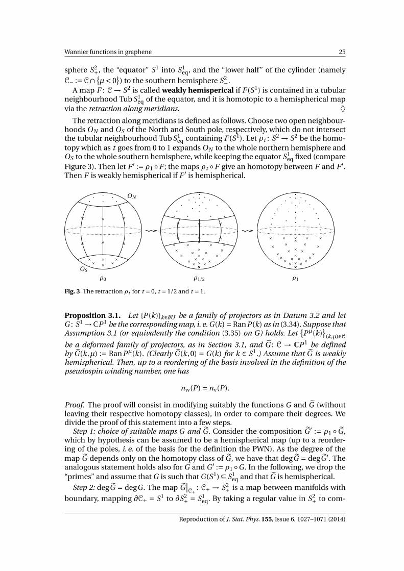
Wannier functions in graphene 25
sphere S2+, the “equator” S1 into S1
eq, and the “lower half” of the cylinder (namelyC− :=C∩
µ< 0) to the southern hemisphere S2
−.A map F : C→ S2 is called weakly hemisperical if F (S1) is contained in a tubular
neighbourhood TubS1eq of the equator, and it is homotopic to a hemispherical map
via the retraction along meridians. ♦
The retraction along meridians is defined as follows. Choose two open neighbour-hoods ON and OS of the North and South pole, respectively, which do not intersectthe tubular neighbourhood TubS1
eq containing F (S1). Let ρt : S2 → S2 be the homo-topy which as t goes from 0 to 1 expands ON to the whole northern hemisphere andOS to the whole southern hemisphere, while keeping the equator S1
eq fixed (compareFigure 3). Then let F ′ := ρ1 F ; the maps ρt F give an homotopy between F and F ′.Then F is weakly hemispherical if F ′ is hemispherical.
ρ0
ON
OS
RR
OO
LL
··
· · ··
××
×× ××
//
ρ1/2
RR
OO
LL
....
..
..
..
.
.
.
..
..
..
. . ..
..
××××
××
××
××
×××××
×××
×
× × ××
××
//
ρ1
....
..
...
..
.
.
.
.
.
.
.
.
.
..
.
.
.
. . ..
.....
×××××××
××
×××
×××××
×××××
× × ×××××
Fig. 3 The retraction ρt for t = 0, t = 1/2 and t = 1.
Proposition 3.1. Let P (k)k∈∂U be a family of projectors as in Datum 3.2 and letG : S1 →CP 1 be the corresponding map, i. e. G(k) = RanP (k) as in (3.34). Suppose thatAssumption 3.1 (or equivalently the condition (3.35) on G) holds. Let
Pµ(k)
(k,µ)∈C
be a deformed family of projectors, as in Section 3.1, and G : C → CP 1 be definedby G(k,µ) := RanPµ(k). (Clearly G(k,0) = G(k) for k ∈ S1.) Assume that G is weaklyhemispherical. Then, up to a reordering of the basis involved in the definition of thepseudospin winding number, one has
nw(P ) = nv(P ).
Proof. The proof will consist in modifying suitably the functions G and G (withoutleaving their respective homotopy classes), in order to compare their degrees. Wedivide the proof of this statement into a few steps.
Step 1: choice of suitable maps G and G . Consider the composition G ′ := ρ1 G ,which by hypothesis can be assumed to be a hemispherical map (up to a reorder-ing of the poles, i. e. of the basis for the definition the PWN). As the degree of themap G depends only on the homotopy class of G , we have that degG = degG ′. Theanalogous statement holds also for G and G ′ := ρ1 G . In the following, we drop the“primes” and assume that G is such that G(S1) ⊆ S1
eq and that G is hemispherical.
Step 2: degG = degG . The map G∣∣C+ : C+ → S2
+ is a map between manifolds with
boundary, mapping ∂C+ = S1 to ∂S2+ = S1
eq. By taking a regular value in S2+ to com-
Reproduction of J. Stat. Phys. 155, Issue 6, 1027–1071 (2014)
26 Domenico Monaco, Gianluca Panati
pute the degree of G , we deduce from our hypotheses (Step 1) that the points in its
preimage all lie in the upper half of the cylinder, so that degG = deg(G
∣∣C+
). On the
other hand, the degree of a map between manifolds with boundary coincides withthe degree of its restriction to the boundaries themselves [9, Theorem 13.2.1]. Weconclude that
degG = deg(G
∣∣C+
)= deg
(G
∣∣∂C+
)= deg
(G
∣∣S1
)= degG
as claimed.Step 3: conclusion. To sum up, putting together Step 1 and Step 2, by (3.36) and
Lemma 3.2 we conclude that
nv =−degG =−degG = nw
and this ends the proof of the Proposition. utFinally, we conclude that nv is intrinsically defined when H=C2. Indeed, the am-
biguity in the choice of the deformation may be removed by choosing a deformationwhich corresponds to a weakly hemispherical map. Then the value of nv is indepen-dent of the choice of a specific deformation among this class, in view of the followingCorollary of the proof.
Corollary 3.1. LetPµ(k)
(k,µ)∈B and Pµ(k)(k,µ)∈B be two deformations of the fam-
ily P (k)k∈R\k0, both corresponding to a weakly hemisperical map with respect to anequator S1
eq ⊂ S2. Then
nv(P ) = nv(P ).
An example of hemispherical deformationPµ(k)
for a family of projectors P (k)
is provided by the canonical models (3.23) and (3.26) of last Subsection, as the readermay easily check. Since the corresponding Hamiltonian Hm(q), as in (3.24) with n =m and e(q) = |q |m , is unitarily conjugated to tight-binding the Hamiltonian (2.12)of m-multilayer graphene, we get that both the eigenspace vorticity and the PWN ofgraphene are equal to m, in accordance with (3.31) and the above Proposition.
As an example of a weakly hemispherical deformation, we can instead considerthe eigenprojectors of the Haldane Hamiltonian, for example for the values of theparameters cited above. By Lemma 3.1, if the values of the parameters (M ,φ) ofHHal(k) are close to those corresponding to the tight-binding Hamiltonian of mono-layer graphene, namely (M ,φ) = (0,0), then its eigenprojectors will also have aneigenspace vorticity equal to 1 in absolute value, in accordance with the numericalevaluation of Remark 3.2.
4 Universality of the canonical models
In this Section, we prove that the local models provided by the projectors (3.23), to-gether with their deformed version (3.26), are universal, meaning the following: if the“outer” eigenspace vorticity of the deformed family of projectors
Pµ
s (k)
is N ∈ Zand if we set nv := sN , with s ∈ +,−, then the nv-canonical projections
Pµ
nv,s(k)
Reproduction of J. Stat. Phys. 155, Issue 6, 1027–1071 (2014)

Wannier functions in graphene 27
will provide an extension of the family, initially defined in B , to the whole B (thenotation is the same of Section 3.1).
More precisely, we will prove the following statement.
Theorem 4.1. Let Ls be the complex line bundle over B defined as in (3.1). Let N ∈Zbe its vorticity around U , defined as in (3.3), and set nv := sN (recall that s ∈ +,−).Then there exists a complex line bundle Ls over B such that
Ls∣∣B 'Ls and Ls
∣∣ C'Pnv,s ,
where Pnv,s is the stratified bundle corresponding to the family of projectors (3.26) forn = nv.
The bundle Ls , appearing in the above statement, allows one to interpolate the“external data” (the bundle Ls) with the canonical model around the singular point(the stratified bundle Pnv,s).
The geometric core of the proof of Theorem 4.1 lies in the following result.
Lemma 4.1. Under the hypotheses of Theorem 4.1, the restriction of the bundles Lsand Pnv,s to the cylindrical surface C are isomorphic:
Ls∣∣C 'Pnv,s
∣∣C.
Proof. The statement follows from the well-known facts that line bundles on anyCW-complex X are completely classified by their first Chern class, living in H 2(X ;Z)(see [45]), and that when X =C' S2 then H 2(C;Z) 'Z, the latter isomorphism beinggiven by integration on C (or, more formally, by evaluation of singular 2-cocycles onthe fundamental class [C] in homology). As a result, one deduces that line bundleson C are classified by their first Chern number. As Ls and Pnv,s have the same Chernnumber, equal to −N , when restricted to the surface C, they are isomorphic. utProof of Theorem 4.1. Vector bundles are given by “gluing” together (trivial) bundlesdefined on open sets covering the base space, so we can expect that we can glue Lsand Pnv,s along C, given that their restrictions on C are isomorphic (as was proved inLemma 4.1). The only difficulty we have to overcome is that C is a closed subset of B .
We argue as follows. Let T be an open tubular neighbourhood of C in B , and let
ρ : T →C be a retraction of T on C. As T ∩C is a deformation retract of C via the map
ρ, we may extend the definition of Ls to T ∩C by letting
Ls∣∣T∩
C
:= ρ∗ (Ls
∣∣C
).
Similarly, we can extend Pnv,s outsideC setting
Pnv,s∣∣T∩B := ρ∗ (
Pnv,s∣∣C
).
With these definitions, one has
(4.1a) Ls∣∣T ' ρ∗ (
Ls∣∣C
)and similarly
Reproduction of J. Stat. Phys. 155, Issue 6, 1027–1071 (2014)

28 Domenico Monaco, Gianluca Panati
(4.1b) Pnv,s∣∣T ' ρ∗ (
Pnv,s∣∣C
).
In fact, let V denote either Ls or Pnv,s . It is known [30, Theorem 14.6] that all complex
line bundles admit a morphism of bundles to UU (1) =(EU (1)
π−→CP∞), the tautolog-
ical bundle8 on CP∞, and that their isomorphism classes are uniquely determinedby the homotopy class of the map between the base spaces. Let
E(V
∣∣T
)
// EU (1)
T
fT // CP∞
and
E(ρ∗ (
V∣∣C
))
// EU (1)
T
fC // CP∞
be those two morphisms of bundles just described; then (4.1a) and (4.1b) will holdas long as we prove that fT and fC are homotopic. Now, the following diagram9
T
ρ
fC //
IdT
""
CP∞
≈C
ι// T
fT
OO
where ι : C ,→ T denotes the inclusion map, is clearly commutative. By definition ofdeformation retract, the maps ιρ and IdT are homotopic: hence
fC = fT ιρ ≈ fT Id = fT
as was to prove.By Lemma 4.1 we have Ls
∣∣C 'Pnv,s
∣∣C, and hence also
ρ∗ (Ls
∣∣C
)' ρ∗ (Pnv,s
∣∣C
).
Equations (4.1a) and (4.1b) thus give
Ls∣∣T 'Pnv,s
∣∣T .
Hence the two line bundles Ls and Pnv,s are isomorphic on the open set T , and thisallows us to glue them. utRemark 4.1 (Families of projectors with many singular points). We concludethis Section with some observations regarding singular families of projectors withmore than one singular point (but still a finite number of them). Denote by S =K1, . . . ,KM ⊂ T∗
2 the set of singular points of the family of rank-1 projectors T∗2 3
8 The infinite complex projective space CP∞ is defined as the inductive limit of the system of canon-ical inclusions CP N ,→ CP N+1; it can be thought of as the space of all lines sitting in some “infinite-dimensional ambient space” C∞. It admits a tautological line bundle with total space
EU (1) := (`, v) ∈CP∞×C∞ : v ∈ ` ,
whose fibre over the line ` ∈CP∞ is the line ` itself, viewed as a copy of C.9 The symbol ≈ denotes homotopy of maps.
Reproduction of J. Stat. Phys. 155, Issue 6, 1027–1071 (2014)
Wannier functions in graphene 29
k 7→ Ps(k); also, pick pair-wise disjoint open balls Ui around Ki (in particular, eachUi contains no singular point other than Ki ). Smoothen Ps(k) into
Pµ
s (k)
as ex-plained in Section 3.1, and compute the M vorticity integers Ni ∈ Z as in (3.3); thisinvolves the choice of a smoothing parameter µ ∈ [−µ0,µ0], and for simplicity wechoose the same sufficiently small µ0 > 0 for all singular points. Call Ls the linebundle associated to such smoothed family of projectors; it is a vector bundle over(T∗
2 × [−µ0,µ0])
\⋃M
i=1 Ci , where Ci :=Ui ×(−µ0,µ0). The above arguments now show
that we can find a bundle Ls , defined on(T∗
2 × [−µ0,µ0])
\(S × µ= 0
), such that
Ls resticts to Ls whenever the latter is defined, while it coincides with Pn(i )v ,s on(
Ui × [−µ0,µ0])
\(
k = Ki ,µ= 0)
, where n(i )v := sNi . Thus, deformations of families
of rank-1 singular projectors with M singular points are uniquely determined by M-tuples of integers, their local vorticities. ♦
5 Decrease of Wannier functions in graphene
In this Section, we will use the n-canonical eigenvectors φn,±(q), that were explicitlycomputed via the canonical models presented in Section , to extract the rate of decayof the Wannier functions of graphene. Actually, we can prove a more general result,under the following
Assumption 5.1. We consider a periodic Schrödinger operator, i. e. an operator inthe form HΓ = −∆+VΓ, acting in L2(R2), where VΓ is real-valued, ∆-bounded withrelative bound zero, and periodic with respect to a lattice Γ ⊂ R2. For a Bloch bandEs of HΓ, we assume that:
(i ) Es intersects the Bloch band Es−110 at finitely many points K1, . . . ,KM , i. e.
Es(k0) = Es−1(k0) =: E0 for every k0 ∈ K1, . . . ,KM ;(i i ) for every k0 ∈ K1, . . . ,KM there exist constants r, v+, v− > 0 and m ∈ 1,2,
possibly depending on k0, such that for |q | < r
(5.1)Es(k0 +q)−E0 = v+|q|m +O(|q |m+1),
Es−1(k0 +q)−E0 =−v−|q|m +O(|q|m+1);
(i i i ) the following semi-gap condition holds true:
infk∈T∗
2
|Es(k)−Ei (k)| : i 6= s, i 6= s −1 =: g > 0;
(i v) the dimension of the eigenspace corresponding to the eigenvalue Es(k) (resp.Es−1(k)) is 1 for every k ∈T∗
2 \ K1, . . . ,KM ;(v) there exists a deformation Hµ(k) of the fibre Hamiltonian H(k), as in (2.1),
such that, if P∗(k) denotes the spectral projection of H(k) onto the eigenval-ues Es(k),Es−1(k), then for all k0 ∈ K1, . . . ,KM the operator P∗(k0)Hµ(k)P∗(k0)is close, in the norm-resolvent sense, to11 P∗(k0)Hµ
m(k)P∗(k0), where Hµm(k)
10 All the following statements remain true, with only minor modifications in the proofs, if Es−1 isreplaced by Es+1.11 With abuse of notation, we denote
Reproduction of J. Stat. Phys. 155, Issue 6, 1027–1071 (2014)

30 Domenico Monaco, Gianluca Panati
is as in (3.25) with n = m and e(q) = |q|m , for the same m as in item ((i i )) anduniformly for |k −k0| < r and µ ∈ [−µ0,µ0].
♦
Condition ((i )) corresponds to considering a semimetallic solid. Condition ((i i ))characterises the local behaviour of the eigenvalues; while some of our results holdtrue for any m ∈ N×, we need the assumption m ∈ 1,2 in order to prove Theorem5.2. Condition ((i i i )) guarantees that the Bloch bands not involved in the relevantintersection do not interfere with the local structure of the eigenprojectors. Con-dition ((i v)) excludes permanent degeneracy of the eigenvalues. Lastly, condition((v)) corresponds to the assumption that the tight-binding Hamiltonian Hµ
m(k) isan accurate approximation, in the norm-resolvent sense, of the original continuousHamiltonian. Notice that we crucially assume d = 2.
It is usually accepted that Assumption 5.1 holds true for (monolayer and bilayer)graphene (with M = 2), since conditions ((i )), ((i i )) and ((i i i )) can be explicitlychecked to hold within the tight-binding approximation, and these conditions areexpected to be stable under approximations. Recently, C. Fefferman and M. Wein-stein [11] provided sufficient conditions on VΓ yielding (i) and (ii) with m = 1. Here-after, the indices s, s −1 will be replaced by +,− to streamline the notation.
We recall that the Wannier function depends on a choice of the phase for the Blochfunction ψ+ (or, equivalently, its periodic part u+) according to the following defini-tion.
Definition 5.1. The Wannier function w+ ∈ L2(R2) corresponding to the Blochfunction ψ+ for the Bloch band E+ is
(5.2) w+(x) := 1
|B|1/2
∫B
dkψ+(k, x) = 1
|B|1/2
∫B
dk eik·xu+(k, [x])
where B is the fundamental unit cell for Γ∗, and [x] = x mod Γ. ♦
Thus w+ is nothing but the Bloch-Floquet anti-transform of the Bloch function ψ+(see Section 2.1). Recall also that the decay rate of the Wannier function as |x| →∞is related to the regularity of the corresponding Bloch function, see e. g. [23, Section2.2] or [35, Equation (2.5)]. In particular, if the Bloch function can be chosen to beC∞-smooth, then the associated Wannier function decays at infinity faster than theinverse of any polynomial.
Since the Wannier function is defined by integration over B, the smoothness ofk 7→ ψ+(k, ·) can be analysed separately in different regions of the Brillouin zone.The problem is therefore reduced to a local analysis of the Bloch functions aroundthe intersection points, as detailed in the next Subsection.
P∗(k0)Hµm(k)P∗(k0) :=
∑a,b∈s,s−1
|ua(k0)⟩(Hµm(k)
)a,b ⟨ub(k0)|
with respect to an orthonormal basis us (k0),us−1(k0) of RanP∗(k0).
Reproduction of J. Stat. Phys. 155, Issue 6, 1027–1071 (2014)

Wannier functions in graphene 31
5.1 Reduction to a local problem around the intersection points
First, notice that the Bloch function relative to the Bloch band E+ is unique, up tothe choice of a k-dependent phase: we assume that such a choice has been per-formed12, and denote the corresponding Bloch function by ψ+(k). Now, let U =Uk0 := k ∈B : |k −k0| < r be the neighbourhood of the intersection point k0 ∈ K1, . . . ,KM for which expansion (5.1) holds, and let χU (k) be a smoothed characteristic functionfor U , namely a smooth function supported in U which is identically 1 on a smallerdisc D ⊂U of radius ρ < r . We assume that such smoothed characteristic functionsare radially symmetric, i. e. χU (k0 + q) = χ(|q |). Then the Bloch function ψ+ may bewritten as
ψ+(k) =M∑
i=1χUKi
(k)ψ+(k)+(
1−M∑
i=1χUKi
(k)
)ψ+(k).
The summands in the first term, call them ψU (k) = ψUKi(k), contain all the infor-
mation regarding the crossing of the two energy bands at the points in K1, . . . ,KM .On the other hand, since the Bloch bands intersect only at these points (Assump-tion 5.1((i ))), then the last term, call it ψ(k), can be assumed to be smooth. As theWannier transform (5.2) is linear, the Wannier function w+(x) corresponding to theBloch function ψ+(k) via (5.2) splits as
w+(x) =M∑
i=1wUKi
(x)+ w(x)
with an obvious meaning of the notation. In the next Subsection we will prove (seeTheorem 5.1) that each of the functions wUKi
has a power-law decay at infinity. More-over, since k 7→ ψ(k) is smooth, we can make the reminder term w decay as fast asthe inverse of a polynomial of arbitrary degree, by choosing χ sufficiently regular.Consequently we get that the asymptotic behaviour of the true Wannier function w+is determined by that of the functions wUKi
.In the following, we will concentrate on one intersection point k0 ∈ K1, . . . ,KM ,
and calculate the rate of decay at infinity of the function wU . Let us also notice that,for reasons similar to the above, the behaviour of wU at infinity does not dependon the particular choice of the cutoff function χU , provided it is sufficiently regular.Indeed, if χU and χ′U are two different cutoffs, both satisfying the above conditions,then their difference χ′′U := χU −χ′U is supported away from the intersection point k0.This means that the corresponding ψ′′
U (k) = χ′′U (k)ψ+(k) is regular, and this in turnimplies that w ′′
U decays fast at infinity. For this reason, we are allowed to choose asimple form for the function χU : in particular, we will choose χ(|q |) to be polynomialin |q| (of sufficiently high degree N ) for |q| ∈ (ρ,r ), i. e.
(5.3) χ(|q |) =
1 if 0 ≤ |q | ≤ ρ,N∑
i=0αi |q |i if ρ < |q| < r,
0 if |q| ≥ r.
12 The decay rate at infinity of Wannier functions may a priori depend on such a choice, but this doesnot happen provided the change of phase is sufficiently smooth, as detailed in Remark 5.1.
Reproduction of J. Stat. Phys. 155, Issue 6, 1027–1071 (2014)

32 Domenico Monaco, Gianluca Panati
The coefficients αi are chosen in order to guarantee that χ is as smooth as required.In particular, having χ ∈C p ([0,+∞)) requires N ≥ 2p −1.
5.2 Asymptotic decrease of the n-canonical Wannier function
We proceed to determine the rate of decay of wU , extracting it from the modelswhich were illustrated in Section 3.2. Clearly
(5.4) wU (x) = 1
|B|1/2
∫B
dkψU (k, x) = 1
|B|1/2
∫U
dk eik·x χU (k)u+(k, [x]).
We claim that its asymptotic behaviour is the same as that of the n-canonical Wan-nier function
(5.5) wcan(x) := 1
|B|1/2
∫U
dk eik·x χU (k)φn(k, [x]) = eik0·x
|B|1/2
∫U
dq eiq ·x χ(|q|)φn(q, [x])
where n is the vorticity of the family of projectorsPµ+(k)
k∈R\k0,µ∈[−µ0,µ0] corre-
sponding to the deformed fibre Hamiltonian Hµ(k), as in Assumption 5.1((v)) (hereR ⊂ B is a contractible region containing U but not intersecting any of the chosenballs centered at the other intersection points), and
(5.6) φn(q, [x]) :=φn,+(q)1 u+(k0, [x])+φn,+(q)2 u−(k0, [x])
with φn,+(q) = (φn,+(q)1,φn,+(q)2
)as in (3.22). We will motivate why the vorticity of
Pµ+(k)
is non-zero in Subsection . To prove this claim, we will establish the following
two main results of this Section.
Theorem 5.1. Let wcan be the n-canonical Wannier function defined as in (5.5), withn 6= 0. Then there exist two positive constants R,c > 0 such that
(5.7) |wcan(x)| ≤ c
|x|2 if |x| ≥ R.
The proof of the previous Theorem is postponed to Subsection .While the proof of Theorem 5.1 does not require restrictions on the value of m in
Assumption 5.1((i i )), it is crucial that m ∈ 1,2 for the techniques employed in ourproof of Theorem 5.2. In the following we will denote by |X |α the operator acting ona suitable domain in L2(R2) by (|X |αw) (x) := |x|αw(x).
Theorem 5.2. There exists a choice of the Bloch function ψ+ such that the followingholds: For wU and wcan defined as in (5.4) and (5.5), respectively, and m ∈ 1,2 as inEquation (5.1), one has
|X |s (wU −wcan) ∈ L2(R2)
for s ≥ 0 depending on m as follows:
• if m = 1, for all s < 2;• if m = 2, for all s < 1.
Reproduction of J. Stat. Phys. 155, Issue 6, 1027–1071 (2014)

Wannier functions in graphene 33
The proof of the previous Theorem is postponed to Subsection .By combining the above two Theorems with the fact that the decay at infinity of
the true Wannier function w+ is equal to the one of wU , as was shown in the previousSubsection, we deduce at once the following
Theorem 5.3. Consider an operator HΓ =−∆+VΓ acting in L2(R2) and a Bloch bandEs satisfying Assumption 5.1. Then there exists a choice of the Bloch function relative tothe Bloch band Es such that the corresponding Wannier function w+ ∈ L2(R2) satisfiesthe following L2-decay condition:
(5.8) |X |αw+ ∈ L2(R2) for every 0 ≤α< 1.
Proof. Fix 0 ≤α< 1. The L2-norm of the function |X |αw+ can be estimated by
∥∥|X |αw+∥∥2
L2(R2) =∫R2
dx |x|2α|w+(x)|2 ≤
≤∫R2
dx |x|2α|w+(x)−wcan(x)|2 +∫R2
dx |x|2α|wcan(x)|2.(5.9)
In order to give a bound to the first integral, we use the result of Theorem 5.2.Firstly we write∫
R2dx |x|2α|w+(x)−wcan(x)|2 =
∫D1
dx |x|2α|w+(x)−wcan(x)|2+
+∫R2\D1
dx |x|2α|w+(x)−wcan(x)|2
where D1 ⊂ R2 is the ball of radius 1 around the origin. The first term on the right-hand side of the above equality is finite, because the function w+−wcan is in L2(R2)(hence a fortiori in L2(D1)) and |x|2α ≤ 1 for x ∈ D1. For x ∈ R2 \ D1 and α ∈ [0,1), byTheorem 5.2 we conclude that∫
R2\D1
dx |x|2α|w+(x)−wcan(x)|2 ≤∥∥|X |α (w+−wcan)
∥∥2L2(R2)
is finite.To show that also the second summand in (5.9) is finite, we use instead Theorem
5.1. Write∫R2
dx|x|2α |wcan(x)|2 =∫
DR
dx|x|2α |wcan(x)|2 +∫R2\DR
dx|x|2α |wcan(x)|2 .
Again by the fact that the Wannier function wcan is in L2(R2), it follows that the firstintegral on the right-hand side is finite. As for the second summand, we use the esti-mate provided by Equation (5.7); thus we have
(5.10)∫R2\DR
dx|x|2α |wcan(x)|2 ≤ const ·∫ ∞
Rd|x| |x| |x|2α |x|−4
and this last integral is convergent if and only if α< 1. ut
Reproduction of J. Stat. Phys. 155, Issue 6, 1027–1071 (2014)

34 Domenico Monaco, Gianluca Panati
Proof of Theorem 5.1
We proceed to the proof of Theorem 5.1, establishing the rate of decay at infinity ofthe n-canonical Wannier function wcan (corresponding to the n-canonical eigen-vector for an eigenvalue crossing). For later convenience, we will prove a slightlymore general result, concerning the Wannier function associated to a Bloch func-tion which is obtained from the n-canonical eigenvector by multiplication times q j ,j ∈ 1,2.
Proposition 5.1. Define
wn,p (x) := eik0·x
|B|1/2
∫U
dq eiq·x q pj χ(|q|)φn(q, [x])
where j ∈ 1,2, p ∈ 0,1, and φn(q, [x]) is as in (5.6). Then there exist two positiveconstants R,c > 0 such that∣∣wn,p (x)
∣∣≤ c
|x|p+2for |x| ≥ R.
Notice that the exponent in the power-law asymptotics for wn,p is independenton n (but the prefactor c will depend on it, as will be apparent from the proof). Thestatement of Theorem 5.1 regarding the decay rate of wcan is a particular case of theabove, namely when p = 0.
Proof. For notational simplicity, we set j = 1, the case j = 2 being clearly analogous.Without loss of generality, we also assume that n > 0. We choose Cartesian coordi-nates in R2 such that x = (0, |x|), and consequently q · x =−2π|q | |x|sinθq . Since then-canonical eigenfunction is
φn,+(q) = einθq /2(cos(nθq /2)sin(nθq /2)
),
we can write
(5.11) wn,p (x) = eik0·x
|B|1/2
[wcos,p (x)u+(k0, [x])+wsin,p (x)u−(k0, [x])
]where
wcos,p (x) :=∫ r
0d|q| |q |p+1χ(|q|)
∫ 2π
0dθq e−i2π|q| |x|sinθq cos(θq )p einθq /2 cos
(n
2θq
),
wsin,p (x) :=∫ r
0d|q| |q |p+1χ(|q|)
∫ 2π
0dθq e−i2π|q| |x|sinθq cos(θq )p einθq /2 sin
(n
2θq
).
The function x 7→ u±(k0, [x]) is Γ-periodic, and as a consequence of its definition(2.2) it is in the Sobolev space W 2,2(T2
Y ), hence continuous; consequently, it is abounded function. Thus, the upper bound on
∣∣wn,p∣∣ is completely determined by
that on the functions wcos,p and wsin,p .Notice that for p ∈ 0,1
Reproduction of J. Stat. Phys. 155, Issue 6, 1027–1071 (2014)

Wannier functions in graphene 35
cos(θq )p einθq /2 cos(n
2θq
)= 1
4
(ei(n+p)θq +ei(n−p)θq +eipθq +e−ipθq
),
cos(θq )p einθq /2 sin(n
2θq
)= 1
4i
(ei(n+p)θq +ei(n−p)θq −eipθq −e−ipθq
),
so that we can write
wcos,p (x) = 1
4
(In+p,p (|x|)+ In−p,p (|x|)+ Ip,p (|x|)+ I−p,p (|x|)) ,
wsin,p (x) = 1
4i
(In+p,p (|x|)+ In−p,p (|x|)− Ip,p (|x|)− I−p,p (|x|)) ,
where
I`,p (|x|) :=∫ r
0d|q| |q |p+1χ(|q|)
∫ 2π
0dθq ei(`θq−2π|q| |x|sinθq ) =
= 1
(2π|x|)p+2
∫ 2πr |x|
0dz zp+1χ
(z
2π|x|
)∫ 2π
0dθq ei(`θq−z sinθq ),
with the change of variables z = 2π|q| |x|.Now, by definition [26]
(5.12)1
2π
∫ 2π
0dθq ei(`θq−z sinθq ) = 1
2π
∫ 2π
0dθq cos
(`θq − z sinθq
)=: J`(z)
is the Bessel function of order `: thus, the functions wcos,p and wsin,p are combina-tions of integrals of the Bessel functions, which explicitly look like
I`,p (|x|) = 1
(2π)p+1|x|−p−2
∫ 2πr |x|
0dz zp+1χ
(z
2π|x|
)J`(z).
In order to evaluate these integrals and establish their asymptotic properties, wesplit
I`,p (|x|) = I (1)`,p (|x|)+ I (2)
`,p (|x|),
where
I (1)`,p (|x|) := 1
(2π)p+1|x|−p−2
∫ 2πρ|x|
0dz zp+1 J`(z),
I (2)`,p (|x|) := 1
(2π)p+1|x|−p−2
∫ 2πr |x|
2πρ|x|dz zp+1χ
(z
2π|x|
)J`(z).
Notice that the function χ does not appear in the integral I (1)`,p , since it is constantly
equal to 1 for 0 ≤ |q| < ρ (compare (5.3)).We now use the fact [26, Sec. 2.5, Eqn. (6)] that for large real t →∞
∫ t
0dz zµ Jν(z) =
2µΓ(ν+µ+1
2
)Γ
(ν−µ+1
2
) −(
2
πt
)1/2
tµh(t ),
Reproduction of J. Stat. Phys. 155, Issue 6, 1027–1071 (2014)

36 Domenico Monaco, Gianluca Panati
whenever ℜ(ν+µ) >−1, where h(t ) = f (t )cosθ(t )+ g (t )sinθ(t ) with
θ(t ) = t −νπ2+ π
4, f (t ) = 1+O(t−2), g (t ) =O(t−1).
This allows to immediately compute the asymptotic rate of I (1)`,p (|x|):
I (1)`,p (|x|) =
2p+1Γ(`+p+2
2
)Γ
(`−p
2
) 1
(2π)p+1|x|−p−2−
− 1
(2π)p+1|x|−p−2
(2
π ·2πρ|x|
)1/2
(2πρ|x|)p+1h(2πρ|x|) =
=Γ
(`+p+2
2
)Γ
(`−p
2
)πp+1
|x|−p−2 − ρp+(1/2)
π|x|−3/2h(2πρ|x|).
We now compute also the asymptotics of I (2)`,p (|x|) for large |x|. We use the explicit
polynomial form (5.3) for the cutoff function χ in the interval (ρ,r ), thus obtaining
I (2)`,p (|x|) = 1
(2π)p+1|x|−p−2
(∫ 2πr |x|
0−
∫ 2πρ|x|
0
)dz zp+1
(N∑
i=0αi
zi
(2π|x|)i
)J`(z) =
= 2πN∑
i=0
αi
(2π|x|)p+i+2
(∫ 2πr |x|
0−
∫ 2πρ|x|
0
)dz zp+i+1 J`(z) =
= 2πN∑
i=0
αi
(2π|x|)p+i+2
[−
(2
π ·2πr |x|
)1/2
(2πr |x|)p+i+1h(2πr |x|)− (r ↔ ρ)
]=
= r p+(1/2)
π
(−
N∑i=0
αi r i
)|x|−3/2h(2πr |x|)+ ρp+(1/2)
π
(N∑
i=0αi ρ
i
)|x|−3/2h(2πρ|x|) =
= ρp+(1/2)
π|x|−3/2h(2πρ|x|)
where in the last equality we used the fact that χ(ρ) = 1 and χ(r ) = 0.From these computations, we deduce that13
I`,p (|x|) =Γ
(`+p+2
2
)Γ
(`−p
2
)πp+1
|x|−p−2 +O(|x|−p− j ) for all j ∈N×.
13 The prefactor can be computed using the factorial relation Γ(z +1) = zΓ(z): one obtains
Γ(`+p+2
2
)Γ
(`−p
2
)πp+1
=
`
2πif p = 0,
`2 −1
4π2 if p = 1.
Reproduction of J. Stat. Phys. 155, Issue 6, 1027–1071 (2014)

Wannier functions in graphene 37
We conclude that the upper bound on the rate of decay at infinity of both wcos,pand wsin,p (and hence that of the Wannier functions wn,p ) is given by a multiple of|x|−p−2, for both p = 0 and p = 1 and independently of n ∈Z. ut
Notice that with the above proof we actually have a stronger control on the asymp-totic behaviour of the function wn,p than what stated in Proposition 5.1: Indeed,from (5.11) we see that wn,p is a combination of functions which behave asymptoti-cally as |x|−p−2 (up to arbitrarily higher order terms), times a Γ-periodic function ofx.
5.3 Asymptotic decrease of the true Wannier function
In this Subsection, we will prove Theorem 5.2. The importance of this result lies inthe fact that we can deduce from it an upper bound on the decay rate at infinityof the true Wannier function in the continuous model of (monolayer and bilayer)graphene, as in Theorem 5.3. Indeed, what we will show in the following is that all thesingularity of the Bloch function u+(k) ∈Hf at the intersection point k0 is encodedin its components along the vectors u+(k0) and u−(k0) in Hf. This is essentially aconsequence of Assumption 5.1((i i i )), namely of the fact that all Bloch bands notinvolved in the intersection at k0 are well separated from the intersecting ones.
True Bloch bundle vs. stratified Bloch bundle
Let us briefly summarise the geometric results of Section 4, in order to specify themto the case under study; we will use all the notation of that Section. Assume thatr > 0 is so small that the ball of radius 2r is all contained in R. Denote as above byP+(k) := |u+(k)⟩⟨u+(k)|k∈R\k0 the family of projectors corresponding to the Blochband E+; we use it as our Datum 3.1, so we smoothen it via a parameter µ ∈ [−µ0,µ0]and calculate the vorticity n ∈Z using the eigenprojectors of the deformation Hµ(k)appearing in Assumption 5.1((v)). Theorem 4.1 then establishes the existence of avector bundle L on B such that:
• outside of a cylinder C ′ of radius r + r ′ < 2r centered at the singular point (k =k0,µ= 0), the bundle L coincides with the bundle L+, which is associated to thesmoothed family of projectors
Pµ+(k)
;
• inside a smaller pointed cylinderC 1 of radius r1 := r − r ′ > 0 centered at the sin-
gular point (k = k0,µ= 0), the bundle L coincides with the n-canonical stratifiedBloch bundle Pn =Pn,+;
• inside the tubular neighbourhood T of width r ′ of the cylindrical surface C= ∂C ,the bundle L is constructed extending the isomorphism of Hermitian bundles
(5.13) L+∣∣C 'Pn
∣∣C
(see Lemma 4.1).
On the other hand, asC is a deformation retract of C, the isomorphism (5.13) ex-
tends to an isomorphism
Reproduction of J. Stat. Phys. 155, Issue 6, 1027–1071 (2014)
38 Domenico Monaco, Gianluca Panati
(5.14) L+∣∣ C'Pn
∣∣ C
which, together with the first items of the list above, allows us to conclude that thebundle L constructed via Theorem 4.1 is isomorphic to the Bloch bundle L+ as bun-dles on the whole B .
We now want to translate the information contained in the latter isomorphismin terms of the associated families of projectors, and of the “sections” of these bun-dles (i. e. Bloch functions). In order to do so, we first show that the vorticity n ofthe family P+(k) equals m ∈ 1,2 as in Assumption 5.1((i i )), so that in particu-lar it is non-zero. Indeed, consider the deformation Hµ(k) of the fibre HamiltonianH(k) = (−i∇y + k)2 +VΓ(y), as in Assumption 5.1((v)), and a circle Λ∗ in the com-plex plane enclosing only the eigenvalues
Eµ+(k),Eµ
−(k)
for |k−k0| andµ sufficientlysmall. Then the Riesz integral
Pµ∗ (k) := i
2π
∮Λ∗
dz(Hµ(k)− z1l
)−1
defines a smooth family of projectors over C = U × (−µ0,µ0) (see [35, Prop. 2.1] fora detailed proof), such that Pµ=0
∗ (k) = P∗(k). By using again the Riesz formula witha different contour Λµ(k) enclosing only the eigenvalue Eµ
+(k) (compare the proofof Proposition 5.2 below), we can realise Pµ
+(k) as a subprojector of Pµ∗ (k). Denoting
Π := P∗(k0), we then have∥∥ΠPµ+(k)Π − ΠPµ
m,+(k)Π∥∥B(Hf)
=∥∥Pµ
+(k)−Pµm,+(k)
∥∥B(RanΠ) =
=∥∥∥∥ i
2π
∮Λµ(k)
dz[(
Hµ(k)− z1l)−1 − (
Hµm(k)− z1l
)−1]∥∥∥∥
B(RanΠ)=
≤ 1
2π|Λµ(k)|
∥∥∥(Hµ(k)− z1l
)−1 − (Hµ
m(k)− z1l)−1
∥∥∥B(RanΠ)
where Hm(k) is as in (3.25) (with n = m and e(q) = |q |m) and Pµm,+(q) is its eigen-
projector. The norm on the right-hand side of the above inequality is uniformlybounded by Assumption 5.1((v)), say by δ > 0, and the length of the circle Λµ(k)can be made to shrink as |q|m when |q|→ 0. Thus we deduce that
(5.15)∥∥Pµ
+(k)−Pµn,+(k)
∥∥B(RanΠ) ≤ const|q|mδ,
and the right-hand side of the above inequality can be made smaller than 1. ByLemma 3.1, we then have
nv(P+) = nv(Pm,+) = m ∈ 1,2
by Assumption 5.1((i i )).The above estimate gives the existence of a Kato-Nagy unitary V µ(k), as in (3.7),
such thatΠPµ
+(k)Π=V µ(k)Pµm,+(k)V µ(k)−1.
This can be restated in terms of the existence of a Bloch function uµ+ (i. e. an eigen-
function of Pµ+) such that
Reproduction of J. Stat. Phys. 155, Issue 6, 1027–1071 (2014)
Wannier functions in graphene 39
(5.16) Πuµ+(k) =V µ(k)φµn(k) for (k,µ) ∈
C ,
whereφµn(q, [x]) :=φµm,+(q)1 u+(k0, [x])+φµm,+(q)2 u−(k0, [x])
with φµm,+(q) = (φµm,+(q)1,φµm,+(q)2
)as in (3.16). Moreover, combining the definition
(3.7) of V µ(k) and the estimate (5.15), one easily checks that V µ(k) actually extendssmoothly to the whole cylinder C , in particular at (k = k0,µ= 0).
We restrict our attention to the slice µ = 0. Denote by weff the Wannier functionassociated via (5.2) to U 3 k 7→ Πu+(k) =: ueff(k). Arguing as in Section 5.1, one de-duces that the asymptotic decay of weff is determined by the integration of ueff on Uin (5.2). Then the equality (5.16) implies that
|B|1/2weff(x) ³∫
Udq eiq ·x χ(|q|)Πu+(k0 +q, [x]) =
=∑
b∈+,−
[∫U
dq eiq·x( ∑
a∈1,2V (k0 +q)a,b χ(|q|)φm,+(q, [x])a
)]ub(k0, [x]).
As was already noticed, the functions u±(k0, ·) do not contribute to the decay at in-finity of weff. On the other hand, by Taylor expansion at k0 we can write
(5.17) V (k0 +q)a,b =V (k0)a,b +2∑
j=1q j
∂V
∂q j(k0)a,b +
2∑j ,`=1
q j q`R j ,`(q)
where the remainder R j ,` is C∞-smooth on U . Consequently, we get(5.18)∫
Udq eiq·xV (k0 +q)a,b χ(|q|)φm,+(q, [x])a =V (k0)a,b
(∫U
dq eiq·x χ(|q|)φm,+(q, [x])a
)+
+2∑
j=1
∂V
∂q j(k0)a,b
(∫U
dq eiq·x q j χ(|q |)φm,+(q, [x])a
)+
+2∑
j ,`=1
∫U
dq eiq·x q j ql R j ,`(q)χ(|q|)φm,+(q, [x])a .
The terms in brackets in the first and second summand have already been esti-mated in Proposition 5.1, and so are known to produce the rate of decay at infinity of|x|−2 and |x|−3, respectively. As for the third summand, we preliminarly notice thatthe function
S(q) := q j ql R j ,`(q)χ(|q |)φm,+(q, [x])a
is in W 2,∞(U ). Indeed, the map q 7→ R j ,`(q)χ(|q |) is smooth and bounded, while forall r, s ∈ 1,2
∂2
∂qr∂qs
(q j q`φm,+(q, [x])a
)is in L∞(U ), since φm,+(q, [x])a is homogeneous of order zero in q .We can now proceed to an integration by parts: observe in fact that
Reproduction of J. Stat. Phys. 155, Issue 6, 1027–1071 (2014)

40 Domenico Monaco, Gianluca Panati
−xr xs
∫U
dq eiq·x S(q) =∫
Udq
∂2
∂qr∂qs
(eiq·x)
S(q) =
=∫
Udq eiq·x ∂2S
∂qr∂qs(q).
The boundary terms vanish because χ is zero on ∂U . By what we have shown above,we obtain that ∣∣∣∣xr xs
∫U
dq eiq·x S(q)
∣∣∣∣≤ |U |∥∥∥∥ ∂2S
∂qr∂qs
∥∥∥∥∞<+∞,
so that the third summand in (5.18) decays faster than |x|−2 at infinity. We concludethat the asymptotic behaviour of weff is that of |x|−2.
Remark 5.1 (Invariance of the decay rate of Wannier functions). Given Theo-rem 5.2, whose proof will be completed in the next Subsection, the above argu-ment shows also that the decay rate of the Wannier function w+ is not affected bya change of phase in the corresponding Bloch function ψ+, provided the phase isat least of class C 2. Indeed, we already know that the decay rate of w+ dependsonly on the local behaviour of ψ+ around the intersection point. The exchange ofψ+(k) with eiθ(k)ψ+(k), for k ∈U , is then equivalent to the exchange of φm,+(k) witheiθ(k)φm,+(k). This exchange is implemented by the action of the unitary diagonaloperator V (k) = eiθ(k)1l ∈ U (2): if the dependence of θ(k) on k ∈ U is C 2, then it ispossible to perform a Taylor expansion as in (5.17), so that the above argument ap-plies. ♦
Proof of Theorem 5.2
Finally, we proceed to show that the decay of weff, the Wannier function correspond-ing to Πu+(k), and of wU , the Wannier function corresponding to the restriction toU of u+(k), are the same. This is achieved by showing that their difference, which isthe Wannier function associated to (1l−Π)u+(k) =: urem(k), decays sufficiently fastat infinity (i. e. at least faster than |x|−2); this in turn will be proved by showing thaturem(k) is sufficiently smooth, say of class W s,2 for some positive s. Indeed, in viewof the results relating regularity of Bloch functions and asymptotic properties of thecorresponding Wannier functions (compare [35, Equation (2.5)]), we have that
(5.19) if urem ∈W s,2(U ;Hf) then |X |s (wU −weff) ∈ L2(R2).
Before establishing the Sobolev regularity of urem, we need to prove some esti-mates on the derivatives of the projector P+(k), and correspondingly on those of theBloch function u+(k).
Proposition 5.2. Let P+(k)k∈
U
be the family of eigenprojectors for the Hamiltonian
HΓ =−∆+VΓ as in Assumption 5.1. Let m ∈ 1,2 be as in (5.1). Then, for all choices ofmulti-indices I ∈ 1,2N , N ∈N, there exists a constant CN > 0 such that
(5.20)∥∥∂N
I P+(k)∥∥B(Hf)
≤ CN
|q |N mfor all k = k0 +q, 0 < |q| < r.
Reproduction of J. Stat. Phys. 155, Issue 6, 1027–1071 (2014)
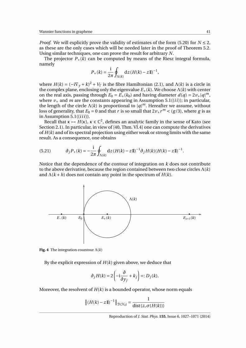
Wannier functions in graphene 41
Proof. We will explicitly prove the validity of estimates of the form (5.20) for N ≤ 2,as these are the only cases which will be needed later in the proof of Theorem 5.2.Using similar techniques, one can prove the result for arbitrary N .
The projector P+(k) can be computed by means of the Riesz integral formula,namely
P+(k) = i
2π
∮Λ(k)
dz (H(k)− z1l)−1,
where H(k) = (−i∇y +k)2 +VΓ is the fibre Hamiltonian (2.1), and Λ(k) is a circle inthe complex plane, enclosing only the eigenvalue E+(k). We chooseΛ(k) with centeron the real axis, passing through E0 = E+(k0) and having diameter d(q) = 2v+|q |m ,where v+ and m are the constants appearing in Assumption 5.1((i i )); in particular,the length of the circle Λ(k) is proportional to |q |m . Hereafter we assume, withoutloss of generality, that E0 = 0 and that r is so small that 2v+r m < (g /3), where g is asin Assumption 5.1((i i i )).
Recall that κ 7→ H(κ), κ ∈ C2, defines an analytic family in the sense of Kato (seeSection 2.1). In particular, in view of [40, Thm. VI.4] one can compute the derivativesof H(k) and of its spectral projection using either weak or strong limits with the sameresult. As a consequence, one obtains
(5.21) ∂ j P+(k) =− i
2π
∮Λ(k)
dz (H(k)− z1l)−1∂ j H(k)(H(k)− z1l)−1.
Notice that the dependence of the contour of integration on k does not contributeto the above derivative, because the region contained between two close circlesΛ(k)and Λ(k +h) does not contain any point in the spectrum of H(k).
OO
//• •E0 E+(k)
Λ(k)
•E−(k)
•Es+1(k)
Fig. 4 The integration countour Λ(k)
By the explicit expression of H(k) given above, we deduce that
∂ j H(k) = 2
(−i
∂
∂y j+k j
)=: D j (k).
Moreover, the resolvent of H(k) is a bounded operator, whose norm equals
∥∥(H(k)− z1l)−1∥∥B(Hf)
= 1
dist(z,σ(H(k)))
Reproduction of J. Stat. Phys. 155, Issue 6, 1027–1071 (2014)
42 Domenico Monaco, Gianluca Panati
whereσ(H(k)) is the spectrum of the fibre Hamiltonian. As z runs on the circleΛ(k),the distance on the right-hand side of the above equality is minimal when z is real,and the minimum is attained at the closest eigenvalue of H(k), namely the selectedBloch band E+(k) or the eigenvalue E−(k). By Assumption 5.1((i i )), we conclude inboth cases that
(5.22)∥∥(H(k)− z1l)−1
∥∥B(Hf)
≤ c
|q|m
for some constant c > 0. In order to go further in our estimate, we need the followingresult.
Lemma 5.1. There exists a constant C > 0 such that∥∥∂ j H(k)(H(k)− z1l)−1∥∥B(Hf)
≤ C
|q |m
uniformly in z ∈Λ(k), for any k ∈
U .
Remark 5.2. Notice that the operator ∂ j H(k)(H(k)−z1l)−1 is indeed a bounded op-erator on Hf. This is because the range of the resolvent (H(k)− z1l)−1 is the domainD=W 2,2(T2
Y ) of H(k), and k 7→ H(k) is strongly differentiable, so that ∂ j H(k) is well-defined on D. ♦
Proof of Lemma 5.1. We recall [41, Chap. XII, Problem 11] that, if H0 is a self-adjointoperator and V ,W are symmetric, then
(5.23) W << H0 and V << H0 =⇒ W << H0 +V ,
where the notation B << A means that B is A-bounded with relative bound zero.Since i∂/∂y j <<−∆ and VΓ <<−∆ by Assumption 5.1, by iterating (5.23) we obtain
i∂
∂y j<<−∆+2ik ·∇y +|k|21l+VΓ = H(k),
so that D j (k) << H(k). By definition of relative boundedness, this means that for anya > 0 there exists b > 0 such that
‖D j (k)ψ‖2 ≤ a2‖H(k)ψ‖2 +b2‖ψ‖2
for any ψ in the domain of H(k).Fix a > 0. Then, by [2, Lemma 2.40 and Eqn. (2.110)], if z0 = ib/a one has
‖D j (k)(H(k)− z1l)−1‖B(Hf) ≤∥∥D j (k) (H(k)− z01l)−1
∥∥B(Hf)
++|z − z0|
∥∥D j (k) (H(k)− z01l)−1∥∥B(Hf)
∥∥(H(k)− z1l)−1∥∥B(Hf)
≤
≤ a +|z − z0| ac
|q|m
where we have used also Equation (5.22). As z varies in the circle Λ(k), whose radiusis proportional to |q |m ¿ 1, we can estimate
Reproduction of J. Stat. Phys. 155, Issue 6, 1027–1071 (2014)

Wannier functions in graphene 43
|z − z0| ≤b
a+1 for every z ∈Λ(k), uniformly in k ∈
U .
As a consequence, there exists a constant C > 0 such that
∥∥D j (k)(H(k)− z1l)−1∥∥B(Hf)
≤ a + ca +b
|q|m ≤ C
|q |m ,
yielding the claim. utPlugging the result of this Lemma and Equation (5.22) into (5.21), and taking into
account the fact that the length of Λ(k) is proportional to |q |m , we obtain that
∥∥∂ j P+(k)∥∥B(Hf)
≤ C1
|q |m .
The second derivatives of P+(k) can be computed similarly, again by means of theRiesz formula (5.21) and taking into account Remark 5.2: we obtain
∂2j ,`P+(k) = i
2π
∮Λ(k)
dz[(H(k)− z1l)−1 (
∂ j H(k)(H(k)− z1l)−1) ·· (∂`H(k)(H(k)− z1l)−1)+ ( j ↔ `)+−(H(k)− z1l)−1∂2
j ,`H(k)(H(k)− z1l)−1]
.
Notice that ∂2j ,`H(k) = δ j ,`1lHf
, so that the last term in the above sum is easily esti-
mated by |q |−m . Again by (5.22) and Lemma 5.1 we obtain that the first two terms arebounded by a constant multiple of |q|−2m . We conclude that∥∥∥∂2
j ,`P+(k)∥∥∥B(Hf)
≤ C2
|q |2m,
uniformly in k ∈
U . utFrom the above estimates on the derivatives of P+(k), we can deduce analogous
estimates for the derivatives of the Bloch function u+(k).
Proposition 5.3. Let P+(k)k∈
U
and m ∈ 1,2 be as in the hypotheses of Proposition
5.2. There exists a function k 7→ u+(k) ∈Hf such that P+(k)u+(k) = u+(k) and, for allchoices of multi-indices I ∈ 1,2N , N ∈N, there exists a constant C ′
N > 0 such that
(5.24)∥∥∂N
I u+(k)∥∥Hf
≤ C ′N
|q|N mfor all k = k0 +q, 0 < |q | < r.
Proof. Again we will prove this statement only for N ≤ 2, the general case being
completely analogous. Fix any point k∗ ∈
U and δ < 1: then, by continuity of themap k 7→ P+(k) away from k0, there exists a neighbourhood U∗ 3 k∗ such that‖P+(k)−P+(k∗)‖B(Hf) ≤ δ < 1 for all k ∈ U∗. The Kato-Nagy formula (3.7) then pro-vides a unitary operator W (k) which intertwines P+(k∗) and P+(k), in the sense that
Reproduction of J. Stat. Phys. 155, Issue 6, 1027–1071 (2014)

44 Domenico Monaco, Gianluca Panati
P+(k) = W (k)P+(k∗)W (k)−1. Choose any u∗ ∈ RanP+(k∗) with ‖u∗‖Hf= 1. Then, by
setting u+(k) :=W (k)u∗ one obtains a unit vector in RanP+(k), and moreover∥∥∂NI u+(k)
∥∥Hf
≤∥∥∂N
I W (k)∥∥B(Hf)
.
Hence, if we prove that the Kato-Nagy unitary W satisfies estimates of the form(5.20), we can deduce that also (5.24) holds.
Set Q(k) := (P+(k)−P+(k∗))2, and notice that by hypothesis ‖Q(k)‖ ≤ δ2. Recallthat the Kato-Nagy unitary is given by the formula
W (k) =G(Q(k)) (P+(k)P+(k∗)+ (1l−P+(k))(1l−P+(k∗))) ,
where G(Q(k)) is the function G(z) := (1−z)−1/2 evaluated on the self-adjoint opera-tor Q(k) by functional calculus. The function G admits a power series expansion
G(z) =∞∑
n=0gn zn
which is absolutely convergent and term-by-term differentiable for |z| ≤ δ< 1 (com-pare (3.8)).
Differentiating the above expression for W (k) with the use of the Leibniz rule forbounded-operator-valued functions, we obtain
∂ j W (k) =G(Q(k))(∂ j P+(k)
)(2P+(k∗)−1l)+
+ (∂ j G(Q(k))
)(P+(k)P+(k∗)+ (1l−P+(k))(1l−P+(k∗))) .
As for the first summand, it follows from the properties of functional calculus that theterm G(Q(k)) is bounded in norm by G(δ2), while 2P+(k∗)−1l has norm at most equalto 3. In the second summand, instead, the operator (P+(k)P+(k∗)+ (1l−P+(k))(1l−P+(k∗))) is clearly uniformly bounded in U∗, while the norm of ∂ j G(Q(k)) can beestimated by ∥∥∂ j G(Q(k))
∥∥≤( ∞∑
n=0n|gn |δ2(n−1)
)∥∥∂ j Q(k)∥∥ .
The term in brackets is finite because also the power series for the derivative of G(z)is absolutely convergent. Moreover, we have that
∂ j Q(k) = (P+(k)−P+(k∗))(∂ j P+(k)
)+ (∂ j P+(k)
)(P+(k)−P+(k∗))
from which we deduce that ∥∥∂ j Q(k)∥∥≤ 2δ
∥∥∂ j P+(k)∥∥ .
In conclusion, using (5.20) we obtain that
∥∥∂ j W (k)∥∥≤ const ·
∥∥∂ j P+(k)∥∥≤ C ′
1
|q |m .
Reproduction of J. Stat. Phys. 155, Issue 6, 1027–1071 (2014)
Wannier functions in graphene 45
The second derivatives of W (k) can be treated similarly, by using again Leibnizrule. One has
∂2j ,`W (k) =G(Q(k))
(∂2
j ,`P+(k))
(2P+(k∗)−1l)++ (∂ j G(Q(k))
)(∂`P+(k)) (2P+(k∗)−1l)+ ( j ↔ `)+
+(∂2
j ,`G(Q(k)))
(P+(k)P+(k∗)+ (1l−P+(k))(1l−P+(k∗))) .
The terms on the first two lines can be estimated as was done above by a multiple of|q|−2m . For the one on the third line, we notice that∥∥∥∂2
j ,`G(Q(k))∥∥∥≤
( ∞∑n=0
n(n −1)|gn |δ2(n−2))∥∥∂ j Q(k)
∥∥ ‖∂`Q(k)‖+
+( ∞∑
n=0n|gn |δ2(n−1)
)∥∥∥∂2j ,`Q(k)
∥∥∥where the series in brackets are finite, due to the absolute convergence of the powerseries for the derivatives of G(z). From the fact that
∂2j ,`Q(k) = (P+(k)−P+(k∗))
(∂2
j ,`P+(k))+
(∂2
j ,`P+(k))
(P+(k)−P+(k∗))++ (∂ j P+(k)
)(∂`P+(k))+ (∂`P+(k))
(∂ j P+(k)
)we derive that ∥∥∥∂2
j ,`Q(k)∥∥∥≤ 2δ
∥∥∥∂2j ,`P+(k)
∥∥∥+2∥∥∂ j P+(k)
∥∥ ‖∂`P+(k)‖ .
Putting all the pieces together, we conclude that
∥∥∥∂2j ,`W (k)
∥∥∥≤ const ·∥∥∥∂2
j ,`P+(k)∥∥∥+const ·
∥∥∂ j P+(k)∥∥ ‖∂`P+(k)‖ ≤ C ′
2
|q|2m
as wanted. utWith the help of the estimates (5.24), we can establish the Sobolev regularity of the
function urem(k).
Proposition 5.4. Let u+ be as constructed in Proposition 5.3 and m ∈ 1,2 as in (5.1).Define urem(k) := (1l−Π)u+(k). Then
• if m = 1, one has urem ∈W s,2(U ;Hf) for all s < 2;• if m = 2, one has urem ∈W s,2(U ;Hf) for all s < 1.
Proof. We begin with the following simple observation: as P+(k) is a subprojector ofP∗(k), we have that
(1l−Π)P+(k) = (P∗(k)−Π)P+(k)
and consequently, as u+(k) is an eigenvector for P+(k), that
urem(k) = (P∗(k)−Π)u+(k).
Reproduction of J. Stat. Phys. 155, Issue 6, 1027–1071 (2014)

46 Domenico Monaco, Gianluca Panati
From this, we deduce that
∂ j urem(k) = ∂ j P∗(k)u+(k)+ (P∗(k)−Π)∂ j u+(k).
The first summand is bounded in norm, because P∗(k) is smooth in k and u+(k) hasunit norm. As for the second summand, we know by (5.24) that
∥∥∂ j u+(k)∥∥≤ C ′
1
|q|m .
Moreover, by the smoothness of the map k 7→ P∗(k) and the definition ofΠ= P∗(k0),we deduce the Lipschitz estimate
(5.25) ‖P∗(k)−Π‖ ≤ L|q |
for some constant L > 0. In conclusion, we get that∥∥∂ j urem(k)∥∥≤ const · |q|−m+1.
Thus, if m = 1, then ∂ j urem is bounded, and hence the function urem is in W 1,∞(U ;Hf).Instead, if m = 2, then we can deduce that urem is in W 1,p (U ;Hf) for all p < 2.
Denoting by
F sp,q
the scale of Triebel-Lizorkin spaces (see e. g. [43]) one has that
W 1,p = F 1p,p ⊆ F 1
p,∞ is continuously embedded in F s2,2 =W s,2 for s = 1−d(1/p −1/2),
in view of [43, Theorem 2.2.3]. Thus, up to a continuous embedding, urem is inW s,2(U ;Hf) for every s < 1, yielding the claim for m = 2.
As for the second derivative
∂2j ,`urem(k) = ∂2
j ,`P∗(k)u+(k)+∂ j P∗(k)∂`u+(k)+ ( j ↔ `)
+ (P∗(k)−Π)∂2j ,`u+(k),
we get that the first term is again bounded; the terms in brackets can be estimatedby (5.24) with a multiple of |q|−m ; and the last summand, again by (5.24) and theLipschitz estimate (5.25), is bounded in norm by a multiple of |q|−2m+1. For m = 1,these two powers of |q| coincide, and we conclude that urem is in W 2,p (U ;Hf) for allp < 2. Again by the interpolation methods of [43, Theorem 2.2.3], we deduce that upto a continuous embedding urem is in W s,2(U ;Hf) for all s < 2, when m = 1. ut
The above result allows us to finally conclude the proof of Theorem 5.2. Indeed, bythe considerations at the beginning of this Subsection (see Equation (5.19)) we havethat
|X |s (wU −weff) ∈ L2(R2)
if m = 1, for all 0 ≤ s < 2if m = 2, for all 0 ≤ s < 1
which is exactly the statement of Theorem 5.2.
Reproduction of J. Stat. Phys. 155, Issue 6, 1027–1071 (2014)
Wannier functions in graphene 47
A Distributional Berry curvature for eigenvalue intersections
Is there a way to define the Berry curvature also for singular families of projectors,i. e. in presence of an eigenvalue intersection? Strictly speaking, notions like “con-nection” and “curvature” make sense only in the case of smooth vector bundles, asthey are defined through differential forms. The eigenspace bundle for an eigenvalueintersection, on the other hand, is singular at the intersection point q = 0 – see forexample (3.13). Thus, in order to define a curvature also in the latter case, we haveto “pay a toll”: this amounts to using differential forms intepreted in a distributionalsense.
We make this last statement more rigorous, at least for the canonical families ofprojectors presented in Section 3.2. We want to recover the Berry curvature for eigen-value intersections from its analogue for avoided crossings, defining for all test func-tions f ∈C∞
0 (U )
(A.1) ωn,±[ f ] := limµ↓0
ωµn,±[ f ]+ lim
µ↑0ωµn,±[ f ],
where T [ f ] denotes the action of the distribution T on the test function f .The distributions on the right-hand side of (A.1) are the ones obtained from the
Berry curvature (compare Equation (3.27))
ωµn,±(q) =±n
2
[∂|q|
(µ√
|q |2 +µ2
)d|q|∧dθq −∂µ
(µ√
|q|2 +µ2
)dθq ∧dµ
].
Explicitly, when these act on a µ-independent test function, the term containing dµdoes not contribute, yielding to
(A.2) ωµn,±[ f ] =±n
2
∫U∂|q|
(µ√
|q|2 +µ2
)f (|q|,θq )d|q|∧dθq .
The right-hand side of this equality changes sign according to whether µ is positiveor negative, but still the two limits for µ ↓ 0 and µ ↑ 0 in (A.1) give the same result,because the change in sign is compensated by the different orientation of the “top”and “bottom” caps of the cylinder C, that are approaching the plane µ= 0 (compareFigure 1). Hence,
ωn,±[ f ] = limµ↓0
±n∫
U∂|q|
(µ√
|q|2 +µ2
)f (|q|,θq )d|q|∧dθq .
Reproduction of J. Stat. Phys. 155, Issue 6, 1027–1071 (2014)

48 Domenico Monaco, Gianluca Panati
We may assume that f is a radial-symmetric test function1, i. e. f = f (|q |). We thushave
(A.3)1
2πωµn,±[ f ] =±n
∫ r
0d|q|∂|q |
(µ√
|q |2 +µ2
)f (|q |).
Notice that
∂|q|
(µ√
|q |2 +µ2
)=− 1
µ
|q|/µ[1+ (|q|/µ)2
]3/2= jµ(−|q |),
where
jµ(|q|) = 1
µj
( |q |µ
), j (|q |) := |q |(
1+|q|2)3/2.
Consider for a moment the variable |q | as varying on the whole real axis, and de-fine
J (|q |) :=− j (|q|)χ(−∞,0](|q|)where χ(−∞,0] is the characteristic function of the negative axis. The function J thensatisfies
J (|q |) ≥ 0 for all |q| ∈R, and∫ +∞
−∞d|q| J (|q |) = 1.
These two properties allow one to construct the so-called approximate identities(compare [46, Theorem 1.18]), namely the functions
Jµ(|q|) := 1
µj
( |q |µ
),
which are known to satisfy
1 Indeed, if f is in C∞0 (U ) and
T µn,±(|q |) :=±n∂|q|
(µ√
|q |2 +µ2
),
then we have
ωµn,±
[f]= ∫
UT µ
n,±(|q |) f (|q |,θq )d|q |∧dθq =∫ r
0d|q |T µ
n,±(|q |)∫ 2π
0dθq f (|q |,θq ).
Set
f (|q |) :=∫ 2π
0dθq f (|q |,θq ).
Then f is a C∞ function, because f is smooth and integration is performed on the compact set S1;moreover, the support of f is contained in a ball of radius r around q = 0, where
r := maxq∈supp f
|q |.
By definition r < r , because f has compact support in U ; hence also f is compactly supported in thesame ball.
Reproduction of J. Stat. Phys. 155, Issue 6, 1027–1071 (2014)

Wannier functions in graphene 49
limµ↓0
(Jµ∗F )(t ) = limµ↓0
∫ +∞
−∞d|q| Jµ(t −|q|)F (|q|) = F (t )
for every compactly-supported function F and all t ∈R. Applying this to the functionF (|q |) = f (|q|)χ(0,+∞)(|q|) (i. e. extending f to zero for negative |q |), we obtain that
f (0) = F (0) = limµ↓0
∫ +∞
−∞d|q| Jµ(−|q |)F (|q|) =
= limµ↓0
∫ +∞
−∞d|q |
(− 1
µj
(−|q |µ
)χ(−∞,0]
(−|q|µ
))χ[0,+∞)(|q |) f (|q |) =
=− limµ↓0
∫ +∞
0jµ(−|q |) f (|q |).
In the last of the above equalities we have used the fact that as µ> 0
χ(−∞,0]
(−|q|µ
)=χ(−∞,0](−|q |) =χ[0,+∞)(|q |).
Now it suffices to observe that on the right-hand side of (A.3) we have the expres-sion ∫ r
0d|q |∂|q|
(µ√
|q|2 +µ2
)f (|q|) =
∫ +∞
0d|q| jµ(−|q|) f (|q|)
because, as f has compact support in U , integration on [0,r ] or on [0,+∞) in the|q|-variable yields the same result. When µ approaches 0 from above, we thus obtain
1
2πωn,±[ f ] = lim
µ↓0
1
2πωµn,±[ f ] =∓n f (0).
In conclusion, as a distribution ωn,± is a multiple of the Dirac delta “function”:
1
2πωn,± =∓nδ0.
In other words, the curvature of the (singular, hence ill-defined!) eigenspace “bun-dle” for an eigenvalue intersection is all concentrated at the intersection point q = 0.Moreover, we can define a Chern number for this eigenspace “bundle” P0
n,±, withabuse of notation, by posing
ch1(P0
n,±)= 1
2π
∫Uωn,± =∓n
∫Uδ0 =∓n.
References
1. AGRACHEV, A.A. : Space of Symmetric Operators with Multiple Ground States, (Russian) Funkt-sional. Anal. i Prilozhen. 45 (2011), no. 4, 1–15. Translation in Funct. Anal. Appl. 45 (2011), no. 4,241—251.
2. AMREIN, W.O. : Hilbert space methods in Quantum Mechanics. EPFL Press, Lausanne, 2009.
Reproduction of J. Stat. Phys. 155, Issue 6, 1027–1071 (2014)

50 Domenico Monaco, Gianluca Panati
3. BELLISSARD, J.; SCHULZ-BALDES, H.; VAN ELST, A. : The Non Commutative Geometry of theQuantum Hall Effect, J. Math. Phys. 35 (1994), 5373–5471.
4. BENA, C.; MONTAMBAUX, G. : Remarks on the tight-binding model of graphene, New Journal ofPhysics 11 (2009), 095003.
5. BROUDER, CH.; PANATI, G.; CALANDRA, M.; MOUROUGANE,CH.; MARZARI, N.: Exponential lo-calization of Wannier functions in insulators, Phys. Rev. Lett. 98 (2007), 046402.
6. CASTRO NETO, A.H.; GUINEA, F.; PERES, N.M.R.; NOVOSELOV, K.S.; GEIM, A.K. : The electronicproperties of graphene, Rev. Mod. Phys. 81 (2009), 109–162.
7. DES CLOIZEAUX, J. : Energy bands and projection operators in a crystal: Analytic and asymptoticproperties, Phys. Rev. 135 (1964), A685–A697.
8. DES CLOIZEAUX, J. : Analytical properties of n-dimensional energy bands and Wannier functions,Phys. Rev. 135 (1964), A698–A707.
9. DUBROVIN, B.A.; NOVIKOV, S.P.; FOMENKO, A.T. : Modern Geometry – Methods and Applica-tions. Part II: The Geometry and Topology of Manifolds. No. 93 in Graduate Texts in Mathematics.Springer-Verlag, New York, 1985.
10. FERMANIAN KAMMERER, C.; LASSER, C. : Wigner measures and codimension two crossings, J.Math. Phys. 44 (2003), 507–527.
11. FEFFERMAN, C.L.; WEINSTEIN, M.I. : Waves in Honeycomb Structures, preprint arXiv:1212.6684(2012).
12. GOERBIG, M.O. : Electronic properties of graphene in a strong magnetic field, preprintarXiv:1004.3396v4 (2011).
13. GRAF, G.M. : Aspects of the Integer Quantum Hall Effect, Proceedings of Symposia in Pure Math-ematics 76 (2007), 429–442.
14. HAGEDORN, G.A. : Classification and normal forms for quantum mechanical eigenvalue cross-ings, Astérisque 210 (1992), 115–134.
15. HAGEDORN, G.A. : Classification and normal forms for avoided crossings of quantum mechani-cal energy levels, Jour. Phys. A 31 (1998), 369–383.
16. HAINZL, C.; LEWIN, M.; SPARBER, C. : Ground state properties of graphene in Hartree-Fock the-ory, J. Math. Phys. 53 (2012), 095220.
17. HALDANE, F.D.M. : Model for a Quantum Hall effect without Landau levels: condensed-matterrealization of the “parity anomaly”, Phys. Rev. Lett. 61 (1988), 2017.
18. HASAN, M.Z.; KANE, C.L. : Colloquium: Topological Insulators, Rev. Mod. Phys. 82 (2010), 3045–3067.
19. KANE, C.L.; MELE, E.J. : Z2 Topological Order and the Quantum Spin Hall Effect, Phys. Rev. Lett.95 (2005), 146802.
20. KATO, T. : Perturbation theory for linear operators. Springer, Berlin, 1966.21. KING-SMITH, R.D. ; VANDERBILT, D. : Theory of polarization of crystalline solids, Phys. Rev. B 47
(1993), 1651–1654.22. KOHN, W. : Analytic Properties of Bloch Waves and Wannier Functions, Phys. Rev. 115 (1959),
809.23. KUCHMENT, P. : Floquet Theory for Partial Differential Equations. Operator Theory: Advances
and Applications, vol. 60. Birkhäuser, 1993.24. LEE, J.M. : Introduction to Smooth Manifolds. No. 218 in Graduate Text in Mathematics.
Springer, 2003.25. LEPORI, L.; MUSSARDO, G.; TROMBETTONI, A. : (3+ 1) Massive Dirac Fermions with Ultracold
Atoms in Optical Lattices, EPL (Europhysics Letters) 92 (2010), 50003.26. LUKE, Y.L. : Integrals of Bessel Functions. McGraw-Hill, 1962.27. MC CANN, E.; FALKO, V. I. : Landau-level degeneracy and quantum Hall effect in a graphite bi-
layer, Phys. Rev. Letters 96 (2006), 086805.28. MARZARI, N.; MOSTOFI, A.A.; YATES, J.R.; SOUZA, I.; VANDERBILT, D. : Maximally localized Wan-
nier functions: Theory and applications, Rev. Mod. Phys. 84 (2012), 1419.29. MARZARI, N.; VANDERBILT, D. : Maximally localized generalized Wannier functions for compos-
ite energy bands, Phys. Rev. B 56 (1997), 12847–12865.30. MILNOR, J.W.; STASHEFF, J.D. : Characteristic Classes. No. 76 in Annals of Mathematical Studies.
Princeton Univesity Press, 1974.31. MIN, H.; MACDONALD, A.H. : Chiral decomposition in the electronic structure of graphene mul-
tilayers, Phys. Rev. B 77 (2008), 155416.32. NENCIU, G. : Existence of the exponentially localized Wannier functions, Commun. Math. Phys.
91 (1983), 81–85.
Reproduction of J. Stat. Phys. 155, Issue 6, 1027–1071 (2014)
Wannier functions in graphene 51
33. NENCIU, G. : Dynamics of band electrons in electric and magnetic fields: Rigorous justificationof the effective Hamiltonians, Rev. Mod. Phys. 63 (1991), 91–127.
34. NOVOSELOV, K. S.; MCCANN, E.; MOROZOV, S.V.; FALKO, V.I.; KATSNELSON, M.I.; GEIM, A.K.;SCHEDIN, F.; JIANG, D. : Unconventional quantum Hall effect and Berry’s phase of 2π in bilayergraphene, Nature Phys. 2 (2006), 177.
35. PANATI, G.; PISANTE, A. : Bloch bundles, Marzari-Vanderbilt functional and maximally localizedWannier functions, Commun. Math. Phys. 322, Issue 3 (2013), 835-875.
36. PANATI, G.; SPARBER, C.; TEUFEL, S. : Geometric currents in piezoelectricity, Arch. Rat. Mech.Anal. 91 (2009), 387–422.
37. PANATI, G.; SPOHN, H.; TEUFEL, S. : Effective dynamics for Bloch electrons: Peierls substitutionand beyond, Commun. Math. Phys. 242 (2003), 547–578.
38. PANATI, G.: Triviality of Bloch and Bloch-Dirac bundles, Ann. Henri Poincaré 8 (2007), 995–1011.39. PARK, C.-H.; MARZARI, N. : Berry phase and pseudospin winding number in bilayer graphene,
Phys. Rev. B 84 (2011), 1 – 5.40. REED, M.; SIMON, B. : Methods of Modern Mathematical Physics, vol. I: Functional Analysis,
revised and enlarged edition. Academic Press, 1980.41. REED, M.; SIMON, B. : Methods of Modern Mathematical Physics, vol. IV: Analysis of Operators.
Academic Press, 1978.42. RESTA, R. : Theory of the electric polarization in crystals, Ferroelectrics 136 (1992), 51–75.43. RUNST, T.; SICKEL, W. : Sobolev Spaces of Fractional Order, Nemytskij Operators, and Nonlinear
Partial Differential Equations. Walter de Gruyter, 1996.44. SOLUYANOV, A.A.; VANDERBILT, D. : Wannier representation of Z2 topological insulators, Phys.
Rev. B 85 (2012), 115415.45. STEENROD, N. : The Topology of Fibre Bundles. Princeton University Press, 1960.46. STEIN, E.M.; WEISS, G. : Introduction to Fourier Analysis on Euclidean Spaces. Princeton Uni-
versity Press, 1971.47. TARRUEL, L.; GREIF, D.; UEHLINGER, TH.; JOTZU, G.; ESSLINGER, T. : Creating, moving and merg-
ing Dirac points with a Fermi gas in a tunable honeycomb lattice, Nature 483 (2012), 302–305.48. THOULESS D.J.; KOHMOTO, M.; NIGHTINGALE, M.P.; DE NIJS, M. : Quantized Hall conductance
in a two-dimensional periodic potential, Phys. Rev. Lett. 49 (1982), 405–408.49. VOISIN, C. : Hodge Theory and Complex Algebraic Geometry I. No. 76 in Cambridge Studies in
Advanced Mathematics. Cambridge University Press, 2002.50. VON NEUMANN, J.; WIGNER, E. : On the behaviour of eigenvalues in adiabatic processes, Phys. Z.
30 (1929), 467. Republished in: Hettema, H. (ed.), Quantum Chemistry: Classic Scientific Papers.World Scientific Series in 20th Century Chemistry, vol. 8. World Scientific, 2000.
51. WALLACE, P.R. : The band theory of graphite, Phys. Rev. 71 (1947), 622–634.52. WANNIER, G.H. : The structure of electronic excitation levels in insulating crystals, Phys. Rev. 52
(1937), 191–197.53. XIAO, D.; CHANG, M.-C.; NIU, Q. : Berry phase effects on electronic properties, Rev. Mod. Phys.
82 (2010), 1959–2007.54. ZHU, S.L.; WANG, B.; DUAN, L.M. : Simulation and detection of Dirac fermions with cold atoms
in an optical lattice, Phys. Rev. Lett. 98 (2007), 260402.
Reproduction of J. Stat. Phys. 155, Issue 6, 1027–1071 (2014)


Part IITopological Insulators

We reproduce here the content of the paper
FIORENZA, D.; MONACO, D.; PANATI, G. : Construction of real-valued localized com-posite Wannier functions for insulators, Ann. Henri Poincaré (2015), DOI 10.1007/s00023-015-0400-6.
and the preprint
FIORENZA, D.; MONACO, D.; PANATI, G. : Z2 invariants of topological insulators asgeometric obstructions, available at arXiv:1408.1030.
Construction of real-valued localized compositeWannier functions for insulators
Domenico Fiorenza, Domenico Monaco, and Gianluca Panati
Abstract We consider a real periodic Schrödinger operator and a physically rele-vant family of m ≥ 1 Bloch bands, separated by a gap from the rest of the spectrum,and we investigate the localization properties of the corresponding composite Wan-nier functions. To this aim, we show that in dimension d ≤ 3 there exists a globalframe consisting of smooth quasi-Bloch functions which are both periodic and time-reversal symmetric. Aiming to applications in computational physics, we provide aconstructive algorithm to obtain such Bloch frame. The construction yields the exis-tence of a basis of composite Wannier functions which are real-valued and almost-exponentially localized.The proof of the main result exploits only the fundamental symmetries of the projec-tor on the relevant bands, allowing applications, beyond the model specified above,to a broad range of gapped periodic quantum systems with a time-reversal symme-try of bosonic type.
Key words: Periodic Schrödinger operators, Wannier functions, Bloch frames.
1 Introduction
The existence of an orthonormal basis of well-localized Wannier functions is a cru-cial issue in solid-state physics [30]. Indeed, such a basis is the key tool to ob-tain effective tight-binding models for a linear or non-linear Schrödinger dynamics[41, 42, 20, 21, 53], it allows computational methods whose cost scales linearly withthe size of the confining box [13], it is useful in the rigorous analysis of perturbed
Domenico FiorenzaDipartimento di Matematica, “La Sapienza” Università di Roma, Piazzale Aldo Moro 2, 00185 Rome,Italye-mail: [email protected]
Domenico MonacoSISSA, Via Bonomea 265, 34136 Trieste, Italye-mail: [email protected]
Gianluca PanatiDipartimento di Matematica, “La Sapienza” Università di Roma, Piazzale Aldo Moro 2, 00185 Rome,Italye-mail: [email protected]
55

56 Domenico Fiorenza, Domenico Monaco, Gianluca Panati
periodic Hamiltonians [3, 28, 9], and it is crucial in the modern theory of polariza-tion of crystalline solids [46, 26, 39] and in the pioneering research on topologicalinsulators [17, 47, 43, 44, 49, 50]
In the case of a single isolated Bloch band, which does not touch any other Blochband, the rigorous proof of the existence of exponentially localized Wannier func-tions goes back to the work of W. Kohn [27], who provided a proof in dimension d = 1for an even potential. The latter assumption was later removed by J. de Cloizeaux [6],who also gave a proof valid for any d > 1 under the assumption that the periodic po-tential is centro-symmetric [5, 6]. The first proof under generic assumptions, againfor any d > 1, was provided by G. Nenciu [32], and few years later a simpler proofappeared [18].
In real solids, Bloch bands intersect each other. Therefore, as early suggested [1, 6],it is more natural to focus on a family of m Bloch bands which is separated by agap from the rest of the spectrum, as e. g. the family of all the Bloch bands be-low the Fermi energy in an insulator or a semiconductor. Accordingly, the notionof Bloch function is weakened to that of quasi-Bloch function and, correspondingly,one considers composite Wannier functions (Definition 2.1). In the multi-band case,the existence of exponentially localized composite Wannier functions is subtle, sinceit might be topologically obstructed. A proof of existence was provided in [34, 33]for d = 1, while a proof in the case d ≤ 3 required more abstract bundle-theoreticmethods [2, 37], both results being valid for any number of bands m ∈ N. In the 1-dimensional case generalizations to non-periodic gapped systems are also possible[35], as well as extensions to quasi-1-dimensional systems [8].
Beyond the abstract existence results, computational physics strived for an ex-plicit construction. On the one hand, Marzari and Vanderbilt [29] suggested a shiftto a variational viewpoint, which is nowadays very popular in computational solid-state physics. They introduced a suitable localization functional, defined on a set ofcomposite Wannier functions, and argued that the corresponding minimizers are ex-pected to be exponentially localized. They also noticed that, for d = 1, the minimiz-ers are indeed exponentially localized in view of the relation between the compositeWannier functions and the eigenfunctions of the reduced position operator [25, 35].For d > 1, the exponential localization of the minimizers follows instead from deeperproperties of the localization functional [38], if d ≤ 3 and some technical hypothe-ses are satisfied. Moreover, there is numerical evidence that the minimizers are real-valued functions, but a mathematical proof of this fact is still missing [29, 2].
On the other hand, researchers are also working to obtain an explicit algorithmyielding composite Wannier functions which are both real-valued and well-localized[7]. As a predecessor in this direction, we mention again the result in [18], which pro-vides an explicit proof in the single-band case, i. e. for m = 1, through the construc-tion of time-reversal symmetric Bloch functions (see below for detailed comments).
In this paper, following the second route, we provide an explicitly constructive al-gorithm to obtain, for any d ≤ 3 and m ∈N, composite Wannier functions which arereal-valued and almost-exponentially localized, in the sense that they decay fasterthan the inverse of any polynomial (Theorem 3.2). The latter result follows from amore general theorem (Theorem 3.1), which applies to a broad range of gapped pe-riodic quantum systems with a time-reversal symmetry of bosonic (or even) type (seeAssumption 3.1). Under such assumption, we explicitly construct a smooth frame ofeigenfunctions of the relevant projector (i. e. quasi-Bloch functions in the applica-tion to Schrödinger operators) which are both pseudo-periodic and time-reversal
Reproduction of Ann. Henri Poincaré (2015), DOI 10.1007/s00023-015-0400-6

Construction of real-valued localized composite Wannier functions for insulators 57
symmetric, in the sense of Definition 3.1. Since the result is proved in a general set-ting, we foresee possible applications to periodic Pauli or Dirac operators, as wellas to tight-binding models as e. g. the one proposed by Haldane [15]. Despite of theapparent similarity, the case of systems with fermionic (or odd) time-reversal sym-metry, relevant in the context of topological insulators [16], is radically different, asemphasized in [51, 14, 10], see Remark 3.1.
We conclude the Introduction with few comments about the relation between ourconstructive algorithm and the proofs of some previous results.The proof provided by Helffer and Sjöstrand for m = 1 and d ∈ N [18], is explicitlyconstructive and yields real-valued Wannier functions. However, the proof has nota direct generalization to the case m > 1 for a very subtle reason, which is occa-sionally overlooked even by experts. We illustrate the crucial difficulty in the sim-plest case, by considering a unitary matrix U (k1) ∈ U(Cm) depending continuouslyon a parameter k1 ∈ T1 = R/2πZ. When mimicking the proof in [18], one defines(e. g. via spectral calculus) the unitary U (k1)k2 , for k2 ∈ [0,1/2], which is well-definedwhenever a determination of the complex logarithm has been chosen in such a waythat the branch-cut does not touch the (point) spectrum of U (k1). As k1 ∈T1 varies,the branch-cut must vary accordingly, and it might happen that the branch-cut fork1 = 2π equals the one for k1 = 0 after a complete wind (or more) in the complexplane. In such eventuality, the rest of the argument fails. In [32], a similar difficultyappears.1 As far as we know, there is no direct way to circumvent this kind of diffi-culty. For this reason, in this paper we develop a radically different tecnique.
The paper is organized as follows. In Section 2 we consider a real periodic Schrödingeroperator and we show that, for a gapped system as e. g. an insulator, the orthog-onal projector on the Bloch states up to the gap satisfies some natural properties(Proposition 2.1). Generalizing from the specific example, the abstract version ofthese properties becomes our starting point, namely Assumption 3.1. In Section 3we state our main results, and we shortly comment on the structure of the proof,which is the content of Section 4. Finally, a technical result concerning the smooth-ing of a continuous symmetric Bloch frame to obtain a smooth symmetric Blochframe, which holds true in any dimension and might be of independent interest, isprovided in Section 5.
Acknowledgments. We are indebted to A. Pisante for many useful comments. G.P.is grateful to H. Cornean and G. Nenciu for useful discussions, and to H. Spohn and S.Teufel for stimulating his interest in this problem during the preparation of [40]. Weare grateful to the Institut Henri Poincaré for the kind hospitality in the framework ofthe trimester “Variational and Spectral Methods in Quantum Mechanics”, organizedby M. J. Esteban and M. Lewin.This project was supported by the National Group for Mathematical Physics (INdAM-GNFM) and from MIUR (Project PRIN 2012).
1 We cite textually from [32]: Unfortunately, we have been unable to prove that T (zq−1) admits ananalytic and periodic logarithm [. . . ], and therefore we shall follow a slightly different route.
Reproduction of Ann. Henri Poincaré (2015), DOI 10.1007/s00023-015-0400-6

58 Domenico Fiorenza, Domenico Monaco, Gianluca Panati
2 From Schrödinger operators to covariant families of projectors
The dynamics of a particle in a crystalline solid can be modeled by use of a periodicSchrödinger operator
HΓ =−∆+VΓ acting in L2(Rd ),
where the potential VΓ is periodic with respect to a lattice (called the Bravais latticein the physics literature)
Γ := SpanZ a1, . . . , ad 'Zd ⊂Rd , with a1, . . . , ad a basis in Rd .
Assuming that
(2.1) VΓ ∈ L2loc(Rd ) for d ≤ 3, or VΓ ∈ Lp
loc(Rd ) with p > d/2 for d ≥ 4,
the operator HΓ is self-adjoint on the domain H 2(Rd ) [45, Theorem XIII.96].In order to simplify the analysis of such operators, one looks for a convenient rep-
resentation which (partially) diagonalizes simultaneously both the Hamiltonian andthe lattice translations. This is provided by the (modified) Bloch-Floquet transform,defined on suitable functions w ∈C0(Rd ) ⊂ L2(Rd ) as
(2.2) (UBF w)(k, y) := 1
|B|1/2
∑γ∈Γ
e−ik·(y+γ) w(y +γ), y ∈Rd , k ∈Rd .
Here B is the fundamental unit cell for the dual lattice Γ∗ := SpanZ b1, . . . ,bd ⊂ Rd ,determined by the basis b1, . . . ,bd which satisfies bi ·a j = 2πδi j , namely
B :=
k =d∑
j=1k j b j ∈Rd : −1/2 ≤ k j ≤ 1/2
.
From (2.2), one immediately reads the (pseudo-)periodicity properties
(2.3)
(UBF w
)(k, y +γ) = (
UBF w)(k, y) for all γ ∈ Γ ,(
UBF w)(k +λ, y) = e−iλ·y (
UBF w)(k, y) for all λ ∈ Γ∗ .
The function(UBF w
)(k, ·), for fixed k ∈Rd , is thus periodic, so it can be interpreted as
an element in the Hilbert space Hf := L2(TdY ), whereTd
Y =Rd /Γ is the torus obtainedby identifying opposite faces of the fundamental unit cell for Γ, given by
Y :=
y =d∑
j=1y j a j ∈Rd : −1/2 ≤ y j ≤ 1/2
.
Following [40], we reinterpret (2.3) in order to emphasize the role of covariancewith respect to the action of the relevant symmetry group. Setting(
τ(λ)ψ)(y) := e−iλ· yψ(y), for ψ ∈Hf,
Reproduction of Ann. Henri Poincaré (2015), DOI 10.1007/s00023-015-0400-6

Construction of real-valued localized composite Wannier functions for insulators 59
one obtains a unitary representation τ : Γ∗ →U(Hf) of the group of translations byvectors of the dual lattice. One can then argue that UBF establishes a unitary trans-formation UBF : L2(Rd ) →Hτ, where Hτ is the Hilbert space
Hτ :=φ ∈ L2
loc(Rd ,Hf) : φ(k +λ) = τ(λ)φ(k) ∀λ ∈ Γ∗, for a.e. k ∈Rd
equipped with the inner product
⟨φ ,ψ
⟩Hτ
=∫B
⟨φ(k) ,ψ(k)
⟩Hf
dk.
Moreover, the inverse transformation U−1BF :Hτ→ L2(Rd ) is explicitely given by
(U−1
BFφ)
(x) = 1
|B|1/2
∫B
dk eik·xφ(k, x).
In view of the identification
Hτ '∫ ⊕
Bdk Hf,
we see that the Schrödinger operator HΓ becomes a fibered operator in the Bloch-Floquet representation, i. e.
UBF HΓU−1BF =
∫ ⊕
Bdk H(k), where H(k) = (− i∇y +k
)2 +VΓ(y).
The fiber operator H(k), k ∈ Rd , acts on the k-independent domain H 2(TdY ) ⊂ Hf,
where it defines a self-adjoint operator. Moreover, it has compact resolvent, and thuspure point spectrum. We label its eigenvalues, accumulating at infinity, in increas-ing order, as E0(k) ≤ E1(k) ≤ ·· · ≤ En(k) ≤ En+1(k) ≤ ·· · , counting multiplicities. Thefunctions Rd 3 k 7→ En(k) ∈R are called Bloch bands. Since the fiber operator H(k) isτ-covariant, in the sense that
H(k +λ) = τ(λ)−1 H(k)τ(λ), λ ∈ Γ∗,
Bloch bands are actually periodic functions of k ∈ Rd , i. e. En(k +λ) = En(k) for allλ ∈ Γ∗, and hence are determined by the values attained at points k ∈B.
A solution un(k) to the eigenvalue problem
H(k)un(k) = En(k)un(k), un(k) ∈Hf, ‖un(k)‖Hf= 1,
constitutes the (periodic part of the) n-th Bloch function, in the physics terminology.Assuming that, for fixed n ∈N, the eigenvalue En(k) is non-degenerate for all k ∈Rd ,the function un : y 7→ un(k, y) is determined up to the choice of a k-dependent phase,called the Bloch gauge.
By definition, the Wannier function wn corresponding to the Bloch function un ∈Hτ is the preimage, via Bloch-Floquet transform, of the Bloch function, i. e.
Reproduction of Ann. Henri Poincaré (2015), DOI 10.1007/s00023-015-0400-6

60 Domenico Fiorenza, Domenico Monaco, Gianluca Panati
(2.4) wn(x) := (U−1
BFun)
(x) = 1
|B|1/2
∫B
dk eik·xun(k, x).
Localization (i. e. decay at infinity) of the Wannier function w = wn and smoothnessof the associated Bloch function u = un are related by the following statement, thatcan be checked easily from the definition (2.2) of the Bloch-Floquet transform (see[38, Sec. 2] for details):
(2.5)w ∈ H s(Rd ), s ∈N⇐⇒ u ∈ L2(B, H s(Td
Y )),
⟨x⟩r w ∈ L2(Rd ), r ∈N⇐⇒ u ∈Hτ∩H rloc(Rd ,Hf),
where we used the Japanese bracket notation ⟨x⟩ = (1+|x2|)1/2. A Wannier functionsuch that ⟨x⟩r w ∈ L2(Rd ) for all r ∈Nwill be called almost-exponentially localized.
As mentioned in the Introduction, to deal with real solids, where generically theBloch bands intersect each other, a multi-band theory becomes necessary. Many ofthe above statements can be formulated even in the case when more than one Blochband is considered. Letσ∗(k) be the set Ei (k) : n ≤ i ≤ n +m −1, k ∈B, correspond-ing to a family of m Bloch bands. Usually, in the applications, σ∗(k) consists of someBloch bands which are physically relevant, as e. g. the bands below the Fermi energyin insulators and semiconductors. Assume the following gap condition:
(2.6) infk∈B
dist(σ∗(k),σ(H(k)) \σ∗(k)
)> 0.
The relevant object to consider in this case is then the spectral projector P∗(k) on theset σ∗(k), which in the physics literature reads
P∗(k) =∑
n∈I∗|un(k)⟩⟨un(k)| ,
where the sum runs over all the bands in the relevant family, i. e. over the set I∗ =n ∈N : En(k) ∈σ∗(k). As proved in [38, Prop. 2.1], elaborating on a longstanding tra-dition of related results [45, 33], the projector P∗(k) satisfies the properties listed inthe following Proposition.
Proposition 2.1. Let P∗(k) ∈B(Hf) be the spectral projector of H(k) correspondingto the set σ∗(k) ⊂ R. Assume that σ∗ satisfies the gap condition (2.6). Then the familyP∗(k)k∈Rd has the following properties:
(p1) the map k 7→ P∗(k) is smooth from Rd to B(Hf) (equipped with the operatornorm);
(p2) the map k 7→ P∗(k) is τ-covariant, i. e.
P∗(k +λ) = τ(λ)P∗(k)τ(λ)−1 ∀k ∈Rd , ∀λ ∈ Γ∗;
(p3) there exists an antiunitary operator2 C acting on Hf such that
P∗(−k) =C P∗(k)C−1 and C 2 = 1.
2 By antiunitary operator we mean a surjective antilinear operator C :H→H, such that⟨Cφ,Cψ
⟩H =⟨
ψ,φ⟩H for any φ,ψ ∈H.
Reproduction of Ann. Henri Poincaré (2015), DOI 10.1007/s00023-015-0400-6

Construction of real-valued localized composite Wannier functions for insulators 61
The antiunitary operator C appearing in (p3) is explicitly given by the complexconjugation in Hf = L2(Td
Y ) and, in particular, one has Cτ(λ) = τ(−λ)C for all λ ∈ Γ∗.In the multi-band case, it is convenient [1, 5] to relax the notion of Bloch function
and to consider quasi-Bloch functions, defined as elements φ ∈Hτ such that
P∗(k)φ(k) =φ(k),∥∥φ(k)
∥∥Hf
= 1, for a.e. k ∈B.
A Bloch frame is, by definition, a family of quasi-Bloch functionsφa
a=1,...,m , con-
stituting an orthonormal basis of RanP∗(k) at a.e. k ∈B.In this context, a non-abelian Bloch gauge appears, since whenever
φa
is a Bloch
frame, then one obtains another Bloch frameφa
by setting
φa(k) =m∑
b=1φb(k)Uba(k) for some unitary matrix U (k).
Equipped with this terminology, we rephrase a classical definition [6] as follows:
Definition 2.1 (Composite Wannier functions). The composite Wannier functionsw1, . . . , wm ⊂ L2(Rd ) associated to a Bloch frame
φ1, . . . ,φm
⊂Hτ are defined as
wa(x) := (U−1
BFφa)
(x) = 1
|B|1/2
∫B
dk eik·xφa(k, x).
♦
An orthonormal basis of U−1BF RanP∗ is readily obtained by considering the trans-
latedwγ,a(x) := wa(x −γ).
In view of the orthogonality of the trigonometric polynomials, the set
wγ,aγ∈Γ,1≤a≤m
is an orthonormal basis of U−1BF RanP∗, which we refer to as a composite Wannier ba-
sis. The mentioned Bloch gauge freedom implies that the latter basis is not unique,and its properties (e. g. localization) will in general depend on the choice of a Blochgauge.
As emphasized in the Introduction, the existence of an orthonormal basis of well-localized Wannier functions is a crucial issue in solid-state physics. In view of (2.5),the existence of a composite Wannier basis consisting of almost-exponentially lo-calized functions is equivalent to the existence of a C∞-smooth Bloch frame forP∗(k)k∈Rd . The existence of the latter might be a priori obstructed since, as noticedby several authors [27, 5, 33], there might be competition between the smoothnessof the function k 7→ φa(k) and its pseudo-periodicity properties, here encoded inthe fact that φa ∈ Hτ must satisfy (2.3). A posteriori, it has been proved that, as aconsequence of the time-reversal symmetry of the system, encoded in property (p3),such obstruction is absent, yielding the existence of a C∞-smooth (actually, analytic)Bloch frame for any d ≤ 3 and m ∈N [37, 2]. The result in [37], however, neither pro-vides explicitly such Bloch frame, nor it guarantees that it is time-reversal symmetric.In the next Sections, we tackle these problems in a more general framework.
Reproduction of Ann. Henri Poincaré (2015), DOI 10.1007/s00023-015-0400-6
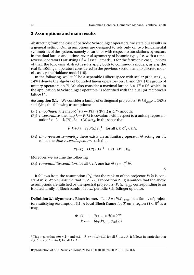
62 Domenico Fiorenza, Domenico Monaco, Gianluca Panati
3 Assumptions and main results
Abstracting from the case of periodic Schrödinger operators, we state our results ina general setting. Our assumptions are designed to rely only on two fundamentalsymmetries of the system, namely covariance with respect to translations by vectorsin the dual lattice and a time-reversal symmetry of bosonic type, i. e. with a time-reversal operator Θ satisfying Θ2 = 1l (see Remark 3.1 for the fermionic case). In viewof that, the following abstract results apply both to continuous models, as e. g. thereal Schrödinger operators considered in the previous Section, and to discrete mod-els, as e. g. the Haldane model [15].
In the following, we let H be a separable Hilbert space with scalar product ⟨·, ·⟩,B(H) denote the algebra of bounded linear operators on H, and U(H) the group ofunitary operators on H. We also consider a maximal lattice Λ ' Zd ⊂ Rd which, inthe application to Schrödinger operators, is identified with the dual (or reciprocal)lattice Γ∗.
Assumption 3.1. We consider a family of orthogonal projectors P (k)k∈Rd ⊂B(H)satisfying the following assumptions:
(P1) smoothness: the map Rd 3 k 7→ P (k) ∈B(H) is C∞-smooth;(P2) τ-covariance: the map k 7→ P (k) is covariant with respect to a unitary represen-
tation3 τ :Λ→U(H), λ 7→ τ(λ) ≡ τλ, in the sense that
P (k +λ) = τλP (k)τ−1λ for all k ∈Rd , λ ∈Λ;
(P3) time-reversal symmetry: there exists an antiunitary operator Θ acting on H,called the time-reversal operator, such that
P (−k) =ΘP (k)Θ−1 and Θ2 = 1lH.
Moreover, we assume the following
(P4) compatibility condition: for all λ ∈Λ one has Θτλ = τ−1λΘ.
♦
It follows from the assumption (P1) that the rank m of the projector P (k) is con-stant in k. We will assume that m < +∞. Proposition 2.1 guarantees that the aboveassumptions are satisfied by the spectral projectors P∗(k)k∈Rd corresponding to anisolated family of Bloch bands of a real periodic Schrödinger operator.
Definition 3.1 (Symmetric Bloch frame). Let P= P (k)k∈Rd be a family of projec-tors satisfying Assumption 3.1. A local Bloch frame for P on a region Ω ⊂ Rd is amap
Φ : Ω −→ H⊕ . . .⊕H=Hm
k 7−→ (φ1(k), . . . ,φm(k))
3 This means that τ(0) = 1lH and τ(λ1 +λ2) = τ(λ1)τ(λ2) for all λ1,λ2 ∈Λ. It follows in particular thatτ(λ)−1 = τ(λ)∗ = τ(−λ) for all λ ∈Λ.
Reproduction of Ann. Henri Poincaré (2015), DOI 10.1007/s00023-015-0400-6
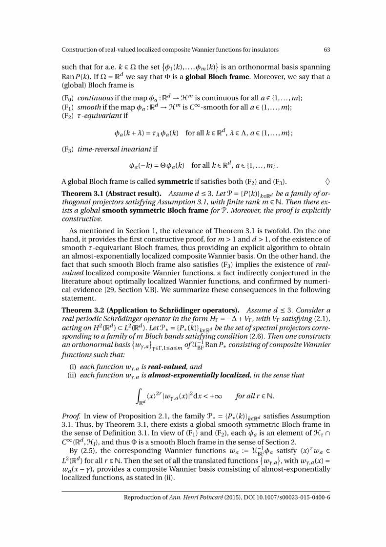
Construction of real-valued localized composite Wannier functions for insulators 63
such that for a.e. k ∈Ω the setφ1(k), . . . ,φm(k)
is an orthonormal basis spanning
RanP (k). If Ω = Rd we say that Φ is a global Bloch frame. Moreover, we say that a(global) Bloch frame is
(F0) continuous if the map φa :Rd →Hm is continuous for all a ∈ 1, . . . ,m;(F1) smooth if the map φa :Rd →Hm is C∞-smooth for all a ∈ 1, . . . ,m;(F2) τ-equivariant if
φa(k +λ) = τλφa(k) for all k ∈Rd , λ ∈Λ, a ∈ 1, . . . ,m ;
(F3) time-reversal invariant if
φa(−k) =Θφa(k) for all k ∈Rd , a ∈ 1, . . . ,m .
A global Bloch frame is called symmetric if satisfies both (F2) and (F3). ♦
Theorem 3.1 (Abstract result). Assume d ≤ 3. Let P = P (k)k∈Rd be a family of or-thogonal projectors satisfying Assumption 3.1, with finite rank m ∈N. Then there ex-ists a global smooth symmetric Bloch frame for P. Moreover, the proof is explicitlyconstructive.
As mentioned in Section 1, the relevance of Theorem 3.1 is twofold. On the onehand, it provides the first constructive proof, for m > 1 and d > 1, of the existence ofsmooth τ-equivariant Bloch frames, thus providing an explicit algorithm to obtainan almost-exponentially localized composite Wannier basis. On the other hand, thefact that such smooth Bloch frame also satisfies (F3) implies the existence of real-valued localized composite Wannier functions, a fact indirectly conjectured in theliterature about optimally localized Wannier functions, and confirmed by numeri-cal evidence [29, Section V.B]. We summarize these consequences in the followingstatement.
Theorem 3.2 (Application to Schrödinger operators). Assume d ≤ 3. Consider areal periodic Schrödinger operator in the form HΓ =−∆+VΓ, with VΓ satisfying (2.1),acting on H 2(Rd ) ⊂ L2(Rd ). Let P∗ = P∗(k)k∈Rd be the set of spectral projectors corre-sponding to a family of m Bloch bands satisfying condition (2.6). Then one constructsan orthonormal basis
wγ,a
γ∈Γ,1≤a≤m of U−1
BF RanP∗ consisting of composite Wannierfunctions such that:
(i) each function wγ,a is real-valued, and(ii) each function wγ,a is almost-exponentially localized, in the sense that∫
Rd⟨x⟩2r |wγ,a(x)|2dx <+∞ for all r ∈N.
Proof. In view of Proposition 2.1, the family P∗ = P∗(k)k∈Rd satisfies Assumption3.1. Thus, by Theorem 3.1, there exists a global smooth symmetric Bloch frame inthe sense of Definition 3.1. In view of (F1) and (F2), each φa is an element of Hτ∩C∞(Rd ,Hf), and thus Φ is a smooth Bloch frame in the sense of Section 2.
By (2.5), the corresponding Wannier functions wa := U−1BFφa satisfy ⟨x⟩r wa ∈
L2(Rd ) for all r ∈N. Then the set of all the translated functions
wγ,a, with wγ,a(x) =
wa(x −γ), provides a composite Wannier basis consisting of almost-exponentiallylocalized functions, as stated in (ii).
Reproduction of Ann. Henri Poincaré (2015), DOI 10.1007/s00023-015-0400-6

64 Domenico Fiorenza, Domenico Monaco, Gianluca Panati
Moreover, Φ satisfies (F3) which in this context reads φa(−k) = Cφa(k) = φa(k),since C is just complex conjugation in L2(Td
Y ). By Definition 2.1, one concludes that
wa(x) = 1
|B|1/2
∫B
dk e−ik·x φa(k, x) = 1
|B|1/2
∫B
dk ei(−k)·x φa(−k, x) = wa(x),
which yields property (i) and concludes the proof. ut
We sketch the structure of the proof of Theorem 3.1, provided in Sections 4 and 5.First, one easily notices that, in view of properties (F2) and (F3), a global symmetricBloch frame Φ : Rd → Hm is completely specified by the values it assumes on theeffective unit cell
Beff :=
k =∑
jk j e j ∈B : k1 ≥ 0
.
Indeed, every point k ∈Rd can be written (with an a.e.-unique decomposition) as k =(−1)sk ′+λ, for some k ′ ∈Beff, λ ∈Λ and s ∈ 0,1. Then the symmetric Bloch frameΦsatisfiesΦ(k) = τλΘsΦ(k ′) for k ′ ∈Beff. Viceversa, a local Bloch frameΦeff :Beff →Hm
can be canonically extended to a global symmetric Bloch frame Φ by posing
(3.1) Φ(k) = τλΘsΦeff(k ′) for k = (−1)sk ′+λ.
However, to obtain a global continuous Bloch frame, the map Φeff : Beff →Hm mustsatisfy some non-trivial “gluing conditions” on the boundary ∂Beff, involving ver-tices, edges (for d ≥ 2), faces (for d ≥ 3), and so on. In Section 4, we investigate indetail such conditions, showing that it is always possible to construct a local contin-uous Bloch frame Φeff :Beff →Hm satisfying them, provided d ≤ 3. More specifically,we assume as given a continuous Bloch frame Ψ :Beff →Hm , called the input frame,which does not satisfy any special condition on the boundary of Beff, as e. g. the out-come of numerical computations in solid-state physics. Then we explicitly constructa unitary matrix Ueff(k) such that the “corrected” frame
Φeff(k)a :=m∑
b=1Ψb(k)Ueff(k)ba
is still continuous and satisfies all the relevant symmetry conditions on ∂Beff. Then,formula (3.1) will provide a global continuous symmetric Bloch frame Φ.A naïf smoothing procedure, based on the Steenrod’s Approximation Theorem, start-ing from Φ would yield a global smooth τ-equivariant Bloch frame which, in gen-eral, does not satisfies property (F3). For this reason, we develop in Section 5 a newsymmetry-preserving smoothing algorithm which, starting from a global continuoussymmetric Bloch frame, produces a global smooth symmetric Bloch frame arbitrar-ily close to the former one (Theorem 5.1). The latter procedure, which holds true inany dimension, yields the global smooth symmetric Bloch frame whose existence isclaimed in Theorem 3.1.
Remark 3.1 (Systems with fermionic time-reversal symmetry). Our results heav-ily rely on the fact that we consider a bosonic (or even) time-reversal (TR) symmetry.
Reproduction of Ann. Henri Poincaré (2015), DOI 10.1007/s00023-015-0400-6

Construction of real-valued localized composite Wannier functions for insulators 65
In other instances, as in the context of TR-symmetric topological insulators [16], andspecifically in the Kane-Mele model [22], assumption (P3) is replaced by
(P3,−) fermionic time-reversal symmetry: there exists an antiunitary operator Θ act-ing on H such that
P (−k) =ΘP (k)Θ−1 and Θ2 =−1lH.
Then the statement analogous to Theorem 3.1 is false: there might be topologicalobstruction to the existence of a continuous symmetric Bloch frame [11, 14]. Oneproves [14, 10] that such obstruction is classified by a Z2 topological invariant ford = 2, and by four Z2 invariants for d = 3, and that the latter equal the indices intro-duced by Fu, Kane and Mele [11, 12]. However, if one does not require time-reversalsymmetry but only τ-equivariance, then a global smooth Bloch frame does exist evenin the fermionic case, as a consequence of the vanishing of the first Chern class andof the result in [37], see [31] for a detailed review. ♦
4 Proof: Construction of a smooth symmetric Bloch frame
In this Section, we provide an explicit algorithm to construct a global smooth sym-metric Bloch frame, as claimed in Theorem 3.1.
Our general strategy will be the following. We consider a local continuous (resp.smooth)4 Bloch frame Ψ : Beff →Hm , which always exists since Beff is contractibleand no special conditions on the boundary are imposed.5 We look for a unitary-matrix-valued map U :Beff →U(Cm) such that the modified local Bloch frame
(4.1) Φa(k) =m∑
b=1Ψb(k)Uba(k), U (k) ∈U(Cm)
satisfies (F2) and (F3) on the boundary ∂Beff. The latter requirement corresponds toconditions on the values that U assumes on the vertices, edges and faces of ∂Beff,according to the dimension. These conditions will be investigated in the next Sub-sections, after a preliminary characterization of the relevant symmetries.
4 A smooth input frame Ψ is required only to write an explicit formula for the continuous extensionfrom the boundary ∂Beff to the whole Beff, as detailed in Remarks 4.2 and 4.3. At a first reading, thereader might prefer to focus on the case of a continuous input frame.5 Moreover, a smooth Ψ can be explicitly constructed by using the intertwining unitary by Kato andNagy [24, Sec. I.6.8] on finitely-many sufficiently small open sets covering Beff. In the applications tocomputational physics,Ψ corresponds to the outcome of the numerical diagonalisation of the Hamil-tonian at fixed crystal momentum, followed by a choice of quasi-Bloch functions and by a standardroutine which corrects the phases to obtain a (numerically) continuous (resp. smooth) Bloch frameon Beff.
Reproduction of Ann. Henri Poincaré (2015), DOI 10.1007/s00023-015-0400-6

66 Domenico Fiorenza, Domenico Monaco, Gianluca Panati
4.1 The relevant group action
Properties (P2) and (P3) are related to some fundamental automorphisms of Rd ,namely the maps c and tλ defined by
(4.2) c(k) =−k and tλ(k) = k +λ for λ ∈Λ.
Since c tλ = t−λc and c2 = t0, one concludes that the relevant symmetries are en-coded in the group
(4.3) Gd := tλ, tλcλ∈Λ ⊂ Aut(Rd ).
We notice that, assuming also (P4), the action of Gd on Rd can be lifted to an ac-tion on Rd ×Fr(m,H), where Fr(m,H) is the set of orthonormal m-frames in H. Tostreamline the notation, we denote by Φ = (φ1, . . . ,φm) an element of Fr(m,H). Anybounded linear or antilinear operator A : H → H acts on frames componentwise,i. e. we set
AΦ := (Aφ1, . . . , Aφm).
Moreover, the space Fr(m,H) carries a free right action6 of the groupU(Cm), denotedby
(Φ/U )b :=m∑
a=1φa Uab .
A similar notation appears in [14]. Notice that, by the antilinearity of the time-reversal operator Θ, one has
Θ(Φ/U ) = (ΘΦ)/U , for all Φ ∈ Fr(m,H), U ∈U(Cm).
A lift of the Gd action from Rd to Rd ×Fr(m,H) is obtained by considering, as gener-ators, the automorphisms C and Tλ, defined by
(4.4) C (k,Φ) = (c(k),ΘΦ) Tλ(k,Φ) = (tλ(k),τλΦ)
for any (k,Φ) ∈ Rd ×Fr(m,H). The relation tλ c = c t−λ implies that, for every λ ∈ Λ,one has to impose the relation
TλC (k,Φ) = C T−λ(k,Φ) ∀(k,Φ) ∈Rd ×Fr(m,H)
i. e. τλΘΦ = Θτ−λΦ ∀Φ ∈ Fr(m,H),
which holds true in view of (P4). Thus the action of Gd is lifted to Rd ×Fr(m,H).
Given a family of projectors P satisfying (P2), (P3) and (P4), it is natural to considerthe set of global Bloch frames for P, here denoted by Fr(P). Notice that
Fr(P) ⊂
f :Rd → Fr(m,H)⊂Rd ×Fr(m,H).
6 This terminology means that Φ/ I =Φ, (Φ/U1)/U2 =Φ/ (U1U2) and that if Φ/U1 =Φ/U2 thenU1 =U2, for all Φ ∈ Fr(m,H) and U1,U2 ∈U(Cm).
Reproduction of Ann. Henri Poincaré (2015), DOI 10.1007/s00023-015-0400-6

Construction of real-valued localized composite Wannier functions for insulators 67
It is easy to check that the action of Gd , previously extended toRd×Fr(m,H), restrictsto Fr(P). Indeed, whenever Φ is an orthonormal frame for RanP (k) one has that
P (tλ(k))τλΦ = τλP (k)τ−1λ τλΦ= τλP (k)Φ= τλΦ,
P (c(k))ΘΦ = ΘP (k)Θ−1ΘΦ=ΘP (k)Φ=ΘΦ,
yielding that τλΦ is an orthonormal frame in Ran(P (tλ(k))) and ΘΦ is an orthonor-mal frame in Ran(P (c(k))).
4.2 Solving the vertex conditions
The relevant vertex conditions are associated to those points k ∈ Rd which have anon-trivial stabilizer with respect to the action of Gd , namely to the points in the set
(4.5) Vd =
k ∈Rd : ∃g ∈Gd , g 6= 1l : g (k) = k
.
Since Gd = tλ, tλ cλ∈Λ and tλ acts freely on Rd , the previous definition reads
Vd =
k ∈Rd : ∃λ ∈Λ : tλc(k) = k
=
k ∈Rd : ∃λ ∈Λ : −k +λ= k= 1/2λλ∈Λ ,
i. e. Vd consists of those points7 which have half-integer coordinates with respect tothe basis e1, . . . ,ed . For convenience, we set kλ := 1/2λ.
If Φ is a symmetric Bloch frame, then conditions (F2) and (F3) imply that
(4.6) Φ(kλ) =Φ(tλc(kλ)) = τλΘΦ(kλ) kλ ∈Vd .
We refer to (4.6) as the vertex condition at the point kλ ∈ Vd . For a generic Blochframe Ψ, instead, Ψ(kλ) and τλΘΨ(kλ) are different. Since they both are orthonor-mal frames in RanP (kλ), there exists a unique unitary matrix Uobs(kλ) ∈U(Cm) suchthat
(4.7) Ψ(kλ)/Uobs(kλ) = τλΘΨ(kλ), λ ∈Λ.
The obstruction unitary Uobs(kλ) must satisfy a compatibility condition. Indeed, byapplying τλΘ to both sides of (4.7) one obtains
τλΘ (Ψ(kλ)/Uobs(kλ)) = τλΘτλΘΨ(kλ)
= τλτ−λΘ2Ψ(kλ) =Ψ(kλ)
where assumption (P4) has been used. On the other hand, the left-hand side alsoreads
7 In the context of topological insulators, such points are called time-reversal invariant momenta(TRIMs) in the physics literature.
Reproduction of Ann. Henri Poincaré (2015), DOI 10.1007/s00023-015-0400-6
68 Domenico Fiorenza, Domenico Monaco, Gianluca Panati
τλΘ (Ψ(kλ)/Uobs(kλ)) = (τλΘΨ(kλ))/Uobs(kλ) ==Ψ(kλ)/
(Uobs(kλ)Uobs(kλ)
).
By the freeness of the action of U(Cm) on frames, one concludes that
(4.8) Uobs(kλ) =Uobs(kλ)T
where MT denotes the transpose of the matrix M .The value of the unknown U , appearing in (4.1), at the point kλ ∈Vd is constrained
by the value of the obstruction matrix Uobs(kλ). Indeed, from (4.6) and (4.1) it followsthat for every λ ∈Λ
Ψ(kλ)/U (kλ) =Φ(kλ) = τλΘΦ(kλ)
= τλΘ (Ψ(kλ)/U (kλ))
= (τλΘΨ(kλ))/U (kλ)
=Ψ(kλ)/Uobs(kλ)U (kλ).
By the freeness of the U(Cm)-action, we obtain the condition8
(4.9) Uobs(kλ) =U (kλ)U (kλ)T.
The existence of a solution U (kλ) ∈U(Cm) to equation (4.9) is granted by the follow-ing Lemma, which can be applied to V =Uobs(kλ) in view of (4.8).
Lemma 4.1 (Solution to the vertex equation). Let V ∈U(Cm) be such that V T =V .Then there exists a unitary matrix U ∈U(Cm) such that V =U UT.
Proof. Since V ∈U(Cm) is normal, it can be unitarily diagonalised. Hence, there ex-ists a unitary matrix W ∈U(Cm) such that
V =W eiM W ∗
where M = diag(µ1, . . . ,µm) and each µ j is chosen so that9 µ j ∈ [0,2π). We set
U =W eiM/2W ∗.
Since V T =V one has W eiM W T =W eiM W ∗, yielding
eiM W TW =W TW eiM ,
i. e. the matrix eiM commutes with A := W TW . Thus also eiM/2 commutes with A(since each µ j is in [0,2π)), hence one has
8 The presence of the transpose in condition (4.9) might appear unnatural in the context of our As-sumptions. A more natural reformulation of condition (4.9), involving an orthogonal structure canon-ically associated to Θ, will be discussed in a forthcoming paper [4].9 The latter condition is crucial: it expresses the fact that the arguments of the eigenvalues ω1, . . . ,ωmof V are “synchronized”, i. e. they are computed by using the same branch of the complex logarithm.
Reproduction of Ann. Henri Poincaré (2015), DOI 10.1007/s00023-015-0400-6
Construction of real-valued localized composite Wannier functions for insulators 69
UUT =W eiM/2 A−1eiM/2 AW ∗ =W eiM W ∗ =V.
utIn view of (4.8), we have the following
Corollary 4.1. For every kλ ∈ Vd there exists a unitary matrix U (kλ) such thatUobs(kλ) = U (kλ)U (kλ)T. In particular, the Bloch frame Φ(kλ) = Ψ(kλ)/U (kλ) sat-isfies the vertex condition (4.6) at the point kλ ∈Vd .
4.3 Construction in the 1-dimensional case
In the 1-dimensional case, the boundary of Beff consists of two vertices v0 = 0 andv1 = ke1 . Given, as an input, a continuous Bloch frame Ψ :Beff →Hm , equation (4.7)provides, for each vertex, an obstruction matrix Uobs(vi ). In view of Corollary 4.1,one obtains a unitary U (vi ) which solves equation (4.9) for kλ = vi , i ∈ 0,1.
SinceU(Cm) is a path-connected manifold, there exists a smooth path W : [0,1/2] →U(Cm) such that W (0) =U (v0) and W (1/2) =U (v1). Moreover, the path W can be ex-plicitly constructed, as detailed in the following Remark.
Remark 4.1 (Interpolation of unitaries). The problem of constructing a smoothinterpolation between two unitaries U1 and U2 in U(Cm) has an easy explicit solu-tion. First, by left multiplication times U−1
1 , the problem is equivalent to the con-struction of a smooth interpolation between I and U−1
1 U2 =: U∗ ∈ U(Cm). SinceU∗ is normal, there exists a unitary matrix S∗ such that S∗U∗S−1
∗ = eiD , with D =diag(δ1, . . . ,δm) a diagonal matrix. Then the map t 7→ W (t ) := S−1
∗ ei2tD S∗ is an ex-plicit smooth interpolation between W (0) = I and W (1/2) =U∗. ♦
We define a local continuous Bloch frame Φeff :Beff →Hm by setting
Φeff(k) =Ψ(k)/W (k), k ∈Beff.
Notice that Φeff satisfies, in view of the construction above, the vertex conditions
(4.10) Φeff(0) =ΘΦeff(0) and Φeff(ke1 ) = τe1ΘΦeff(ke1 ),
which are special cases of condition (4.6). We extend Φeff to a global Bloch frameΦ : R1 → Hm by using equation (3.1). We claim that Φ is a continuous symmetricBloch frame. Indeed, it satisfies (F2) and (F3) in view of (3.1) and it is continuous sinceΦeff satisfies (4.10). On the other hand, Φ is in general non-smooth at the vertices inV1. By using the symmetry-preserving smoothing procedure, as stated in Proposition5.1, we obtain a global smooth symmetric Bloch frameΦsm. This concludes the proofof Theorem 3.1 for d = 1.
4.4 Construction in the 2-dimensional case
The reduced unit cellBeff contains exactly six elements in V2. In adapted coordinates,so that (k1,k2) represents the point k1e1+k2e2 forΛ= SpanZ e1,e2, they are labelled
Reproduction of Ann. Henri Poincaré (2015), DOI 10.1007/s00023-015-0400-6

70 Domenico Fiorenza, Domenico Monaco, Gianluca Panati
as follows (Figure 1):
(4.11)v1 = (0,0), v2 =
(0,−1
2
), v3 =
(1
2,−1
2
),
v4 =(
1
2,0
), v5 =
(1
2,
1
2
), v6 =
(0,
1
2
).
The oriented segment joining vi to vi+1 (with v7 ≡ v1) is labelled by Ei .
E1
E2
E3
E4
E5
E6
v1
v2 v3
v4
v5v6
BeffB
Fig. 1 The effective unit cell (shaded area), its vertices and its edges. We use adapted coordinates(k1,k2) such that k = k1e1 +k2e2.
We start from a local continuous (resp. smooth) Bloch frameΨ :Beff →Hm . GivenΨ, the obstruction matrix defined in (4.7) yields, via Corollary 4.1, a unitary matrixU (vi ) solving equation (4.9), for i ∈ 1, . . . ,4.
Construction of the frame on the 1-skeleton
As in the 1-dimensional case, we exploit the constructive existence of a smooth pathWi : [0,1/2] →U(Cm) such that Wi (0) =U (vi ) and Wi (1/2) =U (vi+1), for i ∈ 1,2,3.These U(Cm)-valued paths are concatenated by setting
U (k) :=
W1(−k2) if k ∈ E1,W2(k1) if k ∈ E2,W3(k2 +1/2) if k ∈ E3,
so to obtain a piecewise-smooth map U : E1 ∪E2 ∪E3 →U(Cm). Let
Reproduction of Ann. Henri Poincaré (2015), DOI 10.1007/s00023-015-0400-6

Construction of real-valued localized composite Wannier functions for insulators 71
Φ(k) :=Ψ(k)/U (k) for k ∈ E1 ∪E2 ∪E3.
We extend the map Φ to a continuous (resp. piecewise-smooth) symmetric Blochframe Φ on ∂Beff by imposing properties (F2) and (F3), i. e. by setting
(4.12) Φ(k) :=
Φ(k) if k ∈ E1 ∪E2 ∪E3
τe1ΘΦ(te1 c(k)) if k ∈ E4
τe2 Φ(t−1e2
(k)) if k ∈ E5
ΘΦ(c(k)) if k ∈ E6.
By construction Φ satisfies all the edge symmetries for a symmetric Bloch frame Φlisted below:
(4.13)
Φ(c(k)) =ΘΦ(k) for k ∈ E1 ∪E6
Φ(te2 (k)) = τe2Φ(k) for k ∈ E2
Φ(te1 c(k)) = τe1ΘΦ(k) for k ∈ E3 ∪E4
Φ(t−1e2
(k)) = τ−1e2Φ(k) for k ∈ E5.
The map Φ : ∂Beff →Hm is continuous (resp. piecewise-smooth), since Φ is con-tinuous (resp. piecewise-smooth) and satisfies by construction the vertex conditionsat vi for i ∈ 1,4.
Extension to the 2-torus
Since both Φ(k) and the input frame Ψ(k) are orthonormal frames in RanP (k), forevery k ∈ ∂Beff, there exists a unique unitary matrix U (k) such that
(4.14) Φ(k) =Ψ(k)/U (k) for k ∈ ∂Beff.
Explicitly, U (k)ab = ⟨ψa(k) , φb(k)
⟩, which also show that the map U is continuous
(resp. piecewise-smooth) on ∂Beff.We look for a continuous extension Ueff : Beff →U(Cm) of U , such that Φeff :=Ψ/
Ueff satisfies the edge symmetries (4.13). Noticing that ∂Beff is homeomorphic to acircle S1, we use some well-known facts in algebraic topology: if X is a topologicalspace, then a continuous map f : S1 → X extends to a continuous map F : D2 →X , where D2 is the 2-dimensional disc enclosed by the circle S1, if and only if itshomotopy class [ f ] is the trivial element in π1(X ). Since, in our case, the space X isthe group U(Cm), we also use the fact that the exact sequence of groups
1 −→ SU(Cm) −→U(Cm)det−−→U (1) −→ 1
induces an isomorphism π1(U(Cm)) ' π1(U (1)). On the other hand, the degree ho-momorphism
(4.15) deg :π1(U (1))∼−→Z, [ϕ : S1 →U (1)] 7−→ 1
2πi
∮S1ϕ(z)−1∂zϕ(z)dz
Reproduction of Ann. Henri Poincaré (2015), DOI 10.1007/s00023-015-0400-6

72 Domenico Fiorenza, Domenico Monaco, Gianluca Panati
establishes an isomorphism of groups π1(U (1)) 'Z. We conclude that a continuousmap f : ∂Beff →U(Cm) can be continuously extended to F : Beff →U(Cm) if and onlyif deg([det f ]) ∈Z is zero.
The following Lemma is the crucial step in the 2-dimensional construction. Itshows that, even if deg([detU ]) = r 6= 0, it is always possible to construct a contin-uous map X : ∂Beff →U(Cm) such that deg([detU X ]) = 0 and Φ/X still satisfies theedge symmetries.10
Lemma 4.2 (Solution to the face-extension problem). Let r ∈ Z. There exists apiecewise-smooth map X : ∂Beff →U(Cm) such that:
(i) deg([det X ]) =−r ;(ii) if a Bloch frameΦ satisfies the edge symmetries (4.13), the frameΦ/X also does;
(iii) X (k) 6= I only for k ∈ E3 ∪E4.
Property (iii) will not be used in this Section, but it will be useful to solve the 3-dimensional problem.
Proof. First, we translate (ii) into an explicit condition on X . For k ∈ E1 ∪E6, condi-tion (ii) means that for every Φ such that Φ(−k) =ΘΦ(k) one has that
(Φ/X ) (−k) =Θ (Φ/X ) (k)
mΦ(−k)/X (−k) =Θ (Φ(k)/X (k))
m(ΘΦ(k))/X (−k) = (ΘΦ(k))/X (k),
yielding the explicit condition
(4.16) X (−k) = X (k), k ∈ E1 ∪E6.
Similarly, one obtains
X (te1 c(k)) = X (k) for k ∈ E3 ∪E4(4.17)
X (te2 (k)) = X (k) for k ∈ E2(4.18)
X (t−1e2
(k)) = X (k) for k ∈ E5.(4.19)
Thus condition (ii) on X is equivalent to the relations (4.16), (4.17), (4.18) and (4.19).We now exhibit a map X : ∂Beff → U(Cm) which satisfies the previous relations,
and such that deg([det X ]) =−r . Define ξ : ∂Beff →C by
(4.20) ξ(k) :=
e−i2πr (k2+1/2) for k ∈ E3 ∪E4
1 otherwise,
and set X (k) := diag(ξ(k),1, . . . ,1) ∈U(Cm) for k ∈ ∂Beff. The map X is clearly piecewise-smooth. Then, one easily checks that:
(i) deg([det X ]) =−r , since deg([det X ]) = deg([ξ]) =−r.
10 This is a special feature of systems with bosonic TR-symmetry: if assumption (P3) is replaced by(P3,−), the analogous statement does not hold true [10].
Reproduction of Ann. Henri Poincaré (2015), DOI 10.1007/s00023-015-0400-6

Construction of real-valued localized composite Wannier functions for insulators 73
(ii) X trivially satisfies relations (4.16), (4.18) and (4.19), since X (k) ≡ I for k ∈ E1 ∪E2 ∪E5 ∪E6. It also satisfies relation (4.17). Indeed, let k = (1/2,k2) ∈ E3 ∪E4.Since te1 c(k) = (1/2,−k2), one has
X (te1 c(k)) = X (1/2,−k2) = diag(ξ(1/2,−k2),1, . . . ,1)
= diag(ξ(1/2,k2),1, . . . ,1) = X (k).
(iii) property (iii) is satisfied by construction.
utSet r := deg([detU ]). In view of Lemma 4.2, the continuous (resp. piecewise-
smooth) map U := U X : ∂Beff →U(Cm) satisfies deg([detU ]) = 0 and hence extendsto a continuous (resp. piecewise-smooth) map Ueff :Beff →U(Cm). Moreover, the ex-tension procedure is explicitely constructive whenever U is piecewise-smooth, asdetailed in Remark 4.2. By setting Φeff(k) :=Ψ(k)/Ueff(k), we obtain a continuoussymmetric Bloch frame on the whole reduced unit cell Beff, which moreover satis-fies the edge symmetries (4.13) in view of item (ii) in Lemma 4.2. Then formula (3.1)defines a global symmetric Bloch frame Φ, which is continuous in view of the factthat Φeff satisfies (4.13). The symmetry-preserving smoothing procedure (Proposi-tion 5.1) yields a global smooth symmetric Bloch frame, arbitrarily close to Φ. Thisconcludes the proof of Theorem 3.1 for d = 2.
Remark 4.2 (Explicit extension to the whole effective cell, d = 2). We emphasizethat the extension of the piecewise-smooth map U : ∂Beff →U(Cm), with deg[detU ] =0, to a continuous (actually, piecewise-smooth) map Ueff : Beff → U(Cm) is explicit.For notational convenience, we use the shorthand U(m) ≡U(Cm).
First notice that the problem of constructing a continuous extension of U can bedecomposed into two simpler problems, since U(m) ≈U(1)×SU(m) (as topologicalspaces), where the identification is provided e. g. by the map
W 7→ (detW,W [) ∈U(1)×SU(m) with W [ = diag(detW −1,1, . . . ,1)W.
Thus the problem is reduced to exhibit a continuous extension of (a) the map f : k 7→detU (k) ∈U(1), and (b) the map f [ : k 7→U [(k) ∈ SU(m).
As for problem (a), let f : ∂Beff → U(1) be a degree-zero piecewise-smooth func-tion. Then, a piecewise-smooth extension F : Beff → U(1) is constructed as follows.Let θ0 ∈ R be such that f (0,−1/2) = ei2πθ0 . Define the piecewise-smooth functionϕ : [0,3] →U(1) as
(4.21) ϕ(t ) =
f (t ,−1/2) if 0 ≤ t ≤ 1/2f (1/2,−1+ t ) if 1/2 ≤ t ≤ 3/2f (2− t ,1/2) if 3/2 ≤ t ≤ 2f (0,5/2− t ) if 2 ≤ t ≤ 3
and set
θ(t ) = θ0 +1
2πi
∫ t
0ϕ(τ)−1ϕ′(τ)dτ, for t ∈ [0,3].
Reproduction of Ann. Henri Poincaré (2015), DOI 10.1007/s00023-015-0400-6

74 Domenico Fiorenza, Domenico Monaco, Gianluca Panati
By the Cauchy integral formula, θ(3) = θ(0)+deg( f ) = θ(0) = θ0. Moreover,
ei2πθ(t ) =ϕ(t )
for every t ∈ [0,3]. Then, one can choose F (k1,k2) = ei2πω(k1,k2), where
ω(k1,k2) :=
−2k2 θ(
k2−2k1+1/24k2
)if k2 ≤−|2k1 −1/2|,
(4k1 −1)θ(1+ k2
4k1−1
)if −|2k1 −1/2| ≤ k2 ≤ |2k1 −1/2|, with k1 ≥ 1/4,
2k2 θ(2− k2+2k1−1/2
4k2
)if k2 ≥ |2k1 −1/2|,
(−4k1 +1)θ(
52 −
k2−4k1+1
)if −|2k1 −1/2| ≤ y ≤ |2k1 −1/2|, with k1 ≤ 1/4.
Note that ω is continuous at (1/4,0) with ω(1/4,0) = 0, since θ is continuous on [0,3]and so there exist a |θ|max ∈R such that |θ(t )| ≤ |θ|max for any t ∈ [0,3].
As for problem (b), while a construction of the continuous extension is possiblefor every m ∈ N, here we provide the details only for m = 2, which is the case ofinterest for the 2-bands models, as e. g. the celebrated Haldane model [15], and issuch that an extension can be made completely explicit by elementary techniques.To obtain an extension for higher m’s, one can reduce to the case m = 2 by recursivelyexploiting the fibrations SU(m −1) −→ SU(m) −→ S2m−1.
Let f [ : k 7→ U [(k) ∈ SU(2) be a piecewise-smooth function. Then a piecewise-smooth extension F [ : Beff → SU(2) is constructed as follows. First, we use the stan-dard identification of SU(2) with the 3-sphere of unit norm vectors in R4 to look atf [ as to a piecewise-smooth function f [ : ∂Beff → S3. Let p ∈ S3 be a point not in the
range11 of f [, and let ψp : S3 \ p → p
⊥ be the stereographic projection from p tothe hyperplane through the origin of R4 orthogonal to the vector p. Explicitly, thismap and its inverse read
(4.22)
ψp (v) = p − 1
⟨v −p |p⟩ (v −p)
ψ−1p (w) = p + 2
||w −p||2 (w −p) .
Second, we define a piecewise-smooth function ϕ[ : [0,3] → S3 by using the sameformula as in (4.21), with f replaced by f [.Then, a piecewise-smooth extension of f [ to a function F [ :Beff → S3 is given by
11 Such a point does exists since the map f [ is piecewise-smooth. Indeed, by an argument analogousto the Sard lemma, one can show that the range of f [ is not dense in S3. This is the only point in theconstruction where we need U piecewise-smooth, and hence a smooth input frame Ψ.
Reproduction of Ann. Henri Poincaré (2015), DOI 10.1007/s00023-015-0400-6
Construction of real-valued localized composite Wannier functions for insulators 75
F [(k1,k2) =
ψ−1p
(−2k2ψp (ϕ( k2−2k1+1/2
4k2))
)if k2 ≤−|2k1 −1/2|,
ψ−1p
((4k1 −1)ψp (ϕ(1+ k2
4k1−1 )))
if −|2k1 −1/2| ≤ k2 ≤ |2k1 −1/2| and k1 ≥ 1/4,
ψ−1p
(2k2 ψp (ϕ(2− k2+2k1−1/2
4k2))
)if k2 ≥ |2k1 −1/2|,
ψ−1p
((−4k1 +1)ψp (ϕ( 5
2 −k2
−4k1+1 )))
if −|2k1 −1/2| ≤ k2 ≤ |2k1 −1/2| and k1 ≤ 1/4.
Notice that F [ is continuous at (1/4,0) with F [(1/4,0) = −p, since ψp ϕ : [0,3] →p⊥ ⊆ R4 is continuous on [0,3]. This provides an explicit piecewise-smooth exten-sion of f [ for the case m = 2. ♦
4.5 Interlude: abstracting from the 1- and 2-dimensional case
Abstracting from the proofs in Subsections 4.3 and 4.4, we distillate two Lemmaswhich will become the “building bricks” of the higher dimensional construction. Tostreamline the statements, we denote by B(d) (resp. B(d)
eff ) the d-dimensional unit cell(resp. effective unit cell) and we adhere to the following convention:
B(0) ' 0 B(1)eff ' [0,1/2],
(4.23)B
(d+1)eff 'B(1)
eff ×B(d) =
(k1,k2, . . . ,kd+1︸ ︷︷ ︸k⊥
) : k1 ∈ [0,1/2], k⊥ ∈B(d) for d ≥ 1.
We also refer to the following statement as the d-dimensional problem:Given a continuous Bloch frame Ψ : B(d)
eff →Hm , construct a continuous Bloch frame
Φeff : B(d)eff →Hm which, via (3.1), continuously extends to a global continuous sym-
metric Bloch frame Φ :Rd →Hm .In other words, Φeff is defined only on the effective unit cell B(d)
eff , but satisfies all the
relations on ∂B(d)eff (involving vertices, edges, faces, . . . ) which allow for a continu-
ous symmetric extension to the whole Rd . Hereafter, we will not further emphasizethe fact that all the functions appearing in the construction are piecewise-smoothwhenever Ψ is smooth, since this fact will be used only in Remark 4.3.
Notice that Subsection 4.2 already contains a solution to the 0-dimensional prob-lem: indeed, in view of Corollary 4.1, for every λ ∈Λ there exists a Bloch frame, de-fined on the point kλ, satisfying the vertex condition (4.6), thus providing a solutionto the 0-dimensional problem in B(0) ' kλ ' 0.
A second look to Subsection 4.3 shows that it contains a solution to the 1-dimensionalproblem, given a solution to the 0-dimensional problem. Indeed, one extracts fromthe construction the following Lemma.
Lemma 4.3 (Macro 1). Let Φone :B(0) ' 0 →Hm be a Bloch frame satisfying
Reproduction of Ann. Henri Poincaré (2015), DOI 10.1007/s00023-015-0400-6

76 Domenico Fiorenza, Domenico Monaco, Gianluca Panati
(4.24) Φone(0) =ΘΦone(0).
Then one constructs a continuous Bloch frame Φtwo :B(1)eff ' [0,1/2] →Hm such that
(4.25)
Φtwo(0) =Φone(0)Φtwo(1/2) = τe2ΘΦtwo(1/2).
In view of (4.25),Φtwo continuously extends, via (3.1), to a global continuous sym-metric Bloch frame, thus providing a solution to the 1-dimensional problem.
Analogously, from the construction in Subsection 4.4 we distillate a general pro-cedure. For convenience, we relabel the edges of B(2)
eff as follows:
E j ,0 =
k =∑
iki ei ∈B(2)
eff : k j = 0
(4.26)
E j ,± =
k =∑
iki ei ∈B(2)
eff : k j =±1/2
(4.27)
From the construction in Subsection 4.4, based on Lemma 4.2, one easily deducesthe following result.
Lemma 4.4 (Macro 2). Assume that ΦS : S →Hm , with S = E1,0 ∪E2,−∪E2,+ ⊂ ∂B(2)eff ,
is continuous and satisfies the following edge symmetries:
(4.28)
ΦS(te2 (k)) = τe2ΦS(k) for k ∈ E2,−ΦS(t−1
e2(k)) = τ−1
e2ΦS(k) for k ∈ E2,+
ΦS(c(k)) =ΘΦS(k) for k ∈ E1,0.
Then one constructs a continuous Bloch frame Φeff :B(2)eff → Fr(m,H) such that
(4.29)
Φeff(k) =ΦS(k) for k ∈ SΦeff(te1 c(k)) = τe1ΘΦeff(k) for k ∈ E1,+.
To obtain (4.29) we implicitly used property (iii) in Lemma 4.2, which guaranteesthat it is possible to obtain the frame Φeff by acting only on the edge E1,+ = E3 ∪E4.Notice that, in view of (4.29),Φeff continuously extends, via (3.1), to a global continu-ous symmetric Bloch frame. Therefore, a solution to the 2-dimensional problem canalways be constructed, whenever a continuous Bloch frame on the 1-dimensionalset S, satisfying the edge symmetries (4.28), is provided.
The previous Lemmas 4.3 and 4.4 will yield a constructive and conceptually clearsolution to the 3-dimensional problem, and a characterization of the obstruction tothe solution to the 4-dimensional problem.
Reproduction of Ann. Henri Poincaré (2015), DOI 10.1007/s00023-015-0400-6

Construction of real-valued localized composite Wannier functions for insulators 77
4.6 Construction in the 3-dimensional case
The faces of ∂B(3)eff are labelled according to the following convention : for j ∈ 1,2,3
we set
F j ,0 =
k =3∑
i=1ki ei : k j = 0
(4.30)
F j ,± =
k =3∑
i=1ki ei : k j =±1/2
(4.31)
Notice that two faces of ∂B(3)eff , namely F1,0 and F1,+ are identifiable with a 2-dimensional
unit cell B(2), while the remaining four faces, namely F2,± and F3,±, are identifiablewith a 2-dimensional effective unit cell B(2)
eff .
•
• •
••
• •
•
••
•
•
•
•
•
•
• •
••
BeffB
k1
k2
k3
Fig. 2 The 3-dimensional (effective) unit cell.
We assume as given a continuous Bloch frame Ψ : B(3)eff → Hm (the input frame)
which does not satisfy any particular symmetry on the boundary ∂B(3)eff . Since F1,0 '
B(2), in view of the construction in Subsection 4.4 we can assume that Ψ has beenalready modified to obtain a continuous Bloch frame Φone : F1,0 →Hm , Φone =Ψ/Uone, which satisfies the edge symmetries (4.13) on F1,0.
For convenience, we decompose the constructive algorithm into few steps:• Step 1. Extend to an edge by Macro 1. Choose a vertex of ∂B(3)
eff contained inF1,+, and let v0 be the corresponding vertex on F1,0. For the sake of concreteness,we choose v∗ = (1/2,1/2,1/2), so that v0 = (0,1/2,1/2). Then Lemma 4.3 (Macro 1)
Reproduction of Ann. Henri Poincaré (2015), DOI 10.1007/s00023-015-0400-6

78 Domenico Fiorenza, Domenico Monaco, Gianluca Panati
yields the existence of a continuous Bloch frame Φtwo : [v0, v∗] ' B(1)eff → Hm such
that Φtwo(v0) =Φone(v0) and Φtwo(v∗) satisfies the vertex condition (4.6) at v∗.• Step 2. Extend by τ-equivariance. By imposing property (F2), Φtwo naturally
extends to the edges t−1e2
([v0, v∗]) and t−1e3
([v0, v∗]). Since Φone is τ-equivariant onF1,0 'B(2), one has that Φtwo(t−1
e j(v0)) =Φone(t−1
e j(v0)) for j ∈ 2,3. In view of that, we
obtain a continuous Bloch frame by setting
(4.32) Φthree(k) :=Φone(k) for k ∈ F1,0,Φtwo(k) for k ∈ tλ([v0, v∗]) for λ ∈ 0,−e2,−e3 .
• Step 3. Extend to small faces by Macro 2. Notice thatΦthree restricted to F3,+ (resp.F2,+) is defined and continuous on a set S3,+ (resp. S2,+) which has the same struc-ture as the set S appearing in Lemma 4.4 (Macro 2), and there satisfies the relationsanalogous to (4.28). Then Φthree continuously extends to the whole F3,+ (resp. F2,+)and the extension satisfies the relation analogous to (4.29) on the edge ∂F j ,+\S j ,+ forj = 3 (resp. j = 2).
•
•
•
•
•
•
•
•
•
(a) Starting on F1,0
•
•
•
• •
•
•
•
•
•
(b) Step 1
•
•
•
• •
•
•
•
•
•
•
•
•
(c) Step 2
•
•
•
•
•
•
•
••
•
•
•
••
(d) Step 3
•
•
•
•
•
•
•
•
•
•
•
•
•
• •
• •
(e) Step 4
•
•
•
•
•
•
•
•
•
•
•
•
•
•
• •
• •
(f) Step 5
Fig. 3 Steps in the construction.
• Step 4. Extend by τ-equivariance. By imposing τ-equivariance (property (F2)),Φthree naturally extends to the faces F3,− and F2,−, thus yielding a continuous Blochframe Φfour defined on the set12 ∂B(3)
eff \ F1,+ =: K0.
12 According to a longstanding tradition in geometry, the choice of symbols is inspired by the Germanlanguage: K0 stands for Kleiderschrank ohne Türen. The reason for this name will be clear in few lines.
Reproduction of Ann. Henri Poincaré (2015), DOI 10.1007/s00023-015-0400-6
Construction of real-valued localized composite Wannier functions for insulators 79
• Step 5. Extend symmetrically to F1,+ by Macro 2. When considering the face F1,+,we first notice that the two subsets13
(4.33) T± = k ∈ F1,+ : ±k2 ≥ 0
are related by a non-trivial symmetry, since te1 c (T±) = T∓. We construct a continu-ous extension of Φfour which is compatible with the latter symmetry.
The restriction of Φfour, defined on K0, to the set S+ = k ∈ ∂F1,+ : k2 ≥ 0
is con-
tinuous and satisfies symmetries analogous to (4.28). Then, in view of Lemma 4.4(Macro 2), Φfour continuously extends to the whole T+ and the extension satisfiesthe relation analogous to (4.29) on the edge ∂T+ \ S+. We denote the extension byΦfive.
To obtain a continuous symmetric Bloch frame Φ : ∂B(3)eff → Fr(m,H) we set
(4.34) Φ(k) :=
Φfour(k) for k ∈ K0
Φfive(k) for k ∈ T+Φfive(te1 c(k)) for k ∈ T−.
The function Φ is continuous in view of the edge and face symmetries which havebeen imposed in the construction.
• Step 6. Extend to the interior of the effective cell. The frame Φ and the inputframe Ψ are related by the equation
(4.35) Φ(k) =Ψ(k)/U (k) k ∈ ∂B(3)eff ,
which yields a continuous map U : ∂B(3)eff →U(Cm).
We show that such a map extends to a continuous map Ueff :B(3)eff →U(Cm). Indeed,
a continuous function f from ∂B(3)eff ≈ S2 to the topological space X can be continu-
ously extended to B(3)eff ≈ D3 if and only if its homotopy class [ f ] is the trivial element
of the group π2(X ). In our case, since π2(U(Cm)) = 0 for every m ∈ N, there is noobstruction to the continuous extension of the map U . Moreover, the extension canbe explicitly constructed, as detailed in Remark 4.3.Equipped with such a continuous extension, we obtain a continuous symmetricBloch frame Φeff :B(3)
eff →Hm by setting
(4.36) Φeff(k) =Ψ(k)/Ueff(k) k ∈B(3)eff .
• Step 7. Use the smoothing procedure. By using (3.1), Φeff extends to a globalcontinuous symmetric Bloch frame. Then the symmetry-preserving smoothing pro-cedure (Proposition 5.1) yields a global smooth symmetric Bloch frame.
This concludes the proof of Theorem 3.1 for d = 3.
Remark 4.3 (Explicit extension to the whole effective cell, d = 3). As in the 2-dimensional case (Remark 4.2), we notice that the extension of the piecewise-smooth14
13 Obviously, these subsets are die Türen, so they are denoted by T±.14 The map U is actually piecewise-smooth, whenever the input frame Ψ is smooth. Although thisfact was not emphasized at every step of the 3-dimensional construction, as we did instead in Section4.4, the reader can easily check it.
Reproduction of Ann. Henri Poincaré (2015), DOI 10.1007/s00023-015-0400-6

80 Domenico Fiorenza, Domenico Monaco, Gianluca Panati
function U : ∂B(3)eff → U(Cm) to B(3)
eff is completely explicit. The problem is again re-duced to the following two subproblems, namely to construct a continuos extensionfrom ∂B(3)
eff to B(3)eff of:
(a) a map f : k 7→ detU (k) ∈U(1), and(b) a map f [ : k 7→U [(k) ∈ SU(m).
As for subproblem (a), given a degree-zero piecewise-smooth function f : ∂B(3)eff →
U(1), a piecewise-smooth extension F : B(3)eff → U(1) is constructed as follows. Con-
sider the region D⊆R2 depicted below
(−1,−1/2) (1,−1/2)
(−1,1/2) (1,1/2)
(−1/2,5/2) (1/2,5/2)
and let ϕ :D→U(1) be the piecewise-smooth function defined by
(4.37) ϕ(s, t ) :=
f (−s − 12 ,−1
2 , t ) if (s, t ) ∈ [−1,−12 ]× [−1
2 , 12 ]
f (0, s, t ) if (s, t ) ∈ [−12 , 1
2 ]× [−12 , 1
2 ]f (s − 1
2 , 12 , t ) if (s, t ) ∈ [ 1
2 ,1]× [−12 , 1
2 ]f (t − 1
2 , s, 12 ) if (s, t ) ∈ [−1
2 , 12 ]× [ 1
2 ,1]f ( 1
2 , s,−t + 32 ) if (s, t ) ∈ [−1
2 , 12 ]× [1,2]
f (−t + 52 , s,−1
2 ) if (s, t ) ∈ [−12 , 1
2 ]× [2, 52 ]
Choose θ0 ∈R be such that f (0,0,0) = e2πiθ0 and set
θ(s, t ) = θ0 +1
2πi
∫ 1
0ϕ(λs,λt )−1 (
sϕs(λs,λt )+ tϕt (λs,λt ))
dλ,
where ϕs and ϕt denote the partial derivatives of ϕ with respect to s and t , respec-tively. One has
e2πiθ(s,t ) =ϕ(s, t )
for any (s, t ) ∈D. Moreover,
Reproduction of Ann. Henri Poincaré (2015), DOI 10.1007/s00023-015-0400-6
Construction of real-valued localized composite Wannier functions for insulators 81
θ(s,−12 ) = θ(s, 5
2 ) for −12 ≤ s ≤ 1
2θ(s,−1
2 ) = θ(−12 ,3+ s) for −1 ≤ s ≤−1
2θ(s,−1
2 ) = θ( 12 ,3− s) for 1
2 ≤ s ≤ 1θ(s, 1
2 ) = θ(−12 , 1
2 − s) for −1 ≤ s ≤−12
θ(s, 12 ) = θ( 1
2 , 12 + s) for 1
2 ≤ s ≤ 1θ(−1, t ) = θ(−1
2 , 32 − t ) for −1
2 ≤ t ≤ 12
θ(1, t ) = θ( 12 , 3
2 − t ) for 12 ≤ t ≤ 1
2
so that θ actually lifts f to a piecewise-smooth function θ : ∂B(3)eff →R. Then, one can
choose F (k1,k2,k3) = e2πiω(k1,k2,k3), where
ω(k1,k2,k3) =
(−4k1 +1)θ(− k3
4k1−1 ,− k24k1−1
)if 0 ≤ k1 ≤ min|1
2 |k2|− 14 |, |1
2 |k3|− 14 |,
2k3 θ(
12 +
k3+2k1−1/24k3
, k22k3
)if max|2k1 − 1
2 |, |k2| ≤ k3 ≤ 12 ,
2k2 θ(
k32k2
, 12 +
k2+2k1−1/24k2
)if max|2k1 − 1
2 |, |k3| ≤ k2 ≤ 12 ,
(4k1 −1)θ(
k34k1−1 , 3
2 −k2
4k1−1
)if max|1
2 |k2|+ 14 |, |1
2 |k3|+ 14 | ≤ k1 ≤ 1
2 ,
−2k3 θ(−1
2 −k3−2k1+1/2
4k3,− k2
2k3
)if −1
2 ≤ k3 ≤ min−|2k1 − 12 |,−|k2|,
−2k2 θ(− k3
2k2, 5
2 −k2−2k1+1/2
4k2
)if −1
2 ≤ k2 ≤ min−|2k1 − 12 |,−|k3|.
Note that ω is continuous at (1/4,0,0) with ω(1/4,0,0) = 0, since θ is continuous onthe compact domain D.
As mentioned in Remark 4.2, the solution to subproblem (b) can be obtained byrecursive reduction of the rank m, up to m = 2. To construct the extension in the casem = 2, we identify SU(2) with S3 and use the stereographic projection (4.22), withrespect to a point p ∈ S3 which is not included in the range15 of the map f [. By usingEquation (4.37), with f replaced by f [, one defines a piecewise-smooth function ϕ :D → S3. Then, a piecewise-smooth extension of f [ to a function F [ : B(3)
eff → S3 isexplicitly given by
15 This point does exist since the map f [ is piecewise-smooth, as argued in footnote11.
Reproduction of Ann. Henri Poincaré (2015), DOI 10.1007/s00023-015-0400-6

82 Domenico Fiorenza, Domenico Monaco, Gianluca Panati
F (k1,k2,k3) =
ψ−1p
((−4k1 +1)ψp
(ϕ(− k3
4k1−1 ,− k24k1−1 )
))if 0 ≤ k1 ≤ min|1
2 |k2|− 14 |, |1
2 |k3|− 14 |,
ψ−1p
(2k3ψp
(ϕ( 1
2 +k3+2k1−1/2
4k3, k2
2k3)))
if max|2k1 − 12 |, |k2| ≤ k3 ≤ 1
2 ,
ψ−1p
(2k2ψp
(ϕ( k3
2k2, 1
2 +k2+2k1−1/2
4k2)))
if max|2k1 − 12 |, |k3| ≤ k2 ≤ 1
2 ,
ψ−1p
((4k1 −1)ψp
(ϕ( k3
4k1−1 , 32 −
k24k1−1 )
))if max|1
2 |k2|+ 14 |, |1
2 |k3|+ 14 | ≤ k1 ≤ 1
2 ,
ψ−1p
(−2k3ψp
(ϕ(−1
2 −k3−2k1+1/2
4k3,− k2
2k3)))
if −12 ≤ k3 ≤ min−|2k1 − 1
2 |,−|k2|,
ψ−1p
(−2k2,ψp
(ϕ(− k3
2k2, 5
2 −k2−2k1+1/2
4k2)))
if −12 ≤ k2 ≤ min−|2k1 − 1
2 |,−|k3|.
Note that F is continuous at (1/4,0,0) with F (1/4,0,0) =−p, since ψp ϕ :D→ p⊥ ⊆R4 is continuous on the compact domainD. The map above provides an explicit con-tinuous extension to B(3)
eff for m = 2. ♦
4.7 A glimpse to the higher-dimensional cases
The fundamental “building bricks” used to solve the 3-dimensional problem (Lemma4.3 and 4.4) can be used to approach the higher-dimensional problems. However,additional topological obstruction might appear, related to the fact that the k-th ho-motopy group πk (U(Cm)), for k ≥ 3, might be non-trivial if m > 1.
We illustrate this phenomenon in the case d = 4. An iterative procedure analogousto the construction in Subsection 4.6, based again only on Lemma 4.3 and 4.4, yieldsa continuous Bloch frame Φ : ∂B(4)
eff →Hm satisfying all the relevant symmetries (onvertices, edges, faces and 3-dimensional hyperfaces). By comparison with the inputframe Ψ : B(4)
eff → Hm , one obtains a continuos map U : ∂B(4)eff → U(Cm) such that
Φ(k) =Ψ(k)/U (k) for all k ∈ ∂B(4)eff . Arguing as in Subsection 4.6, one concludes that
the existence of a continuos extension Ueff : B(4)eff → U(Cm) of U is equivalent to the
fact that the homotopy class [U ] is the trivial element of π3 (U(Cm)). Since the lattergroup is not trivial (for m > 1), there might be a priori topological obstruction to theexistence of a continuous extension. This possible obstruction corresponds, in theabstract approach used in [37, 31], to the appearance for d ≥ 4 of the second Chernclass of the Bloch bundle, which always vanishes for d ≤ 3 or m = 1.
On the other hand, our constructive algorithm works without obstruction in thecase m = 1, since πk
(U(C1)
) = 0 for all k ≥ 2, yielding an explicit construction of aglobal smooth symmetric Bloch frame. However, since a constructive proof in thecase m = 1 is already known for every d ∈N [18], we do not provide the details of theconstruction.
Reproduction of Ann. Henri Poincaré (2015), DOI 10.1007/s00023-015-0400-6
Construction of real-valued localized composite Wannier functions for insulators 83
5 A symmetry-preserving smoothing procedure
In this Section we develop a smoothing procedure which, given a global continu-ous symmetric Bloch frame, yields a global smooth symmetric Bloch frame arbitrarilyclose to the given one. The following Proposition, which holds true in any dimension,might be of independent interest.
Proposition 5.1 (Symmetry-preserving smoothing procedure). For d ∈N, let P=P (k)k∈Rd be a family of orthogonal projectors satisfying Assumption 3.1. Assume thatΦ :Rd →Hm is a global continuous symmetric Bloch frame, i. e. it satisfies properties(F0), (F2) and (F3).Choose ε> 0. Then one constructs a global smooth symmetric Bloch frame Φsm suchthat
(5.1) supk∈Rd
dist(Φ(k),Φsm(k)) < ε
where dist(Φ,Ψ) =(∑
a
∥∥φa −ψa∥∥2H
)1/2is the distance in Fr(m,H).
Notice that, for any Φ ∈ Fr(m,H) and U ,W ∈U(m), one has
(5.2) dist(Φ/U ,Φ/W ) = ‖U −W ‖HS
where ‖U‖2HS = ∑m
a,b=1 |Uab |2 is the Hilbert-Schmidt norm. Thus, the distance be-tween the frames Φ/U and Φ/W is the length of the chord between U and Win the ambient space Cm2 ' Mm(C) ⊃ U(m). On the other hand, each frame spaceFk := FrRanP (k) 'U(m) inherits from U(m) a Riemannian structure16, and the cor-responding geodesic distance d(U ,W ) can be compared to the chord distance (5.2).In a neighborhood of the identity, the geodesic distance and the ambient distanceare locally Lipschitz equivalent, namely
(5.3) 1/2d(I,U ) ≤ ‖I−U‖HS ≤ d(I,U ) ∀U ∈U(M) : ‖I−U‖HS < 1/2τm ,
where τm is defined as the largest number having the following property: The opennormal bundle over U(m) of radius r is embedded inR2m2 ' Mm(C) for every r < τm .The first inequality in (5.3) is a straightforward consequence of [36, Prop. 6.3], wherealso the relation between τm and the principal curvature of U(m) is discussed.
Proof. Following [37], we recall that, to a family of projectors P satisfying properties(P1) and (P2), one can canonically associate a smooth Hermitian vector bundle EP =(EP → Td
∗), where Td∗ = Rd /Λ. In particular, EP is defined by using an equivalence
relation ∼τ on Rd ×H, namely
(k,φ) ∼τ (k ′,φ′) if and only if ∃λ ∈Λ : k ′ = k +λ, φ′ = τλφ.
An equivalence class is denoted by [k,φ]τ. Then, the total space is defined by
16 Recall that U(m) is a Riemannian manifold with respect to the bi-invariant metric defined, for A,Bin the Lie algebra u(m) =
A ∈ Mm(C) : A∗ =−A, by ⟨A , B⟩HS = Tr(A∗B).
Reproduction of Ann. Henri Poincaré (2015), DOI 10.1007/s00023-015-0400-6
84 Domenico Fiorenza, Domenico Monaco, Gianluca Panati
EP =
[k,φ]τ ∈(Rd ×H
)/ ∼τ:φ ∈ RanP (k)
,
and the projectionπ : EP →Td∗ byπ([k,φ]τ) = k (modΛ). The fact thatEP is a smooth
vector bundle follows from (P1) and the Kato-Nagy formula, see [37, 38] for the proof.Moreover, a natural Hermitian structure is induced by the inner product in H.
Equipped with the above definition, we observe that a continuous τ-equivariantglobal Bloch frame Φ : Rd → Hm is identified with a continuous global section σΦof the (principal) bundle of the orthonormal frames of the bundle EP, denoted byFrEP. The identification is given by
σΦ(x) = ([k,φ1(k)]τ, . . . , [k,φm(k)]τ
) ∈ (FrEP)x for x = k mod Λ.
According to a classical result, the Steenrod’s Approximation Theorem ([52]; see [54]for recent generalizations), there exists a smooth global sectionσ′
Φ :Td∗ → FrEP such
thatsupx∈Td∗
dist(σΦ(x),σ′
Φ(x))< 1/2ε.
Going back to the language of Bloch frames, one concludes the existence of aglobal smooth τ-equivariant Bloch frame Φ′
sm :Rd →Hm , such that
(5.4) supk∈Rd
dist(Φ(k),Φ′
sm(k))< 1/2ε.
In general, the Bloch frame Φ′sm does not satisfy property (F3). In order to recover
time-reversal symmetry, we use the following symmetrization procedure.First, we recall that there exists δ> 0 such that the exponential map exp : u(m) →
U(m) is a diffeomorphism from the ball Bδ(0) ⊂ u(m) to the geodesic ball Bδ(I) ⊂U(m), see e. g. [19, Chapter II] or [48, Chapter VII]. In particular, for any U ∈ Bδ(I),there exists a unique AU ∈ Bδ(0) such that
(5.5) U = exp(AU ), U ∈ Bδ(I),
and, moreover, the map U 7→ AU is C∞-smooth on Bδ(I). Since the exponential mapis normalized so that d(I,U ) = ‖AU‖HS, then d(I,U ) = d(I,U ) = d(I,U−1). In particular,both U and U−1 are in the geodesic ball Bδ(I), whenever U ∈ Bδ(I).For U ∈ Bδ(I), the midpoint M(I,U ) between I and U is defined by17
(5.6) M(I,U ) := exp(1/2AU ) ∈ Bδ(I) ⊂U(m).
One immediately checks that, for U ∈ Bδ(I),
M(I,U ) = exp(1/2AU
)= M(I,U )(5.7)
M(I,U−1) = exp(−1/2AU ) =U−1M(I,U ).(5.8)
Moreover,
17 Definition (5.6) agrees with the geodesic midpoint between I and U in the Riemannian manifoldU(m), since the exponential map is normalized so that d(I,exp(sN )) = s, for s < δ and ‖N‖HS = 1.
Reproduction of Ann. Henri Poincaré (2015), DOI 10.1007/s00023-015-0400-6

Construction of real-valued localized composite Wannier functions for insulators 85
(5.9) d(I, M(I,U )) = 1/2d(I,U ).
Consider now two orthonormal framesΦ,Ψ ∈ FrRanP (k), such that dist(Φ,Ψ) < ε.For ε sufficiently small, we define the midpoint M (Φ,Ψ) ∈ FrRanP (k) in the follow-ing way.Let UΦ,Ψ ∈U(m) be the unique unitary such that Ψ =Φ/UΦ,Ψ, namely
(UΦ,Ψ
)ab =⟨
φa ,ψb⟩
. Taking (5.2) and (5.3) into account, one has
ε> dist(Φ,Ψ) = dist(Φ,Φ/UΦ,Ψ) =∥∥I−UΦ,Ψ
∥∥HS ≥ 1/2 d(I,UΦ,Ψ).
Choose ε sufficiently small, namely ε< δ/2. Then UΦ,Ψ is in the geodesic ball Bδ(I) ⊂U(m). By using (5.6), we define
(5.10) M (Φ,Ψ) :=Φ/M(I,UΦ,Ψ) ∈ FrRanP (k).
We show that
M (ΘΦ,ΘΨ) =ΘM (Φ,Ψ)(5.11) M (τλΦ,τλΨ) = τλ M (Φ,Ψ) .(5.12)
Notice preliminarily that, since both Θ and τλ are isometries of H, one has
(5.13) dist(ΘΦ,ΘΨ) = dist(Φ,Ψ) = dist(τλΦ,τλΨ)
for allΦ,Ψ ∈ Fr(m,H). Thus, the midpoints appearing on the left-hand sides of (5.11)and (5.12) are well-defined, whenever dist(Φ,Ψ) < 1/2δ.Equation (5.11) follows from (5.7) and from the fact thatΘ
(Φ/UΦ,Ψ
)= (ΘΦ)/UΦ,Ψ.Indeed, one has
M (ΘΦ,ΘΨ) = M (ΘΦ,Θ
(Φ/UΦ,Ψ
))= M (ΘΦ, (ΘΦ)/UΦ,Ψ
)= (ΘΦ)/M(I,UΦ,Ψ) = (ΘΦ)/M(I,UΦ,Ψ)
= Θ(Φ/M(I,UΦ,Ψ)
)=ΘM (Φ,Ψ) .
Analogously, equation (5.12) follows from the fact that τλ(Φ/UΦ,Ψ
)= (τλΦ)/UΦ,Ψ.
We focus now on the smooth τ-equivariant Bloch frameΦ′sm :Rd →Hm obtained,
via Steenrod’s theorem, from the continuous symmetric frame Φ. Since RanP (k) =ΘRanP (−k), one has that ΘΦ′
sm(−k) is in Fk = FrRanP (k). Thus, we set
(5.14) Φsm(k) := M (Φ′
sm(k),ΘΦ′sm(−k)
) ∈ Fk .
The definition (5.14) is well-posed. Indeed, taking (5.4) and (5.13) into account, onehas
dist(Φ′sm(k),ΘΦ′
sm(−k))(5.15)
≤ dist(Φ′sm(k),Φ(k))+dist(Φ(k),ΘΦ(−k))+dist(ΘΦ(−k),ΘΦ′
sm(−k))
= dist(Φ′sm(k),Φ(k))+dist(Φ(−k),Φ′
sm(−k)) < ε< 1/2δ,
Reproduction of Ann. Henri Poincaré (2015), DOI 10.1007/s00023-015-0400-6

86 Domenico Fiorenza, Domenico Monaco, Gianluca Panati
where we used the fact that the central addendum (in the second line) vanishes sinceΦ satisfies (F3).
We claim that (5.14) defines a smooth symmetric global Bloch frame satisfying(5.1). We explicitly check that:
1. the map k 7→ Φsm(k) is smooth. Indeed, since Θ is an isometry of H, the mapk 7→ ΘΦ′
sm(−k) =: Ψ′sm(k) is smooth. Hence k 7→ UΦ′
sm(k),Ψ′sm(k) ∈ U(m) is smooth,
since(UΦ,Ψ
)ab = ⟨
φa ,ψb⟩
. In view of (5.15) and (5.3), UΦ′sm(k),Ψ′
sm(k) is, for every k ∈Rd , in the geodesic ball Bδ(I) where the exponential map defines a diffeomorphism.As a consequence,
k 7→Φ′sm(k)/M(I,UΦ′
sm(k),Ψ′sm(k)) =Φsm(k)
is smooth from Rd to Hm .2. the Bloch frame Φsm satisfies (F2). Indeed, by using (P4) and (5.12), one obtains
Φsm(k +λ) = M (Φ′
sm(k +λ),ΘΦ′sm(−k −λ)
)= M (
τλΦ′sm(k),Θτ−λΦ′
sm(−k))
= M (τλΦ
′sm(k),τλΘΦ
′sm(−k)
)= τλ M (
Φ′sm(k),ΘΦ′
sm(−k))= τλΦsm(k).
3. the Bloch frame Φsm satisfies (F3). Indeed, by using Θ2 = 1l and (5.11), one has
Φsm(−k) = M (Θ2Φ′
sm(−k),ΘΦ′sm(k)
)= ΘM (
ΘΦ′sm(−k),Φ′
sm(k))
= ΘM (Φ′
sm(k),ΘΦ′sm(−k)
)=ΘΦsm(k),
where we used the fact that M (Φ,Ψ) = M (Ψ,Φ), whenever dist(Φ,Ψ) < δ/2. The lat-ter fact is a direct consequence of (5.8), since
M (Φ,Ψ) = Φ/M(I,UΦ,Ψ) = (Ψ/U−1
Φ,Ψ
)/M(I,UΦ,Ψ)
= Ψ/(U−1Φ,ΨM(I,UΦ,Ψ)
)=Ψ/M(I,U−1Φ,Ψ)
= Ψ/M(I,UΨ,Φ) = M (Ψ,Φ) .
4. equation (5.1) is satisfied in view of (5.15). Indeed, setting UΦ′sm(k),Ψ′
sm(k) ≡U (k)for notational convenience and using (5.2), (5.3) and (5.9), one obtains
dist(Φ′sm(k),Φsm(k)) = dist
(Φ′
sm(k),Φ′sm(k)/M(I,U (k))
)= ‖I−M(I,U (k))‖HS ≤ d(I, M(I,U (k))) = 1/2d(I,U (k))
≤ ‖I−U (k)‖HS = dist(Φ′
sm(k),ΘΦ′sm(−k)
)< ε.
This concludes the proof of the Proposition. ut
Reproduction of Ann. Henri Poincaré (2015), DOI 10.1007/s00023-015-0400-6

Construction of real-valued localized composite Wannier functions for insulators 87
References
1. BLOUNT, E. I. : Formalism of Band Theory. In : Seitz, F., Turnbull, D. (eds.), Solid State Physics 13,pages 305–373, Academic Press, 1962.
2. BROUDER CH.; PANATI G.; CALANDRA M.; MOUROUGANE CH.; MARZARI N.: Exponential local-ization of Wannier functions in insulators. Phys. Rev. Lett. 98 (2007), 046402.
3. CANCÈS, E.; LEWIN, M. : The dielectric permittivity of crystals in the reduced Hartree-Fock ap-proximation. Arch. Ration. Mech. Anal. 197 (2010), 139–177.
4. CERULLI IRELLI, G. ; FIORENZA, D.; MONACO, D.; PANATI, G. : Geometry of Bloch bundles: aunifying quiver-theoretic approach, in preparation (2015).
5. DES CLOIZEAUX, J. : Energy bands and projection operators in a crystal: Analytic and asymptoticproperties. Phys. Rev. 135 (1964), A685–A697.
6. DES CLOIZEAUX, J. : Analytical properties of n-dimensional energy bands and Wannier functions.Phys. Rev. 135 (1964), A698–A707.
7. CORNEAN, H.D.; HERBST, I.; NENCIU, G. : in preparation (2015).8. CORNEAN, H.D.; NENCIU A.; NENCIU, G. : Optimally localized Wannier functions for quasi one-
dimensional nonperiodic insulators. J. Phys. A: Math. Theor. 41 (2008), 125202.9. E, W.; LU, J. : The electronic structure of smoothly deformed crystals: Wannier functions and the
Cauchy-Born rule. Arch. Ration. Mech. Anal. 199 (2011), 407–433.10. FIORENZA, D.; MONACO, D.; PANATI, G. : Z2 invariants of topological insulators as geometric
obstructions, (2014).11. FU, L.; KANE, C.L. : Time reversal polarization and a Z2 adiabatic spin pump. Phys. Rev. B 74
(2006), 195312.12. FU, L.; KANE, C.L.; MELE, E.J. : Topological insulators in three dimensions. Phys. Rev. Lett. 98
(2007), 106803.13. GOEDECKER, S. : Linear scaling electronic structure methods, Rev. Mod. Phys. 71 (1999), 1085–
1111.14. GRAF, G.M.; PORTA, M. : Bulk-edge correspondence for two-dimensional topological insulators,
Commun. Math. Phys. 324 (2013), 851–895.15. HALDANE, F.D.M. : Model for a Quantum Hall effect without Landau levels: condensed-matter
realization of the “parity anomaly”. Phys. Rev. Lett. 61 (1988), 2017.16. HASAN, M.Z.; KANE, C.L. : Colloquium: Topological Insulators. Rev. Mod. Phys. 82 (2010), 3045–
3067.17. HASTINGS, M. B.: Topology and phases in fermionic systems. J. Stat. Mech. Theory Exp. (2008),
L01001.18. HELFFER, B.; SJÖSTRAND, J. : Équation de Schrödinger avec champ magnétique et équation de
Harper. In: Schrödinger operators, Lecture Notes in Physics 345, Springer, Berlin, 1989, 118–197.19. HELGASON, S. : Differential Geometry, Lie Groups, and Symmetric Spaces, Academic Press, New
York, 1978.20. IBAÑEZ-AZPIROZ, J.; EIGUREN, A.; BERGARA, A.; PETTINI, G.; MODUGNO, M. : Tight-binding
models for ultracold atoms in honeycomb optical lattices. Phys. Rev. A 87 (2013), 011602.21. IBAÑEZ-AZPIROZ, J.; EIGUREN, A.; BERGARA, A.; PETTINI, G.; MODUGNO, M. : Self-consistent
tight-binding description of Dirac points moving and merging in two-dimensional optical lat-tices. Phys. Rev. A 88 (2013), 033631.
22. KANE, C.L.; MELE, E.J. : Z2 Topological Order and the Quantum Spin Hall Effect. Phys. Rev. Lett.95 (2005), 146802.
23. KANE, C.L.; MELE, E.J. : Quantum Spin Hall Effect in graphene. Phys. Rev. Lett. 95 (2005), 226801.24. KATO, T. : Perturbation theory for linear operators, Springer, Berlin, 1966.25. KIEVELSEN, S. : Wannier functions in one-dimensional disordered systems: application to frac-
tionally charged solitons. Phys. Rev. B 26 (1982), 4269–4274.26. KING-SMITH, R. D. ; VANDERBILT, D. : Theory of polarization of crystalline solids. Phys. Rev. B 47
(1993), 1651–1654.27. KOHN, W. : Analytic Properties of Bloch Waves and Wannier Functions. Phys. Rev. 115 (1959),
809.28. LEWIN, M.; SÉRÉ, É. : Spectral pollution and how to avoid it (with applications to Dirac and
periodic Schrödinger operators). Proc. Lond. Math. Soc. 100 (2010), 864–900.29. MARZARI, N. ; VANDERBILT, D. : Maximally localized generalized Wannier functions for compos-
ite energy bands. Phys. Rev. B 56 (1997), 12847–12865.
Reproduction of Ann. Henri Poincaré (2015), DOI 10.1007/s00023-015-0400-6

88 Domenico Fiorenza, Domenico Monaco, Gianluca Panati
30. MARZARI, N.; MOSTOFI A.A.; YATES J.R.; SOUZA I.; VANDERBILT D. : Maximally localized Wan-nier functions: Theory and applications. Rev. Mod. Phys. 84 (2012), 1419.
31. MONACO, D.; PANATI, G. : Symmetry and localization in periodic crystals: triviality of Bloch bun-dles with a fermionic time-reversal symmetry, to appear in the proceedings of the conference“SPT2014 – Symmetry and Perturbation Theory”, Cala Gonone, Italy (2014).
32. NENCIU, G. : Existence of the exponentially localised Wannier functions. Commun. Math. Phys.91 (1983), 81–85.
33. NENCIU, G. : Dynamics of band electrons in electric and magnetic fields: Rigorous justificationof the effective Hamiltonians. Rev. Mod. Phys. 63 (1991), 91–127.
34. NENCIU, A.; NENCIU, G. : Dynamics of Bloch electrons in external electric fields. II. The existenceof Stark-Wannier ladder resonances. J. Phys. A15 (1982), 3313–3328.
35. NENCIU, A.; NENCIU, G. : The existence of generalized Wannier functions for one-dimensionalsystems. Commun. Math. Phys. 190 (1988), 541–548.
36. NIYOGI, P.; SMALE, S.; WEINBERGER, S. : Finding the homology of submanifolds with high con-fidence from random samples, Discrete Comput. Geom. 39 (2008), 419–441.
37. PANATI, G.: Triviality of Bloch and Bloch-Dirac bundles. Ann. Henri Poincaré 8 (2007), 995–1011.38. PANATI, G.; PISANTE, A.: Bloch bundles, Marzari-Vanderbilt functional and maximally localized
Wannier functions. Commun. Math. Phys. 322 (2013), 835–875.39. PANATI, G.; SPARBER, C.; TEUFEL, S. : Geometric currents in piezoelectricity. Arch. Rat. Mech.
Anal. 91 (2009), 387–422.40. PANATI, G.; SPOHN, H.; TEUFEL, S. : Effective dynamics for Bloch electrons: Peierls substitution
and beyond. Commun. Math. Phys. 242 (2003), 547–578.41. PELINOVSKY, D.; SCHNEIDER, G.; MACKAY, R. S. : Justification of the lattice equation for a non-
linear elliptic problem with a periodic potential. Commun. Math. Phys. 284 (2008), 803–831.42. PELINOVSKY, D. ; SCHNEIDER, G. : Bounds on the tight-binding approximation for the Gross-
Pitaevskii equation with a periodic potential. J. Differ. Equations 248 (2010), 837–849.43. PRODAN, E. : Robustness of the spin-Chern number. Phys. Rev. B 80 (2009), 125327.44. PRODAN, E. : Disordered topological insulators: A non-commutative geometry perspective. J.
Phys. A 44 (2011), 113001.45. REED M., SIMON, B. : Methods of Modern Mathematical Physics. Volume IV: Analysis of Opera-
tors. Academic Press, New York, 1978.46. RESTA, R. : Theory of the electric polarization in crystals. Ferroelectrics 136 (1992), 51–75.47. RYU, S.; SCHNYDER, A. P.; FURUSAKI, A.; LUDWIG, A. W. W. : Topological insulators and super-
conductors: Tenfold way and dimensional hierarchy. New J. Phys. 12 (2010), 065010.48. SIMON, B. : Representations of Finite and Compact Groups, Graduate studies in mathematics, vol.
10, American Mathematical Society, 1996.49. SOLUYANOV, A.; VANDERBILT, D. : Wannier representation of Z2 topological insulators. Phys. Rev.
B 83 (2011), 035108.50. SOLUYANOV, A.A.; VANDERBILT, D. : Computing topological invariants without inversion sym-
metry, Phys. Rev. B 83 (2011), 235401.51. SOLUYANOV, A.; VANDERBILT, D. : Smooth gauge for topological insulators. Phys. Rev. B (2012),
115415.52. STEENROD, N. : The Topology of Fibre Bundles, Princeton Mathematical Series vol.14, Princeton
University Press, Princeton, 1951.53. WALTERS, R.; COTUGNO, G.; JOHNSON, T. H.; CLARK, S. R.; JAKSCH, D. : Ab initio derivation of
Hubbard models for cold atoms in optical lattices. Phys. Rev. A 87 (2013), 043613.54. WOCKEL, CH. : A generalization of Steenrod’s Approximation Theorem. Arch. Math. (Brno) 45
(2009), 95–104.
Reproduction of the preprint available at arXiv:1408.1030 (2014)
Z2 invariants of topological insulators as geometricobstructions
Domenico Fiorenza, Domenico Monaco, and Gianluca Panati
Abstract We consider a gapped periodic quantum system with time-reversal sym-metry of fermionic (or odd) type, i. e. the time-reversal operator squares to −1l. Weinvestigate the existence of periodic and time-reversal invariant Bloch frames in di-mensions 2 and 3. In 2d , the obstruction to the existence of such a frame is shown tobe encoded in a Z2-valued topological invariant, which can be computed by a sim-ple algorithm. We prove that the latter agrees with the Fu-Kane index. In 3d , instead,four Z2 invariants emerge from the construction, again related to the Fu-Kane-Meleindices. When no topological obstruction is present, we provide a constructive al-gorithm yielding explicitly a periodic and time-reversal invariant Bloch frame. Theresult is formulated in an abstract setting, so that it applies both to discrete modelsand to continuous ones.
Key words: Topological insulators, time-reversal symmetry, Kane-Mele model, Z2invariants, Bloch frames.
1 Introduction
In the recent past, the solid state physics community has developed an increasing in-terest in phenomena having topological and geometric origin. The first occurrenceof systems displaying different quantum phases which can be labelled by topologi-cal indices can be traced back at least to the seminal paper by Thouless, Kohmoto,Nightingale and den Nijs [40], in the context of the Integer Quantum Hall Effect. Thefirst topological invariants to make their appearance in the condensed matter lit-
Domenico FiorenzaDipartimento di Matematica, “La Sapienza” Università di Roma, Piazzale Aldo Moro 2, 00185 Rome,Italye-mail: [email protected]
Domenico MonacoSISSA, Via Bonomea 265, 34136 Trieste, Italye-mail: [email protected]
Gianluca PanatiDipartimento di Matematica, “La Sapienza” Università di Roma, Piazzale Aldo Moro 2, 00185 Rome,Italye-mail: [email protected]
89

90 Domenico Fiorenza, Domenico Monaco, Gianluca Panati
erature were thus Chern numbers: two distinct insulating quantum phases, whichcannot be deformed one into the other by means of continuous (adiabatic) trans-formations without closing the gap between energy bands, are indexed by differentintegers (see [14] and references therein). These topological invariants are relatedto an observable quantity, namely to the transverse (Hall) conductivity of the sys-tem under consideration [40, 14]; the fact that the topological invariant is an integerexplains why the observable is quantized. Beyond the realm of Quantum Hall sys-tems, similar non-trivial topological phases appear whenever time-reversal symme-try is broken, even in absence of external magnetic fields, as early foreseen by Hal-dane [16]. Since this pioneering observation, the field of Chern insulators flourished[36, 7, 11].
More recently, a new class of materials has been first theorized and then experi-mentally realized, where instead interesting topological quantum phases arise whilepreserving time-reversal symmetry: these materials are the so-called time-reversalsymmetric (TRS) topological insulators (see [2, 17] for recent reviews). The pecu-liarity of these materials is that different quantum phases are labelled by integersmodulo 2; from a phenomenological point of view, these indices are connected tothe presence of spin edge currents responsible for the Quantum Spin Hall Effect[20, 21]. It is crucial for the display of these currents that time-reversal symmetry isof fermionic (or odd) type, that is, the time-reversal operator Θ is such that Θ2 =−1l.
In a milestone paper [20], Kane and Mele consider a tight-binding model govern-ing the dynamics of an electron in a 2-dimensional honeycomb lattice subject tonearest- and next-to-nearest-neighbour hoppings, similarly to what happens in theHaldane model [16], with the addition of further terms, including time-reversal in-variant spin-orbit interaction. This prototype model is used to propose a Z2 indexto label the topological phases of 2d TRS topological insulators, and to predict thepresence of observable currents in Quantum Spin Hall systems. An alternative for-mulation for thisZ2 index is then provided by Fu and Kane in [12], where the authorsalso argue that such index measures the obstruction to the existence of a continuousperiodic Bloch frame which is moreover compatible with time-reversal symmetry.Similar indices appear also in 3-dimensional systems [13].
Since the proposals by Fu, Kane and Mele, there has been an intense activity in thecommunity aimed at the explicit construction of smooth symmetric Bloch frames,in order to connect the possible topological obstructions to the Z2 indices [39], andto study the localization of Wannier functions in TRS topological insulators [37, 38].However, while the geometric origin of the integer-valued topological invariants iswell-established (as was mentioned above, they represent Chern numbers of theBloch bundle, in the terminology of [28]), the situation is less clear for the Z2-valuedindices of TRS topological insulators. Many interpretations of the Z2 indices havebeen given, using homotopic or K -theoretic classifications [1, 27, 24, 32, 23], C∗-algebraic and functional-analytic approaches [29, 30, 33, 34], the bulk-edge corre-spondence [3, 15], monodromy arguments [31], or gauge-theoretic methods [10, 4,5]. However, we believe that a clear and simple topological explanation of how theyarise from the symmetries of the system is still in a initiatory stage.
In this paper, we provide a geometric characterization of theseZ2 indices as topo-logical obstructions to the existence of continuous periodic and time-reversal sym-metric Bloch frames, thus substantiating the claim in [12] on mathematical grounds.We consider a gapped periodic quantum system in presence of fermionic time-reversal symmetry (compare Assumption 2.1), and we investigate whether there ex-
Reproduction of the preprint available at arXiv:1408.1030 (2014)

Z2 invariants of topological insulators as geometric obstructions 91
ists a global continuous Bloch frame which is both periodic and time-reversal sym-metric. While in 1d this always exists, a topological obstruction may arise in 2d . Weshow in Section 3 that such obstruction is encoded in aZ2 indexδ, which is moreovera topological invariant of the system, with respect to those continuous deformationswhich preserve the symmetries. We prove that δ ∈Z2 agrees with the Fu-Kane index∆ ∈Z2 [12], thus providing a proof that the latter is a topological invariant (Sections4 and 5). Lastly, in Section 6 we investigate the same problem in 3d , yielding to thedefinition of four Z2-valued topological obstructions, which are compared with theindices proposed by Fu, Kane and Mele in [13]. In all cases where there is no topo-logical obstruction (i. e. the Z2 topological invariants vanish), we also provide anexplicit algorithm to construct a global smooth Bloch frame which is periodic andtime-reversal symmetric (see also Appendix A).
A similar obstruction-theoretic approach to the invariants of 2-dimensional topo-logical insulators was adopted in [15]. In particular, aiming at a proof of the bulk-edge correspondence, there the authors associate a Z2 index to the time-reversal in-variant bundle associated to the bulk Hamiltonian for a semi-infinite crystal, enjoy-ing a time-reversal symmetry of fermionic type.
Even though our starting assumptions on the family of projectors, to which we as-sociate Z2-valued topological invariants, are modeled on the properties of the spec-tral projectors of a time-reversal symmetric Hamiltonian retaining full periodicityin dimension d ≤ 3 (compare Assumption 2.1), the setting of [15] is also covered byour method: our results can be applied to the family of projectors associated to thebulk time-reversal invariant bundle, up to an identification of the coordinates on thebasis torus.
Indeed, the main advantage of our method is that, being geometric in nature, itis based only on the fundamental symmetries of the system, namely invariance by(lattice) translations (i. e. periodicity) and fermionic time-reversal symmetry. Thismakes our approach model-independent; in particular, it applies both to continu-ous and to tight-binding models, and both to the 2-dimensional and 3-dimensionalsetting. To the best of our knowledge, our method appears to be the first obstruction-theoretic characterization of theZ2 invariants in the pioneering field of 3-dimensionalTRS topological insultators. The method proposed here encompasses all modelsstudied by the community, in particular the Fu-Kane-Mele models in 2d and 3d[20, 12, 13], as well as more general tight-binding models in 2 dimensions like theones considered e. g. in [3] and, as already mentioned, in [15].
Another strong point in our approach is that the construction is algorithmic innature, and gives also a way to compute the Z2 invariants in a given system (see for-mulae (3.16) and (5.4)). This makes our proposal well-suited for numerical imple-mentation.
Acknowledgments. We thank H. Schulz-Baldes, G.M. Graf and M. Porta for interest-ing discussions. We are grateful to the Institut Henri Poincaré for the kind hospitalityin the framework of the trimester “Variational and Spectral Methods in QuantumMechanics”, organized by M. J. Esteban and M. Lewin, and to the Erwin SchrödingerInstitute for the kind hospitality in the framework of the thematic programme “Topo-logical Phases of Quantum Matter”, organized by N. Read, J. Yngvason, and M. Zirn-bauer.The project was supported by INdAM-GNFM (Progetto Giovane Ricercatore) and byMIUR (Progetto PRIN 2012).
Reproduction of the preprint available at arXiv:1408.1030 (2014)
92 Domenico Fiorenza, Domenico Monaco, Gianluca Panati
2 Setting and main results
2.1 Statement of the problem and main results
We consider a gapped periodic quantum system with fermionic time-reversal sym-metry, and we focus on the family of spectral eigenprojectors up to the gap, in Bloch-Floquet representation. In most of the applications, these projectors read
(2.1) P (k) =∑
n∈Iocc
|un(k)⟩⟨un(k)| , k ∈Rd ,
where un(k) are the periodic parts of the Bloch functions, and the sum runs over alloccupied bands.
Abstracting from specific models, we let H be a separable Hilbert space withscalar product ⟨·, ·⟩, B(H) denote the algebra of bounded linear operators on H,and U(H) the group of unitary operators on H. We also consider a maximal latticeΛ = SpanZ e1, . . . ,ed ' Zd ⊂ Rd : in applications, Λ is the dual lattice to the period-icity Bravais lattice Γ in position space. The object of our study will be a family oforthogonal projectors P (k)k∈Rd ⊂B(H), satisfying the following
Assumption 2.1. The family of orthogonal projectors P (k)k∈Rd enjoys the follow-ing properties:
(P1) smoothness: the map Rd 3 k 7→ P (k) ∈B(H) is C∞-smooth;(P2) τ-covariance: the map k 7→ P (k) is covariant with respect to a unitary repre-
sentation1 τ : Λ→U(H) of the lattice Λ on the Hilbert space H, i. e.
P (k +λ) = τ(λ)P (k)τ(λ)−1, for all k ∈Rd , for all λ ∈Λ;
(P3,−) time-reversal symmetry: the map k 7→ P (k) is time-reversal symmetric, i. e.there exists an antiunitary operator2 Θ : H→H, called the time-reversal oper-ator, such that
Θ2 =−1lH and P (−k) =ΘP (k)Θ−1.
Moreover, the unitary representation τ : Λ→U(H) and the time-reversal operatorΘ : H→H satisfy
♦(P4) Θτ(λ) = τ(λ)−1Θ for all λ ∈Λ.
Assumption 2.1 is satisfied by the spectral eigenprojectors of most Hamiltoni-ans modelling gapped periodic quantum systems, in presence of fermionic time-reversal symmetry. Provided the Fermi energy lies in a spectral gap, the map k 7→P (k) defined in (2.1) will be smooth (compare (P1)), while τ-covariance and (fermionic)time-reversal symmetry (properties (P2) and (P3,−)) are inherited from the corre-sponding symmetries of the Hamiltonian. In particular, several well-established
1 This means that τ(0) = 1lH and τ(λ1 +λ2) = τ(λ1)τ(λ2) for all λ1,λ2 ∈Λ. It follows in particular thatτ(λ)−1 = τ(λ)∗ = τ(−λ) for all λ ∈Λ.2 Recall that a surjective antilinear operator Θ : H→H is called antiunitary if
⟨Θψ1,Θψ2
⟩= ⟨ψ2,ψ1
⟩for all ψ1,ψ2 ∈H.
Reproduction of the preprint available at arXiv:1408.1030 (2014)
Z2 invariants of topological insulators as geometric obstructions 93
models satisfy the previous Assumption, including the eigenprojectors for the tight-binding Hamiltonians proposed by Fu, Kane and Mele in [20, 12, 13], as well asin many continuous models. Finally, Assumption 2.1 is satisfied also in the tight-binding models studied in [15]: the family of projectors is associated to the vectorbundle used by Graf and Porta to define a bulk index, under a suitable identificationof the variables3 (k1,k2) with the variables (k, z) appearing in [15].
For a family of projectors satisfying Assumption 2.1, it follows from (P1) that therank m of the projectors P (k) is constant in k. We will assume that m <+∞; property(P3,−) then gives that m must be even. Indeed, the formula
(φ,ψ) := ⟨Θφ,ψ
⟩for φ,ψ ∈H
defines a bilinear, skew-symmetric, non-degenerate form on H; its restriction toRanP (0) ⊂H (which is an invariant subspace for the action of Θ in view of (P3,−)) isthen a symplectic form, and a symplectic vector space is necessarily even-dimensional.
The goal of our analysis will be to characterize the possible obstructions to theexistence of a continuous symmetric Bloch frame for the family P (k)k∈Rd , which wedefine now.
Definition 2.1 ((Symmetric) Bloch frame). Let P (k)k∈Rd be a family of projec-tors satisfying Assumption 2.1, and let also Ω be a region in Rd . A Bloch frame forP (k)k∈Rd on Ω is a collection of maps Ω 3 k 7→ φa(k) ∈H, a ∈ 1, . . . ,m, such thatfor all k ∈ Ω the set Φ(k) :=
φ1(k), . . . ,φm(k)
is an orthonormal basis spanningRanP (k). When Ω=Rd , the Bloch frame is said to be global. A Bloch frame is called
(F0) continuous if all functions φa : Ω→H, a ∈ 1, . . . ,m, are continous;(F1) smooth if all functions φa : Ω→H, a ∈ 1, . . . ,m, are C∞-smooth.
We also say that a global Bloch frame is
(F2) τ-equivariant if
φa(k +λ) = τ(λ)φa(k) for all k ∈Rd , λ ∈Λ, a ∈ 1, . . . ,m ;
(F3) time-reversal invariant if
φb(−k) =m∑
a=1Θφa(k)εab for all k ∈Rd , b ∈ 1, . . . ,m
for some unitary and skew-symmetric matrix ε = (εab)1≤a,b≤m ∈ U(Cm), εab =−εba .
A global Bloch frame which is both τ-equivariant and time-reversal invariant iscalled symmetric. ♦
We are now in position to state our goal: we seek the answer to the following
Question (Qd ). Let d ≤ 3. Given a family of projectors P (k)k∈Rd satisfying Assump-tion 2.1 above, is it possible to find a global symmetric Bloch frame for P (k)k∈Rd ,which varies continuously in k, i. e. a global Bloch frame satisfying (F0), (F2) and (F3)?
3 The coordinates (k1, . . . ,kd ) are expressed in terms of a basis e1, . . . ,ed ⊂ Rd generating the latticeΛ as Λ= SpanZ e1, . . . ,ed .
Reproduction of the preprint available at arXiv:1408.1030 (2014)
94 Domenico Fiorenza, Domenico Monaco, Gianluca Panati
We will address this issue via an algorithmic approach. We will show that the exis-tence of such a global continuous symmetric Bloch frame is in general topologicallyobstructed. Explicitly, the main results of this paper are the following.
Theorem 2.1 (Answer to (Q1)). Let d = 1, and let P (k)k∈R be a family of projec-tors satisfying Assumption 2.1. Then there exists a global continuous symmetric Blochframe for P (k)k∈R. Moreover, such Bloch frame can be explicitly constructed.
The proof of Theorem 2.1 is contained in Section 3.3 (see Remark 3.1).
Theorem 2.2 (Answer to (Q2)). Let d = 2, and let P (k)k∈R2 be a family of projec-tors satisfying Assumption 2.1. Then there exists a global continuous symmetric Blochframe for P (k)k∈R2 if and only if
(2.2) δ(P ) = 0 ∈Z2,
where δ(P ) is defined in (3.16). Moreover, if (2.2) holds, then such Bloch frame can beexplicitly constructed.
The proof of Theorem 2.2, leading to the definition of the Z2 index δ(P ), is theobject of Section 3. Moreover, in Section 3.6 we prove that δ(P ) is actually a topo-logical invariant of the family of projectors (Proposition 3.4), which agrees with theFu-Kane index (Theorem 4.1).
Theorem 2.3 (Answer to (Q3)). Let d = 3, and let P (k)k∈R3 be a family of projec-tors satisfying Assumption 2.1. Then there exists a global continuous symmetric Blochframe for P (k)k∈R3 if and only if
(2.3) δ1,0(P ) = δ1,+(P ) = δ2,+(P ) = δ3,+(P ) = 0 ∈Z2,
whereδ1,0(P ),δ1,+(P ),δ2,+(P ) andδ3,+(P ) are defined in (6.1). Moreover, if (2.3) holds,then such Bloch frame can be explicitly constructed.
The proof of Theorem 2.3, leading to the definition of the four Z2 invariantsδ1,0(P ),δ1,+(P ),δ2,+(P ) and δ3,+(P ), is the object of Section 6.
Remark 2.1 (Smooth Bloch frames). Since the family of projectors P (k)k∈Rd sat-isfies the smoothness assumption (P1), one may ask whether global smooth symmet-ric Bloch frames exist for P (k)k∈Rd , i. e. global Bloch frames satisfying (F1), (F2) and(F3). We show in Appendix A that, whenever a global continuous symmetric Blochframe exists, then one can also find an arbitrarily close symmetric Bloch frame whichis also smooth. ♦
2.2 Properties of the reshuffling matrix ε
We introduce some further notation. Let Fr(m,H) denote the set of m-frames, namelym-tuples of orthonormal vectors inH. IfΦ=
φ1, . . . ,φm
is an m-frame, then we canobtain a new frame in Fr(m,H) by means of a unitary matrix M ∈U(Cm), setting
(Φ/M)b :=m∑
a=1φa Mab .
Reproduction of the preprint available at arXiv:1408.1030 (2014)
Z2 invariants of topological insulators as geometric obstructions 95
This defines a free right action of U(Cm) on Fr(m,H).Moreover, we can extend the action of the unitary τ(λ) ∈U(H), λ ∈ Λ, and of the
time-reversal operator Θ : H→H to m-frames, by setting
(τλΦ)a := τ(λ)φa and (ΘΦ)a :=Θφa for Φ= φ1, . . . ,φm
∈ Fr(m,H).
The unitary τλ commutes with the U(Cm)-action, i. e.
τλ (Φ/M) = (τλΦ)/M , for all Φ ∈ Fr(m,H), M ∈U(Cm),
because τ(λ) is a linear operator on H. Notice instead that, by the antilinearity of Θ,one has
Θ(Φ/M) = (ΘΦ)/M , for all Φ ∈ Fr(m,H), M ∈U(Cm).
We can recast properties (F2) and (F3) for a global Bloch frame in this notation as
(F′3) Φ(k +λ) = τλΦ(k), for all k ∈Rd
and
(F′4) Φ(−k) =ΘΦ(k)/ε, for all k ∈Rd .
Remark 2.2 (Compatibility conditions on ε). Observe that, by antiunitarity of Θ,we have that for all φ ∈H
(2.4)⟨Θφ,φ
⟩= ⟨Θφ,Θ2φ
⟩=−⟨Θφ,φ
⟩and hence
⟨Θφ,φ
⟩ = 0; the vectors φ and Θφ are always orthogonal. This motivatesthe presence of the “reshuffling” unitary matrix ε in (F3): the naïve definition of time-reversal symmetric Bloch frame, namely φa(−k) = Θφa(k), would be incompatiblewith the fact that the vectors
φa(k)
a=1,...,m form a basis for RanP (k) for example at
k = 0. Notice, however, that if property (P3,−) is replaced by
(P3,+) Θ2 = 1lH and P (−k) =ΘP (k)Θ−1,
then (2.4) does not hold anymore, and one can indeed impose the compatibility ofa Bloch frame Φ with the time-reversal operator by requiring that Φ(−k) = ΘΦ(k).Indeed, one can show [9] that under this modified assumption there is no topologicalobstruction to the existence of a global smooth symmetric Bloch frame for all d ≤ 3.
We have thus argued why the presence of the reshuffling matrix ε in condition (F3)is necessary. The further assumption of skew-symmetry on ε is motivated as follows.Assume thatΦ= Φ(k)k∈Rd is a time-reversal invariant Bloch frame. Consider Equa-tion (F′
4) with k and −k exchanged, and act on the right with ε−1 to both sides, toobtain
Φ(k)/ε−1 =ΘΦ(−k).
Substituting again the expression in (F′4) for Φ(−k) on the right-hand side, one gets
Φ(k)/ε−1 = (Θ2Φ(k)
)/ε=Φ(k)/ (−ε)
Reproduction of the preprint available at arXiv:1408.1030 (2014)
96 Domenico Fiorenza, Domenico Monaco, Gianluca Panati
and hence we deduce that ε−1 = −ε. On the other hand, by unitarity ε−1 = εT andhence εT =−ε. So εmust be not only unitary, but also skew-symmetric. In particularεε=−1l.
Notice that, according to [18, Theorem 7], the matrix ε, being unitary and skew-symmetric, can be put in the form
(2.5)
(0 1−1 0
)⊕·· ·⊕
(0 1−1 0
)in a suitable orthonormal basis. Hence, up to a reordering of such basis, there is noloss of generality in assuming that ε is in the standard symplectic form4
(2.6) ε=(
0 1ln−1ln 0
)where n = m/2 (remember that m is even). We will make use of this fact later on. ♦
Remark 2.3 (Geometric reinterpretation). Let us recast the above definitions ina more geometric language. Given a smooth and τ-covariant family of projectorsP (k)k∈Rd one can construct a vector bundle P→Td , called the Bloch bundle, hav-ing the (Brillouin) d-torus Td :=Rd /Λ as base space, and whose fibre over the pointk ∈Td is the vector space RanP (k) (see [28, Section 2.1] for details). The main resultin [28] (see also [26]) is that, if d ≤ 3 and if P (k)k∈Rd is also time-reversal symmet-ric, then the Bloch bundle P → Td is trivial, in the category of C∞-smooth vectorbundles. This is equivalent to the existence of a global τ-equivariant Bloch frame:this can be seen as a section of the frame bundle Fr(P) → Td , which is the principalU(Cm)-bundle whose fibre over the point k ∈Td is the set of orthonormal frames inRanP (k).
The time-reversal operator Θ induces by restriction a (non-vertical) automor-phism of P, i. e. a morphism
PΘ //
P
Td θ // Td
where θ : Td →Td denotes the involution θ(k) =−k. This means that a vector in thefibre RanP (k) is mapped via Θ into a vector in the fibre RanP (−k). The morphismΘ : P → P still satisfies Θ2 = −1l, i. e. it squares to the vertical automorphism of Pacting fibrewise by multiplication by −1. ♦
3 Construction of a symmetric Bloch frame in 2d
In this Section, we tackle Question (Qd ) stated in Section 2.1 for d = 2.
4 The presence of a “symplectic” condition may seem unnatural in the context of complex Hilbertspaces. A more abstract viewpoint, based on quiver-theoretic techniques, can indeed motivate theappearence of the standard symplectic matrix [6].
Reproduction of the preprint available at arXiv:1408.1030 (2014)
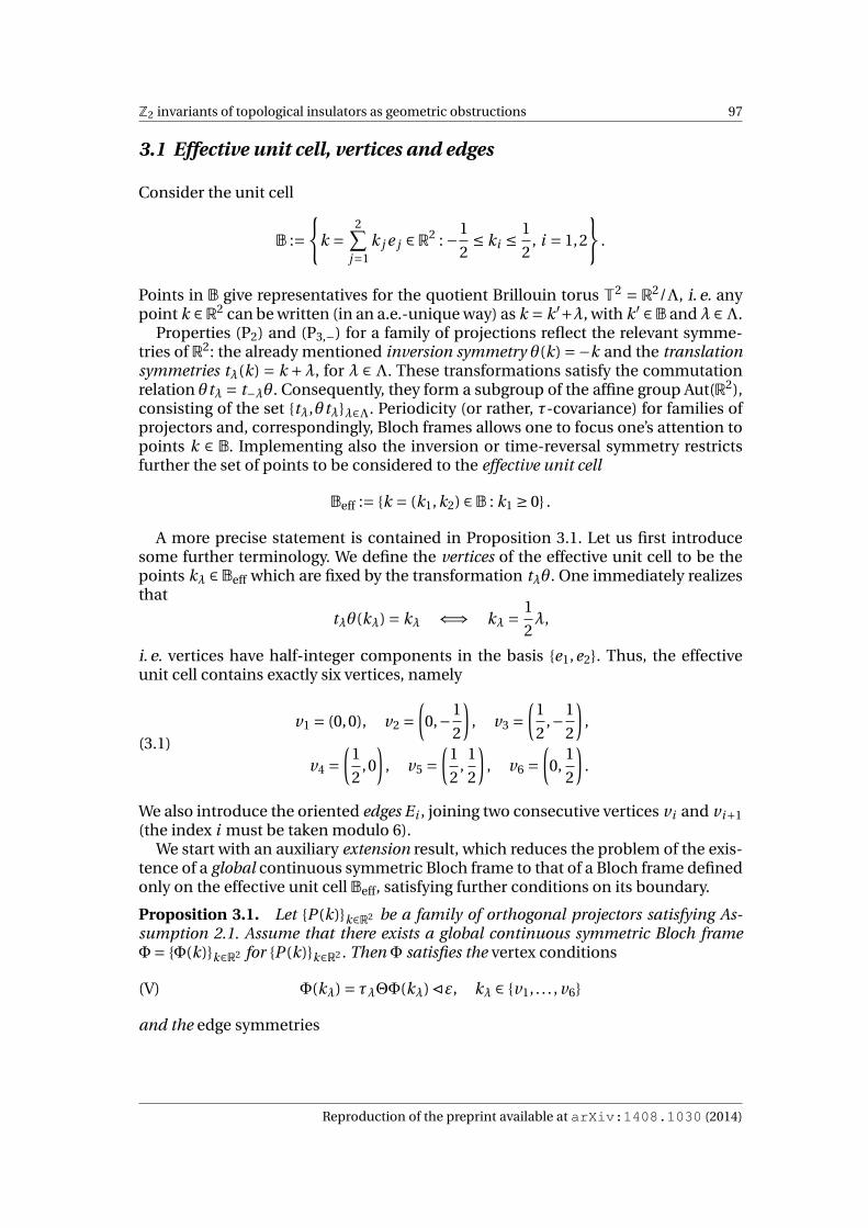
Z2 invariants of topological insulators as geometric obstructions 97
3.1 Effective unit cell, vertices and edges
Consider the unit cell
B :=
k =2∑
j=1k j e j ∈R2 : −1
2≤ ki ≤
1
2, i = 1,2
.
Points in B give representatives for the quotient Brillouin torus T2 = R2/Λ, i. e. anypoint k ∈R2 can be written (in an a.e.-unique way) as k = k ′+λ, with k ′ ∈B andλ ∈Λ.
Properties (P2) and (P3,−) for a family of projections reflect the relevant symme-tries of R2: the already mentioned inversion symmetry θ(k) =−k and the translationsymmetries tλ(k) = k +λ, for λ ∈Λ. These transformations satisfy the commutationrelation θtλ = t−λθ. Consequently, they form a subgroup of the affine group Aut(R2),consisting of the set tλ,θtλλ∈Λ. Periodicity (or rather, τ-covariance) for families ofprojectors and, correspondingly, Bloch frames allows one to focus one’s attention topoints k ∈ B. Implementing also the inversion or time-reversal symmetry restrictsfurther the set of points to be considered to the effective unit cell
Beff := k = (k1,k2) ∈B : k1 ≥ 0 .
A more precise statement is contained in Proposition 3.1. Let us first introducesome further terminology. We define the vertices of the effective unit cell to be thepoints kλ ∈Beff which are fixed by the transformation tλθ. One immediately realizesthat
tλθ(kλ) = kλ ⇐⇒ kλ =1
2λ,
i. e. vertices have half-integer components in the basis e1,e2. Thus, the effectiveunit cell contains exactly six vertices, namely
(3.1)v1 = (0,0), v2 =
(0,−1
2
), v3 =
(1
2,−1
2
),
v4 =(
1
2,0
), v5 =
(1
2,
1
2
), v6 =
(0,
1
2
).
We also introduce the oriented edges Ei , joining two consecutive vertices vi and vi+1(the index i must be taken modulo 6).
We start with an auxiliary extension result, which reduces the problem of the exis-tence of a global continuous symmetric Bloch frame to that of a Bloch frame definedonly on the effective unit cell Beff, satisfying further conditions on its boundary.
Proposition 3.1. Let P (k)k∈R2 be a family of orthogonal projectors satisfying As-sumption 2.1. Assume that there exists a global continuous symmetric Bloch frameΦ= Φ(k)k∈R2 for P (k)k∈R2 . Then Φ satisfies the vertex conditions
(V) Φ(kλ) = τλΘΦ(kλ)/ε, kλ ∈ v1, . . . , v6
and the edge symmetries
Reproduction of the preprint available at arXiv:1408.1030 (2014)
98 Domenico Fiorenza, Domenico Monaco, Gianluca Panati
E1
E2
E3
E4
E5
E6
v1
v2 v3
v4
v5v6
BeffB
Fig. 1 The effective unit cell (shaded area), its vertices and its edges. We use adapted coordinates(k1,k2) such that k = k1e1 +k2e2.
(E)
Φ(θ(k)) =ΘΦ(k)/ε for k ∈ E1 ∪E6,
Φ(te2 (k)) = τe2Φ(k) for k ∈ E2,
Φ(θt−e1 (k)) = τe1ΘΦ(k)/ε for k ∈ E3 ∪E4,
Φ(t−e2 (k)) = τ−e2Φ(k) for k ∈ E5.
Conversely, let Φeff = Φeff(k)k∈Beffbe a continuous Bloch frame for P (k)k∈R2 , de-
fined on the effective unit cell Beff and satisfying the vertex conditions (V) and the edgesymmetries (E). Then there exists a global continuous symmetric Bloch frameΦwhoserestriction to Beff coincides with Φeff.
Proof. Let Φ be a global Bloch frame as in the statement of the Proposition. Thenconditions (F′
3) and (F′4) imply that at the six vertices
Φ(kλ) =Φ(tλθ(kλ)) = τλΦ(θ(kλ)) = τλΘΦ(kλ)/ε,
that is,Φ satisfies the vertex conditions (V). The edge symmetries (E) can be checkedsimilarly, again by making use of (F′
3) and (F′4).
Conversely, assume that a continuous Bloch frame Φeff is given on Beff, and satis-fies (V) and (E). We extend the definition of Φeff to the unit cell B by setting
Φuc(k) :=Φeff(k) if k ∈Beff,ΘΦeff(θ(k))/ε if k ∈B\Beff.
The definition of Φuc can in turn be extended to R2 by setting
Reproduction of the preprint available at arXiv:1408.1030 (2014)
Z2 invariants of topological insulators as geometric obstructions 99
Φ(k) := τλΦuc(k ′) if k = k ′+λ with k ′ ∈B, λ ∈Λ.
The vertex conditions and the edge symmetries ensure that the above defines aglobal continuous Bloch frame; moreover, by construction Φ is also symmetric, inthe sense of Definition 2.1. ut
In view of Proposition 3.1, our strategy to examine Question (Q2) will be to con-sider a continuous Bloch frame Ψ defined over the effective unit cell Beff (whoseexistence is guaranteed by the fact that Beff is contractible and no further symmetryis required), and try to modify it in order to obtain a new continuous Bloch frame Φ,which is defined on the effective unit cell and satisfies also the vertex conditions andthe edge symmetries; by the above extension procedure one obtains a global con-tinuous symmetric Bloch frame. Notice that, since both are orthonormal frames inRanP (k), the given Bloch frameΨ(k) and the unknown symmetric Bloch frameΦ(k)differ by the action of a unitary matrix U (k):
(3.2) Φ(k) =Ψ(k)/U (k), U (k) ∈U(Cm).
Thus, we can equivalently treat the family Beff 3 k 7→U (k) ∈U(Cm) as our unknown.
3.2 Solving the vertex conditions
Let kλ be one of the six vertices in (3.1). If Φ is a symmetric Bloch frame, then, byProposition 3.1,Φ(kλ) satisfies the vertex condition (V), stating the equality betweenthe two frames Φ(kλ) and τλΘΦ(kλ)/ε. For a general Bloch frame Ψ, instead, Ψ(kλ)and τλΘΨ(kλ)/εmay very well be different. Nonetheless, they are both orthonormalframes in RanP (kλ), so there exists a unique unitary matrix Uobs(kλ) ∈ U(Cm) suchthat
(3.3) Ψ(kλ)/Uobs(kλ) = τλΘΨ(kλ)/ε.
The obstruction unitary Uobs(kλ) must satisfy a compatibility condition. In fact, byapplying τλΘ to both sides of (3.3) we obtain that
τλΘ (Ψ(kλ)/Uobs(kλ)) = τλΘ (τλΘΨ(kλ)/ε) == τλΘτλΘΨ(kλ)/ε== τλτ−λΘ2Ψ(kλ)/ε==Ψ(kλ)/ (−ε)
where in the second-to-last equality we used the commutation relation (P4). On theother hand, the left-hand side of this equality is also given by
τλΘ (Ψ(kλ)/Uobs(kλ)) = τλΘΨ(kλ)/Uobs(kλ) == (Ψ(kλ)/
(Uobs(kλ)ε−1))/Uobs(kλ) =
=Ψ(kλ)/(Uobs(kλ)ε−1Uobs(kλ)
).
Reproduction of the preprint available at arXiv:1408.1030 (2014)

100 Domenico Fiorenza, Domenico Monaco, Gianluca Panati
By the freeness of the action ofU(Cm) on frames and the fact that ε−1 =−ε by Remark2.2, we deduce that
(3.4) Uobs(kλ)εUobs(kλ) = ε, i. e. Uobs(kλ)Tε= εUobs(kλ).
Now, notice that the given Bloch frame Ψ(k) and the unknown symmetric BlochframeΦ(k), satisfying the vertex condition (V), differ by the action of a unitary matrixU (k), as in (3.2). We want to relate the obstruction unitary Uobs(kλ) to the unknownU (kλ). In order to do so, we rewrite (V) as
Ψ(kλ)/U (kλ) =Φ(kλ) = τλΘΦ(kλ)/ε== τλΘ (Ψ(kλ)/U (kλ))/ε== τλΘΨ(kλ)/
(U (kλ)ε
)=
= (Ψ(kλ)/
(Uobs(kλ)ε−1))/ (
U (kλ)ε)=
=Ψ(kλ)/(Uobs(kλ)ε−1U (kλ)ε
).
Again by the freeness of the U(Cm)-action, we conclude that
(3.5) U (kλ) =Uobs(kλ)ε−1U (kλ)ε, i. e. Uobs(kλ) =U (kλ)ε−1U (kλ)Tε.
The next Lemma establishes the equivalence between the two conditions (3.4)and (3.5).
Lemma 3.1. Let ε ∈ U(Cm)∩∧2Cm be a unitary and skew-symmetric matrix. Thefollowing conditions on a unitary matrix V ∈U(Cm) are equivalent:
(a) V is such that V Tε= εV ;(b) there exists a matrix U ∈U(Cm) such that V =Uε−1UTε.
Proof. The implication (b) ⇒ (a) is obvious. We prove the implication (a) ⇒ (b).Every unitary matrix can be diagonalized by means of a unitary transforma-
tion. Hence there exist a unitary matrix W ∈ U(Cm) and a diagonal matrix Λ =diag(λ1, . . . ,λm) such that
V =W eiΛW ∗
where the collectioneiλ1 , . . . ,eiλm
forms the spectrum of V . The condition V Tε =
εV is then equivalent to
W eiΛW Tε= εW eiΛW ∗ ⇐⇒ eiΛW TεW =W TεW eiΛ,
i. e. the matrix A :=W TεW commutes with the diagonal matrix eiΛ.According to [18, Lemma in §6], for every unitary matrix Z there exists a unitary
matrix Y such that Y 2 = Z and that Y B = BY whenever Z B = B Z . We can apply thisfact in the case where Z = eiΛ is diagonal, and give an explicit form of Y : Normalizethe arguments λi of the eigenvalues of V so that λi ∈ [0,2π), and define Y := eiΛ/2 =diag
(eiλ1/2, . . . ,eiλm /2
).
We claim now that the matrix
U :=W eiΛ/2W ∗,
Reproduction of the preprint available at arXiv:1408.1030 (2014)
Z2 invariants of topological insulators as geometric obstructions 101
which is clearly unitary, satisfies condition (b) in the statement. Indeed, upon mul-tiplying by W W ∗ = 1l, we get that
Uε−1UTε=W eiΛ/2W ∗ε−1W eiΛ/2W TεW W ∗ =W eiΛ/2 A−1eiΛ/2 AW ∗ =W eiΛW ∗ =V.
This concludes the proof of the Lemma. utThe above result allows us to solve the vertex condition, or equivalently the equa-
tion (3.5) for U (kλ), by applying Lemma 3.1 to V =Uobs(kλ) and U =U (kλ).
3.3 Extending to the edges
To extend the definition of the symmetric Bloch frame Φ(k) (or equivalently of thematrix U (k) appearing in (3.2)) also for k on the edges Ei which constitute theboundary ∂Beff, we use the path-connectedness of the group U(Cm). Indeed, wecan choose a continuous path 5 Wi : [0,1/2] → U(Cm) such that Wi (0) = U (vi ) andWi (1/2) =U (vi+1), where vi and vi+1 are the end-points of the edge Ei . Now set
U (k) :=
W1(−k2) if k ∈ E1,W2(k1) if k ∈ E2,W3(k2 +1/2) if k ∈ E3.
In this way we obtain a continuous map U : E1 ∪ E2 ∪ E3 → U(Cm). Let Φ(k) :=Ψ(k)/U (k) for k ∈ E1∪E2∪E3; we extend this frame to a τ-equivariant, time-reversalinvariant frame on ∂Beff by setting
(3.6) Φ(k) :=
Φ(k) if k ∈ E1 ∪E2 ∪E3,τe1ΘΦ(θt−e1 (k))/ε if k ∈ E4,τe2Φ(t−e2 (k)) if k ∈ E5,ΘΦ(θ(k))/ε if k ∈ E6.
By construction, Φ(k) satisfies all the edge symmetries for a symmetric Blochframe Φ listed in (E), as one can immediately check.
Remark 3.1 (Proof of Theorem 2.1). The above argument also shows that, whend = 1, global continuous symmetric Bloch frames for a family of projectors P (k)k∈Rsatisfying Assumption 2.1 can always be constructed. Indeed, the edge E1 ∪E6 canbe regarded as a 1-dimensional unit cell B(1), and the edge symmetries on it coin-cide exactly with properties (F2) and (F3). Thus, by forcing τ-equivariance, one canextend the definition of the frame continuously on the whole R, as in the proof ofProposition 3.1. Hence, this proves Theorem 2.1. ♦5 Explicitly, a continuous path of unitaries W : [0,1/2] →U(Cm) connecting two unitary matrices U1and U2 can be constructed as follows. Diagonalize U−1
1 U2 = PDP∗, where D = diag(eiµ1 , . . . ,eiµm
)and
P ∈U(Cm). For t ∈ [0,1/2] set
W (t ) =U1PD t P∗, where D t := diag(ei2tµ1 , . . . ,ei2tµm
).
One easily realizes that W (0) =U1, W (1/2) =U2 and W (t ) depends continuously on t , as required.
Reproduction of the preprint available at arXiv:1408.1030 (2014)

102 Domenico Fiorenza, Domenico Monaco, Gianluca Panati
3.4 Extending to the face: aZ2 obstruction
In order to see whether it is possible to extend the frame Φ to a continuous symmet-ric Bloch frame Φ defined on the whole effective unit cell Beff, we first introduce theunitary map U (k) which maps the input frameΨ(k) to the frame Φ(k), i. e. such that
(3.7) Φ(k) =Ψ(k)/U (k), k ∈ ∂Beff
(compare (3.2)). This defines a continuous map U : ∂Beff →U(Cm); we are interestedin finding a continuous extension U : Beff →U(Cm) of U to the effective unit cell.
From a topological viewpoint, ∂Beff is homeomorphic to a circle S1. It is well-known [8, Thm. 17.3.1] that, if X is a topological space, then a continuous mapf : S1 → X defines an element in the fundamental group π1(X ) by taking its homo-topy class [ f ]. Moreover, f extends to a continuous map F : D2 → X , where D2 is the2-dimensional disc enclosed by the circle S1, if and only if [ f ] ∈ π1(X ) is the trivialelement. In our case, the space X is the group U(Cm), and it is also well-known [19,Ch. 8, Sec. 12] that the exact sequence of groups
1 −→ SU(Cm) −→U(Cm)det−−→U (1) −→ 1
induces an isomorphism π1(U(Cm)) ' π1(U (1)). On the other hand, the degree ho-momorphism [8, §13.4(b)]
(3.8) deg: π1(U (1))∼−→Z, [ϕ : S1 →U (1)] 7→ 1
2πi
∮S1
dz ∂z logϕ(z)
establishes an isomorphism of groups π1(U (1)) 'Z. We conclude that a continuousmap f : ∂Beff →U(Cm) can be continuously extended to F : Beff →U(Cm) if and onlyif deg([det f ]) ∈Z is zero.
In our case, we want to extend the continuous map U : ∂Beff →U(Cm) to the wholeeffective unit cell Beff. However, rather than checking whether deg([detU ]) vanishes,it is sufficient to find a unitary-matrix-valued map that “unwinds” the determinantof U (k), while preserving the relevant symmetries on Bloch frames. More precisely,the following result holds.
Proposition 3.2. Let Φ be the Bloch frame defined on ∂Beff that appears in (3.7),satisfying the vertex conditions (V) and the edge symmetries (E). Assume that thereexists a continuous map X : ∂Beff →U(Cm) such that
(X1) deg([det X ]) =−deg([detU ]), and(X2) also the frame Φ/X satisfies (V) and (E).
Then there exists a global continuous symmetric Bloch frame Φ that extends Φ/X tothe whole R2.
Conversely, if Φ is a global continuous symmetric Bloch frame, then its restrictionto ∂Beff differs from Φ by the action of a unitary-matrix-valued continuous map X ,satisfying (X1) and (X2) above.
Proof. If a map X as in the statement of the Proposition exists, then the map U :=U X : ∂Beff → U(Cm) satisfies deg([detU ]) = 0 (because deg is a group homomor-phism), and hence extends continuously to Ueff : Beff →U(Cm). This allows to define
Reproduction of the preprint available at arXiv:1408.1030 (2014)
Z2 invariants of topological insulators as geometric obstructions 103
a continuous symmetric Bloch frame Φeff(k) :=Ψ(k)/Ueff(k) on the whole effectiveunit cell Beff, and by Proposition 3.1 such definition can be then extended continu-ously to R2 to obtain the desired global continuous symmetric Bloch frame Φ.
Conversely, if a global continuous symmetric Bloch frameΦ exists, then its restric-tion Φeff to the boundary of the effective unit cell satisfies Φeff(k) = Ψ(k)/Ueff(k)for some unitary matrix Ueff(k) ∈ U(Cm), and moreover deg([detUeff]) = 0 becauseUeff : ∂Beff → U(Cm) extends to the whole effective unit cell. From (3.7) we deducethat Φeff(k) = Φ(k)/
(U (k)−1Ueff(k)
); the unitary matrix X (k) := U (k)−1Ueff(k) then
satisfies deg([det X ]) = −deg([detU ]), and, when restricted to ∂Beff, both Φeff and Φhave the same symmetries, namely (V) and (E). ut
Proposition 3.2 reduces the question of existence of a global continuous symmet-ric Bloch frame to that of existence of a continuous map X : ∂Beff →U(Cm) satisfyingconditions (X1) and (X2). We begin by imposing condition (X2) on X , and then checkits compatibility with (X1).
We spell out explicitly what it means for the Bloch frame Φ/X to satisfy the edgesymmetries (E), provided that Φ satisfies them. For k = (0,k2) ∈ E1 ∪E6, we obtainthat
Φ(0,−k2)/X (0,−k2) =Θ(Φ(0,k2)/X (0,k2)
)/ε
mΘΦ(0,k2)/ (εX (0,−k2)) =ΘΦ(0,k2)/
(X (0,k2)ε
),
by which we deduce that
(3.9) εX (0,−k2) = X (0,k2)ε, k2 ∈ [−1/2,1/2] .
Similarly, for k = (1/2,k2) ∈ E3 ∪E4, we obtain
(3.10) εX (1/2,−k2) = X (1/2,k2)ε, k2 ∈ [−1/2,1/2] .
Finally, the conditions (E) for k ∈ E2 and k ∈ E5 are clearly the inverse one of eachother, so we can treat both at once. For k = (k1,1/2) ∈ E5, we obtain that
(3.11) X (k1,−1/2) = X (k1,1/2), k1 ∈ [0,1/2] .
Thus we have shown that condition (X2) on X is equivalent to the relations (3.9),(3.10) and (3.11). Notice that these contain also the relations satisfied by X (k) at thevertices k = kλ, which could be obtained by imposing that the frame Φ/ X satifiesthe vertex conditions (V) whenever Φ does. Explicitly, these relations on X (kλ) read
(3.12) εX (kλ) = X (kλ)ε, i. e. X (kλ)TεX (kλ) = ε.
This relation has interesting consequences. Indeed, in view of Remark 2.2, we mayassume that ε is in the standard symplectic form (2.6). Then (3.12) implies that thematrices X (kλ) belong to the symplectic group Sp(2n,C). As such, they must be uni-modular [25], i. e.
(3.13) det X (kλ) = 1.
Reproduction of the preprint available at arXiv:1408.1030 (2014)

104 Domenico Fiorenza, Domenico Monaco, Gianluca Panati
We now proceed in establishing how the properties on X we have deduced from(X2) influence the possible values that the degree of the map ξ := det X : ∂Beff →U (1)can attain. The integral on the boundary ∂Beff of the effective unit cell splits as thesum of the integrals over the oriented edges E1, . . . ,E6:
deg([ξ]) = 1
2πi
∮∂Beff
dz ∂z logdet X (z) =6∑
i=1
1
2πi
∫Ei
dz ∂z logdet X (z).
Our first observation is that all the summands on the right-hand side of the aboveequality are integers. Indeed, from (3.13) we deduce that all maps ξi := det X
∣∣Ei
: Ei →U (1), i = 1, . . . ,6, are indeed periodic, and hence have well-defined degrees: these areevaluated exactly by the integrals appearing in the above sum. We will denote by S1
ithe edge Ei with its endpoints identified: we have thus established that
(3.14) deg([ξ]) =6∑
i=1
1
2πi
∮S1
i
dz ∂z logdet X (z) =6∑
i=1deg([ξi ]).
From Equation (3.11), the integrals over E2 and E5 compensate each other, be-cause the integrands are the same but the orientations of the two edges are opposite.We thus focus our attention on the integrals over S1
1 and S16 (respectively on S1
3 andS1
4). From Equations (3.9) and (3.10), we deduce that if k∗ ∈ 0,1/2 then
X (k∗,k2) = εX (k∗,−k2)ε−1
which implies in particular that
(det X (k∗,k2))−1 = det X (k∗,k2) = det X (k∗,−k2).
Thus, calling z =−k2 the coordinate on S11 and S1
6 (so that the two circles are orientedpositively with respect to z), we can rewrite the above equality for k∗ = 0 as
ξ6(z) = ξ1(−z)
so that
deg([ξ6]) =−deg([ξ1]) (because evaluation at (−z) changes the orientation of S11)
= deg([ξ1]) (because if ϕ : S1 →U (1) then deg([ϕ]) =−deg([ϕ])).
Similarly, for k∗ = 1/2 we get (using this time the coordinate z = k2 on S13 and S1
4)
deg([ξ4]) = deg([ξ3]).
Plugging both the equalities that we just obtained in (3.14), we conclude that
(3.15) deg([ξ]) = 2(deg([ξ1])+deg[ξ3]
) ∈ 2 ·Z.
We have thus proved the following
Reproduction of the preprint available at arXiv:1408.1030 (2014)

Z2 invariants of topological insulators as geometric obstructions 105
Proposition 3.3. Let X : ∂Beff →U(Cm) satisfy condition (X2), as in the statement ofProposition 3.2. Then the degree of its determinant is even:
deg([det X ]) ∈ 2 ·Z.
By the above Proposition, we deduce the followingZ2 classification for symmetricfamilies of projectors in 2 dimensions.
Theorem 3.1. Let P (k)k∈R2 be a family of orthogonal projectors satisfying Assump-tion 2.1. Let U : ∂Beff →U(Cm) be defined as in (3.7). Then there exists a global contin-uous symmetric Bloch frame Φ for P (k)k∈R2 if and only if
deg([detU ]) ≡ 0 mod 2.
Proof. By Proposition 3.2, we know that the existence of a global continuous sym-metric Bloch frame is equivalent to that of a continuous map X : ∂Beff →U(Cm) sat-isfying conditions (X1) and (X2), so that in particular it should have deg([det X ]) =−deg([detU ]). In view of Proposition 3.3, condition (X2) cannot hold in the casewhere deg([detU ]) is odd.
In the case in which deg([detU ]) is even, instead, it just remains to exhibit a mapX : ∂Beff →U(Cm) satisfying (3.9), (3.10) and (3.11), and such that
deg([det X ]) =−deg([detU ]) =−2s, s ∈Z.
In the basis where ε is of the form (2.5), define
X (k) :=
diag(e−2πis(k2+1/2),e−2πis(k2+1/2),1, . . . ,1
)if k ∈ E3 ∪E4,
1l otherwise.
One checks at once that X (k) satisfies (3.9), (3.10) and (3.11) – which are equivalentto (X2), as shown before –, and defines a continuous map X : ∂Beff →U(Cm). Since Xis constant on E1, formula (3.15) for the degree of the determinant of X (k) simplifiesto
deg([det X ]) = 2
(1
2πi
∮S1
3
dz ∂z logdet X (z)
)= 2
(1
2πi
∫ 0
−1/2dk2∂k2 logdet X (1/2,k2)
).
One immediately computes deg([det X ]) =−2s, as wanted. utThe index
(3.16) δ(P ) := deg([detU ]) mod 2
is thus the Z2 topological invariant (see Section 3.6 below) of the family of projec-tors P (k)k∈R2 , satisfying Assumption 2.1, which encodes the obstruction to the ex-istence of a global continuous symmetric Bloch frame. One of our main results, The-orem 2.2, is then reduced to Theorem 3.1.
Reproduction of the preprint available at arXiv:1408.1030 (2014)
106 Domenico Fiorenza, Domenico Monaco, Gianluca Panati
3.5 Well-posedness of the definition of δ
In the construction of the previous Subsection, leading to the definition (3.16) of theZ2 index δ, a number of choices has to be performed, namely the input frame Ψand the interpolation U on E1 ∪E2 ∪E3. This Subsection is devoted to showing thatthe value of the index δ(P ) ∈ Z2 is independent of such choices, and thus is reallyassociated with the bare family of projectors P (k)k∈R2 . Moreover, the index δ is alsoindependent of the choice of a basis e1,e2 for the latticeΛ, as will be manifest fromthe equivalent formulation (5.2) of the invariant we will provide in Section 5.
Gauge independence of δ
As a first step, we will prove that the Z2 index δ is independent of the choice of theinput Bloch frame Ψ.
Indeed, assume that another input Bloch frame Ψnew is chosen: the two frameswill be related by a continuous unitary gauge transformation, say
(3.17) Ψnew(k) =Ψ(k)/G(k), G(k) ∈U(Cm), k ∈Beff.
These two frames will produce, via the procedure illustrated above, two symmetricBloch frames defined on ∂Beff, namely
Φ(k) =Ψ(k)/U (k) and Φnew(k) =Ψnew(k)/Unew(k), k ∈ ∂Beff.
From (3.17) we can rewrite the second equality as
Φnew(k) =Ψ(k)/(G(k)Unew(k)
), k ∈ ∂Beff.
The two frames Φ and Φnew both satisfy the vertex conditions (V) and the edge sym-
metries (E), hence the matrix X (k) := (G(k)Unew(k)
)−1U (k), which transforms Φnew
into Φ, enjoys condition (X2) from Proposition 3.2. Applying Proposition 3.3 we de-duce that
(3.18) deg([detU ]) ≡ deg([
det(GUnew
)])mod 2.
Observe that, since the degree is a group homomorphism,
deg([
det(GUnew
)])= deg([detUnew])+deg([detG]).
The matrix G(k) is by hypothesis defined and continuous on the whole effective unitcell: this implies that the degree of its determinant along the boundary of Beff van-ishes, because its restriction to ∂Beff extends continuously to the interior ofBeff. Thuswe conclude that deg([det(GUnew)]) = deg([detUnew]); plugging this in (3.18) we con-clude that
δ= deg([detU ]) ≡ deg([detUnew]) = δnew mod 2,
as we wanted.
Reproduction of the preprint available at arXiv:1408.1030 (2014)
Z2 invariants of topological insulators as geometric obstructions 107
Invariance under edge extension
Recall that, after solving the vertex conditions and finding the value U (kλ) = U (kλ) atthe vertices kλ, we interpolated those – using the path-connectedness of the groupU(Cm) – to obtain the definition of U (k) first for k ∈ E1∪E2∪E3, and then, imposingthe edge symmetries, extended it to the whole ∂Beff (see Sections 3.2 and 3.3). Wenow study how a change in this interpolation affects the value of deg([detU ]).
Assume that a different interpolation Unew(k) has been chosen on E1 ∪E2 ∪E3,leading to a different unitary-matrix-valued map Unew : ∂Beff →U(Cm). Starting fromthe input frame Ψ, we thus obtain two different Bloch frames:
Φ(k) =Ψ(k)/U (k) and Φnew(k) =Ψ(k)/Unew(k), k ∈ ∂Beff.
From the above equalities, we deduce at once that Φ(k) = Φnew(k)/ X (k), whereX (k) := Unew(k)−1U (k). We now follow the same line of argument as in the previ-ous Subsection. Since both Φ and Φnew satisfy the vertex conditions (V) and the edgesymmetries (E) by construction, the matrix-valued map X : ∂Beff → U(Cm) just de-fined enjoys condition (X2), as in the statement of Proposition 3.2. It follows now byProposition 3.3 that the degree deg([det X ]) is even. Since the degree defines a grouphomomorphism, this means that
deg([det X ]) = deg([detU ])−deg([detUnew]) ≡ 0 mod 2
or equivalently
δ= deg([detU ]) ≡ deg([detUnew]) = δnew mod 2,
as claimed.
3.6 Topological invariance of δ
The aim of this Subsection is to prove that the definition (3.16) of the Z2 index δ(P )actually provides a topological invariant of the family of projectors P (k)k∈R2 , withrespect to those continuous deformation preserving the relevant symmetries speci-fied in Assumption 2.1. More formally, the following result holds.
Proposition 3.4. Let P0(k)k∈R2 and P1(k)k∈R2 be two families of projectors satis-fying Assumption 2.1. Assume that there exists a homotopy Pt (k)k∈R2 , t ∈ [0,1], be-tween P0(k)k∈R2 and P1(k)k∈R2 , such that Pt (k)k∈R2 satisfies Assumption 2.1 forall t ∈ [0,1]. Then
δ (P0) = δ (P1) ∈Z2.
Proof. The function (t ,k) 7→ Pt (k) is a continuous function on the compact set [0,1]×Beff, and hence is uniformly continuous. Thus, there exists µ> 0 such that∥∥Pt (k)−P t (k)
∥∥B(H) < 1 if max
∣∣k − k∣∣ ,
∣∣t − t∣∣<µ.
In particular, choosing t0 <µ, we have that
Reproduction of the preprint available at arXiv:1408.1030 (2014)

108 Domenico Fiorenza, Domenico Monaco, Gianluca Panati
(3.19) ‖Pt (k)−P0(k)‖B(H) < 1 if t ∈ [0, t0], uniformly in k ∈Beff.
We will show that δ(P0) = δ(Pt0 ). Iterating this construction a finite number of timeswill prove that δ(P0) = δ(P1).
In view of (3.19), the Kato-Nagy unitary [22, Sec. I.6.8]
W (k) := (1l− (P0(k)−Pt0 (k))2)−1/2 (
Pt0 (k)P0(k)+ (1l−Pt0 (k))(1l−P0(k))) ∈U(H)
is well-defined and provides an intertwiner between RanP0(k) and RanPt0 (k), namely
Pt0 (k) =W (k)P0(k)W (k)−1.
Moreover, one immediately realizes that the map k 7→ W (k) inherits from the twofamilies of projectors the following properties:
(W1) the map Beff 3 k 7→W (k) ∈U(H) is C∞-smooth;(W2) the map k 7→ W (k) is τ-covariant, in the sense that whenever k and k +λ are
both in Beff for λ ∈Λ, then
W (k +λ) = τ(λ)W (k)τ(λ)−1;
(W3) the map k 7→ W (k) is time-reversal symmetric, in the sense that whenever kand −k are both in Beff, then
W (−k) =ΘW (k)Θ−1.
Let now Ψ0(k)k∈Beffbe a continuous Bloch frame for P0(k)k∈R2 . Extending the
action of the unitary W (k) ∈ U(H) to m-frames component-wise, we can defineΨt0 (k) = W (k)Ψ0(k) for k ∈ Beff, and obtain a continuous Bloch frame
Ψt0 (k)
k∈Beff
forPt0 (k)
k∈R2 . Following the procedure illustrated in Sections 3.2 and 3.3, we can
produce two symmetric Bloch frames for P0(k)k∈R2 andPt0 (k)
k∈R2 , namely
Φ0(k) =Ψ0(k)/U0(k) and Φt0 (k) =Ψt0 (k)/Ut0 (k), k ∈ ∂Beff.
From the above equalities, we deduce that
Φt0 (k) =Ψt0 (k)/Ut0 (k) = (W (k)Ψ0(k))/Ut0 (k) ==W (k)
(Ψ0(k)/Ut0 (k)
)=W (k)(Φ0(k)/
(U0(k)−1Ut0 (k)
))== (
W (k)Φ0(k))/
(U0(k)−1Ut0 (k)
)where we have used that the action of a linear operator inB(H), extended component-wise to m-frames, commutes with the right-action of U(Cm). It is easy to verify that,in view of properties (W1), (W2) and (W3), the frame
W (k)Φ0(k)
k∈∂Beff
gives a con-
tinuous Bloch frame forPt0 (k)
k∈R2 which still satisfies the vertex conditions (V) and
the edge symmetries (E), since Φ0 does. Hence the matrix X (k) := U0(k)−1Ut0 (k) sat-isfies hypothesis (X2), and in view of Proposition 3.3 its determinant has even degree.We conclude that
δ(P0) = deg([detU0]) ≡ deg([detUt0 ]) = δ(Pt0 ) mod 2. ut
Reproduction of the preprint available at arXiv:1408.1030 (2014)

Z2 invariants of topological insulators as geometric obstructions 109
4 Comparison with the Fu-Kane index
In this Section, we will compare our Z2 invariant δ with the Z2 invariant ∆ proposedby Fu and Kane [12], and show that they are equal. For the reader’s convenience, werecall the definition of ∆, rephrasing it in our terminology.
Let Ψ(k) = ψ1(k), . . . ,ψm(k)
be a global τ-equivariant6 Bloch frame. Define the
unitary matrix w(k) ∈U(Cm) by
w(k)ab := ⟨ψa(−k),Θψb(k)
⟩.
In terms of the right action of matrices on frames, one can equivalently say that w(k)is the matrix such that 7
(4.1) ΘΨ(k) =Ψ(−k)/w(k).
Comparing (4.1) with (F′4), we see that if Ψ were already symmetric then w(k) = ε−1
for all k ∈Rd .One immediately checks how w(k) changes when the inversion or translation
symmetries are applied to k. One has that
w(θ(k))ab = ⟨ψa(k),Θψb(−k)
⟩= ⟨Θ2ψb(−k),Θψa(k)
⟩==−⟨
ψb(−k),Θψa(k)⟩=−w(k)ba
or in matrix form w(θ(k)) = −w(k)T. Moreover, by using the τ-equivariance of theframe Ψ one obtains
w(tλ(k))ab = ⟨ψa(θtλ(k)),Θψb(tλ(k))
⟩= ⟨ψa(t−λθ(k)),Θτ(λ)ψb(k)
⟩== ⟨
τ(−λ)ψa(−k),τ(−λ)Θψb(k)⟩= ⟨
ψa(−k),Θψb(k)⟩= w(k)ab
because τ(−λ) is unitary; in matrix form we can thus write w(tλ(k)) = w(k).Combining both these facts, we see that at the vertices kλ of the effective unit cell
we get−w(kλ)T = w(θ(kλ)) = w(t−λ(kλ)) = w(kλ).
6 This assumption is crucial in the definition of the Fu-Kane index, whereas the definition of ourZ2 invariant does not need Ψ to be already τ-equivariant. Nonetheless, the existence of a global τ-equivariant Bloch frame is guaranteed by a straightforward modification of the proof in [28], as de-tailed in [26].7 Indeed, spelling out (4.1) one obtains
Θψb(k) =m∑
c=1ψc (−k)w(k)cb
and taking the scalar product of both sides with ψa(−k) yields
⟨ψa(−k),Θψb(k)
⟩= m∑c=1
⟨ψa(−k),ψc (−k)
⟩w(k)cb =
m∑c=1
δac w(k)cb = w(k)ab
becauseψa(−k)
a=1,...,m is an orthonormal frame in RanP (−k).
Reproduction of the preprint available at arXiv:1408.1030 (2014)
110 Domenico Fiorenza, Domenico Monaco, Gianluca Panati
In other words, the matrix w(kλ) is skew-symmetric, and hence it has a well-definedPfaffian, satisfying (Pf w(kλ))2 = det w(kλ). The Fu-Kane index ∆ is then defined as[12, Equations (3.22) and (3.25)]
(4.2) ∆ := Pθ(1/2)−Pθ(0) mod 2,
where for k∗ ∈ 0,1/2
(4.3) Pθ(k∗) := 1
2πi
(∫ 1/2
0dk2 Tr
(w(k∗,k2)∗∂k2 w(k∗,k2)
)−2logPf w(k∗,1/2)
Pf w(k∗,0)
).
We are now in position to prove the above-mentioned equality between our Z2invariant δ and the Fu-Kane index ∆.
Theorem 4.1. Let P (k)k∈R2 be a family of projectors satisfying Assumption 2.1, andlet δ= δ(P ) ∈Z2 be as in (3.16). Let ∆ ∈Z2 be the Fu-Kane index defined in (4.2). Then
δ=∆ ∈Z2.
Proof. First we will rewrite our Z2 invariant δ, in order to make the comparison with∆ more accessible. Recall that δ is defined as the degree of the determinant of thematrix U (k), for k ∈ ∂Beff, satisfying Φ(k) = Ψ(k)/ U (k), where Φ(k) is as in (3.6).The unitary U (k) coincides with the unitary U (k) for k ∈ E1 ∪E2 ∪E3, where U (k)is a continuous path interpolating the unitary matrices U (vi ), i = 1,2,3,4, i. e. thesolutions to the vertex conditions (compare Sections 3.2 and 3.3). The definition ofU (k) for k ∈ E4 ∪E5 ∪E6 is then obtained by imposing the edge symmetries on thecorresponding frame Φ(k), as in Section 3.3.
We first compute explicitly the extension of U to k ∈ E4 ∪E5 ∪E6. For k ∈ E4, sayk = (1/2,k2) with k2 ≥ 0, we obtain
Φ(k) = τe1ΘΦ(te1θ(k)
)/ε=
= τe1Θ(Ψ
(te1θ(k)
)/U
(te1θ(k)
))/ε=
= (τe1τ−e1ΘΨ(−k)
)/
(U (1/2,−k2)ε
)=
= (Ψ(k)/w(−k))/(U (1/2,−k2)ε
)=
=Ψ(k)/(w(−k)U (1/2,−k2)ε
).
This means that
(4.4) U (k) = w(−k)U (1/2,−k2)ε, k = (1/2,k2) ∈ E4.
Analogously, for k ∈ E5, say k = (k1,1/2), we obtain
(4.5) U (k) = U (k1,−1/2), k = (k1,1/2) ∈ E5.
Finally, for k ∈ E6, say k = (0,k2) with k2 ≥ 0, we obtain in analogy with (4.4)
(4.6) U (k) = w(−k)U (0,−k2)ε, k = (0,k2) ∈ E6.
Reproduction of the preprint available at arXiv:1408.1030 (2014)
Z2 invariants of topological insulators as geometric obstructions 111
Notice that, as w(−1/2,k2) = w(t−e1 (1/2,k2)) = w(1/2,k2), we can actually summa-rize (4.4) and (4.6) as
U (k∗,k2) = w(k∗,−k2)U (k∗,−k2)ε, k∗ ∈ 0,1/2 , k2 ∈ [0,1/2].
Since U and U coincide on E1 and E3, we can further rewrite this relation as
(4.7) w(k∗,k2) = U (k∗,−k2)ε−1U (k∗,k2)T, (k∗,k2) ∈ S1∗,
where S1∗ denotes the edge E1 ∪E6 for k∗ = 0 (respectively E3 ∪E4 for k∗ = 1/2), with
the edge-points identified: the identification is allowed in view of (4.5) and the factthat w(tλ(k)) = w(k).
We are now able to compute the degree of the determinant of U . Firstly, an easycomputation 8 shows that
8 If U (z) ∈U(Cm) has spectrumeiλ j (z)
j=1,...,m , then
∂z logdetU (z) =m∑
j=1e−iλ j (z)∂z eiλ j (z).
On the other hand, writing the spectral decomposition of U (z) as
U (z) =m∑
j=1eiλ j (z)P j (z), P j (z)∗ = P j (z) = P j (z)2, Tr(P j (z)) = 1,
one immediately deduces that
U (z)∗ =m∑
j=1e−iλ j (z)P j (z) and ∂zU (z) =
m∑j=1
(∂z eiλ j (z)
)P j (z)+eiλ j (z)(∂z P j (z)).
Notice now that, taking the derivative with respect to z of the equality P j (z)2 = P j (z), one obtains
P j (z)∂z P j (z) = (∂z P j (z)
)(1l−P j (z)
)so that
∂z P j (z) = P j (z)(∂z P j (z)
)(1l−P j (z)
)+ (1l−P j (z)
)(∂z P j (z)
)P j (z).
From this, it follows by the ciclicity of the trace and the relation P j (z)P`(z) = δ j ,`P j (z) = P`(z)P j (z)that
Tr(P`(z)
(∂z P j (z)
))=Tr(P j (z)P`(z)
(∂z P j (z)
)(1l−P j (z)
))++Tr
((1l−P j (z)
)P`(z)
(∂z P j (z)
)P j (z)
)= 0.
We are now able to compute
Tr(U (z)∗∂zU (z)
)= m∑j ,`=1
Tr(e−iλ`(z)P`(z)
(∂z eiλ j (z)
)P j (z)
)+
+e−i(λ`(z)−λ j (z)
)Tr
(P`(z)
(∂ j P (z)
))==
m∑j ,`=1
e−iλ`(z)(∂z eiλ j (z)
)δ j ,`Tr
(P j (z)
)= m∑j=1
e−iλ j (z)∂z eiλ j (z).
Reproduction of the preprint available at arXiv:1408.1030 (2014)
112 Domenico Fiorenza, Domenico Monaco, Gianluca Panati
deg([detU ]) = 1
2πi
∮∂Beff
dz ∂z logdetU (z) =
= 1
2πi
∮∂Beff
dz Tr(U (z)∗∂zU (z)
)= 6∑i=1
1
2πi
∫Ei
dz Tr(U (z)∗∂zU (z)
).
Clearly we have
(4.8)∫
Ei
dz Tr(U (z)∗∂zU (z)
)= ∫Ei
dz Tr(U (z)∗∂zU (z)
)for i = 1,2,3,
because U and U coincide on E1 ∪E2 ∪E3. Using now Equation (4.5) we compute∫E5
dz Tr(U (z)∗∂zU (z)
)= ∫ 0
1/2dk1 Tr
(U (k1,1/2)∗∂k1U (k1,1/2)
)==−
∫ 1/2
0dk1 Tr
(U (k1,−1/2)∗∂k1U (k1,−1/2)
)==−
∫E2
dz Tr(U (z)∗∂zU (z)
)or equivalently, in view of (4.8) for i = 2,
(4.9)∫
E2+E5
dz Tr(U (z)∗∂zU (z)
)= 0.
Making use of (4.7), we proceed now to evaluate the integrals on E1,E3,E4 andE6, which give the non-trivial contributions to deg([detU ]). Indeed, Equation (4.7)implies
w(k∗,k2)∗ = U (k∗,k2)εU (k∗,−k2)∗,
∂k2 w(k∗,k2) =−∂k2U (k∗,−k2)ε−1U (k∗,k2)T+U (k∗,−k2)ε−1∂k2U (k∗,k2)T,
from which one computes
Tr(w(k∗,k2)∗∂k2 w(k∗,k2)) =−Tr(U (k∗,−k2)∗∂k2U (k∗,−k2)
)++Tr
(U (k∗,k2)∗∂k2U (k∗,k2)
).
Integrating both sides of the above equality for k2 ∈ [0,1/2] yields to(4.10)∫ 1/2
0dk2 Tr(w(k∗,k2)∗∂k2 w(k∗,k2)) =−
∫ 0
−1/2dk2 Tr
(U (k∗,k2)∗∂k2U (k∗,k2)
)++
∫ 1/2
0dk2 Tr
(U (k∗,k2)∗∂k2U (k∗,k2)
)== (−1)1+2k∗
∮S1∗
dz Tr(U (z)∗∂zU (z)
)++2
∫ 1/2
0dk2 Tr
(U (k∗,k2)∗∂k2U (k∗,k2)
).
Reproduction of the preprint available at arXiv:1408.1030 (2014)

Z2 invariants of topological insulators as geometric obstructions 113
The sign s∗ := (−1)1+2k∗ appearing in front of the integral along S1∗ depends on the
different orientations of the two circles, for k∗ = 0 and for k∗ = 1/2, parametrized bythe coordinate z = k2.
Now, notice that
(4.11)
∫ 1/2
0dk2 Tr
(U (k∗,k2)∗∂k2U (k∗,k2)
)= ∫ 1/2
0dk2∂k2 logdetU (k∗,k2)
≡ logdetU (k∗,1/2)
detU (k∗,0)mod 2πi.
Furthermore, evaluating Equation (4.7) at the six vertices kλ, we obtain
w(kλ) = U (kλ)ε−1U (kλ)T
which implies that
(4.12) Pf w(kλ) = detU (kλ)Pfε−1
by the well known property Pf(C ACT) = det(C )Pf(A), for a skew-symmetric matrix Aand a matrix C ∈ Mm(C) [25].
Substituting the latter equality in the right-hand side of Equation (4.11) allows usto rewrite (4.10) as
1
2πi
(∫ 1/2
0dk2 Tr(w(k∗,k2)∗∂k2 w(k∗,k2))−2log
Pf w(k∗,1/2)
Pf w(k∗,0)
)≡
≡ s∗2πi
∫S1∗
dz Tr(U (z)∗∂zU (z)
)mod 2.
On the left-hand side of this equality, we recognize Pθ(k∗), as defined in (4.3). Takingcare of the orientation of S1
∗, we conclude, also in view of (4.9), that
∆≡ Pθ(1/2)−Pθ(0) mod 2
≡ 1
2πi
∫E1+E3+E4+E6
dz Tr(U (z)∗∂zU (z)
)mod 2
≡ deg([detU ]) ≡ δ mod 2.
This concludes the proof. utRemark 4.1 (On the rôle of Pfaffians). Equation (4.7) is the crucial point in theabove argument. Indeed, since detε = 1 (compare Remark 2.2), from (4.7) it followsthat
(4.13) det w(k∗,k2) = detU (k∗,−k2)detU (k∗,k2), (k∗,k2) ∈ S1∗.
If we evaluate this equality at the six vertices kλ, we obtain
(4.14) det w(kλ) = (detU (kλ)
)2 = (Pf w(kλ))2 .
Reproduction of the preprint available at arXiv:1408.1030 (2014)

114 Domenico Fiorenza, Domenico Monaco, Gianluca Panati
Looking at Equation (4.13), we realize that the expression detU (k∗,k2) serves asa “continuous prolongation” along the edges E1,E3,E4,E6 of the Pfaffian Pf w(kλ),which is well-defined only at the six vertices kλ (where the matrix w is skew-symmetric),in a way which is moreover compatible with time-reversal symmetry, since in (4.13)both detU (k∗,k2) and detU (k∗,−k2) appear. This justifies the rather misterious andapparently ad hoc presence of Pfaffians in the Fu-Kane formula for the Z2 index∆. ♦
In view of the equality ∆ = δ ∈ Z2, we have a clear intepretation of the Fu-Kaneindex as the obstruction to the existence of a global continuous symmetric Blochframe, as claimed in [12, App. A].
5 A simpler formula for theZ2 invariant
The fact that theZ2 invariant δ, as defined in (3.16), is well-defined and independentof the choice of an interpolation of the vertex unitaries U (kλ) (see Section ) showsthat its value depends only on the value of U at the vertices. In this Section, we willprovide a way to compute δ ∈Z2 using data coming just from the four time-reversalinvariant momenta v1, . . . , v4 which are inequivalent modulo translational and in-version symmetries of R2. This should be compared with [12, Equation (3.26)].
In the previous Section, we have rewritten our invariant as δ= Pθ(1/2)−Pθ(0) mod2, with
−Pθ(k∗) := 1
2πi
(∫ 0
−1/2dk2 Tr
(w(k∗,k2)∗∂k2 w(k∗,k2)
)+− 2
∫ 0
−1/2dk2 Tr
(U (k∗,k2)∗∂k2U (k∗,k2)
))== 1
2πi
(log
det w(k∗,0)
det w(k∗,−1/2)−2log
detU (k∗,0)
detU (k∗,−1/2)
).
In view of (4.14), the above expression can be rewritten as
δ=4∑
i=1ηvi mod 2, where ηvi := 1
2πi
(log
(detU (vi )
)2 −2logdetU (vi ))
.
Notice that, since deg([detU ]) is an integer, the value (−1)deg([detU ]) is independentof the choice of the determination of log(−1) and is determined by the parity ofdeg([detU ]), i. e. by δ= deg([detU ]) mod 2. Moreover, this implies also that
(−1)δ =4∏
i=1(−1)ηvi
and each (−1)ηvi can be computed with any determination of log(−1) (as long as onechooses the same for all i ∈ 1, . . . ,4). Noticing that, using the principal value of thecomplex logarithm,
Reproduction of the preprint available at arXiv:1408.1030 (2014)
Z2 invariants of topological insulators as geometric obstructions 115
(5.1) (−1)(logα)/(2πi) = (eiπ)(logα)/(2πi) = e(logα)/2 =pα,
it follows that we can rewrite the above expression for (−1)δ as
(5.2) (−1)δ =4∏
i=1
√(detU (vi )
)2
detU (vi )
where the branch of the square root is chosen in order to evolve continuously fromv1 to v2 along E1, and from v3 to v4 along E3. This formula is to be compared with[12, Equation (3.26)] for the Fu-Kane index ∆, namely
(5.3) (−1)∆ =4∏
i=1
√det w(vi )
Pf w(vi ).
Recall now that the value of U at the vertices kλ is determined by solving the ver-tex conditions, as in Section 3.2: U (kλ) =U (kλ) is related to the obstruction unitaryUobs(kλ) by the relation (3.5). In particular, from (3.5) we deduce that
detUobs(kλ) = (detU (kλ))2
so that (5.2) may be rewritten as
(5.4) (−1)δ =4∏
i=1
√detUobs(vi )
detU (vi ).
This reformulation shows that ourZ2 invariant can be computed starting just fromthe “input” Bloch frame Ψ (provided it is continuous on Beff), and more specificallyfrom its values at the vertices kλ. Indeed, the obstruction Uobs(kλ) at the vertices isdefined by (3.3) solely in terms of Ψ(kλ); moreover, U (kλ) is determined by Uobs(kλ)as explained in the proof of Lemma 3.1.
We have thus the following algorithmic recipe to compute δ:
• given a continuous Bloch frameΨ(k) = ψa(k)
a=1,...,m , k ∈Beff, compute the uni-
tary matrix
Uobs(kλ)a,b =m∑
c=1
⟨ψa(kλ),τ(λ)Θψc (kλ)
⟩εcb ,
defined as in (3.3), at the four inequivalent time-reversal invariant momenta kλ =v1, . . . , v4;
• compute the spectrum
eiλ(i )1 , . . . ,eiλ(i )
m
⊂U (1) of Uobs(vi ), so that in particular
detUobs(vi ) = exp(i(λ(i )
1 +·· ·+λ(i )m
));
normalize the arguments of such phases so that λ(i )j ∈ [0,2π) for all j ∈ 1, . . . ,m;
• compute U (vi ) as in the proof of Lemma 3.1: in particular we obtain that
Reproduction of the preprint available at arXiv:1408.1030 (2014)
116 Domenico Fiorenza, Domenico Monaco, Gianluca Panati
detU (vi ) = exp
(i
(λ(i )
1
2+·· ·+ λ(i )
m
2
));
• finally, compute δ from the formula (5.4), i. e.
(−1)δ =4∏
i=1
√exp
(i(λ(i )
1 +·· ·+λ(i )m
))exp
(i
(λ(i )
1
2+·· ·+ λ(i )
m
2
)) .
6 Construction of a symmetric Bloch frame in 3d
In this Section, we investigate the existence of a global continuous symmetric Blochframe in the 3-dimensional setting. In particular, we will recover the four Z2 indicesproposed by Fu, Kane and Mele [13]. We will first focus on the topological obstruc-tions that arise, and then provide the construction of a symmetric Bloch frame in 3dwhen the procedure is unobstructed.
6.1 Vertex conditions and edge extension
The 3-dimensional unit cell is defined, in complete analogy with the 2-dimensionalcase, as
B(3) :=
k =3∑
j=1k j e j ∈R3 : −1
2≤ k j ≤
1
2, j = 1,2,3
(the superscript (3) stands for “3-dimensional”), where e1,e2,e3 is a basis in R3 suchthat Λ = SpanZ e1,e2,e3. If a continuous Bloch frame is given on B(3), then it canbe extended to a continuous τ-equivariant Bloch frame on R3 by considering its τ-translates, provided it satisfies the obvious compatibility conditions of τ-periodicityon the faces of the unit cell (i. e. on its boundary). Similarly, if one wants to studyframes which are also time-reversal invariant, then one can restrict the attention tothe effective unit cell (see Figure 2)
B(3)eff :=
k = (k1,k2,k3) ∈B(3) : k1 ≥ 0
.
Vertices of the (effective) unit cell are defined again as those points kλ which areinvariant under the transformation tλθ: these are the points with half-integer coor-dinates with respect to the lattice generators e1,e2,e3. The vertex conditions for asymmetric Bloch frame read exactly as in (V), and can be solved analogously to the2-dimensional case with the use of Lemma 3.1. This leads to the definition of a uni-tary matrix U (kλ) at each vertex. The definition of U (·) can be extended to the edgesjoining vertices of B(3)
eff by using the path-connectedness of the group U(Cm), as inSection 3.3. Actually, we need to choose such an extension only on the edges whichare plotted with a thick line in Figure 2: then we can obtain the definition of U (·) to
Reproduction of the preprint available at arXiv:1408.1030 (2014)

Z2 invariants of topological insulators as geometric obstructions 117
•
• •
••
• •
•
••
•
•
•
•
•
•
• •
••
BeffB
k1
k3
k2
Fig. 2 The 3-dimensional effective unit cell (shaded area).
all edges by imposing edge symmetries, which are completely analogous to those in(E).
6.2 Extension to the faces: fourZ2 obstructions
We now want to extend the definition of the matrix U (k), mapping an input Blochframe Ψ(k) to a symmetric Bloch frame Φ(k), to k ∈ ∂B(3)
eff . The boundary of B(3)eff con-
sists now of six faces, which we denote as follows:
F1,0 :=
(k1,k2,k3) ∈ ∂B(3)eff : k1 = 0
,
F1,+ :=
(k1,k2,k3) ∈ ∂B(3)eff : k1 =
1
2
,
Fi ,± :=
(k1,k2,k3) ∈ ∂B(3)eff : ki =±1
2
, i ∈ 2,3 .
Notice that F1,0 and F1,+ are both isomorphic to a full unit cellB(2) (the superscript(2) stands for “2-dimensional”), while the faces Fi ,±, i ∈ 2,3, are all isomorphic to a2d effective unit cell B(2)
eff .We start by considering the four faces Fi ,±, i ∈ 2,3. From the 2-dimensional algo-
rithm, we know that to extend the definition of U (·) from the edges to one of thesefaces we need for the associatedZ2 invariant δi ,± to vanish. Not all these four invari-ants are independent, though: indeed, we have that δi ,+ = δi ,− for i = 2,3. In fact,suppose for example that δi ,− vanishes, so that we can extend the Bloch frame Φ to
Reproduction of the preprint available at arXiv:1408.1030 (2014)

118 Domenico Fiorenza, Domenico Monaco, Gianluca Panati
the face Fi ,−. Then, by setting Φ(tei (k)) := τeiΦ(k) for k ∈ Fi ,−, we get an extension ofthe frame Φ to Fi ,+: it follows that also δi ,+ must vanish. Viceversa, exchanging theroles of the subscripts + and − one can argue that if δi ,+ = 0 then also δi ,− = 0; in con-clusion, δi ,+ = δi ,− ∈ Z2, as claimed. We remain for now with only two independentZ2 invariants, namely δ2,+ and δ3,+.
We now turn our attention to the faces F1,0 and F1,+. As we already noticed, theseare 2d unit cellsB(2). Each of them contains three thick-line edges (as in Figure 2), onwhich we have already defined the Bloch frameΦ: this allows us to test the possibilityto extend it to the effective unit cell which they enclose. If we are indeed able to con-struct such an extension to this effective unit cell B(2)
eff , then we can extend it to thewhole face by using the time reversal operator Θ in the usual way: in fact, both F1,0and F1,+ are such that if k lies on it then also−k lies on it (up to periodicity, or equiva-lently translational invariance). The obstruction to the extension of the Bloch frameto F1,0 and F1,+ is thus encoded again in two Z2 invariants δ1,0 and δ1,+; togetherwith δ2,+ and δ3,+, they represent the obstruction to the continuous extension of thesymmetric Bloch frame from the edges of B(3)
eff to the boundary ∂B(3)eff .
Suppose now that we are indeed able to obtain such an extension to ∂B(3)eff , i. e.
that all four Z2 invariants vanish. Then we have a map U : ∂B(3)eff →U(Cm), such that
at each k ∈ ∂B(3)eff the unitary matrix U (k) maps the reference Bloch frame Ψ(k) to a
symmetric Bloch frame Φ(k): Φ(k) =Ψ(k)/U (k). In order to get a continuous sym-metric Bloch frame defined on the whole B(3)
eff , it is thus sufficient to extend the map
U : ∂B(3)eff →U(Cm) to a continuous map U : B(3)
eff →U(Cm).Topologically, the boundary of the effective unit cell in 3 dimensions is equiva-
lent to a sphere: ∂B(3)eff ' S2. Moreover, it is known that, if X is any topological space,
then a continuous map f : S2 → X extends to a continuous map F : D3 → X , de-fined on the 3-ball D3 that the sphere encircles, if and only if its homotopy class[ f ] ∈ [S2; X ] = π2(X ) is trivial. In our case, where X = U(Cm), it is a well-known factthat π2(U(Cm)) = 0 [19, Ch.8, Sec. 12], so that actually any continuous map from theboundary of the effective unit cell to the unitary group extends continuously to amap defined on the whole B(3)
eff . In other words, there is no topological obstruction to
the continuous extension of a symmetric frame from ∂B(3)eff to B(3)
eff , and hence to R3:
indeed, one can argue, as in Proposition 3.1, that a symmetric Bloch frame on B(3)eff
can always be extended to all of R3, by imposing τ-equivariance and time-reversalsymmetry.
In conclusion, we have that all the topological obstruction that can prevent theexistence of a global continuous symmetric Bloch frame is encoded in the four Z2invariants δ1,0 and δi ,+, for i ∈ 1,2,3, given by
(6.1) δ∗(P ) := δ(P
∣∣F∗
), F∗ ∈
F1,0,F1,+,F2,+,F3,+
.
Reproduction of the preprint available at arXiv:1408.1030 (2014)
Z2 invariants of topological insulators as geometric obstructions 119
6.3 Proof of Theorem 2.3
We have now understood how topological obstruction may arise in the constructionof a global continuous symmetric Bloch frame, by sketching the 3-dimensional ana-logue of the method developed in Section 3 for the 2d case. This Subsection is de-voted to detailing a more precise constructive algorithm for such a Bloch frame in 3d ,whenever there is no topological obstruction to its existence. As in the 2d case, wewill start from a “naïve” choice of a continuous Bloch frame Ψ(k), and symmetrizeit to obtain the required symmetric Bloch frame Φ(k) = Ψ(k)/U (k) on the effec-tive unit cell B(3)
eff (compare (3.2)). We will apply this scheme first on vertices, then onedges, then (whenever there is no topological obstruction) to faces, and then to theinterior of B(3)
eff .The two main “tools” in this algorithm are provided by the following Lemmas,
which are “distilled” from the procedure elaborated in Section 3.
Lemma 6.1 (From 0d to 1d ). Let P (k)k∈R be a family of projectors satisfying As-sumption 2.1. Denote B(1)
eff = k = k1e1 : −1/2 ≤ k1 ≤ 0 ' [−1/2,0]. Let Φ(−1/2) be aframe in RanP (−1/2) such that
Φ(−1/2) = τ−e1ΘΦ(−1/2)/ε,
i. e.Φ satisfies the vertex condition (V) at k−e1 =−(1/2)e1 ∈B(1)eff . Then one constructs a
continuous Bloch frame Φeff(k)k∈B(1)eff
such that
Φeff(−1/2) =Φ(−1/2) and Φeff(0) =ΘΦeff(0)/ε.
Proof. Solve the vertex condition at kλ = 0 ∈ B(1)eff using Lemma 3.1, and then extend
the frame to B(1)eff as in Section 3.3. ut
Lemma 6.2 (From 1d to 2d ). Let P (k)k∈R2 be a family of projectors satisfying As-sumption 2.1. Let vi and Ei denote the edges of the effective unit cell B(2)
eff , as defined inSection 3.1. Let Φ(k)k∈E1∪E2∪E3 be a continuous Bloch frame for P (k)k∈R2 , satisfyingthe vertex conditions (V) at v1, v2, v3 and v4. Assume that
δ(P ) = 0 ∈Z2.
Then one constructs a continuous Bloch frame Φeff(k)k∈B(2)eff
, satisfying the vertex con-
ditions (V) and the edge symmetries (E), and moreover such that
(6.2) Φeff(k) =Φ(k) for k ∈ E1 ∪E2.
Proof. This is just a different formulation of what was proved in Section 3.4. Fromthe datum of Φ(k) on the edges E1 ∪E2 ∪E3 one can construct the unitary matrixU : ∂B(2)
eff → U(Cm), such that Φ(k)/U (k) is a symmetric Bloch frame, for k ∈ ∂B(2)eff .
The hypothesis δ(P ) = 0 ∈Z2 ensures that deg([detU ]) = 2s, s ∈Z. The proof of Theo-rem 3.1 then gives an explicit family of unitary matrices X : ∂B(2)
eff →U(Cm) such that
deg([det X ]) = −2s and that Φeff(k) := Φ(k)/(U (k) X (k)
)is still symmetric, so it ex-
Reproduction of the preprint available at arXiv:1408.1030 (2014)
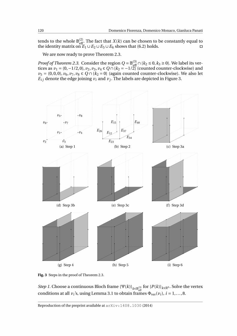
120 Domenico Fiorenza, Domenico Monaco, Gianluca Panati
tends to the whole B(2)eff . The fact that X (k) can be chosen to be constantly equal to
the identity matrix on E1 ∪E2 ∪E5 ∪E6 shows that (6.2) holds. utWe are now ready to prove Theorem 2.3.
Proof of Theorem 2.3. Consider the region Q = B(3)eff ∩ k2 ≤ 0,k3 ≥ 0. We label its ver-
tices as v1 = (0,−1/2,0), v2, v3, v4 ∈Q ∩ k2 =−1/2 (counted counter-clockwise) andv5 = (0,0,0), v6, v7, v8 ∈ Q ∩ k2 = 0 (again counted counter-clockwise). We also letEi j denote the edge joining vi and v j . The labels are depicted in Figure 3.
•v2•v3
•v8
•v4
•v5
•v1
•v6 •v7
(a) Step 1
• •
•
•
•
•
• •
E26
E23
E34
E48
E37E12
E15
(b) Step 2
•
• •
•
•
•
•
•
• •
(c) Step 3a
•
• •
•
••
•
•
•
•
• •
(d) Step 3b
•
• •
•
••
•
•
•
•
•
• •
(e) Step 3c
•
• •
•
••
•
•
•
•
•
•
• •
(f) Step 3d
•
• •
•
• •
••
•
•
•
•
•
•
••
• •
(g) Step 4
•
• •
•
• •
••
•
•
•
•
•
•
••
• •
(h) Step 5
•
• •
•
• •
••
•
•
•
•
•
•
••
• •
(i) Step 6
Fig. 3 Steps in the proof of Theorem 2.3.
Step 1. Choose a continuous Bloch frame Ψ(k)k∈B(3)eff
for P (k)k∈R3 . Solve the vertex
conditions at all vi ’s, using Lemma 3.1 to obtain frames Φver(vi ), i = 1, . . . ,8.
Reproduction of the preprint available at arXiv:1408.1030 (2014)
Z2 invariants of topological insulators as geometric obstructions 121
Step 2. Using repeatedly Lemma 6.1, extend the definition of Φver to the edges E12,E15, E23, E26, E34, E37 and E48, to obtain frames Φedg(k).Step 3. Use Lemma 6.2 to extend further the definition of Φedg as follows.
3a. Extend the definition of Φedg on F3,+: this can be done since δ3,+ vanishes. Thiswill change the original definition of Φedg only on E37.
3b. Extend the definition ofΦedg on F2,−: this can be done sinceδ2,− = δ2,+ vanishes.This will change the original definition of Φedg only on E34.
3c. Extend the definition of Φedg on F1,0 ∩ k3 ≥ 0: this can be done since δ1,0 van-ishes. This will change the original definition of Φedg only on E15. (Here we give
F1,0 the opposite orientation to the one inherited from ∂B(3)eff , but this is inessen-
tial.)3d. Extend the definition ofΦedg on F1,+∩k3 ≥ 0. Although we have already changed
the definition ofΦedg on E37∪E34, this extension can still be performed since wehave proved in Section that δ1,+ is independent of the choice of the extensionof the frame along edges, and hence vanishes by hypothesis. The extension willfurther modify the definition of Φedg only on E48.
We end up with a Bloch frame ΦS defined on
S := F2,−∪F3,+∪(F1,0 ∩ k3 ≥ 0
)∪ (F1,+∩ k3 ≥ 0
).
Step 4. Extend the definition of ΦS to F1,0 ∩ k3 ≤ 0 and F1,+∩ k3 ≤ 0 by setting
ΦS′(k) :=ΦS(k) for k ∈ S,
ΦS′(θ(k)) :=ΘΦS(k)/ε for k ∈ F1,0 ∩ k3 ≥ 0 , and
ΦS′(te1θ(k)) := τe1ΘΦS(k)/ε for k ∈ F1,+∩ k3 ≥ 0 .
This extension is continuous. Indeed, continuity along E15∪θ(E15) = F1,0∩k3 = 0(respectively E48 ∪ te1θ(E48) = F1,+∩ k3 = 0) is a consequence of the edge symme-tries that we have imposed on ΦS in Step 3c (respectively in Step 3d). What wehave to verify is that the definition of ΦS′ that we have just given on t−e2θ(E12) =(F1,0∩ k3 ≤ 0)∩F2,− and te1−e2θ(E34) = (F1,+∩ k3 ≤ 0)∩F2,− agrees with the defini-tion of ΦS on the same edges that was achieved in Step 3b.
We look at t−e2θ(E12), since the case of te1−e2θ(E34) is analogous. If k ∈ E12, thenΦS(t−e2θ(k)) = τ−e2ΘΦS(k)/ε, since in Step 3b we imposed the edge symmetries onF3,−. On the other hand, ΦS′(k) =ΦS(k) on E12 ⊂ S by definition of ΦS′ : we get thenalso
ΦS(t−e2θ(k)) = τ−e2ΘΦS(k)/ε= τ−e2ΘΦS′(k)/ε== τ−e2Θτ−e2ΦS′(te2 (k))/ε
because of the edge symmetries satisfied byΦS′ on the shorter edges of F1,0∩k3 ≥ 0.In view of (P4) and of the definition of ΦS′ on F1,0 ∩ k3 ≤ 0, we conclude that
ΦS(t−e2θ(k)) =ΘΦS′(te2 (k))/ε=ΦS′(θte2 (k)) =ΦS′(t−e2θ(k))
as wanted. This shows that ΦS′ is continuous on
S′ := S ∪ (F1,0 ∩ k3 ≤ 0
)∪ (F1,+∩ k3 ≤ 0
).
Reproduction of the preprint available at arXiv:1408.1030 (2014)

122 Domenico Fiorenza, Domenico Monaco, Gianluca Panati
Step 5. Extend the definition of ΦS′ to F3,− by setting
ΦS′′(k) :=ΦS′(k) for k ∈ S′, and
ΦS′′(t−e3 (k)) := τ−e3ΦS′(k) for k ∈ F3,+.
This extension is continuous on t−e3 (E23) = F2,−∩F3,− because in Step 3b we haveimposed on ΦS the edge symmetries on the shorter edges of F2,−. Similarly, ΦS′′ andΦS′ agree on θ(E26)∪ t−e3 (E26) = F1,0 ∩F3,− and on t−e3 (E37)∪ te1θ(E37) = F1,+∩F3,−,because by construction ΦS′ is τ-equivariant. We have constructed so far a continu-ous Bloch frame ΦS′′ on S′′ := S′∪F3,−.Step 6. Extend the definition of ΦS′′ to F2,+ by setting
Φ(k) :=ΦS′′(k) for k ∈ S′′, and
Φ(te2 (k)) := τe2ΦS′′(k) for k ∈ F2,−.
Similarly to what was argued in Step 5, the edge symmetries (i. e. τ-equivariance)on ∂F2,− and ∂F2,+ imply that this extension is continuous. The Bloch frame Φ is nowdefined and continuous on ∂B(3)
eff .
Step 7. Finally, extend the definition of Φ on the interior of B(3)eff . As was argued before
at the end of Section 6.2, this step is topologically unobstructed. Thus, we end upwith a continuous symmetric Bloch frame Φeff on B(3)
eff . Set now
Φuc(k) :=Φeff(k) if k ∈B(3)
eff ,
ΘΦeff(θ(k))/ε if k ∈B(3) \B(3)eff .
The symmetries satisfied by Φeff on F1,0 (imposed in Step 4) imply that the BlochframeΦuc is still continuous. We extend now the definition ofΦuc to the whole R3 bysetting
Φ(k) := τλΦuc(k ′), if k = k ′+λ with k ′ ∈B(3), λ ∈Λ.
Again, the symmetries imposed onΦuc in the previous Steps of the proof ensure thatΦ is continuous, and by construction it is also symmetric. This concludes the proofof Theorem 2.3. ut
6.4 Comparison with the Fu-Kane-Mele indices
In their work [13], Fu, Kane and Mele generalized the definition of Z2 indices for 2dtopological insulators, appearing in [12], to 3d topological insulators. There the au-thors mainly use the formulation ofZ2 indices given by evaluation of certain quanti-ties at the inequivalent time-reversal invariant momenta kλ, as in (5.3). We briefly re-call the definition of the four Fu-Kane-Mele Z2 indices for the reader’s convenience.
In the 3-dimensional unit cell B(3), there are only eight vertices which are inequiv-alent up to periodicity: these are the points kλ corresponding toλ= (n1/2,n2/2,n3/2),where each n j can be either 0 or 1. These are the vertices in Figure 2 that are con-nected by thick lines. Define the matrix w as in (4.1), where Ψ is a continuous andτ-equivariant Bloch frame (whose existence is guaranteed again by the generaliza-
Reproduction of the preprint available at arXiv:1408.1030 (2014)

Z2 invariants of topological insulators as geometric obstructions 123
tion of the results of [28] given in [26]). Set
ηn1,n2,n3 :=√
det w(kλ)
Pf w(kλ)
∣∣∣∣∣λ=(n1/2,n2/2,n3/2)
.
Then the four Fu-Kane-MeleZ2 indices ν0,ν1,ν2,ν3 ∈Z2 are defined as [13, Eqn.s (2)and (3)]
(−1)ν0 :=∏
n1,n2,n3∈0,1ηn1,n2,n3 ,
(−1)νi :=∏
ni=1, n j 6=i∈0,1ηn1,n2,n3 , i ∈ 1,2,3 .
In other words, the Fu-Kane-Mele 3d index (−1)νi equals the Fu-Kane 2d index (−1)∆
for the face where the i -th coordinate is set equal to 1/2, while the index (−1)ν0 in-volves the product over all the inequivalent time-reversal invariant momenta kλ.
Since our invariants δ1,0 and δi ,+, i = 1,2,3, are defined as the 2-dimensional Z2invariants relative to certain (effective) faces on the boundary of the 3-dimensionalunit cell, they also satisfy identities which express them as product of quantities tobe evaluated at vertices of the effective unit cell, as in Section 5 (compare (5.2) and(5.4)). Explicitly, these expressions read as
(−1)δ1,0 :=∏
n1=0,n2,n3∈0,1ηn1,n2,n3 ,
(−1)δi ,+ :=∏
ni=1, n j 6=i∈0,1ηn1,n2,n3 , i ∈ 1,2,3 ,
where (compare (5.2))
ηn1,n2,n3 :=
√(detU (kλ))2
detU (kλ)
∣∣∣∣∣∣∣λ=(n1/2,n2/2,n3/2)
.
As we have also shown in Section 4 that our 2-dimensional invariant δ agrees withthe Fu-Kane index ∆, from the previous considerations it follows at once that
νi = δi ,+ ∈Z2, i ∈ 1,2,3 , and ν0 = δ1,0 +δ1,+ ∈Z2.
This shows that the four Z2 indices proposed by Fu, Kane and Mele are compatiblewith ours, and in turn our reformulation proves that indeed these Z2 indices repre-sent the obstruction to the existence of a continuous symmetric Bloch frame in 3d .The geometric rôle of the Fu-Kane-Mele indices is thus made transparent.
We also observe that, under this identification, the indices νi , i ∈ 1,2,3, dependmanifestly on the choice of a basis e1,e2,e3 ⊂Rd for the latticeΛ, while the index ν0is independent of such a choice. This substantiates the terminology of [13], where ν0is called “strong” invariant, while ν1, ν2 and ν3 are referred to as “weak” invariants.
Reproduction of the preprint available at arXiv:1408.1030 (2014)

124 Domenico Fiorenza, Domenico Monaco, Gianluca Panati
A Smoothing procedure
Throughout the main body of the paper, we have mainly considered the issue of theexistence of a continuous global symmetric Bloch frame for a family of projectorsP (k)k∈Rd satisfying Assumption 2.1. This Appendix is devoted to showing that, ifsuch a continuous Bloch frame exists, then also a smooth one can be found, arbitrar-ily close to it. The topology in which we measure “closeness” of frames is given bythe distance
dist(Φ,Ψ) := supk∈Rd
( m∑a=1
∥∥φa(k)−ψa(k)∥∥2H
)1/2
for two global Bloch frames Φ = φa(k)
a=1,...,m, k∈Rd and Ψ =
ψa(k)
a=1,...,m, k∈Rd .The following result holds in any dimension d ≥ 0.
Proposition A.1. Let P (k)k∈Rd be a family of orthogonal projectors satisfying As-sumption 2.1. Assume that a continuous global symmetric Bloch frame Φ exists forP (k)k∈Rd . Then for any µ > 0 there exists a smooth global symmetric Bloch frameΦsm such that
dist(Φ,Φsm) <µ.
Proof. We use the same strategy used to prove Proposition 5.1 in [9], to which werefer for most details.
A global Bloch frame gives a section of the principal U(Cm)-bundle Fr(P) → Td ,the frame bundle associated with the Bloch bundle P→Td , whose fibre Fr(P)k =: Fk
over the point k ∈Td consists of all orthonormal bases in RanP (k). The existence ofa continuous global Bloch frame Φ is thus equivalent to the existence of a continousglobal section of the frame bundle Fr(P). By Steenrod’s ironing principle [35, 41],there exists a smooth section of the frame bundle arbitrarily close to the latter con-tinuous one; going back to the language of Bloch frames, this implies for any µ > 0the existence of a smooth global Bloch frame Φsm such that
dist(Φ,Φsm) < 1
2µ.
The Bloch frame Φsm will not in general be also symmetric, so we apply a sym-metrization procedure to Φsm to obtain the desired smooth symmetric Bloch frameΦsm. In order to do so, we define the midpoint between two sufficiently close framesΦ and Ψ in Fk as follows. Write Ψ = Φ/UΦ,Ψ, with UΦ,Ψ a unitary matrix. If Ψ issufficiently close to Φ, then UΦ,Ψ is sufficiently close to the identity matrix 1lm inthe standard Riemannian metric of U(Cm) (see [9, Section 5] for details). As such,we have that UΦ,Ψ = exp
(AΦ,Ψ
), for AΦ,Ψ ∈ u(Cm) a skew-Hermitian matrix, and
exp: u(Cm) →U(Cm) the exponential map1. We define then the midpoint betweenΦand Ψ to be the frame M(Φ,Ψ) :=Φ/exp
(1
2AΦ,Ψ
).
1 It is known that the exponential map exp: u(Cm) →U(Cm) defines a diffeomorphism between a ballBδ(0) ⊂ u(Cm) and a Riemannian ball Bδ(1lm) ⊂ U(Cm), for some δ > 0. When we say that the twoframes Φ and Ψ should be “sufficiently close”, we mean (here and in the following) that the unitarymatrix UΦ,Ψ lies in the ball Bδ(1lm).
Reproduction of the preprint available at arXiv:1408.1030 (2014)

Z2 invariants of topological insulators as geometric obstructions 125
Set
(A.1) Φsm(k) := M (Φsm(k),ΘΦsm(−k)/ε
).
The proof that Φsm defines a smooth global Bloch frame, which satisfies the τ-equivariance property (F′
3), and that moreover its distance from the frame Φ is lessthan µ goes exactly as the proof of [9, Prop. 5.1]. A slightly different argument isneeded, instead, to prove that Φsm is also time-reversal symmetric, i. e. that it sat-isfies also (F′
4). To show this, we need a preliminary result.
Lemma A.1. Let Φ,Ψ ∈ Fk be two frames, and assume that Φ and Ψ/ ε are suffi-ciently close. Then
(A.2) M(Φ,Ψ/ε) = M(Φ/ε−1,Ψ)/ε.
Proof. Notice first that
Ψ=Φ/UΦ,Ψ =⇒ Ψ/ε=Φ/ (UΦ,Ψε
)and Ψ= (Φ/ε−1)/
(εUΦ,Ψ
),
which means that
UΦ,Ψ/ε =UΦ,Ψε and UΦ/ε−1,Ψ = εUΦ,Ψ.
WriteεUΦ,Ψ = exp(A) and UΦ,Ψε= exp(B)
for A,B ∈ Bδ(0) ⊂ u(Cm), where δ > 0 is such that exp: Bδ(0) ⊂ u(Cm) → Bδ(1lm) ⊂U(Cm) is a diffeomorphism. Since the Hilbert-Schmidt norm ‖A‖2
HS := Tr(A∗A) isinvariant under unitary conjugation, also ε−1 Aε ∈ Bδ(0). Then we have that
(A.3) exp(ε−1 Aε
)= ε−1 exp(A)ε= ε−1εUε=Uε= exp(B).
It then follows from (A.3) that B = ε−1 Aε, because the exponential map is a diffeo-morphism. From this we can conclude that
M(Φ/ε−1,Ψ)/ε= (Φ/ε−1)/
(exp
(1
2A
)ε
)=
=Φ/exp
(1
2ε−1 Aε
)=Φ/exp
(1
2B
)=
= M(Φ,Ψ/ε)
which is exactly (A.2). utWe are now in position to prove that Φsm, defined in (A.1), satisfies (F′
4). Indeed,we compute
Reproduction of the preprint available at arXiv:1408.1030 (2014)

126 Domenico Fiorenza, Domenico Monaco, Gianluca Panati
ΘΦsm(k)/ε=ΘM (Φsm(k),ΘΦsm(−k)/ε
)/ε=
= M (ΘΦsm(k),Θ2Φsm(−k)/ε
)/ε= (by [9, Eqn. (5.11)])
= M (ΘΦsm(k),Φsm(−k)/ε−1)/ε= (because −ε= ε−1 by Remark 2.2)
= M (Φsm(−k)/ε−1,ΘΦsm(k)
)/ε= (because M(Φ,Ψ) = M(Ψ,Φ))
= M (Φsm(−k),ΘΦsm(k)/ε
)=Φsm(−k) (by (A.2)).
This concludes the proof of the Proposition. ut
References
1. ALTLAND, A.; ZIRNBAUER, M. : Non-standard symmetry classes in mesoscopic normal-superconducting hybrid structures, Phys. Rev. B 55 (1997), 1142–1161.
2. ANDO, Y. : Topological insulator materials, J. Phys. Soc. Jpn. 82 (2013), 102001.3. AVILA, J.C.; SCHULZ-BALDES, H.; VILLEGAS-BLAS, C. : Topological invariants of edge states for
periodic two-dimensional models, Mathematical Physics, Analysis and Geometry 16 (2013), 136–170.
4. CARPENTIER, D.; DELPLACE, P.; FRUCHART, M.; GAWEDZKI, K. : Topological index for periodicallydriven time-reversal invariant 2D systems, Phys. Rev. Lett. 114 (2015), 106806.
5. CARPENTIER, D.; DELPLACE, P.; FRUCHART, M.; GAWEDZKI, K.; TAUBER, C. : Construction andproperties of a topological index for periodically driven time-reversal invariant 2D crystals,preprint available at arXiv:1503.04157.
6. CERULLI IRELLI, G. ; FIORENZA, D.; MONACO, D.; PANATI, G. : Geometry of Bloch bundles: aunifying quiver-theoretic approach, in preparation (2015).
7. CHANG, C.-Z. et al. : Experimental Observation of the Quantum Anomalous Hall Effect in a Mag-netic Topological Insulator, Science 340 (2013), 167–170.
8. DUBROVIN, B.A.; NOVIKOV, S.P.; FOMENKO, A.T. : Modern Geometry – Methods and Applica-tions. Part II: The Geometry and Topology of Manifolds. No. 93 in Graduate Texts in Mathematics.Springer-Verlag, New York, 1985.
9. FIORENZA, D.; MONACO, D.; PANATI, G. : Construction of real-valued localized compositeWannier functions for insulators, to appear in Ann. Henri Poincaré. Preprint available atarXiv:1408.0527.
10. FRÖHLICH, J. ; WERNER, PH. : Gauge theory of topological phases of matter, EPL 101 (2013),47007.
11. FRUCHART, M. ; CARPENTIER, D. : An introduction to topological insulators, Comptes RendusPhys. 14 (2013), 779–815.
12. FU, L.; KANE, C.L. : Time reversal polarization and a Z2 adiabatic spin pump, Phys. Rev. B 74(2006), 195312.
13. FU, L.; KANE, C.L.; MELE, E.J. : Topological insulators in three dimensions, Phys. Rev. Lett. 98(2007), 106803.
14. GRAF, G.M. : Aspects of the Integer Quantum Hall Effect, Proceedings of Symposia in Pure Math-ematics 76 (2007), 429–442.
15. GRAF, G.M.; PORTA, M. : Bulk-edge correspondence for two-dimensional topological insulators,Commun. Math. Phys. 324 (2013), 851–895.
16. HALDANE, F.D.M. : Model for a Quantum Hall Effect without Landau levels: condensed-matterrealization of the “parity anomaly”, Phys. Rev. Lett. 61 (1988), 2017.
17. HASAN, M.Z.; KANE, C.L. : Colloquium: Topological Insulators, Rev. Mod. Phys. 82 (2010), 3045–3067.
18. HUA, L.-K.: On the theory of automorphic functions of a matrix variable I – Geometrical basis,Am. J. Math. 66 (1944), 470–488.
19. HUSEMOLLER, D.: Fibre bundles, 3rd edition. No. 20 in Graduate Texts in Mathematics. Springer-Verlag, New York, 1994.
20. KANE, C.L.; MELE, E.J. : Z2 Topological Order and the Quantum Spin Hall Effect, Phys. Rev. Lett.95 (2005), 146802.
Reproduction of the preprint available at arXiv:1408.1030 (2014)

References 127
21. KANE, C.L.; MELE, E.J. : Quantum Spin Hall Effect in graphene, Phys. Rev. Lett. 95 (2005), 226801.22. KATO, T. : Perturbation theory for linear operators. Springer, Berlin, 1966.23. KENNEDY, R.; GUGGENHEIM, C. : Homotopy theory of strong and weak topological insulators,
preprint available at arXiv:1409.2529.24. KITAEV, A. : Periodic table for topological insulators and superconductors, AIP Conf. Proc. 1134
(2009), 22.25. MACKEY, D.S.; MACKEY, N. : On the Determinant of Symplectic Matrices. Numerical Analysis
Report 422 (2003), Manchester Centre for Computational Mathematics, Manchester, England.26. MONACO, D.; PANATI, G. : Symmetry and localization in periodic crystals: triviality of Bloch bun-
dles with a fermionic time-reversal symmetry. Proceedings of the conference “SPT2014 – Symme-try and Perturbation Theory”, Cala Gonone, Italy, to appear in Acta App. Math. (2015).
27. MOORE, J.E.; BALENTS, L. : Topological invariants of time-reversal-invariant band structures,Phys. Rev. B 75 (2007), 121306(R).
28. PANATI, G.: Triviality of Bloch and Bloch-Dirac bundles, Ann. Henri Poincaré 8 (2007), 995–1011.29. PRODAN, E. : Robustness of the Spin-Chern number, Phys. Rev. B 80 (2009), 125327.30. PRODAN, E. : Disordered topological insulators: A non-commutative geometry perspective, J.
Phys. A 44 (2011), 113001.31. PRODAN, E. : Manifestly gauge-independent formulations of the Z2 invariants, Phys. Rev. B 83
(2011), 235115.32. RYU, S.; SCHNYDER, A.P.; FURUSAKI, A.; LUDWIG, A.W.W. : Topological insulators and supercon-
ductors: Tenfold way and dimensional hierarchy, New J. Phys. 12 (2010), 065010.33. SCHULZ-BALDES, H. : Persistence of spin edge currents in disordered Quantum Spin Hall sys-
tems, Commun. Math. Phys. 324 (2013), 589–600.34. SCHULZ-BALDES, H. : Z2 indices of odd symmetric Fredholm operators, preprint available at
arXiv:1311.0379.35. STEENROD, N. : The Topology of Fibre Bundles. No. 14 in Princeton Mathematical Series. Prince-
ton University Press, Princeton, 1951.36. STICLET, D. ; PÉCHON, F.; FUCHS, J.-N.; KALUGIN, P.; SIMON P. : Geometrical engineering of a
two-band Chern insulator in two dimensions with arbitrary topological index, Phys. Rev. B 85(2012), 165456.
37. SOLUYANOV, A.A.; VANDERBILT, D. : Wannier representation of Z2 topological insulators, Phys.Rev. B 83 (2011), 035108.
38. SOLUYANOV, A.A.; VANDERBILT, D. : Computing topological invariants without inversion sym-metry, Phys. Rev. B 83 (2011), 235401.
39. SOLUYANOV, A.A.; VANDERBILT, D. : Smooth gauge for topological insulators, Phys. Rev. B 85(2012), 115415.
40. THOULESS D.J.; KOHMOTO, M.; NIGHTINGALE, M.P.; DE NIJS, M. : Quantized Hall conductancein a two-dimensional periodic potential, Phys. Rev. Lett. 49 (1982), 405–408.
41. WOCKEL, CH. : A generalization of Steenrod’s Approximation Theorem, Arch. Math. (Brno) 45(2009), 95–104.

Conclusions


Open problems and perspectives
The line of research in which this dissertation fits, namely that of geometric phasesof quantum matter, is very active, and of course several questions remain to be an-swered. Here we would like to illustrate some possible further developments of theanalysis initiated in the works presented in this dissertation.
1 Disordered topological insulators
The Z2 invariants introduced in [5], which was reproduced in Part II of this thesis,provide a geometric origin for the indices proposed by Fu, Kane and Mele to dis-tinguish different geometric phases in time-reversal symmetric topological insula-tors, when the time-reversal operator is of fermionic nature. It is costumary, in thephysics literature, to dub a phase “topological” if it is stable under (small) perturba-tions of the system: usually these perturbations include disorder and impurities. Ourcurrent formulation cannot encompass also this more general framework, since theintroduction of a random potential usually breaks the periodicity of the system at amicroscopic level; the mathematical consequence of this is that we cannot employthe Bloch-Floquet-Zak transform and pass to the crystal momentum description ofthe system. It should be noticed however that Z2 invariants for disordered quantumspin Hall systems have been already proposed [15, 16], at least under the assumptionof quasi-conservation of spin.
In the context of the quantum Hall effect, it has been suggested by Bellissard andcollaborators (see [1] and references therein) to replace the notion of periodicity withthat of homogeneity. Roughly speaking, this notion requires to consider the Hamil-tonian of the system not as a single operator, but rather as a family of operatorsHωω∈Ω, labelled by the disorder configurations ω ∈ Ω. Such a family is called ho-mogeneous if the periodicity of the system is restored at a macroscopic level, namelyif the Hamiltonian at disorder configuration ω and the one at the “translated disor-der configuration” Tλω are unitarily equivalent:
HTλω = τλ Hωτ−1λ , λ ∈Λ, ω ∈Ω, τ−1
λ = τ∗λ.
Here T : Λ×Ω→Ω, (λ,ω) 7→ Tλω, is an action of Λ ' Zd on Ω, which is assumed tobe ergodic with respect to some probability measure onΩ (used to perform averagesover disorder configurations). One can then set homogeneous families of operators
131

132 Open problems and perspectives
in a C∗-algebraic setting, defining the noncommutative Brillouin zone as the crossedproduct C∗-algebra ANCBZ :=C (Ω)oTΛ; this is in turn made into a noncommutativemanifold by endowing it with derivations ∂1,∂2 and a trace T which plays the rôleof integration. With this structure, the Connes-Chern character (the noncommuta-tive analogue of a Chern number) can be formulated; proving that it stays quantized(namely that it assumes only integer values) requires the use of Fredholm modulestheory.
A tentative approach to give a generalization of the Z2 invariants we proposed in[5] to the framework of disordered media and homogeneous families of operatorswould require to borrow ideas from [1, 18] and follow a similar line of argument.First, one should define a “noncommutative effective Brillouin zone”, enlarging thegroup of macroscopic symmetries Λ to the group G :=ΛoZ2, a semidirect productof Λ (namely the group of lattice translations) with the group Z2 generated, in theusual k-space picture, by the involution θ(k) = −k. The noncommutative effectiveBrillouin zone ANCEBZ :=C (Ω)oG should then be equipped with derivations and in-tegration (trace), to mimic a formula like (3.16) in the reproduction of [5] presentedin Part II. The appropriate Fredholm module should then be defined to prove quan-tization, this time in the Z2 sense.
Although promising, at present this approach remains to be fully explored.
2 Topological invariants for other symmetry classes
Another possible line of investigation concerns the geometric origin of the differenttopological phases in the symmetry classes of the periodic tables of topological in-sulators (compare Table 1 in the Introduction). Pioneering results in this directioncan be found in [8, 2, 3, 4, 19, 17, 7].
The methods we proposed in Part II are amenable to wide generalizations, sincethey rely only on the fundamental symmetries of the quantum system at hand. Inparticular, by considering families of projectors P (k)k∈Sd which are labelled by acrystal momentum in Sd instead of Rd (and eliminating the periodicity condition(P2) from Assumption 2.1 in the Introduction), and/or encoding other types of sym-metries (charge conjugation, chiral symmetry) possibly in combination with one an-other, one should in principle be able to define topological invariants for families ofprojectors in the various Altland-Zirnbauer classes (both for free-fermion systemsand for periodic ones), proceeding again in a step-by-step construction of a Blochframe along the cellular decomposition of the Brillouin zone (from vertices to edges,to faces, and so on).
3 Magnetic Wannier functions
As a last possible development of the line of research covered in this dissertation, wereport on some currently unpublished results, which investigate magnetic Wannierfunctions [12].
As was discussed in the Introduction, it is by now well established [13] that theexistence of a frame composed of exponentially localized Wannier functions for a

References 133
gapped periodic quantum system is equivalent to the triviality of the associatedBloch bundle, or equivalently to the vanishing of its first Chern class. The latter con-dition is ensured by the presence of time-reversal symmetry [13, 11]. It is natural toask what kind of decay at infinity of the Wannier functions is to be expected when thetopology is non-trivial, namely when the Chern class of the Bloch bundle does notvanish. This is generically the case, for example, for magnetic periodic Schrödingeroperators, since the presence of a magnetic field breaks time-reversal symmetry.This is why we refer to Bloch and Wannier functions associated to a topologicallynon-trivial Bloch bundle as magnetic Bloch and Wannier functions, respectively.
To investigate the decay at infinity of magnetic Wannier functions, we proceed asfollows. We illustrate for simplicity the 2-dimensional picture, but our argument canbe adapted also to dimension d = 3. By employing techniques similar to those usedin [5], we are able to construct a Bloch frame Φ which is smooth and τ-equivarianton the boundary ∂B of the fundamental unit cell. This Bloch frame is then extendedto B \ (0,0) by the parallel transport techniques developed in [6]: these allow alsoto estimate the singularity of the resulting Bloch frame at the origin, and one is ableto establish that the extended frame Φ is in H s(B;H) for all s < 1. This requires alsosome arguments similar to those presented in [10] (see Part I of this dissertation).
A separate argument shows instead that, if a more regular frame Φ ∈ H 1(B;H)existed, then the Chern number of the Bloch bundle would vanish, thus implyingthat the bundle itself is trivial, contrary to the “magnetic” assumption. Notice thatthe existence of a frame Φ ∈ H r (B;H) with r > 1 is also excluded, since by Sobolevembedding Φ would be continuous, contradicting the non-triviality assumption onthe Bloch bundle. This shows that the Sobolev regularity of the Bloch frame Φ con-structed above is the best that can be obtained. In turn, such regularity implies thatthe associated Wannier functions w are such that FMV[w] = ∞, where FMV is theMarzari-Vanderbilt localization functional [9, 36], given by the variance of the posi-tion operator in the state w . The physical interpretation of this result is that, just astrivial topology is related to (exponential) localization, non-trivial topology is relatedto delocalization, establishing an even stronger bound between geometric aspectsand transport properties in crystals.
References
1. BELLISSARD, J.; VAN ELST, A.; SCHULZ-BALDES, H. : The noncommutative geometry of the quan-tum Hall effect, J. Math. Phys 35, 5373–5451 (1994).
2. DE NITTIS, G.; GOMI, K. : Classification of “Real” Bloch-bundles: Topological Quantum Systemsof type AI, J. Geom. Phys. 86, 303-338 (2014).
3. DE NITTIS, G.; GOMI, K. : Classification of “Quaternionic” Bloch-bundles, Commun. Math. Phys.339 (2015), 1–55.
4. DE NITTIS, G.; GOMI, K. : Chiral vector bundles: A geometric model for class AIII topologicalquantum systems, available at arXiv:1504.04863.
5. FIORENZA, D.; MONACO, D.; PANATI, G. : Z2 invariants of topological insulators as geometricobstructions, available at arXiv:1408.1030.
6. FREUND, S.; TEUFEL, S. : Peierls substitution for magnetic Bloch bands, available atarXiv:1312.5931.
7. GROSSMANN, J.; SCHULZ-BALDES, H. : Index pairings in presence of symmetries with applica-tions to topological insulators, available at arXiv:1503.04834.
8. KENNEDY, R.; ZIRNBAUER, M.R. : Bott periodicity forZ2 symmetric ground states of free fermionsystems, available at arXiv:1409.2537.

134 Open problems and perspectives
9. MARZARI, N.; MOSTOFI, A.A.; YATES, J.R.; SOUZA I.; VANDERBILT, D. : Maximally localized Wan-nier functions: Theory and applications, Rev. Mod. Phys. 84, 1419 (2012).
10. MONACO, D.; PANATI, G. : Topological invariants of eigenvalue intersections and decrease ofWannier functions in graphene, J. Stat. Phys. 155, Issue 6, 1027–1071 (2014).
11. MONACO, D.; PANATI, G. : Symmetry and localization in periodic crystals: triviality of Bloch bun-dles with a fermionic time-reversal symmetry, Acta Appl. Math. 137, Issue 1, 185–203 (2015).
12. MONACO, D.; PANATI, G.; PISANTE, A.; TEUFEL, S. : Decay of magnetic Wannier functions, inpreparation.
13. PANATI, G. : Triviality of Bloch and Bloch-Dirac bundles, Ann. Henri Poincaré 8, 995–1011 (2007).14. PANATI, G.; PISANTE, A. : Bloch bundles, Marzari-Vanderbilt functional and maximally localized
Wannier functions, Commun. Math. Phys. 322, 835–875 (2013).15. PRODAN, E. : Robustness of the Spin-Chern number, Phys. Rev. B 80, 125327 (2009).16. PRODAN, E. : Disordered topological insulators: A non-commutative geometry perspective, J.
Phys. A 44, 113001 (2011).17. PRODAN, E. : The non-commutative geometry of the complex classes of topological insulators,
Topol. Quantum Matter 1, 1–16 (2014).18. PRODAN, E.; LEUNG, B.; BELLISSARD, J. : The non-commutative nth-Chern number (n ≥ 1), J.
Phys. A 46 (2013), 485202.19. PRODAN, E.; SCHULZ-BALDES, H. : Non-commutative odd Chern numbers and topological
phases of disordered chiral systems, available at arXiv:1402.5002.