GEOMETRICAL REPRESENTATION, PROCESSING, AND CODINGOF VISUAL INFORMATION

Arthur Luiz Amaral da Cunha, Ph.D.Department of Electrical and Computer Engineering

University of Illinois at Urbana-Champaign, 2007Minh N. Do, Adviser

In recent years there has been considerable effort to construct representations for

visual information that exploits geometrical structure. The task of constructing mul-

tidimensional transforms that satisfy some optimality condition such as nonlinear ap-

proximation is ongoing. In this dissertation we make several contributions toward this

work.

In the first part of the dissertation, we propose a class of filter banks that have the

property of directional vanishing moments on the filters. This design criterion is an al-

ternative to the often used frequency localization property. The directional vanishing

moment property, we show, ensures that the filter annihilates directional information,

similar to the wavelet filter that annihilates smooth signals in one dimension. Our

technique produces filters that perform similarly to conventional ones, but that have

significantly shorter support size.

In the second part of the dissertation, we propose a multiscale, multidirection, shift-

invariant, and redundant transform that we call the nonsubsampled contourlet transform.

The redundant transform is tailored to applications where overcompleteness is an advan-

tage, for example image denoising and enhancement. This transform is studied in detail

and an associated filter design methodology is developed. The proposed design ensures

that the transform basis functions are regular, directional, and anisotropic.

In the third part of this dissertation we propose a model for the information rates of

the plenoptic function. Samples of the plenoptic function (POF) are seen in video and

in general visual content, and represent large amounts of information. We distinguish

between two cases, depending on whether the spatial positions of samples of the POF

are known.

In the first case, the video coding case, the spatial locations of the POF are not known.

In this case, we propose a stochastic model for video and compute its information rates.

We model camera motion with discrete random walks. We use information theoretic tools

to precisely characterize how such recurrences affect the overall bitrate. Both lossless and

lossy information rates are derived.

In the second case, we use a simple model to show that the information rates of the

POF are equivalent to the information rates of the scene around it.

GEOMETRICAL REPRESENTATION, PROCESSING, AND CODINGOF VISUAL INFORMATION

BY

ARTHUR LUIZ AMARAL DA CUNHA

Engenheiro, University of Brasilia, 2000Mestrado, Pontifical Catholic University of Rio de Janeiro, 2002

DISSERTATION

Submitted in partial fulfillment of the requirementsfor the degree of Doctor of Philosophy in Electrical and Computer Engineering

in the Graduate College of theUniversity of Illinois at Urbana-Champaign, 2007

Urbana, Illinois

ABSTRACT

In recent years there has been considerable effort to construct representations for

visual information that exploits geometrical structure. Such representations have the

potential to improve image and video processing, understanding, and practice on various

fronts including compression, denoising, and enhancement. The task of constructing

multidimensional transforms that satisfy some optimality condition such as nonlinear

approximation is ongoing. In this dissertation we make several contributions toward this

work.

In the first part of the dissertation, we propose a class of filter banks that have the

property of directional vanishing moments on the filters. Such property is a generalization

of the vanishing moment property in one-dimensional filter banks, and is characterized

by a simple design criterion. This design criterion is an alternative to the often used

frequency localization property. The directional vanishing moment property, we show,

ensures that the filter annihilates directional information, similar to the wavelet filter

that annihilates smooth signals in one dimension. Our technique produces filters that

perform similarly to conventional ones, but that have significantly shorter support size.

The images reconstructed after coefficient truncation exhibit considerably fewer ringing

artifacts. In denoising experiments, the filters proposed outperform the best ones in the

literature while being less complex at the same time.

In the second part of the dissertation, we propose a multiscale, multidirection, shift-

invariant, and redundant transform that we call the nonsubsampled contourlet transform.

The redundant transform is tailored to applications where overcompleteness is an advan-

tage, for example image denoising and enhancement. This transform is studied in detail

and an associated filter design methodology is developed. The proposed design ensures

iii

that the transform basis functions are regular, directional, and anisotropic. Furthermore,

we propose a fast implementation of the transform and study its application in image

denoising, where the nonsubsampled contourlet transform compares favorably to other

similar decompositions in the literature.

In the third part of this dissertation we propose a model for the information rates of

the plenoptic function. The plenoptic function (Adelson and Bergen, 91) describes the

visual information available to an observer at any point in space and time. Samples of the

plenoptic function (POF) are seen in video and in general visual content, and represent

large amounts of information. We distinguish between two cases, depending on whether

the spatial positions of samples of the POF are known.

In the first case, the video coding case, the spatial locations of the POF are not known.

In this case, we propose a stochastic model for video and compute its information rates.

The model has two sources of information representing ensembles of camera motion and

visual scene data (i.e., “realities”). The sources of information are combined, generat-

ing a vector process that we study in detail. We model camera motion with discrete

random walks. Recurrences are a key property associated with a random walk, and are

also observed in some video sequences. We use information theoretic tools to precisely

characterize how such recurrences affect the overall bitrate. Both lossless and lossy in-

formation rates are derived. The model is further extended to account for realities that

change over time. We derive bounds on the lossless and lossy information rates for this

dynamic reality model, stating conditions under which the bounds are tight.

In the second case, we use a simple model to show that the information rates of the

POF are equivalent to the information rates of the scene around it. That is, a random

traversal of the plenotic function for the purpose of rendering at a receiver results in the

information rate of the surrounding scene.

iv

TABLE OF CONTENTS

LIST OF FIGURES . . . . . . . . . . . . . . . . . . . . . . . . . . . . . . . . . ix

LIST OF TABLES . . . . . . . . . . . . . . . . . . . . . . . . . . . . . . . . . . xiii

CHAPTER 1 INTRODUCTION . . . . . . . . . . . . . . . . . . . . . . . . 11.1 Signal Expansions and Filter Banks . . . . . . . . . . . . . . . . . . . . . 1

1.1.1 Signal expansions . . . . . . . . . . . . . . . . . . . . . . . . . . . 11.1.2 Filter banks . . . . . . . . . . . . . . . . . . . . . . . . . . . . . . 2

1.2 The Challenge of Geometry . . . . . . . . . . . . . . . . . . . . . . . . . 31.3 The Plenoptic Function and Its Information Rates . . . . . . . . . . . . . 41.4 Problem Statement and Contributions . . . . . . . . . . . . . . . . . . . 41.5 Dissertation Organization . . . . . . . . . . . . . . . . . . . . . . . . . . 7

CHAPTER 2 FILTER BANKS WITH DIRECTIONAL VANISHINGMOMENTS . . . . . . . . . . . . . . . . . . . . . . . . . . . . . . . . . . . . 102.1 Introduction . . . . . . . . . . . . . . . . . . . . . . . . . . . . . . . . . 102.2 Directional Annihilating Filters . . . . . . . . . . . . . . . . . . . . . . . 132.3 Two-channel Filter Banks with Directional Vanishing Moments . . . . . 16

2.3.1 Preliminaries . . . . . . . . . . . . . . . . . . . . . . . . . . . . . 162.3.2 Two-channel filter banks with DVMs . . . . . . . . . . . . . . . . 182.3.3 Characterization of the product filter . . . . . . . . . . . . . . . . 23

2.4 Design via Mapping . . . . . . . . . . . . . . . . . . . . . . . . . . . . . . 252.4.1 Design procedure . . . . . . . . . . . . . . . . . . . . . . . . . . . 252.4.2 Filter size analysis . . . . . . . . . . . . . . . . . . . . . . . . . . 282.4.3 Design examples . . . . . . . . . . . . . . . . . . . . . . . . . . . 29

2.5 Tree-Structured Filter Banks with Directional Vanishing Moments . . . 322.6 Numerical Experiments . . . . . . . . . . . . . . . . . . . . . . . . . . . 35

2.6.1 Annihilating directional edges . . . . . . . . . . . . . . . . . . . . 352.6.2 Nonlinear approximation with the contourlet transform . . . . . . 372.6.3 Image denoising with the contourlet transform . . . . . . . . . . . 39

2.7 Conclusion . . . . . . . . . . . . . . . . . . . . . . . . . . . . . . . . . . 402.8 The Equivalence Between Ladder and Mapping Designs . . . . . . . . . 41

vi

CHAPTER 3 THE NONSUBSAMPLED CONTOURLET TRANSFORM:THEORY, DESIGN, AND APPLICATIONS . . . . . . . . . . . . . . . 433.1 Introduction . . . . . . . . . . . . . . . . . . . . . . . . . . . . . . . . . . 443.2 Nonsubsampled Contourlets and Filter Banks . . . . . . . . . . . . . . . 46

3.2.1 The nonsubsampled contourlet transform . . . . . . . . . . . . . . 463.2.1.1 The nonsubsampled pyramid (NSP) . . . . . . . . . . . 463.2.1.2 The nonsubsampled directional filter bank (NSDFB) . . 483.2.1.3 Combining the nonsubsampled pyramid and

nonsubsampled directional filter bank in the NSCT . . . 493.2.2 Nonsubsampled filter banks . . . . . . . . . . . . . . . . . . . . . 513.2.3 Frame analysis of the NSCT . . . . . . . . . . . . . . . . . . . . . 52

3.3 Filter Design and Implementation . . . . . . . . . . . . . . . . . . . . . . 553.3.1 Implementation through lifting . . . . . . . . . . . . . . . . . . . 563.3.2 Pyramid filter design . . . . . . . . . . . . . . . . . . . . . . . . . 573.3.3 Fan filter design . . . . . . . . . . . . . . . . . . . . . . . . . . . 603.3.4 Design examples . . . . . . . . . . . . . . . . . . . . . . . . . . . 613.3.5 Regularity of the NSCT basis functions . . . . . . . . . . . . . . . 63

3.4 Applications . . . . . . . . . . . . . . . . . . . . . . . . . . . . . . . . . . 663.4.1 Image denoising . . . . . . . . . . . . . . . . . . . . . . . . . . . . 66

3.4.1.1 Comparison to other transforms . . . . . . . . . . . . . . 663.4.1.2 Comparison to other denoising methods . . . . . . . . . 69

3.5 Conclusion . . . . . . . . . . . . . . . . . . . . . . . . . . . . . . . . . . . 72

CHAPTER 4 THE INFORMATION RATES OF THE PLENOPTICFUNCTION . . . . . . . . . . . . . . . . . . . . . . . . . . . . . . . . . . . . 734.1 Introduction . . . . . . . . . . . . . . . . . . . . . . . . . . . . . . . . . . 74

4.1.1 Background . . . . . . . . . . . . . . . . . . . . . . . . . . . . . . 744.1.2 Prior art . . . . . . . . . . . . . . . . . . . . . . . . . . . . . . . . 754.1.3 Chapter contributions . . . . . . . . . . . . . . . . . . . . . . . . 75

4.2 Definitions and Problem Setup . . . . . . . . . . . . . . . . . . . . . . . . 774.2.1 The video coding problem . . . . . . . . . . . . . . . . . . . . . . 794.2.2 Properties of the random walk . . . . . . . . . . . . . . . . . . . 79

4.3 Information Rates for a Static Reality . . . . . . . . . . . . . . . . . . . . 804.3.1 Lossless information rates for discrete memoryless wall . . . . . . 804.3.2 Memory constrained coding . . . . . . . . . . . . . . . . . . . . . 854.3.3 Lossy information rates . . . . . . . . . . . . . . . . . . . . . . . . 86

4.4 Information Rates for Dynamic Reality . . . . . . . . . . . . . . . . . . . 894.4.1 Lossless information rates . . . . . . . . . . . . . . . . . . . . . . 904.4.2 Lossy information rates for the AR(1) random field . . . . . . . . 98

4.5 The Recording Reality Case . . . . . . . . . . . . . . . . . . . . . . . . . 1024.5.1 A possible code: Shannon + run-length . . . . . . . . . . . . . . . 1064.5.2 Coding with a finite buffer . . . . . . . . . . . . . . . . . . . . . . 108

4.6 Conclusion . . . . . . . . . . . . . . . . . . . . . . . . . . . . . . . . . . . 110

vii

CHAPTER 5 CONCLUSION AND FUTURE DIRECTIONS . . . . . 1125.1 Summary . . . . . . . . . . . . . . . . . . . . . . . . . . . . . . . . . . . 1125.2 Future Directions . . . . . . . . . . . . . . . . . . . . . . . . . . . . . . . 114

5.2.1 Filter banks with directional vanishing moments . . . . . . . . . . 1145.2.2 The nonsubsampled contourlet transform . . . . . . . . . . . . . . 1145.2.3 Complex contourlet transform . . . . . . . . . . . . . . . . . . . . 1155.2.4 Information rates of the plenoptic function . . . . . . . . . . . . . 116

REFERENCES . . . . . . . . . . . . . . . . . . . . . . . . . . . . . . . . . . 118

AUTHOR’S BIOGRAPHY . . . . . . . . . . . . . . . . . . . . . . . . . . 129

viii

LIST OF FIGURES

Figure Page

1.1 Pictorial description of a problem studied in this dissertation. There isa camera following a random trajectory through the plenoptic function.The camera motion adds to the complexity of the dynamic scene beingcontinuously acquired. The underlying scene is either static, or containsmoving objects, or changes over time. . . . . . . . . . . . . . . . . . . . 5

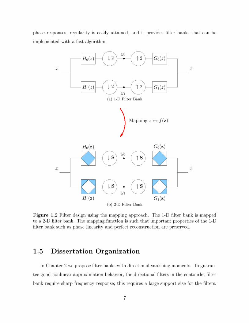
1.2 Filter design using the mapping approach. The 1-D filter bank is mappedto a 2-D filter bank. The mapping function is such that important proper-ties of the 1-D filter bank such as phase linearity and perfect reconstructionare preserved. . . . . . . . . . . . . . . . . . . . . . . . . . . . . . . . . 7

2.1 The directional polyphase representation. Here u = (2, 1)T and r1 =(0, 0)T , r2 = (1, 1)T , r3 = (0, 1)T , and r4 = (1, 0)T . The directionalpolyphase decomposition splits the signal into 1-D subsignals sampledalong the direction u. Those signals tile the whole 2-D discrete plane.We highlight in the picture some of the subsignals. . . . . . . . . . . . . 15

2.2 Illustration of line zero moments as an edge annihilator. The piecewisepolynomial image in (a) was filtered with a 2-D filter C(z1, z2) = (1 − z1z2

2)3.

The output image (b) pixels are approximately zero. . . . . . . . . . . . 172.3 Change of variable is equivalent to a pre/post resampling operation plus

filtering with modified filter. (a) Filter with DVM along u. (b) Equivalentfiltering structure with horizontal DVM. . . . . . . . . . . . . . . . . . . 20

2.4 Filter banks with DVMs along a fixed arbitrary direction are equivalentto a filter bank with DVMs along the horizontal direction. (a) Filter bankin which the filters have DVMs along the direction u. (b) The equivalentfilter bank with DVMs along the horizontal direction. Note that U isconstructed according to Proposition 2 and S = US. . . . . . . . . . . . 21

2.5 Frequency response of analysis and synthesis filters designed with fourth-order directional vanishing moment. The filters degenerate to the 9-7wavelet filters. . . . . . . . . . . . . . . . . . . . . . . . . . . . . . . . . . 30

2.6 Frequency response of analysis and synthesis filters designed with second-order directional vanishing moment. . . . . . . . . . . . . . . . . . . . . . 31

2.7 Two types of prototype fan filter banks used in the DFB expansion tree.Each filter bank has one of its branches featuring a DVM. . . . . . . . . 32

ix

2.8 The DVM directional filter bank. (a) The four-channel DFB with type 0(horizontal) and type 1 (vertical) DVM filter banks. (b) The four-channelequivalent filter bank. The equivalent filter bank has DVMs in three dif-ferent directions. . . . . . . . . . . . . . . . . . . . . . . . . . . . . . . . 33

2.9 Directional vanishing moments on equivalent filters of a 16-channel DFB.Different arrangements of type 0 and type 1 fan filter banks lead to differentnumbers of distinct directions. Each distinct direction is numbered. (a)Tree 1 has 8 distinct directions. (b) Tree 2 has 7 distinct directions. (c)Tree 3 has 6 distinct directions. . . . . . . . . . . . . . . . . . . . . . . . 34

2.10 Equivalent filters in an 8-channel DFB using two-channel filter banks withDVM. The filters are the ones designed in Example 2. Notice the goodfrequency localization in addition to the imposed DVMs (red line). . . . 35

2.11 Decomposition of synthetic image using two schemes. (a) Original image.(b) Wavelet decomposition. (c) DVM decomposition. . . . . . . . . . . . 36

2.12 The DVM Haar filters. In (a) the response of the filter H0(z) = (1 −z−11 z−3

2 )/√

2 is shown. Notice the single DVM that is replicated due toperiodicity. In (b) we have the response of the other Haar filter H10(z) =(1 − z−2

1 z2)/√

2 also used in the experiment. . . . . . . . . . . . . . . . . 372.13 Nonlinear approximation behavior of the contourlet transform with DVM

filters for a toy image. (a) Synthetic piecewise polynomial image. (b) NLAcurves (on a semilog scale). This simple toy image is better representedby the contourlet transform with DVM filters. . . . . . . . . . . . . . . . 38

2.14 Nonlinear approximation behavior of the contourlet transform with DVMfilters for natural images. NLA curves (on a semilog scale) for “Peppers”(a) and “Barbara” (b) images. . . . . . . . . . . . . . . . . . . . . . . . . 39

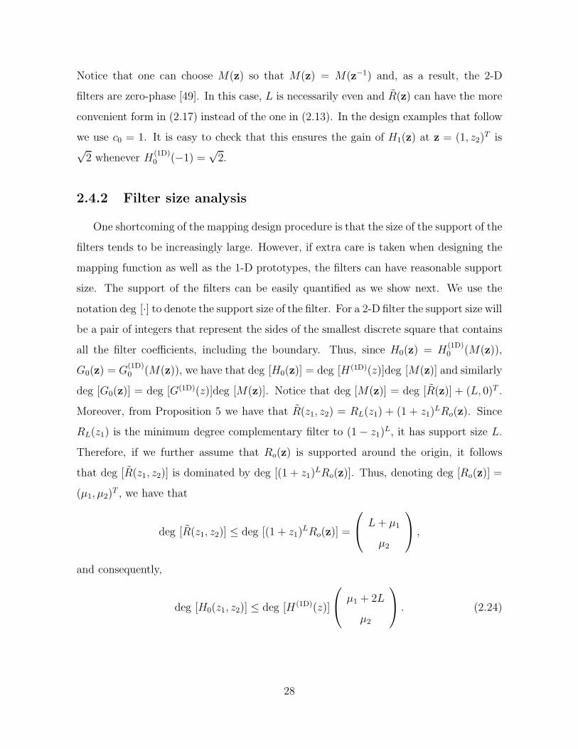
2.15 “Peppers” image reconstructed with 2048 coefficients. (a) PKVA filters,PSNR = 26.05 dB (b) DVM filters of Example 1, PSNR = 26.76 dB. Theimage on the right shows less ringing artifacts. . . . . . . . . . . . . . . . 40

3.1 The nonsubsampled contourlet transform. (a) Nonsubsampled filter bankstructure that implements the NSCT. (b) The idealized frequency parti-tioning obtained with the proposed structure. . . . . . . . . . . . . . . . 47

3.2 The proposed nonsubsampled pyramid is a 2-D multiresolution expan-sion similar to the 1-D nonsubsampled wavelet transform. (a) A three-stage pyramid decomposition. The lighter gray regions denote the aliasingcaused by upsampling. (b) The subbands on the 2-D frequency plane. . 47

3.3 A four-channel nonsubsampled directional filter bank constructed withtwo-channel fan filter banks. (a) Filtering structure. The equivalent filterin each channel is given by Ueq

k (z) = Ui(z)Uj(zQ). (b) Correspondingfrequency decomposition. . . . . . . . . . . . . . . . . . . . . . . . . . . 49

x

3.4 The need for upsampling in the NSCT. (a) With no upsampling, the high-pass at higher scales will be filtered by the portion of the directional filterthat has “bad” response. (b) Upsampling ensures that filtering is done inthe “good” region. . . . . . . . . . . . . . . . . . . . . . . . . . . . . . . 50

3.5 The two-channel nonsubsampled filter banks used in the NSCT. The sys-tem is two times redundant and the reconstruction is error free when thefilters satisfy Bezout’s identity. (a) Pyramid NSFB. (b) Fan NSFB. . . . 51

3.6 Lifting structure for the nonsubsampled filter bank designed with the map-ping approach. The 1-D prototype is factored with the Euclidean algo-rithm. The 2-D filters are obtained by replacing x #→ f(z). . . . . . . . . 56

3.7 Magnitude response of the filters designed in Example 3 with maximallyflat filters. The nonsubsampled pyramid filter bank underlies almost tightanalysis and synthesis frames. . . . . . . . . . . . . . . . . . . . . . . . . 63

3.8 Fan filters designed with prototype filters of Example 3 and diamond max-imally flat mapping filters. . . . . . . . . . . . . . . . . . . . . . . . . . 64

3.9 Basis functions of the nonsubsampled contourlet transform. (a) Basis func-tions of the second stage of the pyramid. (b) Basis functions of third (top8) and fourth (bottom 8) stages of the pyramid. . . . . . . . . . . . . . . 67

3.10 Image denoising with the NSCT and hard thresholding. The noisy inten-sity is 20. (a) Original Lena image. (b) Denoised with the NSWT, PSNR= 31.40 dB. (c) Denoised with the curvelet transform and hard thresh-olding, PSNR = 31.52 dB. (d) Denoised with the NSCT, PSNR = 32.03dB. . . . . . . . . . . . . . . . . . . . . . . . . . . . . . . . . . . . . . . 69

3.11 Comparison between the NSCT-LAS and BLS-GSM denoising methods.The noise intensity is 20. (a) Original Barbara image. (b) Denoised withthe BLS-GSM method, PSNR = 30.28 dB. (c) Denoised with NSCT-LAS,PSNR = 30.60 dB. . . . . . . . . . . . . . . . . . . . . . . . . . . . . . . 71

4.1 The problem under consideration. There is a world and a camera thatproduces a “view of reality” that needs to be coded with finite or infinitememory. . . . . . . . . . . . . . . . . . . . . . . . . . . . . . . . . . . . 76

4.2 A stochastic model for video. (a) Simplified model. (b) The resultingvector process V . Each sample of the vector process is a block of L samplesfrom the process X taken at the position indicated by the random walkWt. In the figure L = 4. . . . . . . . . . . . . . . . . . . . . . . . . . . . 78

4.3 Bounds on information rate. (a) Lower and upper bounds as a function ofpW for the binary wall with pX = 1/2 and L = 8. . . . . . . . . . . . . . 84

4.4 Memory constrained coding. Difference H(V )−H(VM |V M) as a functionof M . When pW = 0.5, the bit rate can be lowered significantly at thecost of large memory. A moderate bit rate reduction is obtained with smallvalues of M when pW = 0.1. The curves are computed using Theorem 1for X uniform over an alphabet of size 256. . . . . . . . . . . . . . . . . 86

xi

4.5 A model for the dynamic reality. (a) It entails a random field that isMarkov in the time dimension t, and i.i.d. in the spatial dimension n. (b)Motion then occurs within this random field. . . . . . . . . . . . . . . . 91

4.6 The binary random field. Innovations are in the form of bit flips causedby binary symmetric channels between consecutive time instants. . . . . 94

4.7 The binary symmetric innovations. (a) The curves show the lower andupper bounds on the entropy rate. Notice that the bounds are sharp forvarious values of pI . (b) Contour plots of the upper bound for various pI

and pW . The lines indicate points of similar entropy but with differentamounts of spatial and temporal innovation. . . . . . . . . . . . . . . . 96

4.8 Memory and Innovations. Shown is the difference between the conditionalentropy and the true entropy for the binary innovations with pX = 0.5,pW = 0.5, and L = 8. The curves show the intuitive fact that when thebackground changes too rapidly, there is little to be gained in bitrate byutilizing more memory. . . . . . . . . . . . . . . . . . . . . . . . . . . . 97

4.9 Differential entropy bounds for the Gaussian AR(1) case as function ofthe innovation parameter ρ. In this example Pe is small enough that thelower and upper bounds practically coincide. Note that the slope of thedifferential entropy curve is influenced by the value of pW . . . . . . . . . 99

4.10 Performance of DPCM with motion for various ρ and pW . For ρ = 0.99 andρ = 0.9 the upper bound is valid for SNR greater than 23 dB and 12.8 dB,respectively. (a) Memory provide considerable gains, pW = 0.5, ρ = 0.99.(b) Modest gains when pW = 0.1. (c) Modest gains when ρ = 0.9, asbackground changes too rapidly. . . . . . . . . . . . . . . . . . . . . . . 103

4.11 The proposed code for the trajectory. The proposed code with buffer sizeK attains an entropy rate of roughly 1/K. Notice that when K is infinity,the code attains the entropy rate bound as the number of samples j goesto infinity. . . . . . . . . . . . . . . . . . . . . . . . . . . . . . . . . . . . 110

5.1 The idealized analytic complex transform. The frame elements are sup-ported on the first and third quadrants of the frequency plane. The realand imaginary parts of each atom are supported in the whole plane fol-lowing the dashed boundaries. . . . . . . . . . . . . . . . . . . . . . . . . 115

5.2 Complex contourlet transform basis functions (4 out of 8 directions shown).real and imaginary parts on top and bottom, respectively. Note the dif-ferent symmetry of the real and imaginary parts. . . . . . . . . . . . . . 116

xii

LIST OF TABLES

Table Page

2.1 Improvement in image denoising. . . . . . . . . . . . . . . . . . . . . . . 41

3.1 Frame bounds evolving with scale for the pyramid filters given in Example3 in Section 3.3. . . . . . . . . . . . . . . . . . . . . . . . . . . . . . . . . 55

3.2 Maximally flat mapping polynomials used in the design of the nonsubsam-pled fan filter bank. . . . . . . . . . . . . . . . . . . . . . . . . . . . . . . 60

3.3 Denoising performance of the NSCT. The left-most columns are hardthresholding and the right-most ones soft estimators. For hard thresh-olding, the NSCT consistently outperforms curvelets and the NSWT. TheNSCT-LAS performs on a par with the more sophisticated estimator BLS-GSM and is superior to the BivShrink estimator of. . . . . . . . . . . . 68

3.4 Relative loss in PSNR performance (dB) when using the NSP with a criti-cally sampled DFB and the LAS estimator with respect to the NSCT-LASmethod. . . . . . . . . . . . . . . . . . . . . . . . . . . . . . . . . . . . . 71

xiii

CHAPTER 1

INTRODUCTION

1.1 Signal Expansions and Filter Banks

1.1.1 Signal expansions

In a variety of signal processing applications, processing can be done more efficiently

over the domain of an invertible linear transform. Early examples of such transforms

in signal processing are the discrete fourier transform (DFT) and the discrete cosine

transform (DCT). A more recent example is the discrete wavelet transform (DWT),

which has been proven effective in a wide range of applications (see e.g., [1]). Transforms

such as these are characterized by a set of vectors that form an orthogonal basis for the

underlying Hilbert space. The DWT has the attractive feature of being multiscale. That

is, it decomposes the signal in several scales, each one characterized by a set of basis

vectors [2]. The multiscale property enables the transform to highlight different features

in different scales, thereby facilitating processing.

An important feature of orthogonal bases is that they are nonredundant. This means

that for finite signals, the number of samples of the transformed signal is the same as

that of the input. This is a crucial property in compression applications. By contrast,

a frame is a redundant transform such that its output for a given input signal can be

reconstructed in a stable way [2, 3].

A frame is characterized by a set of vectors that are linear dependent. This set often

leads to a straightforward expansion resembling that of an orthogonal or biorthogonal

1

basis. Frames are typically better alternatives to orthogonal basis in applications where

redundancy is not a major issue. In addition, in some cases the design of frame systems

can be considerably easier than basis due to the smaller number of constraints.

1.1.2 Filter banks

Filter banks have been a very active research subject in the last 20 years. Since the

discovery of perfect reconstruction filter banks [4–6], great progress has been made. This

culminated in a number of books on the subject [1, 7–10]. Noteworthy is the connection

between tree-structured filter banks and orthogonal wavelet bases [2, 11]. This link

provides an easy interchange between continuous and discrete time that is useful in

understanding and in applications.

Perfect reconstruction filter banks can be critically sampled or oversampled. Critically

sampled filter banks are nonexpansive and underlie orthogonal or biorthogonal bases in

discrete time. In an oversampled filter bank [12, 13], the number of samples in the

output signal is greater than that of the input (i.e., the analysis part is expansive).

Thus, oversampled filter banks implement redundant expansions that under additional

conditions can constitute frames.

Among oversampled filter banks is the nonsubsampled filter bank where the redun-

dancy is given by the number of channels in the bank. Because nonsubsampled filter

banks do not have downsamplers and upsamplers, they have the property of being shift-

invariant. This property is hard to obtain with critically sampled filter banks in that it

requires ideal filters which are nonrealizable.

The theoretical aspects of filter banks are well understood in general, both in one and

several dimensions. However, the design tools existent in the literature mostly focus on

the 1-D and critically sampled case. Recently there have been several methods to design

oversampled 1-D filter banks in the context of framelets [14, 15]. For the multidimensional

case, there are very few design methodologies for both critically sampled and oversampled

cases.

2

1.2 The Challenge of Geometry

Natural images are rich in geometric structure. Yet most image transforms employed

in practice are “geometry blind.” Such transforms are typically constructed with basis

functions that are tensor products of one-dimensional basis functions. The transform

is thus computed on a row-column processing. In words, it treats a 2-D signal as a

collection of 1-D ones. Hence, it fails to exploit regularity on edges, contours, and other

geometrical features of the image.

In recent years, there have been several efforts toward constructing transforms that

exploit geometric structure. For example, Mallat and others constructed the bandelet

transform [16, 17], which is an adaptive transform – it adapts the basis vectors according

to the signal being represented. The wedgelet transform is also adaptive. It tiles smooth

geometry with building block wedge-like tiles [18, 19]. The curvelet transform is a fixed

transform that is a frame. Despite being nonadaptive, the curvelet transform essentially

attains the same theoretical performance of bandelets and wedgelets. Do and Vetterli

[20] constructed the contourlet transform. Contourlets are curvelets’ discrete-time cousin.

The notable feature of contourlets is that the transform can be efficiently computed with

filter banks.

On a related front, signal processing researchers have long tried to build transforms

with additional directionality. For example, the steerable pyramid [21] is a multiscale

transform that has better directional resolution than the separable DWT. The directional

filter bank of Bamberger and Smith is a directional decomposition that can be computed

with quincunx filter banks [22, 23]. The complex wavelet transform of [24] improves

the directional resolution of wavelets while being complex-valued at the same time. This

results in an almost shift-invariant transform with low redundancy that can be computed

efficiently.

3

1.3 The Plenoptic Function and Its Information Rates

The problem of sensing visual information for storage and later reproduction can be

cast in terms of sampling and compressing the plenoptic function [25]. Given a 3-D scene,

the plenoptic function describes the light intensity passing through every viewpoint, in

every direction, for all time, and for every wavelength. It is usually denoted by

POF (x, y, z,φ,ϕ, t,λ),

where (x, y, z) is the point in Euclidean space being considered, t is time, λ is the light

ray wavelength, and the angles (φ,ϕ) characterize the direction at which the light ray

hits the point (x, y, z).

The sampling part of the plenoptic function (POF) has received a lot of attention

recently. In [26] a sampling framework based on epipolar geometry is proposed, while

in [27], the plenoptic function is shown to have infinite bandwidth. In [28], a spectral

analysis of the sampling problem for the plenoptic function is presented.

Compression schemes for several simplifications of the POF are reviewed in [29].

While several algorithms to compress the POF have been proposed, a sound theoretical

understanding of the associated source coding problem is still lacking.

In some applications, the POF falls into the setup shown in Figure 1.1. In it, there is

a camera traversing the plenoptic function. As it moves through the scene, the camera

generates a process that needs to be coded and reproduced at a decoder. The process

can constitute a sequence of snapshots, for example in the case of video. Information

can also be acquired for the purpose of reproducing the scene around the camera, such

as, for example, in the light field.

1.4 Problem Statement and Contributions

Given the context outlined in the previous section, we consider in this dissertation

the following unresolved problems:

4

Figure 1.1 Pictorial description of a problem studied in this dissertation. There isa camera following a random trajectory through the plenoptic function. The cameramotion adds to the complexity of the dynamic scene being continuously acquired. Theunderlying scene is either static, or contains moving objects, or changes over time.

• Is is known that the DWT is the optimal1 representation for 1-D piecewise smooth

signals [1]. This is due to vanishing moments in the filter bank that ensure the

smooth part is zeroed out in the highpass branch. Is there a similar property for

edges in 2-D signals? In this case, how can the corresponding filter bank be designed?

• Given the lack of directionality of the nonsubsampled wavelet transform, we seek to

design and construct a transform that is multiscale, multidirectional, shift-invariant,

and can be implemented using a fast computational algorithm.

• Consider the plenoptic function. We seek to quantify its compression limits. A par-

ticular case of the plenoptic function is that of video. How to construct a statistical

1In the Nonlinear Approximation sense. Let the signal be reconstructed with the N largest-magnitudetransform coefficients. The transform is optimal in the NLA sense if the decay of the mean-squared error(MSE) as a function of N is the fastest possible for that signal.

5

model for a scene that has motion in it such that the information rates such as en-

tropy and rate-distortion can be computed with precision? Another common setup

of the POF is the light field [30, 31]. What are the information rates associated

with this problem?

To address the problems outlined above several contributions are made. These con-

tributions are summarized below:

• We propose a new filter design criterion for multiple dimensions, that is, filters with

directional vanishing moments.

• We characterize the eigensignals of such filters. We also develop a design method-

ology that can be extended to any number of dimensions.

• We propose a new transform construction that is fully shift-invariant. We study this

transform in detail and provide methods for its design and efficient computation.

• We study the compression problem of the plenoptic function. We propose a statis-

tical model for a camera traversing the plenoptic function. Within this model, we

distinguish between two coding problems, that of video and that of the light field.

We then propose a stochastic model for video whereby information rates can be

precisely computed. We also characterize the information rate in the case of the

light field.

Perhaps the greatest challenge in constructing transforms that better handle geometry

and that can be computed with filter banks is filter design. The design of 2-D filter banks

still lacks a definitive tool. The main impairment is the absence of a factorization theorem

in multiple dimensions [32].

In this dissertation we use the mapping approach to design filters. This method is

essentially illustrated in Figure 1.2, for the critically sampled case. It extends easily to

the nonsubsampled case. Despite its simplicity, the mapping design has several advan-

tages over other methods. In particular, it offers seamless control over frequency and

6

phase responses, regularity is easily attained, and it provides filter banks that can be

implemented with a fast algorithm.

H0(z)

H1(z)

G0(z)

G1(z)

x x

y0

y1

↓ 2

↓ 2

↑ 2

↑ 2

(a) 1-D Filter Bank

Mapping z #→ f(z)

y0

y1

H0(z)

H1(z)

G0(z)

G1(z)

x x

↓ S

↓ S

↑ S

↑ S

(b) 2-D Filter Bank

Figure 1.2 Filter design using the mapping approach. The 1-D filter bank is mappedto a 2-D filter bank. The mapping function is such that important properties of the 1-Dfilter bank such as phase linearity and perfect reconstruction are preserved.

1.5 Dissertation Organization

In Chapter 2 we propose filter banks with directional vanishing moments. To guaran-

tee good nonlinear approximation behavior, the directional filters in the contourlet filter

bank require sharp frequency response; this requires a large support size for the filters.

7

We seek to isolate the key filter property that ensures good approximation. In this di-

rection, we propose filters with directional vanishing moments (DVM). These filters, we

show, annihilate information along a given direction. We study two-channel filter banks

with DVM filters. We provide conditions under which the design of DVM filter banks

is possible. A complete characterization of the product filter is thus obtained. We pro-

pose a design framework that avoids two-dimensional factorization using the mapping

technique. The filters designed, when used in the contourlet transform, exhibit nonlinear

approximation comparable to the conventional filters while being shorter and therefore

provide better visual quality with less ringing artifacts.

In Chapter 3 we develop the nonsubsampled contourlet transform (NSCT) and study

its applications. The construction proposed in this chapter is based on a nonsubsampled

pyramid structure and nonsubsampled directional filter banks. The result is a flexible

multiscale, multidirection, and shift-invariant image decomposition that can be efficiently

implemented via the “a trous” algorithm. At the core of the proposed scheme is the

nonseparable two-channel nonsubsampled filter bank. We exploit the less stringent design

condition of the nonsubsampled filter bank to design filters that lead to a NSCT with

better frequency selectivity and regularity when compared to the contourlet transform.

We propose a design framework based on the mapping approach, that allows for a fast

implementation based on a lifting or ladder structure, and only uses one-dimensional

filtering in some cases. In addition, our design ensures that the corresponding frame

elements are regular, symmetric, and the frame is close to a tight one. We assess the

performance of the NSCT in image denoising. The NSCT compares favorably to other

existing methods in the literature.

In Chapter 4 we propose a model to study information rates of the plenoptic function.

The POF setup enables us to construct a stochastic model for video generation. This

model is studied with information theoretic tools, and the associated information rates

are computed. We extend this video model to make it account for dynamic changes

in a scene. Experiments with synthetic sources using DPCM coding suggest that the

introduction of motion in effect makes DPCM perform suboptimally relative to the rate-

8

distortion bound even with perfect knowledge of the motion. We also consider the coding

problem associated with light fields.

In Chapter 5 we make concluding remarks, and we outline our ongoing work and

potential developments to be made in the future.

9

CHAPTER 2

FILTER BANKS WITH DIRECTIONALVANISHING MOMENTS

The contourlet transform was proposed to address the limited directional resolution

of the separable wavelet transform. One way to guarantee good approximation behavior

is to let the directional filters in the contourlet filter bank have sharp frequency response.

This requires filters with large support size. We seek to isolate the key filter property

that ensures good approximation. In this direction, we propose filters with directional

vanishing moments (DVM). These filters, we show, annihilate information along a given

direction. We study two-channel filter banks with DVM filters. We provide conditions

under which the design of DVM filter banks is possible. A complete characterization

of the product filter is thus obtained. We propose a design framework that avoids two-

dimensional factorization using the mapping technique. The filters designed, when used

in the contourlet transform, exhibit nonlinear approximation comparable to the conven-

tional filters while being shorter and therefore provide better visual quality with fewer

ringing artifacts. Furthermore, experiments show that the proposed filters outperform

the conventional ones in image approximation and denoising.

2.1 Introduction

The separable discrete wavelet transform has established itself as a state-of-the art

tool in several image processing applications, including compression, denoising, and fea-

The results of this chapter are presented in references [33–35].

10

ture extraction. A key property, which partially justifies the efficiency of wavelets in

applications, is that it provides a sparse representation for several classes of images.

Such sparsity can be precisely measured in some cases as the decay of the coefficients

magnitude. In spite of its high applicability, it is known that separable wavelets fail to ex-

plore the geometric regularity existent in most natural scenes, thus offering a suboptimal

sparse representation. In this context, it is believed that the next generation transform

coding compression algorithms will use a transform that better handles orientation and

geometric information. In this direction, a number of researchers have proposed image

representation schemes that achieve optimal sparsity behavior for some reasonable image

model. Such is the case of the curvelet tight frames proposed by Candes and Donoho [36].

Inspired by curvelets, Do and Vetterli proposed the contourlet transform [20], which is

a multiscale directional representation constructed in the discrete grid by combining the

Laplacian pyramid [25, 37] and the directional filter bank (DFB) [23]. The distinctive

feature of both curvelets and contourlets is that they are nonadaptive schemes.

Geometric regularity in images is exhibited through the fact that image edges are typ-

ically located along smooth contours. Thus, image singularities (i.e., edges) are localized

in both location and direction. In order to extend 1-D wavelets crucial property for good

approximation, namely vanishing moments [1], new 2-D representations like contourlets

require a new condition named directional vanishing moment [20]. For contourlets, such

property can be imposed by carefully designing the refinement filters. Ideally, if the fil-

ters in the contourlet construction (see [20, 38] for details) are sinc-type filters with ideal

response, then the contourlet atoms are guaranteed to have DVMs in an infinite number

of directions. In practice, however, ideal filters are approximated with a finite number

of coefficients, and to ensure having DVMs, this number has to be large, thus increasing

complexity. Alternatively, if FIR filters with enough DVMs can be obtained, one could

achieve similar performance with potentially shorter filters, which would result in a fast

and efficient decomposition algorithm. In addition, as we learned from the wavelet expe-

rience, short filters (e.g., the filters chosen for the JPEG2000 standard) are very desirable

for images as they are less affected by the Gibbs phenomena artefact.

11

In this chapter we study two-channel critically sampled filter banks with DVMs. The

DVM property leads to a new filter bank design problem and, to the best of our knowl-

edge, this is the first work that addresses this problem. Two-channel filter banks are

attractive since they are simpler to design and can be used in a tree structure to generate

more complicated systems such as the DFB. Our goal is to impose directional vanishing

moments in the contourlet basis function without resorting to long filters. That is, we

attempt to cancel directional information using DVMs instead of good frequency selec-

tivity, thus working with shorter filters and avoiding the Gibbs phenomena (see Figure

2.15). Although our initial motivation for the DVM filter bank design is the contourlet

transform, we point out that our methods are general and can be applied in more general

contexts. Potential applications of the filters designed in this work are in the contourlet

transform of [20], the CRISP-contourlet system [39], and directionlets [40]. A preliminary

version of the present work has appeared in [33].

The chapter is structured as follows. In Section 2.2 we study filters with DVM and the

class of signals that would be annihilated by such filter. In Section 2.3 we study the DVM

in the context of 2-D FIR two-channel filter banks. We provide existence conditions as

well as the design constraints. We also provide a complete characterization of the product

filter of those filter banks. To overcome 2-D factorization, in Section 2.4 we propose a

design procedure using the mapping technique. The design is simple to carry out and

uses the solution introduced in Section 2.3. In Section 2.5 we study the use of filter banks

with DVM in the contourlet construction. Experiments illustrating the approximation

properties of the proposed filters are presented in Section 2.6 and conclusions drawn in

Section 2.7.

Notation: Throughout the chapter we use boldface and capital boldface characters

to represent two-dimensional (2-D) vectors and 2 × 2 matrices, respectively. Thus, a

discrete 2-D signal is denoted by x[n] where n = (n1, n2)T . The 2-D z-transform of a

signal x[n] is denoted by X(z), where it is understood that z is shorthand for (z1, z2)T .

If u = (u1, u2)T is a vector in Z2, then we denote zu = zu11 zu2

2 , whereas zS = (zs1 , zs2)T

with the integer vectors s1 and s2 being the columns of the matrix S. Note that with

12

this notation, if S is a matrix of integers and u is an integer vector, then (zS)u = z(Su).

In the unit sphere we write X(ω) for X(ejω), where ωT = (ω1,ω2)T . We we use both

notations X(z), and X(ω), according to which one is more convenient. A 1-D signal and

its z-transform are denoted by x[n] and X(z), respectively.

2.2 Directional Annihilating Filters

Much of the efficiency of wavelets in analyzing transient signals is due to the vanish-

ing moments in the wavelet function and its practical consequences [1]. Together with

the time localization property, wavelets with vanishing moments provide a sparse repre-

sentation for piecewise polynomial signals. Most successful wavelet filters, such as the

orthogonal Daubechies family and the JPEG2000 filters, were designed with vanishing

moment as a primary design criterion. This is in contrast to early filter bank construc-

tions in which the frequency selectivity was a primary goal. Vanishing moments in a

wavelet transform can be characterized by zeros in the highpass filters of the underlying

filter bank. Suppose H1(z) is the highpass analysis filter of a two-channel filter bank. A

vanishing moment of order d is characterized by d zeros at z = 1 or ω = 0 on the unit cir-

cle. That is, the filter is factored as H1(z) = (1− z)dR1(z). The filter H1(z) is related to

discrete polynomial signals of degree less than d — signals of the form x[n] =∑i

j=0 αjnj ,

with αj real and 0 ≤ i < d. In particular, filtering x[n] with H1(z) produces a zero out-

put (see for example [9, 41]). In other words, the filter H1(z) totally annihilates discrete

polynomials of degree less than d.

For 2-D filter banks with two channels, the vanishing moment concept can be general-

ized as point zeros at z = (1, 1)T or ω = (0, 0)T [42, 43]. However, filters with point-zeros

on the 2-D frequency plane do not cancel piecewise smooth images with discontinuities.

A somewhat different philosophy motivated by contourlets is the directional vanishing

moment in which the zeros are required to be along a line. Formally, we define DVM as

follows.

13

Definition 1 Let C(z) be a discrete filter and u = (u1, u2)T be a 2-D vector of coprime

integers. We say C(z) has a DVM of order d along the direction u if it can be factored

as

C(z) = (1 − zu11 zu2

2 )d R(z), or

C(ω) =(1 − ej(ω1u1+ω2u2)

)dR(ω). (2.1)

For contourlets, the filter C(z) is a composite one, which involves the Laplacian pyramid

filters and the polyphase components of the directional filters [20].

A question of interest is: What signal would be annihilated (i.e., completely filtered

out) by the filter in (3.20)? Such a signal is an eigen-signal of the complementary branch

of a two-channel filter bank where C(z) is an analysis filter. This filter bank will be

studied in detail in the next section. Similar to the 1-D case, 2-D filter banks with

filters of the form in (3.20) have interesting properties with respect to approximation of

smooth signals. In order to see those properties, we introduce the directional polyphase

representation.

Lemma 1 Suppose that u ∈ Z2 and u2 *= 0. Then for every n ∈ Z2 there exists a unique

pair (k, r) where k ∈ Z, r ∈ R := Z × {0, 1, . . . , |u2|− 1} such that

n = ku + r. (2.2)

Proof. Notice that (2.2) is equivalent to having n1 = ku1 + r1 and n2 = ku2 + r2. For

the second equation, k and r2 are uniquely determined as the quotient and remainder of

n2 divided by u2. Given k, from the first equation, r1 is also uniquely determined. !

Throughout the chapter we assume u2 *= 0. The case u2 = 0 can be similarly handled

by swapping the two variables u1,u2. Lemma 1 allows us to partition any 2-D signal x[n]

into a set of disjoint 1-D signals {xr[k] : r ∈ R} with

xr[k] := x[ku + r]. (2.3)

14

n1

n2

xr1 [k]

xr2 [k]

xr3 [k]

xr4 [k]

x[n]

Figure 2.1 The directional polyphase representation. Here u = (2, 1)T and r1 = (0, 0)T ,r2 = (1, 1)T , r3 = (0, 1)T , and r4 = (1, 0)T . The directional polyphase decompositionsplits the signal into 1-D subsignals sampled along the direction u. Those signals tile thewhole 2-D discrete plane. We highlight in the picture some of the subsignals.

Figure 2.1 illustrates the directional polyphase representation. Note that each signal

xr[k] is a 1-D slice of x[n] along the direction u. Therefore, the directional polyphase

representation is distinct from the ordinary polyphase representation. Using Lemma 1,

we can characterize the signals that are annihilated by the filter C(z).

Proposition 1 Let C(z1, z2) be a 2-D filter with a factor (1−zu11 zu2

2 )d. Then a signal x[n]

is annihilated by C(z) if each 1-D signal xr[k] defined in (2.3) is a discrete polynomial

of degree less than d.

Proof. Using Lemma 1 we have that

X(z) =∑

n∈Z2

x[n]z−n

=∑

k∈Z

∑

r∈R

x[ku + r]z−(ku+r)

=∑

r∈R

z−r∑

k∈Z

xr[k]z−ku

=∑

r∈R

z−rXr(zu).

Since the signals xr[k] are polynomials of degree less than d, as in the 1-D case, each

term Xr(zu) is annihilated by a factor (1−zu)d. Thus it follows that X(z) is annihilated

by C(z1, z2). !

15

An immediate consequence of Proposition 1 is that discrete signals sampled from

a continuous-time signal which is smooth away from line discontinuities along a given

direction, are also annihilated by C(z1, z2). In other words, if xc(t) is a continuous-time

piecewise polynomial signal of degree less than d and x[n] = xc(∆Tn), then it follows

that x[n] is annihilated by a filter C(z) with a factor (1 − zu)d.

As an illustration, we filter a piecewise smooth image with a 2-D filter with a third-

order DVM along direction u = (1, 2)T . The image is described by e−x2

−y2

α +1{β1<y−2x<β2}.

Such an image is well approximated by a piecewise polynomial image of sufficiently large

degree d. As can be seen in Figure 2.2, the edge was totally annihilated by the filtering

operation. Notice that the DVM formulation is in the space domain, and the annihilation

of directional edges takes place regardless of the frequency response of the filters. This

is similar to the 1-D wavelet case in which “zeros at π” alone ensures the cancellation of

smooth signals.

2.3 Two-channel Filter Banks with Directional Van-ishing Moments

2.3.1 Preliminaries

Our setup consists of a general two-dimensional critically sampled two-channel filter

bank with a valid sampling S that has downsampling ratio 2, i.e., |det S| = 2. Figure 2.4

(a) illustrates such a filter bank. In this setting, given a set of analysis/synthesis filters

the reconstructed signal is a perfect replica of the original provided that [7]

H0(ω)G0(ω) + H1(ω)G1(ω) = 2, (2.4)

H0(ω + 2πS−Tk1)G0(ω) + H1(ω + 2πS−Tk1)G1(ω) = 0, (2.5)

where k1 is the nonzero integer vector in the set N (S) := {ST x, x ∈ [0, 1) × [0, 1)} [7].

The modulation term 2πS−Tk1 is a function of the sampling lattice generated by S [44].

Because | detS| = 2, the vector 2S−Tk1 has integer entries. Thus, the modulation term

2πS−Tk1 has the form 2πS−Tk1 = (m1π, m2π)T , where (m1, m2)T = 2S−Tk1. Moreover,

16

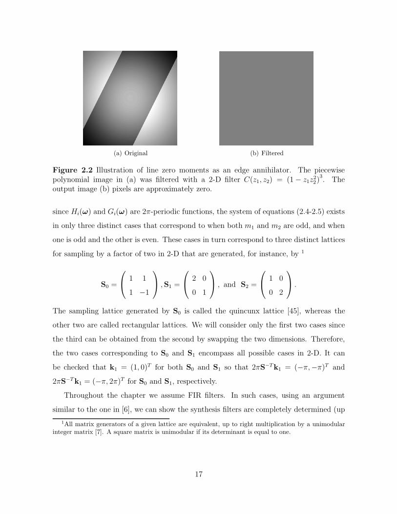
(a) Original (b) Filtered

Figure 2.2 Illustration of line zero moments as an edge annihilator. The piecewisepolynomial image in (a) was filtered with a 2-D filter C(z1, z2) = (1 − z1z2

2)3. The

output image (b) pixels are approximately zero.

since Hi(ω) and Gi(ω) are 2π-periodic functions, the system of equations (2.4-2.5) exists

in only three distinct cases that correspond to when both m1 and m2 are odd, and when

one is odd and the other is even. These cases in turn correspond to three distinct lattices

for sampling by a factor of two in 2-D that are generated, for instance, by 1

S0 =

1 1

1 −1

,S1 =

2 0

0 1

, and S2 =

1 0

0 2

.

The sampling lattice generated by S0 is called the quincunx lattice [45], whereas the

other two are called rectangular lattices. We will consider only the first two cases since

the third can be obtained from the second by swapping the two dimensions. Therefore,

the two cases corresponding to S0 and S1 encompass all possible cases in 2-D. It can

be checked that k1 = (1, 0)T for both S0 and S1 so that 2πS−Tk1 = (−π,−π)T and

2πS−Tk1 = (−π, 2π)T for S0 and S1, respectively.

Throughout the chapter we assume FIR filters. In such cases, using an argument

similar to the one in [6], we can show the synthesis filters are completely determined (up

1All matrix generators of a given lattice are equivalent, up to right multiplication by a unimodularinteger matrix [7]. A square matrix is unimodular if its determinant is equal to one.

17

to a scale factor and a delay) from the pair (H0(ω), G0(ω)) [6] through the relation

H1(ω) = ejωT k1G0(ω + 2πS−Tk1),

G1(ω) = e−jωT k1H0(ω + 2πS−Tk1). (2.6)

As a result, the reconstruction condition reduces to

H0(ω)G0(ω) + H0(ω + 2πS−Tk1)G0(ω + 2πS−Tk1) = 2. (2.7)

The above biorthogonal relation specializes to the orthogonal one when G0(ω) = H0(−ω).

Moreover, we say that G0(ω) is the complementary filter to H0(ω) whenever they satisfy

(2.7).

2.3.2 Two-channel filter banks with DVMs

In general, given the desired direction of the zero moment, the product filter H0(ω)G0(ω)

takes the form

H0(ω)G0(ω) = (1 − ejωT u)LR(ω),

where L denotes the order of the DVM. Substituting this in (2.7) we obtain the design

equation(1 − ejωT u

)LR(ω) +

(1 − ej(ω+2πS−T k1)T u

)LR(ω + 2πS−Tk1) = 2, (2.8)

where R(ω) is the complementary filter to(1 − ejωT u

)L. We always assume that u1 and

u2 are coprime integers. Note that the above relation sets a system of linear equations

which can be solved under certain conditions. Since∣∣det(S−T)

∣∣S=S0 or S1

= 1/2, it follows

that uT 2S−Tk1 is an integer scalar. If uT 2S−Tk1 is even, then a factor (1−ejωT u) exists

in the two left terms of (2.8) in which case an FIR solution is not possible. Consequently,

we see that uT 2S−Tk1 being odd is a necessary condition for solving (2.8). In that case,

(2.8) reduces to(1 − ejωT u

)L

R(ω) +(1 + ejωT u

)L

R(ω + 2πS−Tk1) = 2. (2.9)

Although in principle it is possible to solve (2.8) directly, the following Proposition

simplifies the problem.

18

Proposition 2 Consider the perfect reconstruction equation (2.8) where u has coprime

entries and uT 2S−Tk1 is odd. Then there exists a unimodular integer matrix U such that

if R(ω) solves (2.8) then R(ω) = R(UTω) solves

(1 − ejω1

)LR(ω) +

(1 + ejω1

)LR(ω + 2πS−Tk1) = 2, (2.10)

where S = US. Conversely, if R(ω) is a solution to (2.10) with S given and u as

above, then there exists a matrix U such that R(ω) = R(UTω) is a solution to (2.8) with

S = US.

Proof. We need to construct U so that ej(UT ω)T u = ej(Uu)T ω = ejω1. We then set

U :=

a b

−u2 u1

(2.11)

and choose a, b ∈ Z so that au1 + bu2 = 1. Because u1 and u2 are assumed to be coprime,

such a and b are guaranteed to exist. Since uT 2S−Tk1 is odd, substituting ω #→ UTω

in (2.9) gives (2.10). Conversely, if R(ω) solves (2.10), then set U = U−1 with U as in

(2.11) and substitute ω #→ UTω in (2.10) to get (2.8). !

Remark 1 The fact that U has integer entries and is unimodular implies that it is a

resampling matrix. Hence, the change of variables ω #→ UTω, or equivalently z #→ zU

amounts to a resampling operation of the filter R(z) which can be seen as a rearrange-

ment of the filter coefficients in the 2-D discrete plane. This has the signal processing

interpretation illustrated in Figure 2.3 (in the z-domain). Thus, we see that a filter with

a DVM along a direction other than the horizontal one can be implemented in terms of

a filter with a horizontal DVM plus pre/post resampling operations.

Remark 2 This change of variables can also be done in the filters of a filter bank. We

thus obtain the equivalence shown in Figure 2.4 for a unimodular matrix U and S = US.

The equivalence can be easily checked using multirate identities. The filter bank within

the dotted region in Figure 2.4 (b) is a perfect reconstruction if and only if the filter bank

19

in Figure 2.4 (a) is. Since the equivalence is one-to-one, one can design filter banks with

horizontal DVMs and then, following Proposition 2, obtain filter banks with DVMs in

any direction u such that uT 2S−Tk1 is odd.

Remark 3 Notice that a vertical DVM, i.e., a factor of the form (1 − ejω2)L

could be

obtained similarly, by just exchanging the rows of the matrix U constructed in the proof

above.

x y

(a) H(z) = (1 − zu)LR(z)

↓ U↑ Ux y

(b) H(z) = H(zU) = (1 − z1)L

R(z)

Figure 2.3 Change of variable is equivalent to a pre/post resampling operation plusfiltering with modified filter. (a) Filter with DVM along u. (b) Equivalent filteringstructure with horizontal DVM.

Proposition 2 gives a simpler equation in the sense that a complete characterization

of its solution is possible. Furthermore, with the aid of Proposition 2 we can establish a

sufficient condition for solving (2.8) as the next proposition shows.

Proposition 3 Let uT be an integer vector of coprime integers. Then (2.8) admits an

FIR solution if and only if uT 2S−Tk1 is an odd integer.

Proof. We already discussed necessity. To establish sufficiency, suppose that uT 2S−Tk1

is an odd integer. Using Proposition 2, we can reduce the problem to that of (2.10).

Thus if (2.10) is solvable then we are done. Now consider the modulation shift 2πS−Tk1.

If the first entry of 2πS−Tk1 is an odd multiple of π, then at least a univariate solution

R(ω) = R(ω1) is guaranteed to exist [46]. But because S = US, one can easily check

that the first entry of 2S−Tk1 is 2uTS−T k1, which is odd by assumption. !

If uT 2S−Tk1 is an odd integer we then say that the direction u is admissible for the

sampling matrix S. Proposition 3 asserts that not all DVMs can be obtained for a given

20

↓ S

↓ S ↑ S

↑ SH0(z) G0(z)

H1(z) G1(z)

x x

y0

y1

(a)

↓ U↑ Ux x

y0

y1

H0(zU) G0(zU)

H1(zU) G1(zU)↓ S

↓ S ↑ S

↑ S

(b)

Figure 2.4 Filter banks with DVMs along a fixed arbitrary direction are equivalent to afilter bank with DVMs along the horizontal direction. (a) Filter bank in which the filtershave DVMs along the direction u. (b) The equivalent filter bank with DVMs along thehorizontal direction. Note that U is constructed according to Proposition 2 and S = US.

downsampling matrix S. In particular, for the quincunx lattice generated by S0, we

have that uT 2S−Tk1 = (u1 + u2) so that u is admissible if u1 + u2 is an odd integer,

and similarly for the rectangular lattice generated by S1, uT 2S−Tk1 = u1 so that u is

admissible whenever u1 is odd. For instance, u = (2, 1)T is admissible for S0 but not for

S1, whereas u = (1, 1)T is only admissible for S1.

The aforementioned discussion provides necessary and sufficient conditions for having

one of the branches of the filter bank featuring DVMs. In the context of contourlets (see

Section 2.5) it is desirable to have DVMs in both channels so that the DFB expansion tree

is balanced in the sense that DVMs are present in all frequency channels. Unfortunately,

this is not possible to attain with FIR filters. Likewise, it is neither possible to have

21

different DVMs in the same filter channel. We summarize these assertions in the next

proposition.

Proposition 4 Consider a two-channel 2-D filter bank with FIR filters H0(ω), H1(ω),

G0(ω), and G1(ω), and downsampling matrix S. Let u = (u1, u2)T and v = (v1, v2)T

be two distinct admissible directions. Then the filter bank cannot have the perfect recon-

struction property if one of the following is true:

1. The filter H0(ω) has a factor of (1 − ejωT u) and H1(ω) has factor of (1 − ejωT v)

leaving FIR remainders.

2. One of the filters, say H0(ω), has factors (1−ejωT u) and (1−ejωT v) simultaneously

leaving an FIR remainder.

Proof. 1. If the factor (1 − ejωT u) is in H0(ω), and (1 − ejωT v) in H1(ω), then the

reconstruction condition (2.4) is not satisfied when ejω = (1, 1)T .

2. Suppose H0(ω) has a factor (1 − ejωT u)(1 − ejωT v). Because v is admissible, we

have from Proposition 3 that vT2S−Tk1 is odd. Consequently we have that

(ej(ω+2πS−T k1)

)v

= −ejωT v.

It then follows from (2.6) that G1(ω) has a factor (1 + ejωT v). Consider the system of

equations {1 − ejωT u = 0, 1 + ejωT v = 0}, which is equivalent to

u1 u2

v1 v2

ω1

ω2

=

π

2π

.

Because u and v are distinct we have that u2v1 *= u1v2 which guarantees a solution. It

then follows that H0(ω) and G1(ω) have a common zero, thus violating (2.4). !

The previous proposition shows we can only afford to have DVM in one branch of

the filter bank. In the next section, we present methods for solving the DVM filter bank

design problem in the form of (2.10).

22

2.3.3 Characterization of the product filter

With the aid of Proposition 2 (see also Figure 2.4), in order to design filter banks with

DVMs we need to consider (2.10) with two possible forms for R(ω + 2πS−Tk1), namely

R(ω1+π,ω2) or R(ω1+π,ω2+π), corresponding to the rectangular and quincunx lattices,

respectively. In the z-domain, we equivalently have R(−z1, z2) and R(−z1,−z2). We

denote those two cases collectively as R(−z1, sz2) where s ∈ {1,−1}. It turns out that

a complete characterization of the solution of (2.10) is possible as the next proposition

shows.

Proposition 5 Let s ∈ {1,−1}. An FIR filter R(z1, z2) is the solution to the equation

(1 − z1)LR(z1, z2) + (1 + z1)

LR(−z1, sz2) = 2 (2.12)

if and only if it has the form

R(z1, z2) = RL(z1) + (1 + z1)LRo(z1, z2) (2.13)

with RL(z1) being a univariate solution given explicitly by

RL(z1) =L−1∑

i=0

(L + i − 1

L − 1

)2−(L+i−1)(1 + z1)

i (2.14)

and Ro(z) satisfying

Ro(z1, z2) + Ro(−z1, sz2) = 0. (2.15)

Proof. First, the 1-D complementary filter to (1− z1)L is guaranteed to exist, a conse-

quence of the Bezout theorem for polynomials [46]. Moreover, RL(z1) as in (2.14) is the

1-D minimum degree polynomial that solves (2.12), which can be found by Taylor series

expansion [2]. Furthermore, if Ro(z1, z2) satisfies (2.15), it can be readily checked that

R(z) given in (2.13) solves (2.12).

To prove sufficiency, suppose R(z1, z2) solves (2.12). Let R′(z1, z2) := R(z1, z2) −

RL(z1). Since RL(z1) and R(z1, z2) are both solutions to (2.12) we must have

R′(−z1, sz2)(1 + z1)L = −R′(z1, z2)(1 − z1)

L, (2.16)

23

which implies that R′(z1, z2) = (1+z1)LRo(z1, z2). Now, let z1 *= ±1. Then (2.16) implies

(2.15) and since Ro(z) is an FIR filter, it follows that (2.15) is valid for all z ∈ C2. !

Remark 4 The above proposition is akin to its 1-D counterpart which is used to con-

struct compactly supported wavelets (see e.g., [2]). The distinction occurs in the higher

order term Ro(z1, z2) which now can be any two-dimensional function satisfying (2.15).

This higher order term will make the filter a “truly” 2-D one, meaning a filter with a

nonseparable support. Moreover, the higher order term can be used to control the shape

of the 2-D frequency response.

Remark 5 If L is even, then it is easy to check that

R(z1, z2) = (−2z1)−L/2RL/2

(z1 + z−1

1

2

)

+ (1 + z−11 )LRo(z1, z2) (2.17)

with Ro(z1, z2) satisfying (2.15), also solves (2.12). If in addition Ro(z1, z2) = Ro(z−11 , z−1

2 ),

this solution provides a class of linear-phase biorthogonal filters with DVM in which each

one of the filters in the analysis and synthesis is a degenerate 1-D solution. Thus, this

solution can be seen as a 2-D generalization of the 1-D biorthogonal spline wavelet filters

of [2].

The result also extends to the orthogonal case as the next corollary shows.

Corollary 1 Let s be as in Proposition 5. Consider the orthogonal perfect reconstruction

condition

H0(z1, z2)H0(z−11 , z−1

2 ) + H0(−z1, sz2)H0(−z−11 , sz−1

2 ) = 2,

with H0(z1, z2) = (1 − z1)Lr0(z1, z2). Also set R0(z1, z2) = r0(z1, z2)r0(z−11 , z−1

2 ). Then

R0(z1, z2) has the form

R0(z1, z2) = RL

(z1 + z−1

1

2

)+

(1 +

z1 + z−11

2

)L

R0(z1, z1),

where RL is as in (2.14), and R0(z1, z2) = R0(z−11 , z−1

2 ) satisfies (2.15) .

24

The proof of this corollary is a direct application of Proposition 5 by making the change of

variables z′1 = z1+z−11

2 , and z′2 = z2+z−12

2 . Notice that orthogonal FBs with DVMs could be

obtained using the above result by taking the square root of the filter R0(ω) = |r0(ω)|2.

This requires 2-D spectral factorization, which is a hard task. Furthermore, such a

square root is not guaranteed to exist and one has to carefully select the higher order

term R0(ω) so as to make R0(ω) factorizable. For biorthogonal solutions, one can avoid

spectral factorization using the mapping approach as discussed in the next section.

2.4 Design via Mapping

2.4.1 Design procedure

Due to the lack of a factorization theorem for 2-D polynomials, the design of nonsep-

arable 2-D filter banks is substantially harder than the 1-D counterpart. In particular,

we cannot easily factorize the solution for the product filter given by Proposition 5 into

H0(z) and G0(z) as in (2.7). There are two known ways to avoid factorization: (1)

Constructing the polyphase matrix in a lattice structure and (2) Mapping 1-D filters

to 2-D by appropriate change of variables. Most filters designed in the literature use

one of these two approaches (see, e.g., [32, 47–50].) The first method has the attractive

feature of possible construction of both orthogonal and biorthogonal solutions. How-

ever, it is harder to impose vanishing moments, since the corresponding conditions in the

polyphase domain are nonlinear (see, e.g., [51].) For processing images, orthogonal FBs

have the shortcoming of lack of phase linearity which causes severe visual distortions.

For biorthogonal FIR solutions, one can use the general mapping approach proposed in

[49]. In this approach, we first design 1-D prototype filters H(1D)0 (z), and G(1D)

0 (z), such

that P (1D)(z) := H(1D)0 (z)G(1D)

0 (z) is a halfband filter, i.e.,

P (1D)(z) + P (1D)(−z) = 2. (2.18)

Next, we apply the change of variables z #→ M(z) to map the 1-D filters to 2-D ones:

H0(z) = H(1D)0 (M(z)), G0(z) = G(1D)

0 (M(z)).

25

It can be easily checked that the mapped 2-D filters will satisfy the perfect recon-

struction condition (2.7) provided

M(z1, z2) = −M(−z1, sz2). (2.19)

Notice that for FIR solutions, it is necessary that the 1-D prototype filters have only

positive powers of z. This automatically precludes FIR orthogonal solutions.

Mapping 1-D filters can also be carried over to the polyphase domain as done in [50].

A more careful examination of the filters proposed in [50] reveals that the polyphase

mapping can also be performed in the filter domain, and as such, the technique boils

down to a particular case of the mapping method [52]. For completeness, we include a

derivation of this equivalence in Section 2.8.

In the context of filter banks with DVMs, the goal is to devise a mapping function

M(z) such that each of the 2-D filters H0(z) and G0(z) has a given number of (1 − z1)

factors. In addition we require M(z) so that perfect reconstruction is kept after mapping.

The next proposition shows an explicit form of the required mapping function.

Proposition 6 Let H(1D)0 (z), G(1D)

0 (z) be such that P (1D)(z) = H(1D)0 (z)G(1D)

0 (z) satisfies

(2.18) and let s ∈ {1,−1}. Suppose M(z) is an FIR mapping function such that

M(z1, z2) = (1 − z1)LR(z1, z2) + c0, (2.20)

where c0 is such that H(1D)0 (z) has a factor (z−c0)Na/L, G(1D)

0 (z) has a factor (z−c0)Ns/L,

and R(z1, z2) satisfies the valid mapping equation:

(1 − z1)L R(z1, z2) + (1 + z1)

L R(−z1, sz2) = 2c0. (2.21)

Then

1. The mapped filters H0(z) = H(1D)0 (M(z)) and G0(z) = G(1D)

0 (M(z)) are perfect

reconstruction, i.e., they satisfy

H0(z1, z2)G0(z1, z2) + H0(−z1, sz2)G0(−z1, sz2) = 2. (2.22)

26

2. The mapped filters are factored as

H0(z) = (1 − z1)NaRH0(z), G0(z) = (1 − z1)

NsRG0(z). (2.23)

Proof. Suppose M(z) is as in (2.20). Then, from (2.21) it follows that M(z1, z2) =

−M(−z1, sz2) which is (2.19), hence the mapped filters satisfy (2.22). Moreover, substi-

tuting z #→ M(z) in the factors (z−c0)Na/L of H(1D)0 (z) and (z−c0)Ns/L of G(1D)

0 (z) gives

H0(z) and G0(z) as in (2.23). !

Interestingly, it turns out the valid mapping equation (2.21) is similar to equation

(2.12) for the product filter in Proposition 5. We then can use Proposition 5 to find an

explicit solution to (2.21). In short, we see that the mapping overcomes the need for

spectral factorization and, together with Proposition 5, gives a straightforward design

methodology. Hence, we can formulate the design of DVM filter banks via mapping as

follows.

Problem: Design 2-D filters H(1D)0 (z) and G(1D)

0 (z) satisfying the perfect reconstruction

condition (2.7) and such that H(1D)0 (z) has a factor (1 − z1)Na and G(1D)

0 (z) has factor

(1 − z1)Ns .

Step 1 Design 1-D filters H(1D)0 (z) and G(1D)

0 (z) with Na/L and Ns/L zeros at some

point c0 ∈ C, respectively, and such that P (1D)(z) = H(1D)0 (z)G(1D)

0 (z) satisfies

(2.18).

Step 2 Let M(z) = (1 − z1)LR(z) + c0 with

R(z) = RL(z1) + (1 + z1)LRo(z1, z2), and

Ro(z1, z2) = −Ro(−z1, sz2).

Step 3 Set H0(z) = H(1D)0 (M(z)) and G0(z) = G(1D)

0 (M(z)) to obtain the desired 2-D

filters.

27

Notice that one can choose M(z) so that M(z) = M(z−1) and, as a result, the 2-D

filters are zero-phase [49]. In this case, L is necessarily even and R(z) can have the more

convenient form in (2.17) instead of the one in (2.13). In the design examples that follow

we use c0 = 1. It is easy to check that this ensures the gain of H1(z) at z = (1, z2)T is√

2 whenever H(1D)0 (−1) =

√2.

2.4.2 Filter size analysis

One shortcoming of the mapping design procedure is that the size of the support of the

filters tends to be increasingly large. However, if extra care is taken when designing the

mapping function as well as the 1-D prototypes, the filters can have reasonable support

size. The support of the filters can be easily quantified as we show next. We use the

notation deg [·] to denote the support size of the filter. For a 2-D filter the support size will

be a pair of integers that represent the sides of the smallest discrete square that contains

all the filter coefficients, including the boundary. Thus, since H0(z) = H(1D)0 (M(z)),

G0(z) = G(1D)0 (M(z)), we have that deg [H0(z)] = deg [H(1D)(z)]deg [M(z)] and similarly

deg [G0(z)] = deg [G(1D)(z)]deg [M(z)]. Notice that deg [M(z)] = deg [R(z)] + (L, 0)T .

Moreover, from Proposition 5 we have that R(z1, z2) = RL(z1) + (1 + z1)LRo(z). Since

RL(z1) is the minimum degree complementary filter to (1 − z1)L, it has support size L.

Therefore, if we further assume that Ro(z) is supported around the origin, it follows

that deg [R(z1, z2)] is dominated by deg [(1 + z1)LRo(z)]. Thus, denoting deg [Ro(z)] =

(µ1, µ2)T , we have that

deg [R(z1, z2)] ≤ deg [(1 + z1)LRo(z)] =

L + µ1

µ2

,

and consequently,

deg [H0(z1, z2)] ≤ deg [H(1D)(z)]

µ1 + 2L

µ2

. (2.24)

28

Similarly, for the synthesis filter

deg [G0(z1, z2)] ≤ deg [G(1D)(z)]

µ1 + 2L

µ2

. (2.25)

From the foregoing discussion we see that when µ1 + µ2, by increasing the number

of DVMs in the mapping function, i.e., increasing L, the filter support will be stretched

along the n1 direction. Furthermore, for a fixed mapping function, the support of the

resulting 2-D filter will increase linearly in both n1, n2 directions with the number of

vanishing moments in the prototype filters H(1D)(z). Thus, to avoid the filters being

too large, we point out that the 1-D prototype filters should be as short as possible,

preferably with only one zero at c0. We present design examples next.

2.4.3 Design examples

Example 1 Nonseparable filter family that includes the 1-D 9-7 filters

For the purpose of this example we assume the quincunx lattice and we generate DVMs

along the horizontal direction u1 = 0. Following the discussion in the previous section we

choose the prototype filters H(1D)0 (z) and G(1D)

0 (z) to have zeroes at z = −1. We consider

the minimum degree complementary filter to (1− z)4 which from (2.14) gives the product

filter

P (1D)(z) =1

16(16 − 29z + 20z2 − 5z3)(1 − z)4.

We let each prototype filter have a factor (1 − z)2 and then we split the factor (16 −

29z + 20z2 − 5z3) between the two prototypes assigning the real root to H(1D)0 (z) and the

two complex-conjugate roots to G(1D)0 (z).

In the mapping function we impose the condition M(z1, z2) = M(z−11 , z−1

2 ) so that the

filters are zero-phase. Following (2.20), in order to generate a second-order horizontal

DVM, we set

M(z1, z2) = (1 − z1)2 R(z1, z2) − 1.

29

To guarantee that the map satisfies the valid mapping condition (2.21) and is zero-

phase we use (2.17) to obtain

R(z1, z2) = −z−11

2+(1 + z−1

1

)2Ro(z1, z2).

Notice that Ro(z1, z2) can be any zero-phase filter that satisfies (2.15). For simplicity

we choose Ro(z1, z2) = α(z2 + z−12 ). With α = 0 we recover the 9-7 filters. Figure 2.5

displays the frequency response of the filters when we set α = −4√

2.

(a) |H0(ejω)| (b) |G0(ejω)|

(c) |H1(ejω)| (d) |G1(ejω)|

Figure 2.5 Frequency response of analysis and synthesis filters designed with fourth-order directional vanishing moment. The filters degenerate to the 9-7 wavelet filters.

Example 2 Using the higher order term to improve frequency response

In this example we use the extra degrees of freedom in our proposed design to obtain

filters with low order DVMs and better frequency selectivity. The following filters can be

checked to satisfy (2.18):

H(1D)0 (z) = K

(1 + k2z + k2k3z

2),

G(1D)0 (z) = K−1

(1 − k1z − k3z + k1k2z

2 − k1k2k3z3).

30

To obtain the prototype we choose the constants K, k1, k2, and k3 such that each filter

has a zero at z = −1 and in addition that H(1D)0 (−1) = G(1D)

0 (−1) =√

2. The following

prototypes are obtained:

H(1D)0 (z) =

1

2(1 − z)

(2 + (2 −

√2)z

),

G(1D)0 (z) =

1

2(1 − z)

(2 + (6 − 4

√2)z + (4 − 3

√2)z2

).

We then use the same mapping function of Example 1, but now we let

Ro(z1, z2) = r0

(z1 +

1

z1

)+ r1

(z2 +

1

z2

)

+ r2

(z1 +

1

z1

)(z2 +

1

z2

)2

(2.26)

and optimize the coefficients r0, r1, r2 so that the filters approximate the ideal fan response.

The resulting filters H0(z) and G0(z) have sizes 13 × 9 and 19× 13, respectively. Figure

2.6 displays the frequency response of all the filters.

(a) |H0(ejω)| (b) |G0(ejω)|

(c) |H1(ejω)| (d) |G1(ejω)|

Figure 2.6 Frequency response of analysis and synthesis filters designed with second-order directional vanishing moment.

31

2.5 Tree-Structured Filter Banks with DirectionalVanishing Moments

In order to study the approximation properties of DVM filters we replace the con-

ventional DFB in the contourlet transform with a DFB constructed with fan filter banks

that have DVMs. The DFB is constructed with fan filter banks and pre/post resampling

operations in a tree structure [23]. Referring to the fan-shaped fundamental frequency

support, it is natural to impose vanishing moments along the vertical and horizontal

directions. Notice that there are different ways to impose DVMs in the contourlet trans-

form. For instance, one could consider the Laplacian pyramid in conjunction with the

directional filters to impose DVMs. This is equivalent to considering a 2-D oversampled

filter bank with its highpass channels followed by the DFB. Such a design, however, is

outside the scope of this work.

↓ S0

↓ S0

x

y0

y1

H0(z)

H1(z)

(a) Type 0

↓ S0

↓ S0

x

y0

y1

H0(z)

H1(z)

(b) Type 1

Figure 2.7 Two types of prototype fan filter banks used in the DFB expansion tree.Each filter bank has one of its branches featuring a DVM.

As we already discussed in Proposition 4, for a 2-D, two-channel filter bank, we can

only have DVMs in one of its branches. Thus, for the prototype fan filter bank used

in the DFB, we have the two possible configurations (denoted type 0 and type 1) with

similar frequency decomposition illustrated in Figure 2.7.

In light of that, in each node of the DFB tree structure we use a sheared/rotated

filter bank, according to the DFB expansion rule, obtained from the prototype fan filter

bank of either type 0 or type 1. This naturally opens the question of how to arrange the

filter bank types in the tree structure efficiently. Notice that, for a DFB with l stages,

32

x

y0

y1

y2

y3

↓ S0

↓ S0

↓ S0

↓ S0

↓ S0

↓ S0H0(z)

H1(z)

H0(z)

H1(z)

H0(z)

H1(z)

(a) DFB with DVM filters

x

y3

y2

y1

y0

↓ S0

↓ S0

↓ S0

↓ S0

↓ S0

↓ S0

↓ S0

↓ S0

H0(z)

H1(z)

H0(zS)

H0(zS)

H1(zS)

H1(zS)

(b) Equivalent DFB

Figure 2.8 The DVM directional filter bank. (a) The four-channel DFB with type 0(horizontal) and type 1 (vertical) DVM filter banks. (b) The four-channel equivalentfilter bank. The equivalent filter bank has DVMs in three different directions.

a total of∏l

i=1 2i tree arrangements are possible, each with a different DVM allocation

among the DFB channels. Figure 2.8 illustrates a possible arrangement for a four-channel

DFB. Notice that with type 0 and type 1 prototype fan filter banks we obtain DVMs in

different directions (in this case the two diagonal directions).

For a single node in the DFB tree, the possible DVMs for either type 0 or type 1

fan filter bank to be appended in that node will depend on the overall downsampling

matrix of that particular node. Furthermore, from Proposition 4, we have that each stage

33

3 3

3 3

3 3

1 1

1 1

1 1

1 1

1 1

2

5 5

5

4

6 6

6 6

7

8

6

6 6

3

1

(a) Tree 1

1 1

1 1

1

1

1

1 1

1

1

1

2

3 4

6

2

3

3

4

5

5 5

5

5

5

5

5 5

5

5

6

(b) Tree 2

1

3 1

1

1

1

1

1 1

1

1

1

1

2

2

3

3

3 3

4

4

4

5

6

66

6

4

7

3 1

3

(c) Tree 3

Figure 2.9 Directional vanishing moments on equivalent filters of a 16-channel DFB.Different arrangements of type 0 and type 1 fan filter banks lead to different numbersof distinct directions. Each distinct direction is numbered. (a) Tree 1 has 8 distinctdirections. (b) Tree 2 has 7 distinct directions. (c) Tree 3 has 6 distinct directions.

0 ≤ q ≤ l in the DFB tree introduces DVMs in 2q−1 channels. Heuristically, we observe

that for representing natural images with directional information spread among several

orientations, it is desirable to have the set of distinct DVMs as large as possible. Thus, in

each DFB stage, the goal is to introduce as many “new” DVMs as possible. For instance,

Figure 2.9 displays three possible arrangements for a 24-channel expansion, each with a

different number of distinct directions. It can be verified that the arrangement in Figure

2.9 (a) (Tree 1) yields the maximum number of distinct directions.

We stress that the DVM formulation is a space-domain one. As a result, when

coupled with the DFB tree-structure the DVM filters alone do not ensure the directional

resolution of a DFB with ordinary fan filter. However, if the DVM design also considers

frequency localization such as in Example 2, then the DFB tree structure may have good

localization in the frequency domain. Figure 2.10 shows the equivalent response using

34

the fan filters with DVMs designed in Example 2. Notice that the equivalent filters have

good frequency localization in addition to the DVMs in all but one direction.

Figure 2.10 Equivalent filters in an 8-channel DFB using two-channel filter banks withDVM. The filters are the ones designed in Example 2. Notice the good frequency local-ization in addition to the imposed DVMs (red line).

2.6 Numerical Experiments

2.6.1 Annihilating directional edges

In order to illustrate the potential of the filter banks with DVMs we construct a toy

example using Haar-type filters and bilevel images. That is, we use filters with one DVM

and two nonzero coefficients. As a test image, we use a bilevel polygon image displayed

in Figure 2.11. An efficient representation of the image shown can be obtained in the

following way. Consider an ordinary separable wavelet decomposition with downsampling

along the rows on the first filtering stage. Each level of the line-column wavelet transform

can be seen as a generate 2-D decomposition, where the filters are 1-D. In this case, the

corresponding downsampling matrices for the first and second levels are

1 0

0 2

, and

2 0

0 1

,

35

respectively. The DVM filters in this two-stage filter bank are as follows. On the first

level we use the filter H0(z) = (1−z−11 z−3

2 )/√

2 so that one of the directions is annihilated,

namely the one along the angle θ ≈ 2π/5. Notice that the z1 exponent is odd so, from

Proposition 3, perfect reconstruction is possible. On the second filtering stage we use the

filters H00(z) = (1 − z−11 z3

2)/√

2 in the low-pass branch and H10(z) = (1 − z−21 z2)/

√2 in

the high-pass branch. Using multirate identities [7] we see that the first splitting yields a

DVM along θ ≈ −5π/16 whereas the second yields θ ≈ −6π/77. The frequency response

of both filters used in the experiment is shown in Figure 2.12.

(a) Original (b) Haar (c) DVM

Figure 2.11 Decomposition of synthetic image using two schemes. (a) Original image.(b) Wavelet decomposition. (c) DVM decomposition.

Similar to the ordinary wavelet decomposition, we iterate the filter bank on the low-

pass channel using the same filter bank on each scale. Figure 2.11 shows the four-

scale decomposition. Also shown is the four-level decomposition using Haar filters. As

the pictures show, the DVM filters produce a more efficient decomposition in the sense

that fewer significant coefficients are present. Furthermore, we observe a reduction of

about 50% in the first-order entropy after uniformly quantizing the coefficients in the

two expansions. Note that the DVMs in the expansion closely match the edges in the

image. For general images, we need DVMs along several directions.

36

-2

0

2w2

-2

0

2

w1

00.51

1.52

2.5

-2

0

2w2

(a)

-2

0

2w2

-2

0

2

w1

0

1

2

3

-2

0

2w2

(b)

Figure 2.12 The DVM Haar filters. In (a) the response of the filter H0(z) = (1 −z−11 z−3

2 )/√

2 is shown. Notice the single DVM that is replicated due to periodicity. In(b) we have the response of the other Haar filter H10(z) = (1 − z−2

1 z2)/√

2 also used inthe experiment.

2.6.2 Nonlinear approximation with the contourlet transform

To illustrate the applicability of the directional vanishing moment filters proposed,

we perform an experiment in which we replace the conventional DFB in the contourlet

transform with a DFB built with DVM fan filter banks following the discussion in Section

2.5 (see Figure 2.8). The filters we use are those designed in Example 1. To study

the nonlinear approximation (NLA) behavior of the filters in our proposed design, we

reconstruct the image using the N coefficients with largest magnitude and compute the

resulting PSNR. It is recognized that the faster the asymptotic decay of the NLA error,

the sparser the decomposition. This sparsity is important for potential applications

including denoising and compression [1]. The directional expansion tree we use in each

scale is one that leads to a maximum number of distinct DVMs and is the same for

all test images, hence the expansion is fixed. The analysis filter is zero-phase with 7 ×

13 coefficients and the synthesis with 9 × 17, also zero-phase (see Example 1). As a

comparison, we use the quincunx/fan filters of [50] (PKVA), where the analysis filter has

23 × 23 taps and the synthesis 45 × 45. We observe that the PKVA filters give the best

PSNR performance in the contourlet transform among existing designs in the literature.

37

Figure 2.13 displays the NLA curve obtained for a piecewise polynomial image. For

this synthetic image, a significant improvement is observed. This improvement is due

to the fact that the synthetic image has directional information in a very small set of

directions, which, due to DVMs, are well represented in the expansion.

(a)

10326

28

30

32

34

36

38

40

42

Number of retained coefficients

PSNR

(dB)

DVMPKVAWAVELET

(b) Synthetic

Figure 2.13 Nonlinear approximation behavior of the contourlet transform with DVMfilters for a toy image. (a) Synthetic piecewise polynomial image. (b) NLA curves (on asemilog scale). This simple toy image is better represented by the contourlet transformwith DVM filters.

Figure 2.14 shows the NLA curves for the standard 512×512 “Peppers” and “Barbara”

images. As the plots show, the DVM filters slightly improve over PKVA for both natural

images. For a highly textured image such as “Barbara” there is significant improvement

over wavelets. In contrast, for a smooth image such as “Peppers,” the redundancy

inherent to the contourlet expansion is more apparent. However, when the number of

coefficients is very low, the results are comparable.

Because the DVM filters are considerably shorter, we observe fewer ringing artifacts

when compared against the PKVA filters, even when both give similar PSNR. Figure

2.15 shows the “Peppers” image reconstructed with 2048 coefficients using both of the

filters. As can be seen, the image reconstructed with the DVM filters exhibits many fewer

ringing artifacts. This result is akin to that in the 1-D wavelet case in which subband

filters without vanishing moments produce similar PSNR results, but have more artifacts

due to long filters.

38

103 10422

24

26

28

30

32

34

36

38

Number of retained coefficients

PSNR

(dB)

DVM

PKVA

WAVELET

(a) Peppers

103 10420

22

24

26

28

30

32

34

36

38

Number of retained coefficients

PSNR

(dB)

DVM

PKVA

WAVELET

(b) Barbara

Figure 2.14 Nonlinear approximation behavior of the contourlet transform with DVMfilters for natural images. NLA curves (on a semilog scale) for “Peppers” (a) and “Bar-bara” (b) images.

2.6.3 Image denoising with the contourlet transform

To assess the performance of the DVM filters relative to the conventional approach,

we consider threshold estimators on the contourlet transform domain. Such estimators

are very efficient in removing additive Gaussian noise from images [1]. In our experiment

we consider a hard-threshold applied to the highpass directional subbands. The threshold

is chosen as Tj = KσN,j , where σN,j is the estimated noise standard deviation in that

subband, and K is a constant. We choose K = 3 for the coarse scale and K = 4 for the

finest scale. Table 2.1 shows the PSNR of the denoised images. For comparison purposes

we also include the results obtained with the wavelet transform.2

The DVM filters slightly improve the conventional filters which improves over wavelets.

The improvements are more noticeable in the Barabara image.

2Note that our intent is only to compare the performance of the filters. State-of-the art denoisingmethods often would result in better performance than the ones shown in Table 2.1.

39

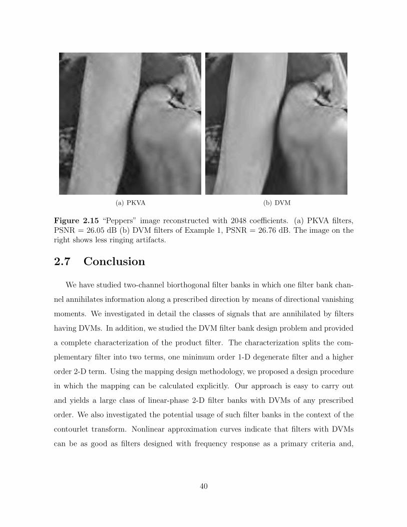
(a) PKVA (b) DVM

Figure 2.15 “Peppers” image reconstructed with 2048 coefficients. (a) PKVA filters,PSNR = 26.05 dB (b) DVM filters of Example 1, PSNR = 26.76 dB. The image on theright shows less ringing artifacts.

2.7 Conclusion

We have studied two-channel biorthogonal filter banks in which one filter bank chan-

nel annihilates information along a prescribed direction by means of directional vanishing

moments. We investigated in detail the classes of signals that are annihilated by filters

having DVMs. In addition, we studied the DVM filter bank design problem and provided

a complete characterization of the product filter. The characterization splits the com-

plementary filter into two terms, one minimum order 1-D degenerate filter and a higher

order 2-D term. Using the mapping design methodology, we proposed a design procedure

in which the mapping can be calculated explicitly. Our approach is easy to carry out

and yields a large class of linear-phase 2-D filter banks with DVMs of any prescribed

order. We also investigated the potential usage of such filter banks in the context of the

contourlet transform. Nonlinear approximation curves indicate that filters with DVMs

can be as good as filters designed with frequency response as a primary criteria and,

40

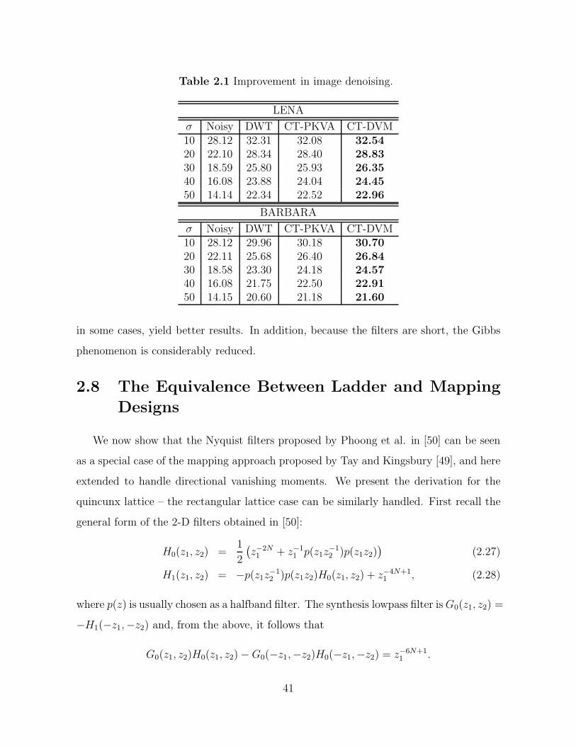
Table 2.1 Improvement in image denoising.

LENA

σ Noisy DWT CT-PKVA CT-DVM10 28.12 32.31 32.08 32.5420 22.10 28.34 28.40 28.8330 18.59 25.80 25.93 26.3540 16.08 23.88 24.04 24.4550 14.14 22.34 22.52 22.96

BARBARA

σ Noisy DWT CT-PKVA CT-DVM10 28.12 29.96 30.18 30.7020 22.11 25.68 26.40 26.8430 18.58 23.30 24.18 24.5740 16.08 21.75 22.50 22.9150 14.15 20.60 21.18 21.60

in some cases, yield better results. In addition, because the filters are short, the Gibbs

phenomenon is considerably reduced.

2.8 The Equivalence Between Ladder and MappingDesigns

We now show that the Nyquist filters proposed by Phoong et al. in [50] can be seen

as a special case of the mapping approach proposed by Tay and Kingsbury [49], and here

extended to handle directional vanishing moments. We present the derivation for the

quincunx lattice – the rectangular lattice case can be similarly handled. First recall the

general form of the 2-D filters obtained in [50]:

H0(z1, z2) =1

2

(z−2N1 + z−1

1 p(z1z−12 )p(z1z2)

)(2.27)

H1(z1, z2) = −p(z1z−12 )p(z1z2)H0(z1, z2) + z−4N+1

1 , (2.28)

where p(z) is usually chosen as a halfband filter. The synthesis lowpass filter is G0(z1, z2) =

−H1(−z1,−z2) and, from the above, it follows that

G0(z1, z2)H0(z1, z2) − G0(−z1,−z2)H0(−z1,−z2) = z−6N+11 .

41

Now, consider the delayed versions of H0(z) and G0(z) given by H0(z1, z2) = z2N1 H0(z1, z2)

and G0(z1, z2) = z4N−11 G0(z1, z2). Then

H0(z1, z2) =1

2

(1 + z2N−1

1 p(z1z−12 )p(z1z2)

)

G0(z1, z2) =1

2

[2 + z2N−1

1 p(z1z−12 )p(z1z2)

×(1 − z2N−1

1 p(z1z−12 )p(z1z2)

)].

The above filters are simply delayed versions of the starting ones, thus being the same fil-

ters for practical purposes. Notice that the filters now satisfy H0(z)G0(z)+H0(z)G0(z) =

2. Setting z := z2N−11 p(z1z

−12 )p(z1z2) in (2.29), we see that the filters can be written in

terms of the 1-D polynomials

H(1D)0 (z) =

1

2(1 + z)

G(1D)0 (z) =

1

2[2 + z (1 − z)] ,

where H(1D)0 (z)G(1D)

0 (z)+H(1D)0 (−z)G(1D)

0 (−z) = 2. Finally note that z2N−11 p(z1z

−12 )p(z1z2)

is odd regardless of the nature of p(z). Hence we have the following result.

Proposition 7 The filters proposed in [50] constitute a particular case of the mapping

design of [49], where the mapping function is M(z1, z2) = z2N−11 p(z1z

−12 )p(z1z2).

42

CHAPTER 3

THE NONSUBSAMPLED CONTOURLETTRANSFORM: THEORY, DESIGN, AND

APPLICATIONS

In this chapter we develop the nonsubsampled contourlet transform (NSCT) and

study its applications. The construction proposed in this chapter is based on a nonsub-

sampled pyramid structure and nonsubsampled directional filter banks. The result is a

flexible multiscale, multidirection, and shift-invariant image decomposition that can be

efficiently implemented via the a trous algorithm. At the core of the proposed scheme is

the nonseparable two-channel nonsubsampled filter bank. We exploit the less stringent

design condition of the nonsubsampled filter bank to design filters that lead to a NSCT

with better frequency selectivity and regularity when compared to the contourlet trans-

form. We propose a design framework based on the mapping approach, that allows for a

fast implementation based on a lifting or ladder structure, and only uses one-dimensional

filtering in some cases. In addition, our design ensures that the corresponding frame

elements are regular, symmetric, and the frame is close to a tight one. We assess the

performance of the NSCT in image denoising. The NSCT compares favorably to other

existing methods in the literature.

This chapter is joint work with Minh Do and Jianping Zhou. The results of this chapter aresummarized in the references [53–55].

43

3.1 Introduction

A number of image processing tasks are efficiently carried out in the domain of an

invertible linear transformation. For example, image compression and denoising are ef-

ficiently done in the wavelet transform domain [1, 8]. An effective transform captures

the essence of a given signal or a family of signals with few basis functions. The set of

basis functions completely characterizes the transform and this set can be redundant or

not, depending on whether the basis functions are linear dependent. By allowing redun-

dancy, it is possible to enrich the set of basis functions so that the representation is more

efficient in capturing some signal behavior. In addition, redundant representations are

generally more flexible and easier to design. In applications such as denoising, enhance-

ment, and contour detection, a redundant representation can significantly outperform a

nonredundant one.

Another important feature of a transform is its stability with respect to shifts of the

input signal. The importance of the shift-invariance property in imaging applications

dates back at least to Daugman [56] and was also advocated by Simoncelli et al. in

[21]. An example that illustrates the importance of shift-invariance is image denoising by

thresholding where the lack of shift-invariance causes pseudo-Gibbs phenomena around

singularities [57]. Thus, most state-of-the-art wavelet denoising algorithms (see for ex-

ample [58–60]) use an expansion with less shift sensitivity than the standard maximally

decimated wavelet decomposition — the most common being the nonsubsampled wavelet

transform (NSWT) computed with the a trous algorithm [61]. 1

In addition to shift-invariance, it has been recognized that an efficient image represen-

tation has to account for the geometrical structure pervasive in natural scenes. In this

direction, several representation schemes have recently been proposed [16, 18–20, 36].

The contourlet transform [20] is a multidirectional and multiscale transform that is con-

structed by combining the Laplacian pyramid [25, 37] with the directional filter bank

1Denoising by thresholding in the NSWT domain can also be realized by denoising multiple circularshifts of the signal with a critically sampled wavelet transform and then averaging the results. This hasbeen termed cycle spinning after [57].

44

(DFB) proposed in [23]. The pyramidal filter bank structure of the contourlet transform

has very little redundancy, which is important for compression applications. However,

designing good filters for the contourlet transfom is a difficult task. In addition, due to

downsamplers and upsamplers present in both the Laplacian pyramid and the DFB, the

contourlet transform is not shift-invariant.

In this chapter we propose an overcomplete transform that we call the nonsubsampled

contourlet transform (NSCT). Our main motivation is to construct a flexible and efficient

transform targeting applications where redundancy is not a major issue (e.g., denoising).

The NSCT is a fully shift-invariant, multiscale, and multidirection expansion that has

a fast implementation. The proposed construction leads to a filter design problem that,

to the best of our knowledge, has not been addressed elsewhere. The design problem

is much less constrained than that of contourlets. This enables us to design filters with

better frequency selectivity, thereby achieving better subband decomposition. Using the

mapping approach we provide a framework for filter design that ensures good frequency

localization in addition to having a fast implementation through ladder steps. The NSCT

has proven to be very efficient in image denoising and image enhancement [53–55].

The chapter is structured as follows. In Section 3.2 we describe the NSCT and its

building blocks. We introduce a pyramid structure that ensures the multiscale feature

of the NSCT and the directional filtering structure based on the DFB. The basic unit in

our construction is the nonsubsampled filter bank (NSFB), which is discussed in Section

3.2. In Section 3.3 we study the issues associated with the NSFB design and implemen-

tation problems. Application of the NSCT in image denoising is discussed in Section 3.4.

Conclusions are drawn in Section 3.5.

Notation: Throughout the chapter, a two-dimensional (2-D) filter is represented by its

z-transform H(z) where z = [z1, z2]T . Evaluated on the unit sphere, a filter is denoted by

H(ejω) where ejω = [ejω1, ejω2]T . If m = [m1, m2]T is a 2-D vector, then zm = zm11 zm2

2 ,

whereas if M is a 2 × 2 matrix, then zM = [zm1, zm2] with m1,m2 the columns of M.

In this chapter we often deal with zero-phase 2-D filters. On the unit sphere, such filters

45

can be written as polynomials in cosω = (cosω1, cosω2)T . We thus write F (x1, x2) for a

zero-phase filter in which x1 and x2 denote cosω1 and cosω2, respectively.

Abbreviations: A number of abbreviations are used throughout the chapter:

NSCT - Nonsubsampled Contourlet Transform.

NSFB - Nonsubsampled Filter Bank.

NSP - Nonsubsampled Pyramid.

NSDFB - Nonsubsampled Directional Filter Bank.

NSWT - Nonsubsampled 2-D Wavelet Transform.

LAS - Local Adaptive Shrinkage.

3.2 Nonsubsampled Contourlets and Filter Banks

3.2.1 The nonsubsampled contourlet transform

Figure 3.1 (a) displays an overview of the proposed NSCT. The structure consists of

a bank of filters that splits the 2-D frequency plane in the subbands illustrated in Figure

3.1(b). Our proposed transform can thus be divided into two shift-invariant parts: (1)

A nonsubsampled pyramid structure that ensures the multiscale property and (2) A

nonsubsampled DFB structure that gives directionality.

3.2.1.1 The nonsubsampled pyramid (NSP)

The multiscale property of the NSCT is obtained from a shift-invariant filtering struc-

ture that achieves a subband decomposition similar to that of the Laplacian pyramid.

This is achieved by using two-channel nonsubsampled 2-D filter banks. Figure 3.2 il-

lustrates the proposed nonsubsampled pyramid (NSP) decomposition with J = 3 stages.

Such expansion is conceptually similar to the 1-D nonsubsampled wavelet transform com-

puted with the a trous algorithm [61] and has J + 1 redundancy, where J denotes the

number of decomposition stages. The ideal passband support of the lowpass filter at

the j-th stage is the region [− π2j ,

π2j ]2. Accordingly, the ideal support of the equivalent

highpass filter is the complement of the lowpass, i.e., the region [− π2j−1 ,

π2j−1 ]2\[− π

2j ,π2j ]2.

46

subband

subbands

directional

Bandpass

subbands

directional

Bandpass

Image

Lowpass

(a)

(π, π)

(−π,−π)

ω1

ω2

(b)

Figure 3.1 The nonsubsampled contourlet transform. (a) Nonsubsampled filter bankstructure that implements the NSCT. (b) The idealized frequency partitioning obtainedwith the proposed structure.

The filters for subsequent stages are obtained by upsampling the filters of the first stage.

This gives the multiscale property without the need for additional filter design. The

proposed structure is thus different from the separable nonsubsampled wavelet transform

(NSWT). In particular, one bandpass image is produced at each stage resulting in J + 1

redundancy. By contrast, the NSWT produces three directional images at each stage

resulting in 3J + 1 redundancy.

H0(z)

H1(z)

H0(z2I)

H1(z2I)

H0(z4I)

H1(z4I)

x

y0

y1

y2

y3

(a)

0 1 2 3

(π, π)

(−π,−π)

ω1

ω2

(b)

Figure 3.2 The proposed nonsubsampled pyramid is a 2-D multiresolution expansionsimilar to the 1-D nonsubsampled wavelet transform. (a) A three-stage pyramid decom-position. The lighter gray regions denote the aliasing caused by upsampling. (b) Thesubbands on the 2-D frequency plane.

47

The 2-D pyramid proposed in [62] is obtained with a similar structure. Specifically,

the NSFB of [62] is built from lowpass filter H0(z). One then sets H1(z) = 1−H0(z), and

the corresponding synthesis filters G0(z) = G1(z) = 1. A similar decomposition can be

obtained by removing the downsamplers and upsamplers in the Laplacian pyramid and

then upsampling the filters accordingly. Those perfect reconstruction systems can be seen

as a particular case of our more general structure. The advantage of our construction is

that it is general and, as a result, better filters can be obtained. In particular, in our

design G0(z) and G1(z) are lowpass and highpass. Thus, they filter certain parts of the

noise spectrum in the processed pyramid coefficients.

3.2.1.2 The nonsubsampled directional filter bank (NSDFB)

The directional filter bank of Bamberger and Smith [23] is constructed by combining

critically sampled two-channel fan filter banks and resampling operations. The result is a

tree-structured filter bank that splits the 2-D frequency plane into directional wedges. A

shift-invariant directional expansion is obtained with a nonsubsampled DFB (NSDFB).

The NSDFB is constructed by eliminating the downsamplers and upsamplers in the DFB.

This is done by switching off the downsamplers/upsamplers in each two-channel filter

bank in the DFB tree structure and upsampling the filters accordingly. This results in a

tree composed of two-channel nonsubsampled filter banks. Figure 3.3 illustrates a four-

channel decomposition. Note that in the second level, the upsampled fan filters Ui(zQ),

i = 0, 1 have checker-board frequency support and, when combined with the filters in

the first level, give the four directional frequency decomposition shown in Figure 3.3.

The synthesis filter bank is obtained similarly. Just like the critically sampled directional

filter bank, all filter banks in the nonsubsampled directional filter bank tree structure are

obtained from a single nonsubsampled filter bank with fan filters (see Figure 3.5 (b)).

Moreover, each filter bank in the NSDFB tree has the same computational complexity

as that of the prototype NSFB.

48

U0(z)

U1(z)

U0(zQ)

U0(zQ)

U1(zQ)

U1(zQ)

x

y0

y1

y2

y3

(a)

0 13

2

(π, π)

(−π,−π)

ω1

ω2

(b)

Figure 3.3 A four-channel nonsubsampled directional filter bank constructed with two-channel fan filter banks. (a) Filtering structure. The equivalent filter in each channel isgiven by Ueq

k (z) = Ui(z)Uj(zQ). (b) Corresponding frequency decomposition.

3.2.1.3 Combining the nonsubsampled pyramid and nonsubsampleddirectional filter bank in the NSCT

The NSCT is constructed by combining the NSP and the NSDFB as shown in Figure

3.1 (a). In constructing the nonsubsampled contourlet transform, care must be taken

when applying the directional filters to the coarser scales of the pyramid. Due to the

tree-structure nature of the NSDFB, the directional response at the lower and upper

frequencies suffers from aliasing, which can be a problem in the upper stages of the

pyramid (see Figure 3.8). This is illustrated in Figure 3.4 (a), where the passband region

of the directional filter is labeled as “Good” or “Bad.” Thus we see that for coarser

scales, the highpass channel in effect is filtered with the bad portion of the directional

filter passband. This results in severe aliasing and in some observed cases a considerable

loss of directional resolution.

We remedy this by judiciously upsampling the NSDFB filters. Denote the k-th direc-

tional filter by Uk(z). Then for higher scales, we substitute Uk(z2mI) for Uk(z), where m is

chosen to ensure that the good part of the response overlaps with the pyramid passband.

Figure 3.4 (b) illustrates a typical example. Note that this modification preserves perfect

49

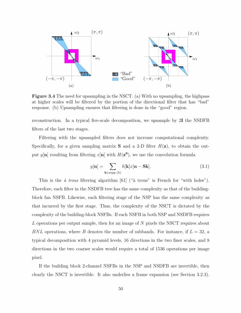
(π, π)

(−π,−π)

ω1

ω2

(a)

“Good”“Bad”

(π, π)

(−π,−π)

ω1

ω2

(b)

Figure 3.4 The need for upsampling in the NSCT. (a) With no upsampling, the highpassat higher scales will be filtered by the portion of the directional filter that has “bad”response. (b) Upsampling ensures that filtering is done in the “good” region.

reconstruction. In a typical five-scale decomposition, we upsample by 2I the NSDFB

filters of the last two stages.

Filtering with the upsampled filters does not increase computational complexity.

Specifically, for a given sampling matrix S and a 2-D filter H(z), to obtain the out-

put y[n] resulting from filtering x[n] with H(zS), we use the convolution formula

y[n] =∑

k∈supp (h)

h[k]x[n − Sk]. (3.1)

This is the a trous filtering algorithm [61] (“a trous” is French for “with holes”).

Therefore, each filter in the NSDFB tree has the same complexity as that of the building-

block fan NSFB. Likewise, each filtering stage of the NSP has the same complexity as

that incurred by the first stage. Thus, the complexity of the NSCT is dictated by the

complexity of the building-block NSFBs. If each NSFB in both NSP and NSDFB requires

L operations per output sample, then for an image of N pixels the NSCT requires about

BNL operations, where B denotes the number of subbands. For instance, if L = 32, a

typical decomposition with 4 pyramid levels, 16 directions in the two finer scales, and 8

directions in the two coarser scales would require a total of 1536 operations per image

pixel.

If the building block 2-channel NSFBs in the NSP and NSDFB are invertible, then

clearly the NSCT is invertible. It also underlies a frame expansion (see Section 3.2.3).

50

The frame elements are localized in space and oriented along a discrete set of directions.

The NSCT is flexible in that it allows any number of 2l directions in each scale. In

particular, it can satisfy the anisotropic scaling law — a key property in establishing

the expansion nonlinear approximation behavior [20, 36]. This property is ensured by

doubling the number of directions in the NSDFB expansion at every other scale. The

NSCT has redundancy given by 1 +∑J

j=1 2lj , where lj denotes the number of levels in

the NSDFB at the j-th scale.

3.2.2 Nonsubsampled filter banks

At the core of the proposed NSCT structure is the 2-D two-channel nonsubsampled

filter bank. Shown in Figure 3.5 are the NSFBs needed to construct the NSCT. In this

chapter we focus exclusively on the FIR case simply because it is easier to implement

in multiple dimensions. For a general FIR two-channel NSFB, perfect reconstruction is

achieved provided the filters satisfy the Bezout identity:

H0(z)G0(z) + H1(z)G1(z) = 1. (3.2)

The Bezout identity puts no constraint on the frequency response of the filters in-

volved. Therefore, to obtain good solutions one has to impose additional conditions on

the filters.

+

H0(z)

H1(z)

G0(z)

G1(z)

x x

y0

y1

(a)

+x x

y0

y1

U0(z)

U1(z)

V0(z)

V1(z)(b)

Figure 3.5 The two-channel nonsubsampled filter banks used in the NSCT. The systemis two times redundant and the reconstruction is error free when the filters satisfy Bezout’sidentity. (a) Pyramid NSFB. (b) Fan NSFB.

51

3.2.3 Frame analysis of the NSCT

The nonsubsampled filter bank can be interpreted in terms of analysis/synthesis op-

erators of frame systems. A family of vectors {φn}n∈Γ constitute a frame for a Hilbert

space H if there exist two positive constants A, B such that for each x ∈ H we have

A‖x‖2 ≤∑

n∈Γ

|〈x,φn〉|2 ≤ B‖x‖2. (3.3)

In the event that A = B the frame is said to be tight. The frame bounds are the tightest

positive constants satisfying (3.3).

Consider the NSFB of Figure 3.5 (a). The family {h0[·−n], h1[·− n]}n∈Z2 is a frame

for *2(Z2) if and only if there exist constants 0 < A ≤ B < ∞ such that [12]

A ≤ |H0(ejω)|2 + |H1(e

jω)|2︸ ︷︷ ︸t(ejω )

≤ B. (3.4)

Thus, the frame bounds of an NSFB can be computed by

A = ess. infω∈[−π,π]2

t(ejω), B = ess. supω∈[−π,π]2

t(ejω), (3.5)

where ess. inf and ess. sup denote the essential infimum and essential supremum, respec-

tively. From (3.4), we see that the frame is tight whenever t(ejω) is almost everywhere

constant. For FIR filters, this means that H0(z)H0(z−1) + H1(z)H1(z−1) = c. Such a

condition can only be met with linear phase FIR filters if H0(z) and H1(z) are either

trivial delays or combinations of two delays (for a formal proof, see [7] pp. 337-338 or

[43]).

Because the NSFB is redundant, an infinite number of inverses exist. Among them,

the pseudo-inverse is optimal in the least square sense [1]. Given a frame of analysis

filters, the synthesis filters corresponding to the frame pseudo-inverse are given by Gi(z) =

Hi(z)/t(z) for i = 0, 1 [12]. In this case, the synthesis filters form the dual frame with

lower and upper frame bounds given by B−1 and A−1, respectively. When the analysis

filters are FIR, then unless the frame is tight, the synthesis filters of the pseudo-inverse

will be IIR.

52

From the above discussion we gather two important points: (1) linear phase filters

and tight frames are mutually exclusive; (2) the pseudo-inverse is desirable, but is IIR if

the frame is not tight. Consequently, an FIR NSFB system with linear phase filters and

with synthesis filters corresponding to the pseudo-inverse is not possible. However, we

can approximate the pseudo-inverse with FIR filters. For a given number of filter taps,

the closer the frame is to being tight, the better an FIR approximation of the pseudo-

inverse can be [13]. Thus, in the designs of the filters we seek linear phase filters that

underly a frame that is as close to a tight one as possible.

In a general FIR perfect reconstruction NSFB system both analysis and synthesis

filters form a frame. If we denote the analysis and synthesis frame bounds by Aa, Ba and

As, Bs, respectively, the frames will be close to tight provided [13]

ra := Aa/Ba ≈ 1, and rs := As/Bs ≈ 1.

We always assume that the filters are normalized so that we have Aa ≤ 1 ≤ Ba. In

case the pseudo-inverse is used, then we also have As ≤ 1 ≤ Bs. The following result

shows the NSCT is a frame operator for *2(Z2) whenever each constituent NSFB forms

a frame.

Proposition 8 In the nonsubsampled contourlet transform, if the pyramid filter bank

constitutes a frame with frame bounds Ap and Bp, and the fan filters constitute a frame

with frame bounds Aq and Bq, then the NSCT is a frame with bounds A and B satisfying

AJpAmin {lj}

q ≤ A ≤ B ≤ BJp Bmax {lj}

q

Proof. Consider the pyramid shown in Figure 3.2 (a). If J = 1, then we have that

‖y0‖2 + ‖y1‖2 ≤ Bp‖x‖2. Now, suppose we have J levels and assume∑J

j=0 ‖yi‖2 ≤

53

BJp ‖x‖2. Then if we further split yJ into y′

J and yJ+1, noting that Bp ≥ 1 we have that

J−1∑

j=0

‖yj‖2 + ‖y′J‖2 + ‖yJ+1‖2 ≤

J−1∑

j=0

‖yj‖2 + Bp‖yJ‖2

≤ Bp

(J−1∑

j=0

‖yj‖2 + ‖yJ‖2

)

≤ BJ+1p ‖x‖2.

Thus, by induction we conclude that∑J

j=0 ‖yi‖2 ≤ BJp ‖x‖2 for any J ≥ 1. A similar

argument shows that in the NSDFB with lj stages, one has that∑2lj−1

k=0 ‖yj,k‖2 ≤ Bljq ‖yj‖2

so that

‖yJ‖2 +J−1∑

j=0

2lj−1∑

k=0

‖yj,k‖2 ≤ ‖yJ‖2 +J−1∑

j=0

Bljq ‖yj‖2

≤ ‖yJ‖2 + Bmax {lj}q

J−1∑

j=0

‖yj‖2

≤ BJBmax {lj}q ‖x‖2.

The bound for A is proved similarly, by just reversing the inequalities. !

Remark 6 When both the pyramid and fan filter banks form tight frames with bound

1, then Ap = Aq = Bp = Bq = 1, and from the above proposition, the nonsubsampled

contourlet transform is also a tight frame with bound 1.

The above estimates on A and B can be accurate in some cases, especially when the

frame is close to a tight one and the number of levels is small (e.g., J = 4). In general,

however, they are not accurate estimates. Their purpose is more of giving an interval for

the frame bounds rather than the actual values. Table 3.1 shows estimates for different

numbers of scales. The actual frame bound is computed from (3.4 - 3.5), whereas the

estimates are the ones given according to Proposition 8.

54

Table 3.1 Frame bounds evolving with scale for the pyramid filters given in Example 3in Section 3.3.

J A actual A estimated B actual B estimated1 0.9586 0.9596 1.0435 1.04352 0.9393 0.9189 1.0504 1.08893 0.9332 0.8808 1.0515 1.13624 0.9316 0.8444 1.0517 1.1857

3.3 Filter Design and Implementation

The filter design problem of the NSCT comprises the two basic NSFBs displayed in

Figure 3.5. The goal is to design the filters imposing the Bezout identity (i.e., perfect

reconstruction) and enforcing other properties such as sharp frequency response, easy

implementation, regularity of the frame elements, and tightness of the corresponding

frames. It is also desirable that the filters are linear-phase.

Two-channel 1-D NSFBs that underlie tight frames are designed in [12]. However, the

design methodology of [12] is not easy to extend to 2-D designs since it relies on spectral

factorization, which is hard in 2-D. If we relax the tightness constraint, then the design

becomes more flexible. In addition, as we alluded to earlier, nontight filters can be linear

phase.

An effective and simple way to design 2-D filters is the mapping approach first pro-

posed by McClellan [63] in the context of digital filters and then used by several authors

[34, 43, 49, 50] in the context of filter banks. In this approach, the 2-D filters are obtained

from 1-D ones. In the context of NSFBs, a set of perfect reconstruction 2-D filters is

obtained in the following way:

Step 1. Construct a set of 1-D polynomials {H(1D)i (x), G(1D)

i (x)}i=0,1 that satisfies the

Bezout identity.

Step 2. Given a 2-D FIR filter f(z), then {H(1D)i (f(z)), G(1D)

i (f(z))}i=0,1 are 2-D filters

satisfying the Bezout identity.

Thus, one has to design the set of 1-D filters and the mapping function f(z) so that

the ideal responses are well approximated with a small number of filter coefficients. In

55

the mapping approach, one can control the frequency and phase responses through the

mapping function. Moreover, if the mapping function is zero-phase, then f(z) = f(z−1)

and it follows that the mapped filters are also zero-phase. In this case, on the unit

sphere, the mapping function is a 2-D polynomial in (cosω1, cosω2). We thus denote it

by F (x1, x2), where it is implicit that f(ejω) = F (cosω1, cosω2).

x xQ(1D)(f(z)) Q(1D)(f(z)) P (1D)(f(z))P (1D)(f(z))

Figure 3.6 Lifting structure for the nonsubsampled filter bank designed with the map-ping approach. The 1-D prototype is factored with the Euclidean algorithm. The 2-Dfilters are obtained by replacing x #→ f(z).

3.3.1 Implementation through lifting

Filters designed with the mapping approach can be efficiently factored into a ladder

[64] or lifting [65] structure that simplifies computations. To see this, assume without loss

of generality that the degree of the highpass prototype polynomial H(1D)1 (x) is smaller

than that of H(1D)0 (x). Suppose also that there are synthesis filters G(1D)

0 (x) and G(1D)1 (x)

such that the Bezout identity is satisfied. In this case it follows that gcd{H(1D)0 , H(1D)

1 } =

1. The Euclidean algorithm then enables us to factor the filters in the following way

[64–66]:

H(1D)0 (x)

H(1D)1 (x)

=N∏

i=0

1 0

P (1D)i (x) 1

1 Q(1D)i (x)

0 1

1

0

. (3.6)

As a result, we can obtain a 2-D factorization by replacing x with f(z). This factor-

ization characterizes every 2-D NSFB derived from 1-D through the mapping method.

Figure 3.6 illustrates the ladder structure with one stage.

In general, the lifting implementation at least halves the number of multiplications

and additions of the direct form [65]. The complexity can be reduced further if the lifting

56

steps in the 1-D prototype are monomials and the mapping filter f(z) has the form

f(z) = f1(zp11 zp2

2 )f2(zq11 zq2

2 ) (3.7)

for suitable f1(z), f2(z), and integers p1, p2, q1, q2. Note that if f(z) is a 1-D filter, then the

2-D filter f(zp1z

q2) for integers p and q has the same complexity as that of f(z). Therefore,

filters of the form in (3.7) have the same complexity as that of separable filters (i.e., filters

of the form f(z) = f(z1)f(z2) ) which amounts to two 1-D filtering operations. Notice

that if f(z) is as in (3.7), then for an arbitrary sampling matrix S, f(zS) also has the form

in (3.20). Consequently, all NSFBs in the NSDFB tree structure can be implemented

with 1-D operations whenever the prototype fan NSFB can be implemented with 1-D

filtering operations. The same reasoning applies to the NSFBs of the NSP.

3.3.2 Pyramid filter design

In the pyramid case, we impose line zeros at ω = (π,ω2) and ω = (ω1, π). Notice

that an N -th order line zero at ω = (π,ω2), for example, amounts to a (1 + ejω1)N

factor in the low pass filter. Such zeros are useful to obtain good approximation of the

ideal frequency response of Figure 3.5, in addition to imposing regularity of the scaling

function. We point out that for the approximation of smooth Cα images, 1 + 2α3 point

zeros at (±π,±π) would suffice [67]. However, our experience shows that point zeros alone

do not guarantee a “reasonable” frequency response of the pyramid filters. The following

proposition characterizes the mapping function that generates zeros in the resulting 2-D

filters.

Proposition 9 Let G(1D)(z) be a polynomial with roots {zi}ni=1 where each zi has multi-

plicity ni. Suppose we want a mapping function F (x1, x2) such that

G(1D) (F (x1, x2)) = (x1 − c)N1 (x2 − d)N2 L(x1, x2), (3.8)

where L(x1, x2) is a bivariate polynomial. Then G(1D)(F (x1, x2)) has the form in (3.8) if

and only if F (x1, x2) takes the form

F (x1, x2) = zj + (x1 − c)N ′

1 (x2 − d)N ′

2 LF (x1, x2), (3.9)

57

for some root zj ∈ {zi}ni=1, where LF (x1, x2) is a bivariate polynomial, and N ′

1, N′2 are

such that N ′1ni ≥ N1 and N ′

2nj ≥ N2.

Proof.

We prove the claim for the case in which the zeros of G(1D)(z) are distinct. The proof

for the case of repeated roots can be handled similarly.

Denote

G(1D)(z) = g0

n∏

i=1

(z − zi), g0 ∈ C. (3.10)

Then sufficiency follows by direct substitution of (3.9) in (3.10).

We prove necessity by induction. Suppose G(1D)(F (x1, x2)) = (x1 − c)N1L(x1, x2)

for some polynomial L(x1, x2). Note that G(1D)(F (c, x2)) = 0 for all x2 if and only if

F (c, x2) = zj for all x2 and some zero zj of G(1D)(z). So, it follows that

(F (x1, x2) − zj)x1=c = 0 for all x2, (3.11)

which implies that F (x1, x2) = zj + (x1 − c)L1(x1, x2) with L1(x1, x2) a polynomial.

Suppose

F (x1, x2) = zj + (x1 − c)k−1Lk−1(x1, x2),

where k ≤ N1. By successively applying the chain rule for differentiation we get that

0 =∂k−1G(1D)(F (x1, x2))

∂xk−11

∣∣∣∣x1=c

= G(1D)′(F (c, x2))∂k−1F (x1, x2)

∂xk−11

∣∣∣∣x1=c

.

Because F (c, x2) = zj and the zj ’s are distinct, we have that G(1D)′(F (c, x2)) *= 0 and

then

∂k−1F (x1, x2)

∂xk−11

∣∣∣∣x1=c

= 0

⇒ ∂k−1F (x1, x2)

∂xk−11

= (x1 − c)L1(x1, x2) (3.12)

⇒ ∂F (x1, x2)

∂x1= (x1 − c)k−1Lk−1(x1, x2), (3.13)

58

where (3.13) follows by successively integrating (3.12). Combining (3.13) with (3.11) we

obtain that F (x1, x2) = zj + (x1 − c)kLk(x1, x2). By induction we conclude that

F (x1, x2) = zj + (x1 − c)N1LN1(x1, x2).

If G(1D)(F (x1, x2)) = (x2−d)N2L(x1, x2) for some polynomial L(x1, x2), then a similar

argument shows that

F (x1, x2) = zi + (x2 − d)N2LN2(x1, x2),

where zi is a zero of G(1D)(z). Thus,

zi − zj = (x1 − c)N1LN1(x1, x2) − (x2 − d)N2LN2(x1, x2),

and hence we have zj = zi. Therefore,

(x1 − c)N1LN1(x1, x2) = (x2 − d)N2LN2(x1, x2),

and so

LN1(x1, x2) = (x2 − d)N2LF (x1, x2),

and (3.9) is established with N ′1 = N1 and N ′

2 = N2. !

The above result holds in general, even for point zeros (as opposed to line zeros as in

Proposition 9). We will explore this extensively in the designs that follow.

Suppose the prototype filters H(1D)0 (x), G(1D)

0 (x) each have zeros at x = −1. Then, in

order to produce a suitable zero-phase mapping function for the pyramid NSFB, we

consider the class of maximally flat filters given by the polynomials [2]

PN,L(x) :=

(1 + x

2

)N L−1−N∑

l=0

(N + l − 1

l

)(1 − x

2

)l

, (3.14)

where N controls the degree of flatness at x = −1 and L controls the degree flatness at

x = 1. Following Proposition 9, we can construct a family of mapping functions as

F (x1, x2) = −1 + 2PN0,L0(x1)PN1,L1(x2) (3.15)

so that zero moments at x1 = −1 and x2 = −1 are guaranteed. Note that, except for

the constant −1, F (x1, x2) has the form of (3.7) and hence can be implemented with 1-D

filtering operations only.

59

Table 3.2 Maximally flat mapping polynomials used in the design of the nonsubsampledfan filter bank.

N FN(x1, x2)

1 12(x1 + x2)

2 14(x1 + x2)(3 − x1x2)

3 116(x1 + x2)(15 − x2

1 − 8x1x2 − x22 + 3x2

1x22)

4 132(x1 + x2)(35 − 5x2

1 − 25x1x2 + 3x31x2 − 5x2

2 + 15x21x

22 + 3x1x3

2 − 5x31x

32)

5 1256(x1 + x2) (315 − 70x2

1 + 3x41 − 280x1x2 + 72x3

1x2 − 70x22 + 228x2

1x22

−30x41x

22 + 72x1x3

2 − 120x31x

32 + 3x4

2 − 30x21x

42 + 35x4

1x42)

3.3.3 Fan filter design

To design the fan filters idealized in Figure 3.5(b) we use the same methodology as

in the pyramid case. The distinction occurs in the mapping function. The fan-shaped

response can be obtained from a diamond-shaped response by simple modulation in one

of the frequency variables. This modulation preserves the perfect reconstruction prop-

erty. A useful family of mapping functions for the diamond-shaped response is obtained

by imposing flatness around ω = (±π,±π) and ω = (0, 0) in addition to point zeros at

(±π,±π). If the mapping function is zero-phase, this amounts to imposing flatness in a

polynomial at (x1, x2) = (−1,−1) and (x1, x2) = (1, 1), and zeros at (x1, x2) = (−1,−1).

Mapping functions satisfying these desiderata with minimum number of polynomial co-

efficients are given by

FN(x1, x2) = −1 + QN (x1, x2), (3.16)

where the polynomials QN (x1, x2) give the class of maximally flat half-band filters with

diamond support. A closed-form expression for QN (x1, x2) is given in [68]. Table 3.2

displays the first six mapping functions FN(x1, x2) for the diamond filter bank.

We point out that diamond maximally flat mapping polynomials can be generated

from 1-D ones by a separable product and then an appropriate change of variables. In

this case the mapping function is separable and has the form f(z) = f1(z1z2)f2(z1z−12 ).

This has been done for instance in [50]. However, the nonseparable solution is generally

shorter (roughly by a factor of 2) while yielding the same number of zeros at the aliasing

60

frequencies and a similar frequency response. For faster implementation, one may choose

the longer mapping filters which can be implemented with 1-D filtering operations.

3.3.4 Design examples

The design through mapping is based on a set of 1-D polynomials that satisfies the

Bezout identity, that is, H(1D)0 (x)G(1D)

0 (x) + H(1D)1 (x)G(1D)

1 (x) = 1. The design can be

simplified if we impose the restriction that

H(1D)1 (x) = G(1D)

0 (−x)and G(1D)1 (x) = H(1D)

0 (−x).

One advantage of this choice is that the frequency response of the filters can be controlled

by the lowpass branch — the highpass will automatically have the complementary re-

sponse. Another advantage is that, under an additional condition, the frame bounds of

the analysis and synthesis frames are the same and can be computed from the 1-D proto-

types. To see this, suppose that f is the mapping function and that Ran(f) = Ran(−f)

with Ran(f) denoting the range of the mapping function f . Then we have that

Aa = infω∈[π,π]2

|H(1D)0 (f(ejω))|2 + |G(1D)

0 (−f(ejω))|2

= infx∈Ran(f)

|H(1D)0 (x)|2 + |G(1D)

0 (−x)|2

= infx∈Ran(−f)

|H(1D)0 (−x)|2 + |G(1D)

0 (x)|2

= infx∈Ran(f)

|H(1D)0 (−x)|2 + |G(1D)

0 (x)|2

= As. (3.17)

A similar argument shows that

Ba = Bs = supx∈Ran(f)

|H(1D)0 (−x)|2 + |G(1D)

0 (x)|2. (3.18)

Example 3 ( Pyramid filters very close to tight ones ) In order to get filters that

are almost tight, we design the prototypes H(1D)0 (x) and G(1D)

0 (x) to be very close to each

other. If we let H(1D)1 (x) = G(1D)

0 (−x) and G(1D)1 (x) = H(1D)

0 (−x), then the following

61

filters can be checked to satisfy the Bezout identity:

H(1D)0 (x) = K

(1 + k2x + k2k3x

2),

G(1D)0 (x) = K−1

(1 − k1x − k3x + k1k2x

2 − k1k2k3x3).

To obtain the prototype we choose the constants K, k1, k2, and k3 such that each filter has

a zero at z = −1 and in addition that H(1D)0 (−1) = G(1D)

0 (−1) =√

2. We obtain

H(1D)0 (x) =

1

2(x + 1)

(√2 + (1 −

√2)x

),

G(1D)0 (x) =

1

2(x + 1)

(√2 + (4 − 3

√2)x + (2

√2 − 3)x2

).

The lifting factorization of the prototype filters is given by

H(1D)0 (x)

H(1D)1 (x)

=

1 αx

0 1

1 0

βx 1

1 γx

0 1

K1

K2

(3.19)

with

α = γ = 1 −√

2, β =1√2, K1 = K2 =

1√2.

Notice that this implementation has 4 multiplies/sample whereas the direct form has

7 multiplies/sample. In this example we set F (x1, x2) = −1+2P2,4(x)P2,4(y) so that each

of the filters has a fourth-order zero at ω1 = ±π and at ω2 = ±π. Since the ladder steps

are monomials, the NSFB can be implemented with 1-D filtering operations. The frame

bounds are computed using (3.17-3.18):

Aa = As = 0.96, Ba = Bs = 1.04.

Thus we have ra = rs = 1.083 and the frame is almost tight. The support size of H0(z)

is 13× 13, whereas G0(z) has support size 19× 19. Figure 3.7 shows the response of the

resulting filters.

Example 4 (Maximally flat fan filters) Using the prototype filters of Example 3, we

modulate a maximally flat diamond mapping function to obtain the maximally flat fan

mapping function. Thus we choose FN (x1, x2) in Table 3.2 with N = 3. We use the

62

-2

0

2-2

0

2

00.250.5

0.75

1

-2

0

2

(a) |H0(ejω)|

-2

0

2-2

0

2

00.250.5

0.75

1

-2

0

2

(b) |G0(ejω)|

-2

0

2-2

0

2

00.250.5

0.75

1

-2

0

2

(c) |H1(ejω)|

-2

0

2-2

0

2

00.250.5

0.75

1

-2

0

2

(d) |G1(ejω)|

Figure 3.7 Magnitude response of the filters designed in Example 3 with maximallyflat filters. The nonsubsampled pyramid filter bank underlies almost tight analysis andsynthesis frames.

lifting factorization of the previous example. The diamond filters obtained have vanishing

moments on the corner points (±π,±π). Figure 3.8 shows the magnitude response of the

filters. The support size of U0(z) is 21× 21, whereas the support size of V0(z) is 31× 31.

3.3.5 Regularity of the NSCT basis functions

The regularity of the NSCT basis functions can be controlled by the NSP low-pass

filters. Denoting by H0(ω) the scaling lowpass filter used in the pyramid (we write H0(ω)

instead of H0(ejω) for convenience), we have the associated scaling function

Φ(ω) :=∞∏

j=1

H0(2−j

ω),

63

-2

0

2-2

0

2

00.250.5

0.75

1

-2

0

2

(a) |U0(ejω)|

-2

0

2-2

0

2

00.250.5

0.75

1

-2

0

2

(b) |V0(ejω)|

-2

0

2-2

0

2

00.250.5

0.75

1

-2

0

2

(c) |U1(ejω)|

-2

0

2-2

0

2

00.250.5

0.75

1

-2

0

2

(d) |V1(ejω)|

Figure 3.8 Fan filters designed with prototype filters of Example 3 and diamond maxi-mally flat mapping filters.

where convergence is in the weak sense. In our proposed design the filter H0(ω) can be

factored as

H0(ω) =

(1 + ejω1

2

)N1(

1 + ejω2

2

)N2

RH0(ω). (3.20)

Notice that the remainder filter RH0(ω) is not separable. Therefore, one cannot separate

the regularity estimation as two 1-D problems. Nonetheless, a similar argument can be

developed and an estimate of the 2-D regularity of the scaling filter is obtained.

Proposition 10 Let H0(ω) be a scaling filter as in (3.20) with the corresponding scaling

function Φ(ω). Let

B = supω∈[π,π]2

|RH0(ω)|.

Then

|Φ(ω)| ≤ C

(1

1 + |ω1|

)N1−log2 B ( 1

1 + |ω2|

)N2−log2 B

.

64

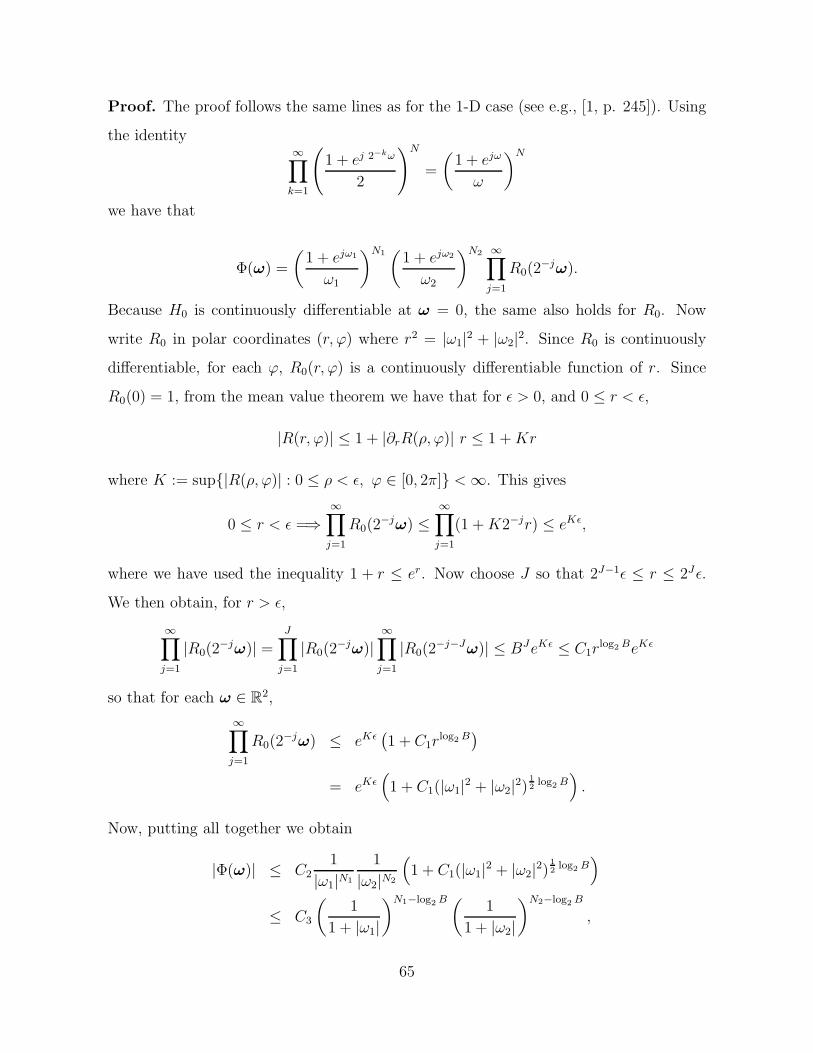
Proof. The proof follows the same lines as for the 1-D case (see e.g., [1, p. 245]). Using

the identity∞∏

k=1

(1 + ej 2−kω

2

)N

=

(1 + ejω

ω

)N

we have that

Φ(ω) =

(1 + ejω1

ω1

)N1(

1 + ejω2

ω2

)N2 ∞∏

j=1

R0(2−j

ω).

Because H0 is continuously differentiable at ω = 0, the same also holds for R0. Now

write R0 in polar coordinates (r,ϕ) where r2 = |ω1|2 + |ω2|2. Since R0 is continuously

differentiable, for each ϕ, R0(r,ϕ) is a continuously differentiable function of r. Since

R0(0) = 1, from the mean value theorem we have that for ε > 0, and 0 ≤ r < ε,

|R(r,ϕ)| ≤ 1 + |∂rR(ρ,ϕ)| r ≤ 1 + Kr

where K := sup{|R(ρ,ϕ)| : 0 ≤ ρ < ε, ϕ ∈ [0, 2π]} < ∞. This gives

0 ≤ r < ε =⇒∞∏

j=1

R0(2−j

ω) ≤∞∏

j=1

(1 + K2−jr) ≤ eKε,

where we have used the inequality 1 + r ≤ er. Now choose J so that 2J−1ε ≤ r ≤ 2Jε.

We then obtain, for r > ε,

∞∏

j=1

|R0(2−j

ω)| =J∏

j=1

|R0(2−j

ω)|∞∏

j=1

|R0(2−j−J

ω)| ≤ BJeKε ≤ C1rlog2 BeKε

so that for each ω ∈ R2,

∞∏

j=1

R0(2−j

ω) ≤ eKε(1 + C1r

log2 B)

= eKε(1 + C1(|ω1|2 + |ω2|2)

12 log2 B

).

Now, putting all together we obtain

|Φ(ω)| ≤ C21

|ω1|N1

1

|ω2|N2

(1 + C1(|ω1|2 + |ω2|2)

12 log2 B

)

≤ C3

(1

1 + |ω1|

)N1−log2 B ( 1

1 + |ω2|

)N2−log2 B

,

65

which completes the proof. !

As an example, consider the prototype filter in Example 3 and the mapping F (x1, x2) =

−1 + 2P1,2(x)P1,2(y). The resulting filter has second-order zeros at ω1 = ±π and at

ω2 = ±π. It can be verified that |RH0(ω)| ! 1.83 and |RG0(ω)| ! 1.49 so that the

regularity exponent2 is at least 2 − log2 1.83 ≈ 1.13 for H0(ω) and 2 − log2 1.49 ≈ 1.43

for G0(ω).

Thus the corresponding scaling functions and wavelets are at least continuous. We

point out that better estimates are possible applying similar 1-D techniques. For instance,

one could prove a result similar to Lemma 7.1.2 in [2], as a consequence of Proposition

10.

Figure 3.9 shows the basis functions of the NSCT obtained with the filters designed

via mapping. As the picture shows, the functions have a good degree of regularity.

3.4 Applications

3.4.1 Image denoising

In order to illustrate the potential of the NSCT design using the techniques previously

discussed, we study additive white Gaussian noise (AWGN) removal from images by

means of thresholding estimators.

3.4.1.1 Comparison to other transforms

To highlight the performance of the NSCT relative to other transforms, we perform

hard threshold on the subband coefficients of the various transforms. We choose the

threshold Ti,j = Kσnijfor each subband. This has been termed K-sigma thresholding in

[69]. We set K = 4 for the finest scale and K = 3 for the remaining ones. We use five

scales of decomposition for nonsubsampled contourlet transform, contourlet transform

2The regularity exponent of a scaling function φ(t) is the largest number α such that Φ(ω) decays asfast as 1

(1+|ω1|+|ω2|)α .

66

Basis functions, Level 2

(a)

Basis functions, Level 3

Basis functions, Level 4

(b)

Figure 3.9 Basis functions of the nonsubsampled contourlet transform. (a) Basis func-tions of the second stage of the pyramid. (b) Basis functions of third (top 8) and fourth(bottom 8) stages of the pyramid.

(CT), and nonsubsampled wavelet transform. For the NSCT and CT we use 4,8,8,16,16

directions in the scales from coarser to finer, respectively.

Table 3.3 (left columns) shows the PSNR results for various transforms and noise

intensities. The results show the NSCT is consistently superior to curvelets and NSWT

67

Table 3.3 Denoising performance of the NSCT. The left-most columns are hard thresh-olding and the right-most ones soft estimators. For hard thresholding, the NSCT con-sistently outperforms curvelets and the NSWT. The NSCT-LAS performs on a par withthe more sophisticated estimator BLS-GSM and is superior to the BivShrink estimatorof.

Lena Comparison to other transforms Comparison to other methods

σ Noisy NSWT Curvelets CT NSCT NSWT-LAS BivShrink BLS-GSM NSCT-LAS

10 28.13 34.26 34.17 31.90 34.69 35.19 35.34 35.59 35.46

20 22.13 31.40 31.52 28.34 32.03 32.12 32.40 32.62 32.50

30 18.63 29.66 30.01 27.10 30.35 30.30 30.54 30.84 30.70

40 16.13 28.37 28.84 25.84 29.10 29.01 - 29.58 29.38

50 14.20 27.41 27.78 24.87 28.10 28.00 - 28.61 28.34

Barb. Comparison to other transforms Comparison to other methods

σ Noisy NSWT Curvelets CT NSCT NSWT-LAS BivShrink BLS-GSM NSCT-LAS

10 28.17 31.58 32.28 29.62 33.01 33.40 33.35 34.03 34.09

20 22.15 27.23 28.89 26.26 29.41 29.45 29.80 30.28 30.60

30 18.63 25.10 26.93 24.42 27.24 27.22 27.65 28.11 28.56

40 16.14 24.02 25.51 23.16 25.79 25.76 - 26.58 27.12

50 14.20 23.37 24.31 22.29 24.79 24.72 - 25.43 26.02

Pepp. Comparison to other transforms Comparison to other methods

σ Noisy NSWT Curvelets CT NSCT NSWT-LAS BLS-GSM NSCT-LAS

10 28.17 33.71 33.59 31.30 33.81 34.35 34.63 34.41

20 22.15 31.19 31.13 28.57 31.60 31.65 32.06 31.82

30 18.63 29.43 29.45 26.81 30.07 29.95 30.41 30.19

40 16.13 28.09 28.01 25.50 28.85 28.65 29.20 28.95

50 14.20 27.04 26.70 24.47 27.82 27.62 28.24 27.93

in PSNR measure. For the “Barbara” image, the NSCT yields improvements in excess

of 1.90 dB in PSNR over the NSWT. The NSCT also is superior to the CT as the results

show. Figure 3.10 displays the reconstructed images using the the NSWT, curvelets, and

NSCT. As the figure shows, both the NSCT and the curvelet transform offer a better

recovery of edge information relative to the NSWT. But improvements can be seen in

the NSCT, particularly around the eye.

68

(a) Original (b) NSWT

(c) Curvelets (d) NSCT

Figure 3.10 Image denoising with the NSCT and hard thresholding. The noisy intensityis 20. (a) Original Lena image. (b) Denoised with the NSWT, PSNR = 31.40 dB. (c)Denoised with the curvelet transform and hard thresholding, PSNR = 31.52 dB. (d)Denoised with the NSCT, PSNR = 32.03 dB.

3.4.1.2 Comparison to other denoising methods

We perform soft thresholding (shrinkage) independently in each subband. Following

[58] we choose the threshold

Ti,j =σ2

Nij

σi,j,n,

69

where σi,j,n denotes the variance of the n-th coefficient at the i-th directional subband

of the j-th scale, and σ2Nij

is the noise variance at scale j and direction i. It is shown

in [58] that shrinkage estimation with T = σ2

σX, and assuming X generalized Gaussian

distributed yields a risk within 5% of the optimal Bayes risk. As studied in [70], contourlet

coefficients are well modeled by generalized Gaussian distributions. The signal variances

are estimated locally using the neighboring coefficients contained in a square window

within each subband and a maximum likelihood estimator. The noise variance in each

subband is inferred using a Monte Carlo technique where the variances are computed for

a few normalized noise images and then averaged to stabilize the results. We refer to this

method as local adaptive shrinkage (LAS). Effectively, our LAS method is a simplified

version of the denoising method proposed in [71] that works in the NSCT or NSWT

domain. In the LAS estimator we use four scales for both the NSCT and NSWT. For

the NSCT we use 3,3,4,4 directions in the scales from coarser to finer, respectively.

To benchmark the performance of the NSCT-LAS scheme we have used two of the

best denoising methods in the literature: (1) bivariate shrinkage with local variance

estimation (BivShrink) [59]; (2) Bayes least-squares with a Gaussian scale-mixture model

(BLS-GSM) proposed in [60]. Table 3.3 (right columns) shows the results obtained.3

The NSCT coupled with the LAS estimator (NSCT-LAS) produced very satisfactory

results. In particular, among the methods studied, the NSCT-LAS yields the best results

for the “Barbara” image, being surpassed by the BLS-GSM method for the other images.

Despite its slight loss in performance relative to BLS-GSM, we believe the NSCT has

potential for better results. This is because by comparison, the BLS-GSM is a consider-

ably richer and more sophisticated estimation method than our simple local thresholding

estimator. However, studying more complex denoising methods in the NSCT domain

is beyond the scope of the present chapter. Figure 3.11 displays the denoised images

with both BLS-GLM and NSCT-LAS methods. As the pictures show, the NSCT offers

3The PSNR values of the BivShrink method were obtained from the tables in [59]. In [59] the authorsdo not use the “Peppers” image as a test image, hence we do not have a BivShrink column for “Peppers.”

70

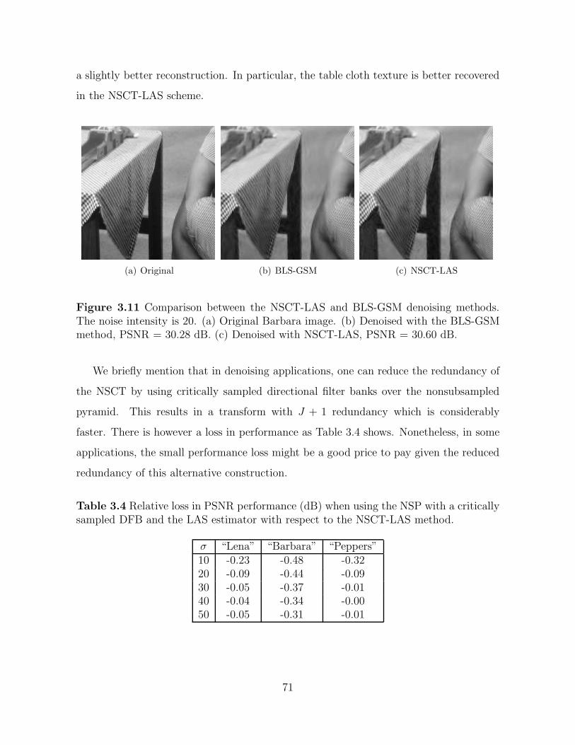
a slightly better reconstruction. In particular, the table cloth texture is better recovered

in the NSCT-LAS scheme.

(a) Original (b) BLS-GSM (c) NSCT-LAS

Figure 3.11 Comparison between the NSCT-LAS and BLS-GSM denoising methods.The noise intensity is 20. (a) Original Barbara image. (b) Denoised with the BLS-GSMmethod, PSNR = 30.28 dB. (c) Denoised with NSCT-LAS, PSNR = 30.60 dB.

We briefly mention that in denoising applications, one can reduce the redundancy of

the NSCT by using critically sampled directional filter banks over the nonsubsampled

pyramid. This results in a transform with J + 1 redundancy which is considerably

faster. There is however a loss in performance as Table 3.4 shows. Nonetheless, in some

applications, the small performance loss might be a good price to pay given the reduced

redundancy of this alternative construction.

Table 3.4 Relative loss in PSNR performance (dB) when using the NSP with a criticallysampled DFB and the LAS estimator with respect to the NSCT-LAS method.

σ “Lena” “Barbara” “Peppers”10 -0.23 -0.48 -0.3220 -0.09 -0.44 -0.0930 -0.05 -0.37 -0.0140 -0.04 -0.34 -0.0050 -0.05 -0.31 -0.01

71

3.5 Conclusion

We have developed a fully shift-invariant version of the contourlet transform, the non-

subsampled contourlet transform. The design of the NSCT is reduced to the design of

a nonsubsampled pyramid filter bank and a nonsubsampled fan filter bank. We exploit

this new, less stringent filter design problem using a mapping approach, thus overcom-

ing the need of factorization. We also developed a lifting/ladder structure for the 2-D

NSFB. This structure, when coupled with the filters designed via mapping, provides

a very efficient implementation that under some additional conditions can be reduced

to 1-D filtering operations. Applications of our proposed transform in image denoising

and enhancement were studied. In denoising, we studied the performance of the NSCT

when coupled with a hard thresholding estimator and a local adaptive shrinkage. For

hard thresholding, our results indicate that the NSCT provides better performance than

competing transform such as the NSWT and curvelets. Concurrently, our local adaptive

shrinkage results are competitive to other denoising methods. In particular, our results

show that a fairly simple estimator in the NSCT domain yields comparable performance

to state-of-the-art denoising methods that are more sophisticated and complex. In image

enhancement, the results obtained with the NSCT are superior to those of the NSWT

both visually and with respect to objective measurements.

72

CHAPTER 4

THE INFORMATION RATES OF THEPLENOPTIC FUNCTION

The plenoptic function (Adelson and Bergen, 91) describes the visual information

available to an observer at any point in space and time. Samples of the plenoptic function

(POF) are seen in video and in general visual content, and represent large amounts of

information.

In this chapter we study the compression limits of the plenoptic function. A model

for the POF is that of a camera moving randomly through space and acquiring samples

of the POF at each time instant. The model has two sources of information representing

ensembles of camera motions and ensembles of visual scene data (i.e., “realities”). An

ensemble of camera motions is obtained by considering discrete random walks, and an

ensemble of realities is modelled with stationary ergodic processes.

Within our model, there are two cases to consider. In the first case, which we refer

to as the “video coding case,” the locations of the samples of the POF are not available

to the encoder, and the goal is to reproduce the sequence of samples of the POF at the

decoder. This results in a stochastic model for video that we study in detail. Both lossless

and lossy information rates are studied. The model is further extended to account for

realities that change over time. We derive bounds on the lossless and lossy information

rates for this dynamic reality model, stating conditions under which the bounds are tight.

Examples with synthetic sources suggest that in the presence of scene motion, simple

The results of this chapter appear in part in the references [72, 73]. Parts of this work were doneduring visits to LCAV-EPFL in Aug-Sept 2005 and May-Jul 2006. This is joint work with Prof. MartinVetterli and Prof. Minh Do.

73

hybrid coding using motion estimation with DPCM performs suboptimally relative to

the true rate-distortion bound.

In the second case, which we refer to as the “recording reality” case, the trajectory

is available at the encoder, and the goal is to reproduce the reality at the decoder. We

show that in this case, the information rate of the resulting process is the same one as

that of the underlying reality process, even in the case of a random traversal. We also

propose a simple code for the process that essentially attains the information rate bound.

4.1 Introduction

4.1.1 Background

Consider a moving camera that takes sample snapshots of an environment over time.

The samples are to be coded for later transmission or storage. Because the movements

of the camera are small relative to the scene, there are large correlations among multiple

acquisitions.

Examples of such scenarios include video compression and the compression of light-

fields. More generally, the compression problem in these examples can be seen as rep-

resenting and compressing samples of the plenoptic function [74]. The 7-D plenoptic

function (POF) describes the light intensity passing through every viewpoint, in every

direction, for all times, and for every wavelength. Thus, the samples of the plenoptic

function can be used to reconstruct a view of reality at the decoder. The POF is usually

denoted by POF (x, y, z,φ,ϕ, t,λ), where (x, y, z) represents a point in 3-D space, (φ,ϕ)

characterizes the direction of the light rays, t denotes time, and λ denotes the wave-

length of the light rays. The POF is usually parametrized in order to reduce its number

of dimensions. This is common in image based rendering [75, 76]. Examples of POF

parameterizations include digital video, the lightfield and lumigraph [30, 31], concentric

mosaics [77], and the surface plenoptic function [28].

74

Regardless of the parametrization, due to the large size of the data set, compression

is essential. Given a parametrization, a typical scenario involves a camera traversing

the domain of the POF and acquiring its samples to be compressed and then stored for

later rendering (see Figure 1.1). The information to be compressed is thus POF (W (t), t)

where the trajectory W (t) collectively represents a sequence of positions and angles where

light rays are acquired. In such context, it is crucial to know the compression limits and

how the parameters involved influence such limits. This would provide a benchmark to

assess compression schemes for such data set.

4.1.2 Prior art

The practical aspects of compressing video and other examples of the plenoptic func-

tion have been studied extensively (see e.g., [28, 78], and references therein). But very

little has been done in terms of rate-distortion analysis and addressing the general ques-

tion of how many bits are needed to code such a source. Due to the complexity inherent to

visual data, the source is difficult to model statistically. As a result, precise information

rates are difficult to obtain. Often, one obtains the rate-distortion behavior resulting from

a particular coding method, such as the hybrid coder used in video. For instance, Girod

in [79] analyzes the rate-distortion performance of hybrid coders using a Gauss-Markov

model for the video sequence as well as for the prediction error that is transmitted as

side information. A similar rate-distortion analysis for light-field compression is done in

[80]. Such models are interesting but they work with the assumption of predictive coding

from the start, thus being somewhat constrained. The compression of the POF is also

studied in [81], but in a distributed setting. Using piece-wise smooth models, the authors

derive operational rate-distortion bounds based on a parametric sampling model.

4.1.3 Chapter contributions

The general problem can be posed as shown in Figure 4.1. There is a physical world

or “reality” (e.g., scenes, objects, moving objects), and a camera that generates a “view

75

of reality” V . This “view of reality” (e.g., a video sequence) is coded with a source coder

with memory M giving an average rate of R bits. This bitstream is decoded with a

decoder with memory M to reconstruct a view of reality V close to the original one in

the MSE sense. We refer to memory and rate in a loose sense. Precise definitions of

memory and rate are given in Section 4.2.1.

In this chapter we propose a simplified stochastic model for the plenoptic function

that bears the elements of the general case. Within our model we distinguish between

two cases:

1. The video coding case. We take the viewpoint that video can be seen as

a 3-D slice of the POF. Our approach is to come up with a statistical model for

video data generation, and within that model establish information rate bounds.

We first propose a model in which the background scene is drawn randomly at time

0, but otherwise does not change as time progresses. Within this “static reality”

model we develop information rates for the lossless and lossy cases. Furthermore, we

compute the conditional information rate that provides a coding limit when memory

resources are constrained. We then extend the model to account for background

scene changes. We then propose a “dynamic reality” that is based on a Markov

random field. We compute bounds on the information rates. For the Gaussian

case, we compute lower and upper bounds that are tight in the high SNR regime.

Examples validating our theoretical findings are presented.

2. The “recording reality” case. In this case, the samples of the POF are coded

and sent with the aim of reproducing the underlying scene, and not the sequence of

MSE+

VIEW OF VIEW OF

REALITY REALITY

V V

ENCODER DECODER

WITH WITH

MEMORY M MEMORY M

CHANNEL

RATE R

“Reality”

Figure 4.1 The problem under consideration. There is a world and a camera thatproduces a “view of reality” that needs to be coded with finite or infinite memory.

76

snapshots taken over time. This is similar to the case one finds in light field coding

where the image samples resulting from a random trajectory in the camera array

are sent to the decoder with the aim of reconstructing the underlying scene (see

[80, 82]). We show, in this case, that the information rate of the resulting source is

the same as the original stationary source representing the visual reality. We also

propose a simple code that within our model, attains the given information rate.

The chapter is organized as follows. Section 4.2 sets up the problem and introduces

notation. The video coding problem is treated in Sections 4.3-4.4. We present results

for the static reality case in Section 4.3, and treat the dynamic case in Section 4.4. In

Section 4.5 we present results for the “recording reality” case. Concluding remarks are

made in Section 4.6.

4.2 Definitions and Problem Setup

We describe a simplified model for the process displayed in Figure 4.1. Consider a

camera moving according to a Bernoulli random walk. The random walk is defined as

follows:

Definition 2 The Bernoulli random walk is the process W = (Wt : t ∈ Z+) such that

Pr {W0 = 0} = 1 and for t ≥ 1,

Wt =t∑

i=1

Ni,

where {Ni} are drawn i.i.d. from the set {−1, 1} with probability distribution Pr{Ni =

1} = pW .

We assume without loss of generality that pW ≤ 0.5.

In front of the camera there is an infinite wall that represents a scene that is projected

onto a screen in front of the camera path (i.e., we ignore occlusion). The wall is modelled

as a 1-D strip “painted” with an i.i.d. process X = (Xn : n ∈ Z) that is independent of

the random walk W . The process X follows some probability distribution pX drawing

77

values from an alphabet X . Here we focus on the rather unrealistic i.i.d. case due to its

simplicity. Generalization to stationary process is left for future work. In the static case,

the wall process X is drawn at t = 0. Figure 4.2 (a) illustrates the proposed model.

Wall

Wt

· · · · · ·X0 X1 X2 X3

Camera Position

Image(t)V0 := (X0, X1, X2, V3)

(a)

V0

V1

V2

V3

V4

V5

V6

Wall process X

Wt

...

· · · · · ·

(b)

Figure 4.2 A stochastic model for video. (a) Simplified model. (b) The resulting vectorprocess V . Each sample of the vector process is a block of L samples from the processX taken at the position indicated by the random walk Wt. In the figure L = 4.

At each random walk time step, the camera sees a block of L samples from the infinite

wall, where L ≥ 1. This results in a vector process V = (Vt : t ∈ Z+) indexed by the

random walk positions, as defined below.

Definition 3 Let W be a random walk independent of X, and let L be an integer greater

than one. The vector process V = (Vt : t ∈ Z+) is defined as

Vt := (XWt, XWt+1, · · · , XWt+L−1). (4.1)

The random walk is a simple stochastic model for an ensemble of camera movements.

It includes camera panning as a special case, i.e., when pW = 0. Notice that consecutive

samples of the vector process, which are vectors of length L, have at least L− 1 samples

that are repeated. Furthermore, because the process X is i.i.d., it follows that the vector

process V is stationary and mean-ergodic. Figure 4.2 (b) illustrates the vector process

V .

78

4.2.1 The video coding problem

Given the vector process V = (V0, V1, · · · ), the coding problem consists in finding an

encoder/decoder pair that is able to describe and reproduce the process V at the decoder

using no more than R bits per vector sample. The decoder reproduces the vector process

V = (V0, V1, · · · ) with some delay. The reproduction can be lossless or lossy with fidelity

D. The encoder encodes each sample Vt based on the observation of M previous vector

samples Vt−1, . . . , Vt−M . Thus, M is the memory of the encoder/decoder. Since encoding

is done jointly, there is a delay incurred. The lossless and lossy information rates of the

process V provide the minimum rate needed to either perfectly reproduce the process

V at the decoder, or to reproduce it within distortion D, respectively. The information

rate (lossless or lossy) is usually only achievable at the expense of infinite memory and

delay [83].

4.2.2 Properties of the random walk

The following notions are needed in what follows.

Definition 4 Let W be a random walk. The set of recurrent paths of length t is the

event set

Rt := {(W0, W1, . . . , Wt) : Wt = Ws for some s, 0 ≤ s < t}.

If a path belongs to Rt, we call it a recurrent path. We call Pr {Rt} the probability of

recurrence at step t.

The probability of the complementary set Pr{Rt}

is called the first-passage proba-

bility. When a site Wt has not occurred before, we refer to it as a new site. A related

quantity is the probability of return.

Definition 5 Let W be a random walk, and let t > s ≥ 0. Consider the event set

T ts := {(W0, W1, . . . , Wt) : Wt = Ws but Wt *= Wi, for any i such that s < i < t}.

We call Pr {T ts } the probability of return at step t after step s.

79

When s = 0 we write T t for T t0 . From Definitions 4 and 5 one can check that

Rt =t⋃

i=1

T tt−i, (4.2)

where the union is a disjoint one. Furthermore, the sets T ts are shift invariant in the

sense that

Pr{T t

s

}= Pr

{T t−s

}. (4.3)

Combining (4.2) and (4.3), we also have that

Pr{Rt}

=t∑

i=0

Pr{T t

t−i

}=

t∑

i=0

Pr{T i}

. (4.4)

In addition to the above, for the case of the Bernoulli random walk we have the

following [84, 85].

Lemma 2 For the Bernoulli random walk with pW ≤ 1/2, the following holds:

(i) limt→∞ P (Rt) = 1 − 2pW .

(ii) For t > 0, Pr {T 2t−1} = 0, and Pr {T 2t} = 2Ct−1 ((1 − pW )pW )t, where Ct :=

1t+1

(2tt

).

4.3 Information Rates for a Static Reality

4.3.1 Lossless information rates for discrete memoryless wall

Denote V t = (V1, . . . , Vt). We assume that V0 is known to the decoder. Unless

otherwise specified, we assume that X takes value on a finite alphabet X . We seek to

quantify the entropy rate of V [86]:

H(V ) = limt→∞

1

tH(V t)

= limt→∞

H(Vt|V t−1). (4.5)

To characterize H(V ), we describe intuitively an upper and a lower bound (resp. sufficient

and necessary rates) that will be formalized in Theorem 1 below. For a sufficient rate,

80

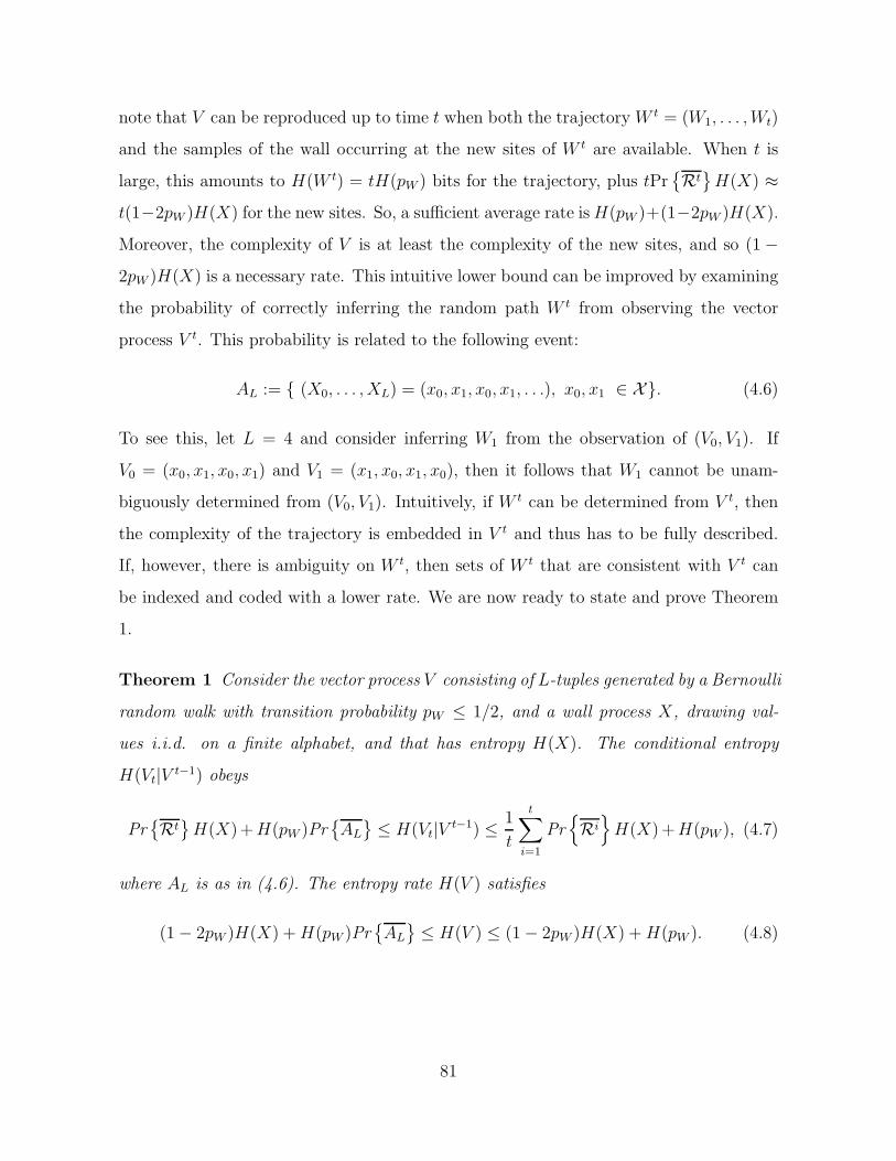
note that V can be reproduced up to time t when both the trajectory W t = (W1, . . . , Wt)

and the samples of the wall occurring at the new sites of W t are available. When t is

large, this amounts to H(W t) = tH(pW ) bits for the trajectory, plus tPr{Rt}

H(X) ≈

t(1−2pW )H(X) for the new sites. So, a sufficient average rate is H(pW )+(1−2pW )H(X).

Moreover, the complexity of V is at least the complexity of the new sites, and so (1 −

2pW )H(X) is a necessary rate. This intuitive lower bound can be improved by examining

the probability of correctly inferring the random path W t from observing the vector

process V t. This probability is related to the following event:

AL := { (X0, . . . , XL) = (x0, x1, x0, x1, . . .), x0, x1 ∈ X}. (4.6)

To see this, let L = 4 and consider inferring W1 from the observation of (V0, V1). If

V0 = (x0, x1, x0, x1) and V1 = (x1, x0, x1, x0), then it follows that W1 cannot be unam-

biguously determined from (V0, V1). Intuitively, if W t can be determined from V t, then

the complexity of the trajectory is embedded in V t and thus has to be fully described.

If, however, there is ambiguity on W t, then sets of W t that are consistent with V t can

be indexed and coded with a lower rate. We are now ready to state and prove Theorem

1.

Theorem 1 Consider the vector process V consisting of L-tuples generated by a Bernoulli

random walk with transition probability pW ≤ 1/2, and a wall process X, drawing val-

ues i.i.d. on a finite alphabet, and that has entropy H(X). The conditional entropy

H(Vt|V t−1) obeys

Pr{Rt}

H(X)+ H(pW )Pr{AL

}≤ H(Vt|V t−1) ≤ 1

t

t∑

i=1

Pr{Ri}

H(X)+ H(pW ), (4.7)

where AL is as in (4.6). The entropy rate H(V ) satisfies

(1 − 2pW )H(X) + H(pW )Pr{AL

}≤ H(V ) ≤ (1 − 2pW )H(X) + H(pW ). (4.8)

81

Proof. For each t we have

H(Vt|V t−1)(a)

≤ 1

t

t∑

i=1

H(Vi|V i−1) =H(V t)

t

(b)

≤ H(V t) + H(W t|V t)

t(4.9)

=H(W t) + H(V t|W t)

t(4.10)

=H(W t) +

∑ti=1 H(Vi|V i−1, W t)

t

(c)= H(pW ) +

1

t

t∑

i=1

H(Vi|V i−1, W i), (4.11)

where (a) follows because H(Vt|V t−1) decreases with t, (b) holds because H(W t|V t) ≥ 0,

and (c) is true because H(W t) = tH(pW ) and (Wi+1, . . . , Wt) is independent of (V i, W i).

Further, it is true that

H(Vi|V i−1, W i = wi, wi is recurrent) = 0.

H(Vi|V i−1, W i = wi, wi is not recurrent) = H(X).

Consequently,

H(Vi|V i−1, W i) =∑

wi∈Ri

Pr{W i = wi

}H(Vi|V i−1, W i = wi)

= Pr{Ri}

H(X). (4.12)

Combining (4.9) and (4.12) gives the upper bound in (4.7). We now turn to the lower

bound. Using the chain rule for mutual information and the information inequality, we

have

H(Vt|V t−1) = H(Vt|V t−1, W t) + I(W t; Vt|V t−1)

= H(Vt|V t−1, W t) + I(W t−1; Vt|V t−1) + I(Wt; Vt|V t−1, W t−1)

≥ H(Vt|V t−1, W t) + I(Wt; Vt|V t−1, W t−1). (4.13)

82

Moreover, because the random walk increment Wt−Wt−1 is independent of (V t−1, W t−1),

it follows that

I(Wt; Vt|V t−1, W t−1) = H(Wt|V t−1, W t−1) − H(Wt|V t, W t−1)

= H(pW ) − H(Wt|V t, W t−1). (4.14)

We proceed by finding an upper bound for H(Wt|V t, W t−1). If (vt, wt−1) is such that Wt

can be inferred with with probability one from (vt, wt−1), then the conditional entropy

is zero. Otherwise, if (vt, wt−1) is such that Wt cannot be inferred with probability one,

then the conditional entropy is at most H(pW ). Thus, denote by At the set of (vt, wt−1)

such that Wt cannot be inferred from (vt, wt−1) with probability one. We have:

H(Wt|V t, W t−1) =∑

(vt,wt−1)

Pr{wt−1,vt

}H(Wt|V t = vt, W t−1 = wt−1

)

≤ H(pW ) Pr{

(wt−1,vt) ∈ At

}.

The event set on the right-hand side above is contained in the event set {Vt−1 =

(x0, x1, . . .), Vt = (x1, x0, . . .)}. By conditioning on (Wt−1, W t), it follows that the prob-

ability of this event is Pr {AL}, where AL is as in (4.6). So the right-hand side above

is upper-bounded by H(pW ) Pr {AL} . Combining this with (4.13 - 4.14) and (4.12), we

assert the lower bound in (4.7). By letting t → ∞ in (4.7) and using Lemma 2 (i) we

obtain (4.8). !

Remark 7 The upper bound of Theorem 1 contains slack. One trivial example is when

the entropy of the process X is 0. In such a case the bound reduces to H(pW ), which is

clearly loose given that the vector process V has zero entropy in this case.

Remark 8 The recurrences of the random walk have the effect of reducing the entropy

of the process. In particular, for a random walk with pW = 1/2, the entropy rate of the

vector process reduces to that of the random walk.

Remark 9 The size of the conditional entropy H(Wt|V t) determines the amount of slack

in the bounds (see (4.9)). Such entropy depends, among other things, on the size of the

alphabet of the process V and on the block length L, as the next example illustrates.

83

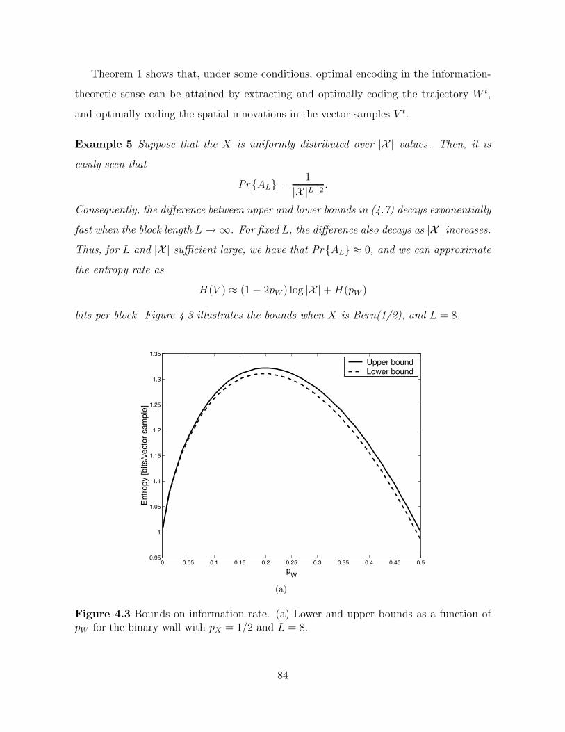
Theorem 1 shows that, under some conditions, optimal encoding in the information-

theoretic sense can be attained by extracting and optimally coding the trajectory W t,

and optimally coding the spatial innovations in the vector samples V t.

Example 5 Suppose that the X is uniformly distributed over |X | values. Then, it is

easily seen that

Pr {AL} =1

|X |L−2.

Consequently, the difference between upper and lower bounds in (4.7) decays exponentially

fast when the block length L → ∞. For fixed L, the difference also decays as |X | increases.

Thus, for L and |X | sufficient large, we have that Pr {AL} ≈ 0, and we can approximate

the entropy rate as

H(V ) ≈ (1 − 2pW ) log |X | + H(pW )

bits per block. Figure 4.3 illustrates the bounds when X is Bern(1/2), and L = 8.

0 0.05 0.1 0.15 0.2 0.25 0.3 0.35 0.4 0.45 0.50.95

1

1.05

1.1

1.15

1.2

1.25

1.3

1.35

pW

Entro

py [b

its/v

ecto

r sam

ple]

Upper boundLower bound

(a)

Figure 4.3 Bounds on information rate. (a) Lower and upper bounds as a function ofpW for the binary wall with pX = 1/2 and L = 8.

84

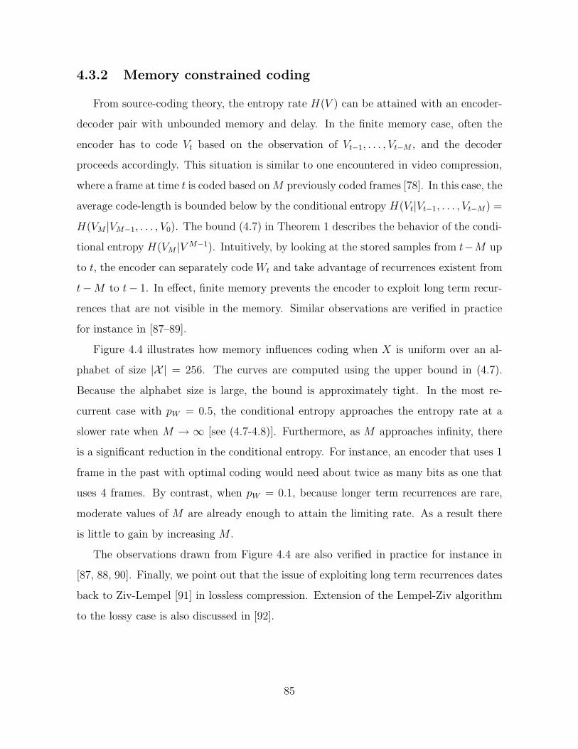
4.3.2 Memory constrained coding

From source-coding theory, the entropy rate H(V ) can be attained with an encoder-

decoder pair with unbounded memory and delay. In the finite memory case, often the

encoder has to code Vt based on the observation of Vt−1, . . . , Vt−M , and the decoder

proceeds accordingly. This situation is similar to one encountered in video compression,

where a frame at time t is coded based on M previously coded frames [78]. In this case, the

average code-length is bounded below by the conditional entropy H(Vt|Vt−1, . . . , Vt−M) =

H(VM |VM−1, . . . , V0). The bound (4.7) in Theorem 1 describes the behavior of the condi-

tional entropy H(VM |V M−1). Intuitively, by looking at the stored samples from t−M up

to t, the encoder can separately code Wt and take advantage of recurrences existent from

t−M to t− 1. In effect, finite memory prevents the encoder to exploit long term recur-

rences that are not visible in the memory. Similar observations are verified in practice

for instance in [87–89].

Figure 4.4 illustrates how memory influences coding when X is uniform over an al-

phabet of size |X | = 256. The curves are computed using the upper bound in (4.7).

Because the alphabet size is large, the bound is approximately tight. In the most re-

current case with pW = 0.5, the conditional entropy approaches the entropy rate at a

slower rate when M → ∞ [see (4.7-4.8)]. Furthermore, as M approaches infinity, there

is a significant reduction in the conditional entropy. For instance, an encoder that uses 1

frame in the past with optimal coding would need about twice as many bits as one that

uses 4 frames. By contrast, when pW = 0.1, because longer term recurrences are rare,

moderate values of M are already enough to attain the limiting rate. As a result there

is little to gain by increasing M .

The observations drawn from Figure 4.4 are also verified in practice for instance in

[87, 88, 90]. Finally, we point out that the issue of exploiting long term recurrences dates

back to Ziv-Lempel [91] in lossless compression. Extension of the Lempel-Ziv algorithm

to the lossy case is also discussed in [92].

85

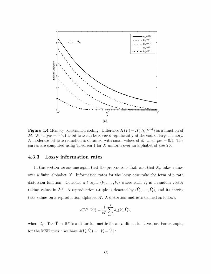
100 101 1020

1

2

3

4

5

6

7

M

Entro

py D

iffer

ence

pW=0.5pW=0.4pW=0.3pW=0.2pW=0.1

HM −H∞

(a)

Figure 4.4 Memory constrained coding. Difference H(V )−H(VM |V M) as a function ofM . When pW = 0.5, the bit rate can be lowered significantly at the cost of large memory.A moderate bit rate reduction is obtained with small values of M when pW = 0.1. Thecurves are computed using Theorem 1 for X uniform over an alphabet of size 256.

4.3.3 Lossy information rates

In this section we assume again that the process X is i.i.d. and that Xn takes values

over a finite alphabet X . Information rates for the lossy case take the form of a rate

distortion function. Consider a t-tuple (V1, . . . , Vt) where each Vj is a random vector

taking values in X L. A reproduction t-tuple is denoted by (V1, . . . , Vt), and its entries

take values on a reproduction alphabet X . A distortion metric is defined as follows:

d(V t, V t) =1

tL

t∑

i=1

ds(Vi, Vi),

where ds : X × X → R+ is a distortion metric for an L-dimensional vector. For example,

for the MSE metric we have d(Vi, Vi) = ‖Vi − Vi‖2.

86

The rate-distortion function for each t, and for given distortion metric, is written as

RV t(D) = infEd(V t,V t)≤D

I(V t; V t)

t, (4.15)

where the infimum of the normalized mutual information I(V t;V t)t is taken over all joint

probability distributions of (V1, . . . , Vt) and (V1, . . . , Vt) such that Ed(V t, V t) ≤ D.

The rate-distortion function for the process V = (V1, V2, . . .) is given by [83]

RV (D) = limt→∞

RV t(D). (4.16)

Because the process V is stationary, it can be shown that the above limit always exists

(see [83, p. 270], or [93]).

By coding the side information W t separately, an upper bound for RV (D) similar to

Theorem 1 can be developed. The upper bound is based on the notion of conditional

rate-distortion [83, 94]. This notion is developed in the lemma below.

Lemma 3 (Gray [94]) Let V be a random vector taking values in X and let W be another

random variable. Define the conditional rate-distortion:

RV |W (D) = infEd(V,V )≤D

I(V ; V |W ), (4.17)

where the infimum is taken over all conditional joint distributions of V and V given W .

The conditional rate-distortion obeys

RV |W (D) ≤ RV (D) ≤ RV |W (D) + I(V ; W ). (4.18)

The conditional rate-distortion of V t conditional on W t is defined as follows:

RV t|W t(D) = infEd(V t,V t)≤D

I(V t; V t|W t)

t, (4.19)

where the infimum is taken over all joint probability distributions of V t and V t conditional

on W t. The conditional rate-distortion can be bounded in terms of the rate-distortion

function of the process X.

87

Proposition 11 The conditional rate-distortion function satisfies

lim supt→∞

RV t|W t(D) ≤ (1 − 2pW )RX(D). (4.20)

Proof. Let λ(wt) denote the number of new sites from the path wt. Then, conditional on

wt, the V t has only λ(wt) entries that need to be encoded. For each (wt, vt), let fwt(vt)

denote the vector with the λ(wt) entries of vt to be coded. Moreover, let V and V be

such that E|Vi[j] − Vi[j]|2 ≤ D for i = 0, . . . , t, and j = 0, . . . , L − 1. We have

I(V t; V t|W t) =∑

wt

Pr{W t = wt

}I(V t; V t|W t = wt)

≥∑

wt

Pr{W t = wt

}I(fwt(V t); fwt(V t)|W t = wt)

≥∑

wt

Pr{W t = wt

}λ(wt)RX(D)

= Eλ(W t)RX(D), (4.21)

where we have used the inequality I(X; Y ) ≥ I(f(X); g(Y )) for measurable functions

f, g [95], and the fact that the process X is i.i.d. and independent of W t, and that the

individual distortions are less than D. The lower bound can be achieved as follows. Let

p∗(X|X) be the test channel that attains RX(D). We let Xn be the result of passing Xn

though the channel p∗(Xn|Xn). For each given wt we construct V t from X and wt. This

results in a joint conditional distribution that attains the lower bound (4.21).

Because the lower bound is attainable, it follows that

RV t|W t(D) ≤ Eλ(W t)

tRX(D).

Moreover, using Lemma 2 it is straightforward to check that t−1Eλ(W t) converges to

(1 − 2pW ), which concludes the proof. !

The above proposition enables us to derive an upper bound for the rate-distortion

function.

88

Theorem 2 Consider the i.i.d. process X such that Xn takes values over a finite alphabet

X . Let RX(D) denote its rate-distortion function. The rate-distortion function of the

process V satisfies

RV (D) ≤ H(pW ) + (1 − 2pW )RX(D). (4.22)

Proof. Using Lemma 3 we have the following bound based on the conditional rate-

distortion function [94]:

RV t|W t(D) ≤ RV t(D) ≤ RV t|W t(D) +1

tI(V t; W t)

≤ RV t|W t(D) + H(pW ).

Letting t → ∞ and using Proposition 11 asserts (4.22). !

Remark 10 Because the alphabet is finite, if the reproduction alphabet X is a superset

of the original alphabet X , then we have that for each t, RV t(D) converges to t−1H(V t)

as D → 0 [83]. Consequently, for large alphabet sizes and large block length, the entropy

rate bound of (4.22) is sharp, and so the above bound on the rate-distortion is also sharp

for small distortion values.

Theorem 2 shows that in the low distortion regime, optimal encoding in the information-

theoretic sense can be attained by extracting and coding W t losslessly, and using the re-

maining bits to optimally code the vector samples corresponding to spatial innovations.

4.4 Information Rates for Dynamic Reality

The model in the previous section assumes a “static background.” More precisely, the

infinite wall process X is drawn at time 0 and does not change after that. In practice,

however, scene background changes with time and a suitable model would have to account

for those changes. New information comes fundamentally in two forms: the first consists

of information that is “seen” by the camera for the first time, while the second consists of

89

changes to old information (e.g., changes in the background). In this section, we propose

a model that accounts for both these sources of new information.

To develop a model for scenes that change over time, we model X as a 2-D random

field indexed by (n, t) ∈ Z × Z+. A simple yet rich model for the field is that of a first

order Markov model over time, and i.i.d. in space. The random field is defined as follows:

Definition 6 The random field is the field RF = {X(t)n : (n, t) ∈ Z × Z+}, such that

(X(0)n : n ∈ Z) is i.i.d. and for each n ∈ Z, the process (X(t)

n : t ∈ Z) is a first order

time-homogeneous Markov process.

The fact that the random field (X(0)n : n ∈ Z) is i.i.d. simplifies calculations con-

siderably. One justification for this model is when the field is Gaussian. In such case,

independence is attained by a simple linear transformation of the process (X(0)n : n ∈ Z).

It can be shown that such transformation preserves the Markovianity on the time dimen-

sion, and the i.i.d. assumption can be justified in this case.

Throughout this section, we assume that the Markov chain of the vector process is

already in steady-state. This assumption is common, for example, in calculating rate-

distortion functions for Gaussian processes with memory [83].

The dynamic vector process V is defined similarly to the static case, but now taking

snapshots or vectors from the random field:

Definition 7 Let RF = {X(t)n : (n, t) ∈ Z × Z+} be a random field, and let W be a

random walk. The dynamic vector process is the process V = (Vt : t ∈ Z+) such that for

each t > 0,

Vt = (X(t)Wt

, X(t)Wt+1, . . . , X

(t)Wt+L−1).

The random field and the corresponding vector process are illustrated in Figure 4.5.

4.4.1 Lossless information rates

In the development that follows we assume, for simplicity, that the random field takes

values on a finite alphabet X . The results can equally be developed for a random field

taking values over R, under suitable technical conditions.

90

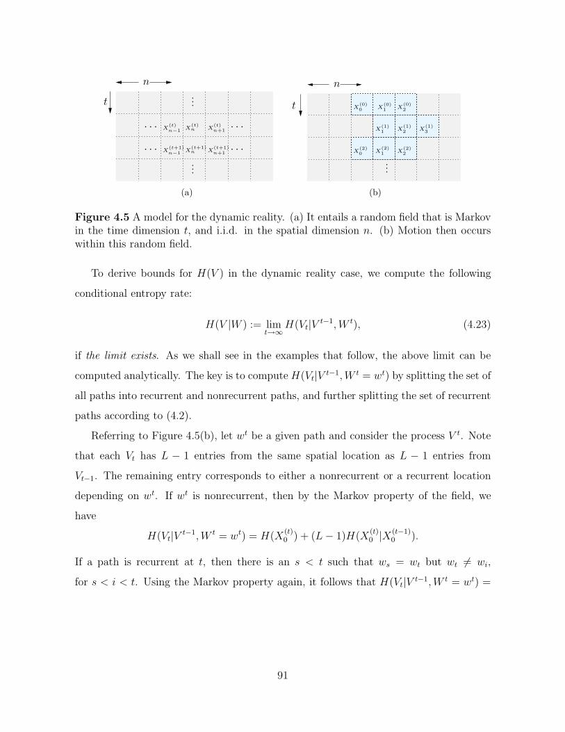
t

n

· · · · · ·

· · · · · ·...

...

X(t)n−1 X

(t)n X

(t)n+1

X(t+1)n−1 X

(t+1)n X

(t+1)n+1

(a)

t

n

...

X(0)0 X

(0)1 X

(0)2

X(1)1 X

(1)2 X

(1)3

X(2)0 X

(2)1 X

(2)2

(b)

Figure 4.5 A model for the dynamic reality. (a) It entails a random field that is Markovin the time dimension t, and i.i.d. in the spatial dimension n. (b) Motion then occurswithin this random field.

To derive bounds for H(V ) in the dynamic reality case, we compute the following

conditional entropy rate:

H(V |W ) := limt→∞

H(Vt|V t−1, W t), (4.23)

if the limit exists. As we shall see in the examples that follow, the above limit can be

computed analytically. The key is to compute H(Vt|V t−1, W t = wt) by splitting the set of

all paths into recurrent and nonrecurrent paths, and further splitting the set of recurrent

paths according to (4.2).

Referring to Figure 4.5(b), let wt be a given path and consider the process V t. Note

that each Vt has L − 1 entries from the same spatial location as L − 1 entries from

Vt−1. The remaining entry corresponds to either a nonrecurrent or a recurrent location

depending on wt. If wt is nonrecurrent, then by the Markov property of the field, we

have

H(Vt|V t−1, W t = wt) = H(X(t)0 ) + (L − 1)H(X(t)

0 |X(t−1)0 ).

If a path is recurrent at t, then there is an s < t such that ws = wt but wt *= wi,

for s < i < t. Using the Markov property again, it follows that H(Vt|V t−1, W t = wt) =

91

H(X(t)0 |X(s)

0 )+(L−1)H(X(t)0 |X(t−1)

0 ). The above argument is explicitly written as follows:

H(Vt|V t−1, W t) =∑

wt∈Rt

H(Vt|V t−1, W t = wt)Pr{W t = wt

}

+∑

wt∈Rt

H(Vt|V t−1, W t = wt)Pr{W t = wt

}

=(H(X(t)

0 ) + (L − 1)H(X(t)0 |X(t−1)

0 ))

Pr{Rt}

+

(t/2)∑

i=1

∑

wt∈T tt−2i

H(Vt|V t−1, W t = wt)Pr{W t = wt

}

=(H(X(t)

0 ) + (L − 1)H(X(t)0 |X(t−1)

0 ))

Pr{Rt}

+(t/2)∑

i=1

[(H(X(t)

0 |X(t−2i)0 ) + (L − 1)H(X(t)

0 |X(t−1)0 )

)Pr

{T t

t−2i

}

= (L − 1)H(X(t)0 |X(t−1)

0 ) + H(X(t)0 )Pr

{Rt}

+(t/2)∑

i=1

H(X(2i)0 |X(0)

0 )Pr{T 2i

0

}.

By letting t → ∞ using Lemma 2 (i) leads to

H(V |W ) = H(X(∞)0 )(1−2pW )+(L−1)H(X(1)

0 |X(0)0 )+

∞∑

i=1

H(X(i)0 |X(0)

0 )Pr{T i}

, (4.24)

where Pr {T i} is the probability of return given in Lemma 2 (ii). The infinite sum in the

left-hand side of (4.24) is well-defined. It is an infinite sum of positive numbers, and it

is bounded above by H(X(∞)0 )

∑∞i=1 Pr {T i} = H(X(∞))2pW .

With the conditional entropy rate in (4.24) we can derive lower and upper bounds

on the entropy rate H(V ). To derive an upper bound, we bound H(V t)t for each t and

let t → ∞. For the lower bound, similar to Section 4.3, we bound H(Vt|V t−1) below.

Because the alphabet X is finite and the process is stationary, the limits of H(V t)t and

H(Vt|V t−1) as t → ∞ coincide.

The upper bound is obtained from the inequality H(V t) ≤ tH(pW )+H(V t|W t). Note

that H(V t|W t) =∑t

i=1 H(Vi|V i−1, W t), so that if H(Vi|V i−1, W t) converges to a limit

as t → ∞, we have necessarily that t−1H(V t|W t) converges to the same limit (see e.g.,

92

[86, p. 64]). So,

limt→∞

H(V t)

t≤ H(pW ) + lim

t→∞

H(V t|W t)

t

= H(pW ) + limt→∞

H(Vt|V t−1, W t)︸ ︷︷ ︸

H(V |W )

.

To derive a lower bound, note that the development leading to (4.13-4.14) for the

static case also holds for the dynamic case. So, we have

H(V t|V t−1) ≥ H(pW ) + H(Vt|V t−1, W t) − H(Wt|V t, W t−1). (4.25)

Thus, a lower bound is obtained by finding an upper bound for H(Wt|W t−1, V t). Be-

cause the process X changes at each time step, we cannot use the event AL to obtain

an upper bound for H(Wt|W t−1, V t) as in the static case. A useful upper bound for

H(Wt|W t−1, V t) is obtained by using Fano’s inequality. Let Pe denote the probability of

error in estimating Wt based on observing Yt := (Vt, Vt−1, Wt−1), i.e.,

Pe = Pr{

W (Yt) *= Wt

},

where W (·) is a given estimator assumed to be the same for all t. Since Wt−1 is observed,

estimating Wt amounts to estimating the increment Nt = Wt − Wt−1. Because V is

stationary and Nt is i.i.d., it follows that Pe does not depend on t. From Fano’s inequality,

we have that

H(Wt|V t, W t−1) ≤ H(Nt|Yt)

≤ H(Pe) + Pe log2(1)

= H(Pe). (4.26)

Consequently, a lower bound is obtained by combining (4.25) with (4.26) above.1 By

letting t → ∞ we arrive at the following:

Theorem 3 Consider the vector process V consisting of L-tuples generated by a Bernoulli

random walk with transition probability pW with pW ≤ 1/2, and the random field RF =

1Sharper lower bounds can be obtained by estimating Nt using (V t, W t−1). However, the estimateusing Yt is easily computed and already leads to a sharp enough bound.

93

{X(t)n : (n, t) ∈ Z × Z+} that is i.i.d. on the n dimension and first-order Markov on the

t dimension. The entropy rate of the process V obeys

H(pW ) + H(V |W ) − H(Pe) ≤ H(V ) ≤ H(pW ) + H(V |W ), (4.27)

where H(V |W ) is as in (4.24), and Pe is the probability of error in estimating W1 based

on the observation of Y1 = (V1, V0, W0) with any estimator W (Y1).

The lower and upper bounds become sharp when Pe → 0. This occurs with large block

sizes and for small changes in the background. The examples that follow illustrate the

sharpness of the above bounds. In the first example, we consider a binary process X,

and on the second a Gaussian process with AR(1) temporal innovations.B

SC

BSC

BSC

. . .

. . . . . .

. . .

. . .. . .

...

...

X(t)n−1 X

(t)n X

(t)n+1

X(t+1)n−1 X

(t+1)n X

(t+1)n+1

Figure 4.6 The binary random field. Innovations are in the form of bit flips caused bybinary symmetric channels between consecutive time instants.

Example 6 BSC innovations

Suppose that at t = 0, the process is a strip of bits that are i.i.d. Bernoulli with initial

distribution pX. Suppose that from t to t + 1 there is a nonzero probability pI that the

bit X(t)n is flipped. This amounts to a binary symmetric channel (BSC) between X(t)

n

and X(t+1)n , as illustrated in Figure 4.6. The t BSCs in series between X(0)

n and X(t)n are

equivalent to a single BSC with transition probability (see [86, p. 221], problem 8)

pI,t = 0.5(1 − (1 − 2pI)

t). (4.28)

94

Note that for pI > 0, we have that limt→∞ pI,t = 0.5. So, for each n, the distribution of

X(t)n converges to the stationary distribution Bern(0.5). Substituting in (4.24) gives for

pI > 0:

H(V |W ) = H(1

2)(1 − 2pW ) + (L − 1)H(pI) +

∞∑

i=1

H(pI,2i)Pr{T 2i

0

}. (4.29)

Notice that when pI = 0 we recover the static case. By using the above in (4.27) we obtain

the corresponding bounds. Figure 4.7 (a) illustrates the lower and upper bounds for L = 8

and pX = 0.5. We compute the bounds using (4.24) and (4.27), where we truncate the

infinite sum in (4.24) at a very large t. The probability Pe is computed through Monte

Carlo simulation using a simple Hamming distance detector. The bounds are surprisingly

robust in this case, and provide good approximation of the true entropy rate. Notice that

when pI increases, the entropy rate of the recurrent case (pW = 0.5) crosses that of the

panning case (pW = 0.05). This is because in the recurrent case a greater amount of bits

is spent coding the innovations.

Figure 4.7 (b) shows the contour plots of the upper bound for various pairs (pI , pW ).

The plot shows how the two innovations are combined to generate a given entropy value.

Notice that when pW approaches 12 , the entropy of the trajectory becomes significant and

it compensates for the lesser amount of spatial innovation.

To measure the effect of memory in the dynamic case, we evaluate the upper bound on

the conditional entropy rate (as in (4.11)), and the upper bound on the true entropy rate

given by (3). Figure 4.8 illustrates the difference between the conditional entropy upper

bound and the true entropy upper bound. The curves are similar to the ones obtained in

the static case with spatial innovation (Figure 4.4), and confirm the very intuitive fact

that memory is less useful when the scene around changes rapidly.

Example 7 AR(1) Innovations.

Although the development leading to Theorem 3 was made for finite alphabets, the

same calculation can be done for a random field taking values on R, provided it has abso-

lutely continuous joint densities. In this case, the entropies involved become differential

95

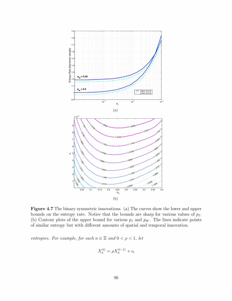
10−4 10−3 10−20.9

1

1.1

1.2

1.3

1.4

1.5

1.6

1.7

1.8

1.9

pI

Entro

py R

ate

[bits

/vec

tor s

ampl

e]

Upper boundLower bound

pW = 0.05

pW = 0.5

(a)

0.05 0.1 0.15 0.2 0.25 0.3 0.35 0.4 0.45 0.5

1

2

3

4

5

6

7

8

9

x 10−3

pW

p I

1.1509

1.2252

1.2252

1.2995

1.2995

1.2995

1.3737

1.37371.3737

1.3737

1.448

1.4481.448

1.448

1.5223

1.52231.5223

1.52231.5965

1.5965 1.5965

1.59651.6708

1.6708 1.6708

1.6708

1.7451

1.7451 1.7451

1.7451

1.81941.8194

1.8194

1.8936 1.8936

1.1509

(b)

Figure 4.7 The binary symmetric innovations. (a) The curves show the lower and upperbounds on the entropy rate. Notice that the bounds are sharp for various values of pI .(b) Contour plots of the upper bound for various pI and pW . The lines indicate pointsof similar entropy but with different amounts of spatial and temporal innovation.

entropies. For example, for each n ∈ Z and 0 < ρ < 1, let

X(t)n = ρX(t−1)

n + εt

96

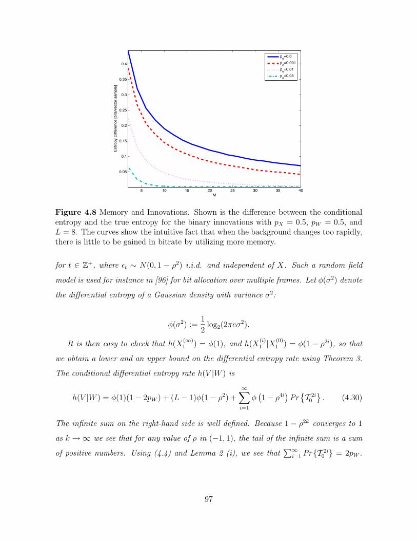
5 10 15 20 25 30 35 40

0.05

0.1

0.15

0.2

0.25

0.3

0.35

0.4

M

Entro

py D

iffer

ence

[bits

/vec

tor s

ampl

e]

pe=0.0pe=0.001pe=0.01pe=0.05

Figure 4.8 Memory and Innovations. Shown is the difference between the conditionalentropy and the true entropy for the binary innovations with pX = 0.5, pW = 0.5, andL = 8. The curves show the intuitive fact that when the background changes too rapidly,there is little to be gained in bitrate by utilizing more memory.

for t ∈ Z+, where εt ∼ N(0, 1 − ρ2) i.i.d. and independent of X. Such a random field

model is used for instance in [96] for bit allocation over multiple frames. Let φ(σ2) denote

the differential entropy of a Gaussian density with variance σ2:

φ(σ2) :=1

2log2(2πeσ

2).

It is then easy to check that h(X(∞)1 ) = φ(1), and h(X(i)

1 |X(0)1 ) = φ(1 − ρ2i), so that

we obtain a lower and an upper bound on the differential entropy rate using Theorem 3.

The conditional differential entropy rate h(V |W ) is

h(V |W ) = φ(1)(1 − 2pW ) + (L − 1)φ(1 − ρ2) +∞∑

i=1

φ(1 − ρ4i

)Pr

{T 2i

0

}. (4.30)

The infinite sum on the right-hand side is well defined. Because 1 − ρ2k converges to 1

as k → ∞ we see that for any value of ρ in (−1, 1), the tail of the infinite sum is a sum

of positive numbers. Using (4.4) and Lemma 2 (i), we see that∑∞

i=1 Pr {T 2i0 } = 2pW .

97

Because φ(·) is concave, we can use Jensen’s inequality as follows:

∞∑

k=1

φ(1 − ρ4k)Pr{T 2k

0

}= 2pW

∞∑

k=1

φ(1 − ρ4k)Pr

{T 2k

0

}

2pW

≤ 2pWφ

(∞∑

k=1

(1 − ρ4k)Pr

{T 2k

0

}

2pW

)

.

Using Lemma 2 (ii) and the generating function for the Catalan numbers [97], one

can further check that

∞∑

k=1

(1 − ρ4k)Pr{T 2k

0

}= ((1 − 4(1 − pW )pWρ

4))1/2 − (1 − 2pW ),

so that the last term is controlled by

∞∑

k=1

φ(1 − ρ4k)Pr{T 2k

0

}≤ 2pWφ

((1 − 4(1 − pW )pWρ4)1/2 − (1 − 2pW )

2pW

). (4.31)

The above upper bound turns out to be a very good approximation of the infinite sum in

(4.30) when pW is close to 0, and when ρ is away from 1.

Notice that for L large and ρ close to 1, Pe and H(Pe) are small so that the bounds

in Theorem 3 are sharp. Figure 4.9 displays the bounds on the differential entropy as

a function of ρ. The bounds are computed following Theorem 3 and (4.30). Here Pe

is inferred via Monte Carlo simulation with 107 trials, and a minimum MSE detector

for Wt. The inferred Pe is so low that the lower and upper bounds practically coincide.

Analytical computation of Pe is a detection problem beyond the scope of this dissertation.

4.4.2 Lossy information rates for the AR(1) random field

Consider the AR(1) innovations of the previous example. Under the MSE distortion

metric it is possible to derive an upper bound to the lossy information rate. The key is

to compute RV t|W t(D) defined as in (4.19) and use the upper bound [94]:

RV t(D) ≤ H(pW ) + RV t|W t(D), (4.32)

98

10−3 10−2 10−1−20

−15

−10

−5

0

5

10

1−ρ2

Diff.

Ent

ropy

Rat

e [b

its/v

ecto

r sam

ple]

Upper Bound

Lower Bound

pW=0.05

pW=0.5

Figure 4.9 Differential entropy bounds for the Gaussian AR(1) case as function of theinnovation parameter ρ. In this example Pe is small enough that the lower and upperbounds practically coincide. Note that the slope of the differential entropy curve isinfluenced by the value of pW .

for each t > 0. The conditional rate-distortion satisfies the Shannon lower bound (SLB)

[83]:

RV t|W t(D) ≥ h(V t|W t)

t− Lφ(D). (4.33)

The key observation is that for a given fixed trajectory wt, the rate-distortion function

of V t is that of a Gaussian vector consisting of the samples of the random field covered

by W t. For a Gaussian vector, the SLB is tight when the per sample distortion is less

than the minimum eigenvalue of the covariance matrix (see [83, p. 111]). The next

proposition gives a condition under which (4.33) is tight, and thus when combined with

(4.32) provides an upper bound on the rate-distortion function.

Proposition 12 Consider the vector process V resulting from the Gaussian AR(1) ran-

dom field with correlation coefficient 0 < ρ < 1, and a Bernoulli random walk with prob-

ability pW ≤ 1/2. The Shannon lower bound for the conditional rate-distortion function

is tight whenever the distortion satisfies

0 < D <1 − ρ1 + ρ

. (4.34)

99

Proof. To assert the claim we rely on the following lemmas:

Lemma 4 Let X1, X2, . . . , Xm be a sequence of Gaussian vectors in Rd such that Xj ∼

N(0, Cj), and where each Cj has spectrum λ(Cj). Let W be a random variable indepen-

dent of X1, . . . , Xm such that Pr {W = j} = µj for j = 1, . . . , m. Consider the mixture

X =m∑

j=1

I{W=j}Xj.

Denote by RX|W (D) the conditional rate-distortion with per-sample MSE distortion D.

Then, if

D ≤ minm⋃

j=1

λ(Cj),

the conditional rate distortion function is

RX|W (D) =m∑

j=1

µjRXj(D).

Proof. Let p(X, X|W ) be such that d−1 E‖X − X‖2 ≤ D. Then,

I(X; X|W ) =m∑

j=1

µjI(X; X|W = j) (4.35)

≥m∑

j=1

µjRXj(Dj) (4.36)

with

d−1E‖X − X‖2 =

m∑

j=1

µjDj ≤ D,

and Dj := d−1 E(‖X − X‖2|W = j). The above is minimized when

R′Xj

(Dj) = θ,

where θ is some constant. Suppose D ≤ min⋃m

j=1 λ(Cj) and Dj = D. We have

RXj(Dj) =

1

d

d∑

p=1

1

2log2(

λj,p

D),

100

where λj,p are the eigenvalues of Cj and moreover R′Xj

(Dj) = −1/D so that conditions

for a minimum are satisfied. The lower bound can be attained by setting

p(X, X|W = j) = p∗j(X, X),

where p∗j(Xj , Xj) attains RXj(Dj). !

Lemma 5 ([98, p. 189]) Let A be a n×n Hemitian matrix, and let 1 ≤ m ≤ n. Let Am

denote a principal submatrix of A, obtained by deleting n−m rows and the corresponding

columns of A. Then, for each integer k such that 1 ≤ k ≤ m, we have

λk(A) ≤ λk(Ak), (4.37)

where λk(A) denotes the k-th largest eigenvalue of matrix A.

Proof of Proposition 12: The SLB for each t > 0 is given by

RV t|W t(D) ≥ h(V t|W t)

t− Lφ(D). (4.38)

Because

I(V t; V t|W t) =∑

W t=wt

Pr{W t = wt

}I(V t; V t|W t = wt),

in view of Lemma 4, it suffices to show that for each t > 0, and for 0 ≤ D ≤ 1−ρ1+ρ , the

boundI(V t; V t|wt)

t≥ h(V t|wt)

t− Lφ(D), for E(d(V t, V t)|wt) ≤ D

is achievable. Given W t = wt, the above bound is attainable if D is smaller than the

minimum eigenvalue of the covariance matrix of the random field samples covered by wt.

Denote this covariance by Cwt := Cov(V t|wt). Because the random field is independent

in the spatial dimension n, the spectrum of the covariance matrix is the disjoint union

of the spectra of the covariance matrices corresponding to the random field samples of

V t at similar location n. Each Cwt is a submatrix of the t× t Toeplitz matrix Tt(ρ) with

101

entries [Tt(ρ)]ij = ρ|i−j|. Since λmin(Tt(ρ)) decreases to (1 − ρ)/(1 + ρ) as t → ∞ [99],

by applying the Lemma above we conclude that

λmin(Cwt) ≥ λmin(Tt(ρ)) ≥1 − ρ1 + ρ

. (4.39)

Therefore, the bound (4.38) is achievable for each t and since the limit of RV t|W t(D)

exists it follows that the bound is achievable for t → ∞. !

Example 8 We simulate the AR(1) dynamic reality model. To compress the process

V t, we estimate the trajectory and send it as side information. With the trajectory at

hand, we encode the samples with DPCM, encoding the residual with entropy constrained

scalar quantization (ECSQ). We build two encoders. In the first one, prediction is done

utilizing only the previously encoded vector sample; in the second, all encoded samples

up to time t are available to the encoder (and decoder). Figure 4.10 illustrates the SNR

as a function of rate when the block-length L = 8. In Figure 4.10 (a) and (b) we have

ρ = 0.99 and the upper bound is valid for SNR greater than 23 dB. In Figure 4.10 (a),

we have pW = 0.5. Because the scene changes slowly and is highly recurrent, the infinite

memory encoder (M = ∞) is about 3.5 dB better than when M = 1. The same behavior

is not observed when the scene is not recurrent (panning case, pW = 0.1, Figure 4.10 (b)

), and when the background changes too rapidly (ρ = 0.9, Figure 4.10 (c)).

4.5 The Recording Reality Case

In some applications, not only the samples of the POF are available, but also the loca-

tion of those samples. Consider the vector process in Definition 3, where X is stationary

taking values on a finite alphabet. Suppose that the position information is available.

In this case, the encoder has access to (Vt, Wt) for each t. In such scenario, usually the

goal is not to reproduce (Vt, Wt) at the decoder, but rather to reconstruct the underlying

scene X. This coding problem is the one encountered for example in the compression of

lightfields (see e.g., [100]).

102

1 1.5 2 2.5 3 3.5 4 4.5 5

10

15

20

25

30

35

40

45

50

Rate [bits/sample]

SNR

[dB]

RUB(D), pW = 0.5, ρ = 0.99 , L=6DPCM & ECSQ, M=∞DPCM & ECSQ, M=1

(a)

1 1.5 2 2.5 3 3.5 4 4.5 5

10

15

20

25

30

35

40

45

50

Rate [bits/sample]

SNR

[dB]

RUB(D), pW = 0.1, ρ = 0.99 , L=6DPCM & ECSQ, M=∞DPCM & ECSQ, M=1

(b)

1 1.5 2 2.5 3 3.5 4 4.5 5

10

15

20

25

30

35

40

Rate [bits/sample]

SNR

[dB]

RUB(D), pW = 0.5, ρ = 0.9 , L=6DPCM & ECSQ, M=∞DPCM & ECSQ, M=1

(c)

Figure 4.10 Performance of DPCM with motion for various ρ and pW . For ρ = 0.99 andρ = 0.9 the upper bound is valid for SNR greater than 23 dB and 12.8 dB, respectively.(a) Memory provide considerable gains, pW = 0.5, ρ = 0.99. (b) Modest gains whenpW = 0.1. (c) Modest gains when ρ = 0.9, as background changes too rapidly.

Because the scene is assumed to be static, only the positions corresponding to new

states need to be transmitted. These states correspond to new visual information being

“seen” by a camera for the first time. It is thus natural to define the sequence of times

that the camera moves into a new location:2

t0 = 0

tj = min{t > tj−1 : Wt *= Wi, 0 ≤ i < tj−1}, for j > 0.

2In probability theory parlance, those are in fact stopping times for the standard filtration generatedby W .

103

The above sequence of stopping times enables us to define the corresponding process of

interest:

Z =(

Zj := (Vtj , Wtj) : j ∈ Z+). (4.40)

The process Z is the subvector process consisting of the samples that contain new spatial

information. We seek to characterize the entropy rate of Z, defined as

H(Z) = limj→∞

1

jH(Z0, Z1, . . . , Zj).

We show next that despite the randomness of the trajectory W , the entropy rate of

the process Z is that of the underlying process X. That is, even in the worst case of a

random trajectory, there is no increase in the entropy rate due to random camera motion.

Theorem 4 Consider the vector process V where the process X is stationary and takes

values on a finite alphabet X . Let Z =(

Zj := (Vtj , Wtj ) : j ∈ Z+), and denote by H(X)

the entropy rate of the process X. Then,

H(Z) = H(X).

Proof.

Denote Wj = Wtj and Vj = Vtj . Assume without loss of generality that V0 is known

to the decoder. Then, for each j,

H(Zj) = H(W j) + H(V j|W j) (4.41)

= H(W j) + H(X1, . . . , Xj). (4.42)

The last equality holds because conditional on W j , each entry of V j contains a single

new sample of X. So, it suffices to assert that

limj→∞

1

jH(W0, . . . , Wj) = 0.

Let Nj = Wj−1−Wj and denote Nj = Ntj . Then, there is a one-to-one correspondence

between W j and N j so that

H(W0, . . . , Wj) = H(N0, . . . , Nj).

104

To check that j−1 H(N0, . . . , Nj) converges to 0, it suffices to show that H(Nj|N j−10 ) =

H(Nj|Nj−1) converges to zero (see [86, p. 64]). This conditional entropy in turn depends

on the transitional probability Pr{Nj |Nj−1

}. The transition probabilities are similar

to the ones in the Gambler’s ruin calculation done for example in [85]. This gives for

pW < 1/2,

Pr{Nj = −1|Nj−1 = 1

}=αj − αj+1

1 − αj+1, and Pr

{Nj = 1|Nj−1 = −1

}=α−j − α−j−1

1 − α−j−1,

where α := pW

1−pW. For pW = 1/2, then

Pr{

Nj = −1|Nj−1 = 1}

= Pr{Nj = 1|Nj−1 = −1

}=

1

j + 1.

So, for 0 ≤ pW ≤ 1/2, both transition probabilities converge to zero when j goes

to infinity, and by continuity, we have that limj→∞ H(Nj|Nj−1) = 0, which asserts the

claim. !

Remark 11 Note that if the trajectory W is deterministic, then the result is obvious.

What Theorem 4 shows is that the same holds even in the case where the trajectory is

random.

Remark 12 The result is also very similar to the rate-distortion problem for remote

sources considered in [83]. In this case the random walk can be seen as a channel between

the wall and the encoder. However, the results in [83] deal with memoryless channels

only and thus are not directly applicable to the problem at hand.

To optimally code a random camera taking samples of the plenoptic function, one

needs an average rate of H(X) bits. Suppose that there is a code for X that attains the

entropy rate H(X). Then, to attain the entropy of Z, a code for the positions W that

has a zero rate on average is required. In the next section we propose a code for the

increments Nj with corresponding average code length that essentially attains the zero

entropy lower bound.

105

4.5.1 A possible code: Shannon + run-length

A code that essentially achieves the entropy rate for the process N is constructed.

For simplicity, we assume that pW = 1/2. The results for pW < 1/2 are analogous.

The process N is a time-varying first-order Markov process and its entropy rate is zero.

Notice that the Lempel-Ziv code is not necessarily optimal as the source is not stationary.

Our proposal uses a run-length code. In this case, we buffer the runs of equal symbols

(“left” or “right” corresponding to −1 or +1). The runs are then coded according to their

probability. Thus we can describe the code as follows: suppose J samples have already

been coded. Thus, we start buffering the samples NJ , NJ+1, etc., until NJ+r *= NJ .

Denote by C the random variable describing the next run of samples. Code C with a

Shannon code [86]. Thus, if C = c its codeword length is

lJ(c) = 6− log PJ(c)7.

From the Gambler’s ruin calculation, the probability of C samples in the next run,

given that J increments Nj where already coded, is

PJ(C) = P (NJ+C−1 *= NJ+C−2)J+C−2∏

j=J

P (Nj = Nj−1)

=1

J + C

C−2∏

j=0

J + j

J + j + 1

=1

J + C

J

J + C − 1. (4.43)

We will show this code has average bits per sample converging to zero as J grows

large. To prove this result, we need the following lemma:

Lemma 6 The function f(x) = log(x)/x is strictly decreasing for x > e.

Proof. Note that f ′(x) = (1 − log x)/x2 so that f ′(x) < 0 for x > e. !

This simple lemma is crucial in the proof of the next proposition.

106

Proposition 13 Consider the run-length-Shannon code for the increments Nj. Then

the average number of bits per run given that J increments have been coded goes to zero

as J → ∞ at a rate of O ((log J)2/J).

Proof. Denote the length in bits of a coded run of length C when J bits have been

coded by lJ(C). Then, using Lemma 6 we have

0 ≤ E

[lJ(C)

C

]≤ E

[1 + log 1/PJ(C)

C

]

=∑

C≥1

PJ(C) (1 + log(1/PJ(C)))

C

=∑

C≥1

1

C

J

(J + C)(J + C − 1)

(1 + log

(J + C)(J + C − 1)

J

)

≤∑

C≥1

1

C

J

(J + C − 1)2

(1 + log

(J + C − 1)2

J

)

=∑

C≥1

1

C

J

(J + C − 1)2

(1 + log J + 2 log

(J + C − 1)

J

)

=∑

C≥1

1

C

(J + J log J)

(J + C − 1)2+

2

CJ

log J+C−1J

(J + C − 1)2.

Now we prove that each of the terms in the right hand side converges to zero. The

first one gives

∑

C≥1

1

C

(J + J log J)

(J + C − 1)2= (J + J log J)

(1

J2+∑

C>1

1

C

1

(J + C − 1)2

)

≤ (J + J log J)

(1

J2+

∫

C≥1

1

C

1

(J + C − 1)2dC

)

= (J + J log J)

(1

J2+

1 − J + J log J

J(J − 1)2

),

where we have used the fact that the term in the summand is decreasing in C. The

majoring term goes to zero essentially as O((logJ)2J−1). For the second term we use

the inequality logx ≤ x − 1 for x > 0. This gives

107

∑

C≥1

2

CJ

log J+C−1J

(J + C − 1)2≤

∑

C≥1

2

C

C − 1

(J + C − 1)2

≤∫

C>1

2

C

C − 1

(J + C − 1)2dC

= 2J − 1 − log J

(J − 1)2,

which goes to zero as ∼ 1/J . Thus, we conclude that E

[lJ (C)

C

]goes to zero at least as

fast as O((log J)2J−1) !

4.5.2 Coding with a finite buffer

The code suggested in the previous section actually requires unbounded buffer sizes

(the runs can have arbitrarily large length). However, one may still get some bounds on

the average bits spent. Suppose we impose a limit on the complexity. That is, we let the

runs be no larger than some maximum value denoted by K. Then, the probability mass

function of the runs now is given by

P KJ (C) =

1

J + C

J

J + C − 1I{1≤C<K} +

J

J + KI{C≥K}. (4.44)

Following the previous development we can assign a Shannon “run-length” code based

on the above probabilities. Thus, when C ≥ K, we assign a run of size K with codeword

length according to its probability. A result similar to Proposition 13 can easily be

derived.

Proposition 14 Consider the Shannon run-length code with the runs bounded by K.

Then the average bit rate on the next run given that J bits have already been coded,

denoted by E

[lKJ (C)

C

], converges to 1/K as J → ∞.

Proof. Note that

E

[lKJ (C)

C

]≤

K∑

C=1

1 − log P KJ (C)

CP K

J (C) +J(1 − log J

J+K

)

K(J + K). (4.45)

108

The first term on the RHS converges to zero. To check that, we consider the maximum

inside the summand. We thus get:

K∑

C=1

1 − log P KJ (C)

CP K

J (C) ≤ KP KJ (1) − K

log P KJ (K)

KP K

J (K). (4.46)

Since for each K, P KJ (K) → 0 as J → ∞, and since x log x → 0 as x → 0, it

follows that the above converges to zero as fast as log J/J . Now, the second term clearly

converges to 1/K. Hence we conclude that

lim supJ→∞

E

[lKJ (C)

C

]≤ 1

K.

To get a lower bound, notice that when J is large, then 1/P KJ (K) approximates 1

from above, so that in turn log 1/P KJ (K) approximates 0 from above. Consequently, we

have that 6log 1/P KJ (K)7 = 1 for J large enough. Thus,

E

[lKJ (C)

C

]≥

K∑

C=1

−1 − log P KJ (C)

CP K

J (C) +J

K(J + K). (4.47)

The first term in the RHS goes to zero. To see that, consider the minimum inside the

summand. The second term in the RHS converges to 1/K. This leads to

1

K≤ lim inf

J→∞E

[lKJ (C)

C

]≤ lim sup

J→∞E

[lKJ (C)

C

]≤ 1

K,

which proves the proposition. !

The above proposition suggests that with sufficient memory, the proposed code can

be very close to the average length of the case where the complexity is not bounded.

We verify the results of Propositions 13 and 14 by simulating the Shannon code for

the run-lengths of new states with computer generated random walks. Thus we apply

our proposed code to several sample paths and average out the results. As Figure 4.11

indicates, in the case where the code has infinite resources, then the coded runs can be

arbitrarily large and consequently the average rate converges to zero, as Proposition 13

109

suggests. In the case where we limit the buffer size to K, the simulation shows the rate

converges to 1/K’, as predicted by Proposition 14.

101 102 103 1040

0.1

0.2

0.3

0.4

0.5

0.6

0.7

j

Aver

age

Rate

K=3K=5K=10K=50K=∞

Figure 4.11 The proposed code for the trajectory. The proposed code with buffer sizeK attains an entropy rate of roughly 1/K. Notice that when K is infinity, the codeattains the entropy rate bound as the number of samples j goes to infinity.

4.6 Conclusion

We have proposed a stochastic model for video that enables the precise computation

of information rates. For the static case, we provided lossless and lossy information rate

bounds that are tight in a number of interesting cases. In some scenarios, the theoretical

results support the ubiquitous hybrid coding paradigm of extracting motion and coding

a motion compensated sequence.

110

We extended the model to account for changes in the background scene, and com-

puted bounds for the lossless and lossy information rates for the particular case of AR(1)

innovations. The bounds for this “dynamic reality” are tight in some scenarios, namely

when the background scene changes slowly with time (i.e., ρ close to 1).

The model explains precisely how long-term motion prediction helps coding in both

static and dynamic cases. In the dynamic model, this is related to the two parameters

(pW , ρ) that symbolizes the rate of recurrence in motion and the rate of changes in

the scene. As (pW , ρ) → (0.5, 1), long term memory predictions result in significant

improvements (in excess of 3.5 dB). By contrast, if either ρ is away from 1, or if pW is

away from 0.5, long term memory brings very little improvement.

Although we developed the results for the Bernoulli random walk, the model can

be generalized to other random walks on Z and Z2. Our current work includes such

generalizations. It also includes estimating ρ and pW for real video signals and fitting

the model to such signals.

We have shown that the entropy of the POF in problems such as the light field reduces

to the entropy of the scene around it. To assert this, we have used a random walk model

and we have shown that the trajectory of the random walk eventually has zero entropy

rate. For the simple example of a 1-D camera and a Bernoulli random walk, we have

shown a simple code that attains the entropy bound.

111

CHAPTER 5

CONCLUSION AND FUTURE DIRECTIONS

5.1 Summary

In the introduction we emphasized that efficient representation of visual information

requires a good understanding and handling of geometrical structure. This is the case in

static images, as well as in motion pictures. We have examined several problems related

to geometrical visual representation, processing, and coding. In particular, the following

was accomplished:

• Digital multidimensional filters with directional vanishing moments were proposed,

and a new filter bank design criteria suitable for multidimensional expansion was

developed. This novel class of filters have the property of annihilating directional

edges in images. The associated filter design problem was studied and characterized.

A flexible design methodology was presented. Applications of the proposed filter

banks in the context of the contourlet transform have shown that the proposed

filters yield reconstructed images with fewer ringing artifacts and thus better visual

quality. Moreover, the proposed filters are shorter and less complex than those of

competing designs.

• The nonsubsampled contourlet transform was proposed. This transform is suit-

able for applications that can afford redundancy and complexity such as denoising,

enhancement, and curvature detection. The proposed construction was studied in

detail and a frame analysis was provided. A design method that allows for regular-

112

ity, as well as frame stability control and sharp frequency resolution, was proposed.

Our design not only ensures the regularity of the basis vectors, but it also ensures

the almost tightness of the associated frame operator, and it has a fast algorithm

that results in substantial computational savings. The proposed transform is shown

to outperform similar transforms such as curvelets and the undecimated wavelet

transform in image denoising via hard-thresholding. Moreover, when coupled with

a fairly simple denoising strategy based on soft-thresholding, the resulting denoising

algorithm performed similar to the more sophisticated denoising scheme of [60].

• A stochastic model to study the information rates of the plenoptic function was

proposed. In the two cases considered, namely that of video and that of light

field, information rates were derived. In the video case, the simplicity of the model

enabled us to compute precise information rates. To the best of our knowledge, ours

is the first model for video that attempts to compute the true information-theoretic

rate-distortion rather than the optimal rate-distortion performance of a particular

coding method. We proposed models for static and dynamic realities and computed

information rates for both models. The proposed methodology gives new insight

into the source coding problem associated with video. In particular, the model

provides a characterization of performance in the presence of long-term memory,

and it also supports the hybrid coding paradigm of compensating for motion prior

to predictive coding in the low distortion regime. In the light field case we have

shown that the entropy of the process of interest reduces to the entropy of the scene

around it. That is, when reconstruction of the scene is the primary objective, the

trajectory and motion of the camera become irrelevant for coding purposes. In our

model we have shown by means of a simple example how a run-length code can

essentially code the trajectories at an average code length close to zero.

We point out that geometry in the POF comes in the form of explicit modeling and

coding of camera positions. This is analogous to capturing edges in images using filters

with directional vanishing moments, or the nonsubsampled contourlet transform.

113

5.2 Future Directions

Exploiting and representing geometrical structure in digital data is a challenging and

active research task. The use of multidimensional filter banks such as the proposed DVM

filter bank, or the NSCT, to decorrelate visual data rich in geometrical structure is a very

promising approach. Moreover, the understanding of the POF in the form of video is

very important from a practical view point. Our proposed model for POF video is simple

and provides a framework in which rate-distortion type calculations can be done. In that

respect, our contribution offers a valuable new perspective with potential to influence

several aspects of video compression. In view of that, in the following we outline some

future research directions to take.

5.2.1 Filter banks with directional vanishing moments

Even though in this dissertation we focused on the use of DVM filters in conjunc-

tion with the contourlet transform, there are many other applications where filter banks

with DVM can be useful. For example, the DVM filters with the NSCT transform can

potentially provide a better complexity/performance tradeoff with better visual quality

in applications such as denoising. Moreover, in critically sampled transforms such as the

one in [39], the DVM filters will likely be a better alternative to filters designed with fre-

quency selectivity as the primary design criterion. The DVM filters can also be useful in

edge and curvature detection. In this case, one can use a multiscale decomposition such

as contourlets coupled with DVM filters to detect straight lines on a single scale. Notice

that since this is an analysis task, there is no need to impose perfect reconstruction and

as a result we can use filters with many DVMs.

5.2.2 The nonsubsampled contourlet transform

The NSCT is a very useful transform. We strongly believe the NSCT have potential

to redefine the state-of-the-art in several image processing applications. In denoising,

for instance, we anticipate that more sophisticated estimation techniques in the NSCT

114

w2

w1

(−π,−π)

(π,π)

Figure 5.1 The idealized analytic complex transform. The frame elements are supportedon the first and third quadrants of the frequency plane. The real and imaginary parts ofeach atom are supported in the whole plane following the dashed boundaries.

domain can lead to even better results. Such techniques will likely involve a better

statistical model for the distribution of the coefficients in the NSCT domain.

One shortcoming of the NSCT is that it can be highly redundant and complex. We

already discussed in Chapter 3 that an alternative to lower complexity is to use a critically

sampled directional filter bank. This alternative suffers from aliasing due to the tree-

structure. However, this aliasing can be substantially reduced by carefully designing

the filters in the DFB. Preliminary experiments with this approach indicate that when

denoising ultrasound images, the new fast NSCT performs similarly to the full NSCT,

but at a much reduced computational cost.

5.2.3 Complex contourlet transform

The greatest shortcoming of the NSCT is its increased redundancy. As alternative to

this shortcoming, we investigate possible ways of constructing a complex contourlet trans-

form (CCT). This alternative is akin the one offered by the complex wavelet transform

(CWT) [24, 101]. The CWT is almost shift-invariant, but it is much less redundant than

the nonsubsampled wavelet transform. The goal is to have a decomposition consisting of

complex filters resulting in the subband decomposition shown in Figure 5.1.

A CCT can be obtained using the Hilbert transformers of [102] as postprocessors.

This leads to a complex contourlet transform in which the basis elements have different

115

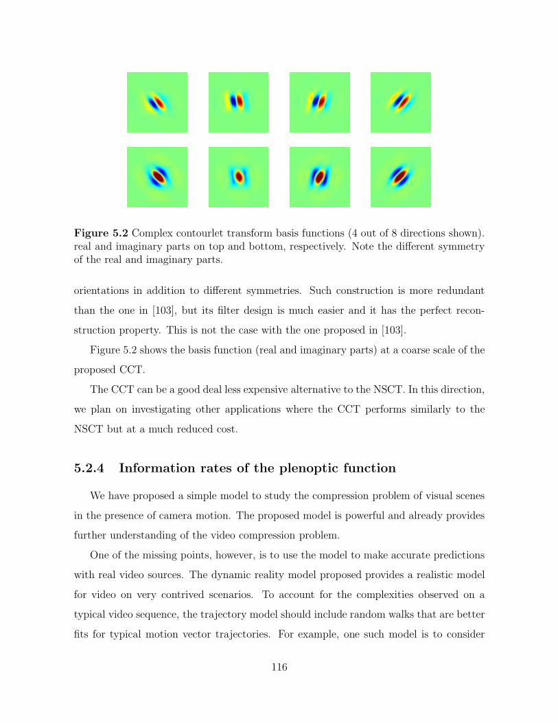
Figure 5.2 Complex contourlet transform basis functions (4 out of 8 directions shown).real and imaginary parts on top and bottom, respectively. Note the different symmetryof the real and imaginary parts.

orientations in addition to different symmetries. Such construction is more redundant

than the one in [103], but its filter design is much easier and it has the perfect recon-

struction property. This is not the case with the one proposed in [103].

Figure 5.2 shows the basis function (real and imaginary parts) at a coarse scale of the

proposed CCT.

The CCT can be a good deal less expensive alternative to the NSCT. In this direction,

we plan on investigating other applications where the CCT performs similarly to the

NSCT but at a much reduced cost.

5.2.4 Information rates of the plenoptic function

We have proposed a simple model to study the compression problem of visual scenes

in the presence of camera motion. The proposed model is powerful and already provides

further understanding of the video compression problem.

One of the missing points, however, is to use the model to make accurate predictions

with real video sources. The dynamic reality model proposed provides a realistic model

for video on very contrived scenarios. To account for the complexities observed on a

typical video sequence, the trajectory model should include random walks that are better

fits for typical motion vector trajectories. For example, one such model is to consider

116

2-D random walks in the Z2 lattice. Preliminary experiments on this direction indicate

that our model can indeed make valuable predictions. For instance, the model provides a

precise characterization of multiframe prediction and how it affects the bitrate. Further

experiments and conclusions in this direction are the goals of our future work.

117

REFERENCES

[1] S. Mallat, A Wavelet Tour of Signal Processing. London, UK: Academic Press,

1999.

[2] I. Daubechies, Ten Lectures on Wavelets. Philadelphia, PA: SIAM, 1992.

[3] J. Duffin and A. C. Schaefer, “A class of nonharmonic Fourier series,” Trans. Amer.

Math. Soc., vol. 72, pp. 341–366, 1952.

[4] M. J. T. Smith and T. P. B. III, “Exact reconstruction techniques for tree-

structured subband coders,” IEEE Trans. Acoust. Speech, and Signal Process.,

vol. 34, pp. 434–441, June 1986.

[5] F. Mintzer, “Filters for distortion-free two-band multirate filter banks,” IEEE

Trans. Acoust. Speech, and Signal Process., vol. 33, pp. 626–630, June 1985.

[6] M. Vetterli, “Filter banks allowing perfect reconstruction,” Signal Processing,

vol. 10, no. 3, pp. 219–244, 1986.

[7] P. P. Vaidyanathan, Multirate Systems and Filterbanks. Englewood Cliffs, NJ:

Prentice Hall, 1993.

[8] M. Vetterli and J. Kovacevic, Wavelets and Subband Coding. Englewood Cliffs,

NJ: Prentice Hall, 1995.

[9] G. Strang and T. Nguyen, Wavelets and Filter Banks. Wellesley, MA: Wellesley-

Cambridge Press, 1996.

118

[10] H. S. Malvar, Signal Processing with Lapped Transforms. Boston, MA: Artech

House, 1992.

[11] S. G. Mallat, “A theory for multiresolution signal decomposition: The wavelet

representation,” IEEE Trans. on Pattern Analysis and Machine Intelligence, vol.

PAMI-11, no. 7, pp. 674–693, 1989.

[12] Z. Cvetkovic and M. Vetterli, “Oversampled filter banks,” IEEE Trans. on Signal

Proc., vol. 46, no. 5, pp. 1245–1255, May 1998.

[13] H. Bolcskei, F. Hlawatsch, and H. G. Feichtinger, “Frame-theoretic analysis of

oversampled filter banks,” IEEE Trans. Signal Proc., vol. 46, no. 12, pp. 3256–

3268, December 1998.

[14] I. W. Selesnick, “The double density wavelet transform,” in Wavelet in Signal and

Image Analysis: From Theory to Practice, A. Petrosian and F. G. Meyer, Eds.

Norwell, MA: Kluwer, 2001.

[15] I. Daubechies, B. Han, A. Ron, and Z. Shen, “Framelets: MRA-based constructions

of wavelet frames,” Appl. Comput. Harmon. Anal., vol. 14, no. 1, pp. 1–46, 2003.

[16] E. L. Pennec and S. Mallat, “Sparse geometric image representation with ban-

delets,” IEEE Trans. Image Proc., vol. 14, no. 4, pp. 423–438, April 2005.

[17] G. Peyre and S. Mallat, “Surface compression with geometric bandelets,” ACM

Transactions on Graphics (SIGGRAPH’05), vol. 14, no. 3, pp. 601–608, 2005.

[18] M. B. Wakin, J. K. Romberg, H. Choi, and R. G. Baraniuk, “Wavelet-domain

approximation and compression of piecewise smooth images,” IEEE Trans. Image

Proc., vol. 15, no. 5, pp. 1071–1087, May 2006.

[19] D. L. Donoho, “Wedgelets: nearly minimax estimation of edges,” Ann. Statist.,

vol. 27, no. 3, pp. 859–897, 1999.

119

[20] M. N. Do and M. Vetterli, “The contourlet transform: An efficient directional

multiresolution image representation,” IEEE Trans. Image Proc., vol. 14, no. 12,

pp. 2091–2106, Dec. 2005.

[21] E. P. Simoncelli, W. T. Freeman, E. H. Adelson, and D. J. Heeger, “Shiftable

multiscale transforms,” IEEE Trans. Info. Theory, vol. 38, no. 2, pp. 587–607,

March 1992.

[22] R. H. Bamberger, “The directional filter bank: A multirate filter bank for the di-

rectional decomposition of images,” Ph.D. dissertation, Georgia Institute of Tech-

nology, 1990.

[23] R. H. Bamberger and M. J. T. Smith, “A filter bank for the directional decompo-

sition of images: Theory and design,” IEEE Trans. Signal Proc., vol. 40, no. 4, pp.

882–893, April 1992.

[24] N. G. Kingsbury, “Image processing with complex wavelets,” Phil. Trans. R. Soc.

Lond., vol. 357, no. 1760, pp. 2543–2560, Sept. 1999.

[25] P. J. Burt and E. H. Adelson, “The Laplacian pyramid as a compact image code,”

IEEE Trans. Communications, vol. 31, no. 4, pp. 532–540, April 1983.

[26] J.-X. Chai, S.-C. Chan, H.-Y. Shum, and X. Tong, “Plenoptic sampling,” in Pro-

ceedings of SIGGRAPH, 2000, pp. 307–318.

[27] M. N. Do, D. Marchand-Maillet, and M. Vetterli, “On the bandlimitedness of the

plenoptic function,” in Proceedings of the IEEE International Conference on Image

Processing (ICIP), vol. 3, Genoa, Italy, 2005, pp. 17–20.

[28] C. Zhang and T. Chen, “Spectral analysis for sampling image-based rendering

data,” IEEE Trans. on CSVT Special Issue on Image-Based Modeling, Rendering

and Animation, vol. 13, pp. 1038–1050, Nov. 2003.

120

[29] H.-Y. Shum, S. B. Kang, and S.-C. Chan, “Survey of image-based representations

and compression techniques,” IEEE Trans. on CSVT Special Issue on Image-Based

Modeling, Rendering and Animation, vol. 13, no. 11, pp. 1020–1037, Nov. 2003.

[30] M. Levoy and P. Hanrahan, “Light field rendering,” in Proceedings of SIGGRAPH,

1996, pp. 31–42.

[31] S. J. Gortler, R. Grzeszczuk, R. Szeliski, and M. Cohen, “The lumigraph,” in

Proceedings of SIGGRAPH, 1996, pp. 43–54.

[32] J. Kovacevic and M. Vetterli, “Nonseparable 2-dimensional and 3-dimensional

wavelets,” IEEE Trans. on Signal Proc., vol. 43, no. 5, pp. 1269–1273, May 1995.

[33] A. L. da Cunha and M. N. Do, “Bi-orthogonal filter banks with directional vanishing

moments,” in Proceedings of the IEEE ICASSP, vol. 4, Philadelphia, PA, 2005, pp.

553–556.

[34] A. L. da Cunha and M. N. Do, “On two-channel filter banks with directional

vanishing moments,” IEEE Trans. Image Proc., to be published, 2007.

[35] A. L. da Cunha and M. Do, “Linear-phase filter design for directional multireso-

lution decompositions,” in Proc. of SPIE Conference on Wavelet Applications in

Signal and Image Processing XI, vol. 5914, San Diego, CA, July 2005, pp. 263–273.

[36] E. J. Candes and D. L. Donoho, “New tight frames of curvelets and optimal rep-

resentations of objects with piecewise C2 singularities,” Comm. Pure and Appl.

Math, vol. 57, no. 2, pp. 219–266, February 2004.

[37] M. N. Do and M. Vetterli, “Framing pyramids,” IEEE Trans. Signal Proc., vol. 51,

no. 9, pp. 2329 – 2342, Sept. 2003.

[38] M. N. Do, “Directional multiresolution image representations,” Ph.D. dissertation,

Swiss Federal Institute of Technology, Lausanne, Switzerland, December 2001.

121

[39] Y. Lu and M. Do, “Crisp-contourlet: A critically sampled directional multireso-

lution representation,” in Proc. SPIE Conf. on Wavelets X, San Diego, CA, Aug.

2003, pp. 655–665.

[40] V. Velisavljevic, B. Beferull-Lozano, M. Vetterli, and P. L. Dragotti, “Direction-

lets: Anisotropic multidirectional representation with separable filtering,” IEEE

Transactions on Image Processing, vol. 15, no. 7, pp. 1916–1933, July 2006.

[41] M. Vetterli, “Wavelets, approximation, and compression,” IEEE Signal Proc. Mag.,

vol. 18, pp. 59–73, Sept. 2001.

[42] A. Cohen and I. Daubechies, “Non-separable bidimensional wavelet bases,” Rev.

Math. Iberoamer, vol. 9, no. 1, pp. 51–137, 1992.

[43] J. Kovacevic and M. Vetterli, “Nonseparable multidimensional perfect reconstruc-

tion filter banks and wavelet bases for Rn,” IEEE Trans. Information Theory,

vol. 38, no. 2, pp. 533–555, March 1992.

[44] E. Viscito and J. P. Allebach, “The analysis and design of multidimensional FIR

perfect reconstruction filter banks for arbitrary sampling lattices,” IEEE Trans.

Circuits and Systems, vol. 38, no. 1, pp. 29–41, Jan. 1991.

[45] M. Vetterli, “Multi-dimensional subband coding: Some theory and algorithms,”

Signal Processing, vol. 6, no. 2, pp. 97–112, 1984.

[46] M. Vetterli and C. Herley, “Wavelets and filter banks: Theory and design,” IEEE

Trans. on Signal Proc., vol. 40, pp. 2207–2232, Sept. 1992.

[47] R. Ansari, C. W. Kim, and M. Dedovic, “Structure and design of two-channel filter

banks derived from a triplet of halfband filters,” IEEE Trans. CAS-II, vol. 46,

no. 12, pp. 1487–1496, December 1999.

[48] D. Wei and S. Guo, “A new approach to the design of multidimensional nonsepara-

ble two-channel orthonormal filter banks and wavelets,” IEEE Signal Proc. Letters,

vol. 7, no. 11, pp. 327–330, November 2000.

122

[49] D. B. H. Tay and N. G. Kingsbury, “Flexible design of multidimensional perfect

reconstruction FIR 2-band filters using transformation of variables,” IEEE Trans.

Image Proc., vol. 2, no. 4, pp. 466–480, October 1993.

[50] S.-M. Phoong, C. W. Kim, P. P. Vaidyanathan, and R. Ansari, “A new class of

two-channel biorthogonal filter banks and wavelet bases,” IEEE Trans. on Signal

Proc., vol. 43, no. 3, pp. 649–661, March 1995.

[51] D. Stanhill and Y. Y. Zeevi, “Two-dimensional orthogonal wavelets with vanishing

moments,” IEEE Trans. Signal Proc., vol. 44, no. 10, pp. 2579–2590, October 1996.

[52] D. B. H. Tay, “Design of filter banks/wavelets using TROV: A survey,” Digital

Signal Processing, vol. 7, no. 4, pp. 229–238, Oct. 1997.

[53] A. L. da Cunha, J. Zhou, and M. Do, “The nonsubsampled contourlet transform:

Theory, design, and applications,” IEEE Trans. Img. Proc., vol. 15, no. 10, pp.

3089–3101, Oct. 2006.

[54] A. L. da Cunha, J. Zhou, and M. Do, “The nonsubsampled contourlet transform:

Filter design and application in denoising,” in Proceedings of the IEEE Interna-

tional Conference on Image Processing (ICIP), vol. 1, Genoa, Italy, 2005, pp. 749–

752.

[55] J. Zhou, A. L. da Cunha, and M. Do, “The nonsubsampled contourlet transform:

Construction and application in enhancement,” in Proceedings of the IEEE Inter-

national Conference on Image Processing (ICIP), vol. 1, Genoa, Italy, 2005, pp.

469–472.

[56] J. G. Daugman, “Uncertainty relation for resolution in space, spatial frequency,

and orientation optimized by two-dimensional visual cortical filters,” J. Opt. Soc.

Am. A, vol. 2, no. 7, pp. 1160–1169, July 1985.

123

[57] R. R. Coifman and D. L. Donoho, “Translation invariant de-noising,” in Wavelets

and Statistics, A. Antoniadis and G. Oppenheim, Eds. New York: Springer-Verlag,

1995, pp. 125–150.

[58] S. G. Chang, B. Yu, and M. Vetterli, “Adaptive wavelet thresholding for image

denoising and compression,” IEEE Trans. Image Proc., vol. 9, no. 9, pp. 1532–

1546, September 2000.

[59] L. Sendur and I. W. Selesnick, “Bivariate shrinkage with local variance estimation,”

IEEE Signal Proc. Letters, vol. 9, no. 12, pp. 438–441, December 2002.

[60] J. Portilla, V. Strela, M. J. Wainwright, and E. P. Simoncelli, “Image denoising

using scale mixtures of Gaussians in the wavelet domain,” IEEE Trans. Image

Proc., vol. 12, no. 11, pp. 1338–1351, 2003.

[61] M. J. Shensa, “The discrete wavelet transform: Wedding the a trous and Mallat

algorithms,” IEEE Trans. Signal Proc., vol. 40, no. 10, pp. 2464–2482, October

1992.

[62] J. L. Starck, F. Murtagh, and A. Bijaoui, Image Processing and Data Analysis.

New York, NY: Cambridge University Press, 1998.

[63] J. H. McClellan, “The design of two-dimensional digital filters by transformation,”

in Proc. 7th Annual Princeton Conf. Information Sciences and Systems, Princeton,

NJ, 1973, pp. 247–251.

[64] S. Mitra and R. Sherwood, “Digital ladder networks,” IEEE Trans. on Audio and

Electroacoustics, vol. AU-21, no. 1, pp. 30–36, February 1973.

[65] W. Sweldens, “The lifting scheme: A custom-design construction of biorthogonal

wavelets,” Appl. Comput. Harmon. Anal., vol. 3, no. 2, pp. 186–200, 1996.

[66] R. E. Blahut, Fast Algorithms for Digital Signal Processing. Reading, MA:

Addison-Wesley, 1985.

124

[67] R. Jia, “Approximation properties of multivariate wavelets,” Mathematics of Com-

putation, vol. 67, pp. 647–665, 1998.

[68] T. Cooklev, T. Yoshida, and A. Nishihara, “Maximally flat half-band diamond-

shaped FIR filters using the Bernstein polynomial,” IEEE Trans. CAS-II, vol. 40,

no. 11, pp. 749–751, Nov. 1993.

[69] J.-L. Starck, E. J. Candes, and D. L. Donoho, “The curvelet transform for image

denoising,” IEEE Trans. Image Proc., vol. 11, no. 6, pp. 670–684, June 2002.

[70] D. D.-Y. Po and M. N. Do, “Directional multiscale modeling of images using the

contourlet transform,” IEEE Trans. Img Proc., vol. 15, no. 6, pp. 1610–1620, June

2006.

[71] S. G. Chang, B. Yu, and M. Vetterli, “Spatially adaptive wavelet thresholding with

context modeling for image denoising,” IEEE Trans. Image Proc., vol. 9, no. 9, pp.

1522–1531, September 2000.

[72] A. L. da Cunha, M. N. Do, and M. Vetterli, “On the information rates of the

plenoptic function,” in Proceedings of the IEEE International Conference on Image

Processing (ICIP), Atlanta, GA, 2006, pp. 2489–2492.

[73] A. L. da Cunha, M. N. Do, and M. Vetterli, “A stochastic model for video and its

information rates,” in Prof. of IEEE Data Compression Conference (DCC), March

2007, pp. 3–12.

[74] E. H. Adelson and J. R. Bergen, “The plenoptic function and the elements of

early vision,” in Computational Models of Visual Processing, M. Landy and J. A.

Movshon, Eds. Cambridge, UK: MIT Press, 1991, pp. 3–20.

[75] D. Forsyth and J. Ponce, Computer Vision: A Modern Approach. Englewood

Cliffs, NY: Prentice Hall, 2002.

125

[76] C. Zhang and T. Chen, “A survey on image-based rendering representation,

sampling and compression,” EURASIP Signal Processing: Image Communication,

vol. 19, pp. 1–28, Jan. 2004.

[77] L.-W. He and H.-Y. Shum, “Rendering with concentric mosaics,” in Proceedings of

SIGGRAPH, 1999, pp. 299–306.

[78] A. Telkap, Digital Video Processing. Upper Saddle River, NJ: Prentice-Hall, 1995.

[79] B. Girod, “The efficiency of motion-compensating prediction for hybrid coding of

video sequences,” IEEE Journal of Selected Areas in Communications, vol. SAC-5,

no. 7, pp. 1140–1154, August 1987.

[80] P. Ramanathan and B. Girod, “Rate-distortion analysis for light field coding and

streaming,” EURASIP Signal Processing: Image Communication, vol. 21, no. 6,

pp. 462–475, July 2006.

[81] N. Gehrig and P. L. Dragotti, “Distributed compression of the plenoptic function,”

in Proc. IEEE Int. Conf. on Image Proc., vol. 1, Singapore, 2004, pp. 529–532.

[82] P. Ramanathan and B. Girod, “Receiver-driven rate-distortion optimized streaming

of light fields,” in Proc. IEEE International Conference on Image Processing, vol. 3,

Genoa, Italy, 2005, pp. 25–28.

[83] T. Berger, Rate-Distortion Theory: A Mathematical Basis for Data Compression.

Englewood Cliffs, NJ: Prentice-Hall, 1972.

[84] J. Rudnick and G. Gaspari, Elements of the Random Walk. Cambridge, UK:

Cambridge University Press, 2004.

[85] W. Feller, An Introduction to Probability Theory and Its Applications. New York,

NY: John Wiley and Sons, 1957.

[86] T. M. Cover and J. A. Thomas, Elements of Information Theory. New York, NY:

John Wiley & Sons, 1991.

126

[87] H. Li and R. Forchheimer, “Extended signal-theoretic techniques for very low bit-

rate video coding,” in Video Coding: The Second Generation Approach. Norwell,

MA: Kluwer, 1996, pp. 383–428.

[88] T. Wiegand, X. Zhang, and B. Girod, “Long-term memory motion-compensated

prediction,” IEEE Trans. CSVT, vol. 9, no. 1, pp. 70–84, February 1999.

[89] C. Herley, “ARGOS: Automatically extracting repeating objects from multimedia

streams,” IEEE Trans. on Multimedia, vol. 8, no. 1, pp. 115–129, Feb 2006.

[90] N. Vasconelos and A. Lippman, “Library-based image coding,” in Proc. IEEE Int.

Conf. Acoust., Speech, and Signal Proc., vol. 5, Adelaide, Australia, April 1994,

pp. 489–492.

[91] J. Ziv and A. Lempel, “Compression of individual sequences via variable-rate cod-

ing,” IEEE Transactions on Information Theory, vol. 24, no. 5, pp. 530–536, Sept.

1978.

[92] Y. Steinberg and M. Gutman, “An algorithm for source coding subject to a fidelity

criterion, based on string matching,” IEEE Trans. Inf. Theory, vol. 39, no. 3, pp.

877–886, May 1993.

[93] M. S. Pinsker, Information and Information Stability of Random Variables. San

Francisco, CA: Holden Day, 1984.

[94] R. M. Gray, “A new class of lower bounds to information rates of stationary sources

via conditional rate-distortion functions,” IEEE Trans. on Info. Theory, vol. IT-19,

no. 4, pp. 480–489, July 1973.

[95] R. M. Gray, Entropy and Information Theory. New York: Springer-Verlag, 1990.

[96] Y. Sermadevi, J. Chen, S. Hemami, and T. Berger, “When is bit allocation for

predictive video coding easy?” in Data Compression Conference (DCC), Snowbird,

UT, 2005, pp. 289–298.

127

[97] R. L. Graham, D. E. Knuth, and O. Patashnik, Concrete Mathematics: A Foun-

dation for Computer Science. Boston, MA: Addison-Wesley Longman Publishing

Co., Inc., 1989.

[98] R. A. Horn and C. R. Johnson, Matrix Analysis. Cambridge, UK: Cambridge

Univ. Press, 1999.

[99] R. M. Gray, “On the asymptotic eigen-value distribution of Toeplitz matrices,”

IEEE Trans. Inf. Theory, vol. 18, no. 6, pp. 725–730, 1972.

[100] M. Magnor and B. Girod, “Data compression for light-field rendering,” IEEE

Transactions on CSVT, vol. 10, no. 3, pp. 338–343, 2000.

[101] I. W. Selesnick, R. G. Baraniuk, and N. G. Kingsbury, “The dual-tree complex

wavelet transform,” IEEE Signal Proc. Mag., vol. 22, no. 6, pp. 123–151, Nov.

2005.

[102] F. C. A. Fernandes, R. L. C. van Spaendonck, and C. S. Burrus, “A new framework

for complex wavelet transforms,” IEEE Trans. Sign. Proc., vol. 51, no. 7, pp. 1825–

1837, July 2003.

[103] T. T. Nguyen and S. Oraintara, “Shift-invariant multiscale multidirectional image

decomposition,” in Proc. of IEEE ICASSP, vol. 2, Toulouse, France, 2006, pp.

153–156.

128