Embed Size (px)
Citation preview
Selecta Mathematica, New Series Vol. 2, No. 3 (1996), 369-414
1022-1824/96/030369-4651.50 + 0.20/0 @ 1996 Birkh~user Verlag, Basel
Geometry of Singularities for the Steady Boussinesq Equations
Russel E. Caflisch*, Nicholas Ercolani t and Gregory Steele t
A b s t r a c t . Analysis and computations are presented for singularities in the solution of the steady Boussinesq equations for two-dimensional, stratified flow. The results show that for codimension 1 singularities, there are two generic singularity types for general solutions, and only one generic singularity type if there is a certain symmetry present. The analysis depends on a special choice of coordinates, which greatly simplifies the equations, showing that the type is exactly that of one dimensional Legendrian singularities, generalized so that the velocity can be infinite at the singu- larity. The solution is viewed as a surface in an appropriate compactified jet space. Smoothness of the solution surface is proved using the Cauehy-Kowalewski Theorem, which also shows that these singularity types are realizable. Numerical results from a special, highly accurate numerical method demonstrate the validity of this geometric analysis. A new analysis of general Legendrian singularities with blowup, i.e., at which the derivative may be infinite, is also presented, using projective coordinates.
1. I n t r o d u c t i o n
The possibility of singularity formation from smooth initial data for the solution of the Euler equations for inviscid, incompressible fluid flow in three dimensions is one of the main unsolved problems of mathematical fluid mechanics. In spite of considerable effort on this problem from analytical, numerical and physical ap- proaches, there is still little convincing evidence either for or against the possibility of singularity formation.
* Research supported in part by the ARPA under URI grant number # N00014092-J-1890. t Research supported in part by the NSF under grant number #DMS93-02013. t Research supported in part by the NSF under grant #DMS-9306488.
370 R .E . Caflisch, N. Ercotani and G. Steele Selecta Math.
In this paper, singularities are analyzed for a rela*ed, but much simpler, system, the steady Boussinesq equations:
u . V p = 0
u . V~ = -p~
V x u = ~ (1.1)
V . u = 0 .
This system describes steady, two-dimensional, stratified (i.e., variable density), incompressible flow in which p is density, u is two dimensional velocity and ~ is vorticity. The buoyancy term p~, plays the role of vortex stretching in the Euler equations. This system is derived in the "Boussinesq limit," in which the variation of density is important in buoyancy terms but insignificant in inertial terms.
For the steady Boussinesq equations (1.1) we will derive the generic tbrm of singularities under certain natural restrictions. Singularities for complex solutions and at, complex spatial positions are considered in this study, but the results are also valid for steady real singularities of real solutions. In addition, we present numerical computations which confirm these generic singularity types.
The problem of singularity formation from smooth initial data for the (time- dependent) Euler or Boussinesq equations is the motivation for this work. Our reasons for studying complex singularities for steady flows are twofold:
First, this problem serves as a vehicle tbr developing methods that may be ap- plicable to singularity formation in the unsteady problem. For example, the present analysis includes solutions with infinite values for velocity and vorticity. Such infi- nite values in the dependent variables were excluded from earlier approaches [11]. In fact, a new analysis of Legendrian singularities at which the "velocities" are infinite, which we call "Legendrian blowup," is also included in the analysis below.
Second, we believe that the form of steady complex singularities may be in- dicative of the form for dynamic real singularities or for nearly singular flow. One reason for this belief is that the genericity results for steady singularities can also be interpreted as genericity results for complex singularities that move in the complex plane without change in ttmir structure. This is described in Appendix A. On the other hand, we have found that, for generic steady singularities, the density p is infi- nite. Since, infinite values of p cannot occur for singularity tbrmation from smooth initial data, this would restrict the set of steady singularities that are relevant to singularity formation. Further discussion of these points is presented in Section 8.
The main result of this paper can be informally stated as follows:
Consider singularities for the steady Boussinesq system (1.1) which have codi- mension 1 and for which the vorticity ~ is infinite. The generic form of such a singularity is of two types:
(1) ¢ ~ za/2; v .~ xl/2; ~ ~ x -~/2 (2) ~) ~ x l /2 ; V ~ x - l / 2 ; ~ ~ X -3 /2 .
Vol. 2 (1996) Singularities for Steady Boussinesq Equations 371
If in addition the stream function ¢ is real analytic and is assumed to have an additional symmetry (¢(x, 0) = ¢ ( - x , 0)), then the singularity type is
(3) ¢,-~ X2/3; V ~ X--1/3; ~ ,~ X -4/3.
In these formulas x and v denote some suitably chosen space and velocity coordi- nates. The term "generic" here is used in the technical sense that is standard in singularity theory (see for instance [2]). A precise statement of this result will be presented in Section 3.
The principal ingredient in this study will be a geometric approach to differen- tial equations, which has been developed by two of the present authors and their coworkers for simpler systems in [11], as well as by Bryant, Griffiths and Hsu [7], [8] and Rakhimov [23]. In this approach the solution of a differential equation is viewed as a surface in an appropriate jet space (described in Section 5), and the PDE serves as a constraint on the possible form of this surface. In particular, for the steady Boussinesq equations, we show that the convective equations can be solved exactly and that incompressibility provides a constraint on the singularity type, but that the vorticity equations do not lead to any constraint. (For other applications of contact geometry to PDE's the reader may be interested in consulting [1].)
The main role of analysis in this approach is to show that such constrained sur- faces are generically smooth, which is demonstrated using the Cauchy-Kowalewski Theorem for analytic solutions of a PDE. Geometric and algebraic methods, such as the singularity theory of Arnold [2], can then be used to analyze the generic types of singularities for this surface.
The background for this study consists of several analytical results and a nu- merical computation:
First, the mathematical significance of Euler or Boussinesq singularity formation (for the time-dependent equations), should it occur, is that it would limit the validity of mathematical existence theory. Beale, Kato and Majda [6] showed that. if the initial velocity u0 is in Sobolev space H s for some s _> 3, but at time t = t* > 0, u(t) is not in H s, then
t*
L I1 ( ,t)[I (1.2) in which ]l" I1~ is the L ~ norm in space and w is the vorticity. Bardos and Benachour [5] proved a related, earlier result in an analytic function class; E and Shu [17] proved a similar result for the Boussinesq equations.
The physical significance of singularities is less clear and depends critically on the robustness and type of singularities. Singularities might serve as an important means for transfer of energy from large to small scales. In this way they could be responsible for the onset of turbulent flow or even for the continuation of fully developed turbulence. A related analytic result, first stated by Onsager [21] and refined in [12], [16], [18], says that if a weak Euler solution does not conserve energy and it has HSlder exponent a on a set of codimension n, then a + n/3 <_ 1/3. This
372 R.E. Caflisch, N. Ercolani and G. Steele Selecta Math.
is physically meaningful, since there is clear evidence that the energy dissipation for the Navier Stokes solution remains nonzero in the zero viscosity limit.
The time-dependent Boussinesq equations are
p t + u . V p = O
V x u = ( (1.3)
V . u = 0 .
As pointed out by Childress et al. [15] and Pumir and Siggia [22], these are very similar to the Euler equations for axisymmetric flow with swirl. The latter equations also involve only two degrees of spatial variation (radius r and axial length z) and are the simplest form of the Euler equations with nontriviat vortex stretching. Pumir and Siggia [22] performed numerical computations for (1.3), which seemed to indicate singularity formation, but further computations by E and Shu [17] did not confirm their results.
A clearcut numerical demonstration of singularities for the Euler equation for ax- isymmetric flow with swirl, but for complex velocity, was performed by Caflisch [9] using a special form of the solution for which the numerical error is extremely small. The computed solutions had singularities of the simple form u ~ x -1/3 , which sug- gested that this singularity might be generic.
These computations can he understood in two ways:
(1) The computations were performed ibr the exact Euler equations with no ap- proximations but with complex initial data. In particular the initial data consists of only nonnegative wavenumbers in tile axial variable z; i.e., it is upper analytic in Z.
(2) These computations also correspond to Moore's approximation for the Euter equations with real initial data. In Moore's approximation, the upper and lower analytic components of the solution are decoupled. Tlm upper analytic part satisfies the Euler equations, but with complex initial data, as ill (1); the lower analytic part is its conjugate. The physical meaning of this approximation is to retain the forward cascade of energy while omitting tile inverse cascade.
It has not yet been possible to relate the results of Moore's approximation back to the real Euler equations, but we conjecture that this approximation is valid, at least qualitatively, as long as the singularities are away from the real axis.
In this paper, numerical singularity results are used to indicate the generic form of singularities for the steady flow problem. The singular solutions constructed in [9] were traveling waves (with imaginary speed), but by Galilean transformation they become steady solutions. In the present investigation, numerical solutions with complex singularities are constructed for the steady Boussinesq equations by a similar procedure as in [9].
Vol. 2 (1996) Singularities for Steady Boussinesq Equations 373
Finally the singularity analysis of this study was motivated by a similar analysis of the generic singularity type for first order systems with at most two speeds by Caflisch, Ercolani, Hou and Landis [11]. That analysis used a generalization of the hodograph transformation to unfold the differential equations. While that unfolding transformation has been generalized [10] to a larger class of equations, including the Boussinesq equations or the Euler equations for axisymmetric flow with swirl, the analysis in the present study is effected through a simpler and more direct transformation of the equations.
The following is an outline of the remainder of the paper: In Section 2 the Boussi- nesq equations are transformed and scaled. The main analytic results on generic singularity type for steady Boussinesq are presented and proved in Section 3. The proof partly relies on an application of the Cauchy Kowalewski theorem, presented in Section 4, to show that the solutions with the singularity types (1), (2) and (3) are actually realizable for the Boussinesq equations, and that the corresponding solution surfaces are smooth.
Although the genericity results are derived directly from the Boussinesq equa- tions, they are motivated by the theory of Legendrian singularities. Therefore, for the nonexpert in singularity theory, we have included Section 5 which presents a self-contained summary of the relevant aspects of the theory of Legendrian sin- gularities (Section 5.1). This section is also included because this work leads to an extension of Legendrian singularity theory to Legendrian blowup (Section 5.2) which is new.
The analytic results of this study are motivated and validated by a numerical construction of singular solutions for the Boussinesq equations with complex veloc- ities, which are described in Section 6 (the numerical method) and Section 7 (the numerical results).
Finally, some conclusions from this study, including a discussion of the signifi- cance of these steady singularities for the time-dependent equations, are presented in Section 8.
While this presentation of results is given in the simplest logical order to help the reader, the actual process by which these results were obtained was an interplay between analysis and numerical computation. Following the numerical solution of the Euler equations for axisymmetric flow with swirl, the Boussinesq equations were solved by the same method, and a solution of the form (3) was obtained. This motivated an analysis of the generic form of singularities which produced singularity types (1) and (2). Since the numerical results did not agree with (2) and since the analysis of the type (2) required some new singularity results for Legendrian surfaces with blowup of the derivative, we were at first skeptical of the validity of the form (2). Further consideration showed, however, that there was a symmetry (¢(x, 0) = ~b(-x, 0)) in the original numerical solutions of Euler and Boussinesq that led to the form (3). Following this observation, we modified the computations to remove this symmetry and then found the correct asymmetric result (2). We also
374 R.E. Caflisch, N. Ercolani and G. Steele Selecta Math.
extended the analysis to show that the generic singularity tbrm of a real -analy t ic solution with symmetry is (3).
2. Unfolding the Steady Boussinesq Equation
The Boussinesq equations for steady, 2D stratified, incompressible fluid flow are
u . Vp = 0 (2.1)
u . v ; = - p ~ (2.2)
2 7 x u = ~ (2.3)
v . u = o (2.4)
in which u = ( u , v ) is velocity, p is density, ~ is vorticity. The incompressibility condition (2.4) implies the existence of a stream function ~p so that
u = - v × ¢ = ( - ¢ ~ , ¢ x ) . (2.5)
It is illuminating to recast the system (2.1)-(2.4) into an exterior differential system using differential forms. Since dg? = ¢ x d x + Cydy = v d x - udy , then equation (2.5), which is equivalent to (2.4), can be written as
d4, = v d x - udy . (2.6)
Similarly equations (2.1) and (2.2) are equivalent to
de A ~p = o (2.7)
d e A de = d~ A dp. (2.8)
This simple reformulation of the equation is surprisingly potent: Equations (2.7) and (2.8) suggest that (y, ¢) would be convenient variables, in terms of which these equations become
which has solution
p~ = 0 (2.9)
(y = - p c (2.10)
p = p(~b) (2.11)
= ~(~b) - yp¢(~b) (2.12)
in which p and ~ are arbitrary functions.
Vol. 2 (1996) Singularities for Steady Boussinesq Equations 375
Next, consider the solution as a surface in ( x , y , u , v , ¢ ) space. Then equa- tion (2.6) or the rescaled form
dx = l d¢ + U dy (2.13) v v
provides a contact constraint on the solution; i.e., a differential form a = d ¢ - v d x +
udy that vanishes everywhere on the solution surface. This surface is a Legendrian surface due to the contact constraint, as discussed in Section 5.
Finally, equations (2.3) and (2.4) can be written in terms of the new independent variables (y, ¢) as
( u ) ( 1 ) (2.14) ~= ~ (u 2 + v2)¢ = 2u v + 2¢. (2.15)
Equation (2.14) is equivalent to the contact constraint (2.13), while (2.15) provides a further constraint on the system.
Several further manipulations of the equations are worthwhile. If (u, v) is finite we can write (2.14), (2.15) as a first order system
(:)+(: v ) ( : ) ; , 10, In this case the previous classification of [11] describes the generic singularities for the system.
Second, suppose that (u, v) becomes infinite. Following the Beale-Kato-Majda result [6], singularities with infinite vorticity are of most interest, so we will assume that ¢ blows up. According to the formula (2.12), blowup of ¢ occurs along fixed values of ~b. Therefore we regularize the singularity through unfolding only the ¢ variable by a mapping ~b = ~b(p). Then we look for a solution which is single valued in y and p. Furthermore we scale the velocity as
# u = 3 ' v = ~ (2.17)
in which fl = fl(p) gives the rate of blowup. As a consequence of (2.12) we may write .¢ as
¢ = (~ - yp)~ (2.18)
in which ~ = ~. Finally we assume that ~ is of the same order as (u 2 + v2)¢ in (2.15) by scaling ~] and p as
r 1 =/3-2ts(p) (2.19)
p = ;~-2,~(p).
376 R. E. Caflisch, N. Ercolani and G. Steele Selecta Math.
The resulting PDE's for tt and u are
= 2/3-:¢p#~.
(2.20)
(2.21)
Integrate these with respect to p to obtain
= f ( v ) + y
(2.22)
j . p
(#2 + u2)(p, y) = 2(~c - y~/) +/32g(y) +/32 /3-1¢p#vdP (2.23)
in which f(y), g(y), t~(p), 7(P), /3(p) and Cp(p) are arbitrary functions. In Section 4, we shall show that these equations have a unique solution which is
analytic in y for any choice of f , g, n,, 7, /3 and Cp and that the solution depends continuously on these functions. The stability (and genericity) result, which is proved in the next section, is with respect to perturbations of these functions.
3. Generic Singularities for Boussinesq
In this section, the generic singularity types for the steady Boussinesq equations are analyzed under certain restrictions. The analysis here is performed directly on tile integral form of the Boussinesq equations (2.22), (2.23), using the PDE results of Section 4. The genericity results are motivated by and could have been derived from Legendrian singularity theory, summarized in Section 5, but the direct derivation presented here is simpler.
The singularities under consideration are restricted as follows:
(a) The singularity set has codimension equal to 1. These are the singularities that are most likely to be observed.
(b) As a function of (y, ¢) the solution depends smoothly on y. This is expected since ~ is a linear function of y for fixed ¢ or p.
Under these restrictions, the generic singularity types for steady Boussinesq are described by the next two theorems. By singularity type we mean an equivalence class under analytic changes of variables. By generic we mean that, two conditions are satisfied. First the singularity type should be stable with respect to perturba- tions. This is called the stability condition. Second, any solution with a singularity type which is not stable may be perturbed into one having only stable singularity types. This is called the density condition. More details concerning these concepts are presented in Section 5.
Vol. 2 (1996) Singularities for Steady Boussinesq Equations 377
T h e o r e m 3.1 (Generic singularities for Boussinesq). Under the restrictions (i), (ii) above, the two generic (i.e., stable and dense) singularity types for the steady Boussinesq equations are a curve of cusps and a curve of blowup folds. Represen- tatives of these two classes are
1 2 1 3 p-1 (i) Cusp. x ~ ~p , v ~ p, ¢ ~ ~p , ~ 1 2 (ii) Blowup fold. x ~ yp , v ~ p - l , ¢ ,~ p, ~ ~ p-3
T h e o r e m 3.2 (Generic real singularities with symmetry for Boussinesq). In ad- dition to restrictions (a), (b), suppose that the ¢ is real analytic and that ¢ is symmetric with respect to reflection in x; i.e.,
¢(x0 + x, y0) = ¢ (x0 - x, y0) (3.1)
for some real point (Xo, Yo) on the singularity locus. Then there is only one generic singularity type, a curve of blowup cusps,
1 3 1 2 p- -4 (iii) Blowup Cusp. x ~ yp , v ~ p - l , ¢ ~ ~p , ~
These singularities can be written in terms of x dependence (omitting constants), as follows:
Without symmetry (i) ~ ~ x 3/2 , v ~ x 1/2, ~ ~ x - 1 / 2
(ii) ¢ ~ x 1/2, v ~ z -1/2, ~ ~ x - 3 / 2 .
With symmetry
(iii) ~ ~ x 2/3, v ~ x -1 /3 , ~ ~ X -4 /3 .
Note that the real analyticity condition of Theorem 3.2 is not satisfied by the nu- merical solutions that are presented in Section 6 and 7.
Proof of Theorem 3.1. We need to show that the singularity types (i) and (ii) are stable with respect to perturbation and that any other solution can be perturbed to one of these two types. The allowable perturbations are those of the solution as a complex surface in C 5 with coordinates (x, y, p, ~, ¢). This surface will in general not be closed, tt may have the form of a surface with complex codimension 1 (real codimension 2) sets removed. These removed sets correspond to the loci where the Boussinesq solution has singularities and are described below. The natural setting for perturbation theory is not such surfaces per se but rather their simply connected universal covers. However, since our perturbation results, related to stability, are local, it will suffice to consider surfaces in C 5 .
In Section 4 below, we show that the solution exists, as an analytic function for y in C and for p on a Riemann surface 7~, for any choice of the "data" (i.e., the functions/3(p), Cp(p), 3'(P), f (Y) , g(Y)) except for a restriction (equation (3.3) below) on the location of the zeroes of/~. In addition, the solution depends smoothly
378 R . E . Caflisch, N. Ercolani and G. Steele Selecta Math.
on this "data." So it suffices to consider perturbations of these functions. Since the stability results are local, only a neighborhood of ( y ,p ) = (0, 0) need be considered.
The Riemann surface T¢ has logarithmic branch points at each of the zeroes of/3. For p near one of these branch points, say Pi of order ni, and for any fixed y, the solution p has the form
,(p) = .o(p) + o ((p -pO log( ; - pO) (3.2)
in which #o is analytic ibr p near Pi. There is a similar form for u. Since the logarithmic part of the solution is at such high order in p, it does not affect the singularity type.
The zeroes of/3 (as well as those of ¢,p) are the places at which the Boussinesq solution has singularities. In a given neighborhood of the variable p, let the zeroes of/3 be P a , . . . , Pm. For the analytic results of Section 4 there there is a restriction that the spacing of the roots needs to be approximately uniform; i.e., for some constant c,
max IPi - PJl <- c rain IPi - Pjl . (3.3) iCj iCj
This class of functions/3 is dense with respect to the usual topology. It is also large enough to consider a neighborhood of a k-th order zero Pl for/3, and its generic perturbation to k simple zeroes P l , . . . ,Pk. The Boussinesq solution is shown to be smooth with respect to such perturbations in Theorem 4.2. Furthermore, any analytic functions Cp(p), ~/(p), f (y) , g(y) are allowed. It would not change anything if/3, Cp (p), V(P) were defined on the Riemann surface 7¢ (defined in the next section) rather than on C. Actually for determining the singularity type only the functions •(p) and Cp(p) are significant.
Generically, there are 3 cases:
(a) /3(0) # 0, Cp(0) !¢ 0. In this case there is no singularity.
(b)/3(0) ¢ 0; ¢p(0) = 0, ¢p~(0) ¢ 0. Then
¢ = a o p 2 + a l p 3 + . . . (3.4)
for some constants a0 and al. In this case, we may set /3 = 1 so that # = u and u = v. Now generically f(0) ~ 0 and 9(0) ~ 0. Thus ~ is a unit and u 2 + v 2, for generic a, is nonvanishing. It follows that
v = bo + blp + . . . (3.5)
for some nonvanishing constants b0 and bl depending on y. Since v = Cx, then
xp ---- •p/V -= cOp 4- Clp 2 -[ - . . . (3.6)
Vol. 2 (1996)
in which
so that
Singularities for Steady Boussinesq Equations
and
Co = 2ao/bo, ca = 3a l /bo - 2aobl/b2o
1 2 1 3 x = "~cop + "~clp + . . . .
Under the transformation
379
(3.7)
(3.8)
v' = v - bo = b l p + . . . (3.10)
this is seen to be a singularity of type (i). In particular for generic 77 and p,
C = (~ - YP)¢ = (~ - yp)~/¢p
= dp -1 + O(1)
for some constant d.
(c) /3(0) = 0, jOp(0) 7 ~ 0, Cp(0) # 0. Then we may set
/3 = p + . . . , ¢ = p + . . . . ( 3 . 11 )
Generically f(O) # 0 and n(O) # O, so that (9) is a unit and
#2 + u2 ~ ~. (3.12)
It follows that generically # and u are O(1) and that u , v are O(~). Then
Xp = Cp = O(p) v
z = O ( p 2)
C = ( ~ - ~ ( ~ - y~) )p = o ( p - 3 ) .
This is a singularity of type (ii), which finishes the proof of Theorem 3.1.
Proo f o f T h e o r e m 3.2. Assume that ¢(x) = ¢ ( - x ) at y = 0, which is a singular point. Then since the unfolding of ¢ is real, ~ is even in p and x is odd in p. Generically, ¢ = cp 2 + . . . . Since # and u are generically nonvanishing,
/ 3 = 0 ( ~ - ~ . ~ ) = O ( x p / ¢ p ) . (3.13)
Since /3 is assumed to not become infinite, then x = O(p) is not allowed. So generically, x = cp 3 + . . . . This completes the proof of Theorem 3.2.
¢ ' = ¢ - 2(ao/co):~
= o & ) (3.9)
380 R.E. Caflisch, N. Ercolani and G. Steele Selecta Math.
4. E x i s t e n c e
In this section we construct solutions of the steady Boussinesq equations (2.20), (2.21) or the integral form (2.22), (2.23). The construction is within the class of analytic functions and follows the proof of the abstract Cauchy-Kowalewski Theo- rem [24]. The solution is unique for a given choice of the functions/3(p), ¢(p), f (y) , 9(y), and depends continuously on the choice of this "data."
The significance of the Cauchy-Kowalewski Theorem is that, within the analytic function class, it effectively reduces the analysis of PDEs to algebraic conditions on the P D E and its data. Although for many problems the restriction to analytic solutions is too severe, it is natural here since singular solutions may be ill-posed in Sobolev space, complex singularities are of interest, and analytic solutions with singularities may serve as canonical examples of more general singularities.
Because equation (2.21) is singular at each value p = Pi at which /3 = 0, its general solution is not analytic in p. Nevertheless, the abstract Cauchy Kowalewski theorem is applicable, since it requires analyticity in the "space-like" variable y but not in the "time-like" variable p.
Furthermore, the solution that we construct is analytic for p on a non-compact Riemann surface ~ = universal covering space of C - { p l , . . . , p.,~}. The fundamental group of C - {P l , - - - , P,~} is generated by m fundamental closed loops. The ith such loop starts at a base point P o ¢ Pj for any j = 1 , . . . , m and encircles Pi without encircling any other pj and then returns to P0- Denote this ith fundamental loop by ei. Every closed path on (2 - {Pl , - - - ,Pm} which is based at po is homotopic to a path of the form
kl . e~:2 . • e k'~ (4.1) w = ell ,2 " " i.,,
for any finite n, where the product a -b denotes concatenation of loops; i.e., the loop constructed by tracing the path a followed by the path b. e k corresponds to going k times around Pi • Thus the fundamental group of C - {p l , . . . ,p,~} is isomorphic to the free group on the m generators e l , . . . , e,,~. There is a 1 - 1 correspondence between homotopy classes of paths and words w (4.1) which represent elements of this free group. The length of such a word is the integer kl + " ' + k , ,
A fundamental domain of g is homeomorphic to C cut along the rays P ~ ) i
emanating from P0 and terminating at Pi. (19o may be chosen so that these rays do not, meet one another except at their common origin P0.) 7~ is the union of infinitely many copies of this fundamental domain (called sheets) labeled by the words w in the free group on m generators. Let ~u, denote the sheet labeled by w. The Cayley diagram of this free group is a tree in which the vertices, are the words and each edge has m branches emerging from it which correspond to the m fundanmntal loops. The different sheets correspond to these vertices and two sheets are identified along opposite sides of their respective i TM cuts if they correspond to two vertices connected by an edge corresponding to e i. For further details on this type of construction we refer to [25].
Vol. 2 (1996) Singularities for Steady Boussinesq Equations 381
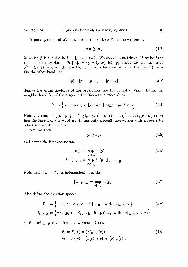
A point p on sheet 7~w of the Riemann surface 7~ can be written as
p = (15, w) (4.2)
in which 15 is a point in C - {Pl , . . . ,Pro}. We choose a metric on 7E which is in the conformality class of ~ [14]. For p = (15, w), let [[P[I denote the distance from pO = (15o, 1), where 1 denotes the null word (the identity in the free group), to p. On the other hand, let
tPl = 1151, IP - Pil = I/5 - Pi[ (4.3)
denote the usual modulus of the projection into the complex plane. Define the neighborhood ~ , of the origin in the Riemann surface ~ by
f~a= {P : IlPlt < a; IP-P i l ' l l og (P-P i ) l 4 < a}. (4.4)
Note that since 1 log(p - Pi)12 = (log IP - Pi[)2 + (arg(p - p~))2 and arg(p - Pi) grows like the length of the word w, ~ has only a small intersection with a sheets for which the word w is long.
Assume that Yo _> aqo (4.5)
and define the function norms
lull,, = sup lu(y) l tYI<Yo
Ilull o,y,,, = sup lu(p,)lyo- ttpH.
(4.6)
Note that if u = u(p) is independent of y, then
IJUlJqo,0,0 : sup [u(p) l. (4.7) pEgtq o
Also define the function spaces
Bv~ = { u : u is analytic in [Yl < Yo, with [u[u o < c~} (4.8)
= {u: u(p,.) E Bvo_~LipL I for p E ~qo with [lUllqo,uo,,~ < co}. 13qo,~o,~
In this setup, p is the time-like variable. Denote
F1 = FI(y) = (f(y),g(y)) (4.9)
F2 = F (p) = Cp( ; ) ,
382 R.E. Caflisch, N. Ercolani and G. Steele Selecta Math.
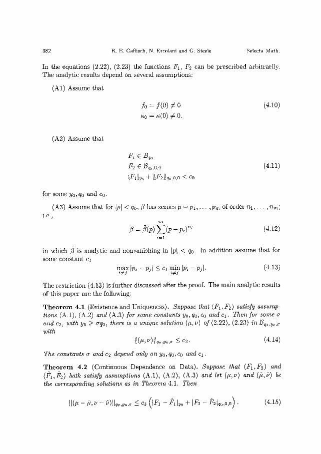
In the equations (2.22), (2.23) the functions F1, F2 can be prescribed arbitrarily. The analytic results depend on several assumptions:
(A1) Assume that
fo = f(0) # 0 (4.10)
'~o = ~(0) ¢ 0.
(A2) Assume that
F1 E By~,
F2 E 13qo,o,o
IF~I~(, + ItF~lt~,,,o,o < co
(4.11)
for some Y0, qo and co.
(A3) Assume that for IP[ < qo,/3 has zeroes p = P t , . . . ,Pro of order n l , . . . , rim; i.e.,
/3 =/3(p) ~ ( p - pi) ~ (4.12) i=1
in which ~ is analytic and nonvanishing in fP[ < qo- In addition assume that. for some constant cl
max [Pi - Pj[ < Cl min [pi - pj[. (4.13) i#j - i#j
The restriction (4.13) is further discussed after tile proof. The main analytic results of this paper are the following:
T h e o r e m 4.1 (Existence and Uniqueness). Suppose that (F1, F2) satisfy assump- tions (A.1), (A.2) and (A.3) for some constants yo,qo,co and cl. Then for some a and c.2~ with Yo >_ ~rqo, there is a unique solution (#, u) of (2.22), (2.23) in 13qo,yo,z with
J](#, U)Nqo,yo,~ <_ c2. (4.14)
The constants a and c2 depend only on yo,qo,co and c1.
T h e o r e m 4.2 (Continuous Dependence on Data). Suppose that (F1,F2) and (F~,F2) both satisfy assumptions (A.1), (A.2), (A.3) and let (#,u) and (/5,~) be the corresponding solutions as in Theorem 4.1. Then
1 t (#- # ,u - u)llq,,,yo,~ <- c3 0F1 -/~llyo + IF2 - P2tqo,O,O). (4.15)
Vol. 2 (1996) Singularities for Steady Boussinesq Equations 383
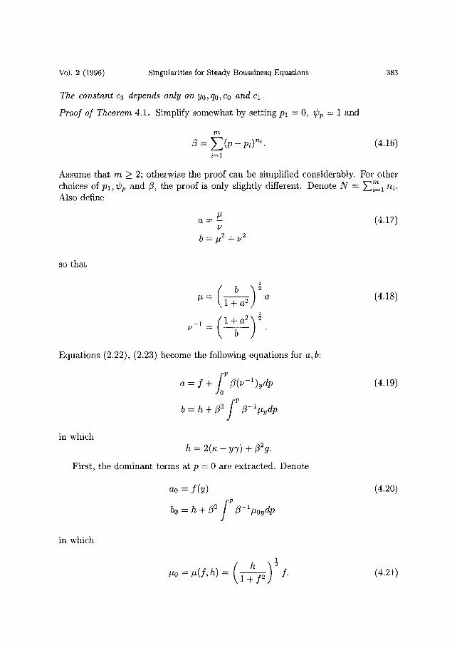
The constant c3 depends only on Yo, qo, co and cl.
Proof of Theorem 4.1. Simplify somewhat by setting Pl = 0, Cp = 1 and
m
= E ( p - pi) n~ . (4.16) i = 1
Assume that m > 2; otherwise the proof can be simplified considerably. For other choices of pl ,¢p and fl, the proof is only slightly different. Denote N = ~ i m l ni. Also define
# a ~ - - - - -
/ /
b = #2 + u2
so that
# = a
u - l = ( l ; a 2 ) ½ _
Equations (2.22), (2.23) become the following equations for a, b:
ff/3( a = f + u -1 )ydp
f b = h + ~2 Z-l t t~d p
in which h = 2 ( ~ - y~) + Z'~g.
First, the dominant terms at p = 0 are extracted. Denote
a0 = f ( v )
bo h +/~2 f P = t3-1#oydp J
in which
1
. o = f.
(4.17)
(4.18)
(4.19)
(4.20)
(4.21)
384 R.E. Caflisch, N. Ercolani and G. Steele Selecta Math.
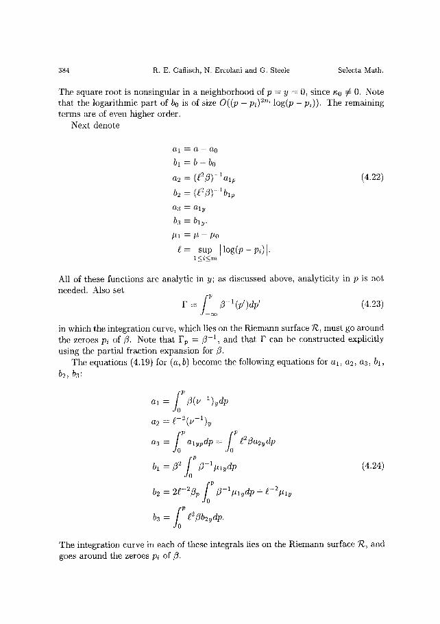
The square root is nonsingular in a neighborhood of p = y = 0, since n0 # 0. Note that the logarithmic part of b0 is of size O ( ( p - pi ) 2'~ log(p - Pi)). The remaining terms are of even higher order.
Next denote
a l = a - ao
bl = b - bo
a2 = ( / ~ 2 / 3 ) - l a l p
b2 = (~2~)-lblp
a3 : a l y
b3 = bly.
[t. 1 : ~ t - - jtt 0
g = sup ] log(p-pd[ . l < i _ < m
(4.22)
All of these functions are analytic in y; as discussed above, analyticity in p is not needed. Also set
p = /3-1(p')dp ' (4.23) oo
in which the integration curve, which lies on the Riemann surface 7~, must go around the zeroes pi of ~ . Note that Fp = / 3 - 1 , and that F can be constructed explicitly using the partial fraction expansion for ,3.
The equations (4.19) for (a, b) become the following equations for al , a2, a3, bl, b2, ha:
~ P5( ) a 1 = l] - 1 y d p
a2 = g--2(y--1)y
a3 = a lypdp = g f la2ydp
bl ~2 fop = fl- lp, lyd p (4.24)
b2 = 2~-2/3. ~-l#lydp + g-21~ly
b3 = g2flb2vdp.
The integration curve in each of these integrals lies on the Riemann surface 7~, and goes around the zeroes pi of ~ .
Vol. 2 (1996) Singularities for Steady Boussinesq Equations 385
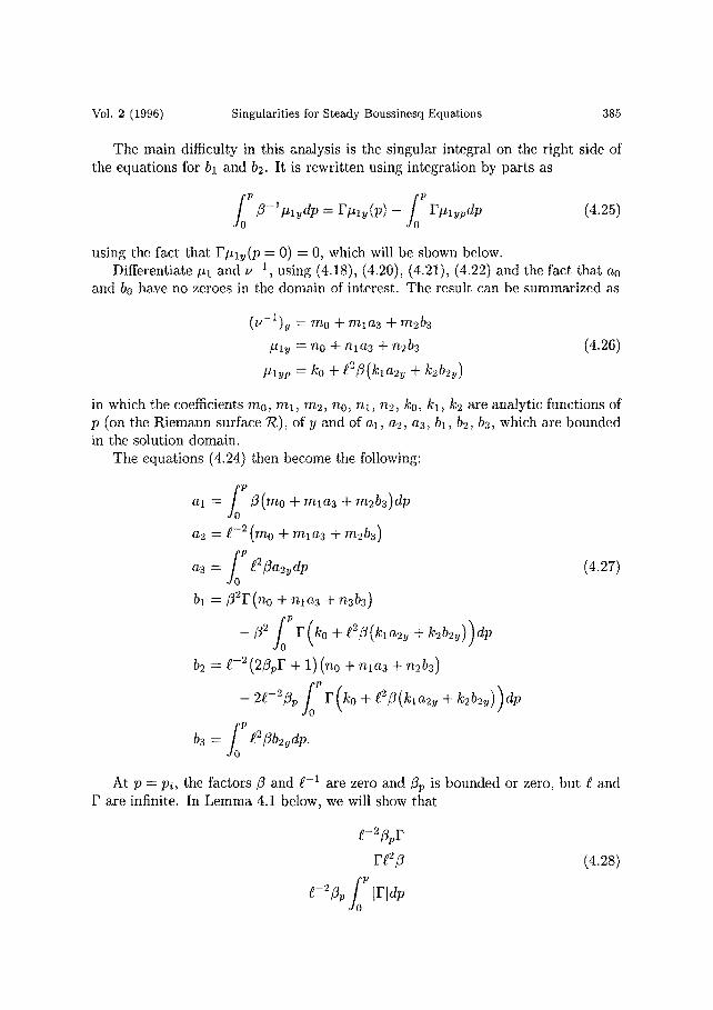
The main difficulty in this analysis is the singular integral on the right side of the equations for bl and b2. It is rewritten using integration by parts as
/o" f[ 3-1# lydp ---- F#ly(P) - F#lypdp (4.25)
using the fact that F#ly(P = 0) = 0, which will be shown below. Differentiate #1 and t, -1, using (4.18), (4.20), (4.21), (4.22) and the fact that a0
and b0 have no zeroes in the domain of interest. The result can be summarized as
(u-1)y = mo + mla3 + m2b3
#ly = no + nla3 + n2b3
]Alyp = ]~0 -Jr e2,1~(kla2y + ]~252y)
(4.26)
in which the coefficients mo, ml, m2, no, nl , n2, ko, kl, k2 are analytic functions of p (on the Riemann surface 7~), of y and of al , a2, a3, bl, b2, b3, which are bounded in the solution domain.
The equations (4.24) then become the following:
~0 p al = /~(rno + rnla3 + m2b3)dp
a2 = ~-2 (rno + mla3 + m2b3)
a3 ---- 2 a2ydp
bl = Z2p(no + nla3 + n3b3)
-/32JooPF(ko+~2~(kla2y +k2b2y))dp
b2 = t~-~ (2~pF + 1)(no + nla3 + n2b3)
2 P k2b2y))dp - 26-' ]3p fo F(ko + ~2j3(kla2y +
b3 = t2 ~b2~dp.
(4.27)
At p = pi, the factors 3 and ~-1 are zero and ~p is bounded or zero, but e and F are infinite. In Lemma 4.1 below, we will show that
e-25pr Ft23
e-~p fop lrldp
(4.28)
386 R . E . Caflisch, N. Ercolani and G. Steele Selecta Math,
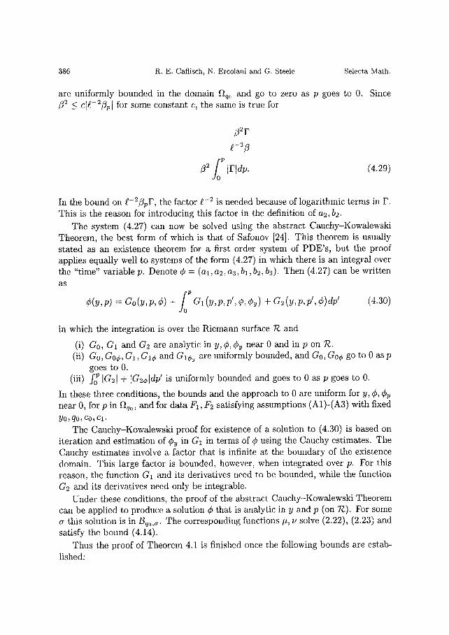
are uniformly bounded in the domain f~qo and go to zero as p goes to 0. Since /32 < c[g-2/3~[ tbr some constant c, the same is true for
/3eP
g-23
3 "2 fov Irldp. (4.29)
In the bound on g-2~pF, the factor g-2 is needed because of logarithmic terms in F. This is the reason for introducing this factor in the definition of a2, b2.
The system (4.27) can now be solved using the abstract Cauchy-Kowalewski Theorem, the best form of which is that of Safonov [24]. This theorem is usually stated as an existence theorem for a first order system of PDE's, but the proof applies equally well to systems of the form (4.27) in which there is an integral over the "time" variable p. Denote ¢ = (al, a2, a3, bl, b2, ba). Then (4.27) can be written as
/0 ¢(y,p) = Go(y,p,¢) + Gl(y,p,p',¢,¢y) +G2(y,p,p',¢)dp' (4.30)
in which the integration is over the Riemann surface 7¢ and
(i) Go, G1 and G2 are analytic in y, ¢, Cv near 0 and in p on 7¢. (ii) Go, Go¢, G1, G1¢ and GI¢,, are uniformly bounded, and Go, Go¢ go to 0 as p
goes to 0. (iii) fo p {G2I + {G2,1dp' is uniformly bounded and goes to 0 as p goes to 0.
In these three conditions, the bounds and the approach to 0 are uniform for y, ¢, Cv near 0, for p in f~qo, and for data F1, F2 satisfying assumptions (A1)-(A3) with fixed yo, qo, co, el.
The Cauchy-Kowalewski proof for existence of a solution to (4.30) is based on iteration and estimation of Cy in G1 in terms of ¢ using the Cauchy estimates. The Cauchy estimates involve a factor that is infinite at the boundary of the existence domain. This large factor is bounded, however, when integrated over p. For this reason, the function G1 and its derivatives need to be bounded, while the function G2 and its derivatives need only be integrable.
Under these conditions, the proof of the abstract Cauchy-Kowalewski Theorem can be applied to produce a solution ¢ that is analytic in y and p (on TO). For some a this solution is in Bq0,#. The corresponding functions p, v solve (2.22), (2.23) and satisfy the bound (4.14).
Thus the proof of Theorem 4.1 is finished once the following bounds are estab- lished:
Vol. 2 (1996)
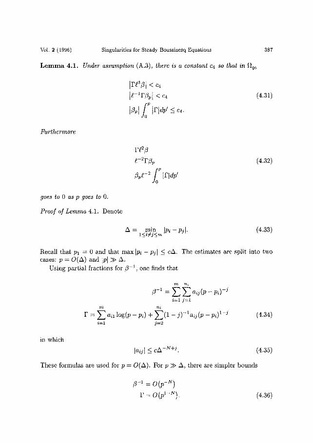
L e m m a 4.1.
Furthermore
goes to 0 as p goes to O.
Proof of Lemma 4.1. Denote
Singularities for Steady Boussinesq Equations
Under assumption (A.3), there is a constant c4 so that in f~qo
]rea3[ < c4
le-lr pl < c4
f [~pl lridp'< c~.
387
(4.31)
re2/3
e-2rgp
9/-2 fo p Irldp'
(4.32)
A = min ]Pi-Pjl. l<_i#j<m (4.33)
Recall that Pl = 0 and that max [Pi - Pj[ < cA. The estimates are split into two cases: p = O(A) and IP[ >> A.
Using partial fractions for/3 -1 , one finds that
n~ n i
~-1 = E E aij(P -- pi) - j i=1 j= l
r = E all log(p - Pi) + E ( 1 - j ) - l a i j ( P - Pi) 1-j i=1 j=2
(4.34)
in which
[aol <_ cA -N+j. (4.35)
These formulas are used for p = O(A). For p >> A there are simpler bounds
=o(p-N) r • O (F1-N). (4.36)
388 R. E. Caflisch, N. Ercolani and G. Steele Selecta Math.
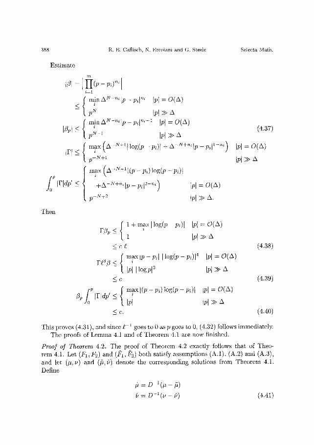
Estimate
i=1
{ ~na~-"~lp-pd'" l;{ = o(A) <-- pN [Pl >> a
{ minAN-'~'lp-pil'~'-~ [p[ = O(A) IGI <
pN-I [p[ )> A
l['I <_ { miax(A-N+iIl°g(P--Pi)] + a-N+"~'Ip-pd'-"' ) p-N+1
p { In~x (A-N+Xl(p--pi)log(p--pi) I
L IrtdP'<- +A-N+n'lP-Pd2-n~) ]P[ = O(A)
p--N+~ Ipl >> A.
(4.37)
IP[ = O(/X)
IPl >> a
Then
1 + max I log(p - Pz)l tPl = O(A) r f l x , _< i
1 tpl >> A
<cg { moxrp-pir I log(p-pdl 4 Ipf = o (A)
- [pl[logpl a Ipl >> A < c
tip [rldp' < - Ipt Ipt >> A <(2.
(4.38)
(4.39)
(4.40)
This proves (4.31), and since 6 -1 goes to 0 as p goes to 0, (4,32) follows immediately. The proofs of Lemma 4.1 and of Theorem 4.1 are now finished.
Proof of Theorem 4.2. The proof of Theorem 4.2 exactly follows that of Theo- rem 4.1. Let (Fl, F2) and (/?1, ~ ) both satisfy assumptions (A.1), (A.2) and (A.3), and let (#,u) and (t~,~) denote the corresponding solutions from Theorem 4.1. Define
/2 = D - l (# - /~)
i, = D-l(u - P) (4.41)
Vol. 2 (1996) Singularities for Steady Boussinesq Equations 389
in which
In the same way, define
D = LF1 - Pll 0 + IF2 - 21 o,o. (4.42)
ai = D - l ( a i - a i )
bi = D - l ( b i - bi)
d~ = D -~ ( a i - d d .
(4.43)
Then the functions Gi satisfy the bounds (i), (ii) and (iii) above. It follows that (#, v) and (/5, P) satisfy the bound (4.15).
No te . (1) Validity of the abstract Cauchy-Kowalewski Theorem without analytic- ity in the "time" variable (p here) was first observed by Nirenberg [20] although it has not been used in an essential way before, to the best of our knowledge. Here p is analytic only on a nontriviat Riemann surface 7~, so that the classical proofs using power series expansions would fail.
(2) Although it is not presented here, further analysis in a neighborhood of P = Pi which is a zero of order n for 3, shows that the solution is analytic in the variables y, p and (p - pi) 2n log(p -P i ) . On the other hand, we have not succeeded in extending this representation to a neighborhood of p containing several zeroes (P l , . . . ,Pro) of order ( n l , . . . ,am) respectively for 3-
(3) The restriction (4.13) on the relative locations of the zeroes Pi for 3 was used to simplify the cancellation between 3 and F in Lemma 4.1. This suffices for the genericity results, but it should be possible to remove the restriction.
5. Legendrian Singularities and Blowup
This section contains a detailed exposition of the key idea introduced in Section 2; namely, the notion of a contact structure for the Boussinesq PDE system and the interpretation of the solution of this system as a constrained Legendrian surface. In previous sections these ideas were introduced as motivation for the transformation of the Boussinesq system into a particularly convenient and elegant form, which reduces the construction and analysis of singular solutions to the study of an integral equation. However, this geometric approach is more than just a convenient device; it clarifies the influence of incompressibility on tile generic singularity type. This understanding enabled us to predict the generic singularity types, which could then be analytically verified.
The first step in a geometric analysis of a PDE system is to consider the graph of a solution as the fundamental object, rather than just the solution function. For the
390 R.E. Caflisch, N. Ercolani and G. Steele Selecta Math.
Boussinesq system, (2.1)-(2.4), the graph of the solution is naturally situated in the large space with coordinates (x, y, u, v, 4, P). Here x = (x, y) are the independent variables and the other variables are dependent, so that the geometric solution is a (2-dimensional) surface, which is a graph over x in this six-dimensional space, if the solution is "classical," i.e., smooth.
Some of the equations in the Boussinesq system have a fundamental geometric character which enables us to reduce the size of this ambient space. In particular equation (2.4), which is the incompressibility condition, implies the existence of a stream function ¢ whose partial derivatives are u and v as described in (2.5). Furthermore, equation (2.1) implies that p is a (arbitrary) function of ¢ as noted in (2.11). Equation (2.3) defines ~ as a second derivative of ¢. This reduction shows that the graph of ~/~ contains all the information needed for the solution of the Boussinesq system.
The notion of a Legendrian surface, which is fundamental to our singularity clas- sification, requires the introduction of a contact structure encoding the differential relation between ¢ and (u, v). Thus, the correct ambient space for our analysis is a space with local coordinates (x, y, u, v, ¢) and the solution surface is the lifting of the graph of ¢ to this space. This space is classically known as the space of 1-jets associated to functions ~b and will be described further below. Tile lifting of the solution surface to this space is called the 1-jet prolongation of the solution surface.
For solution surfaces that are graphs, there are no singularities. The geometric setting just described, however, easily admits generalization of a solution graph to a solution surface which is a smooth surface (not necessarily a graph) in the 1-jet space satisfying the contact constraint. Such a solution may be interpreted as a m u l t i v a l u e d classical solution-classical in the sense that the surface will be assumed to be smooth or even analytic. The Legendrian singularities are the branch curves of these surfaces under projection to x.
In the first subsection below we wilt define all of this precisely and review the standard definition of a Legendrian manifold and a Legendrian singularity. In the second subsection we introduce a directional compactification of the jet space, which extends the theory to singularities at which the velocities, (u, v), blow up. Although this uses standard methods of projectivization, their systematic application to the classification of generic Legendrian blowup as well as to ordinary Legendrian sin- gularities, in the context of solving PDE's, is novel.
5.1 Singularities of Legendrian Mappings
In order to systematically define and analyze m u l t i v a l u e d solutions of the Boussinesq system, it is convenient to rewrite the incompressibility condition in the differential form
d e = u ± • d x (5.1)
in which u -L = ( - v , u).
Vol. 2 (1996) Singularities for Steady Boussinesq Equations 391
This representation of incompressibility has the following interpretation. If F := (x, ¢ (x ) ) denotes the graph of ¢ in C a , then the surface F must satisfy a differential constraint on its tangent planes; namely, that the one-form
c~ = d e - u -k * dx (5.2)
must annihilate the tangent planes to the graph F; i.e.,
OZlTF -- O, (5.3)
where TF denotes the tangent bundle to F. The usefulness of this representation is that a multivalued analytic stream func-
tion may be defined as an analytic surface
s := { ( x , ¢ ) I f ( x , ¢ ) = 0} (5.4)
where f is an analytic function and, most importantly,
c l'rs = O.
The sheets of this surface, under projection onto x,
(5.5)
p: (x, ¢ ) x , (5.6)
then give the branches of the multivalued stream fhnction ¢. More intrinsically a local piece of an odd dimensional complex manifold
equipped with an analytic 1-form c~ satisfying the conditions
1. dot is closed, and 2. dc~l~=o is nondegenerate in each tangent space
is called a local contact manifold. The 1-form is usually called a contact form. In our application the manifold is (25 and the form c~ is defined in (5.2).
In geometric optics there is a concrete realization of a contact manifold which provides some intuition about these structures and is now briefly reviewed. It consists of an n-dimensional observation manifold, ft, parameterized by x = : ( X l , . . . X n ) , on which the rays propagate. /3 = Oft is called the source man- ifold, parameterized by s = ( s l , . . . s ,~ - l ) . The rays emerge perpendicular to /3 pointing into ft. The wavefronts are the level sets of the distance function where distance is measured from the boundary 13. More precisely, let F ( s , x ) denote the distance between a point s on B and x on ft. Then the distance func- tion is
¢ (x ) = local minse t~F(s, x ) . (5.7)
For small values of the distance, ¢ will always be single-valued. On the other hand, for sufficiently large distances ¢ wilt be multivalued generically. Moreover, the
392 R.E. Caflisch, N. Ercolani and G. Steele Selecta Math.
wavefronts, which are the level curves of ~, acquire "wavefront singularities" along the caustics of the rays. We will now reinterpret these familiar constructions from geometric optics in terms of a contact structure, which provides a mathematical definition of wavefront singularity.
To this end we introduce a generating func t ion , F ( s , x ) on B x f~. In the geometric optics model, as mentioned above, F is the distance function. The contact manifold is M = O x C n x C with coordinates ( x , w , ¢ ) and the contact form is a = d e - w • dx . Since da = d x A dw, this two-form is certainly nondegenerate along a = 0. The manifold M in this case is often referred to as the space of 1-jets, denoted by j1 (f~). Two scalar-valued functions F1 and F2 on ft are said to have k th order contact at x E ~ if the Taylor expansions of F1 and F2 at x agree up to order k. Jk(f~)(x,]) denotes the equivalence class of functions F with F ( x ) = f
under the equivalence relation of k th order contact. In this way j k (f~) is naturally a bundle over or°([~) ( = f~ x (2). The bundle projection p : j l (f~) ~ jo( f t ) amounts to forgetting the first derivative in the tile first order Taylor polynomial. Thus p is just the map p ( x , w , ~ ) = (x , ~) .
An n-dimensional submanifold £ of M is called Legendrian if alTO -- O. The generating function F ( s , x ) generates a Legendrian submanifold of the form
£ = { (x , w , ~ ) c M I O F / O s = 0 ;
w = OF/Ox;
¢ = f (s , x) }.
(5.s)
In the geometric optics context, /: is the "manifold of phases" for the wavefronts; the first condition says that the rays are perpendicular to the boundary, B, while the phase vector w is normal to the wavefronts. In this optical model alTL = d e - w • d x = d F - O F / O x • d x ~- 0 by the chain rule. Hence £ is manifestly Legendrian.
A Legendrian project ion P : M -~ N , where N is an (n+l)-dimensional mani- fold, is a submersion 1 whose fibers, p - 1 (Tj) for 7 7 C N, are Legendrian submanifolds of M. In the geometric optics model, the projection map p : j1 (~) _+ j0 (~) de- scribed above and defined by p ( x , w , ¢) = (x, ¢) is Legendrian because the fibers are defined by x = constant and ~ = constant so that a vanishes identically.
A Legendrian mapping is the restriction of a Legendrian projection to a Legen- drian manifold £. In geometric optics, Legendrian mappings arise as the projection of the maniibid of phases onto the (possibly multivalued) graph, F, of the stream function ~ in t2 x C.
1 A submersion is a mapping whose derivative at each point is surjective,
Vol. 2 (1996) Singularities for Steady Boussinesq Equations 393
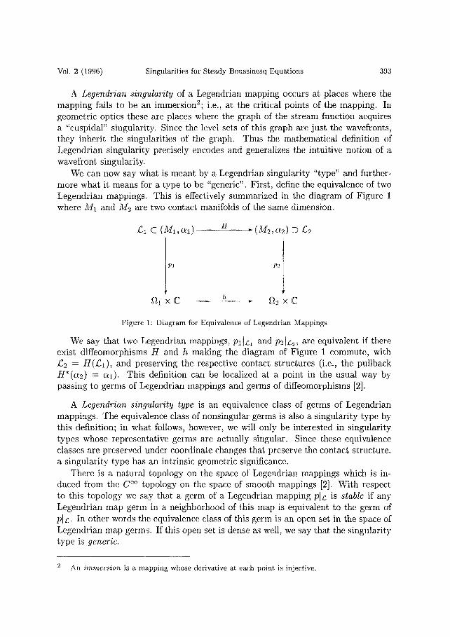
A Legendrian singularity of a Legendrian mapping occurs at places where the mapping fails to be an immersion2; i.e., at the critical points of the mapping. In geometric optics these are places where the graph of the stream function acquires a "cuspidal" singularity. Since the level sets of this graph are just the wavefronts, they inherit the singularities of the graph. Thus the mathematical definition of Legendrian singularity precisely encodes and generalizes the intuitive notion of a wavefront singularity.
We can now say what is meant by a Legendrian singularity "type" and further- more what it means for a type to be "generic". First, define the equivalence of two Legendrian mappings. This is effectively summarized in the diagram of Figure 1 where M1. and M2 are two contact manifolds of the same dimension.
£1 c (M1, al)
~-'~1 X C
H . (M2, a2) ~ £2
P2
" •2 × C
Figure 1: Diagram for Equivalence of Legendrian Mappings
We say that two Legendrian mappings, PilL1 and P2I£:2, are equivalent if there exist diffeomorphisms H and h making the diagram of Figure 1 commute, with £2 = H(£1), and preserving the respective contact structures (i.e., the pullback H*(a2) = a]). This definition can be localized at a point in the usual way by passing to germs of Legendrian mappings and germs of diffeomorphisms [2].
A Legendrian singularity type is an equivalence class of germs of Legendrian mappings. The equivalence class of nonsingular germs is also a singularity type by this definition; in what follows, however, we will only be interested in singularity types whose representative germs are actually singular. Since these equivalence classes are preserved under coordinate changes that preserve the contact structure, a singularity type has an intrinsic geometric significance.
There is a natural topology on the space of Legendrian mappings which is in- duced from the C °° topology on the space of smooth mappings [2]. With respect to this topology we say that a germ of a Legendrian mapping PlL is stable if any Legendrian map germ in a neighborhood of this map is equivalent to the germ of Pin. In other words the equivalence class of this germ is an open set in the space of Legendrian map germs. If this open set is dense as well, we say that the singularity type is generic.
2 An immers ion is a mapping whose derivative at each point is injective.
394 R.E. Caflisch, N. Ercolani and G. Steele Selecta Math.
Although it would appear that the classification problem for Legendrian singu- larities is quite complicated because of all the structures involved, there are ways to reduce it to a tractable singularity calculation. This is particularly true for the following example:
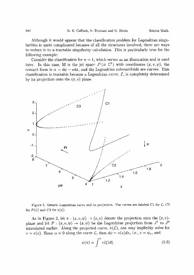
Consider the classification for n = 1, which serves as an illustration and is used later. In this case, M is the jet space j l ( = C3) with coordinates (x, v, ¢) , the contact form is a = d e - v d x , and the Legendrian submanifolds are curves. This classification is tractable because a Legendrian curve, £, is completely determined by its projection onto the (x, v) plane.
3-.
0
-1
-2 8
° - - °
- ' " C1
t"
Pi l P
: . *
: .-")2 2 - ~ 18
5 ~ 1.4
psi 4 1 x
Figure 2. Generic Legendrian curve and its projection. The curves are labeled C1 for E, C2 for P(E) and C3 for ~r(/:).
As in Figure 2, let w : (x, v, ¢) ~ (x, v) denote the projection onto the (x, v)- plane and let P : ( x , v , ¢ ) --> (x, ¢) be the Legendrian projection from j1 to j0 introduced earlier. Along the projected curve, Ir(£), one may implicitly solve for v = v ( x ) . Since a = 0 along the curve L:, then d e = v ( x ) d x , i.e., v = Cx, and
Y = (5.9)
Vol. 2 (1996) Singularities for Steady Boussinesq Equations 395
Thus the curve £ is parameterized by x as (x, v(x), ¢(x)). Notice that if the mapping from 7r(/2) to the x-axis given by (x, v(x)) -4 x is
nonsingular at a point, then the map P :/2 -4 j0 is nonsingular at the corresponding point. This is a consequence of (5.9). Moreover, the singularities of the Legendrian mapping P from £ to the (x, ¢) plane are in one-to-one correspondence with the singularities of the projection from lr(Z;) to the x-axis. But singularities of this latter projection are in 1 : 1 correspondence with critical points of the "inverse" function x(v). We know from Morse theory [19] that the generic critical points of scalar functions are just the simple critical points; i.e., dx/dv = 0 but d2x/dv 2 ¢ O. Any higher order critical point breaks up into several simple points under an arbitrarily small perturbation of x(v). Moreover, it is straightforward to show that there is a local change of variables such that this function has the normal form x(v) = v 2. Therefore generic singularities have the normal form v(x) = x 1/2 and, by (5.9), ¢(x) = ~x 3/2. Thus the image of a Legendrian curve in the (x,¢) plane in the vicinity of a generic singularity has the form of a simple isolated cusp.
5.2 L e g e n d r i a n B l o w u p
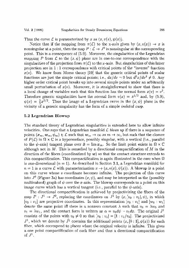
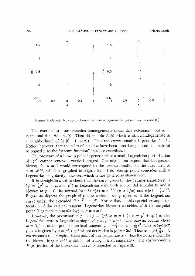
The standard theory of Legendrian singularities is extended here to allow infinite velocities. One says that a Legendrian manifold £ blows up if there is a sequence of points (xm, win, era) E L; such that Wm --+ ec as m --+ co, but such that the closure of P(£) in f~ x C is a hypersurface, possibly singular, with a vertical (i.e., parallel to the C-axis) tangent plane over 5~ = lim xm. So the limit point exists in f~ x C although not in M. This is remedied by a directional compactification of M in the direction of the fibers (coordinatized by w) so that the contact structure extends to this compactification. This compactification is again illustrated in the case when f~ is one-dimensional (n = 1). As described in Section 3.1, a Legendrian manifold for n = 1 is a curve Z; with parameterization x ~ (x, v(x), ¢(x)). A blowup is a point on this curve whose v-coordinate becomes infinite. The projection of this curve into jo (Figure 3a) has coordinates (x, ¢), and may be interpreted as the (possibly multivalued) graph of ~b over the x-axis. The blowup corresponds to a point on this image curve which has a vertical tangent (i.e., parallel to the C-axis).
The directional compactification is achieved by projectivizing the fibers of the map P : j1 ~ j o replacing the coordinates on j t by (x,[vo : vi] ,¢) , in which [v0 : vl] are projective coordinates. In this representation [v0 : vl] and [w0 : Wl] denote the same point iff there is a nonzero constant A such that v0 = Aw0 and vl = Awl, and the contact form is written as a = vod¢ - vldx. The original j1 consists of the points with v o ¢ 0 so that [vo : vl] = [1 : vl/vo]. The projectivized j1, which we denote by j1 contains the additional points (2, [0: 1],¢(2)) for each fiber, which correspond to places where the original velocity is infinite. This gives a one point compactification of each fiber and thus a directional compactification of j1.
396
1.5 i
~ 0.5 ¸
Oi
-0 .5 i -1 -0 .5
R. E. Caflisch, N. Ercolani and G. Steele
a
Selecta Math.
~ 0.5
o
L
.0,5 i -1
b 1.5 I ,
i' , i 1
i 1!
0 1 -0.5 X
. . . . i
0.5 0 0,5 1 X
Figure 3. Generic blowup for Legendrian curve: symmetric (a) and asymmetric (b).
The contact structure remains nondegenerate under this extension. Set w = vo/vl and d~ = dx - wd~b. Then d& = - d w A d~ which is still nondegenerate in
a neighborhood of (2,[0 : 1],~b(2)). Thus the curve remains Legendrian in j l . Notice, however, that the roles of x and ¢ have been interchanged and it is natural to regard x as the "stream function" in these coordinates.
The presence of a blowup point is generic since a small Legendrian perturbation of 7r(L:) cannot remove a vertical tangent. One might first expect that the generic blowup for n = 1 would correspond to the inverse function of the cusp, i.e., to x = ~p3/2, which is graphed in Figure 3a. This blowup point coincides with a Legendrian singularity, however, which is not generic as shown next.
It is straightforward to check that the curve given by the parameterization p -~ ( ¢ = 3 ,~ ~p ,w = p ,x = p3) is Legendrian with both a cuspidal singularity and a
blowup at p 0. Its normal form is v(x) = x -1/3 (v = i / w ) and ¢(x) = 3_~,2/3 Figure 3a depicts the graph of this ¢ which is the projection of the Legendrian curve under the extended P : 3:1 ~ dO. Notice that in this special example the location of the vertical tangent (Legendrian blowup) coincides with the cuspidal point (Legendrian singularity) at p = x = 0.
However, the perturbation p ~ (~ = 3 2 2 p3 7p ,w = p + 5e, x = +ep2) is also Legendrian with a Legendrian singularity at p = x = 0. The blowup occurs where w = 0, i.e., at the point of vertical tangent, p = - ~ e or z = ~ e 3. The projection p --~ x is given by x = p3 + ep~ whose derivative is p(3p + 2e). Thus w = p + ~c = 0 corresponds to a simple critical point of this projection and thus the normal form for the blowup is ~ = x 1/2 which is not a Legendrian singularity. The corresponding P-projection of the Legendrian curve is depicted in Figure 3b.
Vol, 2 (1996) Singularities for Steady Boussinesq Equations 397
So generically a blowup does not coincide with a singularity. However, if there is an additional symmetry imposed on the system, a blowup may be forced to coincide with a Legendrian singularity.
We summarize the results of this section in the following:
P r o p o s i t i o n 5.1. The generic type of a codimension one Legendrian singularity is
¢(x) =
The generic type of a codimension one Legendrian blowup is
= 1112
Proof. The normal form for generic codimension 1 Legendrian singularities was explained at the end of Section 3.1. The normal form for a generic Legendrian blowup may be established along similar lines. First, suppose that the blowup has the form ¢ ( x ) = x~ 12 or xl = ¢2, which corresponds to a curve £ in ]1 for which 7r(/2) has the form wl = 2¢. In order to preserve blowup we only consider perturbations of this curve which continue to pass through the origin Wl = ¢ = 0. Under small perturbations of this type, the curve continues to be locally linear to leading order; i.e., of the form wl = 2(1 + e)¢. Thus, the corresponding curve in j0 will be of the form xl - c = (1 + e)¢ 2 (c is a constant of integration) which is of the same type as the original curve with a vertical tangent located at xl = c. Thus, this type of blowup is stable. On the other hand, any more complicated normal form corresponds to a coincidence of a vertical tangent with a Legendrian singularity. By the first part of this proposition, we may assume that this singularity is equivalent to one of the form ¢(x) = 3_213 7~ , since otherwise a perturbation will break it up into singularities of this type. However, as was demonstrated in the paragraphs preceding the proposition, further perturbation splits the singularity from the blowup, leaving a blowup point with the stated normal form.
6. N u m e r i c a l M e t h o d
This section presents a numerical method for construction of a particular class of solutions to the system
~yp~ - ¢~p~ = 0 (6.1)
Cv~x - Cx(y - Px = 0 (6.2)
-(+ A¢ = 0 (6.3)
with boundary conditions given by
¢(x, +1) =0 (6.4)
¢(x , y) = ¢ ( x + 2~, y) (6.5)
p(~, y) =p(~ + 2~, y). (6.6)
398 R . E . Caflisch, N. Ercolani and G. Steele Selecta Math.
Condition (6.4) states that on the boundary y = =t=1 the normal component of the velocity is 0 and that the total flow in the x direction is 0. After the solution is computed, we then deduce singularity properties (i.e., type and location) via analysis of the Fourier spectrum in x.
6.1 Upper Analytic Solutions
We compute solutions to (6.1), (6.2) and (6.3) which are analytic for Im(x) > 0, and thus can be expanded in a Fourier series in x as
f(x, y) = ~ ]k(y)e ikx, (6.7) k>O
The aim here is to numerically construct steady Boussinesq solutions having sin- gularities of the type derived above. As we argue below, such singularities are observed in a wide range of numerical solutions, at least for the symmetric case. Thus, the computational results provide numerical affirmation for the genericity of these singularities, which has already been established analytically. They also show that there are no global constraints for Boussinesq solutions that are missing from our local singularity analysis.
Upper analyticity may seem to be an overly restrictive assumption, especially in light of our goal to investigate generic singularities. Note, however, that the upper analyticity of a function is a property of an infinite number of its Taylor coefficients. Singularity type, on the other hand, depends on only a finite number of Taylor coefficients; i.e., it is a more local property than is analyticity. Thus we expect that restriction to upper analyticity does not alter the generic singularity type, although we have no proof of this. This expectation has been partially verified since singularity types (ii) and (iii) have been found numerically, as described below. Type (i) has not yet been observed rmmerically.
Introducing upper analytic functions of the form (6.7) in (6.1), (6.2) and (6.3) leads to the following equation for the Fourier coefficients:
(6 .8 )
ik¢k ff--~¢o -ik@k ff~j@ -ikpk = Bk (6.9)
d 2 ^ + - k 2 ¢ k = 0 ( 6 . 1 0 ) ay ~
or equivalently
Vol. 2 (1996) Singularities for Steady Boussinesq Equations 399
in which
) d 2 ^ dy k 2 d-~12"¢k(Y) - + - - + ~k(Y) = Ck (6.11) /dd@ 0 de0 2
dy
ikpk ¢o -- ikCk ~yPO = Ak (6.12)
ik¢k ¢ ¢ 0 - ikCk d ~o - ikpk = Bk (6.13) dy ay
k-1
A k = E i ( k - - I ) [ ~ k - l j ~ D l - - P k - l J ~ ' ~ l ] l=l
ek= Zg(k-t) /=1
Bk Ak Ck= +
ik dd@ ik d¢, o 2" ay
(6.14)
(6.15)
(6.16)
^ ^
It should be noted that the Ak and Bk depend on Ck' ,Pk' and (k' only for k' < k. This system has several important features. First, the nonlinear boundary value
problem (6.1), (6.2) and (6.3) has been reduced to a series of linear two-point boundary value problems in y for the Fourier coefficients. Second, since the com- putation of mode k depends on only modes k' with M < k, the system is lower triangular. Therefore no truncation error is introduced by tile restriction to a finite set of wavenumbers. Finally, since the calculations are performed entirely in wave space, no aliasing error occurs.
The computation is started by specification of the zero mode (P0, ¢0, ~0) of the solution. Then the equation for the first mode (ill, ¢1, ¢1) is an eigenfunction prob- lem. Once these two modes are determined, the remaining modes can be computed by solution of equations (6.8), (6.9) and (6.10). These equations are nonsingular as long as no resonance occurs, and none was found in any of the computations.
6.2 D e t e r m i n a t i o n of the Zero o rde r M o d e
In order to construct solutions to (6.8), (6.9) and (6.10) we need to specify the zero order modes of the Fourier expansion. We select these coefficients in the form
Po =Po(Y) (6.17)
¢ o = - ( 6 . 1 8 )
(~o =0. (6.19)
400 R . E . Caflisch, N. Ercolani and G. Steele Selecta Math.
Equation (6.17) means that the density is stratified in y. Equation (6.18) gives a constant velocity in the x direction.
The equation for ~1 is
dy 2"~bl + ~2.)Po - 1 Y)l = 0 (6.20)
~ 1 ( i l ) = O. (6.21)
We can solve (6.20) either by specifying Po and solving the eigenvalue problem or by specifying ~1 and solving for Po. The latter is in general much simpler and is the approach that we took.
The specification of ¢1 is performed in several steps: First, we determine a preliminary cho ice ~¢~1 = ~/~10 for the extreme case in which the density P0 is a Heaviside function. Then, this extreme Inode, which is discontinuous, is smoothed out to obtain the useable mode ¢i . The smoothing is performed using a function ¢ defined below. Finally, the choice of ¢, and thus of ¢~, is made in two ways. The first, described in Section 6.2.1, is symmetric with respect to y and the second, in Section 6.2.2, is asymmetric.
If the density Po is a Heaviside function H(y), then equations (6.20) and (6.21) for @1 ~o become "~- 1
d (a(y) 1) o=0 (6.22)
= 0
in which 5(y) = -~y'dH Solutions to (6.22) are given by
s i n h ( y - 1) 0 <_ y <_ 1 (6.23) ~O(y) = C _ s i n h ( y + l ) - l _ < y _ < 0
a2 = tanh(1) 2
To obtain smooth data, we construct a smooth transition function ¢ = ¢(y) such that
¢(1) = 1
¢ ( - 1 ) = - 1 (6.24)
and smooth out ~,o as
C t = (¢+----~l)s inh(y-1)
Vol. 2 (1996) Singularities for Steady Boussinesq Equations
In terms of ¢, and thus of ¢1, we can then solve for P0 from
~ 0 = ~2 1- ~ , / .
The conditions ¢ ' ( + 1 ) = ¢ " ( ~ 1 ) = 0
are imposed in order that the limits at =t=1 in (6.26) make sense.
401
(6.26)
(6.27)
3 cl d (6.29)
c2 = 3 ( f " ( 1 ) - 2f '(1)) (6.30)
e3 = ~-~f"(1) (6.31)
in which f (y) = tanh(}) and d = 3f(1) - 3f'(1) + f"(1) . The parameter A is a constant which controls the thickness of the smoothed out Heaviside function.
The resulting solution has the symmetry
¢(-x , -y) = ¢(~, y) (6.32)
which implies that ¢ ( - x ) = ¢(.~) for y = 0. This is the symmetry condition employed in Theorem 3.2. Note however that the solutions here violate the real analyticity condition of Theorem 3.2.
6.2.2 A s y m m e t r i c . The discontinuous solution (6.23) is symmetric in y. This symmetry may be broken by choosing an asymmetric transition function ¢ of the form
) - (co + e l ( y - 1) + c2(y - 1) 2 + c 3 ( y - 1) 3 + c 4 ( y - 1)4), (6.33)
(6.28)
Choose the ci so that ¢ satisfies (6.24), (6.27); i.e.,
6.2.1 S y m m e t r i c . For the symmetric case, we specify a ¢ which maintains the symmetry of the solutions (6.23). We shall use the choice
402 R. E. Caflisch, N. Ercolani and G. Steele Selecta Math.
in which
Co = 1 + c s f ( - 1 )
cl = c 5 f ' ( - 1 )
1 " 1 c2 =-~csf (-) c5 [ ] c3 = - 1 + ~-~ (2f - if)(1) - ( 2 / + 3f ' + 2 f " ) ( - 1 )
1 1 (:"(1)- f"(-1))c5-~c3 C4~--- ~
C5 = 6 [ ( 3 ( f - f ' ) + f " ) ( 1 ) - (3(f + f ' ) + f")(--1)] -1
(6.34)
in which f(y) = tanh((~(~) 2 + (})3). This choice of the ci's insures that the con- ditions (6.24), (6.27) on ¢ and its derivatives are satisfied. The parameters (~ and A control the amount of asymmetry and the sharpness of the approximation to the Heaviside function, respectively.
6.3 Descr ipt ion of Numerical Method
The two-point boundary value problems are solved using a centered fourth-order finite difference scheme. The boundary conditions are handled by using an unbal- anced fourth order scheme at the endpoints. The resulting system was solved by direct Gaussian elimination at the ends, followed by application of the banded solver DGBSL from SLATEC.
Round-off error grows with the wave number, and could eventually destroy the calculation. Although the mechanism which causes this growth is not fully under- stood, it is controlled by the use of high precision calculations. We utilized MPFUN, a multiprecision package developed by David Bailey at NASA [4], [3]. Precision levels of 128 and 200 digits were used in the calculations. The computations were run on a Sun SparcServer 1000.
6.4 Numerical Detect ion of Singularities
The presence and type of singularities was deduced through a numerical analysis of the Fourier coefficients of the computed solution.
6.4.1 Analysis of Fourier Coefficients at Singularity. Consider a function f : C -~ C that can be represented in a neighborhood of x , as
oo
f ( x ) : ( x - -
p = 0
(6.35)
Vol. 2 (1996) Singularities for Steady Boussinesq Equations 403
The summation is assumed to represent a function that is analytic in some neighbor- hood of x. . Under these assumptions, the Fourier coefficients of f are asymptotic t o
]k "~ bk a e- ikx*
Details of this result can be found in [13]. Writing out am b and x, as
; k--+ ~ . (6.36)
(6.36) becomes
a = al + ia2
b = bl exp( ib2)
x . -~ --r2 + irl~
(6.37)
]k ~ b lk at e k~l exp ( ikr2 + ia2 log k + ib2) ; k -~ cx~. (6.38)
In the procedure outlined in Section 6.2, ¢1 is chosen to be real analytic, which leads to
~k (Y) = i k-1 t)k (Y), (6.39)
in which the Oh (Y) are real analytic. This form of the Fourier coefficients corresponds to the following symmetry in x:
7f 7f + ( 40)
in which * denotes complex conjugation. This symmetry causes the singularities to occur in pairs. The asymptotics of the Fourier coefficients of ¢ are then
~ k ~ b l k a l e k ~ l s i n ( k r 2 + a 2 1 o g k + b 2 ) ; k - + c ~ . (6.41)
The Fourier coefficients for p and ~ have a similar form.
6.4.2 Sl id ing P a r a m e t e r F i t . To obtain the values of the parameters in (6.41) we perform a sliding six-parameter fit of the Fourier coefficients. Each parameter fit is performed for every fixed value of y as follows:
At each k, we exactly fit the form in (6.41) to the values of the data at k, k + 1 , . . . , k + 5, using the SLATEC package DNSQE. A fit is deemed successful if the values of the parameters are (approximately) independent of k.
7. C o m p u t a t i o n a l R e s u l t s
The computations were performed for 3200 and 6400 points in y. The precision used was 128 and 200 digits respectively. The parameter A, which controls the sharpness of the approximation to the Heaviside function, was equal to ½ in both the symmetric and asymmetric cases.
404 R.E. Caflisch, N. Ercolani and G. Steele Selecta Math.
7.1 S y m m e t r i c
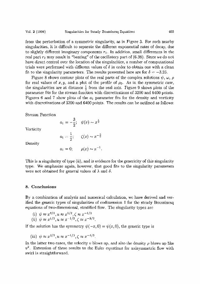
The computational results and the singularity fits are very precise and clean in the symmetric case. Figure 4 shows contour plots of the real parts of the complex solutions on ~/~, w and p for real values of x and y, and a plot of the profile of P0. For each value of y, there is a singularity at some complex value of x. In this solution the closest singularities are at distance ½ from the real axis, and the real parts of the singularity positions x, y are approximately at the centers of the rolls shown in Figure 4. Note, however, that the solution can be given an arbitrary shift in x, so
1 of a solution with singularities that this could also be a plot for x with Ira(x) = located on the real axis.
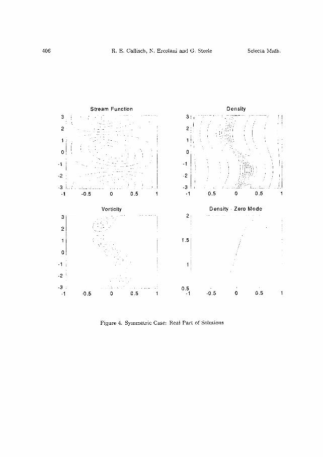
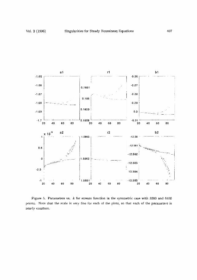
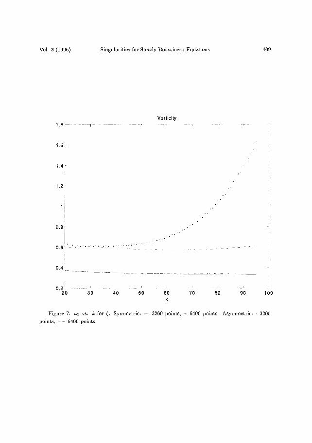
Figure 5 shows plots of the parameter fits for the stream function with dis- cretizations of 3200 and 6400 points. The parameter as is of main interest because it determines singularity type. Figures (6), (7) show plots of the al parameter fits for the density and vorticity with discretizations of 3200 and 6400 points. The results are as follows:
Stream Function
Vorticity
Density
5 2
1 4
a 1 = 5 ;
1 al = - 5 ; p(x) -
This is a singulm'ity of type (iii). Note that the vorticity ~, the density p and the velocity v = •x all blow up at the singularity, and that p = O(v2).
While these results were for A = t /3 , other values of ,~ gave similar results with the same values of al , i.e., with the same singularity type. This is numerical evidence for the genericity of singularity type (iii) in the symmetric case.
As pointed out earlier, the solutions here violate the real analyticity condition of Theorem 3.2. Although the numerical results seem to indicate that the type (iii) singularity is still generic for the complex solutions here, we have been unable to prove it.
7.2 A s y m m e t r i c
The numerical detection of singularity properties in the asymmetric case is not as straightforward as in the symmetric case. Although the full reasons for this difficulty are not very clear, we believe that it is partly because singularities come in pairs that are very close together, for small asymmetry parameter 6, since they come
Vol. 2 (1996) Singularities for Steady Boussinesq Equations 405
from the perturbation of a symmetric singularity, as in Figure 3. For such nearby singularities, it is difficult to separate the different exponential rates of decay, due to slightly different imaginary components r l . In addition, small differences in the real part r2 may result in "beating" of the oscillatory part of (6.38). Since we do not have direct control over the location of the singularities, a number of computational trials were performed with different values of ~ in order to obtain one with a clean fit to the singularity parameters. The results presented here are for 5 = -3.25.
Figure 8 shows contour plots of the real parts of the complex solutions ¢, ~, p for real values of x, y, and a plot of the profile of p0- As in the symmetric case,
1 from the real axis. Figure 9 shows plots of the the singularities are at distance parameter fits for the stream function with discretizations of 3200 and 6400 points. Figures 6 and 7 show plots of the al parameter fits for the density and vorticity with discretizations of 3200 and 6400 points. The results can be outlined as follows:
Stream Function
Vorticity
Density
1
al ~ ; 3
al = 0; p(x) ... x -1 .
This is a singularity of type (ii), and is evidence for the genericity of this singularity type. We emphasize again, however, that good fits to the singularity parameters were not obtained for general values of A and 5.
8. C o n c l u s i o n s
By a combination of analysis and numerical calculation, we have derived and ver- ified the generic types of singularities of codimension 1 for the steady Boussinesq equations of two-dimensional, stratified flow. The singularity types are
(i) ~D ~ x 3 /2 , u ~, x 1/2, ~ ~, x - 1 / 2
(ii) ~b ~ x l / 2 , u ~ x - 1 / 2 , ~ ~ x -3/2.
If tim solution has the symmetry ¢ ( - x , 0 ) = ¢(x, 0), the generic type is
(iii) ¢ ~ x'2/3,u ..~ x - 1 / 3 , ~ ~ x -4/3.
In the latter two cases, the velocity v blows up, and also the density p blows up like v 2. Extension of these results to the Euler equations for axisymmetric flow with swirl is straightforward.
406 R. E. Caflisch, N. Ercolani and G. Steele Selecta Math.
Stream Function
t
0
-2
~ 3 . . . . . . . .
-1 -0.5 0 0.5 1
Vorticity
3 ~ .. . . . . . . i ,i i : :~ / . . . . . . . . . . .
0 . . . . . .
- 3 . . . . . . . . . . . . . . . . . . . . . . . . . . . . . . . . . . . . . . . . . . . . . . . . . . . . . . . . . . . . . . . . . . . . . . . . . . . . . . .
-1 -0.5 0 0.5
Density
3 r i . . . . . . . . ~i-~-i:i:~i . . . . . . . . . . :' I
2 ] ::::~::( " , , ,,,:c,!{ ¢ ( , " ' , i ' i 1 i {:' ' :
0j I '
/ J j , :: ,
-1 -0.5 0 0.5 1
1,5
Density - Zero Mode . . . . r . . . . . . . .
/'
f
0.5 -0.5 0 0.5
Figure 4. Symmetric Case: Real Part of Solutions
Vol. 2 (1996) Singularities for Steady Boussinesq Equations 407
-1.65
- I .66
-t .67
- I .68
- 1 . 6 9
-1.7 2O
a l r l
. . . . . . . . . . . . . . . . . . . . . . . . . . . . . . 0 , 1 8 6 1 ~ . . . . . . . . . . . . . . . . . . . . . . . . . . . . . . .
: I•- •- -=
- i 0 " 1 8 6 r " - . . . . . .
. . . . . . . . . . . . . . . . . . : : 11°"85 i F
. . . . . . . . . . . . . . . . 0.1858 L . . . . . . . . . . . . . . . . . . . . .
40 60 80 20 40 60 80
-0,26
-0.27
-0.28
-0.29
-0.3
-0.31 2O
X 1 0 .3 a2
1 . . . . . . . . . . . . . . . . . . . . . . . 1.5863
0.5
-0.5
- :-: . . . . . . . . . . . . ~ ~ 1 , 5 8 6 2
r2
J ! i
- 1 2 . 8 8 [
- 1 2 , 5 8 1
b l
-12.582 I
-12.583;
I i -12.584
1~5861 . . . . . . . . . . . . . . -12.585 20 40 60 80 20
40 60 80
b2
2 0 4 0 6 0 8 0 4 0 6 0 8 0
Figure 5. Parameters vs. k for stream function in the symmetric case with 3200 and 6400
points. Note that the scale is very fine for each of the plots, so that each of the parameters is
nearly constant.
408 R. E. Caflisch, N. Ercolani and G. Steele Selecta Math.
Density 1 . . . . . . . l . . . . . . . i . . . . . . I . . . . [ . . . . . . . ; . . . . . . . . . F . . . . . . . . . . . . . .
0.8
0.6
0.4[
0.2i . . " " "
. . . . . . . . . . . . . . . . . . . •
i
- 0 . 2
°
_ 0 . 4 i . . . . . . . . ~ . . . . . . . . . : . . . . . . . . . . . . . . . . . ~ . . . . . . . . . . : . . . . . . . . . . : . . . . . . . . 2 0 3 0 4 0 5 0 6 0 7 0 8 0 9 0 1 0 0
k
Figure 6. ai vs. k for p. Symmetric: - - 3200 points, - 6400 points. Asymmetr ic case: - 3200
points, - - 6400 points.
Vol . 2 ( 1 9 9 6 ) S i n g u l a r i t i e s f o r S t e a d y B o u s s i n e s q E q u a t i o n s 4 0 9
Vorticity 1 . 8 ~ . . . . . . . . r . . . . . . . . . . . . . . . . ~ . . . . . . . . . . . . . . . . ~ ~ . . . . . . . . . T
I I
1 . 4 1
1.2
! . o
. o
o
" I
I i
. o f
° °
0.81
/
J
0.4 r
i
0 . 2 ............ ~ ......... ~ ........... ~ ~ ...... ~ . . . . . ~- 20 30 40 50 60 70 80
k
I
90 100
F i g u r e 7. a ] v s . k f o r ~. S y m m e t r i c : - - 3 2 0 0 p o i n t s , - 6 4 0 0 p o i n t s . A s y m m e t r i c : - 3 2 0 0
p o i n t s , - - 6 4 0 0 p o i n t s .
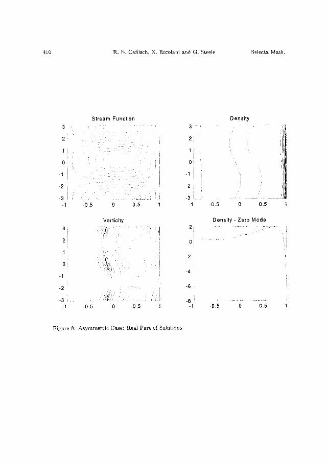
410 R, E. Cafiiseh, N. Ercolani and G. Steele Selecta Math .
3
2
1
0
-1
-2
-3 -1
3 4 ` ¸ ¸
2
t
0
-1
-2
- 3 .
-1
St ream Funct ion
-0.5 0 0,5
Vort ic i ty i
.... /::i?i~: ' : ' . . . . . / i /1
i F
i
-0.5 0 0,5
I
1
3~
21 '
1
0
-1
-2 i
-1
2~
I °l . 2 ¸
- 4 !
- 6
- 8 -1
Dens i ty
I
-0.5 0 0.5 1
Densi ty - Zero Mode
:i!
i!
-0.5 0 0.5
Figure 8. A s y m m e t r i c Case: Real P a r t of Solutions.
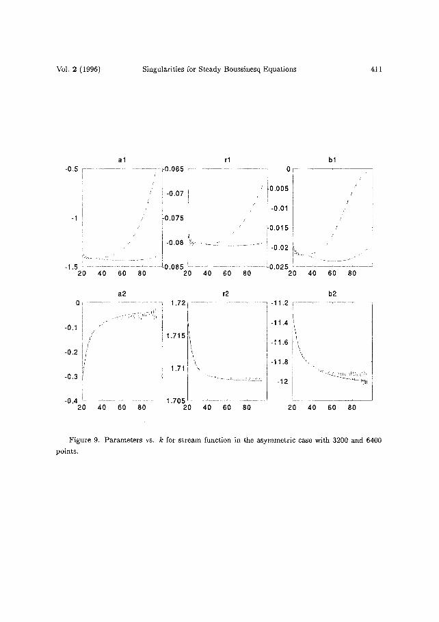
Vol. 2 (1996) Singularities for Steady Boussinesq Equations 411
a l -o.5 . . . . . . . . . . . . . . . . . . . . . . . . . . . . --- o.o65
/
/
/
/
J
-0.07
-1 !0,075
F
I - 0 , 0 8 !
- 1 , 5 . . . . . . . . . . . . . . . . . . . . . . . . . . . . . . . . . . L0,085 2O 40 6O 8O
r l b l
! /
f0,005 /
E f
" -0,01 / /
i 0 015 " r y
~ ............. - ................. ! -0,02 ll .-
I
. . . . . . . . . . . . . . . . ~ o . o 2 5 : . . . . . . . . . . . . . . . . . . . . . . . . . 20 40 60 80 20 40 60 80
a 2 0 ~ . . . . . ' . . . . . ' . . . . ' . . . . . .
-0.1
-0,2
{ !
f !//r -0,3
-0.4 .. . . . . . . . . . . . . . . . . . . . . . . . . . . . . . . . . 20 40 60 80
r2 b2 1.721 . . . . . . . . . . . . . . . . . . . . . . . . . -11.2
1.715
1.71
-11.4
-11,6
-11.8
-12
1.705 . . . . . . . . . . . . . . . . . . . . . . . . . . 20 40 60 80 20 40 60 80
Figure 9. Parameters vs. k for s t ream function in the asymmetric case with 3200 and 6400
points.
412 R . E . Caflisch, N. Ercolani and G. Steele Selecta Math.
The significance of these results is, first, that they demonstrate the effectiveness of the geometric approach for analyzing singularities of PDEs. In particular, we have succeeded here in analyzing problems in which the dependent variables have infinite values at the singularity.
Second, we expect that these results can be a guide in the search for time depen- dent singularities for the Boussinesq and Euler equations. In particular, we expect that such singularities may propagate in the complex space plane ((x, y) C C 2) and that a complex conjugate pair may hit the real plane at some finite time. More- over, the generic singularity types for the steady Boussinesq system are also generic among traveling wave solutions, as shown in Appendix A. Therefore, as long as the singularities remain away from tile real plane, we conjecture that the form of the singularity may be the same (or very similar to) the generic steady singularities described here. When the collision of singularities occurs on the real plane, the singularity type will necessarily change, but still the generic types in the complex plane will influence the possible types of singularities at the collision.
Finally, it is important to point out that nearly singular behavior is indistin- guishable physically and numerically from an actual singularity for many (but not all) purposes. Therefore this theory will still be equally if it can be used in the description of singularities that are not real, but lie in the complex plane close to the real plane.
9. Appendix A. Traveling Waves
Consider solutions to the time dependent problem
Pt -- ~yP:~ + ~ x P y = 0
Ct - %¢x + + px = 0
+ A¢ = 0
(9.1) (9.2) (9.3)
which are traveling waves in x with constant speed i~. This corresponds to solutions in which information (i.e., a singularity) propagates in the complex plane at speed
in the imaginary direction. It follows that any singularities in the complex plane will reach the real axis in finite time. A second interpretation of this ansatz is that the Fourier expansion in z consists of purely growing modes.
Combining the traveling wave ansatz with upper analyticity gives solutions of the following form.
(3O
f ( x , t) = fo(y) + k>0
(9.4)
In this context, the zero order mode is a steady state, the k = 1 term is an unstable linear mode added on to this steady state, and the remaining terms are added to
Vol. 2 (1996) Singularities for Steady Boussinesq Equations 413
make the sum a nonlinear solution. Physically, we can take a steady state in which the density varies smoothly in y and in which there is no fluid motion. This type of steady state is described here by
po=po(y) (9.5) ¢ 0 = 0 (9.6) @ =0. (9.7)
The steady solutions can be recovered from the traveling wave solutions via Galilean invariance; i.e.,
¢..,,,o~,, = <,~,v,, , , , ,~ - iav ( 9 . 8 )
~,,.,,,,.,, = ~, ....... ,,,,~ ( 9 . 9 )
p.~,,,,,~, = p , ....... n,,~. ( 9 . 1 0 )
The zero order modes will be adjusted accordingly to give the form (6.18). Con- sideration of the traveling wave ansatz was the starting point of the numerical investigation of this problem.
This shows that the class of traveling wave solutions is equivalent to the class of steady solutions for the Boussinesq equations.
R e f e r e n c e s
[1] D.V. Alekseevski, A.M. Vinogradov and V.V. Lychagin. Geometry I. Basic Ideas and Con- cepts of Differential Geometry. Springer-Verlag, 1991.
[2] V.I. Arnold, S.M. Gusein-Zade and A.N. Varchenko. Singularities of Differentiable Mappings Volume 1. Birkh£user, 1985.
[3] D. H. Bailey. Automatic translation of Fortran programs to multiprecision. RNR Technical Report RNR-91-025 (1991).
[4] D. H. Bailey. MPFUN: A portable high performance multiprecision package. RNR Technical Report RNR-90-022 (1991).
[5] C. Bardos and S. Benachour. Domaine d'analycite des solutions de l'equation d'Euler dans un ouvert de R n. Annati della Scuola Normate Superiore di Pisa IV,4 (1977), 647-687.
[6] J.T. Beale, T. Kato and A. Majda. Remarks on the breakdown of smooth solutions for the 3-D Euler equations. Comm. Math. Phys. 94 (1984), 61-66.
[7] R. Bryant and P. Griffiths and L. Hsu. Hyperbolic exterior differential systems and their conservation laws. I. and II.. Sel. Math. 1 (1995), 21-112 and 265-323.
[8] R. Bryant and P. Griffiths and L. Hsu. Toward a geometry of differential equations, to appear in the Proceedings of the 1993 JDG Geometry and Topology Conference (dedicated to Raoul Bott) (1994).
[9] R.E. Caflisch. Singularity formation for complex solutions of the 3D incompressible Euler Equations. Physica D 67 (1993), 1-18.
[10] R.E. Caflisch and N. Ercolani. in preparation. [11] R.E. Caflisch, N. Ercolani, T.Y. Hou and Y. Landis. Multi-valued solutions and branch point
singularities for nonlinear hyperbolic or elliptic systems. Comm. Pure Appl. Math. 46 (1993), 453-499.
414 R . E . Caflisch, N. Ercolani and G. Steele Selecta Math.
[12] R.E. Caflisch and I. Klapper and G. Steele. Remarks on singularities, dimension and energy dissipation for ideal hydrodynamics and MHD. Comm. Pure Appl. Math. (to appear).
[13] G.F. Carrier, M. Krook and C.E. Pearson. Functions of a Complex Variable: Theory and Technique. McGraw-Hill, 1966.
[14] S. Chern. Complex Manifolds without Potential Theory, ed. 2. Springer-Verlag, New York, 1979.
[15] S. Childress, G.R. Iertey, E.A. Spiegel and W.R. Young. Blowup of unsteady two-dimensional Euler and Navier-Stokes solutions having stagnation point form. J. Fluid Mech. 203 (1989), 1-22.
[16] P. Constantin, Weinan E, and E. S. Titi. Onsager's conjecture on energy conservation for solutions of Euter's equation. Comm. Math. Phys. 165 (1994), 207--209.
[17] Weinan E and C.W. Shu. Numerical study of the small scale structures in Boussinesq con- vection. Phys. Fluids A 6 (1994), 49-58.
[18] G. Eyink. Energy dissipation without viscosity in ideal hydrodynamics. 1. Fourier analysis and local energy transfer. Physica D 78 (1994), 222-240.
[19] J. Milnor. Morse Theory. Princeton University Press, 1969. [20] L. Nirenberg. An abstract form of the nonlinear Cauchy-Kowalewski theorem. J. Diff. Geom.
6 (1972), 561-576. [21] L. Onsager. Statistical hydrodynamics. Nuovo Cimento (Supplemento) 6 (1949), 279-287. [22] A. Pumir and E.D. Siggia. Development of singular solutions to the axisymmetric Euler
equations. Phys. Fl. A 4 (1992), 1472-1491. [23] A. Rakhimov. Singularities of solutions of quasi-linear equations. Algebra and Analysis (in
Russian) 4 (1992), 217-224. [24] Safonov. The abstract Cauchy-Kovalevskaya Theorem in a weighted Banach space. Comm.
Pure Appl. Math. 48 (1995), 629-637. [25] J, StillwelI. Classical Topology and Combinatorial Group Theory. Springer-Verlag, New York,
1993.
Russel E. Caflisch Mathematics Department University of California Los Angeles, CA 90095-1555 USA e-mail: [email protected]
Nicholas Ercolani Dept. of Mathematics University of Arizona Tucson, AZ 85721 USA e-mail: [email protected]
Gregory Steele Lockhead Martin Western Development Labs 3200 Zanker Rd. MS X-20 San Jose, CA 95134 USA e-mail: [email protected]

![arXiv:math/0602297v1 [math.AG] 14 Feb 2006 · compute them, for example, Brieskorn singularities by A. Hefez and F. Lazzari [21], certain singularities and unimodal singularities](https://img.pdfslide.net/doc/110x75/5c01681a09d3f2fa038c99a6/arxivmath0602297v1-mathag-14-feb-2006-compute-them-for-example-brieskorn.jpg)