23

Introduction

Digital elevation models (DEMs) are increasingly usedfor visual and mathematical analysis of topography,landscapes and landforms, as well as modeling of surfaceprocesses (Bishop and Shroder, 2000; Dikau et al., 1995;Giles, 1998; Millaresis and Argialas, 2000; Tucker et al.,2001). DEMs play also an important tool for the analysis ofglaciers and glaciated terrains (Baral and Gupta, 1997;Duncan et al., 1998; Etzelmüller and Sollid, 1997; Lodwickand Paine, 1985; Sidjak and Wheate, 1999; Theakstone andJacobsen, 1997). Bishop et al. (2002) used a DEM of NangaParbat to map glaciers in the rough mountain terrain of thewestern Himalayas. Gratton et al. (1993) calculated the netradiation field of mountain glacier outlets in the RockyMountains from a DEM.

A DEM offers the most common method for extractingvital topographic information and even enables the modelingof flow across topography, a controlling factor in distributedmodels of landform processes (Dietrich et al., 1993; Desmetand Govers, 1995; Kirkby, 1990). To accomplish this, theDEM must represent the terrain as accurately as possible,since the accuracy of the DEM determines the reliability ofthe geomorphometric analysis. Currently, the automaticgeneration of a DEM from remotely sensed data with sub-pixel accuracy is possible (Krzystek, 1995). A number ofresearchers have studied the effects of DEM resolution onthe estimation of topography (Band et al., 1995; Chang andTsai, 1991; Gao, 1997; Hodgson, 1995; Schoorl et al., 2000;Stefanovic and Wiersema, 1985).

DEMs can be generated from electro-optic scanners suchas ASTER (Advanced Spaceborne Thermal Emission and

Geomorphometry of Cerro Sillajhuay (Andes, Chile/Bolivia):Comparison of Digital Elevation Models (DEMs) from ASTERRemote Sensing Data and Contour Maps

Ulrich KampDepartment of Geography and Environmental Science Program, DePaul University990 W Fullerton Ave, Chicago, IL 60614-2458, U.S.A.E-mail: ukamp@depaul.edu

Tobias BolchDepartment of Geography, Humboldt University BerlinRudower Chausse 16, Unter den Linden 6, 10099 Berlin, GermanyE-mail: tobias.bolch@email.de

Jeffrey OlsenhollerDepartment of Geography and Geology, University of Nebraska - Omaha6001 Dodge Street, Omaha, NE 68182-0199, U.S.A.jolsenho@cosmos.unomaha.edu

Abstract

Digital elevation models (DEMs) are increasingly used for visual and mathematical analysis of topography,landscapes and landforms, as well as modeling of surface processes. To accomplish this, the DEM must represent theterrain as accurately as possible, since the accuracy of the DEM determines the reliability of the geomorphometricanalysis. For Cerro Sillajhuay in the Andes of Chile/Bolivia two DEMs are compared: one derived from contourmaps, the other from a satellite stereo-pair from the Advanced Spaceborne Thermal Emission and ReflectionRadiometer (ASTER). As both DEM procedures produce estimates of elevation, quantative analysis of each DEMwas limited. The original ASTER DEM has a horizontal resolution of 30 m and was generated using tie points (TPs)and ground control points (GCPs). It was then resampled to 15 m resolution, the resolution of the VNIR bands. Fiveparameters were calculated for geomorphometric interpretation: elevation, slope angle, slope aspect, verticalcurvature, and tangential curvature. Other calculations include flow lines and solar radiation. Although elevationsare too low above 5000 m asl., the ASTER DEM offers reliable results when analyzing the macro- and mesorelief, andfor mapping at medium scales (1:100,000 to 1:50,000).

Geocarto International, Vol. 20, No. 1, March 2005 E-mail: geocarto@geocarto.comPublished by Geocarto International Centre, G.P.O. Box 4122, Hong Kong. Website: http://www.geocarto.com

24

Reflection Radiometer). ASTER offers simultaneous along-track stereo-pairs, which eliminate variations caused by multi-date stereo data acquisition. Only some results have beenpublished in peer-reviewed literature about using ASTERdata yet, mostly on simulated ASTER data (Abrams andHook, 1995; Shi, 2001, Welch et al., 1998), or on thepotential of using ASTER data in the future (Raup et al.,2000). Kääb (2002) and Kääb et al. (2002) used ASTERimages for a monitoring of high-mountain terrain deformationand glaciers, respectively; Wessels et al. (2002) used ASTERimages for analyzing supraglacial lakes at Mt. Everest. Chengand Bean (2002) published first results about the generationof ASTER DEMs for Afghanistan. Eckert and Kellenberger(2002) compared two ASTER DEMs from mountainousregions in Switzerland with DEMs from InSAR data and theSwiss DEM25. For steep, forested terrain the calculatedmean difference between the DEMs was only 15-23 m.

This paper compares the quality of two DEMs of theCerro Sillajhuay in the Andes of Chile/Bolivia. One DEMwas derived from contour maps (here: Contour DEM) andthe other was derived from ASTER (here: ASTER DEM).Similar work has been done by Al-Rousan et al. (1997) andAl-Rousan and Petrie (1998), who compared a DEM derived

from a SPOT stereo-pair with a DEM derived from contourmaps (1:50,000 and 1:250,000), and found a very goodagreement between both DEMs.

Fieldwork at the Cerro Sillajhuay was conducted only onthe Chilean side during March and April 1998 and focusedon geomorphological mapping after Kneisel et al. (1998)and Schröder and Makki (1998) with special respect togeomorphological processes as well as glacial and periglacialforms above 4300 m asl. (Bolch and Schröder, 2001). Aerialphotographs with a resolution of approximately 2.5 m from1961 were used for orientation and to monitor thegeomorphological mapping. As fieldwork was not possibleon the Bolivian side, a detailed, realistic geomorphologicalmapping of the entire study area is only possible with thehelp of DEM data.

Study Area

Cerro Sillajhuay (5982 m asl., 19º45' S / 68º42' W) islocated in the Andes of Chile/Bolivia, and represents thehighest peak of the Andes between 19 and 21 degrees south(Fig. 1). The stratovolcano is in a horst running crosswise tothe main north-south orientation of the main Andes ridge as

Figure 1 Location map of the study area in the Andes of Chile/Bolivia. For profiles A and B see Fig. 10.

25

a result of tectonic stress during uplift of the westernCordillera. It rises ~ 2000 m above the surrounding plain(Fig. 2), and is surrounded by several other volcanos. Themedian altitude of the massif is ca. 5030 m asl., and most ofthe terrain lies between 4750 and 5250 m asl. The ca. 3700-m high Salar de Coipasa and Salar de Uyuni on the Bolivianside represent the local erosion level. From here, thepediments smoothly slope up to the Cerro Sillajhuay massif,and only isolated hills break through the generally flat terrain.The massif itself is deeply incised by steeply sloping valleys.For example, the 2-km long Rio Blanco Valley ascends ca.1100 m from mouth to peak. The ridge of the entire massif ismore or less complete, and from here the relief plungesdown to the valleys. In the southeast of the volcano liesCancosa Basin at 3900 m asl., which was formerly coveredby a lake (Schröder et al. 1999).

The study area is part of the Atacama, which is the driestpart of the Andes; precipitation occurs in summer. Bolch andSchröder (2001) assume a precipitation of ca. 200 mm in4500 m asl., and 300-400 mm in 5000 m asl. Cerro Sillajhuayitself is characterized by a local mountain climate with highdiurnal variations in temperature and frequent days withfrost-thaw-cycles. Discharge is orientated to the interior inthe east. Vegetation cover is extremely sparse; grasses andshrubs are dominating and only isolated trees (polylepis)occur.

DEM from Contour Maps

DEM Generation and 3D-VisualizationConverting contour maps is a common way to create

DEMs. For the Cerro Sillajhuay, a DEM was developed bydigitizing contour lines from rectified topographic maps1:50,000 with 50 m-equidistance (1945-6845 Pampa Lirima,1945-6830 Cancosa, 1930-6845 Lagunas Chuncara, 1930-6830 Villa Blanca), which represent the best available mapsfor the study area. Additionally, depth lines and some ridgeswere digitized. Digitizing was carried out using a digitizingtablet and the software ArcView GIS 3.1 from ESRI. TheDEM was developed in the Universal Transverse Mercator(UTM) projection, zone 19S, WGS 84. It covers an area of10 x 17 km with the peak of Cerro Sillajhuay in its center.

Three calculation methods were tested for datainterpolation: triangulated-irregular-networks interpolation(TIN), inverse-distance-weighted interpolation (IDW), andspline interpolation. Both IDW and spline method producedvery good results for areas of high relief, but producedartifacts such as unrealistic low slopes in generally flatterrain. It seems that both methods had problems to handlelarger distances between topographic contours. Best resultswere achieved by using the TIN method.

The first raw DEM contained many artifacts, mainly flatareas caused by the triangles, which are used by the TINmethod for interpolation. Schneider (1998) and Rickenbacher(1998) published first solutions for their elimination, but thedevelopment of real 3D-breaklines is still a problem.

Therefore, in a second step some contour lines were manuallyadded using information on elevation from stereoscopicanalysis of the aerial photographs from 1961 with a resolutionof 2.5 m. In the resulting DEM, nearly all artifacts could beeliminated. A disadvantage of the triangulation is the so-called diamond effect, i.e. each triangle has its own inclinationand exposition, which impedes differentiation of suchlocations. Thus in a third step the TIN-DEM was convertedinto a grid-based DEM using the software ArcInfo 7.2 fromESRI. The grid-based DEM was smoothed two times usingthe ‘quintic’ filter, a nearest-neighbor algorithm of ArcInfo,and the ‘grid generation tool’, a nearest-neighbor filter ofArcView. The horizontal DEM grid resolution was set to 50m, matching the underlying topographic map. It is a commonproblem in DEM generation that smoothing operations leadto generalization, i.e. a loss of some topographic details. Forinstance, Cerro Sillajhuay peak with a height of 5982 m inreality is only 5968 m high in the DEM. Also, somegeomorphological forms such as edges, frost cliffs, andgorges disappear. All in all, the final DEM satisfactorilyreflects reality and is of good use in visualization andmesoscalic geomorphologic analysis (Fig. 3a).

First, 3D-views of the DEM were created using the ‘3D-analyst’ of the ArcView software (Fig. 3b). Unfortunately,

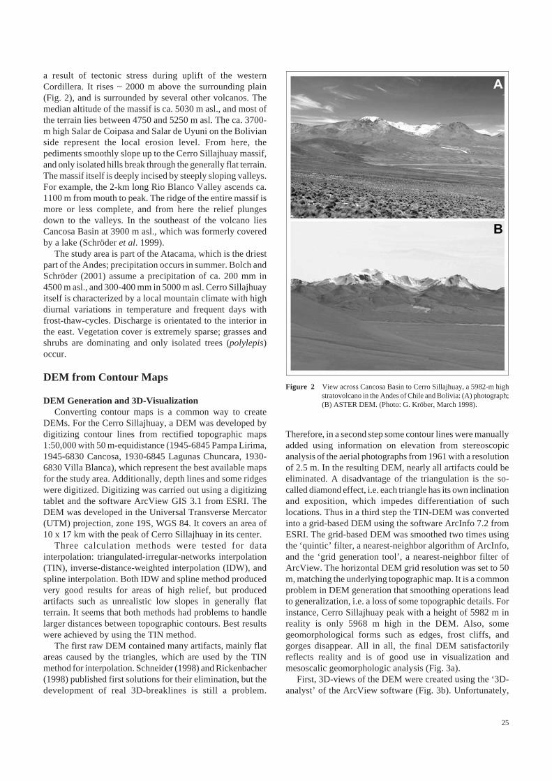
Figure 2 View across Cancosa Basin to Cerro Sillajhuay, a 5982-m highstratovolcano in the Andes of Chile and Bolivia: (A) photograph;(B) ASTER DEM. (Photo: G. Kröber, March 1998).

26

these 3D-views lose sharpness while zooming-in. Thereforefurther 3D-views were developed using an advanced terrainrendering approach as proposed by Röttger et al. (1998).Most terrain data sets are far too large to be renderedinteractively, since the number of mesh triangles easilyexceeds the amount that can be handled by modern graphicsaccelerators. As a work around the continuous-level-of-detail (C-LOD) technique (Akenine-Möller and Haines, 2002)simplifies the underlying triangular mesh such that theresulting reduced number of triangles can be processedinteractively. This is accomplished by starting with a coarserepresentation of the mesh. Then the mesh is refined as longas the local error of the triangulation exceeds one pixel inscreen space coordinates. Thus, the refinement of the meshis performed in a view-dependent fashion, i.e. far distantdetails are represented by lesser triangles than those who arenearby. In this way the mesh is adapted to each specific pointof view in an optimal way. Since the screen space error iskept below one pixel, the shape of the modeled terrain iscompletely preserved for visualization, while at the sametime the number of generated triangles is reducedsignificantly. This property is essential for a thoroughcomparison of the DEMs. Typically, the achieved framerates of this C-LOD algorithm are well beyond the critical 25hertz, such that interactive explorations of the terrain datasets are made possible. By simulating a grid resolution of 5m, the aerial photograph, which was overlaid on the DEM,preserves its sharpness. ‘Fly-by’ simulations provideadditional information about the topography, morphometryand landforms of Cerro Sillajhuay.

ResultsGenerating DEMs from contour maps is easy, and the

results provide reasonable information for geomorphologicalor hydrological interpretation. Unfortunately, it is oftenvery time-consuming. Depending on the availabletopographic maps, DEMs of higher resolution and detailcan be produced, which allows an analysis of the macro-and mesorelief, e.g. rock glaciers (Fig. 3c). For analyzingthe microrelief, interpretation of aerial photographs producesbetter results.

ASTER DEM

Instrument and Data SetASTER is a high-spatial resolution, multi-spectral imaging

system flying aboard TERRA, a satellite launched inDecember 1999 as part of NASA’s Earth Observing System(EOS). An ASTER scene covering 61.5-km x 63-km containsdata from 14 spectral bands. ASTER is comprised of threeseparate instrument subsystems representing different groundresolutions: three bands in the visible and near infraredspectral range (VNIR, 0.5-1.0 µm) with 15 m spatialresolution, six bands in the shortwave infrared spectral range(SWIR, 1.0-2.5 µm) with 30 m resolution, and five bands inthe thermal infrared spectral range (TIR, 8-12 µm) with 90

m resolution. In the VNIR one nadir-looking (3N, 0.76-0.86µm) and one backward-looking (3B, 27.6º off-nadir, taken ~60 sec. later) telescope provide black-and-white stereoimages, which generate an along-track stereo image pairwith a base-to-height ratio of about 0.6. The potential accuracyfor the DEM from ASTER could be on the order of ±7 to ±30m RMSExyz (Long and Welch, 1999). ASTER is capable ofrecording 771 digital stereo pairs per day, and cross-trackpointing out to 136 km allows viewing of any spot on Earthat least once every sixteen days.

One ASTER-level 1A scene, which, as per ASTER L1Aspecifications contains visible/near-IR, mid-IR, thermal-IR,and the matching aft looking near-IR data, acquired on May28, 2001, was downloaded directly from the USGS EROSData Center (EDC) EOSDIS Core System (ECS). Fortunately,Cerro Sillajhuay is located in the center of this image, whichis absolutely cloud-free.

DEM Generation and 3D-VisualizationASTER scenes are distributed in HDF-EOS format, which

can be imported by the software OrthoEngine as part of theGeomatica 8.2 package from PCI Geomatics. Using thissoftware, DEMs can be generated automatically. For DEMextraction only the VNIR nadir and backward images (3Nand 3B) are used. The geometric model is a rigorous one; itreflects the physical reality of the complete viewing geometryand corrects distortions that occur in the imaging processdue to platform, sensor, earth, and cartographic projectionconditions. After rigorous models (collinearity andcoplanarity equations) are computed for the 3N and 3Bimages, a pair of quasi-epipolar images is generated from theimages in order to retain elevation parallax in only onedirection. An automated image-matching procedure is usedto generate the DEM through a comparison of the respectivegray values of these images.

The quality of ASTER DEMs depends on the availabilityof tie points (TPs) and ground control points (GCPs) (PCIGeomatica User’s Guide Version 8.2 October 2001). In thisstudy, 12 TPs and 11 GCPs were collected between thestereo-pair using geo-rectified maps and aerial photos foridentification of characteristic landforms such as moraines,rock glaciers and ridges that were surveyed in the field. Thetotal horizontal RMS was < 1.17 pixel or < 17.5 m. TheDEM was generated using PCI Geomatica, the only softwareat the time designated compliant with NASA’s ATBD forASTER DEMs, at 30 m resolution choosing the ‘highestpossible level of detail’ function, and the holes were filledby choosing the ‘automated interpolation’ function. Theoverall quality of the DEM was outstanding, with only fewartifacts mostly representing lakes. The DEM was re-sampledto 15 m to exploit full ortho-image resolution (Fig. 4a). Thethree-band VNIR nadir-looking image (1, 2, 3N) wasorthorectified using the extracted DEM. Several perspectivescenes and ‘fly-by’ simulations were developed showing theCerro Sillajhuay from different views and in different scales(Figs. 4b, c).

27

Figure 3 (A) Digital elevation model (DEM) of Cerro Sillajhuay derived from contourmaps. (B) Virtual 3D-view. (C) Virtual 3D-view combined with aerialpicture showing rock glaciers in the Tacurma Valley.

Figure 4 (A) Digital elevation model (DEM) of Cerro Sillajhuay derived from ASTERdata. (B) Virtual 3D-view. (C) Virtual 3D-view of Rio Blanco Valley.

Results

The elevations in the ASTER DEM are ofgood accuracy and allow analysis of the macro-and mesorelief. Above 5000 m asl., elevations aretoo low due to internal smoothing procedures ofthe Geomatica software (elevations derived fromASTER DEMs in general are known to be oftenlittle too low; personal communication, PCI).Although particular elevation values may be toolow, the developed 3D-views demonstrate the highquality of the DEM and the potential for moredetailed morphometric image interpretation.

Thematic Analysis of the DEMs

GeomorphometryThe quality of both DEMs from contour maps

and ASTER data was compared focusing ontopography, geomorphology, morphometry, andlandforms. Five geomorphic parameters, whichare useful to identify and describe geomorphologicforms and processes, were extracted using thesoftware ArcInfo and ArcView: elevation, aspect,slope angle, vertical curvature, and tangentialcurvature. Flow lines and the catchment areas ofrock glaciers were extracted using the ‘hydrologicmodeling’ tool 1.1, an extension of the ArcViewsoftware.

The elevation is graphically presented in ahypsometric map with eight classes, which atCerro Sillajhuay at the same time representaltitudinal belts (Figs. 3a; 4a), e.g. the green classis vegetation cover, the yellow class is a transitionzone, and the gray class represents firn fields.

Topography can be generalized into eight aspectclasses, and this may also help to identifygeomorphologic features (Fig. 5a). For example,differences in aspect may be an indicator of valleyasymmetry.

Another map demonstrates the slope angle insix classes (Fig. 5b). The class with the lowestslope has a relatively steep upper boundary (5º) inaccordance with the general relief, whichcomprises nearly no flat areas. Other slope classesmay be useful to identify specific geomorphicforms: for example, rectilinear slopes (German:‘Glatthänge’) have a slope of 25-35º per definitionand should be found in the corresponding twoclasses of the slope map.

Slope curvature is of special interest formorphological and hydrological problems. Bothcurvatures are shown in maps of five classes: Thevertical curvature is the second derivation ofelevation regarding slope (Fig. 5c); and thetangential curvature is the second derivation ofelevation relating to aspect (Fig. 5d). Obviously,

28

A special interest of the study was a focus on theperiglacial forms at Cerro Sillajhuay. A periglacial mapcould be produced using the DEMs (Fig. 6), and the area ofeach periglacial form was calculated (Table 1). Rectilinearslopes cover most of the study area. Non-vegetatedsolifluction mainly appears on the rectilinear slopes; slightlyvegetated solifluction reaches up to the lower limit of therectilinear slopes; and vegetated solifuction is veryexceptionally. Also, rock glaciers occur very rarely ingeneral, but in some valleys they may cover up to 5 % of thearea. Striated and patterned ground, breaking blocks, andfirn cover smaller areas.

Solar RadiationIn the study area, the solar radiation is of special interest

as some authors suppose that the Atacama may have thehighest solar radiation rates on Earth. Schmidt (1999)mentions radiation values of 95 % of the solar constant forca. 3700 m asl., and of 98 % at the Sairecabur, a volcano innorthern Chile (5971 m asl., 22º43’S / 67º53’W). Thereasons for these high values are low latitude, high elevation,dryness, and lack of nearly any clouds.

The solar radiation at Cerro Sillajhuay was computedusing the software SAGA developed by Böhner et al. (1997),which enables an integration of estimated or measuredatmospheric water vapor content and atmospheric pressure.In the map of solar radiation, areas of high radiation areeasy to differentiate from areas of low radiation (Fig. 7). Itis plausible that northern slopes receive higher radiationrates than southern slopes. The influence of the relief isplainly recognizable: the highest values appear on thesummit, which is nearly always exposed to the sun; thelowest rates can be found at southern exposed escarpmentsand a large field of permanent snow. The lowest rates werecalculated for steep slopes, and the highest rates for slopeangles of ~ 15º. These values correlate with fieldmeasurements. For 21 June (winter) absolute radiation valuesrange between ~ 200 and 3000 J/cm2 and for 23 December(summer) it is between ~ 2000 and 3600 J/cm2. On 23December high rates can be found on slightly slopingsurfaces such as the summit area, ridges, valley bottoms,and pediments.

Comparison of the both DEMs

Geomorphometry and Solar RadiationWhen comparing elevation by using a difference image

(Fig. 8), both DEMs show similar values up to ~ 4600 masl. and nearly the same value for the minimum elevation(Table 2). Above ~ 5000 m asl., the calculated elevationfrom both DEMs differ increasingly with elevation, and theASTER DEM elevations are slightly to low. In general, inthe ASTER DEM elevations on overshadowed southernslopes are lower than on northern slopes. Highest differencesdo not occur at the peak but beneath the peak in southeastexposition. Beside this shadow effect the snowfields that

Figure 5 Morphometric parameters of Cerro Sillajhuay deriving from theContour DEM (left), and from the ASTER DEM (right): (a)aspect, (b) slope angle, (c) vertical curvature, (d) tangentialcurvature. For elevation see Figs. 3a and 4a.

ridges have (very) convex and divergent profiles, and valleyshave mostly (very) concave and convergent profiles.Mesoscale objects such as rock glaciers can be identified inseveral locations; the rock glacier front is characterized by aconvex profile curvature and convex tangential curvature.

29

Figure 6 Periglacial map of Cerro Sillajhuay.

ASTER DEM Contour DEM

Mean Elevation 4842 m asl. 4931 m asl.Maximum Elevation 5745 m asl. 5969 m asl.Minimum Elevation 4182 m asl. 4189 m asl.Standard Deviation 348 m 404 m

Difference ASTER DEM - Contour DEM

Mean - 89 mMaximum + 52 mMinimum - 291 mStandard Deviation 59 m

Table 2 Main calculated indices for elevation from bothContour and ASTER DEMs. See also Fig. 11.

set in above 5000 m influence the calculation. Other reasons might bethe small number of available GCPs, and smoothing procedures of theGeomatica software.

Although the slope angles of both DEMs are generally similar (Fig.5b), the ASTER DEM is more precise and reflects reality better. Forexample, the maximum slope angle of the steep cliff in the TacurmaValley is 65º-70º from field measurements; in the ASTER DEM it is61º, and in the Contour DEM it is only 52º. Compared to results fromfield mapping profile and tangential curvature are realistic in bothDEMs, even though the ASTER DEM contains a few artifacts causedby perspective.

Topographic profiles were developed: one for the Tacurma Valley(Fig. 9a), and another one runs from W to E north of the summit (Fig.9b). In general, the difference in calculated elevation from both DEMsincreases with elevation. Whereas nearly no difference can be noticedin elevations below 4500 m asl., the difference increases above 4500

m asl. The ASTER DEM offers more detail ofmesorelief.

A more detailed analysis was undertaken forthe rock glaciers in the Tacurma Valley. The slopeangles of the catchment areas are similar for bothDEMs, whereas the ASTER DEM offers moredetail. By comparing the morphometry of the rockglaciers itself, the ASTER DEM shows morerealistic results: the minimum slope angle of 5ºmatches the field measurements, and the maximumslope angle of 34º represents the general slopeangle of active rock glaciers (35-40º). Knowledgeabout the geomorphometry is also important for ahydrologic modeling. Flow lines and surface run-off were calculated to delimit the catchment areasof the rock glaciers. In the measurement of areaboth DEMs show similar results, especially for themost active rock glaciers (Table 3: B1 and B2),even though the ASTER DEM seems to be moreprecise regarding the flow lines by comparing itwith the virtual image (Fig. 10).

At Cerro Sillajhuay solar radiation is very highand extinction is very low according to itsgeographic position. The calculation of the meandaily solar radiation led to nearly the same ratesfor both DEMs (Table 4). For rock glaciers andespecially their catchment areas, the lowerminimum daily solar radiation rates for steep slopescalculated with the help of the ASTER DEM aremore reliable.

Figure 7 Map of the solar radiation at Cerro Sillajhuay derived from the ContourDEM (left) and the ASTER DEM (right).

Table 1 Areas for different periglacial forms.

Periglacial Form Area in %

Rectilinear slopes 35.0Rock glacier 0.3Non-vegetated solifluction 11.0Slightly vegetated solifluction 10.0Vegetated solifluction 0.1Striated and patterned grounds 1.5Breaking blocks 2.5Firn 2.0

30

Figure 8 Difference image of elevation derived from ASTER and Contour DEMs. See also Table 2.

Daily Solar Contour DEM ASTER DEM Rockglaciers Rockglaciers Catchment CatchmentRadiation (in W/m2) (in W/m2) Contour DEM ASTER DEM Area Contour Area ASTER

(in W/m2) (in W/m2) DEM DEM(in W/m2) (in W/m2)

Mean 267 266 235 239 224 226Minimum 134 88 193 189 134 88Maximum 310 312 267 271 298 305

Table 4 Solar radiation calculated from the Contour DEM and the ASTER DEM (in W/m2).

Rock Glacier Contour DEM ASTER DEM

B1 18.6 ha 17.2 haB2 79.5 ha 79.3 haB3 8.6 ha 6.7 haB4 69.8 ha 62.0 haB5 12.7 ha 14.9 ha

Table 3 Catchment areas of rock glaciers calculated from the ContourDEM and the ASTER DEM.

Discussion

Both DEM generation procedures have advantages aswell as disadvantages. Regarding the Contour DEM, thedigitalizing process of the contours is relatively time-consuming. Although software packages, which include anautomated or semi-automated digitizing tool such as a line-following algorithm, are available, manual corrections are

31

mostly necessary. The base maps themselvesrepresent secondary data, which might containerrors. Furthermore, the interpolation methods,such as IDW, spline, or TIN, are more suitable forraster data than for vector data. On the other hand,it is easier to make changes in the interpolationalgorithm such as using a different weight factorwhile developing a Contour DEM than whiledeveloping an ASTER DEM.

While developing an ASTER DEM by using aspecial commercial software package, the DEMdeveloping algorithm cannot be changed easily.Often, the software offers only a few parametersfor free selection by the operator. For identifyingTPs, the operator needs experience in landformsand land covers, because the quality of the TPs/GCPs is essential for the DEM quality. But whenfamiliar with the software, an operator can developan ASTER DEM relatively quickly. ASTER DEMsare excellent for virtual-reality visualizations,because they represent quasi ortho-images.

Lang and Welch (1999) suggest that RMSExyzvalues for ASTER DEMs should be on the orderof ±7 to ±30 m. DEMs produced in othermountainous areas have a preferential failure mode,i.e., facets with an aspect of 340 to 140 degrees orslopes over 35 degrees. This is likely due to twofactors. First, relative to the ground beingexamined, the aft looking ASTER sensor is set atan azimuth of roughly 10 degrees, making slopeswith an aspect of 10 degrees the least likely to bewell imaged. Second, these slopes receive theleast direct solar illumination, which, by reducingimage contrast, increases the probability of image-to-image correlation failure.

Figure 10 Map of flow lines at Cerro Sillajhuay using the Contour DEM (left) and ASTER DEM (right).

Figure 9 (A) Topographic W-E profile. (B) Topographic (longitudinal) profile ofTacurma Valley. For location of profiles see Fig. 1.

32

Conclusion

For Cerro Sillajhuay, a volcano in the Andes of Chile/Bolivia, DEMs were developed and analyzed by using contourmaps and ASTER remote sensing data. The results presentedhere demonstrate that both DEMs are useful for morphometricanalysis. The scale of a DEM sets the limits for the level ofdetail for geomorphologic analysis. Today, DEMs fromASTER remote sensing data and contour maps are reliablesources for an interpretation of the macro- and mesorelief,whereas ASTER DEMs offer more detail, are often easier todevelop, and available for many parts of the Earth. Theactual purchase price (2003) of an ASTER scene is $55. Ingeneral, the ASTER DEM is more accurate, e.g. cliff facesand steep slopes are easier to identify. Analyzing themicrorelief requires a level of detail, which today’s DEMresolutions deriving from satellite data do not offer. Here,aerial photographs still are the better choice.

ASTER data provides the opportunity for extractingelevation information from nadir and aft images. Thesimultaneous along-track stereo data eliminates radiometricvariations caused by multi-date stereo data acquisition whileimproving image-matching performance. ASTER data mightbe useful for geomorphological mapping especially atmedium scales (1:100,000 and 1:50,000).

Acknowledgements

The authors like to thank H. Schröder and G. Kröber,University of Erlangen-Nuremberg, Germany, for support inthe field, J. Böhner, University of Göttingen, Germany, forsolar radiation calculations, and S. Röttger, University ofStuttgart, Germany, for providing the interactive terrainrenderer. The corresponding terrain-rendering library isdistributed under the terms of the LGPL and can bedownloaded from http://wwwvis.informatik.uni-stuttgart.de/~roettger. Part of this project was funded by the Max KadeFoundation, New York.

References

Abrams, M., and S.J. Hook, 1995. Simulated ASTER data for geologicalstudies, IEEE Transactions on Geoscience and Remote Sensing,33, 692-699.

Akenine-Möller, T, and E. Haines, 2002. Real-time Rendering, 2nd

edition, A. K. Peters, Natick, 900 pp.

Al-Rousan, N., P. Cheng, G. Petrie, T. Toutin, and M.J. Valadan Zoej,1997. Automated DEM extraction and orthoimage generation fromSPOT level 1B imagery, Photogrammetric Engineering and RemoteSensing, 63, 965-974.

Al-Rousan, N., and G. Petrie, 1998. System calibration, geometricaccuracy testing and validation of DEM and orthoimage dataextracted from SPOT stereopairs using commercially availableimage processing systems, International Archives forPhotogrammetry and Remote Sensing, 32, 8-15.

Band, L.E., R. Vertessy, and R.B. Lammers, 1995. The effect ofdifferent terrain representations and resolution on simulated

watershed processes, Zeitschrift fur Geomorphologie, N.F., Suppl.-Bd., 101, 187-199.

Baral, D.J., and R.P. Gupta, 1997. Integration of satellite sensor datawith DEM for the study of snow cover distribution and depletionpattern, International Journal of Remote Sensing, 18, 3889-3894.

Bishop, M.P., R. Bonk, U. Kamp, and J.F. Shroder, 2002. Topographicanalysis and modeling for alpine glacier mapping, Polar Geography,25, 181-201.

Bishop, M.P., and J.F. Shroder, 2000. Remote sensing andgeomorphometric assessment of topographic complexity and erosiondynamics in the Nanga Parbat massif, in Tectonics of the NangaParbat Syntaxis and the Western Himalaya, Eds. M.A. Khan, P.J.Treloar, M.P. Searle, and M.Q. Jan, (= Geological Society London,Special Publications, 170), London, 181-199.

Böhner, J., R. Kothe, and C. Trachinow, 1997. Weiterentwicklung derautomatischen Reliefanalyse auf der Basis von digitalenGelandemodellen, Göttinger Geographische Arbeiten, 100,Gottingen, 3-21.

Bolch, T., and H. Schröder, 2001. Geomorphologische Kartierungund Diversitätsbestimmung der Periglazialformen am CerroSillajhuay (Chile/Bolivien), (= Erlanger Geographische Arbeiten,28), Erlangen, 141 pp.

Chang, K., and B. Tsai, 1991. The effect of DEM resolution on slopeand aspect mapping, Cartography and Geographic InformationSystems, 18, 69-77.

Cheng, P., and L. McBean, 2002. Fly-through data generation ofAfghanistan, Earth Observation Magazine, without page.

Desmet, P.J.J., and G. Govers, 1995. GIS-based simulation of erosionand deposition patterns in an agricultural landscape: a comparisonof model results with soil map information, Catena, 25, 389-401.

Dietrich, W.E., C.J. Wilson, D.R. Montgomery, and J. McKean, 1993.Analysis of erosion thresholds, channel networks, and landscapemorphology using a digital terrain model, Journal of Geology, 101,259-278.

Dikau, R., E.E. Brabb, R.K. Mark, and R.J. Pike, 1995. Morphometriclandform analysis of New Mexico, Zeitschrift für Geomorphologie,N.F., Suppl.-Bd., 101, 109-126.

Duncan, C.C., A.J. Klein, J.G. Masek, and B.L. Isacks, 1998.Comparison of Late Pleistocene and modern glacier extents incentral Nepal based on digital elevation data and satellite imagery,Quaternary Research, 49, 241-254.

Eckert, S., and T. Kellenberger, 2002. Qualitatsanalyse automatischgenerierter digitaler Gelandemodelle aus ASTER Daten,Publikationen der Deutschen Gesellschaft fur Photogrammetrieund Fernerkundung, 11, 337-345.

Etzelmüller, B., and J.L. Sollid, 1997. Glacier geomorphometry - anapproach for analysing long-term glacier surface changes usinggrid-based digital elevation models, Annals of Glaciology, 24,135-141.

Giles, P.T., 1998. Geomorphological signatures: classification ofaggregated slope unit objects from digital elevation and remotesensing data, Earth Surface Processes and Landforms, 23, 581-594.

Gao, J., 1997. Resolution and accuracy of terrain representation bygrid DEMs at a micro scale, International Journal of GeographicInformation Science, 11, 199-212.

Gratton, D.J., P.J. Howarth, and D.J. Marceau, 1990. Combining DEMparameters with Landsat MSS TM imagery in a GIS for mountainglacier characterization, IEEE Transactions on Geoscience andRemote Sensing, 28, 766-769.

33

Hodgson, M.E., 1995. What cell size does the computed slope/aspectangle represent?, Photogrammetric Engeneering and RemoteSensing, 65, 513-517.

Kääb, A., 2002. Monitoring high-mountain terrain deformation fromrepeated air- and spaceborne opitcal data: examples using digitalaerial imagery and ASTER data, Journal of Photogrammetry andRemote Sensing, 57, 39-52.

Kääb, A., C. Huggel, F. Paul, R. Wessels, B. Raup, H. Kieffer, J.Kargel, 2002: Glacier monitoring from ASTER imagery: accuracyand applications, EARSeL Proceedings, LIS-SIG Workshop, Berne,March 11-13, 2002.

Kirkby, M.J., 1990. The landscape viewed through models, Zeitschriftfür Geomorphologie, N.F., Suppl.-Bd., 79, 63-81.

Kneisel, C., F. Lehmkuhl, S. Winkler, E. Tressel, and H. Schroder,1998. Legende für geomorphologische Kartierungen inHochgebirgen (GMK Hochgebirge), Trierer GeographischeStudien, 18, 1-24.

Krzystek, P., 1995. New investigations into the practical performanceof automatic DEM generation, Proceedings, ACSM/ASPRS AnnualConvention, Charlotte, North Carolina, American Society forPhotogrammetry and Remote Sensing, 2, 488-500.

Lodwick, G.D., and S.H. Paine, 1985. A digital elevation model of theBarnes Ice-Cap derived from Landsat MSS data, PhotogrammetricEngineering and Remote Sensing, 51, 1937-1944.

Long, H.R., and R. Welch, 1999. Algorithm Theoretical Basis Documentfor ASTER Digital Elevation Models ver 3.0, NASA DocumentATBD-AST-08.

Millaresis, G.C., and D.P. Argialas, 2000. Extraction and delineationof alluvial fans from digital elevation models and Landsat ThematicMapper images, Photogrammetric Engineering and Remote Sensing,66, 1093-1101.

Raup, B.H., H.H. Kieffer, T.M. Hare, and J.S. Kargel, 2000. Generationof data acquisition requests for the ASTER satellite instrument formonitoring a globally distributed target: Glaciers, IEEE Transactionson Geoscience and Remote Sensing, 38, 1105-1112.

Rickenbacher, M., 1998. Die digitale Modellierung des Hochgebirgesim DGM25 des Bundesamtes fuer Landestopographie, WienerSchriften zur Geographie und Kartographie, 11, 49-55.

Röttger, S., W. Heidrich, P. Slusallek, and H.-P. Seidel, 1998. Real-time generation of continuous levels of detail for height fields,Proceedings Sixth International Conference in Central Europe on

Computer Graphics and Visualization, Plzen, Chech Republic,315-322.

Schmidt, D., 1999. Das Extremklima der nordchilenischenHochatacama unter besonderer Berucksichtigung derHohengradienten, (= Dresdner Geographische Beitrage, 4), Dresden,122 pp.

Schneider, K., 1998. Geomorphologisch plausible Rekonstruktion derdigitalen Repräsentation von Geländeoberflächen aus Höhendaten,Unpublished PhD-Thesis, University Zurich, Switzerland, 226 pp.

Schoorl, J.M., M.P.W. Sonneveld, and A. Veldkamp, 2000. Three-dimensional landscape process modelling: the effect of DEMresolution, Earth Surface Processes and Landforms, 25, 1025-1034.

Schröder, H., T. Bolch, and G. Krober, 1999. LimnischeSedimentationen des Holozäns im Becken von Cancosa (ProvinzIquique, Chile), Mitteilungen der Frankischen GeographischenGesellschaft, 46, 217-229.

Schröder, H., and M. Makki, 1998. Das Periglazial des Llullaillaco(Chile/Argentinien), Petermanns Geographische Mitteilungen, 142,67-84.

Sidjak, R.W., and R.D. Wheate, 1999. Glacier mapping of theIllecillewaet icefield, British Columbia, Canada, using LandsatTM and digital elevation data, International Journal of RemoteSensing, 20, 273-284.

Shi, J., 2001. Estimation of snow fraction using simulated ASTERdata, IAHS Publication, 267, 120-122.

Stefanovic, P., and G. Wiersema, 1985. Insolation from digital elevationmodels for mountain habitat evaluation, ITC Journal, 3, 177-186.

Theakstone, W.H., and F.M. Jacobsen, 1997. Digital terrain modellingof the surface and bed topography of the glacier Austre Okstindbreen,Okstindan, Norway, Geografiska Annaler, 79 A, 201-214.

Tucker, G.E., F. Catani, A. Rinaldo, and R.L. Bras, 2001. Statisticalanalysis of drainage density from digital terrain data,Geomorphology, 36, 187-202.

Welch, R., T. Jordan, H. Lang, and H. Murakami, 1998. ASTER as asource for topographic data in the late 1990’s, IEEE Transactionson Geoscience and Remote Sensing, 36, 1282-1289.

Wessels, R.L., J.S. Kargel, and H.H. Kieffer, 2002. ASTERmeasurement of supraglacial lakes in the Mount Everest region ofthe Himalaya, Annals of Glaciology, 34, 399-408.