GEOPHYSICAL CONTROLS ON FAULT-GROUNDWATER …

GEOPHYSICAL CONTROLS ON FAULT-GROUNDWATER INTERACTION

AT SAN ANDREAS OASIS, AT DOS PALMAS PRESERVE

A Thesis

Presented to the

Faculty of

California State Polytechnic University, Pomona

In Partial Fulfillment

Of the Requirements for the Degree

Master of Science

In

Geological Sciences

By

Drew R. Faherty

2018

ii

SIGNATURE PAGE

THESIS: GEOPHYSICAL CONTROLS ON FAULT-

GROUNDWATER INTERACTION AT SAN

ANDREAS OASIS, AT DOS PALMAS PRESERVE

AUTHOR: Drew Faherty

DATE SUBMITTED: Fall 2018

Department of Geological Sciences

Dr. Jascha Polet _________________________________

Thesis Committee Chair

Geological Sciences

Dr. Stephen Osborn _________________________________

Geological Sciences

Dr. Nick Van Buer _________________________________

Geological Sciences

iii

ACKNOWLEDGEMENTS

iv

ABSTRACT

The San Andreas Oasis has historically provided a reliable source of fresh water

near the northeast margin of the Salton Sea; however, since the recent completion of the

Coachella Canal Lining Project, surface water at the site has begun to disappear. This has

hindered efforts by the Bureau of Land Management (BLM) to preserve and restore the

unique environment created by the Oasis. The BLM has proposed the installation of a

recharge pond near the site, although controls on groundwater dynamics and recharge are

complicated by the presence of the Hidden Springs Fault (HSF), which trends near the

Oasis. Its surface expression is apparent as a lineation against which all plant growth

terminates, suggesting that it may form a partial barrier to subsurface groundwater flow.

We present an application of several geophysical exploration techniques to

delineate aquifer geometry and constrain structural controls on groundwater recharge. A

total of nine direct current (DC) resistivity surveys were performed to the east and west of

the Hidden Springs Fault (HSF). Magnetic profiles were taken across the HSF to better

define its trend and delineate additional faults. Five very low frequency (VLF)

electromagnetic induction profiles were also conducted across the fault zone and in areas

upgradient of the Oasis, where alluvium and poor coupling prevent ground-based

resistivity surveys.

Results suggest the existence of a previously unmapped fault to the northeast of

San Andreas Oasis. Our measurements are consistent with the HSF acting as a barrier to

lateral flow, while also exhibiting transport of water along the fault. Together these two

faults channel southeast-directed flow, localizing groundwater and associated plant growth

v

in a narrow, fault-bounded lineament. Based on this interpretation, we have recommended

that a recharge pond be placed to the north of San Andreas Oasis, allowing recharge to

flow between the two faults.

vi

TABLE OF CONTENTS

SIGNATURE PAGE .......................................................................................................... ii

ACKNOWLEDGEMENTS ............................................................................................... iii

ABSTRACT ....................................................................................................................... iv

LIST OF FIGURES ......................................................................................................... viii

CHAPTER 1: INTRODUCTION ....................................................................................... 1

1.1 Background ................................................................................................................... 1

1.2 Geologic overview of the Salton Trough: The Northeastern Rim ................................ 5

1.3 The Hidden Springs Fault ............................................................................................. 8

1.4 Groundwater-Fault Interactions .................................................................................. 12

1.5 Previous Work at Dos Palmas Preserve ...................................................................... 16

1.5.1 Well Data ................................................................................................................. 16

1.5.2 Geochemical Data .................................................................................................... 18

1.5.3 Seismic Reflection and Refraction ........................................................................... 21

1.6 Research Questions and Hypothesis ........................................................................... 23

CHAPTER 2: METHODS ................................................................................................ 24

2.1 Electrical Resistivity ................................................................................................... 24

2.1.1 Case Studies ............................................................................................................. 28

2.1.2 Equipment ................................................................................................................ 31

2.1.3 Experiment Parameters ............................................................................................ 32

2.1.4 Data Processing Software ........................................................................................ 34

2.1.5 Inversions ................................................................................................................. 34

2.2 Magnetics .................................................................................................................... 37

2.2.1 Rock Magnetic Properties ........................................................................................ 37

2.2.2 Magnetic Expressions of Faulting ........................................................................... 38

2.2.3 Case Studies: Characterization of Intra-Sedimentary Faults Using Magnetics ....... 40

2.2.4 Equipment and Data Collection ............................................................................... 43

2.2.5 Data Processing ........................................................................................................ 44

2.2.6 Data Filtering ........................................................................................................... 46

2.3 Very Low Frequency (VLF) ....................................................................................... 47

2.3.1 Equipment ................................................................................................................ 50

2.3.2 Data Processing ........................................................................................................ 50

2.3.3 Case Studies: Characterization of Saturated Fault Zones using VLF ...................... 53

vii

CHAPTER 3: MEASUREMENTS AND INTERPRETATION ...................................... 58

3.1 VLF Measurements ..................................................................................................... 58

3.1.1 Interpretation of VLF Measurements....................................................................... 67

3.2 Resistivity Inversion Results and Interpretation ......................................................... 70

3.3 Magnetic Survey Results and Interpretation ............................................................... 87

3.4 Integrated Interpretation.............................................................................................. 92

3.5 Tectonic Implications.................................................................................................. 98

CHAPTER 4: CONCLUSIONS ..................................................................................... 102

4.1 Suggestions for Future Work .................................................................................... 104

REFERENCES ............................................................................................................... 105

APPENDIX A: VLF Measurements ............................................................................... 110

APPENDIX B: Water Analysis Results for Dos Palmas Preserve ................................. 119

viii

LIST OF FIGURES

Figure 1: Map of the Salton Sea, with major faults.. .......................................................... 2

Figure 2: Map USGS faults (USGS Fault Map Database, 2018). ...................................... 3

Figure 4: Map of Dos Palmas Preserve, with location of oases and recharge ponds. ........ 4

Figure 3: Interferogram generated from NASA/JPL L-band UAVSAR.. ........................... 4

Figure 5: NW-SE trending seismic reflection profile of the Salton Sea. ............................ 6

Figure 6: Diagram of stratigraphic column of Painted Canyon.. ........................................ 7

Figure 7: Geologic cross-section for the northern half of the primary oasis. ..................... 8

Figure 8: Satellite imagery of San Andreas Oasis, with location of the HSF. .................... 9

Figure 9: Geologic map of Mecca Hills and Northwest corner of Dos Palmas. ............... 10

Figure 10: Mapped location and trend of the Hidden Springs Fault from USGS. ............ 11

Figure 11: CGS (2018) mapped locations of major Quaternary faults. ............................ 11

Figure 12: Diagram of clay-rich fluid barriers along fault surfaces. ................................ 12

Figure 14: Conceptual models of fluid flow for various fault architectures. .................... 15

Figure 13: Diagram of fault zone with architectural components.. .................................. 15

Figure 15: Groundwater contour map for upper confined aquifer. ................................... 17

Figure 16: Stable isotope data and mixing trend for samples collected at Dos Palmas.... 18

Figure 17: Stable isotope data for samples collected at San Andreas Oasis. .................... 19

Figure 18: USGS reflection/refraction profile conducted at Dos Palmas Preserve. ......... 22

Figure 19: Diagram of apparent resistivity ranges for various rock types. ....................... 25

Figure 20: Diagram of resistivity survey. ......................................................................... 26

Figure 21: Diagram of Wenner array electrode configuration.. ........................................ 27

Figure 22: Inversion results for profiles, conducted across the Geleen fault.................... 29

Figure 23: Resistivity profile across the Yalguaraz high in the Central Andes. ............... 30

Figure 24: Resistivity survey conducted adjacent to San Andreas Oasis. ........................ 32

Figure 25: Example of apparent resistivity pseudo-sections. ........................................... 35

Figure 26: Geotomo’s RES2DINV inversion results for a resistivity survey. .................. 36

Figure 27: Magnetic anomalies for various models of intra-sedimentary faults. ............. 39

Figure 28: Map of reduced-to-pole (RTP) aeromagnetic data of the Rio Rancho area. ... 41

Figure 29: Anomaly profiles across aeromagnetic data for sedimentary faults. ............... 42

ix

Figure 30: Comparison of maps of the Hubble Spring Fault. ........................................... 43

Figure 31: Diurnal variation of total magnetic field. ........................................................ 45

Figure 32: Example profile of data overlap. ..................................................................... 46

Figure 34: Tilt-angle of primary magnetic field. .............................................................. 49

Figure 33: Diagram of electrical eddy currents induced in a vertical conductor. ............. 49

Figure 35: Raw VLF measurements collected across the Hidden Springs Fault.. ............ 51

Figure 36: Raw (blue) and Fraser filtered (orange) in-phase component of VLF data. ... 52

Figure 37: Results from VLF survey. ............................................................................... 54

Figure 38: VLF results for a profile conducted along a stream near a coal mine. ............ 55

Figure 39: VLF surveys conducted across the Helendale Fault. ...................................... 57

Figure 40: Primary field propagation directions for stations NLK, NML, and NAA. ..... 58

Figure 41: VLF profiles conducted across San Andreas Oasis and the HSF. ................... 59

Figure 42: Fraser-filtered, in-phase tilt measurements for VLF profile DP_45. .............. 60



Figure 45: Fraser-filtered, in-phase tilt measurements for VLF profile DP_49_2. .......... 65


Figure 47: Map of Fraser-filtered, in-phase VLF measurements across the HSF. ........... 67

Figure 48: Map of VLF measurements for profiles DP_46, DP_49_2, and DP_50.. ....... 68

Figure 49: Map of resistivity surveys conducted at San Andreas Oasis. .......................... 70

Figure 50: Zoomed in map of resistivity profiles at San Andreas Oasis .......................... 71

Figure 51: Inversion results for resistivity survey DF5.. .................................................. 73

Figure 52: Inversion results for resistivity survey DF7. ................................................... 75







Figure 59: Map of interpolated total magnetic field intensity.. ........................................ 88

Figure 60: Final merged and interpolated map of total magnetic field intensity. ............. 89

x

Figure 61: Profile of magnetic measurements along VLF profile DP_49. ....................... 91

Figure 62: Map of Fraser-filtered, in-phase VLF measurements. .................................... 95

Figure 63: Final merged and interpolated map of total magnetic field intensity. ............. 96

Figure 64: Possible groundwater flow directions at Dos Palmas Preserve. ...................... 97

Figure 65: Map of tectonic structures near San Andreas Oasis. ....................................... 99

Figure 66: Diagram of a positive flower structure along a dextral fault. ........................ 100

Figure 67: Diagram of contractional and extensional bends .......................................... 101

Figure 68: Fraser-filtered, in-phase tilt measurements for VLF profile DP_46. ............ 110


Figure 70: Fraser-filtered, in-phase tilt measurements for VLF profile DP_49_2. ........ 112


Figure 72: Map of Fraser-filtered, in-phase VLF measurements. .................................. 114





Figure 77: Map of monitoring well locations at Dos Palmas Preserve........................... 119

Figure 78: Water sample IDs with associated location at Dos Palmas Preserve ............ 120

Figure 79: Isotope results for water samples collected at Dos Palmas Preserve. ........... 121

1

CHAPTER 1: INTRODUCTION

1.1 Background

To the northeast of the Salton Sea, perched in the foothills of the Orocopia

Mountains, there are a series of palm oases. The chalky, sage-pocked landscape rises

from the shoreline, across the highway, up the dusty, rolling slopes awash in alluvium,

and is interrupted by a crowd of palms. The San Andreas Oasis once provided a refuge to

those who traversed the Salton Trough. Dos Palmas Preserve (Fig. 1) has likely grown

significantly beyond its namesake, although this once resilient respite in the desert is

beginning to vanish. The distressed palms lean and tumble and litter the site. The

freshwater pools in San Andreas Oasis have disappeared.

Above Dos Palmas Preserve, a canal runs along the flanks of the mountains and

winds north toward the Coachella Valley, delivering waters sourced from the Colorado

River. For the past seventy years, the canal has existed as an unlined, dirt structure,

carved into the foothills. In an effort to curb unnecessary water loss and prevent leakage

from the previously unlined structure, the canal was lined in 2007. Since completion of

the Coachella Canal Lining Project, there have been observed drops in surface water

across the preserve, particularly at San Andreas Oasis, where the pools have disappeared

entirely (J. Minor, Bureau of Land Management, personal communication, 2016). The

Oasis has likely received substantial supplemental recharge from the previously unlined

canal (Hibbs et al., 2011), however, records of the Oasis (and the presence of water)

predate the canal and go as far back as at least the last couple hundred years, as evidenced

by footpaths worn by the native Cahuilla people (Cornett, 2014). Dos Palmas was also a

2

known stop along the Bradshaw Trail to Yuma, Arizona in the 1860s, and referenced in a

1920 United States Geological Survey (USGS) guide to watering stops in the region

(Brown, 1920). While it may be tempting to cite the canal as the primary control on water

at the Oasis, some records suggest that the number of palms at the site was growing prior

to its construction (Henderson, 1947). Furthermore, subsurface flow may be complicated

by the presence of the Hidden Springs Fault (HSF), which trends adjacent to the San

Andreas Oasis, as well as other faults that have been speculated to exist in this area,

including the Salt Creek Fault to the north and the Mecca Hills Fault Zone to the west

(Fig. 2). Nonetheless, regional InSAR (Interferometric Synthetic Aperture Radar) images

taken after canal completion, from 2009-2016 (Fig. 3) depict localized subsidence within

the Preserve, with measurable negative velocities just south of the canal and to the north

Figure 1: Map of the Salton Sea, with major faults. Dotted pattern indicates areas

underlain by crystalline rock. Location of Dos Palmas Preserve indicated by orange star.

Adapted from Biehler (1964).

3

of San Andreas Oasis. It is also pertinent to consider that California’s historic drought

coincides with a portion of the post-lining period, making it difficult to resolve the

lining’s contribution to the observed changes within the context of climatic influences.

Recharge ponds have been installed at the center of the Preserve to restore flow to

the major springs and oases located immediately to the northeast of San Andreas Oasis,

although it is unclear if San Andreas Oasis receives any of this supplemental recharge

(Fig. 4; GEI Construction and Testing of Water Supply Improvements Report, 2011). The

continued or diminishing presence of groundwater at San Andreas Oasis may have

implications for the long-term sustainability of the habitat. By imaging the subsurface

Figure 2: Map USGS faults (USGS Fault Map Database, 2018) of the northeastern corner

of the Salton Sea. Red triangle denotes location of Dos Palmas Preserve, also shown here.

Hidden Springs Fault (HSF); San Andreas Fault (SAF); Eastern California Shear Zone

(ECSZ). Red box denotes approximate extent of InSAR image in Figure 3. Basemap

from Google Earth imagery (2018).

4

flow paths of water and its interaction with the HSF and other local fault systems, we

Figure 3: Interferogram generated from NASA/JPL L-band UAVSAR (April 2009 –June

2017). Approximate extent of subsidence outlined in blue in upper right inset. Ovals

indicate approximate location of San Andreas Oasis. Color scale displays line of sight

(LOS) displacement (mm).

1.8 km

Figure 4: Map of Dos Palmas Preserve, with location of oases and recharge ponds. Profile

A – A’ denotes location of cross-section in Figure 7. Basemap from Google Earth

imagery (2018).

5

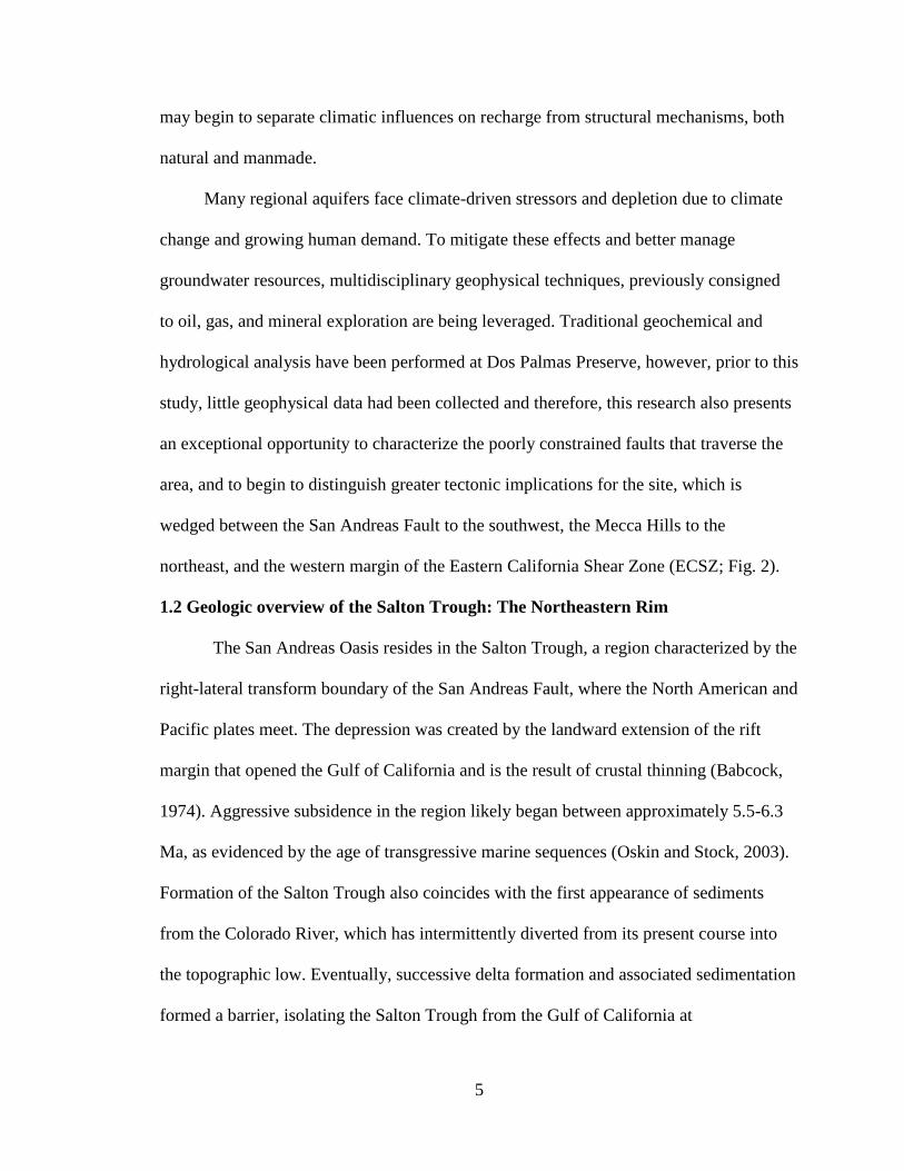
may begin to separate climatic influences on recharge from structural mechanisms, both

natural and manmade.

Many regional aquifers face climate-driven stressors and depletion due to climate

change and growing human demand. To mitigate these effects and better manage

groundwater resources, multidisciplinary geophysical techniques, previously consigned

to oil, gas, and mineral exploration are being leveraged. Traditional geochemical and

hydrological analysis have been performed at Dos Palmas Preserve, however, prior to this

study, little geophysical data had been collected and therefore, this research also presents

an exceptional opportunity to characterize the poorly constrained faults that traverse the

area, and to begin to distinguish greater tectonic implications for the site, which is

wedged between the San Andreas Fault to the southwest, the Mecca Hills to the

northeast, and the western margin of the Eastern California Shear Zone (ECSZ; Fig. 2).

1.2 Geologic overview of the Salton Trough: The Northeastern Rim

The San Andreas Oasis resides in the Salton Trough, a region characterized by the

right-lateral transform boundary of the San Andreas Fault, where the North American and

Pacific plates meet. The depression was created by the landward extension of the rift

margin that opened the Gulf of California and is the result of crustal thinning (Babcock,

1974). Aggressive subsidence in the region likely began between approximately 5.5-6.3

Ma, as evidenced by the age of transgressive marine sequences (Oskin and Stock, 2003).

Formation of the Salton Trough also coincides with the first appearance of sediments

from the Colorado River, which has intermittently diverted from its present course into

the topographic low. Eventually, successive delta formation and associated sedimentation

formed a barrier, isolating the Salton Trough from the Gulf of California at

6

approximately 4 Ma. Since this time, flooding events resulted in a large inland lake,

known as Lake Cahuilla, last appearing in approximately 1700 AD (Cornett, 2014). The

fluxes of this lacustrine environment have created a unique upper sequence of

interbedded conglomerates, sandstones, and finer-grained siltstones and mudstones. The

tectonic evolution of the Southern San Andreas further divides the northern section of the

Salton Sea into a trans-tensional slip regime, with localized uplift in the Mecca Hills and

to the south, at Durmid Hill. A series of step over faults characterize the southern portion

of the Salton Sea, between the San Jacinto and San Andreas faults (Fig 5), where slip is

accommodated primarily through southeast-directed extension and subsidence (Brothers,

2009). This has resulted in relatively young volcanism and geothermal activity in this

area.

To the northeast of the Salton Sea, stratigraphic juxtapositions and faulting are

distinct from corresponding units to the west and south—areas that have been studied in

much greater detail; therefore, broad trends in stratigraphic structure and thicknesses for

the region of Dos Palmas Preserve are partly informed by work conducted to the north, in

Figure 5: NW-SE trending seismic reflection profile of the Salton Sea, with

approximate ages for high stands of Lake Cahuilla. Beginning of southern

extensional section identified by “Hinge zone.” Adapted from Brother, et al.

(2009).

7

the Mecca Hills. While there will be notable differences due to overprinting by the

Painted Canyon Fault, both sites run the same approximate trend along the basin rim and

thus, occupy similar locations near the paleo-shoreline of ancient Lake Cahuilla. Upper

sedimentary units are approximately 1300 m in thickness (Fig 6), with siltstones and

mudstones encountered at depths as shallow as 150 m (inferred from McNabb, 2013). At

Dos Palmas Preserve, clay confining beds separate three aquifers, including a perched

aquifer that extends from the paleo shoreline through the northern half of the large

primary oasis, located in the northern section of the Preserve, as well as upper and lower

confined aquifers (Fig. 7; GEI Construction and Testing of Water Supply Improvements

Report, 2011).

13

00

m

Figure 6: Diagram of stratigraphic column of Painted Canyon. Approximate location of

profile defined by dashed yellow line on geologic map. Dos Palmas Preserve identified in

lower right corner with a star. Adapted from McNabb (2013).

8

1.3 The Hidden Springs Fault

The surface trace of the Hidden Springs Fault (HSF) begins just north of the

Durmid area and continues for 19 km northwest, through Dos Palmas Preserve and into

the southern Mecca Hills (Hays, 1957). The western margin of the San Andreas Oasis is

bounded by a structure apparent in satellite imagery as a sharp, northwest-trending linear

feature, against which all surface growth abruptly terminates (Fig. 8). Further to the west

of the Oasis, there is a distinct escarpment that runs subparallel to this linear feature

(traced by red line in Fig. 8).

Each of these features is consistent with different mapped versions of the fault.

The exact location and sense of motion on the HSF appear to be the subject of

Figure 7: Geologic cross-section for the northern half of the primary oasis. Location

of profile denoted in Figure 4. Adapted from GEI Construction and Testing of Water

Supply Improvements Report (2011).

9

disagreement between two primary groups. The first group (Babcock, 1974; Sylvester,

1976; Dorsey, 2011; McNabb, 2013) have mapped the HSF as a northeast-dipping

normal fault, with right-lateral motion, where the greater Dos Palmas Preserve resides on

the hanging wall (Fig 9). This location and sense of dip-slip motion correspond with the

obvious escarpment further west of the oasis (denoted by red line in Fig. 8), however, it is

noted by Babcock (1974) that surface exposure of the HSF is not visible at the Preserve.

The United States Geological Survey (USGS, 2018) has designated the HSF a

strike-slip fault, with purely right-lateral motion and maps its trace along the linear

surface feature (Fig. 8; Clark, 1984). A difference also exists between the trend of the

HSF as mapped by the USGS compared to that produced by the California Geological

Survey (CGS). The USGS has indicated a left-stepping HSF, which accounts for areas of

localized uplift coincident with the left step (Fig. 10). The CGS, conversely, has omitted

Figure 8: Satellite imagery of San Andreas Oasis, with location of the HSF as mapped by

the USGS (2017)—denoted by black line and by Babcock (1974) and Sylvester (1976),

denoted by red line. Basemap from Google Earth imagery (2018).

10

this step in the HSF and identified the fault to the southeast as a separate structure, known

as the Powerline Fault (Fig. 11; CGS, 2018). However, in a separate report, Bryant

(2012) favors a left-stepping HSF, rather than two distinct faults. This appears consistent

with previous mapping conducted by Babcock (1974). Both maps produced by the USGS

and CGS are consistent to the north of the left step, and depict a single, Oasis-bounding

fault strand.

Figure 9: Geologic map of Mecca Hills and Northwest corner of Dos Palmas Preserve

(approximate location denoted by red star). Adapted from Fattaruso, et al. (2014).

Originally compiled from Sylvester and Smith (1976), Rymer (1991, 1994), and McNabb

(2013). Hidden Springs Fault abbreviated HSF.

11

Figure 10: Mapped location and trend of the Hidden Springs Fault from USGS Fault Map

Database (2017), with left step. Red ovals indicate areas of uplift, expressed as small to

moderate hills to the south of San Andreas Oasis. Mecca Hills Fautl Zone abbreviated

MHFZ; San Andreas Fault abbreviated SAF. Basemap from Google Earth imagery

(2018).

Figure 11: CGS (2018) mapped locations of major Quaternary faults near San Andreas

Oasis, with the HSF and Powerline faults mapped as separate structures; Mecca Hills

Fault Zone abbreviated MHFZ; San Andreas Fault Abbreviated SAF. Basemap from

Google Earth imagery (2018).

12

1.4 Groundwater-Fault Interactions

Faults may act as conduits, partial barriers, or conduit-barriers to subsurface flow,

with the latter two creating fault-bounded aquifers (Bense and Person, 2006; Caine and

Minor, 2009). This structural pattern is especially prevalent throughout the Basin and

Range province of western North America, where regional extension has created an

expanse of craggy mountains punctuated by fault-bounded valleys. The stratigraphic

units of the Salton Trough are shaped by a history of early marine incursions and more

recently, inundations by the Colorado River (Babcock, 1974; Cornett, 2014). An

abundance of fine-grained and clay-rich rocks tends to enable compartmentalized aquifer

systems, as these materials may form seals along fault surfaces (Fig. 12), and thus

prevent lateral fluid migration (Caine and Minor, 2009). Fault permeability is governed

by a variety of factors, including fault core and damage zone widths and structures, grain

size, fluid-rock interactions, fault maturity, as well as fault lithology (Caine et al., 1996;

Minor and Hudson, 2006).

Figure 12: Diagram of clay-rich fluid barriers along fault surfaces. Red arrow

indicates possible relationship along the Hidden Springs Fault at San Andreas Oasis.

Adapted from Caine (2002).

13

Fault zone architecture is composed of two to three primary structural elements,

which include the fault core, a damage zone, and in some instances, a mixed zone (Fig.

13). The fault core accommodates much of the deformation along the fault and may be

composed of clay-rich gouge, fault breccias, chemical alteration zones, or cataclasites.

Fault core composition often varies along strike and dip as the fault cuts through different

rock units and lithologies, producing variations in fault architecture (Caine et al., 1996;

Minor and Hudson, 2006). These differences in lithology may govern the width of the

core, with clay-rich compositions exhibiting both narrow fault cores, as well as narrow

overall fault zone widths relative to silica-rich lithologies (Caine et al., 1996; Caine and

Minor, 2009; Bense et al., 2006). Sections of the Hidden Springs Fault core are exposed

in the Hidden Springs Canyon, located to the northwest of the Preserve, where the fault is

expressed as a near-vertical 10 - 30 cm gouge zone (Hays, 1957). These thicknesses point

to a narrow, clay-rich core.

The fault damage zone envelopes the fault core and is composed of smaller faults,

folds, and fracture networks, which produce additional heterogeneities within the fault

zone. The width or extent of each component exerts significant control on fault

permeability, where the damage zone generally enhances flow and the fault core tends to

prevent it. Combined conduit-barrier systems may form when the width of the fault zone

is composed of approximately equal parts damage zone and fault core (Fig. 14). Fault-

parallel permeability in the shallow zone is, however, enhanced in well-developed, clay-

rich fault cores, as particles are preferentially re-oriented, creating anisotropic

permeability (Caine et al., 1996; Bense et al., 2006). This allows for vertical migration of

fluids or flow along strike, while decreasing permeability perpendicular to the fault.

14

Furthermore, fault permeability evolves over time and is contingent on the stage of fault

development. Fluid flow may induce lithification and create zones of mineralization—

thus, faults that once acted as local conduits may be sealed and create barriers to both

fault-perpendicular and fault parallel flow.

15

Figure 14: Conceptual models of fluid flow for various fault architectures. Adapted

from Caine et al. (1996).

Figure 13: Diagram of fault zone with architectural components. Adapted from

Caine et al. (1996).

16

1.5 Previous Work at Dos Palmas Preserve

1.5.1 Well Data

Previous studies conducted at Dos Palmas Preserve have involved traditional

hydrogeologic investigations into the water chemistry at the main oasis, located to the

northeast of San Andreas Oasis. Water quality and water level data is acquired via

numerous monitoring wells and piezometers distributed along the canal and throughout

the northern section of the large oasis (Fig. 15). The construction of many of these wells,

in addition to bore log and well log data, is related to the Coachella Canal Lining Project

and efforts to monitor its effect on groundwater across the Preserve. While these wells

offer valuable insights on subsurface structure, this data is limited to the area to the

northeast of San Andreas Oasis.

Bore log and drilling data confirm the presence of clay units, apparent both as

clay balls imbedded within conglomerate and sandstone units, and as continuous beds

that act as confining units for the perched aquifer and lower confined aquifers (Bureau of

Reclamation Lower Colorado Region, 2001, Coachella Canal Lining Project

Geohydrology Appendix). Water contours for the upper confined aquifer indicate a depth

to groundwater of 60 ft and a southwest flow direction for areas located approximately 1

km south of the canal (Fig. 15). Some of these structural relationships and depths to

groundwater may be extended further south to San Andreas Oasis. Pump testing has

indicated that there is no communication between the three aquifers—at least, in the

central parts of the Preserve. Furthermore, these tests indicate that water at San Andreas

Oasis likely flows from the confined aquifer. This indicates some form of communication

17

with San Andreas Oasis, either as the unconfined aquifer terminates against the HSF or

becomes very shallow near San Andreas Oasis.

Figure 15: Groundwater contour map for upper confined aquifer, with depth to

groundwater in feet. Inset denotes approximate area included in contour map. Adapted

from Construction and Testing of Water Supply Improvements Report (2011).

18

1.5.2 Geochemical Data

Geochemical analysis conducted across Dos Palmas Preserve from 2007 – 2010

and 2013 – 2016 has revealed two primary source components of groundwater, including

native groundwater derived from precipitation over the Orocopia Mountains and

Colorado river water sourced from the Coachella Canal (Hibbs et al., 2011; Osborn,

2018). Stable isotope data for Deuterium (δD) and Oxygen-18 (δ18O) indicate source

components for the various springs and sample sites throughout the Preserve, where

surface water at San Andreas Spring is most representative of recharge from the canal

(Fig. 16). The 18O and 2H content of precipitation is dictated by a fractionation factor, α,

which is ultimately governed by temperature. Heavier isotopes will remain in a more

condensed phase, whereas lighter isotopes will fractionate into lighter phases at warmer

temperatures. 18O and 2H values for Colorado river water, derived from the Rocky

Mountains, will exhibit more positive values (less depleted in heavier isotopes), while

Native

Groundwater

Figure 16: Stable isotope data and mixing trend for samples collected at

Dos Palmas Preserve. Adapted from Hibbs et al. (2011).

19

natural groundwater at Dos Palmas Preserve will exhibit more negative values (more

depleted), due to higher temperatures and evaporative conditions.

Tritium (3H) data offers valuable insight into the relative ages of groundwater.

Tritium values for precipitation spiked in the 1950s as a result of nuclear weapons

testing, therefore, these spikes serve as an indication of pre and post-bomb pulse

recharge, with values less than approximately 0.5 tritium units (TU) indicative of pre-

1952 recharge (Hibbs et al., 2011). Hibbs et al. (2011) suggests that high tritium levels

(21.0 TU) in water samples at San Andreas Oasis indicate longer residence times relative

to other sites further to the north, with a travel time from the canal to the Oasis of

approximately 25-40 years. This interpretation may, however, be complicated by trends

Native Groundwater

Figure 17: Stable isotope data for samples collected at San Andreas Oasis plotted

with local meteoric water line. Migration of discharge along the mixing line

indicates evolution toward native groundwater. Data provided by Stephen Osborn

(personal communication, 2018).

20

observed in 18O and 2H values, where evolution of groundwater at San Andreas Oasis has

been observed over a relatively short time period (2006 – 2013), as the composition has

begun to shift away from pure canal water toward native groundwater, emphasizing both

the effects of the canal lining on recharge and possibly, representative of a shorter flow

path (Fig. 17). Samples collected at San Andreas Oasis by Osborn (2018) exhibit

similarly high tritium levels (Appendix B-1), however, values for samples collected near

the canal are very similar to those collected 1 km to the south. This trend does not appear

to corroborate the interpretation by Hibbs et al. (2011), where older waters are observed

to the south. Samples collected by Hibbs et al. (2011) to the northeast of San Andreas

Oasis were also taken from wells and surface water, which may partly reflect the

discrepancy between Tritium levels observed near the canal vs. those at San Andreas

Oasis, where samples were collected from surface water. Furthermore, tritium in meteoric

water may exhibit regional and seasonal variability. Surface water in California displays

increased tritium levels as a function of distance from the coast, as well as near urban

areas (Harms et al., 2016). Osborn (2018) thus concludes that tritium results for Dos

Palmas Preserve are inconclusive and warrant further investigation.

Samples were collected at the Lee Property, located to the south of San Andreas

Oasis (Appendix B), near the HSF following a swarm of seismic activity in October

2016. These samples exhibited both high salinity and high concentrations of bromide,

which indicate the presence of deep basin fluids that could have been mobilized along the

HSF by seismically-induced stress changes (Osborn, 2016).

21

1.5.3 Seismic Reflection and Refraction

The USGS conducted a northeast-southwest trending seismic profile across Dos

Palmas Preserve in 2015, with one end of the line traversing the northern tip of San

Andreas Oasis and the HSF. Preliminary interpretation of reflection data suggests the

existence of five additional faults located to the northeast of the Hidden Springs Fault

(Fig. 18; personal communication, R. Catchings, 2018). Additionally, the 1500 m/s P-

wave velocity contour, derived from refraction data, indicates an average depth to

groundwater of approximately 12 meters. Furthermore, there exists a discernable offset or

discontinuity in the depth to this contour across the HSF, which was identified in the

southwest end of the profile. The depth to groundwater near San Andreas Oasis may not,

however, be well-resolved, as data coverage at the end of the profile is likely limited.

22

Figure 18: USGS reflection/refraction profile conducted at Dos Palmas Preserve in 2015.

Thick red tick marks denote reliable fault locations. Thin red ticks indicate possible fault

locations (Personal communication, R. Catchings, 2018).

23

1.6 Research Questions and Hypothesis

Rancho Dos Palmas has been designated an Area of Critical Environmental

Concern for the several endangered plant and animal species that reside in the unique

environment created by the springs. As such, the BLM is currently working to restore this

habitat and mitigate losses associated both with the canal lining and drought. This project

is partially motivated by this endeavor, which will be influenced by our results. The

continued or diminishing presence of groundwater at San Andreas Oasis may have

implications for the long-term sustainability of the habitat. The following research

questions have been guided by these motivations:

1. Can we image the presence of shallow groundwater and provide characterization

of potential subsurface flowpaths around the San Andreas Oasis?

2. How does the presence of faulting affect shallow groundwater dynamics at the

San Andreas Oasis?

3. Is the Hidden Springs Fault acting as a barrier or conduit for flow (or both) at the

San Andreas Oasis?

Satellite imagery depicts a clear termination of palm growth against a linear feature

that is consistent with the mapped trace of the Hidden Springs Fault, suggesting that it

acts as a barrier to subsurface flow. Geochemical data collected near San Andreas Oasis,

however, indicate both a canal-derived source of groundwater, as well as a deeper

component of groundwater, therefore, we hypothesize that the HSF may act as a

combined conduit-barrier to flow.

24

CHAPTER 2: METHODS

To accomplish the objective of this study, several subsurface geophysical survey

methods were selected. Resistivity surveys were conducted near San Andreas Oasis to

image the presence of groundwater in, around and across the HSF. Very Low Frequency

(VLF) electromagnetic induction surveys were used to supplement resistivity, and to

resolve the existence of any conductive bodies due to the presence of water in the HSF.

Magnetic Surveys were also performed to generate a map of the area around the HSF and

the fault scarp to the west of the Oasis to define fault geometry and image any anomalies

due to subsurface contrasts in magnetic susceptibility.

2.1 Electrical Resistivity

Electrical resistivity surveys measure the ease with which subsurface materials

conduct an electrical current. Lateral and vertical variations in subsurface conductivity

may be caused by the presence of pore fluids and other material properties, such as

lithology, grain size, clay content, and mineralogy (Ball et al., 2010; Stummer et al.,

2004). Resistivity tomography is effective at imaging groundwater, as it exploits the

conductive properties of water to image flowpaths amongst other materials with lower

conductivities (Fig. 19). Resistivity is also well-suited for characterization of fault zones,

since the presence of clays and fluids within the damage zone structure often create

distinct contrasts in resistivity across a fault zone (Unsworth et al., 2004; Terrazino et al.,

2011). The presence of clay layers, salt evaporites, and associated salinity levels in

groundwater at Dos Palmas Preserve offer ideal targets for the application of resistivity.

25

Electrical resistivity surveys involve the injection of a direct current between two

electrodes implanted in the ground. A second pair of non-current-carrying electrodes, or

potential electrodes, measures the electrical potential in volts (Fig. 20). The resistance for

each measurement can be determined using Ohm’s Law (Equation 1.1), where V is the

electrical potential in volts, I is the current intensity in amperes, and R is the resistance in

ohm*meters (Ωm).

1.1 𝑉 = 𝐼𝑅

Figure 19: Diagram of apparent resistivity ranges for various rock types and

materials. Adapted from EM GeoSci (2016).

26

Early resistivity surveys were limited to one-dimensional soundings and the

assumption of a laterally homogenous subsurface. Over the past two decades,

multielectrode, computer-controlled surveys have gained popularity and allow for

imaging of more complex structures and lateral heterogeneity (Loke, 2009; Stummer,

2004). This is achieved by varying the active electrode pairs in a multielectrode array,

including the electrode spacing. Multielectrode arrays are therefore capable of capturing

2D resistivity structure along the profile. An apparent resistivity is determined using

equation 1.2, where V is the potential difference (V), I is the current intensity (A), and G

is a geometric factor defined by the electrode configuration.

Figure 20: Diagram of resistivity survey. Current flow from electrode A to B

indicated by solid lines. Dashed lines indicate equipotential surfaces.

Electrical potential is measured in volts at electrodes M and N. Adapted from

Carpenter (2012).

27

1.2 𝜌𝑎 = 𝐺𝑉

𝐼

In a homogenous half space, the measured apparent resistivity, 𝜌𝑎 is a function of

the electrode spacing, or the distance between the source and sink, however, in a

heterogenous subsurface, apparent resistivity is a function of both depth and lateral

variation.

There are several fundamental electrode configurations used in resistivity surveys,

including Wenner, Schlumberger, pole-pole, dipole-dipole, and pole-dipole. Each array

exhibits a variety of advantages and disadvantage, depending on the objective of the

survey. For this study, the primary goal is to image depth to groundwater and resolve any

discontinuities that may occur across the fault; thus, it was imperative to select an array

that optimizes vertical resolution in resistivity models. Wenner arrays (Fig. 21) were

therefore selected, as this configuration exhibits optimum vertical resolution and

Figure 21: Diagram of Wenner array electrode configuration. Alternating

current transmitted through electrodes C1 and C2; the potential difference

is measured between potential electrodes, P1 and P2. Adapted from

Suzuki et al. (2000).

28

maintains a high signal-to-noise ratio (Stummer et al., 2004; Vanneste et al., 2008; Loke

et al., 2010).

2.1.1 Case Studies

The following studies were selected to illustrate the use of resistivity surveys in

characterizion of intra-sedimentary faults. Vanneste et al. (2008) used electrical

resistivity tomography (ERT) to successfully locate the Geleen Fault in the Belgian Maas

River Valley (Fig. 22). Local geology is characterized by sand deposits and young

gravels, which obscure any significant geomorphic expression of the fault. The location

and type of faulting was distinguished by vertical offsets in areas of moderate resistivity

(green) and discontinuities in areas of low resistivity (blue). The moderate-resistivity

sections are representative of the Maas River Gravels (MRG), whereas the lower

resistivity areas are interpreted as wet cover sands (WC). The vertical offset in the MRG

unit was confirmed by drilling on either side of the proposed fault location. Additionally,

drilling revealed saturated gravels and sand on either side of the fault, indicating that the

Geleen Fault does not act as a hydraulic barrier (Vanneste et al., 2008).

29

Figure 22: Inversion results for three profiles, conducted with different electrode spacings

across the Geleen fault in the Belgian Maas River Valley using Wenner arrays.

Conductive features denoted by blues and greens; more resistive zones denoted by red,

orange, and purple. The fault is expressed as an offset or lateral discontinuity in

conductive layers. Fault location indicated by pink arrows. Maas River Gravels (MRG);

Wet Cover Sands (WC); Dry Cover Sands (DC). Adapted from Vanneste et al. (2008).

30

ERT was also used to locate Late Cenozoic faults cutting underlying Paleozoic

basement in the central Andes of Argentina (Fig. 23; Terrizano et al., 2011). Dipole-

dipole arrays were conducted over incision anomalies, which are subtle features in

alluvial environments, where fault motion has influenced the paths of alluvial rivers. Low

resistivity areas correspond with saturated bog sediments at the southwest end of the

profile, whereas shallow, moderate resistivity areas are consistent with alluvial cover.

High-angle, low resistivity features are interpreted as saturated fractures. Underlying

metasedimentary rocks are expressed as blocks of high resistivity structures. ERT was

thus able to image fractures and faults in a relatively high-resistivity environment.

Figure 23: Resistivity profile across the Yalguaraz high in the Central Andes of

Argentina, with interpreted cross-section. Adapted from Terrizano et al. (2011).

31

2.1.2 Equipment

Resistivity surveys were carried out in Wenner arrays across the HSF and on

either side of the fault, using an IRIS Syscal Kid, with 24 electrodes, and a maximum

electrode spacing of 5 meters. Surveys were designed to capture the fault zone and

deployed at the oasis to image any possible changes in depth to groundwater, the

potential presence of fluids inside the fault zone, or abrupt termination of the conductive,

saturated zone against the fault. Profiles were first measured with a measuring tape to

determine the survey length and electrode spacing prior to laying down switcher cables

and the installation of electrodes. In many instances, survey lengths (and therefore, the

depths of investigation) were limited by a barbed wire fence that trends adjacent to the

HSF. Surveys conducted to the east of the fault were designed to maximize electrode

spacing, while maintaining a 30-meter distance from the fence in order to minimize any

influence on measurements.

The twenty-four electrodes are inserted into the ground (or hammered in) at the

designated spacing, with the Syscal Kid switcher unit placed at the center of the survey

line (Fig 24). Two 60-meter switcher cables are arranged adjacent to the electrodes, with

the cables containing electrode attachment points at 5-meter spacings. Alligator clips are

used to connect each electrode to the attachment point in the switcher cable. One end of

each switcher cable is attached to the switcher unit, which contains a 12 V internal

battery, with a maximum power of 25 W, and a maximum current of 500 mA (IRIS

Instruments, n.d.). Global Positioning System (GPS) coordinates for profile endpoints

32

(electrodes 1 and 24) were recorded for each survey. Additionally, the positions of any

large bushes, plants, burn piles, or metallic surface objects were noted.

2.1.3 Experiment Parameters

Prior to beginning each survey, experimental parameters were entered in the

Syscal Kid. First, the stack min and stack max were set at two and four, respectively.

These parameters indicate the range of measurements to be made at each electrode

configuration before the switcher unit moves on to the next electrode combination. A q-

maximum, or quality factor, is assigned, which indicates the target for the maximum

percent standard deviation of measured resistance for each configuration. If this value is

achieved prior to reaching the stack maximum, the unit will move on to the next

Figure 24: Resistivity survey conducted adjacent to the western

margin of San Andreas Oasis. Switcher cable (orange) oriented

along electrodes, with Syscal Kid control unit to the right of the line.

33

configuration. If, however, the q maximum was not reached within the maximum number

of measurements, these measurements typically exhibited high q values and would be

filtered out during data processing. In several instances, exceedingly dry soil conditions

and poor electrode coupling resulted in high errors in the apparent resistivity

measurements. The data from these lines were deemed unusable and discarded. The q

maximum was set at 2% for all surveys, therefore, the unit would continue measurements

until either the standard deviation was ≤ 2% or the maximum stack value was reached.

The minimum stack value indicates the minimum number of measurements for each

electrode configuration.

The electrode spacing (CC/3) for each survey is entered, with a minimum spacing

of 2 meters and a maximum of 5 meters for the surveys performed at San Andreas Oasis.

Wenner PRF was selected for the survey type, which again, offers optimal vertical

resolution for identifying possible discontinuities in the depth to groundwater near the

fault. Finally, the number of electrodes is entered and the survey level selected. The

survey level indicates the number of iterations or electrode spacing combinations to be

used in the survey. A level 1 survey, for instance, uses the shortest spacing for each

electrode combination, such that the survey will sample only very shallow resistivity

structure. A level 7 survey will utilize all possible electrode combinations (84), including

the largest spacings for electrode combinations, therefore, sampling both shallow and

deeper structure along the profile. As a rule of thumb, the maximum depth of

investigation is equal to approximately one half of the total survey length. This may,

however, be affected by subsurface complexities and a variety of conditions. Surveys

conducted at San Andreas Oasis achieved a maximum depth of approximately 20 meters,

34

with an average depth of investigation equal to one quarter the overall survey length. The

limited depth of penetration may have been due to relatively dry soil conditions and

unconsolidated sands in upper surface layers. This likely resulted in a relatively resistive

medium and more rapid dissipation of the injected current with depth.

2.1.4 Data Processing Software

All resistivity measurements were transferred from the Syscal KID and processed

using the IRIS Prosys II software. After transferring the data, each survey is saved as a

Bin format file. An automatic filter was used to remove measurements with anomalously

high (>20000) or low (< .100000001490116) resistivity values, as well as measurements

with a standard deviation greater than 20. Processed files were then exported as a dat

format file, which may be read by Geotomo’s RES2DINV inversion software.

2.1.5 Inversions

Geotomo’s RES2DINV software was used to invert the data and produce a two-

dimensional model of subsurface resistivity. First, a pseudo-section is constructed to

display the measurements for each survey (Fig 25). For Wenner Arrays, each measured

apparent resistivity is plotted at the midpoint of the two potential electrodes, with the

pseudo-depth approximated from the electrode spacing (Demenat et al., 2001; Terrizano

et al., 2012); therefore, measurements conducted at a larger electrode spacings will be

plotted at greater pseudo-depths than those for smaller electrode spacings. The measured

apparent resistivity pseudo-section is only intended to display the original measurements

and for comparison with the apparent resistivity values that can be calculated from the

resistivity model, and does not provide a depiction of subsurface resistivity.

35

In order to generate an accurate two-dimensional model of resistivity, which

offers a true depiction of resistivity as a function of depth and horizontal distance along

the profile, it is necessary to perform an inversion of the measured apparent resistivity

data, which may be seen as an integrated value for the flow-paths taken by the current.

The RES2DINV software first determines an initial inverse model of resistivity. The

model parameters are then iteratively adjusted to achieve a better fit between the

measured apparent resistivity pseudo-section and the pseudo-section that is calculated

from this model (Demenat et al., 2001; Terrizano et al., 2012). The inversion process

utilizes a smoothness constrained least-squares inversion to optimize each model

iteration. Each iteration progresses until the Root Mean Squared (RMS) error in fit

between the model and the apparent resistivity pseudo-section is no longer improving by

5%. At this point, the software produces a final model of subsurface resistivity for the

profile (Fig 26) and a predicted pseudo-section. Comparison of the measured and

predicted pseudo-section can help assess the reliability of specific sections of the model.

Figure 25: Example of apparent resistivity pseudo-sections, with (a) measured apparent

resistivity and (b) calculated apparent resistivity. Final inverse model used to calculate

(b) displayed in Figure 23. Adapted from Terrizano et al. (2012).

36

Figure 26: Geotomo’s RES2DINV inversion results for a resistivity survey conducted

across the Hidden Springs Fault. The top profile displays the measured apparent

resistivity pseudosection. The middle profile depicts the prediction of the apparent

resistivity measurements that would be produced by the inverse model of resistivity

(bottom profile). The bottom profile displays the inverse model of resistivity as a function

of depth and horizontal distance along the profile.

37

2.2 Magnetics

Magnetic surveys measure the Earth’s magnetic field, which partly varies as a

function of latitude and shallow crustal composition. Approximately 80-90% of the field

is generated in the deep Earth and is approximated by a dipolar field (Cambell, 1997;

Nabighian et al., 2005). The remaining field components include field fluctuations that

are generated by the solar wind, as well as the crustal field, which arises due to the

presence of iron-bearing rocks within the shallow crust (Nabighian et al., 2005). The

latter is of most interest in exploration geophysics and structural geology, where rocks of

variable magnetic properties may be juxtaposed and generate significant contrasts in

magnetic field measurements (Grauch and Hudson, 2007).

2.2.1 Rock Magnetic Properties

Total magnetization is the principal magnetic property of importance in the

analysis of ground-based and aeromagnetic surveys (Grauch and Hudson, 2007). The

magnitude of total magnetization is derived from the vector sum of remnant

magnetization and induced magnetization, however, in most instances, remnant

magnetization is often ignored; thus, the total magnetization of various rock types is

largely dictated by magnetite content and the local direction and intensity of the Earth’s

magnetic field (Reynolds et al., 1990; Nabighian et al., 2005; Bath, 1968). While this

relation generally holds for igneous rocks (basalts and gabbros, in particular), tectonic

juxtaposition may also create discernable magnetic anomalies in sedimentary and silica-

rich environments (Grauch and Hudson, 2007). Fault motions place rocks of varying

composition, depositional history and, therefore, magnetic properties adjacent to one

another. While sedimentary rocks may exhibit relatively low total magnetization, the

38

contrasts generated at fault boundaries are often expressed as more subtle, linear

anomalies coincident with strike (Grauch and Hudson, 2007; Nabighian et al., 2005). The

presence of detrital magnetite and alteration of fault zone magnetic properties, including

precipitation of magnetic minerals within the fault provide additional sources of

observable magnetic anomalies in faulted sediments (Gunn, 1997). The expression of an

anomaly is dependent on several key geophysical parameters, which include the depth,

dip, and/or magnitude of the contrast in magnetic properties (Grauch and Hudson, 2007).

2.2.2 Magnetic Expressions of Faulting

Interpretation of data is often supplemented and informed by forward modeling,

where the magnetic response for a relatively simple geophysical model is generated and

evaluated against collected data and known geologic context. While we did not perform

forward modeling in this study, the following figures offer examples of magnetic

anomalies for a variety of fault types and structural relationships, which illustrate the

types of measurements that may be produced at our study site. Figure 27 depicts

aeromagnetic anomalies for several models of intra-sedimentary faults. The models

demonstrate how various physical parameters, such as contrasts in magnetic

susceptibility, vertical offsets, and layer thicknesses can alter the magnetic response.

Fault locations are approximated by the steepest sections of the anomaly gradient, where

fault offsets create a magnetic contrast or edge. This edge may also be located by filtering

the data and identifying maxima in the horizontal gradient of the reduced-to-pole

magnetic data (Grauch and Bankey, 2003).

39

Figure 27: Magnetic anomalies for various models of intra-sedimentary faults. Bold solid

lines indicate total-field anomaly curve, solid gray lines indicate derived horizontal

gradient magnitude of reduced-to-pole data (HGM of RTP), and pseudogravity data

(HGM of pseudogravity) displayed by gray dashed lines. Adapted from Grauch et al.

(2007).

40

2.2.3 Case Studies: Characterization of Intra-Sedimentary Faults Using Magnetics

As discussed in Chapter 1, the HSF cuts alluvium and weakly-magnetic

sedimentary units, which may present challenges for detection using magnetic surveys.

The following studies, however, illustrate examples of the successful application of

magnetic surveys to resolve and characterize faults in sedimentary basins. The central

Rio Grande Rift, located in central New Mexico, is comprised of multiple sedimentary

basins and characterized by numerous intra-sedimentary, quaternary faults. The region

has been studied in great detail using aeromagnetic surveys, which have focused on

constraining basement structure and delineating basements faults from younger, intra-

sedimentary faults (Grauch and Vicki, 2003; Grauch and Hudson, 2007). Grauch and

Hudson (2007) found that many of the shallow sedimentary faults in the Rio Grande Rift

are expressed as relatively subtle, linear anomalies, with amplitudes ranging between 5

nT – 15 nT (Fig. 28, 29 and Fig. 30). The source of these anomalies was interpreted as

tectonic juxtaposition of sediments with varying magnetic properties.

Aeromagnetic surveys conducted over the Amargosa Desert, near the California-

Nevada border were able to successfully identify shallow faults in both Death Valley and

Pahrump Valley (Blakely et al., 2000). In the Pahrump Valley, subtle linear anomalies in

alluvial deposits were associated with an alignment of springs. The source of the anomaly

was interpreted as offsets in magnetic rocks at depth, while the presence of springs

indicated hydraulic conductivity along the fault (Blakely et al., 2000). Similarly, Blakely,

et al. (2000) associated subtle linear anomalies in the Furnace Creek region of Death

Valley with a system of faults that cut felsic, crystalline rock and host an array of linear

springs. These springs, again, suggest that the fault system acts as a conduit for

41

groundwater flow. The source of the anomaly at this location was unknown, however, the

authors suggested some form of fault zone alteration in the otherwise non-magnetic

rocks.

Figure 28: Map of reduced-to-pole (RTP) aeromagnetic data of the Rio

Rancho area, located in the northern half of the Albuquerque Basin, NM.

Profiles A – D displayed in Figure 29. QTs - Quaternary and Tertiary

sediments. QTb - Quaternary and Tertiary basaltic and andesitic rocks,

undifferentiated. Mz - Mesozoic sedimentary rocks. From Grauch and Hudson

(2007).

42

Figure 29: Anomaly profiles across aeromagnetic data gathered for sedimentary faults

in the Rio Grande Rift. Distance along x-axis in meters. Elevation profiles displayed at

a vertical exaggeration of 10. From Grauch and Hudson (2007).

43

2.2.4 Equipment and Data Collection

Data was gathered using a GEM Systems, Inc. ground-based, walking GSM-19T

proton precession magnetometer. The unit collects data every two seconds, including

total magnetic field intensity (nT), a data quality factor, and GPS measurements of

latitude, longitude, and elevation (m). The proton precession magnetometer utilizes a

phenomenon in which nuclear spin states are split into sub-states in the presence of an

ambient magnetic field. The degree to which the spin states partition into sub-states is

proportional to the intensity of the magnetic field and a proportionality factor that

depends solely on physical constants (Nabighian et al., 2005).

Figure 30: Comparison of maps of the Hubble Spring Fault near Albuquerque, NM. (A)

Fault locations from geologic mapping. (B) Results of aeromagnetic survey, with the

Hubble Spring and other faults visible as subtle linear anomalies. (B) Fault map inferred

from aeromagnetic data. From Grauch and Hudson (2007).

44

Surveys were designed to be walked in a grid of evenly-spaced, parallel profiles

across the fault zone(s) and areas of interest. A relatively tight line spacing of

approximately 30 meters was used to acquire high resolution data, which tends to better

capture subtle anomalies associated with fault zone mineralization, geochemical

alteration, and intra-sedimentary lithological contrasts (Nabighian et al., 2005).

2.2.5 Data Processing

Data is exported from the magnetometer control unit as a text file. Prior to any

data processing, a quality check was performed on the data to ensure that each

measurement had an acceptable quality factor. The quality factor consists of a two-digit

number, where the first digit relates to the measurement time or duration, and the second

digit relates to the area being measured. A quality factor of 99 indicates that a

measurement achieved optimal conditions. In an effort to maximize data quantity without

compromising data quality, measurements with a minimum factor of 89 were used in the

analysis of magnetic data.

Longer duration surveys typically include installation of a secondary

magnetometer near the study area to record diurnal variations, which are subsequently

subtracted from the magnetic data. The daily, time-varying component of the Earth’s

magnetic field arises due to solar interactions with the ionosphere, which create 24-hour

cycles in the magnetic field. Magnetic surveys at Dos Palmas Preserve averaged two

hours and were conducted mid-morning or in the early afternoon, which avoided times of

greatest variability in the ionosphere (typically, at sunrise and sunset). Data recorded at

the nearest USGS ground-based geomagnetic observatory, in Tuscon, AZ was examined

for several of the dates and timeframes of magnetic surveys conducted at the Preserve.

45

Records revealed minor variations for the course of the surveys, with maximum diurnal

variations between 1-6 nT (Fig. 31). For this reason, a base station was deemed

unnecessary, which allowed simultaneous use of the department’s two magnetometers for

data collection, as well as surveys with teams of only two participants.

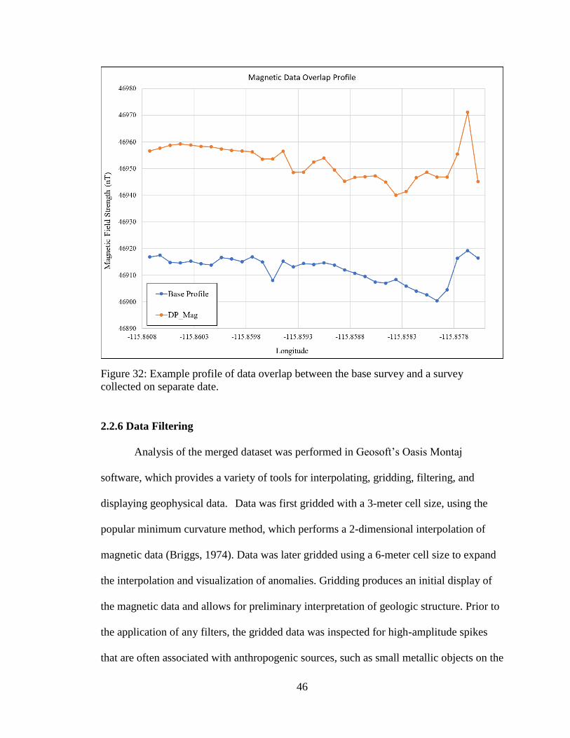
A correction was, however, necessary to merge datasets that were collected on

different dates. A base survey was conducted to acquire measurements that overlapped in

space with lines collected for the same locations during previous surveys and any

subsequent survey was designed to overlap with a section of this base survey. Data

overlaps were then plotted to determine the deviation or offset from the base survey,

which arises due the time-dependent fluctuations in the regional magnetic field (Fig. 32).

The mean difference between the two datasets was calculated and the secondary dataset

was corrected to the base. Once all surveys had been corrected to the base survey, the

datasets were compiled into one database for analysis.

Figure 31: Diurnal variation of total magnetic field recorded at the Tuscon, AZ

geomagnetic observatory on October 20th, 2017. A magnetic survey was conducted at

Dos Palmas on the same date, between 12:30 and 15:00. Vertical axis denotes total field

intensity in nanoteslas, with total variation for the time window in parentheses. The total

variation in the field intensity for the duration of the survey was approximately 1.7 nT.

End 15:00 Start 12:30

46

2.2.6 Data Filtering

Analysis of the merged dataset was performed in Geosoft’s Oasis Montaj

software, which provides a variety of tools for interpolating, gridding, filtering, and

displaying geophysical data. Data was first gridded with a 3-meter cell size, using the

popular minimum curvature method, which performs a 2-dimensional interpolation of

magnetic data (Briggs, 1974). Data was later gridded using a 6-meter cell size to expand

the interpolation and visualization of anomalies. Gridding produces an initial display of

the magnetic data and allows for preliminary interpretation of geologic structure. Prior to

the application of any filters, the gridded data was inspected for high-amplitude spikes

that are often associated with anthropogenic sources, such as small metallic objects on the

Figure 32: Example profile of data overlap between the base survey and a survey

collected on separate date.

47

surface or in the very shallow subsurface. Many of these spikes were removed, although

the presence of a barbed wire fence and a large metal gate produced significant anomalies

near the trace of the Hidden Springs Fault that proved impossible to remove from the

data. This anomaly introduced issues with interpretation, however, the use of multiple

geophysical methods, including Very Low Frequency (VLF) helped circumvent this issue

and provided additional confirmation of observed anomalies.

The reduction to the pole filter is commonly applied to data collected at mid

magnetic latitudes (Nabighian et al., 2005). While the shape of a magnetic anomaly is

governed by the shape and structure of the source, it is also dependent on the orientation

of the source with respect to magnetic north, the inclination and declination of the

source’s magnetization, and the inclination and declination of the local magnetic field.

The reduction to the pole filter transforms an observed anomaly into the anomaly that

would be measured if the measurement had been collected at the magnetic pole;

therefore, relocating the anomaly above its source (Baranov and Naudy, 1964; Nabighian

et al., 2005). The application of this method operates under the assumption that the

direction of magnetization is parallel to the Earth’s magnetic field, or within 25° (Bath,

1968) and neglects remnant magnetization. This assumption should be reasonable for the

region of Dos Palmas Preserve, as rocks and sediment are primarily quaternary in age and

have likely undergone minimal rotation (Grauch and Hudson, 2007; McNabb, 2013).

2.3 Very Low Frequency (VLF)

Very low frequency (VLF) electromagnetic induction is a passive geophysical

technique that measures magnetic fields generated in planar subsurface conductors

(Phillips and Richards, 1975). The VLF method was popularized in the 1970s and 1980s

48

and has gained renewed interest for its success in characterizing a variety of geophysical

targets, including shallow faults, aquifers, and zones of mineralization (Gurer et al., 2009;

Jeng, 2012; Dailey et al., 2014) Global networks of submarine communication

transmitters form the electromagnetic source for VLF surveys. These transmitters

produce signals within the range of 15 -30 kHz, which at large distances, propagate

through the subsurface as horizontally planar, electromagnetic waves (Phillips, 1975).

When the electromagnetic field produced by VLF transmitters encounters a

conductive, planar structure, such as a fault, it will induce eddy currents and a secondary

magnetic field within the structure (Phillips, 1975; Hutchinson and Barta, 2002; Fig. 33).

This secondary field creates a tilt in the primary field within the vicinity of the conductor

(Fig. 34). The tilt is thus a function of the secondary field and also, the electrical

properties of the planar conductor; VLF is therefore effective at characterizing hydrologic

boundaries and vertical, conductive faults, where saturated fault gouge may create

significant tilts in the induced field (Fraser, 1969; Fischer, 1983; Sundararajan, 2007;

Dailey, 2015). For this reason, VLF serves as a compliment to ground-based resistivity

surveys, especially in areas where the installation of lines of electrodes is impractical.

49

Figure 33: Diagram of electrical eddy currents induced in a vertical conductor by

primary VLF signal. Eddy currents generate secondary magnetic field perpendicular

to the primary field. From Phillips (1975).

Figure 34: Tilt-angle of primary magnetic field measured over a vertical,

planar conductor, such as a fault (Top). Tilt of the primary magnetic field

near a planar conductor as a result of secondary field (Bottom). From

Hutchinson and Barta (2002).

50

2.3.1 Equipment

VLF surveys were conducted using a VLF attachment to the GEM System’s

walking magnetometer. Surveys collect both VLF measurements as well as magnetic

data; however, while magnetic measurements are gathered every two seconds, VLF

measurements are collected manually by pressing a button on the control unit. VLF

measurements consist of an in-phase component and a quadrature (out of phase)

component expressed as a percentage of the primary field (Fig. 35). Most applications,

however, only utilize the in-phase component (Lin and Jen, 2010). Prior to beginning a

survey, three VLF source stations may be selected. VLF measurements were recorded

using three source stations, including NLK: 24.8 kHz (Seattle, WA), NML: 25.2 kHz

(Lamour, ND) and NAA: 24.0 kHz (Cutler, ME). Optimum anomaly signal strength is

achieved when profiles trend perpendicular to the radial azimuth of transmitting stations,

while the direction of the primary field propagation is approximately parallel to the strike

of the conductor, as in Figure 33 (Fraser, 1969); therefore, the signal propagation

direction with respect to the target and proposed profile was a significant consideration

when selecting source stations. Station NLK exhibited ideal geometry for SW-NE

profiles across the Hidden Springs fault zone, which trends NW-SE. Measurements were

taken every 20-30 meters.

2.3.2 Data Processing

The location of a fault along a profile is approximated by the point at which the

in-phase component of tilt crosses the x-axis, or passes through zero (Fig. 34; Fraser,

1969). Zero-crossings may, however, be obscured by geologic noise that inhibits

interpretation (Fraser, 1969; Jeng et al., 2012). To address this issue, data was processed

51

using the linear Fraser Filter, which transforms zero-crossings along a profile into peaks

that are repositioned above the conductor (Fraser, 1969). The first filtered value for

consecutive readings is estimated by f1=(M3+M4) - (M1+M2), where M equals the in-

phase component of tilt for each measurement, plotted between measurements 2 and 3

(Fig. 36). Magnetic data that were collected concurrently with VLF will be evaluated

along with Fraser Filtered profiles.

Figure 35: Raw VLF measurements collected across the trace of the Hidden Springs

Fault. In-phase measurements plotted in blue; Out of phase measurements in orange.

52

Figure 36: Raw (blue) and Fraser filtered (orange) in-phase component of VLF data.

53

2.3.3 Case Studies: Characterization of Saturated Fault Zones using VLF

As discussed in the previous sections, VLF surveys are useful for detecting

conductive fault zones. While a variety of factors may influence the electrical properties

of a fault, we are most interested in the presence of water within the HSF and other faults

that may exist near San Andreas Oasis. The following studies demonstrate the ability of

VLF surveys to identify conductive, water-bearing fault zones.

Burkina Vaso, a landlocked country of west Africa, is bounded to the north by the

Sahara Desert and to the south by rainforest. The geology of the region is characterized

by Precambrian granites, meta-sedimentary rock, and volcanics. In an effort to locate

potential groundwater resources and well locations, Palacky et al. (1983) deployed

resistivity and VLF surveys at known fractured zones in both granitic rocks and volcanic

sediments. Despite considerable geological noise, two conductors were identified in VLF

measurements, indicated by zero crossings in the in-phase component of tilt (Fig. 37),

and confirmed in resistivity data by zones of relatively high conductivity. Conductor B

was drilled for ground truth, which both yielded a productive well and confirmed the

success of VLF at this location.

Fractures were also detected using VLF surveys near a mine in the Appalachian

coal basin, where long-wall mining operations have produced fractures that propagate to

the surface and capture stream flow (Hutchinson and Barta, 2002). VLF profiles were

conducted parallel to streams using station NAA (Cutler, Maine) as a source. In-phase

measurements were Fraser-filtered to better identify anomalies. Hutchinson and Barta

(2002) interpreted smaller tilt anomalies as shallow, poorly-developed fractures, whereas

medium-large tilt angles were indicative of deep, saturated, well-developed fractures.

54

Once the located fractures had been grouted and sealed, VLF surveys were repeated at

these locations and revealed significant attenuation of tilt angles, indicating that water

was no longer draining into these structures (Fig. 37).

Figure 37: Results from VLF survey (top) and resistivity profile (middle) conducted

across a granitic fracture zone near the city of Rapadama, Burkina Vaso. VLF results

display both the in-phase and quadrature components of tilt, with zero crossings in the in-

phase component indicative of a planar conductor or saturated fault, denoted by A and B.

Station FUO (Bordeaux, France) used as a source for VLF measurements. Geologic

profile (bottom) displays interpretation of the two fractures zones, with a productive well

placed at fracture zone associated with B. From Palacky et al. (1981).

55

Dailey et al. (2015) utilized VLF, in combination with remote sensing and

geochemical data to resolve sources of groundwater recharge and characterize the effects

of faulting on groundwater flow at a site in the Mojave Desert, located in southeastern

California. This particular study is highly relevant to the work at San Andreas Oasis and

was instrumental in the design and application of VLF surveys over the HSF. The

Mojave River Groundwater Basin (MRGB) and the Morongo Groundwater Basin (MGB)

constitute the primary freshwater reservoirs in the region. Growing development and

increased groundwater withdrawal have produced varying effects on water levels across

the two aquifers, with the central portion of the MRGB experiencing the greatest decline

in water levels. The two groundwater basins are bisected by the Helendale Fault (HF), a

Figure 38: VLF results for a profile conducted along a stream near a coal mine in

southwestern Pennsylvania. VLF data are Fraser-filtered and depict both pre-grouting and

post-grouting measurements. Significant tilt angles are observed in pre-grouting data and

indicate locations of significant water-bearing fractures. Post-grouting data exhibit

attenuation of these large anomalies and indicate a dramatic reduction in conductivity and

therefore, presence of water within fractures. From Hutchinson and Barta (2002).

56

NW-trending dextral fault that originates in the San Bernardino mountains to the south an

terminates to the northwest against the Newberry mountains. It has been hypothesized

that the HF acts as a barrier to lateral groundwater flow. As discussed in Chapter One,

faults may exhibit anisotropic permeability, allowing flow along strike, while restricting

or preventing flow perpendicular to the fault zone. Dailey et al. (2015) performed VLF

and magnetic surveys across mapped surface traces of the HF to resolve any conductive

features created by the presence of water in the fault. The NLK (Seattle, WA) transmitter

station was used as a source for VLF. Data exhibited significant Fraser tilts and magnetic

anomalies coincident with mapped traces of the HF (Fig. 39). These results, along with

geochemical data, indicated that the HF acts as an enhanced flow path along strike,

carrying snowmelt and recharge from the San Bernardino foothills down into the central

parts of the MRGB and MGB, while limiting hydraulic communication between the two

aquifers (Dailey et al., 2015).

57

Figure 39: VLF surveys conducted across the northeastern portion of the Helendale Fault,

with significant Fraser tilts denoted by red circles (top). Mapped fault location indicated

by black dashed line. Red lines denote fault splays mapped from LiDAR and Geoeye-1

imagery. California Alquist-Priolo (AP) zones denoted by blue highlighted buffer on

either side of fault. Fraser tilts for profile P3001 displayed in panel D (middle), with

significant anomalies identified by A1 and A2. Fraser tilts (red) and magnetic data

(black) displayed for profile 0105 in panel E, with significant anomalies identified by B1,

B2, etc. (bottom). Adapted from Dailey et al. (2015).

58

CHAPTER 3: MEASUREMENTS AND INTERPRETATION

3.1 VLF Measurements

The VLF surveys conducted at Dos Palmas Preserve offer some of the most

easily-interpretable results and provide a useful context for subsequent interpretation of

resistivity and magnetic data, therefore the analysis of these surveys will be discussed

first. As detailed in the previous chapter, the electromagnetic response of a conductor is

governed both by the geometry between the source station and the strike of the

conductor. Measurements made using station NLK: 24.8 kHz (Seattle, WA) produced

optimal signal strength and significant Fraser tilts, as the propagation direction of the

primary field is approximately parallel to the trend of the HSF (Fig. 40), with the

magnetic field lines trending perpendicular to strike (Fig. 33). This response is consistent

with the USGS mapped surface trace of the HSF and, as we will show in this section, also

Figure 40: Primary field propagation directions for VLF stations NLK, NML, and NAA,

with station NLK: 24.8 kHz (Seattle, WA) exhibiting ideal geometry with the HSF.

Basemap from Google Earth imagery (2018). Faults from USGS Fault Map Database.

59

provides constraints on a secondary structure observed in VLF measurements to the east

of the Oasis.

Five northeast-southwest VLF profiles were conducted across the region

surrounding San Andreas Oasis and the HSF to capture any hydrologic boundaries or

conductive fault zones, which may be expressed as significant peaks in the filtered, in-

phase measurements (Fig. 41). Four additional profiles were conducted to the northeast of

the Oasis, near the canal. Measurements for these profiles did not exhibit any significant

peaks, aside from one profile, where large tilts coincide with the location of high-voltage

powerlines. This peak was therefore not considered reliable. The measurements for these

profiles are provided in Appendix A.

Figure 42 displays the Fraser-filtered, in-phase component of tilt for profile

DP_45, with measurements for each of the three VLF source stations used. 20

Figure 41: VLF profiles conducted across San Andreas Oasis and the HSF. White circles

indicate locations of VLF measurements. Base map from Google Earth imagery.

Location of the HSF adapted from USGS Fault Map Database (2018).

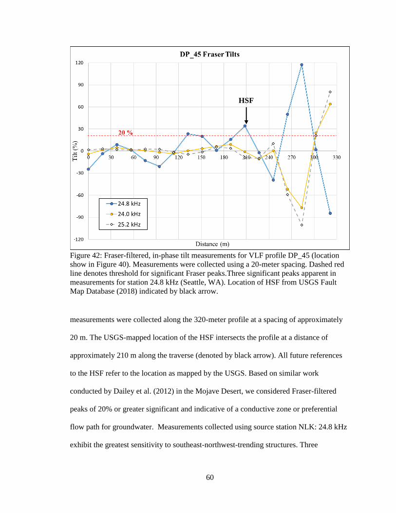
60

measurements were collected along the 320-meter profile at a spacing of approximately

20 m. The USGS-mapped location of the HSF intersects the profile at a distance of

approximately 210 m along the traverse (denoted by black arrow). All future references

to the HSF refer to the location as mapped by the USGS. Based on similar work

conducted by Dailey et al. (2012) in the Mojave Desert, we considered Fraser-filtered

peaks of 20% or greater significant and indicative of a conductive zone or preferential

flow path for groundwater. Measurements collected using source station NLK: 24.8 kHz

exhibit the greatest sensitivity to southeast-northwest-trending structures. Three

Figure 42: Fraser-filtered, in-phase tilt measurements for VLF profile DP_45 (location

show in Figure 40). Measurements were collected using a 20-meter spacing. Dashed red

line denotes threshold for significant Fraser peaks.Three significant peaks apparent in

measurements for station 24.8 kHz (Seattle, WA). Location of HSF from USGS Fault

Map Database (2018) indicated by black arrow.

HSF

61

prominent peaks appear at distances of 135 m, 207 m, and 287 m along the profile for

station NLK. The middle peak (207 m) corresponds with the mapped location of the HSF,

while the other two are located at approximately 45 m on either side of the fault trace.

This may be due to the presence of water in the damage zone structure or saturated fault

splays. The center peak exhibits a large Fraser tilt (117%), indicative of a highly

conductive fault. The remaining figures will display only the Fraser-filtered, in-phase

component of tilt for NLK: 24.8 kHz (Seattle, WA), as the measurements for this source

station consistently offer the largest amplitude peaks. The in-phase and filtered in-phase

measurements for stations NML: 25.2 kHz (LaMoure, ND) and NAA: 24.0 kHz (Cutler,

ME) are provided in Appendix A.

Profile DP_46 includes 37 measurements collected over a 711 m profile, with a

measurement spacing of approximately 20 m (Fig. 43). During this survey, we traversed

both the HSF, as well as the northern section of the San Andreas Oasis (Fig. 41). Similar

to profile DP_45, which was collected on the same day, there is a significant peak (34.2

%) located near the surface trace of the HSF. A second, larger anomaly (54.6%) appears

near the center of the Oasis, at a distance of approximately 260 meters along the profile,

while a third peak (34.5%) appears at 475 m, near the northeast margin of the Oasis. The

middle, high-amplitude peak may indicate the presence of a well-developed, saturated

fault or fault splay near the center of the Oasis. The third peak suggests that a conductive

structure may also bound the northeast margin of the Oasis. The third anomaly is almost

identical in magnitude to the first peak associated with the HSF. This suggests similarities

in conductivity and possibly the maturity of these features.

62

Figure 43: Fraser-filtered, in-phase tilt measurements for VLF profile DP_46, with a

measurement spacing of approximately 20 meters.

63

DP_49 was originally conducted as one long profile, however, when plotting the

measurement locations on a map, there was a slight change in the profile azimuth after

measurement 18. Fortunately, the azimuth remained constant for the remainder of the

profile. The profile was divided into two separate data sets based on azimuth: DP_49 and

DP_49_2. Profile DP_49 is 280 m in length and contains 16 measurements, collected at a

spacing of 15 m (Fig. 44). There is only one significant peak located at 275 m, which

appears to coincide with the trace of the HSF. This indicates that the segment of the HSF

between profiles DP_46 and DP_49 is saturated and may act as a preferential flowpath

for groundwater.


measurement spacing of approximately 15 m.

64

DP_49_2 and DP_50 were conducted to the east of the HSF and traverse the

southern section of the Oasis (Fig. 40). DP_49_2 includes 47 measurements collected

along a 760 m profile (Fig. 45). DP_50 is composed of 28 measurements along a 690 m

profile, with a spacing of 20 m (Fig. 46). The profiles are spaced approximately 110 m

apart and trend parallel to one another. Each profile crosses a linear topographic feature,

also apparent in satellite imagery as a lineation of plant and palm growth to the southeast

of the densely-vegetated section of San Andreas Oasis. Significant Fraser peaks (>20%)

are observed in similar locations along each profile and seem to spatially correlate with

this feature. To better visualize the spatial relationship between the various anomalies, the

following section provides a map view of measurements for the five profiles,

accompanied by an analysis of observed trends in the Fraser peaks.

65

Figure 45: Fraser-filtered, in-phase tilt measurements for VLF profile DP_49_2, with a


66



67

3.1.1 Interpretation of VLF Measurements

Figure 47 illustrates the location of Fraser peaks along each profile. White, hollow

circles indicate measurements with a Fraser tilt below 10%. Yellow circles denote

moderate tilts between 10-20% and red circles indicate significant anomalies (>20%).

While we conservatively defined peaks >20% as significant or indicative of a saturated,

conductive fault, other studies have interpreted smaller peaks as shallow, less-developed

fractures (Hutchinson and Barta, 2002). At San Andreas Oasis, moderate peaks (10-20%)

may represent components of the damage zone structure or shallow splays. Together, a

series of high tilt values (>20%) suggest the presence of at least two primary conductors

bounding the Oasis to the east and west. Along the southwest margin of the Oasis,

profiles DP_45, DP_46, and DP_49 exhibit large peaks that align with the mapped trace

Figure 47: Map of Fraser-filtered, in-phase VLF measurements conducted across the HSF

and San Andreas Oasis. White, hollow circles denote measurements with Fraser tilt <

10%; yellow circles indicate moderate tilts (10-20%); and significant Fraser peaks

(>20%) are denoted by red circles. Basemap from Google Earth imagery.

Fraser tilt > 20%

Fraser tilt 10-20%

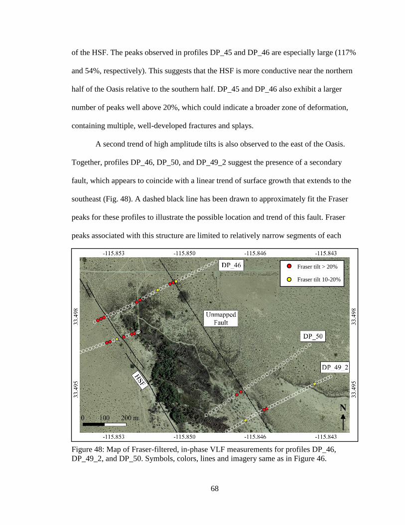
68

of the HSF. The peaks observed in profiles DP_45 and DP_46 are especially large (117%

and 54%, respectively). This suggests that the HSF is more conductive near the northern

half of the Oasis relative to the southern half. DP_45 and DP_46 also exhibit a larger

number of peaks well above 20%, which could indicate a broader zone of deformation,

containing multiple, well-developed fractures and splays.

A second trend of high amplitude tilts is also observed to the east of the Oasis.

Together, profiles DP_46, DP_50, and DP_49_2 suggest the presence of a secondary

fault, which appears to coincide with a linear trend of surface growth that extends to the

southeast (Fig. 48). A dashed black line has been drawn to approximately fit the Fraser

peaks for these profiles to illustrate the possible location and trend of this fault. Fraser

peaks associated with this structure are limited to relatively narrow segments of each

Figure 48: Map of Fraser-filtered, in-phase VLF measurements for profiles DP_46,

DP_49_2, and DP_50. Symbols, colors, lines and imagery same as in Figure 46.

Fraser tilt > 20%

Fraser tilt 10-20%

69

profile, with only a few Fraser tilt values exceeding 20%. We speculate that deformation

along the eastern margin of the Oasis may be more narrowly constrained, whereas, to the

west of the Oasis, deformation is distributed over a broader zone around the HSF,

creating multiple flow pathways and therefore, multiple Fraser peaks.

70

3.2 Resistivity Inversion Results and Interpretation

While VLF measurements offer valuable information on the locations and trend

of conductive, water-bearing faults and fractures near San Andreas Oasis, our analysis of

these features is limited to a qualitative assessment of fault properties and approximate

map location, based on the amplitude and distribution of Fraser peaks. Resistivity data

offer further insight into the 2-dimensional structure of the HSF fault zone, as well as its

role in groundwater flow. A total of 9 resistivity profiles were conducted around San

Andreas Oasis and near the mapped surface trace of the HSF, as well as to the east of the

Oasis (Fig. 49). To better visualize the relationship between each profile and its

proximity to the HSF and other physical surface features, Figure 50 offers a higher

resolution map, focusing on the northern section of San Andreas Oasis. Considering our

Figure 49: Map of resistivity surveys conducted at San Andreas Oasis. Individual profiles

denoted by thick black lines. Location of the HSF (thin black line) from USGS Fault Map

Database (2018). Basemap from Google Earth imagery (2018).

71

objectives to both image groundwater near the Oasis and constrain groundwater-fault

dynamics (i.e., groundwater barrier vs. conduit) we will discuss the inversion results for

each profile from east to west, approaching and crossing the fault zone.

Resistivity survey DF5 was conducted along the eastern margin of San Andreas

Oasis using an electrode spacing of 3.5 m, with electrode 1 placed at the west end of the

profile, nearest the Oasis. The eastern side of the Oasis is characterized by silty Lake

Cahuilla sands and random burn piles punctuate the perimeter. Survey DF5 was located

near one of these ash piles. Surveys DF 1 – DF5 were conducted in late January of 2017,

following moderate precipitation. While surface conditions in this area are generally

Figure 50: Zoomed in map of resistivity profiles conducted at San Andreas Oasis.

Approximate extent indicated by dashed red box in Figure 48. White text displays survey

name followed by location of electrode 1 (A) and electrode 24 (A’). Location of HSF

(thin black line) from USGS Fault Map Database (2018). Basemap from Google Earth

imagery (2018).

72

resistive, we observed a relatively high degree of soil moisture, which allowed for

successful electrode-ground coupling. The inversion model determined subsurface

resistivity to a maximum depth of 15.1 m, with resistivity values ranging from 1 – 42

ohm*m (Fig. 51, bottom). These values are relatively low for unconsolidated sediments,

sandstones, and conglomerates, however, the presence of clays, recent precipitation, and

saline groundwater (due to the presence of evaporites) likely allow for a much lower

resistivity range (Palacky, 1988; Ball et al., 2010). The measured apparent resistivity

pseudosection (top) displays the measurements plotted at the midpoint of the potential

electrodes, with the pseudo-depth approximated from the electrode spacing. The

calculated apparent resistivity pseudosection (middle) is derived from the inverse model

(bottom). The inverse model is iteratively adjusted to achieve a better fit between the

measured apparent resistivity pseudosection (top) and the calculated apparent resistivity

pseudosection (middle; Fig. 51). The RMS error indicates how well the calculated

apparent resistivity and measured apparent resistivity pseudosections fit. A relatively

high RMS of 11.2 % for this profile may be due to large resistivity variations near the

surface and the presence of a burn pile near the center of the profile. A shallow, highly

conductive zone is observed at a depth of approximately 4 m and appears to shallow to

2.7 m in the direction of the Oasis. Resistivity values of this layer are consistent with

saline groundwater. This survey appears to indicate the presence of shallow groundwater

to the east of the Oasis.

73

Fig

ure 5

1: In

versio

n resu

lts for resistiv

ity su

rvey D

F5, w

ith d

epth

and h

orizo

ntal d

istance alo

ng th

e pro

file in m

eters. An T

he to

p

pro

file disp

lays th

e measu

red ap

paren

t resistivity

pseu

dosectio

n. M

easurem

ents co

nducted

usin

g an

electrode sp

acing o

f 3.5

m. T

he

mid

dle p

rofile d

epicts th

e pred

iction o

f the ap

paren

t resistivity

measu

remen

ts that w

ould

be g

enerated

for th

e inverse m

odel o

f

resistivity

(botto

m p

rofile). T

he b

otto

m p

rofile d

isplay

s the in

verse m

odel o

f resistivity

as a functio

n o

f dep

th an

d h

orizo

ntal d

istance

along th

e pro

file.

74

Survey DF7 was conducted in mid-March 2017 to the northwest of profile DF5,

with an electrode spacing of 4 m. Electrode 1 was located on the west end of the profile.

Surface soil conditions were dry relative to the profiles conducted 2 months earlier, as the

region receives much of its annual precipitation in December through February. The

inverse model displays subsurface resistivity to a depth of 17.2 m, with an RMS of

13.6%. Resistivity values range from 1.3 – 60.4 ohm*m, with a highly conductive layer

located at approximately 3 m depth (Fig. 52). This layer exhibits resistivity values and a

thickness similar to those observed in survey DP5 and suggests the presence of

groundwater near the Oasis and to the east of the HSF. There is an interesting stepped

anomaly (indicated by black arrow) at approximately 36 m along the profile. The feature

exhibits conductivity values consistent with both freshwater and clays and may represent

vertical offset along a buried, clay-rich fault. The resistive surface layer is likely

representative of the silty sands that characterize the area around San Andreas Oasis,

which again, may contribute to the high RMS error.

75

Fig

ure 5

2: In

versio

n resu

lts for resistiv

ity su

rvey D

F7, w

ith d

epth

and h

orizo

ntal d

istance alo

ng th

e pro

file in m

eters. Measu

remen

ts

conducted

usin

g an

electrode sp

acing o

f 4 m

. The to

p p

rofile d

isplay

s the m

easured

apparen

t resistivity

pseu

dosectio

n. T

he m

iddle

pro

file dep

icts the p

redictio

n o

f the ap

paren

t resistivity

measu

remen

ts that w

ould

be g

enerated

for th

e inverse m

odel o

f resistivity

(botto

m p

rofile). T

he b

otto

m p

rofile d

isplay

s the in

verse m

odel o

f resistivity

as a functio

n o

f dep

th an

d h

orizo

ntal d

istance alo

ng th

e

pro

file.

76

Survey DF9 was also conducted in March 2017, with an electrode spacing of 3 m

(Fig. 53). Inversion results depict a shallow resistive surface layer, similar to surveys DP5

and DP7, however, the range of resistivity measurements is much larger, with values

from 9.6 to 332 ohm*m. A conductive zone is observed at approximately 3-4 m depth,

although this layer is laterally discontinuous, with resistivity values increasing toward the

HSF. There is a small, conductive feature at 21 m along the profile that appears imbedded

within a more resistive zone. This anomaly may indicate a small pocket of water or clay,

however, while the resistivity values of this feature are consistent with groundwater (1-

100 ohm*m), they are considerably higher than values observed in the shallow

conductive zone to the east (1-10 ohm*m). Since this profile trends normal to the HSF,

this anomaly may indicate the presence of a shallow, south-trending flow channel.

77

Fig

ure 5

3: In

versio

n resu

lts for resistiv

ity su

rvey D

F9, w

ith d

epth

and h

orizo

ntal d

istance alo

ng th

e pro

file in m

eters. Measu

remen

ts

con

ducted

usin

g an

electrod

e spacin

g o

f 3 m

. The to

p p

rofile d

isplay

s the m

easured

apparen

t resistivity

pseu

dosectio

n. T

he m

iddle

pro

file dep

icts the p

redictio

n o

f the ap

paren

t resistivity

measu

remen

ts that w

ould

be g

enerated

for th

e inverse m

odel o

f resistivity

(botto

m p

rofile). T

he b

otto

m p

rofile d

isplay

s the in

verse m

odel o

f resistivity

as a functio

n o

f dep

th an

d h

orizo

ntal d

istance alo

ng th

e

pro

file.

78

Surveys DF1-DF4, including DF6 were conducted further to the south, in a

narrow zone between the Oasis and the HSF. The area is sparsely vegetated and the

surface is covered by an evaporite or precipitate layer, which is localized to the western

fringe of the Oasis. This layer forms a thick crust that was removed prior to insertion of

the electrodes. During surveys DF1-DF4, the soil was relatively wet and exhibited mud

cracks. Surveys were installed between a barbed-wire fence with wooden posts and the

tree line of the Oasis. The fence trends north-south and runs along the approximate

surface trace of the HSF, which in most instances, prevented installation of resistivity

profiles directly over the fault. Survey DF1 was conducted with an electrode spacing of 2

m, with electrode 1 installed on the west end of the profile, nearest the HSF. The inverse

model reaches a maximum depth of 8.6 m, with a resistivity range of 6.3 – 39 ohm*m

(Fig. 54). A conductive surface layer extends from electrode 24 to the center of the

profile and likely captures the wet, hypersaline evaporite layer. This may also account for

a relatively low RMS error of 6.9 %, as this layer allowed for good electrode coupling.

Between electrodes 14 and 24, there is a significant resistivity gradient, which suggests a

change in subsurface properties moving toward the Oasis, with higher resistivity values

encountered toward the east. This may reflect a decrease in water content or the presence

of a fault between the HSF and the Oasis. Near the bottom of the profile, at a depth of

approximately 5 m, there is a conductive zone that trends toward the east. The resistivity

values of this feature, as well as its depth are similar to observations of the conductive

zone in survey DF9 and those to the east of the Oasis. This profile may capture the

western edge of the shallow aquifer as it terminates against the fault zone.

79

Fig

ure 5

4: In

versio

n resu

lts for resistiv

ity su

rvey D

F1, w

ith d

epth

and h

orizo

ntal d

istance alo

ng th

e pro

file in m

eters. Measu

remen

ts

conducted

usin

g an

electrode sp

acing o

f 2 m

. The to

p p

rofile d

isplay

s the m

easured

apparen

t resistivity

pseu

dosectio

n. T

he m

iddle

pro

file dep

icts the p

redictio

n o

f the ap

paren

t resistivity

measu

remen

ts that w

ould

be g

enerated

for th

e inverse m

odel o

f resistivity

(botto

m p

rofile). T

he b

otto

m p

rofile d

isplay

s the in

verse m

odel o

f resistivity

as a functio

n o

f dep

th an

d h

orizo

ntal d

istance alo

ng th

e

pro

file.

80

Survey DF2 was pivoted to the north about electrode 24 to lengthen the profile in

this approximate location. An electrode spacing of 2.5 m was used, which increased the

depth imaged to 10.8 m. Near the center of the profile, there is a lateral resistivity

contrast similar to the one observed in survey DF1 (Fig. 55). The western half of the

profile, from 0 to 25 m, indicates a conductive zone extending from the surface to a depth

of 10.8m. Survey DF2 trends along the lineation of plant growth and oblique to the HSF.

This survey may capture more of the saturated zone along the edge of the Oasis in the

northwest half of the profile.

Survey DF6 was conducted northwest to southeast and traverses both profiles

DF1 and DF2. The inverse model determines subsurface resistivity to a depth of 17.2 m,

with an electrode spacing of 4 m (Fig. 56). The model depicts a largely homogenous

subsurface, with the exception of a conductive zone near electrode 20, at the north end of

the profile. This segment of the survey crosses the conductive surface layer observed in

DF1 and DF2 and may captures the edge of the evaporite layer. Alternatively, it may also

capture the edge of the conductive zone observed in profile DF2 and suggested by the

location of a Fraser peak in VLF survey DP_45. The surveys conducted in this area do

not seem to image the HSF as a single fault strand, but rather, a fault zone with multiple

flow pathways, fractures, and permeability structure. Alternatively, the zone covered by

resistivity surveys DF1, DF2, and DF6 may include a resistive layer or structure that

produces local variability. This relationship will be considered at further length in the

discussion section of this chapter.

81

Fig

ure 5

5: In

versio

n resu

lts for resistiv

ity su

rvey D

F2, w

ith d

epth

and h

orizo

ntal d

istance alo

ng th

e pro

file in m

eters. Measu

remen

ts

conducted

usin

g an

electrode sp

acing o

f 2.5

m. T

he to

p p

rofile d

ispla

ys th

e measu

red ap

paren

t resistivity

pseu

dosectio

n. T

he m

iddle

pro

file dep

icts the p

redictio

n o

f the ap

paren

t resistivity

measu

remen

ts that w

ould

be g

enerated

for th

e inverse m

odel o

f resistivity

(botto

m p

rofile). T

he b

otto

m p

rofile d

isplay

s the in

verse m

odel o

f resistivity

as a functio

n o

f dep

th an

d h

orizo

ntal d

istance alo

ng th

e

pro

file.

82

Fig

ure 5

6: In

versio

n resu

lts for resistiv

ity su

rvey D

F6, w

ith d

epth

and h

orizo

ntal d

istance alo

ng th

e pro

file in m

eters. Measu

remen

ts

con

ducted

usin

g an

electrod

e spacin

g o

f 2 m

. The to

p p

rofile d

isplay

s the m

easured

apparen

t resistivity

pseu

do

section. T

he m

idd

le

pro

file dep

icts the p

redictio

n o

f the ap

paren

t resistivity

measu

remen

ts that w

ould

be g

enerated

for th

e inverse m

odel o

f resistivity

(botto

m p

rofile). T

he b

otto

m p

rofile d

isplay

s the in

verse m

odel o

f resistivity

as a functio

n o

f dep

th an

d h

orizo

ntal d

istance alo

ng th

e

pro

file.

83

Survey DF3 and DF4 were conducted further to the south of profiles DF1 and

DF2, both using an electrode spacing of 3 m. GPS coordinates for DF3 were, however,

were found to be unreliable and placed the profile in the center of the Oasis. This survey

is therefore not included, as we cannot constrain its location. DF4 is the only profile that

crosses the mapped surface trace of the HSF, with electrode 1 located west of the fault.

When setting up the survey, water was observed pooling around some of the electrodes.

The HSF is likely expressed as a conductive feature near the center of the profile (Fig.

57). Low values (~10 ohm*m) are constrained to a narrow, vertical anomaly, while the

region around this anomaly exhibits much higher resistivity values. This suggests that the

HSF may exhibit anisotropic permeability, allowing vertical fluid migration or flow along

dip; however, due to the absence of a shallow, highly conductive zone (as in surveys

DF5, DF7 and DF 9), we speculate that the fault also acts as a barrier to lateral flow

(Caine and Minor, 2009). Additionally, values within the vertical anomaly are within the

range for clay, which supports the notion of a clay-rich fault core, with narrow

architectural components (Caine et al., 1996; Caine and Minor, 2009; Bense et al., 2006).

This suggests that the HSF may be constrained to a single fault strand in the southern half

of the Oasis.

84

Fig

ure 5

7: In

versio

n resu

lts for resistiv

ity su

rvey D

F4, w

ith d

epth

and h

orizo

ntal d

istance alo

ng th

e pro

file in m

eters. Measu

remen

ts

conducted

usin

g an

electrode sp

acing o

f 3 m

. The to

p p

rofile d

isplay

s the m

easured

apparen

t resistivity

pseu

dosectio

n. T

he m

iddle

pro

file dep

icts the p

redictio

n o

f the ap

paren

t resistivity

measu

remen

ts that w

ould

be g

enerated

for th

e inverse m

odel o

f resistivity

(botto

m p

rofile). T

he b

otto

m p

rofile d

isplay

s the in

verse m

odel o

f resistivity

as a functio

n o

f dep

th an

d h

orizo

ntal d

istance alo

ng th

e

pro

file.

85

Survey DF8 was conducted as a north-south trending profile to the west of the

HSF trace, with an electrode spacing of 5 m. Electrode one is oriented at the south end of

the profile, with electrode 24 located to the north, approximately 25 m from the fault

trace. The inverse model displays subsurface resistivity, ranging from 7 to 111 ohm*m, to

a depth of 21.5 m (Fig. 58). There is a resistive surface layer that extends to a depth of

approximately 9 m, which interrupted by a shallow conductive feature, similar to the

conductive zone observed in DF9. This may indicate the presence of another channel, as

speculated in DF9. Lateral flow across the fault appears to be inhibited, as the shallow

conductive zone is discontinuous near the fault and does not appear in profile DF9, to the

west of the HSF.

86

Fig

ure 5

8: In

versio

n resu

lts for resistiv

ity su

rvey D

F8, w

ith d

epth

and h

orizo

ntal d

istance alo

ng th

e pro

file in m

eters. Measu

remen

ts

conducted

usin

g an

electrode sp

acing o

f 5 m

. The to

p p

rofile d

isplay

s the m

easured

apparen

t resistivity

pseu

dosectio

n. T

he m

iddle

pro

file dep

icts the p

redictio

n o

f the ap

paren

t resistivity

measu

remen

ts that w

ould

be g

enerated

for th

e inverse m

odel o

f resistivity

(botto

m p

rofile). T

he b

otto

m p

rofile d

isplay

s the in

verse m

odel o

f resistivity

as a functio

n o

f dep

th an

d h

orizo

ntal d

istance alo

ng th

e

pro

file.

87

3.3 Magnetic Survey Results and Interpretation

VLF and resistivity surveys identify conductive anomalies that are consistent with

the general location and trend of the HSF. The results of these surveys also provide some

indications of fault maturity, lithology, and structure. Magnetic surveys were conducted

to image the fault on a broader scale, as well as provide constraints on the nature of

faulting. As prefaced in Chapter 2, a barbed wire fence is inconveniently located along

the HSF near the Oasis and presented a challenge to obtaining continuous profiles across

the fault zone. Additionally, the presence of metallic surface objects, including metal

gates along the northern section of the Oasis, created significant magnetics responses that

were difficult to remove and therefore, hinder our interpretations of magnetic data at

these locations.

Figure 59 provides the merged results for each of the eight magnetic surveys

conducted at San Andreas Oasis. The map of total magnetic field intensity is interpolated

using the minimum curvature method, with a grid cell size of 3 m. The black lines denote

the walking paths for surveys, which provide an indication of data coverage and anomaly

constraints. Dense coverage was achieved by multiple surveys to the northwest and

northeast of the Oasis. Due to dense vegetation, surveys through the Oasis were not

possible.

88

The final merged map displays the reduced-to-pole, interpolated data, aggregated

to 6 x 6 m cell size to better visualize anomalies (Fig. 60). The black line indicates the

location of the HSF from the USGS Fault Map database (2018). White boxes denote the

locations of metallic surface objects, such as gates and the barbed wire fence, referenced

in the previous section. The western side of the map contains a relatively large anomaly

that is coincident with a topographic high to the west of the Oasis. This topographic

feature has been identified as a possible location for the HSF, although as discussed in

Chapter 1, this structure represents a vertical sense of motion along the fault (Babcock,

Figure 59: Map of interpolated total magnetic field intensity. Measurements are gridded using

the minimum curvature method, with a 3x3 grid cell size. Black line indicates walking path and

data coverage for surveys. Cool colors denote zones of low total magnetic field intensity, while

warmer colors, such as pink and red, indicate higher values.

89

1974; Sylvester, 1976; Dorsey, 2011; McNabb, 2013), whereas, both the USGS and CGS

have inferred purely right-lateral slip along the HSF. The magnetic anomaly exhibits a

relatively large amplitude (+30 nT) and wavelength, which suggest a significant contrast

in subsurface magnetic properties. The outcrop associated with this anomaly is composed

of course-grain sandstones and arkosic conglomerate (Babcock, 1974). These rocks

generally do not exhibit significant magnetic responses; however, in some locations,

Figure 60: Final merged and interpolated map of total magnetic field intensity, gridded

using a 6x6 m cell size. The interpolated map has been reduced to the pole to relocate

anomalies above the source. Cool colors denote zones of low total magnetic field intensity,

while warmer colors, such as pink and red, indicate higher values. The black line denotes the

location of the HSF from the USGS Fault Map Database (2018). The purple line indicates

the location of the Mecca Hills Fault Zone. The location of San Andreas Oasis is

indicated by a white star for reference. White boxes indicate locations of metal surface

objects.

90

upper units contain large, imbedded fragments of schist, derived from the nearby

Orocopia mountains (Babcock, 1974; McNabb, 2013). Additionally, the area

immediately to the east of the exposed outcrop is characterized by sand and alluvial

cover, which combined with vertical offset, may create a significant contrast in magnetic

properties (Gunn, 1997). Considering the topographic relief along this structure, which is

apparent as a 3-4 m scarp, we speculate that this anomaly results from the vertical

juxtaposition of sediments with varying magnetic properties.

A second, linear anomaly parallels the surface trace of the HSF to the northwest

of the Oasis. It is expressed as a short-wavelength anomaly, with an amplitude of

approximately 15-20 nT. These attributes are characteristic of shallow, intra-sedimentary

faults, which tend to be expressed as subtle, linear anomalies (Blakely et al., 2000;

Grauch and Hudson, 2007; Nabighian et al., 2005). While these two structures each cut

sedimentary units, they have distinct magnetic characteristics; therefore, we speculate

that the linear anomaly is likely the magnetic expression of the HSF, whereas the larger

anomaly to the west represents a separate structure. It is difficult to speculate on the

source of this anomaly, although if the HSF permits fluid migration along strike, this may

allow for mineralization or precipitation of magnetic minerals within the fault zone

(Reynolds et al., 1990; Gunn, 1997; Blakely et al., 2000).

A magnetic low appears to encompass the area around the Oasis, with the

presence of the HSF and the normal fault further west forming a significant contrast in

magnetic properties along the western margin of the Oasis. To the east, this contrast is

less pronounced, although there is a subtle, linear anomaly located to the southeast of the

Oasis that may correspond with the conductive structure identified by VLF surveys along

91

the eastern margin of the Oasis (Fig. 60). Figure 61 displays the magnetic measurements

collected during VLF survey DP_49, which were not influenced or limited by the

presence of the barbed wire fence. In this area to the south of the Oasis, the magnetic

expression of the HSF is more subdued, while the linear feature to the east of the Oasis is

expressed as a subtle, narrow peak (~20 nT). We speculate that the cause of this anomaly

may also be related to mineralization or fault zone alteration. In the following section, we

provide an integrated interpretation of results from each of the three geophysical methods

used in this study.

Figure 61: Profile of magnetic measurements collected along VLF profile DP_49.

Locations of HSF trace and the second fault to the east of the Oasis denoted by red

arrows. Map of profile in upper right inset.

92

3.4 Integrated Interpretation

Results of VLF, resistivity and magnetic measurements confirm the trend and

surface trace of the HSF, mapped to a similar location in this area by both the USGS and

CGS. Magnetic data depict a moderate, linear anomaly that aligns with the HSF and is

distinguishable from topography further to the west. The magnetic expression of the HSF

is consistent with observations of other intra-sedimentary faults, which tend to be

characterized by subtle, linear anomalies (Grauch and Hudson, 2007; Nabighian et al.,

2005). VLF and resistivity data indicate a conductive, water bearing fault zone, therefore,

we speculate that the source of the magnetic anomaly associated with the HSF is related

to mineralization within the fault zone or transport of detrital magnetite along the fault.

Detrital magnetite may be sourced from volcanic and metamorphic brought down along a

drainage to the northwest of the Oasis. Results of VLF surveys include multiple Fraser

peaks that align with both the HSF, as well as a second structure to the east of the Oasis,

also apparent as a linear boundary of surface growth. Unfortunately, due to issues with

electrode coupling, we were unable to complete resistivity surveys across this feature,

however, magnetic measurements depict a similar linear anomaly to the southeast of the

Oasis. Fraser peaks along this feature are similar in amplitude to those observed along the

HSF. We speculate that the fault zone exhibits an equivalent degree of saturation and a

clay-rich core. Furthermore, the narrow distribution of Fraser tilts above 20% indicates a

relatively narrow fault zone architecture, where most deformation is likely

accommodated along the fault core. Conversely, VLF surveys performed across the HSF

indicate multiple conductors and we speculate that deformation may be distributed over a

broader damage zone in the northern half of the Oasis.

93

Resistivity surveys detected a highly conductive zone to the east of the HSF,

between the unmapped fault and the Oasis. Due to exceedingly low resistivity values, we

interpret this feature as the shallow aquifer, with a depth to groundwater of approximately

4 m. Surveys conducted further to the west also depict this feature at a similar depth,

however, as profiles approach the HSF, the conductive zone disappears or terminates

against more resistive features, which we interpret as the HSF fault zone. The locations of

some of these boundaries are consistent with Fraser peaks from VLF measurements. In

one resistivity survey conducted across the HSF, we observe a highly conductive, vertical

anomaly, which may capture the saturated fault core, although the zone around this

feature is resistive. In combination with geochemical data collected near the HSF to the

southeast, which suggest a deep, hypersaline source of groundwater (Personal

communication, S. Osborn, 2018), we believe that the HSF may allow vertical migration

of deep basin brines along the fault. The absence of the conductive zone adjacent to the

HSF, along with patterns of plant growth suggest that, while it may permit flow along

strike, it also acts as a barrier to lateral groundwater flow. This scenario tends to

predominate among well-developed, clay-rich lithologies (Caine et al., 1996; Bense et al.,

2006), therefore we speculate the HSF is a relatively mature fault. Profile DF4 depicts a

conductive, vertical structure that is coincident with the surface trace of the HSF (Fig 57).

Further to the south, VLF survey DP_49 exhibits a single Fraser peak (>20%) along a

lineament of plant growth located 20 m to the northeast of the HSF (Fig. 62). We believe

this data suggests a single, constrained fault strand in the southern half of the Oasis,

whereas in the north, strain is partitioned over a broader fault zone.

94

Figure 62 displays the combined locations of Fraser peaks along VLF profiles,

locations of resistivity surveys, and fault locations inferred from offsets in reflectors from

the USGS seismic profile (personal communication, R. Catchings, 2018). The location of

a second fault bounding the east side of the Oasis is identified as a dashed black line.

Note that this location agrees well with the results from the USGS seismic survey. Figure

63 displays the map of total magnetic field intensity, including the location of the HSF

and the second fault, as located from VLF data. While we do not have constraints on the

two-dimensional structure of the second fault, we suspect that it may also form a partial

groundwater barrier, while exhibiting anisotropic permeability along strike. We speculate

that these two structures channel and localize groundwater beneath San Andreas Oasis.

This interpretation requires south-directed groundwater flow, however, as discussed in

95

Chapter 1, various hydrogeologic testing conducted to the northeast, near the Coachella

canal indicate a southwest groundwater flow direction. Therefore, we propose two

possible interpretations: (1) Groundwater flows to the southwest and is brought to the

shallow zone along fractures and faults near the Oasis, which facilitate communication

with the confined aquifer. (2) Groundwater flows southeast from a large drainage and is

channeled between the two faults and into the permeable damage zone beneath the Oasis.

We believe either interpretation is compatible with vertical migration of basin brines

Figure 62: Map of Fraser-filtered, in-phase VLF measurements conducted across the HSF

and San Andreas Oasis. White, hollow circles denote measurements with Fraser tilt <

10%; Yellow circles indicate moderate tilts (10-20%) and significant Fraser peaks

(>20%) are denoted by red circles. Thick black lines indicate locations of resistivity

surveys. Dashed black line denotes potential fault location from VLF measurements.

Blue triangles indicate fault locations from USGS seismic profile. Basemap from Google

Earth imagery.

96

along the HSF. Figure 64 depicts each of the possible flow directions with their

relationship to the fault zone. The drainage to the north offers a shorter flowpath relative

to recharge originating to the northeast, near the canal (Fig. 64). Furthermore,

groundwater flow directions tend to be dominated by topography and geology (Toth,

1963; Condon and Maxwell, 2001; Markland and Worman, 2007). Therefore, we favor

the second model, whereby shallow water flows to the southeast from the drainage

identified in Figure 64 along the impermeable HSF and is channeled between the two

Figure 63: Final merged and interpolated map of total magnetic field intensity, gridded

using 6x6 m cell size. The interpolated map has been reduced to the pole to relocate

anomalies above sources. Cool colors denote zones of low total magnetic field intensity,

while warmer colors, such as pink and red, indicate higher values. Black line denotes

location of HSF from USGS Fault Map Database (2018). Purple line indicates location of

the Mecca Hills Fault Zone. Location of second fault to the east of the Oasis denoted by

dashed black line.

97

faults to the northeast and southwest of San Andreas Oasis. This hypothesis is consistent

with historical accounts of water at San Andreas Oasis prior to canal construction, as this

drainage produces the largest volume of surface flow in the area (J. Minor, Bureau of

Land Management, personal communication, 2016).

Figure 64: Possible groundwater flow directions at Dos Palmas Preserve (blue arrows).

Location of the HSF and Mecca Hills Fault Zone (black solid lines) from USGS Fault

Map Database (2018). Fault to the east of the Oasis is denoted by a dashed black line.

Location of the Fault scarp is indicated by a black dotted line.

98

3.5 Tectonic Implications

Tectonic knowledge of the region encompassing Dos Palmas Preserve is

relatively limited. Various interpretations of geomorphic features along the fault zone

have yielded a variety of fault locations and hypotheses regarding the nature of faulting

(Hays, 1957; Babcock, 1969; Clark, 1984). Fault classification has swung between purely

dextral shear and oblique strike-slip, with east-side down motion. As discussed, the latter

interpretation has been partly informed by the scarp to the west of the Oasis (Babcock,

1974; Sylvester, 1976; Dorsey, 2011), as well as observations of vertical offsets in Box

Canyon (Hays, 1957). Analysis of our magnetic data suggest that the HSF, as mapped

adjacent to San Andreas Oasis, may be separate from the scarp. Aside from subtle

topographic features along the Oasis, there are no clear indicators of vertical motion. This

does not, however, preclude the existence of transpressional or transtensional structures,

which are common along the San Andreas Fault (Sylvester, 1988). A series of hills to the

south of the Oasis appear to be the result of a left step in the fault, which creates a

restraining bend (Fig.10).

VLF and resistivity data collected in the northern half of the Oasis indicate the

presence of multiple conductive fractures, including a fault bounding the east side of the

Oasis. This suggests that in the northern half of the Oasis, the HSF may be characterized

as a zone of deformation, rather than a single fault strand. The USGS identified a series

of additional faults extending to the northeast across the Oasis (Fig. 65). While we do not

have any constraints on the strike of these faults, it is reasonable, based on the trends of

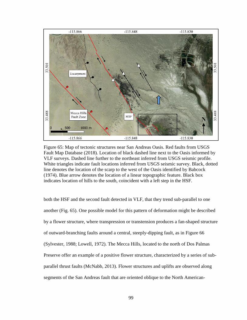
99

both the HSF and the second fault detected in VLF, that they trend sub-parallel to one

another (Fig. 65). One possible model for this pattern of deformation might be described

by a flower structure, where transpression or transtension produces a fan-shaped structure

of outward-branching faults around a central, steeply-dipping fault, as in Figure 66

(Sylvester, 1988; Lowell, 1972). The Mecca Hills, located to the north of Dos Palmas

Preserve offer an example of a positive flower structure, characterized by a series of sub-

parallel thrust faults (McNabb, 2013). Flower structures and uplifts are observed along

segments of the San Andreas fault that are oriented oblique to the North American-

Figure 65: Map of tectonic structures near San Andreas Oasis. Red faults from USGS

Fault Map Database (2018). Location of black dashed line next to the Oasis informed by

VLF surveys. Dashed line further to the northeast inferred from USGS seismic profile.

White triangles indicate fault locations inferred from USGS seismic survey. Black, dotted

line denotes the location of the scarp to the west of the Oasis identified by Babcock

(1974). Blue arrow denotes the location of a linear topographic feature. Black box

indicates location of hills to the south, coincident with a left step in the HSF.

100

Pacific plate slip vector (Sylvester, 1988; Fuis et al., 2012). The HSF and other faults

observed at Dos Palmas Preserve may form the southern expression of the deformation

regime observed in the Mecca Hills. During field surveys, we observed several linear

mounds that align with patterns of surface growth and are consistent with the trend and

location of the HSF and the faults to the east of the Oasis. One of these structures is

identified by a blue arrow in Figure 65. These features, along with the additional faults to

the northeast of the Oasis, may form the northern extent of a positive flower structure,

while the hills to the south of the Oasis (Fig. 65) relate to higher compressional stress and

thus, more topographic development, as in Figure 66. An alternative possibility may

involve the presence of another step in the fault that forms a releasing bend, as in Figure

67. This may help describe the localized presence of shallow groundwater at San Andreas

Oasis, as extension could create a small, compartmentalized sub-basin in the western half

of the Preserve.

Figure 66: Diagram of a positive flower structure along a dextral fault system. Adapted

from Sylvester (1988).

101

Figure 67: Diagram of contractional and extensional bends along a dextral strike-slip

fault. Adapted from Burg (2002).

102

CHAPTER 4: CONCLUSIONS

Subsurface complexities exert significant controls on groundwater dynamics that

often cannot be resolved through the sole use of traditional hydrological techniques. At

Dos Palmas Preserve, constraints on hydrogeologic structure are limited to the northeastern

section of the Preserve, while characterization of the Hidden Springs Fault and its

relationship to groundwater flow at San Andreas Oasis has been primarily informed by

observations of plant growth. Geophysical surveys conducted at San Andreas Oasis

provide constraints on groundwater-fault dynamics and recharge mechanism. Moderate

Fraser filtered peaks (>20%) align well with the mapped trace of the HSF to the west of

the oasis. A second trend of high amplitude tilts is observed to the east of the Oasis and

together, these profiles suggest the presence of a fault trending sub-parallel to the HSF.

Analysis of magnetic data exhibit high amplitude anomalies to the east of the Oasis

that depict two distinct structures. Data confirm the mapped location of the HSF, expressed

as a subtle linear trend of magnetic anomalies along the western margin of the Oasis, while

a second, higher amplitude anomaly appears to correlate with the fault scarp further to the

west. Resistivity inversion models capture a highly conductive zone at a depth of

approximately 4 m, which we have interpreted as a shallow aquifer. This feature extends

west toward the HSF and appears to terminate against the fault zone. We speculate that the

second fault to the east of the Oasis may form a second hydrologic boundary. Therefore,

we propose that southeast-directed flow travels along the HSF and is channeled between

these two structures, localizing groundwater and enabling the existence of the Oasis. Based

on patterns of distributed deformation at the Oasis and broader tectonic context, we

103

speculate that these structures may be part of a flower structure or splay network initiated

by a step on the Hidden Springs Fault.

While the growth of San Andreas Oasis has likely been supplemented by leakage

from the formerly unlined Coachella Canal, our interpretation allows for natural

groundwater recharge mechanisms at the Oasis, which are consistent with historical

records of water at the site. We acknowledge, however, that in the absence of supplemental

flow from the canal, groundwater will likely return to pre-canal levels. Based on our

interpretations and in conjunction with the Bureau of Land management’s effort to restore

and preserve the habitat created by San Andreas Oasis, we have recommended that a

planned recharge pond be installed to the north of the Oasis. This will ensure that south-

directed flow is channeled between the two faults, restoring flow at San Andreas Spring.

104

4.1 Suggestions for Future Work

The regions to the northwest and southeast of San Andreas Oasis remain

unexplored. Further geophysical characterization of the HSF along these segments would

offer a more complete image of fault structure and groundwater flowpaths. Magnetic and

VLF surveys to the north of the Oasis could provide additional constraints on the trend of

the HSF and its relationship to the topographic high to the west. This would also provide

an indication of water-saturation along the northern segment of the fault, as well as the

distribution of conductive planes and therefore, damage zone structure. Surveys to the

southeast of the Oasis would be useful in resolving the trend of the second fault, as well

as confirming the existence of a left step in the HSF. The hill coincident with the step

exhibits year-round vegetation and is referred to by BLM personnel as the “golf course.”

VLF, magnetic, and resistivity surveys around this feature could resolve additional flow

pathways along the HSF.

Interpretation of the secondary fault and its permeability structure is limited to

inferences from VLF data, resistivity surveys conducted to the west of the fault, and

patterns in topography and plant growth. To better constrain its two-dimensional

structure, resistivity profiles should be conducted across the areas identified by large

Fraser tilts. Unfortunately, dry soil conditions prevented electrode coupling in these

areas, therefore, it is recommended that surveys be performed in the winter months,

during the height of precipitation. Ground penetrating radar (GPR) profiles across the

fault may offer additional insight into the damage zone structure. Finally, further analysis

of InSAR data would be useful in constraining groundwater-related subsidence at the

Preserve.

105

REFERENCES

Babcock, E. A. (1974). Geology of the northeast margin of the Salton Trough,

Salton Sea, California. Geological Society of America Bulletin, 85(3), 321-

332.

Ball, L. B., Ge, S., Caine, J. S., Revil, A., & Jardani, A. (2010). Constraining

fault-zone hydrogeology through integrated hydrological and geoelectrical

analysis. Hydrogeology journal, 18(5), 1057-1067.

Bath, G. D. (1968). Aeromagnetic anomalies related to remanent magnetism in

volcanic rock, Nevada Test Site. Nevada Test Site: Geological Society of

America Memoir, 110, 135-146.

Blakely, R. J., Langenheim, V. E., Ponce, D. A., & Dixon, G. L. (2000).

Aeromagnetic survey of the Amargosa Desert, Nevada and California: A

tool for understanding near-surface geology and hydrology. Open-file

Report. U. S. Geological Survey, (188), 32.

Blakely, R.J., 1995, Potential theory in gravity and magnetic applications:

Cambridge, UK, Cambridge University Press, 441 p.

Bense, V. F., & M. A. Person, 2006, Faults as conduit barrier systems to fluid

flow in siliciclastic sedimentary aquifers. Water Resources Research, 42.

Brown, J.S. (1920) Routes to desert watering places in the Salton Sea region,

California. USGS, Water-Supply Paper 490 A.

Briggs, I. C. (1974). Machine contouring using minimum curvature. Geophysics,

39(1), 39-48.

Bryant, W.A. (2012). San Andreas, Hidden Spring, Skeleton Canyon, Mecca Hills

and Related Faults, Riverside and Imperial Counties, California.

California Geological Survey (No. FER-252).

Caine, J. S., Evans, J. P., & Forster, C. B. (1996). Fault zone architecture and

permeability structure. Geology, 24(11), 1025-1028.

Caine, J. S., & Minor, S. A. (2009). Structural and geochemical characteristics of

faulted sediments and inferences on the role of water in deformation, Rio

Grande Rift, New Mexico. Geological Society of America Bulletin, 121(9-

10), 1325-1340.

California Geological Survey, "Geologic Map of California", Accessed Sep 24,

2018, http://maps.conservation.ca.gov/cgs/fam/

106

Campbell, W. C., (1997) Introduction to geomagnetic fields: Cambridge

University Press. Space Science Reviews 83.3, 523-524.

Clark, M. M. (1984). Map showing recently active breaks along the San Andreas

fault and associated faults between Salton Sea and Whitewater River-

Mission Creek, California. U.S. Geological Survey (No. 1483).

Cornett, J.W. (2014) Dos Palmas Preserve: an expanding oasis. California State

University Desert Studies Center 2014 Desert Symposium, 78-82.

Dailey, D., Sauck, W., Sultan, M., Milewski, A., Ahmed, M., Laton, W. R., ... &

Al Harbi, T. (2015). Geophysical, remote sensing, GIS, and isotopic

applications for a better understanding of the structural controls on

groundwater flow in the Mojave Desert, California. Journal of Hydrology:

Regional Studies, 3, 211-232

Demanet, D., Pirard, E., Renardy, F., & Jongmans, D. (2001). Application and

processing of geophysical images for mapping faults. Computers &

geosciences, 27(9), 1031-1037.

Fischer, G., Le Quang, B. V., & Müller, I. (1983). VLF ground surveys, a

powerful tool for the study of shallow two dimensional structures.

Geophysical Prospecting, 31(6), 977-991.

Fraser, D. C. (1969). Contouring of VLF-EM data. Geophysics, 34(6), 958-967.

Fattaruso, L. A., Cooke, M. L., & Dorsey, R. J. (2014). Sensitivity of uplift

patterns to dip of the San Andreas fault in the Coachella Valley,

California. Geosphere, 10(6), 1235-1246.

Grauch, V. J. S., & Hudson, M. R. (2007). Guides to understanding the

aeromagnetic expression of faults in sedimentary basins: Lessons learned

from the central Rio Grande rift, New Mexico. Geosphere, 3(6), 596-623.

Grayson, R., & Western, A. (2001). Terrain and the distribution of soil moisture.

Hydrological Processes, 15(13), 2689-2690.

Gürer, A., Bayrak, M., & Gürer, Ö. F. (2009). A VLF survey using current

gathering phenomena for tracing buried faults of Fethiye–Burdur Fault

Zone, Turkey. Journal of Applied Geophysics, 68(3), 437-447.

Harms, P. A., Visser, A., Moran, J. E., & Esser, B. K. (2016). Distribution of

tritium in precipitation and surface water in California. Journal of

Hydrology, 534, 63-72.

107

Henderson, R. (1947). Waterhole on the Old Bradshaw Trail. Desert Magazine,

10, 4-7.

Hibbs, B. J., Kelliher, M., & Erdelyi, N. (2011). Use of Environmental Isotopes to

Determine Impacts on Wetlands Due to Lining of Irrigation Canals, Salton

Sea Area, California. In World Environmental and Water Resources

Congress 2011: Bearing Knowledge for Sustainability (pp. 1064-1074).

Hutchinson, P. J., & Barta, L. S. (2002). VLF surveying to delineate longwall

mine-induced fractures. The Leading Edge, 21(5), 491-493.

IRIS Instruments (n.d.). Prosys II (version 3.09) [software. Available from

http://www.iris-instruments.com/Support/support.html

IRIS Instruments. (2001). Syscal KID & Syscal KID Switch -24: Operating Manual.

Orléans Cedex 2, France: IRIS Instruments

Jeng, Y., Huang, C. L., Tong, L. T., Lin, M. J., Chen, C. S., & Huang, H. H.

(2012). Mapping possible subsurface granitic bodies in the northeastern

Taiwan mountain belt using the VLF-EM method. Journal of Applied

Geophysics, 85, 25-36.

Kim, Y. S., Peacock, D. C., & Sanderson, D. J. (2004). Fault damage zones.

Journal of structural geology, 26(3), 503-517.

Loke, M. H., Wilkinson, P. B., & Chambers, J. E. (2010). Fast computation of

optimized electrode arrays for 2D resistivity surveys. Computers &

Geosciences, 36(11), 1414-1426.

Marklund, L., & Wörman, A. (2007). The impact of hydraulic conductivity on

topography driven groundwater flow. Publs Inst Geophys Pol Acad Sc E-

7, 159-167.

McNabb, J. C., Dorsey, R. J., Housen, B. A., Dimitroff, C. W., & Messé, G. T.

(2017). Stratigraphic record of Pliocene-Pleistocene basin evolution and

deformation within the southern San Andreas fault zone, Mecca Hills,

California. Tectonophysics, 719, 66-85.

Minor, S. A., & Hudson, M. R. (2006). Regional survey of structural properties

and cementation patterns of fault zones in the northern part of the

Albuquerque basin, New Mexico: Implications for ground-water flow.

Nabighian, M. N., Grauch, V. J. S., Hansen, R. O., LaFehr, T. R., Li, Y., Peirce, J.

W., ... & Ruder, M. E. (2005). The historical development of the magnetic

method in exploration. Geophysics, 70(6), 33ND-61ND.

108

Oskin, M., & Stock, J. (2003). Marine incursion synchronous with plate-boundary

localization in the Gulf of California. Geology, 31(1), 23-26.

Palacky, G. J., Ritsema, I. L., & Jong, S. D. (1981). Electromagnetic prospecting

for groundwater in Precambrian terrains in the Republic of Upper Volta.

Geophysical prospecting, 29(6), 932-955.

Palacky, G. J. (1988). Resistivity characteristics of geologic targets.

Electromagnetic methods in applied geophysics, 1, 53-129.

Phillips, W. J., & Richards, W. E. (1975). Study of the effectiveness of the VLF

method for the location of narrow-mineralized fault zones.

Geoexploration, 13(1-4), 215-226.

Schaller, M. F., & Fan, Y. (2009). River basins as groundwater exporters and

importers: Implications for water cycle and climate modeling. Journal of

Geophysical Research: Atmospheres, 114(D4).

Schatz, R., Putty, R., & Alward, R. (2011). Construction and Testing of Water Supply

Improvements Report.

Stummer, P., Maurer, H., & Green, A. G. (2004). Experimental design: Electrical

resistivity data sets that provide optimum subsurface information.

Geophysics, 69(1), 120-139.

Sundararajan, N., Nandakumar, G., Chary, M. N., Ramam, K., & Srinivas, Y.

(2007). VES and VLF—an application to groundwater exploration,

Khammam, India. The Leading Edge, 26(6), 708-716.

Suzuki, K., Toda, S., Kusunoki, K., Fujimitsu, Y., Mogi, T., & Jomori, A. (2000).

Case studies of electrical and electromagnetic methods applied to mapping

active faults beneath the thick quaternary. Engineering Geology, 56(1-2),

29-45.

Sylvester, A. G. (1988). Strike-slip faults. Geological Society of America Bulletin,

100(11), 1666-1703.

Reynolds, R. L., Rosenbaum, J. G., Hudson, M. R., & Fishman, N. S. (1990).

Rock magnetism, the distribution of magnetic minerals in the Earth’s

crust, and aeromagnetic anomalies. US Geological Survey Bulletin, 1924,

24-45.

Terrizzano, C. M., Fazzito, S. Y., Cortés, J. M., & Rapalini, A. E. (2012).

Electrical resistivity tomography applied to the study of neotectonic

structures, northwestern Precordillera Sur, Central Andes of Argentina.

Journal of South American Earth Sciences, 34, 47-60.

Toth, J. (1963). A theoretical analysis of groundwater flow in small drainage

basins. Journal of geophysical research, 68(16), 4795-4812.

109

Unsworth, M., & Bedrosian, P. A. (2004). On the geoelectric structure of major

strike-slip faults and shear zones. Earth, planets and space, 56(12), 1177-

1184.

Vanneste, K., Verbeeck, K., & Petermans, T. (2008). Pseudo-3D imaging of a

low-slip-rate, active normal fault using shallow geophysical methods: The

Geleen fault in the Belgian Maas River valleyImaging a slow active

normal fault in 3D. Geophysics, 73(1), B1-B9.

110

APPENDIX A: VLF Measurements



111



112

Figure 70: Fraser-filtered, in-phase tilt measurements for VLF profile DP_49_2, with a


113



114

Figure 72: Map of Fraser-filtered, in-phase VLF measurements conducted to the

northeast of San Andreas Oasis. White, hollow circles denote measurements with Fraser

tilt < 10%; Yellow circles indicate moderate tilts (10-20%); and significant Fraser peaks

(>20%) are denoted by red circles. Solid grey line indicates the location of power lines,

which may have influenced measurements observed in survey DP_51. Basemap from

Google Earth imagery.

115



116



117



118



119

APPENDIX B: Water Analysis Results for Dos Palmas Preserve

Figure 77: Map of monitoring well locations at Dos Palmas Preserve. Adapted

from Construction and Testing of Water Supply Improvements Report (2011).

Lee Property

120

Figure 78: Water sample IDs with associated location at Dos Palmas Preserve.

Adapted from Osborn (2018).

121

Figure 79: Isotope results for water samples collected at Dos Palmas Preserve. Adapted

from Osborn (2018).

Documents

GEOPHYSICAL CONTROLS ON FAULT-GROUNDWATER …