894 THE LEADING EDGE December 2018

Geophysical inversion versus machine learning in inverse problems

AbstractGeophysical inversion and machine learning both provide

solutions for inverse problems in which we estimate model param-eters from observations. Geophysical inversions such as impedance inversion, amplitude-variation-with-offset inversion, and travel-time tomography are commonly used in the industry to yield physical properties from measured seismic data. Machine learning, a data-driven approach, has become popular during the past decades and is useful for solving such inverse problems. An advantage of machine learning methods is that they can be imple-mented without knowledge of physical equations or theories. The challenges of machine learning lie in acquiring enough training data and selecting relevant parameters, which are essential in obtaining a good quality model. In this study, we compare geo-physical inversion and machine learning approaches in solving inverse problems and show similarities and differences of these approaches in a mathematical form and numerical tests. Both methods aid in solving ill-posed and nonlinear problems and use similar optimization techniques. We take reflectivity inversion as an example of the inverse problem. We apply geophysical inversion based on the least-squares method and artificial neural networks as a machine learning approach to solve reflectivity inversion using 2D synthetic data sets and 3D field data sets. A neural network with multiple hidden layers successfully generates the nonlinear mapping function to predict reflectivity. For this inverse problem, we test different L1 regularizers for both approaches. L1 regularization alleviates effects of noise in seismic traces and enhances sparsity, especially in the least-squares method. The 2D synthetic wedge model and field data examples show that neural networks yield high spatial resolution.

IntroductionAn inverse problem is the process of predicting the causal

factor from the outcome of measurements, given a partial descrip-tion of a physical system. The inverse problem is a reverse process that predicts an observation out of a model of the system (Tarantola, 2005). Application of inverse theory is applied widely in science and engineering — for example, in geophysics, signal processing, medical imaging, optics, and computer vison. In the field of geophysics, inverse problems aim to retrieve subsurface physical properties from measured geophysical data such as exploration seismic data, magnetotelluric data, and controlled-source elec-tromagnetic (CSEM) data. Full-waveform inversion, simultaneous inversion, and amplitude-variation-with-offset (AVO) inversion are common inversion methods used to recover physical properties such as P- and S-wave velocities or impedance using prestack seismic data.

Yuji Kim1 and Nori Nakata1

Geophysical inverse problems are often ill-posed, nonunique, and nonlinear problems. A deterministic approach to solve inverse problems is minimizing an objective function. Iterative algorithms such as Newton algorithm, steepest descent, or conjugate gradients have been used widely for linearized inversion. Geophysical inversion usually is based on the physics of the recorded data such as wave equations, scattering theory, or sampling theory. Machine learning is a data-driven, statistical approach to solving ill-posed inverse problems. Machine learning has matured during the past decade in computer science and many other industries, including geophysics, as big-data analysis has become common and com-putational power has improved. Machine learning solves the problem of optimizing a performance criterion based on statistical analyses using example data or past experience (Alpaydin, 2009). Machine learning uses two major approaches to solve problems — supervised and unsupervised approaches, which we will discuss later. Artificial neural networks, naïve Bayes, and support vector machines are popular supervised learning methods for classification and regression. Previous studies show that machine learning and conventional geophysical inversion can be combined to solve inverse problems. Ray et al. (2014) introduce joint inversion of marine CSEM data using Bayesian methods. The Bayesian pos-terior seafloor resistivity model is constrained by CSEM inversion data. The joint inversion could avoid subjective regularization in deterministic inversion and reduce computation for Bayesian methods. Reading et al. (2015) apply a random forest classifier with remote-sensed geophysical data to constrain and supplement a geophysical inversion method. Kuzma and Rector (2004) imple-ment nonlinear AVO inversion aided by a support vector machine to yield the nonlinear inverse operator. Reflectivity inversion, or impedance inversion, has also been implemented using machine learning methods such as neural networks (Röth and Tarantola, 1994; Calderon-Macias et al., 2000; Baddari et al., 2010), support vector machines (Rojo-Álvarez et al., 2008), and Bayesian learning (Ji et al., 2008; Yuan and Wang, 2013). The machine learning methods are proven to be effective when non-linearity or noise exist in the data.

Geophysical inversion and machine learning methods both are useful for solving inverse problems. In this study, we compare geophysical inversion based on a least-squares method and a neural network as a supervised machine learning method with examples of reflectivity inversion and make clear the similarities and dif-ferences between them. Least-squares minimizes the sum of the squared error difference between the desired and the actual signal. The least-squares framework is the most popular method not only to retrieve reflectivity but also to recover geophysical properties using other inversion. A neural network, which is used extensively

1The University of Oklahoma, ConocoPhillips School of Geology and Geophysics, Norman, Oklahoma, USA. E-mail: yuji.kim@ou.edu; nnakata@ou.edu.

https://doi.org/10.1190/tle37120894.1.

Dow

nloa

ded

12/0

9/18

to 6

5.21

6.23

3.16

2. R

edis

trib

utio

n su

bjec

t to

SEG

lice

nse

or c

opyr

ight

; see

Ter

ms

of U

se a

t http

://lib

rary

.seg

.org

/

December 2018 THE LEADING EDGE 895

in machine learning, can model nonlinear and complex relation-ships between input and output (Kappler et al., 2005). We first evaluate the resolution of these methods on thin beds using a 2D wedge reflectivity model. Regularization is a key factor to aid gradient descent to converge in an ill-posed problem. We present how a regularization term operates in two algorithms, especially in the presence of Gaussian noise. We also test sensitivity with regard to noise in the data. Finally, we apply these algorithms to field data sets and discuss the results.

Similarities and differences between geophysical inversion and machine learning approaches

Both geophysical inversion and machine learning involve a process that converts input data from the data space to the model space (Constable et al., 2015). An inverse problem can be formu-lated as

y = Hx + w, (1)

where H is a forward operator, y is observed data, and w is the noise component of the data. The objective of the inverse problem is to obtain an unknown model x. Typically in contexts of geophysi-cal inversion, H and y are presumably known, and w and x are unknown to investigators. The objective function (also known as cost function) of the inverse problem in least-squares manner is

L = y −Hx̂2

2, (2)

where x $ is an estimate of model x.Machine learning techniques are frequently classified depend-

ing on whether the technique is unsupervised or supervised. Unsupervised learning analyzes input data based on the distribu-tion or underlying structure of the input data. The training data set in the supervised algorithm, on the other hand, includes input data and labels that are response values of input. In the machine learning approach, the forward operator H can be unknown. Instead, some portion of input data set xn and output data set yn are provided in the supervised learning case as a training data set. Machine learning approaches to inverse problems can be denoted as

Llearn = xn −HΘ† yn 2

2, (3)

where Θ is a parameter set optimized during the learning process, and H †

Θ is a pseudoinverse operator or mapping function that is given by Θ (Adler and Öktem, 2017). For instance, neural networks approximate the inverse mapping from the data space into the model space using a nonlinear basis function with weights and biases. In this case, weights and biases that are determined during the learning process are equivalent to param-eter set, Θ. The set of weights and biases in neuron layers defines the pseudoinverse operator.

SimilaritiesIll-posed and nonunique problem. Inverse problems in geophys-

ics are likely under- or overdetermined, which means fewer or

more equations exist than unknowns in a system. For instance, reflectivity inversion is an underdetermined problem because convolving reflectivity with the seismic wavelet has the effect of applying a low-pass filter. Applying a low-pass filter then causes the seismic traces to miss high-frequency content. The underde-termined problem can have an infinite number of solutions if constraints are not provided. Because inverse problems can be illposed and/or nonunique, a regularization method or a priori information is adopted to reconstruct a feasible model and prevent amplifying noise. In both geophysical inversion and machine learning, overfitting is also avoided by adding regularization terms such as L1 or L2 regularizers.

Nonlinearity. Many geophysics inverse problems are nonlinear. Linear problems have a single minimum when solved with a misfit function. Nonlinear inverse problems, on the other hand, have multiple local minima (Snieder, 1998). It is challenging to search for a global minimum in large-scale nonlinear inverse problems. A deep neural network (DNN) in machine learning is an artificial neural network with multiple hidden layers between the input and output layers. A DNN can build a nonlinear mapping function with such hidden layers and nonlinear activation function (e.g., sigmoid function).

Optimization techniques. Machine learning approaches such as neural networks are similar to geophysical inversion that has a general framework of iterative error minimization using Newton method, conjugate gradient, or steepest descent. Both geophysical inversion and the training process in machine learning methods (e.g., full-waveform inversion and neural network) use forward propagation and back propagation to minimize error in gradient descent. Back propagation can be computed from a partial deriva-tive of objective function. The goal of optimization is to reach the global minimum, the smallest value over the entire range of error functions. However, most inverse or machine learning problems are nonconvex, and thus gradient descent likely converges at local minima (Van der Baan and Jutten, 2000). Both the step size in gradient descent and learning rate in the neural network affect the speed of convergence. An adaptive step size or learning rate can converge the inversion efficiently.

DifferencesTo implement geophysical inversion, a forward operator should

be given to investigators based on parametric equations such as Zoeppritz equations (AVO inversion) or wave equations (full-waveform inversion) describing a specific physical relation of data and model space. Machine learning uses statistical techniques and makes decision boundaries for classification based on data distribution and density for unsupervised learning or human intervention and/or a priori information for supervised learning. Because machine learning methods are data-driven approaches, the feasibility of the method depends on training data sets and hyperparameters that are selected before the learning process.

Regarding reflectivity inversion as an example, when geophysi-cal inversion is applied, a wavelet matrix is assumed to be known as a forward operator. However, machine learning does not use the forward operator or wavelet matrix explicitly. Only sets of seismic traces and reflectivity are used as training data. A machine learning model, which acts as a pseudoinverse operator, can be

Dow

nloa

ded

12/0

9/18

to 6

5.21

6.23

3.16

2. R

edis

trib

utio

n su

bjec

t to

SEG

lice

nse

or c

opyr

ight

; see

Ter

ms

of U

se a

t http

://lib

rary

.seg

.org

/

896 THE LEADING EDGE December 2018

generated in an infinite number of different cases depending on an investigator’s choice of hyperparameters.

Comparison of two methods applied to reflectivity inversionMethodology. The seismic trace s(t) can be considered as a

convolution of the seismic wavelet and earth’s reflectivity, which is denoted by

s(t) = h(t) * r(t) + w(t ), (4)

where h(t) is seismic wavelet, r(t) is reflectivity, and w(t) is seismic noise.

We implement supervised learning to recover true reflectivity r(t) using a DNN and compare it with conventional least-squares inversion (explained later). The advantage of using multiple layers in a neural network is to generate nonlinear mapping functions with high complexity. For the neural network problem, first we need to optimize parameter set Θ and build a pseudoinverse operator H †

Θ from training data sets. The objective function for this operator building is

Llearn =12rn t( )−HΘ

†sn t( )2

2+ λ θ , (5)

where rn(t) is modeled reflectivity as training output data, and sn(t) is measured seismic traces as training input data. The L1 weight penalty or regularization term λ||θ|| is applied to lead sparsity of reflectivity and to prevent overfitting, where θ is a parameter set to be optimized, which is equivalent to a set of weight and bias values in the neural network. λ is a nonnegative regularization parameter.

The learning process of the DNN generates a nonlinear map-ping function H †

Θ, which is equivalent to the pseudoinverse of the forward operator. One can use any existing or synthetic data sets as the training data sets for the DNN if they represent the observed data well. We synthetically generate the training data sets from convolving a 25 Hz Ricker wavelet and reflectivity. The total number of training samples is equivalent to the multiplication of the number of reflectivity models and the number of observations in a reflectivity model (266,200 × 30 observations). Seismic traces

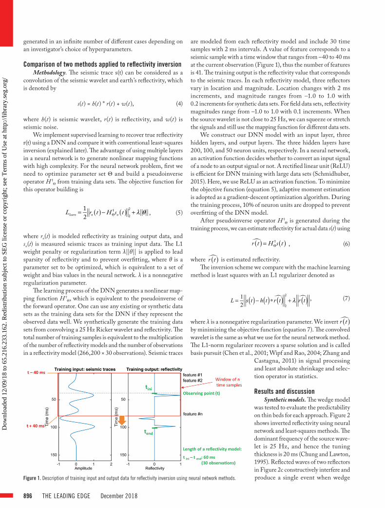
are modeled from each reflectivity model and include 30 time samples with 2 ms intervals. A value of feature corresponds to a seismic sample with a time window that ranges from –40 to 40 ms at the current observation (Figure 1), thus the number of features is 41. The training output is the reflectivity value that corresponds to the seismic traces. In each reflectivity model, three reflectors vary in location and magnitude. Location changes with 2 ms increments, and magnitude ranges from –1.0 to 1.0 with 0.2 increments for synthetic data sets. For field data sets, reflectivity magnitudes range from –1.0 to 1.0 with 0.1 increments. When the source wavelet is not close to 25 Hz, we can squeeze or stretch the signals and still use the mapping function for different data sets.

We construct our DNN model with an input layer, three hidden layers, and output layers. The three hidden layers have 200, 100, and 50 neuron units, respectively. In a neural network, an activation function decides whether to convert an input signal of a node to an output signal or not. A rectified linear unit (ReLU) is efficient for DNN training with large data sets (Schmidhuber, 2015). Here, we use ReLU as an activation function. To minimize the objective function (equation 5), adaptive moment estimation is adopted as a gradient-descent optimization algorithm. During the training process, 10% of neuron units are dropped to prevent overfitting of the DNN model.

After pseudoinverse operator H †Θ is generated during the

training process, we can estimate reflectivity for actual data s(t) using

r t( )! = HȆs t( ) , (6)

where r t( )! is estimated reflectivity.The inversion scheme we compare with the machine learning

method is least squares with an L1 regularizer denoted as

L = 12s t( )− h t( )∗r t( )!

2

2

+ λ r t( )! , (7)

where λ is a nonnegative regularization parameter. We invert r t( )! by minimizing the objective function (equation 7). The convolved wavelet is the same as what we use for the neural network method. The L1-norm regularizer recovers a sparse solution and is called basis pursuit (Chen et al., 2001; Wipf and Rao, 2004; Zhang and

Castagna, 2011) in signal processing and least absolute shrinkage and selec-tion operator in statistics.

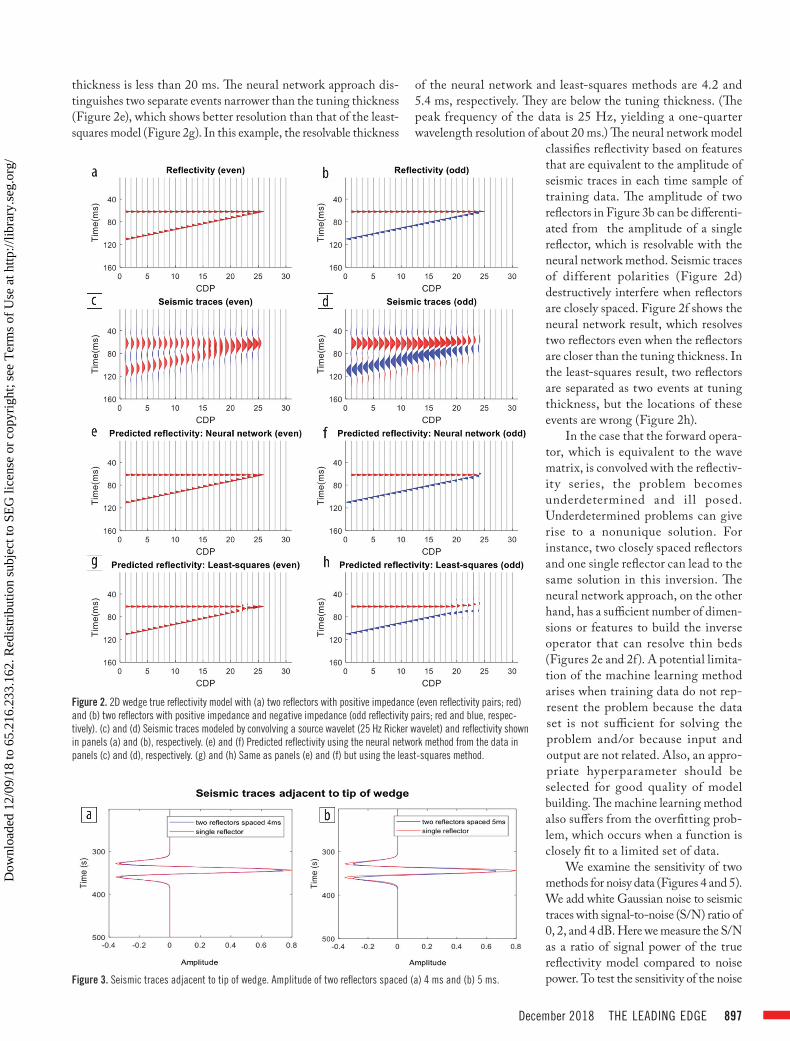
Results and discussionSynthetic models. The wedge model

was tested to evaluate the predictability on thin beds for each approach. Figure 2 shows inverted reflectivity using neural network and least-squares methods. The dominant frequency of the source wave-let is 25 Hz, and hence the tuning thickness is 20 ms (Chung and Lawton, 1995). Reflected waves of two reflectors in Figure 2c constructively interfere and produce a single event when wedge Figure 1. Description of training input and output data for reflectivity inversion using neural network methods.

Dow

nloa

ded

12/0

9/18

to 6

5.21

6.23

3.16

2. R

edis

trib

utio

n su

bjec

t to

SEG

lice

nse

or c

opyr

ight

; see

Ter

ms

of U

se a

t http

://lib

rary

.seg

.org

/

December 2018 THE LEADING EDGE 897

of the neural network and least-squares methods are 4.2 and 5.4 ms, respectively. They are below the tuning thickness. (The peak frequency of the data is 25 Hz, yielding a one-quarter wavelength resolution of about 20 ms.) The neural network model

classifies reflectivity based on features that are equivalent to the amplitude of seismic traces in each time sample of training data. The amplitude of two reflectors in Figure 3b can be differenti-ated from the amplitude of a single reflector, which is resolvable with the neural network method. Seismic traces of different polarities (Figure 2d) destructively interfere when reflectors are closely spaced. Figure 2f shows the neural network result, which resolves two reflectors even when the reflectors are closer than the tuning thickness. In the least-squares result, two reflectors are separated as two events at tuning thickness, but the locations of these events are wrong (Figure 2h).

In the case that the forward opera-tor, which is equivalent to the wave matrix, is convolved with the reflectiv-ity series, the problem becomes underdetermined and ill posed. Underdetermined problems can give rise to a nonunique solution. For instance, two closely spaced reflectors and one single reflector can lead to the same solution in this inversion. The neural network approach, on the other hand, has a sufficient number of dimen-sions or features to build the inverse operator that can resolve thin beds (Figures 2e and 2f). A potential limita-tion of the machine learning method arises when training data do not rep-resent the problem because the data set is not sufficient for solving the problem and/or because input and output are not related. Also, an appro-priate hyperparameter should be selected for good quality of model building. The machine learning method also suffers from the overfitting prob-lem, which occurs when a function is closely fit to a limited set of data.

We examine the sensitivity of two methods for noisy data (Figures 4 and 5). We add white Gaussian noise to seismic traces with signal-to-noise (S/N) ratio of 0, 2, and 4 dB. Here we measure the S/N as a ratio of signal power of the true reflectivity model compared to noise power. To test the sensitivity of the noise

Figure 2. 2D wedge true reflectivity model with (a) two reflectors with positive impedance (even reflectivity pairs; red) and (b) two reflectors with positive impedance and negative impedance (odd reflectivity pairs; red and blue, respec-tively). (c) and (d) Seismic traces modeled by convolving a source wavelet (25 Hz Ricker wavelet) and reflectivity shown in panels (a) and (b), respectively. (e) and (f) Predicted reflectivity using the neural network method from the data in panels (c) and (d), respectively. (g) and (h) Same as panels (e) and (f) but using the least-squares method.

Figure 3. Seismic traces adjacent to tip of wedge. Amplitude of two reflectors spaced (a) 4 ms and (b) 5 ms.

thickness is less than 20 ms. The neural network approach dis-tinguishes two separate events narrower than the tuning thickness (Figure 2e), which shows better resolution than that of the least-squares model (Figure 2g). In this example, the resolvable thickness

Dow

nloa

ded

12/0

9/18

to 6

5.21

6.23

3.16

2. R

edis

trib

utio

n su

bjec

t to

SEG

lice

nse

or c

opyr

ight

; see

Ter

ms

of U

se a

t http

://lib

rary

.seg

.org

/

898 THE LEADING EDGE December 2018

Table 1. Computation time of reflectivity inversion neural network and least-squares methods.

Inversion methods Number of processes

Elapsed time (in seconds)

Neural network

Training 1 837 sInversion 1 0.344 s/trace × (367 × 271) traces = 34,213 s

Least squares 1 1.89 s/trace × (367 × 271) traces – 187,973 s

Figure 4. (a) True reflectivity. (b) Seismic traces modeled from the true reflectivity. White Gaussian noise is added with different S/N levels: noise free, 4, 2, and 0 dB. (c) through (e) Recovered reflectivity using neural network method with the L1 regularization parameter (equation 5); (c) λ = 0, (d) λ = 3·10e-3, (e) λ = 5·10e-3. (f) through (h) Recovered reflectivity using the least-squares method with the L1 regularization parameter (equation 7): (f) λ = 10e-4, (g) λ = 10e-3, (h) λ = 10e-2.

Figure 5. Sensitivity of two algorithms with regard to the noise component of data. (a) Correlation coefficients between true reflectivity model and inverted model at different noise levels. White Gaussian noise is added with S/N level: noise free, 4, 2, and 0 dB. (b) and (c) Correlation coefficients for different L1 regularization coef-ficients at each noise level using (b) neural network and (c) least-squares methods. We test 10 different models to compute the correlation coefficients, and the errorbars represent the standard deviation of different models.

Dow

nloa

ded

12/0

9/18

to 6

5.21

6.23

3.16

2. R

edis

trib

utio

n su

bjec

t to

SEG

lice

nse

or c

opyr

ight

; see

Ter

ms

of U

se a

t http

://lib

rary

.seg

.org

/

December 2018 THE LEADING EDGE 899

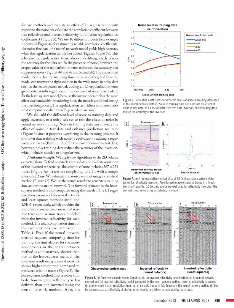
for two methods and evaluate an effect of L1 regularization with respect to the noise, we calculate the correlation coefficient between true reflectivity and inverted reflectivity for different regularization coefficients λ (Figure 5). We use 10 different models (one example is shown in Figure 4a) for estimating reliable correlation coefficients. For noise-free data, the neural network model yields high accuracy when the regularization term is not added (Figures 4c and 5a). This is because the regularization term induces underfitting, which reduces the accuracy for the data set. In the presence of noise, however, the proper value of the regularization term enhances the accuracy and suppresses noise (Figures 4d and 4e and 5a and 5b). The underfitted model means that the mapping function is smoother, and thus the model can recover the right solution in the wide range in noisy data sets. In the least-squares model, adding an L1-regularization term gives better results regardless of the existence of noise. Particularly for the least-squares model, because the inverse operator has the same effect as a bandwidth-broadening filter, the noise is amplified during the inversion process. The regularization term filters out these unde-sired components when their Eigen values are small.

We also add the different level of noise to training data and apply inversion to a noisy test set to test the effect of noise in neural network training. Noise in training data can alleviate the effect of noise in test data and enhance prediction accuracy (Figure 6) since it prevents overfitting in the training process. It is known that training with noise is equivalent to adding a regu-larization factor (Bishop, 1995). In the case of noise-free test data, however, noisy training data reduce the accuracy of the inversion, which behaves similar to a regularizer.

Field data example. We apply two algorithms to the 2D volume extracted from 3D field poststack seismic data and evaluate resolution of the inverted reflectivity. The seismic volume includes 367 × 271 traces (Figure 7a). Traces are sampled up to 2.5 s with a sample interval of 2 ms. We estimate the source wavelet using a statistical method (Figure 7b). We use the source wavelet to generate a training data set for the neural network. The forward operator in the least-squares method is also computed using the wavelet. The L1 regu-larization parameter λ for neural network and least-squares methods are 0 and 1.5E-5, respectively, which provides the minimum error between measured seis-mic traces and seismic traces modeled from the inverted reflectivity for each method. The total computation times of the two methods are compared in Table 1. Even if the neural network method requires computing time for training, the time elapsed for the inver-sion process in the neural network method is comparatively shorter than that of the least-squares method. The inversion result using a neural network shows higher resolution compared to measured seismic traces (Figure 8). The least-squares method also resolves thin beds; however, the reflectivity is less definite than one inverted using the neural network method. Also, the

Figure 6. Correlation coefficients for different levels of noise in training data used in the neural network method. Noise in training data can alleviate the effect of noise in test data. In a case of noise-free test data, however, noisy training data reduce the accuracy of the inversion.

Figure 7. (a) A representative vertical slice of 3D field poststack seismic data tested for reflectivity inversion. An enlarged image of seismic traces in a black box is in Figure 8a. (b) Seismic source wavelet used for reflectivity inversion. The wavelet is extracted using a statistical method.

Figure 8. (a) Observed seismic traces (input data), (b) inverted reflectivity model estimated by neural network method and (c) inverted reflectivity model computed by the least-squares method. Inverted reflectivity in panels (b) and (c) show higher resolution than that of seismic traces in (a). Especially the neural network method (b) bet-ter recovers sparse reflectivity of stratigraphic boundaries, which is indicated by red arrows.

Dow

nloa

ded

12/0

9/18

to 6

5.21

6.23

3.16

2. R

edis

trib

utio

n su

bjec

t to

SEG

lice

nse

or c

opyr

ight

; see

Ter

ms

of U

se a

t http

://lib

rary

.seg

.org

/

900 THE LEADING EDGE December 2018

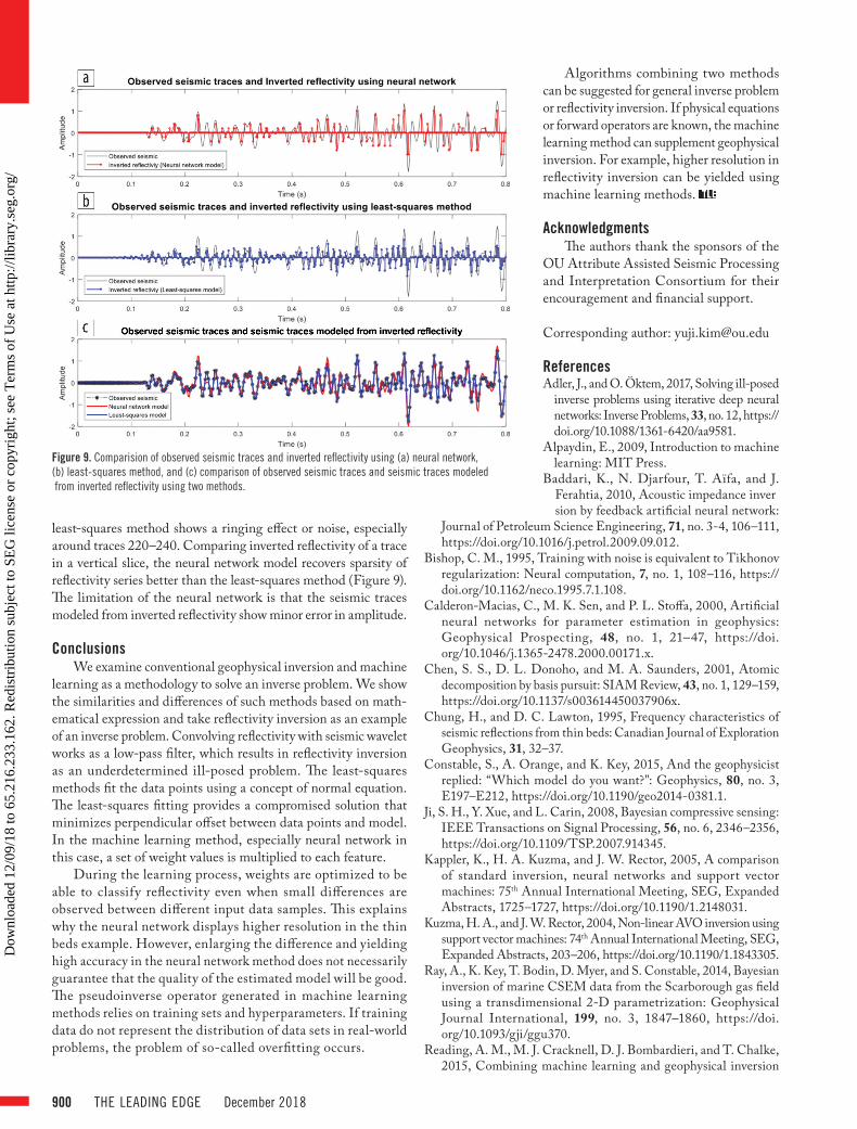
least-squares method shows a ringing effect or noise, especially around traces 220–240. Comparing inverted reflectivity of a trace in a vertical slice, the neural network model recovers sparsity of reflectivity series better than the least-squares method (Figure 9). The limitation of the neural network is that the seismic traces modeled from inverted reflectivity show minor error in amplitude.

ConclusionsWe examine conventional geophysical inversion and machine

learning as a methodology to solve an inverse problem. We show the similarities and differences of such methods based on math-ematical expression and take reflectivity inversion as an example of an inverse problem. Convolving reflectivity with seismic wavelet works as a low-pass filter, which results in reflectivity inversion as an underdetermined ill-posed problem. The least-squares methods fit the data points using a concept of normal equation. The least-squares fitting provides a compromised solution that minimizes perpendicular offset between data points and model. In the machine learning method, especially neural network in this case, a set of weight values is multiplied to each feature.

During the learning process, weights are optimized to be able to classify reflectivity even when small differences are observed between different input data samples. This explains why the neural network displays higher resolution in the thin beds example. However, enlarging the difference and yielding high accuracy in the neural network method does not necessarily guarantee that the quality of the estimated model will be good. The pseudoinverse operator generated in machine learning methods relies on training sets and hyperparameters. If training data do not represent the distribution of data sets in real-world problems, the problem of so-called overfitting occurs.

Algorithms combining two methods can be suggested for general inverse problem or reflectivity inversion. If physical equations or forward operators are known, the machine learning method can supplement geophysical inversion. For example, higher resolution in reflectivity inversion can be yielded using machine learning methods.

AcknowledgmentsThe authors thank the sponsors of the

OU Attribute Assisted Seismic Processing and Interpretation Consortium for their encouragement and financial support.

Corresponding author: yuji.kim@ou.edu

ReferencesAdler, J., and O. Öktem, 2017, Solving ill-posed

inverse problems using iterative deep neural networks: Inverse Problems, 33, no. 12, https://doi.org/10.1088/1361-6420/aa9581.

Alpaydin, E., 2009, Introduction to machine learning: MIT Press.

Baddari, K., N. Djarfour, T. Aïfa, and J. Ferahtia, 2010, Acoustic impedance inver sion by feedback artificial neural network:

Journal of Petroleum Science Engineering, 71, no. 3-4, 106–111, https://doi.org/10.1016/j.petrol.2009.09.012.

Bishop, C. M., 1995, Training with noise is equivalent to Tikhonov regularization: Neural computation, 7, no. 1, 108–116, https://doi.org/10.1162/neco.1995.7.1.108.

Calderon-Macias, C., M. K. Sen, and P. L. Stoffa, 2000, Artificial neural networks for parameter estimation in geophysics: Geophysical Prospecting, 48, no. 1, 21–47, https://doi.org/10.1046/j.1365-2478.2000.00171.x.

Chen, S. S., D. L. Donoho, and M. A. Saunders, 2001, Atomic decomposition by basis pursuit: SIAM Review, 43, no. 1, 129–159, https://doi.org/10.1137/s003614450037906x.

Chung, H., and D. C. Lawton, 1995, Frequency characteristics of seismic reflections from thin beds: Canadian Journal of Exploration Geophysics, 31, 32–37.

Constable, S., A. Orange, and K. Key, 2015, And the geophysicist replied: “Which model do you want?": Geophysics, 80, no. 3, E197–E212, https://doi.org/10.1190/geo2014-0381.1.

Ji, S. H., Y. Xue, and L. Carin, 2008, Bayesian compressive sensing: IEEE Transactions on Signal Processing, 56, no. 6, 2346–2356, https://doi.org/10.1109/TSP.2007.914345.

Kappler, K., H. A. Kuzma, and J. W. Rector, 2005, A comparison of standard inversion, neural networks and support vector machines: 75th Annual International Meeting, SEG, Expanded Abstracts, 1725–1727, https://doi.org/10.1190/1.2148031.

Kuzma, H. A., and J. W. Rector, 2004, Non-linear AVO inversion using support vector machines: 74th Annual International Meeting, SEG, Expanded Abstracts, 203–206, https://doi.org/10.1190/1.1843305.

Ray, A., K. Key, T. Bodin, D. Myer, and S. Constable, 2014, Bayesian inversion of marine CSEM data from the Scarborough gas field using a transdimensional 2-D parametrization: Geophysical Journal International, 199, no. 3, 1847–1860, https://doi.org/10.1093/gji/ggu370.

Reading, A. M., M. J. Cracknell, D. J. Bombardieri, and T. Chalke, 2015, Combining machine learning and geophysical inversion

Figure 9. Comparision of observed seismic traces and inverted reflectivity using (a) neural network, (b) least-squares method, and (c) comparison of observed seismic traces and seismic traces modeled from inverted reflectivity using two methods.

Dow

nloa

ded

12/0

9/18

to 6

5.21

6.23

3.16

2. R

edis

trib

utio

n su

bjec

t to

SEG

lice

nse

or c

opyr

ight

; see

Ter

ms

of U

se a

t http

://lib

rary

.seg

.org

/

December 2018 THE LEADING EDGE 901

for applied geophysics: ASEG Extended Abstracts, 1–5, https://doi.org/10.1071/ASEG2015ab070.

Rojo-Álvarez, J., M. Martínez-Ramón, J. Muñoz-Marí, G. Camps-Valls, C. M. Cruz, and A. R. Figueiras-Vidal, 2008, Sparse deconvolution using support vector machines: EURASIP Journal on Advances in Signal Processing, 1–13.

Röth, G., and A. Tarantola, 1994, Neural networks and inversion of seismic data: Journal of Geophysical Research, 99, no. B4, 6753–6768, https://doi.org/10.1029/93JB01563.

Schmidhuber, J., 2015, Deep learning in neural networks: An overview: Neural Networks, 61, 85–117, https://doi.org/10.1016/j.neunet.2014.09.003.

Snieder, R., 1998, The role of nonlinearity in inverse problems: Inverse Problems, 14, no. 3, 387–404, https://doi.org/10.1088 /0266-5611/14/3/003.

Tarantola, A., 2005, Inverse problem theory and methods for model parameter estimation: Society for Industrial and Applied Mathematics, https://doi.org/10.1137/1.9780898717921.

Van der Baan, M., and C. Jutten, 2000, Neural networks in geo-physical applications: Geophysics, 65, no. 4, 1032–1047, https://doi.org/10.1190/1.1444797.

Wipf, D. P., and B. D. Rao, 2004, Sparse Bayesian learning for basis selection: IEEE Transactions on Signal Processing, 52, no. 8, 2153–2164, https://doi.org/10.1109/TSP.2004.831016.

Yuan, S., and S. Wang, 2013, Spectral sparse Bayesian learning reflectivity inversion: Geophysical Prospecting, 61, no. 4, 735–746, https://doi.org/10.1111/1365-2478.12000.

Zhang, R., and J. Castagna, 2011, Seismic sparse-layer reflectivity inversion using basis pursuit decomposition: Geophysics, 76, no. 6, R147–R158, https://doi.org/10.1190/geo2011-0103.1.

Dow

nloa

ded

12/0

9/18

to 6

5.21

6.23

3.16

2. R

edis

trib

utio

n su

bjec

t to

SEG

lice

nse

or c

opyr

ight

; see

Ter

ms

of U

se a

t http

://lib

rary

.seg

.org

/