Geophysics: A Very Short Introduction

VERY SHORT INTRODUCTIONS are for anyone wanting a stimulating and accessible way intoa new subject. They are written by experts, and have been translated into more than 45 differentlanguages.

The series began in 1995, and now covers a wide variety of topics in every discipline. The VSIlibrary currently contains over 550 volumes—a Very Short Introduction to everything fromPsychology and Philosophy of Science to American History and Relativity—and continues togrow in every subject area.

Very Short Introductions available now:

ACCOUNTING Christopher NobesADOLESCENCE Peter K. SmithADVERTISING Winston FletcherAFRICAN AMERICAN RELIGION Eddie S. Glaude JrAFRICAN HISTORY John Parker and Richard RathboneAFRICAN RELIGIONS Jacob K. OluponaAGEING Nancy A. PachanaAGNOSTICISM Robin Le PoidevinAGRICULTURE Paul Brassley and Richard SoffeALEXANDER THE GREAT Hugh BowdenALGEBRA Peter M. HigginsAMERICAN HISTORY Paul S. BoyerAMERICAN IMMIGRATION David A. GerberAMERICAN LEGAL HISTORY G. Edward WhiteAMERICAN POLITICAL HISTORY Donald CritchlowAMERICAN POLITICAL PARTIES AND ELECTIONS L. Sandy MaiselAMERICAN POLITICS Richard M. ValellyTHE AMERICAN PRESIDENCY Charles O. JonesTHE AMERICAN REVOLUTION Robert J. AllisonAMERICAN SLAVERY Heather Andrea WilliamsTHE AMERICAN WEST Stephen AronAMERICAN WOMEN’S HISTORY Susan WareANAESTHESIA Aidan O’DonnellANALYTIC PHILOSOPHY Michael BeaneyANARCHISM Colin WardANCIENT ASSYRIA Karen RadnerANCIENT EGYPT Ian ShawANCIENT EGYPTIAN ART AND ARCHITECTURE Christina Riggs

ANCIENT GREECE Paul CartledgeTHE ANCIENT NEAR EAST Amanda H. PodanyANCIENT PHILOSOPHY Julia AnnasANCIENT WARFARE Harry SidebottomANGELS David Albert JonesANGLICANISM Mark ChapmanTHE ANGLO-SAXON AGE John BlairANIMAL BEHAVIOUR Tristram D. WyattTHE ANIMAL KINGDOM Peter HollandANIMAL RIGHTS David DeGraziaTHE ANTARCTIC Klaus DoddsANTHROPOCENE Erle C. EllisANTISEMITISM Steven BellerANXIETY Daniel Freeman and Jason FreemanAPPLIED MATHEMATICS Alain GorielyTHE APOCRYPHAL GOSPELS Paul FosterARCHAEOLOGY Paul BahnARCHITECTURE Andrew BallantyneARISTOCRACY William DoyleARISTOTLE Jonathan BarnesART HISTORY Dana ArnoldART THEORY Cynthia FreelandASIAN AMERICAN HISTORY Madeline Y. HsuASTROBIOLOGY David C. CatlingASTROPHYSICS James BinneyATHEISM Julian BagginiTHE ATMOSPHERE Paul I. PalmerAUGUSTINE Henry ChadwickAUSTRALIA Kenneth MorganAUTISM Uta FrithTHE AVANT GARDE David CottingtonTHE AZTECS Davíd CarrascoBABYLONIA Trevor BryceBACTERIA Sebastian G. B. AmyesBANKING John Goddard and John O. S. WilsonBARTHES Jonathan CullerTHE BEATS David SterrittBEAUTY Roger ScrutonBEHAVIOURAL ECONOMICS Michelle BaddeleyBESTSELLERS John SutherlandTHE BIBLE John RichesBIBLICAL ARCHAEOLOGY Eric H. ClineBIG DATA Dawn E. Holmes

BIOGRAPHY Hermione LeeBLACK HOLES Katherine BlundellBLOOD Chris CooperTHE BLUES Elijah WaldTHE BODY Chris ShillingTHE BOOK OF MORMON Terryl GivensBORDERS Alexander C. Diener and Joshua HagenTHE BRAIN Michael O’SheaBRANDING Robert JonesTHE BRICS Andrew F. CooperTHE BRITISH CONSTITUTION Martin LoughlinTHE BRITISH EMPIRE Ashley JacksonBRITISH POLITICS Anthony WrightBUDDHA Michael CarrithersBUDDHISM Damien KeownBUDDHIST ETHICS Damien KeownBYZANTIUM Peter SarrisCALVINISM Jon BalserakCANCER Nicholas JamesCAPITALISM James FulcherCATHOLICISM Gerald O’CollinsCAUSATION Stephen Mumford and Rani Lill AnjumTHE CELL Terence Allen and Graham CowlingTHE CELTS BarryCunliffeCHAOS Leonard SmithCHEMISTRY Peter AtkinsCHILD PSYCHOLOGY Usha GoswamiCHILDREN’S LITERATURE Kimberley ReynoldsCHINESE LITERATURE Sabina KnightCHOICE THEORY Michael AllinghamCHRISTIAN ART Beth WilliamsonCHRISTIAN ETHICS D. Stephen LongCHRISTIANITY Linda WoodheadCIRCADIAN RHYTHMS Russell Foster and Leon KreitzmanCITIZENSHIP Richard BellamyCIVIL ENGINEERING David Muir WoodCLASSICAL LITERATURE William AllanCLASSICAL MYTHOLOGY Helen MoralesCLASSICS Mary Beard and John HendersonCLAUSEWITZ Michael HowardCLIMATE Mark MaslinCLIMATE CHANGE Mark MaslinCLINICAL PSYCHOLOGY Susan Llewelyn and Katie Aafjes-van Doorn

COGNITIVE NEUROSCIENCE Richard PassinghamTHE COLD WAR Robert McMahonCOLONIAL AMERICA Alan TaylorCOLONIAL LATIN AMERICAN LITERATURE Rolena AdornoCOMBINATORICS Robin WilsonCOMEDY Matthew BevisCOMMUNISM Leslie HolmesCOMPARATIVE LITERATURE Ben HutchinsonCOMPLEXITY John H. HollandTHE COMPUTER Darrel InceCOMPUTER SCIENCE Subrata DasguptaCONFUCIANISM Daniel K. GardnerTHE CONQUISTADORS Matthew Restall and Felipe Fernández-ArmestoCONSCIENCE Paul StrohmCONSCIOUSNESS Susan BlackmoreCONTEMPORARY ART Julian StallabrassCONTEMPORARY FICTION Robert EaglestoneCONTINENTAL PHILOSOPHY Simon CritchleyCOPERNICUS Owen GingerichCORAL REEFS Charles SheppardCORPORATE SOCIAL RESPONSIBILITY Jeremy MoonCORRUPTION Leslie HolmesCOSMOLOGY Peter ColesCRIME FICTION Richard BradfordCRIMINAL JUSTICE Julian V. RobertsCRITICAL THEORY Stephen Eric BronnerTHE CRUSADES Christopher TyermanCRYPTOGRAPHY Fred Piper and Sean MurphyCRYSTALLOGRAPHY A. M. GlazerTHE CULTURAL REVOLUTION Richard Curt KrausDADA AND SURREALISM David HopkinsDANTE Peter Hainsworth and David RobeyDARWIN Jonathan HowardTHE DEAD SEA SCROLLS Timothy H. LimDECOLONIZATION Dane KennedyDEMOCRACY Bernard CrickDEPRESSION Jan Scott and Mary Jane TacchiDERRIDA Simon GlendinningDESCARTES Tom SorellDESERTS Nick MiddletonDESIGN John HeskettDEVELOPMENT Ian GoldinDEVELOPMENTAL BIOLOGY Lewis Wolpert

THE DEVIL Darren OldridgeDIASPORA Kevin KennyDICTIONARIES Lynda MugglestoneDINOSAURS David NormanDIPLOMACY Joseph M. SiracusaDOCUMENTARY FILM Patricia AufderheideDREAMING J. Allan HobsonDRUGS Les IversenDRUIDS Barry CunliffeEARLY MUSIC Thomas Forrest KellyTHE EARTH Martin RedfernEARTH SYSTEM SCIENCE Tim LentonECONOMICS Partha DasguptaEDUCATION Gary ThomasEGYPTIAN MYTH Geraldine PinchEIGHTEENTH-CENTURY BRITAIN Paul LangfordTHE ELEMENTS Philip BallEMOTION Dylan EvansEMPIRE Stephen HoweENGELS Terrell CarverENGINEERING David BlockleyTHE ENGLISH LANGUAGE Simon HorobinENGLISH LITERATURE Jonathan BateTHE ENLIGHTENMENT John RobertsonENTREPRENEURSHIP Paul Westhead and Mike WrightENVIRONMENTAL ECONOMICS Stephen SmithENVIRONMENTAL LAW Elizabeth FisherENVIRONMENTAL POLITICS Andrew DobsonEPICUREANISM Catherine WilsonEPIDEMIOLOGY Rodolfo SaracciETHICS Simon BlackburnETHNOMUSICOLOGY Timothy RiceTHE ETRUSCANS Christopher SmithEUGENICS Philippa LevineTHE EUROPEAN UNION John Pinder and Simon UsherwoodEUROPEAN UNION LAW Anthony ArnullEVOLUTION Brian and Deborah CharlesworthEXISTENTIALISM Thomas FlynnEXPLORATION Stewart A. WeaverTHE EYE Michael LandFAIRY TALE Marina WarnerFAMILY LAW Jonathan HerringFASCISM Kevin Passmore

FASHION Rebecca ArnoldFEMINISM Margaret WaltersFILM Michael WoodFILM MUSIC Kathryn KalinakTHE FIRST WORLD WAR Michael HowardFOLK MUSIC Mark SlobinFOOD John KrebsFORENSIC PSYCHOLOGY David CanterFORENSIC SCIENCE Jim FraserFORESTS Jaboury GhazoulFOSSILS Keith ThomsonFOUCAULT Gary GuttingTHE FOUNDING FATHERS R. B. BernsteinFRACTALS Kenneth FalconerFREE SPEECH Nigel WarburtonFREE WILL Thomas PinkFREEMASONRY Andreas ÖnnerforsFRENCH LITERATURE John D. LyonsTHE FRENCH REVOLUTION William DoyleFREUD Anthony StorrFUNDAMENTALISM Malise RuthvenFUNGI Nicholas P. MoneyTHE FUTURE Jennifer M. GidleyGALAXIES John GribbinGALILEO Stillman DrakeGAME THEORY Ken BinmoreGANDHI Bhikhu ParekhGENES Jonathan SlackGENIUS Andrew RobinsonGENOMICS John ArchibaldGEOGRAPHY John Matthews and David HerbertGEOPHYSICS William LowrieGEOPOLITICS Klaus DoddsGERMAN LITERATURE Nicholas BoyleGERMAN PHILOSOPHY Andrew BowieGLOBAL CATASTROPHES Bill McGuireGLOBAL ECONOMIC HISTORY Robert C. AllenGLOBALIZATION Manfred StegerGOD John BowkerGOETHE Ritchie RobertsonTHE GOTHIC Nick GroomGOVERNANCE Mark BevirGRAVITY Timothy Clifton

THE GREAT DEPRESSION AND THE NEW DEAL Eric RauchwayHABERMAS James Gordon FinlaysonTHE HABSBURG EMPIRE Martyn RadyHAPPINESS Daniel M. HaybronTHE HARLEM RENAISSANCE Cheryl A. WallTHE HEBREW BIBLE AS LITERATURE Tod LinafeltHEGEL Peter SingerHEIDEGGER Michael InwoodTHE HELLENISTIC AGE Peter ThonemannHEREDITY John WallerHERMENEUTICS Jens ZimmermannHERODOTUS Jennifer T. RobertsHIEROGLYPHS Penelope WilsonHINDUISM Kim KnottHISTORY John H. ArnoldTHE HISTORY OF ASTRONOMY Michael HoskinTHE HISTORY OF CHEMISTRY William H. BrockTHE HISTORY OF CINEMA Geoffrey Nowell-SmithTHE HISTORY OF LIFE Michael BentonTHE HISTORY OF MATHEMATICS Jacqueline StedallTHE HISTORY OF MEDICINE William BynumTHE HISTORY OF PHYSICS J. L. HeilbronTHE HISTORY OF TIME Leofranc Holford‑StrevensHIV AND AIDS Alan WhitesideHOBBES Richard TuckHOLLYWOOD Peter DecherneyHOME Michael Allen FoxHORMONES Martin LuckHUMAN ANATOMY Leslie KlenermanHUMAN EVOLUTION Bernard WoodHUMAN RIGHTS Andrew ClaphamHUMANISM Stephen LawHUME A. J. AyerHUMOUR Noël CarrollTHE ICE AGE Jamie WoodwardIDEOLOGY Michael FreedenTHE IMMUNE SYSTEM Paul KlenermanINDIAN CINEMA Ashish RajadhyakshaINDIAN PHILOSOPHY Sue HamiltonTHE INDUSTRIAL REVOLUTION Robert C. AllenINFECTIOUS DISEASE Marta L. Wayne and Benjamin M. BolkerINFINITY Ian StewartINFORMATION Luciano Floridi

INNOVATION Mark Dodgson and David GannINTELLIGENCE Ian J. DearyINTELLECTUAL PROPERTY Siva VaidhyanathanINTERNATIONAL LAW Vaughan LoweINTERNATIONAL MIGRATION Khalid KoserINTERNATIONAL RELATIONS Paul WilkinsonINTERNATIONAL SECURITY Christopher S. BrowningIRAN Ali M. AnsariISLAM Malise RuthvenISLAMIC HISTORY Adam SilversteinISOTOPES Rob EllamITALIAN LITERATURE Peter Hainsworth and David RobeyJESUS Richard BauckhamJEWISH HISTORY David N. MyersJOURNALISM Ian HargreavesJUDAISM Norman SolomonJUNG Anthony StevensKABBALAH Joseph DanKAFKA Ritchie RobertsonKANT Roger ScrutonKEYNES Robert SkidelskyKIERKEGAARD Patrick GardinerKNOWLEDGE Jennifer NagelTHE KORAN Michael CookLAKES Warwick F. VincentLANDSCAPE ARCHITECTURE Ian H. ThompsonLANDSCAPES AND GEOMORPHOLOGY Andrew Goudie and Heather VilesLANGUAGES Stephen R. AndersonLATE ANTIQUITY Gillian ClarkLAW Raymond WacksTHE LAWS OF THERMODYNAMICS Peter AtkinsLEADERSHIP Keith GrintLEARNING Mark HaselgroveLEIBNIZ Maria Rosa AntognazzaLIBERALISM Michael FreedenLIGHT Ian WalmsleyLINCOLN Allen C. GuelzoLINGUISTICS Peter MatthewsLITERARY THEORY Jonathan CullerLOCKE John DunnLOGIC Graham PriestLOVE Ronald de SousaMACHIAVELLI Quentin Skinner

MADNESS Andrew ScullMAGIC Owen DaviesMAGNA CARTA Nicholas VincentMAGNETISM Stephen BlundellMALTHUS Donald WinchMAMMALS T. S. KempMANAGEMENT John HendryMAO Delia DavinMARINE BIOLOGY Philip V. MladenovTHE MARQUIS DE SADE John PhillipsMARTIN LUTHER Scott H. HendrixMARTYRDOM Jolyon MitchellMARX Peter SingerMATERIALS Christopher HallMATHEMATICS Timothy GowersThe Meaning of Life Terry EagletonMEASUREMENT David HandMEDICAL ETHICS Tony HopeMEDICAL LAW Charles FosterMEDIEVAL BRITAIN John Gillingham and Ralph A. GriffithsMEDIEVAL LITERATURE Elaine TreharneMEDIEVAL PHILOSOPHY John MarenbonMEMORY Jonathan K. FosterMETAPHYSICS Stephen MumfordTHE MEXICAN REVOLUTION Alan KnightMICHAEL FARADAY Frank A. J. L. JamesMICROBIOLOGY Nicholas P. MoneyMICROECONOMICS Avinash DixitMICROSCOPY Terence AllenTHE MIDDLE AGES Miri RubinMILITARY JUSTICE Eugene R. FidellMILITARY STRATEGY Antulio J. Echevarria IIMINERALS David VaughanMIRACLES Yujin NagasawaMODERN ART David CottingtonMODERN CHINA Rana MitterMODERN DRAMA Kirsten E. Shepherd-BarrMODERN FRANCE Vanessa R. SchwartzMODERN INDIA Craig JeffreyMODERN IRELAND Senia PašetaMODERN ITALY Anna Cento BullMODERN JAPAN Christopher Goto-JonesMODERN LATIN AMERICAN LITERATURE Roberto González Echevarría

MODERN WAR Richard EnglishMODERNISM Christopher ButlerMOLECULAR BIOLOGY Aysha Divan and Janice A. RoydsMOLECULES Philip BallMONASTICISM Stephen J. DavisTHE MONGOLS Morris RossabiMOONS David A. RotheryMORMONISM Richard Lyman BushmanMOUNTAINS Martin F. PriceMUHAMMAD Jonathan A. C. BrownMULTICULTURALISM Ali RattansiMULTILINGUALISM John C. MaherMUSIC Nicholas CookMYTH Robert A. SegalTHE NAPOLEONIC WARS Mike RapportNATIONALISM Steven GrosbyNATIVE AMERICAN LITERATURE Sean TeutonNAVIGATION Jim BennettNELSON MANDELA Elleke BoehmerNEOLIBERALISM Manfred Steger and Ravi RoyNETWORKS Guido Caldarelli and Michele CatanzaroTHE NEW TESTAMENT Luke Timothy JohnsonTHE NEW TESTAMENT AS LITERATURE Kyle KeeferNEWTON Robert IliffeNIETZSCHE Michael TannerNINETEENTH-CENTURY BRITAIN Christopher Harvie and H. C. G. MatthewTHE NORMAN CONQUEST George GarnettNORTH AMERICAN INDIANS Theda Perdue and Michael D. GreenNORTHERN IRELAND Marc MulhollandNOTHING Frank CloseNUCLEAR PHYSICS Frank CloseNUCLEAR POWER Maxwell IrvineNUCLEAR WEAPONS Joseph M. SiracusaNUMBERS Peter M. HigginsNUTRITION David A. BenderOBJECTIVITY Stephen GaukrogerOCEANS Dorrik StowTHE OLD TESTAMENT Michael D. CooganTHE ORCHESTRA D. Kern HolomanORGANIC CHEMISTRY Graham PatrickORGANIzED CRIME Georgios A. Antonopoulos and Georgios PapanicolaouORGANIZATIONS Mary Jo HatchPAGANISM Owen Davies

PAIN Rob BoddiceTHE PALESTINIAN-ISRAELI CONFLICT Martin BuntonPANDEMICS Christian W. McMillenPARTICLE PHYSICS Frank ClosePAUL E. P. SandersPEACE Oliver P. RichmondPENTECOSTALISM William K. KayPERCEPTION Brian RogersTHE PERIODIC TABLE Eric R. ScerriPHILOSOPHY Edward CraigPHILOSOPHY IN THE ISLAMIC WORLD Peter AdamsonPHILOSOPHY OF LAW Raymond WacksPHILOSOPHY OF SCIENCE Samir OkashaPHILOSOPHY OF RELIGION Tim BaynePHOTOGRAPHY Steve EdwardsPHYSICAL CHEMISTRY Peter AtkinsPILGRIMAGE Ian ReaderPLAGUE Paul SlackPLANETS David A. RotheryPLANTS Timothy WalkerPLATE TECTONICS Peter MolnarPLATO Julia AnnasPOLITICAL PHILOSOPHY David MillerPOLITICS Kenneth MinoguePOPULISM Cas Mudde and Cristóbal Rovira KaltwasserPOSTCOLONIALISM Robert YoungPOSTMODERNISM Christopher ButlerPOSTSTRUCTURALISM Catherine BelseyPREHISTORY Chris GosdenPRESOCRATIC PHILOSOPHY Catherine OsbornePRIVACY Raymond WacksPROBABILITY John HaighPROGRESSIVISM Walter NugentPROJECTS Andrew DaviesPROTESTANTISM Mark A. NollPSYCHIATRY Tom BurnsPSYCHOANALYSIS Daniel PickPSYCHOLOGY Gillian Butler and Freda McManusPSYCHOTHERAPY Tom Burns and Eva Burns-LundgrenPUBLIC ADMINISTRATION Stella Z. Theodoulou and Ravi K. RoyPUBLIC HEALTH Virginia BerridgePURITANISM Francis J. BremerTHE QUAKERS Pink Dandelion

QUANTUM THEORY John PolkinghorneRACISM Ali RattansiRADIOACTIVITY Claudio TunizRASTAFARI Ennis B. EdmondsTHE REAGAN REVOLUTION Gil TroyREALITY Jan WesterhoffTHE REFORMATION Peter MarshallRELATIVITY Russell StannardRELIGION IN AMERICA Timothy BealTHE RENAISSANCE Jerry BrottonRENAISSANCE ART Geraldine A. JohnsonREVOLUTIONS Jack A. GoldstoneRHETORIC Richard ToyeRISK Baruch Fischhoff and John KadvanyRITUAL Barry StephensonRIVERS Nick MiddletonROBOTICS Alan WinfieldROCKS Jan ZalasiewiczROMAN BRITAIN Peter SalwayTHE ROMAN EMPIRE Christopher KellyTHE ROMAN REPUBLIC David M. GwynnROMANTICISM Michael FerberROUSSEAU Robert WoklerRUSSELL A. C. GraylingRUSSIAN HISTORY Geoffrey HoskingRUSSIAN LITERATURE Catriona KellyTHE RUSSIAN REVOLUTION S. A. SmithSAVANNAS Peter A. FurleySCHIZOPHRENIA Chris Frith and Eve JohnstoneSCHOPENHAUER Christopher JanawaySCIENCE AND RELIGION Thomas DixonSCIENCE FICTION David SeedTHE SCIENTIFIC REVOLUTION Lawrence M. PrincipeSCOTLAND Rab HoustonSEXUALITY Véronique MottierSHAKESPEARE’S COMEDIES Bart van EsSHAKESPEARE’S SONNETS AND POEMS Jonathan F. S. PostSHAKESPEARE’S TRAGEDIES Stanley WellsSIKHISM Eleanor NesbittTHE SILK ROAD James A. MillwardSLANG Jonathon GreenSLEEP Steven W. Lockley and Russell G. FosterSOCIAL AND CULTURAL ANTHROPOLOGY John Monaghan and Peter Just

SOCIAL PSYCHOLOGY Richard J. CrispSOCIAL WORK Sally Holland and Jonathan ScourfieldSOCIALISM Michael NewmanSOCIOLINGUISTICS John EdwardsSOCIOLOGY Steve BruceSOCRATES C. C. W. TaylorSOUND Mike GoldsmithTHE SOVIET UNION Stephen LovellTHE SPANISH CIVIL WAR Helen GrahamSPANISH LITERATURE Jo LabanyiSPINOZA Roger ScrutonSPIRITUALITY Philip SheldrakeSPORT Mike CroninSTARS Andrew KingSTATISTICS David J. HandSTEM CELLS Jonathan SlackSTRUCTURAL ENGINEERING David BlockleySTUART BRITAIN John MorrillSUPERCONDUCTIVITY Stephen BlundellSYMMETRY Ian StewartTAXATION Stephen SmithTEETH Peter S. UngarTELESCOPES Geoff CottrellTERRORISM Charles TownshendTHEATRE Marvin CarlsonTHEOLOGY David F. FordTHINKING AND REASONING Jonathan St B. T. EvansTHOMAS AQUINAS Fergus KerrTHOUGHT Tim BayneTIBETAN BUDDHISM Matthew T. KapsteinTOCQUEVILLE Harvey C. MansfieldTRAGEDY Adrian PooleTRANSLATION Matthew ReynoldsTHE TROJAN WAR Eric H. ClineTRUST Katherine HawleyTHE TUDORS John GuyTWENTIETH‑CENTURY BRITAIN Kenneth O. MorganTHE UNITED NATIONS Jussi M. HanhimäkiTHE U.S. CONGRESS Donald A. RitchieTHE U.S. SUPREME COURT Linda GreenhouseUTILITARIANISM Katarzyna de Lazari-Radek and Peter SingerUNIVERSITIES AND COLLEGES David Palfreyman and Paul TempleUTOPIANISM Lyman Tower Sargent

VETERINARY SCIENCE James YeatesTHE VIKINGS Julian RichardsVIRUSES Dorothy H. CrawfordVOLTAIRE Nicholas CronkWAR AND TECHNOLOGY Alex RolandWATER John FinneyWEATHER Storm DunlopTHE WELFARE STATE David GarlandWILLIAM SHAKESPEARE Stanley WellsWITCHCRAFT Malcolm GaskillWITTGENSTEIN A. C. GraylingWORK Stephen FinemanWORLD MUSIC Philip BohlmanTHE WORLD TRADE ORGANIZATION Amrita NarlikarWORLD WAR II Gerhard L. WeinbergWRITING AND SCRIPT Andrew RobinsonZIONISM Michael Stanislawski

Available soon:

CRIMINOLOGY Tim NewburnAUTOBIOGRAPHY Laura MarcusDEMOGRAPHY Sarah HarperGEOLOGY Jan ZalasiewiczSOUTHEAST ASIA James R. Rush

For more information visit our website

www.oup.com/vsi/

William Lowrie

GEOPHYSICSA Very Short Introduction

Great Clarendon Street, Oxford, OX2 6DP, United KingdomOxford University Press is a department of the University of Oxford. It furthers the University’s

objective of excellence in research, scholarship, and education by publishing worldwide. Oxford is aregistered trade mark of Oxford University Press in the UK and in certain other countries

© William Lowrie 2018The moral rights of the author have been asserted

First edition published in 2018Impression: 1

All rights reserved. No part of this publication may be reproduced, stored in a retrieval system, ortransmitted, in any form or by any means, without the prior permission in writing of OxfordUniversity Press, or as expressly permitted by law, by licence or under terms agreed with the

appropriate reprographics rights organization. Enquiries concerning reproduction outside the scope ofthe above should be sent to the Rights Department, Oxford University Press, at the address above

You must not circulate this work in any other form and you must impose this same condition on anyacquirer

Published in the United States of America by Oxford University Press 198 Madison Avenue, NewYork, NY 10016, United States of America

British Library Cataloguing in Publication DataData available

Library of Congress Control Number: 2017960669

ISBN 978–0–19–879295–6ebook ISBN 978–0–19–251133–1

Printed in Great Britain by Ashford Colour Press Ltd, Gosport, Hampshire

Links to third party websites are provided by Oxford in good faith and for information only. Oxforddisclaims any responsibility for the materials contained in any third party website referenced in this

work.

Contents

Acknowledgements

List of illustrations

1 What is geophysics?

2 Planet Earth

3 Seismology and the Earth’s internal structure

4 Seismicity—the restless Earth

5 Gravity and the figure of the Earth

6 The Earth’s heat

7 The Earth’s magnetic field

8 Afterthoughts

Further reading

Index

Acknowledgements

Alan Green read and criticized the first draft of this work and made manycorrections and suggestions. I hope he enjoyed our many lively discussionsas much as I did. My wife Marcia drew my attention to sections that werenot clear or would be difficult for a non-scientist to understand. I thankAlan and Marcia for their invaluable help. I am grateful to MarkkuPoutanen of the Finnish Geospatial Research Institute; Christoph Förste ofGFZ, German Research Centre for Geosciences, Potsdam; and DmitryStorchak of the International Seismological Centre, for kindly providing theillustrations of Fennoscandian uplift, the EIGEN6S4 geoid, and globalseismicity, respectively. I also thank an anonymous reader for helping me tocorrect and improve the final text.

List of illustrations

1 Relative dimensions of the planets

2 Schematic drawing of the Earth’s elliptical orbit

3 Precession of the Earth’s rotation axis and orbit, and the variation in orbital eccentricity

4 Cyclical variations in eccentricity, precession index, and obliquityModified from fig. 4 in A. Berger and M. F. Loutre, Astronomical theory of climate change,Journal de Physique de France IV, 121, 1–35 (2004).

5 Particle motions in seismic P- and S-waves, and the corresponding events on a seismogram

6 The fundamental modes of natural oscillation of the Earth

7 Reflection and refraction of seismic rays at an interface

8 Seismic rays in a shallow layer that overlies a layer with higher velocity

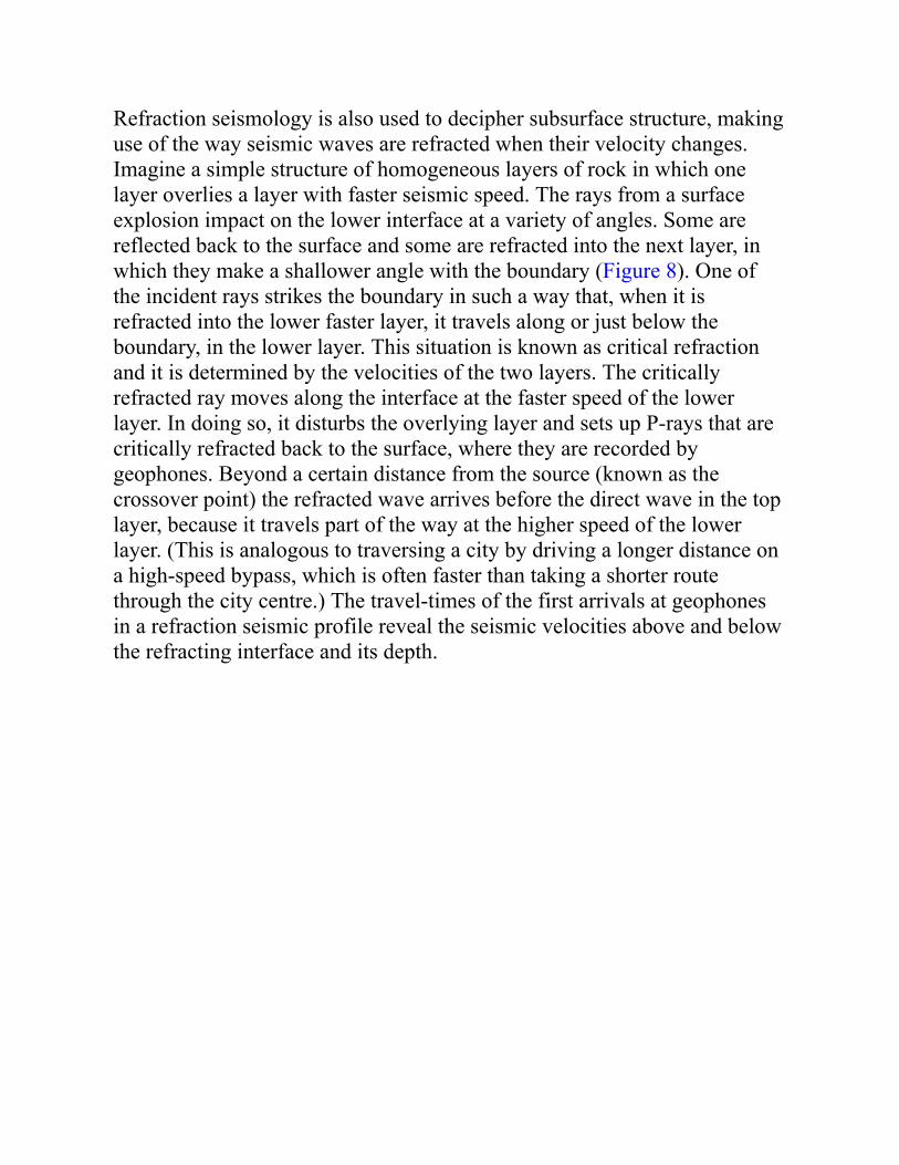
9 Shadow zones and paths of P- and S-waves in the Earth

10 Travel-time curves of body waves from a shallow earthquakeSimplified from fig. A1 in B. L. N. Kennett and E. R. Engdahl, Traveltimes for globalearthquake location and phase identification, Geophysical Journal International, 105, 429–65(1991). Copyright Oxford University Press.

11 Variations of body wave velocities and density with depth in the EarthData sources: (1) Density profile, table II in A. M. Dziewonski and D. L. Anderson, PreliminaryReference Earth Model (PREM), Physics of Earth and Planetary Interiors, 25, 297–356 (1981);(2) Velocity profiles, table 2 in B. L. N. Kennett and E. R. Engdahl, Traveltimes for globalearthquake location and phase identification, Geophysical Journal International, 105, 429–65(1991).

12 Meridian cross-section through the Earth’s interior

13 Simplified P-wave tomographic section through a subduction zoneModified from colour plate 4c in H. Bijwaard, W. Spakman, and E. R. Engdahl, Closing the gapbetween regional and global travel time tomography, Journal of Geophysical Research, 103,30,055–78 (1998).

14 Elastic rebound model for an earthquake with tectonic origin

15 Global distribution of the epicentres of 157,991 earthquakesKindly provided by Dr Dmitry A. Storchak, Director, International Seismological Centre (ISC).<http://www.isc.ac.uk/isc-ehb/>.

16 The major lithospheric platesModified from fig. 1.11 in W. Lowrie, Fundamentals of Geophysics, 2nd edn (CambridgeUniversity Press, 2007). Relative plate motions are calculated from data in C. DeMets, R. G.Gordon, and D. F. Argus, Geologically current plate motions, Geophysical JournalInternational, 181, 1–80 (2010).

17 Hypothetical vertical cross-section through the fault plane of an earthquake

18 Focal mechanisms of earthquakes on three types of tectonic faultModified from fig. 3.37 in W. Lowrie, Fundamentals of Geophysics, 2nd edn (CambridgeUniversity Press, 2007).

19 Fault plane solutions for earthquakes on the mid-Atlantic RidgeCompiled from data in P. Y. Huang, S. C. Solomon, E. A. Bergman, and J. L. Nabelek, Focaldepths and echanisms of Mid-Atlantic Ridge earthquakes from body waveform inversion,Journal of Geophysical Research, 91, 579–98 (1986); and J. F. Engeln, D. A. Wiens, and S.Stein, Mechanisms and depths of Atlantic transform earthquakes, Journal of GeophysicalResearch, 91, 548–77 (1986).

20 Seismicity, fault plane solutions, and motions on strike-slip faults

21 Comparison of an ellipsoid of revolution with a sphere of the same volume

22 Geoid undulations measured from satellite missionsHalftone conversion of a colour plate by courtesy of C. Förste, GFZ German Research Centrefor Geosciences, Potsdam (<http://icgem.gfz-potsdam.de>).

23 Hypothetical variation of a Bouguer gravity anomaly over oceanic and continental crust

24 Present rates of postglacial land uplift in FennoscandiaAfter the Nordic Geodetic Commission model 2006, courtesy of Markku Poutanen, FinnishGeospatial Research Institute.

25 Regions where the Earth’s surface heat flow is higher than the global mean

Based on data taken from H. N. Pollack, S. J. Hurter, and J. R. Johnson, Heat flow from theEarth’s interior: analysis of the global data set, Reviews of Geophysics 31, 267–80 (1993).

26 Variation of global heat flow with the age of oceanic lithosphereReprinted by permission from Macmillan Publishers Ltd: Nature, C. A. Stein and S. Stein, Amodel for the global variation in oceanic depth and heat flow with lithospheric age, 359, 123–9,copyright (1992).

27 Variations of adiabatic and melting-point temperatures with depth in the Earth

28 Cartoon representation of a cross-section through the mantle

29 Sketch of the Earth’s dipole magnetic field

30 Depiction of the Earth’s magnetosphereModified from fig. 5.28 in W. Lowrie, Fundamentals of Geophysics, 2nd edn (CambridgeUniversity Press, 2007).

31 Apparent polar wander paths and the opening of the Atlantic OceanAfter fig 5.67 in W. Lowrie, Fundamentals of Geophysics, 2nd edn (Cambridge UniversityPress, 2007), based on fig. 5.3 in R. Van der Voo, Phanerozoic paleomagnetic poles from Europeand North America and comparisons with continental reconstructions, Reviews of Geophysics28, 167–206 (1990).

32 Marine magnetic anomalies across the East Pacific RiseCreated using data from fig. 3 from W. C. Pitman III and J. R. Heirtzler, Magnetic anomaliesover the Pacific–Antarctic ridge, Science 154, 1164–71 (1966). Reprinted with permission fromAAAS, and A. Cox, Geomagnetic reversals, Science 163, 237–45 (1969).

Chapter 1What is geophysics?

The mining towns in northern Canada are remote from good roads but theyare surrounded by lakes. Aircraft, mounted on floats instead of wheels,serve as a practical means of transport in the forested wilderness. After theice had melted from the lakes in the early summer of 1961, I found myself—a young Scot with a good recent degree in physics but minimum trainingfor the task ahead—disembarking from a float-plane on the shore of a largelake in northern Manitoba, 80 kilometres from the nearest town where themining company that employed me had its headquarters. My companionswere five Cree Indians and a cook, and for the rest of the short northernsummer my job would be to use geophysical equipment to search forpotential sources of nickel in the geological structures buried beneath theforest floor. This was my initiation to the world of geophysical exploration.It convinced me to change from physics to a career as a geophysicist. Inaddition to teaching and laboratory research it involved annual fieldworkthat took me into less developed areas of the world where interestinggeological problems could be addressed.

Geophysics is a field of earth sciences that uses the methods of physics toinvestigate the physical properties of the Earth and the processes that havedetermined and continue to govern its evolution. Geophysical investigationscover a wide range of research fields, extending from surface changes that

can be observed from Earth-orbiting satellites to unseen behaviour in theEarth’s deep interior. The properties of the Earth are complex, such thatsophisticated methods are needed to study its natural processes. In contrastto a physics experiment, which can be conducted under carefully controlledlaboratory conditions, a geophysical investigation is carried out undercircumstances that are set by nature and cannot be completely controlled.This is one reason why earthquake prediction is not yet possible, despiteenormous endeavour by seismologists. An additional complicating factor istime: simulations of geological processes that have taken place overthousands of years have to be computed in a short experimental time.

The timescale of processes occurring in the Earth has a very broad range. Itincludes rapid events like the violent shaking of an earthquake, which maylast fractions of a second to several minutes, depending on the severity ofthe earthquake. However, most geological processes take place very slowly,on very long timescales. For example, slow changes in the Earth’s magneticfield—such as polarity reversals—happen over thousands of years, and themotions of tectonic plates take place over tens of millions of years. Yet longtimescale processes leave measurable traces in the rock record that can beanalysed and understood using geophysical methods.

Although it is often regarded as an offshoot of physics, geophysics handlestopics that interested philosophers long before modern physics evolved as aseparate subject in the 19th century. Until then, physics and chemistrybelonged to ‘natural philosophy’, the study of nature by logical andquantitative methods. The scientific revolution started in the 16th centurywhen Nicolaus Copernicus formulated the heliocentric model of the solarsystem, in which the planets move around the Sun—rather than the Sun andplanets moving around the Earth, which had previously been the orthodoxbelief. The revolution, which extended into the 17th century, was based onthe derivation of fundamental laws from observations of the natural worldby scientists such as Johannes Kepler, Galileo Galilei, William Gilbert, andIsaac Newton. Their respective studies of planetary behaviour, astronomy,geomagnetism, and gravity were among the pioneering contributions toknowledge of the physical world. The principal disciplines of geophysicsstill include planetary gravitational and magnetic fields. The developmentof seismology in the 20th century enabled investigations of the Earth’s

internal structure and composition. Coupled with measurements of the heatflowing out of different regions of the planet’s surface, this knowledge hasled to an improved understanding of the Earth’s internal dynamics.

In the 1960s, data acquired from global seismology and marine geophysicalinvestigations led to the theory of plate tectonics, which provides anexplanation for the structure and evolution of the Earth, includingdisplacements of the continents and the origin of tectonically active zones.This caused a revolution in the way we understand the mobility of theEarth’s surface. It occurred in parallel with advances in digital electronicsthat created a massive increase in computing power, enabling sophisticateddata processing and computer modelling of geological processes. Othertechnological improvements have made it possible to acquire, store, andaccess huge amounts of geophysical data, such as satellite observations oftopography, gravity, and the magnetic field.

The ability to measure physical properties from space has led to substantialadvances in geodesy—the study of the Earth’s shape and gravitational field—with important consequences for interpreting gravity. Gravity depends onthe Earth’s shape and thus varies with position and altitude, both of whichmust be determined precisely. Historically, geodesy required painstakingmeasurements to chart the Earth’s shape and to measure the distancesbetween places and their heights above sea level. Much of the Earth—forexample, the 71 per cent covered by oceans—was inaccessible for suchmeasurements. Space geodesy overcomes these obstacles by providinghigh-quality data for the entire globe in a short time. The most familiar typeof geodetic data from space is provided by the Global Positioning System(GPS) used in millions of portable navigation instruments. The scientificversions of GPS devices, linked in networks and recording continuously,provide location data that enable the measurement of tiny millimetre-scaledisplacements of the Earth’s surface. These include the ongoing verticaluplift of regions that were depressed by ice sheets during the latest ice age,as well as the horizontal motions at tectonic plate boundaries. Thesemotions occur at rates in the range of a few millimetres to centimetres peryear.

The best-known field of geophysics is seismology. Earthquakes are amongthe greatest hazards to mankind, but the study of how seismic wavesgenerated by these events travel through the Earth has revealed theconcentric shell structure of its core, mantle, and crust. Seismometers—theinstruments that record an earthquake’s tremors—were invented in the 19thcentury. Originally they could record only limited ranges of the widespectrum of frequencies of these ground vibrations. The cold warnecessitated the development of seismometers that could be used tosupervise nuclear test-ban treaties. They had to be able to distinguishbetween a small nuclear test and a small earthquake. Progressively,seismometers were developed that could record the entire spectrum offrequencies in an earthquake. The deployment of these ‘broadband’seismometers improved the precision with which earthquakes can belocated, observed, and measured. The development of powerful computersand advanced techniques of data processing have led to an improvedunderstanding of earthquakes and to the growth of a global network ofseismic stations for monitoring them. The modern generation ofseismometers is so sensitive that even the noisy background signal onseismic records can now be analysed in terms of crustal and upper mantlefeatures.

Commercial companies searching for petroleum and mineral resources haveadapted and refined many geophysical methods for their own specificneeds. The feedback from their efforts has greatly enriched geophysics byimproving instrumentation, data processing, and analytical methods. Somegeophysical techniques developed for industrial studies have been adaptedto document and solve environmental problems, which occur primarily inthe shallow layers of the subsurface. Applied and environmental geophysicsare not treated in any detail here, but they are important topics in their ownright and merit separate treatment to do them justice. This book presents ageneral overview of the principal methods of geophysics that havecontributed to our understanding of Planet Earth and how it works.

Chapter 2Planet Earth

Physical lawsA photograph from space of the night side of the Earth shows vividly theeffects of urbanization. Brilliant illuminated patches stand out against adark background, which once would have typified the entire globe. On theEarth, far from this anthropogenic light, the sky on a dark night is a causefor wonder; it probably fascinated our ancestors from time immemorial.Thousands of years ago Chinese astronomers defined the year and monthfrom the repeated motions of the Sun and Moon, respectively. The starsform an apparently steady firmament, but from early times astronomersnoted that some stars seemed to move against this background. The word‘planet’ derives from the name used by the ancient Greeks for these‘wandering stars’. The planets Mercury, Venus, Mars, Jupiter, and Saturnare visible to the naked eye; Uranus is very faintly visible to the naked eye,but in 1781 it became the first planet to be confirmed by telescope. Sinceancient times astronomers have noted and documented the motions of theplanets. They recognized that the motions are systematic and followfundamental rules.

Two important laws of physics determine the behaviour of the Earth as aplanet and the relationship between the Sun and its planets. First, in an

isolated system, in which there is no addition or loss of energy with respectto external sources, the total energy of the system is constant. This is knownas the law of conservation of energy. It means that energy is neither creatednor destroyed, although it can be transformed from one form to another. Forexample, the combustion of coal produces heat (a chemical transformation),which can convert water to steam (a change of state); this can drive aturbine, thus converting thermal energy to the energy of motion (calledkinetic energy), and eventually generating electrical power.

The second law defines the conservation of angular momentum. Themomentum of an object moving in a straight line is defined as the productof its mass and velocity. For a rotating object, the manner in which its massis distributed about the axis of rotation, together with the rate of rotation,define the object’s angular momentum. For a tiny point mass the angularmomentum is the product of its linear momentum and its distance to theaxis about which it is rotating. In the case of an extended object, the angularmomentum is the sum of such quantities for each particle of the object. Theangular momentum of an isolated system is constant. However, the speed ofrotation can still change; for example, if the distance of the object’s mass tothe rotation axis changes. A familiar example is the pirouette in figureskating: as the skater’s arms are drawn inwards, reducing their distance tothe rotation axis, the speed of rotation increases so as to maintain constantangular momentum.

The solar systemAccording to the ‘Big Bang’ model, the universe is believed to haveoriginated 13.8 billion years ago in a state characterized by hightemperature and highly concentrated energy. The energy expanded rapidlyinto the surrounding space, effectively decreasing its density andtemperature. Many individual processes involving subatomic particles tookplace successively in the first seconds. Only a few minutes after the BigBang, nuclei of hydrogen and helium were formed; these elementsconstitute, respectively, about 73 per cent and 25 per cent of the mass of thepresent known universe; the remaining 2 per cent are the elements heavier

than helium. This theory provides a basis for understanding how the solarsystem, and in particular the Earth, formed.

The Sun is a star that originated together with the planets about 4.5 billionyears ago in a vast cloud of molecular hydrogen and interstellar dust,ranging from a few molecules to sub-millimetre size. Gravitationalattraction drew the particles towards their common centre of mass,eventually forming a star, the Sun. It is unlikely that the particle motion waspurely radial, so there would have been a net component of rotation. As thecloud collapsed inwards, distances from the rotation axis decreased and therotation speed of the cloud increased so as to conserve angular momentum.The rotating mixture of gas and dust flattened to form a disc with the newlyformed Sun at its axis of rotation. Collisions between particles wereinevitable in the swirling mass of material. They resulted in the coalescenceof particles to form larger objects. This eventually led to the accumulationof kilometre-sized planetesimals, which in turn accreted to form even largerobjects, called protoplanets. These were several hundred kilometres indiameter, similar in size to the moons of Mars. Collisions between theprotoplanets, in cooperation with mutual gravitational attraction, eventuallyled to the formation of the planets. It has been suggested that early in itshistory the Earth collided with a hypothetical planet similar in size to Mars,creating a ring of debris that eventually coalesced to form the Earth’s onlynatural satellite, the Moon.

The Earth’s own gravity caused the planet to compact, which released heat.This was augmented by heat from radioactive decay, so that eventually theinternal temperature reached the melting point of iron. Gravity caused theheavier elements (predominantly iron and nickel) to sink to form a densecore, while lighter elements moved upwards to form a silicate mantlearound it. A chemically different thin crust formed later on the surface ofthe mantle, and may have been renewed many times. In this way the Earthacquired a layered structure similar to that of a soft-boiled egg: a thin hardshell surrounds a firm mantle, within which there is a liquid core. A layeredinternal structure is found in other planets and their moons, but these areless well determined than the Earth’s.

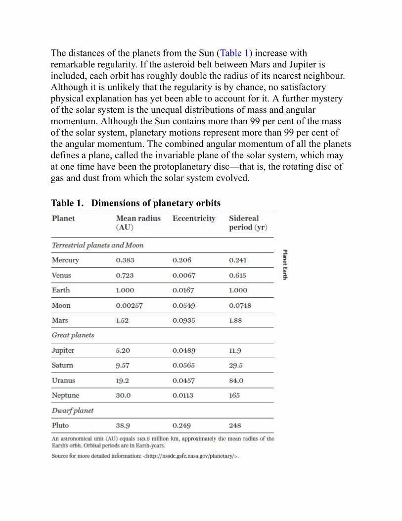
The distances of the planets from the Sun (Table 1) increase withremarkable regularity. If the asteroid belt between Mars and Jupiter isincluded, each orbit has roughly double the radius of its nearest neighbour.Although it is unlikely that the regularity is by chance, no satisfactoryphysical explanation has yet been able to account for it. A further mysteryof the solar system is the unequal distributions of mass and angularmomentum. Although the Sun contains more than 99 per cent of the massof the solar system, planetary motions represent more than 99 per cent ofthe angular momentum. The combined angular momentum of all the planetsdefines a plane, called the invariable plane of the solar system, which mayat one time have been the protoplanetary disc—that is, the rotating disc ofgas and dust from which the solar system evolved.

Table 1. Dimensions of planetary orbits

Eight bodies orbiting the Sun are currently recognized as planets. Theyform two categories (Figure 1) based on their size, composition, anddistance from the Sun. The distances are conveniently measured inastronomical units (AU)—this is roughly the mean radius of the Earth’sorbit around the Sun. The inner, or terrestrial, planets (sequentiallyMercury, Venus, the Earth, and Mars) are closest to the Sun and arecomposed of rock and metal; they are relatively small and are surroundedby few moons and no rings. The outer, or giant, planets (in order ofincreasing distance: Jupiter, Saturn, Uranus, and Neptune) formed furtherfrom the Sun, in colder parts of space. Jupiter and Saturn are gas giants.More than 90 per cent of their masses consists of hydrogen and helium;their atmospheres also contain ammonia and water and they have metallichydrogen cores. Uranus and Neptune are ice giants. Only about 20 per centof their masses consists of hydrogen and helium; beneath their gaseousatmospheres they consist of ices of water, methane, and ammonia. The giantplanets have many moons and are also surrounded by systems of rings ofdust. Between Mars and Jupiter lies the asteroid belt, which consists ofnumerous objects with terrestrial compositions. The smallest are particles ofdust; the four largest are several hundred kilometres in diameter and arereferred to as minor planets. The largest of these, Ceres, is 950 km indiameter and is termed a dwarf planet. All the planets have slightlyelliptical orbits that lie within a few degrees of the Earth’s orbital plane,which is called the ecliptic. This differs by only about 1 degree from theinvariable plane and is used as reference plane for the solar system.

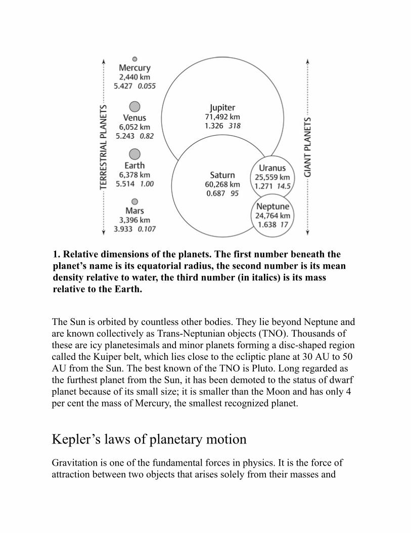
1. Relative dimensions of the planets. The first number beneath theplanet’s name is its equatorial radius, the second number is its meandensity relative to water, the third number (in italics) is its massrelative to the Earth.

The Sun is orbited by countless other bodies. They lie beyond Neptune andare known collectively as Trans-Neptunian objects (TNO). Thousands ofthese are icy planetesimals and minor planets forming a disc-shaped regioncalled the Kuiper belt, which lies close to the ecliptic plane at 30 AU to 50AU from the Sun. The best known of the TNO is Pluto. Long regarded asthe furthest planet from the Sun, it has been demoted to the status of dwarfplanet because of its small size; it is smaller than the Moon and has only 4per cent the mass of Mercury, the smallest recognized planet.

Kepler’s laws of planetary motionGravitation is one of the fundamental forces in physics. It is the force ofattraction between two objects that arises solely from their masses and

varies inversely with the square of their separation. This is the law ofuniversal gravitation, published in 1687 by Isaac Newton. The space inwhich the attraction of a mass is felt is called its gravitational field.

In the late 16th century, the astronomer Tycho Brahe made accurateobservations of the positions of the planets using an astrolabe, an ancientastronomic instrument that was in use since the era of classical Greece.Although Brahe’s measurements were made before the telescope wasinvented, they were so precise that, in 1609 and 1619, Johannes Keplercould combine them into three laws of planetary motion (Figure 2). Theseare: (1) each planetary orbit is an ellipse with the Sun at one of its focalpoints, (2) the radius connecting the planet to the Sun sweeps out equalareas in equal time intervals, and (3) the square of the period of the motionis proportional to the cube of the semi-major axis of the ellipse. In contrastto a circle, which has a constant radius, the shape of an ellipse is defined byits shortest (minor) axis and its longest (major) axis. The deviation of anellipse from a circle is known as its eccentricity; by definition it is 0 for acircle. As the eccentricity increases, the ellipse becomes progressively moreelongate. Except for the orbit of Mercury (which has an eccentricity of 0.2)the planets have nearly circular orbits.

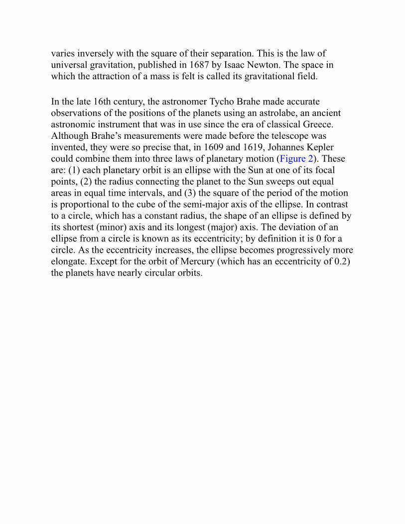
2. Schematic drawing of the Earth’s elliptical orbit, showing thepositions of aphelion and perihelion, the equinoxes and solstices for thenorthern hemisphere. Distance unit is 1 million km (M km).

The motion of a planet about the Sun can be regarded for simplicity as aclosed system, free of external influences. In fact, the other planets doinfluence each other’s motion, but to a lesser degree than the Sun does.Each planet orbits the Sun under its gravitational attraction, which actsalong a radius of its orbit. The radial force results in a constant angularmomentum of the planet about the Sun. As a result, the orbit of the planet isa plane that passes through the Sun. The planet’s orbital motion in thisplane is subject to the conservation of energy. Two types of energy arerelevant to this motion: the energy of the gravitational attraction that bindsthe planet to the Sun, called its potential energy, and the energy associatedwith the speed of its motion, called its kinetic energy. If the planet ismoving so fast that the kinetic energy is greater than the potential energy, itescapes from the solar system on a curved trajectory known as a hyperbola.If the potential energy is dominant, such that the planet cannot escape fromits orbit, and if the force binding it to the Sun varies as the inverse square of

distance (as with gravitation), then the orbit takes the shape of an ellipsewith the Sun at one of its focal points. This is Kepler’s first law.

The Earth has a slightly elliptical orbit, which means that it is about 147million km from the Sun at its closest point—known as perihelion—whilethe distance is 152 million km at its furthest point—called aphelion (Figure2). Perihelion is passed each year around 3 January, and aphelion around 3July. The line joining the extreme points is the major axis of the ellipse, andis called the line of apsides.

Kepler’s second law follows from the conservation of a planet’s angularmomentum about the Sun. It results in equal areas (e.g. A

1 and A

2 in Figure

2) being swept by the radius vector in the same time. Consequently, aplanet’s speed around its orbit is variable: at perihelion, it is moving fasterthan at aphelion. Kepler’s third law results from combining the period ofthe variable planetary motion with the equation of an ellipse (the first law).In 1687 Isaac Newton showed that Kepler’s first and third laws confirmedhis inverse square law of universal gravitation.

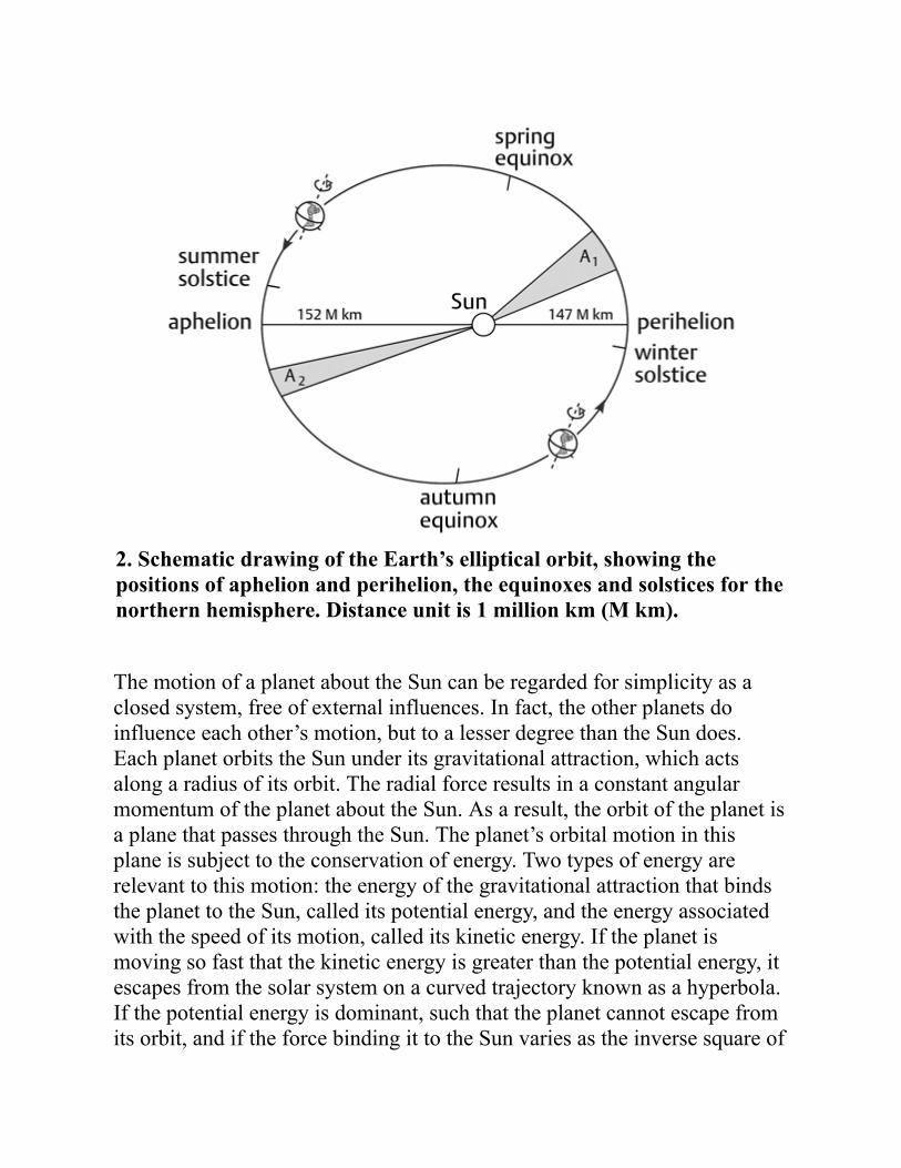
The Earth spins about an axis that is inclined to the pole of the eclipticplane; the axial tilt is called the obliquity of the ecliptic (Figure 3A). Theangle at present measures 23.44 degrees but varies slowly with a period of41,000 yr as a result of interactions with other planets. The obliquity isresponsible for the annual seasons. The motion of the Earth around its orbitchanges the attitude of each hemisphere to the Sun, affecting the length ofthe day. Shortly before perihelion, the obliquity causes the northernhemisphere to be tilted away from the Sun, with the shortest day at thewinter solstice on 21 December. Six months later the northern hemisphereis tilted towards the Sun, and the day is longest at the summer solstice on 21June. The line joining these positions is called the line of solstices. Twiceeach year the rotation axis is normal to the radius to the Sun, so that around21 March and 23 September the day and night are equally long; thesepositions are called the spring and autumn equinoxes and the line joiningthem is called the line of equinoxes. The axial tilt causes the seasons todiffer by six months between the northern and southern hemispheres.Summer in the southern hemisphere occurs near perihelion, so it should be

warmer than summer in the northern hemisphere; correspondingly, southernhemisphere winters fall near aphelion and should be colder. However, thesouthern hemisphere is dominated by oceans and the northern hemisphereby land. The oceans heat up and cool off more slowly than land surfaces,and as a result climates are milder in the southern hemisphere.

3. (A) Precession of the Earth’s rotation axis induced by the Moon’storque on the equatorial bulge. (B) Precession of the major axis of theEarth’s orbit relative to a stellar reference frame. (C) Variation of theeccentricity of the orbit. The diagrams are not to scale.

The Chandler wobbleThe Earth is not a rigid body but reacts elastically in response to deformingforces. Its ideal shape would be a sphere, but the centrifugal forces arisingfrom its rotation cause the shape to flatten slightly about the spin axis, sothat the equatorial diameter is longer than the polar diameter. The slightly

flattened sphere is called an oblate spheroid. The flattening is not large,only about 1 part in 300, but it affects how the Earth rotates.

For example, if the axis of the spinning Earth is displaced, then allowed tospin freely, it exhibits a wobbling motion about its mean location, in thesame way as a spinning top wobbles, if nudged. This motion results fromthe Earth’s unequal internal mass distribution and is called a free nutation,or ‘nodding motion’. The mean direction of the Earth’s rotation axis isconstant but at any instant it may be displaced slightly from its meandirection. The instantaneous axis moves around the mean rotational polewith an average displacement of several metres. The free nutation wasexplained mathematically in 1765 by Leonhard Euler, a Swissmathematician, but was only detected in 1891 by Seth Chandler, anAmerican astronomer, after whom it is called the Chandler wobble. Eulerpredicted a period of about ten months for the motion, but the observedperiod is fourteen months. The 40 per cent increase in period is due to theelastic yielding of the Earth, which allows it to deform to accommodate thedisplacement of the instantaneous rotation axis; Euler’s model had assumeda rigid planet. The mechanism, or ‘nudge’, that excites the Chandler wobblehas not been identified conclusively. Proposed sources have included verylarge earthquakes, atmospheric fluctuations, and ocean-bottom pressurechanges related to oceanic circulation.

The development of Very Long Baseline Interferometry (VLBI) has made itpossible to observe and measure the Chandler wobble precisely. Thistechnique, used in radio astronomy, has been adapted for geodetic purposesas follows. Radio sources—e.g. quasars—that lie outside the Milky Waygalaxy provide a very stable coordinate system against which the motion ofthe planet can be measured. The extraterrestrial radio signals are detectedby radio telescopes combined into large arrays at different places on theEarth. The time differences between the arrival times of repeated signals atseparate arrays are analysed to obtain the orientation of the Earth and itsrotational rate with exceptional accuracy. The VLBI data trace the Chandlerwobble with a precision of a few centimetres, and the rotational period isdetermined to better than 0.1 msec. This enables precise observation ofchanges in the length of the day and the identification of contributingfactors, such as the rotational braking caused by marine tides, changes in

the angular momentum of the atmosphere, and the effects of bodily tides inthe solid Earth.

Effects of the Moon and Jupiter on the Earth’srotation

The Moon’s gravitational attraction disturbs the orientation of the Earth’srotation axis. Due to the obliquity of the Earth’s axis the equatorial bulgeprojects below the plane of the Moon’s orbit on one side of the Earth andabove it on the opposite side. The Moon’s gravitational attraction on thedistant side is weaker than on the closer side, because of the inverse squarelaw. This results in a torque, or turning force, which attempts to bring therotation axis upright, that is, normal to the ecliptic (Figure 3A). However,when a torque acts on a spinning object, it causes the rotational axis tomove while maintaining the angle of tilt (the obliquity in this case). As aresult, the rotation axis moves around the surface of a cone that has the poleto the ecliptic as its axis. This motion is called precession. Viewed fromabove the ecliptic, the Earth’s rotation is anticlockwise, while the directionof precession is clockwise. Because it takes place in the opposite sense tothe Earth’s rotation, the precession is said to be retrograde. Thegravitational attraction of the Sun on the equatorial bulge also causesretrograde precession. Although the Sun is vastly more massive than theMoon, it is much further from the Earth and as a result its effect on theprecession is about half that of the Moon. The combined precession isknown as the precession of the equinoxes, and its period is approximately25,800 yr.

The Earth exerts a reciprocal torque on the Moon, which results in aprecession of the lunar orbit around the Earth with a period of 18.6 yr. Thisthen modulates the amplitude of the lunisolar precession of the Earth’s axisby superposing a small forced nutation. This changes the angle of obliquityby a tiny fluctuating amount—up to 9 seconds of arc—with a period of 18.6yr equivalent to that of the lunar orbital precession. However, this effect isinsignificant compared to the main lunisolar precession.

The gravitational attractions of the other planets—especially Jupiter, whosemass is 2.5 times the combined mass of all the other planets—influence theEarth’s long-term orbital rotations in a complex fashion. The planets movewith different periods around their differently shaped and sized orbits. Theirgravitational attractions impose fluctuations on the Earth’s orbit at manyfrequencies, a few of which are more significant than the rest. Oneimportant effect is on the obliquity: the amplitude of the axial tilt is forcedto change rhythmically between a maximum of 24.5 degrees and aminimum of 22.1 degrees with a period of 41,000 yr. Another gravitationalinteraction with the other planets causes the orientation of the elliptical orbitto change with respect to the stars (Figure 3B). The line of apsides—themajor axis of the ellipse—precesses around the pole to the ecliptic in aprograde sense (i.e. in the same sense as the Earth’s rotation) with a periodof 100,000 yr. This is known as planetary precession. Additionally, theshape of the orbit changes with time (Figure 3C), so that the eccentricityvaries cyclically between 0.005 (almost circular) and a maximum of 0.058;currently it is 0.0167 (Table 1). The dominant period of the eccentricityfluctuation is 405,000 yr, on which a further fluctuation of around 100,000yr is superposed, which is close to the period of the planetary precession.

Milankovitch cycles of climatic variationThe amount of solar energy received by a unit area of the Earth’s surface iscalled the insolation. This can be calculated for the top of the atmospherefrom the known solar irradiation. If the atmosphere were transparent, thesurface insolation would only be affected by the separation of the Earth andthe Sun and the orientation of the surface to the solar energy. These factorschange during the year as the Earth moves around its orbit; the distancefrom the Sun varies and the axis tilts alternately towards the Sun, then awayfrom it, causing the changing seasons.

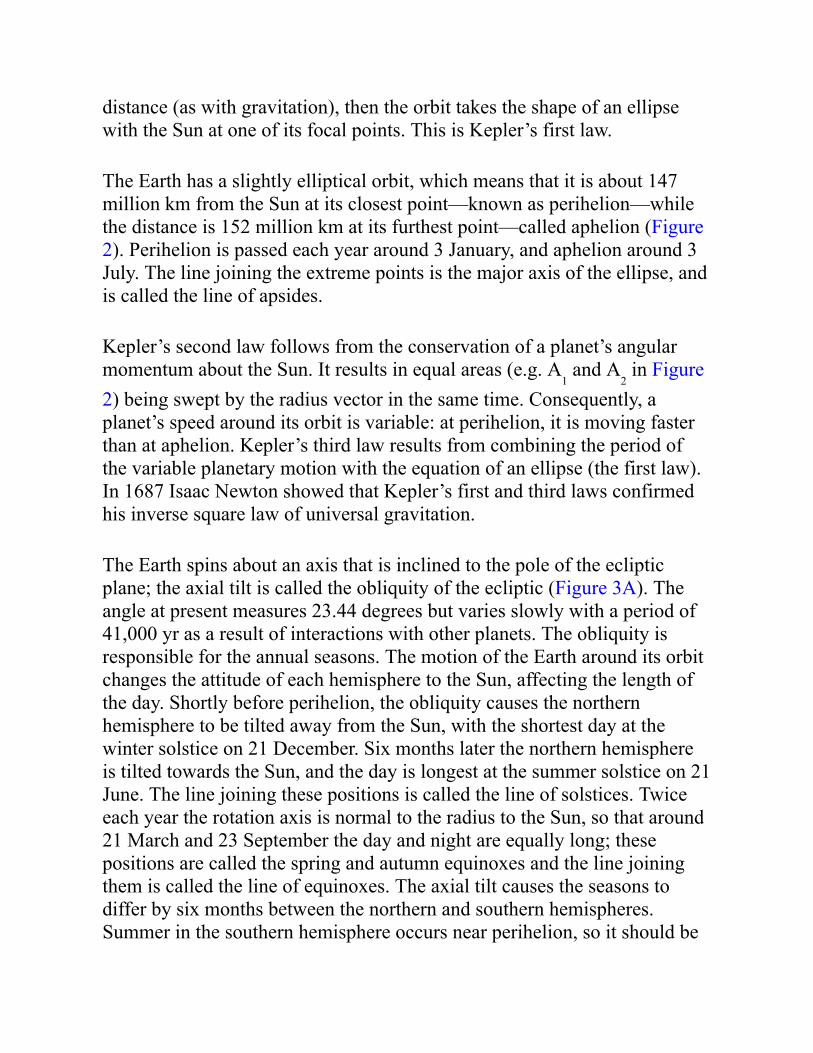
The long-term fluctuations in the Earth’s rotation and orbital parametersinfluence the insolation (Figure 4) and this causes changes in climate. Whenthe obliquity is smallest, the axis is more upright with respect to the eclipticthan at present. The seasonal differences are then smaller and vary lessbetween polar and equatorial regions. Conversely, a large axial tilt causes

an extreme difference between summer and winter at all latitudes. Theinsolation at any point on the Earth thus changes with the obliquity cycle.Precession of the axis also changes the insolation. At present the north polepoints away from the Sun at perihelion; one half of a precessional cyclelater it will point away from the Sun at aphelion. This results in a change ofinsolation and an effect on climate with a period equal to that of theprecession. The orbital eccentricity cycle changes the Earth–Sun distancesat perihelion and aphelion, with corresponding changes in insolation. Whenthe orbit is closest to being circular, the perihelion–aphelion difference ininsolation is smallest, but when the orbit is more elongate this differenceincreases. In this way the changes in eccentricity cause long-term variationsin climate. The periodic climatic changes due to orbital variations are calledMilankovitch cycles, after the Serbian astronomer Milutin Milankovitch,who studied them systematically in the 1920s and 1930s.

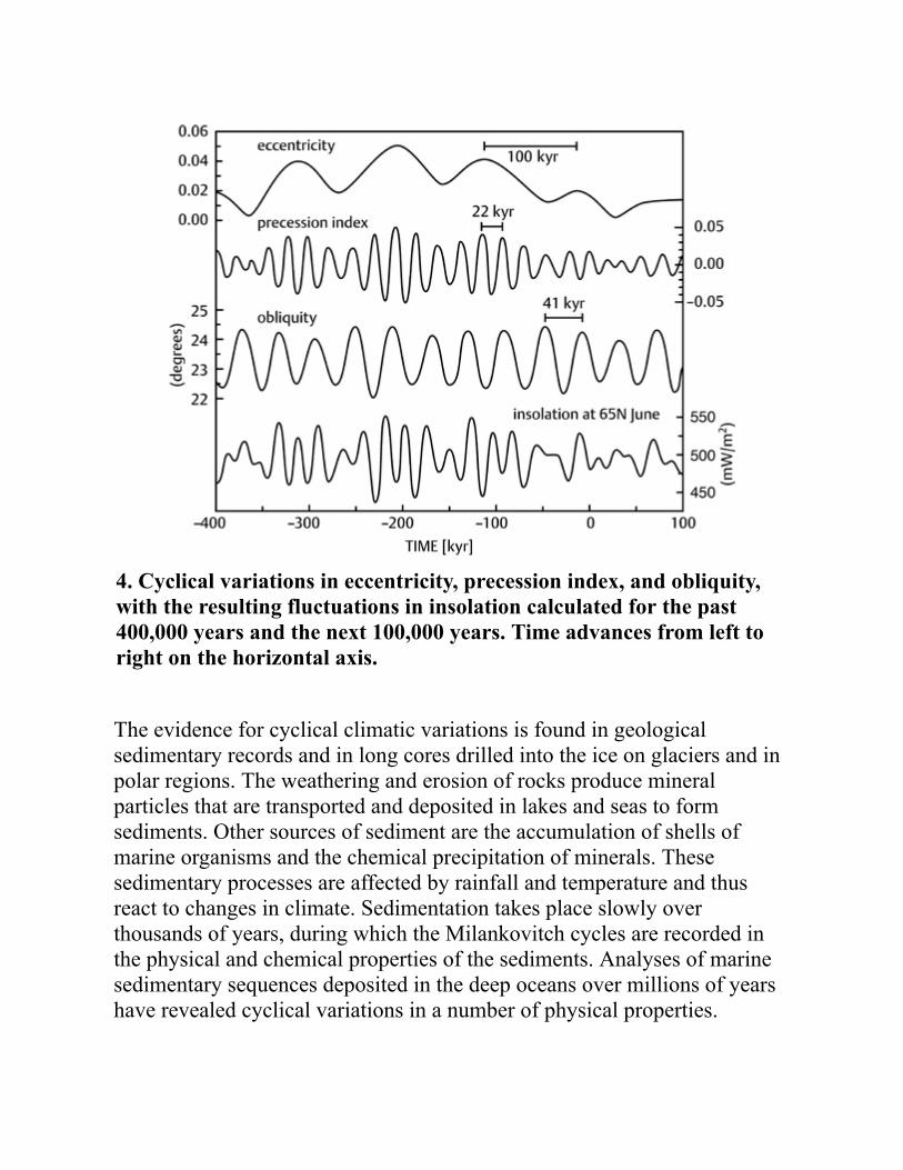
4. Cyclical variations in eccentricity, precession index, and obliquity,with the resulting fluctuations in insolation calculated for the past400,000 years and the next 100,000 years. Time advances from left toright on the horizontal axis.

The evidence for cyclical climatic variations is found in geologicalsedimentary records and in long cores drilled into the ice on glaciers and inpolar regions. The weathering and erosion of rocks produce mineralparticles that are transported and deposited in lakes and seas to formsediments. Other sources of sediment are the accumulation of shells ofmarine organisms and the chemical precipitation of minerals. Thesesedimentary processes are affected by rainfall and temperature and thusreact to changes in climate. Sedimentation takes place slowly overthousands of years, during which the Milankovitch cycles are recorded inthe physical and chemical properties of the sediments. Analyses of marinesedimentary sequences deposited in the deep oceans over millions of yearshave revealed cyclical variations in a number of physical properties.

Examples are bedding thickness, sediment colour, isotopic ratios, andmagnetic susceptibility.

When ice accumulates on a glacier or in polar regions, it absorbs oxygenfrom the atmosphere. Important climate records have been obtained fromstudying isotopes of the oxygen in polar ice cores. Isotopes are separateforms of an element that differ only in the number of neutrons they contain.The two most common isotopes of oxygen contain 16 and 18 neutrons,respectively; their ratio in water depends on the temperature. The records ofoxygen isotope ratios in long ice cores display Milankovitch cycles and areimportant evidence for the climatic changes, generally referred to as orbitalforcing, which are brought about by the long-term variations in the Earth’sorbit and axial tilt.

Apart from its climatic significance, the pattern of Milankovitch cycles in asediment allows it to be dated more completely. The age of a sedimentarysequence is often known at only a small number of widely spaced depths,for example at levels that have been dated radiometrically. Between thesedated horizons there may be distinctive undated features such as faunalextinctions or magnetic polarity reversals, which occur at irregularintervals. The presence of cyclical variations in a physical property of asediment makes it possible to estimate the ages of palaeontological ormagnetic events between the dated levels in a sedimentary record.

Chapter 3Seismology and the Earth’sinternal structure

Elastic deformationSeismology is the most powerful geophysical tool for understanding thestructure of the Earth. It is concerned with how the Earth vibrates. In thesame way that the strings of a guitar vibrate back and forth in a periodicmotion when plucked, the solid material in the Earth reacts to a sudden joltby vibrating. This is particularly evident when an earthquake strikes, but itcan also happen as reaction to a local shock. Physically, seismic behaviourdepends on the relationship between stress and strain in the Earth, so if wewant to understand seismology, it is worthwhile examining these properties.

Stress is defined as the force acting on a unit area. The fractionaldeformation it causes is called strain. The stress–strain relationshipdescribes the mechanical behaviour of a material. When subjected to a lowstress, materials deform in an elastic manner so that stress and strain areproportional to each other and the material returns to its original unstrainedcondition when the stress is removed. Seismic waves usually propagateunder conditions of low stress. If the stress is increased progressively, amaterial eventually reaches its elastic limit, beyond which it cannot return

to its unstrained state. Further stress causes disproportionately large strainand permanent deformation. Eventually the stress causes the material toreach its breaking point, at which it ruptures. The relationship betweenstress and strain is an important aspect of seismology. Two types of elasticdeformation—compressional and shear—are important in determining howseismic waves propagate in the Earth.

Imagine a small block that is subject to a deforming stress perpendicular toone face of the block; this is called a normal stress. The block shortens inthe direction it is squeezed, but it expands slightly in the perpendiculardirection; when stretched, the opposite changes of shape occur. Thesereversible elastic changes depend on how the material responds tocompression or tension. This property is described by a physical parametercalled the bulk modulus. In a shear deformation, the stress acts parallel tothe surface of the block, so that one edge moves parallel to the oppositeedge, changing the shape but not the volume of the block. This elasticproperty is described by a parameter called the shear modulus.

An earthquake causes normal and shear strains that result in four types ofseismic wave. Each type of wave is described by two quantities: itswavelength and frequency. The wavelength is the distance betweensuccessive peaks of a vibration, and the frequency is the number ofvibrations per second. Their product is the speed of the wave. Two types ofwave travel through the body of the Earth and two types spread out at andnear its surface. They are characterized by different kinds of ground motionand their speeds depend in different ways on the elastic properties anddensity of the rocks they travel in.

Seismic body wavesSeismic waves are sensed by a device called a seismometer; the recording iscalled a seismogram, and the combined instrument forms a seismograph.One common type of seismometer consists of a heavy magnet within a coilthat is attached to a casing connected to the ground. The ground, casing,and coil all move in an earthquake, but the inertia of the heavy magnetrestricts its movement, so that relative motion takes place between the

magnet and the coil. This induces an electrical current in the coil, which isamplified electronically and recorded. The principle of a modern broadbandseismometer is similar: a small mass is held motionless relative to the frameof the instrument by an electronic feedback circuit, which measures theforce required to compensate the relative motion caused by ground shaking.

Early seismographs recorded the shaking as a wiggly line traced on paper,but in modern instruments the recording is made digitally and covers a widerange of vibrational frequencies. The seismometer was invented more thana century ago and has been improved continuously, with the result thatmodern instruments are very sensitive. The device was originally designedto register the ground’s displacement, but modern instruments reactprimarily to the ground’s velocity during an earthquake’s shaking. They canalso be designed to record the ground’s acceleration.

A seismic P-wave (also called a primary, compressional, or longitudinalwave) consists of a series of compressions and expansions caused byparticles in the ground moving back and forward parallel to the direction inwhich the wave travels (Figure 5A). The speed of a P-wave depends on thebulk modulus, shear modulus, and density of the medium, and is about 6–7km/s in the Earth’s crust (for comparison: the speed of sound in air is 0.33km/s). It is the fastest seismic wave and can pass through fluids, althoughwith reduced speed. When it reaches the Earth’s surface, a P-wave usuallycauses nearly vertical motion, which is recorded by instruments and may befelt by people but usually does not result in severe damage.

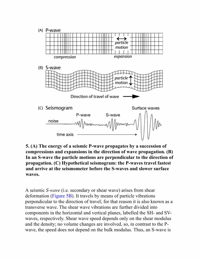
5. (A) The energy of a seismic P-wave propagates by a succession ofcompressions and expansions in the direction of wave propagation. (B)In an S-wave the particle motions are perpendicular to the direction ofpropagation. (C) Hypothetical seismogram: the P-waves travel fastestand arrive at the seismometer before the S-waves and slower surfacewaves.

A seismic S-wave (i.e. secondary or shear wave) arises from sheardeformation (Figure 5B). It travels by means of particle vibrationsperpendicular to the direction of travel; for that reason it is also known as atransverse wave. The shear wave vibrations are further divided intocomponents in the horizontal and vertical planes, labelled the SH- and SV-waves, respectively. Shear wave speed depends only on the shear modulusand the density; no volume changes are involved, so, in contrast to the P-wave, the speed does not depend on the bulk modulus. Thus, an S-wave is

slower than a P-wave, propagating about 58 per cent as fast, with crustalvelocities around 3.5–4 km/s. Moreover, shear waves can only travel in amaterial that supports shear strain. This is the case for a solid object, inwhich the molecules have regular locations and intermolecular forces holdthe object together. By contrast, a liquid (or gas) is made up of independentmolecules that are not bonded to each other, and thus a fluid has no shearstrength. For this reason S-waves cannot travel through a fluid. This hasimportant consequences for understanding the internal structure of theEarth. S-waves have components in both the horizontal and vertical planes,so when they reach the Earth’s surface they shake structures from side toside as well as up and down. They can have larger amplitudes than P-waves. Buildings are better able to resist up-and-down motion than side-to-side shaking, and as a result SH-waves can cause serious damage tostructures.

Seismic surface waves and free oscillationsSurface waves spread out along the Earth’s surface around a point—calledthe epicentre—located vertically above the earthquake’s source, in the sameway that ripples from a splash spread across a pool. Very deep earthquakesusually do not produce surface waves, but the surface waves caused byshallow earthquakes are very destructive. In contrast to seismic bodywaves, which can spread out in three dimensions through the Earth’sinterior, the energy in a seismic surface wave is guided by the free surface.It is only able to spread out in two dimensions and is more concentrated.Consequently, surface waves have the largest amplitudes on the seismogramof a shallow earthquake (Figure 5C) and are responsible for the strongestground motions and greatest damage.

There are two types of surface wave. A Rayleigh wave combines thelongitudinal vibration of a P-wave with the vertical component of vibrationof an S-wave, causing the particles of the surface to move around anelliptical path in the vertical plane. If one visualizes a Rayleigh wavemoving from left to right, the ground particles move around their ellipses inthe anticlockwise direction; this is akin to the motion of particles in a waterwave, except that the latter move in a clockwise sense relative to the

direction of the wave. They cause a rolling motion of the surface, whichmay result in destructive ground-shaking. The Rayleigh waves travel at aspeed that is about 92 per cent of the S-wave speed. A Love wave ariseswhen the horizontal components of shear waves are trapped in the boundarylayer between a free surface and a lower interface. This can produce stronghorizontal shaking, with damaging effects on the foundations of structures.The speed of a Love wave is intermediate between that of S-waves in theboundary layer and the deeper interior.

As a result of their different paths and speeds of propagation, the four typesof seismic wave take different lengths of time to travel between anearthquake and the seismometer. The first arrival on a seismogram is the P-wave, followed next by S-waves, then the surface waves (Figure 5C). Theseismogram is, however, much more complicated than this, because P- andS-waves bounce around in the interior of the Earth, they are bent andreflected at various interfaces, and therefore many arrivals are superposedon a seismogram.

The amplitude of a seismic wave decreases with increasing distance fromthe earthquake source due to three factors: anelastic attenuation, scattering,and geometrical spreading. Anelastic attenuation is the loss of amplitude ofa wave due to absorption of its energy by non-elastic processes as it passesthrough the Earth. Imperfections in the mineral grains that make up theEarth’s interior absorb energy; their effect is complex and is describedsummarily as internal friction. Scattering occurs when a wave suffersreflection and refraction at irregularities or changes in the materialproperties of the medium it is passing through. Geometric spreading refersto the distribution of a wave’s energy over an increasing area as it spreads.Seismic body-wave energy spreads out on a spherical surface around a deepearthquake. At distance r from the source, the area of a spherical wavesurface is proportional to r2, so the energy attenuates as 1/r2. In contrast, thedisturbance of a surface wave spreads out as a circular ring around theepicentre, with circumference proportional to r, so its energy onlyattenuates as 1/r. Thus, the amplitudes of surface waves decrease moreslowly with distance from an earthquake than do the amplitudes of bodywaves. The energy of surface waves from a very large earthquake can travelaround the world several times before it dissipates.

The ground motion in a surface wave is not actually restricted to the surfacebut penetrates some distance into the Earth, decreasing in amplitude withincreasing depth. The ‘penetration depth’ of a surface wave component isusually taken to be the depth where its amplitude has decreased to about athird of its initial value; it is roughly proportional to the wavelength. Asurface wave consists of components with different frequencies, some ofwhich correspond to long wavelengths. Seismic velocities generallyincrease with depth, so the wave components with long wavelengthspenetrate deeper and travel faster than the short wavelength components.Consequently, the shape of a surface wave changes with distance from thesource. This phenomenon is called dispersion. Seismologists analyse thedispersion of surface waves to obtain important information about thephysical properties and structure of the outer layers of the Earth.

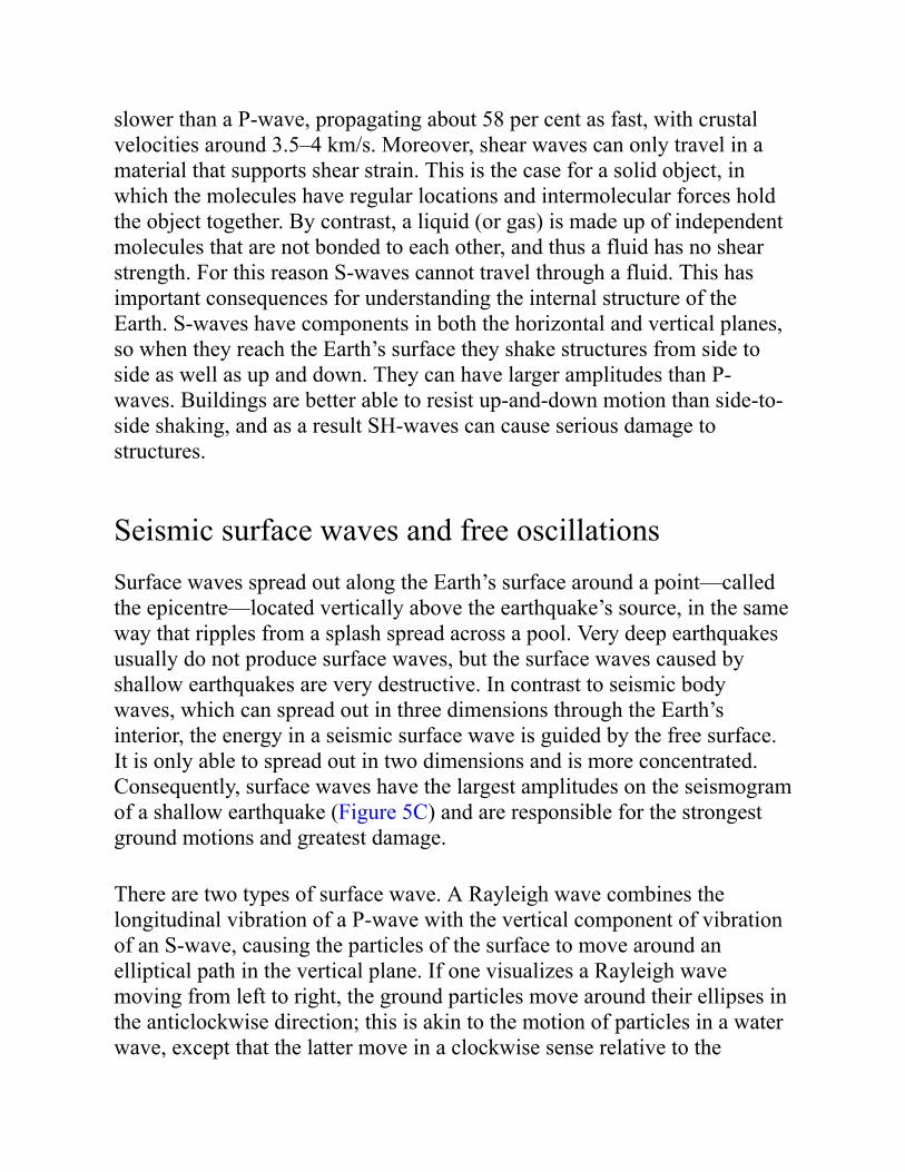
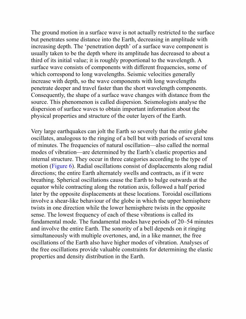
Very large earthquakes can jolt the Earth so severely that the entire globeoscillates, analogous to the ringing of a bell but with periods of several tensof minutes. The frequencies of natural oscillation—also called the normalmodes of vibration—are determined by the Earth’s elastic properties andinternal structure. They occur in three categories according to the type ofmotion (Figure 6). Radial oscillations consist of displacements along radialdirections; the entire Earth alternately swells and contracts, as if it werebreathing. Spherical oscillations cause the Earth to bulge outwards at theequator while contracting along the rotation axis, followed a half periodlater by the opposite displacements at these locations. Toroidal oscillationsinvolve a shear-like behaviour of the globe in which the upper hemispheretwists in one direction while the lower hemisphere twists in the oppositesense. The lowest frequency of each of these vibrations is called itsfundamental mode. The fundamental modes have periods of 20–54 minutesand involve the entire Earth. The sonority of a bell depends on it ringingsimultaneously with multiple overtones, and, in a like manner, the freeoscillations of the Earth also have higher modes of vibration. Analyses ofthe free oscillations provide valuable constraints for determining the elasticproperties and density distribution in the Earth.

6. The fundamental modes of natural oscillation of the Earth and theirobserved periods.

Reflection, refraction, and diffraction of body wavesWhen a seismic wave initially spreads out from a source in a homogeneousmedium, it does so uniformly in all directions and its wavefront is a sphere.A radius of the sphere perpendicular to the wavefront is called a seismicray; it describes the direction of travel of the wavefront. When seismicenergy is incident on the interface separating two materials, it sets upvibrations (i.e. new seismic waves) in the material on both sides of theinterface. Laws similar to those of optics govern the way rays from P- andS-waves interact with an interface at which the elastic properties anddensity—and therefore the seismic velocities—change.

Consider a P-ray incident on an interface, as in Figure 7 (similarconsiderations apply to an incident S-ray). Above the interface the anglesformed between the incident and reflected P-rays and the normal to theinterface are equal: this is the law of seismic reflection. The ray penetratingthe second medium experiences a change of direction that depends on theseismic velocities of the two media. It is called a refracted ray and itsdirection is determined by a mathematical relationship called the law ofseismic refraction. For example, if the second medium has a faster speedthan the first medium, the refracted ray is bent away from the normal to the

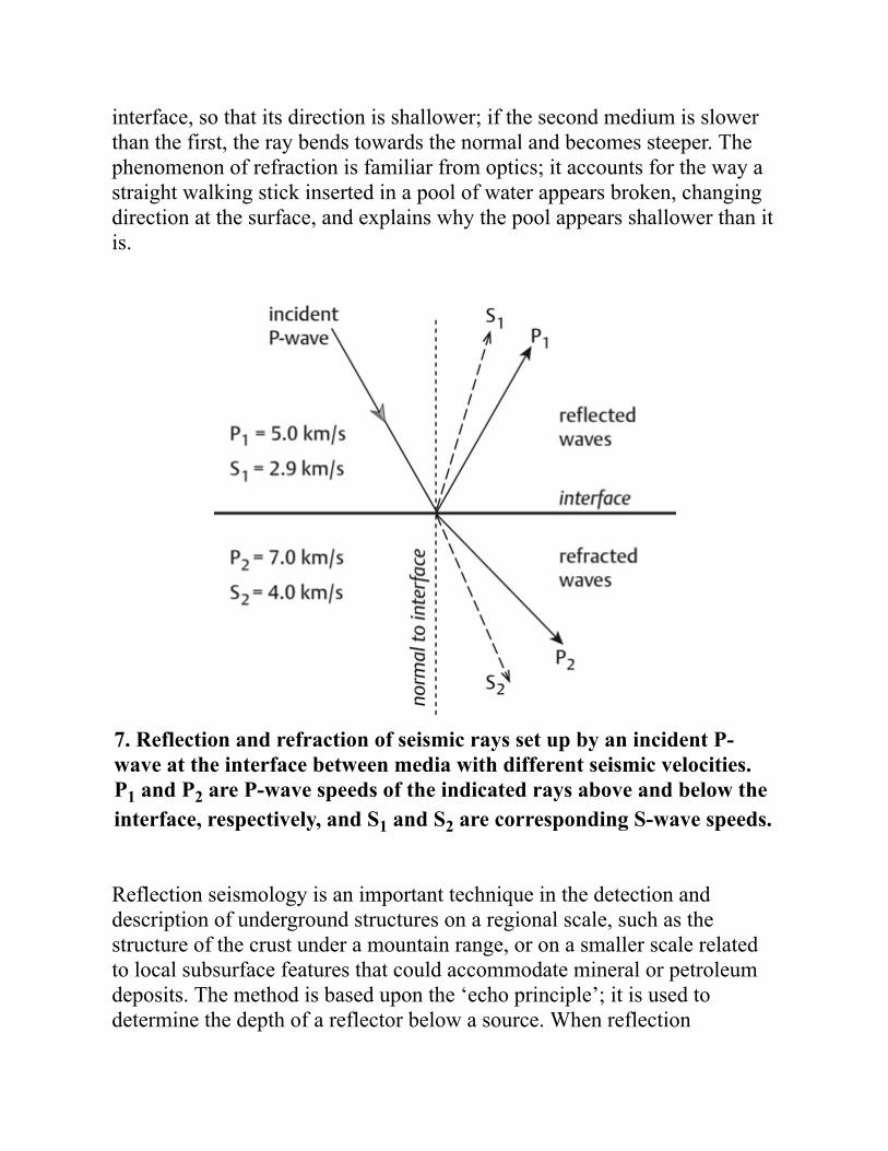
interface, so that its direction is shallower; if the second medium is slowerthan the first, the ray bends towards the normal and becomes steeper. Thephenomenon of refraction is familiar from optics; it accounts for the way astraight walking stick inserted in a pool of water appears broken, changingdirection at the surface, and explains why the pool appears shallower than itis.

7. Reflection and refraction of seismic rays set up by an incident P-wave at the interface between media with different seismic velocities.P1 and P2 are P-wave speeds of the indicated rays above and below theinterface, respectively, and S1 and S2 are corresponding S-wave speeds.

Reflection seismology is an important technique in the detection anddescription of underground structures on a regional scale, such as thestructure of the crust under a mountain range, or on a smaller scale relatedto local subsurface features that could accommodate mineral or petroleumdeposits. The method is based upon the ‘echo principle’; it is used todetermine the depth of a reflector below a source. When reflection

seismology is used to investigate an underground structure, P-waves arecreated by a sudden or continuous energy source at different locations alonga profile across the structure. The waves are reflected at subsurfaceinterfaces where there is a change in the seismic impedance; this is definedas the product obtained by multiplying together the density and the seismicvelocity. On returning to the surface the reflections are recorded by arraysof compact portable seismometers called geophones. The prime informationgained from a reflection seismic survey consists of the depths to subsurfacerock layers as well as the seismic velocities of the layers.

In terrestrial profiling, the source of the P-waves is usually either acontrolled explosion or one or more massive vibrating sources. In marineapplications, a common source is a specialized air-gun, which discharges asudden high-pressure air bubble into the water. Several air-guns may beused at a time, linked in an array, and the reflections are detected by arraysof pressure sensors towed at a fixed depth behind an exploration vessel andlinked to form streamers that may be several kilometres long.

In addition to the useful record created by the source, a seismogramcontains unwanted vibrations that form a background noise, which can spoilthe recording just as traffic noise can disturb a conversation. Reflectionseismology applies several corrective measures to improve the signal-to-noise ratio on seismograms. Surface wave noise caused by the source(‘ground roll’) is reduced by combining the geophones in groups. Thetravel-times of reflections must be corrected for various distortions,resulting from the geometry of the source, geophone, and reflecting surface.A typical reflection survey requires sophisticated data processing andpowerful computation, in order to correctly locate and portray the reflectingsurfaces. The technique is a way of obtaining a three-dimensional picture ofsubsurface structures and their seismic velocity profiles. In the petroleumindustry, reflection seismology is the most important geophysical techniquein exploration. The detailed analysis of some reflection sections can allowchanges in seismic impedance to be interpreted in terms of properties suchas porosity and permeability, and can indicate the possible presence of gasand liquids.

Refraction seismology is also used to decipher subsurface structure, makinguse of the way seismic waves are refracted when their velocity changes.Imagine a simple structure of homogeneous layers of rock in which onelayer overlies a layer with faster seismic speed. The rays from a surfaceexplosion impact on the lower interface at a variety of angles. Some arereflected back to the surface and some are refracted into the next layer, inwhich they make a shallower angle with the boundary (Figure 8). One ofthe incident rays strikes the boundary in such a way that, when it isrefracted into the lower faster layer, it travels along or just below theboundary, in the lower layer. This situation is known as critical refractionand it is determined by the velocities of the two layers. The criticallyrefracted ray moves along the interface at the faster speed of the lowerlayer. In doing so, it disturbs the overlying layer and sets up P-rays that arecritically refracted back to the surface, where they are recorded bygeophones. Beyond a certain distance from the source (known as thecrossover point) the refracted wave arrives before the direct wave in the toplayer, because it travels part of the way at the higher speed of the lowerlayer. (This is analogous to traversing a city by driving a longer distance ona high-speed bypass, which is often faster than taking a shorter routethrough the city centre.) The travel-times of the first arrivals at geophonesin a refraction seismic profile reveal the seismic velocities above and belowthe refracting interface and its depth.

8. Reflection and refraction of seismic ray paths when a shallow layeroverlies a layer with higher velocity; velocities are constant in eachlayer. Geophones on the surface record rays reflected from theinterface as well as refracted rays set up by the wave that travels alongthe interface.

An additional mechanism that can affect the propagation of a seismic waveis diffraction. This occurs when the wave encounters an abrupt ordiscontinuous surface, such as an intruding body or the edge of a layer. Inthe same way that ocean waves bend around the end of a solid jetty, theseismic waves are bent around the edge of an obstacle in their path. P- andS-waves diffracted at the core–mantle boundary provide additional dataabout the Earth’s deep structure.

Paths of seismic body waves through the EarthEarthquake seismologists have deciphered the internal structure of the Earthby studying the reflections and refractions of seismic body waves and thedispersion of surface waves. Imagine a layered Earth in which each layerhas a faster seismic velocity than the one above. At each interface, theincrease of velocity causes an incident seismic wave to be refracted awayfrom the normal to the interface to ever-shallower directions (Figure 7).When the angle of incidence on a layer reaches a critical angle, the wavehas reached its maximum depth; the wave travels from the interface back

towards the surface, refracting towards the normal at each interface itcrosses. If each layer is extremely thin, so that the velocity increasessmoothly with depth, the path of the wave becomes a curved ray. Withineach of the Earth’s major internal regions seismic velocities increaseprogressively with depth. This causes seismic rays to have a curved shape(Figure 9).

9. (A) Shadow zones for seismic P- and S-waves passing through theEarth. (B) Some examples of refracted and reflected P- and S-waveswithin the Earth and their relationships to the boundaries of the innerand outer core. The labels PP, PKP, SKS, etc. identify the pathsfollowed by multiply reflected and refracted rays.

The boundaries between the major internal regions are marked by abruptchanges in density and in the velocities of P- and S-waves, resulting instrong refractions and reflections. The seismic arrivals from internalboundaries are identified on seismograms recorded at observatoriesdistributed over the Earth’s surface. The distance of a point on the surfacefrom the epicentre of an earthquake—its epicentral distance—can bemeasured in kilometres or miles along the surface. However, an epicentraldistance is more conveniently measured by the angle which the surface

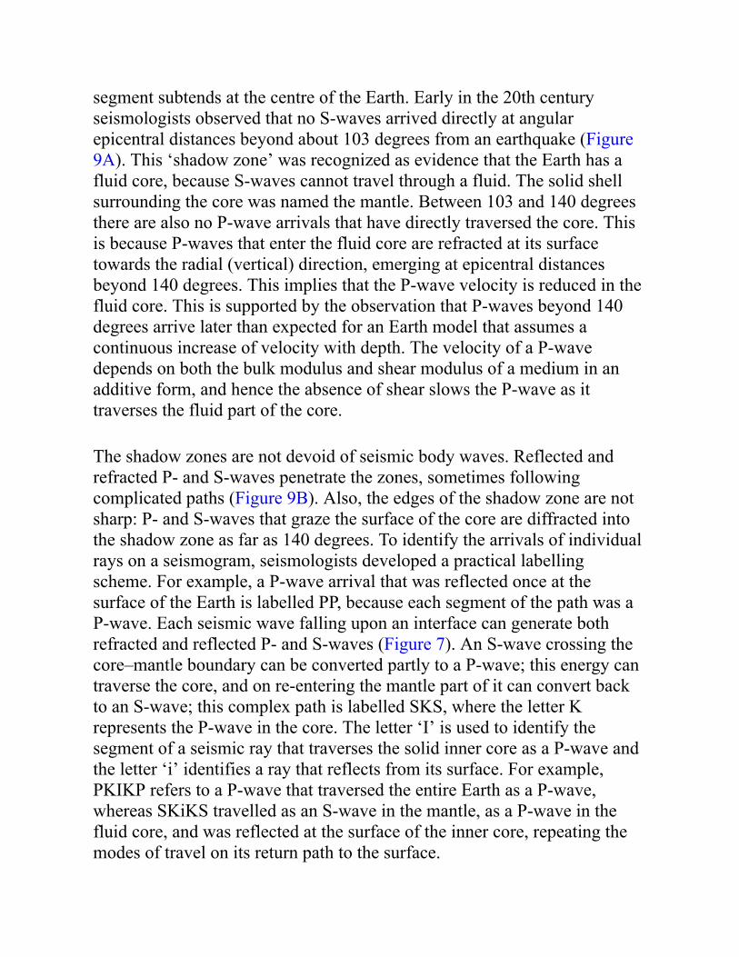
segment subtends at the centre of the Earth. Early in the 20th centuryseismologists observed that no S-waves arrived directly at angularepicentral distances beyond about 103 degrees from an earthquake (Figure9A). This ‘shadow zone’ was recognized as evidence that the Earth has afluid core, because S-waves cannot travel through a fluid. The solid shellsurrounding the core was named the mantle. Between 103 and 140 degreesthere are also no P-wave arrivals that have directly traversed the core. Thisis because P-waves that enter the fluid core are refracted at its surfacetowards the radial (vertical) direction, emerging at epicentral distancesbeyond 140 degrees. This implies that the P-wave velocity is reduced in thefluid core. This is supported by the observation that P-waves beyond 140degrees arrive later than expected for an Earth model that assumes acontinuous increase of velocity with depth. The velocity of a P-wavedepends on both the bulk modulus and shear modulus of a medium in anadditive form, and hence the absence of shear slows the P-wave as ittraverses the fluid part of the core.

The shadow zones are not devoid of seismic body waves. Reflected andrefracted P- and S-waves penetrate the zones, sometimes followingcomplicated paths (Figure 9B). Also, the edges of the shadow zone are notsharp: P- and S-waves that graze the surface of the core are diffracted intothe shadow zone as far as 140 degrees. To identify the arrivals of individualrays on a seismogram, seismologists developed a practical labellingscheme. For example, a P-wave arrival that was reflected once at thesurface of the Earth is labelled PP, because each segment of the path was aP-wave. Each seismic wave falling upon an interface can generate bothrefracted and reflected P- and S-waves (Figure 7). An S-wave crossing thecore–mantle boundary can be converted partly to a P-wave; this energy cantraverse the core, and on re-entering the mantle part of it can convert backto an S-wave; this complex path is labelled SKS, where the letter Krepresents the P-wave in the core. The letter ‘I’ is used to identify thesegment of a seismic ray that traverses the solid inner core as a P-wave andthe letter ‘i’ identifies a ray that reflects from its surface. For example,PKIKP refers to a P-wave that traversed the entire Earth as a P-wave,whereas SKiKS travelled as an S-wave in the mantle, as a P-wave in thefluid core, and was reflected at the surface of the inner core, repeating themodes of travel on its return path to the surface.

Correctly identifying the arrivals on a seismogram and modelling the pathsthey followed has enabled seismologists to develop a global model of theEarth’s internal structure and its composition. Plots of the travel-times ofdifferent seismic phases against the epicentral distances from numerousearthquakes yielded globally averaged travel-time curves (Figure 10).Mathematical procedures—called forward modelling and inversion,respectively—are employed to convert these observations at the Earth’ssurface into the distributions of seismic velocities with depth (Figure 11).The seismic velocities depend on density as well as on the elastic moduli,and so mathematical processing of the velocities yields the variation ofdensity with depth. The analysis of the Earth’s natural oscillations, whichdepend on the radial variations of density and elastic properties, also yieldsa density model. The successful model is checked by several criteria.Integrated over the Earth’s volume the density model must yield the correctmass, and it must also give the correct moment of inertia about the rotationaxis. Density changes abruptly in the Earth at the major internal boundaries(Figure 11), indicating that the discontinuities represent changes incomposition of the materials on either side of a boundary. However, someinternal discontinuities are due to phase changes, in which the compositionremains the same but the material structure changes to a form with differentdensity.

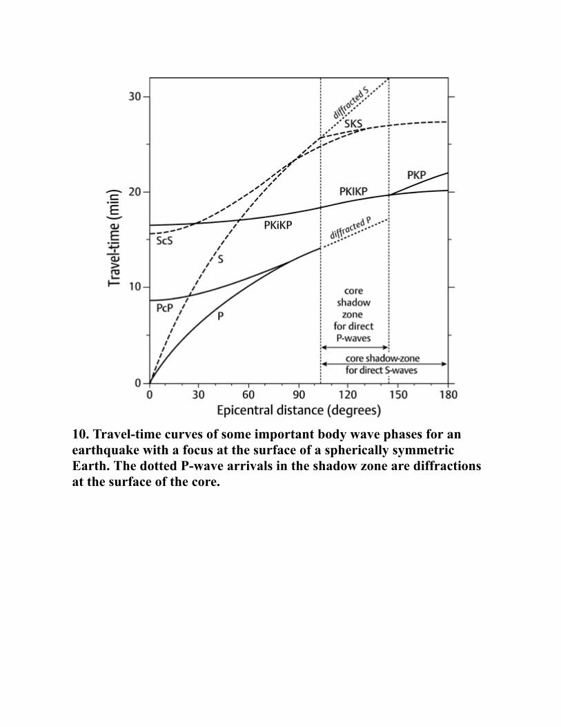
10. Travel-time curves of some important body wave phases for anearthquake with a focus at the surface of a spherically symmetricEarth. The dotted P-wave arrivals in the shadow zone are diffractionsat the surface of the core.

11. Variations of body wave velocities and density with depth in theEarth’s interior.

Internal structure of the EarthThe observation of seismic waves that passed through the Earth, togetherwith their interpreted reflection and refraction at internal boundaries,revealed the internal structure of core, mantle, and crust. In 1906 RichardOldham observed that P-waves were delayed as they traversed the Earthand inferred the existence of a central core with reduced velocity. Theexistence of the core shadow zone for P-waves was established in 1914 byBeno Gutenberg, who calculated a remarkably accurate depth of 2,900 kmfor the core–mantle boundary, now also known as the Gutenbergdiscontinuity. Gutenberg also predicted the existence of PcP and ScS waves,where the lower case ‘c’ indicates that these waves are reflected from thecore–mantle boundary (Figure 9B). These reflections were only identifiedon seismograms much later. In 1926 Harold Jeffreys deduced from the

absence of direct S-waves beyond 103 degrees that the core was fluid. In1936 a Danish seismologist, Inge Lehmann, found evidence for a solidinner core within the fluid core. With a radius of 1,217 km the inner core issmaller than the Moon.

The inner and outer core are extremely hot, with estimated temperaturesaround 4,000 K (4,273°C) and 5,500 K at the core–mantle and inner–outercore boundaries, respectively. They are believed to have similarcompositions, consisting mainly of iron and a small amount of nickel. Theenormous pressure keeps the inner core solid, but the outer core is fluid andis consequently in a state of thermal convection. Like a pan of water heatedfrom below the heated fluid becomes less dense and its buoyancy causes itto rise. The viscosity (or ‘stickiness’) of the fluid in the outer core is low,probably similar to that of water at the Earth’s surface. The iron–nickelcomponents of the outer core are constantly solidifying at the inner–outercore boundary, leaving behind lighter elements within the liquid. These risethrough the denser outer core, creating a compositional form of convectionthat supplements the thermal convection. Consequently, the outer core is ina state of turbulent motion. Seismic data from the inner core show that it isnot only solid but that it is also anisotropic, that is, the seismic velocity isdifferent in the north–south direction from in the east–west direction. Thesolid inner core is thought to have a crystalline structure and the observedanisotropy may be due to preferential alignment of the crystals.

In 1909 Andrija Mohoroviçiç, a Serbian seismologist, observed that thedirect P- and S-waves from an earthquake were overtaken by faster wavesbeyond a particular distance from the epicentre. He interpreted the fasterarrivals as waves refracted at the top of a deeper layer with higher seismicspeeds (as in Figure 8). This defines the boundary between the crust andmantle, which is now called the Mohoroviçiç discontinuity, or Moho forshort. The Moho-depth is equivalent to the crustal thickness. It averages 22km for the Earth as a whole but is very variable; oceanic crust is only 5–10km thick, whereas continental crust is 30–70 km thick and has its maximumthickness under some mountain ranges.

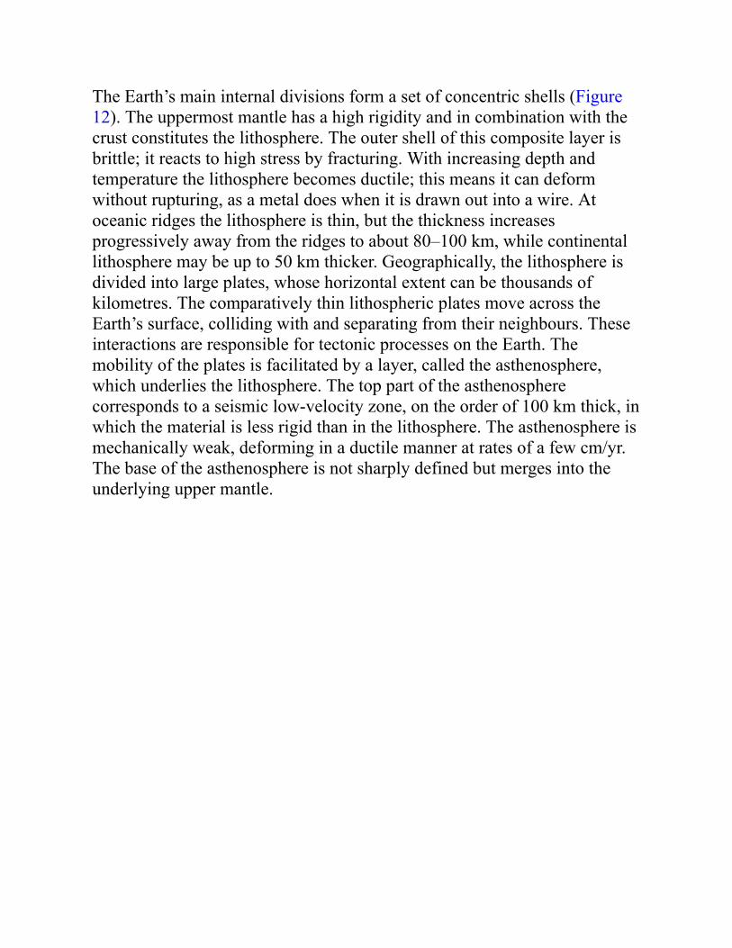
The Earth’s main internal divisions form a set of concentric shells (Figure12). The uppermost mantle has a high rigidity and in combination with thecrust constitutes the lithosphere. The outer shell of this composite layer isbrittle; it reacts to high stress by fracturing. With increasing depth andtemperature the lithosphere becomes ductile; this means it can deformwithout rupturing, as a metal does when it is drawn out into a wire. Atoceanic ridges the lithosphere is thin, but the thickness increasesprogressively away from the ridges to about 80–100 km, while continentallithosphere may be up to 50 km thicker. Geographically, the lithosphere isdivided into large plates, whose horizontal extent can be thousands ofkilometres. The comparatively thin lithospheric plates move across theEarth’s surface, colliding with and separating from their neighbours. Theseinteractions are responsible for tectonic processes on the Earth. Themobility of the plates is facilitated by a layer, called the asthenosphere,which underlies the lithosphere. The top part of the asthenospherecorresponds to a seismic low-velocity zone, on the order of 100 km thick, inwhich the material is less rigid than in the lithosphere. The asthenosphere ismechanically weak, deforming in a ductile manner at rates of a few cm/yr.The base of the asthenosphere is not sharply defined but merges into theunderlying upper mantle.

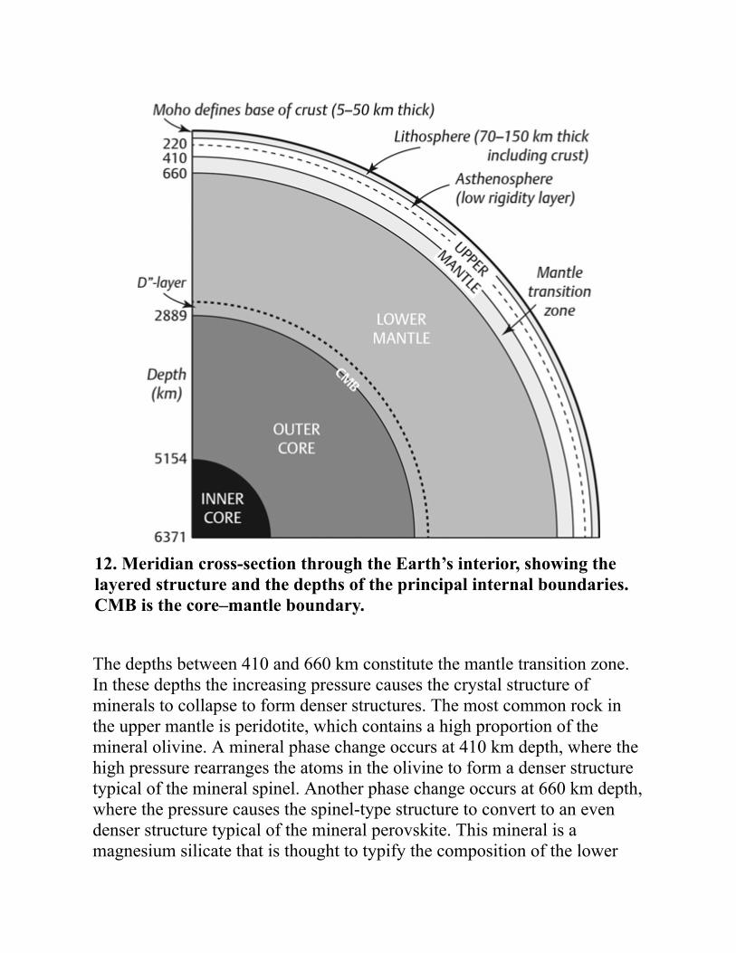
12. Meridian cross-section through the Earth’s interior, showing thelayered structure and the depths of the principal internal boundaries.CMB is the core–mantle boundary.

The depths between 410 and 660 km constitute the mantle transition zone.In these depths the increasing pressure causes the crystal structure ofminerals to collapse to form denser structures. The most common rock inthe upper mantle is peridotite, which contains a high proportion of themineral olivine. A mineral phase change occurs at 410 km depth, where thehigh pressure rearranges the atoms in the olivine to form a denser structuretypical of the mineral spinel. Another phase change occurs at 660 km depth,where the pressure causes the spinel-type structure to convert to an evendenser structure typical of the mineral perovskite. This mineral is amagnesium silicate that is thought to typify the composition of the lower

mantle. Yet another phase transition has been observed under conditionsequivalent to depths of around 2,600 km, involving a phase change fromperovskite to a mineral phase called post-perovskite. This is about the depthwhere seismic evidence indicates an anomalous 150–200 km thick layer ofthe lower mantle just above the core–mantle boundary. Labelled by historicconvention as the D″ layer, this layer is characterized by a variablethickness and variable seismic velocities. Seismic shear wave velocities areanisotropic in this layer, that is, they vary with direction. The velocities ofshear waves that vibrate in the vertical plane are a few per cent slower thanthose that vibrate horizontally, for reasons that are not fully understood.

Seismic tomographyThe travel-time curves for P- and S-waves in Figure 10 are global averages.They are based on countless arrival times, recorded by thousands ofseismographs at a worldwide distribution of seismic stations, in some casesfor decades. In reality, the internal composition and temperature are morecomplicated than in the idealized, layered Earth. The observed travel-timesof individual rays often show small deviations from those in Figure 10. Thedeviations, called travel-time residuals, may be due to local or regionalvariations in the velocity structure. The travel-time residuals are employedin seismic tomography to obtain detailed knowledge of the Earth’s internalvelocity structure. The technique is akin to the medical procedure in whichX-rays are employed to image cross-sections of the human body in greatdetail. Seismic ray paths that pass through a region in many differentdirections are processed in a tomographic analysis, requiring powerfulcomputers and sophisticated computational techniques.

Seismic tomography can be based on the travel-times of P-waves, S-waves,or surface waves. The travel-time residuals are effectively converted tovelocity differences, resulting in three-dimensional images of the velocitydistribution. This may then be interpreted in terms of variations intemperature, composition, or rigidity in the region traversed by the seismicrays, assuming that the speed of a ray does not depend on its direction. If aregion along a ray path is warmer than its surroundings, seismic velocities

may be reduced; if it is cooler, the velocities may be increased. The velocitydistribution then reflects the temperature distribution.

Velocity anomalies in the upper mantle have been related by seismictomography to important aspects of plate tectonics. For example, when theedge of a tectonic plate forms at an oceanic spreading centre, it is hot. Bythe time, millions of years later, it reaches a boundary where it convergeswith another plate it has cooled down and its density has increased. Thedenser oceanic plate is pulled by its own weight—it subducts—beneath theless dense plate, forming a subduction zone, where it sinks into the mantle.The subducting plate is colder and denser than the upper mantle into whichit is plunging. The process results in positive velocity anomalies of a fewper cent in the upper mantle. The results are usually displayed to advantagein coloured images of the tomographic sections. A simplified tomographicimage of the Tonga–Fiji subduction zone shows the cold Pacific platebending downwards into the warmer mantle (Figure 13). In this examplethe subducting plate is deflected when it encounters the 660 kmdiscontinuity, but eventually penetrates into the lower mantle.

13. Simplified P-wave tomographic section through the Tonga–Fijisubduction zone. Small circles represent earthquake foci; the darkshaded region is the subducting Pacific plate.

Structure of the continental crustSeismic refraction profiles parallel and perpendicular to the length of amountain range can be used to investigate crustal structure by determiningthe depths of refracting rock layers and the seismic velocities in theselayers. However, a more detailed picture of the subsurface is obtained fromreflection profiles. Both refraction and reflection investigations have madeimportant contributions to understanding the structure of the continentallithosphere and the depth of the crust–mantle boundary. This kind of large-scale investigation requires cooperation between many partners and inputfrom other disciplines.

In the Canadian Lithoprobe Project, refraction and reflection seismicexperiments were coordinated with geological, geochemical, and othergeophysical studies to investigate the crustal and lithospheric structureunder a 6,000 km long profile across southern Canada at 45–55° N.Extending from the Juan de Fuca active plate in the west to the passiveAtlantic margin in the east, the profile documents a complex tectonichistory in which orogenic belts have been stacked upon each other. (Anorogenic belt forms when a collision between tectonic plates deforms anoceanic or continental plate to form a mountain range.) The Lithoprobeprofile revealed a remarkably consistent Moho-depth of 30–40 km, and avariably thick lithosphere ranging from 70 km at the coastal margins to 200to 250 km in the central continent.

Seismic refraction and reflection formed the basis of the EuropeanGeotraverse Project, a similar international cooperation of earth scientistsfrom many disciplines. The purpose was to determine crustal andlithospheric structure along a north–south profile from northernScandinavia to the southern Mediterranean. This spanned several tectonicprovinces from the ancient Precambrian Scandinavian shield to currentlyactive collision areas in the Mediterranean. The project contributed tounderstanding how the crustal structure across Europe has evolved, andhow it continues to do so.

Seismic noiseThe high sensitivity of seismometers enables them to detect continuoussmall ground motions, known as microseisms, that are not caused byearthquakes. After the arrival of P- and S-waves from an active source orearthquake the ground continues to vibrate. This is the result of multiplereflections and diffractions in the inhomogeneous crust, which have theeffect of adding noise to the signal. The seismic noise on a seismogram iscomposed of many frequencies because it has many causes. It has long beenknown that the interaction of ocean waves on a coastline is one of thecauses. Among the other sources are environmental features such as slow-moving landslides or the motion of material in glaciers and rivers, tectonic

effects that produce cracking in rocks, and human activity related tourbanization or exploitation of resources.

Seismologists have learned how to use the noise as a passive seismic sourcethat provides a continuous record at a seismometer. If it is recorded for along enough time, seismic noise can be assumed to reach the seismometerequally from all directions and can be analysed for information aboutcrustal and upper mantle structure. This is achieved by comparing seismicrecordings from pairs of seismographs using cross-correlation—a statisticaltechnique in which one record is digitally moved past the other to locatesections of the records that are similar. The combined signals of the tworecords cancel each other except where they have travelled along a commonpath, which is the path that joins the recording stations. Each station thussees the other as an apparent seismic source. The output of the cross-correlation has the characteristics of a Rayleigh surface wave that travelledbetween the stations, and can be analysed to obtain information about thevelocity–depth structure in the crust and upper mantle beneath the stations.With long records from a large number of stations, seismic noise analysisgives enough data to produce a seismic tomographic image of subsurfacestructure. The continuous nature of seismic noise makes it a viable tool forlong-term monitoring of time-dependent environmental changes in a widevariety of situations, such as monitoring slopes endangered by landslides, orrecording the motion of glaciers.

The analysis of seismic noise on the Moon is an intriguing example of thispassive method. In 1972 the US Apollo 17 mission installed fourseismometers on the Moon’s surface, forming a triangular array with sidesapproximately 100 m in length. The network operated until 1977. Cross-correlation of seismic noise recorded continuously at pairs of seismometersfor thirty-six weeks in 1976 and 1977 revealed a signal with thecharacteristics of a Rayleigh surface wave. Analysis of the Rayleigh waveyielded an estimate of the near-surface variation of shear wave velocitywith depth and provided new information on the thickness of the lunarregolith (i.e. the layer of loose material covering the surface). Moreover, thesignal-to-noise ratio of the derived Rayleigh wave varied with a period of29.5 days, equivalent to the length of the lunar day. The rhythmic variationwas attributed to solar heating, which causes the surface temperature to

range from –170°C to +110°C. The high temperature gradient results incracking and generates the Rayleigh wave.

Chapter 4Seismicity—the restless Earth

EarthquakesWe were almost asleep when we felt a sudden jolt, closely followed by adull rumble lasting a few seconds, as if a heavy truck had passed by ourhotel. We sat up, wide awake, and my wife exclaimed, ‘That was anearthquake!’ How could it be? After all, we were not in California, whereseismic events are common, but in a small village near Birmingham incentral England. Yet it was indeed a small earthquake of magnitude 4.7, andit happened about 30 km away at a depth of 14 km. It was unusual, but not arare event.

Hundreds of thousands of earthquakes occur worldwide each year. Most ofthem are not noticed by people, because their effects are so weak that onlysensitive instruments record them, or they occur well away from populationcentres. However, some of the tremors are large enough to cause damage,and a few are very destructive. No place on the Earth can be assumed to becompletely earthquake-free, but most earthquakes happen in well-defined,relatively narrow seismic zones. More than 90 per cent of earthquakes havea tectonic origin. That is, they happen on faults, which are planes on whicha volume of solid rock has fractured and blocks of rock on opposite sides ofthe fault have moved relative to each other; the fracture surface is called the

fault plane. Faulting may occur on more than a single surface, in which casethe term fault zone is used.

The elastic rebound model, formulated in 1906 following the San Franciscoearthquake, explains how an earthquake occurs (Figure 14). An elasticmaterial is one that reacts to a force by deforming in such a way that itrecovers its original shape when the force is removed. However, just as foran over-stretched spring, when the force becomes too large, the elastic limitof the material is reached and the material breaks irreversibly. Although it isbased on observations of the San Andreas Fault in California, the elasticrebound model is applicable to earthquakes on other faults. Tectonic forcesslowly produce strain in the rocks on opposite sides of the fault at a rate of afew centimetres per year, except on the fault plane itself, where the rocksare locked in contact with each other (Figure 14A). This slow accumulationof strain may continue for many years, even for hundreds or thousands ofyears, until, at a particular place on the fault, the rocks reach their elasticlimit and break, rebounding as a released spring does. The pent-up elasticstrain energy is then set free suddenly and violently as an earthquake(Figure 14B). Its energy propagates at speeds of several kilometres persecond away from the point of rupture, which is called the focus of theearthquake.

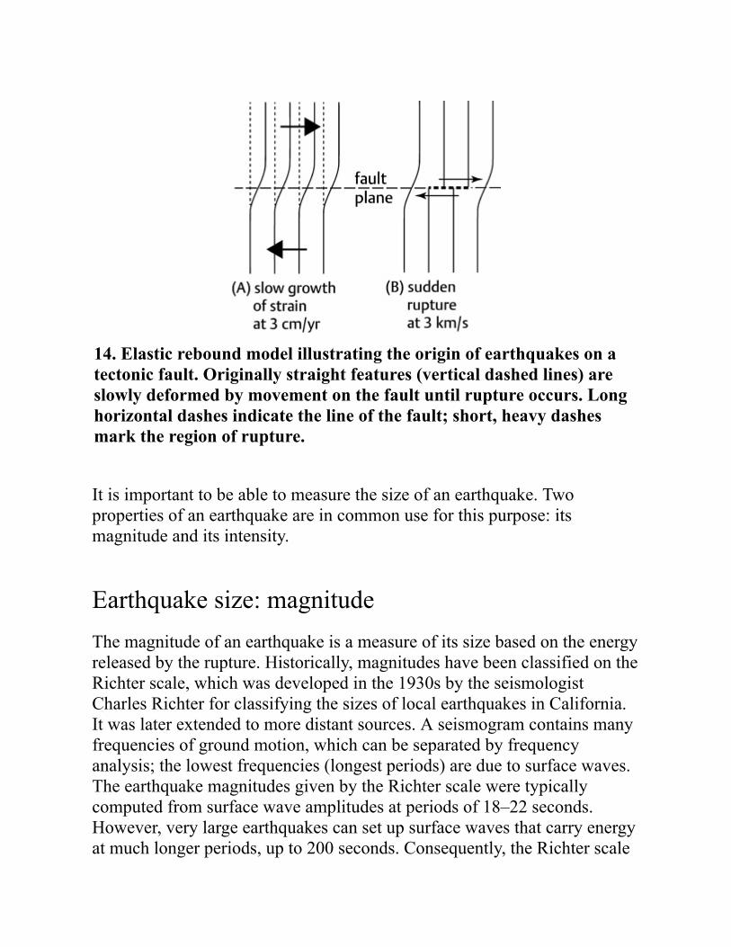
14. Elastic rebound model illustrating the origin of earthquakes on atectonic fault. Originally straight features (vertical dashed lines) areslowly deformed by movement on the fault until rupture occurs. Longhorizontal dashes indicate the line of the fault; short, heavy dashesmark the region of rupture.

It is important to be able to measure the size of an earthquake. Twoproperties of an earthquake are in common use for this purpose: itsmagnitude and its intensity.

Earthquake size: magnitudeThe magnitude of an earthquake is a measure of its size based on the energyreleased by the rupture. Historically, magnitudes have been classified on theRichter scale, which was developed in the 1930s by the seismologistCharles Richter for classifying the sizes of local earthquakes in California.It was later extended to more distant sources. A seismogram contains manyfrequencies of ground motion, which can be separated by frequencyanalysis; the lowest frequencies (longest periods) are due to surface waves.The earthquake magnitudes given by the Richter scale were typicallycomputed from surface wave amplitudes at periods of 18–22 seconds.However, very large earthquakes can set up surface waves that carry energyat much longer periods, up to 200 seconds. Consequently, the Richter scale

underestimates the size of very large earthquakes with magnitudes greaterthan about 8.5.

Although treated as a point source, the focus is in reality a ruptured area ona fault plane. Three quantities determine the size of the earthquake: the areaof the ruptured section of the fault, the average amount by which it slipped,and the elastic shear modulus of the rocks that ruptured. When these threequantities are multiplied together, the product is called the seismic momentof the earthquake. Fast, modern computers make it possible to analyse thecomplete waveform content of a seismogram and to calculate the seismicmoment from the long period vibrations. The seismic moment is a propertyof the source, and seismologists consider it to be the best measure ofearthquake size. It is related to the energy of the earthquake and is used todefine a ‘moment magnitude’. This parameter does not saturate for largeevents and extends the Richter scale to include strong earthquakes. Thesurface wave magnitude is still used for describing the sizes of small tomoderate earthquakes.

At large distances from an earthquake the amplitudes of P-waves withperiods around 1 second can be used in a similar way to surface waves todefine a body wave magnitude (m

b) for the size of an earthquake. This

method has the disadvantage that it saturates for mb larger than 6, but it is

useful for first estimates of the size of distant earthquakes, and also fordiscriminating between earthquakes and nuclear tests.

Magnitude scales allow estimates of the amount of energy released in anearthquake. For example, a magnitude 6 earthquake releases about as muchenergy as 15,000 tonnes of TNT, equivalent to the atomic bomb thatdevastated Hiroshima. In order to handle the wide range of energiesreleased in earthquakes the magnitude scale is logarithmic. As a result, anincrease from one size to the next on the magnitude scale involves a tenfoldincrease in amplitude and a 32-fold increase in the amount of energyreleased. Consequently, a difference of 2 in magnitude corresponds to adifference in energy of 322 or about 1,000 times. For example, the SanFrancisco earthquake in 1906 had a magnitude of 7.9; by comparison, the

largest ever recorded earthquake (in Chile in 1960) had a magnitude of 9.5and released about 250 times more energy.

The number of earthquakes that occur globally each year falls off withincreasing magnitude. Approximately 1.4 million earthquakes annuallyhave magnitude 2 or larger; of these about 1,500 have magnitude 5 orlarger. The number of very damaging earthquakes with magnitude above 7varies from year to year but has averaged about 15–20 annually since 1900.On average, one earthquake per year has magnitude 8 or greater, althoughsuch large events occur at irregular intervals. A magnitude 9 earthquakemay release more energy than the cumulative energy of all otherearthquakes in the same year.

Earthquake size: intensityThe intensity is a qualitative measure of the size of an earthquake based onobserved effects, such as the damage it causes. This depends on localconditions such as the ground stability and the robustness of structures. Agiven earthquake results in different intensities at different places,depending on the distance from the epicentre and the environment of theobserver. Volunteer observers report their observations to a coordinatingseismic observatory, where analysts collate them to rank the size of theevent that was felt at the location of each observer. A numerical value forthe intensity is obtained by comparison with standardized observations on atwelve-part intensity scale, which takes into account the effects of anearthquake on people and buildings, and the degree of damage observed. InNorth America the Modified Mercalli Intensity Scale is used, named afterGiuseppe Mercalli, an early pioneer of the method. The EuropeanMacroseismic Scale (EMS-98, Table 2) is used in Europe, but the scales arevery similar. An Environmental Seismic Intensity Scale (ESI-2007) hasbeen developed to assess intensities of very large earthquakes inuninhabited regions, using environmental effects resulting from theearthquake. Each method enables the estimation of intensity for anearthquake that occurs at the present time and can be applied to past eventsthat are described in old documents and archives, thus providing a means ofassessing the historical seismicity of a region. The estimated intensities can

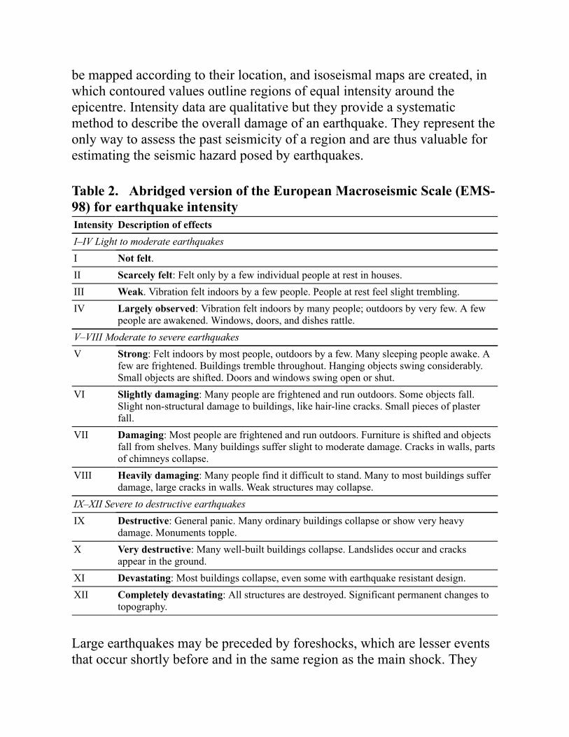
be mapped according to their location, and isoseismal maps are created, inwhich contoured values outline regions of equal intensity around theepicentre. Intensity data are qualitative but they provide a systematicmethod to describe the overall damage of an earthquake. They represent theonly way to assess the past seismicity of a region and are thus valuable forestimating the seismic hazard posed by earthquakes.

Table 2. Abridged version of the European Macroseismic Scale (EMS-98) for earthquake intensityIntensity Description of effectsI–IV Light to moderate earthquakesI Not felt.II Scarcely felt: Felt only by a few individual people at rest in houses.III Weak. Vibration felt indoors by a few people. People at rest feel slight trembling.IV Largely observed: Vibration felt indoors by many people; outdoors by very few. A few

people are awakened. Windows, doors, and dishes rattle.V–VIII Moderate to severe earthquakesV Strong: Felt indoors by most people, outdoors by a few. Many sleeping people awake. A

few are frightened. Buildings tremble throughout. Hanging objects swing considerably.Small objects are shifted. Doors and windows swing open or shut.

VI Slightly damaging: Many people are frightened and run outdoors. Some objects fall.Slight non-structural damage to buildings, like hair-line cracks. Small pieces of plasterfall.

VII Damaging: Most people are frightened and run outdoors. Furniture is shifted and objectsfall from shelves. Many buildings suffer slight to moderate damage. Cracks in walls, partsof chimneys collapse.

VIII Heavily damaging: Many people find it difficult to stand. Many to most buildings sufferdamage, large cracks in walls. Weak structures may collapse.

IX–XII Severe to destructive earthquakesIX Destructive: General panic. Many ordinary buildings collapse or show very heavy

damage. Monuments topple.X Very destructive: Many well-built buildings collapse. Landslides occur and cracks

appear in the ground.XI Devastating: Most buildings collapse, even some with earthquake resistant design.XII Completely devastating: All structures are destroyed. Significant permanent changes to

topography.

Large earthquakes may be preceded by foreshocks, which are lesser eventsthat occur shortly before and in the same region as the main shock. They

indicate the build-up of stress that leads to the main rupture. Largeearthquakes are also followed by smaller aftershocks on the same fault ornear to it; their frequency decreases as time passes, following the mainshock. Aftershocks may individually be large enough to have seriousconsequences for a damaged region, because they can cause alreadyweakened structures to collapse.

Secondary effects of earthquakesThe primary effects of a large earthquake are the result of violent shakingbut secondary effects can be equally devastating. The shaking of the SanFrancisco earthquake in 1906 caused severe damage to structures but it alsobroke water and gas lines. Consequently, when fire broke out, it could notbe brought under control and much of the city burned down. In 1970 amagnitude 7.9 earthquake off the coast of Peru caused extensive directdamage, but it also set off an ice and rock avalanche in the Andes above thetown of Yungay. The ice is thought to have melted to form a lubricatingcushion under the rock mass, which descended at a speed of around 300km/hr on the town and buried it, killing 70,000 people.

An oceanic earthquake with magnitude larger than 7.5 may thrust the entireoverlying water column upwards (or downwards) and trigger the seismicwater wave known as a tsunami. This differs from ordinary waves on thesurface of a lake, sea, or ocean, which are set up by wind action and affectonly the top few metres of water. By contrast, the entire ocean depth isinvolved in a tsunami, which travels away from the source at a speed equalto the square root of the product of gravity (9.8 m/s2) and the water depth.Over the open ocean, which on average is 3,700 metres deep, the tsunamitherefore travels at speeds of around 190 m/s, or 700 km/h, the speed of acommercial jet, but the small height of the wave (only a few tens ofcentimetres) makes it hard to detect. However, when it approachesshallower depths the front of the wave slows down relative to the followingwater-mass. This causes the tsunami to increase in height as it rushesonshore.

The Sumatra–Andaman earthquake in 2004 had a magnitude of 9.1–9.3 andwas thus one of the largest ever recorded. It caused enormous directdevastation and also created the most damaging tsunami in recorded history.About 230,000 people died in this disaster, many of them killed far from theepicentre by the tsunami. The earthquake occurred at a relatively shallowdepth of 30 km, on the boundary between the India–Australia plate and theBurma and Sunda portions of the Eurasian plate. A segment of faultmeasuring around 1,200 km in length slipped by up to 10–15 metres. Theinitial displacement resulted in a sudden uplift of the ocean bottom byseveral metres and created a tsunami. It had an amplitude of only 60 cmover the open ocean (observed by satellite) but the wave height reached upto 30 m when it came ashore. Many lives were lost to the Sumatra tsunamiin Sri Lanka and India; two people were drowned in Port Elizabeth, SouthAfrica, 8,000 km away from the source. In a similar disaster, a tsunamifrom the 2011 Tohoku earthquake overwhelmed the coastal protectivedefences in Japan, destroyed communities, and damaged the Fukushimanuclear plant. About 90 per cent of the world’s earthquakes and 75 per centof its volcanoes occur in the circum-Pacific belt known as the ‘Ring ofFire’. Tsunamis occur often enough in this belt for an early warning systemto have been set up around the Pacific Ocean, but such a system did notexist for the Indian Ocean at the time of the Sumatra earthquake.

Epicentre location and global seismicityThe further a seismic station is from the epicentre of an earthquake, thelonger is the travel-time of a seismic wave. A plot of the travel-time of a P-wave against the distance from the epicentre is a curved line; a similarcurved line is found for the slower S-waves. With increasing epicentraldistance the separation of the P-wave and S-wave travel-time curvesincreases (Figure 10). If the difference between the P-wave and S-wavearrival times for a shallow local earthquake is plotted against the time-axis astraight line is obtained. Its intercept with the time-axis gives the time whenthe earthquake occurred. Seismic velocities vary with depth in the Earth andthus vary along the path travelled by the waves. The velocity–depth profilesare well known, and so the time difference between the P- and S-wavearrivals can be used to compute the distance from the epicentre to the

seismic station. The epicentre must lie on a circle centred on the recordingstation and with radius equal to the epicentral distance. Applying this logicto each of the seismic stations that register the earthquake gives a family ofintersecting circles. The epicentre lies at their common intersection point.Often the circles do not intersect exactly at a point but define a smallpolygon; its geometric centre is taken to be the epicentre, or this can becalculated by more detailed processing. The polygon originates becauseseismic waves travel to the seismograph from the focus and not from theepicentre.

In practice, the inhomogeneity and ellipsoidal shape of the Earth make theprocedure more complicated. After an initial estimate of the earthquakelocation, the travel-times from it to the seismic stations are computed andcompared with the measured times. The earthquake location is thenadjusted and the calculations are repeated; the process is repeated until thediscrepancies in travel-times are minimized. The method is called forwardmodelling; it is an important technique for matching a geological modelwith measured data.

The worldwide picture of seismicity is based on the localization of theepicentres and the focal depths of tens of thousands of earthquakes thathave been catalogued. The global distribution is not uniform (Figure 15).Most epicentres lie in rather narrow zones, some of which are alsocharacterized by active volcanoes. A zone of shallow earthquakesdelineates the oceanic ridges formed by submarine mountain chains. Amore diffuse belt extends through the Mediterranean, the Middle East, andHimalaya, and into northern China. The most seismically active parts of theEarth form a prominent belt around the margins of the Pacific Ocean,adjoined by a zone bounding southern Asia. Both shallow and deepearthquakes characterize this seismic belt; in some places the depthdistribution of earthquakes extends down into the mantle for up to severalhundred kilometres. The seismologists Kiyoo Wadati and Hugo Benioffnoted independently that if the earthquakes around the Pacific are plotted ona cross-section normal to the continental margin they define a seismic zonetens of kilometres thick, dipping at an angle of 30–60 degrees and reachingdepths of up to 700 km. Initially, the seismic zone was interpreted asevidence for motion on a ‘great fault’ that dipped below the overriding

plate. Subsequently, seismologists found that the observed earthquakesoccur as a result of stresses within an inclined slab of lithosphere thatsubducts—i.e. is pulled down—into the upper mantle in subduction zones.

15. Distribution of the epicentres of 157,991 earthquakes in the years1960–2013. The seismicity marks the margins of global tectonic plates.Epicentres located by the International Seismological Centre (ISC)using the EHB algorithm.

The worldwide distribution of earthquakes defines the boundaries of thelithospheric plates (Figure 16). In the late 1960s the seismicity patterndelineated the major plates—Pacific, North and South America, Nazca,Eurasia, Africa, Australia–India, and Antarctica—and a few minor platessuch as the Caribbean, Cocos, Juan de Fuca, Scotia, and Philippines plates.Subsequently, many smaller plates have been defined, as well as regions ofdiffuse seismicity that may be incipient plate boundaries. The East Africanrift zone is a series of rift valleys, thousands of kilometres long,characterized by seismicity and active and dormant volcanoes. Along itslength the original African plate is splitting at 6–7 mm/yr into a westernNubia plate and an eastern Somalia plate. Less clearly, analysis of global

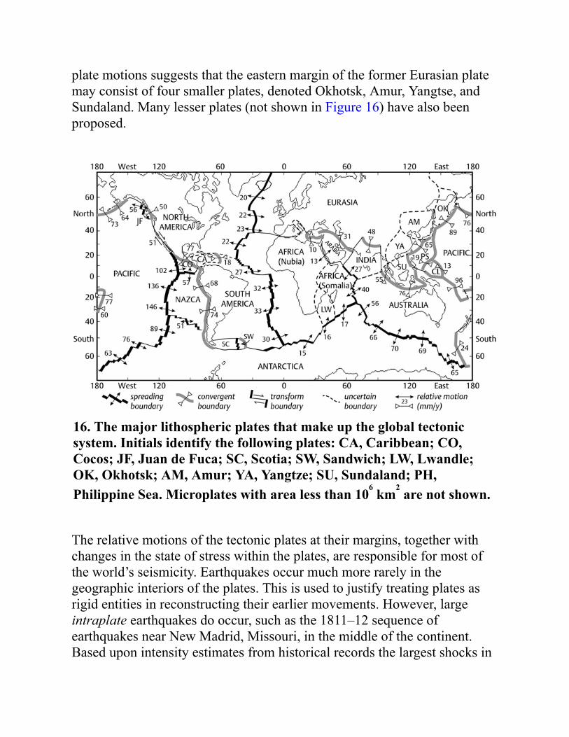
plate motions suggests that the eastern margin of the former Eurasian platemay consist of four smaller plates, denoted Okhotsk, Amur, Yangtse, andSundaland. Many lesser plates (not shown in Figure 16) have also beenproposed.

16. The major lithospheric plates that make up the global tectonicsystem. Initials identify the following plates: CA, Caribbean; CO,Cocos; JF, Juan de Fuca; SC, Scotia; SW, Sandwich; LW, Lwandle;OK, Okhotsk; AM, Amur; YA, Yangtze; SU, Sundaland; PH,Philippine Sea. Microplates with area less than 106 km2 are not shown.

The relative motions of the tectonic plates at their margins, together withchanges in the state of stress within the plates, are responsible for most ofthe world’s seismicity. Earthquakes occur much more rarely in thegeographic interiors of the plates. This is used to justify treating plates asrigid entities in reconstructing their earlier movements. However, largeintraplate earthquakes do occur, such as the 1811–12 sequence ofearthquakes near New Madrid, Missouri, in the middle of the continent.Based upon intensity estimates from historical records the largest shocks in

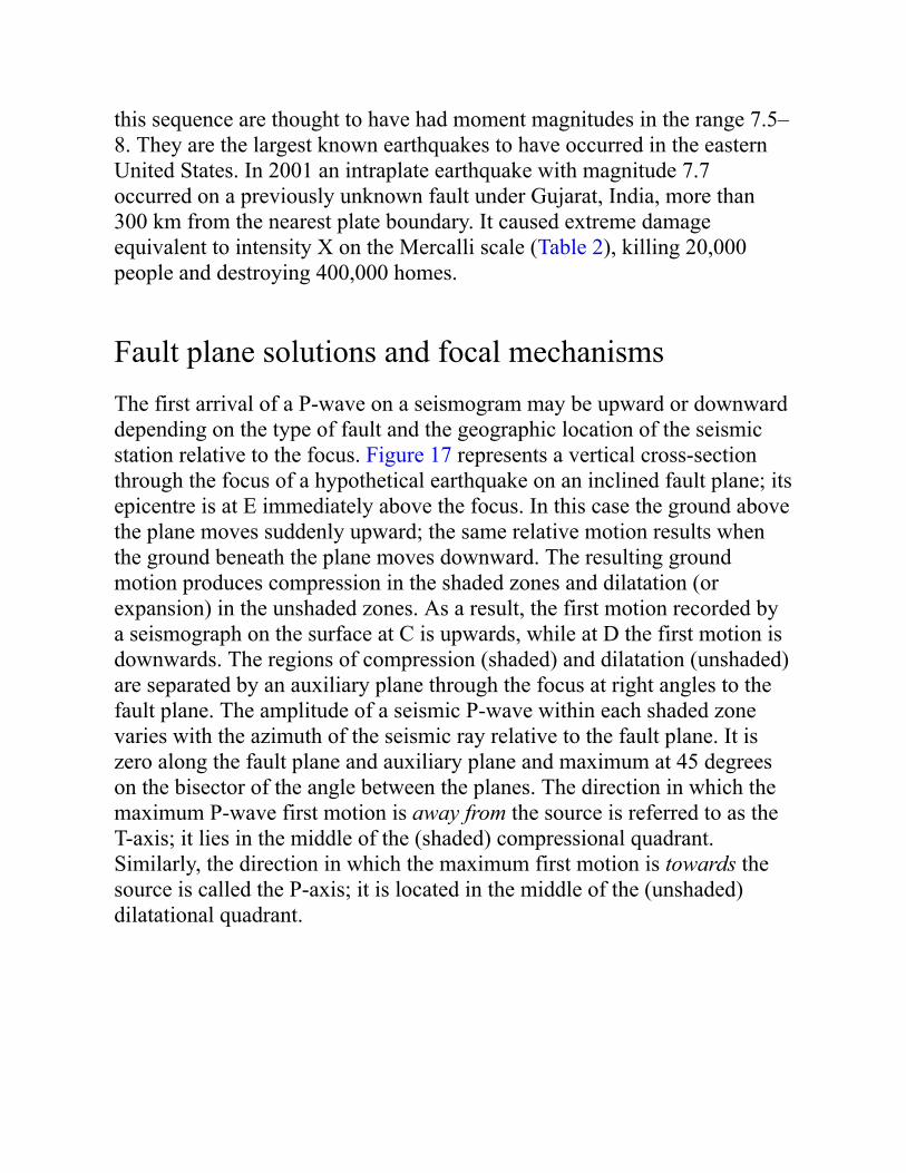
this sequence are thought to have had moment magnitudes in the range 7.5–8. They are the largest known earthquakes to have occurred in the easternUnited States. In 2001 an intraplate earthquake with magnitude 7.7occurred on a previously unknown fault under Gujarat, India, more than300 km from the nearest plate boundary. It caused extreme damageequivalent to intensity X on the Mercalli scale (Table 2), killing 20,000people and destroying 400,000 homes.

Fault plane solutions and focal mechanismsThe first arrival of a P-wave on a seismogram may be upward or downwarddepending on the type of fault and the geographic location of the seismicstation relative to the focus. Figure 17 represents a vertical cross-sectionthrough the focus of a hypothetical earthquake on an inclined fault plane; itsepicentre is at E immediately above the focus. In this case the ground abovethe plane moves suddenly upward; the same relative motion results whenthe ground beneath the plane moves downward. The resulting groundmotion produces compression in the shaded zones and dilatation (orexpansion) in the unshaded zones. As a result, the first motion recorded bya seismograph on the surface at C is upwards, while at D the first motion isdownwards. The regions of compression (shaded) and dilatation (unshaded)are separated by an auxiliary plane through the focus at right angles to thefault plane. The amplitude of a seismic P-wave within each shaded zonevaries with the azimuth of the seismic ray relative to the fault plane. It iszero along the fault plane and auxiliary plane and maximum at 45 degreeson the bisector of the angle between the planes. The direction in which themaximum P-wave first motion is away from the source is referred to as theT-axis; it lies in the middle of the (shaded) compressional quadrant.Similarly, the direction in which the maximum first motion is towards thesource is called the P-axis; it is located in the middle of the (unshaded)dilatational quadrant.

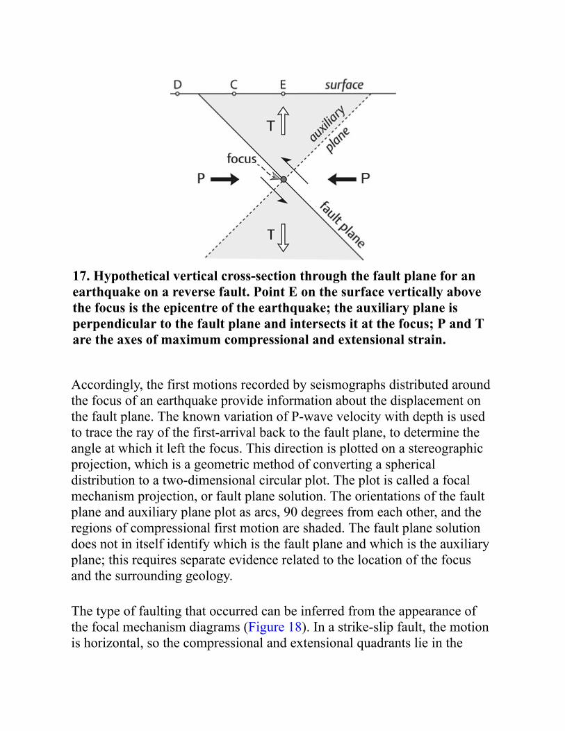
17. Hypothetical vertical cross-section through the fault plane for anearthquake on a reverse fault. Point E on the surface vertically abovethe focus is the epicentre of the earthquake; the auxiliary plane isperpendicular to the fault plane and intersects it at the focus; P and Tare the axes of maximum compressional and extensional strain.

Accordingly, the first motions recorded by seismographs distributed aroundthe focus of an earthquake provide information about the displacement onthe fault plane. The known variation of P-wave velocity with depth is usedto trace the ray of the first-arrival back to the fault plane, to determine theangle at which it left the focus. This direction is plotted on a stereographicprojection, which is a geometric method of converting a sphericaldistribution to a two-dimensional circular plot. The plot is called a focalmechanism projection, or fault plane solution. The orientations of the faultplane and auxiliary plane plot as arcs, 90 degrees from each other, and theregions of compressional first motion are shaded. The fault plane solutiondoes not in itself identify which is the fault plane and which is the auxiliaryplane; this requires separate evidence related to the location of the focusand the surrounding geology.

The type of faulting that occurred can be inferred from the appearance ofthe focal mechanism diagrams (Figure 18). In a strike-slip fault, the motionis horizontal, so the compressional and extensional quadrants lie in the

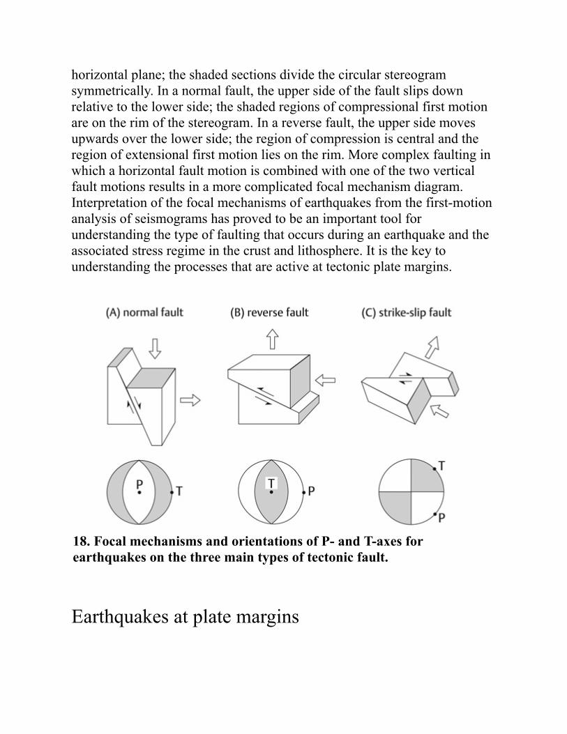
horizontal plane; the shaded sections divide the circular stereogramsymmetrically. In a normal fault, the upper side of the fault slips downrelative to the lower side; the shaded regions of compressional first motionare on the rim of the stereogram. In a reverse fault, the upper side movesupwards over the lower side; the region of compression is central and theregion of extensional first motion lies on the rim. More complex faulting inwhich a horizontal fault motion is combined with one of the two verticalfault motions results in a more complicated focal mechanism diagram.Interpretation of the focal mechanisms of earthquakes from the first-motionanalysis of seismograms has proved to be an important tool forunderstanding the type of faulting that occurs during an earthquake and theassociated stress regime in the crust and lithosphere. It is the key tounderstanding the processes that are active at tectonic plate margins.

18. Focal mechanisms and orientations of P- and T-axes forearthquakes on the three main types of tectonic fault.

Earthquakes at plate margins

An example of fault plane solutions on the mid-Atlantic ridge in the CentralAtlantic is shown in Figure 19. The first-motion patterns show thatearthquakes on the ridge axis result from normal faulting, with horizontal T-axes perpendicular to the strike of the ridge. This indicates that tectonicforces are pulling the crust apart at the ridge. Magma from deep in themantle rises to the surface here, uplifting the oceanic crust to form the ridgeand in the process stretching and cracking it. The magma solidifies andbuilds a continuously renewed edge to the lithospheric plate on either sideof the spreading ridge. The ridge process is called sea-floor spreading andthe plate margin is called a divergent, or constructive, plate boundary.

19. Fault plane solutions for earthquakes on the mid-Atlantic ridgeand on the Gibbs, Vema, and Romanche transform faults. Arrowsshow directions of relative motion with the rates of plate separation inmm/yr.

Through the Mediterranean and Himalayan regions, and around the PacificOcean, the seismicity is related to the presence of mountain belts, deepoceanic trenches, and island arcs. The depth distribution and fault planesolutions of earthquakes indicate that a different tectonic process is activehere from at an ocean ridge. A trench marks the place where an oceanicplate is being pulled by its own weight under a less dense adjacent plate.The subduction process forms a convergent, or destructive, plate boundary.This can happen when the adjacent plate consists of continental lithosphereor younger oceanic lithosphere. Earthquake focal mechanisms show thestate of stress in the subducting plate.

When an oceanic plate subducts, it is forced to bend downward in order toplunge under the less dense adjacent plate, forming a deep-sea trench.These long, narrow features are the deepest regions of the oceans, in placesmore than 10 km deep. Focal mechanisms in the shallow part of thesubducting plate are of the normal fault type (Figure 18A), indicating thatthe upper surface of the plate is being stretched. The bending causeshorizontal compression under this part of the plate, resulting in earthquakeswith a reverse fault mechanism. At the interface between the subductingand overriding plates, a large reverse (or thrust) fault can form (Figure18B); due to its extreme size it is called a megathrust. All historicearthquakes with magnitude greater than 9 have occurred on megathrusts atsubduction zones.

The subducting lithosphere is colder and denser than the underlyingasthenosphere and sinks into it. At greater depths the mantle is more rigidthan the descending slab and resists its motion, causing a state ofcompression within the slab, which is evident in the focal mechanisms ofintermediate and deep earthquakes.

In addition to divergent and convergent plate boundaries, there is a thirdboundary type at which the tectonic plates are neither created nor destroyed,but move past each other. This conservative type of boundary joins twosegments of a converging or diverging boundary. In 1965 the Canadiangeologist John Tuzo Wilson recognized this boundary as a new class offaults related to plate tectonics, and called it a transform fault. Transform

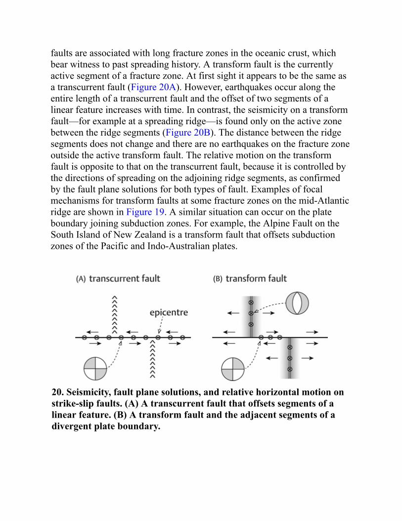
faults are associated with long fracture zones in the oceanic crust, whichbear witness to past spreading history. A transform fault is the currentlyactive segment of a fracture zone. At first sight it appears to be the same asa transcurrent fault (Figure 20A). However, earthquakes occur along theentire length of a transcurrent fault and the offset of two segments of alinear feature increases with time. In contrast, the seismicity on a transformfault—for example at a spreading ridge—is found only on the active zonebetween the ridge segments (Figure 20B). The distance between the ridgesegments does not change and there are no earthquakes on the fracture zoneoutside the active transform fault. The relative motion on the transformfault is opposite to that on the transcurrent fault, because it is controlled bythe directions of spreading on the adjoining ridge segments, as confirmedby the fault plane solutions for both types of fault. Examples of focalmechanisms for transform faults at some fracture zones on the mid-Atlanticridge are shown in Figure 19. A similar situation can occur on the plateboundary joining subduction zones. For example, the Alpine Fault on theSouth Island of New Zealand is a transform fault that offsets subductionzones of the Pacific and Indo-Australian plates.

20. Seismicity, fault plane solutions, and relative horizontal motion onstrike-slip faults. (A) A transcurrent fault that offsets segments of alinear feature. (B) A transform fault and the adjacent segments of adivergent plate boundary.

The displacement of a tectonic plate on the Earth’s spherical surface isequivalent geometrically to rotating the plate about an axis that passesthrough the centre of the sphere. Transform faults and their related fracturezones play an important role in plate tectonics, because they can be used tolocate the pole of relative rotation of two adjoining plates, known as theirEuler pole. Geometrically, the radius of a circle is perpendicular to itscircumference and all the radii of a given circle intersect at its centre.Similarly, great circles (meridians) drawn perpendicular to the transformfaults on a spreading ridge intersect at the Euler pole of relative rotation ofthe adjoining plates. Thus the motions of lithospheric plates on the surfaceof the spherical Earth can be modelled by rotations about Euler poles.Important boundary conditions are placed on the rotations by triplejunctions, which are places where three plate boundaries meet. The threetypes of plate boundary—ridge, trench, and transform fault—can combineto give a large number of possible triple junctions, only a few of whichmaintain their geometry as the adjoining plates move. An example of astable triple junction is where the Eurasian, African, and North Americanplates meet at the Azores in the North Atlantic.

Earthquake monitoring and predictionIn 1996 the Comprehensive Test-Ban Treaty was adopted by a majority ofmembers of the United Nations; a minority of members have not signed orratified it. Earthquake seismologists play an important role in monitoringcompliance with the treaty. A global network of seismic stations recordsevery ground-shaking event. The different characteristics of earthquakesand explosions allow discrimination between them. The source depthprovides an initial clue. Earthquakes may have focal depths of tens tohundreds of kilometres; nuclear tests, even in the deepest drill-holes, occurnear to the Earth’s surface. Secondly, the first motions from an earthquakeexhibit a ‘beach ball’ pattern characteristic of the type of faulting (Figure18), whereas the first motions resulting from an explosion are all upward onseismograms in every direction around the source. Thirdly, when a P-wavefrom an explosion impacts the free surface or an internal discontinuity itcan generate shear waves (Figure 7), which are eventually recorded as S-waves and surface waves. However, the ratio of the energy carried by short-

period (1 s) P-waves to that carried by longer period (20 s) surface waves—i.e. the ratio of body wave magnitude m

b to surface wave magnitude M

s—is

larger for explosions than for earthquakes.

In recent years seismologists have discovered that motion on tectonic faultsdoes not always result in a destructive earthquake. A new class of ‘slowearthquakes’ has been discovered. They result from slow slip on a fault, butthe accumulated elastic energy is released slowly instead of abruptly as inan ordinary ‘fast’ earthquake. The causes of ‘slow earthquakes’ are not yetunderstood.

Earthquakes are a serious hazard for populations, their property, and thenatural environment. Great effort has been invested in the effort to predicttheir occurrence, but as yet without general success. Qualitativeobservations of abnormal animal behaviour and unusual natural phenomenahave been interpreted as indicators of impending earthquakes, especially inChina, where many regions have a high seismic hazard. However, theseprecursors cannot be rigorously evaluated and are not useful for prediction.A successful prediction requires estimating reliably where and when anearthquake will occur, and what its size is likely to be. The problem is bothscientific and political: the responsible authorities must know fairlyprecisely when to evacuate an endangered community, because of thelogistical difficulties and huge expense entailed.

Scientists have made more progress in assessing the possible location of anearthquake than in predicting the time of its occurrence. Although adamaging event can occur wherever local stress in the crust exceeds thebreaking point of underlying rocks, the active seismic belts where this ismost likely to happen are narrow and well defined (Figure 15).Unfortunately many densely populated regions and great cities are locatedin some of the seismically most active regions. The seismic belts are notcontinuously active and contain gaps where earthquakes have not happenedfor some time. According to seismic gap theory, these quiet segments of afault are the most likely locations of future earthquakes. However, this viewis not universally accepted by seismologists, because statistical evaluationsof the occurrences of earthquakes do not support it.

The slow build-up of tectonic stress on a fault cannot be prevented, but itcan be observed and monitored. Sensitive laser-ranging techniques candetect the slow horizontal creep of one side of a fault relative to the other.Satellite geodesy is milestone num="68" unit="page" id="actrade-9780198792956-chapter-4-milestone-68" />able to observe motions ondangerous active faults from space. Seismic networks can monitor smallearthquakes in order to identify foreshocks and spot any increase in theirfrequency or magnitude. Despite these scientific and technical advances, itis not yet possible to forecast reliably where or when an earthquake willoccur, or how large it is likely to be.

Chapter 5Gravity and the figure of the Earth

Gravitation, the Earth’s shape, and gravityAbout 2,500 years ago Pythagoras speculated that the Earth was not flat, aspreviously believed, but was a sphere. In 240 BC the Greek scholarEratosthenes estimated the circumference of the sphere by measuring thedistance between two places in Egypt where he knew the angle of elevationof the Sun at summer solstice. In 1671 a French astronomer measuredaccurately the length of a degree of latitude and estimated the Earth’s radiusto be 6,372 km; a modern value is 6,371 km! Isaac Newton theorizedcorrectly that the Earth’s rotation would cause the sphere to be flattened atthe rotation poles, and predicted that the flattening would amount to about0.4 per cent. Eighteenth-century geodetic measurements by Frenchscientists showed that the length of a degree of latitude was shorter near theequator than near the poles, which is what one would observe on a flattenedsphere; the estimated flattening was about 0.3 per cent, somewhat less thanNewton’s prediction. The slight deviation of the Earth’s shape—or figure—from a sphere is indeed caused by the planet’s rotation and is a veryimportant property. It influences not only the value of gravity anywhere onthe Earth, but also how the planet’s rotation reacts to the gravitationalattraction of extraterrestrial bodies.

When Newton’s law of universal gravitation is written as an equation, itdefines the gravitational constant G. This important physical constant isextremely difficult to measure, because gravitation is weaker than the otherfundamental physical forces. A modern value for G is 6.67408 × 10–11

m3/kg/s2. The relative uncertainty in this measurement is 47 parts permillion. This is much poorer than most physical constants, which are knownat least several thousand times more exactly. However, the product of G andthe Earth’s mass is known more precisely, to several parts per billion.Likewise, the product of G and the mass of each of the other planets isknown precisely. Newtonian gravitation is suitable for resolving situationsin most geophysical investigations. However, where the attracting objectsare very massive or close to each other, Einstein’s theory of generalrelativity must be invoked; for example, it is needed to explain the orbit ofMercury around the Sun.

The Earth’s shape deforms because of the centrifugal force arising from theaxial rotation. This force, which is very familiar from our daily experience,is known as an inertial force. Inertia is the resistance of an object to achange in its state of motion. When a car drives round a corner, the inertiaof a passenger tries to keep the person moving in a straight line. Contactwith the car’s interior presses the person towards the centre of curvature ofthe corner; this force, which keeps the person in the car, is the centripetalforce. The equal and opposite force exerted by the person on the car is thecentrifugal force. If the car door opens, removing the inwards force, thecentrifugal force would eject the person from the car. In the same way, therotating Earth is subject to a centrifugal force that acts perpendicular to, andaway from, the axis of rotation. This force is a tiny fraction (only about 0.3per cent) of the gravitational attraction, but it has large consequences for theEarth’s shape and rotation.

The polar flattening is an elastic deformation resulting from the centrifugalforce (Figure 21). It gives the Earth a shape that is symmetrical about therotation axis; it is an oblate ellipsoid of revolution, or spheroid. This is usedby geophysicists as an ideal, mathematically defined shape for the Earth(e.g. for calculating a theoretical value of gravity), and is known as thereference ellipsoid. Its equatorial radius (6,378.14 km) is 21.39 km larger

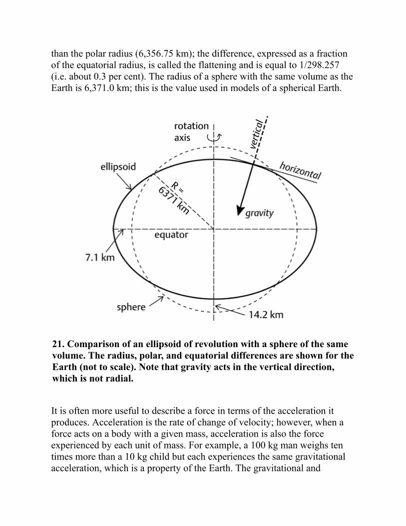
than the polar radius (6,356.75 km); the difference, expressed as a fractionof the equatorial radius, is called the flattening and is equal to 1/298.257(i.e. about 0.3 per cent). The radius of a sphere with the same volume as theEarth is 6,371.0 km; this is the value used in models of a spherical Earth.

21. Comparison of an ellipsoid of revolution with a sphere of the samevolume. The radius, polar, and equatorial differences are shown for theEarth (not to scale). Note that gravity acts in the vertical direction,which is not radial.

It is often more useful to describe a force in terms of the acceleration itproduces. Acceleration is the rate of change of velocity; however, when aforce acts on a body with a given mass, acceleration is also the forceexperienced by each unit of mass. For example, a 100 kg man weighs tentimes more than a 10 kg child but each experiences the same gravitationalacceleration, which is a property of the Earth. The gravitational and

centrifugal accelerations have different directions: gravitational accelerationacts inwards towards the Earth’s centre, whereas centrifugal accelerationacts outwards away from the rotation axis. Gravity is the acceleration thatresults from combining these two accelerations. The direction of gravitydefines the local vertical direction (the plumb line) and thereby thehorizontal plane. Due to the different directions of its componentaccelerations, gravity rarely acts radially towards the centre of the Earth; itonly does so at the poles and at the equator.

For similar reasons the value of gravity varies with latitude. There are tworeasons for this variation. First, at the equator the centrifugal acceleration ismaximum and acts outwards, directly opposite to the direction ofgravitation, thus reducing the equatorial gravity. Meanwhile, an observer atthe poles is located directly on the rotation axis where the centrifugalacceleration is zero, so gravity at the poles is fully equal to the gravitationalacceleration. Secondly, the Earth’s slightly flattened shape brings the polarsurface closer to its centre of mass, strengthening the gravitationalattraction. This is partly counteracted by the extra mass beneath theequatorial bulge, which increases slightly the gravitational attraction at theequator. The end result is that gravity is about 0.5 per cent stronger at thepoles than at the equator.

Gravity on the Earth’s surface and its variation withdepth

The instrument used to measure gravity is a gravimeter. The two types incommon use are designed to measure either the absolute value of gravity ata point or the change in gravity relative to a reference position, or basestation. Absolute gravimeters measure directly the acceleration of a masswhile it is falling in an evacuated chamber. A variant of the method consistsof a two-way, rise-and-fall measurement, made on a mass that is initiallyprojected upwards. The position of the falling mass is detected with a laserinterferometer and the time of fall is measured with an atomic clock. Theinstrument most commonly used for gravity surveying is a relativegravimeter. In principle this device measures the extension of an elastic

spring caused by changes in local gravity relative to a base station, where itis calibrated and an absolute measurement is known. The sensitivity of arelative gravimeter is due to the special design of the spring, which is madeof quartz or metal and housed in a temperature-controlled evacuatedchamber. It is constructed so as to augment the extension caused by a smallchange in gravity.

The absolute value of gravity varies with both latitude and altitude. Thetheoretical value on the reference ellipsoid is known very exactly. It iscalled normal gravity, as its direction is normal (perpendicular) to thesurface of the ellipsoid. A reference formula for normal gravity at anylatitude has been derived, based on a precise reference value for gravity atthe equator. The geophysical unit for measuring gravity is based on the Gal(named after Galileo), which is defined as 1 cm/s2. However, this unit is toolarge to be practical in a geological context. Gravity maps are commonlyprepared in units of one thousandth of a Gal, called a milligal (mGal); thisis equal to 10–3 cm/s2, roughly one millionth of mean gravity. Gravimetersare extremely sensitive devices and the portable relative gravimeters used inmodern geophysical surveying can measure gravity differences a thousandtimes smaller than a milligal, in the range of a microgal (10–6 cm/s2). A newgeneration of gravimeter uses superconducting technology to achieve ameasurement sensitivity in the range of a nanogal (10–9 cm/s2), equivalentto a trillionth (10–12) of gravity at the Earth’s surface.

Using the measured values of gravity and the Earth’s radius, in conjunctionwith the gravitational constant, the mass and volume of the Earth can beobtained. Combining these gives a mean density for the Earth of 5,515kg/m3. The average density of surface rocks is only half of this value, whichimplies that density must increase with depth in the Earth. This was animportant discovery for scientists concerned with the size and shape of theEarth in the 18th and early 19th centuries. The variation of density withdepth in the layered Earth (Figure 11) was later established from theinterpretation of P- and S-wave seismic velocities and the analysis of freeoscillations.

A simple calculation for any depth in a spherical Earth shows that the netgravitational attraction of the layers of material above that depth is zero.Gravitational acceleration at any depth in the Earth is therefore due only tothe mass of material between that depth and the Earth’s centre. This makesit possible to use the density–depth profile to calculate the variation ofgravity with depth in the Earth. The calculation shows that gravity at firstincreases with increasing depth from around 9.8 m/s2 at the Earth’s surfaceto around 10.7 m/s2 at the core–mantle boundary, and from there it sinksalmost linearly to zero at the Earth’s centre.

Pressure increases with depth in the Earth due to the weight of the overlyingrock layers and can be computed for a given depth by combining the depth-profiles of density and gravity. In this way the pressure at the Earth’s centrehas been estimated to be around 360 gigapascals (GPa). A pascal is thephysical unit of pressure. Atmospheric pressure at sea level is close to100,000 Pa, so the pressure at the Earth’s centre is about 3.6 million timeslarger.

The reference ellipsoid and geoidThe energy an object possesses because of its position is its potentialenergy. The position of a man on a diving board 10 m above a pool giveshim a greater potential energy than he would have 5 m above the surface.When the energy is calculated per unit mass, it is called the potential. Themathematical shape of the Earth—the reference ellipsoid—corresponds to asurface on which the potential of gravity is constant; it is called anequipotential surface. The value of the potential on the reference ellipsoid isdefined to be the same as that of mean sea level. Importantly, the value ofgravity itself is not constant on the equipotential—it is the potential ofgravity that is constant. The availability of a reference figure makes itpossible for geophysicists to calculate the theoretical value of gravity at sealevel anywhere on the Earth. The properties of the reference ellipsoid aredefined by an international association of geodesists and it is known as theInternational Reference Ellipsoid.

The reference ellipsoid—bulging over the equivalent sphere by 7 km at theequator and flattened beneath it by 14 km at each pole (Figure 21)—is anidealized representation of the true equipotential surface of gravity, which iscalled the geoid. The ellipsoid is a very good fit to the geoid but it departslocally from it. The deviations are known as geoid undulations and arecommonly of the order of a few metres but can exceed 100 m. They arisefor two reasons. First, the ellipsoid assumes that the interior of the Earth ishomogeneous, which is not the case. For example, large-scale densitydifferences exist in the mantle due to geodynamic processes. These are themain cause of large, broad geoid undulations. Secondly, the Earth’s surfaceis rough, broken by faults, uplifted in mountains, and mostly covered byoceans that contain deep basins and troughs as well as submarinemountains. Topographic irregularities and density variations cause gravityto differ from the theoretical value and the real equipotential surface todeviate from the ellipsoid. Thus, where gravity is stronger or weaker thanexpected, the geoid develops bumps or dimples, respectively, relative to thereference ellipsoid.

Prior to the development of satellite geodesy the elevation of the geoidrelative to the reference ellipsoid was determined from gravimetricmeasurements, which required precise levelling. A mathematical proceduredevised in 1849 by George Stokes was then used to calculate the geoidheight. Beginning in the 1960s, successive satellite missions have providedprogressively more accurate determinations of the geoid and the Earth’sgravity field. Density anomalies affect the orbits of near-Earth satellites,and as a result it is possible to measure the undulations of the geoidaccurately from space (Figure 22). The geoid reaches a depth of 106 mbelow the ellipsoid over southern India, it is 60 m above the ellipsoid overNew Guinea and the North Atlantic, and 40 m above the ellipsoid south ofAfrica. Generally, the broader a geophysical anomaly (of gravity, thegeomagnetic field, or the geoid), the deeper is its source. The large-scalegeoid anomalies are too broad to arise from mass anomalies in the crust orlithosphere. They are attributed to anomalous mass distribution in themantle.

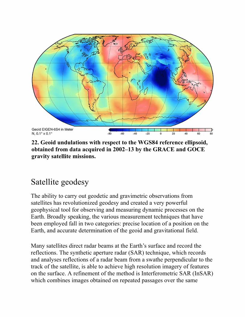
22. Geoid undulations with respect to the WGS84 reference ellipsoid,obtained from data acquired in 2002–13 by the GRACE and GOCEgravity satellite missions.

Satellite geodesyThe ability to carry out geodetic and gravimetric observations fromsatellites has revolutionized geodesy and created a very powerfulgeophysical tool for observing and measuring dynamic processes on theEarth. Broadly speaking, the various measurement techniques that havebeen employed fall in two categories: precise location of a position on theEarth, and accurate determination of the geoid and gravitational field.

Many satellites direct radar beams at the Earth’s surface and record thereflections. The synthetic aperture radar (SAR) technique, which recordsand analyses reflections of a radar beam from a swathe perpendicular to thetrack of the satellite, is able to achieve high resolution imagery of featureson the surface. A refinement of the method is Interferometric SAR (InSAR)which combines images obtained on repeated passages over the same

region. The radar beam is a waveform, that is, it can be visualized as asequence of crests and troughs. If any displacement of the surface occursbetween the recordings, the radar beams will consist of a different numberof wavelengths, or partial wavelengths. If these differ by an odd number ofhalf-wavelengths, one beam will have a crest where the other has a troughand the combined signals will be weakened; this is destructive interference.By contrast, if the difference is a number of full wavelengths, crests andtroughs will be augmented, which is constructive interference. The result ofcombining the images is a set of interference fringes that emphasize, andallow measurement of, the change in land surface between the satelliteover-flights. The method can detect vertical displacements with an accuracyof 1–2 cm that are undetectable by eye, and has a horizontal resolution ofaround 3 m. Amongst many other applications, InSAR studies haveobserved the changes produced by earthquakes in the strain fields aroundfaults, and the swelling of volcanoes before eruption and subsidence of thetopography afterwards.

The Global Positioning System (GPS) is one of the most importanttechniques in modern geodesy. It has revolutionized geodetic observationson scales from local and regional surveys to the motions of global tectonicplates. Similar, but separate, systems are operated by the USA (GPS),Europe (Galileo), and Russia (GLONASS). In full operation, each system isdesigned to consist of 24 satellites in orbits at altitudes of about 19,000–23,000 km (so-called Medium Earth Orbit). The GPS system deploys foursatellites in each of six orbital planes inclined at about 55 degrees to theequator and intersecting the equator at positions that are 60 degrees apart inlongitude. The satellites emit coded signals in the GHz frequency range thatare detected by receivers and converted to a location. Signals from aminimum of four GPS satellites allow the accurate location of a receiveranywhere on the Earth, on land, in aircraft, or at sea, as well as fordetermining the positions of other satellites. The accuracy of location of areceiver is of the order of a few metres. The Galileo system aims to improvethis to better than a metre for general usage, and to centimetre scale forscientific purposes.

Geodesists have developed sophisticated techniques for analysing GPSsignals to improve the accuracy of location. One such method is differential

GPS. This involves a network of GPS receivers operating in a particularregion; the position of one receiver is known very accurately and the otherreceivers in the network determine their locations relative to it. Withdifferential GPS the accuracy of location improves to a few centimetres.Even higher precision is attained with the technique of carrier-phasetracking, which achieves location accuracy on the millimetre scale. Suchexceptional accuracy in determining exactly where a receiver is located hasled to various new applications for geodetic surveying. A precise GPSsurvey of a region can now be made in just a few weeks. The targetedregion could be, for example, an area in which there is crustal deformationsuch as faulting. Repeating the survey at a later time reveals changes in thestrain pattern. A network of permanent GPS sites on an active fault canobserve motions related to earthquakes on the fault, before, during, andafter the event. Such data also provide information about relaxationprocesses in the lithosphere, such as the rebound of topography that wasdepressed in the last ice age. Networks of GPS stations provide anindependent means of observing actively the present motions andinteractions of the global tectonic plates that subdivide the Earth’slithosphere.

Accurate determination of the geoid was an important achievement ofsatellite altimetry. This technique was initiated soon after the start of spaceexploration with artificial satellites. The exact altitude of a satellite ismeasured by tracking its position accurately from a global network of laserstations on the Earth. This gives the height of the satellite above thereference ellipsoid, that is, above mean sea level. Meanwhile, the two-waytravel-time of a microwave radar pulse emitted by the satellite measures itsheight above the sea surface. The difference between the measured heightsis the height of the ocean surface relative to the ellipsoid, that is, the geoidundulation. Satellite geodesy has developed with increasing precision andsophistication, as illustrated by two recent space missions.

The Gravity Recovery and Climate Experiment (GRACE) was launched in2002, deploying two identical satellites in the same polar orbit at an altitudeof 500 km. Their horizontal separation of 220 km is monitored accuratelywith a microwave ranging system that can measure separation changes onthe order of 10 micrometres. When the leading satellite approaches a region

where gravity is stronger than average, the increased attraction causes it tospeed up and, when subsequently it has passed the region, it is sloweddown. In each case this changes the distance to the following satellite,which is affected similarly as it passes over the region. The tiny changes inthe separation of the satellites are converted into gravity anomalies,resulting in a map of the Earth’s gravity field. GRACE results are obtainedmonthly, which allows observation of changes in the gravity field with time.These include, for example, the gravitational changes that accompany themelting of an ice sheet or that result from the adjustment of the Earth afterthe ice-age load of a glacier has disappeared. The changes of GRACE datawith time have been used to compute the viscosity of the Earth’s mantle.

The Gravity Field and Steady-State Ocean Circulation Explorer (GOCE)mission (2009–13) deployed a single satellite in a lower polar orbit, at analtitude of only 255 km. Atmospheric drag at this altitude was compensatedby an ion propulsion system. The on-board instrument was a gravitygradiometer, which used three pairs of accelerometers to measure thegravity gradient—the rate at which gravity changes with position—in threemutually perpendicular directions. The height of the ocean surface,determined over many years by satellite altimetry, is made up of two parts.A static part consists of undulations of the geoid due to the anomalousmasses inside the Earth. On top of this are superposed the effects of oceancurrents, which change with time. When the geoid height is subtracted, thelarge-scale mean dynamic topography of the ocean surface is obtained.Water flows from high points to lower levels, so the elevations anddepressions of the dynamic topography have allowed the ocean currentsystems to be mapped in unprecedented detail.

The results from these satellite missions are usually presented as colouredmaps that dramatically display the spectacular resolution. In regions wheredata from satellites can be combined with terrestrial data (e.g. gravitymeasurements on the continents or satellite altimetry over the oceans) thespatial resolution is further improved, so that it is possible to resolve abump or dent in the geoid or gravitational field smaller than 100 km inhorizontal extent.

The tidesThe Moon’s influence on the Earth’s rotation is stronger than that of the Sunor the other planets in the solar system. The centre of mass of the Earth–Moon pair, called the barycentre, lies at about 4,600 km from the Earth’scentre—well within the Earth’s radius of 6,371 km. The Earth and Moonrotate about this point (like two dancers in a waltz). The elliptical orbit ofthe Earth about the Sun is in reality the track followed by the barycentre.The rotation of the Earth–Moon pair about their barycentre causes acentrifugal acceleration in the Earth that is directed away from the Moon.The lunar gravitational attraction opposes this and the combined effect is todeform the equipotential surface of the tide and draw it out into the shape ofa prolate ellipsoid, resembling a rugby ball. Consequently there is a tidalbulge on the far side of the Earth from the Moon, complementary to thetidal bulge on the near side. The bulges are unequal in size. Each day theEarth rotates under both tidal bulges, so that two unequal tides areexperienced; they are resolved into a daily (diurnal) tide and a twice-daily(semi-diurnal) tide. Although we think of the tides as a fluctuation of sealevel, they also take place in the solid planet, where they are known asbodily earth tides. These are manifest as displacements of the solid surfaceby up to 38 cm vertically and 5 cm horizontally.

The Sun also contributes to the tides, creating semi-annual and annualcomponents. Although the Sun’s mass is vastly greater than that of theMoon, it is much further away from the Earth and consequently the solartidal acceleration is only 45 per cent that of the Moon. Imagining each tidaldisplacement to be shaped like a rugby ball, it is evident that the lunar andsolar tides reinforce each other when the ‘rugby balls’ are parallel. Thishappens when the Sun and Moon are on opposite sides of the Earth (inopposition), as well as when they are on the same side (in conjunction).These reinforcements occur at full moon and new moon, respectively. Ineach situation extra high tides result, called spring tides. Midway betweenthese two geometries the ‘rugby balls’ are perpendicular to each other (inquadrature) and as a result they weaken each other, giving unusually lowtides that are called neap tides.

The displacements of fluid and solid mass have a braking effect on theEarth’s rotation, slowing it down and gradually increasing the length of theday, currently at a rate of 1.8 milliseconds per century. Evidence for thiseffect has been deduced from Babylonian, Chinese, Islamic, and Europeanastronomic records covering the past 2,700 years. It can now be measureddirectly by VLBI, GPS, and other satellite techniques. The reciprocal effectof the Earth’s gravitation on the Moon has slowed lunar rotation about itsown axis to the extent that the Moon’s spin now has the same period as itsrotation about the Earth. That is why it always presents the same face to us.Conservation of angular momentum results in a transfer of angularmomentum from the Earth to the Moon, which is accomplished by anincrease in the Earth–Moon distance of about 3.7 cm/yr (roughly the rate atwhich fingernails grow), and by a slowing of the Moon’s rotation ratesabout its own axis and about the Earth. In time, all three rotations will besynchronous, with a period of 48 present Earth-days. The Moon will thenbe stationary over the Earth and both bodies will present the same face toeach other. This state already exists between the dwarf planet Pluto and itsmoon Charon.

Correction and reduction of gravity measurementsGravity surveying is a valuable technique employed in various types ofgeophysical investigation, whether on a large scale to analyse globalgeodynamics, or on a smaller scale in geophysical prospecting forpetroleum and minerals. The ability of gravimeters to measure gravityanomalies in the microgal range makes it a useful tool in environmentalapplications of geophysics, for example in assessing an archaeological site,where buried walls or cavities may cause tiny local changes in gravity.

A gravity anomaly is the deviation of an individual measurement of gravityfrom the normal gravity at the same location. It is caused by a structure thatlies beneath the reference ellipsoid. Gravity is increased over a high-densitystructure; over a low-density one it is decreased. However, the place wheregravity is measured rarely lies directly on the ellipsoid, so variousadjustments must be carried out to make the comparison possible. Theseinclude local effects particular to the measurement site. First, any

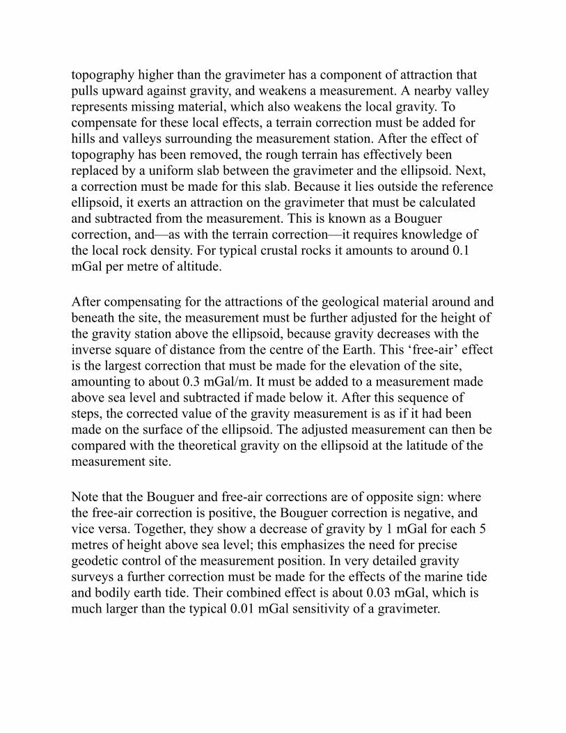
topography higher than the gravimeter has a component of attraction thatpulls upward against gravity, and weakens a measurement. A nearby valleyrepresents missing material, which also weakens the local gravity. Tocompensate for these local effects, a terrain correction must be added forhills and valleys surrounding the measurement station. After the effect oftopography has been removed, the rough terrain has effectively beenreplaced by a uniform slab between the gravimeter and the ellipsoid. Next,a correction must be made for this slab. Because it lies outside the referenceellipsoid, it exerts an attraction on the gravimeter that must be calculatedand subtracted from the measurement. This is known as a Bouguercorrection, and—as with the terrain correction—it requires knowledge ofthe local rock density. For typical crustal rocks it amounts to around 0.1mGal per metre of altitude.

After compensating for the attractions of the geological material around andbeneath the site, the measurement must be further adjusted for the height ofthe gravity station above the ellipsoid, because gravity decreases with theinverse square of distance from the centre of the Earth. This ‘free-air’ effectis the largest correction that must be made for the elevation of the site,amounting to about 0.3 mGal/m. It must be added to a measurement madeabove sea level and subtracted if made below it. After this sequence ofsteps, the corrected value of the gravity measurement is as if it had beenmade on the surface of the ellipsoid. The adjusted measurement can then becompared with the theoretical gravity on the ellipsoid at the latitude of themeasurement site.

Note that the Bouguer and free-air corrections are of opposite sign: wherethe free-air correction is positive, the Bouguer correction is negative, andvice versa. Together, they show a decrease of gravity by 1 mGal for each 5metres of height above sea level; this emphasizes the need for precisegeodetic control of the measurement position. In very detailed gravitysurveys a further correction must be made for the effects of the marine tideand bodily earth tide. Their combined effect is about 0.03 mGal, which ismuch larger than the typical 0.01 mGal sensitivity of a gravimeter.

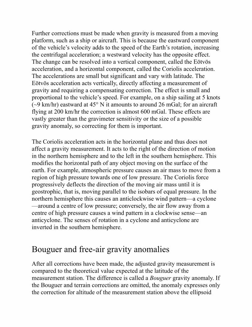
Further corrections must be made when gravity is measured from a movingplatform, such as a ship or aircraft. This is because the eastward componentof the vehicle’s velocity adds to the speed of the Earth’s rotation, increasingthe centrifugal acceleration; a westward velocity has the opposite effect.The change can be resolved into a vertical component, called the Eötvösacceleration, and a horizontal component, called the Coriolis acceleration.The accelerations are small but significant and vary with latitude. TheEötvös acceleration acts vertically, directly affecting a measurement ofgravity and requiring a compensating correction. The effect is small andproportional to the vehicle’s speed. For example, on a ship sailing at 5 knots(~9 km/hr) eastward at 45° N it amounts to around 26 mGal; for an aircraftflying at 200 km/hr the correction is almost 600 mGal. These effects arevastly greater than the gravimeter sensitivity or the size of a possiblegravity anomaly, so correcting for them is important.

The Coriolis acceleration acts in the horizontal plane and thus does notaffect a gravity measurement. It acts to the right of the direction of motionin the northern hemisphere and to the left in the southern hemisphere. Thismodifies the horizontal path of any object moving on the surface of theearth. For example, atmospheric pressure causes an air mass to move from aregion of high pressure towards one of low pressure. The Coriolis forceprogressively deflects the direction of the moving air mass until it isgeostrophic, that is, moving parallel to the isobars of equal pressure. In thenorthern hemisphere this causes an anticlockwise wind pattern—a cyclone—around a centre of low pressure; conversely, the air flow away from acentre of high pressure causes a wind pattern in a clockwise sense—ananticyclone. The senses of rotation in a cyclone and anticyclone areinverted in the southern hemisphere.

Bouguer and free-air gravity anomaliesAfter all corrections have been made, the adjusted gravity measurement iscompared to the theoretical value expected at the latitude of themeasurement station. The difference is called a Bouguer gravity anomaly. Ifthe Bouguer and terrain corrections are omitted, the anomaly expresses onlythe correction for altitude of the measurement station above the ellipsoid

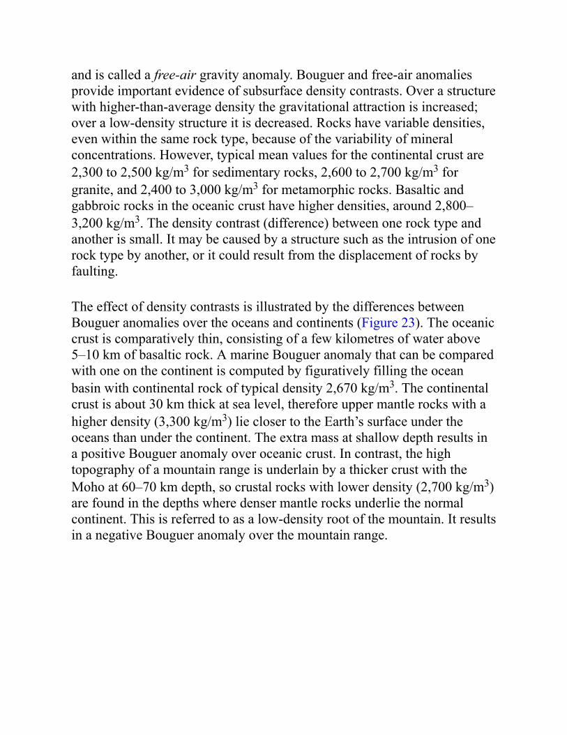
and is called a free-air gravity anomaly. Bouguer and free-air anomaliesprovide important evidence of subsurface density contrasts. Over a structurewith higher-than-average density the gravitational attraction is increased;over a low-density structure it is decreased. Rocks have variable densities,even within the same rock type, because of the variability of mineralconcentrations. However, typical mean values for the continental crust are2,300 to 2,500 kg/m3 for sedimentary rocks, 2,600 to 2,700 kg/m3 forgranite, and 2,400 to 3,000 kg/m3 for metamorphic rocks. Basaltic andgabbroic rocks in the oceanic crust have higher densities, around 2,800–3,200 kg/m3. The density contrast (difference) between one rock type andanother is small. It may be caused by a structure such as the intrusion of onerock type by another, or it could result from the displacement of rocks byfaulting.

The effect of density contrasts is illustrated by the differences betweenBouguer anomalies over the oceans and continents (Figure 23). The oceaniccrust is comparatively thin, consisting of a few kilometres of water above5–10 km of basaltic rock. A marine Bouguer anomaly that can be comparedwith one on the continent is computed by figuratively filling the oceanbasin with continental rock of typical density 2,670 kg/m3. The continentalcrust is about 30 km thick at sea level, therefore upper mantle rocks with ahigher density (3,300 kg/m3) lie closer to the Earth’s surface under theoceans than under the continent. The extra mass at shallow depth results ina positive Bouguer anomaly over oceanic crust. In contrast, the hightopography of a mountain range is underlain by a thicker crust with theMoho at 60–70 km depth, so crustal rocks with lower density (2,700 kg/m3)are found in the depths where denser mantle rocks underlie the normalcontinent. This is referred to as a low-density root of the mountain. It resultsin a negative Bouguer anomaly over the mountain range.

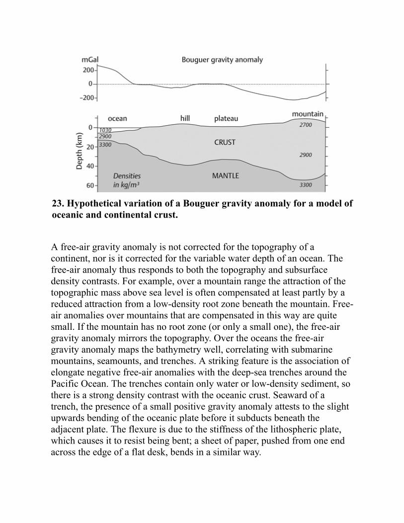
23. Hypothetical variation of a Bouguer gravity anomaly for a model ofoceanic and continental crust.

A free-air gravity anomaly is not corrected for the topography of acontinent, nor is it corrected for the variable water depth of an ocean. Thefree-air anomaly thus responds to both the topography and subsurfacedensity contrasts. For example, over a mountain range the attraction of thetopographic mass above sea level is often compensated at least partly by areduced attraction from a low-density root zone beneath the mountain. Free-air anomalies over mountains that are compensated in this way are quitesmall. If the mountain has no root zone (or only a small one), the free-airgravity anomaly mirrors the topography. Over the oceans the free-airgravity anomaly maps the bathymetry well, correlating with submarinemountains, seamounts, and trenches. A striking feature is the association ofelongate negative free-air anomalies with the deep-sea trenches around thePacific Ocean. The trenches contain only water or low-density sediment, sothere is a strong density contrast with the oceanic crust. Seaward of atrench, the presence of a small positive gravity anomaly attests to the slightupwards bending of the oceanic plate before it subducts beneath theadjacent plate. The flexure is due to the stiffness of the lithospheric plate,which causes it to resist being bent; a sheet of paper, pushed from one endacross the edge of a flat desk, bends in a similar way.

IsostasyLord Cavendish succeeded in measuring the gravitational constant in 1798.Before the value of this constant was known, it was not possible to calculatethe mass or density of the Earth directly from a gravity measurement. In themid-18th century, scientists attempted to calculate the mean density of theEarth by comparing the acceleration of gravity with the horizontal attractionexerted on a suspended mass by a nearby mountain. This was measured bynoting the local deflection of a plumb-line, which defines the verticaldirection. To the surprise of the investigators, the deflections for mountainsin Peru, Ecuador, and Scotland gave inconsistent and unrealistic values forthe Earth’s mean density. In the first half of the 19th century, geodeticsurveying in the Himalaya also showed anomalous deflections of thevertical near mountains. The unusual results were explained by assigningroot-zones to the mountains, in which the rocks have lower density thanexpected. The attraction due to the visible mountain was thus partly offsetby a reduced attraction due to the ‘missing’ amount of mass in the root. Thecompensation of topography by a low-density root, such that the mountaineffectively floats on an underlying layer, is known as isostasy. Threetheoretical models are commonly used to explain the observations.

The first two types, proposed in 1855, are buoyancy models based on theArchimedes principle, which explains how wooden blocks float in water.They envisage a light crust that floats upon a denser substratum. In theAiry–Heiskanen model the crust has a constant density and variablethickness to reflect the topography. It ‘floats’ in the same way as variouslysized blocks of wood in water, which extend to different depths until theyhave the same pressure at their base. This model has a variablecompensation depth, akin to the structure of the crust. In the Pratt–Hayfordmodel the changes in topography are compensated by variable density, withless dense rock under mountains, so that the entire topography has acommon compensation depth. This model resembles floating blocks ofdifferent woods of different densities, projecting above water to differentheights but extending to a common compensation depth. Both isostasymodels use a buoyancy mechanism to explain how an extra mass (e.g. amountain) above sea level is compensated by a lack of mass at depth. The

buoyancy mechanism provides local isostatic compensation: the uplift iscaused by the local vertical difference in density.

A coin placed on a block of wood floating in water causes the block to sinkdeeper until a new balance is reached between its weight and the uplift itreceives from the water. If the coin is removed, the uplift from thesubmerged part of the block is too large for equilibrium and the block rises.In the same manner, isostatic compensation causes the crust to movevertically to seek a new hydrostatic equilibrium in response to changes inthe load on the crust. Thus, when erosion removes surface material or whenan ice-cap melts, the isostatic response is uplift of the mountain. Examplesof this uplift are found in northern Canada and Fennoscandia, which werecovered by a 1–2 kilometre-thick ice sheet during the last ice age; thesurface load depressed the crust in these regions by up to 500 m. The iceage ended about 10,000 years ago, and subsequent postglacial isostaticadjustment has resulted in vertical crustal movements. The land uplift wasinitially faster than it is today, but it continues at rates of up to 9 mm/yr inScandinavia and Finland (Figure 24). The phenomenon has been observedfor decades by repeated high-precision levelling campaigns. Nordicgeodesists now measure the uplift with millimetre-scale accuracy using anetwork of continuously recording GPS stations.

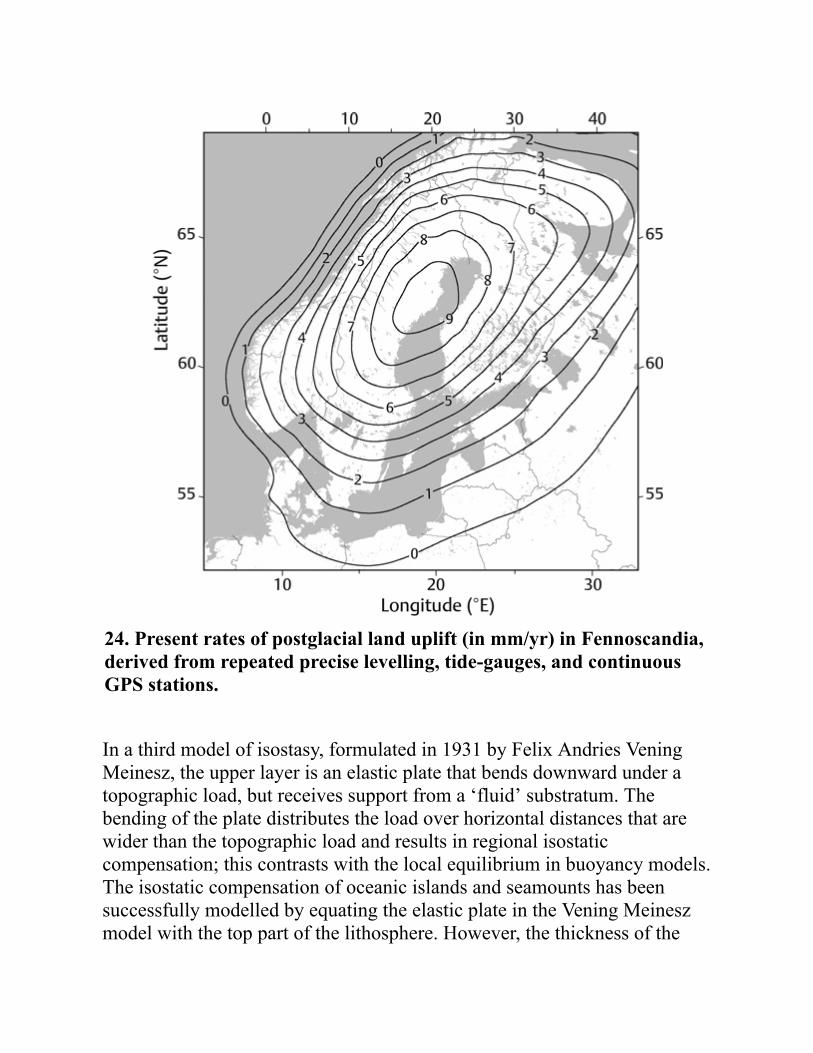
24. Present rates of postglacial land uplift (in mm/yr) in Fennoscandia,derived from repeated precise levelling, tide-gauges, and continuousGPS stations.

In a third model of isostasy, formulated in 1931 by Felix Andries VeningMeinesz, the upper layer is an elastic plate that bends downward under atopographic load, but receives support from a ‘fluid’ substratum. Thebending of the plate distributes the load over horizontal distances that arewider than the topographic load and results in regional isostaticcompensation; this contrasts with the local equilibrium in buoyancy models.The isostatic compensation of oceanic islands and seamounts has beensuccessfully modelled by equating the elastic plate in the Vening Meineszmodel with the top part of the lithosphere. However, the thickness of the

elastic part of the oceanic lithosphere is noticeably less than its seismicthickness. Evidently the increase of temperature with depth results inanelastic behaviour of the deeper lithosphere. This is the same kind ofbehaviour that causes attenuation of seismic waves in the Earth (seeChapter 3). It is an irreversible process that depends on the applied stressand also on the rate of change of the stress. This depends on temperatureand occurs faster at higher temperatures.

A specific type of anelastic behaviour is viscoelasticity. In this mechanism amaterial responds to short-duration stresses in the same way that an elasticbody does, but over very long time intervals it flows like a sticky viscousfluid. The flow of otherwise solid material in the mantle is understood to bea viscoelastic process. This type of behaviour has been invoked to explainthe response of the upper mantle to the loading of northern Canada andFennoscandia by the ice sheets. In each region the weight of an ice sheetdepressed the central area, forcing it down into the mantle. The displacedmantle caused the surrounding land to bulge upward slightly, as a jelly doesaround a point where it is pressed down. As a result of postglacialrelaxation the opposite motion is now happening: the peripheral bulge issinking while the central region is being uplifted. This behaviour involvesboth the flexural rigidity of the lithosphere—its resistance to being bent—and the viscosity of the upper mantle. The depth to which the mantle isinvolved depends on its local structure and on the weight and extent of thesurface load.

Chapter 6The Earth’s heat

Heat sourcesIn popular usage heat and temperature are often taken to be the same, but,although related, they are different concepts which we need to clarify. Themolecules of an object are in constant motion and the energy of this motionis called kinetic energy. Temperature is a measure of the average kineticenergy of the molecules in a given volume. It is measured in degreesCelsius (°C) or in kelvins (K), which have the same dimensions butdifferent reference points. Absolute zero on the Kelvin scale, thetemperature at which all thermal motion ceases, corresponds to –273.15°C.

The total energy of motion of all the molecules in a volume is its internalenergy. When two objects with different temperatures are in contact, theyexchange internal energy until they have the same temperature. The energytransferred is the amount of heat exchanged. Thus, if heat is added to anobject, its kinetic energy is increased, the motions of individual atoms andmolecules speed up, and its temperature rises. Heat is a form of energy andis therefore measured in the standard energy unit, the joule. The expenditureof one joule per second defines a watt, the unit of power. The powerconsumption of devices in daily usage is measured in kilowatts (i.e.

thousands of watts); for example, a modest automobile may have a 100 kWengine.

The rates of heat transfer in the Earth are much smaller than a watt and aremeasured in milliwatts (mW, i.e. thousandths of a watt). The amount ofgeothermal heat flowing per second across a unit of surface area of theEarth is called the geothermal flux, or more simply the heat flow. It ismeasured in mW/m2.

The Earth’s internal heat is its greatest source of energy. It powers globalgeological processes such as plate tectonics and the generation of thegeomagnetic field. The annual amount of heat flowing out of the Earth ismore than 100 times greater than the elastic energy released in earthquakesand ten times greater than the loss of kinetic energy as the planet’s rotationslows due to tidal friction. Although the solar radiation that falls on theEarth is a much larger source of energy, it is important mainly for its effecton natural processes at or above the Earth’s surface. The atmosphere andclouds reflect or absorb about 45 per cent of solar radiation, and the landand ocean surfaces reflect a further 5 per cent and absorb 50 per cent.Almost all of the energy absorbed at the surface and in the clouds andatmosphere is radiated back into space. The solar energy that reaches thesurface penetrates only a short distance into the ground, because water androcks are poor conductors of heat. A rock or beach exposed to the Sun feelswarm to the touch, but this is a superficial effect. The daily temperaturefluctuation in rocks and sediments sinks to less than 1 per cent of its surfaceamplitude in a depth of only 1 metre. The annual seasonal change oftemperature penetrates some nineteen times deeper, but its effects are barelyfelt below 20 m. However, glaciations advanced and retreated with aperiodicity of up 100,000 yr during the most recent ice age. These long-term temperature changes are able to penetrate the Earth to depths ofseveral kilometres. This has to be taken into account when the heat flowingout of the Earth is measured in wells and boreholes.

The internal heat arises from two sources. Part is produced at the presenttime by radioactivity in crustal rocks and in the mantle, and part isprimordial. Their relative contributions are not known exactly but are

thought to be similar. The radiogenic heat source is an ongoing process ofheat production by the decay of radioactive isotopes, principally of uranium238, uranium 235, thorium 232, and potassium 40. These isotopes occurmainly in the crust but some are in the mantle. In contrast, the primordialheat is a remnant left over from the planet’s fiery formation. In its earlymolten state a dense core of heavy elements was formed, surrounded by asilicate mantle of lighter elements, which later became encased in a thin,cool crust. This process of separation is known as differentiation. The Earthsubsequently cooled and continues to do so, slowly losing the heat offormation. The residual amount of the original heat is the primordial sourceof today’s internal heat. The heat flowing from the Earth’s core into themantle is thought to be largely primordial.

The internal heat has to find its way out of the Earth. The three basic formsof heat transfer are radiation, conduction, and convection. Heat is alsotransferred in compositional and phase transitions. Thermal radiation isemitted when the particle motion in an object is converted toelectromagnetic waves in the infrared region of the spectrum. However,temperatures are not high enough for this process to be important in theEarth. Heat is transported throughout the interior by conduction, andconvection plays an important role in the mantle and fluid outer core.

Heat flow through the Earth’s surfaceHeat transport by conduction is most important in solid regions of the Earth.Thermal conduction takes place by transferring energy in the vibrations ofatoms, or in collisions between molecules, without bodily displacement ofthe material. The flow of heat through a material by conduction depends ontwo quantities: the rate at which temperature increases with depth (thetemperature gradient), and the material’s ability to conduct heat, a physicalproperty known as its thermal conductivity. The product of the temperaturegradient and the thermal conductivity defines the heat flow. On thecontinents the local temperature gradient can be measured by observing thetemperatures at several depths in boreholes and deep wells. The thermalconductivity is measured on appropriate rock samples in the laboratory. Inthe oceans the temperature gradient is measured by plunging a long pipe-

like probe into the sediment-covered sea floor. Thermistors (sensitivethermometers) mounted on the surface of the pipe measure the temperatureat different depths in the sediment, from which the temperature gradient iscalculated. The thermal conductivity of the sediment can be measured insitu in the ocean floor, or later in the laboratory on sediment samples if acore is taken when the pipe is withdrawn.

Heat flow varies greatly over the Earth’s surface depending on the localgeology and tectonic situation. The estimated average heat flow is 92mW/m2. Multiplying this value by the Earth’s surface area, which is about510 million km2, gives a global heat loss of about 47,000 GW (a GW, orgigawatt, is one billion watts). For comparison, the energy production of alarge nuclear power plant is about 1 GW.

About one-third of the Earth’s heat loss is through the continents. Theaverage heat flow for continental areas is 71 mW/m2, but the values varygreatly with the type of rock in a given area and its age. The lowest valuesof 20–40 mW/m2 are measured over the Precambrian shield areas. Theseare the oldest regions of crust on the continents. Except for local areas inwhich radiogenic isotopes are concentrated, the ancient rocks that formthese stable regions (called cratons) have had a very long time to cool downsince their formation. By contrast, two-thirds of the Earth’s heat loss isthrough the oceanic lithosphere, where the heat flow averages 105 mW/m2,much higher than the continental heat flow. The oceanic heat flow is higheston oceanic ridges (Figure 25), where the heat flow may locally exceed 500mW/m2. Radiogenic minerals are scarce in the oceanic crust, so only a fewper cent of the oceanic heat flow has a radiogenic origin.

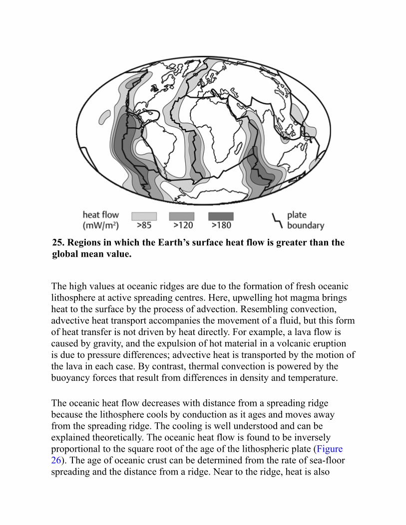
25. Regions in which the Earth’s surface heat flow is greater than theglobal mean value.

The high values at oceanic ridges are due to the formation of fresh oceaniclithosphere at active spreading centres. Here, upwelling hot magma bringsheat to the surface by the process of advection. Resembling convection,advective heat transport accompanies the movement of a fluid, but this formof heat transfer is not driven by heat directly. For example, a lava flow iscaused by gravity, and the expulsion of hot material in a volcanic eruptionis due to pressure differences; advective heat is transported by the motion ofthe lava in each case. By contrast, thermal convection is powered by thebuoyancy forces that result from differences in density and temperature.

The oceanic heat flow decreases with distance from a spreading ridgebecause the lithosphere cools by conduction as it ages and moves awayfrom the spreading ridge. The cooling is well understood and can beexplained theoretically. The oceanic heat flow is found to be inverselyproportional to the square root of the age of the lithospheric plate (Figure26). The age of oceanic crust can be determined from the rate of sea-floorspreading and the distance from a ridge. Near to the ridge, heat is also

removed by hydrothermal circulation through cracks and fissures in theyoung oceanic crust, causing the conductive heat flow to fall below thetheoretical curve. As well as cooling with age, the oceanic plate thickens inproportion to the square root of its age. At a ridge axis the younglithosphere is only a few kilometres thick, but the thickness increases as theplate ages, reaching a value of around 100 km where the lithosphere is olderthan about 60 million years (Myr). Moreover, as the plate ages and cools itbecomes denser and subsides. Consequently, the depth of the ocean alsoincreases as the square root of the plate’s age. Where an oceanic plateconverges with an adjacent plate, a deep trench forms. These are the deepestparts of the world’s oceans and are characterized by very low heat flowvalues.

26. Variation of global heat flow with the age of oceanic lithosphere.Points are global averages for a particular lithospheric age. Low valuesnear the ridge axis are attributed to the circulation of hydrothermalfluids that carry away part of the heat.

When a lithospheric plate subducts at a converging plate margin, theleading edge of the cool slab bends downward into the hotter mantle.Thermal conduction is a slow process and for millions of years the interior

of the subducting slab remains colder and thus denser than its surroundings.The ‘negative buoyancy’ causes the slab to sink into the less dense uppermantle. In the process it exerts a pull on the lithospheric plate which isstronger than other forces that act on it. The ‘slab pull’ is the dominatingforce that drives plate tectonic motions.

Temperature inside the EarthCompared to seismic velocities, density, and gravity, the temperature atdifferent depths in the Earth is not well known. Direct measurement isimpossible below the upper few kilometres that have been penetrated byboreholes or deep mines. In general, the temperature increases with depth,defining a curve called the geotherm. This is affected by local tectonicconditions as well as by the age of surface rocks. The curve is not knownprecisely: estimates of the temperature at crucial depths sometimes differ byhundreds of degrees. Near the Earth’s surface the temperature gradientaverages around 25–30°C per kilometre. A continual increase at this ratewould give an unrealistic temperature of about 200,000°C for the centre ofthe Earth and most of the interior would be molten. Seismic results showthat this is not the case, and so the temperature gradient must decrease withdepth. It is steepest in the crust, and increases much more slowly in themantle.

The relationship between the geotherm and the temperature at whichmelting begins (known as the solidus, or ‘softening point’) can be inferredfrom the physical state of the Earth’s internal structure deduced fromseismic travel-times (Figure 10). The high pressure in the core raises themelting point of iron, which is the core’s main constituent, and enables theinner core to be solid despite the high ambient temperature. This impliesthat the temperature of the inner core must be lower than the melting pointof iron under core conditions. On the other hand, the outer core is molten,and so its temperature lies above the melting point of iron. The boundarybetween the inner and outer cores marks an anchor point for thetemperature curve; it is the melting point of iron at the pressure andtemperature corresponding to that depth. Outside the core, seismologyshows that the mantle and crust are solid for the passage of P- and S-waves,

so temperatures in these domains lie below the melting point. A reductionin shear wave velocity in the asthenosphere implies that it has a reducedrigidity and, by inference, that the temperature comes closer to the solidus.Throughout the mantle the difference between the actual temperature andthe solidus determines the ability of different parts of the interior to flowover long time intervals. In turn, this influences motions of the lithosphericplates at the Earth’s surface and determines the tectonic consequences oftheir interactions with each other.

The inaccessibility of the Earth’s interior means that the temperature–depthprofile (Figure 27) must be determined indirectly. This is attained partlyfrom theoretical models based on known or estimated properties ofmaterials composing the mantle and core. An important limitation on theactual temperature–depth curve is the adiabatic temperature profile. Anadiabatic thermal process is one in which heat is neither gained nor lost.This can be the case when a process occurs too quickly to allow heat to beexchanged, as in the rapid compressions and expansions during the passageof a seismic wave. The variation of temperature with depth under adiabaticconditions defines the adiabatic temperature gradient. The dependence ofthe adiabatic gradient on physical properties, such as the coefficient ofthermal expansion and the specific heat, is well understood and describedby thermodynamic equations. The equations can be applied in provincessuch as the lower mantle or outer core that have consistent physical andthermal properties. The results indicate an adiabatic temperature gradient ofaround 0.8 K/km in the outer core.

27. Variations of adiabatic and melting-point temperatures with depthin the Earth’s interior.

The other limit on the actual temperature profile is the behaviour of thesolidus curve with depth. Melting temperatures of appropriate minerals atkey depths are obtained from laboratory experiments at high pressures. Animportant method employs X-ray diffraction to observe the changes instructure and melting point of minerals at extremely high pressuresproduced by a device known as a diamond anvil cell. The variation ofmelting point is measured over a range of pressures, and the observationsare extrapolated to greater depths outside the experimental range. Forexample, the melting point of iron at the boundary between the outer andinner core has been estimated to be 6,200 K from experiments carried out atlower pressures and extrapolated to the 330 GPa pressure at the boundary.

Thermal convection and mantle flowConsider what would happen in a fluid if the temperature increases withdepth more rapidly than the adiabatic gradient. If a small parcel of materialat a particular depth is moved upward adiabatically to a shallower depth, itexperiences a drop in pressure corresponding to the depth difference and acorresponding adiabatic decrease in temperature. However, the decrease isnot as large as required by the real temperature gradient, so the adiabaticallydisplaced parcel is now hotter and less dense than its environment. Itexperiences a buoyant uplift and continues to rise, losing heat andincreasing in density until it is in equilibrium with its surroundings.Meanwhile, cooler material adjacent to its original depth fills the vacatedplace, closing the cycle. This process of heat transport, in which materialand heat are transported together, is thermal convection. Eventually the lossof heat by convection brings the real temperature gradient close to theadiabatic gradient. Consequently, a well-mixed, convecting fluid has atemperature profile close to the adiabatic curve. Convection is the principalmethod of heat transport in the Earth’s fluid outer core.

Convection is also an important process of heat transport in the mantle. Asalready noted, the mantle exhibits viscoelastic behaviour. It reacts like anelastic solid during the rapid passage of seismic waves and respondsimmediately and reversibly to an applied stress. However, when stressed forlong time intervals at high temperature and pressure, the mantle behaveslike a highly viscous fluid. In response to an applied stress it exhibits anirreversible increase of strain (i.e. change of shape) with time. This is due tothe migration of crystal defects in the mantle minerals. It is a thermallyactivated process, in which the strain rate increases rapidly with increasingtemperature. Over long time intervals, this enables the mantle to flow like ahot viscous fluid, resulting in a temperature-driven bodily transfer of massand heat, that is, thermal convection.

It is important to appreciate the timescale on which flow occurs in themantle. The rate is quite different from the familiar flow of a sticky liquid,such as blood or motor oil, which are three times and 250 times moreviscous than water, respectively. The mantle is vastly stiffer. Estimates of

viscosity for the lower mantle are around 1022 Pa·s (pascal seconds), whichis 1025 times that of water. This is an enormous factor (similar to the ratio ofthe mass of the entire Earth to a kilogram mass). The viscosity varies withinthe mantle, with the upper mantle about 20 times less viscous than thelower mantle. Flow takes place in the mantle by the migration of defectsthrough the otherwise solid material. This is a slow process that producesflow rates on the order of centimetres per year. However, geologicalprocesses occur on a very long timescale, spanning tens or hundreds ofmillions of years. This allows convection to be an important factor in thetransport of heat through the mantle.

The flow patterns of mantle convection are influenced by thermal boundarylayers, which are layers where the rheology and mechanism of heat transferchange. The cold lithosphere, in which heat transfer takes place byconduction, forms an upper boundary layer. Another is the hot D″-layerabove the core–mantle boundary, where the fluid core adjoins theviscoelastic mantle. In this anomalous seismic zone the temperature fallssteeply by about 1,400 K between the outer core and the lower mantle. As aresult, the layer plays an important role in mantle convection. It influencesthe heat flow across the core–mantle boundary and thus may affect theprocesses by which the geomagnetic field is created.

Mantle convection and plumesMantle convection plays a crucial role in the cooling history and evolutionof the planet. Fresh lithosphere is created at ocean ridges and oldlithosphere is consumed in subduction zones; this cycle is maintained byconvection throughout the mantle. The deepest earthquakes occur insubduction zones, but few focal depths lie below the 660 km transitionzone. Focal mechanisms of deep earthquakes indicate that the sinking plateis being compressed at these depths, implying resistance to subductionbeyond the transition zone. However, seismic tomography has shown thatcold subducting plates can penetrate the transition zone (see Figure 13), insome cases descending as far as the D″ layer adjacent to the core–mantleboundary. This has led to a model, favoured by most geodynamicists, ofwhole mantle convection. This process takes place between an upper

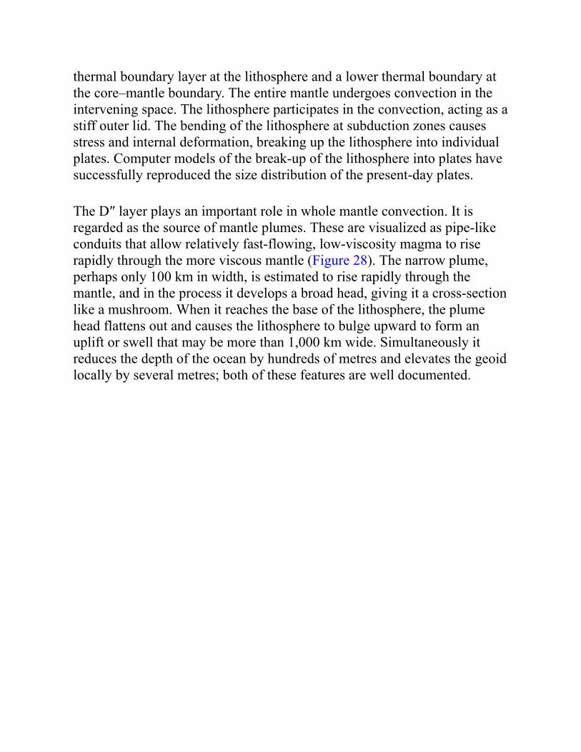
thermal boundary layer at the lithosphere and a lower thermal boundary atthe core–mantle boundary. The entire mantle undergoes convection in theintervening space. The lithosphere participates in the convection, acting as astiff outer lid. The bending of the lithosphere at subduction zones causesstress and internal deformation, breaking up the lithosphere into individualplates. Computer models of the break-up of the lithosphere into plates havesuccessfully reproduced the size distribution of the present-day plates.

The D″ layer plays an important role in whole mantle convection. It isregarded as the source of mantle plumes. These are visualized as pipe-likeconduits that allow relatively fast-flowing, low-viscosity magma to riserapidly through the more viscous mantle (Figure 28). The narrow plume,perhaps only 100 km in width, is estimated to rise rapidly through themantle, and in the process it develops a broad head, giving it a cross-sectionlike a mushroom. When it reaches the base of the lithosphere, the plumehead flattens out and causes the lithosphere to bulge upward to form anuplift or swell that may be more than 1,000 km wide. Simultaneously itreduces the depth of the ocean by hundreds of metres and elevates the geoidlocally by several metres; both of these features are well documented.

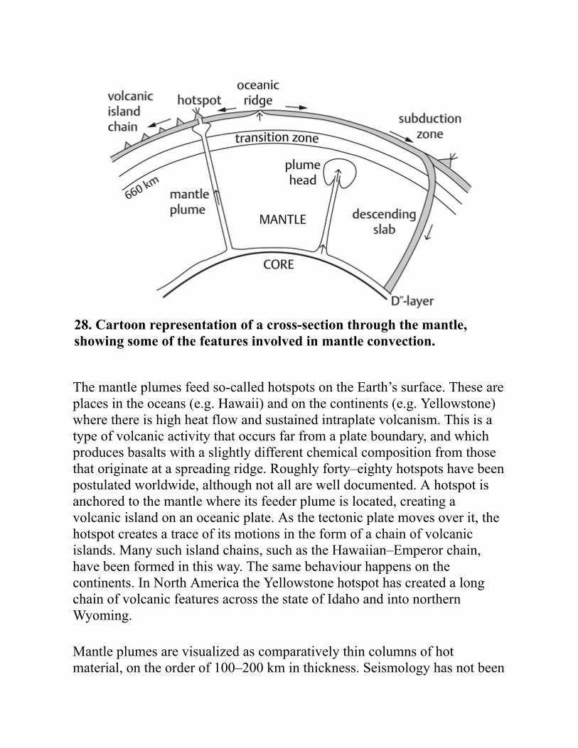
28. Cartoon representation of a cross-section through the mantle,showing some of the features involved in mantle convection.

The mantle plumes feed so-called hotspots on the Earth’s surface. These areplaces in the oceans (e.g. Hawaii) and on the continents (e.g. Yellowstone)where there is high heat flow and sustained intraplate volcanism. This is atype of volcanic activity that occurs far from a plate boundary, and whichproduces basalts with a slightly different chemical composition from thosethat originate at a spreading ridge. Roughly forty–eighty hotspots have beenpostulated worldwide, although not all are well documented. A hotspot isanchored to the mantle where its feeder plume is located, creating avolcanic island on an oceanic plate. As the tectonic plate moves over it, thehotspot creates a trace of its motions in the form of a chain of volcanicislands. Many such island chains, such as the Hawaiian–Emperor chain,have been formed in this way. The same behaviour happens on thecontinents. In North America the Yellowstone hotspot has created a longchain of volcanic features across the state of Idaho and into northernWyoming.

Mantle plumes are visualized as comparatively thin columns of hotmaterial, on the order of 100–200 km in thickness. Seismology has not been

able to establish unequivocally the presence of these narrow featuresbeneath hotspots. In part this is because many hotspots are oceanic and liefar from seismic networks, which are predominantly on land, and thismakes it difficult to image a plume. Some seismic evidence that claimed toshow their existence in tomographic sections has been questioned on thebasis of the imaging method used. On the other hand, seismic tomographyhas revealed two large, broad regions of low shear wave velocity, severalthousand kilometres in extent, located in the lower mantle under Africa andthe central Pacific Ocean, respectively. They have been called superplumes;their size and geometry are different from ‘mushroom-shaped’ plumes.Shear wave velocities are reduced in the superplumes, but their velocitystructure is complex and the reduction in shear wave velocities may be dueto compositional variation rather than temperature anomalies.

An alternative model of mantle convection is preferred by some scientists,in which a separate circulation takes place above the 660 km transition.This would enable a return flow of material from a subduction zone to aridge, and requires two convection systems in the mantle. In this model theoceanic island basalts are presumed to result from melting at shallow depthsin the upper mantle, with ensuing slight isotopic differences with respect tothe oceanic ridge basalts. Stretching and cracking of the lithosphere is thenassumed to allow the melt to rise to the surface to produce the hotspot.Although there are fewer adherents to this model, their arguments havefuelled an intense debate.

Chapter 7The Earth’s magnetic field

The geomagnetic dynamoOur planet is surrounded by a magnetic field, which originates inside theEarth’s molten core. The magnetic field is very important for life on theEarth as it acts as a shield against harmful radiation from space, especiallyfrom the Sun. For centuries it has helped travellers to navigate safely acrossuncharted regions. A magnetic compass aligns with the field and pointsalmost—but not exactly—towards true north. Mankind has learned to copewith the small directional deviations and even to interpret themadvantageously to locate important metallic resources. Yet to most peoplemagnetism remains a mysterious and little understood phenomenon.

Magnetism has been used for navigation since the 11th century, followingthe invention of magnetic compasses that used magnetized iron needles toseek the northerly direction. In 1600 William Gilbert showed that the Earthitself resembles a giant magnet, with its centres of magnetic forceconcentrated near the geographic poles. A freely hanging magnet will alignwith the Earth’s magnetic field, and its opposing ends were recognized asnorth- or south-seeking poles, eventually shortened to ‘magnetic poles’. Anunderstanding of the laws of magnetism emerged, based on the concept ofpoles. A simple magnetic field with two poles was called a dipole, a field

with four poles a quadrupole, eight poles formed an octupole, and so on. Aproper physical understanding of electricity and magnetism evolved early inthe 19th century, when it became evident that all magnetic fields—onmacroscopic, microscopic, and atomic scales—arise from electricalcurrents. Magnetic poles are a fictitious, but sometimes useful, concept. Theclose relationship between magnetism and electricity was emphasized bythe discovery that a changing magnetic field causes an electrical current toflow in a conductor. In 1872 James Clerk Maxwell quantified the knownrelationships between electrical and magnetic phenomena in a set ofequations, which subsequently led to an understanding of electromagneticradiation and the interrelationships between electricity, magnetism, andlight.

The conditions for generating the Earth’s magnetic field are met in themolten core. The core fluid is a good electrical conductor, so the physicalflow of the fluid through magnetic fields in the core induces electricalcurrents, which in turn produce additional magnetic fields in a self-reinforcing process. The fluid flow and electromagnetic interactionsbetween different parts of the core are complex, but massive computingpower has made it possible to model what is happening when the magneticfield is generated. The process involves turbulent fluid motions in the outercore. In addition to buoyancy-driven thermal convection, there is a fluidmotion called compositional convection, which results from solidificationof the inner core. The core fluid consists of iron, nickel, and lower-densityelements. When the inner core solidifies, the lower-density elements are leftbehind in the core fluid. Their lower density makes them buoyant, whichcauses them to rise and sets up a compositionally driven type of convection.

The motions of the core fluid are further influenced by the Coriolis forcethat acts on all moving objects on the rotating Earth. This force actsperpendicular to both the rotation axis and the direction of motion. On theEarth’s surface, as we have seen, it influences the weather by forcing windpatterns to form cyclones and anticyclones. In the Earth’s core its effect isto cause the convecting fluid to form spiralling columns parallel to therotation axis, thereby determining the geometry of electrical currents in thecore. The buoyancy, rotational, and Coriolis forces contribute to a self-sustaining dynamo process that generates the geomagnetic field.

GeomagnetismThe geometry of magnetic field lines is complicated inside the core, butbecomes simpler with increasing radial distance from the centre.Mathematical functions, called spherical harmonics, were developed byCarl Friedrich Gauss in the 1830s to provide a detailed description of thegeomagnetic field. Using the sparse data available at the time, Gaussshowed in 1839 that most of the magnetic field conformed to a dipole andoriginated inside the Earth. Spherical harmonic analysis is used in moderngeophysics to describe the global distributions of magnetic, gravity,thermal, and various other geophysical properties. Applied togeomagnetism it defines the International Geomagnetic Reference Field(IGRF). This is the theoretical magnetic field that best describes the presentfield at any given latitude and longitude. The IGRF consists of a series ofterms that, with increasing number, describe ever smaller, more detailedfeatures of the magnetic field. However, the direction and intensity of thegeomagnetic field change slowly with time, a feature known as secularvariation (secular in this context refers to the slowness of the changes).Some secular changes occur on a human timescale over months, years, orcenturies but others—particularly of the dipole—take place on timescalesspanning thousands to millions of years. To cope with the short-termchanges the magnetic field is constantly monitored and the coefficients ofthe IGRF are updated at regular intervals, usually every four years.

The magnetic field at Earth’s surface is dominantly that of an inclineddipole (Figure 29). If the best-fitting dipole is subtracted from the totalfield, the residual field that is left is referred to as the non-dipole field(NDF). There are two sources for the NDF. The long wavelengthcomponents are generated in the molten core by the fluid motions that alsogenerate the dipole. The short wavelength components are due tomagnetized rocks in the crust, with sources ranging from several kilometresto hundreds of kilometres in extent.

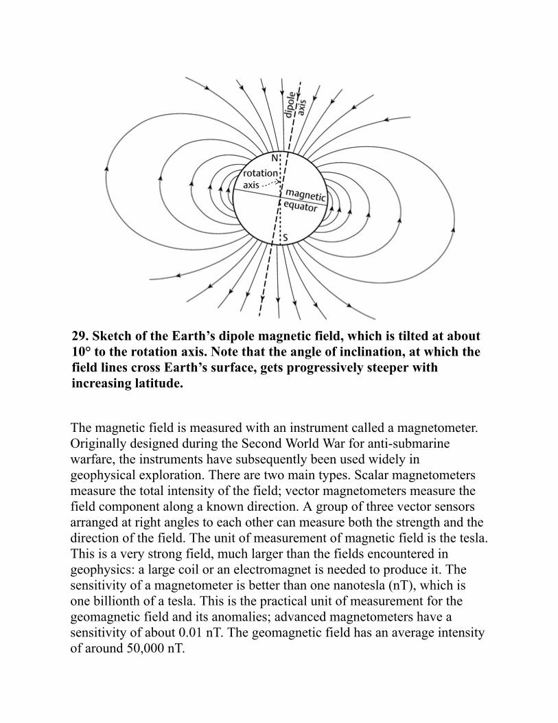
29. Sketch of the Earth’s dipole magnetic field, which is tilted at about10° to the rotation axis. Note that the angle of inclination, at which thefield lines cross Earth’s surface, gets progressively steeper withincreasing latitude.

The magnetic field is measured with an instrument called a magnetometer.Originally designed during the Second World War for anti-submarinewarfare, the instruments have subsequently been used widely ingeophysical exploration. There are two main types. Scalar magnetometersmeasure the total intensity of the field; vector magnetometers measure thefield component along a known direction. A group of three vector sensorsarranged at right angles to each other can measure both the strength and thedirection of the field. The unit of measurement of magnetic field is the tesla.This is a very strong field, much larger than the fields encountered ingeophysics: a large coil or an electromagnet is needed to produce it. Thesensitivity of a magnetometer is better than one nanotesla (nT), which isone billionth of a tesla. This is the practical unit of measurement for thegeomagnetic field and its anomalies; advanced magnetometers have asensitivity of about 0.01 nT. The geomagnetic field has an average intensityof around 50,000 nT.

The magnetometer may be installed at a fixed location, such as a magneticobservatory. A worldwide network of observatories coordinates continuousmonitoring of the global magnetic field, recording its fluctuations withtime. Alternatively, the magnetometer may be mobile and used for a local,regional, or global investigation. In field surveys at or near the surface amagnetometer may be deployed from a ship or aircraft. Magnetic surveyingis relatively inexpensive and fast. Consequently, it is an important techniquein applied geophysics, where it is used to explore an unknown area for itspotential mineral wealth. It is also used in environmental geophysics andarchaeology for local surveys. The goal of any magnetic survey is toidentify places where the measured field differs from the theoretical valueexpected at that place. The deviation, called a magnetic anomaly, is due toinhomogeneity of the subsurface magnetization. Some anomalies may belocal, of shallow origin, and may indicate a crustal feature, such as amineralized dyke or a geological structure of commercial interest. Largeregional anomalies have a deep-seated origin.

An important regional magnetic anomaly is found in the South Atlantic.Maps of the geographic distribution of the non-dipole field show a largeanomalous region over the Atlantic Ocean to the east of South America,where the NDF has a strongly negative value. The origin of the SouthAtlantic anomaly is attributed to a region on the core–mantle boundarybeneath the anomalous area, where the magnetic field has the oppositedirection to the usual magnetic field. This reversed magnetic fluxdiminishes the entire magnetic field in that region. Magnetic fields affectelectrical currents and the Earth’s magnetic field lines act as a shield thatdeflects electrically charged particles from space that continually bombardthe planet. The South Atlantic anomaly reduces the shielding effect locallyand allows extraterrestrial radiation to come closer to Earth’s surface. Theelevated radiation dosage can endanger communication satellites and thehealth of crews and passengers in high-flying aircraft that traverse theregion, especially during times of increased solar emissions, when the Sunejects enormous masses of charged particles.

Since 1980 several space missions (denoted by acronyms like MAGSAT,ØRSTED, CHAMP, SWARM) have been dedicated to measuring thegeomagnetic field. These satellite-borne magnetic surveys have greatly

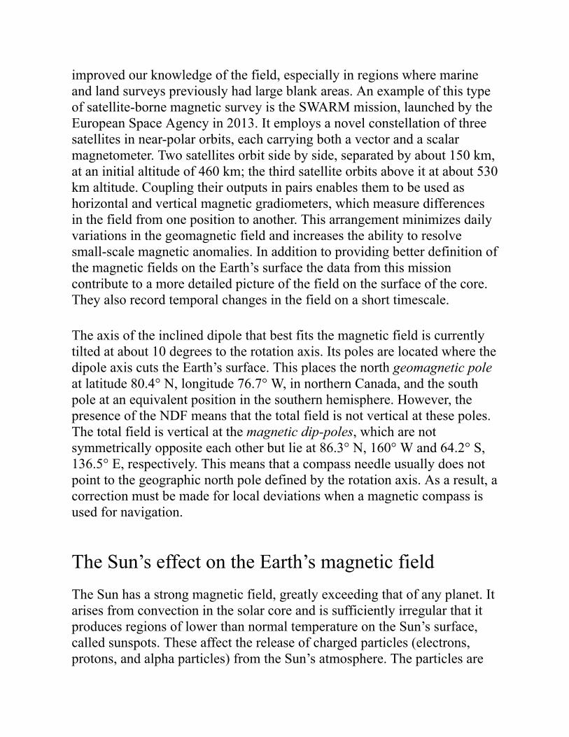
improved our knowledge of the field, especially in regions where marineand land surveys previously had large blank areas. An example of this typeof satellite-borne magnetic survey is the SWARM mission, launched by theEuropean Space Agency in 2013. It employs a novel constellation of threesatellites in near-polar orbits, each carrying both a vector and a scalarmagnetometer. Two satellites orbit side by side, separated by about 150 km,at an initial altitude of 460 km; the third satellite orbits above it at about 530km altitude. Coupling their outputs in pairs enables them to be used ashorizontal and vertical magnetic gradiometers, which measure differencesin the field from one position to another. This arrangement minimizes dailyvariations in the geomagnetic field and increases the ability to resolvesmall-scale magnetic anomalies. In addition to providing better definition ofthe magnetic fields on the Earth’s surface the data from this missioncontribute to a more detailed picture of the field on the surface of the core.They also record temporal changes in the field on a short timescale.

The axis of the inclined dipole that best fits the magnetic field is currentlytilted at about 10 degrees to the rotation axis. Its poles are located where thedipole axis cuts the Earth’s surface. This places the north geomagnetic poleat latitude 80.4° N, longitude 76.7° W, in northern Canada, and the southpole at an equivalent position in the southern hemisphere. However, thepresence of the NDF means that the total field is not vertical at these poles.The total field is vertical at the magnetic dip-poles, which are notsymmetrically opposite each other but lie at 86.3° N, 160° W and 64.2° S,136.5° E, respectively. This means that a compass needle usually does notpoint to the geographic north pole defined by the rotation axis. As a result, acorrection must be made for local deviations when a magnetic compass isused for navigation.

The Sun’s effect on the Earth’s magnetic fieldThe Sun has a strong magnetic field, greatly exceeding that of any planet. Itarises from convection in the solar core and is sufficiently irregular that itproduces regions of lower than normal temperature on the Sun’s surface,called sunspots. These affect the release of charged particles (electrons,protons, and alpha particles) from the Sun’s atmosphere. The particles are

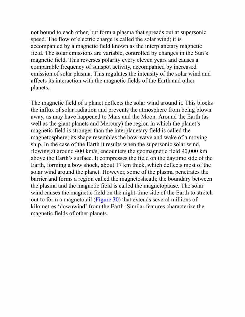
not bound to each other, but form a plasma that spreads out at supersonicspeed. The flow of electric charge is called the solar wind; it isaccompanied by a magnetic field known as the interplanetary magneticfield. The solar emissions are variable, controlled by changes in the Sun’smagnetic field. This reverses polarity every eleven years and causes acomparable frequency of sunspot activity, accompanied by increasedemission of solar plasma. This regulates the intensity of the solar wind andaffects its interaction with the magnetic fields of the Earth and otherplanets.

The magnetic field of a planet deflects the solar wind around it. This blocksthe influx of solar radiation and prevents the atmosphere from being blownaway, as may have happened to Mars and the Moon. Around the Earth (aswell as the giant planets and Mercury) the region in which the planet’smagnetic field is stronger than the interplanetary field is called themagnetosphere; its shape resembles the bow-wave and wake of a movingship. In the case of the Earth it results when the supersonic solar wind,flowing at around 400 km/s, encounters the geomagnetic field 90,000 kmabove the Earth’s surface. It compresses the field on the daytime side of theEarth, forming a bow shock, about 17 km thick, which deflects most of thesolar wind around the planet. However, some of the plasma penetrates thebarrier and forms a region called the magnetosheath; the boundary betweenthe plasma and the magnetic field is called the magnetopause. The solarwind causes the magnetic field on the night-time side of the Earth to stretchout to form a magnetotail (Figure 30) that extends several millions ofkilometres ‘downwind’ from the Earth. Similar features characterize themagnetic fields of other planets.

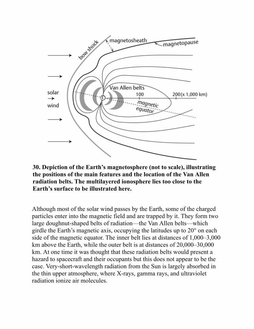
30. Depiction of the Earth’s magnetosphere (not to scale), illustratingthe positions of the main features and the location of the Van Allenradiation belts. The multilayered ionosphere lies too close to theEarth’s surface to be illustrated here.

Although most of the solar wind passes by the Earth, some of the chargedparticles enter into the magnetic field and are trapped by it. They form twolarge doughnut-shaped belts of radiation—the Van Allen belts—whichgirdle the Earth’s magnetic axis, occupying the latitudes up to 20° on eachside of the magnetic equator. The inner belt lies at distances of 1,000–3,000km above the Earth, while the outer belt is at distances of 20,000–30,000km. At one time it was thought that these radiation belts would present ahazard to spacecraft and their occupants but this does not appear to be thecase. Very-short-wavelength radiation from the Sun is largely absorbed inthe thin upper atmosphere, where X-rays, gamma rays, and ultravioletradiation ionize air molecules.

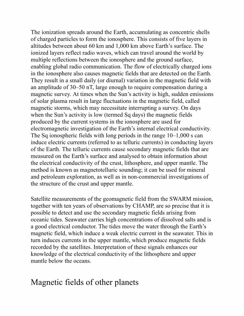
The ionization spreads around the Earth, accumulating as concentric shellsof charged particles to form the ionosphere. This consists of five layers inaltitudes between about 60 km and 1,000 km above Earth’s surface. Theionized layers reflect radio waves, which can travel around the world bymultiple reflections between the ionosphere and the ground surface,enabling global radio communication. The flow of electrically charged ionsin the ionosphere also causes magnetic fields that are detected on the Earth.They result in a small daily (or diurnal) variation in the magnetic field withan amplitude of 30–50 nT, large enough to require compensation during amagnetic survey. At times when the Sun’s activity is high, sudden emissionsof solar plasma result in large fluctuations in the magnetic field, calledmagnetic storms, which may necessitate interrupting a survey. On dayswhen the Sun’s activity is low (termed Sq days) the magnetic fieldsproduced by the current systems in the ionosphere are used forelectromagnetic investigation of the Earth’s internal electrical conductivity.The Sq ionospheric fields with long periods in the range 10–1,000 s caninduce electric currents (referred to as telluric currents) in conducting layersof the Earth. The telluric currents cause secondary magnetic fields that aremeasured on the Earth’s surface and analysed to obtain information aboutthe electrical conductivity of the crust, lithosphere, and upper mantle. Themethod is known as magnetotelluric sounding; it can be used for mineraland petroleum exploration, as well as in non-commercial investigations ofthe structure of the crust and upper mantle.

Satellite measurements of the geomagnetic field from the SWARM mission,together with ten years of observations by CHAMP, are so precise that it ispossible to detect and use the secondary magnetic fields arising fromoceanic tides. Seawater carries high concentrations of dissolved salts and isa good electrical conductor. The tides move the water through the Earth’smagnetic field, which induce a weak electric current in the seawater. This inturn induces currents in the upper mantle, which produce magnetic fieldsrecorded by the satellites. Interpretation of these signals enhances ourknowledge of the electrical conductivity of the lithosphere and uppermantle below the oceans.

Magnetic fields of other planets

Mercury, the closest rocky planet to the Sun, has a global magnetic fieldthat is close to being a dipole. However, the Messenger spacecraft foundthat Mercury’s field is about 100 times weaker than the Earth’s, andcomparable in strength to the external magnetic fields due to the solar wind,which is strong because of Mercury’s closeness to the Sun. As a result theplanet’s bow shock is very close to its surface.

Data from spacecraft that flew past Venus (e.g. Mariner 2 in 1962) ororbited the planet (e.g. Venus Express in 2006) have found that it does nothave a significant magnetic field. This may be because it rotates so slowly:one day on Venus is equivalent to 243 Earth days. Rotation and the relatedCoriolis force, together with convection, are necessary factors for a self-sustaining dynamo, so possibly Venus does not rotate fast enough togenerate a magnetic field. Mars and the Moon do not at present have globaldipole magnetic fields, but orbiting satellites have detected magnetic fieldsrelated to magnetized areas of rock on their surfaces. This suggests thateach may have possessed an internally generated magnetic field in thegeological past. The Moon has a crust, mantle, and small core. However,the radius of the lunar core is only about 10 per cent that of the Moon, andthe core is too small to support a dynamo. Satellite missions to Mars havemeasured intensely magnetized patches of crust but the planet does not havea global magnetic field that could be attributed to an internal dynamo.

The gaseous giant planets Saturn, Uranus, and Neptune have strongercentral dipoles than the Earth, but these planets are so large that themagnetic fields on their surfaces are weaker than those on the Earth. Incontrast, Jupiter has a huge magnetic field produced by a central dynamo inits core of liquid metallic hydrogen. Jupiter’s dipole is 20,000 timesstronger than the Earth’s and occupies a larger share of the planet’s interior.As a result Jupiter’s non-dipole field components are strong relative to itsdipole, which nevertheless predominates. The gaseous giant planet does nothave a solid surface, but at the radial distance of its nominal surface themagnetic field is fourteen times stronger than on the Earth.

Magnetic properties of rocks

The Earth’s magnetic field provides information about processes that arecurrently active deep within the Earth, and also helps scientists tounderstand the tectonic processes that have changed the planet in thegeological past. The ability to analyse properties of the ancient magneticfield is based on the magnetic properties of rocks. A tiny fraction of theminerals in a rock—up to 1 per cent in some igneous and metamorphicrocks, but as low as 0.01 per cent in sedimentary rocks—possess magneticproperties similar to those of iron and are classified loosely asferromagnetic. An important characteristic of these minerals is that they canbe permanently magnetized in the geomagnetic field while they are beingformed, acquiring a remanent magnetization. Equally important, theminerals can retain the remanent magnetization for very long periods oftime.

Why are rocks able to act as magnetic recorders? The extraordinary stabilityof a magnetization in some rocks and sediments is due to the very fine grainsize of the tiny proportion of magnetic minerals they contain, the mostimportant of which are the iron oxides magnetite and hematite. An igneousrock forms from a hot fluid magma; as it cools, mineral grains crystallizeand it solidifies. On further cooling magnetite and hematite grains in therock pass through a critical temperature called the Curie point; below thistemperature the grains behave like tiny magnets, with an importantdistinction. The grains are fixed in the solid rock, but the magnetizationsinside the grains are able to align with and record the direction of themagnetic field in which it cools. Unless the rock is modified by some laterprocess, its thermally acquired remanent magnetization is permanent. Forexample, the oceanic crust that forms at a spreading plate margin consists ofbasalt, an igneous rock, which becomes magnetized as it cools to ambienttemperature in the geomagnetic field. Basalts sampled from oceanic crustthat formed more than one hundred million years ago are still magnetized inthe direction of the field in which they cooled.

Sedimentary rocks are also able to record the magnetic field in which theyform. When a rock weathers and erodes, fine particles are transported bywind or water and deposited in a river bed, lake, or sea. Fine grains ofmagnetite in the waterlogged sediment can behave like miniature compassneedles and align with the magnetic field during or shortly after deposition,

thus acquiring a weak but stable magnetization that dates from the time ofdeposition. The remanent magnetization becomes locked into thesedimentary rock during the natural geochemical processes that caused it toharden. As in lavas, this magnetization also can survive for very long times.For example, the magnetizations of limestones from the Apennines andVenetian Alps still carry a faithful record of the geomagnetic field duringthe Late Jurassic, Cretaceous, and Palaeogene periods of geological time, aninterval that lasted from 155 Myr to 25 Myr ago.

PalaeomagnetismInvestigations of secular variation recorded in the magnetizations of rocksand sediments indicate that, averaged over long geological time intervals,the dipole tilt and the NDF components have mean values close to zero.This means that the long-term magnetic field corresponds to a dipole at thecentre of the Earth with its axis along the rotation axis. This is known as thegeocentric axial dipole (GAD) hypothesis. It is the fundamental assumptionof the discipline of palaeomagnetism, which has documented the motions ofthe continents relative to each other during hundreds of millions of yearsand has shown that the magnetic field has reversed polarity numeroustimes.

The palaeomagnetic method measures the direction of the remanentmagnetization in rocks, specified by two angles: inclination and declination.The inclination is the angle between the direction of the GAD field and thehorizontal surface of the Earth; the declination is the angle between thedepositional magnetic north direction and geographic north. The inclinationof the magnetization is the same as that of the field at which it was acquiredand thus depends on the latitude (Figure 29). At the north magnetic pole thefield points vertically downward and the inclination is 90 degrees;proceeding away from the pole the inclination gets progressively flatteruntil it is horizontal at the equator; in the southern magnetic hemisphere thefield points upwards and has negative inclinations which steepen until thesouth magnetic pole where the direction is vertically upward. A simpleequation describes this variation and allows the latitude of a place to bedetermined from the field inclination. Thus, if the inclination of the

magnetization direction in a rock outcrop is determined, the latitude wherethe rock was formed can be calculated, and from this the distance to theplace where the north magnetic pole was located at that time. Thedeclination of the magnetization describes the direction from the samplingsite to the pole. Thus, if one proceeds from the sampling location in thedirection given by the declination for a distance calculated from theinclination, the location of the ancient geomagnetic north pole can be found.Due to plate tectonic motions since the rock was formed, the ancient poleposition no longer lies on the present rotation axis and so it is known as thevirtual geomagnetic pole (VGP).

Apparent polar wander and continental driftPalaeomagnetic research on both igneous and sedimentary rocks of all ageshas yielded average VGP locations for each age for each continent. It wasobserved early in these studies that the poles for a given continent appearedto move with time, defining a path of apparent polar wander (APW) that isunique to the continent. Moreover, each continent was found to have itsown APW path, located approximately on the opposite side of thegeographic pole from the continent. There is only a single geocentric axialdipole, which clearly could not have moved simultaneously along severaldifferent paths. Consequently, the different APW paths are evidence that theindividual continents have moved relative to the rotation axis, a behaviourcalled continental drift. This slow motion of the continents was firstproposed on the basis of different evidence early in the 20th century toexplain the symmetry of shorelines and geological features across theAtlantic Ocean. The theory was contentious and set geophysicists againstgeologists because a suitable mechanism for moving the continents couldnot be found. Palaeomagnetic evidence for continental drift grew in the1950s but the mechanism remained a mystery until the development ofplate tectonic theory, which allowed the APW paths of individual continentsto be recognized as traces of past plate motions.

The APW paths can be used to reconstruct earlier positions of thecontinents. For example, the palaeomagnetic poles of Europe and NorthAmerica from Silurian times (about 440 Myr ago) to the middle Jurassic

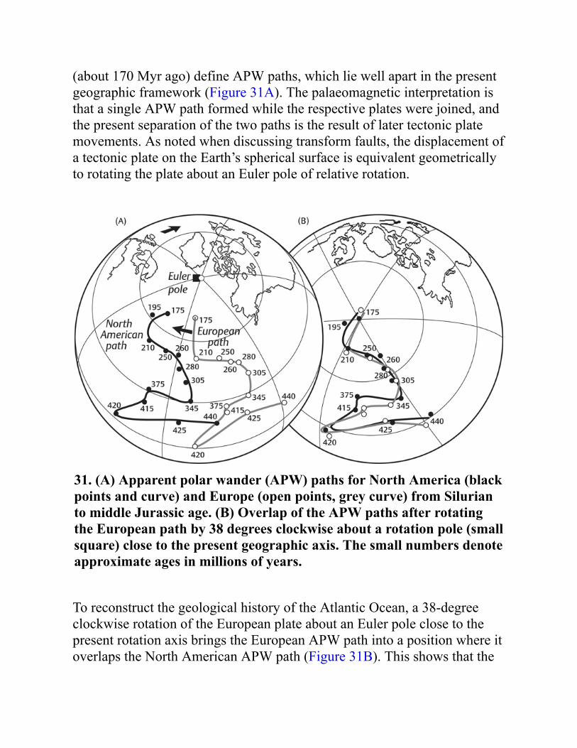
(about 170 Myr ago) define APW paths, which lie well apart in the presentgeographic framework (Figure 31A). The palaeomagnetic interpretation isthat a single APW path formed while the respective plates were joined, andthe present separation of the two paths is the result of later tectonic platemovements. As noted when discussing transform faults, the displacement ofa tectonic plate on the Earth’s spherical surface is equivalent geometricallyto rotating the plate about an Euler pole of relative rotation.

31. (A) Apparent polar wander (APW) paths for North America (blackpoints and curve) and Europe (open points, grey curve) from Silurianto middle Jurassic age. (B) Overlap of the APW paths after rotatingthe European path by 38 degrees clockwise about a rotation pole (smallsquare) close to the present geographic axis. The small numbers denoteapproximate ages in millions of years.

To reconstruct the geological history of the Atlantic Ocean, a 38-degreeclockwise rotation of the European plate about an Euler pole close to thepresent rotation axis brings the European APW path into a position where itoverlaps the North American APW path (Figure 31B). This shows that the

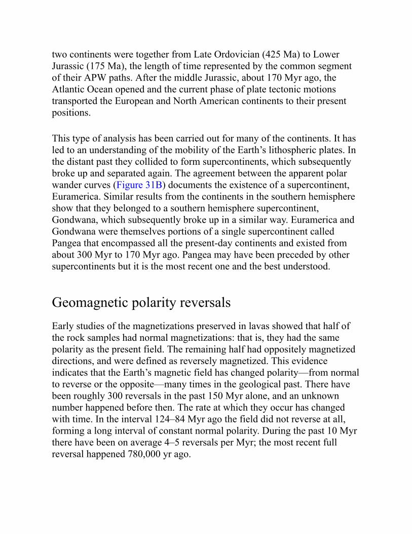
two continents were together from Late Ordovician (425 Ma) to LowerJurassic (175 Ma), the length of time represented by the common segmentof their APW paths. After the middle Jurassic, about 170 Myr ago, theAtlantic Ocean opened and the current phase of plate tectonic motionstransported the European and North American continents to their presentpositions.

This type of analysis has been carried out for many of the continents. It hasled to an understanding of the mobility of the Earth’s lithospheric plates. Inthe distant past they collided to form supercontinents, which subsequentlybroke up and separated again. The agreement between the apparent polarwander curves (Figure 31B) documents the existence of a supercontinent,Euramerica. Similar results from the continents in the southern hemisphereshow that they belonged to a southern hemisphere supercontinent,Gondwana, which subsequently broke up in a similar way. Euramerica andGondwana were themselves portions of a single supercontinent calledPangea that encompassed all the present-day continents and existed fromabout 300 Myr to 170 Myr ago. Pangea may have been preceded by othersupercontinents but it is the most recent one and the best understood.

Geomagnetic polarity reversalsEarly studies of the magnetizations preserved in lavas showed that half ofthe rock samples had normal magnetizations: that is, they had the samepolarity as the present field. The remaining half had oppositely magnetizeddirections, and were defined as reversely magnetized. This evidenceindicates that the Earth’s magnetic field has changed polarity—from normalto reverse or the opposite—many times in the geological past. There havebeen roughly 300 reversals in the past 150 Myr alone, and an unknownnumber happened before then. The rate at which they occur has changedwith time. In the interval 124–84 Myr ago the field did not reverse at all,forming a long interval of constant normal polarity. During the past 10 Myrthere have been on average 4–5 reversals per Myr; the most recent fullreversal happened 780,000 yr ago.

Exactly what causes the field to change polarity is not known, but it is atopic of current research into the geomagnetic dynamo. The power ofsupercomputers is required to construct models of how the magnetic field iscreated and how the process is affected by different factors, such as thegrowth of the solid inner core and the influence of the lower mantle D″layer on convection in the fluid core. Palaeomagnetic results provide someboundary conditions for these computations.

Investigations in lavas and sediments have shown that the intensity of thedipole decreases by an order of magnitude during a polarity reversal. It doesnot vanish, but decreases to a low value and subsequently recovers as thenew polarity is established. The process takes about 5,000–10,000 yr. Atpresent, the intensity of the geomagnetic field is decreasing at roughly 5 percent per century. This does not mean a reversal has started: the decrease inintensity could be a natural fluctuation.

During a polarity reversal, the direction of the field changes more rapidlythan the intensity does, taking about 3,000–5,000 yr to reverse. On a humantimescale the polarity transition is very slow, but on a geological timescaleit is rapid. The polarity interval before and after a reversal is stable andpersists much longer: it is called a polarity chron and may last from 50,000to several million years. Sometimes the normal or reverse polarity chron isinterrupted by shorter intervals of opposite polarity called subchrons. Thepattern of magnetic reversals is irregular but distinctive for different times.This makes it possible for geologists to use the reversal pattern as ageological ‘fingerprint’ to date and correlate sedimentary rocks.

Igneous rocks acquire a thermal remanent magnetization during coolingfrom a molten state. They contain radioactive minerals that allow the rocksto be dated radiometrically, which makes it possible to construct a polarity-age timescale. Early investigations in lavas showed a characteristicsequence of normal and reverse polarity during the last few million years.The same polarity sequence was soon discovered in deep-sea sediments(Figure 32B), which have a depositional remanent magnetization acquiredduring deposition and sedimentation. Although the magnetizations wereacquired by different mechanisms, the igneous and sedimentary polarity

records agree, confirming that the polarity sequence is a feature of thegeomagnetic field, rather than an artefact of the rock, which had beenproposed by critics. The numerical ages of polarity reversals in both recordsare obtained by radiometric dating of the lavas. The dated polarity sequenceis equivalent to a timescale that can be used to determine the ages of rocksand geological events. Numerous subsequent investigations have been madein cores drilled into the sedimentary layers on the ocean floor, as well as inoutcrops of marine sedimentary rocks now exposed on land.

32. (A) Marine magnetic anomalies along a profile across the EastPacific Rise, and the interpreted record of geomagnetic polarity. (B)Geomagnetic polarity sequences from magnetic stratigraphy interrestrial lavas and deep-sea sediments.

The determination of magnetic polarity in stratigraphically dated sedimentsis called magnetic stratigraphy. It has refined and extended the geomagneticpolarity timescale, so that this is now well known for most of the time sincethe breakup of Pangea around 170 Myr ago. This is possible because thepolarity sequence found in lavas, sedimentary rocks, and oceanic sedimentsis also recorded in the magnetization of the oceanic crust formed since thattime. The crustal magnetization disturbs the local geomagnetic field causinganomalies (Figure 32A) that can be measured by a magnetometer towedbehind a ship in a marine magnetic survey.

Oceanic magnetic anomalies and plate tectonicsIn the 1950s marine geophysicists found patterns of strong magneticanomalies in the Pacific Ocean aligned as parallel lineations. Their originwas explained in 1963 by Frederick Vine and Drummond Matthews inCambridge and independently by Lawrence Morley in Canada. The Vine–Matthews–Morley hypothesis relates the striped patterns of magneticanomalies to the processes at oceanic ridges. The ridge is a divergent plateboundary, or spreading margin, where basaltic lavas are extruded that arestrongly magnetized in comparison to other rocks. They acquire a thermalremanent magnetization in the direction of the ambient geomagnetic field inwhich they cool. Sea-floor spreading carries the magnetized oceanic crustaway from the spreading axis. As a result, the oceanic crust is characterizedby magnetized stripes, hundreds of kilometres long and 10–50 km wide andoriented parallel to the spreading ridge, that are magnetized alternately inopposite directions.

The magnetic field above normally magnetized crust has the same directionas the present field and reinforces it, making it locally stronger thanaverage; the difference is a positive anomaly. Conversely, over reverselymagnetized crust the field due to the magnetization is opposite to thepresent field and makes it weaker than average; in this case the difference isa negative anomaly. A magnetic survey across the magnetized stripesmeasures lineated magnetic anomalies with amplitudes of several hundrednanotesla (Figure 32A) corresponding to whether the underlying oceaniccrust has normal or reverse polarity. The magnetic lineation patterns onopposite sides of a spreading ridge are symmetric. The anomaly patternyields a record of the magnetic field reversals that happened during sea-floor spreading. The marine polarity sequence correlates well with polaritysequences found independently in lavas on land and in sediments from theocean floor where they overlap (Figure 32B). These records from differentsources mutually confirm and support each other. Moreover, because theages of the lavas and sediments can be determined, the oceanic magneticanomalies allow the ocean floor to be dated from the anomaly pattern,without needing to take rock samples.

By matching dated magnetic lineations on opposite sides of an oceanicridge, geophysicists have been able to trace and time the motions of tectonicplates. For example, on a magnetic profile across a lineated set of anomalieson the Pacific–Antarctic ocean ridge (Figure 32A) sharp positive anomaliesare evident 80 km east and west of the centre of the anomaly sequence.These were formed at the same time, about 2 Myr ago, when the oppositesides of the ridge were together at the spreading axis. Subsequent platemotion has separated them. If the plates adjoining the ridge are moved backtogether, so that the long stripes of magnetized crust corresponding to thesame anomalies coincide, the positions of the plates 2 Myr ago can bereconstructed. Repeating this exercise for each dated pair of magneticlineations reveals the history of relative motion of the plates and thecontinents that lie on them. The results are more detailed than the‘continental drift’ reconstructions derived from matching palaeomagneticAPW paths. However, the method can only be applied to the presentoceans, which are younger than 160 Myr. The palaeomagnetic method ofmatching APW paths provides reconstructions of ancient supercontinentsfor older epochs, albeit with less detail.

Chapter 8Afterthoughts

Geophysics has made many important advances towards understanding thebehaviour and properties of planet Earth. Geophysical research continues tomake discoveries and developments that benefit society. Many problemspresented by the Earth—such as the prediction of both the time and locationof an earthquake—have been researched by geophysicists for decades butremain unsolved because of the complex nature of their causes.

Many sophisticated geophysical techniques were developed originally forcommercial purposes by the oil and mineral industries but havesubsequently found their way into general use. On a small scale, the field ofenvironmental geophysics uses seismic, magnetic, gravimetric, andelectromagnetic methods to investigate the shallow underground (the top100 m or so) and resolve issues involving the environment; typically thesemight be investigations of geological hazards, the groundwater, orarchaeological sites. At the other extreme of scale and expense, numeroussatellite missions have been carried out with geophysical goals, and havedelivered abundant amounts of new information about the planet,complementing and augmenting existing knowledge, especially about thegravitational and magnetic fields.

The advances in methodology are illustrated by the observation andmeasurement of rates of plate motion. These rates were once based solelyupon the analysis of magnetic anomalies at spreading ridges, but are nowsupplemented by space-geodetic observations made from satellites. Long-term measurements at VLBI stations on different continents have recordedthe changing separations of some continents that result from plate tectonics.For example, the distance between VLBI stations in North America andEurope is increasing steadily at a mean rate of 17 mm/yr (about half as fastas fingernails grow). The best-known space geodetic technique, GPS, whendeployed in global networks of receivers, can observe plate motionsdirectly, even detecting spreading rates at incipient plate boundaries—suchas the East African rift zone—which have not yet formed a classicalspreading ridge.

As in other sciences, new hypotheses are not always accepted initially ingeophysics. This is often because of political and human factors. Ptolemy’sgeocentric model of the solar system used artificial constructs such as‘epicycles’ and ‘equants’ to account for anomalous planetary motions;encouraged by religious dogma, the model was held to be true for morethan 1,500 years. It was only replaced by the heliocentric model ofCopernicus after irrefutable evidence from the planetary observations ofKepler and Galileo became widely accepted. In a like manner, many earthscientists only accepted the theory of plate tectonics when the results ofdeep-sea drilling in the Atlantic Ocean provided hard evidence that the ageof the oceanic crust increased with distance from the mid-oceanic ridge.Similar academic scepticism greeted the hypothesis of Luis and WalterAlvarez that the extinctions of many forms of life at the end of theCretaceous Period (66 Myr ago) resulted from the impact of anextraterrestrial object, an asteroid or comet. The impact theory finallybecame generally accepted when geophysicists located the crater producedby the impact at Chicxulub, off the coast of the Yucatan peninsula inMexico. Similarly, the existence of mantle plumes that feed hotspots hasbeen a controversial topic. Most geodynamicists favour the plume concept,which is compatible with observed geoid and topography anomalies overthe hotspot locations, but some seismologists maintain that the availabledata do not fit plume theory. However, analysis of hotspots indicated thatthere are three different types; some are tied by plumes to the D″ layer at

the core–mantle boundary, some are related to the lower mantlesuperplumes under Africa and the Pacific, and others are linked with ashallower origin. Based on a global shear wave velocity model of themantle, recent seismic analysis has shown vertically continuous low-velocity columns under some—but not all—hotspots. Although broaderthan the expected thin conduits, they lend seismic support to the plumetheory for these hotspots.

The Earth is a bountiful laboratory for scientific investigations. Geophysicshas always been a key player in developing an understanding of how theEarth works. It has an indispensable role in the search for the materialresources that are needed for the smooth functioning of modern society.Geophysics helps to locate the fossil fuels needed to supply our energyneeds, and the rare earth metals that are essential components of everydaydevices, such as mobile phones and computers. On the other hand,geophysics is an important factor in protecting society against naturalhazards by monitoring earthquakes, volcanoes, and unstable slopes, and bywarning against possible tsunamis and the negative effects of solar flares onelectrical networks.

Due to the complexity of many natural topics, geophysical investigationsoften do not yield data that fully comply with a theory. Earth scientistscannot control the natural events that occur, but can only observe and try tounderstand them. The equipment for attaining these goals improvescontinually, in a remarkably rapid and encompassing manner. Land-basedmethods are now augmented in several fields by remarkable observationsfrom space. In some cases multiple sources of evidence are broughttogether to clarify an important issue. For example, palaeomagnetismdocuments plate motion across a stationary hotspot; satellite and marineobservations of gravity, together with oceanic bathymetry, record the effectsof uplift; while seismology and geochemistry contribute to solving thegeodynamic basis of the observations. The processes at work in the Earthare complex and their causes are well hidden, but this provides eachdiscipline of geophysics with interesting challenges to engage present andfuture generations of scientists.

Further reading

Most of the following books are written at an introductory level and aresuitable for a lay reader. They include general books on the earth sciences,in which geophysical topics are handled within a larger framework ofinformation about the Earth. Some books describe specific geophysicaltopics in more detail than is possible in the compressed format of this book.Three are textbooks, perhaps more suited to students who intend to continuea career in earth sciences, but which contain chapters that provide usefulreference material and more in-depth knowledge than contained in thisbook.

Introductory books on the earth sciencesG. C. Brown, C. J. Hawkesworth, and R. C. L. Wilson (eds) (1992), Understanding the Earth,

Cambridge University Press, Cambridge, 551 pp.F. Press, R. Siever, J. Grotzinger, and T. Jordan (2003), Understanding Earth, 4th edn, W. H.

Freeman, San Francisco, 568 pp.M. Redfern (2003), The Earth: A Very Short Introduction, Oxford University Press, Oxford, 141 pp.

Specific topics in geophysicsB. A. Bolt (2003), Earthquakes, 5th edn, W. H. Freeman and Co., New York, 320 pp.R. F. Butler (1992), Paleomagnetism: Magnetic Domains to Geologic Terranes, Blackwell Scientific,

Boston, 319 pp.G. F. Davies (1999), Dynamic Earth: Plates, Plumes and Mantle Convection, Cambridge University

Press, Cambridge, 470 pp.P. Kearey, K. A. Klepeis, and F. J. Vine (2013), Global Tectonics, 3rd edn, John Wiley and Sons,

New York, 496 pp.

P. Molnar (2015), Plate Tectonics: A Very Short Introduction, Oxford University Press, Oxford, 136pp.

Geophysical textbooks for reference or more in-depth readingC. M. R. Fowler (2004), The Solid Earth: An Introduction to Global Geophysics, 2nd edn,

Cambridge University Press, Cambridge, 500 pp.W. Lowrie (2007), Fundamentals of Geophysics, 2nd edn, Cambridge University Press, Cambridge,

381 pp.A. E. Mussett and M. A. Khan (2000), Looking into the Earth: An Introduction to Geological

Geophysics, Cambridge University Press, Cambridge, 492 pp.

Index

Aacceleration 71, 72, 81, 84, 85adiabatic temperature 99, 100, 101advection 96Alpine Fault, New Zealand 65Alvarez, Luis and Walter 128angular momentum 7, 8, 10, 13, 14, 82anisotropy, shear wave 39, 41anomaly

gravity 83, 85, 86, 87magnetic 110, 125, 126seismic velocity 42

aphelion 12, 14, 15, 20apparent polar wander 119, 120, 121apsides 14, 19asteroid belt 11asthenosphere 40, 99astronomical unit 9, 11Atlantic Ocean opening 120auxiliary plane 60

Bbarycentre 81basalt 86, 104, 105, 117, 125Benioff, Hugo 57Big Bang model 7

bow shock 113Brahe, Tycho 12bulk modulus 23, 25, 35

CCeres 11CHAMP satellite mission 111, 115Chandler, Seth 15Chandler wobble 15climatic cycles 19, 20, 21conductivity 95, 114continental drift 119, 126convection 39, 96, 101, 103, 105Copernicus 2, 128core 8

properties 35, 36, 38, 39, 101, 107temperature 99

core–mantle boundary 38, 41, 102, 103, 110Coriolis acceleration 85, 115critical refraction 32, 34crustal structure 39, 43, 44

DD″ layer 41, 102, 103, 122deformation

brittle and ductile 39elastic 22, 23, 70viscoelastic 91

density 25, 86mean for the Earth 74, 88variation with depth 37, 74

differentiation 94diffraction 33, 35, 36dipole magnetic field 107, 109dispersion of surface waves 28, 33diurnal variation of magnetic field 114dynamic topography, ocean surface 81dynamo model, magnetic field 107, 108, 115, 116

E

Earthinternal structure 9, 33, 37, 38, 98magnetic field 2, 106mean density 74, 88orbit 12radius 69, 71, 81rotation 69, 82shape 3, 15, 69, 70tides 82

Earth–Moon distance increase, 82earthquakes 4, 23, 47

damaging seismic waves 26, 27deep focus 26, 27, 57, 64elastic rebound model 48energy release 50focal depths 66fore- and aftershocks 53frequency 50intensity 51, 52, 59location of source 67magnitude 49monitoring 66prediction 66, 67secondary effects 53seismic moment 49slow earthquakes 66

eccentricity of orbit 13, 16, 18, 19ecliptic 11, 17elastic limit 22, 48energy 7, 13, 74, 92Eötvös acceleration and correction 84, 85epicentre 26, 28, 34, 35, 37, 51, 55, 56, 59, 60equatorial bulge 17, 72equinoxes 12, 14, 17equipotential surface 75Euler, Leonhard 15, 65, 120Euler pole of relative rotation 65, 120, 121Euramerica 120European Geotraverse Project 44

Ffault plane solutions 59, 61, 62, 63, 64Fennoscandian uplift 89, 90, 91

figure of the Earth 69flattening of ellipsoidal Earth 15, 69, 71focal mechanism 59, 61, 62, 63, 65focus of earthquake 49, 55, 59forward modelling 37, 55fracture zones 64

GGalileo Galilei 3, 73Galileo positioning system, 78Gauss, Carl Friedrich 108geocentric axial dipole hypothesis 118geodesy 3, 67, 76, 79geoid 75, 76, 77, 80, 81geological time 2geomagnetism 108

dipole and non-dipole fields 109dynamo model of origin 122magnetic poles 106, 112polarity timescale 124

geophone 31, 32geophysical exploration 1, 32geotherm 98geothermal flux 93Gilbert, William 3, 106GOCE satellite mission 80Gondwana 120GPS, Global Positioning System 4, 78, 79, 90, 128GRACE satellite mission 80gravimeter 72, 73, 83, 84gravitation 12, 14, 70, 88gravity

anomaly 83, 85, 86, 87corrections 83, 84direction 72, 73variation with depth 74variation with latitude 72

ground roll 32Gutenberg discontinuity 38Gutenberg, Beno 38

H

Hawaiian hotspot 104heat flow 93, 95, 96, 97, 102heat sources and transport 92, 93, 94, 96hematite 117hotspots 104, 129hydrothermal circulation 97

Iinclination, magnetic 109, 111, 118insolation 18, 19, 20interference fringes 78International Geomagnetic Reference Field 108International Reference Ellipsoid 75interplanetary magnetic field 112intraplate earthquakes 59invariable plane 10inversion 37ionosphere 114isoseismal map 51isostasy 88, 89, 90isotopes 20, 21, 94

JJeffreys, Harold 38Jupiter 9, 10, 11

influence on Earth’s orbit 18magnetic field 116

KKelvin temperature scale 92Kepler, Johannes 3, 12

Llaws of planetary motion 12, 14Lehmann, Inge 38length of the day 14, 17, 82Lithoprobe Project 44lithosphere 39

age 97cooling 96flexure 87plates 40, 57, 58, 103thickness 40, 44, 97

Love wave 27low-velocity zone 40

Mmagnetic field 107, 108, 109, 115magnetic storms 114magnetic stratigraphy 124magnetite 117magnetization of rocks 116, 117, 123, 124magnetometer 109, 124magnetosphere 112, 113magnetotelluric sounding 114magnitude of earthquakes 49, 50, 66mantle 8, 35, 39

convection 102, 103, 104, 105mineral phase changes 38, 41, 43, 103, 105plumes 103, 104, 105, 128

Mars 9, 11, 115Matthews, Drummond 124megathrust 63melting points in the Earth 8, 99, 100, 101Mercalli, Giuseppe 51Mercury 11, 13, 70, 115microplates 58microseisms 44Milankovitch, Milutin 20Moho 39, 44, 87Mohoroviçiç, Andrija 39Moon

magnetic field 115origin 8precession of Earth’s rotation axis 17precession of lunar orbit 18rotation 82tides on the Earth 81

Morley, Lawrence 124

Nnanotesla 110, 125natural oscillations 28, 29, 37Neptune 11New Madrid earthquakes 59Newton, Isaac 3, 12, 14, 69, 70non-dipole magnetic field 112normal gravity 73normal modes of vibration 28nuclear explosion recognition 66nutation 15, 18

Oobliquity 14, 17, 18, 19oceanic features

deep-sea trenches 63, 87, 98depth 97heat flow 95island arcs 63island chains 104magnetic anomalies 124, 125plate thickness 97seismicity 57

Oldham, Richard 38olivine 41orbital forcing 21orogenic belt 44oscillations, natural 26, 28, 29oxygen isotope ratios 20, 21

PP wave 24, 25paleomagnetism 118, 120, 129Pangea 120, 124penetration depth of solar heating 93penetration depth of surface waves 28peridotite 41perihelion 12, 13, 14, 20perovskite 41planetary orbits 9, 13

planetesimals 8planets 6, 9, 10, 11, 12

magnetic fields 115, 116plate boundaries 57, 62, 63, 64, 65plate tectonics 3, 65Pluto 11, 83polarity of magnetic field 2, 21, 122, 124post-perovskite 41potential 75PP, PKP, PKIKP seismic rays 35precession 16, 17, 18, 19pressure at Earth’s centre 74protoplanets 8Pythagoras, spherical Earth 69

Rradiation 106, 107, 111, 112, 114Rayleigh wave 26, 45, 46reference ellipsoid 71, 73, 75, 77, 83reflection and refraction 30, 33

crust and lithosphere structure 43, 44Richter, Charles 49Ring of Fire 54root-zone of mountain 87, 88rotation slowing, Earth and Moon 82

SS wave 24, 25satellite geophysics 67, 76, 79, 80, 111, 115Saturn 11scattering of seismic energy 27sea-floor spreading 63, 125secular variation 108, 118seismic gap theory 67seismic noise 31, 45, 46seismic velocity-depth profiles 37, 45, 55seismicity 47, 56, 57, 59seismogram 23, 26, 27

first-motion analysis 59, 60, 62, 66seismograph 23seismology 4, 22

body-wave velocities 37crust and lithosphere structure 44reflection and refraction 30, 31, 33, 43, 44seismic impedance 31seismic phases 34, 35, 36seismic ray 29, 34tomography 42, 43, 103

seismometer 4, 23, 24shadow zone 34, 35, 38shape of the Earth 75shear modulus 23, 25, 35, 49shear waves 25, 39, 41SKS, SKiKS seismic rays 36slab pull 98solar radiation 93solar system 2, 8, 10solar wind 112solidus 98, 100solstices 14South Atlantic magnetic anomaly 110spinel 41Stokes, George 76stress-strain relationship 22, 23, 48, 102structure of the Earth’s interior 9, 40subduction zone 43, 57, 64, 65, 98, 103Sumatra–Andaman earthquake and tsunami 54Sun 8, 82, 112supercontinent 120superplumes 105, 129surface waves 26, 27, 28, 49SWARM satellite mission 111, 115synthetic aperture radar (InSAR) 76, 78

Ttectonic fault 48, 61, 66tectonic plates 2, 40, 56, 57, 58, 126telluric currents 114, 115temperature 92

core 99depth profile 99, 100gradient 46, 94, 98, 101

test-ban treaty monitoring 4, 66thermal boundary layer 102, 103

tides 81, 82, 115timescale 2, 102transcurrent fault 64transform fault 62, 64Trans-Neptunian Objects 11travel-time curves 36, 37, 41, 55travel-time residuals 42triple junctions 65tsunami 53, 54

UUranus, 6, 11

VVan Allen radiation belts 113, 114Vening Meinesz, Felix Andries 89Venus 11, 115Very Long Baseline Interferometry 16Vine, Frederick 124Vine–Matthews–Morley hypothesis 124virtual geomagnetic pole 119viscoelasticity 91viscosity 80, 91, 102, 103

WWadati, Kiyoo 57

YYellowstone hotspot 104

DESERTSA Very Short Introduction

Nick Middleton

Deserts make up a third of the planet’s land surface, but if you picture adesert, what comes to mind? A wasteland? A drought? A place devoid of alllife forms? Deserts are remarkable places. Typified by drought andextremes of temperature, they can be harsh and hostile; but many desertsare also spectacularly beautiful, and on occasion teem with life. NickMiddleton explores how each desert is unique: through fantastic life forms,extraordinary scenery, and ingenious human adaptations. He demonstrates adesert’s immense natural beauty, its rich biodiversity, and uncovers a longhistory of successful human occupation. This Very Short Introduction tellsyou everything you ever wanted to know about these extraordinary placesand captures their importance in the working of our planet.

www.oup.com/vsi

LANDSCAPES ANDGEOMORPHOLOGYA Very Short Introduction

Andrew Goudie & Heather Viles

Landscapes are all around us, but most of us know very little about howthey have developed, what goes on in them, and how they react to changingclimates, tectonics and human activities. Examining what landscape is, andhow we use a range of ideas and techniques to study it, Andrew Goudie andHeather Viles demonstrate how geomorphologists have built on classicmethods pioneered by some great 19th century scientists to examine ourEarth. Using examples from around the world, including New Zealand, theTibetan Plateau, and the deserts of the Middle East, they examine some ofthe key controls on landscape today such as tectonics and climate, as wellas humans and the living world.

www.oup.com/vsi