Embed Size (px)
Citation preview

1
ADAPTIVE NEURAL NETWORK CONTROL BY ADAPTIVE INTERACTION
George Saikalis
Hitachi America, Ltd.
Research and Development Division
34500 Grand River Avenue
Farmington Hills, Michigan 48335
Feng Lin
Wayne State University
Department of Electrical and Computer Engineering
5050 Anthony Wayne Drive
Detroit, Michigan 48202
Abstract
In this paper, we propose an approach to adaptive neural network control by
using a new adaptation algorithm. The algorithm is derived from the theory of
adaptive interaction. The principle behind the adaptation algorithm is a simple but
efficient methodology to perform gradient descent optimization in the parametric
space. Unlike the approach based on the back-propagation algorithm, this
approach will not require the plant to be converted to its neural network
equivalent, a major obstacle in early approaches. By applying this adaptive
algorithm, the same adaptation as the back-propagation algorithm is achieved
without the need of backward propagating the error throughout a feedback
network. This important property makes it possible to adapt the neural network
controller directly. Control of various systems, including non-minimum phase
systems, is simulated to demonstrate the effectiveness of the algorithm.
Keywords: Adaptive Interaction, Adaptive Control, Neural Network Control, and
Back-propagation

2
1. Introduction
Since their rebirth in 1980’s, neural networks have found applications in many
engineering fields, including control. For example, neural networks have been
used for system identification [1] [2] [3] and adaptive control [4] [5] [6] [7]. Neural
network controllers can control not only linear systems but also nonlinear
systems [8] [9] [10] [11] [12] [13]. Neural network control designs are divided into
two major categories: (1) the direct design where the controller is a neural
network [14] [15] and (2) the indirect design where the controller is not itself a
neural network, but uses neural networks in its design and adaptation [16] [17].
Issues such as robustness [18] and stability [19] have also been discussed.
Many books on neural network control have been published, including [20] [21]
[22] [23].
There are two major factors that contribute to the popularity of neural networks.
The first factor is the ability of neural networks to approximate arbitrary nonlinear
functions [24] [25]. This is important because in many cases control objectives
can be more effectively achieved by using a nonlinear controller. The second
factor is the capability of neural networks to adapt [25] [26]. In fact, the way for
neural networks to adapt is very natural. It requires no model building or
parameter identification. Such a “natural” adaptivity is rather unique among man-
made systems (but abundant in natural systems). It makes control design a much
easy job. For example, we all know how difficult it is to design a nonlinear
controller. However, if we can let a neural network controller to adapt itself, then
we can sit back and relax. (We know that this will make some people nervous, as
they will insist on the proof of stability.)
To adapt neural networks, many learning (or adaptation) algorithms have been
proposed, the two essential categories being the supervised learning and the
unsupervised learning [5] [25] [26]. Within each of these categories, there are
algorithms for feedback and feedforward neural networks. For the unsupervised

3
learning applied to feedback networks, there is the Hopfield and Kohonen
approach among many others. For the unsupervised learning applied to
feedforward networks, there are the learning matrix and counterpropagation. For
the supervised learning applied to feedback networks, there are the Boltzmann
machine, recurrent cascade correlation and learning vector quantization. For the
supervised learning applied to feedforward networks, there are back-propagation,
time delay neural networks and perceptrons. These examples of learning
algorithms are by no means exhaustive; there are many others available in the
literature.
However, there is one main obstacle in the way to adapt neural network
controllers. That is, some most efficient adaptation algorithms such as back-
propagation algorithm cannot be applied directly to neural network controllers. To
use back-propagation algorithm, the system must consist of “pure” neurons. This
is because the back-propagation algorithm relies on a dedicated feedback
network to propagate the error back. No such network can be constructed if the
original system does not consist of pure neurons. However, the neural network
control system is “hybrid” because the plant to be controlled is usually not a
neural network. Therefore is it not possible to apply back-propagation algorithm
to adapt the controller directly.
To bypass this obstacle, people have tried to approximate the plant with a neural
network. But this may not always work because of the error in approximation. So,
what can we do? Fortunately, there is one adaptation algorithm proposed by
Brandt and Lin [27] that can do the same job as the back-propagation algorithm
but requires no feedback networks.
Using Brandt-Lin algorithm, the errors required for adaptation is inferred from
local information in such a way that the error back-propagation is done implicitly
rather than explicitly. As a result, Brandt-Lin algorithm can be implemented in a
simple and straightforward manner without using feedback network.

4
Mathematically, however, it can be shown that Brandt-Lin algorithm is equivalent
to the back-propagation algorithm.
Furthermore, Brandt-Lin algorithm can be applied to arbitrary systems, including
hybrid systems as we are dealing with in neural network control systems. This is
because Brandt-Lin algorithm is derived from a theory of adaptive interaction that
is applicable to a large class of systems. For example, it has been applied to self-
tuning PID controllers [28] and parameter estimation [29].
Using Brandt-Lin algorithm, we can adapt a neural network controller directly
without approximating the plant by a neural network. This not only eliminates the
error in approximation, but also significantly reduces the complexity of design.
The rest of the paper will be organized as follows. In Section 2, we will introduce
the theory of adaptive interaction and review Brandt-Lin algorithm for adaptation
in neural networks. In Section 3, we will propose our adaptive neural network
controller and apply Brandt-Lin algorithm to derive the adaptation law for the
controller. Simulation results will be presented in Section 4.
2. Theory and Background of Interactive Adaptation
The proposed adaptation algorithm is based on a recently developed theory of
adaptive interaction [27]. A general adaptation algorithm developed in the theory
of adaptive interaction is applied to adapt the system coefficients. Depending on
the application and configuration of the algorithm, the adjusted coefficients can
be neural network weights, PID gains or transfer function coefficients. To apply
the algorithm to a control system, the only information needed about the plant is
its Fréchet derivative. Furthermore, it will be shown that the Fréchet derivative
can be approximated by a certain constant. This will make the algorithm robust to
system uncertainties and changes and hence can be applicable to a large class
of systems.

5
The theory of interactive adaptation considers N subsystems called devices.
Each device (indexed by n ∈ Ν := {1,2,…,N}) has an integrable output signal yn
and an integrable input signal xn. The dynamics of each device is described as a
causal functional:
Ν∈Υ→Χ n,:F nnn
where Χn and Υn are the input and output spaces respectively. Therefore, the
relation between input and output of the nth device is given by:
Ν∈== n)],t(x[F)t)(xF()t(y nnnnn o
where ° denotes functional composition.
The interactions among devices are achieved by connections. Figure 1
shows a graphical illustration of devices and their connections. The set of all
connections is denoted by C.
Figure 1: Devices and their connections
In this paper, the following notations are used to represent relations between
devices and connections:
prec is the device whose output is conveyed by connection c,
postc is the device whose input depends on the signal conveyed by c,
In = { c : prec = n } is the set of input interactions for the nth device, and
On = { c : postc = n } is the set of output interactions for the nth device.
Device 1 Device 2
Device 3
Device 4 Device 5
C1
C2 C3 C4
PreC1 PostC1
6
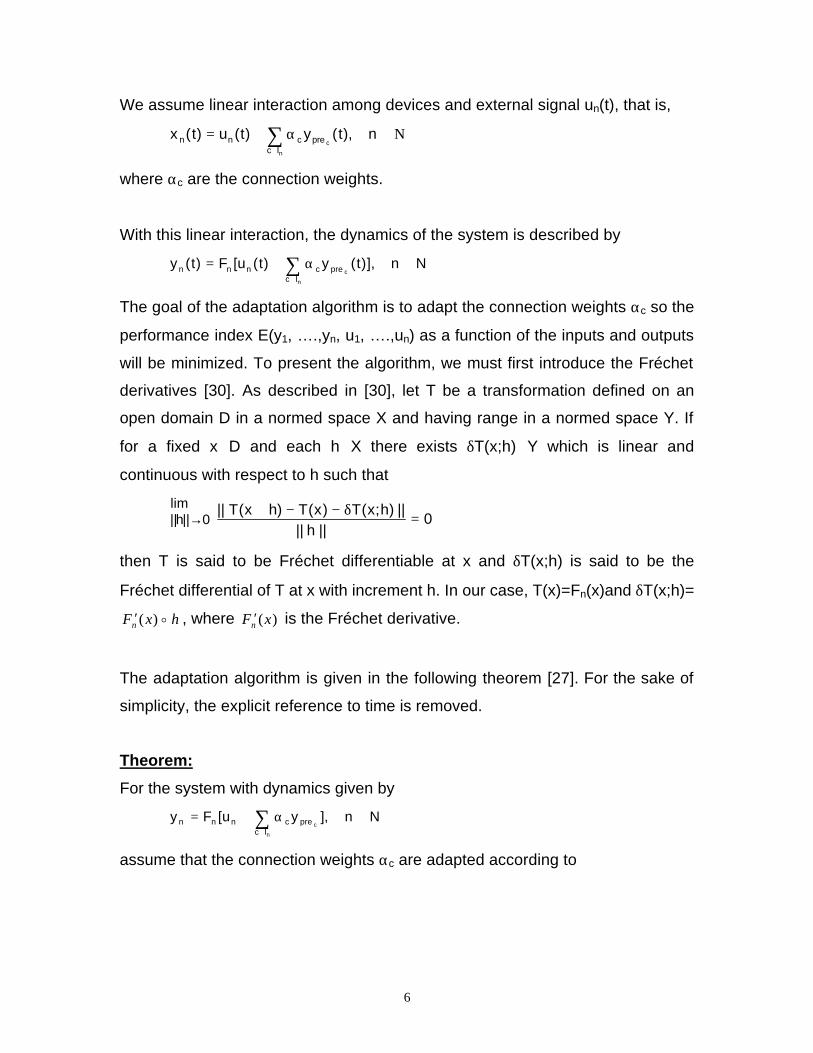
We assume linear interaction among devices and external signal un(t), that is,
∑∈
Ν∈α+=n
cIc
precnn n),t(y)t(u)t(x
where αc are the connection weights.
With this linear interaction, the dynamics of the system is described by
∑∈
∈α+=n
cIc
precnnn Nn],)t(y)t(u[F)t(y
The goal of the adaptation algorithm is to adapt the connection weights αc so the
performance index E(y1, ….,yn, u1, ….,un) as a function of the inputs and outputs
will be minimized. To present the algorithm, we must first introduce the Fréchet
derivatives [30]. As described in [30], let T be a transformation defined on an
open domain D in a normed space X and having range in a normed space Y. If
for a fixed x∈D and each h∈X there exists δT(x;h)∈Y which is linear and
continuous with respect to h such that
lim
0||h|| → 0||h||
||)h;x(T)x(T)hx(T||=
δ−−+
then T is said to be Fréchet differentiable at x and δT(x;h) is said to be the
Fréchet differential of T at x with increment h. In our case, T(x)=Fn(x)and δT(x;h)=
hxFn o)(′ , where )(xFn′ is the Fréchet derivative.
The adaptation algorithm is given in the following theorem [27]. For the sake of
simplicity, the explicit reference to time is removed.
Theorem:
For the system with dynamics given by
∑∈
∈α+=n
cIc
precnnn Nn],yu[Fy
assume that the connection weights αc are adapted according to
7
CcyxFy
E
yxFdy
dE
xFdy
dE
ccc
cpost ccss
s
ss
s
prepostpostOs post
postpostpostpost
postpostpost
ssc ∈′∂
∂−
′
′
= ∑∈
,][)][
][
( oo
oo
o
&& γααα
-------- (1)
where γ > 0 is the adaptation coefficient. If (1) has a unique solution for cα& , c∈C
(that is, the Jacobian determinant must not be zero in the region of interest), then
the performance index E(y1, ….,yn, u1, ….,un) will decrease monotonically with
time and the following equation is always satisfied:
Cc,ddE
cc ∈
αγ−=α&
It is important to note that if Fn and E are instantaneous functions, then the
functional composition ° can be replaced by multiplication. Equation (1) will then
be simplified to:
c
ccc
cpostc
c
cc
postprepostpost
Osss
post
prepostpostc y
E.y].x.[F.
y
y].x.[F
∂∂′γ−αα
′=α ∑
∈
&& -------- (2)
The above equations can be applied to a very general class of systems, including
neural networks, as shown below.
A neural network will be decomposed in multiple devices as described in Figure
1. Figure 2 shows a graphical representation for a simple neural network.
Figure 2: A simple neural network
x1
x2
Σ
Σ
Σ
σ(.)
Log-Sig
Log-Sig
w1
w2
w3
w4
w5
w6
r1
r2
p3
p4
r3
r4
p5
σ(.)
σ(.) r5

8
Here we use the notation commonly used in neural networks as follows.
n is the label for a particular neuron;
s is the label for a particular synapse;
Dn is the set of dendritic (input) synapses of neuron, n;
An is the set of axonic (output) synapses of neuron, n;
pres is the presynaptic neuron corresponding to synapse, s;
posts is the postsynaptic neuron corresponding to synapse, s;
ws is the strength (weight) of synapse, s;
pn is the membrane potential of neuron, n;
rn is the firing rate of neuron, n;
γ is the direct feedback coefficient for all neurons;
fn is the direct feedback signal; and
σ is the sigmoidal function; xe1
1)x( −+
=σ .
Mathematically, the neural network and adaptation algorithm are described as
follows.
∑∈
=n
sDs
presn rwp
)p(r nn σ=
If we denote
∑∑∈∈
==φnn As
ssAs
2sn www
dtd
21 & -------- (3)
then by applying the adaptation law in (2), the weight adaptation becomes:
)f)p((rwssss postpostpostpres γ+−σφ=& -------- (4)
Equations (3) and (4) describe Brandt-Lin algorithm for adaptation in neural
networks. As shown in [27], it is equivalent to back-propagation algorithm but
requires no feedback network to back-propagate the error.

9
3. Adaptive Neural Network Controller
We now apply Brandt-Lin adaptation algorithm to neural network control. The
proposed closed loop configuration of a neural network control system is shown
in Figure 3.
Figure 3: Neural network based control system
To be more specific, the neural network controller have two inputs e1 and e2. e1 is
the error between the set point and the plant output and e2 is a delayed signal
based on e1.
The reason for introducing e2 is as follows. Since the neural network controller is
itself a memory-less device, in order for control output to depend not only on the
current input (error in our case), but also on past inputs, some delayed signals
must be introduced. In this paper, we will consider only one simple delayed
signal. However, in principle, multiple delayed signals can be introduced (that is,
the neural network controller will have more than two inputs). Hence, the
configuration of the neural network controller is further described in Figure 4.
Neural Network Controller
Input Excitation Signal
Proposed Neural Network
Adaptation Algorithm
Σ error-
+
W1 W2 | | Wn
Plant Gp(s)

10
Figure 4: Neural network controller
If we use the simple neural network with two hidden neurons as in Figure 2, then
the neural network controller is shown in Figure 5. More sophisticated neural
network can be used to improve the performance.
Figure 5: Adaptive neural network controller configuration
In Figure 5, we propose two ways to configure he output stage of the controller:
1) tangent sigmoid at the output and 2) constant gain output.
The reason behind the tangent sigmoid (tan-sig) is the ability to provide a dual
polarity signal to the output. Based on simulation results, the simple constant
gain output will also work and often provide a better result.
Mathematically, the input-output relations of neurons are as follows:
Σ Neural Network Controller
Gp(s)
Delay
r e1 y +
-
e2
e1
e2
Σ
Σ
Σ
Log-Sig
+/- Sig
A
Log-Sig
w1
w2
w3
w4
w5
w6
r1
r2
p3
p4
r3
p5

11
r1 = e1 and r2 = e2
p3 = w1r1 + w2r2 and p4 = w3r1 + w4r2
r3 = σ(p3) and r4 = σ(p3)
p5 = w5r3 + w6r4
Let
E = 21e = ( r – y )2 = r2 – 2.y.r + y2
Then
1e.2)yr.(2y.2r.2yE
−=−−=+−=∂∂ .
Apply Brandt-Lin algorithm of Equations (3) and (4), we have
)p(..e)0.)p((rw 3313311 −σφ=γ+−σφ=&
)p(..e)0.)p((rw 3323322 −σφ=γ+−σφ=&
)p(..e)0.)p((rw 4414413 −σφ=γ+−σφ=&
)p(..e)0.)p((rw 4424424 −σφ=γ+−σφ=&
where 553 ww &=φ and 664 ww &=φ .
The adaptation law for w5 and w6 is more complicated as it is linked to the plant
to be controlled. By Equation (2), since Opostc is empty, we have
)e.2.(r].u.[F.w 13post5 c−′γ−=&
If the Fréchet derivative is approximated by a constant that will be absorbed in γ,
then the above expression is approaximated by
135 e.r.w γ=&
Similarly,
146 e.r.w γ=&
The constant γ is considered as the adaptation rate or learning rate. It will be
varied to analyze the rate of adaptation of the neural network controller.

12
4. Simulation results
4.1. Matlab/Simulink model
To demonstrate the theory described previously, software simulation has been
performed. The MatLab/Simulink model is shown in Figure 6.
Figure 6: Simulink model of the adaptive neural network controller

13
4.2. Effects of initial weights
This section covers the investigation of the effect of the initial weights on the
convergence of the algorithm. The following elements are set during the
simulation.
Plant: )474.2s)(526.21s(s
76.88)s(G
++=
Input Signal: Amplitude: 10
Type: Sinewave
requency: 0.01 Hz
Output Stage: Tangent Sigmoid
Learning Rate: γ=10
The results of four simulations with different initial weights are shown in Figures
7-10 and summarized in Table 1. It is observed that te initial weights must have
opposite signs in the hidden units of the neuron connection link.
Table 1: Effects of the initial weights on adaptation
Figure Number Initial Weights Results (500s)
Figure 7 W1=-100, W2=100, W3=100
W4=-100, W5=-100, W6=100
Adapted
Figure 8 W1=-1, W2=1, W3=1
W4=-1, W5=-1, W6=1
Adapted
Figure 9 W1=1, W2=1, W3=1
W4=1, W5=1, W6=1
Not Adapting
Figure 10 W1=100, W2=100, W3=100
W4=100, W5=100, W6=100
Not Adapting

14
Figure 7
Figure 8

15
Figure 9
Figure 10

16
4.3. Effects of learning rates
This section covers the effects of the learning rates on the adaptation. The
following elements are set during simulation.
Plant: )474.2s)(526.21s(s
76.88)s(G
++=
Input Signal: Type: Sinewave
Amplitude: 5
Offset: 5
Frequency: 0.01 Hz
Output Stage: Tangent Sigmoid
Initial Weights: W1=-100, W2=100, W3=100
W4=-100, W5=-100, W6=100
The results of three simulations with different learning rates are shown in Figures
11-13 and summarized in Table 2. It is observed that the larger the learning rate,
the faster the algorithm will adapt. However, if the learning rate is too large, the
output may not be robust and may lead to the system breaking-up. Also, the
weights converge to local minima depending on the different learning rates.
Table 2: Effects of the learning rate on the adaptation algorithm
Figure Number Learning Rate Results (500s)
Figure 11 γ=100 Adapted
Figure 12 γ=10 Adapted
Figure 13 γ=1 Adapted
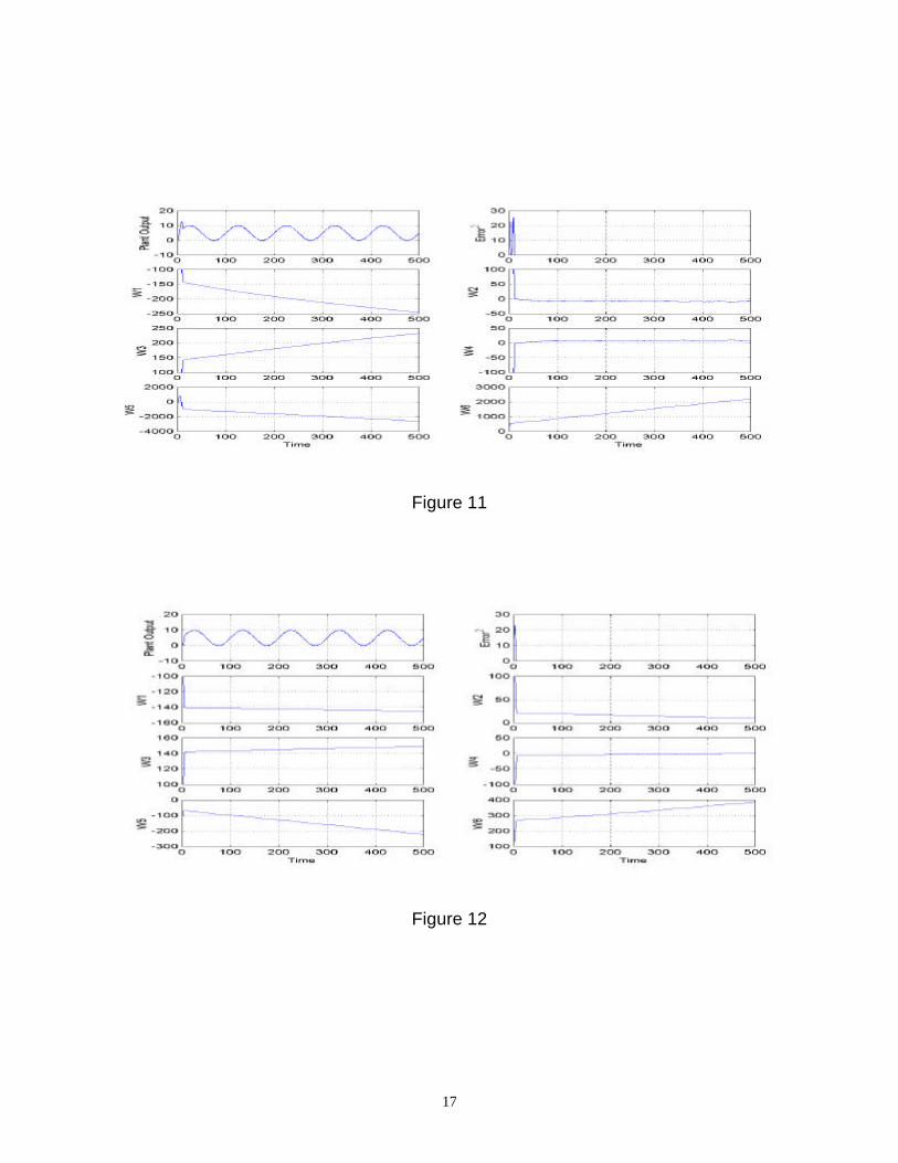
17
Figure 11
Figure 12

18
Figure 13
4.4. Effects of input frequency with output gain versus tan-sigmoid
This section covers the effect of changing the output stage from a tan-sigmoid to
a constant gain. The following elements are set during simulation.
Plant: )474.2s)(526.21s(s
76.88)s(G
++=
Input Signal: Type: Sinewave
Amplitude: 10
Learning Rate: γ=10
Initial Weights: W1=-100, W2=100, W3=100
W4=-100, W5=-100, W6=100
The results of four simulations with two different frequencies are shown in
Figures 14-17 and summarized in Table 3. It is observed that it is easier for the
controller to adapt if the input frequency is low. Also, a constant gain output
provide better adaptation at higher input frequencies.

19
Table 3: Effects of the input frequency and output stage on adaptation
Figure Number Input Frequency Output Stage Results (500s)
Figure 14 0.01 Hz Tan-sigmoid Adapted
Figure 15 0.01 Hz Gain=0.001 Adapted
Figure 16 0.1 Hz Tan-sigmoid Not Adapted
Figure 17 0.1 Hz Gain=0.001 Adapted
Figure 14
Figure 15

20
Figure 16
Figure 17

21
4.5. Effect of different plants
To further validate the adaptation algorithm, the neural network based adaptive
controller is applied to different plants.
Plants: )5)(10(
1000)(2
++=
sssG
)100)(5(
5000)(3
++=
ssssG
)100)(5)(1(
5000)(4
+++=
ssssG
Input Signal: Type: Sinewave
Amplitude: 10
Output Gain: 0.001
Initial Weights: W1=-100, W2=100, W3=100
W4=-100, W5=-100, W6=100
We change the learning rate and input frequency for these plants and see how
high the frequency can be increased. The results of five simulations are shown in
Figures 18-22 and summarized in Table 4. It is observed that the input frequency
can be increased to 10 Hz for G2(s). With third order plants G3(s) and G4(s), a
maximum of 1 Hz input signal is possible. Note that G3(s) is open loop unstable.
Table 4: Effects of input frequency and learning rate on G2(s)
Figure Number Plant Input Frequency Learning Rate Results (500s)
Figure 18 G2(s) 0.01 Hz γ=10 Adapted
Figure 19 G2(s) 0.01 Hz γ=100 Adapted
Figure 20 G2(s) 10 Hz γ=100 Adapted
Figure 21 G3(s) 1 Hz γ=10 Adapted
Figure 22 G4(s) 1 Hz γ=10 Adapted

22
Figure 18
Figure 19

23
Figure 20
Figure 21

24
Figure 22
4.6. Application to non-minimum phase systems
A non-minimum phase system has either a pole or a zero in the right-half of the
s-plane. Since it is well known that it is difficult to apply adaptive control to non-
minimum phase systems, we decide to test the following non-minimum phase
system.
Plants: )5s)(1s(
500)s(6G
+−=
Input Signal: Type: Sinewave
Amplitude: 10
Learning Rate: γ=10
The results of four simulations with different frequencies, output stage and initial
weights are shown in Figures 23-26 and summarized in Table 5. It is observed
that the weight adaptation does occur. The adaptation convergence depends on
two factors: (1) Frequency of the input signal and (2) the magnitude of the initial
weights. The constant gain (= 0.001) is required when dealing with large initial

25
weights and higher frequency. It was found that the tangent sigmoid is suited
when the initial weights are small and the input frequency is low.
Table 6: Effects of the input frequency, output stage and initial weights on G6(s).
Figure
Number
Input
Frequency
Output
Stage
Initial Weights Results (500s)
Figure 23 0.01 Gain=
0.001
W1=-100, W2=100, W3=100
W4=-100, W5=-100, W6=100
Adapted
Figure 24 1 Gain=
0.001
W1=-100, W2=100, W3=100
W4=-100, W5=-100, W6=100
Adapted
Figure 25 0.01 tan-sig W1=-1, W2=1, W3=1
W4=-1, W5=-1, W6=1
Adapted
Figure 26 1 Gain=
0.001
W1=-1, W2=1, W3=1
W4=-1, W5=-1, W6=1
Adapted
Figure 23

26
Figure 24
Figure 25

27
Figure 26
5. Conclusion
The application of theory of adaptive interaction to adaptive neural network
control results in a new direct adaptation algorithm that works very well.
Simulation results show the following characteristics of the algorithm.
- Learning works well with a variety of second and third order plants.
- Controlled plants can be open loop stable or unstable.
- Maximum input frequency depends on the plant order.
- For higher input frequencies and large initial weights the output stage
with a constant gain works better.
- The initial weights must be non-zero and have alternating polarity.
- Faster learning rates are required for higher input frequencies.
- Adaptation is applicable to both minimum phase and non-minimum
phase plants
This new approach does not require the transformation of the continuous time
domain plant into its neural network equivalent. Another benefit for applying the

28
proposed algorithm is that it does not require a separate feedback network to
back propagate the error. The adaptation algorithm is mathematically isomorphic
to the back-propagation algorithm.
6. References
[1] K. S. Narendra and K. Parthasarathy, “Identification and Control of Dynamical Systems
using Neural Networks”, IEEE Transactions on Neural Networks, Vol. 1, pp 1-27, 1990. [2] J. G. Kuschewski, S. Hui and S. H. Zak, “Application of Feedforward Neural Networks to
Dynamical System Identification and Control”, IEEE Transactions on Control Systems Technology, Vol. 1, pp 37-49, 1993.
[3] A. U. Levin and K. S. Narendra, “Control of Nonlinear Dynamical Systems Using Neural
Networks – Part II: Observability, Identification, and Control”, IEEE Transactions on Neural Networks, Vol. 7, pp 30-42, 1996.
[4] F. C. Chen and H. K. Khalil, “Adaptive Control of Nonlinear Systems Using Neural
Networks”, IEEE proceedings on the 29th Conference on Decision and Control, Vol. 44, TA-12-1-8:40, 1990.
[5] K. S. Narendra and K. Parthasarathy, “Gradient Methods for Optimization of Dynamical
Systems Containing Neural Networks”, IEEE Transaction on Neural Network, Vol. 2, pp 252-262, 1991.
[6] T. Yamada and T. Yabuta, “Neural Network Controller Using Autotuning Method for Nonlinear Functions”, IEEE Transactions on Neural Networks, Vol. 3, pp 595-601, 1992.
[7] F. C. Chen and H. K. Khalil, “Adaptive Control of a Class of Nonlinear Discrete-Time
Systems Using Neural Networks”, IEEE Transactions on Automatic Control, Vol. 40, pp 791-801, 1995.
[8] M. A. Brdys and G. L. Kulawski, “ Dynamic Neural for Induction Motor”, IEEE
Transactions on Neural Networks, Vol. 10, pp 340-355, 1999. [9] K. S. Narendra and S. Mukhopadhyay, “Adaptive Control Using Neural Networks and
Approximate Models”, IEEE Transactions on Neural Networks, Vol. 8, pp 475-485, 1997. [10] Y. M. Park, M. S. Choi and K. Y. Lee, “An Optimal Tracking Neuro-Controller for
Nonlinear Dynamic Systems”, IEEE Transactions on Neural Networks, Vol. 7, pp 1099-1110, 1996.
[11] I. Rivals and L. Personnaz, “Non-linear Internal Model Control Using Neural Networks,
Application to Processes with Delay and Design Issues”, IEEE Transactions on Neural Networks, Vol. 11, pp 80-90, 2000.
[12] G. V. Puskorius and L. A. Feldkamp, “Neurocontrol of Nonlinear Dynamical Systems with
Kalman Filter Trained Recurrent Networks”, IEEE Transactions on Neural Networks, Vol. 5, pp 279-297, 1994.

29
[13] J. T. Spooner and K. M. Passino, “Decentralized Adaptive Control of Nonlinear Systems
Using Radial Basis Neural Networks”, IEEE Transactions on Automatic Control, Vol. 44, pp 2050-2057, 1999.
[14] D. Shukla, D. M. Dawson and F. W. Paul, “Multiple Neural-Network Based Adaptive
Controller Using Orthonomal Activation Function Neural Networks”, IEEE Transactions on Neural Networks, Vol. 10, pp 1494-1501, 1999.
[15] J. Noriega and H. Wang, “A Direct Adaptive Neural Network Control for Unknown
Nonlinear Systems and Its Application”, IEEE Transactions on Neural Networks, Vol. 9, pp 27-33, 1998.
[16] S. I. Mistry, S. L. Chang and S. S. Nair, “Indirect Control of a Class of Nonlinear Dynamic
Systems”, IEEE Transactions on Neural Networks, Vol. 7, pp 1015-1023, 1996. [17] K. Warwick, C. Kambhampati, P. Parks and J. Mason, “Dynamic Systems in Neural
Networks”, Neural Network Engineering in Dynamic Control Systems, Springer, pp 27-41, 1995.
[18] S. Mukhopadhyay, K. S. Narendra, “Disturbance Rejection in Nonlinear Systems Using
Neural Networks”, IEEE Transaction in Neural Networks, Vol. 4, pp 63-72, 1993.
[19] M. M. Polycarpou, “Stable Adaptive Neural Control Scheme for Nonlinear Systems”, IEEE Transactions on Automatic Control, Vol. 41, pp 447-451, 1996.
[20] J.J.E. Slotine and L. Weiping, “Applied Nonlinear Control”, Prentice Hall, 1989. [21] D. A. White and D. A. Sofge, “Handbook of Intelligent Control: Neural, Fuzzy and
Adaptive”, VanNostrand Reinhold, 1992. [22] C. J. Harris, C. G. Moore and M. Brown, “Intelligent Control: Aspects of Fuzzy Logic and
Neural Nets”, World Scientific, Chap. 1.7 and 8, 1993. [23] H. Demuth, M. Beale, “Neural Network Toolbox for MatLab”, The Mathworks, Version 3,
1998. [24] J. B. D. Cabrera and K. S. Narendra, “Issues in the Application of Neural Networks for
Tracking Based on Inverse Control”, IEEE Transactions on Automatic Control, Vol. 44, pp 2007-2027, 1999.
[25] D. S. Chen and R. C. Jain, “A Robust Back Propagation Learning Algorithm for Function Approximation”, IEEE Transactions on Neural Networks, Vol. 5, pp 467-479, 1994.
[26] Pierre Baldi, “Gradient Descent Learning Algorithm Overview: A General Dynamical
Systems Perspective”, IEEE Transactions on Neural Networks, Vol. 6, 1pp 182-195, 1995.
[27] R. D. Brandt, F. Lin, “Adaptive Interaction and Its Application to Neural Networks”, Elsevier, Information Science 121, pp 201-215 1999.
[28] F. Lin, R. D. Brandt, G. Saikalis, “Self-Tuning of PID Controllers by Adaptive Interaction”,
IEEE control society, 2000 American Control Conference, Chicago, 2000. [29] F. Lin, R. D. Brandt, G. Saikalis, “Parameter Estimation using Adaptive Interaction”,
preprint, 1998.

30
[30] D. G. Luenberger, “Optimization by Vector Space Methods”, John Wiley and Sons, Chapter 7.3 – Fréchet Derivatives, 1963.