Embed Size (px)
Citation preview
arX
iv:1
806.
0836
2v3
[he
p-th
] 1
7 Ju
l 201
8
CALT-TH 2018-020, IPMU18-0100
De Sitter Space and the Swampland
Georges Obied,a Hirosi Ooguri,b,c Lev Spodyneiko,b Cumrun Vafaa
a Jefferson Physical Laboratory, Harvard University, Cambridge, MA 02138, USA
b Walter Burke Institute for Theoretical Physics
California Institute of Technology, Pasadena, CA 91125, USA
c Kavli Institute for the Physics and Mathematics of the Universe
University of Tokyo, Kashiwa, 277-8583, Japan
It has been notoriously difficult to construct a meta-stable de Sitter (dS) vacuum
in string theory in a controlled approximation. This suggests the possibility that
meta-stable dS belongs to the swampland. In this paper, we propose a swampland
criterion in the form of |∇V | ≥ c ·V for a scalar potential V of any consistent theory
of quantum gravity, with a positive constant c. In particular, this bound forbids dS
vacua. The existence of this bound is motivated by the abundance of string theory
constructions and no-go theorems which exhibit this behavior. We also extend some
of the well-known no-go theorems for the existence of dS vacua in string theory to
more general accelerating universes and reinterpret the results in terms of restrictions
on allowed scalar potentials.
1 Introduction
We live in a universe where the vacuum energy is positive. This can be realized by
having a scalar field potential V with a local minimum at a positive value, leading
to a stable or meta-stable de Sitter (dS) vacuum. However it could also be that
the potential is positive but the scalar field is not at a minimum, as in quintessence
models, as long as |∇V | is sufficiently small and of the order of V itself (for a review
of quintessence models, see [1]). Most of the effort in the string theory community
to realize our universe has been devoted to constructing dS vacua, for example, in
[2–10]. Despite the heroic efforts in these attempts to construct such vacua, there
has been a number of issues raised, for example, in [11–32]. It is thus fair to say that
these scenarios have not yet been rigorously shown to be realized in string theory.
Given the difficulties in obtaining dS-like vacua in string theory, it is natural to
contemplate the alternative possibility where no dS, not even meta-stable dS, can
exist in a consistent quantum theory of gravity (see [33] as well as [32] for raising
this possibility). One may be tempted to conjecture |∇V | > A for some constant
A > 0, which leads to such an exclusion. However, supersymmetric vacua with flat
directions provide counter-examples. To avoid them, we may consider allowing A to
depend on scalar fields φ in such a way that A(φ) ≤ 0 for supersymmetric vacua. A
simple form for such a dependence would be A(φ) = c · V (φ) with positive constant
c, since V ≤ 0 in supersymmetric vacua.
With this motivation, we propose,
|∇V | ≥ c · V, (1.1)
as a swampland criterion in any low energy theory of a consistent quantum theory
of gravity (for a recent review of other swampland criteria see [33]). Here, the norm
|∇V | of the potential gradient is defined using the metric on field space in the kinetic
term of the scalar fields, and c can depend on the macroscopic dimension of spacetime
d. The inequality means that the slope of V cannot be too small when V > 0. We
also propose that c is of order 1 in Planck units. If we take the Planck mass to
infinity while keeping other variables fixed, the inequality becomes |∇V | ≥ 0 and is
trivially satisfied, as expected for a swampland criterion. Though we have not been
able to determine the value of c, we will give an upper bound based on a variety of
top-down constructions from string theory.
Let us discuss a couple of simple examples to illustrate the conjecture (1.1).
They are potential counter-examples, which will turn out to be consistent with the
inequality. Consider a supersymmetric vacuum with zero cosmological constant with
a flat direction. Since |∇V |/V = 0/0 is ill-defined, we need to deform the theory
to test the inequality. Since all parameters in string theory are dynamical, any
continuous deformation of the supersymmetric vacuum will involve a massive field,
V =1
2m2φ2.
1
If we are at φ 6= 0,|∇V |V
=2
|φ| .
This can violate our conjecture when φ grows large. However, the swampland criteria
proposed in [34] claim that changing the value of φ beyond the Planck scale should
give rise to new light states, which would invalidate the simple potential in the above.
We can trust the potential above at most in a region where |φ| . 1 in Planck units.
In this case, we see that |∇V/V | > O(1), which is perfectly consistent with our
conjecture.1 Another case to study, which also occurs commonly in string theory, is
when V crosses 0. Consider a supersymmetric AdS solution and a massive field φ.
Since |∇V | is some non-zero constant when V is crossing 0, |∇V |/V diverges. Thus,
the conjecture (1.1) passes some preliminary checks.
Note that the bound (1.1), while forbidding dS vacua, lends support to quintes-
sence models. In quintessence models, |∇V | typically has to be of the order of V ,
which is small in the current universe when measured in Planck units. However, the
inequality (1.1) suggests that such a small value of |∇V | is natural since it would be
close to the universal swampland bound. Moreover, a small enough slope will lead
to accelerating expansion. For example, in four dimensions, if V is positive and we
consider a single scalar field with
|∂V |V
= λ <√6, (1.2)
constant, the w-parameter relating the energy density ρ and the pressure P as P =
wρ approaches asymptotically to,
w = −1 +λ2
3. (1.3)
The accelerating expansion of the universe requires w < −1/3, namely, λ <√2.
This would be compatible with the inequality (1.1) provided c <√2 for d = 4. It is
shown in [36] that based on current experimental data c . 0.6 in 4 dimensions. As
we will see in this paper, the experimental bound on c is tantalizingly close to and
only slightly less than the values we obtain based on various restrictive assumptions
in string theory.
The main purpose of this paper is to review and examine string-theoretical con-
structions to motivate and test the conjecture (1.1). We emphasize that all bounds
we present in this paper are only meant to serve as upper bounds to the true value of
c because the assumptions we make in deriving them are too restrictive and can be
relaxed. In particular, the bounds we obtain will hold only for the subset of string
1This example motivates the following weaker version of our conjecture, closer in spirit to [34]:
As we get close to small |∇V |/V , a tower of light modes must appear with masses of the order of
exp(−c V/|∇V |) in Planck units and invalidates the effective field theory. This may dovetail nicely
with Vasiliev-type constructions of dS space, where there are infinitely many higher spin massless
states. See [35] for a review of Vasiliev theory.
2
vacua for which those restrictive assumptions are obeyed. Nevertheless, it is impor-
tant to note that the bounds that we obtain under a variety of assumptions all lead
to c ∼ O(1). In Section 2, we review examples from the literature, and generalize
and extend them in various ways. We will take into account quantum and stringy
effects as well as classical effects. This includes scaling arguments in M theory and
also Type II and heterotic string constructions. We also study consequences of the
strong energy condition (SEC) and the null energy condition (NEC), though both of
them are known to be too restrictive in string theory. In section 3, we point out an-
other issue in constructing accelerating universes in string theory. In [37], Farhi and
Guth showed that it is not possible to realize a de Sitter space in an asymptotically
flat space from a smooth initial condition. We extend their result in four dimensions
to an accelerating universe with |∇V |/V <√2. In Appendix A we discuss the Type
II no-go theorems and in Appendix B we discuss further no-go theorems in certain
classes of models. In Appendix C, we discuss the consequences of assuming SEC and
NEC on c.
2 Examples
In this section, we study examples from M theory and string theory constructions.
We first consider M theory compactified on a large manifold, where the supergravity
approximation is applicable, and study the potential it generates in lower dimensions,
where the infinitely many scalar fields come from all possible metric and flux varia-
tions on the compactified manifold. We use scaling arguments in this case to get a
bound on c. Another example we will consider is the O(16)×O(16) heterotic string.
This is a genuinely non-supersymmetric string vacuum in 10 dimensions, which has
a positive vacuum energy [38] but no tachyons. We will show this leads to a value
of c of order 1. We then consider a number of additional examples involving Type
II compactifications with fluxes and orientifold planes. Some of these examples are
from the existing string literature and others are additional examples we study. We
will end this section by discussing bounds for c obtained from SEC and NEC.
While we will not be able to close possible loopholes in all conceivable construc-
tions, the diversity of examples and the simplicity of the arguments used in these
cases to derive the bound (1.1) lends support to our conjecture.
2.1 M Theory Compactifications
Let us start with the 11-dimensional supergravity with the bosonic part of the action,
2κ211S =
∫d11x
√−g(11)
(R− 1
2|G|2
), (2.1)
and consider compactifications to d dimensions on an arbitrary manifold with no
singularities, volume V11−d = e(11−d)ρ, and curvature much less than Planck scale so
3
that we can trust the supergravity approximation. We consider the class of metrics
that take the form2,3
ds2 = dx2d + e2ρ(x)dy211−d = gµν(x)dx
µdxν + e2ρ(x)γab(y)dyadyb. (2.2)
Maldacena and Nunez [11] have proved that one cannot obtain a dS vacuum in such
a setup. In this section, we extend their no-go theorem in the context of M theory
to show that, not only we cannot get dS, where ∇V = 0 and V > 0, but we cannot
even come close to ∇V = 0.
In the effective theory in d dimensions, the metric moduli and flux data of the
internal geometry play the role of scalar fields. Even though there are many (and in
fact infinitely many) such scalar fields controlling the details of the compactification,
we will concentrate only on the overall volume modulus ρ, which for sure is one
of the degrees of freedom of the metric. If we can show that the gradient of the
potential along this direction is large, then that is sufficient to show that |∇V |,which probes the gradient in all directions, is large. There will be two contributions
to the effective potential setting the volume modulus ρ: (i) from the flux term and
(ii) from the curvature term of the internal manifold. We discuss each contribution
separately.
First, we have the term from the Ricci scalar of the compact dimensions. To
an observer in the macroscopic dimensions, this Ricci curvature will manifest itself
only as an integrated and averaged quantity given by e−2ρR11−d, where R11−d is the
average Ricci scalar when the volume of the internal manifold is set to 1. The con-
tribution from this term to the effective potential will have an overall ρ-dependent
factor given by the product e−2ρ · e(11−d)ρ · e−d(11−d)
d−2ρ ∝ e−18 ρ
d−2 , where the second and
third factors come from the metric determinant and the Weyl scaling respectively.
Moreover, the sign of this contribution is opposite that of the integrated curvature.
This means that negatively curved internal manifolds tend to decompactify and vice
versa. Second, we have the contribution from G-flux which is always positive and car-
ries an overall ρ-dependent factor that is given by e(11−d)ρ · e−8ρ · e−d(11−d)
d−2ρ ∝ e−6 d+1
d−2ρ,
where the exponentials come from the metric determinant, the 4 inverse metric fac-
tors, and the Weyl rescaling respectively. To obtain a canonically normalized scalar
field, with the kinetic term 12(∇ρ)2, we need to scale ρ →
√9(11−d)d−2
ρ. This leads to
the effective potential
V = VR e−λ1ρ + VG e−λ2ρ, (2.3)
where λ1 ≡ 6√(d−2)(11−d)
, λ2 ≡ 2(d+1)√(d−2)(11−d)
, VR is proportional to the average of
the Ricci scalar curvature, and VG (which is always positive) is proportional to the
2 Though this ansatz could be generalized by allowing a y-dependent warp factor multiplying the
metric gµν(x)dxµdxν of the macroscopic dimensions, we can set it to be 1 without loss of generality
for the purpose of deriving the gradient of the scalar potential V , as we will explain in Section 2.4
and Appendix C.3Note that in our notation moduli fields with and without a hat are related such that ln ρ ∝ ρ.
This is consistent with the notation in [13] and with our notation used in later sections.
4
average of the G-flux term in the action. If the manifold is on the average negatively
curved and VR ≥ 0 then |∂ρV |/V is bounded below by the smaller of λ1 or λ2, namely,
λ1 for d ≥ 2.
One can also consider cases when the average of the scalar curvature is positive,
with VR < 0. In this case, whenever V < 0, our bound is trivially satisfied. Moreover,
for V > 0, it is easy to see that |∂ρV |/V > λ2 by noting that it must diverge at V = 0,
approaches λ2 as ρ → −∞ and that it is monotonic.
Though our argument above does not rely on supersymmetry, the bound on
|∂ρV |/V also manifests itself in well-known supersymmetric compactifications such as
the Freund-Rubin solutions of the 11-dimensional supergravity giving rise to AdS4×S7 or AdS7 × S4 spacetimes. The metric on the large dimensions is taken to be
that of AdS and that on the compact dimensions is taken to be that of a sphere.
The preferred radius is then set by the effective potential due to a balance between
contributions from the positive flux term, which dominates at small radius, and the
negative curvature term, which dominates at large radius. The regime where V > 0
is of special interest. In this region of the field range, the flux term must dominate
since its contribution is positive, and we again have |∂ρV | > λ2V by considering
limits similar to above.
Finally, the bounds on |∇V |/V we have found in the examples above can be
saturated in string theory constructions. For instance, the bound in the case of
AdS4 × S7 is saturated in the limit of small S7 volume. One may worry that this is
not strictly trustable because the curvature may be too large. However, by choosing
the flux to be large enough one can see that |∇V |/V approaches the above bound
before entering a Planckian curvature regime. Note that any bound presented for
this case can be viewed as an upper bound on the constant c since the latter should
be considered as the infimum of all |∇V |/V over all (reliable) string constructions.
To conclude, we find that compactification of the 11-dimensional supergravity
to d dimensions gives the bound,
|∇V |V
≥ 6√(d− 2)(11− d)
. (2.4)
In particular for d = 4, this yields 6/√14 ∼ 1.6 which gives an upper bound on c in
our conjecture because it is actually realized by the AdS4 × S7 example. As we will
discuss in subsection 2.4, this inequality is also a consequence of the fact that the
11-dimensional action (2.1) satisfies the strong energy condition (SEC). Since the
SEC is often violated in string theory, let us discuss more stringy examples in the
following two subsections and see whether we have similar bounds in string theory.
2.2 O(16)×O(16) Heterotic String
To study effects beyond the supergravity approximation, let us examine compactifi-
cations of the non-supersymmetric heterotic string [38, 39] constructed by twisting
the E8 × E8 theory, which has a 10-dimensional cosmological constant Λ > 0 in its
5
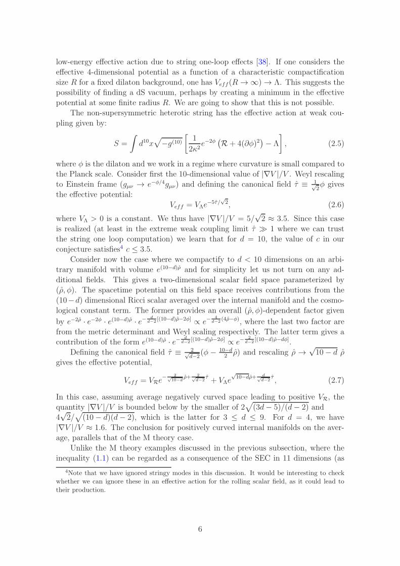
low-energy effective action due to string one-loop effects [38]. If one considers the
effective 4-dimensional potential as a function of a characteristic compactification
size R for a fixed dilaton background, one has Veff(R → ∞) → Λ. This suggests the
possibility of finding a dS vacuum, perhaps by creating a minimum in the effective
potential at some finite radius R. We are going to show that this is not possible.
The non-supersymmetric heterotic string has the effective action at weak cou-
pling given by:
S =
∫d10x
√−g(10)
[1
2κ2e−2φ
(R+ 4(∂φ)2
)− Λ
], (2.5)
where φ is the dilaton and we work in a regime where curvature is small compared to
the Planck scale. Consider first the 10-dimensional value of |∇V |/V . Weyl rescaling
to Einstein frame (gµν → e−φ/4gµν) and defining the canonical field τ ≡ 1√2φ gives
the effective potential:
Veff = VΛe−5τ /
√2, (2.6)
where VΛ > 0 is a constant. We thus have |∇V |/V = 5/√2 ≈ 3.5. Since this case
is realized (at least in the extreme weak coupling limit τ ≫ 1 where we can trust
the string one loop computation) we learn that for d = 10, the value of c in our
conjecture satisfies4 c ≤ 3.5.
Consider now the case where we compactify to d < 10 dimensions on an arbi-
trary manifold with volume e(10−d)ρ and for simplicity let us not turn on any ad-
ditional fields. This gives a two-dimensional scalar field space parameterized by
(ρ, φ). The spacetime potential on this field space receives contributions from the
(10−d) dimensional Ricci scalar averaged over the internal manifold and the cosmo-
logical constant term. The former provides an overall (ρ, φ)-dependent factor given
by e−2ρ · e−2φ · e(10−d)ρ · e− dd−2
[(10−d)ρ−2φ] ∝ e−4
d−2(4ρ−φ), where the last two factor are
from the metric determinant and Weyl scaling respectively. The latter term gives a
contribution of the form e(10−d)ρ · e− dd−2
[(10−d)ρ−2φ] ∝ e−2
d−2[(10−d)ρ−dφ].
Defining the canonical field τ ≡ 2√d−2
(φ − 10−d2
ρ) and rescaling ρ →√10− d ρ
gives the effective potential,
Veff = VRe− 2
√
10−dρ+ 2
√
d−2τ+ VΛe
√10−dρ+ d
√
d−2τ, (2.7)
In this case, assuming average negatively curved space leading to positive VR, the
quantity |∇V |/V is bounded below by the smaller of 2√
(3d− 5)/(d− 2) and
4√2/√(10− d)(d− 2), which is the latter for 3 ≤ d ≤ 9. For d = 4, we have
|∇V |/V ≈ 1.6. The conclusion for positively curved internal manifolds on the aver-
age, parallels that of the M theory case.
Unlike the M theory examples discussed in the previous subsection, where the
inequality (1.1) can be regarded as a consequence of the SEC in 11 dimensions (as
4Note that we have ignored stringy modes in this discussion. It would be interesting to check
whether we can ignore these in an effective action for the rolling scalar field, as it could lead to
their production.
6
we will explain in subsection 2.4), the O(16) × O(16) example is not tied to the
SEC. In fact, as previously discussed, it has a positive potential for a scalar in 10
dimensions, violating the SEC. This example demonstrates that the breaking of the
SEC, in particular the positive cosmological constant in higher dimensions, does
not guarantee stable or meta-stable dS minima after compactification and that our
conjecture still continues to hold in such a case. It is therefore not correct to claim
that, because string theory (as opposed to supergravity theories) contains ingredients
that violate the SEC, it should necessarily be able to accommodate dS vacua.
It is interesting to note that for the usual supersymmetric heterotic string, state-
ments about the lack of classical dS vacua can be made in the perturbative regime
of the heterotic string by relying on world-sheet arguments [23]. This in particular
includes all order α′ stringy corrections to the Einstein equations.
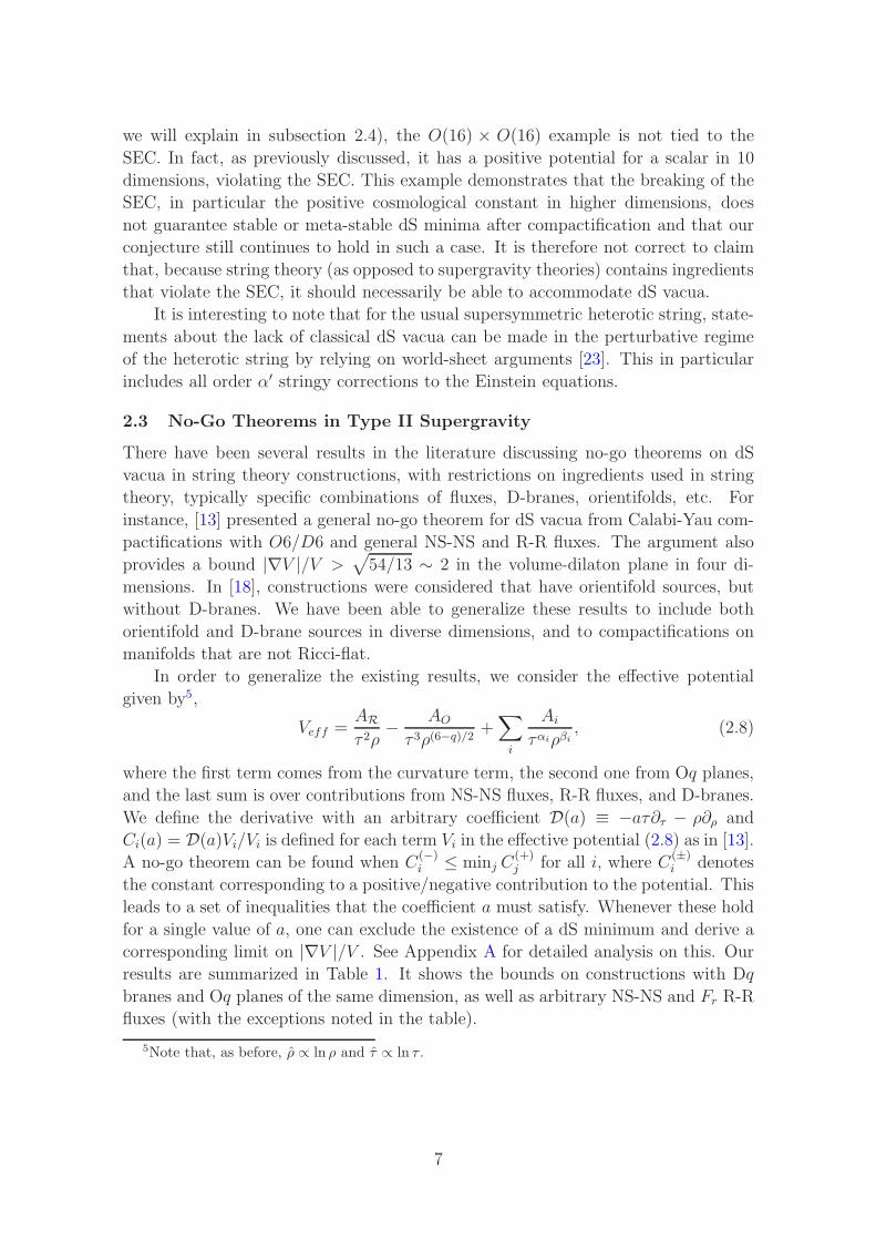
2.3 No-Go Theorems in Type II Supergravity
There have been several results in the literature discussing no-go theorems on dS
vacua in string theory constructions, with restrictions on ingredients used in string
theory, typically specific combinations of fluxes, D-branes, orientifolds, etc. For
instance, [13] presented a general no-go theorem for dS vacua from Calabi-Yau com-
pactifications with O6/D6 and general NS-NS and R-R fluxes. The argument also
provides a bound |∇V |/V >√54/13 ∼ 2 in the volume-dilaton plane in four di-
mensions. In [18], constructions were considered that have orientifold sources, but
without D-branes. We have been able to generalize these results to include both
orientifold and D-brane sources in diverse dimensions, and to compactifications on
manifolds that are not Ricci-flat.
In order to generalize the existing results, we consider the effective potential
given by5,
Veff =ARτ 2ρ
− AO
τ 3ρ(6−q)/2+∑
i
Ai
ταiρβi, (2.8)
where the first term comes from the curvature term, the second one from Oq planes,
and the last sum is over contributions from NS-NS fluxes, R-R fluxes, and D-branes.
We define the derivative with an arbitrary coefficient D(a) ≡ −aτ∂τ − ρ∂ρ and
Ci(a) = D(a)Vi/Vi is defined for each term Vi in the effective potential (2.8) as in [13].
A no-go theorem can be found when C(−)i ≤ minj C
(+)j for all i, where C
(±)i denotes
the constant corresponding to a positive/negative contribution to the potential. This
leads to a set of inequalities that the coefficient a must satisfy. Whenever these hold
for a single value of a, one can exclude the existence of a dS minimum and derive a
corresponding limit on |∇V |/V . See Appendix A for detailed analysis on this. Our
results are summarized in Table 1. It shows the bounds on constructions with Dq
branes and Oq planes of the same dimension, as well as arbitrary NS-NS and Fr R-R
fluxes (with the exceptions noted in the table).
5Note that, as before, ρ ∝ ln ρ and τ ∝ ln τ .
7
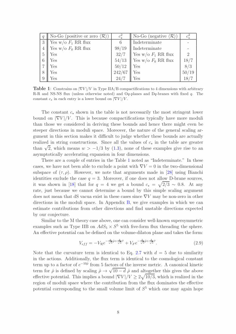
q No-Go (positive or zero 〈R〉) c2⋆ No-Go (negative 〈R〉) c2⋆3 Yes w/o F1 RR flux 6 Indeterminate -
4 Yes w/o F0 RR flux 98/19 Indeterminate -
5 Yes 32/7 Yes w/o F1 RR flux 2
6 Yes 54/13 Yes w/o F0 RR flux 18/7
7 Yes 50/12 Yes 8/3
8 Yes 242/67 Yes 50/19
9 Yes 24/7 Yes 18/7
Table 1: Constrains on |∇V |/V in Type IIA/B compactifications to 4 dimensions with arbitrary
R-R and NS-NS flux (unless otherwise noted) and Oq-planes and Dq-branes with fixed q. The
constant c⋆ in each entry is a lower bound on |∇V |/V .
The constant c⋆ shown in the table is not necessarily the most stringent lower
bound on |∇V |/V . This is because compactifications typically have more moduli
than those we considered in deriving these bounds and hence there might even be
steeper directions in moduli space. Moreover, the nature of the general scaling ar-
gument in this section makes it difficult to judge whether these bounds are actually
realized in string constructions. Since all the values of c⋆ in the table are greater
than√2, which means w > −1/3 by (1.3), none of these examples give rise to an
asymptotically accelerating expansion in four dimensions.
There are a couple of entries in the Table 1 noted as “Indeterminate.” In these
cases, we have not been able to exclude a point with ∇V = 0 in the two-dimensional
subspace of (τ, ρ). However, we note that arguments made in [28] using Bianchi
identities exclude the case q = 3. Moreover, if one does not allow D-brane sources,
it was shown in [18] that for q = 4 we get a bound c⋆ =√
2/3 ∼ 0.8. At any
rate, just because we cannot determine a bound by this simple scaling argument
does not mean that dS vacua exist in these cases since ∇V may be non-zero in other
directions in the moduli space. In Appendix B, we give examples in which we can
estimate contributions from other directions and find unstable directions expected
by our conjecture.
Similar to the M theory case above, one can consider well-known supersymmetric
examples such as Type IIB on AdS5 × S5 with five-form flux threading the sphere.
An effective potential can be defined on the volume-dilaton plane and takes the form:
Veff = −VRe− 2
√
5ρ+ 2
√
3τ+ VF e
− 5√
5ρ+ 5
√
3τ. (2.9)
Note that the curvature term is identical to Eq. 2.7 with d = 5 due to similarity
in the actions. Additionally, the flux term is identical to the cosmological constant
term up to a factor of e−10ρ from 5 factors of the inverse metric. A canonical kinetic
term for ρ is defined by scaling ρ →√10− d ρ and altogether this gives the above
effective potential. This implies a bound |∇V |/V ≥ 2√10/3, which is realized in the
region of moduli space where the contribution from the flux dominates the effective
potential corresponding to the small volume limit of S5 which one may again hope
8
to be trustable given the high degree of supersymmetry. Since this value is actually
realized in one example, it shows that for d = 5 the actual c ≤ 2√10/3 ∼ 3.7.
2.4 Consequences of Energy Conditions
The bound on |∇V |/V for compactifications of the 11-dimensional supergravity de-
rived in section 2.1 is in fact a consequence of SEC in 11 dimensions. Suppose more
generally we start with a theory in D dimensions and compactify it on a (D − d)-
dimensional space with a metric gmn and a warp factor Ω as,
ds2 = Ω(y, t)2(−dt2 + a(t)2d~x2
d−1
)+ gmn(y, t)dy
mdyn. (2.10)
In Appendix C, we derive the bound on the gradient of the effective potential V in
d dimensions,
|∇V |V
≥ λSEC ≡ 2
√D − 2
(D − d)(d− 2), (2.11)
assuming that the D-dimensional theory satisfies SEC. This result is independent
of the choice of the internal metric gmn. Note that the M theory action (2.1) in 11
dimensions satisfies SEC. Indeed, the bound (2.4) on M theory compactifications we
found there is reproduced by setting D = 11, and therefore is simply a consequence
of SEC.
However, we need to take this result with a grain of salt since SEC can easily
be violated in string theory. We should also note that an accelerated expansion of
the universe in d macroscopic dimensions requires (d − 3)ρ + (d − 1)p < 0. For a
constant exponential potential V = V0 exp(−λφ), a solution approaches p = wρ with
w = −1 + 12d−2d−1
λ2, leading to,
|∇V |V
< λaccelerate ≡√
4
d− 2. (2.12)
This is incompatible with (2.11) d > 2. Clearly, SEC is too strong an assumption to
make.
We may also consider NEC, which is satisfied by a broader range of theories,
though it can be violated quantum mechanically. To analyze consequences of NEC,
it is convenient to parametrize the metric as,
ds2 = Ω(y, t)2(−dt2 + a(t)2d~x2
d−1
)+ Ω(y, t)−
2dD−d−2gmn(y, t)dy
mdyn. (2.13)
The power of Ω in front of gmndymdyn is a matter of convention since we can always
redefine gmn to absorb this factor. However, unlike the case of SEC, we need to make
an additional assumption on the internal metric gmn, that the average of its scalar
curvature is either zero or negative, in order to derive a bound on V . Under this
assumption, we find,
|∇V |V
≥ λNEC ≡ 2
√D − d
(D − 2)(d− 2). (2.14)
9
This generalizes the result of [40] that NEC in D dimensions together with a similar
assumption on the internal metric gmn excludes a dS solution in macroscopic dimen-
sions. This NEC bound is compatible with an accelerated expansion of the universe,
namely,
λNEC < λaccelerate < λSEC , (2.15)
for d > 2. However, this is still too strong an assumption. In particular experimental
bounds give a value for c . 0.6 [36] whereas the NEC bound (2.14) – under the
assumptions that the supergravity description is valid and the internal space has
either zero or negative average scalar curvature – would give the bound λNEC =√3/2 ∼ 1.2 for d = 4 and D = 10.
It would be interesting to find out if a bound on |∇V |/V can be obtained with
the averaged null energy condition, which is weaker and is known to be satisfied by
any unitary quantum field theory [41, 42].
3 Accelerating Universe in a Laboratory
Suppose a scalar potential V is such that it allows an asymptotically flat space. We
will show that, even if there is a region in the field space in which V > 0 and,
|∇V |/V < λaccelerate ≡√
4
d− 2, (3.1)
such a region cannot be reached by a classical time evolution starting with a smooth
initial condition in an asymptotically flat space. This can be regarded as generaliza-
tion of the result [37] by Farhi and Guth, from dS to small gradient potentials.
Let us start with a theory in which the vacuum is at V = 0 and consider a
massive field in the theory whose excitation gives V (φ) > 0. In [37], it was shown
that one cannot start with an asymptotically flat space at V = 0 and create a region
which is in the meta-stable dS minimum while avoiding initial singularities. This is
because such a configuration creates an anti-trapped surface inside the dS region,
and Penrose theorem shows that there should have been an initial singularity. This
result can be sharpened by considering not only potentials with a dS minimum, but
also nearly-flat potentials since the same issue arises in these scenarios.
We assume an effective potential that has a minimum at V (φ0) = 0 and also has
some field range over which (3.1) is satisfied. One can imagine starting with φ = φ0
and locally exciting the field in order to reach (3.1). Such a region would drive an
accelerating expansion of spacetime. We should place the domain wall separating
the region (3.1) and φ = φ0 outside of the cosmic event horizon of the accelerating
region so that an observer in the accelerating universe does not see the wall (this is
the same condition required by [37]).
In the accelerating universe, there is an anti-trapped surface, which is a compact
surface where light rays directed inwards and outwards are both diverging. Since
we have chosen the domain wall to be outside of the cosmological event horizon, the
10
anti-trapped surface is not affected by it. Since all configurations of a scalar field
minimally coupled to gravity obeys NEC, the assumptions of the Penrose theorem
are also satisfied and an initial singularity is inevitable. It makes it impossible to
probe the flat potential starting with a smooth initial condition. Note that the same
conclusion is not reached for a steeper potential.
The presence of the initial singularity itself may not be an issue. However, for
a meta-stable dS realized in an asymptotically AdS space, the initial singularity has
led to various puzzles on its holographic meaning [43, 44]. It is straightforward to
generalize these observations to accelerating universes in an asymptotically anti-de
Sitter space, posing challenges to their holographic interpretations.
Acknowledgments
We would like to thank P. Agrawal, G. Horowitz, S. Kachru, D. Marolf, M. Sasaki,
S. Sethi, P. Steinhardt and X. Yin for discussions. We would also like to thank
SCGP Summer Workshop 2017 for hospitality during part of this work. The research
of HO is supported in part by U.S. Department of Energy grant DE-SC0011632,
by the World Premier International Research Center Initiative, MEXT, Japan, by
JSPS Grant-in-Aid for Scientific Research C-26400240, and by JSPS Grant-in-Aid for
Scientific Research on Innovative Areas 15H05895. HO also thanks the hospitality of
the Aspen Center for Physics, which is supported by the National Science Foundation
grant PHY-1607611. The research of CV is supported in part by the NSF grant
PHY-1067976.
A Extensions of no-go theorems in Type II supergravity
We start with the effective potential6
Veff =∑
i
Ai
ταiρβi+
ARτ 2ρ
− AO
τ 3ρ(6−q)/2, (A.1)
and define the derivative D(a) ≡ −aτ∂τ − ρ∂ρ such that it has the following action
on the different contributions
DVi = (aαi + βi)Vi ≡ CiVi, (A.2)
DVR = (2a+ 1)VR ≡ CRVR, (A.3)
DVOq = (3a+6− q
2)VO ≡ COVi. (A.4)
We wish to choose a value for a such that DV = KV +(positive) where K > 0 is
a constant. As such we can group the Ci into two groups, C(+)i and C
(−)i , according
6We are assuming AO > 0, i.e. orientifolds with negative tension. If AO ≤ 0 we can get even a
stronger bound.
11
to whether the contribution to the potential is positive or negative. A no-go theorem
then exists when C(−)i ≤ minj C
(+)j for all i.
For a flat curved internal manifold, with Fr RR flux, Oq-planes and Dp-branes,
the above reduces to the following set of inequalities
2a+ 3 > 0, (A.5)
4a + (r − 3) > 0, (A.6)
3a+6− p
2> 0, (A.7)
2a− q ≤ 0, (A.8)
a + (r − 3)− 6− q
2≥ 0, (A.9)
p− q ≤ 0. (A.10)
For a negatively curved internal manifold, these are augmented by
2a + 1 > 0, (A.11)
a+4− q
2≤ 0. (A.12)
Similarly, for a positively curved internal manifold, these are augmented by
2a+ (r − 4) ≥ 0, (A.13)
a+4− p
2≥ 0. (A.14)
We find all combinations of 3-tuples (p, q, r) with p = q for which ∃a > 0 that satisfies
the above inequalities. For these cases, one has the result (|∇V |/V )2 ≥ c2⋆ which we
report in Table 1. This is obtained exactly as in the method used in [13, 18].
B Unstable Directions in Moduli Space
We now consider an example where the no-go theorems of the previous section seem
to fail and show that the existence of dS vacua is still unclear if one takes into
account additional directions in moduli space [15]. The example is that of Type IIA
supergravity compactified on a 6D manifold with negative curvature. In order to
avoid the above no-go theorems, we include an O4-plane wrapping a homologically
trivial cycle and F2,4 R-R fluxes. We assume a product structure for the internal
manifold so that we can rescale the directions parallel vs. perpendicular to the
O-plane independently.
To begin with, we consider scaling in the volume-dilaton plane. Defining the
moduli
ρ = (Vol6)1/3, τ = e−φ
√Vol6, (B.1)
we work out the (ρ, τ)-dependence of the contributions to the effective 4D potential.
For instance, the term from the internal curvature scales as τ 2ρ−1 ·τ−4 where the last
12
factor is from Weyl rescaling in the 4 non-compact dimensions. Similarly, considering
other contributions leads to a potential of the form
Veff =ARτ 2ρ
− AO
τ 3ρ+
A2ρ
τ 4+
A4
τ 4ρ, (B.2)
where the coefficients Ai generally depend on other moduli we are neglecting. Naıvely,
the above potential can have a de Sitter minimum if one can find a string theory
construction where the coefficients satisfy the condition
192 ≤ (7AO)2
ARA4≤ 196. (B.3)
We show that allowing the internal manifold to scale independently along the direc-
tions transverse to the orientifold plane removes the de Sitter solution. In this case,
the moduli with diagonal kinetic terms are given by:
π = V2/k11 ; σ = V
2/k22 ; τ = e−φ
√V1V2, (B.4)
where Vi are the volumes of the subspaces parallel and transverse to the O-plane and
ki are their dimensions. In the following, we consider an example based on a com-
pactification with an O4-plane wrapping a homologically trivial cycle and arbitrary
F2,4 R-R flux. We allow the rescaling of directions parallel to the orientifold indepen-
dently from perpendicular directions; i.e. (V1, V2) = (V‖, V⊥) with (k1, k2) = (1, 5).
Consider now the scaling behavior of different contributions to the effective po-
tential with the new moduli
Internal Curvature: VR ∝ τ−2σ−1, (B.5)
Orientifold Plane: VO ∝ −τ−3π1/4σ−5/4, (B.6)
2-form Flux (⊥): V2 ∝ τ−4π1/2σ1/2, (B.7)
2-form Flux (‖): V2 ∝ τ−4π−1/2σ3/2, (B.8)
4-form Flux (⊥): V4 ∝ τ−4π1/2σ−3/2, (B.9)
4-form Flux (‖): V4 ∝ τ−4π−1/2σ−1/2. (B.10)
We take the sum of the above contributions with arbitrary coefficients to be the
form of the potential. The existence of a de Sitter minimum requires that the deriva-
tive with respect to each modulus vanishes. This condition gives three equations
−4A4⊥π − 4A4‖σ − 4A2⊥πσ2 − 4A2‖σ
3 + 3AOπ3/4σ1/4τ − 2ARπ
1/2σ1/2τ 2 = 0,
(B.11)
−6A4⊥π − 2A4‖σ + 2A2⊥πσ2 + 6A2‖σ
3 + 5AOπ3/4σ1/4τ − 4ARπ
1/2σ1/2τ 2 = 0,
(B.12)
2A4⊥π − 2A4‖σ + 2A2⊥πσ2 − 2A2‖σ
3 − AOπ3/4σ1/4τ = 0.
(B.13)
13
Forming the linear combination 2×B.11− B.12 +B.13 gives
A4‖ + A2⊥πσ + 2A2‖σ2 = 0, (B.14)
which does not have any positive solutions for σ. Therefore, the three above equations
cannot be simultaneously satisfied with physical solutions for all three moduli and
we do not have a de Sitter minimum.
We note that in the absence of F2 flux oriented completely in the perpendicular
directions (equivalent to setting A2⊥ = 0), we can derive a bound on |∇V |/V . Similar
to Appendix A, we define the derivative D(a, b) = −aτ∂τ − bσ∂σ − π∂π and find a
tuple (a, b) such that DV ≥ KV with K > 0. The tuple (a, b) is found by applying
the inequalities C(−)i ≤ minj C
(+)j where Ci are defined analogously to Appendix A
but with respect to the contributions B.5-B.10. Minimizing the slow-roll parameter
subject to the constraint DV/V ≥ K gives the bound ǫ > 1/2. This bound is not
necessarily realized since we do not have a full string theory construction.
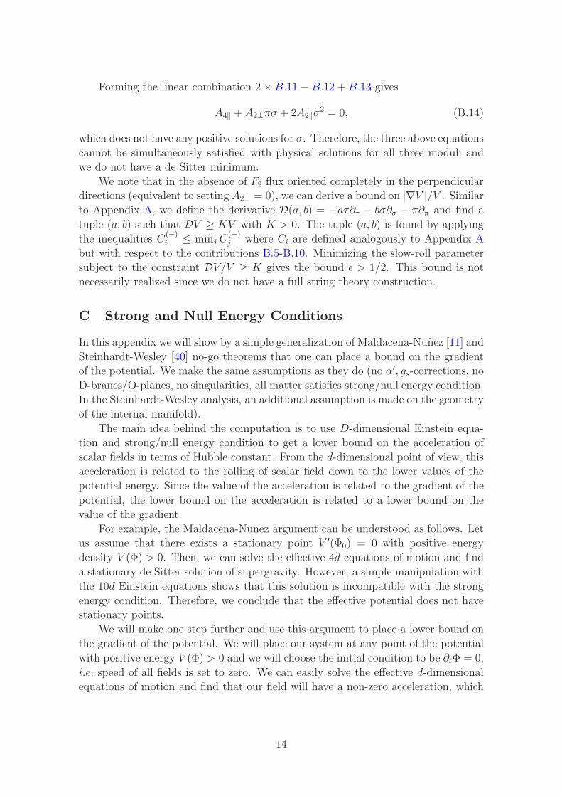
C Strong and Null Energy Conditions
In this appendix we will show by a simple generalization of Maldacena-Nunez [11] and
Steinhardt-Wesley [40] no-go theorems that one can place a bound on the gradient
of the potential. We make the same assumptions as they do (no α′, gs-corrections, no
D-branes/O-planes, no singularities, all matter satisfies strong/null energy condition.
In the Steinhardt-Wesley analysis, an additional assumption is made on the geometry
of the internal manifold).
The main idea behind the computation is to use D-dimensional Einstein equa-
tion and strong/null energy condition to get a lower bound on the acceleration of
scalar fields in terms of Hubble constant. From the d-dimensional point of view, this
acceleration is related to the rolling of scalar field down to the lower values of the
potential energy. Since the value of the acceleration is related to the gradient of the
potential, the lower bound on the acceleration is related to a lower bound on the
value of the gradient.
For example, the Maldacena-Nunez argument can be understood as follows. Let
us assume that there exists a stationary point V ′(Φ0) = 0 with positive energy
density V (Φ) > 0. Then, we can solve the effective 4d equations of motion and find
a stationary de Sitter solution of supergravity. However, a simple manipulation with
the 10d Einstein equations shows that this solution is incompatible with the strong
energy condition. Therefore, we conclude that the effective potential does not have
stationary points.
We will make one step further and use this argument to place a lower bound on
the gradient of the potential. We will place our system at any point of the potential
with positive energy V (Φ) > 0 and we will choose the initial condition to be ∂tΦ = 0,
i.e. speed of all fields is set to zero. We can easily solve the effective d-dimensional
equations of motion and find that our field will have a non-zero acceleration, which
14
is related to the gradient of the potential energy. On the other hand, we can use the
D-dimensional Einstein equation of motion in the same way as in Maldacena-Nunez
paper to get a lower bound on the acceleration. Combining it with the effective
d-dimensional point of view, we will find our bound on the gradient of the potential.
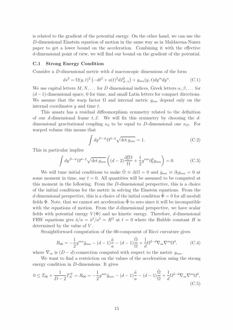
C.1 Strong Energy Condition
Consider a D-dimensional metric with d macroscopic dimensions of the form
ds2 = Ω(y, t)2(−dt2 + a(t)2d~x2
d−1
)+ gmn(y, t)dy
mdyn. (C.1)
We use capital letters M,N, . . . for D dimensional indices, Greek letters α, β, . . . for
(d− 1)-dimensional space, 0 for time, and small Latin letters for compact directions.
We assume that the warp factor Ω and internal metric gmn depend only on the
internal coordinates y and time t.
This ansatz has a residual diffeomorphism symmetry related to the definition
of our d-dimensional frame t, ~x. We will fix this symmetry by choosing the d-
dimensional gravitational coupling κd to be equal to D-dimensional one κD. For
warped volume this means that∫
dyD−dΩd−2√
det gmn = 1. (C.2)
This in particular implies∫
dyD−dΩd−2√
det gmn
((d− 2)
∂20Ω
Ω+
1
2gmn∂2
0gmn
)= 0. (C.3)
We will tune initial conditions to make Ω ≡ ∂tΩ = 0 and gmn ≡ ∂tgmn = 0 at
some moment in time, say t = 0. All quantities will be assumed to be computed at
this moment in the following. From the D-dimensional perspective, this is a choice
of the initial conditions for the metric in solving the Einstein equations. From the
d-dimensional perspective, this is a choice of the initial condition Φ = 0 for all moduli
fields Φ. Note, that we cannot set acceleration Φ to zero since it will be incompatible
with the equations of motion. From the d-dimensional perspective, we have scalar
fields with potential energy V (Φ) and no kinetic energy. Therefore, d-dimensional
FRW equations give a/a = a2/a2 = H2 at t = 0 where the Hubble constant H is
determined by the value of V .
Straightforward computation of the 00-component of Ricci curvature gives
R00 = −1
2gmngmn − (d− 1)
a
a− (d− 1)
Ω
Ω+
1
dΩ2−d∇m∇mΩd, (C.4)
where ∇m is (D − d)-connection computed with respect to the metric gmn.
We want to find a restriction on the values of the acceleration using the strong
energy condition in D-dimensions. It gives
0 ≤ T00 +1
D − 2TNN = R00 = −1
2gmngmn − (d− 1)
a
a− (d− 1)
Ω
Ω+
1
dΩ2−d∇m∇mΩd,
(C.5)
15
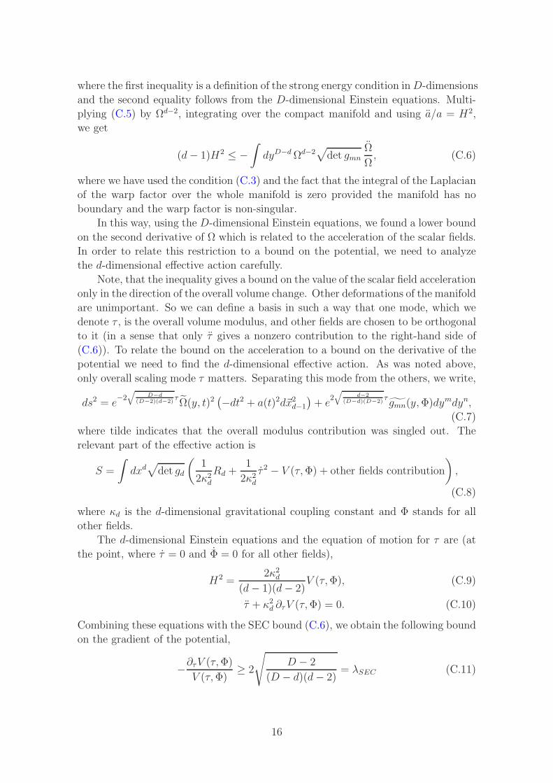
where the first inequality is a definition of the strong energy condition inD-dimensions
and the second equality follows from the D-dimensional Einstein equations. Multi-
plying (C.5) by Ωd−2, integrating over the compact manifold and using a/a = H2,
we get
(d− 1)H2 ≤ −∫
dyD−dΩd−2√det gmn
Ω
Ω, (C.6)
where we have used the condition (C.3) and the fact that the integral of the Laplacian
of the warp factor over the whole manifold is zero provided the manifold has no
boundary and the warp factor is non-singular.
In this way, using the D-dimensional Einstein equations, we found a lower bound
on the second derivative of Ω which is related to the acceleration of the scalar fields.
In order to relate this restriction to a bound on the potential, we need to analyze
the d-dimensional effective action carefully.
Note, that the inequality gives a bound on the value of the scalar field acceleration
only in the direction of the overall volume change. Other deformations of the manifold
are unimportant. So we can define a basis in such a way that one mode, which we
denote τ , is the overall volume modulus, and other fields are chosen to be orthogonal
to it (in a sense that only τ gives a nonzero contribution to the right-hand side of
(C.6)). To relate the bound on the acceleration to a bound on the derivative of the
potential we need to find the d-dimensional effective action. As was noted above,
only overall scaling mode τ matters. Separating this mode from the others, we write,
ds2 = e−2
√
D−d(D−2)(d−2)
τΩ(y, t)2
(−dt2 + a(t)2d~x2
d−1
)+ e
2√
d−2(D−d)(D−2)
τgmn(y,Φ)dy
mdyn,
(C.7)
where tilde indicates that the overall modulus contribution was singled out. The
relevant part of the effective action is
S =
∫dxd
√det gd
(1
2κ2d
Rd +1
2κ2d
τ 2 − V (τ,Φ) + other fields contribution
),
(C.8)
where κd is the d-dimensional gravitational coupling constant and Φ stands for all
other fields.
The d-dimensional Einstein equations and the equation of motion for τ are (at
the point, where τ = 0 and Φ = 0 for all other fields),
H2 =2κ2
d
(d− 1)(d− 2)V (τ,Φ), (C.9)
τ + κ2d ∂τV (τ,Φ) = 0. (C.10)
Combining these equations with the SEC bound (C.6), we obtain the following bound
on the gradient of the potential,
−∂τV (τ,Φ)
V (τ,Φ)≥ 2
√D − 2
(D − d)(d− 2)= λSEC (C.11)
16
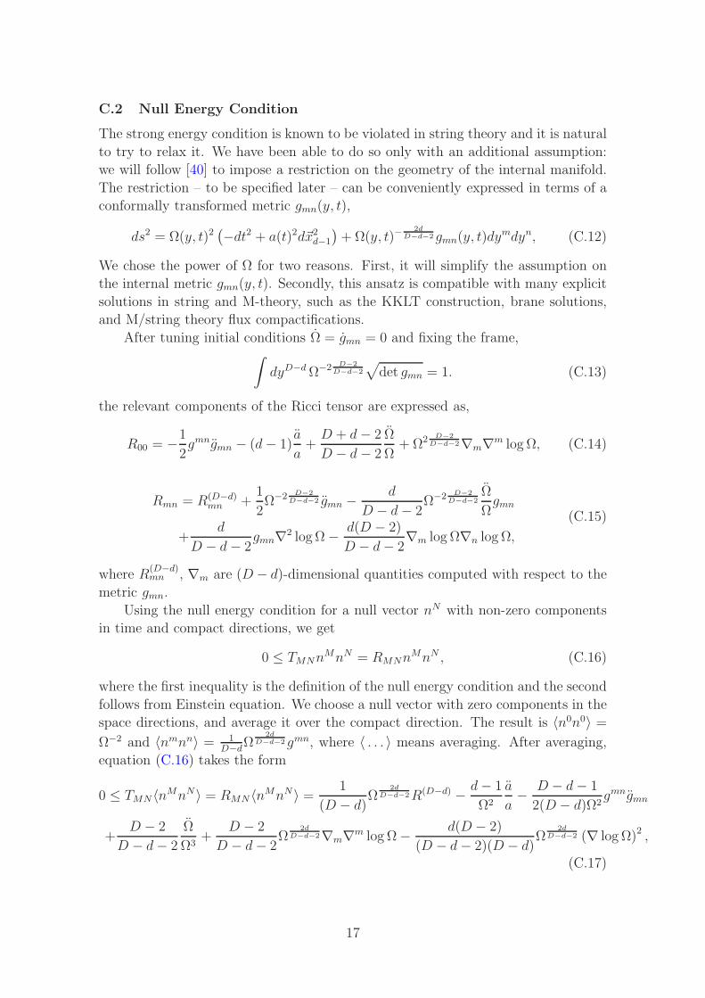
C.2 Null Energy Condition
The strong energy condition is known to be violated in string theory and it is natural
to try to relax it. We have been able to do so only with an additional assumption:
we will follow [40] to impose a restriction on the geometry of the internal manifold.
The restriction – to be specified later – can be conveniently expressed in terms of a
conformally transformed metric gmn(y, t),
ds2 = Ω(y, t)2(−dt2 + a(t)2d~x2
d−1
)+ Ω(y, t)−
2dD−d−2gmn(y, t)dy
mdyn, (C.12)
We chose the power of Ω for two reasons. First, it will simplify the assumption on
the internal metric gmn(y, t). Secondly, this ansatz is compatible with many explicit
solutions in string and M-theory, such as the KKLT construction, brane solutions,
and M/string theory flux compactifications.
After tuning initial conditions Ω = gmn = 0 and fixing the frame,∫
dyD−dΩ−2 D−2D−d−2
√det gmn = 1. (C.13)
the relevant components of the Ricci tensor are expressed as,
R00 = −1
2gmngmn − (d− 1)
a
a+
D + d− 2
D − d− 2
Ω
Ω+ Ω2 D−2
D−d−2∇m∇m log Ω, (C.14)
Rmn = R(D−d)mn +
1
2Ω−2 D−2
D−d−2 gmn −d
D − d− 2Ω−2 D−2
D−d−2Ω
Ωgmn
+d
D − d− 2gmn∇2 log Ω− d(D − 2)
D − d− 2∇m log Ω∇n log Ω,
(C.15)
where R(D−d)mn , ∇m are (D− d)-dimensional quantities computed with respect to the
metric gmn.
Using the null energy condition for a null vector nN with non-zero components
in time and compact directions, we get
0 ≤ TMNnMnN = RMNn
MnN , (C.16)
where the first inequality is the definition of the null energy condition and the second
follows from Einstein equation. We choose a null vector with zero components in the
space directions, and average it over the compact direction. The result is 〈n0n0〉 =Ω−2 and 〈nmnn〉 = 1
D−dΩ
2dD−d−2gmn, where 〈 . . . 〉 means averaging. After averaging,
equation (C.16) takes the form
0 ≤ TMN〈nMnN 〉 = RMN〈nMnN 〉 = 1
(D − d)Ω
2dD−d−2R(D−d) − d− 1
Ω2
a
a− D − d− 1
2(D − d)Ω2gmngmn
+D − 2
D − d− 2
Ω
Ω3+
D − 2
D − d− 2Ω
2dD−d−2∇m∇m log Ω− d(D − 2)
(D − d− 2)(D − d)Ω
2dD−d−2 (∇ log Ω)2 ,
(C.17)
17
where R(D−d) is scalar curvature of the metric gmn.
Multiplying (C.17) by Ω−2d
D−d−2 , integrating over the compact manifold and using
a/a = H2, we find,
(d− 1)H2 ≤∫
dyD−d√det gmn
[− D − 2
D − dΩ−2 D−2
D−d−2Ω
Ω
+1
(D − d)R(D−d) − d(D − 2)
(D − d− 2)(D − d)(∇ log Ω)2
],
(C.18)
where we have used condition (C.13) and that the integral of the Laplacian of the
warp factor over the whole manifold is zero.
The assumption we make on the metric gmn for the internal manifold is the
following: We assume that the integral over the compact manifold of the scalar
curvature is either zero or negative. This condition is motivated by explicit examples
such as KKLT, where the metric takes the form (C.12) with the internal metric gmn
being Ricci flat. We also assume D ≥ d+ 2 so that the last coefficient in the right-
hand side of (C.18) is non-negative. The ansatz becomes singular when D = d + 2,
but this singularity is not important. After the redefinition Ω → Ω(D−d−2) similar
computations lead to the same bound (C.20).
In this case, the following bound holds
(d− 1)H2 ≤ −∫
dyD−dΩ−2 D−2D−d−2
√det gmn
D − 2
D − d
Ω
Ω. (C.19)
Again, using the D-dimensional Einstein equations we found a lower bound on the
acceleration of the scalar fields. Following the same steps as in SEC case, we get the
following bound on the gradient of the potential
−∂τV (Φ)
V (Φ)≥ 2
√D − d
(D − 2)(d− 2)= λNEC. (C.20)
References
[1] S. Tsujikawa, Quintessence: A Review, Class. Quant. Grav. 30 (2013) 214003
[1304.1961].
[2] A. Maloney, E. Silverstein and A. Strominger, De Sitter space in noncritical string
theory, in The future of theoretical physics and cosmology: Celebrating Stephen
Hawking’s 60th birthday. Proceedings, Workshop and Symposium, Cambridge, UK,
January 7-10, 2002, pp. 570–591, 2002, hep-th/0205316,
http://www-public.slac.stanford.edu/sciDoc/docMeta.aspx?slacPubNumber=SLAC-PUB-9228.
[3] S. Kachru, R. Kallosh, A. D. Linde and S. P. Trivedi, De Sitter vacua in string
theory, Phys. Rev. D68 (2003) 046005 [hep-th/0301240].
18
[4] V. Balasubramanian, P. Berglund, J. P. Conlon and F. Quevedo, Systematics of
moduli stabilisation in Calabi-Yau flux compactifications, JHEP 03 (2005) 007
[hep-th/0502058].
[5] A. Westphal, de Sitter string vacua from Kahler uplifting, JHEP 03 (2007) 102
[hep-th/0611332].
[6] X. Dong, B. Horn, E. Silverstein and G. Torroba, Micromanaging de Sitter
holography, Class. Quant. Grav. 27 (2010) 245020 [1005.5403].
[7] M. Rummel and A. Westphal, A sufficient condition for de Sitter vacua in type IIB
string theory, JHEP 01 (2012) 020 [1107.2115].
[8] J. Blbck, U. Danielsson and G. Dibitetto, Accelerated Universes from type IIA
Compactifications, JCAP 1403 (2014) 003 [1310.8300].
[9] M. Cicoli, D. Klevers, S. Krippendorf, C. Mayrhofer, F. Quevedo and R. Valandro,
Explicit de Sitter Flux Vacua for Global String Models with Chiral Matter,
JHEP 05 (2014) 001 [1312.0014].
[10] M. Cicoli, F. Quevedo and R. Valandro, De Sitter from T-branes,
JHEP 03 (2016) 141 [1512.04558].
[11] J. M. Maldacena and C. Nunez, Supergravity description of field theories on curved
manifolds and a no go theorem, Int. J. Mod. Phys. A16 (2001) 822
[hep-th/0007018].
[12] P. K. Townsend, Cosmic acceleration and M theory, in Mathematical physics.
Proceedings, 14th International Congress, ICMP 2003, Lisbon, Portugal, July
28-August 2, 2003, pp. 655–662, 2003, hep-th/0308149.
[13] M. P. Hertzberg, S. Kachru, W. Taylor and M. Tegmark, Inflationary Constraints
on Type IIA String Theory, JHEP 12 (2007) 095 [0711.2512].
[14] L. Covi, M. Gomez-Reino, C. Gross, J. Louis, G. A. Palma and C. A. Scrucca, de
Sitter vacua in no-scale supergravities and Calabi-Yau string models,
JHEP 06 (2008) 057 [0804.1073].
[15] C. Caviezel, P. Koerber, S. Kors, D. Lust, T. Wrase and M. Zagermann, On the
Cosmology of Type IIA Compactifications on SU(3)-structure Manifolds,
JHEP 04 (2009) 010 [0812.3551].
[16] C. Caviezel, T. Wrase and M. Zagermann, Moduli Stabilization and Cosmology of
Type IIB on SU(2)-Structure Orientifolds, JHEP 04 (2010) 011 [0912.3287].
[17] B. de Carlos, A. Guarino and J. M. Moreno, Flux moduli stabilisation, Supergravity
algebras and no-go theorems, JHEP 01 (2010) 012 [0907.5580].
[18] T. Wrase and M. Zagermann, On Classical de Sitter Vacua in String Theory,
Fortsch. Phys. 58 (2010) 906 [1003.0029].
[19] G. Shiu and Y. Sumitomo, Stability Constraints on Classical de Sitter Vacua,
JHEP 09 (2011) 052 [1107.2925].
[20] S. R. Green, E. J. Martinec, C. Quigley and S. Sethi, Constraints on String
Cosmology, Class. Quant. Grav. 29 (2012) 075006 [1110.0545].
19
[21] F. F. Gautason, D. Junghans and M. Zagermann, On Cosmological Constants from
alpha’-Corrections, JHEP 06 (2012) 029 [1204.0807].
[22] I. Bena, M. Grana, S. Kuperstein and S. Massai, Giant Tachyons in the Landscape,
JHEP 02 (2015) 146 [1410.7776].
[23] D. Kutasov, T. Maxfield, I. Melnikov and S. Sethi, Constraining de Sitter Space in
String Theory, Phys. Rev. Lett. 115 (2015) 071305 [1504.00056].
[24] C. Quigley, Gaugino Condensation and the Cosmological Constant,
JHEP 06 (2015) 104 [1504.00652].
[25] K. Dasgupta, R. Gwyn, E. McDonough, M. Mia and R. Tatar, de Sitter Vacua in
Type IIB String Theory: Classical Solutions and Quantum Corrections,
JHEP 07 (2014) 054 [1402.5112].
[26] D. Junghans and M. Zagermann, A Universal Tachyon in Nearly No-scale de Sitter
Compactifications, 1612.06847.
[27] D. Junghans, Tachyons in Classical de Sitter Vacua, JHEP 06 (2016) 132
[1603.08939].
[28] D. Andriot and J. Blbck, Refining the boundaries of the classical de Sitter landscape,
JHEP 03 (2017) 102 [1609.00385].
[29] J. Moritz, A. Retolaza and A. Westphal, Toward de Sitter space from ten
dimensions, Phys. Rev. D97 (2018) 046010 [1707.08678].
[30] S. Sethi, Supersymmetry Breaking by Fluxes, 1709.03554.
[31] D. Andriot, On classical de Sitter and Minkowski solutions with intersecting branes,
JHEP 03 (2018) 054 [1710.08886].
[32] U. H. Danielsson and T. Van Riet, What if string theory has no de Sitter vacua?,
1804.01120.
[33] T. D. Brennan, F. Carta and C. Vafa, The String Landscape, the Swampland, and
the Missing Corner, 1711.00864.
[34] H. Ooguri and C. Vafa, Non-supersymmetric AdS and the Swampland,
Adv. Theor. Math. Phys. 21 (2017) 1787 [1610.01533].
[35] V. E. Didenko and E. D. Skvortsov, Elements of Vasiliev theory, 1401.2975.
[36] P. Agrawal, G. Obied, P. J. Steinhardt and C. Vafa, On the Cosmological
Implications of the String Swampland, To appear. .
[37] E. Farhi and A. H. Guth, An Obstacle to Creating a Universe in the Laboratory,
Phys. Lett. B183 (1987) 149.
[38] L. Alvarez-Gaume, P. H. Ginsparg, G. W. Moore and C. Vafa, An O(16) x O(16)
Heterotic String, Phys. Lett. B171 (1986) 155.
[39] L. J. Dixon and J. A. Harvey, String Theories in Ten-Dimensions Without
Space-Time Supersymmetry, Nucl. Phys. B274 (1986) 93.
[40] P. J. Steinhardt and D. Wesley, Dark Energy, Inflation and Extra Dimensions,
Phys. Rev. D79 (2009) 104026 [0811.1614].
20
[41] T. Hartman, S. Kundu and A. Tajdini, Averaged Null Energy Condition from
Causality, JHEP 07 (2017) 066 [1610.05308].
[42] S. Balakrishnan, T. Faulkner, Z. U. Khandker and H. Wang, A General Proof of the
Quantum Null Energy Condition, 1706.09432.
[43] B. Freivogel, V. E. Hubeny, A. Maloney, R. C. Myers, M. Rangamani and
S. Shenker, Inflation in AdS/CFT, JHEP 03 (2006) 007 [hep-th/0510046].
[44] S. Fischetti, D. Marolf and A. C. Wall, A paucity of bulk entangling surfaces: AdS
wormholes with de Sitter interiors, Class. Quant. Grav. 32 (2015) 065011
[1409.6754].
21


![1 arXiv:1411.7108v2 [hep-th] 8 Jan 2015 formula, which is an … · 2015. 1. 12. · Some Details On The Gopakumar-Vafa and Ooguri-Vafa Formulas Mykola Dedushenko1 and Edward Witten2](https://img.pdfslide.net/doc/110x75/60a158f28b850e1d067bffbf/1-arxiv14117108v2-hep-th-8-jan-2015-formula-which-is-an-2015-1-12-some.jpg)
![Shin Nakamura (Dept.Phys. Kyoto Univ.) Reference: S.N., Hirosi Ooguri (Caltech/IPMU), Chang-Soon Park (Caltech) arXiv:0911.0679[hep-th] (to appear in Phys](https://img.pdfslide.net/doc/110x75/56649e495503460f94b3c1e2/shin-nakamura-deptphys-kyoto-univ-reference-sn-hirosi-ooguri-caltechipmu.jpg)