Georgia Water Resources Institute Annual Technical Report

Georgia Water Resources Institute Annual Technical Report

FY 2004

IntroductionThe GWRI mission is to foster the creation of partnerships, resources, and knowledge base necessary toaddress current water resources challenges in the state of Georgia, the U.S., and the world. Specific GWRIgoals include:

a) Develop new research methods and scientific knowledge to support sustainable river basin planning andmanagement;

b) Educate scientists, engineers, and water professionals in state-of-the-science methods and their potentialapplications; and

c) Disseminate useful information to policy makers, water managers, industry stakeholders, citizen groups,and the general public.

In keeping with the above-stated mission and goals, during Fiscal Year 2004, the Georgia WaterResources Institute (GWRI) was involved in a wide range of activities at the state, national andinternational levels. The following sections summarize these activities as they pertain to research,education, technology transfer, and professional and policy impact.

RESEARCH PROJECTS:

1. Seismic Imaging of Fractured Systems in Crystaline Rock; sponsored by GWRI/USGS104B; 2.Bio-geochemichal Cycling of Arsenic at the Sediment-Water Interface of the Chattahoochee River;sponsored by GWRI/USGS104B; 3. Reductive Biotransformation of Polychloronitrobenzynes underIron-Reducing Conditions; GWRI/USGS104B; 4. Decision Support For Georgia Water ResourcesPlanning and Management; sponsored by GWRI/USGS104G; 5. INFORM: Integrated Forecast andReservoir Management System for Northern California; sponsored by NOAA, California EnergyCommission, and CalFed; 6. Remote Sensing of Precipitation Combining Geostationary and TRMMSatellite Data; sponsored by NASA.

EDUCATION AND TECHNOLOGY TRANSFER:

1. USGS Graduate Student Internship,Groundwater Modeling for Coastal Aquifers; 2. HydrologicEngineering for Dam Design; continuing education course; 3. Advanced Technical Seminar: Seapage forEarthen Dams; continuing education course; 4. Savannah River Basin Workshop; regional workshop(Georgia and South Carolina); 5. Georgia Water Resources Conference; Biennial state water resourcesconference.

PROFESSIONAL AND POLICY IMPACT:

GWRIs continued involvement with the INFORM project brings together all relevant agencies andstakeholder groups associated with the Sacramento and American Rivers in Northern California andprovides opprtunities for significant policy impact. Participating agencies include the National WeatherService, the US Army Corps of Engineers, the US Bureau of Reclamation, the Sacramento Flood ControlAuthority, US EPA, California Department of Water Development, and the California EnergyCommission. The project aims at developing the institutional framework and technical tools necessary tosupport integrated river basin management.

At the state level, the GWRI workshop on the Savannah River brought together stakeholders and stateofficials and planners in a preliminary effort to develop a shared vision strategy for the management of theSavannah River. As a result, the Governors of the two states agreed to form a Committee of Experts andbegin considering various compact issues and alternatives.

Research Program

Seismic imaging of fracture systems in crystalline rock

Basic Information

Title: Seismic imaging of fracture systems in crystalline rock

Project Number: 2004GA56B

Start Date: 3/1/2004

End Date: 2/28/2005

Funding Source: 104B

Congressional District: 5

Research Category: Not Applicable

Focus Category: Groundwater, None, None

Descriptors:

Principal Investigators: Leland Timothy Long

Publication

Final Report

Project G-35-B99

Covering period: March 2004 through February 2005

Seismic imaging of fracture systems in crystalline rock.

Sponsored by:

Georgia Water Research Institute

Principal investigator: Dr. Leland Timothy Long,

Professor of Geophysics

Georgia Institute of Technology

School of Earth and Atmospheric Sciences

Atlanta, GA 30332-0340

(404) 894-2860 (Office) (404) 894-5638 (FAX)

Graduate Assistant: Tatiana Toteva

Georgia Institute of Technology


0


Executive Summary

A critical need in understanding open or fluid filled fractures in crystalline rock is the

ability to reliably identify fractures and to characterize their source zones. This research is

directed toward testing two advanced seismic imaging techniques that have not been used

previously in hydrology. One technique is scattering inversion, which is a three-dimensional

extension of CDP (common depth point) stacking and tomography. The other technique is

surface wave inversion to monitor changes in the water content in shallow soils. Together, these

two techniques could image the fracture systems and surface source zones characteristic of the

Piedmont province. The tests were performed in the Panola Mountain Research Watershed, a

watershed typical of the Piedmont Province.

For the shallow source aquifers above the crystalline rock we compared seismic traces

over time to identify changes in seismic response related to changes in water content. In the

Rhodes-Jordan Well Field (RHWF) near Lawrenceville, GA we observed significant changes in

the seismic signature when comparing data obtained during pumping and without pumping of

water out of the fractures. However, the cause and location of the perturbation could not be

uniquely defined.

At the Panola Mountain Research Watershed (PMRW) we tested the capability of trace

differences (using identical sources, recording sites and instruments) to monitor soil moisture

content. The surface wave data from a line parallel to the streambed in the valley floor showed

significant variations in character with time. The analysis can thus be used as a water content

monitor if calibrated against water level data.

At the PMRW we also established an array of sensors on the exposed rock. In the area of

exposed rock, we have preliminary results from a modified formulation of the scattering

inversion. The data suggest that we will be able to identify and map fractures and surface

features.

These two techniques when applied to appropriate areas could be important tools for the

evaluation of water resources in crystalline rocks. We have demonstrated that they have the

potential of providing quantitative data on the fractures and the near-surface water sources.

The research results have contributed in whole or in part to 6 talks at national and

regional meetings. Two paper describing the techniques are in preparation. The next step in

developing these as viable exploration and monitoring techniques is to refine the techniques with

further tests, more carefully define the types of areas where they can be applied and establish a

protocol for their application.

1


Statement of critical regional water problem

In areas like the Georgia Piedmont, that are underlain by fractured and unweathered

crystalline rock, water resources are limited to surface reservoirs and shallow wells. Because

surface reservoirs are approaching full development, and because new large surface reservoirs

are difficult to site, the water needs of the expanding suburban and urban areas in central Georgia

will have to come from alternate sources. These sources include conservation and ground water.

In crystalline areas the near-surface ground water supplies, usually exploited by shallow wells,

have a capacity that is limited by thin soils, but there exist fracture systems in the crystalline

rocks that can supply significant amounts of water because they draw from a wide area and from

many near-surface shallow aquifers. These fractures and their supply system offer a mechanism

for efficient pumping of water for municipal water supplies. Fracture systems with production

potential are difficult to locate and evaluate, and, hence, are underutilized. A growing need exists

for methods to detect and characterize open productive fracture zones in the metamorphic and

igneous rocks of the Georgia Piedmont. Some communities, for example Lawrenceville, have

successfully tapped such fracture zones as a supplement to surface reservoirs. An increasing

number of Counties and local governments are evaluating ground water in fractures as a primary

or supplemental source to their existing surface water systems because in periods of drought,

surface reservoirs and shallow wells will be depleted before deep fractures. A more important

aspect of productive fracture zones is to understand the geometry of the productive fractures and

their relation to near-surface water sources. A quick and non-intrusive method to locate and

evaluate fracture zones that are productive could save on drilling exploration techniques and

expand available water resources.

Nature, scope, and objectives of the research.

In this work we tested the ability of new seismic analysis methods to image and evaluate

fractured rock aquifer systems. The fractured rock aquifer system studied in this research

consisted of a fracture zone in crystalline rock and the shallow storage or collection zones at the

surface. This is a system that would be typical for well fields in crystalline rock, such as those

found at the Rhodes-Jordan Well Field in Lawrenceville, GA, or the Panola Mountain Research

Watershed (PMRW). Figure 1 is a simplified cross section of the PMRW, which served as the

primary test area for seismic techniques.

Our hypothesis is that new seismic analysis methods can image and quantify fractured

rock aquifer systems. We hypothesize that the fractures can be imaged using high-frequency

scattered or reflected waves using scattering inversion, a technique analogous to the stacking

process in reflection seismic data analysis or pre-stack migration. Furthermore, we hypothesize

that the near-surface source aquifer can be imaged and monitored using surface waves. Most

importantly, we hypothesize that the addition or withdrawal of water from these aquifers can be

monitored by observing slight changes in the waveform over time. Specifically, we proposed to

evaluate coda envelope inversion in an area of known fracture zones in order to assess whether

2

fractures can be detected on a scale of 100 meters. And, we proposed to test the differential

surface wave technique for monitoring variations in water content in a surface aquifer.

Figure 1. Cross section of the Panola Mountain Research Watershed showing proposed

locations of geophones.

The PMRW is a small watershed that is a model for many similar watersheds in the

Piedmont Province of Georgia. The advantage of the PMRW for this research is that it is small

and has been extensively studied. The small scale is an advantage for seismic data acquisition

because smaller non-destructive sources can be used. The disadvantage is the attenuation of the

higher frequencies needed to resolve details. The exposed rock portion of the study area (left side

of figure 1) is where the scattering inversion experiment was performed to attempt to detect a

possible fault/fracture zone below the axis of the valley. The lack of soils greatly reduced the

attenuation of high frequency seismic waves. The PMRW provided a clean rock surface to test

the scattering inversion without interference from surface sediments. However, the location and

extent of fractures in the crystalline rock is only partially documented at the PMRW. The

Rhodes-Jordan Well Field in Lawrenceville was studied as a site where the fractured rock is

below a layer of sediment or fill, but where the fractures have been documented by geophysical

logs from numerous test wells.

At the PMRW the soil fill in the valley were used to test the ability of surface waves to

monitor water content. We used surface waves to measure the velocity structure of the shallow

soil layer before and after a significant rain event. By comparing the seismic velocity

perturbations with stream flow and soil moisture measurements (from independent USGS data)

we proposed to determine the effectiveness of surface wave perturbation measurements to

monitor water content in the soil aquifer. Conventional seismic refraction and surface wave

interpretation were used to determine the thickness and structure of the soil layer.

Specific objectives and summary of results:

Objective 1: The first two objectives relate to the Rhodes-Jordan Well Field (RJWF).

First, we proposed to obtain at least two new sets of data in order to improve the array design for

sensitivity to reflections and their perturbations under different pumping rates. In a field trip

3

during December 2003, we obtained data for the analysis of shallow structures. In a later field

trip on October 8, 2004, we used modified field measurement techniques and a more repeatable

source to attempt to obtain temporal perturbations in reflections from the known fractures.

Objective 2: We proposed to complete an analysis of the shallow structure in order to

assist in the interpretation of temporal changes in scattering. The details of this analysis are

given in Appendix I. The analysis used conventional stacking (averaging) techniques to enhance

arrivals from the depths of the fractures identified in well logs provided by the US Geological

Survey. The analysis showed that the cessation of pumping produced measurable changes in the

seismic response. We were not able to determine in this case whether the change was due to

changes in water pressure within the fracture or to changes in water content in the sediments. A

significant limitation at the RHWF was that the surface waves dominated the record in the time

window expected for arrival of many of the waves scattered off of the fractures. Hence, a coda

sufficiently clean for scattering inversion could not be obtained at this site. Also, the frequency

response of the geophones located in near-surface soils could not be tested for frequencies above

400 Hz, and those frequencies are needed for a reliable scattering inversion.

Objective 3: We had demonstrated a need to improve the high-frequency content and

repeatability of our source. Consequently, we have designed a modified weight drop mechanism

that produces the repeatable and relatively small signals needed in this work. The amplitudes of

the signals generated need not be large because we are operating at comparatively short

distances, typically less than 30 meters.

Figure 2. Simplified diagram of controlled source.

The source consists of a weight that slides down a guide. The impact plate on the bottom

produces the high-frequency source function and the base, which is weighted or attached to the

ground, transmits the signal into the ground. The elastic bands serve to accelerate the mass to

provide a stronger strike within a short distance. The guide and impact plate design assure that

4

the signal for each shot is similar. The trigger is placed on the base. An additional elastic band

was attached later to prevent multiple signals caused by a bouncing of the weight.

Objective 4: In the PMRW, we will lay out two repeatable seismic lines, one parallel to

the valley and one perpendicular. We have set up two orthogonal lines of 16 geophones each in

the valley. The first line is parallel to the stream. The second line starts at the center of the first

line and extends up hill, forming a “T” configuration. The upstream end of the first line is shown

in Figure 3. The area was chosen because it is populated with many water level monitoring pipes

placed into the ground.

Figure 3. Picture of the first line parallel to the streambed (to the right of the figure).

Objective 5 and 6: We proposed to take sets of surface wave measurements along the

lines during periods of similar rainfall and at different times to obtain data during different

phases of significant rain events. We have obtained numerous sets of data on the line parallel to

the streambed and the results are illustrated in Appendix II. The data in Appendix II show that

changes on the order of 5 percent can be expected in the surface wave velocities when comparing

records obtained before and after significant changes in water level in soils. The technique can

resolve velocity changes of less than 1 percent.

Objective 7: By moving the source over many sites on the crystalline rock outcrop we

proposed to provide data for a scattering inversion to identify fractures in the surrounding rock.

The scattering inversion will be performed using arrays of geophones on the outcropping

unweathered rock. This has the advantage of not attenuating the source and will allow excitation

of more high-frequency energy. The results of this analysis are in preparation for presentation at

the American Geophysical Union meeting in May 2005. The preliminary details of this analysis

are given in Appendix III. A significant problem in measuring seismic vibrations on hard rock is

5

the coupling of the geophones to the rock. This was made more difficult by the fact that we

needed to record frequencies in the range of 500 to 1000 Hz. At these frequencies, the

geophones must be very tightly coupled to the rock. We tried making mounts with cement and

screwing the geophones into the mounts and the traditional technique of weighting the

geophones with sand bags. Neither of these worked satisfactorily. The most successful

technique was to mold the geophones into the rock face with modeling clay and use the sand

bags to help maintain contact.

Objective 8: We proposed to perform a comparison of the seismic interpretation with

data from water monitoring sites provided by the USGS. Because of the character of these

measurements, we did not consider this a significant comparison. The data available from the

USGS close to the test site is obtained at the upper weir. Unfortunately, this weir does not block

water flow in the valley sediments, and a significant portion of the water outflow is not

registered. The fate of the water was one aspect studied, but not solved by the Georgia Tech

environmental field methods course EAS4610. We also obtained refraction data from the upper

weir to our test site to assist Dr. Marc Stieglitz in his investigation of the water budget of the

smaller watershed. Dr. Stieglitz is making a detailed study of the USGS water flow data.

Statements of Collaboration:

The field research has been designed to supplement research performed by the U.S.

Geological Survey. Personnel familiar with the Lawrenceville and Panola Mountain sites have

visited our field site and suggested areas of potential additional work. The seismic techniques

have proven valuable in identifying underground structures. The surface wave technique is

effective in determining depth to basement and locating anomalous structures in profiles. We

plan to continue development of these techniques. The preliminary results of scattering inversion

on the hard rock suggest that this technique could be very effective in identifying fractures.

As part of our collaborative efforts, we have obtained a line of data extending from the

upper weir to our test line. This data was designed to help Marc Stieglitz in understanding the

fate of water bypassing the upper weir.

Training Activities

One Ph.D. student, Tatiana Toteva, in geophysics was partially supported by this

research. The results of the scattering inversion will contribute to her Ph.D. thesis. Two

undergraduate students, Chris Keiser and Michael Chen, received partial support working on this

research. Chris Keiser assisted in some of the fieldwork and Michael Chen assisted in computer

programming.

The Panola Mountain Research Watershed during spring semester, 2005, was made the

topic for the capstone senior course, environmental field methods. The course included 14

students who obtained field data and analyzed the data as part of their studies. The topics ranged

from atmospheric pollution to water temperature. One student used seismic data in a seismic

reflection experiment and another student used seismic data in a refraction study. A third student

interpreted ground penetrating radar data obtained as part of the course. The results of these

6

studies were written up in a final report and presented at a class symposium. Copies of the report

have been given to the U.S. Geological Survey, water resources division, in Atlanta.

One MS thesis will be the direct result of studies in the Panola Mountain Research

Watershed. Gabriel Hebert has obtained data and will be writing his M.S. thesis on a

comparison of ground penetrating radar and seismic techniques. The study area brackets the

trench area extensively studied by the U.S. Geological Survey and associated scientists. The

thesis is directed to, first, an evaluation of the advantages of the two techniques and, second, to

solving problems related to flow of water down slope. The significant question to be answered

by this analysis is whether fractures can be found that contribute to diverting fluid from the soil.

Information Transfer

Final report: The contributions of this research are summarized in this final report.

Talks at professional meetings: The research results have contributed in whole or in

part to 6 talks at national and regional meetings. The titles and abstracts for these talks are listed

below

Toteva, Tatiana, and L.T. Long. Differential coda imaging of fractures, American Geophysical

Union Meeting, San Francisco, December 2003.

Abstract: Coda waves have been extensively used to characterize the scattering and

attenuation properties of the earth interior. Their sensitivity to earth’s heterogeneity makes them

a potential tool for mapping fractures within the earth crust and monitoring changes in their

properties. Some lab experiments (Sneider, 2002) show that small change in the temperature can

lead to very subtle change in the velocity, which is detectable in the coda waves and not in the

direct arrivals. We used a finite difference coda to generate acoustic waves, traveling in a

fractured medium. A small change in the velocity within the fractures is not visible on the

seismogram. The effect of that change becomes obvious if one takes the difference in the

seismograms. In the case of elastic medium such differences should be even more prominent.

One possible application of this differential coda imaging technique is detection and monitoring

of open productive fracture zones. These fracture zones may offer larger flow rates and capacity

than shallow surface wells. Use to monitor changes in water pressure associated with initiation

or stopping on pumping on production wells.

Long, L.T., and Toteva, Tatiana. Differential surface wave analysis: a technique to monitor

changes in fluid flow in shallow aquifers. American Geophysical Union Spring Meeting, Montreal,

Canada. May 2004

Abstract: The objective of differential surface-wave analysis is to identify temporal

perturbations in the shear-wave velocity, and hence ultimately to monitor water saturation and/or

water pressure in shallow soils. We directly measure perturbations in velocity by a comparison

of seismic traces obtained before and after a change in the water saturation. Perturbations in

phase velocity are measured as a function of frequency in the frequency domain of the difference

of normalized traces. The perturbed structure can then be computed relative to a reference

structure that need only approximate the actual structure.

7

Michael Chen, Processing the perturbation method. 76th Annual Meeting, Eastern Section

Seismological Society of America, Virginia Polytechnic Institute and State University, Blacksburg,

Virginia. October 31 to November 1, 2004.

Abstract: A software implementation of a perturbation method for shear-wave velocity inversion

from surface waves is presented. Signals from Seismic Unix data files are extracted and processed with

the multiple-filter technique. The dispersion curves are then treated as perturbations to the reference

dispersion from a library of pre-computed curves. Finally, the corresponding reference velocity profile is

perturbed in the equivalent way to yield the shear-wave profile. Orthogonal functions of velocity with

respect to depth are used as the perturbation functions. The software’s code will be freely available under

an open-source license.

Tatiana Toteva, and L.T. Long, Differential Approach for Detecting Temporal Changes in Near-Surface

Earth Layers, 76th Annual Meeting, Eastern Section Seismological Society of America, Virginia

Polytechnic Institute and State University, Blacksburg, Virginia. October 31 to November 1, 2004.

Abstract: The physical parameters (shear wave velocity, density, porosity, etc.) of near-surface

soils and weathered rocks have been extensively studied for the purposes of geotechnical engineering,

hydrology, oil and gas exploration etc. The possibility of using geophysical techniques for monitoring

changes within this upper layer has gained big popularity within the recent years. The objective of this

study is to develop a differential technique for detecting subtly velocity changes within the soil layer. The

differential technique is based on a study of the difference between two normalized traces taken at

successive time intervals. The differences are interpreted as perturbations to a structure. This study has

applied the differential technique to Rayleigh waves. We hypothesized that fluid penetration due to

natural causes (rainfall) or pumping of fluids, would lead to changes in the shear wave velocity, which

could be detected on the differential seismograms. In the traditional approach the soil layer is studied by

inverting the phase velocity dispersion curve for the velocity structure. Instead of the phase velocity we

use group velocity for inversion curve. Group velocity depends on phase velocity and the change of the

phase velocity with frequency. Hence, we hypothesized that group velocity would be more sensitive to

subtle changes in the velocity structure. The technique was tested for two different types of soil

perturbations. We acquired data before and after heavy rain in the Panola Mountain Research Watershed

to test the effect of variations in water table and soil moisture. At a second site, we tested a more

controlled perturbation by pumping water into the soil at a depth of about 1.0 meter. Important factors in

the acquisition of this data were the use of a repeatable weight-drop source and a secure and repeatable

geophone placement. Our results show that the fluid penetration I the soil causes phase changes and time

shifts, detectable on the differential seismograms.

Tatiana Toteva and L.T. Long, ESSSA

Tatiana Toteva, A differential Approach for detecting subtle changes in the near-surface earth

layer, Graduate Student Symposium, School of Earth and Atmospheric Sciences, November, 2004.

Abstract: The near-surface earth layer includes the soil layer and the near-surface rocks. Its

physical parameters (shear wave velocity, density, porosity etc.) have been extensively studied for the

purposes of geotechnical engineering, hydrology, oil and gas exploration etc. The idea of developing

techniques for monitoring changes within this upper layer has gained big popularity within the recent

years. The objective of this study is to develop a differential technique for detecting subtle velocity

changes within the soil layer. We are targeting he upper few meters. The technique utilizes Rayleigh

waves. Wee hypothesized that fluid penetration due to natural causes (rainfall) or pumping of fluids,

would lead to changes in the shear wave velocity, which could be detected on the differential

seismograms. In the traditional approach the soil layer is studied by inverting the phase velocity

dispersion curve for the velocity structure. Instead of using the phase velocity we used group velocity

inversion curve. Group velocity depends on phase velocity and the change of the phase velocity with

frequency. We hypothesized that group velocity would be more sensitive to subtle changes in the velocity

structure. The technique was tested at two different soil sites. We acquired data before and after heavy

8

rain in Panola Mnt., GA and during fluid pumping at the ATL site (Atlanta, GA). We used a repeatable

weight-drop source and 16 geophones (central frequency 16 Hz). Our results show that the fluid

penetration in the soil causes phase changes and time shifts, detectable on the differential seismograms.

Toteva, Tatiana, and L. T. Long. A scattering inversion experiment to identify fractures

on a granite outcrop. American Geophysical Union Meeting, New Orleans, May, 2005.

Abstract: A critical need in understanding open or fluid filled fractures in crystalline

rock is the ability to identify these fractures, to characterize their source zones, to map flow paths

within the fractures, and to assess residence time of water in the system. Fractures are an

important component in the water resources of areas where crystalline rocks crop out at the

surface. We have attempted to use scattered waves to identify and map fractures in a crystalline

rock. Our research was conducted at the Panola Mountain Research Watershed (PMRW), GA.

The scattering technique was tested in an area of exposed rock. We used 16 geophones, 100Hz

each, placed in a circular array with diameter of 16m. A major effort was taken towards

suppressing resonances in the geophones at high frequency. We used clay to better attach the

geophones to the outcrop and sand bags to weight the instruments down to suppress the high

frequency resonance. A small weight drop source was designed to generate high frequency input

signal. The source provides signals in the 300 to 800 Hz range. The source was moved about the

array in distance ranges of 5 to 60 meters. The recorded signals were highly filtered to pass only

waves above 500 Hz. In processing the data, the distance is obtained from the travel time and

direction to the scattering fracture is obtained by using apparent velocity across the array. The

technique provides a theoretical way to map positions of varying scattering efficiency and hence

the location of fractures.

(note: the analysis for this paper is in preparation. Background information and draft

version are given as part of Appendix III)

Pubications: We plan to prepare two papers on data from this study. The first will be an

analysis of the scattering inversion from data obtained on the exposed rock. The second will be

the analysis of temporal changes in the velocity along the test line parallel to the streambed in the

Panola Mountain Research Watershed. The first will document the technique for identifying

fractures and the second will propose this as a means to document and monitor ground water.

Depending of the results, the M.S. thesis by Gabriel Hebert could lead to a publication on the

comparison of seismic and ground penetrating radar techniques.

9

Appendix I.

Analysis of reflection data from the Rhodes-Jordan Well Field

Introduction

The Rhodes-Jordan Well Field is operated by the city of Lawrenceville, Ga. It is located

in Gwinnett County, Georgia (Figure 1.0). The basement rocks are metamorphosed igneous and

sedimentary rocks of the Piedmont province of central Georgia. In this area they are relatively

unweathered and of granitic composition.

Figure 1. The Rhodes Jordan wellfield study area is located in Gwinnett County, GA. in the

Piedmont Physiographic province (Figure from U.S. Geological Survey, Water Resources Division,

Atlanta, GA)

The wells in the well field form a tight cluster downstream of the Lawrenceville City

Lake (Figure 2). Multiple wells were drilled and studied for documentation of depth of joints.

The jointing is typical of the crystalline Piedmont province. The joints sets are the conventional

near-vertical orthogonal sets of joints with nearly horizontal stress release joints, which decrease

in frequency with increased depth. The locations of the principal joints and their depths are

identified in Figure 3.

10

Figure 2. Observation wells in Lawrenceville, GA. The blue arrow poits towards the well which was

used to deleniate fractures. (Figure from U.S. Geological Survey, Water Resources Division,

Atlanta, GA)

Figure 3. Delineation of fractures for well 14FF16. Two fractures were targeted in this study. First

fracture is at 41.76ft (12.73m) and the second fracture is at 73.08ft (22.27m). (Figure from U.S.

Geological Survey, Water Resources Division, Atlanta, GA)

11

Data analysis for shallow structure.

The seismic refraction technique was used to define the thickness of the soil layer. The

data were collected in the fall of 2003. The geophones were spaced at 1 meter and the source

was located a distance of 1m (at 4 meters) from first geophone. The travel times for direct and

refracted waves are picked from the recorded seismograms and are shown on Figure 4.

0 2 4 6 8 10 12 14 16 18 200

0.005

0.01

0.015

0.0194

0.025

0.03

0.035

0.04

0.045

0.05

Travel-time curve

Distance source-receiver [m]

Tra

vel tim

e[s

]

direct

refracted

to=0.0194

Vd=350m/s

Vr=2500m/s

Figure 4. Travel time curves for direct and refracted wave. Velocities are calculated as the slopes of

the two curves – Vdirect=Vsoil=350m/s and Vrefracted=Vrock=2500m/s. The intercept time ti is found to be

0.0194s. The computed depth to soil layer for this line is 3.4 m.

The depth of the soil layer was calculated from the equation:

)(2 22

soilrock

soilrocko

VV

VVth =3.4m

We would expect there to be measurable variations in the thickness of the sediments, but do not

believe this variation is sufficient to affect our results.

In order to obtain more information on the thickness of the sediments, we also performed

a dispersion analysis of the surface waves. The observed dispersion for the data is shown on

Figure 5.

12

10 20 30 40 50 60 70 80 90 1000

50

100

150

200

250

300Group velocity dispersion curve

Frequency [Hz]

Velo

city [

m/s

]

Figure 5. Observed group velocities of Rayleigh waves.

In order to find the structure, we used the forward modeling technique. In the forward

modeling technique, a synthetic dispersion curve is found by varying the velocities and

thicknesses of the soil until a fit to the observed data is found. The resulting velocity and layer

structure is listed in Figure 6. The group velocity tends to increase with frequency, a phenomena

often referred to as reversed dispersion. Reversed dispersion can be caused either by a low

velocity zone at depth, by a sharp increase in velocity with depth, or both. In this case we were

able to fit the dispersion curve with a structure with a low velocity zone and a sharp increase in

velocity with depth. The low-velocity zone is very likely the depth of significant increase in

water content. Also, the near surface soils contained many rock fragments suggesting that the

surface had been reworked and likely contained a significant amount of unweathered crushed

rock that could, in a dry packed condition lead to a higher near-surface velocity. These rocks in

many cases made it difficult to plant the geophones because the spikes could not be pushed into

the ground. The soil thickness of 3.5 m is approximately the same as that estimated from the refraction

analysis.

13

10 20 30 40 50 60 70 80 90 1000

0.05

0.1

0.15

0.2

0.25

0.3

0.35

0.4

0.45

0.5

Observed and theoretical dispersion curves

Frequency [Hz]

Gro

up v

elo

city

[km

/s]

thickness [km] Vs[km/s] Vp[km/s]

0.0025 0.180 0.230

0.0010 0.150 0.200

999.0000 1.600 2.500

Figure 6. Observed (dots) and theoretical (line) dispersion curve.

Data Stacking for reflections

Data reduction in conventional seismic reflection processing includes the stacking of seismic

traces that have reflected from the same reflector. In stacking, the time for the arrival from a

given reflector is identified on each record trace and the traces are time shifted so that the

reflection arrives at the same time on each trace and the traces are added. With proper time shift,

the reflections on each trace will be coherent and will add, while noise and other reflections will

be incoherent and tend to cancel out. The reflections are enhanced and made easier to identify.

In order to stack the traces on the expected times of the reflections from the fractures it is

necessary to compute the expected times of the reflections. The times of the reflections increase

with increased distance from the source. This is the normal move out, or NMO. Using the

velocity profile defined by the refraction analysis, we calculated the NMO corrections for the

fracture depths obtained from the down-hole well logs. The values assumes are; a soil velocity

of Vsoil=340m/s, a thickness of the soil layer h=3.4m, and a velocity of rock Vrock=2500m/s.

With these data, the travel-time (Figure 7a) and the x2-t

2 curve was generated (Figure 4b) for an

assumed fracture depth of 12m.

14

0 2 4 6 8 10 12 14 16 18 200.0265

0.027

0.0275

0.028

0.0285

0.029

0.0295

0.03

0.0305

t [s

]

x [m]

Travel time curve for the reflected wave

a)

0 50 100 150 200 250 300 350 4006.5

7

7.5

8

8.5

9

9.5x 10

-4

t2 [

s2]

x2 [m2]

X2-t2 diagram from the reflected wave

to=0.0269s

Vrms=1397.1m/s

Figure 4. a) travel-time curve for the reflected wave; b) x2-t

2 curve for the reflected wave. The rms

velocity is defined to be 1397.1m/s and the intercept time is t0=0.0269s.

The same computations were performed for the fracture at 23m and are shown in Figure 8.

15

0 5 10 15 20 250.0355

0.036

0.0365

0.037

0.0375

0.038

t [s

]

x [m]


a)

0 50 100 150 200 250 300 350 400 4501.26

1.28

1.3

1.32

1.34

1.36

1.38

1.4

1.42x 10

-3

t2 [

s2]

x2 [m2]


to=0.0357s

Vrms=1702.2m/s

b)



velocity is defined to be 1702.2m/a and the intercept time is t0=0.0357s.

The computations were repeated again for the 40m fracture and the results are shown in Figure 8.

16

0 5 10 15 20 250.0492

0.0494

0.0496

0.0498

0.05

0.0502

0.0504

0.0506

t [s

]

x [m]


a)

0 50 100 150 200 250 300 350 400 4502.42

2.44

2.46

2.48

2.5

2.52

2.54

2.56x 10

-3

t2 [

s2]

x2 [m2]


to=0.0493s

Vrms=1946.3m/s

b)



velocity is defined to be 1946.3m/s and the intercept time is t0=0.0493s.

Arrival times were generated for the direct waves and reflected waves for the fractures at

12, 23, 40m depth in Figure 10a, Figure 10b, and Figure10c, respectively,

17

6 7 8 9 10 11 12 13 140.015

0.02

0.025

0.03

0.035

0.04


Tra

vel tim

e[s

]

Travel time curve for reflector at 12m

direct

reflected

a)

6 7 8 9 10 11 12 13 140.015

0.02

0.025

0.03

0.035

0.04

0.045

0.05

0.055

0.06


Tra

vel tim

e [

s]


direct

reflected

b)

6 7 8 9 10 11 12 13 140.01

0.02

0.03

0.04

0.05

0.06

0.07

0.08

0.09


Tra

vel tim

e [

s]


direct

reflected

c)Figure 10. Travel time curves for direct and reflected waves for a) 12m deep fracture; b) 23m deep

fracture; c) 40m deep fracture.

18

The travel times in Figure 10 are the NMO corrections. These NMO corrections were

applied to each trace and then the traces were added together. Figure 11a shows the original

traces and their variation with distance from the shot. Figure 11b shows the traces after

application of the NMO correction. Figure 11c is the stacked trace. The objective of stacking is

to amplify coherent arrivals, the reflections, and cancel out non-coherent arrivals such as those

from surface waves. The data in Figure 11 show the application of NMO for the 12m fracture.

Figure 12 shows the application of NMO for the 23m fracture. Figure 13 shows the application

of NMO for the 40m fracture.

The stacking was done for two wet records (during pumping) and two dry records (15min

after pimping stopped). Comparison of records taken under similar conditions is a measure of

the repeatability of our measurement of the seismic waves. Figure 14 shows how the amplitude

of the stacked traces differs between dry and wet records. Figure 14 a shows the direct

comparison of two shots before pumping and during wet conditions. Figure 14b shows the direct

comparison of two shots when pumping had stopped, during dry conditions. Figure 14, shows a

comparison of the seismic signal for wet and dry conditions. Because the comparison is not as

great, we computed differences in the traces. Figure 14d shows the comparison of the

differences in these traces. There is a clear difference in the traces with the difference exceeding

twice the noise level as determined by differences between traces obtained under similar

conditions. Figure 15 shows the repeat of the analysis for the fractures at 23m and 40m.

19

0 0.034 0.05 0.1 0.15

0

2

4

6

8

10

12

14

16

Original traces

Time [s]

Tra

ce

a)

0 0.034 0.05 0.1 0.15

-2

0

2

4

6

8

10

12

14

16

Corrected for moveout traces, reflector at 12m

Tim

e [

s]

Trace

b)

0 0.034 0.05 0.1 0.15-2.5

-2

-1.5

-1

-0.5

0

0.5

1

1.5

Time [s]

Am

plit

ude

Stacked trace, reflector at 12, geophone spacing 0.5m

c)Figure 11. a) original traces; b) corrected for nmo traces; c) stack trace, the fracture is nicely

delineated at 0.034s.

20

0 0.01 0.054 0.1 0.15

-2

0

2

4

6

8

10

12

14

16


Tim

e [

s]

Trace

a)

0 0.01 0.054 0.1 0.15-2.5

-2

-1.5

-1

-0.5

0

0.5

1

1.5

2

Time [s]

Am

plit

ude


b)Figure 12. a) NMO traces; b) stack trace delineates the fracture at 23m

21

0 0.01 0.054 0.082 0.1 0.15

-2

0

2

4

6

8

10

12

14

16


Tim

e [

s]

Trace

a)

0 0.01 0.054 0.083 0.1 0.15-2.5

-2

-1.5

-1

-0.5

0

0.5

1

1.5

2

Time [s]

Am

plit

ude


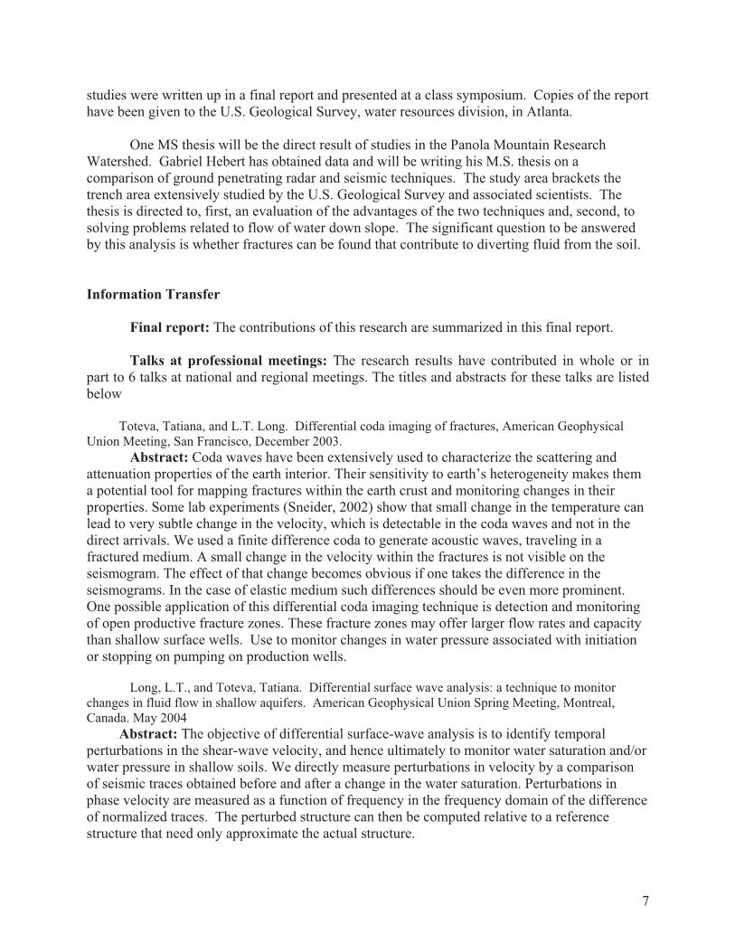
b)Figure 13. a) NMO traces, b) stack trace, the 40m fracture is at 0.082s, although the reflection is

quite weak. The 23m fracture is even more noticeable here.

22

0 0.02 0.04 0.06 0.08 0.1 0.12 0.14 0.16 0.18 0.2-3

-2.5

-2

-1.5

-1

-0.5

0

0.5

1

1.5

2

Time [s]

Am

plit

ud

e

Comparison of two dry stack traces

0 0.02 0.04 0.06 0.08 0.1 0.12 0.14 0.16 0.18 0.2-2.5

-2

-1.5

-1

-0.5

0

0.5

1

1.5

Time [s]

Am

plit

ud

e

Comparison of two wet stack traces

a) b)

0 0.02 0.04 0.06 0.08 0.1 0.12 0.14 0.16 0.18 0.2-1.5

-1

-0.5

0

0.5

1

Ti

Am

plit

ud

e

Comparing differences

me [s]

between wet and dry traces

wet-wet

dry-dry

wet-dry

0 0.02 0.04 0.06 0.08 0.1 0.12 0.14 0.16 0.18 0.2-3

-2.5

-2

-1.5

-1

-0.5

0

0.5

1

1.5

2

Time [s]

Am

plitu

de

Comparison of a wet and a dry stack trace

wet

dry

c) d)Figure 14. Differential analysis for the 12m fracture. a) comparison of the stack trace of two wet

records; b) comparison of the stack trace of two dry records; c) comparison of the stack trace of a

wet and a dry records; d) comparison of the difference between two wet (black line), two dry (blue

line) and a wet and a dry (red line) trace.

23

0 0.02 0.04 0.06 0.08 0.1 0.12 0.14 0.16 0.18 0.2-1.5

-1

-0.5

0

0.5

1

Time [s]

Am

plit

ude

Comparing differences between wet and dry traces, fracture depth 23m

wet-wet

dry-dry

wet-dry

0 0.02 0.04 0.06 0.08 0.1 0.12 0.14 0.16 0.18 0.2-1.5

-1

-0.5

0

0.5

1

Time [s]

Am

plitu

de

Comparing differences between wet and dry traces, fracture depth 40m

wet-wet

dry-dry

wet-dry

a) b)

Figure 15. Comparison of the differences between wet and dry records for a) 23m deep fracture; b)

40m deep fracture.

The resulting difference traces are similar, as might be expected because the move out functions

are similar, but shifted in time. There is a distinct change in seismic properties under the different

pumping conditions. It is not entirely clear that these changes are due to changes in the reflections from

the fractures or to changes in water content in the shallow soil. More signal analysis may resolve the

source of the anomalies.

Chapman, Melinda J. Thomas J. Crawford, and W. Todd Tharpe (1996). Geology and Ground-water

Resources of the Lawrenceville area, Georgia, Water-Resources Investigations Report 98-4233,

U.S. Geological Survey, Denver, CO, 56pp.

24

Appendix II

A Differential Approach for Detecting Temporal Changes in Near-Surface Earth Layers

Based on the presentation by Tatiana Toteva, and L.T. Long, at the 76th Annual Meeting, Eastern Section

Seismological Society of America, Virginia Polytechnic Institute and State University, Blacksburg,

Virginia. October 31 to November 1, 2004.

Abstract: The physical parameters (shear wave velocity, density, porosity, etc.) of near-surface soils and

weathered rocks have been extensively studied for the purposes of geotechnical engineering, hydrology,

oil and gas exploration etc. The possibility of using geophysical techniques for monitoring changes

within this upper layer has gained big popularity within the recent years. The objective of this study is to

develop a differential technique for detecting subtly velocity changes within the soil layer. The

differential technique is based on a study of the difference between two normalized traces taken at

successive time intervals. The differences are interpreted as perturbations to a structure. This study has

applied the differential technique to Rayleigh waves. We hypothesized that fluid penetration due to

natural causes (rainfall) or pumping of fluids, would lead to changes in the shear wave velocity, which

could be detected on the differential seismograms. In the traditional approach the soil layer is studied by

inverting the phase velocity dispersion curve for the velocity structure. Instead of the phase velocity we

use group velocity for inversion curve. Group velocity depends on phase velocity and the change of the

phase velocity with frequency. Hence, we hypothesized that group velocity would be more sensitive to

subtle changes in the velocity structure. The technique was tested for two different types of soil

perturbations. We acquired data before and after heavy rain in the Panola Mountain Research Watershed

to test the effect of variations in water table and soil moisture. At a second site, we tested a more

controlled perturbation by pumping water into the soil at a depth of about 1.0 meter. Important factors in

the acquisition of this data were the use of a repeatable weight-drop source and a secure and repeatable

geophone placement. Our results show that the fluid penetration I the soil causes phase changes and time

shifts, detectable on the differential seismograms.

Introduction

The objective of this study is to demonstrate a differential technique for detecting subtle velocity

changes, particularly those occurring within the near-surface soil layer. We hypothesized that fluid

penetration due to natural causes (rainfall) or the pumping of fluids would lead to changes in the shear

wave velocity, which in turn could be detected by the group velocity dispersion curve. Subtle changes in

seismic velocity can be expressed as subtle time shifts in seismograms. Hence, we obtain seismic data

with the same source and receiver positions at sequential times in order to monitor the change in velocity.

Surface Wave Analysis:

Conventional surface wave analysis uses either the phase velocity or group velocity to

determine the dispersion curve in a specific area. In this study, we will do this along a line,

obtaining dispersion relations for phase and/or group velocity as a function of position along the

line. The standard procedure is to use the dispersion relation to find a layered velocity structure

under the area with the dispersion curve.

Instead of mapping variations in structure (note, the structure could be provided as a

separate analysis) in differential surface-wave interpretation we look for time variations in the

dispersion curves (as indicated by time variations in the seismic trace) induced by changes in

25

fluid content. The reference or average structure is no longer critical to the analysis so long as a

reasonable approximation is available to generate appropriate theoretical differences in

dispersion induced by known perturbations in the structure. For the differential approach, the

reference is not the pre-test velocity structure, which is generally unknown in detail, but is the

seismic trace from the unperturbed structure, which is available from an earlier survey. In the

differential approach, we measure the differences in the dispersion for waves traveling the same

path by direct comparison of two seismic traces recorded at different times. The direct

comparison gives the time shift.

The time shift between two phases can be expressed as the difference between the phases of the

two traces by the equation,

ft

2

where for angles less than 45 degrees,

A

AAref1sin

and the A’s are the amplitudes of the reference trace and the perturbed trace.

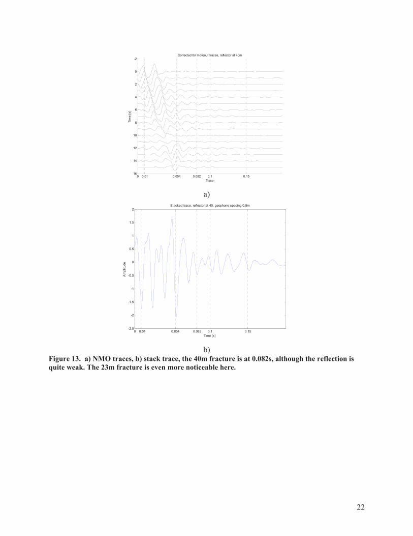
Data for this study were collected at the Panola Mountain Research Watershed using 15 Hz

geophones on the established line. A linear array of geophones with one meter spacing was used for the

recording of the data. The line was marked with permanent concrete geophone mounts. The data taken

after each hurricane represent wet saturated ground. The weight-drop source was placed 5m from the first

geophone. Measurements were taken before and one day after each of two major hurricanes –hurricane

Frances and hurricane Jeane. On comparison (Figure 1.) the phase arrival times look similar for the two

events.

0 0.05 0.1 0.15 0.2 0.25 0.3-4

-2

0

2

4

6

8

10

12

14

16Comparison between after Frances and after Jeane data

Time [s]

Tra

ce

after Frances

after Jeane

Figure 1. Comparison of data recorded during wet periods after two storms.

26

However, in Figure 1, the amplitudes vary along the line. In contrast, both the amplitudes and the

phases appear to vary when comparing data between dry and wet periods (Figure 2).

Figure 2. Comparison between records recorded during dry periods before the storms and wet

period after the storms.

0 0.05 0.1 0.15 0.2 0.25 0.3-4

-2

0

2

4

6

8

10

12

14

16Comparison between dry data and after Frances data

Time [s]

Tra

ce

dry data

after Frances

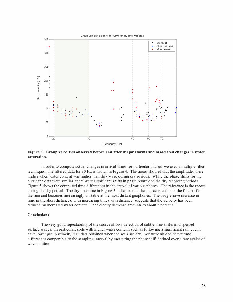
In all tests we showed that the tests over a short time period were repeatable, giving in all cases

almost identical signatures. The differences represent variations in the velocity structure with time. In

order to quantify these changes, we have computed group velocities from the data and for filtered data we

have computed the phase shifts. The group velocities are shown in figure 3. In the 20 to 30 Hertz range,

which is appropriate for a reasonable sampling of the top meter of soil and rock, the velocities following

the two hurricanes were distinctly lower. Reduced velocity would be expected for the increased density

associated with a higher water table

27

0 0.05 0.1 0.15 0.2 0.25 0.3-2

0

2

4

6

8

10

12

14

16Filtered seismograms of dry data and data after the two hurricanes, 30Hz low pass filter

Time [s]

Tra

ce

dry data

after Frances

after Jeane

Figure 4. Data filtered at 30 Hertz showing comparison of data during dry periods and

following hurricanes Frances and Jeane.

5 10 15 201

2

3

4

5

6

7

Time shift with offset, before and after the the two hurricanes, 30Hz

Tim

e s

hift

[s]


dry

Frances

Jeane

Figure 5. Computed time shifts for 30 Hertz.

29

Appendix III

A scattering inversion experiment to identify fractures on a granite

outcrop

Tatiana Toteva and L. T. Long.

Abstract: A critical need in understanding open or fluid filled fractures in crystalline

rock is the ability to identify these fractures, to characterize their source zones, to map flow paths

within the fractures, and to assess residence time of water in the system. Fractures are an

important component in the water resources of areas where crystalline rocks crop out at the

surface. We have attempted to use scattered waves to identify and map fractures in a crystalline

rock. Our research was conducted at the Panola Mountain Research Watershed (PMRW), GA.

The scattering technique was tested in an area of exposed rock. We used 16 geophones placed in

a circular array with diameter of 16m. The free period of the geophones is 100Hz. A major

effort was taken towards suppressing resonances of the geophones at high frequency. We used

clay to better attach the geophones to the outcrop and sand bags to weight the instruments down

to suppress the high frequency resonance. A small weight-drop source was designed to generate

a high-frequency input signal. The source provided signals in the 300 to 800 Hz range. The

source was moved to shot points in the distance range of 5 to 60 meters from the recording array.

The recorded signals were high-pass filtered to allow only waves above 500 Hz. Analysis of the

data gave independent estimates of the velocities of surface waves on the rock and shear and

compressional wave velocities in the rock. In processing the data, the distance of travel of a

scattered wave was obtained from the travel time. The direction to the scattering fracture is

obtained by interpreting maximum the semblance as a function of apparent velocity and direction

of propagation. The technique provides a theoretical way to map positions of varying scattering

efficiency and hence the location of fractures.

Introduction to scattering inversion for fracture detection

Scattering inversion is a form of the 3-dimensional migration used in processing seismic

reflection data in industry. The basis for the scattering inversion we propose has been described

in detail by Chen and Long, (2000a). By combining a two dimensional array of geophones and

sources, the sites of reflections can be located in a 3 dimensional spatial grid. As in the study by

Chen and Long (2000a) the inversion can be improved by performing the stacking by using the

Algebraic Reconstruction Technique (ART). However, in this study we have used beam

focusing with an array of geophones to give the direction of arrival of scattered waves. This

refinement to the Algebraic Reconstruction Technique is a significant improvement because it

strongly limits the source zone of the reflection.

Summary of scattering inversion: The generally accepted model for the seismic coda is

a superposition of wavelets scattered back from many structures (Aki, 1969, Aki and Chouet

1975). This coda model has been refined in order to relate coda decay to the scattering and

attenuation properties of the earth’s crust (Sato, 1977; Frankel and Wennerberg, 1987;

Revenaugh, 2000). A fundamental assumption of the coda model is that intrinsic absorption and

30

the distribution of structures causing scattering is uniform. As a result of this assumption, all

these models predict that the seismic coda should decay smoothly and that the coda decay rate

should be independent of the hypocenter. However, in most recordings of seismic events the rate

of decay deviates from this prediction. As is well known from reflection seismic methods, the

seismic coda does not always decay smoothly, often containing anomalous amplitudes from

waves reflected from structures at depth. These observations suggest that the assumptions

concerning the uniform distribution of structures that scattered wave energy or the uniform

distribution of intrinsic absorption may be violated. This conclusion should have been expected

because the structures that scatter seismic energy are rarely distributed uniformly in the earth's

crust. For example, open fractures that can scatter significant seismic energy are clustered near

fault zones and are more prevalent at shallow depths where the lithostatic pressure is too low to

close joints or fractures.

In the past decade, several studies have attempted to characterize the distribution of

structures that scatter seismic waves. One approach is to apply frequency-wavenumber (F-K)

analysis to the data from dense seismic arrays (e.g. Furumoto et al., 1990). Studies based on this

approach have identified waves scattered from geological structures and topographic relief near

the recording stations. Our approach is the coda envelope inversion technique (Ogilvie, 1988;

Nishigami, 1997; Chen and Long, 2000a, Revenaugh, 2000). One advantage of this approach

over the F-K analysis is that coda envelope inversion does not require a dense array of stations.

An advantage over the Kirchhoff depth-imaging method (Sun et al., 2000) is the reduction in

required data processing. Coda envelope inversion is appropriate when the coda is long

compared to the period of the waves. For shallow scattering, Kirchhoff depth imaging methods

may be required. Part of this research is to define the conditions under which Kirchhoff

migration and coda envelope inversion techniques work best.

The effectiveness of coda envelope inversion can be illustrated by results from Chen and

Long (2000a). Figure 3 shows the distribution of scattering coefficients surrounding the Norris

Lake Community seismicity. The epicenters of the many earthquakes of this swarm are located

near the center of the image. The 5 to 7 stations recording the small earthquakes surround the

epicentral zone.

The areas of greater relative scattering coefficients are closely associated with the

epicentral zone in the center, and near some geologic structures along the east border of the

image area. The distribution relative scattering coefficients showed that fracture density

decreased rapidly with depth. One important observation is that the shallow scattering

coefficients are strongly frequency dependent, indicating scattering from fractures rather than

from velocity contrasts that would be frequency dependent.

31

Figure 3. Relative scattering coefficients at 17 Hz for a depth of 0.25 km.

The theoretical model for the scattered waves in the coda is given in the paper by Chen

and Long (2000a) and can be summarized as follows. The coda energy level at lapse time t is a

function of the source radiation pattern, the numerous velocity anomalies and discontinuities that

scatter seismic energy, and the propagation properties of the medium. Most investigations (Aki

and Chouet, 1975; Sato, 1977) assume that the propagation may be represented by statistical

methods. To obtain information about a non-uniform distribution of scattering coefficients,

deterministic methods such as those of Ogilvie (1988), and Nishigami (1997) must be used. In

the coda envelope inversion of this study, we take advantage of the simple expressions of the

statistical method to find the master curve of coda decay. Then a deterministic method is used to

find the scattering strength of individual structures relative to the master curve of coda decay.

Relative scattering coefficients are the ratio of the actual scattering coefficient of a scattering

structure to the average scattering coefficient of the region. In statistical methods, uniform and

random distributions of scattering structures, spherical radiation of energy from the source,

isotropic scattering and homogeneous velocity structure are usually assumed. Furthermore, if the

scattering does not contain converted phases, and the medium takes up the whole three-

dimensional space, then the mean energy density of scattered waves at frequency can be found

by the single isotropic scattering theory of Sato (1977),

)1()exp()(4

)|,(22

0

0

cs Q

t

t

tK

tV

WgtrE

where W is the total energy radiated from the source at frequency , g0 is the average scattering

coefficient of the random medium, Qc is the coda quality factor, V is the velocity of the S wave, t

is the lapse time of coda waves measured from the earthquake origin, ts is the travel time of

direct S wave, and K(t/ts)=(ts/t)ln[(t+ts)/(t-ts)]. Here we put a subscript 0 for both E and g to

denote that both parameters hold the average value and that they are derived for a uniform

distribution of scattering objects.

32

From the deterministic point of view, the medium consists of discrete scattering structures at

defined locations. If the phases of scattered waves are randomly distributed, we may assume that

the scattered waves can be regarded as incoherent. Then, the energy of the scattered waves

contained within the lapse time window [tj- t/2, tj+ t/2] will be equal to the summation of the

individually scattered waves arriving within this window. In a constant-velocity medium the

scattered waves that meet this travel time condition are contained in an ellipsoidal shell whose

foci are located at the source and receiver. For a source and receiver in close proximity, the shell

is approximated by a sphere whose inner radius is V(tj- t)/2, and whose thickness is V t/2. If the

scattering cross section of each scattering structure takes the average value0, and if the total

number of scattering structures falling into the shell is Nj, then the energy contained in the lapse

time window [tj- t/2, tj+ t/2] is approximated (Aki and Chouet, 1975; Sato, 1977) by,

)2()exp()()4(

)(42

0

0

c

j

j

j

jQ

t

Vt

WNttE

For the uniform distribution of scattering coefficients and the homogeneous distribution

of Qc, equation (2) predicts that the coda wave amplitude will decay smoothly with lapse time

and be random. However, fluctuations in the coda decay are caused by the non-uniform

distribution of scattering coefficient and/or intrinsic absorption. For a non-uniform distribution of

scattering cross sections, we assume that the scattering cross section of each structure is unique.

In this case, the scattering cross section for structure i can be written as i=

i 0, where

i is

called the relative scattering coefficient. The energy contained in the coda waves in a lapse time

window becomes

)3()exp()()4(

)(1

42

0jN

i

i

c

j

j

jQ

t

Vt

WttE

Here the relative scattering coefficient i measures the ratio of the scattering strength of an

individual scattering object to the average scattering strength of the medium.

Following the method of Nishigami (1997) and divided equation (3) by equation (2), we

finally get

)4(1

)(

)(

10

jN

i

jj

j

NtE

tE

Equation (4) indicates that the ratio of observed energy density displayed in individual coda to

the average energy density is independent of the source response and path effects. Also,

equation (4) indicates that the ratio is equal to the average of the relative scattering coefficients

of those structures responsible for the generation of this part of the coda.

For each seismogram, the coda is divided into small time windows, each of which gives an

equation based on equation (4). For these equations, the scattering objects contributing to each

time window are contained in a series of ellipsoidal shells. The number of scatterers can be large,

over 13500 in the Chen and Long (2000a) study. Equation 4 leads to a very large but sparse

matrix.

33

For monitoring the change in scattering coefficients from fractures (4) should be

modified by replacing the vector of the ratio ej=E(t

j)/E

0(t

j) with its change ej and the vector of

the relative scattering coefficients with i .

The coda-envelope-inversion is conventional tomography, in which conventional matrix

inversion methods are not practical. In this study, the iterative Algebraic Reconstruction

Technique (ART) is used to find a solution for equation (4) (Humphreys et al., 1984; Nakanishi,

1985). We first make an arbitrary initial guess at the solution. In this study we assign a value of

one to all i's so that the initial solution represents average background level of scattering

coefficients. We examined other starting solutions but found that we obtained the same solution

for each. We applied a relaxation parameter to control the rate of convergence and a constraint

that all relative scattering coefficients remain positive. In this formulation successive iterations

of the ART algorithm converge to a constrained and damped least square error solution (Kak and

Slaney, 1988, pp280-281). In our study, the relaxation parameter was given a value of 0.1 and

the iterations were truncated when the model parameters change less than 5% for additional

iterations.

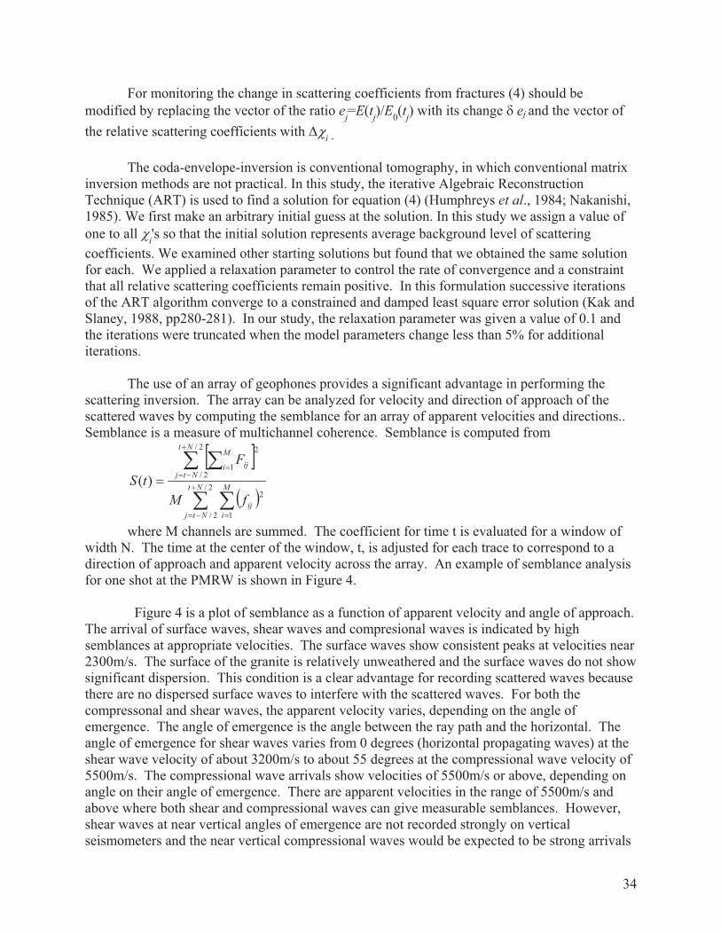
The use of an array of geophones provides a significant advantage in performing the

scattering inversion. The array can be analyzed for velocity and direction of approach of the

scattered waves by computing the semblance for an array of apparent velocities and directions..

Semblance is a measure of multichannel coherence. Semblance is computed from

2/

2/ 1

2

2/

2/

2

1

)(Nt

Ntj

M

i

ij

Nt

Ntj

M

i ij

fM

F

tS

where M channels are summed. The coefficient for time t is evaluated for a window of

width N. The time at the center of the window, t, is adjusted for each trace to correspond to a

direction of approach and apparent velocity across the array. An example of semblance analysis

for one shot at the PMRW is shown in Figure 4.

Figure 4 is a plot of semblance as a function of apparent velocity and angle of approach.

The arrival of surface waves, shear waves and compresional waves is indicated by high

semblances at appropriate velocities. The surface waves show consistent peaks at velocities near

2300m/s. The surface of the granite is relatively unweathered and the surface waves do not show

significant dispersion. This condition is a clear advantage for recording scattered waves because

there are no dispersed surface waves to interfere with the scattered waves. For both the

compressonal and shear waves, the apparent velocity varies, depending on the angle of

emergence. The angle of emergence is the angle between the ray path and the horizontal. The

angle of emergence for shear waves varies from 0 degrees (horizontal propagating waves) at the

shear wave velocity of about 3200m/s to about 55 degrees at the compressional wave velocity of

5500m/s. The compressional wave arrivals show velocities of 5500m/s or above, depending on

angle on their angle of emergence. There are apparent velocities in the range of 5500m/s and

above where both shear and compressional waves can give measurable semblances. However,

shear waves at near vertical angles of emergence are not recorded strongly on vertical

seismometers and the near vertical compressional waves would be expected to be strong arrivals

34

on the vertical geophones. We have assumed that the waves travel their entire path as either

surface waves, shear waves or compressional waves. It is very likely that some portion of the

arrivals at the array represent converted waves. That is, waves that start as a shear wave and on

reflection at a fracture are converted to compressional waves and detected as compressional

waves at the array. These are fortunately not coherent and would not accumulate at one

reflection location as a strong reflection. Hence, converted waves may contribute to the noise

background, but would not interfere with the detection of fractures.

0 50 100 150 200 250 300 3502000

3000

4000

5000

6000

7000

8000

Velo

city [

m/s

]

Azimuth [deg]

Semblance, 0.019-0.021s

0.05

0.1

0.15

0.2

0.25

0.3

0.35

0.4

0.45

Figure 4. is a semblance plot showing a strong compresional wave arrival at 160 degrees. A

shear wave arraival can be seen at 90 degrees and surface wave arrivals appear at 70, 270,

and 360 degrees.

Because the semblance plots give tightly constrained angles of approach for both

compressional and shear waves, iteration with the ART algorithm is not needed to locate

fractures. Iteration would be needed to quantify the strength of scattering from the fracture. In

this analysis we have computed the semblance for multiple times in the coda for about 14 shot

point locations on the granite. The 14 shot point locations were in the shape of a rectangle. In

order to test the imaging program and its ability to locate sources of signals, we applied it to the

time window containing the direct surface wave arrival. The surface wave arrival should point

back to the origin, and correspond to the shot point. The results of this first test are shown in

Figure 5. The only shot points not clearly imaged are those on the left in Figure 5. The

background noise appears as circles surrounding the origin of the recording array.

35

-100 -80 -60 -40 -20 0 20 40 60 80 100-100

-80

-60

-40

-20

0

20

40

60

80

100

0

0.1

0.2

0.3

0.4

0.5

0.6

0.7

0.8

0.9

1

Direct surface wave energy

y c

oo

rdin

ate

[m

]

x coordinate [m]

Figure 5. Inversion for sources using only windows in the arrival time of the surface wave.

The triangles show the actual locations of the shots, the bright squares, particularly those

on the top and right, are indicated sources of the signals.

Bibliography

Aki, K.(1969). Analysis of the seismic coda of local earthquakes as scattered waves, J. Geophys.

Res., 74, 615-631.

Aki, K. and B. Chouet (1975). Origin of coda waves: source, attenuation and scattering effects.

Journal of Geophysical Research, 80, 3322-3342.

Chen, Xiuqi, and L.T. Long (2000a). Spatial distribution of relative scattering coefficients

determined from microearthquake coda. Bulletin. Seismological Society America, 90, 2, pp 512-

524.

Frankel, A. and L. Wennerberg (1987). Energy-flux model of seismic coda: separation of scattering

and intrinsic attenuation, Bull. Seism. Soc. Am. 77, 1223-1251.

Furumoto, M., T. Kunitomo, H. Inoue, I. Yamada, K. Yamaoka, A. Ikami, and Y. Fukao (1990).

Twin source of high-frequency volcanic tremor of Izu-Oshima Volcano, Japan. Geophysical.

Research Letters, 17, 25-27.

Humphreys, E., R. W. Clayton, and B. H. Hager (1984). A tomographic image of mantle structure

beneath southern California. Geophysical Research Letters, 11, 625-627.

Kak, A. C. and M. Slaney (1988). Principles of computerized tomographic imaging. IEEE Press,

New York.

36

Nakanishi, I. (1985). Three-dimensional structure beneath the Hokkaido-Tohoku region as derived

from a tomographic inversion of P-arrival times. Journal Physics of the Earth, 33, 241-256.

Nishigami, K. (1997). Spatial distribution of coda scatterers in the crust around two active volcanoes

and one active fault system in central Japan: inversion analysis of coda envelope. Physics of the

Earth and Planetary Interiors, 104, 75-89.

Ogilvie, J. S. (1988). Modeling of seismic coda, with application to attenuation and scattering in

southeastern Tennessee, M.S. Thesis, Georgia Institute of Technology, Atlanta, Georgia.

Sato, H. (1977). Energy propagation including scattering effects: single isotropic sattering

approximation. J. Phys. Earth, 25, 27-41.

Sun, Yonghe, F.Qin, S. Checkles, and J. P. Leveille, (2000). A beam approach to Kirchhoff depth

imaging, The Leading Edge. 19, 1168-1173.

Revenaugh, J., (2000). The relation of crustal scattering to seismicity in southern California,

Journal of Geophysical Resarch, 105, 25,403-25,422.

37

Decision Support for Georgia Water Resources Planning and Management

Basic Information

Title: Decision Support for Georgia Water Resources Planning and Management



End Date: 2/28/2005



Research Category: None

Focus Category: Management and Planning, None, None

Descriptors: None

Principal Investigators: Kathryn J. Hatcher

Publication

PROGRESS REPORT FOR YEAR 1

Project Title: Decision Support for Georgia Water Resources Planning and Management

Duration: March 1, 2004 - February 28, 2006 (24 months)

Principal Investigator: Kathryn J. Hatcher Institute of Ecology Tel: 706-542-3709 University of Georgia, Athens, Georgia 30602-2202

Executive Summary The ninth biennial Georgia Water Resources Conference was held April 25-27, 2005, to provide a forum for discussion of Georgia water resources and information relevant to the state’s initiative to prepare a comprehensive statewide water resources management plan. Over 25 government, professional, and citizen organizations served to co-sponsor the conference and organize sessions and panels with over 250 speakers in these general tracks: state water plan and policy, Atlanta area water issues, water conservation, instream flow and restoration, watershed protection and TMDLs, flood mapping and stormwater, groundwater, coastal water issues, and river basins including Savannah, Etowah, Flint, and Chattahoochee Rivers. The 2005 onference proceedings with 240 papers is available on CD and as printed volumes. The conference included panels to discuss five state water policy issues selected by the Georgia EPD director: (1) protection of instream and downstream flows, (2) water quantity allocation/reallocation among users, (3) minimum aquifer levels protection policy, (4) water quality allocation (TMDL allocation policy), and (5) water conservation/efficiency and reuse policy. The third day of the conference provided five all-day training courses on these topics: (1) Shared Vision Planning Approach – Linking Participation and Water Planning through a Technical Systems Model (by USACE-IWR), (2) ArcHydro – GIS for Water Resources, (3) Introduction to the Clean Water Act for Watershed Stakeholders (by USEPA-Region 4), (4) Water Quality Modeling using WASP software (by USEPA-ERL), and (5) Stormwater Management using Locally-Based Planning and Management Tools (by UGA-Engr); as well as (6) a workshop on government programs with technical assistance and/or funding for water resources planning and management (hosted by USACE-SAM). Over 40 students from UGA and Georgia Tech provided assistance for the conference sessions, policy panels and training courses.

Main Project Elements

Georgia Water Resources Conference

The ninth biennial Georgia Water Resources Conference was held April 25-27, 2005, at the Georgia Center for Continuing Education, Athens, Georgia. In addition to its traditional purpose of providing a biennial forum for presentation and discussion of major water projects, issues, programs and research in Georgia, the 2005 conference was designed with an additional purpose -- to provide information relevant to the state’s initiative to prepare a comprehensive statewide water resources management plan by 2008. The conference steering committee, which sets the goals and theme for the conference, consisted of representatives from the 5 main sponsors including USGS, NRCS, UGA, the director of the Georgia Water Resources Institute and the director of the Georgia Environmental Protection Division. The EPD director selected the conference theme, “Creating Georgia’s Sustainable Water Future,” and gave the plenary session presentation on Georgia’s initiative to develop a comprehensive statewide water resources

management plan. Governor Sonny Perdue gave the keynote conference address on Georgia water resources.

In addition to the five main sponsors, the conference was supported by over 20 co-sponsoring organizations and a program committee of co-sponsor representatives, who organized 36 of the 70 sessions and panels presented at the conference, and provided exhibits and conference promotion. The conference agenda included over 250 speakers in 70 sessions, with sessions on the Etowah River, Savannah River, Chattahoochee River Basin, Flint River Basin, and Coastal Georgia. The session and panel topics, each with 3-5 speakers, are listed below with the session organizer indicated:

TRACK 1. STATE WATER PLAN AND POLICY + Water Allocation Legal Issues + Regional Water Plans in Georgia (GaEPD) + Plenary Session: Carol Couch, GaEPD Director + Panel: Perspectives on State Water Plan Process (GWC) + Panel: Policy on Water Allocation/Reallocation (UGA) + Poster and Exhibit Session (USDA-NRCS) - Low Impact Development - Integrated Water Resources Planning - Legislative Update and Water Law - Panel: Indicators of Sustainability (GaDNR-P2AD) - Conflict Resolution ^ Technical and Financial Assistance Programs (USACE-SAM) ^ Technical and Financial Assistance Programs II (USACE-SAM) ^ Adopt-A-Stream Monitoring field demonstrations (GaEPD)

TRACK 2. ATLANTA AREA WATER ISSUES + Public Education and Awareness (ARC) + Atlanta Area Stream Quality + Metro District Water Plans Development (MNGWPD) + Metro District Water Plans Implementation (MNGWPD) - Panel: ACF River Federal Water Requirements - ACF River Basin Water Negotiations - Sustainable Mgt w/Lake Lanier Reuse (GW&PCA) - Atlanta Water Supply Issues - Sewage Overflow and Infrastructure ^ Full-day Course on Basin Planning (USACE-IWR)

TRACK 3. INSTREAM FLOW AND RESTORATION + Instream Flow Guidelines for Georgia (TNC) + Instream Flow Studies (Entrix Inc.) + Panel: Policy on Instream/Downstream Flow Protection (UGA) + Streamflow vs Fish Distribution - Aquatic Ecosystems - Imperiled Aquatic Species (USFWS) - Etowah River Habitat Conservation Plan (USFWS) - Stream Restoration (USACE-SAD) - Ecosystem Restoration ^ Full-day Course on Clean Water Act (USEPA Region4)

TRACK 4. FLOOD MAPPING, WATER CONSERVATION

+ Floodplain Mapping using GIS (AWRA-Ga) + GIS Applications in Water Resources (GaEPD) + River Flood Forecasting (NWS-SERFC) + Watershed Assessment - Georgia Sustainability Initiative (GaDNR-P2AD) - Water Conservation in Landscape (GWWC) - Water Conservation - Potable Water Reuse (GW&PCA) - Panel: Policy on Water Conservation and Reuse (UGA) ^ Full-day Course on GIS Use for Water Resources (GaEPD)

TRACK 5. WATERSHED PROTECTION + Stream Riparian Buffers + Runoff Impacts to Stream Quality + Stream Quality Studies + Stream Data for TMDL Models - Watershed Alliances and Education - Watershed Management (USEPA Region4) - Water Quality Permit Trading - Panel: Policy on TMDL Allocation/Reallocation (UGA) - TMDL Plans Development (USEPA Region4) ^ Full-day Course on Water Quality Modeling (USEPA-ERL)

TRACK 6. STORMWATER, SAVANNAH RIVER + Stream Channel Restoration + Adequacy NPDES Stormwater Regulations + Panel: Erosion & Sediment Control (ASCE-Ga) + BMPs for Runoff Control (ASCE-Ga) - Gwinnett County Stormwater Program I (Gwinnett Co) - Gwinnett County Stormwater Program II (Gwinnett Co) - Savannah River Basin Models (USACE-SAV) - Panel: Savannah River Basin Water Use GA/SC (USACE-SAV) ^ Full-day Course on Stormwater Management (UGA-Engr)

TRACK 7. GROUND WATER ISSUES + Conservation Tillage (SWCS-Ga) + Piedmont Ground Water Supply I (GGWA) + Piedmont Ground Water Supply II (GGWA) - Education for Private Well Owners I (UGA-CES) - Education for Private Well Owners II (UGA-CES) - Irrigation Water Use in Georgia - Flint River Basin Models ^ Surface and Ground Water Interactions ^ Coastal Ground Water Levels and Management ^ Panel: Policy on Minimum Ground Water Levels (UGA) ^ Savannah Harbor Dredging Effects on Ground Water ^ Ground Water Contamination

Workshops and Training CoursesThe third day of the conference consisted of workshops and one-day training courses:

* Workshop on Multiple Agency Programs with Technical Assistance and Funding for Water Resources Planning and Management, hosted by US Army Corps of Engineers-Mobile District.

* Workshop on Adopt-A-Stream Monitoring (field demonstrations), by Georgia Environmental Protection Division, Adopt-A-Stream program www.riversalive.org/aas.htm

* Course on the Shared Vision Planning Approach - Linking Participation and Water Planning through a Technical Systems Model, by US Army Corps of Engineers, Institute for Water Resources

www.iwr.usace.army.mil

* Course on ArcHydro: GIS for Water Resources, with application for the Upper Ocmulgee watershed in Georgia, by Dr. David Maidment, University of Texas, and Jack Hampton, PBSJ [48 seats in computer lab] Organized by Georgia Environmental Protection Division.

http://www.ce.utexas.edu/prof/maidment/

* Course on Introduction to Clean Water Act for Watershed Stakeholders, by US Environmental Protection Agency Region IV.

www.epa.gov/r5water/cwa.htm

* Course on Water Quality Modeling using WASP software package, by US EPA Environmental Research Laboratory, Athens.

www.epa.gov/AthensR/research/modeling/wasp.html

* Course on Stormwater Management using Locally-Based Planning and Management Tools, by University of Georgia, Biological and Agricultural Engineering Department.

Conference Co-SponsorsThe conference is sponsored by: U.S. Geological Survey, Georgia Department of Natural Resources, University of Georgia, Georgia Tech – Georgia Water Resources Institute, and USDA Natural Resources Conservation Service.

Additional co-sponsors include Georgia offices of: - American Society of Civil Engineers - American Water Resources Association - American Water Works Association - Association County Commissioners of Georgia - Georgia Municipal Association - Georgia Department of Community Affairs - Georgia Forestry Commission - Georgia Soil and Water Conservation Commission - Georgia Pollution Prevention Assistance Division - Georgia Water & Pollution Control Association - Georgia Ground Water Association - Georgia Lake Society - Georgia Water Wise Council - National Weather Service, SE River Forecast Center - Natural Resources Conservation Service (SCS) - Soil and Water Conservation Society

- Soil Science Society of Georgia - The Georgia Conservancy - Upper Chattahoochee River Keeper - Water Environment Federation - U.S. Army Corps of Engineers, Mobile/Atlanta/Savannah - U.S. Environmental Protection Agency, Region 4 - U.S. Environmental Protection Agency, ERL - U.S. Fish and Wildlife Service

Policy PanelsThe conference program plans, which were outlined by the steering committee in summer 2004 to support the state’s comprehensive water plan process, were modified in fall 2004 after Governor Perdue expressed his wish that the state water plan process would emphasize resolving state water policy issues that were discussed leading up to the legislation mandating the state water plan. To adjust to this new direction, the conference agenda added five water policy panels to cover several of the key state water policy issues:

1. Protection of Instream and Downstream Flows 2. Water Quantity Allocation/Reallocation among Users 3. Minimum Aquifer Levels Protection Policy 4. Water Quality Allocation (TMDL allocation policy) 5. Water Conservation/Efficiency and Reuse Policy

These five topics were selected for the conference by the chair of the Georgia Water Council (the EPD director), responsible for developing the state water plan (www.georgiawatercouncil.org). Each panel consisted of five panelists: a DNR-EPD representative (nominated by the EPD director) to summarize Georgia’s current policy and procedures; three panelists representing diverse interest groups to summarize their group’s desired policy choice and view of the pros/cons for the policy choices; and a technical or legal expert. The purpose of the panels was to begin a policy dialogue and provide information useful as background for the Georgia Water Council in considering several of the key state water policy issues facing Georgia. The panels were not intended to reach consensus or to make recommendations, only to provide useful background information about the difficult water policy issues, the policy choices available, and the pros/cons of each choice from the perspectives of the major groups concerned with the issue. The five panels discussions were held during the conference, with four of the interim panel papers included in the conference proceedings (see list under publications). The policy discussions will be continued with the major stakeholders, and extended versions of policy analysis papers for the five topics will be provided for the Georgia Water Council (www.georgiawatercouncil.org) in the second year of this project.

Student ParticipationOver 40 students from the University of Georgia and Georgia Institute of Technology provided volunteer assistance to the conference. Thirty-six students served as moderator assistants during the conference sessions, operating the A/V equipment and lighting. Three students provided technical and computer assistance for the all-day training course on the ArcHydro software. Ten students provided research assistance during spring semester for the five water policy panels. The student chapter of American Water Resources Association organized the Monday evening event with speaker for the conference, and also organized the team of students who served as moderator assistants. One graduate student, funded by a research assistantship, helped with editing and peer reviewer correspondence for 200+ papers published in the conference proceedings.

Publications

Hatcher, Kathryn J. (editor), Proceedings of the 2005 Georgia Water Resources Conference, Volumes I and II, April 25-27, 2005, Athens, Georgia; sponsored by U.S. Geological Survey, Georgia Department of Natural Resources, USDA Natural Resources Conservation Service, Georgia Institute of Technology – Georgia Water Resources Institute, and The University of Georgia, Athens GA, 931 pages.

Bomar, Robert, Joel Cowan, Ciannat Howett, Kevin Farrell, David Newman, Kathryn Hatcher, “State Water Policy Alternatives for Water Allocation and Reallocation,” in: Proceedings of the 2005 Georgia Water Resources Conference, The University of Georgia, Athens GA, pp. 37-43.

Biagi, John, Jerry Ziewitz, Brian Richter, Bob Scanlon, Billy Turner, Kathryn Hatcher, “State Water Policy Alternatives for Instream and Downstream Flow Protection,” in: Proceedings of the 2005 Georgia Water Resources Conference, The University of Georgia, Athens, GA, pp. 270-278.

Keyes, Alice Miller, Cindy Daniel, Shana Udvardy, Brian Skeens, David Bennett, Kathryn Hatcher, “State Water Policy Alternatives for Water Conservation/Efficiency and Reuse,” in: Proceedings of the 2005 Georgia Water Resources Conference, The University of Georgia, Athens GA, pp. 459-468.

Williams, Vince, Curry Jones, Shana Udvardy, Bill White, Matt Harper, Candace Connell, Kathryn Hatcher, “State Water Policy Alternatives for TMDL Allocation and Reallocation,” in: Proceedings of the 2005 Georgia Water Resources Conference, The University of Georgia, Athens GA, pp. 567-575.

Tasks for Year 2:

Task 1: As a follow-up to the 2005 Georgia Water Resources Conference, the electronic version of the full conference proceedings (over 200 papers) has been provided to the Georgia Water Resources Institute for uploading to the GWRI website. The complete Table of Contents (1989-2005) for the Georgia Water Resources Conference will be updated; this is searchable by author, organization and keyword in a paper’s title. Authors for the 2003 and 2005 conferences will be provided the opportunity to add a web link to their papers in the Table of Contents for readers who wish to read about new developments on the paper’s topic. The electronic version of all back volumes of the conference proceedings (1989-2005) will be provided for the Georgia Water Resources Institute.

Task 2: Review of the state sediment and erosion control program and 319 grant program, with recommendations to the state EPD director for improving the program and for coordinating this program with the state=s existing river basin plans and the pending Statewide Comprehensive Water Plan.

Task 3: The work on the five water policy panel topics, selected by the EPD director, will be continued with further discussions with the major stakeholder groups to help them define their preferred policy alternatives. Extended versions of the policy analysis papers for the five panel topics will be provided for the Georgia Water Council in the second year of this project. The panels were not intended to reach consensus or to make recommendations, only to provide useful background information about the difficult water policy issues, the policy choices available, and the pros/cons of each choice from the perspectives of the major groups concerned with the issue.

Task 4: A survey and summary of information and training needs of water resources professionals in Georgia will be provided. A website will be set up to provide guidance and training materials for comprehensive water resources planning and management, both water quantity and quality, including examples of best practices.

Biogeochemical Cycling of Arsenic at the Sediment-WaterInterface of the Chattahoochee River

Basic Information

Title:Biogeochemical Cycling of Arsenic at the Sediment-Water Interface of theChattahoochee River



End Date: 2/28/2005


CongressionalDistrict:

5

Research Category: None

Focus Category: None, Sediments, Water Quality

Descriptors: None

PrincipalInvestigators:

Martial Taillefert

Publication

1

Biogeochemical Cycling of Arsenic at the Sediment-Water

Interface of the Chattahoochee River

Martial Taillefert


Georgia Institute of Technology, Atlanta GA

May 16, 2005

1.0 Executive Summary

In a previous study, elevated dissolved arsenic concentrations were detected in the

Chattahoochee River (GA) and decreased in concentration with increasing distance from a

suspected point-source, suggesting that arsenic could be scavenged by particles and settle to the

sediment-water interface (SWI). In this study, we investigated the cycling of arsenic in the

sediment of the Chattahoochee River to determine if arsenic is accumulated in the sediment

downstream from two coal-fire power plants and how arsenic is biogeochemically transformed in

these sediments. To realize these objectives, a combination of state-of-the-art analytical

techniques - ICP-MS and voltammetry - with other conventional techniques was used to

determine, with a high spatial resolution, the distribution of arsenic between particulate and

dissolved phase, the redox speciation of arsenic in the dissolved phase, and the distribution of

other redox species (O2, SO42-, NO3

-, Fe(II), Mn(II), and H2S) in the first 10 centimeters of four

sediment cores. Depth profiles suggest that iron oxides scavenge arsenic in the form of arsenate in

the water column and settle to the SWI where they are reduced by iron reducing bacteria. As a

result of microbial iron reduction, dissolved arsenic, in the form of As(V) only, is released and

accumulates in the porewaters near the sediment-water interface, where it can diffuse back to the

overlying waters, with fluxes ranging between 20 and 200 nM/cm2 yr. Sediment slurry

incubations conducted to determine the mechanisms and rate of arsenic biogeochemical

transformations in these sediments confirm that any arsenate added to these sediments is

immediately adsorbed and later released during the reductive dissolution of iron oxides.

Incubations in the presence of low concentrations of arsenate verified that microbial iron

reduction occurs in these sediments and that arsenate is not concomitantly reduced during this

process. Incubations with higher initial arsenate concentrations indicate that the microbial

processes in these sediments may be affected by high inputs of arsenic. Finally, differences

between high discharge rates and base-flow conditions in the Chattahoochee River do not seem to

affect the biogeochemical processes involved in iron and arsenic cycling but may enhance fluxes

across the sediment-water interface.

This investigation was part of the Ph.-D. dissertation of Stephanie Chow and has contributed

to the training of several other undergraduate (Jimmy Elsenbeck, Jennifer King, Dian Putrasahan,

Farhana Yasmin) and graduate (Gwendolyn Bristow, Elizabeth Carey, Judson Partin) students

working under Dr. Taillefert’s direction. These students either participated in field trips or

performed some of the reported chemical analyses. This project resulted in the publication of one

peer-reviewed paper (35), two presentations at professional meetings (American Chemical

Society), one presentation at a local symposium (Georgia Tech), and one seminar (Savannah

River Ecology Laboratory, UGA). Other abstracts and publications will follow in 2005.

2

2.0 Introduction

The adverse human health effects of arsenic have been known for several centuries. The

toxicity and biochemical behavior of arsenic depends on its chemical form. In natural

environments, arsenite (H3AsO3) is not only more mobile but can be greater than 60 times more

toxic than arsenate ( AsO43-), or organoarsenic compounds (1, 2). Reported regions impacted by

elevated arsenic concentrations are Bangladesh, China, India, England, Thailand, and within the

United States (e.g., New Hampshire, New Mexico, Massachusetts, Maine, Michigan, California,

and Oregon). Arsenic input in the natural environment is mainly due to natural sources and coal-

fire power plants because of its ubiquitous presence in coal (3). Coal-fire power plants release

arsenic and other metalloids in the atmosphere during burning. However, the ashes are usually

stored in ponds that may be episodically flooded during storm events and represent significant

sources of arsenic for aquatic systems, especially nearby rivers which are often used for cooling

purpose. Once in rivers, arsenic may be removed by adsorption onto sediments or travel

downstream in solution (3).

In high concentrations, the most toxic fraction, arsenite, may affect ecosystems and can also

present a risk for human health as these waters will eventually recharge water tables and/or lakes

used for the supply of drinking water. The problem of arsenic is a main concern of the Georgia

Environmental Protection Division of the Department of Natural Resources (http://

www.ganet.org//dnr/environ/) and largely recognized in major cities, as part of the heavy metal

class. However, it is equally important to evaluate locations where arsenic exists at low

concentration due to its potential impact on drinking water resources.

Most environmental arsenic problems are a result of mobilization and reduction of arsenic

regulated by biogeochemical processes at redox interfaces (4). In oxic conditions, authigenic iron,

manganese, and aluminium oxides, clays, and particulate organic matter (POM) can remove

metals by sorption or precipitation (5). The adsorption of arsenic in natural waters is mainly

controlled by solid-solution interactions with iron oxides (1, 6-8) because their charge, in contrast

to POM and manganese and aluminum oxides, is slightly positive at circumneutral pH (9), while

arsenate is negatively charged (7, 10-12). As a result, arsenate mobility and bioavailability is

limited in oxic conditions. In suboxic conditions, manganese and iron oxides are reductively

dissolved during organic matter remineralization, potentially releasing trace metals including

arsenate (4), in the dissolved phase. It is also suggested that arsenate may be simultaneously

reduced during the reduction of iron oxides (13), thus turning arsenic-contaminated sediments

into a persistent toxic source. However, little evidence of the simultaneous reduction of iron and

arsenate has been found in natural systems.

In anoxic conditions, arsenate may be reduced to arsenite microbially (14-16) or chemically

by dissolved sulfide (17) and Fe2+ (18, 19) though both chemical reactions are usually slow.

Arsenite is neutral at circumneutral pH and is less susceptible to adsorption onto metal oxides (7,

10, 11). In the presence of dissolved sulfide produced by sulfate-reducing bacteria, arsenite may

form thioarsenite complexes (20) and eventually precipitate as arsenosulfide minerals (21, 22) or,

alternatively, adsorb onto iron sulfide minerals (22). These thioarsenite complexes have yet to be

identified in natural waters but, if they exist, the solubility of arsenite may be enhanced in the

presence of H2S, providing a source of toxic compound in the natural environment.

Finally, arsenite can be rapidly reoxidized in the presence of dissolved oxygen (23) or

3

manganese oxides (24, 25). Thus, desorption and remobilization of arsenic from sediments is

influenced by pH, the activity of microorganisms, and the concentrations of dissolved oxygen,

sulfide and iron in interstitial waters (8, 10, 22, 28-31). In addition, phosphate, bicarbonate,

silicate and organic matter all compete with arsenic for adsorption sites, enhancing arsenic

desorption and thus mobility (31).

3.0 Objectives

It is clear that arsenic is subject to several complex transformations in aquatic systems. As the

sediment is usually the ultimate repository of trace metals and metalloids, it is necessary to

determine quantitatively the fate of arsenic in these systems. In this project, we proposed to

investigate the cycling of arsenic in the sediment of the Chattahoochee River to determine if and

by what mechanism arsenic is accumulated in the sediment downstream from two coal-fire power

plants and how arsenic is biogeochemically transformed in these sediments. The specific

questions we proposed to answer in this project were the following:

To answer question 1, we proposed to monitor in situ the depth profiles of dissolved oxygen,

Mn(II), Fe(II), and H2S at one site in the sediment of the Chattahoochee River downstream from

the suspected arsenic source before, during, and after a storm. Unfortunately, deployment of our

in situ instrument presented logistical problems. We could not find a boat that could deploy our

heavy instrumentation on the Chattahoochee River. We therefore decided to collect sediment

cores and use a non-invasive ex situ approach to monitor depth profiles of the main redox species

involved in arsenic cycling at different sites along the river. After completion of the ex situ

measurements, sediment porewaters were extracted, and the concentration of dissolved arsenic

(Asd) and arsenite as well as the major ions involved in the cycling of arsenic were determined.

Finally, solid phase extractions were performed to quantify amorphous iron oxides and total

extractable arsenic (Ast).

To answer question 2, sediments were collected at the monitoring points according to their

chemical characteristics and sediment slurries manipulated in batch reactor experiments. The

slurries were analyzed as a function of time for arsenite, Asd, Fe(II), Mn(II), and H2S.

Manipulations consisted in providing arsenate to the sediment slurries and following the

evolution of the reactants and products over time to determine the reaction kinetics.

1/ Does arsenic accumulate in the sediment, is remobilized, and diffuse back into the

water column episodically after storm events?

2/ What are the main biogeochemical process regulating the transformation of arsenic

in these iron-rich riverine sediments?

4

4.0 Sampling Site

We selected our field site in the

Chattahoochee River near West Point Lake,

downstream from a point-source of arsenic in

the water column (3). West Point Reservoir

(inset Figure 1) is a 25,900-acre mainstream

Chattahoochee River impoundment located

an hour southwest of Atlanta (GA). West

Point Lake lies on a 35 mile stretch of the

Chattahoochee River between Franklin and

West Point (GA). The lake has a shoreline of

more than 500 miles and runs along and

across the Georgia/Alabama State line. The

lake is controlled by the Army Corps of

Engineers and was impounded in 1974 to

provide drinking water, flood control,

hydroelectric power, navigation, wildlife

development, and general recreation for

Southwest Georgia.

Seven sediment cores (Figure 1) were collected from the outfall of the Chattahoochee River

north of the drinking water reservoir of West Point Lake in LaGrange (GA) based on elevated

total dissolved arsenic concentrations detected in the water column (3). Our study focused in an

area approximately 60 km away from the suspected arsenic source where total dissolved arsenic

was depleted from the water column. The sediment cores were collected in July 2003, three weeks

TABLE 1. Water Levels (feet) and Discharge (cfs) Measured in the

Chattahoochee River at West Point, GA (USGS Station #02339500)

Around the Time of Sampling During Three Consecutive Years

(2002, 2003, 2004).

Date Time Water Level Discharge

[feet] [cfs]

6/11/2002 7:10 2.28 647

6/25/2002 8:15 2.24 816

9/5/2002 8:25 2.1 748

5/9/2003 10:54 21.42 65500

5/9/2003 19.26 20.64 63600

5/10/2003 11:05 19.75 60300

5/12/2003 13:25 8.88 16990

8/6/2003 10:45 5.16 6850

4/5/2004 8:50 6.16 9210

12/1/2004 14:33 5.84 7995

West Point

LaGrange

Franklin

CR- 1

CR- 2

CR- 3

CR- 4

Chattahoochee River GA

CR- 5&6

&7

Figure 1. Study Location in the Chattahoochee River

upstream from West Point Lake (GA). Seven

sediment cores, numbered CR-1 to -7, were collected

along the Chattahoochee River during this study.

Their locations are provided on the map.

5

after Tropical Storm Bill brought approximately 20 foot crests through the study location, and in

May 2004, when the Chattahoochee River was at base-flow conditions (Table 1).

5.0 Methods

Sediment samples were collected with 60 cm long and 10 cm diameter polycarbonate core

liners. Approximately 10 cm of overlying water was collected with each core to maintain the

integrity of the sediment-water interface and minimize exposure to the atmosphere during

transport to the laboratory. To answer question 1, we determined depth profiles of redox

geochemical species at a millimeter resolution in selected sediment cores with gold-mercury (Au/

Hg) voltammetric microelectrodes (32). Voltammetric techniques are attractive to measure

chemical species in sediments because they can detect several analytes at once, they have low

detection limits, and generally do not suffer from matrix problems (e.g., high salinity).

Voltammetric microelectrodes have been successfully built and are routinely utilized in our group

for field deployments (33, 35) or laboratory investigations (34). High resolution voltammetric and

potentiometric profiles of O2(aq), Fe2+, Mn2+, H2S (H2S, HS-, S0, Sx2-), organic-Fe(III)

(aq), FeS(aq),

and pH were obtained by lowering an Au/Hg voltammetric microelectrode and a pH

minielectrode (Diamond General Corp.), in millimeter increments, into each sediment core with a

micro-manipulator (Analytical Instrument Systems, Inc.).

Voltammetric and pH measurements were conducted with a DLK-100A potentiostat that

includes a voltmeter for combination measurements (Analytical Instrument Systems, Inc.).

Dissolved oxygen was measured cathodically by linear sweep voltammetry, while Fe2+, Mn2+,

organic-Fe(III)(aq), H2S, and FeS(aq) were detected by cathodic square wave voltammetry. Prior to

each scan, a conditioning step was applied at -0.1 V for 10 s to clean the microelectrode. Scan

rates of 200 mV/s were used for all measurements (32). The pH was calculated using the Nernst

Law after recording the potential and sample temperature at the minielectrode (36). By using

microelectrodes, a suite of constituents could be measured with a high spatial resolution without

sediment handling, thus minimizing contamination while maximizing the volume of porewater

for other analyses.

Immediately following completion of the electrochemical profiles, the sediments were

sectioned and centrifuged under N2(g) atmosphere, and porewaters were filtered (Norm-Ject sterile

Teflon syringe and Puradisc 0.2µm Whatman filter) and acidified with Trace Metal Grade HCl or

HNO3 (Fisher) as needed for preservations and analysis. All porewaters were extracted and

maintained in a N2(g) atmosphere and kept at 4°C until analysis of As(III), total dissolved arsenic

(Asd), chloride, nitrate, sulfate, total dissolved orthophosphate, and total dissolved silica within 24

hours.

All solutions were prepared with 18 MW-cm Reverse Osmosis (RO) water (Barnstead). All

plasticware and glassware used for trace metal analyses were acid-washed in 2% Trace Metal

Grade HNO3 (Fisher) for one week and rinsed thoroughly with RO water. For As(III) analysis,

standards were made from an As(III) stock solution prepared daily by dissolving As(III) oxide

(Alfa Aesar) in NaOH then acidifying with 12 N HCl (37). Voltammetric measurements for

As(III) were performed with a HMDE using the VA 663 multi-mode mercury drop electrode stand

(Metrohm) coupled to the PGSTAT 12 Autolab potentiostat (Ecochemie). The reference electrode

was an Ag/AgCl/KCl (3 M) with a 0.2 M NaCl glass bridge, and a glassy carbon rod acted as the

6

counter electrode. The solutions were thoroughly degassed with ultra high purity N2(g) in between

each As(III) measurement to prevent reoxidation by dissolved oxygen. As(III) concentrations

were determined by amending the sample with 0.7 mM Cu(II) (CuCl2·2H2O Aldrich) and 1 M

HCl. A potential was applied at -0.4 V for 10 seconds to form an arseno-copper complex (Eq. 1 -

deposition step) (37).

(1)

The potential was then scanned cathodically (from -0.4 V to -1.2 V) at 300 Hz using square

wave voltammetry to reduce Cu(I/II) from the arseno-complex to Cu0 and allow the indirect

measurement of As(III) (Eq. 2 - stripping step).

(2)

Figure 2 shows a triplicate raw data scan of a 1 nM As(III) standard. The detection limit of

the method was 0.25 nM As(III) (at 3 of the blank).

Total dissolved arsenic concentrations (Asd)

were determined in triplicate with an Agilent - 7500a

ICP-MS. Standards were prepared from a 1,000 ppm

in 5% HNO3 As stock solution (Aldrich). An internal

standard of 1 ppb germanium, prepared from 1,000

ppm stock solution (Aldrich) was added to standards

and samples to correct for internal drift of the

instrument. For quality control, Asd standards were

inserted every 10 samples. The detection limit of Asd

was found to be 0.25 nM.

Total dissolved phosphate and silica were

determined by spectrophotometry (38, 39). Sulfate,

nitrate, and chloride were measured by Ion

Chromatography (Dionex Model 300X) with a

bicarbonate buffer as eluent. Amorphous iron oxides

were extracted in triplicate in selected samples using

ascorbate reagent (40). Fe(II) produced during the

extraction was analyzed with the Ferrozine Method

(41). Total extractable arsenic (Ast) was obtained

from aqua regia digestions for 8h at 80oC (42).

Sediment slurry incubations with sediments from

the CR-4 and CR-5 cores were used to determine the mechanisms of accumulation of dissolved

arsenic and iron in the porewaters. These sediments were incubated in overlying water from the

sites. A first set of incubations was conducted with sediments from three different depths in CR-4

and CR-5 to reflect the microbial community changes that may occur with depth in sediments.

This first set of incubations was amended with a low constant concentration of 100 nM arsenate to

reflect the porewater composition at these sites. A second set of incubations was conducted with

the first 10 cm of sediments from CR-4 and CR-5 but with three different initial concentrations of

arsenate to mimic a pollution event. All incubations were performed in sealed 25 ml Dellco

yH3AsIII

O3 xCu Hg 3yH+

3ye–

+ + + Cux

I IIAsy

III–3yH2O+

Cux

I IIAsy

III–3yH

+3ye

–+ + xCu Hg yAs

III–H3+

-1.2 -1.0 -0.8 -0.6 -0.4100

150

200

250

I/n

A

E/V

0 10 20 30 40 50 600

25

50

75

100

125

150 As(III) sensitivity =

0.21(+/-0.01) [Peak Area/nM]

detection limit (3 ) = 0.25 nM

As(III) [nM]

Peak A

rea

Figure 2. Reproducibility of triplicate HMDE

voltammetric measurements of a 1 nM As(III)

standard. The inset shows a typical calibration

curve. The method has a detection limit of 0.25

nM at three standard deviations from the blank

7

Hungate tubes to maintain anaerobic conditions. The tubes and rubber stoppers (septa) were acid

washed, rinsed, dried, and autoclaved to avoid contaminations. The slurries consisted of 5 g of

sediment in each tube, to which 17 ml of autoclaved overlying water from the Chattahoochee

River was added. Each reactor was degassed for 30 minutes before being sealed permanently with

rubber stoppers and aluminum caps. They were kept in the dark and at room temperature but

gently and constantly rotated to homogenize the slurries. At regular time intervals, 2 ml of

porewaters were sampled through the rubber septa with a sterile polypropylene syringe. All

sample extractions were performed under a nitrogen atmosphere to avoid oxidation of reduced

metabolites. Subsamples were immediately analyzed for As(III) by HMDE (see above) and Fe(II)

with the Ferrozine method. The remaining sample was acidified with 0.1 N HNO3 (Fisher) and

analyzed at a later stage for total dissolved As by ICP-MS. Abiotic control slurries were added to

ensure that no oxygen penetrated the Hungate tubes and that no microbes were present in the

autoclaved overlying water from the Chattahoochee River.

6.0 Results

The sediment cores collected in July 2003 were both anoxic, with dissolved oxygen

decreasing from approximately 280 µM in the overlying water to undetectable levels just below

the sediment-water interface (Figure 3a and Figure 4a). As illustrated on Figure 3b, the pH

decreased from 6.4 just below the SWI to 6.1 at 20 mm, then stabilized until 50 mm where it

decreased again to reach 5.8 at 80 mm. Fe(II) rose from undetectable levels (< 5 µM) within 10

mm from the SWI to a maximum of 940 µM in CR-4 (Figure 3a) and 540 µM in CR-5 (Figure

4a). It then stabilized around these values until 40 mm in both CR-4 and CR-5. While Fe(II)

abruptly increased in CR-5 to a maximum of 550 M before decreasing regularly to a minimum

of 100 M at 80 mm, it oscillated between 500 and 900 M below 40 mm in CR-4. Mn(II)

concentrations displayed similar behaviors in both CR-4 and CR-5, except that Mn(II) was

produced at 5 mm below the SWI in CR-4 and directly at the interface for CR-5. It increased to

reach a maximum of 590 µM between 45 and 55 mm in CR-4 (Figure 3a) and 470 µM between 20

and 30 mm in CR-5 (Figure 4a). Below these depths, Mn(II) decreased in both cores to

approximately 100 µM. No H2S (detection limit < 0.2 µM) were detected in these sediments.

Chloride concentrations were approximately 130 µM in the first 10 cm of the sediment then

slightly decreased to 100 µM. Nitrate (Figure 3c) was detected in the overlying water only, at a

concentration of 27 µM. Sulfate concentrations were highest at 47 µM in the overlying water then

diminished regularly to below the detection limit of 2 µM at 43 mm in CR-4 (Figure 3c).

Total dissolved phosphate and total dissolved silica (data not shown) were below detection

limit in both cores. As(III) was not detected in the extracted porewaters using HMDE, even after

increasing the deposition time from 60 to 600 s to improve the detection limit. We therefore

conclude that total dissolved arsenic (Asd) profiles (Figure 3d and Figure 4b) are indicative of

arsenate only. In both cores, the concentration of As(V) was significant at the sediment-water

interface, 25 nM in CR-4 and 75 nM in CR-5, and increased deeper to a maximum of 156 nM

between 15 and 25 mm in CR-4 and 107 nM between 55 and 68 mm in CR-5. As(V) then

decreased to a minimum of 15 nM between 125 and 135 mm in CR-4 and 20 nM between 95 and

105 mm in CR-5.

8

The concentration of amorphous iron oxides, as determined by the ascorbate extraction,

decreased with depth in CR-4, from 170 ±6 µmol/g in the top 5 mm to 75 ±8 µmol/g below 20

mm (the depth depicting the highest dissolved As(V) in the porewaters - Figure 3d and e). CR-5

results displayed a more variable profile with concentrations of amorphous iron oxides ranging

between 108 ±25 µmol/g in the first 50 mm and 78 ±30 µmol/g between 60 mm (depth depicting

the highest As(V) concentration - Figure 4b) and 120 mm. The concentration of total extractable

arsenic followed the trends displayed by iron oxides in both cores, with concentrations ranging

between 20 and 40 nmol/g in both cores (Figure 3f and Figure 4d). These data suggest that arsenic

is adsorbed onto iron oxides and released in solution when iron oxides are reductively dissolved.

6.0 6.4

pH

140

120

100

80

60

40

20

0

0 500 1000

0 500 1000

Depth

- [m

m]

Fe2+

and

Mn2+

- [ M]

O2(aq)

- [ M]

0 50 100 150

SWI

Asd

- [nM]

80 100 120 140

Cl- - [ M]

0 20 40 60

SO4

2- and

NO3

- - [ M]

0 75 150 225

Fe(OH)3(am)

- [ mol/g]

0 20 40 60 80

(a) (b) (c) (d) (f)(e)

Ast

- [nmol/g]

Figure 3. Depth Profiles of: dissolved oxygen, Fe(II), and Mn(II) (a); pH (b); sulfate, nitrate and

chloride (c); total dissolved arsenic (d); amorphous iron oxides (e); and total extractable arsenic (f) in

CR-4 collected in July 2003 in the Chattahoochee River. H2S was below detection limit.

9

The sediment cores collected in May 2004 were, in a similar fashion, both anoxic, with

dissolved oxygen decreasing from approximately 100-150 µM in the overlying water to

undetectable levels just below the sediment-water interface (Figure 5a and Figure 6a). In both

cores, the pH decreased just below the sediment-water interface (Figure 5b and Figure 6b),

indicating that respiration and denitrification were both ongoing in the first 10 mm of these

sediments. Fe(II) was produced below the pH minimum in both cores and reached concentrations

as high as 1 mM at about the same depth (30 mm) before decreasing to below detection limit at 70

mm in CR-6 (Figure 5a) and 500 M in CR-7 (Figure 6a). Mn(II) was detected in CR-6 but not in

CR-7. Interestingly, both cores displayed new features not seen the previous year. First, soluble

organic-Fe(III) was detected below the onset of Fe(II) in both cores (Figure 5b and Figure 6b).

The voltammetric currents for these soluble complexes of Fe(III) were similar, with maximums

around 100 nA. While soluble organic-Fe(III) was maintained at high levels in CR-7, it decreased

to 50 nA below 50 mm in CR-6. Second, sulfur species were detected in both cores (Figure 5b and

Figure 6c). In CR-6, a distinct voltammetric signal for H2S (= H2S + HS- + S2- + S(0) + Sx2-) was

detected about 5 mm below the onset of Fe(II) and soluble organic-Fe(III), reached a maximum as

high as 25 M at 25 mm, and stabilized deeper around 15 M. In CR-7, FeS(aq), instead of H2S,

was detected at the onset of Fe(II) and soluble organic-Fe(III) and reached a steady value around

30 nA below 25 mm. These features suggest that sulfide may be involved in arsenic cycling.

0 100 200 300

(b)(a)

SWI

O2(aq)

- [ M]

0 250 500140

120

100

80

60

40

20

0

Depth

- [m

m]

Mn2+

and

Fe2+

- [ M]

0 50 100 150

Asd - [nM]

0 100 200 300

(d)

Fe(OH)3(am)

- [ mol/g]

0 20 40 60 80

(c)

Asd - [nmol/g]

Figure 4. Depth Profiles of: dissolved oxygen, Fe(II), and Mn(II) (a); total dissolved arsenic

(b); amorphous iron oxides (c); and total extractable arsenic (d) in CR-5 collected in July

2003 in the Chattahoochee River. H2S was below detection limit.

10

Total dissolved arsenic (Asd) in both cores fell in the range of concentrations detected the

previous year (compare Figure 3d, Figure 4b, Figure 5d, and Figure 6c), and, likewise, arsenite

was never detected. Therefore, dissolved arsenic was probably under the form of arsenate in these

porewaters. In general, the dissolved arsenic depth profiles of both cores displayed similar trends.

Asd increased below the sediment-water interface in both cores and reached a maximum of 75 nM

at 35 mm in CR-6 (Figure 5d) and 115 nM at 65 mm in CR-7 (Figure 6c). Both profiles coincided

with the onset of Fe(II) in these porewaters, suggesting that arsenate was released during the

reductive dissolution of iron oxides.

Amorphous iron oxides behaved differently in both cores. CR-6 contained 50 mol/g iron

oxides just below the sediment-water interface and displayed a maximum of 87 mol/g at 20 mm

before decreasing regularly to 25 mol/g at 85 mm (Figure 5e). In contrast, amorphous iron

oxides was more variable in CR-7, with concentrations as high as 166 ±34 mol/g (Figure 6d).

Total extractable arsenic displayed the exact opposite. It was variable in CR-6, with

concentrations ranging around 100 ±30 nmol/g, but CR-7 contained high background

concentrations around 200 ±30 nmol/g at the surface and displayed a maximum of 550 nmol/g

arsenic at 40 mm in the region where Fe(II) reached its maximum. Below 40 mm, it decreased

back to the high background concentrations observed at the surface.

0 50 100

(c)

O2(aq)

- [ M]

0 10 20 30

(a)

H2S - [ M]

0 50 100

(b)

Org-Fe(III)

(aq)

- [nA]

0 500 1000100

90

80

70

60

50

40

30

20

10

0

-10

De

pth

- [

mm

]

Mn2+

and

Fe2+

- [ M]

0 50 100

(d)

Asd

- [nM]

7.3 7.4 7.5 7.6

pH

0 50 100 150

(e)

Ast

- [nmol/g]

0 25 50 75 100

SWI

(f)

Fe(OH)3(am)

- [ mol/g]

Figure 5. Depth Profiles of: dissolved oxygen, Fe(II), and Mn(II) (a); pH and Org-Fe(III)(aq) (b);

H2S (c); total dissolved arsenic (d); amorphous iron oxides (e); and total extractable arsenic (f)

in CR-6 collected in May 2004 in the Chattahoochee River.

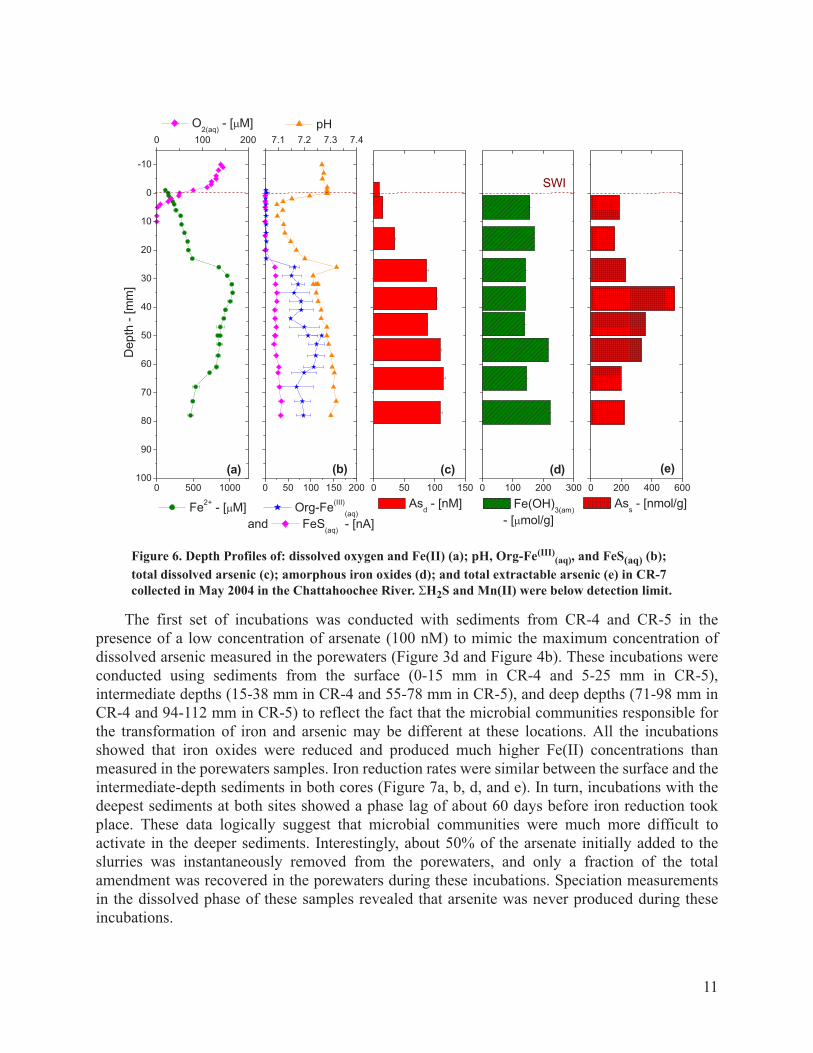
11

The first set of incubations was conducted with sediments from CR-4 and CR-5 in the

presence of a low concentration of arsenate (100 nM) to mimic the maximum concentration of

dissolved arsenic measured in the porewaters (Figure 3d and Figure 4b). These incubations were

conducted using sediments from the surface (0-15 mm in CR-4 and 5-25 mm in CR-5),

intermediate depths (15-38 mm in CR-4 and 55-78 mm in CR-5), and deep depths (71-98 mm in

CR-4 and 94-112 mm in CR-5) to reflect the fact that the microbial communities responsible for

the transformation of iron and arsenic may be different at these locations. All the incubations

showed that iron oxides were reduced and produced much higher Fe(II) concentrations than

measured in the porewaters samples. Iron reduction rates were similar between the surface and the

intermediate-depth sediments in both cores (Figure 7a, b, d, and e). In turn, incubations with the

deepest sediments at both sites showed a phase lag of about 60 days before iron reduction took

place. These data logically suggest that microbial communities were much more difficult to

activate in the deeper sediments. Interestingly, about 50% of the arsenate initially added to the

slurries was instantaneously removed from the porewaters, and only a fraction of the total

amendment was recovered in the porewaters during these incubations. Speciation measurements

in the dissolved phase of these samples revealed that arsenite was never produced during these

incubations.

0 200 400 600

(d)(c) (e)

Ass - [nmol/g]

0 100 200 300

SWI

Fe(OH)3(am)

- [ mol/g]

0 50 100 150 200

Org-Fe(III)

(aq)

and FeS(aq)

- [nA]

0 500 1000

(b)(a)

Fe2+

- [ M]

0 50 100 150

Asd - [nM]

7.1 7.2 7.3 7.4

pH

100

90

80

70

60

50

40

30

20

10

0

-10

0 100 200D

epth

- [m

m]

O2(aq)

- [ M]

Figure 6. Depth Profiles of: dissolved oxygen and Fe(II) (a); pH, Org-Fe(III)(aq), and FeS(aq) (b);

total dissolved arsenic (c); amorphous iron oxides (d); and total extractable arsenic (e) in CR-7

collected in May 2004 in the Chattahoochee River. H2S and Mn(II) were below detection limit.

12

A second set of incubations was conducted to simulate the effect of a contamination by

arsenate. This time, the sediments from the surface and intermediate depths of CR-4 and CR-5

were respectively mixed into two large samples, and three treatments for each sediment were

selected, with respective amendments of 0, 1, and 10 M arsenate. These incubations are still

ongoing but already show interesting results (Figure 8). First, the control slurries (no amendment)

show significant release of dissolved arsenic into the porewaters (Figure 8a and d), with

concentrations reaching that measured in the sediment cores (Figure 3d and Figure 4b). The

accumulation of dissolved arsenic is accompanied by the accumulation of Fe(II), with

concentrations in the same range as measured in the porewaters (Figure 3a and Figure 4) and

during the first 30 days of the first set of incubations (Figure 7). These results suggest that these

incubations are reproducible. It is also interesting to observe that the incubations performed with

the 1 M arsenate amendments (Figure 8b and e) very rapidly produce in both sediments higher

concentrations of Fe(II) than the no amendment controls (Figure 8a and d). Simultaneously,

dissolved arsenic, which was almost completely removed from the porewaters initially, is

produced in much higher concentrations during the course of the incubations than in the no

amendment controls. In turn, the highest arsenic amendment incubations in both CR-4 and CR-5

sediments (Figure 8c and f) release the same Fe(II) concentrations as in the no amendment

controls (Figure 8a and d), while dissolved arsenic, initially completely removed from the

porewaters, is slowly produced in higher concentrations than both the no amendment controls and

the 1 M amendment. These incubations show that only a fraction of the total arsenate added has

been released in the porewaters. They will be pursued until 100% recovery is reached.

0

500

1000

1500

2000

2500

Fe

(II)

- [

M]

b

0

100

200

300

400

As

d -

[n

M]

0

500

1000

1500

2000

2500

0

100

200

300

400

a

0

100

200

300

400

c

0 20 40 60 80 100 120 140

0

500

1000

1500

2000

2500

Time - [days]

0

500

1000

1500

2000

2500

d

0

100

200

300

400

0

100

200

300

400

As

d -

[n

M]

0

500

1000

1500

2000

2500

Fe

(II)

- [

M]

e

0 20 40 60 80 100 120 140

0

500

1000

1500

2000

2500

Time - [days]

0

100

200

300

400

f

Figure 7. Fe(II) and total dissolved arsenic (Asd) produced during sediment slurry incubations

amended with 100 nM arsenate in West Point Lake overlying water: surface sediment from CR-4

(a); CR-4 sediment from intermediate depths (b); deep sediment from CR-4 (c); surface sediment

from CR-5 (d); CR-5 sediment from intermediate depths (e); and deep sediment from CR-5. The

dash line represents the initial concentration of arsenate added to each slurry (right axis).

13

Preliminary speciation measurements indicate that As(III) can be detected in both the 1 and 10

M arsenic amendments after 30 days, suggesting that arsenate reduction must occur in these

sediments.

7.0 Discussion

Altogether, the chemical profiles provide a clear picture of the processes regulating the

cycling of arsenic near the sediment-water interface. The rapid decrease in dissolved oxygen close

to the SWI in each sediment core analyzed indicates that these sediments are anoxic. The

generally low concentration of Fe(II), the absence of nitrate, and the decrease in pH near the SWI

suggest that a combination of aerobic respiration (Eq. 3), denitrification (Eq. 4), and chemical

oxidation of Fe(II) (Eq. 5) occur within the first centimeter of these sediments:

(3)

(4)

(5)

Iron oxidation is confirmed by the high concentration of amorphous iron oxides detected in

the upper sediment of CR-4 and CR-6. Additionally, manganese and iron oxide reduction is

demonstrated with the production of Mn(II) and Fe(II) within the first 3 to 4 cm of these

sediments (Figure 3a to Figure 6a). The occurrence of metal reduction leads to a subsequent

0 5 10 15 20 25 30

0

500

1000

1500

2000

2500

0

200

400

600

800

1000

1200

0 5 10 15 20 25 30

0

500

1000

1500

2000

2500

0

2000

4000

6000

8000

10000

0 5 10 15 20 25 30

0

500

1000

1500

2000

2500

0

20

40

60

80

100

120

140

Fe

2+ -

[M

] b

As

d -

[nM

]c

Time - [days]

a

0 5 10 15 20 25 30

0

500

1000

1500

2000

2500

0

200

400

600

800

1000

1200

0 5 10 15 20 25 30

0

500

1000

1500

2000

2500

0

2000

4000

6000

8000

10000

0 5 10 15 20 25 30

0

500

1000

1500

2000

2500

0

20

40

60

80

100

120

140

Fe

2+ -

[M

] e

As

d -

[nM

]

f

Time - [days]

d

Figure 8. Fe(II) and total dissolved arsenic (Asd) produced during sediment slurry incubations

amended with different initial arsenate concentrations in West Point Lake overlying water: CR-4

sediment with no amendment (a); CR-4 sediment amended with 1 M As(V) (b); CR-4 sediment

amended with 10 M As(V) (c); CR-5 sediment with no amendment (d); CR-5 sediment amended

with 1 M As(V) (e); and CR-5 sediment amended with 10 M As(V). The dash line represents the

initial concentration of arsenate added to each slurry (right axis).

CH2O O2+ HCO3

–H

++

5CH2O 4NO3

–+ 5HCO3

–2N2 H+

+2H2O+ +

4Fe2 +

O2 10H2O+ + 4Fe OH 3 s 8H+

+

14

stabilization of the pH in the sediment porewaters (Figure 3b, Figure 5b, and Figure 6b) because

these reactions consume protons (36). Chemical reduction of manganese and iron oxides by

dissolved sulfide (Eq. 6 and Eq. 7) may occur in sediments. However, the maximum

concentration of dissolved sulfide available from the sulfate present in these freshwater sediments

(i.e. 50 M) is not high enough to account for all the Mn(II) and Fe(II) produced (compare

maximum sulfate to maximum Mn(II) and Fe(II) concentrations in Figure 3 and Figure 4 for

example).

(6)

(7)

Similarly, the chemical reduction of manganese oxides by Fe(II) is also possible (Eq. 8) but is

usually slow above pH 4 (43).

(8)

It can therefore be concluded that most of the reduction of manganese and iron oxides is microbial

in these sediments. Interestingly, Mn(II) reaches the sediment-water interface in core CR-5, sug-

gesting that it diffuses out of the sediment at this location. This feature is well known and due to

the slow oxidation kinetics of Mn(II) at circumneutral pH in the presence of oxygen (44). The dis-

appearance of sulfate within the first 40 mm of CR-4 (Figure 3c) and the occurrence of H2S and

FeS(aq) in CR-6 (Figure 5c) and CR-7 (Figure 6b), respectively, suggest that sulfate reduction pro-

ceeds in these sediments. In the sediments where dissolved sulfide was not detected in the pore-

waters, it must have been removed by precipitation as FeS. Interestingly, thermodynamic

calculations with MINEQL+ using an average pH of 6.1, Fe(II) concentration of 800 M and

assuming 50 M H2S (i.e. the maximum sulfate measured) produced in these sediments indicate

that the solubility product of FeSam and mackinewite are not exceeded. At this point, it is not clear

if the system is not at equilibrium or if the thermodynamic database is inaccurate. Nevertheless,

these profiles indicate that H2S is produced episodically in these sediments and must have a sig-

nificant impact on the cycling of arsenic.

Arsenic is thought to enter the Chattahoochee River upstream of the study location and is

transported in the oxic river water in the form of As(V) (3). As As(V) flows downstream, it may

adsorb onto colloidal and particulate matter contained in the river and settle to the sediment-water

interface. The data indicate that this sediment is not a natural source of arsenic, since the

concentration of dissolved arsenic in all sediment cores, except for CR-7 (Figure 6c), is higher

near the SWI and depleted at depth. Therefore, these data support earlier hypothesis that the

anthropogenic input of arsenic is significant in the Chattahoochee River (3).

The role of manganese and iron on the arsenic cycle has been investigated extensively (8, 10-

12, 17-19, 22, 24-26, 30). In these sediments, adsorption of arsenic should dominate in the upper

sediments which contain the highest concentration of amorphous iron oxides. The adsorption of

arsenic is also affected by the degree of crystallization of the iron oxides because the density of

adsorption sites decreases as the minerals are more crystallized (45). To determine the extent of

adsorption of As(V) onto iron oxides in the first centimeters of these sediments, we implemented

a double-layer surface adsorption model with MINEQL+ using parameters from the literature

(45). The model assumes a specific surface area of 600 m2/g for amorphous iron oxides and two

types of binding sites: high affinity sites with a density of 5 mmol/mol Fe and low affinity sites

MnO2 s H2S 2H+

+ + Mn2 +

S0

2H2O+ +

2Fe OH 3 s H2S 4H+

+ + 2Fe2 +

S0

6H2O+ +

MnO2 s 2Fe2 +

4H2O+ + Mn2 +

2Fe OH 3 s 2H+

+ +

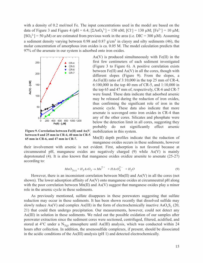
15

with a density of 0.2 mol/mol Fe. The input concentrations used in the model are based on the

data of Figure 3 and Figure 4 (pH = 6.4; [ AsO43-] = 150 nM; [Cl-] = 130 M; [Fe2+] = 10 M;

[SO42-] = 50 M) or are estimated from previous work in the area (i.e. DIC = 300 M). Assuming

a sediment density varying between 0.98 and 0.87 g/cm3 in clayey and silty sediments (46), the

molar concentration of amorphous iron oxides is ca. 0.05 M. The model calculation predicts that

97% of the arsenate in our system is adsorbed onto iron oxides.

As(V) is produced simultaneously with Fe(II) in the

first few centimeters of each sediment investigated

(Figure 3 to Figure 6). A positive correlation exists

between Fe(II) and As(V) in all the cores, though with

different slopes (Figure 9). From the slopes, a

As:Fe(II) ratio of 3:10,000 in the top 25 mm of CR-4,

6:100,000 in the top 40 mm of CR-5, and 1:10,000 in

the top 65 and 47 mm of, respectively, CR-6 and CR-7

were found. These data indicate that adsorbed arsenic

may be released during the reduction of iron oxides,

thus confirming the significant role of iron in the

arsenic cycle. These data also indicate that more

arsenate is scavenged onto iron oxides in CR-4 than

any of the other cores. Silicates and phosphate were

below the detection limit in all cores, suggesting they

probably do not significantly effect arsenic

mobilization in this system.

Mn(II) depth profiles indicate that the reduction of

manganese oxides occurs in these sediments, however

their involvement with arsenic is not evident. First, adsorption is not favored because at

circumneutral pH, manganese oxides are negatively charged (9) while As(V) is mainly

deprotonated (4). It is also known that manganese oxides oxidize arsenite to arsenate (25-27)

according to:

(9)

However, there is an inconsistent correlation between Mn(II) and As(V) in all the cores (not

shown). The lower adsorption affinity of As(V) onto manganese oxides at circumneutral pH along

with the poor correlation between Mn(II) and As(V) suggest that manganese oxides play a minor

role in the arsenic cycle in these sediments.

As previously mentioned, sulfate disappears in these porewaters suggesting that sulfate

reduction may occur in these sediments. It has been shown recently that dissolved sulfide may

slowly reduce As(V) and complex As(III) in the form of electrochemically inactive AsOxSy (20,

21) that could then undergo precipitation. Our measurements, however, could not detect any

As(III) in solution in these sediments. We ruled out the possible oxidation of our samples after

porewater extraction since the sediment cores were sectioned, centrifuged, filtered, acidified, and

stored at 4°C under a N2(g) atmosphere until As(III) analysis, which was conducted within 24

hours after collection. In addition, the arsenosulfide complexes, if present, should be dissociated

in the acidic conditions of the As(III) analysis (pH 1) and detected electrochemically.

0 200 400 600 800 1000 12000

50

100

150

200

250

Fe(II) - [ M]

CR-5

CR-7

CR-6

As(V

) -

[nM

]

CR-4

Figure 9. Correlation between Fe(II) and As(V)

between 0 and 25 mm in CR-4, 40 mm in CR-5,

65 mm in CR-6, and 47 mm in CR-7.

MnO2 s H3AsO3+ Mn2 +

HAsO4

2 –H2O+ +

16

The fact that the sediment is reduced but arsenic is oxidized may be due to the dynamic

nature of the system studied. The first two surficial sediments evaluated in this study (CR-4 and

CR-5) were most likely deposited after the passage of Tropical Storm Bill, which impacted the

site three weeks prior to this investigation. It is possible that the kinetically slow reduction of

As(V) had not occurred so soon after deposition, while microbial iron reduction released As(V) in

solution. Finally, the presence of As(V) and Fe(II) at deeper locations in CR-5 as compared to

CR-4 is probably due to the more turbulent river flow at CR-5 which may bring dissolved oxygen

to the sediment and increase erosion. This process is evidenced by a general decrease in both the

Fe(II) and amorphous iron oxide concentrations in the sediment of CR-5 compared to CR-4

(Figure 3 and Figure 4). Interestingly, the last two sediment cores investigated in this study were

obtained at base-flow conditions for the Chattahoochee River (Table 1). Yet our speciation

measurements did not evidence any As(III), though conditions in these sediments were more

reducing, with the occurrence of both dissolved sulfide (Figure 5c) and FeS(aq) (Figure 6b), a

precursor of FeS(s) precipitation (36).

Diffusive fluxes were calculated for each core using Fick’s Law with the molecular diffusion

coefficient of phosphate as a proxy for that of arsenate (9.1 x 10-5 cm2/sec for H2PO4-). According

to these calculations, approximately 20 to 200 nM/cm2yr of arsenic may be diffusing into the

overlying water column from the sediment depending on the flow conditions in the

Chattahoochee River. Although the arsenic concentrations detected in the porewaters are not

considered high compared to contaminated sites, the data suggest that arsenic is remobilized and

may impact the drinking water reservoir located downstream.

The sediment incubations show that arsenate spiked to the sediment is initially very rapidly

removed from the porewaters, most likely by adsorption onto iron oxides. These incubations also

show that iron reduction occurs in these sediments and that dissolved arsenic is released

concomitantly with the production of Fe(II). Our speciation measurements reveal that arsenic is

under the form of arsenate only when the initial concentration of arsenic is in the range of that

found in the porewaters, suggesting that arsenate reduction does not occur in the sediments of the

Chattahoochee River. The second set of incubations show that when the initial concentration of

arsenic injected to the sediment is elevated, some reduction may occur, though more data are

needed at this point. In addition, it appears that microbial iron reduction is affected by elevated

concentrations of total dissolved arsenic (Figure 8). Arsenic is a toxic compound that, in high

concentration, may inhibit microbial processes.

The first set of incubations was used to calculate the rate of iron reduction assuming a first

order with respect to iron oxides and zero order with respect to the reductant (Eq. 10). The

reductant could either be dissolved sulfide, if its concentration is high enough, or natural organic

matter if iron-reducing bacteria are involved in the transformation of iron oxides. From our field

measurements, we can conclude that the involvement of dissolved sulfide in the production of

Fe(II) is not significant. Therefore, these rates likely represent rates of microbial iron reduction in

these sediments. The rate law of iron reduction is:

(10)

where k is the rate constant (d-1), is the initial concentration of iron oxides ( M) in

these sediments. This rate law has an analytical solution that was used to fit the rate constant k to

td

dFe

2 +k Fe OH 3 s k Fe OH 3 s

0Fe

2 +–= =

Fe OH 3 s

0

17

the data of Figure 7 using a least-square fitting procedure. The initial concentration of iron oxides

was calculated from the sediment extraction measurements (Figure 3e and Figure 4c) assuming a

sediment density of 0.78 g/cm3 (46). Table 2 reports the rate constants determined for each incu-

bation described in Figure 7, except for the deep depths, which displayed a phase lag, as there was

not enough data to provide accurate rate constants. From these calculations, it is obvious that the

rate of reduction increases with depth in these sediments. So far, the incubations cannot be used to

provide rates of release of arsenate in the porewaters. These ongoing incubations will provide this

information at a later time.

8.0 Conclusions

This study successfully combined several analytical techniques to determine the profiles of

major redox species and the speciation of As(III) and As(V) with a high spatial resolution (i.e., <

10 cm) from four sediment cores collected a year apart at two locations in the Chattahoochee

River. Results provide evidence of the accumulation of dissolved arsenic close to the sediment-

water interface at both locations and at both time periods. Depth profiles also display a substantial

correlation between the diagenetic processes involving iron and arsenic in these sediments. They

suggest that iron oxides scavenge arsenic in the form of arsenate in the water column and settle to

the sediment-water interface where they are reduced by iron reducing bacteria. As a result of

microbial iron reduction, As(V) is released and accumulates in the porewaters near the sediment-

water interface, where it can diffuse back to the overlying waters. Interestingly, As(III) was never

found in the porewaters, suggesting that the reduction of As(V) is a slow process that was not

occurring in these sediments. Incubations with sediment slurries conducted in the presence of low

concentrations of arsenate verified that microbial iron reduction occurs in these sediments and

that arsenate is not concomitantly reduced during this process. Incubations of the same sediments

but amended with higher initial arsenate concentrations indicate that the microbial processes in

these sediments may be affected by high inputs of arsenic, including those necessary for

remediation or natural attenuation. Finally, differences between high discharge rates and base-

flow conditions in the Chattahoochee River do not seem to affect the biogeochemical processes

involved in iron and arsenic cycling but may enhance fluxes across the sediment-water interface.

TABLE 2. Sediment Depths Used in the First Set of Incubations

(Figure 7), Initial Concentration of Amorphous Iron Oxides

Measured in these Sediments and Used in the Model, and First

Order Rate Constant (k) Determined in Each of these

Incubations. ND = not determined.

Core

Depth

Incubated [Fe(OH)3(s)]0

k

[mm] mol/g] [1/d]

CR-4 0-15 178.8 0.0198

CR-4 15-38 120.8 0.0203

CR-4 71-98 73.01 ND

CR-5 5-25 97.7 0.0164

CR-5 55-78 90.0 0.0251

CR-5 94-112 83.6 ND

18

9.0 References

1. Ferguson, F.; Gavis, J. Wat. Res. 1972, 6, 1259-1274.

2. Ryu, J.; Gao, S.; Dahlgren, R.A.; Zierenberg, R.A. Geochim. Cosmochim. Acta 2002, 66,

2981-2994.

3. Lesley, M.P.; Froelich, P.N. Proceedings of 2003 Georgia Water Resources Conference.

4. Smedley, P.L.; Kinniburgh, D.G. Appl. Geochem. 2002, 17, 517-568

5. Buffle, J. Complexation Reactions in Aquatic Systems an Analytical Approach; Halsted Press:

a division of Wiley: New York, NY, 1988; p 692.

6. Cullen, W.; Reimer, K.J. Chem. Rev. 1989, 89, 713-764.

7. Jain, A.; Raven, K.P.; Loeppert, R.H. Environ. Sci. Technol. 1999, 33, 1179-1184.

8. Kneebone, P.E.; O’Day, P.A.; Jones, N.; Hering, J.G. Environ. Sci. Technol. 2002, 36, 381-186.

9. Stumm, W. Chemistry of the Solid-Water Interface; John Wiley and Sons, Inc.; New York,

1992.

10. Pierce, M.L.; Moore, C.B. Wat. Res. 1982, 16, 1247-1253.

11. Belzile, N.; Tessier., A. Geochim. Cosmochim. Acta 1990, 54, 103-1039.

12. Mucci, A.; Boudreau, B.; Guignard, C. Appl. Geochem. 2003, 18, 1011-1026.

13. Guo, T.; DeLaune, R.D.; Patrick Jr., W.H. Environ. Intern. 1997, 23, 305-316.

14. Ahmann, D.; Krumholz, L.R.; Hemond, H.F.; Lovley, D.R.; Morel, F.M.M. Environ. Sci.

Technol. 1997, 31, 2923-2930.

15. Harrington, J.M.; Fendorf, S.E.; Rosenzweig, R.F. Environ. Sci. Technol. 1998, 32, 2425-

2430.

16. Oremland, R.S.; Dowdle, P.R.; Hoeft, S.; Sharp, J.O.; Schaffer, J.K.; Miller, L.G; Blum, J.S;

Smith, R.L; Bloom, N.S; Wallschlaeger, D. Geochim. Cosmochim. Acta 2000, 64, 3073-3084.

17. Rochette, E.A.; Bostick, B.C.; Li, G.C.; Fendorf, S. Environ. Sci. Technol. 2000, 34, 4714-

4720.

18. Appelo, C.A.J.; Van Der Weiden, M.J.J.; Tournassat, C.; Charlet, L. Environ. Sci. Technol.

2002, 36, 3096-3103.

19. Charlet, L.; Bosbach, D.; Peretyashko, T. Chem. Geol. 2002,190, 303-319.

20. Wilkin, R.T.; Wallschlager, D.; Ford, R.G. Geochem. Trans. 2003,4, 1-7.

21. Sadiq, M. Mar. Chem. 1997, 31, 285-297.

22. Bostick. B.C.; Fendorf, S. Geochim. Cosmochim. Acta 2003, 67, 909-921.

23. Johnson, D.L.; Pilson, M.E.Q. Environ. Lett. 1975, 8, 157-171.

24. Scott, M.J.; Morgan, J.J. Environ. Sci. Technol. 1995, 29, 1898-1905.

25. Manning, B.A.; Fendorf, S.E.; Goldberg S. Environ. Sci. Technol. 1998, 32, 2383-2388.

26. Chiu, V.Q.; Hering, J.G. Environ. Sci. Technol. 2000, 34, 2029-2034.

19

27. Driehaus, W.; Seith, R.; Jekel, M. Wat. Res. 1995, 29, 297-305.

28. Andreae, M.O. Limnol. Oceanogr. 1979, 24, 440-452.

29. Xu, H.; Allard, B.; Grimvall, A. Water Air Soil Pollut. 1988, 57, 269-278.

30. Mok, W. A.; Wai, C.M. Environ. Sci. Technol. 1990, 24, 102-108.

31. Meng, X.K.; Guo. P.; Bang, S.; Bang, K.W. Toxicol. Letters 2002, 133, 103-111.

32. Brendel, P. J.; Luther, G. W.; III. Environ. Sci. Technol. 1995, 29(3), 751-761.

33. Bull, D. C.; Taillefert, M. Geochem. Trans. 2001, 13, 1-8.

34. Carey, B.; Taillefert, M. Limnol. Oceanogr. 2005, In Press.

35. Chow, S. S.; Taillefert, M. 2005. In: Advances in arsenic research: Integration of

experimental and observational studies and implications for mitigation (O'Day, P. V., D.;

Meng, X.; Benning, L. G., Eds.), ACS Symposium Series, Vol. 915, In Press.

36. Taillefert, M; Rozan, T. F.; Glazer, B.T.; Herszage, J.; Trouwborst, R. E.; Luther III, G. W.

2001. In: Environmental Electrochemistry: Analyses of Trace Element Biogeochemistry (M.

Taillefert; T. F. Rozan, Eds.). ACS Symposium Series, Vol. 811, Washington, D.C. 247-264.

37. Li, H.; Smart, R. B. Anal. Chim. Acta 1996, 325, 25-32.

38. Murphy J.R.; Riley J.P. Anal. Chim. Acta 1962, 27, 31-36.

39. Strickland, J.D.H. J. Amer. Chem. Soc. 1952, 74, 862-876.

40. Kostka, J.E.; Luther III, G.W. Geochim. Cosmochim. Acta 1994, 58, 1701-1710.

41. Stookey, L.L. Anal. Chem. 1970, 42, 779-782.

42. Tessier, A.; Campbell, P. G. C.; Bisson, M. Anal. Chem. 1979, 51, 844-851.

43. Postma, D. Geochim. Cosmochim. Acta 1985, 49, 1023-1033.

44. Stumm, W.; Morgan, J.J. 3rd Ed. Aquatic Chemistry Chemical Equilibria and Rates in Natural

Waters, John-Wiley and Sons, Inc.; New York; 1996.

45. Dzombak, D.A.; Morel, F.M.M. Surface Complexation Modeling: Hydrous Ferric Oxide.

John Wiley and Sons, Inc.; New York; 1990.

46. Kastler, J.A.; Wilberg, P.L. Estuar. Coastal Shelf Sci. 1996, 42, 683-700.

REDUCTIVE BIOTRANSFORMATION OFPOLYCHLORO-NITROBENZENES UNDERIRON-REDUCING CONDITIONS

Basic Information

Title:REDUCTIVE BIOTRANSFORMATION OFPOLYCHLORO-NITROBENZENES UNDER IRON-REDUCING CONDITIONS



End Date: 2/28/2005



5

ResearchCategory:

None

Focus Category: Agriculture, Hydrogeochemistry, Toxic Substances

Descriptors: None


Spyros G. Pavlostathis

Publication

Project Report

REDUCTIVE BIOTRASFORMATION OF POLYCHLORONITROBENZENES UNDER IRON-REDUCING

CONDITIONS

By

Spyros G. Pavlostathis, Principal Investigator Didem Okutman-Tas, Graduate Research Assistant

School of Civil and Environmental Engineering Georgia Institute of Technology


For

Georgia Water Resources Institute Georgia Institute of Technology


May 2005

2

TABLE OF CONTENTS Page

EXECUTIVE SUMMARY 3 1. INTRODUCTION 4 2. BACKGROUND 5 3. RESEARCH METHODOLOGY 7 3.1. Target Compounds 7 3.2. Scope/Hypothesis 7 3.3. Research Objectives 9 3.4. Materials and Methods 9 3.4.1. Culture development 9 3.4.1.1. Iron-reducing enrichment cultures (Cultures A, B, and C) 9 3.4.1.2. Fermentative/methanogenic enrichment culture (Culture D) 10 3.4.2. PCNB biotransformation assays 10 3.4.3. Assessment of the effect of iron reduction on PCA dechlorination 10 3.4.4. Analytical methods 11 4. RESULTS AND DISCUSSION 12 4.1. Iron-reducing enrichment cultures 12 4.1.1. Development and activity of iron-reducing enrichment cultures (Cultures A, B, and C) 12 4.1.2. PCNB biotransformation in an iron-reducing enrichment culture (Culture A) 16 4.2. Fermentative/methanogenic enrichment cultures 17 4.2.1. PCNB biotransformation by the fermentative/methanogenic enrichment culture (Culture D) 17 4.2.2. Effect of iron reduction on PCA dechlorination by the fermentative/ methanogenic enrichment culture (Culture D) 18 5. CONCLUSIONS 22 6. DISSEMINATION OF PROJECT RESULTS 23 7. REFERENCES 23

3

EXECUTIVE SUMMARY

Persistent anthropogenic, hydrophobic organic compounds in the environment pose a chronic threat to the health and safety of humans and wildlife. Despite the fact that chloronitroaromatics are extensively used synthetic compounds in industry and agriculture (e.g., pesticides, fungicides, pharmaceuticals, dyes) and found worldwide in surface and subsurface soils, as well as streambed sediments, studies on their fate and transformation, especially for polychloronitro-substituted compounds, have been rare as compared to either chlorinated or nitroaromatic compounds. To address and explore this paucity of information, the focus of this research was to elucidate the reductive biotransformation of polychloronitrobenzenes, and their corresponding chloroanilines (CAs) under iron-reducing conditions. Several of these compounds are classified as either carcinogenic, potentially carcinogenic, or as methemoglobinemia-causing chemicals. The main parent compound used in the present research was pentachloronitrobenzene (PCNB), a powerful organochlorine fungicide commonly used to combat phytopathogenic fungi. Although PCNB is used in several States, most of its usage is found in the Southeastern US because of its effectiveness against phytopathogenic fungi associated with crops predominantly found in this region.

Our research hypothesis was that reductive dehalogenation of polychlorinated organic compounds under iron-reducing conditions may take place co-metabolically where both Fe(III) and the chlorinated organic compounds merely serve as electron acceptors (primary and secondary electron acceptors, respectively), and/or abiotically, using biologically produced Fe(II) as the terminal electron donor (i.e., as a reductant). The specific objectives of this study were to: a) assess the potential for the microbial reductive transformation of PCNB and CAs under dissimilatory iron-reducing conditions; b) evaluate the effect of iron bioavailability on the amination/dechlorination process; and c) assess the role of humic substances in the iron reduction and PCNB biotransformation processes. Overall, the results of this study indicate that biotransformation of PCNB to pentachloroaniline (PCA) is very fast under both methanogenic and iron reducing conditions. Reduction of the nitro-group of PCNB and production of PCA also takes place under abiotic, reductive conditions. However, the rate of this conversion is highly enhanced under biotic conditions. Further dechlorination of PCA under abiotic, reductive conditions, e.g., in the presence of sulfide and/or Fe(II), was not observed in the present study. Under biotic conditions, the rate of PCNB to PCA biotransformation was higher under methanogenic conditions as compared to iron-reducing conditions. PCA dechlorination did not take place when Fe(III)-EDTA was reduced at a relatively fast rate under biotic conditions. In contrast, PCA dechlorination and iron reduction took place simultaneously when the iron source was less bioavailable (e.g., FeOOH). Addition of anthraquinone 2,6-disulfonate (AQDS), a humic acid model compound, to the culture, increased the rate and extent of FeOOH reduction, which in turn resulted in a significant decrease of the rate and extent of PCA dechlorination. Thus, fast iron reduction suppresses and delays the onset of the reductive dechlorination of PCA.

The results of this study have significant implications relative to the fate and biotransformation of PCNB and PCA under anoxic/anaerobic conditions encountered in most subsurface soil and sediment environments. Based on the observed fast and facile conversion of PCNB to PCA, PCNB is not expected to be persistent in natural systems. However, the bioavailability of iron in natural systems, which in turn is controlled by soluble humic material, has a pronounced effect on the rate and extent of PCA dechlorination and thus on its persistence in natural systems.

4

1. INTRODUCTIONPersistent anthropogenic, hydrophobic organic compounds in the environment pose a chronic threat to the health and safety of humans and wildlife. Despite the fact that chloronitroaromatics are extensively used synthetic compounds in industry and agriculture (e.g., pesticides, fungicides, pharmaceuticals, dyes) and found worldwide in surface and subsurface soils, as well as streambed sediments, studies on their fate and transformation, especially for polychloronitro-substituted compounds, have been rare as compared to either chlorinated or nitroaromatic compounds. To address and explore this paucity of information, the focus of this research was to elucidate the reductive biotransformation of polychloronitrobenzenes (polyCNBs), and their corresponding chloroanilines (CAs) under iron-reducing conditions. Several of these compounds are classified as either carcinogenic, potentially carcinogenic, or as methemoglobinemia-causing chemicals. The main parent compound used in this research was pentachloronitrobenzene (PCNB). PCNB (C6Cl5NO2), a powerful fungicide commonly used to combat phytopathogenic fungi, is a registered organochlorine fungicide used as a seed dressing or soil treatment to control a wide range of fungi species in crops such as cotton, potatoes, wheat, onions, lettuce, tomatoes, tulips, garlic, and others, as well as on grass, lawn flowers, ornamental crops, shrubs and in gardens (EXTOXNET, 1996; U.S. EPA, 2003). PCNB is included in U.S. EPA’s toxicity class III and is among the thirty chemicals included in the U.S. EPA’s list of “Waste Minimization Priority Chemicals”. The U.S. EPA has classified PCNB as a possible cancer causing substance (U.S. EPA, 2003).

During 2000 alone, 23,500 pounds of PCNB were used in six participating States (CA, FL, MI, OR, PA, and TX) in nursery and floriculture, whereas, 5,400 pounds were used in 2002 in the production of a single vegetable (fresh snap beans) in five participating States (FL, GA, NY, NC, and TN)(USDA, 2002; USDA, 2003). Although PCNB is used in several States, most of its usage is found in the Southeastern US because of its effectiveness against phytopathogenic fungi associated with crops predominantly found in this region. For example, in 2000, from the total reported PCNB usage of 543,500 lbs of active ingredient, 331,100 lbs (i.e., 61%) were used in seven States in the region (Table 1).

Table 1. PCNB Use for Two Selected Crops in the Southeastern U.S. (active ingredient in lbs; 2000 data; NASS, 2003)

State Snap Fresh Beans Cotton Upland Alabama FloridaGeorgiaLouisianaMississippi North Carolina South Carolina Tennessee

NA6,9007,200NANANANANA

74,000NANA

48,000109,00017,000

NA69,000

Total > 14,100 > 317,000 NA, data not available

PCNB is extensively used as a fungicide for the prevention and control of certain soil borne diseases on golf courses, sod farms, home lawns and institutional areas where turf is grown. In a recently published report by the USGS on the occurrence of semivolatile organic compounds in streambed sediments of twenty major river basins across the United States, PCNB

5

was detected at a maximum concentration of 180 g/kg (Lopes and Furlong, 2001). Therefore, as the above-mentioned, PCNB-related activities are more intense in the Southeastern US, the fate of PCNB and its biotransformation products is of regional interest.

2. BACKGROUND Polyhalogenated organic compounds tend to be resistant to biodegradation in aerobic environments. Such compounds are more oxidized than their nonhalogenated counterparts due to the presence of highly electronegative halogen substituents, which provide molecular stability. Therefore, as the degree of halogenation increases, reduction of these compounds is more likely to occur than oxidation (Pavlostathis et al., 2003). However, polyhalogenated compounds can be used as electron acceptors in thermodynamically favorable reactions (Dolfing and Beurskens, 1995; Fantroussi et al., 1998; Fetzner and Lingens, 1994; Fetzner, 1998; Middeldorp et al., 1999; Häggblom et al., 2000). Under anaerobic conditions, the reductive transformation of nitroaromatic compounds proceeds with the reduction of one or more aryl nitro groups (-NO2)and the formation of aryl amines. Nitrate, sulfate, and carbonates are alternative electron acceptors commonly considered for anaerobic subsurface processes (i.e., nitrogen reduction, sulfate reduction, and methanogenesis) and bioremediation applications. Relatively recent studies however have demonstrated the significant role of iron and manganese reducing bacteria in the cycling of organic matter and the biotransformation of organic contaminants (Lovley, 1991). The role of dissimilatory iron-reducing bacteria in the reduction of nitrobenzenes has been elucidated (Heijman et al., 1995; Klausen et al., 1995). This transformation involves two coupled reactions, one biotic and mediated by the iron-reducing bacteria, the other abiotic, where reduced iron [Fe(II)] serves as the intermediate electron donor and nitrobenzenes serve as the electron acceptor. The interdependence between the reduction of the organic pollutants and microbial iron reduction in aquifers was demonstrated. The biotic iron reduction step -- which provides the required reducing power for the transformation of the contaminants -- was found to be the rate-limiting process. On the other hand, the reduction of the contaminants leads to a continuous regeneration of the relatively limited, microbially-available Fe(III) pool. Based on published reduction potentials of key redox couples of Fe(III)/Fe(II) and organic compounds (Haderlein and Schwarzenbach, 1995), polychlorinated organic compounds can be reduced by a number of Fe(II)-bearing compounds. Iron-mediated, abiotic dechlorination has been demonstrated for compounds such as carbon tetrachloride and chloroform (Matheson and Tratnyek, 1994; Kriegman-King and Reinhard, 1992; Kriegman-King and Reinhard, 1994). Microbial dechlorination under iron-reducing conditions has been reported for a number of halogenated compounds, including carbon tetrachloride (Picardal et al., 1993), monochlorinated isomers of phenol, and benzoate (Kazumi et al., 1995a; Kazumi et al., 1995b), and vinyl chloride (Bradley and Chapelle, 1996). Despite the fact that chloronitroaromatics are extensively used synthetic compounds in industry and agriculture (e.g., pesticides, fungicides, pharmaceuticals, dyes) and found worldwide in surface and subsurface soils, as well as streambed sediments, studies on their fate and transformation, especially for polychloronitro-substituted compounds, have been rare as compared to either chlorinated or nitroaromatic compounds. An exhaustive literature review did not reveal any information on the definitive reductive dechlorination of polyCNBs under iron-reducing conditions which was the focus of this research. To address and explore this paucity of information, the focus of this research was to elucidate the reductive biotransformation of polyCNBs, and their corresponding chloroanilines (CAs).

6

We have developed methanogenic, mixed cultures from a sediment historically contaminated with chlorinated benzenes and hexachloro-1,3-butadiene (Prytula and Pavlostathis, 1996; Booker and Pavlostathis, 2000; Yeh and Pavlostathis, 2001) as well as dissimilatory iron-reducing, mixed cultures from a non-contaminated soil sample and the contaminated sediment (Doikos, 1998). Iron was provided in the form of ferric-EDTA in order to circumvent limitations related to iron bioavailability. Research carried out in our laboratory with the iron-reducing cultures on the reductive dechlorination of hexachlorobenzene revealed a low rate and extent of dechlorination as compared to those achieved with methanogenic cultures (Doikos, 1998). These results may be an outcome of competition for available electrons by the two simultaneous processes, namely, iron-reduction and dechlorination, or due to complexation of Fe(II) with EDTA and possible inhibition of the dechlorination process. The proposed research expanded the scope of the previously conducted research by the use of PCNB as well as different forms of Fe(III). The role of humic substances has been recognized in electron-transfer reactions in general and more specifically in the biotransformation of recalcitrant compounds (Bradley et al.,1998; Lovley et al., 1998; Scott et al., 1998). Humics could serve as carbon and energy sources in mixed, dissimilatory iron-reducing cultures, as electron-transfer mediators between Fe(II) and halogenated organic compounds (Haderlein and Schwarzenbach, 1995), as well as electron shuttles in the microbial reduction of insoluble Fe(III) compounds (He and Sanford, 2003; Komlos and Jaff , 2004). The role of humic substances in the biotransformation process of PCNB and PCA under dissimilatory, iron-reducing conditions was also assessed in this study. Most of the early studies on the biodegradation of PCNB focused on using fungi and were conducted under aerobic/anoxic conditions. Production of extracellular phenoloxidases by a number of fungal strains was not correlated with their capacity to degrade PCNB (Seiglemurandi et al., 1992; Steiman et al., 1992; Guiraud et al., 1999). Removal of more than 50% of 100 mg/L PCNB by three fungal species was attributed to biosorption and subsequent biodegradation (Lièvremont et al., 1996a). The best PCNB degradation by the fungal species Sporothrix

cyanescens was observed under carbon and nitrogen limitation (Lièvremont et al., 1996b). During the biotransformation of PCNB by four soil micromycetes, six metabolites were identified according to three metabolic pathways (Mora Torres et al., 1996): PCNB pentachloroaniline (C6Cl5NH2) tetrachloroaniline (C6Cl4HNH2); PCNB pentachlorothiophenol (C6Cl5SH) pentachlorothioanisole (C6Cl5SCH3); and PCNB pentachlorophenol (C6Cl5OH) pentachloroanisole (C6Cl5OCH3). PCNB degradation was observed in a large number of soil samples screened for microorganisms capable of degrading PCNB, irrespective of previous application of PCNB to the field. An isolate with a relatively fast PCNB degradation rate was identified as Pseudomonas

aeruginosa. This isolate degraded PNCB best under anoxic conditions and the principal metabolic product of PCNB was pentachloroaniline, thus demonstrating that in anoxic soil environments the main degradation pathway of PCNB is its reduction to pentachloroaniline (Tamura et al., 1995). Co-metabolic mineralization of monochloronitrobenzenes was achieved by a coculture of Pseudomonas putida and a Rhodococcus sp. The former species converted the chloronitrobenzenes to chloro-hydroxyacetanilides by partial reduction and subsequent acetylation, and the later species mineralized the chloro-hydroxyacetanilides to CO2, NH4

+ and Cl- (Park et al., 1999). Sequential dehalogenation of CAs in microcosms developed with aquifer material was achieved under methanogenic, but not sulfidogenic conditions. Dechlorination at the para and ortho position of 2,3,4,5-TeCA resulted in the formation of 2,3,5-TrCA and eventually 3,5-DCA, whereas 3,4-DCA was transformed to 3-CA (Kuhn and Suflita, 1989).

7

Chloronitrobenzenes (3-CNB, 3,4-DCNB, 2,3,4-TrCNB, and PCNB) were transformed in anaerobic, sulfidogenic estuarine sediments with pseudo-first order rate constants ranging from 0.216 to 0.866 day-1. Their transformation proceeded with reduction of the nitro group resulting in the formation of the corresponding chloroanilines, which were further transformed via ortho

and para dechlorination pathways (Susarla et al., 1996). In contrast, chloroanilines were sequentially dechlorinated in the same estuarine sediments with pseudo-first order rate constants ranging from 0.005 to 0.012 day-1 (Susarla et al., 1997). The degradation of 3,4-dihaloanilines by an anaerobic enrichment culture and Rhodococcus sp. strain derived from this culture under nitrate reducing conditions was recently reported to proceed by reductive deamination and formation of 1,2-dihalobenzene (Travkin et al., 2002). Further dehalogenation of the produced dihalobenzene was also observed.

3. RESEARCH METHODOLOGY 3.1. Target Compounds As mentioned above, the focus of this research was primarily on the biotransformation of PCNB and its transformation products (i.e., CAs). The following compounds can theoretically be produced as a result of the sequential reductive dechlorination of pentachloroaniline: tetrachloroanilines (3); trichloroanilines (6); dichloroanilines (6); monochloroanilines (3); and aniline (see Figure 1). Reduction of the nitro group and formation of the electron-donating amino group will lead to electronic and steric effects, which in turn are expected to affect the reductive dechlorination of CAs. It has been shown that substitution of an electron-withdrawing nitro group by an electron-donating amino group strongly decreases the formation of electron donor-acceptor complexes by nitroaromatic compounds (Haderlein et al., 2000).

3.2. Scope/Hypothesis Our research hypothesis was that reductive dehalogenation of polychlorinated organic compounds under iron-reducing conditions may take place by either one or both of the following mechanisms (Figure 2):

a) Co-metabolic biotransformation: both Fe(III) and the chlorinated organic compounds merely serve as electron acceptors (primary and secondary electron acceptors, respectively)(Mechanism I, Figure 2);

b) Abiotic transformation: the reductive dechlorination is mediated abiotically, using Fe(II) as the terminal electron donor (i.e., as a reductant) which is biotically produced from the reduction of Fe(III)(Mechanism II, Figure 2).

The difference between these two mechanisms is that in the first one, Fe(III) is reduced to Fe(II) without regeneration of Fe(III), whereas, according to the second mechanism, the reduction of the chlorinated organic contaminant(s) regenerates and continuously provides microbially available Fe(III) (see Figure 2). In the case of humic substances involvement in the reductive biotransformation process, these substances may serve as an electron shuttle between Fe(II) and the target chloroorganic compound, especially if the Fe(II) is surface-bound. In addition, humic substances may accelerate the biological reduction of amorphous Fe(III) oxyhydroxide. Such possible effects were assessed in the present study.

8

NO2

Cl Cl

Cl

Cl

Cl

NH2

Cl Cl

Cl

Cl

Cl

NH2

Cl Cl

Cl Cl

NH2

Cl

Cl

Cl

Cl

NH2

Cl Cl

Cl

Cl

PCNB

PCA

2,3,4,5 -TeCA 2,3,4,6-TeCA 2,3,5,6-TeCA

NH2

Cl

Cl

Cl

2,3,4-TrCA

NH2

Cl

Cl Cl

2,3,5-TrCA

NH2

Cl Cl

Cl

2,3,6-TrCA

NH2

Cl

Cl

Cl

2,4,5-TrCA

NH2

Cl Cl

Cl

2,4,6-TrCA

NH2

Cl

Cl

Cl

3,4,5-TrCA

NH2

Cl

Cl

2,3-DCA

NH2

Cl

Cl

2,4-DCA

NH2

Cl

Cl

2,5-DCA

NH2

Cl Cl

2,6-DCA

NH2

ClCl

3,4-DCA

NH2

Cl Cl

3,5-DCANH2

Cl

NH2

Cl

NH2

Cl

2-CA 3-CA 4-CANH2

Aniline

ORGANICS

CO2, H2O

Fe (III)

Fe (II)

RCln (oxidized)

MECHANISM I

RHCln-1 (reduced)+ HCl

MECHANISM II

Biotic Abiotic

ORGANICS

CO2, H2O

Fe (III)

Fe (II) RCln (oxidized)

RHCln-1 (reduced)+ HCl

Figure 1. Possible compounds formed by the reductive transformation of PCNB.

Figure 2. Mechanisms potentially involved in the reductive dechlorination of polychlorinated organic compounds under iron-reducing conditions.

9

3.3. Research Objectives The specific objectives of this study were to:

1. Assess the potential for the microbial reductive transformation of PCNB and CAs under dissimilatory iron-reducing conditions.

2. Evaluate the effect of iron bioavailability on the amination/dechlorination process. 3. Assess the role of humic substances in the iron reduction and PCNB biotransformation

processes.

3.4. Materials and Methods 3.4.1. Culture development In order to meet the above-stated research objectives, a number of cultures were developed using a contaminated estuarine sediment as inoculum and monitored for various parameters over several feeding cycles (Table 2). Acetate or glucose and methanol were used as electron donors and Fe(III)-EDTA, Fe(III)-citrate, amorphous ferric hydroxide (FeOOH) and PCNB or PCA were used as electron acceptors.

Table 2. Enrichment cultures and their characteristics.

Culture Electron acceptor-Target Compound Electron donor Iron form

A Fe(III) Acetate Fe(III)-EDTA

B Fe(III) Acetate Fe(III)-citrate

C Fe(III) Acetate FeOOH

D Fermentative/methanogenic-PCNB & PCA glucose/methanol None

The contaminated sediment was obtained from Bayou d’Inde, a tributary of Calcasieu River near Lake Charles, Louisiana, USA. Industrial wastes, including petroleum hydrocarbons, polycylic aromatic hydrocarbons, and polychlorinated aromatic and aliphatic organic compounds have been discharged into this canal. The pH of the sediment sample was 6.6 and the total organic carbon was 5.74 ± 0.02 (expressed as % on a dry weight basis). The location of sediment and details on the sediment sampling have been reported elsewhere (Prytula and Pavlostathis, 1996; Gess and Pavlostathis, 1997). All cultures were developed and incubated in a constant temperature room at 22ºC in the dark to better simulate natural conditions and were mixed once a day by hand.

3.4.1.1. Iron-reducing enrichment cultures (Cultures A, B, and C)

Three iron-reducing cultures were setup in 500 mL serum bottles as follows. Sediment samples (16 g wet basis) were added to the serum bottles, which were capped with butyl rubber stoppers, flushed with N2 and the sediment sample was then diluted to 400 mL with iron-reducing culture mineral media. The media had the following composition (in mg/L): KH2PO4, 1000; NH4Cl,500; CaCl2·2H2O, 100; MgSO4.7H2O, 200; MgCl2·6H2O, 100; MnCl2.4H2O, 100; NaHCO3,2,500. Also, 0.2 mL/L vitamin stock solution (Wolin et al., 1963) and 1 mL/L trace metal stock solution (Mah and Smith, 1981) were added to the media. The cultures were fed with acetate (5 mM) as an electron donor and yeast extract (20 mg/L) and three different iron sources (Fe-citrate, Fe-EDTA and FeOOH ) with a Fe(III) concentration of 25 mM. The pH in each culture

10

was kept between 6 and 7 with the addition of NaHCO3. A volume of each culture was wasted once a week and replaced with fresh media, and an aliquot of electron donor and Fe(III) was added, resulting in a culture retention time of 52 days. Microbial activity in these cultures was monitored by measuring total gas and gas composition, acetate, Fe(II) and total iron concentration. After several feeding cycles, sediment-free cultures were developed by diluting 50 mL of the first generation culture with 1.5 L mineral media in a nitrogen-flushed 2-L glass flask reactor (second generation culture). Because of the complexity of the process, as discussed in the Results and Discussion section, the Fe-citrate fed culture was not transferred to a new reactor.

3.4.1.2. Fermentative/methanogenic enrichment culture (Culture D) This enrichment culture had been developed from the above-mentioned contaminated estuarine sediment as follows. A sediment sample (80 g wet basis) was added and diluted with 1.8 L of mineral media in a N2-flushed, 2-L glass flask reactor, capped with a Teflon-lined stopper. The media had the following composition (in mg/L): K2HPO4, 900; KH2PO4, 500; NH4Cl, 500; CaCl2·2H2O, 100; MgCl2·6H2O, 200; FeCl2·4H2O, 100; Na2S·9H2O, 500; NaHCO3, 1,200; resazurin (redox indicator), 2. Also, 0.2 mL/L vitamin stock solution (Wolin et al., 1963) and 1 mL/L trace metal stock solution (Mah and Smith, 1981) were added to the media. The culture was fed weekly with glucose and a PCNB/methanol solution. Glucose and methanol served as the carbon source and electron donor. At the beginning of each seven-day feeding cycle, glucose, yeast extract, and PCNB in methanol were added resulting in initial concentrations of 333 mg/L, 17 mg/L, 0.089 µM and 53 mg/L, respectively. The culture was kept in the dark in a 22ºC constant temperature room, was stirred once a day using a Teflon-coated stirring bar over a magnetic stir plate, and its pH was kept around 7 with NaHCO3 addition. After several feeding cycles, a culture transfer took place by diluting 100 mL of the first generation culture in 1.8 L mineral media in a N2-flushed, 2-L glass flask reactor (second generation culture). Finally, after several weekly wasting/feeding cycles, a similar culture transfer took place in 2 L of mineral media in a N2-flushed, 9-L glass reactor, and its contents were gradually increased up to 6 L (third generation culture). The retention time of this enrichment culture was 84 d. All batch experiments with the fermentative/methanogenic culture reported here were performed with the sediment-free, third generation mixed culture.

3.4.2. PCNB biotransformation assays The biotransformation of PCNB by the enriched cultures was investigated using 160 mL serum bottles amended with acetate (300 mg/L), yeast extract (20 mg/L) and methanol (246 mg/L). The enriched culture D was able to quickly transform PCNB to PCA and further dechlorinate PCA to predominantly dichloroanilines under methanogenic conditions. Because of the relatively fast transformation of PCNB to PCA under both methanogenic and iron reducing conditions, in subsequent batch experiments, PCA dechlorination rather than PCNB biotransformation was investigated.

3.4.3. Assessment of the effect of iron reduction on PCA dechlorination The impact of Fe(III) on the reductive dechlorination of PCA was investigated using the sediment-derived, third generation mixed culture developed under fermentative/methanogenic conditions (culture D). Fe(III)-EDTA (25 mM) and FeOOH (25 mM) were used as a source of iron in order to assess the rate and extent of PCA dechlorination and iron reduction. Aliquots of culture D were anaerobically transferred to 160 ml serum bottles which were previously caped with Teflon-lined septa and flushed with N2. The cultures were amended with 0.5 µM PCA

11

dissolved in methanol. The Fe(III)-EDTA amended cultures were fed twice with acetate in order to avoid lack of electron donor during the prolonged incubation. Possible inhibitory effects of EDTA (25 mM) and sodium (50 mM) resulting from the disodium salt of EDTA (Na2-EDTA)were also tested. AQDS (200 µM), a humic acid model compound was added to some iron-amended cultures in order to increase the availability and thus the reduction rate of ferric iron. Another control was set up to test for any possible effect of AQDS on the reductive dechlorination of PCA in the absence of iron. Because of the potential of several culture media components (i.e., sulfide, Fe(II), vitamin B12) to abiotically mediate the reductive transformation of PCA, two additional controls were setup, one with only autoclaved culture media and another with autoclaved media plus 25 mM ferrous iron (FeCl2·4H2O), which matched the iron concentration in the culture series amended with either Fe(III)-EDTA or FeOOH (see above).

3.4.4. Analytical methods Liquid/liquid extraction was performed to analyze and quantify PCNB and its biotransformation products. Aliquots of 10 mL samples were extracted in glass tubes with 2 mL isooctane which contained 0.5 mg/L 1,3,5-tribromobenzene (TBB) as an internal standard. The tubes were capped with Teflon-lined stoppers and aluminum crimps, mixed vigorously for 2 min and centrifuged at 3000 rpm for 20 min. The solvent phase was transferred to amber glass autosampler vials, and sealed with Teflon-lined septa and aluminum crimps. The efficiency of the solvent extraction procedure was assessed at a concentration range of 0.03-40 µM PCNB, PCA and the less chlorinated anilines for 2 min, 1 h, 1 d and 3 d extraction period. It was determined that the efficiency was greater than 90% and did not change between 2 min and 3 days extraction period. Analysis of PCNB and biotransformation products was performed with an HP 6890 Series gas chromatograph (GC) equipped with an electron capture detector (ECD) and a 75-m 0.53-mm ID column (J&W Scientific, Folsom, CA, USA). The temperature program used was as follows: 100ºC for 4 min, increased by 2ºC/min up to 210ºC and held for 60 min. Nitrogen was used as the carrier gas at a constant flow rate of 10 mL/min. The detection limits for PCNB, PCA and less chlorinated anilines were as follows: PCNB, 7 nM; PCA, 4 nM; tetrachloroanilines, 9 nM; trichloroanilines, 25 nM; dichloroanilines, 0.15 µM ; monochloroanilines 16 mM. Because of the structural similarity which led to coelution, 2,5-DCA and 2,4-DCA could not be separated during the GC/ECD analysis.

Because of detection limitations in GC/ECD, aniline, monochlorinated and dichlorinated anilines were also measured with a high performance liquid chromatography (HPLC) unit (Hewlett Packard Model 8453, Hewlett Packard Co., Palo Alto, CA) which was equipped with a Zorbax SB-C18 column (3 x 250 mm, 5 µm) (Agilent Technologies, New Castle, DE). The column compartment temperature was set at 40ºC and the injection volume was 10 µL. The eluent mixture was an aqueous solution of 25 mM phosphate buffer (pH = 2.5) (52%) and methanol (48%) and the flow rate was 0.35 mL/min. Spectrometric detection was set at 203 nm. Samples used in HPLC analyses were filtered through 0.20 µm PTFE syringe filters (Cole-Parmer, Vernon Hills, IL) using glass syringes. The detection limits in HPLC for dichlorinated and monochlorinated anilines were 4 µM. 2,5-DCA and 2,4-DCA could also be separated during HPLC analysis.

Gas production was measured by connecting the culture headspace via a needle to an acid-brine solution filled graduated buret and recording the volume of displaced solution, after correcting to atmospheric pressure. Gas composition was determined by a gas chromatography (GC) unit equipped with a thermal conductivity detector. Methane was separated with a 25 m Chrompack Molsieve 5A fused silica 0.53 mm ID column and carbon dioxide was separated

12

with a 25 m Chormpack PoraPlot Q fused silica 0.53-mm ID column. Both columns were operated with helium as the carrier gas with a constant flow rate of 5 mL/min. The 10:1 split injector was maintained at 150ºC and the detector temperature was set at 150ºC. H2 was measured with a GC (HP 5980 Series) equipped with a thermal conductivity detector and a 10 m Chrompack Molsieve 5A fused silica 0.53-mm ID column. The carrier gas was N2 at a constant pressure of 70 psi. All gas samples were analyzed by injecting a 100 µL gas sample.

Methanol and acetate were measured in culture samples filtered through 0.20 µm syringe filters (PVDF-Whatman, Springfield Mill, England) using an HP 5890 Series II GC equipped with a flame ionization detector (FID) and a 35 m Stabilwax-DA 0.53-mm ID column (Restek, Bellefonte, PA, USA). Glucose was measured with a HP Series 1050 HPLC (Hewlett Packard, Palo Alto, CA) equipped with an Aminex HPX-87H-resin packed column (Bio-Rad, Richmond, CA). The column was maintained at 65ºC in an external column heater. The eluent was 0.01 N H2SO4 and the flow rate was 0.6 mL/min.

The oxidation-reduction potential (ORP) was measured following the procedure outlined in Standard Methods (APHA, 1995) using an Orion Research digital pH/milivolt meter model 611 in conjuction with a Sensorex electrode (platinum electrode with an Ag/AgCl reference in a 3.5 M HCl gel). The meter was calibrated prior to use with a shorting lead to establish meter reading at zero milivolts and by using Light’s standard solution [Fe(NH4)2(SO4)2·6H2O, 0.1 M; H2SO4, 1 M]. Fe(II) was quantified with a modification of the method described by Kazumi et al. (1995a, b). Aliquots of 1 mL well-mixed culture were added to 20 mL 0.5 N HCl in 28 mL serum tubes. After 10 min of acidification, an aliquot of 100 µL was filtered and added to a serum tube containing 5 mL of ferrozine solution [1 g/L in 50 mM HEPES (N-2-hydroxyethylpiperazine-N’-2-ethanesulfonic acid) buffer (pH = 7)]. This solution was vortexed for 10 s to develop the characteristic magenta color of the Fe(II)-ferrozine complex. The absorbance of this solution was measured using an HP 8453 UV-Visible spectrophotometer (Hewlett Packard, Palo Alto, CA) with DI water as a blank.

4. RESULTS AND DISCUSSION 4.1. Iron-reducing enrichment cultures 4.1.1. Development and activity of iron-reducing enrichment cultures (Cultures A, B, and C) These cultures were fed with acetate (5mM) and yeast extract (20 mg/L) and three different iron sources (Fe-citrate, Fe-EDTA and FeOOH). The initial Fe(III) concentration was 25 mM which served as the electron acceptor. Development of the enrichment cultures took place without any contaminant (i.e., PCNB, or PCA) amendment. Significant gas production was observed during the development of the Fe-citrate and Fe-EDTA amended cultures (Figure 3A and 3B). After 25 days of incubation, methane was observed in the Fe-citrate amended culture, which also used citrate as an electron donor after a few days of incubation, resulting in significant acetate accumulation (Figure 4A). Significant carbon dioxide and methane production was not observed in the reactor amended with FeOOH (Figure 3A and 3B), although after 65 days of incubation, traces of methane were observed. Significant consumption of acetate was not observed in the culture amended with FeOOH (Figure 4A).

13

CO

2 (

mL

@ 2

20C

)

0

100

200

300

400

TIME (Days)

0 10 20 30 40 50 60 70 80

CH

4 (

mL @

22

0C

)

0

200

400

600

800

1000

1200

1400

1600

Fe-citrate

Fe-EDTA

FeOOH

Fe-citrate

Fe-EDTA

FeOOH

A

B

Figure 3. Cumulative gas production and composition: CO2 (A) and CH4 (B) in the sediment-derived, iron-reducing cultures (first-generation; multiple feeding cycles).

During all feeding cycles, the pH in the Fe-EDTA amended culture remained between 5 and 7. After feeding, the pH increased up to 6.5-7, as a result of media and alkalinity addition and gradually decreased due to the reduction of the newly added Fe(III) (Figure 4B). The pH drop can be explained by the following stoichiometric equation of iron reduction and acetate oxidation: CH3COO- + 8 Fe3+ + 3 H2O CO2 + HCO3

-+ 8 Fe2+ + 8 H+

In the FeOOH amended culture, the pH increased from 7 to 8 over 23 days of incubation, which also indicates that iron reduction was very slow in this culture (Figure 4B).

Iron reduction in all three cultures was monitored by the measurement of Fe(II). Fast Fe(III) reduction was observed in both the Fe-citrate and Fe-EDTA amended cultures. However, Fe(III) reduction was much slower in the FeOOH amended culture (Figure 4C and 4D). Fe(III) reduction was the fastest in the Fe-EDTA amended culture. Because of the observed consumption of citrate and accumulation of a high concentration of acetate in the Fe-citrate amended culture, this culture was not transferred to create a second generation culture. After several feeding cycles, 50 mL inocula from the Fe-EDTA and FeOOH amended cultures were transferred to 2-L glass reactors and were maintained with the same feeding procedure. Headspace gas analysis showed production of CO2 in the Fe-EDTA amended culture, but gas production was not observed during all feeding cycles in the second generation, FeOOH amended culture (Figure 5A). Similar to the first generation culture, the pH increased in the FeOOH amended culture during the incubation. After 15 days of incubation, although the pH was adjusted to 7, CO2 production did not increase in the FeOOH amended culture (Figure 5B).

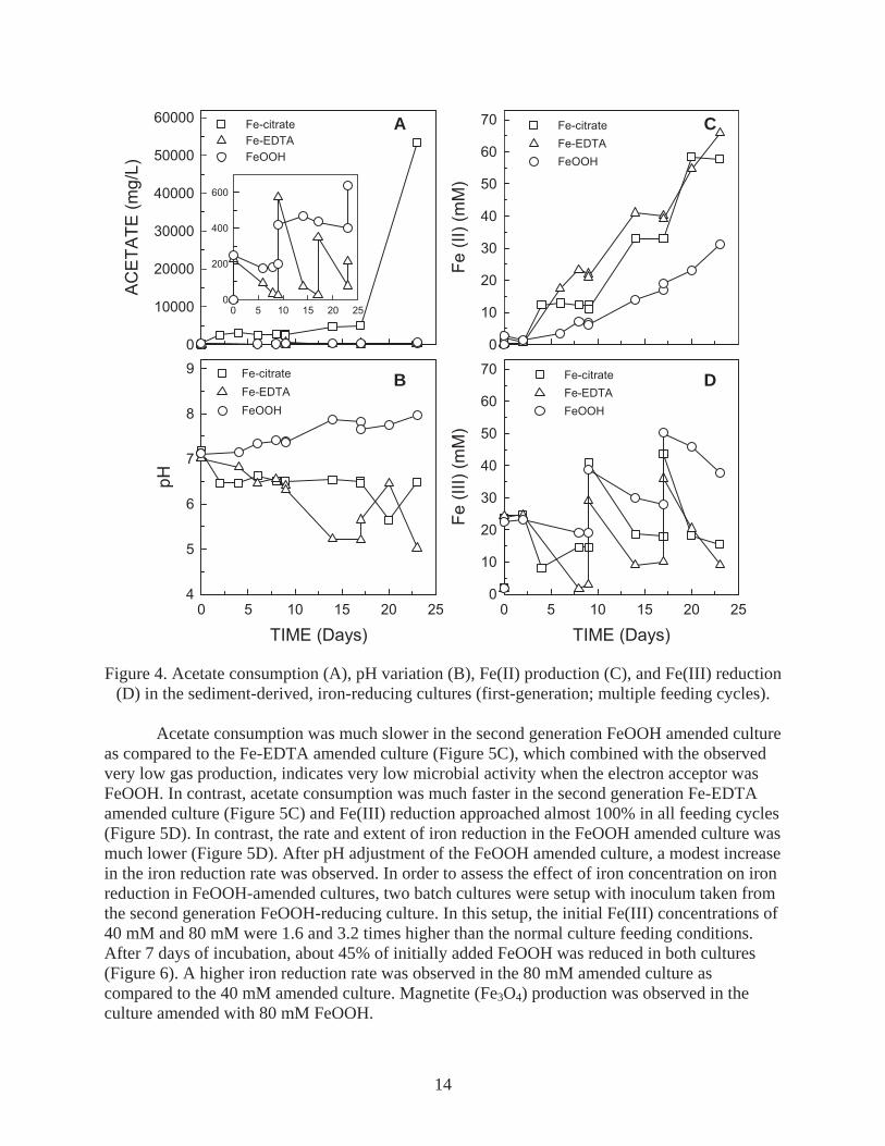
14

Fe

(II

) (m

M)

0

10

20

30

40

50

60

70

TIME (Days)

0 5 10 15 20 25

pH

4

5

6

7

8

9

TIME (Days)

0 5 10 15 20 25

Fe

(II

I) (

mM

)

0

10

20

30

40

50

60

70

AC

ET

AT

E (

mg

/L)

0

10000

20000

30000

40000

50000

60000

0 5 10 15 20 250

200

400

600

Fe-citrate

Fe-EDTA

FeOOH

Fe-citrate

Fe-EDTA

FeOOH

Fe-citrate

Fe-EDTA

FeOOH

Fe-citrate

Fe-EDTA

FeOOH

A

B

C

D

Figure 4. Acetate consumption (A), pH variation (B), Fe(II) production (C), and Fe(III) reduction (D) in the sediment-derived, iron-reducing cultures (first-generation; multiple feeding cycles).

Acetate consumption was much slower in the second generation FeOOH amended culture as compared to the Fe-EDTA amended culture (Figure 5C), which combined with the observed very low gas production, indicates very low microbial activity when the electron acceptor was FeOOH. In contrast, acetate consumption was much faster in the second generation Fe-EDTA amended culture (Figure 5C) and Fe(III) reduction approached almost 100% in all feeding cycles (Figure 5D). In contrast, the rate and extent of iron reduction in the FeOOH amended culture was much lower (Figure 5D). After pH adjustment of the FeOOH amended culture, a modest increase in the iron reduction rate was observed. In order to assess the effect of iron concentration on iron reduction in FeOOH-amended cultures, two batch cultures were setup with inoculum taken from the second generation FeOOH-reducing culture. In this setup, the initial Fe(III) concentrations of 40 mM and 80 mM were 1.6 and 3.2 times higher than the normal culture feeding conditions. After 7 days of incubation, about 45% of initially added FeOOH was reduced in both cultures (Figure 6). A higher iron reduction rate was observed in the 80 mM amended culture as compared to the 40 mM amended culture. Magnetite (Fe3O4) production was observed in the culture amended with 80 mM FeOOH.

15

TIME (Days)

0 20 40 60 80 100 120 140

pH

4

5

6

7

8

9

AC

ET

AT

E (

mg/L

)

0

100

200

300

400

500

600

700

TIME (Days)

0 20 40 60 80 100 120 140

Fe(I

II)

RE

DU

CT

ION

(%

)

0

20

40

60

80

100pH adjustment

CO

2 (

mL @

22

0C

)

0

200

400

600

800

1000

Fe-EDTA

FeOOH

Fe-EDTA

FeOOH

Fe-EDTA

FeOOH

Fe-EDTA

FeOOH

A

B

C

D

TIME (Days)

0 1 2 3 4 5 6 7 8Fe

(III

) R

ED

UC

TIO

N (

%)

0

10

20

30

40

50

40 mM FeOOH

80 mM FeOOH

Figure 5. Cumulative CO2 production (A), pH profile (B), acetate consumption (C), and extent of iron reduction (D) in the sediment-derived, iron-reducing cultures (second-generation; multiple

feeding cycles).

Figure 6. Extent of iron reduction in sediment-derived, FeOOH-amended, second generation, batch cultures.

16

CO

NC

EN

TR

AT

ION

(µ

M)

0

1

2

3

4

5

FE

(III

) o

r F

e(I

I) (

µM

)

0

20

40

60

80

100

120

AC

ET

AT

E (

mg L

-1)

0

200

400

600

800

TIME (Days)

0 10 20 30 40 50 60 70

GA

S (

mL

)

0

5

10

15

20

25

TIME (Days)

0 10 20 30 40 50 60 70

CH4

CO2

PCNB

PCA

2,3,4,5 TeCA

2,3,4,6 TeCA

2,4 or 2,5 DCA

Fe(II)

Fe(III)

A

B

C

D

E

F

4.1.2. PCNB biotransformation in an iron-reducing enrichment culture (Culture A) A batch PCNB biotransformation assay was conducted with the sediment-derived, second generation culture developed under iron reducing conditions (Fe-EDTA). Two sub-cultures were developed: one with Fe(III)-EDTA addition and one without any new iron addition. About 78 mM Fe(II) was present in these cultures at the beginning of the incubation contributed by the inoculum (Figure 7A and 7D). A delay in the transformation of PCNB to PCA was observed in the culture amended with Fe(III)-EDTA. In contrast, PCNB to PCA transformation was complete within 2 days in the culture that was not amended with any Fe(III). In both cultures, PCA was sequentially transformed to TeCAs and TrCAs (Figure 7A and 7D). However, the observed transformation rates in both cultures were significantly slower compared to those observed with the mixed methanogenic, PCNB-dechlorinating enrichment culture (see Section 4.2.1, below). After 10 days of incubation, methane production was observed in both cultures (Figure 7C and 7F). Acetate consumption and CO2 production was higher in the culture amended with Fe(III), compared to that in the culture which was not amended with Fe(III). Transformation of PCNB to PCA was not observed during the 43-day of incubation period in the abiotic control which was setup with autoclaved iron-reducing culture media (data not shown).

Figure 7. PCNB transformation, acetate consumption and gas production (at 22oC) in the sediment-derived, second generation Fe-EDTA reducing cultures (A, B, and C: culture with

Fe(III)-EDTA amendment; D, E, and F: culture without Fe(III)-EDTA amendment).

17

TIME (Days)

0 2 4 6 8 10 12 14 16 18

CO

NC

EN

TR

AT

ION

(µ

M)

0

1

2

3

4

PCNB

PCA

2,4 +2,5 DCA

3,5 DCA

2,4,5 TrCA

2,3,5,6 TeCA

2,3,4,5 TeCA

total

2,3,5 TrCA

4.2. Fermentative/methanogenic enrichment culture 4.2.1. PCNB biotransformation by the fermentative/methanogenic enrichment culture (Culture

D) Complete transformation of PCNB to PCA in the sediment-free, fermentative/methanogenic culture occurred in less than one day (Figure 8). Batch assays performed with the sediment-free enrichment culture resulted in the biotransformation of PCNB to PCA, which was then sequentially dechlorinated as follows: PCA 2,3,4,5- and 2,3,5,6-tetrachloroaniline (TeCA) 2,4,5- and 2,3,5-trichloroaniline (TrCA) 2,4-, 2,5- and 3,5-dichloroaniline (DCA) 3- and 4-chloroaniline (CA) (low levels). The predominant end product was 2,5-DCA (Figure 9).

Figure 8. Time course of PCNB and its biotransformation products during a typical batch biotransformation assay conducted with the PCNB-enriched, mixed methanogenic

culture (Error bars represent mean values ± one standard deviation).

Figure 9. PCNB biotransformation products observed in the fermentative/methanogenic enrichment culture.

NO2

Cl Cl

Cl

Cl

Cl

NH2

Cl Cl

Cl

Cl

Cl NH2

Cl Cl

Cl Cl

NH2

Cl

Cl

Cl

Cl

PCNB

PCA

NH2

Cl

Cl Cl

NH2

Cl

Cl

Cl

NH2

Cl

Cl

NH2

Cl

Cl

NH2

Cl Cl

NH2

Cl

NH2

Cl

2,3,4,5 -TeCA 2,3,5,6-TeCA

2,3,5-TrCA2,4,5-TrCA

2,4-DCA 2,5-DCA 3,5-DCA

3-CA4-CA

18

4.2.2. Effect of iron reduction on PCA dechlorination by the fermentative/methanogenic

enrichment culture (Culture D) As mentioned in the Materials and Methods section, above, complete and fast PCNB

transformation to PCA was observed under any anoxic/anaerobic conditions. Therefore, all subsequent assays were conducted with PCA as opposed to PCNB. The initial biomass concentration in all cultures in this assay was 310 ± 20 mg C/L (measured as particulate organic carbon). The pH and ORP values in the iron-free, control culture were 7.0 ± 0.3 and -170 ± 5 mV, respectively (mean ± standard deviation; n = 3). The initial and final ORP values in the cultures amended with Fe(III)-EDTA or FeOOH were +138 ± 2, -120 ± 4 mV, and -60 ± 14, -120 ± 70 mV, respectively. The higher decrease in the ORP value of the Fe(III)-EDTA amended cultures was mainly due to the exhaustion of Fe(III). Fetzer and Conrad (1993) found no inhibition of methanogenesis at ORP values as high as +420 mV. Therefore, inhibition of methanogenesis due to the relatively high redox potential seems unlikely in all of these cultures. The initial and final pH values in the Fe(III)-EDTA amended cultures were similar to those of the control culture. However, the pH increased from 7.2 ± 0.1 to 8.1 ± 0.4 in the FeOOH amended cultures within 60 days of incubation. The increase in pH was also observed in the sediment-derived FeOOH reducing cultures as mentioned above.

PCA was dechlorinated to 3,5 DCA and 2,4+2,5 DCA and all acetate was consumed in the iron-free, control culture under methanogenic conditions within 10 days of incubation without any delay (Figure 10). However, dechlorination of PCA was not observed in the cultures amended with either Fe(III)-EDTA or Fe(III)-EDTA and AQDS until 30 days of incubation when more than 90% of the added Fe(III) was reduced (Figure 11). The PCA dechlorination pathway was similar to that of the control culture after 30 days of incubation in both the Fe(III)-EDTA and Fe(III)-EDTA plus AQDS amended cultures (Figure 11A and 11B). On the other hand, PCA dechlorination as well as acetate consumption were not observed during 60 days of incubation in the culture amended with Na2-EDTA (Figure 12C). Therefore, EDTA had an inhibitory effect on the dechlorinating and methanogenic culture. In contrast, the presence of iron in the case of Fe-EDTA eliminated the inhibitory effect of EDTA, more likely because of binding with the resulting Fe(II). Straub et al. (2001) suggested that the inhibitory effect of EDTA could be because of its interaction with divalent cations such as Ca2+ or Mg2+, causing an imbalance in the supply of these ions. Such interactions may be detrimental, especially for gram-negative bacteria, which depend on such cations in their outer membranes. PCA dechlorination was not observed in the presence of only culture media or culture media amended with 25 mM ferrous iron (Figure 12A and 12B). PCA dechlorination and acetate consumption in the culture which was amended with 50 mM Na+ proceeded as in the iron-free, control culture without any inhibitory effect (Figure 13A and 13B). AQDS did not have any inhibitory or stimulatory effect on the dechlorination of PCA in the absence of an iron source (Figure 13B).

19

RE

DU

CE

D F

e(I

II)

(%)

0

20

40

60

80

100

TIME (Days)0 10 20 30 40 50 60

RE

DU

CE

D F

e(I

II)

(%)

0

20

40

60

80

100

CO

NC

EN

TR

AT

ION

(µ

M)

0.0

0.1

0.2

0.3

0.4

0.5

TIME (Days)0 10 20 30 40 50 60

CO

NC

EN

TR

AT

ION

(µ

M)

0.0

0.1

0.2

0.3

0.4

0.5

A

B

C

D

PCA

2,4 + 2,5 DCA3,5 DCA

2,4,5 TrCA2,3,5 TrCA

2,3,5,6 TeCA2,3,4,5 TeCA

Reduced Fe(III)

TIME (Days)

0 5 10 15 20 25

CO

NC

EN

TR

AT

ION

(µ

M)

0.0

0.1

0.2

0.3

0.4

0.5

0.6

AC

ET

AT

E (

mg/L

)

0

50

100

150

200

250

300

PCA

2,4 + 2,5 DCA

3,5 DCA

2,4,5 TrCA

2,3,5 TrCA

2,3,5,6 TeCA

2,3,4,5 TeCA

total

Acetate

Figure 10. Time course of PCA and its dechlorination products, as well as acetate consumption in the iron-free, control methanogenic culture (sediment-free culture)

Figure 11. Iron reduction and PCA dechlorination in cultures amended with Fe(III)-EDTA (A), Fe(III)-EDTA and AQDS (B), FeOOH (C), FeOOH and AQDS (D).

20

TIME (Days)

0 10 20 30 40 50 60

CO

NC

EN

TR

AT

ION

(µ

M)

0.0

0.1

0.2

0.3

0.4

0.5

0.6

TIME (Days)

0 10 20 30 40 50 60

TIME (Days)

0 10 20 30 40 50 60

AC

ET

AT

E (

mg

/L)

0

50

100

150

200

250

300A B C

PCA

Acetate

TIME (Days)

0 5 10 15 20 25

CO

NC

EN

TR

AT

ION

(µ

M)

0.0

0.1

0.2

0.3

0.4

0.5

0.6

PCA

2,4 or 2,5 DCA3,5 DCA

2,4,5 TrCA

2,3,5 TrCA

2,3,5,6 TeCA

2,3,4,5 TeCA

total

Acetate

A

TIME (Days)

0 5 10 15 20 25

AC

ET

AT

E (

mg/L

)

0

50

100

150

200

250

300B

Figure 12. PCA in culture media (A), culture media amended with Fe(II) (B), and methanogenic culture amended with Na2-EDTA (C).

Figure 13. PCA dechlorination and acetate consumption in methanogenic cultures amended with either Na+ (A) or AQDS (B).

Dechlorination of PCA started after 2 days of lag period in the culture amended with FeOOH (Figure 11C), but the dechlorination rate was lower than that observed in the control culture. Dechlorination of PCA was slower in the FeOOH and AQDS amended culture (Figure 11D) as compared to the culture amended with only FeOOH. Lovley et al. (1998) showed that the humics analog, AQDS, can be reduced by microorganisms to anthrahydroquinone-2,6-disulfonate (AHQDS) which then abiotically reduces Fe(III). Similar to our results, He and Sanford (2003) reported inhibition of 2-chlorophenol dechlorination by the Anaeromyxobacter

dehalogenans strain 2CP-C when the iron source was soluble (ferric pyrophosphate), whereas insoluble FeOOH did not have a significant effect on the dechlorination of 2-chlorophenol.

Gas production by all cultures during the incubation period is shown in Figure 14. AQDS did not have any inhibitory or stimulatory effect on the methane production of the dechlorinating, mixed fermentative/methanogenic culture. A slight decrease in the rate and

21

TIME (Days)

0 10 20 30 40 50 600

5

10

15

20

TIME (Days)

0 10 20 30 40 50 60

GA

S (

ml @

22

0C

)

0

10

20

30

40 A ControlFe-EDTANa

2-EDTA

NaCl

FeOOHFeOOH+AQDSFe-EDTA+AQDS

AQDS

B

extent of methane production was observed in the culture amended with sodium chloride. An earlier study reported sodium concentrations ranging from 150 to 240 mM to be moderately and 347 mM to be strongly inhibitory to methanogens at mesophilic temperatures (McCarty, 1964). In another study, sodium chloride concentrations over 15.2 mM were inhibitory for Methanobacterium thermoautotrophicm (Patel and Roth, 1977). Similar to the dechlorination activity, methane production was observed after a lag period of 2 days in the cultures amended with FeOOH. Very low methane production and relatively high carbon dioxide production was observed in the cultures amended with Fe(III)-EDTA until 30 days of incubation. However, significant methane production and PCA dechlorination was observed after 30 days of incubation when more than 90% of Fe(III) was reduced to Fe(II). High carbon dioxide production shows that iron-reduction was the main metabolic process in these cultures. The cumulative carbon dioxide production was very similar in the two Fe(III)-EDTA amended cultures. Methane production was lower in the culture amended with both FeOOH and AQDS compared with that of the culture amended with only FeOOH. van Bodegom et al. (2004) reported direct inhibition of methanogenesis in the presence of ferric iron, and found that methanogens grown on H2/CO2were more sensitive to ferric iron than methanogens grown on acetate. A relatively low carbon dioxide production was observed in the cultures amended with FeOOH compared to the Fe(III)-EDTA amended cultures. Both methane and carbon dioxide production was very low in the culture amended with Na2-EDTA, showing very low biological activity in this culture.

Figure 14. Gas production in all PCA-amended cultures. (A) methane; (B) carbon dioxide.

AQDS addition increased the Fe(III) reduction rate to some degree in the Fe(III)-EDTA amended culture, but the Fe(III) reduction rate was considerably increased in the FeOOH amended culture (Figure 15). Complete iron reduction was observed in the Fe(III)-EDTA plus AQDS amended culture after 30 days of incubation, whereas complete iron reduction in the culture without AQDS amendment was observed after 60 days of incubation (Figure 15A). Iron reduction was not observed for the first two days of incubation in the culture amended with FeOOH and AQDS, but after 10 days of incubation, the extent of Fe(III) reduction was significantly higher than in the culture without AQDS amendment (Figure 15B). Similar to our findings, Lovley et al. (1996) reported acceleration of the reduction of amorphous Fe(III) oxyhydroxide by the presence of a very low concentration of AQDS. The role of the humic acid analog AQDS as an electron shuttle provides a strategy for Fe(III) reducers to access insoluble

22

TIME (Days)

0 10 20 30 40 50 60

% R

ED

UC

ED

Fe(I

II)

0

20

40

60

80

100

Fe-EDTA

Fe-EDTA+AQDS

TIME (Days)

0 10 20 30 40 50 60

FeOOH

FeOOH+AQDS

BA

Fe(III) compounds (Lovley et al., 1996). Complete iron reduction was not observed in the cultures amended with FeOOH (Figure 15B). Similarly, it has been demonstrated that even the most available iron oxide -- amorphous hydrous ferric oxide -- cannot be totally consumed during microbial iron reduction (Lovley and Phillips, 1986a and b; Roden and Zachara, 1996).

Figure 15. Iron reduction in cultures amended with Fe-EDTA (A) and FeOOH (B)(The effect of AQDS on the rate and extent of iron reduction is also shown).

5. CONCLUSIONS Based on the results of the present study, the following conclusions are drawn:

1) Enrichment of dissimilatory, iron-reducing cultures using amorphous Fe(III) oxyhydroxide as an electron acceptor is extremely slow as compared to cultures enriched with either Fe(III)-citrate or Fe(III)-EDTA. Thus, the bioavailability of Fe(III) oxyhydroxide at circumneutral pH values is very low.

2) Reduction of the nitro-group of PCNB and production of pentachloroaniline (PCA) is taking place under both abiotic and biotic, reductive conditions. However, the rate of this conversion is highly enhanced under biotic conditions. Under biotic conditions, the rate of PCNB to PCA biotransformation was higher under methanogenic conditions as compared to iron-reducing conditions.

3) Dechlorination of PCA under abiotic, reductive conditions, e.g., in the presence of sulfide and/or Fe(II), was not observed in the present study.

4) PCA dechlorination did not take place when Fe(III)-EDTA was reduced at a relatively fast rate by an enriched, PCA-dechlorinating methanogenic culture, but dechlorination took place after iron reduction was almost complete. The PCA dechlorination pathway was similar to that of the iron-free, control culture.

5) PCA dechlorination and iron reduction took place simultaneously when the iron source was less bioavailable (e.g., FeOOH). However, addition of anthraquinone 2,6-disulfonate (AQDS), a humic acid model compound, to the culture, increased the rate and extent of

23

FeOOH reduction, which in turn resulted in a significant decrease of the rate and extent of PCA dechlorination. Thus, fast iron reduction suppresses and delays the onset of the reductive dechlorination of PCA.

The results of this study have significant implications relative to the fate and biotransformation of PCNB and PCA under anoxic/anaerobic conditions encountered in most subsurface soil and sediment environments. Based on the observed fast and facile conversion of PCNB to PCA, PCNB is not expected to be persistent in natural systems. However, the bioavailability of iron in natural systems, which in turn is controlled by soluble humic material, has a pronounced effect on the rate and extent of PCA dechlorination and thus on its persistence in natural systems.

6. DISSEMINATION OF PROJECT RESULTS The results of this project are being disseminated as follows:

Okutman-Tas, D. and S. G. Pavlostathis. Microbial Reductive Transformation of Pentachloronitrobenzene under Methanogenic Conditions. Manuscript submitted to Environmental Science and Technology.

Okutman-Tas, D. and S. G. Pavlostathis. Microbial Reductive Transformation of Pentachloronitrobenzene under Nitrate-reducing Conditions. Abstract to be presented at the 105th General Meeting, American Society for Microbiology, Atlanta, GA, June 5-9, 2005.

Okutman-Tas, D., and S. G. Pavlostathis. The Influence of Iron Reduction on the Reductive Biotransformation of Pentachloronitrobenzene. Paper to be presented at the Third European Bioremediation Conference, Chania, Greece, July 4-7, 2005.

Okutman-Tas, D. and S. G. Pavlostathis. The Influence of Iron Reduction on the Sequential Microbial Reductive Dechlorination of Pentachloroaniline. Manuscript in preparation.

7. REFERENCES American Public Health Association (APHA); American Water Works Association; and Water

Environment Federation. 1998. Standard Methods for the Examination of Water and

Wastewater, 20th Ed., Washington, D.C. Booker, R. S. and Pavlostathis, S. G.. 2000. Microbial reductive dechlorination of hexachloro-1,3-

butadiene in a methanogenic enrichment culture. Water Res. 34:4437-4445. Bradley, P.M., and F.H. Chapelle. 1996. Anaerobic mineralization of vinyl chloride in Fe(III)-

reducing, aquifer sediments. Environ. Sci. Technol. 30:2084-2086. Bradley P.M., F.H. Chapelle and D.R. Lovley. 1998. Humic acids as electron acceptors for anaerobic

microbial oxidation of vinyl chloride and dichloroethene. Appl. Environ. Microbiol. 64:3102-3105.

Doikos, P. Investigation of the Potential for Microbial Reductive Dechlorination of

Hexachlorobenzene under Iron-Reducing Conditions. MS Thesis, Georgia Institute of Technology, 1998.

Dolfing, J. and Beurskens, J.E.M. 1995. The microbial logic and environmental significance of reductive dehalogenation. In: Advances in Microbial Ecology, Vol. 14, Jones, J.G. (ed.), Plenum Press, New York, NY.

24

Extension Toxicology Network (EXTOXNET). 1996. Pesticide Information Profiles (http://ace.ace.orst.edu).

Fantroussi, S. El, Naveau, H. and Agathos, S.N. 1998. Anaerobic dechlorinating bacteria. Biotechnol.

Prog. 14:167–188. Fetzner, S. 1998. Bacterial dehalogenation. Appl. Microbiol. Biotechnol. 50:633–657. Fetzer, S. and R. Conrad. 1993. Effect of redox potential on methanogenesis by Methanosarcina

barkeri. Arch. Microbiol. 160:108-113. Fetzner, S. and Lingens, F. 1994. Bacterial dehalogenases: biochemistry, genetics, and

biotechnological applications. Microbiol. Rev. 58:641–685. Gess, P., and Pavlostathis, S.G. 1997. Desorption of chlorinated organic compounds from a

contaminated estuarine sediment. Environ. Toxicol. Chem. 16:1598–1605. Guiraud, P., Steiman, R., Ait-Laydi, L., and Seigle-Murandi, F. 1999. Degradation of phenolic and

chloroaromatic compounds by Coprinus spp. Chemosphere 38:2775-2789. Haderlein, S. B., and R. P. Schwarzenbach. 1995. Environmental processes influencing the rate of

abiotic reduction of nitroaromatic compounds in the subsurface. In Biodegradation of

Nitroaromatic Compounds; Spain, J. C. (Ed.); Plenum Press, New York, pp 199-225. Haderlein, S. B., Hofstetter, T. B., and Schwarzenbach, R. P. 2000. Subsurface chemistry of

nitroaromatic compounds. In: Biodegradation of Nitroaromatic Compounds and Explosives,

J.C. Spain, J.B. Hughes, and H-J. Knackmuss (eds), Lewis Publishers, Boca Raton, Florida, USA, pp. 311-356.

Häggblom, M. M., Knight, V. K., and Kerkhof, L. J. 2000. Anaerobic decomposition of halogenated aromatic compounds. Environ. Pollut. 107:199-207.

He, Q., and R. A. Sanford. 2003. Characterization of Fe(III) reduction by chlororespiring Anaeromyxobacter dehalogenans. Appl. Environ. Microbiol. 69:2712-2718.

Heijman, C. G., E. Grieder, C. Holliger, and R. P. Schwarzenbach. 1995. Reduction of nitroaromatic compounds coupled to microbial iron reduction in laboratory aquifer columns. Environ. Sci.

Technol. 29:775-783. Kazumi, J., M.M. Häggblom, and L.Y. Young. 1995a. Diversity of anaerobic microbial processes in

chlorobenzoate degradation: nitrate, iron, sulfate and carbonate as electron acceptors. Appl.

Microbiol. Biotechnol. 43:929-936. Kazumi, J., M.M. Häggblom, and L.Y. Young. 1995b. Degradation of monochlorinated and

nonchlorinated aromatic compounds under iron-reducing conditions. Appl. Environ.

Microbiol. 61:4069-4073. Klausen, I., S. P. Tröber, S. B. Haderlein, and R. P. Schwarzenbach. 1995. Reduction of substituted

nitrobenzenes by Fe(II) in aqueous mineral suspensions. Environ. Sci. Technol. 29:2396-2404.

Komlos, J., and P. R. Jaff . 2004. Effect of iron bioavailability on dissolved hydrogen concentrations during microbial iron reduction. Biodegradation 15:315-325.

Kriegman-King, M. R., and M. Reinhard. 1992. Transformation of carbon tetrachloride in the presence of sulfide, biotite, and vermiculite. Environ. Sci. Technol. 26:2198-2206.

Kriegman-King, M. R., and M. Reinhard. 1994. Transformation of carbon tetrachloride by pyrite in aqueous solution. Environ. Sci. Technol. 28:692-700.

Kuhn, E. P., and Suflita, J. M. 1989. Sequential reductive dehalogenation of chloroanilines by microorganisms from a methanogenic aquifer. Environ. Sci. Technol. 23:848-852.

Lièvremont, D., SeigleMurandi, F., BenoitGuyod, J. L., and Steiman, R. 1996a. Biotransformation and biosorption of pentachloronitrobenzene by fungal mycelia. Mycol. Res. 100:948-954.

Lièvremont, D., SeigleMurandi, F., and BenoitGuyod, J. L. 1996b. Effects of culture parameters on pentachloronitrobenzene removal by Sporothrix cyanescens. Chemosphere 32:361-375.

25

Lopes, T. J., and Furlong, E. T. 2001. Occurrence and potential adverse effects of semivolatile organic compounds in streambed sediment, United States, 1992-1995. Environ. Toxicol.

Chem. 20:727-737. Lovley, D. R. 1991. Dissimilatory Fe(III) and Mn(IV) reduction. Microbiol. Rev. 55:259-287. Lovley, D. R. and E. J. P. Phillips. 1986a. Organic matter mineralization with reduction of ferric iron

in anaerobic sediments. Appl. Environ. Microbiol. 51:683-689. Lovley, D. R. and E. J. P. Phillips. 1986b. Availability of ferric iron for microbial reduction in

bottom sediments of the freshwater tidal Potomac River. Appl. Environ. Microbiol. 52:751-757.

Lovley, D. R., and E. J. P. Phillips. 1988. Novel mode of microbial energy metabolism: Organic carbon oxidation coupled to dissimilatory reduction of iron or manganese. Appl. Environ.

Microbiol. 54:1472-1480. Lovley, D.R. and J.C. Woodward. 1996. Mechanisms of chelator stimulation of microbial Fe(III)-

oxide reduction. Chem. Geol. 132:19-24. Lovley, D.R., J.D. Coates, E.L. Blunt-Harris, E.J.P. Phillips and J. C. Woodward. 1996. Humic

substances as electron acceptors for microbial respiration. Nature 382:445–448. Lovley, D.R., J.L. Fraga, E.L. Blunt-Harris, L.A. Hayes, E.J.P. Phillips, and J.D. Coates. 1998.

Humic substances as a mediator for microbially catalyzed metal reduction. Acta Hydroch.

Hydrob. 26:152-157. Lovley, D.R. and E.L. Blunt-Harris. 1999. Role of humic-bound iron as an electron transfer agent in

dissimilatory Fe(III) reduction. Appl. Environ. Microbiol. 65:4252-4254. Mah, A. R., and M. R. Smith. 1981. The methanogenic bacteria. In: Prokaryotes: A Handbook of

Habitats, Isolation and Identification of Bacteria, Starr, M. P., Ed., Springer-Verlag: New York, NY; pp. 948-977.

Matheson, L. J., and P. G. Tratnyek. 1994. Reductive dehalogenation of chlorinated methanes by iron metal. Environ. Sci. Technol. 28:2045-2053.

McCarty, P.L. 1964. Anaerobic waste treatment fundamentals, part III: Toxic materials and their control. Public Works 95:91-94.

Middeldorp, P.J.M., Luijten, M.L.G.C., van de Pas, B.A., van Eekert, M.H.A., Kengen, S.W.M., Schraa, G., and Stams, A.J.M. 1999. Anaerobic microbial reductive dehalogenation of chlorinated ethenes. Bioremediation J. 3:151–169.

Mora Torres, R. M., Grosset, C., Steiman, R., and Alary, J. 1996. Liquid chromatography study of degradation and metabolism of pentachloronitrobenzene by four soil micromycetes. Chemosphere, 33:683-692.

National Agricultural Statistics Service (NASS). 2003. NASS Database. U.S. Department of Agriculture, Washington, D.C. (http://www.pestmanagement.info/nass/act_dsp_statcs2_state.cfm).

Park, H. S., Lim, S. J., Chang, Y. K., Livingston, A. G., and Kim, H. S. 1999. Degradation of chloronitrobenzenes by a coculture of Pseudomonas putida and a Rhodococcus sp. Appl.

Environ. Microbiol. 65:1083-1091. Patel, G.B. and L.A. Roth. 1977. Effect of sodium chloride on growth and methane production of

methanogens. Can. J. Microbiol. 23:893-7. Pavlostathis, S. G., and M. Prytula. 2000. Kinetics of the sequential microbial reductive

dechlorination of hexachlorobenzene. Environ. Sci. Technol. 34:4001-4009. Pavlostathis, S. G., Prytula, M. T., and Yeh, D. H. 2003. Potential and limitations of microbial

reductive dechlorination for bioremediation applications. Water, Air, & Soil Pollution: Focus

3(3):117-129.

26

Picardal, F.W., R.G. Arnold, H. Couch, A.M. Little, and M.E. Smith. 1993. Involvement of cytochromes in the anaerobic biotransformation of tetrachloromethane by Shewanella

putrefaciens 200. Appl. Environ. Microbiol. 59:3763-3770. Prytula, M. T., and Pavlostathis, S. G. 1996. Effect of contaminant and organic matter bioavailability

on the microbial dehalogenation of sediment-bound chlorobenzenes. Wat. Res. 30:2669-2680.

Roden, E.E. and J.M. Zachara. 1996. Microbial reduction of crystalline iron(III) oxides: Influence of oxide surface area and potential for cell growth. Environ. Sci. Technol. 30:1618-1628.

Scott, D.T., D.M. McKnight, E.L. Blunt-Harris, S.E. Kolesar, and D.R. Lovley. 1998. Quinone moieties act as electron acceptors in the reduction of humic substances by humics-reducing microorganisms. Environ. Sci. Technol. 32:2984-2989.

Seiglemurandi, F., Steiman, R., Benoitguyod, J. L., Muntalif, B., and Sage, L. 1992. Relationship between the biodegradative capability of soil micromycetes for pentachlorophenol and for pentachloronitrobenzene. Sci. Total Environ. 123:291-298.

Steiman, R., Benoitguyod, J. L., Seiglemurandi, F., and Muntalif, B. 1992. Degradation of pentachloronitrobenzene by micromycetes isolated from soil. Sci. Total Environ. 123:299-308.

Straub K.L., M. Benz and B. Schink. 2001. Iron metabolism in anoxic environments at near neutral pH. FEMS Microbiol. Ecol. 34:181-186.

Susarla, S., Masunaga, S., and Yonezawa, Y. 1996. Transformations of chloronitrobenzenes in anaerobic sediment. Chemosphere 32:967-977.

Susarla, S., Yonezawa, Y., and Masunaga, S. 1997. Reductive dehalogenation of chloroanilines in anaerobic estuarine sediment. Environ. Technol. 18:75-83.

Tamura, K., Hasegawa, Y., Kudo, T., and Yamaguchi, I. 1995. Isolation and characterization of PCNB degrading bacterium, Pseudomonas aeruginosa strain-I-41. J. Pestic. Sci. 20:145-151.

Travkin, V., B. P. Baskunov, E. L. Golovlev, M. G. Boersma, S. Boeren, J. Vervoort, W. J. H. van Berkel, I. M. C. M. Rietjens, and L. A. Golovleva. 2002. Reductive deamination as a new step in the anaerobic microbial degradation of halogenated anilines. FEMS Microbiol. Lett.

209:307-312. U.S. Department of Agriculture (USDA). 2002. Agricultural Chemical Usage – 2000 Nursery and

Floriculture Summary. National Agricultural Statistics Service, Washington, D.C. U.S. Department of Agriculture (USDA). 2003. Agricultural Chemical Usage – 2002 Vegetables

Summary. National Agricultural Statistics Service, Washington, D.C. U.S. Environmental Protection Agency (U.S. EPA). 2003. Waste Minimization Priority Chemicals &

Chemical Fact Sheets. Office of Solid Waste and Emergency Response, Washington, D.C. (http://www.epa.gov/epaoswer/hazwaste/minimize/chemlist.htm).

van Bodegom, P.M., J.C.M. Scholten and A.J.M. Stams. 2004. Direct inhibition of methanogenesis by ferric iron. FEMS Microbiol. Ecol. 49:261-268.

Wolin, E. A., Wolin, M. J., Wolfe, R. S. 1963. Formation of methane by bacterial extracts. J. Biol.

Chem. 238:2882-2886. Yeh D.H., and S.G. Pavlostathis. 2001. Development of hexachlorobenzene-dechlorinating mixed

cultures using Polysorbate surfactants as a carbon source. Wat. Sci. Technol. 43(2):43-50.

INFORM: Integrated Forecast and Reservoir ManagementSystem for Northern California

Basic Information

Title:INFORM: Integrated Forecast and Reservoir Management System forNorthern California



End Date: 6/30/2005

Funding Source: Other


5

Research Category: Climate and Hydrologic Processes

Focus Category: Hydrology, Management and Planning, Surface Water

Descriptors: Integrated Forecast-Decision Systems for River Basin Management


Aris P. Georgakakos, Konstantine P. Georgakakos

Publication

1. Georgakakos, K.P., Graham, N.H., Carpenter, T.M., Georgakakos, A.P., and H. Yao, IntegratingClimate-Hydrology Forecasts and Multi-Objective Reservoir Management for Northern California.EOS, Transactions, American Geophysical Union, Vol. 86, No. 12, March 2005, pages 122-127.

2. Georgakakos, A.P., Decision Support Systems for integrated water resources management with anapplication to the Nile Basin Keynote Address, Proceedings, International Federation for AutomaticControl Workshop on Modeling and Control for Participatory Planning and Managing WaterSystems, Venice, Italy, Sep. 29 Oct. 1. Also, in a book entitled Decision Support Systems for WaterResources Management to be published by Elsevier, 2005.

3. Gibson, C.A., J.L. Meyer, N. L. Poff, L.E. Hay, and A. Georgakakos, "Flow Regime Alterationsunder Changing Climate in Two River Basins: Implications for Freshwater Ecosystems," RiverResearch and Applications, 21: 1-16, 2005.

A DECISION SUPPORT SYSTEM FOR THE RESERVOIRS IN NORTHERN CALIFORNIA

Project INFORM

Interim Technical Report 2004-2005

Aris Georgakakos and Huaming Yao Georgia Water Resources Institute


Atlanta, Georgia 30332 (404) 894-2240

April 2005

123.5 123 122.5 122 121.5 121 120.5

38.5

39

39.5

40

40.5

41

41.5

Degrees West Longitude

Degre

es N

ort

h L

atitu

de

Major Resevoirs in Nothern California

TrinityShasta

O rovil le

Folsom

Trinity River

Pit River

Sacramento River

Feather River

N. Fo rk Ame rican River

2

A Decision Support System for the Reservoirs in Northern California

GWRI Progress Report –Year 3 1/2005-04/2005 NOAA Funding Period

The Georgia Water Resources Institute contribution to the INFORM project is to develop

and demonstrate the utility of Decision Support Systems (DSS) for reservoir

management. The DSS consists of databases, interfaces, and various application

programs interlinked to provide meaningful and comprehensive information to decision

makers. During the current NOAA funding period, GWRI efforts focused on the

following project tasks:

Expanding the studied systm of INFORM DSS to include the San Joaquin River,

the Delta, and the Exports to Southern California;

Developing simulation assessment tool for the expanded system;

Model testing.

A brief descrition of the above-mentioned tasks is provided below.

1. The Expaned System

During the last workshop, the GWRI personnel and USBR staff had a discussion on how

to better use the INFORM DSS in the operational and planning process in practice. The

original INFORM DSS modeled only four major reservoirs in the system independently.

The downstream requirements such as minimum flows, delta environmental constraints,

water demands were not considered. However, those requirements are the most important

factors in the reservoir operation and planning process in practice. Based on the

discussion, to make the DSS more useful and realistic, the GWRI team decided to expand

the original project system to incoprorate all the components dowstream of the reservoirs.

Specifically, the expanded system includes five major reservoirs (Clair Engle Lake,

Shasta, Oroville, Folsom, and New Melones), 10 hydro power plants, the delta of the

Sacramento River and the San Joaquin River, and the exports to the southern California

(Figure 1). The objectives of the system are water supply, energy generation, minimum

river flows, and delta environmental requirements.

2. The Simulation Model

The simulation model is a part of the INFORM comprehensive decision support system.

The main goal of the simulation model is to conduct quick assessments under various

conditions such as demand changes, hydrological condition changes, and etc.

Many system data, constraints, and operation rules used in the simulation model are

adopted directly from the existing planning simulation model, a spreadsheet based model

provided by the USBR staff. For convenience, the entire system is divided into 6 sub-

3

systems based on their geological locations and functionalities. The model formulation

and assumptions of each sub system are described in Appendix A.

Northern California Water and Power System Schematic

San Joaquin River

San Lius

Clair Engle Lake

Trinity Power Plant

Lewiston

Lewiston

JF Carr

Wiskeytown

Shasta

Keswick

ShastaSpring Cr

Keswick

Oroville

Thermolito

Folsom

Natoma

New Melones

Tulloch

Goodwin

Oroville

Folsom

Nimbus

Melones

Tracy Pumping

Banks Pumping

San Joaquin River

Amer

ican

Rive

r

Feat

her R

iver

Sacramento River

TrinityRiver Clear Creek

Yuba River

Bear River

Delta-Mendota Canal

California Acqueduct

O’Neill Forebay

To Dos Amigos PP

To Mendota Pool

Sacramento San Joaquin River DeltaReservoir/

Lake

Power Plant

Pumping Plant

River Node

ISV

IFT

IES,IMC,IYB,ITI

DDLT,DBS,DCCWD,DNBA

DDM

DFDM

DDA

DSF

DSB

Northern California Water and Power System Schematic

San Joaquin River

San Lius

Clair Engle Lake

Trinity Power Plant

Lewiston

Lewiston

JF Carr

Wiskeytown

Shasta

Keswick

ShastaSpring Cr

Keswick

Oroville

Thermolito

Folsom

Natoma

New Melones

Tulloch

Goodwin

Oroville

Folsom

Nimbus

Melones

Tracy Pumping

Banks Pumping

San Joaquin River

Amer

ican

Rive

r

Feat

her R

iver

Sacramento River

TrinityRiver Clear Creek

Yuba River

Bear River

Delta-Mendota Canal

California Acqueduct

O’Neill Forebay

To Dos Amigos PP

To Mendota Pool

Sacramento San Joaquin River DeltaReservoir/

Lake

Power Plant

Pumping Plant

River Node

Reservoir/Lake

Power Plant

Pumping Plant

Reservoir/Lake

Power Plant

Pumping Plant

River Node

ISV

IFT

IES,IMC,IYB,ITI

DDLT,DBS,DCCWD,DNBA

DDM

DFDM

DDA

DSF

DSB

Figure 1: System Schematic

3. Assessment Process Using the Simulation Model

The assessment is done by running the simulation model for a selected historical inflow

sequence under various operational conditions. The available historical inflows are from

1968 to 1996 for the four major reservoirs Clair Engle Lake, Shasta, Oroville, and

Folsom. Inflows from other tributaries are not available at this moment. The monthly

average sequences are used in the sample study. The DSS interface provides easy tools to

add new inflow data into the system once they become available. Other operational

constraints such as demands, pumping, and minimum and target river requirement, and

reservoir target storages are all user definable through the interface.

The simulation starts with the inflow forecasts for all locations. Presently, an imbedded

Historical Analog inflow forecasting model is used. The more comprehensive distributed

hydrological model will be integrated as it becomes available. At beginning of each

month, the forecast model is launched and produces monthly inflow sequences up to one

year for all locations. The forecasted inflows, along with the observed inflows up to the

current month from the current water year, are used to compute the river index. Based on

4

the value of river index, the demands and the minimum flow requirements are adjusted

according to the user specified rules. Users can also specify the frequency of the demand

adjustment, i.e., at which months the demands and the minimum flows are adjusted. The

adjusted demands and minimum flows are then used as the planned targets in the

simulation.

Assuming that no extra release is required to meet the delta demands and pumping, the

reservoirs releases are determined simply to meet their local requirements such as target

storage and the minimum flows. If the reservoir releases, along with the contributions of

delta local streams, can meet the delta requirements, then, the initial assumption is valid

and no extra release is required from the reservoirs, the system evolves to the next month

using the actual historical inflows of the current month; otherwise, extra release is

required and is distributed among the reservoirs according to user specified rules,

simulate the system again with the extra release added to the original releases. This

process is repeated for every month until the end of the selected historical period. For

each month, the simulation model records reservoir storage, demand, deficit, energy

generation, and all other quantities of the user’s interests. The recorded sequences are

used for statistical analysis.

The assessment model generates voluminous results after each run. Selected results from

a sample run are presented in Appendix B. The model inputs are described in Appendix

C.

4. Outstanding Issues

The assessment model presetned here is based on a spreadsheet simulation model

provided by the USBR staff. Unfortunately, the spreadsheet model was not fully

functional due to converion problems and did not include full data record required for

conducting the long term assessment. With the help of USBR and DWR staff, we were

able to get some data from the internet and establish necessary assumptions for making

the assessment model workable for demonstration purpose. However, there are still many

outstanding issues we would like to address in the upcoming workshop:

The agreement on the expanded system;

Functionality and input/output for the DSS models;

Details of reservoir contributions to meet the delta and export requirtements;

Rules and policies for reduction of demands and minimum flows at various

locations;

Historical unimparied inflow data at various locations;

Inflow forecasting models at various locations;

Information on the power facilities.

References

Yao, H, and A. Georgakakos, 2001. "Assessment of Folsom Lake Response to Historical

5

and Potential Future Climate Scenarios," Journal of Hydrology. 249, 176-196.

Georgakakos, A., and H. Yao, 2002, "Implications of Climate Variability and Change for

Water Resources Management,” The Climate Report, 3(4), 9-13.

Georgakakos, A. P., and H. Yao, "Evaluation of Water Use Scenarios for the Nile Basin,"

World Bank, ICCON Series Monographs, October 1999, 116p.

Georgakakos, A. P., "Water Resources Planning and Management for the Lake Victoria

Basin," Monograph, FAO Monograph Series, August 2000, 44p.

Georgakakos, A. P., H. Yao, and Y. Yu, “A Control Model for Hydroelectric Energy

Value Optimization,” ASCE J. for Wat. Res. Plan. and Mgt, 123(1), 30-38, 1997.

Georgakakos, A. P., H. Yao, and Y. Yu, “Control Models for Hydroelectric Energy

Optimization,” Water Resources Research, 33(10), 2367-2379, 1997.

Georgakakos, A. P., Yao, H., and Y. Yu, “A Control Model for Dependable Hydropower

Capacity Optimization,” Water Resources Research, 33(10), 2349-2365, 1997.

Georgakakos, A. P., C. Barrett, and B. Attia, "A Decision Support System for the High

Aswan Dam," Proceedings of the Fifth International Workshop on Water Resources

Operations Management, sponsored by ASCE, Georgakakos, A.P., and Q.W. Martin

Eds., pg. 34-66, Arlington, VA, March 4-6, 1996.

Georgakakos, A. P., “Operational Tradeoffs in Reservoir Control,” Water Resources Research, 29(11), 3801-3819, 1993.

Yao, H., and A. P. Georgakakos, “New Control Concepts for Uncertain Water Resources

Systems: 2, Reservoir Management,” Water Resources Research, 29(6), 1517-1526,

1993.

Georgakakos, A. P. and H. Yao, “New Control Concepts for Uncertain Water Resources

Systems: 1, Theory,” Water Resources Research, 29(6), 1505-1516, 1993.

Hooper, E. R., A. P. Georgakakos, and D. P. Lettenmaier, “Optimal Stochastic Operation

of the Salt River Project, Arizona,” ASCE Journal of the Water Resources Planning and Management, Vol. 117, No. 5, pg. 566-587, 1991.

Georgakakos, A. P., "Computer-Aided Management of the Southeastern U.S. Reservoir

System," in "Decision Support Systems," D. P. Loucks, ed., NATO ASI Series, Vol. G

26, pg. 407-428, 1991.

Georgakakos, A. P., "Extended Linear Quadratic Gaussian Control for the Real-Time

Operation of Reservoir Systems," pg. 329 360 in the book entitled "Dynamic

Programming for Optimal Water Resources Systems Analysis," A. Esogbue, ed.,

Prentice Hall Publishing Company, New Jersey, 1989.

Georgakakos, A. P., “Extended Linear Quadratic Gaussian (ELQG) Control: Further

Extensions”, Water Resources Research, Vol. 25, No. 2, pg. 191 - 201, 1989.

Georgakakos, A. P., “The Value of Streamflow Forecasting in Reservoir Control”, Water

Resources Bulletin, Vol. 25 No. 4, pg. 789 800, 1989.

6

Appendix A: Simulation Model Formulation

A.1. Trinity River System

The Trinity River System includes Clair Engle Lake, Trinity Power Plant, Lewiston

Lake, Lewiston Plant, JF Carr Plant, Whiskeytown, Clear Creek, and Spring Creek

Plant.

The Clair Engle Lake is operated to meet the minimum and the target flow in the

Trinity River, and the monthly target storage for Whiskeytown reservoir.

The system dynamics of Clair Engle Lake and Whiskeytown are described by the

following water balance equations:

Whiskeytown:

)()()()),(()()()1( kRkRkRkkSEVPkIkSkS SCCCJFWHWHWHWHWH

Clair Engle Lake (Trinity):

)()),(()()()1( kRkkSEVPkIkSkS CLCLCLCLCLCL

)()()( kRkRkR JFLECL

where:

k is the time step in month;

SWH, IWH, EVPWH are the storage, inflow, evaporation loss for Whiskeytown,

respectively;

RCC is the minimum river flow requirement for Clear Creek;

RSC is the target flow for Spring Creek plant;

RJF is the flow through JF Carr plant;

RLE is the minimum river flow requirement for Trinity River;

SCL, ICL, EVPCL, RCL are the storage, inflow, evaporation loss, and release for Clair

Engle Lake, respectively.

A.2. Shasta Lake System

The Shasta Lake System includes Shasta Lake, Shasta Power Plant, Keswick Lake,

Keswick Plant, and the river reach from Keswick to Wilkins.

The Shasta Lake is operated to meet the minimum and the target flow at Wilkins on

the Sacramento River and share (if specified) the water supply in the Delta.

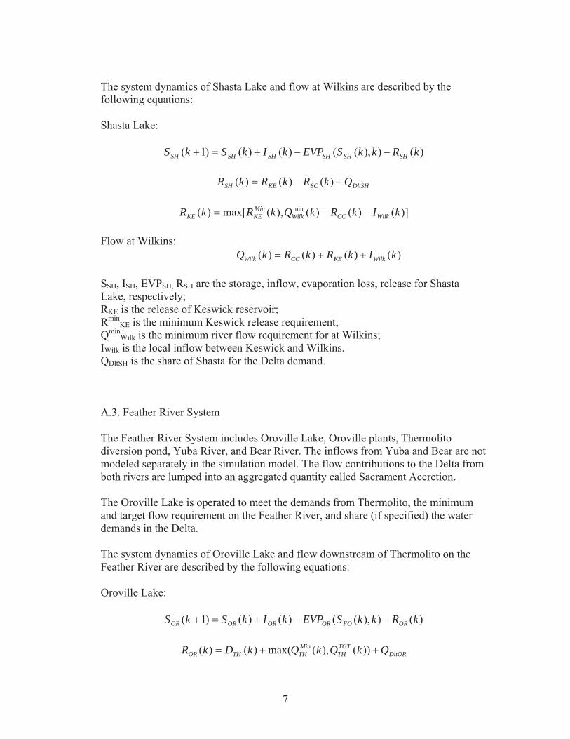
7

The system dynamics of Shasta Lake and flow at Wilkins are described by the

following equations:

Shasta Lake:

)()),(()()()1( kRkkSEVPkIkSkS SHSHSHSHSHSH

DltSHSCKESH QkRkRkR )()()(

)]()()(),(max[)( min kIkRkQkRkR WilkCCWilkMinKEKE

Flow at Wilkins:

)()()()( kIkRkRkQ WilkKECCWilk

SSH, ISH, EVPSH, RSH are the storage, inflow, evaporation loss, release for Shasta

Lake, respectively;

RKE is the release of Keswick reservoir;

Rmin

KE is the minimum Keswick release requirement;

Qmin

Wilk is the minimum river flow requirement for at Wilkins;

IWilk is the local inflow between Keswick and Wilkins.

QDltSH is the share of Shasta for the Delta demand.

A.3. Feather River System

The Feather River System includes Oroville Lake, Oroville plants, Thermolito

diversion pond, Yuba River, and Bear River. The inflows from Yuba and Bear are not

modeled separately in the simulation model. The flow contributions to the Delta from

both rivers are lumped into an aggregated quantity called Sacrament Accretion.

The Oroville Lake is operated to meet the demands from Thermolito, the minimum

and target flow requirement on the Feather River, and share (if specified) the water

demands in the Delta.

The system dynamics of Oroville Lake and flow downstream of Thermolito on the

Feather River are described by the following equations:

Oroville Lake:

)()),(()()()1( kRkkSEVPkIkSkS ORFOOROROROR

DltORTGTTH

MinTHTHOR QkQkQkDkR ))(),(max()()(

8

Flow at Thermolito:

)())( kDkRkQ THORTH

where

SOR, IOR, EVPOR, ROR are the storage, inflow, evaporation loss, and release for

Oroville Lake, respectively;

DTH is the demand from Thermolito;

Qmin

TH and QTGTn

TH are the minimum and target flow requirement downstream of

Thermolito.

QDltOR is the share of Oroville for the Delta demand.

A.4. American River System

The American River System includes Folsom Lake, Folsom Plant, Natoma Lake,

Nimbus Plant, Natoma Plant, and Natoma diversions.

The Folsom Lake is operated to meet the demands from Natoma reservoir and the

minimum and the target flow requirements on the American River, and share (if

specified) the water demands in the Delta.

The system dynamics of Folsom Lake and the flow downstream of Nimbus are

described by the following equations:

Folsom Lake:

)()),(()()()1( kRkkSEVPkIkSkS FOFOFOFOFOFO

DltFOFSFOTGTNI

MinNIFO QkDkDPMkQkQkR )()())(),(max()(

where

SFO, IFO, EVPFO, RFO are the storage, inflow, evaporation loss, release for the Folsom

Lake, respectively;

DPMFO is the demand from Folsom pumping;

DFS is the demand from Folsom South Canal;

Qmin

NI and QTGT

NI are the minimum and target flows downstream of Nimbus.

QDltFO is the share of Folsom Lake for the Delta demand.

A.5. San Joaquin System

9

The San Joaquin System includes New Melones Lake, New Melones Power Plant,

Tulloch Lake, Demands from Goodwin, and the inflows from the main San Joaquin

River.

The New Melones is operated to meet the demands at Goodwin and the minimum and

the target flow requirement downstream.

The system dynamics of New Melones Lake, Tulloch Lake, and the river flow at

Vernalis are described by the following equations:

New Melones:

)()),(()()()1( kRkkSEVPkIkSkS NMNMNMNMNMNM

Tulloch:

)()()()1( kRkRkSkS TUNMTUTU

))(),(max()()()( / kQkQkDkDkR TGTGO

MinGOSSJIDOIDCUPTU

))()1(()()( kSkSkRkR TUTGTTUTUNM

Flow at Vernalis:

)())(),(max()( kIkQkQkQ SJRTGTGO

MinGOVE

where

SNM, INM, EVPNM, RNM are the storage, inflow, evaporation loss, release for the New

Melones Lake, respectively;

STU, RTU are the storage and release for Tulloch, respectively;

DCUP and DOID/SSJD are the demands at Goodwin;

STGT

TU is the target storage for Tulloch Lake;

Qmin

GO and QTGT

GO are the minimum and target flows downstream of Goodwin;

QVE is the river flow at Verlanis;

ISJR is the inflow from Jan Joaquin above Stanilaus junction.

A.6. Delta

The Delta receives inflows from Sacramento, San Joaquin, and several local streams.

In addition to the consumptive use inside the Delta and the environmental constraints,

the Delta provides storage for exporting water to the south part of California through

pumping. Under normal hydrological conditions, the inflows from the Sacramento

River, San Joaquin River, and the local stream flows can meet the needs of Delta

demands and the water export. However, during dry water years, extra water has to

be released from the upper major reservoirs to meet the demands. The required extra

water is shared by the large reservoirs in the Sacramento River basin (Clair Engle

10

Lake, Shasta, Oroville, and Folsom). The shared percentage and operation rules in the

simulation are user defined.

A.6.1. Delta Inflows

The local inflows to the Delta include:

Sacramento Valley Accetion: ISV(k)

Freeport Treatment Plant: IFT(k)

Eastside Stream: IES(k)

Miscellaneous Creeks Inflow: IMC(k)

Yolo bypass: IYB(k)

Transfer Inflow: ITI(l)

Freeport Flow:

)()()()()()()( kIkIkQkQkQkQkQ FTSVTHNIKECCFP

Total Delta Inflow:

)()()()()()( kIkIkIkQkQkI TIYBESVEFPDE

A.6.2. Delta Export

The Delta water exports are implemented by the federal agency (USBR) and the State

Water Department. The federal export includes:

CCWD Diversion: DCCWD

Barker Slough: DBS

Fed Tracy Pumping: DFTPP

Fed Banks on-peak DFBON

Fed Banks off-peak:DFBOFF

Fed Banks Pumping total: DFPPTOT

Fed Banks PP CVC: DFBPPCVC

Fed Banks PP Joint: DFBPPJNT

FED Banks PP Transfer: DFBPPTR

The total federal pumped water is:

)()()()()()()()( kDkDkDkDkDkDkDkD FBPPTRFBPPJNTFBPPCVCFBPPDFBOFFDFBONFTPPFPPTOT

The total federal planned export is:

)()()( kDkDkD CCWDFPPTOTFEXTOT

The state export includes:

NBA Diversion: DNBA

State Banks PP: DSBPP

State Tracy PP: DSTPP

11

The total state planned export is:

)()()()( kDkDkDkD STPPSBPPNBASEXTOT

The total planned export from both federal and state is:

)()()()( kDkDkDkD BSFEXTOTSEXTOTEXTOT

A.6.3. Delta COA

The Delta COA includes the following definitions:

Required Delta Outflow: Qmin

Dlt

Delta Consumptive Use: Ddlt

Combined required reservoir release: QRES

))()()()()()()()()(,0max()( min kIkIkIkIkQkIkQkDkDkQRES YBMCESFTVESVDltEXTOTDlt

Total Federal Storage Withdrawal: DSFTOT

))()(())()(())()(()( kIkRkIkRkIkRkDS FOFOSHKEWHCCFTOT

Total State Storage Withdrawal: DSSTOT

))()(()( kIkRkDS ORORSTOT

Computed Delta Outflow: QDlt

))()()()()()()()()( kIkIkIkDkDkQkIkQkQ YBMCESEXTOTDltVEYBFPDlt

Estimated Excess Outflow: QESTOT

))()(()( kQkQkQ MinDltDltESTOT

Un-stored Flow for Export: QUFE

otherwisekDkDSkifDSkDSkDSkQkD

kQ EXTOTSTOTFTOTSTOTFTOTESTOTEXTOTUFE

,0

)()()()),()(()()()(

Estimated in-basin use of storage withdrawal: Qinbasin

))()()(,0max()( kDkDSkDSkQ EXTOTSTOTFTOTINBSN

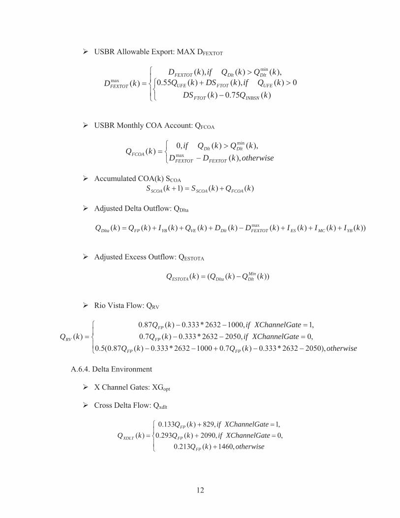
12

USBR Allowable Export: MAX DFEXTOT

)(75.0)(

0)(),()(55.0

),()(),(

)(

min

max

kQkDSkQifkDSkQ

kQkQifkDkD

INBSNFTOT

UFEFTOTUFE

DltDltFEXTOT

FEXTOT

USBR Monthly COA Account: QFCOA

otherwisekDDkQkQifkQ

FEXTOTFEXTOT

DltDltFCOA

),(

),()(,0)(

max

min

Accumulated COA(k) SCOA

)()()1( kQkSkS FCOASCOASCOA

Adjusted Delta Outflow: QDlta

))()()()()()()()()( max kIkIkIkDkDkQkIkQkQ YBMCESFEXTOTDltVEYBFPDlta

Adjusted Excess Outflow: QESTOTA

))()(()( kQkQkQ MinDltDltaESTOTA

Rio Vista Flow: QRV

otherwisekQkQteXChannelGaifkQteXChannelGaifkQ

kQ

FPFP

FP

FP

RV

),20502632*333.0)(7.010002632*333.0)(87.0(5.0

,0,20502632*333.0)(7.0

,1,10002632*333.0)(87.0

)(

A.6.4. Delta Environment

X Channel Gates: XGopt

Cross Delta Flow: Qxdlt

otherwisekQteXChannelGaifkQteXChannelGaifkQ

kQ

FP

FP

FP

XDLT

,1460)(213.0

,0,2090)(293.0

,1,829)(133.0

)(

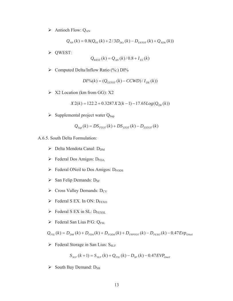
13

Antioch Flow: QAN

))()()(3/2)((8.0)( kQkDkDkQkQ XDltEXTOTDLtVEAN

QWEST:

)(8.0/)()( kIkQkQ ESANWEST

Computed Delta/Inflow Ratio (%:) DI%

))(/))(()%( kICCWDkQkDI DEEXTOT

X2 Location (km from GG): X2

))((65.17)1(23287.02.122)(2 kQLogkXkX Dlt

Supplemental project water QSup

)()()()( kDkDSkDSkQ EXTOTSTOTFTOTSup

A.6.5. South Delta Formulation:

Delta Mendota Canal: DDM

Federal Dos Amigos: DFDA

Federal ONeil to Dos Amigos: DFODS

San Felip Demands: DSF

Cross Valley Demands: DCV

Federal S EX. In ON: DFEXO

Federal S EX in SL: DFEXSL

Federal San Lius P/G: QFSL

ONeilFEXOFPPTOTFODAFDADMFSL EvpkDkDkDkDkDkQ 47.0)()()()()()(

Federal Storage in San Lius: SSLF

OneilSFFSLSLFSLF EVPkDkQkSkS 47.0)()()()1(

South Bay Demand: DSB

14

State Dos Amigos: DSDA

State San Lius P/G: QSSL

ONeilSDASBSEXTOTSSL EvpkDkDkDkQ 53.)()()()(

State Storage in San Lius: SSLS

ONeilSSLSLSSLS EvpkDkSkS 53.0)()()(

15

Appendix B: Simulation Results from the Assessment Model

In the sample run, the historical inflow sequences (Figure B.1) from 1970 to 1995 for

Clair Engle Lake, Shasta, Oroville, and Folsom are used. The monthly average values of

local inflows for all other tributaries are summarized in Table B.1. The monthly reservoir

parameters and constraints (max, min, and target storage, evaporation rates) are listed

Table B.2. The minimum river flow requirements are listed in table B.3. The monthly

demands from all locations are listed in Table B.4.

The river indices of Sacramento and San Joaquin are computed according to the

description posted on the DWR’s website. The water year type is classified in to five

categories: Critical, Below Normal, Normal, Above Norm, and Wet. The demands and

the river flow requirements are adjusted according to the fraction vs. water year type

class value relationship, specified by the user. The default relationship is included in

Table B.5. It applies to all demand locations. If the water year type is above normal, or

wet, then the demand fraction is 1, no reduction is needed. Otherwise, the reduction

fraction is 0.6, 0.4, and 0.2 for normal, below normal, and critical, respectively. The

program actually allows user to specify different relationships for different locations. In

addition, the user can also specify the frequency of the demand adjustment. In the sample

run, the demand adjustment is set twice a year, with one in February and one in October.

Frequent demand adjustments will reduce the reservoir fluctuations, but also result in

large water supply variations.

The selected simulation results are displayed in Figures B.2 to B.7. Figure B.2 shows the

elevation sequences of four major reservoirs. All of them experience significant

drawdown in year 1978, even with the adjusted demands. The inflow sequences (Figure

B.3) indicate that years 1992 and 1993 are dry periods. However, the simulated reservoir

elevations were high. The reason for this is that the demands and minimum flow

requirements are adjusted accordingly based on the water year indices. The reservoir

release sequences are shown in Figure B.4. Figures B.5 and B.6 show the river flow

sequences at selected locations. The delta total inflows and outflows are shown in Figure

B.7. Figure B.8 shows the comparison of the elevation sequences between the default

case and the case with more frequent demand adjustment. The results show that more

frequent adjustments can reduce the reservoir fluctuations. Finally, Figure B.9 shows the

reservoir elevation sequences corresponding to a run with a fixed demand pattern, where

the demands and the minimum flow requirement are independent of the water year types.

In this case, the drought periods 1978, 1992, and 1993 were clearly reflected by the

significant reservoir drawdown.

16

Table B.1: Monthly Inflows for Selected Locations (TAF)

Month WhisktownKeswick-

Wilkens

Sacrament

Misc

Eastside

Streams

Delta Misc

CreeksNew Melones SJR

Jan 8. -211.27 -100. 80.67 25.5 76. 133.Feb 4. -299.69 -220. 60.44 25.5 43. 31.Mar 2. -370.28 -330. 20.72 29. 34. 33.Apr 1. -267.47 -175. 21.89 19. 33. 28.May 1. -117.56 45. 28.71 11.1 31. 33.Jun 2. -125. -15. 33.2 0.8 30. 71.Jul 2. -31.24 121. 30.74 0.9 30. 62.Aug 4. 564.46 981. 21.52 1.2 30. 63.Sep 8. 841.7 1465. 21.52 1.8 30. 78.Oct 12. 1767.58 2482. 40.03 32.3 40. 94.Nov 45. 1021. 1763. 67.33 17.4 70. 103.Dec 16. 74.65 328. 146.34 15.4 110. 126.

17

Figure B.1: Historical Monthly Inflow Sequences.

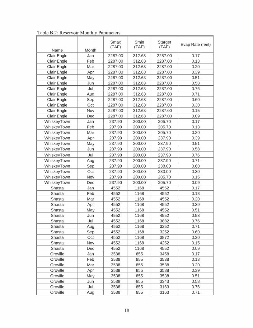
18

Table B.2: Reservoir Monthly Parameters

Name Month

Smax(TAF)

Smin(TAF)

Starget(TAF) Evap Rate (feet)

Clair Engle Jan 2287.00 312.63 2287.00 0.17 Clair Engle Feb 2287.00 312.63 2287.00 0.13 Clair Engle Mar 2287.00 312.63 2287.00 0.20 Clair Engle Apr 2287.00 312.63 2287.00 0.39 Clair Engle May 2287.00 312.63 2287.00 0.51 Clair Engle Jun 2287.00 312.63 2287.00 0.58 Clair Engle Jul 2287.00 312.63 2287.00 0.76 Clair Engle Aug 2287.00 312.63 2287.00 0.71 Clair Engle Sep 2287.00 312.63 2287.00 0.60 Clair Engle Oct 2287.00 312.63 2287.00 0.30 Clair Engle Nov 2287.00 312.63 2287.00 0.15 Clair Engle Dec 2287.00 312.63 2287.00 0.09

WhiskeyTown Jan 237.90 200.00 205.70 0.17 WhiskeyTown Feb 237.90 200.00 205.70 0.13 WhiskeyTown Mar 237.90 200.00 205.70 0.20 WhiskeyTown Apr 237.90 200.00 237.90 0.39 WhiskeyTown May 237.90 200.00 237.90 0.51 WhiskeyTown Jun 237.90 200.00 237.90 0.58 WhiskeyTown Jul 237.90 200.00 237.90 0.76 WhiskeyTown Aug 237.90 200.00 237.90 0.71 WhiskeyTown Sep 237.90 200.00 238.00 0.60 WhiskeyTown Oct 237.90 200.00 230.00 0.30 WhiskeyTown Nov 237.90 200.00 205.70 0.15 WhiskeyTown Dec 237.90 200.00 205.70 0.09

Shasta Jan 4552 1168 4552 0.17 Shasta Feb 4552 1168 4552 0.13 Shasta Mar 4552 1168 4552 0.20 Shasta Apr 4552 1168 4552 0.39 Shasta May 4552 1168 4552 0.51 Shasta Jun 4552 1168 4552 0.58 Shasta Jul 4552 1168 3882 0.76 Shasta Aug 4552 1168 3252 0.71 Shasta Sep 4552 1168 3252 0.60 Shasta Oct 4552 1168 3872 0.30 Shasta Nov 4552 1168 4252 0.15 Shasta Dec 4552 1168 4552 0.09 Oroville Jan 3538 855 3458 0.17 Oroville Feb 3538 855 3538 0.13 Oroville Mar 3538 855 3538 0.20 Oroville Apr 3538 855 3538 0.39 Oroville May 3538 855 3538 0.51 Oroville Jun 3538 855 3343 0.58 Oroville Jul 3538 855 3163 0.76 Oroville Aug 3538 855 3163 0.71

19

Oroville Sep 3538 855 3163 0.60 Oroville Oct 3538 855 3163 0.30 Oroville Nov 3538 855 3163 0.15 Oroville Dec 3538 855 3163 0.09 Folsom Jan 975 83 805 0.17 Folsom Feb 975 83 975 0.13 Folsom Mar 975 83 975 0.20 Folsom Apr 975 83 975 0.39 Folsom May 975 83 975 0.51 Folsom Jun 975 83 975 0.58 Folsom Jul 975 83 700 0.76 Folsom Aug 975 83 575 0.71 Folsom Sep 975 83 575 0.60 Folsom Oct 975 83 575 0.30 Folsom Nov 975 83 575 0.15 Folsom Dec 975 83 675 0.09

New Melones Jan 2420 273 2230 0.17 New Melones Feb 2420 273 2420 0.13 New Melones Mar 2420 273 2420 0.20 New Melones Apr 2420 273 2420 0.39 New Melones May 2420 273 2420 0.51 New Melones Jun 2420 273 2270 0.58 New Melones Jul 2420 273 1970 0.76 New Melones Aug 2420 273 1970 0.71 New Melones Sep 2420 273 1970 0.60 New Melones Oct 2420 273 1970 0.30 New Melones Nov 2420 273 1970 0.15 New Melones Dec 2420 273 2040 0.09

Tulloch Jan 67 57 57 0.00 Tulloch Feb 67 57 57 0.00 Tulloch Mar 67 57 58 0.00 Tulloch Apr 67 57 60 0.00 Tulloch May 67 57 67 0.00 Tulloch Jun 67 57 67 0.00 Tulloch Jul 67 57 67 0.00 Tulloch Aug 67 57 67 0.00 Tulloch Sep 67 57 62 0.00 Tulloch Oct 67 57 57 0.00 Tulloch Nov 67 57 57 0.00 Tulloch Dec 67 57 57 0.00

San Lius Jan 2027 450.00 1000.00 0.17 San Lius Feb 2027 631.60 1464.02 0.13 San Lius Mar 2027 748.10 1806.84 0.20 San Lius Apr 2027 835.60 1975.02 0.39 San Lius May 2027 879.92 1976.43 0.51 San Lius Jun 2027 694.72 1546.00 0.58 San Lius Jul 2027 442.12 1062.95 0.76 San Lius Aug 2027 181.12 642.62 0.71

20

San Lius Sep 2027 9.72 352.64 0.60 San Lius Oct 2027 8.32 312.90 0.30 San Lius Nov 2027 115.02 354.13 0.15 San Lius Dec 2027 286.72 514.21 0.09

Table B.3: Monthly Minimum and Target River Flows

Name Month Rmin (cfs) Rtarget (cfs)

Lewiston Jan 300 300 Lewiston Feb 300 300 Lewiston Mar 300 300 Lewiston Apr 300 300 Lewiston May 3939 300 Lewiston Jun 2507 783 Lewiston Jul 1102 450 Lewiston Aug 450 450 Lewiston Sep 450 450 Lewiston Oct 373 0 Lewiston Nov 300 300 Lewiston Dec 300 300

Clear Creek Jan 150 150 Clear Creek Feb 200 200 Clear Creek Mar 200 200 Clear Creek Apr 200 200 Clear Creek May 200 200 Clear Creek Jun 200 200 Clear Creek Jul 200 200 Clear Creek Aug 200 200 Clear Creek Sep 200 200 Clear Creek Oct 200 200 Clear Creek Nov 90 90 Clear Creek Dec 90 90 Spring Creek Jan 325 325 Spring Creek Feb 306 306 Spring Creek Mar 2749 2749 Spring Creek Apr 252 252 Spring Creek May 813 813 Spring Creek Jun 1681 1681 Spring Creek Jul 2602 2602 Spring Creek Aug 2114 2114 Spring Creek Sep 2017 2017 Spring Creek Oct 1138 1138 Spring Creek Nov 504 504 Spring Creek Dec 244 244

Keswick Jan 3250 3250 Keswick Feb 3250 3250

21

Keswick Mar 3250 3250 Keswick Apr 8000 8000 Keswick May 9600 9600 Keswick Jun 11000 11000 Keswick Jul 14500 14500 Keswick Aug 12000 12000 Keswick Sep 5500 5500 Keswick Oct 7200 7200 Keswick Nov 5700 5700 Keswick Dec 3250 3250 Wilkins Jan 0 0 Wilkins Feb 0 0 Wilkins Mar 0 0 Wilkins Apr 5000 5000 Wilkins May 5000 5000 Wilkins Jun 5000 5000 Wilkins Jul 5000 5000 Wilkins Aug 5000 5000 Wilkins Sep 5000 5000 Wilkins Oct 5000 5000 Wilkins Nov 0 0 Wilkins Dec 0 0

FeatherBelowThermolito Jan 1250 0 FeatherBelowThermolito Feb 1250 0 FeatherBelowThermolito Mar 1250 0 FeatherBelowThermolito Apr 1250 0 FeatherBelowThermolito May 2030 0 FeatherBelowThermolito Jun 0 2706 FeatherBelowThermolito Jul 0 5692 FeatherBelowThermolito Aug 5040 5156 FeatherBelowThermolito Sep 0 4386 FeatherBelowThermolito Oct 1980 2683 FeatherBelowThermolito Nov 1750 1815 FeatherBelowThermolito Dec 1250 0

AmericanRiverbelowNimbus Jan 800 0 AmericanRiverbelowNimbus Feb 800 0 AmericanRiverbelowNimbus Mar 1000 0 AmericanRiverbelowNimbus Apr 1500 0 AmericanRiverbelowNimbus May 2300 0 AmericanRiverbelowNimbus Jun 1800 0 AmericanRiverbelowNimbus Jul 0 0 AmericanRiverbelowNimbus Aug 0 0 AmericanRiverbelowNimbus Sep 0 0 AmericanRiverbelowNimbus Oct 0 0 AmericanRiverbelowNimbus Nov 1000 0 AmericanRiverbelowNimbus Dec 800 0

Goodwin Jan 175 175 Goodwin Feb 150 150

22

Goodwin Mar 268 268 Goodwin Apr 760 760 Goodwin May 800 800 Goodwin Jun 561 561 Goodwin Jul 396 396 Goodwin Aug 352 352 Goodwin Sep 240 240 Goodwin Oct 200 200 Goodwin Nov 200 200 Goodwin Dec 200 200 DeltaExit Jan 6001 6001 DeltaExit Feb 11398 11398 DeltaExit Mar 11401 11401 DeltaExit Apr 7848 7848 DeltaExit May 9319 9319 DeltaExit Jun 7092 7092 DeltaExit Jul 6505 6505 DeltaExit Aug 4261 4261 DeltaExit Sep 3008 3008 DeltaExit Oct 4001 4001 DeltaExit Nov 4655 4655 DeltaExit Dec 4505 4505

Table B.4: Monthly Demands Month Jan Feb Mar Apr May Jun Jul Aug Sep Oct Nov Dec

Thermolito 35 0 11 67 189 178 200 178 78 95 104 71Folsom Pumping 4 4 4 7 8 12 13 12 10 7 5 4

Folsom South Canal 1 1 1 1 2 3 4 4 3 2 1 1OID/SSJID 0 0 14 60 90 90 95 95 74 14 0 0

CVP Contractors 0 0 0 0 0 0 0 0 0 0 0 0CCWD 14 17 18 18 14 14 13 13 13 10 11 13

Barker Slough 2 2 1 2 4 5 7 7 6 5 3 3Federal Tracy PP 258 233 258 250 135 169 270 268 260 258 250 258

Federal Banks On-Peak 0 0 0 0 0 0 28 28 28 0 0 0State Banks PP 390 355 241 68 108 125 271 278 238 175 193 390State Tracy PP 0 0 0 0 0 0 0 0 0 0 0 0

Delta Mendota Canal 30 60 100 120 190 220 270 240 180 110 40 30Federal Dos Amigos 40 50 60 70 110 180 238 178 68 30 30 30Federal O'Neil to Dos

Amigos 0 1 1 1 1 2 2 1 0 0 0 0San Felipe 6 6 10 15 19 20 21 20 13 11 8 8

South Bay/San Jose 2 2 2 5 5 7 7 8 7 12 8 6State Dos Amigos 105 127 158 105 348 348 423 388 269 229 196 61

Delta Consumptive Use -56 -37 -10 63 121 191 268 252 174 118 55 2Freeport Treatment Plant 14 13 14 12 12 12 12 13 12 12 12 13

23

Table B.5: System Parameters

Month X-Channel Gate

O'NeilLoss X_2 Tracy Pump

Cap (cfs) Banks Pump

Cap (cfs) DI STD (%)

Jan 0.5 0.6 50 4200 6400 0.65 Feb 1 0.8 50 4200 6400 0.35 Mar 1 1.2 50 4200 6400 0.35 Apr 1 1.5 50 4300 6400 0.35 May 1 1.7 50 4300 6400 0.35 Jun 0.3 1.4 50 4300 6400 0.35 Jul 0 1.4 50 4600 6400 0.65 Aug 0 0.9 50 4600 6400 0.65 Sep 0 0.7 50 4500 6400 0.65 Oct 0 0.5 50 4300 6400 0.65 Nov 0 0.5 50 4200 6400 0.65 Dec 0 0.3 50 4200 6400 0.65

Table B.6: Demand Adjustment Fraction vs. River Index Value

River Index Code

River Index Value

Demand Fraction

C 1 0.2BN 2 0.4N 3 0.6

AN 4 1W 5 1

24

Figure B.2: Reservoir Elevation Sequences

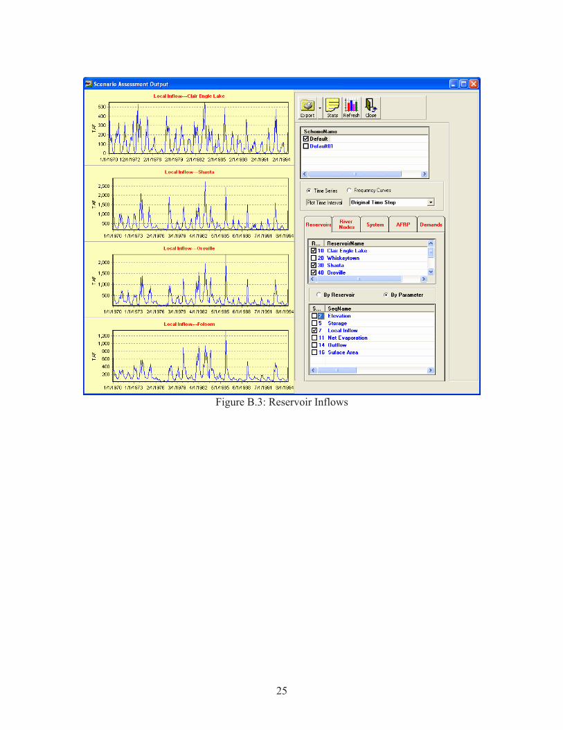
25

Figure B.3: Reservoir Inflows

26

Figure B.4: Reservoir Releases

27

Figure B.5: River Flows at Selected Locations

28

Figure B.6: River Flow at Selected Locations

29

Figure B.7: Selected Delta Sequences

30

Figure B.8: Reservoir comparisons

31

Figure B.9: Reservoir elevation sequences with fixed demand requirement pattern.

32

Appendix C: Assessment Model Inputs

C.1. General Input

Scheme definition;

Control horizon;

Simulation horizon (starting date, ending sate);

Forecasting model options;

Initial values for San Luis Storage, X2 Location, and USBR COA.

33

C.2. Reservoir Data

Initial storage;

Monthly values of maximum, minimum, and target Storage;

Monthly values of downstream flow constraint;

Monthly values of evaporation coefficients;

Monthly values of reservoir withdrawal.

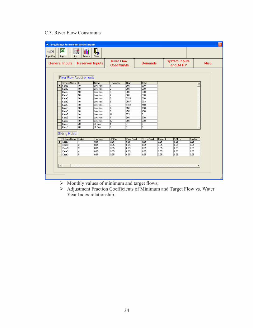
34

C.3. River Flow Constraints

Monthly values of minimum and target flows;

Adjustment Fraction Coefficients of Minimum and Target Flow vs. Water

Year Index relationship.

35

C.4. Demands

Monthly values of demands;

Demand Adjustment Fraction vs. Water Year Index relationship.

36

C.5. System Inputs and AFRP

Monthly values of for X-Channel Gate, O’Neil Evaporation Loss,

Coefficients, Max Tracy Pumping Capacity, Maximum Banks Pumping

Capacity, and Export to Inflow Ratio Constraints;

AFRP constraints for each month.

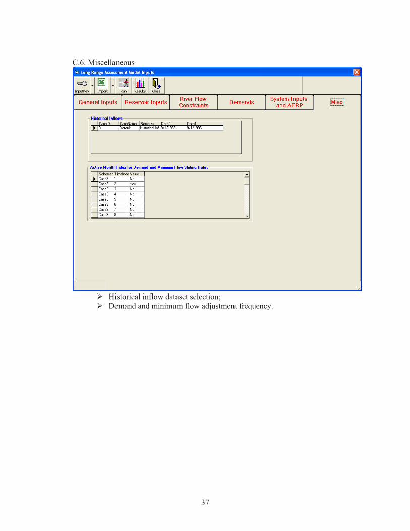
37

C.6. Miscellaneous

Historical inflow dataset selection;

Demand and minimum flow adjustment frequency.

38

Appendix D: Simulation Model Acronyms

Central Valley Project (CVP)

State Water Projects (SWP)

Stockton East Water District (SEWD)

Central San Joaquin Irrigation District (CSJID)

Oakdale/South San Joaquin Irrigation District (OSSJID)

Microsiemens/cm (EC)

Delta Mendota Canal (DMC)

Agreement of Coordinated Operation (COA)

Appendix E: Descriptions and Definitions of Water Year Type and River Index from DWR’s website( http://cdec.water.ca.gov/cgi-progs/iodir/wsi)

The Sacramento valley 40-30-30 index for water year types; Wet, Above

Normal,Below Normal, Dry, and Critical, is used to determine year types for

Delta outflow criteria and Sacramento system requirements.

The San Joaquin Valley 60-20-20 Index is used to determine year types for

flow requirements at Vernalis.

The Sacramento River Index (SRI), is used to trigger relaxation criteria related

to May-June Net Delta Outflow(NDO) requirements. The SRI refers to the

sum of the unimpaired runoff in the water year as published in the DWR

Bulletin 120 for the Sacramento River at Bed Bridge, Feature River inflow to

Oroville, Yuba River at Smartville and American River inflow to Folsom

reservoir.

The Eight River Index is used to trigger criteria related to January Net Delta

Outflow, February to June X2 standards and February export restrictions. The

eight river index refers to the unimpaired runoff for the four locations

mentioned under SRI plus Stanislaus River inflow to New Melones Reservoir,

Tuolumne River inflow to Don Pedro Reservoir, Merced River inflow to

Exchequer Reservoir and San Joaquin River inflow to Millerton Lake.

Sacramento River Runoff is the sum of unimpaired flow in million acre-feet

at:

Sacramento River above Bend Bridge

Feather River at Oroville (aka inflow to Lake Oroville)

Yuba River near Smartville

American River below Folsom Lake

Also known as the "Sacramento River Index", this index was previously used

to determine year type classifications under SWRCB Decision 1485.

39

Also previously referred to as the "4 River Index" or "4 Basin Index".

Index = 0.4 * Current Apr-Jul Runoff (1)

+ 0.3 * Current Oct-Mar Runoff (1)

+ 0.3 * Previous Year's Index (2)

Notes:

(1) Runoff is the sum of unimpaired flow in million acre-feet at:

Sacramento River above Bend Bridge

Feather River at Oroville (aka inflow to Lake Oroville)

Yuba River near Smartville

American River below Folsom Lake

(2) Maximum 10.0 for previous year index term

Year Type Classification: Index based on flow in million acre-feet:

Wet Equal to or greater than 9.2

Above Normal Greater than 7.8, and less than 9.2

Below Normal Greater than 6.5, and equal to or less than 7.8

Dry Greater than 5.4, and equal to or less than 6.5

Critical Equal to or less than 5.4

This index, originally specified in the 1995 SWRCB Water Quality Control

Plan, is used to determine the Sacramento Valley water year type as

implemented in SWRCB D-1641. Year types are set by first of month

forecasts beginning in February. Final determination is based on the May 1

50% exceedence forecast.

San Joaquin Valley Water Year Type Index (60-20-20)

Water Year Index based on flow in million acre feet

Index = 0.6 * Current Apr-Jul Runoff (1)

+ 0.2 * Current Oct-Mar Runoff (1)

+ 0.2 * Previous Year's Index (2)

Notes:

(1) Runoff is the sum of unimpaired flow in million acre-feet at:

Stanislaus River below Goodwin Reservoir (aka inflow to New Melones

Res.)

Tuolumne River below La Grange (aka inflow to New Don Pedro

Reservoir)

Merced River below Merced Falls (aka inflow to Lake McClure)

San Joaquin River inflow to Millerton Lake

(2) Maximum 4.5 for previous year index term

Year Type Classification: Index based on flow in million acre-feet:

Wet Equal to or greater than 3.8

40

Above Normal Greater than 3.1, and less than 3.8

Below Normal Greater than 2.5, and equal to or less than 3.1

Dry Greater than 2.1, and equal to or less than 2.5

Critical Equal to or less than 2.1

This index, originally specified in the 1995 SWRCB Water Quality Control

Plan, is used to determine the San Joaquin Valley water year type as

implemented in SWRCB D-1641. Year types are set by first of month

forecasts beginning in February. Final determination for San Joaquin River

flow objectives is based on the May 1 75% exceedance forecast.

Sacramento Valley and San Joaquin 8 River Index

This index is the sum of the previous month's unimpaired runoff for the 8

rivers that are included in the above Sacramento River Unimpaired Runoff

and San Joaquin Valley Water Year Type Index. A listing of reconstructed

indices based on historical observed runoff is posted at

http://cdec.water.ca.gov/water_supply.html . The official year types are based

on May 1st’s forecasts, not the observed runoff.

41

Remote Sensing of Precipitation Combining Geostationary andTRMM

Basic Information

Title: Remote Sensing of Precipitation Combining Geostationary and TRMM

Project Number: 2004GA101O


End Date: 6/30/2005



Research Category: Climate and Hydrologic Processes

Focus Category: None, None, None

Descriptors: Remote Sensing

Principal Investigators: Aris P. Georgakakos

Publication

Remote Sensing of Precipitation Combining Geostationary and TRMM Satellite Data

First Year Technical Report for Project NRA-02-ES-05,

“The Impact of Precipitation Measurement Missions on Hydrologic and Water Resource Predictions”

Aris Georgakakos and Carlo DeMarchi Georgia Water Resources Institute


Atlanta, Georgia 30332 (404) 894-2240

May 2005

ii

Contents

1 Introduction _______________________________________________________ 1

2 Characteristics of the Estimation Methodology ___________________________ 3

2.1 General structure ______________________________________________ 3

2.2 The IR/VIS-precipitation relation _________________________________ 5

2.3 Uncertainty characterization _____________________________________ 6

3 Rain-gage and Satellite Data _________________________________________ 11

3.1 Meteosat images_______________________________________________ 11

3.1.1 Characteristics of Meteosat images_____________________________ 11

3.1.2 Meteosat data processing ____________________________________ 13

3.2 TRMM images________________________________________________ 16

3.2.1 Characteristics of TRMM images ______________________________ 16

3.2.2 TRMM data processing______________________________________ 18

3.3 Rain-gage data________________________________________________ 21

3.3.1 Characteristics of rain-gage data_______________________________ 21

3.3.2 Rain-gage data processing____________________________________ 21

4 Identification of Convective Storms____________________________________ 23

4.1 Detecting convective-storm occurrence at the pixel level _____________ 24

4.1.1 The training and verification data sets __________________________ 28

4.1.2 Calibration and validation of artificial neural networks _____________ 31

4.2 Relation between IR, stage, and precipitation ______________________ 33

5 Single Pixel Analysis _______________________________________________ 39

5.1 Characteristics of the single pixel estimation process ________________ 39

5.2 Estimation model performance __________________________________ 44

5.2.1 Model calibration (1996-1998) ________________________________ 44

5.2.2 Model validation (1996-1997) ________________________________ 45

5.2.3 Comparison with Adjusted GPI (TRMM product 3B42).____________ 46

5.2.4 Discussion ________________________________________________ 47

5.3 Estimation incorporating precipitation autocorrelation ______________ 50

5.3.1 Autocorrelated model calibration (1996-1998)____________________ 54

5.3.2 Autocorrelated model validation (1996-1997) ____________________ 56

5.3.3 Discussion ________________________________________________ 57

6 Multi-pixel Analysis ________________________________________________ 63

7 Conclusions ______________________________________________________ 64

8 References________________________________________________________ 66

1

1 Introduction

Since its launch in late 1997, the Tropical Rainfall Monitoring Mission (TRMM) satellite

has provided a variety of high quality data that have spurred several advances in

hydrological and meteorological studies. The most innovative TRMM sensor, the

Precipitation Radar (PR), routinely produces highly-reliable and detailed three-

dimensional representations of rain fields that have offered new insights on the physics of

precipitation phenomena (Hirose and Najkamura, 2004; De Angelis et al., 2004). On the

other hand, these high-quality instantaneous precipitation measurements have found

limited direct operational use due to the low PR sampling frequency (7-8 passages per

month at the equator).

To overcome this limitation, TRMM information could be combined with information

provided by other satellite systems with more frequent but less reliable data. Grecu and Anagnostou, 2001, for example, proposed to use PR data for improving passive

microwave precipitation retrieval algorithms, while Bellerby et al., 2000, used PR data

for calibrating a precipitation estimation algorithm based on infrared and visible (IR/VIS)

images from geostationary satellites. However, such efforts are sparse, and no definitive

methodology has been established yet.

The research described herein proposes and evaluates a robust methodology for

operational assessment of precipitation using TRMM PR data and half-hour IR/VIS data

from geostationary satellites. The study recognizes that precipitation estimates based on

satellite images are affected by substantial uncertainty that satellite sensor and

methodology improvements may reduce, but not completely eliminate. Furthermore,

estimation uncertainty varies with time and spatial resolution, respectively ranging from

less than an hour to days and months, and from a few to hundreds of square kilometers.

Thus, a goal of the proposed methodology is to explicitly quantify the uncertainty

associated with precipitation estimation.

2

The proposed methodology is applied and tested in the Lake Victoria basin (Equatorial

Africa). Comparisons with conventional rain gage data from 100 rain gages over a two-

year period (1996-1998) indicate that the method exhibits high estimation reliability.

This report is structured in seven chapters. Chapter 2 illustrates the framework of the

estimation methodology. Chapter 3 describes the data used for calibration and testing.

Chapter 4 investigates a new procedure for identifying convective storms at the pixel

level. Chapter 5 discusses the estimation approach and quantifies its performance at the

pixel level. Chapter 6 outlines the steps required to aggregate the single pixel estimates

over larger regions in a statistically consistent manner. Finally, Chapter 7 summarizes

the research results and outlines the future project plan.

The research described herein has been funded by several sources including the Food and

Agriculture Organization of the United Nations (FAO/UN) under the Nile Decision

Support Program, the United States Geological Survey under the State Water Resources

Program, and NASA (Goddard Space Flight Center, GSFC) under Project NRA-02-ES-

05 entitled “The Impact of Precipitation Measurement Missions on Hydrologic and Water

Resource Predictions.” The last project is a collaborative effort between NASA’s GSFC

(with lead PIs Dr. C. Peters-Liddard and Dr. J.M. Sheppard) and the Georgia Water

Resources Institute (GWRI) at Georgia Tech (with lead PI Dr. A. Georgakakos). This

document serves as the GWRI first year Interim Project Report.

3

2 Characteristics of the Estimation Methodology

2.1 General Structure

Precipitation estimation methodologies using satellite images can be subdivided into

three broad categories:

• Procedures based on IR/VIS images, mainly from geostationary satellites;

• Procedures based on microwave images from low earth orbiting (LEO) satellites;

• Procedures combining IR/VIS images from geostationary satellites with microwave

images from LEO satellites.

Procedures based on IR/VIS images from geostationary satellites

Satellite IR/VIS sensors convey information on cloud presence, type, extent, and

evolution history. Subsequently, IR/VIS procedures transform this information, more or

less empirically, into precipitation estimates. The advantage of these techniques is that

IR/VIS images from geostationary meteorological satellites are available every 15 to 30

minutes with a spatial resolution of 1 to 8 km, allowing a continuous monitoring of the

cloud evolution. Their disadvantage is that this information is only indirectly related to

precipitation and that this relation is subject to considerable variations in time and space

(Arkin and Xie, 1994). Because of this, dense networks of rain gages are needed to

optimize this relation in space and time (for example Todd et al., 1995; Georgakakos et

al., 2001).

Procedures based on microwave images from LEO satellites

The relation of precipitation rate and microwave radiation is more reliable than infrared

or visible radiation. For this reason, microwave sensors provide better estimates of

instantaneous rain (Ebert et al., 1996; Todd et al., 2001). However, microwave image

sensors are presently available only aboard LEO satellites, and this information is only

available every 3 to 6 hours. This low temporal frequency does not provide good

precipitation estimates at the daily-dekad temporal resolution (Ebert et al, 1996).

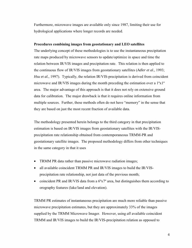
4

Furthermore, microwave images are available only since 1987, limiting their use for

hydrological applications where longer records are needed.

Procedures combining images from geostationary and LEO satellites

The underlying concept of these methodologies is to use the instantaneous precipitation

rate maps produced by microwave sensors to update/optimize in space and time the

relation between IR/VIS images and precipitation rate. This relation is then applied to

the continuous flow of IR/VIS images from geostationary satellites (Adler et al., 1993;

Hsu et al., 1997). Typically, the relation IR/VIS-precipitation is derived from coincident

microwave and IR/VIS images during the month preceding the estimation over a 1ºx1º

area. The major advantage of this approach is that it does not rely on extensive ground

data for calibration. The major drawback is that it requires online information from

multiple sources. Further, these methods often do not have “memory” in the sense that

they are based on just the most recent fraction of available data.

The methodology presented herein belongs to the third category in that precipitation

estimation is based on IR/VIS images from geostationary satellites with the IR/VIS-

precipitation rate relationship obtained from contemporaneous TRMM-PR and

geostationary satellite images. The proposed methodology differs from other techniques

in the same category in that it uses

• TRMM PR data rather than passive microwave radiation images;

• all available coincident TRMM PR and IR/VIS images to build the IR/VIS-

precipitation rate relationship, not just data of the previous month;

• coincident PR and IR/VIS data from a 6ºx7º area, but distinguishes them according to

orography features (lake/land and elevation).

TRMM PR estimates of instantaneous precipitation are much more reliable than passive

microwave precipitation estimates, but they are approximately 33% of the images

supplied by the TRMM Microwave Imager. However, using all available coincident

TRMM and IR/VIS images to build the IR/VIS-precipitation relation as opposed to

5

monthly data partly corrects this deficit. Furthermore, the use of large data sets provides

a more robust assessment of precipitation average spatial distribution and variability.

This is essential for characterizing estimation uncertainty and for applying the procedure

to periods for which microwave data are not available. Also, larger data sets allow for

regionalizing the IR/VIS-precipitation relationship based on orography features rather

than on latitude/longitude, leading to better precipitation estimates in heterogeneous

terrains.

2.2 The IR/VIS-precipitation relation

In the last 30 years several algorithms have been proposed for estimating precipitation

from IR/VIS satellite images. Some of the most commonly used approaches are

summarized below:

• IR threshold for rain/no rain and single precipitation rate;

o fixed in time and space (GPI, Richards and Arkin, 1981; Arkin and Meisner,

1987);

o spatially and temporally varying (Adjusted GPI, Adler et al., 1993; Todd et al.,

1995; Universally Adjusted GPI, Xu et al., 1999);

• Discrimination between convective and stratiform rain (CST, Negri and Adler, 1988;

Negri and Adler, 2002);

• IR/Rain rate probability matching (3B41RT, Huffman et al., 2003; MIRA, Todd et al.,

2001);

• IR Texture – IR, µIR3x3,σIR3x3, µIR5x5,σIR5x5 – (PERSIANN, Hsu et al., 1997);

• Indicator of cloud growth – P(t)=F(IR(t) if IR(t)-IR(t-1)= 0, 0 otherwise – (NESDIS

Autoestimator, Vincente et al.,1998);

• Lookup tables for rain-rate indexed by IR and VIS (King et al., 1995) or IR11, IR11-

IR12, and IR11-WV (Kurino, 1997);

• Bivariate VIS-IR frequency (Tsonis et al., 1996; Georgakakos et al., 2001);

• IR, VIS Texture (PERSIANN, Hsu et al., 1999; Bellerby et al., 2000);

6

The methodology of this work utilizes a “lookup table” approach similar to those of Kinget al. (1995) and Kurino (1997). The approach of these investigators is to develop a

matrix relating rain-rates to satellite IR-VIS pairs. Each element of this matrix represents

the average hourly precipitation rate over an 8 km X 8 km area corresponding to a

satellite observed IR-VIS pair. The average precipitation rates were obtained from six

months of coincident radar and satellite observations. At nighttime, the precipitation rate

is derived as function of the IR alone. This procedure performs better than approaches

that only use IR information (First Algorithm Intercomparison Project, Arkin and Xie,

1994) because the visible data help discriminate raining cumulonimbi from the similarly

cold, but semitransparent, non-raining cirri, and identify precipitation from thick versus

shallow clouds. Since then several other algorithms have added the visible data to the IR

for precipitation estimation (Tsonis et al., 1996; Hsu et al., 1999; Bellerby et al., 2000).

Kurino (1997) used the same general approach, but the rain-rate matrixes were indexed

by triplets, IR11, IR11-IR12, and IR11-WV, where the IR11 is the infrared radiation at 11 µm

(indicated as IR in the rest of the report), IR12 the infrared radiation at 12 µm, and WV is

the infrared radiation at 6.7 µm, also known as water vapor (WV) channel. The value of

IR11-IR12 is used to discriminate cirri, while IR11-WV is useful for deep convection

detection. Bellerby et al. (2000) and Georgakakos et al. (2001) have also used WV for

precipitation estimation.

The look-up table used in this research is indexed by orography, IR, VIS during daytime

or IR-WV during nighttime, storm stage, and month. At each half-hour time slot, the

precipitation over a pixel is determined as function of the satellite observed IR/VIS/WV

radiation in the pixel, orography, and season.

2.3 Uncertainty characterization

As mentioned in the introduction, one of the main research goals is to provide a complete

characterization of the uncertainty inherent in precipitation estimates. This implies that

half-hour precipitation should be treated as a random variable, the distribution of which

7

needs to be defined. The observed IR/VIS/WV values are expected to condition the

mean, variability, and the general shape of this distribution.

A way to characterize the precipitation probability distribution is by assuming a

probabilistic model and fitting it to experimental data. Bell (1987) modeled ocean

precipitation as a temporally and spatially homogeneous and isotropic random process.

He also assumed that there is an average probability f > 0 of rain and that the intensity of

rainy events is distributed lognormally. Further, he modeled the correlation of the

precipitation at different points as a decreasing function of the distance d between the

points. This model was used to assess the ability of microwave LEO sensors to

reconstruct monthly average precipitation over a large and homogeneous area. As such,

there is no dependence between precipitation rate and observed IR/VIS/WV

characteristics.

Fiorucci et al. (2001) also model precipitation as a log-normal random process, and

conditioned the precipitation mean and variance at a pixel (i,j) and time t on the observed

IR radiation at the same location:

⎟⎟⎠

⎞⎜⎜⎝

⎛−=⋅=⎟⎟

⎠

⎞⎜⎜⎝

⎛ −−⎟⎟

⎠

⎞⎜⎜⎝

⎛+

−=

γρµσ

µµ ),),(,(

),),(,(,,,,

,,,,

,, expexp1lkji

lkjitjitjitjitji

tjid

CVM

CM

CIRL

Spatial autocorrelation of precipitation is modeled as exponentially decreasing with

distance, but the authors do not consider temporal autocorrelation.

The distribution of the average precipitation over a period/region could be analytically

derived using the appropriate summation formulas.

An alternative strategy is the ensemble technique, a procedure convenient when

analytical forms of the probability density function are too difficult to derive. In this

case, an ensemble of equally likely values is derived by randomly sampling a distribution

of observed/simulated values. For example, Georgakakos, 1989, used ensembles of past

observed flow sequences with initial values similar to the flows observed at time t and t-1

8

for predicting the range of possible flows at time t+1, t+2, etc. Walser et al., 2004,

assessed the prediction capabilities of mesoscale numerical weather prediction (NWP)

models by randomly perturbing the NWP initial conditions and observing the variability

of the NWP output.

This study adopts the ensemble approach by associating each combination of input

variables with the entire distribution of TRMM PR rain rates observed over a long period

of time. Specifically, at each timeslot, an ensemble of equally likely precipitation values

are obtained by randomly sampling the distribution of PR rates corresponding to

particular combination of IR, VIS, WV, storm stage, orography, and month. This

approach is not limited by a particular probability model over the sample data. Further, it

is easy to update and is relatively robust since outliers do not influence the entire

distribution, but only a small number of cases. The disadvantages of this approach is that

it requires keeping in random computer memory a lot of data and using a Monte Carlo

approach to derive the distribution of precipitation over a region/period. The estimation

procedure for the precipitation over a single pixel can be delineated as follows:

1 The daily Meteosat IR time series (consisting of half-hour values) for a given pixel is

processed by a neural network to determine the presence and evolution (storm stage)

of convective storms (Figure 2.3.1 A).

2 At each timeslot t, the corresponding IR(t) and storm stage(t), defined in Step 1,

identify a distribution of PR samples (Figure 2.3.1 B).

3 One estimate of daily precipitation is generated by randomly sampling the

precipitation rates corresponding to the IR-stage combinations during the day and

summing the resulting half-hour precipitation rates (Figure 2.3.1 C). The process is

repeated N times resulting in N daily precipitation estimates (Figure 2.3.1 B).

4 To assess the accuracy and statistical consistency of the approach, the probabilistic

position of the gage record with respect to the ensemble distribution is recorded

(Figure 2.3.1 D). This value is used to determine various statistics such as the inter-

quartile compliance rate, 95% compliance rate, Kolmogorof-Smirnov compliance

statistic, among others.

9

5 The same approach is used to produce 10-day (dekad) and monthly precipitation

estimates by extending the number of half-hour time series from 48 to 480, or to 48

times the number of days in the desired interval.

6 More sophisticated estimation procedures can be obtained by adding VIS(t)/WV(t),

orography, and the calendar month in the set of indexing variables. A PR

distribution similar to that of Figure 2.3.1 B will be identified by the appropriate

combination of the input values in each time slot. Namely, for each member X of the

ensemble:

Precip(t) = f[IR(t), VIS(t)/WV(t), stage(t), orography, month, �],

where

Precip(t)= precipitation rate at time t for element X;

IR(t)= infrared radiation at time t;

VIS(t)= visible radiation at time t;

WV(t)= water vapor radiation at time t;

� = random error.

To extend this approach over a region, the random errors used for sampling the rain-rate

distributions must be generated in a way that maintains the precipitation spatial

correlation observed in the region. This topic is taken up in Chapter 6.

10

Dai

ly IR

and

Con

vect

ive

Stor

m S

tage

s Ti

me

Serie

s

120

140

160

180

200

220

240

260

280

300

320

1/5/

1996

6:0

01/

5/19

96 1

2:00

1/5/

1996

18:

001/

6/19

96 0

:00

1/6/

1996

6:0

0

IR (K)

02468101214161820

Storm Stages

IR Stag

es

<2

00

0m

Reg

ion -

- S

tage 4

Pix

els

0.4

0.5

0.6

0.7

0.8

0.91

05

10

15

20

25

30

35

40

45

50

Pre

cipit

ati

on (

mm

/h)

Cumulative frequency

190

-210

210

-230

230

-250

250

-270

270

-290

IR R

ange

(K)

Ense

mbl

e of

Pre

cipi

tatio

n Tr

ajec

torie

s

01020304050607080

1/5/

1996

6:0

01/

5/19

96 1

2:00

1/5/

1996

18:

001/

6/19

96 0

:00

1/6/

1996

6:0

0

Prec

ipita

tion

Dis

tribu

tion

0

0.1

0.2

0.3

0.4

0.5

0.6

0.7

0.8

0.91

020

4060

8010

0m

m

Frequency

Gag

e re

cord

Estim

ate

ense

mbl

e

A)

B)

C)

D)

.

Fig

ure

2.3

.1:

Sch

emat

ic o

f th

e en

sem

ble

est

imat

ion o

f dai

ly p

reci

pit

atio

n a

t th

e pix

el l

evel

11

3 Rain-gage and Satellite Data

The proposed precipitation estimation methodology has been evaluated in an area

surrounding Lake Victoria. More specifically, this area is depicted in (Figure 3.1.1 and

Figure 3.3.1) and extends from 29ºE to 36ºE and from 5ºS to 3ºN. Lake Victoria covers

roughly the central 10% of this region. This region is flanked by high mountains, with

Mount Elgon (4155 m) in the east side and Mount Ruwenzori (5109 m) in the west.

The climate of the region is equatorial, but elevation and lake influence contribute to

moderate temperatures all year round. The lowlands in the southern side of the area are

considerably drier than the rest of the basin.

Precipitation is driven mainly by the migration of the Inter Tropical Convergence Zone

with the related northeast and southeast monsoons. Lake Victoria is large enough to

partly modify the general circulation by creating a permanent pressure low attracting

moisture from the Congo rainforest in the west. Further, it creates local precipitation

patterns similar to those created by land-sea interaction. The high mountains in the basin

also influence the climate by creating windward and leeward regions.

This section illustrates the satellite and rain-gage data available to this project as well as

data available for future modeling developments. Data processing for quality control is

also described.

3.1 Meteosat images

3.1.1 Characteristics of Meteosat images

Meteosat is a family of geostationary meteorological satellites located above the point

0°E, 0°N that monitor the weather evolution over the region shown in Figure 3.1.1.

Meteosat‘s main sensor, the VISSR imaging radiometer, produces a digital image of the

full earth disk every 30 minutes in the three channels described in Table 3.1.1. The size

12

of the image elements (pixels) is approximately equal to that indicated in Table 3.1.1 at

the sub-satellite point, but increases moving towards the periphery of the view.

Area Exploitable for

Quantitative Analysis

LVDSS Area

Nile DST AreaMeteosat Earth View

Area Exploitable for

Quantitative Analysis

LVDSS Area

Nile DST AreaMeteosat Earth View

Figure 3.1.1: Full Disk View of the Meteosat Satellites

Table 3.1.1: Characteristics of the VISSR imaging radiometer (Eumetsat, 2000)

Channel Electromagnetic band

(µm)

Sub-satellite

spatial resolution

(km)

Direct and indirect

meteorological information

provided

VIS 0.5 –0.9 2.5 x 2.5

(5.0 x 5.0)

Albedo (daytime) –

Thickness of clouds.

WV 5.7 – 7.1 5.0 x 5.0 Water vapor in the middle

troposphere -- Thickness of

clouds/Overshooting

IR 10.5 –12.5 5.0 x 5.0 Thermal infrared temperature

– Surface temperature and

cloud top’s elevation

Only two channels at a time are normally broadcasted due to restrictions on the receiving

hardware and software. Typically, these two channels are the thermal infrared (IR)

channel and either the visible (VIS) or the water vapor (WV) channel, according to a

predefined schedule. VIS images are available between 5:30 GMT and 22:00 GMT,

13

while the WV images are available between 22:30 GMT and 5:00 GMT. Further, the

VIS channel is transmitted at half its nominal spatial resolution, by sub-sampling the full

resolution image. At 11:30 GMT Meteosat images are available only for the

Mediterranean basin.

Four different Meteosat satellites, Meteosat-4 through Meteosat-7, have provided digital

images over the period 1992-2003. While the general characteristics of images have

remained those described in Table 3.1.1, each satellite’s sensors require specific digital

count – radiance relations. Further, the performance of the sensors vary during their

operational life because of sensor degradation and environmental influences, requiring a

continuous recalibration of the count-radiance relationship. The satellite-specific sensor

count-radiance relation and the calibration coefficients can be retrieved from the

Eumetsat web site (www.eumetsat.de). Some calibration coefficients are also embedded

in the satellite broadcasted digital images as auxiliary parameters. The quality of the

image (i.e., the noise level) is also different from satellite to satellite.

3.1.2 Meteosat data processing

Meteosat digital images were available to this project in three different formats, namely

B.U.R.S.L. Autosat 3.1 (FAO/UN – Egypt images before December 1996), B.U.R.S.L.

Autosat Block 5 (FAO/UN – Egypt images after December 1996 and FAO/UN – Uganda

images), and Eumetsat OpenMTP. All three formats hold much more information than

needed for this study, dramatically increasing storage requirements. Further, extracting

the data from these files is a cumbersome process that easily fails if the digital files are

corrupted. It also requires merging data files in different formats for producing a

continuous sequence of images. For these reasons the digital images have been re-

sampled over a regular rectangular grid with 0.05ºx0.05º resolution and transformed into

a nimbler intermediate format called NileDST Grid Format. (NileDST stands for the Nile

Decision Support System that has been developed by the Georgia Water Resources

Institute at Georgia Tech, Georgakakos, 2004.) The translation process included the

following steps:

14

1. Elimination of missing and noisy lines;

2. Conversion of digital counts into blackbody temperatures (IR and WV channels) and

albedo (VIS channel) with correction of the solar-angle effect for the latter.

3. Filtering of clearly invalid values;

4. Filtering of pixels outside the range AVG5x5 – 3 x STDEV5x5 < pixel value < AVG5x5

+ 3 x STDEV5x5, where AVG5x5 is the channel average over a five pixels by five

pixels square centered on the pixel of interest, and STDEV5x5 is its standard

deviation;

5. Detection and elimination of corrupted, spatially or temporally displaced, and

duplicated images;

6. Correction of the displacement error.

Table 3.1.2: Available Meteosat data

Period Spatial and temporal

coverage of images

Source

06/1992-12/1994 South of 22N FAO – Egypt

01/1995-12/1995 South of 22N – 96% FAO – Egypt +

Eumetsat

01/1996-12/1996 South of 22N – 98% FAO – Egypt +

Eumetsat

01/1997-12/1997 Nile Basin – 98% FAO – Egypt +

Eumetsat

01/1998-09/17/1998 Nile Basin - Complete Eumetsat

09/18/1998-12/1998 South of 10N – Complete FAO Entebbe + Eumetsat

01/1999 South of 5N– Complete Eumetsat

02/1999-25/05/1999 Nile Basin - Complete Eumetsat

06/05/1999-04/2000 Nile Basin – 88% coverage FAO – Egypt

05/2000-07/2000 None

08/2000-14/09/2001 Nile Basin – 83% FAO – Entebbe

15/09/2001-

12/29/2002

Nile Basin – 83% FAO – Entebbe

Satellite digital images in 1996-1997 were frequently affected by one or more lines of

noise like the one shown in Figure 3.1.2. Quality of the remaining files range from good

to optimal in the case of the OpenMTP files.

15

a)b)

c) d)

Figure 3.1.2: a) Example of FAO-Egypt IR Image until 1996. A line of noise slightly

North of Lake Victoria is maintained for illustrative purposes. b) Example of FAO-Egypt

16

VIS Image after 1996. c). Example of FAO-Entebbe IR Image in 1998. d) Example of

Eumetsat IR Image.

3.2 TRMM images

3.2.1 Characteristics of TRMM images

The Tropical Rainfall Measuring Mission (TRMM) is a joint mission between the

National Aeronautics and Space Administration and the National Space Development

Agency (NASDA) of Japan aimed at providing the first detailed and comprehensive

dataset on the four dimensional distribution of rainfall and latent heating over under-

sampled oceanic and tropical continental regimes.

The TRMM satellite is placed on an orbit inclined of 35° with respect to the equator at an

altitude of 350-500 km. This orbit allows TRMM to monitor the tropical areas with

higher temporal frequency and to distribute its passages above the same point uniformly

over the entire twenty-four hour period. This TRMM characteristic is essential for the

proper sampling of precipitation over the tropics given the strong diurnal cycle affecting

rainfall in this area (Li et al., 1996). For the same reason it is essential also for using

precipitation measurements for calibrating estimation procedures based on infrared

images from geostationary satellites (Morrissey and Janowiak, 1996).

This work uses only two of the five TRMM sensors, the Precipitation Radar (PR) and the

TRMM Microwave Imager (TMI). PR is a 2m x 2m phased array antenna operating at

the frequency of 13.8 GHz that provides the vertical distribution of instantaneous

reflectivity along its swath. From this information, the presence and type of rain is

assessed and the rain rate estimated. The beam is electronically scanned cross track ±17°

with respect to nadir in 0.6 s. The swath is subdivided in 49 angle bins each with a near-

surface horizontal diameter of a little more than 4 km. Each angle bin is subdivided in 80

range bins distributed every 250 m from just above the earth ellipsoid to the altitude of 20

km. An effective signal-to-noise ratio of 4 dB is obtained for rain as low as 0.7 mm h-1

(Kummerow et al., 1998, 2000).

17

The short-term drifts in PR performance due to the variation in the solar illumination of

the satellite during its orbits and consequent change in the instrumentation temperature

are contained within 1 dB. An Active Radar Calibrator located in Japan monitors Long-

term changes in the PR performance allowing for timely adjustments in the algorithms

used for deriving precipitation rates. Differences in rainfall reflectivity measures with

ground and airborne radar in Florida and Japan were on average limited within 1 dB

(Kummerow et al., 2000).

Figure 3.2.1: Schematic view of the scan geometries of the three primary rainfall

sensors: TMI, PR, and VIRS(after Kummerow et al., 1998)

TMI is a nine-channel microwave radiometer with architecture similar to the Special

Sensor Microwave/Imager (SSM/I). The main differences are the addition of two 10.7

GHz vertical and horizontal polarization channels, the shift of the frequency of the water

vapor channel from 22.325 to 21.3 GHz, and the higher spatial resolution due to the

18

lower orbit altitude. TMI’s swath is an arc 758.5 km wide (Figure 3.2.1) with a spatial

resolution varying from 63x37 km at 10.65 GHz to 7x5 km at 85.5 GHz (Kummerow et

al., 1998).

PR and TMI are used alone or in combination to produce several types of products,

varying in complexity from the basic reflectivity to monthly precipitation estimates.

3.2.2 TRMM data processing

This project is currently using products “2A23 – PR Qualitative” and “2A25 – PR

Profile” data. The former product first determines whether each range bin is above or

below the ground surface and if the corresponding radar reflectivity is reliable. Then, the

presence of rain is assessed as “possible” (the return power is larger than the 90%-tile

noise) or “certain” (the return power exceeds the “possible” noise level by more than

three times the noise standard deviation).

PR assesses the rain type by merging the results of two different methods for classifying

rain type: the H-method based on the horizontal reflectivity distribution (Steiner et al.,1995) and the V-method based on the reflectivity vertical profile. The final precipitation

classification is obtained by merging the outcomes of the H-Method and V-Method with

other information in the bright band (BB), resulting in a complex categorization of the

rain type. The project, however, retained only the major precipitation classes (stratiform,

convective, and “other” ) by using the following scheme (TSDIS, 2004)

(merged) rainType[i] / 100 = 1: stratiform;

2: convective;

3: other.

Smearing of BB near the antenna scan edges seriously affects the BB detection, which is

about 80% for antenna scan angles in the interval ±7° from nadir, but only about 20% at

the swath edges. Further, the rain/no-rain discrimination seems also to be dependent on

19

the angle-bin. To alleviate the impact of side-lobe clutter, the project does not use the

first and last two pixels of each PR swath.

TRMM data have been re-sampled along the 0.05ºx0.05º NileDST grid for matching with

contemporaneous Meteosat data. When two or more TRMM pixels fall within the same

NileDST pixel the resulting rain is classified as “entirely convective”, “entirely

stratiform”, “entirely mixed”, or “no-rain” if the original TRMM data were of the same

type. If they were of different types, the resulting NileDST pixel is classified as

“partially convective”, “partially stratiform”, or “partially mixed” (Figure 3.2.2).

ConvectivePartly convective

StratiformPartly stratiformMixed

Partly mixedNo-rain

ConvectivePartly convective

StratiformPartly stratiformMixed

Partly mixedNo-rain

>=30 mm/h25 mm/h

20 mm/h15 mm/h10 mm/h

5 mm/h>0 mm/h

Figure 3.2.2: Example of rain type and near surface rain-rate information provided by

TRMM

Product “2A25 – PR Profile” reports the precipitation rate as well as its reliability for

each beam of the PR swath over 80 vertical levels. It also includes additional information

relevant to the precipitation rate retrieval procedure.

20

It was not possible to use precipitation rates at a predetermined elevation or the average

rain between 2 and 4 kilometers, two TRMM products that are frequently used for

precipitation estimates, because of the large variation in elevation in the Lake Victoria

basin makes them either applicable only to a limited portion of the area or too far from

the surface. Near surface rain, on the other hand, is available for all pixels of the basin,

thus allowing a complete coverage of all elevation bands. It also accounts for

precipitation evaporation along raindrop trajectories, an issue that may be relevant in the

drier parts of the basin. On the other hand, near surface rain is likely to be noisier than

precipitation rates averaged over several vertical levels and more strongly affected by

ground clutter. A basin-wide comparison between precipitation rates near the surface and

at 2 kilometers altitude suggested that near surface rates below 0.7 mm/hr are very likely

to be noise and were thus eliminated.

As with the rain type product, 2A25 pixels have been re-sampled to fit the 0.05ºx0.05º

NileDST grid by averaging the precipitation of multiple TRMM pixels falling within the

same NileDST pixel.

Table 3.2.1: Available TRMM data

Period Spatial and temporal

coverage of images

Source

01/1996-12/1996 None

01/1997-12/1997 None

01/1998-12/1999 -5N÷5N, 28E÷38E

816 valid TRMM passages

University of

Connecticut

12/1997-Present Nile Basin

Acquisition in process

NASA

21

3.3 Rain-gage data

3.3.1 Characteristics of rain-gage data

The precipitation estimation procedure has been evaluated using the December 2002

version of the FAO Nile Data Base (NBD-Dec02-2) and some additional data from the

Kenya Ministry of Water, Tanzania Ministry of Water, and the Egyptian Nile Forecast

Center. This data were available to GWRI/Georgia Tech as part of the development of

the Nile DST and other projects.

3.3.2 Rain-gage data processing

Rain gage data have undergone extensive examination to ensure the quality of the

records. The main quality control steps were as follows:

1 Rain gage coordinates have been verified against GIS maps and WMO or national

identification codes;

2 Duplicate and ambiguous precipitation records have been eliminated;

3 Monthly sequences of daily precipitation with less than 90% records have been

dismissed;

4 For each rain-gage, the average precipitation during each month of 1996, 1997, and

1998 has been compared against the 15-year average precipitation. Months with

precipitation outside the normal range or months with insufficient records were

compared against measurement at neighboring stations;

5 Correlation in 10-day precipitation between neighboring stations was checked;

6 Only stations featuring at least 30 months of valid precipitation records in the 1996-

1998 or 20 months of valid precipitation records in the 1996-1997 periods were

retained;

7 Differences in the correlation between daily precipitation and satellite estimates at

neighboring stations were investigated;

22

The resulting data records that passed the previous tests are reported in Table 3.3.1 and in

Figure 3.3.1. The rain gage density in the basin fluctuates significantly making the

examination of the gage records particularly difficult. Therefore, it is likely that despite

all quality control efforts, rain gage data still suffer from a higher percentage of error than

similar data from other parts of the world.

Table 3.3.1: Available rain gage data in the Lake Victoria region

Period Stations with temporal

coverage of at least 83%

Source

01/1996-12/1997 Lake Victoria basin - 98 FAO



A)

23

B)

Figure 3.3.1: Available rain gages with (A) at least 30 months of valid data in the period

1996-1998 (B) at least 20 months of valid data in the period 1996-1997

4 Identification of Convective Storms

Most procedures using infrared and visible images from geostationary satellites for

estimating precipitation have an “instantaneous” nature in the sense that the estimation of

the precipitation at a certain time is based only on the satellite images taken at that

particular time. Some procedures recognize the importance of the temporal change of

cloud characteristics and base their estimates on pairs of consecutive satellite images

(Vincente et al.,1998; Bellerby et al., 2000). On the other hand, it is generally recognized

that convective storms feature three distinct phases—developing, mature, and dissipating-

-each with a distinct rain regime. Using specific relations between cloud characteristics

and precipitation for these different phases of the convective storm and for different types

of storms should yield better precipitation estimates. Such an approach to precipitation

estimation involves two steps:

1. Detecting the onset of the convective storm and its termination;

24

2. Determining the relation between precipitation and cloud characteristics for different

parts of the storm.

4.1 Detecting convective-storm occurrence at the pixel level

Detecting the occurrence of a convective storm over a pixel means identifying the

presence of a pattern that can be associated with this phenomenon, such as that in Figure

4.1.1, in the time series of satellite infrared and visible data for that pixel. This task is

made more complex by the fact that high variable factors, such as storm duration,

intensity, and antecedent condition, confer a large variability to these “signatures”.

Georgakakos et al. (2000) tested several methods for identifying the presence of such

typical patterns. The best results in terms of effectiveness and computing requirements

were obtained by adopting a Multilayer Feed-Forward Neural Network (MFFNN)

specifically trained to recognize a catalog of 6-hour long IR and VIS patterns associated

with typical convective patterns. The convective patterns were selected by determining

storm centers, or cores, where numerous adjacent patterns are identical and similar to that

of Figure 4.1.1. Further away from these storm cores, patterns were identified as non-

core, or transitional, when they began to lose that typical convective shape. As a

consequence of this approach, the number and variety of patterns used for training were

limited.

25

TROPOPAUSE TROPOPAUSE

273 K

233 K

0

3 0

6 0

9 0

1 2 0

1 5 0

1 8 0

2 1 0

2 4 0

2 7 0

3 0 0

3 3 0

1 0 / 1 7 / 1 9 9 8 6 : 0 0 1 0 / 1 7 / 1 9 9 8 1 2 : 0 0 1 0 /1 7 /1 9 9 8 1 8 : 0 0 1 0 / 1 8 / 1 9 9 8 0 : 0 0 1 0 / 1 8 / 1 9 9 8 6 :0 0

T I RV I S

233 K

273 K

Developing M ature Dissipating

Figure 4.1.1: Infrared and Visible pattern during a typical convective storm

This work improves the approach of Georgakakos et al. (2000) in the following aspects:

1. The IR patterns selected for training the MFFNN are not chosen according to their

resemblance to an idealized model, but because they correspond to pixels categorized

as convective in a contemporaneous TRMM PR swath. The non-convective patterns

are chosen among the patterns corresponding to pixels categorized as non-convective

by TRMM.

2. TRMM PR rain type information is also used for validating the MFFNN ability to

discriminate between convective and non-convective patterns.

3. The neural network is trained to recognize only IR patterns, since the daily variation

of the VIS signal, especially that transmitted by Meteosat satellites, makes long

sequences of VIS data difficult to use.

26

4. The IR patterns are composed of between five and eight IR values around the onset of

the developing phase of the storm. Shorter IR patterns limit the computation time,

reduce the effect of missing slots, and are less sensitive to storm duration variability.

5. The explored MFFNNs architectures include both three-layer and four-layer

MFFNNs with several combinations of nodes.

Artificial Neural Networks (ANN) are mathematical devices designed to mimic the

information-processing patterns of the biological neural networks in the brain. A

description of ANN is outside the scope of this report, but a good and concise description

of the neural network properties and applications in hydrology can be found in ASCE,

2000a and 2000b. However, some neural network features for convective pattern

recognition may be of interest:

• Three or four-layer MFFNN with sigmoidal activation functions;

• Number n of input values varying between five and eight;

• Number of nodes in the first hidden layer (the one closer to the input layer) set to n,

2*n, 3*n, 4*n, or 5*n;

• Number of nodes in the second hidden layer (if present) set to n;

• Output value close to one if a convective pattern is present in the input sequence,

close to zero otherwise.

ANN training is done offline and does not interfere with operational convective storm

identification. Namely, for each pixel (i,j) and time slot t the ANN determines if a

convective pattern is present in the sequence IR(i,j,t),…,IR(i,j,t+n) (Figure 4.1.2).

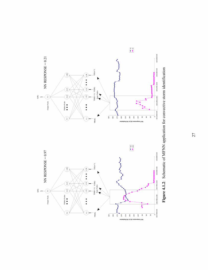
27

0306090120

150

180

210

240

270

300

330

10/1

7/98

6:0

010

/17/

98 1

2:00

10/1

7/98

18:

0010

/18/

98 0

:00

10/1

8/98

6:0

0

TIR Temperature (K) & VIS Radiation

TIR

VIS

0306090120

150

180

210

240

270

300

330

10/1

1/98

6:0

010

/11/

98 1

2:00

10/1

1/98

18:

0010

/12/

98 0

:00

10/1

2/98

6:0

0

TIR Temperature (K) & VIS Radiation

TIR

VIS

TIR

(K)

VIS

(K)

V

IS(k

+7

)T

IR(K

+11

)

1,1

1,13

2,1

2,1

2

3,1

Q(K

)

Out

put

No

de

Hid

den

No

des

Inpu

t N

ode

s2,1

32

,20

1,12

1,20

TIR

(K)

VIS

(K)

V

IS(k

+7

)T

IR(K

+11

)

1,1

1,1

3

2,1

2,1

2

3,1

Q(K

)

Out

put

No

de

Hid

den

No

de

Inpu

t N

ode

s2,1

32

,20

1,1

21

,20

NN

RE

SP

ON

SE

= 0

.97

NN

RE

SP

ON

SE

= 0

.21

Fig

ure

4.1

.2:

Sch

emat

ic o

f M

FN

N a

ppli

cati

on f

or

convec

tive

storm

iden

tifi

cati

on

28

4.1.1 The training and verification data sets

As mentioned in the previous section, the MFFNN is trained to recognize a set of

convective and non-convective IR patterns (training set). A key issue in this process is

identifying when to stop the training. If a neural network is under-trained, it will only be

able to identify the dominant features of the patterns, resulting in large errors. On the

other hand, if over-trained, the network essentially memorizes the specific patterns in the

training set, but cannot identify other similar signals. In view of this, the approach

adopted herein was to train the network on a first data set, and to determine when to stop

training based on its predictive performance over a second data set (verification data set).

Selecting the convective patterns for the training/verification sets

TRMM PR rain type data from the first ten days of each month of 1998 for a total of

1081 patterns were used to select the convective pattern candidates for the MFNN

training and verification sets. However, past work with TRMM data in the Lake Victoria

region suggested that the IR patterns associated with convective storms could be

clustered into three clearly distinct shapes (Figure 4.1.3):

Deep and steep convection

The IR traces belonging to this class (Figure 4.1.3 A) are characterized by a strong and

rapid IR dip (minimum IR below 230 K; dIR/dt of at least –26 K hr-1

). In Figure 4.1.3 A,

the solid purple line marks the borderline with shallow convection, while the green and

triangle line marks the borderline with deep, but slowly building, convection. This class

accounts for 70.2% of patterns and features an average rain rate of 27 mm hr-1

.

Shallow convection

The IR traces belonging to this class (Figure 4.1.3 B) are characterized by a shallow

convection (minimum IR above 230 K) and are frequently found over mountainous areas.

This category accounts for 14.2% of patterns and features an average rain rate of 17.4

mm hr-1

.

29

Dee

p a

nd s

teep

co

nvec

tion

18

0

20

0

22

0

24

0

26

0

28

0

30

0

-4-3

-2-1

01

23

4

Hours

fro

m T

RM

M p

assa

ge

IR (K)

68.5

20.8

33.7

12.3

A)

TR

MM

Pre

cip.

(mm

/h)

Shal

low

convec

tion

18

0

20

0

22

0

24

0

26

0

28

0

30

0

-4-3

-2-1

01

23

4

Ho

urs

fro

m T

RM

M p

assa

ge

IR (K)

2.1

14

15.1

15.4

B)

TR

MM

Pre

cip.

(mm

/h)

Dee

p,

but

slow

ly b

uil

din

g c

onvec

tion

18

0

20

0

22

0

24

0

26

0

28

0

30

0

-4-3

-2-1

01

23

4

Ho

urs

fro

m T

RM

M p

assa

ge

IR (K)

24

9.9

24

21.5

C)

TR

MM

Pre

cip.

(mm

/h)

No

t usa

ble

pat

tern

s

18

0

20

0

22

0

24

0

26

0

28

0

30

0

-4-3

-2-1

01

23

4

Ho

urs

fro

m T

RM

M p

assa

ge

IR (K)

8.4

6.6

9.9

9.4

D)

TR

MM

Pre

cip.

(mm

/h)

Fig

ure

4.1

.3:

Convec

tive

pat

tern

cla

ssif

icat

ion

30

Deep, but slowly building convection

These IR traces (Figure 4.1.3 C) display strong, but gradual, IR dips (minimum IR below

230 K; dIR/dt of less than –20 K hr-1

) and are frequently found over the lake surface.

This class accounts for 13.4% of all patterns and has an average PR surface rain of 22.8

mm hr-1

.

A small fraction of patterns (2.2%) does not fall in any of these three categories nor does

it show an alternative common behavior (Figure 4.1.3 D).

Mixing these distinct patterns in the same training/verification sets would have

diminished the sharpness of the ANN. Since the large majority of the convective patterns

fall in the first category that features the largest average rain rate, it was decided to train

the neural network to recognize only this type of convective patterns. Further, the

convective patterns were aligned around the time at which the IR dip reaches IR=240 K

to emphasize the common pattern (Figure 4.1.5).

Selecting the non-convective patterns for the training/verification sets

A set of patterns corresponding to non-convective patterns must be included in the

training set. These patterns (Figure 4.1.4) include clear sky (solid purple line) and

shallow convective patterns (green line with triangles). Since the purpose of the neural

network is to mark the onset of a convective storm, the set also incorporates IR traces

corresponding to the period antecedent to the storm (red line with x), its mature stage

(blue line with asterisks), and its dissipating phase (dashed dark blue line).

TRMM PR Rain Type maps from the first ten days of each month of 1998 were used to

(1) identify non-convective pixels that were at a distance of at least one or two pixels

from the nearest convective pixel, and (2) to determine the direction in which storms

were moving for selecting pixels at their antecedent, mature, and dissipating phases.

With these additions, the training and verification sets consisted of 379 convective and

379 non-convective patterns each, listed alternating elements of the two types to achieve

a balance between convective and non-convective patterns.

31

180

200

220

240

260

280

300

-4 -3 -2 -1 0 1 2 3 4

Hours from TRMM passage

IR (

K)

0

0

0

0

2.8

TRMM

Precip.

(mm/h)

Figure 4.1.4: IR traces for non convective patterns

4.1.2 Calibration and validation of artificial neural networks

The performance of the ANN architectures described in section 4.1.1 were evaluated

using the following indicators:

CnNnCnFAR

NcCcCcPOD

FARPODAWES

+=

+=

+−= 1

where

AWES = Area-Weighted classification Error Score (Todd et al., 1995);

POD = Probability of Detection;

FAR = False Alarm Rate;

Cc = number of convective patterns detected as convective by the MFFNN;

Cn = number of non-convective patterns detected as convective by the MFFNN;

Nc = number of convective patterns detected as non-convective by the MFFNN;

Nn = number of non-convective patterns detected as non-convective by the MFFNN.

The verification set was developed independently of the set used to calibrate the MFFNN,

but it also consisted of the same type of convective and non-convective patterns. This set

was also used to determine model biases and weights. Thus, to assess model

32

performance, it became necessary to use a third set of patterns completely independent

from the training and verification sets. The third set will be referred to as the validation

set and was developed from all IR patterns coincident with a TRMM PR convective pixel

during the last 20 days of each month of 1998. It also included all non-convective

patterns associated with non-convective TRMM PR pixels at a distance of three or more

pixels from any fully or partially convective pixel during the same period.

Verification POD was above 0.98 and FAR below 2% in all configurations, but shorter

input traces featured higher POD and AWES, probably because reduced input lengths are

less affected by the variability in storm duration and evolution. However, this trend

stopped or even reversed at the 5-value input configuration. The Verification FAR did

not seem to depend significantly on the length of the input. There was no apparent

relation between the number of ANN layers and nodes and its performance over the

verification set, other than the observation that the two layer MFFNNs with many nodes

in the first hidden layer performed somewhat worse than the rest of the ANNs.

Validation statistics were also impressive given that they were derived from a completely

independent set of data: POD is in the 78-81% range, a high value considering that the

validation set included also isolated fully convective pixels and percentages of “shallow

convection”, “deep, but slowly building convection”, and “Not usable” patterns likely

similar to the training/verification period. The validation FAR is in the 3-5% range, also

notably low. Similarly to verification, validation POD and FAR decreased with the

number of input values.

The best results were obtained with 6-value inputs (Figure 4.1.5) followed by 5-value

inputs. This is positive because a reduced input set is less computationally demanding

and less affected by missing values. It also reduces the delay in providing real-time

precipitation estimates. Among all ANN architectures with 6 input values, the best was

the one with two hidden layers of six nodes each. Its validation performance is as

follows:

33

PODvalid = 0.81; FARvalid = 0.04; AWESvalid = 0.23

6-value convective pattern

180

200

220

240

260

280

300

-4 -3 -2 -1 0 1 2 3 4

Hours from IR=240 K

IR (

K)

68.5

20.8

33.7

12.3

E)

TRMM

Precip.

(mm/h)

6-value non-convective pattern

180

200

220

240

260

280

300

-4 -3 -2 -1 0 1 2 3 4

Hours from TRMM passage

IR (

K)

0

0

0

0

2.8

F)

TRMM

Precip.

(mm/h)

Figure 4.1.5: Convective and non-convective traces used for training six-value neural

networks

4.2 Relation between IR, stage, and precipitation

The frequency of TRMM measurement of precipitation at any given location around the

equator varies between once a day for TMI to once every three to four days for PR.

Consequently, TRMM images provide a spatial distribution of precipitation, but cannot

directly provide its temporal distribution. On the other hand, when properly

34

synchronized, the geostationary IR signals in pixels belonging to the same storm show a

strong similarity (Figure 4.2.1). It can be argued that, at any given time, neighboring

pixels are experiencing different temporal phases of the same storm evolution.

Therefore, the TRMM snapshot of precipitation can be also viewed as an image of the

rain-rates associated with different temporal stages of the storm. A proper

synchronization of the TRMM samples according to the storm stage instead of the

measurement time allows for reconstructing the temporal distribution of precipitation for

the storm from the TRMM image (Figure 4.2.1).

A)

>=30 mm/h

25 mm/h

20 mm/h

15 mm/h

10 mm/h

5 mm/h

>0 m/h

>=30 mm/h

25 mm/h

20 mm/h

15 mm/h

10 mm/h

5 mm/h

>0 m/h

B)

TRMM passage 10/17/1998 09:03 Area: (0.025,31.675) - (-0.725,32.375)

150

175

200

225

250

275

300

-1 0 1 2 3 4Hours from the 240 K IR level

Met

eosa

t IR

(K) -

line

s

0

25

50

75

100

125

150TR

MM

Sur

face

Rai

n (m

m/h

) - m

arke

rs

35

Figure 4.2.1: A) TRMM PR spatial rain distribution; B) Temporal precipitation

distribution derived from synchronizing the corresponding IR patterns around the IR=240

K point

A good point for synchronizing the storm IR traces appears to be the time when IR

reaches 240 K during the IR dip, which is characteristic of the developing phase of the

convective cell (Figure 4.2.1). Since the traces used for training the neural network for

recognizing the onset of a convective storm were synchronized around this temperature,

the time when the neural network peaks can also be used as a synchronizing point. In this

case, the neural network not only identifies the presence of a convective storm over a

pixel, but also defines its stage evolution index by the number of half-hour timeslots from

the neural network peak.

It is assumed that the storm ceases to affect a pixel when the pixel IR temperature returns

to 253 K or higher. Further, the storm stage index varies from one (30 minutes before the

Neural Network indicates the convective event) to twenty (ten hours later). The

precipitation rate at the twentieth time slot after the neural network peak (NN+20) is used

for the rare cases when the storm lasts more than ten hours.

Figure 4.2.2 and Figure 4.2.3 show the average precipitation rate derived from 1998-1999

TRMM PR surface rain data as function of IR and storm stage respectively for Lake

Victoria pixels and land pixels between 2000m and 3000m elevation. The “All Pix”

curves include all available pixels without distinction of storm stage. The “Non-Cl”

curves represent the precipitation rate of pixels not identified by the neural network as

belonging to a convective storm.

Chart A shows that the convective storm classification captures the large majority of

intense-rain pixels since the “Non-Cl” precipitation is mostly lower than the average

precipitation. The second slot after the neural network peak corresponds to more or less

the middle of the IR decrease during the development phase and shows high precipitation

intensity over the entire IR range, with increased strength in the lower IR.

36

The following slots (Chart B) have precipitation curves of similar shape, but intensity

decreasing with the distance from the neural network peak. Remarkably, precipitation

intensity for the same IR varies considerably with stage number confirming the

assumption that precipitation rate depends on storm stage. Also, the shapes of the

precipitation curves vary considerably with orography. Rain intensity at low IR is higher

over the lake than over the land, while the reverse is true for IR above 230 K.

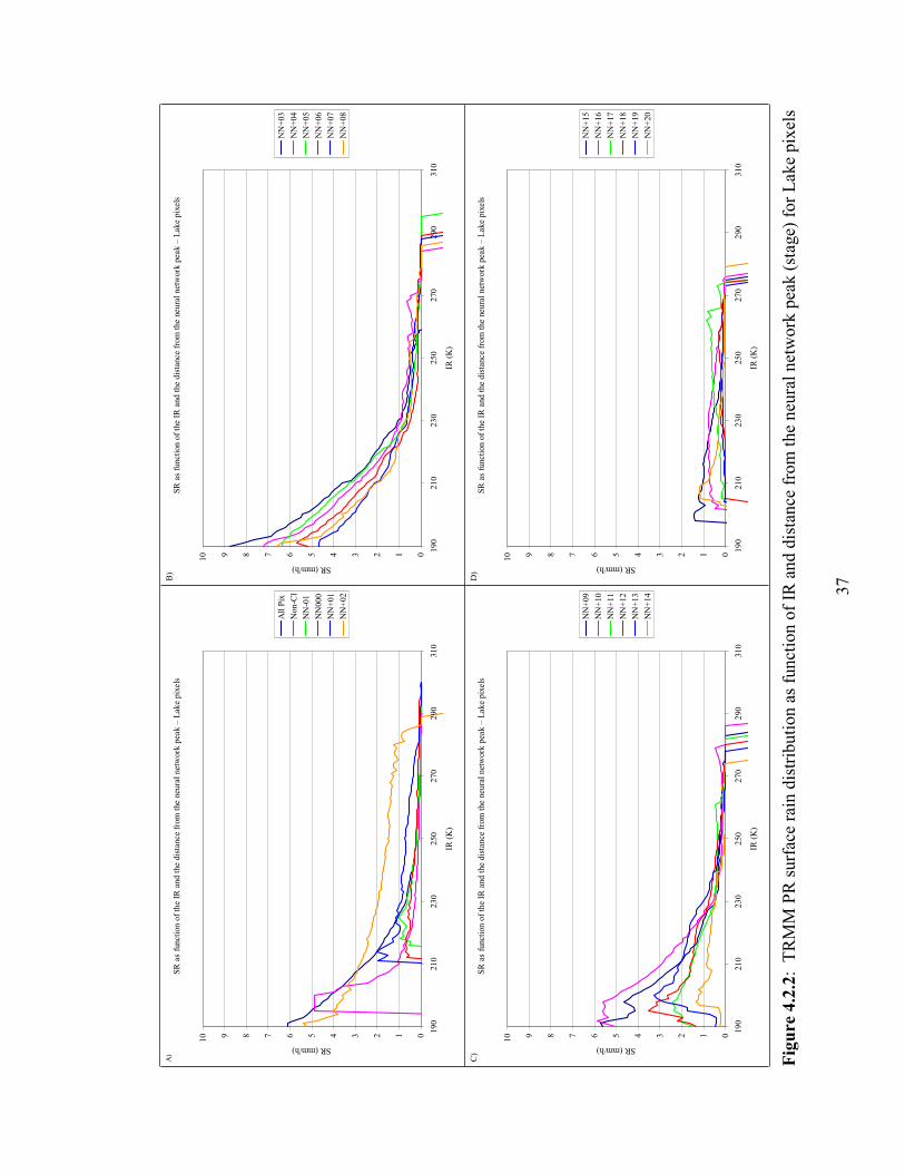
37

SR

as

funct

ion o

f th

e IR

and

the

dis

tance

fro

m t

he

neu

ral

net

work

pea

k –

Lak

e p

ixels

0123456789

10

19

021

02

30

250

270

290

31

0

IR (

K)

SR (mm/h)

All

Pix

No

n-C

l

NN

-01

NN

00

0

NN

+01

NN

+02

A)

SR

as

funct

ion o

f th

e IR

and

the

dis

tance

fro

m t

he

neu

ral

net

work

pea

k –

Lak

e p

ixels

0123456789

10

19

021

02

30

250

270

290

31

0

IR (

K)

SR (mm/h)

NN

+03

NN

+04

NN

+05

NN

+06

NN

+07

NN

+08

B)

SR

as

funct

ion o

f th

e IR

and

the

dis

tance

fro

m t

he

neu

ral

net

work

pea

k –

Lak

e p

ixels

0123456789

10

19

021

02

30

250

270

290

31

0

IR (

K)

SR (mm/h)

NN

+09

NN

+10

NN

+11

NN

+12

NN

+13

NN

+14

C)

SR

as

funct

ion o

f th

e IR

and

the

dis

tance

fro

m t

he

neu

ral

net

work

pea

k –

Lak

e p

ixels

0123456789

10

19

021

02

30

250

270

290

31

0

IR (

K)

SR (mm/h)

NN

+15

NN

+16

NN

+17

NN

+18

NN

+19

NN

+20

D)

Fig

ure

4.2

.2:

TR

MM

PR

surf

ace

rain

dis

trib

uti

on a

s fu

nct

ion o

f IR

and d

ista

nce

fro

m t

he

neu

ral

net

work

pea

k (

stag

e) f

or

Lak

e pix

els

38

SR

as

funct

ion o

f th

e IR

and t

he

dis

tance

from

the

neu

ral

net

work

pea

k –

Pix

els

20

00

-300

0m

0123456789

10

19

021

02

30

250

270

290

31

0

IR (

K)

SR (mm/h)

All

Pix

No

n-C

l

NN

-01

NN

00

0

NN

+01

NN

+02

A)

SR

as

funct

ion o

f th

e IR

and t

he

dis

tance

from

the

neu

ral

net

work

pea

k –

Pix

els

20

00

-300

0m

0123456789

10

19

021

02

30

250

270

290

31

0

IR (

K)

SR (mm/h)

NN

+03

NN

+04

NN

+05

NN

+06

NN

+07

NN

+08

B)

SR

as

funct

ion o

f th

e IR

and t

he

dis

tance

from

the

neu

ral

net

work

pea

k –

Pix

els

20

00

-300

0m

0123456789

10

19

021

02

30

250

270

290

31

0

IR (

K)

SR (mm/h)

NN

+09

NN

+10

NN

+11

NN

+12

NN

+13

NN

+14

C)

SR

as

funct

ion o

f th

e IR

and t

he

dis

tance

from

the

neu

ral

net

work

pea

k –

Pix

els

20

00

-300

0m

0123456789

10

19

021

02

30

250

270

290

31

0

IR (

K)

SR (mm/h)

NN

+15

NN

+16

NN

+17

NN

+18

NN

+19

NN

+20

D)

Fig

ure

4.2

.3:

TR

MM

PR

surf

ace

rain

dis

trib

uti

on a

s fu

nct

ion o

f IR

and d

ista

nce

fro

m n

eura

l n

etw

ork

pea

k f

or

2000-3

000 m

pix

els

39

5 Single Pixel Analysis

5.1 Characteristics of the single pixel estimation process

Precipitation estimation at the pixel level is obtained by integrating the identification and

temporal evolution of convective storms described in Chapter 4 with the estimation

structure described in Chapter 2. Some implementation details of the estimation process

are noted next:

Determination of the rain-rate distributions

The rain-rate distribution as function of IR, VIS/WV, storm stage, orography, and month

have been derived from 816 TRMM passages over the Lake Victoria area during 1998-

1999. This data base consists of more than 1.9 million points.

Number of traces in the precipitation ensemble

Increasing the size of the ensemble reduces the uncertainty in the ensemble statistics

introduced by the random selection of the half-hour precipitation rates composing the

ensemble. By contrast, increasing the size of the ensemble also linearly increases the

computation time. Table 5.1.1 shows that a minimum of 200 ensemble elements is

required for having stable simulation results.

Table 5.1.1: Variation of precipitation estimation statistics using the median of the

ensemble for different ensemble sizes

Entire

period

Daily Dekad Month

Ensemble

elements

Bias/

Gage

Corr MAE/

Gage

95%C Corr MAE/

Gage

95%C Corr MAE/

Gage

95%C

50 0.033 0.439 1.102 0.904 0.646 0.553 0.801 0.741 0.387 0.753

100 0.034 0.442 1.100 0.911 0.648 0.552 0.807 0.744 0.385 0.759

200 0.035 0.443 1.098 0.905 0.649 0.551 0.795 0.743 0.386 0.739

400 0.035 0.445 1.098 0.907 0.648 0.551 0.797 0.744 0.385 0.741

Orography

Figure 4.2.2 and Figure 4.2.3 show that there are deep differences in the precipitation

distribution over different geographical areas. Incorporating these differences in the

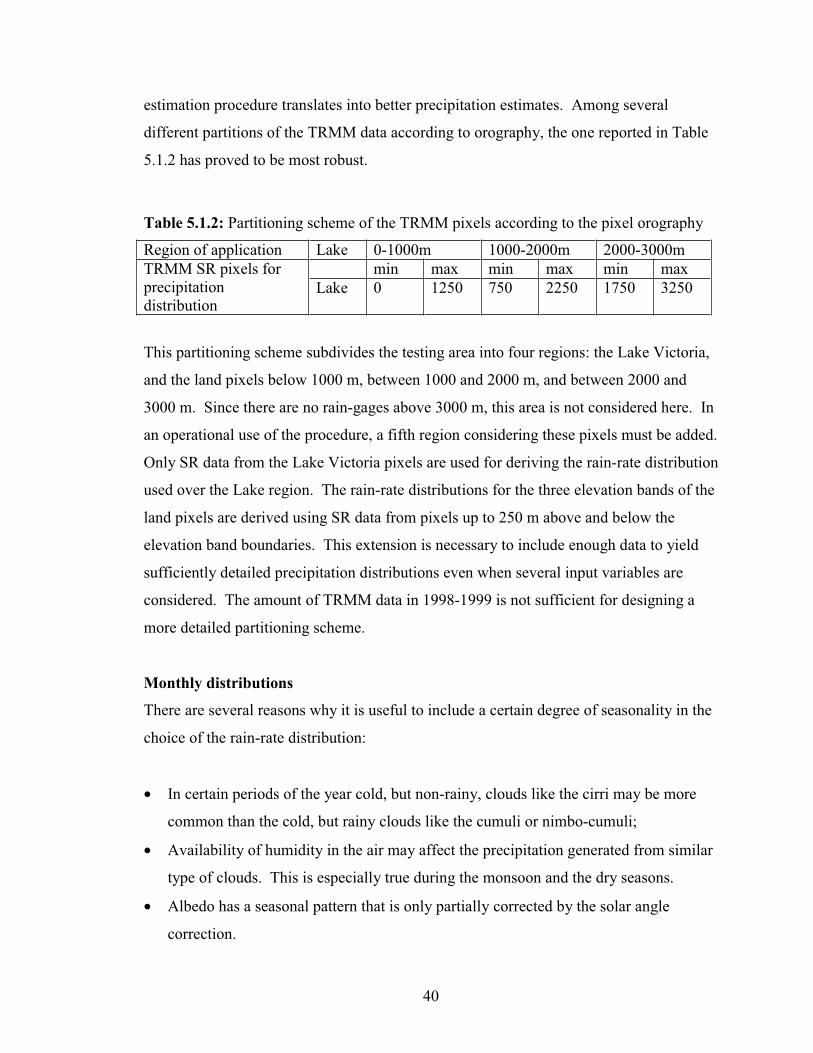
40

estimation procedure translates into better precipitation estimates. Among several

different partitions of the TRMM data according to orography, the one reported in Table

5.1.2 has proved to be most robust.

Table 5.1.2: Partitioning scheme of the TRMM pixels according to the pixel orography

Region of application Lake 0-1000m 1000-2000m 2000-3000m

min max min max min max TRMM SR pixels for

precipitation

distributionLake 0 1250 750 2250 1750 3250

This partitioning scheme subdivides the testing area into four regions: the Lake Victoria,

and the land pixels below 1000 m, between 1000 and 2000 m, and between 2000 and

3000 m. Since there are no rain-gages above 3000 m, this area is not considered here. In

an operational use of the procedure, a fifth region considering these pixels must be added.

Only SR data from the Lake Victoria pixels are used for deriving the rain-rate distribution

used over the Lake region. The rain-rate distributions for the three elevation bands of the

land pixels are derived using SR data from pixels up to 250 m above and below the

elevation band boundaries. This extension is necessary to include enough data to yield

sufficiently detailed precipitation distributions even when several input variables are

considered. The amount of TRMM data in 1998-1999 is not sufficient for designing a

more detailed partitioning scheme.

Monthly distributions

There are several reasons why it is useful to include a certain degree of seasonality in the

choice of the rain-rate distribution:

• In certain periods of the year cold, but non-rainy, clouds like the cirri may be more

common than the cold, but rainy clouds like the cumuli or nimbo-cumuli;

• Availability of humidity in the air may affect the precipitation generated from similar

type of clouds. This is especially true during the monsoon and the dry seasons.

• Albedo has a seasonal pattern that is only partially corrected by the solar angle

correction.

41

The approach taken in this research is to generate a different rain-rate distribution for

each month. However, given the limited amount of data available, using truly monthly

distribution causes a decrease in the detail of the relation between rain-rate and IR/VIS or

IR/WV, resulting in better statistics at the monthly level, but worse at the daily. As a

compromise, the “monthly” precipitation distributions are therefore generated using

TRMM data from the specific month and from the month before and after.

IR and VIS screening

Meteosat images are affected by thermal noise and sometimes from slight changes in the

satellite position and inclination that cause geometric error in the images. Further,

several Meteosat images were missing and were substituted with data obtained from

linearly interpolating the closer available images. TRMM PR surface rain data are also

affected by thermal noise and may be affected by spurious echoes, especially over

mountains. The resampling of the Meteosat and TRMM images to a regular grid

introduces a further source of error. Finally, and likely most importantly, TRMM and

Meteosat images are not always coincident, but may be spaced up to 15 minutes apart.

All these errors cause precipitation rates to be wrongly attributed to high IR and low VIS,

thus increasing the estimation bias and decreasing its correlation. To decrease the impact

of this phenomenon, precipitation rates corresponding to IR > 258K and VIS < 40% have

been screened out.

Statistics for evaluating the precipitation estimate ensemble approach

To assess the effectiveness of the proposed precipitation estimation approach, two aspects

must be considered at the same time:

• The ability of the ensemble average to track the behavior of the gage records;

• The capability of the ensemble to represent in a statistically meaningful way the

uncertainty of the precipitation patterns.

The first aspect is quantified by commonly used statistics:

42

Bias (Bias): For a single gage it is the difference over the simulation period between the

total gage precipitation and the average of the ensemble total precipitation. This value is

given as percentage of the total gage precipitation given the large variation in the

precipitation patterns around the basin. When applied to a group of gages, this statistic is

the average of the single rain-gage relative biases.

Absolute Bias (Abias): it is used only when considering a group of rain-gages. It is the

average of the absolute value of the single rain-gage relative biases. It gives a measure of

the spread of the biases.

Correlation (Corr): For a single gage it is the correlation coefficient between the

ensemble average and the corresponding rain-gage record over the same estimation

period (day, dekad, or month). When applied to a group of gages, this statistic is the

average of single rain-gage correlation.

Rank correlation (Rcorr): For a single gage it is the correlation coefficient between the

rank of the ensemble average and the rank of the corresponding rain gage record over the

same estimation period (day, dekad, or month). When applied to a group of gages, this

statistic is the average of single rain-gage rank correlation.

Mean Absolute Error (MAE): For a single gage it is the average of the absolute

difference between the gage record and the ensemble average over the same estimation

period (day, dekad, or month). This value is given as percentage of the average gage

precipitation. When applied to group of gages, this statistic is the average of the single

rain-gage MAE.

The capability of the ensemble to represent in a statistically meaningful way the

precipitation variability at the gage is quantified by the following statistics:

Average ensemble 95% width (95%R): For a single gage, it is the average of the

differences between the 2.5-percentile and the 97.5-percentile of the estimate ensemble.

When applied to a group of gages, it is the average of the single rain-gage 95% widths.

43

Ensemble 95% compliance (95%C): For a single gage, it is the frequency at which the

gage records fall between the 2.5-percentile and the 97.5-percentile of the ensemble.

When applied to a group of gages, it is the average of the single rain-gage 95%

compliances.

Lower end 95% error (95%L): For a single gage, it is the frequency at which the gage

records are less than the ensemble 2.5-percentile. When applied to a group of gages, it is

the average of the single rain-gage lower end 95% error.

KS-statistics (KS): For a single gage, it is the maximum of the absolute difference

between the distribution of the ensemble-percentiles corresponding to the gage readings

and the 0-1 uniform distribution. The rational behind this index is that the ensemble

represents the variability of precipitation in a statistically meaningful way if the gage

position with respect to the ensemble is uniformly distributed over the entire range.

When applied to a region, it is the average of the single rain-gage KS statistics.

90% KS acceptance (KS10). For a single gage, it is the difference between the gage KS

statistic and the threshold below which rejecting the hypothesis that the percentile

distribution is 0-1 uniform implies a 10% error probability. For groups of rain-gages, it is

the number of gages that have a KS statistic below the critical threshold.

99% KS acceptance (KS01). For a single gage, it is the difference between the gage KS

statistic and the threshold below which rejecting the hypothesis that the percentile

distribution is 0-1 uniform implies a 1% error probability. For groups of rain-gages, it is

the number of gages that have a KS statistic below the critical threshold.

44

5.2 Estimation model performance

5.2.1 Model calibration (1996-1998)

The calibration dataset is composed of 61 gages distributed over the elevation range 630-

2300 m and located mostly in the northern and western sides of the basin (Figure 3.3.1

A). Before the presentation of the results, it is noted that some parameters of the

estimation procedure described earlier (i.e., IR and VIS thresholds, number and limits of

the orographic bands, use of tri-monthly precipitation distribution, among others) were

selected to optimize the results over 1996-1998. In selecting these parameters, however,

care was exercised to ensure that this selection was not too specific to the calibration

dataset. For example, better results could have been obtained if the elevation bands used

for regionalizing the rain-rate distributions were 0-1100, 1100-2000, and 2000-3000

meters instead of the more regular 0-1000, 1000-2000, 2000-3000 m actually adopted.

Furthermore, slightly better results would have been obtained if VIS screening was

performed at 41% instead of 40%. However, such improvements would be minor and

would not add to the general applicability of the method.

Table 5.2.1 reports the performance of the single-pixel estimation procedure

(IVWU_NN) compared against the performance of the single-pixel adaptation of the GPI

technique. According to the later, the rain-rate equals 3 mm h-1

if IR is below 235 K, and

zero otherwise. Results show that the proposed model has a much better bias than the

GPI over the period 1996-1998 and also much better correlation, especially at the daily

level.

Table 5.2.1: IVWU_NN and GPI performance for the calibration period (1996-1998)

Day

Method Bias/

Gage

Abias

/Gage

Corr RCorr MAE/

Gage

95%R 95%C 95%L KS KS10 KS01

GPI 0.77 0.77 0.38 0.51 1.58

IVWU_NN 0.03 0.13 0.44 0.56 1.10 14.5 0.90 0.03 0.36 0 0

Dekad

Method Bias/

Gage

Abias

/Gage

Corr RCorr MAE/

Gage

95%R 95%C 95%L KS KS10 KS01

45

GPI 0.77 0.77 0.60 0.68 0.97

IVWU_NN 0.03 0.13 0.65 0.72 0.55 63.5 0.80 0.12 0.21 31 39

Month

Method Bias/

Gage

Abias

/Gage

Corr RCorr MAE/

Gage

95%R 95%C 95%L KS KS10 KS01

GPI 0.77 0.77 0.71 0.73 0.85

IVWU_NN 0.03 0.13 0.74 0.76 0.39 119.5 0.74 0.14 0.24 27 44

On the other hand, the 95% compliance rate could be acceptable at the monthly level, but

is low especially at the dekad and monthly level.

5.2.2 Model validation (1996-1997)

The validation dataset is composed of 42 gages that were not included in the calibration

dataset. These gages are distributed over the elevation range 816-2400 m and are located

mostly in the southern and eastern sides of the basin, with three gages situated on islands

(Figure 3.3.1 A and B).

Table 5.2.2 shows that the proposed model (IVWU_NN) has a bias slightly higher than

the bias of the calibration set, but is clearly lower than the GPI bias. The correlation is

also higher, reaching almost 0.80 at the monthly level, and continues to be better than

GPI’s correlation, especially at the dekad level. The 95% compliance rate is a little lower

than for the calibration case. Overall, the validation statistics are very similar to the

calibration statistics, supporting the hypothesis that the estimation procedure is generally

valid, independently of the calibration data set.

Table 5.2.2: IVWU_NN and GPI performance for the validation period (1996-1997)

Day

Method Bias/

Gage

Abias

/Gage

Corr RCorr MAE/

Gage

95%R 95%C 95%L KS KS10 KS01

GPI 0.87 0.89 0.41 0.50 1.69

IVWU_NN 0.06 0.17 0.46 0.54 1.14 12.8 0.91 0.03 0.43 0 0

Dekad

Method Bias/

Gage

Abias

/Gage

Corr RCorr MAE/

Gage

95%R 95%C 95%L KS KS10 KS01

GPI 0.87 0.89 0.63 0.72 1.10

46

IVWU_NN 0.06 0.17 0.70 0.76 0.59 58.5 0.77 0.14 0.25 19 26

Month

Method Bias/

Gage

Abias

/Gage

Corr RCorr MAE/

Gage

95%R 95%C 95%L KS KS10 KS01

GPI 0.87 0.89 0.75 0.77 0.98

IVWU_NN 0.06 0.17 0.79 0.81 0.42 110.3 0.69 0.20 0.26 20 33

5.2.3 Comparison with Adjusted GPI (TRMM product 3B42).

The GPI method uses a fixed IR threshold at 235 oK to separate rainy pixels from non-

rainy pixels and applies a fixed precipitation rate of 3 mm hr-1

. The Adjusted GPI

(TRMM product 3B42) also uses a fixed IR threshold of 235 oK to discriminate rainy

pixels from non-rainy ones, but the rain-rate is calibrated by month and by 1ºx1º region.

The optimal rain-rate is determined so that the method applied to coincident IR and

TRMM TMI images over each area reproduces the total observed monthly TMI

precipitation. In

Table 5.2.3 the Adjusted GPI has been derived by applying the appropriate adjusted rain-

rate and 235 K threshold to the single-pixel IR sequence. Unfortunately, this product is

available since January 1998 only.

Table 5.2.3: Partitioning scheme of the TRMM pixels according to the pixel orography

Day

Method Bias/

Gage

Abias

/Gage

Corr RCorr MAE/

Gage

95%R 95%C 95%L KS KS10 KS01

GPI 0.67 0.67 0.42 0.53 1.51

3B42 0.48 0.48 0.41 0.52 1.41

IVWU_NN 0.04 0.17 0.45 0.58 1.11 13.3 0.91 0.02 0.40 0 0

Dekad

Method Bias/

Gage

Bias/

Gage

Corr RCorr MAE/

Gage

95%R 95%C 95%L KS KS10 KS01

GPI 0.67 0.67 0.65 0.70 0.89

3B42 0.48 0.48 0.63 0.68 0.79

IVWU_NN 0.04 0.17 0.64 0.71 0.57 59.7 0.79 0.12 0.31 22 36

Month

Method Bias/ Bias/ Corr RCorr MAE/ 95%R 95%C 95%L KS KS10 KS01

47

Gage Gage Gage

GPI 0.67 0.67 0.75 0.75 0.77

3B42 0.48 0.48 0.72 0.70 0.64

IVWU_NN 0.04 0.17 0.74 0.73 0.41 112.5 0.72 0.15 0.28 35 44

The 1998 dataset is composed of 48 rain-gages with at least 10 months of valid

precipitation data. All gages belong also to the calibration data set.

The 3B42 product bias is substantially lower than the GPI bias, but is still much higher

than the IVWU_NN bias. In terms of correlation, IVWU_NN performs better than the

other two estimators at the daily level, but is slightly worse than the GPI at the dekad and

monthly level. However, it should be noted that monthly correlation with each gage is

here computed with only 10-12 samples.

The fact that the IVWU_NN performance over a fraction of the calibration period is very

similar to the performance over the entire calibration period indicates that the model

performs consistently.

5.2.4 Discussion

The correlation between IVWU_NN and rain gages at the daily level (0.45) seems low,

but the following factors should be considered:

1. The single station correlation varies between 0.29 and 0.61.

2. There is a relevant difference in the spatial scale of the gage (< 1 m2) and satellite

(>25 km2) measured precipitation. The shorter the temporal resolution of the

precipitation estimate, the higher is expected to be the impact of this difference. This

is especially true for the tropics, where precipitation is highly variable.

3. In several parts of the basin, geographical features (mountains, ridges, valleys, and

shorelines) strongly influence precipitation patterns even at the sub-pixel level;

4. Daily rain gage data were often of poor quality. It is very likely that quality control

has eliminated the most problematic gages, but it is also almost certain that errors still

affect several gages, limiting model performance.

48

Figure 5.2.1 may help to better appreciate the daily correlation between rain-gage and

satellite-based precipitation estimates. Gages 10046 and 1000419 are the only two

instances in the dataset for which the closest neighboring gage is located within the same

pixel. The correlations of these two stations with IVWU_NN are 0.54 and 0.51

respectively, while the correlations of the gages with their closest neighbor are 0.64 and

0.77 respectively.

Overall, IVWU_NN average estimation tracks gage data better than GPI and 3B42, both

in terms of bias and in terms of correlation. The performance of the average estimation

show good consistency over the entire calibration set (1996-1998), a subset of it (1998),

and the validation set (1996-1997), indicating that the method is sufficiently robust. This

is especially notable considering that (1) no TRMM data is available for 1996-1997, (2)

the visible data where derived according to two different methodologies in 1996-1997

and 1998-1999 (Eumetsat, 2004; Rigolier et al., 2002), and (3) Meteosat changed satellite

platform in 1996 and 1998. Further, there is a good potential for improving the estimator

performance using more TRMM data.

0

0.1

0.2

0.3

0.4

0.5

0.6

0.7

0.8

0.9

1

0 10 20 30 40 50 60 70 80 90Distance (km)

Cor

rela

tion

100461000419

Figure 5.2.1: Rain-gage daily precipitation correlation of as function of gage distance

(correlation IVWU_NN-10046 =0.54, IVWU_NN-1000419=0.51)

49

By contrast, the representation of precipitation variability is not satisfying. The 95%

compliance rate can be considered acceptable at the daily level (91%), but not at the

dekad (79%) and monthly resolutions (72%).

After extensive investigation, the reason that the model is able to track the precipitation

average well, but it is not able to account for the full extent of precipitation variability

was attributed to the fact that precipitation rates at consecutive timeslots are chosen

independently, ignoring the temporal autocorrelation that may be present. TRMM

images do not directly provide a measure of the precipitation temporal autocorrelation.

Thus, to test this hypothesis, the precipitation temporal autocorrelation was derived from

the spatial TRMM images considering the precipitation correlation in adjacent pixels at

stage t and t-1 as determined by the neural network (Figure 5.2.2).

0

0.1

0.2

0.3

0.4

0.5

0.6

0.7

0.8

0.9

1

0 2 4 6 8 10 12 14 16 18 20Stage

Cor

rela

tion All Pix

StratiformConvectiveEnsemble

Figure 5.2.2: Lag 1 stage autocorrelation of 1998-1999 TRMM-SR data in the Lake

Victoria basin and in the IVWU_NN model.

The precipitation temporal autocorrelation is very significant especially at the later

stages, where stratiform or mixed precipitation is dominant. It is also much stronger than

50

the autocorrelation in the precipitation produced by the IVWU_NN model (the

“Ensemble” series of Figure 5.2.2).

5.3 Estimation incorporating precipitation autocorrelation

The one-step autocorrelation of single-pixel precipitation is implemented by conditioning

the rain-rate distribution on precipitation at time t-1 in addition to IR, VIS/WV, stage,

orography, and month. That is, for each member X of the ensemble:

precipprecip(t)

f[IR(t), VIS(t)/WV(t), stage(t), (t - 1), orography, month, ] stage(t) 0

f[IR(t), VIS(t)/WV(t), stage(t), orography, month, ] stage(t) 0

ε ≥⎧⎪= ⎨

ε <⎪⎩

where

precip(t): precipitation rate at time t for element X;

precip(t-1): precipitation rate at time t-1 for element X;

IR(t): IR at time t;

VIS(t): VIS at time t;

WV(t): WV at time t;

ε: random error;

The derivation of the temporal precipitation relation from TRMM data is possible only

for the timeslots belonging to a convective storm. The precipitation over pixels not

belonging to a convective storm event (identified by the ANN) is presumed to be

temporally uncorrelated.

The rational of this approach is that the new input variable (precip(t-1)) restricts the pool

of available precipitation rates that can be used to build the rain-rate distributions for time

t, thus establishing a relation between precipitation at time t and at time t-1. At the same

time, an entire set of possible precipitation rates is associated with precip(t-1), thus

51

directly accounting for the random component of this relation. An important aspect of

this approach is that it is not based on any hypothesis on the probabilistic distribution of

the instantaneous rain-rates, something that is very suitable to the markedly skewed

distribution of TRMM SR data.

Adding precip(t-1) to the input variable set further fragments the data available for

building the rain-rate distributions and prevents the use of VIS(t)/WV(t) and month

information during convective storms . Consequently, the precipitation at time t is

determined according to the following formula:

precipprecip(t)

f[IR(t), stage(t), (t - 1), orography, ] stage(t) 0

f[IR(t), VIS(t)/WV(t), stage(t), orography, month, ] stage(t) 0

ε ≥⎧⎪= ⎨

ε <⎪⎩

The average of the precipitation distributions used to determine precip(t) (Figure 5.3.1

and Figure 5.3.2) behaves as expected: the average rate increases with decreasing IR and

with increasing precip(t-1). Further, the average rain rate peaks between stages 3 and 7.

The segmentation of the IR(t)/precip(t-1) space looks very rough for stage(t)=0, but this

is actually due to the fact that most of the precip(t-1) data in this case is zero. The

following stages are characterized by a larger variety of precip(t-1), so that the resulting

rain-rate map is more finely detailed.

Figure 5.3.2 shows the effect that the subdivision of TRMM PR data according to the

orography may have on the average rain-rate mapping and, consequently, on the rain-rate

distributions: the lake pixels are barely enough to guarantee an acceptably detailed

mapping of the precipitation. For example, precipitation maps for stage 0 to stage 1 and

precip(t-1)>0 are insensitive to IR. The future availability of more TRMM PR under this

project would enable a more accurate estimation of these relationships.

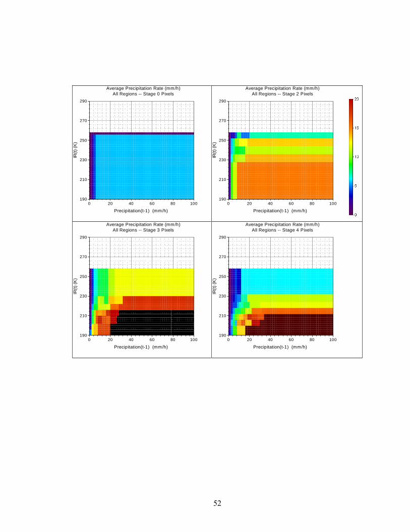
52

0 20 40 60 80 100190

210

230

250

270

290

Precipitation(t-1) (mm/h)

IR(t)

(K)

Average Precipitation Rate (mm/h)All Regions -- Stage 0 Pixels

0 20 40 60 80 100190

210

230

250

270

290

Precipitation(t-1) (mm/h) IR

(t) (K

)


0 20 40 60 80 100190

210

230

250

270

290


IR(t)

(K)


0 20 40 60 80 100190

210

230

250

270

290


IR(t)

(K)


53

0 20 40 60 80 100190

210

230

250

270

290


IR(t)

(K)

Average Precipitation Rate (mm/h)All Regions -- Stage 5, 6, 7 Pixels

0 20 40 60 80 100190

210

230

250

270

290


IR(t)

(K)

Average Precipitation Rate (mm/h)All Regions -- Stage 8, 9, 10 Pixels

Figure 5.3.1: Average precipitation rate as function of IR and precip(t-1) for all regions

and at least 75 TRMM data per bin

0 20 40 60 80 100190

210

230

250

270

290


IR(t)

(K)

Average Precipitation Rate (mm/h)Lake -- Stage 0 Pixels

0 20 40 60 80 100190

210

230

250

270

290


IR(t)

(K)


0 20 40 60 80 100190

210

230

250

270

290


IR(t)

(K)


0 20 40 60 80 100190

210

230

250

270

290


IR(t)

(K)


54

0 20 40 60 80 100190

210

230

250

270

290


IR(t)

(K)

Average Precipitation Rate (mm/h)Lake -- Stage 5, 6, 7 Pixels

0 20 40 60 80 100190

210

230

250

270

290


IR(t)

(K)

Average Precipitation Rate (mm/h)Lake -- Stage 8, 9, 10 Pixels

Figure 5.3.2: Average precipitation rate as function of IR and precip(t-1) for lake pixels

and at least 75 TRMM data per bin

5.3.1 Autocorrelated model calibration (1996-1998)

Table 5.3.1 reveals that the autocorrelated estimator (IVWA_NN) has a bias similar in

magnitude to that of the uncorrelated estimator (IVWU_NN), but a slightly lower

absolute bias. On the other hand, its correlation with rain-gage data is lower than that of

the IVWU_NN, especially at the monthly level. This is the effect of not including

VIS/WV and month in the variable used to identify the precipitation distribution to be

used during storm events.

Table 5.3.1: IVWU_NN and IVWA_NN performance for the calibration period (1996-

1998)

Day

Method Bias/

Gage

Abias

/Gage

Corr RCorr MAE/

Gage

95%R 95%C 95%L KS KS10 KS01

IVWU_NN 0.03 0.13 0.44 0.56 1.10 14.5 0.90 0.03 0.36 0 0

IVWA_NN -0.02 0.12 0.43 0.55 1.09 20.4 0.94 0.00 0.37 0 0

Dekad

Method Bias/

Gage

Abias

/Gage

Corr RCorr MAE/

Gage

95%R 95%C 95%L KS KS10 KS01

IVWU_NN 0.03 0.13 0.65 0.72 0.55 63.5 0.80 0.12 0.21 31 39

IVWA_NN -0.02 0.12 0.63 0.71 0.56 91.5 0.92 0.04 0.18 33 45

Month

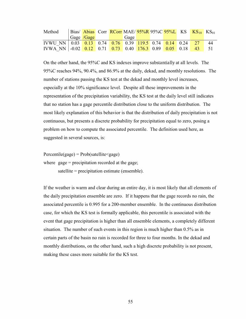
55

Method Bias/

Gage

Abias

/Gage

Corr RCorr MAE/

Gage

95%R 95%C 95%L KS KS10 KS01

IVWU_NN 0.03 0.13 0.74 0.76 0.39 119.5 0.74 0.14 0.24 27 44

IVWA_NN -0.02 0.12 0.71 0.73 0.40 176.3 0.89 0.05 0.18 43 51

On the other hand, the 95%C and KS indexes improve substantially at all levels. The

95%C reaches 94%, 90.4%, and 86.9% at the daily, dekad, and monthly resolutions. The

number of stations passing the KS test at the dekad and monthly level increases,

especially at the 10% significance level. Despite all these improvements in the

representation of the precipitation variability, the KS test at the daily level still indicates

that no station has a gage percentile distribution close to the uniform distribution. The

most likely explanation of this behavior is that the distribution of daily precipitation is not

continuous, but presents a discrete probability for precipitation equal to zero, posing a

problem on how to compute the associated percentile. The definition used here, as

suggested in several sources, is:

Percentile(gage) = Prob(satellite<gage)

where gage = precipitation recorded at the gage;

satellite = precipitation estimate (ensemble).

If the weather is warm and clear during an entire day, it is most likely that all elements of

the daily precipitation ensemble are zero. If it happens that the gage records no rain, the

associated percentile is 0.995 for a 200-member ensemble. In the continuous distribution

case, for which the KS test is formally applicable, this percentile is associated with the

event that gage precipitation is higher than all ensemble elements, a completely different

situation. The number of such events in this region is much higher than 0.5% as in

certain parts of the basin no rain is recorded for three to four months. In the dekad and

monthly distributions, on the other hand, such a high discrete probability is not present,

making these cases more suitable for the KS test.

56

Given that the uncorrelated dekad and monthly performances improved when “monthly”

precipitation distributions were used, there is a good chance that these performances will

further improve when additional TRMM PR data are used.

Figure 5.3.3 shows that adding precip(t-1) to the criteria used for selecting precip(t)

successfully increases the autocorrelation of the ensemble sequences to a level closer to

that determined from the TRMM images.

0

0.1

0.2

0.3

0.4

0.5

0.6

0.7

0.8

0.9

1

0 2 4 6 8 10 12 14 16 18 20Convective storm stage

Cor

rela

tion

All PixelIVWU_NNIVWA_NN

Figure 5.3.3: One-step autocorrelation of convective storm precipitation determined

directly from the TRMM data (All Pixel) and as reproduced by the IVWU_NN and

IVWA_NN models.

5.3.2 Autocorrelated model validation (1996-1997)

The IVWA_NN model performance for the validation data set is similar to that for the

calibration set. As with IVWU_NN, the bias is slightly higher, most likely because the

southern part of the basin, which was practically absent from the calibration set, is less

rainy. IVWA_NN correlation is also higher than in the calibration dataset, similar to

IVWU_NN. The 95% compliance rate is a couple of points lower than in calibration,

probably because of the bias increase.

57

Overall, the absolute model performance is very similar to that of the calibration set and

the relative differences with IVWU_NN are also exhibited.

Table 5.3.2: IVWU_NN and IVWA_NN performance for the validation period (1996-

1997)

Day

Method Bias/

Gage

Abias

/Gage

Corr RCorr MAE/

Gage

95%R 95%C 95%L KS KS10 KS01

IVWU_NN 0.06 0.17 0.46 0.54 1.14 12.8 0.91 0.03 0.43 0 0

IVWA_NN 0.03 0.16 0.44 0.53 1.14 18.6 0.95 0.00 0.42 0 0

Dekad

Method Bias/

Gage

Abias

/Gage

Corr RCorr MAE/

Gage

95%R 95%C 95%L KS KS10 KS01

IVWU_NN 0.06 0.17 0.70 0.76 0.59 58.5 0.77 0.14 0.25 19 26

IVWA_NN 0.03 0.16 0.66 0.75 0.60 87.7 0.89 0.05 0.23 21 29

Month

Method Bias/

Gage

Abias

/Gage

Corr RCorr MAE/

Gage

95%R 95%C 95%L KS KS10 KS01

IVWU_NN 0.06 0.17 0.79 0.81 0.42 110.3 0.69 0.20 0.26 20 33

IVWA_NN 0.03 0.16 0.76 0.79 0.44 166.6 0.87 0.07 0.19 33 39

5.3.3 Discussion

The previous sections showed that IVWA_NN has a very small average bias both with

respect to the calibration and verification data sets. To fully understand the model

capability, however, it is necessary to observe the distribution of model performance

across the gage stations. Thus, the IVWA_NN performance for the entire 1996-1997

dataset is now considered, using all 98 gages to better represent the precipitation

distribution over the region. Figure 5.3.4 A shows that the absolute value of the relative

bias is above 50% for only 1% of all stations and below 20% for 77% of gages. Figure

5.3.4 B shows that the monthly correlation is below 0.5 in only 3% of cases and above

0.7 in 68% of cases. Figure 5.3.4 C shows that the monthly 95% compliance rate is

below 0.8 in only 18% of the stations. Further, assuming that the three gages with the

lowest compliance rate are outliers, the average compliance rate increases to 89%.

58

Figure 5.3.5 sorts the gages West to East and South to North, so that it is very likely that

adjacent gages are relatively close. Figure 5.3.5 A shows that there is not a clear relation

between bias and elevation. By contrast, monthly correlation reveals two areas in the

western mountains where correlations are distinctly lower. This, however, does not seem

to be a direct consequence of elevation, since there are gages at high elevation where

correlation is good, but most likely a consequence of a complex orography.

A)-0.6

-0.4

-0.2

0

0.2

0.4

0.6

1 6 11 16 21 26 31 36 41 46 51 56 61 66 71 76 81 86 91 96Bias

(%)

B)

0

0.1

0.2

0.3

0.4

0.5

0.6

0.7

0.8

0.9

1

1 6 11 16 21 26 31 36 41 46 51 56 61 66 71 76 81 86 91 96

Mon

thly

Corre

latio

n

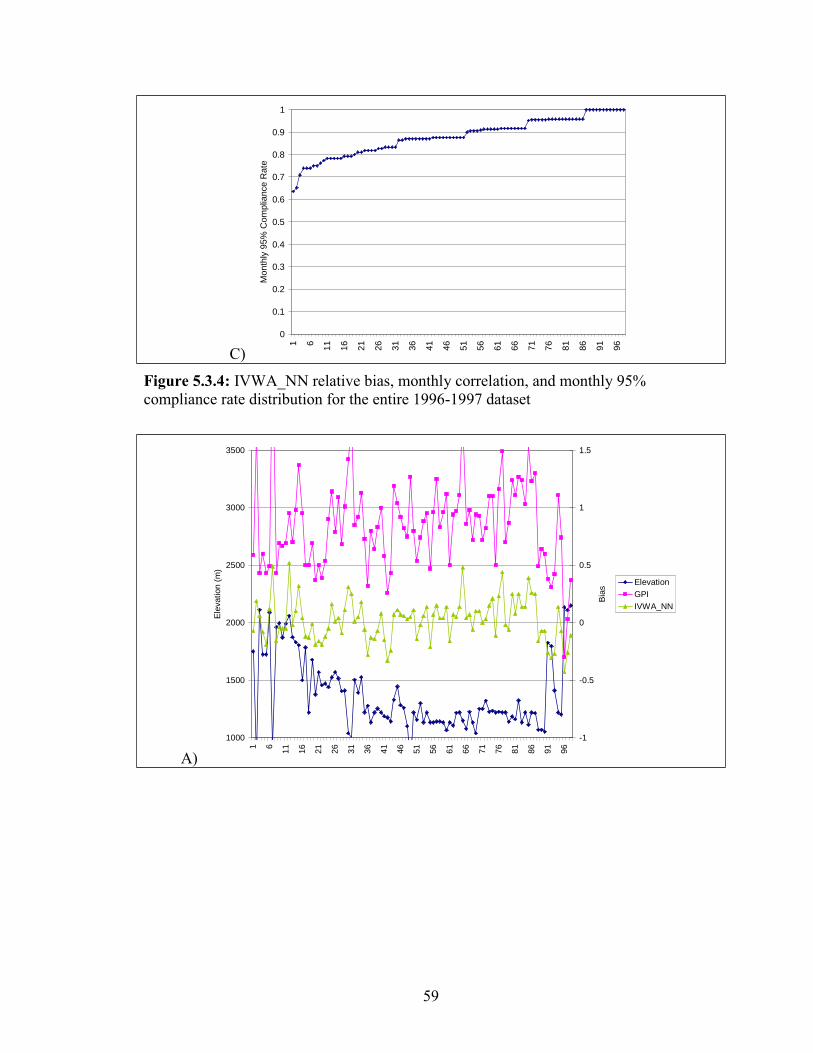
59

C)

0

0.1

0.2

0.3

0.4

0.5

0.6

0.7

0.8

0.9

1

1 6 11 16 21 26 31 36 41 46 51 56 61 66 71 76 81 86 91 96

Mon

thly

95%

Com

plia

nce

Rate

Figure 5.3.4: IVWA_NN relative bias, monthly correlation, and monthly 95%

compliance rate distribution for the entire 1996-1997 dataset

A)

1000

1500

2000

2500

3000

3500

1 6 11 16 21 26 31 36 41 46 51 56 61 66 71 76 81 86 91 96

Elev

atio

n (m

)

-1

-0.5

0

0.5

1

1.5

Bias

ElevationGPIIVWA_NN

60

B)

1000

1500

2000

2500

3000

3500

1 6 11 16 21 26 31 36 41 46 51 56 61 66 71 76 81 86 91 96

Elev

atio

n (m

)

0.4

0.5

0.6

0.7

0.8

0.9

Mon

thly

Cor

rela

tion

ElevationGPIIVWA_NN

Figure 5.3.5: Relative bias and monthly correlation of the GPI and IVWA_NN models as

function of the gage elevation for the entire 1996-1997 dataset

Figure 5.3.6 A shows that four of the gages for which IVWA_NN overestimates

precipitation are situated in the Rift Valley, a deep and dry valley surrounded by very

high mountains in the western side of the region.

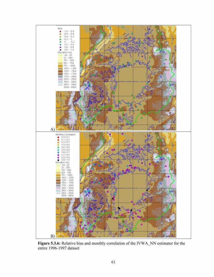
61

A)

B)

Figure 5.3.6: Relative bias and monthly correlation of the IVWA_NN estimator for the

entire 1996-1997 dataset

62

Two other gages where IVWA_NN overestimates precipitation are located in the very

orographically complex region of Mbarara in the western side of the basin. IVWA_NN

seems also to overestimate precipitation in some areas shortly inland of the Lake Victoria

shoreline. A possible explanation of this phenomenon, is that clouds carried by the lake

breeze lose most of their humidity when they come over the shore because of

convergence and are relatively dry when they move inland. IVWA_NN somewhat

underestimates precipitation on the eastern mountains, probably due to a higher

contribution of shallow precipitation of orographic origin in this area.

Figure 5.3.6 B shows that the gages with poor correlation are concentrated around some

orographically complex regions in the western side of the basin and on a location along

the western shore of Lake Victoria. These observations, however, have to be re-

evaluated after eliminating the possibility of questionable rain gage data quality.

63

6 Multi-pixel Analysis

Most hydrological applications of remotely sensed precipitation interest areas larger than

a single 5x5 km pixel requiring the aggregation of the precipitation over several pixels.

As shown in Figure 6.1, instantaneous precipitation is strongly spatially correlated.

Ignoring this correlation when randomly selecting the rain-rates for the single pixels

would still probably yield good estimates of mean areal precipitation over a larger area,

but it would underestimate its variability much like the effect of temporal autocorrelation.

Therefore, the correct characterization of the statistical properties of precipitation for

multiple pixels requires generating a random precipitation field at each time step and for

each member of the ensemble. The precipitation random field must be generated

consistently with the spatial correlation structure derived from the TRMM images (Figure

6.1) and the single pixel probability densities associated with the observed IR, VIS/WV,

and stage conditions. One possible approach that this may be accomplished in the

Turning Bands Method of Mantoglou and Wilson, 1982. The multi-pixel analysis will be

addressed in the next phase of this work.

TRMM Precipitation Correlation as Function of Distance and Stage

0

0.1

0.2

0.3

0.4

0.5

0.6

0.7

0.8

0.9

1

All

Not-Clas

s -1 0 1 2 3 4 5 6 7 8 9 10 11 12 13 14 15 16 17 18 19 20

Stage

Cor

rela

tion

Coe

ffici

ent S-1

S-2S-3S-4S-5S-6S-7S-8S-9S-10

Figure 6.1: Precipitation spatial correlation in the Lake Victoria region as function of the

storm stage and distance in pixels (s-1, s-2, etc.)

64

7 Conclusions

A precipitation estimation methodology using TRMM PR and geostationary satellite

images has been developed. The methodology exploits infrared and visible images,

geography, and seasonality, and uses a neural network for identifying major storms at the

pixel level and for reconstructing their temporal evolution. In addition, the methodology

provides a full characterization of estimation uncertainty.

The methodology has been tested at the pixel level over a three-year period on a complex

environment showing better average performances than GPI and 3B42. Further,

estimation variability is consistent with gage precipitation variability.

The procedure is robust and performs consistently also for years for which TRMM data

are not available. The method is constrained by the limited number of data (two years)

used for building the relation between IR/VIS/WV and precipitation. It is expected that

model performance will improve if more TRMM data become available.

A strategy for estimating precipitation over larger areas in a statistically consistent way

has been devised and is currently being implemented.

65

Acknowledgements

The research described herein has been funded by several sources including the Food and

Agriculture Organization of the United Nations (FAO/UN) under the Nile Decision

Support Program, the United States Geological Survey under the State Water Resources

Program, and NASA (Goddard Space Flight Center, GSFC) under Project NRA-02-ES-

05 entitled “The Impact of Precipitation Measurement Missions on Hydrologic and Water

Resource Predictions.” The last project is a collaborative effort between NASA’s GSFC

(with lead PIs Dr. C. Peters-Liddard and Dr. J.M. Sheppard) and the Georgia Water

Resources Institute (GWRI) at Georgia Tech (with lead PI Dr. A. Georgakakos). The

authors are very grateful to the above-mentioned sponsoring agencies and collaborators.

66

References

Arkin , P.A. and P. Xie (1994). The global precipitation climatology project: First

Algorithm Intercomparison Project. Bull. Amer. Meteor. Soc. 75: 401-419.

Arkin, P.A. and B.N. Meisner (1987). The relationship between large-scale convective

rainfall and cold cloud over the western hemisphere during 1982-84. Mon. Wea. Rev. 115: 51-74

Adler, R.F., J.A. Negri, P.R. Keehn, and I.M. Hakkarinen (1993). Estimation of monthly

rainfall over Japan and surrounding waters from a combination of low-orbit

microwave and geosynchronous IR data. J. Appl. Meteor. 32: 335-356.

ASCE Task Committee on Application of Artificial Neural Networks in Hydrology

(2000a). Artificial neural networks in hydrology. I: preliminary concepts.

Journal Of Hydrologic Engineering, 5(2), 115-123.

ASCE Task Committee on Application of Artificial Neural Networks in Hydrology

(2000b). Artificial neural networks in hydrology. II: hydrologic applications.

Journal Of Hydrologic Engineering, 5(2), 124-137.

Bell, T.L. (1987). A space-time stochastic model of rainfall for satellite remote-sensing

studies. J. Geophys. Res. 92(D8), 9631-9643.

Bellerby, T., M. Todd, D. Kniveton, and C. Kidd (2000). Rainfall estimation from a

combination of TRMM Precipitation Radar and GOES multispectral satellite

imagery trough the use of an Artificial Neural Network. J. Appl. Meteor. 39: 2115

– 2128.

De Angelis, C.F., G.R. McGregor, and C. Kidd (2004). A 3 year climatology of rainfall

characteristics over tropical and subtropical South America based on Tropical

Rainfall Measurement Mission precipitation radar data. Int. J. of Climatology24(3): 385-399.

Ebert, E.E., M.J. Manton, P.A. Arkin, R.J. Allam, G.E. Holpin, and A. Gruber. Results

from the GPCP Algorithm Intercomparison Programme. Bull. Am. Met. Soc. 77(12): 2875-2887.

Eumetsat (2004). Meteosat VIS channel calibration information.

http://www.eumetsat.de/en/dps/mpef/calibration/vis_calibration.html accessed on

5/12/2004.

Eumetsat (2000). The Meteosat System, Revision 4. Eumetsat Technical Report EUM TD

05, pp. 66. Darmstadt, Germany.

Fiorucci, P., P. LA Barbera, L.G. Lanza, and R. Minciardi (2001). A geostatistical

approach to multisensor rain field reconstruction and downscaling. Hydrol. Earth Sys. Sci. 5(2): 201-213.

Georgakakos, A.P., (2004). Decision Support Systems for integrated water resources

management with an application to the Nile Basin. Key note Address, Proceedings, International Federation for Automatic Control Workshop on

Modeling and Control for Participatory Planning and Managing Water Systems,

Venice, Italy, Sep. 29 – Oct. 1.

Georgakakos, A.P., H. Yao, K. Brumbellow, C. De Marchi, S. Bourne, and M. Mullusky

(2000). Lake Victoria Decision Support System. Technical Report GWRI-2000-

1. Georgia Water Resources Institute, Atlanta, GA.

67

Georgakakos, A.P (1989). The value of streamflow forecasting in reservoir operation.

Water Resour. Bull. 25(4): 789-800.

Georgakakos, K.P., D. Tsintikidis, B. Attia, and J. Roskar (2001). Estimation of pixel-

scale daily rainfall over the Nile River catchments using multi-spectral

METEOSAT data. In Remote Sensing and Hydrology 2000. IAHS Publ. No 267,

Wallingford, U.K.

Grecu, M. and E.N. Anagnostou (2001). Overland precipitation estimation from TRMM

passive microwave observations. J. Appl. Meteor. 40(8): 1367-1380.

Hirose, M. and K. Nakamura (2004). Spatiotemporal variation of the vertical gradient of

rainfall rate observed by the TRMM precipitation radar. J. Clim. 17(17): 3378-

3397.

Huffman, G.J., R.F. Adler, E.F. Stocker, D.T. Bolvin, and E.J. Nelkin (2003). Analysis of

TRMM 3-hourly multi-satellite precipitation estimates computed in both real and

post-real time. In Proc. 12th Conf. Satellites, Meteorology and Oceanography,

Long Beach, CA, Feb. 9-13, 2003.

Hsu, K., X. Gao, S. Sorooshian, and H.V. Gupta (1997). Precipitation estimation from

remotely sensed information using artificial neural networks, J. Appl. Meteor. 36,:

1176-1190.

Hsu, K., H.V. Gupta, X. Gao, and S. Sorooshian (1999). Estimation of physical variables

from multi-channel remotely sensed imagery using a neural network: application

to rainfall estimation. Water Resources Research 35(5): 1605-1618.

King, P.W.S., W.D. Hogg, and P.A. Arkin (1995). The role of visible data in improving

satellite rain-rate estimates. J. Appl. Meteor. 34: 1608-1621.

Kummerow, C., J. Simpson, O. Thiele, W. Barnes, A.T.C. Chang, E. Stocker, R.F. Adler,

A. Hou, R. Kakar, F. Wentz, P. Ashcroft, T. Kozu, Y. Hong, K. Okamoto, T.

Iguchi, H. Kuroiwa, E. Im, Z. Haddad, G. Huffman, B. Ferrier, W.S. Holson, E.

Zipser, E.A. Smith, T.T. Wilheit, G. North, T. Krishnamurti, and K. Nakamura

(2000). The status of the Tropical Rainfall Measuring Mission (TRMM) after two

years in orbit. J. Appl. Meteor. 39: 1965-192.

Kummerow, C., W. Barnes, T. Kozu, J. Shiue, and J. Simpson (1998). The Tropical

Rainfall Measuring Mission (TRMM) sensor package. J. Atmos. Oceanic Technol. 15: 809-817.

Kurino, T. (1997) A satellite infrared technique for estimating “deep/shallow”

precipitation. Adv. Space Res. 19(3): 511-514.

Li, Q., R. L. Bras, and D. Veneziano (1996). Analysis of Darwin rainfall data:

Implications on sampling strategies. J. Appl. Meteor. 35: 372-385.

Mantoglou, A., and J.L. Wilson (1982). The turning bands method for simulation of

random fields using line generation by a spectral method. Water Resour. Res. 18(5): 1379-1394.

Morrissey, M.L. and J.E. Janowiak (1996). Sampling-induced conditional biases in

satellite climate-scale rainfall estimates. J. Appl. Meteor. 35: 541 – 548.

Negri, A.J. and R.F. Adler (2002). A TRMM-calibrated rainfall algorithm applied over

Brazil. J. Geophys. Res. 107(D20), 8048-8062.

Negri, A.J. and R.F. Adler (1988). A satellite infrared technique to estimate tropical

convective and stratiform rainfall. J.Climate Appl. Meteor. 27: 30-51.

68

Richards, F. and P. Arkin (1981). On the relationship between satellite-observed cloud

cover and precipitation. Mon. Wea. Rev. 109: 1080-1093.

Rigollier, C., M. Lefèvre, Ph. Blanc, and L. Wald (2002). The operational calibration of

images taken in the visible channel of the Meteosat-series of satellites. J. Atmos. Oceanic Technology 19(9): 1285-1293

Sorooshian, S., K-L Hsu, X. Gao, H.V. Gupta, B. Imam, and D. Braithwaite (2000).

Evaluation of PERSIANN system satellite-based estimates of tropical rainfall.

Bull. Am. Met. Soc. 81: 2035-2046.

Steiner, M., R.A. Houze, Jr., and S.E. Yuter (1995): "Climatological characterization of

three-dimensional storm structure from operational radar and rain gauge data", J.Appl. Meteor. 34: pp.1978-2007.

Todd, M.C., C.K. Kidd, D.R. Kniveton, and T.J. Bellerby (2001). A combined satellite

infrared and passive microwave technique for estimation of small scale rainfall

over the global tropics and sub-tropics. J. Atmos. Oceanic Technology 18: 742-

755

Todd, M.C., E.C. Barrett, M.J. Beaumont, and J. Green (1995). Satellite identification of

rainy days over the upper Nile River basin using an optimum infrared rain/no rain

threshold temperature model. J. Appl. Meteor., 34, 2600-2611.

TSDIS (2004) Interface Control Specification Between the Tropical Rainfall Measuring Mission Science Data and Information System (TSDIS) and the TSDIS Science User (TSU): File Specifications for TRMM Products - Level 2 and Level 3.

TSDIS-P907, Volume 4. Greenbelt, Maryland

Tsonis, A.A., G.N. Triantafyllou, and K.P. Georgakakos (1996). Hydrological

applications of satellite data. 1. rainfall estimation. J. Geophys. Res. 101(D21),

26517-26525.

Vincente, G.A., R.A. Scofield, and W.P. Menzel (1998). The operational GOES infrared

rainfall estimation technique. Bull. Am. Met. Soc. 79: 1883-1898.

Walser, A., D. Lüthi, and C. Schär (2004). Predictability of precipitation in a cloud-

resolving model. Mon. Wea. Rev. 132: 560-577.

World Meteorological Organization (1974). Hydrometeorological survey of the catchments of lakes Victoria, Kyoga, and Albert: Burundi, Egypt, Kenya, Rwanda, Sudan, United Repubblic of Tanzania and Uganda. V. 1, PT. 1-2: Meteorology and Hydrology of the basin. Report WMO-RAF—66-025; WMO-TR—1.

Geneva, Switzerland.

Xu, L., X. Gao, S. Sorooshian, P.A. Arkin, and B. Imam (1999). A microwave infrared

threshold technique to improve the GOES precipitation index. J. Appl. Meteor.

38: 569-579.

Information Transfer Program

Hydrologic Engineering for Dam Design

Basic Information

Title: Hydrologic Engineering for Dam Design

Project Number: 2004GA98O


End Date: 10/13/2004



Research Category: Engineering

Focus Category: Hydrology, Floods, Water Supply

Descriptors: Continuing Education Course

Principal Investigators: Bert Holler

Publication

Georgia Water Resources Conference, April 2005

Basic Information

Title: Georgia Water Resources Conference, April 2005



End Date: 6/30/2005




Focus Category: Water Quantity, Water Quality, Management and Planning

Descriptors: Biennial statewide conference

Principal Investigators:

Publication

Proceedings of the

2005Georgia Water ResourcesConference

April 25, 26 and 27, 2005 Athens, Georgia

Sponsored by: U.S. Geological Survey Georgia Department of Natural Resources Natural Resources Conservation Service The University of Georgia Georgia Institute of Technology

EditorKathryn J. Hatcher

Institute of Ecology The University of Georgia Athens, Georgia U.S.A.

Georgia Water Resources Conference Steering Committee

Nap Caldwell, Georgia DNR Environmental Protection Division Carol Couch, Georgia DNR Environmental Protection Division Robert R. Pierce, U.S. Geological Survey Kathryn J. Hatcher, Institute of Ecology, The University of Georgia Jimmy Bramblett, USDA Natural Resources Conservation Service Aris Georgakakos, Georgia Water Research Institute and School of

Civil Engineering, Georgia Institute of Technology

Conference Co-Sponsors

American Society of Civil Engineers, Georgia Section American Water Resources Association, Georgia Section American Water Works Association, Georgia Section Association County Commissioners of Georgia Georgia Soil and Water Conservation Commission Georgia Water & Pollution Control Association Georgia Ground Water Association Georgia Lake Society Georgia Municipal Association Georgia Water Wise Council National Weather Service, Southeast River Forecast Center Natural Resources Conservation Service (SCS) Soil and Water Conservation Society Soil Science Society of Georgia Water Environment Federation, Georgia The Georgia Conservancy Upper Chattahoochee River Keeper U.S. Army Corps of Engineers: South Atlantic Division U.S. Army Corps of Engineers, Mobile District U.S. Army Corps of Engineers, Savannah District U.S. Environmental Protection Agency, Region IV U.S. Environmental Protection Agency, Environmental Research Lab U.S. Fish and Wildlife Service

Each article in the proceedings may be viewed by clicking on the hyperlinked page number in the Table of Contents below.

Website http://ga.water.usgs.gov/gwrc

Related Publications:Hatcher, Kathryn J. (editor):

Proceedings of the 1989 Georgia Water Resources Conference May 16 and 17, 1989 ISBN: 0-935835-01-6 LOC# 89-84386 (245 pages)

Proceedings of the 1991 Georgia Water Resources Conference March 19 and 20, 1991 ISBN: 0-935835-02-4 LOC# 91-70247 (356 pages)

Proceedings of the 1993 Georgia Water Resources Conference April 20 and 21, 1993 ISBN: 0-935835-03-2 LOC# 92-76060 (412 pages)

Proceedings of the 1995 Georgia Water Resources Conference April 11 and 12, 1995 ISBN: 0-935835-04-0 LOC# 95-68015 (412 pages)

Proceedings of the 1997 Georgia Water Resources Conference March 20, 21 and 22, 1997 ISBN: 0-935835-05-9 LOC# 97-71355 (550 pages)

Proceedings of the 1999 Georgia Water Resources Conference March 30 and 31, 1999 ISBN: 0-935835-06-7 LOC# 99-61857 (604 pages)

Proceedings of the 2001 Georgia Water Resources Conference March 26 and 27, 2001 ISBN: 0-935835-07-5 LOC# 2001087837 (793 pages)

Proceedings of the 2003 Georgia Water Resources Conference April 23 and 24, 2003 ISBN: 0-935835-09-1 LOC# 2003104494 (900 pages)

Hatcher, Kathryn J. (editor). 1950 - Proceedings of the 2005 Georgia Water Resources Conference

2005Library of Congress Control Number: 2005926249 ISBN 0-935835-09-1 Printed in United States of America.

This book was published by the Institute of Ecology, The University of Georgia, Athens, Georgia 30602-2202. The views and statements advanced in this publication are solely those of the authors and do not represent official views or policies of The University of Georgia, the U.S. Geological Survey, the Georgia Water Research Institute as authorized by the Water Research Institutes Authorization Act of 1990 (P.L. 101-397) or the other conference sponsors.

TABLE OF CONTENTS

KEYNOTE SPEAKERS Monday Luncheon: Conference Keynote Address on Georgia Water Resources..........................................................................................*

Governor Sonny Perdue, Governor of Georgia Tuesday Luncheon: Georgia Water Resources: Where Are We; How Did We Get Here; and Where Are We Going? ................................1

James E. Kundell, Vinson Institute of Government, University of GeorgiaMonday Dinner at Flinchum=s Phoenix: Pictures of Four Georgia Rivers: Stories, Images, and Observations............................................................................*

Ben Emanuel, Georgia River Survey

TRACK I. STATE WATER PLAN AND POLICY

Water Allocation Legal IssuesModerator: Robert S. Bomar, Deputy Attorney General, Georgia Department of Law Water Reallocation in Georgia: If Not a Market, Then What? .....................................................................................6

Wilson G. Barmeyer, Georgia Law Review, University of GeorgiaRebutting Regulated Riparian .....................................................................................................................................10

John R. Wodraska, PBS&J Interbasin Transfer and Basin of Origin Protection in Georgia....................................................................................13

Stephen Draper, The Draper GroupGeorgia Code and the Model Water Code: A Comparison of Rules for Surface Water Withdrawals .........................17

Michael Wald, School of Public and International Affairs, University of Georgia

Regional Water Plans Moderator and Organizer: Robin McDowell, Georgia DNR Environmental Protection Division Sound Science Studies in Coastal Georgia and Comprehensive Statewide Water Management Planning ..................19

Napoleon Caldwell, Georgia DNR Environmental Protection DivisonMiddle Chattahoochee Watershed Stewardship Program: A BluePrint for Successful

Communities Project...............................................................................................................................................* Dorothy Rodrigue McDaniel, The Georgia Conservancy

The Next Wave of Regional Water Planning: Case Study on the Northwest Georgia Regional Water Resources Partnership ...............................................................................................................................21Jerry Jennings, Trish Reifenberger, Brown & Caldwell

Status of the Flint River Regional Water Development and Conservation Plan .........................................................25Rob McDowell, Georgia Environmental Protection Division

Plenary Session Moderator: Robert R. Pierce, U.S. Geological Survey Creating Georgia's Sustainable Water Future - The Road Forward ..............................................................................*

Carol Couch, Director, Georgia Environmental Protection Division

Panel: Perspectives on State Water Plan ProcessModerator: Rick Brownlow, Atlanta Regional Commission Organizer: Julie Mayfield, The Georgia Conservancy and Georgia Water Coalition The Process for Developing the Initial Edition of Georgia=s Comprehensive Statewide

Water Management Plan ......................................................................................................................................29Napoleon Caldwell, Georgia Environmental Protection Divsion

Views on Developing Georgia=s First Comprehensive Statewide Water Management Plan .....................................31

- Nap Caldwell, Georgia EPD - Bob Scanlon, City of Savannah - Kevin Green, Metropolitan Atlanta Chamber of Commerce - Julie Mayfield, The Georgia Conservancy - Rob McDowell, Georgia EPD

Panel: Water Allocation/Reallocation Policy Moderator: Michael Wald, School of Public and International Affairs, University of Georgia Assistant Moderator: Sarah Gaines, Ecology, University of Georgia Organizer: Kathryn Hatcher, University of GeorgiaState Water Policy Alternatives for Water Allocation and Reallocation (post) ..........................................................37 - Kevin Farrell, Georgia Environmental Protection Division - Bob Bomar, Deputy Attorney General, Georgia Department of Law - Cianatt Howett, Southern Environmental Law Center - Joel Cowan, Board of Metro North Georgia Water Planning District - David Newman, School of Forest Resources, University of Georgia

Low Impact DevelopmentModerator: Bruce Ferguson, School of Environmental Design, University of Georgia Evaluating Alternatives for Coastal Development ......................................................................................................44 Patricia McIntosh, Georgia Conservancy; Jill Huntington, Georgia Coastal Management

Program: One Conservation Way; Nancy Cofer-Shabica and Amanda Rutherford, PerotSystems Government Services (PSGS) onsite contractor at NOAA Coastal Services Center

Growth Readiness for Georgia: Water Quality Matters ..............................................................................................47Randy Hartmann, GA Dept of Community Affairs; and Joel Haden, SustainableDevelopment Project Manager, Tennessee Valley Authority

The Water Resources Component of the Ecological Footprint of a Federal ResearchLaboratory in Athens, Georgia ..............................................................................................................................50Stephen R. Kraemer, US EPA National Exposure Research Laboratory, Athens

New Directions in Low Impact Development - Implications for Urban Redevelopment ............................................54Neil Weinstein, Low Impact Development, Inc.

Integrated Water Resources PlanningModerator: Ade Oke, Georgia DNR Environmental Protection Division Developing Statewide Water Plans: Needs and Challenges .......................................................................................58

Pat Gleason, Dan Rodrigo, and Paul Brown, Camp, Dresser &McKeeSouth Carolina Water Plan C Second Edition .............................................................................................................63

Bud Badr, South Carolina DNR, Land-Water Conservation; Andrew Wachob and Joseph A Gellici, Hydrologist, South Carolina DNR The Yellow River Law: A Framework for Integrated River Basin Management ........................................................66

George F. McMahon, ARCADIS Tennessee Valley Authority (TVA) Reservoir Operations Study and Programmatic EIS B Alternatives Analysis and Balancing in Water Management ..................................................................................* Paul Leonard, ENTRIX, Inc.

Legislative Update and Water Policy Moderator: Stephen Draper, Draper Group Environmental Issues in the 2005 Georgia Legislature ..............................................................................................76 Sally Bethea, Upper Chattahoochee RiverkeeperGeorgia Water Law: How to Go Forward Now?........................................................................................................78 Joseph Dellapenna, Villanova University

Panel: Indicators for SustainabilityModerator and Organizer: PJ Newcomb, GaDNR-Pollution Prevention Assistance Division

Panel Discussion: Indicators for Sustainable Water Resources in Georgia .................................................................90 PJ Newcomb, Georgia DNR Pollution Prevention Assistance DivisionSpeakers: - Nap Caldwell, Georgia Environmental Protection Division - Michael Chang, Earth & Atmospheric Science, Georgia Institute of Technology - Gary Hawkins, Biological and Agricultural Engineering, University of Georgia - Zaneta Ivery, Georgia Department of Community Affairs

Conflict ResolutionDeveloping Consensus among Stakeholders in Water Resources Planning ...............................................................93 Dan Rodrigo and Paul Brown, CDM Inc.A New Framework for Water Conflict Resolution ......................................................................................................98 George McMahon, ARCADIS G&M, Inc.Modeling for Conflict Resolution Using Parameterization of Operations and Strong Stakeholder Initiatives ..........105 Wei Zeng and David E. Hawkins, GaDNR-EPD; George F. McMahon, ARCADIS Inc.

Agency Tech Assistance & Funds for Local Water Resources Planning- Management, I and IIModerator and Organizer: Donata Renfrow, US Army Corps of Engineers, Mobile District - Nap Caldwell - GA EPD Senior Planning and Policy Advisor for Water - Ben Dickerson, GA DOT, Ecologist, Office of Environment and Location - Mark Bartlett - Federal Highway Administration, Asst. Division Administrator - Jimmy Bramblett, USDA Natural Resources Conservation Service (invited) - Wallace Brittain, National Park Service, Division Chief for the Recreation and Conservation Division - David Horning, US Fish and Wildlife Service-- Representative to the SE Natural Resources Leaders Group - Larry Prather, US Army Corps of Engineers, HQ, Asst. Director of Civil Works, Legislation and Planning - Hudson Slay, US EPA, Region IV, Watershed Branch - Jeff Hughes, USEPA Region IV, Environmental Finance Center

Workshop: Adopt-A-Stream MonitoringGeorgia Adopt-A-Stream: Field Demonstrations .....................................................................................................113

Harold Harbert and Kimberly Morris-Zarneke, Adopt-A-Stream Program, Georgia Environmental Protection Division

TRACK II. ATLANTA AREA WATER ISSUES

Public Education and Awareness Moderator and Organizer: Kelley O’Brien, Atlanta Regional Commisson Sponsor: Atlanta Regional Commission Making a Splash: The Clean Water Campaign from Grassroots to Mass Media......................................................115 Kelley O=Brien, Atlanta Regional CommissionGeorgia Adopt-A-Stream Program and Georgia Project Wet: Tools for an Urban Watershed .................................119

Harold L. Harbert,Kimberly Morris-Zarneke, and Mary Martin Giroux, GA DNR-EPD, Georgia Adopt-A-StreamUtilizing Existing Resources to Broaden Reach of Residents ......................................................................................*

Ann Kirk, Keep Smyrna Beautiful, Smyrna City HallRemembering the Community in Community Outreach - Why LanCool is Cool! ...................................................121

Marci Hawk Davis, Brown&Caldwell

Atlanta Area Stream Quality Moderator: Mark N. Landers, U.S. Geological Survey

Characterization of Anthropogenic Organic Compounds in the Source Water and Finished Water for the City of Atlanta, October 2002--September 2004 ......................................................................................125Elizabeth A. Frick and Melinda Dalton, US Geological Survey

Some Initial Sediment-associated Trace Element Results from the City of Atlanta, Georgia, Water-quality Monitoring Network......................................................................................................................132Arthur J. Horowitz, Kent J. Elrick, and James J. Smith, US Geological Survey

Preliminary Analysis of the Water Quality Variability of Urban Streams, Atlanta, Georgia, May 2003 - October 2004 ....................................................................................................................................136 Norman E. (Jake) Peters, USGSEvaluation of the Long-term Impacts of Urbanization on a Piedmont Headwater Stream: A Comparison of Physical, Biological, and Chemical Indicators of Response ....................................................140 Robert Bourne and Ted Mikalsen, Cobb Co. Water System; and Steve Shelton, GA EPDThe Effects of Development on Conductivity Levels In Urban Streams ..................................................................147

Ted Mikalsen, GaEPD

Planning for the Future: Development of the Metro District Water Management PlansModerator and Organizer: Pat Stevens, Atlanta Regional Commission Sponsor: Metropolitan North Georgia Water Planning District From Creation to Plans: The Metropolitan North Georgia Water Planning District and the First Integrated Water Resources Plans ..................................................................................................148 Pat Stevens, Atlanta Regional Commission; and Rob Bocarro, MACTEC Engineering, Inc.Creating an Integrated Plan for Long-term Wastewater Management for 16 Metropolitan Counties: Ground-breaking Collaboration among Utilities .................................................................................................151

Pamela Burnett, Metcalf&Eddie, Inc.Preparing the Water Supply and Water Conservation Management Plan for Metro North Georgia: Process and Results ..............................................................................................................................................154 David M. Ashley, Jordan, Jones & Goulding, Inc.Watershed Management Planning for the Metropolitan North Georgia Water Planning District ............................157

Doug Baughman, Heather Dyke, Betsy Massie, and Avinash Patwardhan, CH2M HILL

Launching Plans into Action: Implementation of the Metro District Water Plans Moderator and Organizer: Rick Brownlow, Atlanta Regional Commission Sponsor: Metropolitan North Georgia Water Planning District The Water District Plans - One Year Later: Implementation and Ongoing Planning ...............................................161 Rick Brownlow, Atlanta Regional Commission

Implementation of Watershed Management Requirements and Model Ordinances .................................................164 Steve Haubner, Atlanta Regional Commission

Implementation of the Metropolitan North Georgia Water Planning District=s Water Conservation Measures ......168Cindy Daniel, Atlanta Regional Commission

Panel: ACF Basin Federal Water RequirementsModerator and Organizer: George William (Jerry) Sherk, Colorado School of Mines The Corps' Conundrum: Reconciling Conflicting Statutory Requirements in the ACF River Basin ........................171

George William Sherk, Colorado School of Mines Growing Water Demand and Inevitable Litigation: The Missouri and ACF River Basins........................................174

Don Blankenau, Attorney, Fennemore Craig P.C.Quantifying the Federal Requiement: Water for Fish and Wildlife in the Apalachicola-Chattahoochee-Flint River Basin ..................................................................................................187

Jerry Ziewitz, US FWSWater Quality and Minimum Instream Flow ................................................................................................................*

Howard Marshall, USEPA (retired)An Appraisal of Consumptive Demand Limit for the Upper Chattahoochee Basin .................................................181

Steve Leitman, Damayan Water Project, Quincy FLACF River Allocation IssuesModerator: Aris Georgakakos, Georgia Water Resources Institute, Georgia Institute of Technology

The State of the Chattahoochee River -- A Call to Action ........................................................................................184Mark Crisp, Guernsey&Co; and Dick Timmerberg, West Point Lake Coalition

Reflections on the ACF and ACT Basin Compacts ..................................................................................................189Harold D. Melton, Governor's Office,and R. Todd Silliman,McKenna Long & Aldridge LLP

The Utton Center=s Model Compacts Project ..........................................................................................................193George William Sherk, Colorado School of Mines

Sustainable Utilities Management, Lanier ReuseModerator: Pamela Burnett, Metcalf & Eddy, Inc. Sponsor: Georgia Water & Pollution Control Association Sustainable Water Resources Management by Georgia Utilities: Clayton County Water Authority ......................196

Mike Thomas, Clayton County Water AuthorityWater Reuse - A Water Supply Option in the Metropolitan Atlanta Area? ..............................................................200

Paula Feldman Yari, Jordan, Jones & Goulding, Inc.Sustainable Water Resources for Gwinnett County, Georgia ....................................................................................204 James Scarbrough, Gwinnett County Department of Public Utilities

Atlanta Water Supply IssuesModerator: Trish Reifenberger, Brown & Caldwell, Inc. Integrated Water Resources Management in North Georgia - Implications of Wastewater Management Policy......207

David J. Sample and Robert A. Bocarro, MACTEC Engineering IncDecentralized Wastewater Treatment: Planning, Alternatives, Management ...........................................................212

Linda MacGregor, McKenzie MacGregor IncorporatedHickory Log Creek Reservoir: A New Approach to Sustainable Water Management .............................................217

George McMahon, ARCADIS G&M, Inc., and A. Roy Fowler, Cobb County-Marietta Water AuthorityAlternative to Federal Appropriations Federal Hydropower Rehab in the Southeast ................................................222

Al Pless, Southeastern Power Administration

Sewage Overflow and InfrastructureModerator: Dieter Franz, Brown & Caldwell, Inc. Development of an SSO Mitigation Plan: What We Can Learn from the Field ........................................................225 David Sample, Robert A. Bocarro, Margaret Tanner, and Monique Latalladi,MACTEC Engineering and Consulting, Inc.Implementing a Cost Effective Inflow and Infiltration Program and the Benefits for Watershed Management .......................................................................................................................................229 Rob Bocarro, MACTEC Engineering and ConsultingIdentifying Sewage Failures in Urban Environments: Examples from Athens, GA .................................................218

Denise Carroll and Todd Rasmussen, University Of Georgia, School of Forest ResourcesAsset Management for Water Resources Infrastructure ...........................................................................................232 Ron Cagle, Jordan, Jones & Goulding, Inc.

TRACK III. INSTREAM FLOW AND RESTORATION

Instream Flow Guidelines for GeorgiaModerator and Organizer: Mary Davis, The Nature Conservancy Legal Issues Surrounding Stream Flow in Georgia ..................................................................................................240

Ciannat Howett and Gilbert B. Rogers, Southern Environmental Law CenterSome "Pros and Cons" of Alternative Methods of Defining Instream Flow Requirements ......................................243

Mary Freeman, US Geological SurveyInstream Flow Guidelines and Protection of Georgia=s Aquatic Habitats ................................................................247 Mary M. Davis, The Nature Conservancy

Instream Flow Studies in Georgia

Moderator and Organizer: Erik Dilts, Entrix, Inc. The Evolution of Georgia=s Instream Flow Policy ...................................................................................................252 Nap Caldwell, Georgia Environmental Protection DivisionEffects of Surface Water Withdrawals and Reservoirs on Stream Fishes in the Georgia Piedmont..........................255

Mary Freeman, US Geological SurveyTime-Series Stream Temperature And Dissolved Oxygen Modeling In The Lower Flint River Basin ....................258

Guoyuan Li and C. Rhett Jackson, University of Georgia, School of Forest ResourcesDevelopment of an Integrated Flow Regime Recommendation for the Cheoah River, N.C. ....................................262

Erik Dilts and Paul Leonard, ENTRIX, Inc.; and Donley Hill, U.S. Forest ServiceEssential Decisions for an Instream Flow Policy ......................................................................................................266

Andrew G. Keeler, School of Public Policy and Management, Ohio State University; and Todd Rasmussen, School of Forest Resources, University of Georgia

Panel: Instream/Downstream Flow Protection PolicyModerator: Alan Covich, Institute of Ecology, University of Georgia Assistant Moderator: Ryan Eaves, MPA Program, University of Georgia Organizer: Kathryn Hatcher, Institute of Ecology, University of Georgia State Water Policy Alternatives for Instream and Downstream Flow Protection (post) ...........................................270- John Biagi, Georgia DNR Wildlife Resources Division - Jerry Ziewitz, US Fish & Wildlife Service - Brian Richter, The Nature Conservancy - Bob Scanlon, GMA representative - Billy Turner, Columbus Water Works

Streamflow and Fish DistributionModerator: Becky Champion, Columbus State University Biodiversity in the Chattahoochee Headwaters--Rare Fishes Found in Recent Study ..............................................279

Darcie Holcomb, Upper Chattahoochee RiverkeeperBuried Alive: Potential Consequences of Burying Headwater Streams in Drainage Pipes ......................................283

Judy Meyer and Krista L. Jones, Institute of Ecology, University of Georgia; and Geoffrey C. Poole, Eco-metrics, Inc.Waters to the Sea: The Chattahoochee River CD .........................................................................................................* Becky Champion, Columbus State University

Aquatic Ecosystems Moderator: William Tietjen, Georgia Southwestern University Wood Debris Recruitment from Differing Riparian Landforms in a Gulf Coastal Plain Stream: The Role of Floods ..............................................................................................................................................287

Stephen Golladay and Juliann Battle, Joseph W. Jones Ecological Research CenterMicrohabitat Preferences by Aquatic Invertebrates Influence Bioassessment Metrics in Piedmont Streams of Georgia and Alabama ........................................................................................................291

M. Brian Gregory, U. S. Geological SurveyComparison of Bioassessment Methods of Ecological Condition Using Aquatic Macroinvertebrate Assemblages in Southwest Georgia Headwater Streams .....................................................................................297

Rebecca T. Winn, International Paper; Thomas L. Crisman, University of Florida; and Stephen W. Golladay, J. W. Jones Ecological Research Center at IchauwayFoodweb Modeling for P.C.B. in the Twelvemile Creek Arm of Lake Hartwell, GA/SC.........................................301

Brenda Rashleigh and M. Craig Barber, U.S. Environmental Protection Agency, Athens, GA; and David M. Walters, U.S. Environmental Protection Agency, Cincinnati, OHEvaluating Management Needs of Lake Blackshear, Georgia ..................................................................................305

Martin Lebo, Weyerhaeuser Company; H. E. Cofer, Dept. of Geology; W. L. Tietjen and P. Y. Williams, Dept of Biology, Georgia Southwestern State University; and D. Partridge, GA Department of Natural ResourcesImperiled Aquatic SpeciesModerator: Sandra Tucker, U.S. Fish and Wildlife Service

Current Status of Endemic Mussels in the Lower Ocmulgee and Altamaha Rivers .................................................309Jason Wisniewski, Greg Krakow, and Brett Albanese, Georgia DNR Natural Heritage Program

The Swamp Eel, Monopterus Sp. Cf. M. Albus, in the Chattahoochee River System, Fulton County, Georgia........................................................................................................................................313

Carrie A. Straight and Thomas R. Reinert and Byron J. Freeman, Institute of Ecology, UGA; and Jay Shelton, School of Forest Resources, University of GeorgiaSpring Creek Watershed Partnership in Southwest Georgia .....................................................................................317

Sandra Abbott, US Fish & Wildlife ServiceDesign of an Environmental Monitoring Program for the Lake Allatoona/Upper Etowah River Watershed......................................................................................................................................319

James B. (Sam) Stribling and Steven R. Davie, TetraTech Inc.

Etowah Habitat Conservation Plan Moderator: Sandra Tucker, US Fish and Wildlife Service Etowah Habitat Conservation Plan ..............................................................................................................................* Sandy Tucker, US FWS, and Laurie Fowler, University of Georgia, Institute of EcologyDeveloping Measures of Success for the Etowah River Basin ..................................................................................323

Candace Stoughton and Mary Davis, The Nature Conservancy, Etowah River OfficePrioritizing River Restoration Sites in the Etowah River, Georgia ...........................................................................326

Will Duncan and Robin Goodloe, U.S. Fish and Wildlife Service; Mark C. Leao and Eric Prowell, School of Forest Resources, University of GeorgiaThe Etowah Habitat Conservation Plan Outreach Program: A Social Networks Based Approach to Public Participation and Stakeholder Involvement ..........................................................................................329 Curt Gervich, University of Georgia, Institute of Ecology

Stream RestorationModerator: Jamie Higgins, US Army Corps of Engineers, South Atlantic Division Implementation of Natural Channel Design on Two Georgia Power Stream Restoration Projects ..........................332

Steve Jones, Environmental Services, Inc.; Jim Candler, Georgia Power CompanyButler Creek Aquatic Ecosystem Restoration Project ...............................................................................................335 Dean Trawick, Matthew Lang, Inez Bergerson, and Maria Chin, US Army Corps of Engineers, Mobile ALRestoration of Peters Creek, Spartanburg, South Carolina ........................................................................................338

J. Mark Ballard and Dan Rice, Jordan, Jones & Goulding, Inc.; and Roger Rhodes, Spartanburg Water System, Spartanburg, SCChattahoochee River Restoration: Removal of City Mills and Eagle and Phenix Dams ..........................................342

Michael J. Eubanks and James O. Buckalew, U.S. Army Corps of Engineers

Ecosystem RestorationModerator: Jamie Higgins, US Army Corps of Engineers, South Atlantic Division Considerations for Developing a Model for Measuring Aquatic Ecosystem Improvement from Restoration of Urban Development .....................................................................................................................346

E. Aylin Lewallen and Paul M. Leonard, ENTRIX, Inc.Restoration of the Wormsloe Plantation Salt Marsh in Savannah, Georgia ..............................................................350

Dan Rice, Jordan, Jones & Goulding, Inc.; Susan Knudson and Lisa Westberry, GA DOTConstruction of an Offshore Bird Nesting Island at Savannah Harbor .....................................................................354

William Bailey, US Army Corps of Engineers, Savannah DistrictCase Studies of Phytoremediation of Petrochemicals and Chlorinated Solvents in Soil and Groundwater ..............358

Valentine Nzengung, Department of Geology

TRACK IV. FLOODPLAIN MAPPING, CONSERVATION

Floodplain GIS Mapping

Moderator and Organizer: Kimberly Zimmerman Shorter, City of Roswell Sponsor: Georgia Chapter of American Water Resources Association Floodplain Modeling Applications for Emergency Management and Stakeholder Involvement A Case Study: New Braunfels, Texas .................................................................................................................360 Emily Holtzclaw, Betty Leite, and Rick Myrick, CH2M HILL Inc.Pilot Application of Automated Floodplain Generator Tool For Priority Area 3 of Cobb County, Georgia .......... e362

Darren Baird, Steve Jencen and Elizabeth Krousel, AMEC Earth and EnvironmentalInnovative Floodplain Management .........................................................................................................................363

David Briglio, P.E., Jordan, Jones & Goulding, Inc.

GIS Applications for Water Resources Moderator and Organizer: Scott Bales, Georgia Environmental Protection Division Georgia’s Map Modernization Scoping Effort .........................................................................................................367

Nolton G. Johnson and Michael DePue, Georgia EPD Riverine Flood Hazard Modeling in HAZUS-MH: Overview of Model Implementation ........................................371

Subrahmanyam Muthukumar, Center for GIS, Georgia Institute of TechnologyComprehensive Water Resources Management Through Geographic Information Systems.....................................375

Bruce B. Taylor, Clayton County Water AuthorityPractical Applications of GIS for Water Resources- Gwinnett County Case Study ..................................................377

Sam Crampton, Dewberry; and Sam Fleming, Gwinnett County Dept. of Public Utilities

Georgia River Forecasting and ClimatologyModerator and Organizer: Mark Fuchs, Southeast River Forecast Center, NWS A Climatological Assessment of Flood Events in Georgia .......................................................................................381

Jeffrey C. Dobur and James Noel, National Weather Service Forecast OfficeCommunication of Critical Hydrometeorological Information during the 2004 Tropical Storm Season in Georgia.............................................................................................................................................................386

Mark Fuchs, Southeast River Forecast CenterUsing The National Weather Service AHPS Web Site..............................................................................................389

Jack Bushong, Southeast River Forecast Center (SERFC) National Weather ServicePanel: Effectiveness of NWS Products during 2004 Tropical Season Moderator: Mark Fuchs, Southeast River Forecast Center, National Weather Service - John Feldt, Hydrologist-in-Charge, SERFC/NWS - Brian McCallum, Assistant District Chief, Georgia District, US Geological Survey - Joel Galt, Georgia Power, Southern Company Generation and Marketing - Brock Long, FEMA Hurricane Program Specialist, Atlanta - Dan Brown, GEMA Chief of Communications, Atlanta - Memphis Vaughan, US Army Corps of Engineers, Mobile District - Ed Fiegle, Georgia DNR Safe Dams Program.

Watershed AssessmentDeveloping and Implementing a Source Water Protection Plan for Macon Water Authority=s Drinking Water Sources ........................................................................................................391

Mark Wyzalek, Manager, Macon Water AuthorityThe Use of In-house Resources by a Municipality to Conduct a Watershed Assessment ............................................*

Bob Bourne, Cobb County Water SystemWater Quality Implications of Bio-Fuels Development in Georgia ..........................................................................395

Sara Barczak, Southern Alliance for Clean Energy; Keshav Das, Faculty of Engineering, UGA; Rita Kilpatrick, Southern Alliance for Clean EnergyMulti-Year Research on the Use of Constructed Wetlands for Advanced Wastewater Treatment ...........................399

Gene W. Eidson, Southeastern Natural Sciences AcademyDesigning Constructed Wetlands for Mitigating Risks from Flue Gas Desulfurization Wastewater .......................404

George M. Huddleston III, Cynthia Murray-Gulde, and F. Douglas Mooney, Entrix, Inc.; John H. Rodgers, Jr., Clemson University

Georgia Sustainability Initiative Moderator and Organizer: Robert Donaghue, Georgia Pollution Prevention Assistance Division Water Conservation at Delta Air Line: Significiant Water and Wastewater Reduction ..........................................408

Chris Shannon and Paul Dellinger, Delta Air Lines; Adrienne Thorpe, DNR Pollution Prevention Assistance DivisionCity of Atlanta Partners with P2AD To Help Water Customers Save Money ..........................................................411

Judy Adler, Pollution Prevention Assistance Division; Ben Taube City of Atlanta; PJ Newcomb and Adrienne Thorpe, Pollution Prevention Assistance DivisionIndustry Taking Action - Case Study of a Water Use Efficiency Program in Coca-Cola Plants ..............................414 Pranav Padhiar, Coca-Cola Enterprises, and Patricia Anderson, Nalco AllianceLocal Utility and Industries Partner to Achieve Phosphorus Reduction ...................................................................417

John C. Allen, GaDNR Pollution Prevention Assistance DivisionVisions of a Sustainable Georgia ..................................................................................................................................*

Robert Donaghue, GaDNR Pollution Prevention Assistance Division

Water Conservation in Landscape Moderator: Rose Mary Seymour, Biological and Agric. Engineering Dept., University of Georgia Sponsor: Georgia Water Wise Council and GWPCA A Community Approach to Water Conservation.......................................................................................................420 Andrew Pearson, Athens Clarke County Water Conservation, and Paul A. Thomas, UGACapturing Rain Water to Replace Irrigation Water for Landscapes: Rain Harvesting and Rain Gardens .................423

Rose Mary Seymour, University of Georgia- Griffin CampusWater-Wise Demonstration Landscape: A Case Study in Water Conservation.........................................................427

Gary Wade, UGA HorticultureA Case Study: The Implementation of a Water Conservation Plan by Georgia Golf Course Superintendents................................................................................................................................431

Clint Waltz and R. N. Carrow, Crop and Soil Sciences, UGA; Mark Esoda, Altanta Golf Club; and F. T. Siple, Lanier Golf ClubDevelopment of a Water Conservation Educational Program for Turfgrass Professionals........................................435 F. Clint Waltz and R. N. Carrow, Crop and Soil Sciences, University of Georgia New Guide for Green Industries on Water Conservation Best Management Practices .............................................438

Rose Mary Seymour, Clint Waltz, Gil Landry, Gary Wade, Bob Westerfield, and David Berle, University of Georgia (poster)

Water ConservationModerator: Kevin Green, Metropolitan Atlanta Chamber of Commerce Economic Feasibility of Recycling Chiller Water in Poultry Processing Plants by Ultrafiltration............................440 Horacio Saravia and Jack E. Houston, UGA Agric. & Applied Economics; Romeo Toledo and Heather M. Nelson, UGA Dept. of Food Science and Technology Water Conservation Opportunities Through Energy Efficiency in Georgia ..............................................................444

Sara Barcza and Rita Kilpatrickk, Southern Alliance for Clean Energy Using Dynamic Utility Systems Models for Water Use Accountability and Planning in Georgia ............................448

Joe Volpe and Charlie Voss, Golder Associates Inc.Building a State of Water Conservation: GA EPD Strengthens Water Conservation in Policy and Planning...........451 Alice Miller Keyes, Georgia DNR Environmental Protection Division

Potable Water ReuseModerator and Organizer: Alice Cook and Dieter Franz, Brown &Caldwell Inc. Sponsor: Georgia Water & Pollution Control Association Potable Water Reuse: Health Considerations ..............................................................................................................*

Christine Moe, Public Health Emory Univ. Impacts of Water Re-use on Drinking Water Treatment Plant Practices ................................................................. e454

R. Wayne Jackson, Cobb County - Marietta Water Authority

Lake Lanier Water Quality ........................................................................................................................................455 Val M. Perry, Lake Lanier Association

Panel: Public Perception of Water Potable Reuse - Science, Risk, and Necessity .............................457Moderator: Frank Stephens, Gwinnett Co. Public Utilities - Christine Moe, Emory University - Wayne Jackson, Cobb County/Marietta Water Authoriy - Mike Leonard, Brown&Caldwell

Panel: Water Conservation/Efficiency and Reuse PolicyModerator: Gail Cowie, Vinson Institute of Government, University of Georgia Organizer: Kathryn Hatcher, Institute of Ecology, University of Georgia Assistant Moderator: Lauren Burch and Julia Beckhusen, University of Georgia State Water Policy Alternatives for Water Conservation/Efficiency and Reuse (post) .............................................459 - Alice Miller Keyes, Georgia EPD - Cindy Daniel, Atlanta Regional Commission - Shana Udvardy, The Georgia Conservancy - Brian Skeens, Georgia Water & Pollution Control Assoc. - David Bennett, Georgia Soil & Water Conservation Comm.

TRACK V. WATERSHED PROTECTION

Stream Riparian BuffersModerator: Judy Meyer, Institute of Ecology, University of Georgia Potential Trout Population Response to Reduced Riparian Buffer Widths for North Georgia ..................................469 Krista L. Jones, Geoffrey C. Poole, Judy L. Meyer, William Bumback, and Elizabeth Kramer, Institute of Ecology, University of Georgia Developing Riparian Guidelines on Forest Service Land in the Southern Appalachians ..........................................470 Jack Holcomb, USDA Forest Service Southern RegionA Statewide Analysis of Riparian Vegetation Change, from 1974 to 1998...............................................................474 Elizabeth Kramer and Bill Bumback, Institute of Ecology, University of Georgia

Runoff Impacts to Stream QualityModerator: David Radcliffe, Crop and Soil Sciences Dept., University of Georgia Using the Georgia P-Index to Identify High Risk Management of Poultry Litter ....................................................478

Julia Gaskin, Keith Harris, and Mark Risee, UGA Biological & Agricultural Engineering Dept.; Miguel Cabrera, UGA Crop and Soil ScienceHydrologic and Water Quality Implications of Management of Tall Fescue Pastures in a Southern Piedmont Environment...................................................................................................................482

Dinku Endale, A. J. Franzluebbers, J. A. Stuedemann, and D. H. Franklin, USDA-ARS; and N. S. Hill, University of Georiga, Crop and Soil ScienceLand Use Effects on Suspended Sediment Yield in Six Small Georgia Watersheds .................................................486

Ken Bradshaw, David Radcliffe, Karin Lichtenstein, UGA Crop and Soil Sciences; Mark Risse and Mark Bakker, UGA Biological and Agricultural Engineering; C. Rhett Jackson and Daniel Markewitz, UGA School of Forest ResourcesEvaluation of Total Phosphorus in the Ocmulgee-Oconee-Altamaha River Basin of Georgia..................................490

Josh Romeis and Rhett Jackson, University of Georgia- Forest Resources

Stream Quality StudiesModerator: Brenda Rashleigh, U.S. EPA, Environmental Research Laboratory, Athens Phosphorus, Sediment, and E.coli Loads in Unfenced Streams in the Georgia Piedmont ........................................494

H. L. Byers, Monte K. Matthews, Miguel L. Cabrera, John G. Andrae, David E. Radcliffe, Carl S. Hoveland, Department of Crop and Soil Sciences, UGA; Dorcas H. Franklin,

USDA-ARS, JPCS-NRCC; Mark A. McCann, Department of Animal and Dairy Science, University of Georgia; Holli A. Kuykendall, Grazingland Water Quality Specialist, USDA-NRCS; Vaughn H. Calvert II, Central Research and Education Center, Eatonton, GA (poster)Survival And Regrowth of Fecal Enterococci in Desiccated and Rewetted Sediments.............................................499

Peter G. Hartel, Karen Rodgers, and Jared A. Fisher, UGA Dept. of Crop & Soil Sciences; Jennifer L. McDonald, and Lisa C. Gentit, UGA Marine Extension Service; Ernesto Otero and Yaritza Rivera-Torres, UGA Dept of Marine Sciences; Tamara L. Bryant and Stephen H. Jones, University of New Hampshire, Natural Resources Department Diel Turbidity Fluctuations in Streams, Gwinnett County, Georgia..........................................................................503

Stephanie Gillain, U. S. Geological SurveyEffects of Tropical Depressions Ivan and Jeanne on Water Quality of the Upper Oconee River Basin: Results from a Watershed Group Monitoring Program...................................................................509

Sue Eggert, UGA Department of Entomology; David Wenner, UGA Dept of Geology; Deanna Conners, UGA Institute of Ecology; Elizabeth Little, UGA Dept of Plant Pathology; Melanie Ruhlman, U.S.D.A- Natural Resources Conservation Service; and Lina Wayo, University of Georgia Watershed Group Monitoring Programs: An Investigation of Nitrate Contamination at the State Botanical Gardens of Georgia ..............................................................................................................................513

David B. Wenner, UGA Department of Geology; Sue Eggert, UGA Dept of Entomology; and Elizabeth Little, UGA Dept of Plant Pathology

Stream Data for TMDL ModelsModerator: Josh Romeis, School of Forest Resources, University of Georgia Reconnaissance of Baseflow Water Quality in Georgia ............................................................................................516

S. Jack Alhadeff and Mark N. Landers, U S Geological SurveyDissolved Oxygen Characteristics of Georgia Streams .............................................................................................520

Thomas R. Dyar and S. Jack Alhadeff, U. S. Geological SurveyThe Use of Hydroacoustic Current Meters to Measure the Flow of Georgia Streams...............................................522

Anthony J. Gotvald, U. S. Geological SurveyImproving Stream Solute Load Estimation by Using the Composite Method: A Comparative Analysis Using Data from the Panola Mountain Research Watershed .......................................524

Brent T. Aulenbach, U S Geological Survey, and Richard P. Hooper, CUASHIOrganic Waste Contamination Indicators in Small Georgia Piedmont Streams ........................................................529

Roger Burke and Jon Molinero, USEPA

Watershed Alliances and EducationThe Upper Flint River Watershed Alliance: Finding Solutions to Common Goals ..................................................533

Leigh Askew and Corinne Blencoe, Office of Environmental Management, Georgia Department of Community AffairsAchieving the WaterFirst Designation - Highlights of Five Communities ...............................................................536

Leigh Askew, Environmental Management, Georgia Dept of Community AffairsWater Education Tools For Specific Audiences .......................................................................................................540

Joe Krewer, Georgia Department of Community AffairsFLOW: Forging Leadership in our Watershed, Garden Club of GA.............................................................................*

Becky Champion, Columbus State UniversityInitiative for Watershed Excellence...........................................................................................................................543

William L. Cox and Mark Nuhfer, U..S Environmental Protection Agency, Region IV

Watershed Management: Working Toward ResultsModerator: Hudson Slay, EPA Region 4 Watershed Management Office EPA=s Watershed Management Office: Organizing for Results ..............................................................................545 William L. Cox, Director Watershed Management Office, US EPA-Region 4Georgia Environmental Protection Division TMDL Based Wasteload Allocations ..................................................547

Vince Williams, Georgia EPDThe TMDL Process... What Happens Next? The Practical Experience Implementing TMDL Plans in the Suwannee Basin................................................................................................................................549 Emily Perry, South Georgia Regional Development CenterImplementing Water Quality Improvements Strategies in the Coosawattee River/Carter=s Lake Watershed ..........553 Karl Kreis, North Georgia Regional Development Center

Water Quality Permit TradingModerator: Curt Fehn, US Environmental Protection Agency-Region IV Assistant Moderator: Justin Welch, Institute of Ecology, University of Georgia An Evaluation of Water Quality Trading in Georgia Watersheds .............................................................................555

Kristin Rowles, Georgia State University, Policy StudiesPollutant Trading: Estimating Costs of Phosphorus Removal in Wastewater Treatment Facilities ..........................559

Feng Jiang and M B Beck, UGA School of Forest Resources; K Rowles and R G Cummings, Georgia State UniversityWater Quality Trading in Georgia: Addressing Two Potential Impediments to Success...........................................564

Nanette Nelson, UGA Institute of Ecology; Andrew Keeler, School of Public Policy & Management, Ohio State University

Panel: TMDL Allocation/Reallocation PolicyModerator: Emily Perry, South Georgia Regional Development Center Assistant Moderator: Candace Connell, MPA program, University of Georgia State Water Policy Alternatives for TMDL Allocation and Reallocation (post)........................................................567 - Vince Williams, Georgia Environmenal Protection Division - Curry Jones, US Environmental Protection Agency, Region4 - Bill White, Ga Soil and Water Conservation Commission - Shana Udvardy, Georgia Water Coalition - Matt Harper, Atlanta Regional Commission

TMDL Plans DevelopmentModerator: Curry Jones, U.S. Environmental Protection Agency, Region IV Organizer: Gail Mitchell, U.S. Environmental Protection Agency, Region IV Site Specific Water Quality Criteria in TMDL Development........................................................................................*

James Greenfield, US Environmental Protection Agency, Region IVTMDL Development Process for Nutrients in Coosa Basin .........................................................................................*

Elizabeth Booth, Georgia EPDThe Sucessess and Challanges of Implementing Sediment and Pathogen TMDL=s in Stekoa Creek.......................576

Dick L. Fowler, US Forest Service; and Jeff Duvall, Developer

TRACK VI. STORMWATER, SAVANNAH RIVER

Stream Channel RestorationModerator: Justin Ellis, Institute of Ecology, University of Georgia Conducting Rapid Fluvial Geomorpic Assessments Based on the Channel Evolution Model: A Case Study in Griffin, Georgia .........................................................................................................................578

Nick Jokay and Brian Watson, Tetra Tech Inc.Implementation of Natural Channel Design on an Urban Stream Restoration Project on a Confined Stream Channel in Fulton Co., Georgia....................................................................................................................*

Ron Spears and Steve Jones, Environmental Services, Inc.Clayton County Water Authority=s Gateway Stream Restoration Project ................................................................583 Phillip Sacco and Emily Holtzclaw, CH2M HILL; Kim Zimmerman and Mike Thomas, Clayton County Water Authority

Adequacy of NPDES Stormwater RegulationsModerator: Doug Baughman, CH2M HILL Controlling Construction Stormwater Runoff............................................................................................................586

Alice Champagne, Upper Chattahoochee RiverkeeperRegulating Industrial Stormwater ..............................................................................................................................590

Elizabeth Nicholas, General Counsel, Upper Chattahoochee RiverkeeperImplementation of Georgia's New NPDES Industrial Storm Water Requirements ...................................................593

Martin Hamann, LFR Levine FrickeEmploying Certification to Safeguard Water Supplies ..............................................................................................597

Terence Centner, University of Georgia, Agricultural and Applied EconomicsAgricultural Environmental Management Systems to Protect Water Quality............................................................601

Carrie Lynn Presley Fowler and Terence J. Centner, UGA Agric.&Applied Economics;and L. Mark Risse, University of Georgia, Biological and Agricultural Engineering

Panel: Erosion and Sediment Control .............................................................................................................605Sponsor: Georgia Section ASCE Environmental Tech Group Moderator: Jo Ann Macrina, Manhard Inc .Panel of Speakers: - Ray Wilke: Effective Erosion and Sediment Control - Steve McCutcheon: Application of BMPs and Technology - Terry Sturm: Instream Sediment Sources in Peachtree Creek - David Bennett: HB 285 & Mandatory Education Program for Erosion and Sediment Control in Georgia

BMPs for Runoff ControlModerator: David Sample, MACTEC Inc. Sponsor: Georgia Section of ASCE, Environmental Technical Group Using Impervious Surface Limits to Protect Imperiled Fish Species.............................................................................* Seth Wenger, UGA Institute of EcologyResults and Evaluations: ACity of Griffin TEA-21 Highway Corridor @ Griffin,Georgia ........................................607

Brant Keller and Courtney Nolan, Griffin Public Works & UtilitiesUse of Green Roofs for Ultra-Urban Stream Restoration in the Georgia Piedmont(USA)........................................612

Timothy Carter, UGA Institute of Ecology; and Todd Rasmussen, School of Forest Resources, University of GeorgiaGreenscapes and Greenbuilding: Integrating AEngineered Soils@ as a Stormwater Best Management Practice in Sustainable Landscape Construction ..................................................................................................617

Wayne King., ERTH Products LLCField Evaluation of Compost and Mulches for Erosion Control................................................................................621 Mark Risse and Julia W. Gaskin, UGA Biol.&Agric. Engineering, L. Britt Faucette, Filtrex Inc., Carl F. Jordan, UGA Institute of Ecology; Miguel Cabrera and Larry T. West, UGA Crop and Soil Sciences

Gwinnett County Stormwater Management IModerator: Janet Vick, Gwinnett County Department of Public Utilities Organizer: David Chastant, Gwinnett County Department of Public Utilities Implementing Storm Water Development Regulations B Experiences in Gwinnett County, Georgia ......................626

David Chastant, Gwinnett County, Storm Water Management DivisionWatershed Improvement Planning Gwinnett County, Georgia .................................................................................630

Pete Wright, Engineer, Storm Water Management, Gwinnett County Public UtilitiesDotting Your i's: Remedying iDiCs B at the Local Level .........................................................................................634

Steve Leo, Gwinnett County Dept. of Public UtilitiesStormwater Utility Implementation Using GIS .........................................................................................................638

Bridget Lawlor and Eric Rothstein, CH2M HILL; and Alex Mohajer, Stormwater Programs, DeKalb County Roads and Drainage

Storm Water Management Program Implementation- Experiences in Gwinnett County, Georgia - IIModerator: David Chastant, Gwinnett County Dept. of Public UtilitiesStorm Water Infrastructure B Lessons Learned Gwinnett County, Georgia .............................................................642

Janet P. Vick, Gwinnett County Public Utilities, Storm Water Management Implementation of a Natural Resources Conservation Service Watershed Dam Program B Gwinnett County ........645

Sam Fleming, Gwinnett County Department of Public UtilitiesUpgrading the NRCS Y-14 Dam in Gwinnett County ..............................................................................................649 Gregg W. Hudock and Richard W. Humphries, Golder Associates Inc., Sam Fleming and Terry West, Gwinnett County Department of Public Utilities Seasonality and Trends in Stream W`ater Quality in Gwinnett County, Georgia, 1996-2003...................................653 Mark N. Landers, U.S. Geological Survey

Savannah River Basin Analysis I and IIModerator: William Bailey, US Army Corps of Engineers, Savannah District Organizer: Leroy Crosby, US Army Corps of Engineers, Savannah District Savannah River Basin Comprehensive Study: Overview and Assessment/Feasibility .................................................* Leroy Crosby, US Army Corps of Engineers - Savannah DistrictUpdating the Savannah River Drought Plan ..................................................................................................................* William Lynch, US Army Corps of Engineers - Savannah DistrictRES-SIM Model of Savannah River..............................................................................................................................* Stan Simpson and Jason Ward, US Army Corps of Engineers -Savannah DistrictEcosystem Flows for Savannah River ...........................................................................................................................* Amanda Wrona, The Nature Conservancy

Panel: Planning for Water Uses in Savannah Basin .......................................................................................*Moderator: Leroy Crosby, US Army Corps of Engineers - Savannah District - Freddy Vang, SC DNR Land-Water-Conservation Division - Sen. Bob Waldrep, Savannah River Basin Coalition - Frank Carl, Savannah River Keeper - Max Hicks, City of Augusta, Public Utilities - Mike Massey, Lake Volunteer Organizations - Mike Grey , Hartwell Lake Chamber Coalition - William Lynch, US Army Corps of Engineers

TRACK VII. GROUND WATER AND COASTAL

Conservation Tillage's Importance in the State Water PlanModerator: Gary Hawkins, Biological and Agric. Engineering, University of Georgia Sponsor: Soil and Water Conservation Society, GA Chapter Organizer: Wayne Reeves ARS, and Gary Hawkins UGA Benefits of Conservation Tillage on Rainfall and Water Management ....................................................................658

Francisco J. Arriaga and Kip Balkcom, National Soil Dynamics Laboratory, USDA-ARSConservation Tillage to Manage Water and Supplemental Irrigation in Georgia ......................................................661 C.C. Truman, USDA-ARS Southeast Watershed Research Lab, D.L. Rowland, USDA-ARS, National Peanut Research Lab; Conservation Tillage in Georgia: Economics and Water Resources .........................................................................665

D. W. Reeves, D.A. Abrahamson, H.H. Schomberg, USDA-ARS Natural Resource Conservation Center; M.L. Norfleet, USDA-NRCS RIAD; H. Causarano, Auburn University; G.L. Hawkins, Biological and Environmental Engineering, University of Georgia Continuous No-tillB How It Pays Everyone from the Farm to the City ....................................................................669 Dan Towery, Ag Conservation Solutions [paper only]

Piedmont Ground Water Supply ISession Organizer: Lester J. Williams, Hydrologist, USGS Moderator: John Costello, Georgia Geologic Survey Common Types of Water-bearing Features in Bedrock, Rockdale County, Georgia ...............................................671

Lester Williams and William C. Burton, U.S. Geological SurveyJoint Systems and Their Potential Influence on Groundwater in the LithoniaBConyers Area, Georgia ...................678

Donna D. Tucker and Lester J. Williams, U.S. Geological SurveyGround Water Exploration and Development in Igneous and Metamorphic Rocks of the Southern Piedmont/Blue Ridge ...........................................................................................................................680

Thomas J. Crawford and Randy L. Kath, University of West GeorgiaSurface Water and Ground Water Exploration and Development in the Georgia Piedmont: Carroll County, an On-Going Case Study ..............................................................................................................*

Jim Baxley, Carroll County Water AuthorityEstablishment of a Groundwater and Surface-Water Monitoring Network to Assess the Potential Effects of Groundwater Development in an Igneous and Metamorphic Rock Aquifer, and Preliminary Data,Lawrenceville, Georgia, 2003- 2004 ................................................................................685

Phillip N. Albertson, US Geological Survey

Piedmont Ground Water Supply IISession Organizer: Lester J. Williams, Hydrologist, USGS Moderator: John Costello, Georgia Geologic Survey Hydraulic Logging Methods--a Summary of Field Methods Used in Fractured Bedrock Systems ..........................693

Carole Johnson and John H. Williams and Lester J. Williams, U.S. Geological Survey Transient Changes in Fracture Aperture During Hydraulic Well Tests in Fractured Gneiss ....................................699

Todd Schweisinger, E. Svenson, L.C. Murdoch, Clemson University, Geological SciencesAir-Slug Low-Pressure Straddle-Packers System to Facilitate Characterization of Fractured BedRock ..................703

Erik Svenson, T. Schweisinger, L.C. Murdoch, Clemson University, Geological Sciences The Identification and Mapping of Ground-Water Bearing Crystalline Bedrock Fractures Within The Georgia Piedmont Using the Electrical Resistivity Technique .............................................................*

H. Dan Harman, Jr., P. G., Ground-Water Services, Inc.

Education for Private Well Owners I and IIModerator: Leticia Sonon, University of Georgia Organizers: Tina Pagan and Dr. Paul Vendrell, University of Georgia; Debbie Warner, USGSA Closer Look at SouthEast Regional Drinking Water Wells: Identyifying Problems Using a Down Well Camera ................................................................................................................................707

Paul Vendrell, Feed and Environmental Water Lab, University of Georgia; Tina Pagan, University of Georgia Cooperative Extension Service; Mark Risse, Department of Biological and Agricultural Engineering, University of Georgia; William Thom, University of Kentucky, Department of AgronomyChemical Contamination Of Individual Water Wells: 1993 - 2003 ..............................................................................*

Jane M. Perry, Director, Chemical Hazards Program, Environmental Health and Injury Prevention Branch, Georgia Division of Public HealthWater Quality in Georgia=s Private Drinking Water Wells .....................................................................................713

Dr. Leticia Sonon, Paul Vendrell, and Rick Hitchcock, Agricultural and Environmental Services Laboratories, University of Georgia (poster)Coweta County's Well Ordinance: A Proactive Approach to Protect the Drinking Water and Health of Well Owners ........................................................................................................................................717

Patricia Gammans, GA Dept. of Public Health, Newnan GAWell Protection Solution: New Tools for Educating Individuals on Wellhead Management ..................................718

Tina Pagan, University of Georgia Cooperative Extension Service; Paul Vendrell, Feed and Environmental Water Lab, University of Georgia; Mark Risse, Department of Biological and Agricultural Engineering, University of GeorgiaEducational Circulars and Private Well Owner Resources: Providing Drinking Water Information to the Public ..........................................................................................721

Jorge H. Atiles, Department of Family and Consumer Sciences, University of Georgia

A Georgia County Agent=s Perspective: Delivering an Effective County Program to Private Wells Owners .........723 J. Keith Fielder, Putnam County Extension Service Southwest Georgia - Albany Health District's Abandoned Well Program ................................................................725

Melvin F. Jones, Georgia Public Health, Southwest Georgia Health DistrictPANEL: Private Wells and Groundwater Protection ...................................................................................................*

Thomas J. Crawford, University of West Georgia

Irrigation Water Use I and IIModerator: Jim Hook, University of Georgia Estimating the Value of Irrigation Water in Georgia ................................................................................................728

Kyle C. Spurgeon, Jeffrey D. Mullen, Agricultural and Applied Economics Department, University of Georgia Irrigation Management Strategies in Georgia ...........................................................................................................731

Yingzhuo Yu, Jeffrey D. Mullen, Agricultural and Applied Economics, University of Georgia; Gerrit Hoogenboom, Biological and Agricultural Engineering, University of GeorgiaStatus of Georgia's Irrigation Infrastructure ..............................................................................................................735

Kerry A. Harrison, James E. Hook, University of Georgia at TiftonReal-time Monitoring of Water Withdrawals Used for Farm Irrigation .......................................................................*

Dr. James E. Hook, University of Georgia, National Environmentally Sound Production Agriculture LaboratoryThe Potential of a Decision Support System to Simulate for Irrigation Scheduling in Southwest Georgia ..............740

Axel Garcia y Garcia, Larry C. Guerra, and Gerrit Hoogenboom, Biological and Agricultural Engineering, University of Georgia; James E. Hook, Crop and Soil Sciences, University of Georgia at Tifton; Kerry A. Harrison, Biological and Agricultural Engineering, University of Georgia at Tifton

Flint River Basin ModelsModerator: Rob McDowell, Georgia EPD Two-dimensional Flood-Inundation Model of the Flint River at Albany, Georgia ...................................................744

Jonathan Musser and Thomas R. Dyar, U. S. Geological SurveyConstructing a Hydrologic Model of the Ichawaynochaway Creek Watershed .......................................................748

Wei Zeng and Menghong Wen, GaDNR Environmental Protection DivisionWatershed Modeling and Calibration for Spring Creek Sub-basin in Flint Basin of Georgia Using EPA BASINS/HSPF Modeling Tool ........................................................................................................752

Yi Zhang and Menghong Wen, Basin Analysis Program, Georgia DNR Environmental Protection DivisionAutomatic Calibration and Predictive Uncertainty Analysis of a Semi-distributed Watershed Model .....................756

Zhulu Lin and David Radcliffe, UGA Department of Crop and Soil Sciences

Surface and Ground Water InteractionsGround Water Conditions in Georgia 2003 ..............................................................................................................760

David Leeth, U. S. Geological SurveyUsing Stream Gage Data to Quantify Surface Water/Ground Water Exchanges Between the Upper Floridan Aquifer and the Lower Flint River, Georgia, USA, 1989-2003 .................................................764

S. P. Opsahl, Scott E. Chapal, and Christopher C. Wheeler, J.W. Jones Ecological Research Center The Framework of GIS-based Decision Support Systems (DSS) for Water Resources Management at the Flint River Basin ..................................................................................................................769 Yi Zhang, David Hawkins, Wei Zeng and Menghong Wen, Georgia DNR EPD

The Surface/Vadose Package for Computing Runoff, Evapotranspiration, and Net Recharge in MODFLOW .............................................................................................................................773

Greg Council, GeoTrans, Inc.

Coastal Ground Water LevelsModerator: Greg Cherry, U.S. Geological Survey Impact of a Major Industrial Shutdown of Groundwater Flow and Quality in the St. Marys Area, Southeastern Georgia and Northeastern Florida, 2001-2003 ..............................................................................778

Michael F. Peck, Keith W. McFadden, and David C. Leeth, U. S. Geological SurveyModeling the Freshwater Lens Below Barrier Islands with the Sea Water Intrusion (SWI) Package ......................782

Mark Bakker and Deborah J. Borden, UGA Biological & Agricultural EngineeringComputation of Leakance of the Middle Semiconfining Unit, Floridan Aquifer System, Berwick Plantation, Chatham County, Georgia....................................................................................................785

Robert E. Faye, Robert E. Faye & Assoc., Inc.; Harold E. Gill, Carter & Sloope, Inc.Georgia Coastal Sound Science Initiative 2005 - What Have We Learned? ............................................................789

John Clarke and Dorothy F. Payne, U S Geological Survey, Atlanta, GA; and William F. Falls, U S Geological Survey, Columbia, SC

Panel: Minimum Ground Water Level Policy (post).......................................................................................* Moderator: Rick Krause, US Geological Survey (retired) Assistant Moderator: Amber Alfonso, University of Georgia - Bill McLemore, Georgia Geologic Survery, GaDNR-EPD - John Clarke, US Geological Survey - Ed Urheim, Georgia Rural Water Association repr. - David Kyler, Center for a Sustainable Coast - Gary Black, Georgia Agribusiness Council

Savannah Harbor Project- Ground Water EffectsAssessment of Saltwater Migration Through The Upper Floridan Confining Unit in The Savannah Harbor Area ..................................................................................................................................792

H. Cardwell Smith and Margarett G. McIntosh, U.S. Army Corps of Engineers, Savannah DistrictSaltwater Intrusion Modeling of the Savannah Harbor Expansion Project ...............................................................796

Mark Maimone and R. Paul Hossain, Camp Dresser & McKeeIdentifying Impacts to Estuarine Wetlands from the Savannah Harbor Expansion Project ......................................800

William Bailey, US Army Corps of Engineers

Ground Water ContaminationModerator: Nate Toll, School of Forest Resources, University of Georgia Strontium Isotope Systematics of Stream Base Flow within the Georgia Piedmont Province ..................................803

Seth Rose, Department of Geology, Georgia State University; and Paul D. Fullagar, Geological Sciences, University of North Carolina-Chapel Hill Estimating Time to Achieve Groundwater Protection Standards using Exponential Decline Plots .........................807

John Raymer, Jordan Jones & GouldingAnalysis of Groundwater Flow Paths and Potential for Interstate Migration of Contaminants in the Vicinity of the Savannah River Site, Georgia and South Carolina, 2002B 2020 .................................................810

Gregory S. Cherry, U S Geological Survey

POSTER AND EXHIBIT SESSION

Ecological Surveys of Four River Corridors in Georgia ...........................................................................................812B. N. Emanuel, R. Dean Hardy, Richard A. Milligan, Jr., and Bryan L. Nuse,

Georgia River Survey Coastal Region Training Center for the Georgia Adopt A Stream Program at Savannah State University ..............816

Joseph P. Richardson, Marine Sciences Program, Savannah State UniversityUsing Adopt-A-Stream in the Coastal Plain: A Look at the Macroinvertebrate Index .............................................819

Tara K. Muenz, Joseph W. Jones Ecological Research Center and UGA Institute of Ecology; Stephen W. Golladay, Joseph W. Jones Ecological Research Center; and George Vellidis, University of Georgia, Tifton Campus, Tifton, GARestoration Status of the Robust Redhorse ...............................................................................................................823

William Bailey, US Army Corps of Engineers, Savannah DistrictDistribution of Unionid Mussels in Tributaries of the Lower Flint River, Southwestern Georgia: An Examination of Current and Historical Trends ..............................................................................................828

Charlotte A. Chastain, Stephen W. Golladay, and Tara K. Muenz, Joseph W. Jones Ecological Research CenterWatershed Monitoring Group Programs: Impact and Assessment of Oil and Sewage Spills in Hunnicutt Creek; Athens, Georgia ......................................................................................................................832

Lina Wayo, David Wenner, and Valentine Nzengung, UGA Geology; and Mark McConnell, Board Member, Upper Oconee Watershed NetworkCommunity Partners for Healthy Streams: A Pollution Prevention Strategy ............................................................836

Jennifer McCoy, Cobb County Water System, Adopt-A-Stream CoordinatorSalamander Predation on Aquatic Macroinvertebrates .............................................................................................838

Richard D. Schulthies and Darold P. Batzer, UGA Department of EntomologyMacroinvertebrates in Headwater Streams of the Piedmont ......................................................................................842 Melissa Churchel and D. P. Batzer, UGA Entomology; and C. Rhett Jackson, University of Georgia, School of Forest Resources Efficacy of Four Different Sampling Methods of Wetland Macroinvertebrates ........................................................845 Jennifer.A. Henke and D.P. Batzer, University of Georgia, EntomologyBiomat Effects on Wastewater Infiltration from On-Site System Dispersal Trenches .............................................848

Shelby D. Finch, Larry T. West, and Elizabeth V. Hufstetler, UGA Crop and Soil SciencesEvaluation of Permeability Estimates for Soils in the Southern Piedmont in Georgia .............................................852

M.E. Abreu and Larry T. Test, University of Georgia, Soil and Crop SciencesUtilizing Instrumentation to Measure Acoustic Reflectance as a Surrogate for Suspended Sediment Concentrations along a Piedmont River in Rockdale County, Georgia ..............................................856

Daniel Stephens, U.S. Geological SurveyEffects of Forestry Practices on Hydrology and Sediment Transport Behavior of Headwater Streams in Southwest Georgia .............................................................................................................................858

William. B. Summer and C. Rhett Jackson, UGA Warnell School of Forest Resources; D. Jones and S. W. Golladay, International Paper; and M. Miwa, J W Jones Ecological Research CenterEvaluation of Phosphate, and Escherichia Coli Concentra-tions during a Spring Storm in the North Oconee River, Athens, Georgia ................................................................................................................862

Elizabeth Purvis and David Wenner, University of Georgia, GeologyStormwater Methods and Trends for "First Flush" Treatment in Georgia ................................................................866 Larry Weidmann, Watermann Water Quality

Trends in Agricultural Sources of Nitrogen in the Altamaha River Watershed ........................................................869Sylvia C. Schaefer, UGA Institute of Ecology; and Merryl Alber, University

of Georgia, Marine SciencesEffects of Hurricanes Frances, Ivan and Jeanne on Georgia Irrigators .....................................................................873

Julia Beckhusen and Joseph B. Goodenbery, University of Georgia, Dept. of Agricultural and Applied Economics; Gerrit Hoogenboom, Dept. of Biological and Agricultural Engineering. University of Georgia, Griffin, Georgia; Jeffrey D. Mullen, Dept. of Agricultural and Applied

Economics, UGAThe Impact of Local Weather Variability on Irrigation Water Use in Georgia .........................................................876

Larry C. Guerra, Axel Garcia y Garcia, and Gerrit Hoogenboom, Biological and Agricultural Engineering, UGA; James E. Hook, National Environmentally Sound Production Agriculture Laboratory and Crop and Soil Sciences Department, UGA, Tifton, GA; Kerry A. Harrison, Cooperative Extension Service, UGA, Tifton, GA and Vijendra K. Boken, The University of Mississippi Geoinformatics Center, Department of Geology and Geological Engineering

Development of Water Use Projections for Ground Water Flow Models in the Coastal Plain of Georgia and South Carolina, 2000--2035 ...........................................................................................................880

Julia Fanning and Gregory S. Cherry, U. S. Geological SurveyBroiler Water Demand: Forecasting with Structural and Time Series Models ........................................................882

Jack E. Houston, UGA Department of Agricultural & Applied Economics; Murali Adhikari, Alabama A&M University, Department of Ag Business; and Laxmi Paudel, UGA Department of Agricultural and Applied EconomicsOperate a Wastewater Treatment Plant from the Palm of Your Hand ......................................................................886

James Hall and William C. Harrington, PARSONSVolatile Organic Compounds in Streams near Wastewater Outfalls, Rockdale County, Georgia, 2002-2004 ..............................................................................................................................890

Jolene Jones, U. S. Geological SurveyInterpretation of Anthropogenic Enrichment of Metal Concentrations in Sediments from a Savannah Harbor Boat Slip .................................................................................................................................896

Patrick Graham, Applied Technology & Management, Inc.Comparing Transport Times Through Salinity Zones in the Ogeechee and Altamaha River Estuaries Using Squeezebox ......................................................................................................................900

Joan E. Sheldon And Merryl Alber, UGA Dept. of Marine SciencesWater Quality Conditions near Cumberland Island, Georgia ...................................................................................904

Merryl Alber and Janice Flory, UGA Marine Sciences; and Karen Payne, University of Georgia, Marine Extension Service, Spatial Technology CenterCombining Targeted Sampling and Bacterial Source Tracking(BST) During Calm Versus Windy or Stormy Beach Conditions ....................................................................................................................................909

Jennifer McDonald, Lisa C. Gentit, Keith W. Gates, Katy L. Austin, and Carolyn N. Belcher, University of Georgia Marine Extension Service; Peter G. Hartel, Karen Rodgers, Jared A. Fisher, and Sarah N. J. Hemmings, UGA Department of Crop and Soil Sciences; and Karen A. Payne, UGA Marine Extension Service, Savannah, GADetailed Geologic Mapping of Aquifer Recharge Areas in the Upper Coastal Plain of SW Georgia ......................913

Mark D. Cocker, Georgia Geologic SurveyPotential Effects of GroundWater Development in Eastern Camden County, Georgia, on Ground Water Resources of Cumberland Island National Seashore ................................................................................917

Sherlyn Priest and John S. Clarke, U.S. Geological Survey, Peachtree Business CenterUranium, Radium, and Radon in Well Water in South Carolina: Distribution and Problems ..................................921

Peter A. Stone, Robert J. Devlin, Bruce Crawford, and David G. Baize, SC Dept. Health And Environmental ControlWell and Spring Vulnerability to Contamination in the Mountains and Inner Piedmont of South Carolina: A Tritium Survey Testing Local Recharging .....................................................................................................924

Peter A. Stone, H. Lee Mitchell, and R. Todd Adams, SC Dept. Health and EnvironmentalControl Saltwater Contamination Due to Well Construction ProblemsCA Case Study from Vernonburg, Georgia ..............927 Mark E. Hall and Michael F. Peck, USGSPreliminary Chlorofluorocarbon Ages for Groundwater Samples from Production Wells in the Lawrenceville area, Georgia ................................................................................................................................929

Nicole Vermillion, Georgia State University, and Lester Williams, USGS

2004 Advanced Technical Seminar: Seepage for Earthen Dams

Basic Information

Title: 2004 Advanced Technical Seminar: Seepage for Earthen Dams



End Date: 11/4/2004




Focus Category: None, None, None

Descriptors: Professional Education Seminar


Publication

Savannah River Workshop

Basic Information

Title: Savannah River Workshop



End Date: 11/19/2004




Focus Category: Management and Planning, Water Quality, Water Quantity

Descriptors: Regional Workshop


Publication

Savannah River Workshop (November 18

th-19th, 2004, Savannah, GA)

Organized by

The South Carolina Water Resources Center

The Georgia Water Resources Institute

Tentative Agenda

Thursday, November 18, 2004

6:30 PM: Reception and informal discussions

Friday, November 19, 2004

9:00 AM: Welcoming remarks and workshop objectives

9:15 – 10:45 AM: State Overview Presentations on the Savannah River South Carolina (SCDHEC, SCDNR) Georgia (Ga EPD, Ga DNR)

10:30-10:45 AM: Break

10:45 – 12:00 N: Federal Agency Panel US Army Corps of Engineers US Geological Survey US Environmental Protection Agency

12:00 – 1:15 PM: Lunch Speaker: “Legal Framework for Water Sharing Compacts;

Southeast US Experience”

1:15 - 2:45 PM: University and Stakeholder Panel

2:45 – 3:00 PM: Break

3:00 – 3:45 PM: Break out sessions on Information Needs

3:45 – 4:00 PM: Plenary summary reports

4:00 – 4:45 PM: Break out sessions on Partnerships

4:45 – 5:00 PM: Plenary summary reports

5:00 – 5:30 PM: Workshop Recommendations

5:30 PM: Adjourn

Student Support

Student Support

CategorySection 104Base Grant

Section 104RCGP Award

NIWR-USGSInternship

SupplementalAwards

Total

Undergraduate 1 0 0 1 2

Masters 0 0 0 3 3

Ph.D. 4 0 0 3 7

Post-Doc. 0 0 0 1 1

Total 5 0 0 8 13

Notable Awards and Achievements

Publications from Prior ProjectsNone

Documents

Georgia Water Resources Institute Annual Technical Report