Embed Size (px)
Citation preview
P
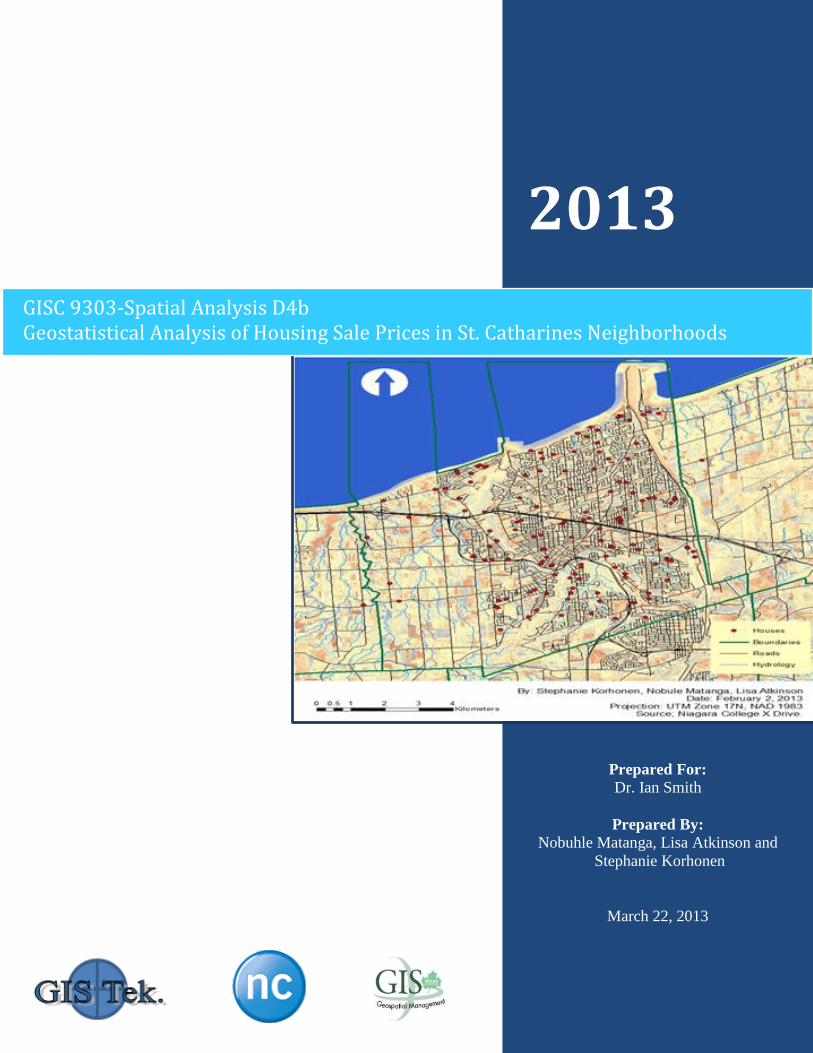
2013
Prepared For:
Dr. Ian Smith
Prepared By:
Nobuhle Matanga, Lisa Atkinson and
Stephanie Korhonen
March 22, 2013
GISC 9303-Spatial Analysis D4b Geostatistical Analysis of Housing Sale Prices in St. Catharines Neighborhoods
135 Taylor Road, S.S #4
Niagara-on-the-lake, ON
Tel: 1-289-241-7627
Email: [email protected]
March 22, 2013
File: GISC93084b
Mr. Ian D. Smith
M.Sc., OLS, OLIP, EP
Post-Graduate Professor of Environmental Sciences and GIS
Niagara-on-the-lake Campus, Niagara College
Room E313
135 Taylor Road, S.S #4
On, L0S 1J0
Dear Mr. Smith:
Re: Submission of GISC93084b Please accept this letter as the formal submission of Deliverable 4b Geostatical Report for
GISC9308 – Spatial Analysis.
This geostatistical report outlines all intentions for undertaking the statistical investigation on the
Average Housing Sale Prices in St. Catharine Neighborhoods. The attached report beings by
highlights the study area, objectives, goals, methodologies and preliminary statistical assessment.
This report concludes with a comparison of the IDW and Kriging results created from the
obtained dataset. Supplemented material include: a summary of collected raw data, statistical
calculations, and graphing of the dataset. Overall it was determined that the IDW method
resulted in a better prediction surface.
Please do not hesitate to contact us for any additional information at 1-289-241-7627. Thank
you for your time and attention.
Sincerely,
Nobuhle Matanga, B.Sc.
GIS-GM Graduate Candidate
GIS Tek.
N.M. /
Enclosures: 1) [Geostatical Collection Report],
2) [Statistical Calculations and Graphing of Data Set].
Cc. Lisa Atkinson, BA
Stephanie Korhonen, BA
Geo Tek | Geostatistics Report i
March 22, 2013
Executive Summary
This geostatistical report begins by providing an in-depth summary of the study area,
objectives, goals methodologies and preliminary statistical assessment of the Housing Sale Prices
in St. Catharine Neighborhoods, for the obtained dataset. The geographic data is defined as
UTM Easting and Northing coordinates; whereas the z value is presented as housing cost.
Formal maps, displaying the housing locations and the study area extent are located within
Appendix A, and a full glossary of terms is located in Appendix B. The purpose of this
investigation is to determine the feasibility of this dataset for future geostatistical studies. The
St. Catharines housing price dataset can be summarized as follows; there are a total of 138
observations used in this study, the mean price is $367,270, the median price is $259,950, more
importantly there is a kurtosis of 22.14, skewness of 3.9814 and a standard deviation of 2188.1.
As a result of the positive skew in this dataset, a log transformation is required before spatial
importation can be conducted. The second half of this report discusses the prediction surfaces
created using both the kriging and IDW techniques. Although both surfaces provide adequate
representations of wealth zones in the St. Catharine’s area, the kriging results are more skewed
due to outliers. Therefore it was concluded that the IDW provides a more accurate classification
of poverty and affluence in St. Catharines area. As a result the information from the IDW results
will essentially allow contractors to maximize profit and minimize cost.
Geo Tek | Geostatistical Report ii
March 22, 2013
Table of Contents
Executive Summary ..................................................................................................................... i
1.0 Project Understanding ............................................................................................................ 1
1.1 Study Area ............................................................................................................................. 1
1.2 Project Goal ........................................................................................................................... 2
1.3 Objectives and Benefits of this Project this Project .............................................................. 2
2.0 Summary of Methodology ..................................................................................................... 2
2.1 Data Collection ...................................................................................................................... 2
2.2 Determining Sample Size ...................................................................................................... 2
2.3 Formatting and Displaying Data in ArcGIS .......................................................................... 3
2.3.1 Creation of a file Geodatabase ................................................................................... 3
2.3.2 Creating Metadata for file Geodatabase .................................................................... 3
2.3.3 Importing X, Y data into ArcGIS .............................................................................. 3
2.3.4 Projecting Data........................................................................................................... 3
2.3.4 Georeferencing Neighborhood Boundaries Data ....................................................... 3
2.4 Geostatistical Analysis of Data in ArcGIS ............................................................................ 4
2.4.1 Summary statistics ..................................................................................................... 4
2.4.2 Histogram ................................................................................................................... 6
2.4.3 Normal QQ Plots........................................................................................................ 8
2.5 Kriging Interpolation ........................................................................................................... 12
2.6 Inverse Distance Weighted (IDW) Interpolation ................................................................ 17
3.0 Results and Discussion ...................................................................................................... 19
3.1 Kriging vs. Inverse Distance Weighted (IDW) ................................................................... 19
3.1.1 Similarities ............................................................................................................... 19
3.1.2 Differences ............................................................................................................... 20
4.0 Conclusions ......................................................................................................................... 25
5.0 References ........................................................................................................................... 26
APPENDIX A (Formal Maps) ..........................................................................................................
APPENDIX B (Glossary of Terms and Parameters) ........................................................................ APPENDIX C (Raw Data)................................................................................................................
Geo Tek | Geostatistical Report iii
March 22, 2013
List of Figures
Figure 1 : Formal Map of Study Area ............................................................................................. 1
Figure 2 Summary Statistics Tool in ArcGIS, Image Source ArcGIS ........................................... 4
Figure 3: Summary statistics for Easting Observations, Image Source ArcGIS ............................. 5
Figure 4: Summary statistics for House Prices, Image Source ArcGIS .......................................... 5
Figure 5: Summary statistics for Northing Observations, Image Source ArcGIS .......................... 5
Figure 6 Northing Observations Histogram, Image Source ArcGIS.............................................. 6
Figure 7: House Prices Histogram, Image Source ArcGIS ............................................................. 7
Figure 8 Easting Observations Histogram, Image Source ArcGIS ................................................. 7
Figure 9 House Price Normal QQPlot, Image Source ArcGIS ....................................................... 8
Figure 11: Northing Observation QQPlot, Image Source ArcGIS .................................................. 9
Figure 10: Easting Observations QQPlot, Image Source ArcGIS................................................... 9
Figure 12 Normal QQ plot of Housing Prices with Log Transformation, Image Source ArcGIS10
Figure 13 Histogram of House Prices with Log Transformation, Image Source ArcGIS ............ 11
Figure 14 : Study Semivariogram, Image Source ArcGIS ............................................................ 12
Figure 15: Kriging Parameters Used In Study ............................................................................. 14
Figure 16: IDW Parameters Used In Study .................................................................................. 17
Figure 17: House Price Zone Classification, Image Source ArcGIS ........................................... 19
Figure 18: Real Estate Sale Prediction, St. Catharines, Ontario and Surrounding Area: Quadrant
1..................................................................................................................................................... 21
Figure 19: Real Estate Sale Prediction, St. Catharines, Ontario and Surrounding Area: Quadrant
2..................................................................................................................................................... 22
Figure 20: Real Estate Sale Prediction, St. Catharines, Ontario and Surrounding Area: Quadrant
3..................................................................................................................................................... 23
Figure 21: Real Estate Sale Prediction, St. Catharines, Ontario and Surrounding Area: Quadrant
4..................................................................................................................................................... 24
Figure 22: Example of Spatial Interpolation, Image Source: Niagara College ............................. 2
Figure 23: Kriging Calculation, Image Source: Niagara College .................................................. 3
Figure 24: IDW Calculation, Image Source: Niagara College ...................................................... 4
List of Tables
Table 1 : Cross Validation Assessment of Kriging Results .......................................................... 15
Table 2:Cross Validation Assessment of IDW Results ............................................................... 18
March 22, 2013
1.0 Project Understanding
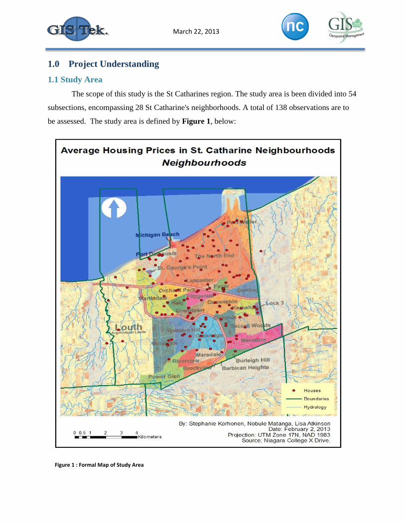
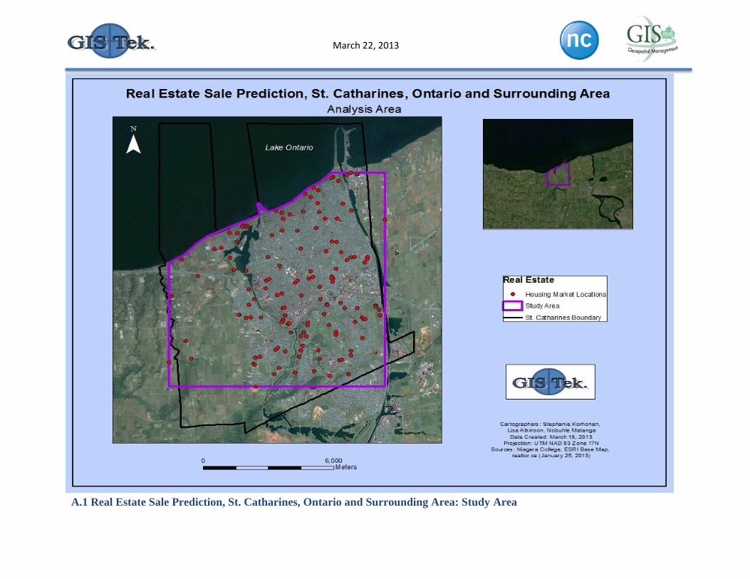
1.1 Study Area
The scope of this study is the St Catharines region. The study area is been divided into 54
subsections, encompassing 28 St Catharine's neighborhoods. A total of 138 observations are to
be assessed. The study area is defined by Figure 1, below:
Figure 1 : Formal Map of Study Area
Geo Tek | Geostatistical Report 2
March 22, 2013
1.2 Project Goal
The goal of this spatial statistical assessment is to determine areas of poverty and
affluence in St Catharine's, using sample residential housing sale prices.
1.3 Objectives and Benefits of this Project this Project
This project will allow for a practical assessment of future building projects, within a
specified neighborhood, in order to maximize profit, and minimize cost.
2.0 Summary of Methodology
2.1 Data Collection
The housing cost and address data is collected from the Relators® Canada Incorporated
website. This website is owned by the Canadian Real Estate Association and the National
Association of Realtors® (Realtors.ca, 2013). The data available on the website is provided by
realtors from across Canada, and is updated hourly (Realtors.ca, 2013). A Multiresolution
Seamless Image Database (MrSID) file, of the Niagara region and corresponding municipalities
boundaries, is provided by Niagara College. Subsequently, UTM NAD 83 Zone 17N Easting
and Northing coordinates are obtained via Google Earth. Google Earth is a real world
representation of superimposed images obtained from satellite imagery, aerial photography, and
GIS 3D globe. This platform is available at no cost to public users.
2.2 Determining Sample Size
All the sample data was collected on January 25, 2013. This dataset includes residential
houses that are for sale. On January 25, 2013 there were a total of 360 houses for sale in St
Catharines. However, in order to avoid large generalizations and minimize inaccuracies, the St.
Catharines region was divided into 54 equal area subsections. From these subsections
maximum, median and minimum values were obtained, therefore reducing the sample size to
138 observations.
Geo Tek | Geostatistical Report 3
March 22, 2013
2.3 Formatting and Displaying Data in ArcGIS
2.3.1 Creation of a file Geodatabase
The file geodatabase associated with this deliverable is created using ArcCatalog and is
set as the default geodatabase within the map document properties. This ensures a common
projection for all assessment products, and ensures products are exported to the correct
geodatabase, and finally, reduces project costs associated with data transfer.
2.3.2 Creating Metadata for file Geodatabase
Metadata (tags, summary, description, credits and use limitations) are created for the file
geodatabase using ArcCatalog. Metadata is essential for data management purposes; it provides
the user with information such as data source and data function.
2.3.3 Importing X, Y data into ArcGIS
An excel table composed of longitude, latitude and price values is transformed to a
shapefile via ArcGIS. The Easting coordinates are assigned as X values, the Northing
coordinates are assigned as Y values, and the price observations are assigned as Z values within
the attribute table.
2.3.4 Projecting Data
All of the imported data was reprojected into UTM Zone 17N, NAD 1983, this is the
desired format for all the data used in this study.
2.3.4 Georeferencing Neighborhood Boundaries Data
Georeferencing is the process of assigning raster data sets to a map coordinate, positional
reference, system (Smith, 2013). The purpose of this is to rectify data. Thus, a jpeg image of St
Catharine's neighborhood boundaries is correlated to the MrSID file of the Niagara Region, via
the Georeferencing tool in ArcGIS. This data management tool is used to allocate three control
point pairs to each image to warp the jpeg images to the MrSID referenced data. Control points
are geographic references, easily identifiable upon both the non-referenced image and the
referenced image. When georeferencing raster data, at least three, well distributed control points
must be established to ensure precise image warp effects.
Geo Tek | Geostatistical Report 4
March 22, 2013
2.4 Geostatistical Analysis of Data in ArcGIS
2.4.1 Summary statistics
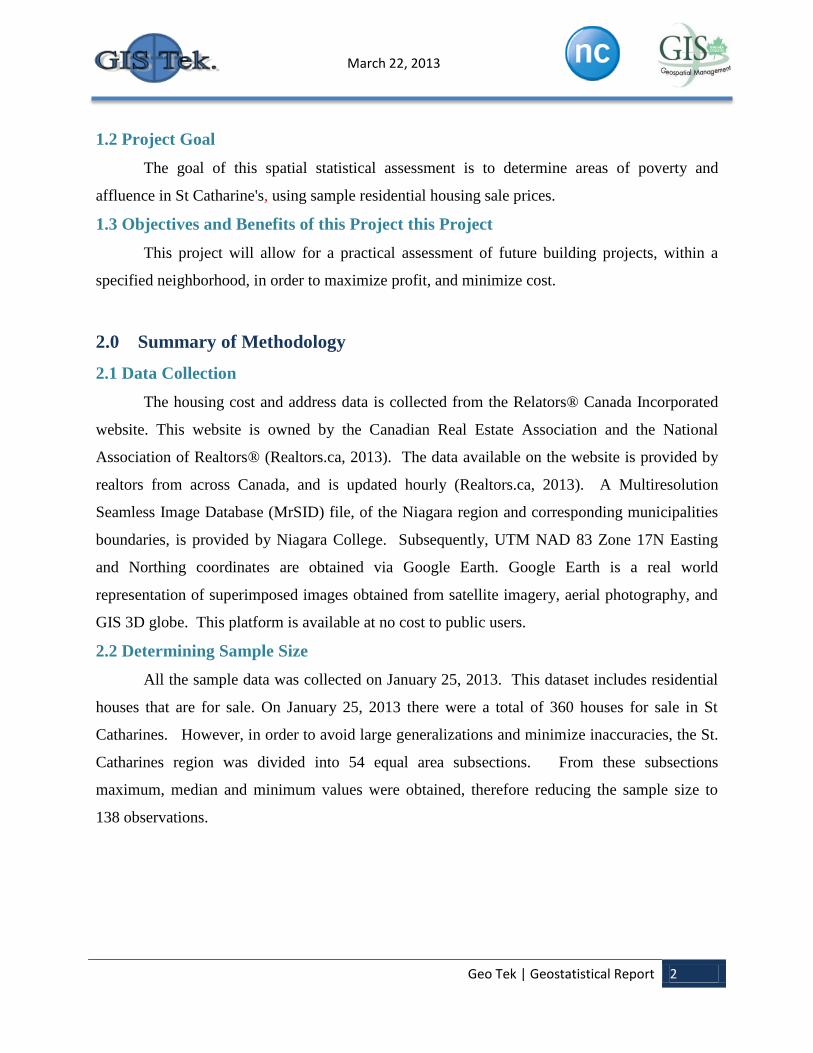
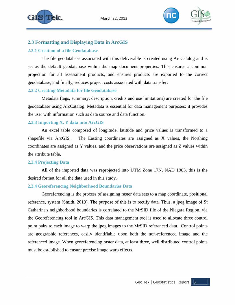
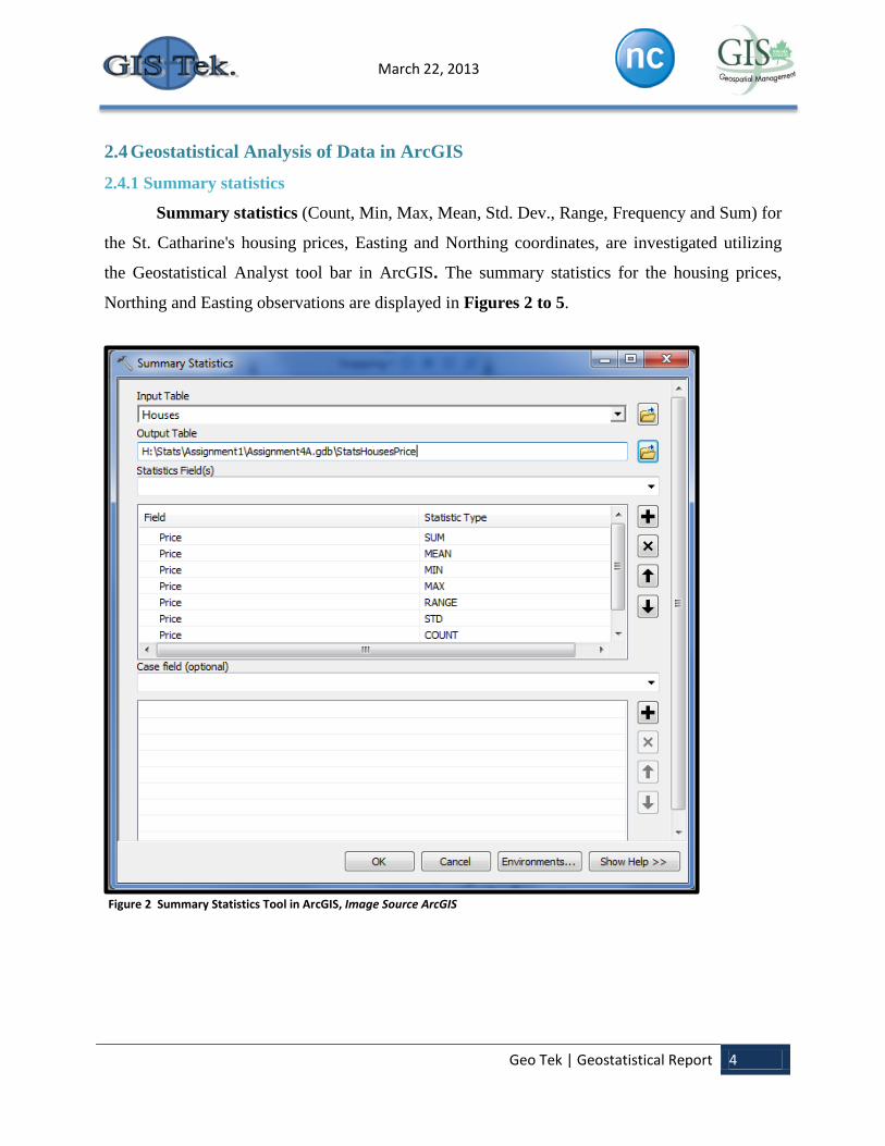
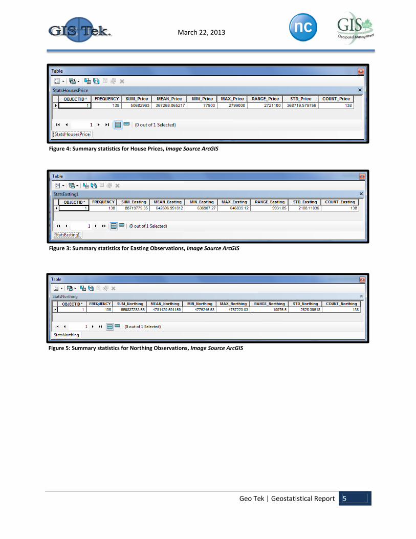
Summary statistics (Count, Min, Max, Mean, Std. Dev., Range, Frequency and Sum) for
the St. Catharine's housing prices, Easting and Northing coordinates, are investigated utilizing
the Geostatistical Analyst tool bar in ArcGIS. The summary statistics for the housing prices,
Northing and Easting observations are displayed in Figures 2 to 5.
Figure 2 Summary Statistics Tool in ArcGIS, Image Source ArcGIS
Geo Tek | Geostatistical Report 5
March 22, 2013
Figure 4: Summary statistics for House Prices, Image Source ArcGIS
Figure 3: Summary statistics for Easting Observations, Image Source ArcGIS
Figure 5: Summary statistics for Northing Observations, Image Source ArcGIS

Geo Tek | Geostatistical Report 6
March 22, 2013
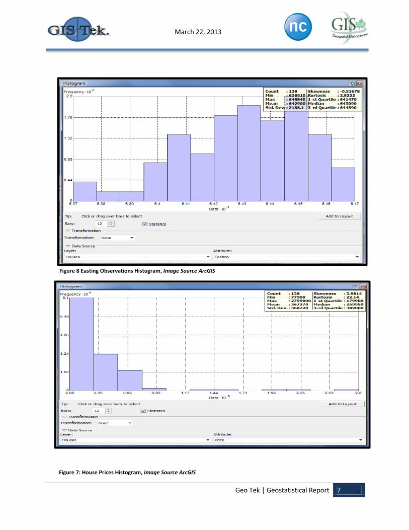
2.4.2 Histogram
Histograms for the St. Catharines housing prices, Easting and Northing coordinates are
created using the Geostatistical Analyst tool bar in ArcGIS. The number of bins used for our
histograms (12) is determined by rounding the square root of the sample size (138). This was
rounded because the square root of 138 is 11.74 and a decimal number cannot be used for the
number of bins. The histograms are used to assess the frequency distribution of the values
within the dataset. The presented histograms, display statistical analyses provided by the
Geostatistical Analyst tool such inclusing, skewness, kurtosis, median, 1-st Quartile and 3-rd
Quartile. The Northing observations are normally distributed while, the Easting values have a
negative skew and the price observations have a positive skew (Figures 6-8).
Figure 6 Northing Observations Histogram, Image Source ArcGIS
Geo Tek | Geostatistical Report 7
March 22, 2013
Figure 8 Easting Observations Histogram, Image Source ArcGIS
Figure 7: House Prices Histogram, Image Source ArcGIS
Geo Tek | Geostatistical Report 8
March 22, 2013
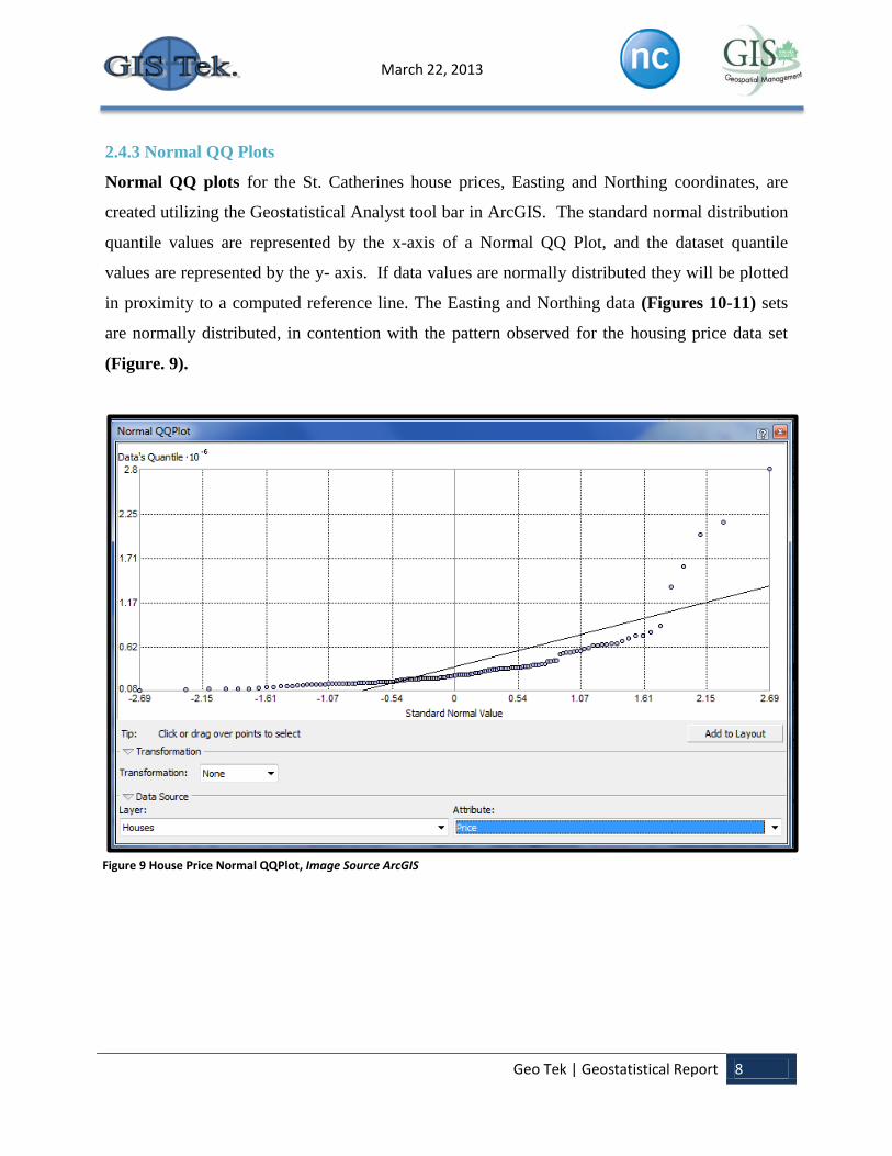
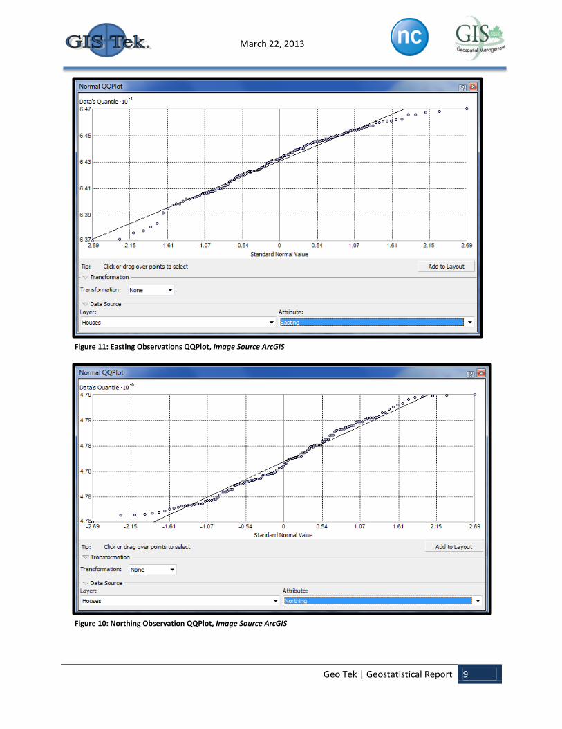
2.4.3 Normal QQ Plots
Normal QQ plots for the St. Catherines house prices, Easting and Northing coordinates, are
created utilizing the Geostatistical Analyst tool bar in ArcGIS. The standard normal distribution
quantile values are represented by the x-axis of a Normal QQ Plot, and the dataset quantile
values are represented by the y- axis. If data values are normally distributed they will be plotted
in proximity to a computed reference line. The Easting and Northing data (Figures 10-11) sets
are normally distributed, in contention with the pattern observed for the housing price data set
(Figure. 9).
Figure 9 House Price Normal QQPlot, Image Source ArcGIS
Geo Tek | Geostatistical Report 9
March 22, 2013
Figure 11: Easting Observations QQPlot, Image Source ArcGIS
Figure 10: Northing Observation QQPlot, Image Source ArcGIS
Geo Tek | Geostatistical Report 10
March 22, 2013
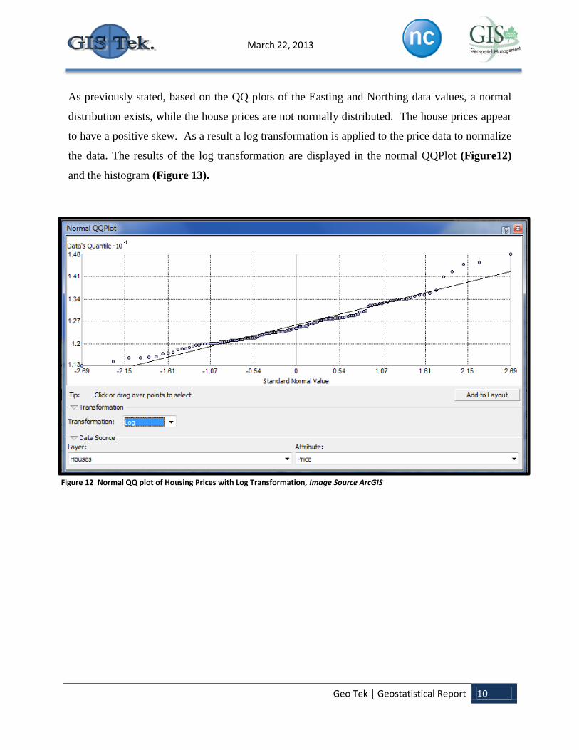
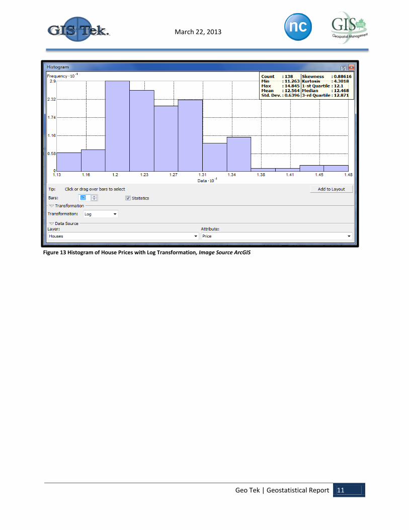
As previously stated, based on the QQ plots of the Easting and Northing data values, a normal
distribution exists, while the house prices are not normally distributed. The house prices appear
to have a positive skew. As a result a log transformation is applied to the price data to normalize
the data. The results of the log transformation are displayed in the normal QQPlot (Figure12)
and the histogram (Figure 13).
Figure 12 Normal QQ plot of Housing Prices with Log Transformation, Image Source ArcGIS
Geo Tek | Geostatistical Report 11
March 22, 2013
Figure 13 Histogram of House Prices with Log Transformation, Image Source ArcGIS
Geo Tek | Geostatistical Report 12
March 22, 2013
2.5 Kriging Interpolation
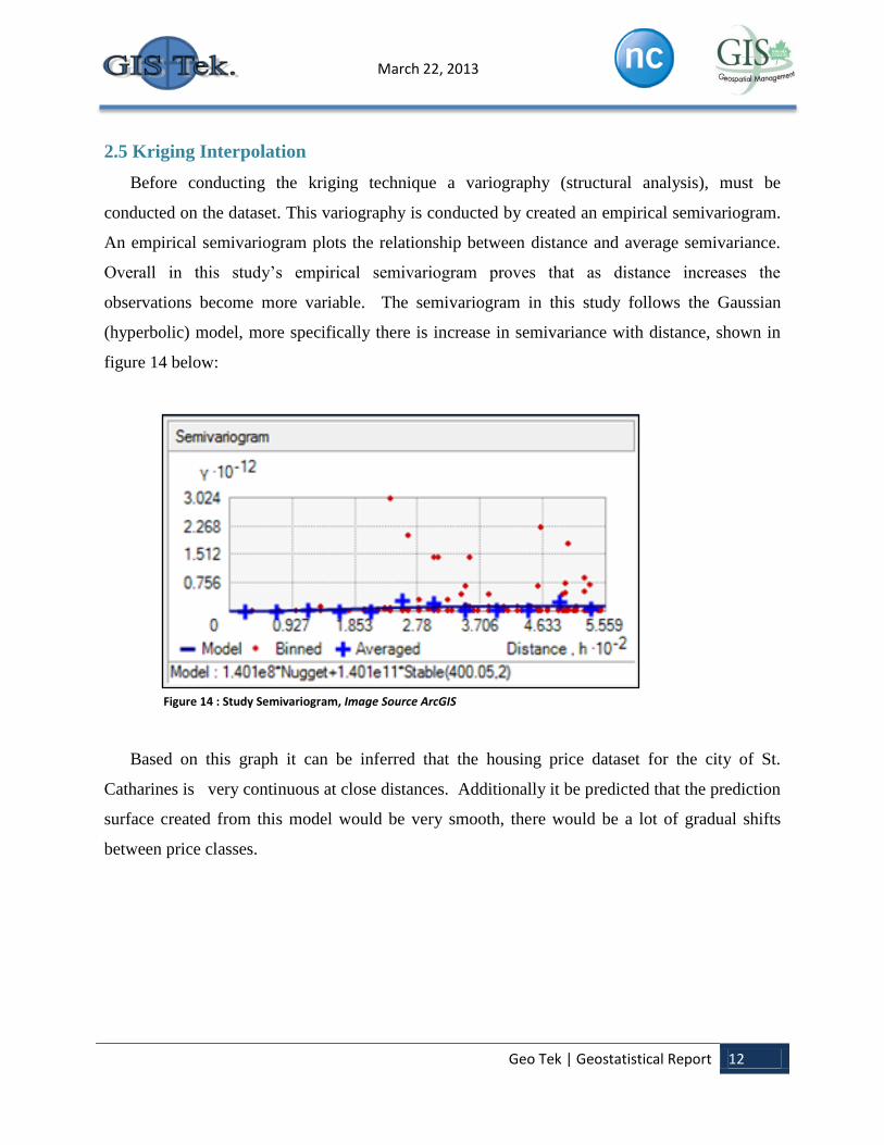
Before conducting the kriging technique a variography (structural analysis), must be
conducted on the dataset. This variography is conducted by created an empirical semivariogram.
An empirical semivariogram plots the relationship between distance and average semivariance.
Overall in this study’s empirical semivariogram proves that as distance increases the
observations become more variable. The semivariogram in this study follows the Gaussian
(hyperbolic) model, more specifically there is increase in semivariance with distance, shown in
figure 14 below:
Based on this graph it can be inferred that the housing price dataset for the city of St.
Catharines is very continuous at close distances. Additionally it be predicted that the prediction
surface created from this model would be very smooth, there would be a lot of gradual shifts
between price classes.
Figure 14 : Study Semivariogram, Image Source ArcGIS
Geo Tek | Geostatistical Report 13
March 22, 2013
Additionally the pre-kriging structural analysis determine that the housing price dataset
for St. Catharines is anisotropic (directional). Housing price is depends on direction and distance.
The reason for this is that houses that are closer together generally cost the same. Moreover
housing cost is also depended on geographic location, for example housing cost tends to increase
going towards waterfront properties and decreases the inner city, and this is illustrated in both the
IDW and Kriging surface results
In order to interpolate the housing cost across a surface, ordinary kriging is employed to
display the housing cost variance. For this investigation, ordinary kriging is utilized, so that the
constant mean is assumed as unknown, as is a common best practice of geostatistical analysis
(Smith, 2013). The Kriging results depend on the semivariogram model. This technique
classifies data using the semivariogram and relative distance. Additionally, kriging settings are
enforced, via the interactive kriging tool window. These settings are summarized by Figure 15,
shown below:

Geo Tek | Geostatistical Report 14
March 22, 2013
Figure 15: Kriging Parameters Used In Study
Geo Tek | Geostatistical Report 15
March 22, 2013
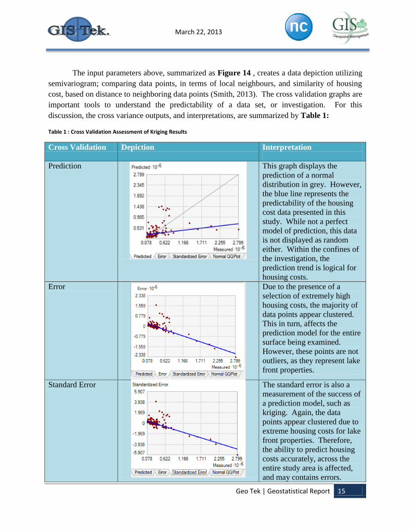
The input parameters above, summarized as Figure 14 , creates a data depiction utilizing
semivariogram; comparing data points, in terms of local neighbours, and similarity of housing
cost, based on distance to neighboring data points (Smith, 2013). The cross validation graphs are
important tools to understand the predictability of a data set, or investigation. For this
discussion, the cross variance outputs, and interpretations, are summarized by Table 1:
Table 1 : Cross Validation Assessment of Kriging Results
Cross Validation Depiction Interpretation
Prediction
This graph displays the
prediction of a normal
distribution in grey. However,
the blue line represents the
predictability of the housing
cost data presented in this
study. While not a perfect
model of prediction, this data
is not displayed as random
either. Within the confines of
the investigation, the
prediction trend is logical for
housing costs.
Error
Due to the presence of a
selection of extremely high
housing costs, the majority of
data points appear clustered.
This in turn, affects the
prediction model for the entire
surface being examined.
However, these points are not
outliers, as they represent lake
front properties.
Standard Error
The standard error is also a
measurement of the success of
a prediction model, such as
kriging. Again, the data
points appear clustered due to
extreme housing costs for lake
front properties. Therefore,
the ability to predict housing
costs accurately, across the
entire study area is affected,
and may contains errors.
Geo Tek | Geostatistical Report 16
March 22, 2013
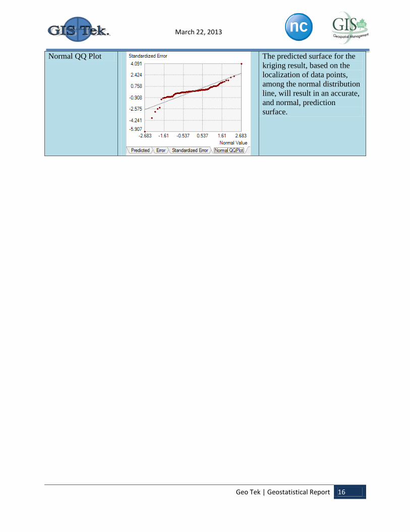
Normal QQ Plot
The predicted surface for the
kriging result, based on the
localization of data points,
among the normal distribution
line, will result in an accurate,
and normal, prediction
surface.
Geo Tek | Geostatistical Report 17
March 22, 2013
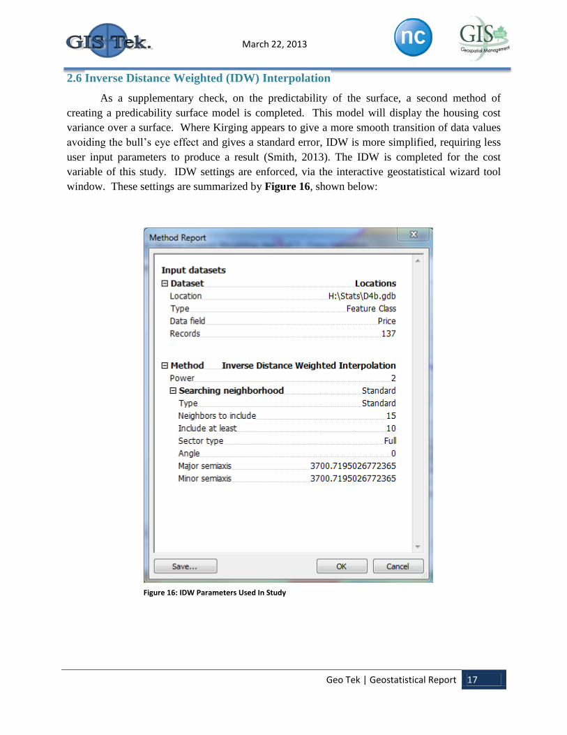
2.6 Inverse Distance Weighted (IDW) Interpolation
As a supplementary check, on the predictability of the surface, a second method of
creating a predicability surface model is completed. This model will display the housing cost
variance over a surface. Where Kirging appears to give a more smooth transition of data values
avoiding the bull’s eye effect and gives a standard error, IDW is more simplified, requiring less
user input parameters to produce a result (Smith, 2013). The IDW is completed for the cost
variable of this study. IDW settings are enforced, via the interactive geostatistical wizard tool
window. These settings are summarized by Figure 16, shown below:
Figure 16: IDW Parameters Used In Study
Geo Tek | Geostatistical Report 18
March 22, 2013
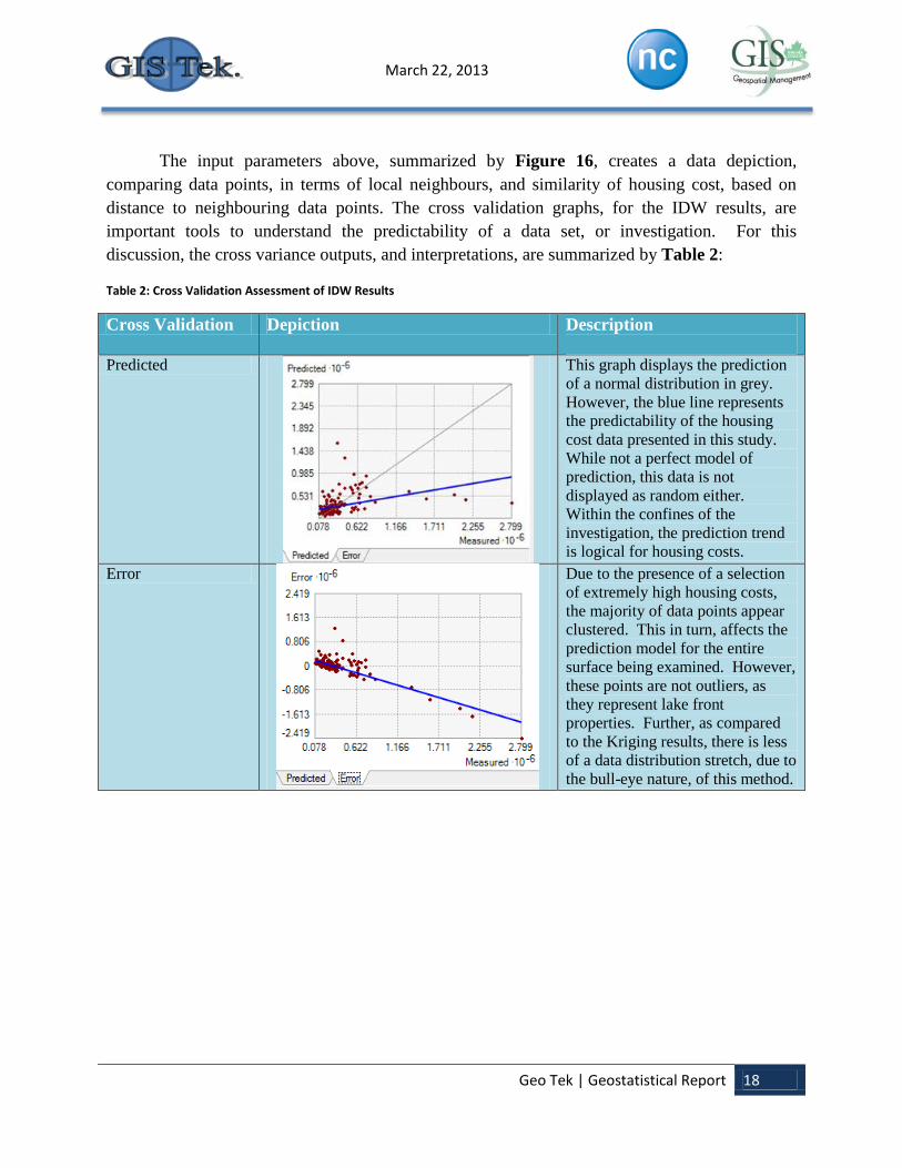
The input parameters above, summarized by Figure 16, creates a data depiction,
comparing data points, in terms of local neighbours, and similarity of housing cost, based on
distance to neighbouring data points. The cross validation graphs, for the IDW results, are
important tools to understand the predictability of a data set, or investigation. For this
discussion, the cross variance outputs, and interpretations, are summarized by Table 2:
Table 2: Cross Validation Assessment of IDW Results
Cross Validation Depiction Description
Predicted
This graph displays the prediction
of a normal distribution in grey.
However, the blue line represents
the predictability of the housing
cost data presented in this study.
While not a perfect model of
prediction, this data is not
displayed as random either.
Within the confines of the
investigation, the prediction trend
is logical for housing costs.
Error
Due to the presence of a selection
of extremely high housing costs,
the majority of data points appear
clustered. This in turn, affects the
prediction model for the entire
surface being examined. However,
these points are not outliers, as
they represent lake front
properties. Further, as compared
to the Kriging results, there is less
of a data distribution stretch, due to
the bull-eye nature, of this method.
Geo Tek | Geostatistical Report 19
March 22, 2013
3.0 Results and Discussion
3.1 Kriging vs. Inverse Distance Weighted (IDW)
3.1.1 Similarities
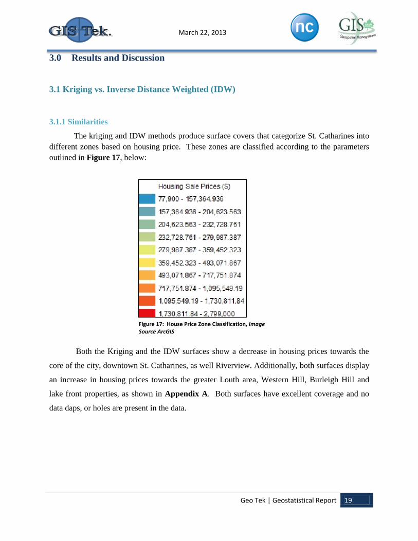
The kriging and IDW methods produce surface covers that categorize St. Catharines into
different zones based on housing price. These zones are classified according to the parameters
outlined in Figure 17, below:
Both the Kriging and the IDW surfaces show a decrease in housing prices towards the
core of the city, downtown St. Catharines, as well Riverview. Additionally, both surfaces display
an increase in housing prices towards the greater Louth area, Western Hill, Burleigh Hill and
lake front properties, as shown in Appendix A. Both surfaces have excellent coverage and no
data daps, or holes are present in the data.
Figure 17: House Price Zone Classification, Image Source ArcGIS
Geo Tek | Geostatistical Report 20
March 22, 2013
3.1.2 Differences
In the Kriging surface there is a more pronounced presence of extreme housing prices,
both high and low. In comparison to the IDW results, a more gradual transition between areas of
high housing costs and low housing costs is present. Due to the generalization of the IDW
results there is a larger error for predicting housing cost, as opposed to the Kriging results, which
show a greater amount of localized detail. For a better assessment of the differences the larger
study area, is divided into quadrants.
Geo Tek | Geostatistical Report 21
March 22, 2013
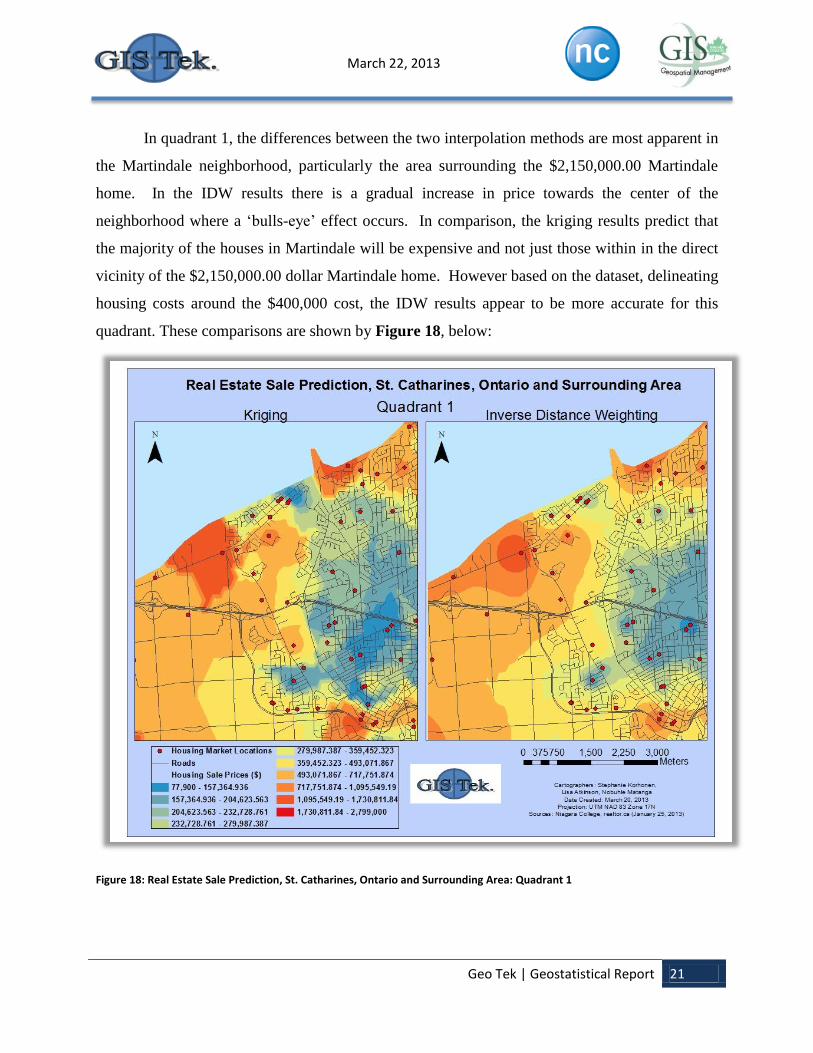
In quadrant 1, the differences between the two interpolation methods are most apparent in
the Martindale neighborhood, particularly the area surrounding the $2,150,000.00 Martindale
home. In the IDW results there is a gradual increase in price towards the center of the
neighborhood where a ‘bulls-eye’ effect occurs. In comparison, the kriging results predict that
the majority of the houses in Martindale will be expensive and not just those within in the direct
vicinity of the $2,150,000.00 dollar Martindale home. However based on the dataset, delineating
housing costs around the $400,000 cost, the IDW results appear to be more accurate for this
quadrant. These comparisons are shown by Figure 18, below:
Figure 18: Real Estate Sale Prediction, St. Catharines, Ontario and Surrounding Area: Quadrant 1
Geo Tek | Geostatistical Report 22
March 22, 2013
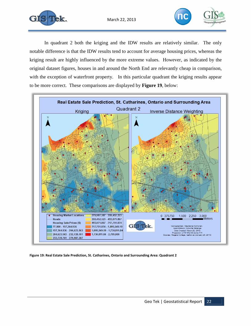
In quadrant 2 both the kriging and the IDW results are relatively similar. The only
notable difference is that the IDW results tend to account for average housing prices, whereas the
kriging result are highly influenced by the more extreme values. However, as indicated by the
original dataset figures, houses in and around the North End are relevantly cheap in comparison,
with the exception of waterfront property. In this particular quadrant the kriging results appear
to be more correct. These comparisons are displayed by Figure 19, below:
Figure 19: Real Estate Sale Prediction, St. Catharines, Ontario and Surrounding Area: Quadrant 2
Geo Tek | Geostatistical Report 23
March 22, 2013
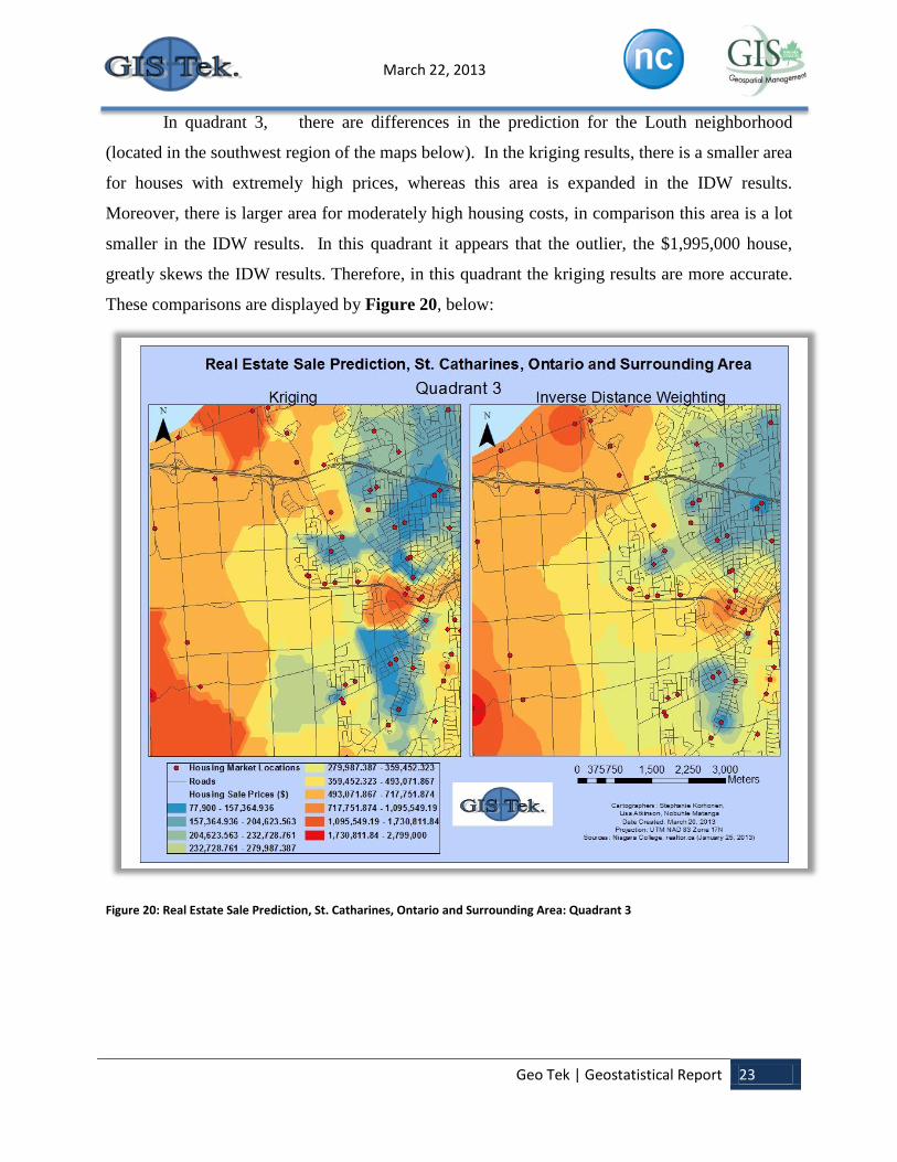
In quadrant 3, there are differences in the prediction for the Louth neighborhood
(located in the southwest region of the maps below). In the kriging results, there is a smaller area
for houses with extremely high prices, whereas this area is expanded in the IDW results.
Moreover, there is larger area for moderately high housing costs, in comparison this area is a lot
smaller in the IDW results. In this quadrant it appears that the outlier, the $1,995,000 house,
greatly skews the IDW results. Therefore, in this quadrant the kriging results are more accurate.
These comparisons are displayed by Figure 20, below:
Figure 20: Real Estate Sale Prediction, St. Catharines, Ontario and Surrounding Area: Quadrant 3
Geo Tek | Geostatistical Report 24
March 22, 2013
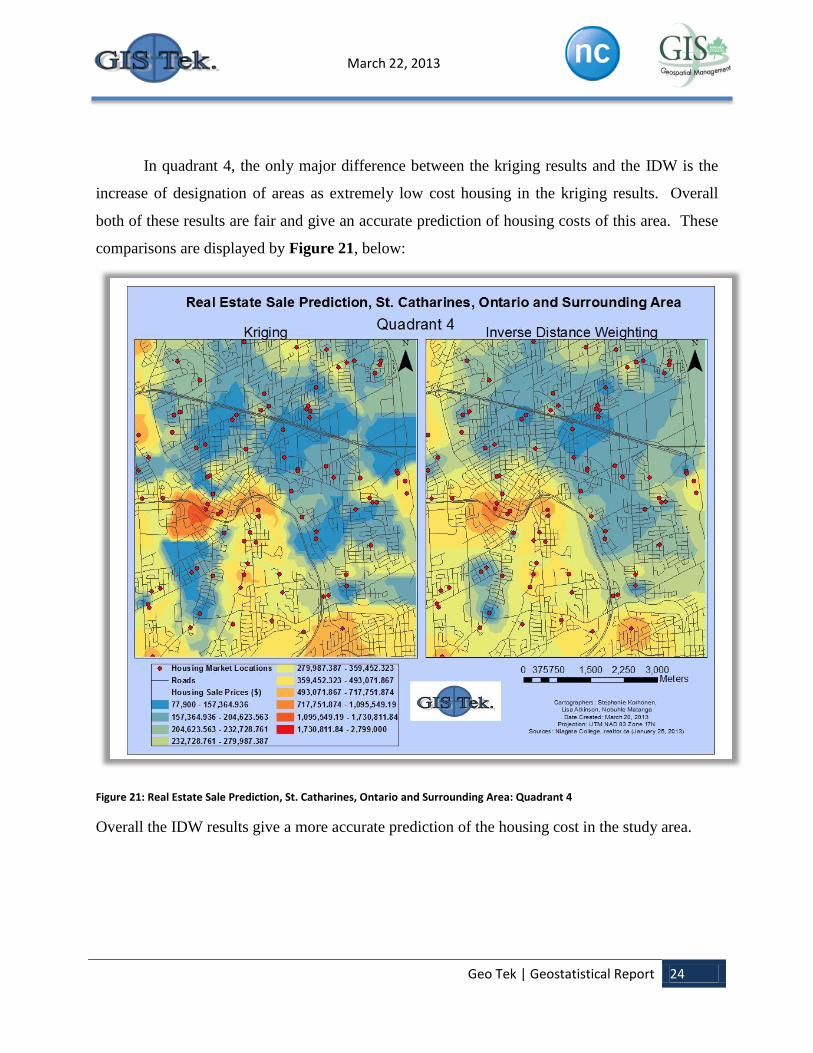
In quadrant 4, the only major difference between the kriging results and the IDW is the
increase of designation of areas as extremely low cost housing in the kriging results. Overall
both of these results are fair and give an accurate prediction of housing costs of this area. These
comparisons are displayed by Figure 21, below:
Figure 21: Real Estate Sale Prediction, St. Catharines, Ontario and Surrounding Area: Quadrant 4
Overall the IDW results give a more accurate prediction of the housing cost in the study area.
Geo Tek | Geostatistical Report 25
March 22, 2013
4.0 Conclusions
To conclude, an in-depth summary of the study area, objectives, goals, methodologies
and preliminary statistical assessment of the House Sale Prices in St. Catharine Neighbors study
dataset was outlined in the beginning of this report. Based on the results of the statistical
assessment, the dataset was declared suitable for a geostatistical analysis. A geostatistical
analysis, utilizing both kriging and IDW interpolation methods, was conducted on this study
area. Both of these methods produced prediction surfaces that divided St. Catharines into
different zones based on housing price. A comparison of these two surfaces reveals that the
IDW results is less skewed towards outliers and is therefore the more representative surface. In
turn the IDW results correctly determine areas of poverty and affluence in St. Catharines which
will influence of the location of future building project in this city. The IDW surface will
essentially allow contractors to maximize profit and minimize cost.
Geo Tek | Geostatistical Report 26
March 22, 2013
5.0 References
5.1. Lectures
Smith, Ian. Week 1- Introduction to Stats. GISC9308-Spatial Analysis. Niagara
College. PDF.
Smith, Ian. Week 2- Multivariate Statistics. GISC9308-Spatial Analysis. Niagara
College. PDF.
Smith, Ian. Week 3- Sampling. GISC9308-Spatial Analysis. Niagara College. PDF.
Smith, Ian. Week 4- Introduction to Spatial Analyst. GISC9308-Spatial Analysis.
Niagara College. PDF.
Smith, Ian. Week 7- Regression and Interpolation. GISC9308-Spatial Analysis.
Niagara College. PDF.
Smith, Ian. Week 8- Geostatistical Analyst. GISC9308-Spatial Analysis. Niagara
College. PDF.
5.2 Software
ArcGIS (2008) ArcGIS Desktop Education Edition (Version 10). Computer program.
Available at http://www.esri.com/products 5,Sept, 2012
5.3 Terms of Reference
"Assignment4- Geostatistical Analysis of Student Collected Spatial Data."
GISC9308-Spatial Analysis. Niagara College. Web.
5.4 Textbook
Ormsby , Napoleon , Burke , Carolyn Groessl and, Laura Bowden. Getting to Know
ArcGIS Desktop; for ArcGIS 10. Redlands: Esri press. 2010. Print.
5.5 Websites
"ArcGIS Resources." ArcGIS. Esri, n.d. Web. 20 Jan 2013.

Geo Tek | Geostatistical Report 27
March 22, 2013
<http://resources.arcgis.com>.
"Realtors.ca." The Canadian Real Estate Association. Web. 20 Jan 2013.
<http://www.realtor.ca/>.

March 22, 2013
APPENDIX A (Formal Maps)
March 22, 2013
A.1 Real Estate Sale Prediction, St. Catharines, Ontario and Surrounding Area: Study Area
Geo Tek | Geostatistical Report 2
March 22, 2013
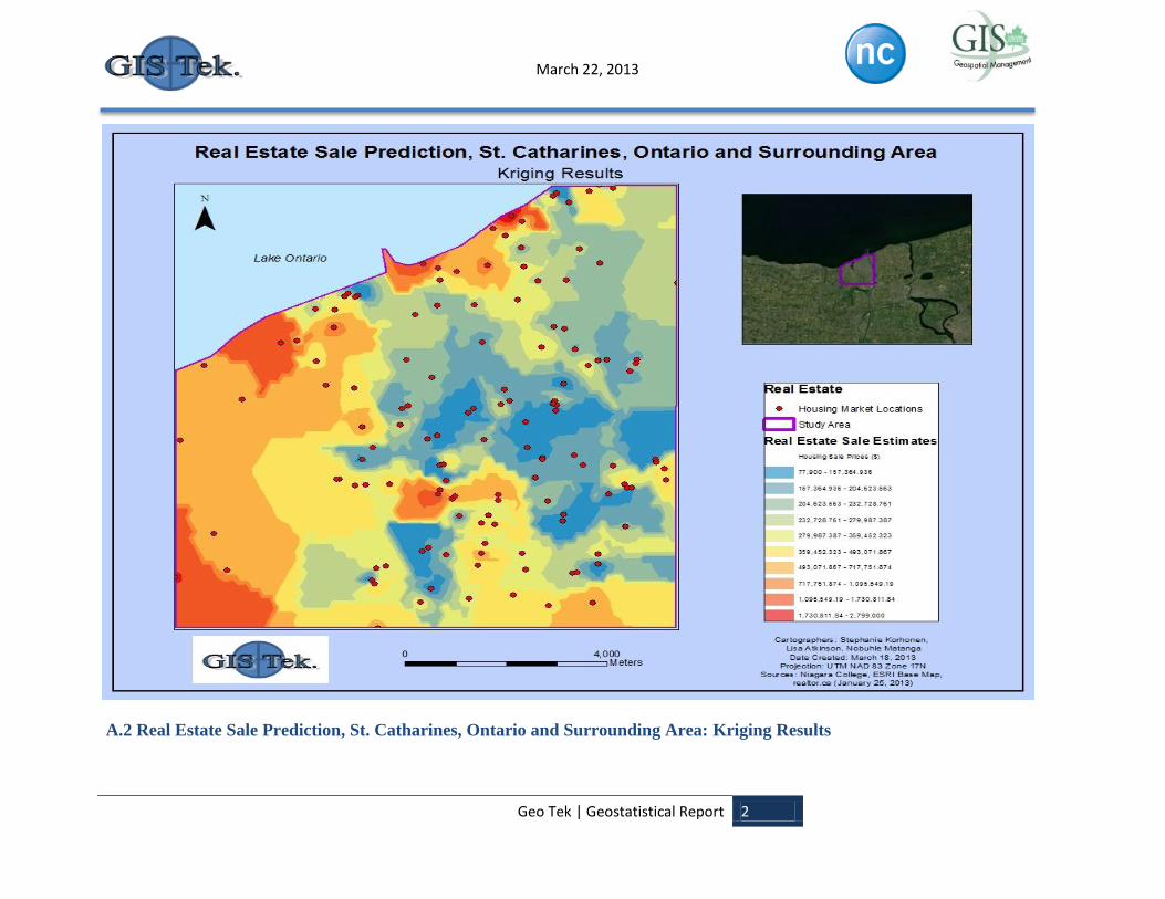
A.2 Real Estate Sale Prediction, St. Catharines, Ontario and Surrounding Area: Kriging Results

Geo Tek | Geostatistical Report 3
March 22, 2013
A.3 Real Estate Sale Prediction, St. Catharines, Ontario and Surrounding Area: Inverse Distance Weighting Results

March 22, 2013
APPENDIX B (Glossary of Terms)
Geo Tek | Geostatistical Report 2
March 22, 2013
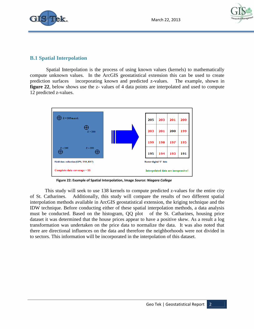
B.1 Spatial Interpolation
Spatial Interpolation is the process of using known values (kernels) to mathematically
compute unknown values. In the ArcGIS geostatistical extension this can be used to create
prediction surfaces incorporating known and predicted z-values. The example, shown in
figure 22, below shows use the z- values of 4 data points are interpolated and used to compute
12 predicted z-values.
This study will seek to use 138 kernels to compute predicted z-values for the entire city
of St. Catharines. Additionally, this study will compare the results of two different spatial
interpolation methods available in ArcGIS geostatistical extension, the kriging technique and the
IDW technique. Before conducting either of these spatial interpolation methods, a data analysis
must be conducted. Based on the histogram, QQ plot of the St. Catharines, housing price
dataset it was determined that the house prices appear to have a positive skew. As a result a log
transformation was undertaken on the price data to normalize the data. It was also noted that
there are directional influences on the data and therefore the neighborhoods were not divided in
to sectors. This information will be incorporated in the interpolation of this dataset.
Figure 22: Example of Spatial Interpolation, Image Source: Niagara College
Geo Tek | Geostatistical Report 3
March 22, 2013
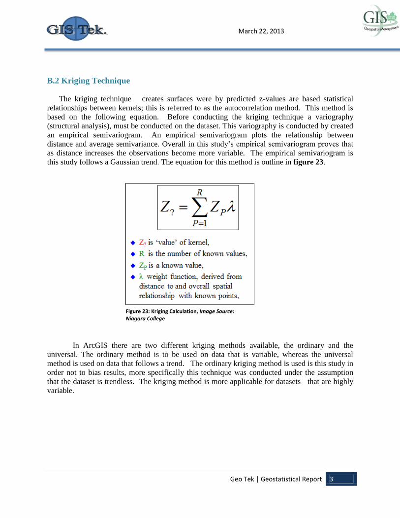
B.2 Kriging Technique
The kriging technique creates surfaces were by predicted z-values are based statistical
relationships between kernels; this is referred to as the autocorrelation method. This method is
based on the following equation. Before conducting the kriging technique a variography
(structural analysis), must be conducted on the dataset. This variography is conducted by created
an empirical semivariogram. An empirical semivariogram plots the relationship between
distance and average semivariance. Overall in this study’s empirical semivariogram proves that
as distance increases the observations become more variable. The empirical semivariogram is
this study follows a Gaussian trend. The equation for this method is outline in figure 23.
In ArcGIS there are two different kriging methods available, the ordinary and the
universal. The ordinary method is to be used on data that is variable, whereas the universal
method is used on data that follows a trend. The ordinary kriging method is used is this study in
order not to bias results, more specifically this technique was conducted under the assumption
that the dataset is trendless. The kriging method is more applicable for datasets that are highly
variable.
Figure 23: Kriging Calculation, Image Source: Niagara College

Geo Tek | Geostatistical Report 4
March 22, 2013
B.3 Inverse Distance Weighted (IDW) Technique
The IDW technique creates surfaces were by predicted z-values are directly based on
surrounding kernels; this is referred to as the deterministic method. This method is based on the
following equation. The equation for this method is outline in figure 24.
Additionally, the IDW method is more applicable for datasets were distance greatly effects
influence.
Figure 24: IDW Calculation, Image Source: Niagara College

March 22, 2013
APPENDIX C (Raw Data)

March 22, 2013
Grid Number Neighbourhood Price Address Easting Northing
1 North End $2,799,000.00 15 Lantana Circle , St Catharines 643553.52 4786445.99
1 North End $339,900.00 5 lakebreeze Crescent , St Catharines 643761.79 4786315.68
1 North End $364,900.00 1 Warrington Place, St Catharines 643433.92 4785962.26
1 North End $689,900.00 39 Royal York Road, St Catharines 643188.45 4786135.16
2 North End $102,500.00 11 Grandview Drive, St Catharines 644447.55 4787008.56
2 North End $189,900.00 78 Melody Trail, St Catharines 644698.48 4786792.85
2 North End $269,900.00 103 Arthur Street, St Catharines 644376.37 4786942.22
3 Port Weller $189,500.00 9 Shoreham Street, St Catharines 645284.67 4787223.03
3 Port Weller $329,900.00 6 Moes Crescent, St Catharines 645564.06 4787138.55
3 Port Weller $569,000.00 4 Yonge Street, St Catharines 645093.33 4787070.34
4 Port Dalhousie $179,000.00 65 Main Street, St Catharines 640511.41 4784479.55
4 Port Dalhousie $299,500.00 10 Ann Street, St Catharines 640464.39 4784434.50
4 Port Dalhousie $260,000.00 94 Dalhousie Avenue , St Catharines 640327.44 4784526.88
4 Port Dalhousie $294,000.00 99 DalhousieAvenue , St Catharines 640261.58 4784467.25
5 Michigan Beach $1,599,900.00 14 Shore Boulevard, St Catharines 641820.34 4785262.42
5 Michigan Beach $559,900.00 5 Xavier Court, St Catharines 642478.20 4785079.13
5 Michigan Beach $589,900.00 3 Cricket Hallow Road, St Catharines 642107.59 4785154.62
5 Port Dalhousie $274,900.00 27 Simpson Road, St Catharines 642143.90 4784860.87
6 North End $799,000.00 164 A Lakeshore Road, St Catharines 643081.77 4785220.63
6 North End $209,000.00 25 Murray Street, St Catharines 643747.83 4785657.60
6 North End $299,000.00 13 Costen Boulevard, St Catharines 643807.56 4785198.63
7 North End $189,900.00 584 Bunting Road, St Catharines 645313.51 4785289.58
7 North End $244,900.00 20 Pearce Avenue, St Catharines 644903.32 4785637.49
Geo Tek | Geostatistical Report 2
March 22, 2013
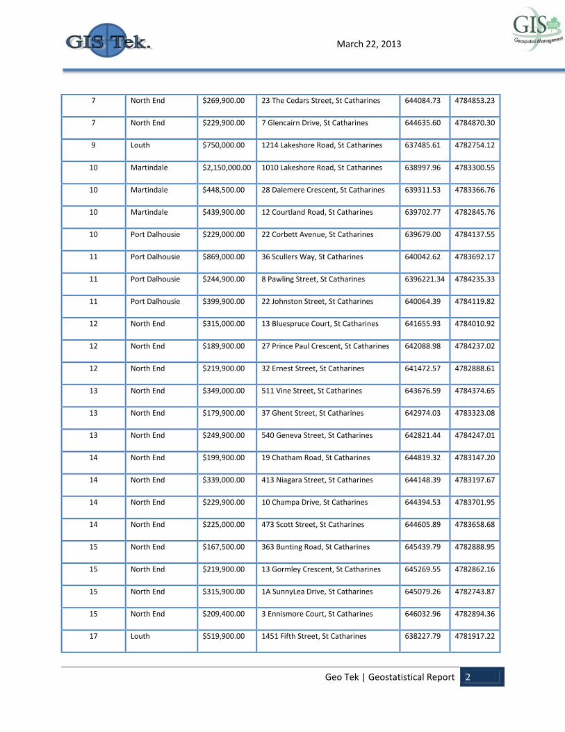
7 North End $269,900.00 23 The Cedars Street, St Catharines 644084.73 4784853.23
7 North End $229,900.00 7 Glencairn Drive, St Catharines 644635.60 4784870.30
9 Louth $750,000.00 1214 Lakeshore Road, St Catharines 637485.61 4782754.12
10 Martindale $2,150,000.00 1010 Lakeshore Road, St Catharines 638997.96 4783300.55
10 Martindale $448,500.00 28 Dalemere Crescent, St Catharines 639311.53 4783366.76
10 Martindale $439,900.00 12 Courtland Road, St Catharines 639702.77 4782845.76
10 Port Dalhousie $229,000.00 22 Corbett Avenue, St Catharines 639679.00 4784137.55
11 Port Dalhousie $869,000.00 36 Scullers Way, St Catharines 640042.62 4783692.17
11 Port Dalhousie $244,900.00 8 Pawling Street, St Catharines 6396221.34 4784235.33
11 Port Dalhousie $399,900.00 22 Johnston Street, St Catharines 640064.39 4784119.82
12 North End $315,000.00 13 Bluespruce Court, St Catharines 641655.93 4784010.92
12 North End $189,900.00 27 Prince Paul Crescent, St Catharines 642088.98 4784237.02
12 North End $219,900.00 32 Ernest Street, St Catharines 641472.57 4782888.61
13 North End $349,000.00 511 Vine Street, St Catharines 643676.59 4784374.65
13 North End $179,900.00 37 Ghent Street, St Catharines 642974.03 4783323.08
13 North End $249,900.00 540 Geneva Street, St Catharines 642821.44 4784247.01
14 North End $199,900.00 19 Chatham Road, St Catharines 644819.32 4783147.20
14 North End $339,000.00 413 Niagara Street, St Catharines 644148.39 4783197.67
14 North End $229,900.00 10 Champa Drive, St Catharines 644394.53 4783701.95
14 North End $225,000.00 473 Scott Street, St Catharines 644605.89 4783658.68
15 North End $167,500.00 363 Bunting Road, St Catharines 645439.79 4782888.95
15 North End $219,900.00 13 Gormley Crescent, St Catharines 645269.55 4782862.16
15 North End $315,900.00 1A SunnyLea Drive, St Catharines 645079.26 4782743.87
15 North End $209,400.00 3 Ennismore Court, St Catharines 646032.96 4782894.36
17 Louth $519,900.00 1451 Fifth Street, St Catharines 638227.79 4781917.22
Geo Tek | Geostatistical Report 3
March 22, 2013
18 Martindale $350,000.00 56 Henley Drive, St Catharines 640455.75 4782190.58
18 Martindale $639,900.00 1 Brooklyn Court, St Catharines 639889.22 4782250.50
19 Martindale $279,000.00 70 Scott Street, St Catharines 646839.12 4784794.59
19 Martindale $166,000.00 104 Ventura Drive, St Catharines 641388.35 4781674.62
19 Martindale $219,900.00 118 Haig Street, St Catharines 641521.65 4781748.97
19 Orchid Park $214,900.00 11 Fonthill Court, St Catharines 641979.42 4782457.18
20 Orchid Park $269,900.00 11 Kingsway Crescent, St Catharines 643354.16 4781780.11
20 Orchid Park $177,000.00 11 Hill Park Lane, St Catharines 643412.50 4782160.41
20 Fitzgerald $169,900.00 21 Sandown Street, St Catharines 643525.30 4781880.17
20 Orchid Park $132,000.00 222 Carlton Street, St Catharines 642801.30 4781675.35
21 Facer $229,900.00 68 Parkview Road, St Catharines 644413.60 4781881.45
21 Facer $164,900.00 50 Parkview Road, St Catharines 644454.89 4781775.37
21 Facer $159,900.00 54 Cosby Avenue, St Catharines 644376.99 4781807.82
21 North End $117,500.00 110 Garnett Street, St Catharines 644587.06 4782301.41
22 Bunting $190,000.00 24 Huntley Crescent, St Catharines 645907.72 4782612.61
22 Bunting $229,900.00 15 Rendale Avenue, St Catharines 646017.00 4782802.31
23 Louth $629,900.00 1665 Gregory Road, St Catharines 637008.61 4780897.32
25 Martindale $629,900.00 40 Tulip Tree Common, St Catharines 640599.05 4781227.53
25 Martindale $149,900.00 6 Barton Street, St Catharines 640599.53 4780431.14
25 Martindale $359,900.00 5 Inglis Circle, St Catharines 640144.49 4779930.68
26 Haig $119,900.00 153 Pleasant Avenue, St Catharines 642095.95 4781014.32
26 Haig $259,900.00 44 Chicory Crescent, St Catharines 641354.83 4781289.07
26 Haig $174,900.00 21 Taylor Avenue, St Catharines 641891.45 4780930.48
27 Fitzgerald $77,900.00 173 Vine Street, St Catharines 643841.79 4781353.66
27 Fitzgerald $226,900.00 56 Maple Street, St Catharines 643011.45 4780915.30
Geo Tek | Geostatistical Report 4
March 22, 2013
27 Fitzgerald $154,900.00 42 McGhie Street, St Catharines 642705.71 4781574.66
27 Fitzgerald $154,900.00 59 Vine Street, St Catharines 643870.98 4780723.05
28 Queenston $99,794.00 30 Parkview Road, St Catharines 644430.96 4781628.54
28 Queenston $204,900.00 62 Chelsea Street, St Catharines 644804.36 4780530.40
28 Queenston $155,000.00 25 Berryman Avenue, St Catharines 644171.39 4780463.24
28 Queenston $159,900.00 17 Berryman Avenue, St Catharines 644178.28 4780425.61
29 Kernahan $89,500.00 23 Emmett Road, St Catharines 646401.30 4780417.82
29 Queenston $224,900.00 97 Bunting Road, St Catharines 645575.73 4780266.74
29 Queenston $179,900.00 25 Lorne Street, St Catharines 644976.29 4780278.76
29 Kernahan $160,000.00 31 Emmett Road, St Catharines 646418.58 4780362.62
30 Lock 3 $538,800.00 15 MacKenzie King Avnue, St
Catharines
646576.55 4780191.10
31 Louth $649,000.00 2098 Seventh Street, St Catharines 637672.50 4778582.77
33 Vansickle $309,900.00 66 Elderwood Drive, St Catharines 640673.75 4779794.27
33 Vansickle $435,000.00 53 West Farmington Drive, St
Catharines
640468.37 4779775.04
33 Vansickle $389,900.00 74 Sawmill Road, St Catharines 641140.93 4779810.22
33 Vansickle $359,900.00 228 First Street, St. Catharines 640108.41 4779939.54
34 Western Hill $549,900.00 29 Yates Street, St. Catharines 642391.57 4779453.21
34 Western Hill $649,900.00 14 Trafalgar Street, St. Catharines 642447.13 4779513.39
34 Western Hill $749,900.00 10 Norris Place, St. Catharines 642152.28 4779680.03
34 Western Hill $1,350,000.00 55 Yates Street, St. Catharines 642104.50 4779564.31
35 Western Hill $289,900.00 63 Glenridge Avenue, St. Catharines 643105.28 4779041.31
35 Western Hill $374,800.00 54 Highland Avenue, St. Catharines 643297.83 4779404.20
35 Western Hill $149,900.00 23 Hainer Street, St. Catharines 642523.17 4779029.04
35 Glenridge $650,000.00 43 Highland Avenue, St. Catharines 643290.53 4779546.38
Geo Tek | Geostatistical Report 5
March 22, 2013
36 Glenridge $139,000.00 6 Phelps Street, St. Catharines 644589.87 4779059.90
36 Glenridge $239,900.00 2 Marren Street, St. Catharines 644266.91 4779394.41
36 Oakdale $189,900.00 298 Oakdale Avenue, St. Catharines 644029.78 4779967.80
37 Secord Woods $357,500.00 28 Woodrow Street, St. Catharines 645790.40 4779806.49
37 Oakdale $132,900.00 27 Battersea Avenue, St. Catharines 645473.22 4779559.71
37 Secord Woods $174,900.00 37 Greenwood Avenue, St. Catharines 645849.50 4779719.24
37 Secord Woods $159,900.00 52 Greenwood Avenue, St. Catharines 645943.29 4779720.40
38 Secord Woods $329,900.00 3 Alex Grant Place, St. Catharines 646621.41 4779921.26
39 Louth $1,995,000.00 3420 Ninth Street, St. Catharines 636907.27 4777505.39
39 Louth $569,900.00 1673 St. Paul Street, St. Catharines 637937.85 4777679.81
41 Vansickle $349,900.00 15 Consiglia Drive, St. Catharines 640886.08 4777726.63
41 Vansickle $359,900.00 52 Strada Blvd., St. Catharines 641083.64 4777791.16
42 Vansickle $114,000.00 48 Church Hill Street, St. Catharines 641797.25 4778145.97
42 Western Hill $224,000.00 28 Cumming Street, St. Catharines 642267.18 4778061.14
42 Vansickle $165,000.00 35 Lloyd Street, St. Catharines 641915.16 4778243.01
43 Western Hill $254,900.00 45 Rivercrest Drive, St. Catharines 643041.78 4778346.23
43 Western Hill $399,999.00 111 South Drive, St. Catharines 643231.63 4778819.56
43 Western Hill $449,900.00 47 Hillcrest Avenue, St. Catharines 642967.70 4778852.48
43 Glenridge $369,900.00 25 Riverview Blvd., St. Catharines 642888.28 4777800.39
44 Glenridge $275,000.00 71 Village Road, St. Catharines 643832.64 4777690.53
44 Glenridge $379,000.00 27 Adelene Crescent, St. Catharines 643763.57 4778099.34
44 Glenridge $144,000.00 168 Oakdale Avenue, St. Catharines 644579.04 4778896.22
45 Secord Woods $219,500.00 16 Rampart Drive, St. Catharines 645808.10 4778756.05
45 Merritton $103,900.00 20 Chestnut Street, St. Catharines 645265.43 4777841.19
45 Merritton $349,900.00 368 Merritt Street, St. Catharines 645263.62 4778087.06
Geo Tek | Geostatistical Report 6
March 22, 2013
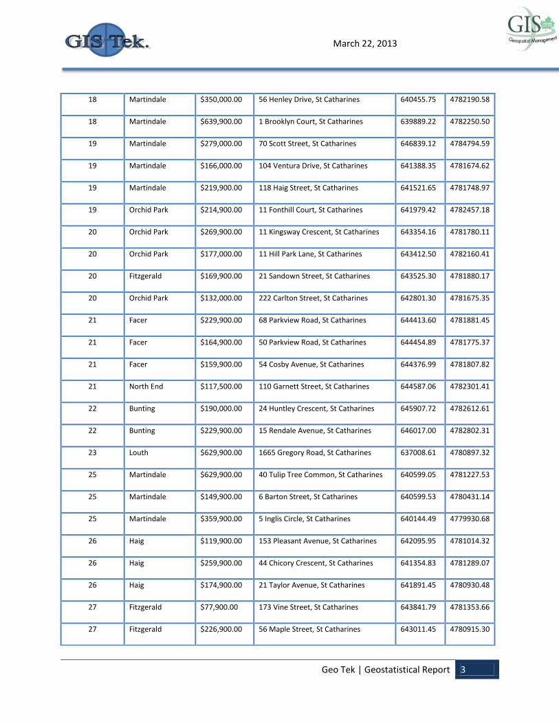
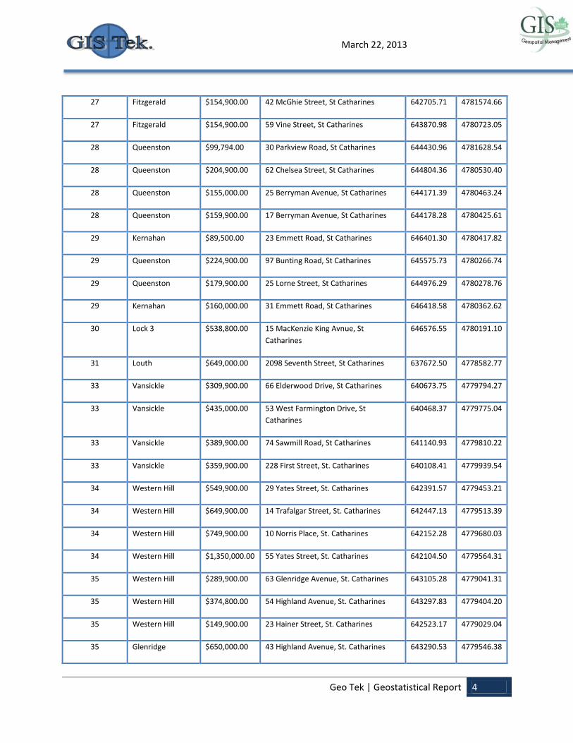
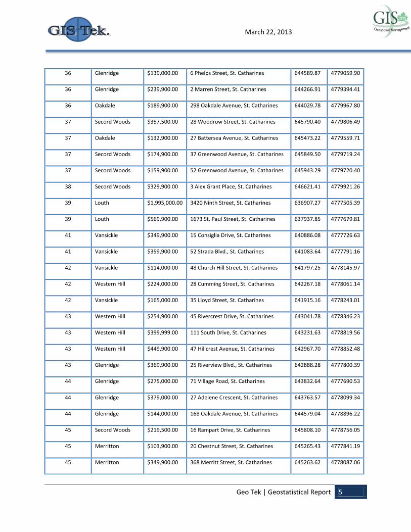
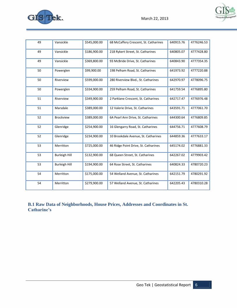
B.1 Raw Data of Neighborhoods, House Prices, Addresses and Coordinates in St.
Catharine’s
49 Vansickle $545,000.00 68 McCaffery Crescent, St. Catharines 640915.76 4776246.53
49 Vansickle $186,900.00 218 Rykert Street, St. Catharines 640805.07 4777428.80
49 Vansickle $369,800.00 93 McBride Drive, St. Catharines 640843.90 4777354.35
50 Powerglen $99,900.00 198 Pelham Road, St. Catharines 641973.92 4777220.88
50 Riverview $599,000.00 280 Riverview Blvd., St. Catharines 642970.97 4778096.75
50 Powerglen $334,900.00 259 Pelham Road, St. Catharines 641759.54 4776895.80
51 Riverview $349,900.00 2 Parklane Crescent, St. Catharines 642717.47 4776976.48
51 Marsdale $389,000.00 12 Valerie Drive, St. Catharines 643591.71 4777061.70
52 Brockview $389,000.00 6A Pearl Ann Drive, St. Catharines 644300.64 4776809.85
52 Glenridge $254,900.00 16 Glengarry Road, St. Catharines 644756.71 4777608.79
52 Glenridge $234,900.00 10 Brookdale Avenue, St. Catharines 644859.36 4777633.17
53 Merritton $725,000.00 46 Ridge Point Drive, St. Catharines 645174.02 4776881.33
53 Burleigh Hill $132,900.00 68 Queen Street, St. Catharines 642267.02 4779903.42
53 Burleigh Hill $194,900.00 64 Rose Street, St. Catharines 640824.33 4780720.23
54 Merritton $175,000.00 54 Welland Avenue, St. Catharines 642151.79 4780291.92
54 Merritton $279,900.00 57 Welland Avenue, St. Catharines 642205.43 4780310.28