2-1 INTRODUCTION

This chapter reviews those physical and engineering properties of soils of principal interestfor the analysis and design of foundation elements considered in this text. These primarilyinclude the following:

1. Strength parameters1

Stress-strain modulus (or modulus of elasticity), Es\ shear modulus, G', and Poisson'sratio, /x; angle of internal friction, (/>; soil cohesion, c

2. Compressibility indexes for amount and rate of settlementCompression: index, Cc, and ratio, C'c; recompression: index, Cr, and ratio, C,!!; coefficientof consolidation, cv\ coefficient of secondary compression, Ca

3. Gravimetric-volumetric dataUnit weight, y; specific gravity, Gs\ void ratio, e, or porosity, n\ water content, w/ (where/ = Af for natural, L for liquid limit, or P for plastic limit; e.g., Wp = plastic limit)

Symbols and definitions generally follow those of ASTM D 653 except E5, G', and /JL (refer also to "List of primarysymbols" following the Preface). It is common to subscript E for soil as E5, for concrete Ec, etc. G' will be used forshear modulus, as Gs is generally used for specific gravity. The symbol fi is commonly used for Poisson's ratio;however, ASTM D 653 suggests v, which is difficult to write by hand.

GEOTECHNICALAND INDEX PROPERTIES:

LABORATORY TESTING; SETTLEMENTAND STRENGTH CORRELATIONS

CHAPTER

2

4. Permeability, also called hydraulic conductivity (sometimes required)k = coefficient of permeability (or hydraulic conductivity)

The symbols shown here will be consistently used throughout the text and will not besubsequently identified/defined.

The more common laboratory tests also will be briefly commented on. For all laboratorytests we can immediately identify several problems:

1. Recovery of good quality samples. It is not possible to recover samples with zero distur-bance, but if the disturbance is a minimum—a relative term—the sample quality may beadequate for the project.

2. Necessity of extrapolating the results from the laboratory tests on a few small samples,which may involve a volume of ±0.03 m3, to the site, which involves several thousandsof cubic meters.

3. Laboratory equipment limitations. The triaxial compression text is considered one of thebetter test procedures available. It is easy to obtain a sample, put it into the cell, applysome cell pressure, and load the sample to failure in compression. The problem is thatthe cell pressure, as usually used, applies an even, all around (isotropic) compression. Insitu the confining pressure prior to the foundation load application is usually anisotropic(vertical pressure is different from the lateral value). It is not very easy to apply anisotropicconfining pressure to soil samples in a triaxial cell—even if we know what to use forvertical and lateral values.

4. Ability and motivation of the laboratory personnel.

The effect of these several items is to produce test results that may not be much refinedover values estimated from experience. Items 1 through 3 make field testing a particularlyattractive alternative. Field tests will be considered in the next chapter since they tend to beclosely associated with the site exploration program.

Index settlement and strength correlations are alternatives that have value in preliminarydesign studies on project feasibility. Because of both test limitations and costs, it is usefulto have relationships between easily determined index properties such as the liquid limitand plasticity index and the design parameters. Several of the more common correlations arepresented later in this chapter. Correlations are usually based on a collection of data froman extensive literature survey and used to plot a best-fit curve or to perform a numericalregression analysis.

2-2 FOUNDATIONSUBSOILS

We are concerned with placing the foundation on either soil or rock. This material may beunder water as for certain bridge and marine structures, but more commonly we will placethe foundation on soil or rock near the ground surface.

Soil is an aggregation of particles that may range very widely in size. It is the by-productof mechanical and chemical weathering of rock. Some of these particles are given specificnames according to their sizes, such as gravel, sand, silt, clay, etc., and are more completelydescribed in Sec. 2-7.

Soil, being a mass of irregular-shaped particles of varying sizes, will consist of the particles(or solids), voids (pores or spaces) between particles, water in some of the voids, and air takingup the remaining void space. At temperatures below freezing the pore water may freeze, withresulting particle separation (volume increase). When the ice melts particles close up (volumedecrease). If the ice is permanent, the ice-soil mixture is termed permafrost It is evident thatthe pore water is a variable state quantity that may be in the form of water vapor, water, or ice;the amount depends on climatic conditions, recency of rainfall, or soil location with respectto the GWT of Fig. 1-1.

Soil may be described as residual or transported. Residual soil is formed from weatheringof parent rock at the present location. It usually contains angular rock fragments of varyingsizes in the soil-rock interface zone. Transported soils are those formed from rock weatheredat one location and transported by wind, water, ice, or gravity to the present site. The termsresidual and transported must be taken in the proper context, for many current residual soilsare formed (or are being formed) from transported soil deposits of earlier geological peri-ods, which indurated into rocks. Later uplifts have exposed these rocks to a new onset ofweathering. Exposed limestone, sandstone, and shale are typical of indurated transported soildeposits of earlier geological eras that have been uplifted to undergo current weathering anddecomposition back to soil to repeat the geological cycle.

Residual soils are usually preferred to support foundations as they tend to have better en-gineering properties. Soils that have been transported—particularly by wind or water—areoften of poor quality. These are typified by small grain size, large amounts of pore space,potential for the presence of large amounts of pore water, and they often are highly com-pressible. Note, however, exceptions that produce poor-quality residual soils and good-qualitytransported soil deposits commonly exist. In general, each site must be examined on its ownmerits.

2-3 SOIL VOLUME AND DENSITY RELATIONSHIPS

The more common soil definitions and gravimetric-volumetric relationships are presented inthis section. Figure 2-1 illustrates and defines a number of terms used in these relationships.

Void ratio e. The ratio of the volume of voids Vv to the volume of soils Vs in a given volumeof material, usually expressed as a decimal.

e = Y^ 0 < e « : o o (2-1)*s

For soils, e ranges from about 0.35 in the most dense state to seldom over 2 in the looseststate.

Porosity n. The ratio of the volume of voids to the total volume Vu expressed as either adecimal or a percentage.

. - £ (2-2)Water content w. The ratio of the weight of water Ww to the weight of soil solids W5,

expressed as a percentage but usually used in decimal form.

(2-3)

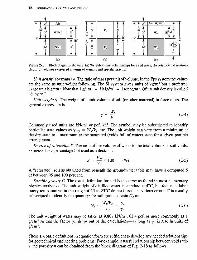
Figure 2-1 Block diagrams showing: (a) Weight/volume relationships for a soil mass; (b) volume/void relation-ships; (c) volumes expressed in terms of weights and specific gravity.

Unit density (or mass) p. The ratio of mass per unit of volume. In the Fps system the valuesare the same as unit weight following. The SI system gives units of kg/m3 but a preferredusage unit is g/cm3. Note that 1 g/cm3 = 1 Mg/m3 = 1 tonne/m3. Often unit density is called"density."

Unit weight y. The weight of a unit volume of soil (or other material) in force units. Thegeneral expression is

r - ^ (2-4)

Commonly used units are kN/m3 or pcf, kef. The symbol may be subscripted to identifyparticular state values as ydry = Ws/Vt, etc. The unit weight can vary from a minimum atthe dry state to a maximum at the saturated (voids full of water) state for a given particlearrangement.

Degree of saturation S. The ratio of the volume of water to the total volume of soil voids,expressed as a percentage but used as a decimal.

S = Y^L x 100 (%) (2-5)

A "saturated" soil as obtained from beneath the groundwater table may have a computed Sof between 95 and 100 percent.

Specific gravity G. The usual definition for soil is the same as found in most elementaryphysics textbooks. The unit weight of distilled water is standard at 4°C, but the usual labo-ratory temperatures in the range of 15 to 25°C do not introduce serious errors. G is usuallysubscripted to identify the quantity; for soil grains, obtain Gs as

Gs = ^ = 2L ( 2 .6)

The unit weight of water may be taken as 9.807 kN/m3, 62.4 pcf, or more commonly as 1g/cm3 so that the factor yw drops out of the calculations—as long as ys is also in units ofg/cm3.

These six basic definitions in equation form are sufficient to develop any needed relationshipsfor geotechnical engineering problems. For example, a useful relationship between void ratioe and porosity n can be obtained from the block diagram of Fig. 2-\b as follows:

(a) (b) (C)

Water

Air

Soil

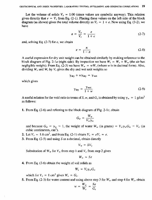
Let the volume of solids Vs = 1.00 (since values are symbolic anyway). This relationgives directly that e = Vv from Eq. (2-1). Placing these values on the left side of the blockdiagram (as shown) gives the total volume directly as Vt = 1 + e. Now using Eq. (2-2), wehave

and, solving Eq. (2-7) for e, we obtain

* = ^ - (2-8)1 - n

A useful expression for dry unit weight can be obtained similarly by making reference to theblock diagram of Fig. 2-Ia (right side). By inspection we have Wt = Ws + Ww (the air hasnegligible weight). From Eq. (2-3) we have Ww = wWs (where w is in decimal form). Also,dividing Ws and Wt by Vt gives the dry and wet unit weights so

Tdry + Wydry = 7 wet

which gives

7 d i y " 1 + w ( 2 9 )

A useful relation for the void ratio in terms of S, w, and G5 is obtained by using yw = 1 g/cm3

as follows:

1. From Eq. (2-6) and referring to the block diagram of Fig. 2-Ic, obtain

and because Gw = yw = 1, the weight of water Ww (in grams) = VwyWGW = Vw (incubic centimeters, cm3).

2. Let V, = 1.0 cm3, and from Eq. (2-1) obtain Vv = eVs = e.

3. From Eq. (2-5) and using S as a decimal, obtain directly

vw = svv

Substitution of Ww for Vw from step 1 and Vv from step 2 gives

Ww = Se

4. From Eq. (2-6) obtain the weight of soil solids as

Ws = VsywGs.

which for V5 = I cm3 gives Ws = Gs.5. From Eq. (2-3) for water content and using above step 3 for Ww and step 4 for Ws, obtain

6. Solving step 5 for the void ratio e, we obtain

e = ^Gs (2-10)

and when 5 = 1 (a saturated soil), we have e = wGs.

The dry unit is often of particular interest. Let us obtain a relationship for it in terms of watercontent and specific gravity of the soil solids Gs. From Fig. 2-Ic the volume of a given massVt = 1 + e, and with e obtained from Eq. (2-10) we have

Also, in any system of units the weight of the soil solids is

Vfs = VsJwG8 = ywGs when V5 = I as used here

The dry unit weight is

s — JwG87 d r y ~ V^ - I + ( W A ) G , ( 2 " U )

and for S = 100 percent,

From Eq. (2-9) the wet unit weight is

7wet = 7dry(l + w)

_ ywGs(l + w)I + (w/S)Gs

These derivations have been presented to illustrate the use of the basic definitions, togetherwith a basic block diagram on which is placed known (or assumed) values. It is recommendedthat a derivation of the needed relationship is preferable to making a literature search to findan equation that can be used.

Example 2-1. A cohesive soil specimen (from a split spoon; see Chap. 3 for method) was subjectedto laboratory tests to obtain the following data: The moisture content w = 22.5 percent; G5 = 2.60.To determine the approximate unit weight, a sample weighing 224.0 g was placed in a 500-cm3

container with 382 cm3 of water required to fill the container. The reader should note the use ofstandard laboratory units.

Required.

1. The wet unit weight, ywet

2. The dry unit weight, ydry3. Void ratio e and porosity n

4. Degree of saturation S

5. Dry bulk specific gravity

Solution.

Step 1. The wet unit weight is obtained from total sample weight as

* - " TT1 " ( 3 0 0 2 2 ^ ) C m ' - L 8 9 8 *** (WCt ^ ^

and from Sec. 1-7 we have

ywet = 1.898 X 9.807 = 18.61 kN/m3

Step 2. The dry unit weight is obtained using Eq. (2-9):

Td^ = { | | = 15.19 kN/m3

Step 3. The void ratio e and porosity n require some volume computations as follows:

_. Ws 1.898/1.225 3 3Vs = jr— = 9 mn m = 0.596 cm3 (orm3)usyw 2.60(1.0)

Vv = Vt-Vs = 1.000 - 0.596 = 0.404 cm3 (using cm)

-vt- g£-*»V 0 404

n = y = y ^ - = 0.404 (or 40.4%)

Step 4. To find the degree of saturation S it will be necessary to find the volume of water in thevoids. The weight of water Ww is the difference between the dry and wet weights; therefore,

1 OQO

Ww = 1.898 - J ^ = 0.349 g (in 1 cm3 of soil)

From Eq. (2-6) for Gw obtain Vw = Ww when using g and cm3; therefore,

V 0 ^495 = t X 10° = O404 X 10° - UA%

Step 5. The dry bulk specific gravity is obtained as (dimensionless)

y^_ _ \5A9 _°b - yw " 9.807 ^ L 5 4 9

////

2-4 MAJOR FACTORS THAT AFFECTTHE ENGINEERING PROPERTIES OF SOILS

Most factors that affect the engineering properties of soils involve geological processes actingover long time periods. Among the most important are the following.

Natural Cementation and Aging

All soils undergo a natural cementation at the particle contact points. The process of agingseems to increase the cementing effect by a variable amount. This effect was recognizedvery early in cohesive soils but is now deemed of considerable importance in cohesionlessdeposits as well. The effect of cementation and aging in sand is not nearly so pronounced asfor clay but still the effect as a statistical accumulation from a very large number of graincontacts can be of significance for designing a foundation. Care must be taken to ascertainthe quantitative effects properly since sample disturbance and the small relative quantity ofgrains in a laboratory sample versus site amounts may provide difficulties in making a valuemeasurement that is more than just an estimate. Field observations have well validated theconcept of the cementation and aging process. Loess deposits, in particular, illustrate thebeneficial effects of the cementation process where vertical banks are readily excavated.

Overconsolidation

A soil is said to be normally consolidated (nc) if the current overburden pressure (columnof soil overlying the plane of consideration) is the largest to which the mass has ever beensubjected. It has been found by experience that prior stresses on a soil element produce animprint or stress history that is retained by the soil structure until a new stress state exceedsthe maximum previous one. The soil is said to be overconsolidated (or preconsolidated) ifthe stress history involves a stress state larger than the present overburden pressure.

Overconsolidated cohesive soils have received considerable attention. Only more recentlyhas it been recognized that overconsolidation may be of some importance in cohesionlesssoils. A part of the problem, of course, is that it is relatively easy to ascertain overconsolidationin cohesive soils but very difficult in cohesionless deposits. The behavior of overconsolidatedsoils under new loads is different from that of normally consolidated soils, so it is important—particularly for cohesive soils—to be able to recognize the occurrence.

The overconsolidation ratio (OCR) is defined as the ratio of the past effective pressure p'cto the present overburden pressure p'o:

OCR = E£ (2-13)P'o

A normally consolidated soil has OCR = 1 and an overconsolidated soil has OCR > 1.OCR values of 1-3 are obtained for lightly overconsolidated soils. Heavily overconsolidatedsoils might have OCRs > 6 to 8.

An underconsolidated soil will have OCR < 1. In this case the soil is still consolidating.Over- or preconsolidation may be caused by a geologically deposited depth of overburdenthat has since partially eroded away. Of at least equally common occurrence are preconsoli-dation effects that result from shrinkage stresses produced by alternating wet and dry cycles.These readily occur in arid and semiarid regions but can occur in more moderate climates aswell. Chemical actions from naturally occurring compounds may aid in producing an over-consolidated soil deposit. Where overconsolidation occurs from shrinkage, it is common foronly the top 1 to 3 meters to be overconsolidated and the underlying material to be normallyconsolidated. The OCR grades from a high value at or near the ground surface to 1 at thenormally consolidated interface.

Mode of Deposit Formation

Soil deposits that have been transported, particularly via water, tend to be made up of smallgrain sizes and initially to be somewhat loose with large void ratios. They tend to be fairlyuniform in composition but may be stratified with alternating very fine material and thinsand seams, the sand being transported and deposited during high-water periods when streamvelocity can support larger grain sizes. These deposits tend to stabilize and may become verycompact (dense) over geological periods from subsequent overburden pressure as well ascementing and aging processes.

Soil deposits developed'where the transporting agent is a glacier tend to be more varied incomposition. These deposits may contain large sand or clay lenses. It is not unusual for glacialdeposits to contain considerable amounts of gravel and even suspended boulders. Glacialdeposits may have specific names as found in geology textbooks such as moraines, eskers,etc.; however, for foundation work our principal interest is in the uniformity and quality ofthe deposit. Dense, uniform deposits are usually not troublesome. Deposits with an erraticcomposition may be satisfactory for use, but soil properties may be very difficult to obtain.Boulders and lenses of widely varying characteristics may cause construction difficulties.

The principal consideration for residual soil deposits is the amount of rainfall that hasoccurred. Large amounts of surface water tend to leach materials from the upper zones togreater depths. A resulting stratum of fine particles at some depth can affect the strength andsettlement characteristics of the site.

Quality of the Clay

The term clay is commonly used to describe any cohesive soil deposit with sufficient clayminerals present that drying produces shrinkage with the formation of cracks or fissures suchthat block slippage can occur. Where drying has produced shrinkage cracks in the depositwe have a fissured clay. This material can be troublesome for field sampling because thematerial may be very hard, and fissures make sample recovery difficult. In laboratory strengthtests the fissures can define failure planes and produce fictitiously low strength predictions(alternatively, testing intact pieces produces too high a prediction) compared to in situ testswhere size effects may either bridge or confine the discontinuity. A great potential for strengthreduction exists during construction where opening an excavation reduces the overburdenpressure so that expansion takes place along any fissures. Subsequent rainwater or even localhumidity can enter the fissure so that interior as well as surface softening occurs.

A clay without fissures is an intact clay and is usually normally consolidated or at least hasnot been overconsolidated from shrinkage stresses. Although these clays may expand fromexcavation of overburden, the subsequent access to free water is not so potentially disastrousas for fissured clay because the water effect is more nearly confined to the surface.

Soil Water

Soil water may be a geological phenomenon; however, it can also be as recent as the latestrainfall or broken water pipe. An increase in water content tends to decrease the shear strengthof cohesive soils. An increase in the pore pressure in any soil will reduce the shear strength. Asufficient increase can reduce the shear strength to zero—for cohesionless soils the end result

is a viscous fluid. A saturated sand in a loose state can, from a sudden shock, also becomea viscous fluid. This phenomenon is termed liquefaction and is of considerable importancewhen considering major structures (such as power plants) in earthquake-prone areas.

When soil water just dampens sand, the surface tension produced will allow shallow ex-cavations with vertical sides. If the water evaporates, the sides will collapse; however, con-struction vibrations can initiate a cave-in prior to complete drying. The sides of a verticalexcavation in a cohesive soil may collapse from a combination of rainfall softening the claytogether with excess water entering surface tension cracks to create hydrostatic water pres-sure.

In any case, the shear strength of a cohesive soil can be markedly influenced by water. Evenwithout laboratory equipment, one has probably seen how cohesive soil strength can rangefrom a fluid to a brick-like material as a mudhole alongside a road fills during a rain andsubsequently dries. Ground cracks in the hole bottom after drying are shrinkage (or tension)cracks.

Changes in the groundwater table (GWT) may produce undesirable effects—particularlyfrom its lowering. Since water has a buoyant effect on soil as for other materials, lowering theGWT removes this effect and effectively increases the soil weight by that amount. This canproduce settlements, for all the underlying soil "sees" is a stress increase from this weightincrease. Very large settlements can be produced if the underlying soil has a large void ratio.Pumping water from wells in Mexico City has produced areal settlements of several meters.Pumping water (and oil) in the vicinity of Houston, Texas, has produced areal settlementsof more than 2 meters in places. Pumping to dewater a construction site can produce settle-ments of 30 to 50 mm within short periods of time. If adjacent buildings cannot tolerate thisadditional settlement, legal problems are certain to follow.

2-5 ROUTINE LABORATORY INDEX SOIL TESTS

Some or all of the following laboratory tests are routinely performed as part of the foundationdesign process. They are listed in the descending order of likelihood of being performed fora given project.

Water Content w

Water content determinations are made on the recovered soil samples to obtain the natural wa-ter content w#. Liquid (W>L) and plastic (wp) tests are commonly made on cohesive soils bothfor classification and for correlation studies. Water content determinations are also commonlymade in soil improvement studies (compaction, using admixtures, etc.).

Atterberg Limits

The liquid and plastic limits are routinely determined for cohesive soils. From these two limitsthe plasticity index is computed as shown on Fig. 2-2a. The significance of these three termsis indicated in Fig. 2-2a along with the qualitative effect on certain cohesive soil propertiesof increasing either Ip or w/,. The plasticity index is commonly used in strength correlations;the liquid limit is also used, primarily for consolidation estimates.

The liquid and plastic limit values, together with WM, are useful in predicting whethera cohesive soil mass is preconsolidated. Since an overconsolidated soil is more dense, the void

ratio is smaller than in the soil remolded for the Atterberg limit tests. If the soil is locatedbelow the groundwater table (GWT) where it is saturated, one would therefore expect thatsmaller void ratios would have less water space and the WM value would be smaller. Fromthis we might deduce the following:

If WM is close to WL, soil is normally consolidated.If WM is close to Wp, soil is some- to heavily overconsolidated.If WM is intermediate, soil is somewhat overconsolidated.If WM is greater than w/,, soil is on verge of being a viscous liquid.

Although the foregoing gives a qualitative indication of overconsolidation, other methodsmust be used if a quantitative value of OCR is required.

We note that WM can be larger than H>L, which simply indicates the in situ water contentis above the liquid limit. Since the soil is existing in this state, it would seem that overbur-den pressure and interparticle cementation are providing stability (unless visual inspectionindicates a liquid mass). It should be evident, however, that the slightest remolding distur-bance has the potential to convert this type of deposit into a viscous fluid. Conversion maybe localized, as for pile driving, or involve a large area. The larger WM is with respect to WL,the greater the potential for problems. The liquidity index has been proposed as a means ofquantifying this problem and is defined as

^ = WM-Wp = WM-Wp ( 2 1 4 )

WL ~ wp Ip

where, by inspection, values of Ii > 1 are indicative of a liquefaction or "quick" potential.Another computed index that is sometimes used is the relative consistency,2 defined as

Ic = ^ f ^ (2-Ua)IP

Here it is evident that if the natural water content WM ̂ WL, the relative consistency is Ic ̂0; and if WM > WL, the relative consistency or consistency index IQ < 0.

Where site evidence indicates that the soil may be stable even where WM ̂ WL, othertesting may be necessary. For example (and typical of highly conflicting site results reportedin geotechnical literature) Ladd and Foott (1974) and Koutsoftas (1980) both noted near-surface marine deposits underlying marsh areas that exhibited large OCRs in the upper zoneswith WM near or even exceeding Wi. This is, of course, contradictory to the previously givengeneral statements that if WM is close to Wi the soil is "normally consolidated" or is about tobecome a "viscous liquid."

Grain Size

The grain size distribution test is used for soil classification and has value in designing soilfilters. A soil filter is used to allow drainage of pore water under a hydraulic gradient with

2This is the definition given by ASTM D 653, but it is more commonly termed the consistency index, particularlyoutside the United States.

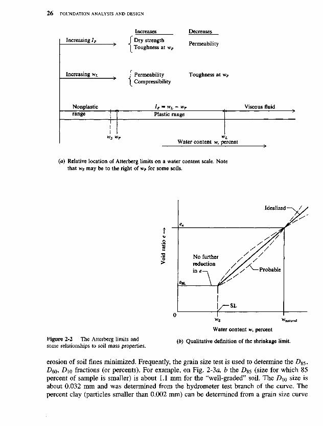
Figure 2-2 The Atterberg limits andsome relationships to soil mass properties.

erosion of soil fines minimized. Frequently, the grain size test is used to determine the Dg5,D60, Dio fractions (or percents). For example, on Fig. 2-3a, b the D85 (size for which 85percent of sample is smaller) is about 1.1 mm for the "well-graded" soil. The Dio size isabout 0.032 mm and was determined from the hydrometer test branch of the curve. Thepercent clay (particles smaller than 0.002 mm) can be determined from a grain size curve

Water content w, percent

(b) Qualitative definition of the shrinkage limit.

Voi

d r

atio

e(a) Relative location of Atterberg limits on a water content scale. Note

that ws may be to the right of wP for some soils.

Idealized

Probable

No furtherreductionin e

Water content w, percent

Viscous fluidPlastic range

Nonplasticrange

Increasing wL

Increasing 1P

Increases

Dry strengthToughness at wP

PermeabilityCompressibility

Toughness at wP

Permeability

Decreases

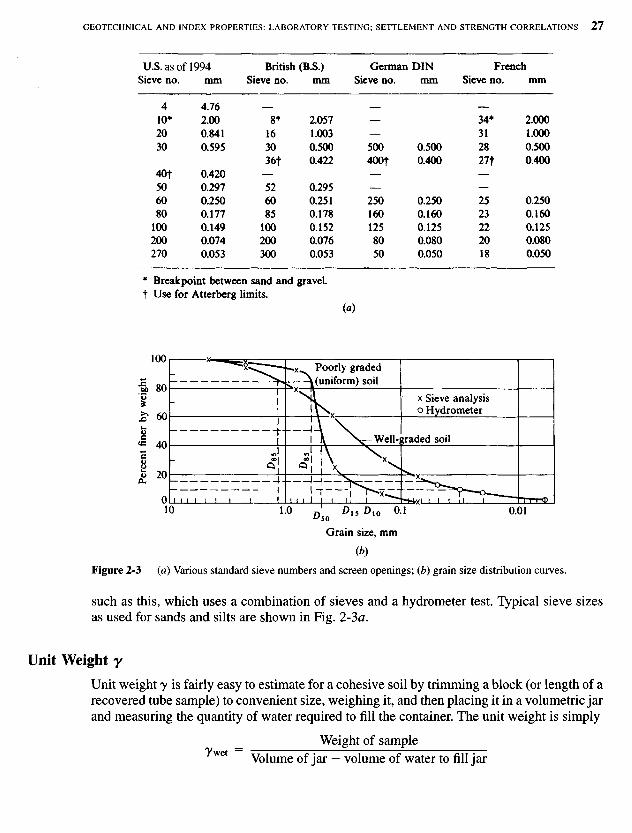
Figure 2-3 (a) Various standard sieve numbers and screen openings; (b) grain size distribution curves.

such as this, which uses a combination of sieves and a hydrometer test. Typical sieve sizesas used for sands and silts are shown in Fig. 2-3a.

Unit Weight y

Unit weight y is fairly easy to estimate for a cohesive soil by trimming a block (or length of arecovered tube sample) to convenient size, weighing it, and then placing it in a volumetric jarand measuring the quantity of water required to fill the container. The unit weight is simply

_ Weight of sampleVolume of jar - volume of water to fill jar

Grain size, mm

Per

cent

fin

er b

y w

eigh

t

U.S. as of 1994Sieve no.

410*2030

4Of506080

100200270

mm

4.762.000.8410.595

0.4200.2970.2500.1770.1490.0740.053

British (B.S.)Sieve no.

8*163036t

526085

100200300

mm

2.0571.0030.5000.422

0.2950.2510.1780.1520.0760.053

German DINSieve no.

50040Ot

2501601258050

mm

0.5000.400

0.2500.1600.1250.0800.050

FrenchSieve no.

34*312827f

2523222018

mm

2.0001.0000.5000.400

0.2500.1600.1250.0800.050

Breakpoint between sand and gravel.Use for Atterberg limits.

(a)

Poorly graded(uniform) soil

Sieve analysisHydrometer

Well-graded soil

If the work is done rapidly so that the sample does not have time to absorb any of the addedwater a very reliable value can be obtained. The average of several trials should be used ifpossible.

The unit weight of cohesionless samples is very difficult (and costly) to determine. Esti-mated values as outlined in Chap. 3 are often used. Where more accurate values are necessary,freezing and injection methods are sometimes used; that is, a zone is frozen or injected with ahardening agent so that a somewhat undisturbed block can be removed to be treated similarlyas for the cohesive sample above. Where only the unit weight is required, good results can beobtained by recovering a sample with a piston sampler (described in Chap. 3). With a knownvolume initially recovered, later disturbance is of no consequence, and we have

_ Weight of sample recoveredet Initial volume of piston sample

The unit weight is necessary to compute the in situ overburden pressure po used to es-timate OCR and is necessary in the computation of consolidation settlements of Chap. 5.It is also used to compute lateral pressures against soil-retaining structures and to estimateskin resistance for pile foundations. In cohesionless materials the angle of internal friction<f> depends on the unit weight and a variation of only 1 or 2 kN/m3 may have a substantialinfluence on this parameter.

Relative Density Dr

Relative density is sometimes used to describe the state condition in cohesionless soils. Rel-ative density is defined in terms of natural, maximum, and minimum void ratios e as

Dr = *max_~ €n (2-15)^max ^min

It can also be defined in terms of natural (in situ), maximum, and minimum unit weight y as

Dr = ( 7n ~ 7min V ^ ) (2-16)\7max - y m i n / V Y* /

The relative density test can be made on gravelly soils if the (—) No. 200 sieve (0.074 mm)material is less than 8 percent and for sand/ soils if the fines are not more than about 12percent according to Holtz (1973).

The relative density Dr is commonly used to identify potential liquefaction under earth-quake or other shock-type loadings [Seed and Idriss (1971)]; however, at present a somewhatmore direct procedure is used [Seed et al. (1985)]. It may also be used to estimate strength(Fig. 2-30).

It is the author's opinion that the Dr test is not of much value since it is difficult to obtainmaximum and minimum unit weight values within a range of about ±0.5 kN/m3. The averagemaximum value is about this amount under (say 20.0 kN/m3 - 0.5) and the minimum aboutthis over (say, 15.0 kN/m3 + 0.5). The definition is for the maximum and minimum values,but average values are usually used. This value range together with the uncertainty in obtain-ing the in situ value can give a potential range in computed Dr of up to 30 to 40 percent (0.3to 0.4). Chapter 3 gives the common methods of estimating the in situ value of Dr. A simple

laboratory procedure is given in Bowles (1992) (experiment 18) either to compute Dr or toobtain a unit weight for quality control.

Specific Gravity Gs

The specific gravity of the soil grains is of some value in computing the void ratio when theunit weight and water content are known. The test is of moderate difficulty with the majorsource of error deriving from the presence of entrapped air in the soil sample. Since G5 doesnot vary widely for most soils, the values indicated here are commonly estimated withoutperforming a test.

Soil G5

Gravel 2.65-2.68Sand 2.65-2.68Silt, inorganic 2.62-2.68Clay, organic 2.58-2.65Clay, inorganic 2.68-2.75

A value of Gs = 2.67 is commonly used for cohesionless soils and a value of 2.70 for inor-ganic clay. Where any uncertainty exists of a reliable value of G5, one should perform a teston a minimum of three small representative samples and average the results. Values of G5 ashigh as 3.0 and as low as 2.3 to 2.4 are not uncommon.

Shrinkage Limit Ws

This is one of the Atterberg limit tests that is sometimes done. The shrinkage limit is qualita-tively illustrated in Fig. 2-2b. It has some value in estimating the probability of expansive soilproblems. Whereas a low value of Ws indicates that only a little increase in water content canstart a volume change, the test does not quantify the amount of AV. The problem of makingsome kind of estimate of the amount of soil expansion is considered in Sec. 7-9.4.

2-6 SOIL CLASSIFICATION METHODSIN FOUNDATION DESIGN

It is necessary for the foundation engineer to classify the site soils for use as a foundation forseveral reasons:

1. To be able to use the database of others in predicting foundation performance.2. To build one's own local database of successes (or any failures).3. To maintain a permanent record that can be understood by others should problems later

develop and outside parties be required to investigate the original design.4. To be able to contribute to the general body of knowledge in common terminology via

journal papers or conference presentations. After all, if one is to partake in the contributionsof others, one should be making contributions to the general knowledge base and not bejust a "taker."

The Unified Soil Classification System (USCS) of Table 2-1 is much used in foundationwork. A version of this system has been standardized by ASTM as D 2487 (in Volume 04.08:Soil and Rock; Dimension Stone; Geosynthetics). The standardized version is similar to theoriginal USCS as given by Casagrande (1948) but with specified percentages of sand orgravel passing specific sieves being used to give the "visual description" of the soil. Theoriginal Casagrande USCS only classified the soil using the symbols shown in Table 2-1(GP, GW, SM, SP, CL, CH, etc.), based on the indicated percentages passing the No. 4 andNo. 200 sieves and the plasticity data. The author has always suggested a visual descriptionsupplement such as the following:

Soil data available Soil description (using Table 2-1)

Sand, Cu = 7; Cc = 1.3, 95% passing No. Well-graded, brown sand with a trace of4 sieve, brown color gravel, SW

Gravel, 45% passes No. 4, 25% passes No. Tan clayey gravel with sand, GC200; wL = 42, wP = 22, tan color

70% passes No. 4 and 18% passes No. 200 Organic gravelly, clayey sand, SCsieve; wL = 56; wP = 24. Sample is firmand dark in color with a distinct odor

It is evident in this table that terms "trace" and "with" are somewhat subjective. Thesoil color, such as "blue clay," "gray clay," etc., is particularly useful in soil classification.In many areas the color—particularly of cohesive soils—is an indication of the presence of the

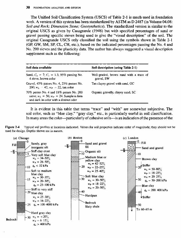
Figure 2-4 Typical soil profiles at locations indicated. Values for soil properties indicate order of magnitude; they should not beused for design. Depths shown are in meters.

(a) Chicago (b) Boston (c) London

Sandy, grayinorganic siltStiff clay crustVery soft blue clay

Soft to mediumblue clay

Stiff to very stiffblue clay

Hard gray clay

Bedrock

Sand and gravelfill

Organic silt

Medium blue oryellow clay

Soft blue clay

Hardpan

BedrockSlaty shale

Fill

Sand and gravel

Brown clay

Stiffer

Blue clay

Stiffer

same soil stratum as found elsewhere. For example the "soft blue clay" on the soil profile ofFig. 2-4 for Chicago has about the same properties at any site in the Chicago area.

In foundation work the terms loose, medium, and dense, as shown in Table 3-4, and consis-tency descriptions such as soft, stiff, very stiff, etc., as shown in Table 3-5, are also commonlyused in foundation soil classification. Clearly, all of these descriptive terms are of great useto the local geotechnical engineer but are somewhat subjective. That is, there could easily besome debate over what is a "medium" versus a "dense" sand, for example.

The D 2487 standard removed some of the subjectiveness of the classification and requiresthe following terminology:

< 15% is sand or gravel use name (organic clay, silt, etc.)

15% < x < 30% is sand or gravel describe as clay or silt with sand, or clay

or silt with gravel

> 30% is sand or gravel describe as sandy clay, silty clay, or gravelly

clay, gravelly silt

The gravel or sand classification is based on the percentage retained on the No. 4 (gravel)sieve or passing the No. 4 and retained on the No. 200 (sand) sieves. This explanation is onlypartial, as the new standard is too lengthy for the purpose of this textbook to be presented indetail.

Although not stated in D 2487, the standard is devised for using a computer program3

to classify the soil. Further, not all geotechnical engineers directly use the ASTM standard,particularly if their practice has a history of success using the original USC system.

General Comments on Using Table 2-1

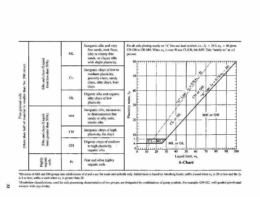
1. When the WL-IP intersection is very close to the "A" or WL = 50% line, use dual symbolssuch as SC-SM, CL-ML, organic OL-OH, etc. to indicate the soil is borderline.

2. If the WL-IP intersection is above the "U" line one should carefully check that the testsand data reduction are correctly done. It may require redoing the limits tests as a check.The reason for this caution is that this line represents the upper limit of real soils so faranalyzed.

Peat and Organic Soils

Strictly, peat is not a soil but rather an organic deposit of rotting wood from trees, plants,and mosses. If the deposit is primarily composed of moss, it may be termed a sphagnumpeat. If the deposit has been somewhat contaminated with soil particles (silt, clay, sand) itmay be named for the soil particles present as peaty silt, peaty sand, peaty clay, and so on. Ifthe soil contamination is substantial (in a relative sense) the soil is more likely to be termed an

3A compiled computer program for use with D 2487 (along with several others) is available with the laboratorytext Engineering Properties of Soils and Their Measurement, 4th ed., (1992), McGraw-Hill Book Company, NewYork, NY 10020; TeL: (212) 512-2012.

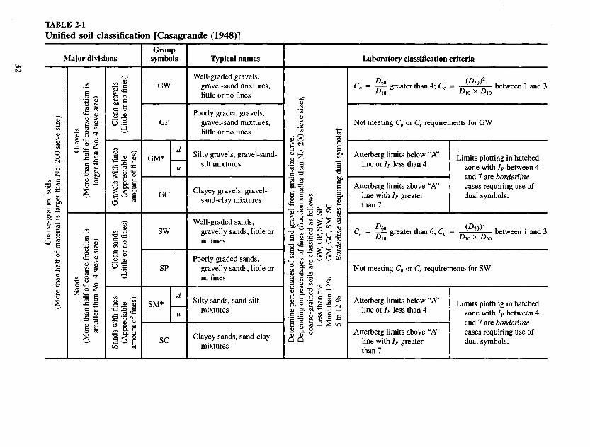
TABLE 2-1

Unified soil classification [Casagrande (1948)]

Laboratory classification criteriaTypical namesGroup

symbolsMajor divisions

Not meeting Cu or Cc requirements for GW

Cu = ^ greater than 4; Cc = JD3°\ between 1 and 3Dio ^10 X ^MO

Limits plotting in hatchedzone with IP between 4and 7 are borderlinecases requiring use ofdual symbols.

Atterberg limits below "A"line or IP less than 4

Atterberg limits above "A"line with IP greaterthan 7

Cu = TT- greater than 6; Cc = _ ^ between 1 and 3

Not meeting Cu or Cc requirements for SW

Limits plotting in hatchedzone with Ip between 4and 7 are borderlinecases requiring use ofdual symbols.

Atterberg limits below "A"line or IP less than 4

Atterberg limits above "A"line with IP greaterthan 7

Well-graded gravels,gravel-sand mixtures,little or no fines

Poorly graded gravels,gravel-sand mixtures,little or no fines

Silty gravels, gravel-sand-silt mixtures

Clayey gravels, gravel-sand-clay mixtures

Well-graded sands,gravelly sands, little orno fines

Poorly graded sands,gravelly sands, little orno fines

Silty sands, sand-siltmixtures

Clayey sands, sand-claymixtures

GW

GP

GM

GC

SW

SP

SM

SC

d

u

d

u

*Division of GM and SM groups into subdivisions of d and u are for roads and airfields only. Subdivision is based on Atterberg limits; suffix d used when Wi is 28 or less and the Ipis 6 or less; suffix u used when Wi is greater than 28.

!Borderline classifications, used for soils possessing characteristics of two groups, are designated by combinations of group symbols. For example: GW-GC, well-graded gravel-sandmixture with clay binder.

Inorganic silts and veryfine sands, rock flour,silty or clayey finesands, or clayey siltswith slight plasticity

Inorganic clays of low tomedium plasticity,gravelly clays, sandyclays, silty clays, leanclays

Organic silts and organicsilty clays of lowplasticity

Inorganic silts, micaceousor diatomaceous finesandy or silty soils,elastic silts

Inorganic clays of highplasticity, fat clays

Organic clays of mediumto high plasticity,organic silts

Peat and other highlyorganic soils

ML

CL

OL

MH

CH

OH

Pt

Liquid limit, wL

A-Chart

For all soils plotting nearly on "A" line use dual symbols, i.e., Ip = 29.5, WL = 60 gives

CH-OH or CH-MH. When wL is near 50 use CL/CH, ML/MH. Take "nearly on" as ±2

percent.

organic soil. Generally a "peat" deposit is classified as such from visual inspection of therecovered samples.

There have been a number of attempts to quantify various engineering properties of peat(or peaty) deposits; however, it is usually necessary to consider the properties of each site.Several engineering properties such as unit weight, compressibility, and permeability will beheavily dependent on the type, relative quantity, and degree of decomposition (state) of theorganic material present. Several recent references have attempted to address some of theseproblems:

Landva and Pheeney (1980)Berry and Vickers (1975)Edil and Dhowian (1981)Loetal. (1990)Fox etal. (1992)Stinnette (1992)

Organic soils are defined as soil deposits that contain a mixture of soil particles and or-ganic (peat) matter. They may be identified by observation of peat-type materials, a dark color,and/or a woody odor. ASTM (D 2487 Section 11.3.2) currently suggests that the organic clas-sification (OL, OH shown on the "A" chart of Table 2-1) be obtained by performing the liquidlimit on the natural soil, then oven-drying the sample overnight and performing a second liq-uid limit test on the oven-dry material. If the liquid limit test after oven drying is less than 75percent of that obtained from the undried soil, the soil is "organic." Oven drying of organicsoils requires special procedures as given in ASTM D 2974.

After performing the liquid and plastic limits, one classifies an organic soil using the "A"chart of Table 2-1. The soil may be either an organic silt OL, OH, or an organic clay OL, OHdepending on the liquid limit Wp and plasticity index Ip and where these values plot on the"A" chart. It is necessary to use both the qualifier "organic silt" or "organic clay" and thesymbol OL or OH.

Approximate Field Procedures for Soil Identification

It is sometimes useful to be able to make a rapid field identification of the site soil for somepurpose. This can be done approximately as follows:

1. Differentiate gravel and sand by visual inspection.2. Differentiate fine sand and silt by placing a spoonful of the soil in a deep jar (or test tube)

and shaking it to make a suspension. Sand settles out in \\ minutes or less whereas siltmay take 5 or more minutes. This test may also be used for clay, which takes usually morethan 10 minutes. The relative quantities of materials can be obtained by observing thedepths of the several materials in the bottom sediment.

3. Differentiate between silt and clay as follows:a. Clay lumps are more difficult to crush using the fingers than silt.b. Moisten a spot on the soil lump and rub your finger across it. If it is smooth it is clay;

if marginally streaked it is clay with silt; if rough it is silt.

c. Form a plastic ball of the soil material and shake it horizontally by jarring your hand.If the material becomes shiny from water coming to the surface it is silt.

4. Differentiate between organic and inorganic soils by visual inspection for organic materialor a smell test for wood or plant decay odor.

2-7 SOIL MATERIAL CLASSIFICATION TERMS

The soil classification terms shown in Table 2-1 are widely used in classification. A numberof other terms are used both by engineers and construction personnel, or tend to be localized.A few of these terms will be defined here as a reader convenience.

Bedrock

This is a common name for the parent rock, but generally implies a rock formation at a depth inthe ground on which a structure may be founded. All other rocks and soils are derived from theoriginal bedrock formed from cooling of molten magma and subsequent weathering. Bedrockextends substantially downward to molten magma and laterally in substantial dimensions.The lowermost part is igneous rock formed by cooling of the molten magma. This may, ormay not, be overlain by one or more layers of more recently formed sedimentary rocks suchas sandstone, limestone, shale, etc. formed from indurated soil deposits. The interface layersbetween igneous and sedimentary rocks may be metamorphic rocks formed from intense heatand pressure acting on the sedimentary rocks. In some cases a bedding rock layer—usuallysedimentary in origin—may overlie a soil deposit. In earthquake areas the parent rock maybe much fractured. Past areal uplifts may have produced zones of highly fragmented parentrock at the bedrock level.

Considering these factors, one might say that generally, bedrock makes a satisfactory foun-dation, but good engineering practice requires that one check the geological history of the site.In this context it is fairly common to refer to the bedrock with respect to the geological ageof estimated formation as Cambrian, pre-Cambrian, etc.

Boulders

Boulders are large pieces of rock fractured from the parent material or blown out of volcanos(called bombs in this case). They may have volumes ranging from about \ to 8 or 10 m3 andweigh from about one-half to several hundred tonnes. They may create disposal or excavationproblems on or near the ground surface and problems in soil exploration or pile driving atgreater depths when suspended in the soil matrix, as in glacial till. Large ones may be suitableto found pile or caissons on; however, size determination may be difficult, and placing a largeload on a small suspended boulder may be disastrous.

Gravels and Smaller

Rock fragments smaller than boulders grade into cobbles, pebbles, gravel, sand, silt, andcolloids in order of size as shown on Table 2-2. Crushed stone is gravel manufactured bycrushing rock fragments from boulders or obtained from suitable rock formations by min-ing. Bank-run gravel is a common term for naturally occurring gravel lenses deposited along

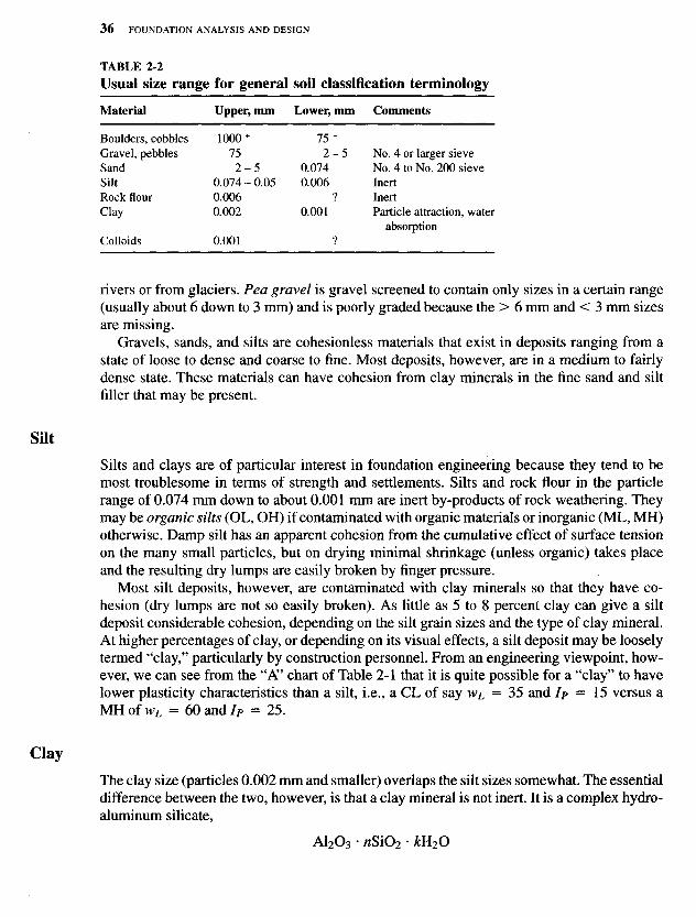
TABLE 2-2

Usual size range for general soil classification terminology

Material Upper, mm Lower, mm Comments

Boulders, cobbles 1000+ 75 ~Gravel, pebbles 75 2 - 5 No. 4 or larger sieveSand 2 - 5 0.074 No. 4 to No. 200 sieveSilt 0.074-0.05 0.006 InertRock flour 0.006 ? InertClay 0.002 0.001 Particle attraction, water

absorptionColloids 0.001 ?

rivers or from glaciers. Pea gravel is gravel screened to contain only sizes in a certain range(usually about 6 down to 3 mm) and is poorly graded because the > 6 mm and < 3 mm sizesare missing.

Gravels, sands, and silts are cohesionless materials that exist in deposits ranging from astate of loose to dense and coarse to fine. Most deposits, however, are in a medium to fairlydense state. These materials can have cohesion from clay minerals in the fine sand and siltfiller that may be present.

Silt

Silts and clays are of particular interest in foundation engineering because they tend to bemost troublesome in terms of strength and settlements. Silts and rock flour in the particlerange of 0.074 mm down to about 0.001 mm are inert by-products of rock weathering. Theymay be organic silts (OL, OH) if contaminated with organic materials or inorganic (ML, MH)otherwise. Damp silt has an apparent cohesion from the cumulative effect of surface tensionon the many small particles, but on drying minimal shrinkage (unless organic) takes placeand the resulting dry lumps are easily broken by finger pressure.

Most silt deposits, however, are contaminated with clay minerals so that they have co-hesion (dry lumps are not so easily broken). As little as 5 to 8 percent clay can give a siltdeposit considerable cohesion, depending on the silt grain sizes and the type of clay mineral.At higher percentages of clay, or depending on its visual effects, a silt deposit may be looselytermed "clay," particularly by construction personnel. From an engineering viewpoint, how-ever, we can see from the "A" chart of Table 2-1 that it is quite possible for a "clay" to havelower plasticity characteristics than a silt, i.e., a CL of say Wi = 35 and Ip = 15 versus aMHofH>L = 60and//> = 25.

Clay

The clay size (particles 0.002 mm and smaller) overlaps the silt sizes somewhat. The essentialdifference between the two, however, is that a clay mineral is not inert. It is a complex hydro-aluminum silicate,

where n and k are numerical values of attached molecules and vary for the same mass. Theclay mineral has a high affinity for water, and individual particles may absorb 10O+ times theparticle volume. The presence or absence (during drying) of water can produce very largevolume and strength changes. Clay particles also have very strong interparticle attractiveforces, which account in part for the very high strength of a dry lump (or a clay brick). Waterabsorption and interparticle attraction collectively give the activity and cohesion to clay (andto soils containing clay minerals).

The three principal identified clay minerals can be characterized in terms of activity andplasticity:

Montmorillonite (or smectite)—Most active of the identified minerals. The activity, interms of affinity for water and swell, makes this material ideal for use as a drilling mud insoil exploration and in drilling oil wells. It is also commonly injected into the ground aroundbasement walls as a water barrier (swells to close off water flow paths) to stop basementleaks. It is also blended with local site material to produce water barriers to protect the GWTfrom sanitary landfill drainage. The Ip of an uncontaminated montmorillonite is 15O+.

Illite—A clay mineral that is intermediate in terms of activity. The Ip of a pure illite rangesfrom about 30 to 50.

Kaolinite—The clay mineral with the least activity. This material is commonly used in theceramic industry and for brick manufacture. It is sometimes used as an absorbent for stomachmedicine. The Ip of a pure kaolinite ranges from about 15 to 20.

Montmorillonite deposits are found mostly in arid and semiarid regions. All clay miner-als weather into less active materials, e.g., to illite and then to kaolinite. As a consequencemost "clay" deposits contain several different clay minerals. Only deposits of relatively pureclay have commercial value. Most of the remainder represent engineering problems. For ex-ample, in temperate regions it is not unusual for deposits to contain substantial amounts ofmontmorillonite or even lenses of nearly pure material.

Clay deposits with certain characteristics are common to certain areas and have beennamed for the location. For example the "Chicago blue clay," "Boston blue clay," "Londonclay" shown in Fig. 2-4 are common for those areas. Leda clay is found in large areas ofOttawa Province in Canada and has been extensively studied and reported in the CanadianGeotechnical Journal.

Local Terminology

The following are terms describing soil deposits that the geotechnical engineer may en-counter. Familiarity with their meaning is useful.

a. Adobe. A clayey material found notably in the Southwest.

b. Caliche. A conglomeration of sand, gravel, silt, and clay bonded by carbonates and usuallyfound in arid areas.

c. Glacial till or glacial drift. A mixture of material that may include sand, gravel, silt, andclay deposited by glacial action. Large areas of central North America, much of Canada,northern Europe, the Scandinavian countries, and the British Isles are overlain with glacial

till or drift. The term drift is usually used to describe any materials laid down by theglacier. The term till is usually used to describe materials precipitated out of the ice, butthe user must check the context of usage, as the terms are used interchangeably. Morainesare glacial deposits scraped or pushed ahead (terminal), or alongside the glacier (lateral).These deposits may also be called ground moraines if formed by seasonal advances andretreats of a glacier. The Chicago, Illinois, area, for example, is underlain by three identi-fiable ground moraines.

d. Gumbo. A clayey or loamy material that is very sticky when wet.e. Hardpan. This term may be used to describe caliche or any other dense, firm deposits that

are excavated with difficulty./ Loam. A mixture of sand, clay, silt; an organic material; also called topsoil.

g. Loess. A uniform deposit of silt-sized material formed by wind action. Often found alongthe Mississippi River, where rising damp air affects the density of the air transporting thematerial, causing it to deposit out. Such deposits are not, however, confined to the Mis-sissippi Valley. Large areas of Nebraska, Iowa, Illinois, and Indiana are covered by loess.Large areas of China, Siberia, and southeastern Europe (southern Russia and Ukraine)and some areas of western Europe are covered with loess. Loess is considered to be atransported soil.

h. Muck. A thin watery mixture of soil and organic material.i. Alluvial deposits. Soil deposits formed by sedimentation of soil particles from flowing

water; may be lake deposits if found in lake beds; deltas at the mouths of rivers; marinedeposits if deposited through saltwater along and on the continental shelf. Alluvial depositsare found worldwide. For example, New Orleans, Louisiana, is located on a delta deposit.The low countries of The Netherlands and Belgium are founded on alluvial deposits fromthe Rhine River exiting into the North Sea. Lake deposits are found around and beneaththe Great Lakes area of the United States and Canada. Large areas of the Atlantic coastalplain, including the eastern parts of Maryland, Virginia, the Carolinas, the eastern part andmost of south Georgia, Florida, south Alabama, Mississippi, Louisiana, and Texas consistof alluvial deposits. These deposits formed when much of this land was covered with theseas. Later upheavals such as that forming the Appalachian mountains have exposed thismaterial. Alluvial deposits are fine-grained materials, generally silt-clay mixtures, silts,or clays and fine to medium sands. If the sand and clay layers alternate, the deposit is avarved clay. Alluvial deposits are usually soft and highly compressible.

j . Black cotton soils. Semitropical soils found in areas where the annual rainfall is 500 to750 mm. They range from black to dark gray. They tend to become hard with very largecracks (large-volume-change soils) when dry and very soft and spongy when wet. Thesesoils are found in large areas of Australia, India, and southeast Asia.

k. Late rites. Another name for residual soils found in tropical areas with heavy rainfalls.These soils are typically bright red to reddish brown in color. They are formed initially byweathering of igneous rocks, with the subsequent leaching and chemical erosion due tothe high temperature and rainfall. Collodial silica is leached downward, leaving behindaluminum and iron. The latter becomes highly oxidized, and both are relatively insolublein the high-pH environment (greater than 7). Well-developed laterite soils are generallyporous and relatively incompressible. Lateritic soils are found in Alabama, Georgia, South

Carolina, many of the Caribbean islands, large areas of Central and South America, andparts of India, southeast Asia, and Africa.

/. Saprolite. Still another name for residual soils formed from weathered rock. These depositsare often characterized by a particle range from dust to large angular stones. Check thecontext of use to see if the term is being used to describe laterite soils or residual soils.

m. Shale. A fine-grained, sedimentary rock composed essentially of compressed and/or ce-mented clay particles. It is usually laminated, owing to the general parallel orientation ofthe clay particles, as distinct from claystone or siltstone, which are indurated deposits ofrandom particle orientation. According to Underwood (1967), shale is the predominantsedimentary rock in the Earth's crust. It is often misclassified; layered sedimentary rocksof quartz or argillaceous materials such as argillite are not shale. Shale may be grouped as(1) compaction shale and (2) cemented (rock) shale. The compaction shale is a transitionmaterial from soil to rock and can be excavated with modern earth excavation equipment.Cemented shale can sometimes be excavated with excavation equipment but more gener-ally requires blasting. Compaction shales have been formed by consolidation pressure andvery little cementing action. Cemented shales are formed by a combination of cementingand consolidation pressure. They tend to ring when struck by a hammer, do not slake inwater, and have the general characteristics of good rock. Compaction shales, being of anintermediate quality, will generally soften and expand upon exposure to weathering whenexcavations are opened. Shales may be clayey, silty, or sandy if the composition is pre-dominantly clay, silt, or sand, respectively. Dry unit weight of shale may range from about12.5 kN/m3 for poor-quality compaction shale to 25.1 kN/m3 for high-quality cementedshale.

2-8 IN SITU STRESSES AND K0 CONDITIONS

Any new foundation load—either an increase (+) from a foundation or a decrease ( - ) froman excavation—imposes new stresses on the existing state of "locked in" stresses in the foun-dation soil mass. The mass response is heavily dependent on the previous stress history, soone of the most important considerations in foundation engineering is to ascertain this stressimprint. The term imprint is used since any previously applied stresses that are larger thanthose currently existing have been locked into the soil structure and will affect subsequentstress-response behavior until a new set of larger stresses are applied to produce a new im-print. Of course, the stress history is lost in varying degrees (or completely) when the soilis excavated/remolded or otherwise disturbed as in sample recovery. Factors contributing toloss of stress history during sampling are outlined in Sec. 3-5.

In situ, the vertical stresses act on a horizontal plane at some depth z. These can be com-puted in any general case as the sum of contributions from n strata of unit weight yr andthickness Zi as

n

Po = ^ JiZt (a)i = l

The unit weight for a homogeneous stratum is of the general form

(b)

with the constants A\, A2, and m determined by obtaining weight values at several depths zand plotting a best-fit curve. In practice, at least for reasonable depths on the order of 5 to10 meters, a constant value is often (incorrectly) used. An alternative is to divide the depositinto several "layers" and use a constant unit weight y,- for each as in Eq. (a).

In most cases involving geotechnical work, the effective stress p'o is required so that belowthe GWT one uses the effective soil unit weight computed as

y' = 7 sat - Tw (c)

For any soil deposit formation the plan area is usually rather large and the depth continuallyincreases until either deposition or interior weathering stops. This change produces a gradualvertical compression of the soil at any given depth; similarly, y increases under compressionso that in nearly all cases unit weight y — f (depth). Since the lateral dimension is largethere is little reason for significant lateral compression to occur. For this reason it is logical toexpect that vertical locked-in effective stresses p'o would be larger than the effective lateralstresses a'h at the same point. We may define the ratio of the horizontal to vertical stresses as

K = ^ (d)Po

which is valid for any depth z at any time.Over geological time the stresses in a soil mass at a particular level stabilize into a steady

state and strains become zero. When this occurs the vertical and lateral stresses become prin-cipal stresses acting on principal planes.4 This effective stress state is termed the at-rest orK0 condition with K0 defined as

Ko = ^t (2-17)Po

Figure 2-5 qualitatively illustrates the range of K0 and the relationship of po and ah in anyhomogeneous soil. Note the qualitative curves for preconsolidation in the upper zone of somesoil from shrinkage/chemical effects. This figure (see also Fig. 2-45) clearly illustrates theanisotropic (av ¥^ ah) stress state in a soil mass.

Because of the sampling limitations given in Sec. 3-5 it is an extremely difficult task tomeasure K0 either in the laboratory or in situ. A number of laboratory and field methodsare cited by Abdelhamid and Krizek (1976); however, from practical limitations the directsimple shear device (Fig. 2-266) is the simplest for direct laboratory measurements. Fieldmethods will be considered in the next chapter, but note that they are very costly for theslight improvement—in most cases—over using one of the simple estimates following. Inthese equations use the effective angle of internal friction </>' and not the total stress value.

Jaky (1948) presented a derived equation for K0 that is applicable to both soil and agri-cultural grains (such as corn, wheat, oats, etc.) as

4Stresses acting on planes on which no strains or shearing stresses exist are defined as principal stresses, and theplanes are principal planes.

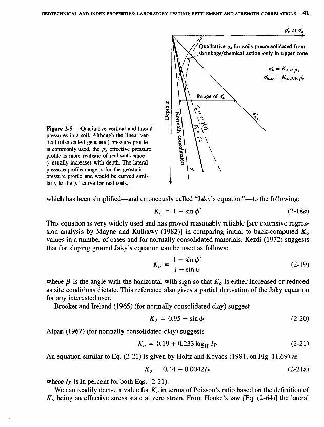
Figure 2-5 Qualitative vertical and lateralpressures in a soil. Although the linear ver-tical (also called geostatic) pressure profileis commonly used, the p"0 effective pressureprofile is more realistic of real soils sincey usually increases with depth. The lateralpressure profile range is for the geostaticpressure profile and would be curved simi-larly to the p"o curve for real soils.

which has been simplified—and erroneously called "Jaky's equation"—to the following:

K0 = l-sin</>' (2-18a)

This equation is very widely used and has proved reasonably reliable [see extensive regres-sion analysis by Mayne and Kulhawy (1982)] in comparing initial to back-computed K0

values in a number of cases and for normally consolidated materials. Kezdi (1972) suggeststhat for sloping ground Jaky's equation can be used as follows:

_ l - s i n < f r 'Ko ~ l + sin/3 ( 2 " 1 9 )

where /3 is the angle with the horizontal with sign so that K0 is either increased or reducedas site conditions dictate. This reference also gives a partial derivation of the Jaky equationfor any interested user.

Brooker and Ireland (1965) (for normally consolidated clay) suggest

K0 = 0 . 9 5 - s i n 0 ' (2-20)

Alpan (1967) (for normally consolidated clay) suggests

K0 = 0.19 H- 0.233 log10 Ip (2-21)

An equation similar to Eq. (2-21) is given by Holtz and Kovacs (1981, on Fig. 11.69) as

K0 = 0.44 + 0.0042/p (2-2Ia)

where Ip is in percent for both Eqs. (2-21).We can readily derive a value for K0 in terms of Poisson's ratio based on the definition of

K0 being an effective stress state at zero strain. From Hooke's law [Eq. (2-64)] the lateral

Dep

th z

Qualitative <rh for soils preconsolidated fromshrinkage/chemical action only in upper zone

Range of

strain in terms of the effective horizontal (JC, z) and vertical (y) stresses is

€x = 0 = -=r(crx - }i(Ty - pat) = ez

With (Tx = az = K0(Ty we obtain, on substitution into the preceding and canceling,

K0 = J ^ - (2-22)

For a cohesionless soil /JL is often assumed as 0.3 to 0.4, which gives K0 = 0.43 to 0.67, witha value of 0.5 often used.

It is extremely difficult to obtain a reliable estimate of K0 in a normally consolidated soil,and even more so in overconsolidated soils (OCR > 1). A number of empirical equationsbased on various correlations have been given in the literature [see the large number withcited references given by Mesri and Hay at (1993)]. Several of the more promising ones are:

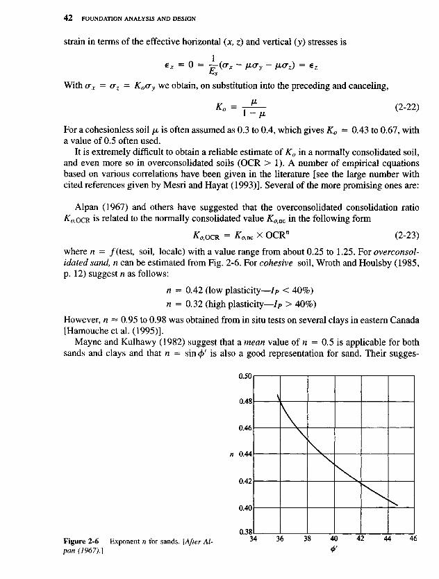
Alpan (1967) and others have suggested that the overconsolidated consolidation ratio^aOCR is related to the normally consolidated value Ko>nc in the following form

^ , O C R = Ko,nc X OCR" (2-23)

where n = /(test, soil, locale) with a value range from about 0.25 to 1.25. For overconsol-idated sand, n can be estimated from Fig. 2-6. For cohesive soil, Wroth and Houlsby (1985,p. 12) suggest n as follows:

n = 0.42 (low plasticity—1P < 40%)

n = 0.32 (high plasticity—IP > 40%)

However, n ~ 0.95 to 0.98 was obtained from in situ tests on several clays in eastern Canada[Hamouche et al. (1995)].

Mayne and Kulhawy (1982) suggest that a mean value of n = 0.5 is applicable for bothsands and clays and that n = sin</>' is also a good representation for sand. Their sugges-

Figure 2-6 Exponent n for sands. [After Al-pan (1967).]

n

<t>'

tions are based on a semi-statistical analysis of a very large number of soils reported in theliterature.

The exponent n for clays was also given by Alpan (1967) in graph format and uses theplasticity index IP (in percent). The author modified the equation shown on that graph toobtain

n = 0.54 X 1(T 7 ^ 8 1 (2-24)

And, as previously suggested (for sands), we can use

n = SiTi(I)' (2'7Aa)

The n-values previously given by Wroth and Houlsby (1985) can be obtained from Eq.(2-24) using an average "low plasticity" Ip of about 30 (n = 0.42) and a "high plasticity" Ipof about 65 percent (n = 0.32).

Mayne (1984) suggests that the range of valid values for the overconsolidated KOOCR usingEq. (2-23) for cohesive soils depends on the normalized strength ratio sjp'c being less than4—at least for noncemented and intact clays. Therefore, this ratio is indirectly used for Eq.(2-23), but it will be directly used in the following section.

2-8.1 Overconsolidated K0 Conditions

The equation for the overconsolidation ratio (OCR) was given in Sec. 2-4, and it is repeatedhere for convenience:

OCR = ^- (2-13)Po

In this equation the current overburden pressure p'o can be computed reasonably well, butthe value of the preconsolidation pressure p'c is at best an estimate, making a reliable compu-tation for OCR difficult. The only method at present that is reasonably reliable is to use theconsolidation test described in Sec. 2-10 to obtain p'c. The alternative, which is likely to beless precise, is to use some kind of in situ testing to obtain the sjp • ratio (where / = o or c)and use a chart such as Fig. 2-36 given later in Sec. 2-11.9.

There are a number of empirical correlations for OCR based on the su/p'o ratio (theundrained shear strength, su, divided by the current in situ effective overburden pressure p'o)and on in situ tests that are defined later in Chap. 3. The following were taken from Chang(1991):

For the field vane test:

OCR = 22(sM//7;)fv(/p)-a48

0.08 + 0.55/p

For the cone penetrometer test:

[see Eq. (2-60)]

These two 5-values are then used to compute the OCR as

OCR = (^S1)U3+(UM(SS1)

Section 3-11.1 gives an alternative method to compute the OCR from a cone penetration testusing Eqs. (3-17).

For the flat dilatometer test:

OCR = 0 .24/^ 3 2

In these equations Ip = plasticity index in percentage; qc = cone resistance; po = total(not effective) overburden pressure; Nk = cone factor that is nearly constant at Nk = 12 forOCR < 8; KD = horizontal stress index for the dilatometer. AU of these terms (see Symbollist) are either used later in this chapter or in Chap. 3. There are a number of other equationsgiven by Chang but these tend to summarize his discussion best.

With the value of OCR and the current in situ effective pressure p'o one can use Eq. (2-13)to back-compute the preconsolidation pressure p'c.

An estimate for KOOCK is given by Mayne (1984) based on the analysis of a number ofclay soils reported in the literature. The equation is as follows:

^,OCR = Ko,nc(A + Sjp'o) (2-25)

In this equation note that the ratio su/p'o uses the effective current overburden pressure p'o.The variable A depends on the type of laboratory test used to obtain the sjp'c ratio as follows:

Test A Comments

CAT0UC 0.7 K0 -consolidated—undrained compressionCIUC 0.8 Isotropically consolidatedC^0DSS 1.0 Direct simple shear test

The upper limit of KOtOCR appears to be the passive earth pressure coefficient Kp (definedin Chap. 11), and a number of values reported in the literature range from 1.5 to 1.7. It wouldappear that the upper limit of any normally consolidated soil would be KOjnc < 1.0 since afluid such as water has K0 = 1.0 and no normally consolidated soil would have a value thislarge.

Example 2-2. Compare K0 by the several approximate methods given in this section for both anormally consolidated (nc) clay and for a clay with a known value of OCR = 5.0.

Other data: <f>' = 20° IP = 35% (nc)0' = 25° Ip = 32% (OCR = 5)

Solution. For the normally consolidated case, we may write the following:

1. Use Brooker and Ireland's Eq. (2-20):

Ko,nc = 0.95 - sincf)' = 0.95 - sin20 = 0.61

2. Use Eqs. (2-21):

In the absence of better data, use the average of these as

„ _ 0.61 + 0.55 + 0.59 _

For the overconsolidated case, we calculate as follows:

1. Use Eq. (2-23), but first use Eq. (2-24) to find exponent n:

n = 0.54 X 1(T7^81 -> n = 0.42 for//> = 32%

Now, KO,OCR = Ko,nc X OCR" -^ use Ko>nc = 0.58 just found

KO,OCR = 0.58 X OCR042 = 0.58 X 5042 = 1.14

2. Use Eq. (2-2Aa) for an alternative n:

n = sin<£' = sin 25 = 0.423

KO,OCR = 0.58 x 50423 = 1.15 (vs. 1.14 just computed)

3. Use Eq. (2-25) and assume CIUC testing so A = 0.8. Also estimate a value for sjp'c. For thisuse Eq. (2-59) following:

^ - = 0 . 4 5 ^ [Eq. (2-59)]Po

= 0.45(0.35)° 5 = 0.27 (using nc value for IP)

Substitution into Eq. (2-25) gives

tfo.ocR = 0.58(0.8 + 0.27) = 0.62We can obtain a best estimate using all three values to obtain

1.14+1.15 + 0.62A-̂ OCR = ^ = W.^7

or, since 0.62 is little different from the average nc value of 0.58, we might only use the twovalues of 1.14 and 1.15 to obtain

1.14+1.15A.O>OCR = 2 •

One should use a value of about 1.1, as 1.14 implies more precision than is justified by theseprocedures.

Conventional usage is to call all values K0. For computations such as in this example it is nec-essary to distinguish between the normally consolidated value Ko>nc and the overconsolidated valueK0 OCR as a compact means of identification in equations such as Eqs. (2-23) and (2-25).

////

(2-21):

(2-2Ia):

Next Page