Geotechnical remediation of transportation infrastructures

Retrospective Theses and Dissertations Iowa State University Capstones, Theses andDissertations

2007

Geotechnical remediation of transportationinfrastructures: nondestructive evaluation of bridgesubstructures and stabilization of soft foundationsoilsMohamed Magdi MekkawyIowa State University

Follow this and additional works at: https://lib.dr.iastate.edu/rtd

Part of the Civil Engineering Commons

This Dissertation is brought to you for free and open access by the Iowa State University Capstones, Theses and Dissertations at Iowa State UniversityDigital Repository. It has been accepted for inclusion in Retrospective Theses and Dissertations by an authorized administrator of Iowa State UniversityDigital Repository. For more information, please contact [email protected].

Recommended CitationMekkawy, Mohamed Magdi, "Geotechnical remediation of transportation infrastructures: nondestructive evaluation of bridgesubstructures and stabilization of soft foundation soils" (2007). Retrospective Theses and Dissertations. 15572.https://lib.dr.iastate.edu/rtd/15572

http://lib.dr.iastate.edu/?utm_source=lib.dr.iastate.edu%2Frtd%2F15572&utm_medium=PDF&utm_campaign=PDFCoverPages

http://lib.dr.iastate.edu/?utm_source=lib.dr.iastate.edu%2Frtd%2F15572&utm_medium=PDF&utm_campaign=PDFCoverPages

https://lib.dr.iastate.edu/rtd?utm_source=lib.dr.iastate.edu%2Frtd%2F15572&utm_medium=PDF&utm_campaign=PDFCoverPages

https://lib.dr.iastate.edu/theses?utm_source=lib.dr.iastate.edu%2Frtd%2F15572&utm_medium=PDF&utm_campaign=PDFCoverPages

https://lib.dr.iastate.edu/theses?utm_source=lib.dr.iastate.edu%2Frtd%2F15572&utm_medium=PDF&utm_campaign=PDFCoverPages

https://lib.dr.iastate.edu/rtd?utm_source=lib.dr.iastate.edu%2Frtd%2F15572&utm_medium=PDF&utm_campaign=PDFCoverPages

http://network.bepress.com/hgg/discipline/252?utm_source=lib.dr.iastate.edu%2Frtd%2F15572&utm_medium=PDF&utm_campaign=PDFCoverPages

https://lib.dr.iastate.edu/rtd/15572?utm_source=lib.dr.iastate.edu%2Frtd%2F15572&utm_medium=PDF&utm_campaign=PDFCoverPages

mailto:[email protected]

Geotechnical remediation of transportation infrastructures: nondestructive evaluation of

bridge substructures and stabilization of soft foundation soils by

Mohamed Magdi Mekkawy

A dissertation submitted to the graduate faculty

in partial fulfillment of the requirements for the degree of

DOCTOR OF PHILOSOPHY

Major: Civil Engineering (Geotechnical Engineering)

Program of Study Committee: David J. White, Major Professor

Wayne Klaiber Charles Jahren Chris Williams Igor Beresnev

Iowa State University

Ames, Iowa

2007

Copyright © Mohamed Magdi Mekkawy, 2007. All rights reserved.

UMI Number: 3289374

32893742008

UMI MicroformCopyright

All rights reserved. This microform edition is protected against unauthorized copying under Title 17, United States Code.

ProQuest Information and Learning Company 300 North Zeeb Road

P.O. Box 1346 Ann Arbor, MI 48106-1346

by ProQuest Information and Learning Company.

ii

TABLE OF CO$TE$TS

LIST OF FIGURES .................................................................................................................................... VI

LIST OF TABLES ....................................................................................................................................... X

1. INTRODUCTION .................................................................................................................................... 1

1.1. OVERVIEW .......................................................................................................................................... 1

1.1.1. Performance of Granular Shoulders ...................................................................................... 1 1.1.2. Nondestructive Evaluation of Bridge Substructures .............................................................. 2

1.2. SCOPE AND OBJECTIVES ................................................................................................................. 2

1.2.1. Performance of Granular Shoulders ...................................................................................... 2 1.2.2. Nondestructive Evaluation of Bridge Substructures .............................................................. 3

1.3. DISSERTATION ORGANIZATION ................................................................................................... 3

1.4. REFERENCES ...................................................................................................................................... 4

2. PERFORMANCE PROBLEMS AND STABILIZATION TECHNIQUES FOR GRANULAR SHOULDERS .................................................................................................................................. 5

2.1. ABSTRACT .......................................................................................................................................... 5

2.2. INTRODUCTION ................................................................................................................................. 6

2.3. FIELD OBSERVATIONS ..................................................................................................................... 8

2.4. VEHICLE TIRE-AGGREGATE INTERACTION ............................................................................... 9

2.5. TEST SECTIONS ................................................................................................................................ 10

2.5.1. Test Section No. 1: Polymer Emulsion – Highway 122 Clear Lake, IA ............................. 10 2.5.2. Test Section No. 2: Foamed Asphalt – Highway I-35 ......................................................... 11 2.5.3. Test Section No. 3: Soybean Oil – Highway 18 Rudd, IA .................................................. 12 2.5.4. Test Section No. 4: Portland Cement – 16th St. Ames, IA ................................................... 13 2.5.5. Test Section No. 5: Fly Ash – Highway 34 Batavia, IA ...................................................... 14 2.5.6. Test Section No. 6: Geogrid Stabilization – Highway 218 Nashua, IA ............................... 15

2.6. SUMMARY AND CONCLUSIONS .................................................................................................. 17

iii

2.7. RECOMMENDATIONS ..................................................................................................................... 17

2.7.1. Shoulder Construction ......................................................................................................... 18 2.7.2. Shoulder Reconstruction ...................................................................................................... 18

ACKNOWLEDGMENTS .......................................................................................................................... 18

REFERENCES ........................................................................................................................................... 18

3. MECHANICALLY REINFORCED GRANULAR SHOULDERS ON SOFT SUBGRADE: FULL SCALE FIELD CHARACTERIZATION AND LABORATORY BOX STUDY ....................... 41

3.1. ABSTRACT ........................................................................................................................................ 41

3.2. INTRODUCTION ............................................................................................................................... 42

3.3. BACKGROUND ................................................................................................................................. 43

3.4. FIELD OBSERVATIONS ................................................................................................................... 45

3.5. TEST SECTION: GEOGRID STABILIZATION – HIGHWAY 218 NASHUA, IA......................... 46

3.5.1. Site Description ................................................................................................................... 46 3.5.2. Stabilization of Test Section ................................................................................................ 46 3.5.3. Field Monitoring .................................................................................................................. 47

3.6. LABORATORY BOX STUDY .......................................................................................................... 49

3.6.1. Test Setup ............................................................................................................................ 49 3.6.2. Materials .............................................................................................................................. 50 3.6.3. Test Results .......................................................................................................................... 50

3.6.3.1. Test No. 1 – Control ............................................................................................ 50 3.6.3.2. Test Nos. 2, 3, and 4 – Geogrid1 ......................................................................... 51 3.6.3.3. Test Nos. 5 and 6 – Geogrid2 and Geogrid3 ....................................................... 52 3.6.3.4. Test Nos. 7 and 8 – Woven and Nonwoven Geotextiles ..................................... 53 3.6.3.5. Test No. 9 – Recycled Asphalt Pavement ............................................................ 53 3.6.3.6. Test No. 10 – Class C fly Ash ............................................................................. 54

3.7. SHOULDER DESIGN CHARTS ........................................................................................................ 54



REFERENCES ........................................................................................................................................... 57

iv

4. ASSESSMENT OF PILE DETERIORATION AND RESIDUAL PILE CAPACITY USING NONDESTRUCTIVE STRESS WAVE TECHNIQUES ............................................................. 79

4.1. ABSTRACT ........................................................................................................................................ 79

4.2. INTRODUCTION ............................................................................................................................... 80

4.3. BACKGROUND ................................................................................................................................. 81

4.3.1. Biological Deterioration ...................................................................................................... 81 4.3.1.1 Fungi ..................................................................................................................... 81 4.3.1.2. Bacteria ................................................................................................................ 82 4.3.1.3. Insects .................................................................................................................. 82

4.3.2. Mechanical Deterioration .................................................................................................... 82 4.3.2.1. Abrasion ............................................................................................................... 82 4.3.2.2. Overloading ......................................................................................................... 83 4.3.2.3. Other Mechanical Factors .................................................................................... 83

4.4. FIELD RECONNAISSANCE ............................................................................................................. 83

4.5. LABORATORY TESTING ................................................................................................................ 84

4.5.1. Ultrasonic Stress Wave Test ................................................................................................ 84 4.5.1.1. Background .......................................................................................................... 84 4.5.1.2. Difficulties and Limitations ................................................................................. 85 4.5.1.3. Description of Equipment .................................................................................... 85 4.5.1.4. Image Processing ................................................................................................. 86 4.5.1.5. Test Procedure ..................................................................................................... 87 4.5.1.6. Test Verification and Repeatability ..................................................................... 87 4.5.1.7. Test Results .......................................................................................................... 89

4.5.2. Axial Compression Tests ..................................................................................................... 89 4.5.3. Correlation between Compression and Ultrasonic Stress Wave Tests ................................ 90



REFERENCES ........................................................................................................................................... 91

5. INFLUENCE OF TIMBER PILE DETERIORATION ON LOAD DISTRIBUTION FOR LOW VOLUME BRIDGE SUBSTRUCTURES .................................................................................. 112

5.1. ABSTRACT: ..................................................................................................................................... 112

5.2. INTRODUCTION ............................................................................................................................. 113

v

5.3. BACKGROUND ............................................................................................................................... 114

5.4. STATIC LOAD TESTS..................................................................................................................... 115

5.4.1. Site Description ................................................................................................................. 115 5.4.2. Test Setup and Instrumentation ......................................................................................... 116 5.4.3. Test Results ........................................................................................................................ 118

5.4.3.1. Test No. 1 – Nondestructive Test ...................................................................... 118 5.4.3.2. Test No. 2 – Pile No. 7 Jacked ........................................................................... 119 5.4.3.3. Test No. 3 – Pile 7 Removed ............................................................................. 119 5.4.3.4. Test No. 4 – Pile Nos. 3 and 7 Jacked ............................................................... 120 5.4.3.5. Test No. 5 – Pile No. 3 Removed and Pile No. 7 Jacked ................................... 121 5.4.3.6. Test No. 6 – Pile Nos. 3 and 7 Removed ........................................................... 122 5.4.3.7. Test No. 7 – Pile Nos. 3, 6 and 7 Removed ....................................................... 123 5.4.3.8. Test No. 8 – Pile No. 7 Repaired ....................................................................... 123

5.5. SUMMARY AND CONCLUSIONS ................................................................................................ 124

5.6. FUTURE RESEARCH ...................................................................................................................... 125

ACKNOWLEDGMENTS ........................................................................................................................ 126

REFERENCES ......................................................................................................................................... 126

6. RECOMMENDATIONS AND FUTURE RESEARCH ...................................................................... 140

6.1. Performance of Granular Shoulder ....................................................................................... 140 6.2. Nondestructive Evaluation of Bridge Substructures ............................................................. 140

vi

LIST OF FIGURES

FIG. 2.1 Common granular shoulder problems ................................................................. 26

FIG. 2.2 Shoulder rutting observed at Highway 34 Batavia, Iowa (a) shoulder rutting =

127 mm (b) CBR profile .................................................................................................. 27

FIG. 2.3 Edge drop-off along the pavement edge (a) shoulder drop-off = 76 mm (b)

elevation profile relative to the pavement edge .............................................................. 28

FIG. 2.4 Fines content increase with distance from the pavement edge (a) granular

shoulder section (b) grain size distribution of granular material ................................... 29

FIG. 2.5 Granular Shoulder section stabilized with soybean oil in 2001 .......................... 30

FIG. 2.6 Vehicle tire-aggregate interaction (a) high speed camera mounted to the front of

the pickup truck (b) image captured using the high speed video camera (c) High speed

video camera placed at the side of the road (d) Screenshot of the software used to

monitor aggregate trajectory .......................................................................................... 31

FIG. 2.7 Aggregate trajectory relative to the direction of vehicle travel ........................... 32

FIG. 2.8 Test section 2o. 1 (a) topical application of the polymer emulsion product (b)

delamination of the stabilized granular material after 1 month (c) elevation profiles with

time showing redevelopment of edge drop-off ................................................................ 33

FIG. 2.9 FA stabilization (a) full depth reclamation of FA and class C fly ash (b) FA

surface sealed using chip seal (c) edge drop-off caused by failure of FA stabilized

section (d) asphalt patch placed on the deteriorated shoulder ....................................... 34

FIG. 2.10 Test section 2o. 3 (a) Shoulder edge drop-off with tire marks along the

pavement edge (b) 76 mm edge drop-off after eight months from shoulder repair (c)

elevation profile with time relative to the pavement edge ............................................... 35

FIG. 2.11 Shoulder section on 16th St. (a) erosion and migration of aggregate (b) mixing

the cement with the granular material (c) hard granular surface formed after seven days

from construction (d) 76 mm edge drop-off developed after eight months ..................... 36

FIG. 2.12 Variation of CIV profile with time ..................................................................... 37

FIG. 2.13 Higher rut depth observed along the control section after one month from

shoulder reconstruction................................................................................................... 38

vii

FIG. 2.14 Severe rutting extending to the underlying clay layer ....................................... 39

FIG. 2.15 Geogrid stabilization (a) rolling the BX1200 geogrid over the soft subgrade

layer (b) spreading crushed limestone over the geogrid (c) exposed BX1200 geogrid at

about 2.4 from the pavement edge after 10 months ........................................................ 40

FIG. 3.1 Shoulder section on new Highway 34 bypass (a) visually suitable shoulder (b) 76

mm rut developed with a few truck passes ...................................................................... 64

FIG. 3.2 Profile of the rut depth measured inside the wheel path and CIV measured at 0.6

m from the pavement edge ............................................................................................... 65

FIG. 3.3 Moisture-density relationship for the subgrade material .................................... 66

FIG. 3.4 Schematic diagram of the test section (a) plan view (b) cross section ................ 67

FIG. 3.5 Shoulder reconstruction using geogrids (a) motor grader removing the

contaminated granular layer (b) pneumatic roller used to compact the subgrade (c)

rolling the geogrid over the subgrade (d) spreading the aggregate over the geogrid (e)

rutting developed at the control section after one month (f) no rutting at the geogrid

stabilized section after one month ................................................................................... 68

FIG. 3.6 Plate load test results immediately after construction......................................... 69

FIG. 3.7 Profile of CIV with time at 1.2 m from the pavement edge .................................. 70

FIG. 3.8 DCP results before and after stabilization (a) Geogrid1 (b) Geogrid2 (c)

Geogrid3.......................................................................................................................... 71

FIG. 3.9 Exposed geogrid after 10 months (a) Geogrid3* (b) Geogrid1 .......................... 72

FIG. 3.10 Schematic of the laboratory apparatus setup (a) Steel frame and hydraulic

actuator used for loading the stabilized soil (b) steel box used to contain the soil ........ 73

FIG. 3.11 Laboratory box setup (a) applying a static load to compact the soil (b) applying

cyclic loading through a 150 mm loading plate .............................................................. 74

FIG. 3.12 Summary of cumulative measured soil displacement for all tests ..................... 75

FIG. 3.13 Measured and predicted soil displacement for Geogrid1 tests ......................... 76

FIG. 3.14 Comparison between measured and predicted soil displacement ..................... 77

FIG. 3.15 Relationship between subgrade CBR and expected granular shoulder rut depth

......................................................................................................................................... 78

viii

FIG. 4.1 Timber pile biological deterioration (a) reduction of pile cross section (b)

complete deterioration of pile section ............................................................................. 97

FIG. 4.2 Compression failure of pile section caused by overloading (a) separation of pile

section (b) “mushrooming” of fibers at a hollow section ............................................... 98

FIG. 4.3 2ew steel pile driven adjacent to a defective timber pile .................................... 99

FIG. 4.4 Complete replacement of the timber substructure ............................................. 100

FIG. 4.5 Concept of stress wave timing for detecting internal decay (modified from Wang

et al. 2004)..................................................................................................................... 101

FIG. 4.6 Internal pile deterioration that is difficult to detected using the stress wave

technique ....................................................................................................................... 102

FIG. 4.7 James Instrument Velocity Meter ...................................................................... 103

FIG. 4.8 Construction of model grid of nodes with intervening voxels (modified from

Leiphart 1997) ............................................................................................................... 104

FIG. 4.9 Incremental testing to obtain multiple two-dimensional images ...................... 105

FIG. 4.10 Comparison of tomography and digital images generated for damaged piles 106

FIG. 4.11 2ormal distribution plots of the damaged pile sections evaluating accuracy and

precision of the ultrasonic stress wave test procedure (a) squared cavity; 84 mm x 112

mm (b) circular cavity; diameter = 114 mm (c) circular cavity; diameter = 38 mm (d)

squared cavity; 76 mm x 76 mm (e) radial crack (f) irregular outer cavity ................. 108

FIG. 4.12 Generated tomography images of a timber pile specimen .............................. 109

FIG. 4.13 Stress-strain data for timber pile sections ....................................................... 110

FIG. 4.14 Correlation between E determined using ultrasonic stress wave tests and axial

compression tests (a) average velocity perpendicular to the grain (b) minimum velocity

perpendicular to the brain (c) average velocity parallel to the grain .......................... 111

FIG. 5.1 Humboldt County Bride (a) east view of the bridge (b) center pier added in the

1970s (c) cutting the timber piles supporting the bridge pier (d) east abutment (e)

removing the bridge superstructure (f) new box culvert ............................................... 129

FIG. 5.2 Schematic diagram of the east abutment (a) elevation view showing expose pile

length and strain transducer locations (b) top view ..................................................... 130

ix

FIG. 5.3 Results of CPT sounding conducted near the east abutment ............................ 131

FIG. 5.4 Applying three load increments by positioning the truck wheels on the centerline

of the abutment (a) rear wheel of the tandem axle (b) front wheel of the tandem axle (c)

front axle ....................................................................................................................... 132

FIG. 5.5 Axle footprints showing the different loading stages and live load orientations

....................................................................................................................................... 133

FIG. 5.6 Test setup and instrumentation (a) Wheel loads measured using a portable

axle/wheel scale (b) strain transducers attached to the piles and backwall ................. 134

FIG. 5.7 Destructive static load tests (a) removing pile 2o. 7 (b) a section from pile 2os. 3

and 7 removed (c) a section near the ground level is removed from pile 2o. 6 (d)

mechanical jack and load cell used to restore the dead load carried by pile 2o. 7 ..... 135

FIG. 5.8 Test 2o. 1 north edge of the bridge (a) location of strain transducers and live

loads (b) pile strains (c) backwall strains ..................................................................... 136

FIG. 5.9 Average microstrains measured at each pile at loading stage three ................. 137

FIG. 5.10 Repairing pile 2o. 7 using the splicing technique ........................................... 138

FIG. 5.11 Static load test at the south end with pile 2os. 3 and 6 removed and pile 2o. 7

repaired (a) location of strain transducers and live loads (b) pile strains (c) backwall

strains ............................................................................................................................ 139

x

LIST OF TABLES

TABLE 2.1 Engineering properties of the granular material ........................................... 22

TABLE 2.2 Average CBRSG values with time for Test Section 2o. 5 ................................ 23

TABLE 2.3 Summary of E values measured with time from shoulder reconstruction ...... 24

TABLE 2.4 Summary of E values for Test Section 2o. 6 determined from plate load

testing .............................................................................................................................. 25

TABLE 3.1 Engineering properties of test section and laboratory box study materials .. 60

TABLE 3.2 Engineering properties of the selected geosynthetics .................................... 61

TABLE 3.3 Summary of E values determined from plate load testing .............................. 62

TABLE 3.4 Summary of soil properties measured before and after each test .................. 63

TABLE 4.1 Summary of destructive and nondestructive test results ................................ 96

1

1. I$TRODUCTIO$

1.1. OVERVIEW

In 1989, the Geotechnical Board of the National Research Council documented the role of

geotechnical engineers in addressing the needs of society (NRC 2006). Societal needs were grouped

into seven general categories:

1. Waste management,

2. Infrastructure development and rehabilitation,

3. Construction efficiency and innovation,

4. National security,

5. Resource discovery and recovery,

6. Mitigation of natural hazards, and

7. Frontier exploration and development.

It can be seen that infrastructure development and rehabilitation was a critical need and thus

advancing the role of geotechnical engineers in infrastructure development was necessary. Until

today, the area of infrastructure development and rehabilitation is considered inhibited mainly due to

insufficient financial resources that can address all infrastructure needs. Maintenance and

rehabilitation costs are typically amplified by the failure to predict the need for timely maintenance

and the failure to include life-cycle costs analysis during initial project development (NRC 2006). In

fact, and according to the American Society of Civil Engineers’ 2005 update of its 2003 Report Card

on America’s Infrastructure (ASCE 2005), the field of infrastructure development showed no

improvement and continued to degradation over 2003, when it assigned grades between C and D to its

12 categories of infrastructure systems, with an average grade of D. The estimated investment needed

to bring infrastructure conditions to acceptable levels is $1.6 trillion over the next five years.

In this dissertation, two topics related to improving and developing the national infrastructure

system were selected and studies. These topics are (1) improving the performance of granular

shoulders that often undergo rutting and edge drop-offs and (2) characterizing the behavior of low

volume bridges with unknown foundations using nondestructive techniques.

1.1.1. Performance of Granular Shoulders

Shoulders are an important element of the highway system providing space for emergency

stops, a recovery zone for errant vehicles, structural support to the pavement, drainage, improved

2

sight distance, passage for bicyclists and increased roadway width to accommodate agricultural

vehicles. Although the construction of granular shoulders is initially less expensive compared to

paved shoulders (by up to 70%), they often add expense later because they require more frequent

maintenance and have performance problems (Price 1990). Such performance problems include

erosion, rutting, edge drop-off and slope irregularities. Current maintenance procedures for granular

shoulders in Iowa typically involve shoulder re-grading, placing additional material, and re-

compaction. These maintenance and repair problems are costly and need investigation to better

understand the factors that contribute to these problems. The overall goal of this research was to

improve performance while keeping ownership costs low.

1.1.2. $ondestructive Evaluation of Bridge Substructures

According to the National Bridge Inventory, there are approximately 580,000 highway

bridges. The type and/or depth of the foundations of about 104,000 of these bridges are unknown. In

most cases, there are no design or as-built bridge plans, and no documentation of the type, depth,

geometry, or materials incorporated in the foundations (Olson et al. 1998). These unknown bridge

foundations pose a significant problem to State Department of Transportations.

In Iowa, problems with unknown bridge foundations are often associated with timber

substructures. Timber piles can undergo deterioration, which, at initial stages, can be difficult to

detect. Further, information regarding soil profile and pile length is often unavailable. There are

currently no reliable means to estimate the residual capacity of an in-service deteriorated pile; and

thus, the overall safety of the bridge cannot be determined. The lack of a reliable evaluation method

may result in conservative and costly maintenance practices such as replacing the entire substructure

system. If procedures can be developed to assess the integrity of existing substructures and

rehabilitate/strengthen inadequate substructures components, it will be possible to extend the life of

those bridges that have adequate superstructures.

1.2. SCOPE A$D OBJECTIVES

1.2.1. Performance of Granular Shoulders

The objectives of this research were as follows:

• Identify practices for design, construction, and maintenance of granular shoulders that result

in reduced rutting and edge drop-off, improved safety, reduced maintenance costs, and extend

performance life with recommendations specific to Iowa materials and conditions.

3

• Document several granular shoulder sites where poor and good performance had been

observed in order to better understand the factors contributing to shoulder problems.

• On a pilot study basis, evaluate and compare the performance of several test sections using

chemical stabilization (e.g. fly ash and cement) and mechanical reinforcement (e.g. geogrid)

techniques including application of waste and recycled materials in construction.

1.2.2. $ondestructive Evaluation of Bridge Substructures

The objectives of this research study were as follows:

• Develop an evaluation procedure for timber substructures.

• Develop various procedures for rehabilitation/strengthening/ replacing inadequate

components or entire timber substructure.

• Evaluate the behavior of poor performing timber substructure systems.

1.3. DISSERTATIO$ ORGA$IZATIO$

This dissertation is compiled of four journal papers to be submitted to geotechnical

engineering journals. Each paper appears as a dissertation chapter and includes reference to pertinent

literature, significant findings based on field and/or laboratory data, and recommendations. The first

two papers discuss performance problems of granular shoulders and some practical solutions, which

can help mitigate field problems. The last two papers discuss evaluation of low volume timber

substructure foundations and their influence on the overall safety of the bridge. Following the main

body of the dissertation is a future research chapter proposing additional field and laboratory

experimentations, which, if implemented, can help validate the recommendations suggested in each

paper.

The first paper presents the performance problems of granular shoulders in Iowa and the

results of stabilizing six test sections. The findings of a field investigation documenting the

performance problems of granular shoulders in Iowa are discussed. Based on these findings, six

granular shoulder test sections were constructed and monitored. The granular layer was stabilized at

four test sections using chemical stabilizers, whereas the soft subgrade layer was stabilized at two test

sections using class C fly ash and geogrid stabilization. A key outcome of this paper is to reduce

maintenance cost and improve the long term performance of granular shoulders.

The second paper presents field and laboratory experimentations aimed to stabilize the soft

foundation soils that underlies granular shoulders. A shoulder test section with a soft underlying

4

subgrade soils was stabilized with three geogrid types. By continuously monitoring the test section,

the effectiveness of using biaxial geogrids in eliminating shoulder rutting was evaluated. Further, the

results of a laboratory study where a shoulder section was constructed, stabilized with selected

mechanical and chemical stabilizers, and subjected to cyclic loading are discussed. Finally this paper

presents shoulder design charts, which can be used for QC/QA and to design stable shoulder sections.

The third paper presents a laboratory procedure used to evaluate timber piles. Since there are

currently no reliable means in estimating the residual capacity of timber piles and detect internal pile

deterioration, a laboratory procedure, which uses ultrasonic stress wave technique, was developed to

correlate the compressive strength of timber piles to the ultrasonic wave speed propagating through

the timber material. The laboratory procedure was also used to generate two-dimensional

tomography images revealing the internal pile condition. This paper proposes a procedure for

evaluating timber substructures to improve the safety of low volume bridges and avoid costly

maintenance.

The fourth paper discusses the influence of timber pile deterioration on load distribution for

low volume bridges. The results of a case history, where nondestructive and destructive static load

tests conducted at one bridge abutment instrumented with strain transducers and load cells, were used

to evaluate the load distribution through timber substructures with different degrees of pile damage.

To determine the feasibility of repairing timber piles, one pile was repaired using the splicing

technique, which was evaluated by measuring the percent capacity restored. This paper is a

preliminary step towards understanding the complex behavior of bridges supported on poor

performing timber substructures.

1.4. REFERE$CES

ASCE, (2005). Report Card for America’s Infrastructure. http://www.asce.org/reportcard/ 2005/index.cfm..Accessed November 2, 2007.

NRC, (2006). Geological and geotechnical engineering in the new millennium: opportunities for research and technological innovation. National Academy Press, Washington, D.C.

Price, D. A. (1990). Experimental gravel shoulders. Final Report, Report No. CDOH-DTD-R-90-2.

Colorado Department of Highways.

Olson, L. D., Jalinoos, F., and Aouad, M. F. (1998). Determination of unknown subsurface bridge foundations., U.S. Department of Transportation, Federal Highway Administration, Washington, D.C.

5

2. PERFORMA$CE PROBLEMS A$D STABILIZATIO$ TECH$IQUES FOR GRA$ULAR

SHOULDERS

2.1. ABSTRACT

Granular shoulder is Iowa suffer from several performance problems that require better

design, construction, and maintenance solutions. Shoulder problems such as edge drop-off and

rutting can directly affect the drivers’ safety and are an ongoing maintenance expense. Shoulder

rutting results mainly from bearing capacity failure of the underlying subgrade layer. Erosion by

surface runoff, wind induced by high profile vehicles, and vehicle off-tracking are all factors that

contribute to edge drop-off development. A field study, which was carried out to document

performance of granular shoulders in Iowa, revealed that two thirds of the inspected sections had an

edge drop-off greater than 38 mm, and 40% had a subgrade layer with a California Bearing Ratio

(CBR) less than 10. Further, vehicle induced wind erosion causes reduction in the fines content near

the pavement edge. A high speed camera, used to study vehicle tire-aggregate interaction, showed

that vehicle off-tracking displace aggregate away from the pavement edge. Based on the findings of

the field study, six shoulder sections were stabilized using chemical and mechanical stabilization

techniques. At four sections, the granular layer was chemically stabilized using polymer emulsion,

foamed asphalt, Portland cement, and soybean oil. The soft subgrade layer of two shoulder sections

was stabilized using class C fly ash and biaxial geogrid. This paper discusses the major performance

problems of granular shoulders, the repair and performance of six stabilized test sections, and

recommendations to improve the long term performance of granular shoulders.

6

2.2. I$TRODUCTIO$

Rutting and edge drop-off along the edge of the pavement are common performance problems

often associated with granular shoulders. Rutting is usually repaired by placing additional granular

material, which is a short term solution and does not prevent the problem from reoccurring. Edge

drop-off is mitigated by reclaiming and grading the granular material. This also does not prevent the

redevelopment of edge drop-offs. Several researchers studied these performance problems and the

mechanism by which they occur. According to Giroud and Han (2004), rutting occurs mainly due to

one of the following mechanisms:

• Compaction of the base course aggregate and/or subgrade soil under repeated traffic loading.

• Bearing capacity failure in the base course or subgrade due to normal and shear stresses

induced by initial traffic.

• Bearing capacity failure in the base course or subgrade after repeated traffic loads which can

result in progressive deterioration of the base course, reduction in effective base course

thickness from the base course contamination by the subgrade soil, a reduction in the ability

of the base course to distribute traffic loads to the subgrade, or a decrease in the subgrade

strength due to pore pressure build up or disturbance.

• Lateral displacement of base course and subgrade material due to the accumulation of

incremental plastic strains induced by each load cycle.

Edge drop-offs found along the edge of the pavement can lead a driver to overcorrect upon re-

entry onto the paved surface. This overcorrection may cause the vehicle to cross into opposing traffic

or leave the opposite side of the roadway. According to Wagner and Kim (2004), shoulder drop-offs

were observed more frequently along the inside of horizontal curves. A research study examining the

gravel loss characteristics by Berthelot and Carpentier (2003) demonstrated that high traffic speeds

and high traffic volumes contribute to gravel loss. This mainly occurs by off-tracking of vehicles

onto the shoulder section, which contributes to gravel loss near the pavement edge and increases the

edge drop-offs. In the same study, it was reported that gravel samples retrieved from an unpaved road

surface along the wheel paths were cleared of surface gravel almost immediately under the impact of

heavy traffic. In addition, the coarse gravel particles were pushed to the center of the lane within a

few truck passes. Further, between 5 and 43% of the coarse-size particles were ground to sand-size

particles. Once the wheel tracks are formed at a granular shoulder, water infiltration rates are reduced

compared to the non-tracked portion, which in turn increase the surface runoff causing greater erosion

even though ruts are not present. When a rut does form, runoff is prevented from flowing across the

7

shoulder and is confined to the rut. The confined flow causes additional erosion (Foltz 1996).

Another factor that contributes to edge drop-off along the pavement edge, as well as degradation of

the shoulder section, is dust emission (Moosmuller et al. 1998). Emissions from granular shoulders

are attributed to aerodynamic forces caused by high speed, high profile vehicles such as tractor-

trailers (Jones et al. 2001). The loss of fines from the granular structure surface leads initially to a

reduction in cohesion of the surface layer and subsequently its disintegration. This also increases the

surface irregularity and triggers edge drop-off formation (Jones et al. 1984). To reduce dust emission

from granular surfaces in Iowa, Bergeson et al. (1990) suggest the use of granular material graded on

the fine side of the Iowa DOT Class A gradation for granular surfaces and shoulders. This gradation

is believed to have sufficient fines (No. 40 to No. 200 sieve) to act as a binder for the coarser

particles, which in turn promotes the formation of a strong surface. In their study to control fugitive

dust, Bergeson and Brocka (1996) suggested treating unpaved roads with bentonite. Their study

demonstrated that 70% dust reduction can be achieved at a 9% bentonite treatment level.

Asphalt overlay is another common source of drop-off at the pavement edge (Humphreys and

Parham 1994). Roadways are often resurfaced without restoring the adjacent shoulders to bring them

up to the resurfaced roadway level.

White et al. (2007) recently completed a research study with the objective of examining granular

shoulders in Iowa and developing cost effective repair procedures. During the course of the study, a

field investigation was conducted to document common shoulder performance problems (See Figure

2.1). About two thirds of the inspected sections had an edge drop-off greater than 38 mm, whereas

40% had a subgrade layer with a California Bearing Ratio (CBR) less than 10. By analyzing the grain

size distribution with distance from the pavement at one shoulder section, it was noted that wind

erosion causes reduction in the fines content near the pavement edge. A high speed camera, used to

study vehicle tire-aggregate interaction, showed that off-tracking vehicles contribute to edge drop-off

development by displacing aggregate away from the wheel path.

To recommend repair methods for the edge drop-off and shoulder rutting problems, six shoulder

sections were stabilized using chemical and mechanical stabilization techniques. Their performance

was monitored and evaluated with time using in situ testing methods. The granular layer at four

sections was chemically stabilized using polymer emulsion, foamed asphalt, Portland cement, or

soybean oil. The soft subgrade layer of two shoulder sections was stabilized using class C fly ash and

selected geogrid types.

8

2.3. FIELD OBSERVATIO$S

Several performance problems are associated with granular shoulders. A field investigation

was carried out to document the frequent performance problems in Iowa that require immediate

consideration. Shoulder maintenance and repair techniques were also documented during the field

study. The details of this field investigation, where the performance of 25 granular shoulder sections

across the state of Iowa was documented, are reported in White et al. (2007). The most frequent

problems observed were soft subgrade and edge drop-off along the pavement edge. Other problems

noted were changes in the granular material gradation with distance from the pavement edge and

shoulder slopes higher than the 4% specified by the Iowa Department of Transportation (DOT). At

about 40% of the inspected sections, the subgrade layer had a CBR (CBRSG) less than 10. The

CBRSSG value was determined by calculating a weighted average of the CBR values between 200 and

500 mm deep using Dynamic Cone Penetration (DCP) testing. With repetitive traffic loading,

shoulder sections overlying soft subgrade may undergo bearing capacity failure and lateral

displacement of the granular and subgrade material. Figure 2.2 shows a shoulder section on Highway

34 near Batavia, IA with rutting of about 127 mm and a CBRSG of five.

Approximately two thirds of the inspected shoulder sections had an edge drop-off greater

than 38 mm. In Iowa, edge drop-offs are repaired once they exceed 38 mm. Figure 2.3a shows a 76

mm shoulder drop off. The elevation profile at this section relative to the pavement edge was

measured every 76 mm up to a distance of 1.5 m from the pavement (See Figure 2.3b). In addition to

the 76 mm edge drop-off, the elevation profile shows that the shoulder slope was about 10%, which

was calculated using the first and last measurement of the elevation profile. This slope was higher

than the 4% specified by the Iowa DOT.

Changes in gradation are primarily caused by migration of aggregate away from the

pavement due to off-tracking of vehicles and wind induced by high profile vehicles. To document

changes in gradation of the granular material across one shoulder section, aggregate samples were

collected with distance from the pavement. This shoulder section was about 2.4 m wide, the edge line

was 635 mm from the pavement edge, and the granular layer comprised of crushed limestone (See

Figure 2.4a). Aggregate samples were collected for grain size analysis every 300 mm from the

pavement edge up to a distance of 1.5 m. The results of the grain size analysis, which are shown in

Figure 2.4b, reveal that the percent fines increase gradually with distance from the pavement edge.

According to the Unified Soil Classification System (USCS), the granular material gradually changed

from well graded gravel near the pavement to silty sand at 1500 mm away from the pavement (See

9

Table 2.1). The loss of fines can reduce cohesion of the surface layer resulting in loose coarse

aggregate. If not maintained, this section can undergo longitudinal rutting.

One of the good performing shoulder sections observed during the field investigation was a

section stabilized with soybean oil. The section was about 3 m wide and consisted of crushed

limestone. The original width of the stabilized area was 900 mm; however, with time the stabilized

area deteriorated to 300 mm (See Figure 2.5). According to the district Operation Manager, the

soybean oil was applied in 2001 and no maintenance work has been required since the application.

2.4. VEHICLE TIRE-AGGREGATE I$TERACTIO$

Aggregate migration away from the pavement caused by off-tracking is an important factor in

the formation of edge drop-offs. An approach was conceived to study vehicle tire-aggregate

interaction for granular shoulders. This was accomplished by observing the trajectory of aggregates

using a high speed camera. A granular shoulder section, which was about 3 m wide with an edge line

50 mm from the pavement edge and consisted of crushed limestone, was selected to be monitored

using the special high speed camera.

To capture the vehicle tire-aggregate behavior, three attempts were conducted where a pickup

truck was driven on a shoulder at constant 60 km/h. For the first two attempts, the high speed camera

was attached to the front of the truck (See Figure 2.6a). The captured video showed aggregate

elevated and displaced away from the pavement edge as shown in Figure 2.6b. In the third attempt,

the high speed camera was placed at the side of road (See Figure 2.6c). By using a series of high

speed digital images captured at different times after the aggregate came in contact with the tire and a

special software viewer enables the user to record x-y coordinates at a given time interval (See Figure

2.6d), the vehicle tire-aggregate interaction was studies. The trajectory of three aggregate particles

was calculated by recording the coordinates of the tire diameter in the viewer and scaling it to the

actual tire dimension. The results, shown in Figure 2.7, indicate that aggregates are elevated upward

and pushed in the opposite direction of the vehicle travel. The time 0.0 seconds represents the time

where the front wheel is directly over the monitored aggregates. Repeated off-tracking of vehicles

will thus eventually clear the shoulder surface from aggregate and cause edge drop-off, which is

consistent with the gradation measurements conducted during the field reconnaissance.

10

2.5. TEST SECTIO$S

Six granular shoulder sections were selected to test chemical and mechanical stabilization

products. The test sections were either experiencing an edge drop-off or severe rutting from soft

subgrade layer. The granular layers of four test sections were chemically stabilized using a polymer

emulsion product, foamed asphalt, soybean oil, or Portland cement. The soft subgrade layer at two

sections was stabilized using class C fly ash and three geogrid products.

2.5.1. Test Section $o. 1: Polymer Emulsion – Highway 122 Clear Lake, IA

The outside shoulder test section was approximately 450 m long by 2.4 m wide. The 150 to

300 mm adjacent to the pavement was experiencing erosion due to wind and vehicle off-tracking.

Elevation profiles relative to the pavement edge, obtained at 15 and 90 m from the beginning of the

test section, revealed an edge drop-off ranging between 38 and 76 mm. Further, the slopes at 15 and

90 m were 8 and 10%, respectively. A sample of the granular material was obtained and classified as

GM (silty gravel; A-1-b). The in situ moisture content of the soil was about 4.9%. A polymer

emulsion product was the selected on a trial basis for this test section.

The selected polymer, which has a pH ranging from 4.0 to 9.5, stabilizes the soil by coating

and bonding each particle to create a solid mass. According to Bushman et al. (2004), a highly

durable surface is created, which will endure the stresses of climatic extremes and heavy vehicle

traffic. Additional aggregate may be added, particularly if the soil contains clay, to improve water

drainage. The polymer usually dries in two to three hours and cures in 24 to 36 hours.

The polymer, which was diluted with water at a ratio of 3:1 by volume, was topically applied

as shown in Figure 2.8a. The polymer was sprayed on the surface using a special distributor across a

distance of 0.9 m adjacent to the pavement. Three passes were performed and in each pass about 0.87

m3 were topically applied. After the third pass, the shoulder was compacted using a pneumatic tire

roller. It was noted that the time needed for the polymer to seep through the shoulder material

increased compared to the previous two passes.

To monitor the performance of the stabilized section, DCP tests were performed with time

after applying the polymer. The tests were performed inside the stabilized area (0.4 m from

pavement) and outside the stabilized area (1.1 m from pavement) to compare strength gain at both

locations. The tests were performed immediately after applying and compacting the polymer (i.e. 0

hours) and were repeated again at the same location after two hours, three hours, six days and 30 days

from the reconstruction date. The results show no significant increase in CBR in the upper 200 mm.

11

In addition, there was no significant difference between CBR values inside and outside the stabilized

area.

After two months from shoulder repair, it was observed that the 150 to 300 mm strip adjacent

to the pavement was delaminated resulting in a 12 mm edge drop-off (See Figure 2.8b). The polymer

penetrated a distance of approximately 12 mm forming a thin granular film over the shoulder granular

material. It is believed that under repeated traffic loads, this film started to delaminate exposing the

untreated granular material. Elevation profiles measured at 90 m with time reveal that topically

stabilizing the granular layer did not prevent edge drop-off development (See Figure 2.8c). After one

month an edge drop-off of 30 mm was measured. Additional vehicle off-tracking increased the edge

drop-off to 55 mm after three months. After three months, crushed limestone material was added in

areas where the edge drop-off exceeded 50 mm.

One improvement to the shoulder repair procedure can be to use higher dilution ratio such as

7:1 to increase polymer infiltration through the granular layer. In addition, mixing and compacting

the polymer with the granular layer may produce a more stable shoulder.

2.5.2. Test Section $o. 2: Foamed Asphalt – Highway I-35

The paved shoulders on the northbound of I-35 (from milepost 147 to 155) were being

reconstructed due to severe distress. The distresses included alligator cracking, shoulder drop-off,

and longitudinal and transverse cracking. Stabilization of the granular layer using foamed asphalt

(FA) was selected as the repair process because of its previous good performance at a shoulder

section placed in 2001 on Highway U.S. 30 west of Boone, IA. A section on the outside shoulder at

the northbound lane near milepost 152.30 was selected for monitoring during and after construction.

The shoulder section was about 1.8 m wide with an edge line offset of 114 mm from the pavement

edge.

The construction procedures included mixing about 3 to 4% class C fly ash with the granular

material prior to placing the FA. Full depth reclamation of existing shoulder materials with FA and

fly ash was conducted to a depth of 250 mm using a reclaimer as shown in Figure 2.9a. The

reclaiming drum was 2.4 m wide. Water was added to the reclaimed foamed asphalt via water truck

that followed the road reclaimer to achieve moisture content near the optimum for compaction.

Compaction of FA was accomplished by a vibratory pad food followed by a smooth drum roller.

Two days after construction, the FA surface was sealed using a seal coat (chip seal) as shown in

Figure 2.9b.

12

As part of monitoring and evaluating the reconstruction procedure, a standard Proctor test of

the FA stabilized material was performed revealing an optimum moisture content and a maximum dry

unit weight of 14% and 18.2 kN/m3, respectively. Using a nuclear gage device, the field moisture

content and the field dry unit weight were determined with depth at five locations (1.5 m apart) along

the monitored shoulder section. Overall, the field moisture contents were on the dry side of optimum

moisture content (1% to 2% below optimum). When compared to the maximum dry unit weight, the

relative compaction in the field varied from 95 to 100% compaction. DCP tests were conducted

before and after compaction and at six days after reconstruction. The results show that immediately

after compaction, the CBR value increased from 0.4 to 14 for the upper 300 mm. Additional strength

gain was observed after six days as the CBR value increased to 59. This shows that FA was

successful in increasing the short term strength of reclaimed material. After 10 months from

reconstruction, the test section failed along the pavement edges. Due to this failure, and as shown in

Figure 2.9c, edge drop-offs varying from 76 to 127 mm were formed. Along horizontal curved road

sections, where vehicle off-tracking is likely, edge drop-offs had developed in a number of places.

Thus, the area adjacent to the pavement edge was patched as shown in Figure 2.9d. FA was

successful in improving the shoulder short term performance as evidenced by the increase in CBR

values. However, this stabilization technique failed to withstand loads imposed by off-tracking

vehicles at the pavement edge.

2.5.3. Test Section $o. 3: Soybean Oil – Highway 18 Rudd, IA

This section was located on a super elevated curve with an edge line offset of about 150 mm

from the pavement edge. Edge drop-off at this location was most likely caused by vehicles off-

tracking and erosion from surface runoff (See Figure 2.10a). Soil samples were obtained with

distances from the pavement edge for laboratory grain size distribution analysis. The samples

obtained at 0.2 and 0.9 m were collected from the eroded area and were classified as SW-SM (well

graded sand with silt; A-1-a) and GW (well graded gravel; A-1-a), respectively. The samples

collected at 1.2 and 1.8 m from the pavement edge classified as SM (silty sand; A-1-b). The results

show that the granular material closer to the pavement contains fewer fines. Loss of fine material,

which is attributed to off-tracking, wind or water erosion, resulted in loose surface aggregate, which

migrated away from the pavement edge.

Soybean oil was the selected stabilizer for this section. The stabilized section was about 130

m long by 0.9 m wide. The top 150 mm adjacent to the pavement were tilled using a shoulder

reclaimer. Using an Iowa DOT distributor, two applications were carried out at a rate of about 3.2

13

l/m2. After each application, the oil was mixed with the granular material using the shoulder

reclaimer. The granular material was then compacted by driving a loaded aggregate truck over the

stabilized section followed by one pass using a pneumatic roller. Prior to applying a final topical

application, the distributor was plugged with soybean oil. During transportation and application of

the stabilizer, the soybean oil product was not continuously agitated, which led to separation of the

soybean oil and emulsion. Therefore, the topical application was not carried out. About 18 tons of

new crushed limestone was added and compacted using a loaded aggregate truck and a pneumatic

roller over the stabilized area. Upon completion, the entire section was bladed.

The elevation profile relative to the pavement was monitored before and after reconstruction.

Before stabilization an edge drop-off of about 80 mm was measured. Immediately after stabilization,

the edge drop-off was eliminated and the shoulder slope was about 9%. Two months from the

reconstruction date, an edge drop-off of about 50 mm was measured (See Figure 2.10). DCP test

results conducted at 0.2 and 0.9 m inside the stabilized area after two months from shoulder repair

indicated that the soybean oil did not provide significant strength gain in the upper 200 mm. After

eight months from reconstruction, the edge drop-off increased to about 76 mm. The soybean oil

applied at this test section did not prevent the redevelopment of edge drop-offs.

Another soybean oil product that does not separate was investigated in the laboratory by

White et al. (2007). The laboratory results showed that this product can improve the stability and

strength of granular material and can be applied on a trial basis at a granular test section.

2.5.4. Test Section $o. 4: Portland Cement – 16th St. Ames, IA

The test section was about 3.6 m with an edge line offset 50 mm from the pavement edge.

Edge drop-off and wash boarding were ongoing problems at this section (Figure 2.11a). The shoulder

drop-off varied from 76 to 100 mm. A sample of the granular material was obtained and classified as

SW-SM (well graded sand with silt; A-1-a).

The test section was 0.2 m deep by 60 m long by 0.5 m wide and was located on a horizontal

curve where the measured edge drop-off was highest. The upper 150 mm of the granular material

were mixed with 10% cement and about 340 liters of water needed for compaction and cement

hydration. The shoulder was first bladed to level the surface and eliminate edge drop-offs. Water

was added to the granular material via a water tank mounted on a truck ahead of the shoulder

reclaimer. The reclaimer was used to mix the granular material and water bringing the field moisture

content to about 7%. Following the soil mixing, about 680 kg of cement were spread over the

14

reclaimed section using manual labor. Using the shoulder reclaimer, two passes were carried out to

ensure uniform mixing of the cement with the granular material and water (See Figure 2.11b).

Finally, the soil was compacted using a smooth drum roller. Because of high traffic demand on 16th

St, the section was immediately opened to traffic after reconstruction was completed.

Several site inspections were performed to document the section performance. After seven

days, it was observed that a hard surface, with a width of about 200 mm, was formed along the first

30 m of the stabilized area (See Figure 2.11c). Wash boarding and minor erosion was observed

towards the end of the section. The variation in the section performance can be attributed to the non

uniformity and insufficiency of moisture (required for cement hydration) in the second 30 m section.

Clegg Impact Value (CIV) profiles were collected at 7, 14, and 28 days from construction to monitor

strength gain throughout the stabilized area (See Figure 2.12). The results demonstrate a significant

strength gain after seven days. The average CIV increased from 40 before stabilization to 91 after

stabilization. Additional strength gain was measured after 14 days evidenced by the increase in CIV

to 108. No further strength gain was measured after 28 days. The section was inspected after 4

months from reconstruction. Edge drop-off varying from 25 to 50 mm was noted (See Figure 2.11d).

After 8 months, the edge drop-off increased to 76 mm. Even though the strength of the shoulder

section increased after stabilization, the shoulder section continued to erode.

2.5.5. Test Section $o. 5: Fly Ash – Highway 34 Batavia, IA

At this shoulder section, the subgrade supporting the crushed limestone layer was a clay

paleosol layer with high plasticity and high in-situ moisture content (about 25%). The subgrade was

classified as CH (fat clay; A-7-6) with a liquid limit equal to 50 and a plasticity index equal to 32.

The shoulder section was experiencing severe rutting under traffic loadings. At one location, the rut

depth ranged from 127 to 178 mm. DCP tests conducted at several locations along the shoulder

section demonstrated a CBR value of the granular and subgrade layer of about 13 and 6, respectively.

Reconstruction of the westbound 2.4 m wide shoulder started on October 31, 2005. The

upper 150 mm of crushed limestone were windrowed using a motor grader. Some of the limestone

rock was contaminated with the subgrade clay. A semi trailer bottom dump truck spread the fly ash

on top of the subgrade layer (approximately 15% to 20%). The top 300 mm of the subgrade were

mixed with fly ash using a full depth road reclaimer. Water was added using a water truck to increase

the moisture content of the mix. Next, a pad foot roller was used to compact the stabilized mix. No

time was allowed for the mixture to cure, and crushed limestone was recovered using a motor grader

15

and compacted using a smooth wheel roller. No additional limestone rock was added. Some locations

were left unstabilized to serve as control sections.

A 4.6 km test section (from milepost 207.80 to 204.95) was continuously monitored to

document strength gain and detect signs of distress or rut development. DCP tests were conducted

with time at 0.9 and 1.8 m from the pavement edge. The CBRSG values of the clay layer are

summarized in Table 2.2. The results show that after 19 months the repaired sections were still

gaining strength evidenced by the increase in CBR. On average, the CBR values after 19 months

increased by a factor of 3 and 2.5 relative to the values measured immediately after stabilization at 1

and 1.8 m, respectively. To monitor changes in the elastic modulus (E), plate load tests were carried

out at 7, 12, and 19 months. The tests were conducted by applying load on a 300 mm steel plate and

measuring plate deflection using 3 linear variable differential transducers (LVDTs). The results

reveal that after 19 months from stabilization, E and ER2 (modulus measured during reloading)

increased at all test sections. For example, at milepost 207.75, E increased from 3.19 to 4.02 MPa,

whereas ER2 increased from 6.38 to 8.76 MPa. On average, E measured after 19 months increased by

about 20% compared to values measured at 12 months (See Table 2.3). Figure 2.13 shows the rut

depth developed after seven months. The rut depth was about 5 and 150 mm for the stabilized and

control sections, respectively. After 19 months, visual observations confirmed that no rutting

developed along the stabilized sections.

2.5.6. Test Section $o. 6: Geogrid Stabilization – Highway 218 $ashua, IA

This shoulder section was experiencing severe rutting due to soft subgrade conditions (See

Figure 2.14). The problematic shoulder section extended a distance of about 9.6 km (from milepost

224 to 218). Regions with soft subgrade were identified and isolated by driving a fully loaded dump

truck (21,337 kg) over the shoulder section and measuring the rut depth at pre-identified locations

along the wheel path. In addition, CIV and DCP tests were conducted. The region with highest rut

depth and lowest CIV, indicating soft conditions, extends from milepost 220.85 to 219.60 (about

2,000 m). DCP tests conducted within this region showed a CBR of 6 in the upper 200 mm and 5 at a

depth between 200 and 500 mm.

Geogrid was selected to stabilize the shoulder section. Three geogrid types were selected;

Tensar BX1200, BX1100, and BX4100. The geogrids were placed at the interface between the

subgrade and an overlying 200 mm crushed limestone layer. The test section was approximately 310

m long starting from milepost 220.60 up to milepost 220.40 and was about 2.4 m wide. The first 60

16

m was a control section and was left unstabilized. Following the control section was a 100 m long

section stabilized with BX1200 geogrid. Two sections, each 75 m long, followed the BX1200

section. These sections were stabilized with BX1100 and BX4100. Using a motor grader, the

existing granular layer was stripped and discarded because of its contamination with clay from the

underlying subgrade layer. About 450 tons of crushed limestone were delivered to the site and placed

on the pavement adjacent to the test section. The subgrade was leveled using a skid loader and

compacted using a pneumatic roller. The geogrids were rolled over the soft subgrade starting with

BX1200 followed by BX1100 then BX4100 (See Figure 2.15a). Beyond approximately 300 m, the

BX4100 geogrid was damaged. The damage occurred during transportation of the geogrid to the site.

The defective grid was installed without alteration to study the effect of improper geogrid installation.

A motor grader followed by a pneumatic roller was used to spread and compact the aggregate (See

Figure 2.15b). After placing the aggregate layer, parts of the geogrids were not properly covered with

aggregate (2.4 m away from pavement) and the edges of the geogrids were exposed.

The section was inspected regularly to document its performance. After one month, about

120 mm rut was observed in the control section. The stabilized sections showed no signs of rutting.

Plate load tests were conducted immediately after construction, at three months, and at 10 months.

The section stabilized with BX1200 geogrid displayed the highest E immediately after construction.

E was also slightly higher at the section stabilized with the BX1100 geogrid compared to the BX4100

section due to the small difference in their aperture stability modulus (the aperture stability modulus

of BX1100 and BX4100 are 3.2 and 2.8 kg-cm/deg, respectively). The lowest E and highest soil

deflection were measured at the control section. Plate load test results obtained after three months

showed higher E for all the geogrid sections compared to values measured immediately after

construction. On average, ER2 increased by about 36, 18 and 42% for the BX1200, BX1100 and

BX4100 sections, respectively. The increase in E with time can be caused by progressive lateral

confinement of aggregate due to repetitive traffic loads. Further, as the section is loaded, the

subgrade layer deforms applying tension forces to the geogrid, which adds to the stability of the

section. The E measured at the control section after three months (i.e. 15 and 30 m) increased

compared to the values measured immediately after construction due to the addition of limestone rock

to alleviate the rutting. Plate load test results obtained at 10 months show a reduction of E by 23%

and 8% for the control section and the BX1100 section, respectively. The sections stabilized with the

BX1200 and the BX4100 geogrids continued to show increase in E after 10 months by 5 and 26%,

respectively, compared to values measured after three months (See Table 2.4). At 10 months,

additional parts of the BX1200 and BX1100 geogrids were exposed as shown in Figure 2.15c. The

17

exposed geogrids were at a distance of 2.4 m from the pavement edge where the geogrids were

initially overlaid by 25 to 50 mm of rock.

2.6. SUMMARY A$D CO$CLUSIO$S

• The two major problems observed during field investigations were edge drop-off and soft

subgrade layers. Two thirds of the inspected sites had an edge drop-off greater than 38 mm,

whereas 40% had a CBRSG value less than 10.

• Changes in fines content and granular material gradation occurs due to wind or water erosion

and/or vehicle off-tracking.

• Tire aggregate interaction was studied using a high speed video camera. The results showed

that vehicle off-tracking elevated and displaced aggregate away from the pavement edge.

• The section stabilized with a topical application of polymer emulsion performed inadequately

and did not alleviate shoulder erosion. One improvement to the shoulder repair procedure is

to use a higher dilution ratio for a higher infiltration depth (e.g. 7:1 or 9:1). Further, mixing

and compacting the polymer with the granular layer may result in a more durable shoulder

section.

• The section stabilized with class C fly ash and FA was successful in improving the properties

of the shoulder section for a short duration. For longer durations, the stabilized section

showed significant signs of distress near the pavement edge.

• The soybean oil product used to stabilize one shoulder section was not successful in

mitigating edge drop-off formation. Furthermore, the oil and emulsion of the soybean oil

product used separate if not continuously agitated. Similarly, the section stabilized with

Portland cement did not prevent edge drop-off formation.

• Both the fly ash and geogrid stabilization methods were successful in eliminating shoulder

rutting and improving the shoulder performance.

2.7. RECOMME$DATIO$S

• At edge drop-off shoulder sections, it is recommended to evaluate the use of mixing polymer

emulsion products with the granular layer.

• Investigate with other soybean oil products due to its previous success in laboratory

experimentation and in stabilizing a shoulder section observed during field investigation.

18

2.7.1. Shoulder Construction

• It is recommended that the minimum weighted average CBR value of the subgrade layers

(200 to 500 mm deep) should be about 12. Further, the weighted average CBR value for the

granular layer should not be less than 10.

2.7.2. Shoulder Reconstruction

• In cases of shoulder rutting due to bearing capacity failure of the subgrade, it is proposed to

use fly ash or geogrid stabilization. In the case of geogrid stabilization, the overlying

granular layer should have a uniform thickness to avoid exposure of the geogrid.

ACK$OWLEDGME$TS

The Iowa Department of Transportation and the Iowa Highway Research Board sponsored

this study under contract TR-531. Numerous people assisted the authors in identifying shoulder

sections for investigation. The technical steering committee helped refine the research tasks and

provided suggestions. The authors would like to thank Iowa DOT personnel and materials suppliers

who helped us throughout the project.

REFERE$CES

Bergeson, K. L., Kane, M. J., and Callen, D. O. (1990). Crushed stone granular surfacing materials,

ISU-ERI-AMES 90-411, Iowa State University, Ames, IA.

Bergeson, K. L., and Brocka, S. G. (1996). “Bentonite treatment for fugitive dust control.”

Semisesquicentennial Transportation Conference Proceedings, Iowa State University, Ames,

IA.

Berthelot, C., and Carpentier, A. (2003). “Gravel loss characterization and innovative preservation

treatments of gravel roads.” Transportation Research Record, 1819(2), 180-184.

Bushman, W. H., Freeman, T. E., and Hoppe, E. J. (2004). Stabilization techniques for unpaved

roads, Virginia Transportation Research Council, Virginia Department of Transportation,

Charlottesville, VA.

Foltz, R. B. (1996). Traffic and no-traffic on an aggregate surfaced road: Sediment production

differences, USDA Forest Service, Washington, D.C.

19

Giroud, J. P, and Han, J. (2004). “Design method for geogrid-reinforced unpaved roads. I.

Development of design method.” Journal of Geotechnical and Geoenvironmental

Engineering, 130(8), 775-786.

Humphreys, J. B., and Parham, J. A. (1994). The elimination or mitigation of hazards associated with

pavement edge dropoffs during roadway resurfacing, University of Tennessee Transportation

Center, University of Tennessee, Knoxville, TN.

Jones, D., Sadzik, E., and Wolmarans, I. (2001). “The incorporation of dust palliatives as a

maintenance option in unsealed road management systems.” Australian Road Research

Board (ARRB) Conference, Melbourne, Australia, 1-12.

Jones, T. E., Robinson, R., and Snaith, M. S. (1984). “A field study on the deterioration of unpaved

roads and the effect of different maintenance strategies.” Proceedings of the Eighth Regional

Conference for Africa on Soil Mechanics and Foundation Engineering, Harare, South Africa,

293-303.

Moosmuller, H. Gillies, J. A. Roger, C. F., DuBois, D.W., Chow, J.C., Watson, J.G., and Langston,

R. (1998). “Particulate emission rates for unpaved shoulders along a paved road.” Journal of

the Air & Waste Management Association, 48, 398-407.

Wagner, C., and Kim Y. S., (2004). “Construction of a safe pavement edge: Minimizing the effects of

shoulder dropoff.” TRB 2005 annual meeting (CD-Rom), Washington, D.C.

White D. J., Mekkawy, M. M., Jahren, C. T., Smith, D., and Suleiman, M. T. (2007). Effective

shoulder design and maintenance, Iowa Department of Transportation Report No. IHRB

Project TR-531, Ames, IA.

$OTATIO$S

CIV = Clegg Impact Value

CBRSG = California Bearing Ratio of the subgrade layer

E, ER2 = Modulus measured during the load and reload cycles

D10 = Sieve size through which 10% of the particles would pass


20


Cu = Coefficient of uniformity

Cc = Coefficient of gradation

%P#4 = Percent passing the No. 4 sieve


LIST OF TABLES

TABLE 2.1 Engineering properties of the granular material

TABLE 2.2 Average CBRSG values with time for Test Section No. 5

TABLE 2.3 Summary of E values measured with time from shoulder reconstruction

TABLE 2.4 Summary of E values for Test Section No. 6 determined from plate load testing

LIST OF FIGURES

FIG. 2.1 Common granular shoulder problems

FIG. 2.2 Shoulder rutting observed at Highway 34 Batavia, Iowa (a) shoulder rutting = 127 mm

(b) CBR profile

FIG. 2.3 Edge drop-off along the pavement edge (a) shoulder drop-off = 76 mm – Hwy 18

milepost 184.55 E.B. (b) elevation profile relative to the pavement edge – Hwy 18 milepost 184.55

E.B.

FIG. 2.4 Fines content increase with distance from the pavement edge (a) granular shoulder

section (b) grain size distribution of granular material

FIG. 2.5 Granular Shoulder section stabilized with soybean oil in 2001

FIG. 2.6 Vehicle tire-aggregate interaction (a) high speed camera mounted to the front of a pickup

truck (b) image captured using the high speed video camera (c) High speed video camera placed at

the side of the road (d) Screenshot of the software used to monitor aggregate trajectory

FIG. 2.7 Aggregate trajectory relative to the direction of vehicle travel

21

FIG. 2.8 Test section No. 1 (a) topical application of the polymer emulsion product (b)

delamination of the stabilized granular material after 1 month (c) elevation profiles with time showing

redevelopment of edge drop-off

FIG. 2.9 FA stabilization (a) full depth reclamation of FA and class C fly ash (b) FA surface sealed

using chip seal (c) edge drop-off caused by failure of foamed asphalt stabilized section (d) asphalt

patch placed on the deteriorated shoulder

FIG. 2.10 Test section No. 3 (a) Shoulder edge drop-off with tire marks along the pavement edge

(b) 76 mm edge drop-off after eight months from shoulder repair (c) elevation profile with time

relative to the pavement edge

FIG. 2.11 Shoulder section on 16th St. (a) erosion and migration of aggregate (b) mixing the

cement with the granular material (c) hard granular surface formed after seven days from construction

(d) 76 mm edge drop-off developed after eight months

FIG. 2.12 Variation of CIV profile with time

FIG. 2.13 Higher rut depth observed along the control section after one month from shoulder

reconstruction

FIG. 2.14 Severe rutting extending to the underlying clay layer

FIG. 2.15 Geogrid stabilization (a) rolling the BX 1200 geogrid over the soft subgrade layer (b)

spreading crushed limestone over the geogrid (c) exposed BX1200 geogrid at about 2.4 from the

pavement edge after 10 month

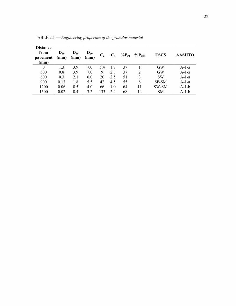
22

TABLE 2.1 Engineering properties of the granular material

Distance

from

pavement

(mm)

D10

(mm)

D30

(mm)

D60

(mm) Cu Cc %P#4 %P200 USCS AASHTO

0 1.3 3.9 7.0 5.4 1.7 37 1 GW A-1-a 300 0.8 3.9 7.0 9 2.8 37 2 GW A-1-a 600 0.3 2.1 6.0 20 2.5 51 3 SW A-1-a 900 0.13 1.8 5.5 42 4.5 55 8 SP-SM A-1-a 1200 0.06 0.5 4.0 66 1.0 64 11 SW-SM A-1-b 1500 0.02 0.4 3.2 133 2.4 68 14 SM A-1-b

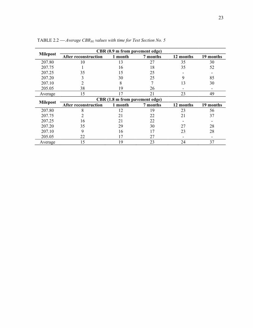
23

TABLE 2.2 Average CBRSG values with time for Test Section 2o. 5

Milepost CBR (0.9 m from pavement edge)

After reconstruction 1 month 7 months 12 months 19 months

207.80 10 13 27 35 30 207.75 1 16 18 35 52 207.25 35 15 25 - - 207.20 3 30 25 9 85 207.10 2 8 7 13 30 205.05 38 19 26 - -

Average 15 17 21 23 49

Milepost CBR (1.8 m from pavement edge)

After reconstruction 1 month 7 months 12 months 19 months

207.80 8 12 19 23 56 207.75 2 21 22 21 37 207.25 16 21 22 - - 207.20 35 29 30 27 28 207.10 9 16 17 23 28 205.05 22 17 27 - -

Average 15 19 23 24 37

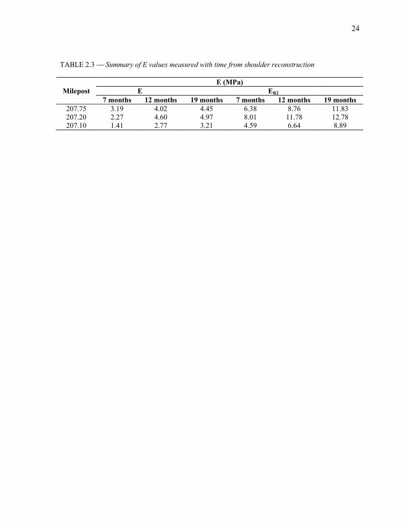
24

TABLE 2.3 Summary of E values measured with time from shoulder reconstruction

Milepost

E (MPa)

E ER2

7 months 12 months 19 months 7 months 12 months 19 months

207.75 3.19 4.02 4.45 6.38 8.76 11.83 207.20 2.27 4.60 4.97 8.01 11.78 12.78 207.10 1.41 2.77 3.21 4.59 6.64 8.89

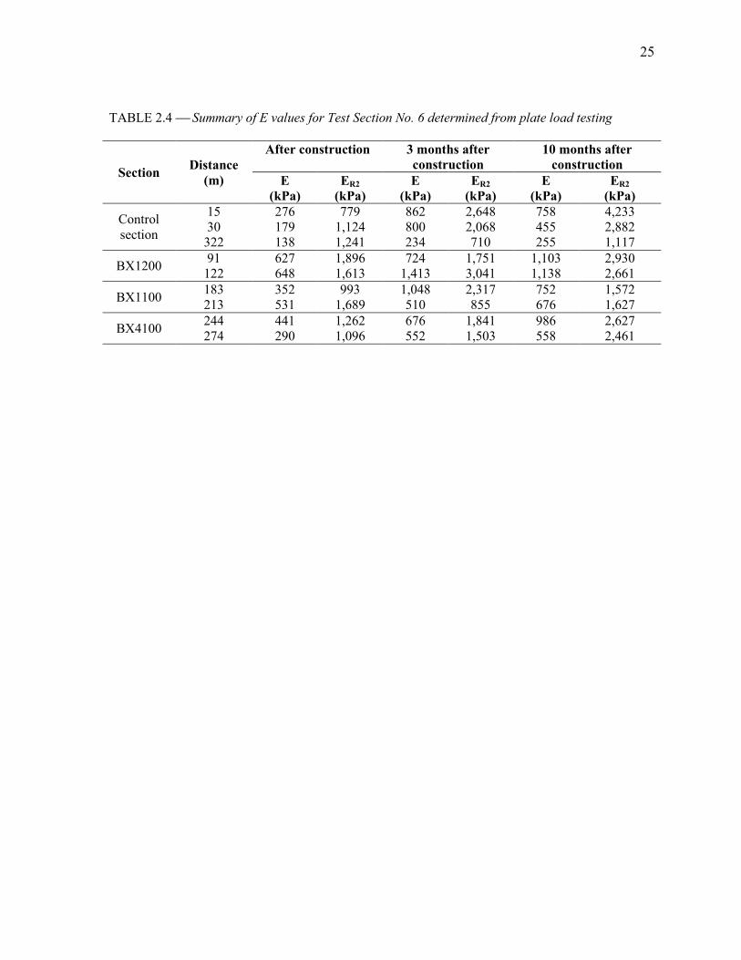
25

TABLE 2.4 Summary of E values for Test Section 2o. 6 determined from plate load testing

Section Distance

(m)

After construction 3 months after

construction

10 months after

construction

E

(kPa)

ER2

(kPa)

E

(kPa)

ER2

(kPa)

E

(kPa)

ER2

(kPa)

Control section

15 276 779 862 2,648 758 4,233 30 179 1,124 800 2,068 455 2,882 322 138 1,241 234 710 255 1,117

BX1200 91 627 1,896 724 1,751 1,103 2,930 122 648 1,613 1,413 3,041 1,138 2,661

BX1100 183 352 993 1,048 2,317 752 1,572 213 531 1,689 510 855 676 1,627

BX4100 244 441 1,262 676 1,841 986 2,627 274 290 1,096 552 1,503 558 2,461

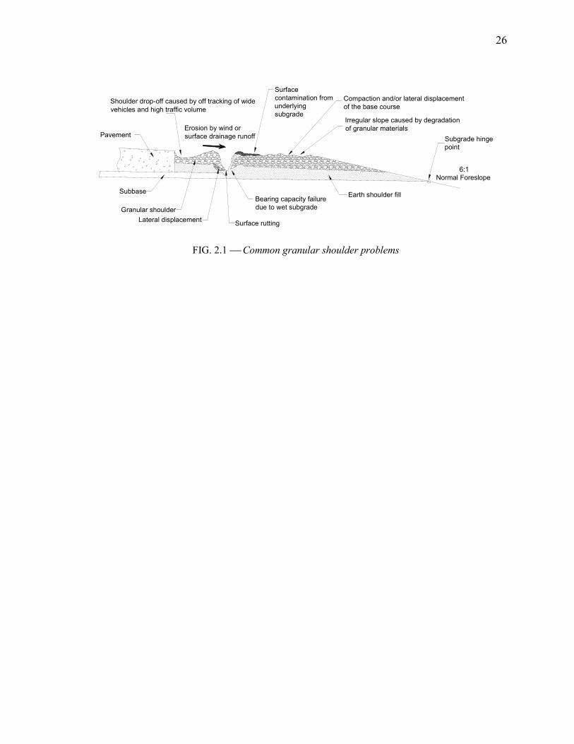
26

Subbase

Pavement

Earth shoulder fillBearing capacity failure

due to wet subgrade

Irregular slope caused by degradation

of granular materials

Shoulder drop-off caused by off tracking of wide

vehicles and high traffic volume

Granular shoulder

Erosion by wind or

surface drainage runoff

6:1

Normal Foreslope

Subgrade hinge

point

Compaction and/or lateral displacement

of the base course

Surface rutting

Surface

contamination from

underlying

subgrade

Lateral displacement

FIG. 2.1 Common granular shoulder problems

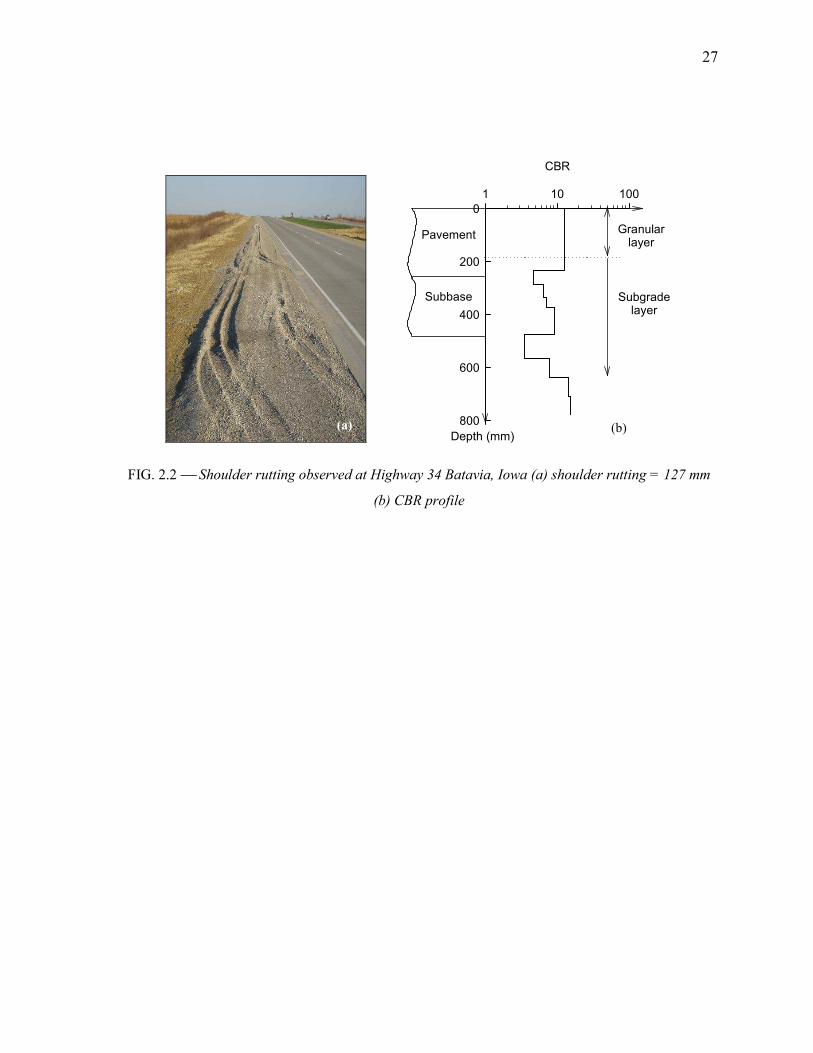
27

CBR

1 10 100

Depth (mm)

0

200

400

600

800

Granularlayer

Subgradelayer

Pavement

Subbase

FIG. 2.2 Shoulder rutting observed at Highway 34 Batavia, Iowa (a) shoulder rutting = 127 mm

(b) CBR profile

(a) (b)

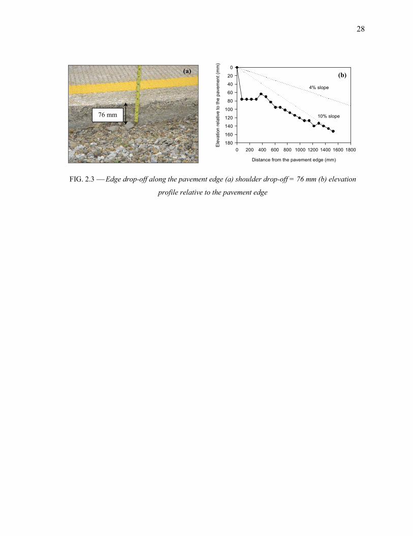
28

Distance from the pavement edge (mm)

0 200 400 600 800 1000 1200 1400 1600 1800

Ele

va

tion

rela

tive t

o th

e p

ave

men

t (m

m)

0

20

40

60

80

100

120

140

160

180

4% slope

10% slope

FIG. 2.3 Edge drop-off along the pavement edge (a) shoulder drop-off = 76 mm (b) elevation

profile relative to the pavement edge

76 mm

(a) (b)

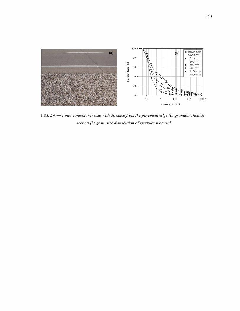
29

Grain size (mm)

0.0010.010.1110

Pe

rce

nt fin

er

(%)

0

20

40

60

80

100

Distance from pavement

0 mm

300 mm

600 mm

900 mm

1200 mm

1500 mm

FIG. 2.4 Fines content increase with distance from the pavement edge (a) granular shoulder

section (b) grain size distribution of granular material

(a) (b)

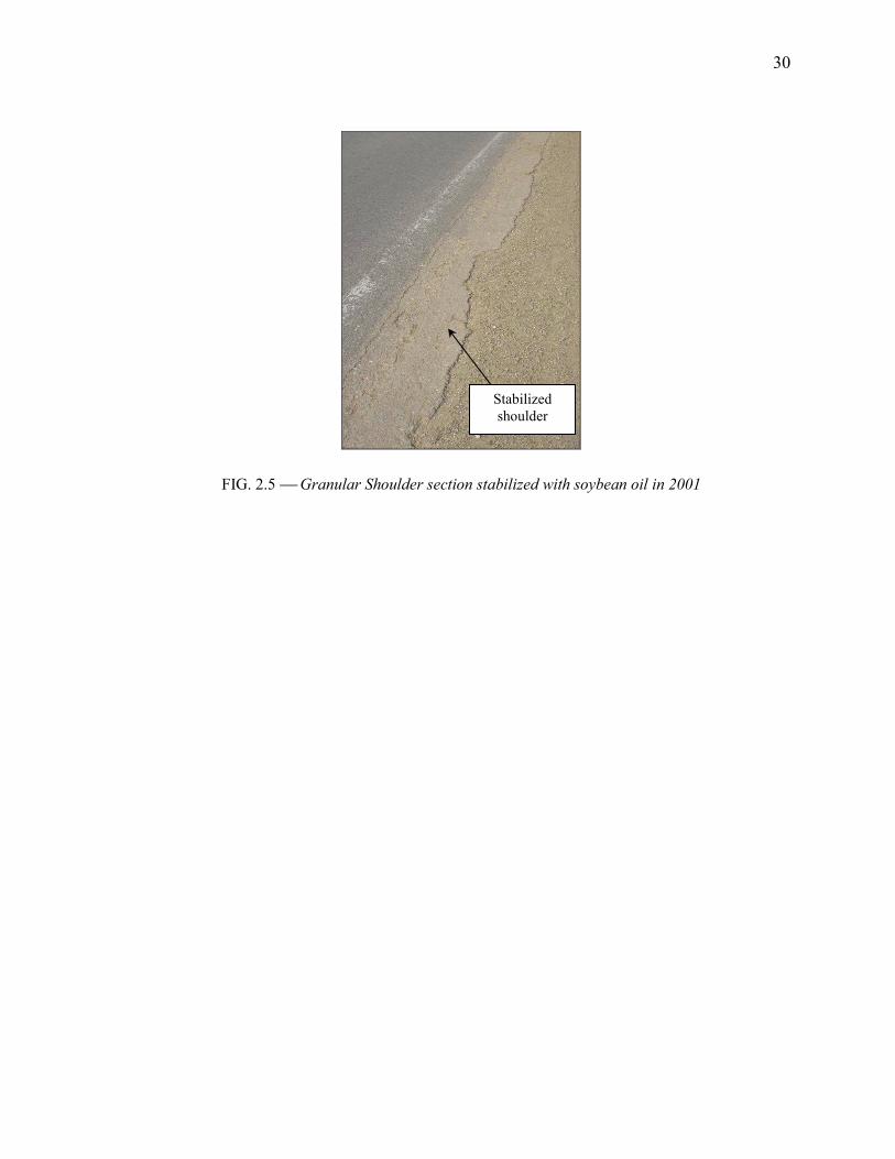
30

FIG. 2.5 Granular Shoulder section stabilized with soybean oil in 2001

Stabilized

shoulder

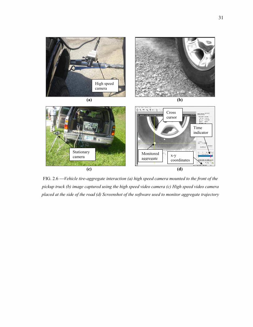
31

(a) (b)

(c) (d)

FIG. 2.6 Vehicle tire-aggregate interaction (a) high speed camera mounted to the front of the

pickup truck (b) image captured using the high speed video camera (c) High speed video camera

placed at the side of the road (d) Screenshot of the software used to monitor aggregate trajectory

Monitored

aggregate

Cross

cursor

x-y coordinates

Time

indicator

High speed camera

Stationary

camera

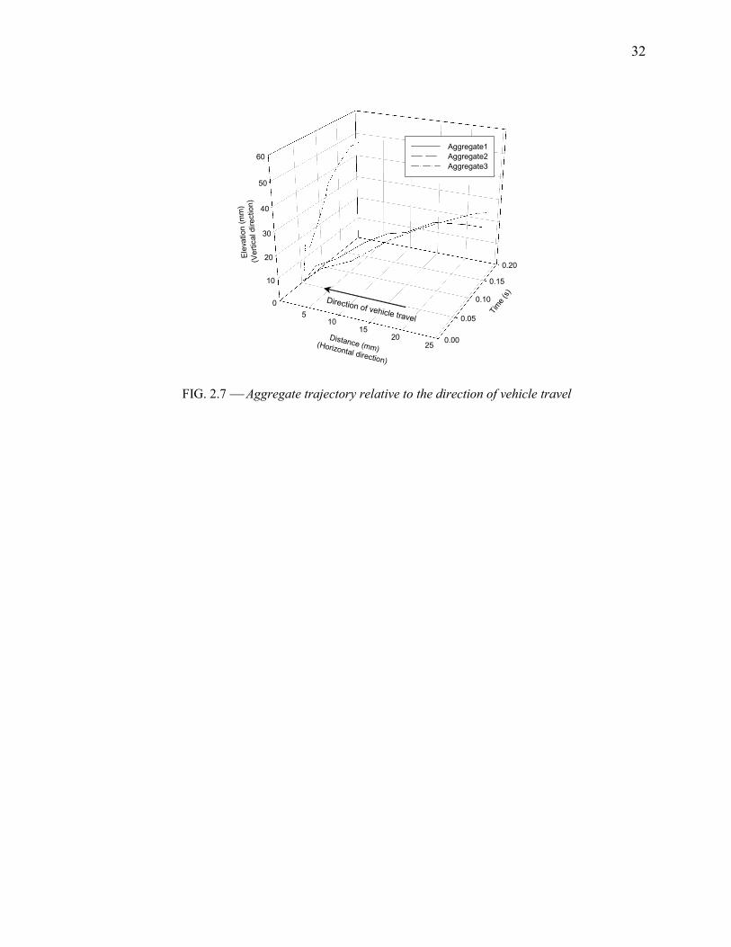
32

0

10

20

30

40

50

60

0.00

0.05

0.10

0.15

0.20

510

1520

25

Ele

vation (

mm

)

(Vert

ical direction)

Tim

e (s

)

Distance (mm)(Horizontal direction)

Aggregate1

Aggregate2

Aggregate3

Direction of vehicle travel

FIG. 2.7 Aggregate trajectory relative to the direction of vehicle travel

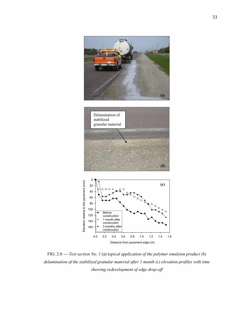
33

Distance from pavement edge (m)

0.0 0.2 0.4 0.6 0.8 1.0 1.2 1.4 1.6

Ele

va

tion

re

lative

to

th

e p

avem

ent

(mm

) 0

20

40

60

80

100

120

140

160

Before construction

1 month afterconstruction

3 months afterconstruction

FIG. 2.8 Test section 2o. 1 (a) topical application of the polymer emulsion product (b)

delamination of the stabilized granular material after 1 month (c) elevation profiles with time

showing redevelopment of edge drop-off

Delamination of stabilized

granular material

(b)

(a)

(c)

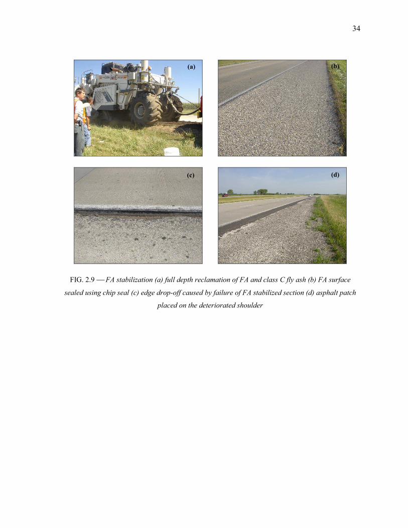
34

FIG. 2.9 FA stabilization (a) full depth reclamation of FA and class C fly ash (b) FA surface

sealed using chip seal (c) edge drop-off caused by failure of FA stabilized section (d) asphalt patch

placed on the deteriorated shoulder

(a) (b)

(c) (d)

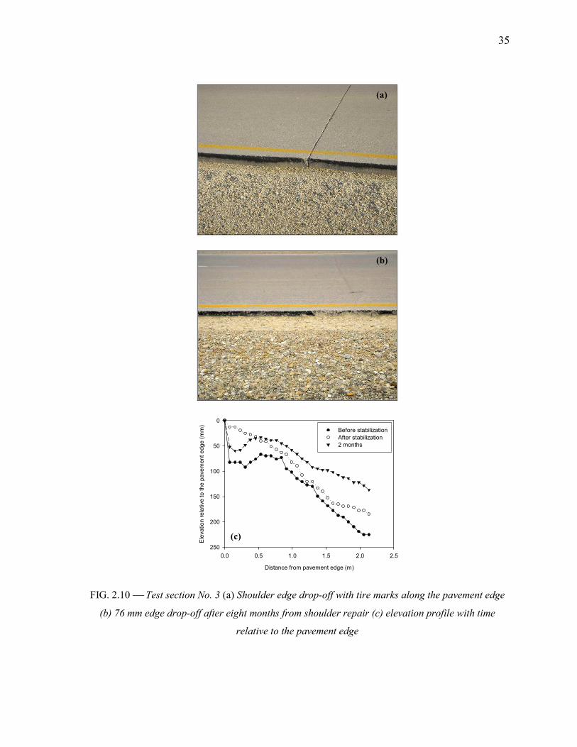
35

Distance from pavement edge (m)

0.0 0.5 1.0 1.5 2.0 2.5

Ele

va

tio

n r

ela

tive

to

th

e p

ave

me

nt

edg

e (

mm

)

0

50

100

150

200

250

Before stabilization

After stabilization

2 months

FIG. 2.10 Test section 2o. 3 (a) Shoulder edge drop-off with tire marks along the pavement edge

(b) 76 mm edge drop-off after eight months from shoulder repair (c) elevation profile with time

relative to the pavement edge

(a)

(b)

(c)

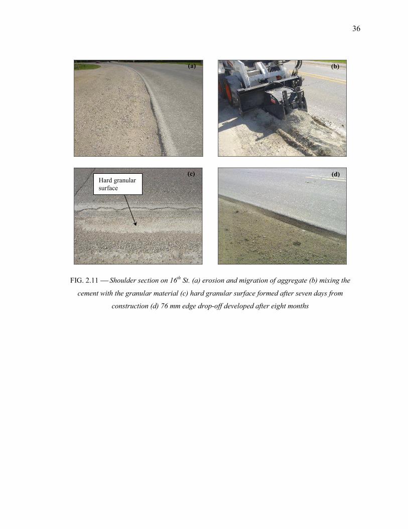
36

FIG. 2.11 Shoulder section on 16th St. (a) erosion and migration of aggregate (b) mixing the

cement with the granular material (c) hard granular surface formed after seven days from

construction (d) 76 mm edge drop-off developed after eight months

(a) (b)

(c) (d) Hard granular

surface

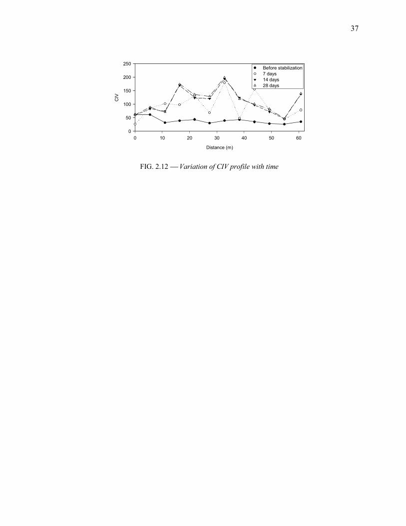
37

Distance (m)

0 10 20 30 40 50 60

CIV

0

50

100

150

200

250Before stabilization

7 days

14 days

28 days

FIG. 2.12 Variation of CIV profile with time

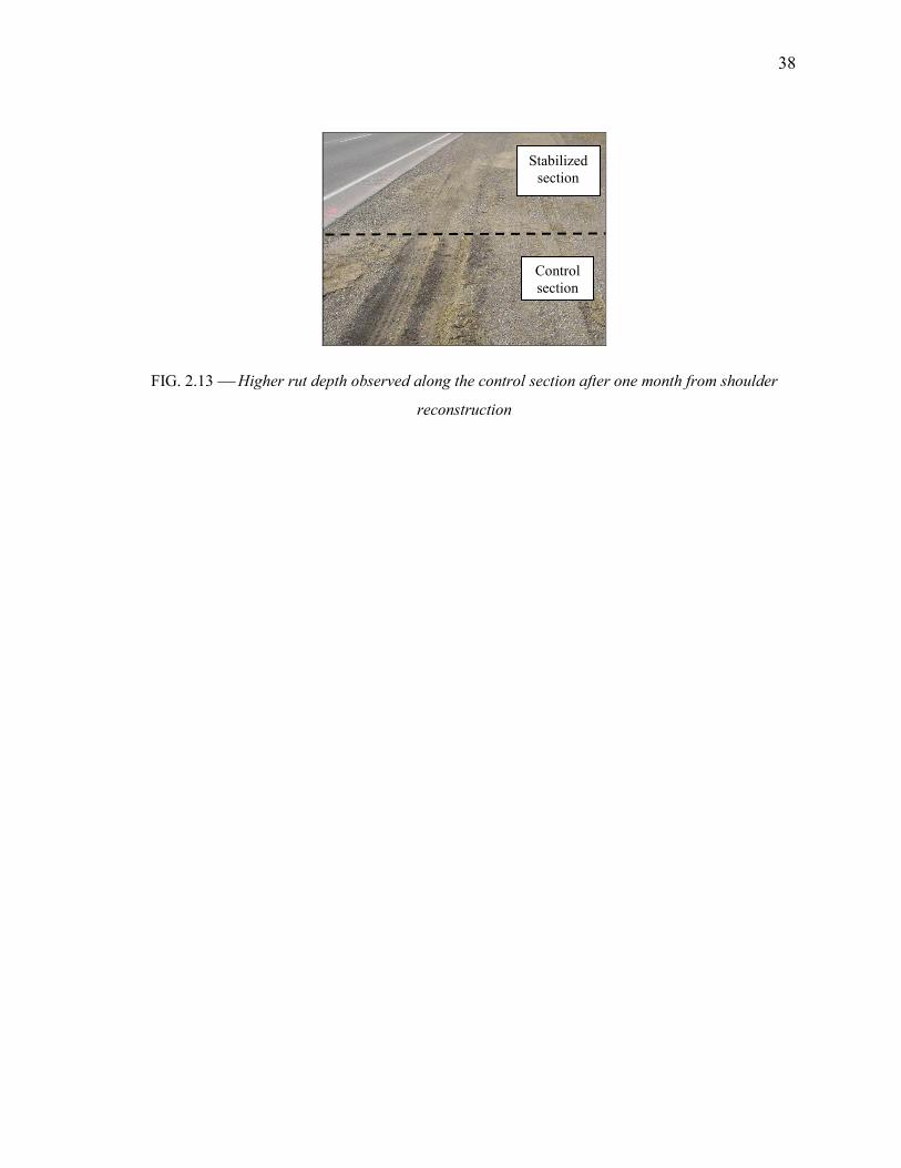
38

FIG. 2.13 Higher rut depth observed along the control section after one month from shoulder

reconstruction

Control

section

Stabilized

section

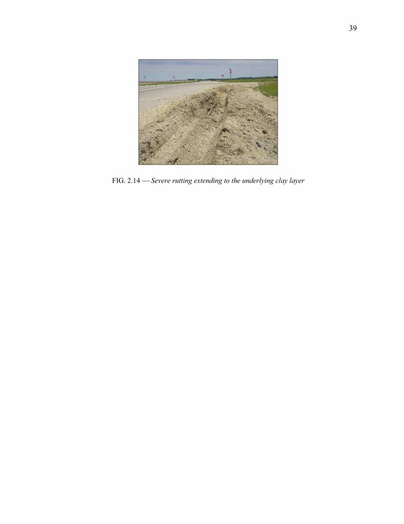
39

FIG. 2.14 Severe rutting extending to the underlying clay layer

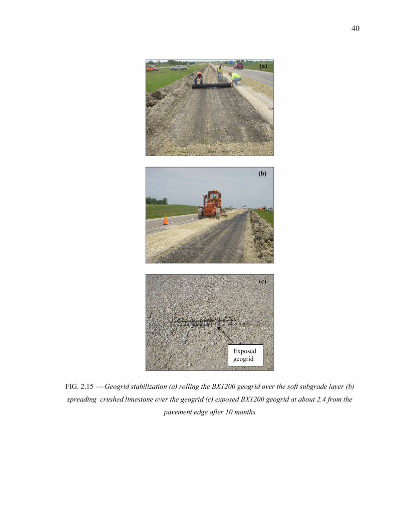
40

FIG. 2.15 Geogrid stabilization (a) rolling the BX1200 geogrid over the soft subgrade layer (b)

spreading crushed limestone over the geogrid (c) exposed BX1200 geogrid at about 2.4 from the

pavement edge after 10 months

(a)

(b)

Exposed

geogrid

(c)

41

3. MECHA$ICALLY REI$FORCED GRA$ULAR SHOULDERS O$ SOFT SUBGRADE:

FULL SCALE FIELD CHARACTERIZATIO$ A$D LABORATORY BOX STUDY

3.1. ABSTRACT

Shoulder rutting is a serious performance problem encountered at granular shoulders

overlying soft subgrade. When subjected to traffic loads, granular shoulders develop considerable

rutting due to bearing capacity failure of the underlying soft subgrade soil. In addition to being

hazardous to drivers, severely rutted shoulders are difficult to maintain. A field reconnaissance study

in Iowa showed that out of 25 problematic shoulder sections, 40% suffered from a soft subgrade

layer, where the California Bearing Ratio (CBR) was 10 or less. A 310 m test section was

constructed where the soft granular shoulder was stabilized by placing three biaxial geogrids at the

interface of the granular and subgrade layers. Monitoring the test section for a period of 10 months,

demonstrated the success of the geogrids in improving the overall shoulder performance. Further, a

laboratory apparatus was constructed to simulate a shoulder section overlying a soft subgrade. Cyclic

loading with different loading stages was used to study the performance of the laboratory model

under selected mechanical and chemical stabilizers. To help construct stable shoulders, design charts

based on allowable rut depth and subgrade CBR were developed. In this paper, a summary of the

field reconnaissance study, the construction and monitoring of a geogrid stabilized test section, and

the results of a scaled laboratory model are discussed. Finally, shoulder design charts, which were

verified by field and laboratory measurements, are presented.

42

3.2. I$TRODUCTIO$

One of the most hazardous performance problems associated with granular shoulders is

shoulder rutting. Shoulder rutting is often encountered when the shoulder overlies a soft subgrade.

When subjected to traffic loads, granular shoulders develop considerable rutting due to bearing

capacity failure of the underlying soft subgrade soil. In addition to being hazardous to drivers,

severely rutted shoulders are difficult to maintain. Adding granular material and shoulder balding are

typical maintenance practices of rutted shoulders. However, these maintenance practices are

temporary solutions since they do not address the problem or prevent rutting from redeveloping.

A recent study by White et al. (2007) investigated field performance of 25 granular shoulder

sections in Iowa. The objective of the study was to improve shoulder performance while keeping

ownership costs low. Almost half of the inspected sections had a subgrade layer with a California

Bearing Ratio (CBR) of 10 or less. Shoulder sections overlying subgrade soils with low CBR values

may undergo bearing capacity failure and lateral displacement of the granular and subgrade material

with repeated traffic loads. On a pilot study basis, one test section with a soft subgrade was stabilized

by placing three geogrids at the interface between the subgrade and the granular layer. Monitoring

the test section over a period of 10 months demonstrated the success of geogrid stabilization in

eliminating edge rut. Besides the field test section, a laboratory box study was constructed to

simulate a shoulder section overlying a soft subgrade. The objective of this laboratory study was to

evaluate mechanical and chemical stabilizers in alleviating shoulder rutting. The laboratory shoulder

section was subjected to cyclic loading with three loading stages. The test setup comprised of a

loading frame, reaction beam, hydraulic actuator, and a steel box to contain the soil.

To help design stable granular shoulder, design charts were developed from the semi-

empirical method proposed by Giroud and Han (2004b), and from an equation developed by the U.S.

Army Corps of Engineers in 1989 predicting surface rutting for low volume roads. The charts, which

are based on an allowable rut depth and the subgrade CBR (CBRSG) were validated using field and

laboratory measurements. Similar charts can be generated for any axle load, tire pressure, and/or

granular layer thickness. The overall scope of the field and laboratory experimentations was:

• Evaluate the use of geogrid reinforcement as a maintenance practice for severely rutted

shoulders.

• Compare and contrast, through laboratory testing, selected mechanical and chemical

stabilizers.

43

• Develop simple designs tools, which will result in more stable shoulder sections and predict

the behavior of existing ones.

3.3. BACKGROU$D

According to Fannin and Sigurdsson (1996), where traffic is channelized, rut is defined as the

distance between the initial elevation of the surface before trafficking and the lower point in the rut

beneath the wheel. Where traffic is not channelized, an erratic pattern of ruts develop, which can be

defined as the distance between adjacent high and low spots of the base course thickness (Giroud and

Han 2004a). According to Giroud and Han (2004a), surface rutting occurs by one or more of the

following mechanisms:

• Compaction of the base course aggregate and/or subgrade soil under repeated traffic loading.

• Bearing capacity failure in the base course or subgrade due to normal and shear stresses

induced by initial traffic.

• Bearing capacity failure in the base course or subgrade after repeated traffic loads which can

result in progressive deterioration of the base course, reduction in effective base course

thickness from the base course contamination by the subgrade soil, a reduction in the ability

of the base course to distribute traffic loads to the subgrade, or a decrease in the subgrade

strength due to pore pressure build up or disturbance.

• Lateral displacement of base course and subgrade material due to the accumulation of

incremental plastic strains induced by each load cycle.

During the last decades the use of geosynthetics to reinforce unpaved structures has shown a

marked increase. Geosynthetics, which are typically placed at the interface between the base course

and the subgrade, can carry higher traffic volumes, and can prevent lateral movement of the base

aggregate stiffening the layer so it distributes wheel loads over a greater area of the subgrade (Tensar

Earth Technologies, Inc. 1996). According to Berg et al. (2000), Giroud and Han (2004a) and Powell

et al. (1999), the following are benefits of using geosynthetics:

• Reducing the stress on the subgrade.

• Increasing the bearing capacity of the subgrade.

• Preventing the subgrade fines from pumping into the base.

• Preventing contamination of the base materials allowing for more open graded, free-draining

aggregates.

• Reducing the depth of excavation required for the removal of unsuitable subgrade materials.

44

• Reducing the thickness of the aggregate layer required to stabilize the subgrade.

• Minimizing subgrade disturbance during construction.

• Minimizing maintenance and extending the life of the pavement.

• Preventing development and growth of local shear zones and allows the subgrade to support

stresses close to the plastic limit while acting as if it is still in the elastic limit.

Two types of geosynthetics are typically used: geotextiles and geogrids. Geogrids and woven

geotextiles have been used as a reinforcement to increase the resistance to traffic loadings (Giroud

and Noiray, 1981). Non-woven geotextiles have been mainly used for separation of the base course

aggregate and the subgrade.

The fundamental reinforcement mechanisms involving the use of geogrids are: (a) lateral

restraint, (b) improved bearing capacity, and (c) tensioned membrane effect. Lateral restraint refers to

the interlocking and confinement of aggregate during loading restricting the lateral flow of the

material. This increases the modulus of the base course material, which therefore, increases the

vertical stress distribution applied to the subgrade. Improved bearing capacity is achieved by shifting

the failure envelope from the weak subgrade to the stiffer base course. The tensioned membrane

effect is based upon the concept of an improved vertical stress distribution resulting from tensile

stress in a deformed membrane. In early research stages, the tensioned membrane effect was believed

to govern the reinforcement mechanism. However, later research demonstrated that reinforcement

benefits are obtained without significant deformation, and that lateral restraint is the primary

reinforcement mechanism followed by the improved bearing capacity concept (U.S. Army Corps of

Engineers 2003).

Geogrids may interlock with aggregates if there is an appropriate relationship between the

aperture size and the aggregate particles size. The effectiveness of the interlocking, however,

depends on the in-plane stiffness of the geogrid and the stability of the geogrid ribs and junctions.

Therefore, the interlocking mechanisms for unpaved structures are different for geotextiles and

geogrids. There are two benefits of interlocking between the geogrid and the base course aggregate:

(a) lateral movement of the base course aggregate is reduced and as a result, no outward shear stresses

are transmitted to the subgrade; and (b) the bottom confined surface of the base course provides a

rough surface that resists lateral movement of the subgrade, which generates inward shear stresses.

According to results of the theory of plasticity, outward shear stresses decrease the bearing capacity,

whereas inward shear stresses increase the bearing capacity. The stresses induced by vehicular loads

tend to be oriented outward (Giroud and Han 2004a). The presence of outward shear stresses can

45

reduce the bearing capacity to as little as one half of the value of purely vertical loading. When

geosynthetics are used, the outward shear stresses are picked up by the reinforcement, which is put

into tension, and purely vertical loads are transmitted to the subgrade mobilizing its full bearing

capacity (Milligan et al. 1989).

Separation of subgrade and base course materials appears to be very important on the thinnest

base course layer, where the geotextile outperforms the geogrid. The geogrid outperforms the

geotextile on the thicker base course layer where reinforcement rather than separation benefits

dominates (Fannin and Sigurdsson 1996).

In this study, the design method presented by Giroud and Han (2004a and 2004b) is adopted for

comparing measured and predicted soil displacement as well as developing shoulder design charts.

The design method takes into account the mechanical properties of geogrids. Influence of geogrids is

accounted for by the bearing capacity factor (Nc), which implies interlock between the geogrid and

the base course materials, and aperture stability modulus (J) which is linked to the increase in stress

distribution angle. The design method also accounts for the quality of the base course materials, the

variation in the stress distribution angle with number of load cycles, and the influence of rut depth.

Only failure of subgrade soil is considered in this method. The subgrade is assumed to be saturated

and have low permeability (behaves in an undrained manner) (Giroud and Han 2004a and Tensar

Earth Technologies, Inc. 1996).

3.4. FIELD OBSERVATIO$S

A reoccurring problem observed during a field investigation, conducted to document granular

shoulders performance problems in Iowa, was soft subgrade soils. Dynamic Cone Penetration (DCP)

testing revealed that about half of the inspected shoulder sections had a CBRSG of 10 or less.

Visually, a section may appear suitable similar to the test section observed on the new Highway 34

bypass (See Figure 3.1a). However, when loaded, pumping and rutting developed along the wheel

path as shown in Figure 3.1b. About 76 mm of rut developed along the wheel path after six truck

passes. Full depth DCP tests conducted with distance from the pavement edge showed that the CBR

value in the upper 200 mm of crushed limestone varied from 6 to 12. The underlying earth shoulder

fill layer had a CBR value of 4 to 10, whereas the subgrade underlying the earth shoulder fill had a

CBR value of 2 to 29. Currently, Iowa Department of Transportation (DOT) does not have a design

requirement for the CBRSG, which can allow shoulders to be constructed over soft foundation soils.

46

3.5. TEST SECTIO$: GEOGRID STABILIZATIO$ – HIGHWAY 218 $ASHUA, IA

3.5.1. Site Description

The inside granular shoulder was experiencing severe rutting due to soft subgrade conditions.

At some locations, 200 mm ruts were observed. The problematic shoulder section extended a

distance of about 9.6 km (from milepost 224 to 218). Regions with a soft subgrade layer were located

by driving a fully loaded dump truck (21,337 kg) over the shoulder section and measuring rut depth at

along the wheel path. Also, Clegg Impact and DCP tests were conducted along the wheel path. The

profile of rut depth and Clegg Impact Value (CIV) with distance starting from milepost 224 is shown

in Figure 3.2. The region with the highest rut depth and lowest CIV, indicating soft conditions,

extends from 220.85 to 219.60 (about 2,000 m). DCP tests conducted within this region showed a

weighted average CBR of 6 in the upper 200 mm and 5 at a depth between 200 and 500 mm.

The engineering properties of the subgrade and granular material are shown in Table 3.1.

The subgrade material was classified as SC (clayey sand; A-4), whereas the granular material was

classified as GW (well graded gravel; A-1-a). The subgrade soil optimum moisture content and

maximum dry unit weight determined using standard Proctor test were 15% and 17.9 kN/m3,

respectively. The in situ moisture contents and unit weights were determined at 14 locations along

the section using driven cores and compared to the standard Proctor curve (See Figure 3.3). The data

shows that the in situ unit weights were lower than the standard Proctor curve even in good

performing sections. However, unit weights measured between milepost 220.60 and 219.80 were

significantly lower than the maximum dry unit weight. Also, most field moisture contents were

higher than the optimum moisture content.

3.5.2. Stabilization of Test Section

Three geogrid types, referred to in this paper as Geogrid1, Geogrid2, and Geogrid3, were

selected to stabilize the shoulder section. The properties of the geogrids are presented in Table 3.2.

The purpose of using three geogrid types was to compare performance as there are mechanical and

cost differences between them. The geogrids were placed at the interface between the subgrade and a

new 200 mm overlying crushed limestone layer. As shown in Figure 3.4, the test section was

approximately 310 m long starting from milepost 220.60 up to milepost 220.40 and was about 2.4 m

wide. The first 60 m was a control section and was left unstabilized. Following the control section

was a 100 m long section stabilized with geogrid1. Two sections, each 75 m long, followed the

Geogrid1 section. These sections were stabilized with Geogrid2 and Geogrid3.

47

As shown in Figure 3.5a, the existing granular layer was stripped using a motor grader and

discarded because of its contamination with the underlying subgrade soil. About 450 tons of crushed

limestone were delivered to the site and placed on the pavement adjacent to the test section. The

subgrade was leveled using a skid loader and then compacted using a pneumatic roller (See Figure

3.5b). Using a power saw, the geogrids were cut to 2.4 m wide to match the width of the stabilized

area. The geogrids were rolled over the soft subgrade starting with Geogrid1 followed by Geogrid2

then Geogrid3 (See Figure 3.5c). The shoulder beyond approximately 300 m was not included in the

test section because Geogrid3 was damaged during transportation. The defective grid, denoted by

Geogrid3*, was placed without alteration to document the effect of improper geogrid installation. . A

motor grader followed by a pneumatic roller were used to spread and compact the aggregate. At the

end of construction, it was noted that parts of the geogrids were not adequately covered with

aggregate (2.4 m away from pavement) and the edges of the geogrids were exposed (See Figure 3.5d).

The entire process of excavation of contaminated material, geogrid placement, aggregate placement,

and compaction took approximately five hours. Upon construction completion, the section was

opened to traffic. Unlike some chemical stabilization, a geogrid are quickly installed and does not

require curing time, which reduces disturbance to traffic.

3.5.3. Field Monitoring

The first inspection was performed after one month from the date of construction. Edge rut

of about 127 mm rut was observed at the control section as shown in Figure 3.5e. The stabilized

sections showed no signs of rutting (See Figure 3.5f).

Plate load tests were conducted immediately after construction, at three months, and at 10

months. Results measured immediately demonstrated that the highest modulus for both the loading

(E) and reloading (ER2) stages were measured at the section that was stabilized with Geogrid1. E was

also slightly higher at the section stabilized with Geogrid2 compared to the section stabilized with

Geogrid3 (See Figure 3.6). This may be attributed to the small difference in their aperture stability

modulus (the aperture stability modulus of Geogrid2 and Geogrid3 are 3.2 and 2.8 kg-cm/deg,

respectively). The lowest E and highest soil deflection were measured at the control section. Plate

load test results obtained after three months showed higher E for all the geogrid sections compared to

the values measured immediately after construction. On average, ER2 increased by about 36, 18 and

42% for Geogrid1, Geogrid2, and Geogrid3 sections, respectively. The increase in E with time can

be caused by progressive lateral confinement of aggregate due to repetitive traffic loads. Further, as

the section is loaded, the subgrade layer deforms to a geometry that mobilizes tension forces to the

48

geogrid, which adds to the stability of the sections. At the control section, E values measured after

three months increased compared to the values measured immediately after construction due to the

addition of limestone rock that several weeks after construction to alleviate the rutting. Plate load test

results obtained after 10 months showed a reduction in E values for the control section and Geogrid2

section by about 23 and 8%, respectively. The sections stabilized with Geogrid1 and Geogrid3

continued to show increase in E with time by 5 and 26%, respectively, compared to the values

measured at three months. Table 3.3 summarizes the plate load test results.

Using a 20 kg hammer, CIV tests were performed every 15 m as shown in Figure 3.7.

Immediately after geogrid installation, CIVs increased. CIVs also increased at the control section as

a result of subgrade compaction during the geogrid installation procedure and the addition of virgin

rock material. After three months, additional strength at the stabilized sections was measured as

indicated by the further increase in CIVs. CIVs measured at the control section did not increase.

There was no significant difference between the CIVs measured at the geogrid sections even though

the aperture stability modulus, and thus stiffness, varied for each geogrid type. It is possible that the

CIV value for the 20 kg Clegg hammer is influenced by a relatively shallow depth and thus was

unable to detect different degrees of confinement. At 10 months, CIVs were reduced in all the

stabilized sections. Relative loosening of the granular layer after the freeze-thaw period may be the

reason behind this reduction.

DCP tests were also used to monitor the shoulder section performance. DCP tests conducted

before and after stabilization showed an increase in CBR of the granular layer (CBRGL) at all

stabilized sections (See Figure 3.8). For the Geogrid1 section, CBRGL increased from 3 to 18, while

for Geogrid2 and Geogrid3 sections, CBRGL increased from 4 to 19 and 3 to 17, respectively. There

was no significant change in CBR values below the depth of the geogrid.

Parts of the defective Geogrid3 were exposed after four months from installation as shown in

Figure 3.9a. The exposure was a result of severe rutting. As expected, improper installation of a

geogrid will not provide reinforcement benefits. After 10 months, additional geogrids were exposed.

The exposed portions were at a distance of about 2.4 m from the pavement edge where the grids were

overlaid by 25 to 50 mm of rock (See Figure 3.9b).

Despite the small reduction in strength parameters and geogrid exposure, geogrid

stabilization improved the shoulder performance and eliminated shoulder rutting. To prevent geogrid

49

exposure in future stabilization applications, the thickness of the granular layer should be constant. A

nominal 150 mm to 200 mm granular layer thickness is recommended.

3.6. LABORATORY BOX STUDY

The objective of this laboratory study was to evaluate selected mechanical and chemical

stabilizers and alternative granular material in alleviating shoulder rutting. By constructing a

laboratory box simulating a shoulder section overlying a soft subgrade, stabilizing the subgrade,

subjecting the shoulder to 15,000 load cycles, and recording cumulative soil displacement, the

effectiveness of each stabilizer was evaluated.

3.6.1. Test Setup

The laboratory apparatus consisted of a loading frame, reaction beam, and a hydraulic

actuator (See Figure 3.10a). The actuator had a maximum force of 250 kN and a dynamic stroke of

150 mm. A 0.2 m3 steel box was used to contain the soil, which was loaded using a 150 mm diameter

loading plate. The steel box comprised of twelve 200 mm c-channels assembled together to form a

0.6 m x 0.6 m x 0.6 m box (See Figure 3.10b). To minimize friction and stress concentrations, a

compressible 12 mm thick neoprene pad and a Teflon sheet were placed at the interface between the

soil and the steel box. The subgrade soil was placed at the bottom of the box and compacted in 76

mm lifts by applying a static load to reach a final depth of 300 mm. The reinforcement was placed at

the interface between the subgrade and the overlying granular layer. Similar to the foundation layer,

the granular layer was compacted by applying a static load to reach a final thickness of about 150 mm

(See Figure 3.11). To ensure soft foundation conditions for all tests, the target range of CBRSG values

was selected to vary between 3 and 5, except for the chemical stabilization test where the target

CBGSG was above 20. The target range of CBRGL values was 4 to 7.

The hydraulic actuator was used to apply a sinusoidal load pulse to the 150 mm diameter

loading plate. Three incremental cyclic loads were applied to the soil each sustained for 5,000 cycles

(total of 15,000 cycles) at a frequency of 1 Hz. The initial cyclic pressure was 275 kPa, which was

then increased to 550 kPa and then 827 kPa. The applied pressures were selected to simulate the

stress applied by 0.5, 1.0, and 1.5 of the America-British standard axle load (8,150 kg) at a tire

inflation pressure of 550 kPa and a 150 mm of tire contact area (Giroud and Han 2004b). The

frequency of one cycle per second was sufficient in sustaining the applied load despite the large

deflections observed at some tests. The hydraulic actuator control system was used to collect

displacement data at predetermined load cycles. DCP, Clegg hammer and Light Weight

50

Deflectometer (LWD) test with a 200 mm diameter loading plate were used to document the changes

in CBR, CIV and E, respectively, for each soil layer before and after the test.

During the test, and at each loading stage, the deflection of the reaction beam was measured

using a dial gage. A linear relationship was noted between the load applied and the beam deflection.

The measured deflections were taken into account when calculating the corresponding soil

displacement.

3.6.2. Materials

The soil used as a subgrade material was Paleosol clay, which was classified as CH (fat clay;

A-7-6). The materials used for the granular layer were Class A crushed limestone and Recycled

Asphalt Pavement (RAP). The crushed limestone was classified as SP-SM (poorly graded sand with

silt; A-1-a) with optimum moisture content and a maximum dry unit weight of 6% and 21.9 kN/m3,

respectively. The RAP material was classified as GP (well graded gravel; A-1-a). The fines content

was about 0.5% compared to 10% for the crushed limestone (Table 3.1).

The laboratory study investigated the performance of three biaxial geogrid types, woven and

one nonwoven geotextiles in. The geogrids selected were the same as the ones used in the test section

(i.e. Geogrid1, Geogrid2, and Geogrid3). The geotextiles used were a woven geotextile film used

mainly for soil separation and stabilization, and a needle-punched nonwoven geotextile fiber. The

properties of the selected geosynthetics are summarized in Table 3.2. For the chemical stabilization

test, class C fly ash from Ottumwa Generating Station (OGS) was selected as the stabilization agent

for the subgrade.

3.6.3. Test Results

Ten tests were carried out evaluating two types of granular materials (crushed limestone and

RAP), three types of geogrids, woven and non-woven geotextiles, and chemical stabilization using

class C fly ash. The subgrade moisture content for the first nine tests was 25% during placement. For

Test No. 10 (using class C fly ash), the subgrade moisture content was 21%. Table 3.4 summarizes

the soil properties before and after each test.

3.6.3.1. Test 2o. 1 – Control

The first test was conducted to simulate the observed field condition where a granular

shoulder overlies a soft subgrade layer. The dry unit weight for the subgrade and granular layers

were 19 kN/m3 and 13.4 kN/m3, respectively. The CBRSG value, calculated from DCP tests,

51

increased from 3 to 9 after the test was completed as a result of subgrade soil densification. Almost

no change in properties of the granular material was noted before and after the test. The displacement

recorded by the hydraulic actuator control system is shown in Figure 3.12. The maximum soil

displacement after 15,000 cycles was 284 mm. Visual inspection of the subgrade layer after the test

revealed considerable aggregate punching into the subgrade to a depth of approximately 50 mm.

3.6.3.2. Test 2os. 2, 3, and 4 – Geogrid1

In test Nos. 2, 3, and 4, Geogrid1 was placed at the interface between the granular and

subgrade layers. During test No. 1, the dimensions of Geogrid1 were 6 mm shorter than the

dimensions of the box to eliminate any interaction between the grid and the box. The dry unit weight

of the subgrade and granular layers were 18.6 kN/m3 and 14 kN/m3, respectively. The CBRSG value

increased from 5 to 7 after the test indicating less soil densification compared to Test No. 1. Further,

the subgrade modulus determined by LWD (ELWD) increased from 7.0 to 12.0 MPa. No significant

change in the properties of the granular layer was measured. The maximum measured soil

displacement at 15,000 cycles was 125 mm, which was about 40% less than that measured for the

control test. The measured soil displacement was compared to the calculated soil displacement at the

end of each loading stage using the semi-empirical method outlined in Giroud and Han (2004). The

calculated and measured soil displacements were similar at the end of the first loading stage (i.e. at

5,000 cycles). However, the calculated soil displacement was lower than the measured one at the end

of the second and third loading stages (See Figure 3.13). Examining the unanchored geogrid after the

test revealed that the geogrid was pulled to the center of the box (a phenomenon that would not occur

in the field) under the effect of repetitive cyclic loading. This observation may explain the difference

between the measured and predicted soil displacement. Similar to the control test, most of the soil

displacement occurred during the first 500 cycles of each load increment. The amount of aggregate

punching through the subgrade layer was reduced compared to Test No. 1 but was not eliminated.

Visual inspection revealed an aggregate punching depth of about 25 mm.

During Test No. 3, the 4 corners of the geogrid were anchored using steel rods driven to the

bottom of the subgrade layer. The dry unit weight of the subgrade and granular layers were 19.2

kN/m3 and 14.2 kN/m3, respectively. As a result of soil displacement, the CBRSG value increased

from 5 to 8 and the ELWD increased from 8.0 to 11.0 MPa. The results show no change in the

properties of the granular layer before and after the test. Figure 3.13 demonstrates the measured and

predicted soil displacement with increasing number of cycles. Partially anchoring the geogrid

decreased the soil displacement by about 10% compared to Test No. 2 (geogrid was not anchored).

52

Further, partially anchoring the geogrid decreased the difference between measured and predicted soil

displacement. At 15,000 cycles the difference between the measured and predicted soil displacement

was 47 mm for Test No. 2 and 35 mm for Test No. 3. Visual inspection showed punching of

aggregate through the subgrade soil to a depth of about 25 mm.

The setup of Test No. 4 was similar to the previous two tests except that the entire perimeter

of Geogrid1 was fixed to eliminate any geogrid movement. This was accomplished by locking the

geogrid between the c-channels, which were used to assemble the sides of the steel box. The dry unit

weight of the subgrade and granular layers were 18.7 kN/m3 and 13.8 kN/m3, respectively. The

CBRSG value increased from 4 to 7 after the test. Also, the subgrade ELWD increased from 8.0 to 10.0

MPa. CBR and ELWD values of the granular layer did not change considerably before and after the

test. Figure 3.13 shows the measured and predicted soil displacement with increasing number of

cycles. As a result of locking the entire geogrid perimeter, the measured soil displacement was

further reduced compared to Test Nos. 2 and 3. At 15,000 cycles, the soil displacement was 40%

lower than that measured in Test No. 3. Furthermore, minimizing the movement of the geogrid

reduced the differences between the measured and predicted soil displacement at all three loading

stages. Therefore, other mechanical reinforcements used later in this laboratory study were fixed to

the steel box in a similar manner.

3.6.3.3. Test 2os. 5 and 6 – Geogrid2 and Geogrid3

The soft subgrade was stabilized with Geogrid2 in Test No. 5 and Geogrid3 in Test No.6.

The engineering properties of both geogrids are summarized in Table 3.2. The dry unity weight of

the subgrade and granular layers for Test No. 5 were 18.7 kN/m3 and 13.5 kN/m3, respectively. After

the test, the CBRSG value increased from 5 to 8 and ELWD increased from 9.0 to 12.0 MPa. The soil

displacement measured at 15,000 cycles was about 12% higher than that measured during Test No. 4.

However, the soil displacement was about 70% less than the control test (See Figure 3.12).

The dry unit weight of the subgrade and granular soils for Test No. 6, which was stabilized

with Geogrid3, were 19.2 kN/m3 and 14,2 kN/m3, respectively. Due to soil densification, the CBRSG

value increased from 5 to 9 and ELWD increased from 9.0 to 16.0 MPa. Similar to previous tests, the

properties of the granular layer did not change. There was no difference between the soil

displacements measured during Test Nos. 5 and 6 (See Figure 3.12). This may be attributed to the

somewhat similar aperture stability modulus and tensile strength of the geogrids. Comparing the

results of the three geogrid types, it is apparent that Geogrid1 showed better performance;

53

nonetheless, the other geogrid types significantly reduced the soil displacement when compared to the

control test.

3.6.3.4. Test 2os. 7 and 8 – Woven and 2onwoven Geotextiles

The subgrade layer was stabilized with woven and nonwoven geotextiles for Test Nos. 7 and

8, respectively. These geotextiles are used primarily for soil separation and stabilization. The

engineering properties of the selected geotextiles are summarized in Table 3.2. After the test, the

CBRSG value increased from 4 to 10 and its ELWD increased from 9.0 to 14.0 MPa. The CBR and

ELWD of the granular layer did not change. When compared to Test Nos. 5 and 6 (Geogrid2 and

Geogrid3), the soil displacement was lower by about 28% for the first and second loading stages. At

the third loading stage, the soil displacement exceeded those measured at Test Nos. 5 and 6 by 11%

(See Figure 3.12). One advantage of using a woven geotextiles is the complete separation of granular

and subgrade materials, which eliminated aggregate punching into the subgrade layer.

For Test No. 8, a nonwoven geotextile was selected to stabilize the soft subgrade soil. The

dry unit weight of the granular and subgrade soils before the test were 14 kN/m3 and 18.9 kN/m3,

respectively. An increase in CBRSG value from 4 to 9 and ELWD from 7.0 to 16.0 MPa was observed

after the test. For the first 5000 cycles, both the woven and nonwoven geotextiles showed similar

performances. At higher number of cycles, the nonwoven geotextile showed better performance. The

nonwoven geotextile managed to reduce the soil displacement by up to 14% compared to the woven

geotextile test. Further, for the first two loading stages, the nonwoven geotextile outperformed the

geogrids; however at the third loading stage, the soil displacement increased rapidly to exceed those

measured at the geogrid stabilized tests (i.e. Test Nos. 4, 5, and 6) (See Figure 3.12). Visual

observations showed that the nonwoven geotextile prevented aggregate punching through the

subgrade.

3.6.3.5. Test 2o. 9 – Recycled Asphalt Pavement

Due to the increasing use of recycled material in shoulder applications, this test aimed to

document the performance of RAP material when used as a granular layer. Similar to the setup of

Test No. 4, the underlying subgrade was stabilized by placing Geogrid1 at the interface between both

layers. The dry unit weight of the granular and subgrade soils before the tests were 14 kN/m3 and

19.2 kN/m3, respectively. The CBRSG and ELWD values increase from 4 to 8 and from 8.0 to 12.0

MPa, respectively. Compared to Test No. 4, where the granular layer comprised of crushed

limestone, the soil displacement was about 50% higher (See Figure 3.12). The lower percentage of

54

fines in the RAP material may have contributed in a less stable granular layer; and thus, higher

displacements.

3.6.3.6. Test 2o. 10 – Class C fly Ash

This test evaluated the performance of unpaved shoulder systems under chemical stabilization

of the subgrade soil. The subgrade soil in this laboratory study was stabilized using about 20% OGS

class C fly ash. The moisture content of the subgrade material prior to mixing the fly ash was about

21%. The fly ash was mixed with the subgrade material, compacted in 76 mm lift, and allowed to

cure for seven days at approximately 70o F. The granular material used in this test comprised of

crushed limestone. The strength of the subgrade layer was periodically measured using DCP test

until a CBRSG value of about 21 was reached. The dry unit weight of the granular and subgrade soils

before the tests were 13.8 kN/m3 and 19.7 kN/m3, respectively. The CBRSG value increased from 21

to 24 after the test was completed. Further, the ELWD increased from 28.0 to 31 MPa. There was no

considerable change in the properties of the granular layer. At 15,000 cycles, the measured soil

displacement was 48 mm, which was the lowest soil displacement compared to all tests (See Figure

3.12). Stabilizing the subgrade material using fly ash reduced the soil displacement by 42, 62, and

61% compared to Test Nos. 4, 5, and 6, respectively. Compared to the control test, fly ash

stabilization reduced soil displacement by about 85%.

The measured soil displacement for all tests was compared to the predicted soil displacement

computed using the design method proposed by Giroud and Han (2004) (See Figure 3.14). Overall,

there is a good agreement between the measured and predicted soil displacement. Except for Test

Nos. 2 and 3, where Geogrid1 was not locked to the steel box, the design method over predicted the

soil displacement. The highest over prediction was observed at Test No. 8 (nonwoven geotextiles)

and was about 25%. This design method can therefore be used to predict rutting at granular

shoulders.

3.7. SHOULDER DESIG$ CHARTS

Shoulder design charts were developed to help design stable shoulders and mitigate rutting

that occurs due to bearing capacity failure of the subgrade. The design charts were developed from

the design method proposed by Giroud and Han (2004) and an equation developed by the U.S. Army

Corps of Engineers in 1989 predicting surface rutting for low volume roads (Bolander et al. 1995).

The charts can be a rapid tool for designing new granular shoulders and provide basis for QC/QA

specifications. An example of a design chart is shown in Figure 3.15. This chart was developed for a

55

150 mm thick granular layer, 80 kN load, 550 kPa tire pressure, and a CBRGL of 6, which are

commonly encountered field values. To use this chart, an allowable rut depth for a granular shoulder

section is selected and the corresponding CBRSG is computed for a certain number of load cycles (N).

Similar charts can be generated for any set of shoulder parameters. Field and laboratory rut depth

measurements were used to validate the developed chart. The measured rut depths are in a relatively

good agreement with the charts developed using the Giroud and Han (2004) method indicating that

this chart is applicable for designing granular shoulders. The method proposed by the U.S. Army

Corps of Engineers, however, appears to be overestimating the rut depth.


A common shoulder performance problems in Iowa is granular shoulders overlying soft

subgrade soils. Several instances of this problem have occurred for newly constructed roads that have

shoulder subgrade material that provides inadequate support. The result is a shoulder that is both

hazardous and difficult to maintain. Field observations of granular shoulder across the state of Iowa

demonstrated that many existing sections have a soft subgrade layer where the CBRSG is 10 or less.

This paper focuses on design and maintenance solutions, which would eliminate the rutting problem.

A maintenance alternative such as mechanical stabilization was evaluated by constructing a test

section, where the soft subgrade was stabilized using three biaxial geogrids. The shoulder

performance was evaluated over a period of 10 month using various in situ tests. Overall, all three

geogrid types were effective in mitigating shoulder rutting and improving strength properties as

evidenced by the increase in CBR, CIV, and E with time. Compared to chemical stabilization,

geogrid stabilization allows for a more rapid reconstruction. Further, the repaired section can be

opened immediately for traffic with no curing time required. Other mechanical and chemical

stabilization alternatives such as woven and nonwoven geotextiles, fly ash, and the use of alternative

shoulder granular material like RAP were evaluated by conducting a laboratory box study. Subjected

to 15,000 cyclic loads, each stabilizer was evaluated based on the cumulative measured soil

displacement. The following conclusions are withdrawn from the laboratory study:

• The control test showed the highest soil displacement, which was about 284 mm after 15,000

cycles.

• By locking the mechanical reinforcements between the box c-channels the soil displacement

was reduced, which better simulated field conditions. Locking the mechanical

reinforcements also resulted in smaller differences between measured and predicted soil

displacements.

56

• The CBR and ELWD values of the subgrade layer always increased after the test as a result of

soil densification. The soil properties of the granular layer did not change.

• Geogrid1 reduced soil displacement by about 75% compared to the control test, whereas

Geogrid2 and Geogrid 3 reduced soil displacement by about 70%. All geogrids, however, did

not prevent aggregate punching through the subgrade layer.

• The woven and non-woven geotextiles reduced the soil displacement by about 70% compared

to the control test. The performance of the nonwoven geotextile started to deteriorate after

the third loading stage. Both woven and nonwoven geotextiles were successful in separating

the granular and subgrade layers.

• Using RAP as a granular material resulted in a 50% increase in soil displacement compared

to using crushed limestone.

• Stabilizing the subgrade soil with 20% class C fly ash resulted in the lowest cumulative soil

displacement.

• For all tests where the reinforcements were fixed to the steel box and for the fly ash

stabilization test, the Giroud and Han (2004) semi-empirical method over predicted the soil

displacements at the end of each loading stage. In tests where the reinforcements were not

fixed, the measured soil displacement was considerably higher than the predicted values.

The results of the field and laboratory studies indicate that mechanical reinforcement as well as

fly ash stabilization are effective methods in repairing granular shoulder with soft foundations.

To design new unreinforced granular shoulders, the provided design chart can be a simple design

tool in selecting an adequate CBRSG that will yield a more stable shoulder section. The chart may

also provide bases for QA/QC.

ACK$OWLEDGME$TS

The Iowa Department of Transportation and the Iowa Highway Research Board sponsored

this study under contract TR-531. Numerous people assisted the authors in identifying shoulder

sections for investigation. The technical steering committee helped refine the research tasks and

provided suggestions. The authors would like to thank Iowa DOT personnel and materials suppliers

who helped us throughout the project.

57

REFERE$CES

Berg, R. R., Christopher, B. R., and Perkins, S. (2000). “Geosynthetic reinforcement of the aggregate

base/subbase courses of pavement structures.” Geosynthetics Materials Association,

Roseville, MN.

Bolander, P., Marocco, D., and Kennedy, R. (1995). Earth and Aggregate Surfacing Design Guide

for Low Volume Roads. United States Department of Agriculture, Forest Service, Report No.

FHWA-FLP-96-001, Washington, D.C.

Fannin, R. J., and Sigurdsson, O. 1996. “Field observations on stabilization of unpaved roads with

geosynthetics.” Journal of Geotechnical Engineering, 122 (7), 544-553.

Giroud, J. P, and Han, J. (2004a). “Design method for geogrid-reinforced unpaved roads. I.

Development of design method.” Journal of Geotechnical and Geoenvironmental

Engineering, 130(8), 775-786.

Giroud, J. P, and Han, J. (2004b). “Design method for geogrid-reinforced unpaved roads. II.

Calibration and applications.” Journal of Geotechnical and Geoenvironmental Engineering,

130(8), 787-797.

Giroud, J. P., and Noiray, L. (1981). “Geotextile-reinforced unpaved road design.” Journal of the

Geotechnical Engineering Division, Proceedings of the American Society of Civil Engineers,

107(GT9), 1233-1254.

Milligan, G. W. E., Jewell, R A., Houlsby, G. T., and Burd, H. J. (1989). “A new approach to the

design of unpaved roads-part I.” Ground Engineering, 25-29.

Powell, W., Keller, G.R., and Brunette, B. (1999). “Application for geosynthetics on forest service

low-volume roads.” Transportation Research Record, 1652, 113-120.

Tensar Eath technologies, Inc. (1996). “Design guideline for flexible pavements with Tensar geogrid

base layers.” Tensar Technical 2ote, TTN:BR96.

U.S. Army Corps of Engineers. (2003). “Use of geogrids in pavement construction.” Technical Letter

2o. 1110-1-189, Washington, D.C.

58

White D. J., Mekkawy, M. M., Jahren, C. T., Smith, D., and Suleiman, M. T. (2007). “Effective

shoulder design and maintenance.” Center for Transportation Research and Education, Iowa

Department of Transportation, Report No. TR-531, Ames, IA.

$OTATIO$S

Nc = Bearing capacity factor

J = Aperture stability modulus

CIV = Clegg Impact Value

CBRSG, CBRGL = California Bearing Ratio of the subgrade and granular layers

E, ER2 = Modulus measured during the load and reload cycles

ELWD = Modulus measured using light weight deflectometer

D10, D30, and D60 = Sieve size through which 10%, 30%, and 60% of the particles would pass

Cu = Coefficient of uniformity

Cc = Coefficient of gradation



LIST OF TABLES

TABLE 3.1 Engineering properties of test section and laboratory box study materials

TABLE 3.2 Engineering properties of the selected geosynthetics

TABLE 3.3 Summary of E values determined from plate load testing

TABLE 3.4 Summary of soil properties measured before and after each test

LIST OF FIGURES

FIG. 3.1 Shoulder section on new Highway 34 bypass (a) visually suitable shoulder (b) 76 mm rut

developed with a few truck passes

59

FIG. 3.2 Profile of the rut depth measured inside the wheel path and CIV measured at 0.6 m from

the pavement edge

FIG. 3.3 Moisture-density relationship for the subgrade material

FIG. 3.4 Schematic diagram of the test section (a) plan view (b) cross section

FIG. 3.5 Shoulder reconstruction using geogrids (a) motor grader removing the contaminated

granular layer (b) pneumatic roller used to compact the subgrade (c) rolling the geogrid over the

subgrade (d) spreading the aggregate over the geogrid (e) rutting developed at the control section after

one month (f) no rutting at the geogrid stabilized section after one month

FIG. 3.6 Plate load test results immediately after construction

FIG. 3.7 Profile of CIV with time at 1.2 m from the pavement edge

FIG. 3.8 DCP results before and after stabilization (a) Geogrid1 (b) Geogrid2 (c) Geogrid3

FIG. 3.9 Exposed geogrid after 10 months (a) Geogrid3* (b) Geogrid1

FIG. 3.10 Schematic of the laboratory apparatus setup (a) Steel frame and hydraulic actuator used

for loading the stabilized soil (b) steel box used to contain the soil

FIG. 3.11 Laboratory box setup (a) applying a static load to compact the soil (b) applying cyclic

loading through a 150 mm loading plate

FIG. 3.12 Summary of cumulative measured soil displacement for all tests

FIG. 3.13 Measured and predicted soil displacement for Geogrid1 tests

FIG. 3.14 Comparison between measured and predicted soil displacement


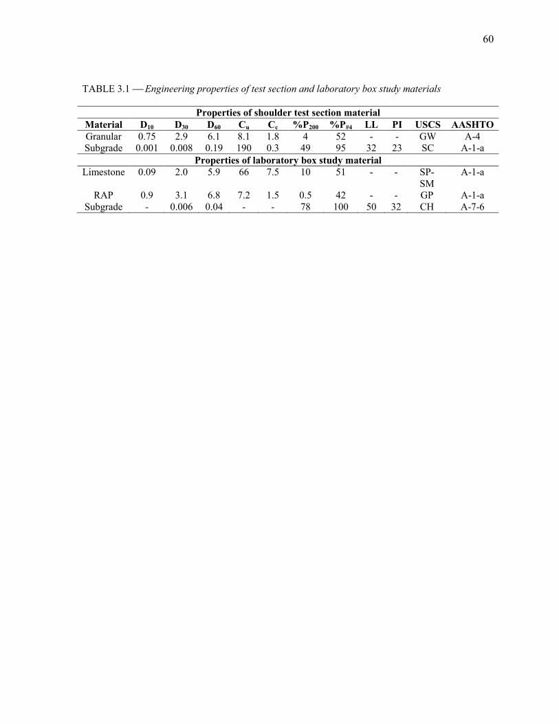
60

TABLE 3.1 Engineering properties of test section and laboratory box study materials

Properties of shoulder test section material

Material D10 D30 D60 Cu Cc %P200 %P#4 LL PI USCS AASHTO

Granular 0.75 2.9 6.1 8.1 1.8 4 52 - - GW A-4 Subgrade 0.001 0.008 0.19 190 0.3 49 95 32 23 SC A-1-a

Properties of laboratory box study material

Limestone 0.09 2.0 5.9 66 7.5 10 51 - - SP-SM

A-1-a

RAP 0.9 3.1 6.8 7.2 1.5 0.5 42 - - GP A-1-a Subgrade - 0.006 0.04 - - 78 100 50 32 CH A-7-6

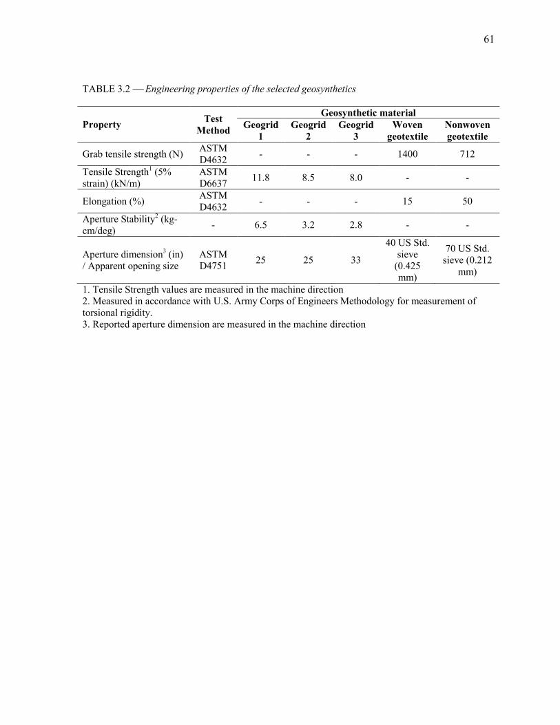
61

TABLE 3.2 Engineering properties of the selected geosynthetics

Property Test

Method

Geosynthetic material

Geogrid

1

Geogrid

2

Geogrid

3

Woven

geotextile

$onwoven

geotextile

Grab tensile strength (N) ASTM D4632

- - - 1400 712

Tensile Strength1 (5% strain) (kN/m)

ASTM D6637

11.8 8.5 8.0 - -

Elongation (%) ASTM D4632

- - - 15 50

Aperture Stability2 (kg-cm/deg)

- 6.5 3.2 2.8 - -

Aperture dimension3 (in) / Apparent opening size

ASTM D4751

25 25 33

40 US Std. sieve (0.425 mm)

70 US Std. sieve (0.212

mm)

1. Tensile Strength values are measured in the machine direction 2. Measured in accordance with U.S. Army Corps of Engineers Methodology for measurement of torsional rigidity. 3. Reported aperture dimension are measured in the machine direction

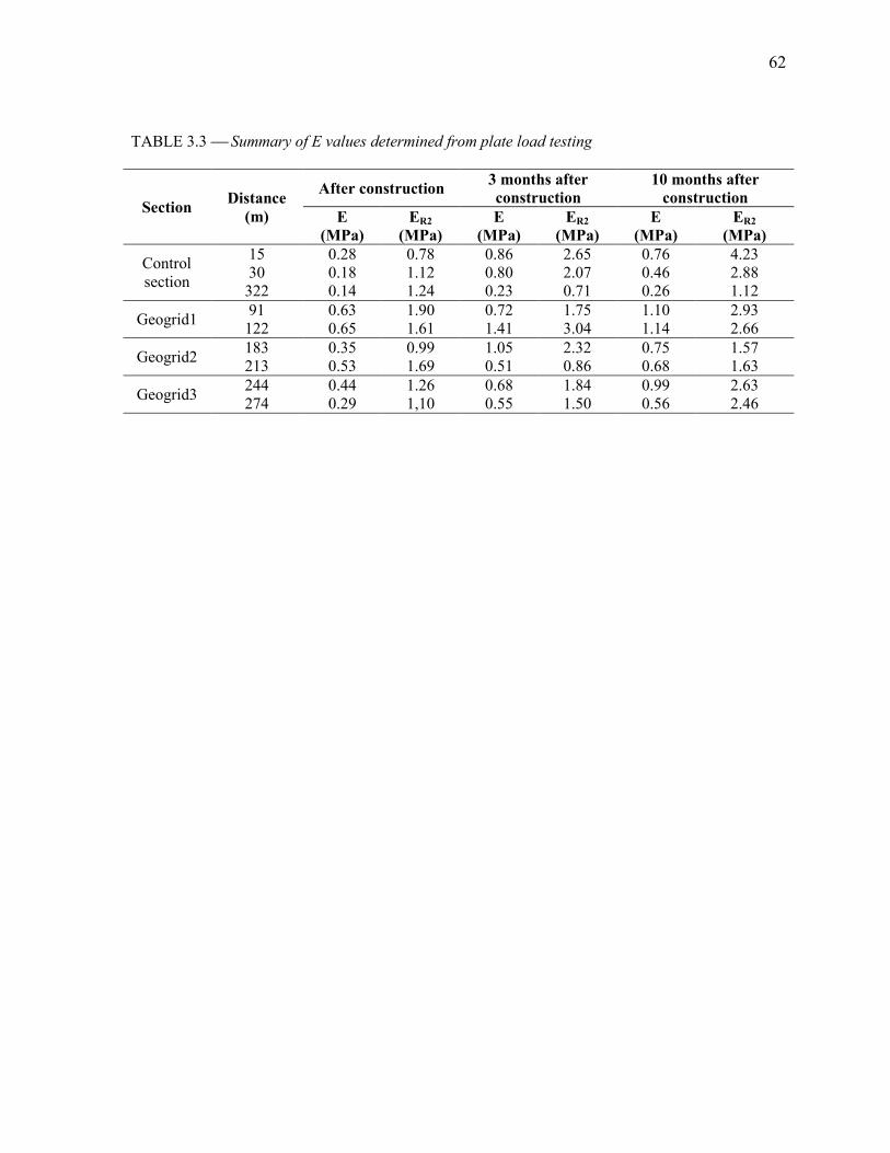
62

TABLE 3.3 Summary of E values determined from plate load testing

Section Distance

(m)

After construction 3 months after

construction

10 months after

construction

E

(MPa)

ER2

(MPa)

E

(MPa)

ER2

(MPa)

E

(MPa)

ER2

(MPa)

Control section

15 0.28 0.78 0.86 2.65 0.76 4.23 30 0.18 1.12 0.80 2.07 0.46 2.88 322 0.14 1.24 0.23 0.71 0.26 1.12

Geogrid1 91 0.63 1.90 0.72 1.75 1.10 2.93 122 0.65 1.61 1.41 3.04 1.14 2.66

Geogrid2 183 0.35 0.99 1.05 2.32 0.75 1.57 213 0.53 1.69 0.51 0.86 0.68 1.63

Geogrid3 244 0.44 1.26 0.68 1.84 0.99 2.63 274 0.29 1,10 0.55 1.50 0.56 2.46

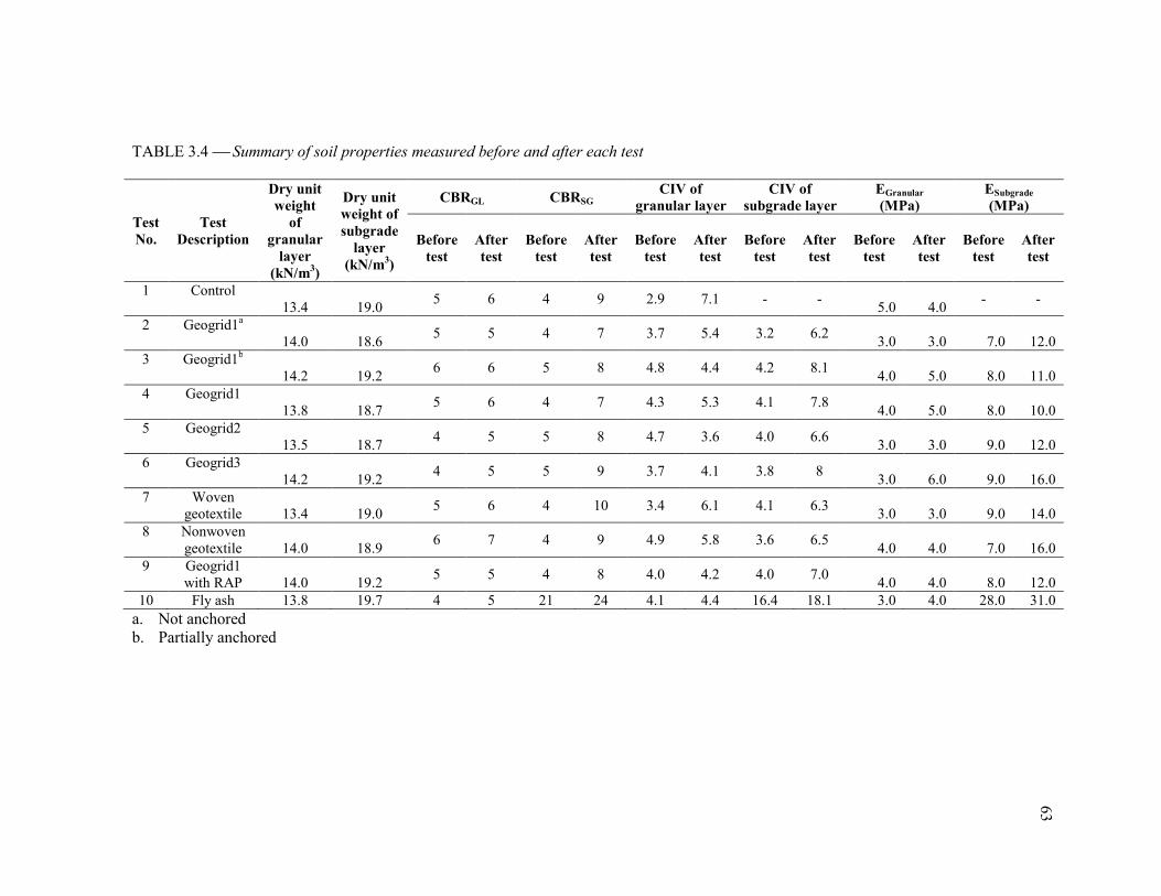
TABLE 3.4 Summary of soil properties measured before and after each test

Test

$o.

Test

Description

Dry unit

weight

of

granular

layer

(k$/m3)

Dry unit

weight of

subgrade

layer

(k$/m3)

CBRGL CBRSG CIV of

granular layer

CIV of

subgrade layer

EGranular

(MPa)

ESubgrade

(MPa)

Before

test

After

test

Before

test

After

test

Before

test

After

test

Before

test

After

test

Before

test

After

test

Before

test

After

test

1 Control 13.4 19.0

5 6 4 9 2.9 7.1 - - 5.0 4.0

- -

2 Geogrid1a

14.0 18.6 5 5 4 7 3.7 5.4 3.2 6.2

3.0 3.0 7.0 12.0

3 Geogrid1b

14.2 19.2 6 6 5 8 4.8 4.4 4.2 8.1

4.0 5.0 8.0 11.0

4 Geogrid1

13.8 18.7 5 6 4 7 4.3 5.3 4.1 7.8

4.0 5.0 8.0 10.0

5 Geogrid2

13.5 18.7 4 5 5 8 4.7 3.6 4.0 6.6

3.0 3.0 9.0 12.0

6 Geogrid3

14.2 19.2 4 5 5 9 3.7 4.1 3.8 8

3.0 6.0 9.0 16.0

7 Woven geotextile 13.4 19.0

5 6 4 10 3.4 6.1 4.1 6.3 3.0 3.0 9.0 14.0

8 Nonwoven geotextile 14.0 18.9

6 7 4 9 4.9 5.8 3.6 6.5 4.0 4.0 7.0 16.0

9 Geogrid1 with RAP 14.0 19.2

5 5 4 8 4.0 4.2 4.0 7.0 4.0 4.0 8.0 12.0

10 Fly ash 13.8 19.7 4 5 21 24 4.1 4.4 16.4 18.1 3.0 4.0 28.0 31.0

a. Not anchored b. Partially anchored

63

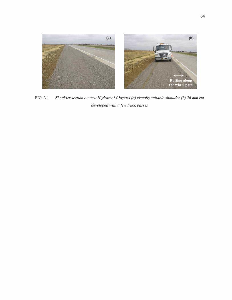
64

FIG. 3.1 Shoulder section on new Highway 34 bypass (a) visually suitable shoulder (b) 76 mm rut

developed with a few truck passes

(a) (b)

Rutting along

the wheel path

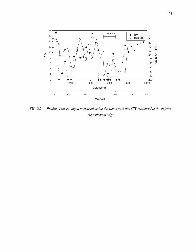
65

Distance (m)

0 2000 4000 6000 8000 10000

CIV

0

2

4

6

8

10

12

14

16

18

Ru

t d

epth

(m

m)

0

20

40

60

80

100

120

140

160

180

200

Milepost

218219220221222223224

CIV

Rut depth

Test section

FIG. 3.2 Profile of the rut depth measured inside the wheel path and CIV measured at 0.6 m from

the pavement edge

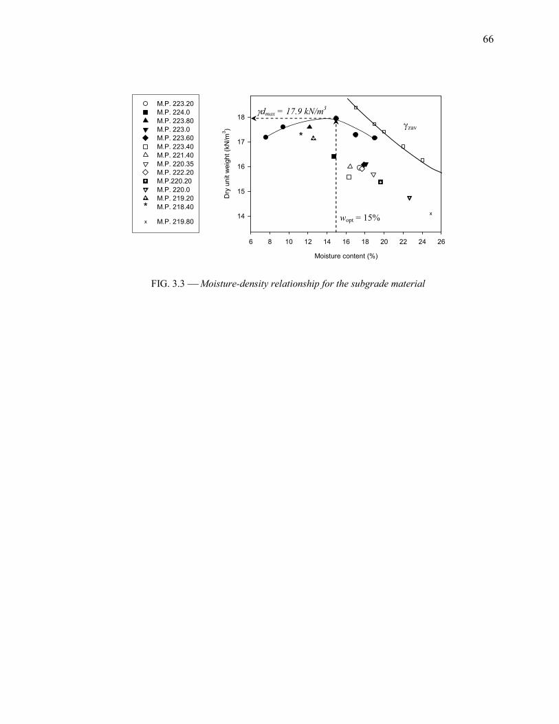
66

Moisture content (%)

6 8 10 12 14 16 18 20 22 24 26

Dry

un

it w

eig

ht

(kN

/m3)

14

15

16

17

18

*

x

M.P. 223.20

M.P. 224.0

M.P. 223.80

M.P. 223.0

M.P. 223.60

M.P. 223.40

M.P. 221.40

M.P. 220.35

M.P. 222.20

M.P.220.20

M.P. 220.0

M.P. 219.20

M.P. 218.40*

M.P. 219.80x

FIG. 3.3 Moisture-density relationship for the subgrade material

γzav

wopt = 15%

γdmax = 17.9 k2/m3

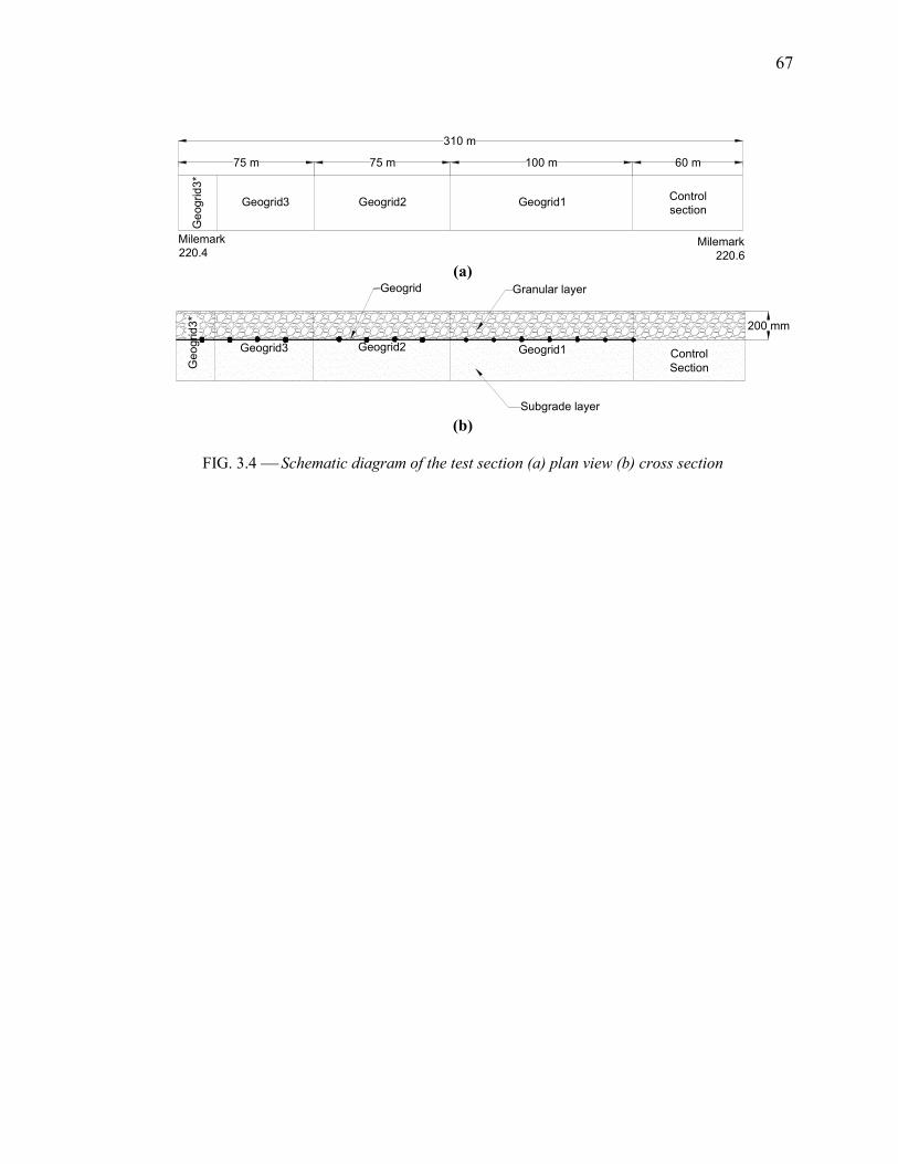
67

310 m

Geogrid2Geogrid3 Geogrid1Control

section

Milemark

220.6

Milemark

220.4

75 m 75 m 100 m 60 m

Ge

og

rid

3*

(a)

200 mm

Subgrade layer

Granular layerGeogrid

Geogrid1Geogrid2Geogrid3

Ge

og

rid

3*

Control

Section

(b)

FIG. 3.4 Schematic diagram of the test section (a) plan view (b) cross section

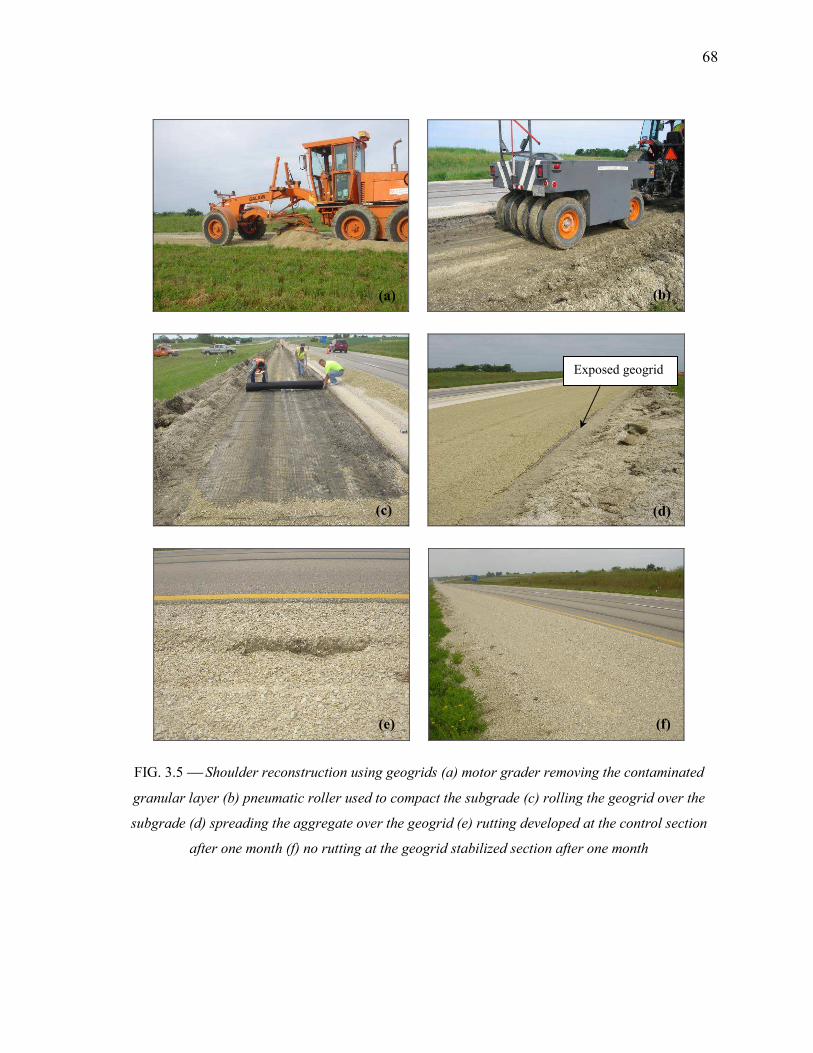
68

FIG. 3.5 Shoulder reconstruction using geogrids (a) motor grader removing the contaminated

granular layer (b) pneumatic roller used to compact the subgrade (c) rolling the geogrid over the

subgrade (d) spreading the aggregate over the geogrid (e) rutting developed at the control section

after one month (f) no rutting at the geogrid stabilized section after one month

(a) (b)

(d) (c)

Exposed geogrid

(e) (f)

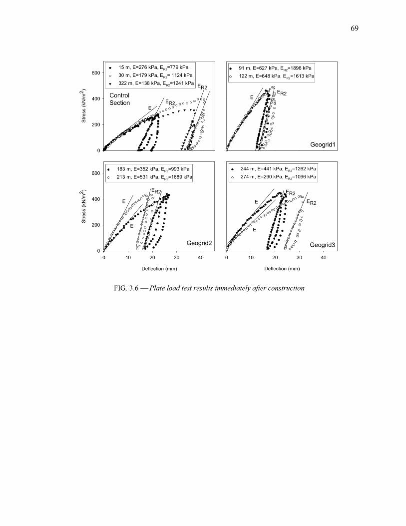
69

Str

ess (

kN

/m2

)

0

200

400

600

Deflection (mm)

0 10 20 30 40

Str

ess (

kN

/m2

)

0

200

400

600

Deflection (mm)

0 10 20 30 40

Control

Section

Geogrid1

Geogrid2 Geogrid3

E

ER2

ER2

E

E

E

E

E

ER2

ER2

ER2

ER2

15 m, E=276 kPa, ER2

=779 kPa

30 m, E=179 kPa, ER2

= 1124 kPa

322 m, E=138 kPa, ER2

=1241 kPa

91 m, E=627 kPa, ER2

=1896 kPa

122 m, E=648 kPa, ER2

=1613 kPa

183 m, E=352 kPa, ER2

=993 kPa

213 m, E=531 kPa, ER2

=1689 kPa

244 m, E=441 kPa, ER2

=1262 kPa

274 m, E=290 kPa, ER2

=1096 kPa

FIG. 3.6 Plate load test results immediately after construction

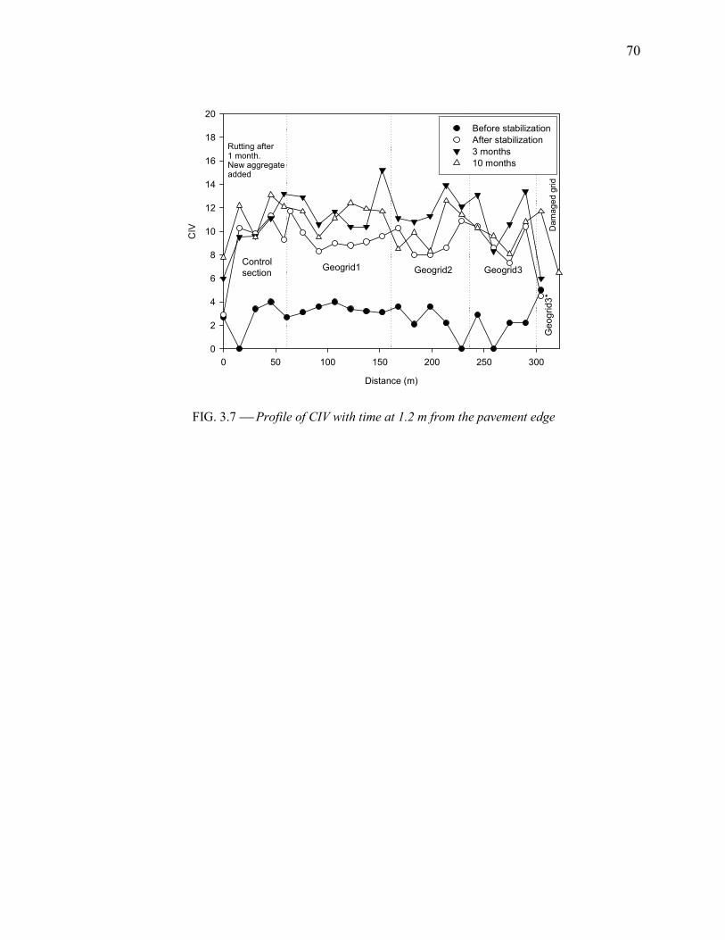
70

Distance (m)

0 50 100 150 200 250 300

CIV

0

2

4

6

8

10

12

14

16

18

20

Before stabilization

After stabilization

3 months

10 months

Control

sectionGeogrid1 Geogrid2 Geogrid3

Geog

rid3

*

Rutting after1 month.New aggregateadded

Da

ma

ge

d g

rid

FIG. 3.7 Profile of CIV with time at 1.2 m from the pavement edge

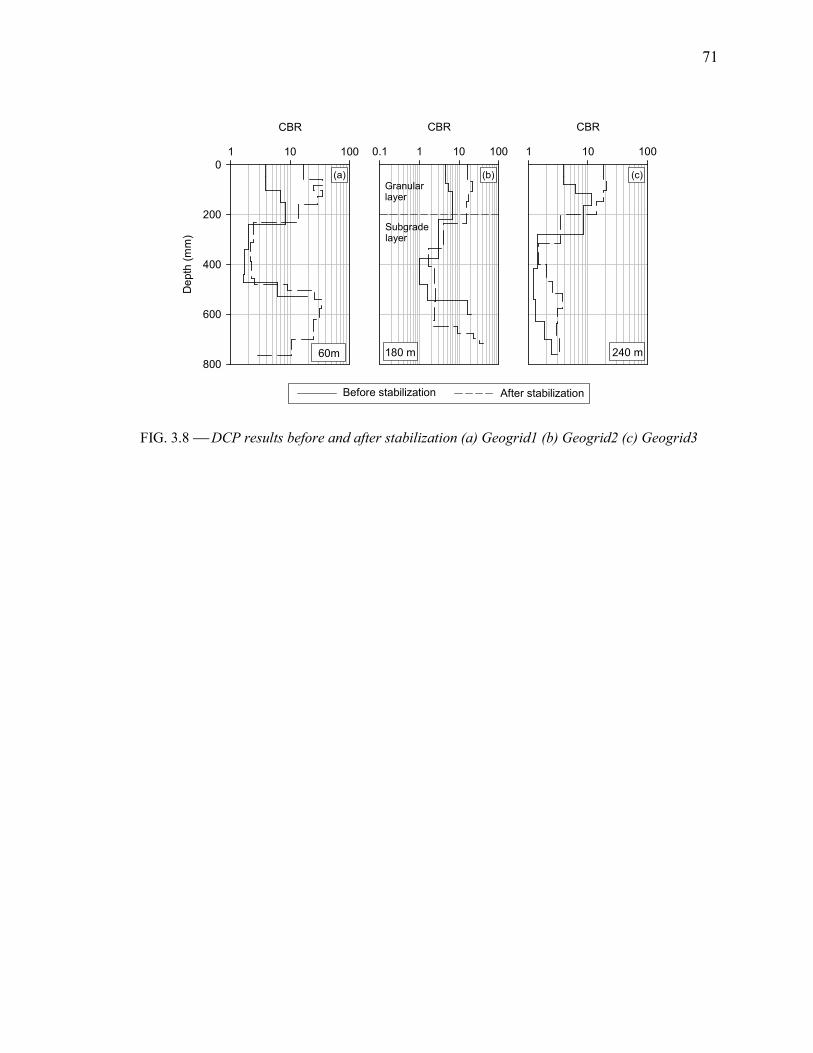
71

CBR

1 10 100

De

pth

(m

m)

0

200

400

600

800

CBR

0.1 1 10 100

CBR

1 10 100

Before stabilization After stabilization

60m 180 m 240 m

(a) (b) (c)Granularlayer

Subgradelayer

FIG. 3.8 DCP results before and after stabilization (a) Geogrid1 (b) Geogrid2 (c) Geogrid3

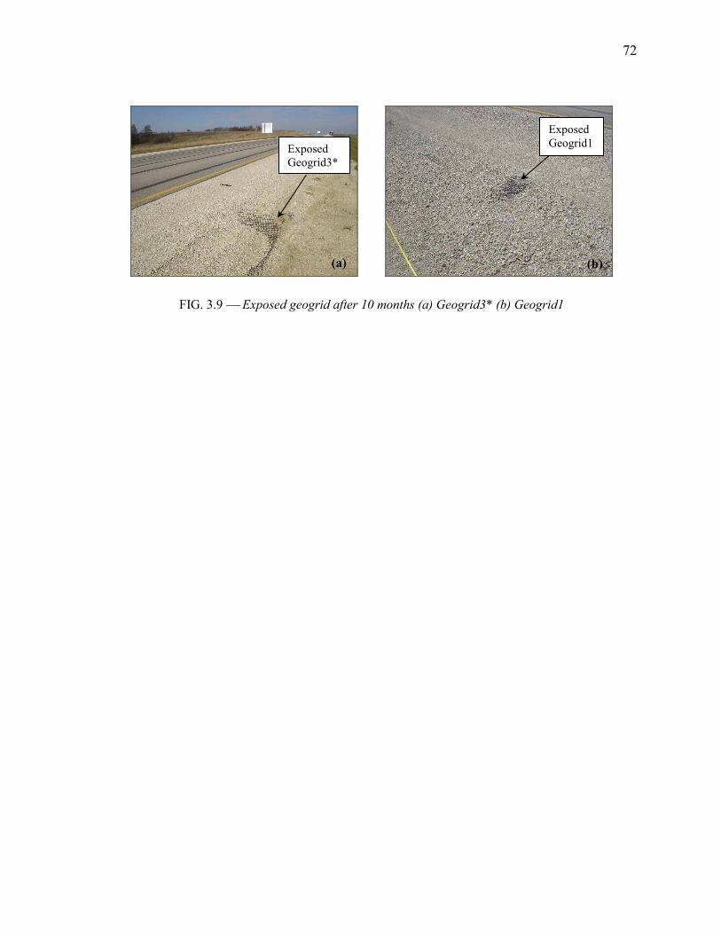
72

FIG. 3.9 Exposed geogrid after 10 months (a) Geogrid3* (b) Geogrid1

(a) (b)

Exposed Geogrid3*

Exposed

Geogrid1

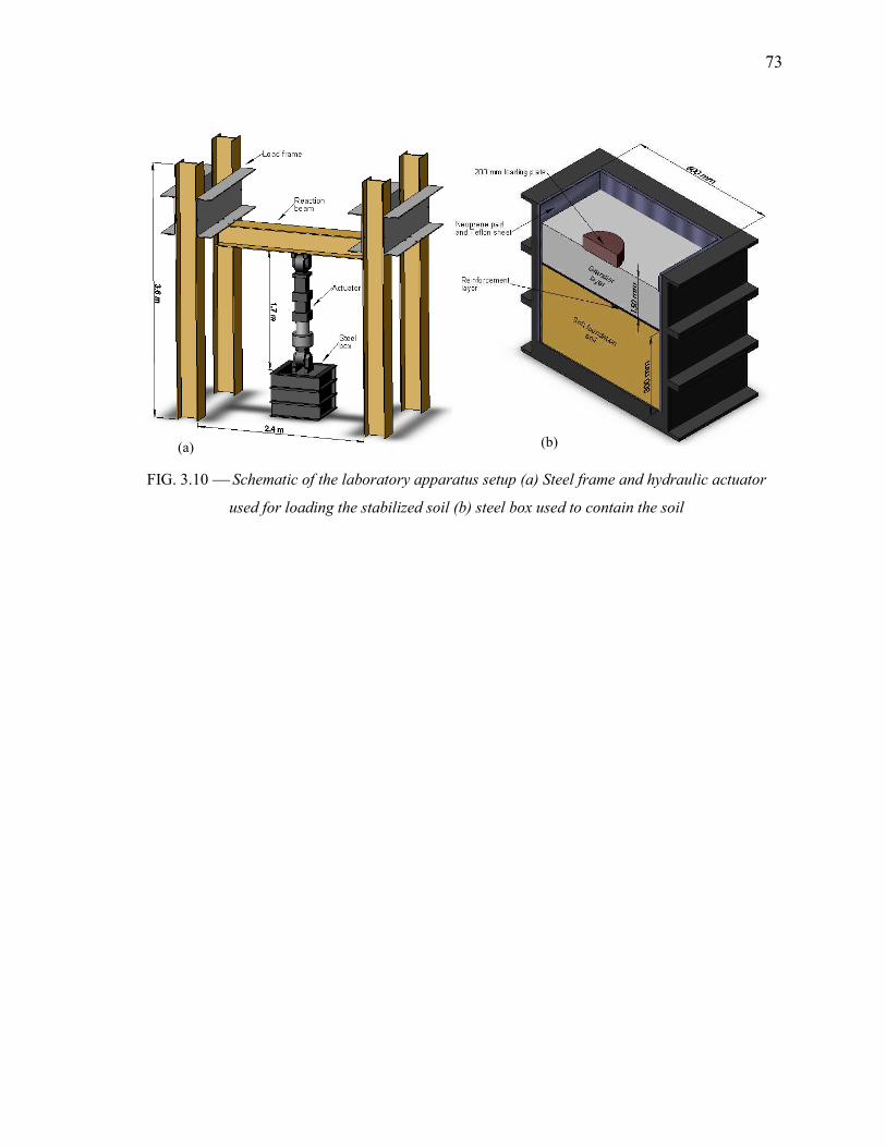
73

FIG. 3.10 Schematic of the laboratory apparatus setup (a) Steel frame and hydraulic actuator

used for loading the stabilized soil (b) steel box used to contain the soil

(a) (b)

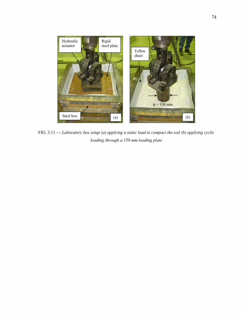
74

FIG. 3.11 Laboratory box setup (a) applying a static load to compact the soil (b) applying cyclic

loading through a 150 mm loading plate

Rigid

steel plate

φ = 150 mm

Hydraulic

actuator

Steel box

Teflon sheet

(a) (b)

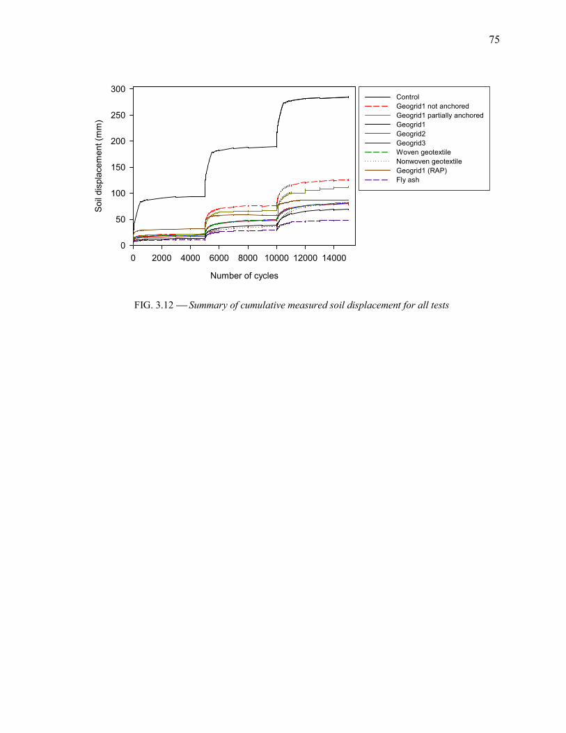
75

Number of cycles

0 2000 4000 6000 8000 10000 12000 14000

Soil

dis

pla

cem

ent (m

m)

0

50

100

150

200

250

300Control

Geogrid1 not anchored

Geogrid1 partially anchored

Geogrid1

Geogrid2

Geogrid3

Woven geotextile

Nonwoven geotextile

Geogrid1 (RAP)

Fly ash

FIG. 3.12 Summary of cumulative measured soil displacement for all tests

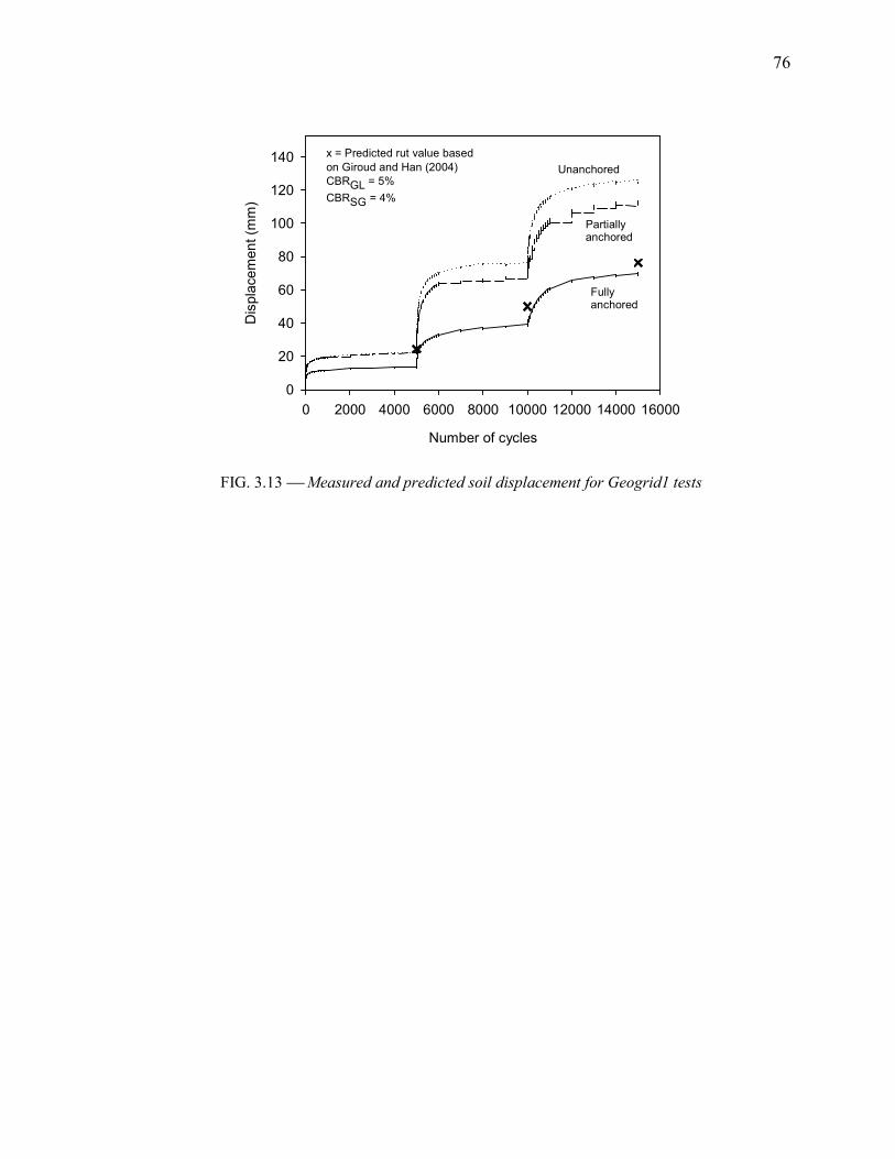
76

Number of cycles

0 2000 4000 6000 8000 10000 12000 14000 16000

Dis

pla

ce

men

t (m

m)

0

20

40

60

80

100

120

140 x = Predicted rut value based

on Giroud and Han (2004)

CBRGL = 5%

CBRSG = 4%

Unanchored

Partiallyanchored

Fully anchored

FIG. 3.13 Measured and predicted soil displacement for Geogrid1 tests

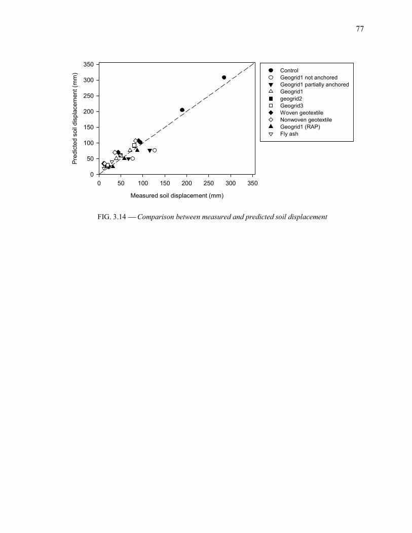
77

Measured soil displacement (mm)

0 50 100 150 200 250 300 350

Pre

dic

ted s

oil

dis

pla

ce

men

t (m

m)

0

50

100

150

200

250

300

350Control

Geogrid1 not anchored

Geogrid1 partially anchored

Geogrid1

geogrid2

Geogrid3

Woven geotextile

Nonwoven geotextile

Geogrid1 (RAP)

Fly ash

FIG. 3.14 Comparison between measured and predicted soil displacement

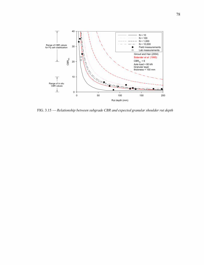
78

Rut depth (mm)

0 50 100 150 200

CB

RS

G

0

10

20

30

40

N = 10

N = 100

N = 1,000

N = 10,000

Field measurements

Lab measurements

CBRGL = 6

Axle load = 80 kNGranular layer thickness = 150 mm

Range of CBR valuesfor Fly ash stabilization

Range of in situ CBR values

Giroud and Han (2004)

Bolander et al. (1995)


79

4. ASSESSME$T OF PILE DETERIORATIO$ A$D RESIDUAL PILE CAPACITY USI$G

$O$DESTRUCTIVE STRESS WAVE TECH$IQUES

4.1. ABSTRACT

Timber piles are one of the most common foundation elements used in bridge construction.

However if not properly preserved, timber piles can be susceptible to biological and physical

deterioration. Currently, there are no reliable means in evaluating deteriorated timber piles, which

often leads to costly maintenance practices. The results of a field investigation, in which 49 low

volume bridges with timber substructure across the state of Iowa were inspected, showed that 50% of

the inspected substructures suffered from biological deterioration, which typically occurred near the

ground level. Mechanical deterioration as evidenced by mushrooming and bulging of the timber piles

was observed in 30% of the inspected substructures. A laboratory study was undertaken with the

objective of estimating the residual capacity of deteriorated pile sections by correlating the modulus

of elasticity (E) determined by axial compression tests and the dynamic elastic modulus (MOEd)

determined using the nondestructive ultrasonic stress wave technique. The ultrasonic stress wave

technique was also used to produce two-dimensional tomography images revealing the internal pile

condition. Presented in this paper are the findings of a field reconnaissance study and the details of a

procedure developed to assess the residual capacity of timber piles and to detect internal pile decay.

80

4.2. I$TRODUCTIO$

Problems with unknown foundations are often associated with timber substructures. Timber

piles can undergo deterioration, which in initial stages, can be difficult to detect. There are currently

no reliable means to estimate the residual bearing capacity of an in-service deteriorated pile; thus, the

overall capacity of the bridge cannot be determined. The lack of a reliable evaluation method often

results in conservative and costly maintenance practices such as replacing the entire substructure

system. Several pertinent studies categorized the causes of timber pile deterioration into biological

and mechanical factors. The main biological factors include fungi, bacteria, and insect attack,

whereas the main mechanical factors include abrasion and overloading. Fungi, which break down

and utilize wood cells, generally attack wood above the water level where oxygen levels are

sufficient. Bacterial decay progresses slowly, compared to fungal deterioration, and causes softening

of wood, which makes timber piles excessively absorptive to moisture. Insect attack is evidenced by

tunnels or cavities in the wood, which often contain wood powder. Pile abrasion, which causes a

reduction in the pile cross sectional area, generally occurs due to the impact of floating debris and/or

ice in streams. The most common cause of pile overloading is significant loss of bearing capacity of

adjacent piles. However, overloading of piles can also result from continuous heavy loads, infrequent

severe loads and loss of the pile structural capacity (Wang et al. 2000, Lopez-Anido et al. 2004,

Toutanji 2004, Aggour 1991, USDA 1999, and Manuel 1984).

A recent study was completed by White et al. (2007) with the objective of investigating

frequent timber substructure problems in Iowa, developing nondestructive evaluation procedures for

timber piles, and recommending repair methods to restore the capacity of partially deteriorated piles.

During the course of the study, 49 low volume road bridges with timber substructures were inspected.

About 50% of the inspected substructures suffered from biological deterioration, which typically

occurred near the ground level. Mechanical deterioration as evidenced by mushrooming and bulging

of the timber pile was observed in 30% of the inspected substructures. The ability of a nondestructive

ultrasonic stress wave technique in identifying pile internal decay was evaluated by producing two-

dimensional tomography images of deteriorated pile sections and comparing them to digital images of

the actual pile deterioration. Furthermore, a correlation was established between the Dynamic

Modulus of Elasticity (MOEd) calculated from the nondestructive ultrasonic stress wave test and

modulus of elasticity (E) determined from the axial compression test of 12 timber pile sections to

estimate the residual capacity of deteriorated piles.

81

4.3. BACKGROU$D

Timber piles are a commonly used foundation elements used because of their relatively low

cost compared to steel and concrete. Timber piles are also easily installed and more available

compared to other materials (Chen and Kim 1997 and U.S. Army Corps of Engineers et al. 2001).

The disadvantage of using timber piles, however, is their susceptibility to damage and degradation.

Timber pile decay can be alleviated by the use of preservatives. However, the long term performance

is still a concern (Lopez-Anido et al. 2004).

According to Toutanji (2004), timber deterioration, in most cases, is continuous and the

degrading actions from one or more agents change the timber properties making it susceptible to

degradation from other agents. The causes of timber pile deterioration can be categorized into

biological deterioration and mechanical deterioration. Biological deterioration includes (1) fungi, (2)

bacteria, and (3) insect attack. Mechanical deterioration includes (1) abrasion, (2) overloading, and

(3) fire. Wang et al. (2000) reported that 7,000 to 8,000 tons of mechanically or biologically

deteriorated timber piles are currently removed from U.S. Naval facilities annually at a cost of at least

$20 million per year.

4.3.1. Biological Deterioration

4.3.1.1 Fungi

Fungi have the unique capacity to break down and utilize wood cell wall material as food

(Johnson 2004). Fungi generally attack above the water level where sufficient oxygen allows them to

survive and decay the wood. For this reason, foundation piles buried below the water table or ground

level are not subjected to decay by typical wood-decay fungi. Fungi decay also depends heavily on

temperature and moisture conditions. For fungi to be active and degrade wood, the moisture content

of wood has to be 30% or higher (Lopez-Anido et al. 2004). The fungus in an area of decaying wood

is generally invisible but present as a growing network of microscopic threads randomly penetrated

throughout the wood (Johnson 2004). There are two major decay fungi recognized: brown-rot, often

termed “dry rot” and white-rot. Brown-rot fungi extensively remove cellulose causing the wood to

have a brown color, which contributes to cracking across the grain, shrinking, collapse, and crushing

into powder (USDA 1999). A danger with brown-rot fungi decay is that wood can lose up to 70% of

its modulus of rupture and E yet appear visually sound (Lopez-Anido et al. 2004). White-rot fungi

removes both lignin and cellulose leaving the wood with a “whiter” than normal color; it does not

cause cracks across the grain, and until severely degraded, it retains its outward dimensions and does

82

not shrink or collapse. Soft rot is a third kind of decay with less importance; it is caused by wet

conditions that cause softening of the wood. However, its effect is relatively shallow and therefore it

is most likely to damage thin pieces of wood (USDA 1999 and U.S. Army Corps of Engineers et al.

2001). In addition to moduli, decay affects toughness of wood or its ability to withstand impacts

which is followed by strength reduction. According to the USDA (1999), by the time 1% of weight

loss has occurred in wood by fungal attack, losses in toughness range from 6 to 50%. By the time

10% weight loss has occurred, strength losses are expected to exceed 50%. At this stage, decay is

only detectable microscopically; therefore, it may be reasonably assumed that wood with visual

evidence of decay has been greatly reduced in all strength values.

4.3.1.2. Bacteria

Aggour (1991) stated that wood that has been wet for a considerable length of time will

probably contain bacteria. Bacterial deterioration proceeds slowly compared to fungal decay, and has

little effect on wood properties, except over long periods. Bacteria however, can cause softening and

make wood excessively absorptive to moisture and preservatives during treatment (Aggour 1991).

Bacteria may also destroy preservatives such as creosotes making the wood more susceptible to

degradation from less chemically tolerated organisms (USDA 1999).

4.3.1.3. Insects

Out of 26 insect orders, termites, beetles, bees, wasps, and ants are the primary causes of

most insect-related deterioration. Insect attack is generally apparent from tunnels or cavities in the

wood, which often contain wood powder. In addition to removing portions of the wood structure,

insects may also carry decay fungi that further deteriorate wood (USDA 1999).

4.3.2. Mechanical Deterioration

4.3.2.1. Abrasion

According to Manuel (1984), abrasion of timber piles can occur by impact from floating

debris and/or ice in streams. The velocity of water moving past the pile and the quantity, shape, size,

and hardness of particles being transported have been linked to the rate of abrasion (U.S. Army Corps

of Engineers et al. 2001).

83

4.3.2.2. Overloading

Overloading of piles can result from continuous heavy loads, infrequent severe loads, loss of

the pile structural capacity, or more frequently, significant loss of adjacent supports. Failure of one

pile requires the adjacent pile to carry extra load. Continuous overloading results in several modes of

compression failure including splitting of the top portion and misalignment or “mushrooming” at a

hollow portion after breakage (USDA 1999).

4.3.2.3. Other Mechanical Factors

Other noteworthy mechanical agents that damage timber piles are fire, connection failure,

which exposes untreated wood allowing entry for fungi or insects, ultraviolet degradation, which

causes scaling of the timber surface, chemical degradation, and foundation settlement (Manuel 1984).

4.4. FIELD RECO$$AISSA$CE

A field reconnaissance was performed to identify the causes of timber substructure problems

in low volume road (LVR) bridges in Iowa as well as identifying common maintenance practices.

During the field reconnaissance, 49 LVR bridges were inspected. About 50% of the inspected

substructures suffered from biological deterioration, which typically occurred near the ground or

water level where conditions are favorable for bacteria, fungi, and insect growth. Biological decay

can result in considerable reduction in pile cross sectional area as shown in Figure 4.1a. If allowed to

progress, biological decay may result in complete failure of the pile section (See Figure 4.1b).

Physical deterioration was observed in 30% of the inspected substructures. Mechanical deterioration

existed in many forms such as cracks and splits, reduction of pile cross section by abrasion, broken

piles, and brooming of the pile. Overloading the piles was observed in 20% of the inspected

substructures. Overloading, which is mostly caused by failure of adjacent pile(s), can result in a

compression failure of the pile and separation of the top portion of the pile as shown in Figure 4.2a.

A compression failure can also be in the form of bulging of wood fibers or “mushrooming” at a

hollow pile section (See Figure 4.2b). Other causes of pile deterioration observed that were less

frequent and less threatening to the pile’s integrity were ultraviolet degradation and pile cap

deterioration.

Several substructure remediation techniques were observed. These techniques included

addition of a timber or steel pile adjacent to the defective pile and constructing a new substructure

system (i.e. replacing all existing piles). When deterioration is localized in one pile, a new pile

(timber or steel) is driven next to the faulty pile as shown in Figure 4.3. Complete replacement of the

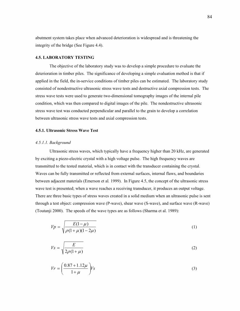
84

abutment system takes place when advanced deterioration is widespread and is threatening the

integrity of the bridge (See Figure 4.4).

4.5. LABORATORY TESTI$G

The objective of the laboratory study was to develop a simple procedure to evaluate the

deterioration in timber piles. The significance of developing a simple evaluation method is that if

applied in the field, the in-service conditions of timber piles can be estimated. The laboratory study

consisted of nondestructive ultrasonic stress wave tests and destructive axial compression tests. The

stress wave tests were used to generate two-dimensional tomography images of the internal pile

condition, which was then compared to digital images of the pile. The nondestructive ultrasonic

stress wave test was conducted perpendicular and parallel to the grain to develop a correlation

between ultrasonic stress wave tests and axial compression tests.

4.5.1. Ultrasonic Stress Wave Test

4.5.1.1. Background

Ultrasonic stress waves, which typically have a frequency higher than 20 kHz, are generated

by exciting a piezo-electric crystal with a high voltage pulse. The high frequency waves are

transmitted to the tested material, which is in contact with the transducer containing the crystal.

Waves can be fully transmitted or reflected from external surfaces, internal flaws, and boundaries

between adjacent materials (Emerson et al. 1999). In Figure 4.5, the concept of the ultrasonic stress

wave test is presented; when a wave reaches a receiving transducer, it produces an output voltage.

There are three basic types of stress waves created in a solid medium when an ultrasonic pulse is sent

through a test object: compression wave (P-wave), shear wave (S-wave), and surface wave (R-wave)

(Toutanji 2000). The speeds of the wave types are as follows (Sharma et al. 1989):

)21)(1(

)1(

µµρµ−+

−=

EVp (1)

)1(2 µρ +=

EVs (2)

VsVr

++

=µ

µ1

12.187.0 (3)

85

Where Vp = the speed of the P-wave, Vs = the speed of the S-wave, Vr = the speed of the R-

wave, E = modulus of elasticity, ρ = the mass density, and µ = Poisson’s ratio. It can be seen that the

speed of the propagating wave is directly dependent on the material properties through which the

wave is traveling.

4.5.1.2. Difficulties and Limitations

A single stress wave measurement can only detect internal decay that is greater than 20% of

the total cross section of the timber pile (Emerson et al. 1999). Therefore, multiple measurements are

often conducted to increase the test reliability. In the field, however, it is not always feasible to

access the complete circumference of the pile due to the presence of the backwall behind the timber

pile. Another limitation is coupling of the sensors with the timber surface. Most piles exhibit splits

and cracks, which result in poor acoustic coupling between the transducer and the timber surface

leading to unstable reading (Emerson et al. 1999). Furthermore, in severe internal pile deterioration,

and due to high stress wave attenuation in void spaces, a stress wave travel time measurement may

not be obtained. An example of a deteriorated pile observed during the field reconnaissance phase is

shown in Figure 4.6. The rapid attenuation of the wave in the hollow region hindered the detection of

the intact area near the pile core and prevented the wave from reaching the receiving transducer.

4.5.1.3. Description of Equipment

A James Instrument Velocity Meter (James V-Meter); shown in Figure 4.7, equipment

manufactured by James Instruments, Inc. was used in this study. The instrument utilizes an ultrasonic

pulse generator to impart a stress wave into the specimen. As the transmitting transducer imparts a

wave into the member, the timer unit begins timing passage of the wave, and as it reaches the

receiving transducer, the timer stops. The transducers are p-type transducers (i.e. detect P-waves

only) with a resonant frequency of 54 kHz. A key consideration when using this equipment is

coupling; to obtain reliable results, the surface of the specimen must be free of debris, mud, or dirt. A

coupling agent, provided by the manufacturer, is often used to facilitate measurements (Wang et al.

2004). Even with the use of ample coupling agent, it was difficult to obtain a stable reading between

the flat transducer surface and the round timber surface. Therefore, the authors decided to retrofit the

velocity meter with two brass cones as shown in the Figure 4.7. By providing two fixed contact

points at the pile surface, the acoustic coupling of the transducers with the timber surface was

improved. The coupling agent was used at the interface between the transducers and the cones to

prevent wave attenuation. To calibrate the device with the retrofitted cones, which were attached to

86

the transducers, at the beginning of each test the brass cones were brought in contact and an “offset”

reading was taken and subtracted from all future readings.

4.5.1.4. Image Processing

The acoustical imaging software used in this laboratory study was 3DTOM: Three-

Dimensional Geophysical Tomography developed by Jackson and Tweeton (1996) at the United

States Bureau of Mines. The program uses an ASCII text input file, which includes source-receiver

coordinates, and travel times, to produce a velocity tomogram. The tomogram is created by using a

simultaneous iterative reconstruction technique (SIRT); model is constructed as a grid of nodes with

intervening voxels (See Figure 4.8). SIRT includes three cyclic procedures that are repeated until

pre-selected criteria are met. These procedures are (1) forward computation of model travel time, (2)

calculation of residual travel times, and (3) application of velocity corrections. Forward computation

of model travel time compares a calculated travel time of a particular ray to the measured travel time

of that ray using Equation 4 (Jackson and Tweeton 1996).

∑=

=M

1j

ijji dpt (4)

Where M = number of voxels in the image reconstruction grid, ti = measured travel time for

ray i, dij = the distance traveled by ray I through voxel j, and pj = the average slowness (inverse

velocity) of the ray in voxel j. The variable dij = nonzero for the voxels at which ray i passes.

The residual of each ray (difference between the left hand side and right hand side of

Equation 4) is used to calculate incremental correction factors for all voxels sampled by a particular

ray. Since the imaging process uses simultaneous reconstruction method, the correction factors of all

individual rays are calculated and accumulated before being applied to the voxels (Jackson and

Tweeton 1996). The correction factor for ray i in voxel j is calculated as follows:

∑=

=M

1k

2

ikp

iji

ij

)(dN

d∆t∆p (5)

Where ∆pij = the slowness correction of ray i in voxel j, ∆ti = the travel time residual for ray i,

dij is the path length for ray i in voxel j, Np = the number of rays in voxel j, M = the number of voxels

in the grid, and dik = the path length of ray i in each of the M voxels in the grid.

87

The incremental slowness corrections are summed to obtain a net correction factor for voxel j

as shown in the Equation 6.

∑=

=N

1ijij ∆p∆p (6)

Where ∆pj = the slowness correction of voxel j, N = number of rays, and ∆pij = the slowness

correction of ray i in voxel j. For example, if there are three rays that pass through voxel number 4,

Equation 6 would become:

342414

3

1

44 pppppi

i ∆+∆+∆=∆=∆ ∑=

Correction factors for each grid node are then obtained by averaging the corrections

calculated for each voxel attached to that node.

4.5.1.5. Test Procedure

Multiple measurements were performed at each cross section to create a tomographic image.

The 20 measurements were used in this laboratory study for each two-dimensional cross section,

which was accomplished by marking eight test points (See Figure 4.9) on the pile circumference.

Multiple images of the internal condition of the pile were generated by repeating the test every 100

mm along the length of the pile. The purpose of generating multiple two-dimensional images is an

attempt to separate strong and weak areas inside the pile.

4.5.1.6. Test Verification and Repeatability

To verify that the selected imaging reconstruction technique and test procedure produce

reliable results, tomographic images generated at the surface of several piles were compared to digital

images. Four pile sections were damaged to simulate biological deterioration by creating a cavity

near the pile core as shown in Figure 4.10, which would not necessarily be visible from the outside of

an in-service pile. A radial cut was made for one pile section to simulate pile cracking, which

typically develops due to wet-dry cycles or during pile driving (See Figure 4.10e). The height and

diameter of these pile sections were about 127 mm and 292 mm, respectively. Another pile section

used in this study was obtained from a bridge abutment that had been replaced in August 2005. The

pile had considerable outer damage as depicted in Figure 4.10f. The pile height and diameter were

approximately 600 mm and 300 mm, respectively. A ninth point was marked at the pile

88

circumference adjacent to the damaged area. Preliminary testing revealed that without this additional

point, the damaged area could not be detected since no wave travel path was reflected from the

damaged area. This is not considered a limitation in the field because this type of external decay is

visually detectable and does not necessarily require nondestructive methods. The results,

demonstrated by the tomography images shown in Figure 4.10, indicate that the selected test

procedure and image reconstruction technique were successful in capturing the approximate shape,

size, and location of the internal damage. Results also show that the velocities in the hollow areas

were lower than the intact parts of the pile sections. Velocities in hollow areas were generally less

than 0.51 mm/µs.

The accuracy and repeatability of the test procedure were evaluated by repeating the

ultrasonic stress wave test 10 times for each pile section. In each test, the locations of the eight test

points, where the transmitting and receiving transducers were positioned, were shifted and a

tomography image was generated (i.e. 10 tomograms were created for each pile section). From each

image, the region enclosed by a velocity less than 0.51 mm/µs was measured to estimate the hollow

area of the pile section, which was then compared to the true area. The difference between the true

cavity area and the mean measured area for each pile section gave an indication of the accuracy of the

test procedure, whereas the difference between the measured areas gave an indication of the test

procedure repeatability (precision). Normal distribution plots of the measured areas for the six pile

sections are presented in Figure 4.11. The dashed lines depicted in the figure represent the true cavity

areas. Apart from the results shown in Figure 4.11a, where the damage comprised of a square cavity

with an actual area of 9,408 mm2 and a computed area of 9,194 mm2, the results demonstrate that the

test procedure and/or the image reconstruction process have a “biased” tendency to over predict the

cavity area. The results shown in Figure 4.10b through 4.10f demonstrate that the computed areas

were higher than the actual measured areas. The percent error between the actual cavity area and the

mean predicted cavity area ranged from 2.3 to 41%. The results also show that the size of the internal

defect may have an influence on the test precision. Small defects relative to the pile diameter, such as

the 38 mm in diameter cavity and the radial crack, have a higher percent error. This may be

attributed to the number of measurements, which can only identify defects with limited precision.

Increasing the number of measurements may decrease the influence of the internal defect size and

shape on precision of the test procedure.

To determine whether the orientation of the transmitter and receiver transducers influenced

the test precision, the mean and standard deviation of the percent error were calculated. Each pile

89

section had a different standard deviation of the percent error indicating that the orientation of the

transducers influenced the precision of the test procedure. This can be explained by the anisotropy of

acoustic propagating velocities in wood (i.e. the elastic properties and the associated acoustical

properties are very different in the radial, tangential, and longitudinal directions).

4.5.1.7. Test Results

The ultrasonic stress wave test was performed on 12 timber pile sections. For each section,

multiple radial measurements, using the transducers arrangement outlined earlier, were performed

every 100 mm producing a two-dimensional tomogram and revealing the pile internal condition. Out

of the 12 specimens, nine were previously in service and three were new. Typical tomography output

generated for each pile specimen is presented in Figure 4.12 (for the detailed results of this laboratory

study refer to White et al. 2007).

For each timber pile, and form every tomographic image, an average velocity perpendicular

to the grain was computed. The average velocities at the pre-selected elevations were then compared

and a minimum and an average velocity were determined for the entire pile section. The density and

travel time parallel to the grain were also measured. By knowing the pile length, the velocity parallel

to the grain was calculated. By using Equation 1 and an Poisson’s ratio of 0.49, which is a typical

value for southern yellow pine timber piles commonly used in Iowa, a MOEd was calculated using the

minimum velocities perpendicular to the grain, average velocities perpendicular to the grain, and the

velocity parallel to the grain. A summary of pile properties, measured velocities, and calculated

MOEd are presented in Table 4.1. It was noted that the ultrasonic wave speed parallel to the grain

was about 2-5 times higher than the wave speed perpendicular to the grain.

4.5.2. Axial Compression Tests

Upon completion of the nondestructive evaluation, each pile section was tested in

compression to determine its modulus of elasticity. A universal testing machine, which recorded the

applied load and also displacement, with a capacity of 1779 kN was used to load the timber pile

sections to failure. The compression machine recorded the applied load and displacement. A stress-

strain curve was produced for every pile section as shown in Figure 4.13. The stress-strain curves

show that pile Nos. 1, 2, and 3, which were new piles, displayed a clear linear elastic region and a

distinct yield point beyond which the pile section failed. The yield points for other pile sections,

which were in-service prior to testing and endured varying degrees of deterioration, were less distinct.

90

These pile sections also showed higher displacement prior to failure. Overall, all pile sections

demonstrated ductile behavior. Modulus of elasticity values are summarized in Table 4.1.

4.5.3. Correlation between Compression and Ultrasonic Stress Wave Tests

Linear regression models, shown in Figure 4.14, were developed correlating E determined

from axial compression tests to MOEd predicted from (1) average velocity for the entire pile section

perpendicular to the grain, (2) minimum velocity for the entire pile section perpendicular to the grain,

and (3) average velocity parallel to the grain. The results show that there is a correlation (R2 = 0.5)

between E and MOEd determined from velocities perpendicular to the grain. There is no significant

difference between the models derived from the average and minimum velocities perpendicular to the

grain. The model developed using the velocity parallel to the grain showed the lowest correlation (R2

= 0.3). The results, therefore, demonstrate the potential of the test procedure in predicting the

residual capacity of in-service deteriorated piles.


If not properly preserved and maintained, timber piles can undergo biological and mechanical

deterioration due to various reason. This deterioration can significantly reduce the pile bearing

capacity and threaten the structural integrity of the bridge. There are no reliable inspection

techniques available to evaluate the structural integrity of deteriorated piles or detect pile decay at

early stages, which often leads to conservative and costly maintenance. A field reconnaissance

conducted to evaluate timber substructures in Iowa demonstrated that biological deterioration in the

form of fungal, bacterial, or insect attack mostly occurs near the ground/water level where conditions

are favorable. When left untreated, biological deterioration can lead to the loss of a pile’s structural

capacity. Mechanical deterioration as evidenced by abrasion, broken piles, and bulging and

mushrooming of timber piles was observed at about 30% of the inspected sections. Mechanical

deterioration often leads to reduction in pile cross section and load transfer to adjacent piles.

A laboratory study was conducted to evaluate the potential of using nondestructive ultrasonic

stress wave technique to determine the internal condition of timber piles. Also, the study aimed to

establish a correlation between destructive and nondestructive test method, which can assist in

estimating the capacity of in-service piles. Combined with SIRT, the ultrasonic stress wave method

was used to generate two-dimensional tomography images from multiple ultrasonic stress wave

measurements. The selected test method and imaging reconstruction technique were able to display

the internal condition of several piles that had internal defects of various sizes and shapes. The test

91

method, however, has a tendency to over predict the size of the internal defect. The prediction error

increases as the size of the internal defect decrease. Increasing the number of test measurements can

improve the accuracy of the test method.

MOEd parallel and perpendicular to the grain were calculated for 12 timber pile sections

using velocities computed from the generated tomography images. Following the nondestructive

tests, axial compression tests were performed to calculate modulus of elasticity. Linear regression

models showed that there is a correlation between MOEd derived from velocities perpendicular to the

grain and modulus of elasticity (R2 = 0.5). It is therefore concluded that the ultrasonic stress wave

technique can be correlated to the residual capacity of timber piles and is a promising tool in

evaluating deteriorated in-service timber substructure systems.

Since this laboratory study is an initial step towards characterizing bridges with unknown

foundation, additional research is required to evaluate (1) different transducers and their orientations,

(2) alternative image reconstruction techniques and their influence on the accuracy of the

tomographic images, (3) alternative ultrasonic stress wave devices, which may have better coupling to

the timber surface, and (4) the application of the recommended laboratory procedures on other bridge

foundation types and elements such as concrete piles and timber pile caps.

ACK$OWLEDGME$TS

This research project was sponsored by the Iowa Department of Transportation and the Iowa

DOT Research Board under contract TR-522. The authors would like to thank the County Engineers

that assisted in identifying bridges with poor timber substructures for investigation. The authors

would also like to thank the project Technical Advisory Committee, Iowa DOT personnel and

materials suppliers for providing the timber pile specimens, Douglas Wood, manager of the Iowa

State University structures laboratory, and numerous undergraduate research assistants that helped

with the sample preparation and testing.

REFERE$CES

Aggour, M. S., (1991). “Nondestructive Testing of Timber Piles for Structures,” Transportation

Research Record, 1331, 36-44.

Chen, S. and Kim, Y. R., (1997). "Condition Assessment of Installed Timber Piles by Dispersive

Wave Propagation," Transportation Research Record, 1546, 112-120.

92

Emerson, R. N., Pollock D. G., Kainz, J. A., Fridley, K. J., Melean, D., and Ross, R. J. (1999).

“Nondestructive evaluation techniques for timber bridges.” Fifth World Conference on

Timber Engineering, 4(1), Montreaux, Switzerland.

Jackson, M. J., and Tweeton, D. R., (1996). 3DTOM: Three-dimensional geophysical tomography,

United States Bureau of Mines.

Johnson, K. A., (2004). Repair and Rehabilitation of Treated Timber Bridges, Wheeler Lumber,

LLC, Bloomington, MN.

Leiphart, G. S., (1997). Acoustic tomography of concrete using a James Instrument Velocity Meter,

Masters of Science Thesis, University of Colorado, Denver, CO.

Lopez-Anido, R., Michael, Goodell, B., and Sandford, T. C., (2004). “Assessment of Wood Pile

Deterioration due to Marine Organisms,” Journal of Waterway, Port, Coastal and Ocean

Engineering, ASCE, 130(2), 70-76.

Manuel, F. S., (1984). Evaluation and Improvement of Existing Bridge Foundations, Report 2o.

FHWA/RD-83/061, Federal Highway Administration, Mclean, VA.

Sharma. H. D., Dukes, M. T., and Olsen, D. M. (1989). “Field measurements of dynamic moduli and

Poisson’s ratio of refuse and underlying soils at a landfill site.” Symposium of Geotechnics of

Waste Fills: Theory and Practice, Pittsburgh, Pa.

Toutanji, H. A., (2000). “Ultrasonic wave velocity signal interpretation of simulated concrete bridge

decks,” Materials and Structures, Vol. 33, 207-215.

Toutanji, H. A., (2004). Multimedia Technology for Timber Bridge Repair, University Transportation

Center for Alabama, The University of Alabama, Report No. FHWA/CA/OR, Tuscaloosa,

AL.

U.S. Army Corps of Engineers, Naval Facilities Engineering Command, and Air Force Civil

Engineering Support Agency, (2001). Unified facilities criteria (UFC)—Maintenance and

Operation: Maintenance of Waterfront Facilities, Washington, D.C. Publication No. UCF 4-

150-07.

U.S. Department of Agriculture, Forest Service, Forest Products Laboratory, (1999). Wood

Handbook: Wood as an Engineering Material, Gen. Tech. Rep. FPL-GTR-113. Madison, WI.

93

Wang, X., Divos, F., Pillon, C., Brashaw, B. K., Ross, R. J., and Pellerin R. F., (2004). “Assessment

of Decay in Standing Timber Using Stress Wave Timing Nondestructive Evaluation Tools. A

Guide for Use and Interpretation,” United States Department of Agriculture, Forest Service,

Forest Products Laboratory, Madison, WI.

Wang, X., Ross, R., Erickson, J. R. Forsman, J. W., McGinnis, G. D., and De Groot, R. C., (2000).

“Nondestructive Methods of Evaluating Quality of Wood in Preservative-Treated Piles,”

United States Department of Agriculture, Forest Service, Forest Products Laboratory,

Madison, WI.

White, D. J., Mekkawy, M. M., Klaiber, F. W., Wipf, T. J., (2007). Investigation of Steel Stringer

Bridges: Substructure and Superstructure, Volume II, Iowa Department of Transportation,

Report No. TR-522, Ames, IA.

$OTATIO$S

Vp, Vs, and Vr = The speed of the P-wave, S-wave, and R-wave

E = Elastic modulus

ρ = Mass density

µ = Poisson’s ratio.

M = Number of voxels in the image reconstruction grid

ti = Measured travel time for ray i

dij = Distance traveled by ray I through voxel j

pj = Average slowness (inverse velocity) of the ray in voxel j

∆pij = Slowness correction of ray i in voxel j

∆ti = Travel time residual for ray i

Np = Number of rays in voxel j

dik = Path length of ray i in each of the M voxels in the grid

94

∆pj = Slowness correction of voxel j

N = Number of rays

MOEd = Dynamic modulus of elasticity

LIST OF TABLES

TABLE 4.1 Summary of destructive and nondestructive test results

LIST OF FIGURES

FIG. 4.1 Timber pile biological deterioration (a) reduction of pile cross section (b) complete

deterioration of pile section

FIG. 4.2 Compression failure of pile section caused by overloading (a) separation of pile section

(b) “mushrooming” of fibers at a hollow section

FIG. 4.3 New steel pile driven adjacent to a defective timber pile

FIG. 4.4 Complete replacement of the timber substructure

FIG. 4.5 Concept of stress wave timing for detecting internal decay (modified from Wang et al.

2004)

FIG. 4.6 Internal pile deterioration that is difficult to detected using the stress wave technique

FIG. 4.7 James Instrument Velocity Meter

FIG. 4.8 Construction of model grid of nodes with intervening voxels (modified from Leiphart

1997)

FIG. 4.9 Incremental testing to obtain multiple two-dimensional images

FIG. 4.10 Comparison of tomography and digital images generated for damaged piles

FIG. 4.11 Normal distribution plots of the damaged pile sections evaluating accuracy and

precision of the ultrasonic stress wave test procedure (a) squared cavity; 84 mm x 112 mm (b) circular

cavity; diameter = 114 mm (c) circular cavity; diameter = 38 mm (d) squared cavity; 76 mm x 76 mm

(e) radial crack (f) irregular outer cavity

95

FIG. 4.12 Generated tomography images of a timber pile specimen

FIG. 4.13 Stress-strain data for timber pile sections


compression tests (a) average velocity perpendicular to the grain (b) minimum velocity perpendicular

to the brain (c) average velocity parallel to the grain

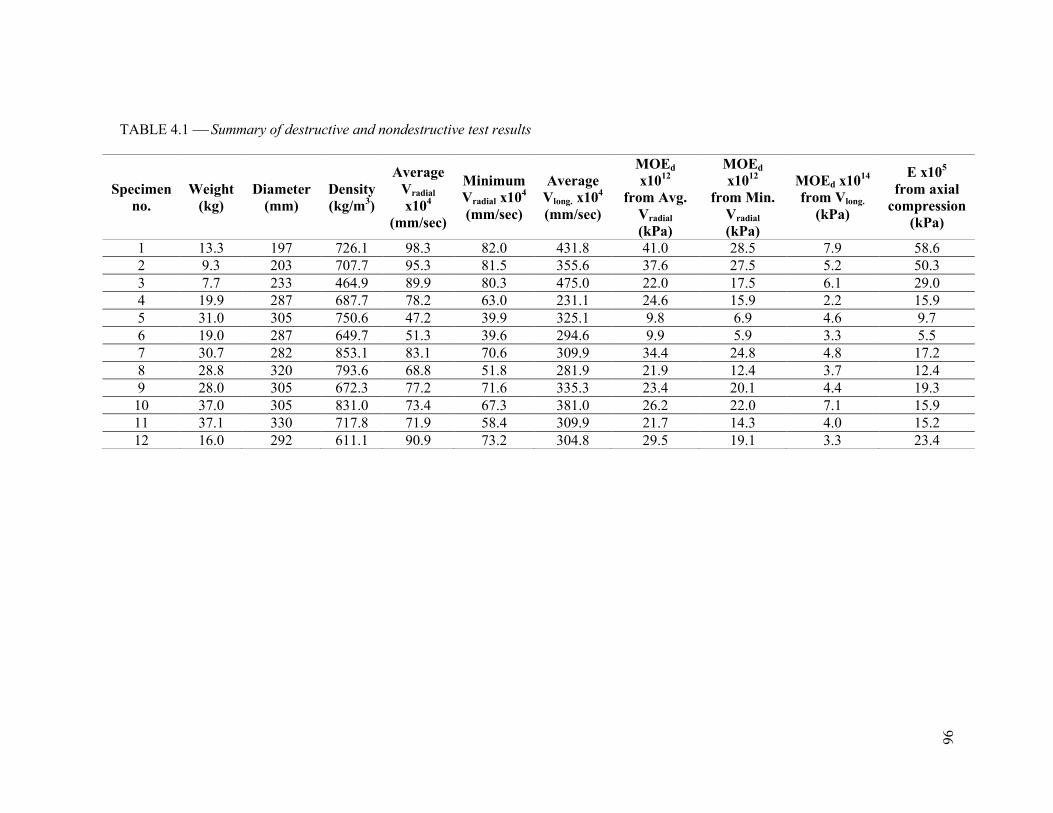
96

TABLE 4.1 Summary of destructive and nondestructive test results

Specimen

no.

Weight

(kg)

Diameter

(mm)

Density

(kg/m3)

Average

Vradial

x104

(mm/sec)

Minimum

Vradial x104

(mm/sec)

Average

Vlong. x104

(mm/sec)

MOEd

x1012

from Avg.

Vradial

(kPa)

MOEd

x1012

from Min.

Vradial

(kPa)

MOEd x1014

from Vlong.

(kPa)

E x105

from axial

compression

(kPa)

1 13.3 197 726.1 98.3 82.0 431.8 41.0 28.5 7.9 58.6

2 9.3 203 707.7 95.3 81.5 355.6 37.6 27.5 5.2 50.3

3 7.7 233 464.9 89.9 80.3 475.0 22.0 17.5 6.1 29.0

4 19.9 287 687.7 78.2 63.0 231.1 24.6 15.9 2.2 15.9

5 31.0 305 750.6 47.2 39.9 325.1 9.8 6.9 4.6 9.7

6 19.0 287 649.7 51.3 39.6 294.6 9.9 5.9 3.3 5.5

7 30.7 282 853.1 83.1 70.6 309.9 34.4 24.8 4.8 17.2

8 28.8 320 793.6 68.8 51.8 281.9 21.9 12.4 3.7 12.4

9 28.0 305 672.3 77.2 71.6 335.3 23.4 20.1 4.4 19.3

10 37.0 305 831.0 73.4 67.3 381.0 26.2 22.0 7.1 15.9

11 37.1 330 717.8 71.9 58.4 309.9 21.7 14.3 4.0 15.2

12 16.0 292 611.1 90.9 73.2 304.8 29.5 19.1 3.3 23.4

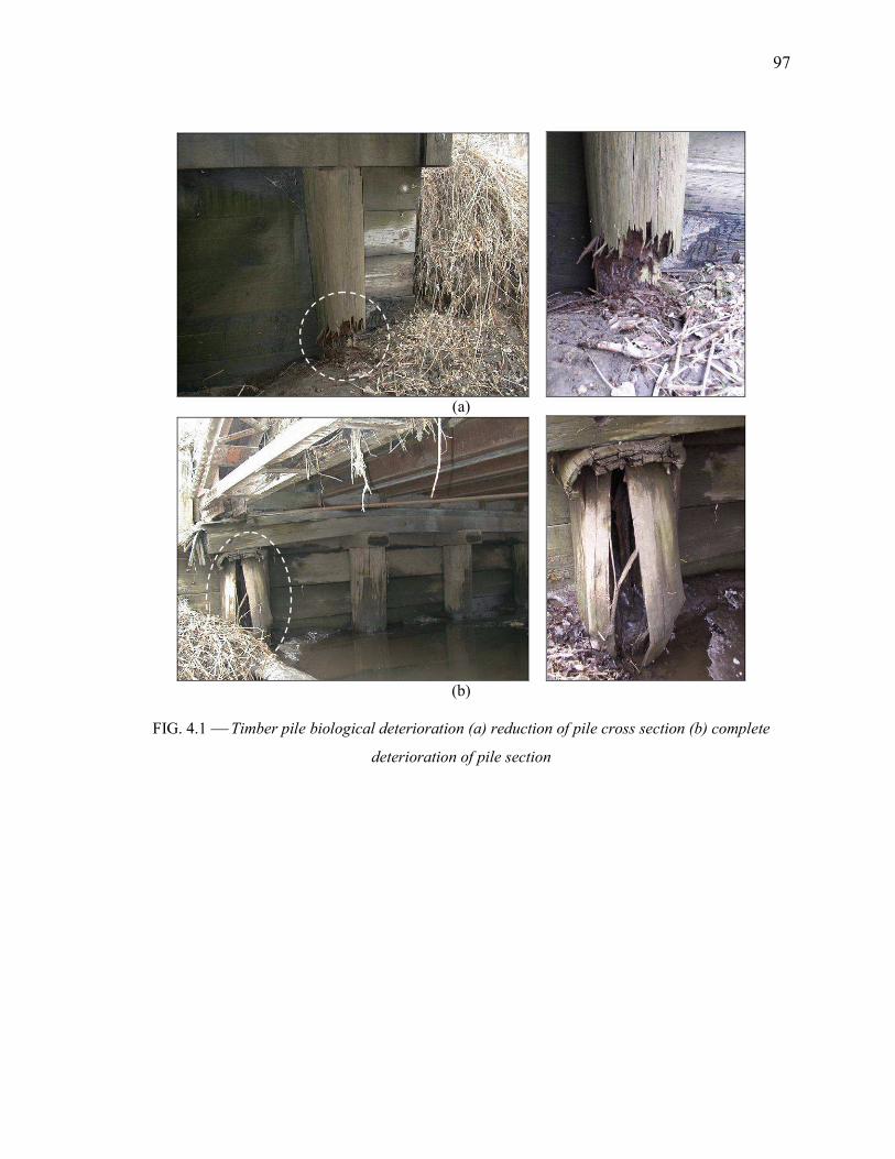
97

(a)

(b)

FIG. 4.1 Timber pile biological deterioration (a) reduction of pile cross section (b) complete

deterioration of pile section

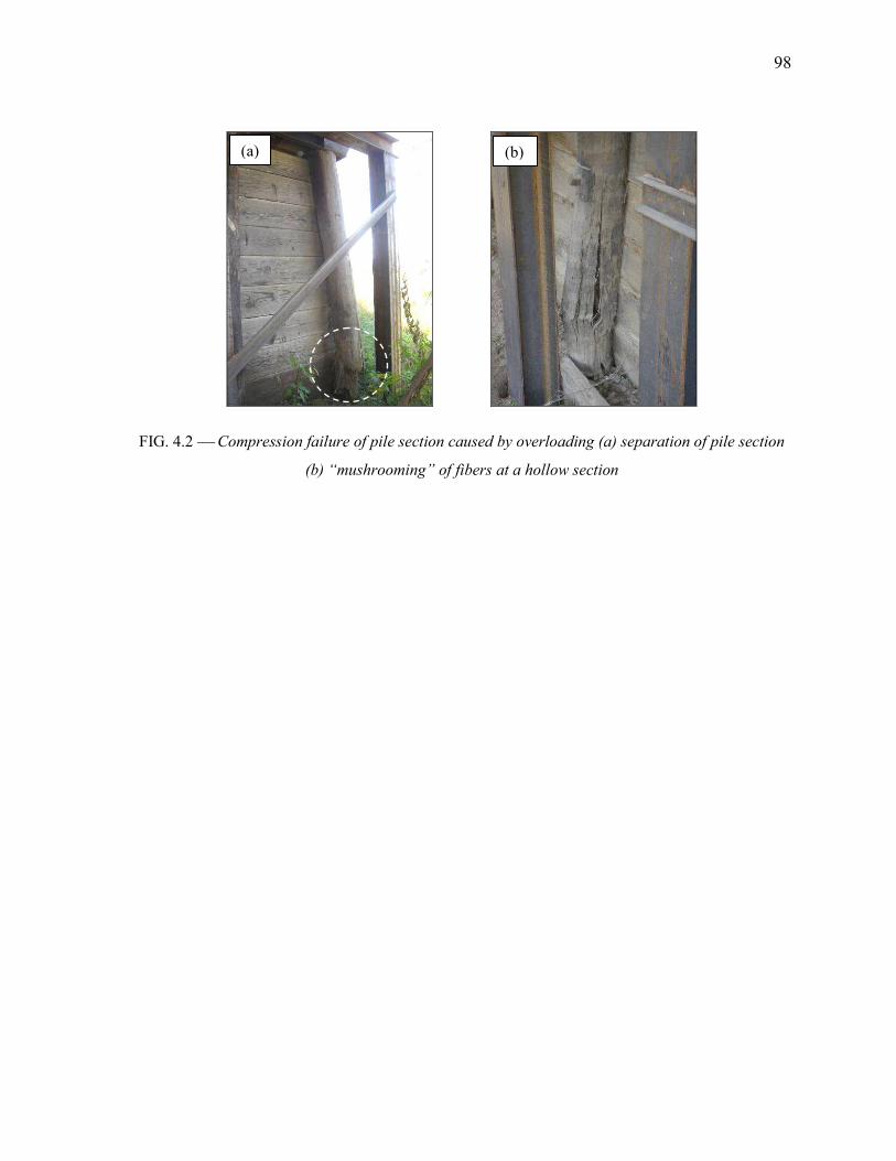
98

FIG. 4.2 Compression failure of pile section caused by overloading (a) separation of pile section

(b) “mushrooming” of fibers at a hollow section

(a) (b)

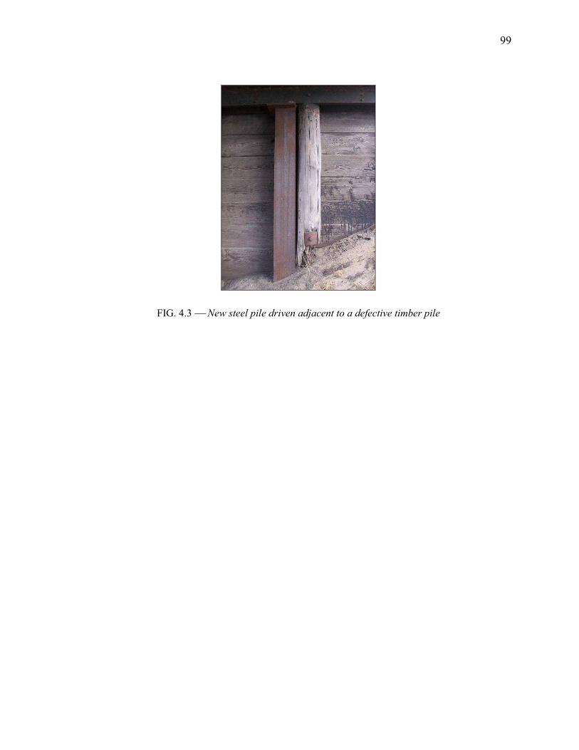
99

FIG. 4.3 2ew steel pile driven adjacent to a defective timber pile

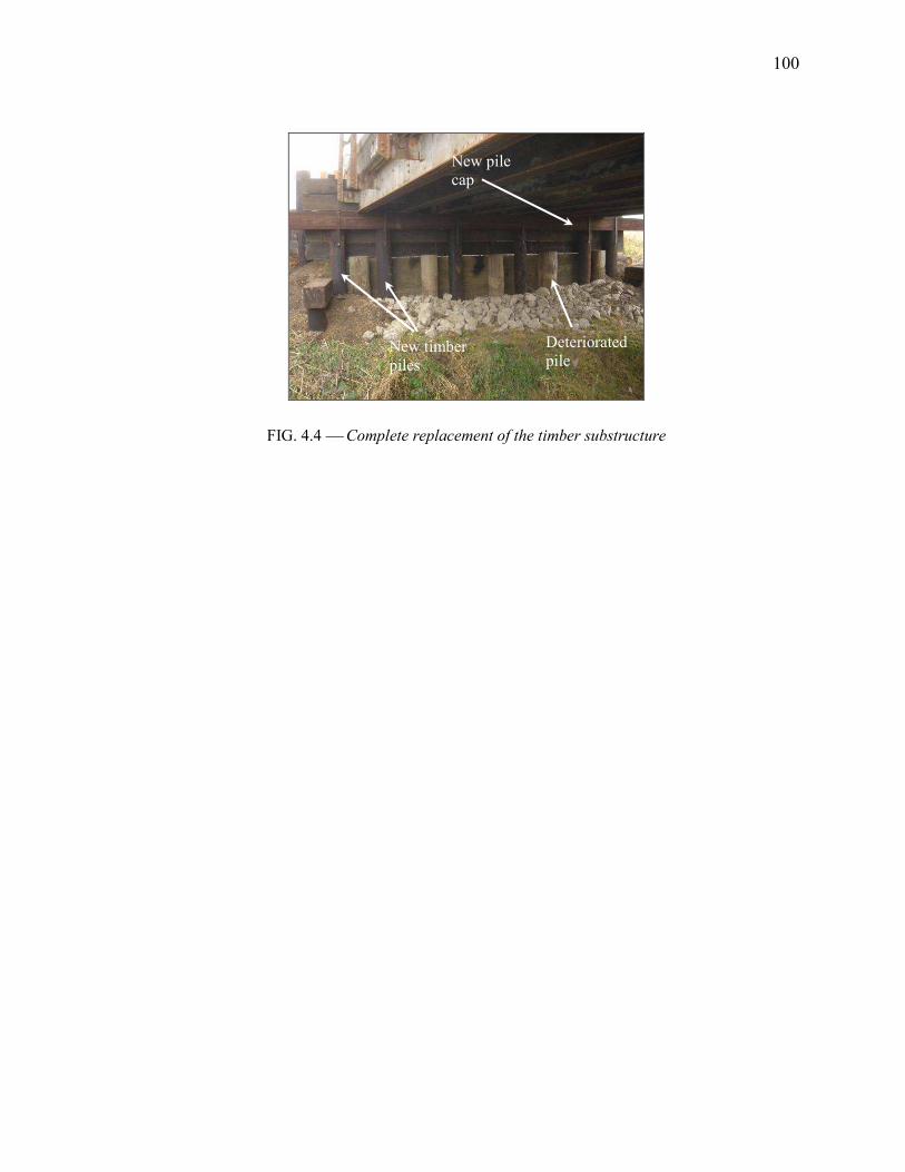
100

FIG. 4.4 Complete replacement of the timber substructure

New timber piles

New pile cap

Deteriorated pile

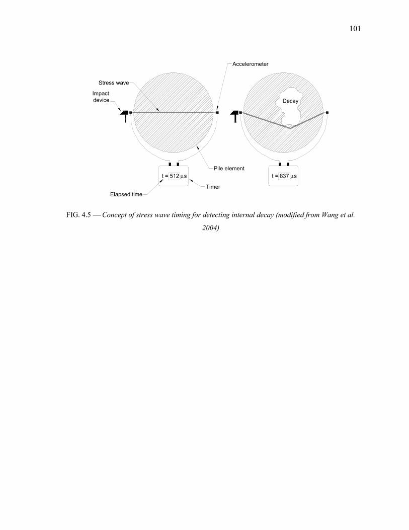
101

t = 512 µs t = 837 µs

Stress wave

Impact

device

Accelerometer

Pile element

Elapsed time

Timer

Decay

FIG. 4.5 Concept of stress wave timing for detecting internal decay (modified from Wang et al.

2004)

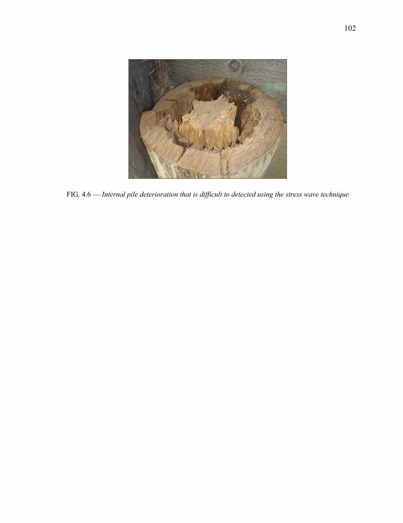
102

FIG. 4.6 Internal pile deterioration that is difficult to detected using the stress wave technique

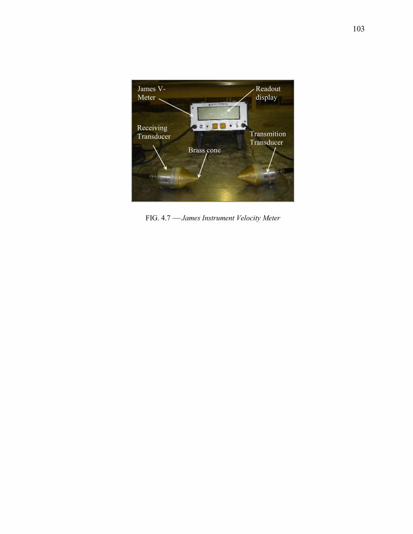
103

FIG. 4.7 James Instrument Velocity Meter

Receiving Transducer

James V-Meter

Transmition Transducer

Readout display

Brass cone

104

ri

voxel vj

v1 v2

vM

ri+1

ri+2 d ij

FIG. 4.8 Construction of model grid of nodes with intervening voxels (modified from Leiphart

1997)

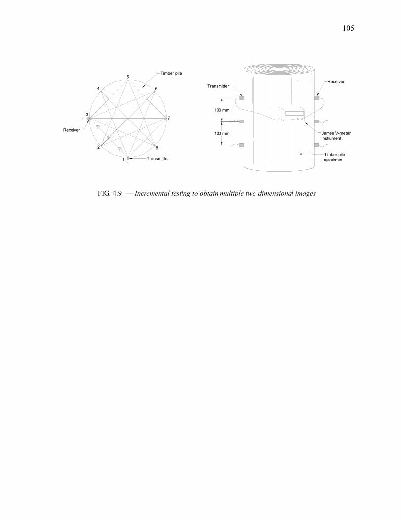
105

1

2

3

4

5

Transmitter

Receiver

Timber pile

TransmitterReceiver

James V-meter

instrument

100 mm

100 mm

Timber pile

specimen

6

7

8

FIG. 4.9 Incremental testing to obtain multiple two-dimensional images

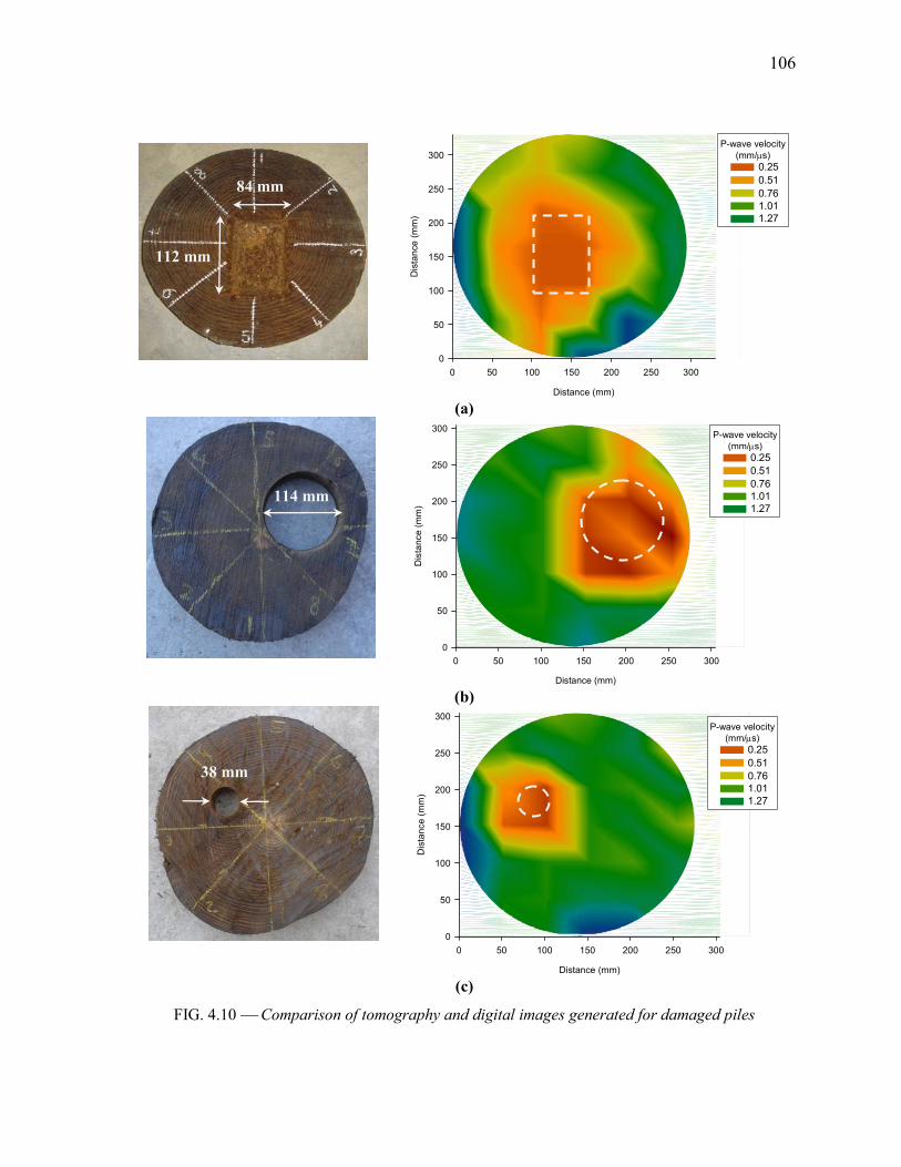
106

Distance (mm)

0 50 100 150 200 250 300

Dis

tan

ce

(m

m)

0

50

100

150

200

250

300

0.01

0.02

0.03

0.04

0.05

P-wave velocity

(mm/µs)

0.25

0.51

0.76

1.01

1.27

(a)

Distance (mm)

0 50 100 150 200 250 300

Dis

tance (

mm

)

0

50

100

150

200

250

300

0.01

0.02

0.03

0.04

0.05

P-wave velocity

(mm/µs)

0.25

0.51

0.76

1.01

1.27

(b)

Distance (mm)

0 50 100 150 200 250 300

Dis

tance (

mm

)

0

50

100

150

200

250

300

0.01

0.02

0.03

0.04

0.05

P-wave velocity

(mm/µs)

0.25

0.51

0.76

1.01

1.27

(c)

FIG. 4.10 Comparison of tomography and digital images generated for damaged piles

84 mm

112 mm

114 mm

38 mm

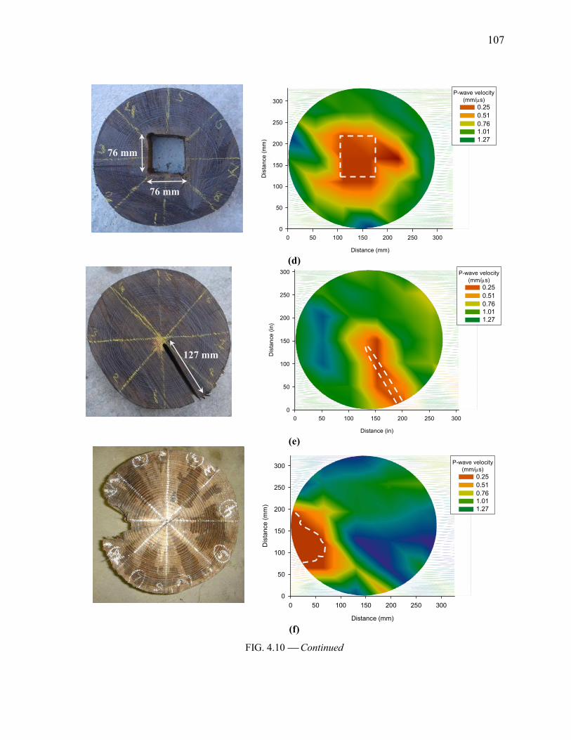
107

Distance (mm)

0 50 100 150 200 250 300

Dis

tance (

mm

)

0

50

100

150

200

250

3000.01

0.02

0.03

0.04

0.05

P-wave velocity

(mm/µs)

0.25

0.51

0.76

1.01

1.27

(d)

Distance (in)

0 50 100 150 200 250 300

Dis

tan

ce

(in

)

0

50

100

150

200

250

300

0.01

0.02

0.03

0.04

0.05

P-wave velocity

(mm/µs)

0.25

0.51

0.76

1.01

1.27

(e)

Distance (mm)

0 50 100 150 200 250 300

Dis

tance

(m

m)

0

50

100

150

200

250

300

0.01

0.02

0.03

0.04

0.05

P-wave velocity

(mm/µs)

0.25

0.51

0.76

1.01

1.27

(f)

FIG. 4.10 Continued

76 mm

76 mm

127 mm

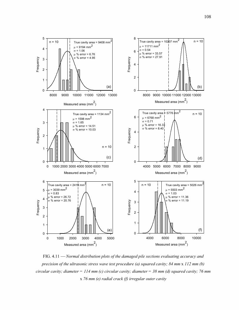
108

Measured area (mm2

)

8000 9000 10000 11000 12000 13000

Fre

qu

en

cy

0

2

4

6

8True cavity area = 10207 mm

2

µ = 11711 mm2

σ = 0.54

µ % error = 33.57

σ % error = 27.91

(b)

Measured area (mm2

)

0 1000 2000 3000 4000 5000 6000 7000

Fre

qu

en

cy

0

1

2

3

4

True cavity area = 1134 mm2

µ = 1598 mm2

σ = 1.65

µ % error = 14.51

σ % error = 10.03

(c)

Measured area (mm2

)

4000 5000 6000 7000 8000 9000

Fre

qu

en

cy

0

2

4

6

True cavity area = 5776 mm2

µ = 6768 mm2

σ = 0.71

µ % error = 16.33

σ % error = 8.40

(d)

Measured area (mm2

)

0 1000 2000 3000 4000 5000

Fre

qu

en

cy

0

1

2

3

4

5


2

µ = 3039 mm2

σ = 0.83

µ % error = 26.72

σ % error = 20.76

(e)

Measured area (mm2

)

4000 6000 8000 10000

Fre

qu

en

cy

0

1

2

3

4


2

µ = 5503 mm2

σ = 1.03

µ % error = 11.36

σ % error = 11.19

(f)

Measured area (mm2

)

8000 9000 10000 11000 12000 13000

Fre

qu

en

cy

0

1

2

3

4


2

µ = 9194 mm2

σ = 1.06

µ % error = 6.76

σ % error = 4.95

(a)

n = 10 n = 10

n = 10

n = 10

n = 10 n = 10

FIG. 4.11 2ormal distribution plots of the damaged pile sections evaluating accuracy and

precision of the ultrasonic stress wave test procedure (a) squared cavity; 84 mm x 112 mm (b)

circular cavity; diameter = 114 mm (c) circular cavity; diameter = 38 mm (d) squared cavity; 76 mm

x 76 mm (e) radial crack (f) irregular outer cavity

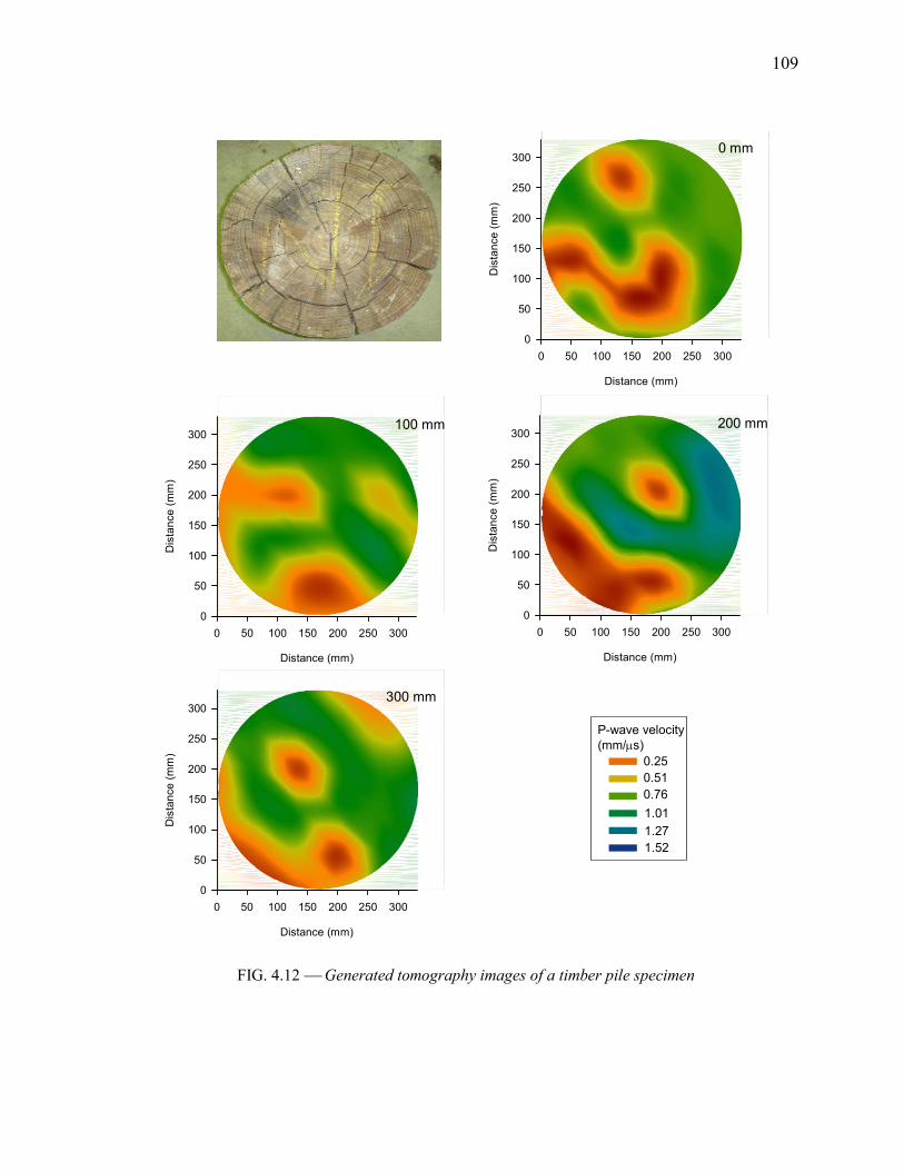
109

0.01

0.02

0.03

0.04

0.05

0.06

Distance (mm)

0 50 100 150 200 250 300

Dis

tan

ce

(m

m)

0

50

100

150

200

250

300

Distance (mm)

0 50 100 150 200 250 300

Dis

tan

ce

(m

m)

0

50

100

150

200

250

300

Distance (mm)

0 50 100 150 200 250 300

Dis

tan

ce

(m

m)

0

50

100

150

200

250

300

Distance (mm)

0 50 100 150 200 250 300

Dis

tan

ce

(m

m)

0

50

100

150

200

250

300

0 mm

100 mm 200 mm

300 mm

0.25

P-wave velocity

(mm/µs)

0.51

0.76

1.01

1.27

1.52

FIG. 4.12 Generated tomography images of a timber pile specimen

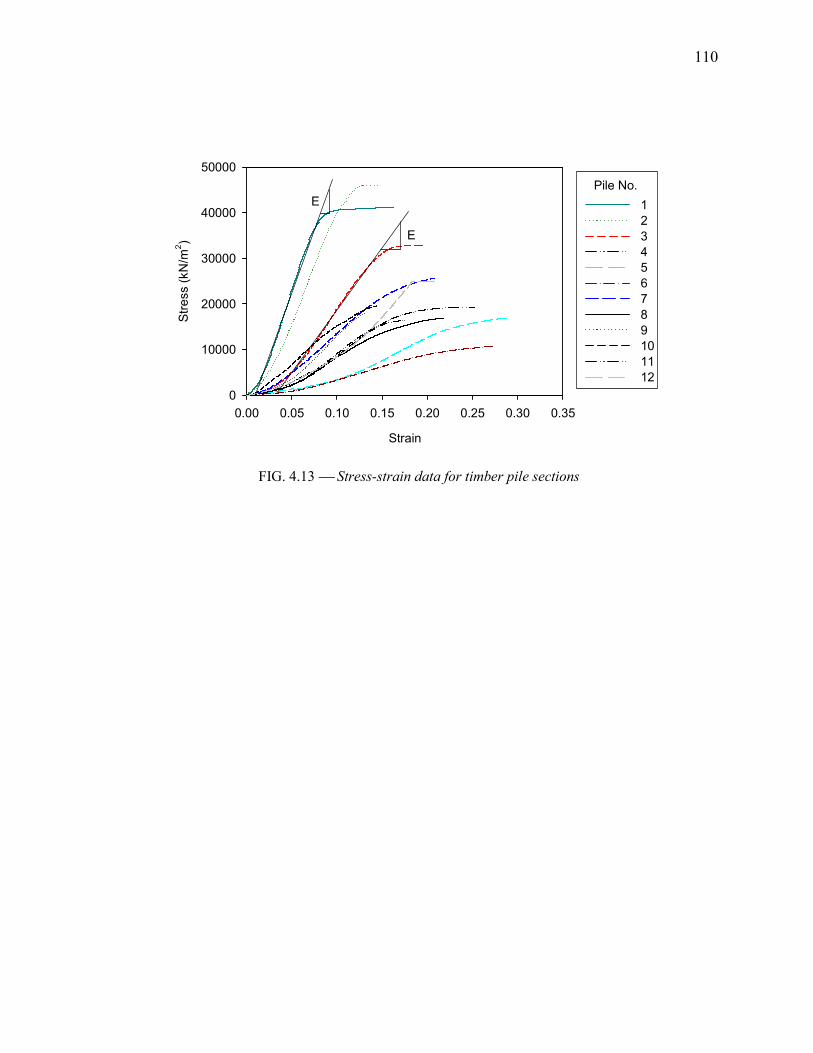
110

Strain

0.00 0.05 0.10 0.15 0.20 0.25 0.30 0.35

Str

ess (

kN

/m2)

0

10000

20000

30000

40000

50000

1

2

3

4

5

6

7

8

9

10

11

12

Pile No.

E

E

FIG. 4.13 Stress-strain data for timber pile sections

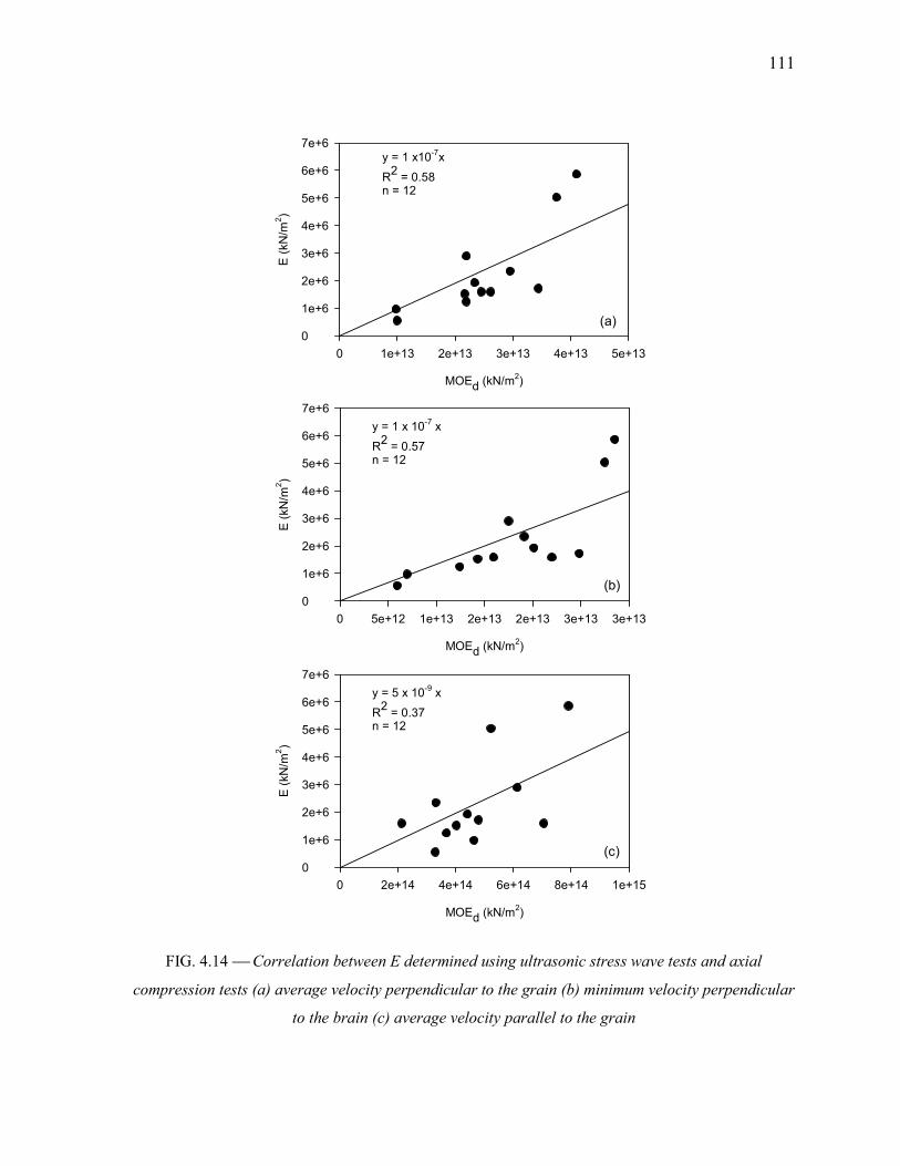
111

MOEd (kN/m2)

0 1e+13 2e+13 3e+13 4e+13 5e+13

E (

kN

/m2)

0

1e+6

2e+6

3e+6

4e+6

5e+6

6e+6

7e+6y = 1 x10

-7x

R2

= 0.58n = 12

MOEd (kN/m2)

0 5e+12 1e+13 2e+13 2e+13 3e+13 3e+13

E (

kN

/m2)

0

1e+6

2e+6

3e+6

4e+6

5e+6

6e+6

7e+6

y = 1 x 10-7

x

R2

= 0.57n = 12

MOEd (kN/m2)

0 2e+14 4e+14 6e+14 8e+14 1e+15

E (

kN

/m2)

0

1e+6

2e+6

3e+6

4e+6

5e+6

6e+6

7e+6

y = 5 x 10-9

x

R2

= 0.37n = 12

(a)

(b)

(c)


compression tests (a) average velocity perpendicular to the grain (b) minimum velocity perpendicular

to the brain (c) average velocity parallel to the grain

112

5. I$FLUE$CE OF TIMBER PILE DETERIORATIO$ O$ LOAD DISTRIBUTIO$ FOR

LOW VOLUME BRIDGE SUBSTRUCTURES

5.1. ABSTRACT:

Deterioration of timber piles by biological and mechanical factors can lead to considerable

reduction in pile capacity. The influence of that deterioration on the load distribution through the

substructure components is not fully understood yet essential to the overall safety and rating of the

bridge system. To better understand the effects of pile deterioration, nondestructive and destructive

static load tests were completed on a low volume road bridge abutment instrumented with load cells

and strain transducers. Three out of the seven supporting timber piles were consecutively removed to

simulate pile damage. After removing each pile, the abutment was loaded and pile strains were

measured. To measure pile loads, mechanical jacks and load cells were utilized to restore the dead

load carried by two out of the three removed piles. The abutment was then loaded and the data were

used to determine the stress and moduli of elasticity in each pile and thus predict the variation of load

distribution with different degrees of pile damage. To determine the feasibility of repairing a

localized deteriorated pile sections, one of the removed piles was repaired using a splicing technique

after which the percent restoration of pile bearing capacity was measured. Presented in this paper is a

case study evaluating the load distribution in a partially deteriorated timber abutment using pile

instrumentation, nondestructive and a destructive static load tests.

113

5.2. I$TRODUCTIO$

Deterioration of timber piles by biological and mechanical factors can lead to considerable

reduction in pile capacity. The influences of pile deterioration on load distribution through the

substructure components and the integrity of other intact piles are not fully understood yet essential to

the overall safety of the bridge system. In many cases, bridge design plans, pile length, and

subsurface profiles are not available, which further complicates the assessment of the bridge

substructure. Currently, the bridge rating system in Iowa does not account for the substructure

condition, which in many cases can be the governing factor for the overall bridge performance.

White et al. (2007) investigated the causes of timber pile deterioration in Iowa by inspecting 49 low

volume bridges with timber substructures. Furthermore, a questionnaire was sent to Iowa County

Engineers to obtain information on common substructure problems and typical remediation

techniques employed. The findings of this study demonstrated that most biological deterioration

occurred near the ground level where conditions are favorable for bacterial and fungal decay.

Physical pile deterioration occurred primarily because of overloading of timber piles. According to

the questionnaire results, most counties rely on visual inspection to assess substructure components.

In addition, the most frequent maintenance practice used in Iowa is driving a steel H-pile adjacent to

the defective timber pile. This maintenance solution is not always cost effective especially with

partially deteriorated piles that can be repaired using simple alternative repair methods.

To better understand the effect of pile deterioration on substructure performance, static load

tests on one bridge abutment were conducted; the load tests included one nondestructive and seven

destructive tests. During the tests, the timber piles and backwall were instrumented using strain

transducers and load cells. For the destructive load tests, three out of the seven supporting timber

piles were consecutively removed to simulate pile damage. After removing each pile, the abutment

was loaded and the pile and backwall strains were measured. To measure pile loads, mechanical

jacks and load cells were utilized to restore the dead load carried by two out of the three removed

piles. The abutment was then loaded and the data were used to determine the stresses in each pile and

thus predict the variation in load distribution with different degrees of pile deterioration. One of the

removed piles was repaired using the splicing technique and the percent of pile capacity restored was

measured. The objectives of the destructive load tests were to understand timber substructure

behavior under different pile deterioration and load orientation scenarios, and to evaluate the

effectiveness of a simple pile repair technique in restoring the capacity of the damaged pile.

114

5.3. BACKGROU$D

Holt et al. (1994) estimated that there are about 240,000 bridges in the United States

supported on Timber piles. Almost 7,000 to 8,000 tons of deteriorated timber piles are annually

removed from U.S. Naval facilities because of mechanical and biological deterioration. The cost of

removing these piles is about $20 million per year according to Wang et al. (2000). Biological

deterioration of timber piles, which can result of softening of the pile section, is mainly caused by

fungi, bacteria, and insect attack. Fungi and bacteria attack timber piles only when oxygen and water

levels are favorable. Physical deterioration occurs primarily due to abrasion, pile overloading and

infrequent severe loads (USDA 1999). The severity of pile damage due to abrasion is related to the

velocity of water moving past the pile and the quantity, shape, size, and hardness of the floating

debris (U.S. Army Corps of Engineers et al. 2001). Pile overloading results in different forms of

compression failure such as splitting of the top portion and mushrooming of the pile at a hollow

portion after breakage (USDA 1999). The stages of timber pile deterioration due to overloading

include development of initial entry holes, active deterioration of the inner core with significant

increase in the size of the hollow space, compression failure of the shell, and finally separation of the

hanging top portion of the pile from the pile cap (Buslov and Scola 1991).

Timber substructure problems in Iowa were identified by White et al. (2007) by inspecting 49

low volume brides with poor performing substructures. The results indicated that biological decay,

which occurred at half of the inspected sections, occurred near the ground or water level and resulted

in soft or hollow pile sections. Physical deterioration, on the other hand, occurred at about one third

of the inspected bridges. Reduction of pile cross section, broken piles, and brooming are all forms of

physical deterioration that were observed.

To obtain additional information on common substructure problems and typical remediation

techniques used in Iowa, a questionnaire (which had a 60% return rate) was sent to Iowa County

Engineers. The major factors causing deterioration in timber piles identified by Iowa County

Engineers are scour, physical deterioration, biological deterioration and misalignment. There was

agreement however that biological deterioration of timber piles is the primary factor. Most counties

rely on visual inspection in assessing substructure components. Nondestructive evaluation techniques

are almost never used as part of the bridge inspection. The questionnaire results also show that

driving steel piles adjacent to defective piles is the most frequent maintenance practice implemented.

Fewer counties use timber piles and concrete casings to strengthen deteriorated piles.

115

Ritter (1992) divided the bridge substructure maintenance into three categories. The first

category is preventative maintenance, in which the repair involves keeping the structure in a good

state. At this stage, deterioration has not started, but conditions or potential are present. The simplest

preventative maintenance is moisture control (Seavy and Larson 2002). Other preventative

maintenance includes the use of surface treatments, fumigants, and repair of small to medium cracks.

The second category is early remedial maintenance. At this stage, deterioration is present; however,

the capacity or performance of the structure is not affected. More severe damage is imminent unless

corrective action is taken. Concrete jacketing, fiber reinforced polymer (FRP), and posting and

splicing are common remedial maintenance practices. Remedial maintenance can be used when

about 10 to 40% of the pile cross sectional area has been lost by deterioration (Purvis 1994). The last

category is major maintenance, which involves immediate corrective measures to restore the structure

to its original condition (Ritter 1992). Adding supplemental piles or replacing the entire substructure

are the two major maintenance methods used (U.S. Army Corps of Engineers et al. 2001). Adding

supplemental piles is almost exclusively practiced in Iowa regardless of the pile degree of

deterioration; this practice is not always the most cost effective maintenance practice.

5.4. STATIC LOAD TESTS

5.4.1. Site Description

The bridge selected for load testing was located in Humboldt County, Iowa. The bridge was

10 m long and 7.3 m wide with a concrete deck, four steel girders, and 0o skew (See Figure 5.1a). A

center pier was added to the originally simple span bridge in the 1970s to prevent the bridge from

being posted as a result of low load rating (See Figure 5.1b). The pier was installed by driving two

timber piles on each side of the bridge which supported a steel beam at the mid span of the bridge.

Since this investigation only evaluated simple span bridges, prior to testing the pier was removed by

cutting the supporting timber piles and lowering the steel beam (See Figure 5.1c).

The bridge abutments were comprised of seven timber piles in front of a timber backwall,

three timber piles in each wingwall, and a double steel c-channel cap. At the east abutment, where

the static load tests were performed, piles were numbered one through seven starting from the north

edge of the bridge (See Figure 5.1d); as may be seen in this figure, part of a previous concrete bridge

abutment was still in place. Upon completion of the load tests, the bridge was removed and replaced

with a new box culvert (See Figure 5.1e and Figure 5.1f). The pile diameters were about 280 mm and

the average expose pile length and spacing at the east abutment were 1.4 m and 1.2 m, respectively

116

(See Figure 5.2a). Visual inspection revealed advanced section loss in pile No. 6 near the ground

level. The pile diameter at the time of inspection was about 76 mm. Tie back rods (22 mm in

diameter) were used to connect the wingwall piles as demonstrated in Figure 5.2b. According to the

bridge plane, the total pile length of the pile in front of the backwall was 7.6 m, whereas the total

length of the wingwall piles was 6 m.

A Cone Penetration Test (CPT) was conducted near the east abutment to determine the

subsurface conditions. The electronic piezocone CPT soundings were performed using a 20 ton

capacity truck mounted rig. The electronic cone had a 60o tip angle, tip area of 10 cm2, a net area

ratio of 0.8, and a friction sleeve area of 150 cm2. The cone was advanced at a rate of about 25 mm/s.

The CPT sounding detected minimal excess pore pressure, which is generally associated with high silt

and sand content soils that are able to rapidly dissipate pore water pressures. The soil profile

comprised of thin layers of sandy silt to clayey silt and silty sand to sandy silt. At about 4.4 m below

grade, a weathered limestone bedrock or dense fine grained soil layer was encountered. The

soundings were advanced to equipment refusal at a depth of 5.4 m (See Figure 5.3). Based on the soil

stratigraphy and documented pile lengths, it is believed that the piles were driven to the top of the

bedrock layer. An electronic water level indicator showed that the ground water level was about 4 m

below grade.

5.4.2. Test Setup and Instrumentation

Static load tests were conducted using a fully loaded tandem axle truck. Eight incremental

point loads were applied by positioning the truck at predetermined locations on the bridge deck. The

back wheel of the rear axle was positioned on the centerline of the east abutment to apply the first

load increment. To apply a second load increment, the truck was repositioned on the bridge deck so

the front wheel of the rear axle is over the centerline of the abutment. The third load was applied by

positioning the wheels of the front axle over the centerline of the abutment (See Figure 5.4). The

fourth, fifth, and sixth load increments are applied in a similar way but on the other abutment.

Loading stage Nos. 0 and 7 represent the beginning and the end of the test where the truck is

completely off the bridge. At load increment No. 6, no load is applied at the monitored east abutment

since the applied axial load was resisted by the west abutment. The incremental loads (See Figure

5.5) were applied at three lanes along the bridge deck (north, centerline, and south edges). The load

from each wheel was measured using portable axle/wheel weighing scales (See Figure 5.6a). By

knowing the truck dimensions, the total load carried by the east abutment at each loading stage was

calculated.

117

To measure strains, the piles in each abutment were instrumented with strain transducers.

The strain transducers used were manufactured by Bridge Diagnostics, Inc. (BDI). Each strain

transducer was 112 mm x 30 mm x 10 mm with either a 4.5 m or 7.6 m wire attached. Each

transducer also has a unique number through which it can be identified by the data acquisition system.

An extension was attached to the strain transducer to increase the 76 mm gage length to 600 mm.

The larger gauge length enabled averaging strains over a larger area to capture the behavior of a

localized deteriorated zone along the exposed pile (See Figure 5.6b). Typically, the strain transducers

were attached to the piles using brass woodscrews that were about 50 mm long. Due to the non-

homogeneity of wood, the exposed portion of each pile was instrumented with more than one strain

transducer to capture pile behavior about both the strong and weak sections. The arrangements of the

strain transducers were generally based on weak and strong regions along the pile identified by

nondestructive ultrasonic stress wave testing and pile coring. In addition to instrumenting pile

elements, strain transducers were also attached to the timber backwall to measure strains induced by

axial and/or lateral loads.

The exposed timber piles at the east abutment were instrumented as shown in Figure 5.2a.

All piles were instrumented with three strain transducers except Piles Nos. 3 and 7 which were

instrumented with five strain transducers. Every transducer was identified by two numbers (e.g. 1-2).

The first number denotes the strain transducer number, whereas the second number denotes the pile

number. Six strain transducers were attached to the backwall as shown in Figure 5.2a. All strain

transducers were 600 mm long.

In nondestructive static load tests various loads were applied to the instrumented bridge

abutment and strains were recorded. The destructive load tests were carried out by consecutively

removing a 400 mm section from Piles Nos. 3 and 7 (See Figure 5.7a). The east abutment with

sections of piles Nos. 3 and 7 removed is shown in Figure 5.7b. A 100 mm section near the ground

level, where the pile diameter was 76 mm, was removed from Pile No. 6 (See Figure 5.7c). After

removing each pile, the bridge was load tested and the strains in intact piles were recorded. A load

cell and a mechanical jack were placed in the region were a portion of the pile was removed (See

Figure 5.7d) to measure the load carried by the damaged piles. Before loading the abutment, the

mechanical jack was used to apply load on the pile; the load was gradually increased to restore the

original dead load, which was initially carried by the pile before removing the section. This was

accomplished by monitoring the pile strains before and after removing the pile section and restoring

118

the pile strains to their initial values. Once the initial strain was restored, the load carried by the pile

was recorded using the load cell. This procedure was carried out for both Piles Nos. 3 and 7.

5.4.3. Test Results

Described in this section are the results of one nondestructive and seven destructive tests;

The pile and backwall strains at the third loading stage, which yielded the highest strains, were used

to evaluate the substructure performance for every test.

5.4.3.1. Test 2o. 1 – 2ondestructive Test

This test was conducted at the east abutment with all piles intact. The abutment was first

loaded at the north edge of the bridge. A typical output showing the magnitude of axial loads, pile

strains and backwall strains is presented in Figure 5.8. Since pile lateral movement parallel and

perpendicular to the backwall was not measured, it was difficult to separate pile strains due to axial

compression and bending. Pile Nos. 1, 2, and 3, which were directly under the axial loads, had the

highest strains (See Figure 5.8b). The highest strain (about -39 microstrains) was in Pile No. 1. At

higher loading stages, the pile strains were reduced since more load was being transferred to the west

abutment. The strain also decreased in piles away from the location of the applied loads. The

backwall was in compression at loading Stages 1 through 4. The backwall strain at higher load stages

was either zero or positive indicating tension (See Figure 5.8c).

Loading the abutment at the centerline transferred most of the load to Piles Nos. 3 and 5,

which were directly under the axial loads. The highest strain was in Pile No. 3 and was about -30

microstrains. Moving the load to the centerline of the bridge deck resulted in about 30% reduction in

the backwall strains between Piles Nos.1 and 2, 2 and 3, and 3 and 4. At the south edge of the bridge

(between pile Nos. 4 and 7) the backwall strains increased by approximately a factor of 4.

The third nondestructive test was at the south edge of the bridge. Similar to previous tests,

the load was concentrated under the location of the applied loads. Pile No. 7 displayed the highest

strain, which was about -34 microstrains. The load decreased with increasing distance from the

location of axial loads. Pile No. 6, which had a diameter of about 76 mm near the ground level,

displayed small strains. Strains in Pile No. 1 were positive, which may be due to pile bending caused

by loading the bridge at the south edge.

119

5.4.3.2. Test 2o. 2 – Pile 2o. 7 Jacked

In the first destructive test at the east abutment a section of Pile No. 7 was removed and

replaced with a mechanical jack and load cell. Load was applied through the mechanical jack to

restore the pile initial strains. Two tests were conducted; one with the loading at the centerline and

one with the loading at the south edge of the bridge deck. The pile strains measured during the eight

destructive tests are summarized in Figure 5.9.

The strains resulting from loading the abutment at the centerline of the bridge deck were

equal to those measured in Test No1. This indicates that the procedure of jacking Pile No. 7 was

successful in restoring the abutment initial loading condition. Using the load cell, the live load

carried by Pile No. 7 was recorded and the stresses in the pile were determined. The stresses varied

laterally and longitudinally through the pile section illustrating the non-homogeneity of wood. The

results also demonstrate that the load carried by Pile No. 7 was about 8% of the total applied axial

load.

The abutment was next loaded at the south edge. Compared to the nondestructive load test

conducted at the south edge, the strains in Pile No. 7 decreased by about 45%, whereas the strains of

pile No. 5 increased by approximately 30%. It is possible that jacking Pile No. 7 resulted in a

relatively weaker pile compared to its initial condition, and as a result, the load was transferred to the

adjacent Pile No. 5. No load was transferred to Pile No. 6 since as previously noted the pile was

deteriorated. There were no significant changes in the strains in other piles. Furthermore, the

backwall strains at the south edge of the abutment (Pile Nos. 4 through 7) increased by about 40%.

Loading the abutment at the south end resulted in an increase in the percent load carried by Pile No. 7

to about 35% of the total applied axial load.

5.4.3.3. Test 2o. 3 – Pile 7 Removed

The third destructive test simulated complete deterioration of an exterior pile. This was

achieved by removing the mechanical jack and load cell.

The first load test was completed with the loading at the north edge of the bridge. The pile

strains were approximately equal to those measured during Test No.1. This is because Pile No. 7 did

not resist any load when the abutment was loaded at the opposite edge. The backwall strains were

also similar to the nondestructive test except those measured between Pile Nos. 6 and 7, which

increased by 60%. It can therefore be concluded that an exterior pile does not have a significant

120

influence if the live load is concentrated on the edge opposite to the location of the deteriorated pile in

the bridge.

Loading the abutment at the centerline of the bridge deck resulted in a 25% strain increase in

Pile No. 5 and about 3% strain increase in Piles Nos. 3 and 4 compared to the nondestructive test at

the same location. Most of the load carried by Pile No. 7 was therefore transferred to the next

adjacent sound pile. The backwall strain also increased between Piles Nos. 6 and 7 by about 63%.

Due to the partial bearing of the pile cap on the backwall (a common connection detail observed for

this family of bridges), and due to the removal of Pile No. 7, the backwall resisted a higher load

evidenced by the increase in negative strains.

The third test was completed with the loading at south edge of the bridge directly above the

removed pile. The strains in Pile No. 5 increased by approximately 60%, whereas the strains in Piles

Nos. 3 and 4 increased by 20 and 45%, respectively. The results demonstrate that most of the load

initially carried by Pile No. 7 was being resisted by adjacent Pile No. 5. The results also show that

pile bending at the north edge increased. This was evidenced by the increase in positive strains in

Piles Nos. 1 and 2. In Pile No. 1, the strain increased from +8.5 microstrains, measured during the

nondestructive test at this location, to +20.2 microstrains, whereas in Pile No. 2, the strain increased

from 0 microstrains to +9.2 microstrains. This was also observed at the backwall strains between

Piles No. 1 and 2, which increased from +7.2 microstrains to +20.5 microstrains. Furthermore, the

backwall strains under the applied load (i.e. between pile Nos. 6 and 7) increased from -38

microstrains at Test No. 1, to -80 microstrains since more load is being transferred and resisted by the

south end of the backwall. Backwall strains measured between Piles Nos. 4 and 5, and 5 and 6 also

increased by almost 100%.

5.4.3.4. Test 2o. 4 – Pile 2os. 3 and 7 Jacked

In this destructive test, a 400 mm section was removed from Pile No. 3 after which both Piles

Nos. 3 and 7 were jacked to their initial measured strains. A load cell was placed above each

mechanical jack to measure the live load carried by each pile. Three load tests were conducted with

the load being applied at the north, centerline, and south edges.

The results of the north edge test illustrate that the strains in Pile No. 3 decreased by about

45% compared to those measured during Test No.1. As a result, the strains in the adjacent Piles Nos.

2 and 4 increased by about 39 and 6%, respectively. The results indicate that the load carried by Pile

No. 3 was about 10% of the total load. No significant change was observed in the backwall strains

121

compared to the strains measured in the nondestructive test except between Piles Nos. 3 and 4. The

strain measured in this location increased by approximately 60%. A possible explanation for this

increase is that the mechanical jack did not fully restore the timber pile to its initial condition as

evidenced by the strain reduction in the pile compared to the nondestructive test strains; therefore, the

backwall at this location resisted more axial load due to partial bearing of the pile cap on the

backwall.

The abutment was next loaded at the centerline of the bridge deck. When compared to Test

Nos. 1, 2, and 3, the strains in Pile No. 3 was reduced by approximately 40%. As a result, the

backwall strain between Piles Nos. 3 and 4 increased by 60%. Similarly, the strain in pile No. 7 was

reduced by approximately 35%, whereas the backwall strain between Piles Nos. 6 and 7 increased by

45%. The percent load carried by Piles Nos. 3 and 7 was 13 and 9%, respectively.

The results of loading the abutment at the south edge of the bridge show a strain reduction in

Piles Nos. 3 and 7 compared to Test Nos. 1 and 2. The strain in Pile No. 3 decreased by about 25, 34,

and 36% compared to Test Nos. 1, 2, and 3, respectively. The strain reduction in Pile No. 3 was

coupled with an increase in backwall strain between Piles Nos. 3 and 4. The backwall strain at this

location increased by 33 and 28% compared to Test Nos. 1 and 2, respectively. The results also show

that the strain in the adjacent Pile No. 4 increased by 27 and 6% compared to Test Nos. 1 and 2,

respectively. However, there was no significant strain increase in Pile No. 2. Similar to Pile No. 3,

the strain in Pile No. 7 decreased by approximately 50 and 30% compared to Test Nos. 1 and 2,

respectively. This was accompanied by a 55% increase in backwall strains.

5.4.3.5. Test 2o. 5 – Pile 2o. 3 Removed and Pile 2o. 7 Jacked

In this test, the mechanical jack and load cell were removed from Pile No. 3 to simulate

complete deterioration of an interior pile, whereas Pile No. 7 remained jacked. Two load tests were

performed; one along the north edge and one along the centerline of the bridge.

The abutment was first loaded at the north edge of the bridge. Removing Pile No. 3 resulted

in an increase in strain in adjacent Piles Nos. 2 and 4 compared to Test No. 4 (Piles Nos. 3 and 7

jacked). The strain in Piles Nos. 2 and 4 increased by 27 and 16%, respectively. The backwall

between Piles Nos. 3 and 4 resisted higher loads evidenced by the increase in strain, which was about

70%.

122

Loading the abutment at the centerline of the bridge deck resulted in a strain increase in Piles

Nos. 2 and 4 by 50 and 12%, respectively, compared to Test No. 4. Furthermore, a 40% increase in

the backwall strain between Piles Nos. 3 and 4 was measured. The percent load carried by Pile No. 7

was 9%, which is equal to that measured during Test No. 4.

5.4.3.6. Test 2o. 6 – Pile 2os. 3 and 7 Removed

To simulate deterioration in more than one pile, Piles Nos. 3 and 7 were removed. Three load

tests were carried out by loading the abutment at the north, centerline, and south edges.

The pile strains induced by loading the abutment at the north edge of the bridge were

compared to the strain measured in Test No. 5. The pile and backwall strains in both tests were

almost equal. This confirms previous conclusions and demonstrates that a deteriorated interior pile

has more influence than a deteriorated exterior one on load distribution through the substructure when

the bridge is loaded at the edge opposite to the deteriorated pile.

When the abutment was loaded at the centerline of the bridge deck, the influence of the

exterior Pile No. 7 became more apparent. This was determined by comparing strains in Pile No. 5

during Test Nos. 4, 5, and 6. The strains in Test No. 4 were about -23 microstrains. When Pile No. 3

was removed, the strain remained almost the same (about -24 microstrains); however, when Pile No.

7 was removed the strain increased to -28 microstrains (20% increase). The exterior Pile No. 7 does

not appear to have any influence on Piles Nos. 1 through 4 since their strains did not change from

those measured in Test No. 5. The influence of removing Pile No. 7 on backwall strains was noticed

between Piles Nos. 5 and 6 and Nos. 6 and 7. The strain increased by 28% between Piles Nos. 5 and

6 relative to Test No. 5, whereas the strain between Piles Nos. 6 and 7 increased by 77%, which is

similar to results obtained from Test No. 2 (Pile No. 7 removed).

The last test was carried out at the south edge of the bridge. Comparing the results to Test

No. 3, where Pile No. 7 was removed, revealed that the strain in Pile No. 4 increased by 15% as a

result of removing Pile No. 3. Further, the backwall strain between Piles Nos. 3 and 4 increased by

almost 100% since the backwall was resisting additional axial load, which was previously resisted by

Pile No. 3. Also, the positive strains in Pile Nos. 1 and 2 during Test No. 3 were reduced by 12 and

40%, respectively.

123

5.4.3.7. Test 2o. 7 – Pile 2os. 3, 6 and 7 Removed

This test was conducted to study the substructure behavior when three piles are damaged.

Piles No. 3, 6, and 7 were removed and three load tests were performed with the load at the north,

centerline, and south edges.

The first load test was completed with the load at the north edge of the bridge. Removing

pile No. 6 did not have major influence on the strains developed throughout the substructure since

pile and backwall strains were similar to those measured during test No. 6.

Loading the abutment at the centerline of the bridge resulted in a 7% strain increase in the

adjacent Pile No. 5 compared to strains measured in Test No.6..

Loading the abutment at the south edge of the bridge resulted in about 25% strain increase in

Pile No. 5 compared to Test No. 6, where only Pile Nos. 3 and 7 were removed. In addition,

removing Pile No. 6 resulted in higher positive strains in Pile Nos. 1 and 2 compared to Test No. 6.

The strain in Piles Nos. 1 and 2 increased by 7 and 24%, respectively. Furthermore, the negative

backwall strain between Piles Nos. 5 and 6 increased by approximately 10%, while the backwall

strain between Piles Nos. 6 and 7 increased by about 15%. The positive backwall strain between

Piles Nos. 1 and 2 increased by 20%. The influence of a deteriorated pile on load distribution through

the substructure becomes more significant when the live load is closer to the location of the

deteriorated pile.

5.4.3.8. Test 2o. 8 – Pile 2o. 7 Repaired

This test was carried out to determine the feasibility of repairing localized deteriorated

sections of the timber pile. The section removed from Pile No. 7 was replaced with a new pile section

(See Figure 5.10), which was spliced and attached to the existing pile using two 300 mm long steel

screws. Three tests were conducted with the loading applied along the north, centerline, and south

edges of the bridge, and the percent strain restored in Pile No. 7 was measured

The effectiveness of the repair method could not be evaluated during the north edge test since

the load resisted by Pile No. 7 was negligible.

The pile strains induced from loading the abutment at the centerline of the bridge reflected

the success in partially restoring the capacity of Pile No. 7 as evidenced by the pile strain

measurement, which was about -24 microstrains. The pile repair resulted also in a reduction of the

124

strain measured in Pile No. 5 by about 15% compared to Test No. 6. The backwall strain between

Pile Nos. 6 and 7 was also reduced by 45%. The strains in Pile No. 7 were about three times higher

than Test No. 5 (Pile No. 3 removed and pile No. 7 jacked).

The abutment was finally loaded with the loading at the south edge of the bridge. The live

load location and magnitude, pile strains and backwall strain are shown in Figure 5.11. Similar to the

centerline load test, repairing Pile No. 7 reduced the strain in adjacent pile No. 5 by 25% compared to

Test No. 6. Furthermore, the backwall strain between Piles Nos. 6 and 7 was reduced by 40%. The

strain in Pile No. 7 was about 3.5 times higher than that measured during Test No. 5. Repairing pile

No. 7 resulted also in reducing positive strains in Piles Nos. 1 and 2 during Test No. 6 (Piles Nos. 3,

6, and 7 removed) by about 40 and 15%, respectively.


Deterioration of timber piles by biological and physical factors reduces the pile bearing

capacity. This reduction influences the load distribution through the bridge substructure and can be

the reason behind overloading adjacent piles. In Iowa, bridge ratings do not account for the condition

of the substructure, which in many cases may be the governing factor for the overall capacity of the

bridge.

The causes of timber pile deterioration in Iowa as reported by White et al. (2007) are

biological deterioration mostly occurring near the ground or water level and physical deterioration

due to overloading. A questionnaire sent to Iowa County Engineers confirmed that biological

deterioration is the main cause of timber pile deterioration. Furthermore, visual inspection is what

most counties rely on in assessing substructure components.

Pile maintenance can be categorized into (1) preventative maintenance such as the use of

fumigants, (2) remedial maintenance, which is used to repair decay in localized areas using methods

such as posting and splicing, and (3) major maintenance, which is used when deterioration has

progressed to the point where major structural components have experienced moderate to severe

strength loss. Adding supplemental piles is a common maintenance practice.

Static load tests were conducted at one bridge abutment to measure pile and backwall strains

with different degrees of induced deterioration. The abutment was loaded with a fully loaded tandem

axle dump truck. One nondestructive and seven destructive load tests, where three of the seven

125

supporting timber piles were consecutively removed, were completed. The findings from the load

tests are as follows:

• Pile strains were typically higher near the applied load and decreased with increasing distance

from the location of the live load. Strains varied laterally and longitudinally along the

exposed pile length. This verifies the non-uniformity of wood material and the complexity in

characterizing the load distribution through the substructure.

• Since pile lateral movement parallel and perpendicular to the backwall was not measured, it

was difficult to separate pile strains due to axial compression and bending.

• Positive strain values can also be attributed to bending acting on the exterior pile when the

abutment is loaded at the opposite edge.

• Destructive static load tests showed that pile deterioration resulted in load transfer to adjacent

piles and to the backwall behind the deteriorated pile. The percent load transfer to each

adjacent pile may depend on pile spacing, relative pile stiffness, and location of the applied

loads relative to the deteriorated pile. The load transfer to the backwall was attributed to the

pile cap-backwall detail where the cap is partially resting on the backwall. The backwall may

therefore be resisting both axial and lateral loads.

• Repairing one exterior pile using the splicing technique partially restored its capacity. Strains

in adjacent piles and backwall were reduced.

5.6. FUTURE RESEARCH

The load tests provided valuable insights on the behavior of deteriorated timber substructures.

However, this field experimentation is considered a preliminary step towards understanding a

complex system where design methods and reliable evaluation techniques are unavailable. Therefore,

the following additional research is proposed:

• Additional destructive load tests are needed for bridge abutments with fewer number

of supporting piles. It is believed that the behavior of substructures with fewer piles

will more likely be influenced by pile deterioration.

• On a pilot study basis, evaluate alternative pile repair methods such as FRP and

concrete jacketing by load testing and monitoring the substructure performance.

• The splicing repair technique was successful in restoring part of the bearing capacity

of a damaged pile; however, it is recommended to also evaluate its ability in restoring

the bending capacity of timber piles.

126

• Laboratory scaled models, where each pile and the backwall are instrumented with

load cells, strain transducers and earth pressure cells would, provide useful

information on the performance of timber substructures. Results would provide a

basis for a numerical model that may help understand the behavior of the pile cap-

backwall connection detail.

• For future abutment load tests, it is proposed to measure the pile lateral movement

parallel and perpendicular to the backwall so that pile strains induced by axial and

bending loads can be separated.

• Develop evaluation criteria for timber substructures for use in bridge ratings.

ACK$OWLEDGME$TS

This research project was sponsored by the Iowa Department of Transportation and the Iowa

DOT Research Board under contract TR-522. The authors would like to thank the project Technical

Advisory Committee and the County Engineers that participated in the questionnaire. The authors

would also like to thank Douglas Wood, and undergraduate research assistants for their help with

instrumentation and data collection. Special thanks to Humboldt County Engineers for their help in

identifying the bridge, providing bridge plans, and assistance in conducting the load tests.

REFERE$CES

Aggour, M. S., (1991). “Nondestructive Testing of Timber Piles for Structures,” Transportation

Research Record, 1331, 36-44.

Buslov, V. M., and Scola, P. T. (1991). “ Inspection and Structural Evaluation of Timber Piers: Case

Study.” Journal of Structural Engineering., 117(9), 2725-2741.

Holt, D.J., Chen, S., and Douglas, R.A. (1994). “Determining Lengths of Installed Timber Piles by

Dispersive Wave Propagation.” Transportation Research Record., 1447, 110-115.

Purvis, R. L. (1994). Underwater Bridge Maintenance and repair, National Cooperative Highway

Research Program, Synthesis of Highway Practice 200, Transportation Research Board,

Washington, D.C.

Ritter, M. A. (1992). Timber Bridges: Design, Construction, Inspection, and Maintenance. United

States Department of Agriculture, Forest Service, Forest Products Laboratory, Madison, WI.

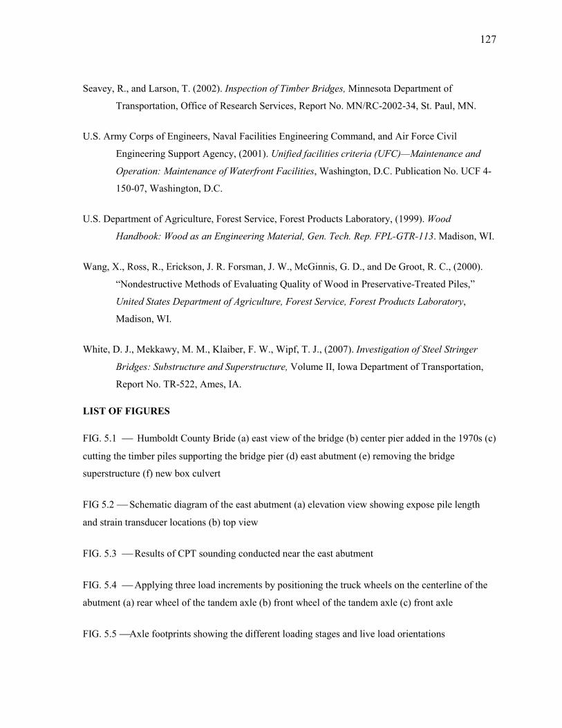
127

Seavey, R., and Larson, T. (2002). Inspection of Timber Bridges, Minnesota Department of

Transportation, Office of Research Services, Report No. MN/RC-2002-34, St. Paul, MN.

U.S. Army Corps of Engineers, Naval Facilities Engineering Command, and Air Force Civil

Engineering Support Agency, (2001). Unified facilities criteria (UFC)—Maintenance and

Operation: Maintenance of Waterfront Facilities, Washington, D.C. Publication No. UCF 4-

150-07, Washington, D.C.

U.S. Department of Agriculture, Forest Service, Forest Products Laboratory, (1999). Wood

Handbook: Wood as an Engineering Material, Gen. Tech. Rep. FPL-GTR-113. Madison, WI.

Wang, X., Ross, R., Erickson, J. R. Forsman, J. W., McGinnis, G. D., and De Groot, R. C., (2000).

“Nondestructive Methods of Evaluating Quality of Wood in Preservative-Treated Piles,”

United States Department of Agriculture, Forest Service, Forest Products Laboratory,

Madison, WI.

White, D. J., Mekkawy, M. M., Klaiber, F. W., Wipf, T. J., (2007). Investigation of Steel Stringer

Bridges: Substructure and Superstructure, Volume II, Iowa Department of Transportation,

Report No. TR-522, Ames, IA.

LIST OF FIGURES

FIG. 5.1 Humboldt County Bride (a) east view of the bridge (b) center pier added in the 1970s (c)

cutting the timber piles supporting the bridge pier (d) east abutment (e) removing the bridge

superstructure (f) new box culvert

FIG 5.2 Schematic diagram of the east abutment (a) elevation view showing expose pile length

and strain transducer locations (b) top view

FIG. 5.3 Results of CPT sounding conducted near the east abutment

FIG. 5.4 Applying three load increments by positioning the truck wheels on the centerline of the

abutment (a) rear wheel of the tandem axle (b) front wheel of the tandem axle (c) front axle


128

FIG. 5.6 Test setup and instrumentation (a) Wheel loads measured using a portable axle/wheel

scale (b) strain transducers attached to the piles and backwall

FIG. 5.7 Destructive static load tests (a) removing pile No. 7 (b) a section from pile Nos. 3 and 7

removed (c) a section near the ground level is removed from pile No. 6 (d) mechanical jack and load

cell used to restore the dead load carried by pile No. 7

FIG. 5.8 Test No. 1 north edge of the bridge (a) location of strain transducers and live loads (b)

pile strains (c) backwall strains

FIG. 5.9 Average microstrains measured at each pile at loading stage three

FIG. 5.10 Repairing pile No. 7 using the splicing technique

FIG. 5.11 Static load test at the south end with pile Nos. 3 and 6 removed and pile No. 7 repaired

(a) location of strain transducers and live loads (b) pile strains (c) backwall strains

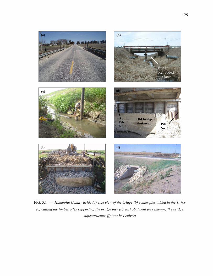
129

FIG. 5.1 Humboldt County Bride (a) east view of the bridge (b) center pier added in the 1970s

(c) cutting the timber piles supporting the bridge pier (d) east abutment (e) removing the bridge

superstructure (f) new box culvert

Bridge pier added at a later

Pile

$o. 1 Pile

$o. 7

Old bridge

abutment

(a) (b)

(c) (d)

(e) (f)

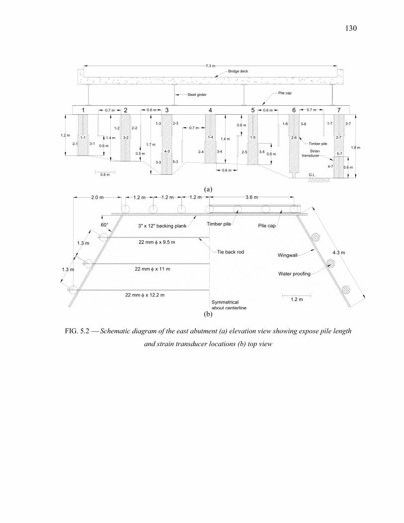
130

1 2 3 4 5 6 7

1-1

2-1 3-1

1-2 2-2

3-2

1-3 2-3

3-3

4-3

5-3

1-4

2-4 3-4

1-5

2-5 3-5

1-6

2-6

3-6 1-7

2-7

3-7

4-7

5-7

0.6 m

0.7 m

0.5 m

0.6 m

0.7 m

0.7 m

0.6 m

0.6 m

0.6 m

0.6 m

0.6 m

7.3 m

Bridge deck

Steel girder Pile cap

Timber pile

G.L .

1.2 m1.4 m

1.7 m

1.4 m

1.8 mStrian

transducer

0.6 m

(a)

1.2 m

1.2 m 1.2 m 1.2 m

1.3 m

1.3 m

22 mm φ x 12.2 m

22 mm φ x 11 m

22 mm φ x 9.5 m

60°

Tie back rod

3" x 12" backing plank Timber pile Pile cap

Symmetrical

about centerline

Wingwall

Water proofing

3.6 m2.0 m

4.3 m

(b)

FIG. 5.2 Schematic diagram of the east abutment (a) elevation view showing expose pile length

and strain transducer locations (b) top view

131

Tip resistance, Qc (MPa)

0 10 20 30 40 50

De

pth

(m

)

0

1

2

3

4

5

Side friction, Fs (MPa)

0.0 0.1 0.2 0.3 0.4

Pore pressure, Pw (kPa)

-80 -60 -40 -20 0

Sandy siltto clayey silt

Sandy siltto clayey silt

Clay

Clay

Silty sand tosandy silt

Limestonebedrock or dense

fine-graiedsoil

FIG. 5.3 Results of CPT sounding conducted near the east abutment

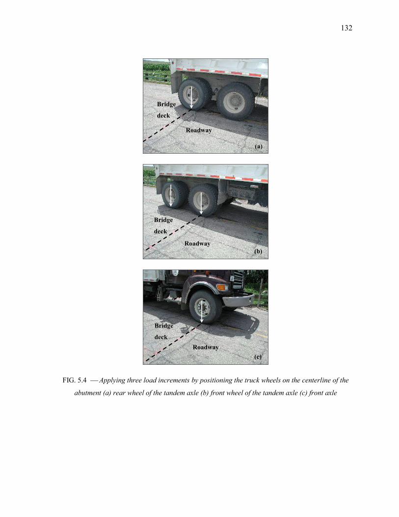
132

FIG. 5.4 Applying three load increments by positioning the truck wheels on the centerline of the

abutment (a) rear wheel of the tandem axle (b) front wheel of the tandem axle (c) front axle

Bridge

deck

Roadway

Bridge

deck

Bridge

deck

Roadway

Roadway

(a)

(b)

(c)

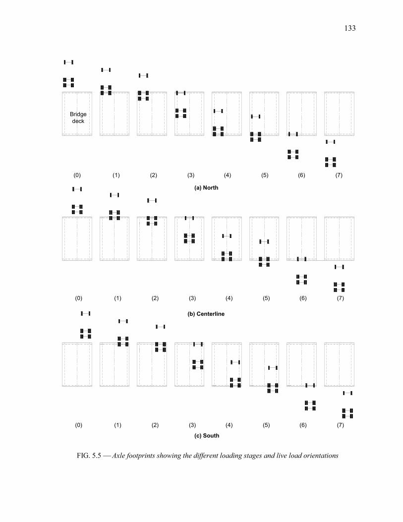
133

Bridge

deck

(a) North

(b) Centerline

(c) South

(0) (1) (2) (3) (4) (5) (6) (7)

(0) (1) (2) (3) (4) (5) (6) (7)

(0) (1) (2) (3) (4) (5) (6) (7)


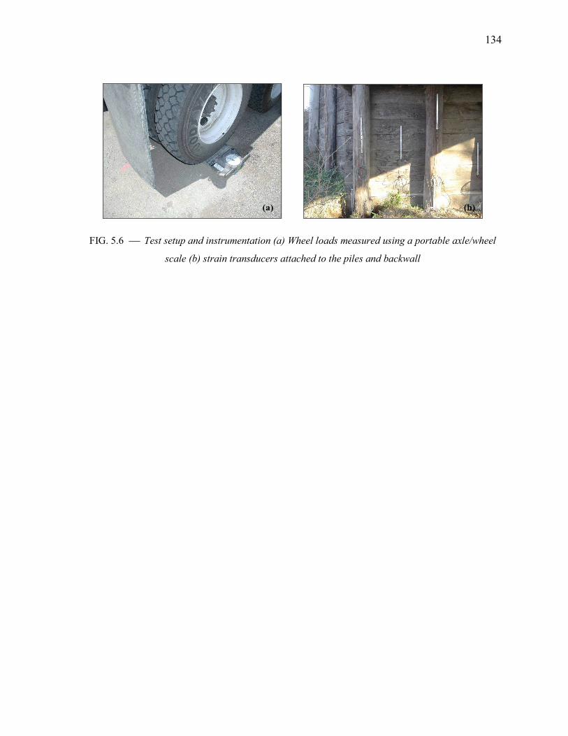
134

FIG. 5.6 Test setup and instrumentation (a) Wheel loads measured using a portable axle/wheel

scale (b) strain transducers attached to the piles and backwall

(a) (b)

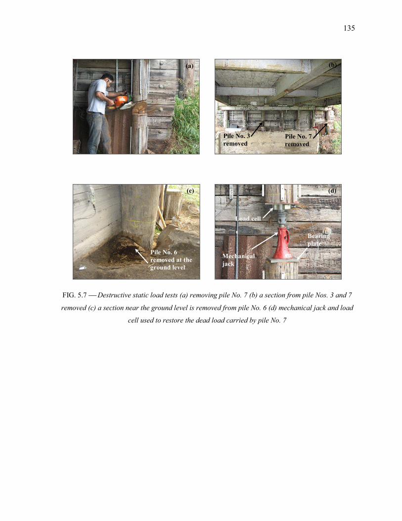
135

FIG. 5.7 Destructive static load tests (a) removing pile 2o. 7 (b) a section from pile 2os. 3 and 7

removed (c) a section near the ground level is removed from pile 2o. 6 (d) mechanical jack and load

cell used to restore the dead load carried by pile 2o. 7

Pile $o. 3

removed Pile $o. 7

removed

Mechanical

jack

Load cell

Bearing

plate

(a) (b)

(c) (d)

Pile $o. 6

removed at the

ground level

136

0.6 m

0.7 m

0.5 m

0.6 m

0.7 m

0.7 m

0.6 m

0.6 m

0.6 m

0.6 m

0.6 m

7.3 m

G.L .

1.2 m1.4 m

1.7 m

1.4 m

0.6 m

1 2 3 4 5 6 7

1-1

2-1 3-1

1-2 2-2

3-2

1-3 2-3

3-3

4-3

5-3

1-4

2-4 3-4

1-5

2-5 3-5

1-6

2-6

3-6 1-7

2-7

3-7

4-7

5-7

1) 3,850 kg 4,460 kg

2) 7,170 kg 8,580 kg

3) 7,080 kg 8,290 kg

4) 2,310 kg 2,670 kg

5) 1,360 kg 1,550 kg

(a)

0 1 2 3 4 5 6 7

Mic

rostr

ain

-40

-30

-20

-10

0

10

1-1

2-1

3-1

0 1 2 3 4 5 6 7

1-2

2-2

3-2

0 1 2 3 4 5 6 7

1-3

2-3

3-3

4-3

5-3

Load configuration

0 1 2 3 4 5 6 7

1-4

2-4

3-4

0 1 2 3 4 5 6 7

1-5

2-5

3-5

0 1 2 3 4 5 6 7

1-6

2-6

3-6

0 1 2 3 4 5 6 7

1-7

2-7

3-7

4-7

5-7

(b)

0 1 2 3 4 5 6 7

Mic

rostr

ain

-25

-20

-15

-10

-5

0

5

10

15

0 1 2 3 4 5 6 7 0 1 2 3 4 5 6 7

Load configuration

0 1 2 3 4 5 6 7 0 1 2 3 4 5 6 7 0 1 2 3 4 5 6 7

(c)

FIG. 5.8 Test 2o. 1 north edge of the bridge (a) location of strain transducers and live loads (b)

pile strains (c) backwall strains

137

Mic

rostr

ain

-50

-40

-30

-20

-10

0

10

20

30

North

Centerline

South

Pile 1

Mic

rostr

ain

-50

-40

-30

-20

-10

0

10

20Pile 2

Mic

rostr

ain

-40

-30

-20

-10

0

Pile 3

Mic

rostr

ain

-22

-20

-18

-16

-14

-12

-10

-8Pile 4

Mic

rostr

ain

-60

-50

-40

-30

-20

-10

0Pile 5

Test Number

1 2 3 4 5 6 7 8

Mic

rostr

ain

-8

-6

-4

-2

0

Pile 6

Test Number

1 2 3 4 5 6 7 8

Mic

rostr

ain

-80

-60

-40

-20

0

20Pile 7

FIG. 5.9 Average microstrains measured at each pile at loading stage three

138

FIG. 5.10 Repairing pile 2o. 7 using the splicing technique

139

3 4 5 6 7

1-1

2-1 3-1

1-2 2-2

3-2

1-3 2-3

3-3

4-3

5-3

1-4

2-4 3-4

1-5

2-5 3-5

1-6

2-6

3-6 1-7

2-7

3-7

4-7

5-7

1) 3,850 kg 4,460 kg

2) 7,170 kg 8,580 kg

3) 7,080 kg 8,290 kg

4) 2,310 kg 2,670 kg

5) 1,360 kg 1,550 kg

0.6 m

0.7 m

0.5 m

0.6 m

0.7 m

0.7 m

0.6 m

0.6 m

0.6 m

0.6 m

0.6 m

7.3 m

G.L .

1.2 m1.4 m

1.7 m

1.4 m

0.6 m

1 2

(a)

0 1 2 3 4 5 6 7

Mic

rostr

ain

-70

-60

-50

-40

-30

-20

-10

0

10

1-1

2-1

3-1

0 1 2 3 4 5 6 7

1-2

2-2

3-2

0 1 2 3 4 5 6 7

1-3

2-3

3-3

4-3

5-3

Load configuration

0 1 2 3 4 5 6 7

1-4

2-4

3-4

0 1 2 3 4 5 6 7

1-5

2-5

3-5

0 1 2 3 4 5 6 7

1-6

2-6

3-6

0 1 2 3 4 5 6 7

1-7

2-7

3-7

4-7

5-7

(b)

0 1 2 3 4 5 6 7

Mic

rostr

ain

-70

-60

-50

-40

-30

-20

-10

0

10

0 1 2 3 4 5 6 7

Load configuration

0 1 2 3 4 5 6 7 0 1 2 3 4 5 6 7 0 1 2 3 4 5 6 7 0 1 2 3 4 5 6 7

(c)

FIG. 5.11 Static load test at the south end with pile 2os. 3 and 6 removed and pile 2o. 7 repaired

(a) location of strain transducers and live loads (b) pile strains (c) backwall strains

140

6. RECOMME$DATIO$S A$D FUTURE RESEARCH

6.1. Performance of Granular Shoulder

As a result of the findings presented in the first and second papers, the following

recommendations and additional research are proposed:

• A minimum weighted average CBR value of the subgrade layers up to a depth of 500 mm

should be about 12. The weighted average CBR value for the granular layer should not be

less than 10.

• The provided design charts can be used as a design guide for construction of new shoulders.

The design charts can also be used as a basis for QA/QC.

• In cases of shoulder rutting due to bearing capacity failure of the subgrade, it is proposed to

use fly ash or geogrid stabilization.

• At edge drop-off shoulder sections, it is recommended to evaluate the use of mixing polymer

emulsion products such with the granular layer.

• Investigate with other soybean oil products due to its previous success in stabilizing 1

shoulder section.

• On a pilot study basis, construct and monitor a granular shoulder test section constructed with

controlled subgrade and granular CBR values.

6.2. $ondestructive Evaluation of Bridge Substructures

The findings of the third and fourth papers led to the following recommendations and future

research:

• Additional research is required for the proposed ultrasonic stress wave evaluation technique.

The additional research should focus on (1) evaluating different ultrasonic transducer

orientations (2) alternative image reconstruction techniques (3) alternative ultrasonic devices,

and (4) the application of the developed procedure on alternative bridge foundation types

such as concrete piles.

• Additional destructive load tests are needed for bridge abutments with fewer number of

supporting piles.

• Construct and instrument laboratory scaled models of low volume road bridge abutments to

better understand the behavior of deteriorated substructures. The output of this laboratory

study may also provide a basis for a numerical model.

141

• For future abutment load test, it is proposed to measure the pile lateral movement parallel and

perpendicular to the backwall so that the pile strains induced by axial and bending loads can

be separated.

• Develop evaluation criteria for timber substructures for use in bridge ratings.

Documents

Geotechnical remediation of transportation infrastructures