Embed Size (px)
Citation preview

DEPARTMENT OF THE INTERIOR U.S. GEOLOGICAL SURVEY
Geotechnical testing of marine sediment
by
William J. Winters 1
Open-File Report 88-36
Prepared in cooperation with theU.S. Environmental Protection Agency under
interagency agreement DW14931699-01
This report is preliminary and has not been reviewed for conformity with U.S. Geological Survey editorial standards and stratigraphic nomenclature. Any use of trade names is for descriptive purposes only and does
not imply endorsement by the USGS or the EPA.
iwoods Hole, Massachusetts 02543
January 1988

TABLE OF CONTENTS
Page
Abstract................................................................. 1
Water Content*........................................................... 2
Atterberg Limits......................................................... 7
Liquid Limit.......................................................... 7
Casagrande Drop Cup............................................... 7
Fall-Cone Penetrometer*........................................... 14
Plastic Limit*........................................................ 17
Grain Specific Gravity................................................... 21
Water Filled Pycnometer............................................... 21
Gas Pressurized Pycnometer*........................................... 23
Laboratory Vane Shear Strength*.......................................... 28
One-Dimensional Consolidation*........................................... 36
Static Consolidated-Undrained Triaxial Compressive Strength*............. 43
Acknowledgements......................................................... 51
References............................................................... 52
(*) - Test currently performed at the USGS Marine Geotechnical Testing Laboratory in Woods Hole, Massachusetts.
ABSTRACT
This report presents procedures and approximate costs (1987) for performing seven types of geotechnical tests. Many of the procedures use standards published by the American Society for Testing and Materials (ASTM); however, testing soft marine sediment often requires additions to or modification of those standards. Where applicable, comments and discussion of the methods are presented.
Most of these test procedures are presently used in the Marine Geotechnical Testing Laboratory in Woods Hole, Massachusetts. Other procedures are presented for comparative and informational purposes. Future modification of the procedures may occur if deemed necessary. Other laboratories within the USGS may use slightly different procedures or perform tests other than are presented in this report.
Cost estimates are based on a batch rate at a functioning geotechnical testing laboratory and do not include start-up costs.
WATER CONTENT
INTRODUCTION
The water content, defined as the mass of water (including dissolved components such as salt) divided by the mass of soil solids, is one of the most important and fundamental soil parameters. It is also one of the simplest to determine. The water content can indicate possible grain sizes of a sample because clay particles tend to adsorb water to their surfaces. For instance, a high water content typically indicates that a sediment has a high clay content. Some clay minerals, such as montmorillonite (smectite), have a greater tendency than others to attract water particles (Larabe and Whitman, 1969, p. 44). A low water content, on the other hand, may mean that a coarser grain size is present or that a clay has been heavily loaded, which caused some of the adsorbed water to be squeezed out. When compared to other measured properties such as Atterberg limits, water content can be used to predict certain engineering behavior or may be evidence that particular geologic processes have occurred. Water content is used in many phase relation equations and is related to the shear strength of a saturated clay (Lambe, 1951, p. 8).
PROCEDURE
Applicable ASTM standard: D2216-80, Standard method for laboratory determination of water (moisture) content of soil, rock, and soil-aggregate mixtures (ASTM, 1987, p. 355-358).
1. Select a representative specimen that has a mass of at least 25 g. If a discontinuity or change in sediment type is encountered at a particular level, representative specimens should be obtained from each material. Spacing between specimen subsampling depends on the overall test-program objectives and should be specified as an appropriate interval, e.g., 10 cm. If a sample had previously been bagged, thoroughly remold the sediment with a spatula before obtaining a water content specimen.
2. Record the cruise and core identifiers, sample interval, water content jar identifier, and mass of a clean dry water content container.
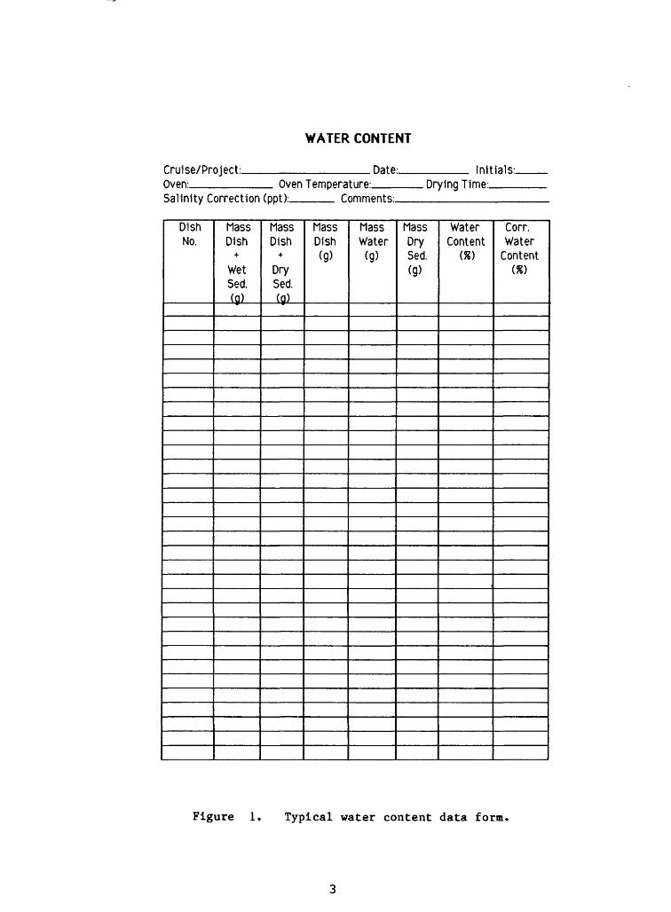
3. Place the moist specimen in the container and determine the mass of the container plus moist material by using a balance that has a precision of ±0.01 g. Record the combined mass on a data form (e.g., Fig. 1).
4. Place the sample and container into a drying oven that can maintain its drying temperature within ±5 °C. Depending on the type of sediment being dried, an oven temperature between 60 °C and 110 °C should be used. Geotechnical testing laboratories often use a temperature of 105 °C (Lambe, 1951, p. 10), however, an oven temperature of 60 ± 5 °C may be more appropriate for materials containing significant amounts of hydrated water or organic material (Liu and Evett, 1984, p. 7).
WATER CONTENT
Cruise/Project:. Oven:_____
Date:. Initials:.Oven Temperature:. Drying Time:.
Salinity Correction (ppt):. Comments:.
Dish No.
Mass Dish
+Wet Sed.(g)
Mass Dish
+Dry Sed.(g)
Mass Dish(g)
Mass Water
(g)
Mass Dry Sed.(g)
Water Content
(X)
Corr. Water
Content (X)
Figure 1. Typical water content data form,

5. After the material has dried to a constant mass, remove the container from the oven (typically 8 to 24 hours).
6. Immediately place the hot container into a desiccator to cool.
7. When the sample has cooled to a temperature at which it can easily be handled, place the container and sample on the balance to determine the combined mass of the container and dry sediment. Record the results. The dried water content sample can be saved for future grain specific gravity testing. The dried sample should not be used for grain-size analysis or x-ray diffraction studies.
8. Subtract the mass of the container and dried sediment from the mass of the container and wet sediment to obtain the mass of water without dissolved salt.
9. Determine the mass of dried sediment and salt precipitate by subtracting the container mass from the combined mass of the container and dried material.
10. The water content of the specimen (w) uncorrected for salt content in the pore fluid, can be determined from the following equation: w = mass of the water -5- mass of the dry sediment and salt.
11. The water content (WG ) corrected for salt in the pore fluid, can be determined from Table 1 (assuming a salinity of 35 ppt). Find the appropriate percentage in the right column, and add it to the uncorrected water content. For example, if the uncorrected water content value was 95%, 7% should be added to that to produce the corrected water content: 102%.
The corrected water content can also be determined from the following equation using any salinity value:
^s) Mw
Mw)
1000-^, w ___ inn w = x ^ : x 100
where: WQ = water content (in percent) corrected for a particularsalinity value,
S = salinity (in ppt), MW = mass of water without salt, and M0 = mass of sediment including salt.S
12. The report (data sheet) should include the following:- Water content of the specimen to the nearest 0.1% or 1%, depending
on the purpose and required precision of the test.- Indication of test specimen having a low mass (below 25 g).- Indication of test specimen containing more than one soil type
(layered, etc.).- Indication of any material (size and amount) removed from the test
specimen.- The method of drying if different from oven-drying at 110±5 °C.
4
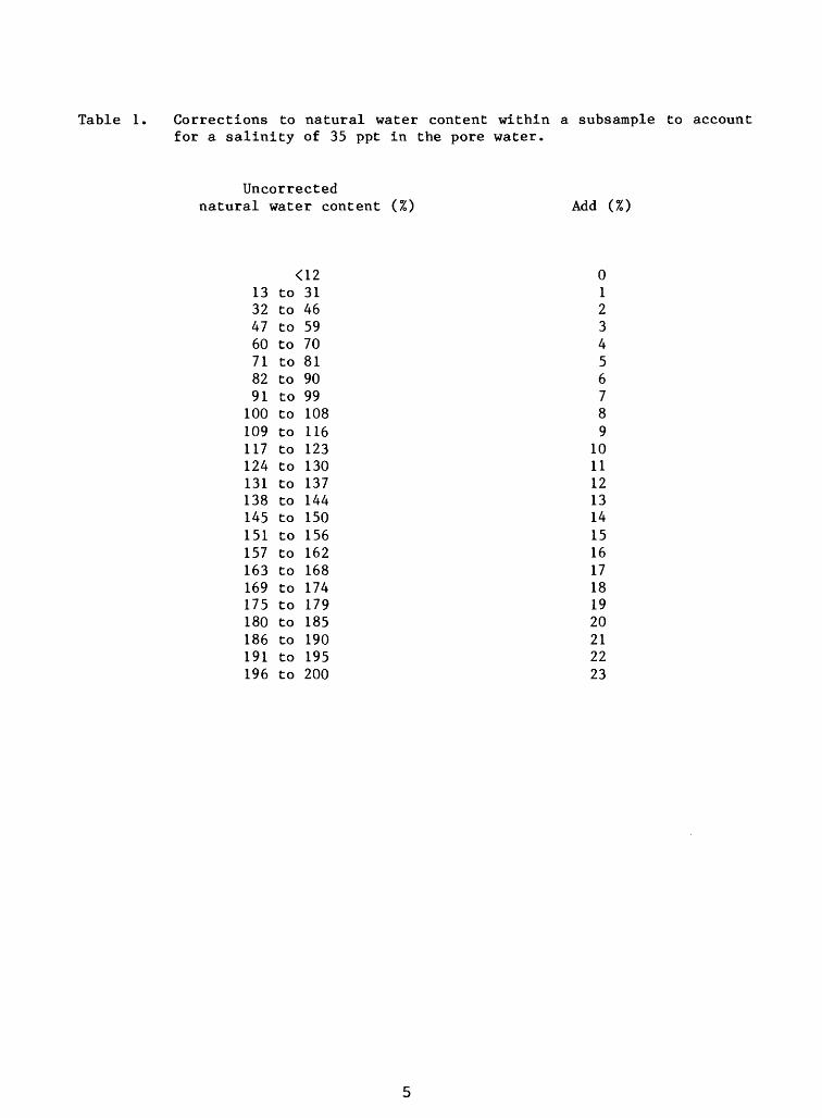
Table 1. Corrections to natural water content within a subsample to account for a salinity of 35 ppt in the pore water.
Uncorrected natural water content (%) Add (%)
<12 013 to 31 132 to 46 247 to 59 360 to 70 471 to 81 582 to 90 691 to 99 7100 to 108 8109 to 116 9117 to 123 10124 to 130 11131 to 137 12138 to 144 13145 to 150 14151 to 156 15157 to 162 16163 to 168 17169 to 174 18175 to 179 19180 to 185 20186 to 190 21191 to 195 22196 to 200 23
COMMENTS
An accurate determination of water content depends on adequate sampling, handling, shipping, and storage of core sections or water content samples (Booth, 1987). Leakage of pore water must be prevented, as must compaction of unsampled sediment cores still within liners. Core sections or sample bags should be well sealed.
Water contents must be corrected for the salt that precipitates out of the pore water during drying because corrections can exceed 10% of the actual water content value.
The equation used to determine water content must always be stated because some investigators define it as mass of water (including salt) divided by the total sample mass. Using that definition, the water content must be less than 100%, whereas the definition in this section allows the water content to exceed 100%.
QUALITY ASSURANCE
Although ASTM (1987) has not yet developed requirements for the precision and accuracy of this test method, Bennett and others (1970) estimated that the precision was ± 1%. The method is suitable for all marine sediments, although great care must be taken in some sediment types (e.g., sands) and in surface sediments to ensure that the data represent the in situ conditions.
COST ANALYSIS
Time required for each water content analysis (not including drying or cooling times): 10 minutes
Cost per sample at batch rate: $4.00
6

ATTERBERG LIMITS (LIQUID AND PLASTIC LIMITS)
INTRODUCTION
The liquid limit and plastic limit (called Atterberg limits) are the two parameters used most often to distinguish the boundaries between the consistency states of fine-grained soils. The liquid limit is the water content that separates liquid- from plastic-behaving remolded sediment, and the plastic limit separates plastic from semisolid behavior. Therefore, if the water content is above the liquid limit, the remolded sediment will behave like a liquid; if the water content is below the liquid limit, but above the plastic limit, the remolded sample will exhibit plastic behavior.
The Atterberg limits are very useful parameters because they indicate the water contents over which sediment behaves plastically. Liquid and plastic limits are related to the amount of water that is attracted to the surfaces of the individual sediment particles. Nonplastic behavior is typically exhibited by predominantly coarse-grained material. Typically, the higher the clay mineral content of a sediment, the greater will be the amount of adsorbed water on the clay particles and, hence, the higher the Atterberg limits.
Other sample parameters that can be determined from Atterberg limits include the plasticity index (Ip ) which is the difference between the liquid limit and plastic limit and the liquidity index (IL ) [(natural water content minus plastic limit) T Ip ], which relates the in situ water content to the Atterberg limits. The latter is useful for estimating approximate sediment stress histories. The plasticity index is often plotted versus liquid limit on a plasticity chart (Fig. 2); the location of the data indicates what type of sediment is present and also the amount of compressibility that can be expected to follow engineering-type loading (Peck and others, 1974, p. 22).
Two methods of determining the liquid limit are currently in use. Within the United States, the ASTM method of using a brass drop cup is more popular. Elsewhere, however, the fall-cone method prevails. Some data exist that indicate better precision can be obtained with the fall-cone method (Head, 1980).
LIQUID LIMIT
Test Method A: Casagrande Drop Cup
In the following method, the liquid limit is defined as the water content at which both sides of a remolded pat of soil, placed in a standard cup and cut by a groove of standard dimensions, will flow together at the base of the groove for a distance of 13 mm ( 0.5 in.) when the soil is subjected to 25 shocks from the cup being dropped 10 mm in a standard liquid-limit apparatus operated at a rate of 2 shocks per second.
PROCEDURE
Applicable ASTM Standard: D4318-84, Standard test method for liquid limit, plastic limit, and plasticity index of soils (ASTM, 1987, p. 763-778).

400
300
200
100
Bentoni (Wyoming)
Volcanic "(Mexico Cityf*1
Various types of peat
Organic silt and cloy (Flushing meadows,L.I.)
\fSodium Montmorillonite LL = 300 to 600 PI = 250 to 550
70
60
50
40 50 60
Liquid limit
90
Figure 2. Plasticity chart showing location of some types of soil (Hunt, 1984, p. 148). The following abbreviations are used; C: clay; H: high plasticity; L: low plasticity; LL: liquid limit; M: silt; 0: organic; and PI: plasticity index.

1. Obtain a representative sediment sample. Note that although ASTM recommends removing material retained on a No. 40 sieve (425-ym) that practice artificially biases the test results to indicate that a more plastic material is present.
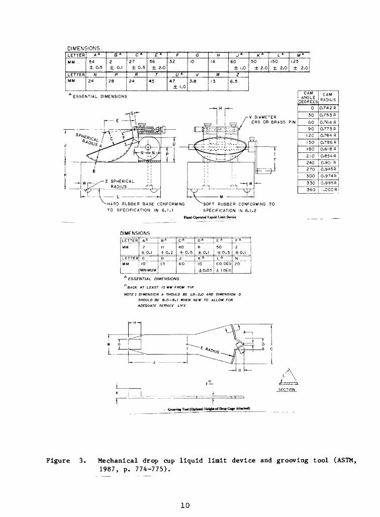
2. After calibrating the apparatus, place a portion of the remolded soil in the cup of the liquid limit device (Fig. 3) at the point where the cup rests on the base. Squeeze it down, and spread it into the cup to a depth of about 10 ram at its deepest point, tapering it to form an approximately horizontal surface. Take care to eliminate air bubbles from the soil.
3. Form a groove in the soil by drawing the tool, beveled edge forward, through the soil. When cutting the groove, hold the grooving tool against the surface of the cup and draw it in an arc, maintaining the tool perpendicular to the surface of the cup throughout its movement. In soils where a groove cannot be made in one stroke without tearing the soil, cut the groove with several strokes of the grooving tool. Alternatively, cut the groove to slightly less than required dimensions with a spatula and use the grooving tool to bring the groove to final dimensions. Exercise extreme care to prevent sliding the soil pat relative to the surface of the cup.
4. Verify that no crumbs of soil are present on the base or the underside ofthe cup. Lift and drop the cup by turning the crank at a rate of 1.9 to2.1 drops per second until the two halves of the soil pat come in contactat the bottom of the groove along a distance of 13 mm (0.5 in.).
5. Verify that an air bubble has not caused premature closure by observing that both sides of the groove have flowed together with approximately the same shape. If a bubble has caused premature closing of the groove, reform the soil in the cup, adding a small amount of soil to make up for any lost in the grooving operation, and repeat steps 2 to 4. If the soil slides on the surface of the cup, repeat steps 2 through 4 at a different water content. If, after several trials at successively higher and lower water contents, the soil pat continues to slide in the cup or if the number of blows required to close the groove is always less than 25, record that the liquid limit could not be determined, and report the soil as nonplastic without performing the plastic limit test.
6. Remix the soil sample on the glass plate without adding to, or removing pore water from the sediment and return a pat of soil to the cup, performing steps two through five. When the operator has recorded at least two trials within one count from each other, record the number of drops, N, required to close the groove. Remove a slice of soil approximately 20 mm wide, extending from edge to edge of the soil cake at right angles to the groove and including that portion of the groove in which the soil flowed together. Place in a weighed container and cover.
7. Return the soil remaining in the cup to the glass plate. Wash and dry the cup and grooving tool prior to the next trial.
8. Remix the soil specimen on the glass plate, adding or reducing water to increase or decrease the water content of the soil and change the number
DIMENSIONSLETTER
MM
LETTER
MM
A
54± 0.5
N
24
e " 2± O.I
P
28
C *
27
± 0.5
R
24
E a
56
± 2.0
r45
F
32
t/ A
47± 1.0
G
10
V
3.8
H
16
W
13
J°
60
± 1.0
z6.5
K a
50
± 2.0
L a
150
± 2.0
W a
125
± 2.0
ESSENTIAL DIMENSIONS
V DIAMETER CRS OR BRASS PIN
-HARD RUBBER BASE CONFORMING ^SOFT RUBBER CONFORMING TO
TO SPECIFICATION IN 6.1.1 SPECIFICATION IN 6.1.2
Hand-Operated Liquid Limit Device
DIMENSIONSLETTER
MM
LETTER]MM
A A
2
IjtO.I
G10
MINIMUM
B a
II±0.2
H13
C A
40
±0.5
J60
D A
8±0.1K A
10
±0.05
E
50±0.5L a
60 DEG
± 1 DEG
F A
Zi ±0.1
IN
20
ESSENTIAL DIMENSIONS
° BACK AT LEAST 15 MM FROM TIP
NOTE : DIMENSION A SHOULD BE I.9-2.Q AND DIMENSION D
SHOULD BE 8.0-8.1 WHEW NEW TO ALLOW FOR
ADEQUATE SERVICE LIFE
1 -r-N G
1 ^
H
^----"i
~~~~ .1"
--^ i
oU-
Croovia, Tool (Optional Htight-of-Drop Gaje Attached)
SECTION
Figure 3. Mechanical drop cup liquid limit device and grooving tool (ASTM, 1987, p. 774-775).
10
of blows required to close the groove. Repeat steps two through seven for at least two additional sets of trials. One set of the trials should be for a closure requiring 25 to 35 blows; one for closure between 20 and 30 blows; and one trial for a closure requiring 15 to 25 blows. NOTE: Some investigators add saline water to the sediment or use absorbent material to remove pore water so that the salinity of the sediment is not changed.
9. Determine the water content, wc , of the soil specimen from each trial in accordance with the prior section, making sure that the water contents are corrected, at least approximately, for salt content. Make all weighings on the same balance. Initial weighings should be performed immediately after completion of the test.
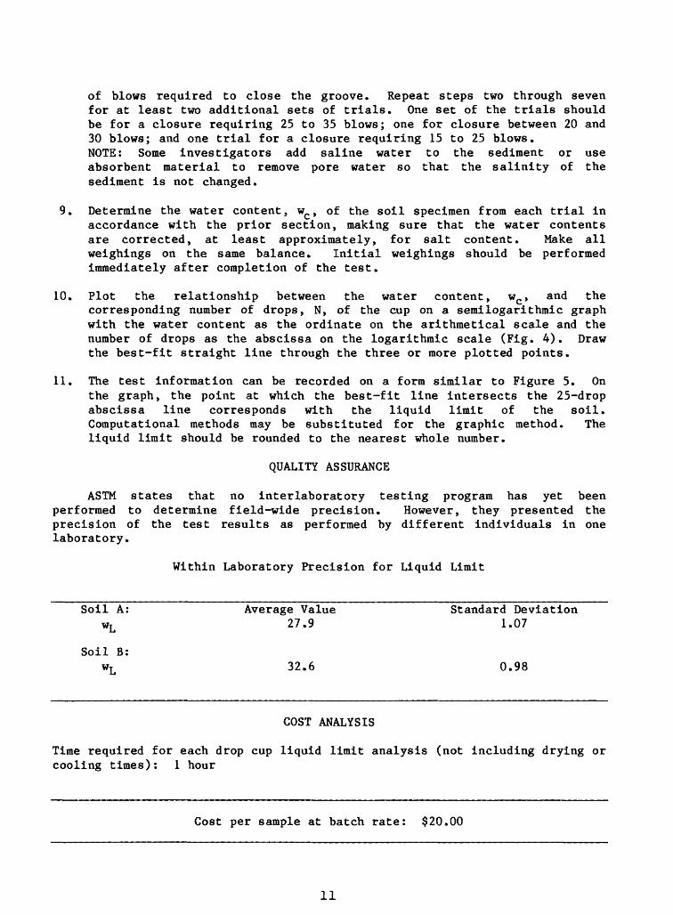
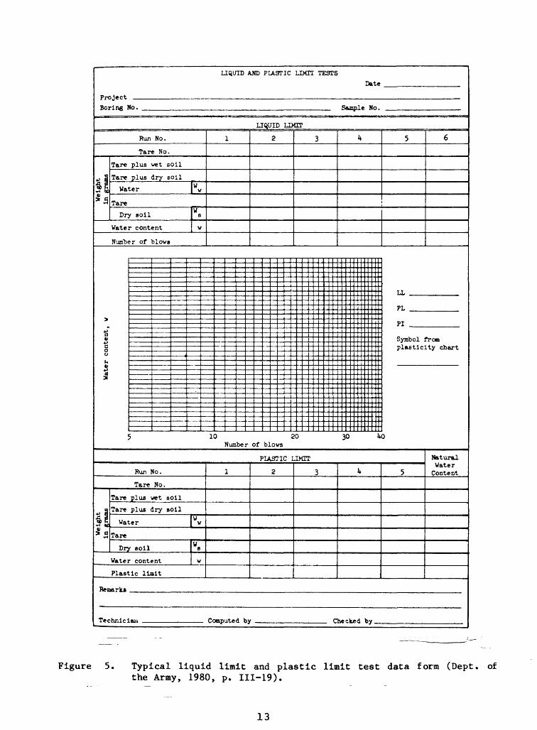
10. Plot the relationship between the water content, wc , and the corresponding number of drops, N, of the cup on a semilogarithmic graph with the water content as the ordinate on the arithmetical scale and the number of drops as the abscissa on the logarithmic scale (Fig. 4). Draw the best-fit straight line through the three or more plotted points.
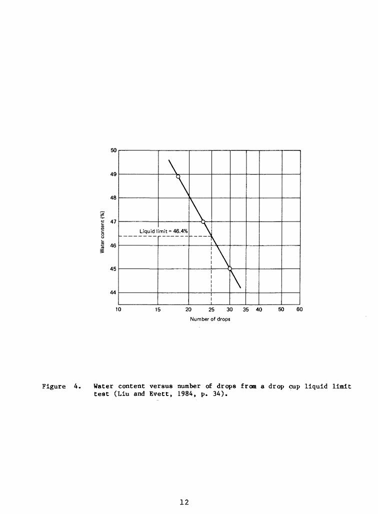
11. The test information can be recorded on a form similar to Figure 5. On the graph, the point at which the best-fit line intersects the 25-drop abscissa line corresponds with the liquid limit of the soil. Computational methods may be substituted for the graphic method. The liquid limit should be rounded to the nearest whole number.
QUALITY ASSURANCE
ASTM states that no interlaboratory testing program has yet been performed to determine field-wide precision. However, they presented the precision of the test results as performed by different individuals in one laboratory.
Within Laboratory Precision for Liquid Limit
Soil A: WL
Soil B:WL
Average Value 27.9
32.6
Standard Deviation 1.07
0.98
COST ANALYSIS
Time required for each drop cup liquid limit analysis (not including drying or cooling times): 1 hour
Cost per sample at batch rate: $20.00
11
15 20 25 30
Number of drops
35 40 50 60
Figure 4. Water content versus number of drops from a drop cup liquid limit test (Liu and Evett, 1984, p. 34).
12
LIQUID AJJD PLASTIC LIMIT TESTS
Date
Project
Boring 1*0. Sfljnple No
LIQUID LIMTT
Run No.
ii»al
Tare No.
Tare
Tare
plus wet soil
plus dry soil
Water [ Ww
Tare
Dry soil
Water content
W
V
Number of blows
Water content, w
i
1 2 3
"
j
k 5
LL
PL
PI
Symbol
6
from Lty chart
5 10 20 30 UONumber of blows
PLASTIC LIMIT
Run No.
4J B
SBSa
H
Tare No.
Tare
Tare
plufi wet soil
plus dry soil
Water [Ww
Tare
Dry soil
Water content
Ws
w
Plastic limit
Remark*
1 2 3 k 5
Natural Water
Content
TerhnlMiui . . Pnmputed by Ch*pk*4 by
Figure 5. Typical liquid limit and plastic limit test data form (Dept. of the Army, 1980, p. 111-19).
13

Test Method B: Fall-Cone Penetroraeter
In the following method, the liquid limit is defined as the water content at which a cone with specific dimensions and mass penetrates the flat surface of remolded sediment to a prescribed distance.
PROCEDURE
Applicable standard: BS 1377, 1975, Test 2 (A); British standard test for liquid limit - cone penetrometer method, British Standards Institution, Lond on, Eng1and.
1. Obtain a representative sediment sample.
2. Thoroughly remold the material in a large evaporating dish with a spatula.
3. Fill the metal penetrometer cup with sediment, being careful not to trap air bubbles within the sediment during the placement procedure.
4. Evenly scrape off any material above the top of the cup with a spatula or wire saw, leaving a flat sediment surface.
5. Place the sediment onto the liquid limit device making sure that the cone tip barely comes into contact with the sediment surface (Fig. 6).
6. Release the cone and allow it to penetrate the sediment for exactly 5 seconds; record the penetration depth.
7. Remove the sediment cup from the device, clean the cone, and remold the sediment within the cup. Repeat steps two through six until the second penetration is within 0.2 mm of the previous depth.
8. With a small spatula, take a water content subsample from the zone adjacent to the penetration void.
9. Return the remaining sediment from the penetrometer cup to the evaporating dish. Change the water content so that three equally spaced penetrations between 10 and 30 mm are obtained.
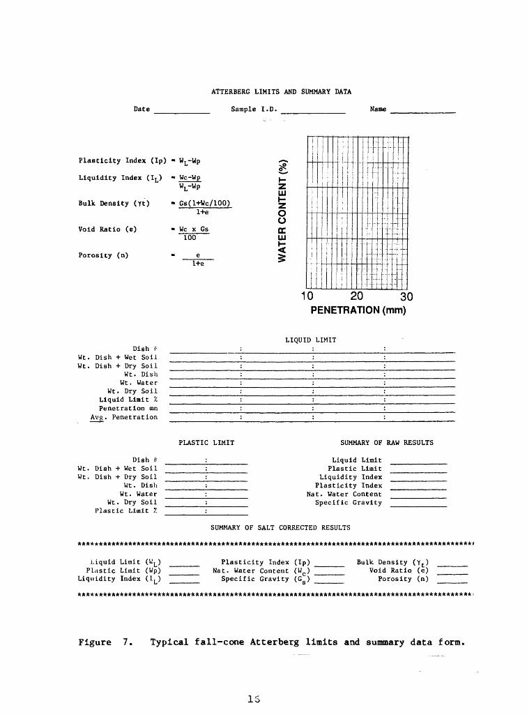
10. Plot the water content versus penetration depth for the three trials on a data form (Fig. 7) and determine the liquid limit (corrected for salt content) related to the standard penetration depth for the particular cone in use. For example, a cone with a mass of 80.00±0.05 g and an apex angle of 30 degrees requires a penetration of 20 mm to define the liquid limit. Round off the liquid limit value to the nearest whole number.
QUALITY ASSURANCE
The precision of the fall-cone penetrometer liquid limit test is not known at the present time, however, it may be more precise than the drop cup method.
14

Figure 6. Fall cone penetrometer and electric timer used for determining the liquid limit of sediment (the timer automatically stops penetration after five seconds have elapsed).
15
Date
ATTERBERG LIMITS AND SUMMARY DATA
Sample I.D. ___________ Name
Plasticity Index (Ip) - WL~Wp
Liquidity Index (IL)
Bulk Density (Yt)
Void Ratio (e)
Porosity (n)
Gs(l+Wc/100) 1+e
We x Gs100
111H-
o oDC 111
1+e
10 20 30 PENETRATION (mm)
LIQUID LIMITDish ?'
Wt. Dish + Wet SoilWt. Dish + Dry Soil
Wt. DishWt. Water
Wt. Dry SoilLiquid Limit %Penetration mm
Avg. Penetration
PLASTIC LIMIT SUMMARY OF RAW RESULTS
Dish £Wt. Dish + Wet SoilWt. Dish + Dry Soil
Wt. DishWt. Water
Wt. Dry SoilPlastic Limit '/.
Liquid LimitPlastic Limit
Liquidity IndexPlasticity Index
Nat. Water ContentSpecific Gravity
SUMMARY OF SALT CORRECTED RESULTS
Liquid Limit (WL )Plastic Limit (Wp)
Liquidity Index (I L )
Plasticity Index (Ip)Nat. Water Content (Wc )
Specific Gravity (G g )
Bulk Density (Y t )Void Ratio (e)
Porosity (n)
Figure 7. Typical fall-cone Atterberg limits and summary data form,
16

COST ANALYSIS
Time required for each fall cone liquid limit analysis (not including drying and cooling times): 1 hour
Cost per sample at batch rate: $20.00
DISCUSSION
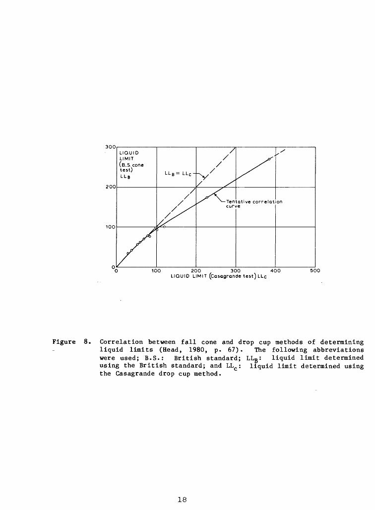
Head (1980) states that although the fall-cone is no quicker to perform, it is more dependable because the test mechanics are based on the remolded static shear strength alone, without dynamic factors entering the analysis. Head also notes that the cone method produces more consistent results than the Casagrande method. Some researchers note that up to liquid limits of 100 percent, results between the two methods show little difference (Fig. 8) (Head, 1980, p. 67; Wasti and Bezirci, 1986).
PLASTIC LIMIT
INTRODUCTION
The plastic limit test is typically performed immediately after the liquid limit test and provides the lowest water-content value at which a soil behaves plastically in a remolded state. The plastic limit is determined by first pressing a small portion of plastic soil together, rolling it into a 3.2-mm (1/8-in) diameter thread (which gradually removes the water), and repeating the process until the thread crumbles and can no longer be pressed together and rerolled. The water content of the soil at this stage is reported as the plastic limit.
PROCEDURE
Applicable ASTM standard: D4318-84, Standard test method for liquid limit, plastic limit, and plasticity index of soils (ASTM, 1987, p. 763-778).
1. Select approximately a 20-g representative portion of soil from the material prepared for the liquid limit test. Thoroughly remold the sample.
2. Change the water content of the soil to a consistency at which it can be rolled by spreading and remolding continuously on a glass plate to encourage evaporation. The drying process may be accelerated by exposing the soil to the air current from an electric fan or by blotting with hard surface paper towels or high-wet-strength filter paper (to avoid adding fiber to the soil).
3. From the 20-g mass, select a 1.5- to 2.0-g portion. Form the test specimen into an ellipsoidal mass. Roll this mass between the palm or fingers and the ground-glass plate with just enough pressure to roll the mass into a thread of uniform diameter along its entire length.
17
300
200
LIQUID LIMIT(B.S.cone test)
LL B = LLC
X
Tentative correlation curve
100
100 200 300 400 LIQUID LIMIT (Casagrande test) LLc
500
Figure 8. Correlation between fall cone and drop cup methods of determining liquid limits (Head, 1980, p. 67). The following abbreviations were used; B.S.: British standard; LL^: liquid limit determined using the British standard; and LLQ : liquid limit determined using the Casagrande drop cup method.
18

The thread should be further deformed on each stroke so that its diameter is continuously reduced and its length extended until the diameter reaches 3.2±0.5 mm (0.125±.020 in.). This should take no more than two minutes. The amount of hand or finger pressure required will vary greatly according to the soil.
A normal rate of rolling for most soils should be 80 to 90 strokes per minute, counting a stroke as one complete motion of the hand forward and back to the starting position. This rate of rolling may have to be decreased for very fragile soils.
A. When the diameter of the thread is approximately 3.2 mm, break the thread into several pieces. Squeeze the pieces together, knead together, reform into an ellipsoidal mass, and reroll to 3.2 mm. Repeat this gathering, kneading and rerolling, until the thread crumbles under the pressure required for rolling and the soil can no longer be rolled into a 3.2-mm diameter thread. If crumbling occurs when the thread has a diameter greater than 3.2 mm, this shall be considered a satisfactory end point, provided the soil has been previously rolled into a thread 3.2 mm in diameter.
5. Gather the portions of the crumbled thread together and place them in a preweighed container. Immediately cover the container.
6. Select another 1.5- to 2.0-g portion of soil from the original 20-g specimen and repeat steps three to five until the container holds at least 6 g of soil.
7. Repeat the full process until a second container, holding at least 6 g of soil, is prepared.
8. Determine the salt-corrected water content, in percent, of the soil contained in the containers (refer to that procedural section) and enter all data on a test form such as Figure 7. Plastic limit results should be rounded off to the nearest whole number. If either the liquid limit or the plastic limit cannot be determined, or if the plastic limit is greater than the liquid limit, the sediment is nonplastic (NP).
COMMENTS
The test method for determining the plastic limit is straightforward; however, ASTM standard D4318-84 should be consulted to insure that the rate of rolling of the thread, time allowed to perform the test, etc. are properly performed. If the ASTM standard is not followed exactly (except for the removal of the 425-iam fraction), the results can be misleading. For example, a non-plastic soil can appear to exhibit slight plasticity.
Numerous investigators have found that liquid limit and plastic limit values are significantly affected by the amount of organic matter that is present in the sediment (Booth and Dahl, 1986). Typically, an increase in organic content increases both the liquid and plastic limits. Therefore, organic content should be measured and reported for those sediments suspected of containing significant amounts of organic matter.
19

QUALITY ASSURANCE
ASTM states that no interlaboratory testing program has as yet been performed to determine field-wide precision. However, the precision within one laboratory of the test method performed by different individuals is as follows:
Within Laboratory Precision for Plastic Limit
Soil A:
Wp
wp
Average Value
21.9 20.1
Standard Deviation
1.07 1.21
COST ANALYSIS
Time required for each plastic limit determination (not including drying or cooling times): 30 minutes
Cost per sample at batch rate: $10.00
20
GRAIN SPECIFIC GRAVITY
INTRODUCTION
The specific gravity of soil is defined as the ratio of the mass of a unit volume of a material at a stated temperature to the mass in air of the same volume of gas-free distilled water at a stated temperature (ASTM, 1987, p. 210). The grain specific gravity can be used, in conjunction with the salt-corrected water content, to estimate in situ overburden stresses as well as the possible presence of certain minerals.
Two methods are presently used to determine the grain specific gravity. The traditional method, (method A, below) involves filling a glass pycnometer with sediment and distilled water; removing the entrapped air (possibly by boiling); cooling to room temperature; measuring the water's temperature; weighing the device; and finally, determining the grain specific gravity after correcting the density of the water for temperature. Newer methods rely on a self-contained apparatus that simply involve weighing the sample and placing it into the pycnometer to measure volume (some devices are completely automated and measure volumes of five samples simultaneously), and then making a simple calculation.
Test Method A: Water-Filled Pycnometer
PROCEDURE
Applicable ASTM Standard: D854-83, Standard test method for specific gravity of soils (ASTM, 1987, p. 210-213).
1. Calibrate pycnometer.
2. Place a sediment sample in the pycnometer. If a volumetric flask is used, the sample should have a mass of at least 25 g; if a stoppered bottle is used, the sample should have a mass of at least 10 g.
3. Add sufficient distilled water to fill the volumetric flask about three- fourths full or the stoppered bottle about half full.
4. Remove entrapped air by: subjecting the contents to a partial vacuum or boiling gently for at least 10 minutes, occasionally rolling the pycnometer to assist in the removal of the air. Subject the contents to reduced air pressure either by connecting the pycnometer directly to an aspirator or vacuum pump or by using a bell jar. Note: some soils boil violently when subjected to reduced air pressure. If that happens reduce the air pressure at a slower rate or use a larger flask. Allow heated samples to come to ambient temperature before proceeding with the analysis.
5. Fill the pycnometer with distilled water, clean the outside, and dry with a clean, dry cloth. Determine the weight of the pycnometer and contents, and the temperature of the contents. Calculate the specific gravity of the soil according to the ASTM standard D854-83 and record the information on a form similar to Figure 9. Grain specific gravity should be reported to two decimal places.
21

Soils Testing Laboratory Specific Gravity Determination
Sample No.
Boring No.
Depth __
Description of Sample
Tested by ______
Project No.
Location _
Date
[A] Calibration of Pycnometer
(1) Weight of dry, clean pycnometer, Wp
(2) Weight of pycnometer + water, Wpw _
(3) Observed temperature of water, 7/ _
[Bj Specific Gravity Determination
Determination No.:
Weight of pycnometer -I- soil + water,wpm (g)
Temperature, Tx (°C)
Weight of pycnometer + water at Tx , Wpw (a\Tx ) (g)
Evaporating dish no.
Weight of evaporating dish, W^ (g)
Weight of evaporating dish + oven-dried soil, Wds (g)
Weight of solids, Ws (g)
Conversion factor, K
Specific gravity of soil
C KWg5 Ws + Wpw (rtTx }-Wpws
1 2 3
Figure 9. Typical data form for grain specific gravity determined using the water filled pycnoaeter method (Liu and Evett, 1984, p. 23).
22

QUALITY ASSURANCE
ASTM has determined the precision of the test for cohesive soils as:
Standard Acceptable Deviation Difference *
Single-operator precision 0.021 0.06 Multilaboratory precision 0.056 0.16
*The difference between the results of two properly conducted tests should notexceed the acceptable difference.Methods are not presently available to determine accuracy.
COST ANALYSIS
Time required for each test: 2 hours
Cost per analysis at batch rate: $40.00
Test Method B: Gas-Pressurized Pycnometer
PROCEDURE
1. Grind an oven dried sample to a fine sand-sized powder using a mortar and pestle.
2. Place the sample in a small evaporating dish or water content tin and leave it in an oven at a temperature between 60 °C and 110 °C for a minimum of eight hours.
3. Remove the sample from the oven and let it cool to room temperature in a desiccator so that moisture in the air won't be adsorbed by any clay minerals.
4. Place the sample into a pycnometer cup of known mass and place it into the pycnometer (Fig. 10).
5. Determine the volume of the soil grains according to the manufacturer's instructions.
6. Remove the sample and cup from the pycnometer. Determine the mass of the sample and cup.
7. Specific gravity is determined by dividing the mass of soil grains by the volume of soil grains and is reported to two decimal places.
23

Figure 10. Gas pressurized pycnometer,
24
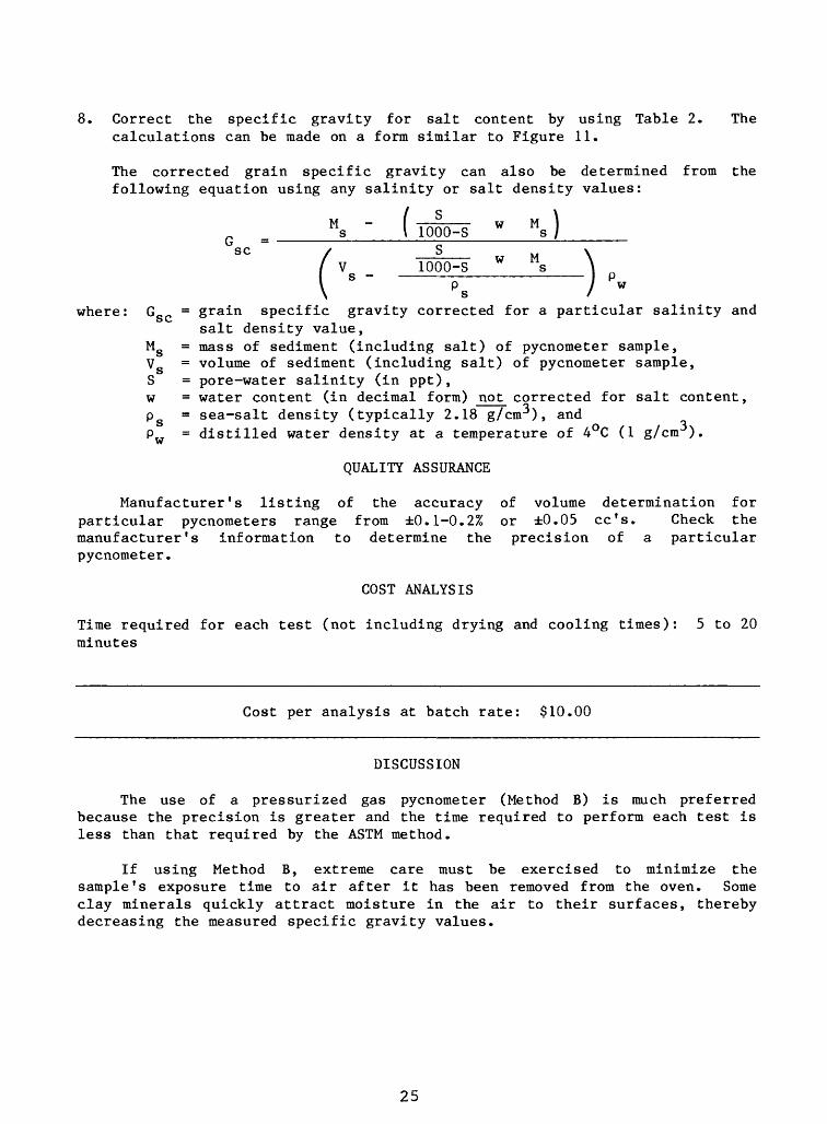
8. Correct the specific gravity for salt content by using Table 2. The calculations can be made on a form similar to Figure 11.
The corrected grain specific gravity can also be determined from the following equation using any salinity or salt density values:
G sc
M s
/ v
1 S\ 1000-S
s1000-S
w
w
M ) s /
M \8 \ n
p s
where: G_ c = grain specific gravity corrected for a particular salinity andsalt density value,
Mg = mass of sediment (including salt) of pycnometer sample, Vs = volume of sediment (including salt) of pycnometer sample, S = pore-water salinity (in ppt),w = water content (in decimal form) not corrected for salt content, p = sea-salt density (typically 2.18 g/cnr*), and Pw = distilled water density at a temperature of 4°C (1 g/cm ).
QUALITY ASSURANCE
Manufacturer's listing of the accuracy of volume determination for particular pycnometers range from ±0.1-0.2% or ±0.05 cc's. Check the manufacturer's information to determine the precision of a particular pycnometer.
COST ANALYSIS
Time required for each test (not including drying and cooling times): 5 to 20 minutes
Cost per analysis at batch rate: $10.00
DISCUSSION
The use of a pressurized gas pycnometer (Method B) is much preferred because the precision is greater and the time required to perform each test is less than that required by the ASTM method.
If using Method B, extreme care must be exercised to minimize the sample's exposure time to air after it has been removed from the oven. Some clay minerals quickly attract moisture in the air to their surfaces, thereby decreasing the measured specific gravity values.
25
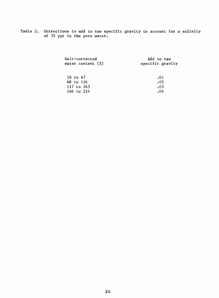
Table 2. Corrections to add to raw specific gravity to account for a salinity of 35 ppt in the pore water.
Salt-corrected Add to raw water content (%) specific gravity
18 to 67 .0168 to 116 .02117 to 165 .03166 to 214 .04
26

PYCNOMETER
SAMPLE ID WEIGHT MEASURED VOLUME
TARE CORRECTED VOLUME
S.G.RAW SALT COR
SALT COR. W.C.
Figure 11. Form for recording data and determining grain specific gravity by gas pressurized pycnometer.
27

LABORATORY VANE SHEAR STRENGTH
INTRODUCTION
The miniature vane shear test is performed to determine an approximate value of the undrained shear strength in fine-grained soil. The sensitivity (that is the ratio of natural undrained shear strength divided by the remolded undrained shear strength) can also be calculated. The test consists of inserting a four-bladed vane into the sediment, rotating the shaft connected to the blades, and measuring the torque required to shear the sediment. By assuming a particular failure surface within the soil, the undrained shear strength (su ) can be calculated.
Although ASTM (1987) has a standard for vane shear testing in the field, it does not yet have one for laboratory testing although such a standard is presently under review. The related method D2573-72, standard test method for field vane shear test in cohesive soil, is currently being revised. Some information is pertinent to both types of tests.
PROCEDURE
1. Insure that the core section and vane shear machine (Fig. 12) are securely positioned so that neither will move during testing.
2. Take an initial reading on the rotation dial or set the initial reading to 0°.
3. Insert the vane into the sediment so that the top of the vane is about one vane height below the sediment surface. The center of the vane should be at least 1.5 vane diameters away from any liner surface or wall.
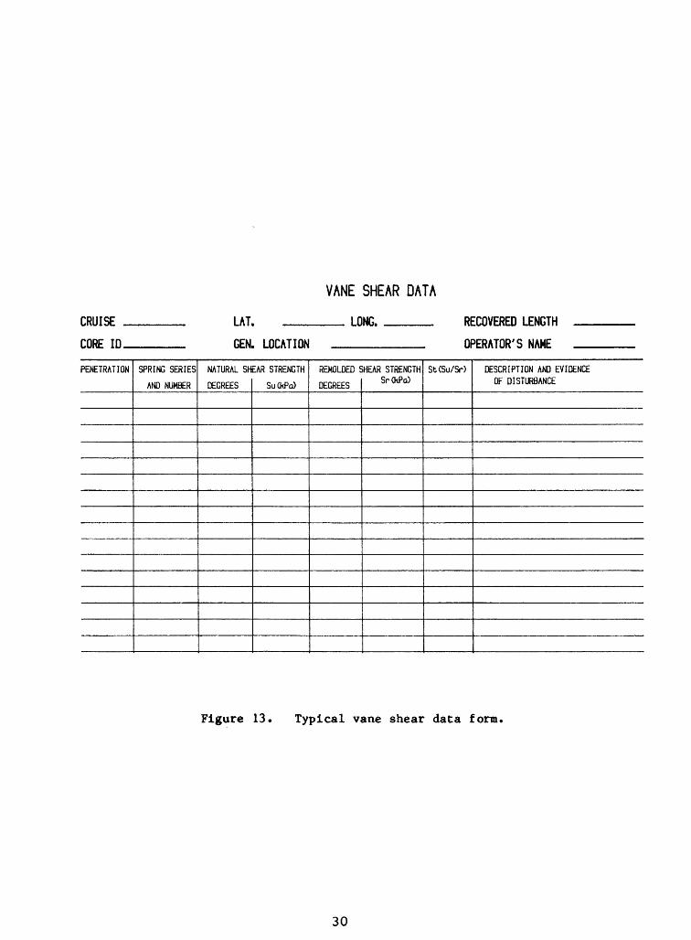
4. Rotate the vane, or the spring top, at a rate of 90° per minute until a peak torque is reached. Record the peak value on a data form similar to Figure 13.
5. Remove the drive belt and remold the sediment by rotating the vane by hand rapidly through at least one revolution. Another, more time consuming, method is to remove the sediment and physically remold it within a plastic bag to avoid entrapping air. Carefully replace the sediment into a container and re-insert the vane.
6. Reattach the belt (if necessary), rotate the vane, and read the peak torque. Record the peak value as the remolded peak on the data form.
7. Extract the vane.
8. Remove a 10- to 20-g water-content sample from the zone where the vane test was run.
9. Insert a non-water-absorbing plug in the resulting hole.
28

Figure 12. Vane shear machine that uses a spring to apply torque to the vane.
29
CRUISE .
CORE ID.
LAT.
VANE SHEAR DATA
__ LONG. _____
GEN. LOCATION
RECOVERED LENGTH
OPERATOR'S NAME
PENETRATION SPRING SERIES
AND NUMBER
NATURAL SH
DEGREES
EAR STRENGTH
SuCkPo)
REMOLDED £
DEGREES
HEAR STRENGTH Sr(kPa)
St(Su/Sr) DESCRIPTION AND EVIDENCE OF DISTURBANCE
Figure 13. Typical vane shear data form.
30
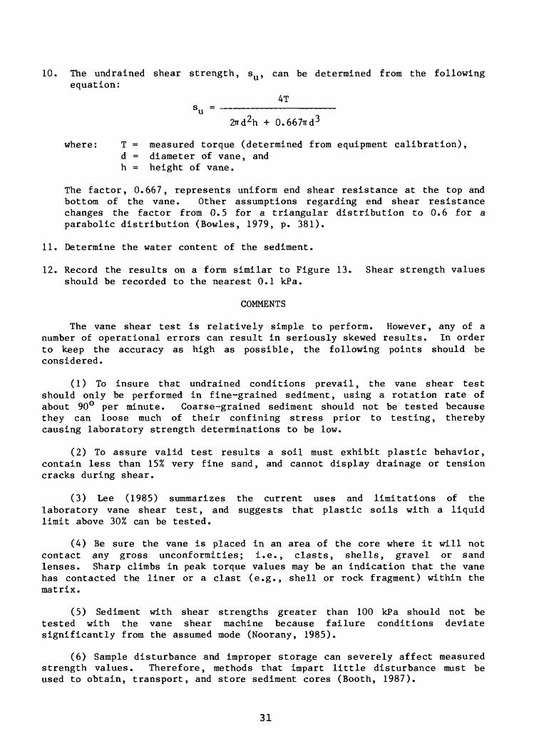
10. The undrained shear strength, su , can be determined from the following equation:
4Tsu =
27rd 2h + 0.667ird3
where: T = measured torque (determined from equipment calibration),d = diameter of vane, andh = height of vane.
The factor, 0.667, represents uniform end shear resistance at the top and bottom of the vane. Other assumptions regarding end shear resistance changes the factor from 0.5 for a triangular distribution to 0.6 for a parabolic distribution (Bowles, 1979, p. 381).
11. Determine the water content of the sediment.
12. Record the results on a form similar to Figure 13. Shear strength values should be recorded to the nearest 0.1 kPa.
COMMENTS
The vane shear test is relatively simple to perform. However, any of a number of operational errors can result in seriously skewed results. In order to keep the accuracy as high as possible, the following points should be considered.
(1) To insure that undrained conditions prevail, the vane shear test should only be performed in fine-grained sediment, using a rotation rate of about 90° per minute. Coarse-grained sediment should not be tested because they can loose much of their confining stress prior to testing, thereby causing laboratory strength determinations to be low.
(2) To assure valid test results a soil must exhibit plastic behavior, contain less than 15% very fine sand, and cannot display drainage or tension cracks during shear.
(3) Lee (1985) summarizes the current uses and limitations of the laboratory vane shear test, and suggests that plastic soils with a liquid limit above 30% can be tested.
(4) Be sure the vane is placed in an area of the core where it will not contact any gross unconformities; i.e., clasts, shells, gravel or sand lenses. Sharp climbs in peak torque values may be an indication that the vane has contacted the liner or a clast (e.g., shell or rock fragment) within the matrix.
(5) Sediment with shear strengths greater than 100 kPa should not betested with the vane shear machine because failure conditions deviatesignificantly from the assumed mode (Noorany, 1985).
(6) Sample disturbance and improper storage can severely affect measured strength values. Therefore, methods that impart little disturbance must be used to obtain, transport, and store sediment cores (Booth, 1987).
31
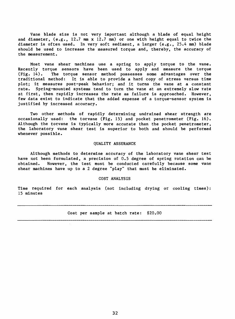
Vane blade size is not very important although a blade of equal height and diameter, (e.g., 12.7 mm x 12.7 mm) or one with height equal to twice the diameter is often used. In very soft sediment, a larger (e.g., 25.4 mm) blade should be used to increase the measured torque and, thereby, the accuracy of the measurement.
Most vane shear machines use a spring to apply torque to the vane. Recently torque sensors have been used to apply and measure the torque (Fig. 14). The torque sensor method possesses some advantages over the traditional method: It is able to provide a hard copy of stress versus time plot; it measures post-peak behavior; and it turns the vane at a constant rate. Spring-mounted systems tend to turn the vane at an extremely slow rate at first, then rapidly increases the rate as failure is approached. However, few data exist to indicate that the added expense of a torque-sensor system is justified by increased accuracy.
Two other methods of rapidly determining undrained shear strength are occasionally used: the torvane (Fig. 15) and pocket penetrometer (Fig. 16). Although the torvane is typically more accurate than the pocket penetrometer, the laboratory vane shear test is superior to both and should be performed whenever possible.
QUALITY ASSURANCE
Although methods to determine accuracy of the laboratory vane shear test have not been formulated, a precision of 0.5 degree of spring rotation can be obtained. However, the test must be conducted carefully because some vane shear machines have up to a 2 degree "play" that must be eliminated.
COST ANALYSIS
Time required for each analysis (not including drying or cooling times): 15 minutes
Cost per sample at batch rate: $20.00
32
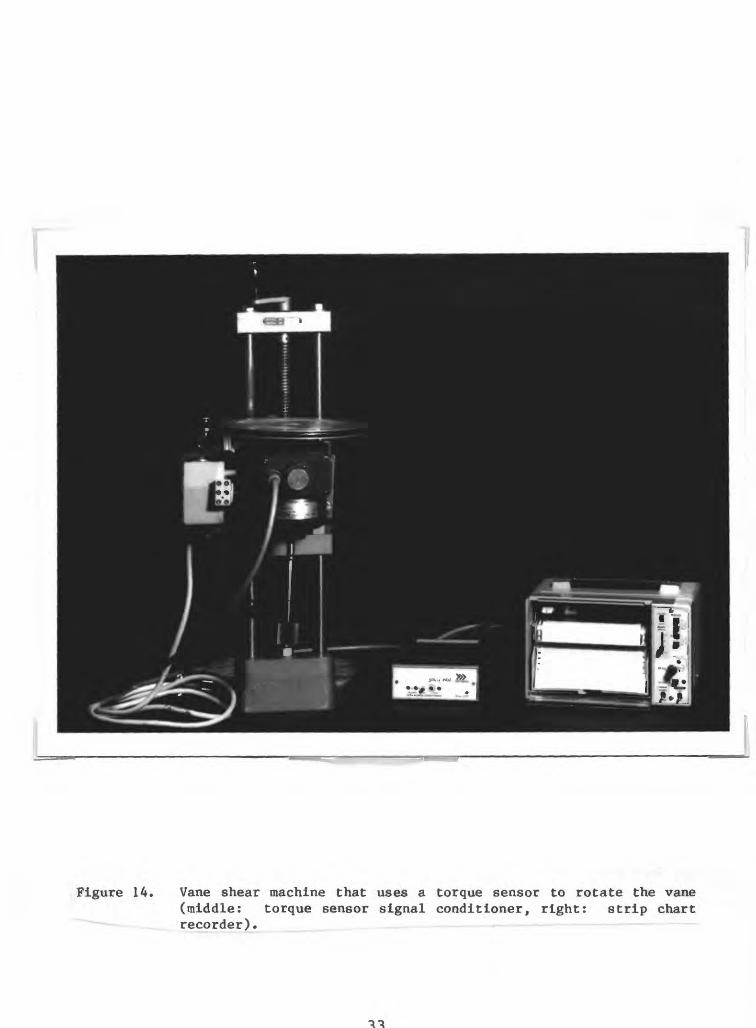
Figure 14. Vane shear machine that uses a torque sensor to rotate the vane(middle: torque sensor signal conditioner, right: strip chartrecorder).
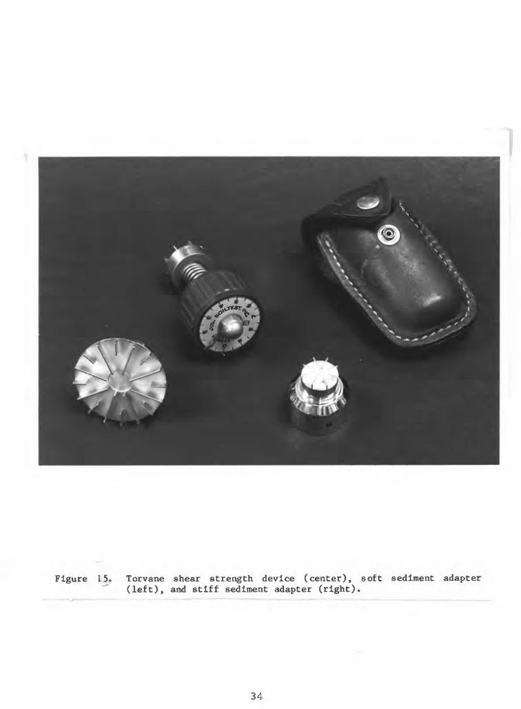
Figure 15. Torvane shear strength device (center), soft sediment adapter ~" (left), and stiff sediment adapter (right).
34
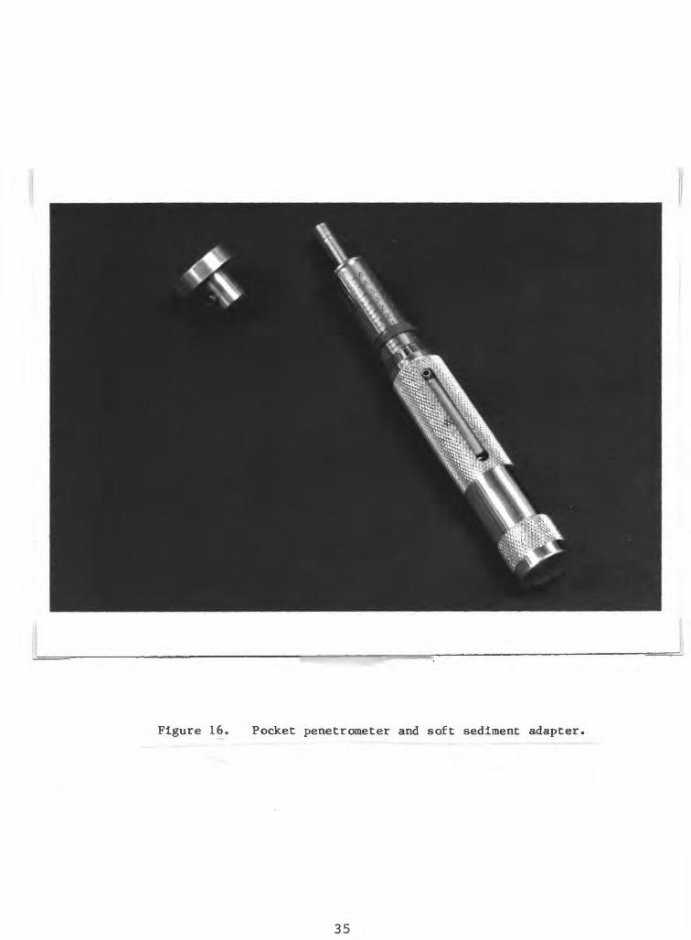
Figure 16. Pocket penetrometer and soft sediment adapter,
35
ONE-DIMENSIONAL CONSOLIDATION
INTRODUCTION
The constant-rate-of-strain consolidation (CRSC) test is performed to evaluate the laterally confined one-dimemsional stress-strain properties of a cylindrical wafer of sediment. Test results can be used to determine the stress history (maximum past stress) and the rate at which consolidation occurs. Typically, a test is performed in four parts: saturation, loading, rebound, and reload.
Results from this test often are used to predict the amount and rate of settlement of a proposed engineering structure.
PROCEDURE
Applicable ASTM standard: D4186-82, Standard test method for one- dimensional consolidation properties of soils using controlled-strain loading (ASTM, 1987, p. 709-715).
1. Flush the equipment lines with de-aired water. De-air the porous stones.
2. Place the test specimen into the CRSC system's confining ring either by carefully trimming a sediment sample to the correct dimensions or by pushing a cutting ring into the sediment. Softer sediment typically requires the latter technique.
3. Trim the sample to the correct height with a wire saw and fill any irregularities in the sample with material from the trimmings. Obtain water content samples from the top, middle, and bottom trimmings.
4. Determine the weight and dimensions of the sample and record the data on a form similar to Figure 17.
5. Place the sample on the machine pedestal and assemble the confining apparatus, including filter papers and porous stones (Fig. 18).
6. Place the top cap on the sample. The top cap should be made of a strong light-weight material. This is extremely important when testing very soft marine sediment.
7. Assemble the chamber and fill it with de-aired water.
8. Connect the load, deformation, pore-pressure, and cell pressure (or differential transducer) measuring devices. Check that systems are operating correctly and that measurements are within bounds.
9. Make sure the sample does not swell. This is done either by limiting potential vertical deformation or by applying just enough seating stress to counteract the swelling tendencies of the sediment. It is extremely important to not overload the sample at this point.
36

CONSTANT RATE OF STRAIN CONSOLIDATION TEST
Test I.D./File Name:_______________
_______________ Date/Start:_______
________________ Tested By:________
Project Title:_ (Cruise No.) Core I.D.:
Subsectioned Interval (m):
Test Sample Interval (m):_
System Number:_________
0 Readings:___________
Raw Disc:
End:
Rate of Feed (mm/min):_
Gearbox Lever (A-E):_
Cell Press. (kPa):___
Back Press. (kPa):___
Reduced Disc:
PRE-CONSOLIDATION SPECIMEN DATA
Diameter (mm) _______
Height (mm) _______
Wt. cutting ring +filter papers + sample (g)Wt. cutting ring +filter papers (g)
Wt. wet sample (g)
SAMPLE DESCRIPTION AND COMMENTS
WATER CONTENT FROM TRIMMINGStop side bottom
Container ID ____ ____ _____
Wt. wet soil +container (g) ____ ____ ____
Wt. dry soil + container (g) ____ _____ _____Wt. water (g) ____ ____ ____
Wt. container (g)____ _____ ____
Wt. dry soil (g) ____ ____ ____
Water content (%)____ ____ ____
Wt. wet sample + container (g)
Average wc (%)
POST-CONSOLIDATION SPECIMEN DATA
Height (mm) ______
Container I.D. ____
Wt. dry sample + container (g)____
Wt. container (g) ____
Wt. Dry sample (g) ____
Wt. water (g) ____
Water content (%) ____
Pre-consol wc (%) ____
Wt. dry sample + container (g)
Wt. water (g)
Wt. dry sample (g)
Water content (%)
Post-consol wc (%)
Figure 17. Typical CRS consolidation test data form.
37
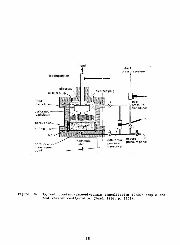
to back pressure system
loading piston
oil recess oilfiller plug
load transducer
perforated load platen
porous disc
cutting ring
seals
pore pressure measurement point
backpressuretransducer
differentialpressuretransducer
to pore pressure panel
Figure 18. Typical constant-rate-of-strain consolidation (CRSC) sample and test chamber configuration (Head, 1986, p. 1208).
38

10. Fully saturate the sediment Interstitial pore spaces and equipment lines with water by dissolving any remaining bubble-phase gas. This is accomplished by elevating the cell pressure (often to 300 kPa) without allowing any pore fluid drainage. Determine a pseudo-B-coefficient if possible. The B-coefficient (change in pore pressure divided by change in chamber pressure) indicates complete saturation if the value is 1.00. Lower values typically represent partially saturated soils that may require higher stresses to insure adequate saturation. An attempt should be made to reach full saturation, but, if this cannot be achieved, make sure that the sample is at least nearly saturated (B > 0.95) before continuing.
11. Let pore pressures within all systems and components equilibrate, often overnight.
12. Vertically strain the sample at a rate that will produce a change in pore pressure that is between 3% and 20% of the applied vertical stress at any time during the test. The strain rate may be adjusted during the test if it appears that the excess porewater pressure will not fall within those limits.
13. At discrete intervals, record load, deformation, cell pressure, and pore pressure response during the test.
14. If required, put a rebound curve into the test to determine unloading and recorapression characteristics.
15. Continue to apply load until the capacity of the system is reached or until no further information is required.
16. Remove the sample from the testing device; determine dimensions, mass, and water content. Record information on a form similar to Figure 17.
17. Determine compression characteristics from the ASTM standard or other related articles dealing with this test (e.g., Lambe, 1951; Lambe and Whitman, 1969). The following plots should be generated for each CRSC test with the vertical effective stress (kPa; logarithm scale) as the abscissa: (1) void ratio, (2) excess pore pressure (kPa), (3) excess pore pressure divided by the total vertical stress (%), (4) coefficient of consolidation (cm2 per second), and (5) coefficient of permeability (cm per second). Test information can be summarized on a data sheet similar to Figure 19.
COMMENTS
Although the CRS consolidation test is not often used for coarse-grained material, it is applicable to all fine-grained sediment. Very soft marine sediment, however, typically presents additional problems. When handling those samples, care must be exercised to avoid sediment deformation during the trimming process. Also, because normally consolidated and under-consolidated shallow-subbottom samples have typically experienced very low maximum past stresses, the sample must not be overloaded during the initial stages of the test. The piston bushings in the chamber must possess minimal friction or severe overestimations of the maximum past stress could result. To insure the
39

CONSTANT RATE OF STRAIN CONSOLIDATION TEST RESULTS
Test I.D./File Name:_______________
Project/Cruise:_________________ Date Core Obtained:___
Location of Core:_____________________ Lat.:_______ Long.:
Core Retrieval: Shape & Dimensions:
Method of Shipping & Handling:
Storage:_________________ Temperature:
Problems in Handling/Storage:_
Boring/Core ID:_________
Extruded Sample Increment (m):
Type of Material:__________
Tested Sample Increment (m):
Problems/Comments of Test:
Validity/Discrepancies of Test:_________
Frame:_____ Load Cell:_____ u Trans.:
Test Performed By:_______________
Data Reduction By:_________________
Checked By:_____________________
Raw Disc:_________________________
Saturation Pressure (kPa):___________
Strain Rate (mm/min): __
LVDT:
Date of Consol.:
Date:_________
Date:
Reduced Disc:
Time for Consol:
B Coefficients; Initial: Final :
Bulk Density Before Consolidation
Heights (cm); Initial: ________ Final:
(day/hour/min):
Area (cm2 ):
Water Content (%); Trimgs: Calc. Init.: Final:
Ave. w Above Test Sample (*):_____; Gg :
Ave. Gg Above Test Sample:______; Meas:_
; Meas: ; Assumed
; Assumed:
Average Effective Unit Wt (kN/m3 ):
! °'vm (kPa):_ ; Casagrande: ; Other:
o' e (kPa):_ ; OCR:
Figure 19. Constant-rate-of-strain consolidation test summary form,
40

Cc (lab); max:______; ave:______; min:
Test No:
; Cc (field):__
Cr (lab):______
cy (cm2 /sec) @ o' vo :_
k (cm/sec) @ o' vo :_
; @
: @
. el - e2 _.
el - e3
__; ave. virgin:
; ave. virgin:__
A classification based on disturbance ind«a ml»ht be ai follow:
.15 Vary little disturbance ("undisturbed").15-. 30 Sswll amount of disturbance.30-.SO Moderate disturbance.50-.70 Much disturbanca
.70 Extrsne disturbance (molded)
Curve Type: normal____, sensitive____, remolded______, continuous curve
rebound changes Cc slope: no____, yes_____
Test Suite Results: averaged______, weighted________
o' vo (kPa):_______ o'^ (kPa):________
o' e (kPa):________ OCR:________
Cc (lab): max:
Cr (lab):_____
, ave: , min: ; Cc (field):
(cm2 /sec) @ o' -. , ave. virgin:
k (cm/sec) @ o' vo :_ , ave. virgin:
Comments/Notes:
Figure 19 (cont). Constant-rate-of-strain consolidation test summary form,
41
best possible test results, the sediment should be sampled, handled, transported, and stored in a manner that will minimally disturb the samples (Booth, 1987).
Note: Another, less desirable method using an oedometer apparatus, is sometimes used to determine consolidation properties of material. Because it utilizes an incremental loading schedule that requires complete dissipation of excess pore pressure between loadings, it is a very time-consuming test and often requires weeks to perform. The incremental loading test only gives one data point for each applied load (a load increment takes 12 to 24 hours to complete), whereas the CRS consolidation test presents an almost continuous void ratio-stress curve. Within the above limitations, the incremental loading system is still adequate for testing most soils and it is, indeed, the more traditional approach. The ASTM Standard for the incremental test is D2435-80, standard test method for one-dimensional consolidation properties of soils (ASTM, 1987, p. 388-394).
QUALITY ASSURANCE
ASTM states that undisturbed soil samples from homogeneous soil deposits at the same location often exhibit significantly different consolidation properties. Because of sample variability, no method exists to evaluate the comparative precision of various consolidation tests on undisturbed samples.
A suitable test material and method of sample preparation have not been developed for determining laboratory variances due to the difficulty in producing identical cohesive soil samples. Therefore, no estimates of precision for this test method are available.
COST ANALYSIS
Time required for each consolidation test (not including drying or cooling times): 2-4 days
Cost per consolidation test: $400.00
42

STATIC CONSOLIDATED-UNDRAINED TRIAXIAL COMPRESSIVE STRENGTH
INTRODUCTION
The triaxial test measures the drained and undrained stress-strain properties of soil. A right-circular cylinder of sediment is enclosed in a watertight membrane within a fluid-filled test chamber. After saturation of entrapped bubble-phase air into the pore water is completed, radial and vertical stresses on the sample are elevated and consolidation is allowed by permitting drainage. After consolidation is finished, the sample is vertically loaded at a constant strain rate until failure (typically 15 percent strain) is reached. This predetermined strain level will, in most cases, allow the sample to reach its peak strength. While sample compression is progressing either the operator or an automatic data acquisition system is recording axial load, axial deformation, pore pressure, and cell pressure.
Although three main types of triaxial , tests are performed, (unconsolidated-undrained (UU); consolidated-drained (CD); and consolidated-undrained (CU)); the test method discussed here pertains specifically to the CU test. However, with only slight modifications in the testing procedure, the other two types of tests can be run.
The shear strength of sediment in triaxial compression depends on the stresses applied, the time allowed for consolidation, the strain rate, and the stress history of the soil. In this test, strength is measured under undrained conditions, and the test is applicable to field conditions where soils that have fully consolidated under one set of stresses are subjected to a rapid stress change without time for drainage to occur. Data from the test can be used to determine soil characteristics in terms of total or effective stresses.
PROCEDURE
ASTM does not yet have a standard for the consolidated-undrained test, although one is presently in review. However, it does give a test standard for the unconsolidated-undrained test (D2850-82, Standard test method for unconsolidated, undrained compressive strength of cohesive soils in triaxial compression: ASTM, 1987, p. 451-456).
1. Apply silicone grease to the trlaxial-chamber bottom pedestal and to the sample's top cap.
2. Flush all system lines with de-aired water. Some investigators use salt water in the pore pressure lines; however, that fluid has a severe corrosive effect on most metal fittings. De-air the porous stones by boiling.
3. Trim the sediment sample to the appropriate dimensions: its height should be approximately twice its diameter. For most sediment, a standard soil lathe can be used for trimming. However, some extremely soft marine sediment will deform under their own weight if left standing. For those sediments, a miniature thin-walled piston sampler can be used to obtain a relatively undisturbed sample (Winters, 1987). In operation, the piston is held fixed at the sediment surface while the thin-walled tube, having
43
an inside-diameter equal to the outside diameter of the test sample, is pushed into the sediment. Although this sampling technique disturbs the sediment somewhat, the procedure does allow otherwise unsuitable sediment to be tested. Record applicable information on a data form similar to Figure 20.
4. Quickly place the sample on the triaxial machine pedestal, making sure that the top and bottom porous stones and filter papers are in the correct position.
5. Place the top cap, made of a strong, light-weight material, on the sediment.
6. Place radial filter paper drains on the sample.
7. Place a thin membrane over the sample and seal both the bottom pedestal and top cap with two "0" rings.
8. Assemble the chamber and fill it with de-aired water (Fig. 21).
9. Connect all measuring devices (load cell, strain gage, pore- and cell- pressure measuring devices or differential transducer) to the chamber after insuring that they are operating correctly.
10. Slowly saturate the sample by simultaneously or alternately increasing the cell pressure and back pressure in less than 50-kPa increments. Do not saturate in increments greater than the final consolidation stress. Final back pressure should be at least 300 kPa.
11. After saturation is complete, usually overnight, as indicated by a B- coefficient (change in pore pressure divided by the change in cell pressure) greater than 0.95, allow all stresses to equilibrate.
12. Consolidate the sample to the required stress by elevating the cell pressure above the back pressure and permitting drainage. Sometimes, especially if large consolidation stresses are to be applied to very soft sediment, the final consolidation state is reached by alternatingly increasing the cell pressure and allowing drainage between increments. Plot the volume change of the sample according to the log-time or square- root-time method (Bishop and Henkel, 1962; Dept. of the Army, 1980). If the log-time method is used, allow consolidation to continue for at least one log cycle of time (or overnight) after primary consolidation has ceased. If the square-root-time method is used, consolidation should continue for at least two hours after primary consolidation has ceased.
13. Close the drainage valve and shear the sample at a constant rate such that pore-pressure equalization occurs throughout the sample. For fine-grained sediment, an appropriate strain rate typically will cause 15% strain to occur after several hours. If a test is performed at too fast a rate, severe pore-pressure measurement inaccuracies could result.
14. Measure and record load, deformation, and pore- and cell-pressure (or differential transducer) readings throughout the test.
44

TRIAXIAL DATA SHEETTest ID/Consol. File Name: Project Title:___~ (Cruise No.) Core ID:Subsectioned Interval (m): Test Sample Interval (m):_ System Number:__________ Raw Disc:______________ Reduced Disc:___________ Consol. Rdgs.:________-
Test ID/Shear File Name:_Date/Start:
Tested By:__________Rate of Feed (mm/min): Gearbox Lever (A-E):_~_ Cell Press. (kPa):___ Back Press. (kPa) :___ Consol. Stress (kPa):_ Shear Rdgs.:______-
End:
Membrane:______________ "B" value from printout: _ Final Dvol rdg. (cc):____ Initial Dvol rdg. (cc) :__ Total water expelled (cc): Trimmed Diameter (mm) :___ Trimmed Ht. (mm):_______ Piston Factor (mm) :______ Piston Ht. (mm):
INIT RDGS PP kPa:_____ DL mm:______ AX kN:______ CP kPa:
SHEARED SAMPLE
Init. Ht. (PH-PF) (mm):_ Piston Ht. (mm):_____"Calc. Post-Consol Ht. (mm):_ Piston Ht. (mm):__________ Calc. Post-Shear Ht. (mm):_ Post-Consol Ht. (LVDT) (mm): Meas. Post-Shear Ht. (mm):
POST SHEAR CP = ____ PP = ____
C-P =
WATER CONTENT FROM TRIMMINGSTop Side Bottom
Container ID ____ ____ Wt. wet soil +container (g)
Wt. dry soil +container (g)
Wt. water (g) Wt. container (g) Wt. dry soil (g) Water content (g) w salt corrected(%) Average w (%) SAMPLE DESCRIPTION
PRE-SHEAR SPECIMEN DATA
Wt . 2 f.p. + wet sample (g)
Wt.Wt. Wt.Wt.
2 f. papers (g) wet sample (g) dry sample (below) (g) water (g)
Water content (%)wc
POST-SHEAR SPECIMEN DATA
Container ID Wt . wet sample + membrane + cont. (g) Wt. dry sample + cont. (j Wt. membrane (g) Wt. container (g) Wt. wet sample (g) Wt. dry sample (g) Wt. water (g)Water content (%)
COMMENTS AND OBSERVATIONS
Figure 20. Typical triaxial test data form.
45

post and bracket for strain dial gauge stem
piston bushing
air bleed plug
drainage line
porous discs membrane
BASE PEDESTAL
PISTON
oil filler valve orplug
CELL TOP
retaining collar
CELL BODY
TOP CAP
cell fluid
CELL BASE
Figure 21. Typical components of a triaxial test device (Head, 1986, p. 801).
46

15. Continue loading until 15 percent axial strain occurs.
16. Remove the sample from the chamber. Record the dimensions and mass on a data form similar to Figure 20.
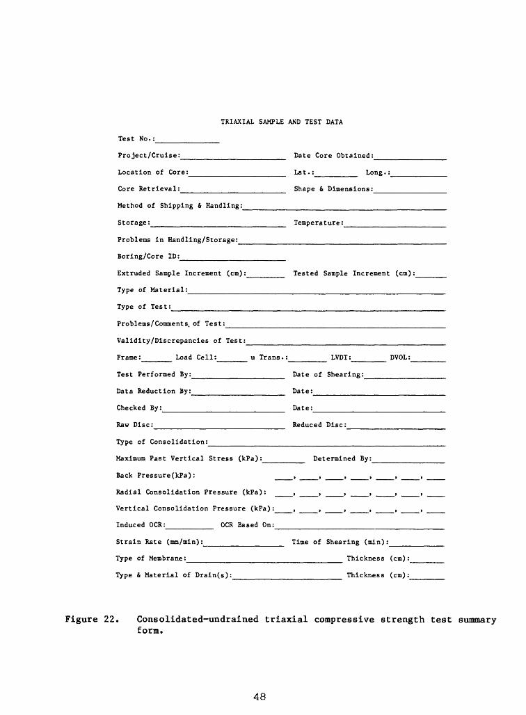
17. Perform required calculations and plot data as specified (Bishop and Henkel, 1962; Head, 1986). As a minimum, the following plots should be produced: (1) volume change during consolidation (cc) versus the square root or logarithm of time (minutes); (2) q ((0^ minus o^) divided by 2; kPa) versus p f ((a'j^ plus 0*3) divided by 2; kPa); (3) q (kPa) versus strain (percent); and (4) change in pore pressure (kPa) versus strain (percent). The results can be summarized on a form similar to Figure 22.
COMMENTS
The consolidated-undrained triaxial compressive strength with pore pressure measurement test is a valuable tool. In addition to determining static strength characteristics that could be used for total stress analyses such as waste package seabed penetration, the test can also be used to measure drained parameters that are useful for analyzing slower in situ shear mechanisms where sufficient time is available for complete pore-pressure dissipation.
Almost all deep-sea sediments can be tested using the procedures described above. However, particles that are greater than 1/6 the diameter of the test sample must not be present prior to testing. To insure that the best possible test results are obtained, the sediment should be sampled, handled, transported, and stored in a manner that will minimally disturb the samples (Booth, 1987).
Testing soft sediment presents special problems. Extreme care must be exercised in the handling and trimming of the samples. Friction in the top- cell piston bushing should be minimal or severe strength overestimations can result. Thin membranes, for example, prophylactics, should be used so that inordinate amounts of measured load won't be due to membrane stiffness.
Opinions vary on how to obtain strength measurements in certain circumstances. Some investigators would suggest consolidating to the in situ overburden stress; some wouldn't consolidate the sample at all; and others would first consolidate to stresses much higher than the in situ values, then, knowing the stress history, would back calculate what the undrained shear strength could be. A combination of all three test types is possible. More sophisticated tests, for example, anisotropically consolidated triaxial strength tests, can also be performed. Lee (1985) presents a summary of current methodologies used for performing triaxial testing on marine sediment.
When evaluating the strength characteristics of marine sediment, a laboratory that has had previous experience in determining and interpreting offshore strength characteristics should be consulted.
47
TRIAXIAL SAMPLE AND TEST DATA
Test No.:
Project/Cruise:
Location of Core:
Core Retrieval:
Date Core Obtained;
La t.:________ Long.:
Shape & Dimensions:___
Method of Shipping & Handling:
Storage:________________ Temperature:
Problems in Handling/Storage:
Boring/Core ID:_______________
Extruded Sample Increment (cm):
Type of Material:___________
Type of Test:______________
Tested Sample Increment (cm):
Problems/Comments, of Test:
Validity/Discrepancies of Test:__________
Frame:_______ Load Cell:______ u Trans.:
Test Performed By:_________________
Data Reduction By:_________________
Checked By:______________________
Raw Disc:__________________________
Type of Consolidation:______________
LVDT: DVOL:
Date of Shearing:
Date:_________
Date:
Reduced Disc:
Maximum Past Vertical Stress (kPa):__
Back Pressure(kPa):
Radial Consolidation Pressure (kPa):
Vertical Consolidation Pressure (kPa):
Induced OCR:__________ OCR Based On:
Strain Rate (mm/min):_____________
Type of Membrane:________________
Determined By:
Time of Shearing (mln):
Type & Material of Drain(s):
Thickness (cm):
Thickness (cm):
Figure 22. Consolidated-undrained triaxial compressive strength test summary form.
48

Test No:_
Height/Diameter; Trimmed:_______ ___ Tested:
Membrane Correction Applied: ______ Filter Drain Correction Applied:
Bulk Density Before Consolidation
Heights (cm); Initial: ________ Consolidation: ______ Final:
Water Content (%); Initial:_______ Consolidation:_______ Final:o
Volume (cnr); Initial:____ After Consolidation:
Area (cm2 ); Inital:______; Consol. Area (cnrj-A^Consol. volume*'Consol. Height
B Coefficients; Before Consolidation:________
After Consolidation:_______, ________
Before Shearing:___________
At Failure; q (kPa):____________ p 1 (kPa):_
A Coefficient:_______
Change in Pore Water Pressure (kPa):
Axial Strain (%):_________
Type of Failure:________________
$' (maximum) (degrees):__________ Su/p' - c/p':_
$' (at maximum q) (degrees):_______
4>' (at peak-max. obi.) (organics only) (degrees):__
Comments/Notes:
Figure 22 (cont). Consolidated-undrained triaxial compressive strength testsummary form.
49
QUALITY ASSURANCE
Methods for determining accuracy and precision have not been formulated for the CU triaxial test by ASTM. Lee and Clausner (1979) state that even when using special techniques to minimize disturbance, the best accuracy attainable is ±20 percent. Typically, accuracy is much worse.
COST ANALYSIS
Time required for each triaxial test (not including drying and cooling times): 2-4 days
Cost per triaxial test: $400.00
50
ACKNOWLEDGEMENT S
The author is grateful to the reviewers of this report, Rob Kayen, Ron Circe', and Elizabeth Winget, for their valuable comments and suggestions. Dann Blackwood is thanked for providing all of the photographs.
Funding for this report was provided under Interagency Agreement DW14931699-01 with the U.S. Environmental Protection Agency.
51
REFERENCES
American Society for Testing and Materials, 1987, 1987 Annual book of ASTMstandards, vol. 04.08: Soil and rock; building stones; geotextiles:Philadelphia, Pa, 1189 p.
Bennett, R. H., Keller, G. H., and Busby, R. F., 1970, Mass propertyvariability in three closely spaced deep-sea sediment cores: Journal ofSedimentary Petrology, v. 40, n. 3, p. 1038-1043.
Booth, J.S., 1987, Sampling and shipboard recommendations, chapter 2: inBooth, J.S., ed., Methods manual for sediment monitoring at deep-oceanlow-level radioactive waste disposal sites: U.S. Geological Surveyadministrative report to the U.S. Environmental Protection Agency underinteragency agreement DW14931699-01, Woods Hole, Mass., p. 13-23.
Booth, J.S., and Dahl, A.G., 1986, A note on the relationships between organicmatter and some geotechnical properties of a marine sediment: MarineGeotechnology, v. 6, n. 3, p. 281-297.
Bowles, J.E., 1979, Physical and geotechnical properties of soils: New York,McGraw-Hill 478 p.
British Standards Institution, 1975, Standard test for liquid limit-conepenetrometer method: London, England.
Dept. of the Army, 1980, Laboratory soils testing: Washington, B.C., EngineerManual EM 1110-2-1906, 388 p.
Head, K.H., 1986, Manual of soil laboratory testing, volume 3: effectivestress tests: New York, Wiley, p. 743-1238.
Head, K. H., 1980, Manual of soil laboratory testing, volume 1: soilclassification and compaction tests: London, Pentech Press, 339 p.
Hunt, R. E., 1984, Geotechnical engineering investigation manual: New York,McGraw Hill, 983 p.
Lambe, T. W., 1951, Soil testing for engineers: New York, John Wiley, 165 p. Lambe, T. W., and Whitman, R. V., 1969, Soil mechanics: New York, John Wiley,
553 p. Lee, H.J., and Clausner, J.E., 1979, Seafloor soil sampling and geotechnical
parameter determination - handbook: U.S. Naval Civil EngineeringLaboratory Technical Report R873: Port Hueneme, Cal., 128 p.
Lee, H.J., 1985, State of the art: laboratory determination of the strengthof marine soils, _in_ Chaney, R.C., and Demars, K.R., eds., Strength testingof marine sediments: laboratory and in-situ measurements: Philadelphia,Pa, American Society for Testing and Materials Special TechnicalPublication 883, p. 181-250.
Liu, Cheng, and Evett, J.B., 1984, Soil properties tesing, measurement, andevaluation: Englewood Cliffs, N.J., Prentice-Hall, 315 p.
Noorany, I., 1985, Laboratory soil properties, in Rocker, Karl, Jr., ed.,Handbook for marine geotechnical engineering: Port Hueneme, CA, NavalCivil Engineering Laboratory, 19 p.
Peck, R. B., Hanson, W. E., and Thornburn, T. H., 1974, Foundationengineering: New York, John Wiley, 514 p.
Wasti, Y. and Bezirici, M. H., 1986, Determination of the consistency limitsof soils by the fall cone test: Canadian Geotechnical Journal, v. 23,n. 2, p. 241-246.
Winters, W.J., 1987, Guidelines for handling, storing, and preparing softmarine sediment for geotechnical testing: U.S. Geological Survey Open- File Report 87-278, 11 p.
52