Embed Size (px)
Citation preview
KalpaTechnology for change
Excel Basic
Contents1. Getting Started............................................................................................................................................2
1.1 Starting Excel..................................................................................................................................21.2 Spreadsheet terminology...............................................................................................................31.3 Getting help.....................................................................................................................................31.4 Navigating workbooks....................................................................................................................3
2. Entering and editing data...........................................................................................................................42.1 Entering and editing text and values............................................................................................42.2 Entering and editing formulas.......................................................................................................52.3 Working with pictures.....................................................................................................................52.4 Saving and updating workbooks...................................................................................................6
3. Modifying worksheets.................................................................................................................................73.1 Moving and copying Data..............................................................................................................73.2 Absolute and Relative References.............................................................................................10
4. Using Function..........................................................................................................................................114.1 The Parts of a Function:..............................................................................................................114.2 To Calculate the Sum of a Range of Data Using AutoSum:...................................................114.3 To Access Other Functions in Excel:.........................................................................................12
5. Formatting worksheets.............................................................................................................................135.1 Formatting Texts...........................................................................................................................135.2 Formatting rows and columns.....................................................................................................145.3 Formatting Numbers....................................................................................................................145.4 Conditional Formatting.................................................................................................................155.5 Table formats................................................................................................................................16
6. Printing.......................................................................................................................................................196.1 To View the Spreadsheet in Print Preview:...............................................................................196.2 To Use the Print Titles command:..............................................................................................196.3 Print worksheet:............................................................................................................................20
7. Working with Charts..................................................................................................................................207.1 Identifying the Parts of a Chart...................................................................................................207.2 Creating a Chart...........................................................................................................................207.3 To Move the Chart to a Different Worksheet:...........................................................................21
8. Managing Large Workbooks....................................................................................................................228.1 Splitting and Freezing Panes......................................................................................................228.2 How to Move or Copy Excel 2007 Worksheets to Other Workbooks....................................238.3 Arranging Windows in Excel 2007 Workbooks.........................................................................248.4 How to Protect an Excel 2007 Workbook..................................................................................26
Web site: www.kalpa.org.np email: [email protected] (01-6923341) 1
KalpaTechnology for change
1. Getting StartedExcel is a spreadsheet program that is offered by Microsoft as a part of their Office Suite. A spreadsheet is a tool that helps you organize, analyze and evaluate data. Here are some examples of Excel being used in our day to day work:
Create Budget reports, survey results and all financial transactions that most of you use it for. Creating charts for better representation. Organize data in lists. Automate complex tasks. Add your own examples to the list!!
1.1 Starting ExcelExcel 2007 offers a wide range of customizable options that allow you to make Word work the best for you. To access these customizable options: Click the Office Button Click Excel Options
Popular These features allow you to personalize your work environment with language, color schemes, user name and allow you to access the Live Preview feature. The Live Preview feature allows you to preview the results of applying design and formatting changes without actually applying it.Display This feature allows you to modify how the document content is displayed on the screen and when printed. You can opt to show or hide certain page elements. Proofing This feature allows you personalize how word corrects and formats your text. You can customize auto correction settings and have word ignore certain words or errors in a document.Save This feature allows you personalize how your document is saved. You can specify how often you want auto save to run and where you want the documents saved.Advanced This feature allows you to specify options for editing, copying, pasting, displaying, printing and saving.Customize allows you to add features to the Quick Access Toolbar. If there are tools that you are utilizing frequently, you may want to add these to the Quick Access Toolbar.
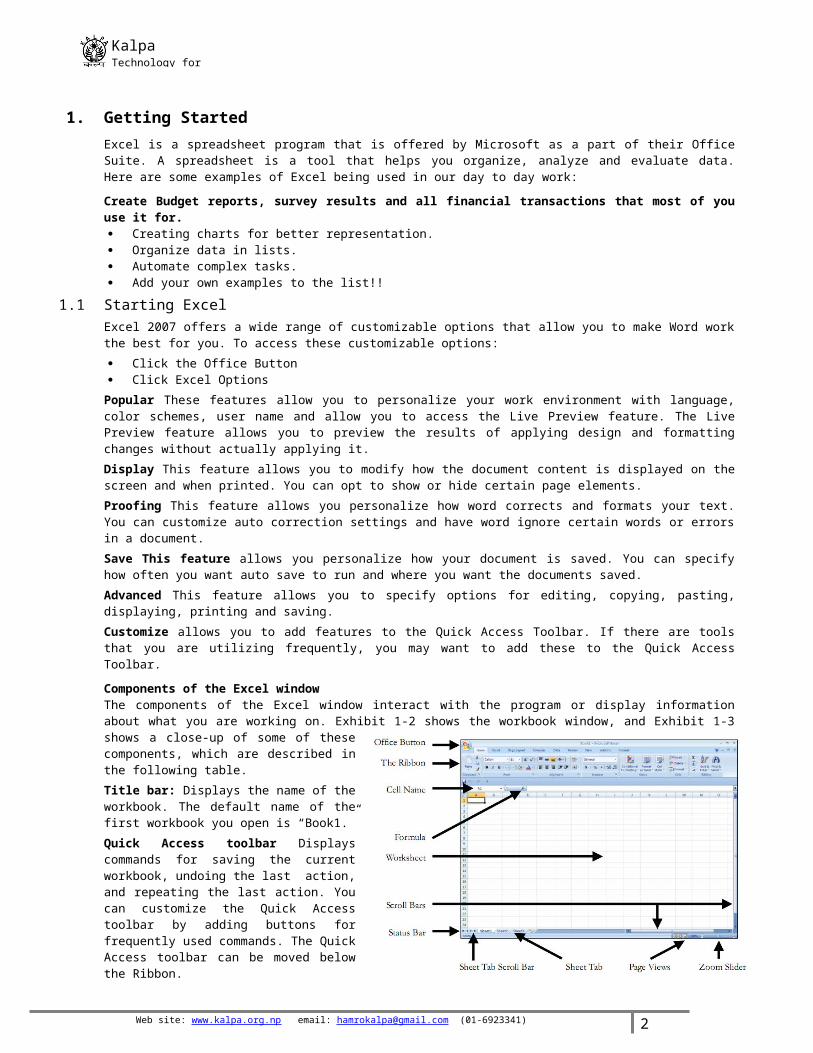
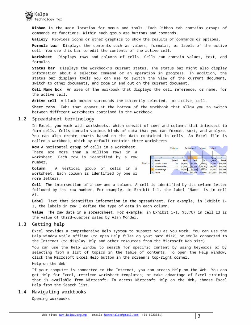
Components of the Excel window The components of the Excel window interact with the program or display information about what you are working on. Exhibit 1-2 shows the workbook window, and Exhibit 1-3 shows a close-up of some of these components, which are described in the following table. Title bar: Displays the name of the workbook. The default name of the first workbook you open is “Book1.” Quick Access toolbar Displays commands for saving the current workbook, undoing the last action, and repeating the last action. You can customize the Quick Access toolbar by adding buttons for frequently used commands. The Quick Access toolbar can be moved below the Ribbon. Ribbon Is the main location for menus and tools. Each Ribbon tab contains groups of commands or functions. Within each group are buttons and commands. Gallery Provides icons or other graphics to show the results of commands or options. Formula bar Displays the contents—such as values, formulas, or labels—of the active cell. You use this bar to edit the contents of the active cell. Worksheet Displays rows and columns of cells. Cells can contain values, text, and formulas. Status bar Displays the workbook’s current status. The status bar might also display information about a selected command or an operation in progress. In addition, the status bar displays tools you can use to switch the view of the current document, switch to other documents, and zoom in and out on the current document. Cell Name box An area of the workbook that displays the cell reference, or name, for the active cell. Active cell A black border surrounds the currently selected, or active, cell. Sheet tabs Tabs that appear at the bottom of the workbook that allow you to switch between different worksheets contained in the workbook
Web site: www.kalpa.org.np email: [email protected] (01-6923341) 2
KalpaTechnology for change
1.2 Spreadsheet terminologyIn Excel, you work with worksheets, which consist of rows and columns that intersect to form cells. Cells contain various kinds of data that you can format, sort, and analyze. You can also create charts based on the data contained in cells. An Excel file is called a workbook, which by default contains three worksheetsRow A horizontal group of cells in a worksheet. There are more than a million rows in a worksheet. Each row is identified by a row number. Column A vertical group of cells in a worksheet. Each column is identified by one or more letters. Cell The intersection of a row and a column. A cell is identified by its column letter followed by its row number. For example, in Exhibit 1-1, the label “Name” is in cell A1. Label Text that identifies information in the spreadsheet. For example, in Exhibit 1-1, the labels in row 1 define the type of data in each column. Value The raw data in a spreadsheet. For example, in Exhibit 1-1, $5,767 in cell E3 is the value of third-quarter sales by Alan Monder.
1.3 Getting helpExcel provides a comprehensive Help system to support you as you work. You can use the Help window while offline (to open Help files on your hard disk) or while connected to the Internet (to display Help and other resources from the Microsoft Web site).You can use the Help window to search for specific content by using keywords or by selecting from a list of topics in the table of contents. To open the Help window, click the Microsoft Excel Help button in the screen’s top-right corner. Help on the Web If your computer is connected to the Internet, you can access Help on the Web. You can get Help for Excel, retrieve worksheet templates, or take advantage of Excel training that is available from Microsoft. To access Microsoft Help on the Web, choose Excel Help from the Search list.
1.4 Navigating workbooksOpening workbooks Explanation To begin working in an Excel workbook, you first need to open it. You can use the Office Button to open workbooks.
To open a workbook: Click the Office Button and choose Open to display the Open dialog box. Use the Look in list to specify the folder containing the workbook you want to use. Select the workbook and click Open (or double-click the workbook name).
Moving around in worksheets At any given time, one cell in the worksheet is the active cell. The active cell is where the data you enter will appear. The address of the active cell appears in the Name box, which is to the left of the formula bar. There are several techniques for moving around in a worksheet. Some navigation techniques make a different cell active, while others move only your view of the worksheet, without activating a different cell.
The following table summarizes various worksheet navigation techniques: Click a cell Makes the cell active. Press arrow key Selects an adjacent cell, making it active. Press Tab Select the cell one column to the right. Press Shift+Tab Selects the cell one column to the left. Press Ctrl+Home Selects cell A1. Press Ctrl+End Selects the cell at the intersection of the last row and last column of data in a worksheet. Click the scroll arrow Moves the view of the worksheet one row or column. This technique does not change
the active cell. Click in the scrollbar Moves the view of the worksheet one screen up, down, left, or right, depending on which
side of the scroll box you click (and in which scrollbar). This technique does not change the active cell.
Drag the scroll box Moves the view of the worksheet quickly without changing the active cell.Press Ctrl+G Opens a dialog box where you can enter the address for a cell you want to move to. Drag the slider on the zoom bar Zooms in or out on the current document. The zoom bar is located on the
status bar, near the bottom-right corner of the window.
Web site: www.kalpa.org.np email: [email protected] (01-6923341) 3
KalpaTechnology for change
2. Entering and editing data 2.1 Entering and editing text and values
After you create a workbook, you can begin entering data in cells. Cell entries can include many types of data, including text and values. When you type, data is entered in the active cell.
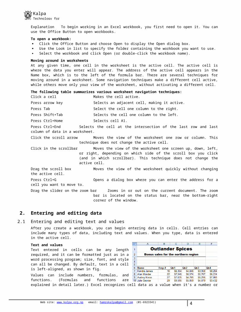
Text and values Text entered in cells can be any length required, and it can be formatted just as in a word processing program; size, font, and style can all be changed. By default, text in a cell is left-aligned, as shown in fig. Values can include numbers, formulas, and functions. (Formulas and functions are explained in detail later.) Excel recognizes cell data as a value when it’s a number or when it begins with +, -, =, @, #, or $. By default, a value in a cell is right-aligned.
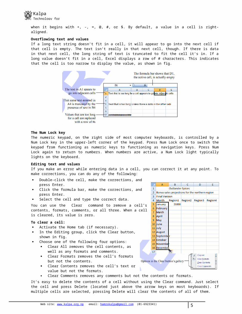
Overflowing text and values If a long text string doesn’t fit in a cell, it will appear to go into the next cell if that cell is empty. The text isn’t really in that next cell, though. If there is data in that next cell, the long string of text is truncated to fit the cell it’s in. If a long value doesn’t fit in a cell, Excel displays a row of # characters. This indicates that the cell is too narrow to display the value, as shown in fig.
The Num Lock key The numeric keypad, on the right side of most computer keyboards, is controlled by a Num Lock key in the upper-left corner of the keypad. Press Num Lock once to switch the keypad from functioning as numeric keys to functioning as navigation keys. Press Num Lock again to return to numbers. When numbers are active, a Num Lock light typically lights on the keyboard.
Editing text and values If you make an error while entering data in a cell, you can correct it at any point. To make corrections, you can do any of the following: Double-click the cell, make the corrections, and press Enter. Click the formula bar, make the corrections, and press Enter. Select the cell and type the correct data.
You can use the Clear command to remove a cell’s contents, formats, comments, or all three. When a cell is cleared, its value is zero.
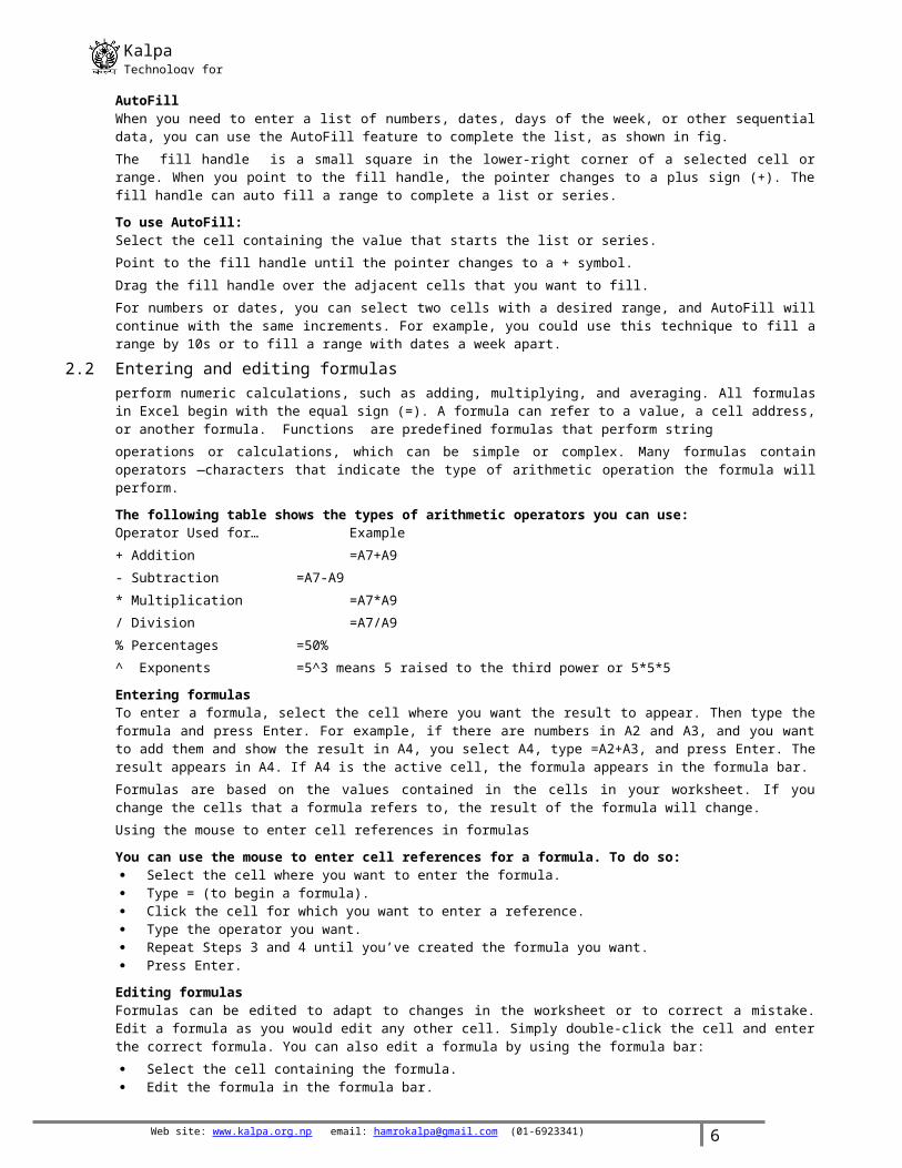
To clear a cell: Activate the Home tab (if necessary). In the Editing group, click the Clear button, shown in fig. Choose one of the following four options:
Clear All removes the cell contents, as well as any formats and comments.
Clear Formats removes the cell’s formats but not the contents.
Clear Contents removes the cell’s text or value but not the formats.
Clear Comments removes any comments but not the contents or formats.
Web site: www.kalpa.org.np email: [email protected] (01-6923341) 4
KalpaTechnology for change
It’s easy to delete the contents of a cell without using the Clear command. Just select the cell and press Delete (located just above the arrow keys on most keyboards). If multiple cells are selected, pressing Delete will clear the contents of all of them.
AutoFillWhen you need to enter a list of numbers, dates, days of the week, or other sequential data, you can use the AutoFill feature to complete the list, as shown in fig. The fill handle is a small square in the lower-right corner of a selected cell or range. When you point to the fill handle, the pointer changes to a plus sign (+). The fill handle can auto fill a range to complete a list or series.
To use AutoFill: Select the cell containing the value that starts the list or series. Point to the fill handle until the pointer changes to a + symbol. Drag the fill handle over the adjacent cells that you want to fill. For numbers or dates, you can select two cells with a desired range, and AutoFill will continue with the same increments. For example, you could use this technique to fill a range by 10s or to fill a range with dates a week apart.
2.2 Entering and editing formulasperform numeric calculations, such as adding, multiplying, and averaging. All formulas in Excel begin with the equal sign (=). A formula can refer to a value, a cell address, or another formula. Functions are predefined formulas that perform string operations or calculations, which can be simple or complex. Many formulas contain operators —characters that indicate the type of arithmetic operation the formula will perform.
The following table shows the types of arithmetic operators you can use: Operator Used for… Example + Addition =A7+A9 - Subtraction =A7-A9 * Multiplication =A7*A9 / Division =A7/A9 % Percentages =50% ^ Exponents =5^3 means 5 raised to the third power or 5*5*5
Entering formulas To enter a formula, select the cell where you want the result to appear. Then type the formula and press Enter. For example, if there are numbers in A2 and A3, and you want to add them and show the result in A4, you select A4, type =A2+A3, and press Enter. The result appears in A4. If A4 is the active cell, the formula appears in the formula bar. Formulas are based on the values contained in the cells in your worksheet. If you change the cells that a formula refers to, the result of the formula will change. Using the mouse to enter cell references in formulas
You can use the mouse to enter cell references for a formula. To do so: Select the cell where you want to enter the formula. Type = (to begin a formula). Click the cell for which you want to enter a reference. Type the operator you want. Repeat Steps 3 and 4 until you’ve created the formula you want. Press Enter.
Editing formulas Formulas can be edited to adapt to changes in the worksheet or to correct a mistake. Edit a formula as you would edit any other cell. Simply double-click the cell and enter the correct formula. You can also edit a formula by using the formula bar: Select the cell containing the formula. Edit the formula in the formula bar. Press Enter.
2.3 Working with pictures You can insert pictures and other graphics files to illustrate and enhance worksheets and printed reports, as shown in. Excel supports dozens of industry-standard picture file formats, including .bmp, .jpg, .eps, and .tif.
To place a picture in a worksheet: Activate the Insert tab. In the Illustrations group, click the Insert Picture From File button. The Insert Picture dialog box appears.
Web site: www.kalpa.org.np email: [email protected] (01-6923341) 5
KalpaTechnology for change
Navigate to the picture’s location, select the file, and click Insert. The picture appears in the worksheet, and the Picture Tools tab is activated.
Use the tools on the Picture Tools tab to modify the picture as necessary.
Moving pictures When you insert a picture into a worksheet, Excel places it in the approximate middle of your screen. You can move a picture so that it appears and prints in a specific place in a worksheet. To move a picture: Point anywhere within the picture. The pointer changes to a four-headed arrow. Drag the picture. As you drag, the picture remains stationary, but a shadow of it moves with the pointer. Position the outline box where you want the picture to be. Release the mouse button. The picture moves to the location of the outline box.
Resizing pictures There are several ways to resize a picture: Select the picture; this activates the Picture Tools tab. In the Size group, enter new values in the Height and
Width boxes. In the Size group, click the Dialog Box Launcher button (in the lower-right corner of the group). The Size and
Properties dialog box appears with the Size tab activated. Under Size and Rotate, or under Scale, resize the picture.
Point to one of the sizing handles at the corners of the picture frame. The pointer changes to a double-headed arrow. Drag a sizing handle to resize the picture.
To resize a picture proportionally, click and hold Shift before dragging the sizing handles. This forces the picture’s height and width to resize at the same rate.
2.4 Saving and updating workbooks Saving a workbook stores your data for future use. Every time you change anything in a worksheet, you’ll need to save the worksheet (update it) if you want to keep your changes.
Saving a file for the first time The first time you save a workbook, you need to assign a file name and location for the file. You must also choose a file format. Some typical file formats include: Format Extension Description Microsoft Excel Workbook .xlsx This is the default workbook format for Excel 2007. XML Data .xml The XML format is useful for data that must be transferred between
applications. Text .txt Files saved in plain text format can be opened by any word
processor or text editor. Comma Separated Values .csv Data fields in a CSV file are delimited by commas. Excel 97 - Excel 2003 .xls This is the workbook format that can be opened by earlier versions of
Excel. Web Page .html This format enables the workbook to be published as a Web page.
To save a workbook for the first time: Click the Office Button and choose Save, or click the Save button on the Quick Access toolbar. The Save As
dialog box opens because this file does not yet have a file name. From the Save in list, select the drive and folder where you want to save the workbook. In the File name box, enter a name for the workbook. From the Save as type list, select the file format in which you want to save the workbook. Click Save. Creating folders If you don’t want to save your workbook in an existing folder, use the Save As dialog box to create a new folder.
Here’s how: From the Save in list, select the location where you want to create the folder. In the Save As dialog box, click the Create New Folder button to open the New Folder dialog box. In the Name box of the New Folder dialog box, type a name for the folder. Click OK. The new folder appears in the Save in list.
Web site: www.kalpa.org.np email: [email protected] (01-6923341) 6
KalpaTechnology for change
3. Modifying worksheets3.1 Moving and copying Data
It is important to know how to move information from one cell to another in Excel. Learning the various ways will save you time and make working with Excel easier. Certain methods are more appropriate depending on how much information you need to move and where it will reside on the spreadsheet. In this lesson you will learn how to cut, copy, and paste, as well as drag and drop information.
To Copy and Paste Cell Contents: Select the cell or cells you wish to copy. Click the Copy command in the Clipboard group on the Home tab or Ctlr + C. The border of the selected cells will
change appearance. Select the cell or cells where you want to paste the information. Click the Paste command or Ctlr + V. The copied information will now appear in the new cells. To select more than one adjoining cell, left-click one of the cells, drag the cursor until all the cells are selected,
and release the mouse button. The copied cell will stay selected until you perform your next task, or you can double-click the cell to deselect it.
To Cut and Paste Cell Contents: Select the cell or cells you wish to cut. Click the Cut command in the Clipboard group on the Home tab or Ctlr + X. The border of the selected cells will
change appearance. Select the cell or cells where you want to paste the information. Click the Paste command or Ctlr + V. The cut information will be removed from the original cells and now
appear in the new cells. The keyboard shortcut for Paste is the Control Key and the V key.
To Drag and Drop Information: Select the cell or cells you wish to move. Position your mouse pointer near one of the outside edges of the selected cells. The mouse pointer changes from
a large, white cross to a black cross with 4 arrows. Left-click and hold the mouse button and drag the cells to the new location. Release the mouse button and the information appears in the new location.
To Use the Fill Handle to Fill Cells: Position your cursor over the fill handle until the large white cross becomes a thin, black cross. Left-click your mouse and drag it until all the cells you want to fill are highlighted. Release the mouse button and all the selected cells are filled with the information from the original cell.
The fill handle doesn't always copy information from one cell directly into another cell. Depending on the data entered in the cell, it may fill the data in other ways. For example, if I have the formula =A1+B1 in cell C1, and I use the fill handle to fill the formula into cell C2, the formula doesn't appear the same in C2 as it does in C1. Instead of =A1+B1, you will see =A2+B2.You can use the fill handle to fill cells horizontally or vertically.
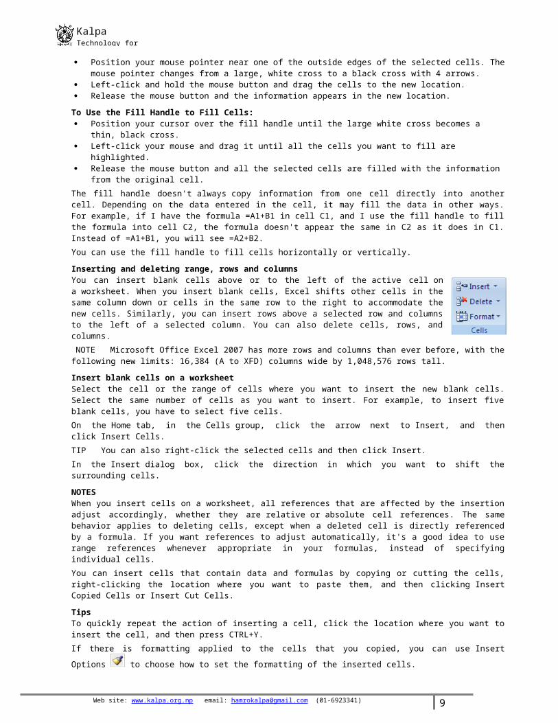
Inserting and deleting range, rows and columnsYou can insert blank cells above or to the left of the active cell on a worksheet. When you insert blank cells, Excel shifts other cells in the same column down or cells in the same row to the right to accommodate the new cells. Similarly, you can insert rows above a selected row and columns to the left of a selected column. You can also delete cells, rows, and columns. NOTE Microsoft Office Excel 2007 has more rows and columns than ever before, with the following new limits: 16,384 (A to XFD) columns wide by 1,048,576 rows tall.
Insert blank cells on a worksheetSelect the cell or the range of cells where you want to insert the new blank cells. Select the same number of cells as you want to insert. For example, to insert five blank cells, you have to select five cells.On the Home tab, in the Cells group, click the arrow next to Insert, and then click Insert Cells.TIP You can also right-click the selected cells and then click Insert.In the Insert dialog box, click the direction in which you want to shift the surrounding cells.
NOTES When you insert cells on a worksheet, all references that are affected by the insertion adjust accordingly, whether they are relative or absolute cell references. The same behavior applies to deleting cells, except when a deleted cell is directly referenced by a formula. If you want references to adjust automatically, it's a good idea to use range references whenever appropriate in your formulas, instead of specifying individual cells.You can insert cells that contain data and formulas by copying or cutting the cells, right-clicking the location where you want to paste them, and then clicking Insert Copied Cells or Insert Cut Cells.
Web site: www.kalpa.org.np email: [email protected] (01-6923341) 7
KalpaTechnology for change
Tips To quickly repeat the action of inserting a cell, click the location where you want to insert the cell, and then press CTRL+Y.
If there is formatting applied to the cells that you copied, you can use Insert Options to choose how to set the formatting of the inserted cells.
Insert rows on a worksheetDo one of the following: To insert a single row, select either the whole row or a cell in the row above which you want to
insert the new row. For example, to insert a new row above row 5, click a cell in row 5. To insert multiple rows, select the rows above which you want to insert rows. Select the same
number of rows as you want to insert. For example, to insert three new rows, you select three rows.
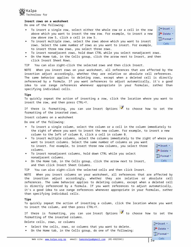
To insert nonadjacent rows, hold down CTRL while you select nonadjacent rows. On the Home tab, in the Cells group, click the arrow next to Insert, and then click Insert Sheet Rows.
TIP You can also right-click the selected rows and then click Insert.NOTE When you insert rows on your worksheet, all references that are affected by the insertion adjust accordingly, whether they are relative or absolute cell references. The same behavior applies to deleting rows, except when a deleted cell is directly referenced by a formula. If you want references to adjust automatically, it's a good idea to use range references whenever appropriate in your formulas, rather than specifying individual cells.
Tips To quickly repeat the action of inserting a row, click the location where you want to insert the row, and then press CTRL+Y.
If there is formatting, you can use Insert Options to choose how to set the formatting of the inserted rows.Insert columns on a worksheetDo one of the following: To insert a single column, select the column or a cell in the column immediately to the right of where you want to
insert the new column. For example, to insert a new column to the left of column B, click a cell in column B. To insert multiple columns, select the columns immediately to the right of where you want to insert columns.
Select the same number of columns as you want to insert. For example, to insert three new columns, you select three columns.
To insert nonadjacent columns, hold down CTRL while you select nonadjacent columns. On the Home tab, in the Cells group, click the arrow next to Insert, and then click Insert Sheet
Columns.TIP You can also right-click the selected cells and then click Insert.NOTE When you insert columns on your worksheet, all references that are affected by the insertion adjust accordingly, whether they are relative or absolute cell references. The same behavior applies to deleting columns, except when a deleted cell is directly referenced by a formula. If you want references to adjust automatically, it's a good idea to use range references whenever appropriate in your formulas, rather than specifying individual cells.
Tips To quickly repeat the action of inserting a column, click the location where you want to insert the column, and then press CTRL+Y.
If there is formatting, you can use Insert Options to choose how to set the formatting of the inserted columns.Delete cells, rows, or columns Select the cells, rows, or columns that you want to delete. On the Home tab, in the Cells group, do one of the following: To delete selected cells, click the arrow next to Delete, and then click Delete Cells. To delete selected rows, click the arrow next to Delete, and then click Delete Sheet Rows. To delete selected columns, click the arrow next to Delete, and then click Delete Sheet
Columns.TIP You can right-click a selection of cells, click Delete, and then click the option that you want. You can also right-click a selection of rows or columns and then click Delete.If you are deleting a cell or a range of cells, in the Delete dialog box, click Shift cells left, Shift cells up, Entire row, or Entire column.If you are deleting rows or columns, other rows or columns automatically shift up or to the left.
Tips To quickly repeat deleting cells, rows, or columns, select the next cells, rows, or columns, and then press CTRL+Y.
Web site: www.kalpa.org.np email: [email protected] (01-6923341) 8
KalpaTechnology for change
If needed, you can restore deleted data immediately after you delete it. On the Quick Access Toolbar, clickUndo Delete, or press CTRL+Z.
NOTES Pressing DELETE deletes the contents of the selected cells only, not the cells themselves.Excel keeps formulas up to date by adjusting references to the shifted cells to reflect their new locations. However, a formula that refers to a deleted cell displays the #REF! error value.
Modifying Columns, Rows, & CellsWhen you open a new, blank workbook, the cells, columns, and rows are set to a default size. You do have the ability to change the size of each, and to insert new columns, rows, and cells, as needed. In this lesson, you will learn various methods to modify the column width and row height, in addition to how to insert new columns, rows, and cells.
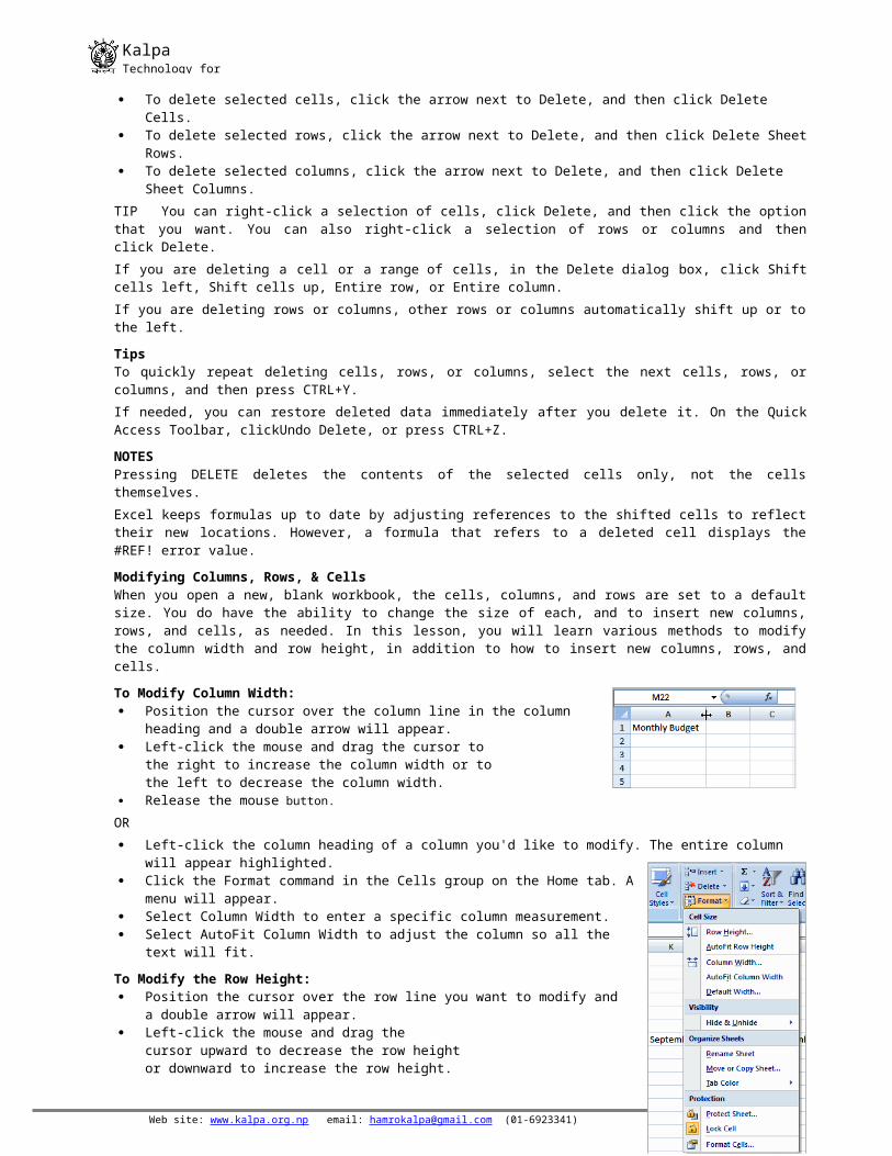
To Modify Column Width: Position the cursor over the column line in the column heading and a double
arrow will appear. Left-click the mouse and drag the cursor to the right to increase the column
width or to the left to decrease the column width. Release the mouse button.
OR Left-click the column heading of a column you'd like to modify. The entire column will appear highlighted. Click the Format command in the Cells group on the Home tab. A menu will appear. Select Column Width to enter a specific column measurement. Select AutoFit Column Width to adjust the column so all the text will fit.
To Modify the Row Height: Position the cursor over the row line you want to modify and a double arrow will
appear. Left-click the mouse and drag the cursor upward to decrease the row height
or downward to increase the row height. Release the mouse button.
OR Click the Format command in the Cells group on the Home tab. A menu will appear. Select Row Height to enter a specific row measurement. Select AutoFit Row Height to adjust the row so all the text will fit.
To Insert Rows: Select the row below where you want the new row to appear. Click the Insert command in the Cells group on the Home tab. The row will appear.
The new row always appears above the selected row.Make sure that you select the entire row below where you want the new row to appear and not just the cell. If you select just the cell and then click Insert, only a new cell will appear.
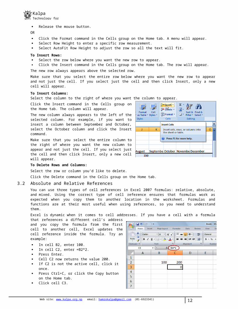
To Insert Columns:Select the column to the right of where you want the column to appear.Click the Insert command in the Cells group on the Home tab. The column will appear.The new column always appears to the left of the selected column. For example, if you want to insert a column between September and October, select the October column and click the Insert command.Make sure that you select the entire column to the right of where you want the new column to appear and not just the cell. If you select just the cell and then click Insert, only a new cell will appear.To Delete Rows and Columns:Select the row or column you’d like to delete.Click the Delete command in the Cells group on the Home tab.
3.2 Absolute and Relative ReferencesYou can use three types of cell references in Excel 2007 formulas: relative, absolute, and mixed. Using the correct type of cell reference ensures that formulas work as expected when you copy them to another location in the worksheet. Formulas and functions are at their most useful when using references, so you need to understand them.
Web site: www.kalpa.org.np email: [email protected] (01-6923341) 9
KalpaTechnology for change
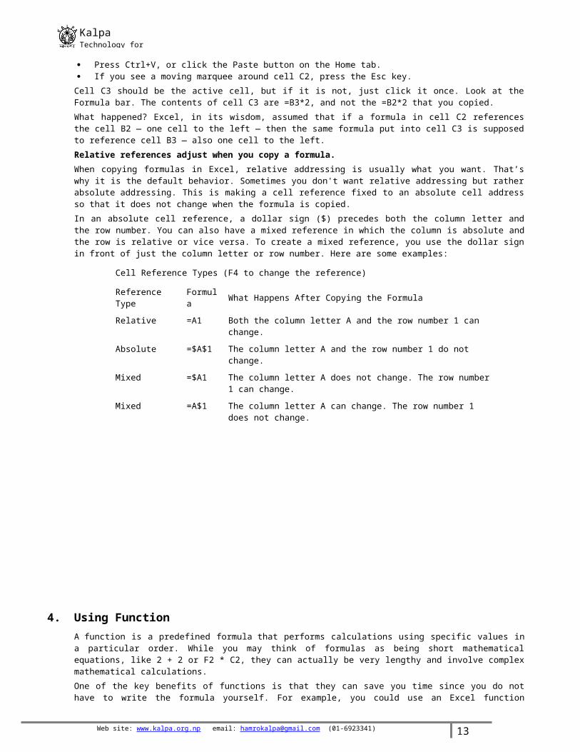
Excel is dynamic when it comes to cell addresses. If you have a cell with a formula that references a different cell’s address and you copy the formula from the first cell to another cell, Excel updates the cell reference inside the formula. Try an example: In cell B2, enter 100. In cell C2, enter =B2*2. Press Enter. Cell C2 now returns the value 200. If C2 is not the active cell, click it once. Press Ctrl+C, or click the Copy button on the Home
tab. Click cell C3. Press Ctrl+V, or click the Paste button on the Home
tab. If you see a moving marquee around cell C2, press
the Esc key.Cell C3 should be the active cell, but if it is not, just click it once. Look at the Formula bar. The contents of cell C3 are =B3*2, and not the =B2*2 that you copied.What happened? Excel, in its wisdom, assumed that if a formula in cell C2 references the cell B2 — one cell to the left — then the same formula put into cell C3 is supposed to reference cell B3 — also one cell to the left.Relative references adjust when you copy a formula.When copying formulas in Excel, relative addressing is usually what you want. That’s why it is the default behavior. Sometimes you don't want relative addressing but rather absolute addressing. This is making a cell reference fixed to an absolute cell address so that it does not change when the formula is copied.In an absolute cell reference, a dollar sign ($) precedes both the column letter and the row number. You can also have a mixed reference in which the column is absolute and the row is relative or vice versa. To create a mixed reference, you use the dollar sign in front of just the column letter or row number. Here are some examples:
Cell Reference Types (F4 to change the reference)
Reference Type Formula What Happens After Copying the Formula
Relative =A1 Both the column letter A and the row number 1 can change.
Absolute =$A$1 The column letter A and the row number 1 do not change.
Mixed =$A1 The column letter A does not change. The row number 1 can change.
Mixed =A$1 The column letter A can change. The row number 1 does not change.
4. Using FunctionA function is a predefined formula that performs calculations using specific values in a particular order. While you may think of formulas as being short mathematical equations, like 2 + 2 or F2 * C2, they can actually be very lengthy and involve complex mathematical calculations.
Web site: www.kalpa.org.np email: [email protected] (01-6923341) 10
KalpaTechnology for change
One of the key benefits of functions is that they can save you time since you do not have to write the formula yourself. For example, you could use an Excel function called Average to quickly find the average of a range of numbers or the Sum function to find the sum of a cell range.In this lesson, you will learn how to use basic functions such as SUM and AVG, use functions with more than one argument, and how to access the other Excel 2007 functions.
4.1 The Parts of a Function:Each function has a specific order, called syntax, which must be strictly followed for the function to work correctly.Syntax Order: All functions begin with the = sign. After the = sign define the function name (e.g., Sum). Then there will be an argument. An argument is the cell
range or cell references that are enclosed by parentheses. If there is more than one argument, separate each by a comma.
An example of a function with one argument that adds a range of cells, A3 through A9:An example of a function with more than one argument that calculates the sum of two cell ranges:Excel literally has hundreds of different functions to assist with your calculations. Building formulas can be difficult and time-consuming. Excel's functions can save you a lot of time and headaches.Excel's Different FunctionsThere are many different functions in Excel 2007. Some of the more common functions include:Statistical Functions: SUM - summation adds a range of cells together. AVERAGE - average calculates the average of a range of cells. COUNT - counts the number of chosen data in a range of cells. MAX - identifies the largest number in a range of cells. MIN - identifies the smallest number in a range of cells.
Financial Functions: Interest Rates Loan Payments Depreciation Amounts
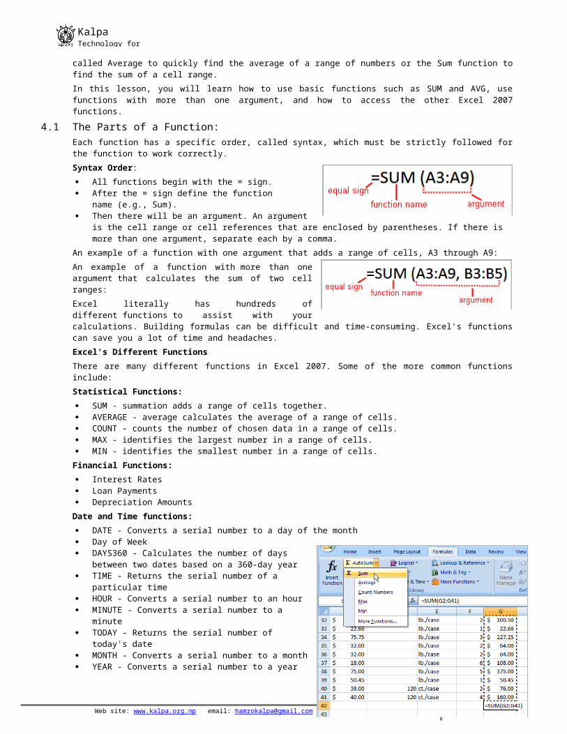
Date and Time functions: DATE - Converts a serial number to a day of the month Day of Week DAYS360 - Calculates the number of days between two
dates based on a 360-day year TIME - Returns the serial number of a particular time HOUR - Converts a serial number to an hour MINUTE - Converts a serial number to a minute TODAY - Returns the serial number of today's date MONTH - Converts a serial number to a month YEAR - Converts a serial number to a year
You don't have to memorize the functions but should have an idea of what each can do for you.
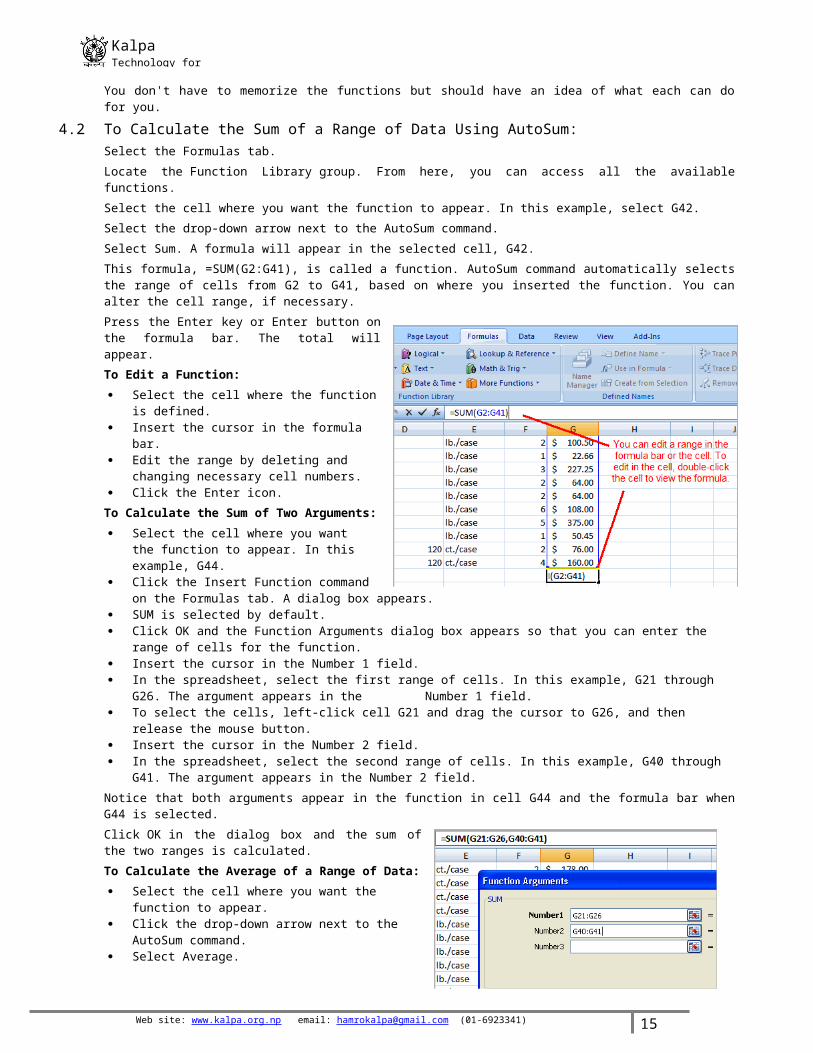
4.2 To Calculate the Sum of a Range of Data Using AutoSum:Select the Formulas tab.Locate the Function Library group. From here, you can access all the available functions.Select the cell where you want the function to appear. In this example, select G42.Select the drop-down arrow next to the AutoSum command.Select Sum. A formula will appear in the selected cell, G42.This formula, =SUM(G2:G41), is called a function. AutoSum command automatically selects the range of cells from G2 to G41, based on where you inserted the function. You can alter the cell range, if necessary.
Web site: www.kalpa.org.np email: [email protected] (01-6923341) 11
KalpaTechnology for change
Press the Enter key or Enter button on the formula bar. The total will appear. To Edit a Function: Select the cell where the function is defined. Insert the cursor in the formula bar. Edit the range by deleting and changing
necessary cell numbers. Click the Enter icon.
To Calculate the Sum of Two Arguments: Select the cell where you want the function to
appear. In this example, G44. Click the Insert Function command on the
Formulas tab. A dialog box appears. SUM is selected by default. Click OK and the Function Arguments dialog
box appears so that you can enter the range of cells for the function.
Insert the cursor in the Number 1 field. In the spreadsheet, select the first range of
cells. In this example, G21 through G26. The argument appears in the Number 1 field. To select the cells, left-click cell G21 and drag the cursor to G26, and then release the mouse button. Insert the cursor in the Number 2 field. In the spreadsheet, select the second range of cells. In this example, G40 through G41. The argument appears in
the Number 2 field.Notice that both arguments appear in the function in cell G44 and the formula bar when G44 is selected.Click OK in the dialog box and the sum of the two ranges is calculated.To Calculate the Average of a Range of Data: Select the cell where you want the function to appear. Click the drop-down arrow next to the AutoSum
command. Select Average. Click on the first cell (in this example, C8) to be
included in the formula. Left-click and drag the mouse to define a cell range
(C8 through cell C20, in this example). Click the Enter icon to calculate the average.
4.3 To Access Other Functions in Excel: Using the point-click-drag method, select a cell range to be included in the formula. On the Formulas tab, click on the drop-down part of the AutoSum button. If you don't see the function you want to use (Sum, Average, Count, Max, Min), display additional functions by
selecting More Functions. The Insert Function dialog box opens. There are three ways to locate a function in the Insert Function dialog box:
You can type a question in the Search for a function box and click GO, or You can scroll through the alphabetical list of functions in the Select a function field, or You can select a function category in the Select a category drop-down list and review the corresponding
function names in the Select a function field. Select the function you want to use and then click the OK button.
5. Formatting worksheets5.1 Formatting Texts
Once you have entered information into a spreadsheet, you will need to be able to format it. In this lesson, you will learn how to use the bold, italic, and underline commands; modify the font style, size, and color; and apply borders and fill colors.To Format Text in Bold or Italics: Left-click a cell to select it or drag your cursor over the text in the formula bar to select it. Click the Bold or Italics command.
Web site: www.kalpa.org.np email: [email protected] (01-6923341) 12
KalpaTechnology for change
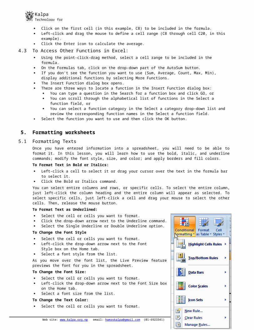
You can select entire columns and rows, or specific cells. To select the entire column, just left-click the column heading and the entire column will appear as selected. To select specific cells, just left-click a cell and drag your mouse to select the other cells. Then, release the mouse button.To Format Text as Underlined: Select the cell or cells you want to format. Click the drop-down arrow next to the Underline command. Select the Single Underline or Double Underline option.
To Change the Font Style Select the cell or cells you want to format. Left-click the drop-down arrow next to the Font Style box on the Home tab. Select a font style from the list.
As you move over the font list, the Live Preview feature previews the font for you in the spreadsheet.To Change the Font Size: Select the cell or cells you want to format. Left-click the drop-down arrow next to the Font Size box on the Home tab. Select a font size from the list.
To Change the Text Color: Select the cell or cells you want to format. Left-click the drop-down arrow next to the Text Color command. A color
palette will appear. Select a color from the palette.
OR Select More Colors. A dialog box will appear. Select a color. Click OK.
To Add a Border: Select the cell or cells you want to format. Click the drop-down arrow next to the Borders command on the Home tab.
A menu will appear with border options. Left-click an option from the list to select it. You can change the line style and color of the border. To add a Fill Color: Select the cell or cells you want to format. Click the Fill command. A color palette will appear. Select a color.
OR Select More Colors. A dialog box will appear. Select a color. Click OK.
You can use the fill color feature to format columns and rows, and format a worksheet so that it is easier to read.To Format Numbers and Dates: Select the cell or cells you want to format. Left-click the drop-down arrow next to the Number Format box. Select one of the options for formatting numbers. By default, the numbers appear in the General category, which means there is no special formatting.
In the Number group, you have some other options. For example, you can change the U.S. dollar sign to another currency format, numbers to percents, add commas, and change the decimal location.
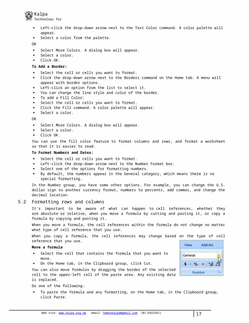
5.2 Formatting rows and columnsIt's important to be aware of what can happen to cell references, whether they are absolute or relative, when you move a formula by cutting and pasting it, or copy a formula by copying and pasting it.When you move a formula, the cell references within the formula do not change no matter what type of cell reference that you use.When you copy a formula, the cell references may change based on the type of cell reference that you use.Move a formula Select the cell that contains the formula that you want to move. On the Home tab, in the Clipboard group, click Cut.
Web site: www.kalpa.org.np email: [email protected] (01-6923341) 13
KalpaTechnology for change
You can also move formulas by dragging the border of the selected cell to the upper-left cell of the paste area. Any existing data is replaced.Do one of the following: To paste the formula and any formatting, on the Home tab, in the Clipboard group, click Paste. To paste the formula only, on the Home tab, in the Clipboard group, click Paste, click Paste Special, and then
click Formulas. Copy a formula Select the cell that contains the formula that you want to copy. On the Home tab, in the Clipboard group, click Copy.
Do one of the following: To paste the formula and any formatting, on the Home tab, in the Clipboard group, click Paste. To paste the formula only, on the Home tab, in the Clipboard group, click Paste, click Paste Special, and then
click Formulas.NOTE You can paste only the formula results. On the Home tab, in the Clipboard group, click Paste, click Paste Special, and then click Values.Verify that the cell references in the formula produce the result that you want. If necessary, switch the type of reference by doing the following: Select the cell that contains the formula. In the formula bar , select the reference that you want to change. Press F4 to switch between the combinations. The following table summarizes how a reference type updates if a formula that contains the reference is copied
two cells down and two cells to the right.
NOTE You can also copy formulas into adjacent cells by using the fill handle . After verifying that the cell references in the formula produce the result that you want in step 4, select the cell that contains the copied formula, and then drag the fill handle over the range that you want to fill.
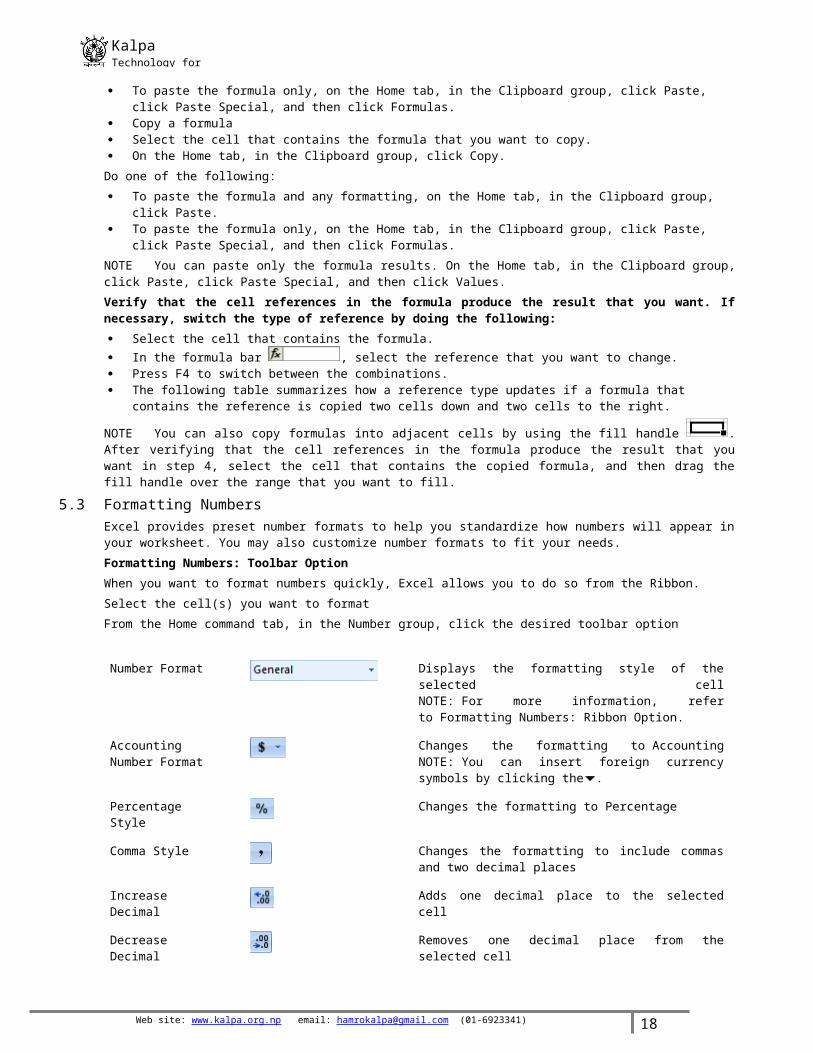
5.3 Formatting NumbersExcel provides preset number formats to help you standardize how numbers will appear in your worksheet. You may also customize number formats to fit your needs.Formatting Numbers: Toolbar OptionWhen you want to format numbers quickly, Excel allows you to do so from the Ribbon.Select the cell(s) you want to formatFrom the Home command tab, in the Number group, click the desired toolbar option
Number Format Displays the formatting style of the selected cellNOTE: For more information, refer to Formatting Numbers: Ribbon Option.
Accounting Number Format
Changes the formatting to AccountingNOTE: You can insert foreign currency symbols by clicking the .
Percentage Style Changes the formatting to Percentage
Comma Style Changes the formatting to include commas and two decimal places
Increase Decimal Adds one decimal place to the selected cell
Decrease Decimal Removes one decimal place from the selected cell
Format Cells: Number
Accesses the Format Cells dialog boxFor more information, refer to Formatting Numbers: Dialog Box Option.
Formatting Numbers: Ribbon OptionThe Ribbon offers a simple way to apply number formatting. To customize number formatting, refer to Formatting Numbers: Dialog Box Option.Select the cell(s) you want to format
Web site: www.kalpa.org.np email: [email protected] (01-6923341) 14
KalpaTechnology for change
From the Home command tab, in the Number group, click NUMBER FORMAT » select the desired number formatThe cell is formatted.
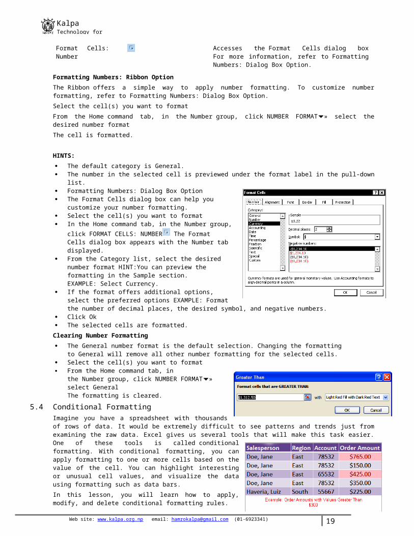
HINTS: The default category is General. The number in the selected cell is previewed under the format label in the pull-down list. Formatting Numbers: Dialog Box Option The Format Cells dialog box can help you customize your
number formatting. Select the cell(s) you want to format In the Home command tab, in the Number group,
click FORMAT CELLS: NUMBER The Format Cells dialog box appears with the Number tab displayed.
From the Category list, select the desired number format HINT:You can preview the formatting in the Sample section.EXAMPLE: Select Currency.
If the format offers additional options, select the preferred options EXAMPLE: Format the number of decimal places, the desired symbol, and negative numbers.
Click Ok The selected cells are formatted.
Clearing Number Formatting The General number format is the default selection. Changing the formatting to General will remove all other
number formatting for the selected cells. Select the cell(s) you want to format From the Home command tab, in the Number group,
click NUMBER FORMAT » select GeneralThe formatting is cleared.
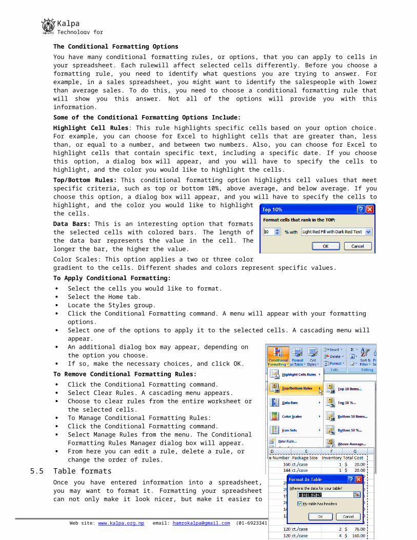
5.4 Conditional FormattingImagine you have a spreadsheet with thousands of rows of data. It would be extremely difficult to see patterns and trends just from examining the raw data. Excel gives us several tools that will make this task easier. One of these tools is called conditional formatting. With conditional formatting, you can apply formatting to one or more cells based on the value of the cell. You can highlight interesting or unusual cell values, and visualize the data using formatting such as data bars.In this lesson, you will learn how to apply, modify, and delete conditional formatting rules.The Conditional Formatting OptionsYou have many conditional formatting rules, or options, that you can apply to cells in your spreadsheet. Each rulewill affect selected cells differently. Before you choose a formatting rule, you need to identify what questions you are trying to answer. For example, in a sales spreadsheet, you might want to identify the salespeople with lower than average sales. To do this, you need to choose a conditional formatting rule that will show you this answer. Not all of the options will provide you with this information.Some of the Conditional Formatting Options Include:Highlight Cell Rules: This rule highlights specific cells based on your option choice. For example, you can choose for Excel to highlight cells that are greater than, less than, or equal to a number, and between two numbers. Also, you can choose for Excel to highlight cells that contain specific text, including a specific date. If you choose this option, a dialog box will appear, and you will have to specify the cells to highlight, and the color you would like to highlight the cells.Top/Bottom Rules: This conditional formatting option highlights cell values that meet specific criteria, such as top or bottom 10%, above average, and below average. If you choose this option, a dialog box will appear, and you will have to specify the cells to highlight, and the color you would like to highlight the cells.Data Bars: This is an interesting option that formats the selected cells with colored bars. The length of the data bar represents the value in the cell. The longer the bar, the higher the value.Color Scales: This option applies a two or three color gradient to the cells. Different shades and colors represent specific values.To Apply Conditional Formatting: Select the cells you would like to format. Select the Home tab.
Web site: www.kalpa.org.np email: [email protected] (01-6923341) 15
KalpaTechnology for change
Locate the Styles group. Click the Conditional Formatting command. A menu will appear with your formatting options. Select one of the options to apply it to the selected cells. A cascading menu will appear. An additional dialog box may appear, depending on the option you
choose. If so, make the necessary choices, and click OK.
To Remove Conditional Formatting Rules: Click the Conditional Formatting command. Select Clear Rules. A cascading menu appears. Choose to clear rules from the entire worksheet or the selected cells. To Manage Conditional Formatting Rules: Click the Conditional Formatting command. Select Manage Rules from the menu. The Conditional Formatting
Rules Manager dialog box will appear. From here you can edit a rule, delete a rule, or change the order of
rules.
5.5 Table formatsOnce you have entered information into a spreadsheet, you may want to format it. Formatting your spreadsheet can not only make it look nicer, but make it easier to use. In a previous lesson we discussed many manual formatting options such as bold and italics. In this lesson, you will learn how to use the predefined tables styles in Excel 2007 and some of the Table Tools on the Design tab.To Format Information as a Table: Select any cell that contains information. Click the Format as Table command in the Styles group on the Home
tab. A list of predefined tables will appear. Left-click a table style to select it. A dialog box will appear. Excel has automatically selected the cells for
your table. The cells will appear selected in the spreadsheet and the range will appear in the dialog box.
Change the range listed in the field, if necessary. Verify the box is selected to indicate your table has headings, if it does.
Deselect this box if your table does not have column headings. Click OK. The table will appear formatted in the style you chose.
By default, the table will be set up with the drop-down arrows in the header so that you can filter the table, if you wish.In addition to using the Format as Table command, you can also select the Insert tab, and click the Table command to insert a table.To Modify a Table: Select any cell in the table. The Table Tools Design tab will become active. From here you can modify the table in
many ways. Select a different table in the Table Styles Options group. Click the More drop-down arrow to see more table
styles. Delete or add a Header Row in the Table Styles Options group. Insert a Total Row in the Table Styles Options group. Remove or add banded rows or columns. Make the first and last columns bold. Name your table in the Properties group. Change the cells that make up the table by clicking Resize Table.
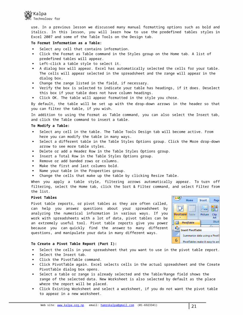
When you apply a table style, filtering arrows automatically appear. To turn off filtering, select the Home tab, click the Sort & Filter command, and select Filter from the list.Pivot TablesPivot table reports, or pivot tables as they are often called, can help you answer questions about your spreadsheet by analyzing the numerical information in various ways. If you work with spreadsheets with a lot of data, pivot tables can be an extremely useful tool. Pivot table reports give you power because you can quickly find the answer to many different questions, and manipulate your data in many different ways.
To Create a Pivot Table Report (Part I): Select the cells in your spreadsheet that you want to use in the pivot table report.
Web site: www.kalpa.org.np email: [email protected] (01-6923341) 16
KalpaTechnology for change
Select the Insert tab. Click the PivotTable command. Click PivotTable again. Excel selects cells in the actual spreadsheet and the Create PivotTable dialog box opens. Select a table or range is already selected and the Table/Range field shows the range of the selected data. New
Worksheet is also selected by default as the place where the report will be placed. Click Existing Worksheet and select a worksheet, if you do not want the pivot table to appear in a new worksheet. Click OK.
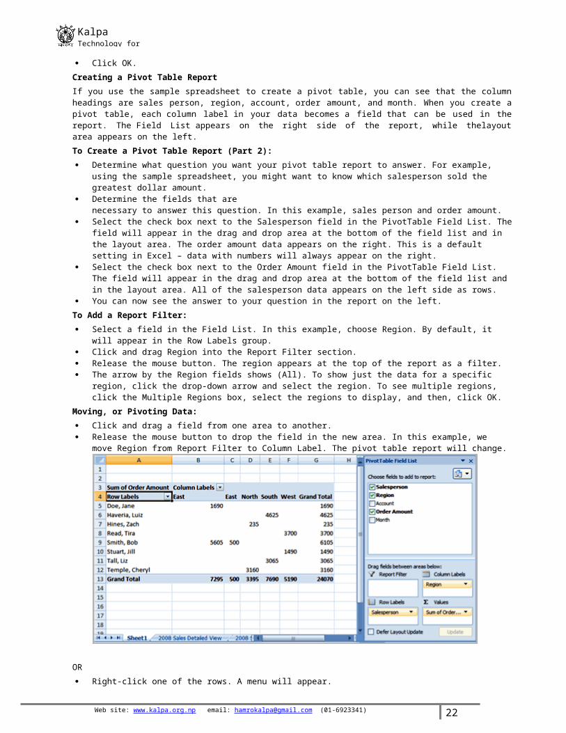
Creating a Pivot Table ReportIf you use the sample spreadsheet to create a pivot table, you can see that the column headings are sales person, region, account, order amount, and month. When you create a pivot table, each column label in your data becomes a field that can be used in the report. The Field List appears on the right side of the report, while thelayout area appears on the left.To Create a Pivot Table Report (Part 2): Determine what question you want your pivot table report to answer. For example, using the sample spreadsheet,
you might want to know which salesperson sold the greatest dollar amount. Determine the fields that are necessary
to answer this question. In this example, sales person and order amount. Select the check box next to the Salesperson field in the PivotTable Field List. The field will appear in the drag
and drop area at the bottom of the field list and in the layout area. The order amount data appears on the right. This is a default setting in Excel – data with numbers will always appear on the right.
Select the check box next to the Order Amount field in the PivotTable Field List. The field will appear in the drag and drop area at the bottom of the field list and in the layout area. All of the salesperson data appears on the left side as rows.
You can now see the answer to your question in the report on the left.To Add a Report Filter: Select a field in the Field List. In this example, choose Region. By default, it will appear in the Row Labels group. Click and drag Region into the Report Filter section. Release the mouse button. The region appears at the top of the report as a filter. The arrow by the Region fields shows (All). To show just the data for a specific region, click the drop-down arrow
and select the region. To see multiple regions, click the Multiple Regions box, select the regions to display, and then, click OK.
Moving, or Pivoting Data: Click and drag a field from one area to another. Release the mouse button to drop the field in the new area. In this example, we move Region from Report
Filter to Column Label. The pivot table report will change.
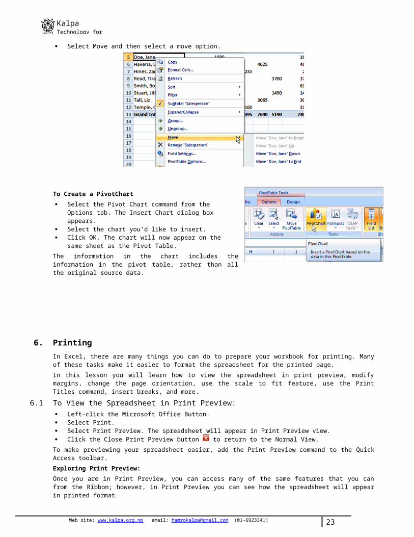
OR Right-click one of the rows. A menu will appear. Select Move and then select a move option.
Web site: www.kalpa.org.np email: [email protected] (01-6923341) 17
KalpaTechnology for change
To Create a PivotChart Select the Pivot Chart command from the Options tab. The
Insert Chart dialog box appears. Select the chart you’d like to insert. Click OK. The chart will now appear on the same sheet as the
Pivot Table.The information in the chart includes the information in the pivot table, rather than all the original source data.
6. PrintingIn Excel, there are many things you can do to prepare your workbook for printing. Many of these tasks make it easier to format the spreadsheet for the printed page. In this lesson you will learn how to view the spreadsheet in print preview, modify margins, change the page orientation, use the scale to fit feature, use the Print Titles command, insert breaks, and more.
6.1 To View the Spreadsheet in Print Preview: Left-click the Microsoft Office Button. Select Print. Select Print Preview. The spreadsheet will appear in Print Preview view. Click the Close Print Preview button to return to the Normal View.
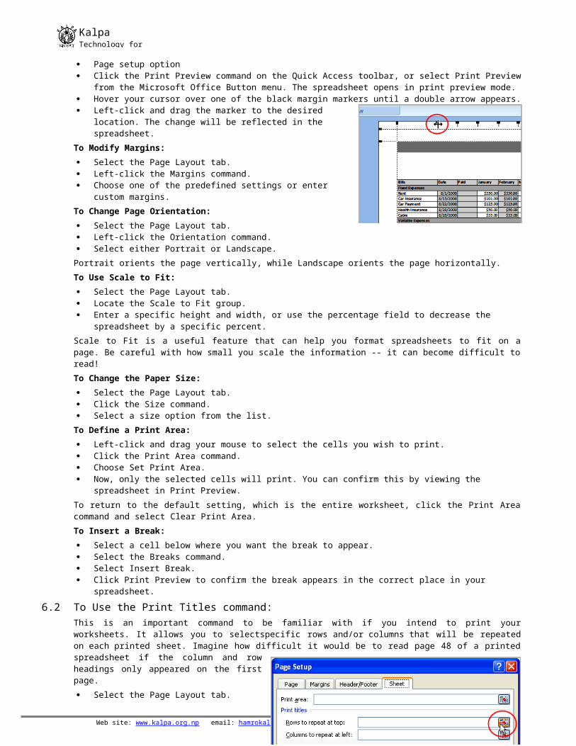
To make previewing your spreadsheet easier, add the Print Preview command to the Quick Access toolbar.Exploring Print Preview:Once you are in Print Preview, you can access many of the same features that you can from the Ribbon; however, in Print Preview you can see how the spreadsheet will appear in printed format. Page setup option Click the Print Preview command on the Quick Access toolbar, or select Print Preview from the Microsoft Office
Button menu. The spreadsheet opens in print preview mode. Hover your cursor over one of the black margin markers until a double arrow appears. Left-click and drag the marker to the desired location. The change
will be reflected in the spreadsheet.To Modify Margins: Select the Page Layout tab. Left-click the Margins command. Choose one of the predefined settings or enter custom margins.
To Change Page Orientation: Select the Page Layout tab.
Web site: www.kalpa.org.np email: [email protected] (01-6923341) 18
KalpaTechnology for change
Left-click the Orientation command. Select either Portrait or Landscape.
Portrait orients the page vertically, while Landscape orients the page horizontally.To Use Scale to Fit: Select the Page Layout tab. Locate the Scale to Fit group. Enter a specific height and width, or use the percentage field to decrease the spreadsheet by a specific percent.
Scale to Fit is a useful feature that can help you format spreadsheets to fit on a page. Be careful with how small you scale the information -- it can become difficult to read!To Change the Paper Size: Select the Page Layout tab. Click the Size command. Select a size option from the list.
To Define a Print Area: Left-click and drag your mouse to select the cells you wish to print. Click the Print Area command. Choose Set Print Area. Now, only the selected cells will print. You can confirm this by viewing the spreadsheet in Print Preview.
To return to the default setting, which is the entire worksheet, click the Print Area command and select Clear Print Area.To Insert a Break: Select a cell below where you want the break to appear. Select the Breaks command. Select Insert Break. Click Print Preview to confirm the break appears in the correct place in your spreadsheet.
6.2 To Use the Print Titles command:This is an important command to be familiar with if you intend to print your worksheets. It allows you to selectspecific rows and/or columns that will be repeated on each printed sheet. Imagine how difficult it would be to read page 48 of a printed spreadsheet if the column and row headings only appeared on the first page. Select the Page Layout tab. Click the Print Titles command. The Page
Setup dialog box appears. Click the icon at the end of the field. Select the first row in the spreadsheet that
you want to appear on each printed page. Repeat for the column, if necessary. Click OK.
6.3 Print worksheet: Left-click the Microsoft Office Button. Select Print Print. The Print dialog box appears. Select a printer if you wish to use a printer other than the default setting. Click Properties to change any necessary settings. Choose whether you want to print specific pages, all of the worksheet, a selected area, the active sheet, or the
entire workbook. Select the number of copies you'd like to print. Click OK.
You can select Quick Print to bypass the Print dialog box.
7. Working with ChartsA chart is a tool you can use in Excel to communicate your data graphically. Charts allow your audience to more easily see the meaning behind the numbers in the spreadsheet, and make showing comparisons and trends a lot easier. In this lesson, you will learn how to insert and modify Excel charts and see how they can be an effective tool for communicating information.
Web site: www.kalpa.org.np email: [email protected] (01-6923341) 19
KalpaTechnology for change
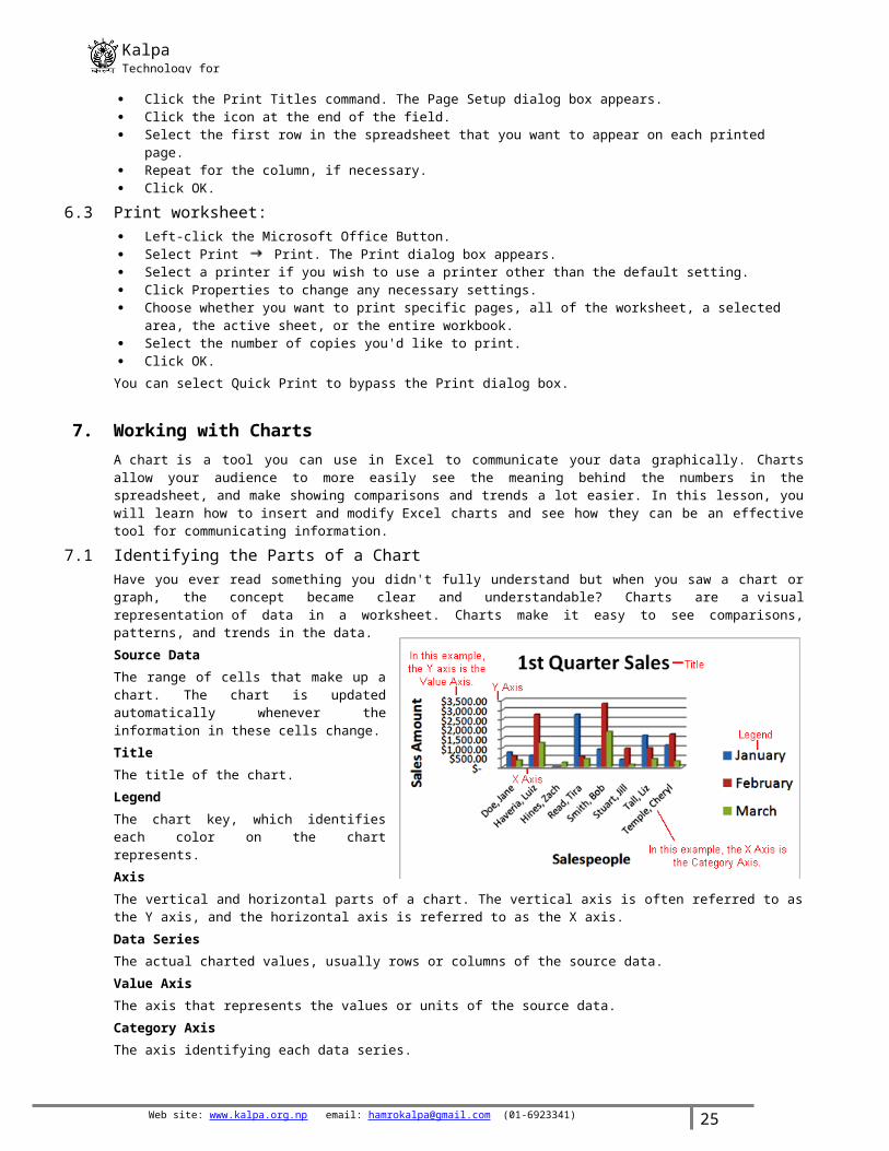
7.1 Identifying the Parts of a ChartHave you ever read something you didn't fully understand but when you saw a chart or graph, the concept became clear and understandable? Charts are a visual representation of data in a worksheet. Charts make it easy to see comparisons, patterns, and trends in the data.Source DataThe range of cells that make up a chart. The chart is updated automatically whenever the information in these cells change.TitleThe title of the chart.LegendThe chart key, which identifies each color on the chart represents.AxisThe vertical and horizontal parts of a chart. The vertical axis is often referred to as the Y axis, and the horizontal axis is referred to as the X axis.Data SeriesThe actual charted values, usually rows or columns of the source data.Value AxisThe axis that represents the values or units of the source data.Category AxisThe axis identifying each data series.
7.2 Creating a ChartCharts can be a useful way to communicate data. When you insert a chart in Excel, it appears in the selected worksheet with the source data, by default.To Create a Chart: Select the worksheet you want to work with. In this example, we use the Summary worksheet. Select the cells that you want to chart, including the column titles and the row labels. Click the Insert tab. Hover over each Chart option in the Charts group to learn more about it. Select one of the Chart options. In this example, we use the Columns command. Select a type of chart from the list that appears. For this example, we use a 2-D Clustered Column. The chart
appears in the worksheet.Once you insert a chart, a new set of Chart Tools, arranged into 3 tabs, will appear above the Ribbon. These are only visible when the chart is selected.To Change the Chart Type: Select the Design tab. Click the Change Chart Type command. A dialog box appears. Select another chart type. Click OK.
The chart in the example compares each salesperson's monthly sales to his/her other month's sales; however you can change what is being compared. Just click the Switch Row/Column Data command, which will rotate the data displayed on the x and y axes. To return to the original view, click the Switch Row/Column command again.Change Chart Layout: Select the Design tab. Locate the Chart Layouts group. Click the More arrow to view all your layout options. Left-click a layout to select it.
If your new layout includes chart titles, axes, or legend labels, just insert your cursor into the text and begin typing to add your own text.To Change Chart Style: Select the Design tab. Locate the Chart Style group. Click the More arrow to view all your style options.
Web site: www.kalpa.org.np email: [email protected] (01-6923341) 20
KalpaTechnology for change
Left-click a style to select it.
7.3 To Move the Chart to a Different Worksheet: Select the Design tab. Click the Move Chart command. A dialog box appears. The current location of the chart is selected. Select the desired location for the chart (i.e. choose an existing worksheet, or select New Sheet and name it).
8. Managing Large Workbooks 8.1 Splitting and Freezing Panes
Splitting or freezing panes allow you to hold sections of a worksheet in place so they are visible at all times whilst scrolling through the worksheet. This is especially useful for large worksheets because you can hold the column and row headings in place whilst you scroll through your data.Splitting panes on a worksheetSplitting panes allows you to see multiple areas of a worksheet at once. So you can make changes to the data in cell D500 whilst viewing the data in cell D5. Select the cell where you want to split the worksheet
The worksheet will be split above and to the left of the active cell creating four panes. Click the View tab on the Ribbon Click the Split button in the Window group
The worksheet is split into sections that can be navigated individually without moving the other sections.
Click and drag the panes to adjust the location of the split.
Web site: www.kalpa.org.np email: [email protected] (01-6923341) 21
KalpaTechnology for change
Click the Split button in the Window group on the Ribbon again to remove the split.Worksheets can also be split using the split buttons at the top and to the right of the worksheets scroll bars. To split the worksheet, drag the relevant split button onto the area of the worksheet where you wish to create the split.Freezing panes on a worksheetFreezing panes is similar to splitting panes except that the panes are immobilised. Freeze panes is used to hold headers in place so that they can always been seen when scrolling through the worksheet. Click the View tab on the Ribbon Click the Freeze Panes button in the Window group
A list appears with three optionsFreeze Panes: Freezes the worksheet above and to the left of the active cell.Ensure that you select the required cell before clicking this option. Unlike split panes, frozen panes cannot be moved. You need to unfreeze the panes and then freeze again.Freeze Top Row: Freezes the top row, keeping it visible whilst you scroll through the rest of the worksheet.Freeze First Column: Freezes the first column, keeping it visible whilst you scroll through the rest of the worksheet
Select the desired option from the listThe relevant panes are frozen and the worksheet can be navigated as required To unfreeze panes, click the Freeze Panes button in the Window
group and select Unfreeze PanesComparing Two Excel 2007 Worksheets Side by SideYou can use the View Side by Side command button on the View tab in Excel 2007 to quickly and easily do a side-by-side comparison of any two worksheet windows that you have open. When you click this button after opening two workbook windows, Excel automatically tiles the windows.To compare two worksheets side by side, follow these steps: Open the two workbooks you want to compare. Display the worksheet in each workbook that you want to compare side by side.
Click the View Side by Side button in the Window group of the View tab.If you have more than two windows open when you click the View Side by Side command button, Excel opens the Compare Side by Side dialog box, where you click the name of the window that you want to compare with the one that’s currently active and click OK.
Scroll down or across a worksheet.Both worksheets scroll together because the Synchronous Scrolling setting is enabled by default when you click the View Side by Side button. (Optional) Click the Synchronous Scrolling button in the Window group if you want to turn off simultaneous
scrolling. Turning off simultaneous scrolling allows you to scroll through one
worksheet without the other one scrolling, too. (Optional) Click the Reset Window Position button if you want to reset
the window positions of the two workbooks after resizing one or both windows.
You might have resized a window to get a better look at some data.When you’re done comparing the worksheets, click the View Side by Side button in the Window group again.Excel returns to Normal view.
Web site: www.kalpa.org.np email: [email protected] (01-6923341) 22
KalpaTechnology for change
8.2 How to Move or Copy Excel 2007 Worksheets to Other WorkbooksIn Excel 2007, you may need to move or copy a particular worksheet from one workbook to another. You can use the Move or Copy dialog box to simplify the process. To move or copy worksheets between workbooks, follow these steps: Open the workbook with the worksheet(s) that you want to move or
copy and the workbook that is to contain the moved or copied worksheet(s).
Both the source and destination workbooks ned to be open, though you don't need to see both of them.
Display the workbook that contains the worksheet(s) that you want to move or copy.
This is your source workbook. Select the worksheet(s) that you want to move or copy.
If you want to select a group of neighboring sheets, click the first tab and then hold down Shift while you click the last tab. To select nonadjacent sheets, click the first tab and then hold down Ctrl while you click each of the other sheet tabs. Right-click one of the selected sheet tabs and then click Move or Copy on the
shortcut menu.Excel opens the Move or Copy dialog box, where you indicate whether you want to move or copy the selected sheet(s) and where to move or copy them. In the To Book drop-down list, select the workbook to which you want to copy or
move the worksheets.If you want to move or copy the selected worksheet(s) to a new workbook rather than to an existing one that you have open, select the (New Book) option at the top of the To Book drop-down list. Select where in the new workbook you want to drop the worksheets.
In the Before Sheet list box, select the name of the sheet that the worksheet(s) you’re about to move or copy should precede. If you want the sheet(s) that you’re moving or copying to appear at the end of the workbook, choose the (Move to End) option. If you want to copy the sheets rather than move them, select the Create a
Copy check box.By default, this option is deselected. Click OK to complete the move or copy operation. A worksheet has found a new home!
If you prefer a more direct approach, you can move or copy sheets between open workbooks by dragging their sheet tabs from one workbook window to another (hold down the Ctrl key as you drag a sheet tab to create a copy). Use the Arrange All command on the View tab to display all workbooks onscreen. Note that this method works with a bunch of sheets as well as with a single sheet; just be sure that you select all their sheet tabs before you begin the drag-and-drop procedure.
8.3 Arranging Windows in Excel 2007 WorkbooksYou can open multiple workbook windows in Excel 2007 and arrange them into windows of varying displays so that you can view different parts of a worksheet from each workbook on the screen at one time.After you arrange windows, activate the one you want to use (if it’s not already selected) by clicking it. In the case of the cascade arrangement (described below), you need to click the worksheet window’s title bar, or you can click its button on the taskbar.Follow these steps to arrange workbook windows in Excel 2007: Open the workbooks that you want to arrange. You’ll want to open at least two workbooks and select the worksheet in each
workbook that you want to display. Click the Arrange All button in the Window group on the View tab.
The Arrange Windows dialog box appears.
Select the desired Arrange setting in the Arrange Windows dialog box.Make one of the following selections:Tiled: Select this option button to have Excel arrange and size the windows so that they all fit side by side on the screen in the order in which you opened them.
Web site: www.kalpa.org.np email: [email protected] (01-6923341) 23
KalpaTechnology for change
Horizontal: Select this option button to have Excel size the windows equally and place them one above the other.
Four worksheet windows arranged with the Horizontal option.Vertical: Select this option button to have Excel size the windows equally and place them next to each other.
Cascade: Select this option button to have Excel arrange and size the windows so that they overlap one another with only their title bars showing.
Web site: www.kalpa.org.np email: [email protected] (01-6923341) 24
KalpaTechnology for change
Click OK.The workbooks are arranged on-screen based on your selection in the previous step.If you want to have Excel show only the windows that you have open in the current workbook, select the Windows of Active Workbook check box in the Arrange Windows dialog box.If you close one of the windows you’ve arranged, Excel doesn’t automatically resize the other open windows to fill in the gap. To fix this, click the Arrange All command again on the View tab, select the desired arrangement, and click OK.
8.4 How to Protect an Excel 2007 WorkbookExcel 2007 includes a Protect Workbook command that prevents others from making changes to the layout of the worksheets in a workbook. You can assign a password when you protect a workbook so that only those who know the password can unprotect the workbook and make changes to the structure and layout of the worksheets.Protecting a workbook does not prevent others from making changes to the contents ofcells. To protect cell contents, you must use the Protect Sheet command button on the Review tab.Protecting a workbookFollow these steps to protect an Excel 2007 workbook: Click the Protect Workbook command button in the Changes group on
the Review tab.Excel opens the Protect Structure and Windows dialog box, where the Structure check box is selected by default. With the Structure check box selected, Excel won’t let anyone mess around with the sheets in the workbook (by deleting them or rearranging them).
You can protect the structure and windows in a workbook.(Optional) If you want to protect any windows that you set up, select the Windows check box.When selected, this setting keeps the workbook windows in the same size and position each time you open the workbook.To assign a password that must be supplied before you can remove the protection from the worksheet, type the password in the Password (optional) text box. Click OK.
If you typed a password in the Password (optional) text box, Excel opens the Confirm Password dialog box. Re-enter the password in the Reenter Password to Proceed text box exactly as you typed it Step 3, and then click OK.Unprotecting a workbookTo remove protection from the current workbook, follow these steps: Click the Unprotect Workbook command button in the Changes group on the Review tab.
If you assigned a password when protecting the workbook, type the password in the Password text box and click OK.
If you create a workbook with contents to be updated by several different users on your network, you can use the Protect and Share Workbook command to ensure that Excel tracks all the changes made and that no user can intentionally or inadvertently remove Excel’s tracking of changes. Follow these steps: Click the Protect and Share Workbook command button in the
Changes group on the Review tab.The Protect Shared Workbook dialog box appears.
Web site: www.kalpa.org.np email: [email protected] (01-6923341) 25
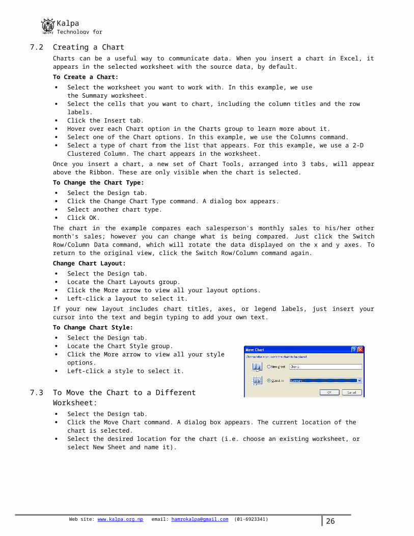
KalpaTechnology for change
Select the Sharing with Track Changes check box.
Protect a shared workbook so that users cannot remove Excel’s tracking of changes.To assign a password that each user must supply before he or she can open the workbook to make any changes, type a password in the Password (optional) text box and click OK.
Web site: www.kalpa.org.np email: [email protected] (01-6923341) 26