- 1 - 03/10/2001

Getting the best of the IBM Enterprise Storage

Server (ESS) with Oracle

AIX environment

July 2001 Fabienne Lepetit EMEA Joint Solutions Center IBM/Oracle Christine O’Sullivan IBM Montpellier PSSC

Thanks to : � Paul Bramy from EMEA Joint Solutions Center Oracle/IBM for his participation to the tests � Peter Kimmel from IBM SSG, EMEA Storage Competence Center for his support and recommendations

- 2 - 03/10/2001

1. Introduction......................................................................................................................................................................4

1.1. How this document is organized ...........................................................................................................................4 1.2. Test environment .....................................................................................................................................................4

1.2.1. Presentation of the test environment.........................................................................................................4 1.2.1.1. The hardware Environment....................................................................................................................4 1.2.1.2. The Oracle environment .........................................................................................................................5

1.2.2. Monitoring..........................................................................................................................................................6 2. Oracle layouts on an ESS...........................................................................................................................................7

2.1. Comparison between various layouts: implementing an Oracle DB on the ESS. .........................................7 2.1.1. Striping data across all the arrays : balanced method(ESS1)...............................................................8 2.1.2. Isolation method (ESS2) following Oracle DB rules of implementation..............................................8

2.1.2.1. I/O intensive tables (TES and COM) isolated on 2 arrays.............................................................8 2.1.2.2. I/O intensive tables (TES and COM) isolated on 3 arrays.............................................................9 2.1.2.3. I/O intensive tables (TES and COM) “isolated” on 4 arrays..........................................................9 2.1.2.4. Synthesis : comparisons between the different layouts............................................................... 10

3. FLASHCOPY TESTS ................................................................................................................................................. 13 3.1. FlashCopy overview................................................................................................................................................ 13

3.1.1. When will Flascopy be used?........................................................................................................................ 13 3.1.2. Flashcopy and Oracle database................................................................................................................... 13

3.2. Use of the Flashcopy function in a production environment ........................................................................ 14 3.2.1. Oracle backup overview................................................................................................................................ 14

3.2.1.1. Cold backup.............................................................................................................................................. 14 3.2.1.2. Hot backup............................................................................................................................................... 14

3.3. The tests ................................................................................................................................................................. 15 3.3.1. The Flashcopy test environment................................................................................................................. 16 3.3.2. Flashcopy of an offline database ............................................................................................................... 16 3.3.3. Flashcopy of an online database ................................................................................................................. 17 3.3.4. Restore on the same machine...................................................................................................................... 18 3.3.5. Restore on a different machine................................................................................................................. 23 3.3.6. Flashcopy Questions and Answers ............................................................................................................ 24

4. Conclusion ................................................................................................................................................................... 25 5. ANNEXE 1 : ESS....................................................................................................................................................... 26

5.1. ESS Architecture................................................................................................................................................. 26 5.1.1. What is the ESS? ......................................................................................................................................... 26 5.1.2. Components of the ESS ? ........................................................................................................................... 26 5.1.3. Disks and ranks.............................................................................................................................................. 28 5.1.4. ESS advanced Copy Services ..................................................................................................................... 29

5.2. ESS rules ................................................................................................................................................................ 30 5.2.1. General considerations: ............................................................................................................................... 30

5.2.1.1. The Balanced Method............................................................................................................................ 31 5.2.1.2. The Isolation Method. .......................................................................................................................... 31

6. ANNEXE 2 : AIX Concepts..................................................................................................................................... 32 6.1. -AIX logical volume manager (LVM) overview................................................................................................. 32

6.1.1. AIX storage structures (VG, PV, LV …) ................................................................................................... 32 6.1.2. striping (physical partition stripping, LVM fine stripping) .................................................................. 32

- 3 - 03/10/2001

7. ANNEXE 3 : ORACLE Concepts............................................................................................................................. 35 7.1. Oracle overview..................................................................................................................................................... 35

7.1.1. Objects and dependencies .......................................................................................................................... 35 7.1.1.1. Redologs .................................................................................................................................................. 35 7.1.1.2. Rollback segments................................................................................................................................. 36 7.1.1.3. Data and indexes................................................................................................................................... 36 7.1.1.4. Other components ................................................................................................................................ 36

7.2. Implementing Oracle database on AIX............................................................................................................ 38 7.2.1. File-systems & raw-devices ........................................................................................................................ 38 7.2.2. Striping ........................................................................................................................................................... 38 7.2.3. Asynchronous I/O......................................................................................................................................... 38

8. ANNEXE 4 : Oracle DB layout............................................................................................................................... 40 8.1.1. Oracle rules of implementation.................................................................................................................. 40

8.1.1.1. Decisional support system (DSS) ...................................................................................................... 40 8.1.1.2. Online Transaction Processing (OLTP) ............................................................................................. 42

9. ANNEXE 5 : Bibliography ....................................................................................................................................... 43 �

- 4 - 03/10/2001

1. Introduction Different choices can be made to implement an Oracle database on an IBM Enterprise Storage Server (ESS). The purpose of this document is to help in making those choices and to give an illustration of the kind of performance gains that could be obtained just modifying data placement on the ESS. You will also find in this paper, information relative to the use of the IBM ESS flashcopy function in an Oracle database environment on AIX 4.3. Procedures to backup and restore an offline or online Oracle database using the ESS copy services are described in the paragraph “flashcopy tests”. This document is not a performance guide and have no intent to demonstrate the maximum throughput you can achieve with an ESS F20 (official benchmarks and papers delivered by the IBM’s Labs will be your source if you are looking for this information).

1.1. How this document is organized This paper contains 3 main parts and is organized as follow: The first part explains our test environment The second part of the document provides comparison between various Oracle database layouts on an ESS. The third part of the document addresses flashcopy tests. You will find in the annexes an overview of the Enterprise Storage Server (ESS) architecture, AIX operating system and Oracle database components and rules of implementation.

1.2. Test environment

1.2.1. Presentation of the test environment

We have chosen to implement a data mart database (form of data warehouse environment) in an AIX environment using 4 different layouts. The purpose of the tests was to measure the performance gain obtained for different SQL queries by respecting Oracle general implementation rules and separating your most I/O intensive tables on different ESS raid arrays.

1.2.1.1. The hardware Environment As illustrated in the figure below, we have connected a Pseries 680 to an ESS F20 via 4 FC adapters (6227). We have used 6 arrays (3 per cluster) to implement the Oracle database. 6 volumes of 20 GB have been defined on the ESS (one per array).

- 5 - 03/10/2001

Disk Interface

SSA160

SSA160

SSA160

SSA160

cluster 2CACHE NVS

CACHENVScluster 1

SSA160

SSA160

SSA160

SSA160

ESS1 DB Flash ESS1 ESS2 DB ESS1 DB Flash ESS1

ESS2 DB

Flash ESS1 ESS2 DB

ESS1 DB Flash ESS1 ESS2 DB

Flash ESS1 ESS2 DB ESS1 DB ESS1 DB

Not usedfor the test

Not usedfor the test

LSS10

ESS1 DB

LSS15LSS14

LSS13LSS12

LSS11

Flash ESS1 ESS2 DB

LSS16 LSS17

Pseries 68024 processors32 GB4 FC adaptersAIX 4.3.3SDD 1.2.0.4 Oracle 8.1.6

FCS1A0-58

FCS060-58

FCS2D0-58

FCS3E0-58

Not usedfor the test

Not usedfor the test

ESS 2105 F20Cache : 4 GB/clusterNVS : 192 MB/cluster 9.1GB disks

Test Environment

ESS1 = balanced method ESS2 = isoaltion method

1.2.1.2. The Oracle environment For our tests we have used a data mart database. A data mart is a simple form of a data warehouse that is focused on a single subject (or functional area), such as Sales or Finance or Marketing. A data mart is a relational database that is designed for query and analysis rather than transaction processing. It usually contains historical data that is derived from transaction data, but it can include data from other sources. The characteristics of a datamart environment are: - Number of users from 10 to 50 (depends on department size) - Database size <= 100 GB - Ad hoc queries Our Data mart environment The database size was 100 GB. The different selected queries used for the test have been collected during the work of users in real Decisional (DSS ) environment. For the tests, we have run one scenario (a group of different queries: simple,

- 6 - 03/10/2001

moderate and complex) representative of the work of users and each query has a certain weight in the scenario. This weight depends on the frequency of the query (number of time, it is started during the scenario). The queries mainly produce read requests. The database has been distributed over 6 arrays. The database was composed of 6 tables presented hereunder :

Table # rows tes_tb 173.810.620 ami_tb 11.802.180 tic_tb 166 bli_tb 21.473 com_tb 96.467.340 nef_tb 16.954.200

The 2 mains and more I/O intensive tables were : TES_TB and COM_TB. Their respective size was 34 GB and 18 GB.

1.2.2. Monitoring The system has been monitored thanks to AIX standard tools like vmstat, sar, iostat. The Oracle database has been monitored by the orastats.sql script, written by Keith Murphy from Oracle, which provides a lot of information about the database like hit ratios, wait events, system statistics or I/O against tablespaces or datafiles. To monitor disk activities we mainly used “iostat” command and monitor tools. The iostat tool provides data on the activity of physical volumes. It allows to identify most accessed disks, which can become bottlenecks. The busier a disk is, the more likely that I/Os to that disk will have to wait longer. It is also important to find out what kind of disk I/ O is taking place on the busier disk. The ESS cache, disk group has been monitored using storwatch Expert. IBM Storwatch expert (ESS Expert) is a product of the IBM Storwatch family that enables you to gather various information about IBM 2105 Enterprise Storage Server. ESS Expert helps in doing performance management. ESS Expert provides performance reports.

- 7 - 03/10/2001

2. Oracle layouts on an ESS

2.1. Comparison between various layouts: implementing an Oracle DB on the ESS.

Not all database environments can be tuned the same way. The first step in tuning should be identifying the database environment. There are different kinds of applications, and each one can exercise different database components. OLTP update-intensive applications demand a more efficient logging and locking mechanism than any other kind of application. Multi-processor applications are more suited for OLTP since there are usually many users using the database simultaneously. Client/server and distributed configurations can also be used to increase transaction throughput. Decision Support (DSS) applications depend on efficient query optimization plans, clustered indexes, and fast disk drives. Mixed environments are difficult to tune since there are parameters that benefit some applications while degrading performance of others. A query that is tuned to run faster has to be tested with all other applications running together to verify that the overall performance really improves. Disk bottlenecks are not unusual and are mostly due to a lack of multiple disk arms rather than the efficiency among all the different disk drives that IBM offers. Placement of the log file and database tables depends on the environment and data utilization. These are basically two disk uses; random and sequential. They require different disk for better performance. The following 4 figures, describes the 4 different layouts chosen to implement the Oracle database on the ESS. The first one uses the balanced method (every LV so every database objects striped on the 6 arrays used for the tests). The 3 next ones are variants of the isolation method principally modifying the I/O intensive tables (TES and COM) layout.

- 8 - 03/10/2001

2.1.1. Striping data across all the arrays : balanced method(ESS1)

TES_TB /TES_ID X C OM _TB / C OM _ID X

O THER s TB / OTHER _ID XLOG

Archive lo gTEM P

SYS

TES_TB / TES_IDX C OM _TB / C O M _ID X

O TH ERs TB / O THER _ID XLOG

ArchivelogTEM P

SYS

TES_TB /TES_ID X C OM _TB / C OM _ID X

O THER s TB / OTHER _ID XLOG

Archive lo gTEM P

SYS

TES_TB /TES_ID X C OM _TB / C O M _ID X

O TH ERs TB / O THER _ID XLOG

ArchivelogTEM P

SYS

TES_TB / TES_ ID X C OM _TB / C OM _ID X

O THER s TB / OTHER _ID XLOG

Archive lo gTEM P

SYS

TES_TB / TES_IDX C OM _TB / C O M _ID X

O TH ERs TB / O THER _ID XLOG

ArchivelogTEM P

SYS

Balanced method : A ll data s triped on the 6 arrays

C luster 1 C luster 2

DA 1

DA 2

DA 3

DA 1

DA 2

DA 3

A R RA Y 1 A R RA Y 2

A RR A Y 3 A R RA Y 4

A RR A Y 5 AR R AY 6

2.1.2. Isolation method (ESS2) following Oracle DB rules of implementation

2.1.2.1. I/O intensive tables (TES and COM) isolated on 2 arrays

TES_TB TEMP

TES_TB COM_IDX

COM_TBOTHER_IDXArchivelog

TEMPLOG

TES_IDXOTHERs TB

LOGSYS

COM_TB

Isolation method : first implementation

ARRAY 1 ARRAY 2

ARRAY 3 ARRAY 4

ARRAY 5 ARRAY 6

DA 1

DA 3

DA 2

DA 1

DA 3

DA 2

Cluster 1 Cluster 2

- 9 - 03/10/2001

2.1.2.2. I/O intensive tables (TES and COM) isolated on 3 arrays

TES_TB TEMP

TES_TB COM_IDX

COM_TB OTHER_IDXArchivelog

TEMPTES_TB

TES_IDXCOM_TB

OTHERs TB LOGSYS

COM_TB

Isolation Method : Second implementation

Cluster 1 Cluster 2

DA 1

DA 2

DA 3

DA 1

DA 2

DA 3

ARRAY 1 ARRAY 2

ARRAY 3 ARRAY 4

ARRAY 5 ARRAY 6

2.1.2.3. I/O intensive tables (TES and COM) “isolated” on 4 arrays This implementation is very closed to the balanced method.

Isolation Method : Third Implementation

TES_TB TEMP

COM_TB

TES_TB COM_IDX

COM_TB OTHER_IDXArchivelog

TES_TB

TEMPTES_TB

TES_IDXCOM_TB

RBS

OTHERs TB LOGSYS

COM_TB

Cluster 1 Cluster 2

DA 1

DA 2

DA 3

DA 1

DA 2

DA 3

ARRAY 1 ARRAY 2

ARRAY 3 ARRAY 4

ARRAY 5 ARRAY 6

- 10 - 03/10/2001

2.1.2.4. Synthesis : comparisons between the different layouts Here are the results obtained with the different implementations. The table below gives, per implementation type (column 3 to 6), the elapsed time of the whole scenario (see row 2 : “scenario1”) and the elapsed time per query (row 3 to the end). Tests Accessed

tables in the queries

Balanced method (ESS1)

Isolation method (ESS2) : first layout

Isolation method (ESS2) : second layout

Isolation method (ESS2) : third layout

Scenario1 start 11:56 End 13:11 Elapsed= 1H15

start = 15:44 End = 16h54 Elapsed = 1H10

start= 14:24 End = 15 :22 Elapsed= 58 mn

start= 9h27 End= 10h43 Elapsed =1H16

Query1 IDX NEF IDX TES IDX COM

2mn 17 1mn32 1mn26 1mn54

Query2 IDX TES IDX NEF

2mn 28 2mn21 2mn24 2m24

Query3 FULL TES IDX AMI IDX NEF

10mn53 8mn06 6mn12 12mn09

Query4 IDX TES 16s/17s 14s 14/15s 16 /17

Query5 IDX TES 2mn40 2mn46 1mn57 2m41

Query6 IDX TES 1mn05 51s 50s 56s

Query7 IDX TES 9s 9s 12s 9s

Query8 FULL COM IDX TES

12mn39 8mn51 7mn 09 11m38

Query9 Create as select TES

13mn41 12mn26 10mn21 12m37

Query10 IDX TES FULL COM

7mn33 4mn25 3m48 7m18

Query11 IDX TES 1mn37 2mn03 1m55 1m30

Query12 FULL AMI FULL NEF

2mn26 2mn51 2mn55 2m52

Query13 IDX TES IDX COM

10s 41 sec 41s 9/10s

Query14 IDX COM 6s 5s 4s 5s

Query15 IDX NEF 1s <1s 1s 1s

Query16 IDX TES 6s 4s 4s

Query17 Full COM 1mn58 5m02 3mn04 2m06

Query18 Create table as select Full scan TES

6mn30 10mn13 7mn45 7m31

Query19 FULL AMI 54s 54s 52s 51s

Query20 FULL COM 12/13s 12/13s 12/13s 12/13s

Query21 <1s <1s <1s <1s

Query22 FULL COM 6mn07 4m48 4mn14 6mn40

Query23 IDX TES 18 s 46s 14s 16s

- 11 - 03/10/2001

The yellow column (column 5) gives the result of the second implementation (for the isolation method). This data layout gave the best result, stripping the most accessed tables (COM and TES) on 3 different arrays. Conclusion on different layouts : If we compare the result of scenario1 with the balanced method implementation and the result given by the best-tested method (isolation method: second layout), we see a gain of 22% (in term of elapsed time) for the whole scenario (58 minutes instead of 1 hour 15 minutes). In the first layout of the isolation method (column 4), the more I/O intensive tables were each stripped on 2 different arrays and we had heavy contention on the disks containing those tables (TES and COM). So, we didn’t get any improvement. The real improvement came with the second implementation (column 5), stripping TES and COM tables on 3 different arrays. What can be observed: If you look into details to the result of each query (see table below), you can see that the real gain is on queries that touch multiple tables. Obviously, some queries that only work on one I/O intensive table and generate a full table scan (like Query17 or Query18) will have lower performance in the isolation method than in the balanced method: only 3 arrays (so 24 disks) for TES and COM tables will be used instead of 6 arrays (48 disks). The real gain appears for queries that use several tables (for example Query3). Placing those tables with heavy sequential on the same disk or array as another heavily accessed table or table with random access, may cause the I/O performance to be degraded like it is the case for the balanced method where all the tables are mixed on the same disks.

- 12 - 03/10/2001

Table : The gain (in percentage) between the balanced method and the best implementation of the isolation method

Tests Accessed tables

in the queries Balanced method (ESS1)

Isolation method (ESS2): second layout

ESS2/ESS1

Scenario1 start 11:56 End 13:11 Elapsed= 1H15

start= 14:24 End = 15 :22 Elapsed= 58 mn

Time difference between ESS1 et ESS2 = 17 mn ESS2/ESS1=- 22%

Query1 IDX NEF IDX TES IDX COM

2mn 17 1mn26 - 37%

Query2 IDX TES IDX NEF

2mn 28 2mn24 + 2%

Query3 FULL TES IDX AMI IDX NEF

10mn53 6mn12 - 43%

Query4 IDX TES 16s/17s 14/15s - 11%

Query5 IDX TES 2mn40 1mn57 - 26%

Query6 IDX TES 1mn05 50s - 23%

Query7 IDX TES 9s 12s + 33%

Query8 FULL COM IDX TES

12mn39 7mn 09 - 43 %

Query9 Create as select TES 13mn41 10mn21 - 24%

Query10 IDX TES FULL COM

7mn33 3m48 - 49 %

Query11 IDX TES 1mn37 1m55 + 18%

Query12 FULL AMI FULL NEF

2mn26 2mn55 + 19%

Query13 IDX TES IDX COM

10s 41s

Query14 IDX COM 6s 4s - 33%

Query15 IDX NEF 1s 1s

Query16 IDX TES 6s 4s - 33 %

Query17 Full COM 1mn58 3mn04 + 55%

Query18 Create table as select Full scan TES

6mn30 7mn45 + 19%

Query19 FULL AMI 54s 52s - 37 %

Query20 FULL COM 12/13s 12/13s

Query21 <1s <1s

Query22 FULL COM 6mn07 4mn14 - 30 %

Query23 IDX TES 18 s 14s - 22 %

- 13 - 03/10/2001

3. FLASHCOPY TESTS

3.1. FlashCopy overview

The Enterprise Storage Server (ESS) supports several hardware-assisted copy functions for two purposes: mirroring for disaster recovery solutions, and copy functions that provide an instant copy of the data. Copy Services is a separately sold feature of the Enterprise Storage Server. FlashCopy is a fast point in time copy technique designed to replicate all data on an entire LUN to another LUN within the same ESS Logical Storage Subsystem. FlashCopy makes a single point-in-time (T0) copy of an ESS logical volume. The target copy is available once the FlashCopy command has been processed; Point-in-time copy functions give you an instantaneous copy, or “view”, of what the original data looked like at a specific point-in-time. This is known as the T0 (time-zero) copy. From the ESS Copy Services Web Interface one can graphically select ‘source’ and ‘target’ LUNs to be used in the actual FlashCopy operation. Further, FlashCopy provides two convenient options relative to the ‘copy’; No Background Copy or Full Copy. Generally if one is making a copy of the data for backup, one would use the no background copy option as the data will be read only once. The ESS provides access to the target volume immediately after the FlashCopy ‘source’ and ‘target’ relationship is established. Point in time data is maintained on the ‘target’ volume as the production application updates the ‘source’ volume. With the “no copy” option, no physical copy of ‘unchanged’ data occurs. The background full copy option is generally utilized when high access to the ‘target’ Lun is expected, as in a Data Base Query server, D/R or application test LUNs. Again, the ESS quickly establishes the ‘source’ ‘target’ relationship providing application access to the source and target volumes immediately. In the background, ‘under the covers’ the ESS quietly copies all data from the ‘source’ to the ‘target’ LUN.

3.1.1. When will Flascopy be used? The point-in-time copy created by FlashCopy is typically used where you need a copy of production data to be produced with minimal application downtime. It can be used for ‘offline’ or ‘online’ backup, testing of new applications, or for creating a database for data mining purposes. The copy looks exactly like the original source volume and is an instantly available, binary copy.

3.1.2. Flashcopy and Oracle database An Oracle database is made of several types of files. When you “flashcopy” a database, you should be sure to do a flashcopy of all the ESS volumes containing the following files :

• all the data files • the control file • he database initialization parameter file • the redo logs • the archivelog files

All the Oracle data files that are source devices are paired with target devices.

- 14 - 03/10/2001

3.2. Use of the Flashcopy function in a production environment

3.2.1. Oracle backup overview A database must regularly be backed up in order to protect the data from loss due to hardware, software, or user error. If the database is in no archivelog mode, then backups can only be taken when the instance of the database is shutdown (using either « shutdown » or « shutdown immediate »). This kind of backup is also called « cold » or « offline » backups. If the database is in archivelog mode, then « cold » or « hot » backups may be taken. « Hot » or « online » backups are taken while the instance of the database is up and running.

3.2.1.1. Cold backup

A cold backup is performed with an offline database. To guarantee that database's data files are consistent, the database must be shutdown because of an instance failure or abort. If data files are inconsistent, the full recovery of such a backup won’t be possible. A cold backup is necessarily a full backup. All the files composing the database must be backed up. The following elements must be backed up:

• Data files (name of data files are stored in v$datafile table) • control files (name of control files are set via control_files parameter) • log files (name of members of redolog groups are specified in v$logfile) After the database is shutdown, these elements are backed up on the OS side (for example, via tar, dd, cp, FlashCopy...)

Process of a cold backup : 1. create a list of files which must be backed up 2. shutdown the database 3. backup the files 4. restart the instance of the database

3.2.1.2. Hot backup A hot backup is performed with an up and running instance of database. The database stay available during the backup. It is possible to backup all or a part of the database A Hot Backup is a backup taken while a database is open and operating in archivelog mode. This kind of backup is also known as online backup. The online backup procedure is very similar to taking offline backups but there are 2 additional steps involved. You should issue a begin backup command before you start the backup and an end begin backup command after the backup is completed. For example : Svrmgrl> alter tablespace users begin backup; Svrmgrl> alter tablespace users end backup; These commands are issued, respectively, before and after the hot backup of tablespace users is taken.

- 15 - 03/10/2001

What happens during an hot backup ? The « begin backup » command tells all files related to the tablespace that an online backup has begun on the tablespace (if this statement is not executed before the backup, the backup is not good). Oracle will flush to disk all data buffers that belong to the datafiles being backed up, and the system control number (SCN) will be affected. The headers of the datafiles componing the tablespace are frozen and the sequence number in the header can not be modified. The SCN for the file header is set to the SCN at the beginning of the backup and won’t change until the backup has ended. So, when a restore is performed after a disk crash, redologs can be applied from the moment of an open database backup. During the backup, redologs will have entire blocks written to them. The execution of the « end backup » statement will make an entry in the redolog with the same checkpoint SCN as the begin backup. The SCN is also stored in the header of the online backup datafiles. Process of a hot backup :

1. check the database is in archivelog mode 2. issue the command : « alter tablespace <tablespace name> begin backup ; » 3. backup the files componing the database 4. issue the command : « alter tablespace <tablespace name> end backup ; » 5. repeat the procedure (points 2, 3 and 4) for all the tablespaces to backup

The online backup includes a backup of the data files, the current control file, and all the archived log files created during the period of the backup. All the archive log files generated after the online backup are required for a complete recovery. The advantages of using online backups compared to offline backups are as follows:

- The database is completely accessible to users while backups are being made, including access to tablespaces that are being backed up.

- All data files do no have to be backed up at the same time(partial backup can be obtained). Redo log can be applied to partially backed up tablespaces to perform full database recovery.

3.3. The tests

The objectives of the test was : 1- To use the flashcopy function to create a T0 copy of an Oracle database and to describe the

procedures that have to be run depending if the database is “flashcopied” offline or online. 2- To restore the copied database first on a the same server where the source database is

already running and then on a different server.

- 16 - 03/10/2001

3.3.1. The Flashcopy test environment The database was stored on 6 ESS logical volumes and we have created 6 target volumes for the flashcopy (as shown in the figure below). Then we have prepared one task to pair the Oracle datafiles that are 6 source devices with the 6 target using storwatch specialist interface. This task has then been called from the server in a script that includes the different steps necessary to “flashcopy” the database (see the relative paragraph “flashcopy of an offline (or online) database” for the detail of those steps).

Flashcopy Configuration

Disk Interface

SSA160

SSA160

SSA160

SSA160

cluster 2CACHE NVS

CACHENVScluster 1

SSA160

SSA160

SSA160

SSA160

ArraysArrays

DB volume 1 source

volume 1btarget

DB volume 5 source

volume 5b target

DB volume 3 source

volume 3btarget

ArraysArrays

DB volume 4 source

LSS 10

LSS 14

LSS 13

DB volume 2 source

volume 2b target

DB volume 6 source

LSS 11

LSS 12

LSS 15

volume 4btarget

volume 6btarget

flashcopy task : "flashdb"volume 1 paired with volume 1bvolume 2 paired with volume 2bvolume 3 paired with volume 3bvolume 4 paired with volume 4bvolume 5 paired with volume 5bvolume 6 paired with volume 6b

3.3.2. Flashcopy of an offline database

This operation is similar to a cold backup for the environment preparation. The steps are the following : 1) Shutdown the database 2) Unmount the filesystems 3) Run the flashcopy task that will copy the ESS volumes containing the datafiles, the control files, the initialization files and the archive log files 4) Wait for the flashcopy task result. When the task returns a “successful” acknowledgement, you can restart the source database

- 17 - 03/10/2001

3.3.3. Flashcopy of an online database

This case requires similar actions as the ones necessary for a hot backup. The production database is running. The steps to run a flashcopy of an online database are the following : 1) Put the database in archivelog mode

Sql>startup mountSql>alter database archivelogSql>alter database open

2) Put every tablespaces in Begin Backup mode running the “alter tablespace begin backup” command for each tablespace containing datafile(s)

When a alter tablespace begin backup command is issued, the data files that belong to the tablespace get flagged as hot-backup-in-progress. This command would checkpoint all the data files that are in hot backup mode. This means that any dirty buffers (modified blocks still in memory) that belong to the data files in hot backup mode are flushed to disk. 3) Start the flashcopy task (previously prepared with storwatch interface)

• Flashcopy RsExecuteTask 4) Wait for the succesfull return code and then issue the “alter tablespace end backup” command for each tablespace containing datafile(s) 5) Restore the T0 database (target volume) This requires a recover database procedure >varyonvg VG1

>su – oracle>svrmgrl (sqlplus internal nolog) sql>startup mountsql>alter database recoversql>alter database open

Notes : The “alter database recover” command can be used with an archivelog filename as parameter (archivelog file copied with the flashcopy) or « alter database recover automatic ». It can be long before getting the “statement proceeded” message.

Several tests have been run to verify which updates are included in the copied database (on the flashcopy target volume). 4 different scripts have been run :

• script 1 : before the flashcopy, • script 2 : between the alter tablespace begin backup and the start of the flashcopy • script 3 : between the start of the flashcopy and the flashcopy OK message • script 4 : after the flashcopy OK message

- 18 - 03/10/2001

Those different scripts inserted rows in 4 different tables and gave the opportunity to really know which database updates were included in the T0 database copy. In conclusion and as illustrated in the following figure, only the insert made before the flashcopy command (script 1 & script 2) are part of the T0 database copy.

Flashcopy of an online Oracle Database

Flashcopytask

1) Switch LOG --> Archive12) Alter TBSBegin Backup

TaskOK

T0

Real CopyAlter tablespaceEnd Backup

T1 Oracle DB_1

Tn Oracle DB_1

T0 Oracle DB_1

Source

EndCopy

Insert of rows in table "after"started after the end_backupcommand

"Insert of rows in table "flash" started during the flashcopy process :between the RsExecute task andits return code OK

Insert of rows in table"before" started before the alter tablespace begin backup command

Tn oracle DBcontains the rows inserted in tables "before", "between","flash"and "after"

Tn

TargetT0 Oracle DBcontains the rows insertedin tables "before" and between + the Archive1file generated by swich log before the begin backupno rows in "flash " and"after" table

Target

TIME Source

Insert of rows in table "between" started between the alter tablespace begin backup and the flashcopy RsExecute task

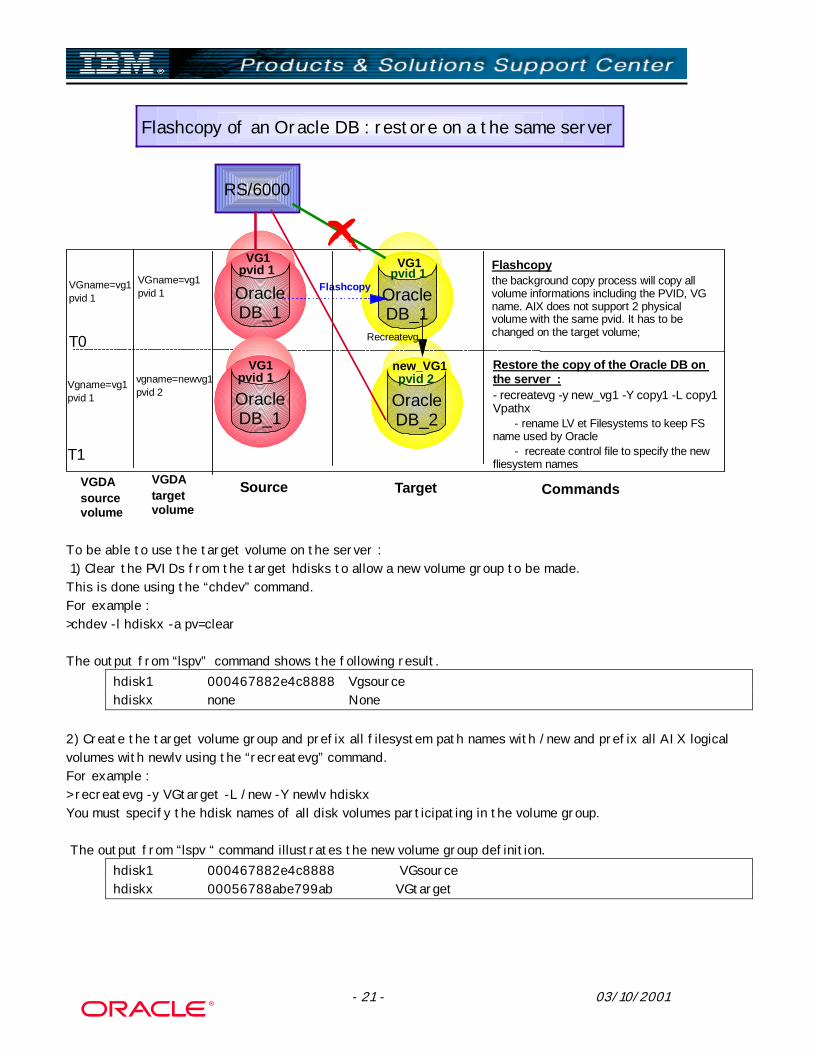
3.3.4. Restore on the same machine Three main actions must be done in order to restore the target database (stored on the flashcopy target volumes) on the same machine running the source database.

1- Backup the control file on the production database 2- Use the recreatevg command on the target volumes 3- Recreate the control file for the target database

- 19 - 03/10/2001

Step 1 : A new control file has to be generated issuing ALTER DATABASE BACKUP CONTROLFILE TO TRACE right after ending hot backup mode on the production Database· This command create a SQL script (recreate.sql in this example) that can be used later to create a new control file for the target database. As the server will access the target database (data files) with a path different from the source database, the previously created file has to be edited and modified so that it points to the right data files. Do not forget (in step 3) to create new INIT.ORA file for the secondary database and to modify the ORACLE_SID variable. Result of an « alter database backup controlfile to trace ; » statement :

Dump file /opt/oracle/v8150/admin/BM/udump/ora_51130_BM.trcOracle8i Enterprise Edition Release 8.1.5.0.0 - ProductionWith the Partitioning and Java optionsPL/SQL Release 8.1.5.0.0 - ProductionORACLE_HOME = /opt/oracle/v8150System name: AIXNode name: asterixRelease: 3Version: 4Machine: 004000134C00Instance name: BMRedo thread mounted by this instance: 1Oracle process number: 24Unix process pid: 51130, image: oracle@asterix (TNS V1-V3)*** SESSION ID:(15.4549) 2001.08.07.12.02.54.000*** 2001.08.07.12.02.54.000# The following commands will create a new control file and use it# to open the database.# Data used by the recovery manager will be lost. Additional logs may# be required for media recovery of offline data files. Use this# only if the current version of all online logs are available.STARTUP NOMOUNTCREATE CONTROLFILE REUSE DATABASE "BM" NORESETLOGS NOARCHIVELOG

MAXLOGFILES 32MAXLOGMEMBERS 2MAXDATAFILES 254MAXINSTANCES 8MAXLOGHISTORY 904

LOGFILEGROUP 1 '/ora/BM/redo01.log' SIZE 80000K,GROUP 2 '/ora/BM/redo02.log' SIZE 80000K

DATAFILE'/ora/BM/system01.dbf','/ora/BM/oemrep01.dbf','/ora/BM/rbs01.dbf','/ora/BM/temp01.dbf','/ora/BM/users01.dbf','/ora/BM/indx01.dbf','/ora/BM/INUB00_DATA01.dbf','/ora/BM/INUB00_IDX01.dbf','/ora/BM/INUB00_IDX02.dbf','/ora/BM/INUB00_IDX03.dbf','/ora/BM/INUB00_DATA02.dbf','/ora/BM/INUB00_DATA03.dbf','/ora/BM/INUB00_DATA04.dbf','/ora/BM/INUB00_IDX04.dbf','/ora/BM/extend/INUB00_DATA05.dbf','/ora/BM/extend/INUB00_DATA06.dbf','/ora/BM/extend/INUB00_IDX05.dbf','/ora/BM/extend/INUB00_DATA07.dbf','/ora/BM/extend/INUB00_DATA08.dbf'

CHARACTER SET US7ASCII

- 20 - 03/10/2001

;# Recovery is required if any of the datafiles are restored backups,# or if the last shutdown was not normal or immediate.RECOVER DATABASE# Database can now be opened normally.ALTER DATABASE OPEN;#

Step 2: Issue a “recreatevg” command on the target volumes To access to the content of the target volume, the Volume Group Descriptor Area (VGDA) of the target volume has to be modified as explained below. The VGDA is located at the beginning of each physical volume. It contains information that describes all the logical volumes and all the physical volumes that belong to the volume group of which that physical volume is a member. Each physical volume has a PV identifier (PVID) as soon as it is integrated in a VG. This PVID is unique to the system. As the flashcopy function copy all the blocks of the source ESS volume (hdisk) on the target volume it will also copy the VGDA of the disk that includes information that must unique for the AIX system (PVID). For the server that has to access to the source and the target volumes, some procedure has to be followed in order to allocate a new PVID to the target volume and to change the names of the volume group, the logical volumes and the filesystems. This procedure can be done running the recreatevg command. This command allocates new physical volume identifiers (PVID) for the member disks. The recreatevg command is packaged as a PTF for AIX 4.3.3 in APAR IY10456 and higher. It is officially available in: - AIX 4.3.3 Recommended Maintenance Level 05 (RML05) - AIX 4.3.3 RML06 It is shipping also in the beta code level AIX 5L As described in the next figure, as soon as the source volume will have been copied to the target volume, this last one will have the same volume group data structures as the source volume.

- 21 - 03/10/2001

Oracle DB_2

VGDAsource volume

Source Target CommandsVGDA target volume

Oracle DB_1

Oracle DB_1

RS/6000

Flashcopy

Recreatevg

pvid 1 pvid 1VGname=vg1pvid 1

T0

VGname=vg1pvid 1

Vgname=vg1pvid 1

T1

vgname=newvg1pvid 2

Flashcopythe background copy process will copy all volume informations including the PVID, VG name. AIX does not support 2 physical volume with the same pvid. It has to be changed on the target volume;

Restore the copy of the Oracle DB on the server :- recreatevg -y new_vg1 -Y copy1 -L copy1 Vpathx

- rename LV et Filesystems to keep FS name used by Oracle

- recreate control file to specify the new fliesystem names

pvid 2

VG1 VG1

new_VG1

Oracle DB_1

pvid 1VG1

Flashcopy of an Oracle DB : restore on a the same server

To be able to use the target volume on the server : 1) Clear the PVIDs from the target hdisks to allow a new volume group to be made. This is done using the “chdev” command. For example : >chdev -l hdiskx -a pv=clear The output from “lspv” command shows the following result.

hdisk1 000467882e4c8888 Vgsource hdiskx none None

2) Create the target volume group and prefix all filesystem path names with /new and prefix all AIX logical volumes with newlv using the “recreatevg” command. For example : > recreatevg -y VGtarget -L /new -Y newlv hdiskx You must specify the hdisk names of all disk volumes participating in the volume group. The output from “lspv “ command illustrates the new volume group definition.

hdisk1 000467882e4c8888 VGsource hdiskx 00056788abe799ab VGtarget

- 22 - 03/10/2001

The filesystem named /base in the source volume group is renamed to /new/base in the target volume group. Notice, also, that the logical volume and JFS log logical volume have been renamed. 3) Mount the new filesystems belonging to the target to make them accessible. Step 3: Modify and execute the SQL script generated in step 1 to recreate the control files for the second database (target) In the controlfiles of the backed up environment, all the datafiles of the database are referenced with their full path. So, if the restore is performed on the same machine in order to duplicate an environment and recreate an other one (for exemple, a « test environment »), datafile name and path will conflict. To solve this problem, the control files of the second database must be re-created using the .sql files generated in step 1 with the « alter database backup controlfile to trace ; » command issued on the SOURCE DB. In summary : � Edit this script and change the paths and/or datafiles name. See « Script of controlfiles re-

creation below». � Create a new ORA.INI file (Use init.ora from the source database and make at least the following

changes: change control-files parameter so that it will point to a new location accessible by the second database) and export the new “ORACLE_SID”

� RUN the modified SQL script (recreate.sql) generated in step 1 on the target database � svrmgrl

• >Connect internal • >startup nomount • >start recreate.sql

Script of controlfiles re-creation :

Some modifications must be done in the file generated by the « alter database backup controlfile to trace ; » statement in order to get a usable script for creation of the second environment controlfiles :

STARTUP NOMOUNTCREATE CONTROLFILE REUSE DATABASE "BM2" NORESETLOGS NOARCHIVELOG

MAXLOGFILES 32MAXLOGMEMBERS 2MAXDATAFILES 254MAXINSTANCES 8MAXLOGHISTORY 904

LOGFILEGROUP 1 '/ora/BM2/redo01.log' SIZE 80000K,GROUP 2 '/ora/BM2/redo02.log' SIZE 80000K

DATAFILE'/ora/BM2/system01.dbf','/ora/BM2/oemrep01.dbf','/ora/BM2/rbs01.dbf','/ora/BM2/temp01.dbf','/ora/BM2/users01.dbf','/ora/BM2/indx01.dbf','/ora/BM2/INUB00_DATA01.dbf','/ora/BM2/INUB00_IDX01.dbf','/ora/BM2/INUB00_IDX02.dbf','/ora/BM2/INUB00_IDX03.dbf','/ora/BM2/INUB00_DATA02.dbf','/ora/BM2/INUB00_DATA03.dbf','/ora/BM2/INUB00_DATA04.dbf','/ora/BM2/INUB00_IDX04.dbf','/ora/BM2/extend/INUB00_DATA05.dbf',

- 23 - 03/10/2001

'/ora/BM2/extend/INUB00_DATA06.dbf','/ora/BM2/extend/INUB00_IDX05.dbf','/ora/BM2/extend/INUB00_DATA07.dbf','/ora/BM2/extend/INUB00_DATA08.dbf'

CHARACTER SET US7ASCII;# Recovery is required if any of the datafiles are restored backups,# or if the last shutdown was not normal or immediate.RECOVER DATABASE# Database can now be opened normally.ALTER DATABASE OPEN;

3.3.5. Restore on a different machine In case the copy of the Oracle database is used on a different server that does not access simultaneously to the source and the target volumes, there is no need to use the recreatevg command (as described in the “Restore on the same machine” paragraph) but just to run a cfgmgr command under AIX, import and vary on the VG (importvg) on this server and mount the database. Don’t forget to first install the Oracle code on this server with the same Oracle user and group (and the same UID and GUID) as the ones used on the primary server.

OracleDB

offline

Time

T0

Source Target

RS/6000 BRS/6000 A

T1

Flashcopyfew seconds

Flashcopyof the OracleDB (in VG1)

InformationsActions

In case of offline backup, the Oracel DB must be shutdown first, and the filesystem unmounted. The target volume must be varied off.Then the flashcopy command is issued and after few seconds (when it returns OK) the source and the target volume can be accessed again.

Copy In case the restore of the target volume is done pn a second server, the VG has just to be varied on on the RS/6000 B and the database to be started up.

Flashcopy of an Oracle DB : restore on a second server

OracleDB Copy

Oracle DB

varyonvg

VG1

VG1 VG1

- 24 - 03/10/2001

3.3.6. Flashcopy Questions and Answers Q1.Is it necessary to shutdown the Oracle database before running a flashcopy of the database volumes Answer : Stopping the database is not a must, when you let your Oracle run in archiveLog mode, when we use BeginBackup etc. / same procedure as for online backup, as the process of FlashCopy needs only a very short time. A point of consistency is only there with the log. Q2. Will the updates done between the begin and the end backup be included in the target volumes ? Answer : Updates between beginBackup and endBackup are NOT supposed to be included in the copy. FlashCopy is like a Polaroid/snapshot, after it has been taken no more updates on the subject will be transferred to the copy. - Flashcopy makes a logical copy to the 'TARGETVOLUMES'. As you normally have several volumes to be flashed, a script/Job is recommended for such a process. Q3. What about the data that is still in memory on the server (Oracle buffers), and in the ESS NVS at the moment of the "begin bakup" command ? Answer : - Data in the memory: Oracle has already written them to the disks(see next point “Q4” ). So this is no issue. - Data in the ESS NVS : This is also no issue, since FlashCopy goes via the cache and would have to use these data first.

Q4 - How can we be sure that all the data of the T0 database is flushed to disk before beginning the real copy ? Does Oracle force the write on disk? Answer : An extra flush is not necessary, since all the data are in both the memory and the disk all the time anyway. Oracle always works in the fsync/o_dsynch mode, so no extra need to switch something on. It works like a flush would have just taken place. Q5. What is sync/fsync Calls Answer : If a file is opened with O_SYNC or O_DSYNC, then each write will cause the data for that write to be flushed to disk before the write returns. If the write causes a new disk allocation (the file is being extended instead of overwriting an existing page), then that write will also cause a corresponding JFS log write. Forced synchronization of the contents of real memory and disk takes place in several ways: • An application program makes an fsync() call for a specified file. This causes all of the pages that contain modified data for that file to be written to disk. The writing is complete when the fsync() call returns to the program.

- 25 - 03/10/2001

• An application program makes a sync() call. This causes all of the file pages in memory that contain modified data to be scheduled for writing to disk. The writing is not necessarily complete when the sync() call returns to the program. • When sync() or fsync() calls occur, log records are written to the JFS log device to indicate that the modified data has been committed to disk. Q5- What to be included in the database FlashCopy copy? what about the active log file ? Answer : For a hot backup, you copy everything except the so-far active logfile, instead of the so far active logfile you would copy the archive log. Reason is that a log switch takes place for the time of an online backup, for this time the so-far active log file is in fact not active anymore. For a cold backup (e.g. to clone your full system, and when there is time to take everything down) on the other hand you just take everything offline and then just copy all the files that you have. Q6- How can I make a copy without making a copy? The answer is, “Use the Nocopy option when defining a flashcopy.” The Nocopy option makes the copied data available immediately after the flashcopy operations (few seconds). Although the target logical disks now contain a “virtual” copy of the source data, ESS may not need to move any data to the target physical disks. The concept is the following : the target physical disk (or the portions of storage of the underlying RAID arrays) merely contain reserved storage, just in case the data needs to be physically copied. The ESS uses the target storage only after a host write operation causes logical source and target data to differ. Until that time, the logical source and target data are identical, and the ESS uses the source physical disks for application read requests. When an application writes data to either source or target, ESS first stores the data in cache, and notifies the application that the write is complete. Some time later, before ESS moves modified data to disk, it also moves an appropriate portion of data from the source to target physical disks. If no write operations occur to a given item of data, then ESS services read requests for either logical copy (source or target) from a single physical image of the data on the source disks.

4. Conclusion In term of database layouts on the ESS, several choices could be done. Not all database environments can be tuned the same way. A good knowledge of the database and of the access types is very useful to choose an efficient implementation. The data placement on the ESS will depends on the data and workloads from one or different kinds of independent servers that will use the ESS. Deciding the placement of your application data within an ESS significantly influences performance. In our data mart case, the isolation method has quite well improved the performances decreasing the RUN elapsed time from 1 hour and 15 minutes to 58 minutes. In other words, we gained 22% for the whole scenario. The flashcopy function works fine with Oracle database either if the database is offline or online.

- 26 - 03/10/2001

5. ANNEXE 1 : ESS

5.1. ESS Architecture

5.1.1. What is the ESS? The IBM Enterprise Storage Server (ESS) is IBM storage product. The ESS uses IBM's Seascape Architecture with advanced hardware and software technologies to deliver breakthrough levels of performance and maximize data sharing across the enterprise. The ESS provides customers scalability and flexibility across many platforms and configurations. The Enterprise Storage Server (ESS) consists of a Storage Server and serial disks (SSA). The Storage server is composed of two Cluster Processor Complexes (clusters), each with four-way RISC SMPs and automatic failover and failback. 10K RPM 9GB, 18GB and 36GB SSA disk devices are supported on eight dual loop SSA adapters, and can be configured as RAID-5 arrays or as JBODs. Usable RAID-5 storage capacities range from 420GB to 11.2TB. The ESS incorporates a fault tolerant design featuring redundancy across all of its major component groups. It offers dynamic sparing, redundant power and cooling, dual AC power, and seven-day battery backup for the NVS. The ESS supports many diverse platforms including the PSeries running AIX and many leading UNIX variants, XSeries and other Intel-based PC servers running Windows NT and Novell Netware, and ISeries running OS/400. In addition, the ESS supports ZSeries. Any combination of these heterogeneous platforms may be used with the ESS. The connectivity options include up to thirty-two ESCON connections for Zseries and SCSI and FC connections for the open world or a combination of the three. The ESS high performance, attachment flexibility and large capacity allow to a consolidate data from different platforms on to a single high performance, high availability box. With a capacity of up to 11 TB and up to 32 host connections, an ESS can meet both high capacity requirements and performance expectations.

5.1.2. Components of the ESS ? The ESS can be broken down into the following components: • The storage server itself is composed of two clusters that provide the facilities with advanced functions to control and manage data transfer. Should one cluster fail, the remaining cluster can take over the functions of the failing cluster.

- 27 - 03/10/2001

Cages / Disk Arrays

DC Power Supplies

RISC Processors +Device Adapters

Host Adapters

Fans / AC-Power

Rack Batteries

A cluster is made up of the following subcomponents: • Host adapters: The ESS has 4 Host Adapter bays, two in each cluster. Each bay supports up to 4 host adapters (HA). The ESS supports up to 32 SCSI ports or ESCON channels or 16 FC adapters. Combination of SCSI, FC and ESCON HA is supported. Each HA is connected to both clusters through the Common Parts Interconnect (CPI) buses. Each cluster can handle I/O from any HA. • Device adapters: The ESS uses the SSA 160 technology in its device adapters. Each device adapter card supports two independent SSA loops. There are four pairs of device adapters in an ESS. Disk drives are attached to a pair of device adapters, one in each cluster, so that the drives are accessible from either cluster. At any given time, a disk drive is managed by only one device adapter. • Cluster complex: The cluster complex provides the management functions for the ESS. It consists of cluster processors, cluster memory, cache, nonvolatile storage (NVS) and related logic: • Cluster processors: The cluster complex contains four cluster processors (CP) configured as symmetrical multiprocessors (SMP). The cluster processors execute the licensed internal code that controls operation of the cluster. • Cluster memory / cache: These are used to store instructions and data for the cluster processors. The cache memory is used to store cached data from the disk drives. The cache memory is accessible by the local cluster complex, by device adapters in the local cluster, and by host adapters in either cluster. • Nonvolatile storage (NVS): This is used to store a nonvolatile copy of active written data. The NVS is accessible to either cluster-processor complex and to host adapters in either cluster. Data may also be transferred between the NVS and cache. • The disk drives : They are grouped into ranks and are managed by the clusters. The ranks can be configured as RAID 5 or non-RAID arrays (Just a Bunch of Disks -- JBOD).

- 28 - 03/10/2001

5.1.3. Disks and ranks As illustrated in the figure below, the disks are installed in group of 8 disks (‘8-packs’). Each group of 8 disks is configured as :

• RAID rank of 6 (6 disks for data) + P (1 parity disk) + S (1 spare disk) • RAID rank of 7 (7 disks for data) + P (parity disk) • JBOD (Just a Bunch Of Disks) - no parity

Disk InterfaceArrays Arrays Arrays

Arrays Arrays Arrays

Arrays Arrays Arrays

Arrays Arrays Arrays

Arrays Arrays Arrays

Arrays Arrays Arrays

Arrays Arrays Arrays

Arrays Arrays Arrays

SSA160

SSA160

SSA160

SSA160

cluster 2CACHE NVS

CACHENVScluster 1

ArraysArraysArrays

ArraysArraysArrays

ArraysArraysArrays

ArraysArraysArrays

ArraysArraysArrays

ArraysArraysArrays

ArraysArraysArrays

ArraysArraysArrays

SSA160

SSA160

SSA160

SSA160

upperinterfaces

controllers

lowerInterfaces

up to 48disk arrays

dual-active4-way SMP

eight SSAdisk adapters

up to 16host adapters

RAID 56+p+s& 7+p

Rank types : • RAID-rank :

The rank is composed of 8 disks. Each rank is formatted as a set of logical volumes. Here, a « logical volume » is equivalent to an AIX hdisk (see figure below). The number of LV in a rank depends on the capacity of the disks in the array. LV are striped across all the data and parity disks in the array.

- 29 - 03/10/2001

Disk Interface

SSA160

SSA160

SSA160

SSA160

cluster 2CACHE NVS

CACHENVScluster 1

SSA160

SSA160

SSA160

SSA160

Raid Rank Raid Rank Raid Rank Raid Rank

Raid Rank Raid Rank

Raid Rank Raid Rank

LSS10

R aid Rank

LSS15LSS14

LSS13LSS12

LSS11

R aid R ank

LSS16 LSS17

FCS1A0-58

FCS2D0-58

FCS3E0-58

Creating an ESS logical volume on a RAID Array (or rank)

9 GB

AIX sees 1 hdisk for this 9GB volum e

RAID Rank : 8 physical disk

9 GB ESS Logical Volum e or LUN

• Non-RAID rank Each disk in the group of 8 is a rank (so, there are 8 ranks in a JBOD group). Each disk is

formatted as a set of logical volumes. A JBOD rank is not RAID-protected.

Following disks can be used within an 8-pack: • 9.1 GB - 10000 RPM (for highest performance) • 18.2 GB - 10000 RPM (for high performance and capacity) • 36,4 GB - 10000 RPM (for high capacity and standard performance)

5.1.4. ESS advanced Copy Services Copy Services is a separately sold feature of the Enterprise Storage Server. It brings powerful data copying and mirroring technologies to Open Systems environments previously available only for mainframe storage. Two features of Copy Services for the Open Systems environment: • Peer-to-Peer Remote Copy (PPRC) • FlashCopy PPRC is a synchronous protocol that allows real-time mirroring of data from one Logical Unit (LUN) to another LUN in another ESS. This secondary ESS can be located at another site some distance away. PPRC is application independent. Because the copying function occurs at the disk subsystem level, the application has no knowledge of its existence.

- 30 - 03/10/2001

The PPRC protocol guarantees that the secondary copy is up-to-date by ensuring that the primary copy will be written only if the primary receives acknowledgment that the secondary copy has been written. FlashCopy makes a single point-in-time (T0) copy of a LUN. The target copy is available once the FlashCopy command has been processed. FlashCopy provides an instant or point-in-time copy of an ESS logical volume. Point-in-time copy functions give you an instantaneous copy, or “view”, of what the original data looked like at a specific point-in-time. This is known as the T 0 (time-zero) copy. The point-in-time copy created by FlashCopy is typically used where you need a copy of production data to be produced with minimal application downtime. It can be used for online backup, testing of new applications, or for creating a database for data mining purposes. The copy looks exactly like the original source volume and is an instantly available, binary copy.

5.2. ESS rules 5.2.1. General considerations:

The data placement on the ESS will depends on the data and workloads from one or different kinds of independent servers that will use the ESS. Sharing resource in ESS has advantages for storage administration and resource sharing, but does have some implications for workload planning. Resource sharing has the benefit that a larger resource pool (e.g. disk drives or cache) is available for critical applications. However, some care should be taken to ensure that uncontrolled or unpredictable applications do not interfere with mission critical work. This requires the same kind of workload planning you use when mixing various types of work on a server. If your workload is truly ’mission critical’, you may want to consider isolating it from other workloads. This is particularly true if other workloads are unimportant (from a performance perspective) or very unpredictable in their demands. In general, try to use as many ranks as possible for your application or database. Using many ranks makes the cumulative bandwidth of all ranks available to the system. Each rank is primarily assigned to one of the two clusters of the ESS. Try to balance the number of used ranks between Cluster 1 and 2. This way, the resources (e.g., cache and NVRAM) are equally exploited on both clusters. Similarly, try to use ranks from as many device adapter pairs and SSA loops as possible. This again yields the cumulative bandwidth of all resources. The size of the volumes allocated on the ESS does not influence performance. To limit the number of physical volumes to administrate on host side (and thereby to limit the number of volume groups), the ESS volumes should be chosen large enough. Use all ESS adapters that you have or as many as possible for a certain server or application, in order to prevent bottlenecks that could occur if too few adapters are used. The flexibility of assigning ESS volumes to hosts systems, host adapters, and finally volume groups increases with smaller ESS volumes. The subsystem device driver (SDD, formerly DPO) can be used for load balancing and fail over purposes. It offers the option to use more than one SCSI/FC path from an ESS volume to the host system. As explained into details in the “IBM Enterprise Storage Server Performance Monitoring and Tuning Guide”, deciding the placement of your application data within an ESS significantly influences performance. Different method can be followed to place data on an ESS:

- 31 - 03/10/2001

5.2.1.1. The Balanced Method.

With this approach, try to use all of the available resources within an ESS in a balanced fashion: RAID arrays, disk adapters, clusters, memory buses, and host interfaces. The key advantages of striping are that it: balances work across disks, allows parallel access, and eliminates bottlenecks on individual disks. Applications see the benefits of faster access to “hot” databases on “hot” logical disks accessed by concurrent users and transactions. To balance the activity across the 2 clusters, Use at least two SCSI or FC ports from your Server to access to the ESS. When selecting SCSI, or fibre channels to assign to a given server or processor, spread them across the four adapter bays. Attempt to balance total I/O activity across the bays.

5.2.1.2. The Isolation Method. With this approach, isolate application data or specific tables or objects of a database on a specific set of RAID arrays, SSA loops, device adapter, ESS cluster within ESS, thereby avoiding the sharing of resources with other applications using the ESS. This will isolate use of memory buses, microprocessors, and cache resource. Use this approach with care, and only when you have done a very careful job of matching the workload requirements with the capabilities within the components of the ESS. In order to illustrate the impact of those methods, and what kind of performance gains could be obtained, we have used both methods for the same database environment.

- 32 - 03/10/2001

6. ANNEXE 2 : AIX Concepts

6.1. -AIX logical volume manager (LVM) overview The set of operating system commands, library subroutines and other tools that allow you to establish and control logical volume storage is called the Logical Volume Manager (LVM). The LVM controls disk resources by mapping data between a more simple and flexible logical view of storage space and the actual physical disks

6.1.1. AIX storage structures (VG, PV, LV …) The four basic logical storage concepts are : Physical volumes, volume groups, physical partition and logical volumes. Each individual fixed disk is called « Physical Volume » (PV) and has a name (for example hdisk0). An ESS logical volume (or LUN) is seen as a physical volume (hdisk) by the AIX system. The PVs are grouped in « Volume groups » (VG) as shown in the figure below. A VG is composed of one or more PV.

PVPV

PVPhys.Volume

VG

An hdisk could be :

Internal disk

ESS logical volumeor LUN

SSA disk

hdisk0

hdiskn

hdisk1

All of the physical volumes in a volume group are divided into physical partitions (PP) of the same size. Within each volume group, one or more logical volumes (LV) are defined. A LV can reside in only one VG and it can reside on one or more disks inside the VG. Logical volumes provide the mechanism to make disk space available for use, giving users and applications the ability to access data stored on them. A file system is a set of files, directories and other structures. File systems maintain information and identify the location of a file or directory’s data. The Journaled File system is the native file system type of AIX. Each journaled file system resides on separate logical volume.

6.1.2. striping (physical partition stripping, LVM fine stripping)

Striping, available in AIX Version 4, is a technique for allocating the data in a logical volume evenly across several disk drives. This allows for more parallel access to the data in the logical volume. Striping is designed to increase the read/ write performance of frequently accessed files.

- 33 - 03/10/2001

So, the striping is a way to spread data contained in a Logical Volume across many disks (at least two) ; therefore, I/Os can run in parallel to access data.

Physically, in a non-striped LV, blocks as distributed as shown hereunder:

19 212023222625

2427

2 4

31 6 5

8 7 913

1110 121514

1716 18

In a striped logical volume, blocks are distributed as following:

3 9615122421

1827

410

711613

2219 2511

52 81714

2320 26

The AIX LVM provides two different techniques for striping data : Physical Partition (PP) striping and LVP striping What is the “Physical Partition (PP) striping”?

Physical partition striping refers to the technique of spreading the physical partitions of a logical volume across 2 or more physical disk drives. With PP striping, the size of the data stripe is the size of the physical partition, which is typically 4,8 or 16 MB. The PP size must be at least 1 MB. Generally, the PP size should be set as small as possible, subject to AIX restrictions. As of AIX 4.3.2, there can be no more than 1016 PPs per physical device. This needs to be taken into consideration for high capacity drives to ensure that the PP size chosen does not result in the limit of PPs per device being reached. Logical volume striping can improve I/O performance by distributing I/O load. A heavily accessed logical volume can be striped by spreading it across multiple physical volumes on a physical partition level. Striping at a physical partition level might effectively distribute I/O load due to random access of data within a tablespace. In the statement of logical volume creation, the physical volumes participating to the LV are entered and the option defining the range of physical volume used for the LV among the physical volumes chosen is set to « maximum ». So, the LV will be distributed across all the PV using « blocks » of the PP size.

- 34 - 03/10/2001

What is the “LVM striping”? Also known as fine striping, it attempts to distribute the I/O load by placing data stripes on multiple physical disks. However LVM striping differs from PP stripping in its use of a more granular or fine data stripe. The stripe unit size must be a power of 2 in the range of 4 KB to 128 KB and is specified when the logical volume is created.

- 35 - 03/10/2001

7. ANNEXE 3 : ORACLE Concepts

7.1. Oracle overview Objects contained in a Oracle database (tables, indexes etc...) are stored in tablespaces. A tablespace is composed of 1 to n datafiles.

Database

Tablespace

Table Index...

OS File

divided in

componed of

contains

hdiskcreated on

7.1.1. Objects and dependencies This paragraph lists Oracle objects and explains the general I/O characteristics of the major Oracle database files:

7.1.1.1. Redologs

Redologs & data : Separate redologs from data and indexes The log file contains recovery information. Redolog files maintain a high writing rate since every single committed transaction requires a redolog entry record to support recovery processes. If these files are on common disks, then there is potential for disk contention. When data is inserted or modified, both data files and redolog files will require a write operation. Keeping the redo log files on separate disks from data files will avoid impacting other write operations. This advice should be followed when updates and inserts take place...

- 36 - 03/10/2001

Redologs & archivelog mode : Place redologs and archivelog on different disks In archivelog mode the redologs and archivelog must be placed on different disks. During archiving, simultaneously, on one hand, the disk where is located the current redolog is read, and, on the other hand, the disk of destination of archived redolog is written. So, it is better to separate redologs from their archive. Multiplexed redolog : Separate sets of multiplexed redologs For security reasons, redologs can be multiplexed (for example : 2 groups of 3 redologs members) ; in this case, there are two current redologs and they’re accessed simultaneously. So, these two sets of redologs should be placed on a separate disks (for performance and security, which is the first goal of multiplexing !).

7.1.1.2. Rollback segments

Dedicate disk(s) for rollback segments When transactions containing insert, update and delete statements are performed, undo is written in the rollback segments. So, since rollback segments are continuously accessed where writes occur in the database, they should reside on dedicated disks. Separate redologs and rollback segments Since redologs and rollback segments are both continuously accessed when update and insert and delete activity take place, they must be separate one from each other.

7.1.1.3. Data and indexes

Separate data from their indexes When indexes exist on a table both read and write operations will eventually require to access both structures in the same transaction. When the data files that keep the tables are stored in different disks separated from index data files the operating system will be able to perform simultaneous operations reducing the contention in the I/O system.

Spread heavy-accessed data and indexes The goal of the tuning process is to spread I/O, so, simultaneously heavy-accessed data (and indexes) should not reside on same disks and should be, as far as possible, spread accross several disks.

7.1.1.4. Other components

System tablespace. The system tablespace is usually not very accessed. So, it can resides with other datafiles... Temporary tablespace. The temporary tablespace is mainly used for sorts. So, it requires attention if many and large sorts are performed (typically, in Decisional environment).

- 37 - 03/10/2001

6.1.5 Summary

Although it may not be practical for small Oracle installations, try to isolate each of the major types of Oracle data files (see the rules of implementation section) on their own sets of disks. Here is a summary of the main Oracle data files and their use : Access

Type Recommendations and explanations

Data Sequential Read/ Write or Random Read/Write

If indexes are correctly used, they are read first before accessing to data. So, it could be possible to place data and indexes on the same disk. As several user sessions can access the same data, it can generate I/O activities at the same time on data1 and IDX_data1 and so I/O contention. So, if possible, separate data from their indexes.

IDX_data Random Read/Write Sequential Read/Write

In OLTP environment, Intensive random read (select using index) or write (each time an insert, update, delete is executed) are done on index files. Sequential access can occur on index file each time an “index scan” is done.

Redo Logs Sequential Read / Write

The log file is heavily used in update-intensive environments. The log file contains recovery information. If there are no updates to the database, there is no data to write to the log file. The data is written sequentially to the Redo log file. Data warehousing environments that have high read content do not stress log files. In this case, feel free to mix logs and data on RAID arrays. Consider isolating log files on separate arrays for high volume write-intensive environment

Archivelog Sequential Write

Log and Archivelog files tend to be used at the same time. For instance during archiving, the online redo log is being read at the same time the archive log file is being written. If both the online redo log file and the archive log file are on the same disk, there may be I/O contention on this disk or array due to the concurrent access of both files. Try to isolate archivelog from Redo log files.

RBS Semi-sequential Read/Write

Contains a before image of all database block updates. In OLTP environments with significant update activity, rollback segments can experience a great deal of read/write activity. In Datawarehouse environment RBS are less used.

TEMP sequential Read/write

Used to contain sort segments when sorts are too large to be performed entirely in memory. Sort segment blocks tend to be written (and then read) sequentially. For Oracle environments, which perform a large number of sorts, performance can be significantly impacted by temp file placement

- 38 - 03/10/2001

7.2. Implementing Oracle database on AIX

7.2.1. File-systems & raw-devices The utilization of file-system vs raw-devices generates a fair amount of debate from time to time. Some of the reasons for the debate are:

• the file-systems are continually improved and can provide better I/O performance than raw-devices.

• the difficulty of raw-devices administration decreases because more powerful LVM interfaces eases the configuration and backup of raw partitions.

No official message are found on the subject. However, some customers like to use UNIX commands which only work on filesystem files. Data files of a database can be located on file systems or raw-devices. A file system can contain 1 or n data files. Only one data file can be placed on a raw-device.

Here are the syntaxes of creation of tablespaces (file-system vs raw-device) : File-system :

create tablespace EMPLOYEE_DATA datafile («/data/employee/empl1.dbf»size 500M, «/data/employee/empl2.dbf» size 500M) ;

Raw_device :create tablespace EMPLOYEE_DATAdatafile («/dev /rlv_empl1» size 500M,«/dev/rlv_empl2» size 500M) ;

7.2.2. Striping It is advise by Oracle to use stripe size of 32 or 64KB because these values are good for most workloads. The stripe size must be a multiple of the database block size. Striping should be used to implement data files allowing parallel access to data across many disks and reducing potential I/O contention.

7.2.3. Asynchronous I/O

Synchronous I/O occurs while you wait. An application’s processing cannot continue until the I/O operation is complete. In contrast, asynchronous I/O operations run in the background and do not block user applications. This improves performance, because I/O operations and applications processing can run simultaneously. Many applications, such as databases and file servers, take advantage of the ability to overlap processing and I/O. Depending on the distribution of I/O requests across the disks, AIO can effectively interleave multiple I/O operations to improve I/O subsystem throughput. When running Oracle on AIX, asynchronous I/O (AIO) should be used (smitty aio). Generally, AIO results in faster database access.

- 39 - 03/10/2001

The AIX parameters minservers (number of AIO servers started) and maxservers (maximum number of AIO that can be started) should be tuned. The use of AIO is enabled for Oracle via the parameter ‘use_async_io’ (v7) or ‘disk_asynch_io’ (v8) set to true.

- 40 - 03/10/2001

8. ANNEXE 4 : Oracle DB layout

The goal of this paragraph is to present some general rules of implementation on disks of a database. The fastest way that Oracle can read or modify a block is when the information is already loaded in memory in the buffer cache. When this does not occur, Oracle will need to read the information directly from the data file incurring I/O operations, which usually are much more expensive. When data is retrieved from the physical disk, disk contention must be reduced. Disk contention occurs when multiple processes try to access the same disk simultaneously. Disk contention can be reduced, thereby increasing performance, by distributing the disk I/O more evenly over the available disks. Decreasing disk I/O can also reduce disk contention.

8.1.1. Oracle rules of implementation

Data warehouse and OLTP systems have vastly different requirements. Here are some examples of the notable differences between typical data warehouses and OLTP systems: A typical data warehouse query may scan thousands or millions of rows. For example, "Find the total sales for all customers last month." A typical OLTP operation may access only a handful of records. For example, "Retrieve the current order for a given customer." The rules of implementation change some how with the type of workload. The 2 next figures will give a synthesis of the database objects possible cohabitation: What can be stored on the same disk, what can be an alternative if there are not enough different disk to separate all the database objects and what shouldn’t been mixed on the same disk.

8.1.1.1. Decisional support system (DSS)

This first table deals with DSS environment and gives a matrix of objects (data, indexes, Log …) layout on disk. In the table below, - Data1 = I/O intensive table - Sequential Access - Data2 = lI/O intensive table - Random access - Data3 = low I/O activity In this table, we consider that the type of query run against the database is mainly « select » sql order (DSS environment).

- 41 - 03/10/2001

Data Layout for DSS environment

Not recommendedOK Possible

Data1 IDX_data1 Data2 IDX_data2 Data3 IDX_data3 LOGset 1

LOG set 2 Archivelog RBS TEMP

Data1 N/AIDX_data1 N/AData2 N/AIDX_data2 N/AData3 N/AIDX_data3 N/ALOG set 1 N/ALOG set 2 N/AArchivelog N/ARBS N/ATEMP N/A

In DSS environment, I/O access is usually read access (select) except for sort operations that generate write access on the “TEMP” files. So Log files are not frequently used. That’s the reason why the log files could be mixed with data files. Nevertheless, if could happen that DSS queries include table creations (for example “create table as select”), so write operations. If it generates an important write activity, you’ll prefer the rules described in the OLTP paragraph for the LOG, RBS and Archivelog files.

- 42 - 03/10/2001

8.1.1.2. Online Transaction Processing (OLTP)

The main differences between DSS and OLTP environment is the type of I/O access (sequential/random), the percentage of read and write requests and the intensity of some object . For example, In OLTP environment, LOG and RBS files are heavily used and TEMP file are lightly used. For DSS (or data warehouse) environment, it is the contrary: queries usually generate a lot of sorts (using TEMP file) and have high read content so, do not stress log.

Data Layout for OLTP environment

Data1 = I/O intensive table - Random AccessData2 = lI/O intensive tableData3 = low I/O activity

Yellow columns and rows = the main changes beteween OLTP and DTWH

OK

Possible

Not recommended

Data1 IDX_data1 Data2 IDX_data2 Data3 IDX_data3 LOGset 1

LOGset 2 Archivelog RBS TEMP

Data1 N/AIDX_data1 N/AData2 N/AIDX_data2 N/AData3 N/AIDX_data3 N/ALOG set 1 N/ALOG set 2 N/AArchivelog N/ARBS N/ATEMP N/A

- 43 - 03/10/2001

9. ANNEXE 5 : Bibliography Redbooks : - IBM Enterprise Storage Server - Performance Monitoring and Tuning Guide - IBM Storwatch ESS Expert : Hands-on usage Guide

- Implementing ESS Copy Services on UNIX and Windows NT Performance of Enterprise Storage Server F Model in Open Systems Environments : Planning and Configuration Considerations written by IBM SSD Performance Team Oracle8 I Designing and Tuning for Performance Release 2 (8.1.6) “Oracle8 backup and recovery handbook” written by Rama Velpuri and Anand Adkoli