Ghahramani 2015 Nature - Apollo Home

Probabilistic machine learning and artificial intelligence

Zoubin GhahramaniUniversity of Cambridge

May 28, 2015

This is the author version of the following paper published by Nature on 27 May, 2015:

Ghahramani, Z. (2015) Probabilistic machine learning and artificial intelligence. Nature521:452–459.

How can a machine learn from experience? Probabilistic modelling provides a frame-

work for understanding what learning is, and has therefore emerged as one of the

principal theoretical and practical approaches for designing machines that learn from

data acquired through experience. The probabilistic framework, which describes how

to represent and manipulate uncertainty about models and predictions, plays a central

role in scientific data analysis, machine learning, robotics, cognitive science, and artifi-

cial intelligence. This article provides an introduction to this probabilistic framework,

and reviews some state-of-the-art advances in the field, namely, probabilistic program-

ming, Bayesian optimisation, data compression, and automatic model discovery.

Introduction

The key idea behind the probabilistic framework to machine learning is that learning can be thought

of as inferring plausible models to explain observed data. A machine can use such models to make

predictions about future data, and decisions that are rational given these predictions. Uncertainty

plays a fundamental role in all of this. Observed data can be consistent with many models, and

therefore which model is appropriate given the data is uncertain. Similarly, predictions, about

future data and the future consequences of actions, are uncertain. Probability theory provides a

framework for modelling uncertainty.

This article starts with an introduction to the probabilistic approach to machine learning and

Bayesian inference, and then reviews some of the state-of-the-art in the field. The central thesis

is that many aspects of learning and intelligence depend crucially on the careful probabilistic

representation of uncertainty. Probabilistic approaches have only recently become a main-stream

paradigm in artificial intelligence [1], robotics [2], and machine learning [3, 4]. Even now, there is

controversy in these fields about how important it is to fully represent uncertainty. For example,

1

recent advances using deep neural networks to solve challenging pattern recognition problems such

as speech recognition [5], image classification [6, 7], and prediction of words in text [8], do not overtly

represent the uncertainty in the structure or parameters of those neural networks. However, my

focus will not be on these types of pattern recognition problems, characterised by the availability

of large amounts of data, but rather on problems where uncertainty is really a key ingredient, for

example where a decision may depend on the amount of uncertainty.

In particular, I highlight five areas of current research at the frontiers of probabilistic machine learn-

ing, emphasising areas which are of broad relevance to scientists across many fields: (1) Probabilis-

tic programming—a general framework for expressing probabilistic models as computer programs,

which could have a major impact on scientific modelling; (2) Bayesian optimisation—an approach to

globally optimising unknown functions; (3) Probabilistic data compression; (4) Automating the dis-

covery of plausible and interpretable models from data; and (5) Hierarchical modelling for learning

many related models, for example for personalised medicine or recommendation. While significant

challenges remain, the coming decade promises substantial advances in artificial intelligence and

machine learning based on the probabilistic framework.

1 Probabilistic modelling and the representation of uncertainty

At a most basic level, machine learning seeks to develop methods for computers to improve their

performance at certain tasks based on observed data. Typical examples of such tasks might include

detecting pedestrians in images taken from an autonomous vehicle, classifying gene-expression

patterns from leukaemia patients into subtypes by clinical outcome, or translating English sentences

into French. However, as we will see, the scope of machine learning tasks is even broader than

these pattern classification or mapping tasks, and can include optimisation and decision making,

compressing data, and automatically extracting interpretable models from data.

Data are the key ingredient of all machine learning systems. But data, even so called “Big Data”,

are useless on their own until one extracts knowledge or inferences from them. Almost all machine

learning tasks can be formulated as making inferences about missing or latent data from the ob-

served data—we will variously use the terms inference, prediction or forecasting to refer to this

general task. Elaborating the example mentioned above, consider classifying leukaemia patients

into one of the four main subtypes of this disease, based on each patient’s measured gene-expression

patterns. Here the observed data are pairs of gene-expression patterns and labelled subtypes, and

the unobserved or missing data to be inferred are the subtypes for new patients. In order to make

inferences about unobserved data from the observed data, the learning system needs to make some

assumptions; taken together these assumptions constitute a model. A model can be very simple

2

and rigid, such as a classical statistical linear regression model, or complex and flexible, such as

a large and deep neural network or even a model with infinitely many parameters. We return to

this point in the next section. A model is considered to be well-defined if it can make forecasts or

predictions about unobserved data having been trained on observed data (otherwise, if the model

can’t make predictions it can’t be falsified, in the sense of Karl Popper, or as Wolfgang Pauli said

the model is “not even wrong”). For example, in the classification setting, a well-defined model

should be able to provide predictions of class labels for new patients. Since any sensible model will

be uncertain when predicting unobserved data, uncertainty plays a fundamental role in modelling.

There are many forms of uncertainty in modelling. At the lowest level, model uncertainty is

introduced from measurement noise, e.g., pixel noise or blur in images. At higher levels, a model

may have many parameters, such as the coefficients of a linear regression, and there is uncertainty

about which values of these parameters will be good at predicting new data. Finally, at the highest

levels, there is often uncertainty about even the general structure of the model: is linear regression

appropriate or a neural network, if the latter, how many layers, etc.

The probabilistic approach to modelling uses probability theory to express all forms of uncertainty

[9]. Probability theory is the mathematical language for representing and manipulating uncertainty

[10], in much the same way as calculus is the language for representing and manipulating rates of

change. Fortunately, the probabilistic approach to modelling is conceptually very simple: probabil-

ity distributions are used to represent all the uncertain unobserved quantities in a model (including

structural, parametric, and noise-related) and how they relate to the data. Then the basic rules

of probability theory are used to infer the unobserved quantities given the observed data. Learn-

ing from data occurs through the transformation of the prior probability distributions (defined

before observing the data), into posterior distributions (after observing data). The application of

probability theory to learning from data is called Bayesian learning (Box 1).

Apart from its conceptual simplicity, there are several appealing properties of the probabilistic

framework for machine intelligence. Simple probability distributions over single or a few variables

can be composed together to form the building blocks of larger more complex models. The domi-

nant paradigm in machine learning over the last two decades for representing such compositional

probabilistic models has been graphical models [11], with variants including directed graphs (a.k.a.

Bayesian networks and belief networks), undirected graphs (a.k.a. Markov networks and random

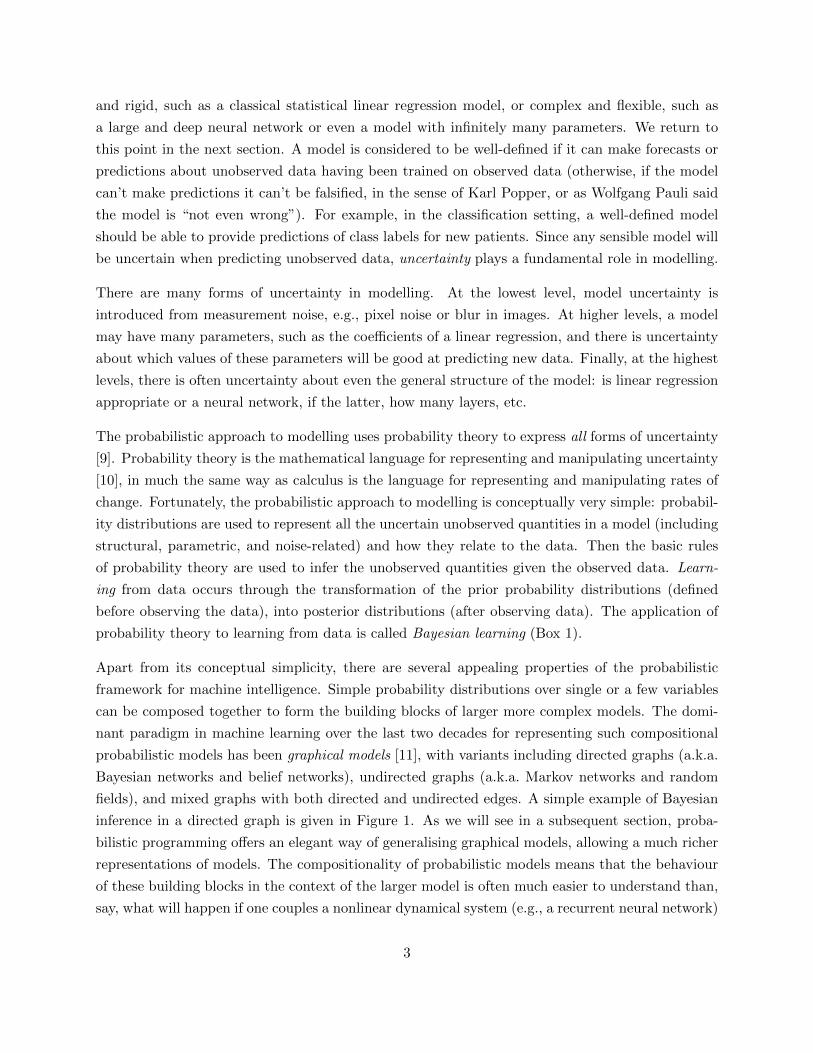
fields), and mixed graphs with both directed and undirected edges. A simple example of Bayesian

inference in a directed graph is given in Figure 1. As we will see in a subsequent section, proba-

bilistic programming offers an elegant way of generalising graphical models, allowing a much richer

representations of models. The compositionality of probabilistic models means that the behaviour

of these building blocks in the context of the larger model is often much easier to understand than,

say, what will happen if one couples a nonlinear dynamical system (e.g., a recurrent neural network)

3

to another. In particular, for a well-defined probabilistic model, it is always possible to generate

data from the model; such “imaginary” data provide a window into the “mind” of the probabilistic

model, helping us understand both the initial prior assumptions and what the model has learned

at any later stage.

Probabilistic modelling also has some conceptual advantages over alternatives as a normative theory

for learning in artificially intelligent (AI) systems. How should an AI system represent and update

its beliefs about the world in light of data? The Cox axioms define some desiderata for representing

beliefs; a consequence of these axioms is that ‘degrees of belief’, ranging from “impossible” to

“absolutely certain”, must follow all the rules of probability theory [12, 10, 13]. This justifies the use

of subjective Bayesian probabilistic representations in AI. An argument for Bayesian representations

in AI that is motivated by decision theory is given by the Dutch-Book theorems. The argument

rests on the idea that the strength of beliefs of an agent can be assessed by asking the agent whether

it would be willing to accept bets at various odds (ratios of payoffs). The Dutch-Book theorems

state that unless an AI system’s (or human’s, for that matter) degrees of beliefs are consistent

with the rules of probability it will be willing to accept bets that are guaranteed to lose money

[14]. Because of the force of these and many other arguments on the importance of a principled

handling of uncertainty for intelligence, Bayesian probabilistic modelling has emerged not only as

the theoretical foundation for rationality in AI systems but also as a model for normative behaviour

in humans and animals [15, 16, 17, 18] (but see [19] and [20]), and much research is devoted to

understanding how neural circuitry may be implementing Bayesian inference [21, 22].

Although conceptually simple, a fully probabilistic approach to machine learning poses a number

of computational and modelling challenges. Computationally, the main challenge is that learning

involves marginalising (i.e., summing out) all the variables in the model except for the variables of

interest (c.f. Box 1). Such high-dimensional sums and integrals are generally computationally hard,

in the sense that for many models there is no known polynomial-time algorithm for performing

them exactly. Fortunately, a number of approximate integration algorithms have been developed,

including Markov chain Monte Carlo (MCMC) methods, variational approximations, expectation

propagation, and sequential Monte Carlo [23, 24, 25, 26]. It’s worth noting that computational

techniques are one area where Bayesian machine learning differs from much of the rest of machine

learning: for Bayesians the main computational problem is integration, whereas for much of the

rest of the community the focus is on optimisation of model parameters. However, this dichotomy

is not as stark as it appears: many gradient-based optimisation methods can be turned into in-

tegration methods through the use of Langevin and Hamiltonian Monte Carlo methods [27, 28],

while integration problems can be turned into optimisation problems through the use of variational

approximations[24]. We revisit optimisation in a later section.

The main modelling challenge for probabilistic machine learning is that the model should be flexible

4

enough to capture all the properties of the data required to achieve the prediction task of interest.

One approach to addressing this challenge is to develop a prior that encompasses an open-ended

universe of models that can adapt in complexity to the data. The key statistical concept underlying

flexible models that grow in complexity with the data is nonparametrics.

2 Flexibility through nonparametrics

One of the lessons of modern machine learning is that the best predictive performance is often

obtained from highly flexible learning systems, especially when learning from large data sets. Flex-

ible models can make better predictions because to a greater extent they allow data to “speak for

themselves”.1 There are essentially two ways of achieving flexibility. The model could have a large

number of parameters compared to the data set (for example, the neural network used recently to

achieve near-state-of-the-art translation of English and French sentences is a probabilistic model

with 384 million parameters [29]). Alternatively, the model can be defined using nonparametric

components.

The best way to understand nonparametric models is through comparison to parametric ones. In a

parametric model, there are a fixed finite number of parameters, and no matter how much training

data are observed, all the data can do is set these finitely-many parameters that control future

predictions. In contrast, nonparametric approaches have predictions that grow in complexity with

the amount of training data, either by considering a nested sequence of parametric models with

increasing numbers of parameters or by starting out with a model with infinitely many parameters.

For example, in a classification problem, whereas a linear (i.e., parametric) classifier will always

predict using a linear boundary between classes, a nonparametric classifier can learn a nonlinear

boundary whose shape becomes more complex with more data. Many nonparametric models can be

derived starting from a parametric model and considering that happens as the model grows to the

limit of infinitely many parameters [30]. Clearly, fitting a model with infinitely many parameters

to finite training data would result in “overfitting”, in the sense that the model’s predictions might

reflect quirks of the training data rather than regularities that can be generalised to test data.

Fortunately, Bayesian approaches are not prone to this kind of overfitting since they average over,

rather than fit, the parameters (c.f. Box 1). Moreover, for many applications we have such huge

data sets that the main concern is underfitting from the choice of an overly simplistic parametric

model, rather than overfitting.

A review of Bayesian nonparametrics is outside the scope of this article (see for example [31, 32, 9]),

1But note that all predictions involve assumptions and therefore the data are never exclusively “speaking forthemselves”.

5

but it’s worth mentioning a few of the key models. Gaussian processes (GPs) are a very flexible

nonparametric model for unknown functions, and are widely used for regression, classification, and

many other applications that require inference on functions [33]. Consider learning a function

relating the dose of some chemical to the response of an organism to that chemical. Instead

of modelling this relationship with, say, a linear parametric function, a GP could be used to

directly learn a nonparametric distribution of nonlinear functions consistent with the data. A

notable example of a recent application of Gaussian processes is GaussianFace, a state-of-the-art

approach to face recognition that outperforms humans and deep learning methods [34]. Dirichlet

processes (DPs) are a nonparametric model with a long history in statistics [35] and are used for

density estimation, clustering, time series analysis, and modelling the topics of documents [36]. To

illustrate DPs, consider an application to modelling friendships in a social network, where each

person can belong to one of many communities. A DP makes it possible to have a model where

the number of inferred communities (i.e., clusters) grows with the number of people [37]. DPs have

also been used for clustering gene expression patterns [38, 39]. The Indian buffet process (IBP)

[40] is a nonparametric model which can be used for latent feature modelling, learning overlapping

clusters, sparse matrix factorisation, or to nonparametrically learn the structure of a deep network

[41]. Elaborating the social network modelling example, an IBP-based model allows each person

to belong to some subset of a large number of potential communities (e.g., as defined by different

families, workplaces, schools, hobbies, etc) rather than a single community, and the probability of

friendship between two people depends on the number of overlapping communities they have [42]. In

this case, the latent features of each person correspond to the communities, which are not assumed

to be observed directly. The IBP can be thought of as a way of endowing Bayesian nonparametric

models with “distributed representations” as popularised in the neural network literature [43]. An

interesting link between Bayesian nonparametrics and neural networks is that, under fairly general

conditions, a neural network with infinitely many hidden units is equivalent to a Gaussian process

[44]. Note that the above nonparametric components should be thought of again as building blocks,

which can be composed into more complex models as described in the introduction. The following

section describes an even more powerful way of composing models, via probabilistic programming.

3 Probabilistic Programming

The basic idea in probabilistic programming it to use computer programs to represent probabilistic

models2[45, 46, 47]. One way to do this is for the computer program to define a generator for

data from the probabilistic model, i.e., a simulator (Figure 2). This simulator makes calls to a

random number generator in such a way that repeated runs from the simulator would sample

2http://probabilistic-programming.org

6

different possible data sets from the model. This simulation framework is more general than the

graphical model framework described previously since computer programs can allow constructs

such as recursion (functions calling themselves) and control flow statements (e.g., if statements

resulting in multiple paths a program can follow) which are difficult or impossible to represent in a

finite graph. In fact, for many of the recent probabilistic programming languages that are based on

extending Turing-complete languages (a class that includes almost all commonly-used languages),

it is possible to represent any computable probability distribution as a probabilistic program [48].

The full potential of probabilistic programming comes from automating the process of inferring

unobserved variables in the model conditioned on the observed data (c.f. Box 1). Conceptually,

conditioning needs to compute input states of the program that generate data matching the ob-

served data. Whereas normally we think of programs running from inputs to outputs, conditioning

involves solving the inverse problem of inferring the inputs (in particular the random number calls)

that match a certain program output. Such conditioning is performed by a universal inference

engine, usually implemented by Monte Carlo sampling over possible executions over the simulator

program that are consistent with the observed data. The fact that defining such universal inference

algorithms for computer programs is even possible is somewhat surprising, but it is related to the

generality of certain key ideas from sampling such as rejection sampling, sequential Monte Carlo

[25], and “approximate Bayesian computation” [49].

As an example, imagine you write a probabilistic program that simulates a gene regulatory model

relating unmeasured transcription factors to the expression levels of certain genes. Your uncertainty

in each part of the model would be represented by the probability distributions used in the simulator.

The universal inference engine can then condition the output of this program on the measured

expression levels, and automatically infer the activity of the unmeasured transcription factors and

other uncertain model parameters. Another application of probabilistic programming implements

a computer vision system as the inverse of a computer graphics program [50].

There are several reasons why probabilistic programming could prove revolutionary for machine

intelligence and scientific modelling.3 Firstly, the universal inference engine obviates the need to

manually derive inference methods for models. Since deriving and implementing inference methods

is generally the most rate-limiting and bug-prone step in modelling, often taking months, automat-

ing this step so that it takes minutes or seconds will massively accelerate the deployment of machine

learning systems. Second, probabilistic programming could be potentially transformative for the

sciences, since it allows for rapid prototyping and testing of different models of data. Probabilis-

tic programming languages create a very clear separation between the model and the inference

procedures, encouraging model-based thinking [51].

3Its potential has been noticed by DARPA which is currently funding a major programme called PPAML.

7

There are a growing number of probabilistic programming languages. BUGS, STAN, AutoBayes,

and Infer.NET [52, 53, 54, 55] allow only a restrictive class of models to be represented as compared

to systems based on Turing-complete languages. In return for this restriction, inference in such

languages can be much faster than for the more general languages, such as IBAL, BLOG, Figaro,

Church, Venture, and Anglican [56, 57, 58, 59, 60, 61, 62]. A major emphasis of recent work is on

fast inference in general languages (e.g., [63]). Nearly all approaches to probabilistic programming

are Bayesian since it’s hard to create other coherent frameworks for automated reasoning about

uncertainty. Notable exceptions are systems like Theano, which is not itself a probabilistic pro-

gramming language but uses symbolic differentiation to speed up and automate optimisation of

parameters of neural networks and other probabilistic models [64].

While parameter optimisation is commonly used to improve probabilistic models, in the next section

we will describe recent work on how probabilistic modelling can be used to improve optimisation!

4 Bayesian optimisation

Consider the very general problem of finding the global maximum of an unknown function which

is expensive to evaluate (say, evaluating the function requires performing lots of computation, or

conducting an experiment). Mathematically, for a function f on a domain X , the goal is to find a

global maximiser x∗:

x∗ = arg maxx∈X

f(x).

Bayesian optimisation poses this as a problem in sequential decision theory: where should one

evaluate next so as to most quickly maximize f , taking into account the gain in information about

the unknown function f [65, 66]? For example, having evaluated at three points measuring the

corresponding values of the function at those points, {(x1, f(x1)), (x2, f(x2)), (x3, f(x3))}, which

point x should the algorithm evaluate next, and where does it believe the maximum to be? This is

a classic machine intelligence problem with a wide range of applications in science and engineering,

e.g., from drug design to robotics—where the function could be the drug’s efficacy or the speed of

a robot’s gait respectively. Basically, it can be applied to any problem involving the optimisation

of expensive functions; the qualifier “expensive” comes because Bayesian optimisation might use

substantial computational resources to decide where to evaluate next, and these resources have to

be traded off with the cost of function evaluations.

The current best-performing global optimisation methods maintain a Bayesian representation of

the probability distribution over the uncertain function f being optimised, and use this uncertainty

to decide where (in X ) to query next [67, 68, 69]. In continuous spaces, most Bayesian optimi-

sation methods use Gaussian processes (as described in the section on nonparametrics) to model

8

the unknown function. An illustration of Bayesian optimisation is shown in Figure 3. A recent

high-impact application has been in optimising the training process for machine learning mod-

els, including deep neural networks [70]. We can see this and related recent work [71] as further

examples of the application of machine intelligence to improve machine intelligence

There are interesting links between Bayesian optimisation and reinforcement learning (RL). Specif-

ically, Bayesian optimisation is a sequential decision problem where the decisions (choices of x to

evaluate) do not affect the state of the system (i.e., the actual function f). Such state-less sequen-

tial decision problems fall under the rubric of multi-arm bandits [72], a subclass of RL problems.

More broadly, important recent work takes a Bayesian approach to learning to control uncertain

systems [73] (and see the review [74]). Faithfully representing uncertainty about the future outcome

of actions is particularly important in decision and control problems. Good decisions rely on good

representations of the probability of different outcomes and their relative payoffs.

More generally, Bayesian optimisation is a special case of Bayesian numerical computation [75, 76]

which is re-emerging as a very active area of research4, and also includes topics such as solving

ordinary differential equations and numerical integration. In all these cases, probability theory

is being used to represent computational uncertainty, that is, the uncertainty one has about the

outcome of a deterministic computation.

5 Data Compression

Consider the problem of compressing data so as to communicate it or store it in as few bits are

possible, in such a manner that the original data can be recovered exactly from the compressed data.

Methods for such lossless data compression are ubiquitous in information technology, from computer

hard drives to data transfer over the internet. Data compression and probabilistic modelling are

two sides of the same coin, and Bayesian machine learning methods are increasingly advancing the

state of the art in compression. The connection between compression and probabilistic modelling

was established in Shannon’s seminal work on the source coding theorem [77] which states that the

number of bits required to losslessly compress data is bounded by the entropy of the probability

distribution of the data. All commonly used lossless data compression algorithms (e.g., gzip, etc)

can be viewed as probabilistic models of sequences of symbols.

The link to Bayesian machine learning is that the better the probabilistic model one learns, the

higher the compression rate can be [78]. These models need to be flexible and adaptive, since

different kinds of sequences have very different statistical structure (say, Shakespeare’s plays, or

computer source code). It turns out that some of the world’s current best compression algorithms

4See http://www.probabilistic-numerics.org/

9

(e.g., Sequence Memoizer, and PPM-DP) are equivalent to Bayesian nonparametric models of

sequences, and improvements to compression are being made by understanding better how to

learn the statistical structure of sequences [79, 80]. Future advances in compression will come with

advances in probabilistic machine learning, including special compression methods for non-sequence

data such as images, graphs, and other structured objects.

6 Automatically discovering interpretable models from data

One of the grand challenges of machine learning is to fully automate the process of learning and

explaining statistical models from data. This it the goal of the Automatic Statistician, a system that

can automatically discover plausible models from data, and explain what it has discovered in plain

English [81]. This could be useful to almost any field of endeavour that is reliant on extracting

knowledge from data. In contrast to much of the machine learning literature which has been

focused on extracting increasing performance improvements on pattern recognition problems using

techniques such as kernel methods, random forests, or deep learning, the Automatic Statistician

needs to build models that are composed of interpretable components, and to have a principled

way of representing uncertainty about model structures given data. It also needs to be able to give

reasonable answers not just for big data sets but also for small ones. Bayesian approaches provide

an elegant way of trading off the complexity of the model and the complexity of the data, and

probabilistic models are compositional and interpretable as described previously.

A prototype version of the Automatic Statistician takes in time-series data and automatically

generates 5-15 page reports describing the model it has discovered (Figure 4)5. This system is

based on the idea that probabilistic building blocks can be composed together via a grammar to

build an open-ended language of models [82]. In contrast to work on equation learning (e.g., [83]),

the models attempt to capture general properties of functions (e.g., smoothness, periodicity, trends)

rather than a precise equation. Handling uncertainty is at the core of the Automatic Statistician; it

makes use of Bayesian nonparametrics to give it the flexibility to obtain state-of-the-art predictive

performance, and the marginal likelihood (Box 1) is the key metric it uses to search the space of

models.

Important earlier work includes statistical expert systems [84, 85] and the Robot Scientist, inte-

grating machine learning and scientific discovery in a closed loop with an experimental platform in

microbiology to automate the design and execution of new experiments [86]. AutoWeka is a recent

project that automates learning classifiers, making heavy use of the Bayesian optimisation tech-

niques described previously [71]. Efforts to automate the application of machine learning methods

5www.automaticstatistician.com

10

to data have recently gained momentum, and may ultimately result in AI systems for data science.

7 Perspectives

The information revolution has resulted in the availability of ever larger collections of data. What

is the role of uncertainty in modelling such “Big Data”? Classical statistical results state that

under certain regularity conditions, in the limit of large data sets the posterior distribution of the

parameters for Bayesian parametric models converges to a single point around the maximum likeli-

hood estimate. Does this mean that Bayesian probabilistic modelling of uncertainty is unnecessary

if you have a lot of data?

There are at least two reasons this is not the case [87]. First, as we have seen, Bayesian nonpara-

metric models have essentially infinitely many parameters, so no matter how much data one has,

their capacity to learn should not saturate, and their predictions should continue to improve.

A second reason is that many large data sets are in fact large collections of small data sets. For

example, in areas like personalised medicine and recommendation systems, there might be a large

amount of data, but there is still a relatively small amount of data for each patient or client,

respectively. To customise predictions for each person it becomes necessary to build a model for

each person—with its inherent uncertainties—and to couple these models together in a hierarchy

so that information can be borrowed from other similar people. We call this the personalisation of

models, and it is naturally implemented using hierarchical Bayesian approaches such as hierarchical

Dirichlet processes [36], and Bayesian multi-task learning [88, 89].

Probabilistic approaches to machine learning and intelligence are a very active area of research with

wide ranging impact beyond traditional pattern recognition problems. As we have outlined, these

problems include data compression, optimisation, decision making, scientific model discovery and

interpretation, and personalisation. The key distinction between problems in which a probabilistic

approach is important and problems which can be solved using non-probabilistic machine learning

approaches is whether uncertainty plays a central role. Moreover, most traditional optimisation-

based machine learning approaches have probabilistic analogues which handle uncertainty in a more

principled manner: for example, Bayesian neural networks represent the parameter uncertainty

in neural networks [44], and mixture models are a probabilistic analogue for clustering methods

[78]. While probabilistic machine learning often defines how to solve a problem in principle, the

central challenge in the field is finding how in practice to do so in a computationally efficient

manner [90, 91]. There are many approaches to the efficient approximation of computationally

hard inference problems. Modern inference methods have made it possible to scale to millions of

data points, making probabilistic methods computationally competitive with traditional methods

11

[92, 93, 94, 95]. Ultimately, intelligence relies on understanding and acting in an imperfectly sensed

and uncertain world. Probabilistic modelling will continue to play a central role in the development

of ever more powerful machine learning and artificial intelligence systems.

Acknowledgements

ZG wishes to acknowledge EPSRC grant EP/I036575/1, the DARPA PPAML programme, a Google

Focused Research Award for the Automatic Statistician, and generous support from Microsoft

Research. Also acknowledged is valuable input from Hong Ge, Matthew W. Hoffman, Adam Scibior,

Max Welling, Daniel Wolpert, and the anonymous reviewers.

References

[1] Russell, S. & Norvig, P. Artificial Intelligence: A Modern Approach (Prentice-Hall, Engle-

wood Cliffs, NJ, 1995).

[2] Thrun, S., Burgard, W. & Fox, D. Probabilistic Robotics (The MIT Press, 2006).

[3] Bishop, C. M. Pattern Recognition and Machine Learning (Springer, New York, 2006).

[4] Murphy, K. P. Machine learning: a probabilistic perspective (MIT press, 2012).

[5] Hinton, G. et al. Deep neural networks for acoustic modeling in speech recognition: The

shared views of four research groups. Signal Processing Magazine, IEEE 29, 82–97 (2012).

[6] Krizhevsky, A., Sutskever, I. & Hinton, G. E. Imagenet classification with deep convolutional

neural networks. In Advances in neural information processing systems, 1097–1105 (2012).

[7] Sermanet, P. et al. Overfeat: Integrated recognition, localization and detection using con-

volutional networks. In International Conference on Learning Representations (ICLR 2014)

(arXiv preprint arXiv:1312.6229, 2014).

[8] Bengio, Y., Ducharme, R., Vincent, P. & Janvin, C. A neural probabilistic language model.

The Journal of Machine Learning Research 3, 1137–1155 (2003).

[9] Ghahramani, Z. Bayesian nonparametrics and the probabilistic approach to modelling. Philo-

sophical Transactions of the Royal Society A 371, 20110553 (2013).

[10] Jaynes, E. T. Probability theory: the logic of science (Cambridge University Press, 2003).

12

There are two simple rules that underlie probability theory.

Sum rule: P (x) =∑

y∈Y P (x, y)

Product rule: P (x, y) = P (x)P (y|x)

Here x and y correspond to observed or uncertain quantities, taking values in some sets X andY, respectively. For example, x and y might relate to the weather in Cambridge and London,respectively, both taking values in the set X = Y = {rainy, cloudy, sunny}. P (x) corresponds tothe probability of x, which can be either a statement about the frequency of observing a particularvalue, or a subjective belief about it. P (x, y) is the joint probability of observing x and y, andP (y|x) is the probability of y conditioned on observing the value of x. The sum rule states thatthe marginal of x is obtained by summing (or integrating for continuous variables) the joint overy. The product rule states that the joint can be decomposed as the product of the marginal andthe conditional. Bayes rule is a corollary of these two rules:

P (y|x) =P (x|y)P (y)

P (x)=

P (x|y)P (y)∑y∈Y P (x, y)

.

We can apply probability theory to machine learning by replacing symbols above: We replace x byD to denote the observed data, we replace y by θ to denote the unknown parameters of a model,and we condition all terms on m, the class of probabilistic models we are considering. We thus get:

Learning:

P (θ|D,m) =P (D|θ,m)P (θ|m)

P (D|m)

P (D|θ,m) likelihood of parameters θ in model mP (θ|m) prior probability of θP (θ|D,m) posterior of θ given data D

For example, the data D might be a time-series of hourly observations of the weather in Cambridgeand London, and the model might attempt to capture the joint weather patterns at both locationsover successive hours, with parameters θ modelling correlations over time and space. Learning isthe transformation of prior knowledge or assumptions about the parameters P (θ|m), via the dataD, into posterior knowledge about the parameters, P (θ|D,m). This posterior is now the prior tobe used for future data. A learned model can be used to predict or forecast new unseen test data,Dtest, also by simply applying the sum and product rule:

Prediction:

P (Dtest|D,m) =

∫P (Dtest|θ,D,m)P (θ|D,m) dθ

Finally, different models can be compared by applying Bayes rule at the level of m:

Model Comparison:

P (m|D) =P (D|m)P (m)

P (D)

P (D|m) =

∫P (D|θ,m)P (θ|m) dθ

The term P (D|m) is the marginal likelihood or model evidence, and implements a preference forsimpler models known as Bayesian Ockham’s Razor [96, 78, 97].

Figure 1: Bayesian machine learning13

rare disease

genetic predisposition

symptom genetic markers

p(gen pred = T ) = 10-4

p(gen marker = T | gen pred = T) = 0.8p(gen marker = T | gen pred = F) = 0.01

p(symptom = T | rare disease = T) = 0.8p(symptom = T | rare disease = F) = 0.01

p(rare disease = T | gen pred =T) = 0.1p(rare disease = T | gen pred =F) = 10-6

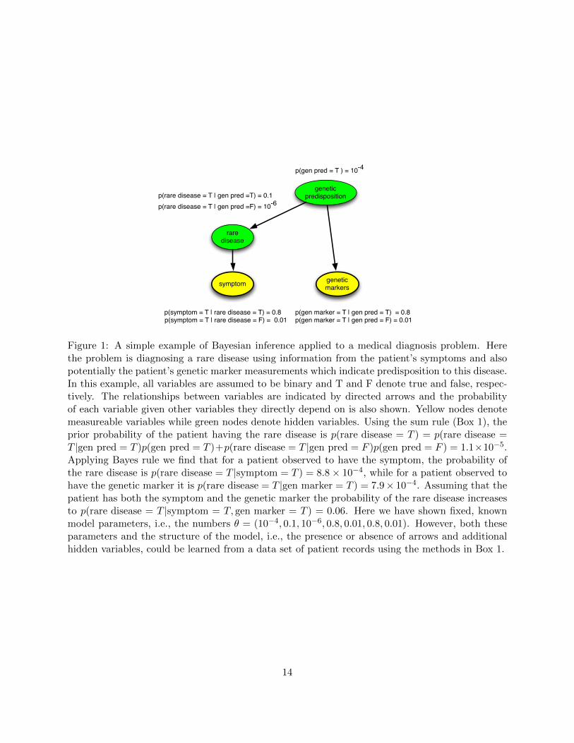
Figure 1: A simple example of Bayesian inference applied to a medical diagnosis problem. Herethe problem is diagnosing a rare disease using information from the patient’s symptoms and alsopotentially the patient’s genetic marker measurements which indicate predisposition to this disease.In this example, all variables are assumed to be binary and T and F denote true and false, respec-tively. The relationships between variables are indicated by directed arrows and the probabilityof each variable given other variables they directly depend on is also shown. Yellow nodes denotemeasureable variables while green nodes denote hidden variables. Using the sum rule (Box 1), theprior probability of the patient having the rare disease is p(rare disease = T ) = p(rare disease =T |gen pred = T )p(gen pred = T )+p(rare disease = T |gen pred = F )p(gen pred = F ) = 1.1×10−5.Applying Bayes rule we find that for a patient observed to have the symptom, the probability ofthe rare disease is p(rare disease = T |symptom = T ) = 8.8× 10−4, while for a patient observed tohave the genetic marker it is p(rare disease = T |gen marker = T ) = 7.9× 10−4. Assuming that thepatient has both the symptom and the genetic marker the probability of the rare disease increasesto p(rare disease = T |symptom = T, gen marker = T ) = 0.06. Here we have shown fixed, knownmodel parameters, i.e., the numbers θ = (10−4, 0.1, 10−6, 0.8, 0.01, 0.8, 0.01). However, both theseparameters and the structure of the model, i.e., the presence or absence of arrows and additionalhidden variables, could be learned from a data set of patient records using the methods in Box 1.

14

statesmean = [‐1, 1, 0] # Emission parameters.

initial = Categorical([1.0/3, 1.0/3, 1.0/3]) # Prob distr of state[1].

trans = [Categorical([0.1, 0.5, 0.4]), Categorical([0.2, 0.2, 0.6]),

Categorical([0.15, 0.15, 0.7])] # Trans distr for each state.

data = [Nil, 0.9, 0.8, 0.7, 0, ‐0.025, ‐5, ‐2, ‐0.1, 0, 0.13]

@model hmm begin # Define a model hmm.

states = Array(Int, length(data))

@assume(states[1] ~ initial)

for i = 2:length(data)

@assume(states[i] ~ trans[states[i‐1]])

@observe(data[i] ~ Normal(statesmean[states[i]], 0.4))

end

@predict states

end

anglicanHMM :: Dist [n]

anglicanHMM = fmap (take (length values) . fst) $ score (length values ‐ 1)

(hmm init trans gen) where

states = [0,1,2]

init = uniform states

trans 0 = fromList $ zip states [0.1,0.5,0.4]



gen 0 = certainly (‐1)

gen 1 = certainly 1

gen 2 = certainly 0

values = [0.9,0.8,0.7] :: [Double]

addNoise = flip Normal 1

score 0 d = d

score n d = score (n‐1) $ condition d (prob . (`pdf` (values !! n))

. addNoise . (!! n) . snd)

Example Probabilistic Program for a Hidden Markov Model (HMM)

Julia

Haskell

states[1] states[2] states[3]

data[1] data[2] data[3]

initial trans

statesmean

...

...

Figure 2: (a) A probabilistic program in Julia defining a simple 3-state hidden Markov model(HMM), inspired by an example in [62]. An HMM is a widely-used probabilistic model for sequentialand time series data which assumes the data were obtained by transitioning stochastically betweena discrete number of hidden states [98]. The first four lines define the model parameters and thedata. Here trans is the 3× 3 state-transition matrix, initial is the initial state distribution, andstatesmean are the mean observations for each of the three states; actual observations are assumedto be noisy versions of this mean with Gaussian noise. The function hmm() starts the definition ofthe HMM, drawing the sequence of states with the @assume statements, and conditioning on theobserved data with the @observe statements. Finally @predict states that we wish to infer thestates and data; this inference is done automatically via the universal inference engine which reasonsover the configurations of this computer program. It would be trivial to modify this program sothat the HMM parameters are unknown rather than fixed. (b) A graphical model corresponding tothe HMM probabilistic program showing dependencies between the parameters (cyan), hidden statevariables (green) and observed data (yellow). This graphical model highlights the compositionalnature of probabilistic models.

15

Pos

terio

r

t=3

Acq

uisi

tion

func

tion

nextpoint

Pos

terio

r newobserv.

t=4

Acq

uisi

tion

func

tion

Figure 3: A simple illustration of Bayesian optimisation in one dimension. The goal is to maximisesome true unknown function f (not shown). Information about this function is gained by makingobservations (circles, top panels), which are evaluations of the function at specific x values. Theseobservations are used to infer a posterior distribution over the function values (shown as mean,blue line, and standard deviations, blue shaded area) representing the distribution of possiblefunctions; note that uncertainty grows away from the observations. Based on this distribution overfunctions, an acquisition function is computed (green shaded area, bottom panels), which representsthe gain from evaluating the unknown function f at different x values; note that the acquisitionfunction is high where the posterior over f has both high mean and large uncertainty. Differentacquisition functions can be used such as “expected improvement” or “information-gain”. The peakof the acquisition function (red line) is the best next point to evaluate, and is therefore chosen forevaluation (red dot, new observation). The left and right panels show an example of what couldhappen after three and four functions evaluations, respectively.

16

An automatic report for the dataset : 10-sulphuric

The Automatic Statistician

Abstract

This report was produced by the Automatic Bayesian Covariance Discovery(ABCD) algorithm.

1 Executive summary

The raw data and full model posterior with extrapolations are shown in figure 1.

Raw data

1960 1965 1970 1975 1980 1985 1990 19950

50

100

150

200

250

Figure 1: Raw data (left) and model posterior with extrapolation (right)

The structure search algorithm has identified nine additive components in the data. The first 4additive components explain 90.5% of the variation in the data as shown by the coefficient of de-termination (R2) values in table 1. The first 8 additive components explain 99.8% of the variationin the data. After the first 6 components the cross validated mean absolute error (MAE) does notdecrease by more than 0.1%. This suggests that subsequent terms are modelling very short termtrends, uncorrelated noise or are artefacts of the model or search procedure. Short summaries of theadditive components are as follows:

• A very smooth function.• A constant. This function applies from 1964 until 1990.• An approximately periodic function with a period of 1.0 years.• A smooth function. This function applies from 1969 until 1977.• A smooth function. This function applies from 1964 until 1969 and from 1977 onwards.• A periodic function with a period of 2.6 years. This function applies until 1964.• Uncorrelated noise. This function applies until 1964.• Uncorrelated noise. This function applies from 1964 until 1990.• Uncorrelated noise. This function applies from 1990 onwards.

Model checking statistics are summarised in table 2 in section 4. These statistics have revealedstatistically significant discrepancies between the data and model in component 1.

The rest of the document is structured as follows. In section 2 the forms of the additive componentsare described and their posterior distributions are displayed. In section 3 the modelling assumptions

1

An automatic report for the dataset : 03-mauna


Abstract


1 Executive summary


Raw data

1960 1965 1970 1975 1980 1985 1990 1995 2000 2005−30

−20

−10

0

10

20

30

40


The structure search algorithm has identified five additive components in the data. The first additivecomponent explains 98.6% of the variation in the data as shown by the coefficient of determination(R2) values in table 1. The first 2 additive components explain 99.9% of the variation in the data.After the first 3 components the cross validated mean absolute error (MAE) does not decrease bymore than 0.1%. This suggests that subsequent terms are modelling very short term trends, uncor-related noise or are artefacts of the model or search procedure. Short summaries of the additivecomponents are as follows:

• A very smooth monotonically increasing function.

• An approximately periodic function with a period of 1.0 years.

• A smooth function.

• Uncorrelated noise.

• A rapidly varying smooth function.

Model checking statistics are summarised in table 2 in section 4. These statistics have not revealedany inconsistencies between the model and observed data.

The rest of the document is structured as follows. In section 2 the forms of the additive componentsare described and their posterior distributions are displayed. In section 3 the modelling assumptionsof each component are discussed with reference to how this affects the extrapolations made by themodel. Section 4 discusses model checking statistics, with plots showing the form of any detecteddiscrepancies between the model and observed data.

1

An automatic report for the dataset : 02-solar


Abstract


1 Executive summary


Raw data

1650 1700 1750 1800 1850 1900 1950 2000 20501360

1360.5

1361

1361.5

1362


The structure search algorithm has identified eight additive components in the data. The first 4additive components explain 92.3% of the variation in the data as shown by the coefficient of de-termination (R2) values in table 1. The first 6 additive components explain 99.7% of the variationin the data. After the first 5 components the cross validated mean absolute error (MAE) does notdecrease by more than 0.1%. This suggests that subsequent terms are modelling very short termtrends, uncorrelated noise or are artefacts of the model or search procedure. Short summaries of theadditive components are as follows:

• A constant.• A constant. This function applies from 1643 until 1716.• A smooth function. This function applies until 1643 and from 1716 onwards.• An approximately periodic function with a period of 10.8 years. This function applies until

1643 and from 1716 onwards.• A rapidly varying smooth function. This function applies until 1643 and from 1716 on-

wards.• Uncorrelated noise with standard deviation increasing linearly away from 1837. This func-

tion applies until 1643 and from 1716 onwards.• Uncorrelated noise with standard deviation increasing linearly away from 1952. This func-

tion applies until 1643 and from 1716 onwards.• Uncorrelated noise. This function applies from 1643 until 1716.

Model checking statistics are summarised in table 2 in section 4. These statistics have revealedstatistically significant discrepancies between the data and model in component 8.

1

Automatic construction and description of nonparametric modelsJames Robert Lloyd1, David Duvenaud1, Roger Grosse2,

Joshua B. Tenenbaum2, Zoubin Ghahramani1

1: Department of Engineering, University of Cambridge, UK 2: Massachusetts Institute of Technology, USA

This analysis was automatically generated Modelling structure throughGaussian process kernels

• The kernel specifies which structures are likely under the GP prior- which determines the generalisation properties of the model.

SquaredExponential (SE)

Periodic(Per)

Linear(Lin)

local variation repeating structure linear functions

• Composite kernels can express many types of structure

Lin ⇥ Lin SE ⇥ Per Lin + Per SE + Per

quadraticfunctions

locallyperiodic

periodicwith trend

periodicwith noise

SE ⇥ Lin Lin ⇥ Per SE1 + SE2 SE1 ⇥ SE2

increasingvariation

growingamplitude

f1(x1) +f2(x2) f (x1, x2)

• Building composite kernels previously required human expertise

We can build models by a greedy search

No structure

SE Lin

Lin + Per Lin ⇥ SE

Lin ⇥ SE + SE . . . Lin ⇥ (SE + Per)

. . . . . . . . .

. . .

. . . Lin ⇥ Per

Per

Automatically describing model properties

How to automatically describe arbitrarily complex kernels:

• The kernel is distributed into a sum of products

• Sums of kernels are sums of functions so each product is described separately

• Each kernel in a product modifies the model in a consistent way. . .

• . . . so one kernel is described by a noun phrase, and the others modify it

• Text descriptions are complemented by plots of the posterior

Kernels can be distributed into a sum of products

SE ⇥�Lin + Per + SE

�

becomes (after simplification)

(SE ⇥ Lin) + (SE ⇥ Per) + (SE).

Sums of kernels correspond to sums of functions

entire signal

= + +

SE ⇥ Lin SE ⇥ Per SEsmooth trend + periodicity + short-term deviation

If f1(x) ⇠ gp(0, k1) and f2(x) ⇠ gp(0, k2) then f1(x)+f2(x) ⇠ gp(0, k1+k2).Therefore, a sum of kernels can be described as a sum of independent functions.

Each kernel in a product roughly corresponds to an adjective

Kernel How it modifies the prior

SE functions change smoothlyPer functions repeatLin standard deviation varies linearly

Example description

SE|{z}approximately

⇥ Per|{z}periodic function

⇥ Lin|{z}with linearly growing amplitude

Per has been chosen to act as the noun while SE and Lin modify the description

Code available at github.com/jamesrobertlloyd/gpss-research







Periodic(Per)

Linear(Lin)




quadraticfunctions

locallyperiodic

periodicwith trend

periodicwith noise


increasingvariation

growingamplitude

f1(x1) +f2(x2) f (x1, x2)



No structure

SE Lin



. . . . . . . . .

. . .

. . . Lin ⇥ Per

Per










�


(SE ⇥ Lin) + (SE ⇥ Per) + (SE).


entire signal

= + +






Example description

SE|{z}approximately











Periodic(Per)

Linear(Lin)




quadraticfunctions

locallyperiodic

periodicwith trend

periodicwith noise


increasingvariation

growingamplitude

f1(x1) +f2(x2) f (x1, x2)



No structure

SE Lin



. . . . . . . . .

. . .

. . . Lin ⇥ Per

Per










�


(SE ⇥ Lin) + (SE ⇥ Per) + (SE).


entire signal

= + +






Example description

SE|{z}approximately





that the test statistic was larger in magnitude under the posterior compared to the prior unexpectedlyoften.

ACF Periodogram QQ# min min loc max max loc max min1 0.502 0.582 0.341 0.413 0.341 0.6792 0.802 0.199 0.558 0.630 0.049 0.7853 0.251 0.475 0.799 0.447 0.534 0.7694 0.527 0.503 0.504 0.481 0.430 0.6165 0.493 0.477 0.503 0.487 0.518 0.381

Table 2: Model checking statistics for each component. Cumulative probabilities for minimum ofautocorrelation function (ACF) and its location. Cumulative probabilities for maximum of peri-odogram and its location. p-values for maximum and minimum deviations of QQ-plot from straightline.

The nature of any observed discrepancies is now described and plotted and hypotheses are given forthe patterns in the data that may not be captured by the model.

4.1 Moderately statistically significant discrepancies

4.1.1 Component 2 : An approximately periodic function with a period of 1.0 years

The following discrepancies between the prior and posterior distributions for this component havebeen detected.

• The qq plot has an unexpectedly large positive deviation from equality (x = y). Thisdiscrepancy has an estimated p-value of 0.049.

The positive deviation in the qq-plot can indicate heavy positive tails if it occurs at the right of theplot or light negative tails if it occurs as the left.

QQ uncertainty plot for component 2

−250 −200 −150 −100 −50 0 50 100 150 200 250−300

−200

−100

0

100

200

300

400

Figure 17: ACF (top left), periodogram (top right) and quantile-quantile (bottom left) uncertaintyplots. The blue line and shading are the pointwise mean and 90% confidence interval of the plotsunder the prior distribution for component 2. The green line and green dashed lines are the corre-sponding quantities under the posterior.

4.2 Model checking plots for components without statistically significant discrepancies

4.2.1 Component 1 : A very smooth monotonically increasing function

No discrepancies between the prior and posterior of this component have been detected

8

2.4 Component 4 : An approximately periodic function with a period of 10.8 years. Thisfunction applies until 1643 and from 1716 onwards

This component is approximately periodic with a period of 10.8 years. Across periods the shape ofthis function varies smoothly with a typical lengthscale of 36.9 years. The shape of this functionwithin each period is very smooth and resembles a sinusoid. This component applies until 1643 andfrom 1716 onwards.

This component explains 71.5% of the residual variance; this increases the total variance explainedfrom 72.8% to 92.3%. The addition of this component reduces the cross validated MAE by 16.82%from 0.18 to 0.15.

Posterior of component 4

1650 1700 1750 1800 1850 1900 1950 2000−0.8

−0.6

−0.4

−0.2

0

0.2

0.4

0.6Sum of components up to component 4

1650 1700 1750 1800 1850 1900 1950 20001360

1360.5

1361

1361.5

1362

Figure 8: Pointwise posterior of component 4 (left) and the posterior of the cumulative sum ofcomponents with data (right)

Figure 9: Pointwise posterior of residuals after adding component 4

that the test statistic was larger in magnitude under the posterior compared to the prior unexpectedlyoften.

ACF Periodogram QQ# min min loc max max loc max min1 0.502 0.582 0.341 0.413 0.341 0.6792 0.802 0.199 0.558 0.630 0.049 0.7853 0.251 0.475 0.799 0.447 0.534 0.7694 0.527 0.503 0.504 0.481 0.430 0.6165 0.493 0.477 0.503 0.487 0.518 0.381

Table 2: Model checking statistics for each component. Cumulative probabilities for minimum ofautocorrelation function (ACF) and its location. Cumulative probabilities for maximum of peri-odogram and its location. p-values for maximum and minimum deviations of QQ-plot from straightline.

The nature of any observed discrepancies is now described and plotted and hypotheses are given forthe patterns in the data that may not be captured by the model.

4.1 Moderately statistically significant discrepancies

4.1.1 Component 2 : An approximately periodic function with a period of 1.0 years

The following discrepancies between the prior and posterior distributions for this component havebeen detected.

• The qq plot has an unexpectedly large positive deviation from equality (x = y). Thisdiscrepancy has an estimated p-value of 0.049.

The positive deviation in the qq-plot can indicate heavy positive tails if it occurs at the right of theplot or light negative tails if it occurs as the left.

Figure 17: ACF (top left), periodogram (top right) and quantile-quantile (bottom left) uncertaintyplots. The blue line and shading are the pointwise mean and 90% confidence interval of the plotsunder the prior distribution for component 2. The green line and green dashed lines are the corre-sponding quantities under the posterior.

4.2 Model checking plots for components without statistically significant discrepancies

4.2.1 Component 1 : A very smooth monotonically increasing function

No discrepancies between the prior and posterior of this component have been detected

8

(a)

(b) (c)

(d)

Figure 4: A flow diagram describing the Automatic Statistician. (a) The input to the system isdata, in this case represented as time series. (b) The system searches over a grammar of models todiscover a good interpretation of the data, using Bayesian inference to score models (Box 1). (c)Components of the model discovered are translated into English phrases. (d) The end result is areport with text, figures and tables, describing in detail what has been inferred about the data,including a section on model checking and criticism [99, 100].

17

[11] Koller, D. & Friedman, N. Probabilistic graphical models: Principles and techniques (The

MIT Press, 2009).

[12] Cox, R. T. The algebra of probable inference (Johns Hopkins University Press, Baltimore,

MD, 1961).

[13] Van Horn, K. S. Constructing a logic of plausible inference: a guide to Cox’s theorem.

International Journal of Approximate Reasoning 34, 3–24 (2003).

[14] De Finetti, B. La prevision: ses lois logiques, ses sources subjectives. In Annales de l’institut

Henri Poincare, vol. 7(1), 1–68 (Presses universitaires de France, 1937).

[15] Knill, D. & Richards, W. Perception as Bayesian inference (Cambridge University Press,

1996).

[16] Griffiths, T. L. & Tenenbaum, J. B. Optimal predictions in everyday cognition. Psychological

Science 17, 767–773 (2006).

[17] Wolpert, D. M., Ghahramani, Z. & Jordan, M. I. An internal model for sensorimotor inte-

gration. Science 269, 1880–1882 (1995).

[18] Tenenbaum, J. B., Kemp, C., Griffiths, T. L. & Goodman, N. D. How to grow a mind:

Statistics, structure, and abstraction. Science 331, 1279–1285 (2011).

[19] Marcus, G. F. & Davis, E. How robust are probabilistic models of higher-level cognition?

Psychological Science 24, 2351–2360 (2013).

[20] Goodman, N. D. et al. Relevant and robust a response to Marcus and Davis (2013). Psycho-

logical Science 0956797614559544 (2015).

[21] Doya, K., Ishii, S., Pouget, A. & Rao, R. P. N. Bayesian Brain: Probabilistic Approaches to

Neural Coding (The MIT Press, 2007).

[22] Deneve, S. Bayesian spiking neurons I: inference. Neural Computation 20, 91–117 (2008).

[23] Neal, R. M. Probabilistic inference using Markov chain Monte Carlo methods. Technical

Report CRG-TR-93-1, Department of Computer Science, University of Toronto (1993).

[24] Jordan, M., Ghahramani, Z., Jaakkola, T. & Saul, L. An introduction to variational methods

in graphical models. Machine Learning 37, 183–233 (1999).

[25] Doucet, A., de Freitas, J. F. G. & Gordon, N. J. Sequential Monte Carlo Methods in Practice

(Springer-Verlag, New York, 2000).

18

[26] Minka, T. P. Expectation propagation for approximate Bayesian inference. In Uncertainty

in Artificial Intelligence, vol. 17, 362–369 (2001).

[27] Neal, R. M. MCMC using Hamiltonian dynamics. In S. Brooks A. Gelman, G. J. & Meng,

X.-L. (eds.) Handbook of Markov Chain Monte Carlo (Chapman & Hall / CRC Press, 2010).

[28] Girolami, M. & Calderhead, B. Riemann manifold Langevin and Hamiltonian Monte Carlo

methods. Journal of the Royal Statistical Society: Series B (Statistical Methodology) 73,

123–214 (2011).

[29] Sutskever, I., Vinyals, O. & Le, Q. V. Sequence to sequence learning with neural networks.

In Ghahramani, Z., Welling, M., Cortes, C., Lawrence, N. & Weinberger, K. (eds.) Advances

in Neural Information Processing Systems 27, 3104–3112 (Curran Associates, Inc., 2014).

[30] Neal, R. M. Bayesian mixture modeling. In Maximum Entropy and Bayesian Methods,

197–211 (Springer Netherlands, 1992).

[31] Orbanz, P. & Teh, Y. W. Bayesian nonparametric models. In Encyclopedia of Machine

Learning (Springer, 2010).

[32] Hjort, N., Holmes, C., Muller, P. & Walker, S. (eds.) Bayesian Nonparametrics (Cambridge

University Press, 2010).

[33] Rasmussen, C. E. & Williams, C. K. I. Gaussian Processes for Machine Learning (MIT Press,

Cambridge, 2006).

[34] Lu, C. & Tang, X. Surpassing human-level face verification performance on LFW with

GaussianFace. In Proceedings of the 29th AAAI Conference on Artificial Intelligence (AAAI)

(2015).

[35] Ferguson, T. S. A Bayesian analysis of some nonparametric problems. The Annals of Statistics

1, 209–230 (1973).

[36] Teh, Y. W., Jordan, M. I., Beal, M. J. & Blei, D. M. Hierarchical Dirichlet processes. Journal

of the American Statistical Association 101, 1566–1581 (2006).

[37] Kemp, C., Tenenbaum, J. B., Griffiths, T. L., Yamada, T. & Ueda, N. Learning systems of

concepts with an infinite relational model. In Proceedings of the 21st National Conference on

Artificial Intelligence (2006).

[38] Medvedovic, M. & Sivaganesan, S. Bayesian infinite mixture model based clustering of gene

expression profiles. Bioinformatics 18, 1194–1206 (2002).

19

[39] Rasmussen, C. E., De la Cruz, B. J., Ghahramani, Z. & Wild, D. L. Modeling and visualiz-

ing uncertainty in gene expression clusters using Dirichlet process mixtures. Computational

Biology and Bioinformatics, IEEE/ACM Transactions on 6, 615–628 (2009).

[40] Griffiths, T. L. & Ghahramani, Z. The Indian buffet process: An introduction and review.

Journal of Machine Learning Research 12, 1185–1224 (2011).

[41] Adams, R. P., Wallach, H. & Ghahramani, Z. Learning the structure of deep sparse graphical

models. In Teh, Y. W. & Titterington, M. (eds.) 13th International Conference on Artificial

Intelligence and Statistics, 1–8 (Chia Laguna, Sardinia, Italy, 2010). URL .

[42] Miller, K., Jordan, M. I. & Griffiths, T. L. Nonparametric latent feature models for link

prediction. In Advances in Neural Information Processing Systems, 1276–1284 (2009).

[43] Hinton, G. E., McClelland, J. L. & Rumelhart, D. E. Distributed representations. In Parallel

Distributed Processing: Explorations in the Microstructure of Cognition. Volume 1: Founda-

tions, 77–109 (MIT Press, Cambridge, MA, 1986).

[44] Neal, R. M. Bayesian Learning for Neural Networks (Springer-Verlag, New York, 1996).

[45] Koller, D., McAllester, D. & Pfeffer, A. Effective Bayesian inference for stochastic programs.

In Proceedings of the 14th National Conference on Artificial Intelligence (AAAI) (1997).

[46] Goodman, N. D. & Stuhlmuller, A. The Design and Implementation of Probabilistic Pro-

gramming Languages (2015). Electronic, Retrieved 2015/3/22 from http://dippl.org.

[47] Pfeffer, A. Practical Probabilistic Programming (Manning Publications, 2015).

[48] Freer, C., Roy, D. & Tenenbaum, J. B. Towards common-sense reasoning via conditional

simulation: Legacies of Turing in artificial intelligence. In Turing’s Legacy (ASL Lecture

Notes in Logic) (2012).

[49] Marjoram, P., Molitor, J., Plagnol, V. & Tavare, S. Markov chain Monte Carlo without

likelihoods. Proceedings of the National Academy of Sciences 100, 15324–15328 (2003).

[50] Mansinghka, V., Kulkarni, T. D., Perov, Y. N. & Tenenbaum, J. Approximate Bayesian

image interpretation using generative probabilistic graphics programs. In Advances in Neural

Information Processing Systems 26, 1520–1528 (2013).

[51] Bishop, C. M. Model-based machine learning. Philosophical Transactions of the Royal Society

A 371, 20120222 (2013).

[52] Lunn, D. J., Thomas, A., Best, N. & Spiegelhalter, D. WinBUGS–a Bayesian modelling

framework: concepts, structure, and extensibility. Statistics and Computing 10, 325–337

(2000).

20

[53] Stan Development Team. Stan Modeling Language Users Guide and Reference Manual, Ver-

sion 2.5.0 (2014). URL http://mc-stan.org/.

[54] Fischer, B. & Schumann, J. AutoBayes: A system for generating data analysis programs

from statistical models. Journal of Functional Programming 13, 483–508 (2003).

[55] Minka, T. P., Winn, J. M., Guiver, J. P. & Knowles, D. A. Infer.NET 2.4 (2010). Microsoft

Research Cambridge. http://research.microsoft.com/infernet.

[56] Pfeffer, A. IBAL: A probabilistic rational programming language. In IJCAI, 733–740 (2001).

[57] Milch, B. et al. BLOG: Probabilistic models with unknown objects. In Proc. 19th Interna-

tional Joint Conference on Artificial Intelligence (IJCAI), 1352–1359 (2005).

[58] Goodman, N., Mansinghka, V., Roy, D., Bonawitz, K. & Tenenbaum, J. Church: a language

for generative models. In Uncertainty in Artificial Intelligence, vol. 22, 23 (2008).

[59] Pfeffer, A. Figaro: An object-oriented probabilistic programming language. Tech. Rep.,

Charles River Analytics (2009).

[60] Wingate, D., Stuhlmuller, A. & Goodman, N. D. Lightweight implementations of probabilis-

tic programming languages via transformational compilation. In Artificial Intelligence and

Statistics (2011).

[61] Mansinghka, V., Selsam, D. & Perov, Y. Venture: a higher-order probabilistic programming

platform with programmable inference. arXiv preprint (2014).

[62] Wood, F., van de Meent, J. W. & Mansinghka, V. A new approach to probabilistic program-

ming inference. In Proceedings of the 17th International conference on Artificial Intelligence

and Statistics (2014).

[63] Li, L., Wu, Y. & Russell, S. J. SWIFT: Compiled inference for probabilistic programs. Tech.

Rep. UCB/EECS-2015-12, EECS Department, University of California, Berkeley (2015). URL

http://www.eecs.berkeley.edu/Pubs/TechRpts/2015/EECS-2015-12.html.

[64] Bergstra, J. et al. Theano: a CPU and GPU math expression compiler. In Proceedings of the

Python for Scientific Computing Conference (SciPy) (2010).

[65] Kushner, H. A new method of locating the maximum point of an arbitrary multipeak curve

in the presence of noise. Journal of Basic Engineering 86, 97–106 (1964).

[66] Jones, D. R., Schonlau, M. & Welch, W. J. Efficient global optimization of expensive black-

box functions. Journal of Global Optimization 13, 455–492 (1998).

21

[67] Brochu, E., Cora, V. M. & de Freitas, N. A tutorial on Bayesian optimization of expensive cost

functions, with application to active user modeling and hierarchical reinforcement learning

(2010). http://arXiv.org/abs/1012.2599.

[68] Hennig, P. & Schuler, C. J. Entropy search for information-efficient global optimization.

Journal of Machine Learning Research 13, 1809–1837 (2012).

[69] Hernandez-Lobato, J. M., Hoffman, M. W. & Ghahramani, Z. Predictive entropy search

for efficient global optimization of black-box functions. In Advances in Neural Information

Processing Systems (2014).

[70] Snoek, J., Larochelle, H. & Adams, R. P. Practical Bayesian optimization of machine learning

algorithms. In Advances in Neural Information Processing Systems (2012).

[71] Thornton, C., Hutter, F., Hoos, H. H. & Leyton-Brown, K. Auto-WEKA: Combined selection

and hyperparameter optimization of classification algorithms. In Proceedings of the 19th ACM

SIGKDD International Conference on Knowledge Discovery and Data Mining, KDD ’13, 847–

855 (ACM, New York, NY, USA, 2013).

[72] Robbins, H. Some aspects of the sequential design of experiments. Bulletin of the American

Mathematical Society 55, 527–535 (1952).

[73] Deisenroth, M. P. & Rasmussen, C. E. PILCO: A model-based and data-efficient approach

to policy search. In 28th International Conference on Machine Learning (2011).

[74] Poupart, P. Bayesian reinforcement learning. In Encyclopedia of Machine Learning, 90–93

(Springer, 2010).

[75] Diaconis, P. Bayesian numerical analysis. In Statistical Decision Theory and Related Topics

IV, vol. 1, 163–175 (Springer-Verlag, 1988).

[76] O’Hagan, A. Bayes-Hermite quadrature. Journal of Statistical Planning and Inference 29,

245–260 (1991).

[77] Shannon, C. & Weaver, W. The Mathematical Theory of Communication (University of

Illinois Press, Urbana, IL, 1949).

[78] MacKay, D. J. C. Information Theory, Inference, and Learning Algorithms (Cambridge

University Press, 2003).

[79] Wood, F., Gasthaus, J., Archambeau, C., James, L. & Teh, Y. W. The Sequence Memoizer.

Communications of the ACM 54, 91–98 (2011).

22

[80] Steinruecken, C., Ghahramani, Z. & MacKay, D. J. C. Improving PPM with dynamic pa-

rameter updates. In Data Compression Conference (DCC 2015) (2015).

[81] Lloyd, J. R., Duvenaud, D., Grosse, R., Tenenbaum, J. B. & Ghahramani, Z. Automatic con-

struction and natural-language description of nonparametric regression models. In Twenty-

Eighth AAAI Conference on Artificial Intelligence (AAAI-14) (2014).

[82] Grosse, R. B., Salakhutdinov, R. & Tenenbaum, J. B. Exploiting compositionality to explore

a large space of model structures. In Uncertainty in Artificial Intelligence (2012).

[83] Schmidt, M. & Lipson, H. Distilling free-form natural laws from experimental data. Science

324, 81–85 (2009).

[84] Wolstenholme, D. E., O’Brien, C. M. & Nelder, J. A. GLIMPSE: a knowledge-based front

end for statistical analysis. Knowledge-Based Systems 1, 173–178 (1988).

[85] Hand, D. J. Patterns in statistical strategy. In Gale, W. A. (ed.) Artificial intelligence and

statistics (1986).

[86] King, R. D. et al. Functional genomic hypothesis generation and experimentation by a robot

scientist. Nature 427, 247–252 (2004).

[87] Welling, M. et al. Bayesian inference with Big Data: A snapshot from a workshop. In BIBiD

(2014). URL http://www.ics.uci.edu/∼welling/publications/papers/ISBA.pdf.

[88] Bakker, B. & Heskes, T. Task clustering and gating for Bayesian multitask learning. Journal

of Machine Learning Research 4, 83–99 (2003).

[89] Houlsby, N., Hernandez-Lobato, J. M., Huszar, F. & Ghahramani, Z. Collaborative Gaussian

processes for preference learning. In Advances in Neural Information Processing Systems 26,

2096–2104 (Curran Associates, Inc., 2012).

[90] Russell, S. J. & Wefald, E. Do the right thing: Studies in limited rationality (MIT press,

1991).

[91] Jordan, M. I. On statistics, computation and scalability. Bernoulli 19, 1378–1390 (2013).

[92] Hoffman, M., Blei, D., Paisley, J. & Wang, C. Stochastic variational inference. Journal of

Machine Learning Research 14, 1303–1347 (2013).

[93] Hensman, J., Fusi, N. & Lawrence, N. D. Gaussian processes for big data. In Uncertainty in

Artificial Intelligence (2013).

23

[94] Korattikara, A., Chen, Y. & Welling, M. Austerity in MCMC land: Cutting the Metropolis-

Hastings budget. In Proceedings of the 31th International Conference on Machine Learning,

ICML 2014, Beijing, China, 21-26 June 2014, 181–189 (2014).

[95] Paige, B., Wood, F., Doucet, A. & Teh, Y. W. Asynchronous anytime sequential Monte

Carlo. In Advances in Neural Information Processing Systems (2014).

[96] Jefferys, W. H. & Berger, J. O. Ockham’s Razor and Bayesian Analysis. American Scientist

80, 64–72 (1992).

[97] Rasmussen, C. E. & Ghahramani, Z. Occam’s Razor. In Advances in Neural Information

Processing Systems 13, 294–300 (MIT Press, Cambridge, MA, 2001).

[98] Rabiner, L. R. A tutorial on hidden Markov models and selected applications in speech

recognition. Proc. of the IEEE 77, 257–86. (1989).

[99] Gelman, A. et al. Bayesian Data Analysis, Third Edition (Chapman & Hall/CRC Texts in

Statistical Science. Taylor & Francis, 2013).

[100] Lloyd, J. R. & Ghahramani, Z. Statistical model criticism using kernel two sample tests

(2015). http://mlg.eng.cam.ac.uk/Lloyd/papers/kernel-model-checking.pdf.

24

Documents

Ghahramani 2015 Nature - Apollo Home