Embed Size (px)
Citation preview

Ghost-imaging-enhanced non-invasive spectral characterization of
stochastic x-ray free-electron-laser pulses
Kai Li,1, 2, ∗ Joakim Laksman,3 Tommaso Mazza,3 Gilles Doumy,2
Dimitris Koulentianos,2 Alessandra Picchiotti,4 Svitovar Serkez,3 Nina
Rohringer,5, 6 Markus Ilchen,7 Michael Meyer,3 and Linda Young1, 2, 8, †
1Department of Physics, The University of Chicago, Chicago, IL 60637 USA
2Chemical Sciences and Engineering Division,
Argonne National Laboratory, Lemont, IL 60439 USA
3European XFEL, Holzkoppel 4, 22869 Schenefeld Germany
4The Hamburg Centre for Ultrafast Imaging, Hamburg University,
Luruper Chaussee 149, 22761, Hamburg, Germany
5Center for Free-Electron Laser Science CFEL,
Deutsches Elektronen-Synchrotron DESY,
Notkestraße 85, 22607 Hamburg, Germany
6Department of Physics, Universitat Hamburg, 20355 Hamburg, Germany
7Deutsches Elektronen-Synchrotron DESY,
Notkestraße 85, 22607 Hamburg, Germany
8James Franck Institute, The University of Chicago, Chicago, IL 60637 USA
(Dated: November 2, 2021)
1
arX
iv:2
110.
1019
7v2
[ph
ysic
s.at
om-p
h] 3
0 O
ct 2
021

Abstract
High-intensity ultrashort X-ray free-electron laser (XFEL) pulses are revolutionizing the study
of fundamental nonlinear x-ray matter interactions and coupled electronic and nuclear dynamics.
To fully exploit the potential of this powerful tool for advanced x-ray spectroscopies, a nonin-
vasive spectral characterization of incident stochastic XFEL pulses with high resolution is a key
requirement. Here we present a new methodology that combines high-acceptance angle-resolved
photoelectron time-of-flight spectroscopy and ghost imaging to dramatically enhance the quality
of spectral characterization of x-ray free-electron laser pulses. Implementation of this non-invasive
high-resolution x-ray diagnostic can greatly benefit the ultrafast x-ray spectroscopy community by
functioning as a transparent beamsplitter for applications such as transient absorption spectroscopy
as well as covariance-based x-ray nonlinear spectroscopies where the shot-to-shot fluctuations in-
herent to a SASE XFEL pulse are a powerful asset.
∗ [email protected]† [email protected]
2

I. INTRODUCTION
X-ray free-electron lasers, with brilliance ten orders of magnitude higher than syn-
chrotrons, continuous tunability over the soft and hard x-ray regimes and sub-femtosecond
pulse duration [1], have emerged as a powerful tool both to explore fundamental non-
linear x-ray interactions in isolated atomic and molecular systems [2–7], and, to follow
photoinduced electronic and nuclear dynamics on their intrinsic femtosecond timescales via
pump/probe techniques [8, 9]. For the latter objective, core-level x-ray transient absorption
(XTAS) with ultrafast x-ray pulses has become a workhorse - it projects core electronic
states onto unoccupied valence/Rydberg states, thereby capturing the evolution of valence
electronic motion following an excitation pulse. However, realization of XTAS is challenging
at XFELs where the x-ray pulses with bandwidth ∆E/E ∼ 1%, typically produced by
self-amplified spontaneous emission (SASE), have spiky temporal and spectral profiles that
vary stochastically on a shot-by-shot basis [10–14]. The traditional approach for XTAS
with XFELs is to monochromatize the SASE beam[15, 16] and scan the monochromatic
beam (∆E/E ∼ 0.01%) across the desired spectral range. This makes inefficent use of the
full XFEL beam, imposes limits on time resolution via the uncertainty principle, and, by
reducing the pulse intensities, hampers realization of nonlinear x-ray spectroscopies. An al-
ternative approach is to monitor incident and transmitted intensity to obtain an absorption
spectrum, IT (ω)/I0(ω), across the entire SASE bandwidth. With this approach one may
realize novel experimental techniques employing correlation analysis that take advantage of
the intrinsic stochastic nature of XFELs pulses [17–20]. By using pulses with uncorrelated
fluctuations one can leverage the noise such that each repetition of the experiment, i.e.
each XFEL shot, represents a new measurement under different conditions. As an example,
spectral ghost imaging has been applied to obtain an absorption spectrum with energy reso-
lution better than the averaged SASE bandwidth [21, 22]. In general, the characterization of
the incident pulses is essential to this class of novel covariance spectroscopies as previously
demonstrated in UV regime [23].
Several diagnostic tools have demonstrated well-resolved spectral measurements on a
single-shot basis without compromising the quality of the x-ray beam. A commonality
is the use of optical elements to split the incident x-ray beam into reference and sample
beams. Beamsplitters for hard x-rays use crystal Bragg diffraction [24, 25] while diffraction
3

gratings are used for soft x-rays[26, 27]. An alternative is to use photoionization of a dilute
target gas and measure the kinetic energy of ejected photoelectrons to retrieve the incident
photon spectrum via the photoelectric effect [28–30]. Indeed, the use of an array of 16
electron time-of-flight spectrometers (eTOFs) radially distributed about the propagating
x-ray beam (colloquially named the ”cookie-box”) has enabled the measurement of the
position, polarization, and central energy of an x-ray photon beam as demonstrated at the
PETRA-P04 beamline [28]. At XFELs, while it is straightforward to measure the central
photon energy with the cookie-box [29] as has been demonstrated for two-color x-ray pulses
[31] and to obtain simultaneous polarization diagnostics [32, 33], it is more challenging to
obtain single-shot spectra with an energy resolution comparable to a grating spectrometer.
Here we use a ghost-imaging algorithm to improve the energy resolution of the raw
cookie-box measurements. Thousands of SASE spectra were measured simultaneously by
a cookie-box and a grating spectrometer and ghost imaging was applied to compute the
response matrix of the cookie-box. The response matrix was then used to reconstruct the
x-ray spectrum with energy resolution improved from ∼ 1 eV to 0.5 eV at a central energy
of 910 eV for a resolution of ∆E/E ∼ 1/2000 under the present conditions. This response
matrix derived from ghost imaging also provides predictive power for the spectral profile of
yet-to-be-measured XFEL pulses.
II. RESULTS
A. Spectral ghost imaging
Ghost imaging is an experimental technique which uses statistical fluctuations of an
incident beam to extract information about an object using a beam replica that has not
physically interacted with the object [34]. It can be used in the spatial[35, 36], temporal[18]
and spectral[21, 22] domains. Traditional ghost imaging requires a beam splitter to separate
the incident beam into two replicas, the object beam and the reference beam. The object
beam interacts with the sample and a low-resolution detector is used to measure the signal
whose intensity is proportional to the interaction and the incident beam. The reference beam
is directly measured by a high-resolution detector to extract knowledge of the incident beam.
The incident light source varies shot-by-shot and numerous measurements are carried out to
4

calculate the correlation function between the two signals from the object and the reference
beams. The correlation function of the measurements is analyzed to extract information of
the sample. The advantage of ghost imaging is that the object beam does not necessarily
need to be strong – thus protecting the samples from radiation damage. In addition, due to
the fluctuations of the light source and correlation analysis, ghost imaging is robust to noise
and background signals.
Ghost imaging essentially maps the high-resolution signal onto the low-resolution one,
making it an ideal tool to calibrate devices with high resolution. The correlation function
generated by ghost imaging contains information on the response of a device to the different
incident signals. This extracted information can be further used to correct defects or dis-
crimination present in a device. The ghost imaging calibration method reconstructs a high
quality signal that achieves resolution beyond the low-resolution instrumental limit. The
stochastic nature of a SASE XFEL makes it well-suited for ghost imaging in the temporal
and spectral domains. Here, ghost imaging is used to calibrate the eToFs of the cookie-box
and obtain a response matrix, which is then applied to reconstruct a more accurate incident
x-ray spectrum. One challenge for applying the ghost imaging method in the x-ray regime is
the requirement of a beamsplitter. Although x-ray beamsplitters are available as mentioned
above, the non-invasive gas-target measurement is suitable to replace the function of the
beamsplitter.
B. Experimental procedure
The energy spectrum of the incident x-ray beam was characterized non-invasively by pho-
toionization of dilute neon gas at the center of an array of 16-eToFs, i.e. the cookie-box[29]
as shown in Fig. 1. The arrival times of Ne 1s photoelectrons were measured by the eToFs
located in the plane perpendicular to the beam propagation direction (see Supplementary
Note 1). SIMION simulations were carried out to establish a traditional calibration between
the electron time-of-flight and kinetic energy, Ek, given the drift tube length and retardation
voltages. The incident photon energy was derived by adding the Ne 1s binding energy, 870
eV, to the measured Ek. The spectrum obtained by cookie-box for several random shots us-
ing this traditional method is shown in Fig. 1 as the object measurement. Under the present
experimental conditions, the energy resolution achievable by the cookie-box was around 1
5

FIG. 1. Schematic of the experimental setup. SASE XFEL pulses first interact with dilute
neon gas in the cookie-box chamber where the kinetic energies of 1s photoelectrons are measured
by the array of eToFs. The transmitted x-ray pulse is then focused on the VLS grating by a
spherical mirror and dispersed on a YAG:Ce crystal. The induced fluorescence is recorded by a
charge-coupled device (CCD) as a 2D image from which the single-shot ”reference” spectrum is
extracted.
eV, which is not comparable to the high-resolution grating spectrometer measurement where
0.2 eV FWHM (∆E/E) can be readily achieved.
After passing through cookie-box, the same FEL beam was characterized by a spec-
trometer based on a VLS grating and a Ce:YAG screen as shown in Fig. 1 as the reference
measurement. The cookie-box contains very dilute gas which does not attenuate or otherwise
alter the x-ray beam. Thus, ideally the same spectrum would be obtained from the electron
(cookie-box) and photon (grating spectrometer) measurements. However, the measurement
of a single random shot shown in Fig. 3a reveals differences. The grating spectrometer res-
olution is much higher than the resolution of the cookie-box, thus creating a large deviation
between the two spectra. The use of ghost imaging to retrieve a response matrix which is
then used to improve the performance of the cookie-box measurements is demonstrated in
the following.
6

C. Principle of reconstruction
Theoretically the photoelectron signal c (after normalization to the gas density) is pro-
portional to the incident photon spectrum s as measured by the spectrometer
c = As (1)
where A relates the cookie-box signals to the incident photon spectrum, is an (m × n)
matrix with the cookie-box ToF points m = 137 and the spectrograph pixels n = 1900 in
the region of interest between 895 and 920 eV. This equation resembles the basic equation in
ghost imaging and is usually used to obtain sample information by solving for A. However,
in order to predict the incident spectrum based on cookie-box measurements, we formally
write equation (1) as
s = Rc (2)
where the response matrix R is the formal inverse of matrix A. R maps the low-resolution
cookie-box measurements to high-resolution grating spectrometer measurements. In other
words, R is a calibration matrix contains information of the characteristics of eToFs. After
retrieving the response matrix R, according to equation (2), it can be used to generate
high-resolution spectrum with the intrinsic defects and broadening of cookie-box removed.
D. Ghost imaging reconstructed spectrum
To solve equation (2), we take advantage of the N independent measurements obtained.
Each shot gives a realization of si and cj in equation si =∑m
j=1Rijcj with m unknown
variables Rij. Combining all measurements gives N independent linear equations which can
be solved to uniquely determine the unknown variables if N > m. Instead of directly solving
these equations, the response matrix elements are determined by least square regression, i.e.
by minimizing the quantity |s − Rc|2. Single-photon Ne 1s ionization exhibits a dipole
angular distribution pattern due to the linear (horizontal) polarization of the x-rays and
the spherical 1s electron orbital. To increase the signals, we combined six eToFs near the
polarization direction which have strong 1s peaks, to form the cookie-box measurement
vector c with dimension m = 6× 137 = 822.
The calculated cookie-box response matrix using all shots (N = 15337) is shown in Fig. 2.
Compared with the traditional calibration function, which just maps ToFs onto kinetic
7
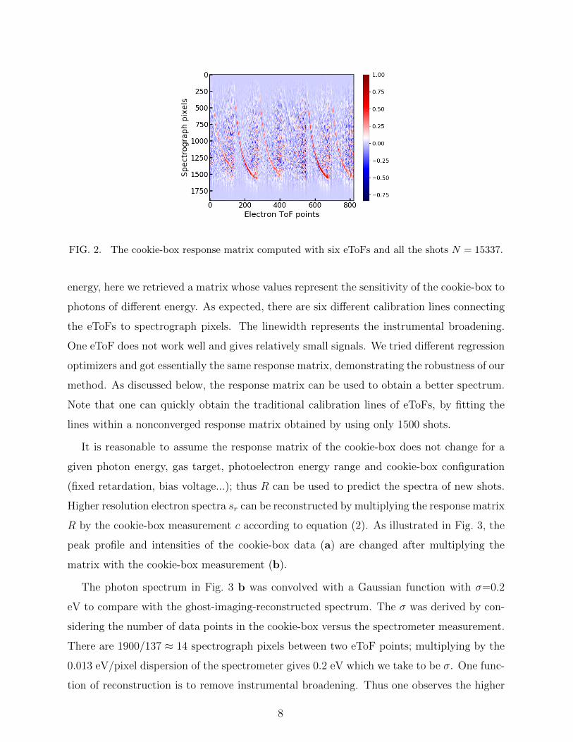
FIG. 2. The cookie-box response matrix computed with six eToFs and all the shots N = 15337.
energy, here we retrieved a matrix whose values represent the sensitivity of the cookie-box to
photons of different energy. As expected, there are six different calibration lines connecting
the eToFs to spectrograph pixels. The linewidth represents the instrumental broadening.
One eToF does not work well and gives relatively small signals. We tried different regression
optimizers and got essentially the same response matrix, demonstrating the robustness of our
method. As discussed below, the response matrix can be used to obtain a better spectrum.
Note that one can quickly obtain the traditional calibration lines of eToFs, by fitting the
lines within a nonconverged response matrix obtained by using only 1500 shots.
It is reasonable to assume the response matrix of the cookie-box does not change for a
given photon energy, gas target, photoelectron energy range and cookie-box configuration
(fixed retardation, bias voltage...); thus R can be used to predict the spectra of new shots.
Higher resolution electron spectra sr can be reconstructed by multiplying the response matrix
R by the cookie-box measurement c according to equation (2). As illustrated in Fig. 3, the
peak profile and intensities of the cookie-box data (a) are changed after multiplying the
matrix with the cookie-box measurement (b).
The photon spectrum in Fig. 3 b was convolved with a Gaussian function with σ=0.2
eV to compare with the ghost-imaging-reconstructed spectrum. The σ was derived by con-
sidering the number of data points in the cookie-box versus the spectrometer measurement.
There are 1900/137 ≈ 14 spectrograph pixels between two eToF points; multiplying by the
0.013 eV/pixel dispersion of the spectrometer gives 0.2 eV which we take to be σ. One func-
tion of reconstruction is to remove instrumental broadening. Thus one observes the higher
8
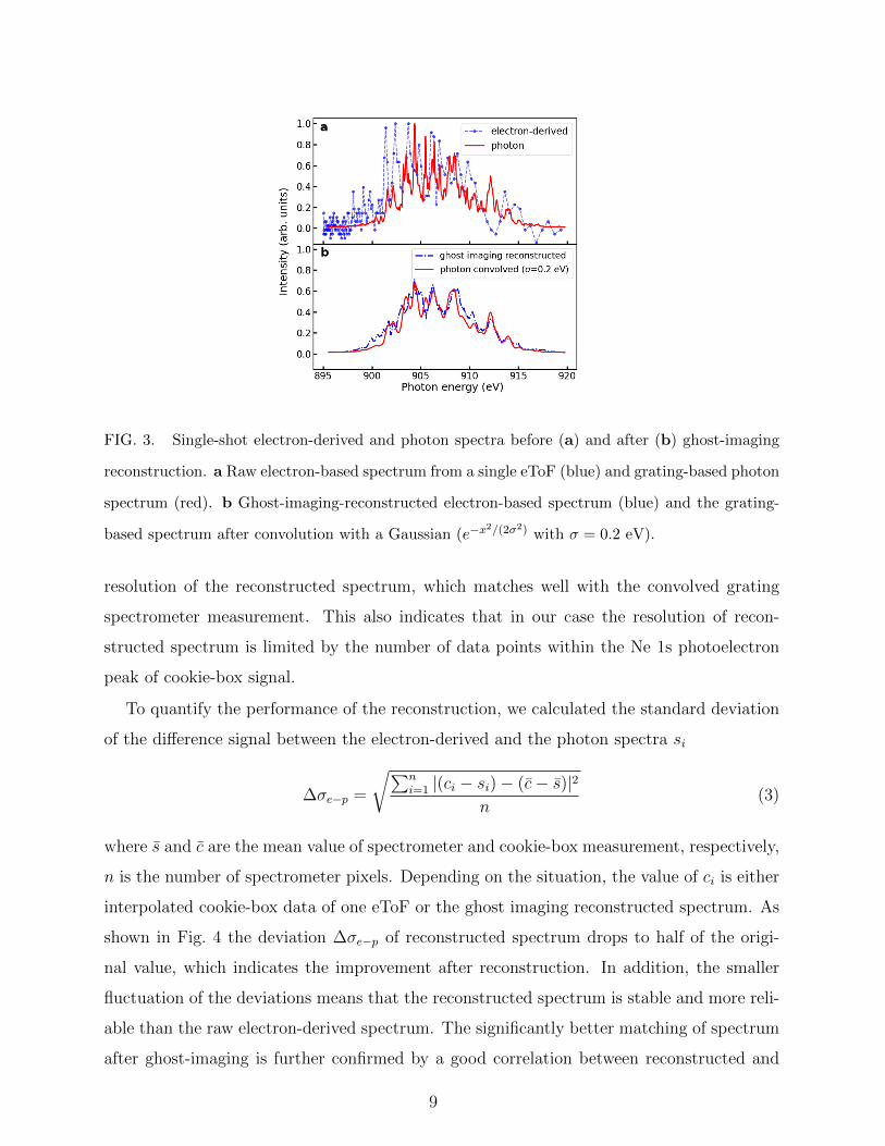
FIG. 3. Single-shot electron-derived and photon spectra before (a) and after (b) ghost-imaging
reconstruction. a Raw electron-based spectrum from a single eToF (blue) and grating-based photon
spectrum (red). b Ghost-imaging-reconstructed electron-based spectrum (blue) and the grating-
based spectrum after convolution with a Gaussian (e−x2/(2σ2) with σ = 0.2 eV).
resolution of the reconstructed spectrum, which matches well with the convolved grating
spectrometer measurement. This also indicates that in our case the resolution of recon-
structed spectrum is limited by the number of data points within the Ne 1s photoelectron
peak of cookie-box signal.
To quantify the performance of the reconstruction, we calculated the standard deviation
of the difference signal between the electron-derived and the photon spectra si
∆σe−p =
√∑ni=1 |(ci − si)− (c− s)|2
n(3)
where s and c are the mean value of spectrometer and cookie-box measurement, respectively,
n is the number of spectrometer pixels. Depending on the situation, the value of ci is either
interpolated cookie-box data of one eToF or the ghost imaging reconstructed spectrum. As
shown in Fig. 4 the deviation ∆σe−p of reconstructed spectrum drops to half of the origi-
nal value, which indicates the improvement after reconstruction. In addition, the smaller
fluctuation of the deviations means that the reconstructed spectrum is stable and more reli-
able than the raw electron-derived spectrum. The significantly better matching of spectrum
after ghost-imaging is further confirmed by a good correlation between reconstructed and
9

FIG. 4. Improvement in spectral resolution from the ghost imaging algorithm. ∆σe−p is the
standard deviation of the difference between cookie-box and spectrometer measurements. Original
(blue) and after the ghost-imaging reconstruction (red). Data from six eToFs and all the shots
were used to converge the regression and determine the response matrix R. The results of 1000
shots are shown here.
photon spectrum i.e. averaging 0.72 Pearson correlation coefficient across the spectrum (see
Supplementary Note 2).
E. Predictive power and performance analysis
One of the most interesting aspects of the ghost imaging method is its predictive power
for future shots. This requires numerous ”learning” shots to obtain a converged response
matrix. Data from six eToFs were used and the response matrix learned from different
number of shots is then used to predict the spectra for 100 new shots that were not used in
the regression. As shown in Fig. 5, when fewer shots are used, the deviation of the learning
shots is small because the regression is under-determined. Meanwhile, the deviation for the
new shots is large, indicating a poor predictive power of an unconverged response matrix.
As the information from more shots are included in the regression process, the deviation of
learning shots rises, whereas the deviation for the new shots decreases indicating the gain
of predictive power. The regression converges when the deviation of learning and prediction
meet around 8000 shots (roughly 10 times the number of unknown variables i.e. cookie-box
vector elements). It is important to note that as more shots are used the error bar for the
10

FIG. 5. Number of learning shots required for robust predictive capability. The standard deviation
for learning and prediction shots as a function of number of shots used in the regression. The
inserted plot at fewer number of learning shots (1433) shows a marked jump in standard deviation
from learning to prediction shots, while the standard deviation remains relatively constant when
more learning shots (7568) are used.
prediction, which measures the fluctuation of the deviation, also decreases, which means the
prediction becomes more stable.
Combining electron spectra from several eToFs increases the signal intensities and sup-
presses the noise. However, the eToF signals cannot be added on top of each other directly,
due to the different calibrations of each eTOF. As mentioned before, we put the signals from
different eToFs together to form a larger vector and differences of eToFs are automatically
taken into account when calculating the response matrix. The upper panel and the lower
panel of Fig. 6 show the spectrum of a random shot where one eToF with strongest signal
and six eToFs are used, respectively. Compared with the Gaussian convolved spectrometer
measurement clearly indicates the advantages of using six eToFs. The inset plot shows that
the normalized deviation drops gradually from 1 for one eToF to 0.87 with six eToFs. The
data from different eToFs complement with each other and improve the correlation with the
spectrometer measurement thus resulting in the better overall reconstructed spectrum.
Our analysis indicates that the performance of the ghost imaging reconstruction depends
on experimentally controllable parameters, number of shots used, number of eTOFs used.
Ghost imaging is based on the correlation between the object measurement and the reference
measurement, i.e. the sensitivity of the cookie-box signals to the fluctuations of the incident
11

FIG. 6. Improved reconstruction as a function number of eTOFs used. The reconstructed
spectrum and Gaussian convolved spectrum using one eToF (a) and six eToFs (b). All the shots
are used to get a converged result. The inserted plot shows the decrease in the standard deviation
when more eToFs are used.
spectrum as measured by a grating spectrometer. Obtaining better correlation function and
reconstruction, i.e. response matrix and spectrum with higher resolution, requires more data
points within the Ne 1s photoelectron peak as well as high signal-to-noise ratio. More data
points in the eTOF spectrum can be obtained by increasing the retardation voltages to slow
the electrons, using larger drift length tubes, or, more simply by increasing the digitizer
sampling rate which is presently 2 GHz. In addition, increased detection sensitivity can
be readily achieved by using more eToFs or by increasing the gas density to produce more
photoelectrons and a higher signal-to-noise ratio (see discussion in Supplementary Note 3).
III. DISCUSSION
Despite the considerable improvement to achieve resolution ∆E/E ∼ 1/2000, the ghost-
imaging reconstruction of a single-shot XFEL spectrum under the current experimental
conditions can not characterize completely the SASE structure containing inter-spike spac-
ings down to ∼ 0.1 eV, corresponding to a required resolution of ∆E/E ∼ 1/10000. For
this particular case using the Ne 1s photoelectron, the width of the final state Ne 1s−1 of
0.27 eV represents another barrier. However, the ability to reconstruct an averaged spectral
12

FIG. 7. Effect of averaging on the deviation between ghost-imaging-reconstructed and grating-
based spectra. (a) Upper panel shows the averaged spectrum for a group of 1000 shots. The
spectrum is divided into regions 1-4, going from low to high photon energies. Lower panel shows
corresponding spectral percentage deviation for a single 1000-shot group (dashed) and averaged
over 7 1000-shot groups (solid). (b) The percentage deviation as a function of number of averaged
shots for spectral regions 1-4.
profile with high fidelity is of considerable interest. High-precision incident spectra obtained
by averaging are extremely useful for transient absorption measurements, e.g. when a dis-
persive spectrometer is placed after the sample to extract spectral features below the SASE
bandwidth as was done previously in the XUV spectral range for strong-field induced modi-
fications of the lineshape of a doubly-excited state in He [37]. This averaging method is very
common for pump/probe transient absorption experiments, e.g. with broadband soft x-ray
high-harmonic generation (HHG) sources where single-shot spectra sequentially taken with
pump-on and pump-off configurations are averaged to obtain spectral transients [38, 39].
The effect of shot averaging for ghost-imaging reconstruction is shown in Fig. 7 where
the deviation between the ghost-imaging-reconstructed spectrum and the grating spectrum
is shown. These deviations were evaluated as follows: measurements were randomly selected
13

to form 7 groups of spectra with X shots in each group. The spectra within each group were
then ensemble averaged. Fig. 7a shows the result for X=1000 shots with the lower panel
displaying the normalized deviations (∆s/s) for photon energies, i:
|∆s/s|i =
∑Xk=1
∣∣cki − ski∣∣ /ski
X(4)
where the upper index k denotes the shot number. The deviation for one group is shown as
a gray-dashed line, and that for the average of 7 groups is shown as a black-solid line.
The deviations show a spectral dependence as is clear from the lower panel of Fig. 7a .
The data were divided into 4 regions separated at 901.75, 907.5, 913.25 eV as depicted in
Fig. 7a. The percentage deviations (∆s/s) for each region are shown in Fig. 7b as a function
of the number of shots averaged. The ∆s/s decreases from around 28% for single-shot to 3%
and 1% for 100 and 1000 shots, respectively. It is clear that the ghost imaging reconstructed
spectrum matches significantly better with the grating spectrum after averaging hundreds
of shots. This demonstrates the accuracy of the calculated response matrix. If the single-
shot deviation comes from random noise, the deviation after averaging X shots will be
proportional to 1/√X. The log-log plot inset in Fig. 7b clearly shows a negative power
relationship. A curve fit of the data in region (2) yields a function of 1/X0.45, which is
close to the expected 1/√X. We note that the deviation is somewhat larger in region (1)
which corresponds to the low-photon-energy, low-photoelectron-kinetic-energy region. This
may due to the small cookie-box signals (corresponding to a low signal-to-noise ratio) for
electrons with lower kinetic energy. Region (1) also has a relatively small 0.53 Pearson
coefficient (see further discussion in Supplementary Note 2). Averaging to achieve a ∼ 1%
precision after ∼ 1000 shots (requiring only 1 ms at MHz repetition rates using the non-
invasive photoelectron spectroscopy scheme) can foster the realization of transient absorption
measurements at FELs [37].
Returning to the single-shot spectral profile measurements, the ghost imaging reconstruc-
tion demonstrated here is easy to apply for better calibration and resolution improvement
of other instruments designed for XFEL diagnostics such as the newly inaugurated angle-
resolved photoelectron spectroscopy (ARPES) instrument at LCLS [30]. After a training
period using multiple eTOFs in conjunction with a high-resolution spectrograph to obtain
a converged response matrix, spectral profiles of new shots with enhanced resolution can
be obtained at MHz repetition rates. From an XFEL-machine perspective, the enhanced
14

energy resolution for an ARPES-based x-ray photon diagnostic, which has already demon-
strated characterization of spatial, temporal and polarization properties, is a sought-after
breakthrough since it enables a deeper understanding of the machine operation and allows
for a fast-feedback on SASE-formation characteristics.
From a scientific perspective, the high-resolution, non-invasive single-shot incident x-
ray spectrum characterization achieved here is anticipated to benefit standard photon-
in/photon-out transient absorption spectroscopy at XFELs enabling exploration of non-
linear effects arising from propagation through dense absorbing media [40]. It represents
a step forward for all techniques that require incident spectral characterization such as s-
TrueCARS [19] and others that take advantage of the intrinsic stochastic nature of XFEL
pulses [17, 18, 20]. Moreover, an incident pulse spectral characterization should enable a
greater depth of understanding for processes where the SASE-pulse structure can play an
important role, such as the recently-discovered transient resonance phenomena in core-hole
dynamics in gaseous media which rely on mapping out narrow energy levels of highly elu-
sive states of matter [7], SASE-FEL studies of chiral dynamics using photoelectron circular
dichroism which have been compromised by averaging over subtle dynamics due to the
large bandwidth [41] and resonance-enhanced scattering for single-particle imaging [42]. In
summary, the use of a multiple photoelectron spectrometer array as a transparent high-
resolution beamsplitter as demonstrated in this work is expected to be a huge asset for both
the technological and scientific development of x-ray spectroscopies at XFELs.
IV. METHODS
A. XFEL photon delivery
Our experiment was performed on the SQS (Small Quantum Systems) branch of the
SASE3 beamline at the European XFEL [43, 44] with SASE soft x-rays at 910 eV central
photon energy. The averaged FWHM bandwidth of the XFEL pulses was 9 eV and the
standard deviation of pulse energy fluctuation was 9% for an average pulse energy of 3.8
mJ as measured with an x-ray gas monitor detector (XGM). The XFEL ran at a 10 Hz
repetition rate over a 25 minutes data acquisition time to obtain N = 15337 shots.
15

B. Electron measurement - cookie-box photoelectron spectrometer array
The cookie-box is located far from any x-ray focus points and the SASE beam spot size
was estimated to be ∼ 5 mm in diameter, ensuring the photoionization remains within the
linear regime. The number of photoelectrons generated is proportional to the product of
the gas density and the photoionization cross section. The base background gas pressure in
the chamber is 1× 10⁻⁸ mbar and the pressure of gas injected was adjustable from 1× 10⁻⁷
mbar to 1 × 10⁻⁵ mbar. The gas density was set to 2.5 × 10⁻⁷ during our experiment.
The retardation voltage of 30 V slowed photoelectrons with 40 eV initial kinetic energy to
10 eV. The total time-of-flight for Ne 1s photoelectrons from the interaction region to the
detector is ∼ 60 ns (see ToF signals in Supplementary Note 1). The detector signals from
the microchannel plate (MCP) stack were recorded every 0.5 ns. The electrons were slowed
in order to create a 1s photoelectron peak with more ToF sampling points while keeping the
signal well above the background.
C. Photon measurement - grating spectrograph
The FEL beam (3.8 mJ/pulse) was attenuated prior to the spherical mirror with Kr gas
(transmission = 35.5%); combined with the grating efficiency of 36%, 0.49 mJ was incident
on the screen. The VLS grating has a groove density of 150 lines/mm, with the imaging
screen located at 99 mm distance from the grating, in the focus of the spherical premirror.
The emitted fluorescence from the Ce:YAG screen was detected by a camera to produce
the photon spectrum [31]. The spectral range recorded on the YAG screen was from 895.5
eV to 919.8 eV and was spread over 1900 pixels. The estimated resolving power for the
spectrometer, based on independent measurements, is E/∆E = 10000 [45]. This allows
to resolve the single SASE spikes of the XFEL pulses, which show a minimum spacing of
σ = 90 meV in the present measurements.
V. DATA AVAILABILITY
The experimental data were collected during beamtime 2935 at the European XFEL.
The metadata are available at [https://in.xfel.eu/metadata/doi/10.22003/XFEL.EU-DATA-
002935-00].
16

ACKNOWLEDGMENTS
This work was supported by the U.S. Department of Energy, Office of Science, Basic
Energy Science, Chemical Sciences, Geosciences and Biosciences Division under contract
number DE-AC02-06CH11357. We thank Chuck Kurtz for assistance with Figure 1. We
thank Natalia Gerasimova for assistance with the grating spectrometer setup and operation.
We acknowledge European XFEL in Schenefeld, Germany for provision of the x-ray free-
electron laser beam time at the SASE 3 undulator and thank the staff for their assistance.
AUTHOR CONTRIBUTIONS
K.L. and L.Y. conceived the use of ghost-imaging reconstruction for high-resolution spec-
tral characterization with multiple photoelectron spectrometers. T.M., J.L., M.M., K.L.,
L.Y. planned and designed the experiment. T.M. and J.L. set up the experimental configu-
ration and performed data collection together with K.L., D.K., G.D., A.P., M.M., M.I. and
L.Y.. S.S. and N.R. provided discussions on spectral averaging analysis. K.L. performed
data analysis and together with L.Y. interpretation. K.L. and L.Y. wrote the paper. All
authors discussed the results and contributed to the final manuscript.
[1] Duris, J. et al. Tunable isolated attosecond x-ray pulses with gigawatt peak power from a
free-electron laser. Nature Photonics 14, 30–36 (2020).
[2] Young, L. et al. Femtosecond electronic response of atoms to ultra-intense x-rays. Nature
466, 56–61 (2010).
[3] Hoener, M. et al. Ultraintense x-ray induced ionization, dissociation, and frustrated absorption
in molecular nitrogen. Phys. Rev. Lett. 104, 253002 (2010).
[4] Doumy, G. et al. Nonlinear atomic response to intense ultrashort x rays. Phys. Rev. Lett.
106, 083002 (2011).
[5] Kanter, E. P. et al. Unveiling and driving hidden resonances with high-fluence, high-intensity
x-ray pulses. Phys. Rev. Lett. 107, 233001 (2011).
[6] Rudenko, A. et al. Femtosecond response of polyatomic molecules to ultra-intense hard x-rays.
Nature 546, 129 (2017).
17

[7] Mazza, T. et al. Mapping resonance structures in transient core-ionized atoms. Phys. Rev. X
10, 041056 (2020).
[8] Young, L. et al. Roadmap of ultrafast x-ray atomic and molecular physics. Journal of Physics
B: Atomic, Molecular and Optical Physics 51, 032003 (2018).
[9] Wolf, T. J. A. et al. Probing ultrafast ππ ∗ /nπ∗ internal conversion in organic chromophores
via k-edge resonant absorption. Nat. Commun. 8, 29 (2017).
[10] Kim, K.-J. An analysis of self-amplified spontaneous emission. Nuclear Instruments and
Methods in Physics Research Section A: Accelerators, Spectrometers, Detectors and Associated
Equipment 250, 396–403 (1986).
[11] Andruszkow, J. et al. First observation of self-amplified spontaneous emission in a free-electron
laser at 109 nm wavelength. Physical Review Letters 85, 3825 (2000).
[12] Milton, S. et al. Exponential gain and saturation of a self-amplified spontaneous emission
free-electron laser. Science 292, 2037–2041 (2001).
[13] Geloni, G. et al. Coherence properties of the european xfel. New Journal of Physics 12,
035021 (2010).
[14] Hartmann, N. et al. Attosecond time–energy structure of x-ray free-electron laser pulses.
Nature Photonics 12, 215–220 (2018).
[15] Lemke, H. T. et al. Femtosecond x-ray absorption spectroscopy at a hard x-ray free electron
laser: Application to spin crossover dynamics. The Journal of Physical Chemistry A 117,
735–740 (2013).
[16] Higley, D. J. et al. Femtosecond x-ray magnetic circular dichroism absorption spectroscopy
at an x-ray free electron laser. Review of Scientific Instruments 87, 033110 (2016).
[17] Kimberg, V. & Rohringer, N. Stochastic stimulated electronic x-ray raman spectroscopy.
Structural Dynamics 3, 034101 (2016).
[18] Ratner, D., Cryan, J., Lane, T., Li, S. & Stupakov, G. Pump-probe ghost imaging with sase
fels. Physical Review X 9, 011045 (2019).
[19] Cavaletto, S. M., Keefer, D. & Mukamel, S. High temporal and spectral resolution of stim-
ulated x-ray raman signals with stochastic free-electron-laser pulses. Physical Review X 11,
011029 (2021).
[20] Kayser, Y. et al. Core-level nonlinear spectroscopy triggered by stochastic x-ray pulses. Nature
communications 10, 1–10 (2019).
18

[21] Driver, T. et al. Attosecond transient absorption spooktroscopy: a ghost imaging approach
to ultrafast absorption spectroscopy. Physical Chemistry Chemical Physics 22, 2704–2712
(2020).
[22] Li, S. et al. Time-resolved pump–probe spectroscopy with spectral domain ghost imaging.
Faraday Discussions 228, 488–501 (2021).
[23] Tollerud, J. O. et al. Femtosecond covariance spectroscopy. Proceedings of the National
Academy of Sciences 116, 5383–5386 (2019).
[24] Zhu, D. et al. A single-shot transmissive spectrometer for hard x-ray free electron lasers.
Applied Physics Letters 101, 034103 (2012).
[25] Makita, M. et al. High-resolution single-shot spectral monitoring of hard x-ray free-electron
laser radiation. Optica 2, 912–916 (2015).
[26] Engel, R. Y. et al. Parallel broadband femtosecond reflection spectroscopy at a soft x-ray
free-electron laser. Applied Sciences 10, 6947 (2020).
[27] Brenner, G. et al. Normalized single-shot x-ray absorption spectroscopy at a free-electron
laser. Opt. Lett. 44, 2157–2160 (2019).
[28] Viefhaus, J. et al. The variable polarization xuv beamline p04 at petra iii: Optics, mechanics
and their performance. Nuclear Instruments and Methods in Physics Research Section A:
Accelerators, Spectrometers, Detectors and Associated Equipment 710, 151–154 (2013).
[29] Laksman, J. et al. Commissioning of a photoelectron spectrometer for soft x-ray photon
diagnostics at the european xfel. Journal of synchrotron radiation 26, 1010–1016 (2019).
[30] Walter, P. et al. Multi-resolution electron spectrometer array for future free-electron laser
experiments. Journal of Synchrotron Radiation 28, 1364–1376 (2021).
[31] Serkez, S. et al. Opportunities for two-color experiments in the soft x-ray regime at the
european xfel. Applied Sciences 10, 2728 (2020).
[32] Lutman, A. A. et al. Polarization control in an x-ray free-electron laser. Nature Photonics
10, 468–472 (2016).
[33] Hartmann, G. et al. Circular dichroism measurements at an x-ray free-electron laser with
polarization control. Review of scientific instruments 87, 083113 (2016).
[34] Padgett, M. J. & Boyd, R. W. An introduction to ghost imaging: quantum and classical.
Philosophical Transactions of the Royal Society A: Mathematical, Physical and Engineering
Sciences 375, 20160233 (2017).
19

[35] Pelliccia, D., Rack, A., Scheel, M., Cantelli, V. & Paganin, D. M. Experimental x-ray ghost
imaging. Physical review letters 117, 113902 (2016).
[36] Yu, H. et al. Fourier-transform ghost imaging with hard x rays. Physical review letters 117,
113901 (2016).
[37] Ott, C. et al. Strong-field extreme-ultraviolet dressing of atomic double excitation. Phys. Rev.
Lett. 123, 163201 (2019).
[38] Attar, A. R. et al. Femtosecond x-ray spectroscopy of an electrocyclic ring-opening reaction.
Science 356, 54–59 (2017).
[39] Pertot, Y. et al. Time-resolved x-ray absorption spectroscopy with a water window high-
harmonic source. Science 355, 264–267 (2017).
[40] Li, K., Labeye, M., Ho, P. J., Gaarde, M. B. & Young, L. Resonant propagation of x rays
from the linear to the nonlinear regime. Physical Review A 102, 053113 (2020).
[41] Ilchen, M. et al. Site-specific interrogation of an ionic chiral fragment during photolysis using
an x-ray free-electron laser. Communications Chemistry 4, 119 (2021).
[42] Ho, P. J. et al. The role of transient resonances for ultra-fast imaging of single sucrose
nanoclusters. Nature Communications 11, 167 (2020).
[43] Decking, W. et al. A mhz-repetition-rate hard x-ray free-electron laser driven by a supercon-
ducting linear accelerator. Nature Photonics 14, 391–397 (2020).
[44] Tschentscher, T. et al. Photon beam transport and scientific instruments at the european
xfel. Applied Sciences 7, 592 (2017).
[45] Gerasimova, N. & et al. Manuscript under preparation.
20

Supplementary information of ”Ghost-imaging-enhanced
non-invasive spectral characterization of stochastic x-ray
free-electron-laser pulses”
Kai Li,1, 2, ∗ Joakim Laksman,3 Tommaso Mazza,3 Gilles Doumy,2
Dimitris Koulentianos,2 Alessandra Picchiotti,4 Svitovar Serkez,3 Nina
Rohringer,5, 6 Markus Ilchen,7 Michael Meyer,3 and Linda Young1, 2, 8, †
1Department of Physics, The University of Chicago, Chicago, IL 60637 USA
2Chemical Sciences and Engineering Division,
Argonne National Laboratory, Lemont, IL 60439 USA
3European XFEL, Holzkoppel 4, 22869 Schenefeld Germany
4The Hamburg Centre for Ultrafast Imaging, Hamburg University,
Luruper Chaussee 149, 22761, Hamburg, Germany
5Center for Free-Electron Laser Science CFEL,
Deutsches Elektronen-Synchrotron DESY,
Notkestraße 85, 22607 Hamburg, Germany
6Department of Physics, Universitat Hamburg, 20355 Hamburg, Germany
7Deutsches Elektronen-Synchrotron DESY,
Notkestraße 85, 22607 Hamburg, Germany
8James Franck Institute, The University of Chicago, Chicago, IL 60637 USA
(Dated: November 2, 2021)
∗ [email protected]† [email protected]
1
arX
iv:2
110.
1019
7v2
[ph
ysic
s.at
om-p
h] 3
0 O
ct 2
021

I. SUPPLEMENTARY NOTE 1: DETAILS OF ETOF PERFORMANCE
The single-shot and shot-averaged signals (y) from one eToF along the polarization di-
rection are shown in Supplementary Fig. 1. The standard deviation of the signals σy(ω)
at different photon energies are shown in shaded region. The photoionization of different
atomic sub-shell electrons and Auger decay lead to different peaks as denoted in the figure.
With 2.4 × 10⁻⁷ mbar and 0.3 Mb Ne 1s photoionization cross section at 910 eV [1], an
incident x-ray pulse with an average of 2.6 × 10¹³ photons would generate around 144000
photoelectrons per pulse. Given the geometry of the cookie-box spectrometer [2], ∼ 300 Ne
1s photoelectrons are detected by each eToF along the polarization direction. The x-ray
beam diameter in the cookie-box is estimated to be 5 mm. For a 40 eV Ne 1s photoelectron,
this beam diameter creates a flight path ToF delay of ∆t = 1.3 ns, which limits the raw
cookie-box resolution to above 0.9 eV. The σy(ω) represents the shot-to-shot fluctuation
of SASE pulses plus the noise of the ToF. As shown below in Supplementary Fig. 3a, the
standard deviation to mean value ratio (σy(ω)/y(ω)) is calculated to represent the noise-
to-signal ratio of the eToF signals. The background of the eToF signals is assumed to be
equal to the average signal between 100 to 120 ns. It is subtracted on a shot-by-shot basis
to obtain background-free signals.
Supplementary Figure 1. Cookie-box photoelectron signal of one eToF along the polarization
direction. The averaged and single-shot signal is in red solid and blue dashed line, respectively.
The standard deviation of signals is in pink shaded area.
2

II. SUPPLEMENTARY NOTE 2: CORRELATION ANALYSIS
The analysis of correlations between the true photon spectrum and ghost-imaging-
reconstructed spectrum are shown in Supplementary Fig. 2. The spectral intensity is
integrated over 1-eV energy bins. For the bin between 908 to 909 eV, the correlation of
5000 shots is shown in (a). A good correlation is indicated by the dots along the line
(gray dashed) with a slope equaling one. The Pearson correlation coefficient [3] across the
spectrum is shown in (b). The Pearson coefficient stays around 0.75 at the central photon
energy and decreases to 0.5 at the two wings.
Supplementary Figure 2. The correlation between the true photon spectrum from the spectrom-
eter and the ghost-imaging-reconstructed spectrum. a The correlation between photon spectrum
and ghost imaging reconstructed spectrum integrated within 908 - 909 eV. b Pearson correlation
coefficient at different photon energies.
3

III. SUPPLEMENTARY NOTE 3: LIMITATIONS TO SINGLE-SHOT RECON-
STRUCTION
The ghost imaging reconstruction works by learning the response of cookie-box and then
using the response matrix to predict the incident spectrum based on the cookie-box signal.
The predictive power is limited by the information recorded in the cookie-box measurement,
i.e. the cookie-box signal-to-noise ratio and the number of ToF points within the Ne 1s
photoelectron peak.
Supplementary Figure 3. Improved signal to noise with increased Ne pressure. (a) Standard
deviation to mean value ratio of cookie-box and spectrometer signal with different gas pressure.
The ghost imaging reconstructed spectrum and convolved photon spectrum at (b) 1.8×10⁻⁷ mbar,
(c) 3.2 × 10⁻⁷ mbar.
To estimate the noise level of signals, we calculated the standard deviation to mean
value ratio at different photon energies σy(ω)/y(ω) for the cookie-box and spectrometer
measurements. Supplementary Fig. 3a shows the mean value of σy(ω)/y(ω) within the main
peak 900.5 ≤ ω ≤ 911 eV with different gas densities inside the cookie-box. The averaged
standard deviation to mean value ratio (SMR) of spectrometer stays the same while the
SMR value of cookie-box decreases with higher gas pressure. As mentioned before, the
4
standard deviation of cookie-box signals comes from both the fluctuation of SASE pulse
and the noise in the eToF signal. Assuming the noise of spectrometer can be ignored, the
deviation of SMR value from the value of spectrometer measures the noise level of cookie-
box. As expected, with higher gas density, the SMR of cookie-box decreases and approaches
that of the spectrometer, which indicates lower noise level, i.e. better signal-to-noise ratio,
when more photoelectrons are generated. The ghost imaging reconstructed spectrum and
convolved photon spectrum of a random shot at different gas pressure 1.8 × 10⁻⁷ and 3.2 ×10⁻⁷ mbar are shown in Supplementary Fig. 3b and c, respectively.
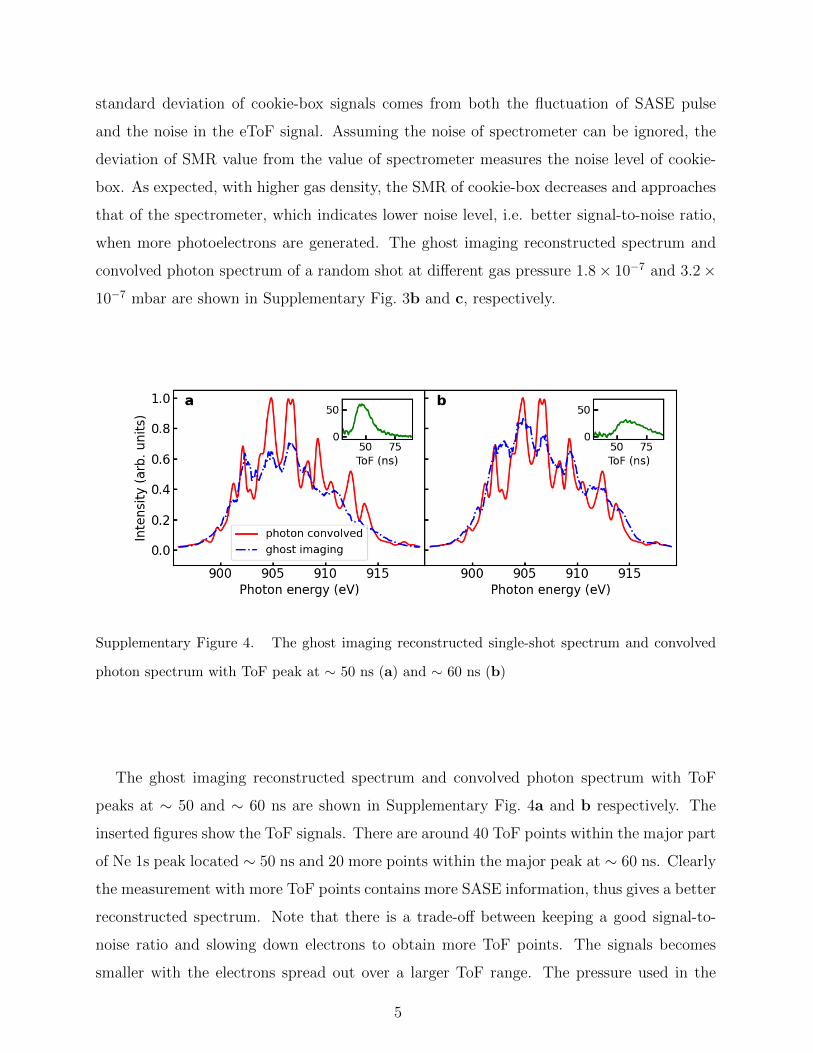
Supplementary Figure 4. The ghost imaging reconstructed single-shot spectrum and convolved
photon spectrum with ToF peak at ∼ 50 ns (a) and ∼ 60 ns (b)
The ghost imaging reconstructed spectrum and convolved photon spectrum with ToF
peaks at ∼ 50 and ∼ 60 ns are shown in Supplementary Fig. 4a and b respectively. The
inserted figures show the ToF signals. There are around 40 ToF points within the major part
of Ne 1s peak located ∼ 50 ns and 20 more points within the major peak at ∼ 60 ns. Clearly
the measurement with more ToF points contains more SASE information, thus gives a better
reconstructed spectrum. Note that there is a trade-off between keeping a good signal-to-
noise ratio and slowing down electrons to obtain more ToF points. The signals becomes
smaller with the electrons spread out over a larger ToF range. The pressure used in the
5

experiment was below the maximum allowed in the chamber 1 × 10⁻⁵ mbar [4].
[1] Coreno, M. et al. Measurement and ab initio calculation of the ne photoabsorption spectrum
in the region of the k edge. Phys. Rev. A 59, 2494–2497 (1999).
[2] Buck, J. Online time-of-flight photoemission spectrometer for x-ray photon diagnostics. Con-
ceptual Design Report of XFEL.EU TR-2012-002 (2012).
[3] Moore, D. S., Notz, W. & Fligner, M. A. The basic practice of statistics, vol. 32 (Wh Freeman
New York, 2013).
[4] Laksman, J. et al. Commissioning of a photoelectron spectrometer for soft x-ray photon diag-
nostics at the european xfel. Journal of synchrotron radiation 26, 1010–1016 (2019).
6