arX

iv:1

004.

2803

v1 [

astr

o-ph

.GA

] 16

Apr

201

0Astronomy & Astrophysicsmanuscript no. 13279man c© ESO 2010April 19, 2010

Giant pulses from the Crab pulsarA wide-band study

R. Karuppusamy1,3, B. W. Stappers2,3, and W. van Straten4

1 Sterrenkunde Instituut Anton Pannenkoek, University of Amsterdam, Kruislaan 403, Amsterdam, The Netherlandse-mail:ramesh.karuppusamy@gmail.com

2 Jodrell Bank Centre for Astrophysics, School of Physics andAstronomy, The University of Manchester, Manchester M13 9PL, UK.e-mail:Ben.Stappers@manchester.ac.uk

3 Stichting ASTRON, Postbus 2, 7990 AA, Dwingeloo, The Netherlands4 Centre for Astrophysics and Supercomputing, Swinburne University of Technology, Hawthorn, VIC 3122, Australia

e-mail:vanstraten.willem@gmail.com

ABSTRACT

The Crab pulsar is well-known for its anomalous giant radio pulse emission. Past studies have concentrated only on the very brightpulses or were insensitive to the faint end of the giant pulseluminosity distribution. With our new instrumentation offering a largebandwidth and high time resolution combined with the narrowradio beam of the Westerbork Synthesis Radio Telescope (WSRT), weseek to probe the weak giant pulse emission regime. The WSRT was used in a phased array mode, resolving a large fraction of theCrab nebula. The resulting pulsar signal was recorded usingthe PuMa II pulsar backend and then coherently dedispersed and searchedfor giant pulse emission. After careful flux calibration, the data were analysed to study the giant pulse properties. Theanalysis includesthe distributions of the measured pulse widths, intensities, energies, and scattering times. The weak giant pulses areshown to form aseparate part of the intensity distribution. The large number of giant pulses detected were used to analyse scattering and scintillationin giant pulses. We report for the first time the detection of giant pulse emission at both the main- and interpulse phases within a singlerotation period. The rate of detection is consistent with the appearance of pulses at either pulse phase as being independent. Thesepulse pairs were used to examine the scintillation timescales within a single pulse period.

Key words. pulsars - neutron stars - emission mechanism - giant pulses

1. Introduction

Identified as the supernova remnant that resulted from SN 1054,the Crab nebula is one of the strongest radio sources in thesky, and it harbours the young neutron star PSR B0531+21.The pulsar is visible across the entire observable electromag-netic spectrum, and at radio wavelengths it is the second bright-est pulsar in the northern sky. PSR B0531+21 was discoveredby Staelin & Reifenstein (1968), soon after the discovery ofpulsars. This pulsar is noted for several features including thenear orthogonal alignment of the magnetic and rotational axisthat gives rise to the observed interpulse emission. The aver-age emission profile of the pulsar, obtained by averaging thera-dio emission from many rotations of the star, exhibits a numberof features that change quite remarkably with radio frequency(Moffett & Hankins 1994). The single pulses show a large vari-ation in amplitude and duration as a function of time. The mostenigmatic of these are its occassional intense bursts knownasgiant pulses (Heiles et al. 1970; Staelin & Sutton 1970). Thegiant pulses can be extremely narrow, of the order of 0.4ns(Hankins & Eilek 2007) and the pulse flux can be several 1000times the average pulse flux. The ultrashort durations of thegi-ant pulses imply very high equivalent brightness temperatures(Hankins et al. 2003) indicating that they originate from non-thermal, coherent emission processes. In this work, we definegiant pulses as the pulses with a significantly narrower widththan the average emission and contain a flux of at least 10 timesthe mean flux density of the pulsar.

The Crab pulsar is one of just a handful of pulsars that havebeen shown to have giant pulse emission. Some other pulsars,like the young Vela pulsar, also show narrow, bursty emissioncalled giant micropulses (Johnston et al. 2001). The fluxes ofthese micropulses are within a factor of 3 times the averagepulse flux. In the pulsars that show giant pulse emission, thepulse intensity and energy distributions exhibit power-law statis-tics (Argyle & Gower 1972), while the giant micropulses giverise to log-normal distributions (Cairns et al. 2001). In contrast,the bulk of the pulsar population have pulse intensities anden-ergies that follow either a normal or an exponential distribution(Hesse & Wielebinski 1974; Ritchings 1976). This indicatesthatthe giant pulses and micropulses may form a different emissionpopulation.

The Crab giant pulses have been studied by different groups,yet the nature of the emission process remains elusive. In thevery early studies at low sky frequencies, the data were af-flicted by dispersion smearing and scattering (Heiles et al.1970;Gower & Argyle 1972), but the power-law nature of the inten-sity distribution of giant pulses was identified. In the nextma-jor study, Lundgren et al. (1995) discuss a multi-wavelength ob-servation of giant pulse emission, and note the possibilityofa weak giant pulse emission population at radio wavelengths,which they are unable to resolve owing to insufficient sensitivity.Sallmen et al. (1999) found that the Crab giant pulses are broadband at radio wavelengths. They also determine giant pulse spec-tral indices in the range of -2.2 to -4.9 using their widely spacedobservation bands and 29 simultaneously detected giant pulses.

2 R. Karuppusamy et al.: Giant pulses from the Crab pulsar

Observations by Hankins et al. (2003) revealed that giant pulsesat 5.5 GHz contain nanosecond wide subpulses and the presenceof such narrow features has been predicted in numerical mod-elling by Weatherall (1998). At these frequencies the radioemis-sion character of the Crab pulsar changes, with the interpulseemission becoming dominant. A multi-wavelength radio obser-vation of Crab giant pulses with widely spaced frequency bands(0.43 GHz and 8.8 GHz) is presented by Cordes et al. (2004),who discuss the effects of scintillation over a wide range of fre-quencies. Popov & Stappers (2007) and Eilek et al. (2002) in-vestigated pulse width distributions and find that narrow pulsestend to be brighter. Bhat et al. (2008) carried out a similar analy-sis in addition to scattering and dispersion variations in the neb-ula. All of these studies point to the peculiarity of the Crabpulsarand its puzzling emission process, and motivates further study infiner detail using a large number of pulses. For the work dis-cussed in this paper, we utilised the wide band capabilitiesof thenew pulsar machine, PuMa–II (Karuppusamy et al. 2008) andthe Westerbork Synthesis Radio Telescope (WSRT) in the coher-ent tied-array mode. At small hour angles, the synthesised beamof the WSRT effectively resolves out the Crab nebula, reduc-ing the nebular contribution to the system temperature. Thus theWSRT and PuMa–II combination makes this study much moresensitive in terms of signal-to-noise ratio achieved, and in num-ber of pulses than was possible in the past. The rest of the paperis organised as follows: in§2 we describe the observational setup and data reduction, flux calibration is discussed in§3, thegiant pulse characteristics are discussed in§4. We report detec-tions of double giant pulses in§5, and the scattering analysis ispresented in§6.

2. Observations and data reduction

The radio observations of the Crab pulsar reported here werecarried out as part of a multi-wavelength observation with theIntegralγ-ray telescope and the WSRT on 11 October 2005. TheWSRT observations were from UTC 03.h56.m50.s to 09.h36.m20.s

with a break of three minutes in the middle of the observationto switch data disks. The results of theγ-ray observations willbe reported elsewhere.

The pulsar was observed at eight different sky frequenciesin the L–Band, which is the most sensitive front-end receiver atthe WSRT (T sys = 30 K). The sky frequencies (see Table. 1)were chosen to be free of radio frequency interference. Two or-thogonal polarisations of 8×20 MHz analogue signals from eachtelescope were 2-bit sampled at the Nyquist rate of 40 MHz. The

Parameter Value

Observation duration . . . . . . . . . . . . 21420 sStart Epoch . . . . . . . . . . . . . . . . . . . . . 53654.726505 (MJD)Sky frequencies . . . . . . . . . . . . . . . . . 1311a,1330, 1350, 1370, 1392a

1410, 1428a,b,1450 MHzBandwidth . . . . . . . . . . . . . . . . . . . . . 8× 20 MHzNominalTsys . . . . . . . . . . . . . . . . . . . 30 KBeam size . . . . . . . . . . . . . . . . . . . . . . 21′′ × 1741′′ c

a These frequencies are not uniformly spaced to avoid interference.b This band was not recorded due to disk failure.c The beam size varies as a function of the observation time. See text

for details.

Table 1. Telescope parameters and observation details.

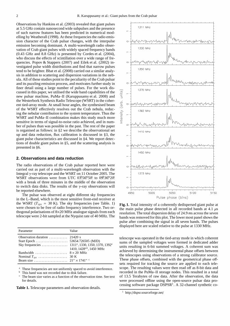
Fig. 1. Total intensity of a coherently dedispersed giant pulse atthe main pulse phase detected in all recorded bands at 4.1µsresolution. The total dispersion delay of 24.9ms across the sevenbands was removed for this plot. The lower most panel shows thepulse after combining the signal in all seven bands. The pulsesdisplayed here are scaled relative to the pulse at 1330 MHz.

telescope was operated in the tied-array mode in which coherentsums of the sampled voltages were formed in dedicated adderunits resulting in 6-bit summed voltages. A coherent sum wasachieved by determining the instrumental phase offsets betweenthe telescopes using observations of a strong calibrator source.These phase offsets, combined with the geometrical phase off-sets required for tracking the source are applied to each tele-scope. The resulting values were then read off as 8-bit data andrecorded in the PuMa–II storage nodes. This resulted in a totalof 13.5 Terabytes of raw data. After the observation, the datawere processed offline using the open-source pulsar data pro-cessing software package DSPSR1. A 32-channel synthetic co-

1 http://dspsr.sourceforge.net/

R. Karuppusamy et al.: Giant pulses from the Crab pulsar 3

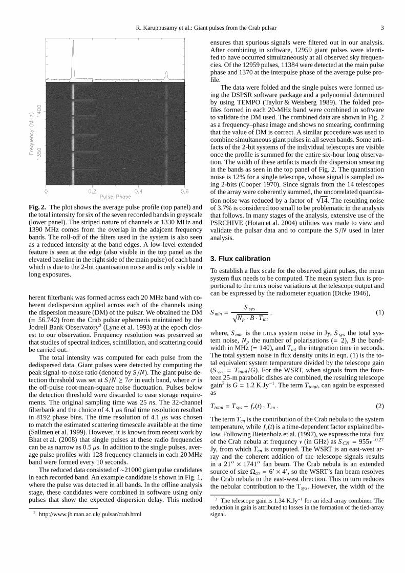
Fig. 2. The plot shows the average pulse profile (top panel) andthe total intensity for six of the seven recorded bands in greyscale(lower panel). The striped nature of channels at 1330 MHz and1390 MHz comes from the overlap in the adajcent frequencybands. The roll-off of the filters used in the system is also seenas a reduced intensity at the band edges. A low-level extendedfeature is seen at the edge (also visible in the top panel as theelevated baseline in the right side of the main pulse) of eachbandwhich is due to the 2-bit quantisation noise and is only visible inlong exposures.

herent filterbank was formed across each 20 MHz band with co-herent dedispersion applied across each of the channels usingthe dispersion measure (DM) of the pulsar. We obtained the DM(= 56.742) from the Crab pulsar ephemeris maintained by theJodrell Bank Observatory2 (Lyne et al. 1993) at the epoch clos-est to our observation. Frequency resolution was preservedsothat studies of spectral indices, scintillation, and scattering couldbe carried out.

The total intensity was computed for each pulse from thededispersed data. Giant pulses were detected by computing thepeak signal-to-noise ratio (denoted byS/N). The giant pulse de-tection threshold was set atS/N ≥ 7σ in each band, whereσ isthe off-pulse root-mean-square noise fluctuation. Pulses belowthe detection threshold were discarded to ease storage require-ments. The original sampling time was 25ns. The 32-channelfilterbank and the choice of 4.1µs final time resolution resultedin 8192 phase bins. The time resolution of 4.1µs was chosento match the estimated scattering timescale available at the time(Sallmen et al. 1999). However, it is known from recent work byBhat et al. (2008) that single pulses at these radio frequenciescan be as narrow as 0.5µs. In addition to the single pulses, aver-age pulse profiles with 128 frequency channels in each 20 MHzband were formed every 10 seconds.

The reduced data consisted of∼21000 giant pulse candidatesin each recorded band. An example candidate is shown in Fig. 1,where the pulse was detected in all bands. In the offline analysisstage, these candidates were combined in software using onlypulses that show the expected dispersion delay. This method

2 http://www.jb.man.ac.uk/ pulsar/crab.html

ensures that spurious signals were filtered out in our analysis.After combining in software, 12959 giant pulses were identi-fed to have occurred simultaneously at all observed sky frequen-cies. Of the 12959 pulses, 11384 were detected at the main pulsephase and 1370 at the interpulse phase of the average pulse pro-file.

The data were folded and the single pulses were formed us-ing the DSPSR software package and a polynomial determinedby using TEMPO (Taylor & Weisberg 1989). The folded pro-files formed in each 20-MHz band were combined in softwareto validate the DM used. The combined data are shown in Fig. 2as a frequency–phase image and shows no smearing, confirmingthat the value of DM is correct. A similar procedure was used tocombine simultaneous giant pulses in all seven bands. Some arti-facts of the 2-bit systems of the individual telescopes are visibleonce the profile is summed for the entire six-hour long observa-tion. The width of these artifacts match the dispersion smearingin the bands as seen in the top panel of Fig. 2. The quantisationnoise is 12% for a single telescope, whose signal is sampled us-ing 2-bits (Cooper 1970). Since signals from the 14 telescopesof the array were coherently summed, the uncorrelated quantisa-tion noise was reduced by a factor of

√14. The resulting noise

of 3.7% is considered too small to be problematic in the analysisthat follows. In many stages of the analysis, extensive use of thePSRCHIVE (Hotan et al. 2004) utilities was made to view andvalidate the pulsar data and to compute theS/N used in lateranalysis.

3. Flux calibration

To establish a flux scale for the observed giant pulses, the meansystem flux needs to be computed. The mean system flux is pro-portional to the r.m.s noise variations at the telescope output andcan be expressed by the radiometer equation (Dicke 1946),

S min =S sys

√

Np · B · Tint

, (1)

where,S min is the r.m.s system noise in Jy,S sys the total sys-tem noise,Np the number of polarisations (= 2), B the band-width in MHz (= 140), andTint the integration time in seconds.The total system noise in flux density units in eqn. (1) is the to-tal equivalent system temperature divided by the telescopegain(S sys = Ttotal/G). For the WSRT, when signals from the four-teen 25-m parabolic dishes are combined, the resulting telescopegain3 is G = 1.2 K.Jy−1. The termTtotal, can again be expressedas

Ttotal = T sys + fν(t) · Tcn . (2)

The termTcn is the contribution of the Crab nebula to the systemtemperature, whilefν(t) is a time-dependent factor explained be-low. Following Bietenholz et al. (1997), we express the total fluxof the Crab nebula at frequencyν (in GHz) asS CN = 955ν−0.27

Jy, from whichTcn is computed. The WSRT is an east-west ar-ray and the coherent addition of the telescope signals resultsin a 21′′ × 1741′′ fan beam. The Crab nebula is an extendedsource of sizeΩcn = 6′ × 4′, so the WSRT’s fan beam resolvesthe Crab nebula in the east-west direction. This in turn reducesthe nebular contribution to the Tsys. However, the width of the

3 The telescope gain is 1.34 K.Jy−1 for an ideal array combiner. Thereduction in gain is attributed to losses in the formation ofthe tied-arraysignal.

4 R. Karuppusamy et al.: Giant pulses from the Crab pulsar

Fig. 3. The upper panel shows the change in minimum detectablesignalS min within a 4.1µs time interval during the first 5 hours ofthe 6-hour observation. The hour angle of the source is displayedon the top ordinate axis. The lower panel is the observed changein peak signal-to-noise ratio of the detected signal. The depen-dence of the signal-to-noise ratio on the hour angle of source isdiscussed in the text.

WSRT’s fan beam is not a constant, but is a function of the ob-servation time. While the source is being tracked, the effectivewidth of the synthesised beam changes with hour angle (HA)and it is expressed asΩA(t) = Ωcn · λ/D · cos(HA). In this ex-pressionHA = t−RA, wheret is the local sideral time, the max-imum baselineD = 2700m, andRA is the right ascension of theCrab pulsar. The fraction of the nebular contribution can beex-pressed asfν(t) = ΩA(t)/Ωcn, which reaches its minimum valueof 0.13 at zenith. As the source is tracked towards the horizon,the projected distance between the dishes decreases andΩA(t) in-creases. Consequently, the observing system becomes less sensi-tive toward larger hour angles, or when the source rises and sets.This time dependence of the system noise is included in our fluxcalibration. The variation inS min is shown for a bandwidth of140 MHz,Np = 2 andτ = 4.1 µs in the upper panel of Fig. 3. Aplot of the pulse intensity during the observation (lower panel ofFig. 3) confirms this reduction in sensitivity.

The peak flux of the giant pulses were computed using themodified radiometer equation (Lorimer, D. R. and Kramer, M.2005) for the pulsar case,S peak = (S/N) · S min. With the aboveconsiderations of the nebular contribution toTtotal and withT sys = 30K in the WSRT’s L–Band, the system retained suffi-ciently high sensitivity in the first 15000 seconds of the obser-vation. Two other factors have been neglected in this calibrationprocedure and do not contribute significantly to theT sys : the rel-

ative change in the orientation of the WSRT’s fan beam and theCrab nebula over the course of observation and the partial shad-owing of three telescopes out of the 14 for HA> 54 (the last 3hours of our observation).

4. Single-pulse statistics

For the analysis that follows, all pulses that were flux-calibratedas described in the previous section were used. The discussedchange in system sensitivity does not limit this analysis thanksto our careful flux calibration procedure. While approximately70% of the pulses were detected in all seven bands simultane-ously, the rest were detected in two or more of the seven bandsrecorded. For the results described below, where applicable, onlythose pulses that were detected in all seven bands were used andexplicitly mentioned.

4.1. Pulse intensity distributions

The giant pulse fluxes of the Crab pulsar contribute tothe long exponential tail of the single pulse intensity his-tograms (Argyle & Gower 1972), while the normal pulsarsshow Gaussian or exponential pulse intensity distributions(Hesse & Wielebinski 1974). Fig. 4 shows the average pulseflux distribution for pulses detected in at least two of the sevenrecorded bands. The average pulse flux is computed by integrat-ing all emission within the equivalent width,Weq of the giantpulse (see§4.4). This value is averaged over the pulse period toobtain the average pulse flux. The pulse in each band was de-tected based on a threshold of 7σ. A pulse detected in two bandssatisfies the

√2 × 7 = 9.89σ limit. In the first three hours of

the observation (when the system was most sensitive), the fluxequivalent system noise in 4.1µs is 109 Jy. Averaged over thepulse period, a pulse ofS/N = 9.89σ corresponds to an aver-age pulse flux density of 3.9 Jy. This implies that it is sensitiveto all pulses greater than 27× 〈F〉, where〈F〉 = 14mJy is theaverage flux density of the Crab pulsar. Therefore, the flux dis-tribution computed here contains a good fraction of weak giantpulses compared to those reported elsewhere (see Table. 2).

The intensity distributions displayed in Fig. 4 shows at leasttwo components: a peak at or below∼ 4 Jy – the weak pulses thatmay comprise the trailing part of the normal pulse distribution.The next component peaking at∼ 20 Jy resembles a lognormaldistribution with a power-law tail. The bright giant pulsesresultin the extended power-law tail and is described byNF ∝ Fα,whereNF is the number of pulses detected in 1.8 Jy flux intervalsof F. The value ofα = −2.79± 0.01 andα = −3.06± 0.06 wasdetermined from the best fits to the data in the interval 118 Jy≤ F ≤ 2000 Jy and 40 Jy≤ F ≤ 596 Jy for the giant pulses inthe main- and interpulse, respectively. Visual inspectionof Fig.4 shows that the distribution is multi-modal, with giant pulses inthe regionF >∼ 10 Jy and the pulses below this limit possiblyrepresenting normal pulses.

It is worth noting the differences in the intensity distribu-tions displayed in Fig. 4. While the distribution of the giantpulses in the main pulse phase shows a clear turn over at∼20Jy, the emergence of a bimodality in the region containing weakpulses is evident in the intensity distribution of the interpulse gi-ants. The distribution corresponding to the interpulse phase alsoshows a flattening in the 10–30 Jy region. The clear excess ofweak pulses in both the distributions in the regionF ≤ 4Jy isdue to our method of settingWeq = 4.1 µs (equal to the timeresolution). In this case the emission window we consideredis

R. Karuppusamy et al.: Giant pulses from the Crab pulsar 5

Fig. 4. Distribution of the pulse intensity of all giant pulsesdetected at the main- and interpulse phases in the upper andlower panels, respectively. The long tail results from the giantpulse emission. The best fit power-law curve is shown with slope−2.79±0.01 for the pulses in main pulse phase and−3.06±0.06for the pulses in the interpulse phase. Both distributions show anexcess near 4Jy and come from the rounding off in Weq. [see textfor details].

Reference Frequency Threshold(MHz) (Jy)

Lundgren et al. (1995) . . . . . . . . . . . 800 120.0Popov & Stappers (2007) . . . . . . . . 1197 5.9 a

Bhat et al. (2008) . . . . . . . . . . . . . . . 1300/1470 22.3 b

This paper . . . . . . . . . . . . . . . . . . . . . . 1373 3.9

a Equivalent average pulse computed flux from the quoted 6σ peakflux density of 142 Jy, assuming 0.036 pulse duty cycle.

b Average pulse flux density extrapolated for 7σ threshold, 4.1µstime resolution and pulse duty cycle≈ 0.036.

Table 2. Reported sensitivity to the Crab giant pulse observa-tions in the literature.

dominated by noise or weak and narrow pulses. The slopes ofthe power-law models obtained here can be compared to the val-ues reported earlier. Fig. 4 of Lundgren et al. (1995) shows aslope of−3.46± 0.04 for data at 800 MHz, which is slightlysteeper than the slopes of the main- and interpulse distributionsderived here. Cordes et al. (2004) derive a value of∼ -2.3 at 433MHz and Bhat et al. (2008) found−2.33± 0.14 at 1300 MHz,which are comparable to the slope the main pulse intensity dis-tribution in our work. The slopes of the intensity distribution re-ported here generally agree considering the effect of low numberstatisics and/or dispersion smearing in the observations reportedelsewhere. While this experiment was sensitive to much lower

fluxes, the long observation time has also enabled the detectionof rarer bright pulses.

4.2. Pulse energy distributions

Fig. 5. The cumulative probablity distribution of the energy ingiant pulses detected at the main pulse and the interpulse phasesin the upper and lower panels, respectively. The y-axis is thefraction of the total number of pulses and pulse energy is plottedon the x-axis. Also shown are the occurrence rates per minute,second and hour.

The relative occurrence rates of giant pulses is displayed asa cumulative probablity distribution of the individual pulse ener-gies in Fig. 5. The pulse energy is computed by multiplying theequivalent width,Weq, and the average pulse flux. As describedin §4.1, we computed the best fits to the cumulative probablitydistributions of the main- and interpulse giants. The power-lawcurve withα = −2.13± 0.007 andα = −1.97± 0.006 fits thedata for pulse energies at the main- and inter pulse phases, re-spectively. The break seen at∼2000 Jy.µs is consistent with thebreak value reported by Popov & Stappers (2007). The emissionat the interpulse phase shows a somewhat shallower power-law.

It is known from Popov & Stappers (2007) that the power-law index has a width dependence, varying from−1.7 to−3.2as the pulse width increases. Based on this variation, the indexwe find is in good agreement with Popov & Stappers (2007) andBhat et al. (2008) (−1.88 ± 0.02 at 1300 MHz). However, wefit only a single power law unlike the two power-law fits foundby these authors. Partial fits to the low-energy pulses yieldmorethan two components, with shallower power-law indices indicat-ing a simple dual-component fit is insufficient. One explanationfor this can be the bias introduced by settingWeq = 4.1 µs fornarrow pulses, overestimating the pulse energy. However, thiscan only be a minor contribution and is an argument that thereisa clear break in the intensity distribution. To compare the occur-

6 R. Karuppusamy et al.: Giant pulses from the Crab pulsar

rence rates we see here, we proceed to derive the rates from thearrival times of the giant pulses in the next section.

4.3. Giant pulse rates

The distribution of the separation times between successive gi-ant pulses is plotted in Fig. 6. If the giant pulses are mutuallyexclusive events independent of each other, then the arrival timeseparation follows a Poisson process (Lundgren et al. 1995). Theprobablity of a giant pulse occurring in the intervalx is thengiven byP(x) = µx.e−µx, whereµ is the mean pulse rate. Sinceour data only consist of giant pulses, we expected to see an ex-ponential reduction in the separation time between the pulses.Fig. 6 shows the fits to the separation times at both the inter-andmain-pulse phases.

Fig. 6. The symbols show the distribution of separation timesbetween successive giant pulses at the main- and interpulsephases and the solid lines are the best fits to the distribution.The top ordinate axis corresponds to the curve and data for thepulses at the main pulse phase and are offset by 450 for clarity.

Functions with an exponential decay with time constants1/τ = 1.1± 0.02 and 1/τ = 0.172± 0.003 are in excellent agree-ment with the data at the main- and interpulse phases, respec-tively. From the values ofτ, the mean giant pulse rates are onemain- pulse giant every 0.9 seconds and one inter pulse giantevery 5.81 seconds observed above our threshold limit of 3.9Jy.At these frequencies, the interpulse giants are comparatively lessnumerous as is evident from our data. For comparision, the inter-pulse giants are brighter and more frequent in frequency bandsabove 5.5 GHz (Cordes et al. 2004). The combined rate of thegiant pulses (fit and data not shown) is one pulse every 0.803seconds. The foregoing discussion confirms earlier predictionsthat the giant pulse rate increases with frequency for the Crabpulsar (Lundgren et al. 1995; Sallmen et al. 1999). The effect ofthe WSRT’s sensitivity reduction towards the end of the obser-vation, as displayed in Fig. 3, may have contributed to the longtail of the distribution, where fewer pulses were detected than inthe first half of the observation. However, the rate derived hereis robust, since the system had sufficiently high sensitivity in thefirst half of the observation.

4.4. Width distributions

The equivalent pulse width,Weq is defined as the width of a top-hat pulse with height equal to the peak intensity of the pulse. Weqfor the giant pulses detected in all seven bands was computed.

Fig. 7. Plot of intensity against pulse width for the main-and interpulse windows in the top left and lower left panels.Histograms of equivalent pulse widths are shown in the top rightand lower right panels. The distribution has an exponentialen-velope. For pulses with computedWeq < 4.1 µs due to randomnoise fluctuations the widths were rounded off to 4.1µs.

The results are displayed in panels on the right in Fig. 7. WeexpressWeq as

Weq =1

Imax×

n2∑

i=n1

Ii × 4.1 µs , (3)

whereImax is the peak intensity,Ii the intensity in the pulse emis-sion window defined by binsi = n1 · · n2 and is equal to 1ms inour case. ThusWeq can be viewed as the equivalent width of arectangular pulse inµs that has the same area as the giant pulse,with heightImax.

The giant pulses at these frequencies can be quite narrow. Forinstance, Bhat et al. (2008) find pulse widths to be 0.5µs andEilek et al. (2002) found 0.2µs. Our method of data reductionallowed a time resolution of 4.1µs, so pulses withWeq < 4.1µswere taken to have a width equal to 4.1µs. This results in somepulses being underestimated in flux and overestimated in equiv-alent width. The computed equivalent widths range from 4.1µsto ∼120 µs, and we find that bright pulses tend to be narrowas seen in the left hand panels of Fig. 7. This was also sug-gested by Sallmen et al. (1999) and shown by Eilek et al. (2002).Popov & Stappers (2007) found a similar behaviour in additionto a width-dependent break in the power-law fits to the pulse-energy distribution.

In the seven closely spaced radio bands observed, we notethat a vast majority of the pulses have widths larger than 4.1µs. This is seen in the pulse width histograms at the two pulsephases, displayed in the panels on the right in Fig. 7. The dis-tribution shows a peak at∼16µs, which is 4 times our ultimatetime resolution in the main pulse, and the peak shifts towards

R. Karuppusamy et al.: Giant pulses from the Crab pulsar 7

narrower timescales for the interpulses. We find less than 9%ofthe pulses withWeq = 4.1 µs, indicating that the majority of thepulses show wider widths than our time resolution. The shapeof the width distribution is similar at both the main- and inter-pulse phases.The contribution to the tail region of the distribu-tion comes from scatter broadened pulses.

4.5. Spectral index of giant pulses

The data were recorded in 7 different radio bands each 20 MHzwide in the frequency range 1300–1450 MHz, and several thou-sands of pulses were detected simultaneously in all bands. Thespectral index of individual pulses was computed by modellingthe flux variation of a giant pulse asS (ν) ∝ νk. Here,S (ν) is theflux of the giant pulse at frequencyν, andk the spectral index.The histograms of the derived spectral indices are displayed inFig. 8 for the giants at both pulse phases. A large dispersioninthe spectral index is seen, with values−1.44± 3.3 for the main-and−0.6± 3.5 for the interpulse giants.

Fig. 8. Histogram of spectral indices for the giant pulses de-tected at the main pulse (bottom panel) and the interpulse phase(top panel). The spread in the distributions is indicative of fittingerrors. See text for details.

These spectral index values are quite a bit shallower thanthose detected previously (see Introduction) over wider fre-quency separations. We therefore consider the effects of diffrac-tive interstellar scintillation (DISS) on the spectral index esti-mates. Strong DISS results in pulse intensity variations withineach of the seven bands. The effect of scintillation is to modu-late the observed pulsar signal in both time and frequency. Thisis seen as regions of enhanced or diminished brightness in agrey scale plot of the intensity as a function of time and fre-quency. These regions are known as scintles. We estimate thescintillation bandwidth based on the pulse scatter timescales,τs = 395±50µs at sky frequency of 200 MHz, as reported in the

work of Bhat et al. (2007). We further make use of their revisedτs ∝ ν−3.5 frequency scaling and consider that the scintillationbandwidth and scattering timescale are related by 2π∆νdτs = C1, where the constantC1 = 1.05 for a thin scattering screen(Cordes et al. 2004). From these considerations∆νd ≈ 0.25–0.38MHz in the 1300–1460 MHz band. On examining a few giantpulses by eye, it was clear that some of the scintles are resolved,while some were narrower than our channel width of∆ν = 0.625MHz. Thus, in the flux obtained by integrating the signal in the20MHz-wide bands, the scintles tend to average out. This im-plies that scintillation does not cause the spread in the individualgiant-pulse spectral indices. Moreover, with such narrow scin-tillation bandwidths, averaging over many giant pulse spectralindex determinations as we have done here would give an aver-age spectral index that reflects the true average spectral index.

Refractive interstellar scintillation (RISS) cannot corrugatethe spectra of single pulses, since the pulse intensity variationsdue to RISS are noticeable in observation of the order of a fewdays (Lundgren et al. 1995). However, the pulses do have a sig-nificant structure that is intrinsic to the emission process. Oneexample is displayed in Fig. 1 and these pulses do contributeto the spread in the computed spectral indices. In this figure, itis clear that the leading short burst shows considerable varia-tion across the seven bands, while the scattered trailing part ofthe pulse is correlated across frequency. This is again similar towhat Hankins & Eilek (2007) find, as shown in their Fig. 4, butat a much higher frequency of∼9 GHz.

Sallmen et al. (1999) find that the spectral index variationis between−4.9 and−2.2 based on 29 pulses they observedin two bands centred at 1.4 GHz and 0.6 GHz. The spreadin the indices computed here and that of Sallmen et al. (1999)points to the stochastic nature of the giant pulse emission processand/or the disturbed plasma flow in the magnetosphere causedby strong plasma turbulence (Hankins & Eilek 2007). The giantpulses used in this analysis were detected in all seven bandsandrepresent 70% of all detected pulses in our data. Since each ofour bands is 20 MHz wide, detection in seven bands implies anemission bandwidth of at least∆ν = 140 MHz. This suggeststhat the emission bandwidth of Crab giant pulses is potentiallygreater than∆ν/ν = 0.1, unlike the giant pulse emission fromthe millisecond pulsar B1937+21 (Popov & Stappers 2003). Wenote that the∆ν/ν = 0.8 for the Crab giant pulses reported bySallmen et al. (1999) was based on 29 simultaneous giant pulsesfrom their 90-minute observation (∼ 161086 stellar rotations).Those 29 pulses could have been chance detections, while the∆ν/ν = 0.1 limit derived here comes from a much larger sampleof giant pulses so is more robust. We detected a total of 17587giant pulses, of which approximately 4000 were detected in lessthan 7 bands. Clearly it is impossible to include the pulses de-tected in only a few bands in this analysis as that would increasethe dispersion in the spectral indices computed; however, thislack of detection in all bands, for pulses which were clearlyde-tected in the other bands, is an argument for there being somenarrow band effects that appear to modulate the giant pulse in-tensity.

5. Double giant pulses

During direct inspection of some giant pulses, it was noticed thatoccasional giant pulse emission was evident at both the main-and interpulse phases within a single rotation period of thestar.To determine how many such pulses were present, the follow-ing search algorithm was used. First, the giant pulses detectedin all seven bands were combined in software across the fre-

8 R. Karuppusamy et al.: Giant pulses from the Crab pulsar

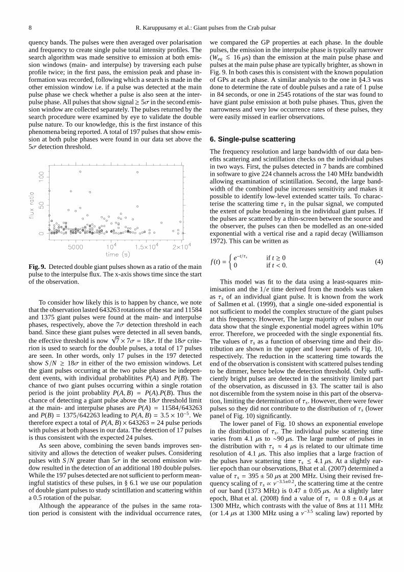
quency bands. The pulses were then averaged over polarisationand frequency to create single pulse total intensity profiles. Thesearch algorithm was made sensitive to emission at both emis-sion windows (main- and interpulse) by traversing each pulseprofile twice; in the first pass, the emission peak and phase in-formation was recorded, following which a search is made in theother emission window i.e. if a pulse was detected at the mainpulse phase we check whether a pulse is also seen at the inter-pulse phase. All pulses that show signal≥ 5σ in the second emis-sion window are collected separately. The pulses returned by thesearch procedure were examined by eye to validate the doublepulse nature. To our knowledge, this is the first instance of thisphenomena being reported. A total of 197 pulses that show emis-sion at both pulse phases were found in our data set above the5σ detection threshold.

Fig. 9. Detected double giant pulses shown as a ratio of the mainpulse to the interpulse flux. The x-axis shows time since the startof the observation.

To consider how likely this is to happen by chance, we notethat the observation lasted 643263 rotations of the star and11584and 1375 giant pulses were found at the main- and interpulsephases, respectively, above the 7σ detection threshold in eachband. Since these giant pulses were detected in all seven bands,the effective threshold is now

√7× 7σ = 18σ. If the 18σ crite-

rion is used to search for the double pulses, a total of 17 pulsesare seen. In other words, only 17 pulses in the 197 detectedshowS/N ≥ 18σ in either of the two emission windows. Letthe giant pulses occurring at the two pulse phases be indepen-dent events, with individual probablititesP(A) and P(B). Thechance of two giant pulses occurring within a single rotationperiod is the joint probablityP(A, B) = P(A).P(B). Thus thechance of detecting a giant pulse above the 18σ threshold limitat the main- and interpulse phases areP(A) = 11584/643263andP(B) = 1375/642263 leading toP(A, B) = 3.5× 10−5. Wetherefore expect a total ofP(A, B) × 643263= 24 pulse periodswith pulses at both phases in our data. The detection of 17 pulsesis thus consistent with the expected 24 pulses.

As seen above, combining the seven bands improves sen-sitivity and allows the detection of weaker pulses. Consideringpulses withS/N greater than 5σ in the second emission win-dow resulted in the detection of an additional 180 double pulses.While the 197 pulses detected are not sufficient to perform mean-ingful statistics of these pulses, in§ 6.1 we use our populationof double giant pulses to study scintillation and scattering withina 0.5 rotation of the pulsar.

Although the appearance of the pulses in the same rota-tion period is consistent with the individual occurrence rates,

we compared the GP properties at each phase. In the doublepulses, the emission in the interpulse phase is typically narrower(Weq <∼ 16µs) than the emission at the main pulse phase andpulses at the main pulse phase are typically brighter, as shown inFig. 9. In both cases this is consistent with the known populationof GPs at each phase. A similar analysis to the one in§4.3 wasdone to determine the rate of double pulses and a rate of 1 pulsein 84 seconds, or one in 2545 rotations of the star was found tohave giant pulse emission at both pulse phases. Thus, given thenarrowness and very low occurrence rates of these pulses, theywere easily missed in earlier observations.

6. Single-pulse scattering

The frequency resolution and large bandwidth of our data ben-efits scattering and scintillation checks on the individualpulsesin two ways. First, the pulses detected in 7 bands are combinedin software to give 224 channels across the 140 MHz bandwidthallowing examination of scintillation. Second, the large band-width of the combined pulse increases sensitivity and makesitpossible to identify low-level extended scatter tails. To charac-terise the scattering timeτs in the pulsar signal, we computedthe extent of pulse broadening in the individual giant pulses. Ifthe pulses are scattered by a thin-screen between the sourceandthe observer, the pulses can then be modelled as an one-sidedexponential with a vertical rise and a rapid decay (Williamson1972). This can be written as

f (t) =

e−t/τs if t ≥ 00 if t < 0. (4)

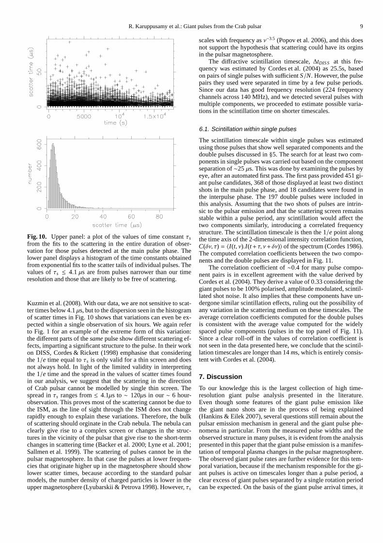
This model was fit to the data using a least-squares min-imisation and the 1/e time derived from the models was takenas τs of an individual giant pulse. It is known from the workof Sallmen et al. (1999), that a single one-sided exponential isnot sufficient to model the complex structure of the giant pulsesat this frequency. However, The large majority of pulses in ourdata show that the single exponential model agrees within 10%error. Therefore, we proceeded with the single exponentialfits.The values ofτs as a function of observing time and their dis-tribution are shown in the upper and lower panels of Fig. 10,respectively. The reduction in the scattering time towardstheend of the observation is consistent with scattered pulses tendingto be dimmer, hence below the detection threshold. Only suffi-ciently bright pulses are detected in the sensitivity limited partof the observation, as discussed in§3. The scatter tail is alsonot discernible from the system noise in this part of the observa-tion, limiting the determination ofτs. However, there were fewerpulses so they did not contribute to the distribution ofτs (lowerpanel of Fig. 10) significantly.

The lower panel of Fig. 10 shows an exponential envelopein the distribution ofτs. The individual pulse scattering timevaries from 4.1µs to ∼90 µs. The large number of pulses inthe distribution withτs ≈ 4 µs is related to our ultimate timeresolution of 4.1µs. This also implies that a large fraction ofthe pulses have scattering timeτs ≤ 4.1 µs. At a slightly ear-lier epoch than our observations, Bhat et al. (2007) determined avalue ofτs = 395± 50 µs at 200 MHz. Using their revised fre-quency scaling ofτs ∝ ν−3.5±0.2, the scattering time at the centreof our band (1373 MHz) is 0.47± 0.05µs. At a slightly laterepoch, Bhat et al. (2008) find a value ofτs = 0.8 ± 0.4 µs at1300 MHz, which contrasts with the value of 8ms at 111 MHz(or 1.4µs at 1300 MHz using aν−3.5 scaling law) reported by

R. Karuppusamy et al.: Giant pulses from the Crab pulsar 9

Fig. 10. Upper panel: a plot of the values of time constantτs

from the fits to the scattering in the entire duration of obser-vation for those pulses detected at the main pulse phase. Thelower panel displays a histogram of the time constants obtainedfrom exponential fits to the scatter tails of individual pulses. Thevalues ofτs ≤ 4.1 µs are from pulses narrower than our timeresolution and those that are likely to be free of scattering.

Kuzmin et al. (2008). With our data, we are not sensitive to scat-ter times below 4.1µs, but to the dispersion seen in the histogramof scatter times in Fig. 10 shows that variations can even be ex-pected within a single observation of six hours. We again referto Fig. 1 for an example of the extreme form of this variation:the different parts of thesame pulse show different scattering ef-fects, imparting a significant structure to the pulse. In their workon DISS, Cordes & Rickett (1998) emphasise that consideringthe 1/e time equal toτs is only valid for a thin screen and doesnot always hold. In light of the limited validity in interpretingthe 1/e time and the spread in the values of scatter times foundin our analysis, we suggest that the scattering in the directionof Crab pulsar cannot be modelled by single thin screen. Thespread inτs ranges from≤ 4.1µs to∼ 120µs in our∼ 6 hour-observation. This proves most of the scattering cannot be due tothe ISM, as the line of sight through the ISM does not changerapidly enough to explain these variations. Therefore, thebulkof scattering should orginate in the Crab nebula. The nebulacanclearly give rise to a complex screen or changes in the struc-tures in the vicinity of the pulsar that give rise to the short-termchanges in scattering time (Backer et al. 2000; Lyne et al. 2001;Sallmen et al. 1999). The scattering of pulses cannot be in thepulsar magnetosphere. In that case the pulses at lower frequen-cies that originate higher up in the magnetosphere should showlower scatter times, because according to the standard pulsarmodels, the number density of charged particles is lower in theupper magnetosphere (Lyubarskii & Petrova 1998). However,τs

scales with frequency asν−3.5 (Popov et al. 2006), and this doesnot support the hypothesis that scattering could have its orginsin the pulsar magnetosphere.

The diffractive scintillation timescale,∆tDIS S at this fre-quency was estimated by Cordes et al. (2004) as 25.5s, basedon pairs of single pulses with sufficientS/N. However, the pulsepairs they used were separated in time by a few pulse periods.Since our data has good frequency resolution (224 frequencychannels across 140 MHz), and we detected several pulses withmultiple components, we proceeded to estimate possible varia-tions in the scintillation time on shorter timescales.

6.1. Scintillation within single pulses

The scintillation timescale within single pulses was estimatedusing those pulses that show well separated components and thedouble pulses discussed in§5. The search for at least two com-ponents in single pulses was carried out based on the componentseparation of∼25 µs. This was done by examining the pulses byeye, after an automated first pass. The first pass provided 451gi-ant pulse candidates, 368 of those displayed at least two distinctshots in the main pulse phase, and 18 candidates were found inthe interpulse phase. The 197 double pulses were included inthis analysis. Assuming that the two shots of pulses are intrin-sic to the pulsar emission and that the scattering screen remainsstable within a pulse period, any scintillation would affect thetwo components similarly, introducing a correlated frequencystructure. The scintillation timescale is then the 1/e point alongthe time axis of the 2-dimensional intensity correlation function,C(δν, τ) = 〈I(t, ν).I(t+ τ, ν+ δν)〉 of the spectrum (Cordes 1986).The computed correlation coefficients between the two compo-nents and the double pulses are displayed in Fig. 11.

The correlation coefficient of∼0.4 for many pulse compo-nent pairs is in excellent agreement with the value derived byCordes et al. (2004). They derive a value of 0.33 consideringthegiant pulses to be 100% polarised, amplitude modulated, scintil-lated shot noise. It also implies that these components haveun-dergone similar scintillation effects, ruling out the possibility ofany variation in the scattering medium on these timescales.Theaverage correlation coefficients computed for the double pulsesis consistent with the average value computed for the widelyspaced pulse components (pulses in the top panel of Fig. 11).Since a clear roll-off in the values of correlation coefficient isnot seen in the data presented here, we conclude that the scintil-lation timescales are longer than 14ms, which is entirely consis-tent with Cordes et al. (2004).

7. Discussion

To our knowledge this is the largest collection of high time-resolution giant pulse analysis presented in the literature.Even though some features of the giant pulse emission likethe giant nano shots are in the process of being explained(Hankins & Eilek 2007), several questions still remain about thepulsar emission mechanism in general and the giant pulse phe-nomena in particular. From the measured pulse widths and theobserved structure in many pulses, it is evident from the analysispresented in this paper that the giant pulse emission is a manifes-tation of temporal plasma changes in the pulsar magnetosphere.The observed giant pulse rates are further evidence for thistem-poral variation, because if the mechanism responsible for the gi-ant pulses is active on timescales longer than a pulse period, aclear excess of giant pulses separated by a single rotation periodcan be expected. On the basis of the giant pulse arrival times, it

10 R. Karuppusamy et al.: Giant pulses from the Crab pulsar

Fig. 11. Correlation coefficients of the spectra within a singlepulse period. Top panel shows correlation between the two com-ponents of giant pulse, while lower panel is the double giants.The separation between the componentsτ is shown in the ab-scissa.

was concluded that the observed giant pulse emission does notcome from a steady emission beam loosely bound to the stellarsurface (Lundgren et al. 1995; Sallmen et al. 1999). We confirmthat our data do not support such a model, for if such a beamwith random wobbles operates, a characteristic width in thegi-ant pulses can be expected. In other words, the distributionof thepulse widths would be normally distributed with a mean width.

The power-law nature of the giant pulse intensity distribu-tions was shown by Lundgren et al. (1995), and they inferredthat the normal pulses formed a separate part of the intensitydistributions. In this work, we have shown conclusively thatthe giant pulses consist of two distinct populations especiallyfor those pulses found at the inter pulse phase. We see a def-inite change in the shape of the distribution of pulse energiesas we go to lower energies and we also see a slight broadeningof the pulses. These pulses still seem to be distinct from whatmight be called “normal pulses”: they are still narrower thanmost subpulses and are at least 27 times brighter than the nor-mal pulses. The slope of the distribution containing these pulsesis different from rest of the intensity distribution. These pulsescould possibly be the trailing part of the distribution inferred byLundgren et al. (1995). Moreover, how these relate to the pre-cursor emission is unclear, which can clearly be improved uponusing the double giant pulses. While there is evidence of a broad-ening of the pulses as they weaken in intensity, they do not ap-pear to be as broad as standard subpulses. This finding has im-plications in the model derived by Petrova (2004), where a clearpower-law distribution is explained, but not a weak giant pop-ulation. The power-law index derived also has implicationsfor

interpreting giant pulse emission on the basis of self organisedcriticality (Bak et al. 1987), as suggested by Cairns (2004).

The spectral index of the Crab giant pulses reported in thiswork suggests that the emission bandwidth is at least∆ν/ν > 0.1and may approach the upper limit∆ν/ν = 0.2 predicted in nu-merical models by Weatherall (1998). Hankins & Eilek (2007)find a similar emission bandwidth at 9.5 GHz. Moreover, theaverage spectral index of giant pulses at the interpulse phase isflatter than the giant pulses at the main pulse phase. This possi-bly explains the dominant and bright nature of interpulse giantsat ν > 5 GHz. We note the prominent emergence of bimodalityin the intensity distribution of the interpulses relative to the mainphase pulses. Furthermore, (Hankins & Eilek 2007) find upwarddrifting emission bands in the spectrum of the interpulses giantsand not in the main pulse giants. These differences strongly sug-gest a different nature to the interpulses. To explain the driftingemission bands, Lyutikov (2007) derived an excess plasma den-sity of ∼105 and a large Lorentz factor of the emitting particlesof the order of∼107, and this condition is satisfied close to thelight cylinder over the magnetic equator. However, the modelproposed by Lyutikov (2007) is only valid forν > 5 GHz, wherethe emission bands are observed. While results from our obser-vations can neither support nor rule out this model, the differ-ence in pulse intensity distributions we find indicates thattheinterpulse giants are different in nature.

It is worth noting that the pulsar signal is a stochastic processthat contributes to the measurement noise of the pulsed intensity.This is especially true in the case of giant pulse emission, wherepulsed flux can exceed 1500 Jy, an order of magnitude greaterthan the system equivalent flux density (SEFD) of approximately145 Jy. Source-intrinsic noise increases the measurement uncer-tainty of various derived parameters, such as the pulsed fluxden-sity, pulse width, scattering time, and spectral index van Straten(2009). In addition, any temporal and/or spectral correlations –either intrinsic to the giant pulse emission or induced by inter-stellar scintillation – will also affect the uncertainties of any de-rived parameters. The vast majority of the pulses presentedinthis analysis have average flux densities that are lower thantheSEFD, and we do not expect that self-noise will significantlyal-ter the results of this analysis. To accurately quantify theimpactof self-noise on parameter distributions (such as those presentedin Figures 4,5,7, and 8) would require extensive simulations thatare beyond the scope of the present work but may provide addi-tional insight in a future paper.

The previously unreported double pulses we found are con-sistent with the occurrence rate on a purely probabilistic ba-sis. Collecting even more of these pulse pairs would allow forbetter checks of the statistics of occurrence to ascertain thatthey are chance occurrences and not indicative of some longerterm underlying phenomenon driving the giant pulse emisision.Moreover detecting more of these pulses at higher time resolu-tion would provide further insight into the nature of these pulses.Hankins & Eilek (2007) found that the giant pulses at the inter-pulse phase show an additional dispersion when compared tothe pulses at the main pulse phase. The closest pulse pair theywere able to examine were separated by 12 minutes. One maygain new insight into the excess dispersion seen at the interpulsephase by examining the double giant pulses, which are the clos-est giant pulse pair possible.

Scattering analysis of single pulses presented in this papershow a variety of scattering times and corroborates with theanalysis of Sallmen et al. (1999). They show that scatteringfrommultiple screens or a single thick screen is excluded because ofthe observed frequency independence of the pulse component

R. Karuppusamy et al.: Giant pulses from the Crab pulsar 11

separation. From this it was concluded that the multiple compo-nents that make up the giant pulses are intrinisic to the emissionmechanism. Using multiple components and the double pulses,we conclude that the scintillation timescales are greater than 14ms, which indicates that there are no large changes in the numberdensity of the scattering medium along the line of sight throughthe nebula on similar timescales. That the multiple componentswe detect in the giant pulses are spaced by at least 25µs im-plies that the magnetosphere and/or the plasma does not changeon these timescales, if the source intrinsic emission is less than25 µs. On the other hand, giant pulses may consist of overlap-ping nano shots. In this case the competing models make use ofplasma turbulence leading to modulational instablity (Weatherall1998) or the induced Compton scattering of low-frequency radiowaves (Petrova 2004) in the magnetosphere to explain the originof the nano shots. While with our data we are not sensitive to thepulses less than 4.1µs duration, there is an indication that theemission bandwidth∆ν/ν > 0.1, suggesting that the pulses canpotentially have structure as narrow as 3.6ns at this frequency.

8. Conclusions

The large collection of single pulses we gathered has allowed usto perform a range of statistics with the data. After carefulfluxcalibration, a detailed analysis of the pulse intensities,energies,widths, and separation times was done by computing distribu-tions of these quantities. In the single-pulse intensity distribu-tions, we find a clear evidence of two distinct populations inthegiant pulses. The giant pulse separation times show a Poissiondistribution, and the rate of occurrence of giant pulses wasdeter-mined. Spectral indices for a large number of giant pulses werecomputed with the narrowly spaced multi band data. Significantdispersion in the spectral indices was found and a small negativeaverage spectral index was found for the main- and interpulsegiants, and they are flatter than the average pulse emission.Wealso note that in some cases there is evidence for intensity modu-lation with bandwidths that are smaller than the full band but notconsistent with scintillation effects. The previously undetecteddouble giant pulses were presented and we find that they arenot more frequent than would be expected by chance. The scat-ter time for a large number of giant pulses was determined bymodelling the scatter broadening as an exponenial functionandthe distribution of scatter times was computed. The double giantpulses were reported for the first time and it is found that theyare not very different from the normal giant pulses. Using multi-ple emission components either at the main- or interpulse phaseand the double giant pulses, we find no evidence of variation ofthe scattering material on timescales shorter than 14ms basedon the correlation coefficient computed for emission within asingle-pulse period.

Acknowledgements. The WSRT is operated by ASTRON. We thank the ob-servers for setting up the observations. The PuMa–II instrument and one ofus, RK, are funded by Nederlands Onderzoekschool Voor Astronomie (NOVA).We acknowledge the use of SAO/NASA Astrophysics Data System. RK thanksMaciej Serylak for his helpful comments. We thank the anonymous refree forcomments that improved this paper.

ReferencesArgyle, E. & Gower, J. F. R. 1972, Astrophys. J., 175, L89Backer, D. C., Wong, T., & Valanju, J. 2000, Astrophys. J., 543, 740Bak, P., Tang, C., & Wiesenfeld, K. 1987, Physical Review Letters, 59, 381Bhat, N. D. R., Tingay, S. J., & Knight, H. S. 2008, ApJ, 676, 1200Bhat, N. D. R., Wayth, R. B., Knight, H. S., et al. 2007, ApJ, 665, 618Bietenholz, M. F., Kassim, N., Frail, D. A., et al. 1997, Astrophys. J., 490, 291

Cairns, I. H. 2004, ApJ, 610, 948Cairns, I. H., Johnston, S., & Das, P. 2001, Astrophys. J., 563, L65Cooper, B. F. C. 1970, Aust. J. Phys., 23, 521Cordes, J. M. 1986, Astrophys. J., 311, 183Cordes, J. M., Bhat, N. D. R., Hankins, T. H., McLaughlin, M. A., & Kern, J.

2004, Astrophys. J., 612, 375Cordes, J. M. & Rickett, B. J. 1998, Astrophys. J., 507, 846Dicke, R. H. 1946, Rev. Sci. Instrum., 17, 268Eilek, J. A., Arendt, Jr., P. N., Hankins, T. H., & Weatherall, J. C. 2002, in

Neutron Stars, Pulsars, and Supernova Remnants, ed. W. Becker, H. Lesch,& J. Trumper, 249–+

Gower, J. F. R. & Argyle, E. 1972, Astrophys. J., 171, L23Hankins, T. H. & Eilek, J. A. 2007, ApJ, 670, 693Hankins, T. H., Kern, J. S., Weatherall, J. C., & Eilek, J. A. 2003, Nature, 422,

141Heiles, C., Campbell, D. B., & Rankin, J. M. 1970, Nature, 226, 529Hesse, K. H. & Wielebinski, R. 1974, Astron. Astrophys., 31,409Hotan, A. W., van Straten, W., & Manchester, R. N. 2004, Proc.Astron. Soc.

Aust., 21, 302Johnston, S., van Straten, W., Kramer, M., & Bailes, M. 2001,Astrophys. J.,

Lett., 549, L101Karuppusamy, R., Stappers, B., & van Straten, W. 2008, PASP,120, 191Kuzmin, A., Losovsky, B. Y., Jordan, C. A., & Smith, F. G. 2008, A&A, 483, 13Lorimer, D. R. and Kramer, M. 2005, Handbook of Pulsar Astronomy

(Cambridge University Press)Lundgren, S. C., Cordes, J. M., Ulmer, M., et al. 1995, Astrophys. J., 453, 433Lyne, A. G., Pritchard, R. S., & Graham-Smith, F. 2001, MNRAS, 321, 67Lyne, A. G., Pritchard, R. S., & Smith, F. G. 1993, MNRAS, 265,1003Lyubarskii, Y. E. & Petrova, S. A. 1998, Astron. Astrophys.,333, 181Lyutikov, M. 2007, MNRAS, 381, 1190Moffett, D. A. & Hankins, T. H. 1994, BAAS, 184, 2103Petrova, S. A. 2004, A&A, 424, 227Popov, M. V., Kuz’min, A. D., Ul’yanov, O. M., et al. 2006, Astronomy Reports,

50, 562Popov, M. V. & Stappers, B. 2003, Astronomy Reports, 47, 660Popov, M. V. & Stappers, B. 2007, Astron. Astrophys., 470, 1003Ritchings, R. T. 1976, MNRAS, 176, 249Sallmen, S., Backer, D. C., Hankins, T. H., Moffett, D., & Lundgren, S. 1999,

Astrophys. J., 517, 460Staelin, D. H. & Reifenstein, III, E. C. 1968, Science, 162, 1481Staelin, D. H. & Sutton, J. M. 1970, Nature, 226, 69Taylor, J. H. & Weisberg, J. M. 1989, Astrophys. J., 345, 434van Straten, W. 2009, ApJ, 694, 1413Weatherall, J. C. 1998, ApJ, 506, 341Williamson, I. P. 1972, MNRAS, 157, 55+