Embed Size (px)
Citation preview

January 2007
GIPSA Livestock and Meat Marketing Study
Contract No. 53-32KW-4-028
Volume 3: Fed Cattle and Beef Industries Final Report
Prepared for
Grain Inspection, Packers and Stockyard Administration U.S. Department of Agriculture
Washington, DC 20250
Prepared by
RTI International Health, Social, and Economics Research
Research Triangle Park, NC 27709
RTI Project Number 0209230


RTI Project Number 0209230
GIPSA Livestock and Meat Marketing Study
Contract No. 53-32KW-4-028
Volume 3: Fed Cattle and Beef Industries Final Report
January 2007
Prepared for
Grain Inspection, Packers and Stockyard Administration U.S. Department of Agriculture
Washington, DC 20250
Prepared by
RTI International Health, Social, and Economics Research
Research Triangle Park, NC 27709
RTI International is a trade name of Research Triangle Institute.


iii
Abstract
Over time, the variety, complexity, and use of alternative marketing arrangements (AMAs) have increased in the livestock and meat industries. Marketing arrangements refer to the methods by which livestock and meat are transferred through successive stages of production and marketing. Increased use of AMAs raises a number of questions about their effects on economic efficiency and on the distribution of the benefits and costs of livestock and meat production and consumption between producers and consumers. This volume of the final report focuses on AMAs used in the fed cattle and beef industry and addresses the following parts of the Grain Inspection, Packers and Stockyards Administration (GIPSA) Livestock and Meat Marketing Study:
Part C. Determine extent of use, analyze price differences, and analyze short-run market price effects of AMAs.
Part D. Measure and compare costs and benefits associated with spot marketing arrangements and AMAs.
Part E. Analyze the implications of AMAs for the livestock and meat marketing system.
This final report follows the publication of an interim report for the study that used qualitative sources of information to identify and classify AMAs and to describe their terms, availability, and reasons for use. The portion of the study contained in this volume of the final report is based on quantitative analyses using industry survey data from producers, feeders, packers, processors, wholesalers, retailers, and food services operators, as well as transactions data and profit and loss (P&L) statements from packers and processors.
This volume of the final report presents the results of analyses of the effects of AMAs on the markets for fed cattle and beef products. Economic and statistical models were developed and estimated to examine the effects of AMAs on fed cattle and beef prices, procurement costs, quality, price risk, and consumers

iv
and producers. Results of analyses of the estimated effects of hypothetical restrictions on AMAs are also presented.
The principal contributors to this volume of the final report are the following:
Mary K. Muth, PhD, RTI International (Project Manager)
John Del Roccili, PhD, formerly with Econsult, West Chester University, and AERC, LLC (formerly Beef Team Leader; deceased)
Martin Asher, PhD, Wharton School of the University of Pennsylvania and AERC, LLC
Joseph Atwood, PhD, Montana State University
Gary Brester, PhD, Montana State University
Sheryl C. Cates, RTI International (Data Collection Manager)
Michaela Coglaiti, RTI International
Shawn Karns, RTI International
Stephen Koontz, PhD, Colorado State University and AERC, LLC
John Lawrence, PhD, Iowa State University and AERC, LLC
Yanyan Liu, PhD, RTI International
John Marsh, PhD, Montana State University
Brigit Martin, MA, Econsult
John Schroeter, PhD, Iowa State University and AERC, LLC
Justin Taylor, MS, RTI International
Catherine Viator, MS, RTI International
We would like to thank the anonymous peer reviewers and GIPSA staff who provided comments on earlier drafts, which helped us improve the report. We also thank Sharon Barrell and Melissa Fisch for editing assistance.
This report and the study on which it is based were completed under a contract with GIPSA, U.S. Department of Agriculture (USDA). Any opinions, findings, and conclusions or recommendations expressed in this report are those of the authors and do not necessarily reflect the views of GIPSA or USDA.

v
Contents
Section Page
Abstract iii
1 Introduction and Background 1-1
1.1 Overview of the Fed Cattle and Beef Industries........... 1-2 1.1.1 Stages of Beef Cattle Production..................... 1-2 1.1.2 Location and Size of Beef Cattle Operations...... 1-7 1.1.3 Trends in Beef Cattle Operations....................1-11 1.1.4 Imports and Exports of Cattle and Beef ..........1-13
1.2 Overview of Marketing Arrangements in the Fed Cattle and Beef Industries ......................................1-15
1.3 Description of the Beef Packer Transactions Data.......1-17 1.3.1 Beef Packer Purchase Transactions Data .........1-17 1.3.2 Beef Packer Sales Transactions Data ..............1-22
1.4 Organization of the Fed Cattle and Beef Study Volume................................................................1-22
2 Volume Differences, Price Differences, and Short-Run Spot Market Price Effects Associated with Alternative Marketing Arrangements 2-1
2.1 Cattle and Beef Volumes, by Type of Marketing Arrangement ......................................................... 2-1
2.2 Price Differences Associated with Marketing Arrangements in the Fed Cattle and Beef Industry .....2-25 2.2.1 Fed Cattle and Beef Prices, by Type of
Marketing Arrangement: Averages and Trends .......................................................2-25
2.2.2 Analysis of the Relationship between Fed Cattle and Beef Transactions Prices and Use of Marketing Arrangements...........................2-30

vi
2.3 Effects of Marketing Arrangements on Cash Market Prices in the Fed Cattle and Beef industry .................2-38
2.4 Summary.............................................................2-42
3 Economies of Scale, Costs Differences, and Efficiency Differences Associated with Alternative Marketing Arrangements 3-1
3.1 Qualitative Evidence of the Effects of AMAs on Costs.................................................................... 3-1
3.2 Description of Profit and Loss Statement Data ............ 3-3
3.3 Methodology for Analyzing Profit and Loss Data .......... 3-5 3.3.1 Total Costs per Head Model............................ 3-5 3.3.2 Average Gross Margin per Head Model............. 3-9 3.3.3 Average Profit per Head Model ....................... 3-9 3.3.4 Model Estimation Details ..............................3-10
3.4 Results of Profit and Loss Data Analysis....................3-11 3.4.1 Descriptive Statistics from the P&L Data .........3-11 3.4.2 Results of Estimation of the Volume Models.....3-13 3.4.3 Results of Average Total Cost, Gross
Margin, and Profit Model Estimation ...............3-16 3.4.4 Simulation Scenario Results ..........................3-23 3.4.5 Efficiency and Multiplant Coordination
Results ......................................................3-27
3.5 Summary.............................................................3-29
4 Quality Differences Associated with Alternative Marketing Arrangements 4-1
4.1 Descriptive Results Related to Quality Differences Across Marketing Arrangements ............................... 4-1
4.2 Results of Analysis of Quality Differences Associated with Alternative Marketing Arrangements Using Transactions Data ..................... 4-9 4.2.1 Analysis of Quality Using Individual Quality
Measures .................................................... 4-9 4.2.2 Construction of a Quality Index .....................4-12 4.2.3 Analysis of Quality Differences across AMAs
Using a Quality Index...................................4-13 4.2.4 Analysis of Quality Differences across
Valuation Methods Using a Quality Index ........4-15
4.3 Results of Analysis of Quality Differences Associated with Alternative Marketing Arrangements Using MPR Data ................................4-17

vii
4.3.1 Model Development Using MPR Data ..............4-21 4.3.2 Beef Quality Empirical Results Using MPR
Data..........................................................4-23
4.4 Effect of Beef Quality on Retail Beef Demand.............4-25 4.4.1 A Reduced-Form Retail Model of Beef
Quality.......................................................4-25 4.4.2 Data and Estimation of the Reduced-Form
Retail Beef Quality Model..............................4-27
4.5 Summary of the Effects of Alternative Marketing Arrangements on Beef Quality.................................4-29
5 Risk Shifting Associated with Alternative Marketing Arrangements 5-1
5.1 Risk Shifting in Marketing Arrangements.................... 5-1 5.1.1 Types of Risk and the Role of AMAs in Risk
Mitigation.................................................... 5-1 5.1.2 Risk-Related Reasons for Use of Alternative
Marketing Arrangements ............................... 5-4
5.2 Evidence of Risk Shifting Associated with Alternative Marketing Arrangements ......................... 5-6 5.2.1 Fed Cattle Transactions Prices ........................ 5-6 5.2.2 Fed Cattle Price Volatility Testing .................... 5-8 5.2.3 Regression Analysis Results on Fed Cattle
Price Risk ...................................................5-13
5.3 Summary.............................................................5-16
6 Measurement of the Economic Effects of Restricting Alternative Marketing Arrangements 6-1
6.1 Model Development ................................................ 6-1 6.1.1 Modeling Strategy ........................................ 6-2 6.1.2 An Equilibrium Displacement Model of the
Beef Industry............................................... 6-6
6.2 Estimating Demand and Supply Elasticities in the Beef Industry .......................................................6-13 6.2.1 Structural Model Required for Econometric
Estimates...................................................6-14 6.2.2 Previous Research on Beef Industry
Elasticities ..................................................6-15 6.2.3 Conceptual Beef Model for Estimating
Elasticities ..................................................6-18 6.2.4 Model Specification ......................................6-20 6.2.5 Other Model Considerations ..........................6-24

viii
6.2.6 Model Dynamics ..........................................6-25
6.3 Data Considerations ..............................................6-27
6.4 Statistical and Estimation Procedure Considerations ...6-27
6.5 Empirical Results...................................................6-29 6.5.1 Demand.....................................................6-29 6.5.2 Demand Quantity Transmission Elasticities......6-34 6.5.3 Supply .......................................................6-34 6.5.4 Supply Quantity Transmission Elasticities........6-39 6.5.5 Elasticity Summary......................................6-39
6.6 Oligopsony Markdown Pricing..................................6-40 6.6.1 Estimates of Oligopsony Markdown Price
Distortions .................................................6-41 6.6.2 Effects of Oligopsony Markdowns ...................6-41
6.7 Quality Changes Caused By Changes in Procurement Methods ............................................6-43 6.7.1 Changes in Retail Demand (Meat Quality)
Resulting from a 25% Reduction in Formula and Packer Ownership Slaughter Cattle Procurement...............................................6-44
6.7.2 Changes in Retail Demand (Meat Quality) Resulting from a 100% Reduction in Formula and Packer Ownership Slaughter Cattle Procurement......................................6-44
6.8 Cost Changes Caused by Changes in Procurement Methods...............................................................6-45
6.9 Estimated Changes in Potential Market Power Caused by Changes in Procurement Methods.............6-45 6.9.1 Monthly Model for Estimating Oligopsony
Market Power..............................................6-46 6.9.2 Data Development and Estimation of the
Monthly Potential Market Power Model............6-47 6.9.3 Empirical Estimates of Procurement Methods
on Potential Market Power ............................6-48 6.9.4 Estimated Changes in Potential Market
Power Caused by a 25% Reduction in Formula and Packer Ownership Procurement ...6-49
6.9.5 Estimated Changes in Potential Market Power Caused by a 100% Reduction in Formula and Packer Ownership Procurement ...6-50
6.10 Simulation Results.................................................6-50 6.10.1 Results of a 25% Reduction in Formula and
Packer Ownership Procurement .....................6-50
ix
6.10.2 Results of a 100% Reduction in Formula and Packer Ownership Procurement .....................6-54
6.10.3 Results of a 100% Reduction in Formula and Packer Ownership Procurement, Assuming the Elimination of Potential Oligopsony Power ........................................................6-55
6.10.4 Potential Market Power, Processing Costs, and AMAs...................................................6-58
6.11 Summary of Changes in Procurement Methods on Prices, Quantities, and Producer surplus ...................6-59
7 Implications of Alternative Marketing Arrangements 7-1
7.1 Expected Effects of Changes in Marketing Arrangements Based on the Industry Interviews......... 7-1
7.2 Implications of and Incentives for Changes in Use of Marketing Arrangements over Time....................... 7-5 7.2.1 Assessment of Economic Incentives for
Increased or Decreased Use of AMAs............... 7-6 7.2.2 Implications of Expected Changes in Use of
AMAs over Time ........................................... 7-9
8 References 8-1
Appendixes
A Supplementary Analysis of Price Differences across Marketing Arrangements ......................................... A-1
B Stochastic Equilibrium Displacement Models............... B-1

x
Figures
Number Page
1-1 Typical Cattle Production Timeline: Spring-Calved Beef Animal ......................................................................... 1-3
1-2 Typical Cattle Production Timeline: Fall-Calved Beef Animal ......................................................................... 1-5
1-3 U.S. Inventory of Beef Cows, 2002................................... 1-8 1-4 Number of Cattle on Feed Sold, 2002 ............................... 1-9 1-5 Location of Federally Inspected Plants that Slaughter
Steers and Heifers ........................................................1-10 1-6 U.S. Cattle Inventory, 1990–2005...................................1-12 1-7 U.S. Commercial Steer and Heifer Slaughter, 1990–2004 ...1-12 1-8 U.S. Steer and Heifer Packer Four-Firm Concentration
Ratio (CR4), Selected Years 1992–2004...........................1-13 1-9 Total U.S. Cattle Imports and Exports, 1990–2004 ............1-14 1-10 Total U.S. Beef and Veal Imports and Exports, 1990–
2004...........................................................................1-14 1-11 Marketing Arrangements for Sale or Transfer of Feeder
and Fed Cattle by Beef Producers....................................1-16 1-12 Marketing Arrangements for Sale or Transfer of Meat
Products from Packers...................................................1-18
2-1 Average Weekly Price of Cattle from Lots with 60% or More Choice/Select Quality Grade or Yield Grade 2 or 3, by Marketing Arrangement, October 2002–March 2005 ......2-28
3-1 Average Total Cost per Head Curve for a Representative Fed Cattle Slaughter Plant .............................................3-18
3-2 Example Beta Distribution for Fed Cattle Procurement Volumes Before and After a 90% Increase in Procurement Variance (Mean Value Is Held Constant) ........3-26
xi
4-1 USDA Beef Yield Grade, by Number of Head Slaughtered, Using MPR Data, April 2001– December 2005............................................................4-18
4-2 USDA Quality Beef Grade, by Number of Head Slaughtered, Using MPR Data, April 2001– December 2005............................................................4-18
4-3 USDA Average Beef Quality Grade Using Aggregate Data, April 2001–December 2005 ...................................4-20
5-1 Average Weekly Price of Cattle from Lots with 60% or More Choice/Select Quality Grade or Yield Grade 2 or 3, by Purchase Method, October 2002–March 2005 ................ 5-7
5-2 Average Weekly Price of Low-Quality Cattle, by Valuation Method, October 2002–March 2005 ...................5-12
5-3 Average Weekly Price of High-Quality Cattle, by Valuation Method, October 2002–March 2005 ...................5-12
6-1 Effects on the Beef Sector of Imposing Additional Procurement Costs on the Retail Level .............................. 6-3
6-2 Effects on the Beef Sector of Imposing Additional Procurement Costs on the Retail and Farm Levels............... 6-4
6-3 Changes in Farm-Level Producer Surplus Resulting from Imposing Additional Procurement Costs on the Retail and Farm Levels ............................................................ 6-5
6-4 Effects of Market Power and Changes in Market Power on Equilibrium Quantities and Prices in the Retail, Slaughter, and Farm Levels............................................. 6-5

xii
Tables
Number Page
1-1 Summary of Available Data on Purchases of Steers and Heifers, October 2002–March 2005 .................................1-20
1-2 Summary Statistics for Livestock Purchase Lot Characteristics, October 2002–March 2005.......................1-21
1-3 Summary of Available Data on Sale of Beef Products, by Packers, October 2002–March 2005 ................................1-23
1-4 Summary Statistics for Beef Sales Lot Characteristics, October 2002–March 2005.............................................1-23
2-1 Summary of Livestock Ownership Methods, by Plant Size, October 2002–March 2005 ...................................... 2-6
2-2 Summary of Livestock Purchase Methods, by Plant Size, October 2002–March 2005.............................................. 2-7
2-3 Summary of Livestock Pricing Methods, by Plant Size, October 2002–March 2005.............................................. 2-8
2-4 Summary of Types of Formula Bases Used for Livestock Pricing, by Plant Size, October 2002–March 2005 ............... 2-9
2-5 Summary of Livestock Valuation Methods, by Plant Size, October 2002–March 2005.............................................2-10
2-6 Summary of Livestock Ownership Methods, by Region, October 2002–March 2005.............................................2-12
2-7 Summary of Livestock Purchase Methods, by Region, October 2002–March 2005.............................................2-13
2-8 Summary of Livestock Pricing Methods, by Region, October 2002–March 2005.............................................2-15
2-9 Summary of Types of Formula Bases Used for Livestock Pricing, by Region, October 2002–March 2005 ..................2-16
2-10 Summary of Livestock Valuation Methods, by Region, October 2002–March 2005.............................................2-17
xiii
2-11 Summary of Beef Sales Methods, by Plant Size, October 2002–March 2005.........................................................2-18
2-12 Summary of Beef Sales Pricing Methods, by Plant Size, October 2002–March 2005.............................................2-19
2-13 Summary of Types of Formula Bases Used for Beef Sales, by Plant Size, October 2002–March 2005................2-20
2-14 Summary of Beef Sales Methods, by Region, October 2002–March 2005.........................................................2-22
2-15 Summary of Beef Sales Pricing Methods, by Region, October 2002–March 2005.............................................2-23
2-16 Summary of Types of Formula Bases Used for Beef Sales, by Region, October 2002–March 2005 ....................2-24
2-17 Fed Cattle Prices, by Marketing Arrangement by Size of Plant ($ per Pound Carcass Weight), October 2002–March 2005 .................................................................2-26
2-18 Fed Cattle Prices, by Marketing Arrangement by Region ($ per Pound Carcass Weight), October 2002– March 2005 .................................................................2-27
2-19 Descriptive Statistics for the Variables in the Price Difference Model for Fed Cattle Purchase Transactions, October 2002–March 2005.............................................2-32
2-20 Parameter Estimates for the Price Difference Models of Fed Cattle Purchase Transactions, October 2002– March 2005 .................................................................2-35
2-21 Estimated Average Price Differences among AMAs for Beef Breed Fed Cattle Purchase Transactions, October 2002–March 2005 (Cents per Pound Carcass Weight) ........2-36
2-22 Estimated Average Price Differences among AMAs for Dairy Breed Fed Cattle Purchase Transactions, October 2002–March 2005 (Cents per Pound Carcass Weight) ........2-36
2-23 Descriptive Statistics for the Variables in the Cash Market Price Model for Fed Cattle Procurement Transactions, October 2002–March 2005..........................2-40
2-24 Parameter Estimates for the Cash Market Price Model for Fed Cattle Purchase Transactions, October 2002– March 2005 .................................................................2-41
3-1 Weighted Average Summary Statistics for Variables Used in the Average Total Cost per Head, Average Gross Margin per Head, Average Profit per Head, and Volume Equations ....................................................................3-12
3-2 Weighted Average Results of the Models of Total Plant Volumes, as a Function of AMA Volumes ..........................3-14
3-3 Weighted Average Results of the Average Total Cost per Head, Average Gross Margin per Head, and Average Profit per Head Equations ..............................................3-16

xiv
3-4 Estimated Effects of Restricting Fed Cattle AMA Volumes on Monthly Average Total Costs per Head, Average Gross Margins per Head, and Average Profit per Head........3-24
4-1 Beef Quality Measures Based on Transactions Data, by Fed Cattle Procurement Method, October 2002– March 2005 .................................................................. 4-4
4-2 Beef Quality Measures Based on Transactions Data, by Beef Sales Method, October 2002–March 2005................... 4-8
4-3 Descriptive Statistics for the Variables in the Fed Cattle Quality Difference Model, Using Fed Cattle Purchase Transactions Data, October 2002–March 2005 ..................4-10
4-4 Tobit Parameter Estimates in the Fed Cattle Quality Difference Models, Using Fed Cattle Purchase Transactions Data, October 2002–March 2005 ..................4-11
4-5 Estimated Average Quality Differences among AMAs for Fed Cattle Purchase Transactions, Computed at the Means of the Variables (%), October 2002–March 2005 .....4-11
4-6 Descriptive Statistics for Market Prices, Premiums, and Discounts Used to Construct the Quality Index, October 2002–March 2005.............................................4-13
4-7 OLS Parameter Estimates for the Quality Index Model in Terms of AMAs ($/cwt Liveweight), October 2002– March 2005 .................................................................4-14
4-8 Estimated Average Quality Index Differences among AMAs for Fed Cattle Purchase Transactions ($/cwt Liveweight), October 2002–March 2005 ...........................4-15
4-9 Descriptive Statistics for the Quality Index Model in Terms of Valuation Methods ($/cwt Liveweight), October 2002–March 2005.............................................4-16
4-10 OLS Parameter Estimates for the Quality Index Model in Terms of Valuation Method ($/cwt Liveweight), October 2002–March 2005.............................................4-17
4-11 Variable Definitions for the Slaughter Beef Quality Model, Using MPR Data..................................................4-22
4-12 Elasticity Estimates for the Slaughter Beef Quality Model, Using MPR Data..................................................4-24
4-13 Variable Definitions for the Retail Beef Quality Model, Using Aggregate Data ...................................................4-26
5-1 Average Weekly Prices per Hundred Pounds Carcass Weight, by Fed Cattle Purchase Method, October 2002–March 2005 .................................................................. 5-8
5-2 Pairwise Tests of Equal Variances, by Fed Cattle Purchase Method, October 2002–March 2005 ...................5-10
5-3 Pairwise Tests of Equal Variances for Low-Quality Fed Cattle, by Valuation Method, October 2002–March 2005.....5-13

xv
5-4 Pairwise Tests of Equal Variances for High-Quality Fed Cattle, by Valuation Method, October 2002–March 2005.....5-13
5-5 Estimated Price Variance Differences (Percentage Higher or Lower) among Marketing Arrangements Used for Purchasing Fed Beef Cattle, October 2002–March 2005 ......5-15
5-6 Estimated Price Variance Differences (Percentage Higher or Lower) among Marketing Arrangements Used for Purchasing Dairy Breed Fed Cattle ..................................5-15
6-1 Variable Definitions for the Beef Equilibrium Displacement and Structural Models ................................. 6-9
6-2 Parameter Definitions, Short-Run and Long-Run Elasticity Estimates Used in the Equilibrium Displacement Model, and Standard Deviations of Beef Model Elasticities ..........................................................6-12
6-3 3SLS (Double Log) Estimates of Domestic Retail Beef Demand ......................................................................6-31
6-4 3SLS (Double Log) Estimates of Wholesale Beef Demand ...6-32 6-5 3SLS (Double Log) Estimates of Domestic Slaughter and
Feeder Cattle Demand, and OSL (Double Log) Estimates of Import Slaughter Cattle Demand.................................6-33
6-6 Parameter Definitions and Quantity Transmission Elasticity Estimates .......................................................6-35
6-7 SUR (Double Log) Demand Quantity Transmission Elasticities ...................................................................6-35
6-8 3SLS (Double Log) Estimates of Feeder Cattle Supply ........6-36 6-9 3SLS (Double Log) Estimates of Domestic Slaughter
Cattle Supply ...............................................................6-36 6-10 3SLS (Double Log) Estimates of Wholesale and Retail
Beef Supply .................................................................6-37 6-11 SUR (Double Log) Supply Quantity Transmission
Elasticities ...................................................................6-40 6-12 Short-Run Percentage Changes in Prices and Quantities
Given a 5% Increase in Wholesale Processing Costs (a Decrease in the Wholesale Derived Beef Supply Function) and a 0.005 Percentage Point Reduction in Potential Oligopsony Market Power Using a Nonstochastic Simulation...............................................6-43
6-13 Variable Definitions for the Beef Potential Market Power Model .........................................................................6-47
6-14 Percentage Changes in Prices and Quantities Given a 25% Reduction in Formula and Packer Ownership Beef Procurement ................................................................6-52
6-15 Changes in Producer and Consumer Surplus Given a 25% Reduction in Formula and Packer Ownership Beef Procurement, Billion $ ...................................................6-53

xvi
6-16 Percentage Changes in Prices and Quantities Given a 100% Reduction in Formula and Packer Ownership Beef Procurement ................................................................6-55
6-17 Changes in Producer and Consumer Surplus Given a 100% Reduction in Formula and Packer Ownership Beef Procurement, Billion $ ...................................................6-56
6-18 Percentage Changes in Prices and Quantities Given a 100% Reduction in Formula and Packer Ownership Beef Procurement and the Elimination of Potential Oligopsony Power .........................................................................6-57
6-19 Changes in Producer and Consumer Surplus Given a 100% Reduction in Formula and Packer Ownership Beef Procurement and the Elimination of Potential Oligopsony Power, Billion $ ............................................................6-58

ES-1
Executive Summary
As part of the congressionally mandated Livestock and Meat Marketing Study, this volume of the final report presents the results of analyses of the effects of alternative marketing arrangements (AMAs) in the fed cattle and beef industries. This final report focuses on determining the extent of use of AMAs, analyzing price differences and price effects associated with AMAs, measuring the costs and benefits associated with using AMAs, and assessing the broad range of implications of AMAs. The analyses in this volume were conducted using the results of industry interviews, the industry survey data, transactions and profit and loss (P&L) statement data from beef packers, mandatory price reporting (MPR) data, and data from other publicly available sources.
In this report, AMAs refer to all possible alternatives to the cash or spot market. AMAs include arrangements such as forward contracts, marketing agreements, procurement or marketing contracts, packer ownership, custom feeding, and custom slaughter. Cash or spot market transactions refer to transactions that occur immediately, or “on the spot.” These include auction barn sales; video or electronic auction sales; sales through order buyers, dealers, and brokers; and direct trades.
It is important to note that the data collection period, October 2002 through March 2005, was an unusual time for the U.S. beef industry. First, the industry was in transition from the end of the liquidation phase and start of the expansion phase in the cattle cycle. Second, discovery of bovine spongiform encephalopathy (BSE) in Canada in May 2003 closed the U.S. border to Canadian cattle and beef imports. Boxed beef imports

Volume 3: Fed Cattle and Beef Industries
ES-2
from Canada resumed in September 2003, but restricted cattle imports did not begin until July 2005. This immediate restriction on the supply of cattle in the United States led to unprecedented cattle prices and producer profits in October 2003 (fed cattle prices reached levels 30% higher than the previous record high). Third, the discovery of BSE in the United States led to suspended beef exports in late December 2003, causing an immediate and significant decline in beef and cattle prices in early 2004. The tight domestic supply of cattle with resumed beef imports and restricted exports pressured packer margins and resulted in negative packer returns during a portion of the study period. In spite of, or perhaps because of, the turmoil in the markets, fed cattle prices posted record high annual average prices in 2003, which were surpassed in 2004, and then topped again in 2005.
With that backdrop on market conditions, the primary conclusions for this final report, as they relate to the fed cattle and beef industries, are as follows:
The beef producers and packers interviewed believed that some types of AMAs helped them manage their operations more efficiently, reduced risk, and improved beef quality. Feedlots identified cost savings of $1 to $17 per head from improved capacity utilization, more standardized feeding programs, and reduced financial commitments required to keep the feedlot at capacity. Packers identified cost savings of $0.40 per head in reduced procurement cost. Both agreed that if packers could not own cattle, higher returns would be needed to attract other investors and that beef quality would suffer in an all-commodity market place.
Eighty-five percent of small producers surveyed used only the cash market when selling to packers, compared with 24% for large producers, and pricing methods also differed by size of operation. Large producers used multiple pricing methods, including individually negotiated pricing (74% of producers), public auction (35%), and formula pricing (57%). In comparison, small producers used individually negotiated pricing (32%), public auction (84%), and formula pricing (6%). Four times as many large producers sold cattle on a carcass weight basis with a grid compared with small producers.
Ten percent of large beef packers surveyed reported using only the cash or spot market to

Executive Summary
ES-3
purchase cattle, compared with 78% of small beef packers. Large packers relied heavily on direct trade and less on auction barns and dealers or brokers for their cattle procurement compared with small packers. Conversely, small packers used AMAs for approximately half as much on a percentage basis as large packers. Both large and small packers used multiple pricing methods when buying cattle, including individually negotiated prices, formula pricing, public auction, and internal transfer pricing. While nearly all packers bought some cattle on a liveweight basis, 88% of large packers purchased cattle based on carcass weight with grids, while almost no small packers used this type of valuation.
Neither the producers nor packers surveyed expected the use of AMAs to change dramatically in the next 3 years. In addition, they indicated that their use of AMAs had not changed significantly from 3 years earlier. Auction markets were the predominate marketing method across all producers selling cattle and calves. Based on the survey results, which tend to represent smaller packers, 19% of fed cattle are purchased through auctions. This is a substantially higher percentage than the estimate based on the transactions data obtained from larger packers.
The producers surveyed that used AMAs identified the ability to buy/sell higher quality cattle, improve supply management, and obtain better prices as the leading reasons for using AMAs. In contrast, the producers surveyed that used only cash markets identified independence, flexibility, quick response to changing market conditions, and ability to buy at lower prices and sell at higher prices as primary reasons for using only cash or spot markets.
The packers surveyed that used AMAs said that their top three reasons for using AMAs were to improve week-to-week supply management, secure higher quality cattle, and allow for product branding in retail stores. Much like producers, packers that used only cash markets identified independence, flexibility, quick response to changing market conditions, and securing higher quality cattle as reasons for using only the cash or spot market.
Transactions data summarized from the 29 largest beef packing plants during the time period of the study included more than 58 million cattle and 590,000 transactions and indicated that the cash or spot market was the predominate purchase

Volume 3: Fed Cattle and Beef Industries
ES-4
method used. Specific estimates of the percentage of cattle purchased through each type of marketing arrangement are as follows:
– 61.7% cash or spot market
– 28.8% marketing agreements
– 4.5% forward contracts
– 5.0% packer owned, other method, or missing information
Thus, marketing agreements are the primary AMA used in the fed cattle and beef industries, but other types of AMAs are used extensively by individual firms for specific reasons that benefit their operations.
Transactions data indicate that packing plants in the Cornbelt/Northeast used AMAs less frequently than plants in the High Plains or West regions. High Plains plants procured 61% of cattle by direct trade, 30% through marketing agreements, and a very small percentage through auctions and forward contracts. Cornbelt/Northeast plants bought the majority of their cattle by direct trade, but some were purchased through auctions and marketing agreements. Plants in the West bought a lower percentage by direct trade compared with the other regions and a higher percentage through marketing agreements and auction barns.
Individually negotiated pricing was the most common method used to determine purchase prices for fed cattle. Specifically, 60% of cattle purchased by plants in the High Plains used individually negotiated pricing, with a similar percentage in the Cornbelt/Northeast and a substantially lower percentage in the West. Formula pricing was used to purchase 34% of the cattle in the High Plains, with a higher percentage in the West and a substantially lower percentage in the Cornbelt/Northeast. The formula was based most often on either U.S. Department of Agriculture (USDA)-reported prices or subscription service prices. Cornbelt/Northeast packers purchased the largest percentage of cattle on a liveweight basis (47%) in comparison with the High Plains (40%) and the West (25%). Packers in the West purchased more than half of their cattle using carcass weight with grid valuation, while packers in the High Plains and Cornbelt/Northeast used this valuation method for 42% and 44% of their purchases, respectively. The remainder were
Note: To ensure the confidentiality of the companies that provided data for this study, the packer ownership category is often combined with other categories in the summary statistics presented in this volume. Results of analysis for the packer ownership category are provided in cases for which the results do not reveal company-specific confidential information.

Executive Summary
ES-5
predominately purchased on a carcass weight basis without a grid.
Regression analysis of the relationship between all fed cattle transactions prices and use of marketing arrangements indicates that, relative to direct trade transactions, prices for fed cattle sold through auction barns tended to be somewhat higher and prices for fed cattle sold through forward contracts tended to be somewhat lower. These results are likely due, in part, to the differences in risk associated with the two methods: auction barn sales are subject to greater price risk, but forward contracts ensure market access and a guaranteed price for cattle producers. However, the results also are influenced by the period of the analysis, during which fed cattle prices were at record highs. The prices for fed cattle sold through marketing agreements and transferred through packer ownership were relatively similar to direct trade. Prices for cattle under packer ownership are internal transfer prices that are typically based on external market prices; thus, implications of the results for packer-owned cattle are less clear.
Regression analysis of the relationship between cash market (auction barns, dealers and brokers, and direct trade) transactions prices for fed cattle and use of marketing arrangements suggests that if capacity utilization within a plant increases through the use of AMAs, firms pay slightly less per pound for cattle purchased in the cash market. Specifically, a 10 percentage point increase in capacity utilization through AMAs is associated with a 0.4 cent per pound carcass weight decrease in the cash market price. Furthermore, if more cattle are available through AMAs within the following 21 days, cash market prices decrease slightly. Specifically, a 10% reduction in the volume of cash market transactions, assuming that volume is shifted into AMAs, is associated with a 0.11% decrease in the cash market price.
Beef packer plant-level P&L data showed significant economies of scale in beef packing, and costs were decreasing across the entire data range analyzed. When both are operated close to capacity, smaller plants are at an absolute cost disadvantage compared with larger plants. When larger plants operate with smaller volumes, they have higher costs than smaller plants operating close to capacity and, thus, have an incentive to increase throughput. For all plants, large and small, average total cost increases sharply as

Volume 3: Fed Cattle and Beef Industries
ES-6
volumes are reduced. A representative plant operating at 95% of the maximum observed volume is 6% more efficient than a plant operating in the middle of the observed range of volumes and is 14% more efficient than a plant operating at the low end of the observed range.
Based on an analysis of P&L statements, procurement of cattle through AMAs results in production cost savings to the plants that use them. However, the results differ across firms and plants. Some plants benefited substantially from AMAs and other plants did not appear to capture any benefits. The weighted average industry total production cost savings associated with AMAs was approximately $6.50 per animal. For an industry with an average loss of $2.40 per head during the 30-month sample period, this is a substantial benefit.
Marketing agreements are the most widely used AMAs in the beef industry, and thus restrictions on the use of marketing agreements would have the greatest negative effects on costs of production in the beef packing industry. Forward contracts and packer-owned cattle were used, but to a much lesser extent. Therefore, restrictions on the use of packer ownership and forward contracts for cattle would have lesser effects on costs of production.
While the results differ by plant and firm, simulation analysis indicates that reducing or eliminating AMAs would result in higher average total cost (ATC) for slaughtering and processing beef cattle and, likewise, reduced gross margins and packer profits. The average increase to beef slaughter and processing ATC would be 4.7% with a hypothetical elimination of AMAs and 0.9% with a hypothetical 25% reduction is use of AMAs. Packer profits are estimated to decrease by 6.0% and 1.5% if AMAs were reduced by 100% or 25%, respectively.
Beef quality has a positive effect on beef demand, the producers and packers interviewed and surveyed believe that AMAs are important for beef quality, and quantitative analyses suggest that AMAs are often associated with higher quality. Regression analysis of MPR data found a small but positive relationship between formula and packer ownership procurement and USDA Quality Grade and found no statistical relationship between cash purchases and USDA Quality Grade. Regression analysis on transactions data found that marketing agreement cattle

Executive Summary
ES-7
had a higher percentage Choice and Prime carcasses without increasing the percentage of Yield Grade 4 and 5 carcasses and had only modest declines in Yield Grade 1 and 2 carcasses. Other procurement methods had a greater trade-off between preferred quality grade and preferred yield grade. Furthermore, marketing agreement cattle and packer-owned cattle were associated with relatively higher quality compared with direct trade cattle, as measured by a composite quality index, but the small percentage of cattle sold through auction barns was associated with the highest quality and the highest variability in quality. The small percentage of cattle sold through forward contracts was associated with the lowest quality but also the lowest variability in quality.
The producers and packers surveyed that use AMAs value them as a method of dealing with production, market access, and price risks. More specifically, feedlots believed that AMAs allow them to secure or sell better quality cattle and calves and improve operational management, efficiency, and capacity utilization. Packers identified AMAs as an important element of branded products and meeting consumer demand by producing a higher quality, more consistent product.
Regression analysis accounting for cattle quality and sales month found that auction market and forward contract prices were more volatile than direct trade, marketing agreement, and packer-owned cattle prices. Furthermore, the volatility of prices for direct trade and marketing agreement cattle were relatively similar. Results were generally consistent for fed beef cattle and fed dairy cattle.
Hypothetical reductions in AMAs, as represented by formula arrangements (marketing agreements and forward contracts) and packer ownership, are found to have a negative effect on producer and consumer surplus measures. Beef and cattle supplies and quality decreased and retail and wholesale beef prices increased because of reductions in AMAs. However, feeder and fed cattle prices decreased because of higher slaughter and processing costs resulting from the AMA restrictions. The short-run, long-run, and cumulative present value surplus for producers and consumers associated with reduced AMA volumes are all negative. Over 10 years, a hypothetical 25% restriction in AMA volumes resulted in a decrease in cumulative present value of surplus of

Volume 3: Fed Cattle and Beef Industries
ES-8
– 2.67% for feeder cattle producers,
– 1.35% for fed cattle producers,
– 0.86% for wholesale beef producers (packers), and
– 0.83% for beef consumers.
A hypothetical 100% restriction in AMA volumes resulted in a decrease in cumulative present value surplus of
– 15.96% for feeder cattle producers,
– 7.82% for fed cattle producers,
– 5.24% for wholesale beef producers (packers), and
– 4.56% for beef consumers.
Thus, feeder cattle producers lose more surplus relative to the other sectors under either scenario. In addition, the estimated changes would imply a reduction in the competitiveness of beef relative to other meats.
The cost savings and quality improvements associated with the use of AMAs outweigh the effect of potential oligopsony market power that AMAs may provide packers. In the model simulations, even if the complete elimination of AMAs would eliminate market power that might currently exist, the net effect would be reductions in prices, quantities, and producer and consumer surplus in almost all sectors of the industry because of additional processing costs and reductions in beef quality. Collectively, this suggests that reducing the use of AMAs would result in economic losses for beef consumers and the beef industry.
Decisions regarding methodologies, assumptions, and data sources used for the study had to be made in a short period of time. The analyses presented in this volume are based on the best available data, using methodologies developed to address the study requirements under the time constraints of the study. Some analyses were limited based on availability and quality of the transactions and P&L statement data. However, secondary data were used, as available, to supplement primary data to conduct the analyses.

1-1
Introduction and 1 Background
As part of the congressionally mandated Livestock and Meat Marketing Study, this volume of the final report presents the results of analyses of the effects of alternative marketing arrangements (AMAs) in the fed cattle and beef industries. The types of questions posed by the Livestock and Meat Marketing Study include the following: What types of marketing arrangements are used? What is the extent of their use? Why do firms enter into the various arrangements? What are the terms and characteristics of these arrangements? What are the effects and implications of the arrangements on participants and on the livestock and meat marketing system?
The overall study comprises five parts based on the performance work statement in the contract with GIPSA. An interim report released in August 2005 addressed Parts A and B of the study (Muth et al., 2005). The interim report described marketing arrangements used in the livestock and meat industries and defined key terminology.1 Results presented in the interim report were preliminary because they were based on assessments of the livestock and meat industries using published data, reviews of the relevant literature, and industry interviews.
This final report describes the results of quantitative analyses, addressing Parts C, D, and E of the study as follows:
Part C. Determine extent of use, analyze price differences, and analyze short-run market price effects of AMAs.
1 A glossary of terms used in the study is included in a separate
document.
Alternative marketing arrangements include all possible alternatives to use of cash or spot markets for conducting transactions.

Volume 3: Fed Cattle and Beef Industries
1-2
Part D. Measure and compare costs and benefits associated with spot and alternative marketing arrangements.
Part E. Analyze the implications of AMAs for the livestock and meat marketing system.
The analyses presented in this volume address these final three parts of the study, using information from industry interviews,2 data from the industry surveys (described in Volume 2), transactions data and profit and loss statements from packers and processors, and a variety of publicly available data. Analyses conducted for the Livestock and Meat Marketing Study are limited to economic factors associated with spot and alternative marketing arrangements and do not analyze policy options or make policy recommendations.
1.1 OVERVIEW OF THE FED CATTLE AND BEEF INDUSTRIES The beef industry is the largest livestock and meat production industry in the United States. The industry comprises a large number of interrelated sectors that encompass numerous producers, stockers, feeders, packers, processors, distributors, retailers, and exporters across a large number of geographic locations. In this section, we describe the stages of beef cattle production and location of operations as background information for analyses described in later sections of this volume.3
1.1.1 Stages of Beef Cattle Production
In many regions of the country, beef calves are born primarily in the spring and graze pasture with the cow during the summer (Figure 1-1). Calves are weaned during the fall of their birth year and marketed at 400 to 600 pounds. These animals are referred to as calves or weaned calves in the marketing system. Some female animals (about 16% of total inventory) are held back or are not marketed and become breeding stock replacements.
2 A description of the process for conducting the interviews and the
complete findings from the interviews are provided in the interim report (Muth et al., 2005).
3 A more complete overview of the fed cattle and beef industries is provided in the interim report (Muth et al., 2005).
The interim report released in August 2005 addressed the first two parts of the study. This final report focuses on the final three parts of the study (Parts C, D, and E).

Section 1 — Introduction and Background
1-3
Figure 1-1. Typical Cattle Production Timeline: Spring-Calved Beef Animal The method of raising cattle can vary depending on the available resources and the desired finished weight.
Calf Feedlot
Feedlot
Feedlot
Wheat PastureDry Lot
Backgrounding Lot
Summer Grass Pasture
Dry LotBackgrounding Lot
7–9 months 4–6 months 4–5 months 4–6 months
2–3 months 6–8 months
5–7 months
18–24 months
Feb, Mar, Apr
Weaned Calf400–600 lbs
Feeder Cattle600–800 lbs
Feeder Cattle750–950 lbs
Fed Cattle1,250–1,350 lbs
Fed Cattle1,200–1,300 lbs
Fed Cattle1,150–1,250 lbs
Feeder Cattle550–600 lbs
Calved
The marketed weaned calves are backgrounded in preconditioning lots, backgrounded on backgrounding operations, placed on winter wheat pasture, or placed in other winter pasture systems. Animals may or may not be confined in a lot with other animals. Preconditioning lots and backgrounding lots may involve confinement, but pasture systems do not. Calves are fed forage or hay and some nutritional and protein supplements in confined operations. Grazing largely involves open-range feeding and some supplements. Backgrounding operations use inexpensive feed to add weight to the animal. At this stage, the animal primarily grows bone frame and some muscle, as opposed to heavy muscling and fat of later feeding stages.
Winter pasturing systems tend to be located in the southern United States, and winter wheat pasture systems are located in Kansas, Oklahoma, and Texas. Animals sold from these backgrounding enterprises are referred to as feeder cattle, yearlings, or stocker cattle. They weigh between 600 and 800 pounds and are marketed during the spring. At that time, the feeder cattle enter a feedlot or are placed onto summer

Volume 3: Fed Cattle and Beef Industries
1-4
pasture. Which path the animals take depends on the animal’s size: smaller animals (stocker cattle) are pastured and larger animals are placed into feedlots. The price of high-energy feed, such as corn, also influences an animal’s path. Expensive grain feed encourages additional grazing and fewer cattle being fed in feedlots. Summer-pastured cattle are marketed in the fall as feeder animals and weigh between 750 and 950 pounds.
Animals that enter the feedlot in the spring as yearlings or the fall as feeder cattle are fed a high-energy ration for 4 to 6 months. The length of the feeding period depends on the cost of feeder cattle, the cost of feed, the price of fed animals, the premiums or discounts associated with meat quality, and the size of the animal entering the feedlot. Corn or corn by-products are the main cattle feed, but sorghum and barley also are often used. The diet also contains some forage to support the ruminant animal stomach and some high-protein feed, such as soybean meal. Again, a large variety of roughage feeds is used, including grass hays, corn silage, green-chopped hays, sugar beet pulp, and citrus and other fruit pulps. Cattle-feeding operations tend to locate near inexpensive sources of forage feeds and energy feeds.
The above discussion describes the primary beef production system. However, in some beef cow-calf operations, cows calve during the fall. These operations are in the minority and tend to be located in the southern United States (Figure 1-2). Some calving operations are year round, but these are atypical. Fall calving operations attempt to capture counter seasonal patterns in calf prices. Cows are calved in the fall, and calves graze winter grass pastures with supplemental feed and are either sold as weaned calves in the spring to producers that place the animals on summer pasture or retained by the producer for summer pasture grazing.
After grazing for the summer, feeder animals usually go into preconditioning lots or backgrounding lots for 1 to 2 months and then into a feedlot and on feed during the winter. The path the animal takes depends on the animal’s size. Small animals are preconditioned in a lot, whereas larger animals may go to the feedyard. Animals are fed 4 to 6 months in the feedlot. The feeding schedule is the same as for cattle that were spring-born calves. Marketing fed cattle that were fall-born calves is similar to the marketing of spring-born calves.
The length of the feeding period depends on the cost of feed, the price of fed animals, the premiums or discounts associated with meat quality, and the size of the animal entering the feedlot.
Section 1 — Introduction and Background
1-5
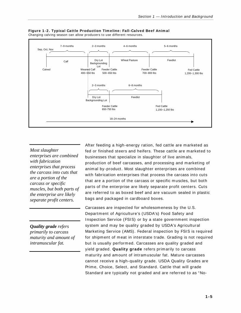
Figure 1-2. Typical Cattle Production Timeline: Fall-Calved Beef Animal Changing calving season can allow producers to use different resources.
Calf
Weaned Calf400–550 lbs
Feeder Cattle500–650 lbs
Feeder Cattle700–800 lbs
Fed Cattle1,200–1,300 lbs
Fed Cattle1,150–1,250 lbs
Feeder Cattle650-750 lbs
Feedlot
Feedlot
Dry LotBackgrounding
Lot
Wheat Pasture
Dry LotBackgrounding Lot
7–9 months 2–3 months 4–6 months 5–6 months
2–3 months 6–8 months
Sep, Oct, Nov
Calved
18–24 months
After feeding a high-energy ration, fed cattle are marketed as fed or finished steers and heifers. These cattle are marketed to businesses that specialize in slaughter of live animals, production of beef carcasses, and processing and marketing of animal by-product. Most slaughter enterprises are combined with fabrication enterprises that process the carcass into cuts that are a portion of the carcass or specific muscles, but both parts of the enterprise are likely separate profit centers. Cuts are referred to as boxed beef and are vacuum sealed in plastic bags and packaged in cardboard boxes.
Carcasses are inspected for wholesomeness by the U.S. Department of Agriculture’s (USDA’s) Food Safety and Inspection Service (FSIS) or by a state government inspection system and may be quality graded by USDA’s Agricultural Marketing Service (AMS). Federal inspection by FSIS is required for shipment of meat in interstate trade. Grading is not required but is usually performed. Carcasses are quality graded and yield graded. Quality grade refers primarily to carcass maturity and amount of intramuscular fat. Mature carcasses cannot receive a high-quality grade. USDA Quality Grades are Prime, Choice, Select, and Standard. Cattle that will grade Standard are typically not graded and are referred to as “No-
Most slaughter enterprises are combined with fabrication enterprises that process the carcass into cuts that are a portion of the carcass or specific muscles, but both parts of the enterprise are likely separate profit centers.
Quality grade refers primarily to carcass maturity and amount of intramuscular fat.

Volume 3: Fed Cattle and Beef Industries
1-6
Roll.”4 Connective tissue in meat is more substantial in older animals, and meat flavor may be stronger and “gamier.” Intramuscular fat, the fat tissues that are within the muscle as opposed to fat layers between muscles, impart mild flavors and hold moisture in cooking. Thus, intramuscular fat is desirable and results in a higher quality grade. Yield grade is the amount of meat or salable meat in the carcass. USDA Yield Grades are numbered 1 through 5. Increases in the amount of fat cover between the hide and carcass and fat deposits close to edible organs result in a lower yield grade. Smaller muscles also result in lower yield grades.
Cow-calf operations may be cattle businesses only or the business may diversify into other ranching enterprises, such as haying, and other farming operations, such as row crops. The diversification choice depends largely on the environment. Western cow-calf operations tend to be cattle operations only, with some haying if irrigation water is available. Midwestern and southern cow-calf operations tend to be combined with farming enterprises in which cattle graze on land that cannot be used for row crops.
Stocker cattle operations or backgrounding operations are enterprises with surplus forage. Rarely are backgrounding operations single enterprises. It is more cost-effective to move the cattle to the forage than the forage to the cattle. The most common practice is to purchase yearlings for grazing on summer pasture so that the enterprise can essentially market cheap grass through growth on a ruminant animal. Some weaned calves are marketed in the fall because summer pasture will not be available until the following spring. Large proportions of these animals go onto winter wheat pasture in the southern High Plains, followed by grass pasture in the southeastern United States. However, calves can be wintered anywhere with substantive pasture, such as dormant grass with high available protein, but may require supplemental feeding and hay. Many but not all calves in the northern states are shipped south for pasturing.
4 The term “No-Roll” originated from an earlier practice in which the
USDA Quality Grade was rolled on the fat along the length of the carcass using an ink wheel. Carcasses that were “No-Roll” did not receive a quality grade.
Yield grade is the amount of meat or salable meat in the carcass.
Cow-calf operations may be cattle businesses only or the business may diversify into other ranching enterprises, such as haying, and other farming operations, such as row crops.
Stocker cattle operations or backgrounding operations are enterprises with surplus forage.

Section 1 — Introduction and Background
1-7
Cattle-feeding operations are concentrated in the southern Plains States, High Plains States, and the Midwest. Feeder cattle move from pasture and backgrounding systems to feedlots in these regions. Large numbers of animals are confined together in these feeding operations, but the animals are also in the outdoors. Cattle-feeding operations are specialized operations. However, the operations may be part of a larger enterprise that grows and manufactures feed. These feedlots grow a portion of their feed supplies, such as corn silage and other forages, and purchase some of the grain needed for feeding. Many cattle-feeding operations own several feedyards. These feedyards are operated by on-site management, but central management may make decisions and capture economies in feed purchasing, feed manufacturing, animal procurement and marketing, financing, and risk management.
1.1.2 Location and Size of Beef Cattle Operations
Cow-calf operations, as illustrated in Figure 1-3, are widely distributed across the United States, although cow-calf operations are concentrated in the Midwest and southern United States because the climate and rainfall are supportive of pastures in these regions. Cow-calf production is also present in the western United States and is important to western agriculture, even though the climate does not support extensive forage production.
Figure 1-4 shows that cattle-feeding operations are concentrated in the southern Plains States, High Plains States, and the Midwest. Large numbers of animals are confined in these feeding operations. Cattle feeding moved to the High Plains from the Corn Belt with the development of irrigated row crop agriculture over the aquifers in the High Plains. However, these regions remain corn deficient and receive shipments of grain from the Midwest for cattle feeding. The improved performance of animals on feed outweighs the transportation costs. The dry climate also makes animal waste management less of an issue than in the wetter and more populous Midwest and Corn Belt states.
Cattle-feeding operations are concentrated in the southern Plains States, High Plains States, and the Midwest.

Volume 3: Fed Cattle and Beef Industries
1-8
Figure 1-3. U.S. Inventory of Beef Cows, 2002 Cow-calf operations are located throughout the country, but are concentrated in the Midwest and South.
Source: U.S. Department of Agriculture, National Agricultural Statistics Service (USDA, NASS). 2004. “2002 Census of Agriculture.” Washington, DC: USDA. <http://www.nass.usda.gov/research/atlas02/>.
Cattle slaughtering and processing operations are located close to cattle-feeding regions (Figure 1-5). Given advances in technology, it is more economical to move meat to people than to move cattle to people. Meatpacking operations that are not located close to cattle-feeding operations are located in regions with larger numbers of beef and dairy herd animals. Most cow slaughter plants are located in Wisconsin and Pennsylvania to be close to dairy production in the Northeast and Southeast.
The majority of cattle operations are relatively small in scale. More than 97% of all beef cattle operations have less than 500 head, and approximately 79% have less than 100 head (USDA, NASS, 2006). Despite the large proportion of small cattle operations, almost half of U.S. cattle come from large operations. Operations with 500 or more head maintain 42% of cattle inventories, and half of those cattle are held on operations with 1,000 or more head.

Section 1 — Introduction and Background
1-9
Figure 1-4. Number of Cattle on Feed Sold, 2002 Cattle feeding is concentrated in the Plains States.
Source: U.S. Department of Agriculture, National Agricultural Statistics Service. 2004. “2002 Census of Agriculture.” Washington, DC: USDA. <http://www.nass.usda.gov/research/atlas02/>.
Overall, the structure of the cow-calf sector is very similar to the beef cattle industry; however, the scale is slightly smaller. Approximately 90% of all beef cow operations have less than 100 head, and 78% have less than 50 head. Nearly 47% of the U.S. beef cow inventory is held on operations with less than 100 head. Operations with 500 or more head of beef cows account for less than 15% of the total inventory.
Data from the USDA/ERS Agricultural Resource Management Survey (ARMS) indicate that cattle production is not the primary occupation for the majority of cow-calf producers in covered states.5 Between 2000 and 2004, an average of 72% of cow-calf producers were classified as Limited Resource,
5 The states included in the 1996 ARMS of cow-calf producers were:
California, Colorado, Florida, Idaho, Illinois, Kansas, Kentucky, Louisiana, Missouri, Montana, Nebraska, New Mexico, North Dakota, Oklahoma, and Oregon.

Volu
me 3
: Fed C
attle and B
eef Industries
1-1
0
Figure 1-5. Location of Federally Inspected Plants that Slaughter Steers and Heifersa
a Plants that slaughtered at least 50 head of steers and heifers in fiscal year 2004 (October 1, 2003, through September 30, 2004) are included. Of 492 plants, 34 are classified by FSIS as large, with 500 or more employees; 89 are classified as small, with 10 to 499 employees; and 369 are classified as very small, with fewer than 10 employees or less than $2.5 million in annual sales. Plants in Alaska (2) and Hawaii (7) are not shown.
Source: RTI International. 2005. Enhanced Facilities Database. Prepared for the U.S. Department of Agriculture, Food Safety and Inspection Service. Research Triangle Park, NC: RTI.
Legend 34 large plants ( ) 89 small plants ( ) 369 very small plants ( )

Section 1 — Introduction and Background
1-11
Retired, or Lifestyle producers (USDA/ERS, 2007). These part-time producers relied on off-farm income to subsidize their farming activities. On average, farming activities reduced part-time producers household income by $3,000, and off-farm activities contributed $49,000 to household income. Full-time cow-calf producers averaged positive returns from both on-farm ($45,000) and off-farm ($49,000) activities between 2000 and 2004.
1.1.3 Trends in Beef Cattle Operations
Prior to the 1970s, animal inventories trended strongly upward. However, beef animal inventories have been decreasing steadily since then. Two cattle cycles ago, there was a large “bust” phase of the cycle, which resulted in very large inventories, very low prices, and substantial losses. Beef cow inventories have declined steadily since the subsequent liquidation. Beef production—pounds of beef produced and marketed—declined initially but has been relatively stable to exhibiting moderate growth since the late 1970s. Recently, during the immediate past liquidation phase of the cattle cycle and with record low corn and other feed prices, beef production achieved new record highs. Figure 1-6 shows the change in cattle inventories during the most recent cattle cycle. The cyclical nature of cattle production is evident based on trends in the number of cattle slaughtered. As seen in Figure 1-7 the number of steers and heifers slaughtered declined during the initial buildup phase (1990–1992) and then gradually increased throughout the herd buildup phase. Because of the biological lags in production, steer and heifer slaughter typically does not begin to decline until after breeding herds have started to be liquidated.
Four meat packers slaughter and process more than 80% of the fed cattle marketed in the United States (Figure 1-8). All four of those packers own multiple plants, and three slaughter and process multiple species of animals. Concentration in beef packing increased sharply during the wave of mergers in the late 1980s and early 1990s, as declining demand forced beef packers to seek cost savings through economies of scale.6 However, since then the level of concentration has been relatively stable to slightly declining. Concentration levels in boxed beef processing are slightly higher than for fed animal slaughter.
6 Concentration refers to the portion of industry volume accounted for
by the largest firms. The four-firm concentration ratio (CR4), which is a common measure of concentration, is the summation of the market shares of the four largest firms.
The cyclical nature of cattle production is evident based on trends in the number of cattle slaughtered.
Concentration in the beef packing industry increased sharply in the late 1980s and early 1990s, but has been relatively stable since then.

Volume 3: Fed Cattle and Beef Industries
1-12
Figure 1-6. U.S. Cattle Inventory, 1990–2005 Cattle inventory categories include breeding cattle (beef cows, beef heifers, and bulls), steers and heifers (steers over 500 pounds and heifers other than those considered beef heifers), and calves. Milk cows and dairy heifers are not included in this figure.
010,00020,00030,00040,00050,00060,00070,00080,00090,000
100,000
1990
1991
1992
1993
1994
1995
1996
1997
1998
1999
2000
2001
2002
2003
2004
2005
Thou
sand
Hea
d
Breeding Cattle Steers & Heifers Calves
Source: U.S. Department of Agriculture, Economic Research Service, Market & Trade Economics Division. 2006. Red Meat Yearbook. Stock #94006. Washington, DC: USDA. <http://usda.mannlib.cornell.edu/MannUsda/ viewDocumentInfo.do?documentID=1354.>
Figure 1-7. U.S. Commercial Steer and Heifer Slaughter, 1990–2004 Commercial steer and heifer slaughter includes animals slaughtered at federally inspected and nonfederally inspected plants but does not include animals slaughtered on the farm.
24,000
25,000
26,000
27,000
28,000
29,000
30,000
31,000
1990
1991
1992
1993
1994
1995
1996
1997
1998
1999
2000
2001
2002
2003
2004
Thou
sand
Hea
d
Source: U.S. Department of Agriculture, Economic Research Service, Market & Trade Economics Division. 2006. Red Meat Yearbook. Stock #94006. Washington, DC: USDA. <http://usda.mannlib.cornell.edu/MannUsda/ viewDocumentInfo.do?documentID=1354.>

Section 1 — Introduction and Background
1-13
Figure 1-8. U.S. Steer and Heifer Packer Four-Firm Concentration Ratio (CR4), Selected Years 1992–2004 The CR4s show the percentage of all steers and heifers that were slaughtered at plants owned by the four largest firms during the respective year. The total number of plants operated by those firms is also included. Percentages are based on total federally inspected slaughter numbers.
0
5
10
15
20
25
30
1992 1993 1994 1995 1996 1997 1998 1999 2000 2001 2002 2003 200475
76
77
78
79
80
81
82
Number of Plants Concentration Percentage
Num
ber o
f Pla
nts
Perc
enta
ge o
f FSI
S-In
spec
ted
Slau
ghte
r
Source: U.S. Department of Agriculture, Grain Inspection, Packers and Stockyards Administration (USDA, GIPSA). 2006. Packers and Stockyards Statistical Report. SR-06-1. Washington, DC: GIPSA.
1.1.4 Imports and Exports of Cattle and Beef
The United States is a net importer of live cattle (Figure 1-9). Recent trade restrictions have altered the international market, but the United States has traditionally imported live cattle from Canada and Mexico. These cattle are imported as finished cattle ready for immediate slaughter and feeder cattle that will be fed out in domestic feedlots. Very few live cattle are exported.
In addition to imports of live cattle, the United States is a net importer of beef (Figure 1-10). In 2003, beef imports were approximately 11% of U.S. beef consumption, and beef exports were approximately 10% of U.S. beef production (USDA, Economic Research Service [ERS], 2004b). Canada has been a growing supplier of beef to the U.S. market, but the majority of imports are from New Zealand and Australia. Grass-fed beef produced in Australia and New Zealand is much different from grain-fed beef produced domestically. Much of this beef is used in processed products, particularly ground beef (USDA, ERS, 2004a).

Volume 3: Fed Cattle and Beef Industries
1-14
Figure 1-9. Total U.S. Cattle Imports and Exports, 1990–2004 The United States is a net importer of live cattle. Live animal trade is typically restricted to North America.
0
500,000
1,000,000
1,500,000
2,000,000
2,500,000
3,000,000
1990 1991 1992 1993 1994 1995 1996 1997 1998 1999 2000 2001 2002 2003 2004
Hea
d
Cattle Exports Cattle Imports
Source: U.S. Department of Agriculture, Economic Research Service, Market & Trade Economics Division. 2006. Red Meat Yearbook. Stock #94006. Washington, DC: USDA. <http://usda.mannlib.cornell.edu/MannUsda/ viewDocumentInfo.do?documentID=1354.>
Figure 1-10. Total U.S. Beef and Veal Imports and Exports, 1990–2004 The United States is a net importer of beef and veal. Canada, Australia, and New Zealand are the primary sources of imported beef and veal. Mexico, Japan, and Canada are the primary destinations for U.S. exported beef and veal.
500,000
1,000,000
1,500,000
2,000,000
2,500,000
3,000,000
3,500,000
4,000,000
1990 1991 1992 1993 1994 1995 1996 1997 1998 1999 2000 2001 2002 2003 2004
Tho
usan
d Po
unds
(C
arca
ss W
eigh
t)
Exports Imports
Source: U.S. Department of Agriculture, Economic Research Service, Market & Trade Economics Division. 2006. Red Meat Yearbook. Stock #94006. Washington, DC: USDA. <http://usda.mannlib.cornell.edu/MannUsda/ viewDocumentInfo.do?documentID=1354.>

Section 1 — Introduction and Background
1-15
1.2 OVERVIEW OF MARKETING ARRANGEMENTS IN THE FED CATTLE AND BEEF INDUSTRIES In this report, cash or spot market transactions refer to transactions that occur immediately or “on the spot.” These include auction barn sales; video or electronic auction sales; sales through order buyers, dealers, and brokers; and direct trades. The terms “cash market” and “spot market” are used interchangeably. “Alternative marketing arrangements” (AMAs) refer to all possible alternatives to the cash or spot market. These include arrangements such as forward contracts, marketing agreements, procurement or marketing contracts, packer owned, custom feeding, and custom slaughter. For AMAs at the producer level, livestock may be owned by the individual(s) that owns the farm or facility, or the livestock may be owned by a different party.
In addition to the type of procurement or sales method, other key dimensions that define each type of marketing arrangement used in the industry are ownership method of the animal or product, pricing method, and valuation method for livestock. Pricing method is further defined by formula base, if formula pricing is used, and internal transfer pricing method, if the product is transferred within a single company.
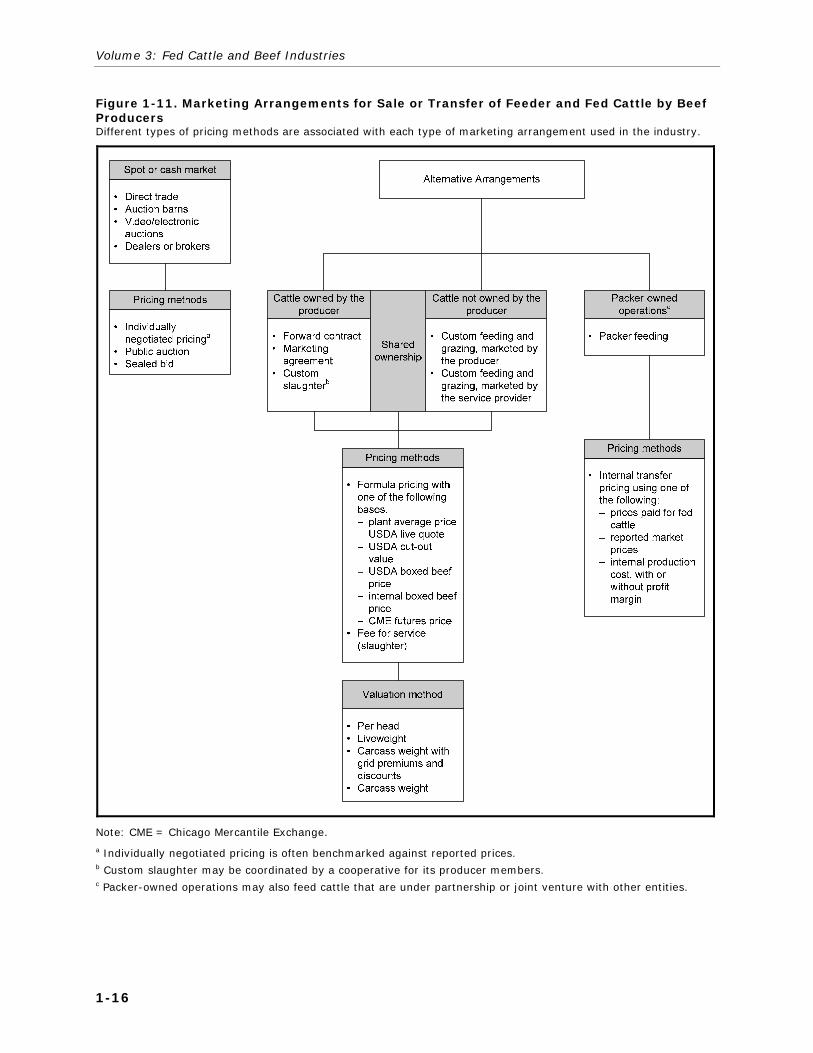
Figure 1-11 illustrates the types of marketing arrangements used for sales or transfers of feeder and fed cattle. The key dimensions of marketing arrangements at each stage include the ownership method for the animal or product while it is at the feedlot (e.g., cattle owned by the producer or owner of the feedlot, jointly owned by the producer and packer, and packer owned) and the pricing method used. If formula pricing is used, a formula base price must also be specified. The valuation method might be on a per-head basis, liveweight basis, or carcass weight basis or on the accumulated value of individual cuts. Carcass weight valuation methods may also incorporate a grid that offers premiums or discounts based on carcass grade classifications. Premiums and discounts may change weekly based on supply and demand conditions or may be fixed for some period. If animals or products are shipped from one establishment to another owned by the same company, an internal transfer pricing method must also be specified.
Key dimensions that define a marketing arrangement include procurement or sales
method,
ownership method of the animal or product,
pricing method (including formula pricing base and internal transfer pricing method), and
valuation method for livestock.
Volume 3: Fed Cattle and Beef Industries
1-16
Figure 1-11. Marketing Arrangements for Sale or Transfer of Feeder and Fed Cattle by Beef Producers Different types of pricing methods are associated with each type of marketing arrangement used in the industry.
Note: CME = Chicago Mercantile Exchange.
a Individually negotiated pricing is often benchmarked against reported prices. b Custom slaughter may be coordinated by a cooperative for its producer members. c Packer-owned operations may also feed cattle that are under partnership or joint venture with other entities.

Section 1 — Introduction and Background
1-17
The types of buying and selling mechanisms vary by stage of the beef production system. Figure 1-12 illustrates the types of marketing arrangements used for sales or transfers of all types of meat products (including beef) by packers. Under AMAs, meat products might be sold by the packer or transferred to another establishment owned by the same company or to the owner of the livestock if custom slaughtered. Spot or cash market sales of meat are primarily conducted via individual negotiations. Transactions may be for carcasses, single cuts, or a variety of cuts. Sales representatives usually start negotiations for individual cuts based on a price list and usually must meet sales quotas. Listed prices are discounted if inventories of that cut are plentiful. Other pricing practices used for meat products might include two-part pricing, volume discounts, exclusive dealings, and bundling.
1.3 DESCRIPTION OF THE BEEF PACKER TRANSACTIONS DATA Many of the analyses conducted for this volume were based on transactions data obtained from beef packers. We obtained usable fed cattle purchase data from 29 beef packing plants and usable beef sales data from 24 beef packing plants. We describe the data preparation process and content of the purchase data set and the sales data set below.
1.3.1 Beef Packer Purchase Transactions Data
Prior to tabulating and analyzing the fed cattle purchase transactions data, we systematically examined the purchase data set to isolate and address data inconsistencies, data reporting errors, or extraneous data. Specific data preparation procedures were as follows:
Cattle totals by yield grade. Plants were asked to record the distribution of cattle into yield grades. For some data records, the number of head in the sale lot did not correspond to the sum of the distribution of yield grades. For cases where the sum of the yield grades was less than the number of head in the sale lot, we allocated the difference to the Yield Grade Other category. For cases where the sum of the yield grades was greater than the number of head in the sale lot, we used the yield total as the number of head in the sale lot.
The types of buying and selling mechanisms vary by stage of the beef production system.
For this volume of the report, we used fed cattle purchase records from 29 plants (owned by 10 companies) and beef product sales records from 24 plants (owned by 8 companies), in addition to many other data sources.
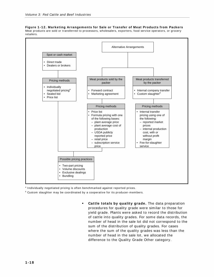
Volume 3: Fed Cattle and Beef Industries
1-18
Figure 1-12. Marketing Arrangements for Sale or Transfer of Meat Products from Packers Meat products are sold or transferred to processors, wholesalers, exporters, food service operators, or grocery retailers.
• Direct trade• Dealers or brokers
• Individually negotiated pricinga
• Sealed bid• Price list
• Internal company transfer• Custom slaughterb
• Internal transfer pricing using one of the following:– reported market
prices– internal production
cost, with or without profit margin
• Fee-for-slaughter service
Alternative Arrangements
Spot or cash market
Pricing methods
Pricing methods
Meat products transferred by the packer
• Two-part pricing• Volume discounts• Exclusive dealings• Bundling
Possible pricing practices
• Price list• Formula pricing with one
of the following bases:– plant average price– plant average cost of
production– USDA publicly
reported price– retail price– subscription service
price
Pricing methods
• Forward contract• Marketing agreement
Meat products sold by the packer
a Individually negotiated pricing is often benchmarked against reported prices. b Custom slaughter may be coordinated by a cooperative for its producer-members.
Cattle totals by quality grade. The data preparation procedures for quality grade were similar to those for yield grade. Plants were asked to record the distribution of cattle into quality grades. For some data records, the number of head in the sale lot did not correspond to the sum of the distribution of quality grades. For cases where the sum of the quality grades was less than the number of head in the sale lot, we allocated the difference to the Quality Grade Other category.

Section 1 — Introduction and Background
1-19
Dairy cattle. Some plants did not record the mix of cattle in the sale lot (i.e., steers, heifers, cows, or bulls). If a data record indicated a cattle type of primarily beef cattle and the lot was also distributed over the quality grades then the number of head in the sale lot was allocated to steers. If a data record indicated a cattle type of primarily dairy cattle then the record was not retained.
Irreconcilable cattle numbers by various categories. Data records with yield grades, quality grades, or cattle mixes that could not be reconciled with the number of head in the sale lot were deleted (39,719 records deleted).
Transaction dates. Data records with purchase or pricing dates outside the data collection period were deleted (39 additional records deleted).
Small cattle lots. Data records with five or less head in a sale lot were deleted (36,657 additional records deleted). Lots with five or less head were considered to be odd lots, often representing “out” cattle.
Missing carcass weights. Data records that did not contain a hot weight were deleted. This was necessary because all prices were analyzed on a carcass weight basis (4,343 additional records deleted).
Out-of-range carcass weights. Data records that had an average carcass weight greater than or equal to 500 pounds and less than or equal to 1,000 pounds were retained. All records outside this range were deleted (569 additional records deleted).
Missing total cost information. Data records that did not contain total cost were deleted. This was necessary because all prices were based on total cost (981 additional records deleted).
Out-of-range prices. Data records where cost per pound (i.e., carcass weight) was between $0.86 and $1.98 per pound were retained. This range represents $0.10 below the minimum and $0.10 above the maximum prices indicated in mandatory price reporting (MPR) data during the October 2002 through March 2005 period. All records outside this range were deleted (20,482 additional records deleted).
Prior to data preparation, the data set included 725,148 fed cattle purchase records representing 59,820,187 head of cattle. After data preparation, the final data set included 591,410 fed cattle purchase records representing 58,066,144 head of

Volume 3: Fed Cattle and Beef Industries
1-20
cattle.7 However, even after data preparation, many records were missing important fields (e.g., date of purchase, date of pricing, purchase method, and pricing method) or did not break down costs into their individual components. In some cases, these missing fields limited our ability to conduct the analyses for the study.8
Table 1-1 provides the distribution of these records by region and plant size. The majority (84%) of the fed cattle slaughtered were slaughtered in plants located in the High Plains region. In addition, 75% of the cattle were slaughtered in large plants with slaughter capacity greater than 20,000 head per week. Table 1-2 provides a further breakdown of the characteristics of the fed cattle purchase transactions in the analysis data set.
Table 1-1. Summary of Available Data on Purchases of Steers and Heifers, October 2002–March 2005
Plant Characteristic No. of Plants No. of Lots Purchased
No. of Cattle Purchased
% of Cattle Purchased
Region
Cornbelt/Northeast 5 98,140 4,377,325 8.0%
High Plains 17 426,787 48,496,683 84.0%
West 7 66,483 5,132,136 9.0%
Plant size
Small 15 202,350 14,256,150 25.0%
Large 14 389,060 43,749,994 75.0%
Total 29 591,410 58,006,144 100.0%
Regions are defined as follows:
Cornbelt/Northeast: IA, IL, MI, MN, PA, WI
High Plains: CO, KS, NE, TX
West: AZ, CA, ID, UT, WA
Sizes are defined as follows:
Small has capacity < 20,000 head/week.
Large has capacity > 20,000 head/week.
7 The data preparation process resulted in a loss of only 3% of the fed
cattle in the data set. 8 More details on data preparation are provided in Volume 2, Section
12.
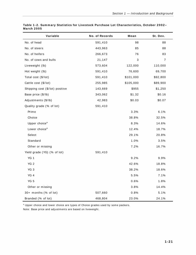
Section 1 — Introduction and Background
1-21
Table 1-2. Summary Statistics for Livestock Purchase Lot Characteristics, October 2002–March 2005
Variable No. of Records Mean St. Dev.
No. of head 591,410 98 88
No. of steers 443,963 85 88
No. of heifers 266,673 76 83
No. of cows and bulls 21,147 3 7
Liveweight (lb) 573,604 122,000 110,000
Hot weight (lb) 591,410 76,600 69,700
Total cost ($/lot) 591,410 $101,000 $92,800
Cattle cost ($/lot) 255,985 $105,000 $89,900
Shipping cost ($/lot) positive 143,669 $955 $1,250
Base price ($/lb) 343,062 $1.32 $0.16
Adjustments ($/lb) 42,983 $0.03 $0.07
Quality grade (% of lot) 591,410
Prime 3.3% 6.1%
Choice 38.8% 32.5%
Upper choicea 8.3% 14.6%
Lower choicea 12.4% 18.7%
Select 29.1% 20.8%
Standard 1.0% 3.5%
Other or missing 7.2% 16.7%
Yield grade (YG) (% of lot) 591,410
YG 1 9.2% 9.9%
YG 2 42.6% 18.8%
YG 3 38.2% 18.6%
YG 4 5.5% 7.1%
YG 5 0.6% 1.8%
Other or missing 3.8% 14.4%
30+ months (% of lot) 507,660 0.8% 5.1%
Branded (% of lot) 468,804 23.0% 24.1%
a Upper choice and lower choice are types of Choice grades used by some packers.
Note: Base price and adjustments are based on liveweight.

Volume 3: Fed Cattle and Beef Industries
1-22
1.3.2 Beef Packer Sales Transactions Data
Prior to tabulating the sales transactions data, we systematically examined the sales data set to isolate and address data inconsistencies, data reporting errors, or extraneous data. Specific data preparation procedures were as follows:
Out-of-range list prices. Data records that had a list price more than three standard deviations (plus or minus) from the mean list price were deleted (25,931 records deleted). With the large number of products, we could not identify precisely which values were actual errors and which were extreme values, so all of these values were considered errors and subsequently deleted.
Out-of-range gross prices. Data records that had a gross price more than three standard deviations (plus or minus) from the mean gross price were deleted (27,068 additional records deleted). With the large number of products, we could not identify precisely which values were actual errors and which were extreme values, so all of these values were considered errors and subsequently deleted.
Prior to data preparation, the data set included 5,969,333 beef product sales records (excluding by-products). After data preparation, the final data set included 5,916,334 beef product sales. However, selling method and pricing method were missing from a substantial number of records.
Table 1-3 provides the distribution of these records by region and plant size. The majority (83%) of beef products sold were sold by plants located in the High Plains region. In addition, 75% of the beef products sold were from large plants with slaughter capacity greater than 20,000 head per week. Table 1-4 provides a further breakdown of the characteristics of the fed cattle sales transactions in the analysis data set.
1.4 ORGANIZATION OF THE FED CATTLE AND BEEF STUDY VOLUME In the remaining sections of this volume, we present results of the study for the fed cattle and beef industries. Section 2 provides results on volume differences, price differences, and market price effects associated with AMAs. Section 3 provides results on economies of scale, cost, and efficiency differences

Section 1 — Introduction and Background
1-23
Table 1-3. Summary of Available Data on Sale of Beef Products, by Packers, October 2002–March 2005
Plant Characteristic No. of Plants
No. of Transactions (Records) No. of Pounds
% of Pounds Sold
Region
Cornbelt/Northeast 5 526,251 2,794,114,501 9%
High Plains 15 4,131,466 26,336,083,611 83%
West 4 1,258,617 2,652,024,239 8%
Plant size
Small 11 2,122,176 7,804,461,294 25%
Large 13 3,794,158 23,977,761,056 75%
Total 24 5,916,334 31,782,222,350 100%
Regions are defined as follows:
Cornbelt/Northeast: IA, IL, MI, MN, PA, WI
High Plains: CO, KS, NE, TX
West: AZ, CA, ID, UT, WA
Sizes are defined as follows:
Small has capacity < 20,000 head/week.
Large has capacity > 20,000 head/week.
Table 1-4. Summary Statistics for Beef Sales Lot Characteristics, October 2002–March 2005
Variable No. of Records Mean St. Dev.
Total weight (lb) 5,916,334 5,372 28,505
List price ($/lb) 3,777,206 2.74 4.29
Gross price ($/lb) 5,365,067 2.62 1.95
Price adjustments ($/lb) 4,325,933 0.004 0.17
Net price ($/lb) 5,365,067 2.57 1.97
Shipping cost ($/lb) 5,492,076 0.06 0.07
Commission cost ($/lb) 4,597,904 0.01 0.06
No. of Records % of Records
Buyer type
Meat processor/food manufacturer 557,021 10.7%
Wholesaler/broker/distributor 840,380 16.1%
Retailer 1,651,586 31.6%
Food service operator 1,049,524 20.1%
Foreign buyer 170,021 3.3%
Other 961,210 18.4%
Branded 905,384 15.3%
Other certification D D
(continued)

Volume 3: Fed Cattle and Beef Industries
1-24
Table 1-4. Summary Statistics for Beef Sales Lot Characteristics, October 2002–March 2005 (continued)
Variable No. of Records % of Records
Quality grade
Prime 115,614 2.0%
Choice 1,887,640 31.9%
Upper choice 321,309 5.4%
Lower choice 119,700 2.0%
Select 1,318,829 22.3%
Other or missing 2,153,242 36.4%
Product classification
Carcass or side D D
Primal cut 1,605,997 27.2%
Subprimal cut 2,653,306 44.9%
Ground and trimmings 970,454 16.4%
Portion cut 0 0.0%
Case ready D D
Processed ready-to-eat (RTE) 0 0.0%
Processed not ready-to-eat (NRTE) 0 0.0%
Other or missing D D
Trim level
3/4 inch 1,743,577 47.9%
1/4 inch 63,072 1.7%
1/8 inch 1,077,513 29.6%
Practically free 621,218 17.1%
Peeled/denuded 136,522 3.8%
Tenderized/marinated 0 D
Added ingredients D D
Refrigeration
Chilled/fresh 4,927,360 92.7%
Frozen 389,448 7.3%
Other 126 0.0%
Packaging
Vacuum 2,646,257 89.8%
Gas D D
Paper D D
Combination D D
Other 248,268 8.4%
D = Results suppressed.

Section 1 — Introduction and Background
1-25
associated with AMAs. Section 4 provides results on quality differences, and Section 5 provides results on risk shifting associated with AMAs. Section 6 provides results on the measurement of economic effects associated with restricting AMAs by simulating hypothetical scenarios. Finally, Section 7 describes the implications of AMAs, including the incentives associated with changing the use of AMAs and the expected effects of possible changes in use of AMAs over time.
Note that each section of this volume addresses the requirements of the study, as defined in the performance work statement for the contract. Section 2 addresses Part C; Sections 3, 4, and 5 address Part D; and Sections 6 and 7 address Part E.
In addition to these sections, Appendix A includes supplementary analyses of price differences across AMAs, and Appendix B provides further technical details on the modeling approach presented in Section 6.


2-1
Volume Differences, Price Differences, and Short-Run Spot Market Price Effects Associated with Alternative Marketing 2 Arrangements
In this section, we present results on volume differences associated with AMAs, price differences across AMAs, and the effects of AMAs on cash market prices. The discussion and analyses in this section are based on data from the industry survey and on the transactions data obtained from beef packers.
2.1 CATTLE AND BEEF VOLUMES, BY TYPE OF MARKETING ARRANGEMENT As a result of the multiple data collection methods used for the study, we obtained estimates of the volume of cattle sold through AMAs from multiple sources. Our primary focus in this section is on the methods for selling or transferring fed cattle from feeders to packers, but we also discuss methods of selling or transferring beef products from packers to processors or other entities. As discussed in Volume 2 of this study, 293 beef producers responded to the industry survey (270 small
Volume 3: Fed Cattle and Beef Industries
2-2
producers and 23 large producers).1 In addition, 64 beef packing plants responded to the industry survey (34 small and 30 large).2
From the weighted industry survey results, beef producer sales arrangements to packers are as follows:
Ownership arrangements. Based on the responses, 78.0% of small producers are sole owners of all cattle on their operations, while 31.3% of large producers are sole owners of all cattle on their operations. Large producers made more use of partner arrangements, shared ownership, joint ventures, and custom feeding (39.9% of cattle sold for large producers versus 14.9% for small producers). (See Volume 2, Table 6-2, Question S2.2.)
Sales methods to packers. An estimated 85.0% of small producers used only the cash or spot market to sell cattle in the past year compared with 23.8% of large producers. Large producers made more use of AMAs such as forward contracts, marketing agreements, packer ownership, internal transfers, and custom feeding and slaughtering (52.5% of head sold for large producers and 8.5% for small producers). Among large producers, the most frequently used were forward contracts and marketing agreements. (See Volume 2, Table 6-5, Question S5.2).
Pricing methods. Large producers used multiple pricing methods in the past year with the most common being individually negotiated pricing (73.9% of producers), public auction (34.8% of producers), and formula pricing (56.5% of producers). In contrast, small producers used primarily individually negotiated pricing (31.7%) and public auction (83.6%). Only 5.7% of small producers used formula pricing. (See Volume 2, Table 6-5, Question S5.3.)
Valuation methods. Large producers more frequently sold cattle based on carcass weight with a grid (60.0% of producers) compared with small producers (14.6% of producers) in the past year. Otherwise, the percentages of producers using liveweight and carcass weight without a grid were similar across size categories. (See Volume 2, Table 6-5, Question S5.5.)
1 Large beef producers are defined as the 25 largest feedlots and 25
largest cow-calf operations in the United States, and small beef producers are the remainder.
2 Large beef packers are defined as the 60 largest beef packers, based on slaughter volume, and small beef packers are the remainder.
Volumes of fed cattle sales volumes by type of marketing arrangement are estimated from three sources: industry survey
responses for beef cattle producer sales of fed cattle (293 producer responses)
industry survey responses for beef packer purchases of fed cattle (64 packing plant responses)
transactions data for beef packer purchases of fed cattle (29 packing plant responses)

Section 2 — Volume Differences, Price Differences, and Short-Run Spot Market Price Effects Associated with Alternative Marketing Arrangements
2-3
Across all these characteristics of marketing arrangements, producers indicated that their sales methods in the past year were relatively similar to the methods they used 3 years ago and the methods they expect to use 3 years from now. The only exception is a slight decline in the expected percentage of cattle sold through auction barns over time, although the expected percentage still remains high.
Responses on the industry survey from beef packers provide information on the purchase of cattle from producers (i.e., the other side of the transactions described above). From the weighted industry survey results, beef packer purchase arrangements from producers were as follows:
Ownership arrangements. Based on the responses, 80.8% of small and 60.9% of large plants are sole owners of all cattle slaughtered in their establishments. On a percentage of head basis, small plants and large plants are sole owners of similar percentages (87.1% of cattle for small plants and 84.1% of cattle for large plants). No beef packing plants that responded to the survey reported that they have joint venture ownership arrangements, but a small percentage have shared ownership arrangements (5.2% of cattle for small packing plants and 3.0% of cattle for large packing plants) and other types of ownership arrangements (7.7% of cattle for small packing plants and 13.0% of cattle for large packing plants).3 (See Volume 2, Table 7-2, Question S2.1.)
Purchase methods. An estimated 77.8% of small beef packing plants used only the cash or spot market to purchase cattle, while only 10.0% of large beef packing plants used only the cash or spot market. Large packing plants used auction barns and dealers or brokers for fewer purchases (9.4% of head versus 37.8% of head for small packing plants), but used more direct trade (53.9% of head versus 40.4% for small packing plants). In addition, large packing plants procured a higher percentage of cattle through AMAs including forward contracts, marketing agreements, and packer fed/owned (33.4% of head for large packing plants and 18.1% of
3 A joint venture refers to situations in which a business and one or more other
businesses join together under a contractual agreement for a specific venture, such as use of specific animal genetics or brand names. In contrast, shared ownership refers to situations in which the original owner and an operation (business) both retain partial ownership of livestock or meat products (that is, a vertical arrangement).

Volume 3: Fed Cattle and Beef Industries
2-4
head for small packing plants). (See Volume 2, Table 7-2, Question S2.2.)
Pricing methods. Large packing plants used multiple pricing methods, with the most common being formula pricing (93.3% of plants), individually negotiated pricing (90.0% of plants), public auction (50.0% of plants), and internal transfer pricing (33.3% of plants). In contract, small packing plants used primarily individually negotiated pricing (67.7% of plants), public auction (41.9% of plants), and formula pricing (19.4% of plants). (See Volume 2, Table 7-2, Question S2.3.) The most frequently used base price for formulas, with or without a grid, were distributed across seven different types of prices. (See Volume 2, Table 7-2, Questions S2.4a and S2.4b.)
Valuation methods. Large packing plants more frequently purchased cattle based on liveweight (90.0% of plants) compared with small packing plants (50.0% of plants). A high percentage of large packing plants used carcass weight with grids (86.7% of plants), while almost no small packing plants used this type of valuation. A high percentage of both large and small packing plants used carcass weight not dependent on grid valuation methods. (See Volume 2, Table 7-2, Question S2.6.)
Across all of these characteristics of marketing arrangements, packers indicated that their purchase methods in the past year were relatively similar to the methods they used 3 years ago and to the methods they expect to use 3 years from now. The only exceptions are a very slight decline in public auction purchases and a very slight increase in formula pricing.
In contrast to purchases of fed cattle by packers, sales of beef products by packers are typically through the cash or spot market (83.6% of sales revenue). Forward contracts, marketing agreements, internal company transfers, and other types of AMAs comprise the remaining 16.4% of sales. Approximately 70% of beef packing plants use only the cash or spot market to sell beef products. Overall, packers responded that the percentages across marketing arrangements were similar 3 years ago and are expected be similar 3 years into the future. (See Volume 2, Table 7–2, Question 5.2.) Thus, although AMAs are often used to buy cattle, the sales arrangements for beef products are less formal. This suggests that, on the sales side, the link between purchases of live cattle to meet specific buyer requirements is often relatively informal.

Section 2 — Volume Differences, Price Differences, and Short-Run Spot Market Price Effects Associated with Alternative Marketing Arrangements
2-5
In addition to the volume data from survey results, the transaction data collected from beef packing plants provides information about the volume of live cattle and beef products traded through different marketing arrangements.4 As discussed in Volume 2 of this study, 29 beef packing plants provided usable purchase transaction data and 24 beef packing plants provided usable sales transaction data. All of these plants are classified as large in the industry survey. Therefore, to distinguish among plants in the analysis of the transactions data, we classified plants into sizes as follows:
Large plants have slaughter capacities greater than 20,000 head per week.
Small plants have slaughter capacities less than 20,000 head per week.
This size classification divides the plants into an approximately equal number of plants in each category.
Based on the transactions data for the October 2002 through March 2005 period, by plant size, beef packer purchase arrangements from producers are as follows:
Ownership arrangements. Table 2-1 shows that more than 97% of cattle slaughtered at small plants and 80% of cattle slaughtered at large plants were owned solely by the plant. A very small percentage of the cattle slaughtered at small and large plants were owned by both the packing plant and the producer (i.e., shared ownership). The remaining cattle were reported as having other ownership arrangements or the ownership arrangements were not reported.
Purchase methods. Packers purchased the majority of their cattle through direct trade and marketing agreements, regardless of size (Table 2-2). Small plants purchased 46% of their cattle through direct trade, 28% through marketing agreements, and 13% from auction barns. Large plants purchased 61% of their cattle through direct trade and 29% through marketing agreements. A very small percentage of the cattle purchased by large plants came from auction barns.
4 Differences in the volume estimates from survey results and
transaction data summaries result from the difference in two samples. The weighted survey responses make inferences to the entire population of beef producers and packers. The transaction data collection included usable data for the purposes of the study for only 29 of the largest beef packing plants.

Volume 3: Fed Cattle and Beef Industries
2-6
Table 2-1. Summary of Livestock Ownership Methods, by Plant Size, October 2002–March 2005
Categorya Sole
Ownership Shared
Ownership Other or Missing Total
Small beef packing plants
No. of lots 198,188 D D 202,350
% of lots 97.9% 100.0%
No. of head 13,923,727 D D 14,298,688
% of head 97.4% 100.0%
Large beef packing plants
No. of lots 318,591 D D 389,060
% of lots 81.9% 100.0%
No. of head 35,060,740 D D 43,767,752
% of head 80.1% 100.0%
All beef packing plants
No. of lots 516,779 D D 591,410
% of lots 87.4% 100.0%
No. of head 48,984,467 D D 58,066,440
% of head 84.4% 100.0%
a Sizes are defined as follows:
Small has capacity < 20,000 head/week.
Large has capacity > 20,000 head/week.
D = Results suppressed.
Pricing methods. Individually negotiated pricing was the most common method used to determine purchase prices for fed cattle (48% of cattle for small plants and 60% of cattle for large plants) (Table 2-3). Approximately one-third of the cattle purchased by large and small plants were priced using a formula. Live prices reported by the USDA were the most common formula base prices (Table 2-4).
Valuation methods. Small plants purchased approximately 51% of their cattle using carcass weight with grid valuation and 27% on a liveweight basis (Table 2-5). In comparison, large plants purchased approximately 43% of their cattle on a liveweight basis and 40% using carcass weight with grid valuation. Both small and large plants purchased approximately 13% of their cattle on carcass weight basis without a grid.

2-7
Sectio
n 2
— V
olu
me D
ifferences, Price D
ifferences, an
d S
hort-R
un S
pot M
arket Price E
ffects Asso
ciated w
ith A
lternative M
arketing A
rrangem
ents
Table 2-2. Summary of Livestock Purchase Methods, by Plant Size, October 2002–March 2005
Categorya Auction Barns
Dealers or Brokers
Direct Trade
Forward Contract
Marketing Agreement
Packer Fed/Owned
Other or Missing Total
Small beef packing plants
No. of lots 37,459 3,524 95,829 8,559 44,731 4,529 7,719 202,350
% of lots 18.5% 1.7% 47.4% 4.2% 22.1% 2.2% 3.8% 100.0%
No. of head 1,816,939 228,128 6,638,116 737,345 4,003,867 389,805 484,488 14,298,688
% of head 12.7% 1.6% 46.4% 5.2% 28.0% 2.7% 3.4% 100.0%
Large beef packing plants
No. of lots D D 242,425 14,488 113,974 D D 389,060
% of lots 62.3% 3.7% 29.3% 100.0%
No. of head D D 26,757,900 1,888,872 12,744,448 D D 43,767,752
% of head 61.1% 4.3% 29.1% 100.0%
All beef packing plants
No. of lots 44,237 338,254 23,047 158,705 27,167 591,410
% of lots 7.5% 57.2% 3.9% 26.8% 4.6% 100.0%
No. of head 2,426,488 33,396,016 2,626,217 16,748,315 2,869,405 58,066,440
% of head 4.2% 57.5% 4.5% 28.8% 5.0% 100.0%
a Sizes are defined as follows:
Small has capacity < 20,000 head/week.
Large has capacity > 20,000 head/week.
D = Results suppressed.

2-8
Volu
me 3
: Fed C
attle and B
eef Industries
Table 2-3. Summary of Livestock Pricing Methods, by Plant Size, October 2002–March 2005
Categorya Negotiated Public Auction Formula Pricing Internal Transfer
Other or Missing Total
Small beef packing plants
No. of lots 99,584 D 51,006 D D 202,350
% of lots 49.2% 25.2% 100.0%
No. of head 6,826,722 D 4,667,417 D D 14,298,688
% of head 47.7% 32.6% 100.0%
Large beef packing plants
No. of lots 234,624 D 133,847 D D 389,060
% of lots 60.3% 34.4% 100.0%
No. of head 26,346,160 D 14,730,179 D D 43,767,752
% of head 60.2% 33.7% 100.0%
All beef packing plants
No. of lots 334,208 D 184,853 D D 591,410
% of lots 56.5% 31.3% 100.0%
No. of head 33,172,882 D 19,397,596 D D 58,066,440
% of head 57.1% 33.4% 100.0%
a Sizes are defined as follows:
Small has capacity < 20,000 head/week.
Large has capacity > 20,000 head/week.
D = Results suppressed.

2-9
Sectio
n 2
— V
olu
me D
ifferences, Price D
ifferences, an
d S
hort-R
un S
pot M
arket Price E
ffects Asso
ciated w
ith A
lternative M
arketing A
rrangem
ents
Table 2-4. Summary of Types of Formula Bases Used for Livestock Pricing, by Plant Size, October 2002–March 2005
Categorya
Plant Average Price
or Cost of Production
USDA Live Quote
USDA Dressed or
Carcass Quote
CME Cattle
Futures Subscription Service Price
Not Applicable
Not Reported Total
Small beef packing plants
No. of lots D 17,297 D D D 151,345 D 202,350
% of lots 8.5% 74.8% 100.0%
No. of head D 1,370,692 D D D 9,631,305 D 14,298,688
% of head 9.6% 67.4% 100.0%
Large beef packing plants
No. of lots D 35,321 D D D 255,213 D 389,060
% of lots 9.1% 65.6% 100.0%
No. of head D 3,512,715 D D D 29,037,573 D 43,767,752
% of head 8.0% 66.3% 100.0%
All beef packing plants
No. of lots D 52,618 89,206b 406,558 D 591,410
% of lots 8.9% 15.1% 68.7% 100%
No. of head D 4,883,407 8,885,342b 38,668,878 D 58,066,440
% of head 8.4% 15.3% 66.6% 100%
a Sizes are defined as follows:
Small has capacity < 20,000 head/week.
Large has capacity > 20,000 head/week. b Totals combine USDA dressed or carcass quote, CME cattle futures, and subscription service price.
D = Results suppressed.

2-1
0
Volu
me 3
: Fed C
attle and B
eef Industries
Table 2-5. Summary of Livestock Valuation Methods, by Plant Size, October 2002–March 2005
Categorya Liveweight Carcass Weight,
Without Grid Carcass Weight,
With Grid Other or Missing Total
Small beef packing plants
No. of lots 61,352 21,276 103,277 16,445 202,350
% of lots 30.3% 10.5% 51.0% 8.1% 100.0%
No. of head 3,828,852 1,776,397 7,326,609 1,366,830 14,298,688
% of head 26.8% 12.4% 51.2% 9.6% 100.0%
Large beef packing plants
No. of lots 148,218 51,699 176,502 12,641 389,060
% of lots 38.1% 13.3% 45.4% 3.2% 100.0%
No. of head 18,984,258 5,711,105 17,647,798 1,424,592 43,767,752
% of head 43.4% 13.0% 40.3% 3.3% 100.0%
All beef packing plants
No. of lots 209,570 72,975 279,779 29,086 591,410
% of lots 35.4% 12.3% 47.3% 4.9% 100.0%
No. of head 22,813,110 7,487,502 24,974,407 2,791,422 58,066,440
% of head 39.3% 12.9% 43.0% 4.8% 100.0%
a Sizes are defined as follows:
Small has capacity < 20,000 head/week.
Large has capacity > 20,000 head/week.

Section 2 — Volume Differences, Price Differences, and Short-Run Spot Market Price Effects Associated with Alternative Marketing Arrangements
2-11
For additional comparisons of beef packer purchases, we classified plants into regions, as follows:
Cornbelt/Northeast: Iowa, Illinois, Michigan, Minnesota, Pennsylvania, Wisconsin
High Plains: Colorado, Kansas, Nebraska, Texas
West: Arizona, California, Idaho, Utah, Washington
This regional classification puts a larger number of plants in the High Plains region relative to the other two regions, but groups those that are likely to have similarities because of their geographic locations.
By plant region, beef packer purchase arrangements based on the transactions data for October 2002 through March 2005 are as follows:
Ownership arrangements. Table 2-6 shows that more than 99% of cattle slaughtered at plants in the Cornbelt/Northeast region were under sole ownership. In comparison, only 82% to 93% of the cattle slaughtered at plants in the High Plains and West regions were under sole ownership. A small percentage of the cattle slaughtered at plants in the West region were owned by both the packing plant and the producer (i.e., shared ownership), and almost no cattle slaughtered in the Cornbelt/Northeast and High Plains regions were under shared ownership. In addition, a small percentage of the cattle slaughtered in plants in the High Plains region were reported as having other ownership arrangements or the ownership arrangements were not reported.
Purchase methods. Table 2-7 highlights the frequent use of direct trade and marketing agreements across all regions. Packing plants in all three regions purchased the majority of their cattle through direct trade and marketing agreements. In addition, packing plants in the West and Cornbelt/Northeast regions purchased a small percentage of their cattle from auction barns, while packing plants in the High Plains made almost no purchases through auction. The lower reliance on auction barn purchases in the High Plains is likely because these packers are purchasing primarily from large feedlots.

Volume 3: Fed Cattle and Beef Industries
2-12
Table 2-6. Summary of Livestock Ownership Methods, by Region, October 2002–March 2005
Categorya Sole
Ownership Shared
Ownership Other or Missing Total
Beef packing plants in Cornbelt/Northeast region
No. of lots 98,132 D D 98,140
% of lots 99.99% 100.00%
No. of head 4,401,620 D D 4,402,616
% of head 99.98% 100.00%
Beef packing plants in High Plains region
No. of lots 356,318 D D 426,787
% of lots 83.50% 100.00%
No. of head 39,816,074 D D 48,523,086
% of head 82.10% 100.00%
Beef packing plants in West region
No. of lots 62,329 D D 66,483
% of lots 93.80% 100.00%
No. of head 4,766,773 D D 5,140,738
% of head 92.70% 100.00%
All beef packing plants
No. of lots 516,779 D D 591,410
% of lots 87.40% 100.00%
No. of head 48,984,467 D D 58,066,440
% of head 84.40% 100.00%
a Regions are defined as follows:
Cornbelt/Northeast: IA, IL, MI, MN, PA, WI
High Plains: CO, KS, NE, TX
West: AZ, CA, ID, UT, WA
D = Results suppressed.

2-1
3
Sectio
n 2
— V
olu
me D
ifferences, Price D
ifferences, an
d S
hort-R
un S
pot M
arket Price E
ffects Asso
ciated w
ith A
lternative M
arketing A
rrangem
ents
Table 2-7. Summary of Livestock Purchase Methods, by Region, October 2002–March 2005
Categorya Auction Barns
Dealers or Brokers
Direct Trade
Forward Contract
Marketing Agreement
Packer Fed/Owned
Other or Missing Total
Beef packing plants in Cornbelt/Northeast region
No. of lots D D D D D D 0 98,140
% of lots 0.0% 100.0%
No. of head D D D D D D 0 4,402,616
% of head 0.0% 100.0%
Beef packing plants in High Plains region
No. of lots D D 271,537 15,553 121,459 D D 426,787
% of lots 63.6% 3.6% 28.5% 100.0%
No. of head D D 29,774,631 2,037,183 14,327,902 D D 48,523,086
% of head 61.4% 4.2% 29.5% 100.0%
Beef packing plants in West region
No. of lots D D D D D 4,528 D 66,483
% of lots 6.8% 100.0%
No. of head D D D D D 389,769 D 5,140,738
% of head 7.6% 100.0%
All beef packing plants
No. of lots 44,237 338,254 23,047 158,705 27,167 591,410
% of lots 7.5% 57.2% 3.9% 26.8% 4.6% 100.0%
No. of head 2,426,488 33,396,016 2,626,217 16,748,315 2,869,405 58,066,440
% of head 4.2% 57.5% 4.5% 28.8% 5.0% 100.0% a Regions are defined as follows:
Cornbelt/Northeast: IA, IL, MI, MN, PA, WI High Plains: CO, KS, NE, TX West: AZ, CA, ID, UT, WA
D = Results suppressed.

Volume 3: Fed Cattle and Beef Industries
2-14
Pricing methods. Individual negotiated pricing was the most common method used to determine purchase prices for fed cattle (Table 2-8). Formula pricing was used for the purchase of about half of the cattle in the West, and 34% of the cattle in the High Plains. The price most commonly used as the formula base varied by region (Table 2-9). Packing plants in the West region most often used live quotes reported by the USDA for the formula base and a small percentage used subscription service prices. A moderate percentage of the formula-priced cattle in the High Plains region were based on a dressed price reported by the USDA. A high percentage of the formula-priced cattle in the Cornbelt/Northeast were based on a subscription service price.
Valuation methods. Table 2-10 shows that packing plants in the Cornbelt/Northeast purchased the largest percentage of cattle on a liveweight basis (47% of all purchases, compared with 40% in the High Plains and 25% in the West). Packing plants in the West purchased more than half of their cattle using carcass weight with grid valuation, while packing plants in the High Plains and Cornbelt/Northeast used this valuation method for 42% and 44% of their purchases, respectively. Carcass weight without grid valuation accounted for a small percentage of purchases by packing plants in all three regions.
Comparing Tables 2-11 through 2-13 reveals the similarities between small and large packing plant sales for the period from October 2002 through March 2005. The most common sales method used by both large and small packing plants was the cash market, accounting for 31% and 35% of beef product pounds sold, respectively. However, packers could not identify or did not indicate the sales method for approximately 40% of beef products sold because this is information that they have limited use for in the management of their operations. Approximately 36% of packing plant sales used individually negotiated pricing to determine sales prices, and 19% of beef pounds sold by small packing plants and 26% of beef pounds sold by large packing plants used formula pricing. However, as with the sales method, packers could not identify or did not indicate the pricing method for a moderate percentage of the beef product sold. Small packing plants almost exclusively used prices reported by the USDA for the base of their formula-priced beef product sales. In addition to USDA-reported prices,

2-1
5
Sectio
n 2
— V
olu
me D
ifferences, Price D
ifferences, an
d S
hort-R
un S
pot M
arket Price E
ffects Asso
ciated w
ith A
lternative M
arketing A
rrangem
ents
Table 2-8. Summary of Livestock Pricing Methods, by Region, October 2002–March 2005
Categorya Negotiated Public
Auction Formula Pricing
Internal Transfer
Other or Missing Total
Beef packing plants in Cornbelt/ Northeast region
No. of lots D D D 0 D 98,140
% of lots 0.0% 100.0%
No. of head D D D 0 D 4,402,616
% of head 0.0% 100.0%
Beef packing plants in High Plains region
No. of lots 261,855 D 144,284 D 6,793 426,787
% of lots 61.4% 33.8% 1.6% 100.0%
No. of head 29,171,653 D 16,653,820 D 868,946 48,523,086
% of head 60.1% 34.3% 1.8% 100.0%
Beef packing plants in West region
No. of lots D D D D 8,095 66,483
% of lots 12.2% 100.0%
No. of head D D D D 518,413 5,140,738
% of head 10.1% 100.0%
All beef packing plants
No. of lots 334,208 D 184,853 D D 591,410
% of lots 56.5% 31.3% 100.0%
No. of head 33,172,882 D 19,397,596 D D 58,066,440
% of head 57.1% 33.4% 100.0% a Regions are defined as follows:
Cornbelt/Northeast: IA, IL, MI, MN, PA, WI
High Plains: CO, KS, NE, TX
West: AZ, CA, ID, UT, WA D = Results suppressed.

Volu
me 3
: Fed C
attle and B
eef Industries
2-1
6
Table 2-9. Summary of Types of Formula Bases Used for Livestock Pricing, by Region, October 2002–March 2005
Categorya
Plant Average Price or Cost of
Production USDA Live
Quote
USDA Dressed or
Carcass Quote
CME Cattle Futures
Subscription Service Price
Not Applicable
Not Reported Total
Beef packing plants in Cornbelt/Northeast region
No. of lots D 0 D D D 87,998 0 98,140
% of lots 0.0% 89.7% 0.0% 100.0%
No. of head D 0 D D D 3,948,250 0 4,402,616
% of head 0.0% 89.7% 0.0% 100.0%
Beef packing plants in High Plains region
No. of lots D 35,344 D D D 282,503 D 426,787
% of lots 8.3% 66.2% 100.0%
No. of head D 3,517,722 D D D 31,869,266 D 48,523,086
% of head 7.3% 65.7% 100.0%
Beef packing plants in West region
No. of lots D 17,274 0 0 D 36,057 0 66,483
% of lots 26.0% 0.0% 0.0% 54.2% 0.0% 100.0%
No. of head D 1,365,685 0 0 D 2,851,362 0 5,140,738
% of head 26.6% 0.0% 0.0% 55.5% 0.0% 100.0%
All beef packing plants
No. of lots D 52,618 89,206b 406,558 D 591,410
% of lots 8.9% 15.1% 68.7% 100.0%
No. of head D 4,883,407 8,885,342b 38,668,878 D 58,066,440
% of head 8.4% 15.3% 66.6% 100.0%
a Regions are defined as follows:
Cornbelt/Northeast: IA, IL, MI, MN, PA, WI
High Plains: CO, KS, NE, TX
West: AZ, CA, ID, UT, WA b Totals combine USDA dressed or carcass quote, CME cattle futures, and subscription service price. D = Results suppressed.

2-1
7
Sectio
n 2
— V
olu
me D
ifferences, Price D
ifferences, an
d S
hort-R
un S
pot M
arket Price E
ffects Asso
ciated w
ith A
lternative M
arketing A
rrangem
ents
Table 2-10. Summary of Livestock Valuation Methods, by Region, October 2002–March 2005
Categorya Liveweight Carcass Weight,
Without Grid Carcass Weight,
With Grid Other or Missing Total
Beef packing plants in Cornbelt/ Northeast region
No. of lots 47,001 D 44,939 D 98,140
% of lots 47.9% 45.8% 100.0%
No. of head 2,055,531 D 1,947,690 D 4,402,616
% of head 46.7% 44.2% 100.0%
Beef packing plants in High Plains region
No. of lots 150,841 55,157 197,385 23,404 426,787
% of lots 35.3% 12.9% 46.2% 5.5% 100.0%
No. of head 19,459,388 6,231,258 20,404,712 2,427,729 48,523,086
% of head 40.1% 12.8% 42.1% 5.0% 100.0%
Beef packing plants in West region
No. of lots 11,728 D 37,455 D 66,483
% of lots 17.6% 56.3% 100.0%
No. of head 1,298,191 D 2,622,005 D 5,140,738
% of head 25.3% 51.0% 100.0%
All beef packing plants
No. of lots 209,570 72,975 279,779 29,086 591,410
% of lots 35.4% 12.3% 47.3% 4.9% 100.0%
No. of head 22,813,110 7,487,502 24,974,407 2,791,422 58,066,440
% of head 39.3% 12.9% 43.0% 4.8% 100.0% a Regions are defined as follows:
Cornbelt/Northeast: IA, IL, MI, MN, PA, WI
High Plains: CO, KS, NE, TX
West: AZ, CA, ID, UT, WA
D = Results suppressed.

Volu
me 3
: Fed C
attle and B
eef Industries
2-1
8
Table 2-11. Summary of Beef Sales Methods, by Plant Size, October 2002–March 2005
Categorya Cash or Spot
Market Forward Contract
Marketing Agreement
Internal Company Transfer
Other or Missing Total
Small beef packing plants
No. of records 806,451 D D D 1,127,598 2,122,176
% of records 38.0% 53.1% 100.0%
No. of pounds 2,755,949,363 D D D 3,323,020,638 7,804,461,294
% of pounds 35.3% 42.6% 100.0%
Large beef packing plants
No. of records 1,352,007 D D D 920,376 3,794,158
% of records 35.6% 24.3% 100.0%
No. of pounds 7,387,730,790 D D D 8,856,907,757 23,977,761,056
% of pounds 30.8% 36.9% 100.0%
All beef packing plants
No. of records 2,158,458 1,090,949 463,455 155,498 2,047,974 5,916,334
% of records 36.5% 18.4% 7.8% 2.6% 34.6% 100.0%
No. of pounds 10,143,680,153 5,762,756,758 3,104,424,008 591,433,037 12,179,928,395 31,782,222,350
% of pounds 31.9% 18.1% 9.8% 1.9% 38.3% 100.0%
a Sizes are defined as follows:
Small has capacity < 20,000 head/week.
Large has capacity > 20,000 head/week.
D = Results suppressed.

2-1
9
Sectio
n 2
— V
olu
me D
ifferences, Price D
ifferences, an
d S
hort-R
un S
pot M
arket Price E
ffects Asso
ciated w
ith A
lternative M
arketing A
rrangem
ents
Table 2-12. Summary of Beef Sales Pricing Methods, by Plant Size, October 2002–March 2005
Categorya Negotiated Formula Pricing Sealed Bid
Internal Transfer Pricing
Other or Missing Total
Small beef packing plants
No. of records 814,067 136,286 D D D 2,122,176
% of records 38.4% 6.4% 100.0%
No. of pounds 2,826,374,154 1,487,015,802 D D D 7,804,461,294
% of pounds 36.2% 19.1% 100.0%
Large beef packing plants
No. of records 1,419,076 1,343,430 D D D 3,794,158
% of records 37.4% 35.4% 100.0%
No. of pounds 8,460,146,247 6,237,322,048 D D D 23,977,761,056
% of pounds 35.3% 26.0% 100.0%
All beef packing plants
No. of records 2,233,143 1,479,716 D D D 5,916,334
% of records 37.7% 25.0% 100.0%
No. of pounds 11,286,520,401 7,724,337,850 D D D 31,782,222,350
% of pounds 35.5% 24.3% 100.0%
a Sizes are defined as follows:
Small has capacity < 20,000 head/week.
Large has capacity > 20,000 head/week.
D = Results suppressed.

Volu
me 3
: Fed C
attle and B
eef Industries
2-2
0
Table 2-13. Summary of Types of Formula Bases Used for Beef Sales, by Plant Size, October 2002–March 2005
Categorya Plant Average
Price USDA-Reported
Price Other Market
Price Other or Missing Total
Small beef packing plants
No. of records 0 135,697 0 589 136,286
% of records 0.0% 99.6% 0.0% 0.4% 100.0%
No. of pounds 0 1,464,304,308 0 22,711,494 1,487,015,802
% of pounds 0.0% 98.5% 0.0% 1.5% 100.0%
Large beef packing plants
No. of records D 1,041,711 D D 1,343,430
% of records 77.5% 100.0%
No. of pounds D 4,479,397,265 D D 6,237,322,048
% of pounds 71.8% 100.0%
All beef packing plants
No. of records D 1,177,408 D D 1,479,716
% of records 79.6% 100.0%
No. of pounds D 5,943,701,573 D D 7,724,337,850
% of pounds 76.9% 100.0%
a Sizes are defined as follows:
Small has capacity < 20,000 head/week.
Large has capacity > 20,000 head/week.
D = Results suppressed.

Section 2 — Volume Differences, Price Differences, and Short-Run Spot Market Price Effects Associated with Alternative Marketing Arrangements
2-21
large packing plants also used other market prices as the base for a small percentage of their formula-priced beef product sales. These other market prices are typically unique combinations of multiple market prices.
Segregating packing plant sales by geographic location yields results similar to the totals (Tables 2-14 through 2-16). That is, beef packing plant sales methods do not differ substantially across regions. However, sales from High Plains’ packing plants differ somewhat from the others in three ways. First, more than 20% of the beef sold by packing plants in the High Plains was sold using forward contracts. In contrast, forward contracts accounted for a small percentage of the beef sold by packing plants in the West and in the Cornbelt/Northeast. Second, corresponding to the higher use of forward contracts in the High Plains region, a higher proportion of beef product sales were priced using formula pricing. Third, a small percentage of the beef products formula priced by packing plants in the High Plains was based on an other market price. Packing plants in the Cornbelt/Northeast and the West did not report formula pricing any sales on an other market price.
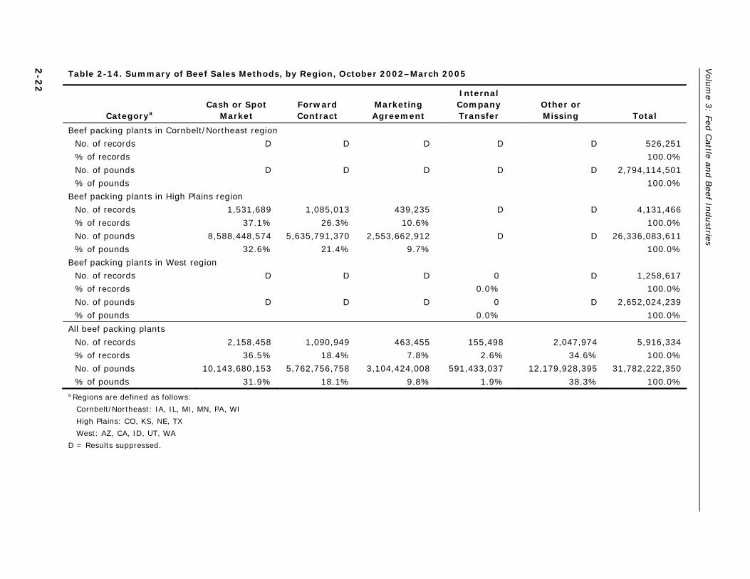
Volu
me 3
: Fed C
attle and B
eef Industries
2-2
2
Table 2-14. Summary of Beef Sales Methods, by Region, October 2002–March 2005
Categorya Cash or Spot
Market Forward Contract
Marketing Agreement
Internal Company Transfer
Other or Missing Total
Beef packing plants in Cornbelt/Northeast region
No. of records D D D D D 526,251
% of records 100.0%
No. of pounds D D D D D 2,794,114,501
% of pounds 100.0%
Beef packing plants in High Plains region
No. of records 1,531,689 1,085,013 439,235 D D 4,131,466
% of records 37.1% 26.3% 10.6% 100.0%
No. of pounds 8,588,448,574 5,635,791,370 2,553,662,912 D D 26,336,083,611
% of pounds 32.6% 21.4% 9.7% 100.0%
Beef packing plants in West region
No. of records D D D 0 D 1,258,617
% of records 0.0% 100.0%
No. of pounds D D D 0 D 2,652,024,239
% of pounds 0.0% 100.0%
All beef packing plants
No. of records 2,158,458 1,090,949 463,455 155,498 2,047,974 5,916,334
% of records 36.5% 18.4% 7.8% 2.6% 34.6% 100.0%
No. of pounds 10,143,680,153 5,762,756,758 3,104,424,008 591,433,037 12,179,928,395 31,782,222,350
% of pounds 31.9% 18.1% 9.8% 1.9% 38.3% 100.0% a Regions are defined as follows:
Cornbelt/Northeast: IA, IL, MI, MN, PA, WI
High Plains: CO, KS, NE, TX
West: AZ, CA, ID, UT, WA
D = Results suppressed.

2-2
3
Sectio
n 2
— V
olu
me D
ifferences, Price D
ifferences, an
d S
hort-R
un S
pot M
arket Price E
ffects Asso
ciated w
ith A
lternative M
arketing A
rrangem
ents
Table 2-15. Summary of Beef Sales Pricing Methods, by Region, October 2002–March 2005
Categorya Negotiated Formula Pricing Sealed Bid
Internal Transfer Pricing
Other or Missing Total
Beef packing plants in Cornbelt/Northeast region
No. of records D D 0 D D 526,251
% of records 0.0% 100.0%
No. of pounds D D 0 D D 2,794,114,501
% of pounds 0.0% 100.0%
Beef packing plants in High Plains region
No. of records 1,598,001 1,457,933 D D 1,026,103 4,131,466
% of records 38.7% 35.3% 24.8% 100.0%
No. of pounds 9,633,501,910 7,144,398,279 D D 9,409,835,820 26,336,083,611
% of pounds 36.6% 27.1% 35.7% 100.0%
Beef packing plants in West region
No. of records D D 0 0 D 1,258,617
% of records 0.0% 0.0% 100.0%
No. of pounds D D 0 0 D 2,652,024,239
% of pounds 0.0% 0.0% 100.0%
All beef packing plants
No. of records 2,233,143 1,479,716 D D D 5,916,334
% of records 37.7% 25.0% 100.0%
No. of pounds 11,286,520,401 7,724,337,850 D D D 31,782,222,350
% of pounds 35.5% 24.3% 100.0% a Regions are defined as follows:
Cornbelt/Northeast: IA, IL, MI, MN, PA, WI High Plains: CO, KS, NE, TX West: AZ, CA, ID, UT, WA
D = Results suppressed.

Volu
me 3
: Fed C
attle and B
eef Industries
2-2
4
Table 2-16. Summary of Types of Formula Bases Used for Beef Sales, by Region, October 2002–March 2005
Categorya Plant Average
Price USDA-Reported
Price Other Market
Price Other or Missing Total
Beef packing plants in Cornbelt/Northeast region
No. of records 0 D 0 D 10,664
% of records 0.0% 0.0% 100.0%
No. of pounds 0 D 0 D 160,749,985
% of pounds 0.0% 0.0% 100.0%
Beef packing plants in High Plains region
No. of records D 1,156,214 D 20,859 1,457,933
% of records 79.3% 1.4% 100.0%
No. of pounds D 5,386,473,495 D 93,182,008 7,144,398,279
% of pounds 75.4% 1.3% 100.0%
Beef packing plants in West region
No. of records 0 D 0 D 11,119
% of records 0.0% 0.0% 100.0%
No. of pounds 0 D 0 D 419,189,587
% of pounds 0.0% 0.0% 100.0%
All beef packing plants
No. of records D 1,177,408 D D 1,479,716
% of records 79.6% 100.0%
No. of pounds D 5,943,701,573 D D 7,724,337,850
% of pounds 76.9% 100.0% a Regions are defined as follows:
Cornbelt/Northeast: IA, IL, MI, MN, PA, WI
High Plains: CO, KS, NE, TX
West: AZ, CA, ID, UT, WA
D = Results suppressed.

Section 2 — Volume Differences, Price Differences, and Short-Run Spot Market Price Effects Associated with Alternative Marketing Arrangements
2-25
2.2 PRICE DIFFERENCES ASSOCIATED WITH MARKETING ARRANGEMENTS IN THE FED CATTLE AND BEEF INDUSTRY In this section, we present the results of descriptive analyses on price differences and trends, by type of marketing arrangement, and quantitative analyses of the relationship between transactions prices and AMAs. We then estimate the relationships between transactions prices and AMAs for all transactions and for only cash market transactions.
2.2.1 Fed Cattle and Beef Prices, by Type of Marketing Arrangement: Averages and Trends
Fed cattle purchase lots typically range from 10 to 200 cattle per lot.5 Within an individual lot, the quality and characteristics of cattle may vary substantially depending on breed, distribution of steers versus heifers, whether any cattle are culled cows or bulls, weight range, quality grade, and yield grade. To analyze differences in transactions prices, it is necessary to adjust for differences in the composition and quality of the lot. However, prior to conducting the analysis that controls for these characteristics, it is useful to compare a summary of average prices across plant sizes (Table 2-17) and regions (Table 2-18) by type of marketing arrangement.
We computed prices per pound by dividing the total cost of each lot by the total carcass weight of each lot. We then calculated a weighted average price and standard deviation by each type of marketing arrangement. The total cost of a lot comprises
cost of the cattle in the lot,
shipping costs (which may be paid by the packer or by the producer),
commission costs,
miscellaneous costs (e.g., feed), and
price adjustments for quality.
5 Smaller lots of cattle are typically off-quality cattle that are not
quality graded.

Volu
me 3
: Fed C
attle and B
eef Industries
2-2
6
Table 2-17. Fed Cattle Prices, by Marketing Arrangement by Size of Plant ($ per Pound Carcass Weight), October 2002–March 2005
Categorya Auction Barns
Dealers or Brokers
Direct Trade
Forward Contract
Marketing Agreement
Packer Fed/Owned
Other or Missing Total
Small beef packing plants
Total cost ($/lb)
Weighted average 1.34 1.32 1.32 1.30 1.30 1.35 1.28 1.31
St. dev. 0.00016 0.00016 0.00016 0.00014 0.00017 0.00016 0.00015 0.00016
Large beef packing plants
Total cost ($/lb)
Weighted average D D 1.32 1.28 1.31 D 1.20 1.31
St. dev. 0.00019 0.00020 0.00018 0.00018 0.00019
All beef packing plants
Total cost ($/lb)
Weighted average 1.34 1.32 1.32 1.29 1.31 1.32 1.27 1.31
St. dev. 0.00017 0.00019 0.00018 0.00018 0.00018 0.00019 0.00016 0.00018
a Sizes are defined as follows:
Small has capacity < 20,000 head/week.
Large has capacity > 20,000 head/week.
D = Results suppressed.

2-2
7
Sectio
n 2
— V
olu
me D
ifferences, Price D
ifferences, an
d S
hort-R
un S
pot M
arket Price E
ffects Asso
ciated w
ith A
lternative M
arketing A
rrangem
ents
Table 2-18. Fed Cattle Prices, by Marketing Arrangement by Region ($ per Pound Carcass Weight), October 2002–March 2005
Categorya Auction Barns
Dealers or Brokers
Direct Trade
Forward Contract
Marketing Agreement
Packer Fed/Owned
Other or Missing Total
Beef packing plants in Cornbelt/Northeast region
Total cost ($/lb)
Weighted average D D D D D NA NA 1.31
St. dev. NA NA 0.00014
Beef packing plants in High Plains region
Total cost ($/lb)
Weighted average D D 1.31 1.28 1.31 D 1.20 1.31
St. dev. 0.00019 0.00020 0.00019 0.00018 0.00019
Beef packing plants in West region
Total cost ($/lb)
Weighted average D D D 1.33 1.31 1.35 1.28 1.33
St. dev. 0.00012 0.00015 0.00016 0.00015 0.00016
All beef packing plants
Total cost ($/lb)
Weighted average 1.34 1.32 1.32 1.29 1.31 1.32 1.27 1.31
St. dev. 0.00017 0.00019 0.00018 0.00018 0.00018 0.00019 0.00016 0.00018
NA = not applicable a Regions are defined as follows:
Cornbelt/Northeast: IA, IL, MI, MN, PA, WI
High Plains: CO, KS, NE, TX
West: AZ, CA, ID, UT, WA
Averages are weighted by number of head.
D = Results suppressed.

Volume 3: Fed Cattle and Beef Industries
2-28
Because of substantial variation in reporting of costs by packers, we use the total costs of the lot rather than the cattle cost to compute averages. However, cattle cost typically comprises 97% to 99% of the total cost of the lot. Therefore, the total cost of the lot is a reasonable approximation of the cost of the cattle in the lot.
Figure 2-1 shows the average weekly prices, by marketing arrangement, for a selected group of cattle in the transaction data. Lots with 60% or more cattle in the Choice or Select Quality Grade or lots with 60% or more cattle in Yield Grade 2 or 3 were included in the calculation of the average. All prices trended upward during the data collection period. This trend is partially explained by the phase of the cattle cycle, which changed from liquidation in 2003 and 2004 to rebuilding in 2005. During the rebuilding phase, animal supplies were relatively tight and cattle prices were rising. Cattle supplies within the United States also tightened because of the ban on Canadian cattle imports from May 2003 to July 2005. The U.S. border was closed to Canadian cattle because of the discovery of BSE. Additionally, the first case of BSE in the United States was discovered in December 2003.
Figure 2-1. Average Weekly Price of Cattle from Lots with 60% or More Choice/Select Quality Grade or Yield Grade 2 or 3, by Marketing Arrangement, October 2002–March 2005
90100110120130140150160170180
Octobe
r '02
Novem
ber '0
2
Decem
ber '0
2
Februa
ry '03
March '
03
April '0
3
June
'03
July
'03
Augus
t '03
Octobe
r '03
Novem
ber '0
3
Janu
ary '0
4
Februa
ry '04
March '
04
May '0
4
June
'04
Augus
t '04
Septem
ber '0
4
Octobe
r '04
Decem
ber '0
4
Janu
ary '0
5
Februa
ry '05
Pric
e pe
r Hun
dred
Pou
nds
(Car
cass
Wei
ght)
Auction Direct trade Forward contractMarketing agreement Packer owned Other purchase method
Section 2 — Volume Differences, Price Differences, and Short-Run Spot Market Price Effects Associated with Alternative Marketing Arrangements
2-29
The overall average price received for the October 2002 through March 2005 period was $1.31 per carcass weight pound. The average prices across types of marketing arrangements differed by 20 cents across sizes of plants (see Table 2-17) and by 24 cents across regions (see Table 2-18). When comparing average prices across plant sizes and regions, it is important to keep in mind that differences in prices are not necessarily due to differences in the type of marketing arrangement used. Differences could reflect that plants in certain regions or size categories typically purchase specific types of cattle based on their needs.
With these caveats in mind, prices varied 7 cents per pound across marketing arrangements for small packing plants and 20 cents per pound for large packing plants. Prices are generally similar for small and large packing plants. By region, prices paid by packing plants varied 11 cents per pound across marketing arrangements in the Cornbelt/Northeast, 20 cents per pound in the High Plains, and 16 cents per pound in the West. Noted regional differences are as follows:
Packing plants in the High Plains and West paid the lowest price for cattle purchased through other marketing arrangements or unspecified marketing arrangements.
Packing plants in the Cornbelt/Northeast paid the lowest price for cattle procured through marketing agreements.
Packing plants in the Cornbelt/Northeast and High Plains paid the highest average price for cattle purchased through auction barns. This likely reflects the need to purchase more cattle through auction after the closure of the U.S.–Canadian border in order to help maintain a higher capacity utilization for plants in this region.
Packing plants in the West paid the highest price for cattle purchased from dealers or brokers. This likely reflects that many purchases of cattle through dealers and brokers represent special sales of cattle purchased to meet specialized buyer requirements.
In discussing differences in prices across types of marketing arrangements, it is important to keep in mind that the prices were influenced by the unique time period of the data set. Cash market and AMA prices were generally trending upward, except during the May 2003 through December 2003 period (see Figure 2-1). Forward contract prices often had lower prices than
Volume 3: Fed Cattle and Beef Industries
2-30
the other types of marketing arrangements, because these prices are set further in advance of the other prices and thus take longer to adjust to unexpected market conditions (e.g., discovery of BSE).
2.2.2 Analysis of the Relationship between Fed Cattle and Beef Transactions Prices and Use of Marketing Arrangements
In this section, we analyze the relationship between purchase prices for fed cattle and the use of marketing arrangements, while controlling for other characteristics of the transactions that affect fed cattle prices. We include both cash market and AMA transactions in the model and evaluate whether individual types of marketing arrangements are associated with higher or lower prices for cattle. We conduct the analysis using the transactions data for the 29 of the largest beef packing plants in the United States for the October 2002 through March 2005 period. The methodology is based on Ward, Koontz, and Schroeder (1998), with changes to reflect a newer data set.
The model is specified as
tit
tititi
tititi
uMONTHD
PLANTDAMADbeefcattled
CHCATTLEAMADPRICE
++
++×+
+++=
_
___
__
4
33
210
βββ
βββ (2.1)
where t indexes kill week for each lot of fed cattle, t = 1,…,T; i indexes transactions (i.e., fed cattle lots purchased by packers), i = 1,…,It; PRICEti is transaction price on a per pound carcass weight basis; βs are parameters to estimate, and uti is a random error term. In addition, D_AMAti is a vector of binary variables that indicates the type of marketing arrangement used for purchase of the lot, including
direct trade (d_direct)6 (as the base group),
auction barns (d_auction),
forward contract (d_forward),
packer owned (d_packer), and
marketing agreement (d_marketing).
6 Transactions through dealers or brokers are combined with the
transactions through direct trade because they account for a very small fraction of the total transactions (less than 1%) and are another type of cash market purchase.

Section 2 — Volume Differences, Price Differences, and Short-Run Spot Market Price Effects Associated with Alternative Marketing Arrangements
2-31
CATTLE_CHti is a vector of cattle characteristics, including
whether the fed cattle are a beef or dairy breed (d_beefcattle),
the number of head in the lot (numberofhead),
the percentage of Yield Grade 4 or 5 cattle in the lot (yg45_pct),
the percentage of cattle with Quality Grade of Prime or Choice in the lot (primechoice_pct),
the percentage of cattle that were classified as heavy weight or light weight in the lot according to the definition of heavy weight or light weight used by each individual packer (outweight_pct), and
the percentage of cattle that were eligible for a branded or a certification program in the lot (branded_pct).
We also include the interaction term of d_beefcattle and D_AMA so that the price premium/discount associated with each marketing arrangement is allowed to be different for beef cattle and dairy cattle (fed dairy steers). We also include 28 plant binary variables (D_PLANT) to control for the plant-level unobserved fixed effects, such as location and installed capital equipment. Furthermore, 29 binary variables that indicate the month in which the cattle were killed (D_MONTH) are included in the model. In this way, we control for seasonality, trend, and other possible unobserved effects related to each month. In particular, these monthly binary variables help control for the effect of the market disruptions that occurred as a result of the BSE discoveries in Canada and the United States during this period. Table 2-19 provides the definitions, means, standard deviations, minimums, and maximums of the variables included in the model, with the exception of the plant and monthly binary variables. Note that transactions with prices below $0.86 and above $1.98 per carcass weight pound were excluded from the model (see the explanation in Section 1.3.1).
Because we used high-frequency data, we take two features of the data into account. First, the price (conditional on the explanatory variables) may be correlated within the same week and across neighboring weeks,7 even though we have
7 We are concerned about the correlation within a week rather than
within a day because the cattle market is generally a weekly market (i.e., packers arrange their procurement and production activities week by week).

Volume 3: Fed Cattle and Beef Industries
2-32
Table 2-19. Descriptive Statistics for the Variables in the Price Difference Model for Fed Cattle Purchase Transactions, October 2002–March 2005
Variable Notation Mean Std. Dev. Min Max
price Transaction price in $ per pound carcass weight
1.3100 0.140 0.86 1.98
d_direct Direct trade purchase (1 = yes, 0 = no)
0.5800 0.490 0.00 1.00
d_auction Auction purchase (1 = yes, 0 = no) D D 0.00 1.00
d_forward Forward contract purchase (1 = yes, 0 = no)
0.0400 0.200 0.00 1.00
d_packer Packer-owned procurement (1 = yes, 0 = no)
D D 0.00 1.00
d_marketing Marketing agreement procurement (1 = yes, 0 = no)
0.2800 0.450 0.00 1.00
d_beefcattle Mostly beef breed cattle in the lot (1 = yes, 0 = no)
0.7800 0.420 0.00 1.00
numberofhead Number of head in the lot (100s) 0.9900 0.890 0.06 15.21
yg45_pct % Yield Grade 4 or 5 in the lot 0.0830 0.0980 0.00 1.00
primechoice_pct % Prime or Choice in the lot 0.6400 0.240 0.00 1.00
outweight_pct % heavy weight or light weight cattle in the lot
0.3300 0.370 0.00 1.00
branded_pct % cattle eligible for branded or certification program in the lot
0.1900 0.230 0.00 1.00
D = Results suppressed.
controlled for the monthly fixed effects. Second, the volatility of the price (conditional on the explanatory variables) may vary by time, AMA choice, or some other explanatory variables. That is, we may have a heteroskedasticity problem. If the correlation and/or heteroskedasticity exist but we failed to model them, our inferences would be invalid.
Therefore, to reflect these two features of the data, we model the structure of the error term uti as
titti vu ε+= , (2.2)
where vt is an unobserved weekly effect, which is constant for all transactions with delivery date in week t, and tiε is a transaction-specific random error term with constant variance. We further assume vt and εti are uncorrelated with the explanatory variables and uncorrelated with each other, and

Section 2 — Volume Differences, Price Differences, and Short-Run Spot Market Price Effects Associated with Alternative Marketing Arrangements
2-33
⎪⎪⎪
⎩
⎪⎪⎪
⎨
⎧
>−
=−
=
=
1,0
1,
,
),( 2
2
stif
stif
stif
vvCov v
v
st ρσ
σ
(2.3)
and
).___
__exp()(
43
210
tittiti
tititi
MONTHDAMADbeefcattled
CHCATTLEAMADuVar
ςδδδδδ
++×+
+++= (2.4)
Both the covariance in Eq. (2.3) and the variance in Eq. (2.4) are conditional on the explanatory variables. The setup of Eqs. (2.3) and (2.4) captures the correlation and heteroskedasticity features of transactions price data, as we discussed above. Eq. (2.3) assumes that the conditional covariance of prices between any two transactions delivered in the same week is 2
vσ , the conditional covariance of prices between two transactions delivered in neighboring weeks is
2vρσ , and the conditional covariance of transaction prices is
zero otherwise. Eq. (2.4) assumes that the variance of transaction prices depends on the choice of marketing arrangement, cattle characteristics, and delivery month.
In the model described by Eqs. (2.1) through (2.4), the parameters of interest are β1, β3, δ1, and δ3. The β1 and β3
parameters indicate the average price differences associated with AMAs, holding other explanatory variables fixed. The δ1 and δ3 parameters indicate the differences of price volatility associated with AMAs, holding CATTLE_CH and D_MONTH fixed. We discuss the estimated β1 and β3 parameters in this section and return to a discussion of the estimated δ1 and δ3 parameters in Section 5 on risk shifting.
Prior to estimating Eq. (2.1), we tested the following three null hypotheses for the existence of heteroskedasticity and/or correlation in the error term:
Hypothesis 1:
truenotHHvsH 0143210 :.0: ==== δδδδ
Hypothesis 2:
0:.0: 21
20 >= vv HvsH σσ
Volume 3: Fed Cattle and Beef Industries
2-34
Hypothesis 3:
0:.0: 21
20 >= vv HvsH ρσρσ .
If the null hypothesis for Hypothesis 1 is true, we would not have to model heteroskedasticity. If the null hypothesis for Hypothesis 2 is true, we would not have to model the price correlation among transactions within the same week.8 If the null hypothesis for Hypothesis 3 is true, we would not have to model the price correlation between neighboring weeks. However, Wald tests reject each of the three hypotheses at the 1% significance level.9 These results support modeling both heteroskedasticity and correlation in the error term.
Eq. (2.1) is estimated using ordinary least squares (OLS) and the estimates for the parameters, the βs, are reported in the second column of Table 2-20.10, 11 The standard errors are consistent with the error structure in Eqs. (2.3) and (2.4).
The results suggest that while holding other explanatory variables fixed, (1) beef breed direct trade cattle are priced 2.7 cents per pound higher than dairy breed direct trade cattle, (2) cattle with higher yield grades or higher quality grade receive a higher average price, (3) a 1% increase in branded cattle in a lot is related to a 2.7 cent per pound higher average price, and (4) the price of light weight or heavy weight cattle is discounted. In addition, average prices are slightly higher for larger cattle lots.
Tables 2-21 and 2-22 summarize the estimated average price differences among AMAs for beef cattle and dairy cattle respectively. All the differences are individually significant at the 5% level, based on Wald tests. The average prices are closest among the direct trade, marketing agreement, and packer-owned transactions, with the estimated differences ranging from 0.1 to 1.2 cents per pound carcass weight. The
8 Of course, if the null hypothesis 2 is true, the null hypothesis 3 must
also be true, unless the model is misspecified. 9 The Breusch-Pagan test and the White test also reject the null
hypothesis of homoskedasticity at the 1% level. 10 Theoretically, Feasible Generalized Least Squares (FGLS) is more
efficient than OLS. However, FGLS is computationally difficult (if not impossible) because of the size of the data set and the complexity of the error structure.
11 We also estimated Eq. (2.1) using quantile regression and report the coefficient estimates for different price quantiles7 in Appendix A of this volume.

Section 2 — Volume Differences, Price Differences, and Short-Run Spot Market Price Effects Associated with Alternative Marketing Arrangements
2-35
Table 2-20. Parameter Estimates for the Price Difference Models of Fed Cattle Purchase Transactions, October 2002–March 2005
Variable
Price Coefficient (Std. Error)
Log(var(u)) Coefficient (Std. Error)
d_auction 0.016 (0.0011)
0.92 (0.053)
d_forward –0.047 (0.0008)
0.56 (0.025)
d_packer –0.012 (0.0017)
–0.32 (0.073)
d_ma -0.006 (0.0005)
–0.22 (0.013).
d_beefcattle 0.027 (0.0003)
–0.16 (0.010)
d_beefcattle*d_auction 0.093 (0.0016)
0.54 (0.055)
d_beefcattle*d_forward -0.000017 (0.0008)a
0.52 (0.032)
d_beefcattle*d_packer 0.013 (0.0018)
0.22 (0.075)
d_beefcattle*d_ma 0.012 (0.00043)
0.019 (0.016)a
numberofhead 0.0049 (0.0001)
–0.10 (0.0035)
yg45_pct –0.073 (0.001)
0.70 (0.033)
primechoice_pct 0.062 (0.0005)
–0.23 (0.012)
outweight_pct –0.021 (0.0005)
0.31 (0.0092)
branded_pct 0.027 (0.0006)
–0.16 (0.014)
Other variablesb Not reported
No. of observations (lots) 571,608 571,608
R2 0.7744 0.1260
a Coefficient is insignificant at the 5% level. All other variables are significant at the 5% level. b The “other variables” include an intercept, monthly binary variables, and plant binary variables.

Volume 3: Fed Cattle and Beef Industries
2-36
Table 2-21. Estimated Average Price Differences among AMAs for Beef Breed Fed Cattle Purchase Transactions, October 2002–March 2005 (Cents per Pound Carcass Weight)
Marketing Arrangement
Direct Trade Auction
Forward Contract
Packer Owned
Marketing Agreement
Direct trade — –10.9 4.7 –0.1 –0.6
Auction 10.9 — 15.6 10.8 10.3
Forward contract –4.7 –15.6 — –4.8 –5.3
Packer owned 0.1 –10.8 4.8 — –0.5
Marketing agreement 0.6 –10.3 5.3 0.5 —
Note: The differences are computed as the average price for each AMA listed in the left column minus each listed in the top row.
Table 2-22. Estimated Average Price Differences among AMAs for Dairy Breed Fed Cattle Purchase Transactions, October 2002–March 2005 (Cents per Pound Carcass Weight)
Marketing Arrangement
Direct Trade Auction
Forward Contract
Packer Owned
Marketing Agreement
Direct trade — –1.6 4.7 1.2 0.6
Auction 1.6 — 6.3 2.8 2.2
Forward contract –4.7 –6.3 — –3.5 –4.1
Packer owned –1.2 –2.8 3.5 0.0 –0.6
Marketing agreement –0.6 –2.2 4.1 0.6 —
Note: The differences are computed as the average price for each AMA listed in the left column minus each listed in the top row.
auction barn transactions price is estimated to be about 10.9 cents higher for beef breed cattle and 1.7 cents higher for dairy breed cattle than for the corresponding direct trade cattle, although both are cash market procurement methods. Transactions prices associated with forward contract transactions are the lowest among all the procurement methods. This result may suggest that farmers who choose forward contracts are willing to give up some revenue in order to secure market access and to fix the price at least 2 weeks before delivery.
The result that auction barn prices are the highest and forward contract prices are the lowest could also be due, in part, to the unique time period of the analysis, including the stage of the cattle cycle and the closure of the border with Canada after the discovery of BSE in May 2003. Our model compares the prices among procurement methods for the cattle delivered in the

Section 2 — Volume Differences, Price Differences, and Short-Run Spot Market Price Effects Associated with Alternative Marketing Arrangements
2-37
same month but does not control for the pricing dates related to individual transactions. Transactions prices are correlated with the expectation of market conditions at the delivery date based on the information available at the pricing date. The difference between pricing dates and delivery dates is systematically different among procurement methods.
According to the transactions data, on average, forward contract cattle are priced 12 days ahead of delivery date, direct trade cattle are priced six days ahead, and auction barn cattle are priced only two days ahead. Consider a forward contract lot and an auction barn lot that are delivered at the same time. If there is an positive market shock (e.g., the closure of the border with Canada) that occurs before the pricing time of auction barn cattle but is not expected at the time when forward contract cattle are priced. The forward contract cattle would be priced lower than the auction barn cattle due to the unexpected random market shock. If the time period represented in the data was long enough, this would not bias the estimation results because positive shocks should be offset by negative shocks in the long run. However, this may not be true in this case because the represented time period is relatively short. That is, if the unexpected market shock is systematically positive during our represented period, failing to control for market expectations at the pricing date would bias the estimates of price differences among procurement methods. It is difficult to incorporate the pricing date information because these data are unreliable in the data set and are only available for about 40% of the total transactions. However, we believe the effect of this bias is limited because the largest average pricing date difference among procurement methods is a maximum of 12 days. We examined the average two-week price difference in the Nebraska cash market for steers and found that this difference is both economically and statistically insignificant (the mean value of the difference is 0.18 cent per pound dressed weight, and the P value of the t-test is 0.78).

Volume 3: Fed Cattle and Beef Industries
2-38
2.3 EFFECTS OF MARKETING ARRANGEMENTS ON CASH MARKET PRICES IN THE FED CATTLE AND BEEF INDUSTRY In this section, we analyze the relationship between cash market prices for fed cattle and the use of AMAs, while controlling for other characteristics of the transactions that affect cash market prices. The transactions included in the model represent all cash market purchases (auction barn and combined dealer/broker and direct trade) for the October 2002 through March 2005 period. We conducted the analysis using the transactions data from 29 of largest beef packing plants in the United States. As in Section 2.2, the methodology is based on Ward, Koontz, and Schroeder (1998), with changes to reflect a newer data set.
The model is specified as
,uMONTH_DPLANT_D
CH_CATTLEMARKETama_nutilizatio
showlistother_directgrid_direct
nogrid_directauction_dPRICE
titti
titti
ttiti
tititi
+++
++
++++
++=
109
876
543
210
βββββ
ββββββ
(2.5)
where d_auction, direct_nogrid, direct_grid, and direct_other are binary variables indicating auction barn transactions,12 direct trade transactions using carcass weight not dependent on grid valuation, direct trade transactions using carcass weight dependent on grid valuation, and direct trade transactions with another valuation method. The base group is the variable for direct trade transactions using liveweight valuation (i.e., the binary variable was omitted from the regressions). The vector MARKET includes two weekly lagged price variables:
price_choice (the value of boxed beef cutout for Choice quality grade in the preceding week)
price_futures (the previous week’s closing live cattle futures market price for the nearby contract)
These variables serve as proxies for cattle market expectations. The vectors CATTLE_CH, D_PLANT and D_MONTH are the same as described in Section 2.2.2.
12 In almost all auction barn transactions, cattle are valued by
liveweight. In this sample, only 9 out of 38,583 auction barn transactions used some valuation method other than liveweight.

Section 2 — Volume Differences, Price Differences, and Short-Run Spot Market Price Effects Associated with Alternative Marketing Arrangements
2-39
Showlist and utilization_ama are the key variables in this regression. These variables are computed as follows:
Showlist is computed as the total number of cattle (in 100,000 head) purchased through auction barns or direct trade that were delivered to the 29 beef packing plants within the subsequent 21 days, calculated from the previous Friday. This serves as a proxy for the total available cattle for delivery in the cash market (i.e., the cattle available for delivery that are not under AMAs).
Utilization_ama is the proportion of average weekly AMA delivery relative to the weekly slaughter capacity for a plant.
Both showlist and utilization_ama capture the effect of AMAs on cash market transaction prices. However, the two variables differ in two ways. First, showlist is a market-level variable, while utilization_ama is at the plant level. Second, we expect the coefficient of utilization_ama to be negative because, when relatively high capacity utilization is being maintained through use of AMAs,13 the packer would be expected to negotiate less aggressively, thus tending to pay less in the cash market (Schroeter and Azzam, 2003). In contrast, the direction of the effect of showlist on cash market prices is an empirical question. When more cattle are procured by AMAs, fewer are available in the cash market (i.e., showlist decreases). However, the demand for cash market cattle by packers would also be reduced. Therefore, the overall effect is unknown conceptually (Schroeder et al., 1993). The descriptive statistics for the variables included in Eq. (2.3) are summarized in Table 2-23.
We estimate Eq. (2.5) using OLS with Huber-White heteroskedasticity-robust standard errors. The parameter estimates are reported in Table 2-24. Compared with direct trade transactions with live weight valuation, the average cattle price associated with auction barn transactions is 2.4 cents higher, direct trade transactions with carcass weight not dependent on grid valuation are 1.3 cents lower, and direct trade transactions with carcass weight dependent on grid valuation are 1.8 cents lower, holding other explanatory variables in the model fixed. As with the results in Section 2.2.2, cattle with better quality (such as better yield grade,
13 One major reason that packers use AMAs is to maintain a relative
high capacity utilization.

Volume 3: Fed Cattle and Beef Industries
2-40
Table 2-23. Descriptive Statistics for the Variables in the Cash Market Price Model for Fed Cattle Procurement Transactions, October 2002–March 2005
Variable Notation Mean Std. Dev. Min Max
price Transaction price in $ per pound carcass weight 1.3800 0.120 0.86 1.98
d_auction Auction (1 = yes, 0 = no) 0.1000 0.310 0.00 1.00
direct_nogrid Direct trade purchases valued by carcass weight, not dependent on grid value (1 = yes, 0 = no)
0.1700 0.370 0.00 1.00
direct_grid Direct trade purchases valued by carcass weight dependent on grid value (1 = yes, 0 = no)
0.2800 0.450 0.00 1.00
direct_other Direct trade purchases valued by other than liveweight or carcass weight (1 = yes, 0 = no)
0.0040 0.063 0.00 1.00
showlist Number of cattle available in the cash market in the next 21 days (in 100,000 head)
8.6000 0.760 6.50 10.30
utilization_ama Capacity utilization from AMA cattlea 0.1700 0.170 0.00 1.00
price_choice Choice boxed beef cutout value in the preceding week
1.4600 0.140 1.25 1.94
price_futures Previous week’s closing live cattle futures market price for the nearby contract
0.8600 0.058 0.75 1.01
d_beefcattle Mostly beef breed cattle in the lot (1 = yes, 0 = no)
0.8300 0.380 0.00 1.00
numberofhead Number of head in the lot (100s) 0.9600 0.860 0.06 15.20
yg45_pct % Yield Grade 4 or 5 in the lot 0.0950 0.110 0.00 1.00
primechoice_pct % Prime or Choice in the lot 0.6600 0.250 0.00 1.00
outweight_pct % heavy weight or light weight cattle in the lot 0.3600 0.376 0.00 1.00
branded_pct % cattle eligible for branded or certification program in the lot
0.2000 0.250 0.00 1.00
a Plant capacity is each plant’s stated maximum operating capacity given its current operating schedule.
better quality grade, beef breed, and eligible for a branded or certification program) receive premiums on the cash market, and cattle with undesirable characteristics (such as light weight or heavy weight) are discounted. Also, large cattle lots receive statistically significant but economically small premiums.
As expected, capacity utilization through AMAs (utilization_ama) has a negative coefficient. The results suggest that if capacity utilization through AMAs in a plant (as measured by utilization_ama) increases by 10 percentage points, the plant pays 0.4 cents per carcass weight pound less for cattle purchased in the cash market. Showlist has a positive coefficient, which suggests that 100,000 more cattle available in the cash market (or 100,000 fewer cattle through AMAs) increases the cash market price by 0.18 cents. Alternatively, the estimated showlist coefficient indicates that a 10% increase in total cattle available through AMAs (within the next 21 days)

Section 2 — Volume Differences, Price Differences, and Short-Run Spot Market Price Effects Associated with Alternative Marketing Arrangements
2-41
Table 2-24. Parameter Estimates for the Cash Market Price Model for Fed Cattle Purchase Transactions, October 2002–March 2005
Variable Coefficienta
(Robust Standard Error)
d_auction 0.0240 (0.00190)
direct_nogrid –0.0130 (0.00039)
direct_grid –0.0180 (0.00043)
direct_other –0.0110 (0.02700)
showlist 0.0018 (0.00040)
utilization_ama –0.0400 (0.00190)
price_futures 0.6200 (0.01400)
price_choice 0.2000 (0.00460)
beefcattle 0.0370 (0.00073)
numberofhead 0.0055 (1.8 × 10⁻⁴)
yg45_pct –0.0920 (0.00320)
primechoice_pct 0.0630 (0.00140)
outweight_pct –0.0260 (0.00110)
branded_pct 0.0300 (0.00120)
Other variablesb Not reported
No. of cash market observations 203,017
F(55,202961) 5,010
R2 0.6571
a All coefficients are significant at the 5% level. b The “other variables” include an intercept, monthly binary variables, and plant binary variables.

Volume 3: Fed Cattle and Beef Industries
2-42
decreases the cash market price by 0.11% on average.14 This is an important result because it suggests that thin cash markets result in slightly lower prices.
Our empirical result suggests a negative (partial) correlation between spot market prices and AMA delivery by packers (both at the plant level and market level). This result is consistent with the results of many previous empirical studies using weekly or monthly market-level time-series data (See section 3.3.1 of the interim report (Muth et al., 2005) for a summary of this literature.). Many researchers have attempted to explain the negative relationship between AMA delivery and cattle market price. A typical explanation is that the negative correlation is due to price manipulation. However, a recent study by Schroeter (2007) suggests that this negative correlation may be an artifact of cattle delivery timing decisions made by price-taking market participants.
2.4 SUMMARY In this section, we summarized volumes and prices for fed cattle purchases by beef packers and analyzed price relationships across different type of marketing arrangements. The data used for the analysis are from October 2002 through March 2005, and thus the results may be influenced by the fact that the cattle cycle was in the contraction phase and by the discovery of BSE in Canada in May 2003 and in the United States in December 2003. The survey data are from 293 beef cattle producer and feeder responses and 64 beef packing plant responses across a range of sizes. The purchase data represent all purchases of fed cattle by 29 of the largest beef packing plants during the time period and include 58,066,440 head sold in 591,410 transactions.
Based on the survey data and transactions data, most packing plants are sole owners of the cattle slaughtered in their plants, but a small percentage of cattle are under shared ownership arrangements with the producer. Cash market transactions include auction barns, direct trade, and dealer/broker sales, while AMAs include forward contracts, marketing agreements, and packer ownership. Custom slaughtering in which the
14 This percentage is calculated by multiplying 0.1 by the coefficient on
the showlist variable (0.0018) by the average level of the showlist variable (8.6), divided by the average transaction price (1.38).

Section 2 — Volume Differences, Price Differences, and Short-Run Spot Market Price Effects Associated with Alternative Marketing Arrangements
2-43
producer retains ownership of the cattle and beef through slaughter also occurs, but is not represented in the data. Summaries of the purchase transactions data, which are generally in line with the survey responses, indicate the following:
The highest percentage of fed cattle sales to packing plants are through direct trade (58% of head slaughtered), followed by sales through marketing agreements (29% of head slaughtered). Fed cattle sales using auction barns, dealers or brokers, forward contracts, and packer fed/owned each represent a very small percentage of fed cattle transactions. Smaller beef packing plants rely much more on auction barn purchases than do larger beef packing plants. Beef packing plants in the Cornbelt/Northeast rely much more on auction barn purchases and plants in the West rely much more on marketing agreements compared with the other regions.
Negotiated pricing is the most common pricing method (57% of head slaughtered), followed by formula pricing (33% of head slaughtered). Smaller beef packing plants rely much more on auction pricing than larger beef packing plants. Beef packing plants in the West rely more on formula pricing and much less on negotiated pricing compared with the Cornbelt/Northeast and plants in the West rely on formula pricing somewhat more than plants in the High Plains.
The most common formula bases used in formula pricing are, in order of frequency, USDA live quotes, USDA dressed or carcass quotes, and subscription service prices. The use of formula bases is similar across plant sizes but different across regions. In particular, plants in the West use USDA live quotes much more frequently than the other regions and do not use USDA dressed or carcass quotes; plants in the Cornbelt/Northeast primarily use subscription service prices.
Fed cattle are most often valued on a carcass weight with grid (43% of fed cattle purchases) and on a liveweight (39% of fed cattle purchases) basis. Small beef packing plants rely somewhat more on carcass weight with grid valuation and less on a liveweight basis than larger beef packing plants. Beef packing plants in the Cornbelt/Northeast tend to use more liveweight valuation compared with the other regions, and beef packing plants in the West tend to use more carcass weight with grid and much less liveweight valuation than the other regions.

Volume 3: Fed Cattle and Beef Industries
2-44
Summaries of the beef sales transactions data indicate that the cash or spot market is the most common method of selling beef products by beef packing plants (32% of pounds sold). Forward contracts are also used but primarily by large beef packing plants and packing plants in the High Plains regions. However, many packing plants do not track or did not report the type of sales method used. Thus, all results of the sales data summaries should be interpreted with caution. For those plants that did indicate information about beef sales method, negotiated pricing was most often used (36% of pounds), followed by formula pricing (24% of pounds), particularly for large beef packing plants in the High Plains. The bases of formulas were USDA-reported prices for the vast majority of formula pricing transactions across all plant sizes and regions.
Summaries of fed cattle purchase transactions indicate that prices were relatively similar across purchase methods. The overall average price on a carcass weight basis was $1.31 per pound during the time period of the data. Average prices ranged from $1.27 per pound to $1.34 by type of marketing arrangement used, with some differences by size and location of plant. However, differences in prices reflect not only the type of marketing arrangement but also the quality of cattle and local market conditions.
We conducted an econometric analysis of the relationship between all fed cattle transactions prices and use of marketing arrangements, while controlling for differences in cattle quality and delivery month. The results indicate that relative to direct trade transactions, prices for fed cattle sold through auction barns tend to be somewhat higher and prices for fed cattle sold through forward contracts tend to be somewhat lower. These results are likely due, in part, to the differences in risk associated with the two methods; auction barn sales are somewhat more risky and have a higher cost because of commissions and weight shrink, but forward contracts ensure market access and a guaranteed price for cattle producers. The prices for fed cattle sold through marketing agreements and transferred through packer ownership are relatively similar to direct trade.
We also conducted an econometric analysis of the relationship between cash market (auction barns, dealers and brokers, and direct trade) transactions prices for fed cattle and use of
Section 2 — Volume Differences, Price Differences, and Short-Run Spot Market Price Effects Associated with Alternative Marketing Arrangements
2-45
marketing arrangements, which provides evidence of the effect of AMA supplies on the markets for cattle. The results suggest that if capacity utilization through the use of AMAs within a plant increases, plants pay slightly less per pound for cattle purchased in the cash market. Specifically, a 10% increase in capacity utilization through AMAs is associated with a 0.4 cent per pound carcass weight decrease in the cash market price. Furthermore, if more cattle are available through AMAs within the following 21 days, cash market prices decrease slightly. Specifically, a 10% increase in cattle available through AMAs is associated with a 0.11% decrease in the cash market price. However, these results are not necessarily indicative of manipulation of prices by packers but could instead be resulting from benign cattle delivery timing decisions made by price-taking market participants.


3-1
Economies of Scale, Costs Differences, and Efficiency Differences Associated with Alternative Marketing 3 Arrangements
In this section, we present results on the economies of scale, cost differences, and efficiency differences associated with AMAs. First, we describe qualitative evidence regarding the effects of AMAs on costs in the beef industry from the industry interviews and industry survey. Then we present the results of analyses using profit and loss (P&L) statement data from beef packing firms.
3.1 QUALITATIVE EVIDENCE OF THE EFFECTS OF AMAS ON COSTS The use of AMAs has effects on the cost of procurement of cattle and on the cost of production of beef by packers. In the earlier phase of the study, we interviewed producers and packers on the effect of AMAs on beef cattle and beef products (see Muth et al., 2005, Section 1.3 for a discussion of the interview process). The fed cattle producers we interviewed said that when selling cattle to packers, the use of AMAs instead of cash markets affects costs because of

Volume 3: Fed Cattle and Beef Industries
3-2
a need for fewer employees to manage many of the activities associated with production;
better feeding programs;
the ability to be able to obtain services such as financing, risk management, and procurement;
reduced costs of production of $1.25 to $10.00 per head, as reported by some producers, or 17% to 22% of costs, as reported by other producers; and
increased capacity utilization of the feedyard from a range of 77% to 80% to a range of 97% to 100%.
On the packer side, packers said that when purchasing cattle from producers, the use of AMAs instead of cash markets affects costs because of
the need for fewer buyers (approximately $0.40 per head), and
increased efficiencies in the production process.
However, the respondents indicated that the ability to obtain cattle to fit specific programs for meeting consumer demand and the ability to provide a consistent supply of quality product were other important reasons for using AMAs.
In the industry surveys described in Volume 2 of this report, we asked fed cattle producers and beef packers the three most important reasons for using either the cash market or an AMA. For fed cattle producer sales, 22.8% of respondents who use only the cash or spot market indicated doing so because it reduces the costs of activities for selling calves and cattle. In contrast, only 12.8% of respondents who use an AMA indicated doing so because it reduces the costs of activities for selling calves and cattle. Thus, based on the survey results, the costs of activities for selling calves and cattle appear to not be a major factor in the use of marketing arrangements, but do appear to be a more important factor for producers that choose to use only the cash market. Therefore, although the interview results indicate that cost reductions due to the use of AMAs can be substantial, higher selling prices, reduced price variability, and the ability to sell higher quality cattle are more important.
We obtained too few responses to make comparisons regarding the costs of buying and selling activities between respondents that use only the cash market and those that use an AMA for beef packer purchases. However, the most important reasons

Section 3 — Economies of Scale, Costs Differences, and Efficiency Differences Associated with Alternative Marketing Arrangements
3-3
for using only the cash market for beef packer purchases are that it allows for independence, complete control, and flexibility of one’s own businesses. Respondents also believe they can obtain higher quality cattle. Thus, the effects of marketing arrangements on costs are less important than these factors. The most important reasons for using AMAs are because they improve week-to-week supply management and because the respondents believe they can obtain higher quality cattle. Improved week-to-week supply management likely has an effect on costs of production and is consistent with the interview responses.
3.2 DESCRIPTION OF PROFIT AND LOSS STATEMENT DATA In this section, we describe the P&L data obtained from the largest beef packing firms.1 The P&L data are by plant, within each firm that slaughters and processes fed beef cattle. All results presented are aggregated across plants and firms included in the analysis. Thus, although results specific to any individual packer are not presented, all analyses were conducted on P&L data from individual plants.
The volume of head slaughtered and processed by the firms included in the analysis for the October 2002 through March 2005 period was more than 80% of USDA-reported federally inspected steer and heifer slaughter. All of the firms included in the analysis provided P&L information for each of their plants. Many smaller beef packers were not included in the analyses because they did not have P&L data in electronic form. Although other smaller beef packers provided electronic data, they could not be included in the analysis for a variety of reasons. These reasons included incomplete data (e.g., missing fields), changes in accounting systems during the data collection period resulting in changes in the format of data reported, and extremely small volumes relative to the industry as a whole. Twenty-one plants owned by four beef packing companies reported data suitable for this analysis.
1 This is the first economic analysis of P&L data from the beef packing
industry that has been conducted as part of an industry study. GIPSA has collected packer P&L data but only reports the data aggregated across firms. Therefore, it is not possible to examine individual firm performance or individual plant performance. This is the first study to examine plants and firm performance with the same information that firm managers have.

Volume 3: Fed Cattle and Beef Industries
3-4
P&L data are maintained differently across the major packers. The structure of the P&L statements is different across firms, and there are large variations in the categories of information that are detailed. For example, some firms reported very detailed by-product revenue information, while other firms reported very few lines associated with revenue categories. The placement of specific types of information within P&L statements also varies across packers. Some firms reported labor as a variable cost, while others reported labor with other costs that are most likely fixed costs. Likewise, some firms reported plant costs as a fixed cost, and some reported plant costs with other costs that are most likely variable costs. Some of the largest firms reported slaughter and fabrication on separate P&L statements, even when the slaughter and fabrication operations were at the same facility site. The other firms combined slaughter and fabrication into a single P&L statement.
While all beef packing firms complied with the request for P&L data, analysis was only attempted for those with data in electronic form. In most cases, the electronic form of the P&L data were exact images of P&L statements. The level of detail provided in P&L statements varied by company. As mentioned above, they also differed in how they categorized variable and fixed costs. Thus, only data from plants that provided cost and revenue data in an electronic format and in sufficient detail were used in the analysis.
Because of the differences in P&L statements across firms, only basic information can be compared with confidence. Thus, the details reported in this section focus on
average total costs per head (ATC),
average gross margin per head (AGM), and
average profit per head (PPH).
Total costs, total gross margin, and total profits are available for each plant from each monthly P&L statement.2 We divided each total by the number of head slaughtered or processed each month to create an average value per head per month figure. We constructed these variables for each plant within each firm included in the analysis.
2 For plants that maintain P&L statements on a weekly basis, we
aggregated the data to a monthly basis.

Section 3 — Economies of Scale, Costs Differences, and Efficiency Differences Associated with Alternative Marketing Arrangements
3-5
3.3 METHODOLOGY FOR ANALYZING PROFIT AND LOSS DATA This section describes the methodology used to analyze the beef packer P&L data. Because of the differences in P&L statements across firms, the analyses of costs and revenues focus on total costs, gross margins, and profit. We conducted more detailed analysis of the firms that provided more detailed data and found the results to be generally consistent with those in this report. However, specifics of the disaggregated firm analyses will not be presented in order to preserve confidentiality and because comparisons across firms may be misleading. Fixed costs associated with plants could be easily identified for some packers and were of expected magnitudes. However, efforts to identify fixed costs for other packers resulted in magnitudes that were not reasonable.
Below, we describe the details of the models for ATC, AGM, and PPH. We present the results in Section 3.4. Models are estimated for each plant. However, the results are aggregated over all plants to protect confidentiality. The aggregate plant can be thought of as a “representative” plant for the industry.
3.3.1 Total Costs per Head Model
The primary modeling effort using P&L data involves regressing ATC as a function of the volume processed or slaughtered and the percentages of volumes that are procured through AMAs. The basic ATC model is as follows:
,)_()_(
)_()ln(
43
210
tj
jtjtt
ttt
xPOPMAP
FCPVolumePerHeadTotalCosts
εαββ
βββ
+++
+++=
∑ (3.1)
where t denotes the month within the sample. The variables P_FC, P_MA, and P_PO denote forward contract, marketing agreement, and packer-owned fed cattle, respectively, expressed as a percentage of total monthly procurement volumes. xj represents a trend variable and labor, energy, and capital input price variables obtained from the U.S. Bureau of Labor statistics sources. However, none of the input price variables were significant and of the correct sign and, thus, were removed from the final specification.
Initially, separate models were estimated for each plant within each company. The semilogarithm form of the model specified above was found to be most appropriate for the majority of the

Volume 3: Fed Cattle and Beef Industries
3-6
plants. Thus, we used the semilogarithm form in all cases for uniformity across the firms and plants and for simplicity in programming the policy simulations. Quadratic ATC functions were not used for Eq. (3.1) because the data showed no points where ATC increased with higher volumes. Increasing ATCs with larger volumes was not observed in the data.
Coefficients on the AMA variables in Eq. (3.1) measure whether higher volumes of fed cattle purchased through AMAs are associated with lower ATC, as expressed on monthly plant-level P&L statements. In other words, the coefficients are direct-effect measurements of the cost differences caused by the use of AMAs for procuring cattle. Furthermore, these coefficients represent the cost differences that the firms see or recognize through their P&L accounting.
The model can be used to calculate or simulate changes in ATCs when AMA volumes are changed or limited because of policy intervention. For example, if a hypothetical restriction required that no cattle be procured through AMAs, then substituting zero for the AMA variables enables a calculation of the change in ATCs due to the restriction, while holding all else constant. Likewise, the effects of other types of restrictions can be simulated by varying the values substituted into Eq. (3.1). However, resulting estimates are specific to the sample of 30 months covered by the data collection (October 2002 through March 2005).
When using the model to conduct policy simulations, in addition to the direct effects, there are two important indirect effects that result. First, if a policy change results in reduced volumes of cattle slaughtered and processed at packing plants, then the effect of those changes can be measured through the volume coefficient in the ATC model. Thus, the cost impact of the volume reduction needs to be measured. Second, if a policy change results in changes in the variability in the number of cattle slaughtered and processed through packing plants, then the change needs to be measured. Random draws from the new distribution of cattle can be used with the ATC equation to measure the changes in average total costs due to a more variable supply of cattle for slaughter. The slope and curvature of the ATC function and increasing variability of procurement will result in increased costs.

Section 3 — Economies of Scale, Costs Differences, and Efficiency Differences Associated with Alternative Marketing Arrangements
3-7
Model of Plant-Level Volumes
Determining the changes in plant-level volumes and changes in variability brought about by changes in AMA volumes requires two additional modeling efforts. Changes in volumes are modeled as follows:
,)()(
)()(
43
210
ttt
ttt
POMA
FCUSDAFIVolume
εβββββ
++
+++= (3.2)
where the total volume of head slaughtered and processed at a plant (Volume) is modeled as a function of AMA volumes (FC, MA, and PO) measured in number of head and the monthly USDA federally inspected steer and heifer slaughter volumes (USDAFI) measured in thousands of head. We estimated one model for each plant so that plant-specific associations are measured. The USDAFI variable captures general changes in supply numbers. During the study period, cattle numbers were initially large because the market was in the liquidation phase of the cattle cycle. Cattle numbers were smaller toward the end of the sample, as the cycle changed to the expansion phase. In addition to the cattle cycle effects, a distinct seasonal pattern was also observed in the USDAFI variable. The model measures how changes in the total volume of cattle slaughtered and processed at a plant vary with changes in AMA volumes, while holding the total volume of cattle in the marketplace constant. Some plants readily substitute cash market cattle for AMA-procured cattle. For example, if volume of marketing agreement cattle decreases by 1,000 head, then those cattle might be offset by an increase of 900 cash market cattle and the total cattle purchase volume will decrease by 100 head. On the other hand, some plants substitute fewer cash market cattle to make up for variations in volumes of cattle procured through AMAs. For example, if the volume of AMA cattle decreases 1,000 head, then those cattle might be offset by 200 cash market cattle and the total volume will decrease by 800 head. Substantial differences occur across plants, and some plants appear to readily substitute across types of AMAs while other plants do not. However, this substitution holds constant the variations in total U.S. fed steer and heifer slaughter volumes.
As with the ATC model in Eq. (3.1), the volume model in Eq. (3.2) can be used to simulate changes in individual plant volumes when AMA volumes are changed or limited because of

Volume 3: Fed Cattle and Beef Industries
3-8
policy intervention. If a hypothetical restriction required that no cattle be procured through AMAs, then substituting zero for the AMA variables would enable a calculation of the change in plant slaughter volumes due to the restriction, while holding all else constant. Likewise, the effects of other types of restrictions can be simulated by varying the values substituted into Eq. (3.2).
Model of Plant Volume Variability
The second modeling effort measures indirect effects on costs due to variability of plant-level cattle volumes obtained from different fed cattle procurement sources. By definition, the variance of plant volumes is the variance of the sum of the different procurement sources, as follows:
).(
)()(
4321 XXXXVarPOMAFCCashVarVolumeVar
+++=+++=
(3.3)
A constant is multiplied by each procurement source to maintain the mean level of total volume, as follows:
∑ ∑∑= ==
+
=+++=4
1
4
1
4
1
2
44332211
.),()(
)()(
i jjiji
iii XXCovkkXVark
XkXkXkXkVarVolumeVar
(3.4)
For example, if half of the volume for a plant is procured from AMA sources, and if policy intervention prohibits the use of AMAs, then to maintain the mean total volume the plant will have to procure twice the volume from the cash market. The cash procurement constant is adjusted so that reductions in cattle through AMAs are added to the constant, ensuring the mean of total volume is preserved. Because of this adjustment, the variance changes are mean preserving. This method allows for estimation of a variability effect caused by changing use of AMAs, but changes in the variability of plant volumes are not confounded by changes in the mean of plant volumes.
The variance calculation can be used to simulate changes in variability of plant volumes when AMA volumes are limited because of policy intervention. If a hypothetical policy intervention requires that no cattle be procured through AMAs, then zeroing out the variables that represent AMA volumes will allow for calculation of the change in plant-level volume variability due to the policy change. These changes in variance are used in the simulation scenarios for the variance parameter presented in Section 3.4.4.

Section 3 — Economies of Scale, Costs Differences, and Efficiency Differences Associated with Alternative Marketing Arrangements
3-9
3.3.2 Average Gross Margin per Head Model
The second primary modeling effort using P&L data involves modeling AGM as a function of the slaughter volume and the percentages of volumes procured through AMAs. The basic AGM model is as follows:
,)_()_(
)_()ln(/
43
210
tjtj
jtt
ttt
xPOPMAP
FCPVolumeHeadMarginGross
εαββ
βββ
++++
++=
∑ (3.5)
where t denotes the month within the sample and P_FC, P_MA, and P_PO denote forward contract, marketing agreement, and packer-owned procurement of cattle, respectively, expressed as a percentage of the total monthly volume. Initially, separate models were estimated for each plant within a company. Other variables, represented by xj in Eq. (3.5), were found to be important for this model. These other variables include a trend variable and the deflated monthly USDA ERS farm-to-wholesale price spread. The price spread variable captures general conditions that all packers face in the markets for cattle and beef, and plant specific variables included in the model measure the performance of the plant relative to those market conditions.
Gross margins are calculated as the difference between meat and by-product revenues and fed cattle purchase costs. The model is used to examine whether margins for plants with larger AMA volumes are larger than for plants with larger cash market volumes. The model helps determine whether AMA cattle generate more revenue or reduced costs for the packer because of factors such as better quality, better quality control, or participation in a branded program beef. However, the source of the improved margins is not identified in the data and any improvements to margins may be specific to the time period included in the data collection. Nonetheless, the uniqueness of the P&L data provides an opportunity to measure the effect on margins caused by AMA use if it is observed in the data.
3.3.3 Average Profit per Head Model
The third main modeling effort using P&L data involves modeling PPH as a function of slaughter volume and the percentages of volumes that are procured through AMAs. The basic PPH model is as follows:

Volume 3: Fed Cattle and Beef Industries
3-10
∑ +++
+++=
jtjtjtt
ttt
xPOPMAP
FCPVolumeHeadProfit
,)_()_(
)_()ln(/
43
210
εαββ
βββ (3.6)
where t denotes the month within the sample and P_FC, P_MA, and P_PO denote forward contract, marketing agreement, and packer-owned procurement of cattle, respectively, expressed as a percentage of the total monthly volume. Other variables, represented by xj in Eq. (3.6), were found to be important for this model. These other variables include a trend variable and the deflated monthly USDA ERS farm-to-wholesale price spread.
Profits can be defined as gross margins minus total costs. All firms include other special revenues (e.g., facility equipment sales) and other nonrecurring costs (e.g., management bonuses) in their P&L statements. Eq. (3.6) is used to examine whether profits are associated with purchasing fed cattle using AMAs rather than on the cash market. That is, the model helps determine whether AMA cattle generate more profits for the packer. Changes in PPH due to changes in AMA volumes are not used in the simulation model presented in Section 6 but are used as validation for the ATC and AGM models. Specifically, changes in costs and changes in revenue should approximately total changes in profits.
3.3.4 Model Estimation Details
The ATC (Eq. [3.1]), AGM (Eq. [3.5]), and PPH (Eq. [3.6]) equations are estimated jointly for all plants within a firm using seemingly unrelated regression (SUR). The block of equations also contains other equations specific to each packer. For example, labor costs, plant costs, sales costs, boxed beef revenue, cattle costs, and other costs and revenues were available from some of the firm P&L statements. Models explaining the relationships among these variables were estimated along with the ATC, AGM, and PPH models. Cost-related items were estimated with the same specification as the ATC model, and revenue-related items were estimated with the same specification as the AGM model. The limiting feature is that SUR cannot be estimated for cases in which a linear combination of some of the dependent variables equals another dependent variable. In these cases, equations were dropped from the system to allow estimation. However, we also examined the results of OLS estimation of these dropped

Section 3 — Economies of Scale, Costs Differences, and Efficiency Differences Associated with Alternative Marketing Arrangements
3-11
equations. There is strong cross-equation correlation in the system of estimated equations. The errors for all of the ATC, AGM, and PPH models across plants are highly correlated. Specifically, there are strong negative correlations between the errors for the ATC models and the errors for the AGM and PPH models, and there are also strong positive correlations between the errors for the AGM models and the PPH models. The SUR method appears to improve the model estimates, while also improving model efficiency.
3.4 RESULTS OF PROFIT AND LOSS DATA ANALYSIS In this section, we begin with a description of the summary statistics of the data used in the modeling efforts and then we present results of the models described in Section 3.3. We also present the estimated effects on costs of the simulation scenarios in modeling the economic effects of restricting AMAs (see Section 6). Finally, we describe the implications of the results for determining whether efficiencies occur through use of AMAs.
3.4.1 Descriptive Statistics from the P&L Data
Summary statistics for ATC, AGM, and PPH are reported in Table 3-1. Values shown in Table 3-1 are weighted averages across plants, using the relative proportion of head slaughtered as the weights. As indicated in the table, the weighted average values for the time period of the data are as follows:
ATC is $138.61 per head.
AGM is $140.73 per head.
PPH is a loss of –$2.40 per head.
ATC and AGM are typical values for costs and revenues. ATC does not include cattle costs, and AGM is revenue from beef and by-product sales net of cattle costs. The average PPH value is negative because some firms included irregular costs and revenues in their P&L statements. In addition, it was an unprofitable time for some beef packers because of tight cattle

Volume 3: Fed Cattle and Beef Industries
3-12
Table 3-1. Weighted Average Summary Statistics for Variables Used in the Average Total Cost per Head, Average Gross Margin per Head, Average Profit per Head, and Volume Equations
Variable Mean Standard Deviation Minimum Maximum
Average total cost per head (ATC) $138.61 10.7476 120.3196 164.2098
Average gross margin per head (AGM) $140.72 38.8241 22.6245 211.9827
Average profit per head (PPH) –$2.40 43.8242 –137.3646 73.3409
AMA volumes (%)
Forward contract 0.0424 0.0414 0.0020 0.1661
Marketing agreement 0.2951 0.0742 0.1716 0.4594
Packer owned Da D D D
Other 0.0016 0.0024 0.0000 0.0092
AMA volumes (no. of head)
Forward contract 18,216 4,086 196 16,884
Marketing agreement 145,227 9,398 14,121 52,121
Packer owned D D D D
Other 1,340 250 0 1,004
Total fed cattle volume (no. of head) 426,759 14,341 68,102 127,845
D = Results suppressed. a Based on data presented in Section 2, this value has an upper bound of 0.05.
supplies. However, many individual plants or firms were profitable during most of the sample period, and some firms were more profitable than others. No one firm had all plants operating at an average positive profit for the entire period. However, the cost and profit variation within each firm was larger than across firms. High-cost firms are also high-gross margin firms, indicating either that additional processing creates additional value or that there are accounting differences across firms. The most profitable firm was a low-cost firm and relatively low-gross margin firm.
The variables for the percentage of fed cattle purchased through AMAs were created for each plant within each firm using the transactions data. The P&L data are monthly. Thus, the different sources of cattle by cash and AMA methods were totaled for each month for each plant within each firm, using the transactions data. The total numbers of cattle procured by each type of marketing arrangement are very close to the total numbers of cattle slaughtered and processed, as reported on

Section 3 — Economies of Scale, Costs Differences, and Efficiency Differences Associated with Alternative Marketing Arrangements
3-13
the P&L statements. The average discrepancy was less than 1%, and the largest discrepancy was less than 2%.
Summary statistics of the AMA percentage variables are also reported in Table 3-1. For the period represented in the data, the weighted average percentages of AMAs used are as follows:
marketing agreements—29.5% of the fed cattle volume
forward contracts—4.2% of the fed cattle volume
packer owned—less than 5% of the fed cattle volume
other method—0.2% of the fed cattle volume
missing—less than 1% of the fed cattle volume
The remainder of the volume was through auction barns or direct trade (approximately 60%). The percentage variables used in the models and reported in the tables range from zero to one. For example, a 10% increase is 0.10. Large variation in procurement methods occurs across firms and for different plants within firms. The modeling methods described in Section 3.2 measure and account for the differences across plants within firms.
Other variables were included in the ATC model, but most were found to be unimportant in explaining the variation in ATCs across firms. These other variables are denoted as xj in Eq. (3.1). For example, labor, energy, and capital input price variables were obtained from U.S. Bureau of Labor Statistics sources and included in the preliminary models. None of these variables were significant and of the correct sign, so were removed them from the final model. However, we did include a trend variable in the final model. Based on the estimated coefficient on the trend variable, real average total costs increased for most plants and firms over the sample period. We also included interactions terms between the input price variables and the AMA variables, but none of these interaction terms were significant. All of the dollar variables were deflated to 2004 dollars. However, inflation was mild in the sample period and deflating had little effect on the results.
3.4.2 Results of Estimation of the Volume Models
Results of the volume models (Eq. [3.2] and a first differenced version of Eq. [3.2]) are reported in Table 3-2. We estimated these equations in levels and first differences using OLS. However, we did not find large differences in the results, and

Volume 3: Fed Cattle and Beef Industries
3-14
Table 3-2. Weighted Average Results of the Models of Total Plant Volumes, as a Function of AMA Volumes
Plant Volume Levels
(Eq. [3.2])
Plant Volume Changes (Eq. [3.2] in First
Differences)
Header Coefficient
(Standard Error) Implied
Elasticitiesa Coefficient
(Standard Error)
Mean dependent variable 103733 — –574.1694
Standard deviation of error 8558.2429 — 9186.7250
Intercept 90261.7364 (6950.7315)
— –339.5124 (1718.4385)
Quantity of forward contract cattle
0.2289 (0.5226)
+0.0098 0.1140 (0.4742)
Quantity of marketing agreement cattle
0.5125 (0.3154)
+0.1744 0.3827 (0.3434)
Quantity of packer-owned cattle
0.0394 (0.0957)
+0.0012 0.0507 (0.1006)
R2 0.6561 — 0.5527
a The elasticities are calculated from the weighted average values.
therefore, we present and discuss the results of estimation in levels. The coefficients, standard errors, and model statistics presented in Table 3-2 are weighted averages across all plants in the sample. The weights are the volume of cattle slaughtered or processed at that plant. Thus, the results can be considered to reflect a representative plant in the industry.
Based on the results of estimation of Eq. (3.2), decreases in procurement of fed cattle through marketing agreements, forward contracts, and packer-owned sources result in a substitution of cattle purchased in the cash market. The coefficients and implied elasticities for forward contract and packer-owned cattle are small compared with marketing agreement cattle. The specific results are as follows:
A 1% decline in forward contract cattle is estimated to result in a 0.0098% decline in the total volume of cattle purchased and a 0.9902% increase in the volume of cattle purchased in the cash market.
A 1% decline in packer-owned cattle is estimated to result in a 0.0120% decline in the total volume of cattle purchased and a 0.9880% increase in the volume of cattle purchased in the cash market.

Section 3 — Economies of Scale, Costs Differences, and Efficiency Differences Associated with Alternative Marketing Arrangements
3-15
A 1% decline in marketing agreement cattle is estimated to result in a 0.1744% decline in the total volume of cattle purchased and a 0.8256% increase in the volume of cattle purchased in the cash market.
Thus, based on these results, it appears that packers readily substitute cattle purchased on the cash market for cattle procured through forward contracts and packer ownership. Based on these results, and because the percentage of cattle that are forward contracted or packer owned is small, a policy that affects forward contracting or packer-owned procurement of fed cattle would have little effect on individual plants or the overall market. However, such a policy would have a large effect on some packers and some plants owned by specific packers. Unlike with forward contract and packer-owned cattle, packers do not appear to be able to readily substitute cash market cattle for marketing agreement cattle. Therefore, a policy that affects procurement of cattle through marketing agreements likely would result in packers operating plants at lower volumes. Cattle slaughter plants that currently procure a substantial portion of their cattle through marketing agreements would be particularly affected.
Based on results of estimation of Eq. (3.3), volumes of cattle procured through the cash market are typically almost twice as variable as the volumes of cattle procured through AMAs. Thus, elimination of AMAs would increase the variability of volumes slaughtered and processed at plants. Specifically, the weighted average variability of volumes at cattle slaughter plants is 174% greater when cattle are procured only through the cash market compared with when cattle are procured through both the cash market and AMAs. In other words, the mean-preserving variance change suggests that if packers are required to purchase all cattle in the cash market, the monthly slaughter and processing volumes would be 74% more variable than current slaughter and processing volumes. Because of the curvature of the ATC function, costs would also increase (see discussion in Section 3.4.3).
This general conclusion about the relative magnitude of the variability is supported by secondary data provided by USDA AMS’ MPR, which began in 2001. MPR data provide information of the volume of transactions through the cash market and AMA sources. Since 2001, there have been fairly large changes in cash market volumes and AMA volumes. However, the

Volume 3: Fed Cattle and Beef Industries
3-16
variability of cash volumes, as measured by month-to-month changes, is clearly larger than for AMA volumes. Depending on the sampling interval, monthly cash market volume variability is two to four times larger than AMA volume variability.
3.4.3 Results of Average Total Cost, Gross Margin, and Profit Model Estimation
Results of the ATC (Eq. [3.1]), AGM (Eq. [3.5]), and PPH (Eq. [3.6]) models are presented in Table 3-3. The model coefficients, standard errors, and summary statistics are weighted averages across all of the plants; the weights are the total volume slaughtered and processed for each plant over the sample period. Model efficiency is clearly improved between the OLS and SUR results. However, the SUR results are more uniform and more coefficients are significant across plants for the volume and percentage of AMA variables.
Table 3-3. Weighted Average Results of the Average Total Cost per Head, Average Gross Margin per Head, and Average Profit per Head Equationsa
Average Total Cost (Eq. [3.1])
Average Gross Margin (Eq. [3.5])
Average Profit (Eq. [3.6])
Mean dependent variable 138.6078 140.0170 –2.3963
Standard deviation of error 7.4986 34.5537 36.8929
Intercept 497.0765 (88.53819)
–287.5320 (384.0612)
–800.6312 (408.1619)
Ln (Volume) –31.2401 (7.6893)
37.0480 (33.3851)
69.2281 (35.4712)
Percentage of forward contract cattleb
–16.5507 (30.5976)
–90.7020 (134.4086)
–73.9346 (141.2289)
Percentage of marketing agreement cattleb
–12.1548 (20.2700)
30.6730 (92.6972)
48.5780 (98.5002)
Percentage of packer-owned cattleb
3.3190 (7.4724)
1.3886 (27.6756)
–1.7875 (30.4790)
R2 0.5763 0.3947 0.4567
a Values in parentheses are weighted average standard errors.
b Estimated coefficients represent estimated effects on a cents per head basis.
Average Total Cost Model Results
The primary result from the ATC model (Eq. [3.1]) estimates shows that there are substantial economies of size for meat packing firms. Larger firms have substantially lower costs at higher slaughter volumes. The predicted values from the

Section 3 — Economies of Scale, Costs Differences, and Efficiency Differences Associated with Alternative Marketing Arrangements
3-17
estimated equation fit through the center of the actual data in a each XY plot. In addition, the predicted values from the estimated equations do not miss the data at the edges of the data ranges. The volume variable in the ATC models accounts for 70% to 90% of the reported R2. The results for a representative firm have an R2 of 58%.
Based on the individual plant model results, when larger plants operate with smaller volumes, they have higher costs than smaller plants operating close to capacity. Thus, the importance of large plants operating at capacity is apparent. Likewise, small plants appear to have cost advantages relative to large plants when volumes are smaller. However, smaller plants are at an absolute cost disadvantage compared with larger plants when both are operated at close to capacity. The lowest cost for larger plants is typically $1 to $3 per head lower than the lowest cost for smaller plants.
However, for all plants, ATCs increase sharply as volumes are reduced. Figure 3-1 illustrates the ATC function for a representative plant over the representative range of plant slaughter volumes. A representative plant operating at 95% of the maximum observed volume is 6% more efficient than a plant operating in the middle of the observed range of volumes and is 14% more efficient than a plant operating at the low end of the observed range. The ATC function displays some curvature but the curvature is slight. We also observe this slight curvature in the raw data; ATCs decline sharply and continuously over the observed slaughter volumes. In addition, ATCs never appear to increase at higher volumes in the data, nor is there a flat spot reflecting the minimum of the function. This result is similar to much of the past research on meat packing economics and specifically to the results found by Ward (1990, 1993) and summarized in MacDonald (2003). However, the result remains striking. The magnitude of scale economies is substantial and clearly a main factor in the decision-making process of meat packing firms.
The effects of AMA volumes on ATC are somewhat mixed but primarily as hypothesized. In general, increases in the percentages of cattle procured through AMAs, while holding total volume constant, are associated with lower ATCs. AMAs appear to allow for predictable cattle procurement volumes and cattle quality and thus enable the packer to reduce slaughter

Volume 3: Fed Cattle and Beef Industries
3-18
Figure 3-1. Average Total Cost per Head Curve for a Representative Fed Cattle Slaughter Plant
Ave
rage
Tot
al C
ost (
$/H
ead)
and processing costs. However, for some plants, the percentages of cattle procured through AMAs appear to have no effect, and in other plants, higher percentages of cattle procured through AMAs are associated with higher total slaughter and processing costs. Approximately 49% of the coefficients on the AMA variables were negative, and 51% were positive. Negative signs were expected prior to estimation. Of the negative coefficients, 33% were statistically significant, and of the positive coefficients, 9% were statistically significant.
The weighted average results in Table 3-3 indicate that a 1% increase in the percentage of cattle procured through marketing agreements is associated with a $0.12 per head (0.1%) decrease in slaughter and processing costs, holding the total volume slaughtered and processed constant. This result appears to be statistically insignificant in Table 3-3, but the reported coefficient and standard error include all of the significant and insignificant results across all plants and firms. The plants with statistically significant coefficients in the ATC models have estimated coefficients in the –$0.12 to –$0.18 per head range, for a 1% change in procurement of fed cattle

Section 3 — Economies of Scale, Costs Differences, and Efficiency Differences Associated with Alternative Marketing Arrangements
3-19
though marketing agreements. Based on examination of the individual firm-level equation estimates, some firms and some plants within those firms are able to reduce plant operating costs using AMAs, whereas some firms are not experiencing those same cost reductions.
While the percentage of cattle procured through marketing agreements has the largest significant effects on ATCs based on the individual firm-level estimates, the percentage of cattle procured through forward contracts also has a large effect, although many of the individual plant coefficients are insignificant. For a representative plant, a 1% increase in the percentage of cattle procured through forward contracts is associated with a $0.17 per head (0.1%) decrease in slaughter and processing costs, holding the total volume slaughtered and processed constant. However, the percentage of cattle procured through forward contracts is much smaller than that for marketing agreements, so the total effect of forward contract cattle on slaughter and processing costs is smaller. Most of the results for individual plants were insignificant, but some individual plants experienced reduced costs due to procurement of cattle through forward contracts.
Finally, the sign of the coefficient associated with the percentage of cattle procured through packer ownership is not as expected and the estimated coefficients are statistically insignificant. These results occur both for a representative plant and for individual plants. The results imply that a reduction in the percentage of cattle procured through packer ownership reduced ATCs. For a representative plant, a 1% increase in the percentage of cattle procured through packer ownership is associated with a $0.03 per head (<0.1%) increase in slaughter and processing costs, holding the total volume slaughtered and processed constant. The result is counterintuitive because, if packer-owned cattle result in higher costs, it is not clear why packers would own cattle. However, it may be that cattle are owned by the packer for reasons other than improving plant operations, and these reasons are not apparent on the P&L statements. Another explanation is that the results are due to the uniqueness of the time period and short time frame of the sample. Furthermore, very few firms own cattle and, for firms that do own cattle, they use these cattle to supply relatively few plants.

Volume 3: Fed Cattle and Beef Industries
3-20
One of the unique characteristics of the period included in the analysis was the border closing for live imports of cattle and beef from Canada after the discovery of bovine spongiform encephalopathy (BSE) in Canada in May 2003. This closure caused major disruptions in the U.S. market. Then, in January 2004, many countries stopped allowing imports of beef from the United States because of the discovery of BSE in the United States at the end of December 2003. The time period between the closing of the border with Canada and the closing of the border to exports was a period of disrupted flow of cattle and beef. The prices of fed cattle in the United States increased above $1.00 per pound liveweight, which is a historical market precedent.
Based on our examination of the data, the packers that have packer-owned cattle appeared to have foreseen the shortage of fed cattle in fall 2003. They owned larger numbers of fed cattle than they typically do, and many of these fed cattle were slaughtered and processed in fall 2003. The costs of slaughtering and processing that appear in packer P&L statements during fall 2003 are larger than typical costs because of the reduced volumes slaughtered during that time. It is likely that some other factors affected costs associated with packer-owned cattle, but the regression model assigns the higher costs to slaughtering and processing of packer-owned cattle. It could be that packer-owned cattle are not higher cost cattle but that firms with packer-owned cattle experienced higher costs associated with disruption of the market. The firms and plants for which packer-owned cattle increased costs operate in regions that were more affected by the loss of Canadian fed cattle imports and beef products exports.
When considering the results of the ATC models, there are also issues within firms related to accounting practices and the usefulness of examining accounting data to understand economic behavior. For example, the ATCs for all plants within some firms were substantially lower than other firms within the same month. In addition, firms may have had substantially higher ATCs in one plant while simultaneously having substantially lower ATCs in other plant. It appears that firms are making decisions about the assignment of costs and revenues to plants within the firm. We included binary variables in the models to account for these differences across plants. However, there is some question as to whether subtle changes

Section 3 — Economies of Scale, Costs Differences, and Efficiency Differences Associated with Alternative Marketing Arrangements
3-21
in costs can be observed with substantial confidence when the accounting data also contain “random” assignments of costs (from the econometrician’s standpoint). Thus, there will be some sample-specific results and plant-specific results that cannot be explained.
Another general observation is that costs were higher and profits lower for some firms and some plants within firms during the market disruptions of 2003. These changes cannot be attributed solely to reduced volumes and the market condition variables included in the models. In other words, the unique market disruptions during the time period of the data appear to have caused higher costs within some firms.
Average Gross Margin and Profit Model Results
Table 3-3 also reports results of the AGM (Eq. [3.5]) and PPH (Eq. [3.6]) models. As with the ATC models, the AGM and PPH models showed relative changes in those variables in response to larger volumes of cattle purchased. In general, slaughtering and processing costs in the beef packing industry decrease, margins increase, and profits increase when fed cattle supplies are relatively large. Gross margins increase because, although beef product prices were lower for larger fed cattle supplies, reductions in cattle costs are proportionally greater. In addition, profits per head are greater for larger fed cattle supplies because margins increase and slaughtering and processing costs per head decrease. However, the magnitude of the change in costs is not as great as the change in gross margins, although this conclusion should be made cautiously. The volume variables in the AGM models are frequently insignificant, but the coefficients themselves are larger than the estimated coefficients in the ATC models. In any case, the conclusion is that increased profitability experienced by beef packing firms when fed cattle supplies are large is clearly associated with cost economies. Still, the farm-to-wholesale price spread variable (represented by xj in the equations) accounts for 50% to 60% of the reported R2 in the AGM and PPH models. Thus, market conditions are the primary determinants of gross margins and profitability. Cattle slaughter volumes are the next most important variables, followed by the AMA variables.
The effects of the percentage of fed cattle procured through AMAs on gross margins and profits are much more mixed than

Volume 3: Fed Cattle and Beef Industries
3-22
the ATC results, but the direction of the effects are primarily as hypothesized. Increased percentages of cattle procured through AMAs are associated with higher gross margins and higher profits. In contrast, there are many plants at which cattle procurement through AMAs has no effect on gross margins and profits and some particular cases in which cattle procurement through AMAs are associated with lower gross margins and profits. However, as with ATC model results, some firms clearly use AMAs to enhance the value of meat sold relative the fed cattle cost. Yet, some firms are clearly not able to use AMAs to procure fed cattle with greater meat product value or to increase profits.
Plant-level effects of AMAs are not presented in Table 3-3, but the results indicate clear differences across firms. These results may be specific to the period of the analysis, but they are observable in these fairly simple models of gross margins and profits per head.
The weighted average results indicate that increases in the percentage of cattle procured through marketing agreements have a positive effect on AGM and PPH. Specifically, a 1% increase in the percentage of cattle procured through marketing agreements is associated with a $0.31 per head increase in AGM and a $0.49 per head increase in PPH, holding the total volume slaughtered and processed constant. Although the weighted average results presented in Table 3-3 appear to be insignificant, for some plants, the percentage of cattle procured through marketing agreements is associated with higher AGM and PPH and the estimated coefficients are statistically significant. However, for other plants, the coefficient estimate for the percentage of cattle procured through AMAs is insignificant in both models.
Approximately 35% of the coefficients on the AMA variables in the AGM models were positive and 65% were negative. Positive signs were expected prior to estimation. Of the positive coefficients, 40% were statistically significant, and of the negative coefficients, 14% were statistically significant. Approximately 62% of the coefficients on the AMA variables in the PPH were positive and 37% were negative. Positive signs were expected prior to estimation. Of the positive coefficients, 44% were statistically significant, and of the negative coefficients, 11% were statistically significant.

Section 3 — Economies of Scale, Costs Differences, and Efficiency Differences Associated with Alternative Marketing Arrangements
3-23
In contrast to the effects of marketing agreements, the percentage of fed cattle procured through forward contracts appears to have a negative effect on AGM and PPH. For a representative plant, a 1% increase in the percentage of fed cattle procured through forward contracts is associated with a $0.91 per head decrease in AGM and a $0.74 per head decrease in PPH, holding the total volume slaughtered and processed constant. While many of the estimated coefficients for individual plants are insignificant, the results for several other plants indicate that increases in the percentage of cattle procured through forward contracts reduces margins and profits. In any case, the total volume of fed cattle procured through forward contracts is small and therefore the total effect of forward contracted cattle is small, even though the marginal impacts are large. At first it appears that packers are poor market timers with respect to forward contracting decisions. However, based on a close examination of the data for the plants in which the percentage of fed cattle procured through forward contracts has the greatest effect on margins and profits, the number of forward contracts for these plants increased during the time when total fed cattle supplies were the tightest.
Finally, the effect of the percentage of fed cattle procured through packer ownership on AGM and PPH is mixed. Specifically, the effect on AGM is positive and the effect on PPH is negative. However, the results are primarily statistically insignificant. Thus, the results for packer ownership are generally consistent with the ATC model, and limitations to the analysis discussed above apply.
3.4.4 Simulation Scenario Results
Results from the ATC and AGM models are used to calculate the estimated changes in costs associated with hypothetical restrictions on AMAs for the simulation model presented in Section 6. The scenarios included in the analysis are (1) a 25% reduction in volumes of cattle procured through AMAs and (2) a 100% reduction in volumes (or elimination) of cattle procured through AMAs. We simulated the effects of these scenarios in the ATC, AGM, and PPH models, which hold constant other variables included in the model, and incorporated the volume and variance calculations. The policy interventions suggested within each scenario are incorporated into the cost, gross

Volume 3: Fed Cattle and Beef Industries
3-24
margin, and profit models. We then multiplied the estimated effects by the percentage of industry cattle slaughter volumes represented by the firms in the analysis. This adjustment assumes that the effects of the simulation scenarios do not generalize to the other smaller firms in the industry.
The estimated cost, revenue, and profit changes for each scenario are presented in Table 3-4. Three types of cost changes are presented. The first cost change is the direct cost change measured by the estimated coefficients on P_FC, P_MA, and P_PO. For example, in scenario 2 in which all AMAs are eliminated, the variables are replaced with zero, the absolute change in ATC for each plant is calculated, and then the absolute change in ATC is converted to a percentage basis.
Table 3-4. Estimated Effects of Restricting Fed Cattle AMA Volumes on Monthly Average Total Costs per Head, Average Gross Margins per Head, and Average Profit per Head
Effect 25% Reduction in
AMA Volumes 100% Reduction in
AMA Volumes
Percentage change in average total cost
Direct measurement +0.0022 +0.0088
Change due to reduced volumes +0.0049 +0.0257
Change due to increased variability +0.0015 +0.0123
Total percentage change in average total cost +0.0086 +0.0468
Percentage change in total volume –0.0196 –0.0804
Percentage change in variability +0.1090 +0.7390
Percentage change in revenue (measured through changes in gross margin)
–0.0095 –0.0380
Percentage change in profit –0.0149 –0.0595
The second cost change is that implied by the volume change. The volume models are used to calculate a change in plant volumes under each scenario. This estimated change in volume is then used in the ATC equation to calculate an absolute change in ATC, and then the absolute change in ATC is converted to a percentage basis. This change in costs due to change in volume does not include the direct change in ATC measurements; the two are embedded but the direct effect is netted out.

Section 3 — Economies of Scale, Costs Differences, and Efficiency Differences Associated with Alternative Marketing Arrangements
3-25
The third cost change is due to increased volume variability. First, we make a random draw from the distribution of volumes observed in the data. This distribution has a variance implied by the simulation scenario. Each random draw from the distribution of volumes is used in the ATC equation to calculate a predicted ATC value. Randomness in the ATC equation is added by including a random draw from the distribution of error terms from the ATC model. The number of replications (or random draws) used is 10,000. The change in costs due to changes in variability does not include the direct change in ATC measurements; the two are embedded but the direct effect is netted out. The change in variability also does not include a change in volume. The mean volume is preserved and only the variance is changed.
The distribution of cattle volumes slaughtered and processed for each plant is assumed to be a generalized beta distribution unique to that plant. The distribution of ATC model errors is a normal distribution based on statistical tests, but the plant volumes are not. If a normal distribution was used to simulate changes in plant volumes, the random draws at the top end of the distribution would be much larger than any volumes observed in the data. However, each plant has an installed capacity above which the plant cannot process. Using a generalized beta distribution addresses this problem. The maximum parameter is chosen to be 5% more than the observed maximum and the minimum parameter is chosen to be zero. The other two parameters in the beta distribution, α and β, are estimated through maximum likelihood. The variance is then increased by the prescribed amount by changing the parameter values. In all cases, the distribution is broader, with more mass in the top end of the distribution (but not equal to or over the maximum of the range) and with more mass in the lower end of the distribution over the center of the volume range. Example beta distributions are shown in Figure 3-2. One distribution uses parameters similar to actual plants (i.e., the “before” line), and the second shows the change in the distribution shape resulting from increasing the variance by 90% (i.e., the “after” line).

Volume 3: Fed Cattle and Beef Industries
3-26
Figure 3-2. Example Beta Distribution for Fed Cattle Procurement Volumes Before and After a 90% Increase in Procurement Variance (Mean Value is Held Constant)
0
12,50
0
25,00
0
37,50
0
50,00
0
62,50
0
75,00
0
87,50
0
100,0
00
112,5
00
125,0
00
137,5
00
150,0
00
162,5
00
175,0
00
187,5
00
200,0
00
Prob
abili
ty D
ensi
ty F
unct
ion
Valu
e
In the simulation, the percentage AMA variables are used to calculate the direct effects in each simulation scenario if the coefficient estimates are significant at the 10% level.3 The estimated effects of a 25% reduction in AMA use (scenario 1) are as follows:
a total increase in ATC of 0.86% resulting from
– a 0.22% direct increase in ATC,
– a 0.49% increase in ATC due to reduced volumes, and
– a 0.15% increase in ATC due to increased variability in slaughter and processing volumes
a decrease in cattle procurement volume of 1.96%
an increase in cattle procurement variability of 10.90%
a decrease in gross margin of 0.95%
a 1.49% decrease in PPH
3 In some cases, coefficients that were significant at the 11% or 12%
level were used if the magnitudes were reasonable.

Section 3 — Economies of Scale, Costs Differences, and Efficiency Differences Associated with Alternative Marketing Arrangements
3-27
The estimated effects of a 100% reduction in AMA use (scenario 2) are as follows:
a total increase in ATC of 4.68% resulting from
– a 0.88% direct increase in ATC,
– a 2.57% increase in ATC due to reduced volumes, and
– a 1.23% increase in ATC due to increased variability in slaughter and processing volumes
a decrease in cattle procurement volume of 8.04%
an increase in cattle procurement variability of 73.90%
a 3.8% decrease in gross margin
a 5.95% decrease in PPH
3.4.5 Efficiency and Multiplant Coordination Results
In addition to the simulation scenario results, the P&L data analysis allows us to draw conclusions regarding efficiency within the beef packing industry. Although the results of the analysis are specific to individual firms, we can discuss the general results. We estimated the ATC equation, Eq. (3.1), separately for plant costs only, labor costs only, and procurement and sales costs only for the packing firms that provided detailed data. For plants with a statistically significant percentage of AMA variables in the ATC model, the same variables were significant in exploratory models that were estimating using fixed costs instead of total costs for a subset of the plants. The percentages of AMA variables were also more likely to be significant in the exploratory fixed cost models where the same variables were not significant in the total cost models. The percentage of AMA variables were almost never significant in the models of costs using measures of variable costs, such as labor expenses, or in the models of costs using measures of fixed costs that are not related to production, such as corporate management costs or sales costs. An estimated 85% to 100% of the reduction in ATC that is associated with the percentages of AMA use is due to reductions in plant-related fixed costs. For some individual plants, labor costs also are lower because of procurement of cattle through AMAs, but these results do not apply to all plants. Plants with lower labor costs tend to be plants with very large and relatively stable volumes of cattle procured through AMAs. Plants with variations in AMA procurement volumes do not exhibit the same lower
Volume 3: Fed Cattle and Beef Industries
3-28
levels of labor costs and may in fact have higher labor costs associated with procurement of cattle through AMAs.
Other interesting efficiency-related conclusions can be drawn with the P&L data. Monthly plant slaughter and fabrication volumes are highly positively correlated across plants within firms. Furthermore, the volumes are positively correlated in levels and first differences. That is, when a firm increases volumes slaughtered and processed, it does so at all plants. Likewise, when it decreases volumes, it does so at all plants. Thus, firms do not appear to be making multiplant production decisions. Even if a firm has two plants that are reasonably close geographically, volumes appear to increase and decrease at both plants simultaneously. We do not observe instances in the data in which one plant is operating at full capacity while another plant is operating at less than capacity.
However, for two reasons, it is difficult to draw strong conclusions about multiplant coordination by observing differences in volumes across plants. First, transportation costs are ignored and are not in the P&L data. It may be cost prohibitive to transship to neighboring plants even if they are nearby. Furthermore, the decision to transship is not solely the plant’s decision but is also the cattle feeder’s decision. Shipment affects cattle quality and an alternative plant may not be acceptable to the cattle feeder. Second, the ATC equation does not have much curvature and is rather steep. Thus, a small reduction in volume at all plants may have roughly the same cost impact as a large reduction at one plant.
In contrast to the firms in which volumes in individual plants appear to move in the same direction simultaneously, a few firms appear to conduct some degree of multiplant coordination. In particular, these firms appear to reduce volume most frequently at one or two plants. However, the multiplant coordination is not readily apparent. Also, during part of the time period, it is clear that many plants were operating at relatively low capacity and experiencing losses as a result. Even small packing plants that are close to large packing plants continued to operate, but both sizes of plants were operating at substantially reduced volumes. It is interesting to note that some plants operated with persistent losses throughout the entire sample. In addition, some firms operated all plants at less than 60% of capacity for several months. Based on these

Section 3 — Economies of Scale, Costs Differences, and Efficiency Differences Associated with Alternative Marketing Arrangements
3-29
observations, it appears that multiplant coordination is lacking and that individual plants appear to be operated as separate profit centers.
3.5 SUMMARY In conclusion, this analysis of P&L data from beef packers is the first of its kind. The data provided an opportunity to examine packer plant–level P&L data for evidence of economies of size and cost economies related to procurement of cattle through different types of AMAs.
The research results clearly document economies of size in beef packing. Average total cost functions are downward sloping over the entire range of volumes slaughtered and processed. In addition, there appears to be substantial cost savings to firms and to the market when plants operate at capacity and substantial diseconomies and losses when plants do not. The excess capacity currently present in the industry is an economic problem because, from a cost and efficiency standpoint, the excess investment in plant capacity is an economic loss.
Based on the results presented in this section, procurement of cattle through AMAs results in cost savings to the firms that use them. However, the results differ across firms. Some firms benefit substantially from AMAs and other firms do not appear to capture any benefits. We draw these conclusions from beef packing firms’ own accounting data. The direct cost savings from AMAs is approximately 0.9% of ATCs, or approximately $1.22 per head. Packers also experience additional cost savings from reduced variability in cattle supplies ($1.70 per head) and increased slaughter volumes ($3.56 per head) at packing plants. The total cost savings associated with AMAs is approximately $6.50 per animal. For an industry with an average loss of $2.40 per head during the 30-month sample, this is a substantial benefit.
Thus, the results indicate clear evidence that procurement of cattle through AMAs results in reduced costs and increased profitability for the firms that use them, although it is important to keep in mind that the results differ across firms. While some firms appear to be reducing costs through some means by procuring cattle through AMAs, others do not.

Volume 3: Fed Cattle and Beef Industries
3-30
It is also important to keep in mind that within the beef industry, AMAs are largely marketing agreements. Forward contracts and packer ownership are used, but to a lesser extent. Thus, restrictions on the use of marketing agreements would have the greatest negative effects on the beef industry. Restrictions on the use of packer ownership and forward contracts for cattle would have lesser effects.

4-1
Quality Differences Associated with Alternative Marketing 4 Arrangements
In this section, we present an analysis of differences in animal and meat quality associated with use of marketing arrangements. In particular, we focus on the effects of AMAs between fed cattle producers and beef packers. Some analysts believe that the use of AMAs facilitates quantity and quality requirements of meat processors (Schroeder et al., 1991; Ward and Bliss, 1989). The desire for higher quality fed cattle is a result of increasing consumer demand for higher quality retail beef.
The results in this section are based on information obtained through industry interviews conducted for the study, analysis of transactions data obtained from 29 beef packing plants, and analysis of MPR data.
4.1 DESCRIPTIVE RESULTS RELATED TO QUALITY DIFFERENCES ACROSS MARKETING ARRANGEMENTS The use of AMAs affects the quality of cattle that packers are able to procure, thus affecting the quality of beef products sold. As noted in Section 1, quality in the beef industry is measured primarily by quality grade, which refers to carcass maturity and amount of intramuscular fat, and by yield grade, which

Volume 3: Fed Cattle and Beef Industries
4-2
measures the amount of saleable meat in the carcass. Quality grades include Prime, Choice, Select, Standard, and no-roll or ungraded, and yield grades range from Yield Grade 1 through 5. Unlike the hog industry, the use of these quality measures is relatively consistent across the beef industry.
In the earlier phase of the study, we interviewed producers and packers about the effects of AMAs on beef cattle and beef products (see Muth et al., 2005, Sections 1 through 3 for a discussion of the interview process). Beef producers said that cattle quality would suffer in an all-cash market environment because it is more difficult to control quality when using the cash market rather than using long-term or forward contract arrangements. Although many believe it is possible to purchase quality cattle in the cash market, they also believe that the quality of cattle procured in the cash market is more variable.. In addition, the ability to obtain quality cattle on the cash market depends on experience of buyers and existing relationships between buyers and sellers.
When selling to packers, cattle producers believe that, as a result of delivering higher quality cattle, they obtain a premium of 1% to 1.5%, $1/cwt (liveweight basis), or $15 to 17 per animal for cattle sold under an AMA compared with the cash market. Some producers stated that they need formula sales under a marketing agreement to obtain premiums for producing cattle for customized buying programs.
Packers said the ability to obtain quality cattle under AMAs was a much stronger incentive than issues related to procurement costs. Because beef product buyers are demanding higher quality products, packers use AMAs to ensure that cattle purchased meet the quality standards needed to meet buyer requirements for beef products.
In the industry survey described in Volume 2 of this report, we asked beef producers and beef packers the three most important reasons for using either cash markets or AMAs. For cattle producers, 16.3% of respondents who use only the cash or spot market report doing so because it allows for the sale of higher quality calves and cattle. In contrast, 51.6% of respondents who use an AMA report doing so because it allows for the sale of higher quality calves and cattle. For respondents that use only the cash market, seven other reasons for using these types of arrangements ranked higher than quality. In
Qualitative information from the industry interviews and industry surveys indicate that the effect of AMAs on quality of cattle and beef products is an important factor in their use.

Section 4 — Quality Differences Associated with Alternative Marketing Arrangements
4-3
contrast, for respondents that use AMAs, quality was ranked highest. (See Volume 2, Table 6-1, Questions 7.1 and 7.2.)
For beef packer purchases of live cattle, 44.3% of respondents that use only the cash market report doing so because it allows for the procurement of higher quality fed cattle. In contrast, 53.8% of respondents that use an AMA report doing so because it secures higher quality fed cattle. Interestingly, this reason was ranked second among the list of possible reasons for both groups of respondents. However, packer survey respondents also indicated that AMAs allow for product branding in retail sales (46.2%) and improve efficiency of operations due to animal uniformity (42.3%). Packers also indicated a variety of other reasons for using AMAs. (See Volume 2, Table 7-1, Questions 4.1 and 4.2.)
Finally, for packer sales of beef products, the ability to sell higher quality products was not a primary motivator in selecting the type of marketing arrangements used with buyers. However, 72% of packers using AMAs for the sale of beef products responded that AMAs increase their flexibility in responding to consumer demand. These responses indicate that providing the highest level of quality might not be as important as logistical issues related to quantity and delivery timing. (See Volume 2, Table 7-1, Questions 7.1 and 7.2.)
Table 4-1 presents measures of quality (i.e., quality grade, yield grade, branded/certified, and weight range) by type of marketing arrangement for fed steers and heifers purchased by packers from October 2002 through March 2005. The table shows numbers and percentages of head for each procurement method–quality measure combination. In total, 60.8% of cattle graded Choice or better. The highest percentage of cattle grading Choice or better (78.7%) were purchased through dealers and brokers, but only a small percentage of all cattle were traded using this method. Many sales through dealers and brokers represent specialty sales of small lots of cattle that primarily service high-quality niche markets. The second and third highest percentages of cattle grading Choice or better were purchased through auction barns and marketing agreements, each with slightly less then 65%. Cattle purchased through direct trade (60.0%) and forward contracts (61.5%) graded similar to the total. The lowest percentage of cattle grading Choice or better were packer-fed/owned cattle. Packer-
Quality of purchased cattle is based on quality grade,
yield grade,
certification or branding, and
weight range.

Volu
me 3
: Fed C
attle and B
eef Industries
4-4
Table 4-1. Beef Quality Measures Based on Transactions Data, by Fed Cattle Procurement Method, October 2002–March 2005
Quality Measure Auction Barns
Dealers or Brokers Direct Trade
Forward Contract
Marketing Agreement
Packer Fed/Owned
Other or Missing Total
Quality grade Prime
No. of head 116,380 42,999 760,822 70,135 298,965 24,933 19,909 1,334,142 % of head 6.0% 9.0% 2.3% 2.7% 1.8% 1.1% 3.5% 2.3%
Choice No. of head 1,049,428 332,444 10,646,490 840,909 5,799,483 243,505 261,751 19,174,010 % of head 53.8% 69.7% 31.9% 32.0% 34.6% 10.6% 46.1% 33.0%
Upper choice No. of head D 0 3,501,318 273,577 2,276,544 D D 6,244,745 % of head 0.0% 10.5% 10.4% 13.6% 10.8%
Lower choice No. of head D 0 5,119,625 430,930 2,201,590 D D 8,539,462 % of head 0.0% 15.3% 16.4% 13.1% 14.7%
Select No. of head 502,154 78,620 10,267,438 875,146 5,409,723 1,001,764 208,244 18,343,088 % of head 25.8% 16.5% 30.7% 33.3% 32.3% 43.5% 36.7% 31.6%
Standard No. of head 29,423 1,211 307,830 27,516 230,672 11,213 8,469 616,334 % of head 1.5% 0.3% 0.9% 1.0% 1.4% 0.5% 1.5% 1.1%
Other quality grade or missing
No. of head D D 2,792,493 108,005 531,340 171,712 D 3,814,660 % of head 8.4% 4.1% 3.2% 7.5% 6.6%
Total No. of head 2,426,488 33,396,016 2,626,217 16,748,315 2,869,405 58,066,440 % of head 100.00% 100.00% 100.00% 100.00% 100.00% 100.00%
Yield grade YG 1
No. of head 123,955 24,946 3,172,095 225,651 1,890,053 200,385 24,447 5,661,531 % of head 6.4% 5.2% 9.5% 8.6% 11.3% 8.7% 4.3% 9.8%
YG 2 No. of head 1,154,935 183,448 13,103,948 1,146,197 7,122,314 880,077 264,973 23,855,891 % of head 59.2% 38.4% 39.2% 43.6% 42.5% 38.2% 46.6% 41.1%
(continued)

Sectio
n 4
— Q
uality D
ifferences A
ssociated
with
Altern
ative Marketin
g A
rrangem
ents
4-5
Table 4-1. Beef Quality Measures Based on Transactions Data, by Fed Cattle Procurement Method, October 2002–March 2005 (continued)
Quality Measure Auction Barns
Dealers or Brokers Direct Trade
Forward Contract
Marketing Agreement
Packer Fed/Owned
Other or Missing Total
YG 3 No. of head 553,713 222,292 12,983,464 1,018,918 6,589,808 897,026 233,311 22,498,531 % of head 28.4% 46.6% 38.9% 38.8% 39.3% 39.0% 41.1% 38.7%
YG 4 No. of head 42,099 40,700 2,085,836 152,877 895,955 141,250 23,424 3,382,140 % of head 2.2% 8.5% 6.2% 5.8% 5.4% 6.1% 4.1% 5.8%
YG 5 No. of head D D 232,655 15,434 85,878 12,785 D 363,279 % of head 0.7% 0.6% 0.5% 0.6% 0.6%
Other yield grade or missing No. of head D D 1,818,019 67,142 164,309 D 17,807 2,305,067 % of head 5.4% 2.6% 1.0% 3.1% 4.0%
Total No. of head 2,426,488 33,396,016 2,626,217 16,748,315 2,869,405 58,066,440 % of head 100.00% 100.00% 100.00% 100.00% 100.00% 100.00%
Branded/certified No. of head 63,093 D 6,533,165 580,427 3,224,494 818,968 D 11,373,171 % of head 3.2% 19.6% 22.1% 19.3% 35.6% D 19.6%
Weight range Heavy weight
No. of head 34,325 D 9,147,158 457,396 4,282,405 122,718 D 14,380,608 % of head 1.8% 27.4% 17.4% 25.6% 5.3% 24.8%
Light weight No. of head 428,912 D 324,579 24,069 243,002 20,110 D 1,047,343 % of head 22.0% 1.0% 0.9% 1.5% 0.9% 1.8%
Unknown No. of head D D 23,924,279 2,144,752 12,222,908 D D 42,638,489 % of head 71.6% 81.7% 73.0% 73.4%
Total No. of head 2,426,488 33,396,016 2,626,217 16,748,315 2,869,405 58,066,440 % of head 100.00% 100.0% 100.0% 100.0% 100.00% 100.0%
D = Results suppressed.

Volume 3: Fed Cattle and Beef Industries
4-6
fed/owned cattle may be of lower quality because packers use these cattle for capacity utilization. In addition, relatively few packers own cattle, so the difference in quality may be due to differences in plant-specific priorities.
In total, 89.6% of cattle were Yield Grade 1 through 3. The percentages across different marketing methods are relatively similar, but cattle purchased through auction barns had a higher percentage of Yield Grade 1 through 3 (94.0%), as did cattle purchased through marketing agreements (93.1%). Similar to the quality grades noted above, packer-fed/owned cattle had a lower percentage of Yield Grade 1 through 3 (85.9%).
Packer-owned cattle were most likely to qualify for a branded or certification program (35.6%), while cattle purchased at auctions or through other marketing arrangements were least likely to qualify for a branding or certification program. Between 19% and 22% of the cattle purchased through marketing agreements, direct trade, dealers/brokers, and forward contracts were eligible for branding or certification programs.
A final quality measure relates to whether cattle are identified as heavy weight or light weight relative to the desired weight range for the packing plant. Based on the results of the industry survey, heavy weight cattle are typically those with carcass weights greater than 850 pounds,0F
1 and light weight cattle are typically those with carcass weights less than 575 pounds.1F
2 Cattle purchased through auction barns were more often classified as light weight (22.0% of cattle purchased). For the other methods, the percentage of light weight cattle was 1.5% or less. Most of the cattle purchased through dealers and brokers were classified as heavy weight. Approximately one-quarter of the cattle purchased through direct trade and marketing agreements were classified as heavy weight (27.4% and 25.6%, respectively). Overall, cattle purchased or procured through other marketing arrangements, packer fed/owned, and forward contracts were most likely to be within the desired weight range for the packer.
1 The 95% confidence interval for the upper weight limit before cattle
are classified as heavy weight is 787 to 921 pounds. 2 The 95% confidence interval for the lower weight limit before cattle
are classified as light weight is 521 to 633 pounds.

Section 4 — Quality Differences Associated with Alternative Marketing Arrangements
4-7
Table 4-2 presents measures of quality (i.e., quality grade, yield grade, branded, and other certification) by type of marketing arrangement for beef sold by packers from October 2002 through March 2005. The table shows numbers and percentages of pounds for each sales method–quality measure combination. Collectively, of all the beef products sold by packers, 38% (by weight) did not report the sales method used. However, for the beef sales records that designated sales method, product characteristics were similar. Less than 1% of the meat sold through each sales method graded Prime, and approximately 27% to 33% graded Choice. More than one-quarter of the beef sold through cash markets, forward contracts, and marketing agreements graded Select. In contrast, nearly one-half of internal transfers were Select beef products. The quantity of branded beef products ranged from 9% to 15%. Very few products carried any other type of certification.

Volu
me 3
: Fed C
attle and B
eef Industries
4-8
Table 4-2. Beef Quality Measures Based on Transactions Data, by Beef Sales Method, October 2002–March 2005
Quality Measure Cash or Spot
Market Forward Contract Marketing Agreement
Internal Company Transfer Other or Missing Total
Quality grade
Prime
No. of pounds 54,342,710 19,489,508 8,424,508 3,239,405 54,422,767 139,918,898
% of pounds 0.5% 0.3% 0.3% 0.5% 0.4% 0.4%
Choice
No. of pounds 2,928,073,693 1,567,083,175 705,577,143 175,556,952 2,644,805,509 8,021,096,472
% of pounds 28.9% 27.2% 22.7% 29.7% 21.7% 25.2%
Upper choice
No. of pounds 302,182,528 D D D 374,940,927 849,062,443
% of pounds 3.0% 3.1% 2.7%
Lower choice
No. of pounds 107,836,029 D D D 64,533,963 244,751,280
% of pounds 1.1% 0.5% 0.8%
Select
No. of pounds 2,797,534,554 1,481,855,843 815,789,389 268,392,481 1,601,815,508 6,965,387,776
% of pounds 27.6% 25.7% 26.3% 45.4% 13.2% 21.9%
Other quality grade or missing
No. of pounds 3,953,710,640 2,571,082,281 1,456,002,581 141,800,260 7,439,409,720 15,562,005,482
% of pounds 39.0% 44.6% 46.9% 24.0% 61.1% 49.0%
Total
No. of pounds 10,143,680,153 5,762,756,758 3,104,424,008 591,433,037 12,179,928,395 31,782,222,350
% of pounds 100.00% 100.00% 100.00% 100.00% 100.00% 100.00%
Branded
No. of pounds 972,711,781 840,417,309 262,739,086 60,057,143 525,631,668 2,661,556,987
% of pounds 9.6% 14.6% 8.5% 10.2% 4.3% 8.4%
D = Results suppressed.

Section 4 — Quality Differences Associated with Alternative Marketing Arrangements
4-9
4.2 RESULTS OF ANALYSIS OF QUALITY DIFFERENCES ASSOCIATED WITH ALTERNATIVE MARKETING ARRANGEMENTS USING TRANSACTIONS DATA In this section, we analyze the relationship between AMAs and quality of cattle using quality grade and yield grade as measures of quality using transactions data. We conducted the analysis for individual measures of quality first and then using a constructed quality index. We estimated models using the quality index to analyze differences across AMAs and across methods of fed cattle valuation.
4.2.1 Analysis of Quality Using Individual Quality Measures
In this section, we analyze the relationship between individual measures of quality for fed cattle and the use of marketing arrangements, while controlling for seasonality and the fixed effects of slaughter plants. Specifically, we calculated the percentage of cattle in each lot by yield grade and quality grade and regressed this variable on the procurement method and a set of control variables. The dependent variable (i.e., the percentage of cattle in the lot in each quality and yield grade category) ranges between 0 and 1. A large percentage of observations have values of 0 or 1 because a lot might not have any cattle or all of its cattle might be of a specific quality or yield grade. For example, no cattle were classified as Yield Grade 4 or 5 in approximately 29% of the lots. Because of this feature of the data, we used a Tobit model to estimate the following four equations individually:
)]1,__
__min(,0max[_12
43
210
titti
tititi
uSEASONDPLANTD
beefcattleDAMADpctyg
++
+++=
βββββ
(4.1)
)]1,__
__min(,0max[_45
43
210
titti
tititi
uSEASONDPLANTD
beefcattleDAMADpctyg
++
+++=
βββββ
(4.2)
)]1,__
__min(,0max[_
43
210
titti
tititi
uSEASONDPLANTD
beefcattleDAMADpcteprimechoic
++
+++=
βββββ
(4.3)
)]1,__
__min(,0max[_
43
210
titti
tititi
uSEASONDPLANTD
beefcattleDAMADpcttbelowselec
++
+++=
βββββ
(4.4)
where yg12_pct and yg45_pct are the percentages of cattle in the lot that were classified as Yield Grade 1 or 2 (better yield grade), and Yield Grade 4 or 5 (worse yield grade), respectively, and primechoice_pct and belowselect_pct are the

Volume 3: Fed Cattle and Beef Industries
4-10
percentages of the cattle that were classified as Prime or Choice (better quality grade), and below the grade Select (worse quality grade), respectively. 2F
3 The notations of D_AMA, d_beefcattle, and D_PLANT were described in Section 2.2.2. D_SEASON is a vector of binary variables that indicate the month of the year when the cattle were delivered. The random error term, uti, is assumed normally distributed, conditional on the explanatory variables. The descriptive statistics of the variables are summarized in Table 4-3.
Table 4-3. Descriptive Statistics for the Variables in the Fed Cattle Quality Difference Model, Using Fed Cattle Purchase Transactions Data, October 2002–March 2005
Variable Notation Mean Std. Dev. Min Max
yg12_pct % Yield Grade 1 or 2 in the lot 0.530 0.220 0.00 1.00
yg45_pct % Yield Grade 4 or 5 in the lot 0.062 0.081 0.00 1.00
primechoice_pct % Prime or Choice quality grade in the lot 0.640 0.240 0.00 1.00
belowselect_pct % Standard or below quality grade in the lot 0.065 0.110 0.00 1.00
d_direct Direct trade purchase (1 = yes, 0 = no) 0.580 0.490 0.00 1.00
d_auction Auction purchase (1 = yes, 0 = no) D D 0.00 1.00
d_forward Forward contract purchase (1 = yes, 0 = no) 0.040 0.200 0.00 1.00
d_packer Packer owned procurement (1 = yes, 0 = no) D D 0.00 1.00
d_marketing Marketing agreement purchase (1 = yes, 0 = no) 0.280 0.450 0.00 1.00
d_beefcattle Mostly beef breed cattle in the lot (1 = yes, 0 = no) 0.780 0.420 0.00 1.00
D = Results suppressed.
Table 4-4 reports the parameter estimates (βs) for the four equations using 572,000 cattle purchase lots representing approximately 58 million head of cattle for the October 2002 through March 2005 period. The base group of the regressions is direct trade (i.e., the direct trade binary variable was omitted from the regressions). Table 4-5 reports the expected difference of the percentage of cattle in a lot by yield grade or quality grade between each type of marketing arrangement. Note that the values in Table 4-4 are not necessarily equal to the corresponding difference of the coefficients on the binary variables for each marketing arrangement because of the use of
3 Separate regressions were not run for middle quality cattle (Yield
Grade 3 and Select quality grade).

Section 4 — Quality Differences Associated with Alternative Marketing Arrangements
4-11
Table 4-4. Tobit Parameter Estimates in the Fed Cattle Quality Difference Models, Using Fed Cattle Purchase Transactions Data, October 2002–March 2005
Coefficienta (Std. Error)
Variable yg12_pct yg45_pct primechoice_pct belowselect_pct
d_auction –0.1163 (0.0053)
0.0599 (0.0026)
0.2508 (0.0053)
–0.0223 (0.0038)
d_forward 0.0111 (0.0014)
–0.0054 (0.0007)
–0.0097 (0.0014)
–0.0090 (0.0010)
d_packer –0.0572 (0.0016)
0.0182 (0.0008)
0.0240 (0.0016)
–0.0166 (0.0012)
d_marketing –0.0122 (0.0007)
–0.0049 (0.0003)
0.0219 (0.0006)
–0.0258 (0.0005)
d_beefcattle –0.0320 (0.0010)
0.0344 (0.0006)
–0.0117 (0.0011)
–0.0144 (0.0008)
Other variablesb Not reported
No. of observations (lots) 571,608 571,608 571,608 571,608
LR Chi-square 192811 125389 97039 101424
Prob > Chi-square 0.0000 0.0000 0.0000 0.0000
a All coefficients are significant at the 5% level. b The “other variables” include an intercept, monthly (seasonality) binary variables, and plant binary variables.
Table 4-5. Estimated Average Quality Differences among AMAs for Fed Cattle Purchase Transactions, Computed at the Means of the Variables (%), October 2002–March 2005
Marketing Arrangement
% Yield Grade 1 or 2
% Yield Grade 4 or 5
% Prime or Choice
% Quality Grade Lower than Select
Auction –12.0 4.5 22.0 –1.3
Forward contract 1.1 –0.3 –0.9 –0.6
Packer owned –5.7 1.2 2.3 –1.0
Marketing agreement –1.2 –0.3 2.1 –1.5
Note: The differences are computed as the estimated percentage of cattle in each lot by yield grade or quality grade for the AMAs listed minus that for direct trade.
the Tobit model. Compared with direct trade cattle, fed cattle sold through auction barns and packer-owned cattle have better quality grades but worse yield grades, forward contract cattle have better yield grades and a slightly larger percentage are classified as Select, and marketing agreement cattle have better quality grades and a slightly larger percentage classified as Yield Grade 3. On average, auction barn cattle have the highest quality grade (22% more are classified as Prime or

Volume 3: Fed Cattle and Beef Industries
4-12
Choice compared to direct trade cattle) but the lowest yield grade (12% less are classified as Yield Grade 1 or 2 compared to direct trade cattle) among all of the five marketing arrangements. Packer-owned cattle and market agreement cattle are slightly higher in quality grade (about 2% more are classified as Prime or Choice) than direct trade cattle. Direct trade cattle and forward contract cattle share similar quality characteristics (both yield grade and quality grade).
An inverse relationship between quality grade and yield grade is expected. There is a positive correlation between intramuscular fat (marbling) and external fat that increases yield grade. Most of the procurement methods show a tradeoff between preferred Yield Grades (1 and 2) and preferred Quality Grades (Prime and Choice) and less preferred Yield Grades (4 and 5). The marketing agreement cattle, perhaps because of tighter specifications, include more Prime and Choice cattle without increases in Yield Grade 4 and 5 and only a modest reduction in Yield Grade 1 and 2.
4.2.2 Construction of a Quality Index
In this section, we construct a quality index that summarizes the quality information of each cattle lot into a composite measure using several quality measures. The quality index is used as a dependent variable to explore the relationship between cattle quality and AMAs and the relationship between cattle quality and valuation method. This index incorporates information on quality grade, type of cattle, and whether the cattle are under a certification program. However, yield grade information is not incorporated because yield grade is not a meaningful quality indicator for beef at the retail level. Specifically, the quality index (qindex) for each lot is constructed as follows:
,)__(
)__()_
_()__(
)__()_
_()__(
ti
titi
ti
titi
titi
binaryedairycattldiscountedairycattl
pctcertifiedpremiumcertifiedpcterqualityoth
priceerqualityothpctstandardpricestandard
pctselectpriceselectpctchoice
pricechoicepctprimepriceprimeqindex
×−
−×+×
×+×+
+×+×
×+×=
(4.5)
where prime_pctti, choice_pctti, select_pctti, and standard_pctti are the percentages of cattle in the lot that were classified as prime, choice, select, and standard, respectively. The variable qualityother_pctti refers to the percentage of cattle that were of lower quality than grade Select or were not graded. The

Section 4 — Quality Differences Associated with Alternative Marketing Arrangements
4-13
variable dairycattle_binaryti is a binary variable that is set equal to one for fed cattle lots that primarily consist of dairy breeds. The notations and values of prime_price, choice_price, select_price, standard_price, qualityother_price, certified_premium, and dairycattle_discount are summarized in Table 4-6. Note that these values are fixed because they are computed using average market prices, adjusted for premiums or discounts. Therefore, this quality index should be free of the effects of short-term demand shifters. We then can interpret that the variable qindexti is a quality-adjusted average market price for individual lots of cattle.
Table 4-6. Descriptive Statistics for Market Prices, Premiums, and Discounts Used to Construct the Quality Index, October 2002–March 2005
Variable Description Value
($/cwt)
choice_price Average live fed steer price (Nebraska direct) for Choice grade cattle over the data collection period
83.31
prime_price choice_price plus average premium for Prime grade cattle 90.40
select_price choice_price minus average discount for Select grade cattle 73.35
standard_price choice_price minus average discount for Standard grade cattle
64.83
qualityother_price choice_price minus the average discount for bullocks/stags, hardbone, and dark cutter
57.54
certified_premium Average premium for certified cattle 1.81
dairycattle_discount Average discount for dairy cattle 1.97
4.2.3 Analysis of Quality Differences across AMAs Using a Quality Index
In this section, we analyze the relationship between the fed cattle quality index and the use of marketing arrangements, while controlling for seasonality and the fixed effects of slaughter plants. The model is specified as
titi
ttiti
uPLANTD
SEASONDAMADqindex
++
+++=
_
__
3
210
ββββ
(4.6)
and
).__exp()( 210 tittiti SEASONDAMADuVar ςδδδ +++= (4.7)

Volume 3: Fed Cattle and Beef Industries
4-14
The definitions of D_AMAti, D_SEASONt, and D_PLANTti are the same as in Section 4.2.1. The summary statistics for D_AMA were listed in Table 4-3. The coefficient on D_AMAti in Eq. (4.6) indicates the relationship between each type of marketing arrangement and higher or lower than average cattle quality. The coefficient on D_AMAti in Eq. (4.7) indicates the relationship between each type of marketing arrangement and cattle quality consistency across lots.
Table 4-7 reports parameter estimates from Eqs. (4.6) and (4.7). Auction barn cattle have the highest average quality and the least consistent quality. Compared with direct trade cattle, the quality of packer-owned cattle and marketing agreement cattle are both higher and more consistent. The quality of forward contract cattle is lower but more consistent than direct trade cattle.
Table 4-7. OLS Parameter Estimates for the Quality Index Model in Terms of AMAs ($/cwt Liveweight), October 2002–March 2005
Variable
Quality Index Coefficienta
(Robust Std. Error)
Var(u) Coefficient (Std. Error)
d_auction 3.24 (0.064)
29.50 (0.160)
d_forward –0.19 (0.019)
–2.98 (0.210)
d_packer 0.68 (0.024)
–0.97 (0.230)
d_ma 0.57 (0.010)
–1.53 (0.093)
Other variablesb Not reported
No. of observations (lots) 571,608 571,608
F statistic F(42,571565) = 9,403 F(15,571592) = 2,412
Prob > F 0.0000 0.0000
R2 0.2772 0.0595
a All coefficients are significant at the 5% level. b The “other variables” include an intercept, monthly (seasonality) binary variables, and plant binary variables.
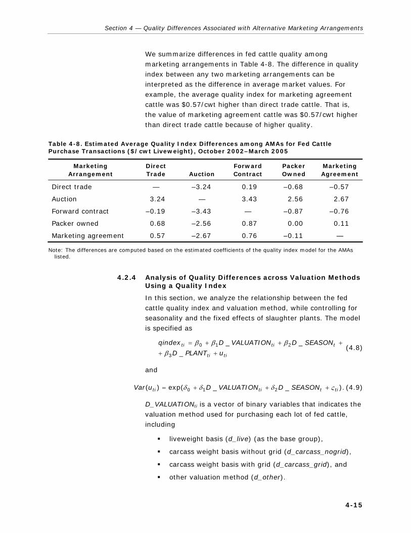
Section 4 — Quality Differences Associated with Alternative Marketing Arrangements
4-15
We summarize differences in fed cattle quality among marketing arrangements in Table 4-8. The difference in quality index between any two marketing arrangements can be interpreted as the difference in average market values. For example, the average quality index for marketing agreement cattle was $0.57/cwt higher than direct trade cattle. That is, the value of marketing agreement cattle was $0.57/cwt higher than direct trade cattle because of higher quality.
Table 4-8. Estimated Average Quality Index Differences among AMAs for Fed Cattle Purchase Transactions ($/cwt Liveweight), October 2002–March 2005
Marketing Arrangement
Direct Trade Auction
Forward Contract
Packer Owned
Marketing Agreement
Direct trade — –3.24 0.19 –0.68 –0.57
Auction 3.24 — 3.43 2.56 2.67
Forward contract –0.19 –3.43 — –0.87 –0.76
Packer owned 0.68 –2.56 0.87 0.00 0.11
Marketing agreement 0.57 –2.67 0.76 –0.11 —
Note: The differences are computed based on the estimated coefficients of the quality index model for the AMAs listed.
4.2.4 Analysis of Quality Differences across Valuation Methods Using a Quality Index
In this section, we analyze the relationship between the fed cattle quality index and valuation method, while controlling for seasonality and the fixed effects of slaughter plants. The model is specified as
titi
ttiti
uPLANTD
SEASONDVALUATIONDqindex
++
+++=
_
__
3
210
ββββ
(4.8)
and
).__exp()( 210 tittiti SEASONDVALUATIONDuVar ςδδδ +++= (4.9)
D_VALUATIONti is a vector of binary variables that indicates the valuation method used for purchasing each lot of fed cattle, including
liveweight basis (d_live) (as the base group),
carcass weight basis without grid (d_carcass_nogrid),
carcass weight basis with grid (d_carcass_grid), and
other valuation method (d_other).

Volume 3: Fed Cattle and Beef Industries
4-16
The definitions of D_SEASONti, and D_PLANTti are the same as in Section 4.2.1. The summary statistics for qindex and D_VALUATION are listed in Table 4-9. The coefficient on D_VALUATIONti in Eq. (4.8) indicates the relationship between each type of valuation method and higher or lower than average cattle quality. The coefficient on D_VALUATIONti in Eq. (4.9) indicates the relationship between each type of valuation method and higher or lower cattle quality consistency across lots.
Table 4-9. Descriptive Statistics for the Quality Index Model in Terms of Valuation Methods ($/cwt Liveweight), October 2002–March 2005
Variable Description Mean Std. Dev. Min Max
qindex Quality index 78.90 3.85 55.57 91.52
d_live Liveweight basis (1 = yes, 0 = no) 0.36 0.48 0.00 1.00
d_carcass_nogrid Carcass weight basis without grid (1 = yes, 0 = no)
0.13 0.33 0.00 1.00
d_carcass_grid Carcass weight basis with grid (1 = yes, 0 = no)
0.49 0.50 0.00 1.00
d_other Other valuation method (1 = yes, 0 = no) 0.02 0.15 0.00 1.00
Table 4-10 reports the parameter estimates from Eqs. (4.8) and (4.9). The quality of cattle valued on a carcass weight basis was higher and more consistent than the quality of cattle valued on a liveweight basis. However, the quality improvement associated with carcass weight valuation appears to be modest. Compared with cattle valued on a liveweight basis, cattle valued on a carcass weight with grid basis were worth $0.46/cwt (liveweight) more because of better quality, and cattle valued on a carcass weight without grid basis were worth $0.15/cwt more (liveweight) because of better quality.

Section 4 — Quality Differences Associated with Alternative Marketing Arrangements
4-17
Table 4-10. OLS Parameter Estimates for the Quality Index Model in Terms of Valuation Method ($/cwt Liveweight), October 2002–March 2005
Variable
Quality Index Coefficienta
(Robust Std. Error)
Var(u) Coefficient (Std. Error)
d_carcass_nogrid 0.15 (0.014)
–5.92 (0.14)
d_carcass_grid 0.46 (0.009)
–2.58 (0.09)
d_other 0.16 (0.026)
–5.64 (0.29)
Other variablesb Not reported
No. of observations (lots) 571,608 571,608
F statistic F(41,571566) = 9,563 F(14,571593) = 194
Prob > F 0.0000 0.0000
R2 0.2744 0.0047
a All coefficients are significant at the 5% level. b The “other variables” include an intercept, monthly (seasonality) binary variables, and plant binary variables.
4.3 RESULTS OF ANALYSIS OF QUALITY DIFFERENCES ASSOCIATED WITH ALTERNATIVE MARKETING ARRANGEMENTS USING MPR DATA In addition to the analyses of quality using the individual transactions data, we also examined the effects of AMAs on quality using MPR data. MPR data provided by the Livestock Marketing Information Center (LMIC) include quality and yield grade information for fed slaughter cattle. MPR data also report the number of head slaughtered in each yield grade category.
Figure 4-1 presents cattle production by yield grades for the April 2001 through December 2005 period. According to these data, Yield Grades 2 and 3 dominate (84%) carcass beef production.
Quality grade data provided by LMIC include Prime, Choice, Select, and Other (i.e., Standard). Figure 4-2 presents the number of cattle slaughtered within each USDA quality grade from April 2001 through December 2005. These data indicate that Choice grade accounts for about 57% of graded slaughter cattle, while Select grade accounts for about 39%. Prime grade represents about 3% of graded slaughter cattle.

Volume 3: Fed Cattle and Beef Industries
4-18
Figure 4-1. USDA Beef Yield Grade, by Number of Head Slaughtered, Using MPR Data, April 2001–December 2005
0
200,000
400,000
600,000
800,000
1,000,000
1,200,000
Apr 20
01
Jul 2
001
Oct 20
01
Jan 2
002
Apr 20
02
Jul 2
002
Oct 20
02
Jan 2
003
Apr 20
03
Jul 2
003
Oct 20
03
Jan 2
004
Apr 20
04
Jul 2
004
Oct 20
04
Jan 2
005
Apr 20
05
Jul 2
005
Oct 20
05
Month
Hea
d
Yield Grade 1 Yield Grade 2 Yield Grade 3 Yield Grade 4 Yield Grade 5
Figure 4-2. USDA Quality Beef Grade, by Number of Head Slaughtered, Using MPR Data, April 2001–December 2005
0200,000400,000600,000
800,000
1,000,0001,200,0001,400,0001,600,0001,800,000
Apr
200
1
Jul 2
001
Oct
200
1
Jan
2002
Apr
200
2
Jul 2
002
Oct
200
2
Jan
2003
Apr
200
3
Jul 2
003
Oct
200
3
Jan
2004
Apr
200
4
Jul 2
004
Oct
200
4
Jan
2005
Apr
200
5
Jul 2
005
Oct
200
5
Month
Hea
d
Prime Choice Select Other

Section 4 — Quality Differences Associated with Alternative Marketing Arrangements
4-19
We use average quality grade as a quality indicator of slaughter cattle and quantify the relationship between this variable, other exogenous factors, and procurement methods.3F
4 Quality grades are reported as categorical data in MPR data. Our modeling strategy requires that numerical values for quality be developed for use as dependent variables in the regression analyses. In addition, an increase in the value of this dependent variable should reflect increased quality that would be manifest in increased retail demand.
Similar to the procedure used for transactions data described in Section 4.2.2, a numerical quality variable was calculated based on the monthly number of fed cattle slaughtered within each categorical quality grade (Prime, Choice, Select, and Other), using MPR data. A numerical value for each categorical grade was developed based on average reported premiums and discounts for fed slaughter cattle (relative to Choice grade) during the sample period. Specifically, the variable is calculated using the following procedure:
1. The premium for Prime relative to Choice grade fed cattle over the sample period (April 2001 to December 2005) averaged $6.57/cwt. The average discounts for Select and Other grade fed cattle relative to Choice grade cattle over the sample period were –$9.41/cwt and –$17.68/cwt, respectively.
2. The average premium and discounts were then applied to the average Choice grade nominal fed steer price ($79.15/cwt) that occurred over the sample period. Thus, the average value of Choice grade fed steers equals $79.15/cwt. The average value of Prime grade fed steers equals $85.72/cwt ($79.15 + $6.57). Applying this procedure to Select and Other grade fed cattle results in average values of $69.74/cwt and $61.47/cwt, respectively.
3. An index for Prime, Select, and Other quality grades relative to Choice grade is then constructed using the above-average fed steer values. Thus, the Prime/Choice index (1.083) is calculated as $85.72 / $79.15. The Select/Choice index (0.881) is calculated as $69.74 / $79.15. The Standard/Choice index equals 0.777. Note that the index is equal to 1.000 for Choice grade fed cattle, is larger than 1.000 for higher quality
4 Quality grade was selected over yield grade because the former is
associated with meat tenderness and provides an indicator of retail beef quality.

Volume 3: Fed Cattle and Beef Industries
4-20
fed cattle, and is smaller than 1.000 for lower quality fed cattle.
4. The final monthly numerical quality variable is calculated as a weighted average of the monthly numbers of fed cattle slaughtered in each quality grade. The index values created above are used as the weights. Specifically,
tQG qprime qchoice qselect qother
qprime qchoice qselect qother
1.083( ) 1.000( ) 0.881( ) 0.777( )
/ ,
= + + +⎡ ⎤⎣ ⎦+ + +⎡ ⎤⎣ ⎦
(4.10)
where q(•) is the number of head slaughtered that graded Prime, Choice, Select, or Other in each month. These data were obtained from the Livestock Marketing Information Center (LMIC, 2006). The use of fixed weights is appropriate when considering composite products that include quality changes (Nelson, 1991; Theil, 1952-53). Quality changes within a composite category are captured entirely by an index that uses fixed relative prices as weights for individual components.
Figure 4-3 presents the average quality grade (QG) for the April 2001 through December 2005 period.
Figure 4-3. USDA Average Beef Quality Grade Using Aggregate Data, April 2001–December 2005
0.9440.9460.9480.9500.9520.9540.9560.9580.9600.9620.964
Apr
200
1
Jul 2
001
Oct
200
1
Jan
2002
Apr
200
2
Jul 2
002
Oct
200
2
Jan
2003
Apr
200
3
Jul 2
003
Oct
200
3
Jan
2004
Apr
200
4
Jul 2
004
Oct
200
4
Jan
2005
Apr
200
5
Jul 2
005
Oct
200
5
Beef Quality

Section 4 — Quality Differences Associated with Alternative Marketing Arrangements
4-21
Our constructed average quality grade variable decreased slightly during the period, which corresponds to a slight decrease in the percentage of cattle graded Choice or better. A linear regression of QG onto a time trend indicated that the quality grade number decreased by about 0.005% per month. The coefficient of variation for QG was relatively small (0.003%). The Jarque-Bera statistic failed to reject the null hypothesis of a normal distribution for QG. The Augmented Dickey-Fuller (ADF) unit root test failed to reject the null hypothesis of a unit root in the quality grade variable at the α = 0.05 level. The results of these tests have implications for the modeling approach described below.
4.3.1 Model Development Using MPR Data
Average beef quality grade is expected to be influenced by several factors, including feedlot profitability, technology, inventory levels, wholesale demand, and procurement methods. We specify this relationship as
( )t tQG PS PN T IF WB pf po pc s s s2 3 4/ , , , , , , , , , μ1= ζ + . (4.11)
Table 4-11 presents the variable definitions and descriptive statistics. Average quality grade number (QG) is hypothesized to be a function of the slaughter steer/corn price ratio (PS / PN); a linear trend term that is a proxy for technological change in the beef sector (T); cattle on feed inventories (IF); wholesale demand for beef (WB); formula (pf), packer ownership (po), and cash (pc) procurement methods; and seasonality (s). The disturbance term (μt) is assumed to possess white noise properties.
The price ratio (PS / PN) represents the expected profitability of cattle feedlots. The effect of this variable is difficult to assess a priori. An increase in this ratio would represent an increase in expected profitability, which could lead to longer cattle feeding periods and may result in more carcasses grading Choice rather than Select. However, increased profitability could also encourage contemporaneous fed cattle marketings and result in lower average live weight of slaughter cattle and reduce quality. Technology (T) captures improved genetics that could increase carcass quality. Because a specific measure of technological change is not available, a linear trend term is used as a proxy.
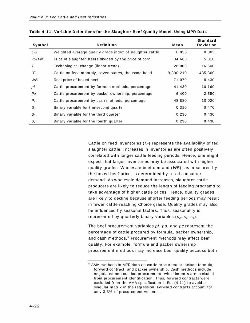
Volume 3: Fed Cattle and Beef Industries
4-22
Table 4-11. Variable Definitions for the Slaughter Beef Quality Model, Using MPR Data
Symbol Definition Mean Standard Deviation
QG Weighted average quality grade index of slaughter cattle 0.956 0.003
PS/PN Price of slaughter steers divided by the price of corn 34.660 5.010
T Technological change (linear trend) 28.000 16.600
IF Cattle on feed monthly, seven states, thousand head 9,390.210 435.360
WB Real price of boxed beef 71.070 8.430
pf Cattle procurement by formula methods, percentage 41.430 10.160
Po Cattle procurement by packer ownership, percentage 6.400 2.550
Pc Cattle procurement by cash methods, percentage 48.880 10.020
S2 Binary variable for the second quarter 0.310 0.470
S3 Binary variable for the third quarter 0.230 0.430
S4 Binary variable for the fourth quarter 0.230 0.430
Cattle on feed inventories (IF) represents the availability of fed slaughter cattle. Increases in inventories are often positively correlated with longer cattle feeding periods. Hence, one might expect that larger inventories may be associated with higher quality grades. Wholesale beef demand (WB), as measured by the boxed beef price, is determined by retail consumer demand. As wholesale demand increases, slaughter cattle producers are likely to reduce the length of feeding programs to take advantage of higher cattle prices. Hence, quality grades are likely to decline because shorter feeding periods may result in fewer cattle reaching Choice grade. Quality grades may also be influenced by seasonal factors. Thus, seasonality is represented by quarterly binary variables (s2, s3, s4).
The beef procurement variables pf, po, and pc represent the percentage of cattle procured by formula, packer ownership, and cash methods.4F
5 Procurement methods may affect beef quality. For example, formula and packer ownership procurement methods may increase beef quality because both
5 AMA methods in MPR data on cattle procurement include formula,
forward contract, and packer ownership. Cash methods include negotiated and auction procurement, while imports are excluded from procurement identification. Thus, forward contracts were excluded from the AMA specification in Eq. (4.11) to avoid a singular matrix in the regression. Forward contracts account for only 3.3% of procurement volumes.

Section 4 — Quality Differences Associated with Alternative Marketing Arrangements
4-23
methods allow for packers to acquire beef supplies that meet specific customer demands. We tested whether each procurement method significantly influences average quality grade. In addition, if the procurement variables are significantly different from zero, we test whether the coefficients (marginal impacts) differ between the three procurement methods.
4.3.2 Beef Quality Empirical Results Using MPR Data
The sample period for the quality model consists of monthly data from April 2001 through December 2005, which corresponds to the availability of MPR data. All data used in Eq. (4.11) were obtained from the LMIC, various issues of the USDA Red Meats Yearbook, and various issues of the USDA Feed Yearbook. The boxed beef price (WB) was deflated by the consumer price index (CPI) (1982–1984 = 100).
Eq. (4.11) was initially estimated with two-period (t and t – 1) distributed lags to account for expectations and rigidities in beef quality adjustments. Because of collinearity between wholesale demand price (WD) and the feedlot profitability variable (PS / PN), the former was omitted from the final specification. Lags on all of the independent variables, however, were not statistically significant based on the Wald coefficient restriction test. A Koyck term was significantly different from zero at the α = 0.05 level. Thus, exogenous shocks to independent variables cause average quality grade to adjust along a geometric time path.
The Breusch-Godfrey Lagrangian Multiplier (LM) test indicated the existence of serial correlation of order one. Thus, Eq. (4.11) was estimated using nonlinear least squares. The final regression results (estimated in double logs) of the beef quality equation are presented in Eq. (4.11) with t-ratios in parentheses:

Volume 3: Fed Cattle and Beef Industries
4-24
t t t t
t t t
t
QG ln PS PN T IF
pf po pc s s
s 1
ln 0.271 0.003 ( / ) 0.0001ln 0.028 ln
( 4.456) ( 1.146) ( 0.799) (3.978)
0.009 ln 0.002 ln 0.008 ln 0.003 2 0.001 3
(1.755) (1.741) (1.320) ( 4.547) ( 1.707)
0.002 4 0.805
( 3.381) (8.512)
μ −
= − − − +
− − −
+ + + − −
− −
− +
−
R S E QG mean2 0.826 . . 0.001 (log ) 0.045.= = = −
(4.12)
The critical t-values at the α = 0.05 level and α = 0.10 level are 2.021 and 1.684, respectively, with 42 degrees of freedom.
The lagged dependent variable was not significantly different from zero and, therefore, was omitted from the specification. The modulus of the single inverted autoregressive root equaled 0.805. Thus, the stochastic error structure had a stable pattern. Excluding the autoregressive error structure, the cumulative sum of squares (CUSUM) test of Eq. (4.12) indicated that the estimated coefficients were stable at the α = 0.05 level.
All variables except feedlot profitability (PS / PN), trend, and the cash procurement variable (pc) were statistically different from zero at either the α = 0.05 or α = 0.10 level. The regression results indicate that increases in cattle on feed inventories are associated with improved beef quality, perhaps because of lengthier feeding periods. Specifically, a 1% increase in inventories causes a 0.028% improvement in beef quality (Table 4-12).
Table 4-12. Elasticity Estimates for the Slaughter Beef Quality Model, Using MPR Data
Exogenous Variables Elasticity
Technological change (T) 0.000
Cattle on feed (IF) 0.028
Feedlot profitability (PS / PN) 0.000
Formula cattle procurement (pf) 0.009
Cash cattle procurement (pc) 0.000
Packer ownership procurement (po) 0.002

Section 4 — Quality Differences Associated with Alternative Marketing Arrangements
4-25
Cash procurement was not statistically different from zero. However, formula and packer ownership procurement methods are associated with improved beef quality. Their elasticity estimates, however, are small. For example, a 1% increase in formula procurement increases quality by 0.009%. A 1% increase in packer ownership procurement increases beef quality by 0.002%.
4.4 EFFECT OF BEEF QUALITY ON RETAIL BEEF DEMAND The demand for beef at the retail level depends on the price of beef, the price of meat substitutes, income, and tastes and preferences. The latter is likely associated with product quality, habits, health, nutrition, and food safety attributes (Capps and Schmitz, 1991; Pollack, 1970). In this section, we estimate the impacts of changes of beef quality on retail demand. The results are later used to estimate the impacts of AMAs on beef product quality, and are subsequently included in the equilibrium displacement model to estimate changes in producer and consumer surplus that may result from changes in AMAs (see Section 6).
4.4.1 A Reduced-Form Retail Model of Beef Quality
We develop a reduced-form price equation for beef at the retail level that incorporates product quality through the inclusion of USDA quality grades, as established at the wholesale level. If changes in AMAs influence fed cattle quality, then retail-level beef quality also will be affected. A priori, if a change in procurement method improves product quality, then one would expect the demand for beef at the retail level to increase.
To estimate these effects, we developed a monthly structural model of primary retail demand and derived retail supply. The primary demand specification is based on utility maximization principles. The derived retail supply is based on profit maximization principles of firms producing retail beef products (Varian, 1992). Because we assume that monthly beef supplies are fixed, the model is specified with inverse demand and supply equations.
The structural specification of the beef model is as shown below.

Volume 3: Fed Cattle and Beef Industries
4-26
Retail beef demand:
( )d dr r r rPB f QB PP PY Y QG1 , , , ,= (4.13)
Retail beef supply:
( )s sir rPB f QB PBX RC S2 , , ,= (4.14)
Market-clearing quantity:
d sr r rQB QB QB= = (4.15)
Market-clearing price:
d sr r rPB PB PB= = (4.16)
Table 4-13 provides variable definitions and descriptive statistics. Error terms have been suppressed but are assumed to have white noise characteristics.
Table 4-13. Variable Definitions for the Retail Beef Quality Model, Using Aggregate Data
Symbol Definition Mean Standard Deviation
PBr Real retail beef price, cents/pound 201.380 13.890
QBr Per capita beef consumption, retail weight, quarterly, pounds
16.640 0.600
PPr Real retail pork price, cents/pound 147.280 4.070
PYr Real retail poultry price, cents/pound 57.580 3.110
Y Real per capita consumption expenditures, dollars 14,600.470 429.960
QG Weighted average quality grade index of slaughter cattle
0.956 0.003
PBX Real boxed beef price, dollars/hundredweight 71.910 7.440
RC Real costs of retail beef processing, food marketing processing cost index (1987 = 100)
306.200 5.980
S2 Second quarter seasonal binary variable 0.286 0.457
S3 Third quarter seasonal binary variable 0.214 0.415
S4 Fourth quarter seasonal binary variable 0.214 0.415

Section 4 — Quality Differences Associated with Alternative Marketing Arrangements
4-27
Eq. (4.13) indicates that the inverse retail demand price for beef ( d
rPB ) is a function of the per capita retail beef demand quantity ( d
rQB ), retail price of pork (PPr), retail price of poultry (PYr), per capita consumption expenditures (Y), and beef quality (QG).
Eq. (4.14) indicates that the inverse retail supply price of beef ( s
rPB ) is a function of the per capita retail supply quantity of beef ( s
rQB ), the price of wholesale boxed beef (PBX), retail food marketing costs (RC), and seasonality (Si). Eqs. (4.15) and (4.16) are market-clearing quantities and price relations.
Using Eqs. (4.13) and (4.14), Eqs. (4.15) and (4.16) can be written in a reduced form as
( )3 , , , , , , , ir r r rPB f QB PP PY Y QG PBX RC S= . (4.17)
Thus, retail beef price is a function of structural demand and supply arguments. A priori, the marginal impact of quality preference (QG) on retail price (PBr) is expected to be positive. That is, an increase in quality grade number indicates an increase in quality and retail beef demand.
4.4.2 Data and Estimation of the Reduced-Form Retail Beef Quality Model
Data for the estimation of Eq. (4.17) were obtained from the LMIC, USDA, and the Economic Report of the President. Beef quantity data were obtained from the USDA’s Red Meat Yearbook. Per capita consumption expenditures and CPI were obtained from the Economic Report of the President. All dollar values were deflated by the CPI. The price variables and USDA quality grades were obtained from the LMIC. Retail food marketing costs were obtained from the USDA’s Agricultural Outlook. Retail food marketing costs and per capita consumption expenditures were available only on a quarterly basis. Therefore, each of 3 months within any quarter was assigned the same value (the quarterly observation) for these two variables.
The sample period included April 2001 through December 2005. The null hypothesis of no unit roots was rejected for the dependent variable and several independent variables at the α = 0.05 level based on ADF unit root tests. An ADF test of the residuals of Eq. (4.17) indicated that the equation was

Volume 3: Fed Cattle and Beef Industries
4-28
cointegrated. Therefore, the equation was estimated with the data in levels but with natural logarithm transformations.
Because of potential market dynamics, Eq. (4.17) was estimated as an infinite distributed lag approximated by an autoregressive distributed lag (ARDL) structure (Greene, 2003). One-period lags on each of the independent variables and on the dependent variable were also included. We used the Wald test as a criterion for omitting insignificant estimated coefficients. The Breusch-Godfrey LM test failed to reject the null hypothesis of no autoregressive errors of orders one and two. Thus, the OLS regression results of Eq. (4.17) are
r r t r t r t
tr t t t
t t
PB QB PP PY
PY Y QG QG
PBX PBX RC
, 1 , ,
, 1 1 1
1
ln 4.107 0.131ln 0.244 ln 0.177 ln
( 1.444) ( 1.700) (2.234) (1.732)
0.279 ln 0.402 ln 0.471ln 0.328 ln
( 2.768) (1.623) (1.930) ( 1.326)
0.067 ln 0.177 ln 0.226 ln
−
− − −
−
= − − + +
− −
− + + −
− −
+ + + t
r t
r
s s s PB
R S E PB mean
2 3 4 , 1
2
(1.507) (3.414) (1.566)
0.011 0.015 0.018 0.550 ln
(1.571) (2.043) (2.861) (7.447)
0.965 . . 0.013 (log ) 5.303
−+ + + +
= = =
(4.18)
The critical t-values at the α = 0.05 and α = 0.10 levels are 2.021 and 1.684, respectively (42 degrees of freedom).
The CUSUM test for parameter stability failed to reject the null hypothesis of parameter stability at the α = 0.05 level. The first-order difference equation implies geometric distributed lags in retail beef prices. Equilibrium adjustments (95%) occur in about 5 months. The modulus of the single root (absolute value of the 0.550 coefficient) is less than unity, indicating dynamic stability of retail prices.
Most of the signs of the estimated coefficients are consistent with theoretical expectations. From the demand perspective, the coefficients on per capita beef consumption and consumer expenditures are negative and positive, respectively. The coefficient for retail pork price is positive, while the sum of the two coefficients on retail poultry price is negative, which is contrary to expectations for consumption substitutes.

Section 4 — Quality Differences Associated with Alternative Marketing Arrangements
4-29
From a supply perspective, the estimated coefficients for the price of boxed beef and food marketing costs are positive. Increases in either of these inputs into producing retail beef would be expected to shift supply to the left and increase retail beef price.
The primary purpose of estimating Eq. (4.18) is to obtain an estimate of the impact of quality on retail demand. The two coefficients on the quality variable sum to 0.143, which indicates that an increase in the quality grade index increases retail beef price because of an increase in retail beef demand. For example, a 10% increase in the quality grade index increases retail beef price by 1.43% in the short run and 3.18% in the long run.5F
6
4.5 SUMMARY OF THE EFFECTS OF ALTERNATIVE MARKETING ARRANGEMENTS ON BEEF QUALITY Based on the results of the industry interviews and survey, beef producers and packers believe that AMAs are important for beef quality. Producers indicated that AMAs allow them to better market higher quality cattle. Packers reported that they used AMAs to procure higher quality cattle and to better meet downstream customer demand. Both believed that signals for attributes of quality beyond simply quality grade would be difficult in a cash-only marketing system.
A summary of the fed cattle purchase transactions data indicates that the percentage of higher quality grade cattle differs across the procurement methods. Although very small in number, the percentage of Choice or better cattle bought through dealers and brokers and auction markets was higher than the percentages of other purchase methods. Marketing agreement cattle had the next highest percentage of Choice or better, followed by forward contract, direct trade purchases, and packer-owned cattle. Overall, 61% of cattle were graded Choice or better, with slightly more cash or spot market cattle than AMA cattle grading Choice or better.
6 The long-run elasticity estimate of 0.318 is calculated by dividing the
sum of the two estimated coefficients for quality (0.143) by one minus the coefficient estimate on the lagged dependent variable, or 0.45.

Volume 3: Fed Cattle and Beef Industries
4-30
Using transactions data, we estimated three quality models. These models and their key results were as follows:
First, we estimated the effect of procurement method on various individual measures of quality and found that, after controlling for seasonal and plant effects, cattle sold through marketing agreements had a higher percentage of Choice and Prime carcasses without increases in the percentage of Yield Grade 4 and 5 carcasses, and only a modestly lower percentage of Yield Grade 1 and 2 carcasses. Other procurement methods had larger trade-offs between quality grade and yield grade.
Second, we estimated the effect of procurement method on a quality index that combines several measures of quality and found that, after controlling for seasonal and plant effects, the relatively small volume of cattle procured through auction barns were associated with the highest quality relative to other methods, but also with the highest quality variation. Cattle procured through marketing agreements or packer ownership were of higher quality and had lower quality variances than cattle procured through direct trade. Forward contracts were associated with the lowest quality cattle relative to other methods.
Third, we estimated the effect of valuation method on the quality index and found that, after controlling for seasonal and packing plant effects, carcass weight valuation with a grid was associated with higher quality relative to liveweight valuation. Carcass weight valuation without a grid also was associated with higher quality relative to liveweight valuation, but the magnitude of the effect was smaller than for carcass weight valuation with a grid.
Finally, using MPR data, we estimated a monthly model to determine if AMAs influence beef quality. USDA quality grade was used as a proxy for beef quality. A quality grade variable based on premium and discounts relative to Choice grade was constructed such that an increase in the variable is associated with an increase in quality. Technological change did not appear to affect beef quality during the sample period. Feedlot profitability did not have a statistically significant effect on quality. Formula and packer ownership procurement methods increased beef quality, although the effects were relatively small. However, beef quality was not influenced by cash procurement. These results are consistent with anecdotal evidence that AMAs have

Section 4 — Quality Differences Associated with Alternative Marketing Arrangements
4-31
positive, although small, impacts on beef quality. Finally, we estimated a model that quantified the effects of beef carcass quality on retail beef demand. The statistical results indicate that increases (and decreases) in carcass beef quality grades directly affect retail beef prices positively (negatively).


5-1
Risk Shifting Associated with Alternative Marketing 5 Arrangements
In this section, we present a discussion of the effects of AMAs on risk shifting in the fed cattle and beef industries. The results presented in this section are based, in part, on the industry survey described in Volume 2 and on beef packer purchase transactions data.
5.1 RISK SHIFTING IN MARKETING ARRANGEMENTS In this section, we discuss the types of risk in the fed cattle and beef industries and the role AMAs play in mitigating each type of risk. We then discuss the risk-related reasons for using AMAs cited by respondents to the industry survey.
5.1.1 Types of Risk and the Role of AMAs in Risk Mitigation
Beef industry participants face multiple types of risk, and the sources of risk vary by the stage of production. Most risks faced by producers and packers can be categorized as production, price, or market access risks. We describe each type below, followed by a discussion of how marketing arrangements do or do not mitigate each type of risk.

Volume 3: Fed Cattle and Beef Industries
5-2
Production Risk
Sources of production risk can vary significantly across stages of beef production. For example, cow-calf producers and stockers use pasture and open range to sustain their herds; therefore, they are subject to considerable risks from the availability and quality of natural vegetation. Conversely, cattle feeders maintain confined operations and feed their cattle a high-energy ration in which the variability of natural vegetation is replaced with cultivated crops. Despite technological differences, cattle producers at all stages face some level of risk from feed availability and quality, animal health, and weather.
Two additional sources of production risk that affect beef producers are yield and grading risks. Yield risk refers to the variation in the proportion of a live animal that produces a usable carcass. Grading risk is related to yield risk in that it includes the amount of saleable cuts that can be produced from a carcass (i.e., yield grade), but it also incorporates the overall quality of the meat (i.e., quality grade).
The sources of production risk differ as fed cattle move downstream to the packer. Beef packers face multiple sources of production risk as they employ labor, capital, and live cattle resources for the production of fresh, frozen, or processed beef products.
AMAs provide very little opportunity to shift production risk among market participants. For example, in a forward contract or marketing agreement, the individual producer maintains all of the production risk while raising cattle for delivery. Exceptions to this include custom feeding arrangements, in which the cattle owner (e.g., a cow-calf producer or packer) retains some portion of the production risk, or shared ownership arrangements, which shift some risk to the feedlot that is partnering in ownership of the cattle.
Some valuation methods for cattle provide an avenue to transfer production risk among market participants. However, each valuation method can be associated with a number of different types of AMAs. Thus, the effect of the valuation method in shifting production risk is not necessarily directly attributable to a specific AMA.
Carcass weight valuation, relative to liveweight, transfers yield risk from the packer to the producer. Furthermore, carcass
Section 5 — Risk Shifting Associated with Alternative Marketing Arrangements
5-3
weight valuation with a grid (grade and yield) transfers both yield risk and grading risk from the packer to the producer. Therefore, to the extent that carcass or grade and yield valuation are associated with a particular AMA, the AMA shifts yield and grading risk from packers to producers.
Price Risk
Price risk stems from increases and decreases in both input (e.g., feeder cattle, feed) and output (e.g., fed cattle) prices. Similar to production risk, the specific source or degree of price risk is dependent on the stage of production. Research by Mark, Schroeder, and Jones (2000) found fed cattle and feeder cattle prices, followed by corn prices, to be the largest contributors to variability in feedlot profits. Similarly, Lawrence, Wang, and Loy (1999) attributed more than 50% of the variation in feedlot profits to fed cattle prices and another 20% to feeder cattle prices.
Packers also face considerable price risk as a margin-based business. Beef packers are subject to variation in live cattle prices on the input side and meat and by-product prices on the output side (Ward, 2002).
Futures markets for feeder cattle and live cattle are available to industry participants regardless of the use of AMAs and provide a method to shift price risk to a third party through organized futures exchanges. The degree to which AMAs can shift price risk among market participants depends on the type of arrangement and the specific terms of the arrangement. In custom feeding arrangements, all of the market price risk is borne by the owner of the cattle. The feedlot raising the cattle is paid based on cattle performance or yardage, regardless of market conditions.
Forward contracts allow producers to lock in a price while their cattle are still on feed, effectively shifting price risk to the packer. However, packers can take an offsetting position in the futures market to mitigate the additional price risk associated with futures prices, although they still hold the basis risk.
Marketing agreements do not inherently shift price risk among the participants. Marketing agreements using a negotiated (flat) price can shift the fed cattle price risk to the packer, but the input (feeder cattle and corn) price risk remains. However, this type of agreement is likely to have a mechanism to adjust

Volume 3: Fed Cattle and Beef Industries
5-4
for market conditions. Most marketing agreements that use formula pricing do not shift price risk between packers and producers, because the transaction price is determined based on a current market price.1 However, producers and packers in a marketing agreement of this type can use the futures market to offset price risk from the market price.
Market Access Risk
In the context of cattle markets, market access risk typically refers to the availability of a timely and appropriate market outlet. As perishable commodities, live cattle and beef products must be sold within a fairly narrow time frame. Cattle held beyond the optimal marketing period begin to decrease in value because of excessive fat gain and the rising cost of gain. Fresh beef products with a limited shelf life must be sold at significant discounts, frozen, or discarded; all of which lead to decreased total value.
AMAs between producers and packers eliminate market access risk for both parties to the transaction. The specific terms of an AMA may vary as to which participant chooses the exact day of delivery, but the nature of the arrangements ensure a market outlet. Upstream producers using AMAs to facilitate retained ownership (i.e., custom feeding) guarantee a spot for their cattle in the feedyard, but not with a packer. These producers would need an additional agreement with a packer to mitigate market access risk for their fed cattle.
5.1.2 Risk-Related Reasons for Use of Alternative Marketing Arrangements
Survey responses presented in Volume 2 provide insight into producers’ and packers’ risk-related reasons for using AMAs. We describe these responses below.
Producer Survey Responses
Most cattle producers did not explicitly state that they used AMAs to reduce their risk exposure. However, many of the reasons why producers use AMAs can be interpreted as methods to mitigate price, production, or market access risk.
1 One exception is the use of marketing agreements that use a formula
price based on the cost of production. This type of marketing agreement shifts price risk to the packer and locks in a profit margin for the producer.

Section 5 — Risk Shifting Associated with Alternative Marketing Arrangements
5-5
Three of the top five reasons producers use AMAs to procure cattle are related to production risk. The response items were as follows:
Secures higher quality calves and cattle (95.0% of producers)
Improves week-to-week supply management (51.2% of producers)
Improves efficiency of operations due to animal uniformity (46.2% of producers)
Collectively, these reasons indicate that AMAs facilitate the procurement of a reliable supply of consistent, high-quality cattle. The benefits of securing consistent, high-quality cattle for a feedlot likely includes a lower average cost of production through more efficient operations and improved capacity utilization.
Examining producers’ motivations for using AMAs to sell cattle clearly shows their desire to alleviate risk. The most direct example of this desire is that “Reduces risk exposure” was one of the top five responses for both small and large producers (34.5%). Other risk-related responses by small and large producers centered on market access. These responses were as follows:
Allows for sale of higher quality calves and cattle (51.6% of producers)
Facilitates or increases market access (19.7% of producers)
Secures a buyer for calves and cattle (26.5% of producers)
Ensuring a timely market outlet for cattle enables producers to focus their resources on production as opposed to marketing and increases their likelihood of being financially rewarded for their efforts.
Packer Survey Responses
Beef packers have the same motivations to use AMAs as cattle producers. Three of the top five reasons packers use AMAs to procure fed cattle are the same reasons producers use AMAs for procurement:
Improves week-to-week supply management (57.7% of packers)

Volume 3: Fed Cattle and Beef Industries
5-6
Secures higher quality fed cattle (53.8% of packers)
Improves efficiency of operations due to animal uniformity (42.3% of packers)
The similarity of these responses indicates that despite the fundamental differences in production of live cattle compared with beef, both packers and producers have a desire to decrease production variability and procure a reliable supply of consistent, high-quality cattle.
The other top reasons packers use AMAs for procurement are related to market access risk. Specifically, these reasons were as follows:
Allows for product branding in retail sales (46.2% of packers)
Allows for market access (42.3% of packers)
The response to “Allows for market access” does not indicate whether packers use AMAs to guarantee access to input or output markets. However, the response “Allows for product branding in retail sales” implies that packers use AMAs to guarantee access to both input and output markets. In other words, for packers to ensure that they can provide retailers with a sufficiently consistent product to carry a brand label, they procure cattle through AMAs.
5.2 EVIDENCE OF RISK SHIFTING ASSOCIATED WITH ALTERNATIVE MARKETING ARRANGEMENTS In this section, we compare price differences and volatility for beef packer purchase transactions by type of marketing method and discuss the implications for risk management.
5.2.1 Fed Cattle Transactions Prices
We calculated weekly average prices by purchase method from the beef packer purchase transactions data. The purchase methods included in this analysis are listed below:
auctions—purchases from auction barns
direct trade—purchases through direct trade or through a dealer or broker2
2 Most of these transactions are direct trade; very few transactions
occurred through dealers and brokers.
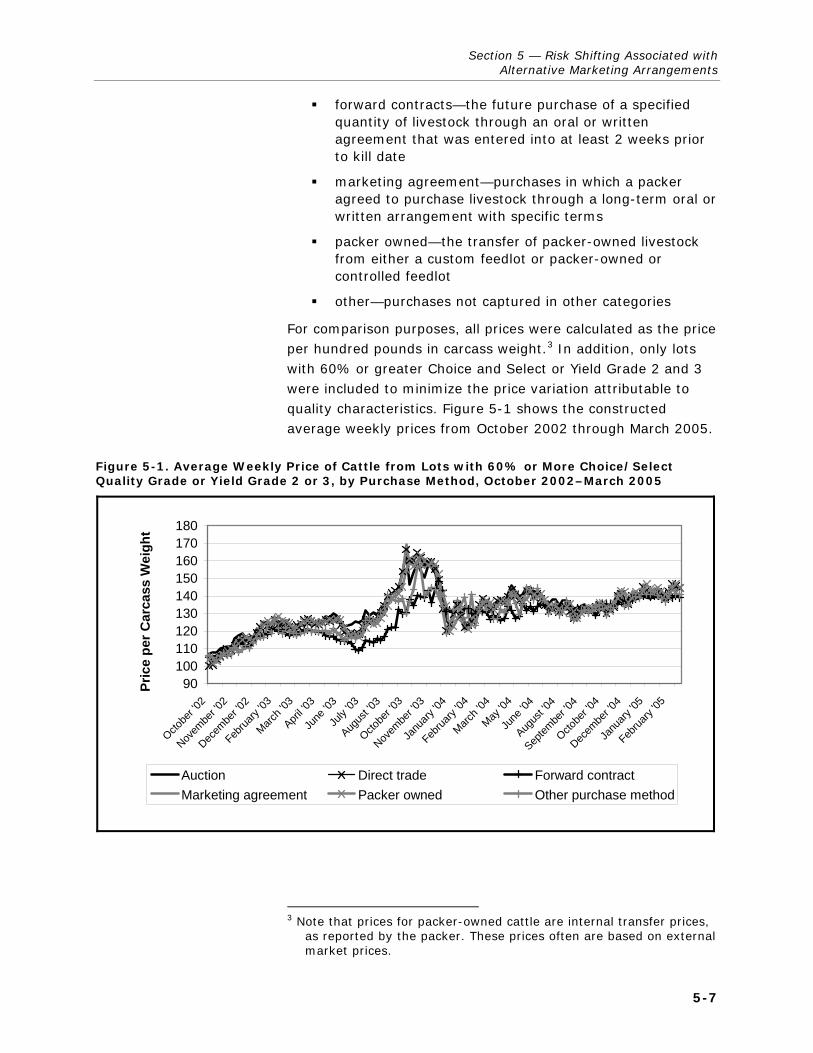
Section 5 — Risk Shifting Associated with Alternative Marketing Arrangements
5-7
forward contracts—the future purchase of a specified quantity of livestock through an oral or written agreement that was entered into at least 2 weeks prior to kill date
marketing agreement—purchases in which a packer agreed to purchase livestock through a long-term oral or written arrangement with specific terms
packer owned—the transfer of packer-owned livestock from either a custom feedlot or packer-owned or controlled feedlot
other—purchases not captured in other categories
For comparison purposes, all prices were calculated as the price per hundred pounds in carcass weight.3 In addition, only lots with 60% or greater Choice and Select or Yield Grade 2 and 3 were included to minimize the price variation attributable to quality characteristics. Figure 5-1 shows the constructed average weekly prices from October 2002 through March 2005.
Figure 5-1. Average Weekly Price of Cattle from Lots with 60% or More Choice/Select Quality Grade or Yield Grade 2 or 3, by Purchase Method, October 2002–March 2005
90100110120130140150160170180
Octobe
r '02
Novem
ber '0
2
Decem
ber '0
2
Februa
ry '03
March '
03
April '0
3
June
'03
July
'03
Augus
t '03
Octobe
r '03
Novem
ber '0
3
Janu
ary '0
4
Februa
ry '04
March '
04
May '0
4
June
'04
Augus
t '04
Septem
ber '0
4
Octobe
r '04
Decem
ber '0
4
Janu
ary '0
5
Februa
ry '05
Pric
e pe
r Car
cass
Wei
ght
Auction Direct trade Forward contractMarketing agreement Packer owned Other purchase method
3 Note that prices for packer-owned cattle are internal transfer prices,
as reported by the packer. These prices often are based on external market prices.

Volume 3: Fed Cattle and Beef Industries
5-8
The mean price of each purchase method differed by less than $6.00/cwt during this period (Table 5-1). Auctions had the highest mean price at $132.60/cwt, and forward contracts had the lowest mean price of $127.00/cwt. Direct trade transactions had the highest variance and the highest average weekly volume, while forward contracts had the lowest variance and a relatively low average weekly volume during this period. The lower mean and variance of forward contracts was due, in part, to foregoing higher prices that the others received because the market moved higher after producers established the contract price during the period of the data. Interestingly, auction barn sales had a relatively low variance among the types of marketing arrangements; however, the average weekly volume through auction barns also was relatively low.
Table 5-1. Average Weekly Prices per Hundred Pounds Carcass Weight, by Fed Cattle Purchase Method, October 2002–March 2005
Fed Cattle Prices
Purchase Method Mean Max Min Variance
Approximate Average Head
per Week
Auction $132.60 $164.72 $107.04 122.43 20,000
Direct trade and dealer/broker $132.04 $166.56 $100.17 167.41 260,000
Forward contract $127.00 $148.43 $103.81 111.30 20,000
Marketing agreement $132.25 $169.08 $101.11 162.84 130,000
Packer owned $131.86 $163.22 $101.61 160.65 20,000
Other purchase method $129.17 $156.78 $103.73 129.51 2,000
5.2.2 Fed Cattle Price Volatility Testing
Measuring the volatility of prices provides an indicator of the risk market participants face. In this context, risk refers to both upside and downside risk; that is, risk due to price increases and decreases. Comparing the volatility of price series by type of fed cattle purchase method provides some indication of the relative risk of each type of purchase method. We describe the results of price volatility testing below.
Testing Procedure
A Wald statistic derived by Knoeber and Thurman (1995) was used to test the null hypothesis of equal variance across

Section 5 — Risk Shifting Associated with Alternative Marketing Arrangements
5-9
purchase methods. Knoeber and Thurman proposed this test statistic as a way of testing for equal variance among two correlated price series.
The test statistic is calculated as
21
212
42
41
22
21
22
⎥⎥
⎦
⎤
⎢⎢
⎣
⎡⎟⎠⎞
⎜⎝⎛ −+
−=
sssn
ssT , (5.1)
where 21s and 2
2s are the sample variances of the two price series being compared, 12s is the sample covariance, and n is the number of observations. Under the null hypothesis, T is asymptotically standard normal.
The null and alternative hypotheses used in the pairwise tests are
( ) ( )( ) ( )ji1
ji0
PMvar PMvar H
PMvar PMvar H
>=
==, (5.2)
where PMi and PMj are the average weekly price series for fed cattle purchase method i and j (i ≠ j).
Empirical Results
Using a pairwise approach to testing the variance of the six different fed cattle marketing arrangements, ranked by variance, results in 15 unique comparisons. The Wald test statistics and corresponding P values are reported in Table 5-2.
Based on these comparisons, purchase methods fall into two categories. The variances of the three marketing arrangements with the highest variances (direct trade, marketing agreement, and packer owned) are not statistically different from each other at the 95% confidence level. Of the three marketing arrangements with the lowest variances, other purchase method and auctions are not statistically different from each other and auctions are not statistically different from forward contracts. However, the variance of other purchase method is statistically different from the variance of forward contracts.

Volume 3: Fed Cattle and Beef Industries
5-10
Table 5-2. Pairwise Tests of Equal Variances, by Fed Cattle Purchase Method, October 2002–March 2005
Variancei vs. Variancej Wald Test Statistic P Value
Direct tradea vs. marketing agreement 1.08 0.1393
Direct tradea vs. packer owned 0.86 0.1950
Direct tradea vs. other purchase method 2.91 0.0018
Direct tradea vs. auction 5.38 0.0000
Direct tradea vs. forward contract 3.44 0.0003
Marketing agreement vs. packer owned 0.27 0.3931
Marketing agreement vs. other purchase method 2.62 0.0045
Marketing agreement vs. auction 4.92 0.0000
Marketing agreement vs. forward contract 3.25 0.0006
Packer owned vs. other purchase method 2.43 0.0076
Packer owned vs. auction 3.98 0.0000
Packer owned vs. forward contract 3.46 0.0003
Other purchase method vs. auction 0.68 0.2494
Other purchase method vs. forward contract 1.61 0.0535
Auction vs. forward contract 0.86 0.1957
a Direct trade includes a small volume of dealer/broker transactions.
Individually, the null hypothesis of equal variance is rejected when comparing direct trade, marketing agreement, and packer owned prices to other purchase method, auction, and forward contract prices. Therefore, results of the pairwise variance test, using average weekly prices, imply that fed cattle prices under direct trade, marketing agreements, or packer ownership are essentially equally risky. While producers do not face price risk with packer-owned cattle, those using direct trade and marketing agreements face more risk than producers using other purchase methods, auctions, and forward contracts.
We conducted two additional sets of pairwise variance tests to investigate the potential to shift risk through different valuation methods. Using the same methodology as described above, we calculated the average weekly price of cattle sold using liveweight, carcass weight without grade and yield adjustments

Section 5 — Risk Shifting Associated with Alternative Marketing Arrangements
5-11
(i.e., nongrid), and carcass weight with grade and yield adjustments (i.e., grid) valuation methods.
A preliminary analysis of differences in prices between marketing arrangements for lots where 60% or more were Choice and Select or Yield Grade 2 and 3 indicated very little difference by valuation method. This implies that, if any differences in prices occurred, they may be offsetting. Therefore, we calculated prices for low- and high-quality cattle lots and conducted additional statistical tests. Low-quality lots were defined as those with 60% or more of the cattle having a quality grade of Select or lower (regardless of yield grade), or Yield Grade 4 and 5 (regardless of quality grade). High-quality lots were defined as those with 60% or more of the cattle grading Prime (regardless of yield grade) or Yield Grade 1 and 2 (regardless of quality grade). Figures 5-2 and 5-3 show the relative comparisons of averages prices for low- and high-quality cattle lots by type of valuation method.
The results of the pairwise variance tests indicate that producers selling low-quality cattle face more risk if they sell using carcass weight grade and yield valuation methods relative to liveweight or carcass weight without grade and yield (Table 5-3). This result is fairly intuitive in that grade and yield valuation transfers the packer’s production risk of yield and grading to producers. Interestingly, the variance tests also indicate that selling low-quality cattle on a liveweight basis is more risky than selling on a carcass weight basis without grade and yield. This result implies that yield risk was not effectively transferred from packer to producers using carcass weight without grade and yield valuation for low-quality cattle sold during this time frame.
The results of tests of differences in the variance of prices for high-quality cattle met with prior expectations regarding the ranking of variances by valuation method. Specifically, carcass weight with grade and yield and carcass weight without grade and yield valuation methods individually had higher variances than liveweight valuation (Table 5-4). Furthermore, we are unable to reject the null hypothesis of equal variances between carcass weight with grade and yield and carcass weight without grade and yield valuation methods.

Volume 3: Fed Cattle and Beef Industries
5-12
Figure 5-2. Average Weekly Price of Low-Quality Cattle, by Valuation Method, October 2002–March 2005
90100110120130140150160170180
Octobe
r '02
Novem
ber '0
2
Decem
ber '0
2
Februa
ry '03
March '
03
April '0
3
June
'03
July
'03
Augus
t '03
Octobe
r '03
Novem
ber '0
3
Janu
ary '0
4
Februa
ry '04
March '
04
May '0
4
June
'04
Augus
t '04
Septem
ber '0
4
Octobe
r '04
Decem
ber '0
4
Janu
ary '0
5
Februa
ry '05
Pric
e pe
r Car
cass
Wei
ght
Liveweight Carcass weight without grade and yield Carcass weight with grade and yield
Figure 5-3. Average Weekly Price of High-Quality Cattle, by Valuation Method, October 2002–March 2005
90100110120130140150160170180
Octobe
r '02
Novem
ber '0
2
Decem
ber '0
2
Februa
ry '03
March '
03
April '0
3
June
'03
July
'03
Augus
t '03
Octobe
r '03
Novem
ber '0
3
Janu
ary '0
4
Februa
ry '04
March '
04
May '0
4
June
'04
Augus
t '04
Septem
ber '0
4
Octobe
r '04
Decem
ber '0
4
Janu
ary '0
5
Februa
ry '05
Pric
e pe
r Car
cass
Wei
ght
Liveweight Carcass weight without grade and yield Carcass weight with grade and yield

Section 5 — Risk Shifting Associated with Alternative Marketing Arrangements
5-13
Table 5-3. Pairwise Tests of Equal Variances for Low-Quality Fed Cattle, by Valuation Method, October 2002–March 2005
Variancei vs. Variancej Wald Test Statistic P Value
Carcass weight, grade and yield vs. liveweight 4.56 0.0000
Carcass weight, grade and yield vs. carcass weight, not grade and yield 4.24 0.0000
Liveweight vs. carcass weight, not grade and yield 1.88 0.0304
Table 5-4. Pairwise Tests of Equal Variances for High-Quality Fed Cattle, by Valuation Method, October 2002–March 2005
Variancei vs. Variancej Wald Test Statistic P Value
Carcass weight, grade and yield vs. liveweight 0.65 0.2580
Carcass weight, grade and yield vs. carcass weight, not grade and yield 4.11 0.0000
Liveweight vs. carcass weight, not grade and yield 3.51 0.0002
5.2.3 Regression Analysis Results on Fed Cattle Price Risk
In this section, we explore the same research question as in Section 5.2.2—whether and how transaction price volatility differs across marketing arrangements—using a different methodology. First, we use individual transactions data, rather than the aggregated market-level data. Second, we take into account several cattle characteristics and seasonality, while analyzing the relationship between price volatility and the choice of marketing arrangement.
The empirical model is the same as that described in Section 2.2.2, but now our focus is on the heteroskedasticity model (Eq. [2.4]) in this section. The notations and summary statistics of the explanatory variables are presented in Section 2.2.2 and Table 2-19. The parameter estimates (the δs in Eq. [2.4]) are reported in the last column of Table 2-20. The primary conclusions regarding volatility from these results are as follows:
Compared with direct trade, the price variances are much higher for auction barn transactions and forward contracts and slightly lower for packer owned and marketing agreement transactions, holding cattle

Volume 3: Fed Cattle and Beef Industries
5-14
characteristics (variable CATTLE_CH) and month of sale (variable D_MONTH) fixed. These results are opposite to those indicated in Table 5-1, because the heteroskedasticity model accounts for the variability caused by differences in quality of cattle and month of sale across individual transactions.
Other parameter estimates suggest that price volatility is
– lower for fed beef cattle than fed dairy cattle,
– lower for cattle that are eligible for a branded and certification program,
– lower for cattle of higher yield grade (i.e., a lower yield grade number) and quality grade,
– lower for cattle within the regular weight range, and
– lower for cattle sold in large lots.
To summarize, cattle that have desirable characteristics (such as beef breed, high yield grade, high quality grade, eligible for a branded or certification program, and within the regular weight range) obtain not only higher average prices but also lower price volatility (see Table 2-20).
The estimated differences (percentage higher or lower) in price variance among marketing arrangements for fed beef cattle and for fed dairy cattle are reported in Tables 5-5 and 5-6, respectively. All the difference estimates are individually significant at the 5% level based on Wald tests. Among the five marketing arrangements, auction barn transactions are associated with the highest average price and highest price volatility. It appears that selling through auction barns should appeal more to less risk-averse cattle feeders. Like auction markets, forward contract transaction prices are determined in a competitive environment. After accounting for quality and sales month, forward contracts are more risky than direct trade or marketing agreements. The average price difference between auction barn transactions and forward contracts ($0.06/lb carcass weight for beef cattle and $0.16/lb carcass weight for fed dairy cattle) could be considered a risk premium to compensate feeders who sell their cattle in auction barns for bearing more price volatility (46% higher variance for beef cattle and 43% higher variance for fed dairy cattle) and market access risk. Packer-owned fed dairy cattle have slightly lower average prices (1.2 cents per pound carcass weight) and

Section 5 — Risk Shifting Associated withAlternative Marketing Arrangements
5-15
Table 5-5. Estimated Price Variance Differences (Percentage Higher or Lower) among Marketing Arrangements Used for Purchasing Fed Beef Cattle, October 2002–March 2005
Marketing Arrangement AuctionDirect Trade and Dealer/Broker
Forward Contract
Marketing Agreement
Packer Owned
Auction 0% 331% 46% 426% 376%
Direct trade and dealer/broker
–77% 0% –66% 22% 11%
Forward contract –32% 194% 0% 260% 225%
Marketing agreement –81% –18% –72% 0% –10%
Packer owned –79% –10% –69% 11% 0%
Note: The differences are computed as the price variance of each AMA listed in the left column divided by each listed in the top row minus one.
Table 5-6. Estimated Price Variance Differences (Percentage Higher or Lower) among Marketing Arrangements Used for Purchasing Dairy Breed Fed Cattle
Marketing Arrangement AuctionDirect Trade and Dealer/Broker
Forward Contract
Marketing Agreement
Packer Owned
Auction 0% 151% 43% 213% 246%
Direct trade and dealer/broker
–60% 0% –43% 25% 38%
Forward contract –30% 75% 0% 118% 141%
Marketing agreement –68% –20% –54% 0% 11%
Packer owned –71% –27% –59% –10% 0%
Note: The differences are computed as the price variance of each AMA listed in the left column divided by eachlisted in the top row minus one.
slightly lower price variance (20% lower) than direct trade. Packer-owned fed beef cattle have slightly higher average price (0.1 cent per pound carcass weight) and slightly lower price variance (10% lower) than direct trade. This is consistent with the fact that internal transfer prices for packer-owned cattle are usually based on an average cash market price. Transactions through marketing agreements are associated with slightly lower price volatility (18% lower variance for fed beef cattle and 27% lower for fed dairy cattle) than those through direct trade. Given that average prices for marketing agreement cattle and direct trade cattle are very close and that marketing agreements help secure market access while direct trade does not, it appears that a risk-averse feeder has less incentive to choose direct trade when marketing agreements are available.
Volume 3: Fed Cattle and Beef Industries
5-16
However, marketing agreements require a strong bilateral relationship between feeder and packer and might not be available for all feeders.
5.3 SUMMARY Beef market participants face production, price, and market access risk. The survey of producers and packers indicates that those that use AMAs value them as a method of dealing with these risks. The AMAs allow them to secure or sell better quality cattle and calves and improve operational management and efficiency. Interviews with feedlots and packers identified packer ownership specifically as an important risk management strategy to improve capacity utilization without excess financial leverage. Packers also identified AMAs an important element of branded products and meeting consumer demand by producing a higher quality, more consistent product.
Transactions data were analyzed to evaluate the price levels and variability during the data collection period. The data were aggregated by procurement method for transactions that were 60% Choice or Select or Yield Grade 2 and 3, which are the bulk of the fed cattle traded. The differences in average prices can be explained partly by the fact that prices were generally trending upward during the time period of the data set. Based on these averages, auction markets had the highest average price and the second lowest variance of prices. Forward contracts had the lowest average price, partly because these prices are set further in advance of delivery compared with the other types of AMAs and because prices were rising, and forward contracts had the lowest variance partly because these contracts missed out on high prices that occurred during the time period of the data set. Marketing agreement and packer-owned cattle had a mean and variance of prices similar to direct trade cattle in the aggregated data. Results of pairwise variance tests, using average weekly prices, imply that fed cattle prices under direct trade, marketing agreements, or packer ownership are essentially equally risky. In addition, producers using direct trade and marketing agreements appear to face more price risk than producers using other purchase methods, auctions, and forward contracts.
In contrast to the summary statistics, regression analysis accounting for cattle quality and sales month found

Section 5 — Risk Shifting Associated with Alternative Marketing Arrangements
5-17
substantially different results. When controlling for seasonality and plant effects, prices for auction barn fed cattle were more volatile than all other purchase methods. Prices for direct trade fed cattle were less volatile than auction barn and forward contract cattle, but slightly more volatile than marketing agreement and packer-owned cattle. Note that prices for packer-owned cattle are internal transfer prices that are based on external market prices, so comparisons with packer-owned cattle prices are less relevant than the other comparisons. Prices for forward contract cattle were less volatile than auction sales, but much more volatile than all other types. Finally, prices for marketing agreement cattle were less volatile than all other procurement methods other than packer ownership. The results for fed beef and fed dairy cattle were generally similar.
Therefore, AMAs help reduce production risk and market access risk, as identified by respondents to the survey, and, based on the transactions data, AMAs also reduce price variability compared with direct trade in some cases. Furthermore, in the future, if AMAs are used to facilitate traceability programs, they may help reduce quality variation, which, in turn, would contribute to reduced price volatility under AMAs.


6-1
Measurement of the Economic Effects of Restricting Alternative Marketing 6 Arrangements
In this section, we estimate short- and long-run changes in equilibrium prices and quantities of live cattle and beef that would result from hypothetical changes in current fed cattle procurement methods. We develop an equilibrium displacement model that incorporates estimated procurement costs, and potential changes in product quality at the retail level and accounts for interrelationships along the beef marketing chain. In addition, we estimate cumulative changes in consumer surplus at the retail level and producer surplus at each level of the beef marketing chain to determine the economic effects of changes in procurement methods on consumers, producers, and importers of live cattle and beef. Then, we incorporate the potential for cattle processing market power and estimate the effects of changes in that power resulting from changes in livestock procurement methods. Finally, we contrast the model simulation results with qualitative information obtained through interviews with producers and packers.
6.1 MODEL DEVELOPMENT This section describes the modeling strategy for estimating the economic effects of changes in procurement methods on consumers, producers, and importers of live cattle and beef. An equilibrium displacement model is presented and used as the

Volume 3: Fed Cattle and Beef Industries
6-2
primary approach to estimating changes in producer and consumer surplus. Later sections describe the parameterization of the model and its simulation results.
6.1.1 Modeling Strategy
We develop an equilibrium displacement model assuming that limits on current procurement methods will impose additional marketing costs on suppliers at each market level. Conceptually, such costs shift relevant supply functions upward and to the left in each affected sector. A reduction in supply at the retail level causes a reduction in quantity demanded at that level. Concurrently, this change causes reductions in derived demand at each prior level in the marketing chain. In a competitive market, the impacts and distribution of added marketing costs on prices and quantities at each market level are determined by the size of cost impacts and relative supply and demand elasticities at each level.
Figure 6-1 illustrates the relevant market linkages for a simplified case in which the beef industry marketing chain is separated into retail and farm sectors. To simplify the illustration, fixed input proportions between the farm input (feeder cattle) and marketing services are assumed. Retail demand (Dr) and farm (feeder) supply (Sf) are considered the “primary” relations, while the demand for feeder cattle (Df) and the retail supply of beef (Sr) are considered “derived” relations (Tomek and Robinson, 1990). The intersection of demand and supply at each level determines relative market-clearing prices (Pr) and (Pf) and market-clearing quantity (Qo). In this case, the farm-level market-clearing quantity is represented graphically on a retail weight equivalent basis. The difference in equilibrium prices (Pr – Pf) represents the farm–retail price spread or marketing margin.
If changes in AMAs increased costs only at the retail level, retail supply would shift from Sr to S′r, and the farm-level derived demand for feeder cattle would decline to D′ƒ (Figure 6-1). Retail price would increase to P′r and farm price would decline to P′ƒ. Marketing cost increases would be reflected by a larger marketing margin (P′r – P′ƒ), and a new equilibrium quantity would be established at Q1. If retail demand were relatively

Section 6 — Measurement of the Economic Effects of Restricting Alternative Marketing Arrangements
6-3
Figure 6-1. Effects on the Beef Sector of Imposing Additional Procurement Costs on the Retail Level
Pr
Quantity
Price
0
Pf
Sr
Dr
Q0Q1
Sf
Df
Pr′
Pf′
Sr′
Df′
inelastic, consumer expenditures would increase, but farm revenues and producer surplus would decline, along with farm price and quantity.
Figure 6-2 extends this simplified case by illustrating a situation in which procurement costs increase at both the retail and farm levels. The initial equilibrium occurs at Pr, Pf, and Q0. Increased procurement costs associated with AMAs are reflected in reductions in both derived retail supply (S″r) and primary farm supply (S″ƒ). The derived demand for feeder cattle declines to D″ƒ. The new equilibrium prices are at P″r and P″ƒ, and the new equilibrium quantity is Q2. Whether P″ƒ is higher or lower than Pf depends on relative supply and demand shifts and elasticities at each level. However, Q2 is unambiguously less than Qo. That is, the quantity of cattle traded decreases because of increased procurement costs.
In Figure 6-2, the new equilibrium farm price P″ƒ is higher than the original farm price of Pf. Nonetheless, the higher farm price does not mean that producers are better off because of associated declines in farm output. Producer surplus effects can be measured by the change in producer surplus that results

Volume 3: Fed Cattle and Beef Industries
6-4
Figure 6-2. Effects on the Beef Sector of Imposing Additional Procurement Costs on the Retail and Farm Levels
Pr
Quantity
Price
0
Pf
Sr
Dr
Q0Q2
Sf
Df
Pr″
Pf″
Sr″
Df″
Sf″
from moving from the original equilibrium (Pf, Qo) to the new equilibrium (P″ƒ, Q2). In Figure 6-3, shaded area A represents farm-level producer surplus at the original equilibrium price and quantity, and shaded area B represents farm-level producer surplus as a result of increased procurement costs that affect the retail and farm levels. Assuming linear supply and demand functions, elasticity estimates and equilibrium prices and quantities can be used to calculate the sizes of the shaded areas. Absent a consumer demand increase, the change in producer surplus illustrated in Figure 6-3 must be negative and is expressed as
( ) ( )f fPS B A P Q P Qα α⎡ ⎤ ⎡ ⎤Δ = − = − − −⎣ ⎦⎣ ⎦"
1 2 0 01/2 1/2 , (6.1)
where ΔPS represents the change in producer surplus.
Figure 6-4 illustrates the case in which a third market (slaughter cattle) has been added between the farm and retail levels. Beef processors have a derived demand for slaughter cattle (Ds). Cattle feedlots provide a derived supply (Ss) of slaughter cattle. In addition, suppose that beef processors are able to use market power to drive a wedge between the

Section 6 — Measurement of the Economic Effects of Restricting Alternative Marketing Arrangements
6-5
Figure 6-3. Changes in Farm-Level Producer Surplus Resulting from Imposing Additional Procurement Costs on the Retail and Farm Levels
Pr
Quantity
Price
0
Pf
Q0Q2
Pr″
Pf″
Sr
Dr
Sf
Df
Sr″
Sf″
Df′0
1
B
A
Figure 6-4. Effects of Market Power and Changes in Market Power on Equilibrium Quantities and Prices in the Retail, Slaughter, and Farm Levels

Volume 3: Fed Cattle and Beef Industries
6-6
slaughter cattle demand price ( dsP ) and the slaughter cattle
supply price ( ssP ) at equilibrium quantity Qm. This results in an
equilibrium retail price of Pr and an equilibrium farm price of Pf. A restriction on formula, contracted, or packer ownership marketing arrangements could reduce the market power of processors. In this case, the wedge between d
sP and ssP would
narrow, say to dsP ′ and .s
sP ′ Quantity equilibrium would be established at '.mQ This requires an increase in the retail derived supply function to rS′ and an increase in the farm-level derived demand function to .fD′ The size of these shifts depends on the relative sizes of the absolute value of the primary retail-level own-price elasticity of demand and the primary farm-level own-price elasticity of supply (Tomek and Robinson, 1990).
Figures 6-1 through 6-4 illustrate only the cost-side effects of changes in procurement methods on retail- and farm-level prices and quantities. However, based on analyses presented in Section 4, changes in procurement methods also may be detrimental to product quality. If so, consumer demand for domestically produced beef products would decline and be represented by a downward shift in the primary demand curve.
6.1.2 An Equilibrium Displacement Model of the Beef Industry
An equilibrium displacement model is a linear approximation to a set of underlying and unknown demand and supply functions. The model’s accuracy depends on the degree of nonlinearity of the true demand and supply functions and the magnitude of deviations from equilibrium being considered. If these deviations are relatively small, then a linear approximation of the true demand and supply functions should be relatively accurate (Brester, Marsh, and Atwood, 2004; Brester and Wohlgenant, 1997; Wohlgenant, 1993). Although total producer surplus measurements obtained from linear supply functions may or may not reflect actual values, changes in producer surplus caused by shifts in linear supply or demand functions should approximate actual changes, provided that such shifts are relatively small.
A general structural model of supply and demand relationships in the beef industry provides the framework for an equilibrium displacement model. The beef industry is modeled as a series of primary and derived demand and supply relations and associated equilibria within the farm–retail marketing chain.

Section 6 — Measurement of the Economic Effects of Restricting Alternative Marketing Arrangements
6-7
The model incorporates variable input proportions among live cattle, beef, and marketing service inputs by allowing production quantities to vary across market levels (Tomek and Robinson, 1990; Wohlgenant, 1993). The use of variable input proportions permits input substitution in response to changing output and input prices (Wohlgenant, 1989).
We modeled the domestic beef marketing chain by considering four distinct sectors: retail (consumer), wholesale (processor), slaughter (cattle feeding), and farm (feeder cattle). Live cattle imports at the slaughter level are incorporated into the model because changes in AMAs are expected to affect the purchase of both domestic and imported slaughter cattle. We also assume that beef packers may be able to exert oligopsony power in the purchase of slaughter cattle.1
In general terms, the structural supply and demand model is given by the following (error terms have been omitted):
Retail Beef Sector
Retail beef primary demand:
( )rd r rB B BQ f P1 ,= Z (6.2)
Retail beef derived supply:
( )rs r wB B BQ f P Q2 , ,= W r
B (6.3)
Wholesale Beef Sector
Wholesale beef derived demand:
( )wd w rd wB B B BQ f P Q3 , ,= Z (6.4)
Wholesale beef derived supply:
( )ws w dss iss wB B B B BQ f P Q Q4 , , ,= W (6.5)
Slaughter Beef Sector
Domestic slaughter cattle derived demand:
( )dsd dsd wd dsB B B BQ f P Q5 , ,= Z (6.6)
1 The potential for market power is included in this model to make the
specification and results as general as possible, rather than to directly test for whether such market power exists.

Volume 3: Fed Cattle and Beef Industries
6-8
Domestic slaughter cattle derived supply:
( )dss dss fs dsB B B BQ f P Q6 , ,= W (6.7)
Domestic slaughter cattle market power price wedge:
( )7 ,dsd dssB BP f P θ= (6.8)
Imported slaughter cattle derived demand:
( )isd isd w dsd isB B B B BQ f P Q P8 , , ,= Z (6.9)
Imported slaughter cattle derived supply:
( )iss iss isB B BQ f P9 ,= W (6.10)
Imported slaughter cattle market power price wedge:
( )10 ,isd issB BP f P θ= (6.11)
Feeder Cattle Sector
Feeder cattle derived demand:
( )fd f dsd dfB B B BQ f P Q11 , ,= Z (6.12)
Domestic feeder cattle primary supply:
( )fs f dfB B BQ f P12 ,= W (6.13)
Variable definitions are presented in Table 6-1. The four beef market sectors are linked by upstream quantity (weight) variables among the demand equations and downstream quantity (weight) variables among the supply equations (Wohlgenant, 1993). Each ij
BZ and ijBW (i = domestic [d] or
imported [i] beef or cattle and j = market levels [r—retail, w—wholesale, s—slaughter, f—farm]) represent vectors of demand and supply shifters. These shifters are defined in Section 6.2.4, where we describe the structural model and empirical results.
The equilibrium displacement model was developed by assuming the existence of market-clearing quantities (e.g., rd
BQ = rs
BQ = rBQ ). Eqs. (6.2) through (6.13) were then totally
differentiated, and log differentials were used to express the relations in elasticity form. This results in the following equilibrium displacement model that was used to approximate changes from initial equilibrium in the U.S. beef industry:

Section 6 — Measurement of the Economic Effects of Restricting Alternative Marketing Arrangements
6-9
Table 6-1. Variable Definitions for the Beef Equilibrium Displacement and Structural Models
Symbol Definition Mean Standard Deviation
rdBQ Quantity (per capita) of domestic retail beef, pounds (retail
weight) 74.26 8.50
wdBQ Quantity of wholesale domestic beef, billion pounds (carcass
weight) 23.92 1.54
dsBQ Quantity of domestic slaughter beef, billion pounds
(liveweight) 40.44 2.53
isBQ Quantity of imported slaughter beef, billion pounds
(liveweight) 0.79 0.56
dfBQ Quantity of domestic feeder cattle, billion pounds
(liveweight) 26.08 2.43
drBP Real price of domestic retail beef, cents per pound 224.66 40.93
drpP Real price of domestic retail pork, cents per pound 170.56 31.82
ryP Real price of domestic retail broilers, cents per pound 76.45 20.04
drLP Real price of domestic retail lamb, cents per pound 271.66 56.13
dwBP Real price of domestic wholesale (boxed) beef, cents per
pound 99.01 29.46
dsBP Real price of domestic slaughter beef, $/cwt 59.67 17.50
dspP Real price of domestic slaughter pork, $/cwt 43.72 20.84
dfBP Real price of domestic feeder cattle, $/cwt 63.48 17.11
ijBZ Demand shifters for the ith market (import/domestic) at the
jth market level —a —a
ijBW Supply shifters for the ith market at the jth market level —a —a
θ Beef processor market power wedge —a —a
drBz Change in consumer demand for domestic beef caused by
changes in procurement method —a —a
drBw Changes in costs of supplying domestic retail beef caused by
changes in procurement method —a —a
dwBw Changes in costs of supplying domestic wholesale beef
caused by changes in procurement method —a —a
dsBw Changes in costs of supplying domestic slaughter cattle
caused by changes in procurement method —a —a
dfBw Changes in costs of supplying domestic feeder cattle caused
by changes in procurement method —a —a
(continued)

Volume 3: Fed Cattle and Beef Industries
6-10
Table 6-1. Variable Definitions for the Beef Equilibrium Displacement and Structural Models (continued)
Symbol Definition Mean Standard Deviation
ρ /dsd dssB BP P and /isd iss
B BP P —a —a
bcQ Quantity of domestic breeding cattle, million head 36.14 3.55
wkP Real price of wholesale pork, cents per pound 58.56 24.84
wLP Real price of wholesale lamb, cents per pound 123.75 30.36
wyP Real price of wholesale broilers, cents per pound 50.15 17.50
eM Real per capita red meat and poultry consumption expenditures, billion dollars
329.16 51.86
cM Index of food marketing costs (1987 = 100) 312.29 24.90
cL Index of food labor costs (1987 = 100) 324.30 26.96
bW Real meat packing wage rate, dollars per hour 7.92 1.85
bpP Real price of beef by-products, cents per pound 15.55 4.76
Ex Real U.S./Canadian exchange rate 1.35 0.36
K Beef packer four-firm concentration ratio 59.54 22.27
nP Real price of no. 2 yellow corn, dollars per bushel 2.52 1.38
hyP Real price of hay, dollars per ton 66.76 17.52
BT Technology in cattle feeding, average dressed weight of beef, pounds
740.38 45.15
BE Binary variable for North American BSE occurrences, 2003–2005 = 1.0; 0 otherwise
0.09 0.29
a Variables without means and standard deviations are inputs to the model and thus do not have data values.
r r r rB B BEQ EP Ezη= + (6.14)
r r r rw w rB B s B BEQ EP EQ Ewτ= ∈ + + (6.15)
w w w wr rB B d BEQ EP EQη τ= + (6.16)
0.97 0.03w w w ws ds ws is wB B s B s B BEQ EP EQ EQ Ewτ τ= ∈ + + + (6.17)
ds ds dsd sw wB B d BEQ EP EQη τ= + (6.18)
ds ds dss sf df sB B s B BEQ EP EQ Ewτ= ∈ + + (6.19)
( ) ( )1 / 1 /dsd dssB BEP EP Eρ ρ θ= + (6.20)
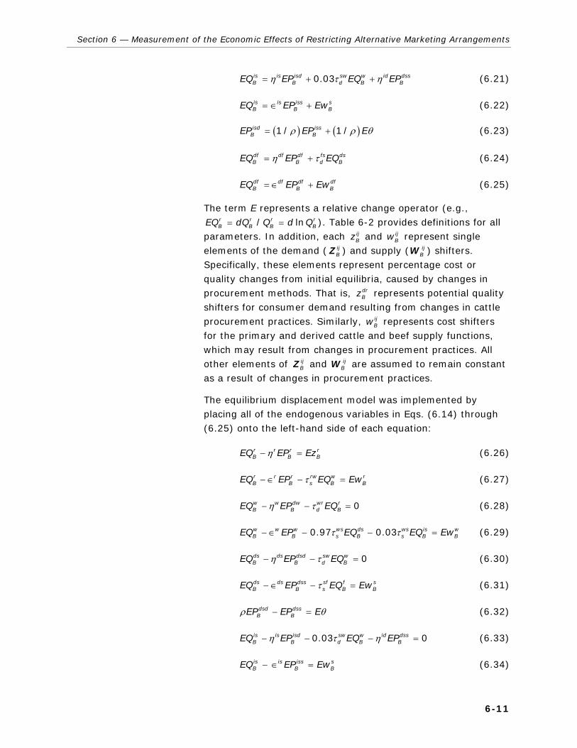
Section 6 — Measurement of the Economic Effects of Restricting Alternative Marketing Arrangements
6-11
0.03is is isd sw w id dssB B d B BEQ EP EQ EPη τ η= + + (6.21)
is is iss sB B BEQ EP Ew= ∈ + (6.22)
( ) ( )1 / 1 /isd issB BEP EP Eρ ρ θ= + (6.23)
df df df fs dsB B d BEQ EP EQη τ= + (6.24)
df df df dfB B BEQ EP Ew= ∈ + (6.25)
The term E represents a relative change operator (e.g., r r r rB B B BEQ dQ Q d Q/ ln= = ). Table 6-2 provides definitions for all
parameters. In addition, each ijBz and ij
Bw represent single elements of the demand ( ij
BZ ) and supply ( ijBW ) shifters.
Specifically, these elements represent percentage cost or quality changes from initial equilibria, caused by changes in procurement methods. That is, dr
Bz represents potential quality shifters for consumer demand resulting from changes in cattle procurement practices. Similarly, ij
Bw represents cost shifters for the primary and derived cattle and beef supply functions, which may result from changes in procurement practices. All other elements of ij
BZ and ijBW are assumed to remain constant
as a result of changes in procurement practices.
The equilibrium displacement model was implemented by placing all of the endogenous variables in Eqs. (6.14) through (6.25) onto the left-hand side of each equation:
r r r rB B BEQ EP Ezη− = (6.26)
r r r rw w rB B s B BEQ EP EQ Ewτ− ∈ − = (6.27)
0w w dw wr rB B d BEQ EP EQη τ− − = (6.28)
0.97 0.03w w w ws ds ws is wB B s B s B BEQ EP EQ EQ Ewτ τ− ∈ − − = (6.29)
0ds ds dsd sw wB B d BEQ EP EQη τ− − = (6.30)
ds ds dss sf f sB B s B BEQ EP EQ Ewτ− ∈ − = (6.31)
dsd dssB BEP EP Eρ θ− = (6.32)
0.03 0is is isd sw w id dssB B d B BEQ EP EQ EPη τ η− − − = (6.33)
is is iss sB B BEQ EP Ew− ∈ = (6.34)

Volume 3: Fed Cattle and Beef Industries
6-12
Table 6-2. Parameter Definitions, Short-Run and Long-Run Elasticity Estimates Used in the Equilibrium Displacement Model, and Standard Deviations of Beef Model Elasticities
Estimatea
Parameter Definition Short Run
Long Run
Short-Run Standard Deviationa
rη Own-price elasticity of primary demand for retail domestic beef
–0.864 –1.173 0.113
dwη Own-price elasticity of derived demand for wholesale domestic beef
–0.584 –0.936 0.105
dsη Own-price elasticity of derived demand for domestic slaughter cattle
–0.401 –0.529 0.150
isη Own-price elasticity of derived demand for imported slaughter cattle
–3.212 –6.049 1.033
idη Cross-price elasticity of derived demand for imported slaughter cattle with respect to U.S. slaughter cattle
1.196 2.252 0.566
dfη Own-price elasticity of derived demand for domestic feeder cattle
–0.135 –0.754 0.045
r∈ Own-price derived supply elasticity of retail beef
0.349 2.154 0.068
dw∈ Own-price derived supply elasticity of wholesale beef
0.424 0.591 0.132
ds∈ Own-price derived supply elasticity of domestic slaughter cattle
0.133 0.496 0.047
is∈ Own-price derived supply elasticity of imported slaughter cattle
10.000 10.000 n.a.
df∈ Own-price primary supply elasticity of feeder cattle
0.103 0.240 0.013
n.a. = not applicable a Short-run standard deviations for each elasticity are obtained from the structural model that is presented later in
the report. Long-run standard deviations are not needed for the analysis.
isd issB BEP EP Eρ θ− = (6.35)
0f f f fs dsB B d BEQ EP EQη τ− − = (6.36)
f f f fB B BEQ EP Ew− ∈ = (6.37)
For any given set of elasticity estimates, Eqs. (6.26) through (6.37) can be used to determine the relative changes in endogenous quantities and prices for any given exogenous

Section 6 — Measurement of the Economic Effects of Restricting Alternative Marketing Arrangements
6-13
changes in costs, market power, or consumer demand. In matrix notation, Eqs. (6.26) through (6.37) can be written as
A • Y = B • X, (6.38)
where A is a 12x12 nonsingular matrix of elasticities; Y is a 12x1 vector of changes in the endogenous price and quantity variables; B is a 12x6 matrix of parameters associated with the exogenous variables; and X is a 6x1 vector of percentage changes in the exogenous cost, demand, and market power shift variables. Relative changes in the endogenous variables (Y) caused by relative changes in marketing (procurement) costs and benefits (X) are calculated by solving Eq. (6.38) as
Y = A–1 • B • X. (6.39)
6.2 ESTIMATING DEMAND AND SUPPLY ELASTICITIES IN THE BEEF INDUSTRY Solutions for Y in Eq. (6.39) require elasticity estimates for elements of the matrix A. The extant literature reports various demand and supply elasticity estimates for the beef industry. In some cases, dozens of estimates have been reported. For other elasticities, however, only a few are available. In addition, reported elasticity estimates tend to vary in magnitude because of differing sample periods, estimation methods, modeling procedures, and research objectives.
Consequently, we estimated a system of structural demand and supply equations in the domestic beef sector so that resulting elasticity estimates are consistent with respect to sample period and model specification, data generation, methodology, and evaluation procedures.
U.S. beef trade equations are not explicitly estimated because changes in AMAs are not expected to significantly affect these sectors. However, U.S. demand for slaughter cattle imports is estimated because such purchases could be affected by changes in AMAs.
Most of the estimates of U.S. demand elasticities for beef have focused on the retail level, while supply elasticity estimates have focused on the live cattle sector (Brester and Wohlgenant, 1991; Chavas, 1983; Dahlgran, 1987; Eales, 1994; Eales and Unneveher, 1988, 1993; Marsh, 1994, 1999; Moschini and
Volume 3: Fed Cattle and Beef Industries
6-14
Meilke, 1989; Ospina and Shumway, 1979; Rucker, Burt, and LaFrance, 1984; Rosen, Murphy, and Scheinkman, 1994).
Researchers often include vertical relationships when estimating demand and supply elasticities in the livestock/beef marketing sector (Brester and Marsh, 1983; Marsh, 1983, 2003; Shonkwiler and Hinckley, 1985; Wohlgenant, 1989). Primary and derived demand and supply elasticity estimates in the live cattle industry also show substantial variation in magnitude because of differing sample periods and research methodologies. In some cases, reported supply elasticity estimates are inconsistent with expected signs.
6.2.1 Structural Model Required for Econometric Estimates
To effectively evaluate economic effects of marketing arrangements in the beef sector, vertical relationships among demand and supply sectors in the cattle/beef marketing channel should be estimated jointly (Arzac and Wilkinson, 1979; Brester and Marsh, 1983; Brester, Marsh, and Atwood, 2004; Gardner, 1975; Marsh, 2003; Tomek and Robinson, 1990; Wohlgenant, 1989). For our structural analysis, the market levels of the beef industry considered are
1. feeder calf production, noted as the feeder cattle level;
2. feedlot production for slaughter, noted as the slaughter cattle level;
3. live cattle imports at the slaughter level;
4. carcass beef production, noted as the wholesale level;
5. retail beef production, noted as the retail level.
The implied demand and supply relationships are characterized by variables unique to each level and also by variables specific to other vertical sectors. For example, meat packer demand for slaughter cattle depends on cattle slaughter price, carcass price at the wholesale level, marketing costs, and the potential for meat packer market concentration.
The advantages of specifying multimarket levels in an econometric model rest with properties of the parameter estimates and comprehensiveness of the comparative statics. A system of demand and supply equations allows parameter estimates to account for vertical market information and stochastic error processes that improve the consistency and asymptotic efficiency of parameter estimates (Greene, 2003).

Section 6 — Measurement of the Economic Effects of Restricting Alternative Marketing Arrangements
6-15
For example, parameter estimates of a single-demand equation at the feeder cattle level ignore endogenous, exogenous, and error term information implicit in a demand system that includes downstream slaughter, wholesale, and retail levels (Marsh, 2003; Wohlgenant, 1989).
In a systems model, the comparative statics are contingent on model stability and total elasticities. These elasticities measure direct and indirect changes in equilibrium prices and quantities at all market levels from arbitrary shocks (Marsh, 2003; Wohlgenant, 1989). Beef market constituents (buyers and sellers) at these levels have vested interests in public and private policy changes, which can be evaluated using comparative statics. Examples include beef quality changes that may shift consumer preferences (retail demand) or government restrictions on contracting arrangements that could affect cattle finisher and meat packer transaction and plant utilization costs. The result could be a shift in the feedlot supply of and the packer demand for slaughter cattle. Moreover, the relative elasticities of primary demand and primary supply, the nature of marketing margins, and the source of market shock(s) determine the distribution of price, quantity, and consumer and producer changes between the marketing levels (Brester, Marsh, and Atwood, 2004; Gardner, 1975; Tomek and Robinson, 1990).
6.2.2 Previous Research on Beef Industry Elasticities
Research involving demand, supply, and price determination in the beef industry has been extensive because of the importance of red meat and poultry consumption in the United States (Babula, 1996). For example, 2005 retail per capita consumption of all red meats (beef, veal, pork, and lamb) and poultry (broilers and turkey) was 221 pounds (USDA, ERS, 2006). Per capita beef consumption was 65.5 pounds in 2005, or about 39% of total meat consumption. In 1970, red meat and poultry per capita consumption was 190.5 pounds, and beef represented 84.6 pounds or 44% of total meat consumption.
The decline in per capita beef consumption has been attributed to declining beef demand since the mid-1970s (Marsh, 2003; Purcell, 1989). The demand for beef declined by almost 70% between 1976 and 1997 (Marsh, 2003). Changing consumer preferences for red meats, inconsistent product quality, relative

Volume 3: Fed Cattle and Beef Industries
6-16
meat prices, and lack of product innovation contributed to this decline. However, from 1998 to 2005, beef demand increased an average of 1.5% per year (LMIC, 2006). During this period, the demand for pork remained constant, lamb demand declined, and poultry demand increased (USDA, ERS, 2006).
The U.S. beef industry consists of several sectors, including cow-calf (feeder cattle) and yearling (backgrounding) production, cattle finishing, meat packing and processing, and wholesaling and retailing. Cow-calf producers supply feeder cattle to the cattle finishing sector and, thus, represent the primary supply for the beef industry. Research related to this sector has included estimated cyclical feeder cattle production (Foster and Burt, 1992; Jarvis, 1974; Marsh, 1999, 2003; Nerlove, Fornari, and Tanizaki, 1992; Rosen, Murphy, and Scheinkman, 1994; Rucker, Burt, and LaFrance, 1984). Supply responses have generally been related to changes in input and output price expectations and the dynamics of biological factors involved in herd expansion and contraction. Feeder cattle supply response also involves imports from Mexico and Canada, which represent 2% to 4% of total U.S. feeder cattle supplies (Cockerham, 1995; Marsh, 2001; Peel, 1996). Feedlots provide the derived demand for feeder cattle at this level. This demand is conditional on slaughter cattle prices, feed costs, and technological change (Anderson and Trapp, 1997; Brester and Marsh, 1983; Buccola, 1980; Marsh, 2001; Shonkwiler and Hinckley, 1985).
At the slaughter level, meat packers represent the derived demand for slaughter cattle and feedlots represent the derived slaughter cattle supply. These responses have been analyzed extensively (Arzac and Wilkinson, 1979; Brester and Marsh, 1983, 2001; Freebairn and Rausser, 1975; Marsh, 1994; Hayenga and Hacklander, 1970; Nelson and Spreen, 1978; Wohlgenant, 1989). Slaughter supply generally has been estimated as a dynamic relationship with respect to slaughter cattle prices, feed costs, and technological change using various distributed lags (Marsh, 2003). Meat packer demand for slaughter steers and heifers has been estimated as a function of wholesale carcass prices, slaughter by-product values, marketing costs, and consumer income. Wohlgenant (1989) has shown that variable input proportions exist in this sector because processors have some ability to substitute between

Section 6 — Measurement of the Economic Effects of Restricting Alternative Marketing Arrangements
6-17
slaughter cattle and marketing inputs to produce table cuts of beef.
Relatively less econometric modeling has occurred in the wholesale level of the beef sector (Brester and Marsh, 1983; Crom, 1970; Marsh, 1988; Marsh and Brester, 1985). Meat processors produce boxed beef and represent the derived supply at this level. Derived supply has been estimated as a function of wholesale beef prices, packer carcass by-product values, marketing costs, and technological change. Retailers represent the derived demand for boxed beef at the wholesale level. Derived demand has been estimated as a function of wholesale beef prices, marketing costs, and various retail-level factors.
The retail level consists of retailers who represent derived supply and consumers who represent primary demand. A plethora of studies have estimated retail demand elasticities in the red meat industry (Braschler, 1983; Chavas, 1983; Dahlgran, 1987; Eales, 1994; Eales and Unneveher, 1988; George and King, 1971; Huang, 1993; Huang and Haidacher, 1983; Moschini and Meilke, 1984; Wohlgenant, 1985, 1989). These studies considered a variety of research issues, including the estimation of direct price, indirect price, and expenditure elasticities; testing of economic restrictions; testing for structural change; and forecasting retail meat prices and quantities. Again, retail beef demand elasticity estimates vary considerably. Little research has been conducted with the goal of estimating derived retail supply elasticities.
International trade has become an increasingly important aspect of the U.S. beef industry (Capps, Tasi, Kirby, and Williams, 1994). In 1975, U.S. cattle and beef imports (on a carcass weight basis) totaled 7.8% of total U.S. beef supplies. By 2005, the import share had increased to 15.8% (USDA, ERS, 2006). The United States imports feeder cattle from Canada and Mexico for backgrounding and finishing and slaughter cattle from Canada for processing. The United States also imports ground beef and trimmings from Australia, New Zealand, and Canada and imports boxed beef from Canada (Brester, Marsh, and Plain, 2003). Research on this sector has centered on the effects of meat import regulations and trade liberalization agreements on U.S. cattle and beef prices

Volume 3: Fed Cattle and Beef Industries
6-18
(Brester, 1996; Brester, Marsh, and Smith, 1999; Cockerham, 1995; Freebairn and Rausser, 1975; Peel, 1996; Marsh, 1998).
The United States primarily exports table cut beef to the Pacific Rim (Japan and South Korea), Mexico, and Canada. Small quantities of breeding cattle are exported to Canada and Mexico, and a relatively small number of feeder cattle are exported to Canada under the Restricted Feeder Cattle Program (Young and Marsh, 1998). In 2002, U.S. beef exports totaled 2.45 billion pounds, 31% of which was exported to Japan, 26% to South Korea, 24% to Mexico, and 10% to Canada (USDA/ERS, 2004a). Beef and live exports as a percentage of U.S. beef supplies increased from less than 1% in 1975 to 9.2% in 2002. In 2005, however, exports declined to 2.5% of U.S. supplies because of the U.S. 2003 BSE case. Overall, strong increases in export demand have resulted from increased incomes in importing countries, greater demands for animal-source protein, and increased trade liberalization (Miljkovic, Marsh, and Brester, 2004). Increased foreign demand for U.S. beef has offset some of the reductions in domestic beef demand (Marsh, 1994).
Research on U.S. beef exports has focused primarily on the effects of foreign beef demand on U.S. cattle prices (Brester and Marsh, 1999; Capps, Kirby, and Williams, 1994; Gorman, Mori, and Lin, 1990; Miljkovic, Marsh, and Brester, 2002). The price elasticity of Japanese demand for U.S. beef exports was estimated as –0.215 (Miljkovic, Marsh, and Brester, 2002) and –0.210 (Capps, Kirby, and Williams, 1994). Research also has shown that U.S. beef exports and prices are sensitive to changes in foreign incomes, tariffs, and exchange rates (Miljkovic, Marsh, and Brester, 2002).
6.2.3 Conceptual Beef Model for Estimating Elasticities
This current research requires information on primary and derived demand and supply structures and related price elasticities. Thus, an econometric model of vertical demand and supply relationships in the beef farm-to-retail marketing system is required. U.S. import demand for slaughter cattle is also econometrically estimated to obtain direct and substitute elasticities.
According to Gardner (1975) and Tomek and Robinson (1990), integrating marketing-chain relationships improves the

Section 6 — Measurement of the Economic Effects of Restricting Alternative Marketing Arrangements
6-19
estimation accuracy of upstream and downstream demand and supply responses. For example, the derived demand elasticity for cattle at the farm level is jointly a function of the primary demand elasticity, marketing margins, factors specific to other market levels, net imports, and factors specific to the farm level such as feed costs (Marsh, 2003; Wohlgenant, 1989).
A crucial aspect of our econometric model is the estimation of primary demand and primary supply because shifts in these functions affect derived demand and supply functions. Moreover, the effects of initial conditions or shocks in the marketing sector also depend on primary-level elasticities. For example, increased costs incurred by meat packers shift derived slaughter demand and wholesale and retail supply functions. Subsequently, the distribution of these cost changes on prices and quantities at the retail and farm levels is conditional on elasticities of retail demand and farm supply (Brester, Marsh, and Atwood, 2004; Lusk and Anderson, 2004).
The microeconomic theory underlying the behavioral relations of primary consumer demand for beef and primary producer supply of beef are derived from first-order conditions of constrained utility maximization and firm profit maximization, respectively (Varian, 1992). Moreover, the derived (input) demands and derived (output) supplies in the marketing chain are a function of first-order conditions of firm profit maximization. This optimization principle can be demonstrated by considering a cattle feeding firm that purchases 700- to 800-pound feeder cattle and grain finishes them to 1,200 to 1,400 pounds for sale to meat packers. The firm’s unconstrained profit function would be
1
p
B B f f i ii
P Q P Q rqπ=
= − − Σ , (6.40)
where π is the feeding firm’s profit; PB is the price of slaughter cattle; QB is liveweight quantity of slaughter cattle; Pf is price of feeder cattle; Qf is liveweight quantity of feeder cattle purchased; and ri and qi are prices and quantities of other inputs such as feed, labor, medical, and other supplies in the finishing operation. Following Varian (1992), the finisher’s supply function for slaughter cattle is based on solving the first-order condition of profit maximization:

Volume 3: Fed Cattle and Beef Industries
6-20
( ) ( )
, ,, , .B f i
B B f iB
P P rQ P P r
P
π∂=
∂ (6.41)
Eq. (6.41) indicates that the supply function of slaughter cattle depends on the output price of slaughter cattle (PB), input price of feeder cattle (Pf), and other input costs (ri).
Similarly, the demand function for feeder cattle is based on solving first-order conditions of profit maximization:
( ) ( )
, ,, , ,B f i
f f B if
P P rQ P P r
P
π−∂=
∂ (6.42)
which indicates that the input demand function for feeder cattle depends on the input price of feeder cattle, output price of slaughter cattle, and other input costs. Because π is a convex function, the second-order derivatives of the left-hand sides of Eqs. (6.41) and (6.42) ensure a nonnegative slope of output supply and a nonpositive slope of input demand.
The optimization principle holds for any profit-maximizing (or cost-minimizing) firm in competitive marketing channels. Thus, aggregating the relevant micro-level functions of cattle feeder producers, cattle finishers, beef packers and processors, and meat retailers yields the appropriate primary and derived market-level functions. The input price vector, ri, in Eq. (6.42) also could include marketing costs, a relevant proxy for the effects of marketing margins in vertically related agricultural demand and supply functions (Tomek and Robinson, 1990).
6.2.4 Model Specification
The structural beef model of primary-to-derived vertical relationships is an improvement over more limited specifications. For purposes of estimating elasticities, we assume that the beef market is competitive. Hence, individual sellers face infinitely elastic demands and individual buyers face infinitely elastic supplies. This assumption may be questioned because of increased meat packing and retail grocery concentration since the 1980s. However, studies have indicated meat and livestock price distortions from potential market power in these markets are relatively minor (Azzam and Anderson, 1996; Azzam and Schroeter, 1991; Brester and Marsh, 2001; Marsh and Brester, 2004; Morrison-Paul, 2001). Cross-equation parametric restrictions are not imposed because of the disaggregate nature of the vertical marketing structure.

Section 6 — Measurement of the Economic Effects of Restricting Alternative Marketing Arrangements
6-21
The structural specifications of the beef model are as follows:
Retail Beef Sector
Retail beef demand:
( )1 , , , , ,rd rd r r rB B L K YQ h P P P P Me BE= (6.43)
Domestic retail beef supply:
( )2 , , , , ,rs rs w r r rB B B c L K YQ h P P L P P P= (6.44)
Market-clearing quantity:
rd rs rB B LQ Q Q= = (6.45)
Market-clearing price:
rd rs rB B BP P P= = (6.46)
Wholesale Beef Sector
Wholesale beef demand:
( )3 , , , , ,wd wd r w w wB B B L K Y cQ h P P P P P L= (6.47)
Wholesale beef supply:
( )4 , , , , ,ws ws ds w wB B B bp c L KQ h P P P M P P= (6.48)
Market-clearing quantity:
wd ws wB B BQ Q Q= = (6.49)
Market-clearing price:
wd ws wB B BP P P= = (6.50)
Domestic Slaughter Cattle Sector
Domestic slaughter cattle demand:
( )5 , , , , ,dsd dsd dw dsdB B B B bp KQ h P P W P P K= (6.51)
Domestic slaughter cattle supply:
( )6 , , , ,dss dss fB B B n BQ h P P P T BE= (6.52)
Market-clearing quantity:
dsd dss dsB B BQ Q Q= = (6.53)

Volume 3: Fed Cattle and Beef Industries
6-22
Market-clearing price:
dsd dss dsB B BP P P= = (6.54)
Import Slaughter Cattle Sector
Import slaughter cattle demand:
( )7 , , , ,isd isd dsd wbpB B B B BQ h P P W P P= (6.55)
Import slaughter cattle beef supply:
( )8 , ,iss iss sB B B xQ h P C E= (6.56)
Market-clearing quantity:
isd iss isB B BQ Q Q= = (6.57)
Market-clearing price:
isd iss isB B BP P P= = (6.58)
Feeder Cattle Sector
Feeder cattle demand:
( )9 , , ,fd fd dsdB B B N BQ h P P P T= (6.59)
Feeder cattle supply:
( )10 , ,fs fsB B hy bcQ h P P Q= (6.60)
Market-clearing quantity:
fd fs fB B BQ Q Q= = (6.61)
Market-clearing price:
fd fs fB B BP P P= = (6.62)
Table 6-1 provides variable definitions for the beef model. The demand and supply equations are expressed with quantities as the dependent variables. At all market-level sectors, prices and quantities are assumed to be in equilibrium within annual time periods.
Eqs. (6.43) and (6.44) represent primary retail demand and derived retail supply of beef, respectively. Retail demand per capita is a function of domestic retail beef price ( rd
BP ); retail prices of lamb, pork, and poultry ( , ,r r r
L K YP P P ); per capita meat

Section 6 — Measurement of the Economic Effects of Restricting Alternative Marketing Arrangements
6-23
expenditures (Me); and a binary variable (BE) representing the 2003 U.S. BSE case. Retail supply is a function of retail beef price ( r
BP ); wholesale beef price ( wBP ); food labor costs (Lc);
and the retail prices of lamb ( rLP ), pork ( r
KP ), and poultry ( rYP ).
Wholesale demand and supply of beef are given by Eqs. (6.47) and (6.48). Wholesale demand is a function of wholesale domestic beef price ( dw
BP ), retail beef price ( rBP ), wholesale
prices of competitive meats ( , ,w w wL K YP P P ), and food labor costs
(Lc). Wholesale beef supply is a function of wholesale domestic beef price ( dw
BP ), input price of domestic slaughter cattle ( dsBP ),
beef by-product value (Pbp), food marketing cost (Mc), and wholesale prices of lamb ( w
LP ) and pork ( wKP ).
Domestic beef slaughter demand and supply are given in Eqs. (6.51) and (6.52). Domestic slaughter (meat packer) demand is a function of domestic slaughter cattle price ( ds
BP ), domestic wholesale price of beef ( dw
BP ), wages in meat packing plants (WB), beef by-product value (Pbp), and beef packer concentration (K). Domestic slaughter supply (by cattle feeders) is a function of domestic slaughter cattle price ( ds
BP ), input price of feeder cattle ( f
BP ), the input price of feed corn (Pn), feedlot technology (TB), and a binary variable representing the 2003 U.S. BSE case (BE).
Eqs. (6.55) and (6.56) provide specifications for import demand and supply of slaughter cattle. U.S. import demand for slaughter cattle is a function of import slaughter cattle price ( isd
BP ), domestic slaughter cattle price ( dsdBP ), wages in meat
packing plants (WB), price of wholesale beef ( wBP ), and beef by-
product values (Pbp). The import supply of slaughter cattle is a function of the price of imported slaughter cattle ( is
BP ), cost of producing imported slaughter cattle ( s
BC ), and the U.S./Canadian exchange rate (Ex).
Domestic demand for feeder cattle (by cattle finishers) and the supply of feeder cattle (by cow-calf producers) is presented in Eqs. (6.59) and (6.60). The derived demand for feeder cattle is a function of feeder cattle price ( f
BP ), the price of slaughter cattle ( ds
BP ), the price of corn (PN), and feedlot technology (TB). The primary supply of feeder cattle is a function of the price of feeder cattle ( f
BP ), the price of hay (Phy), and the quantity of breeding cattle (Qbc).

Volume 3: Fed Cattle and Beef Industries
6-24
6.2.5 Other Model Considerations
The structural model includes a variety of economic factors, such as feed prices, prices of competitive meats, consumer expenditures on meat, meat packer concentration, input prices, food marketing costs, and exchange rates. The sample period includes several decades during which other factors may also be of potential significance. Two specific events include (1) structural change in meat demand and the meat price freeze of the early 1970s (Knutson, Penn, and Boehm, 1990; Moschini and Meilke, 1989) and (2) the 2003 Canadian and U.S. cases of BSE.
Comprehensive price and wage controls imposed by the Nixon Administration in August 1971 for 90 days included ceilings on meat prices. Immediately after the controls were lifted in November 1971, food prices, especially meat prices, increased substantially. Per capita beef consumption declined precipitously in the late 1970s. The decline was thought to be the result of a variety of factors, including real price declines of competing meats, changes in consumer income distributions, changing demographics, increased demand for convenience foods, and changing consumer preferences (Moschini and Meilke, 1989). Tests for structural changes in beef demand in the mid-1970s have generated mixed results. Moschini and Meilke (1989) found that structural change negatively affected beef, positively affected poultry, and did not affect pork demand. However, other studies either did not find structural change or were able to attribute declines in beef demand to other factors.
Initial outbreaks of BSE in Canada (May 2003) and the United States (December 2003) are potentially important market events in that demand and price expectations of consumers and producers may have been altered. Therefore, a BSE binary variable is included in the primary retail demand and derived slaughter supply of fed cattle.
To formally test for impacts of the meat price freeze and structural change in beef demand, binary variables for 1971, 1972, and 1975 through 2005 were included in the retail beef demand equation. The regression results failed to reject the null hypotheses of no influence of either market shock at the " = 0.05 level.

Section 6 — Measurement of the Economic Effects of Restricting Alternative Marketing Arrangements
6-25
A binary variable for 2003 through 2005 was included in the primary retail demand and derived slaughter supply equations in the final specification to account for BSE occurrences.
6.2.6 Model Dynamics
Conceptually, the U.S. beef model represents a set of economically integrated demand and supply relations in the farm–retail marketing chain. The static form of the model can be represented in general matrix notion as
t t tY Zβ μ+ Γ = , (6.63)
where Yt is a Gx1 vector of endogenous variables, Zt is a Kx1 vector of exogenous variables, μt is a Gx1 vector of disturbance terms, β is a GxG matrix of coefficients for the Yt vector, and Γ is a GxK matrix of coefficients for the Zt vector. The model assumes nonzero, off-diagonal terms for the β matrix, rank identification of the Γ matrix, and a nondiagonal covariance matrix for μt, or contemporaneously correlated errors (Johnston and DiNardo, 1997). The μts within each equation are assumed to be normally distributed with zero mean and constant variance; however, their time-series properties may be autoregressive (Greene, 2003).
Because of the nonzero, off-diagonal terms of the β matrix, testing for equation cointegration is not necessary (Johnston and DiNardo, 1997). Thus, the model is estimated in data-level form by three-stage least squares (3SLS). The estimator yields consistent and asymptotically efficient coefficient distributions (Greene, 2003).
The presence of biological lags, technical production constraints production, and buyer and seller expectations likely generate dynamic responses in livestock and meat supply and demand behavior (Brester and Marsh, 1983; Marsh, 2003; Rucker, Burt, and LaFrance, 1984; Tomek and Robinson, 1990; Whipple and Menkhaus, Whipple, and Ward, 1989). Thus, Eq. (6.83) is modified to account for partial adjustment processes in the behavioral relations through autoregressive distributed lags (ARDL) or ARMAX models (i.e., ARDL with autocorrelated errors) (Greene, 2003; Marsh, 2003). In this context, the model can be rewritten as
( ) ( )t t tL Y L Zβ μ+ Γ = , (6.64)

Volume 3: Fed Cattle and Beef Industries
6-26
where β(L) and Γ(L) are polynomial lag operators that impose finite lag structures on the endogenous (Yt) and exogenous (Zt) vectors. The lag operators are given as
2 31 2 3( ) 1 p
pL L L L Lβ β β β β= − − − K (6.65)
and
2 30 1 2 3( ) q
qL L L L LΓ = Γ + Γ + Γ + Γ ΓK . (6.66)
Thus, the polynomial form β(L)Yt of Eq. (6.65) gives LpYt = Yt-p, and the polynomial form Γ(L)Zt of Eq. (6.66) gives LqZt = Zt-q. Solving for the Yτ vector of Eq. (6.64) gives
t t t
LY Z
L L( ) 1( ) ( )
μβ βΓ
= + , (6.67)
which conceptually gives Yt as an infinite distributed lag function of Zt and μt (Greene, 2003). The implied set of polynomial coefficient weights for Zt are formed by the rational generating function, Γ(L) / β(L). The infinite moving average (MA) error structure for μt is restricted by the polynomial weights of β(L). The rational generating function allows for short-run flexibility in the distributed lag patterns of the exogenous variables. However, the long-run behavior of each Z variable is conditioned by β(L) (Greene, 2003).
Pragmatically, for annual models, empirical lags on the dependent variables (p in Eq. [6.65]) and the independent variables (q in Eq. [6.66]) for livestock and meat are usually of order 1 or 2 (Marsh, 2003). Several researchers have examined the cyclical nature of beef cattle inventories (Rosen, Murphy, and Scheinkman, 1994; Rucker, Burt, and LaFrance, 1984). Because of cattle inventory cycles on the supply side of the beef market, p is initially specified in the polynomial denominator as order 2 (permitting complex roots or cycling), and q is initially specified as order 1 in the polynomial numerator. For the demand side of the market, p and q of the polynomials are initially set at lag order 1. Setting q to an order of 1 implies geometric distributed lags in demand behavior.
The number of parameters for empirical estimation is relatively large using the initial lag order specifications. To achieve a more parsimonious set of parameters and improve estimation efficiency, higher order lags are truncated if they are found to be statistically insignificant. However, for any given variable, if

Section 6 — Measurement of the Economic Effects of Restricting Alternative Marketing Arrangements
6-27
contemporaneous and lag values are all found to be insignificant, the parameter value with the largest t-statistic is retained in the model to maintain theoretical consistency.
6.3 DATA CONSIDERATIONS The sample period consists of annual data for the years 1970 through 2005. Cattle and beef price and quantity data, beef by-products, food marketing and labor costs, meat packer wages, substitute meat prices, corn and hay prices, and trade data were obtained from various USDA sources, including Agricultural Statistics; Livestock, Dairy and Poultry Situation and Outlook reports; Red Meats Yearbook; Dairy, Livestock, and Poultry: U.S. Trade and Prospects; and the American Sheep Industry Association. Other data were obtained from the Economic Report of the President, international financial statistics of the International Monetary Fund (various issues), and USDA, GIPSA (2006). Complete data series were available for most variables included in the model, with the exception of retail lamb prices and wholesale lamb cut-out values. Missing observations for these series were imputed as described in Volume 5, Section 6.
6.4 STATISTICAL AND ESTIMATION PROCEDURE CONSIDERATIONS We assume that beef price is jointly determined with beef quantity in the retail beef demand function (Eales and Unneveher, 1993). Therefore, unit root and cointegration tests are not conducted because nonstationarity would not alter estimation procedures or inferences if data are simultaneously determined (Johnston and DiNardo, 1997). In addition, the model is estimated in data-level form, with all variables (except the binary variables) transformed into natural logarithms.
Specification of group expenditures (rather than consumer income or total expenditures) in conditional demand systems (i.e., weakly separable) is a common procedure in applied demand models (LaFrance, 1991). However, group expenditures must be uncorrelated with error terms to avoid biased and inconsistent parameter estimates. Therefore, the current model uses total consumer meat expenditures (i.e., expenditures on beef, pork, lamb, broilers, and turkey) as an income variable in the retail beef demand function. A Wu-

Volume 3: Fed Cattle and Beef Industries
6-28
Hausman test failed to reject the null hypothesis of no simultaneous equation bias at the α = 0.05 level.
Based on the beef model assumptions and statistical tests, the Eviews 5.1 3SLS estimator was used because of the potential for a nondiagonal covariance matrix of autoregressive (AR) errors (Quantitative Micro Software, 2004). Because the model is specified with equilibrium quantities as dependent variables, the demand and supply equations are estimated in separate blocks to reduce demand and supply identification problems.
In applied agricultural economics research, demand and supply equations often are econometrically estimated using a combination of inverse and ordinary demand and supply functions to aid in identifying each equation (Eales and Unneveher, 1993; Eales, 1996; Marsh, 2003; Babula, 1997). However, the equilibrium displacement model for beef is specified such that estimates of elasticities (rather than flexibilities) of demand and supply are required. Theoretically, the inverses of price flexibilities obtained from inverse demand and/or supply functions provide lower-bound estimates for elasticities. Empirically, these inverses often generate unreasonably large and inconsistent elasticity estimates. We investigated this issue by estimating the beef demand functions as price-dependent relations in conjunction with ordinary supply functions. This approach yielded several inconsistencies among elasticity estimates across the model. Therefore, we ameliorated the identification issues by estimating ordinary demand functions and ordinary supply functions in separate regression blocks.
The rational distributed lag model also could be estimated using quarterly data. However, many observations on some of the key variables were not reported on a quarterly basis.
Finally, BSE events in Canada and the United States resulted in trade restrictions in 2003, 2004, and 2005 between the two countries. Hence, we could not estimate the U.S. import demand for Canadian slaughter cattle along with the other demand functions. Therefore, the function was estimated separately, and the results are reported in the following section.

Section 6 — Measurement of the Economic Effects of Restricting Alternative Marketing Arrangements
6-29
6.5 EMPIRICAL RESULTS The demand and supply functions of the beef model were estimated in separate blocks using 3SLS to avoid identification problems. The domestic demand and supply elasticities and the imported fed cattle demand elasticities are econometrically estimated. The imported slaughter supply elasticities are assumed to be highly elastic and arbitrarily set to 10.0.
In general, the empirical results support the rational lag hypotheses because each equation contains a significant parameter estimate of a first-order lagged dependent variable, or geometric (Koyck) distributed lags (Pindyck and Rubinfeld, 1998). The modulus of the single root in each difference equation is less than unity, implying stable dynamic structures. Based on Durbin h tests, the demand and supply equations did not require AR error corrections in the 3SLS estimator.
The 3SLS blocks indicated contemporaneously correlated errors, with zero-order correlations as high as 0.81 within the demand block and as high as 0.73 within the supply block. The systems estimator also provided the standard errors and covariances of the parameter (elasticity) estimates required for the equilibrium displacement model (Brester, Marsh, and Atwood, 2004). The adjusted R2s and standard errors of 3SLS regression are presented but should be interpreted with caution because of the generalized least squares (GLS) error covariance transformations of the product moment matrices (Greene, 2003).
Estimating theoretically specified supply and demand models is necessary to obtain consistent and efficient estimates of the elasticities needed to implement the equilibrium displacement model. Many of the estimated elasticities, however, are not directly used in the equilibrium displacement model.
6.5.1 Demand
A 3SLS estimator is used to obtain consistent and efficient elasticity estimates for use in the equilibrium displacement model. All of the estimates of interest (own-price and cross-price elasticities) are significantly different from zero at the α = 0.05 level.2 The price elasticities follow two patterns that are consistent with stable difference equations and marketing
2 Some of the parameter estimates (elasticities) in the demand block
were not statistically different from zero at the α = 0.05 level.
Volume 3: Fed Cattle and Beef Industries
6-30
margin behavior (Griliches, 1967; Tomek and Robinson, 1990). First, the short-run elasticities are considerably smaller than the long-run elasticities. This suggests that consumers and intermediate purchasers are influenced by habit formations and institutional rigidities (Pollack, 1970). These expectations are manifest in partial adjustment processes, as evidenced by significant coefficient estimates on the lagged dependent variables. Second, the absolute value of demand elasticity coefficients decreases from the retail level to the farm level. This is consistent with relative price spreads and primary and derived demand theory (Gardner, 1975; Tomek and Robinson, 1990; Wohlgenant, 1989).
Table 6-2 summarizes the demand elasticity estimates obtained from the 3SLS estimates presented in Tables 6-3 through 6-5. The long-run elasticities are calculated by dividing the short-run elasticities by 1.0 minus the estimated coefficients of the appropriate lagged dependent variables. The short-run and long-run retail demand elasticities for beef are –0.864 and –1.793, respectively. Previous studies have reported various own-price retail beef demand elasticity estimates. For example, Alston and Chalfant (1991) reported several elasticity estimates ranging from –0.66 to –1.04 using annual data from 1960 through 1988. Eales and Unneveher (1988) estimated a beef demand elasticity of –0.57 and a retail demand elasticity for table cuts of –0.684 using annual data from 1965 through 1985. Moschini and Meilke (1989) reported a pre-structural change elasticity of –0.983 and a post-structural change estimate of –1.050. Brester and Schroeder (1995) reported a retail own-price elasticity of demand of –0.56.
The short- and long-run beef demand elasticities at the wholesale level were –0.584 and –0.936, respectively. Both were more inelastic than the retail demand elasticities, which is consistent with Gardner’s (1975) relative price spread theory. Marsh (1992) reported wholesale elasticities consistent with margin theory that ranged from –0.469 to –0.567 using quarterly data. Marsh and Brester (1985) reported a long-run beef wholesale own-price demand elasticity of –0.990 using monthly data from 1970 through 1981.

Section 6 — Measurement of the Economic Effects of Restricting Alternative Marketing Arrangements
6-31
Table 6-3. 3SLS (Double Log) Estimates of Domestic Retail Beef Demand
Dependent Variable
Regressors Domestic Retail Beef Demand
( )drBQ
Constant –1.131 (–3.211)
Domestic retail beef price ( )drBP –0.864
(–7.762)
Retail lamb price ( )rLP 0.006
(1.181)
Retail pork price ( )rKP –0.112
(–1.895)
Retail poultry price ( )rYP –0.103
(–1.575)
Meat expenditures ( )eM 1.195 (5.075)
Lagged meat expenditures ( )1etM − 0.337 (3.914)
BSE binary variable ( )BE –0.002 (–0.100)
Lagged domestic retail beef demand ( )1drBtQ − 0.518
(7.692)
Regression statistics
Adjusted R2 0.959
Standard error of the regression 0.022
Log mean of the dependent variable 4.305
At the domestic slaughter level, the short- and long-run derived demand elasticities were both inelastic. For fed slaughter cattle, the elasticities were –0.401 and –0.529. Wohlgenant (1989) reported a slaughter-level demand elasticity of –0.50, under the assumption of fixed input proportions, and –0.76, assuming variable input proportions technology using annual data from 1956 through 1983. Marsh (1992) reported an own-price elasticity of demand for slaughter cattle ranging from –0.506 through –0.657 using 1975 through 1989 annual data. Brester and Marsh (1983) report an elasticity of –0.348 using 1960 to 1980 annual data.

Volume 3: Fed Cattle and Beef Industries
6-32
Table 6-4. 3SLS (Double Log) Estimates of Wholesale Beef Demand
Dependent Variable
Regressors Wholesale Beef Demand
( )dwBQ
Constant 1.446 (1.716)
Domestic wholesale beef price ( )dwBP –0.584
(–5.586)
Domestic retail beef price ( )drBP 0.384
(2.484)
Wholesale lamb price ( )wLP 0.057
(1.078)
Wholesale pork price ( )wKP 0.014
(0.429)
Wholesale poultry price ( )wYP 0.070
(1.235)
Food labor costs ( )cM –0.003 (–0.024)
Lagged domestic wholesale beef demand ( )1dwBtQ − 0.376
(2.797)
Regression statistics
Adjusted R2 0.691
Standard error of the regression 0.036
Log mean of the dependent variable 3.170
Because of data limitations, the U.S. demand for imported slaughter cattle was estimated separately from the system of demand equations. Annual data from 1970 through 2002 were used. The ADF test failed to reject the null hypothesis of unit roots in all variables at the α = 0.05 level. However, the augmented ADF test indicated that the function was cointegrated at the α = 0.05 level. A Hausman test failed to reject the null hypothesis of no simultaneous equation bias for both U.S. and Canadian slaughter cattle prices at the α = 0.05 level. Because of the high correlation between these two prices (correlation coefficient of 0.89), the price of U.S. feeder cattle was used as an instrument for the price of U.S. slaughter cattle. The Breusch-Godfrey LM test failed to reject the null hypothesis of no first- or second-order serial correlation in the residuals. The CUSUM test for parameter stability failed to

Section 6 — Measurement of the Economic Effects of Restricting Alternative Marketing Arrangements
6-33
Table 6-5. 3SLS (Double Log) Estimates of Domestic Slaughter and Feeder Cattle Demand, and OSL (Double Log) Estimates of Import Slaughter Cattle Demand
Dependent Variables
Regressors
Domestic Slaughter
Cattle Demand ( )ds
BQ
Imported Slaughter
Cattle Demand ( )is
BQ
Feeder Cattle Demand ( )df
BQ
Constant 4.222 (7.896)
1.298 (0.731)
–2.607 (–2.289)
Domestic slaughter cattle price ( )dsBP –0.401
(–2.670) 1.196
(2.114) 0.238
(3.591)
Wholesale beef price ( )1dw
BtP − 0.053 (0.368)
1.423 (1.678)
Meat packer wages ( )W 0.045 (0.523)
–1.139 (–1.624)
Beef by-product price (Pbp) 0.040 (1.260)
Beef packer concentration (K) –0.086 (–1.708)
Price slaughter hog ( )dsKP 0.030
(1.339)
Lagged domestic slaughter beef demand ( )1dsBtP − 0.242
(3.383)
Imported slaughter cattle price ( )isBP –3.212
(–3.110)
Lagged imported slaughter cattle demand ( )1isBtQ − 0.469
(3.198)
Domestic feeder cattle price ( )dfBP –0.135
(–3.015)
Price of corn ( )nP 0.002 (0.106)
Technology ( )fT 0.420 (2.992)
Lagged domestic feeder cattle demand ( )1dfBtQ − 0.821
(8.626)
Regression statistics
Adjusted R2 0.852 0.837 0.945
Standard Error of the Regression 0.024 0.296 0.021
Log Mean of the Dependent Variable 3.695 –0.410 3.261

Volume 3: Fed Cattle and Beef Industries
6-34
reject the null hypothesis of stable parameters. Table 6-2 indicates that the short-run own-price derived demand elasticity for imported slaughter cattle is –3.212. The long-run elasticity was calculated to be –6.049 (Table 6-2). The short-run, cross-price elasticity of demand for imported Canadian slaughter cattle with respect to the price of U.S. slaughter cattle is 1.196, and the long-run estimate is 2.252 (Table 6-2). These elastic demand responses indicate that Canadian slaughter cattle are close substitutes for U.S. slaughter cattle.
The derived demand for feeder cattle represents the major input demanded by cattle finishers. The estimated short- and long-run demand elasticities at this level are relatively inelastic (–0.135 in the short run and –0.754 in the long run). Brester and Marsh (1983) reported an own-price elasticity of demand for cattle placements of –0.622 using annual data from 1960 through 1980. Shonkwiler and Hinckley (1985) used a rational expectations model to estimate a cattle placement demand elasticity of –0.909. Marsh (2001) used a reduced-form model to obtain an estimate of the own-price elasticity of demand for feeder cattle of –0.644 using 1970 through 1999 annual data.
6.5.2 Demand Quantity Transmission Elasticities
Estimates of quantity transmission elasticities are used in the equilibrium displacement model to provide linkage between the vertically connected demand sectors. These estimates are obtained from the SUR estimation of four equations separate from the structural model. The transmissions elasticity estimates are summarized in Table 6-6. Table 6-7 provides the complete SUR estimation results of regressing the appropriate quantity variable at each level onto the appropriate upstream quantity variable. Double log specifications are used so that resulting parameter estimates are interpreted as transmission elasticities.
6.5.3 Supply
The supply block of the 3SLS beef model consists of equations for feeder cattle, slaughter cattle, wholesale beef, and retail beef (Tables 6-8 through 6-10). Several of the slope coefficients were not statistically different from zero. However, all own-price supply elasticities are significant at the α = 0.05 level. The rational lag structure was stable in that the modulus of each of the single roots of the difference equation coefficient estimates was less than unity. The dynamics resulted in

Section 6 — Measurement of the Economic Effects of Restricting Alternative Marketing Arrangements
6-35
Table 6-6. Parameter Definitions and Quantity Transmission Elasticity Estimates
Parameter Definition Estimatea Standard Deviationa
wrdτ Percentage change in wholesale beef quantity given a
1% change in retail beef quantity 0.978 0.097
swdτ Percentage change in domestic and imported slaughter
cattle quantity given a 1% change in wholesale beef quantity
0.936 0.043
fsdτ Percentage change in feeder cattle quantity given a 1%
change in domestic slaughter cattle quantity 0.834 0.084
rwsτ Percentage change in retail beef quantity given a 1%
change in wholesale beef quantity 0.715 0.081
wssτ Percentage change in wholesale beef quantity given a
1% change in domestic and imported slaughter cattle quantity
0.929 0.053
sfsτ Percentage change in domestic slaughter cattle quantity
given a 1% change in feeder cattle quantity 0.944 0.031
a These estimates are obtained from the structural model that is presented later in the report.
Table 6-7. SUR (Double Log) Demand Quantity Transmission Elasticities
Dependent Variables
Regressors
Wholesale Beef Quantity
( )dwBQ
Domestic Slaughter
Cattle Quantity ( )ds
BQ
Feeder Cattle Quantity ( )df
BQ
Constant –1.918 (–3.791)
0.728 (5.361)
1.502 (2.763)
Domestic retail beef quantity ( )drBQ 0.978
(10.110)
Imported live cattle quantity ( )irBQ
Domestic wholesale beef quantity ( )dwBQ 0.936
(21.871)
Domestic slaughter beef quantity ( )dsBQ 0.834
(9.973)
Regression statistics
Adjusted R2 0.864 0.955 0.984
Standard error of the regression 0.024 0.014 0.008
Log mean of the dependent variable 3.170 3.695 3.261
Note: Quantity transmission equations corrected for first-order autocorrelation in residuals.

Volume 3: Fed Cattle and Beef Industries
6-36
Table 6-8. 3SLS (Double Log) Estimates of Feeder Cattle Supply
Dependent Variable
Regressors Feeder Cattle Supply
( )dfBQ
Constant 0.005 (0.041)
Breeding cow inventory ( )bcQ 0.350 (3.347)
Lagged domestic feeder calf price ( )1dfBtQ − 0.103
(7.786)
Lagged hay price ( )1hy tP − –0.068 (–3.296)
Lagged domestic feeder cattle supply ( )1fbtQ − 0.570
(4.643)
Regression statistics
Adjusted R2 0.970
Standard error of the regression 0.016
Log mean of the dependent variable 3.261
Table 6-9. 3SLS (Double Log) Estimates of Domestic Slaughter Cattle Supply
Dependent Variable
Regressors Domestic Slaughter Cattle Supply
( )dsBQ
Constant –0.552 (–0.506)
Lagged domestic slaughter cattle price ( )1dsBtP − 0.133
(2.818)
Domestic feeder calf price ( )dfBP –0.161
(–5.711)
Lagged corn price ( )1ntP − –0.001 (–0.046)
Feedlot technology ( )BT 0.253 (1.677)
Lagged domestic slaughter cattle supply ( )1dsBtQ − 0.732
(8.424)
Regression statistics
Adjusted R2 0.829
Standard error of the regression 0.026
Log mean of the dependent variable 3.695
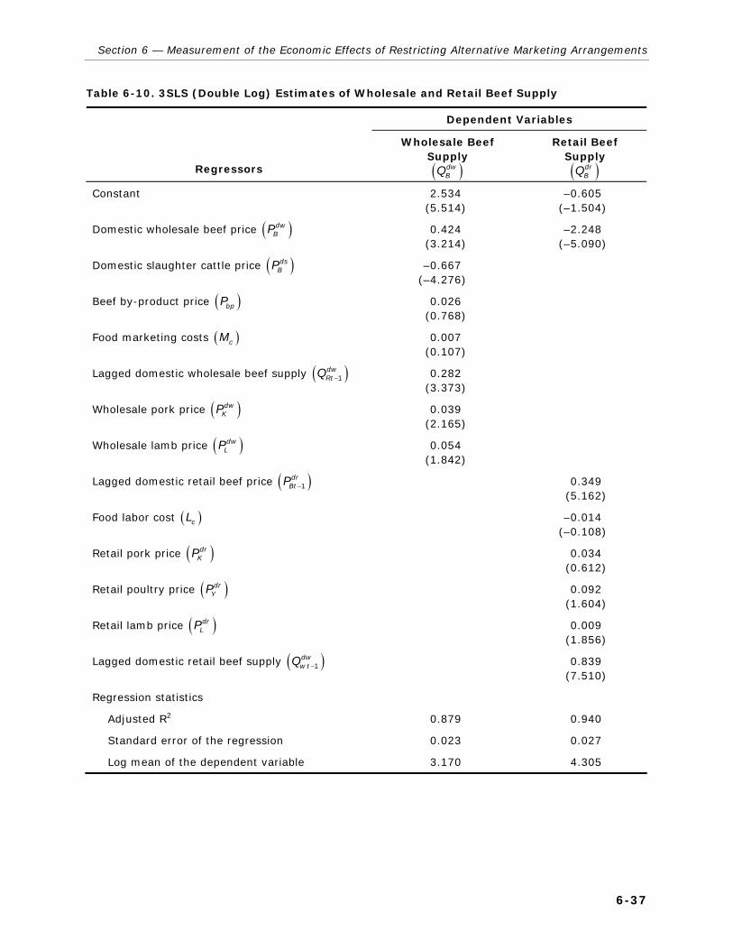
Section 6 — Measurement of the Economic Effects of Restricting Alternative Marketing Arrangements
6-37
Table 6-10. 3SLS (Double Log) Estimates of Wholesale and Retail Beef Supply
Dependent Variables
Regressors
Wholesale Beef Supply ( )dw
BQ
Retail Beef Supply ( )dr
BQ
Constant 2.534 (5.514)
–0.605 (–1.504)
Domestic wholesale beef price ( )dwBP 0.424
(3.214) –2.248
(–5.090)
Domestic slaughter cattle price ( )dsBP –0.667
(–4.276)
Beef by-product price ( )bpP 0.026 (0.768)
Food marketing costs ( )cM 0.007 (0.107)
Lagged domestic wholesale beef supply ( )1dwRtQ − 0.282
(3.373)
Wholesale pork price ( )dwKP 0.039
(2.165)
Wholesale lamb price ( )dwLP 0.054
(1.842)
Lagged domestic retail beef price ( )1drBtP − 0.349
(5.162)
Food labor cost ( )cL –0.014 (–0.108)
Retail pork price ( )drKP 0.034
(0.612)
Retail poultry price ( )drYP 0.092
(1.604)
Retail lamb price ( )drLP 0.009
(1.856)
Lagged domestic retail beef supply ( )1dww tQ − 0.839
(7.510)
Regression statistics
Adjusted R2 0.879 0.940
Standard error of the regression 0.023 0.027
Log mean of the dependent variable 3.170 4.305

Volume 3: Fed Cattle and Beef Industries
6-38
substantial differences between short-run and long-run supply elasticities. For livestock production, biological rigidities are generally manifest in relatively inelastic short-run supply responses. However, in the long run, relaxed biological constraints and near constant-returns-to-scale technologies cause relatively large supply responses (Marsh, 2003; Wohlgenant, 1989).
The primary supply of beef is represented by the calf crop equation (6.80). Breeding cow inventories are included in the specification and represent the production base for producing calves. The short-run and long-run calf crop inventory elasticities are 0.103 and 0.240 (0.103 / [1 – 0.570]), respectively (Table 6-8). Estimates of the long-run supply price elasticities of breeding inventories have generally exceeded unity (Foster and Burt, 1992; Marsh, 1999; Rucker, Burt, and LaFrance, 1984). However, Buhr and Kim (1997) used quarterly data from 1970 through 1990 and estimated short-run and long-run own-price elasticities of supply for calf crops as 0.05 and 0.46. The relatively small long-run elasticity estimates are caused by the inclusion of breeding cow inventories in the econometric specification. Breeding cow inventories account for long-run cyclical behavior (Rosen, Murphy, and Scheinkman, 1994; Rucker, Burt, and LaFrance, 1984).
The domestic supply of slaughter cattle is positively affected by slaughter cattle price, with short-run and long-run own-price supply elasticities of 0.133 and 0.496 (0.133 / [1 – 0.732]), respectively (Table 6-9). Marsh (2003) estimated short-run and long-run supply elasticities for slaughter cattle of 0.264 and 0.593, respectively, using annual data from 1970 through 1990.
The own-price elasticity of supply for imported slaughter cattle was assumed to equal 10.0 in the short run and long run. That is, we assume that the Canadian cattle industry is able to supply the U.S. packing industry with additional cattle without requiring increases in price. This assumption is consistent with historical Canadian supply relationships with respect to the U.S. beef industry.
The domestic wholesale supply of beef (carcass weight) is derived from primary feeder cattle production and slaughter cattle dressed weights. The behavioral relationship indicates that beef packers positively respond to wholesale price changes
Section 6 — Measurement of the Economic Effects of Restricting Alternative Marketing Arrangements
6-39
and negatively respond to changes in the input price of slaughter cattle (Table 6-10). The coefficient for food labor costs was not statistically significant. The short-run and long-run own-price elasticities of wholesale beef supply are 0.424 and 0.591 (0.424 / [1 – 0.282]), respectively. Bedinger and Bobst (1988) estimated the long-run own-price elasticity of supply for wholesale beef as 0.200 using quarterly data from 1965 through 1983.
The retail beef supply elasticities are positive with respect to retail price and negative with respect to boxed beef price (Table 6-10). The short-run and long-run retail beef own-price elasticities of supply are 0.349 and 2.154 (0.349 / [1 – 0.839]). The relatively elastic long-run supply elasticity is consistent with Wohlgenant’s (1989) argument that retail meat supply is a function of constant returns to scale production technologies. The cross-price elasticity of retail supply with respect to boxed beef price was –0.248 in the short run and –1.540 (–0.248 / [1 – 0.839]) in the long run.
6.5.4 Supply Quantity Transmission Elasticities
Estimates of quantity transmission elasticities are used in the equilibrium displacement model to provide a linkage between the vertically connected supply sectors. These estimates were obtained from the SUR estimation of four equations separate from the structural model. The supply quantity transmission elasticities are summarized in Table 6-6. Table 6-11 provides the complete SUR results of regressing the appropriate quantity variable at each level onto the appropriate downstream quantity variable. Double log specifications are used so that resulting parameter estimates are interpreted as transmission elasticities.
6.5.5 Elasticity Summary
3SLS estimation of annual rational distributed lag demand and supply equations in the beef marketing channel yielded statistically significant price elasticity estimates consistent with a priori expectations. That is, coefficient signs were consistent with theoretical constructs, and long-run elasticities were more elastic than short-run elasticities because technical, biological, and institutional constraints are less restrictive over time. Some of the market-level elasticities were comparable with other beef studies. For some of the beef and cattle data series, missing observations were imputed from observed data.

Volume 3: Fed Cattle and Beef Industries
6-40
Table 6-11. SUR (Double Log) Supply Quantity Transmission Elasticities
Dependent Variables
Regressors
Retail Beef Quantity ( )dr
BQ
Wholesale Beef Quantity
( )dwBQ
Domestic Slaughter
Cattle Quantity ( )ds
BQ
Constant 2.944 (11.351)
–0.260 (–1.324)
–0.033 (–0.154)
Domestic wholesale beef quantity ( )dwBQ 0.715
(8.860)
Imported live beef quantity ( )iwBQ
Domestic slaughter beef quantity ( )dsBQ 0.929
(17.504)
Domestic feeder beef quantity ( )dfBQ 0.944
(30.837)
Regression statistics
Adjusted R2 0.836 0.959 0.987
Standard error of the regression 0.021 0.013 0.007
Log mean of the dependent variable 5.207 3.170 3.695
Note: Quantity transmission equations corrected for first-order serial correlation in residuals.
The estimated model also yielded price elasticities among vertical sectors that conform to relative price spreads and primary and derived demand and supply expectations. That is, whether agricultural markets are characterized by fixed or variable input proportions, margin theory would indicate smaller demand elasticities proceeding from primary demand to derived demands and larger supply elasticities proceeding from primary supply to derived supplies (Gardner, 1975; Wohlgenant, 1989). The consistency of these results lends credibility to the market-level measurements in the equilibrium displacement model (Brester, Marsh, and Atwood, 2004).
6.6 OLIGOPSONY MARKDOWN PRICING Eqs. (6.20) and (6.23) in the equilibrium displacement model indicate that oligopsony power in the domestic wholesale processing sector may drive a price wedge between the derived demand and derived supply prices of domestic slaughter cattle and imported slaughter cattle. The parameter ρ represents the ratio /dsd dss
B BP P and /isd issB BP P . Thus, in the absence of
oligopsony markdown power, the value of ρ equals 1 as dsd dss
B BP P= and isd issB BP P= . The value of ρ increases as
Section 6 — Measurement of the Economic Effects of Restricting Alternative Marketing Arrangements
6-41
oligopsony power increases. As illustrated in Figure 6-4, increases in market power would cause a larger price wedge between dsd
BP and dssBP and a reduction in quantity from the
perfectly competitive market equilibrium. A similar result occurs for import slaughter cattle.
6.6.1 Estimates of Oligopsony Markdown Price Distortions
Published estimates of the degree of oligopsony markdown power are available for the beef industry and are used in the equilibrium displacement model. Schroeter (1988) extended Appelbaum‛s (1979, 1982) model for estimating monopoly market power to the problem of estimating monopsony price distortions in the slaughter cattle market. Using annual data from 1951 to 1983, Schroeter reported markdown price distortions ranging from 0.009% to 0.025% depending on the year. The average price distortion for the reported years was 0.013. This corresponds to an estimate of ρ of 1.013.
Azzam and Schroeter (1991) considered the degree of oligopsony price distortions across 13 regional slaughter cattle markets in 1986. Their estimate of markdown price distortions was less than 1%. This was a lower estimate of price distortions than the 1.2% to 2.5% estimates reported by earlier research (Menkaus, St. Clair, and Ahmaddaud, 1981; Quail et al., 1986; Ward, 1981). Koontz, Garcia, and Hudson (1993) used data from 1980 to 1986 and estimated slaughter cattle price distortions of 0.5% to 0.8% in a dynamic model of two-phase collusive pricing strategies. Muth and Wohlgenant‛s (1999) estimate of oligopsony markdown price behavior was not statistically different from zero using a variety of functional forms for the beef industry. Using quarterly data from 1978 to 1993, Weliwita and Azzam (1996) estimated oligopsony price distortions of 2.7% for fed cattle markets during a time of declining beef demand. Stiegert, Azzam, and Brorsen (1993) reported monopsony markdown pricing estimates ranging from 0.0% to 3.8% depending on the year considered. The average of their annual estimates was 1.31%.
6.6.2 Effects of Oligopsony Markdowns
The above estimates of oligopsony markdown price distortions in slaughter cattle prices range from 0.0% to 3.8%. This translates into an estimate of ρ that ranges from 1.000 to 1.038. Because the estimates vary and we want to include the most extreme estimates, the equilibrium displacement model

Volume 3: Fed Cattle and Beef Industries
6-42
will treat ρ as a random variable that ranges between 1.000 and 1.050 with most of the mass centered over 1.015 (the mean) for the domestic and imported slaughter cattle sector.
We assume that the data used in the model have been generated by a beef processing industry that has been able to exercise small amounts of oligopsony pricing power in the slaughter cattle industry. Therefore, although a restriction on the amount of a given AMA is likely to increase processing costs, it could also have an offsetting effect of reducing market power.
To illustrate this case, we use the elasticity estimates presented above to parameterize the equilibrium displacement model. Note that this is merely a simplified illustration. Simulations of the effects of potential changes in AMAs are presented in Section 6.10. For the current illustration, assume that a reduction in an AMA increases processing costs by 5%. We further assume that ρ is equal to 1.015. The short-run (Year 1) changes in equilibrium prices and quantities from a nonstochastic simulation are presented in the first column of Table 6-12. Prices and quantities change in the expected directions. For example, retail beef price increases by 2.81%, while retail beef quantity declines by 2.43%. Wholesale beef price increases and wholesale beef quantity declines. Domestic and imported slaughter cattle prices and quantities decline, as does feeder cattle price and quantity.
The second column of Table 6-12 presents changes in equilibrium prices and quantities caused by a 5% increase in processing costs coupled with a 0.005 percentage point reduction in market power (i.e., a reduction in ρ from 1.015 to 1.010). The accompanying reduction in market power offsets some of the effects of the cost increases. Note that price and quantity changes are slightly smaller in this second case. The only exception is that domestic and imported slaughter cattle demand price declines are larger than those presented in the first column. This is consistent with a reduction in market power.

Section 6 — Measurement of the Economic Effects of Restricting Alternative Marketing Arrangements
6-43
Table 6-12. Short-Run Percentage Changes in Prices and Quantities Given a 5% Increase in Wholesale Processing Costs (a Decrease in the Wholesale Derived Beef Supply Function) and a 0.005 Percentage Point Reduction in Potential Oligopsony Market Power Using a Nonstochastic Simulation
Endogenous Variables
No Change in Potential Market
Power
A Reduction in Potential Market
Power
Retail beef price 2.81% 2.75%
Retail beef quantity –2.43% –2.38%
Wholesale beef price 4.10% 4.01%
Wholesale beef quantity –4.77% –4.67%
Domestic slaughter cattle demand price –7.15% –7.17%
Domestic slaughter cattle supply price –7.25% –6.77%
Domestic slaughter cattle quantity –1.46% –1.37%
Imported slaughter cattle demand price –0.66% –0.99%
Imported slaughter cattle supply price –0.67% –0.51%
Imported slaughter cattle quantity –6.71% –5.07%
Feeder cattle price –5.13% –4.79%
Feeder cattle quantity –0.53% –0.49%
6.7 QUALITY CHANGES CAUSED BY CHANGES IN PROCUREMENT METHODS Restrictions on slaughter cattle procurement methods may potentially affect the quality of beef. Changes in AMAs may influence genetic development, cattle feeding, nutrition, logistics, and price incentives related to quality. Changes in beef quality are manifest in consumer demand. If beef quality is reduced, then consumer demand for beef will decline relative to other meat (i.e., pork, poultry, and lamb) substitutes. Such a decline is then transferred to upstream derived demands for wholesale beef, slaughter cattle, and feeder cattle. Although no direct measure of beef quality is available at the retail level, MPR data provide carcass quality measures. Therefore, the impacts of changes in AMAs on carcass quality grades are used to proxy changes in beef quality at the retail level.
Eq. (4.6) in Section 4.3.2 presented the estimates of the effects of AMAs on beef carcass quality, and Eq. (4.12) in Section 4.4.2 presented estimates of changes in beef carcass quality on retail demand price. The results indicated that the procurement of slaughter cattle through packer ownership and through formula

Volume 3: Fed Cattle and Beef Industries
6-44
procurement methods directly influenced quality. These results are combined in the next section to calculate the impacts of a 25% and a 100% reduction in the use of AMAs to procure slaughter cattle.
6.7.1 Changes in Retail Demand (Meat Quality) Resulting from a 25% Reduction in Formula and Packer Ownership Slaughter Cattle Procurement
A comparative statics procedure is used to estimate the impacts on retail demand of a reduction in formula and packer ownership cattle procurement. The impacts are obtained by using the product of elasticities presented in Eq. (4.6) and Eq. (4.12). Specifically, the reduction in retail demand is given by
% % % %25,
% % % % %r rp p QG QG
pf po QG pf po
⎛ ⎞Δ Δ ⎛ ⎞Δ Δ= + × −⎜ ⎟ ⎜ ⎟Δ + Δ Δ Δ Δ⎝ ⎠⎝ ⎠
(6.68)
where the left-hand term is the percentage change in inverse retail beef demand given additive percentage changes in formula and packer ownership procurement. The first term on the right side of Eq. (6.68) is the percentage change in retail price given a percentage change in quality (QG) that was estimated based on Eq. (4.12). The second term on the right side represents the percentage change in quality grade caused by a percentage change in formula procurement and the percentage change in quality grade caused by a percentage change in packer ownership procurement, as presented in Eq. (4.6). The last term on the right represents a 25% reduction in formula and packer ownership procurement.
Using estimates presented in Sections 4.2 and 4.3, a reduction in formula and packer ownership procurement is estimated to reduce retail beef demand by 0.039%, as calculated in Eq. (6.69):
0.143 × (0.009 + 0.002) × (–25.0) = –0.039%. (6.69)
6.7.2 Changes in Retail Demand (Meat Quality) Resulting from a 100% Reduction in Formula and Packer Ownership Slaughter Cattle Procurement
Eq. (6.68) is also applied to the case in which formula and packer ownership cattle procurement is reduced by 100% (i.e., eliminated). Eq. (6.70) indicates that this scenario would result in a reduction of retail demand for beef of 0.157%:
(0.143) × (0.009 + 0.002) × (–100.0) = –0.157%. (6.70)

Section 6 — Measurement of the Economic Effects of Restricting Alternative Marketing Arrangements
6-45
6.8 COST CHANGES CAUSED BY CHANGES IN PROCUREMENT METHODS Restrictions on fed cattle slaughter procurement methods would impose additional costs on beef packers. Costs would increase because of increased transactions costs and decreased efficiencies in slaughtering and processing. These changes in costs would likely be reflected in changes in output prices for wholesale beef or input prices for fed cattle.
The estimation of the cost changes resulting from restrictions on AMAs for fed cattle purchases was presented in Section 3 of this volume. The specific estimates used in the simulations (see Table 3-4) are as follows:
For a 25% reduction in the use of AMAs for procurement of fed cattle, we assume a 0.86% increase in costs.
For a 100% reduction in the use of AMAs for procurement of fed cattle, we assume a 4.68% increase in costs.
6.9 ESTIMATED CHANGES IN POTENTIAL MARKET POWER CAUSED BY CHANGES IN PROCUREMENT METHODS If present, oligopsony power in the beef packing sector is likely manifest in downward pressure on domestic and imported slaughter cattle prices. Figure 6-4 illustrates the market power impacts as a wedge between slaughter cattle demand price and slaughter cattle supply price. The size of this wedge depends on the relative size of oligopsony power. Nonetheless, if oligopsony market power is related to AMAs, then reductions in formula and packer ownership procurement should reduce market power and narrow the difference between slaughter cattle demand and supply prices.
Several methods exist to directly estimate the degree of oligopsony market power (Appelbaum, 1982; Muth and Wohlgenant, 1999; Crespi, Gao, and Peterson, 2005; Schroeter, 1988; Stiegert, Azzam, and Brorsen, 1993). However, data limitations in the beef processing industry for the MPR period prevent the direct application of these approaches.

Volume 3: Fed Cattle and Beef Industries
6-46
6.9.1 Monthly Model for Estimating Oligopsony Market Power
Because of data limitations, the following beef market power equation is specified:
( )2 3 4, , , , , ,t t t t t tBM MC TB QB PB s s sψ μ= + , (6.71)
where BM is the four firm concentration ratio of steer and heifer slaughter; MC represents food marketing processing costs; TB represents technological change in the beef processing industry (trend); QB is wholesale beef production; PB is retail beef price; s2, s3, and s4 represent seasonal binary variables for the second, third, and fourth quarters of each calendar year; and μt
is a random error term with white noise properties. Table 6-13 presents the variable definitions and descriptive statistics. The variable BMt is assumed to include potential market power along with other processor profitability factors. Given that Eq. (6.71) is properly specified (i.e., processing costs, technology, production volume, and retail demand price are expected to affect the concentration ratio), the estimated residuals (i.e., the difference between the actual and predicted values of BMt) could plausibly represent an estimate of potential market power. Of course, it is likely that the residuals of Eq. (6.71) contain other factors beyond those associated with potential market power. However, the estimated residuals would represent the largest potential market power effects possible.
To the extent that the residuals of Eq. (6.71) represent (the largest possible) effects of potential market power, we regress those residuals onto the percentage of AMA cattle procurement. That is, formula or packer ownership procurement methods could reduce competition for fed cattle and lower prices below those that would occur in a perfectly competitive market (Schroeder et al., 1991). Therefore, we estimate the following equation:
( )2 3 4, , , , ,t t t t tMBF f pf po pc s s s ε= + , (6.72)
where MBF is potential beef market power (i.e., the residuals from Eq. [6.71]), pf is the proportion of cattle procured by formula methods, po is the proportion of cattle procured by packer ownership, pc is the proportion of cattle procured through cash methods, si represent quarterly seasonal binary variables, and ,t is a white noise error term.

Section 6 — Measurement of the Economic Effects of Restricting Alternative Marketing Arrangements
6-47
Table 6-13. Variable Definitions for the Beef Potential Market Power Model
Symbol Definition Mean Standard Deviation
BM Four firm concentration ratio, steer and heifer slaughter
81.310 0.400
MC Real food marketing processing cost index (1987 = 100.0)
306.200 5.980
TB Beef processing technology (trend) 28.000 16.600
QB Quantity of wholesale beef production, billion pounds 2.150 0.180
PB Real retail beef price, cents/lb 201.380 13.890
MBF Beef potential market power, residuals of Eq. (6.71) 0.000 0.002
pf Beef procurement by formula, share (%) 41.430 10.160
po Beef procurement by packer ownership, share (%) 6.410 2.380
pc Beef procurement by cash methods, share (%) 48.890 10.020
S2 Second quarter seasonal binary variable 0.286 0.457
S3 Third quarter seasonal binary variable 0.214 0.415
S4 Fourth quarter seasonal binary variable 0.214 0.415
Eq. (6.72) permits measuring the marginal impacts of AMAs on potential market power. For example, if beef packers are constrained on the amount of cattle they purchase through AMAs, this may reduce processing efficiencies. However, such an action may also reduce potential oligopsony market power.
6.9.2 Data Development and Estimation of the Monthly Potential Market Power Model
The sample period for the estimation of the potential market power model (Eq. 6.71) consists of monthly observations from April 2001 (the beginning of MPR) through December 2005. Annual data for the beef concentration ratio were obtained from the USDA/GIPSA Packers and Stockyards Statistical Report, and monthly observations were obtained by linear interpolation. Monthly wholesale beef production and retail beef prices were obtained from LMIC. Food marketing costs were obtained on a quarterly basis from Agricultural Outlook (USDA, various issues). The AMA beef procurement data were obtained from the USDA’s Mandatory Price Reporting Datamart (http://mpr.datamart.ams.usda.gov). The retail beef price and

Volume 3: Fed Cattle and Beef Industries
6-48
food marketing cost variables were deflated by the CPI. The CPI data were obtained from the Economic Report of the President.
Eq. (6.71) is estimated in double log form. The OLS results are as follows:
2 3 4
2
ln 4.943 0.143ln 0.008ln
(41.528) ( 8.286) (1.423)
0.041ln 0.002 0.001 0.001
(6.857) ( 2.407) ( 1.175) ( 0.832)
0.771 . . 0.002 (log ) 4.398.
t t t
t
BM MC QB
PB s s s
R S E BM mean
= − +
−
+ − − −
− − −
= = =
(6.73)
The critical t-values at the α = 0.05 and α = 0.10 significance levels are 1.960 and 1.645 (50 degrees of freedom). The trend variable was omitted from the regression because of multicollinearity with several variables. The adjusted R2 statistic is relatively small so that the residuals of the equation likely contain information beyond that attributable to potential market power effects. That is, the residuals should represent the largest possible market power effects.
The residuals of Eq. (6.73) are nonnormally distributed (using a Jacque-Bera test statistic) with a mean near zero and a standard deviation of 0.002. These residuals are used as the dependent variable in Eq. (6.72) of the monthly market power model as a proxy for MBF. Because this proxy likely contains information in addition to the effects of potential market power, the estimated parameters of Eq. (6.72) should be considered an upper bound of the potential market power effects resulting from changes in procurement methods.
6.9.3 Empirical Estimates of Procurement Methods on Potential Market Power
The market power equation (Eq. [6.72]) is estimated using monthly data from April 2001 through December 2005. The estimated equation includes distributed lag adjustments. In initial regressions, the contemporaneous monthly AMA values and the first-order lag on the dependent variable (Koyck term) were not statistically different from zero based on the Wald coefficient test. Hence, those coefficients were omitted in the final regression. The Breusch-Godfrey LM test indicated that AR(1) and AR(2) error components were required. Eq. (6.72) was estimated in double logs using nonlinear least squares and

Section 6 — Measurement of the Economic Effects of Restricting Alternative Marketing Arrangements
6-49
the residuals from Eq. (6.73) as the dependent variable. The regression results are
-1 -1 -1
2 3 4 -1 -2
2
0.013 0.005 ln 0.002 ln 0.005 ln
(1.941) (1.772) (2.257) (1.551)
0.003 0.002 0.001 0.914 - 0.244
(4.784) (4.062) (1.905) (5.677) (-1.661)
0.652 . . 0.001 ( ) 0.001.
t t t t
t t
MBF pf po pc
s s s
R S E MBF mean
μ μ
= + + +
+ + + +
= = =
(6.74)
The dependent variable is already in log form because it represents the residuals of Eq. (6.73). Therefore, a second logarithmic transformation is not used. The reported mean for the dependent variable differs slightly from that presented in Table 6-13 because the specified lags result in the loss of three degrees of freedom. The critical t-values at the α = 0.05 and α = 0.10 significance levels are 2.021 and 1.684 (42 degrees of freedom). The inverted AR roots are conjugate complex with a modulus of 0.498, which indicates that the stochastic error process is stable. The model explains about 65% of the variation in the dependent variable. The coefficient estimate for cash procurement is not statistically different from zero.
Results indicate that formula (pf) and packer ownership (po) procurement methods are statistically significant in determining potential market power. However, their economic effects are small. A 10% increase in formula procurement is associated with a 0.05% increase in potential market power, while a 10% increase in packer ownership procurement is associated with a 0.02% increase in potential market power. The relatively inelastic responses indicate that reductions in the use of AMAs would have only small impacts on potential market power.
The following two sections present the calculations needed to use these estimates of changes in potential market power in the equilibrium displacement model.
6.9.4 Estimated Changes in Potential Market Power Caused by a 25% Reduction in Formula and Packer Ownership Procurement
The empirical estimation of Eq. (6.74) required the use of the residuals from Eq. (6.73) as a proxy for potential market power. The results indicate that a 1% decrease in formula and packer ownership procurement is related to a 0.005 and a

Volume 3: Fed Cattle and Beef Industries
6-50
0.002 percentage point decline in market power (D), respectively. Cash procurement did not statistically affect beef processor market power. Eq. (6.75) presents the calculations used to estimate the change in potential market power resulting from a 25% reduction in both formula and packer ownership procurement:
( ) ( )
25.00 25.00
0.005 25.00 0.002 25.00 0.175%.
MBF MBFpf po
∂ ∂⎛ ⎞ ⎛ ⎞× − + × − =⎜ ⎟ ⎜ ⎟∂ ∂⎝ ⎠ ⎝ ⎠
× − + × − = −
(6.75)
Thus, a 25% reduction in formula and packer ownership procurement is expected to reduce beef potential market power by 0.175 percentage points.
6.9.5 Estimated Changes in Potential Market Power Caused by a 100% Reduction in Formula and Packer Ownership Procurement
An analogous procedure is followed to estimate the impact of a 100% reduction (i.e., complete elimination) of formula and packer ownership procurement on potential market power. The 100% reduction in both methods yields
( ) ( )
100.0 100.0
0.005 100.0 0.002 100.0 0.700%.
MBF MBFpf po
∂ ∂⎛ ⎞ ⎛ ⎞× − + × − =⎜ ⎟ ⎜ ⎟∂ ∂⎝ ⎠ ⎝ ⎠
× − + × − = −
(6.76)
Thus, a 100% reduction in formula and packer ownership procurement is expected to reduce beef potential market power by 0.700 percentage points, a relatively small effect.
6.10 SIMULATION RESULTS In this section, we present the results of simulations of potential changes in AMAs that would reduce or eliminate various procurement methods. The simulations are conducted using the inputs described in Sections 6.7, 6.8, and 6.9.
6.10.1 Results of a 25% Reduction in Formula and Packer Ownership Procurement
A 25% reduction in formula and packer ownership procurement is expected to have three initial effects on the beef sector. First, beef quality is expected to decline and decrease primary demand by 0.039% (Eq. [6.69]). Second, processing costs

Section 6 — Measurement of the Economic Effects of Restricting Alternative Marketing Arrangements
6-51
would increase because of changes in procurement methods. Thus, the wholesale derived supply function is expected to shift upwards and to the left by 0.86% (Section 6.8). Third, potential market power is expected to decline by 0.175 percentage points (Eq. [6.75]). These three inputs are used in the equilibrium displacement model to estimate price, quantity, and consumer and producer surplus changes resulting from a 25% reduction in formula and packer ownership procurement.
Table 6-14 reports simulated mean changes in the endogenous price and quantity variables and associated 95% confidence intervals for a 25% reduction in formula and packer ownership procurement. Most estimates are significantly different from zero at either the 5% or 10% level. The short-run time period represents changes in prices and quantities that occur at the end of Year 1.
In the short run, all prices decline with the exception of small increases in retail and wholesale beef prices. Retail beef price increases by 0.46%, wholesale beef price increases by 0.70%, domestic slaughter cattle supply price declines by 1.27%, and feeder cattle price declines by 0.10%. In addition, all quantities decline by a small amount. Essentially, these results reflect that the positive effect of reduced potential oligopsony processor market power is unable to offset the negative effects of increased processing costs and decreased retail demand.
To estimate long-run effects, we assume that the beef market would return to an equilibrium after 10 years of adjustments to changes in cattle procurement. We multiplicatively increase supply and demand elasticities between the short-run estimates (Year 1) and long-run estimates (Year 10). The long-run results represent changes in prices and quantities that would occur in Year 10 relative to initial levels. The long-run price effects follow the short-run results in terms of direction. However, the long-run changes in prices are generally smaller than the short-run changes because of increasing supply and demand elasticities. For example, domestic slaughter cattle supply price declines by 0.65%, and feeder cattle prices decline by 0.08% in the long run. With the exception of wholesale beef quantity and domestic slaughter cattle quantity, the long-run quantity declines are slightly smaller than the short-run declines because, again, of more elastic supply responses over time.

Volume 3: Fed Cattle and Beef Industries
6-52
Table 6-14. Percentage Changes in Prices and Quantities Given a 25% Reduction in Formula and Packer Ownership Beef Procurementa
Endogenous Variables Short Run Long Run (Year 10)
Retail beef price 0.46% (0.26, 0.77)
0.17% (0.09, 0.29)
Retail beef quantity –0.43% (–0.67, –0.27)
–0.24% (–0.38, –0.14)
Wholesale beef price 0.70% (0.43, 1.12)
0.66% (0.42, 1.05)
Wholesale beef quantity –0.82% (–1.20, –0.59)
–0.84% (–1.30, –0.57)
Domestic slaughter cattle demand price –1.43% (–3.17, –0.70)
–0.81% (–1.63, –0.44)
Domestic slaughter cattle supply price –1.27% (–3.02, –0.53)
–0.65% (–1.46, –0.26)
Domestic slaughter cattle quantity –0.25% (–0.62, –0.08)
–0.38% (–0.88, –0.14)
Imported slaughter cattle demand price –0.25% (–0.48, –0.16)
–0.20% (–0.37, –0.13)
Imported slaughter cattle supply price –0.08%b (–0.31, 0.01)
–0.03%c
(–0.20, 0.05)
Imported slaughter cattle quantity –0.75%b (–3.11, 0.13)
–0.28%c (–1.96, 0.45)
Feeder cattle price –0.10% (–0.28, –0.02)
–0.08% (–0.21, –0.02)
Feeder cattle quantity –0.94% (–2.66, –0.24)
–0.34% (–0.85, –0.10)
Note: All other values are significantly different from zero at the 5% level. a This scenario corresponds to a 0.039% decrease in retail beef demand, a 0.86% decrease in the wholesale
derived beef supply function, and a 0.175 percentage point reduction in beef packer potential oligopsony power. b Significantly different from zero at the 10% level. c Not significantly different from zero.
Table 6-15 presents changes in producer surplus at each level of the marketing chain and changes in consumer surplus at the retail level. Most estimates are at least significantly different from zero at the α = 0.10 level. Short-run results are presented in the first column, and long-run results are presented in the second column. Changes in producer surplus contain a dynamic element in that producer surplus increases or decreases occur over time. Therefore, it is appropriate to consider cumulative changes in producer surplus that accrue as an industry adjusts from a short- to a long-run equilibrium. To simulate these

Section 6 — Measurement of the Economic Effects of Restricting Alternative Marketing Arrangements
6-53
Table 6-15. Changes in Producer and Consumer Surplus Given a 25% Reduction in Formula and Packer Ownership Beef Procurement, Billion $a,b
Surplus Measure Short Run
Long Run (Year 10) Cumulative
Cumulative Present Value
Percentage of Total Present
Value Cumulative
Surplus
Producer surplus
Retail beef producer surplus
–$0.0980 –$0.0870 –$1.504 –$1.161 –0.36%
Wholesale beef producer surplus
–$0.1430 –$0.1910 –$1.654 –$1.261 –0.86%
Domestic slaughter cattle producer surplus
–$0.5580 –$0.2500 –$3.886 –$3.107 –1.35%
Import slaughter cattle producer surplus
–$0.0004c –$0.0001d –$0.003d –$0.002d –1.10%d
Feeder cattle producer surplus
–$1.0690 –$0.1740 –$5.141 –$4.273 –2.67%
Total change in domestic producer surplus
–$1.8670 –$0.7030 –$12.184 –$9.802 –1.14%
Total change in import producer surplus
–$0.0004c –$0.0001d –$0.003d –$0.002d –1.10%d
Total change in producer surplus
–$1.8670 –$0.7030 –$12.187 –$9.804 –1.14%
Consumer surplus
Retail beef consumer surplus
–$0.3710 –$0.1510 –$2.539 –$2.037 –0.83%
a This scenario corresponds to a 0.039% decrease in retail beef demand, a 0.86% decrease in the wholesale derived beef supply function, and a 0.175 percentage point reduction in beef packer potential oligopsony power.
b Producer and consumer surplus are calculated relative to 2000–2003 average quantities and prices. c Significantly different from zero at the 10% level. d Not significantly different from zero.
cumulative effects, we assume that it takes 10 years to adjust from the short run to the long run in the meat industry.
The third column of Table 6-15 (labeled “Cumulative”) presents the simple summation of producer and consumer surplus changes over 10 years for each market level. The fourth column (labeled “Cumulative Present Value”) presents the present value of these changes in producer and consumer surplus, assuming a 5% discount rate. Over the 10-year adjustment period, all sectors lose surplus. Finally, percentage changes in the net present value of producer and consumer surplus with respect to total producer and consumer surplus

Volume 3: Fed Cattle and Beef Industries
6-54
over the 10-year period are presented in the last column of Table 6-15. The feeder cattle sector loses a higher percentage of producer surplus (2.67%) relative to all other beef production sectors.
6.10.2 Results of a 100% Reduction in Formula and Packer Ownership Procurement
A 100% reduction in formula and packer ownership procurement is expected to reduce retail beef demand by 0.157% (Eq. [6.70]), increase wholesale processing costs by 4.68% (Section 6.8), and reduce potential market power by 0.70 percentage points (Eq. [6.76]). Table 6-16 reports mean changes in the endogenous price and quantity variables and associated 95% confidence intervals for a 100% reduction in formula and packer ownership procurement. Most estimates are at least significantly different from zero at the 10% level.
With the exception of retail and wholesale beef prices, all prices and quantities decline in the short run. Retail beef prices increase by 2.57%, and retail beef quantities decline by 2.35%. Slaughter and feeder cattle prices decline by 7.12% and 0.54%, respectively.
The long-run price and quantity results follow the short-run results in terms of direction, with generally smaller price declines. Again, these results are consistent with increasing supply and demand elasticities over time. For example, domestic slaughter cattle supply prices decline by 3.68%, and feeder cattle prices decline by 0.47% in the long run. Domestic slaughter and feeder cattle quantities decline by 2.15% and 1.96% in the long run.
Table 6-17 presents changes in producer surplus at each level of the marketing chain and changes in consumer surplus at the retail level. In general, most estimates are at least significantly different from zero at the α = 0.10 level. Short-run results are presented in the first column, and long-run results are presented in the second column. The third column of Table 6-17 (labeled “Cumulative”) presents the simple summation of producer and consumer surplus changes over 10 years for each market level.
The fourth column of Table 6-17 (labeled “Cumulative Present Value”) presents the present value of 10 years of changes in producer and consumer surplus, assuming a 5% discount rate.

Section 6 — Measurement of the Economic Effects of Restricting Alternative Marketing Arrangements
6-55
Table 6-16. Percentage Changes in Prices and Quantities Given a 100% Reduction in Formula and Packer Ownership Beef Procurementa
Endogenous Variables Short Run Long Run (Year 10)
Retail beef price 2.57% (1.45, 4.27)
0.97% (0.52, 1.64)
Retail beef quantity –2.35% (–3.64, –1.46)
–1.29% (–2.04, –0.75)
Wholesale beef price 3.87% (2.42, 6.17)
3.67% (2.39, 5.85)
Wholesale beef quantity –4.51% (–6.59, –3.23)
–4.62% (–7.10, –3.12)
Domestic slaughter cattle demand price –7.73% (–17.23, –3.78)
–4.33% (–8.73, –2.28)
Domestic slaughter cattle supply price –7.12% (–16.71, –3.11)
–3.68% (–8.14, –1.60)
Domestic slaughter cattle quantity –1.42% (–3.45, –0.45)
–2.15% (–4.84, –0.84)
Imported slaughter cattle demand price –1.18% (–2.46, –0.69)
–0.96% (–1.91, –0.56)
Imported slaughter cattle supply price –0.49% (–1.78, 0.005)
–0.27%b (–1.22, 0.13)
Imported slaughter cattle quantity –4.90% (–17.77, 0.05)
–2.67%b (–12.21, 1.27)
Feeder cattle price –0.54% (–1.54, –0.14)
–0.47% (–1.18, –0.13)
Feeder cattle quantity –5.30% (–14.73, –1.41)
–1.96% (–4.80, –0.58)
a This scenario corresponds to a 0.157% decrease in retail beef demand, a 4.68% decrease in the wholesale derived beef supply function, and a 0.70 percentage point reduction in beef packer potential oligopsony power.
b Not significantly different from zero. All other values are significantly different from zero at the 5% level.
Over the 10-year adjustment period, all sectors lose producer surplus. The last column indicates that the feeder cattle sector loses a higher percentage of producer surplus (15.96%) relative to all other beef production sectors.
6.10.3 Results of a 100% Reduction in Formula and Packer Ownership Procurement, Assuming the Elimination of Potential Oligopsony Power
For illustration purposes, it is instructive to consider a case in which a 100% reduction in formula and packer ownership procurement would completely eliminate potential oligopsony market power. The research presented above does not support

Volume 3: Fed Cattle and Beef Industries
6-56
Table 6-17. Changes in Producer and Consumer Surplus Given a 100% Reduction in Formula and Packer Ownership Beef Procurement, Billion $a,b
Surplus Measure Short Run
Long Run (Year 10) Cumulative
Cumulative Present Value
Percentage of Total Present
Value Cumulative
Surplus
Producer surplus
Retail beef producer surplus –$0.547 –$0.467 –$8.230 –$6.366 –2.00%
Wholesale beef producer surplus
–$0.838 –$1.109 –$9.639 –$7.351 –5.24%
Domestic slaughter cattle producer surplus
–$3.116 –$1.415 –$21.813 –$17.430 –7.82%
Imported slaughter cattle producer surplus
–$0.003 –$0.001c –$0.020d –$0.016d –7.67%
Feeder cattle producer surplus
–$6.000 –$0.996 –$29.004 –$24.094 –15.96%
Total change in domestic producer surplus
$10.501 –$3.987 –$68.687 –$55.242 –6.64%
Total change in imported producer surplus
–$0.002 –$0.001c –$0.020c –$0.016d –7.67%d
Total change in producer surplus
$10.503 –$3.988 –$68.707 –$55.258 –6.64%
Consumer surplus
Retail beef consumer surplus –$2.002 –$0.806 –$13.657 –$10.962 –4.56%
a This scenario corresponds to a 0.157% decrease in retail beef demand, a 4.68% decrease in the wholesale derived beef supply function, and a 0.70 percentage point reduction in beef packer potential oligopsony power.
b Producer and consumer surplus are calculated relative to 2000–2003 average quantities and prices. c Not significantly different from zero. d Significantly different from zero at the 10% level.
such a scenario. However, if the goal of a complete elimination of formula and packer ownership procurement is to eliminate potential oligopsony power, it is interesting to consider a hypothetical situation in which that actually occurs. Note that potential oligopsony power could still occur within cash markets. However, we ignore that possibility in this simulation.
This simulation follows that of Section 6.10.2, except that the potential market power parameter (ρ) is assumed to equal 1 after the elimination of formula and packer ownership procurement. That is, it is assumed that a price wedge would no longer exist between the demand and supply prices for domestic and imported slaughter cattle.

Section 6 — Measurement of the Economic Effects of Restricting Alternative Marketing Arrangements
6-57
Table 6-18 reports mean changes in the endogenous price and quantity variables and associated 95% confidence intervals for this scenario. All short-run estimates are at least significantly different from zero at the 10% level, as are most of the long-run estimates.
Table 6-18. Percentage Changes in Prices and Quantities Given a 100% Reduction in Formula and Packer Ownership Beef Procurement and the Elimination of Potential Oligopsony Powera
Endogenous Variables Short Run Long Run (Year 10)
Retail beef price 2.48% (1.41, 4.15)
0.90% (0.48, 1.56)
Retail beef quantity –2.28% (–3.50, –1.40)
–1.21% (–1.95, –0.71)
Wholesale beef price 3.73% (2.32, 5.97)
3.43% (2.21, 5.59)
Wholesale beef quantity –4.36% (–6.38, –3.13)
–4.33% (–6.72, –2.92)
Domestic slaughter cattle demand price –7.76% (–17.59, –3.84)
–4.52% (–8.95, –2.52)
Domestic slaughter cattle supply price –6.38% (–15.81, –2.40)
–3.09% (–7.58, –1.06)
Domestic slaughter cattle quantity –1.27% (–3.31, –0.37)
–1.79% (–4.47, –0.55)
Imported slaughter cattle demand price –1.71% (–2.92, –1.24)
–1.37% (–2.23, –0.98)
Imported slaughter cattle supply price –0.23%b (–1.46, 0.002)
0.11%b (–0.76, 0.50)
Imported slaughter cattle quantity –2.35%b (–14.65, 2.36)
1.07%b (–7.61, 5.04)
Feeder cattle price –0.49% (–1.44, –0.11)
–0.39% (–1.04, –0.10)
Feeder cattle quantity –4.74% (–14.03, –1.16)
–1.64% (–4.35, –0.41)
a This scenario corresponds to a 0.157% decrease in retail beef demand and a 4.68% decrease in the wholesale derived beef supply function.
b Not significantly different from zero. All other values are significantly different from zero at the 5% level.
The results reported in Table 6-18 are very similar to those reported in Table 6-16. That is, even if the elimination of formula and packer ownership cattle procurement would completely eliminate potential oligopsony power, the net effects would be to reduce price and quantities in almost all sectors

Volume 3: Fed Cattle and Beef Industries
6-58
because of additional processing costs and reductions in beef quality.
Table 6-19 presents changes in producer surplus at each level of the marketing chain and changes in consumer surplus at the retail level in response to this hypothetical scenario. Again, the results are virtually identical to those reported in Table 6-17.
Table 6-19. Changes in Producer and Consumer Surplus Given a 100% Reduction in Formula and Packer Ownership Beef Procurement and the Elimination of Potential Oligopsony Power, Billion $a,b
Header Short Run
Long Run (Year 10) Cumulative
Cumulative Present Value
Percentage of Total Present
Value Cumulative
Surplus
Producer surplus
Retail beef producer surplus –$0.530 –$0.440 –$7.867 –$6.091 –1.92%
Wholesale beef producer surplus
–$0.807 –$1.036 –$9.150 –$6.988 –4.97%
Domestic slaughter cattle producer surplus
–$2.792 –$1.187 –$19.059 –$15.270 –6.79%
Imported slaughter cattle producer surplus
–$0.001 –$0.001c –$0.004c –$0.003c –1.54%c
Feeder cattle producer surplus
–$5.366 –$0.832 –$25.427 –$21.171 –13.79%
Total change in domestic producer surplus
–$9.495 –$3.496 –$61.503 –$49.520 –5.92%
Total change in imported producer surplus
–$0.001 –$0.001c –$0.004c –$0.003c –1.54%c
Total change in producer surplus
–$9.496 –$3.496 –$61.507 –$49.523 –5.91%
Consumer surplus
Retail beef consumer surplus –$1.937 –$0.760 –$13.083 –10.511 –4.37%
a This scenario corresponds to a 0.157% decrease in retail beef demand and a 4.68% decrease in the wholesale derived beef supply function.
b Producer and consumer surplus are calculated relative to 2000–2003 average quantities and prices. c Not significantly different from zero.
6.10.4 Potential Market Power, Processing Costs, and AMAs
Section 6.10.3 illustrates a hypothetical case in which a 100% reduction in formula and packer ownership procurement would completely eliminate potential oligopsony market power. However, these results are dependent upon the assumption of the initial size of oligopsony markdown pricing behavior. That
Section 6 — Measurement of the Economic Effects of Restricting Alternative Marketing Arrangements
6-59
is, if such potential market power is large enough initially, then elimination of that potential market power could theoretically offset increased processing costs and reduced beef quality in terms of changes in producer surplus.
Therefore, the equilibrium displacement model was used in a static simulation to determine the minimum size of initial potential market power for which, upon its removal through the complete elimination of AMAs, slaughter cattle producers would be invariant to such an action. The model indicates that an initial oligopsony markdown pricing of fed cattle of 4.28% would have to exist in order for benefits and costs of reducing AMAs to be equivalent. Most empirical estimates of oligopsony markdowns in beef are generally less than 3.8%.
Finally, it is interesting to consider relative magnitudes of negative effects of changes in AMAs in processing costs and beef quality versus the positive effects of reductions in potential market power. A static simulation was conducted to further investigate these tradeoffs. The above simulation was repeated (i.e., a 100% reduction in AMAs and the complete elimination of potential market power), and the negative impacts on processing costs and beef quality were altered until the discounted net present value of domestic slaughter cattle producer surplus was unaffected by changes in AMAs.
The results indicate that domestic slaughter cattle producers would be indifferent to the elimination of AMAs if that action would cause no change in beef quality and only a 1.71% increase in processing costs. Note that Section 6.7.2 estimates that the complete elimination of AMAs would reduce retail demand because of a reduction in beef meat quality by 0.157%, and Section 6.8 indicates that this action would increase processing costs by 4.68%.
6.11 SUMMARY OF CHANGES IN PROCUREMENT METHODS ON PRICES, QUANTITIES, AND PRODUCER SURPLUS We developed a stochastic, dynamic, equilibrium displacement model of the U.S. beef industry. The model includes supply and demand relations for the feeder cattle, domestic slaughter cattle, imported slaughter cattle, wholesale beef carcasses, and retail beef demand sectors. The model explicitly considers oligopsony markdown pricing behavior by beef packers and

Volume 3: Fed Cattle and Beef Industries
6-60
correlations among elasticity estimates. The model is parameterized by econometrically estimating a structural demand supply system of equations using publicly available annual data from 1970 to 2003.
The equilibrium displacement model also requires estimates of changes in costs that may occur if restrictions are placed on specific AMAs. We estimated a monthly, reduced-form model of boxed beef, slaughter cattle, and feeder cattle prices. A potential market power equation based on packer concentration ratios is included. The system is estimated using monthly MPR data. The monthly model is used to estimate the effects of changes in marginal costs at the packer level and changes in potential oligopsony market power in response to assumed restrictions on the use of AMAs. In addition, we incorporate potential changes in beef quality resulting from changes in AMAs.
Specifically, we simulate the results of a 25% reduction in the procurement of domestic and imported slaughter cattle by formula and packer ownership procurement. We also simulate changes caused by a 100% reduction in formula and packer ownership procurement of slaughter cattle. In both cases, it is assumed that these reductions caused increased procurement via other methods.
The equilibrium displacement model quantifies the effects of the above changes in AMAs on annual equilibrium prices, quantities, producer surplus, and consumer surplus over a 10-year period. In addition, Monte Carlo simulations (1,000) are used to construct empirical probability distributions so that the statistical significance of each endogenous variable can be evaluated. Empirical results are reported for short-term (1 year), long-term (10 years), and cumulative effects. All sectors lose producer (consumer) surplus in the short and long runs.
Furthermore, the feeder cattle production sector loses the most producer surplus relative to all other sectors in both absolute and percentage terms. Feeder cattle producers collectively lose the most producer surplus by restricting the use of AMAs because the derived demand and primary supply elasticity estimates at this level are more inelastic relative to other levels. That is, feeder cattle producers are less able to make short-run supply adjustments to price changes relative to other sectors. In addition, feeder cattle producers have the most to lose from

Section 6 — Measurement of the Economic Effects of Restricting Alternative Marketing Arrangements
6-61
decreases in the demand for beef because the own-price elasticity of the derived demand for feeder cattle is also more inelastic relative to other sectors. Therefore, to the extent that a reduction in AMAs reduces processing cost efficiencies and beef quality by more than the gains obtained from reductions in potential market power, the feeder cattle sector is harmed more than any other cattle/beef production sector.
For illustration purposes, a third simulation was conducted in which a 100% reduction in formula and packer ownership procurement was assumed to completely eliminate potential oligopsony market power. The results were not significantly different from those reported above. That is, even if the elimination of formula and packer ownership cattle procurement would completely eliminate potential oligopsony power, the net effects would be to reduce price, quantities, and producer and consumer surplus in almost all sectors because of additional processing costs and reductions in beef quality.
Finally, two additional simulations were conducted. The first evaluated the amount of oligopsony markdown pricing that must currently exist so that the complete elimination of that potential market power (by eliminating the use of AMAs) would result in no change in producer surplus at the slaughter cattle level. The analysis indicates that the current level of markdown pricing would have to be 4.28%, which is generally larger than empirical estimates for the beef industry. The second additional simulation evaluated the amount of increased processing costs that could be offset by reductions in potential market power so that producer surplus in the slaughter cattle sector would be unaffected. The simulation indicates that a 1.71% increase in processing costs (assuming no changes in beef quality) could be offset by reductions in potential market power. However, under the scenario in which a 100% reduction in AMAs occurs, we estimate that processing costs would increase by 4.68%.


7-1
Implications of Alternative Marketing 7 Arrangements
In this section, we describe the implications of AMAs, based on the outcome of the combined set of research activities conducted for the study. First, we describe qualitative results from the interviews with beef producers and packers regarding the implications of restricting the use of marketing arrangements. Then, we assess the economic implications of and incentives for changes in the use of AMAs in the beef industry in the future.
7.1 EXPECTED EFFECTS OF CHANGES IN MARKETING ARRANGEMENTS BASED ON THE INDUSTRY INTERVIEWS As part of this study, we interviewed cattle feeders and packers in person and asked a series of questions regarding their opinions on how restricting packer ownership would impact their business. We conducted the interviews in early 2005 at the producer’s or packer’s office.0F
1 The questions we asked included the following:
What kind of immediate adjustments would your company have to make if packer ownership of livestock were restricted?
1 A description of the process for conducting the interviews and the
complete findings from the interviews is provided in the interim report for the study (Muth et al., 2005).

Volume 3: Fed Cattle and Beef Industries
7-2
What effects would restrictions on packer ownership of livestock have on how your company operates in the long run?
If this method affects costs, what would you guess is the percentage change in costs compared with using the spot market?
If this method affects quality, what would you guess is the percentage change in value compared with using the spot market?
The feeder responses to the question of immediate adjustments were mixed. Some thought that they would go out of business and that the adjustments would have a dramatic effect on the structure and stability of the industry. Others thought that the adjustments would have no impact on their business or that effects would depend on how narrowly packer ownership was defined. Still others had no opinion.
One implication of restricting AMAs that was noted by several respondents was the impact on risk-bearing ability and capacity utilization. Full or partial packer ownership of a pen of cattle reduces the equity the feeder (or other cattle owners) must provide to feed cattle. Packer ownership also allows the feeders to secure better terms from lenders. Feeders may be able to own more of the cattle that are currently owned by packers, but they would face a capital constraint preventing them from owning all the cattle. The individual feedlots would have underutilized capacity or would have to find new investors to replace the capital packers once provided.
To attract capital that is not in cattle feeding would require a higher rate of return than cattle feeding currently offers; otherwise, that capital would already have been invested in cattle feeding. Given that the supply and demand of beef is relatively fixed in the short run, fed cattle prices are not expected to change substantially. Thus, higher rates of return would have to come from downward pressure on feeder cattle price. Likewise, if feeders have more debt and/or more risk, the higher cost of borrowing will result in lower bids for feeder cattle.
Packers indicated that in the short run they simply would adjust to a restriction on packer ownership and that the extent of adjustment would depend on how the restrictions were defined. Packers that own feedlots in addition to cattle would have to
Prior to conducting the quantitative analyses for this study, we interviewed fed cattle producers and beef packers to obtain qualitative information about the short- and long-term effects of a ban on packer ownership of livestock.
One implication of restricting AMAs that was noted by several respondents was the affect on risk-bearing ability and capacity utilization.
Packers indicated that in the short run they simply would adjust to a restriction on packer ownership and that the extent of adjustment would depend on how the restrictions were defined.
Section 7 — Implications of Alternative Marketing Arrangements
7-3
liquidate assets, which is more disruptive than not replacing cattle once they are sold.
In the short run, feeders and packers would adjust to restrictions on packer ownership. Packers face the same beef demand and cattle supply, but they would buy more cattle through other methods. Individual feeders that have packer-owned cattle would face increased risk and higher financing costs because they must own or find owners for the cattle that packers currently own. Packers expect that they would have to reduce capacity utilization if packer ownership were banned. In the short run, because cattle supplies are fixed, someone would own and feed the cattle, but there would be a higher rate of return or higher finance costs to replace the capital that is removed, thus leading to downward pressure on feeder cattle prices.
Feeders and packers identified two primary long-run effects of restricting packer ownership of cattle. The first effect, consistent with short-run impacts, would be increased risk and reduced feedlot capacity utilization due to removing capital from the feeding sector. The second effect would be reduced product quality by moving back to a commodity market. In particular, feeders and packers expressed concern about the difficulty of meeting the needs for customized product in branded programs if packer ownership was restricted. New strategies would have to be developed to meet this segment of the market; otherwise feeders and packers would miss out on these higher-value consumer markets.
Several respondents have an expectation that removing or restricting capital to the feeder sector ultimately will lead to reduced capacity, particularly during downturns in the market. Greater quality concerns, more risk, and less capital will lead to a smaller beef industry.
Feeders thought that their costs would increase if packer ownership were restricted. Cost savings associated with packer-owned cattle come in the form of operational efficiency and lower average overhead cost through improved throughput.
Operational efficiency from packer ownership results in more consistent operations. The number of cattle in the feedlot is more consistent from month to month. Labor is used more efficiently because of this predictability. For example, a labor
Feeders and packers expressed concern about the difficulty of meeting the needs for customized product in branded programs if packer ownership was restricted.
Volume 3: Fed Cattle and Beef Industries
7-4
efficiency of one person per 1,500 to 1,600 cattle may be achieved using packer ownership rather than an industry average of one per 1,000 cattle. Feeders with packers as a major customer have more consistent cattle and feeding programs and the consistency improves efficiency. For example, a feedlot might need fewer feed trucks and could have larger feed batch runs, because a high percentage of the cattle would be on the same program (instead of having many different types of cattle and diets). Some feeders reported a 20 percentage point increase in capacity utilization due to packer ownership, which spreads overhead costs over more cattle.
Cost savings were estimated in the 17% to 22% range across those interviewed. With $0.30 per day yardage cost and 150 days on feed, total feedlot cost per head is $45.00; thus, cost savings would be $7.65 to $9.90 per head. Labor cost savings estimates account for much of this gain and were reported to be in the $1.25 to $10.00 per head range. Quality premium loss estimates are over and above the efficiency gains and ranged from $15.00 to $17.00 per head.
Packers estimated their change in costs from restricting packer ownership would be less than those reported by feeders. They noted some lost efficiencies and the need to add more cattle buyers to return to an all-cash procurement system (for example, an additional buyer cost of $0.40 per head). Packers’ particular concerns were related to beef quality and potential loss of customers for higher quality products.
Feeders and packers expressed concern about the impact on quality if packer ownership were restricted. They expected to revert to a commodity market with few incentives for higher quality cattle. Feeders reported this loss to be worth $1.00/cwt or higher.
We compared the opinions of feeders and packers with the equilibrium displacement model (EDM) results discussed in Section 6. The interviews and models were in agreement that the changes in quality and prices are expected to be small because of restricting AMAs. They also agree that everyone from consumers to cow-calf producers would be worse off because of the restrictions; quality would be reduced in the long run, costs would increase for feeders and packers, and cattle supplies would decline.
Packers estimated that their change in costs from restricting packer ownership would be less than the change reported by feeders.

Section 7 — Implications of Alternative Marketing Arrangements
7-5
The EDM predicted a larger decline in fed cattle prices than in feeder cattle prices as a result of restrictions on AMAs. However, the implications of the comments from feeders was that feeding margins would have to improve in order to justify the added risk or to attract new investment to replace packers’ current investment in cattle. Improved feeding margins would require a larger decline in feeder cattle prices than in fed cattle prices—the opposite of what the EDM predicted, although for a slightly different scenario.
7.2 IMPLICATIONS OF AND INCENTIVES FOR CHANGES IN USE OF MARKETING ARRANGEMENTS OVER TIME Based on our assessment of the beef industry from the industry interviews, industry survey, and analyses of the transactions data, we expect the use of AMAs in the beef industry to remain at levels similar to their current use. Almost 50% of feeder cattle originate from herd sizes of less than 35 head. These producers are not likely to seek use of AMAs. Often, cattle are produced on land with a low opportunity cost. In addition, large genetic differences exist among beef cattle breeds, because certain breeds are more suited to particular climates in the United States and cattle are raised outside. Given these factors, there are few incentives for major changes in the production and marketing practices for beef cattle. However, if a country of origin labeling (COOL) requirement or a mandatory national animal identification system (NAIS) is implemented, the cost of cattle production will increase and could cause some small producers to exit. Furthermore, if the demand for quality increases dramatically, producers with poor genetic lines of cattle will likely exit the industry. In addition, increased requirements for food safety practices and certification could potentially increase incentives for using AMAs. If any of these scenarios occurs, the use of AMAs in the beef industry likely will change substantially.
In the subsections below, we assess the economic incentives for and implications of changes in the use of AMAs for fed cattle purchases and beef product sales.
Based on the evidence from this study, we expect the use of AMAs in the fed cattle and beef industry to remain at levels similar to their current levels.

Volume 3: Fed Cattle and Beef Industries
7-6
7.2.1 Assessment of Economic Incentives for Increased or Decreased Use of AMAs
In this section, we summarize our findings related to the economic incentives for changes in the use of AMAs in the fed cattle and beef industry. This discussion is within the context of hypothetical restrictions on the use of AMAs.
Summary measure of the economic incentives associated with the use of AMAs. Buyers and sellers of livestock and meat may have a number of different economic incentives associated with using alternative or cash marketing arrangements or the cash market. Buyers of livestock and meat may choose to use specific marketing arrangements because they reduce the cost of procurement, improve the quality of animals and products purchased, aid in risk management, and generate efficiencies in procurement and marketing. Likewise, sellers of livestock and meat may choose to use specific marketing arrangements because they facilitate market access, reduce the cost of selling, increase the price received, and reduce risk.
As presented in Section 6, a measure of the economic incentives associated with use of AMAs is the consumer and producer surplus changes that would result if their use was restricted. The empirical analyses indicate small but statistically significant effects result from restrictions on the use of AMAs. Beef product quality decreases, consumer demand for beef decreases, slaughter and processing costs increase, and oligopsony markdowns decrease from an assumed initial level. For the scenario in which AMAs, as represented by formula (i.e., marketing agreement and forward contracts) and packer ownership arrangements, are reduced by 25%, producer surplus decreases by an estimated $1.9 billion and consumer surplus decreases by an estimated $0.4 billion in the short run. For the scenario in which these AMAs are reduced by 100%, producer surplus decreases by an estimated $10.5 billion and consumer surplus decreases by an estimated $2.0 billion in the short run. The results also indicate that the positive effect of reduced potential oligopsony market power that might result from restricting AMAs is unable to offset the negative effects of increased processing costs and reduced quality associated with restricting AMAs. In describing these results, it is important to note that the economic incentives associated with using
The empirical analyses indicate that small but statistically significant effects result from restrictions on the use of AMAs.
The results also indicate that the positive effect of reduced potential oligopsony market power that might result from restricting AMAs is unable to offset the negative effects of increased processing costs and reduced quality associated with restricting AMAs.

Section 7 — Implications of Alternative Marketing Arrangements
7-7
individual types of AMAs by individual industry participants may differ from the results for the industry as a whole.
System-wide long-run effects of major types of marketing arrangements on the livestock and meat industries. To examine the system-wide long-run effects of AMAs, we calculated the consumer and producer surplus changes in Year 10 following a restriction on the use of AMAs. Based on a scenario of a 25% reduction in the use of AMAs, producer surplus declines by an estimated $0.7 billion and consumer surplus declines by an estimated $0.2 billion in Year 10 following the restriction. Furthermore, based on a scenario of a 100% reduction in the use of AMAs, producer surplus declines by an estimated $4.0 billion and consumer surplus declines by an estimated $0.8 billion in Year 10 following the restriction. Thus, the effects diminish somewhat over time. As with the short-run results described above, the economic incentives associated with using individual types of AMAs by individual industry participants may differ from the results for the industry as a whole.
The most significant types of spot and alternative marketing arrangements based on the likelihood that the arrangement is or will be used extensively in the livestock and meat industries, including the types of marketing arrangements that are likely to grow in importance and usage and those that are likely to decrease in importance. Based on the transactions data for October 2002 through March 2005, the most significant types of marketing arrangements used in the sale of fed cattle to beef packers are direct trade (58% of head slaughtered) followed by marketing agreements (29% of head slaughtered). Auction barn sales are used much less often but, as indicated in the survey results, more so by smaller producers and smaller packers. Sales through dealers and brokers, forward contracts, and packer ownership are each estimated to be less than 5% of the total fed cattle transactions in the industry. Thus, in total, cash market methods of selling fed cattle predominate. As indicated in the results of the industry survey and interviews, the use of AMAs used in the sale of fed cattle is not expected to change greatly in the future.
For packer sales, the transactions data indicate that the most significant type of marketing arrangements used for the sale of
In total, cash market methods of selling fed cattle predominate.

Volume 3: Fed Cattle and Beef Industries
7-8
beef products is the cash market. However, many packers did not indicate the sales method used for beef products because they do not track these data. Forward contracts, marketing agreements, and internal company transfers were used, but to a much lesser extent. As with fed cattle transactions, the types and volumes of AMAs used in the sale of beef products are not expected to change greatly in the future based on the results of the industry survey and interviews.
Summary effects of combinations of marketing arrangements across different stages of the supply chain (e.g., used by a combination of producers, packers, retailers, foodservice operators, exporters). At a strategic level, producers, packers, meat processors, and retailers make decisions to procure inputs that will satisfy the quality, volume, and price requirements of their buyers. For example, based on the industry interviews, some marketing arrangements are used upstream (e.g., between the producer and packer) to meet requirements for meat products downstream (e.g., between the packer and retailer). However, based on the data maintained by packers and processors, it is difficult to model specifically the relationship among marketing arrangements across multiples stages of production. Thus, it is unclear whether the use of AMAs for the purchase of fed cattle is associated with the use of AMAs for the sale of beef products.
Major summary effects of AMAs on consumer demand. Consumer demand for meat is affected by the use of AMAs if those arrangements allow for the production of higher quality products and/or sale of beef products at lower prices. Based on the analysis of the transactions data, we found that fed cattle purchased through marketing agreements had a higher percentage of Choice and Prime Quality Grade cattle without a higher percentage of Yield Grade 4 and 5 cattle. Other procurement methods appear to have a larger tradeoff between preferred quality grade and preferred yield grade. However, quality grades are the measure of quality relevant to the consumer. Using a composite quality index, marketing agreement cattle and packer-owned cattle were associated with relatively higher quality compared with direct trade cattle, but the small percentage of cattle sold through auction barns was associated with the highest quality and the highest variability in quality. The small percentage of cattle sold through forward contract cattle was associated with the lowest quality but also
Based on the results of the different analyses conducted, AMAs are typically associated with higher quality and appear to be used specifically to ensure quality, but the small percentage of cattle sold through auction barns is associated with higher quality in some cases.

Section 7 — Implications of Alternative Marketing Arrangements
7-9
the lowest variability in quality. The percentage of cattle used for branded beef product was relatively similar across most types of AMAs, but substantially higher for packer-fed/owned cattle and substantially lower for cattle purchased through auction barns. Additional analyses conducted using MPR data showed that the use of AMAs for cattle procurement had a relatively small but statistically significant effect on beef quality. Thus, based on the results of the different analyses conducted, AMAs are typically associated with higher quality and appear to be used specifically to ensure quality, but the small percentage of cattle sold through auction barns is associated with higher quality in some cases.
7.2.2 Implications of Expected Changes in Use of AMAs over Time
In this subsection, we summarize our findings related to the implications of expected changes in the use of AMAs for fed cattle purchases and beef product sales.
Implications changes in use of marketing arrangements on price discovery. Price discovery refers to the process by which a buyer and a seller agree on a price for a specific transaction. Price discovery thus depends on the pricing method used for each type of marketing arrangement. The association between types of marketing arrangements and types of pricing methods in the fed cattle and beef industry is as follows:
auction barns: auction pricing
direct trade: individually negotiated pricing and sometimes formula pricing
dealers or brokers: individually negotiated pricing and sometimes formula pricing
marketing agreements: formula pricing
forward contracts: formula pricing
packer ownership: internal transfer pricing1F
2
The price discovery process is most apparent for auction pricing, followed by individually negotiated pricing. In the case of formula pricing, the base price is most often based on a publicly available price such as USDA live quotes or dressed
2 Some packers consider their internal transfer pricing mechanism to
be formula pricing, because the internal transfer price is based on a publicly reported price.

Volume 3: Fed Cattle and Beef Industries
7-10
(carcass) quotes, but, in some cases, the base price is based on plant average prices, plant average costs, or a subscription service price. Internal transfer prices also are often based on a publicly reported price. If the base price used in formula pricing is not reflective of a true market price, then the price discovery process is impeded. However, because prices are reported under MPR for different types of marketing arrangements, the effect of the use of AMAs on the price discovery process is minimal. 2F
3
Implications of expected changes in use of marketing arrangements on thin markets. Markets are considered thin when the volume of transactions is so few that prices are highly volatile and transactions prices do not always reflect prices in other markets with the same quality of livestock or meat. Cattle procured through AMAs are not sold in auction barns and, thus, may cause thinness of auction markets. Prior to MPR, price, quantity, and quality information for cattle sold through AMAs were not publicly reported or were reported only on a voluntary basis. Without publicly reported data, changes in the use of AMAs can cause cash markets to become relatively thin. However, with the reauthorization of MPR, the effects of changes in the use of AMAs on thinness of markets are attenuated.
An analysis of the relationship between use of AMAs and cash market prices in the beef industry indicates that an increase in the use of AMAs is associated with decreases in the cash market price for fed cattle. However, these results are not necessarily indicative of manipulation of prices by packers but could instead be resulting from benign cattle delivery timing decisions made by price-taking market participants. Furthermore, as noted by Xia and Sexton (2004), removing a share of cattle from the cash market affects both supply and demand in that market. Thus, in a competitive market, the effect on price is ambiguous because it depends on the relative magnitudes of the shifts and on demand and supply elasticities.
Implications of expected changes in use of marketing arrangements on risk management. Participants in the
3 The Livestock Mandatory Pricing Act was passed by congress in 1999,
implemented in 2001, and expired in 2005. It was then reauthorized in 2006, and reimplementation is expected in 2007. In the meantime, many packers are continuing to report prices on a voluntary basis.
Because prices are reported under MPR for different types of marketing arrangements, the effect of the use of AMAs on the price discovery process is minimal.
Section 7 — Implications of Alternative Marketing Arrangements
7-11
production and marketing of fed cattle and beef face production, price, and market access risk. Most AMAs provide little opportunity to shift production risk among market participants. The exceptions are custom feeding arrangements, in which the cattle owners (either a cow-calf producer or a packer) retain some portion of the production risk, or shared ownership arrangements, which shift some risk to the feedlot that is partnering in ownership of the cattle. Thus, changes in the use of these types of AMAs would affect management of production risk. As with production risk, most AMAs provide little opportunity to shift price risk, but each type of marketing arrangement has different levels of price volatility. The exceptions are custom feeding arrangements, in which all of the market price risk is borne by the owner of the cattle, and forward contracts, in which producers shift price risk to the packer. Based on results of analyses for this study, prices for fed cattle during the October 2002 through March 2005 period were least volatile for marketing agreements and most volatile for auction barn sales when controlling for month of sale and cattle quality. In contrast to production and price risk, all AMAs eliminate market access risk for both the buyer and the seller. Thus, changes in the use of AMAs will have affects on production and price risk for only certain types of AMAs, but changes in the use of any type of AMA will affect market access risk. Specifically, reduced use of AMAs would increase market access risk for both buyers and sellers.
Implications of expected changes in use of marketing arrangements on competitiveness among meats. Competitiveness among meats changes if prices or quality of products change. Based on the simulations conducted in this volume, restrictions on the use of AMAs would decrease the quality of beef products. Beef products are substitutes for other types of meat and poultry, and thus a decrease in the quality of beef due to reductions in the use of AMAs would decrease the competitiveness of beef relative to its substitutes.
Implications of expected changes in use of marketing arrangements on ease of entry into each stage of the livestock and meat industries. Ease of entry refers to whether individuals who would like to enter the beef production industry are able to do so. Ease of entry is affected by the availability of AMAs, because financing of production operations often depends on the assurance of market access and price risk
Changes in the use of AMAs will have effects on production and price risk for only certain types of AMAs, but changes in the use of any type of AMA will affect market access risk.
Beef products are substitutes for other types of meat and poultry, and thus a decrease in the quality of beef due to reductions in the use of AMAs would decrease the competitiveness of beef relative to its substitutes.
If AMAs reduce the viability of public auctions, it may be more difficult for smaller producers to obtain market access.

Volume 3: Fed Cattle and Beef Industries
7-12
management offered by AMAs. However, it may be more difficult for small producers to use AMAs than for large producers because it is more costly for packers to negotiate with many small producers compared with fewer large producers. Therefore, if AMAs reduce the viability of public auctions, it may be more difficult for smaller producers to obtain market access.
Implications of expected changes in use of marketing arrangements on concentration in livestock production and feeding and in meatpacking, structure of the livestock industry, and structure of the meatpacking industry. Based on the analyses conducted for this study, there appear to be no clear effects of the changes in the use of AMAs on concentration and structure of the beef industry. During the past decade, concentration, as measured by CR4, has been relatively flat, as have trends in the use of AMAs in the fed cattle and beef industry. Because the beef packing industry exhibits significant economies of scale, there is an incentive for plants to increase in size, and larger plants tend to rely more on AMAs. Thus, a reduction in the use of AMAs would increase costs of production and possibly reduce the incentive for plants to grow larger in size.
Even without changes in the use of AMAs, we expect to see changes in the structure of the fed beef cattle industry in the near future for two reasons. First, some beef packing plants are expected to close because of the period of losses experienced by many plants during the past few years. Second, beef cattle feedlots and cow-calf producers are faced with higher corn prices, which are expected to remain high for the foreseeable future, and this may reduce the viability of many enterprises. Thus, while the structure of the industry is expected to change, regardless of whether AMA use is restricted, the net effect on the companies that own packing plants is unclear, as is the effect on concentration in the industry.
Because the beef packing industry exhibits significant economies of scale, there is an incentive for plants to increase in size, and larger plants tend to rely more on AMAs.

8-1
8 References
Alston, J., and J. Chalfant. 1991. “Can We Take the Con out of Meat Demand Studies?” Western Journal of Agricultural Economics 16(July):36-48.
Anderson, J.D., and J.N. Trapp. 1997. “An Analysis of the Effect of Corn Prices on Feeder Cattle Prices.” In Proceedings of NCR-134 Conference: Applied Commodity Price Analysis, Forecasting and Market Risk Management, B. Wade Brorsen, ed., pp. 240-54. St. Louis, MO.
Appelbaum, E. 1979. “Testing Price Taking Behavior.” Journal of Econometrics 9:283-294.
Appelbaum, E. 1982. “The Estimation of the Degree of Oligopoly Power.” Journal of Econometrics 19:287-299.
Arzac, E.R., and M. Wilkinson. 1979. “A Quarterly Econometric Model of United States Livestock and Feed Grain Markets and Some of Its Policy Implications.” American Journal of Agricultural Economics 61:297-308.
Azzam, A.M., and D.G Anderson. 1996. “Assessing Competition in Meatpacking: Economic History, Theory, and Evidence.” GIPSA-RR 96-6. Washington, DC: Packers and Stockyards Programs, Grain Inspection, Packers and Stockyards Administration, U.S. Department of Agriculture.
Azzam, A.M., and J.R. Schroeter. 1991. “Implications of Increased Regional Concentration and Oligopsonistic Coordination in the Beef Packing Industry.” Western Journal of Agricultural Economics 16:374-381.

Volume 3: Fed Cattle and Beef Industries
8-2
Babula, R.A. 1996. “An Empirical Examination of U.S. Lamb-Related Import and Domestic Market Relationships near the Farmgate.” Journal of International Food & Agribusiness Marketing 8(2):65-82.
Babula, R.A. 1997. “Economic Effects of a Countervailing Duty Order on the U.S. Lamb Meat Industry.” Agricultural and Resource Economics Review 26(1):82-93.
Bedinger, T., and B.W. Bobst. 1988. A Dynamic Analysis of Demand and Supply Relationships for the U.S. Beef Cattle Industry and their Policy Implications. Agricultural Economics Research Report Number 49, Kentucky Agricultural Experiment Station (March).
Braschler, C. 1983. “The Changing Demand Structure for Pork and Beef in the 1970s: Implications for the 1980s.” Southern Journal of Agricultural Economics 15:105-110.
Brester, G.W. 1996. “Estimation of the U.S. Import Demand Elasticity for Beef: The Importance of Disaggregation.” Review of Agricultural Economics 18:31-42.
Brester, G.W., and J.M. Marsh. 1983. “A Statistical Model of the Primary and Derived Market Levels in the U.S. Beef Industry.” Western Journal of Agricultural Economics 8:34-49.
Brester, G.W., and J.M. Marsh. 1999. U.S. Beef and Cattle Imports and Exports: Data Issues and Impacts on Cattle Prices. Policy Issue Paper Number 9, Trade Research Center, Department of Agricultural Economics and Economics, Montana State University, Bozeman (April).
Brester, G.W., and J.M. Marsh. 2001. “The Effects of U.S. Meat Packing and Livestock Production Technologies on Marketing Margins and Prices.” Journal of Agricultural and Resource Economics 26(2):445-462.
Brester, G.W., and T.C. Schroeder. 1995. “The Impacts of Brand and Generic Advertising on Meat Demand.” American Journal of Agricultural Economics 77(November):969-979.
Brester, G.W., and M.K. Wohlgenant. 1991. “Estimating Interrelated Demands for Meats Using New Measures for Ground and Table Cut Beef.” American Journal of Agricultural Economics 73(November):1182-1194.
Brester, G.W., and M.K. Wohlgenant. 1997. “Impacts of the GATT/Uruguay Round Trade Negotiations on U.S. Beef and Cattle Prices.” Journal of Agricultural and Resource Economics 22:145-156.
Section 8 — References
8-3
Brester, G.W., J.M. Marsh, and J. Atwood. 2004. “Distributional Impacts of Country-of-Origin Labeling in the U.S. Meat Industry.” Journal of Agricultural and Resource Economics 29(2):206-227.
Brester, G.W., J.M. Marsh, and R.L. Plain. 2003. “International Red Meat Trade.” Veterinary Clinics Food Animal Practice 19:493-518.
Brester, G.W., J.M. Marsh, and V.H. Smith. 1999. Potential Impacts of Tariffs on U.S. Imports of Canadian Live Cattle. Briefing Paper Number 9, Trade Research Center, Department of Agricultural Economics and Economics, Montana State University, Bozeman (September).
Buccola, S.T. 1980. “An Approach to the Analysis of Feeder Cattle Price Differentials.” American Journal of Agricultural Economics 62(August):574-580.
Buhr, B.L., and H. Kim. 1997. “Dynamic Adjustments in Vertically Linked Markets.” American Journal of Agricultural Economics 79:126-138.
Capps, O., and J.D. Schmitz. 1991. “A Recognition of Health and Nutrition Factors in Demand Analysis.” Journal of Agricultural and Resource Economics 16(July):21-35.
Capps, O., R. Tsai, R. Kirby, and G.W. Williams. 1994. “A Comparison of Demands for Meat Products in the Pacific Rim Region.” Journal of Agricultural and Resource Economics 19(July):210-224.
Chavas, J.-P. 1983 “Structural Change in the Demand for Meat.” American Journal of Agricultural Economics 65:148-153.
Cockerham, L.L. 1995. “The Impact of the Northern American Free Trade Agreement on the U.S. Feeder Cattle Markets.” Unpublished M.S. thesis, Department of Agricultural Economics, Oklahoma State University, Stillwater.
Crespi, J.M., Z. Gao, and H.H. Peterson. 2005. “A Simple Test of Oligopsony Behavior with an Application to Rice Milling.” Journal of Agricultural & Food Industrial Organization 3:1-17.
Crom, R.A. 1970. A Dynamic Price-Output Model of the Beef and Pork Sectors. Technical Bulletin Number 1426, Washington, DC: U.S. Department of Agriculture, Economic Research Service.

Volume 3: Fed Cattle and Beef Industries
8-4
Dahlgran, R.A. 1987. “Complete Flexibility Systems and the Stationarity of U.S. Meat Demand.” Western Journal of Agricultural Economics 12:152-163.
Davis, G.C., and M.C. Espinoza. 1998. “A Unified Approach to Sensitivity Analysis in Equilibrium Displacement Models.” American Journal of Agricultural Economics 80:868-879.
Eales, J.S. 1994. “The Inverse Lewbel Demand System.” Journal of Agricultural and Resource Economics 19(July):173-183.
Eales, J.S. 1996. “A Symmetric Approach to Canadian Meat Demand Estimation.” Journal of Agricultural and Resource Economics 21:368-380.
Eales, J.S., and L.J. Unneveher. 1988. “Demand for Beef and Chicken Products: Separability and Structural Change.” American Journal of Agricultural Economics 70:521-532.
Eales, J.S., and L.J. Unneveher. 1993. “Simultaneity and Structural Change in U.S. Meat Demand.” American Journal of Agricultural Economics 75:259-268.
Economic Report of the President. Various issues. Washington, DC: Government Printing Office.
Foster, K.A., and O.R. Burt. 1992. “A Dynamic Model of Investment in the U.S. Beef-Cattle Industry.” Journal of Business and Economic Statistics 10(October):419-426.
Freebairn, J.W., and G.C. Rausser. 1975. “Effects of Changes in the Level of U.S. Beef Imports.” American Journal of Agricultural Economics 57(November):676-688.
Gardner, B.L. 1975. “The Farm-Retail Price Spread in a Competitive Food Industry.” American Journal of Agricultural Economics 57(August):399-409.
George, P.S., and G.A. King. 1971. Consumer Demand for Food Commodities in the United States with Projections for 1980. Monograph Number 26, Giannini Foundation. Davis, CA: University of California.
Gorman, W.D., H. Mori, and B.H. Lin. 1990. “Beef in Japan: The Challenge for U.S. Exports.” Journal of Food Distribution Resources 21(February):17-29.
Greene, W.H. 2003. Econometric Analysis, 5th ed. Upper Saddle River, NJ: Prentice-Hall, Inc.
Griliches, Z. 1967. “Distributed Lags: A Survey.” Econometrica 35:16-49.
Section 8 — References
8-5
Hayenga, M.L., and D. Hacklander. 1970. “Monthly Supply-Demand Relationships for Fed Cattle and Hogs.” American Journal of Agricultural Economics 52(November):535-544.
Huang, K.S. 1993. A Complete System of U.S. Demand for Food. Technical Bulletin Number 1821, Economic Research Service (September).
Huang, K.S., and R.C. Haidacher. 1983. “Estimation of a Composite Food Demand System for the United States.” Journal of Business & Economic Statistics 1:285-291.
Iman, R.L., and W.J. Conover. 1982. “A Distribution-Free Approach to Inducing Rank Correlation among Input Variables.” Communications in Statistics: Simulation and Computation 11(3):311-334.
International Monetary Fund. “International Financial Statistics.” Various issues. Washington, DC: U.S. Department of Agriculture.
Jarvis, L.S. 1974. “Cattle as Capital Goods and Ranchers as Portfolio Managers: An Application to the Argentine Cattle Sector.” Journal of Political Economy 82:489-520.
Johnston, J., and J. DiNardo. 1997. Econometric Models, 4th ed. New York: McGraw-Hill Companies, Inc.
Knoeber, C.R., and W.N. Thurman. 1995. “Don’t Count Your Chickens...: Risk and Risk Shifting in the Broiler Industry.” American Journal of Agricultural Economics 77:486-496.
Knutson, R.O., J.B. Penn, and W.T. Boehm. 1990. Agricultural and Food Policy, 2nd ed. New Jersey: Prentice Hall.
Koontz, S.R., P. Garcia, and M.A. Hudson. 1993. “Meatpacker Conduct in Fed Cattle Pricing: An Investigation of Oligopsony Power.” American Journal of Agricultural Economics 75:537-548.
LaFrance, J.T. 1991. “When is Expenditure ‘Exogenous’ in Separable Demand Models?” Western Journal of Agricultural Economics 16 (July):49-62.
Lawrence, J.D., Z. Wang, and D. Loy. 1999. “Elements of Cattle Feeding Profitability in Midwest Feedlots.” Journal of Agriculture and Applied Economics 31(2):349-357.

Volume 3: Fed Cattle and Beef Industries
8-6
Livestock Marketing Information Center (LMIC). 2006. “Spreadsheets.” Lakewood, CO: Livestock Marketing Information Center. <www.lmic.info/tac/spreadsheets/spreadsheets.html>.
Lusk, J.L., and J.D. Anderson. 2004. “Effects of Country-of-Origin Labeling on Meat Producers and Consumers.” Journal of Agricultural and Resource Economics 29:185-205.
MacDonald, J.M. 2003. “Beef and Pork Packing Industries.” The Veterinary Clinics: Food Animal Practice 19:419-443.
Mark, D.R., T.C. Schroeder, and R. Jones. 2000. “Identifying Economic Risk in Cattle Feeding.” Journal of Agribusiness 18(3):331-344.
Marsh, J. 1983. “A Rational Distributed Lag Model of Quarterly Live Cattle Prices.” American Journal of Agricultural Economics 65(3):539-547.
Marsh, J.M. 1988. “The Effects of the Dairy Termination Program on Live Cattle and Wholesale Beef Prices.” American Journal of Agricultural Economics 70(November):919-928.
Marsh, J.M. 1992. “USDA Data Revisions of Choice Beef Prices and Price Spreads: Implications for Estimating Demand Responses.” Journal of Agricultural and Resource Economics 17(December):323-334.
Marsh, J.M. 1994. “Estimating Intertemporal Supply Response in the Fed Beef Market.” American Journal of Agricultural Economics 76:444-453.
Marsh, J.M. 1998. “NAFTA and GATT: Implications for U.S. Beef Market Prices.” In Markets, Prices, Policies, and Risks The Economic Future of Agriculture in the Northern Plains. Conference Proceedings, Trade Research Center, Department of Agricultural Economics and Economics, Montana State University, Bozeman (May).
Marsh, J.M. 1999. “Economic Factors Determining Changes in Dressed Weights of Live Cattle and Hogs.” Journal of Agricultural and Resource Economics 24(2):313-326.
Marsh, J.M. 2001. “U.S. Feeder Cattle Prices: Effects of Finance and Risk, Cow-Calf and Feedlot Technologies, and Mexican Feeder Imports.” Journal of Agricultural and Resource Economics 26(December):463-477.

Section 8 — References
8-7
Marsh, J.M. 2003. “Impacts of Declining U.S. Retail Beef Demand on Farm-Level Beef Prices and Production.” American Journal of Agricultural Economics 85:902-913.
Marsh, J.M., and G.W. Brester. 1985. “Short-Term Adjustments in Yellow Sheet Carcass Prices for Red Meats.” American Journal of Agricultural Economics 67:591-599.
Marsh, John M., and G.W. Brester. 2004. “Wholesale-Retail Marketing Margin Behavior in the Beef and Pork Industries.” Journal of Agricultural and Resource Economics 29(1):45-64.
Menkhaus, D.J., J.S. St. Clair, and A.Z. Ahmaddaud. 1981. “The Effects of Industry Structure on Price: A Case in the Beef Industry.” Western Journal of Agricultural Economics 6(2):147-153.
Miljkovic, D., J.M. Marsh, and G.W. Brester. 2002. “Japanese Import Demand for U.S. Beef and Pork: Effects on U.S. Red Meat Exports and Livestock Prices.” Journal of Agricultural and Applied Economics 34(3):501-512.
Miljkovic, D., J.M. Marsh, and G.W. Brester. 2004. “Effects of Japanese Import Demand on U.S Livestock Prices: Reply.” Journal of Agricultural and Applied Economics 36(1):257-260.
Morrison-Paul, C.J. 2001. “Market and Cost Structure in the U.S. Beef Packing Industry: A Plant-Level Analysis.” American Journal of Agricultural Economics 83:64-76.
Moschini, G. and K. Meilke. 1984. “Parameter Stability in the U.S. Demand for Meat.” American Journal of Agricultural Economics 9(1984):271-282.
Moschini, G., and K.D. Meilke. 1989. “Modeling the Pattern of Change in U.S. Meat Demand.” American Journal of Agricultural Economics 71:253-261.
Muth, M.K., G. Brester, J. Del Roccili, S. Koontz, B. Martin, N. Piggott, J. Taylor, T. Vukina, and M. Wohlgenant. July 2005. Spot and Alternative Marketing Arrangements in the Livestock and Meat Industries: Interim Report. Prepared for the U.S. Department of Agriculture, Grain Inspection, Packers and Stockyards Administration.
Muth, M.K., and M.K. Wohlgenant. 1999. “Measuring the Degree of Oligopsony Power in the Beef Packing Industry in the Absence of Marketing Input Quantity Data.” Journal of Agricultural and Resource Economics 24(2):299-312.

Volume 3: Fed Cattle and Beef Industries
8-8
Nelson, G.L., and T.H. Spreen. 1978. “Monthly Steer and Heifer Supply.” American Journal of Agricultural Economics 60(February):117-125.
Nelson, J.A. 1991. “Quality Variation and Quantity Aggregation in Consumer Demand for Food.” American Journal of Agricultural Economics 73:1204-1212.
Nerlove, M., H. Fornari, and H. Tanizaki. 1992. “A Time-Series Model of the U.S. Cattle Industry, 1944-1990.” Unpublished manuscript. Philadelphia: University of Pennsylvania.
Ospina, E., and R.C. Shumway. 1979. Disaggregated Econometric Analysis of U.S. Beef Slaughter Supply. Technical Monograph Number 9, Texas Agricultural Experiment Station, Texas A&M University.
Peel, D.S. 1996. “U.S. and Mexican Cattle and Beef Trade.” Paper presented at Tri-National Research Symposium, NAFTA and Agriculture: Is the Experiment Working? San Antonio, TX.
Pindyck, R.S., and D.L. Rubinfeld. 1998. Econometric Models and Economic Forecasts, 4th ed. Boston: Irwin, McGraw-Hill.
Pollack, R.A. 1970. “Habit Formation and Dynamic Demand Functions.” Journal of Political Economy 78(July):745-763.
Purcell, W.D. 1989. “The Case of Beef Demand: A Failure by the Discipline.” Choices 4:16-19.
Quail, G., B. Marion, F. Geithman, and J. Marquardt. 1986. “The Impact of Packer Buyer Concentration on Live Cattle Prices.” University of Wisconsin, NC-117, working paper 89. Madison, WI: University of Wisconsin.
Quantitative Micro Software, LLC. March 2004. Eviews 5.1. Irvine, CA: Quantitative Micro Software, LLC.
Rosen, S., K. Murphy, and J. Scheinkman. 1994. “Cattle Cycles.” Journal of Political Economy 102:468-492.
RTI International. 2005. “Enhanced Facilities Database.” Prepared for the U.S. Department of Agriculture, Food Safety and Inspection Service. Research Triangle Park, NC: RTI.
Rucker, R.R., O.R. Burt, and J.T. LaFrance. 1984. “An Econometric Model of Cattle Inventories.” American Journal of Agricultural Economics 66(May):131-144.

Section 8 — References
8-9
Schroeder, T.C., R. Jones, J. Mintert, and A. Barkley. 1991. The Impacts of Captive Supplies on the Fed Cattle Industry. Resource Bulletin 7-91, Research Institute on Livestock Pricing, Virginia Tech University, Blacksburg, VA: Virginia Tech University (October).
Schroeder, T.C., R. Jones, J. Mintert, and A.P. Barkley. 1993. “The Impact of Forward Contracting on Fed Cattle Transactions Prices.” Review of Agricultural Economics 15(2):325-337.
Schroeter, J.R. 1988. “Estimating the Degree of Market Power in the Beef Packing Industry.” The Review of Economics and Statistics 70:158-162.
Schroeter, J.R. 2007. “Captive Supplies and Cash Market Prices for Fed Cattle: A Dynamic Rational Expectations Model of Delivery Timing.” Iowa State University Economics Working Paper #07002. Ames, IA: Iowa State University.
Schroeter, J.R. and A. Azzam. 2003. “Captive Supplies and the Spot Market Price of Fed Cattle: The Plant-Level Relationship.” Agribusiness 19(4):489-504.
Shonkwiler, J.S., and S. Hinckley. 1985. “A Generalized Supply Response/Factor Demand Model and Its Application to the Feeder Cattle Market.” Western Journal of Agricultural Economics 10:245-253.
Stiegert, K.W., A. Azzam, and B.W. Brorsen. 1993. “Markdown Pricing and Cattle Supply in the Beef Packing Industry.” American Journal of Agricultural Economics 75:549-558.
Theil, H. 1952–53. “Qualities, Prices and Budget Enquiries.” Review of Economic Studies 19:129-147.
Tomek, W.G., and K.L. Robinson. 1990. Agricultural Product Prices, 3rd ed. Ithaca, NY: Cornell University Press.
U.S. Department of Agriculture, Economic Research Service (USDA, ERS). Feed Yearbook. Various issues. Washington, DC: U.S. Department of Agriculture.
U.S. Department of Agriculture, Economic Research Service (USDA, ERS). 2004a. “Cattle: Trade.” Washington, DC: U.S. Department of Agriculture. <http://www.ers.usda.gov/Briefing/Cattle/ Trade.htm>. Last updated February 18, 2004.

Volume 3: Fed Cattle and Beef Industries
8-10
U.S. Department of Agriculture, Economic Research Service (USDA, ERS). 2004b. Red Meat Yearbook. Stock #94006. Washington, DC: U.S. Department of Agriculture. <http://usda.mannlib.cornell.edu/data-sets/ livestock/94006/>.
U.S. Department of Agriculture, Economic Research Service (USDA, ERS). 2006. Red Meat Yearbook Statistical Series, 1970–2005. Washington, DC: USDA. <http://usda.mannlib.cornell.edu/datasets/livestock;94006/>.
U.S. Department of Agriculture, Economic Research Service (USDA, ERS). 2007. Farm Business and Household Survey Data: Customized Data Summaries from ARMS. <http://www.ers.usda.gov/Data/Arms/app/Farm.aspx>. January.
U.S. Department of Agriculture, Grain Inspection, Packers and Stockyards Administration (USDA, GIPSA). 2006. Packers and Stockyards Statistical Report, 2004 Reporting Year. GIPSA SR-06-1. Washington, DC: GIPSA.
U.S. Department of Agriculture, National Agricultural Statistics Service (USDA, NASS). 2004. “2002 Census of Agriculture.” Washington, DC: U.S. Department of Agriculture. <http://www.nass.usda.gov/ research/atlas02/>.
U.S. Department of Agriculture, National Agricultural Statistics Service (USDA, NASS). 2006. “Farms, Land in Farms, and Livestock Operations, 2005 Summary.” Sp Sy 4 (06). Washington, DC: NASS.
Varian, H. 1992. Microeconomic Analysis, 3rd ed. New York: W.W. Norton and Co.
Ward, C., and T. Bliss. 1989. Forward Contracting of Fed Cattle: Extent, Benefits, Impacts, and Solutions. Research Bulletin Number 4-89, Research Institute on Livestock Pricing (November).
Ward, C.E. 1981. “Short-period Pricing Models for Fed Cattle and Impacts of Wholesale Carcass Beef and Live Cattle Futures Market Prices.” Southern Journal of Agricultural Economics 13:125-132.
Ward, C.E. 1990. “Meatpacking Plant Capacity and Utilization: Implications for Competition and Pricing.” Agribusiness: An International Journal 6:65-73.

Section 8 — References
8-11
Ward, C.E. 1993. “Comparative Analysis of Cattle Slaughtering and Fabrication Costs.” Agribusiness: An International Journal 9:441-451.
Ward, C.E. 2002. “A Review of Causes for and Consequences of Economic Concentration in the U.S. Meatpacking Industry.” Current Agriculture, Food, and Resource Issues: A Journal of the Canadian Agricultural Economics Society 3:1-28.
Ward, C.E., S.R. Koontz, and T.C. Schroeder. 1998. “Impacts from Captive Supplies on Fed Cattle Transactions Prices.” Journal of Agricultural and Resource Economics. 23(2):494-514.
Weliwita, A., and A.M. Azzam. 1996. “Identifying Implicit Collusion Under Declining Output Demand.” Journal of Agricultural and Resource Economics 21:235-246.
Whipple, G.D., and D.J. Menkhaus. 1989. “Supply Response in the U.S. Sheep Industry.” American Journal of Agricultural Economics 71:126-135.
Wohlgenant, M. 1985. “Estimating Cross-Elasticities of Demand for Beef.” Western Journal of Agricultural Economics 10(1985):322-329.
Wohlgenant, M.K. 1989. “Demand for Farm Output in a Complete System of Demand Functions.” American Journal of Agricultural Economics 71:241-252.
Wohlgenant, M.K. 1993. “Distribution of Gains from Research and Promotion in Multi-State Production Systems: The Case of the U.S. Beef and Pork Industries.” American Journal of Agricultural Economics 75:642-651.
Xia, T. and R.J. Sexton. 2004. “The Competitive Implications of Top-of-the-Market and Related Contract-Pricing Clauses American Journal of Agricultural Economics 86(1):124-138.
Young, L.M., and J.M. Marsh. 1998. “Integration and Interdependence in the U.S. and Canadian Live Cattle and Beef Sectors.” The American Review of Canadian Studies (Autumn):335-354.

Appendix A: Supplementary Analysis of Price Differences across Marketing Arrangements


A-1
Table A-1. Coefficient Estimates for Quantile Regressions of Price Differences by Type of Marketing Arrangement, October 2002–March 2005
Fed Dairy Cattle Fed Beef Cattle
Quantile d_
auction d_
foward d_
packer d_
marketing d_
auction d_
forward d_
packer d_
marketing d_
beefcattle
5 –1.91 –8.79 –0.96 0.08 8.50 –1.59 1.50 1.28 4.34
10 –1.20 –7.73 –1.31 –0.27 10.03 –0.85 1.64 1.39 3.88
15 –0.19 –6.90 –1.51 –0.42 10.45 –0.42 1.78 1.43 3.44
20 0.39 –6.14 –1.71 –0.49 11.38 –0.42 1.92 1.43 3.10
25 0.83 –5.24 –1.85 –0.53 12.13 –0.72 2.00 1.43 2.90
30 1.33 –4.70 –1.92 –0.54 12.43 –0.77 2.03 1.41 2.76
35 1.73 –4.28 –1.87 –0.57 12.24 –0.66 1.95 1.40 2.62
40 1.84 –4.02 –1.80 –0.58 12.50 –0.43 1.86 1.37 2.46
45 1.90 –3.79 –1.77 –0.59 11.94 –0.20 1.76 1.35 2.35
50 2.00 –3.47 –1.71 –0.59 11.51 –0.15 1.63 1.30 2.23
55 2.08 –3.28 –1.72 –0.61 10.85 0.05 1.57 1.28 2.07
60 2.11 –2.97 –1.89 –0.58 9.55 0.13 1.68 1.20 1.95
65 2.27 –2.69 –1.82 –0.61 7.69 0.15 1.61 1.16 1.84
70 2.40 –2.46 –1.70 –0.62 5.52 0.13 1.43 1.10 1.79
75 2.81 –2.20 –1.59 –0.61 2.45 0.14 1.30 0.99 1.71
80 3.00 –2.01 –1.70 –0.66 0.28 0.34 1.40 0.95 1.58
85 3.39 –1.74 –1.62 –0.68 –2.01 0.57 1.28 0.86 1.41
90 3.60 –1.61 –1.98 –0.76 –3.18 1.04 1.60 0.82 1.21
95 4.79 –1.28 –2.25 –0.72 –5.03 2.11 1.72 0.62 1.10

Appendix B: Stochastic Equilibrium Displacement Models


B-1
Elasticity-based computable equilibria (equilibrium displacement models) or partial equilibria models are commonly used when assessing the effects and/or the costs of potential changes in economic policy or structure. Elasticity-based computable equilibria models are attractive in that they are obtained by simple manipulation or row operations of differential approximations to economic models and are accurate to the degree that the underlying system can be linearly approximated (Davis and Espinoza, 1998; Brester, Marsh, and Atwood, 2004).
In economic modeling, the system’s actual parameters are usually unknown and must be estimated or assumed. Most studies use some combination of assumed, previously published, and/or statistically estimated shares and elasticities. In all cases, it should be recognized that uncertainty exists with respect to the model’s actual parameters and, as a result, with respect to the policy effects derived using estimated parameters. Davis and Espinoza (1998) illustrate the importance of examining the sensitivity of changes in prices and quantities (as well as producer and consumer surplus) relative to variations in selected elasticity estimates. Also, as a practical matter, the amount of uncertainty with respect to model parameters may vary across parameters. For example, if a number of researchers and statistical methodologies have obtained similar estimates for a given elasticity, the degree of uncertainty with respect to the given elasticity will be less than for a parameter for which published estimates have varied widely across researchers and methodologies.
An additional complication in policy models is that subsets of the model’s economic parameters are likely to be correlated, nonnormally distributed, and possibly intractable. For example, elasticities of supply in a vertically structured model might be positively correlated and restricted to be positive, while own-demand elasticities might be positively correlated and restricted to be negative (Davis and Espinoza, 1998). Brester, Marsh, and Atwood (2004) use Monte Carlo simulations of an equilibrium displacement model in which elasticities among vertical demand and supply sectors are correlated.
As indicated below, if independent marginal distributions of a model’s parameters can be approximated, Monte Carlo simulation techniques can be used to introduce correlation

Volume 3: Fed Cattle and Beef Industries
B-2
between marginal pseudo-samples from possibly widely divergent statistical families of distributions. However, in such cases, the common methods for generating correlated multivariate normal random variates are inappropriate if applied directly to the marginal pseudo-samples themselves.
We use a variant of the Iman-Conover (1982) process for generating correlated random variables. The Iman-Conover process is attractive in that marginal distributions can be simulated independently from most continuous distributions. Each of the independently generated marginal samples is then merely reordered to obtain a rank correlation similar to the desired correlation structure. The Iman-Conover process is straightforward and easy to implement in most common spreadsheets and statistical packages. The following examples were developed in “R”—a free public source statistical modeling software package.
We first demonstrate why traditional procedures for generating correlated multivariate normal random variates are inappropriate for a general set of marginal distributions. We then demonstrate the use of Iman-Conover procedures for introducing correlation while preserving all marginal pseudo-samples.
B.1 GENERATING MULTIVARIATE NORMAL PSEUDO-SAMPLES The most commonly used procedures for generating correlated multivariate normal samples exploit the fact that linear combinations of normal random variates are themselves normally distributed. Assume that an n by k multivariate normal “sample” ZC with covariance matrix Σ is desired. A common procedure to generate such a sample matrix is to initially populate an n by k matrix Z1 with randomly and independently generated normal (0,1) random variates. If the random variates in Z1 are independently generated, the expected covariance matrix of Z1 is a k by k identity matrix I1. However, for finite samples the realized sample covariance matrix is computable as
1 1 1 1
1 1 ˆˆ 1 11Z n n nZ I Z CZ
n nΣ
⎡ ⎤⎛ ⎞′ ′= −⎢ ⎥⎜ ⎟− ⎝ ⎠⎣ ⎦ (B.1)

Appendix B — Stochastic Equilibrium Displacement Models
B-3
and may not equal Ik. In the above expression, 1 n is an n by 1 vector with each element equal to 1, and C is the sample covariance operator. Procedures similar to those presented in Greene (2003) can be used to easily demonstrate that ˆY C Y′ is the sample covariance matrix of any corresponding sample matrix Y.
Before proceeding, we apply an Iman-Conover “whitening” process by factoring
1Z U UΣ ′= using a Cholesky or similar factorization algorithm. If Z1 was generated randomly, the matrix U will be nonsingular and a “whitened” sample matrix ZW can be constructed as ZW = Z1U-1. Because the columns of ZW are linear combinations of the columns of Z1, the n by k sample ZW will be multivariate normal with sample covariance matrix:
( ) ( ) ( )1
11 1 1 1 1, 1 1
ˆ ˆˆ ˆ .Z W W W Z kZ CZ U Z CZ U U U U U U U IΣ Σ −− − − − −′ ′′ ′ ′ ′= = = = = (B.2)
Obtaining a multivariate normal sample ZC with sample covariance matrix Σ is accomplished by factoring Σ = V’ V and generating ZC = ZWV, which has sample covariance matrix:
ˆ ˆˆ ˆ .C WZ C C W W ZZ CZ V Z CZ V V V VΣ Σ′ ′′ ′ ′= = = = = ∑ (B.3)
Because each column of ZC is generated as linear combinations of the columns of ZW, the columns in ZC are distributed multivariate normal while having a sample covariance equal to the desired covariance matrix Σ. The panels in Figure B-1 plot the results of applying the above process with 2,000 observations on two normal variates with a target correlation of 0.7. The top three panels are histograms of the two independently generated normal (0,1) variates and a joint scatter plot. The bottom three panels in Figure B-1 present histograms and a joint scatter plot of the two marginals after the above transformations were applied. The resulting correlation between the two marginals is 0.7.
In the following discussion we return to the multivariate normal matrix ZC because it is integral to the variant of the Iman-Conover procedure that we use. In the next section, we demonstrate why the above process for generating correlated random variables (taking linear combinations of independently generated marginals) is not appropriate when working with nonadditively regenerative marginal distributions.

Volume 3: Fed Cattle and Beef Industries
B-4
Figure B-1. Plots of Normally Random Variates Before and After Transformation
B.2 LINEAR COMBINATIONS OF NONREGENERATIVE DISTRIBUTIONS The top three panels in Figure B-2 present histograms and a joint scatter plot from a 2,000 by 2 bivariate pseudo-sample Y1 generated as two independent uniform 3, 3− distributions with mean 0 and variance 1. The histograms and scatter plot of the marginal distributions indicate that the pseudo-samples appear to be uniformly and independently distributed over the
3, 3− interval.
Assume that a correlated bivariate uniform distribution is desired with correlation 0.7. Because the uniform distribution is not additively regenerative, generating correlated variates using the Cholesky decomposition weighted-average procedure destroys the original marginal distributions. The middle three panels in Figure B-2 demonstrate this result. With a bivariate distribution, the Cholesky decomposition transformation leaves the first marginal unchanged. However, the second variate is reconstructed as a linear combination of both the original marginal samples. The second histogram in the middle set of panels clearly shows that the resulting variate is not uniformly distributed although the correlation between the two transformed random variates is 0.7. The scatter plot of the joint observations is presented in the third panel of Figure B-2.

Appendix B — Stochastic Equilibrium Displacement Models
B-5
Figure B-2. Results of Generating Correlated Uniform Random Variates
The results of applying the Iman-Conover process to the uniform marginal samples are presented in the third panel of plots in Figure B-2.1
1 As we indicate above, the Iman-Conover process can easily be
implemented in Excel or other programming environments. Following is R code that can be used to compute the reordered correlated pseudo-sample. The user calls the function with the YI and SIGMA matrices. The function returns the correlated YC sample matrix.
ImanConover=function(yi,sigma) {yc=yi ydim=dim(yi) # record the dimension of the YI matrix zi=matrix(rnorm(ydim[1]*ydim[2]),ydim[1],ydim[2]) # populate the
normal(0,1) ZI matrix zc=(zi %*% (solve(chol(cov(zi)))) %*% (chol(sigma)) # create the
correlated ZC matrix for (j in 1:ncols) { ys=sort(yi[,j]) yc[,j]=ys[rank(zc[,j])] # create the correlated YC matrix } yc }

Volume 3: Fed Cattle and Beef Industries
B-6
Because the Iman-Conover process merely involves reordering the original marginal pseudo-sample, the process has clearly not affected the histograms of the marginal distributions. The Pearson correlation of the transformed variates for this example is about 0.695. The third plot in panel three is a scatter plot of the joint distribution after the reordering process.
The Iman-Conover process can easily be used to generate correlated random variables over a wide range of possible functional forms for the marginal distributions in an economic policy simulation model.
B.3 GENERAL SIMULATION ISSUES All simulations were conducted after selecting prior distributions for each of the elasticities used in the model. We apply nonstandard beta priors to the estimated demand and supply elasticities. The use of nonstandard beta distributions maintains original means and standard deviations for each elasticity. In addition, nonstandard beta distributions allow demand elasticities to be constrained to always be negative and supply elasticities to always be positive.
A sensitivity analysis of an equilibrium displacement model should consider both variations of elasticity estimates and correlations among these estimates (Davis and Espinoza, 1998). We assume that demand elasticities are uncorrelated with supply elasticities across the SUR block models. However, estimated correlations among the demand elasticities and among the supply elasticities are used in the simulation.
All of the Monte Carlo simulations conducted in Section 6 are the result of 1,000 iterations. Empirical distributions are generated for each endogenous variable and for all estimates of changes in consumer and producer surplus. We use these empirical distributions to develop reported means, confidence intervals, and P values for our results (Brester, Marsh, and Atwood, 2004).