Giving in Networks ∗

Alejandro Montecinos † Francisco Parro‡

November 13, 2018

Abstract

This paper uses a network approach to study the giving behavior of self-interested

individuals motivated by social relations. Our theory accommodates the well-defined

productive networks that characterize modern economies, differentiates the production

network from the social context in which agents interact, and treats the production net-

work as a different object from the giving network. We show that voluntary giving can

arise among selfish agents who do not maintain any direct pre-existing productive rela-

tionship. We also provide conditions under which some agents never receive voluntary

gifts from other members of the society. The model also illustrates how the social context

endogenously determines who are the givers and the receivers.

JEL Classification: O31, L13, C72

Keywords: Giving, voluntary giving, social effects, networks.

∗We would like to thank all participants at the seminars at the Centro de Economıa y Polıtica Regional(CEPR) of the Universidad Adolfo Ibanez, Centro de Economıa Aplicada (CEA) of the Universidad de Chile ...

†Universidad Adolfo Ibanez, School of Business and Centro de Economıa y Polıtica Regional (CEPR); e-mailaddress: amontecinos@uai.cl.

‡Universidad Adolfo Ibanez, School of Business; e-mail address: francisco.parro@uai.cl.

1

1 Introduction

In the Theory of Moral Sentiments Adam Smith asks :“Why do people give away wealth for

the good of others?”. This question appears to deeply contrast with Smith’s egoistic and

market-oriented representation of individual behavior in The Wealth of Nations. More than

two hundred years after Adam Smith’s seminal works, the study of the relation between self-

interested individuals and voluntary giving remains relevant for academics and policy makers.

This long lasting research has differentiated altruistic giving (Kolm, 1966) from non-altruistic

giving. The motives for the latter type of giving are non-altruistic normative, self-interest, and

social effects.1 In this paper we build on the self-interested aspect of transfers to study how

underlying social structures affect giving. Thus, we focus on the social effect motive for giving

caused by social relations.2 We use networks to model the social relations of self-interested

individuals, some of whom receive a negative shock on their welfare. The framework provided

by our theory allows us to study how the combination between the underlying social structure

and a shock on the welfare of some of its members, determine the pattern of the voluntary

redistribution of welfare through giving.3 This giving pattern forms a network of transfers or

giving network.

Our paper’s main contribution is to provide a general but tractable framework to un-

derstand the role of the interaction between a production network, the welfare it generates,

and a shock on the welfare of selfish agents on their voluntary transfers. The latter triplete is

referred as the social context. This contribution stems from the fact that our theory contains

three distinguishing elements. The first element is the accommodation of the well-defined pro-

ductive networks that characterize modern economies in a general theory of giving. In modern

economies, agents –people, firms, or countries– interact in a variety of production networks,

where they carry out market and non-market exchanges and collect an output from peer-to-peer

interactions. For instance, firms exchange goods and services in complex networks; countries

are interconnected by financial and trade networks; and individuals maintain productive links

1 See Kolm (2006) for a broader discussion of non-altruistic motives for giving. For an in depth descriptionof altruistic motives for giving see Laferrere and Wolff (2006).

2Kolm (2006) argues that the social effect motive for giving based on social relations aims to maintain orinitiate a relation.

3 We focus on voluntary giving as opposed to compulsory giving in the form of taxes. Wicksteed (1910),Pareto (1916), Nash (1950), Kolm (1966), Samuelson (1954), and Becker (1974) study the relation betweenvoluntary and compulsory giving. For a broad discussion on the latter topic see Ythier (2006).

2

with a subset of coworkers at the workplace. Family and friendship ties also form complex

networks and individuals collect non-market goods such as love, support, or advice from those

interactions. In general, almost any type of human action can indeed be thought in terms of

such production networks.

The second distinguishing element of our theory is that it differentiates the production

network from the social context in which agents interact. Consider the following example.

Suppose a production network with agents (individuals, firms, or countries) A, B, and C and

a given amount of resources owned by each of them. Suppose a case where agent A is severely

hit by a tragic event and, thus, B and C become potential givers of transfers. Now suppose

a second case where B and C is more severely harmed than A, which converts them in the

potential receivers of transfers from A. The comparison between these two cases illustrates that

the roles of receivers and givers emerge from the interaction between a production network and

a shock. Therefore, given a production network the same agent may assume the role of a giver

or the role of a receiver depending on the shock she suffers. Thus, who are the givers and the

receivers in a network is not confined to the production network alone but to the whole social

context.

The third distinguishing element of our model is that it treats the production network and

the giving network as two different objects. The definition of gift is compatible with observing

direct transfers from agents indirectly related or even not related in the production network.

Consider again the above example. Even though A could have no productive links with C,

a transfer could flow from A to C. In other words, a perfect overlap between the production

network and the giving network is not necessary, and the latter network may include the transfer

of both market and non-market goods.4

The conjuction of these three characteristic elements of our theory accomodates (i) the

exchange of market and non-markets goods in productive networks, (ii) the separation between

the production network and the social context, and (iii) the possibility of giving among agents

that do not maintain a direct pre-existing productive relationship.

We use our model to show how the topology of a network interacts with a shock to

4Remittances and inheritances are examples of monetary gifts. Humanitarian programs, a free teachinglesson, or an invitation for dinner are possible examples of non-monetary gifts. An advice or providing healingto someone are examples of non-market gifts.

3

induce the role of a voluntary giver as opposed to agents having fixed roles independent from

the social context in which the agents act. In our model, agents derive revenues from their

interaction with other agents in a given initial production network. The production network is

hit by heterogeneous exogenous shocks. The shocks, the production network, and the revenues

generated by the production network, induce two classes of agents: poor and rich. If a shock

is large enough, then it destroys productive links. Well-off agents can sustain some of her

productive links by forming a giving network through which they directly transfer resources to

a subset of the poor agents. Therefore, rich and poor agents are determined by the location

and intensity of the shock entering the network. Rich agents play the role of givers and poor

agents receive the transfers from the rich.

Using this network-based approach to giving, first we show how giving can arise from

the interaction of selfish agents that only aim to maximize the revenues they collect in a given

production network. The latter occurs because agents seek to maintain direct and indirect

productive social relations. Thus, giving can reach agents located at the maximal distance in

the production network from the giver. Our model also implies that the location and intensity

of a shock’s entrance to the production network and the production network itself determine

the giving network. This occurs because our model endogenously determines which agents are

givers and the potential receivers. Moreover, we find general conditions under which some

agents never receive transfers from any giver. In addition, we provide general conditions under

which all the links in the giving network exist in the production network. Analogously, we

find general conditions under which some link in the giving network does not exist in the

production network. Our model also has important implications for the empirical analysis

of giving because, as we show later, the observation of a giving network does not identify the

underlying production network. Lastly, we prove that in complex production networks focalized

transfers sustain the whole network.

Finally, this paper contributes to a wide range of applications where social relations

motivate gifts that take the form of direct monetary, non-monetary, or non-market transfers.

Some of the areas of these applications are corporate ownwership and control (Dixit, 1983;

Fama and Jensen, 1983), financial stability (Acemoglu et al., 2015), and family economics

(Becker, 1976 and 1981). This wide scope of areas of contribution stems from three properties

4

of giving: it does not necessary imply reciprocity, giving can be carried out between agents who

do not hold any direct pre-existing productive relationship, and giving can involve the transfer

of market and non-market goods.

The remainder of the paper is structured as follows. Section 2 presents the model and

the characterization of an individual’s optimal behavior in the model. Section 3 delves into

some of giving patterns implied by the model. In Section 4 the main results of the paper

are explained. Section 5 discusses different applications of the theory to family economics,

corporate governance, empirical analysis of giving, and financial rescues. Finally, Section 6

concludes.

2 The Model

In this section we build the model that we use to study the social motives for giving by focusing

on the underlying social context and its implied giving network. Going forward, first we define

several network theory concepts that we use throughout the paper. Second, we define a social

structure as the formal expression of the social context. Third, we introduce the building block

of the model: the definition of a layer in a social structure. These two definitions imply a

two-classes society with rich and poor agents, where the former choose how much to give to

the latter. Next, we explain how agents’ gifts affect the social structure by changing the layers.

Then, we define a giving agent’s payoff. Finally, we analyze a giving agents’ optimization

problem, which generates the giving agent’s direct transfers or giving decision. The solution to

this problem describes the giving network in a single–rich–agent social structure, or the best

response when there are multiple rich agents.

2.1 Preliminary definitions

A set of nodes N contains elements indexed 1,2,3, ..., n, where n denotes the cardinality of N .

A dyadic relation, or link, between two different nodes i and j in N is denoted by ij. The set

of links between two nodes in N is G. Thus, a network g is a pair (N,G). The existence of

the link ij in g is denoted as ij ∈ g. The network g is undirected if ij = ji.5 The set of all

5We adopt the convention that ii ∉ g. In addition, a directed network is such that ij ≠ ji.

5

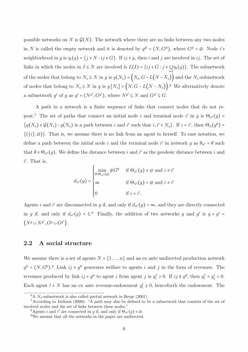
possible networks on N is G(N). The network where there are no links between any two nodes

in N is called the empty network and it is denoted by g∅ = (N,G∅), where G∅ = ∅. Node i’s

neighborhood in g is ηi(g) = j ∈ N ∶ ij ∈ G. If ij ∈ g, then i and j are involved in ij. The set of

links in which the nodes in I ⊆ N are involved is L(I) = ij ∈ G ∶ j ∈ ⋃i∈Iηi(g). The subnetwork

of the nodes that belong to Ns ⊆ N in g is g(Ns) = (Ns,G−L(N −Ns)) and the Ns-subnetwork

of nodes that belong to Ns ⊆ N in g is g [Ns] = (N,G −L(N −Ns)).6 We alternatively denote

a subnetwork g′ of g as g′ = (N g′ ,Gg′), where N g′ ⊆ N and Gg′ ⊆ G.

A path in a network is a finite sequence of links that connect nodes that do not re-

peat.7 The set of paths that connect an initial node i and terminal node i′ in g is Θii′(g) =

g(Ns) ∈ G(Ns) ∶ g(Ns) is a path between i and i′ such that i, i′ ∈ Ns. If i = i′, then Θii(g0) =

(i,∅). That is, we assume there is no link from an agent to herself. To ease notation, we

define a path between the initial node i and the terminal node i′ in network g as θii′ = θ such

that θ ∈ Θii′(g). We define the distance between i and i′ as the geodesic distance between i and

i′. That is,

dii′(g) =

⎧⎪⎪⎪⎪⎪⎪⎪⎪⎪⎨⎪⎪⎪⎪⎪⎪⎪⎪⎪⎩

minθ∈Θii′(g)

#Gθ if Θii′(g) ≠ ∅ and i ≠ i′

∞ if Θii′(g) = ∅ and i ≠ i′

0 if i = i′.

Agents i and i′ are disconnected in g if, and only if dii′(g) =∞, and they are directly connected

in g if, and only if dii′(g) = 1.8 Finally, the addition of two networks g and g′ is g + g′ =

(N g ∪N g′ ,Gg ∪Gg′).

2.2 A social structure

We assume there is a set of agents N = 1, ..., n and an ex ante undirected production network

g0 = (N,G0).9 Link ij ∈ g0 generates welfare to agents i and j in the form of revenues. The

revenues produced by link ij ∈ g0 to agent i from agent j is yji > 0. If ij ∉ g0, then yji = yij = 0.

Each agent l ∈ N has an ex ante revenue-endowment yll ≥ 0, henceforth the endowment. The

6A Ns-subnetwork is also called partial network in Berge (2001).7According to Jackson (2008): “A path may also be defined to be a subnetwork that consists of the set of

involved nodes and the set of links between these nodes.”8Agents i and i′ are connected in g if, and only if Θii′(g) ≠ ∅.9We assume that all the networks in the paper are undirected.

6

revenue matrix Y ∈ Rn2

+ describes the revenue sources of each agent in the ex ante production

network. That is, ij ∈ g0 implies that element ij in Y is yji , ij ∉ g0 implies that element ij

in Y is zero, and element ii in Y is agent i’s endowment, yii. For a fixed ex ante production

network g0 and its corresponding revenue matrix Y , Πl (g0, Y ) = Pl(g0, Y ) − y is agent l’s ex

ante payoff under g0, where Pl ∶ G(N) ×Rn2

+ → R+ such that Pl (g0, Y ) = yll +∑l′∈ηl(g0) yl′

l is l’s

ex ante total revenue, and y ≥ 0 is l’s subsistence level (which is homogeneous across agents).

That is, agent l’s total revenue under g0 is exclusively derived from her ex ante endowment and

l’s direct interactions with her neighbors. Therefore, the elimination of a link in g0 reduces the

revenues for at least two agents. Assumption 1 formalizes the idea that ex ante and for each

agent, g0 generates a total revenue that is at least as large as the agents’ subsistence level.

Assumption 1. Πl (g0, Y ) ≥ 0 for all l ∈ N .

The ex ante production network receives an exogenous shock ε = (ε1, ..., εn), which simul-

taneously affect all the agents. Agent l’s shock on her ex ante payoff is εl ∈ R. Thus, agent l’s

interim payoff under g0 is Πl (g0, Y ) − εl. If Πl (g0, Y ) − εl < 0, then agent l’s revenues under g0

cannot meet the subsistence level y. In this case, we say that l dies. The death of an agent has

two consequences. First, each of l’s links are eliminated, which implies that for l and each of

l’s neighbors the revenues generated by the former links are lost. Second, l’s endowment, yll , is

destroyed, which implies that none of the surviving agents can use the endowment of a dead

agent, i.e. endowments are non-transferable after death. We assume, however, that an agent’s

endowment is transferable while still alive.

Definition 1. A social structure is a triplete α = (g0, Y, ε) such that α ∈ G(N) ×Rn2

+ ×Rn.

Therefore, a social structure is composed by the ex ante production network g0, the

revenues derived from the interactions of agents in g0 denoted by Y , and the shock vector ε.

Hence, a social structure is the formal expression of the social context. Absent any giving, if

for some agent l her interim payoff is such that Πl (g0, Y ) − εl < 0, then g0 cannot be the ex

post production network. In the next section we study how transfers affect the agents’ interim

payoffs, thereby affecting the ex post production network.

7

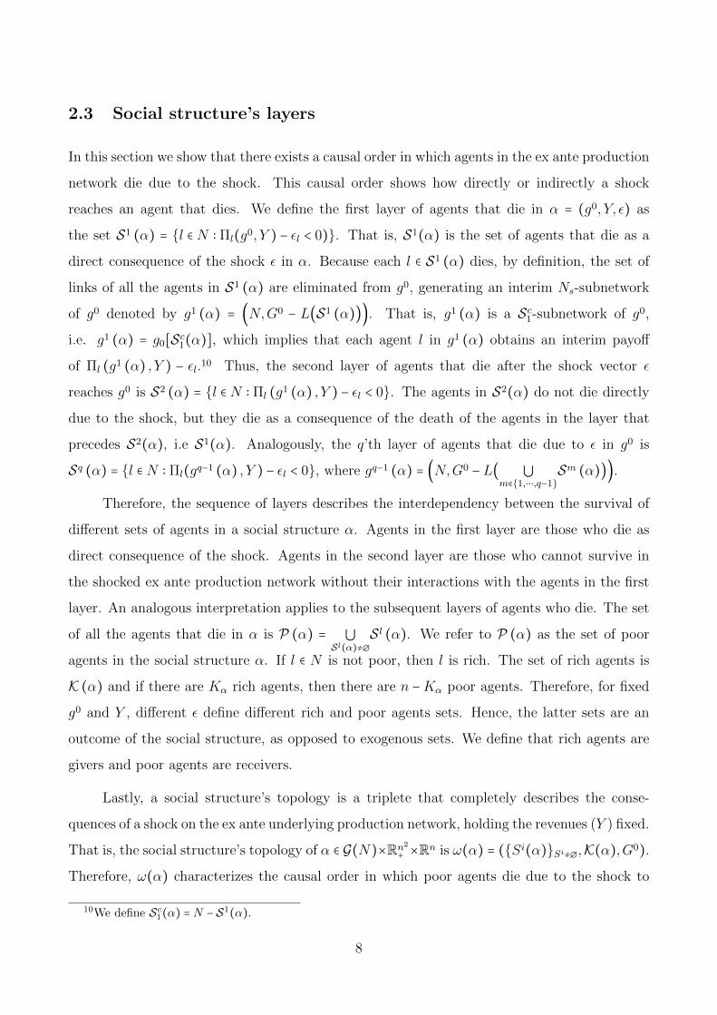
2.3 Social structure’s layers

In this section we show that there exists a causal order in which agents in the ex ante production

network die due to the shock. This causal order shows how directly or indirectly a shock

reaches an agent that dies. We define the first layer of agents that die in α = (g0, Y, ε) as

the set S1 (α) = l ∈ N ∶ Πl(g0, Y ) − εl < 0). That is, S1(α) is the set of agents that die as a

direct consequence of the shock ε in α. Because each l ∈ S1 (α) dies, by definition, the set of

links of all the agents in S1 (α) are eliminated from g0, generating an interim Ns-subnetwork

of g0 denoted by g1 (α) = (N,G0 − L(S1 (α))). That is, g1 (α) is a Sc1-subnetwork of g0,

i.e. g1 (α) = g0[Sc1(α)], which implies that each agent l in g1 (α) obtains an interim payoff

of Πl (g1 (α) , Y ) − εl.10 Thus, the second layer of agents that die after the shock vector ε

reaches g0 is S2 (α) = l ∈ N ∶ Πl (g1 (α) , Y ) − εl < 0. The agents in S2(α) do not die directly

due to the shock, but they die as a consequence of the death of the agents in the layer that

precedes S2(α), i.e S1(α). Analogously, the q’th layer of agents that die due to ε in g0 is

Sq (α) = l ∈ N ∶ Πl(gq−1 (α) , Y ) − εl < 0, where gq−1 (α) = (N,G0 −L( ⋃m∈1,⋯,q−1

Sm (α))).

Therefore, the sequence of layers describes the interdependency between the survival of

different sets of agents in a social structure α. Agents in the first layer are those who die as

direct consequence of the shock. Agents in the second layer are those who cannot survive in

the shocked ex ante production network without their interactions with the agents in the first

layer. An analogous interpretation applies to the subsequent layers of agents who die. The set

of all the agents that die in α is P (α) = ⋃Sl(α)≠∅

S l (α). We refer to P (α) as the set of poor

agents in the social structure α. If l ∈ N is not poor, then l is rich. The set of rich agents is

K (α) and if there are Kα rich agents, then there are n −Kα poor agents. Therefore, for fixed

g0 and Y , different ε define different rich and poor agents sets. Hence, the latter sets are an

outcome of the social structure, as opposed to exogenous sets. We define that rich agents are

givers and poor agents are receivers.

Lastly, a social structure’s topology is a triplete that completely describes the conse-

quences of a shock on the ex ante underlying production network, holding the revenues (Y ) fixed.

That is, the social structure’s topology of α ∈ G(N)×Rn2

+ ×Rn is ω(α) = (Si(α)Si≠∅,K(α),G0).

Therefore, ω(α) characterizes the causal order in which poor agents die due to the shock to

10We define Sc1(α) = N − S1(α).

8

g0 under Y , and who are the rich agents in the ex ante production network who survive and

have the choice of giving in α.11 The set Ω(N) = ω(α) ∶ α ∈ G(N) × Rn2

+ × Rn is the set

of all possible social structures’ topologies on N . Hereafter, we focus the analysis in social

structures where there exists at least one rich agent and one poor agent, which is defined by

the set A = α ∈ G(N) ×Rn2

+ ×Rn ∶ K(α) ≠ ∅ and P(α) ≠ ∅.

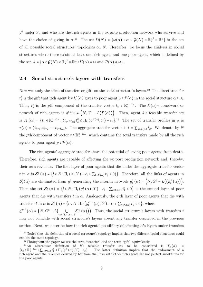
2.4 Social structure’s layers with transfers

Now we study the effect of transfers or gifts on the social structure’s layers.12 The direct transfer

tpk is the gift that rich agent k ∈ K (α) gives to poor agent p ∈ P(α) in the social structure α ∈ A.

Thus, tpk is the pth component of the transfer vector tk ∈ Rn−Kα+ . The K(α)–subnetwork or

network of rich agents is gK(α) = (N,G0 − L(P(α))). Then, agent k’s feasible transfer set

is Tk (α) = tk ∈ Rn−Kα+ ∶ ∑p∈P(α) t

pk ≤ Πk (gK(α), Y ) − εk.13 The set of transfer profiles in α is

τ(α) = (tk=1, tk=2,⋯, tk=Kα). The aggregate transfer vector is t = ∑k∈K(α) tk. We denote by tp

the pth component of vector t ∈ Rn−Kα+ , which contains the total transfers made by all the rich

agents to poor agent p ∈ P(α).

The rich agents’ aggregate transfers have the potential of saving poor agents from death.

Therefore, rich agents are capable of affecting the ex post production network and, thereby,

their own revenues. The first layer of poor agents that die under the aggregate transfer vector

t in α is S1t (α) = l ∈ N ∶ Πl (g0, Y ) − εl +∑k∈K(α) t

lk < 0). Therefore, all the links of agents in

S1t (α) are eliminated from g0 generating the interim network g1

t (α) = (N,G0 − L((S1t (α))).

Then the set S2t (α) = l ∈ N ∶ Πl (g1

t (α) , Y ) − εl +∑k∈K(α) tlk < 0 is the second layer of poor

agents that die with transfers t in α. Analogously, the q’th layer of poor agents that die with

transfers t in α is Sqt (α) = l ∈ N ∶ Πl (gq−1t (α) , Y ) − εl +∑k∈K(α) t

lk < 0, where

gq−1t (α) = (N,G0 − L( ⋃

m∈1,⋯,q−1Smt (α))). Thus, the social structure’s layers with transfers t

may not coincide with social structure’s layers absent any transfer described in the previous

section. Next, we describe how the rich agents’ possibility of affecting α′s layers under transfers

11Notice that the definition of a social structure’s topology implies that two different social structures couldexhibit the same topology.

12Throughout the paper we use the term “transfer” and the term “gift” equivalently.13An alternative definition of k′s feasible transfer set to be considered is Tk (α) =

tk ∈ Rn−Kα+ ∶ ∑p∈P(α) tpk ≤ Πk(g∅ (α) , Y ) − εk. The latter definition implies that the endowment of arich agent and the revenues derived by her from the links with other rich agents are not perfect substitutes forthe poor agents.

9

determines their payoffs.

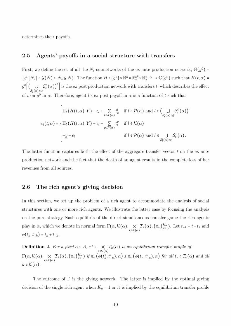
2.5 Agents’ payoffs in a social structure with transfers

First, we define the set of all the Ns-subnetworks of the ex ante production network, G(g0) =

g0[Ns] ∈ G(N) ∶ Ns ⊆ N. The function H ∶ g0×Rn×Rn2

+ ×Rn−K+ → G(g0) such that H(t, α) =

g0[( ⋃Slt(α)≠∅

S lt (α))c] is the ex post production network with transfers t, which describes the effect

of t on g0 in α. Therefore, agent l’s ex post payoff in α is a function of t such that

πl(t, α) =

⎧⎪⎪⎪⎪⎪⎪⎪⎪⎪⎪⎪⎪⎨⎪⎪⎪⎪⎪⎪⎪⎪⎪⎪⎪⎪⎩

Πl (H(t, α), Y ) − εl + ∑k∈K(α)

tlk if l ∈ P(α) and l ∈ ( ⋃Slt(α)≠∅

S lt (α))c

Πl (H(t, α), Y ) − εl − ∑p∈P(α)

tpl if l ∈ K(α)

−y − εl if l ∈ P(α) and l ∈ ⋃Slt(α)≠∅

S lt (α) .

The latter function captures both the effect of the aggregate transfer vector t on the ex ante

production network and the fact that the death of an agent results in the complete loss of her

revenues from all sources.

2.6 The rich agent's giving decision

In this section, we set up the problem of a rich agent to accommodate the analysis of social

structures with one or more rich agents. We illustrate the latter case by focusing the analysis

on the pure-strategy Nash equilibria of the direct simultaneous transfer game the rich agents

play in α, which we denote in normal form Γ(α,K(α), ⨉k∈K(α)

Tk(α),πkKαk=1). Let t−k = t− tk and

φ(tk, t−k) = tk + t−k.

Definition 2. For a fixed α ∈ A, τ∗ ∈ ⨉k∈K(α)

Tk(α) is an equilibrium transfer profile of

Γ(α,K(α), ⨉k∈K(α)

Tk(α),πkKαk=1) if πk (φ(t∗k, t

∗−k), α) ≥ πk (φ(tk, t

∗−k), α) for all tk ∈ Tk(α) and all

k ∈ K(α).

The outcome of Γ is the giving network. The latter is implied by the optimal giving

decision of the single rich agent when Kα = 1 or it is implied by the equilibrium transfer profile

10

τ∗ ∈ ⨉k∈K(α)

Tk(α) when Kα > 1.14

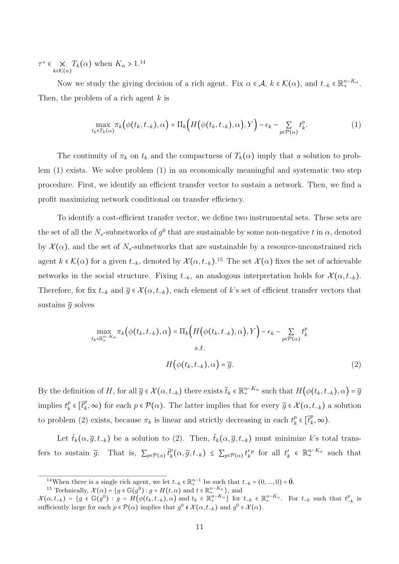
Now we study the giving decision of a rich agent. Fix α ∈ A, k ∈ K(α), and t−k ∈ Rn−Kα+ .

Then, the problem of a rich agent k is

maxtk∈Tk(α)

πk(φ(tk, t−k), α) = Πk(H(φ(tk, t−k), α), Y ) − εk − ∑p∈P(α)

tpk. (1)

The continuity of πk on tk and the compactness of Tk(α) imply that a solution to prob-

lem (1) exists. We solve problem (1) in an economically meaningful and systematic two step

procedure. First, we identify an efficient transfer vector to sustain a network. Then, we find a

profit maximizing network conditional on transfer efficiency.

To identify a cost-efficient transfer vector, we define two instrumental sets. These sets are

the set of all the Ns-subnetworks of g0 that are sustainable by some non-negative t in α, denoted

by X (α), and the set of Ns-subnetworks that are sustainable by a resource-unconstrained rich

agent k ∈ K(α) for a given t−k, denoted by X (α, t−k).15 The set X (α) fixes the set of achievable

networks in the social structure. Fixing t−k, an analogous interpretation holds for X (α, t−k).

Therefore, for fix t−k and g ∈ X (α, t−k), each element of k’s set of efficient transfer vectors that

sustains g solves

maxtk∈Rn−Kα+

πk(φ(tk, t−k), α) = Πk(H(φ(tk, t−k), α), Y ) − εk − ∑p∈P(α)

tpk

s.t.

H(φ(tk, t−k), α) = g. (2)

By the definition of H, for all g ∈ X (α, t−k) there exists tk ∈ Rn−Kα+ such that H(φ(tk, t−k), α) = g

implies tpk ∈ [tpk,∞) for each p ∈ P(α). The latter implies that for every g ∈ X (α, t−k) a solution

to problem (2) exists, because πk is linear and strictly decreasing in each tpk ∈ [tpk,∞).

Let tk(α, g, t−k) be a solution to (2). Then, tk(α, g, t−k) must minimize k’s total trans-

fers to sustain g. That is, ∑p∈P(α) tpk(α, g, t−k) ≤ ∑p∈P(α) t

′kp for all t′k ∈ Rn−Kα

+ such that

14When there is a single rich agent, we let t−k ∈ Rn−1+ be such that t−k = (0, ...,0) = 0.15 Technically, X (α) = g ∈ G(g0) ∶ g =H(t, α) and t ∈ Rn−Kα+ , and

X (α, t−k) = g ∈ G(g0) ∶ g = H(φ(tk, t−k), α) and tk ∈ Rn−Kα+ for t−k ∈ Rn−Kα+ . For t−k such that tp−k is

sufficiently large for each p ∈ P(α) implies that g0 ∉ X (α, t−k) and g0 ∈ X (α).

11

g = H(φ(t′k, t−k), α). Therefore, a rich agent’s transfers to a poor agent that are greater than

the amount of resources needed by the latter to stay alive are not efficient. This inefficiency

occurs because a lower amount can accomplish the same objective. The latter also implies that

the solution to problem (2) can be characterized in terms of the poor agents’ subsistence needs,

as we next show.

We define poor agent p′s subsistence needs in an arbitrary production network g when

she receives transfers t ∈ R+, under a fix revenue matrix Y ∈ Rn2

+ and a vector shock ε ∈ Rn+

as rp(α, g, t) = maxεp −Πp(g, Y ) − t,0. That is, rp(α, g, t) are the resources that p needs to

survive in g when she receives transfers t. We use the definition of rp to characterize an efficient

transfer vector to sustain g in problem (2).

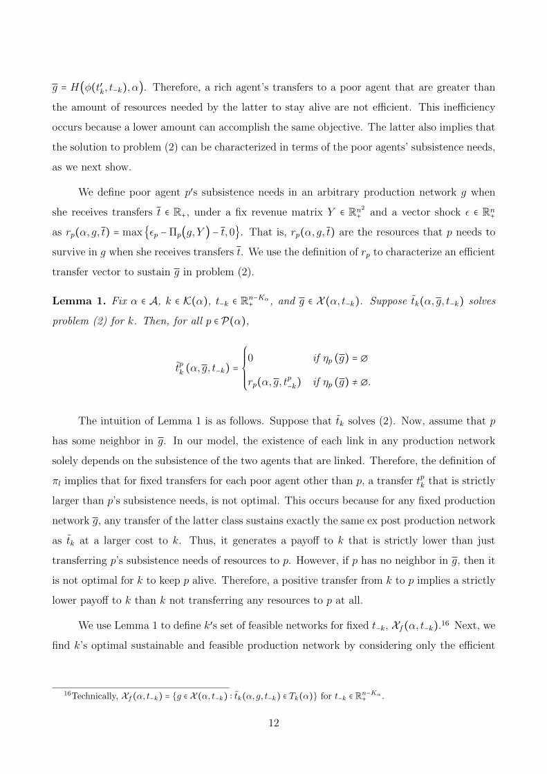
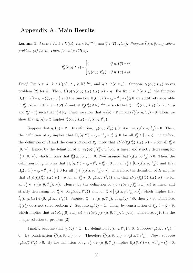
Lemma 1. Fix α ∈ A, k ∈ K(α), t−k ∈ Rn−Kα+ , and g ∈ X (α, t−k). Suppose tk(α, g, t−k) solves

problem (2) for k. Then, for all p ∈ P(α),

tpk (α, g, t−k) =

⎧⎪⎪⎪⎪⎨⎪⎪⎪⎪⎩

0 if ηp (g) = ∅

rp(α, g, tp−k) if ηp (g) ≠ ∅.

The intuition of Lemma 1 is as follows. Suppose that tk solves (2). Now, assume that p

has some neighbor in g. In our model, the existence of each link in any production network

solely depends on the subsistence of the two agents that are linked. Therefore, the definition of

πl implies that for fixed transfers for each poor agent other than p, a transfer tpk that is strictly

larger than p’s subsistence needs, is not optimal. This occurs because for any fixed production

network g, any transfer of the latter class sustains exactly the same ex post production network

as tk at a larger cost to k. Thus, it generates a payoff to k that is strictly lower than just

transferring p’s subsistence needs of resources to p. However, if p has no neighbor in g, then it

is not optimal for k to keep p alive. Therefore, a positive transfer from k to p implies a strictly

lower payoff to k than k not transferring any resources to p at all.

We use Lemma 1 to define k′s set of feasible networks for fixed t−k, Xf(α, t−k).16 Next, we

find k’s optimal sustainable and feasible production network by considering only the efficient

16Technically, Xf(α, t−k) = g ∈ X (α, t−k) ∶ tk(α, g, t−k) ∈ Tk(α) for t−k ∈ Rn−Kα+ .

12

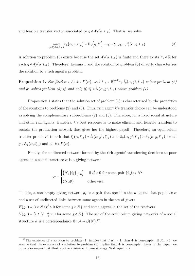
and feasible transfer vector associated to g ∈ Xf(α, t−k). That is, we solve

maxg∈Xf (α,t−k)

πk(α, g, t−k) = Πk(g, Y ) − εk −∑p∈P(α) tpk(α, g, t−k). (3)

A solution to problem (3) exists because the set Xf(α, t−k) is finite and there exists πk ∈ R for

each g ∈ Xf(α, t−k). Therefore, Lemma 1 and the solution to problem (3) directly characterizes

the solution to a rich agent’s problem.

Proposition 1. For fixed α ∈ A, k ∈ K(α), and t−k ∈ Rn−Kα+ , tk(α, g∗, t−k) solves problem (2)

and g∗ solves problem (3) if, and only if, t∗k = tk(α, g∗, t−k) solves problem (1) .

Proposition 1 states that the solution set of problem (1) is characterized by the properties

of the solutions to problems (2) and (3). Thus, rich agent k’s transfer choice can be understood

as solving the complementary subproblems (2) and (3). Therefore, for a fixed social structure

and other rich agents’ transfers, k’s best response is to make efficient and feasible transfers to

sustain the production network that gives her the highest payoff. Therefore, an equilibrium

transfer profile τ∗ is such that t∗k(α, t∗−k) = tk(α, g

∗, t∗−k) and πk(α, g∗, t∗−k) ≥ πk(α, g, t∗−k) for all

g ∈ Xf(α, t∗−k) and all k ∈ K(α).

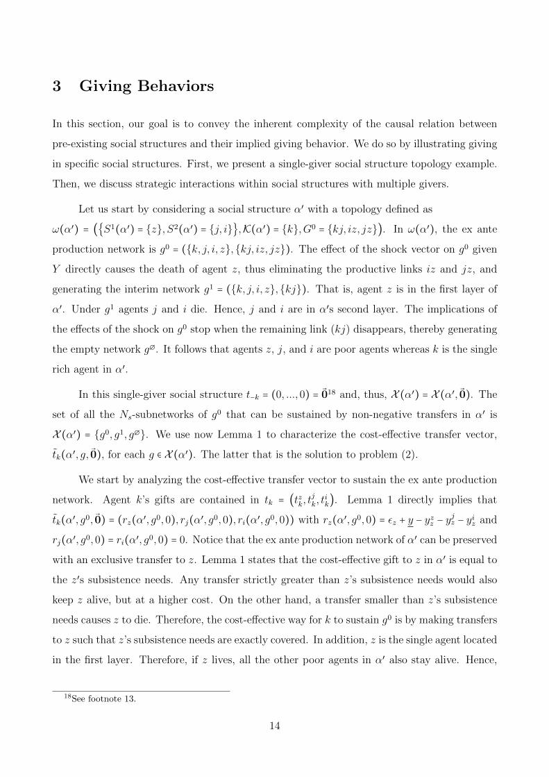
Finally, the undirected network formed by the rich agents’ transferring decisions to poor

agents in a social structure α is a giving network

gT =

⎧⎪⎪⎪⎪⎨⎪⎪⎪⎪⎩

(N,ijtji>0) if tji > 0 for some pair (i, j) ∈ N2

(N,∅) otherwise.

That is, a non–empty giving network gT is a pair that specifies the n agents that populate α

and a set of undirected links between some agents in the set of givers

E(gT ) = i ∈ N ∶ tji > 0 for some j ∈ N and some agents in the set of the receivers

U(gT ) = i ∈ N ∶ tij > 0 for some j ∈ N. The set of the equilibrium giving networks of a social

structure α is a correspondance Φ ∶ A→ G(N).17

17The existence of a solution to problem (1) implies that if Kα = 1, then Φ is non-empty. If Kα > 1, weassume that the existence of a solution to problem (1) implies that Φ is non-empty. Later in the paper, weprovide examples that illustrate the existence of pure strategy Nash equilibria.

13

3 Giving Behaviors

In this section, our goal is to convey the inherent complexity of the causal relation between

pre-existing social structures and their implied giving behavior. We do so by illustrating giving

in specific social structures. First, we present a single-giver social structure topology example.

Then, we discuss strategic interactions within social structures with multiple givers.

Let us start by considering a social structure α′ with a topology defined as

ω(α′) = (S1(α′) = z, S2(α′) = j, i,K(α′) = k,G0 = kj, iz, jz). In ω(α′), the ex ante

production network is g0 = (k, j, i, z,kj, iz, jz). The effect of the shock vector on g0 given

Y directly causes the death of agent z, thus eliminating the productive links iz and jz, and

generating the interim network g1 = (k, j, i, z,kj). That is, agent z is in the first layer of

α′. Under g1 agents j and i die. Hence, j and i are in α′s second layer. The implications of

the effects of the shock on g0 stop when the remaining link (kj) disappears, thereby generating

the empty network g∅. It follows that agents z, j, and i are poor agents whereas k is the single

rich agent in α′.

In this single-giver social structure t−k = (0, ...,0) = 018 and, thus, X (α′) = X (α′, 0). The

set of all the Ns-subnetworks of g0 that can be sustained by non-negative transfers in α′ is

X (α′) = g0, g1, g∅. We use now Lemma 1 to characterize the cost-effective transfer vector,

tk(α′, g, 0), for each g ∈ X (α′). The latter that is the solution to problem (2).

We start by analyzing the cost-effective transfer vector to sustain the ex ante production

network. Agent k’s gifts are contained in tk = (tzk, tjk, t

ik). Lemma 1 directly implies that

tk(α′, g0, 0) = (rz(α′, g0,0), rj(α′, g0,0), ri(α′, g0,0)) with rz(α′, g0,0) = εz + y − yzz − yjz − yiz and

rj(α′, g0,0) = ri(α′, g0,0) = 0. Notice that the ex ante production network of α′ can be preserved

with an exclusive transfer to z. Lemma 1 states that the cost-effective gift to z in α′ is equal to

the z′s subsistence needs. Any transfer strictly greater than z’s subsistence needs would also

keep z alive, but at a higher cost. On the other hand, a transfer smaller than z’s subsistence

needs causes z to die. Therefore, the cost-effective way for k to sustain g0 is by making transfers

to z such that z’s subsistence needs are exactly covered. In addition, z is the single agent located

in the first layer. Therefore, if z lives, all the other poor agents in α′ also stay alive. Hence,

18See footnote 13.

14

the resource needs for j and i under g0 are null. Thus, the cost-effective gifts for these agents

involve zero transfers.

Let us now focus on k’s cost-efficient form to sustain g1. Lemma 1 implies that the cost-

effective transfer vector to sustain g1 considers null transfers to z and i and transfers that match

j’s subsistence needs under g1. The Ns-subnetwork g1 does not contain the productive links

that involve either z or i. Thus, positive transfers to z or i would not be a cost-effective way

for k to sustain g1. The rich agent, however, transfers a positive amount to j, which equal j’s

subsistence needs. The intuition of the latter is analogous to the one discussed in the previous

paragraph. Therefore, tk(α′, g1, 0) = (0, rj(α′, g0,0),0) with rj(α′, g1,0) = εj +y−yjj −y

kj . Lastly,

the rich agent could choose g∅. In this case, Lemma 1 implies that tk(α′, g∅, 0) = (0,0,0) by

an analogous argument as in the previous two cases.

Having solved problem (2), we define the set of Ns-subnetworks that contains only net-

works that are sustainable and feasible for k in α′. That is, Xf(α′, 0) = g0, g1, g∅.19 Then,

k must choose a network in the set Xf(α′, 0). The latter choice is the rich agent’s solution to

problem (3). When choosing an Ns-subnetwork under α′, the rich agent considers that she has

a unique productive link in the ex ante production network: kj. Thus, when choosing between

g0, g1, and g∅, the rich agent’s tradeoff considers the benefits of kj, i.e. yjk or 0, and the cost

of sustaining kj, i.e. either the cost of sustaining g0 or g1.

Suppose the rich agent decides to sustain her productive link with j. She can do so by

transferring resources to z or j. Agent k has no direct pre-existing relation with z in g0. On

the other hand, agent j does have a direct pre-existing relation to k in the ex ante production

network. Agent k’s minimum cost of a life-saving transfer to z is εz +y−yzz −yjz −yiz, and k’s cost

efficient life-saving transfer to j is εj + y − yjj − y

kj . These cost-effective transfer vectors imply

that either g0 or g1 are sustained. However, k’s revenue from her productive link with j, yjk,

could be small compared with the cost of keeping alive either j or z–at the minimum cost–. In

this case, k does not become a giver in α′ and the cost of this action for her is simply zero.

19Equivalently, Xf(α′, 0) = g ∈ X (α′) ∶ ∑p∈j,i,z tpk(α′, g, 0) ≤ ykk − y − εk.

15

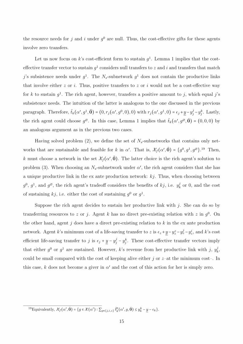
Using Proposition 1, we characterize the equilibrium giving network of α′:

gT (α′) =

⎧⎪⎪⎪⎪⎪⎪⎪⎪⎪⎨⎪⎪⎪⎪⎪⎪⎪⎪⎪⎩

(k, j, i, z,kz) if rz(α′, g0,0) ≤ minrj(α′, g1,0), yjk, ykk − y − εk

(k, j, i, z,kj) if rj(α′, g1,0) ≤ minrz(α′, g0,0), yjk, ykk − y − εk

(k, j, i, z,∅) else.

(4)

Equation (4) allows the illustration of important aspects of the relation between a pre-

existing social structure and their implied giving network. Suppose that α′ is such that is

optimal for k to save agent z:

(a) rz(α′, g0,0) < rj(α′, g1,0) (it is less expensive to save z than j),

(b) rz(α′, g0,0) < yjk (the revenues for k from her link with j are greater than the cost of

keeping alive z), and

(c) rz(α′, g0,0) < ykk − y − εk (feasibility).

Conditions (a) through (c) imply that an equilibrium giving network of α′ is gT (α′) = (k, j, i, z,kz).

There are several economic properties of gT (α′) that are worth further discussing.

First, the equilibrium giving network is not an Ns-subnetwork of the ex ante production

network. Namely, the equilibrium giving network connects agents who do not have any direct

pre-existing relation in the production network. This undocking between the giving network and

the ex ante production network limits the external validity of studies on giving that exclusively

occurs between agents with a direct pre-existing social relation. For expositional purposes,

suppose that a researcher tries to extract information on the giving behavior of agent k by

exclusively studying her gifts to j, with whom k is directly connected in the production network.

The researcher would conclude that k is not a giver since she does not observe any transfer

from k to j. However, this conclusion is invalid since k is a giver, only that her transfers go to

z an not to j. Therefore, this example suggests that placing the analysis of the social effects

motives for giving in the social context is crucial.

Second, under α′ we have that conditions (a) through (c) imply that the giving network

sustains the entire ex ante production network. Moreover, the causal order in which the poor

16

agents die in α′ implies that the preservation of the first layer sustains all the remaining layers.

Therefore, every agent in α′ survives, which implies that the entire ex ante production network

is sustained. This occurs because z is the single agent located in the first layer. Hence, the

current example suggests that gifts sustaining the first layer, as opposed to transfers to all the

poor agents, are sufficient to sustain the entire ex ante production network.

Third, the existence of a causal order in which agents die in a given social structure,

unveils sufficient conditions on the social structure’s topology for the existence of segregation

in private giving. In this example, the mere existence of two, or more, layers of poor agents is

a sufficient condition to make some poor agents not to receive positive transfers from the rich

agent. Suppose that all the poor agents are sustained by the giving of k. Then, all the agents

located in the first layer are kept alive and the entire ex ante production network would be

preserved. Therefore, it can not be optimal for the rich agent to make transfers to all the poor

agents in α′.

Let us now focus on agent i. In α′, there is no path in g0 such that i is located between

the rich agent and the first layer of poor agents. Hence, i is completely irrelevant for k to

sustain her link with j. Therefore, transferring resources to i is never optimal for k.20

Finally, two different social structures can generate the same equilibrium giving network.

Let social structure α′′ ≠ α′ be such that gT (α′′) = gT (α′). Suppose

ω(α′′) = (S1(α′′) = z, j, i,K(α′′) = k,G0 = kz). Following analogous steps to those pre-

viously described in the analysis of α′, we can characterize the solution to the problem of the

rich agent in α′′ as

gT (α′′) =

⎧⎪⎪⎪⎪⎨⎪⎪⎪⎪⎩

(k, j, i, z,kz) if rz(α, g0,0) ≤ minyzk, ykk − y − εk

(k, j, i, z,∅) else.

(5)

If rz(α′′, g0,0) < minyzk, ykk − y − εk, expression 5 indicates that gT (α′′) = (k, j, i, z,kz),

which implies that gT (α′′) = gT (α′). The economic relevance of the latter observation is that

two different social structures are observationally equivalent with respect to the equilibrium

giving network that they form.

20This fact does not implies that agent i dies.

17

Strategic Interactions

In this subsection, we illustrate how to use our theory to study strategic interactions

between rich agents. We discuss some new insights that stem from this analysis. We conclude

by showing that the results extracted from the analysis of α′ are also present in some social

structures which exhibit strategic interactions.

Consider a social structure α characterized by ω(α) = (S1(α) = j,K(α) = k1, k2,G0 = k1j, k2j).

Thus, there are two rich agents in α (k1 and k2) and each of them is connected to the

same poor agent (j). The direct transfer game in which k1 and k2 participate is Γk1,k2 =

Γ(α,k1, k2, Tk1(α)×Tk2(α),πk1(t, α), πk2(t, α)). We focus the analysis on the pure-strategy

Nash equilibria of Γk1,k2 . Thus, k1 and k2 must non-cooperatively and simultaneously decide the

transfers to j. Notice that, if aggregate transfers (tj) are equal or greater than j’s subsistence

needs (rj(α, g0,0) = y+εj−yjj −y

k1j −yk2j ), then tj sustains the ex ante production network. If the

latter does not occur, the empty network g∅ is generated. Therefore, the set of Ns-subnetworks

that can be sustained in α by a non-negative aggregate transfer vector contains the ex ante

production network and the empty network. That is, X (α) = g0, g∅.

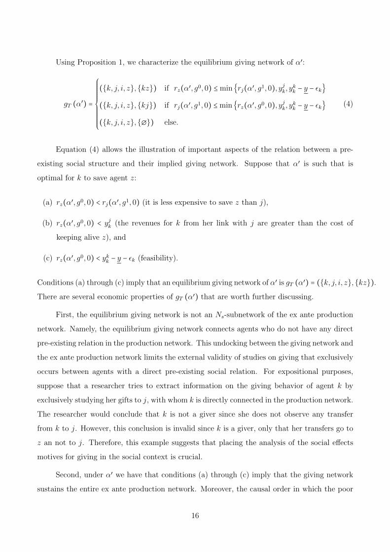
The problems solved by k1 and k2 are symmetric. In addition, for both rich agents the

strategy space is a strict subset of R+, i.e. tk and t−k are non-negative scalars. Following the

procedure described in Section 2.6, we analyze how agent k ∈ K(α) solves problem (2). Agent k

must choose the cost-effective gifts to sustain each of the Ns-subnetworks in X (α, t−k) ⊆ X (α).

The cost-effective way to preserve g0 for k is through gifts that exactly cover j’s subsistence

needs, net of the resources transferred by −k.21 Therefore, tk(α, g0, t−k) = rj(α, g0, t−k), where

rj(α, g0, t−k) = rj(α, g0,0) − t−k. In addition, it is straightforward to conclude that the cost-

effective transfer for k to sustain the empty network is zero, for any amount of the other rich

agent’s transfer. That is, tk(α, g∅, t−k) = 0 for any t−k ∈ R+.

Once that each rich agent’s cost-effective way of sustaining eachNs-subnetwork in X (α, t−k)

is computed, the feasible set Xf(α, t−k) is determined.22 Then, for each rich agent, problem (3)

is solved following analogous steps as for the single-giver case. As stated by Proposition 1, this

procedure computes rich agent k’s best response transfers to rich agent −k’s transfers.

21See Lemma 1 and its interpretation.22In this case, Xf(α, t−k) = g ∈ X (α, tk) ∶ tk(α, g0, t−k) ≤ ykk − y − εk.

18

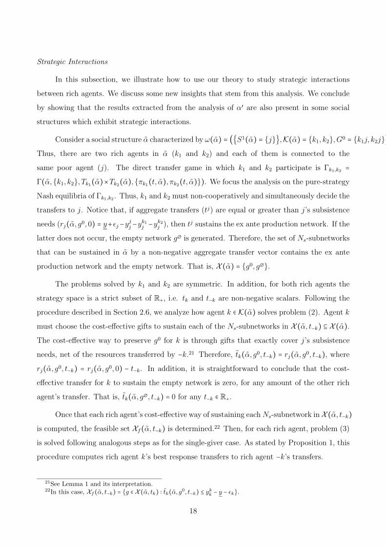
In order to characterize the latter solution, we define a technical threshold that represents

an upper bound for the optimality of k’s transfers. Agent k’s optimal transfers cannot exceed

neither yjk nor ykk − y − εk. A transfer greater than yjk is not optimal because the amount of the

gift would exceed the revenues collected from the productive link that it sustains. In addition,

a gift greater than ykk − y − εk would exceed the amount of resources that k has available to

transfer. Let tk(α) be the maximum amount that makes k’s transfer to j optimal. Then,

tk(α) = minyjk, ykk − y − εk for k ∈ k1, k2. Thus, in α, the optimal transfers of k to −k’s

transfers are

tbrk (α, t−k) =

⎧⎪⎪⎪⎪⎨⎪⎪⎪⎪⎩

rj(α, g0, t−k) if rj(α, g0, t−k) ≤ tk(α)

0 else.

(6)

In this case, by construction, tbrk (α, t−k) is a function for k ∈ k1, k2. We use now the

latter best response function characterization to provide the solution to the transfer game Γk1,k2 .

First, suppose that tk1 + tk2 < rj(α, g0,0).23 Then, the sum of the maximum amount of

resources that is optimal to transfer by the rich agents is not enough to sustain j in the ex ante

production network. Therefore, the rich agents are not wealthy enough to keep j alive, or the

productive link with j is not valuable enough as to encourage them to sustain the poor agent

in ex ante production network. Therefore, there is no giving in this case.

Suppose now that tk1+tk2 ≥ rj(α, g0,0), tk1 < rj(α, g

0,0) and tk2 < rj(α, g0,0). In this case,

the sum of the maximum amount of resources that is optimal for the rich agents to transfer to

j is enough to keep the poor agent alive. However, it is not individually optimal to sustain j.

Here, the strategic interaction between the rich agents triggers two types of equilibria. The first

type of equilibrium is characterized by having each rich agent transferring a strictly positive

amount of resources to j. Therefore, each reach agent has a link with j in the giving network. In

the second equilibrium, the agents transfer no resources to j, which implies that the equilibrium

giving network is the empty network.

A third case is tk1 ≥ rj(α, g0,0) and tk2 ≥ rj(α, g

0,0). These conditions imply that, even

though t−k = 0, it is optimal for k to sustain j. Therefore, giving is always observed in this type

of social structures. Moreover, multiple equilibria also exist. Thus, this third case highlights

that it is possible to observe a dissimilar giving behavior among identical agents.

23Here, we use tki = tki(α) to ease notation.

19

Lastly and without loss of generality, suppose that tk1 + tk2 ≥ rj(α, g0,0), tk1 ≥ rj(α, g

0,0),

and tk2 < rj(α, g0,0). In this case, it is optimal for k1 to make transfers to j even though k2

makes no gifts. Therefore, k1 can individually sustain j, hence forming a link with the poor

agent in the giving network, which is not possible for k2. The condition tk1 > tk2 implies that

agent k1 can optimally afford bigger gifts to j than k2. We interpret the latter as k1 having a

comparative advantage in giving with respect to k2. Moreover, we can observe specialization

in the production of giving when k1 individually sustain j in the ex ante production network.

Notice the specialized agent is precisely who carries comparative advantages in the production

of giving (k1). The formal analysis for the previous four paragraphs is in Appendix A.

We now provide an example to show that the results derived for α′ can also be present

in social structures that exhibit strategic interactions. Consider a social structure α with

a topology ω(α) = (S1(α) = z,S2(α) = j, i,K(α) = k1, k2,G0 = k1j, k2j, iz, jz). Sup-

pose that

(i) yk1k1 +yk2k2−2y−εk1 −εk2 < y+εj −y

jj −y

k1j −yk2j (it is not feasible for the rich agents to sustain

j),

(ii) yk1k1 − y − εk1 > rz(α, g0,0) (it is feasible for k1 to individually sustain z),

(iii) yk2k2 − y − εk2 > rz(α, g0,0) (it is feasible for k2 to individually sustain z),

(iv) yjk1 > rz(α, g0,0) (it is optimal for k1 to sustain z),

(v) yjk2 > rz(α, g0,0) (it is optimal for k2 to sustain z),

Condition (i) implies that aggregate resources are not enough to cover j’s subsistence

needs. Conditions (ii) and (iii), on the other hand, imply that it is feasible for each rich agent

to sustain z in the ex ante production network. Moreover, conditions (iv) and (v) imply that

it is also optimal for them to sustain z. By sustaining z each of the rich agents can preserve

the productive link with j and the value of that link is greater than z’s subsistence needs.

Moreover, a direct implication of the topology structure of α is that gifts to i do not allow the

subsistence of j but the subsistence of z ensures that both j and i stay alive. Therefore, agent

i is irrelevant for the rich agents to preserve the productive link they have with j.

20

The analysis of this social structure follows the steps described in this subsection. We

have that conditions (i) through (v) imply that Φ(α) = g1, g2, g3 with

g1 = (k1, k2, j, i, z,k1z), g2 = (k1, k2, j, i, z,k2z), and g3 = (k1, k2, j, i, z,k1z, k2z).

That is, the equilibrium giving network correspondence includes giving networks in which either

one rich agent makes transfers to z or both do so.

Notice that the equilibrium giving network does not resemble the ex ante production

network in α. That is, even though z does not have any type of direct pre-existing relation

with neither k1 nor k2 in the ex ante production network, one or both of them optimally make

a gift to z. Moreover, private giving sustains the entire ex ante production network because

the subsistence of z is sufficient for the survival of j and i given the structure of layers that

characterize α. In addition, some poor agents in α are segregated from giving. The intuition

of the latter result is exactly the same as the one developed above for the case of a single-giver

social structure: sustaining the first layer of agents is sufficient to sustain the entire network

and, thus, no agent rich agent will find optimal to transfer resources to all the poor individuals.

The social structure α also shows that there is a second reason why a poor agent could be

segregated from giving, which concerns to agent i: the subsistence of this agent is irrelevant for

sustaining k1’s and/or k2’s link with j. All these results were already derived for a single-giver

social structure and we have shown now that they can also be observed in a multi-givers social

structure.

We end the discussion of this section by illustrating how two different multi-givers social

structures can produce exactly the same equilibrium giving network. Consider a social structure

α′ with topology ω(α′) = (S1(α′) = z, j, i,K(α′) = k1, k2,G0 = k1z, k2z). Suppose

(I) yk1k1 − y − εk1 > rz(α, g0,0) (it is feasible for k1 to individually sustain z),

(II) yk2k2 − y − εk2 > rz(α, g0,0) (it is feasible for k2 to individually sustain z),

(III) yzk1 > rz(α, g0,0) (it is optimal for k1 to sustain z),

(IV) yzk2 > rz(α, g0,0) (it is optimal for k2 to sustain z),

Then, under conditions (I) to (IV), we have that Φ(α′) = Φ(α) even though the geometry

of ex ante production network in these social structures is different. Therefore, the result

21

regarding the fact that two different social structures are observationally equivalent with respect

to the equilibrium giving network that they induce can also be derived for a multi-givers social

structure.

4 Results

In this section we generalize the insights that stemmed from the analysis carried out in Section

3. We start by defining some concepts that we will use to state and analyze the main results

of the paper.

We define the direct diffusion network in the social structure α asDIF (α) = ∑k∈K(α)

∑j∈S1(α)

∑θ∈Θkj(g0)

θ.

The set of agents who do not belong to NDIF (α), or ramified agents, is NR(α) = P(α)−NDIF (α).24

The set of agents that connect the direct diffusion network to its ramified agents in g given α, or

frontier, is P(α, g) = p ∈ P(α)∩NDIF (α) ∶ ηp(g)∩NR(α) ≠ ∅ . An element of P(α, g) is a fron-

tier agent in g given α. The set of ramified agents that stems from a frontier agent p′ in g given

α is P(α, g, p′) = p ∈ NR(α) ∶ Θpp′(g) ≠ ∅ for p′ ∈ P(α, g) and dpp′(g) ≤ dpp′′(g) ∀ p′′ ∈ P(α, g).

A ramification of p′ ∈ P(α, g0) is a subnetwork g0 (p′ ∪ P(α, g0, p′)).

We use Lemmas 3 through ?? in Appendix B to prove Proposition 2 ahead. Altogether,

these technical lemmas are used to show that the survival of a frontier agent keeps all the agents

in its ramification alive. In addition, the survival of ramified agents who are disconnected from

the direct diffusion network does not affect the rich agents’ payoffs. Hence, it is not optimal

for the rich agents to make gifts to ramified agents.

Proposition 2. For a fixed social structure α, a poor agent receives strictly positive transfers

only if she is in the direct diffusion network.

Proposition 2 characterizes where in the ex ante production network gifts are received.

Concretely, it states that transfers are allocated to agents in the direct diffusion network.

This location-based characterization of the receivers, directly implies that ramified agents are

excluded/segregated from the rich agents’ gifts. However, being segregated from the rich agents’

giving is compatible with some ramified agents’ survival as long as the corresponding agents in

24Recall that according to the definition provided in section 2.2, DIF (α) = (NDIF (α),GDIF (α)).

22

the frontier survive.

However, Proposition 2 does not imply that the existence of ramified agents is the sole

sufficient condition for rich agents’ segregated giving behavior. Even in social structures with

no ramified agents, some poor agents in the direct diffusion network could be segregated from

receiving strictly positive transfers from some rich agent in equilibrium.

Proposition 3. A multilayer social structure topology implies that there is at least one poor

agent that does not receive positive transfers in equilibrium.

Positive gifts that keep alive all the poor agents of a social structure imply, by construction,

the survival of all the agents located in the first layer. In the latter case, the productive links

between the agents in the first layer and those located in the successive layers are sustained.

Thus, all the poor agents that are not located in the first layer stay alive even without receiving

gifts from the rich agents. Therefore, an equilibrium giving network cannot exhibit positive

transfers to all the poor agents of a multilayer social structure.

So far, we have analyzed how a social structure causes giving. However, one could also ask

what can be learned about the social structure from an observed equilibrium giving network.

Each of the following three propositions (4, 5, and 6) study the extent of the informational

content of an observed (equilibrium) giving network regarding the ex ante production network.

We discuss how these propositions bring implications for the empirical analysis of giving in

Section 5.

The set of all the social structures where all the poor agents are either disconnected or

directly connected with the rich agents in the ex ante production network is A.25 The ex ante

production networks of the social structures in A correspond to the types of relations studied by

Becker (1976, 1981) in the context of altruism. The following proposition states the information

that can be extracted from a giving network induced by social structures in A.

Proposition 4. In social structures where all the poor agents are either disconnected or directly

connected with the rich agents in the ex ante production network, the equilibrium giving network

is such that there are no links that do not exist in the ex ante production network.

Proposition 4 states that, for each social structure in A, the set of links of the equilibrium

25That is, A = α ∈ A ∶ dpk(g0) = 1,∞ for all p ∈ P(α) and all k ∈ K(α).

23

giving network is a subset of the links of the ex ante production network. This occurs because

the survival of poor agents that are disconnected from the rich agents does not affect the payoffs

of the latter individuals. Thus, it is not optimal for any rich agent to transfer resources to agents

with whom there is not a direct or indirect relation. This implies that only poor agents that

are directly connected to rich agents receive gifts in social structures in A. This result contains

two economic implications. First, transfers between two agents informs on the existence of a

productive link between these individuals in the ex ante production network. Second, observing

transfers from a rich agent to a directly connected poor agent in g0 characterizes the giving

behavior of the rich agent in the entire social structure: there is no giving beyond a rich agent’s

neighborhood in the ex ante production network.

However, the social structures in A are not adequate for describing complex social struc-

tures.26 This fact raises the question about the limitations of the informational content of giving

behavior with respect to the ex ante production network in less constrained social structures

than those in A.

Proposition 5. There exists some social structure such that some of its equilibrium giving

network contains a link between agents that are not directly connected in the ex ante production

network.

Proposition 5 implies that an observed transfer from one rich agent to a poor agent

does not provide certainty about the existence of a link between these agents in the ex ante

production network. In addition, the giving behavior cannot be characterized by observing

transfers between neighboring agents in g0. The latter is consequence on the fact that giving

can occur beyond close relations, as our examples of Section 3 already illustrated. Therefore,

Proposition 5 warns about potential biases when empirically studying giving solely in the

context of direct relations.

Propositions 4 and 5 highlighted that the equilibrium giving network is not sufficient to

infer neither the social structure nor the ex ante production network. In addition, there is

another motive for caution when inferring pre-existing relations from an equilibrium giving

network.

26The set of complex social structures is Ac.

24

Proposition 6. For each social structure in A with three or more agents, there exists a social

structure with a different underlying ex ante production network such that both induce the same

equilibrium giving network.

Thus, Proposition 6 shows that even though the observed giving network could convey

information on the ex ante production network, it will never be enough to completely infer

g0. It follows that that different social structures are observationally equivalent regarding the

giving network they induce: any observed transfers can be induced by two different ex ante

production networks.27

Finally, we show that strictly positive transfers to all the poor agents that populate a social

structure is not necessarily a cost-effective way of sustaining the entire production network.

Proposition 7. In any social structure, transfers to all the non isolated poor agents located in

the first layer, equal or greater than their subsistence needs, are sufficient to sustain the entire

ex ante production network.

Proposition 7 is a direct consequence of the structure of layers intrinsic to any social

structure. The layers in a social structure determine the casual order in which agents in the ex

ante production network die due to the shock. Concretely, they determine the group of agents

that die as direct consequence of the shock that hits the economy and the group of agents that

die as consequence of the disappearance of the productive links that they have with the former

agents. Then, positive transfers that sustain a subset of agents can be sufficient to prevent the

death of individuals who do not die as a direct consequence of the shock.

5 Discussion

The examples we develop ahead highlight how the theory presented in this paper has the po-

tential to enrich the study of several economics phenomena. First, we sketch an application of

our theory to study how non-altruistic motives affect giving in the context of the family. Then,

we suggest how the context of a firm may affect the firm’s decisions on corporate ownership

and control. Third, we discuss how our framework could be applied for the analysis of optimal

27It is trivial to obtain analogous results to Proposition 6 by marginally changing Y or ε.

25

rescue-policies in complex financial networks. Finally, we highlight the kind of biases that ig-

noring the social context of giving decisions introduce in experiments that study giving.

Family Economics

Becker provided the first formal analysis of giving within a family.28 The motive for giv-

ing in Becker’s analysis arises from parents’ altruistic preferences. One could wonder whether

altruistic preferences are needed to observe intra-family transfers. Our theory shows that trans-

fers within the family can arise from social motives. We also highlight that the preservation of

family relations may express itself in transfers beyond the family’s sphere. To illustrate these

insights, consider the social structure α′, which was studied in Section 3. Let us interpret the

rich agent k as the parent and the poor agent j as the child. These agents are directly con-

nected in an ex ante production network and collect some market or non-market goods from

that relation; for instance, love. In our model, transfers from the parent to the child are not

motivated by Beckerian altruistic preferences. What motives these transfers is the preservation

of the productive link that the parent has with the child. Moreover, our Proposition 4 implies

that, to preserve that link, a parent could transfer resources outside the family circle.29 Our

theory constitutes a non-exclusive alternative to Becker’s analysis of giving within the family.

When Does Corporate Ownership Induce Corporate Control?

The separation between corporate ownership and corporate control is one of the oldest

issues discussed in the corporate governance literature.30 Demsetz and Lehn (1985) made early

efforts to study how corporate ownership causes corporate control by describing the market

for corporate control. More recently, some efforts have been made to describe de consequences

28See, for instance, Becker (1976), Becker (1981), Becker and Tomes (1986), Becker and Barro (1988), amongothers.

29For instance, to agent z in α′.30Vitali et al. (2011) define corporate control as “the chances of seeing one’s own interest prevailing in the

business strategy of the firm” whereas simple ownership does not imply such influence in the firm’s strategy.Several papers study the differences between ownership and control (Cantillo, 1998; Frank and Mayer, 1997).Traditionally the relation between corporate ownership and control has been studied from the perspectiveof agency costs (Berle and Means, 1932; Jensen and Meckeling, 1976), considering externalities produced byupstream or downstream firms (Dixit, 1983), considering incomplete contracts (Klein et al., 1978; Grossmanand Hart, 1986; Hart and Moore, 1990) or from the perspective of the agency problem caused by dispersedownership (Fama and Jensen, 1983).

26

of the structure of corporate ownership and control on financial stability (La Porta et al.,

1999), with some of them using network theoretical methodologies (Glattfelder, 2010; Vitali et

al., 2011). The theory we develop in this paper complements the latter efforts by providing a

general framework to study the causal relation from corporate ownership structure to corporate

control.

Suppose that the ex ante production network represents the corporate ownership network

where each link implies a profit flow from the “owned” firm to the stock holder firm and a

capital flow from the stock holder to the “owned” firm. Analogously, suppose that the giving

network represents increases of capital for the survival of the “owned” firms due to a direct or

indirect shock. An increase in the capital investment of firm a in firm b may lead firm a to con-

trol firm b. Then, one can use our theory as a framework to understand changes in the network

of corporate control as a response for maintaining the profitability of an ex post parent com-

pany with respect to a subsidiary. Applying our theory as described above contribute to this

corporate ownership and control literature by shedding light on how the roles of the companies

might change depending on the nature of the shock that affects the ownership network. This

complements the analysis of Shleifer and Vishny (1986) by providing another channel through

which dispersed ownership affects corporate control.

Which Bank is Optimally Saved in a Financial Crisis?

After the 2008 global financial crisis, the resilience and stability of banking systems have

received much attention (Plosser, 2009; Blume et al., 2011). Early studies suggested that the

structure of the interbank claims affects the system’s resilience (Allen and Gale, 2000; Freixas

et al., 2000). More recently, Acemoglu et al., (2015) study financial contagion holding the

financial network fixed. Our model complements the latter efforts by suggesting a rescue-policy

taking the financial network’s structure and its associated contagion pattern as given.

Suppose that the ex ante production network represents the financial network, and sup-

pose that the giving network represents a structured collection of rescue packages to troubled

banks. Then, our model facilitates the determination of an optimal rescue-policy. Moreover, by

considering the existence and properties of the direct diffusion network and the set of ramified

agents (Propositions 2, 3, and 7), our framework provides criteria to handle bank defaults in

27

complex financial networks.

Study of Social Motives for Giving in Experiments

Field experiments (Frey and Meier, 2004; Armin, 2007; Meier, 2007; Carpenter et al.,

2008; Shang and Croson, 2009; DellaVigna et al., 2012; Zarghamee et al., 2017; among others)

are frequently used to empirically study giving. These experiments consist on the observation

of transfers from one specific group (the treated individuals) to another under factual and

counterfactual scenarios. Proposition 5 warns about potential biases when empirically studying

giving using small-scale field experiments. This proposition shows that it is the entire social

structure what matters to understand giving motivated by social effects. However, it is unlikely

that the design considered in a small-scale field experiment captures the entire social structure.

This difficulty casts doubts regarding the external validity of the results derived from this

empirical methodology when studying the social motives for giving.

6 Conclusions

In this paper we develop a general theory of giving in networks. Our model accommodates

different aspects that are intrinsic to human societies. First, the exchange of market and non-

market goods in networks; second, the complexity of the social context beyond the production

network as a determinant of agents' choices; and the imperfect overlap between the production

network and the giving network.

The use of networks to model social relations permits a precise characterization of giving

behaviors that are motivated by social motives. We show that voluntary giving can arise

from selfish agents who do not even maintain a pre-existing productive relationship with the

recipients of the gifts. The theory presented in this paper also emphasizes that the location and

intensity of an event that hits the production network—what we called “a shock”—determines

which agents are givers and the receivers. Moreover, the position of the givers and receivers

determine the number, the quantity , and the actual recipients of the gifts. Also our model

permits the recognition of general conditions under which some agents are segregated from

giving. Lastly, the paper provides general conditions under which focalized transfers sustain

28

the complete production network.

Finally, our theory can be applied to understand a diversity of phenomena that involve

the possibility for agents to carry out voluntary transfers. We discussed examples related to the

literature on family economics, corporate governance, macro-finance, and field experiments.

References

[1] Acemoglu, D., Ozdaglar, A., and Thabaz-Salehi, A. 2015. “Systemic Risk and Stability in

Financial Networks.” American Economic Review, 105(2): 564–608

[2] Allen, F. and Gale, D. 2000. “Financial Contagion.” Journal of Political Economy, 108(1):

1–33.

[3] Becker, G. S. 1974. “A Theory of Social Interactions.” Journal of Political Economy, 82(6):

1063–1093.

[4] Becker, G. S. 1976. “Altruism, Egoism, and Genetic Fitness: Economics and Sociobiology.”

Journal of Economic Literature, 14(3): 817–826.

[5] Becker, G. S. 1981. “Altruism in the Family and Selfishness in the Market Place.” Econom-

ica, 48(189): 1–15.

[6] Becker, G. S. and Tomes, N. 1986. “Human Capital and the Rise and Fall of Families.”

Journal of Labor Economics, 4(3): S1–S39.

[7] Becker, G. S. and Barro, R. 1988. “A Reformulation of the Economic Theory of Fertility.”

Quarterly Journal of Economics, 103(1): 1–25.

[8] Berge, C., 2001.The Theory of Graph, New York, Dover Publications Inc.

[9] Berle, A. and Means, G. 1932. The Modern Corporation and Private Property. New York,

MacMillan.

[10] Blume, L., Easley, D., Kleinberg, J., and Tardos, E. 2011. Network Formation in the Pres-

ence of Contagious Risk. Proceedings of the 12th ACM Conference on Electronic Commerce.

29

[11] Cantillo, M. 1998. “The Rise and Fall of Bank Control in the United States: 1890-1939.”

American Economic Review, 88(5): 1077–1093.

[12] Carpenter, J., Holmes, J., and Matthews, P. H. 2008. “Charity Auctions: A Field Experi-

ment.” Economic Journal, 118(January): 92–113.

[13] DellaVigna, S. List, J. A., and Malmendier, U. 2012. “Testing for Altruism and Social

Pressure in Charitable Giving.” Quarterly Journal of Economics, 127(1): 1–56.

[14] Demsetz, H. and Lehn, K. 1985. “The Structure of Corporate Ownership: Causes and

Consequences.” Journal of Political Economy, 93(6): 1155–1177.

[15] Dixit, A. 1983. “Vertical Integration in a Monopolistically Competitive Industry.” Inter-

national Journal of Industrial Organization, 1(1): 63–78.

[16] Falk, A. 2007. “Gift Exchange in the Field.” Econometrica, 75(5): 1501–1511.

[17] Fama, E. and Jensen, M. 1983. “Separation of Ownership and Control.” Journal of Law

and Economics, 26(2): 301–325.

[18] Fischbacher, U., Gachter, S., and Fehr, E. 2001. “Are People Conditionally Cooperative?

Evidence from a Public Goods Experiment.” Economics Letters, 71(3): 397–404.

[19] Franks, J. and Mayer, C. 1997. “Corporate Ownership and Control in the UK, Germany,

and France.” Journal of Applied Corporate Finance, 9(4): 30–45.

[20] Freixas, X., Parigi, B. M., and Rochet, J. 2000. “Systemic Risk, Interbank Relations, and

Liquidity Provision by the Central Bank.” Journal of Money, Credit and Banking, 32(3):

611–638.

[21] Frey, B. S. and Meier, S. 2004. “Social Comparison and Pro-Social Behavior: Testing

A¢AAConditional CooperationA¢AA in a Field Experiment.” American Economic Review,

94(5): 1717–1722.

[22] Glattfelder, J.B. 2010. “Ownership Networks and Corporate Control Mapping Economic

Power in a Globalized World.” Doctoral Thesis, https://doi.org/10.3929/ethz-a-006208696

30

[23] Gneezy, U., Haruvy, E., and Yafe, H. 2004. “The Inefficiency of Splitting the Bill: A Lesson

in Institution Design.” Economic Journal, 114(April): 265–280.

[24] Grossman, S. and Hart, O. 1986. “The Cost and Benefits of Ownership: A. Theory of

Vertical and Lateral Integration.” Journal of Political Economy, 94(4): 691–719

[25] Hart, O. and Moore, J. 1990. “Property Rights and the Nature of the Firm.” Journal of

Political Economy, 98(6): 1119–1158.

[26] Jackson, M., 2008. Social and Economic Networks. New Jersey, Princeton University Press.

[27] Jensen, M. and Meckelling, W. 1976. “Theory of the Firm: Managerial Behavior, Agency

Costs and Ownership Structure.” Journal of Financial Economics, 3(4): 305–360.

[28] Keser, C. and van Winden, F. 2000. “Conditional Cooperation and Voluntary Contribu-

tions to Public Goods.” Scandinavian Journal of Economics, 102(1): 23–29.

[29] Klein, B., Crawford, R., and Alchian, A. 1978. “Vertical Integration, Appropriable Rents

and the Competitive Contracting Process.” Journal of Law and Economics, 21(2): 297-326.

[30] Kolm, S.-C. 1966. The Optimal Production of Social Justice. In: Guitton, H., Margolis,

J. (Eds.). International Economic Association Conference on Public Economics, Biarritz.

Proceedings. Economie Publique (CNRS, Paris), pp.109–177.

[31] Kolm S.-C. 2006. “Introduction to the Economics of Giving, Altruism and Reciprocity.”

In: Handbook of The Economics of Giving, Altruism and Reciprocity, Vol. 1. Amsterdam:

North-Holland, pp. 1–122.

[32] Kolm, S.-C. and Ythier, J. M. 2006. Handbook of the Economics of Giving, Altruism and

Reciprocity, North Holland.

[33] Laferrere, A. and Wolff, F. 2006. “Microeconomic Models of Family Transfers.” In: Hand-

book of The Economics of Giving, Altruism and Reciprocity, Vol. 2. Amsterdam: North-

Holland, pp. 889–961.

[34] La Porta, R., Lopez-de-Silanes, F., and Shleifer, A.1999. “Corporate Ownership Around

the World.” Journal of Finance, 54(2): 471–517.

31

[35] Meier, S. 2007. “Do Subsidies Increase Charitable Giving in the Long Run? Matching

Donations in a Field Experiment.” Journal of the European Economic Association, 5(6):

1203–1222.

[36] Nash, J.F. Jr., 1950. “Equilibrium in N-person Games.” Proceedings of the National

Academy of Sciences. 36() 48–49.

[37] Pareto, V. 1916. TraitA© de Sociologie GA©nA©rale. Geneve: Droz.

[38] Plosser, C. 2009. “Redesigning Financial System Regulation.” A speech at the New York

University Conference ‘Restoring Financial Stability: How to Repair a Failed System’.

[39] Samuleson, P.A. 1954. “The Pure Theory of Public Expenditure.” Review of Economics

and Statistics, 36(4) 387–389.

[40] Shang, J., and Croson, R. 2009. “A Field Experiment in Charitable Contribution: The Im-

pact of Social Information on the Voluntary Provision of Public Goods”, Economic Journal,

199(October): 1422–1439.

[41] Shleifer, A. and Vishny, R. 1986. “Large Shareholders and Corporate Control.” Journal of

Political Economy, 94(3): 461–488.

[42] Vitali, S., Glattfelder, J.B., and Barttison, S. 2011. “The Network of Global Control.”

PLoS ONE 6(10):e25995. doi:10.1371/journal.pone.0025995.

[43] Wicksteed, P.H. 1910. The Common Sense of Political Economy. London: Macmillan.

[44] Ythier, J.M. “The Economic Theory of Gift-Giving: Perfect Substitutability of Transfers

and Redistribution of Wealth.” In: Handbook of The Economics of Giving, Altruism and

Reciprocity, Vol. 1. Amsterdam: North-Holland, pp. 227–369.

[45] Zarghamee, Homa S., Messer, Kent D., Fooks, Jacob R., Schulze, William D., Wu, Shang,

and Yan, J. 2017. “Nudging Charitable Giving: Three Field Experiments.” Journal of

Behavioral and Experimental Economics, 66: 137–149.

32

Appendix A: Main Results

Lemma 1. Fix α ∈ A, k ∈ K(α), t−k ∈ Rn−Kα+ , and g ∈ X (α, t−k). Suppose tk(α, g, t−k) solves

problem (2) for k. Then, for all p ∈ P(α),

tpk (α, g, t−k) =

⎧⎪⎪⎪⎪⎨⎪⎪⎪⎪⎩

0 if ηp (g) = ∅

rp(α, g, tp−k) if ηp (g) ≠ ∅.

Proof. Fix α ∈ A, k ∈ K(α), t−k ∈ Rn−Kα+ , and g ∈ X (α, t−k). Suppose tk(α, g, t−k) solves

problem (2) for k. Then, H(φ(tk(α, g, t−k), t−k), α) = g. For fix g′ ∈ X (α, t−k), the function

Πk(g′, Y ) − εk −∑p∈P(α) tpk and the function Πp(g′, Y ) − εp + t

p−k + t

pk ≥ 0 are additively separable

in tpk. Now, pick any p ∈ P(α) and let t′k(tpk) ∈ R

n−Kα+ be such that t′k

l = tlk(α, g, t−k) for all l ≠ p

and t′kp = tpk such that tpk ∈ R+. First, we show that ηp(g) = ∅ implies tpk(α, g, t−k) = 0. Then, we

show that ηp(g) ≠ ∅ implies tpk(α, g, t−k) = rp(α, g, tp−k).

Suppose that ηp (g) = ∅. By definition, rp(α, g, tp−k) ≥ 0. Assume rp(α, g, t

p−k) = 0. Then,

the definition of rp implies that Πp(g, Y ) − εp + tp−k + t

pk ≥ 0 for all tpk ∈ [0,∞). Therefore,

the definition of H and the construction of t′k imply that H(φ(t′k(tpk), t−k), α) = g for all tpk ∈

[0,∞). Hence, by the definition of πl, πk(φ(t′k(tpk), t−k), α) is linear and strictly decreasing for

tpk ∈ [0,∞), which implies that tpk(α, g, t−k) = 0. Now assume that rp(α, g, tp−k) > 0. Then, the

definition of rp implies that Πp(g, Y ) − εp + tp−k + t

pk < 0 for all tpk ∈ [0, rp(α, g, t

p−k)) and that

Πp(g, Y ) − εp + tp−k + t

pk ≥ 0 for all tpk ∈ [rp(α, g, t

p−k),∞). Therefore, the definition of H implies

that H(φ(t′k(tpk), t−k), α) = g for all tpk ∈ [0, rp(α, g, t

p−k)) and that H(φ(t′k(t

pk), t−k), α) = g for

all tpk ∈ [rp(α, g, tp−k),∞). Hence, by the definition of πl, πk(φ(t′k(t

pk), t−k), α) is linear and

strictly decreasing for tpk ∈ [0, rp(α, g, tp−k)) and for tpk ∈ [rp(α, g, t

p−k),∞), which implies that

tpk(α, g, t−k) ∈ 0, rp(α, g, tp−k). Suppose tpk = rp(α, g, t

p−k). If ηp(g) ≠ ∅, then g ≠ g. Therefore,

t′k(tpk) does not solve problem 2. Suppose ηp(g) = ∅. Then, by construction of t′k, g = g = g,

which implies that πk(φ(t′k(0), t−k), α) > πk(φ(t′k(rp(α, g, t

p−k), t−k), α). Therefore, t′k (0) is the

unique solution to problem (2).

Finally, suppose that ηp (g) ≠ ∅. By definition rp(α, g, tp−k) ≥ 0. Suppose rp(α, g, t

p−k) =

0. By construction tpk(α, g, t−k) ≥ 0. Therefore tpk(α, g, t−k) ≥ rp(α, g, tp−k). Now, suppose

rp(α, g, tp−k) > 0. By the definition of rp, t

pk < rp(α, g, t

p−k) implies Πp(g, Y ) − εp + t

p−k + t

pk < 0,

33

which contradicts ηp (g) ≠ ∅. Therefore, tpk(α, g, t−k) ≥ rp(α, g, tp−k). Now we complete the

proof by showing that tpk(α, g, t−k) = rp(α, g, tp−k). The definitions of πl and rp imply that

Πp(g, Y ) − εp + tp−k + t

pk ≥ 0 for all tpk ∈ [rp(α, g, t

p−k),∞). Hence, the definition of H and the

construction of t′k imply that H(φ(t′k(tpk), t−k), α) = g for all tpk ∈ [rp(α, g, t

p−k),∞). There-

fore, the definition of πl implies that πk(φ(t′k(tpk), t−k), α) is linear and strictly decreasing for

tpk ∈ [rp(α, g, tp−k),∞). Thus, by optimality tpk(α, g, t−k) = rp(α, g, t

p−k).

Proposition 1. For fixed α ∈ A, k ∈ K(α), and t−k ∈ Rn−Kα+ , tk(α, g∗, t−k) solves problem (2)

and g∗ solves problem (3) if, and only if, t∗k = tk(α, g∗, t−k) solves problem (1) .

Proof. Fix α ∈ A, k ∈ K(α), and t−k ∈ Rn−Kα+ . First we prove the only if part. Let tk(α, g, t−k) be

a solution to problem (2) for g = g. Let t∗k = tk(α, g∗, t−k). Then, H(φ(t∗k, t−k), α) = g

∗. Suppose

g∗ solves problem (3). By construction, Πk(H(φ(t∗k, t−k), α), Y )−εk− ∑p∈P(α)

t∗pk = Πk(g∗, Y )−εk−

∑p∈P(α)

tpk(α, g∗, t−k). Suppose t∗k does not solves problem (1). Then, Πk(H(φ(t′k, t−k), α), Y )−εk−

∑p∈P(α)

t′pk > Πk(H(φ(t∗k, t−k), α), Y )− εk − ∑p∈P(α)

t∗pk for some t′k ∈ Rn−Kα+ . Let H(φ(t′k, t−k), α) = g

′.

Let tk(α, g′, t−k) be the solution of problem (2) for g = g′. Then, Πk(g′, Y )−εk− ∑p∈P(α)

tpk(α, g′, t−k) ≥

Πk(g′, Y ) − εk − ∑p∈P(α)

t′kp. Suppose g′ = g∗. Therefore, Πk(g∗, Y ) − εk − ∑

p∈P(α)tpk(α, g

∗, t−k) >

Πk(g∗, Y ) − εk − ∑p∈P(α)

tpk(α, g∗, t−k), which is a contradiction. Now, suppose that g′ ≠ g∗. Then,

Πk(g′, Y ) − εk − ∑p∈P(α)

tpk(α, g′, t−k) > Πk(g∗, Y ) − εk − ∑

p∈P(α)tpk(α, g

∗, t−k), which contradicts that

g∗ solves problem (3). Therefore πk(φ(t∗k, t−k), α) ≥ πk(φ(t′k, t−k), α) for all t′k ∈ Tk (α).

Now we prove the if part. Suppose t∗k is such that πk(φ(t∗k, t−k), α) ≥ πk(φ(t′k, t−k), α) for

all t′k ∈ Tk (α), i.e. t∗k solves problem (1). Suppose t∗k does not solve problem (2) for g = g∗. Then,

there exists t′k ∈ Rn−Kα+ such that H(φ(t′k, t−k), α) = g

∗ and Πk(g∗, Y )−εk− ∑p∈P(α)

t′pk > Πk(g∗, Y )−

εk − ∑p∈P(α)

t∗pk . Therefore, Πk(H(φ(t′k, t−k), α), Y )− εk − ∑p∈P(α)

t′pk > Πk(H(φ(t∗k, t−k), α), Y )− εk −

∑p∈P(α)

t∗pk , which contradicts πk(φ(t∗k, t−k), α) ≥ πk(φ(t′k, t−k), α) for all t′k ∈ Tk (α). Thus, t∗k

solves problem (2) for g = g∗, i.e. t∗k = tpk(α, g

∗, t−k). Suppose g∗ does not solve problem (3).

Then, there exists g′ ∈ Xf(α, t−k) such that Πk(g′, Y ) − εk − ∑p∈P(α)

tpk(α, g′, t−k) >Πk(g∗, Y ) − εk −

∑p∈P(α)

tpk(α, g∗, t−k). Let t′k = t

pk(α, g

′, t−k) andH(φ(t′k, t−k), α) = g′. Therefore, Πk(H(φ(t′k, t−k), α), Y )−

εk − ∑p∈P(α)

t′kp > Πk(H(φ(t∗k, t−k), α), Y ) − εk − ∑

p∈P(α)t∗kp, which contradicts πk(φ(t∗k, t−k), α) ≥

πk(φ(t′k, t−k), α) for all t′k ∈ Tk (α).

34

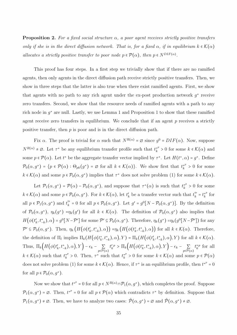
Proposition 2. For a fixed social structure α, a poor agent receives strictly positive transfers

only if she is in the direct diffusion network. That is, for a fixed α, if in equilibrium k ∈ K(α)

allocates a strictly positive transfer to poor node p ∈ P(α), then p ∈ NDIF (α).

This proof has four steps. In a first step we trivially show that if there are no ramified

agents, then only agents in the direct diffusion path receive strictly positive transfers. Then, we

show in three steps that the latter is also true when there exist ramified agents. First, we show

that agents with no path to any rich agent under the ex-post production network g∗ receive

zero transfers. Second, we show that the resource needs of ramified agents with a path to any

rich node in g∗ are null. Lastly, we use Lemma 1 and Proposition 1 to show that these ramified

agent receive zero transfers in equilibrium. We conclude that if an agent p receives a strictly

positive transfer, then p is poor and is in the direct diffusion path.

Fix α. The proof is trivial for α such that NR(α) = ∅ since g0 = DIF (α). Now, suppose

NR(α) ≠ ∅. Let τ∗ be any equilibrium transfer profile such that t∗p

k > 0 for some k ∈ K(α) and

some p ∈ P(α). Let t∗ be the aggregate transfer vector implied by τ∗. Let H(t∗, α) = g∗. Define

P0(α, g∗) = p ∈ P(α) ∶ Θpk(g∗) = ∅ for all k ∈ K(α). We show first that t∗p

k > 0 for some

k ∈ K(α) and some p ∈ P0(α, g∗) implies that τ∗ does not solve problem (1) for some k ∈ K(α).

Let P1(α, g∗) = P(α) − P0(α, g∗), and suppose that τ∗(α) is such that t∗p

k > 0 for some

k ∈ K(α) and some p ∈ P0(α, g∗). For k ∈ K(α), let t′k be a transfer vector such that t′p

k = t∗p

k for

all p ∈ P1(α, g∗) and t′p

k = 0 for all p ∈ P0(α, g∗). Let g′ = g0[N − P0(α, g∗)]. By the definition

of P0(α, g∗), ηk(g∗) =ηk(g′) for all k ∈ K(α). The definition of P0(α, g∗) also implies that

H(φ(t′k, t∗−k), α) = g

0[N −P ′] for some P ′ ⊆ P0(α, g∗). Therefore, ηk(g∗) =ηk(g0[N −P ′]) for any

P ′ ⊆ P0(α, g∗). Then, ηk (H(φ(t′k, t∗−k), α)) =ηk (H(φ(t∗k, t

∗−k), α)) for all k ∈ K(α). Therefore,

the definition of Πl implies Πk(H(φ(t∗k, t∗−k), α), Y ) = Πk(H(φ(t′k, t

∗−k), α), Y ) for all k ∈ K(α).

Thus, Πk(H(φ(t′k, t∗−k), α), Y ) − εk − ∑

p∈P(α)t′kp > Πk(H(φ(t∗k, t

∗−k), α), Y ) − εk − ∑

p∈P(α)t∗kp for all

k ∈ K(α) such that t∗p

k > 0. Then, τ∗ such that t∗p

k > 0 for some k ∈ K(α) and some p ∈ P(α)

does not solve problem (1) for some k ∈ K(α). Hence, if τ∗ is an equilibrium profile, then t∗p= 0

for all p ∈ P0(α, g∗).

Now we show that t∗p= 0 for all p ∈ NR(α)∩P1(α, g∗), which completes the proof. Suppose

P1(α, g∗) = ∅. Then, t∗p= 0 for all p ∈ P(α) which contradicts τ∗ by definition. Suppose that

P1(α, g∗) ≠ ∅. Then, we have to analyze two cases: P(α, g∗) = ∅ and P(α, g∗) ≠ ∅.

35

First, let us suppose that P(α, g∗) = ∅. The definition of P1(α, g∗) and DIF (α) imply

that P(α)∩NDIF (α) ⊆ P1(α, g∗) ≠ ∅. Now we proceed to show that P(α)∩NDIF (α) = P1(α, g∗).

Suppose P(α) ∩ NDIF (α) ⊂ P1(α, g∗). Then, there exists p ∈ P1(α, g∗) such that p ∉ P(α) ∩

NDIF (α). Then, p ∈ P(α) implies that p ∈ NR(α). Also, p ∈ P1(α, g∗) implies that Θkp(g∗) ≠ ∅

for some k ∈ K(α). Therefore, (i) Θpp(g∗) ≠ ∅ for some p ∈ P(α)∩NDIF (α), or (ii) p ∈ ηk(g∗) for

some k ∈ K(α). Suppose condition (i). Then there exists θpp ∈ Θpp(g∗) such that p ∈ NDIF (α).

Then P(α, g∗) = ∅ implies that p ∉ NR(α), which contradicts p ∈ NR(α). Suppose condition

(ii). Then, there are two cases. First, p ∈ S1(α). Then there exists θkj ∈ Θkj(g∗) for k ∈ K(α)

and j ∈ S1(α) such that p = j and p ∈ N θkj , which contradicts p ∈ NR(α). Second, p ∉ S1(α).

Then, p ∈ P(α) implies that p ∈ S i(α) for i > 1. Thus, the definition of layer implies that

there exists some j ∈ S1(α) and j ≠ p such that θkj ∈ Θkj(g∗) for k ∈ K(α) and p ∈ N θkj , which

also contradicts p ∈ NR(α). Hence, P(α) ∩NDIF (α) = P1(α, g∗). The assumption P(α, g∗) = ∅

implies that P(α)∩NDIF (α) ∩NR(α) = ∅. Therefore, P1(α, g∗)∩NR(α) = ∅. In the first part of

the proof we showed that τ∗ implies that t∗p= 0 for all p ∈ P0(α, g∗). Therefore, the definition

of P1(α, g∗) implies that if t∗p> 0, then p ∈ NDIF (α).

Now, suppose P(α, g∗) ≠ ∅. Pick any p′ ∈ P(α, g∗). The definition of Ns-subnetwork

implies that P(α, g∗, p′) ⊆ P(α, g0, p′). Now we proceed to show that P(α, g∗, p′) = P(α, g0, p′).

Suppose P(α, g∗, p′) ⊂ P(α, g0, p′). Then, there exists l′ ∈ P(α, g0, p′) such that l′ ∉ P(α, g∗, p′).

By Lemma 6, Πp(g0[P(α, g0, p′) ∪ p′], Y ) − εp ≥ 0 for all p ∈ P(α, g0, p′). Lemma 6 also

implies that ηp(g0) = ηp(g0[P(α, g0, p′) ∪ p′]) for all p ∈ P(α, g0, p′). Then, p′ ∈ P(α, g∗)

and l′ ∉ P(α, g∗, p′) imply that there exists some l′′ ∈ P(α, g0, p′) such that l′′ ≠ l′ and

Πl′′(g0[P(α, g0, p′) ∪ p′], Y ) − εl′′ + t∗l′′

< 0, which contradicts Lemma 5, or contradicts the

definition of Tk(α) for some k ∈ K(α). Hence, P(α, g∗, p′) = P(α, g0, p′).

Therefore, Πp(g0[P(α, g∗, p′)], Y ) − εp ≥ 0 for all p ∈ P(α, g∗, p′). Then, the definition

of rp implies that rp(α, g∗,0) = 0 for all p ∈ P(α, g∗, p′). To complete the proof for the case

P(α, g∗) ≠ ∅, we show as an intermediary step that ⋃p′∈P(α,g∗) P(α, g∗, p′) = NR(α) ∩ P1(α, g∗),

which, we will show, implies rp(α, g∗,0) = 0 for all p ∈ NR(α) ∩ P1(α, g∗). The definition

of P(α, g∗, p′) implies that ⋃p′∈P(α,g∗) P(α, g∗, p′) ⊆ NR(α). The definition of P(α, g∗, p′) also

implies that there exists θpp′ ∈ Θpp′(g0) for all p ∈ P(α, g∗, p′) and p′ ∈ P(α, g∗). The definition

of P(α, g∗) implies that that there exists θp′k ∈ Θp′k(g0) for p′ ∈ P(α, g∗) and k ∈ K(α) such

36

that N θp′k ⊆ NDIF (α). Pick any θpp′ ∈ Θpp′(g0) and θp′k ∈ Θp′k(g0) such that N θp′k ⊆ NDIF (α).

Suppose that there is no path θpp′ + θp′k ∈ Θpk(g0). Then, the definition of path implies that

there exists z ∈ N θp′k and z ∈ N θpp′ such that z ≠ p′. The definition of path also implies that

dpz(θpp′) < dpp′(θpp′). Moreover z ∈ N θp′k implies that z ∈ NDIF (α). Then dpz(θpp′) < dpp′(θpp′)

and z ∈ NDIF (α) contradict p ∈ P(α, g∗, p′). Therefore, ⋃p′∈P(α,g∗) P(α, g∗, p′) = P1(α, g∗). Thus,

⋃p′∈P(α,g∗) P(α, g∗, p′) = NR(α) ∩P1(α, g∗).

Hence, rp(α, g∗,0) = 0 for all p ∈ NR(α) ∩P1(α, g∗). The latter implies that, by Lemma 1,

tpk(α, g∗, t∗−k) = 0 for each k ∈ K(α), and each p ∈ NR(α) ∩ P1(α, g∗). Therefore, Proposition 1

implies that if τ∗ is an equilibrium transfer profile, then t∗p= 0 for each p ∈ (NR(α)∩P1(α, g∗))∪

P0(α, g∗). Therefore, by construction, P(α)−((NR(α)∩P1(α, g∗))∪P0(α, g∗)) = NDIF (α)∩P(α)

which implies that if t∗p> 0, then p ∈ NDIF (α).

Proposition 3. In a multilayer social structure topology, there is at least one poor node that

does not receive positive transfers in equilibrium. That is, if ω(α) is multilayer, then #U(gT ) <

n −Kα for all gT ∈ Φ(α).

Proof. Pick any α ∈ A such that ω(α) is multilayer. Let t∗ be an equilibrium aggregate transfer

vector. Let g∗T be a giving network implied by t∗. By construction #U(g∗T ) ≤ n −Kα. Suppose

#U(g∗T ) = n −Kα. Then, t∗ is such that t∗p> 0 for all p ∈ P(α). We first show that t∗

p> 0 for

all p ∈ P(α) implies H(α, t∗) = g0. Then we use Lemma 1 to complete the proof.

Suppose g0 = ∅. Then X (α) = g0. Thus H(α, t∗) = g0. Now suppose that g0 ≠ ∅ and

H(α, t∗) = g ∈ X (α) such that g ≠ g0. Then g ≠ g0 implies that there exists p ∈ P(α) such

that ηp(g0) ≠ ∅ and ηp(g) = ∅. Hence, Lemma 1 implies that tpk(α, g, t∗−k) = 0 for all k ∈ K(α).

Therefore, t∗p> 0 for all p ∈ P(α) does not solve problem (2) for g = g. Thus, Proposition 1

implies that t∗p> 0 for all p ∈ P(α) does not solve problem (1), which contradicts the definition

of t∗. Therefore, H(α, t∗) = g0. Suppose ηp(g0) = ∅ for some p ∈ P(α). Then, Lemma 1 implies

that tpk(α, g0, t∗−k) = 0 for all k ∈ K(α). Therefore, t∗

p> 0 for all p ∈ P(α) does not solve problem

(2) for g = g. Thus, Proposition 1 implies that t∗p> 0 for all p ∈ P(α) does not solve problem

(1), which contradicts the definition of t∗. Suppose now that ηp(g0) ≠ ∅ for all p ∈ P(α). By the

definition of layer, Πp(g0, Y ) − εp ≥ 0 for all p ∉ S1(α). Thus, rp(α, g0,0) = 0 for all p ∉ S1(α).

Then, Lemma 1 implies that tpk(α, g0, t∗−k) = 0 for all p ∉ S1(α) and all k ∈ K(α). Therefore,

t∗p> 0 for all p ∈ P(α) does not solve problem (2) for g = g. Thus, Proposition 1 implies that

37

t∗p> 0 for all p ∈ P(α) does not solve problem (1), which contradicts the definition of t∗. Hence,

#U(gT ) < n −Kα for all gT ∈ Φ(α).

Proposition 4. In social structures where all the poor agents are either disconnected or directly

connected with the rich agents in the ex ante production network, the equilibrium giving network

is such that there are no links that do not exist in the ex ante production network. That is, if

α ∈ A, then GgT ⊆ Gg0 for gT ∈ Φ(α).

Proof. Pick any α ∈ A. Let τ∗ be an equilibrium transfer profile. Let t∗ be the equilibrium

aggregate transfer vector implied by τ∗. Let g∗T be any equilibrium giving network implied

by t∗. First, suppose g∗T = g∅. Then, Gg∗T = ∅. Therefore, Gg∗T ⊆ Gg0 . Now, suppose that

g∗T ≠ g∅ and Gg∗T ⊈ Gg0 . Then, kp ∈ Gg∗T and kp ∉ Gg0 for some k ∈ K(α) and some p ∈ P(α).

Pick any k ∈ K(α) such that kp ∈ Gg∗T and kp ∉ Gg0 for some p ∈ P(α). Let P = p ∈

P(α) ∶ kp ∈ Gg∗T and kp ∉ Gg0. The definition of giving network implies that t∗p

k> 0 for

all p ∈ P. Let t′k

be a transfer vector such that t′p

k= t∗

p

kfor all p ∈ P(α) − P and t

′p

k= 0

for all p ∈ P. By the definition of A, dkp(g0) = ∞ for all p ∈ P. Hence, Θkp(g

0) = ∅ for

all p ∈ P. Thus, ηk (H(φ(t′k, t∗−k

), α)) =ηk (H(φ(t∗k, t∗−k

), α)). Therefore, the definition of Πl

implies Πk(H(φ(t∗k, t∗−k

), α), Y ) = Πk(H(φ(t′k, t∗−k

), α), Y ). Thus, Πk(H(φ(t′k, t∗−k

), α), Y ) − εk −

∑p∈P(α)

t′kp > Πk(H(φ(t∗

k, t∗−k

), α), Y ) − εk − ∑p∈P(α)

t∗kp. Then, τ∗ such that t∗

p

k> 0 for all p ∈ P does

not solve problem (1) for k ∈ K(α). Hence, Gg∗T ⊆ Gg0 .

Proposition 5. In the set of social structures where there exists at least one indirect connections

between a poor agent and a rich agent, there exists some social structure such that some of its

equilibrium giving network contains a link between agents that are not directly connected in the

ex ante production network. That is, there exists α ∈ A such that GgT /⊆ Gg0 for gT ∈ Φ(α).

Proof. Pick α ∈ A such that g0 = (1, ..., n − 1, n,k1,12,23, ..., n − 1n), K(α) = k, and

n + 1 = n. Suppose

(i) yi+1i > εi + y − yii − y

i−1i for all i ∈ 1, ..., n − 1

(ii) 0 < εn + y − ynn − yn−1n < εi + y − yii − y

i−1i < y1

k for all i ∈ 1, ..., n − 1

(iii) ykk − y − εk > εn + y − ynn − y

n−1n .

38

The definitions of g0 and K(α) imply that α ∈ Ac. Moreover Y ∈ Rn2

+ and ε ∈ Rn imply

that α satisfies conditions (i), (ii), and (iii). We now derive the solution to problem (2) for k

in α. We then derive the solution of problem (3) for k in α. Lastly, we use Proposition 1 to

complete the proof.

Condition (i) implies that ri (α, g0[N − i + 2, ..., n],0) = 0 for all i ∈ 1, ..., n − 2 and

rn−1 (α, g0,0) = 0. Condition (ii) implies that ri (α, g0[N − i + 1, ..., n],0) = εi + y − yii − yi−1i

for all i ∈ 1, ..., n − 1 and rn (α, g0,0) = εn + y − ynn − yn−1n . Let tk(α, g,0) be a k’s solution to

problem (2) for g ∈ X (α,0) (Las funciones X (α,0) y X (α) estan bien definidas, pero la notacion

es mala. Hay que cambiarla). In section 2.6 we show that tk(α, g,0) exists for each g ∈ X (α,0).

Conditions (i) and (ii) imply that X (α,0) = ⋃i∈1,..,n−1

g0[N − i + 1, ..., n] ∪ g0 ∪ g∅. Then,

Lemma 1 implies that tk(α, g,0) is such that

(a) tik(α, g,0) = εi+y−yii −y

i−1i and ti

′

k (α, g,0) = 0 for all i′ ≠ i and i′ ∈ P(α), for i ∈ 1, .., n−1

and g = g0[N − i + 1, ..., n].

(b) tnk(α, g,0) = εn + y − ynn − y

n−1n and ti

′

k (α, g,0) = 0 for all i′ ∈ 1, .., n − 1 and g = g0

(c) tik(α, g,0) = 0 for all i ∈ 1, ..., n and g = g∅.

Let g∗ be a k’s solution to problem (3). We showed in section 2.6 that g∗ exists. Now,

we prove that g∗ = g0. Condition (iii) implies that Xf(α,0) = X (α,0). The definition of g0

implies that ηk(g) = 1 for all g ∈ Xf(α,0) such that g ≠ g∅, and ηk(g) = ∅ for g = g∅. Then,

implications (a) through (c) and condition (ii) imply that g∗ = g0.

Thus Proposition 1 implies that t∗n

k = εn + y − ynn − yn−1n and t∗

i

k = 0 for all i ∈ 1, .., n − 1

solve problem (1) for k ∈ K(α). Then K(α) = k implies that t∗ such that t∗n

k = εn+y−ynn−yn−1n

and t∗i

k = 0 for all i ∈ 1, .., n − 1 is an equilibrium transfer vector. Hence there exists α ∈ Ac

such that GgT ⊈ Gg0 for gT ∈ Φ(α).

Proposition 6. For each social structure there exists a social structure with a different under-

lying ex ante production network such that both induce the same equilibrium giving network.

Formally, pick any α ∈ A. Suppose g∗T ∈ Φ(α) exists. Then, there exists α ∈ A such that g0 ≠ g0,

g∗T = gT , and gT ∈ Φ(α).

39

Proof. The proof has two parts. We first prove Proposition 6 for the case g∗T ≠ g∅. To do so,

we first pick an economy α which ex ante production network is by construction different from

the ex ante production network in α. We show that α induces the same giving network as α.

Then, we prove the statement of Proposition 6 for g∗T = g∅ following analogous steps as for the

case g∗T ≠ g∅.

Pick α ∈ A. Suppose Φ(α) ≠ ∅. Pick any g∗T ∈ Φ(α). Suppose g∗T ≠ g∅. Let α ∈ A be such

that the ex ante production network of α is g0 = (N, G), and ω(α) = (N −E(g∗T ),E(g∗T ), G);

where

G =

⎧⎪⎪⎪⎪⎪⎪⎪⎪⎪⎨⎪⎪⎪⎪⎪⎪⎪⎪⎪⎩

Gg∗T if g∗T ≠ g0

Gg∗T ∪ k′k′′ if g∗T = g0 and #E(g∗T ) > 1

Gg∗T ∪ p0p1 if g∗T = g0 and #E(g∗T ) = 1,

with k′, k′′ ∈ K(α), p0, p1 ∈ P(α), and

(i) rp(α, g0,0) = c > 0 for all p ∈ P(α),

(ii) ypk > c for each k ∈ K(α) and all p ∈ P(α) ∩ ηk(g0),

(iii) Πk (gK(α), Y ) − εk > #P(α) × c for all k ∈ K(α), and

(iv) yp′

p = 0 for p, p′ ∈ P(α) such that pp′ ∈ G and p, p′ ∩ ⋃k∈K(α)

ηk(g0) = p.

The definitions of Πk (gK(α), Y ) and rp(α, g0,0) imply that conditions (i) through (iv) are inde-

pendent. Moreover, the definitions of Πk (gK (α) , Y ) and rp(α, g0,0), and Y ∈ Rn2

+ and ε ∈ Rn

imply that there exists α such that conditions (i) to (iv) are satisfied.

Consider a transfer profile τ such that for each k ∈ K(α), let tpk = c/#(ηp(g0) ∩K(α)) for

all p ∈ P(α)∩ηk(g0) and tpk = 0 for all p ∈ P(α)∩ [ηk(g0)]c, which implies the aggregate transfer

vector t. Let gT be the giving network implied by τ . Then, the definitions of giving network

and G imply that gT = g∗T . By the construction of G, g0 ≠ g0. Now we prove that τ is an

equilibrium transfer profile.

First, condition (iii) implies that τ is feasible. Suppose τ ′ is an equilibrium trans-

fer profile such that τ ′ ≠ τ . Let t′ be the aggregate transfer vector implied by τ ′. Then

t′k ≠ tk for some k ∈ K(α). Pick any k ∈ K(α) such that t′k ≠ tk and denote this agent

40

by k. Suppose t′kp > 0 for some p ∈ P(α) ∩ [ηk(g

0)]c and t′kp = tp

kotherwise. Then, the

construction of τ ′ and condition (i) implies that t′pk+ tp

k= rp(α, g0,0) for all p ∈ P(α) ∩

ηk(g0). Then, ηk (H(φ(t′

k, t−k), α)) =ηk (H(φ(tk, t−k), α)). Therefore, the definition of Πl im-

plies Πk(H(φ(t′k, t−k), α), Y ) = Πk(H(φ(tk, t−k), α), Y ). Thus, Πk(H(φ(t′

k, t−k), α), Y ) − εk −

∑p∈P(α)

t′kp < Πk(H(φ(tk, t−k), α), Y ) − εk − ∑

p∈P(α)tpk. Then, τ ′ does not solve problem (1) for

k ∈ K(α).

Suppose that t′kp > c/#(ηp(g0) ∩ K(α)) for some p ∈ P(α) ∩ ηk(g

0) and t′kp = tp

koth-

erwise. Then, the construction of τ ′ and condition (i) implies that t′kp + tp

−k> rp(α, g0,0)

for some p ∈ P(α) ∩ ηk(g0) and t′

kp + tp

−k≥ rp(α, g0,0) for all p ∈ P(α) ∩ ηk(g

0). Then,

ηk (H(φ(t′k, t−k), α)) =ηk (H(φ(tk, t−k), α)). Therefore, the definition of Πl implies

Πk(H(φ(t′k, t−k), α), Y ) = Πk(H(φ(tk, t−k), α), Y ). Thus, Πk(H(φ(t′

k, t−k), α), Y )−εk− ∑

p∈P(α)t′kp <

Πk(H(φ(tk, t−k), α), Y ) − εk − ∑p∈P(α)

tpk. Then, τ ′ does not solve problem (1) for k ∈ K(α).

Suppose now that t′kp = c such that 0 ≤ c < c/#(ηp(g0)∩K(α)) for some p ∈ P(α)∩ ηk(g

0)

and t′kp = tp

kotherwise. The construction of τ ′ and condition (i) implies that t′

kp+tp

−k< rp(α, g0,0)

for some p ∈ P(α) ∩ ηk(g0), and t′

kp + tp

−k≤ rp(α, g0,0) for all p ∈ P(α) ∩ ηk(g

0). Let P ′ = p ∈

P(α) ∶ t′kp + tp

−k< rp(α, g0,0). The construction of G and condition (i) also imply that there

exists α such that G = Gg∗T ∪ p0p1, p0, p1 ∈ P(α), and p0, p1 ∩ ⋃k∈K(α)

ηk(g0) = p0, p1. In the

latter case, rp0(α, g0[N − p1],0) < c and rp1(α, g

0[N − p0],0) < c, which implies that there exists

P ′′ = ηk (H(φ(t′k, t−k), α)) − ηk (H(φ(tk, t−k), α)) such that P ′′ ⊆ P(α) and P ′ ⊆ P ′′. Therefore,

the definition of Πl implies Πk(H(φ(tk, t−k), α), Y )−Πk(H(φ(t′k, t−k), α), Y ) = ∑p∈P ′′ y

p

k. By the

construction of τ ′, ∑p∈P(α) tpk −∑p∈P(α) t

′kp = ∑p∈P ′ c/#(ηp(g0)∩K(α))−∑p∈P ′ c. Then, condition

(ii) implies that Πk(H(φ(t′k, t−k), α), Y )− εk − ∑

p∈P(α)t′kp < Πk(H(φ(tk, t−k), α), Y )− εk − ∑

p∈P(α)tpk.

Then, τ ′ does not solve problem (1) for k ∈ K(α).

Lastly, suppose that t′kp > 0 for some p ∈ P(α) ∩ [ηk(g

0)]c and t′pk≠ c/#(ηp(g0) ∩ K(α))

for some p ∈ P(α) ∩ ηk(g0) and t′kp = tp

kotherwise. Condition (iv) implies that rp(α, g0,0) =

rp(α, g0[N − p′],0) for p, p′ ∈ P(α) such that pp′ ∈ G and p, p′ ∩ ⋃k∈K(α)

ηk(g0) = p. Thus,

condition (iv) and p′ ∉ ⋃k∈K(α)

ηk(g0) imply that a transfer profile τ such that tp′

k > 0 does not solve

problem (1) for all k ∈ K(α). Therefore, we can proceed analogously as before to prove that a

transfer profile τ ′ such that t′kp > 0 for some p ∈ P(α)∩[ηk(g

0)]c and tpk ≠ c/#(ηp(g0)∩K(α)) for

41

some p ∈ P(α)∩ηk(g0) and t′kp = tp

kotherwise does not does not solve problem (1) for k ∈ K(α).

Hence, if τ ′ is an equilibrium transfer profile, then τ ′ = τ .

We now complete the proof by proving Proposition 6 for the case g∗T = g∅. Suppose

g∗T = g∅. Denote the ex ante production network of an economy α′ by g0 = (N, G′). Let α′ ∈ A

be such that ω(α′) = (N − k1, k2,k1, k2, G′), where

G′ =

⎧⎪⎪⎪⎪⎨⎪⎪⎪⎪⎩

∅ if g∗T ≠ g0

k1k2 if g∗T = g0;

and

1. rp(α′, g0′,0) > 0 for all p ∈ P(α′), and

2. Πk (gK (α′) , Y ) − εk = 0 for all k1, k2 ∈ K(α′)

The definitions of Πk (gK(α), Y ) and rp(α, g0,0) imply that conditions (1) and (2) are

independent. Moreover, the definitions of Πk (gK (α) , Y ) and rp(α, g0,0), and Y ∈ Rn2

+ and

ε ∈ Rn imply that there exists α such that conditions (1) and (2) are satisfied.

Let τ ′ be an equilibrium transfer profile. Let t′ be the implied aggregate transfer by τ ′.

The definition of Tk implies that t′ must be such that t′kp = 0 for all k ∈ K(α′) and all p ∈ P(α′).

Let g′T be the giving network implied by τ ′. Then, g′T = g∅. By the construction of G′, g0 ≠ g′0,

which completes the proof.

Proposition 7. In any social structure, transfers to all the non isolated poor agents located in

the first layer, equal or greater than their subsistence needs, are sufficient to sustain the entire

ex ante production network. Formally, pick any α ∈ A. Then, H(t, α) = g0 if, and only if

tp ≥ rp(α, g0,0) for all p ∈ S1(α) such that ηp(g0) ≠ ∅.

Proof. Pick any α ∈ A. Let P ′ = p ∈ P(α) ∶ ηp(g0) = ∅. Let t be an aggregate transfer

vector such that tp ≥ rp(α, g0,0) for all p ∈ S1(α) ∩ [P ′]c. By the definition of layer and the

function rp, rp(α, g0,0) = εp − Πp(g0, Y ) > 0 for all p ∈ S1(α). Then, by the construction of t,

Πp(g0, Y )−εp+tp ≥ 0 for all p ∈ S1(α)∩[P ′]c. By the definition of layer, Πl(g0, Y )−εl ≥ 0 for all l ∈

⋃i>1 Si(α). The definition of Ns-subnetwork and the definition of P ′ imply that g0 = g0[N −P ′].

42

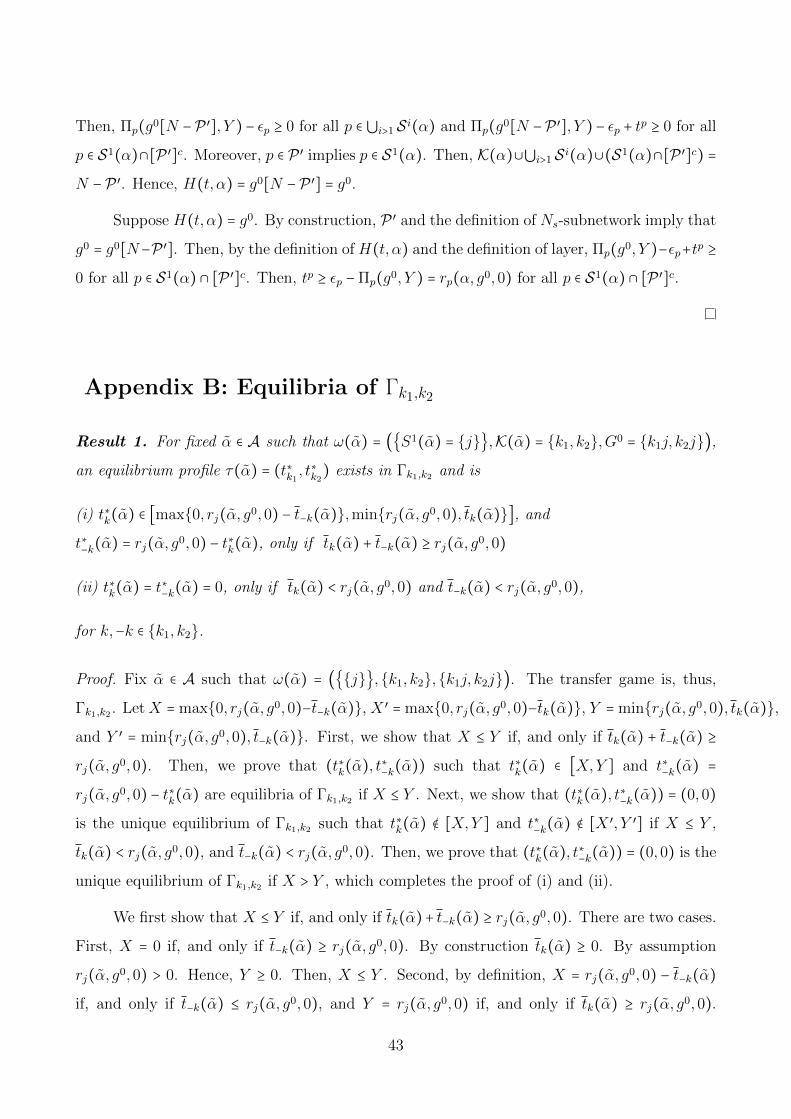
Then, Πp(g0[N −P ′], Y )− εp ≥ 0 for all p ∈ ⋃i>1 Si(α) and Πp(g0[N −P ′], Y )− εp + tp ≥ 0 for all

p ∈ S1(α)∩[P ′]c. Moreover, p ∈ P ′ implies p ∈ S1(α). Then, K(α)∪⋃i>1 Si(α)∪(S1(α)∩[P ′]c) =

N −P ′. Hence, H(t, α) = g0[N −P ′] = g0.

Suppose H(t, α) = g0. By construction, P ′ and the definition of Ns-subnetwork imply that

g0 = g0[N−P ′]. Then, by the definition of H(t, α) and the definition of layer, Πp(g0, Y )−εp+tp ≥

0 for all p ∈ S1(α) ∩ [P ′]c. Then, tp ≥ εp −Πp(g0, Y ) = rp(α, g0,0) for all p ∈ S1(α) ∩ [P ′]c.

Appendix B: Equilibria of Γk1,k2

Result 1. For fixed α ∈ A such that ω(α) = (S1(α) = j,K(α) = k1, k2,G0 = k1j, k2j),

an equilibrium profile τ(α) = (t∗k1 , t∗k2) exists in Γk1,k2 and is

(i) t∗k(α) ∈ [max0, rj(α, g0,0) − t−k(α),minrj(α, g0,0), tk(α)], and

t∗−k(α) = rj(α, g0,0) − t∗k(α), only if tk(α) + t−k(α) ≥ rj(α, g0,0)

(ii) t∗k(α) = t∗−k(α) = 0, only if tk(α) < rj(α, g0,0) and t−k(α) < rj(α, g0,0),

for k,−k ∈ k1, k2.

Proof. Fix α ∈ A such that ω(α) = (j,k1, k2,k1j, k2j). The transfer game is, thus,

Γk1,k2 . LetX = max0, rj(α, g0,0)−t−k(α), X ′ = max0, rj(α, g0,0)−tk(α), Y = minrj(α, g0,0), tk(α),

and Y ′ = minrj(α, g0,0), t−k(α). First, we show that X ≤ Y if, and only if tk(α) + t−k(α) ≥

rj(α, g0,0). Then, we prove that (t∗k(α), t∗−k(α)) such that t∗k(α) ∈ [X,Y ] and t∗−k(α) =

rj(α, g0,0) − t∗k(α) are equilibria of Γk1,k2 if X ≤ Y . Next, we show that (t∗k(α), t∗−k(α)) = (0,0)

is the unique equilibrium of Γk1,k2 such that t∗k(α) ∉ [X,Y ] and t∗−k(α) ∉ [X ′, Y ′] if X ≤ Y ,

tk(α) < rj(α, g0,0), and t−k(α) < rj(α, g0,0). Then, we prove that (t∗k(α), t∗−k(α)) = (0,0) is the

unique equilibrium of Γk1,k2 if X > Y , which completes the proof of (i) and (ii).

We first show that X ≤ Y if, and only if tk(α)+ t−k(α) ≥ rj(α, g0,0). There are two cases.

First, X = 0 if, and only if t−k(α) ≥ rj(α, g0,0). By construction tk(α) ≥ 0. By assumption

rj(α, g0,0) > 0. Hence, Y ≥ 0. Then, X ≤ Y . Second, by definition, X = rj(α, g0,0) − t−k(α)

if, and only if t−k(α) ≤ rj(α, g0,0), and Y = rj(α, g0,0) if, and only if tk(α) ≥ rj(α, g0,0).

43

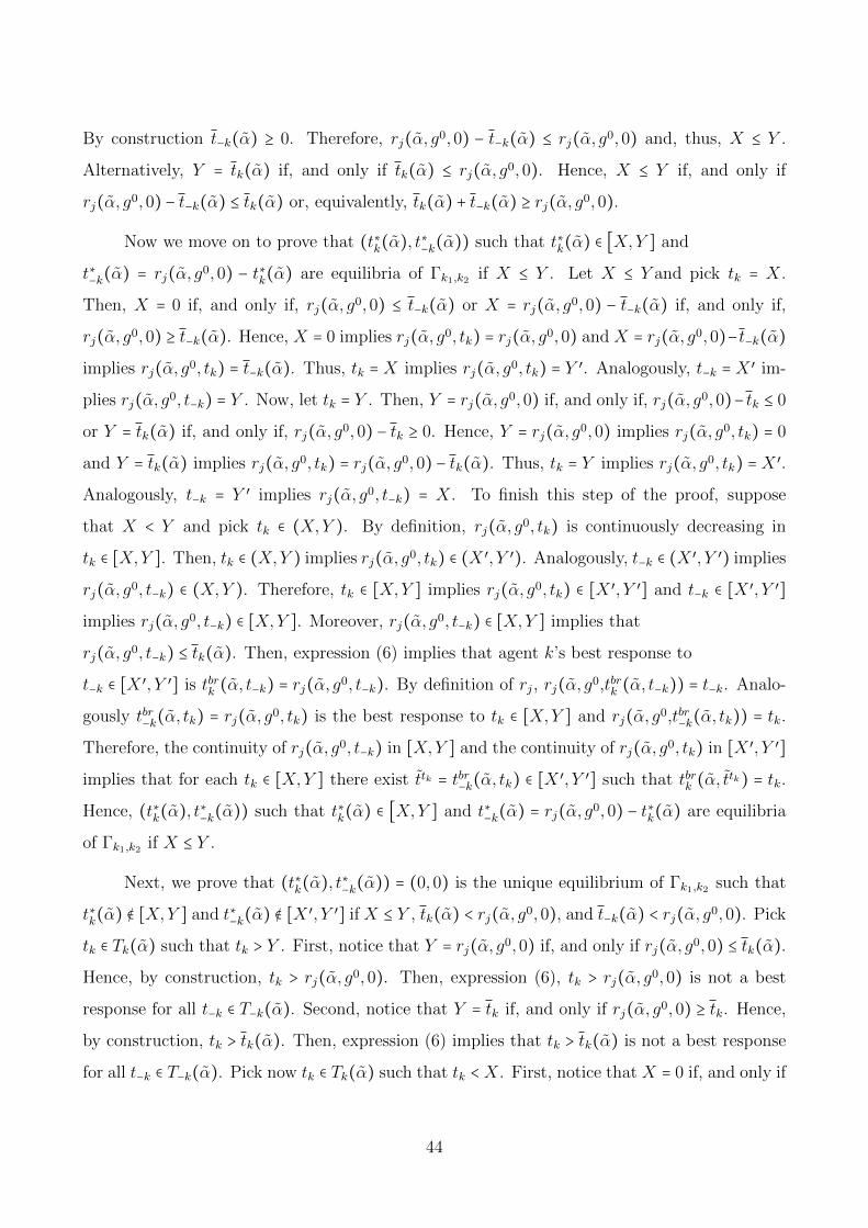
By construction t−k(α) ≥ 0. Therefore, rj(α, g0,0) − t−k(α) ≤ rj(α, g0,0) and, thus, X ≤ Y .

Alternatively, Y = tk(α) if, and only if tk(α) ≤ rj(α, g0,0). Hence, X ≤ Y if, and only if

rj(α, g0,0) − t−k(α) ≤ tk(α) or, equivalently, tk(α) + t−k(α) ≥ rj(α, g0,0).

Now we move on to prove that (t∗k(α), t∗−k(α)) such that t∗k(α) ∈ [X,Y ] and

t∗−k(α) = rj(α, g0,0) − t∗k(α) are equilibria of Γk1,k2 if X ≤ Y . Let X ≤ Y and pick tk = X.

Then, X = 0 if, and only if, rj(α, g0,0) ≤ t−k(α) or X = rj(α, g0,0) − t−k(α) if, and only if,

rj(α, g0,0) ≥ t−k(α). Hence, X = 0 implies rj(α, g0, tk) = rj(α, g0,0) and X = rj(α, g0,0)−t−k(α)

implies rj(α, g0, tk) = t−k(α). Thus, tk = X implies rj(α, g0, tk) = Y ′. Analogously, t−k = X ′ im-

plies rj(α, g0, t−k) = Y . Now, let tk = Y . Then, Y = rj(α, g0,0) if, and only if, rj(α, g0,0)− tk ≤ 0

or Y = tk(α) if, and only if, rj(α, g0,0) − tk ≥ 0. Hence, Y = rj(α, g0,0) implies rj(α, g0, tk) = 0

and Y = tk(α) implies rj(α, g0, tk) = rj(α, g0,0) − tk(α). Thus, tk = Y implies rj(α, g0, tk) = X ′.

Analogously, t−k = Y ′ implies rj(α, g0, t−k) = X. To finish this step of the proof, suppose

that X < Y and pick tk ∈ (X,Y ). By definition, rj(α, g0, tk) is continuously decreasing in

tk ∈ [X,Y ]. Then, tk ∈ (X,Y ) implies rj(α, g0, tk) ∈ (X ′, Y ′). Analogously, t−k ∈ (X ′, Y ′) implies

rj(α, g0, t−k) ∈ (X,Y ). Therefore, tk ∈ [X,Y ] implies rj(α, g0, tk) ∈ [X ′, Y ′] and t−k ∈ [X ′, Y ′]

implies rj(α, g0, t−k) ∈ [X,Y ]. Moreover, rj(α, g0, t−k) ∈ [X,Y ] implies that

rj(α, g0, t−k) ≤ tk(α). Then, expression (6) implies that agent k’s best response to

t−k ∈ [X ′, Y ′] is tbrk (α, t−k) = rj(α, g0, t−k). By definition of rj, rj(α, g0,tbrk (α, t−k)) = t−k. Analo-

gously tbr−k(α, tk) = rj(α, g0, tk) is the best response to tk ∈ [X,Y ] and rj(α, g0,tbr−k(α, tk)) = tk.

Therefore, the continuity of rj(α, g0, t−k) in [X,Y ] and the continuity of rj(α, g0, tk) in [X ′, Y ′]

implies that for each tk ∈ [X,Y ] there exist ttk = tbr−k(α, tk) ∈ [X ′, Y ′] such that tbrk (α, ttk) = tk.

Hence, (t∗k(α), t∗−k(α)) such that t∗k(α) ∈ [X,Y ] and t∗−k(α) = rj(α, g

0,0) − t∗k(α) are equilibria

of Γk1,k2 if X ≤ Y .

Next, we prove that (t∗k(α), t∗−k(α)) = (0,0) is the unique equilibrium of Γk1,k2 such that

t∗k(α) ∉ [X,Y ] and t∗−k(α) ∉ [X ′, Y ′] if X ≤ Y , tk(α) < rj(α, g0,0), and t−k(α) < rj(α, g0,0). Pick

tk ∈ Tk(α) such that tk > Y . First, notice that Y = rj(α, g0,0) if, and only if rj(α, g0,0) ≤ tk(α).

Hence, by construction, tk > rj(α, g0,0). Then, expression (6), tk > rj(α, g0,0) is not a best

response for all t−k ∈ T−k(α). Second, notice that Y = tk if, and only if rj(α, g0,0) ≥ tk. Hence,

by construction, tk > tk(α). Then, expression (6) implies that tk > tk(α) is not a best response

for all t−k ∈ T−k(α). Pick now tk ∈ Tk(α) such that tk <X. First, notice that X = 0 if, and only if

44

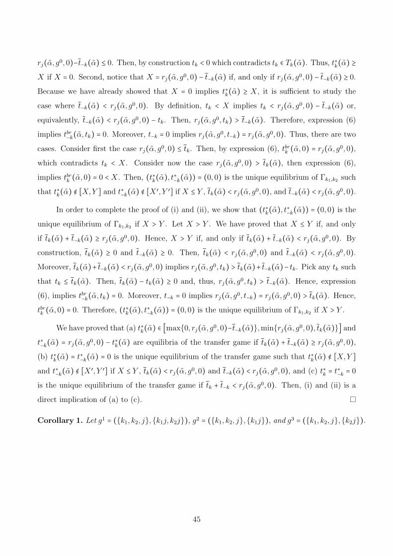
rj(α, g0,0)−t−k(α) ≤ 0. Then, by construction tk < 0 which contradicts tk ∈ Tk(α). Thus, t∗k(α) ≥

X if X = 0. Second, notice that X = rj(α, g0,0) − t−k(α) if, and only if rj(α, g0,0) − t−k(α) ≥ 0.

Because we have already showed that X = 0 implies t∗k(α) ≥ X, it is sufficient to study the

case where t−k(α) < rj(α, g0,0). By definition, tk < X implies tk < rj(α, g0,0) − t−k(α) or,

equivalently, t−k(α) < rj(α, g0,0) − tk. Then, rj(α, g0, tk) > t−k(α). Therefore, expression (6)

implies tbr−k(α, tk) = 0. Moreover, t−k = 0 implies rj(α, g0, t−k) = rj(α, g0,0). Thus, there are two

cases. Consider first the case rj(α, g0,0) ≤ tk. Then, by expression (6), tbrk (α,0) = rj(α, g0,0),

which contradicts tk < X. Consider now the case rj(α, g0,0) > tk(α), then expression (6),

implies tbrk (α,0) = 0 < X. Then, (t∗k(α), t∗−k(α)) = (0,0) is the unique equilibrium of Γk1,k2 such

that t∗k(α) ∉ [X,Y ] and t∗−k(α) ∉ [X ′, Y ′] if X ≤ Y , tk(α) < rj(α, g0,0), and t−k(α) < rj(α, g0,0).

In order to complete the proof of (i) and (ii), we show that (t∗k(α), t∗−k(α)) = (0,0) is the

unique equilibrium of Γk1,k2 if X > Y . Let X > Y . We have proved that X ≤ Y if, and only

if tk(α) + t−k(α) ≥ rj(α, g0,0). Hence, X > Y if, and only if tk(α) + t−k(α) < rj(α, g0,0). By

construction, tk(α) ≥ 0 and t−k(α) ≥ 0. Then, tk(α) < rj(α, g0,0) and t−k(α) < rj(α, g0,0).

Moreover, tk(α)+ t−k(α) < rj(α, g0,0) implies rj(α, g0, tk) > tk(α)+ t−k(α)− tk. Pick any tk such

that tk ≤ tk(α). Then, tk(α) − tk(α) ≥ 0 and, thus, rj(α, g0, tk) > t−k(α). Hence, expression

(6), implies tbr−k(α, tk) = 0. Moreover, t−k = 0 implies rj(α, g0, t−k) = rj(α, g0,0) > tk(α). Hence,

tbrk (α,0) = 0. Therefore, (t∗k(α), t∗−k(α)) = (0,0) is the unique equilibrium of Γk1,k2 if X > Y .

We have proved that (a) t∗k(α) ∈ [max0, rj(α, g0,0)−t−k(α),minrj(α, g0,0), tk(α)] and

t∗−k(α) = rj(α, g0,0) − t∗k(α) are equilibria of the transfer game if tk(α) + t−k(α) ≥ rj(α, g0,0),

(b) t∗k(α) = t∗−k(α) = 0 is the unique equilibrium of the transfer game such that t∗k(α) ∉ [X,Y ]

and t∗−k(α) ∉ [X ′, Y ′] if X ≤ Y , tk(α) < rj(α, g0,0) and t−k(α) < rj(α, g0,0), and (c) t∗k = t∗−k = 0

is the unique equilibrium of the transfer game if tk + t−k < rj(α, g0,0). Then, (i) and (ii) is a

direct implication of (a) to (c).

Corollary 1. Let g1 = (k1, k2, j,k1j, k2j), g2 = (k1, k2, j,k1j), and g3 = (k1, k2, j,k2j).

45

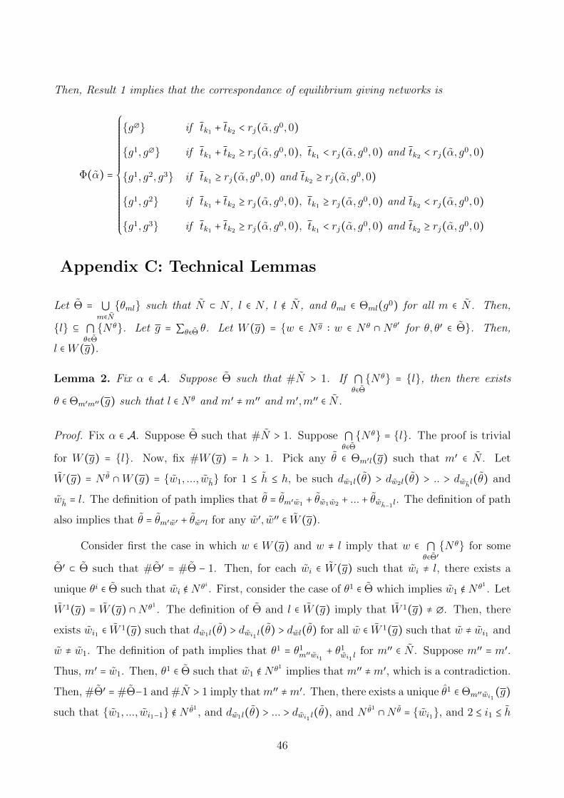
Then, Result 1 implies that the correspondance of equilibrium giving networks is

Φ(α) =

⎧⎪⎪⎪⎪⎪⎪⎪⎪⎪⎪⎪⎪⎪⎪⎪⎪⎪⎨⎪⎪⎪⎪⎪⎪⎪⎪⎪⎪⎪⎪⎪⎪⎪⎪⎪⎩

g∅ if tk1 + tk2 < rj(α, g0,0)

g1, g∅ if tk1 + tk2 ≥ rj(α, g0,0), tk1 < rj(α, g

0,0) and tk2 < rj(α, g0,0)

g1, g2, g3 if tk1 ≥ rj(α, g0,0) and tk2 ≥ rj(α, g

0,0)

g1, g2 if tk1 + tk2 ≥ rj(α, g0,0), tk1 ≥ rj(α, g

0,0) and tk2 < rj(α, g0,0)

g1, g3 if tk1 + tk2 ≥ rj(α, g0,0), tk1 < rj(α, g

0,0) and tk2 ≥ rj(α, g0,0)

Appendix C: Technical Lemmas

Let Θ = ⋃m∈N

θml such that N ⊂ N , l ∈ N , l ∉ N , and θml ∈ Θml(g0) for all m ∈ N . Then,

l ⊆ ⋂θ∈Θ

N θ. Let g = ∑θ∈Θ θ. Let W (g) = w ∈ N g ∶ w ∈ N θ ∩ N θ′ for θ, θ′ ∈ Θ. Then,

l ∈W (g).

Lemma 2. Fix α ∈ A. Suppose Θ such that #N > 1. If ⋂θ∈Θ

N θ = l, then there exists

θ ∈ Θm′m′′(g) such that l ∈ N θ and m′ ≠m′′ and m′,m′′ ∈ N .

Proof. Fix α ∈ A. Suppose Θ such that #N > 1. Suppose ⋂θ∈Θ

N θ = l. The proof is trivial

for W (g) = l. Now, fix #W (g) = h > 1. Pick any θ ∈ Θm′l(g) such that m′ ∈ N . Let

W (g) = N θ ∩W (g) = w1, ..., wh for 1 ≤ h ≤ h, be such dw1l(θ) > dw2l(θ) > .. > dwhl(θ) and

wh = l. The definition of path implies that θ = θm′w1 + θw1w2 + ... + θwh−1l. The definition of path

also implies that θ = θm′w′ + θw′′l for any w′, w′′ ∈ W (g).

Consider first the case in which w ∈ W (g) and w ≠ l imply that w ∈ ⋂θ∈Θ′

N θ for some

Θ′ ⊂ Θ such that #Θ′ = #Θ − 1. Then, for each wi ∈ W (g) such that wi ≠ l, there exists a

unique θi ∈ Θ such that wi ∉ N θi . First, consider the case of θ1 ∈ Θ which implies w1 ∉ N θ1 . Let

W 1(g) = W (g) ∩N θ1 . The definition of Θ and l ∈ W (g) imply that W 1(g) ≠ ∅. Then, there

exists wi1 ∈ W1(g) such that dw1l(θ) > dwi1 l(θ) > dwl(θ) for all w ∈ W 1(g) such that w ≠ wi1 and

w ≠ w1. The definition of path implies that θ1 = θ1m′′wi1

+ θ1wi1 l

for m′′ ∈ N . Suppose m′′ = m′.

Thus, m′ = w1. Then, θ1 ∈ Θ such that w1 ∉ N θ1 implies that m′′ ≠m′, which is a contradiction.

Then, #Θ′ = #Θ−1 and #N > 1 imply that m′′ ≠m′. Then, there exists a unique θ1 ∈ Θm′′wi1(g)

such that w1, ..., wi1−1 ∉ N θ1 , and dw1l(θ) > ... > dwi1 l(θ), and N θ1 ∩N θ = wi1, and 2 ≤ i1 ≤ h

46

for m′′ ≠m′. The next step of the proof consists in the study of the two family of cases for i1:

i1 = h and 2 ≤ i1 < h. With the latter step, we build a set of paths Θ = θ1, ..., θq such that

1 ≤ q ≤ h − 1, where each element of Θ has analogous properties to the ones derived for θ1.

Suppose i1 = h. Then, N θ1 ∩ N θ = l. Then, by the definition of path, there exists

θ ∈ Θm′m′′(g) such that l ∈ N θ and m′ ≠ m′′ and m′,m′′ ∈ N . Consider now 2 ≤ i1 < h. Then,

#Θ′ = #Θ−1 implies that there exists a unique θ2 ∈ Θ such that wi1 ∉ Nθ2 . Moreover, wi1 ∈ N

θ1

implies that θ2 ≠ θ1. Let W 2(g) = W (g) ∩ N θ2 . The definition of Θ and l ∈ W (g) imply

that W 2(g) ≠ ∅. Suppose wi1−1 ∉ N θ2 . Then, there exists θ1 and θ2 such that θ1 ≠ θ2, and

wi1−1 ∉ N θ1 and wi1−1 ∉ N θ2 , which contradicts #Θ′ = #Θ − 1. Thus, wi1−1 ∈ N θ2 . Moreover,

θ2 ∈ Θ, i1 ≠ h, and dwhl(θ) < dwl(θ) for all w ∈ W (g) such that w ≠ wh imply that there exists

wi2 ∈ W 2(g) such that dwi1 l(θ) > dwi2 l(θ) > dwl(θ) for all w ∈ W 2(g) such that w ≠ wi1 and

w ≠ wi2 . Then the definition of path implies that θ2 = θ2mwi1−1

+ θ2wi1−1wi2

+ θ2wi2 l

for some m ∈ N .

Then, there exists a unique θ2 ∈ Θwi1−1wi2(g) such that wi1 , ..., wi2−1 ∉ N θ2 , and dwi1−1l(θ) >

dwi1 l(θ) > ... > dwi2 l(θ), and N θ2 ∩N θ = wi1−1, wi2, and 3 ≤ i2 ≤ h. We can proceed analogously

to show that there exists a unique θd ∈ Θwid−1−1wid(g) such that wid−1 , ..., wid−1 ∉ N θd , and

dwid−1−1l(θ) > dwid−1 l(θ) > ... > dwid l(θ), and N θd ∩N θ = wid−1−1wid, for d ∈ 2, ..., q such that

wiq = wh. Let Θ = θ1, ..., θq such that 1 ≤ q ≤ h − 1.

Let θ = θm′,wi1−1+∑

qa=1 θ

a +∑q−2a=1 θwia wia+1−1 + θwiq−1 l. We show now that the definition of θ,

and the definition of θa and Θ imply θ ∈ Θm′m′′(g) such that l ∈ N θ and m′ ≠m′′ and m′,m′′ ∈ N .

Let ˜Θ = θm′,wi1−1, θwi1 wi2−1 , ..., θwiq−2 wiq−1−1 , θwiq−1 l and let ˜N = ⋃

θ∈ ˜Θ

N θ. Denote by θi the ith

element of ˜Θ. First, the definition of θ and dw1l(θ) > dw2l(θ) > .. > dwhl(θ) directly imply that

N θi ∩N θj = ∅ for any θi, θj ∈ ˜Θ such that i ≠ j. Second, the definition of θa directly implies

that N θa ∩˜N = wia for a = 1 and N θa ∩

˜N = wia−1−1, wia for a ∈ 2, ..., q. Finally, we show

now that the construction of Θ implies that N θi ∩N θj = ∅ for all θi, θj ∈ Θ such that i ≠ j.

Pick any θi, θj ∈ Θ such that i ≠ j. Let θi ∈ Θziz′i(g) such that dzil(θ

i) > dz′il(θi), and θj ∈

Θzjz′j(g) such that dzj l(θ

j) > dz′j l(θj). The definition of Θ and i ≠ j imply that zi ≠ zi′ ≠ zj ≠ zj′ .

Suppose N θi ∩N θj ≠ ∅. Then, there exists w ∈W (g) such that θi = θiziw + θiwz′i

, θj = θjzjw + θjwz′j

,

and θiziw + θjwz′j

∈ Θziz′j(g). Without loss of generality suppose j > i. Then N θ1 ∩N θ = wi1 and

N θd ∩N θ = wid−1−1wid for d = 2, ..., q and the definition of θ imply that there exists θ′ ∈ Θ

such that θ′ = θiziw + θjwz′j

+ θz′j l if i = 1 or θ′ = θmzi + θiziw

+ θjwz′j+ θz′j l for some m ∈ N if i > 1. By

47

the definition of θi there exist w′ ∈ W (g) such that w′ ∉ N θi . By the definition of θj there exist

w′′ ∈ W (g) such that w′′ ≠ w′ and w′′ ∉ N θj . Therefore, j > i implies that dw′l(θ) > dw′′l(θ).

Consider the case i = 1. By construction, w′′ ∉ θj implies that w′′ ∉ Nθjwz′j . By the definition of

θj, then dzj l(θ) > dw′′l(θ) > dz′j l(θ). The definition of path implies that dz′j l(θ) ≥ dbl(θ) for all

b ∈ Nθz′jl . Then, w′′ ∉ N

θz′jl . Moreover, i = 1 implies that N

θiziw ∩ W (g) = ∅. Then, w′′ ∈ W (g)

implies that w′′ ∉ Nθiziw . Hence, w′′ ∉ N θ′ . The construction of Θ implies that there exists θj ∈ Θ

such that θj = θmzj + θj + θz′j l for some m ∈ N . By construction, θ′ ≠ θj. Moreover, the definition

of path and dzj l(θ) > dw′′l(θ) > dz′j l(θ) implies that w′′ ∉ N θmzj ∪Nθz′jl . Thus, there exists θ′ ∈ Θ

and θj ∈ Θ such that θ′ ≠ θj and w′′ ∉ N θ′ and w′′ ∉ N θj , which contradicts #Θ′ = #Θ − 1. To

complete this part of the proof, we show that the same conclusion holds for i > 1. Suppose that

i > 1. By the definition of θi, then dzil(θ) > dw′l(θ) > dz′il(θ). The definition of path implies

that dbl(θ) ≥ dzil(θ) for all b ∈ N θmzi . Suppose w′′ ∈ N θmzi . Then, dw′′l(θ) ≥ dzil(θ) and, thus,

dw′′l(θ) > dw′l(θ), which contradicts j > i. Thus, w′′ ∉ N θmzi . Moreover, i > 1 implies that

N θziw ∩ W (g) = zi. Suppose w′′ = zi. Then, dw′′l(θ) > dw′l(θ) which contradicts j > i. We

have already proved that w′′ ∉ Nθjwz′j ∪N

θz′jl . Hence, w′′ ∉ N θ′ . By construction, θ′ ≠ θj. Thus,

there exists θ′ ∈ Θ and θj ∈ Θ such that θ′ ≠ θj and w′′ ∉ N θ′ and w′′ ∉ N θj , which contradicts

#Θ′ = #Θ − 1.

By the definition of path, N θii′ ∩N θi′i′′ = i′ implies that θii′ + θi′i′′ is a path between i

and i′′ such that i′ ∈ N θii′+θi′i′′ . Therefore, the definition of θ, and the definition of θa and Θ

imply θ ∈ Θm′m′′(g) such that l ∈ N θ and m′ ≠m′′ and m′,m′′ ∈ N

To complete the proof, we generalize now the previous result for the case where

#Θ′ < #Θ − 1 for some w ∈W (g). The construction of θ implies that

θ = θm′w1 + θw1w2 + ... + θwh−1wh + θwhwh+1 + ...θwam′′ , where a = # (N θ ∩W (g)), wi ∈ N θ ∩W (g)

for all 1 ≤ i ≤ a, and wh = l. Suppose g is such that wi ∈ W (g) and wi ≠ l implies that

wi ∈ ⋂θ∈Θ′′(i)

N θ for some Θ′′(i) ⊂ Θ such that 2 ≤ #Θ′′(i) < #Θ − 1. Then, wi ∈ ⋂θ∈Θ′′(i)

N θ

for each wi ∈ (w1,w2, ...,wa − l). Suppose, without loss of generality that θ ∉ Θ′′(i) and

θ ∈ Θ′′(i) for i ≠ i for wi ∈ (w1,w2, ...,wa − l). Suppose first 1 < i < a − 1. Then, there

exists θ′wi−1wi+1

∈ Θwi−1wi+1(g) such that wi ∉ N

θ′

wi−1

wi+1 and N

θ′

wi−1

wi+1 ∩N θ = wi−1wi+1. Then,

there exists θ′= θm′w1 + θw1w2 + ...+ θ

′wi−1wi+1

+ ...+ θwa−1m′′ ∈ Θm′m′′(g) such that l ∈ N θ, m′ ≠m′′

and m′,m′′ ∈ N . Suppose now i = 1. Then, an analogous analysis implies that there exists

48

θ′= θ

′m′w2

+ ... + θwa−1m′′ ∈ Θm′m′′(g) such that l ∈ N θ, m′ ≠ m′′ and m′,m′′ ∈ N . Suppose now

i = a − 1. Then, there exists θ′= θm′w1 + ... + θ

′wa−2m′′ ∈ Θm′m′′(g) such that l ∈ N θ, m′ ≠m′′ and

m′,m′′ ∈ N . Let θ′(b) = θm′w1 + θw1w2 + ... + θwbm′′ such that w1, w2, ..., wb ⊆ w1,w2, ...,wa.

Let Ω = θ′(b) ∶ 1 ≤ b ≤ a. Thus, g such that wi ∈ ⋂

θ∈Θ′′(i)N θ for all wi ∈ W (g) such that

wi ≠ l implies that there exists θ′(b) ∈ Θm′m′′(g) such that θ

′(b) ∈ Ω, l ∈ N θ

′(b), m′ ≠ m′′ and

m′,m′′ ∈ N .

Lemma 3. Fix α ∈ A. If p′, p′′ ∈ NDIF (α) such that θ ∈ Θp′p′′(g0), then p ∈ N θ implies p ∈

NDIF (α).

Proof. Fix α ∈ A. Pick any p′, p′′ ∈ NDIF (α) such that θ ∈ Θp′p′′(g0). Suppose N θ /⊆ NDIF (α).

Let g = θ +DIF (α). Let W (g) = w ∈ N ∶ w ∈ N θ ∩NDIF (α). Then p′, p′′ ∈ W (g). Let wi be

the i’th element of the set W (g). Then, the definition of path implies that θ = ∑#W (g)−1i=1 θwiwi+1 .

By assumption, there exists some l ∈ N θ such that l ∉ NDIF (α). Pick any θwiwi+1 such that

l ∈ N θwiwi+1 and l ∉ NDIF (α). Fix θwiwi+1 and l. By definition, wi,wi+1 ∈ NDIF (α). Then, there

exists θ ∈ Θwik(g) such that N θ ⊆ NDIF (α) for some k ∈ K(α). There also exists θ ∈ Θwij(g)

such that N θ ⊆ NDIF (α) for some j ∈ S1(α). Analogously there exists θ ∈ Θwi+1k(g) such that

N θ ⊆ NDIF (α) for some k ∈ K(α). There also exists θ ∈ Θwi+1j(g) such that N θ ⊆ NDIF (α) for

some j ∈ S1(α).

Let Ω′(i) = θ ∈ ⋃k∈K(α)

Θwik(g) ∶ Nθ ⊆ NDIF (α) and

Ω′′(i) = θ ∈ ⋃j∈S1(α)

Θwij(g) ∶ Nθ ⊆ NDIF (α). The definition of path and the construction of θ

imply that θwi,wi+1 = θwil + θlwi+1 such that (a) N θwil ∩N θwi+1l = l, (b) N θwil ∩NDIF (α) = wi,

and (c) N θlwi+1 ∩ NDIF (α) = wi+1. Then, θ ∈ Ω′(i) implies that θ + θwil ∈ Θlk(g) for some

k ∈ K(α). Analogously, θ ∈ Ω′′(i) implies that θ + θwil ∈ Θlj(g) for some j ∈ S1(α). The same

argument holds for the case wi+1. Thus, θ ∈ Ω′(i + 1) implies that θ + θlwi+1 ∈ Θlk(g) for some

k ∈ K(α), and θ ∈ Ω′′(i + 1) implies that θ + θlwi+1 ∈ Θlj(g) for some j ∈ S1(α).

Let Ω(i) = ⋃θ∈Ω(i)

θ + θwil such that Ω(i) = Ω′(i)∪ Ω′′(i), and let Ω = Ω(i)∪ Ω(i+ 1). Now

we prove that l ∉ NDIF (α) implies that there exists l′ ≠ l such that l′ ∈ ⋂θ∈ΩN θ, which contradicts

wi,wi+1 ∈ NDIF (α). By assumption l ∉ NDIF (α). By contradiction suppose ⋂θ∈ΩN θ = l. By

Lemma ?? and the construction of Ω, there exists θ ∈ Θm′m′′(g) such that l ∈ N θ and m′ ≠ m′′

49

and m′,m′′ ∈ K(α) ∪ S1(α). Without loss of generality, suppose m′ ∈ K(α) and m′′ ∈ S1(α).

Then, there exists θ ∈ Θkj(g) such that l ∈ N θ for some k ∈ K(α) and for some j ∈ S1(α). Thus,

l ∈ NDIF (α), which contradicts l ∉ NDIF (α). Suppose m′,m′′ ∈ K(α). Fix θ ∈ Θm′m′′(g) and

denote this path by θm′m′′ . The construction of Ω implies that there exists some θ ∈ Θlj(g) for

some j ∈ S1(α). Pick θ ∈ Ω such that θ ∈ Θlj′′(g) for some j′′ ∈ S1(α). Suppose N θm′m′′∩N θ = l.

Then, the definition of path implies that there exists θ ∈ Θkj(g) such that l ∈ N θ for some

k ∈ K(α) and for some j ∈ S1(α). Thus, l ∈ NDIF (α), which contradicts l ∉ NDIF (α). Now

suppose that N θm′m′′ ∩N θ = W with l ⊂ W . Let w ∈ W such that dwj′′(θ) < daj′′(θ) for all

a ∈ W such that a ≠ w. The definition of path implies that θ = θlw+ θwj′′ and θm′m′′ = θm′w+θwm′′ .

Therefore, dwj′′(θ) < daj′′(θ) for all a ≠ w and a ∈ W implies that N θm′m′′ ∩N θwj = w. The

definition of path also implies that θm′m′′ = θm′l + θlm′′ . Suppose w ∈ N θm′l . Then, there exists

θ = θj′′w + θwm′′ ∈ Θm′′j′′(g) such that l ∈ N θ for j′′ ∈ S1(α) and m′′ ∈ K(α), which implies

that l ∈ NDIF (α). Suppose w ∈ N θlm′′ . Then, there exists θ = θj′′w + θwm′ ∈ Θm′j′′(g) such

that l ∈ N θ for some j′′ ∈ S1(α) and m′ ∈ K(α), which implies that l ∈ NDIF (α). Therefore,

w ∈ N θm′l ∪N θlm′′ such that m′,m′′ ∈ K(α) contradicts l ∉ NDIF (α). Analogously m′,m′′ ∈ S1(α)

contradicts l ∉ NDIF (α). Hence, l ⊂ ⋂θ∈ΩN θ. Therefore, there exists l′ ≠ l such that l′ ∈ ⋂

θ∈ΩN θ.

Now we show that the existence of the latter l′ contradicts wi,wi+1 ∈ NDIF (α). The

construction of Ω implies that N θlwi ⊆ N θ for all θ ∈ Ω(i). The construction of Ω also implies

that N θlwi+1 ⊆ N θ for all θ ∈ Ω(i + 1). Then l′ ∈ ⋂θ∈ΩN θ implies that there are four cases: (i)

l′ ∈ N θlwi and l′ ∈ N θlwi+1 , (ii) l′ ∈ N θlwi and l′ ∉ N θlwi+1 , (iii) l′ ∉ N θlwi and l′ ∈ N θlwi+1 , or

(iv) l′ ∉ N θlwi and l′ ∉ N θlwi+1 . First, we assume (i). In this case, N θlwi ∩ N θlwi+1 = l, l′,

which contradicts (a). Second, we assume (ii). By the construction of Ω, l′ ∉ N θlwi+1 implies

that l′ ∈ (N θ − wi+1) for some θ ∈ Ω(i + 1). Then, the definition of Ω(i + 1) implies that

l′ ∈ NDIF (α) . Thus, l′ ∈ N θlwi implies that N θlwi ∩NDIF (α) = l′,wi, which contradicts (b).

Third, we assume (iii). By the construction of Ω, l′ ∉ N θlwi implies that l′ ∈ (N θ − wi) for

some θ ∈ Ω(i). Then, the definition of Ω(i) implies that l′ ∈ NDIF (α) . Thus, l′ ∈ N θlwi+1 implies

that N θlwi+1 ∩NDIF (α) = l′,wi+1, which contradicts (c). Thus, l′ ∉ N θlwi and l′ ∉ N θlwi+1 .

We show now that the latter set of contradictions imply wi,wi+1 ∉ NDIF (α). Pick any

θ′, θ′′ ∈ Ω(i) ∪ Ω(i + 1). Then l′ ∉ N θlwi and l′ ∉ N θlwi+1 and l′ ∈ ⋂θ∈ΩN θ implies that there exists

l′ ≠ wi and l′ ≠ wi+1 such that l′ ∈ N θ′ ∩ N θ′′ . Hence, there is no path θ ∈ Θkj(g) such that

50

wi ∈ N θ for some k ∈ K(α), and no path θ ∈ Θkj(g) such that wi+1 ∈ N θ for some j ∈ S1(α).

Therefore, α ∈ A such that DIF (α) is a subnetwork of g implies that wi,wi+1 ∉ NDIF (α), which

is by construction a contradiction.

Lemma 4. Fix α ∈ A. Let p′, p′′ ∈ P(α, g0), p′ ≠ p′′, p ∈ P(α, g0, p′), and p ∈ ηp(g0). Then,

p ∉ P(α, g0, p′′).

Proof. We prove Lemma 4 in two parts. First, we show that all the nodes in the shortest path

to p′ are located in a ramification. Then, we use this result to prove that p′, p′′ ∈ P(α, g0),

p ∈ P(α, g0, p′), p ∈ ηp(g0) and p ∈ P(α, g0, p′′) are incompatible conditions.

Fix α ∈ A. Let p′, p′′ ∈ P(α, g0), p′ ≠ p′′, p ∈ P(α, g0, p′), and p ∈ ηp(g0). Suppose

p ∈ P(α, g0, p′′). The definition of p implies that there exists θ′ ∈ Θpp′(g0) such that dpp′(θ′) ≤

dpm(g0) for all m ∈ P(α, g0). The definition of p implies that there exists θ′′ ∈ Θpp′′(g0) such

that dpp′′(θ′′) ≤ dpm(g0) for all m ∈ P(α, g0). Fix θ′ and θ′′. Let Q(θ′) = (N θ′ −p, p′)∩NDIF (α)

and

Q(θ′′) = (N θ′′ − p, p′′) ∩ NDIF (α). We want to prove that Q(θ′) = ∅ and Q(θ′′) = ∅. The

proof is trivial for N θ′ − p, p′ = ∅. Suppose Q(θ′) ≠ ∅. Then, there exists l ∈ Q(θ′) such

that dlp(θ′) ≤ dip(θ′) for all i ∈ Q(θ′) and dlp(θ′) < dip(θ′) for all i ∈ Q(θ′) such that i ≠ l. The

definition of l and p ∈ NR(α) imply that ηl(θ′) ∩NR(α) ≠ ∅. By the definition of subnetwork,

ηl(g0) ∩ NR(α) ≠ ∅. Therefore, l ∈ P(α, g0). By the definition of path, l ∈ N θ′ implies that

dpl(θ′) < dpp′(θ′), which contradicts dpp′(θ′) ≤ dpm(g0) for all m ∈ P(α, g0). Hence, Q(θ′) = ∅.

The proof to show that Q(θ′′) = ∅ is analogous.

We prove now that p′, p′′ ∈ P(α, g0), p ∈ P(α, g0, p′), and p ∈ ηp(g0) implies p ∉ P(α, g0, p′′).

The definition of η and p ∈ ηp(g0) imply that Θpp′ ≠ ∅. Pick any θ ∈ Θpp′ . Suppose p ⊂

N θ ∩N θ′′ . The definition of path implies that, if w ∈ N θii′ and w ≠ i, then dwi′(θii′) < dii′(θii′).

Then, there exists z ∈ N θ ∩ N θ′′ such that z ≠ p and dzp′′(θ′′) ≤ dip′′(θ′′) for all i ∈ N θ ∩ N θ′′

and dzp′′(θ′′) < dip′′(θ′′) for all i ∈ N θ ∩ N θ′′ and i ≠ z. The definition of path implies that

θ′′ = θ′′pz + θ′′zp′′ such that N θ′′pz ∩ N θ′′

zp′′ = z, and θ = θpz + θzp′ such that N θpz ∩ N θzp′ = z.

Suppose there exists z′ ∈ N θ′′zp′′ ∩ N θzp′ such that z′ ≠ z. If z = p′, then N θ′′

zp′′ ∩ N θzp′ = p′,

which contradicts z′ ≠ z such that z′ ∈ N θ′′zp′′ ∩N θzp′ . If z = p′′, then N θ′′

zp′′ ∩N θzp′ = p′′, which

contradicts z′ ≠ z such that z′ ∈ N θ′′zp′′ ∩N θzp′ . If, z ≠ p′ and z ≠ p′′, then the definition of path

implies that dz′p′′(θ′′zp′′) < dzp′′(θ′′zp′′). Then, θ′′ = θ′′pz + θ′′zp′′ implies that dz′p′′(θ′′) < dzp′′(θ′′),

51

which contradicts dzp′′(θ′′) ≤ dip′′(θ′′) for all i ∈ N θ∩N θ′′ . Hence, N θ′′zp′′ ∩N θzp′ = z. Therefore,

there exists θ ∈ Θp′p′′(g0) such that z ∈ N θ. Then, Lemma 3 and the definitions of p′ and p′′

imply that z ∈ NDIF (α), which contradicts Q(θ′′) = ∅. Hence, N θ ∩ N θ′′ = p. Then, there

exists θ ∈ Θp′p′′(g0) such that p ∈ N θ. Therefore, Lemma 3 and the definitions of p′ and p′′

imply that p ∈ NDIF (α), which contradicts p ∈ P(α, g0, p′′).

Lemma 5. Fix α ∈ A. Suppose p′ ∈ P(α, g0). Then, Πp(g0[P(α, g0, p′) ∪ p′], Y ) − εp ≥ 0 for

all p ∈ P(α, g0, p′).

Proof. We prove Lemma 5 in two steps. First, we show that ηp(g0[P(α, g0, p′)∪p′]) = ηp(g0)

for all p ∈ P(α, g0, p′). Then, we use the definition of layer to complete the proof.

Fix α ∈ A. Suppose p′ ∈ P(α, g0). The definition of an Ns-subnetwork implies that

ηp(g0[P(α, g0, p′) ∪ p′]) ⊆ ηp(g0) for all p ∈ P(α, g0, p′). Pick p ∈ P(α, g0, p′) and sup-

pose ηp(g0[P(α, g0, p′) ∪ p′]) ≠ ηp(g0). Then, there exists p such that p ∈ ηp(g0) and

p ∉ ηp(g0[P(α, g0, p′) ∪ p′]). Now we show the impossibility of the latter.

Suppose p ∈ NDIF (α). By the definition of P, p ∈ NR(α). Then, by the definition of P,

p ∈ ηp(g0) implies p ∈ P(α, g0). By construction p ∈ ηp(g0), which implies that dpp(g0) ≤ dpp′(g0).

Suppose dpp(g0) = dpp′(g0). Then, p ∈ ηp(g0) implies that p′ ∈ ηp(g0). Therefore, p ≠ p′ implies

that there exists θ ∈ Θp′p(g0) such that p ∈ N θ, which by Lemma 3 contradicts p ∈ P(α, g0, p′).

Hence, dpp(g0) < dpp′(g0) which, by the definition of P, also contradicts p ∈ P(α, g0, p′). Thus,

p ∈ NR(α). Therefore, p ∈ ηp(g0) implies that p ∈ P(α, g0, p′) or p ∈ P(α, g0, p′′) for some p′′ ∈

P(α, g0). By Lemma 4, p ∉ P(α, g0, p′′). If p ∈ P(α, g0, p′), then p ∈ ηp(g0[P(α, g0, p′) ∪ p′]),

which is by construction a contradiction. Hence, ηp(g0[P(α, g0, p′) ∪ p′]) = ηp(g0) for all

p ∈ P(α, g0, p′). Thus, the definition of Πl implies Πp(g0[P(α, g0, p′) ∪ p′], Y ) = Πp(g0, Y ) for

all p ∈ P(α, g0, p′).

Now we use the definition of layer to complete the proof. Suppose p ∈ S1(α). The

definition of p implies that there exists θ′ ∈ Θpp′(g0). The definition of p′ implies that there exists

θ′′ ∈ Θp′k(g0) for some k ∈ K(α). Fix k ∈ K(α). Pick any θ′ ∈ Θpp′(g0) and any θ′′ ∈ Θp′k(g0).

Then, there exists z ∈ N θ′ ∩N θ′′ such that z ≠ k and dzk(θ′′) ≤ dik(θ′′) for all i ∈ N θ′ ∩N θ′′ and

dzk(θ′′) < dik(θ′′) for all i ∈ N θ′ ∩N θ′′ and i ≠ z. The definition of path implies that θ′ = θ′pz +θ′zp′

52

such that N θ′pz∩N θ′zp′ = z, and θ′′ = θ′′p′z+θ

′′zk such that N θ′′

p′z∩N θ′′zk = z. Suppose there exists

z′ ∈ N θ′zp′ ∩N θ′′zk such that z′ ≠ z. Then, the definition of path implies that dz′k(θ′′zk) < dzk(θ

′′zk).

Then, θ′′ = θ′′p′z + θ′′zk implies that dz′k(θ′′) < dzk(θ′′), which contradicts dzk(θ′′) < dik(θ′′) for

all i ∈ N θ′ ∩N θ′′ and i ≠ z. Then, N θ′pz ∩N θ′′zk = z. Thus, θ′pz + θ′′zk ∈ Θpk(g0) for k ∈ K(α).

Therefore, p ∈ S1(α) implies that p ∈ NDIF (α), which contradicts p ∈ P(α, g0, p′). Hence,

p ∉ S1(α). Then, the definition of layer implies Πp(g0, Y ) − εp ≥ 0. Therefore, p ∈ P(α, g0, p′)

implies that Πp(g0[P(α, g0, p′) ∪ p′], Y ) − εp ≥ 0.

53