Embed Size (px)
Citation preview
GLAD Commands ManualVer. 6.1
Applied Optics Research

Applied Optics Research
1087 Lewis River Rd. #217, Woodland, WA 98674
Tel: (360) 225 9718, Fax: (360) 225 0347, email: [email protected]
www.aor.com
Copyright 1986-2018 Applied Optics Research. All Rights Reserved.
Reproduction of this manual is prohibited.
iii
Table of Contents1. Tables of Commands . . . . . . . . . . . . . . . . . . . . . . . . . . . . . . . . . . . . . . . . . . . . . . . . . . . . . . . . v
Table of all commands . . . . . . . . . . . . . . . . . . . . . . . . . . . . . . . . . . . . . . . . . . . . . . . . . . . . . . . . . . . . . vTable of aberrations commands . . . . . . . . . . . . . . . . . . . . . . . . . . . . . . . . . . . . . . . . . . . . . . . . . . . . . . ixTable of begin-end commands . . . . . . . . . . . . . . . . . . . . . . . . . . . . . . . . . . . . . . . . . . . . . . . . . . . . . . . ixTable of component commands . . . . . . . . . . . . . . . . . . . . . . . . . . . . . . . . . . . . . . . . . . . . . . . . . . . . . . xTable of diagnostic commands . . . . . . . . . . . . . . . . . . . . . . . . . . . . . . . . . . . . . . . . . . . . . . . . . . . . . . xTable of input-output commands . . . . . . . . . . . . . . . . . . . . . . . . . . . . . . . . . . . . . . . . . . . . . . . . . . . . . xiTable of language commands . . . . . . . . . . . . . . . . . . . . . . . . . . . . . . . . . . . . . . . . . . . . . . . . . . . . . . xiiTable of laser gain commands . . . . . . . . . . . . . . . . . . . . . . . . . . . . . . . . . . . . . . . . . . . . . . . . . . . . . . xiiTable of operator commands . . . . . . . . . . . . . . . . . . . . . . . . . . . . . . . . . . . . . . . . . . . . . . . . . . . . . . .xiiiTable of positioning commands . . . . . . . . . . . . . . . . . . . . . . . . . . . . . . . . . . . . . . . . . . . . . . . . . . . . .xiiiTable of propagation commands . . . . . . . . . . . . . . . . . . . . . . . . . . . . . . . . . . . . . . . . . . . . . . . . . . . . xiv
2. Introduction . . . . . . . . . . . . . . . . . . . . . . . . . . . . . . . . . . . . . . . . . . . . . . . . . . . . . . . . . . . . . . 151.1 Documentation . . . . . . . . . . . . . . . . . . . . . . . . . . . . . . . . . . . . . . . . . . . . . . . . . . . . . . . . . . . . . . 15
1.1.1. Using the online documentation . . . . . . . . . . . . . . . . . . . . . . . . . . . . . . . . . . . . . . . . . . . 151.1.2. Printed versions of the manuals . . . . . . . . . . . . . . . . . . . . . . . . . . . . . . . . . . . . . . . . . . . 16
1.2 Installing GLAD . . . . . . . . . . . . . . . . . . . . . . . . . . . . . . . . . . . . . . . . . . . . . . . . . . . . . . . . . . . . . 161.3 Using GLAD. . . . . . . . . . . . . . . . . . . . . . . . . . . . . . . . . . . . . . . . . . . . . . . . . . . . . . . . . . . . . . . . 16
1.3.1. The Integrated Design Environment (IDE). . . . . . . . . . . . . . . . . . . . . . . . . . . . . . . . . . . 161.3.1.1 Interactive Input Window . . . . . . . . . . . . . . . . . . . . . . . . . . . . . . . . . . . . . . . . . 161.3.1.2 GladEdit . . . . . . . . . . . . . . . . . . . . . . . . . . . . . . . . . . . . . . . . . . . . . . . . . . . . . . 171.3.1.3 Command Composer . . . . . . . . . . . . . . . . . . . . . . . . . . . . . . . . . . . . . . . . . . . . . 201.3.1.4 Controls . . . . . . . . . . . . . . . . . . . . . . . . . . . . . . . . . . . . . . . . . . . . . . . . . . . . . . . 221.3.1.5 IDE Demo . . . . . . . . . . . . . . . . . . . . . . . . . . . . . . . . . . . . . . . . . . . . . . . . . . . . . 221.3.1.6 IDE Help . . . . . . . . . . . . . . . . . . . . . . . . . . . . . . . . . . . . . . . . . . . . . . . . . . . . . . 23
1.3.2. Watch . . . . . . . . . . . . . . . . . . . . . . . . . . . . . . . . . . . . . . . . . . . . . . . . . . . . . . . . . . . . . . . 231.3.3. Traceback Window . . . . . . . . . . . . . . . . . . . . . . . . . . . . . . . . . . . . . . . . . . . . . . . . . . . . . 241.3.4. Highlighting source text lines . . . . . . . . . . . . . . . . . . . . . . . . . . . . . . . . . . . . . . . . . . . . . 241.3.5. Variable monitor window . . . . . . . . . . . . . . . . . . . . . . . . . . . . . . . . . . . . . . . . . . . . . . . . 251.3.6. HTML output . . . . . . . . . . . . . . . . . . . . . . . . . . . . . . . . . . . . . . . . . . . . . . . . . . . . . . . . . 251.3.7. Running GLAD as a console program . . . . . . . . . . . . . . . . . . . . . . . . . . . . . . . . . . . . . . 271.3.8. Making a video . . . . . . . . . . . . . . . . . . . . . . . . . . . . . . . . . . . . . . . . . . . . . . . . . . . . . . . . 28
1.4 Command Language . . . . . . . . . . . . . . . . . . . . . . . . . . . . . . . . . . . . . . . . . . . . . . . . . . . . . . . . . . 301.4.1. Data Input Lines . . . . . . . . . . . . . . . . . . . . . . . . . . . . . . . . . . . . . . . . . . . . . . . . . . . . . . . 311.4.2. Command Parsing . . . . . . . . . . . . . . . . . . . . . . . . . . . . . . . . . . . . . . . . . . . . . . . . . . . . . . 31
1.4.2.1 Command lines and assignment lines . . . . . . . . . . . . . . . . . . . . . . . . . . . . . . . . 321.4.2.2 Conditional line or if command . . . . . . . . . . . . . . . . . . . . . . . . . . . . . . . . . . . . 381.4.2.3 Comments . . . . . . . . . . . . . . . . . . . . . . . . . . . . . . . . . . . . . . . . . . . . . . . . . . . . . 39
1.4.3. Aliases . . . . . . . . . . . . . . . . . . . . . . . . . . . . . . . . . . . . . . . . . . . . . . . . . . . . . . . . . . . . . . . 391.4.4. Breaks . . . . . . . . . . . . . . . . . . . . . . . . . . . . . . . . . . . . . . . . . . . . . . . . . . . . . . . . . . . . . . . 401.4.5. File Names and Folders. . . . . . . . . . . . . . . . . . . . . . . . . . . . . . . . . . . . . . . . . . . . . . . . . . 401.4.6. Registry settings . . . . . . . . . . . . . . . . . . . . . . . . . . . . . . . . . . . . . . . . . . . . . . . . . . . . . . . 401.4.7. Command Line Description Conventions. . . . . . . . . . . . . . . . . . . . . . . . . . . . . . . . . . . . 41
Jump to: , iii Theory Examples

iv GLAD Commands Manual
1.4.8. Help . . . . . . . . . . . . . . . . . . . . . . . . . . . . . . . . . . . . . . . . . . . . . . . . . . . . . . . . . . . . . . . . . 411.4.9. Batch mode . . . . . . . . . . . . . . . . . . . . . . . . . . . . . . . . . . . . . . . . . . . . . . . . . . . . . . . . . . . 42
1.5 Good Programing Practice, Solving Problems, and Technical Support . . . . . . . . . . . . . . . . . . . 421.5.1. Organizing a problem for solution . . . . . . . . . . . . . . . . . . . . . . . . . . . . . . . . . . . . . . . . . 421.5.2. Debugging . . . . . . . . . . . . . . . . . . . . . . . . . . . . . . . . . . . . . . . . . . . . . . . . . . . . . . . . . . . . 431.5.3. Technical Support . . . . . . . . . . . . . . . . . . . . . . . . . . . . . . . . . . . . . . . . . . . . . . . . . . . . . . 441.5.4. General questions about concepts . . . . . . . . . . . . . . . . . . . . . . . . . . . . . . . . . . . . . . . . . . 441.5.5. Specific questions about particular command files. . . . . . . . . . . . . . . . . . . . . . . . . . . . . 44
1.6 New features . . . . . . . . . . . . . . . . . . . . . . . . . . . . . . . . . . . . . . . . . . . . . . . . . . . . . . . . . . . . . . . . 441.6.1. Enhancements from Ver. 5.9 to 6.0. . . . . . . . . . . . . . . . . . . . . . . . . . . . . . . . . . . . . . . . . 441.6.2. Enhancements from Ver. 5.8 to 5.9. . . . . . . . . . . . . . . . . . . . . . . . . . . . . . . . . . . . . . . . . 451.6.3. Enhancements from Ver. 5.7 to 5.8. . . . . . . . . . . . . . . . . . . . . . . . . . . . . . . . . . . . . . . . . 461.6.4. Enhancements from Ver. 5.6 to 5.7. . . . . . . . . . . . . . . . . . . . . . . . . . . . . . . . . . . . . . . . . 481.6.5. Enhancements from Ver. 5.5 to 5.6. . . . . . . . . . . . . . . . . . . . . . . . . . . . . . . . . . . . . . . . . 521.6.6. Enhancements from Ver. 5.4 to 5.5. . . . . . . . . . . . . . . . . . . . . . . . . . . . . . . . . . . . . . . . . 531.6.7. Enhancements from Ver. 5.3 to 5.4. . . . . . . . . . . . . . . . . . . . . . . . . . . . . . . . . . . . . . . . . 551.6.8. Enhancements from Ver. 5.2 to 5.3. . . . . . . . . . . . . . . . . . . . . . . . . . . . . . . . . . . . . . . . . 561.6.9. Enhancements from Ver. 5.1 to 5.2. . . . . . . . . . . . . . . . . . . . . . . . . . . . . . . . . . . . . . . . . 581.6.10. Enhancements from Ver. 5.0 to 5.1. . . . . . . . . . . . . . . . . . . . . . . . . . . . . . . . . . . . . . . . . 58
1.7 Incompatibilities with earlier versions . . . . . . . . . . . . . . . . . . . . . . . . . . . . . . . . . . . . . . . . . . . . 601.7.1. Incompatibilities of Ver. 5.8 with 5.7 . . . . . . . . . . . . . . . . . . . . . . . . . . . . . . . . . . . . . . . 601.7.2. Incompatibilities of Ver. 5.7 with 5.6 . . . . . . . . . . . . . . . . . . . . . . . . . . . . . . . . . . . . . . . 601.7.3. Incompatibilities of Ver. 5.6 with 5.5 . . . . . . . . . . . . . . . . . . . . . . . . . . . . . . . . . . . . . . . 601.7.4. Incompatibilities of Ver. 5.5 with 5.4 . . . . . . . . . . . . . . . . . . . . . . . . . . . . . . . . . . . . . . . 601.7.5. Incompatibilities of Ver. 5.4 with 5.3 . . . . . . . . . . . . . . . . . . . . . . . . . . . . . . . . . . . . . . . 601.7.6. Incompatibilities of Ver. 5.3 with 5.2 . . . . . . . . . . . . . . . . . . . . . . . . . . . . . . . . . . . . . . . 60
1.8 License levels . . . . . . . . . . . . . . . . . . . . . . . . . . . . . . . . . . . . . . . . . . . . . . . . . . . . . . . . . . . . . . . 611.8.1. GLAD 60 features: . . . . . . . . . . . . . . . . . . . . . . . . . . . . . . . . . . . . . . . . . . . . . . . . . . . . . 611.8.2. GLAD Pro 60P has all GLAD 60 features and adds: . . . . . . . . . . . . . . . . . . . . . . . . . . . 611.8.3. GLAD 64 (60P64) has all features of GLAD (60P) and adds: . . . . . . . . . . . . . . . . . . . 61
3. Command Descriptions . . . . . . . . . . . . . . . . . . . . . . . . . . . . . . . . . . . . . . . . . . . . . . . . . . . . . 63
4. Security Key . . . . . . . . . . . . . . . . . . . . . . . . . . . . . . . . . . . . . . . . . . . . . . . . . . . . . . . . . . . . 349
5. Installing GLAD . . . . . . . . . . . . . . . . . . . . . . . . . . . . . . . . . . . . . . . . . . . . . . . . . . . . . . . . . 350
Jump to: , iv Theory Examples
Tables of Commands
Table of all commandsABCD . . . . . . . . . . . . . . . . . . . . General ABCD paraxial operator. . . . . . . . . . . . . . . . . . . . . Operator 63ABR or ABERRATION . . . . . Aberrations. . . . . . . . . . . . . . . . . . . . . . . . . . . . . . . . . . . . .Aberration 64ABERRATION/GRIN . . . . . . . Gradient index aberration. . . . . . . . . . . . . . . . . . . . . . . . . .Aberration 65ABERRATION/RADIAL . . . . Special radial aberrations for axicons. . . . . . . . . . . . . . . . .Aberration 65ABERRATION/(ripple) . . . . . . Adds phase grating. . . . . . . . . . . . . . . . . . . . . . . . . . . . . . .Aberration 66ABERRATION/(Seidel) . . . . . Adds Seidel aberration. . . . . . . . . . . . . . . . . . . . . . . . . . . .Aberration 67ABERRATION/ZERNIKE . . . Adds Zernike aberration. . . . . . . . . . . . . . . . . . . . . . . . . . .Aberration 69ADAPT . . . . . . . . . . . . . . . . . . Adaptive mirror model. . . . . . . . . . . . . . . . . . . . . . . . . . . Component 71ADD . . . . . . . . . . . . . . . . . . . . . Adds beams coherently or incoherently. . . . . . . . . . . . . . . . Operator 72ALIAS . . . . . . . . . . . . . . . . . . . Builds a table of alias names. . . . . . . . . . . . . . . . . . . . . . . . Language 73AMPLITUDE . . . . . . . . . . . . . Takes square root or real part of distribution. . . . . . . . . . . . Operator 74ARRAY . . . . . . . . . . . . . . . . . . Defines beam array size and polarization state. . . . . . . . . . Begin-end 75AUTOCORRELATION . . . . . Calculates autocorrelation. . . . . . . . . . . . . . . . . . . . . . . . . . . Operator 77AXICON . . . . . . . . . . . . . . . . . Axicon elements. . . . . . . . . . . . . . . . . . . . . . . . . . . . . . . . Component 77BANNER . . . . . . . . . . . . . . . . . Displays start up banner. . . . . . . . . . . . . . . . . . . . . . . . . . . Language 84BEAMS . . . . . . . . . . . . . . . . . . Turns on/off beams for propagation commands. . . . . . . .Propagation 84BEER . . . . . . . . . . . . . . . . . . . . Beer's Law saturated gain. . . . . . . . . . . . . . . . . . . . . . . . . . Laser gain 85BELL . . . . . . . . . . . . . . . . . . . . Rings bell.. . . . . . . . . . . . . . . . . . . . . . . . . . . . . . . . . . . . . . Language 87BINARY . . . . . . . . . . . . . . . . . Binary optics. . . . . . . . . . . . . . . . . . . . . . . . . . . . . . . . . . . Component 88BLOOM . . . . . . . . . . . . . . . . . . Atmospheric thermal blooming.. . . . . . . . . . . . . . . . . . . . .Aberration 89BLOOM/ALTITUDE . . . . . . . Sets altitude information for BLOOM. . . . . . . . . . . . . . . .Aberration 90BLOOM/PROP . . . . . . . . . . . . Propagate with thermal blooming. . . . . . . . . . . . . . . . . . . .Aberration 90BLOOM/SET . . . . . . . . . . . . . . Set atmospheric blooming parameters. . . . . . . . . . . . . . . .Aberration 94BREAK . . . . . . . . . . . . . . . . . . Implements a break point for debugging.. . . . . . . . . . . . . . Language 95C, CC, or COMMENT . . . . . . . Line comment (displayed in output . . . . . . . . . . . . . . . . . . Language 96CAPTION . . . . . . . . . . . . . . . . Start text block for caption. . . . . . . . . . . . . . . . . . . . . . . . . Language 97CLAP . . . . . . . . . . . . . . . . . . . . Implements a clear aperture. . . . . . . . . . . . . . . . . . . . . . . Component 97CLAP/GEN . . . . . . . . . . . . . . . Implements a clear aperture of general shape. . . . . . . . . . Component 98CLEAR . . . . . . . . . . . . . . . . . . Reset all points in array. . . . . . . . . . . . . . . . . . . . . . . . . . . . Begin-end 99CO2GAIN . . . . . . . . . . . . . . . . Frantz-Nodvik CO2 gain for pulsed systems. . . . . . . . . . . Laser gain 100CONJUGATE . . . . . . . . . . . . . Conjugates the beam. . . . . . . . . . . . . . . . . . . . . . . . . . . . . . . Operator 101CONVOLVE . . . . . . . . . . . . . . Convolves beam with a smoothing function. . . . . . . . . . . . . Operator 102COPY . . . . . . . . . . . . . . . . . . . . Copies one beam to another. . . . . . . . . . . . . . . . . . . . . . . . . Operator 104CORNERCUBE . . . . . . . . . . . Corner cube reflector. . . . . . . . . . . . . . . . . . . . . . . . . . . . . Component 106COSINE . . . . . . . . . . . . . . . . . . Single cycle of cosine irradiance.. . . . . . . . . . . . . . . . . . . . Begin-end 107CRYSTAL . . . . . . . . . . . . . . . . Anisotropic medium for propagation. . . . . . . . . . . . . . . . Component 108DATE . . . . . . . . . . . . . . . . . . . . Displays date and time. . . . . . . . . . . . . . . . . . . . . . . . . . . . Language 109DEBUG . . . . . . . . . . . . . . . . . . Controls diagnostic information for internal AOR use. . . . Language 109DECLARE . . . . . . . . . . . . . . . . Assigns names to variables (also see variables command). Language 109DERIVATIVE . . . . . . . . . . . . . Take spatial derivatives. . . . . . . . . . . . . . . . . . . . . . . . . . . . . Operator 110DIST . . . . . . . . . . . . . . . . . . . . Propagate assuming simple optical axis (see prop).. . . . .Propagation 111DOUBLE . . . . . . . . . . . . . . . . . Frequency doubling.. . . . . . . . . . . . . . . . . . . . . . . . . . . . . Component 112ECHO . . . . . . . . . . . . . . . . . . . Controls echo of input commands to the output. . . . . . . . . Language 117EDIT . . . . . . . . . . . . . . . . . . . . Control GladEdit windows from command lines. . . . . . . . Language 118ENCIRCLED . . . . . . . . . . . . . . Calculates encircled energy. . . . . . . . . . . . . . . . . . . . . . . . Diagnostics 119
Jump to: , v Theory Examples
GLAD Commands Manual
END . . . . . . . . . . . . . . . . . . . . . End and/or restart GLAD. . . . . . . . . . . . . . . . . . . . . . . . . . Begin-end 120ENERGY . . . . . . . . . . . . . . . . . Calculate the total energy (or power). . . . . . . . . . . . . . . . Diagnostics 121EXIT . . . . . . . . . . . . . . . . . . . . End and/or restart GLAD. . . . . . . . . . . . . . . . . . . . . . . . . . Begin-end 122EXTRUDE . . . . . . . . . . . . . . . . Extrudes a 1D distribution.. . . . . . . . . . . . . . . . . . . . . . . . . . Operator 122FIBER . . . . . . . . . . . . . . . . . . . Initalize with an analytical fiber mode for step index fiber.Begin-end 123FIELD . . . . . . . . . . . . . . . . . . . Displays table of complex amplitude values.. . . . . . . . . . Diagnostics 123FILELIST . . . . . . . . . . . . . . . . Lists the open beam files. . . . . . . . . . . . . . . . . . . . . . . . . . Diagnostics 124FITBOX . . . . . . . . . . . . . . . . . . Fit bounding box at specified level. . . . . . . . . . . . . . . . . . Diagnostics 125FITEGAUSS . . . . . . . . . . . . . . Fit embedded gaussian from M2 theory. . . . . . . . . . . . . . Diagnostics 125FITFOCUS . . . . . . . . . . . . . . . Fits and/or removes focus and astigmatism. . . . . . . . . . . Diagnostics 128FITFWHM . . . . . . . . . . . . . . . . Fit full-width-half-maximum to distribution.. . . . . . . . . . Diagnostics 129FITGEO . . . . . . . . . . . . . . . . . . Calculates beam width by average radius . . . . . . . . . . . . Diagnostics 130FITKNIFE . . . . . . . . . . . . . . . . Fit beam width by knife-edge test data. . . . . . . . . . . . . . . Diagnostics 131FITLEVEL . . . . . . . . . . . . . . . . Fits beam width to level of energy or intensity. . . . . . . . . Diagnostics 131FITMSQUARED . . . . . . . . . . . Calculates beam width and M-squared. . . . . . . . . . . . . . . Diagnostics 132FITPHASE . . . . . . . . . . . . . . . . Fits tilt, focus, and astigmatism.. . . . . . . . . . . . . . . . . . . . Diagnostics 133FITSLIT . . . . . . . . . . . . . . . . . . Fits beam width from slit response curve. . . . . . . . . . . . . Diagnostics 134FITZERN . . . . . . . . . . . . . . . . . Fits Zernike polynomials to wavefront. . . . . . . . . . . . . . . Diagnostics 135FLIP . . . . . . . . . . . . . . . . . . . . . Flip the distribution in the array. . . . . . . . . . . . . . . . . . . . . . Operator 139FOCUS . . . . . . . . . . . . . . . . . . Find or move to paraxial focus or waist. . . . . . . . . . . . . . . . Operator 139FUNCTIONS . . . . . . . . . . . . . . Various operators on beam data. . . . . . . . . . . . . . . . . . . . . . Operator 140GAIN . . . . . . . . . . . . . . . . . . . . Laser gain. Also see BEER. . . . . . . . . . . . . . . . . . . . . . . . . Laser gain 141GAIN/GTHREE . . . . . . . . . . . . Rate equation gain for general three level atom. . . . . . . . . Laser gain 143GAIN/RATE . . . . . . . . . . . . . . Rate equation laser gain. . . . . . . . . . . . . . . . . . . . . . . . . . . Laser gain 145GAIN/RUBY . . . . . . . . . . . . . . Rate equation gain for ruby laser.. . . . . . . . . . . . . . . . . . . . Laser gain 151GAIN/THREE . . . . . . . . . . . . . Rate equation gain for three level model. . . . . . . . . . . . . . Laser gain 155GAIN/SEMICONDUCTOR . . Semiconductor gain.. . . . . . . . . . . . . . . . . . . . . . . . . . . . . . Laser gain 157GAIN/COHERENT . . . . . . . . . Coherent pulse propagation—short pulses. . . . . . . . . . . . . Laser gain 159GAIN/ABSORBER . . . . . . . . . Saturable absorber. . . . . . . . . . . . . . . . . . . . . . . . . . . . . . . . Laser gain 161GAIN/SHEET . . . . . . . . . . . . . Gain sheet formulation for multiple beams.. . . . . . . . . . . . Laser gain 162GAUSSIAN . . . . . . . . . . . . . . . Set beam to gaussian function.. . . . . . . . . . . . . . . . . . . . . . Begin-end 163GEODATA . . . . . . . . . . . . . . . . Output table of surrogate gaussian properties. . . . . . . . . . Diagnostics 165GLASS . . . . . . . . . . . . . . . . . . . Properties of optical glass for Lensgroup. . . . . . . . . . . . . Component 167GLOBAL . . . . . . . . . . . . . . . . . Initialize global positioning.. . . . . . . . . . . . . . . . . . . . . . . Positioning 168GRATING . . . . . . . . . . . . . . . . Diffractin grating.. . . . . . . . . . . . . . . . . . . . . . . . . . . . . . . Component 169HALFGAUSSIAN . . . . . . . . . . Gaussian with different left and right sides.. . . . . . . . . . . . Begin-end 174HELP . . . . . . . . . . . . . . . . . . . . Activates text-based Help (see PDF manuals). . . . . . . . . . Language 174HERMITE . . . . . . . . . . . . . . . . Initialize beam to Hermite polynomials. . . . . . . . . . . . . . . Begin-end 175HIGHNA . . . . . . . . . . . . . . . . . High numerical aperture lens. . . . . . . . . . . . . . . . . . . . . . Component 175HOMOGENIZER . . . . . . . . . . Beam homogenizer. . . . . . . . . . . . . . . . . . . . . . . . . . . . . . Component 176HTML . . . . . . . . . . . . . . . . . . . Control HTML viewer.. . . . . . . . . . . . . . . . . . . . . . . . . . . . Language 178IF . . . . . . . . . . . . . . . . . . . . . . . Logical branching in the command file.. . . . . . . . . . . . . . . Language 180INFILE . . . . . . . . . . . . . . . . . . . Reads beam data from an external file. . . . . . . . . . . . . . Input-output 181INITIALIZE . . . . . . . . . . . . . . Reinitialize to starting condition. . . . . . . . . . . . . . . . . . . . . . Operator 186INT2PHASE, INT2WAVES . . Converts irradiance to phase screen. . . . . . . . . . . . . . . . . . . Operator 187INTEGRATE . . . . . . . . . . . . . . Integrates intensity or amplitude. . . . . . . . . . . . . . . . . . . . . . Operator 187INTENSITY . . . . . . . . . . . . . . Makes table of irradiance values. . . . . . . . . . . . . . . . . . . . Diagnostics 188INTMAP . . . . . . . . . . . . . . . . . Simple integer intensity map.. . . . . . . . . . . . . . . . . . . . . . Diagnostics 189INVERSE . . . . . . . . . . . . . . . . Calculates inverse of beam distribution. . . . . . . . . . . . . . . . Operator 189IRRADIANCE . . . . . . . . . . . . . Takes absolute value squared of beam data. . . . . . . . . . . . . Operator 190
Jump to: , vi Theory Examples
JABERR . . . . . . . . . . . . . . . . . Jones calculus polarization aberrations. . . . . . . . . . . . . . . .Aberration 190JONES . . . . . . . . . . . . . . . . . . . Jones calculus operations. . . . . . . . . . . . . . . . . . . . . . . . . . . Operator 191JSURF . . . . . . . . . . . . . . . . . . . Fresnel transmission and reflection coefficients. . . . . . . . Component 193LAGUERRE . . . . . . . . . . . . . . Initializes beam to Laguerre-Gaussian. . . . . . . . . . . . . . . . Begin-end 195LENS . . . . . . . . . . . . . . . . . . . . Implements ideal lens. . . . . . . . . . . . . . . . . . . . . . . . . . . . Component 196LENSARRAY . . . . . . . . . . . . . Array of lenses. . . . . . . . . . . . . . . . . . . . . . . . . . . . . . . . . Component 197LENSGROUP . . . . . . . . . . . . . Exact ray tracing analysis of lenses and mirrors. . . . . . . . Component 200LENSGROUP/APPEND . . . . . Adds a lens deck file to the lens library. . . . . . . . . . . . . . Component 202LENSGROUP/BUILD . . . . . . Build the physical optics equivalent of a lens. . . . . . . . . . Component 202LENSGROUP/DEFINE . . . . . Define a lens group. . . . . . . . . . . . . . . . . . . . . . . . . . . . . . Component 203LENSGROUP/RUN . . . . . . . . Implement the lens group. . . . . . . . . . . . . . . . . . . . . . . . . Component 213LENSGROUP/TRACE . . . . . . Single ray, fan, and spot traces of lensgroup.. . . . . . . . . . Component 214LINE . . . . . . . . . . . . . . . . . . . . Display source line number. . . . . . . . . . . . . . . . . . . . . . . . . Language 216LORENTZIAN . . . . . . . . . . . . Initialize beam with generalized Lorentzian function.. . . . Begin-end 216MACRO . . . . . . . . . . . . . . . . . . Controls macros of commands. . . . . . . . . . . . . . . . . . . . . . Language 217MAGNIFY . . . . . . . . . . . . . . . . Applies magnification to the beam. . . . . . . . . . . . . . . . . . . . Operator 219MANUAL. . . . . . . . . . . . . . . . . Open PDF document from command line.. . . . . . . . . . . . . Language 219MEMORY . . . . . . . . . . . . . . . . Sets properties of dynamic memory allocation. . . . . . . . . . Begin-end 221MIRROR . . . . . . . . . . . . . . . . . Ideal mirror. . . . . . . . . . . . . . . . . . . . . . . . . . . . . . . . . . . . Component 222MIRROR/GLOBAL . . . . . . . . Mirror with global positioning and aberration. . . . . . . . . Component 224MULT . . . . . . . . . . . . . . . . . . . Multiply the beam by a constant or another beam. . . . . . . . Operator 226NBEAM . . . . . . . . . . . . . . . . . . Resets the number of active beams. . . . . . . . . . . . . . . . . . . Begin-end 230NOISE . . . . . . . . . . . . . . . . . . . Sets properties of dynamic memory allocation. . . . . . . . . Component 230NOOP . . . . . . . . . . . . . . . . . . . Do-nothing command. . . . . . . . . . . . . . . . . . . . . . . . . . . . . Language 232NORMALIZE . . . . . . . . . . . . . Normalizes non-zero values in beam. . . . . . . . . . . . . . . . . . Operator 232OBS . . . . . . . . . . . . . . . . . . . . . Implement obscuration. . . . . . . . . . . . . . . . . . . . . . . . . . . Component 232OPO . . . . . . . . . . . . . . . . . . . . . Optical parametric oscillator. . . . . . . . . . . . . . . . . . . . . . . . Laser gain 234OPTIMIZE . . . . . . . . . . . . . . . . Damped least squares optimization.. . . . . . . . . . . . . . . . . . Language 235OTF . . . . . . . . . . . . . . . . . . . . . Optical transfer function. . . . . . . . . . . . . . . . . . . . . . . . . . Diagnostics 238OUTFILE . . . . . . . . . . . . . . . . . Writes beam data to file.. . . . . . . . . . . . . . . . . . . . . . . . . Input-output 239PACK . . . . . . . . . . . . . . . . . . . . Packs data for some nonlinear optic command.. . . . . . . .Propagation 241PARABOLA . . . . . . . . . . . . . . Makes parabolic intensity distribution. . . . . . . . . . . . . . . . Begin-end 242PAUSE . . . . . . . . . . . . . . . . . . . Pauses until user hits [ENTER].. . . . . . . . . . . . . . . . . . . . . Language 243PEAK . . . . . . . . . . . . . . . . . . . . Sets and displays peak irradiance. . . . . . . . . . . . . . . . . . . . . Operator 243PHASE . . . . . . . . . . . . . . . . . . . Piston and random phase aberration. . . . . . . . . . . . . . . . . .Aberration 244PHASE/KOLMOGOROV . . . . Atmospheric aberration, Kolmogorov model. . . . . . . . . . .Aberration 245PHASE/PISTON . . . . . . . . . . . Adds piston aberration. . . . . . . . . . . . . . . . . . . . . . . . . . . .Aberration 246PHASE/RANDOM . . . . . . . . . Adds smoothed random phase.. . . . . . . . . . . . . . . . . . . . . .Aberration 246PHASE/SCREEN . . . . . . . . . . Adds smoothed random phase (quick). . . . . . . . . . . . . . . .Aberration 247PHASE2INT . . . . . . . . . . . . . . Converts phase distribution to intensity distribution.. . . . . . Operator 248PIB . . . . . . . . . . . . . . . . . . . . . . Power-in-the-bucket calculation. . . . . . . . . . . . . . . . . . . . Diagnostics 248PLOT . . . . . . . . . . . . . . . . . . . . Various graphics. . . . . . . . . . . . . . . . . . . . . . . . . . . . . . . . Diagnostics 250PLOT/BITMAP . . . . . . . . . . . . Several styles of bitmap plots. . . . . . . . . . . . . . . . . . . . . . Diagnostics 255PLOT/CONTOUR . . . . . . . . . . Several styles of bitmap plots. . . . . . . . . . . . . . . . . . . . . . Diagnostics 256PLOT/ELLIPTICAL . . . . . . . . Plot of polarization using elliptical display. . . . . . . . . . . . Diagnostics 258PLOT/HISTOGRAM . . . . . . . Histogram of irradiance values. . . . . . . . . . . . . . . . . . . . . Diagnostics 258PLOT/ISOMETRIC . . . . . . . . . Cross-hatch isometric. . . . . . . . . . . . . . . . . . . . . . . . . . . . Diagnostics 259PLOT/LISO . . . . . . . . . . . . . . . Single-direction scan isometric plot. . . . . . . . . . . . . . . . . Diagnostics 259PLOT/ORTHOGRAPHIC . . . . Plots with variable size diamonds. . . . . . . . . . . . . . . . . . . Diagnostics 260PLOT/PLOT_LOG . . . . . . . . . Direct control of watch.dat data. . . . . . . . . . . . . . . . . . . . Diagnostics 261
Jump to: , vii Theory Examples
GLAD Commands Manual
PLOT/SYSTEM . . . . . . . . . . . Draws the configuration of the identified system. . . . . . . Diagnostics 262PLOT/UDATA . . . . . . . . . . . . . Plots data in UDATA arrays. . . . . . . . . . . . . . . . . . . . . . . Diagnostics 262PLOT/VECTOR . . . . . . . . . . . Plot polarization with vectors in complex plane. . . . . . . . Diagnostics 263PLOT/XSLICE . . . . . . . . . . . . Plot a slice through x-direction. . . . . . . . . . . . . . . . . . . . . Diagnostics 264PLOT/YSLICE . . . . . . . . . . . . Plot a slice through y-direction. . . . . . . . . . . . . . . . . . . . . Diagnostics 265PLOT/ZIGZAG . . . . . . . . . . . . Plot configuration of zigzag amplifier.. . . . . . . . . . . . . . . Diagnostics 267POINT . . . . . . . . . . . . . . . . . . . Set or display values at a point in an array. . . . . . . . . . . . Diagnostics 267POLES . . . . . . . . . . . . . . . . . . . Calculate number of phase poles.. . . . . . . . . . . . . . . . . . . Diagnostics 268POPTEXT . . . . . . . . . . . . . . . . Display data in popup windows. . . . . . . . . . . . . . . . . . . . . Language 269PRIVILEGES . . . . . . . . . . . . . Display and set privileges. Code and key information. . . . Language 270PROJECT . . . . . . . . . . . . . . . . Project sum of irradiance along y onto a single row. . . . . . Language 270PROP . . . . . . . . . . . . . . . . . . . . Diffraction propagation in global coordinates. . . . . . . . .Propagation 271RAMAN . . . . . . . . . . . . . . . . . Raman scattering model. . . . . . . . . . . . . . . . . . . . . . . . . . . Laser gain 274RAMAN/TRANSIENT . . . . . . Transient Raman model.. . . . . . . . . . . . . . . . . . . . . . . . . . . Laser gain 274RAY . . . . . . . . . . . . . . . . . . . . . Set global position and direction. . . . . . . . . . . . . . . . . . . . Positioning 276READ . . . . . . . . . . . . . . . . . . . Select device from which to read commands. . . . . . . . . Input-output 277REAL2PHASE, REAL2WAVES Real part converted to phase. . . . . . . . . . . . . . . . . . . . . . . . Operator 278RESCALE . . . . . . . . . . . . . . . . Rescale the beam distribution in the array. . . . . . . . . . . . . . Operator 279RESONATOR . . . . . . . . . . . . . Set up and run resonators. . . . . . . . . . . . . . . . . . . . . . . . . . Language 281RMS . . . . . . . . . . . . . . . . . . . . . Calculates wavefront rms. . . . . . . . . . . . . . . . . . . . . . . . . Diagnostics 283ROD . . . . . . . . . . . . . . . . . . . . . Calculates effect of circular walls. . . . . . . . . . . . . . . . . . . Component 284ROOF . . . . . . . . . . . . . . . . . . . . Roof prism.. . . . . . . . . . . . . . . . . . . . . . . . . . . . . . . . . . . . Component 284ROTATE . . . . . . . . . . . . . . . . . Rotate distribution in the array. . . . . . . . . . . . . . . . . . . . . . . Operator 285SAMPLING . . . . . . . . . . . . . . . Check for adequate sampling and aliasing. . . . . . . . . . . . Diagnostics 285SERVER . . . . . . . . . . . . . . . . . Controls and lists server mode status. . . . . . . . . . . . . . . . . Language 286SET . . . . . . . . . . . . . . . . . . . . . Set various system values. . . . . . . . . . . . . . . . . . . . . . . . . . Begin-end 287SFG . . . . . . . . . . . . . . . . . . . . . Sum frequency generation.. . . . . . . . . . . . . . . . . . . . . . . . . Laser gain 290SFOCUS . . . . . . . . . . . . . . . . . Self-focusing. . . . . . . . . . . . . . . . . . . . . . . . . . . . . . . . . . . . Laser gain 291SHIFT . . . . . . . . . . . . . . . . . . . Shift distribution in the array.. . . . . . . . . . . . . . . . . . . . . . . . Operator 293SINC . . . . . . . . . . . . . . . . . . . . Define sinc function. . . . . . . . . . . . . . . . . . . . . . . . . . . . . . Begin-end 294SLAB . . . . . . . . . . . . . . . . . . . . Various commands for waveguide slabs. . . . . . . . . . . . . . Component 294SNOISE . . . . . . . . . . . . . . . . . . Spontaneous emission noise for RRAMAN (obsolete) . . . Laser gain 298SPIN . . . . . . . . . . . . . . . . . . . . . Expand diagonal into rotationally symmetric function. . . . . Operator 298SPLIT . . . . . . . . . . . . . . . . . . . . Divide aperture into complementary parts. . . . . . . . . . . . . . Operator 299SSD . . . . . . . . . . . . . . . . . . . . . Calculate spectral dispersion due to EO modulation. . . . Component 300STATION . . . . . . . . . . . . . . . . . Marks HTML output with station number. . . . . . . . . . . . . Language 300STATUS . . . . . . . . . . . . . . . . . . Gives status information on the beam(s).. . . . . . . . . . . . . Diagnostics 301STREHL . . . . . . . . . . . . . . . . . Calculates Strehl ratio. . . . . . . . . . . . . . . . . . . . . . . . . . . . Diagnostics 302SURFACE . . . . . . . . . . . . . . . . All propagating beams move to global position. . . . . . . . Positioning 302SYSTEM . . . . . . . . . . . . . . . . . Call system operations outside GLAD. . . . . . . . . . . . . . . . Language 303TABLE . . . . . . . . . . . . . . . . . . . Reads a table of user-defined values. . . . . . . . . . . . . . . . . . Language 304TARGET . . . . . . . . . . . . . . . . . Controls target movement for BLOOM command. . . . . . .Aberration 305THERMAL . . . . . . . . . . . . . . . Finite-element thermal modeling. . . . . . . . . . . . . . . . . . . Component 306THRESHOLD . . . . . . . . . . . . . Set low irradiance values to zero.. . . . . . . . . . . . . . . . . . . . . Operator 311TIME . . . . . . . . . . . . . . . . . . . . Measure elapsed time. . . . . . . . . . . . . . . . . . . . . . . . . . . . . Language 311TITLE . . . . . . . . . . . . . . . . . . . Defines the plot title. . . . . . . . . . . . . . . . . . . . . . . . . . . . . . Language 312TRANSPOSE . . . . . . . . . . . . . Transpose the array. . . . . . . . . . . . . . . . . . . . . . . . . . . . . . . . Operator 313UDATA . . . . . . . . . . . . . . . . . . Create and display summary plots. . . . . . . . . . . . . . . . . . Diagnostics 313UNIFORMITY . . . . . . . . . . . . Calculate irradiance nonuniformity. . . . . . . . . . . . . . . . . . Diagnostics 316UNITS . . . . . . . . . . . . . . . . . . . Set and display sample spacing.. . . . . . . . . . . . . . . . . . . . . Begin-end 317
Jump to: , viii Theory Examples
VALLEY . . . . . . . . . . . . . . . . . Computes minimum irradiance in array. . . . . . . . . . . . . . Diagnostics 318VARIABLES . . . . . . . . . . . . . . Declare, set, and monitor variable values. . . . . . . . . . . . . . Language 318VARIANCE . . . . . . . . . . . . . . . Calculate wavefront rms error. . . . . . . . . . . . . . . . . . . . . . Diagnostics 325VERTEX . . . . . . . . . . . . . . . . . Controls vertex location and rotation. . . . . . . . . . . . . . . . Positioning 326VERTEX/LOCATE . . . . . . . . . Specify vertex location in global coordinates. . . . . . . . . . Positioning 327VERTEX/ROTATE . . . . . . . . . Specify vertex rotation in global coordinates. . . . . . . . . . Positioning 327WATCH . . . . . . . . . . . . . . . . . . Controls Watch.exe from command line. . . . . . . . . . . . . . . Language 329WAVE4 . . . . . . . . . . . . . . . . . . Four-wave mixing. . . . . . . . . . . . . . . . . . . . . . . . . . . . . . . . Laser gain 329WAVELENGTH . . . . . . . . . . . . Set and display beam wavelength. . . . . . . . . . . . . . . . . . . . Begin-end 331WAVES2INT . . . . . . . . . . . . . . Wavefront is transformed to intensity. . . . . . . . . . . . . . . . . . Operator 332WRITE . . . . . . . . . . . . . . . . . . . Control writing of output data. . . . . . . . . . . . . . . . . . . . . Input-output 332ZBOUND . . . . . . . . . . . . . . . . . Position and size of Rayleigh range. . . . . . . . . . . . . . . . . Diagnostics 333ZIGZAG . . . . . . . . . . . . . . . . . Zigzag amplifier . . . . . . . . . . . . . . . . . . . . . . . . . . . . . . . . Component 334ZONE . . . . . . . . . . . . . . . . . . . . Extend region of constant units. . . . . . . . . . . . . . . . . . . . .Propagation 341ZREFF . . . . . . . . . . . . . . . . . . . Current location of beam along chief ray. . . . . . . . . . . . .Propagation 344
Table of aberrations commandsABR or ABERRATION . . . . . Aberrations. . . . . . . . . . . . . . . . . . . . . . . . . . . . . . . . . . . . .Aberration 64ABERRATION/GRIN . . . . . . . Gradient index aberration. . . . . . . . . . . . . . . . . . . . . . . . . .Aberration 65ABERRATION/RADIAL . . . . Special radial aberrations for axicons. . . . . . . . . . . . . . . . .Aberration 65ABERRATION/(ripple) . . . . . . Adds phase grating. . . . . . . . . . . . . . . . . . . . . . . . . . . . . . .Aberration 66ABERRATION/(Seidel) . . . . . Adds Seidel aberration. . . . . . . . . . . . . . . . . . . . . . . . . . . .Aberration 67ABERRATION/ZERNIKE . . . Adds Zernike aberration. . . . . . . . . . . . . . . . . . . . . . . . . . .Aberration 69BLOOM . . . . . . . . . . . . . . . . . . Atmospheric thermal blooming.. . . . . . . . . . . . . . . . . . . . .Aberration 89BLOOM/ALTITUDE . . . . . . . Sets altitude information for BLOOM. . . . . . . . . . . . . . . .Aberration 90BLOOM/PROP . . . . . . . . . . . . Propagate with thermal blooming. . . . . . . . . . . . . . . . . . . .Aberration 90BLOOM/SET . . . . . . . . . . . . . . Set atmospheric blooming parameters. . . . . . . . . . . . . . . .Aberration 94JABERR . . . . . . . . . . . . . . . . . Jones calculus polarization aberrations. . . . . . . . . . . . . . . .Aberration 190PHASE . . . . . . . . . . . . . . . . . . . Piston and random phase aberration. . . . . . . . . . . . . . . . . .Aberration 244PHASE/KOLMOGOROV . . . . Atmospheric aberration, Kolmogorov model. . . . . . . . . . .Aberration 245PHASE/PISTON . . . . . . . . . . . Adds piston aberration. . . . . . . . . . . . . . . . . . . . . . . . . . . .Aberration 246PHASE/RANDOM . . . . . . . . . Adds smoothed random phase.. . . . . . . . . . . . . . . . . . . . . .Aberration 246PHASE/SCREEN . . . . . . . . . . Adds smoothed random phase (quick). . . . . . . . . . . . . . . .Aberration 247TARGET . . . . . . . . . . . . . . . . . Controls target movement for BLOOM command. . . . . . .Aberration 305
Table of begin-end commandsARRAY . . . . . . . . . . . . . . . . . . Defines beam array size and polarization state. . . . . . . . . . Begin-end 75CLEAR . . . . . . . . . . . . . . . . . . Reset all points in array. . . . . . . . . . . . . . . . . . . . . . . . . . . . Begin-end 99COSINE . . . . . . . . . . . . . . . . . . Single cycle of cosine irradiance.. . . . . . . . . . . . . . . . . . . . Begin-end 107END . . . . . . . . . . . . . . . . . . . . . End and/or restart GLAD. . . . . . . . . . . . . . . . . . . . . . . . . . Begin-end 120EXIT . . . . . . . . . . . . . . . . . . . . End and/or restart GLAD. . . . . . . . . . . . . . . . . . . . . . . . . . Begin-end 122FIBER . . . . . . . . . . . . . . . . . . . Initalize with an analytical fiber mode for step index fiber.Begin-end 123GAUSSIAN . . . . . . . . . . . . . . . Set beam to gaussian function.. . . . . . . . . . . . . . . . . . . . . . Begin-end 163HALFGAUSSIAN . . . . . . . . . . Gaussian with different left and right sides.. . . . . . . . . . . . Begin-end 174HERMITE . . . . . . . . . . . . . . . . Initialize beam to Hermite polynomials. . . . . . . . . . . . . . . Begin-end 175LAGUERRE . . . . . . . . . . . . . . Initializes beam to Laguerre-Gaussian. . . . . . . . . . . . . . . . Begin-end 195LINE . . . . . . . . . . . . . . . . . . . . Display source line number.. . . . . . . . . . . . . . . . . . . . . . . . Language 216LORENTZIAN . . . . . . . . . . . . Initialize beam with generalized Lorentzian function.. . . . Begin-end 216
Jump to: , ix Theory Examples
GLAD Commands Manual
MEMORY . . . . . . . . . . . . . . . . Sets properties of dynamic memory allocation. . . . . . . . . . Begin-end 221NBEAM . . . . . . . . . . . . . . . . . . Resets the number of active beams. . . . . . . . . . . . . . . . . . . Begin-end 230PARABOLA . . . . . . . . . . . . . . Makes parabolic intensity distribution. . . . . . . . . . . . . . . . Begin-end 242SET . . . . . . . . . . . . . . . . . . . . . Set various system values. . . . . . . . . . . . . . . . . . . . . . . . . . Begin-end 287SINC . . . . . . . . . . . . . . . . . . . . Define sinc function. . . . . . . . . . . . . . . . . . . . . . . . . . . . . . Begin-end 294UNITS . . . . . . . . . . . . . . . . . . . Set and display sample spacing.. . . . . . . . . . . . . . . . . . . . . Begin-end 317WAVELENGTH . . . . . . . . . . . Set and display beam wavelength. . . . . . . . . . . . . . . . . . . . Begin-end 331
Table of component commandsADAPT . . . . . . . . . . . . . . . . . . Adaptive mirror model. . . . . . . . . . . . . . . . . . . . . . . . . . . Component 71AXICON . . . . . . . . . . . . . . . . . Axicon elements. . . . . . . . . . . . . . . . . . . . . . . . . . . . . . . . Component 77CLAP . . . . . . . . . . . . . . . . . . . . Implements a clear aperture. . . . . . . . . . . . . . . . . . . . . . . Component 97CLAP/GEN . . . . . . . . . . . . . . . Implements a clear aperture of general shape. . . . . . . . . . Component 98CORNERCUBE . . . . . . . . . . . Corner cube reflector. . . . . . . . . . . . . . . . . . . . . . . . . . . . . Component 106CRYSTAL . . . . . . . . . . . . . . . . Anisotropic medium for propagation. . . . . . . . . . . . . . . . Component 108DOUBLE . . . . . . . . . . . . . . . . . Frequency doubling.. . . . . . . . . . . . . . . . . . . . . . . . . . . . . Component 112GLASS . . . . . . . . . . . . . . . . . . . Properties of optical glass for Lensgroup. . . . . . . . . . . . . Component 167GRATING . . . . . . . . . . . . . . . . Diffractin grating.. . . . . . . . . . . . . . . . . . . . . . . . . . . . . . . Component 169HIGHNA . . . . . . . . . . . . . . . . . High numerical aperture lens. . . . . . . . . . . . . . . . . . . . . . Component 175HOMOGENIZER . . . . . . . . . . Beam homogenizer. . . . . . . . . . . . . . . . . . . . . . . . . . . . . . Component 176JSURF . . . . . . . . . . . . . . . . . . . Fresnel transmission and reflection coefficients. . . . . . . . Component 193LENS . . . . . . . . . . . . . . . . . . . . Implements ideal lens. . . . . . . . . . . . . . . . . . . . . . . . . . . . Component 196LENSARRAY . . . . . . . . . . . . . Array of lenses. . . . . . . . . . . . . . . . . . . . . . . . . . . . . . . . . Component 197LENSGROUP . . . . . . . . . . . . . Exact ray tracing analysis of lenses and mirrors. . . . . . . . Component 200LENSGROUP/APPEND . . . . . Adds a lens deck file to the lens library. . . . . . . . . . . . . . Component 202LENSGROUP/BUILD . . . . . . Build the physical optics equivalent of a lens. . . . . . . . . . Component 202LENSGROUP/DEFINE . . . . . Define a lens group. . . . . . . . . . . . . . . . . . . . . . . . . . . . . . Component 203LENSGROUP/RUN . . . . . . . . Implement the lens group. . . . . . . . . . . . . . . . . . . . . . . . . Component 213LENSGROUP/TRACE . . . . . . Single ray, fan, and spot traces of lensgroup.. . . . . . . . . . Component 214MIRROR . . . . . . . . . . . . . . . . . Ideal mirror. . . . . . . . . . . . . . . . . . . . . . . . . . . . . . . . . . . . Component 222MIRROR/GLOBAL . . . . . . . . Mirror with global positioning and aberration. . . . . . . . . Component 224NOISE . . . . . . . . . . . . . . . . . . . Sets properties of dynamic memory allocation. . . . . . . . . Component 230OBS . . . . . . . . . . . . . . . . . . . . . Implement obscuration. . . . . . . . . . . . . . . . . . . . . . . . . . . Component 232ROD . . . . . . . . . . . . . . . . . . . . . Calculates effect of circular walls. . . . . . . . . . . . . . . . . . . Component 284ROOF . . . . . . . . . . . . . . . . . . . . Roof prism.. . . . . . . . . . . . . . . . . . . . . . . . . . . . . . . . . . . . Component 284SLAB . . . . . . . . . . . . . . . . . . . . Various commands for waveguide slabs. . . . . . . . . . . . . . Component 294SSD . . . . . . . . . . . . . . . . . . . . . Calculate spectral dispersion due to EO modulation. . . . Component 300THERMAL . . . . . . . . . . . . . . . Finite-element thermal modeling. . . . . . . . . . . . . . . . . . . Component 306ZIGZAG . . . . . . . . . . . . . . . . . Zigzag amplifier . . . . . . . . . . . . . . . . . . . . . . . . . . . . . . . . Component 334
Table of diagnostic commandsENCIRCLED . . . . . . . . . . . . . . Calculates encircled energy. . . . . . . . . . . . . . . . . . . . . . . . Diagnostics 119ENERGY . . . . . . . . . . . . . . . . . Calculate the total energy (or power). . . . . . . . . . . . . . . . Diagnostics 121FIELD . . . . . . . . . . . . . . . . . . . Displays table of complex amplitude values.. . . . . . . . . . Diagnostics 123FILELIST . . . . . . . . . . . . . . . . Lists the open beam files. . . . . . . . . . . . . . . . . . . . . . . . . . Diagnostics 124FITBOX . . . . . . . . . . . . . . . . . . Fit bounding box at specified level. . . . . . . . . . . . . . . . . . Diagnostics 125FITEGAUSS . . . . . . . . . . . . . . Fit embedded gaussian from M2 theory. . . . . . . . . . . . . . Diagnostics 125
Jump to: , x Theory Examples

FITFOCUS . . . . . . . . . . . . . . . Fits and/or removes focus and astigmatism. . . . . . . . . . . Diagnostics 128FITFWHM . . . . . . . . . . . . . . . . Fit full-width-half-maximum to distribution.. . . . . . . . . . Diagnostics 129FITGEO . . . . . . . . . . . . . . . . . . Calculates beam width by average radius . . . . . . . . . . . . Diagnostics 130FITKNIFE . . . . . . . . . . . . . . . . Fit beam width by knife-edge test data. . . . . . . . . . . . . . . Diagnostics 131FITLEVEL . . . . . . . . . . . . . . . . Fits beam width to level of energy or intensity. . . . . . . . . Diagnostics 131FITMSQUARED . . . . . . . . . . . Calculates beam width and M-squared. . . . . . . . . . . . . . . Diagnostics 132FITPHASE . . . . . . . . . . . . . . . . Fits tilt, focus, and astigmatism.. . . . . . . . . . . . . . . . . . . . Diagnostics 133FITSLIT . . . . . . . . . . . . . . . . . . Fits beam width from slit response curve. . . . . . . . . . . . . Diagnostics 134FITZERN . . . . . . . . . . . . . . . . . Fits Zernike polynomials to wavefront. . . . . . . . . . . . . . . Diagnostics 135GEODATA . . . . . . . . . . . . . . . . Output table of surrogate gaussian properties. . . . . . . . . . Diagnostics 165INTENSITY . . . . . . . . . . . . . . Makes table of irradiance values. . . . . . . . . . . . . . . . . . . . Diagnostics 188INTMAP . . . . . . . . . . . . . . . . . Simple integer intensity map.. . . . . . . . . . . . . . . . . . . . . . Diagnostics 189OTF . . . . . . . . . . . . . . . . . . . . . Optical transfer function. . . . . . . . . . . . . . . . . . . . . . . . . . Diagnostics 238PIB . . . . . . . . . . . . . . . . . . . . . . Power-in-the-bucket calculation. . . . . . . . . . . . . . . . . . . . Diagnostics 248PLOT . . . . . . . . . . . . . . . . . . . . Various graphics. . . . . . . . . . . . . . . . . . . . . . . . . . . . . . . . Diagnostics 250PLOT/BITMAP . . . . . . . . . . . . Several styles of bitmap plots. . . . . . . . . . . . . . . . . . . . . . Diagnostics 255PLOT/CONTOUR . . . . . . . . . . Several styles of bitmap plots. . . . . . . . . . . . . . . . . . . . . . Diagnostics 256PLOT/ELLIPTICAL . . . . . . . . Plot of polarization using elliptical display. . . . . . . . . . . . Diagnostics 258PLOT/HISTOGRAM . . . . . . . Histogram of irradiance values. . . . . . . . . . . . . . . . . . . . . Diagnostics 258PLOT/ISOMETRIC . . . . . . . . . Cross-hatch isometric. . . . . . . . . . . . . . . . . . . . . . . . . . . . Diagnostics 259PLOT/LISO . . . . . . . . . . . . . . . Single-direction scan isometric plot. . . . . . . . . . . . . . . . . Diagnostics 259PLOT/ORTHOGRAPHIC . . . . Plots with variable size diamonds. . . . . . . . . . . . . . . . . . . Diagnostics 260PLOT/PLOT_LOG . . . . . . . . . Direct control of watch.dat data. . . . . . . . . . . . . . . . . . . . Diagnostics 261PLOT/SYSTEM . . . . . . . . . . . Draws the configuration of the identified system. . . . . . . Diagnostics 262PLOT/UDATA . . . . . . . . . . . . . Plots data in UDATA arrays. . . . . . . . . . . . . . . . . . . . . . . Diagnostics 262PLOT/VECTOR . . . . . . . . . . . Plot polarization with vectors in complex plane. . . . . . . . Diagnostics 263PLOT/XSLICE . . . . . . . . . . . . Plot a slice through x-direction. . . . . . . . . . . . . . . . . . . . . Diagnostics 264PLOT/YSLICE . . . . . . . . . . . . Plot a slice through y-direction. . . . . . . . . . . . . . . . . . . . . Diagnostics 265PLOT/ZIGZAG . . . . . . . . . . . . Plot configuration of zigzag amplifier.. . . . . . . . . . . . . . . Diagnostics 267POINT . . . . . . . . . . . . . . . . . . . Set or display values at a point in an array. . . . . . . . . . . . Diagnostics 267POLES . . . . . . . . . . . . . . . . . . . Calculate number of phase poles.. . . . . . . . . . . . . . . . . . . Diagnostics 268RMS . . . . . . . . . . . . . . . . . . . . . Calculates wavefront rms. . . . . . . . . . . . . . . . . . . . . . . . . Diagnostics 283SAMPLING . . . . . . . . . . . . . . . Check for adequate sampling and aliasing. . . . . . . . . . . . Diagnostics 285STATUS . . . . . . . . . . . . . . . . . . Gives status information on the beam(s).. . . . . . . . . . . . . Diagnostics 301STREHL . . . . . . . . . . . . . . . . . Calculates Strehl ratio. . . . . . . . . . . . . . . . . . . . . . . . . . . . Diagnostics 302UDATA . . . . . . . . . . . . . . . . . . Create and display summary plots. . . . . . . . . . . . . . . . . . Diagnostics 313UNIFORMITY . . . . . . . . . . . . Calculate irradiance nonuniformity. . . . . . . . . . . . . . . . . . Diagnostics 316VALLEY . . . . . . . . . . . . . . . . . Computes minimum irradiance in array. . . . . . . . . . . . . . Diagnostics 318VARIANCE . . . . . . . . . . . . . . . Calculate wavefront rms error. . . . . . . . . . . . . . . . . . . . . . Diagnostics 325ZBOUND . . . . . . . . . . . . . . . . . Position and size of Rayleigh range. . . . . . . . . . . . . . . . . Diagnostics 333
Table of input-output commandsINFILE . . . . . . . . . . . . . . . . . . . Reads beam data from an external file. . . . . . . . . . . . . . Input-output 181OUTFILE . . . . . . . . . . . . . . . . . Writes beam data to file.. . . . . . . . . . . . . . . . . . . . . . . . . Input-output 239READ . . . . . . . . . . . . . . . . . . . Select device from which to read commands. . . . . . . . . Input-output 277
Jump to: , xi Theory Examples
GLAD Commands Manual
WRITE . . . . . . . . . . . . . . . . . . . Control writing of output data. . . . . . . . . . . . . . . . . . . . . Input-output 332
Table of language commandsALIAS . . . . . . . . . . . . . . . . . . . Builds a table of alias names. . . . . . . . . . . . . . . . . . . . . . . . Language 73BANNER . . . . . . . . . . . . . . . . . Displays start up banner. . . . . . . . . . . . . . . . . . . . . . . . . . . Language 84BELL . . . . . . . . . . . . . . . . . . . . Rings bell.. . . . . . . . . . . . . . . . . . . . . . . . . . . . . . . . . . . . . . Language 87BREAK . . . . . . . . . . . . . . . . . . Implements a break point for debugging.. . . . . . . . . . . . . . Language 95C, CC, or COMMENT . . . . . . . Line comment (displayed in output . . . . . . . . . . . . . . . . . . Language 96CAPTION . . . . . . . . . . . . . . . . Start text block for caption. . . . . . . . . . . . . . . . . . . . . . . . . Language 97DATE . . . . . . . . . . . . . . . . . . . . Displays date and time. . . . . . . . . . . . . . . . . . . . . . . . . . . . Language 109DEBUG . . . . . . . . . . . . . . . . . . Controls diagnostic information for internal AOR use. . . . Language 109DECLARE . . . . . . . . . . . . . . . . Assigns names to variables (also see variables command). Language 109ECHO . . . . . . . . . . . . . . . . . . . Controls echo of input commands to the output. . . . . . . . . Language 117EDIT . . . . . . . . . . . . . . . . . . . . Control GladEdit windows from command lines. . . . . . . . Language 118HELP . . . . . . . . . . . . . . . . . . . . Activates text-based Help (see PDF manuals). . . . . . . . . . Language 174HTML . . . . . . . . . . . . . . . . . . . Control HTML viewer.. . . . . . . . . . . . . . . . . . . . . . . . . . . . Language 178IF . . . . . . . . . . . . . . . . . . . . . . . Logical branching in the command file.. . . . . . . . . . . . . . . Language 180MACRO . . . . . . . . . . . . . . . . . . Controls macros of commands. . . . . . . . . . . . . . . . . . . . . . Language 217MANUAL. . . . . . . . . . . . . . . . . Open PDF document from command line.. . . . . . . . . . . . . Language 219NOOP . . . . . . . . . . . . . . . . . . . Do-nothing command. . . . . . . . . . . . . . . . . . . . . . . . . . . . . Language 232OPTIMIZE . . . . . . . . . . . . . . . . Damped least squares optimization.. . . . . . . . . . . . . . . . . . Language 235PAUSE . . . . . . . . . . . . . . . . . . . Pauses until user hits [ENTER].. . . . . . . . . . . . . . . . . . . . . Language 243POPTEXT . . . . . . . . . . . . . . . . Display data in popup windows. . . . . . . . . . . . . . . . . . . . . Language 269PRIVILEGES . . . . . . . . . . . . . Display and set privileges. Code and key information. . . . Language 270PROJECT . . . . . . . . . . . . . . . . Project sum of irradiance along y onto a single row. . . . . . Language 270RESONATOR . . . . . . . . . . . . . Set up and run resonators. . . . . . . . . . . . . . . . . . . . . . . . . . Language 281SERVER . . . . . . . . . . . . . . . . . Controls and lists server mode status. . . . . . . . . . . . . . . . . Language 286STATION . . . . . . . . . . . . . . . . . Marks HTML output with station number. . . . . . . . . . . . . Language 300SYSTEM . . . . . . . . . . . . . . . . . Call system operations outside GLAD. . . . . . . . . . . . . . . . Language 303TABLE . . . . . . . . . . . . . . . . . . . Reads a table of user-defined values. . . . . . . . . . . . . . . . . . Language 304TIME . . . . . . . . . . . . . . . . . . . . Measure elapsed time. . . . . . . . . . . . . . . . . . . . . . . . . . . . . Language 311TITLE . . . . . . . . . . . . . . . . . . . Defines the plot title. . . . . . . . . . . . . . . . . . . . . . . . . . . . . . Language 312VARIABLES . . . . . . . . . . . . . . Declare, set, and monitor variable values. . . . . . . . . . . . . . Language 318WATCH . . . . . . . . . . . . . . . . . . Controls Watch.exe from command line. . . . . . . . . . . . . . . Language 329
Table of laser gain commandsBEER . . . . . . . . . . . . . . . . . . . . Beer's Law saturated gain. . . . . . . . . . . . . . . . . . . . . . . . . . Laser gain 85CO2GAIN . . . . . . . . . . . . . . . . Frantz-Nodvik CO2 gain for pulsed systems. . . . . . . . . . . Laser gain 100GAIN . . . . . . . . . . . . . . . . . . . . Laser gain. Also see BEER. . . . . . . . . . . . . . . . . . . . . . . . . Laser gain 141GAIN/GTHREE . . . . . . . . . . . . Rate equation gain for general three level atom. . . . . . . . . Laser gain 143GAIN/RATE . . . . . . . . . . . . . . Rate equation laser gain. . . . . . . . . . . . . . . . . . . . . . . . . . . Laser gain 145GAIN/RUBY . . . . . . . . . . . . . . Rate equation gain for ruby laser.. . . . . . . . . . . . . . . . . . . . Laser gain 151GAIN/THREE . . . . . . . . . . . . . Rate equation gain for three level model. . . . . . . . . . . . . . Laser gain 155GAIN/SEMICONDUCTOR . . Semiconductor gain.. . . . . . . . . . . . . . . . . . . . . . . . . . . . . . Laser gain 157GAIN/COHERENT . . . . . . . . . Coherent pulse propagation—short pulses. . . . . . . . . . . . . Laser gain 159GAIN/ABSORBER . . . . . . . . . Saturable absorber. . . . . . . . . . . . . . . . . . . . . . . . . . . . . . . . Laser gain 161GAIN/SHEET . . . . . . . . . . . . . Gain sheet formulation for multiple beams.. . . . . . . . . . . . Laser gain 162OPO . . . . . . . . . . . . . . . . . . . . . Optical parametric oscillator. . . . . . . . . . . . . . . . . . . . . . . . Laser gain 234
Jump to: , xii Theory Examples
OPO . . . . . . . . . . . . . . . . . . . . . Optical parametric oscillator. . . . . . . . . . . . . . . . . . . . . . . . Laser gain 234RAMAN . . . . . . . . . . . . . . . . . Raman scattering model. . . . . . . . . . . . . . . . . . . . . . . . . . . Laser gain 274RAMAN/TRANSIENT . . . . . . Transient Raman model.. . . . . . . . . . . . . . . . . . . . . . . . . . . Laser gain 274SFG . . . . . . . . . . . . . . . . . . . . . Sum frequency generation.. . . . . . . . . . . . . . . . . . . . . . . . . Laser gain 290SFOCUS . . . . . . . . . . . . . . . . . Self-focusing. . . . . . . . . . . . . . . . . . . . . . . . . . . . . . . . . . . . Laser gain 291SNOISE . . . . . . . . . . . . . . . . . . Spontaneous emission noise for RRAMAN (obsolete) . . . Laser gain 298WAVE4 . . . . . . . . . . . . . . . . . . Four-wave mixing. . . . . . . . . . . . . . . . . . . . . . . . . . . . . . . . Laser gain 329
Table of operator commandsABCD . . . . . . . . . . . . . . . . . . . . General ABCD paraxial operator. . . . . . . . . . . . . . . . . . . . . Operator 63ADD . . . . . . . . . . . . . . . . . . . . . Adds beams coherently or incoherently. . . . . . . . . . . . . . . . Operator 72AMPLITUDE . . . . . . . . . . . . . Takes square root or real part of distribution. . . . . . . . . . . . Operator 74AUTOCORRELATION . . . . . Calculates autocorrelation. . . . . . . . . . . . . . . . . . . . . . . . . . . Operator 77CONJUGATE . . . . . . . . . . . . . Conjugates the beam. . . . . . . . . . . . . . . . . . . . . . . . . . . . . . . Operator 101CONVOLVE . . . . . . . . . . . . . . Convolves beam with a smoothing function. . . . . . . . . . . . . Operator 102COPY . . . . . . . . . . . . . . . . . . . . Copies one beam to another. . . . . . . . . . . . . . . . . . . . . . . . . Operator 104DERIVATIVE . . . . . . . . . . . . . Take spatial derivatives. . . . . . . . . . . . . . . . . . . . . . . . . . . . . Operator 110EXTRUDE . . . . . . . . . . . . . . . . Extrudes a 1D distribution.. . . . . . . . . . . . . . . . . . . . . . . . . . Operator 122FLIP . . . . . . . . . . . . . . . . . . . . . Flip the distribution in the array. . . . . . . . . . . . . . . . . . . . . . Operator 139FOCUS . . . . . . . . . . . . . . . . . . Find or move to paraxial focus or waist. . . . . . . . . . . . . . . . Operator 139FUNCTIONS . . . . . . . . . . . . . . Various operators on beam data. . . . . . . . . . . . . . . . . . . . . . Operator 140INITIALIZE . . . . . . . . . . . . . . Reinitialize to starting condition. . . . . . . . . . . . . . . . . . . . . . Operator 186INT2PHASE, INT2WAVES . . Converts irradiance to phase screen. . . . . . . . . . . . . . . . . . . Operator 187INTEGRATE . . . . . . . . . . . . . . Integrates intensity or amplitude. . . . . . . . . . . . . . . . . . . . . . Operator 187INVERSE . . . . . . . . . . . . . . . . Calculates inverse of beam distribution. . . . . . . . . . . . . . . . Operator 189IRRADIANCE . . . . . . . . . . . . . Takes absolute value squared of beam data. . . . . . . . . . . . . Operator 190JONES . . . . . . . . . . . . . . . . . . . Jones calculus operations. . . . . . . . . . . . . . . . . . . . . . . . . . . Operator 191MAGNIFY . . . . . . . . . . . . . . . . Applies magnification to the beam. . . . . . . . . . . . . . . . . . . . Operator 219MULT . . . . . . . . . . . . . . . . . . . Multiply the beam by a constant or another beam. . . . . . . . Operator 226NORMALIZE . . . . . . . . . . . . . Normalizes non-zero values in beam. . . . . . . . . . . . . . . . . . Operator 232PEAK . . . . . . . . . . . . . . . . . . . . Sets and displays peak irradiance. . . . . . . . . . . . . . . . . . . . . Operator 243PHASE2INT . . . . . . . . . . . . . . Converts phase distribution to intensity distribution.. . . . . . Operator 248REAL2PHASE, REAL2WAVES Real part converted to phase. . . . . . . . . . . . . . . . . . . . . . . . Operator 278RESCALE . . . . . . . . . . . . . . . . Rescale the beam distribution in the array. . . . . . . . . . . . . . Operator 279ROTATE . . . . . . . . . . . . . . . . . Rotate distribution in the array. . . . . . . . . . . . . . . . . . . . . . . Operator 285SHIFT . . . . . . . . . . . . . . . . . . . Shift distribution in the array.. . . . . . . . . . . . . . . . . . . . . . . . Operator 293SPIN . . . . . . . . . . . . . . . . . . . . . Expand diagonal into rotationally symmetric function. . . . . Operator 298SPLIT . . . . . . . . . . . . . . . . . . . . Divide aperture into complementary parts. . . . . . . . . . . . . . Operator 299THRESHOLD . . . . . . . . . . . . . Set low irradiance values to zero.. . . . . . . . . . . . . . . . . . . . . Operator 311TRANSPOSE . . . . . . . . . . . . . Transpose the array. . . . . . . . . . . . . . . . . . . . . . . . . . . . . . . . Operator 313WAVES2INT . . . . . . . . . . . . . . Wavefront is transformed to intensity. . . . . . . . . . . . . . . . . . Operator 332
Table of positioning commandsGLOBAL . . . . . . . . . . . . . . . . . Initialize global positioning.. . . . . . . . . . . . . . . . . . . . . . . Positioning 168RAY . . . . . . . . . . . . . . . . . . . . . Set global position and direction. . . . . . . . . . . . . . . . . . . . Positioning 276SURFACE . . . . . . . . . . . . . . . . All propagating beams move to global position. . . . . . . . Positioning 302VERTEX . . . . . . . . . . . . . . . . . Controls vertex location and rotation. . . . . . . . . . . . . . . . Positioning 326VERTEX/LOCATE . . . . . . . . . Specify vertex location in global coordinates. . . . . . . . . . Positioning 327
Jump to: , xiii Theory Examples
GLAD Commands Manual
VERTEX/ROTATE . . . . . . . . . Specify vertex rotation in global coordinates. . . . . . . . . . Positioning 327
Table of propagation commandsBEAMS . . . . . . . . . . . . . . . . . . Turns on/off beams for propagation commands. . . . . . . .Propagation 84BEAMS . . . . . . . . . . . . . . . . . . Turns on/off beams for propagation commands. . . . . . . .Propagation 84BEER . . . . . . . . . . . . . . . . . . . . Beer's Law saturated gain. . . . . . . . . . . . . . . . . . . . . . . . . . Laser gain 85DIST . . . . . . . . . . . . . . . . . . . . Propagate assuming simple optical axis (see prop).. . . . .Propagation 111PACK . . . . . . . . . . . . . . . . . . . . Packs data for some nonlinear optic command.. . . . . . . .Propagation 241PROP . . . . . . . . . . . . . . . . . . . . Diffraction propagation in global coordinates. . . . . . . . .Propagation 271ZONE . . . . . . . . . . . . . . . . . . . . Extend region of constant units. . . . . . . . . . . . . . . . . . . . .Propagation 341ZREFF . . . . . . . . . . . . . . . . . . . Current location of beam along chief ray. . . . . . . . . . . . .Propagation 344
Jump to: , xiv Theory Examples
15
1. Introduction
This document describes operation of the General Laser Analysis and Design (GLAD) program. GLAD may be used to analyze a large variety of optical and laser systems. GLAD performs a complete diffraction analysis of all aspects of a system. Optical beams are represented by complex amplitude distribution. This method gives a much more powerful capability for analysis than is possible with ray tracing programs. The physical optics methods used in GLAD are essential for analyzing and designing laser systems and form many non-laser systems where diffraction plays an important role. The physical optics description used in GLAD and the way GLAD is organized provide great generality and flexibility so that a great diversity of systems may be modeled. This is in contrast to some simple programs which only model idealized two-mirror bare-cavity resonators of provide only very limited and/or inefficient diffraction analysis capability.
GLAD includes most types of optical components including lenses, mirrors, apertures, binary optics, many types of gratings, beam splitters, beam combiners, Fresnel transmission and reflections losses, polarization effects, binary optics, etc. GLAD includes a great variety of nonlinear effects such as laser gain, Raman conversion, four-wave mixing, frequency doubling, thermal blooming, etc. GLAD can model almost any type of optical resonator, including any number of elements, gain, nonlinear elements, branching, etc.
1.1 DocumentationGLAD is documented in several volumes:GLAD Users Guide (guide.pdf)GLAD Command Descriptions (commands.pdf)GLAD Theory Manual (theory.pdf)GLAD Examples (examples.pdf)
1.1.1 Using the online documentationAdobe Acrobat Reader™ Ver. 7.0 (or higher) is required for viewing the *.pdf files—to be found on the
GLAD CD or available free from www.adobe.com. The Acrobat Reader provides extensive capability to customize the view, search the document, jump to specified locations (hypertext features), and to launch another application. The user will benefit from being familiar with the methods of setting views and navigating in PDF documents as explained in the Acrobat Reader help documentation. Note that one can return to the previous view with Alt ← (hold down Alt and hit left arrow).
The GLAD online manuals make extensive use of hypertext links, including linking between the three major documents: GLAD Commands, Theory, and Examples Manuals. The three documents should be located in the same folder for proper functioning of hypertext links.
Hypertext links include:• Jump between manuals using the blue highlighted items in the footnote on each page:
“Jump to: , “.• Table of contents lines highlighted in blue.• Jump to selected page numbers. For example, you can jump to the index on page (345).• Page numbers in the index (highlighted in blue) are linked to the respective items.• Jump to commands (blue Courier text). Here is an example of a link to a command: .
Theory Examples
gain
Jump to: , 15 Theory Examples
16 GLAD Commands Manual
• Jump to chapters and sections highlighted in blue text, for example GLAD Theory Manual, or Example .
• Launch GLAD to run an example file indicated by black text surrounded by a green box. All of the examples in the GLAD Examples Manual may be launched from the document. Here is an example that can be launched from this document .
• Equations numbers, figure numbers, and table numbers (in black text) are hypertext linked to the page displaying the item.
1.1.2 Printed versions of the manualsAlthough many customers find the online manuals most convenient because of the hypertext linking,
paper copies of the GLAD Theory and Commands manuals are provided with purchase of GLAD. The color images in the online manual are optimized to have the highest possible screen resolution and consequently do not print well, particularly the thousands of color images in the GLAD Examples Manual. AOR prints a special version of this document that has all illustrations in full color and is optimized to give excellent results on our color printers. This printed copy of the GLAD Examples Manual may be purchased from AOR as a separate item.
1.2 Installing GLADSee the last page of this manual for instructions on installation and information about registration (350).
See the second to last page for information about the security key (349).
1.3 Using GLADGLAD is designed with the objective of building a tool capable of modeling all physical optics and laser
systems—no matter how complex. The command line format used in GLAD makes it possible to describe either simpler or quite complex systems. The hundreds of sample command files that are provided with GLAD (see the examples folder) make it easy to get started with GLAD. All examples are ready to run. You can use these examples as starting templates for your own applications. If you need technical support, it is easy and convenient to email your command file to AOR so that we can give you specific help with your questions.
1.3.1 The Integrated Design Environment (IDE)The primary method of running GLAD is to run through the Integrated Design Environment (IDE).
From the main MS Windows menu select, Start, Programs, GLAD 6.1, GLAD IDE. A typical arrangement of windows is shown in Fig. 1.1. When GLAD is first installed, Introduction to GLAD (intro.pdf) is also brought up to help first-time users. The three windows in Fig. 1.1. consist of the Interactive Input, GLAD Output, and Watch windows.
1.3.1.1 Interactive Input WindowThe Interactive Input window is used for entering commands line-by-line. Command files may be run
directly from the Interactive Input window (or from a command file). The GLAD editor is the preferred method of building command files, 1.3.1.2, GladEdit (17). The GLAD Output window gives line-by-line
Sect. 9.4
Ex95
if.inp
Jump to: , 16 Theory Examples
17
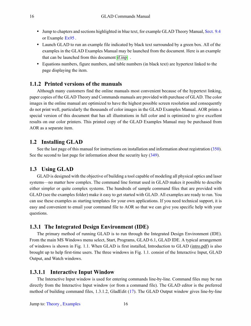
text output. HTML output is also provided in a separate window as related below. The Watch window displays graphic files as they are generated by GLAD. You may position and resize these windows as you wish. The window position and size data are stored in glad.ini located in the GLAD installation directory.
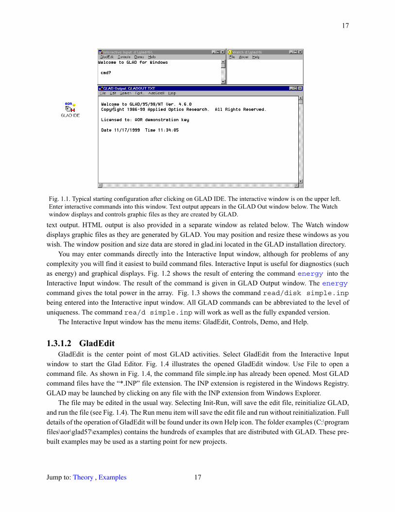
You may enter commands directly into the Interactive Input window, although for problems of any complexity you will find it easiest to build command files. Interactive Input is useful for diagnostics (such as energy) and graphical displays. Fig. 1.2 shows the result of entering the command into the Interactive Input window. The result of the command is given in GLAD Output window. The command gives the total power in the array. Fig. 1.3 shows the command read/disk simple.inpbeing entered into the Interactive input window. All GLAD commands can be abbreviated to the level of uniqueness. The command rea/d simple.inp will work as well as the fully expanded version.
The Interactive Input window has the menu items: GladEdit, Controls, Demo, and Help.
1.3.1.2 GladEditGladEdit is the center point of most GLAD activities. Select GladEdit from the Interactive Input
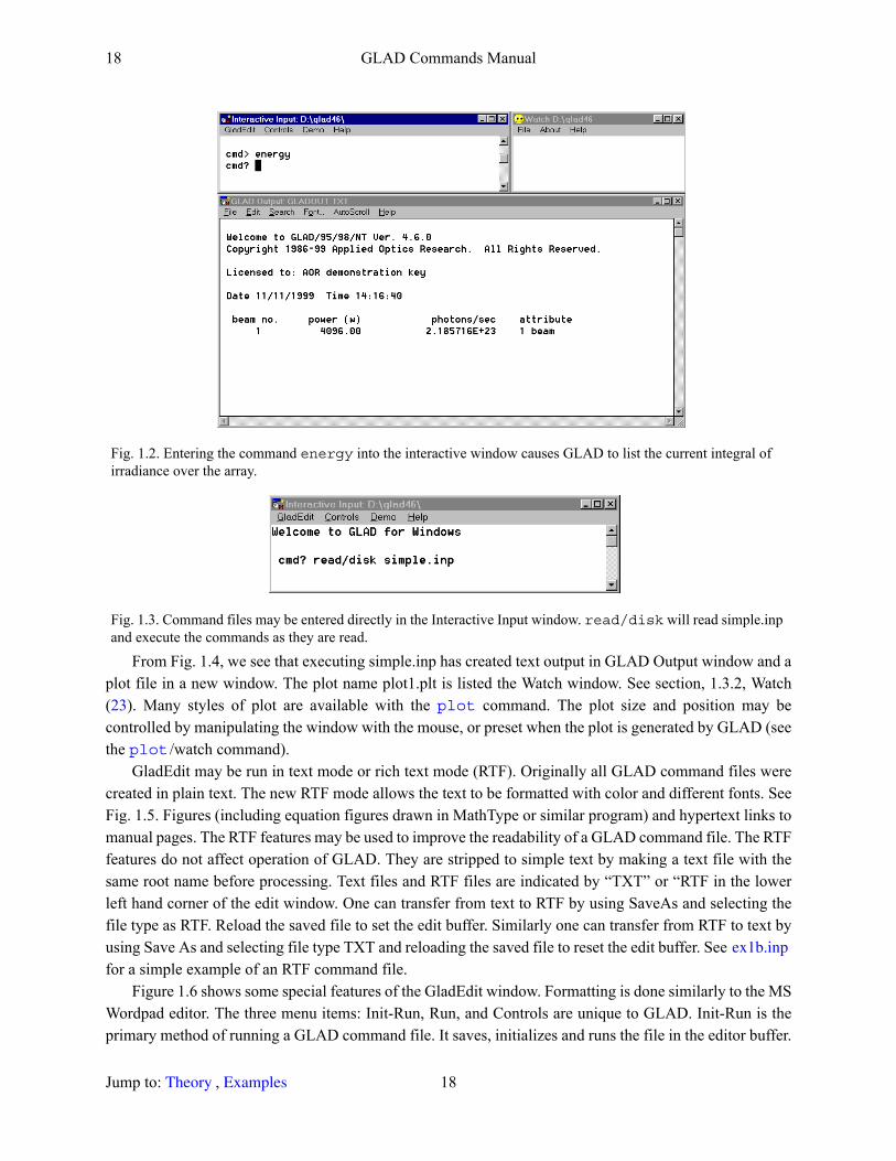
window to start the Glad Editor. Fig. 1.4 illustrates the opened GladEdit window. Use File to open a command file. As shown in Fig. 1.4, the command file simple.inp has already been opened. Most GLAD command files have the “*.INP” file extension. The INP extension is registered in the Windows Registry. GLAD may be launched by clicking on any file with the INP extension from Windows Explorer.
The file may be edited in the usual way. Selecting Init-Run, will save the edit file, reinitialize GLAD, and run the file (see Fig. 1.4). The Run menu item will save the edit file and run without reinitialization. Full details of the operation of GladEdit will be found under its own Help icon. The folder examples (C:\program files\aor\glad57\examples) contains the hundreds of examples that are distributed with GLAD. These pre-built examples may be used as a starting point for new projects.
Fig. 1.1. Typical starting configuration after clicking on GLAD IDE. The interactive window is on the upper left. Enter interactive commands into this window. Text output appears in the GLAD Out window below. The Watch window displays and controls graphic files as they are created by GLAD.
energy energy
Jump to: , 17 Theory Examples
18 GLAD Commands Manual
From Fig. 1.4, we see that executing simple.inp has created text output in GLAD Output window and a plot file in a new window. The plot name plot1.plt is listed the Watch window. See section, 1.3.2, Watch(23). Many styles of plot are available with the command. The plot size and position may be controlled by manipulating the window with the mouse, or preset when the plot is generated by GLAD (see the /watch command).
GladEdit may be run in text mode or rich text mode (RTF). Originally all GLAD command files were created in plain text. The new RTF mode allows the text to be formatted with color and different fonts. See Fig. 1.5. Figures (including equation figures drawn in MathType or similar program) and hypertext links to manual pages. The RTF features may be used to improve the readability of a GLAD command file. The RTF features do not affect operation of GLAD. They are stripped to simple text by making a text file with the same root name before processing. Text files and RTF files are indicated by “TXT” or “RTF in the lower left hand corner of the edit window. One can transfer from text to RTF by using SaveAs and selecting the file type as RTF. Reload the saved file to set the edit buffer. Similarly one can transfer from RTF to text by using Save As and selecting file type TXT and reloading the saved file to reset the edit buffer. See for a simple example of an RTF command file.
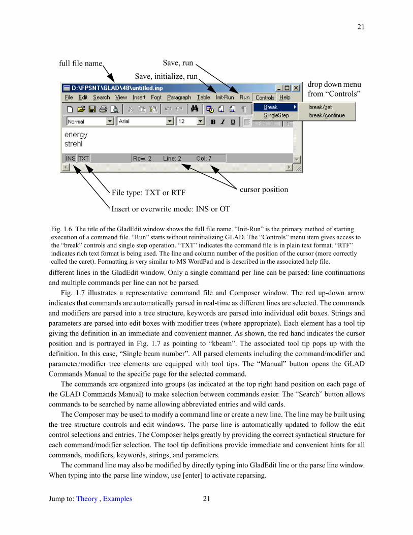
Figure 1.6 shows some special features of the GladEdit window. Formatting is done similarly to the MS Wordpad editor. The three menu items: Init-Run, Run, and Controls are unique to GLAD. Init-Run is the primary method of running a GLAD command file. It saves, initializes and runs the file in the editor buffer.
Fig. 1.2. Entering the command energy into the interactive window causes GLAD to list the current integral of irradiance over the array.
Fig. 1.3. Command files may be entered directly in the Interactive Input window. read/disk will read simple.inp and execute the commands as they are read.
plot
plot
ex1b.inp
Jump to: , 18 Theory Examples
19
Run saves and runs the command file but does not reinitialize. This can be useful if part of the command sequence is contained in a secondary file to be run after the primary file that is run by Init-Run. The Controls menu item gives access to the break controls and single step operation. Command files can be either in plain text (TXT) or rich text format (RTF) — both under the file extension INP. The current file type in the editor buffer is indicated by TXT or RTF as shown in Fig. 1.6. The line and column of the caret position (often incorrectly called the cursor) are also indicated on the bottom of the editor window. GLAD displays the line number with the report of execution error.
Hyperlinks may be created from “Insert” on the GladEdit menu. Any GLAD command may be included in a hyperlink. The command is executed when the hyperlink is double clicked. A hyperlink is created from the menu of GladEdit from Insert, Hyperlink. Among the most useful commands are that can launch and control Adobe PDF documents and that can run other applications and launch documents.
PDF documents may be opened to a named destination or page number using the command. Examples of hyperlinks include:
manual/destination ‘commands.pdf energy’manual/page ‘commands.pdf 252’manual/dest ‘d:\\temp\\temp.pdf’system/launch ‘d:\\temp\\temp.doc’
In the first example, “energy” is the named destination in the PDF document for the command. In the second example, “252” indicates the page number of the PDF document to be displayed. Single quotes are required if the string contains blanks. Hyperlinks require the use of double back slashes to represent the
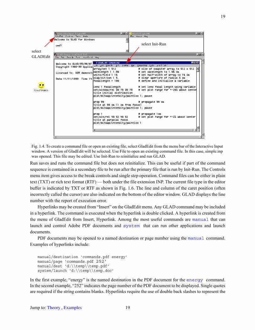
Fig. 1.4. To create a command file or open an existing file, select GladEdit from the menu bar of the Interactive Input window. A version of GladEdit will be selected. Use File to open an existing command file. In this case, simple.inp was opened. This file may be edited. Use Init-Run to reinitialize and run GLAD.
selectGLADEdit
select Init-Run
manual system
manual
energy
Jump to: , 19 Theory Examples
20 GLAD Commands Manual
back slashes character used in file paths. See the commands for a complete description of the named destinations that may be used in GLAD documents and the command for information on executing applications and launching documents. Hyperlinks can not be edited. To change a hyperlink, delete it and recreate it.
The default type face for the Glad editor is “FixedSys” and the default point size is 12 points. These defaults may be changed by modifying the file glad.ini to be found in the installation folder. In glad.ini, change GladEditFontName and GladEditFontHeight to the desired default values for typeface name and font size.
1.3.1.3 Command ComposerThe Command Composer is used for both parsing and composing GLAD command lines. It is
accessible from GladEdit by either clicking with the right mouse button (“right clicking”) or selecting “Controls”, “Command Composer” from the menu of the GladEdit window. Once activated, the Command Composer will dynamically parse command lines in GladEdit as the cursor is moved up or down to select
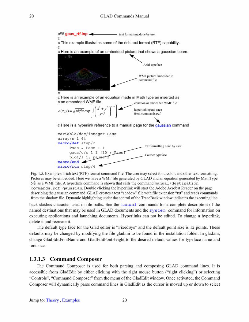
Fig. 1.5. Example of rich text (RTF) format command file. The user may select font, color, and other text formatting. Pictures may be embedded. Here we have a WMF file generated by GLAD and an equation generated by MathType 5® as a WMF file. A hyperlink command is shown that calls the command manual/destination commands.pdf gaussian. Double clicking the hyperlink will start the Adobe Acrobat Reader on the page describing the gaussian command. GLAD creates a text “shadow” file with file extension “txt” and reads commands from the shadow file. Dynamic highlighting under the control of the TraceBack window indicates the executing line.
c## gaus_rtf.inp
c
c This example illustrates some of the rich text format (RTF) capability.
c
c Here is an example of an embedded picture that shows a gaussian beam.
c
c Here is an example of an equation made in MathType an inserted as
c an embedded WMF file.
2 2
2( , ) exp
sgxp
x y
a x y pkflu
ro
⎡ ⎤⎛ ⎞+= −⎢ ⎥⎜ ⎟⎢ ⎥⎝ ⎠⎣ ⎦
c Here is a hyperlink reference to a manual page for the gaussian command
variable/dec/integer Passarray/s 1 64macro/def step/o
Pass = Pass + 1gaus/c/c 1 1 [10 + Pass]plot/l 1; pause 2
macro/endmacro/run step/4
text formatting done by user
Ariel typeface
WMF picture embedded in command file
equation as embedded WMF file
hyperlink opens page from commands.pdf
text formatting done by user
Courier typeface
manual system
Jump to: , 20 Theory Examples
21
different lines in the GladEdit window. Only a single command per line can be parsed: line continuations and multiple commands per line can not be parsed.
Fig. 1.7 illustrates a representative command file and Composer window. The red up-down arrow indicates that commands are automatically parsed in real-time as different lines are selected. The commands and modifiers are parsed into a tree structure, keywords are parsed into individual edit boxes. Strings and parameters are parsed into edit boxes with modifier trees (where appropriate). Each element has a tool tip giving the definition in an immediate and convenient manner. As shown, the red hand indicates the cursor position and is portrayed in Fig. 1.7 as pointing to “kbeam”. The associated tool tip pops up with the definition. In this case, “Single beam number”. All parsed elements including the command/modifier and parameter/modifier tree elements are equipped with tool tips. The “Manual” button opens the GLAD Commands Manual to the specific page for the selected command.
The commands are organized into groups (as indicated at the top right hand position on each page of the GLAD Commands Manual) to make selection between commands easier. The “Search” button allows commands to be searched by name allowing abbreviated entries and wild cards.
The Composer may be used to modify a command line or create a new line. The line may be built using the tree structure controls and edit windows. The parse line is automatically updated to follow the edit control selections and entries. The Composer helps greatly by providing the correct syntactical structure for each command/modifier selection. The tool tip definitions provide immediate and convenient hints for all commands, modifiers, keywords, strings, and parameters.
The command line may also be modified by directly typing into GladEdit line or the parse line window. When typing into the parse line window, use [enter] to activate reparsing.
Fig. 1.6. The title of the GladEdit window shows the full file name. “Init-Run” is the primary method of starting execution of a command file. “Run” starts without reinitializing GLAD. The “Controls” menu item gives access to the “break” controls and single step operation. “TXT” indicates the command file is in plain text format. “RTF” indicates rich text format is being used. The line and column number of the position of the cursor (more correctly called the caret). Formatting is very similar to MS WordPad and is described in the associated help file.
Save, initialize, run
Save, run
cursor positionFile type: TXT or RTF
Insert or overwrite mode: INS or OT
drop down menu from “Controls”
full file name
Jump to: , 21 Theory Examples
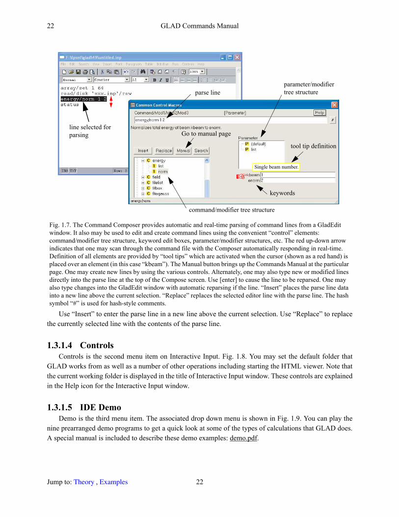
22 GLAD Commands Manual
Use “Insert” to enter the parse line in a new line above the current selection. Use “Replace” to replace the currently selected line with the contents of the parse line.
1.3.1.4 ControlsControls is the second menu item on Interactive Input. Fig. 1.8. You may set the default folder that
GLAD works from as well as a number of other operations including starting the HTML viewer. Note that the current working folder is displayed in the title of Interactive Input window. These controls are explained in the Help icon for the Interactive Input window.
1.3.1.5 IDE DemoDemo is the third menu item. The associated drop down menu is shown in Fig. 1.9. You can play the
nine prearranged demo programs to get a quick look at some of the types of calculations that GLAD does. A special manual is included to describe these demo examples: demo.pdf.
Fig. 1.7. The Command Composer provides automatic and real-time parsing of command lines from a GladEdit window. It also may be used to edit and create command lines using the convenient “control” elements: command/modifier tree structure, keyword edit boxes, parameter/modifier structures, etc. The red up-down arrow indicates that one may scan through the command file with the Composer automatically responding in real-time. Definition of all elements are provided by “tool tips” which are activated when the cursor (shown as a red hand) is placed over an element (in this case “kbeam”). The Manual button brings up the Commands Manual at the particular page. One may create new lines by using the various controls. Alternately, one may also type new or modified lines directly into the parse line at the top of the Compose screen. Use [enter] to cause the line to be reparsed. One may also type changes into the GladEdit window with automatic reparsing if the line. “Insert” places the parse line data into a new line above the current selection. “Replace” replaces the selected editor line with the parse line. The hash symbol “#” is used for hash-style comments.
line selected for parsing
parse line
command/modifier tree structure
keywords
parameter/modifier tree structure
Single beam number.
tool tip definition
☞
Go to manual page
Jump to: , 22 Theory Examples

23
1.3.1.6 IDE HelpHelp is the fourth menu item of Interactive Input. Fig. 1.10 shows the corresponding drop down m
menu. IDE.HLP is the Windows help file for the IDE. The various PDF file give detailed information about the commands, theory, examples, and introductory materials. Up-to-date versions of the PDF version of the manuals are maintained on the AOR web site www.aor.com.
1.3.2 WatchWatch is an independent program that runs in parallel with GLAD. Watch performs the work of
displaying files as they are created by GLAD, so that GLAD does not have to wait for the graphic tasks to be completed. You may run Watch independently of GLAD to recreate the last display. Click on the Watch icon: yellow smile face.Watch may also be used to view other plot files (*.PLT) that have previously been created. Refer to the Help icon from the Watch menu.
Fig. 1.8. The Controls menu item allows selection of a number of operations. See section, Help (41), for a detailed explanation. Use “Set default folder” to select the folder for GLAD to work from. The current working folder is displayed in the title of this window.
Fig. 1.9. The Demo menu item runs preselected examples. Select Start to begin the demo, Skip to skip to the next example, and Quit to end the demonstration. See Demo.pdf in the installation folder for a description of the examples.
Fig. 1.10. IDE Help gives specific information about operating GLAD IDE. Details about the commands, examples, and theory are in the respective PDF files, viewed with the Adobe Acrobat Reader.
title displays current working folder
Jump to: , 23 Theory Examples
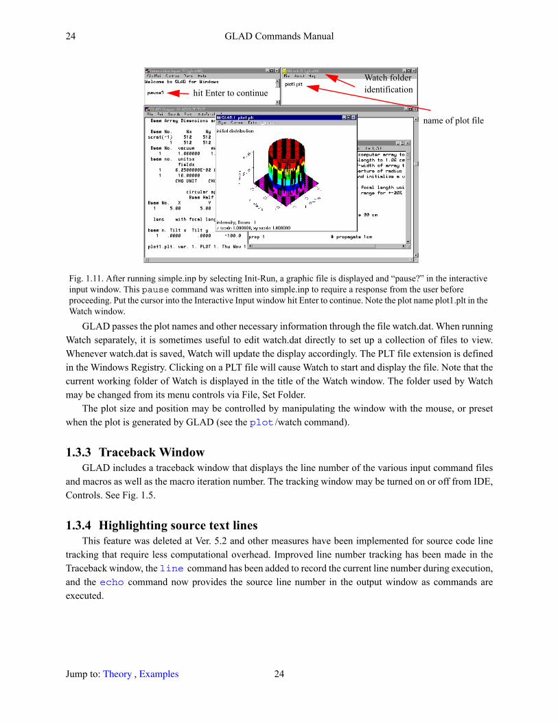
24 GLAD Commands Manual
GLAD passes the plot names and other necessary information through the file watch.dat. When running Watch separately, it is sometimes useful to edit watch.dat directly to set up a collection of files to view. Whenever watch.dat is saved, Watch will update the display accordingly. The PLT file extension is defined in the Windows Registry. Clicking on a PLT file will cause Watch to start and display the file. Note that the current working folder of Watch is displayed in the title of the Watch window. The folder used by Watch may be changed from its menu controls via File, Set Folder.
The plot size and position may be controlled by manipulating the window with the mouse, or preset when the plot is generated by GLAD (see the /watch command).
1.3.3 Traceback WindowGLAD includes a traceback window that displays the line number of the various input command files
and macros as well as the macro iteration number. The tracking window may be turned on or off from IDE, Controls. See Fig. 1.5.
1.3.4 Highlighting source text linesThis feature was deleted at Ver. 5.2 and other measures have been implemented for source code line
tracking that require less computational overhead. Improved line number tracking has been made in the Traceback window, the command has been added to record the current line number during execution, and the command now provides the source line number in the output window as commands are executed.
Fig. 1.11. After running simple.inp by selecting Init-Run, a graphic file is displayed and “pause?” in the interactive input window. This pause command was written into simple.inp to require a response from the user before proceeding. Put the cursor into the Interactive Input window hit Enter to continue. Note the plot name plot1.plt in the Watch window.
Watch folder identification
name of plot file
hit Enter to continue
plot
line echo
Jump to: , 24 Theory Examples
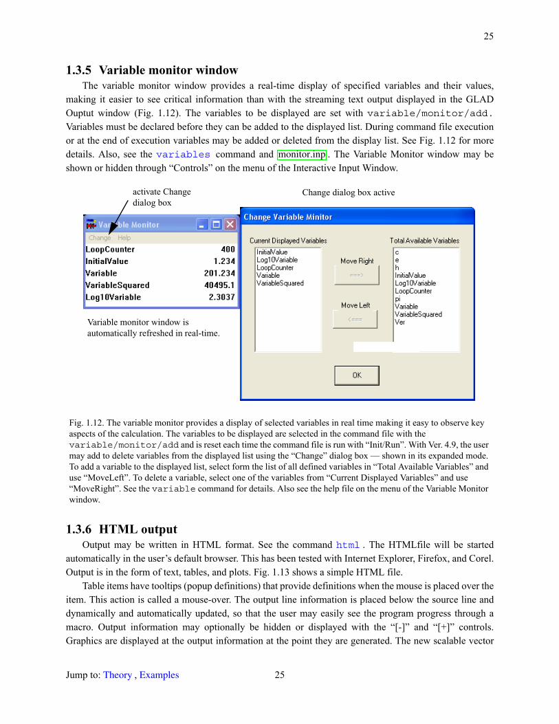
25
1.3.5 Variable monitor windowThe variable monitor window provides a real-time display of specified variables and their values,
making it easier to see critical information than with the streaming text output displayed in the GLAD Ouptut window (Fig. 1.12). The variables to be displayed are set with variable/monitor/add.Variables must be declared before they can be added to the displayed list. During command file execution or at the end of execution variables may be added or deleted from the display list. See Fig. 1.12 for more details. Also, see the command and . The Variable Monitor window may be shown or hidden through “Controls” on the menu of the Interactive Input Window.
1.3.6 HTML outputOutput may be written in HTML format. See the command . The HTMLfile will be started
automatically in the user’s default browser. This has been tested with Internet Explorer, Firefox, and Corel. Output is in the form of text, tables, and plots. Fig. 1.13 shows a simple HTML file.
Table items have tooltips (popup definitions) that provide definitions when the mouse is placed over the item. This action is called a mouse-over. The output line information is placed below the source line and dynamically and automatically updated, so that the user may easily see the program progress through a macro. Output information may optionally be hidden or displayed with the “[-]” and “[+]” controls. Graphics are displayed at the output information at the point they are generated. The new scalable vector
Fig. 1.12. The variable monitor provides a display of selected variables in real time making it easy to observe key aspects of the calculation. The variables to be displayed are selected in the command file with the variable/monitor/add and is reset each time the command file is run with “Init/Run”. With Ver. 4.9, the user may add to delete variables from the displayed list using the “Change” dialog box — shown in its expanded mode. To add a variable to the displayed list, select form the list of all defined variables in “Total Available Variables” and use “MoveLeft”. To delete a variable, select one of the variables from “Current Displayed Variables” and use “MoveRight”. See the variable command for details. Also see the help file on the menu of the Variable Monitor window.
variables monitor.inp
activate Change dialog box
Variable monitor window is automatically refreshed in real-time.
Change dialog box active
html
Jump to: , 25 Theory Examples
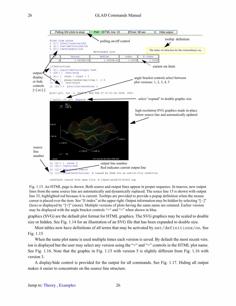
26 GLAD Commands Manual
graphics (SVG) are the default plot format for HTML graphics. The SVG graphics may be scaled to double size or hidden. See Fig. 1.14 for an illustration of an SVG file that has been expanded to double size.
Most tables now have definitions of all terms that may be activated by set/definitions/on. See Fig. 1.15
When the same plot name is used multiple times each version is saved. By default the most recent vers. ion is displayed but the user may select any version using the “<“ and “>” controls in the HTML plot name. See Fig. 1.16. Note that the graphic in Fig. 1.13 with version 5 is slightly different from Fig. 1.16 with version 3.
A display/hide control is provided for the output for all commands. See Fig. 1.17. Hiding all output makes it easier to concentrate on the source line structure.
Fig. 1.13. An HTML page is shown. Both source and output lines appear in proper sequence. In macros, new output lines from the same source line are automatically and dynamically replaced. The souce line 15 is shown with output line 33, highlighted red because it is current. Tooltips are provided to provide a popup definition when the mouse cursor is placed over the item. See “E-index” at the upper right. Output information may be hidden by selecting “[ ]” (less) or displayed by “[+]” (more). Multiple versions of plots having the same name are retained. Earlier version may be displayed with the angle bracket controls “<“ and “>” when shown in blue.
Polling ON (click to stop) Poll HTML line: 33 Timer: 98 sec Hide output
First time notes3 (1)[ ]html/location/off4 (2)[ ]set/definitions/on5 (3)[-]wavelength/list
[+]Definitions
6 (4)[ ]macro/define/single test7 (29)[ ] html/stop
8 (6)[ ] count = count + 1
9 (7)[ ] phase/random/sqr/clap 1 .1 510 (8)[ ] html/start
11 (30)[-] plot/liso/wavefront 1
plot1.plt, ver. 5, PLOT 5, Wed Feb 27 01:51:28 2008, 3653
[-]plot1.<5>.plt (Expand)
12 (31)[ ] pause 213 (32)[ ]macro/end
14 (12)[ ]macro/run test/5
15 (33)[-]read/back/noclose # issued by GLAD for an end-of-file condition
read/back issued from open file: F:\fpsnt\glad\53\html5.inp
Wavelength List
No. Vacuum Medium Index E-index
1 1.0600E+01 1.0600E+01 1.0000 1.0000
tooltip definition
angle bracket controls select betweenplot versions: 1, 2, 3, 4, 5
select “expand” to double graphic size
outputdisplayor hidecontrols[+] or [-]
polling on/off control
output line number.Red indicates current output line
sourcelinenumber
The index of refraction for the extraordinary ray.
cursor on item
high resolution SVG graphics made in-placebelow source line and automatically updated
-
Jump to: , 26 Theory Examples
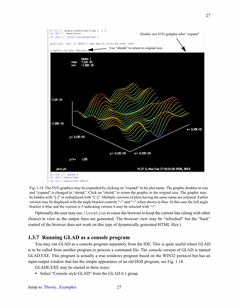
27
Optionally the user may use /location to cause the browser to keep the current line (along with other choice) in view as the output lines are generated. The browser view may be “refreshed” but the “back” control of the browser does not work on this type of dynamically generated HTML files.)
1.3.7 Running GLAD as a console programYou may run GLAD as a console program separately from the IDE. This is quite useful where GLAD
is to be called from another program to process a command file. The console version of GLAD is named GLAD.EXE. This program is actually a true windows program based on the WIN32 protocol but has an input-output window that has the simple appearance of an old DOS program, see Fig. 1.18.
GLADE.EXE may be started in three ways:• Select “Console style GLAD” from the GLAD 6.1 group.
Fig. 1.14. The SVG graphics may be expanded by clicking on “expand” in the plot name. The graphic doubles in size and “expand” is changed to “shrink”. Click on “shrink” to return the graphic to the original size. The graphic may be hidden with “[-]” or redisplayed with “[+]”. Multiple versions of plots having the same name are retained. Earlier version may be displayed with the angle bracket controls “<“ and “>” when shown in blue. In this case the left angle bracket is blue and the version is 5 indicating version 4 may be selected with “<“.
9 (7)[ ] phase/random/sqr/clap 1 .1 510 (8)[ ] html/start
11 (30)[-] plot/liso/wavefront 1
plot1.plt, ver. 5, PLOT 5, Wed Feb 27 01:51:28 2008, 3653
[-]plot1.<5>.plt (Shrink)
12 (31)[ ] pause 213 (32)[ ]macro/end
14 (12)[ ]macro/run test/5
Double size SVG grahphic after “expand”.
Use “shrink” to return to original size.
Jump to: , 27 Theory Examples
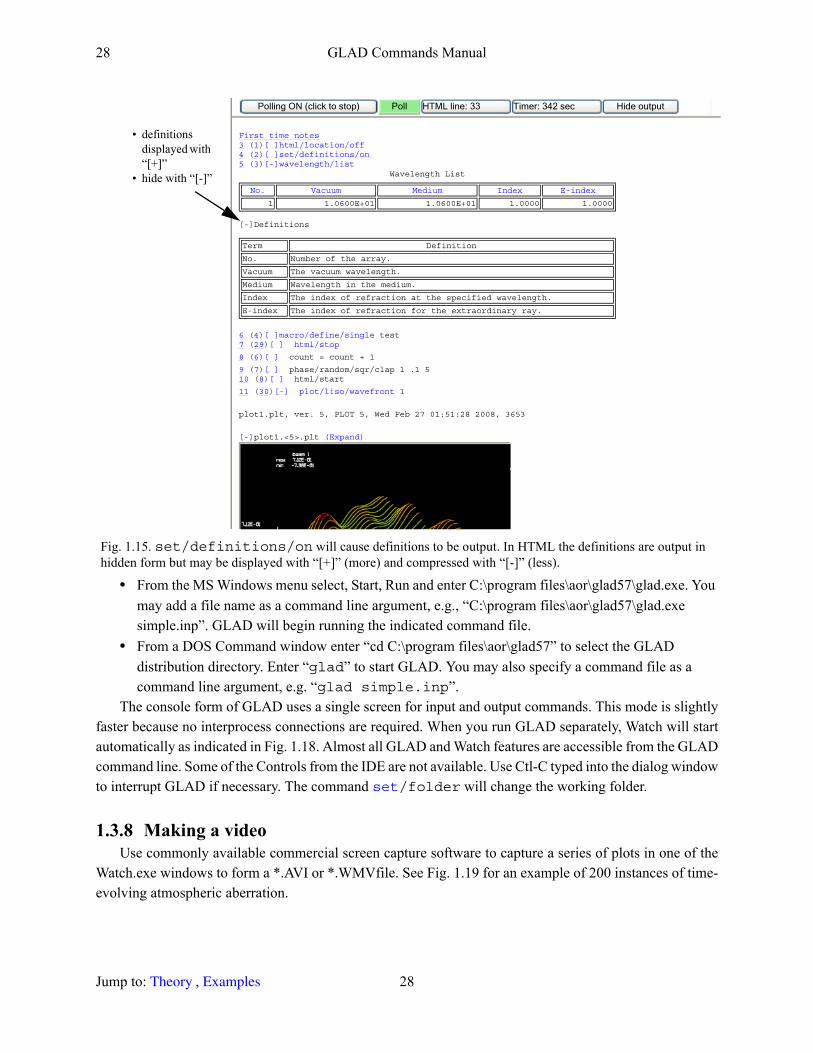
28 GLAD Commands Manual
• From the MS Windows menu select, Start, Run and enter C:\program files\aor\glad57\glad.exe. You may add a file name as a command line argument, e.g., “C:\program files\aor\glad57\glad.exe simple.inp”. GLAD will begin running the indicated command file.
• From a DOS Command window enter “cd C:\program files\aor\glad57” to select the GLAD distribution directory. Enter “glad” to start GLAD. You may also specify a command file as a command line argument, e.g. “glad simple.inp”.
The console form of GLAD uses a single screen for input and output commands. This mode is slightly faster because no interprocess connections are required. When you run GLAD separately, Watch will start automatically as indicated in Fig. 1.18. Almost all GLAD and Watch features are accessible from the GLAD command line. Some of the Controls from the IDE are not available. Use Ctl-C typed into the dialog window to interrupt GLAD if necessary. The command /folder will change the working folder.
1.3.8 Making a videoUse commonly available commercial screen capture software to capture a series of plots in one of the
Watch.exe windows to form a *.AVI or *.WMVfile. See Fig. 1.19 for an example of 200 instances of time-evolving atmospheric aberration.
Fig. 1.15. set/definitions/on will cause definitions to be output. In HTML the definitions are output in hidden form but may be displayed with “[+]” (more) and compressed with “[-]” (less).
Polling ON (click to stop) Poll HTML line: 33 Timer: 342 sec Hide output
First time notes3 (1)[ ]html/location/off4 (2)[ ]set/definitions/on5 (3)[-]wavelength/list
[-]Definitions
6 (4)[ ]macro/define/single test7 (29)[ ] html/stop
8 (6)[ ] count = count + 1
9 (7)[ ] phase/random/sqr/clap 1 .1 510 (8)[ ] html/start
11 (30)[-] plot/liso/wavefront 1
plot1.plt, ver. 5, PLOT 5, Wed Feb 27 01:51:28 2008, 3653
[-]plot1.<5>.plt (Expand)
Wavelength List
No. Vacuum Medium Index E-index
1 1.0600E+01 1.0600E+01 1.0000 1.0000
Term Definition
No. Number of the array.
Vacuum The vacuum wavelength.
Medium Wavelength in the medium.
Index The index of refraction at the specified wavelength.
E-index The index of refraction for the extraordinary ray.
• definitions displayed with “[+]”
• hide with “[-]”
set
Jump to: , 28 Theory Examples
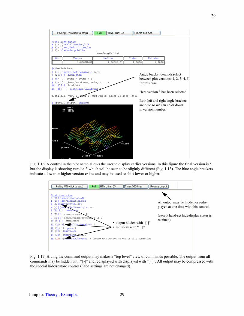
29
Fig. 1.16. A control in the plot name allows the user to display earlier versions. In this figure the final version is 5 but the display is showing version 3 which will be seen to be slightly different (Fig. 1.13). The blue angle brackets indicate a lower or higher version exists and may be used to shift lower or higher.
Fig. 1.17. Hiding the command output may makes a “top level” view of commands possible. The output from all commands may be hidden with “[-]” and redisplayed with displayed with “[+]”. All output may be compressed with the special hide/restore control (hand settings are not changed).
Polling ON (click to stop) Poll HTML line: 33 Timer: 144 sec
First time notes3 (1)[ ]html/location/off4 (2)[ ]set/definitions/on5 (3)[-]wavelength/list
[+]Definitions
6 (4)[ ]macro/define/single test7 (29)[ ] html/stop
8 (6)[ ] count = count + 1
9 (7)[ ] phase/random/sqr/clap 1 .1 510 (8)[ ] html/start
11 (30)[-] plot/liso/wavefront 1
plot1.plt, ver. 5, PLOT 5, Wed Feb 27 02:35:35 2008, 3653
[-]plot1.<3>.plt (Expand)
Wavelength List
No. Vacuum Medium Index E-index
1 1.0600E+01 1.0600E+01 1.0000 1.0000
Angle bracket controls select between plot versions: 1, 2, 3, 4, 5 for this case.
Here version 3 has been selected.
Both left and right angle bracketsare blue so we can up or downin version number.
Polling ON (click to stop) Poll HTML line: 33 Timer: 3076 sec Restore output
First time notes3 (1)[ ]html/location/off4 (2)[ ]set/definitions/on5 (3)[+]wavelength/list
6 (4)[ ]macro/define/single test7 (29)[ ] html/stop
8 (6)[ ] count = count + 1
9 (7)[ ] phase/random/sqr/clap 1 .1 510 (8)[ ] html/start
11 (30)[+] plot/liso/wavefront 1
12 (31)[ ] pause 213 (32)[ ]macro/end
14 (12)[ ]macro/run test/5
15 (33)[+]read/back/noclose # issued by GLAD for an end-of-file condition
• output hidden with “[-]”• redisplay with “[+]”
All output may be hidden or redis-played at one time with this control.
(except hand-set hide/display status is retained)
Jump to: , 29 Theory Examples
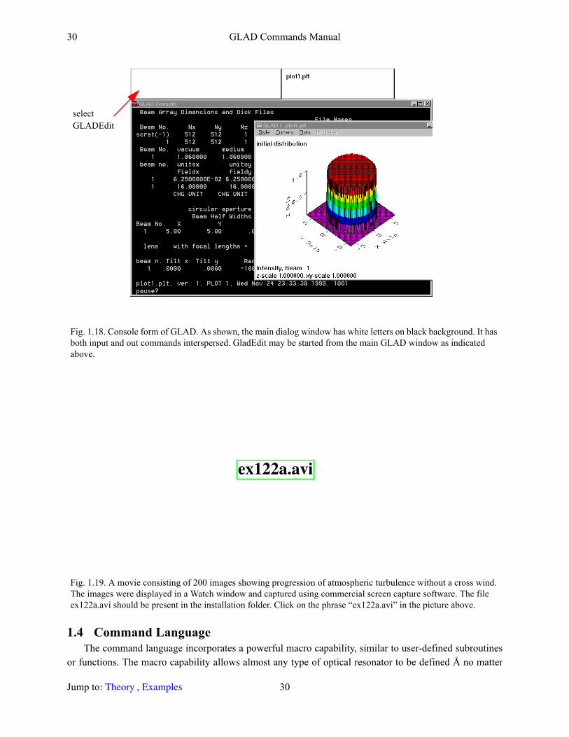
30 GLAD Commands Manual
1.4 Command LanguageThe command language incorporates a powerful macro capability, similar to user-defined subroutines
or functions. The macro capability allows almost any type of optical resonator to be defined Å no matter
Fig. 1.18. Console form of GLAD. As shown, the main dialog window has white letters on black background. It has both input and out commands interspersed. GladEdit may be started from the main GLAD window as indicated above.
Fig. 1.19. A movie consisting of 200 images showing progression of atmospheric turbulence without a cross wind. The images were displayed in a Watch window and captured using commercial screen capture software. The file ex122a.avi should be present in the installation folder. Click on the phrase “ex122a.avi” in the picture above.
select GLADEdit
ex122a.avi
Jump to: , 30 Theory Examples
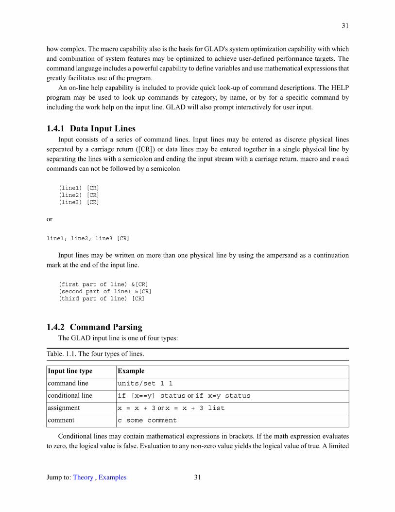
31
how complex. The macro capability also is the basis for GLAD's system optimization capability with which and combination of system features may be optimized to achieve user-defined performance targets. The command language includes a powerful capability to define variables and use mathematical expressions that greatly facilitates use of the program.
An on-line help capability is included to provide quick look-up of command descriptions. The HELP program may be used to look up commands by category, by name, or by for a specific command by including the work help on the input line. GLAD will also prompt interactively for user input.
1.4.1 Data Input LinesInput consists of a series of command lines. Input lines may be entered as discrete physical lines
separated by a carriage return ([CR]) or data lines may be entered together in a single physical line by separating the lines with a semicolon and ending the input stream with a carriage return. macro and readcommands can not be followed by a semicolon
(line1) [CR](line2) [CR](line3) [CR]
or
line1; line2; line3 [CR]
Input lines may be written on more than one physical line by using the ampersand as a continuation mark at the end of the input line.
(first part of line) &[CR](second part of line) &[CR](third part of line) [CR]
1.4.2 Command ParsingThe GLAD input line is one of four types:
Conditional lines may contain mathematical expressions in brackets. If the math expression evaluates to zero, the logical value is false. Evaluation to any non-zero value yields the logical value of true. A limited
Table. 1.1. The four types of lines.
Input line type Example
command line units/set 1 1
conditional line if [x==y] status or if x=y status
assignment x = x + 3 or x = x + 3 list
comment c some comment
Jump to: , 31 Theory Examples
32 GLAD Commands Manual
number of rational expressions may be written in the non-bracket form, but the mathematical expressions are more powerful and the recommended approach.
Assignment lines may take the parameter list to cause a display of the result.The command line is of the form:
command/mod1/mod2/mod3 string values parameters
Commands and their modifiers must be on the left, followed by strings, values, and parameters in that order, if required. Fields are separated by one or more blanks.
1.4.2.1 Command lines and assignment linesThe command line and modifiers establish the operation to be performed. Command line parsing
proceeds as follows:• read command and modifiers from the left and transfer control to the appropriate routine• look for parameters on the right that match the parameter list for that command.• evaluate mathematical expressions in square brackets, right to left• Alias and variable substitution• string extraction.• numbers in order of occurrence• command assignment with an equal sign (lvalue = rvalue)Numerical values take the form of numbers, variables, mathematical expressions (which are evaluated
to numbers and numerical assignments.
Table. 1.2. Elements of the command line.
Command line component Description
command Defines function to be used.
mod1, mod2, mod3 Modifiers of the command line to direct operations of the function.
string A string of characters to define a title, filename, macro name, lens name, system commands, etc. Strings have no preassigned values. File names should be enclosed in single quotes if they contain slashes, “/”, or other special characters. Some strings have modifiers as do commands. Variables may be included in strings if preceded by the “@” symbol.
values Variables, numbers, mathematical expressions, or numerical assignments.
parameters Parameters are similar to commands but are on the right end of the command line, after values. Parameters are checked against the list of preassigned values. Variables and expressions may be included in parameters names and their modifier names. Optional parameters are listed in brackets in the command descriptions. Literal parameter names are listed in typewrite font (Courier). Reference to the first or second parameter are shown in parentheses and in a proportional font (Times Roman). Neither the brackets nor the parentheses shown in the listing of parameters should not be entered.
Jump to: , 32 Theory Examples
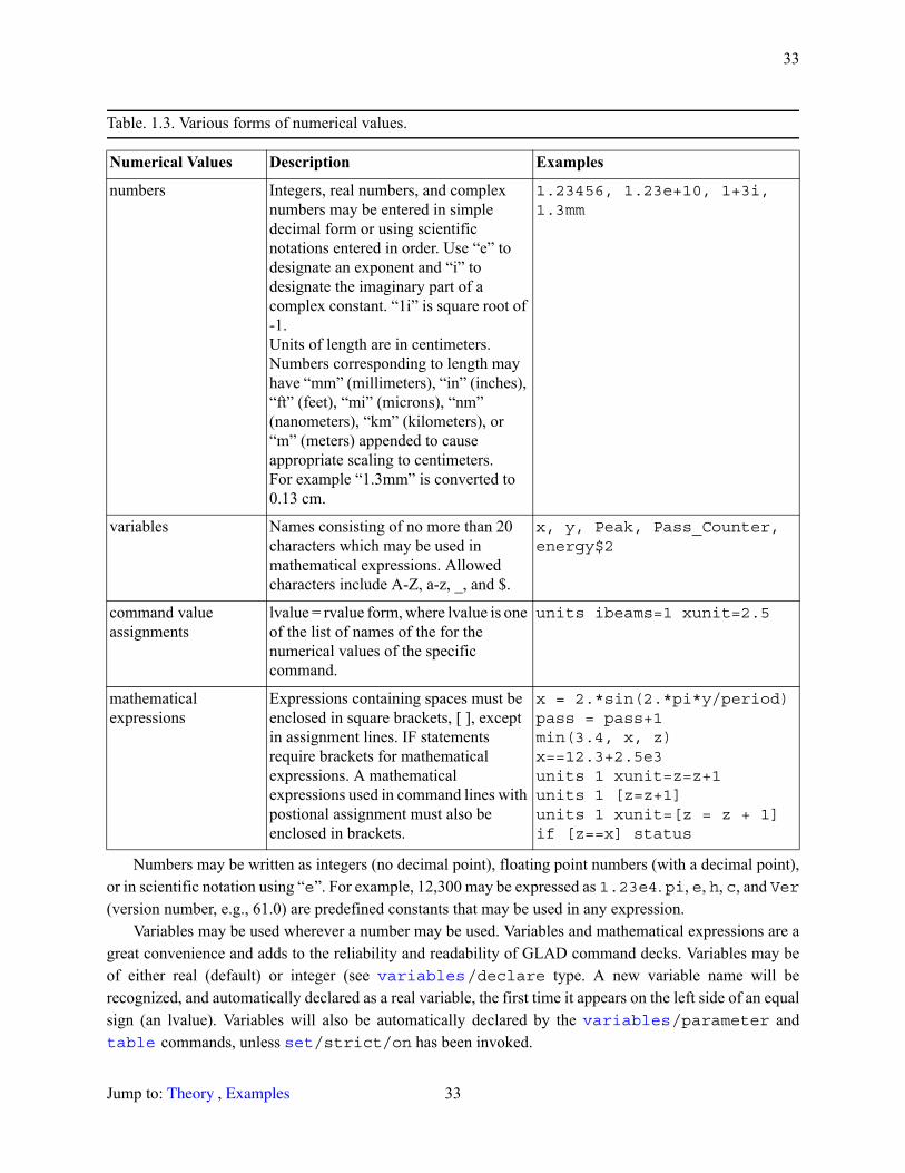
33
Numbers may be written as integers (no decimal point), floating point numbers (with a decimal point), or in scientific notation using “e”. For example, 12,300 may be expressed as 1.23e4. pi, e, h, c, and Ver(version number, e.g., 61.0) are predefined constants that may be used in any expression.
Variables may be used wherever a number may be used. Variables and mathematical expressions are a great convenience and adds to the reliability and readability of GLAD command decks. Variables may be of either real (default) or integer (see /declare type. A new variable name will be recognized, and automatically declared as a real variable, the first time it appears on the left side of an equal sign (an lvalue). Variables will also be automatically declared by the /parameter and
commands, unless /strict/on has been invoked.
Table. 1.3. Various forms of numerical values.
Numerical Values Description Examples
numbers Integers, real numbers, and complex numbers may be entered in simple decimal form or using scientific notations entered in order. Use “e” to designate an exponent and “i” to designate the imaginary part of a complex constant. “1i” is square root of -1.Units of length are in centimeters. Numbers corresponding to length may have “mm” (millimeters), “in” (inches), “ft” (feet), “mi” (microns), “nm” (nanometers), “km” (kilometers), or “m” (meters) appended to cause appropriate scaling to centimeters.For example “1.3mm” is converted to 0.13 cm.
1.23456, 1.23e+10, 1+3i, 1.3mm
variables Names consisting of no more than 20 characters which may be used in mathematical expressions. Allowed characters include A-Z, a-z, _, and $.
x, y, Peak, Pass_Counter, energy$2
command value assignments
lvalue = rvalue form, where lvalue is one of the list of names of the for the numerical values of the specific command.
units ibeams=1 xunit=2.5
mathematical expressions
Expressions containing spaces must be enclosed in square brackets, [ ], except in assignment lines. IF statements require brackets for mathematical expressions. A mathematical expressions used in command lines with postional assignment must also be enclosed in brackets.
x = 2.*sin(2.*pi*y/period)pass = pass+1min(3.4, x, z)x==12.3+2.5e3units 1 xunit=z=z+1units 1 [z=z+1]units 1 xunit=[z = z + 1]if [z==x] status
variables
variables table set
Jump to: , 33 Theory Examples
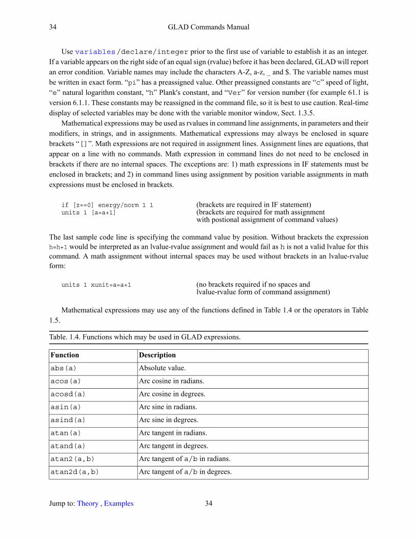
34 GLAD Commands Manual
Use /declare/integer prior to the first use of variable to establish it as an integer. If a variable appears on the right side of an equal sign (rvalue) before it has been declared, GLAD will report an error condition. Variable names may include the characters A-Z, a-z, _ and $. The variable names must be written in exact form. “pi” has a preassigned value. Other preassigned constants are “c” speed of light, “e” natural logarithm constant, “h” Plank's constant, and “Ver” for version number (for example 61.1 is version 6.1.1. These constants may be reassigned in the command file, so it is best to use caution. Real-time display of selected variables may be done with the variable monitor window, Sect. 1.3.5.
Mathematical expressions may be used as rvalues in command line assignments, in parameters and their modifiers, in strings, and in assignments. Mathematical expressions may always be enclosed in square brackets “[]”. Math expressions are not required in assignment lines. Assignment lines are equations, that appear on a line with no commands. Math expression in command lines do not need to be enclosed in brackets if there are no internal spaces. The exceptions are: 1) math expressions in IF statements must be enclosed in brackets; and 2) in command lines using assignment by position variable assignments in math expressions must be enclosed in brackets.
if [z==0] energy/norm 1 1 (brackets are required in IF statement)units 1 [a=a+1] (brackets are required for math assignment
with postional assignment of command values)
The last sample code line is specifying the command value by position. Without brackets the expression h=h+1 would be interpreted as an lvalue-rvalue assignment and would fail as h is not a valid lvalue for this command. A math assignment without internal spaces may be used without brackets in an lvalue-rvalue form:
units 1 xunit=a=a+1 (no brackets required if no spaces andlvalue-rvalue form of command assignment)
Mathematical expressions may use any of the functions defined in Table 1.4 or the operators in Table 1.5.
Table. 1.4. Functions which may be used in GLAD expressions.
Function Description abs(a) Absolute value.
acos(a) Arc cosine in radians.
acosd(a) Arc cosine in degrees.
asin(a) Arc sine in radians.
asind(a) Arc sine in degrees.
atan(a) Arc tangent in radians.
atand(a) Arc tangent in degrees.
atan2(a,b) Arc tangent of a/b in radians.
atan2d(a,b) Arc tangent of a/b in degrees.
variables
Jump to: , 34 Theory Examples
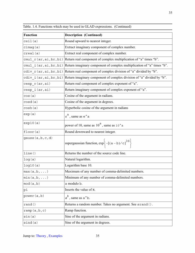
35
ceil(a) Round upward to nearest integer.
cimag(a) Extract imaginary component of complex number.
creal(a) Extract real component of complex number.
cmul_r(ar,ai,br,bi) Return real component of complex multiplication of “a” times “b”.
cmul_i(ar,ai,br,bi) Return imaginary component of complex multiplication of “a” times “b”.
cdiv_r(ar,ai,br,bi) Return real component of complex division of “a” divided by “b”.
cdiv_i(ar,ai,br,bi) Return imaginary component of complex division of “a” divided by “b”.
cexp_r(ar,ai) Return real component of complex exponent of “a”.
cexp_i(ar,ai) Return imaginary component of complex exponent of “a”.
cos(a) Cosine of the argument in radians.
cosd(a) Cosine of the argument in degrees.
cosh(a) Hyperbolic cosine of the argument in radians
exp(a), same as e^a
exp10(a)power of 10, same as , same as 10^a
floor(a) Round downward to nearest integer.
gauss(a,b,c,d)
supergaussian function,
line() Returns the number of the source code line.
log(a) Natural logarithm.
log10(a) Logarithm base 10.
max(a,b,...) Maximum of any number of comma-delimited numbers.
min(a,b,...) Minimum of any number of comma-delimited numbers.
mod(a,b) a modulo b.
pi Inserts the value of π.
power(a,b) , same as a^b.
rand() Returns a random number. Takes no argument. See srand().
ramp(a,b,c) Ramp function.
sin(a) Sine of the argument in radians.
sind(a) Sine of the argument in degrees.
Table. 1.4. Functions which may be used in GLAD expressions. (Continued)
Function Description (Continued)
ea
10a
a b–( ) c⁄[ ]2d
–
exp
ab
Jump to: , 35 Theory Examples

36 GLAD Commands Manual
Command line assignments are similar in form to variable assignments: both have the form lvalue = rvalue. However, for command line assignments the lvalues have specific names for each command. The names of the lvalues for numerical assignments may be truncated, provided the truncated form is unique among the list of numerical assignment names for the particular command-modifier sequence. Lvalues may contain variables or aliases preceded by @).
Examples:Consider the command that gives the pixel-to-pixel spacing:
units ibeams xunit yunit
The following command lines are valid:x = sin(pi/2)list 1, (assignment line needs no brackets)units 1 [y^2] [y=x+1.5] (2, command assignment by position with math expressionsunits 1 xunit=y^2 yunit=y=x+1.5 (3, command line assignments)
sinh(a) Hyperbolic sine of the argument in radians.
srand(a) Set random number with integer value a. Returns 0. See rand(). Returns value of previous seed.
sqrt(a) Square root.
step(a,b) Step function: 1 if , 0 otherwise.
tan(a) Tangent of the argument in radians.
tand(a) Tangent of the argument in degrees.
tanh(a) Hyperbolic tangent if the argument in radians.
time() Number of seconds since January 1, 1970 GMT.
udata(a,b)udata(a,b,c)
Udata value for row = a and column = b. (b = 0 gives x-values). With just two values specified, the current data set is used. Optional value c specifies the data set. If c = 0, absolute addressing is used for the rows.
Table. 1.5. Operators which may be used in GLAD expressions, in descending order of precedence.
Function Description
() Parentheses.
+, - Unary positive and negative sign. Examples: +3.2, -x.
^ Exponent (raise to power).
*, /, % Multiply, divide, remainder.
!, >, <, >=, <=, ||, &&, ==, != Not operator (negation), greater, lesser, greater or equal, less or equal, or, and, equal, not equal.
= Assignment.
Table. 1.4. Functions which may be used in GLAD expressions. (Continued)
Function Description (Continued)
a b≥
units
Jump to: , 36 Theory Examples

37
units 1 x=y^2 y=y=x+1.5 (4, abbreviated lvalues)units 1 [x = y^2] y = [y = x+1.5] (5, spaces require brackets)units 1 x = y^2 y = y=x+1.5 (6, expressions without spaces, no brackets required)
In the first line, x is recognized as a variable name and is assigned the value 1.0.In the second line, math expressions are used to assign xunit values and yunit values by position.
Since processing proceeds from right to left, y=x+1.5 is processed first. y is recognized as a new variable name and assigned the value 2.5. /strict/off may be used to prevent such on-the-fly definitions of new variables. The second mathematical expression y^2 uses the variable y, as just established on the same line to the right, and the expression takes the value 6.25 for the xunit assignment.
In the third line, the predefined values xunit and yunit are used in the lvalue-rvalue form of assignment (left value equals right value). If the lvalue-rvalue form is used, the assignments may be made in any order on the line. In general, math expressions used in command lines should be enclosed in brackets, but brackets may be dropped if there are no spaces in the math expression. See included with the example files.
In the fourth line, the full name of the lvalues are abbreviated from xunit to x and from yunit to y. The numerical assignment x=y^2 is recognized as an abbreviated form of xunit=y^2. The lvalue y on the far left of y=y=x+1.5 is recognized as an abbreviated form of the numerical assignment name yunitand the value 2.5 is assigned to it.
In the fifth line spaces are included in the math expressions, so brackets are required.Notice in the sixth line that the spaces may be placed in the lvalue-rvalue expression on either side of
the equal sign. The mathematical expression "y=x+1.5" has no spaces and therefore does not need brackets. The lines above are equivalent to the command lines:
x=1y=6.25units 1 6.25 2.5
Orunits ibeams=1 xunit=6.25 yunit=2.5
The variables x and y are available for use elsewhere in the program. Assuming the variables x and yare defined, other equivalent forms are:
units 1 y xunits 1 x=y y=xunits 1 x=[y] y=[x]
Variables may be used in strings or parameters and their modifiers by preceding them with the “@” symbol. For example consider the use of integer variables in the example below,
variable/declare/int ii=1plot/watch [email protected]=i+1plot/watch [email protected]
These code lines establish plot names plot1.plt and plot2.plt successively. If variables are included in titles, the title is updated to include the current value of the variable.
set
brackets.inp
Jump to: , 37 Theory Examples
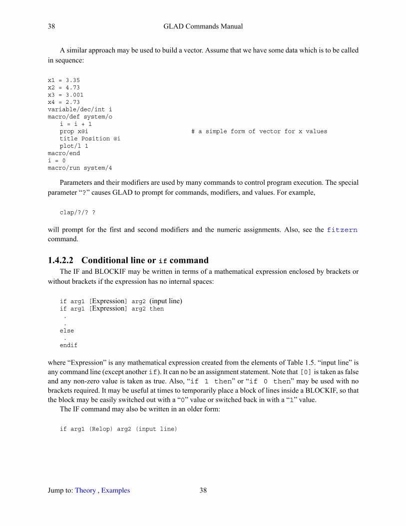
38 GLAD Commands Manual
A similar approach may be used to build a vector. Assume that we have some data which is to be called in sequence:
x1 = 3.35x2 = 4.73x3 = 3.001x4 = 2.73variable/dec/int imacro/def system/o
i = i + 1prop x@i # a simple form of vector for x valuestitle Position @iplot/l 1
macro/endi = 0macro/run system/4
Parameters and their modifiers are used by many commands to control program execution. The special parameter “?” causes GLAD to prompt for commands, modifiers, and values. For example,
clap/?/? ?
will prompt for the first and second modifiers and the numeric assignments. Also, see the command.
1.4.2.2 Conditional line or if commandThe IF and BLOCKIF may be written in terms of a mathematical expression enclosed by brackets or
without brackets if the expression has no internal spaces:
if arg1 [Expression] arg2 (input line)if arg1 [Expression] arg2 then . .else .endif
where “Expression” is any mathematical expression created from the elements of Table 1.5. “input line” is any command line (except another if). It can no be an assignment statement. Note that [0] is taken as false and any non-zero value is taken as true. Also, “if 1 then” or “if 0 then” may be used with no brackets required. It may be useful at times to temporarily place a block of lines inside a BLOCKIF, so that the block may be easily switched out with a “0” value or switched back in with a “1” value.
The IF command may also be written in an older form:
if arg1 (Relop) arg2 (input line)
fitzern
Jump to: , 38 Theory Examples
39
where arg1 and arg2 are numbers, variables, or mathematical expressions enclosed in brackets. Relop should be one of the relational operators <, >, =, <=, =>, != or <>. A number or mathematical expression is judged false if zero, true otherwise. If the condition is true, the input line is processed. See the command description for details. The if command may also be used in the form of a BLOCKIF,
if arg1 (Relop) arg2 then . .else .endif
The commands in the BLOCKIF are processed only if the expression is true. IF blocks may be nested to any number of levels.
1.4.2.3 CommentsComment lines are identified by the pattern “c ” in columns 1 and 2 (lower case “c” followed by a
space), “$ ”, or “//”. These comments are not processed by GLAD. The c-style or $-style comment is terminated by a semicolon so that other commands may be placed on the same entry line. The double slash comment is treated as a c-style comment. In-line comments are identified by “#” or “//”. Nothing on the entry line is processed after # or // including semicolons.
c this is a comment up to the semicolon; energy/norm 1 2.0 # more commentProcessing of the c-style command jumps to the semicolon. The energy command will be processed.
A comment may also be started by a numeric digit (0-9) as the first character. For example
131;energy/norm 1 1
treats “131” as a comment. This feature may be used to number commands or to create line numbers.A comment beginning with “C ” (upper case C) or comment will make a comment that is displayed.
See the command. Variables and aliases will be expanded. For example:
x = 3C x = @x
will print
C x = 3.000
to the output device. The format of the variables may be defined with C/format or /formatsimilarly to /format.
1.4.3 AliasesCharacter string substitutions may be used to create aliases for any string of up to 20 non-blank
characters. The alias name may consist of the characters A-Z, a-z, 0-9, _ and $. The leading character should not be a number. The aliased pattern many contain any non-blank characters. GLAD will substitute blanks
if
comment
comment title
Jump to: , 39 Theory Examples
40 GLAD Commands Manual
for comas when the alias name is replaced, so that blanks may be introduced into the alias string. For example
alias xxx units,1,2@xxx
has the same effect as units 1 2.
1.4.4 BreaksGLAD may be interrupted form command file by the Break menu item. break/set activates the
interrupt menu when the command file is running. The user may then elect to continue, stop immediately, or create a break point. If a break point is placed, the user may issue /continue, either from the Interactive Input window or from GladEdit, to cause GLAD to continue execution. GLAD may also be interrupted from the Interactive Input window under the Controls menu item.
1.4.5 File Names and FoldersFile names are entered for the /disk, /disk, /disk, , and
commands. GLAD allows the file names to be specified as string variables in the form 'filename', where the single quotes are used to delimit the string variable. Single quotes are not needed if he string contains no spaces or forward slashes. The case is not altered and any characters may be included in the string variable. Consider an example,
write/disk '../outputdata/out.dat'/overwrite
This example will cause the output to be directed to the file “out.dat” with the path name consisting of a subdirectory of the current directory called “outputdata”.
The current working directory may be set through GLAD IDE, Controls, Set default folder. The current working directory may also be changed through the GLAD command /folder. For example:
set/folder 'd:\myfiles'
A popup dialog box for folder selection may also be generated from GLAD with the command:
set/folder/popupmenu
See details under the command.For compatibility with earlier versions the /path command is retained. The specified path will be
placed in front of all input and output files. Also for compatibility with earlier versions, pathnames and filenames for beam arrays may be set with the /path and /name commands.
1.4.6 Registry settingsGLAD sets the name of the installation folder into the MS Windows operating system registry. The
installation directory and other registry information is set at the time of installation from the distribution CD.
break
read write plot infile outfile
set
set set
array array
Jump to: , 40 Theory Examples
41
The utility setup_61.exe (requires administritative privileges) will reset the all registry information to the default values, and the system folder will be set to the folder in which setup_61.exe is located when it is run. It performs the same registry operations as installation from the CD and, indeed, is called by “setup.exe” or “setup_32.exe” from the CD installation. The utility reg_r61.exe will display current values (does not require administrative privileges).
If one is knowledgeable in working with the registry, the settings may be explicitly changed. It is wise to back up the registry before making any changes. Run “regedit.exe”. Locate
HKEY_CLASSES_ROOT\AppliedOpticsResearch\Shell\Open\Command
You will find a data value giving the folder name. For example “C:\AOR\GLAD61\ide.exe %1”.HKEY_CLASSES_ROOT\AppliedOpticsResearch\DefaultIcon should be set to the same value of folder name.
HKEY_CLASSES_ROOT\AppliedOpticsResearchWatch\Shell\Open\Command
You will find a data value giving the folder name. For example: C:\AOR\GLAD61\watch.exe %1.HKEY_CLASSES_ROOT\AppliedOpticsResearchWatch\DefaultIcon should be set to the same value.
One should also have HKEY_CLASSES_ROOT\.inp with REG_SZ set to AppliedOpticsResearch and ContentType set to application/inp and HKEY_CLASSES_ROOT\.plt with REG_SZ set to “AppliedOpticsResearch.Watch” and Content Type set to “application/plt”.
Data definiting window locations and various operational data is located in HKEY_CURRENT_USER\Software\AppliedOptics Research\6.1
1.4.7 Command Line Description ConventionsIn describing command lines, we will identify the following types of entitiesExplicit parameters or commands—Courier font (evenly spaced typewriter letters)
clap/(Modifier1)/(Modifier2) ibeams
clap is an explicit command word, “Modifier1” and “Modifier2” are names of character strings to be entered, “ibeams” is the name of a numeric value.
Modifiers may be character strings or numbers. For example,
macro/run (Filename)/icount
“Filename” is the name of the filename to be used. icount is the name of the number to be used as the filename modifier. In the list of modifiers, the default modifier is always listed first.
1.4.8 HelpOnline help is available in three forms. Both IDE.EXE, WATCH.EXE, GLAD Output, and GladEdit
have MS Windows Help files available from the associated menu to describe operation of these windows programs. You can also access the full set of GLAD manuals in online form from the IDE Help item on the IDE.EXE menu bar. These online documents use the Adobe Acrobat Reader and provide high quality online viewing and support printing of selected pages with high resolution.
Jump to: , 41 Theory Examples
42 GLAD Commands Manual
1.4.9 Batch modeGLAD may be run by other programs that are capable of issuing a system command of the form:
glad filename noconsole
The optional “noconsole” parameter causes GLAD to run without console window, top level window, or Watch. The traceback window may also be turned off by setting “tracebackwindow=0” in glad.ini located in the GLAD system directory.
The file “startup” may also be used. GLAD first looks for a file called startup (no file extension). If the file is found, it is read before any other commands are read. This feature provides a convenient means of initializing GLAD without display to the terminal. It also provides a means to run the program in batch mode, since all commands may be put into the startup file.
A customers application may be called in the middle of a GLAD run by using the /execute command. For example:
outfile/beam file1.dat/no/binary 1system/execute/wait customer.exe file1.dat file2.datinfile/beam file2.dat/no/binary 1
The modifier wait is used to cause GLAD to stop until customer.exe completes.GLAD may also be run in a batch file (*.BAT) so that a customer’s programs may be interspersed with
GLAD operations. For example the file batch.bat might take the form:
start /wait glad start.inp noconsolestart /wait customer.exe file1.dat file2.datstart /wait glad end.inp noconsole
where GLAD generates file1.dat using from the command file start.inp. Customers program customer.exe inputs file1.data and outputs file2.dat. GLAD then continues the calculation by using
to read file2.dat. The file batch.bat may be run in the same way as an executable file.
1.5 Good Programing Practice, Solving Problems, and Technical SupportGLAD may be considered a programming language for physical optics. As such, some of the principles
of good programing practice and debugging will prove helpful. A well organized approach will make it much easier to obtain technical support should that be necessary.
1.5.1 Organizing a problem for solutionA complex problem is best solved in stages, beginning with a very simple representation and adding
complexity in stages. In many cases, one can start from one of the examples from the GLAD Examples Manual and modify it to suit the new requirements. Generally one makes a new sub-example to test a new feature, ultimately one would have versions “a”, “b”, “c”, etc. One should verify the reasonableness of the result for each stage before going to the next. It is wise to save the various stages in case it is necessary to reverify certain performance features. This provides an excellent way of validating the model in easily understood stages.
system
outfile
infile
Jump to: , 42 Theory Examples
43
Consider the example of designing a stable laser. If you have not modeled a stable cavity laser before, you might begin by familiarizing yourself with Example 33, adapting the example to suit the new configuration, and add new features. One do this in the following steps:
• Become familiar with Ex 33, a bare cavity, stable resonator• Make a copy into a new name. For example MyLaser1.inp• Change the length and mirror curvatures. Examine output of /test to verify that the
laser is stable.• Verify that the resonator is indeed stable and that the surrogate gaussian is indeed an eigenfunction.
Do this by checking the values of the surrogate gaussian by running and noting the parameters. Then run /run 1 followed by and check that the surrogate gaussian is unchanged. Repeat this test again just to be sure. If this test fails, look for some complex logic that may cause the resonator to change from one pass to another.
• Now try using random noise as a starting point. You will want to use one of the functions that does not alter the surrogate gaussian. For example “clear 1 0” followed by “noise 1 1” would initialize beam 1 to uncorrelated random noise. One could also construct a desired starting distribution in another array (use attribute “data”) and copy it to the array propagating in the cavity using “copy/con”.
• One can then make a new sub-example and add laser gain.
1.5.2 DebuggingIf a command file fails to give the expected result, endeavor to isolate the specific command that
separates the region of expected behavior from unexpected behavior. This is the principle of “divide and conquer”. One can use /set or /screen to interrupt the program at a certain point. If a problem only occurs after a certain number of passes in a resonator, one may use IF logic so that the break only occurs at the desired pass.
Once the specific command that causes the problem is identified, check the description of the command carefully to be sure of the use of parameters. Graphic plots just be fore and just after the command may be helpful as well as energy checks and other diagnostic commands. For example if an aperture is defined with global positioning in a very complex folded and decentered system, one might interrupt the code just before and just after the aperture in question to check the vertex position and rotation and the global beam position and direction.
For a complex command, one may also wish to check its use from the examples supplied with GLAD. One may also wish to construct a simple test case to become familiar the use of the command in question.
In some cases it is not clear which command is causing the problem. Our usual approach is to make a copy of the troublesome file and try to simplify the copy as much as possible while still observing the error. For example one may delete plots and comments and still have the problem. Perhaps the problem will still exist if a simple plane wave input is used. If so, use the simplest solution. Quite often this process of simplification, will reveal the source of the problem.
It is our observation over many years, that those who do not intent macro definitions and logic branches, have much more trouble than those who do. When we receive a command file as part of a technical support request, the first thing we do is indent macros and logic branches if this has not been done by the customer.
resonator
geodata resonator geodata
break read
Jump to: , 43 Theory Examples
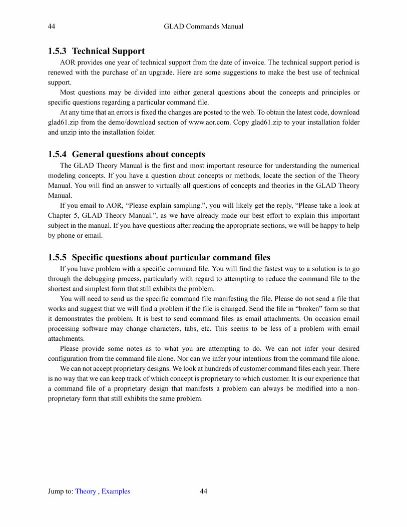
44 GLAD Commands Manual
1.5.3 Technical SupportAOR provides one year of technical support from the date of invoice. The technical support period is
renewed with the purchase of an upgrade. Here are some suggestions to make the best use of technical support.
Most questions may be divided into either general questions about the concepts and principles or specific questions regarding a particular command file.
At any time that an errors is fixed the changes are posted to the web. To obtain the latest code, download glad61.zip from the demo/download section of www.aor.com. Copy glad61.zip to your installation folder and unzip into the installation folder.
1.5.4 General questions about conceptsThe GLAD Theory Manual is the first and most important resource for understanding the numerical
modeling concepts. If you have a question about concepts or methods, locate the section of the Theory Manual. You will find an answer to virtually all questions of concepts and theories in the GLAD Theory Manual.
If you email to AOR, “Please explain sampling.”, you will likely get the reply, “Please take a look at Chapter 5, GLAD Theory Manual.”, as we have already made our best effort to explain this important subject in the manual. If you have questions after reading the appropriate sections, we will be happy to help by phone or email.
1.5.5 Specific questions about particular command filesIf you have problem with a specific command file. You will find the fastest way to a solution is to go
through the debugging process, particularly with regard to attempting to reduce the command file to the shortest and simplest form that still exhibits the problem.
You will need to send us the specific command file manifesting the file. Please do not send a file that works and suggest that we will find a problem if the file is changed. Send the file in “broken” form so that it demonstrates the problem. It is best to send command files as email attachments. On occasion email processing software may change characters, tabs, etc. This seems to be less of a problem with email attachments.
Please provide some notes as to what you are attempting to do. We can not infer your desired configuration from the command file alone. Nor can we infer your intentions from the command file alone.
We can not accept proprietary designs. We look at hundreds of customer command files each year. There is no way that we can keep track of which concept is proprietary to which customer. It is our experience that a command file of a proprietary design that manifests a problem can always be modified into a non-proprietary form that still exhibits the same problem.
Jump to: , 44 Theory Examples
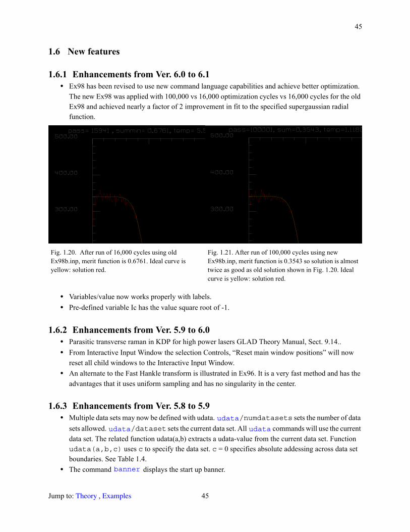
45
1.6 New features
1.6.1 Enhancements from Ver. 6.0 to 6.1• Ex98 has been revised to use new command language capabilities and achieve better optimization.
The new Ex98 was applied with 100,000 vs 16,000 optimization cycles vs 16,000 cycles for the old Ex98 and achieved nearly a factor of 2 improvement in fit to the specified supergaussian radial function.
• Variables/value now works properly with labels.• Pre-defined variable Ic has the value square root of -1.
1.6.2 Enhancements from Ver. 5.9 to 6.0• Parasitic transverse raman in KDP for high power lasers GLAD Theory Manual, Sect. 9.14..
• From Interactive Input Window the selection Controls, “Reset main window positions” will now reset all child windows to the Interactive Input Window.
• An alternate to the Fast Hankle transform is illustrated in Ex96. It is a very fast method and has the advantages that it uses uniform sampling and has no singularity in the center.
1.6.3 Enhancements from Ver. 5.8 to 5.9• Multiple data sets may now be defined with udata. /numdatasets sets the number of data
sets allowed. /dataset sets the current data set. All commands will use the current data set. The related function udata(a,b) extracts a udata-value from the current data set. Function udata(a,b,c) uses c to specify the data set. c = 0 specifies absolute addessing across data set boundaries. See Table 1.4.
• The command displays the start up banner.
Fig. 1.20. After run of 16,000 cycles using old Ex98b.inp, merit function is 0.6761. Ideal curve is yellow: solution red.
Fig. 1.21. After run of 100,000 cycles using new Ex98b.inp, merit function is 0.3543 so solution is almost twice as good as old solution shown in Fig. 1.20. Ideal curve is yellow: solution red.
udata udata udata
banner
Jump to: , 45 Theory Examples
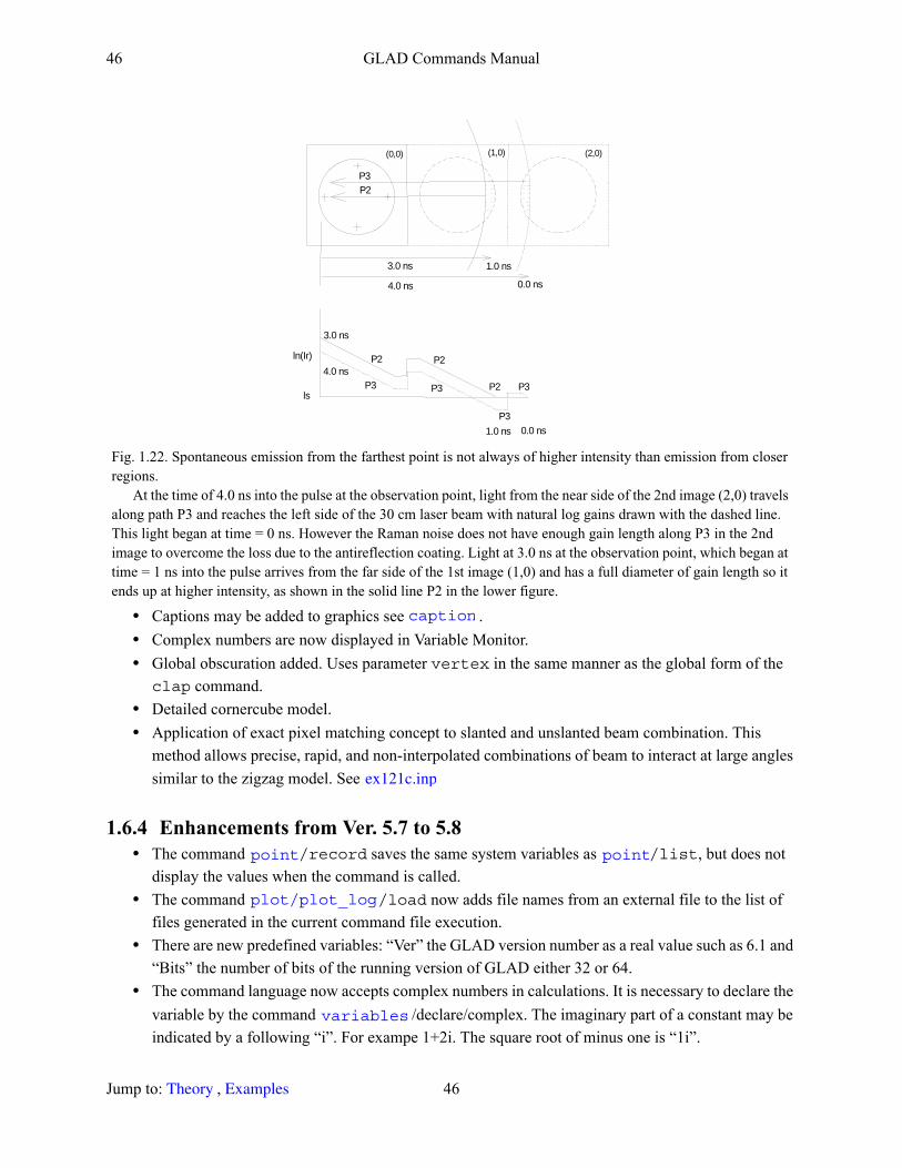
46 GLAD Commands Manual
• Captions may be added to graphics see .• Complex numbers are now displayed in Variable Monitor.• Global obscuration added. Uses parameter vertex in the same manner as the global form of the clap command.
• Detailed cornercube model.• Application of exact pixel matching concept to slanted and unslanted beam combination. This
method allows precise, rapid, and non-interpolated combinations of beam to interact at large angles similar to the zigzag model. See
1.6.4 Enhancements from Ver. 5.7 to 5.8• The command /record saves the same system variables as /list, but does not
display the values when the command is called.• The command /load now adds file names from an external file to the list of
files generated in the current command file execution.• There are new predefined variables: “Ver” the GLAD version number as a real value such as 6.1 and
“Bits” the number of bits of the running version of GLAD either 32 or 64.• The command language now accepts complex numbers in calculations. It is necessary to declare the
variable by the command /declare/complex. The imaginary part of a constant may be indicated by a following “i”. For exampe 1+2i. The square root of minus one is “1i”.
Fig. 1.22. Spontaneous emission from the farthest point is not always of higher intensity than emission from closer regions.
At the time of 4.0 ns into the pulse at the observation point, light from the near side of the 2nd image (2,0) travels along path P3 and reaches the left side of the 30 cm laser beam with natural log gains drawn with the dashed line. This light began at time = 0 ns. However the Raman noise does not have enough gain length along P3 in the 2nd image to overcome the loss due to the antireflection coating. Light at 3.0 ns at the observation point, which began at time = 1 ns into the pulse arrives from the far side of the 1st image (1,0) and has a full diameter of gain length so it ends up at higher intensity, as shown in the solid line P2 in the lower figure.
1.0 ns
4.0 ns
0.0 ns
3.0 ns
ln(Ir)
3.0 ns
4.0 ns 0.0 ns
1.0 ns
(0,0) (1,0) (2,0)
ls
P3P2
P3
P2
P2 P3P3
P2
P3
caption
ex121c.inp
point point
plot/plot_log
variables
Jump to: , 46 Theory Examples

47
Fig. 1.23. The degenerate FFT model is compared against a square array. Fresnel number 12 is shown for a1024 ×1024 array calculation (yellow) and the method of degenerate FFT (green) using a 1024 ×1 array. Some edge droop is evident with the degenerate FFT method due to interpolation but the method achieves uniform sampling un like the Fast Hankle transform and has no singularity at the center point.
Fig. 1.24. Beam slanted at 40 degrees to be added. Fig. 1.25. Beam slanted at 40 degrees (see Fig.1.24) added to unslanted beam. Note slanted beam passes outside the region of the unslanted beam at the bottom left.
Jump to: , 47 Theory Examples
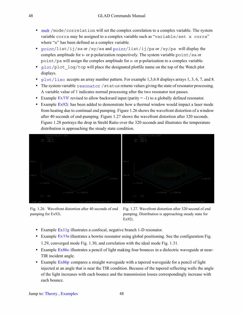
48 GLAD Commands Manual
• /mode/correlation will set the complex correlation to a complex variable. The system variable corra may be assigned to a complex variable such as “variable/set x corra” where “x” has been defined as a complex variable.
• /list/ij/sa or /xy/sa and /list/ij/pa or /xy/pa will display the complex amplitude for s- or p-polarization respectively. The system variable point/sa or point/pa will assign the complex amplitude for s- or p-polarization to a complex variable.
• /plot_log/top will place the designated plotfile name on the top of the Watch plot displays.
• accepts an array number pattern. For example 1,3,6:8 displays arrays 1, 3, 6, 7, and 8.• The system variable /status returns values giving the state of resonator processing.
A variable value of 1 indicates normal processing after the two resonator test passes.• Example revised to allow backward input (parity = -1) to a globally defined resonator.• Example has been added to demonstrate how a thermal window would impact a laser mode
from heating due to continual end pumping. Figure 1.26 shows the wavefront distortion of a window after 40 seconds of end-pumping. Figure 1.27 shows the wavefront distortion after 320 seconds. Figure 1.28 portrays the drop in Strehl Ratio over the 320 seconds and illustrates the temperature distribution is approaching the steady state condition.
• Example illustrates a confocal, negative branch 1-D resonator.• Example illustrates a bowtie resonator using global positioning. See the configuration Fig.
1.29, converged mode Fig. 1.30, and correlation with the ideal mode Fig. 1.31. • Example illustrates a pencil of light making four bounces in a dielectric waveguide at near-
TIR incident angle. • Example compares a straight waveguide with a tapered waveguide for a pencil of light
injected at an angle that is near the TIR condition. Because of the tapered reflecting walls the angle of the light increases with each bounce and the transmission losses correspondingly increase with each bounce.
Fig. 1.26. Wavefront distortion after 40 seconds of end pumping for Ex92i.
Fig. 1.27. Wavefront distortion after 320 second of end pumping. Distribution is approaching steady state for Ex92i.
mult
point point
plot
plot/liso resonator
Ex33f
Ex92i
Ex11g
Ex33n
Ex86o
Ex86p
Jump to: , 48 Theory Examples
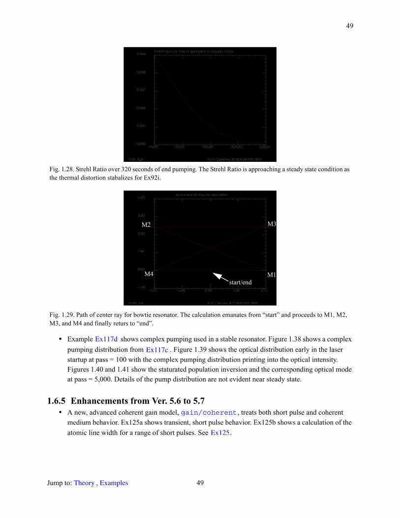
49
• Example shows complex pumping used in a stable resonator. Figure 1.38 shows a complex pumping distribution from . Figure 1.39 shows the optical distribution early in the laser startup at pass = 100 with the complex pumping distribution printing into the optical intensity. Figures 1.40 and 1.41 show the staturated population inversion and the corresponding optical mode at pass = 5,000. Details of the pump distribution are not evident near steady state.
1.6.5 Enhancements from Ver. 5.6 to 5.7• A new, advanced coherent gain model, , treats both short pulse and coherent
medium behavior. Ex125a shows transient, short pulse behavior. Ex125b shows a calculation of the atomic line width for a range of short pulses. See .
Fig. 1.28. Strehl Ratio over 320 seconds of end pumping. The Strehl Ratio is approaching a steady state condition as the thermal distortion stabalizes for Ex92i.
Fig. 1.29. Path of center ray for bowtie resonator. The calculation emanates from “start” and proceeds to M1, M2, M3, and M4 and finally returs to “end”.
start/endM1M4
M2 M3
Ex117d
Ex117c
gain/coherent
Ex125
Jump to: , 49 Theory Examples
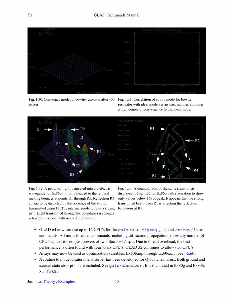
50 GLAD Commands Manual
• GLAD 64 now can use up to 16 CPU’s for the rate, gain, and /list commands. All multi-threaded commands, including diffraction propagation, allow any number of CPU’s up to 16—not just powers of two. See /cpu. Due to thread overhead, the best performance is often found with four to six CPU’s. GLAD 32 continues to allow two CPU’s.
• Arrays may now be used as optimization variables. Ex60b.inp through Ex60e.inp. See .• A routine to model a saturable absorber has been developed for Q-switched lasers. Both ground and
excited state absorption are included. See . It is illustrated in Ex80g and Ex80h. See .
Fig. 1.30. Converged mode for bowtie resonator after 400 passes.
Fig. 1.31. Correlation of cavity mode for bowtie resonator with ideal mode versus pass number, showing a high degree of convergence to the ideal mode.
Fig. 1.32. A pencil of light is injected into a dielectric waveguide for Ex86o, initially headed to the left and making bounces at points R1 through R5. Reflection R3 appers to be distorted by the presence of the strong transmitted beam T1. The intermal mode follows a zigzag path. Light transmitted through the boundaries is strongly refracted in accord with near-TIR condition.
Fig. 1.33. A countour plot of the same situation as displayed in Fig. 1.32 for Ex86o with staturation to show only values below 1% of peak. It appears that the strong transmiited beam from R1 is affecting the reflection behaviour at R3.
R1 R2
R3
R4T1
T2
R5
T3
R1
T2
R4T3
T1
R5
R3
R2
gain zigzag energy
set
Ex60
gain/absorber Ex80
Jump to: , 50 Theory Examples
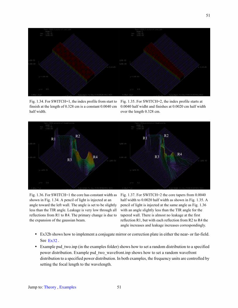
51
• Ex32b shows how to implement a conjugate mirror or correction plate in either the near- or far-field. See .
• Example psd_two.inp (in the examples folder) shows how to set a random distribution to a specified power distribution. Example psd_two_wavefront.inp shows how to set a random wavefront distribution to a specified power distribution. In both examples, the frequency units are controlled by setting the focal length to the wavelength.
Fig. 1.34. For SWITCH=1, the index profile from start to finsish at the length of 0.328 cm is a constant 0.0040 cm half width.
Fig. 1.35. For SWITCH=2, the index profile starts at 0.0040 half widht and finishes at 0.0020 cm half width over the length 0.328 cm.
Fig. 1.36. For SWITCH=1 the core has constant width as shown in Fig. 1.34. A pencil of light is injected at an angle toward the left wall. The angle is set to be slightly less than the TIR angle. Leakage is very low through all reflections from R1 to R4. The primary change is due to the expansion of the gaussian beam.
Fig. 1.37. For SWITCH=2 the core tapers from 0.0040 half width to 0.0020 half width as shown in Fig. 1.35. A pencil of light is injected at the same angle as Fig. 1.36 with an angle slightly less than the TIR angle for the tapered wall. There is almost no leakage at the first reflection R1, but with each reflection from R2 to R4 the angle increases and leakage increases correspondingly.
R1R2
R3R4
R1 R2
R3 R4
Ex32
Jump to: , 51 Theory Examples
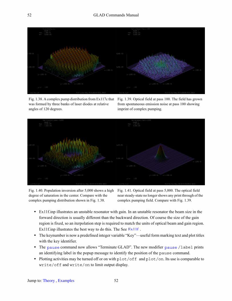
52 GLAD Commands Manual
• Ex11f.inp illustrates an unstable resonator with gain. In an unstable resonator the beam size in the forward direction is usually different than the backward direction. Of course the size of the gain region is fixed, so an iterpolation step is required to match the units of optical beam and gain region. Ex11f.inp illustrates the best way to do this. The See .
• The keynumber is now a predefined integer variable “Key”—useful form marking text and plot titles with the key identifier.
• The command now allows “Terminate GLAD”. The new modifier /label prints an identifying label in the popup message to identify the position of the pause command.
• Plotting activities may be turned off or on with plot/off and plot/on. Its use is comparable to write/off and write/on to limit output display.
Fig. 1.38. A complex pump distribution from Ex117c that was formed by three banks of laser diodes at relative angles of 120 degrees.
Fig. 1.39. Optical field at pass 100. The field has grown from spontaneous emission noise at pass 100 showing imprint of complex pumping.
Fig. 1.40. Population inversion after 5,000 shows a high degree of saturation in the center. Compare with the complex pumping distribution shown in Fig. 1.38.
Fig. 1.41. Optical field at pass 5,000. The optical field near steady-state no longer shows any print through of the complex pumping field. Compare with Fig. 1.39.
Ex11f
pause pause
Jump to: , 52 Theory Examples
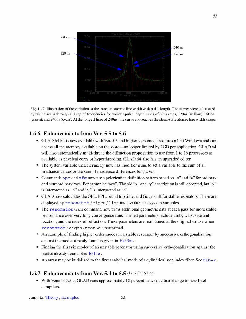
53
1.6.6 Enhancements from Ver. 5.5 to 5.6• GLAD 64 bit is now available with Ver. 5.6 and higher versions. It requires 64 bit Windows and can
access all the memory available on the syste—no longer limited by 2GB per application. GLAD 64 will also automatically multi-thread the diffraction propogation to use from 1 to 16 processors as available as physical cores or hyperthreading. GLAD 64 also has an upgraded editor.
• The system variable uniformity now has modifier sum, to set a variable to the sum of all irradiance values or the sum of irradiance differences for /two.
• Commands and now use a polarization definition pattern based on “o” and “e” for ordinary and extraordinary rays. For example: “oeo”. The old “x” and “y” description is still accepted, but “x” is interpreted as “o” and “y” is interpreted as “e”.
• GLAD now calculates the OPL, PPL, round trip time, and Gouy shift for stable resonators. These are displayed by /eigen/list and available as system variables.
• The /run command now trims additional geometric data at each pass for more stable performance over very long convergence runs. Trimed parameters include units, waist size and location, and the index of refraction. These parameters are maintained at the original valuse when
/eigen/test was performed.• An example of finding higher order modes in a stable resonator by successive orthogonalization
against the modes already found is given in .• Finding the first six modes of an unstable resonator using successive orthogonalization against the
modes already found. See .• An array may be initialized to the first analytical mode of a cylindrical step index fiber. See .
1.6.7 Enhancements from Ver. 5.4 to 5.5• With Version 5.5.2, GLAD runs approximately 18 percent faster due to a change to new Intel
compilers.
Fig. 1.42. Illustration of the variation of the transient atomic line width with pulse length. The curves were calculated by taking scans through a range of frequencies for various pulse length times of 60ns (red), 120ns (yellow), 180ns (green), and 240ns (cyan). At the longest time of 240ns, the curve approaches the stead-state atomic line width shape.
240 ns
180 ns
60 ns
120 ns
opo sfg
resonator resonator
resonator
Ex33m
Ex11e
fiber
t /1.6.7 /DEST pd
Jump to: , 53 Theory Examples

54 GLAD Commands Manual
• Notice of expiration of technical support and version upgrade period has been added to the banner displayed at the start of the program for convenient reference.
• GLAD 5.5 supports running from a non-administrative account. Installation still requires administrative privliges.
• Trigonometric functions that accept degrees as arguments or return values in degree have been added. Each function is identified by a trailing “d” in the name. Functions include: sind, cosd, tand, tan2d, asind, acosd, atand, and atan2d.
• The function time() has been added to give the time in seconds since January 1, 1970 GMT. It can be used to generate a unique random seed in the expression i = srand(time()).
• The command /ginversion will integrate over z for 3D arrays if the section number is set to zero and yield a value with units of [j]. Similarly the variable produced by energy/ginversion will yield the same value for 3D arrays if the section number is set to zero.
• /zslice now prints field data for a z-slice through a 3D array.• /real, /aimaginary, /real, and /aimaginary have
been added.• The title of the security key may be changed at the time of upgrade following the instructions
included with the upgrade password.• Keyread.exe provides a user interface when called by means of the short cut. This the same as
executing “keyread.exe menu”. The interactive menu may be called from GLAD by /keyread. A log file named keyread61.log is generated and contains information
about keyread activity.• A closed-form solution for steady-state solution for the upper and lower levels based on the pumping
rate and the incident irradiance. This is implemented in /steady. A numerical check is illustrated in .
• /rate/steady and /rate/step now have a “list” parameter to provide a list of overall properties and properties of the center step. illustrates the use of this feature to gain insight into the numerical calculations of gain.
• /three/step now have a “list” parameter to list overall properties and properties of the center step. illustrates the use of this feature to gain insight into the numerical calculations of gain.
• Section provides more detail about the pump rate for three-layer gain with a single upper state.• The Watch refresh time may now be set under the File, Preferences. The default is 1.5. This may be
changed within the range 0.1 to 10 seconds.• The offset values of graphic files may be specified in pixel coordinates relative to the lower, left
corner of Watch.exe. See /watch and .• The Watch program has a new menu item “Restore to Watch.dat” to restore the position and size of
all graphic files to the original condition specified by GLAD through watch.dat. This removes the effect of user resizing or repositioning.
• The Watch program will now correctly set only the size if xsize or ysize is specified without the need to specify xoff or yoff.
• Column labels on the listing may be set with /clabel.
energy
intensity infile infile outfile outfile
privileges
gain/rate Ex69j
gain gain Ex69f
gain Ex69g
Sect
plot plot/plot_log
udata udata
Jump to: , 54 Theory Examples
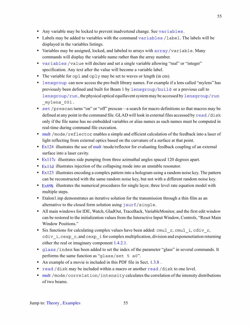
55
• Any variable may be locked to prevent inadvertend change. See .• Labels may be added to variables with the command /label. The labels will be
displayed in the variables listings.• Variables may be assigned, locked, and labeled to arrays with /variable. Many
commands will display the variable name rather than the array number.• /value will declare and set a single variable allowing “real” or “integer”
specification. Any text after the value will become a variable label.• The variable for opl and oply may be set to waves or length (in cm).• can now access the pre-built library names. For example if a lens called “mylens” has
previously been defined and built for Beam 1 by or a previous call to , the physical optical equillavent system may be accessed by
_mylens_001.
• /prescan turns “on” or “off” prescan—a search for macro definitions so that macros may be defined at any point in the command file. GLAD will look in external files accessed by /disk only if the file name has no embedded variables or alias names as such names must be computed in real-time during command file execution.
• /mode/reflector enables a simple and efficient calculation of the feedback into a laser of light reflecting from external optics based on the curvature of a surface at that point.
• illustrates the use of /mode/reflector for evaluating feedback coupling of an external surface into a laser cavity.
• illustrates side pumping from three azimuthal angles spaced 120 degrees apart.• illustrates injection of the collapsing mode into an unstable resonator.• illustrates encoding a complex pattern into a hologram using a random noise key. The pattern
can be reconstructed with the same random noise key, but not with a different random noise key.• illustrates the numerical procedures for single layer, three level rate equation model with
multiple steps.• Etalon1.inp demonstrates an iterative solution for the transmission through a thin film as an
alternative to the closed form solution using /single.• All main windows for IDE, Watch, GladOut, TraceBack, VariableMonitor, and the first edit window
can be restored to the initialization values from the Interactive Input Window, Controls, “Reset Main Window Positions.”
• Six functions for calculating complex values have been added: cmul_r, cmul_i, cdiv_r, cdiv_i, cexp_r, and cexp_i for complex multiplication, division and exponenetiation returning either the real or imaginary component .
• /index has been added to set the index of the parameter “glass” in several commands. It performs the same function as “glass/set 5 a0”.
• An example of a movie is included in this PDF file in Sect. .• /disk may be included within a macro or another /disk to one level.• /mode/correlation/intensity calculates the correlation of the intensity distributions
of two beams.
variables variables
array
variables
lensgroup lensgroup/build
lensgroup/run lensgroup/run
set read
mult
Ex124 mult
Ex117c
Ex11d
Ex123
Ex69k
jsurf
1.4.2.1
glass
1.3.8
read read mult
Jump to: , 55 Theory Examples

56 GLAD Commands Manual
• /list now displays the round trip time and /set (variable) resonator/roundtriptime sets a variable to the round trip time. The round trip time may be used for the gain pumping time. The frequency separation of longitudinal modes is the inverse of the round trip time.
• /label allows the user to add an identifying label for the pause. Variables may be included by preceeding them by the “@” symbol.
1.6.8 Enhancements from Ver. 5.3 to 5.4• The family of plots displayed by Watch may be moved as a group by moving the main Watch
window. This makes it easy to drag all Watch windows across the screen or onto a second monitor for a dual-monitor setup.
• GLAD now pre-scans the entire command file and identifies and saves all macros. Locating the macros at the bottom of the command file after end can improve readibility.
• The position and size of the first editor window is saved and used as the default for the next execution of GLAD.
• Enhanced metafile (EMF) graphics may be generated from Watch or from /meta/emf.• The GladOut display may be cleared from the command line /screen/clear.• The pattern “//” may be used as an in-line, non-displayed comment similar to “#”.• The command /ginversion displays the integrated population inversion in j/cm.• A variable may be set to the population inversion at a point with point/ginversion or the
integrated population inversion with energy/ginversion in j/cm.• The modifier ginversion has been added to most plots to show the population inversion
distribution.• /udata/set with no column identifiers lists current identifiers.• Prism ends with variable angles on the input and output faces are now incorporated into the command
to model a zigzag amplifier. See Example .• displays the configuration of the zigzag amplifier in gain or beam coordinates.• The command displays the current source line in the output. The function line() returns
the current source code line.
1.6.9 Enhancements from Ver. 5.2 to 5.3• The command has been completely rewritten to provide dynamic generation of HTML output
with automatic update by sourceline, tables with tooktip definitions, and scalable vector graphic (SVG) graphics that may be expanded and the range of plot versions viewed. See Sect. 1.3.6. The old GLAD HTML viewer is no longer used after Ver. 5.2.
• The command has been enhanced. This command now tests the system macro, issues an internal resonator/set command, and makes a second test to verify stable behavior. The resonator/set command is no longer needed explicitly and the double tests catch many errors causing instability of the round trip ABCD matrix that a single test would not.
• The internal testing by the now, by default, ignores gain, plot, thermal, and udata commands.
resonator variables
pause
plot write
energy
plot
zigzag Ex121b
plot/zigzag line
html
resonator
resonator
Jump to: , 56 Theory Examples
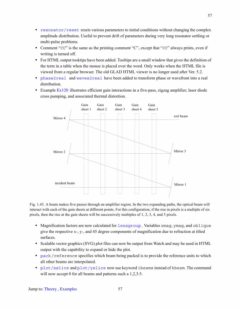
57
• resets various parameters to initial conditions without changing the complex amplitude distribution. Useful to prevent drift of parameters during very long resonator settling or multi-pulse problems.
• Comment “CC” is the same as the printing comment “C”, except that “CC” always prints, even if writing is turned off.
• For HTML output tooktips have been added. Tooltips are a small window that gives the definition of the term in a table when the mouse is placed over the word. Only works when the HTML file is viewed from a regular browser. The old GLAD HTML viewer is no longer used after Ver. 5.2.
• and have been added to transform phase or wavefront into a real distribution.
• Example illustrates efficient gain interactions in a five-pass, zigzag amplifier; laser diode cross pumping, and associated thermal distortion.
• Magnification factors are now calculated for . Variables xmag, ymag, and oblique give the respective x-, y-, and 45 degree components of magnification due to refraction at tilted surfaces.
• Scalable vector graphics (SVG) plot files can now be output from Watch and may be used in HTML output with the capability to expand or hide the plot.
• /reference specifies which beam being packed is to provide the reference units to which all other beams are interpolated.
• and now use keyword ibeams instead of kbeam. The command will now accept 0 for all beams and patterns such a 1,2,3:5.
Fig. 1.43. A beam makes five passes through an amplifier region. In the two expanding paths, the optical beam will interact with each of the gain sheets at different points. For this configuration, if the rise in pixels is a multiple of six pixels, then the rise at the gain sheets will be successively multiples of 1, 2, 3, 4, and 5 pixels.
resonator/reset
phase2real waves2real
Ex120
Gainsheet 1
Mirror 2
Mirror 4
Mirror 1incident beam
Gainsheet 2
Gain sheet 3
Gainsheet 4
Gainsheet 5
Mirror 3
exit beam
lensgroup
pack
plot/xslice plot/yslice
Jump to: , 57 Theory Examples
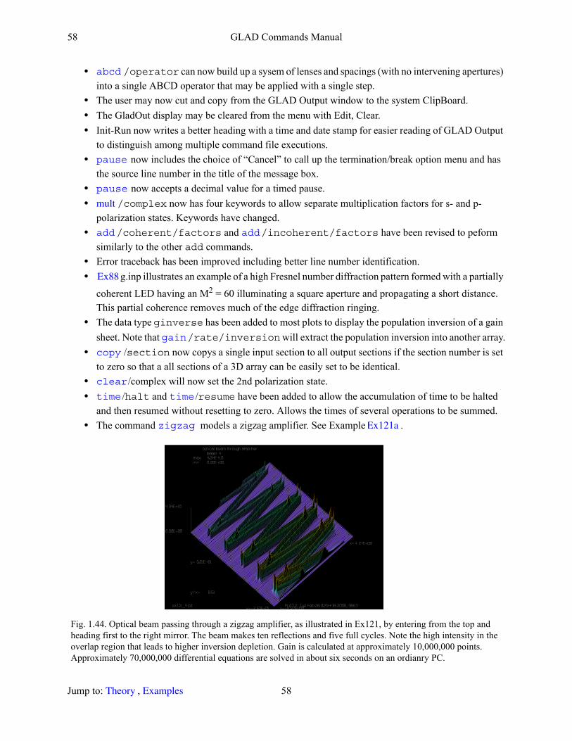
58 GLAD Commands Manual
• /operator can now build up a sysem of lenses and spacings (with no intervening apertures) into a single ABCD operator that may be applied with a single step.
• The user may now cut and copy from the GLAD Output window to the system ClipBoard.• The GladOut display may be cleared from the menu with Edit, Clear.• Init-Run now writes a better heading with a time and date stamp for easier reading of GLAD Output
to distinguish among multiple command file executions.• now includes the choice of “Cancel” to call up the termination/break option menu and has
the source line number in the title of the message box.• now accepts a decimal value for a timed pause.• /complex now has four keywords to allow separate multiplication factors for s- and p-
polarization states. Keywords have changed.• /coherent/factors and /incoherent/factors have been revised to peform
similarly to the other add commands.• Error traceback has been improved including better line number identification.• g.inp illustrates an example of a high Fresnel number diffraction pattern formed with a partially
coherent LED having an M2 = 60 illuminating a square aperture and propagating a short distance. This partial coherence removes much of the edge diffraction ringing.
• The data type ginverse has been added to most plots to display the population inversion of a gain sheet. Note that /rate/inversion will extract the population inversion into another array.
• /section now copys a single input section to all output sections if the section number is set to zero so that a all sections of a 3D array can be easily set to be identical.
• /complex will now set the 2nd polarization state.• /halt and /resume have been added to allow the accumulation of time to be halted
and then resumed without resetting to zero. Allows the times of several operations to be summed.• The command models a zigzag amplifier. See Example .
Fig. 1.44. Optical beam passing through a zigzag amplifier, as illustrated in Ex121, by entering from the top and heading first to the right mirror. The beam makes ten reflections and five full cycles. Note the high intensity in the overlap region that leads to higher inversion depletion. Gain is calculated at approximately 10,000,000 points. Approximately 70,000,000 differential equations are solved in about six seconds on an ordianry PC.
abcd
pause
pause mult
add add
Ex88
gain copy
clear time time
zigzag Ex121a
Jump to: , 58 Theory Examples
59
• The commands now have the option to display the population inversion with /ginversion.• /coherent/con and /incoherent/con accept decentration keywords and allow
allow the arrays to be of different size.
1.6.10Enhancements from Ver. 5.1 to 5.2• /jones allows implementation of a 2D array where each element of the array is a
Jones matrix. This allows the Jones matrix operations to vary across the aperture. See example jones1.inp and jones2.inp.
• implements three level gain where both upper and lower levels may consist of multiple levels forming a manifold.
• Example illustrates how to implement sub-sampling of the round-trip time of a resonator.• For macros, the Traceback window now gives the absolute line position in the file for easier
reference.• The command gives the source line position and source file name. The system variable line
gives the source line position. The command now gives the source line position.• The command now takes a beam number range.
1.6.11 Enhancements from Ver. 5.0 to 5.1• A model of three-level gain has been added. See . Also see .• A detailed numerical check of the four-level, rate equation gain equations. See .• A procedure was developed for doing through-focus diffraction calculations projected onto a tilted
surface. See tilt.inp.• Memory will now be automatically expanded as required up to the maximum physical memory
available .• /exp added.• Several accelerator keys have been revised to conform with MS Wordpad®, MS Word®, and many
other text editing programs. Ctrl S (hold down Ctrl, then strike S key) “Save” to save the file. Shift Ctrl S invokes “Save As”. Ctrl F invokes the search dialog box. F3 does a forward search with the same search string. Shift F3 does a backward search with the same string. Ctrl P invokes the print operation. Shift Ctrl P invokes the print setup dialog box.
• Numbers corresponding to length may have “mm” (millimeters), “in” (inches), “ft” (feet), “mi” (microns), “nm” (nanometers), “km” (kilometers), or “m” (meters) appended to cause appropriate scaling to centimeters. For example 1.3mm will be read as 0.13 cm.
• The command can now either correct directly or create a phase plate.• The elements and now have either \global or \nonglobal forms.• The maximum number of variables has been increased from 400 to 999, with five predefined
constants (and 994 available for use in command files. The predefined constants are π, e, h, c, and the version number Ver.
• The macro library is now held in memory for faster execution. This library may be displayed by the /maclib/show command. Highlighting of lines and commands is now done in the macro
library as well as in the source files. The library is rebuilt each time Init-Run is executed.
plot add add
mult/beam
gain/three
Ex119
line echo
clear
gain/three Ex69e
Ex69f
memory functions
adapt roof cornercube
set
Jump to: , 59 Theory Examples
60 GLAD Commands Manual
• Line numbers may be added, updated, or removed by Controls on the GladEdit menu.• Command files may be reformatted automatically with indents for different levels of macros, IF-
ELSE-THEN constructs, and pack/in and pack/out blocks. Indenting the source text greatly improves readability. See Controls, Indent on the GladEdit menu.
• The Traceback window now identifies multiple commands on the same line.• Highlighting now displays lines dynamically in both the source and macro library and identifies
command position for multiple commands on one line. Highlighting may be turned on or off from Controls from either the Interactive Input Window or any GladEdit window.
• The GladEdit windows may be controlled from a GLAD command file or the Interactive Input Window by the command . Files may be opened. Windows may be hidden or shown.
• Command now provides microsecond accuracy and the system variable time gives the value from the most recent call to time/show.
• /fresnel/refl allows for general complex index of refractions to accommodate reflection from metal surfaces or TIR with absorbing material on the low index side.
• and now may now be applied to irradiance as well as wavefront.• A model of semiconductor gain has been added. See . Also see example
.• The keyword ibeams now accepts beam number ranges and sequences in addition to “0” for all
beams and a single beam number. For example “:2,6:8,11,13,19:” processes beams 2 and below, 6 to 8, 11, 13, and 19 and higher.
• Definitions of terms used in output tables will be displayed or hidden with the /definitions command. For example using set/definitions/on before geodata will cause the definitions to be printed at the end.
• /msquared has been added to calculate M-squared by second moment.
1.7 Incompatibilities with earlier versions
1.7.1 Incompatibilities of Ver. 5.8 with 5.7• The variable parity used in /def no longer reverses the paraxial direction indicator.• Commands connect and disconnect are obsolete and have been deleted. Use the equivalent
commands infile and outfile with string modifiers noheader and binary.
1.7.2 Incompatibilities of Ver. 5.7 with 5.6None.
1.7.3 Incompatibilities of Ver. 5.6 with 5.5• In optimization tables /cha and /del have been deleted. Use /clear to remove all table entries.
Tables may be rebuilt after being cleared.• times has been droped in optimize/run which will now run only once.
edit time
jsurf
rms timevariance
gain/semiconductor Ex69d
set
fitgeo
global
Jump to: , 60 Theory Examples
61
1.7.4 Incompatibilities of Ver. 5.5 with 5.4• The keyword nstep has been deleted from gain/step for three-level and four-level gain. Only
one step is required or appropriae for Frantz-Nodvik gain.• /opl now leaves the phase of the beam receiving the sum unchanged.
1.7.5 Incompatibilities of Ver. 5.4 with 5.3None.
1.7.6 Incompatibilities of Ver. 5.3 with 5.2• Line highlighting in GladEdit has been reactivated with improvements and is active with error
traceback. Switching highlighting on causes highlighting of the current line in the edit window.• /dist is obsolete use /prop.• and now use keyword ibeams instead of kbeam. The command
will now accept 0 for all beams and patterns such a 1,2,3:5.• /complex has different keywords to allow for different multiplication of p-polarization.• /coherent/factors and /incoherent/factors have been revised.• no longer alters the global coordinate system for the beam respective.• The menu item “Run” on the GladEdit menu has been renamed to “NoInit-Run”.• /init/coarse and /show/coarse have been deleted. All timer functions use the
high precision clock.
1.8 License levelsThere are three license levels: GLAD, GLAD Pro and GLAD 64.
1.8.1 GLAD 61 features:• Intended for laser and physical optics engineering modeling.• Native 32 bit code. Runs on both 32 and 64 bit operating systems.• Limited to 2GB system memory.• Laser resonators: stable, unstable, ring lasers.• Detailed four-level laser gain, steady-state gain, gain sheets.• Complex physical optics systems.• Finite element thermal modeling.• Propagation in 3D geometry.• Astigmatism of tilted and decentered mirrors.• Idealized refractive elements.• Dielectric waveguide modeling.
1.8.2 GLAD Pro 61P has all GLAD 61 features and adds:• Intended for both engineering modeling and advanced research.
add
co2gain co2gain plot/xslice plot/yslice
mult
add add flip
time time
Jump to: , 61 Theory Examples
62 GLAD Commands Manual
• Native 32 bit code. Runs on both 32 and 64 bit operating systems.• Limited to 2GB system memory.• Diffration propagation multi-threading supports two CPU’s.• Detailed ray tracing calculations of tilted and decentered mirrors.• Detailed ray tracing calculations of complex lens groups with tilts and decenters.• Damped least squares optimization of all system parameters.• In addition to detailed four-level gain, includes three-level gain, and semiconductor gain.• Nonlinear optics: Raman, frequency doubling, four-wave mixing, optical limiting, sum frequency
generation.• Zigzag amplifier.• Atmospheric effects: turbulence and thermal blooming.• High NA vector diffraction calculations.• Lens array features.
1.8.3 GLAD 64 (61P64) has all features of GLAD (61P) and adds: • Performance enhancement and coherent gain model.• Requires 64 bit operating system.• Native 64 bit code is faster than 32 bit code.• Security dongle supports both GLAD Pro (32 bit) and GLAD 64 (64 bit). Customer has access to
both GLAD Pro (32bit) as well as GLAD 64 bit.• Can access all available memory on the computer.• Multi-threading of four-level gain and diffraction propagation up to 16 CPU’s.• Coherent gain for short pulse effects.
Jump to: , 62 Theory Examples
ABCD ABCD
2. Command Descriptions
ABCD General ABCD paraxial operator. Operator
Description: ABCDThis command models general systems and gradient index media in terms of the ABCD matrix. /set,
/list, and /last control the ABCD operator for the specified beam.The ABCD operator using /direct may be used to represent an arbitrary optical system. applied to
any of the beams and will implement propagation, change of index, magnification change, and optical power.
(1)
One can represent a simple system of lenses and spacings that has no intervening apertures by a single ABCD operator. This can save calculation time as only one diffraction propagation is required and is particularly effective for an imaging system. One can either specify the entire system with /direct or build up the ABCD operator in steps.
Using /direct explicitly specifies an arbitrary ABCD matrix and applies it to the specified beam. Only a single propagation step is required in combination with appropriate magnification, index of refraction, and beam curvature changes. The determinant of the matrix is the index of refraction and must be identical for both x- and y-directions.
Instead of specifying the total ABCD matrix by means of /direct, the ABCD matrix may be built-up by initializing a separate ABCD matrix with /set and then specifying the components of a simple lens system with spaces by /lens and /prop. The total length will be determined from the sum of all /propspecifications. Alternately any system element may be specified in general ABCD form with /multiply. The built-up ABCD system is implemented with the /apply command.
Command Form(s): ABCD abcd/set kbeam
abcd/list kbeam
abcd/last
abcd/operator/direct kbeam ax bx cx dx ay by cy dy
abcd/operator/set ax bx cx dx ay by cy dy
abcd/operator/multiply ax bx cx dx ay by cy dy
abcd/operator/lens xfl yfl
abcd/operator/prop zstep
abcd/operator/list
abcd/operator/apply kbeam
Ax Bx
Cx Dx
Ay By
Cy Dy
Jump to: , 63 Theory Examples
ABERRATION ABERRATION
Example of abcd/operatorSystem with three lenses and three spacings (requiring three propagation steps)lens/sph 1 F1prop T1 1lens/sph 1 F2prop T2 1lens/sph 1 F3prop T3 1
ABCD operation implementing the entire system with a single step: /applyabcd/oper/set # reset local ABCD matrixabcd/oper/lens F1 # build up ABCD operatorabcd/oper/prop T1abcd/oper/lens F2abcd/oper/prop T2abcd/oper/lens F3abcd/oper/prop T3 # total length is now T1 + T2 + T3abcd/oper/apply 1 # apply ABCD operator with a single step
ABR or ABERRATION Aberrations. Aberration
Modifier 1 Description /set Sets the ABCD operator to the unity matrix./list Lists the current ABCD matrix (default)./last Lists the last change ABCD matrix./operator/direct Iimplements the ABCD operator directly (default)./operator/set Sets ABCD operator without applying it. By default the ABCD matrix is set
to the unit matrix./operator/multiply Multiplies the specified ABCD operator without applying it./operator/lens ABCD of idealized lens multiplies the currnt ABCD operator without
applying it./operator/prop ABCD multiplies the currnt ABCD operator without applying it./operator/list Lists the stored ABCD operator.abcd/operator/apply Applies the current ABCD operator.
Numerical Values Description Defaultskbeam Unique beam number.ax, bx, cx, dx Matrix elements for x-direction. 1,0,0,1
ay, by, cy, dy Matrix elements for y-direction. ax, bx, cx, dx
System Variable Data Description abcd/(mod)mod = ax, bx, cx, dx, ay, by, cy, dy
Current ABCD properties of kbeam.
Command Form(s): ABERRATION Phase gratings.Seidel aberration.
aberration/ripple aberration/seidel
Jump to: , 64 Theory Examples
ABR ABERRATION/RADIAL
Description: ABRVarious types of aberration. Random aberrations of gaussian distribution and Kolmogorov atmospheric
aberration are implemented with the command. Also see .
ABERRATION/GRIN Gradient index aberration. Aberration
Description: ABERRATION/GRINThis command implements a gradient index lens (GRIN):
(2)
where is the wavefront error per step, are the coordinates, and is the wavelength. The aberration is added but diffraction propagation is not performed. Use prop zstep to add diffraction effects.
ABERRATION/RADIAL Special radial aberrations for axicons. Aberration
Zernike aberration.Radial mode aberration.Gradient index aberration.
Command Form(s): ABERRATION/GRIN aberration/grin ibeams deltan exp zstep rnorm xdec ydec
Numerical Values Description Defaultsibeams Beam number (0 to select all beams). Accepts pattern. 1 to nbeamdeltan Range of index of refraction that is modulated for
abr/grin.0
exp Coefficient for exponent for abr/grin. 0
zstep Step length. 0.
rnorm Normalization radius (cm). largest of x- or y-beam size
xdec, ydec Decenter of aberration. (0., 0.)
Command Form(s): ABERRATION/RADIALaberration/radial/decenter ibeams ewav azdeg irefbeam
abertation/radial/tilt ibeams ewav azdeg rnorm irefbeam
Command Form(s): ABERRATION (Continued) aberration/zernike aberration/radial aberration/grin
phase/kolmogorov phase
W x y,( ) Deltan Zstep•
λ0------------------------------------------- x Xdec–( )2 x Ydec–( )2+
Rnorm2
-------------------------------------------------------------------
Exp2
------------
=
W x y,( ) x y,( ) λ0
Jump to: , 65 Theory Examples
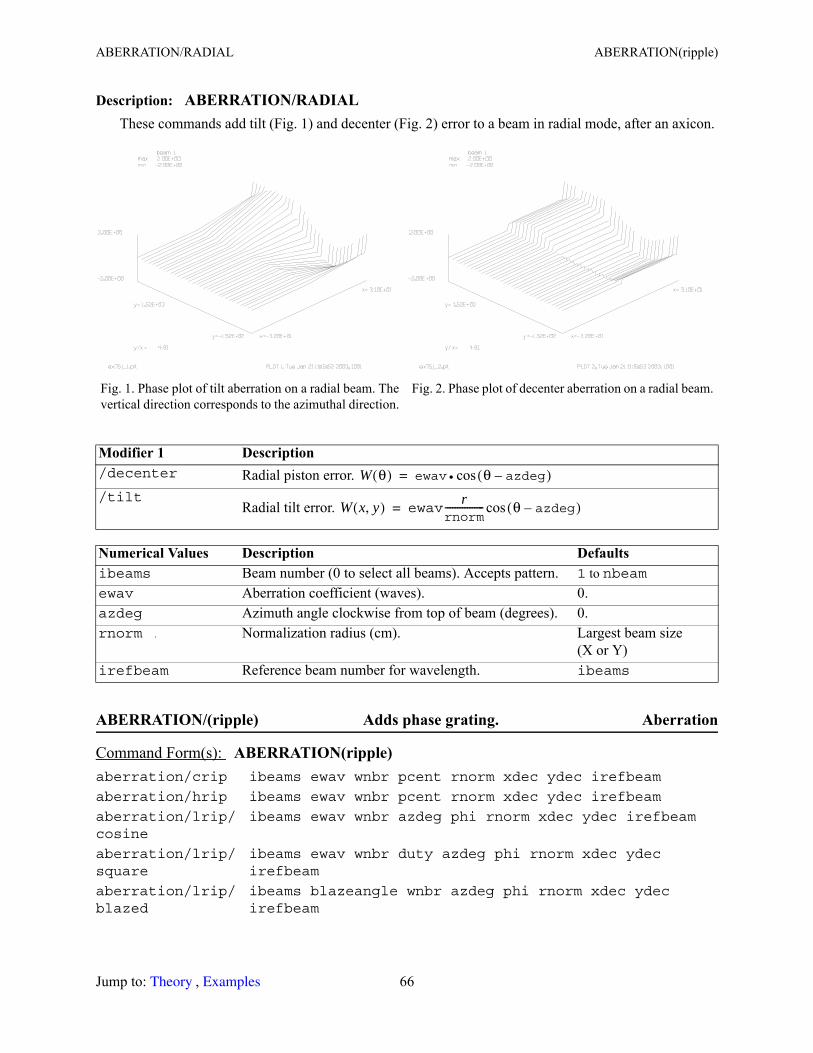
ABERRATION/RADIAL ABERRATION(ripple)
Description: ABERRATION/RADIALThese commands add tilt (Fig. 1) and decenter (Fig. 2) error to a beam in radial mode, after an axicon.
ABERRATION/(ripple) Adds phase grating. Aberration
Fig. 1. Phase plot of tilt aberration on a radial beam. The vertical direction corresponds to the azimuthal direction.
Fig. 2. Phase plot of decenter aberration on a radial beam.
Modifier 1 Description /decenter Radial piston error. /tilt
Radial tilt error.
Numerical Values Description Defaultsibeams Beam number (0 to select all beams). Accepts pattern. 1 to nbeamewav Aberration coefficient (waves). 0.azdeg Azimuth angle clockwise from top of beam (degrees). 0.rnorm Normalization radius (cm). Largest beam size
(X or Y)irefbeam Reference beam number for wavelength. ibeams
Command Form(s): ABERRATION(ripple) aberration/crip ibeams ewav wnbr pcent rnorm xdec ydec irefbeam
aberration/hrip ibeams ewav wnbr pcent rnorm xdec ydec irefbeam
aberration/lrip/cosine
ibeams ewav wnbr azdeg phi rnorm xdec ydec irefbeam
aberration/lrip/square
ibeams ewav wnbr duty azdeg phi rnorm xdec ydec irefbeam
aberration/lrip/blazed
ibeams blazeangle wnbr azdeg phi rnorm xdec ydec irefbeam
W θ( ) ewav θ azdeg–( )cos•=
W x y,( ) ewavr
rnorm---------------- θ azdeg–( )cos=
Jump to: , 66 Theory Examples
ABERRATION/(ripple) ABERRATION/SEIDEL
Description: ABERRATION/(ripple)These commands put a phase ripple (grating) into the beam distribution. Also, see .
ABERRATION/(Seidel) Adds Seidel aberration. Aberration
Modifier 1 Description /crip
Circular ripple.
/hrip Hexagonal ripple.
/lrip Linear ripple.
Modifier 2 Description /cosine Cosine phase linear ripple./square Square profile phase linear ripple./blazed Blazed phase grating.
Numerical Values Description Defaultsibeams Beam number (0 to select all beams). 1 to nbeamewav Aberration coefficient (waves). 0.
blazeangle Angle of blazing. Refracted/reflected angle should match diffracted angle for best efficiency.
duty Duty cycle (ratio of raised region to line width). 0.5
azdeg Azimuth angle clockwise from top of beam (degrees). 0.
wnbr Number of cycles from center to rnorm.pcent pcent = 0 or 1. 0 for null at center, 1 for peak at center. 0.phi Phase at center (degrees). 0.
rnorm Normalization radius (cm) for /crip or half width for /hrip.
largest beam size (X or Y)
xdec, ydec Coordinates of aberration center. 0., 0.irefbeam Reference beam number for wavelength. ibeams
Command Form(s): ABERRATION/SEIDEL aberration/ast/polar
ibeams ewav azdeg rnorm xdec ydec irefbeam
grating
W r( ) ewav2πr•wnbrrnorm
------------------------- r x2 y2+=,sin•=
W x y,( ) ewav2πr•wnbrRnorm
-------------------------
yx----- 1
3-------> r 3
2------- y x
2-----+=,
yx----- 1
3-------≤ r x=,
,sin•=
W x y,( ) ewav y Azdeg( )cos x Azdeg( )sin+[ ]2π•wnbrrnorm
---------------------- Phi+
sin•=
Jump to: , 67 Theory Examples
ABERRATION/(Seidel) ABERRATION/(Seidel)
Description: ABERRATION/(Seidel)These commands put Seidel and similar aberrations into the beam distribution.
aberration/ast/cartesian
ibeams ewavx ewavy rnorm xdec ydec irefbeam
aberration/coma ibeams ewav azdeg rnorm xdec ydec irefbeam
aberration/focus ibeams ewav rnorm xdec ydec irefbeam
aberration/sph ibeams ewav rnorm xdec ydec irefbeam
aberration/tilt/runout
ibeams ewav azdeg rnorm xdec ydec irefbeam
aberration/tilt/angle
ibeams thetarad azdeg xdec ydec irefbeam
aberration/cone ibeams ewav rnorm xdec ydec irefbeam
Modifier 1 Description Mathematical form/ast/polar Astigmatism.
/ast/cartesian Astigmatism.
/coma Coma.
/focus Focus.
/sph Spherical.
/tilt Tilt.
/fold Folding.
/cone Cone.
/grin GRIN.
Modifier 2 Description ast/polar Astigmatism in polar coordinates (default).ast/cartesian Astigmatism in x- and y-coordinates.tilt/runout Define the angle by the height of the tilt of the angle at radius rnorm.tilt/angle Define the tilt angle in radians.
Command Form(s): ABERRATION/SEIDEL (Continued)
W r θ,( ) ewavr
rnorm------------------ 2
cos2 θ azdeg–( )=
W x y,( ) ewavxx
rnorm------------------ 2
ewavyy
rnorm------------------ 2
+=
W x y,( ) ewavxr
rnorm------------------ 3
cos θ azdeg–( )=
W x y,( ) ewavr
rnorm------------------ 2
=
W x y,( ) ewavr
rnorm------------------ 4
=
W x y,( ) ewavr
rnorm------------------ cos θ azdeg–( )=
W x y,( ) ewavr
rnorm------------------ cos θ azdeg–( )=
W x y,( ) ewav rrnorm------------------=
W x y,( ) deltan2πλ0------rexp=
Jump to: , 68 Theory Examples
ABERRATION/ZERNIKE ABERRATION/ZERNIKE
ABERRATION/ZERNIKE Adds Zernike aberration. Aberration
Description: ABERRATION/ZERNIKEThese commands put Zernike aberrations into the beam distribution.
fold/runout Define the angle by the height of the folding error at radius rnorm. Similar to tilt except the absolute value of radius is used.
fold/runout Define the fold angle in radians. Similar to tilt except the absolute value of radius is used.
Numerical Values Description Defaultsibeams Beam number (0 to select all beams). 1 to nbeamewav Aberration coefficient (waves). 0.ewavx, ewavy X- and y-components of aberration (\coefficient (waves).thetarad Tilt angle in radians.azdeg Azimuth angle clockwise from top of beam (degrees). 0.rnorm Normalization radius (cm). largest beam size
(X or Y)xdec, ydec Coordinates of aberration center. 0., 0.irefbeam Reference beam number for wavelength. ibeams
Command Form(s): ABERRATION/ZERNIKE /rad/rotational ibeams nrad coef rnorm rignore xdec ydec irefbeam
[(parameter)]/sin/rotational ibeams nrad mazi coef rnorm rignore xdec ydec
irefbeam [(parameter)]/cos/rotational ibeams nrad mazi coef rnorm rignore xdec ydec
irefbeam [(parameter)]/rad/anamorphic ibeams nrad mazi coef xnorm ynorm xignore yignore
xdec ydec irefbeam [(parameter)]/sin/anamorphic ibeams nrad mazi coef xnorm ynorm xignore yignore
xdec ydec irefbeam [(parameter)]/cos/anamorphic ibeams nrad mazi coef xnorm ynorm xignore yignore
xdec ydec irefbeam [(parameter)]/number/(Modifer 3) ibeams rnorm rignore xdec ydec irefbeam
Modifier 2 Description /rad Radial Zernike. /sin Sine Zernike. /cos Cosine Zernike.
Modifier 2 Description (Continued)
W r θ,( ) Rn r( )=
W x y,( ) Rnm r( ) mθ( )sin=
W x y,( ) Rnm r( ) mθ( )cos=
Jump to: , 69 Theory Examples
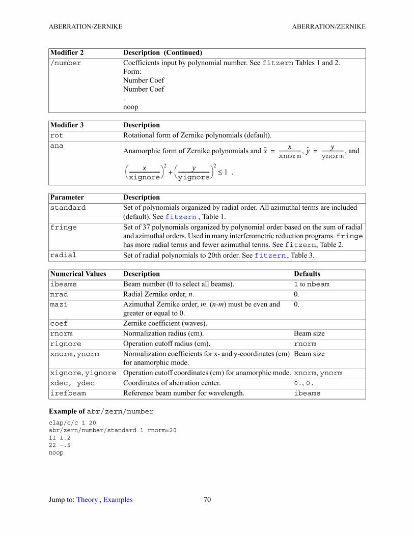
ABERRATION/ZERNIKE ABERRATION/ZERNIKE
Example of abr/zern/number clap/c/c 1 20abr/zern/number/standard 1 rnorm=2011 1.222 -.5noop
/number Coefficients input by polynomial number. See fitzern Tables 1 and 2.Form:Number CoefNumber Coef.noop
Modifier 3 Description rot Rotational form of Zernike polynomials (default).ana
Anamorphic form of Zernike polynomials and , , and
.
Parameter Description standard Set of polynomials organized by radial order. All azimuthal terms are included
(default). See , Table 1.fringe Set of 37 polynomials organized by polynomial order based on the sum of radial
and azimuthal orders. Used in many interferometric reduction programs. fringe has more radial terms and fewer azimuthal terms. See fitzern, Table 2.
radial Set of radial polynomials to 20th order. See , Table 3.
Numerical Values Description Defaultsibeams Beam number (0 to select all beams). 1 to nbeamnrad Radial Zernike order, n. 0.mazi Azimuthal Zernike order, m. (n-m) must be even and
greater or equal to 0. 0.
coef Zernike coefficient (waves).rnorm Normalization radius (cm). Beam sizerignore Operation cutoff radius (cm). rnorm
xnorm,ynorm Normalization coefficients for x- and y-coordinates (cm) for anamorphic mode.
Beam size
xignore, yignore Operation cutoff coordinates (cm) for anamorphic mode. xnorm, ynormxdec, ydec Coordinates of aberration center. 0., 0.irefbeam Reference beam number for wavelength. ibeams
Modifier 2 Description (Continued)
x xxnorm------------------= y y
ynorm------------------=
xxignore------------------------- 2 y
yignore------------------------- 2
+ 1≤
fitzern
fitzern
Jump to: , 70 Theory Examples
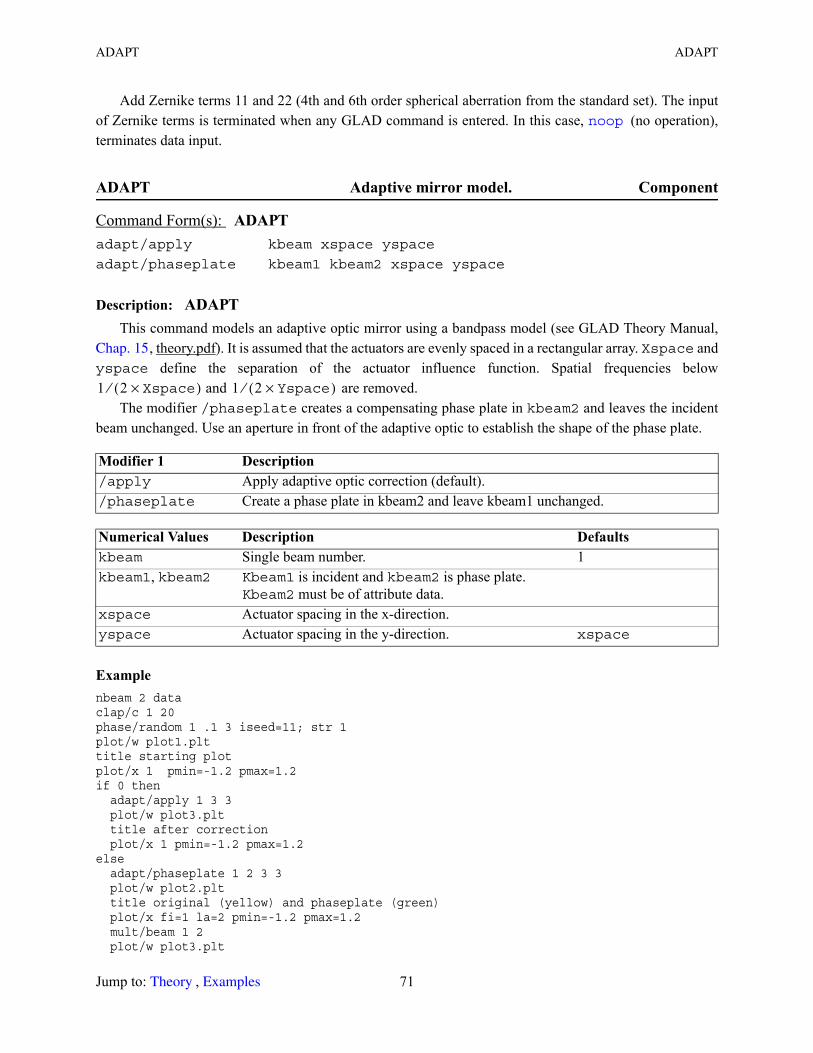
ADAPT ADAPT
Add Zernike terms 11 and 22 (4th and 6th order spherical aberration from the standard set). The input of Zernike terms is terminated when any GLAD command is entered. In this case, (no operation), terminates data input.
ADAPT Adaptive mirror model. Component
Description: ADAPTThis command models an adaptive optic mirror using a bandpass model (see GLAD Theory Manual,
, theory.pdf). It is assumed that the actuators are evenly spaced in a rectangular array. Xspace and yspace define the separation of the actuator influence function. Spatial frequencies below
and are removed.The modifier /phaseplate creates a compensating phase plate in kbeam2 and leaves the incident
beam unchanged. Use an aperture in front of the adaptive optic to establish the shape of the phase plate.
Examplenbeam 2 dataclap/c 1 20phase/random 1 .1 3 iseed=11; str 1plot/w plot1.plttitle starting plotplot/x 1 pmin=-1.2 pmax=1.2if 0 then adapt/apply 1 3 3 plot/w plot3.plt title after correction plot/x 1 pmin=-1.2 pmax=1.2else adapt/phaseplate 1 2 3 3 plot/w plot2.plt title original (yellow) and phaseplate (green) plot/x fi=1 la=2 pmin=-1.2 pmax=1.2 mult/beam 1 2 plot/w plot3.plt
Command Form(s): ADAPT adapt/apply kbeam xspace yspace
adapt/phaseplate kbeam1 kbeam2 xspace yspace
Modifier 1 Description /apply Apply adaptive optic correction (default). /phaseplate Create a phase plate in kbeam2 and leave kbeam1 unchanged.
Numerical Values Description Defaultskbeam Single beam number. 1kbeam1, kbeam2 Kbeam1 is incident and kbeam2 is phase plate.
Kbeam2 must be of attribute data.xspace Actuator spacing in the x-direction.yspace Actuator spacing in the y-direction. xspace
noop
Chap. 15
1 2 Xspace×( )⁄ 1 2 Yspace×( )⁄
Jump to: , 71 Theory Examples
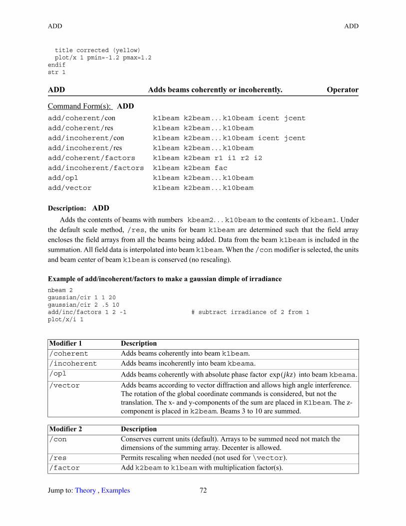
ADD ADD
title corrected (yellow) plot/x 1 pmin=-1.2 pmax=1.2endifstr 1
ADD Adds beams coherently or incoherently. Operator
Description: ADDAdds the contents of beams with numbers kbeam2. . . k10beam to the contents of kbeam1. Under
the default scale method, /res, the units for beam k1beam are determined such that the field array encloses the field arrays from all the beams being added. Data from the beam k1beam is included in the summation. All field data is interpolated into beam k1beam. When the /con modifier is selected, the units and beam center of beam k1beam is conserved (no rescaling).
Example of add/incoherent/factors to make a gaussian dimple of irradiancenbeam 2gaussian/cir 1 1 20gaussian/cir 2 .5 10add/inc/factors 1 2 -1 # subtract irradiance of 2 from 1plot/x/i 1
Command Form(s): ADD add/coherent/con k1beam k2beam . . . k10beam icent jcentadd/coherent/res k1beam k2beam . . . k10beamadd/incoherent/con k1beam k2beam . . . k10beam icent jcentadd/incoherent/res k1beam k2beam . . . k10beamadd/coherent/factors k1beam k2beam r1 i1 r2 i2
add/incoherent/factors k1beam k2beam fac
add/opl k1beam k2beam . . . k10beamadd/vector k1beam k2beam . . . k10beam
Modifier 1 Description /coherent Adds beams coherently into beam k1beam. /incoherent Adds beams incoherently into beam kbeama. /opl Adds beams coherently with absolute phase factor into beam kbeama./vector Adds beams according to vector diffraction and allows high angle interference.
The rotation of the global coordinate commands is considered, but not the translation. The x- and y-components of the sum are placed in K1beam. The z-component is placed in k2beam. Beams 3 to 10 are summed.
Modifier 2 Description /con Conserves current units (default). Arrays to be summed need not match the
dimensions of the summing array. Decenter is allowed./res Permits rescaling when needed (not used for \vector)./factor Add k2beam to k1beam with multiplication factor(s).
jkz( )exp
Jump to: , 72 Theory Examples
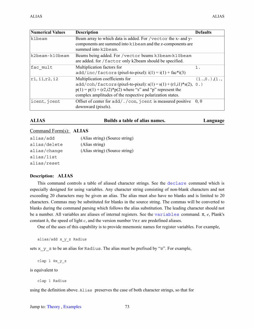
ALIAS ALIAS
ALIAS Builds a table of alias names. Language
Description: ALIASThis command controls a table of aliased character strings. See the command which is
especially designed for using variables. Any character string consisting of non-blank characters and not exceeding 20 characters may be given an alias. The alias must also have no blanks and is limited to 20 characters. Commas may be substituted for blanks in the source string. The commas will be converted to blanks during the command parsing which follows the alias substitution. The leading character should not be a number. All variables are aliases of internal registers. See the command. π, e, Plank's constant h, the speed of light c, and the version number Ver are predefined aliases.
One of the uses of this capability is to provide mnemonic names for register variables. For example,
alias/add x_y_z Radius
sets x_y_z to be an alias for Radius. The alias must be prefixed by “@”. For example,
clap 1 @x_y_z
is equivalent to
clap 1 Radius
using the definition above. Alias preserves the case of both character strings, so that for
Numerical Values Description Defaultsk1beam Beam array to which data is added. For /vector the x- and y-
components are summed into k1beam and the z-components are summed into k2beam.
k2beam-k10beam Beams being added. For /vector beams k3beam-k10beam are added. for /factor only k2beam should be specified.
fac_mult Multiplication factors for add/inc/factors (pixel-to-pixel): i(1) = i(1) + fac*i(3)
1.
r1, i1,r2, i2 Multiplication coefficients foradd/coh/factors (pixel-to-pixel): s(1) = s(1) + (r1,i1)*s(2), p(1) = p(1) + (r2,i2)*p(2) where “s” and “p” represent the complex amplitudes of the respective polarization states.
(1.,0.),(1.,0.)
icent, jcent Offset of center for add/./con, jcent is measured positive downward (pixels).
0, 0
Command Form(s): ALIAS alias/add (Alias string) (Source string)alias/delete (Alias string)alias/change (Alias string) (Source string)alias/list
alias/reset
declare
variables
Jump to: , 73 Theory Examples
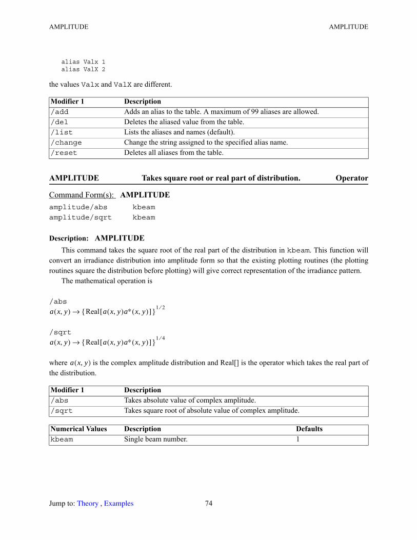
AMPLITUDE AMPLITUDE
alias Valx 1alias ValX 2
the values Valx and ValX are different.
AMPLITUDE Takes square root or real part of distribution. Operator
Description: AMPLITUDEThis command takes the square root of the real part of the distribution in kbeam. This function will
convert an irradiance distribution into amplitude form so that the existing plotting routines (the plotting routines square the distribution before plotting) will give correct representation of the irradiance pattern.
The mathematical operation is
/abs
/sqrt
where is the complex amplitude distribution and Real[] is the operator which takes the real part of the distribution.
Modifier 1 Description /add Adds an alias to the table. A maximum of 99 aliases are allowed./del Deletes the aliased value from the table./list Lists the aliases and names (default)./change Change the string assigned to the specified alias name./reset Deletes all aliases from the table.
Command Form(s): AMPLITUDE amplitude/abs kbeam
amplitude/sqrt kbeam
Modifier 1 Description /abs Takes absolute value of complex amplitude. /sqrt Takes square root of absolute value of complex amplitude.
Numerical Values Description Defaultskbeam Single beam number. 1
a x y,( ) Real a x y,( )a∗ x y,( )[ ]{ }1 2⁄→
a x y,( ) Real a x y,( )a∗ x y,( )[ ]{ }1 4⁄→
a x y,( )
Jump to: , 74 Theory Examples
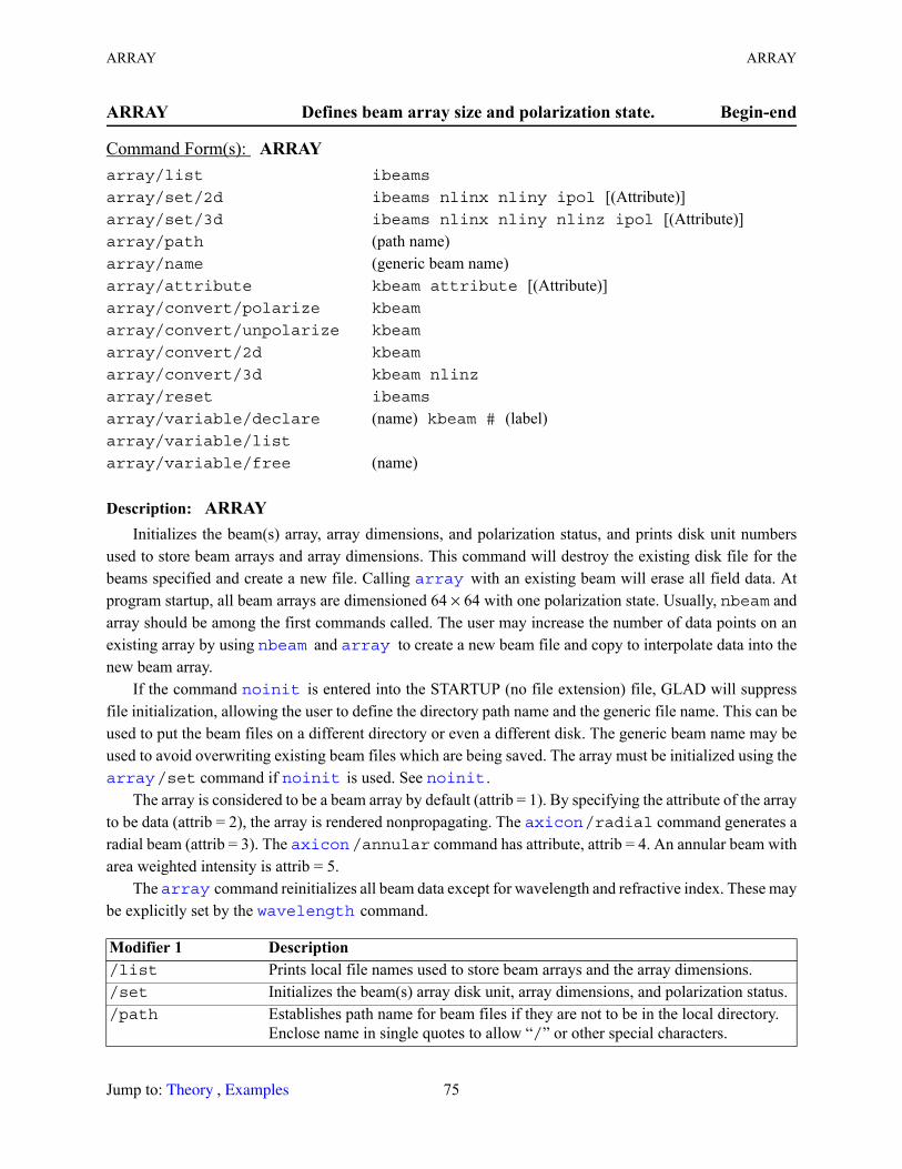
ARRAY ARRAY
ARRAY Defines beam array size and polarization state. Begin-end
Description: ARRAYInitializes the beam(s) array, array dimensions, and polarization status, and prints disk unit numbers
used to store beam arrays and array dimensions. This command will destroy the existing disk file for the beams specified and create a new file. Calling with an existing beam will erase all field data. At program startup, all beam arrays are dimensioned 64 × 64 with one polarization state. Usually, nbeam and array should be among the first commands called. The user may increase the number of data points on an existing array by using and to create a new beam file and copy to interpolate data into the new beam array.
If the command is entered into the STARTUP (no file extension) file, GLAD will suppress file initialization, allowing the user to define the directory path name and the generic file name. This can be used to put the beam files on a different directory or even a different disk. The generic beam name may be used to avoid overwriting existing beam files which are being saved. The array must be initialized using the
/set command if is used. See .The array is considered to be a beam array by default (attrib = 1). By specifying the attribute of the array
to be data (attrib = 2), the array is rendered nonpropagating. The /radial command generates a radial beam (attrib = 3). The /annular command has attribute, attrib = 4. An annular beam with area weighted intensity is attrib = 5.
The command reinitializes all beam data except for wavelength and refractive index. These may be explicitly set by the command.
Command Form(s): ARRAY array/list ibeams
array/set/2d ibeams nlinx nliny ipol [(Attribute)]array/set/3d ibeams nlinx nliny nlinz ipol [(Attribute)]array/path (path name) array/name (generic beam name) array/attribute kbeam attribute [(Attribute)]array/convert/polarize kbeam
array/convert/unpolarize kbeam
array/convert/2d kbeam
array/convert/3d kbeam nlinz
array/reset ibeams
array/variable/declare (name) kbeam # (label)array/variable/list
array/variable/free (name)
Modifier 1 Description /list Prints local file names used to store beam arrays and the array dimensions./set Initializes the beam(s) array disk unit, array dimensions, and polarization status./path Establishes path name for beam files if they are not to be in the local directory.
Enclose name in single quotes to allow “/” or other special characters.
array
nbeam array
noinit
array noinit noinit
axicon axicon
array wavelength
Jump to: , 75 Theory Examples
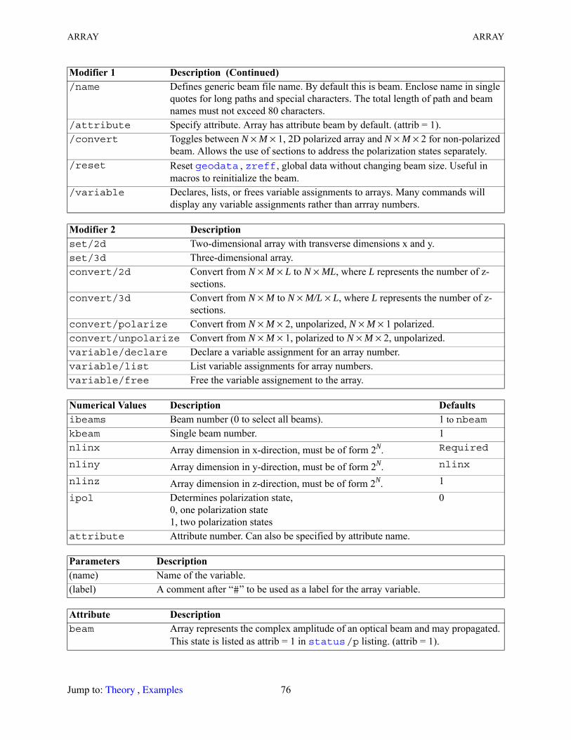
ARRAY ARRAY
/name Defines generic beam file name. By default this is beam. Enclose name in single quotes for long paths and special characters. The total length of path and beam names must not exceed 80 characters.
/attribute Specify attribute. Array has attribute beam by default. (attrib = 1)./convert Toggles between N × M × 1, 2D polarized array and N × M × 2 for non-polarized
beam. Allows the use of sections to address the polarization states separately./reset Reset , , global data without changing beam size. Useful in
macros to reinitialize the beam./variable Declares, lists, or frees variable assignments to arrays. Many commands will
display any variable assignments rather than arrray numbers.
Modifier 2 Description set/2d Two-dimensional array with transverse dimensions x and y.set/3d Three-dimensional array.convert/2d Convert from N × M × L to N × ML, where L represents the number of z-
sections.convert/3d Convert from N × M to N × M/L × L, where L represents the number of z-
sections.convert/polarize Convert from N × M × 2, unpolarized, N × M × 1 polarized. convert/unpolarize Convert from N × M × 1, polarized to N × M × 2, unpolarized. variable/declare Declare a variable assignment for an array number.variable/list List variable assignments for array numbers.variable/free Free the variable assignement to the array.
Numerical Values Description Defaultsibeams Beam number (0 to select all beams). 1 to nbeamkbeam Single beam number. 1nlinx Array dimension in x-direction, must be of form 2N. Required
nliny Array dimension in y-direction, must be of form 2N. nlinx
nlinz Array dimension in z-direction, must be of form 2N. 1ipol Determines polarization state,
0, one polarization state1, two polarization states
0
attribute Attribute number. Can also be specified by attribute name.
Parameters Description (name) Name of the variable.(label) A comment after “#” to be used as a label for the array variable.
Attribute Description beam Array represents the complex amplitude of an optical beam and may propagated.
This state is listed as attrib = 1 in /p listing. (attrib = 1).
Modifier 1 Description (Continued)
geodata zreff
status
Jump to: , 76 Theory Examples
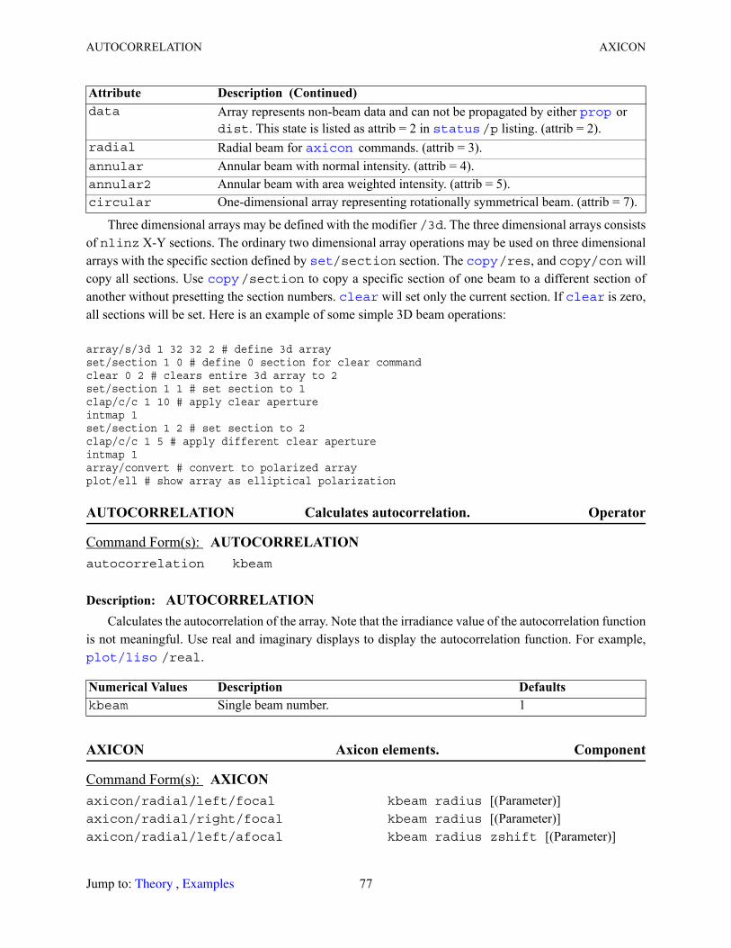
AUTOCORRELATION AXICON
Three dimensional arrays may be defined with the modifier /3d. The three dimensional arrays consists of nlinz X-Y sections. The ordinary two dimensional array operations may be used on three dimensional arrays with the specific section defined by /section section. The /res, and copy/con will copy all sections. Use /section to copy a specific section of one beam to a different section of another without presetting the section numbers. will set only the current section. If is zero, all sections will be set. Here is an example of some simple 3D beam operations:
array/s/3d 1 32 32 2 # define 3d arrayset/section 1 0 # define 0 section for clear commandclear 0 2 # clears entire 3d array to 2set/section 1 1 # set section to 1clap/c/c 1 10 # apply clear apertureintmap 1set/section 1 2 # set section to 2clap/c/c 1 5 # apply different clear apertureintmap 1array/convert # convert to polarized arrayplot/ell # show array as elliptical polarization
AUTOCORRELATION Calculates autocorrelation. Operator
Description: AUTOCORRELATIONCalculates the autocorrelation of the array. Note that the irradiance value of the autocorrelation function
is not meaningful. Use real and imaginary displays to display the autocorrelation function. For example, /real.
AXICON Axicon elements. Component
data Array represents non-beam data and can not be propagated by either or dist. This state is listed as attrib = 2 in /p listing. (attrib = 2).
radial Radial beam for commands. (attrib = 3).annular Annular beam with normal intensity. (attrib = 4).annular2 Annular beam with area weighted intensity. (attrib = 5).circular One-dimensional array representing rotationally symmetrical beam. (attrib = 7).
Command Form(s): AUTOCORRELATION autocorrelation kbeam
Numerical Values Description Defaultskbeam Single beam number. 1
Command Form(s): AXICON axicon/radial/left/focal kbeam radius [(Parameter)]axicon/radial/right/focal kbeam radius [(Parameter)]axicon/radial/left/afocal kbeam radius zshift [(Parameter)]
Attribute Description (Continued) prop
status axicon
set copy copy
clear clear
plot/liso
Jump to: , 77 Theory Examples
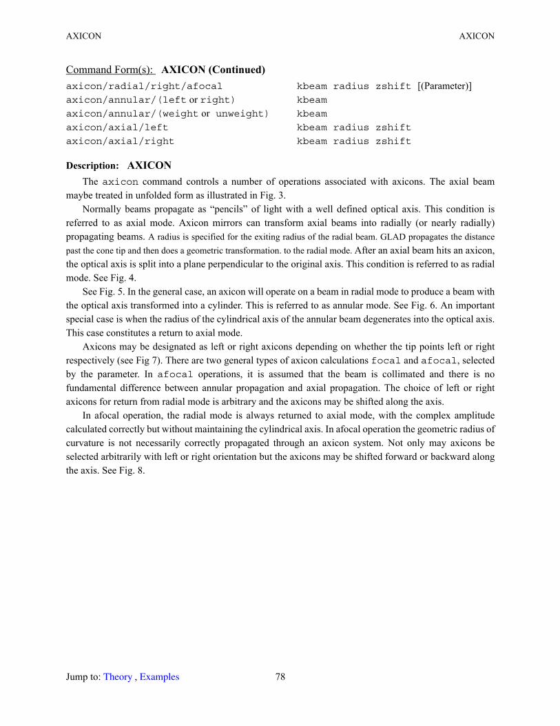
AXICON AXICON
Description: AXICONThe axicon command controls a number of operations associated with axicons. The axial beam
maybe treated in unfolded form as illustrated in Fig. 3. Normally beams propagate as “pencils” of light with a well defined optical axis. This condition is
referred to as axial mode. Axicon mirrors can transform axial beams into radially (or nearly radially) propagating beams. A radius is specified for the exiting radius of the radial beam. GLAD propagates the distance past the cone tip and then does a geometric transformation. to the radial mode. After an axial beam hits an axicon, the optical axis is split into a plane perpendicular to the original axis. This condition is referred to as radial mode. See Fig. 4.
See Fig. 5. In the general case, an axicon will operate on a beam in radial mode to produce a beam with the optical axis transformed into a cylinder. This is referred to as annular mode. See Fig. 6. An important special case is when the radius of the cylindrical axis of the annular beam degenerates into the optical axis. This case constitutes a return to axial mode.
Axicons may be designated as left or right axicons depending on whether the tip points left or right respectively (see Fig 7). There are two general types of axicon calculations focal and afocal, selected by the parameter. In afocal operations, it is assumed that the beam is collimated and there is no fundamental difference between annular propagation and axial propagation. The choice of left or right axicons for return from radial mode is arbitrary and the axicons may be shifted along the axis.
In afocal operation, the radial mode is always returned to axial mode, with the complex amplitude calculated correctly but without maintaining the cylindrical axis. In afocal operation the geometric radius of curvature is not necessarily correctly propagated through an axicon system. Not only may axicons be selected arbitrarily with left or right orientation but the axicons may be shifted forward or backward along the axis. See Fig. 8.
axicon/radial/right/afocal kbeam radius zshift [(Parameter)]axicon/annular/(left or right) kbeam
axicon/annular/(weight or unweight) kbeam
axicon/axial/left kbeam radius zshift
axicon/axial/right kbeam radius zshift
Command Form(s): AXICON (Continued)
Jump to: , 78 Theory Examples
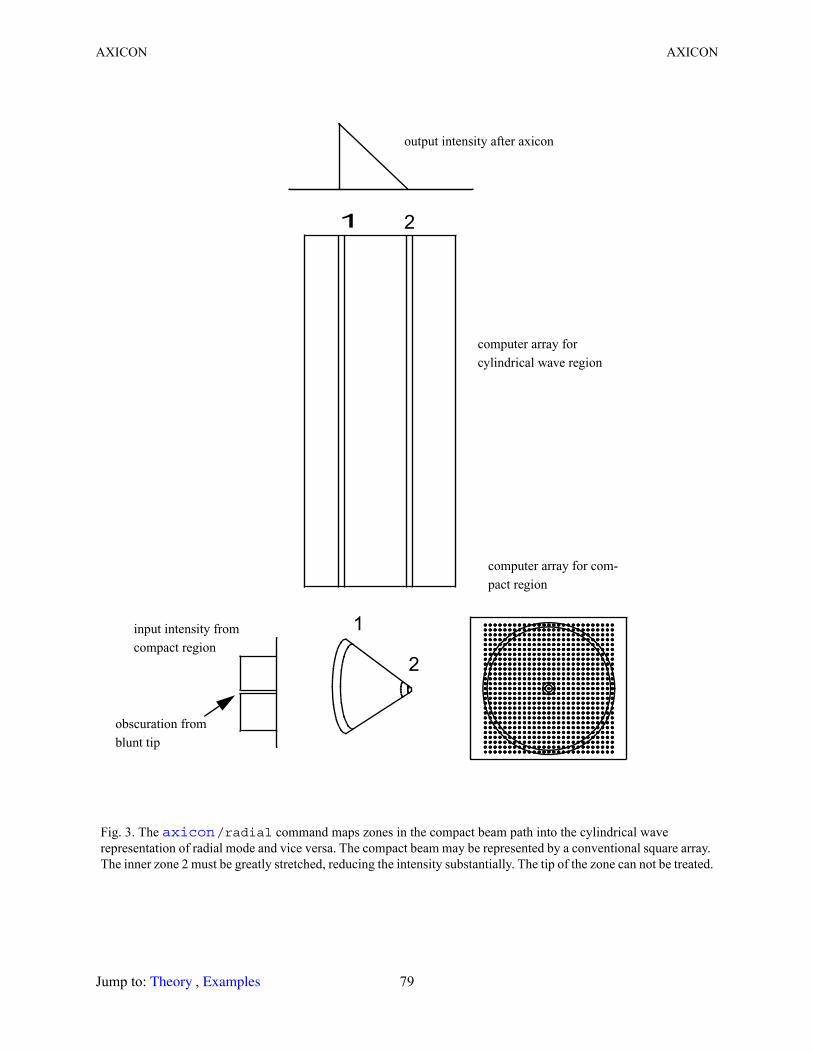
AXICON AXICON
Fig. 3. The /radial command maps zones in the compact beam path into the cylindrical wave representation of radial mode and vice versa. The compact beam may be represented by a conventional square array. The inner zone 2 must be greatly stretched, reducing the intensity substantially. The tip of the zone can not be treated.
� �
�
�
obscuration from blunt tip
input intensity from compact region
computer array for com-pact region
computer array for cylindrical wave region
output intensity after axicon
axicon
Jump to: , 79 Theory Examples
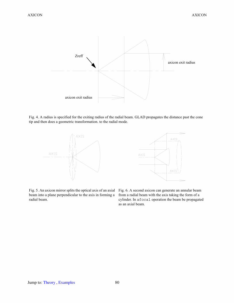
AXICON AXICON
Fig. 4. A radius is specified for the exiting radius of the radial beam. GLAD propagates the distance past the cone tip and then does a geometric transformation. to the radial mode.
Fig. 5. An axicon mirror splits the optical axis of an axial beam into a plane perpendicular to the axis in forming a radial beam.
Fig. 6. A second axicon can generate an annular beam from a radial beam with the axis taking the form of a cylinder. In afocal operation the beam be propagated as an axial beam.
axicon exit radius
axicon exit radius
Zreff
Jump to: , 80 Theory Examples

AXICON AXICON
Fig. 7. Axicon mirrors are divided into left and right forms depending on which way the apex points. GLAD locates the axicon at with the apex at the current Zreff position.
Fig. 8. The position of the optical axis in radial mode is established at the apex of Cone 1 (unless zshift is specified). Cone 2, to return from radial mode, may also be shifted. Zshift applies only to afocal operation.
right coneleft cone
shift
cone 1
cone 2
Jump to: , 81 Theory Examples
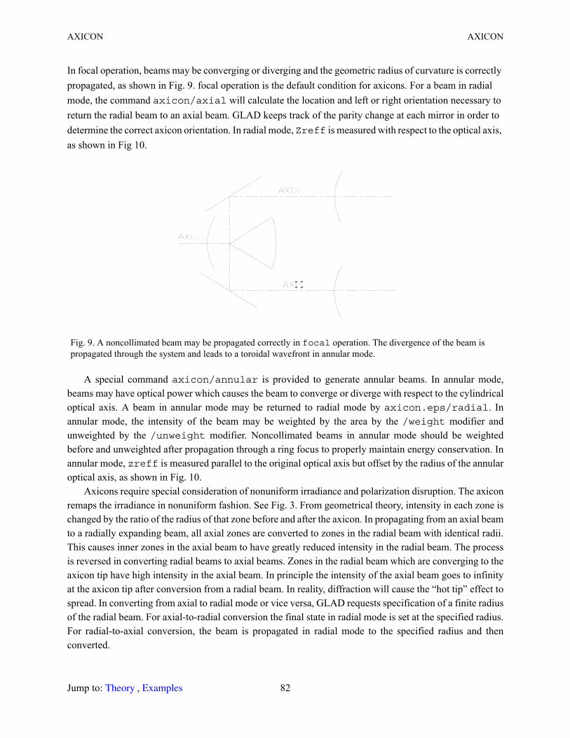
AXICON AXICON
In focal operation, beams may be converging or diverging and the geometric radius of curvature is correctly propagated, as shown in Fig. 9. focal operation is the default condition for axicons. For a beam in radial mode, the command axicon/axial will calculate the location and left or right orientation necessary to return the radial beam to an axial beam. GLAD keeps track of the parity change at each mirror in order to determine the correct axicon orientation. In radial mode, Zreff is measured with respect to the optical axis, as shown in Fig 10.
A special command axicon/annular is provided to generate annular beams. In annular mode, beams may have optical power which causes the beam to converge or diverge with respect to the cylindrical optical axis. A beam in annular mode may be returned to radial mode by axicon.eps/radial. In annular mode, the intensity of the beam may be weighted by the area by the /weight modifier and unweighted by the /unweight modifier. Noncollimated beams in annular mode should be weighted before and unweighted after propagation through a ring focus to properly maintain energy conservation. In annular mode, zreff is measured parallel to the original optical axis but offset by the radius of the annular optical axis, as shown in Fig. 10.
Axicons require special consideration of nonuniform irradiance and polarization disruption. The axicon remaps the irradiance in nonuniform fashion. See Fig. 3. From geometrical theory, intensity in each zone is changed by the ratio of the radius of that zone before and after the axicon. In propagating from an axial beam to a radially expanding beam, all axial zones are converted to zones in the radial beam with identical radii. This causes inner zones in the axial beam to have greatly reduced intensity in the radial beam. The process is reversed in converting radial beams to axial beams. Zones in the radial beam which are converging to the axicon tip have high intensity in the axial beam. In principle the intensity of the axial beam goes to infinity at the axicon tip after conversion from a radial beam. In reality, diffraction will cause the “hot tip” effect to spread. In converting from axial to radial mode or vice versa, GLAD requests specification of a finite radius of the radial beam. For axial-to-radial conversion the final state in radial mode is set at the specified radius. For radial-to-axial conversion, the beam is propagated in radial mode to the specified radius and then converted.
Fig. 9. A noncollimated beam may be propagated correctly in focal operation. The divergence of the beam is propagated through the system and leads to a toroidal wavefront in annular mode.
Jump to: , 82 Theory Examples
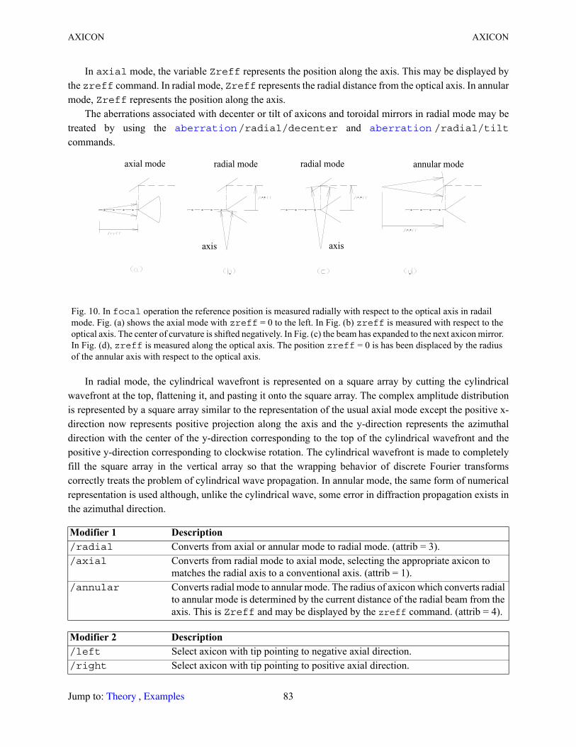
AXICON AXICON
In axial mode, the variable Zreff represents the position along the axis. This may be displayed by the zreff command. In radial mode, Zreff represents the radial distance from the optical axis. In annular mode, Zreff represents the position along the axis.
The aberrations associated with decenter or tilt of axicons and toroidal mirrors in radial mode may be treated by using the /radial/decenter and /radial/tilt
commands.
In radial mode, the cylindrical wavefront is represented on a square array by cutting the cylindrical wavefront at the top, flattening it, and pasting it onto the square array. The complex amplitude distribution is represented by a square array similar to the representation of the usual axial mode except the positive x-direction now represents positive projection along the axis and the y-direction represents the azimuthal direction with the center of the y-direction corresponding to the top of the cylindrical wavefront and the positive y-direction corresponding to clockwise rotation. The cylindrical wavefront is made to completely fill the square array in the vertical array so that the wrapping behavior of discrete Fourier transforms correctly treats the problem of cylindrical wave propagation. In annular mode, the same form of numerical representation is used although, unlike the cylindrical wave, some error in diffraction propagation exists in the azimuthal direction.
Fig. 10. In focal operation the reference position is measured radially with respect to the optical axis in radail mode. Fig. (a) shows the axial mode with zreff = 0 to the left. In Fig. (b) zreff is measured with respect to the optical axis. The center of curvature is shifted negatively. In Fig. (c) the beam has expanded to the next axicon mirror. In Fig. (d), zreff is measured along the optical axis. The position zreff = 0 is has been displaced by the radius of the annular axis with respect to the optical axis.
Modifier 1 Description /radial Converts from axial or annular mode to radial mode. (attrib = 3)./axial Converts from radial mode to axial mode, selecting the appropriate axicon to
matches the radial axis to a conventional axis. (attrib = 1)./annular Converts radial mode to annular mode. The radius of axicon which converts radial
to annular mode is determined by the current distance of the radial beam from the axis. This is Zreff and may be displayed by the zreff command. (attrib = 4).
Modifier 2 Description /left Select axicon with tip pointing to negative axial direction. /right Select axicon with tip pointing to positive axial direction.
aberration aberration
axial mode
axisaxis
radial mode radial mode annular mode
Jump to: , 83 Theory Examples

BANNER BEAMS
BANNER Displays start up banner. Language
Description: BANNERDisplayes the start up banner.
BEAMS Turns on/off beams for propagation commands. Propagation
/weight Weight the intensity in annular mode by the area of the annular zone. (attrib = 5)./unweight Restore unweighted intensity. (attrib = 4).
Modifier 3 Description focal Beam may be noncollimated and geometric radii are preserved (default). Beam
may be returned to axial mode only by using /axial and letting GLAD select the correct axicon orientation and position to properly convert the radial axis to a simple line axis.
afocal Assumes beam is collimated and does not preserve geometric radii. Beam may be restored to axial mode by any second axicon.
Numerical Values Description Defaultsibeam Beam number (0 to select all beams). 1 to nbeamradius The exit radius in radial mode to end axicon conversion
for /radial or to begin axicon conversion for /axial.
zshift Translation of the axicon along the axis for afocal operation.
Parameter Description mirror Implements the axicon including the effects of a mirror (default).nomirror Implements the axicon except that the mirror reflection is not included.
Command Form(s): BANNER banner
Command Form(s): BEAMS beams/list ibeams
beams/all/on
beams/all/off
beams/on k1 . . . knbeams/off k1 . . . kn
Modifier 2 Description (Continued)
axicon
axicon axicon
Jump to: , 84 Theory Examples
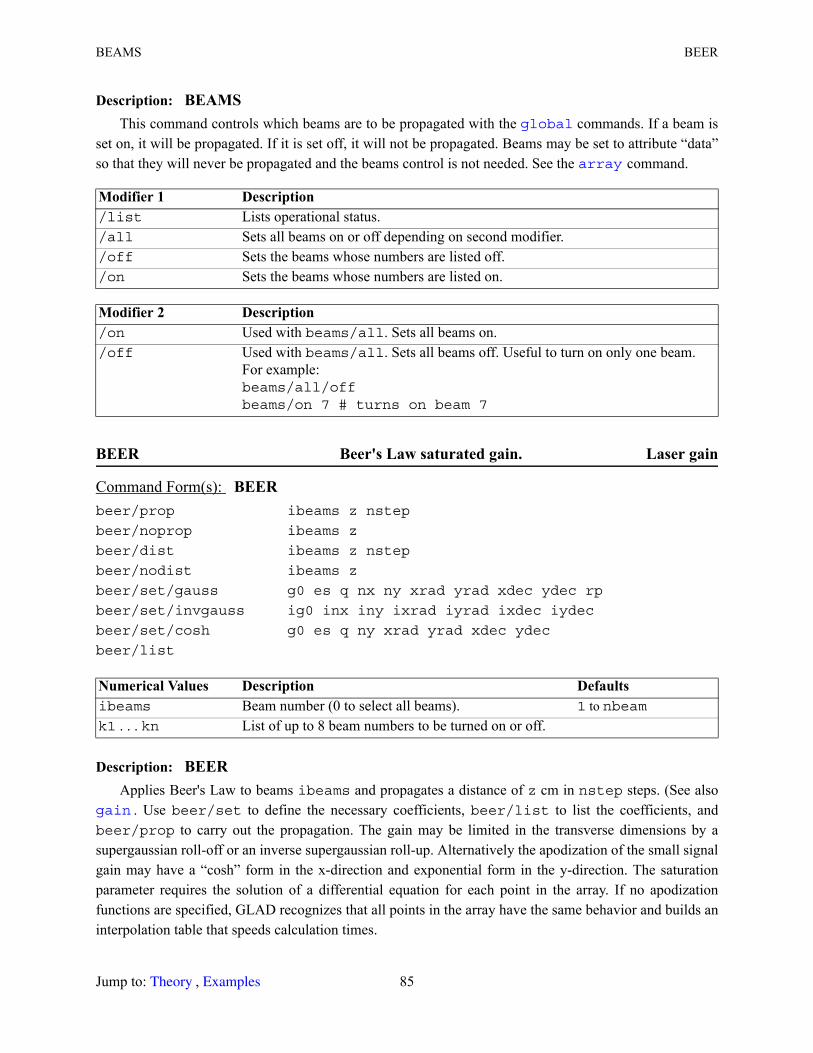
BEAMS BEER
Description: BEAMSThis command controls which beams are to be propagated with the commands. If a beam is
set on, it will be propagated. If it is set off, it will not be propagated. Beams may be set to attribute “data” so that they will never be propagated and the beams control is not needed. See the command.
BEER Beer's Law saturated gain. Laser gain
Description: BEERApplies Beer's Law to beams ibeams and propagates a distance of z cm in nstep steps. (See also
. Use beer/set to define the necessary coefficients, beer/list to list the coefficients, and beer/prop to carry out the propagation. The gain may be limited in the transverse dimensions by a supergaussian roll-off or an inverse supergaussian roll-up. Alternatively the apodization of the small signal gain may have a “cosh” form in the x-direction and exponential form in the y-direction. The saturation parameter requires the solution of a differential equation for each point in the array. If no apodization functions are specified, GLAD recognizes that all points in the array have the same behavior and builds an interpolation table that speeds calculation times.
Modifier 1 Description /list Lists operational status./all Sets all beams on or off depending on second modifier./off Sets the beams whose numbers are listed off./on Sets the beams whose numbers are listed on.
Modifier 2 Description /on Used with beams/all. Sets all beams on./off Used with beams/all. Sets all beams off. Useful to turn on only one beam.
For example:beams/all/offbeams/on 7 # turns on beam 7
Numerical Values Description Defaultsibeams Beam number (0 to select all beams). 1 to nbeamk1 . . . kn List of up to 8 beam numbers to be turned on or off.
Command Form(s): BEER beer/prop ibeams z nstep
beer/noprop ibeams z
beer/dist ibeams z nstep
beer/nodist ibeams z
beer/set/gauss g0 es q nx ny xrad yrad xdec ydec rp
beer/set/invgauss ig0 inx iny ixrad iyrad ixdec iydec
beer/set/cosh g0 es q ny xrad yrad xdec ydec
beer/list
global
array
gain
Jump to: , 85 Theory Examples
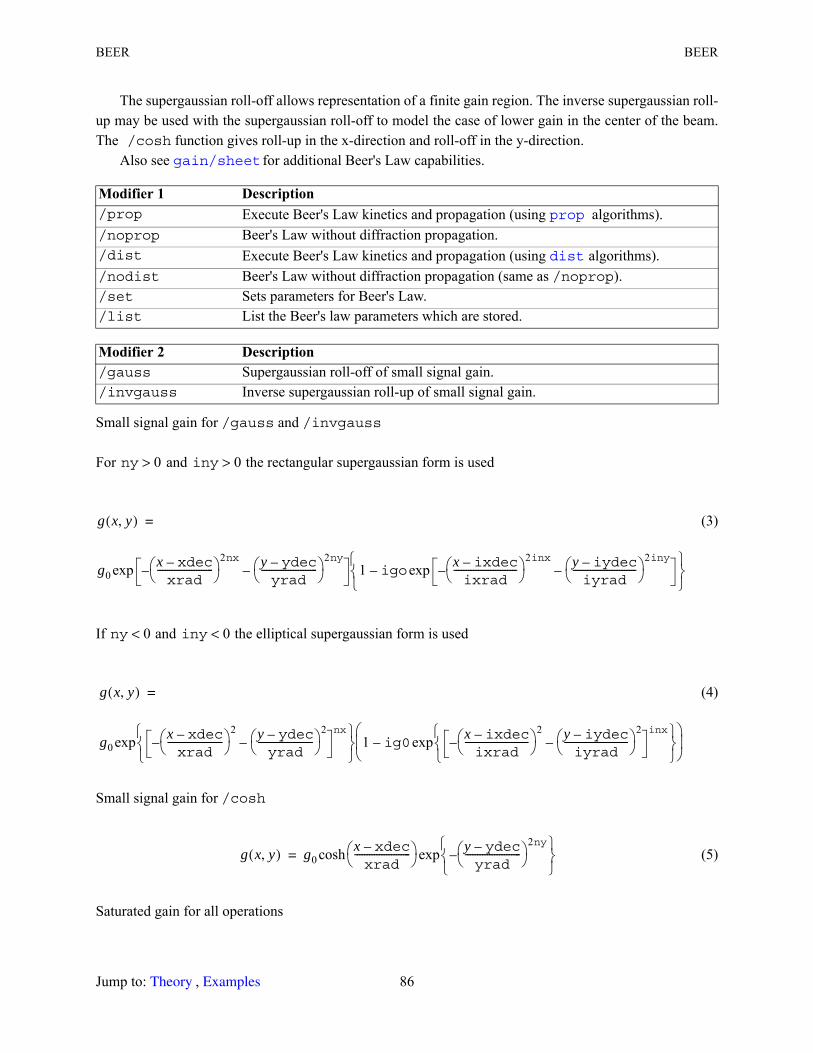
BEER BEER
The supergaussian roll-off allows representation of a finite gain region. The inverse supergaussian roll-up may be used with the supergaussian roll-off to model the case of lower gain in the center of the beam. The /cosh function gives roll-up in the x-direction and roll-off in the y-direction.
Also see for additional Beer's Law capabilities.
Small signal gain for /gauss and /invgauss
For and the rectangular supergaussian form is used
(3)
If and the elliptical supergaussian form is used
(4)
Small signal gain for /cosh
(5)
Saturated gain for all operations
Modifier 1 Description /prop Execute Beer's Law kinetics and propagation (using algorithms)./noprop Beer's Law without diffraction propagation./dist Execute Beer's Law kinetics and propagation (using algorithms)./nodist Beer's Law without diffraction propagation (same as /noprop)./set Sets parameters for Beer's Law./list List the Beer's law parameters which are stored.
Modifier 2 Description /gauss Supergaussian roll-off of small signal gain./invgauss Inverse supergaussian roll-up of small signal gain.
gain/sheet
prop
dist
ny 0> iny 0>
g x y,( )
g0x xdec–xrad
----------------------- –
2nx y ydec–yrad
----------------------- 2ny
–exp 1 igox ixdec–ixrad
-------------------------- –
2inx y iydec–iyrad
-------------------------- 2iny
–exp–
=
ny 0< iny 0<
g x y,( )
g0x xdec–xrad
----------------------- –
2 y ydec–yrad
----------------------- 2
–nx
exp 1 ig0x ixdec–ixrad
-------------------------- –
2 y iydec–iyrad
-------------------------- 2
–inx
exp–
=
g x y,( ) g0x xdec–xrad
----------------------- cosh y ydec–
yrad----------------------- –
2ny
exp=
Jump to: , 86 Theory Examples
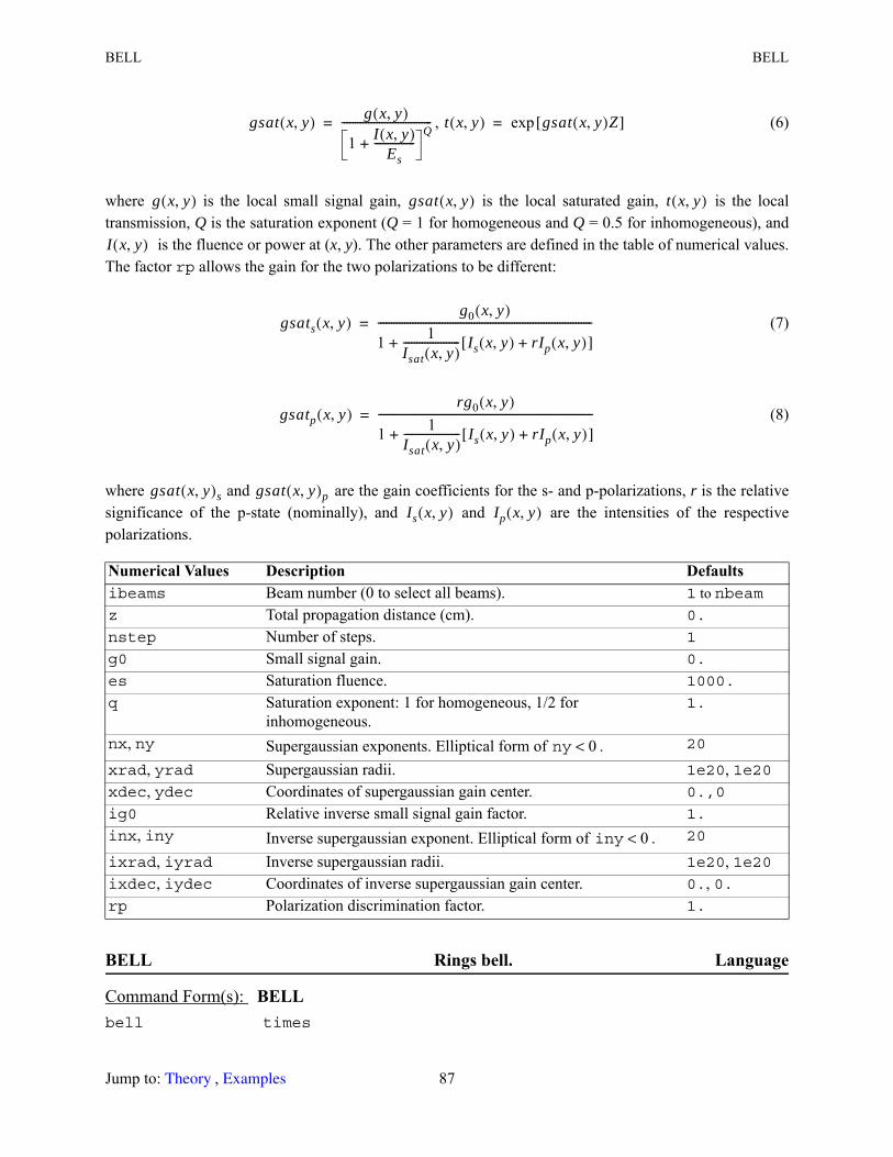
BELL BELL
, (6)
where is the local small signal gain, is the local saturated gain, is the local transmission, Q is the saturation exponent (Q = 1 for homogeneous and Q = 0.5 for inhomogeneous), and
is the fluence or power at (x, y). The other parameters are defined in the table of numerical values. The factor rp allows the gain for the two polarizations to be different:
(7)
(8)
where and are the gain coefficients for the s- and p-polarizations, r is the relative significance of the p-state (nominally), and and are the intensities of the respective polarizations.
BELL Rings bell. Language
Numerical Values Description Defaultsibeams Beam number (0 to select all beams). 1 to nbeamz Total propagation distance (cm). 0.
nstep Number of steps. 1
g0 Small signal gain. 0.
es Saturation fluence. 1000.
q Saturation exponent: 1 for homogeneous, 1/2 for inhomogeneous.
1.
nx, ny Supergaussian exponents. Elliptical form of . 20
xrad, yrad Supergaussian radii. 1e20, 1e20xdec, ydec Coordinates of supergaussian gain center. 0.,0
ig0 Relative inverse small signal gain factor. 1.
inx, iny Inverse supergaussian exponent. Elliptical form of . 20
ixrad, iyrad Inverse supergaussian radii. 1e20, 1e20ixdec, iydec Coordinates of inverse supergaussian gain center. 0., 0.rp Polarization discrimination factor. 1.
Command Form(s): BELL bell times
gsat x y,( ) g x y,( )
1 I x y,( )Es
---------------+Q
----------------------------------= t x y,( ) gsat x y,( )Z[ ]exp=
g x y,( ) gsat x y,( ) t x y,( )
I x y,( )
gsats x y,( )g0 x y,( )
1 1Isat x y,( )--------------------- Is x y,( ) rIp x y,( )+[ ]+
--------------------------------------------------------------------------------=
gsatp x y,( )rg0 x y,( )
1 1Isat x y,( )--------------------- Is x y,( ) rIp x y,( )+[ ]+
--------------------------------------------------------------------------------=
gsat x y,( )s gsat x y,( )pIs x y,( ) Ip x y,( )
ny 0<
iny 0<
Jump to: , 87 Theory Examples
BELL BINARY
Description: BELLRings bell on computer specified number of times.
BINARY Binary optics. Component
Description: BINARYThis command implements binary gratings and lenses. The binary surface may be constructed with the
/surface modifier or implemented directly as a phase screen. The binary surface may be implemented later as a phase screen with the , int2waves, or command. The binary surface may be plotted as irradiance.
Numerical Values Description Defaultstimes Number of times to ring bell. 1
Command Form(s): BINARY binary/grating/surface kbeam period level nlevels azdeg phase
binary/grating/phasescreen ibeams rindex period level nlevels azdeg phase
binary/lens/surface kbeam xrad yrad level nlevels
binary/lens/phasescreen ibeams rindex xrad yrad level nlevels
binary/lens/residual ibeams rindex xrad yrad level nlevels
binary/surface kbeam level nlevels
Modifier 1 Description /grating Binary linear grating./lens Binary lens./surface Form binary optic from current irradiance distribution. See Fig. 11.
Modifier 2 Description /surface Creates a surface array containing the surface profile. Use to
implement the surface function as a phase screen./phasescreen Implements the binary optic directly into the array(s) (default for grating)./residual Implements a binary lens with the basic phase radius of curvature treated as a
standard lens plus residuals. This enables the binary optic to be incorporated with the standard propagation control algorithms (default for lens).
Numerical Values Description Defaultsibeams Beam number (0 to select all beams). 1 to nbeamkbeam Single beam number. 1
rindex Index of refraction for /phasescreen or /residual. 1
period Period of the grating.xrad, yrad Radii of curvature for lens. 1e20, xradlevel Height of the surface profile (asymptotic).nlevels Number of sublevels per major level.
int2phase sfocus
int2phase
Jump to: , 88 Theory Examples

BLOOM BLOOM
BLOOM Atmospheric thermal blooming. Aberration
Description: BLOOMBloom is the general thermal blooming command. Parameters may be set by bloom/set and listed
by bloom/list. The GLAD feature set is required. The propagation including blooming phase errors, fitting of tilt and focus errors, and diffraction propagation is accomplished by . Target parameters are set by the command.
azdeg Azimuth angle in degrees, counter-clockwise from vertical. 90
phase Phase shift (degrees) of grating per period. 0.
Fig. 11. A surface divided into major levels of thickness and into 8 sublevels to create a binary optic. The major levels, of height L, may be subtracted without optical effect at wavelength λ, i.e., by removing the hatched areas. The sublevels produce some diffractive loss into high angle scattering. Note that the maximum height of the binary optic is , where N is the number of sublevels. The mathematical description of the binary optic surface is , optical phase induced = where is the least integer function (rounds down to next integer value).
Command Form(s): BLOOM
bloom/list
Numerical Values Description (Continued) Defaults
s x y,( )
λn 1–------------
λn 1–------------
binary optics equivalent
λ n 1–( )⁄( )
N 1–( ) N⁄[ ] λ n 1–( )⁄[ ]S′ x y,( ) L N⁄( )mod Ns x y,( )( ) L⁄( ) N 1 N⁄( ) Ns x y,( )( ) L⁄( )[ ]– N,{ }=
2π( ) λ⁄( ) n 1–( )S′ x y,( )
bloom/set
bloom/altitude bloom/prop
bloom/set target
Jump to: , 89 Theory Examples
BLOOM/ALTITUDE BLOOM/PROP
To set the parameter, call before calling any other bloom commands.
BLOOM/ALTITUDE Sets altitude information for BLOOM. Aberration
Description: BLOOM/ALTITIDEThis routine establishes values for the atmosphere based on the U.S. Standard Atmosphere and on
absorption values based on published data by Woods, et. al. Values set are temperature, relative pressure, relative temperature, density, heat conductivity, and absorption of CO2, H2O and aerosols.
References1. Frank J. Regan, An Atmosphere Model, ACCESS Vol. 6, No. 6, p33 (1987), author may be reached
at Naval Surface Weapons Center, White Oak Laboratory, Silver Spring, Maryland 20903-5000.
2. U.S. Standard Atmosphere 1976, National Oceanographic and Atmospheric Administration, Washington D.C. (1976).
3. A.D. Woods, M. Camac and E.T. Gerry, Appl. Opt., Vol 10 p1877 (1971).
BLOOM/PROP Propagate with thermal blooming. Aberration
Modifier 1 Description /set Set boom parameters./list List bloom parameters./altitude Define altitude./prop Implement propagation with thermal blooming.
Command Form(s): BLOOM/ALTITUDE bloom/altitude/set height
bloom/altitude/list
Modifier 1 Description /set Define and store Beer's law parameters./list List parameters.
Numerical Values Description Defaultsheight Height in the atmosphere (km). 1.
Command Form(s): BLOOM/PROP bloom/prop/xy/(modifier 3) ibeams z nstep relwind
bloom/prop/xonly/(modifier 3) ibeams z nstep
bloom/prop/fft/(modifier 3 ibeams z nstep
bloom/set
Jump to: , 90 Theory Examples
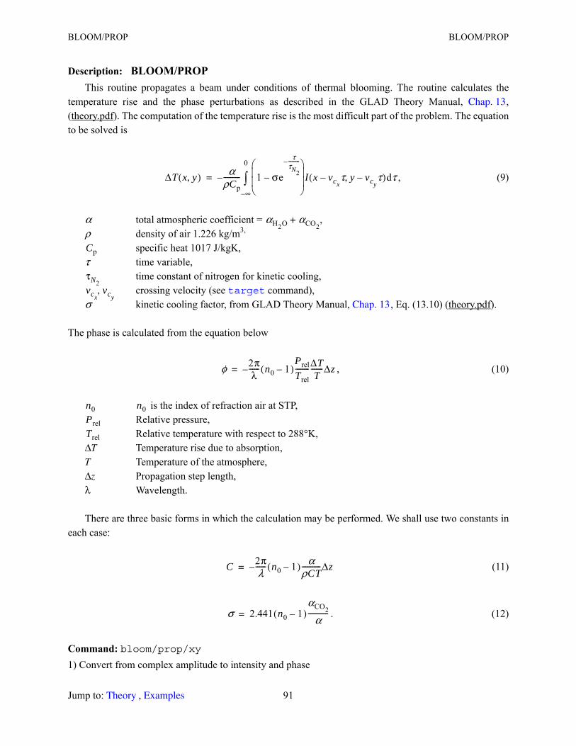
BLOOM/PROP BLOOM/PROP
Description: BLOOM/PROPThis routine propagates a beam under conditions of thermal blooming. The routine calculates the
temperature rise and the phase perturbations as described in the GLAD Theory Manual, , (theory.pdf). The computation of the temperature rise is the most difficult part of the problem. The equation to be solved is
, (9)
α total atmospheric coefficient = ,ρ density of air 1.226 kg/m3,
specific heat 1017 J/kgK,τ time variable,
time constant of nitrogen for kinetic cooling,crossing velocity (see command),
σ kinetic cooling factor, from GLAD Theory Manual, , Eq. (13.10) (theory.pdf).
The phase is calculated from the equation below
, (10)
is the index of refraction air at STP,Relative pressure,Relative temperature with respect to 288°K,
ΔT Temperature rise due to absorption,T Temperature of the atmosphere,Δz Propagation step length,λ Wavelength.
There are three basic forms in which the calculation may be performed. We shall use two constants in each case:
(11)
. (12)
Command: bloom/prop/xy1) Convert from complex amplitude to intensity and phase
Chap. 13
ΔT x y,( ) αρCp---------- 1 σe
ττN2
---------–
–
I x vcxτ– y vcy
τ–,( ) τd∞–
0
–=
αH2O αCO2+
Cp
τN2vcx
vcy, target
Chap. 13
φ 2πλ
------ n0 1–( )–PrelTrel--------ΔT
T-------Δz=
n0 n0PrelTrel
C 2πλ
------ n0 1–( ) αρCT-----------Δz–=
σ 2.441 n0 1–( )αCO2
α------------=
Jump to: , 91 Theory Examples
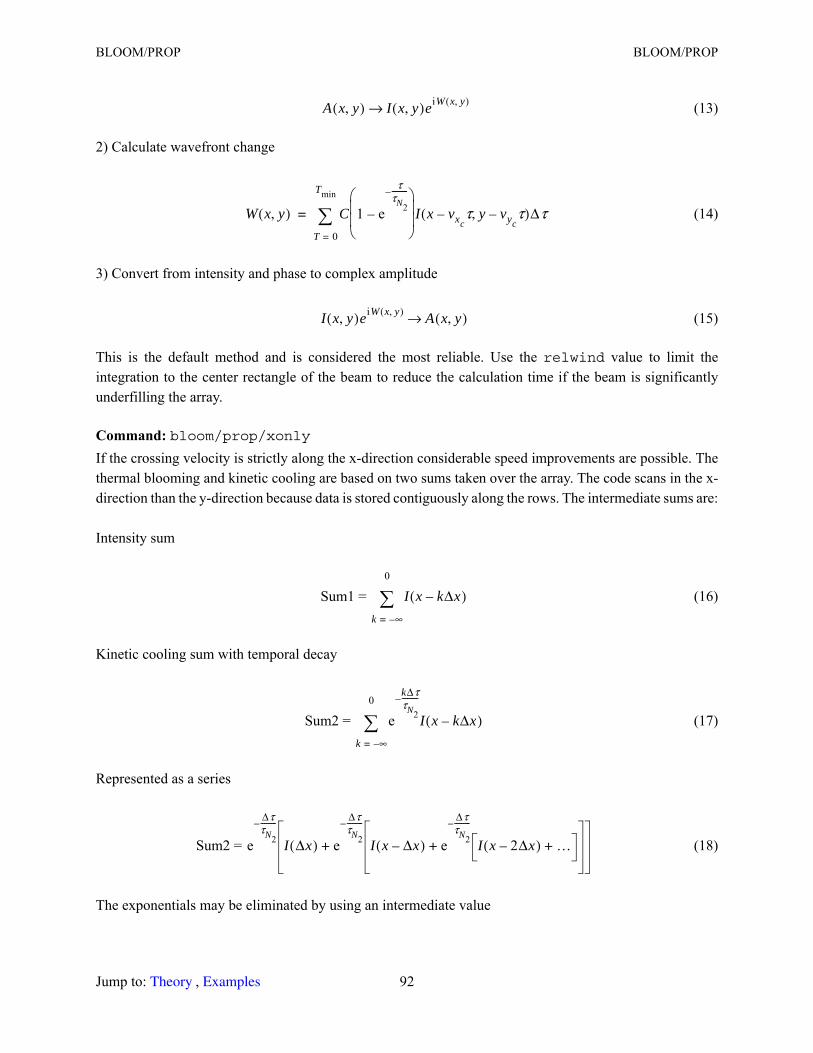
BLOOM/PROP BLOOM/PROP
(13)
2) Calculate wavefront change
(14)
3) Convert from intensity and phase to complex amplitude
(15)
This is the default method and is considered the most reliable. Use the relwind value to limit the integration to the center rectangle of the beam to reduce the calculation time if the beam is significantly underfilling the array.
Command: bloom/prop/xonlyIf the crossing velocity is strictly along the x-direction considerable speed improvements are possible. The thermal blooming and kinetic cooling are based on two sums taken over the array. The code scans in the x-direction than the y-direction because data is stored contiguously along the rows. The intermediate sums are:
Intensity sum
Sum1 = (16)
Kinetic cooling sum with temporal decay
Sum2 = (17)
Represented as a series
Sum2 = (18)
The exponentials may be eliminated by using an intermediate value
A x y,( ) I x y,( )eiW x y,( )→
W x y,( ) CT 0=
Tmin
1 e
ττN2
---------–
–
I x vxcτ– y vyc
τ–,( )Δτ=
I x y,( )eiW x y,( ) A x y,( )→
I x kΔx–( )k ∞–=
0
e
kΔττN2
---------–
I x kΔx–( )k ∞–=
0
e
ΔττN2
---------–
I Δx( ) e+
ΔττN2
---------–
I x Δx–( ) e
ΔττN2
---------–
I x 2Δx–( ) …++
Jump to: , 92 Theory Examples
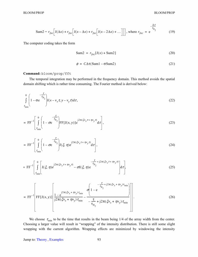
BLOOM/PROP BLOOM/PROP
Sum2 = , where (19)
The computer coding takes the form
(20)
(21)
Command: bloom/prop/fftThe temporal integration may be performed in the frequency domain. This method avoids the spatial
domain shifting which is rather time consuming. The Fourier method is derived below:
, (22)
, (23)
, (24)
, (25)
. (26)
We choose to be the time that results in the beam being 1/4 of the array width from the center. Choosing a larger value will result in “wrapping” of the intensity distribution. There is still some slight wrapping with the current algorithm. Wrapping effects are minimized by windowing the intensity
rfac I Δx( ) rfac+ I x Δx–( ) rfac I x 2Δx–( ) …++ rfac e
ΔττN2
---------–
=
Sum2 rfac I x( ) Sum2+[ ]=
φ CΔτ Sum1 σSum2–( )=
1 σe
ττN2
---------–
–
I x vxτ– y vyτ–,( ) τdτmin
0
FF 1– 1 σe
ττN2
---------–
–
FF I x y,( )[ ]ej2π ξvxτ ηvyτ+( )
τdτmin
0
=
FF 1– 1 σe
ττN2
---------–
–
I ξ η,( )ej2π ξvxτ ηvyτ+( )
τdτmin
0
=
FF 1– I ξ η,( )ej2π ξvxτ ηvyτ+( )
σI ξ η,( )e
ττN2
--------- j2π ξvxτ ηvyτ+( )+–
– τdτmin
0
=
FF 1– FF I x y,( )[ ] 1 ej2π ξvx ηvy+( )τmin–
j2π ξvx ηvy+( )τmin------------------------------------------------
σ 1 e
ττN2
---------– j2π ξvx ηvy+( )τmin+
–
ττN2
-------– j2π ξvx ηvy+( )τmin+------------------------------------------------------------------------–=
τmin
Jump to: , 93 Theory Examples

BLOOM/SET BLOOM/SET
distribution to the inner one-half rectangle. Some slight wrapping is still evident. Upon completion of the blooming step, the scratch array contains the heating profile. This may be observed by using /abs
-1. The scratch array may also be examined by copy -1 kbeam, where Kbeam is another array, however the other diagnostic routines will square the array before displaying it which is inappropriate for the heating profile.
The phase calculations are followed by an internal call to to remove tilt and focus error and to invoke a diffraction propagation. If Nstep is specified then successive steps of kinetics and diffraction will be used—each of length Z/Nstep.
BLOOM/SET Set atmospheric blooming parameters. Aberration
Description: BLOOM/SETMeaning of parameters are defined with command.
Modifier 3 Description /fitphase Fit and remove defocus and tilt to phase at each propagation step. Tilt and decenter
terms are included in paraxial values accessible from defocus and tilt commands. Defocus correction is incorporated into values (default).
/nofitphase Turns off phase fitting. Useful if the beam has become so broken up that there is no clear value for overall tilt or defocus.
Numerical Values Description Defaultsibeams Beam number (0 to select all beams). 1 to nbeamz Propagation distance. 0.
nstep Number of steps to use in propagation. 1
relwind Relative window bloom/prop/xy. 1.
Command Form(s): BLOOM/SET bloom/set xvelocity yvelocity height ah2o temp aco2 tn2 rind dens
conduc spcheat aaer prel trel
Numerical Values Description Defaultsxvelocity,yvelocity
Velocity components of wind (m/sec). 0., 0.
height Height in the atmosphere (km). 1.
ah2o Water absorption coefficient (1/km). 0.001
temp Air temperature (Kelvin). 281
aco2 CO2 absorption coefficient (1/km). 0.03
tn2 Time constant for N2 (sec) (affects kinetic cooling). 0.002
rind (n-1) where n is the index of air. 2.74 × 10⁻⁴
dens Density of air (kg/m3). 1.226
conduc Conductivity of air (w/mK). 0.02525
spcheat Specific heat (J/kgK). 1017
intmap
fitphase
geodata
bloom/prop
Jump to: , 94 Theory Examples
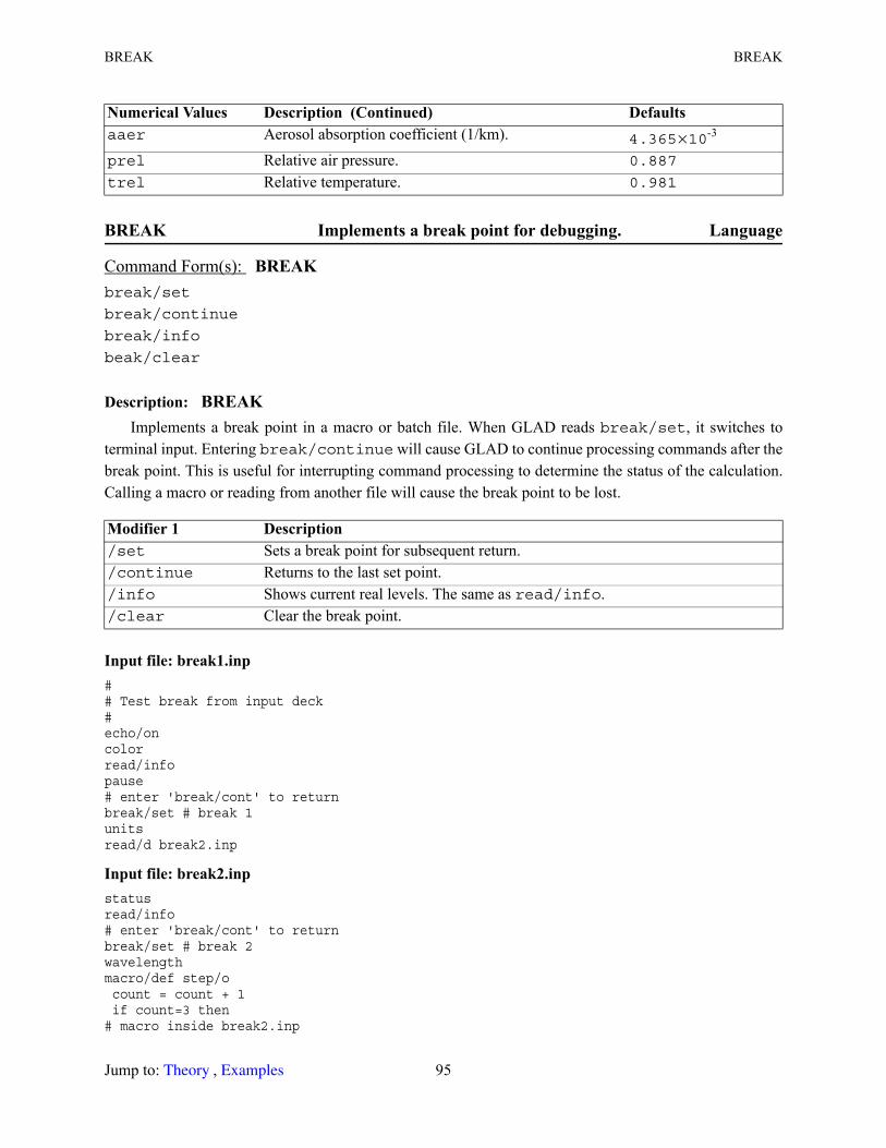
BREAK BREAK
BREAK Implements a break point for debugging. Language
Description: BREAKImplements a break point in a macro or batch file. When GLAD reads break/set, it switches to
terminal input. Entering break/continue will cause GLAD to continue processing commands after the break point. This is useful for interrupting command processing to determine the status of the calculation. Calling a macro or reading from another file will cause the break point to be lost.
Input file: break1.inp## Test break from input deck#echo/oncolorread/infopause# enter 'break/cont' to returnbreak/set # break 1unitsread/d break2.inp
Input file: break2.inpstatusread/info# enter 'break/cont' to returnbreak/set # break 2wavelengthmacro/def step/o count = count + 1 if count=3 then# macro inside break2.inp
aaer Aerosol absorption coefficient (1/km). 4.365 × 10⁻³
prel Relative air pressure. 0.887
trel Relative temperature. 0.981
Command Form(s): BREAK break/set
break/continue
break/info
beak/clear
Modifier 1 Description /set Sets a break point for subsequent return./continue Returns to the last set point./info Shows current real levels. The same as read/info./clear Clear the break point.
Numerical Values Description (Continued) Defaults
Jump to: , 95 Theory Examples

C C or CC
read/info pause# enter 'break/cont' to return break/set # break 3 endifmacro/endmacro/run step/4
C, CC, or COMMENT Line comment (displayed in output Language
Description: C or CCThe command C (upper case “C”) or comment define a comment that is displayed during execution.
Note that c (some string) (lower case “c” or “$” followed by at least one space) defines a non-displayed comment (see Sect. 1.4.2.3). “//” acts the same as “c “. Both “#” and “//” may be used to define the start of a non-displayed comment and the remainder of the line will be ignored. Comments “c{“ and “c}” define comments that start and end indent blocks respectively.
Variables may be used in displayed comments. Preceed the variable by “@”. For example:
comment distance = @zor
C distance = @z
will display the current value of z in the comment. The variables values are automatically updated.CC is the same as C except that it prints even if writing is turned off.
C/format e 12 6C pi = @pi, h = @h
Command Form(s): C C/define (comment string)C/format (Type) iwidth idecC/write
CC/define (comment string)CC/format (Type) iwidth idecCC/write
Modifier 1 Description (no modifier) Defines (/define) and writes (/write) a comment./define Defines a comment without writing. /format Establishes the format of real displayed values. The formats are based on Fortran
conventions: F(iwidth).(idec), fixed floating point number of Width total characters and Dec numbers to the right of the decimal point; 1PE(Width).(Dec) creates a number with an exponent; 1PG(Width).(Dec) writes in fixed floating point format if the numbers will fit the width or numbers with exponent otherwise. If no format is specified, the current format is printed.
/write Updates and displays the most recently defined displayed comment.
Jump to: , 96 Theory Examples
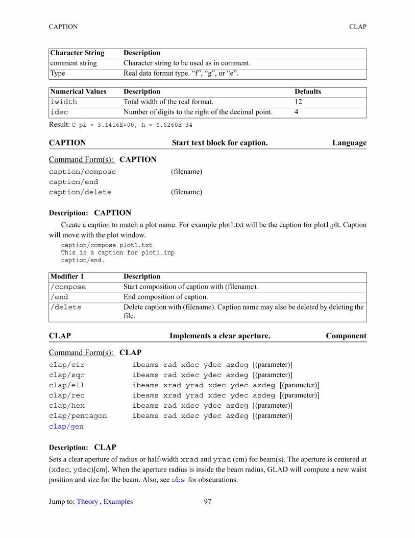
CAPTION CLAP
Result: C pi = 3.1416E+00, h = 6.6260E-34
CAPTION Start text block for caption. Language
Description: CAPTIONCreate a caption to match a plot name. For example plot1.txt will be the caption for plot1.plt. Caption
will move with the plot window.caption/compose plot1.txtThis is a caption for plot1.inpcaption/end.
CLAP Implements a clear aperture. Component
Description: CLAPSets a clear aperture of radius or half-width xrad and yrad (cm) for beam(s). The aperture is centered at (xdec, ydec)[cm]. When the aperture radius is inside the beam radius, GLAD will compute a new waist position and size for the beam. Also, see for obscurations.
Character String Description comment string Character string to be used as in comment.Type Real data format type. “f”, “g”, or “e”.
Numerical Values Description Defaultsiwidth Total width of the real format. 12idec Number of digits to the right of the decimal point. 4
Command Form(s): CAPTION caption/compose (filename)caption/end
caption/delete (filename)
Modifier 1 Description /compose Start composition of caption with (filename)./end End composition of caption./delete Delete caption with (filename). Caption name may also be deleted by deleting the
file.
Command Form(s): CLAP clap/cir ibeams rad xdec ydec azdeg [(parameter)]clap/sqr ibeams rad xdec ydec azdeg [(parameter)]clap/ell ibeams xrad yrad xdec ydec azdeg [(parameter)]clap/rec ibeams xrad yrad xdec ydec azdeg [(parameter)]clap/hex ibeams rad xdec ydec azdeg [(parameter)]clap/pentagon ibeams rad xdec ydec azdeg [(parameter)] clap/gen
obs
Jump to: , 97 Theory Examples
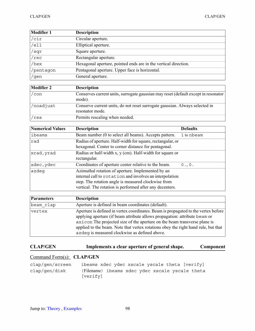
CLAP/GEN CLAP/GEN
CLAP/GEN Implements a clear aperture of general shape. Component
Modifier 1 Description /cir Circular aperture./ell Elliptical aperture./sqr Square aperture./rec Rectangular aperture./hex Hexagonal aperture, pointed ends are in the vertical direction./pentagon Pentagonal aperture. Upper face is horizontal./gen General aperture.
Modifier 2 Description /con Conserves current units, surrogate gaussian may reset (default except in resonator
mode)./noadjust Conserve current units, do not reset surrogate gaussian. Always selected in
resonator mode./res Permits rescaling when needed.
Numerical Values Description Defaultsibeams Beam number (0 to select all beams). Accepts pattern. 1 to nbeamrad Radius of aperture. Half-width for square, rectangular, or
hexagonal. Center to corner distance for pentagonal.xrad,yrad Radius or half-width x, y (cm). Half-width for square or
rectangular.xdec,ydec Coordinates of aperture center relative to the beam. 0., 0.azdeg Azimuthal rotation of aperture. Implemented by an
internal call to rotation and involves an interpolation step. The rotation angle is measured clockwise from vertical. The rotation is performed after any decenters.
Parameters Description beam_clap Aperture is defined in beam coordinates (default).vertex Aperture is defined in vertex coordinates. Beam is propagated to the vertex before
applying aperture (if beam attribute allows propagation: attribute beam or axicon The projected size of the aperture on the beam transverse plane is applied to the beam. Note that vertex rotations obey the right hand rule, but that azdeg is measured clockwise as defined above.
Command Form(s): CLAP/GEN clap/gen/screen ibeams xdec ydec xscale yscale theta [verify]
clap/gen/disk (Filename) ibeams xdec ydec xscale yscale theta [verify]
Jump to: , 98 Theory Examples
CLAP/GEN CLEAR
Description: CLAP/GENThe general aperture is defined by specifying a series of points that generate a polygon. The command
parameters can be used to offset, rescale, and rotate the polygon to fit the required size and position of the current beam. The x-coordinate of point is Xo(i) = Xdec + X(i) * Xscale. If a rotation angle is specified, the rotation is counterclockwise about the centroid of the data points.
The general aperture data has the format
nptsx(1),y(1) . . .x(npts),y(npts)
where: npts = number of data points.
CLEAR Reset all points in array. Begin-end
Modifier 2 Description /screen Reads from screen./tty Same as /screen. Obsolete./disk Reads from file.
Character String Description Filename Local file containing data to define general aperture.null No local file. Used to allow specification of verify as the second parameter
when no file name is specified.
Numerical Values Description Defaultsibeams Beam number (0 to select all beams). 1 to nbeamxrad, yrad Radius of aperture (cm). Requiredxdec, ydec Decentering parameters. 0., 0.xscale, yscale Scale factors. 1., 1.theta Rotation angle (deg). 0.0
Parameters Description Defaultsverify Enables viewing aperture with orthographic plot. Does
not apply aperture to beam.Not selected. Aperture is applied.
Command Form(s): CLEAR clear/intensity ibeams value
clear/complex ibeams real imaginary preal pimaginary
Jump to: , 99 Theory Examples
CLEAR CO2GAIN
Description: CLEARSets all points in the beam array with an intensity defined by value. Other beam parameters such as
units and geometric factors are not changed. For 3D beams, setting the section number to zero in advance will cause clear to set all sections.
CO2GAIN Frantz-Nodvik CO2 gain for pulsed systems. Laser gain
Description: CO2GAINApplies Frantz-Nodvik kinetics for CO2 pulsed lasers. Use co2gain/set to define the necessary
coefficients, co2gain/list to list the coefficients, and co2gain/prop to carry out the propagation. The gain may be limited in the transverse dimensions by a supergaussian roll-off.
(27)
(28)
where g(x,y) is the local small signal gain, gsat(x,y) is the local saturated gain, t(x,y) is the local transmission, and I(x,y) is the fluence or power at (x,y) and the other parameters are defined below.
Reference1. L. M. Frantz and J. S. Nodvik, “Theory of pulse propagation in a laser amplifier”, J. Appl. Phys., 34,
No. 8, 2346–2349, Aug. 1963.
Modifier 1 Description /intensity Set intensity to indicated value (default)./complex Set complex amplitude to indicated values.
Numerical Values Description Defaultsibeams Beam number (0 to select all beams). 1 to nbeamvalue Intensity to be set. 0.0real Real part of complex word for /complex. 0.0imaginary Imaginary part of complex word for /complex. 0.0preal Real part of complex word of 2nd polarization state. 0.pimaginary Imaginary part of complex word of 2nd polarization
state.0.
Command Form(s): CO2GAIN co2gain/prop ibeams z nstep
co2gain/set g0 es nx ny xrad yrad xdec ydec
co2gain/list
g x y,( ) g0x xdec–xrad
----------------------- –
2nx y ydec–yrad
----------------------- 2ny
–exp=
t x y,( ) esI x y ),( )------------------ 1 g x y,( )z I x y,( )
es--------------- 1–
exp+
ln=
Jump to: , 100 Theory Examples
CONJUGATE CONJUGATE
CONJUGATE Conjugates the beam. Operator
Description: CONJUGATEModels a phase conjugate mirror (/beam). The GLAD is required. The phase in the array is conjugated,
the direction of the beam is reversed, and the k-vector is reversed in the global data and the wavefront error is flipped in sign as shown below in Fig. 12.
The form /amplitude conjugates the complex amplitude field without changing the beam direction.
Modifier 1 Description /prop Execute propagation./list List the co2gain stored parameters./set Define and store co2gain parameters.
Numerical Values Description Defaultsibeams Beam number (0 to select all beams). 1 to nbeamz Total propagation distance (cm). Requirednstep Number of steps. 1
g0 Small signal gain.es Saturation fluence. 1000
nx, ny Supergaussian exponents. 100, 100xrad, yrad Supergaussian radii. 1e20
Xdec, ydec Coordinates of beam center. 0., 0.
Command Form(s): CONJUGATE conjugate/beam kbeam
conjugate/amplitude kbeam
Modifier 1 Description /beam Conjugates the beam as a real phase conjugator would do./amplitude Conjugates the complex amplitude without changing the beam direction.
Numerical Values Description Defaultskbeam Single beam number. 1
Jump to: , 101 Theory Examples
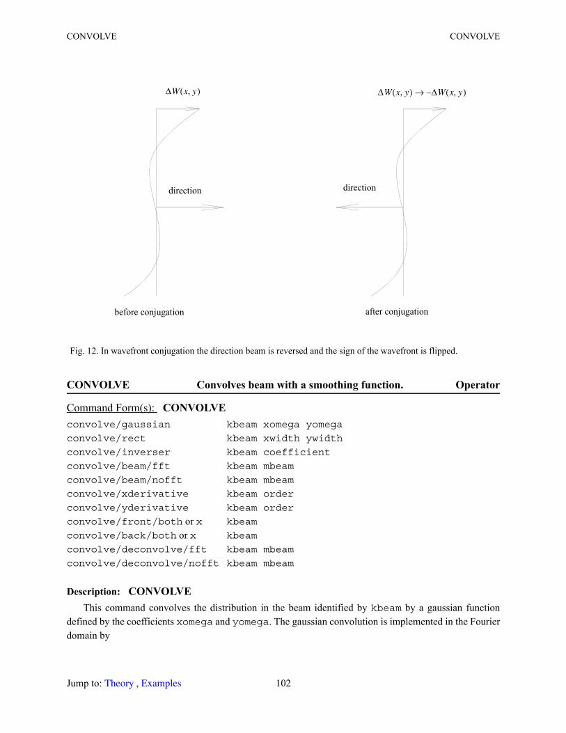
CONVOLVE CONVOLVE
CONVOLVE Convolves beam with a smoothing function. Operator
Description: CONVOLVEThis command convolves the distribution in the beam identified by kbeam by a gaussian function
defined by the coefficients xomega and yomega. The gaussian convolution is implemented in the Fourier domain by
Fig. 12. In wavefront conjugation the direction beam is reversed and the sign of the wavefront is flipped.
Command Form(s): CONVOLVE convolve/gaussian kbeam xomega yomega
convolve/rect kbeam xwidth ywidth
convolve/inverser kbeam coefficient
convolve/beam/fft kbeam mbeam
convolve/beam/nofft kbeam mbeam
convolve/xderivative kbeam order
convolve/yderivative kbeam order
convolve/front/both or x kbeam
convolve/back/both or x kbeam
convolve/deconvolve/fft kbeam mbeam
convolve/deconvolve/nofft kbeam mbeam
ΔW x y,( )
direction direction
ΔW x y,( ) ΔW x y,( )–→
before conjugation after conjugation
Jump to: , 102 Theory Examples
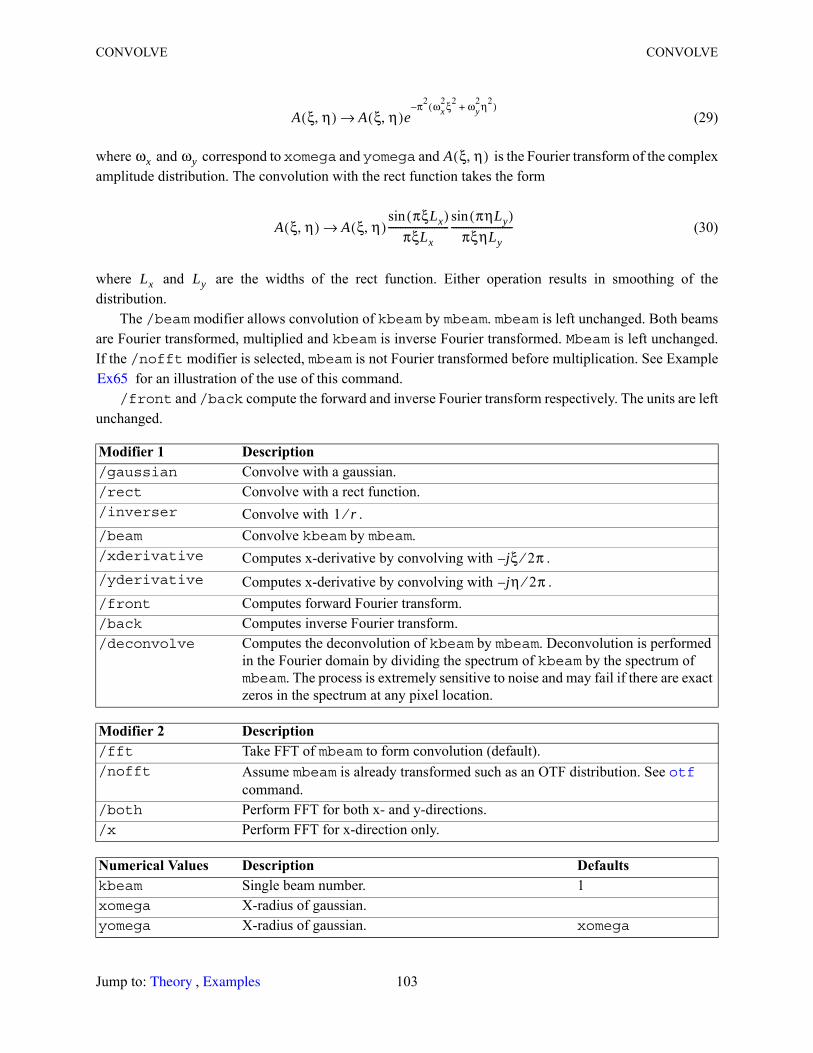
CONVOLVE CONVOLVE
(29)
where and correspond to xomega and yomega and is the Fourier transform of the complex amplitude distribution. The convolution with the rect function takes the form
(30)
where and are the widths of the rect function. Either operation results in smoothing of the distribution.
The /beam modifier allows convolution of kbeam by mbeam. mbeam is left unchanged. Both beams are Fourier transformed, multiplied and kbeam is inverse Fourier transformed. Mbeam is left unchanged. If the /nofft modifier is selected, mbeam is not Fourier transformed before multiplication. See Example
for an illustration of the use of this command./front and /back compute the forward and inverse Fourier transform respectively. The units are left
unchanged.
Modifier 1 Description /gaussian Convolve with a gaussian./rect Convolve with a rect function./inverser Convolve with ./beam Convolve kbeam by mbeam./xderivative Computes x-derivative by convolving with ./yderivative Computes x-derivative by convolving with ./front Computes forward Fourier transform./back Computes inverse Fourier transform./deconvolve Computes the deconvolution of kbeam by mbeam. Deconvolution is performed
in the Fourier domain by dividing the spectrum of kbeam by the spectrum of mbeam. The process is extremely sensitive to noise and may fail if there are exact zeros in the spectrum at any pixel location.
Modifier 2 Description /fft Take FFT of mbeam to form convolution (default)./nofft Assume mbeam is already transformed such as an OTF distribution. See
command./both Perform FFT for both x- and y-directions./x Perform FFT for x-direction only.
Numerical Values Description Defaultskbeam Single beam number. 1xomega X-radius of gaussian.yomega X-radius of gaussian. xomega
A ξ η,( ) A ξ η,( )eπ2 ωx
2ξ2 ωy2η2
+( )–→
ωx ωy A ξ η,( )
A ξ η,( ) A ξ η,( )πξLx( )sin
πξLx-------------------------
πηLy( )sinπξηLy
-------------------------→
Lx Ly
Ex65
1 r⁄
jξ– 2π⁄
jη– 2π⁄
otf
Jump to: , 103 Theory Examples
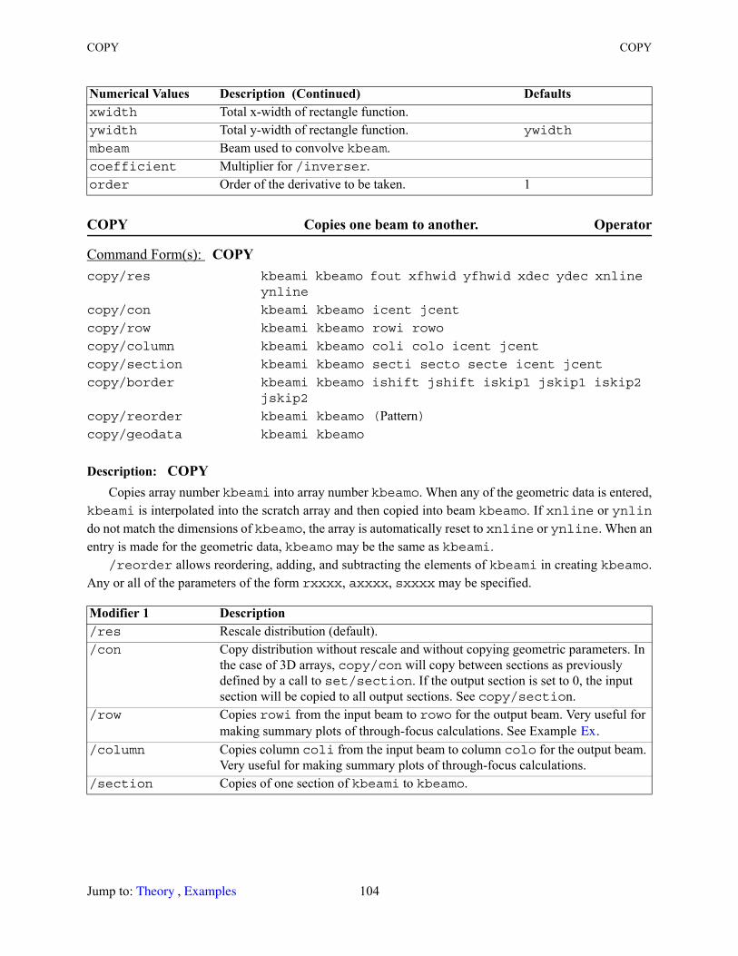
COPY COPY
COPY Copies one beam to another. Operator
Description: COPYCopies array number kbeami into array number kbeamo. When any of the geometric data is entered,
kbeami is interpolated into the scratch array and then copied into beam kbeamo. If xnline or ynlindo not match the dimensions of kbeamo, the array is automatically reset to xnline or ynline. When an entry is made for the geometric data, kbeamo may be the same as kbeami.
/reorder allows reordering, adding, and subtracting the elements of kbeami in creating kbeamo. Any or all of the parameters of the form rxxxx, axxxx, sxxxx may be specified.
xwidth Total x-width of rectangle function.ywidth Total y-width of rectangle function. ywidth
mbeam Beam used to convolve kbeam.coefficient Multiplier for /inverser.order Order of the derivative to be taken. 1
Command Form(s): COPY copy/res kbeami kbeamo fout xfhwid yfhwid xdec ydec xnline
ynline
copy/con kbeami kbeamo icent jcent
copy/row kbeami kbeamo rowi rowo
copy/column kbeami kbeamo coli colo icent jcent
copy/section kbeami kbeamo secti secto secte icent jcent
copy/border kbeami kbeamo ishift jshift iskip1 jskip1 iskip2 jskip2
copy/reorder kbeami kbeamo (Pattern)copy/geodata kbeami kbeamo
Modifier 1 Description /res Rescale distribution (default)./con Copy distribution without rescale and without copying geometric parameters. In
the case of 3D arrays, copy/con will copy between sections as previously defined by a call to set/section. If the output section is set to 0, the input section will be copied to all output sections. See copy/section.
/row Copies rowi from the input beam to rowo for the output beam. Very useful for making summary plots of through-focus calculations. See Example .
/column Copies column coli from the input beam to column colo for the output beam. Very useful for making summary plots of through-focus calculations.
/section Copies of one section of kbeami to kbeamo.
Numerical Values Description (Continued) Defaults
Ex5
Jump to: , 104 Theory Examples
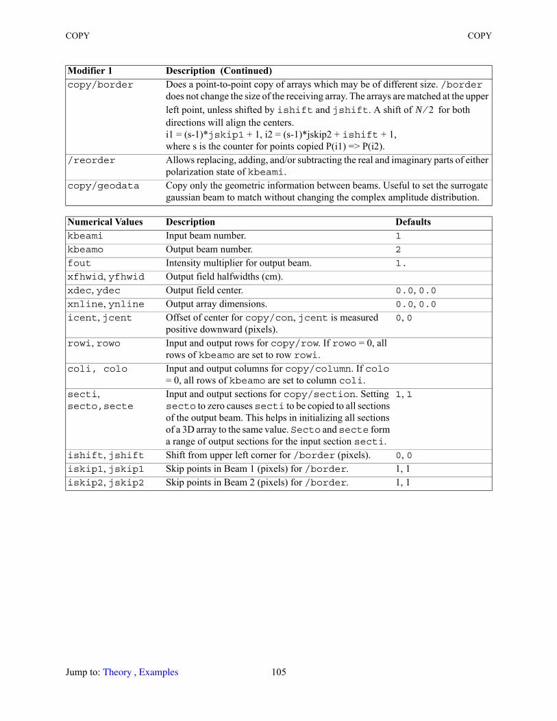
COPY COPY
copy/border Does a point-to-point copy of arrays which may be of different size. /border does not change the size of the receiving array. The arrays are matched at the upper left point, unless shifted by ishift and jshift. A shift of for both directions will align the centers.i1 = (s-1)*jskip1 + 1, i2 = (s-1)*jskip2 + ishift + 1,where s is the counter for points copied P(i1) => P(i2).
/reorder Allows replacing, adding, and/or subtracting the real and imaginary parts of either polarization state of kbeami.
copy/geodata Copy only the geometric information between beams. Useful to set the surrogate gaussian beam to match without changing the complex amplitude distribution.
Numerical Values Description Defaultskbeami Input beam number. 1
kbeamo Output beam number. 2
fout Intensity multiplier for output beam. 1.
xfhwid, yfhwid Output field halfwidths (cm).xdec, ydec Output field center. 0.0, 0.0xnline, ynline Output array dimensions. 0.0, 0.0icent, jcent Offset of center for copy/con, jcent is measured
positive downward (pixels).0, 0
rowi, rowo Input and output rows for copy/row. If rowo = 0, all rows of kbeamo are set to row rowi.
coli, colo Input and output columns for copy/column. If colo = 0, all rows of kbeamo are set to column coli.
secti, secto,secte
Input and output sections for copy/section. Setting secto to zero causes secti to be copied to all sections of the output beam. This helps in initializing all sections of a 3D array to the same value. Secto and secte form a range of output sections for the input section secti.
1, 1
ishift, jshift Shift from upper left corner for /border (pixels). 0, 0iskip1, jskip1 Skip points in Beam 1 (pixels) for /border. 1, 1iskip2, jskip2 Skip points in Beam 2 (pixels) for /border. 1, 1
Modifier 1 Description (Continued)
N 2⁄
Jump to: , 105 Theory Examples
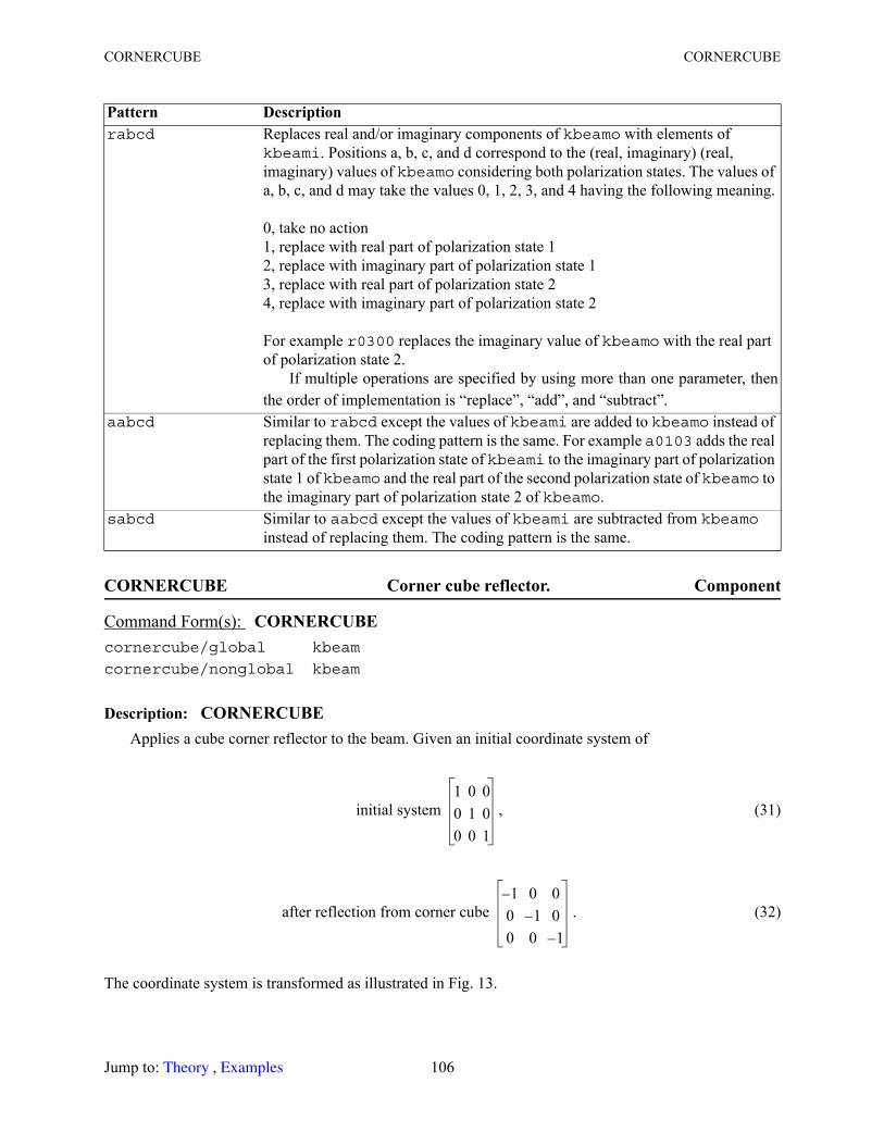
CORNERCUBE CORNERCUBE
CORNERCUBE Corner cube reflector. Component
Description: CORNERCUBEApplies a cube corner reflector to the beam. Given an initial coordinate system of
initial system , (31)
after reflection from corner cube . (32)
The coordinate system is transformed as illustrated in Fig. 13.
Pattern Description rabcd Replaces real and/or imaginary components of kbeamo with elements of
kbeami. Positions a, b, c, and d correspond to the (real, imaginary) (real, imaginary) values of kbeamo considering both polarization states. The values of a, b, c, and d may take the values 0, 1, 2, 3, and 4 having the following meaning.
0, take no action1, replace with real part of polarization state 12, replace with imaginary part of polarization state 13, replace with real part of polarization state 24, replace with imaginary part of polarization state 2
For example r0300 replaces the imaginary value of kbeamo with the real part of polarization state 2.
If multiple operations are specified by using more than one parameter, then the order of implementation is “replace”, “add”, and “subtract”.
aabcd Similar to rabcd except the values of kbeami are added to kbeamo instead of replacing them. The coding pattern is the same. For example a0103 adds the real part of the first polarization state of kbeami to the imaginary part of polarization state 1 of kbeamo and the real part of the second polarization state of kbeamo to the imaginary part of polarization state 2 of kbeamo.
sabcd Similar to aabcd except the values of kbeami are subtracted from kbeamo instead of replacing them. The coding pattern is the same.
Command Form(s): CORNERCUBE cornercube/global kbeam
cornercube/nonglobal kbeam
1 0 00 1 00 0 1
1– 0 00 1– 00 0 1–
Jump to: , 106 Theory Examples
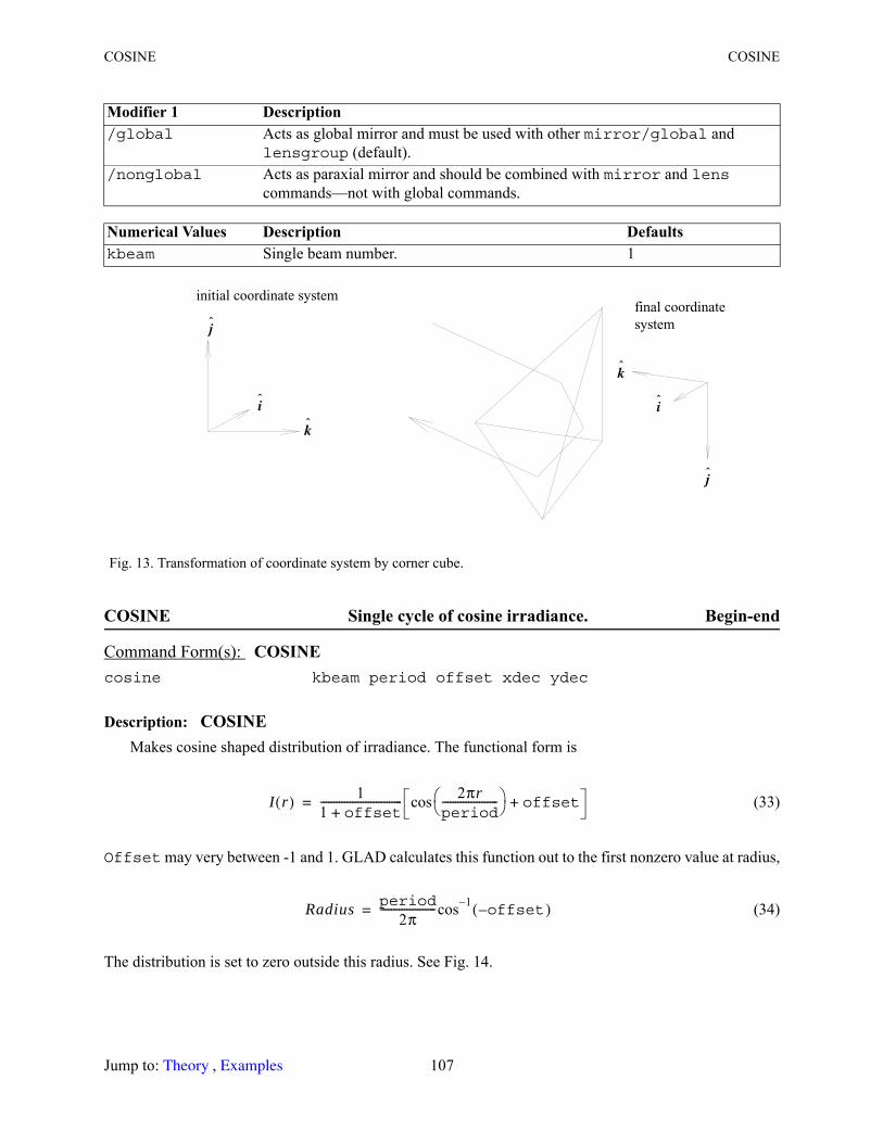
COSINE COSINE
COSINE Single cycle of cosine irradiance. Begin-end
Description: COSINEMakes cosine shaped distribution of irradiance. The functional form is
(33)
Offset may very between -1 and 1. GLAD calculates this function out to the first nonzero value at radius,
(34)
The distribution is set to zero outside this radius. See Fig. 14.
Modifier 1 Description /global Acts as global mirror and must be used with other mirror/global and
lensgroup (default)./nonglobal Acts as paraxial mirror and should be combined with mirror and lens
commands—not with global commands.
Numerical Values Description Defaultskbeam Single beam number. 1
Fig. 13. Transformation of coordinate system by corner cube.
Command Form(s): COSINE cosine kbeam period offset xdec ydec
initial coordinate systemfinal coordinate system
i
k
j
i
k
j
I r( ) 11 offset+------------------------------- 2πr
period--------------------- cos offset+=
Radius period2π
---------------------cos 1–offset–( )=
Jump to: , 107 Theory Examples
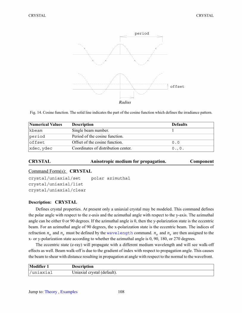
CRYSTAL CRYSTAL
CRYSTAL Anisotropic medium for propagation. Component
Description: CRYSTALDefines crystal properties. At present only a uniaxial crystal may be modeled. This command defines
the polar angle with respect to the z-axis and the azimuthal angle with respect to the y-axis. The azimuthal angle can be either 0 or 90 degrees. If the azimuthal angle is 0, then the y-polarization state is the eccentric beam. For an azimuthal angle of 90 degrees, the x-polarization state is the eccentric beam. The indices of refraction and must be defined by the command. and are then assigned to the x- or y-polarization state according to whether the azimuthal angle is 0, 90, 180, or 270 degrees.
The eccentric state (e-ray) will propagate with a different medium wavelength and will see walk-off effects as well. Beam walk-off is due to the gradient of index with respect to propagation angle. This causes the beam to shear with distance resulting in propagation at angle with respect to the normal to the wavefront.
Fig. 14. Cosine function. The solid line indicates the part of the cosine function which defines the irradiance pattern.
Numerical Values Description Defaultskbeam Single beam number. 1period Period of the cosine function.offset Offset of the cosine function. 0.0
xdec, ydec Coordinates of distribution center. 0., 0.
Command Form(s): CRYSTAL crystal/uniaxial/set polar azimuthal
crystal/uniaxial/list
crystal/uniaxial/clear
Modifier 1 Description /uniaxial Uniaxial crystal (default).
period
offset
Radius
no ne wavelength no ne
Jump to: , 108 Theory Examples
DATE DECLARE
DATE Displays date and time. Language
Description: DATEWrites date and time to output file.
DEBUG Controls diagnostic information for internal AOR use. Language
Description: DEBUGThis command controls the debug function for diagnostic information. It is primarily for AOR use. An
example of rdwr is illustrated in and .
DECLARE Assigns names to variables (also see variables command). Language
Modifier 2 Description /set Sets the crystal properties./list List crystal properties./clear Clear crystal properties and return to ordinary isotropic propagation.
Numerical Values Description Defaultspolar Polar angle of crystal axis with respect to z-axis. 0.azimuthal Azimuthal angle with respect to y-axis measured
clockwise. Angle must be 0, 90, 180, and 270 degrees.0.
Command Form(s): DATE date
Command Form(s): DEBUG debug/add (keyword1) . . . (keyword10)debug/delete (keyword1) . . . (keyword10)debug/list
debug/reset
Modifier 1 Description /add Adds a debug name./delete Deletes a name./list Lists all current debug names./reset Clears all debug names.
Parameters Description Defaultskeyword Keyword selected from the source code listing.
Command Form(s): DECLARE declare/real (Variable 1) (Variable 2) . . .
Ex73 Ex74
Jump to: , 109 Theory Examples

DECLARE DERIVATIVE
Description: DECLAREDeclare assigns variable names to either real or integer register addresses. See the
command for a more convenient method of defining variables. This command is the same as /declare. The variable name may consist of the characters a-z, A-Z, 0-9, and _. The leading
character should not be a number. The declare command is case sensitive: “x” is a different variable from “X”. Declare assigns the variables to register values beginning at 200 and decrementing with each new variable declared.
For example,declare/real X_rad Y_radX_rad = 13.25Y_rad = 23.6clap 1 X_rad Y_rad.
DERIVATIVE Take spatial derivatives. Operator
Description: DERIVATIVETakes derivative of real and imaginary components of field. Also see /xderivative and
/yderivative for Fourier method of calculating derivatives.
declare/integer (Variable 1) (Variable 2) . . .declare/list
declare/export
Modifier 1 Description /real Declare real variable. /integer Declare integer variable./list Lists the variables and the associated register addresses./export Simpler form of list suitable for exporting with write/disk (filename),
followed by variables/export. Can be read in by read/disk (filename).
Command Form(s): DERIVATIVE derivative/x/linear kbeam
derivative/y/linear kbeam
derivative/x/spline kbeam
derivative/y/spline kbeam
Modifier 1 Description x Calculate x-derivatives (default).y Calculate y-derivatives.
Modifier 2 Description linear Calculate derivatives by finite-difference using nearest neighbors (default).spline Fit splines to function and differentiate splines analytically.
Command Form(s): DECLARE (Continued)
variables
variables
convolve convolve
Jump to: , 110 Theory Examples
DIST DIST
DIST Propagate assuming simple optical axis (see prop). Propagation
Description: DISTApplies diffraction propagation. Also see the command. The angular spectrum propagator is the
only one fully integrated into the propagation control algorithms. We recommend that the users not use the other propagation algorithms except in special circumstances. By default all beams are propagated.
GLAD will automatically select an appropriate propagator and units for the specified distance. The default propagator and default units will produce accurate results and, while always accurate, may not be optimum for a given problem. The knowledgeable user may make the sampling more efficient by changing the units and/or using an alternate propagator. Overriding the default conditions will increase the risk of introducing such errors as aliasing, energy loss, inadequate resolution, and accumulated numerical errors. Users are advised to read the theory section and have a basic knowledge of the propagators and unit selection before attempting to override the automatic unit or propagator control.
Only propagations which result in a gain of physical path length are physically meaningful. The command does not protect the user from making nonphysical propagations. The command is designed to move forward or backward along a principal optical axis. The direction of the beam is reversed each time the beam strikes a mirror. The command should use positive or negative values of z to correspond to the beam direction. The command gives the direction of the beam as a positive or negative movement along the z-axis. GLAD tracks the axial position with the parameter, zreff. Small angle tilts and decenters are allowed, but the optical path lengths are not correctly calculated.
The prop command is a more powerful propagation command which allows movement in a general three-dimensional space when used with the , , and commands.
Propagation of a beam against the forward direction of a beam can produce errors when a lens is encountered. The proper way to go through a lens in the negative z-direction is to use a mirror to reverse the propagation direction of the beam. For a beam initially moving in the plus z-direction, the commands below show incorrect and correct commands to go through a lens in the negative z-direction..
Numerical Values Description Defaultskbeam Single beam number. 1
Command Form(s): DIST dist/spectp z kbeam1 . . . kbeam9 [xonly] [list]dist/finitdif z kbeam1 . . . kbeam9dist/avgkern z kbeam1 . . . kbeam9
Incorrect Correctdist -100 mirror/flat 1
lens 1 100 dist -100
lens 1 100
Modifier 1 Description /spectp Spectrum of plane waves propagator (default).
(recommended for all applications).
prop
dist dist
dist status
global vertex mirror/global
Jump to: , 111 Theory Examples
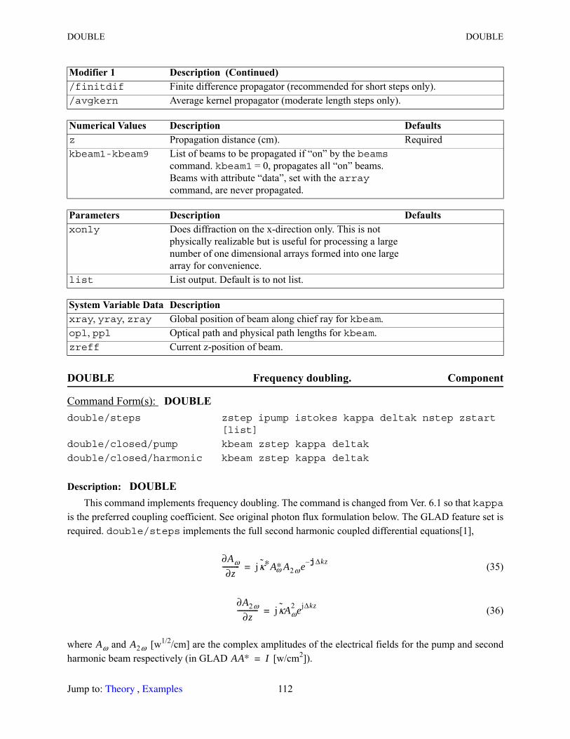
DOUBLE DOUBLE
DOUBLE Frequency doubling. Component
Description: DOUBLEThis command implements frequency doubling. The command is changed from Ver. 6.1 so that kappa
is the preferred coupling coefficient. See original photon flux formulation below. The GLAD feature set is required. double/steps implements the full second harmonic coupled differential equations[1],
(35)
(36)
where and [w1/2/cm] are the complex amplitudes of the electrical fields for the pump and second harmonic beam respectively (in GLAD [w/cm2]).
/finitdif Finite difference propagator (recommended for short steps only)./avgkern Average kernel propagator (moderate length steps only).
Numerical Values Description Defaultsz Propagation distance (cm). Requiredkbeam1-kbeam9 List of beams to be propagated if “on” by the beams
command. kbeam1 = 0, propagates all “on” beams. Beams with attribute “data”, set with the array command, are never propagated.
Parameters Description Defaultsxonly Does diffraction on the x-direction only. This is not
physically realizable but is useful for processing a large number of one dimensional arrays formed into one large array for convenience.
list List output. Default is to not list.
System Variable Data Description xray, yray, zray Global position of beam along chief ray for kbeam.opl, ppl Optical path and physical path lengths for kbeam.zreff Current z-position of beam.
Command Form(s): DOUBLE double/steps zstep ipump istokes kappa deltak nstep zstart
[list]
double/closed/pump kbeam zstep kappa deltak
double/closed/harmonic kbeam zstep kappa deltak
Modifier 1 Description (Continued)
∂Aω∂z
---------- jκ∗A∗ω A2ω e j– Δkz=
∂A2ω∂z
------------ jκAω2 ejΔkz=
Aω A2ωAA∗ I=
Jump to: , 112 Theory Examples
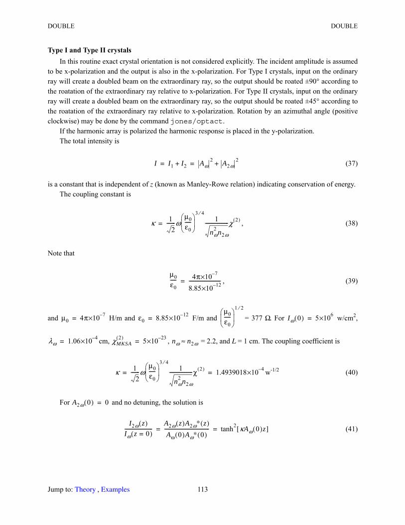
DOUBLE DOUBLE
Type I and Type II crystalsIn this routine exact crystal orientation is not considered explicitly. The incident amplitude is assumed
to be x-polarization and the output is also in the x-polarization. For Type I crystals, input on the ordinary ray will create a doubled beam on the extraordinary ray, so the output should be roated ±90° according to the roatation of the extraordinary ray relative to x-polarization. For Type II crystals, input on the ordinary ray will create a doubled beam on the extraordinary ray, so the output should be roated ±45° according to the roatation of the extraordinary ray relative to x-polarization. Rotation by an azimuthal angle (positive clockwise) may be done by the command jones/optact.
If the harmonic array is polarized the harmonic response is placed in the y-polarization.The total intensity is
(37)
is a constant that is independent of z (known as Manley-Rowe relation) indicating conservation of energy.The coupling constant is
, (38)
Note that
, (39)
and H/m and F/m and = 377 Ω. For w/cm2,
cm, , = 2.2, and L = 1 cm. The coupling coefficient is
w-1/2 (40)
For and no detuning, the solution is
(41)
I I1 I2+ Aω2 A2ω
2+= =
κ 12
-------ωμ0ε0-----
3 4⁄1
nω2 n2ω
-------------------χ 2( )=
μ0ε0----- 4π 7–×10
8.85 12–×10--------------------------=
μ0 4π 7–×10= ε0 8.85 12–×10=μ0ε0-----
1 2⁄
Iω 0( ) 5 6×10=
λω 1.06 4–×10= χMKSA2( ) 5 23–×10= nω n2ω≈
κ 12
-------ωμ0ε0-----
3 4⁄1
nω2 n2ω
-------------------χ 2( ) 1.4939018 4–×10= =
A2ω 0( ) 0=
I2ω z( )Iω z 0=( )-----------------------
A2ω z( )A2ω∗ z( )Aω 0( )Aω∗ 0( )
------------------------------------- tanh2 κAω 0( )z[ ]= =
Jump to: , 113 Theory Examples
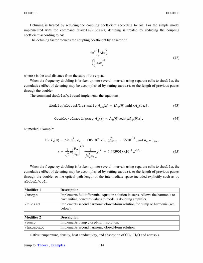
DOUBLE DOUBLE
Detuning is treated by reducing the coupling coefficient according to . For the simple model implemented with the command double/closed, detuning is treated by reducing the coupling coefficient according to .
The detuning factor reduces the coupling coefficient by a factor of
(42)
where z is the total distance from the start of the crystal. When the frequency doubling is broken up into several intervals using separate calls to double, the
cumulative effect of detuning may be accomplished by setting zstart to the length of previous passes through the doubler.
The command double/closed implements the equations:
double/closed/harmonic , (43)
double/closed/pump , (44)
Numerical Example:
For , cm, , and ,
w-1/2. (45)
When the frequency doubling is broken up into several intervals using separate calls to double, the cumulative effect of detuning may be accomplished by setting zstart to the length of previous passes through the doubler or the optical path length of the intermediate space included explicitly such as by global/opl.
elative temperature, density, heat conductivity, and absorption of CO2, H2O and aerosols.
Modifier 1 Description /steps Implements full differential equation solution in steps. Allows the harmonic to
have initial, non-zero values to model a doubling amplifier./closed Implements second harmonic closed-form solution for pump or harmonic (see
below).
Modifier 2 Description /pump Implements pump closed-form solution./harmonic Implements second harmonic closed-form solution.
Δk
Δk
sin2 12---Δkz
12---Δkz 2
----------------------------
A2ω z( ) jAω 0( )tanh κAω 0( )z[ ]=
Aω z( ) Aω 0( )sech κAω 0( )z[ ]=
Iω 0( ) 5 6×10= λω 1.0 4–×10= χMKSA2( ) 5 23–×10= nω n2ω≈
κ 12
-------ωμ0ε0-----
3 4⁄1
nω2 n2ω
-------------------χ 2( ) 1.4939018 4–×10= =
Jump to: , 114 Theory Examples
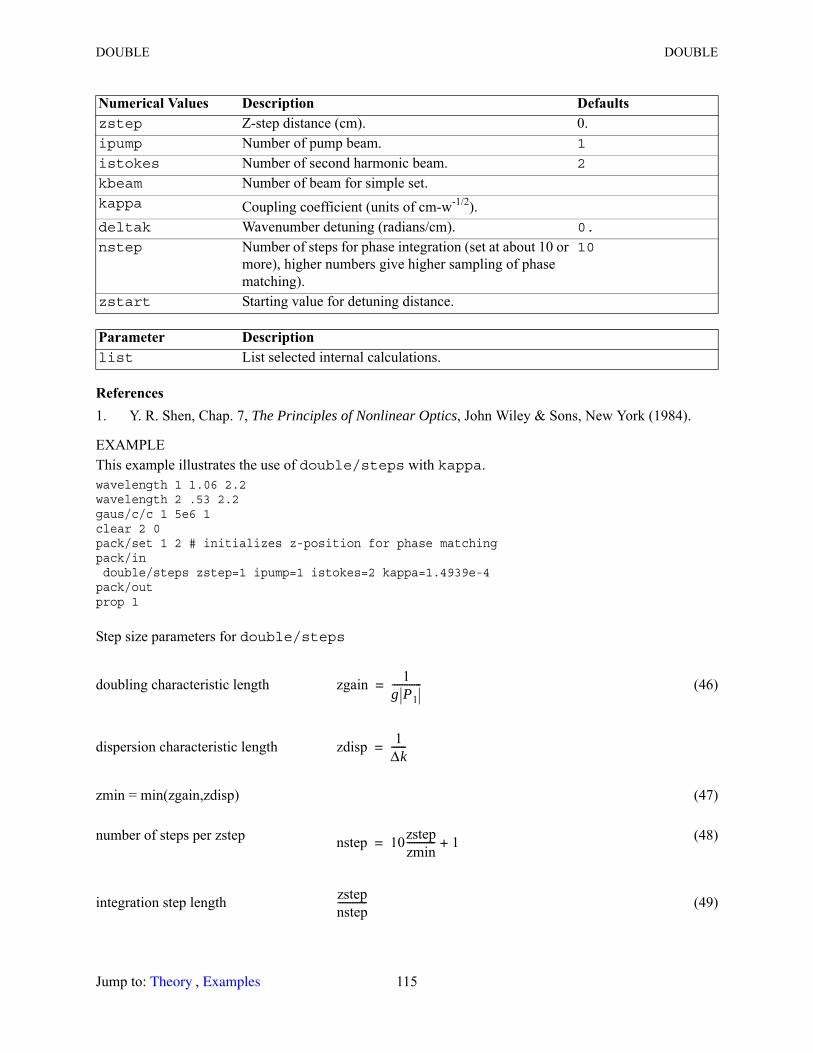
DOUBLE DOUBLE
References1. Y. R. Shen, Chap. 7, The Principles of Nonlinear Optics, John Wiley & Sons, New York (1984).
EXAMPLEThis example illustrates the use of double/steps with kappa.wavelength 1 1.06 2.2wavelength 2 .53 2.2gaus/c/c 1 5e6 1clear 2 0pack/set 1 2 # initializes z-position for phase matchingpack/in double/steps zstep=1 ipump=1 istokes=2 kappa=1.4939e-4pack/outprop 1
Step size parameters for double/steps
doubling characteristic length (46)
dispersion characteristic length
zmin = min(zgain,zdisp) (47)
number of steps per zstep (48)
integration step length (49)
Numerical Values Description Defaultszstep Z-step distance (cm). 0.ipump Number of pump beam. 1
istokes Number of second harmonic beam. 2
kbeam Number of beam for simple set.kappa Coupling coefficient (units of cm-w-1/2).deltak Wavenumber detuning (radians/cm). 0.
nstep Number of steps for phase integration (set at about 10 or more), higher numbers give higher sampling of phase matching).
10
zstart Starting value for detuning distance.
Parameter Description list List selected internal calculations.
zgain 1g P1------------=
zdisp 1Δk------=
nstep 10zstepzmin------------ 1+=
zstepnstep------------
Jump to: , 115 Theory Examples
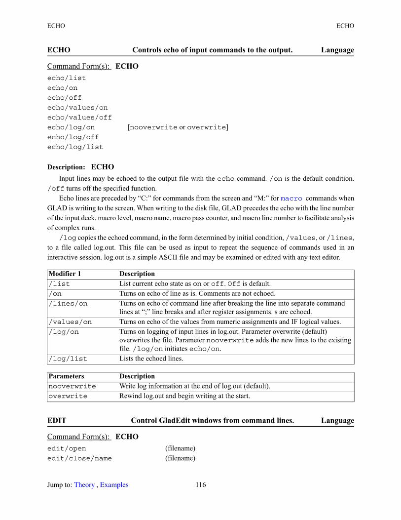
ECHO ECHO
ECHO Controls echo of input commands to the output. Language
Description: ECHOInput lines may be echoed to the output file with the echo command. /on is the default condition.
/off turns off the specified function.Echo lines are preceded by “C:” for commands from the screen and “M:” for commands when
GLAD is writing to the screen. When writing to the disk file, GLAD precedes the echo with the line number of the input deck, macro level, macro name, macro pass counter, and macro line number to facilitate analysis of complex runs.
/log copies the echoed command, in the form determined by initial condition, /values, or /lines, to a file called log.out. This file can be used as input to repeat the sequence of commands used in an interactive session. log.out is a simple ASCII file and may be examined or edited with any text editor.
EDIT Control GladEdit windows from command lines. Language
Command Form(s): ECHO echo/list
echo/on
echo/off
echo/values/on
echo/values/off
echo/log/on [nooverwrite or overwrite]echo/log/off
echo/log/list
Modifier 1 Description /list List current echo state as on or off. Off is default./on Turns on echo of line as is. Comments are not echoed./lines/on Turns on echo of command line after breaking the line into separate command
lines at “;” line breaks and after register assignments. s are echoed./values/on Turns on echo of the values from numeric assignments and IF logical values./log/on Turns on logging of input lines in log.out. Parameter overwrite (default)
overwrites the file. Parameter nooverwrite adds the new lines to the existing file. /log/on initiates echo/on.
/log/list Lists the echoed lines.
Parameters Description nooverwrite Write log information at the end of log.out (default).overwrite Rewind log.out and begin writing at the start.
Command Form(s): ECHO edit/open (filename)edit/close/name (filename)
macro
Jump to: , 116 Theory Examples
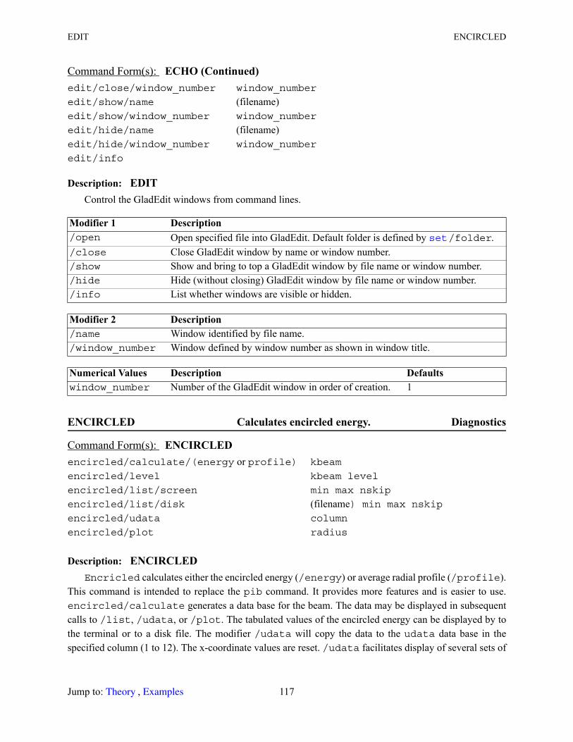
EDIT ENCIRCLED
Description: EDITControl the GladEdit windows from command lines.
ENCIRCLED Calculates encircled energy. Diagnostics
Description: ENCIRCLEDEncricled calculates either the encircled energy (/energy) or average radial profile (/profile).
This command is intended to replace the pib command. It provides more features and is easier to use. encircled/calculate generates a data base for the beam. The data may be displayed in subsequent calls to /list, /udata, or /plot. The tabulated values of the encircled energy can be displayed by to the terminal or to a disk file. The modifier /udata will copy the data to the udata data base in the specified column (1 to 12). The x-coordinate values are reset. /udata facilitates display of several sets of
edit/close/window_number window_number
edit/show/name (filename)edit/show/window_number window_number
edit/hide/name (filename)edit/hide/window_number window_number
edit/info
Modifier 1 Description /open Open specified file into GladEdit. Default folder is defined by /folder./close Close GladEdit window by name or window number./show Show and bring to top a GladEdit window by file name or window number./hide Hide (without closing) GladEdit window by file name or window number./info List whether windows are visible or hidden.
Modifier 2 Description /name Window identified by file name./window_number Window defined by window number as shown in window title.
Numerical Values Description Defaultswindow_number Number of the GladEdit window in order of creation. 1
Command Form(s): ENCIRCLED encircled/calculate/(energy or profile) kbeam
encircled/level kbeam level
encircled/list/screen min max nskip
encircled/list/disk (filename) min max nskipencircled/udata column
encircled/plot radius
Command Form(s): ECHO (Continued)
set
Jump to: , 117 Theory Examples
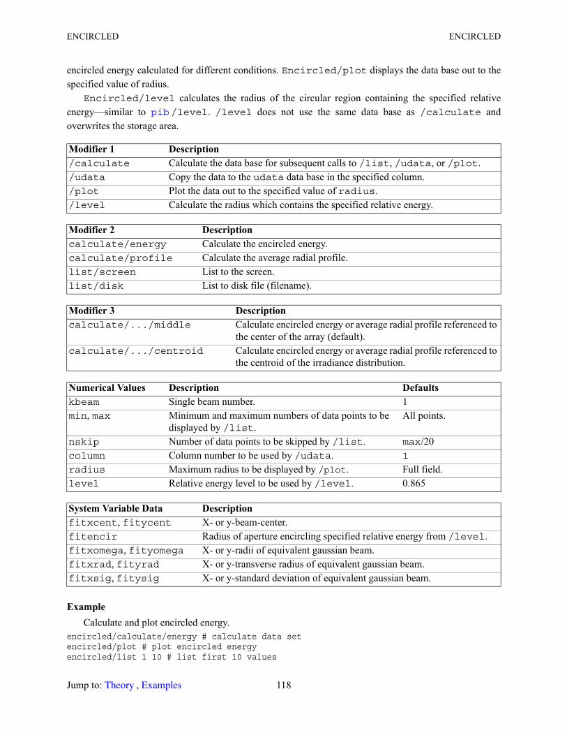
ENCIRCLED ENCIRCLED
encircled energy calculated for different conditions. Encircled/plot displays the data base out to the specified value of radius.
Encircled/level calculates the radius of the circular region containing the specified relative energy—similar to /level. /level does not use the same data base as /calculate and overwrites the storage area.
ExampleCalculate and plot encircled energy.
encircled/calculate/energy # calculate data setencircled/plot # plot encircled energyencircled/list 1 10 # list first 10 values
Modifier 1 Description /calculate Calculate the data base for subsequent calls to /list, /udata, or /plot./udata Copy the data to the udata data base in the specified column./plot Plot the data out to the specified value of radius./level Calculate the radius which contains the specified relative energy.
Modifier 2 Description calculate/energy Calculate the encircled energy.calculate/profile Calculate the average radial profile.list/screen List to the screen.list/disk List to disk file (filename).
Modifier 3 Description calculate/.../middle Calculate encircled energy or average radial profile referenced to
the center of the array (default).calculate/.../centroid Calculate encircled energy or average radial profile referenced to
the centroid of the irradiance distribution.
Numerical Values Description Defaultskbeam Single beam number. 1min, max Minimum and maximum numbers of data points to be
displayed by /list.All points.
nskip Number of data points to be skipped by /list. max/20column Column number to be used by /udata. 1
radius Maximum radius to be displayed by /plot. Full field.level Relative energy level to be used by /level. 0.865
System Variable Data Description fitxcent, fitycent X- or y-beam-center.fitencir Radius of aperture encircling specified relative energy from /level.fitxomega, fityomega X- or y-radii of equivalent gaussian beam.fitxrad, fityrad X- or y-transverse radius of equivalent gaussian beam.fitxsig, fitysig X- or y-standard deviation of equivalent gaussian beam.
pib
Jump to: , 118 Theory Examples

END ENERGY
encircled/calculate/profil # calculate average radial profileencircled/plot # plot average radial profileencircled/udata 1 # put data in column 1 of UDATAplot/udata # plot udata to show same dataencircled/level 1 .5 # find radius containing 50% of energyvariab/set radius fitencir # put radius into a variable
END End and/or restart GLAD. Begin-end
Description: ENDIf called interactive from the Interactive Input window, End reinitializes GLAD. If called from a disk
file or macro end stops reading the file or macro (the same as /back). See also .Also see to restart GLAD to with initial values without ending the program.
ENERGY Calculate the total energy (or power). Diagnostics
Description: ENERGYEnergy/list writes all beam energies and photon counts. The energy in the beam is found by,
Energy = , (50)
where is the complex amplitude and Δx and Δy are the beam units. The summation is taken over all points in the array.
Energy/ginversion integrates the population inversion over a gain array to yield j/cm.The /norm modifier will normalize the energy of a unique beam. The percent loss is printed. Percent
loss is defined to be
Percent loss = 100*(enorm - Eold)/Enorm (51)
where Eold is the energy before the renormalization.
Command Form(s): END end
Command Form(s): ENERGY energy/list ibeams
energy/ginversion ibeams
energy/norm kbeam enorm [list]
Modifier 1 Description /list List energy values.
read readexit
initialize
A x y,( ) 2ΔxΔy
A x y,( )
Jump to: , 119 Theory Examples
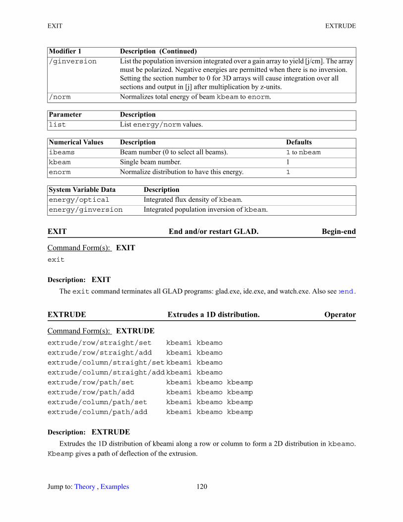
EXIT EXTRUDE
EXIT End and/or restart GLAD. Begin-end
Description: EXITThe exit command terminates all GLAD programs: glad.exe, ide.exe, and watch.exe. Also see .
EXTRUDE Extrudes a 1D distribution. Operator
Description: EXTRUDEExtrudes the 1D distribution of kbeami along a row or column to form a 2D distribution in kbeamo.
Kbeamp gives a path of deflection of the extrusion.
/ginversion List the population inversion integrated over a gain array to yield [j/cm]. The array must be polarized. Negative energies are permitted when there is no inversion. Setting the section number to 0 for 3D arrays will cause integration over all sections and output in [j] after multiplication by z-units.
/norm Normalizes total energy of beam kbeam to enorm.
Parameter Description list List energy/norm values.
Numerical Values Description Defaultsibeams Beam number (0 to select all beams). 1 to nbeamkbeam Single beam number. 1enorm Normalize distribution to have this energy. 1
System Variable Data Description energy/optical Integrated flux density of kbeam.energy/ginversion Integrated population inversion of kbeam.
Command Form(s): EXIT exit
Command Form(s): EXTRUDE extrude/row/straight/set kbeami kbeamo
extrude/row/straight/add kbeami kbeamo
extrude/column/straight/set kbeami kbeamo
extrude/column/straight/add kbeami kbeamo
extrude/row/path/set kbeami kbeamo kbeamp
extrude/row/path/add kbeami kbeamo kbeamp
extrude/column/path/set kbeami kbeamo kbeamp
extrude/column/path/add kbeami kbeamo kbeamp
Modifier 1 Description (Continued)
readend
Jump to: , 120 Theory Examples
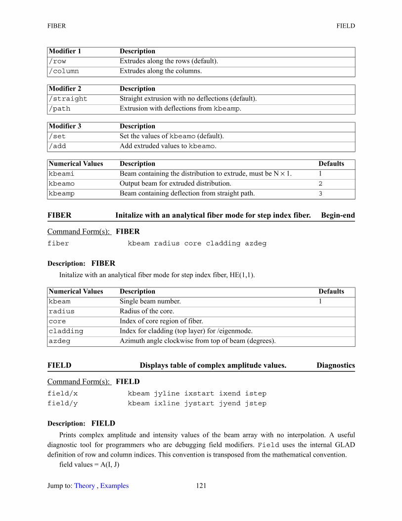
FIBER FIELD
FIBER Initalize with an analytical fiber mode for step index fiber. Begin-end
Description: FIBERInitalize with an analytical fiber mode for step index fiber, HE(1,1).
FIELD Displays table of complex amplitude values. Diagnostics
Description: FIELDPrints complex amplitude and intensity values of the beam array with no interpolation. A useful
diagnostic tool for programmers who are debugging field modifiers. Field uses the internal GLAD definition of row and column indices. This convention is transposed from the mathematical convention.
field values = A(I, J)
Modifier 1 Description /row Extrudes along the rows (default)./column Extrudes along the columns.
Modifier 2 Description /straight Straight extrusion with no deflections (default)./path Extrusion with deflections from kbeamp.
Modifier 3 Description /set Set the values of kbeamo (default)./add Add extruded values to kbeamo.
Numerical Values Description Defaultskbeami Beam containing the distribution to extrude, must be N × 1. 1kbeamo Output beam for extruded distribution. 2
kbeamp Beam containing deflection from straight path. 3
Command Form(s): FIBER fiber kbeam radius core cladding azdeg
Numerical Values Description Defaultskbeam Single beam number. 1radius Radius of the core.core Index of core region of fiber.cladding Index for cladding (top layer) for /eigenmode.azdeg Azimuth angle clockwise from top of beam (degrees).
Command Form(s): FIELD field/x kbeam jyline ixstart ixend istep
field/y kbeam ixline jystart jyend jstep
Jump to: , 121 Theory Examples
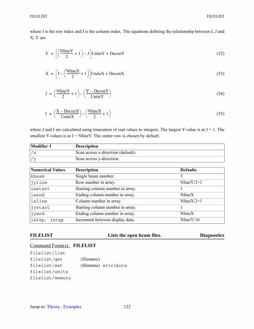
FILELIST FILELIST
where J is the row index and I is the column index. The equations defining the relationship between I, J and X, Y are
(52)
(53)
(54)
(55)
where J and I are calculated using truncation of real values to integers. The largest Y-value is at J = 1. The smallest Y-values is at J = NlineY. The center row is chosen by default.
FILELIST Lists the open beam files. Diagnostics
Modifier 1 Description /x Scan across x-direction (default)./y Scan across y-direction.
Numerical Values Description Defaultskbeam Single beam number. 1jyline Row number in array. NlineY/2+1ixstart Starting column number in array. 1ixend Ending column number in array. NlineXixline Column number in array. NlineX/2+1jystart Starting column number in array. 1jyend Ending column number in array. NlineXistep, jstep Increment between display data. NlineY/16
Command Form(s): FILELIST filelist/list
filelist/get (filename)filelist/set (filename) attributefilelist/units
filelist/memory
Y NlineY2
----------------- 1+ J– UnitsY DecenY+=
X I NlineX2
----------------- 1+ – UnitsX DecenX+=
J NlineY2
----------------- 1+ Y DecenY–
UnitsY------------------------------ –=
I X DecenX–UnitsX
------------------------------ NlineX
2----------------- 1+ –=
Jump to: , 122 Theory Examples
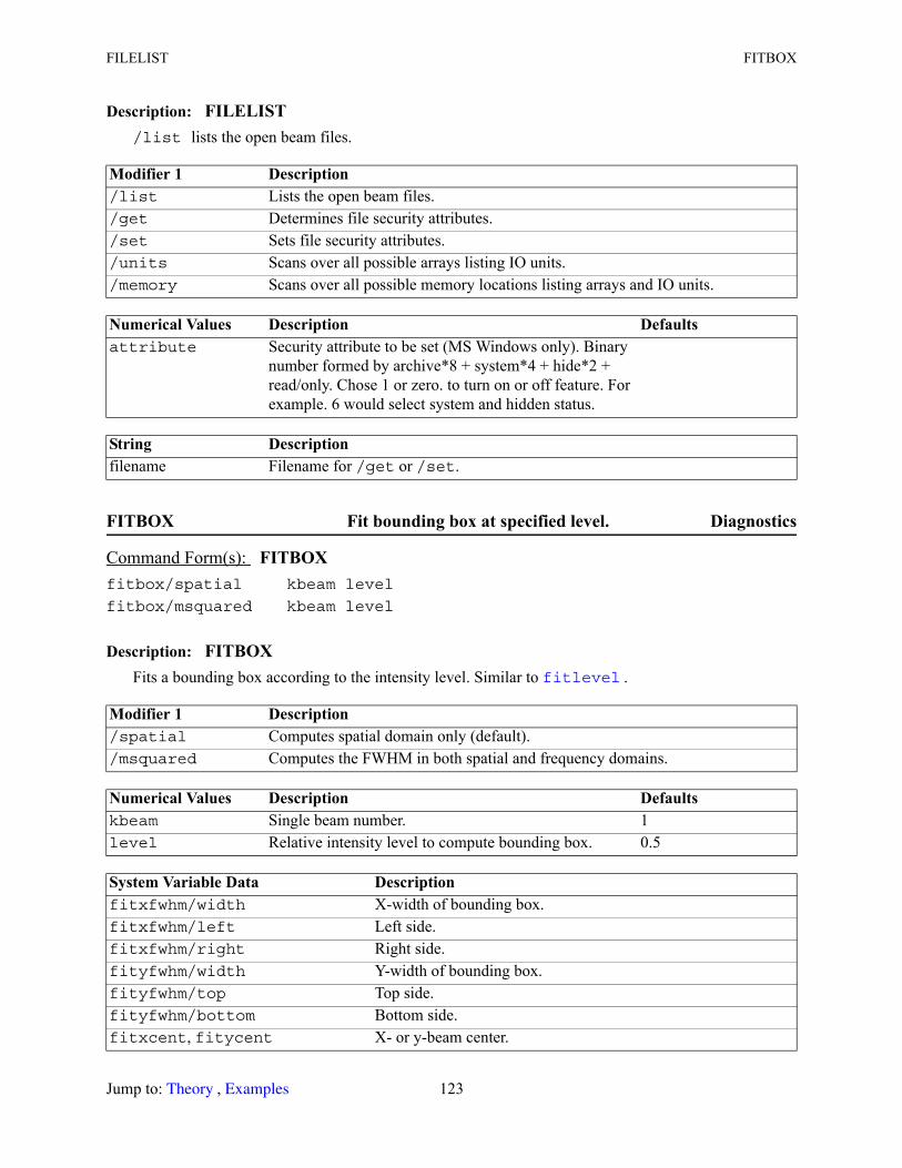
FILELIST FITBOX
Description: FILELIST/list lists the open beam files.
FITBOX Fit bounding box at specified level. Diagnostics
Description: FITBOXFits a bounding box according to the intensity level. Similar to .
Modifier 1 Description /list Lists the open beam files./get Determines file security attributes./set Sets file security attributes./units Scans over all possible arrays listing IO units./memory Scans over all possible memory locations listing arrays and IO units.
Numerical Values Description Defaultsattribute Security attribute to be set (MS Windows only). Binary
number formed by archive*8 + system*4 + hide*2 + read/only. Chose 1 or zero. to turn on or off feature. For example. 6 would select system and hidden status.
String Description filename Filename for /get or /set.
Command Form(s): FITBOX fitbox/spatial kbeam level
fitbox/msquared kbeam level
Modifier 1 Description /spatial Computes spatial domain only (default)./msquared Computes the FWHM in both spatial and frequency domains.
Numerical Values Description Defaultskbeam Single beam number. 1level Relative intensity level to compute bounding box. 0.5
System Variable Data Description fitxfwhm/width X-width of bounding box.fitxfwhm/left Left side.fitxfwhm/right Right side.fityfwhm/width Y-width of bounding box.fityfwhm/top Top side.fityfwhm/bottom Bottom side.fitxcent, fitycent X- or y-beam center.
fitlevel
Jump to: , 123 Theory Examples
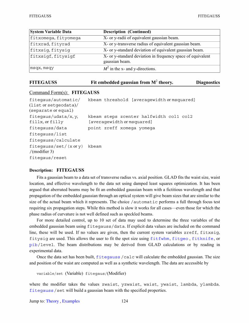
FITEGAUSS FITEGAUSS
FITEGAUSS Fit embedded gaussian from M2 theory. Diagnostics
Description: FITEGAUSSFits a gaussian beam to a data set of transverse radius vs. axial position. GLAD fits the waist size, waist
location, and effective wavelength to the data set using damped least squares optimization. It has been argued that aberrated beams may be fit an embedded gaussian beam with a fictitious wavelength and that propagation of the embedded gaussian through an optical system will give beam sizes that are similar to the size of the actual beam which it represents. The choice /automatic performs a full through focus test requiring six propagation steps. While this method is slow it works for all cases—even those for which the phase radius of curvature is not well defined such as speckled beams.
For more detailed control, up to 10 set of data may used to determine the three variables of the embedded gaussian beam using fitegauss/data. If explicit data values are included on the command line, these will be used. If no values are given, then the current system variables zreff, fitxsig, fitysig are used. This allows the user to fit the spot size using , , , or
/level. The beam distributions may be derived from GLAD calculations or by reading in experimental data.
Once the data set has been built, /calc will calculate the embedded gaussian. The size and position of the waist are computed as well as a synthetic wavelength. The data are accessible by
variable/set (Variable) fitegaus/(Modifier)
where the modifier takes the values zwaist, yzwaist, waist, ywaist, lambda, ylambda. /set will build a gaussian beam with the specified properties.
fitxomega, fityomega X- or y-radii of equivalent gaussian beam.fitxrad, fityrad X- or y-transverse radius of equivalent gaussian beam.fitxsig, fitysig X- or y-standard deviation of equivalent gaussian beam.fitxsigf, fitysigf X- or y-standard deviation in frequency space of equivalent
gaussian beam.msqx, msqy M2 in the x- and y-directions.
Command Form(s): FITEGAUSS fitegaus/automatic/(list or setgeodata)/(separate or equal)
kbeam threshold [averagewidth or msquared]
fitegaus/udata/x, y, fillx, or filly
kbeam steps zcenter halfwidth col1 col2 [averagewidth or msquared]
fitegauss/data point zreff xomega yomega
fitegauss/list
fitegauss/calculate
fitegauss/set/(x or y)/(modifier 3)
kbeam
fitegaus/reset
System Variable Data Description (Continued)
fitfwhm fitgeo fitknife pib
fitegauss
fitegauss
Jump to: , 124 Theory Examples
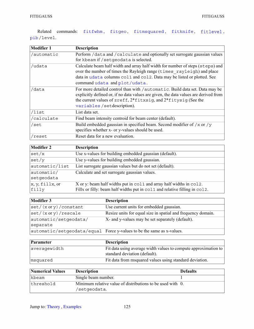
FITEGAUSS FITEGAUSS
Related commands: , , , , , /level.
Modifier 1 Description /automatic Perform /data and /calculate and optionally set surrogate gaussian values
for kbeam if /setgeodata is selected./udata Calculate beam half width and array half width for number of steps (steps) and
over the number of times the Rayleigh range (times_rayleigh) and place data in columns col1 and col2. Data may be listed or plotted. See command and .
/data For more detailed control than with /automatic. Build data set. Data may be explicitly defined or, if no data values are given, the data values are derived from the current values of zreff, 2*fitxsig, and 2*fitysig (See the
/setdescription)./list List data set./calculate Find beam intensity centroid for beam center (default)./set Build embedded gaussian in specified beam. Second modifier of /x or /y
specifies whether x- or y-values should be used./reset Reset data for a new evaluation.
Modifier 2 Description set/x Use x-values for building embedded gaussian (default).set/y Use y-values for building embedded gaussian.automatic/list List surrogate gaussian values but do not set (default).automatic/setgeodata
Calculate and set surrogate gaussian values.
x, y, fillx, or filly
X or y: beam half widths put in col1 and array half widths in col2.Fillx or filly: beam half widths put in col1 and relative filling in col2.
Modifier 3 Description set/(x or y)/constant Use current units for embedded gaussian.set/(x or y)/rescale Resize units for equal size in spatial and frequency domain.automatic/setgeodata/separate
X- and y-values may be set separately (default).
automatic/setgeodata/equal Force y-values to be the same as x-values.
Parameter Description averagewidth Fit data using average width values to compute approximation to
standard deviation (default).msquared Fit data from msquared values using standard deviation.
Numerical Values Description Defaultskbeam Single beam number. 1threshold Minimum relative value of distributions to be used with
/setgeodata.0.
fitfwhm fitgeo fitmsquared fitknife fitlevel pib
udata udata plot/udata
variables
Jump to: , 125 Theory Examples
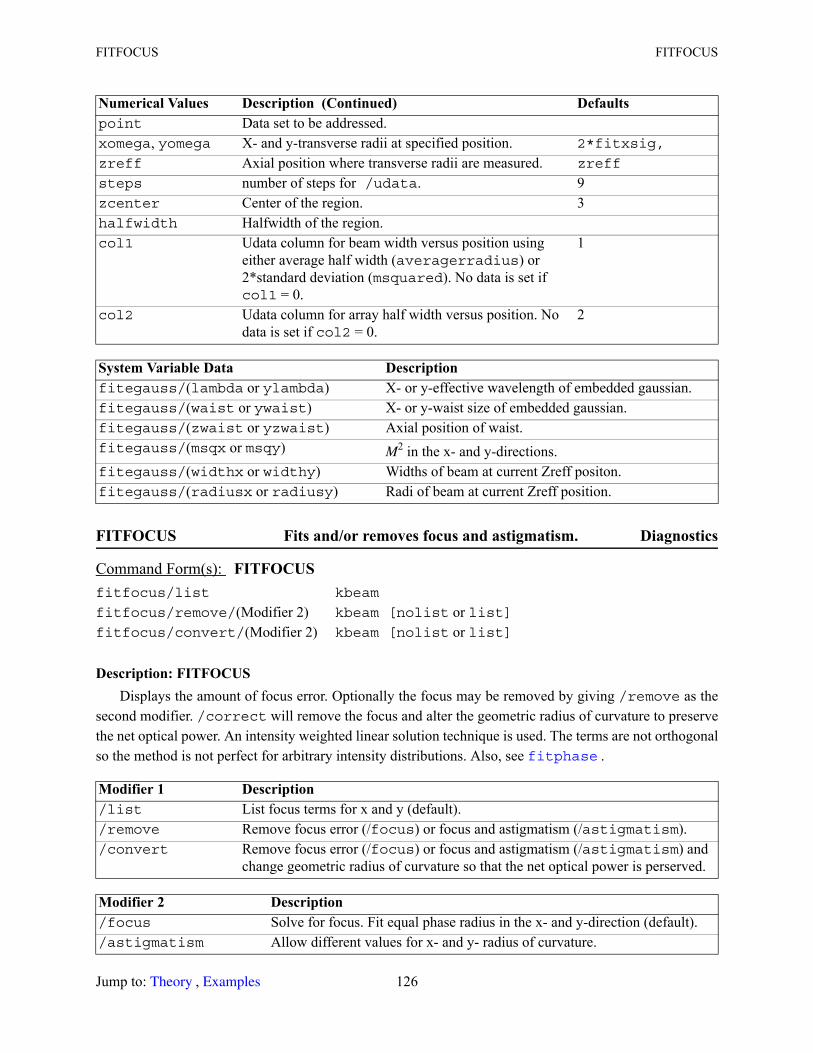
FITFOCUS FITFOCUS
FITFOCUS Fits and/or removes focus and astigmatism. Diagnostics
Description: FITFOCUSDisplays the amount of focus error. Optionally the focus may be removed by giving /remove as the
second modifier. /correct will remove the focus and alter the geometric radius of curvature to preserve the net optical power. An intensity weighted linear solution technique is used. The terms are not orthogonal so the method is not perfect for arbitrary intensity distributions. Also, see .
point Data set to be addressed.xomega, yomega X- and y-transverse radii at specified position. 2*fitxsig,
zreff Axial position where transverse radii are measured. zreff
steps number of steps for /udata. 9zcenter Center of the region. 3halfwidth Halfwidth of the region. col1 Udata column for beam width versus position using
either average half width (averagerradius) or 2*standard deviation (msquared). No data is set if col1 = 0.
1
col2 Udata column for array half width versus position. No data is set if col2 = 0.
2
System Variable Data Description fitegauss/(lambda or ylambda) X- or y-effective wavelength of embedded gaussian.fitegauss/(waist or ywaist) X- or y-waist size of embedded gaussian.fitegauss/(zwaist or yzwaist) Axial position of waist.fitegauss/(msqx or msqy) M2 in the x- and y-directions.fitegauss/(widthx or widthy) Widths of beam at current Zreff positon.fitegauss/(radiusx or radiusy) Radi of beam at current Zreff position.
Command Form(s): FITFOCUS fitfocus/list kbeam
fitfocus/remove/(Modifier 2) kbeam [nolist or list]fitfocus/convert/(Modifier 2) kbeam [nolist or list]
Modifier 1 Description /list List focus terms for x and y (default)./remove Remove focus error (/focus) or focus and astigmatism (/astigmatism)./convert Remove focus error (/focus) or focus and astigmatism (/astigmatism) and
change geometric radius of curvature so that the net optical power is perserved.
Modifier 2 Description /focus Solve for focus. Fit equal phase radius in the x- and y-direction (default)./astigmatism Allow different values for x- and y- radius of curvature.
Numerical Values Description (Continued) Defaults
fitphase
Jump to: , 126 Theory Examples
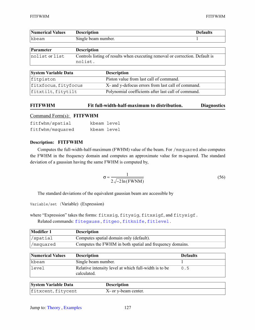
FITFWHM FITFWHM
FITFWHM Fit full-width-half-maximum to distribution. Diagnostics
Description: FITFWHMComputes the full-width-half-maximum (FWHM) value of the beam. For /msquared also computes
the FWHM in the frequency domain and computes an approximate value for m-squared. The standard deviation of a gaussian having the same FWHM is computed by,
(56)
The standard deviations of the equivalent gaussian beam are accessible by
Variable/set (Variable) (Expression)
where “Expression” takes the forms: fitxsig, fitysig, fitxsigf, and fitysigf.Related commands: , , , .
Numerical Values Description Defaultskbeam Single beam number. 1
Parameter Description nolist or list Controls listing of results when executing removal or correction. Default is
nolist.
System Variable Data Description fitpiston Piston value from last call of command.fitxfocus, fityfocus X- and y-defocus errors from last call of command.fitxtilt, fitytilt Polynomial coefficients after last call of command.
Command Form(s): FITFWHM fitfwhm/spatial kbeam level
fitfwhm/msquared kbeam level
Modifier 1 Description /spatial Computes spatial domain only (default)./msquared Computes the FWHM in both spatial and frequency domains.
Numerical Values Description Defaultskbeam Single beam number. 1level Relative intensity level at which full-width is to be
calculated.0.5
System Variable Data Description fitxcent, fitycent X- or y-beam center.
σ 12 2 FWNM( )ln–-------------------------------------------≈
fitegauss fitgeo fitknife fitlevel
Jump to: , 127 Theory Examples
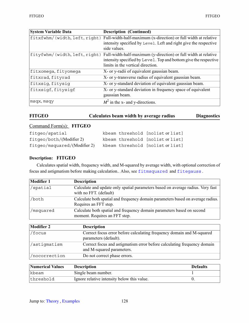
FITGEO FITGEO
FITGEO Calculates beam width by average radius Diagnostics
Description: FITGEOCalculates spatial width, frequency width, and M-squared by average width, with optional correction of
focus and astigmatism before making calculation.. Also, see and .
fitxfwhm/(width, left, right) Full-width-half-maximum (x-direction) or full width at relative intensity specified by Level. Left and right give the respective side values.
fityfwhm/(width, left, right) Full-width-half-maximum (y-direction) or full width at relative intensity specified by Level. Top and bottom give the respective limits in the vertical direction.
fitxomega, fityomega X- or y-radii of equivalent gaussian beam.fitxrad, fityrad X- or y-transverse radius of equivalent gaussian beam.fitxsig, fitysig X- or y-standard deviation of equivalent gaussian beam.fitxsigf, fitysigf X- or y-standard deviation in frequency space of equivalent
gaussian beam.msqx, msqy M2 in the x- and y-directions.
Command Form(s): FITGEO fitgeo/spatial kbeam threshold [nolist or list]fitgeo/both/(Modifier 2) kbeam threshold [nolist or list]fitgeo/msquared/(Modifier 2) kbeam threshold [nolist or list]
Modifier 1 Description /spatial Calculate and update only spatial parameters based on average radius. Very fast
with no FFT. (default)/both Calculate both spatial and frequency domain parameters based on average radius.
Requires an FFT step./msquared Calculate both spatial and frequency domain parameters based on second
moment. Requires an FFT step.
Modifier 2 Description /focus Correct focus error before calculating frequency domain and M-squared
parameters (default)./astigmatism Correct focus and astigmatism error before calculating frequency domain
and M-squared parameters./nocorrection Do not correct phase errors.
Numerical Values Description Defaultskbeam Single beam number. 1threshold Ignore relative intensity below this value. 0.
System Variable Data Description (Continued)
fitmsquared fitegauss
Jump to: , 128 Theory Examples
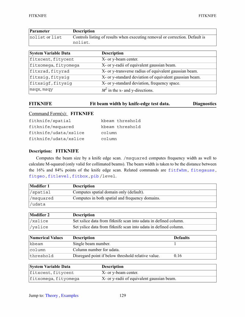
FITKNIFE FITKNIFE
FITKNIFE Fit beam width by knife-edge test data. Diagnostics
Description: FITKNIFEComputes the beam size by a knife edge scan. /msquared computes frequency width as well to
calculate M-squared (only valid for collimated beams). The beam width is taken to be the distance between the 16% and 84% points of the knife edge scan. Related commands are , ,
, , , /level.
Parameter Description nolist or list Controls listing of results when executing removal or correction. Default is
nolist.
System Variable Data Description fitxcent, fitycent X- or y-beam center.fitxomega, fityomega X- or y-radii of equivalent gaussian beam.fitxrad,fityrad X- or y-transverse radius of equivalent gaussian beam.fitxsig,fitysig X- or y-standard deviation of equivalent gaussian beam.fitxsigf,fitysig X- or y-standard deviation, frequency space.msqx, msqy M2 in the x- and y-directions.
Command Form(s): FITKNIFE fitknife/spatial kbeam threshold
fitknife/msquared kbeam threshold
fitknife/udata/xslice column
fitknife/udata/xslice column
Modifier 1 Description /spatial Computes spatial domain only (default)./msquared Computes in both spatial and frequency domains./udata
Modifier 2 Description /xslice Set xslice data from fitknife scan into udata in defined column./yslice Set yslice data from fitknife scan into udata in defined column.
Numerical Values Description Defaultskbeam Single beam number. 1column Column number for udata.threshold Disregard point if below threshold relative value. 0.16
System Variable Data Description fitxcent, fitycent X- or y-beam center.fitxomega, fityomega X- or y-radii of equivalent gaussian beam.
fitfwhm fitegauss fitgeo fitlevel fitbox pib
Jump to: , 129 Theory Examples
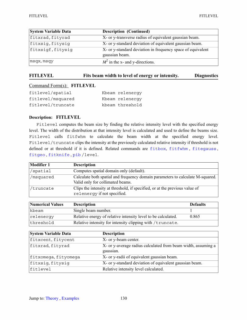
FITLEVEL FITLEVEL
FITLEVEL Fits beam width to level of energy or intensity. Diagnostics
Description: FITLEVELFitlevel computes the beam size by finding the relative intensity level with the specified energy
level. The width of the distribution at that intensity level is calculated and used to define the beams size. Fitlevel calls fitfwhm to calculate the beam width at the specified energy level. Fitlevel/truncate clips the intensity at the previously calculated relative intensity if threshold is not defined or at threshold if it is defined. Related commands are , , ,
, , /level.
fitxrad,fityrad X- or y-transverse radius of equivalent gaussian beam.fitxsig,fitysig X- or y-standard deviation of equivalent gaussian beam.fitxsigf,fitysig X- or y-standard deviation in frequency space of equivalent
gaussian beam.msqx, msqy M2 in the x- and y-directions.
Command Form(s): FITLEVEL fitlevel/spatial Kbeam relenergy
fitlevel/msquared Kbeam relenergy
fitlevel/truncate kbeam threshold
Modifier 1 Description /spatial Computes spatial domain only (default)./msquared Calculate both spatial and frequency domain parameters to calculate M-squared.
Valid only for collimated beams./truncate Clips the intensity at threshold, if specified, or at the previous value of
relenergy if not specified.
Numerical Values Description Defaultskbeam Single beam number. 1relenergy Relative energy of relative intensity level to be calculated. 0.865threshold Relative intensity for intensity clipping with /truncate.
System Variable Data Description fitxcent, fitycent X- or y-beam center.fitxrad, fityrad X- or y-average radius calculated from beam width, assuming a
gaussian.fitxomega, fityomega X- or y-radii of equivalent gaussian beam.fitxsig, fitysig X- or y-standard deviation of equivalent gaussian beam.fitlevel Relative intensity level calculated.
System Variable Data Description (Continued)
fitbox fitfwhm fitegauss fitgeo fitknife pib
Jump to: , 130 Theory Examples

FITMSQUARED FITPHASE
FITMSQUARED Calculates beam width and M-squared. Diagnostics
Description: FITMSQUAREDCalculates spatial width, frequency width, and M-squared with optional correction of focus and
astigmatism before making calculation. M-squared is calculated by product of spatial and frequency standard deviations. Also, see and .
FITPHASE Fits tilt, focus, and astigmatism. Diagnostics
Command Form(s): FITMSQUARED fitmsquared/spatial kbeam threshold [nolist or list]fitmsquared/both/(Modifier 2) kbeam threshold [nolist or list]
Modifier 1 Description /spatial Calculate and update only spatial parameters.. Very fast with no FFT. This choice
does not calculate M-squared values as no frequency information is calculated. (default)
/both Calculate both spatial and frequency domain parameters. Requires an FFT step.
Modifier 2 Description /focus Correct focus error before calculating frequency domain and M-squared
parameters (default)./astigmatism Correct focus and astigmatism error before calculating frequency domain
and M-squared parameters./nocorrection Do not correct phase errors.
Numerical Values Description Defaultskbeam Single beam number. 1threshold Ignore relative intensity below this value. 0.
Parameter Description nolist or list Controls listing of results when executing removal or correction. Default is
nolist.
System Variable Data Description fitxcent, fitycent X- or y-beam center.fitxomega, fityomega X- or y-radii of equivalent gaussian beam.fitxrad,fityrad X- or y-transverse radius of equivalent gaussian beam.fitxsig,fitysig X- or y-standard deviation of equivalent gaussian beam.fitxsigf,fitysig X- or y-standard deviation, frequency space.msqx, msqy M2 in the x- and y-directions.
Command Form(s): FITPHASE fitphase/(Modifier 1)/(Modifier 2) kbeam [Parameter]
fitgeo fitegauss
Jump to: , 131 Theory Examples
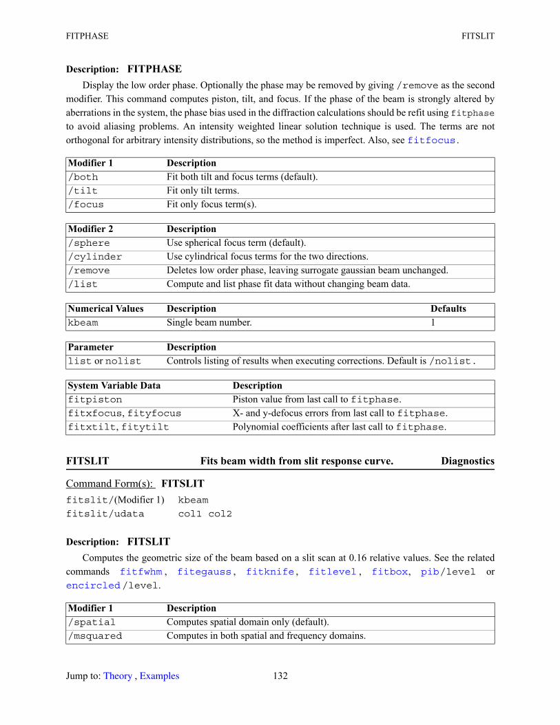
FITPHASE FITSLIT
Description: FITPHASEDisplay the low order phase. Optionally the phase may be removed by giving /remove as the second
modifier. This command computes piston, tilt, and focus. If the phase of the beam is strongly altered by aberrations in the system, the phase bias used in the diffraction calculations should be refit using fitphaseto avoid aliasing problems. An intensity weighted linear solution technique is used. The terms are not orthogonal for arbitrary intensity distributions, so the method is imperfect. Also, see .
FITSLIT Fits beam width from slit response curve. Diagnostics
Description: FITSLITComputes the geometric size of the beam based on a slit scan at 0.16 relative values. See the related
commands , , , , , /level or /level.
Modifier 1 Description /both Fit both tilt and focus terms (default)./tilt Fit only tilt terms./focus Fit only focus term(s).
Modifier 2 Description /sphere Use spherical focus term (default)./cylinder Use cylindrical focus terms for the two directions./remove Deletes low order phase, leaving surrogate gaussian beam unchanged./list Compute and list phase fit data without changing beam data.
Numerical Values Description Defaultskbeam Single beam number. 1
Parameter Description list or nolist Controls listing of results when executing corrections. Default is /nolist.
System Variable Data Description fitpiston Piston value from last call to fitphase.fitxfocus, fityfocus X- and y-defocus errors from last call to fitphase.fitxtilt, fitytilt Polynomial coefficients after last call to fitphase.
Command Form(s): FITSLIT fitslit/(Modifier 1) kbeam
fitslit/udata col1 col2
Modifier 1 Description /spatial Computes spatial domain only (default)./msquared Computes in both spatial and frequency domains.
fitfocus
fitfwhm fitegauss fitknife fitlevel fitbox pib encircled
Jump to: , 132 Theory Examples
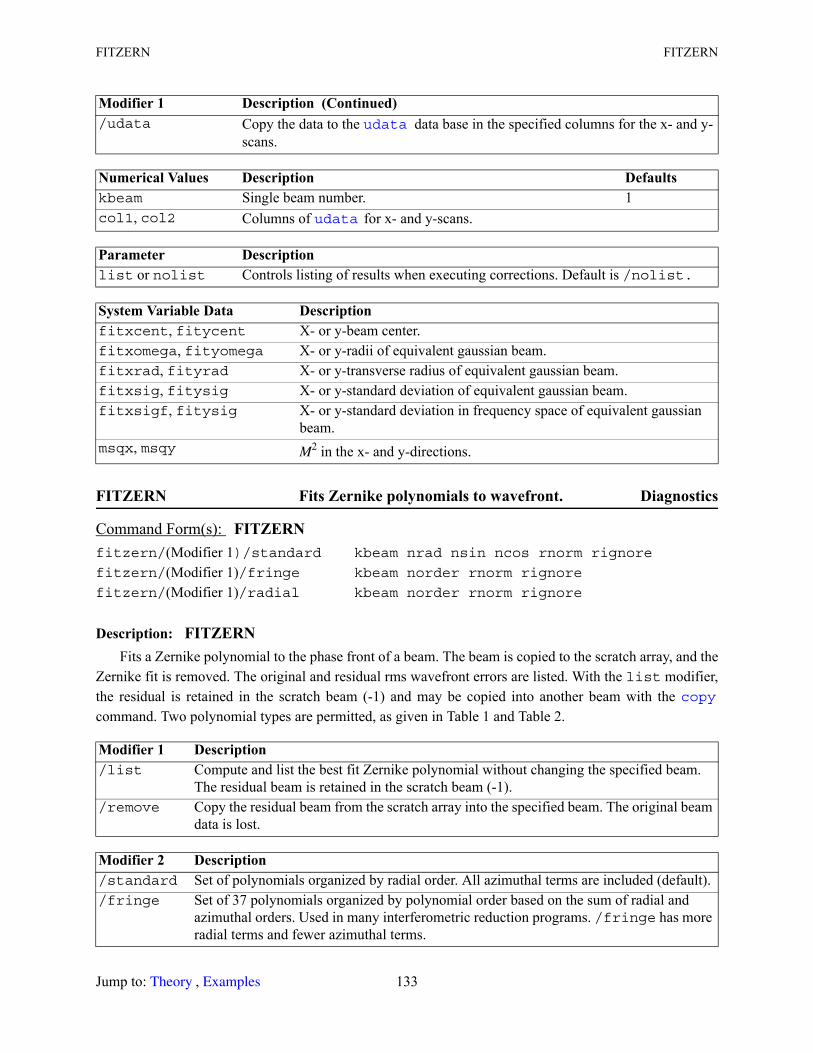
FITZERN FITZERN
FITZERN Fits Zernike polynomials to wavefront. Diagnostics
Description: FITZERNFits a Zernike polynomial to the phase front of a beam. The beam is copied to the scratch array, and the
Zernike fit is removed. The original and residual rms wavefront errors are listed. With the list modifier, the residual is retained in the scratch beam (-1) and may be copied into another beam with the command. Two polynomial types are permitted, as given in Table 1 and Table 2.
/udata Copy the data to the data base in the specified columns for the x- and y-scans.
Numerical Values Description Defaultskbeam Single beam number. 1col1, col2 Columns of for x- and y-scans.
Parameter Description list or nolist Controls listing of results when executing corrections. Default is /nolist.
System Variable Data Description fitxcent, fitycent X- or y-beam center.fitxomega, fityomega X- or y-radii of equivalent gaussian beam.fitxrad, fityrad X- or y-transverse radius of equivalent gaussian beam.fitxsig, fitysig X- or y-standard deviation of equivalent gaussian beam.fitxsigf, fitysig X- or y-standard deviation in frequency space of equivalent gaussian
beam.msqx, msqy M2 in the x- and y-directions.
Command Form(s): FITZERN fitzern/(Modifier 1)/standard kbeam nrad nsin ncos rnorm rignore
fitzern/(Modifier 1)/fringe kbeam norder rnorm rignore
fitzern/(Modifier 1)/radial kbeam norder rnorm rignore
Modifier 1 Description /list Compute and list the best fit Zernike polynomial without changing the specified beam.
The residual beam is retained in the scratch beam (-1)./remove Copy the residual beam from the scratch array into the specified beam. The original beam
data is lost.
Modifier 2 Description /standard Set of polynomials organized by radial order. All azimuthal terms are included (default)./fringe Set of 37 polynomials organized by polynomial order based on the sum of radial and
azimuthal orders. Used in many interferometric reduction programs. /fringe has more radial terms and fewer azimuthal terms.
Modifier 1 Description (Continued) udata
udata
copy
Jump to: , 133 Theory Examples
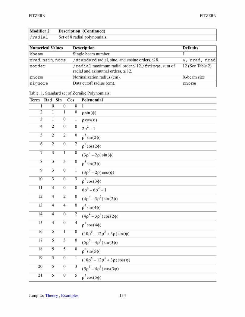
FITZERN FITZERN
/radial Set of 8 radial polynomials.
Numerical Values Description Defaultskbeam Single beam number. 1nrad, nsin, ncos /standard radial, sine, and cosine orders, ≤ 8. 4, nrad, nrad
norder /radial maximum radial order ≤ 12./fringe, sum of radial and azimuthal orders, ≤ 12.
12 (See Table 2)
rnorm Normalization radius (cm). X-beam sizerignore Data cutoff radius (cm). rnorm
Table. 1. Standard set of Zernike Polynomials. Term Rad Sin Cos Polynomial
1 0 0 0 12 1 1 03 1 0 14 2 0 0
5 2 2 0
6 2 0 2
7 3 1 0
8 3 3 0
9 3 0 1
10 3 0 3
11 4 0 0
12 4 2 0
13 4 4 0
14 4 0 2
15 4 0 4
16 5 1 0
17 5 3 0
18 5 5 0
19 5 0 1
20 5 0 3
21 5 0 5
Modifier 2 Description (Continued)
ρ φ( )sinρ φ( )cos
2ρ2 1–
ρ2 2φ( )sin
ρ2 2φ( )cos
3ρ3 2ρ–( ) φ( )sin
ρ3 3φ( )sin
3ρ3 2ρ–( ) φ( )cos
ρ3 3φ( )cos
6ρ4 6ρ2– 1+
4ρ4 3ρ2–( ) 2φ( )sin
ρ4 4φ( )sin
4ρ4 3ρ2–( ) 2φ( )cos
ρ4 4φ( )cos
10ρ5 12ρ3– 3ρ+( ) ϕ( )sin
5ρ5 4ρ3–( ) 3φ( )sin
ρ5 5φ( )sin
10ρ5 12ρ3– 3ρ+( ) ϕ( )cos
5ρ5 4ρ3–( ) 3ϕ( )cos
ρ5 5φ( )cos
Jump to: , 134 Theory Examples
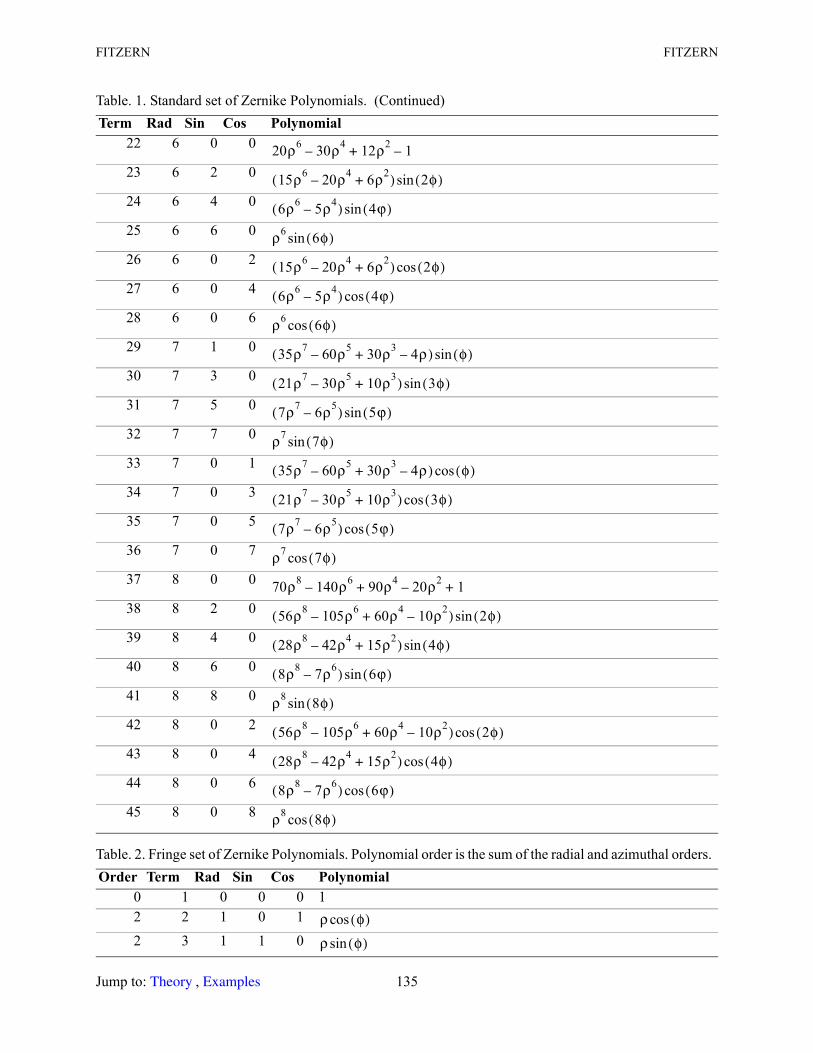
FITZERN FITZERN
22 6 0 0
23 6 2 0
24 6 4 0
25 6 6 0
26 6 0 2
27 6 0 4
28 6 0 6
29 7 1 0
30 7 3 0
31 7 5 0
32 7 7 0
33 7 0 1
34 7 0 3
35 7 0 5
36 7 0 7
37 8 0 0
38 8 2 0
39 8 4 0
40 8 6 0
41 8 8 0
42 8 0 2
43 8 0 4
44 8 0 6
45 8 0 8
Table. 2. Fringe set of Zernike Polynomials. Polynomial order is the sum of the radial and azimuthal orders. Order Term Rad Sin Cos Polynomial
0 1 0 0 0 12 2 1 0 12 3 1 1 0
Table. 1. Standard set of Zernike Polynomials. (Continued)Term Rad Sin Cos Polynomial
20ρ6 30ρ4– 12ρ2 1–+
15ρ6 20ρ4– 6ρ2+( ) 2φ( )sin
6ρ6 5ρ4–( ) 4ϕ( )sin
ρ6 6φ( )sin
15ρ6 20ρ4– 6ρ2+( ) 2φ( )cos
6ρ6 5ρ4–( ) 4ϕ( )cos
ρ6 6φ( )cos
35ρ7 60ρ5– 30ρ3 4ρ–+( ) φ( )sin
21ρ7 30ρ5– 10ρ3+( ) 3φ( )sin
7ρ7 6ρ5–( ) 5ϕ( )sin
ρ7 7φ( )sin
35ρ7 60ρ5– 30ρ3 4ρ–+( ) φ( )cos
21ρ7 30ρ5– 10ρ3+( ) 3φ( )cos
7ρ7 6ρ5–( ) 5ϕ( )cos
ρ7 7φ( )cos
70ρ8 140ρ6– 90ρ4 20ρ2– 1+ +
56ρ8 105ρ6– 60ρ4 10ρ2–+( ) 2φ( )sin
28ρ8 42ρ4– 15ρ2+( ) 4φ( )sin
8ρ8 7ρ6–( ) 6ϕ( )sin
ρ8 8φ( )sin
56ρ8 105ρ6– 60ρ4 10ρ2–+( ) 2φ( )cos
28ρ8 42ρ4– 15ρ2+( ) 4φ( )cos
8ρ8 7ρ6–( ) 6ϕ( )cos
ρ8 8φ( )cos
ρ φ( )cosρ φ( )sin
Jump to: , 135 Theory Examples
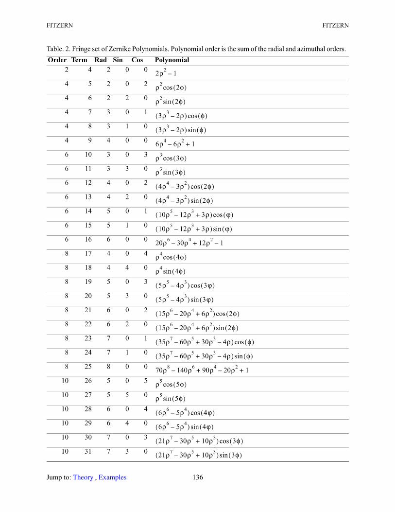
FITZERN FITZERN
2 4 2 0 0
4 5 2 0 2
4 6 2 2 0
4 7 3 0 1
4 8 3 1 0
4 9 4 0 0
6 10 3 0 3
6 11 3 3 0
6 12 4 0 2
6 13 4 2 0
6 14 5 0 1
6 15 5 1 0
6 16 6 0 0
8 17 4 0 4
8 18 4 4 0
8 19 5 0 3
8 20 5 3 0
8 21 6 0 2
8 22 6 2 0
8 23 7 0 1
8 24 7 1 0
8 25 8 0 0
10 26 5 0 5
10 27 5 5 0
10 28 6 0 4
10 29 6 4 0
10 30 7 0 3
10 31 7 3 0
Table. 2. Fringe set of Zernike Polynomials. Polynomial order is the sum of the radial and azimuthal orders. Order Term Rad Sin Cos Polynomial
2ρ2 1–
ρ2 2φ( )cos
ρ2 2φ( )sin
3ρ3 2ρ–( ) φ( )cos
3ρ3 2ρ–( ) φ( )sin
6ρ4 6ρ2– 1+
ρ3 3φ( )cos
ρ3 3φ( )sin
4ρ4 3ρ2–( ) 2φ( )cos
4ρ4 3ρ2–( ) 2φ( )sin
10ρ5 12ρ3– 3ρ+( ) ϕ( )cos
10ρ5 12ρ3– 3ρ+( ) ϕ( )sin
20ρ6 30ρ4– 12ρ2 1–+
ρ4 4φ( )cos
ρ4 4φ( )sin
5ρ5 4ρ3–( ) 3ϕ( )cos
5ρ5 4ρ3–( ) 3ϕ( )sin
15ρ6 20ρ4– 6ρ2+( ) 2φ( )cos
15ρ6 20ρ4– 6ρ2+( ) 2φ( )sin
35ρ7 60ρ5– 30ρ3 4ρ–+( ) φ( )cos
35ρ7 60ρ5– 30ρ3 4ρ–+( ) φ( )sin
70ρ8 140ρ6– 90ρ4 20ρ2– 1+ +
ρ5 5φ( )cos
ρ5 5φ( )sin
6ρ6 5ρ4–( ) 4ϕ( )cos
6ρ6 5ρ4–( ) 4ϕ( )sin
21ρ7 30ρ5– 10ρ3+( ) 3φ( )cos
21ρ7 30ρ5– 10ρ3+( ) 3φ( )sin
Jump to: , 136 Theory Examples
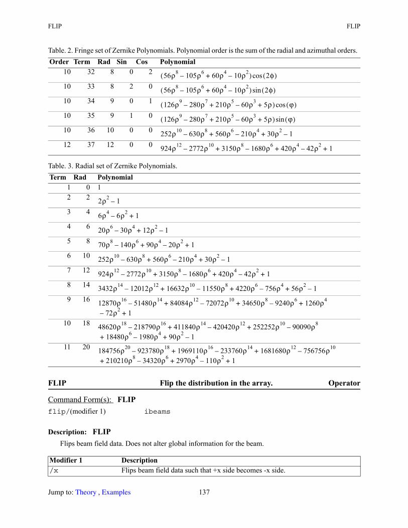
FLIP FLIP
FLIP Flip the distribution in the array. Operator
Description: FLIPFlips beam field data. Does not alter global information for the beam.
10 32 8 0 2
10 33 8 2 0
10 34 9 0 1
10 35 9 1 0
10 36 10 0 0
12 37 12 0 0
Table. 3. Radial set of Zernike Polynomials. Term Rad Polynomial
1 0 12 2
3 4
4 6
5 8
6 10
7 12
8 14
9 16
10 18
11 20
Command Form(s): FLIP flip/(modifier 1) ibeams
Modifier 1 Description /x Flips beam field data such that +x side becomes -x side.
Table. 2. Fringe set of Zernike Polynomials. Polynomial order is the sum of the radial and azimuthal orders. Order Term Rad Sin Cos Polynomial
56ρ8 105ρ6– 60ρ4 10ρ2–+( ) 2φ( )cos
56ρ8 105ρ6– 60ρ4 10ρ2–+( ) 2φ( )sin
126ρ9 280ρ7– 210ρ5 60ρ3– 5ρ+ +( ) ϕ( )cos
126ρ9 280ρ7– 210ρ5 60ρ3– 5ρ+ +( ) ϕ( )sin
252ρ10 630ρ8– 560ρ6 210ρ4– 30ρ2 1–+ +
924ρ12 2772ρ10– 3150ρ8 1680ρ6– 420ρ4 42ρ2– 1+ + +
2ρ2 1–
6ρ4 6ρ2– 1+
20ρ6 30ρ4– 12ρ2 1–+
70ρ8 140ρ6– 90ρ4 20ρ2– 1+ +
252ρ10 630ρ8– 560ρ6 210ρ4– 30ρ2 1–+ +
924ρ12 2772ρ10– 3150ρ8 1680ρ6– 420ρ4 42ρ2– 1+ + +
3432ρ14 12012ρ12– 16632ρ10 11550ρ8– 4220ρ6 756ρ4– 56ρ2 1–+ + +
12870ρ16 51480ρ14– 84084ρ12 72072ρ10– 34650ρ8 9240ρ6– 1260ρ4
72ρ2– 1+ + +
+
48620ρ18 218790ρ16– 411840ρ14 420420ρ12– 252252ρ10 90090ρ8–18480ρ6 1980ρ4– 90ρ2 1–
+ ++ +
184756ρ20 923780ρ18– 1969110ρ16 233760ρ14– 1681680ρ12 756756ρ10–210210ρ8 34320ρ6– 2970ρ4 110ρ2– 1
+ ++ + +
Jump to: , 137 Theory Examples
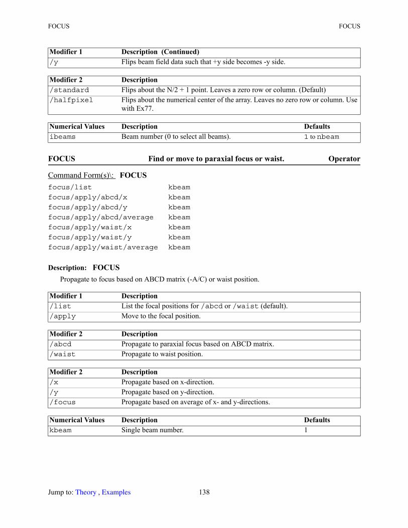
FOCUS FOCUS
FOCUS Find or move to paraxial focus or waist. Operator
Description: FOCUSPropagate to focus based on ABCD matrix (-A/C) or waist position.
/y Flips beam field data such that +y side becomes -y side.
Modifier 2 Description /standard Flips about the N/2 + 1 point. Leaves a zero row or column. (Default)/halfpixel Flips about the numerical center of the array. Leaves no zero row or column. Use
with Ex77.
Numerical Values Description Defaultsibeams Beam number (0 to select all beams). 1 to nbeam
Command Form(s)\: FOCUS focus/list kbeam
focus/apply/abcd/x kbeam
focus/apply/abcd/y kbeam
focus/apply/abcd/average kbeam
focus/apply/waist/x kbeam
focus/apply/waist/y kbeam
focus/apply/waist/average kbeam
Modifier 1 Description /list List the focal positions for /abcd or /waist (default)./apply Move to the focal position.
Modifier 2 Description /abcd Propagate to paraxial focus based on ABCD matrix./waist Propagate to waist position.
Modifier 2 Description /x Propagate based on x-direction./y Propagate based on y-direction./focus Propagate based on average of x- and y-directions.
Numerical Values Description Defaultskbeam Single beam number. 1
Modifier 1 Description (Continued)
Jump to: , 138 Theory Examples
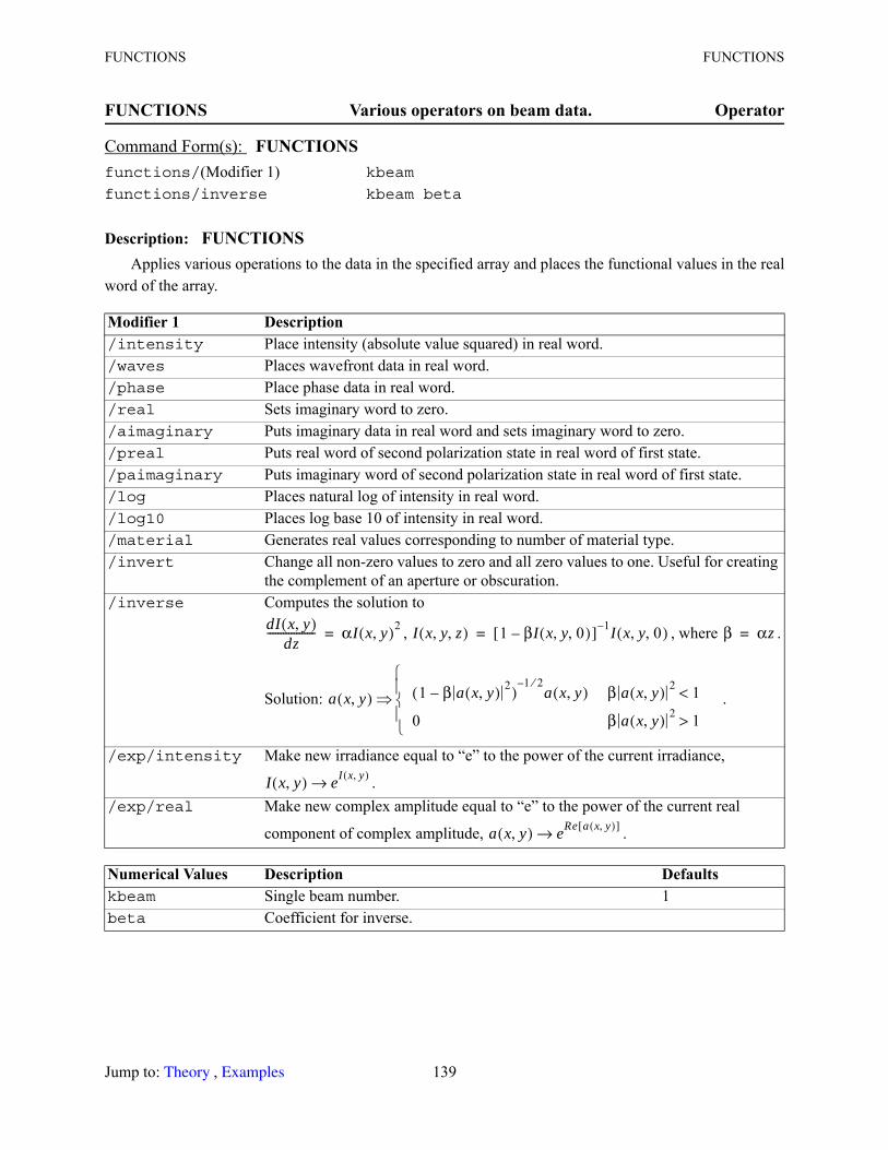
FUNCTIONS FUNCTIONS
FUNCTIONS Various operators on beam data. Operator
Description: FUNCTIONSApplies various operations to the data in the specified array and places the functional values in the real
word of the array.
Command Form(s): FUNCTIONS functions/(Modifier 1) kbeam
functions/inverse kbeam beta
Modifier 1 Description /intensity Place intensity (absolute value squared) in real word./waves Places wavefront data in real word./phase Place phase data in real word./real Sets imaginary word to zero./aimaginary Puts imaginary data in real word and sets imaginary word to zero./preal Puts real word of second polarization state in real word of first state./paimaginary Puts imaginary word of second polarization state in real word of first state./log Places natural log of intensity in real word./log10 Places log base 10 of intensity in real word./material Generates real values corresponding to number of material type./invert Change all non-zero values to zero and all zero values to one. Useful for creating
the complement of an aperture or obscuration./inverse Computes the solution to
, , where .
Solution: .
/exp/intensity Make new irradiance equal to “e” to the power of the current irradiance,
./exp/real Make new complex amplitude equal to “e” to the power of the current real
component of complex amplitude, .
Numerical Values Description Defaultskbeam Single beam number. 1beta Coefficient for inverse.
dI x y,( )dz
------------------ αI x y,( )2= I x y z, ,( ) 1 βI x y 0, ,( )–[ ] 1– I x y 0, ,( )= β αz=
a x y,( ) 1 β a x y,( ) 2–( )1 2⁄–
a x y,( ) β a x y,( ) 2 1<
0 β a x y,( ) 2 1>
I x y,( ) eI x y,( )→
a x y,( ) eRe a x y,( )[ ]→
Jump to: , 139 Theory Examples
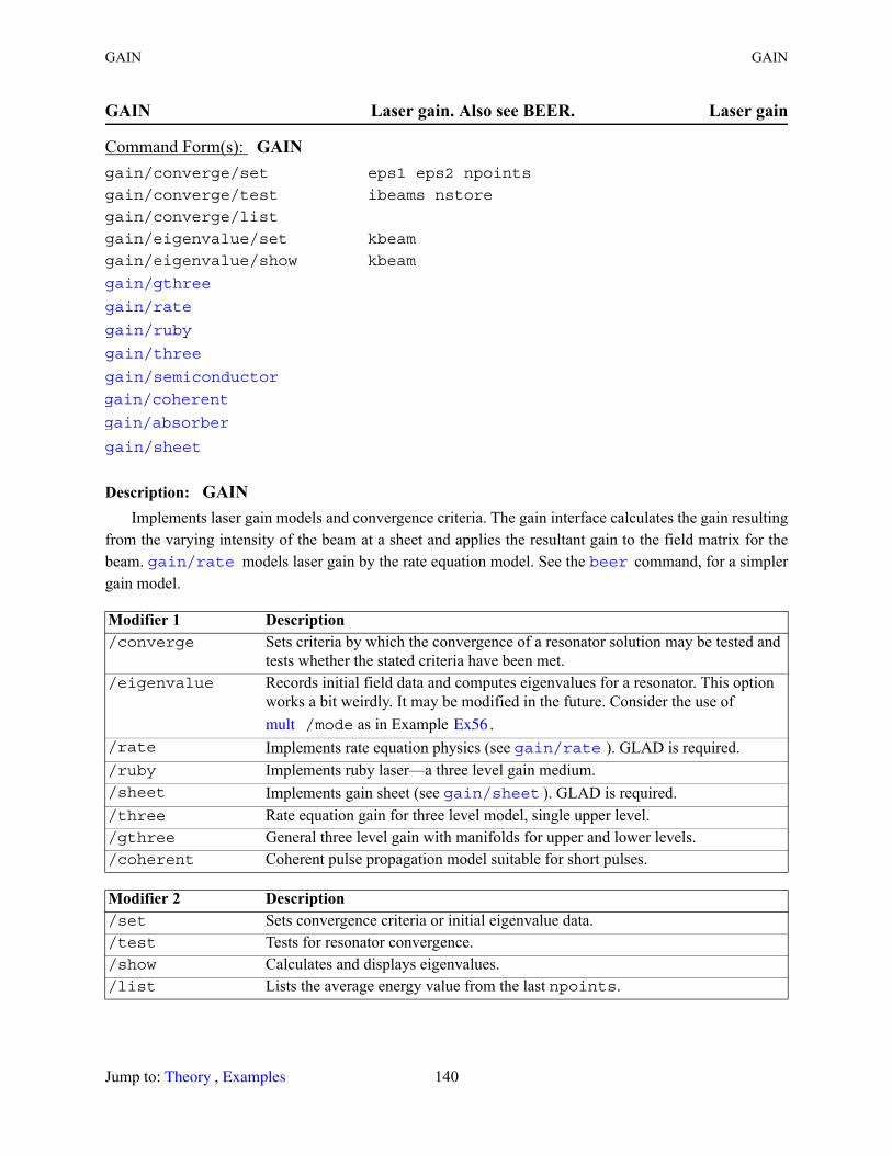
GAIN GAIN
GAIN Laser gain. Also see BEER. Laser gain
Description: GAINImplements laser gain models and convergence criteria. The gain interface calculates the gain resulting
from the varying intensity of the beam at a sheet and applies the resultant gain to the field matrix for the beam. models laser gain by the rate equation model. See the command, for a simpler gain model.
Command Form(s): GAIN gain/converge/set eps1 eps2 npoints
gain/converge/test ibeams nstore
gain/converge/list
gain/eigenvalue/set kbeam
gain/eigenvalue/show kbeam
Modifier 1 Description /converge Sets criteria by which the convergence of a resonator solution may be tested and
tests whether the stated criteria have been met. /eigenvalue Records initial field data and computes eigenvalues for a resonator. This option
works a bit weirdly. It may be modified in the future. Consider the use of /mode as in Example .
/rate Implements rate equation physics (see ). GLAD is required./ruby Implements ruby laser—a three level gain medium./sheet Implements gain sheet (see ). GLAD is required./three Rate equation gain for three level model, single upper level./gthree General three level gain with manifolds for upper and lower levels./coherent Coherent pulse propagation model suitable for short pulses.
Modifier 2 Description /set Sets convergence criteria or initial eigenvalue data./test Tests for resonator convergence. /show Calculates and displays eigenvalues. /list Lists the average energy value from the last npoints.
gain/gthree gain/rate gain/ruby gain/three gain/semiconductor gain/coherent gain/absorber gain/sheet
gain/rate beer
mult Ex56
gain/rate
gain/sheet
Jump to: , 140 Theory Examples

GAIN/GTHREE GAIN/GTHREE
Example of gain/converge/test variab/dec countgain/conv/set eps1=.2 npoints=4macro/def step/o count = count + 1 arg = 1 - exp(-count/5) energy/norm 1 arg gain/conv/test 1 x variab/set Energy 1 energy udata/set count count Energy if x=1 macro/exit/allmacro/endmacro step/9udata/listc We see that the Energy at pass 6 was .698814c and at pass 9 was .834717. The relative energy change iscc rel energy change .162813 = (.834717 - .698814)/.834717cc Since .162813 is less than eps1 = .2, the process convergesc on the 9th pass
GAIN/GTHREE Rate equation gain for general three level atom. Laser gain
Numerical Values Description Defaultseps1 Fractional change in energy convergence criterion. 0.eps2 Criterion based on change in absolute value of field of center point.
If the change in energy or field is less than the appropriate criterion, convergence is considered to have occurred. If both criteria are set, both must be met for convergence.
0.
npoints Number of iterations over which the energy change is computed. 5
nstore Variable name or integer register address where the convergence returned. One is returned if the convergence criteria are met, zero if not.
1
ibeams Beam selector. If 1 <= ibeams <= current number of beams then beam number ibeams is selected. If ibeams = 0, all active beams are selected.
0
zstep Distance through gain medium.
Command Form(s): GAIN/GTHREE gain/gthree/set width cavity tspont t20 offset
gain/gthree/list
gain/gthree/(noise or nonoise)gain/gthree/step zstep time
gain/gthree/pump/(set or add) kbeami kbeamo wavelength
gain/gthree/n2level/(set or add) kbeami kbeamo wavelength
gain/gthree/ntotal/(set or add) kbeami kbeamo wavelength
gain/gthree/upper freq0 degeneracy freq1 freq2 freq3 freq4 freq5 freq6 freq7 freq8 freq9
Jump to: , 141 Theory Examples
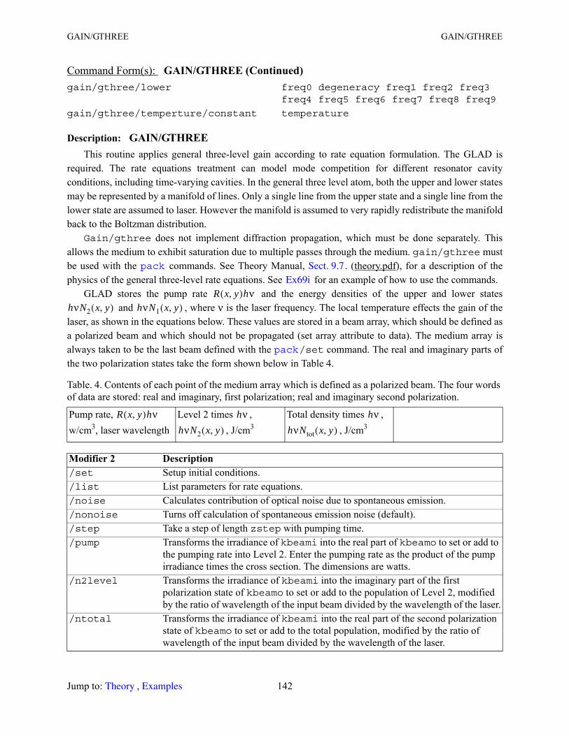
GAIN/GTHREE GAIN/GTHREE
Description: GAIN/GTHREEThis routine applies general three-level gain according to rate equation formulation. The GLAD is
required. The rate equations treatment can model mode competition for different resonator cavity conditions, including time-varying cavities. In the general three level atom, both the upper and lower states may be represented by a manifold of lines. Only a single line from the upper state and a single line from the lower state are assumed to laser. However the manifold is assumed to very rapidly redistribute the manifold back to the Boltzman distribution.
Gain/gthree does not implement diffraction propagation, which must be done separately. This allows the medium to exhibit saturation due to multiple passes through the medium. gain/gthree must be used with the commands. See Theory Manual, . (theory.pdf), for a description of the physics of the general three-level rate equations. See for an example of how to use the commands.
GLAD stores the pump rate and the energy densities of the upper and lower states and , where ν is the laser frequency. The local temperature effects the gain of the
laser, as shown in the equations below. These values are stored in a beam array, which should be defined as a polarized beam and which should not be propagated (set array attribute to data). The medium array is always taken to be the last beam defined with the /set command. The real and imaginary parts of the two polarization states take the form shown below in Table 4.
gain/gthree/lower freq0 degeneracy freq1 freq2 freq3 freq4 freq5 freq6 freq7 freq8 freq9
gain/gthree/temperture/constant temperature
Table. 4. Contents of each point of the medium array which is defined as a polarized beam. The four words of data are stored: real and imaginary, first polarization; real and imaginary second polarization.
Pump rate, w/cm3, laser wavelength
Level 2 times , , J/cm3
Total density times , , J/cm3
Modifier 2 Description /set Setup initial conditions./list List parameters for rate equations./noise Calculates contribution of optical noise due to spontaneous emission./nonoise Turns off calculation of spontaneous emission noise (default)./step Take a step of length zstep with pumping time./pump Transforms the irradiance of kbeami into the real part of kbeamo to set or add to
the pumping rate into Level 2. Enter the pumping rate as the product of the pump irradiance times the cross section. The dimensions are watts.
/n2level Transforms the irradiance of kbeami into the imaginary part of the first polarization state of kbeamo to set or add to the population of Level 2, modified by the ratio of wavelength of the input beam divided by the wavelength of the laser.
/ntotal Transforms the irradiance of kbeami into the real part of the second polarization state of kbeamo to set or add to the total population, modified by the ratio of wavelength of the input beam divided by the wavelength of the laser.
Command Form(s): GAIN/GTHREE (Continued)
pack Sect. 9.7
Ex69iR x y,( )hν
hνN2 x y,( ) hνN1 x y,( )
pack
R x y,( )hν hνhνN2 x y,( )
hνhνNtot x y,( )
Jump to: , 142 Theory Examples
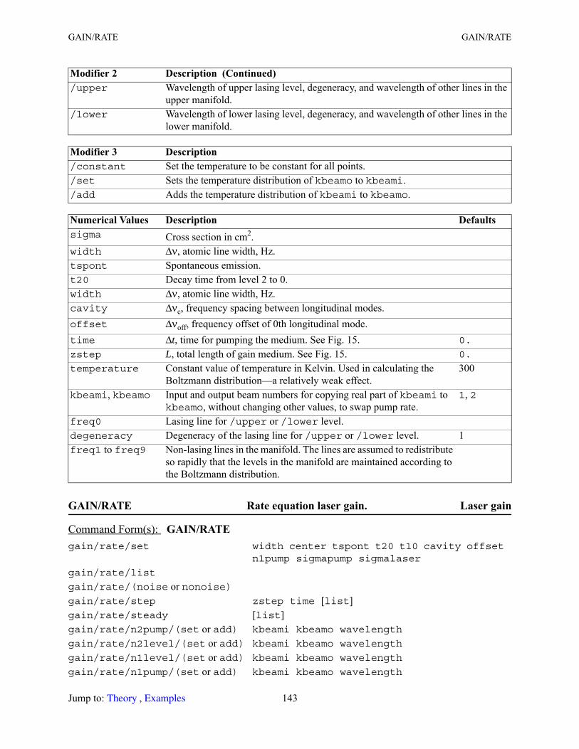
GAIN/RATE GAIN/RATE
GAIN/RATE Rate equation laser gain. Laser gain
/upper Wavelength of upper lasing level, degeneracy, and wavelength of other lines in the upper manifold.
/lower Wavelength of lower lasing level, degeneracy, and wavelength of other lines in the lower manifold.
Modifier 3 Description /constant Set the temperature to be constant for all points./set Sets the temperature distribution of kbeamo to kbeami./add Adds the temperature distribution of kbeami to kbeamo.
Numerical Values Description Defaultssigma Cross section in cm2.width Δν, atomic line width, Hz.tspont Spontaneous emission.t20 Decay time from level 2 to 0.width Δν, atomic line width, Hz.cavity Δνc, frequency spacing between longitudinal modes.offset Δνoff, frequency offset of 0th longitudinal mode.time Δt, time for pumping the medium. See Fig. 15. 0.
zstep L, total length of gain medium. See Fig. 15. 0.
temperature Constant value of temperature in Kelvin. Used in calculating the Boltzmann distribution—a relatively weak effect.
300
kbeami, kbeamo Input and output beam numbers for copying real part of kbeami to kbeamo, without changing other values, to swap pump rate.
1, 2
freq0 Lasing line for /upper or /lower level.degeneracy Degeneracy of the lasing line for /upper or /lower level. 1freq1 to freq9 Non-lasing lines in the manifold. The lines are assumed to redistribute
so rapidly that the levels in the manifold are maintained according to the Boltzmann distribution.
Command Form(s): GAIN/RATE gain/rate/set width center tspont t20 t10 cavity offset
n1pump sigmapump sigmalaser
gain/rate/list
gain/rate/(noise or nonoise)gain/rate/step zstep time [list]gain/rate/steady [list]gain/rate/n2pump/(set or add) kbeami kbeamo wavelength
gain/rate/n2level/(set or add) kbeami kbeamo wavelength
gain/rate/n1level/(set or add) kbeami kbeamo wavelength
gain/rate/n1pump/(set or add) kbeami kbeamo wavelength
Modifier 2 Description (Continued)
Jump to: , 143 Theory Examples

GAIN/RATE GAIN/RATE
Description: GAIN/RATEThis routine applies gain according to the rate equations. The GLAD is required. It is similar to
except that the pumping transverse distribution and the population inversion distribution are saved. The rate equations treatment can model mode competition for different resonator cavity conditions, including time-varying cavities. does not implement diffraction, which must be done separately. This allows the medium to exhibit saturation due to multiple passes through the medium.
must be used with the commands. See Theory Manual, (theory.pdf), for a description of the physics of the rate equations. /step is illustrated in Fig. 15.
GLAD stores the pump rate into level 2 and the energy densities of the upper and lower states and , where ν is the laser frequency. These values are stored in a beam array, which should be defined as a polarized beam and which should not be propagated (set array attribute to data). The medium array is always taken to be the last beam defined with the /set command. See Example for an example of the use of rate equations kinetics. The real and imaginary parts of the two polarization states take the form shown below in Table 5. The data storage is for sigmapump not equal to zero, as illustrated in Table. 6. may be used for side pumping.
gain/rate/inversion kbeami kbeamo zstep
Fig. 15. For the command gain/rate/step, a time slice of the pulse of length Δt has energy density I(0)Δt. It interacts with a gain region of length L = zstep, having energy density ΔN(0)•hν•zstep/0.5.
Table. 5. Contents of each point of the medium array which is defined as a polarized beam. The four words of data are stored: real and imaginary, first polarization; real and imaginary second polarization. For default condition with /nopumpsaturate selected.
pump rate,
w/cm3, laser wavelength
Level 2 times , , J/cm3
Level 1times , , J/cm3
N1pump(x,y),
Command Form(s): GAIN/RATE (Continued)
gain/sheet
gain/sheet
gain/rate pack Sect. 9.3
gain/rate
gain region
square temporal pulse
Δ� �
R2 x y,( )hνhνN2 x y,( ) hνN1 x y,( )
pack Ex56
slab/pump
R2 x y,( )hν hνhνN2 x y,( )
hνhνN1 x y,( )
R1 x y,( )
Jump to: , 144 Theory Examples

GAIN/RATE GAIN/RATE
Table. 6. For sigmapump not equal to zero. Contents of each point of the medium array which is defined as a polarized beam. The four words of data are stored: real and imaginary, first polarization; real and imaginary second polarizationmax pump rate,
w/cm3, laser wavelength
Level 2 times , , J/cm3
Level 1 times , , J/cm3
N1pump(x,y),
Modifier 2 Description /set Setup initial conditions./list List parameters for rate equations./noise Calculates contribution of optical noise due to spontaneous emission./nonoise Turns off calculation of spontaneous emission noise (default)./step Take a step of length zstep with pumping time./steady Steady-state gain based on closed-form solution. See GLAD Theory Manual,
(theory.pdf). Should be inside pack/in, pack/out block. See .
/n2pump Transforms the irradiance of kbeami into the real part of kbeamo to set or add to the pumping rate into Level 2, modified by the ratio of wavelength of the input beam divided by the wavelength of the laser.
/n2level Transforms the irradiance of kbeami into the imaginary part of the first polarization state of kbeamo to set or add to the population of Level 2, modified by the ratio of wavelength of the input beam divided by the wavelength of the laser.
/n1level Transforms the irradiance of kbeami into the real part of the second polarization state of kbeamo to set or add to the population of Level 1, modified by the ratio of wavelength of the input beam divided by the wavelength of the laser.
/n1pump Transforms the irradiance of kbeami into the imaginary part of the second polarization state of kbeamo to set or add to the pumping rate into Level 1, modified by the ratio of wavelength of the input beam divided by the wavelength of the laser.
/inversion Calculate the stored energy density of kbeami (for two-level model) by and store in kbeamo for gain sheet length of zstep.
Modifier 3 Description /set Set the specified parameter./add Add to the specified parameter.
Parameter Description list List overall parameters and center point properties for gain/rate/steady
and gain/rate/step.
Numerical Values Description Defaultswidth Δν, atomic line width, Hz.center Center of the atomic line, Hz.tspont τspont, spontaneous emission time constant. 0.
R2 x y,( )hνhν
hνN2 x y,( )hν
hνN1 x y,( )R1 x y,( )
Sect. 9.3 Ex69j
0.5 N2 N1–( )hν
Jump to: , 145 Theory Examples
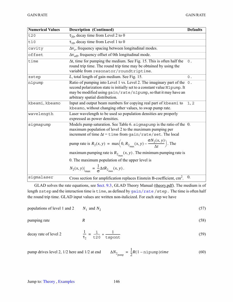
GAIN/RATE GAIN/RATE
GLAD solves the rate equations, see , GLAD Theory Manual (theory.pdf). The medium is of length zstep and the interaction time is time, as defined by /step. The time is often half the round trip time. GLAD input values are written non-italicized. For each step we have
populations of level 1 and 2 and (57)
pumping rate R (58)
decay rate of level 2 (59)
pump drives level 2, 1/2 here and 1/2 at end (60)
t20 τ20, decay time from Level 2 to 0t10 τ10, decay time from Level 1 to 0cavity Δνc, frequency spacing between longitudinal modes.offset Δνoff, frequency offset of 0th longitudinal mode.time Δt, time for pumping the medium. See Fig. 15. This is often half the
round trip time. The round trip time may be obtained by using the variable from resonator/roundtriptime.
0.
zstep L, total length of gain medium. See Fig. 15. 0.
n1pump Ratio of pumping into Level 1 vs. Level 2. The imaginary part of the second polarization state is initially set to a constant value N1pump. It may be modified using gain/rate/n1pump, so that it may have an arbitrary spatial distribution.
0.
kbeami, kbeamo Input and output beam numbers for copying real part of kbeami to kbeamo, without changing other values, to swap pump rate.
1, 2
wavelength Laser wavelength to be used so population densities are properly expressed as power densities.
sigmapump Models pump saturation. See Table 6. sigmapump is the ratio of the maximum population of level 2 to the maximum pumping per increment of time Δt = time from gain/rate/set. The local
pump rate is . The
maximum pumping rate is . The minimum pumping rate is
0. The maximum population of the upper level is
.
0.
sigmalaser Cross section for amplification replaces Einstein B-coefficient, cm2. 0.
Numerical Values Description (Continued) Defaults
R2 x y,( ) max 0 R2maxx y,( )
σN2 x y,( )Δt
-----------------------–, =
R2maxx y,( )
N2 x y,( )max
1σ---ΔtR2max
x y,( )=
Sect. 9.3
gain/rate
N1 N2
1τ2----- 1
t20----- 1
tspont---------------------+=
ΔN2pump
12---R 1 n1pump–( )time=
Jump to: , 146 Theory Examples
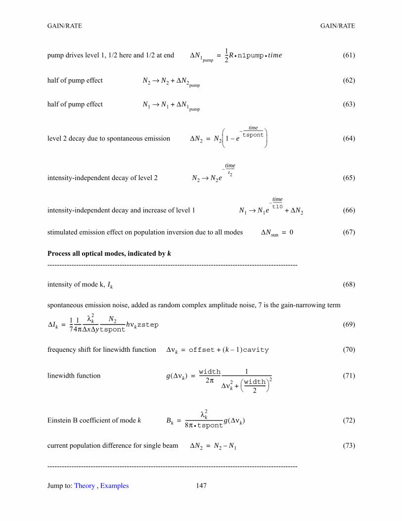
GAIN/RATE GAIN/RATE
pump drives level 1, 1/2 here and 1/2 at end (61)
half of pump effect (62)
half of pump effect (63)
level 2 decay due to spontaneous emission (64)
intensity-independent decay of level 2 (65)
intensity-independent decay and increase of level 1 (66)
stimulated emission effect on population inversion due to all modes (67)
Process all optical modes, indicated by k--------------------------------------------------------------------------------------------------------
intensity of mode k, (68)
spontaneous emission noise, added as random complex amplitude noise, 7 is the gain-narrowing term
(69)
frequency shift for linewidth function (70)
linewidth function (71)
Einstein B coefficient of mode k (72)
current population difference for single beam (73)
--------------------------------------------------------------------------------------------------------
ΔN1pump
12---R n1pump time••=
N2 N2 ΔN2pump+→
N1 N1 ΔN1pump+→
ΔN2 N2 1 etime
tspont-----------–
–
=
N2 N2e
timet2-----–
→
N1 N1etimet10-----–
ΔN2+→
ΔNsun 0=
Ik
ΔIk17--- 1
4π------
λk2
ΔxΔy-------------
N2tspont---------------------hνkzstep=
Δνk offset k 1–( )cavity+=
g Δνk( ) width2π
------------------ 1
Δνk2 width
2------------------ 2
+
------------------------------------------=
Bkλk
2
8π tspont•-------------------------------g Δνk( )=
ΔN2 N2 N1–=
Jump to: , 147 Theory Examples
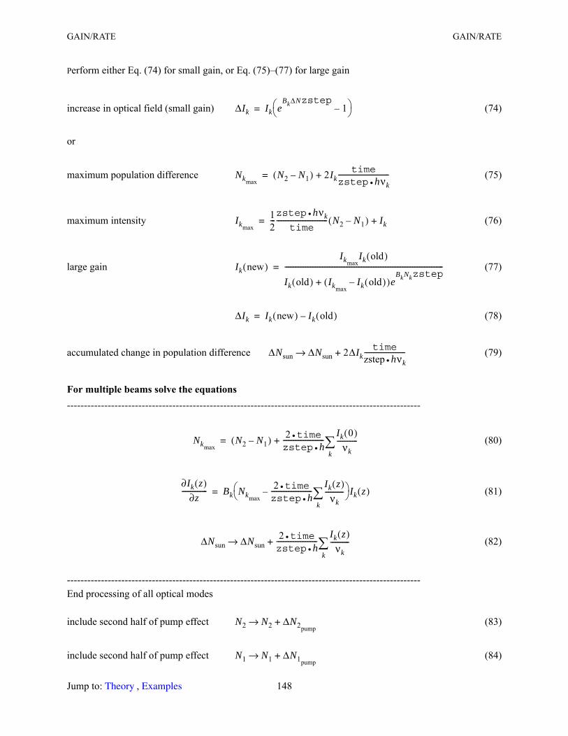
GAIN/RATE GAIN/RATE
Perform either Eq. (74) for small gain, or Eq. (75)–(77) for large gain
increase in optical field (small gain) (74)
or
maximum population difference (75)
maximum intensity (76)
large gain (77)
(78)
accumulated change in population difference (79)
For multiple beams solve the equations--------------------------------------------------------------------------------------------------------
(80)
(81)
(82)
--------------------------------------------------------------------------------------------------------End processing of all optical modes
include second half of pump effect (83)
include second half of pump effect (84)
ΔIk Ik eBkΔNzstep
1– =
NkmaxN2 N1–( ) 2Ik
timezstep hνk•------------------------------+=
Ikmax
12---zstep hνk•
time------------------------------ N2 N1–( ) Ik+=
Ik new( )Ikmax
Ik old( )
Ik old( ) IkmaxIk old( )–( )e
BkNkzstep+
---------------------------------------------------------------------------------------------=
ΔIk Ik new( ) Ik old( )–=
ΔNsun ΔNsun 2ΔIktime
zstep hνk•------------------------+→
NkmaxN2 N1–( ) 2 time•
zstep h•------------------------ Ik 0( )
νk------------
k+=
∂Ik z( )∂z
--------------- Bk Nkmax
2 time•
zstep h•------------------------ Ik z( )
νk-----------
k–
Ik z( )=
ΔNsun ΔNsun2 time•
zstep h•------------------------ Ik z( )
νk-----------
k+→
N2 N2 ΔN2pump+→
N1 N1 ΔN1pump+→
Jump to: , 148 Theory Examples
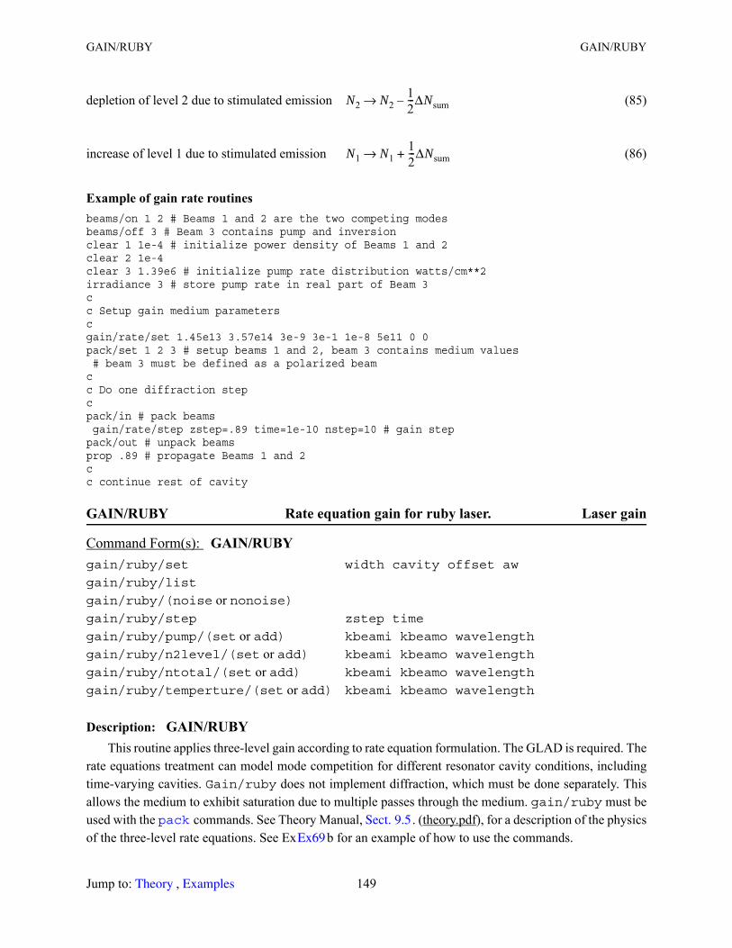
GAIN/RUBY GAIN/RUBY
depletion of level 2 due to stimulated emission (85)
increase of level 1 due to stimulated emission (86)
Example of gain rate routinesbeams/on 1 2 # Beams 1 and 2 are the two competing modesbeams/off 3 # Beam 3 contains pump and inversionclear 1 1e-4 # initialize power density of Beams 1 and 2clear 2 1e-4clear 3 1.39e6 # initialize pump rate distribution watts/cm**2irradiance 3 # store pump rate in real part of Beam 3cc Setup gain medium parameterscgain/rate/set 1.45e13 3.57e14 3e-9 3e-1 1e-8 5e11 0 0pack/set 1 2 3 # setup beams 1 and 2, beam 3 contains medium values # beam 3 must be defined as a polarized beamcc Do one diffraction stepcpack/in # pack beams gain/rate/step zstep=.89 time=1e-10 nstep=10 # gain steppack/out # unpack beamsprop .89 # propagate Beams 1 and 2cc continue rest of cavity
GAIN/RUBY Rate equation gain for ruby laser. Laser gain
Description: GAIN/RUBYThis routine applies three-level gain according to rate equation formulation. The GLAD is required. The
rate equations treatment can model mode competition for different resonator cavity conditions, including time-varying cavities. Gain/ruby does not implement diffraction, which must be done separately. This allows the medium to exhibit saturation due to multiple passes through the medium. gain/ruby must be used with the commands. See Theory Manual, . (theory.pdf), for a description of the physics of the three-level rate equations. See Ex b for an example of how to use the commands.
Command Form(s): GAIN/RUBY gain/ruby/set width cavity offset aw
gain/ruby/list
gain/ruby/(noise or nonoise)gain/ruby/step zstep time
gain/ruby/pump/(set or add) kbeami kbeamo wavelength
gain/ruby/n2level/(set or add) kbeami kbeamo wavelength
gain/ruby/ntotal/(set or add) kbeami kbeamo wavelength
gain/ruby/temperture/(set or add) kbeami kbeamo wavelength
N2 N212---ΔNsum–→
N1 N112---ΔNsum+→
pack Sect. 9.5
Ex69
Jump to: , 149 Theory Examples
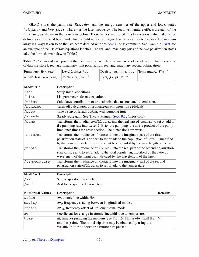
GAIN/RUBY GAIN/RUBY
GLAD stores the pump rate and the energy densities of the upper and lower states and , where ν is the laser frequency. The local temperature effects the gain of the
ruby laser, as shown in the equations below. These values are stored in a beam array, which should be defined as a polarized beam and which should not be propagated (set array attribute to data). The medium array is always taken to be the last beam defined with the /set command. See Example for an example of the use of rate equations kinetics. The real and imaginary parts of the two polarization states take the form shown below in Table 7.
Table. 7. Contents of each point of the medium array which is defined as a polarized beam. The four words of data are stored: real and imaginary, first polarization; real and imaginary second polarization.
Pump rate, w/cm3, laser wavelength
Level 2 times , , J/cm3
Denisty total times , , J/cm3
Temperature,
Modifier 2 Description /set Setup initial conditions./list List parameters for rate equations./noise Calculates contribution of optical noise due to spontaneous emission./nonoise Turns off calculation of spontaneous emission noise (default)./step Take a step of length zstep with pumping time./steady Steady-state gain. See Theory Manual, , (theory.pdf)./pump Transforms the irradiance of kbeami into the real part of kbeamo to set or add to
the pumping rate into Level 2. Enter the pumping rate as the product of the pump irradiance times the cross section. The dimensions are watts.
/n2level Transforms the irradiance of kbeami into the imaginary part of the first polarization state of kbeamo to set or add to the population of Level 2, modified by the ratio of wavelength of the input beam divided by the wavelength of the laser.
/ntotal Transforms the irradiance of kbeami into the real part of the second polarization state of kbeamo to set or add to the total population, modified by the ratio of wavelength of the input beam divided by the wavelength of the laser.
/temperature Transforms the irradiance of kbeami into the imaginary part of the second polarization state of kbeamo to set or add to the temperature.
Modifier 3 Description /set Set the specified parameter./add Add to the specified parameter.
Numerical Values Description Defaultswidth Δν, atomic line width, Hz.cavity Δνc, frequency spacing between longitudinal modes.offset Δνoff, frequency offset of 0th longitudinal mode.aw Coefficient for change in atomic linewidth due to temperture.time Δt, time for pumping the medium. See Fig. 15. This is often half the
round trip time. The round trip time may be obtained by using the variable from resonator/roundtriptime.
0.
R x y,( )hνhνN2 x y,( ) hνN1 x y,( )
pack Ex69
R x y,( )hν hνhνN2 x y,( )
hνhνNtot x y,( )
T x y,( )
Sect. 9.5
Jump to: , 150 Theory Examples
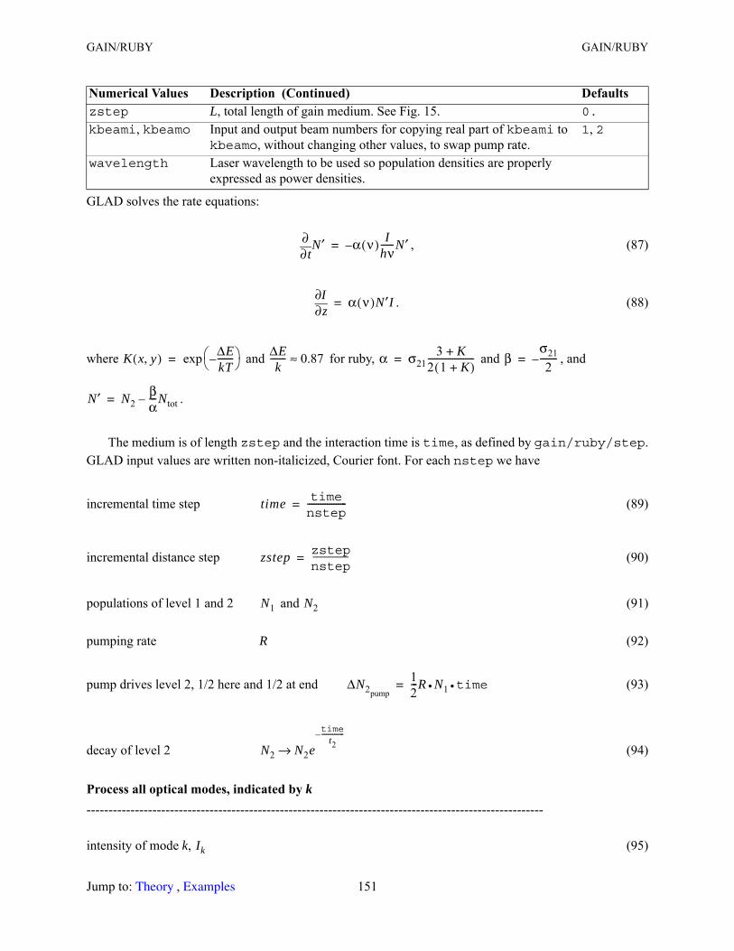
GAIN/RUBY GAIN/RUBY
GLAD solves the rate equations:
, (87)
. (88)
where and for ruby, and , and
.
The medium is of length zstep and the interaction time is time, as defined by gain/ruby/step. GLAD input values are written non-italicized, Courier font. For each nstep we have
incremental time step (89)
incremental distance step (90)
populations of level 1 and 2 and (91)
pumping rate R (92)
pump drives level 2, 1/2 here and 1/2 at end (93)
decay of level 2 (94)
Process all optical modes, indicated by k--------------------------------------------------------------------------------------------------------
intensity of mode k, (95)
zstep L, total length of gain medium. See Fig. 15. 0.
kbeami, kbeamo Input and output beam numbers for copying real part of kbeami to kbeamo, without changing other values, to swap pump rate.
1, 2
wavelength Laser wavelength to be used so population densities are properly expressed as power densities.
Numerical Values Description (Continued) Defaults
t∂∂ N′ α ν( ) I
hν------N′–=
z∂∂I α ν( )N′I=
K x y,( ) ΔEkT-------–
exp=ΔEk
------- 0.87≈ α σ213 K+
2 1 K+( )---------------------= β
σ212
--------–=
N′ N2βα---Ntot–=
time timenstep------------------=
zstep zstepnstep---------=
N1 N2
ΔN2pump
12---R N1 time••=
N2 N2e
timet2
--------------–
→
Ik
Jump to: , 151 Theory Examples
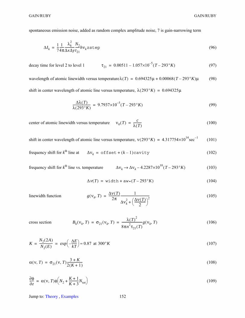
GAIN/RUBY GAIN/RUBY
spontaneous emission noise, added as random complex amplitude noise, 7 is gain-narrowing term
(96)
decay time for level 2 to level 1 (97)
wavelength of atomic linewidth versus temperature (98)
shift in center wavelength of atomic line versus temperature,
(99)
center of atomic linewidth versus temperature (100)
shift in center wavelength of atomic line versus temperature, (101)
frequency shift for kth line at (102)
frequency shift for kth line vs. temperature (103)
(104)
linewidth function (105)
cross section (106)
at (107)
(108)
(109)
ΔIk17--- 1
4π------
λk2
ΔxΔy-------------
N2t21------hνkzstep=
τ21 0.00511 1.057 5–×10 T 293°K–( )–=
λ T( ) 0.694325μ 0.00068 T 293°K–( )μ+=
λ 293°K( ) 0.694325μ=
Δλ T( )λ 293°K( )------------------------ 9.7937 5–×10 T 293°K–( )=
ν0 T( ) cλ T( )-----------=
ν 293°K( ) 4.317754 14×10 sec 1–=
Δνk offset k 1–( )cavity+=
Δνk Δνk 4.2287 10×10 T 293°K–( )–→
Δν T( ) width aw T 293°K–( )•+=
g νk T,( ) Δν T( )2π
--------------- 1
Δνk2 Δν T( )
2--------------- 2
+
---------------------------------------=
Bk νk T,( ) σ21 νk T,( ) λ T( )2
8πn2τ21 T( )----------------------------g νk T,( )= =
KN2 2A( )N2 E( )
------------------ ΔEkT-------–
exp 0.87≈= = 300°K
α ν T,( ) σ21 ν T,( ) 3 K+2 K 1+( )---------------------=
∂φ∂z------ α ν T,( )φ N2
K 1+K 3+-------------Ntot+
=
Jump to: , 152 Theory Examples
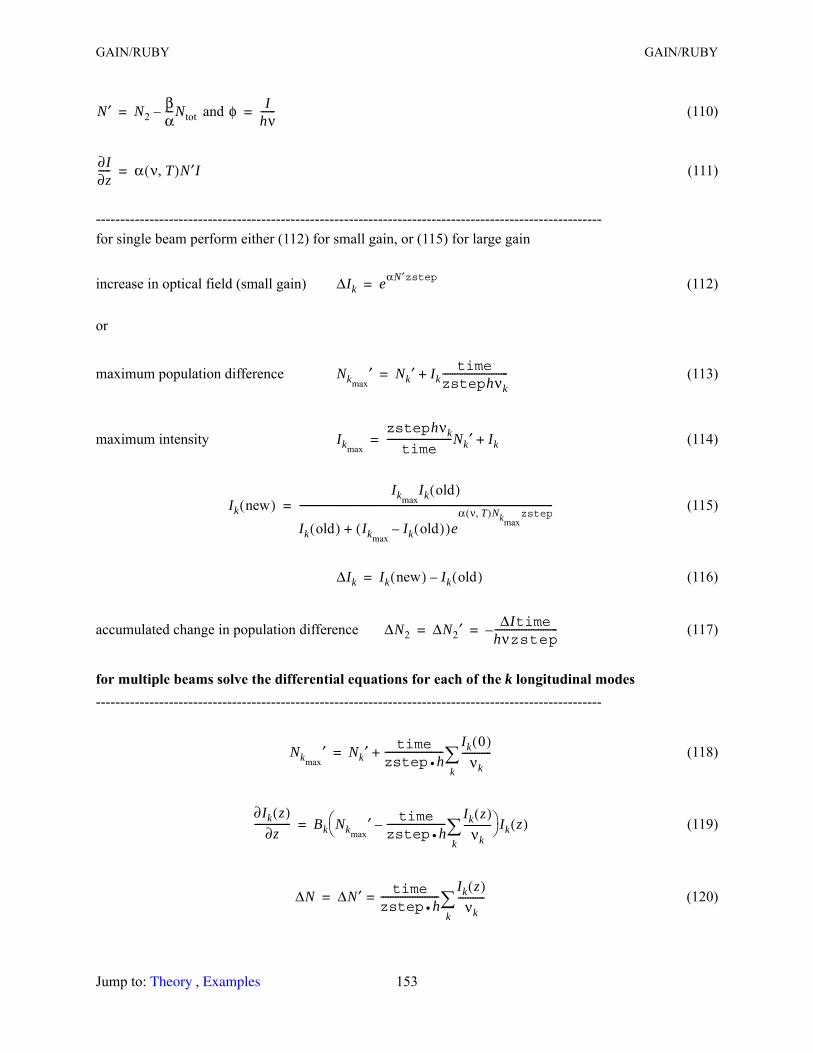
GAIN/RUBY GAIN/RUBY
and (110)
(111)
--------------------------------------------------------------------------------------------------------for single beam perform either (112) for small gain, or (115) for large gain
increase in optical field (small gain) (112)
or
maximum population difference (113)
maximum intensity (114)
(115)
(116)
accumulated change in population difference (117)
for multiple beams solve the differential equations for each of the k longitudinal modes--------------------------------------------------------------------------------------------------------
(118)
(119)
(120)
N′ N2βα---Ntot–= φ I
hν------=
∂I∂z----- α ν T,( )N′I=
ΔIk eαN ′zstep=
Nkmax′ Nk′ Ik
timezstephνk---------------------------+=
Ikmax
zstephνktime
---------------------------Nk′ Ik+=
Ik new( )Ikmax
Ik old( )
Ik old( ) IkmaxIk old( )–( )e
α ν T,( )Nkmaxzstep
+
--------------------------------------------------------------------------------------------------------=
ΔIk Ik new( ) Ik old( )–=
ΔN2 ΔN2′ ΔItimehνzstep--------------------------–= =
Nkmax′ Nk′ time
zstep h•------------------------ Ik 0( )
νk------------
k+=
∂Ik z( )∂z
--------------- Bk Nkmax′ time
zstep h•------------------------ Ik z( )
νk-----------
k–
Ik z( )=
ΔN ΔN′ timezstep h•------------------------ Ik z( )
νk-----------
k==
Jump to: , 153 Theory Examples
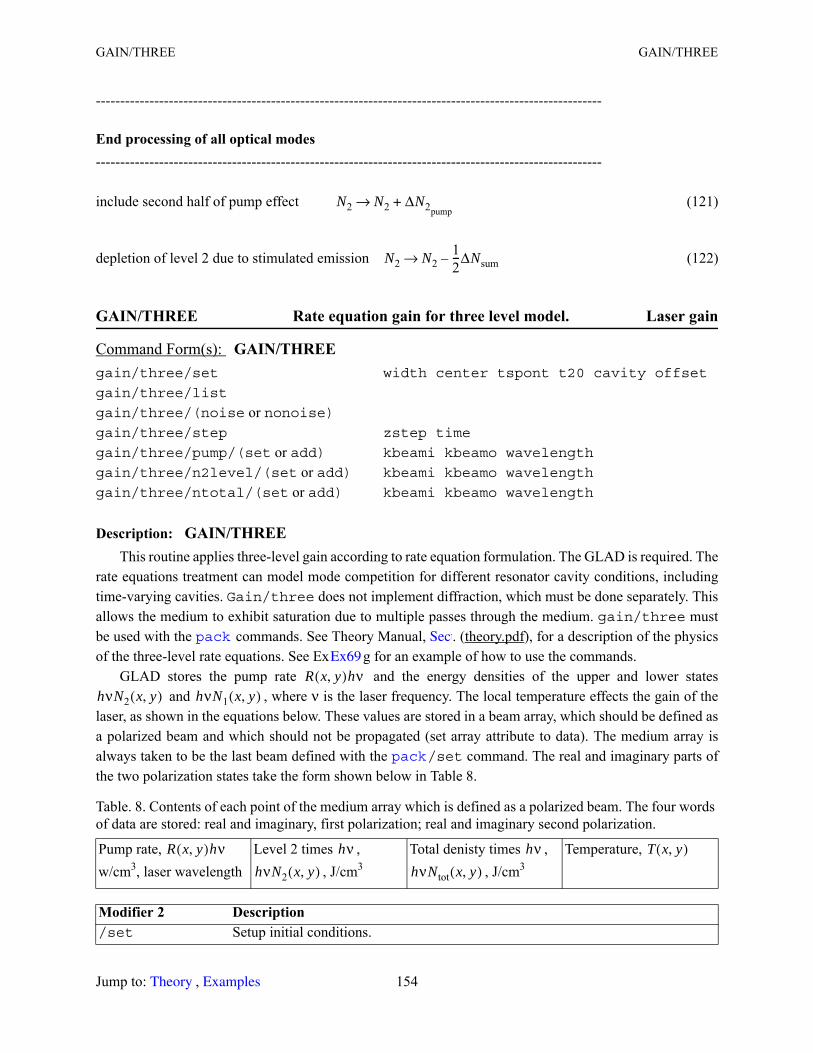
GAIN/THREE GAIN/THREE
--------------------------------------------------------------------------------------------------------
End processing of all optical modes--------------------------------------------------------------------------------------------------------
include second half of pump effect (121)
depletion of level 2 due to stimulated emission (122)
GAIN/THREE Rate equation gain for three level model. Laser gain
Description: GAIN/THREEThis routine applies three-level gain according to rate equation formulation. The GLAD is required. The
rate equations treatment can model mode competition for different resonator cavity conditions, including time-varying cavities. Gain/three does not implement diffraction, which must be done separately. This allows the medium to exhibit saturation due to multiple passes through the medium. gain/three must be used with the commands. See Theory Manual, . (theory.pdf), for a description of the physics of the three-level rate equations. See Ex g for an example of how to use the commands.
GLAD stores the pump rate and the energy densities of the upper and lower states and , where ν is the laser frequency. The local temperature effects the gain of the
laser, as shown in the equations below. These values are stored in a beam array, which should be defined as a polarized beam and which should not be propagated (set array attribute to data). The medium array is always taken to be the last beam defined with the /set command. The real and imaginary parts of the two polarization states take the form shown below in Table 8.
Command Form(s): GAIN/THREE gain/three/set width center tspont t20 cavity offset
gain/three/list
gain/three/(noise or nonoise)gain/three/step zstep time
gain/three/pump/(set or add) kbeami kbeamo wavelength
gain/three/n2level/(set or add) kbeami kbeamo wavelength
gain/three/ntotal/(set or add) kbeami kbeamo wavelength
Table. 8. Contents of each point of the medium array which is defined as a polarized beam. The four words of data are stored: real and imaginary, first polarization; real and imaginary second polarization.
Pump rate, w/cm3, laser wavelength
Level 2 times , , J/cm3
Total denisty times , , J/cm3
Temperature,
Modifier 2 Description /set Setup initial conditions.
N2 N2 ΔN2pump+→
N2 N212---ΔNsum–→
pack Sect
Ex69R x y,( )hν
hνN2 x y,( ) hνN1 x y,( )
pack
R x y,( )hν hνhνN2 x y,( )
hνhνNtot x y,( )
T x y,( )
Jump to: , 154 Theory Examples
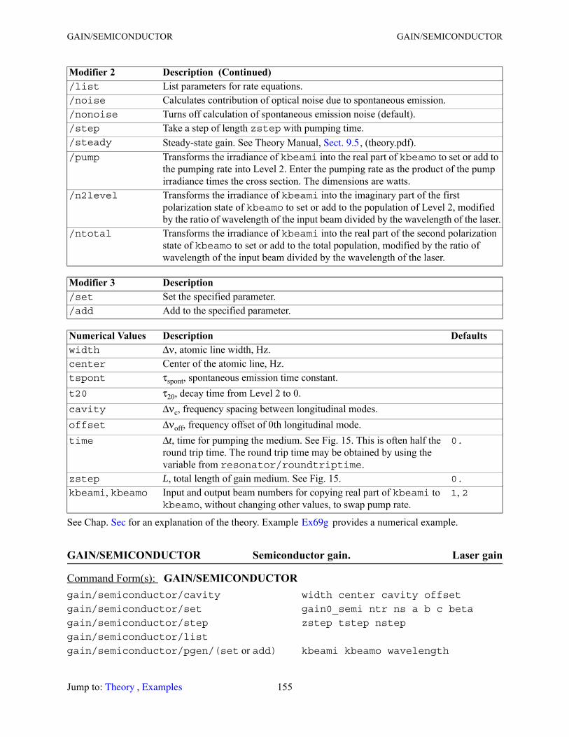
GAIN/SEMICONDUCTOR GAIN/SEMICONDUCTOR
See Chap. for an explanation of the theory. Example provides a numerical example.
GAIN/SEMICONDUCTOR Semiconductor gain. Laser gain
/list List parameters for rate equations./noise Calculates contribution of optical noise due to spontaneous emission./nonoise Turns off calculation of spontaneous emission noise (default)./step Take a step of length zstep with pumping time./steady Steady-state gain. See Theory Manual, , (theory.pdf)./pump Transforms the irradiance of kbeami into the real part of kbeamo to set or add to
the pumping rate into Level 2. Enter the pumping rate as the product of the pump irradiance times the cross section. The dimensions are watts.
/n2level Transforms the irradiance of kbeami into the imaginary part of the first polarization state of kbeamo to set or add to the population of Level 2, modified by the ratio of wavelength of the input beam divided by the wavelength of the laser.
/ntotal Transforms the irradiance of kbeami into the real part of the second polarization state of kbeamo to set or add to the total population, modified by the ratio of wavelength of the input beam divided by the wavelength of the laser.
Modifier 3 Description /set Set the specified parameter./add Add to the specified parameter.
Numerical Values Description Defaultswidth Δν, atomic line width, Hz.center Center of the atomic line, Hz.tspont τspont, spontaneous emission time constant.t20 τ20, decay time from Level 2 to 0.cavity Δνc, frequency spacing between longitudinal modes.offset Δνoff, frequency offset of 0th longitudinal mode.time Δt, time for pumping the medium. See Fig. 15. This is often half the
round trip time. The round trip time may be obtained by using the variable from resonator/roundtriptime.
0.
zstep L, total length of gain medium. See Fig. 15. 0.
kbeami, kbeamo Input and output beam numbers for copying real part of kbeami to kbeamo, without changing other values, to swap pump rate.
1, 2
Command Form(s): GAIN/SEMICONDUCTOR gain/semiconductor/cavity width center cavity offset
gain/semiconductor/set gain0_semi ntr ns a b c beta
gain/semiconductor/step zstep tstep nstep
gain/semiconductor/list
gain/semiconductor/pgen/(set or add) kbeami kbeamo wavelength
Modifier 2 Description (Continued)
Sect. 9.5
Sec Ex69g
Jump to: , 155 Theory Examples
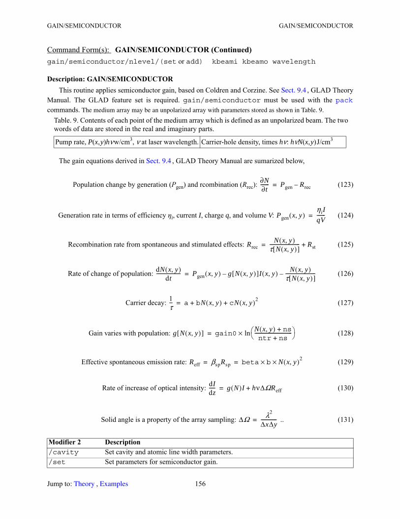
GAIN/SEMICONDUCTOR GAIN/SEMICONDUCTOR
Description: GAIN/SEMICONDUCTORThis routine applies semiconductor gain, based on Coldren and Corzine. See , GLAD Theory
Manual. The GLAD feature set is required. gain/semiconductor must be used with the commands. The medium array may be an unpolarized array with parameters stored as shown in Table. 9.
The gain equations derived in , GLAD Theory Manual are sumarized below,
Population change by generation (Pgen) and rcombination (Rrec): (123)
Generation rate in terms of efficiency ηi, current I, charge q, and volume V: (124)
Recombination rate from spontaneous and stimulated effects: (125)
Rate of change of population: (126)
Carrier decay: (127)
Gain varies with population: (128)
Effective spontaneous emission rate: (129)
Rate of increase of optical intensity: (130)
Solid angle is a property of the array sampling: .. (131)
gain/semiconductor/nlevel/(set or add) kbeami kbeamo wavelength
Modifier 2 Description /cavity Set cavity and atomic line width parameters./set Set parameters for semiconductor gain.
Command Form(s): GAIN/SEMICONDUCTOR (Continued)
Sect. 9.4
pack
Table. 9. Contents of each point of the medium array which is defined as an unpolarized beam. The two words of data are stored in the real and imaginary parts.
Pump rate, P(x, y)hν w/cm3, ν at laser wavelength. Carrier-hole density, times hν: hνN(x, y) J/cm3
Sect. 9.4
∂N∂t------- Pgen Rrec–=
Pgen x y,( )ηiIqV-------=
RrecN x y,( )
τ N x y,( )[ ]------------------------- Rst+=
dN x y,( )dt
-------------------- Pgen x y,( ) g N x y,( )[ ]I x y,( )–N x y,( )
τ N x y,( )[ ]-------------------------–=
1τ--- a bN x y,( ) cN x y,( )2+ +=
g N x y,( )[ ] gain0N x y,( ) ns+ntr ns+
------------------------------- ln×=
Reff βspRsp beta b× N x y,( )2×= =
dIdz----- g N( )I hνΔΩReff+=
ΔΩ λ2
ΔxΔy-------------=
Jump to: , 156 Theory Examples
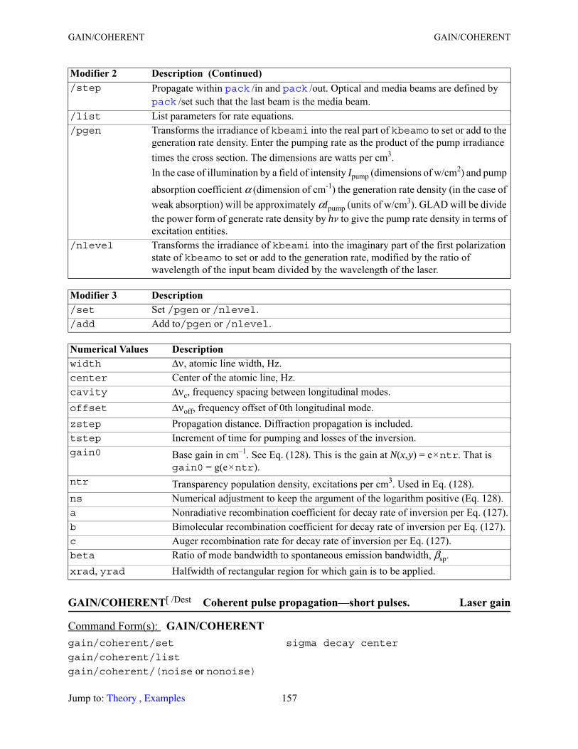
GAIN/COHERENT GAIN/COHERENT
GAIN/COHERENT Coherent pulse propagation—short pulses. Laser gain
/step Propagate within /in and /out. Optical and media beams are defined by /set such that the last beam is the media beam.
/list List parameters for rate equations./pgen Transforms the irradiance of kbeami into the real part of kbeamo to set or add to the
generation rate density. Enter the pumping rate as the product of the pump irradiance times the cross section. The dimensions are watts per cm3.In the case of illumination by a field of intensity Ipump (dimensions of w/cm2) and pump absorption coefficient α (dimension of cm-1) the generation rate density (in the case of weak absorption) will be approximately αIpump (units of w/cm3). GLAD will be divide the power form of generate rate density by hν to give the pump rate density in terms of excitation entities.
/nlevel Transforms the irradiance of kbeami into the imaginary part of the first polarization state of kbeamo to set or add to the generation rate, modified by the ratio of wavelength of the input beam divided by the wavelength of the laser.
Modifier 3 Description /set Set /pgen or /nlevel./add Add to/pgen or /nlevel.
Numerical Values Description width Δν, atomic line width, Hz.center Center of the atomic line, Hz.cavity Δνc, frequency spacing between longitudinal modes.offset Δνoff, frequency offset of 0th longitudinal mode.zstep Propagation distance. Diffraction propagation is included.tstep Increment of time for pumping and losses of the inversion.gain0 Base gain in cm–1. See Eq. (128). This is the gain at N(x, y) = e × ntr. That is
gain0 = g(e × ntr).ntr Transparency population density, excitations per cm3. Used in Eq. (128).ns Numerical adjustment to keep the argument of the logarithm positive (Eq. 128).a Nonradiative recombination coefficient for decay rate of inversion per Eq. (127).b Bimolecular recombination coefficient for decay rate of inversion per Eq. (127).c Auger recombination rate for decay rate of inversion per Eq. (127).beta Ratio of mode bandwidth to spontaneous emission bandwidth, βsp.
xrad, yrad Halfwidth of rectangular region for which gain is to be applied.
Command Form(s): GAIN/COHERENT gain/coherent/set sigma decay center
gain/coherent/list
gain/coherent/(noise or nonoise)
Modifier 2 Description (Continued) pack pack
pack
[ /Dest
Jump to: , 157 Theory Examples

GAIN/COHERENT GAIN/COHERENT
Description: GAIN/COHERENTThis routine applies gain according to tcoherent pulse propagation theory. See . For short
pulses, the rate equation approximation approach may predict the release of energy from the population inversion too quickly. Gain/coherent does not implement diffraction, which must be done separately. This allows the medium to exhibit saturation due to multiple passes through the medium. gain/threemust be used with the commands. See Theory Manual, . (theory.pdf), for a description of the physics of the three-level rate equations. See Ex g for an example of how to use the commands.
GLAD stores the pump rate and the population inversion where νis the laser frequency. The local temperature effects the gain of the laser, as shown in the equations below. These values are stored in a beam array, which should be defined as a polarized beam and which should not be propagated (set array attribute to data). The medium array is always taken to be the last beam defined with the /set command. The real and imaginary parts of the two polarization states take the form shown below in Table 8.
gain/coherent/step zstep time [list]gain/coherent/pump/(set or add) kbeami kbeamo wavelength
gain/coherent/inversion/(set or add) kbeami kbeamo wavelength
Table. 10. Contents of each point of the medium array which is defined as a polarized beam. The four words of data are stored: real and imaginary, first polarization; real and imaginary second polarization.Pump rate, irradiance times absorption times
, w/cm3, laser wavelength
Population inversion times ,
,
j/cm3
Real part, moving average of E-field times population inversion for internal use.
Imaginary part, moving average of E-field times population inversion for internal use.
Modifier 2 Description /set Setup initial conditions./list List parameters for rate equations./noise Calculates contribution of optical noise due to spontaneous emission./nonoise Turns off calculation of spontaneous emission noise (default)./step Take a step of length zstep with pumping time./pump Transforms the irradiance of kbeami into the real part of kbeamo to set or add to
the pumping rate into Level 2. Enter the pumping rate as the product of the pump irradiance times the absorption. The dimensions are watts/cm3.
/inversion Transforms the real part of kbeami into the imaginary part of the first polarization state of kbeamo to set or add to the population inversion modified by the ratio of wavelength of the input beam divided by the wavelength of the laser.
Modifier 3 Description /set Set the specified parameter./add Add to the specified parameter.
Command Form(s): GAIN/COHERENT (Continued)
Sect. 9.15
pack Sect
Ex69R x y,( )hν hν N2 x y,( ) N1 x y,( )–( )
pack
hν R x y,( )hνhν
hν N2 x y,( ) N1 x y,( )–( )
Jump to: , 158 Theory Examples

GAIN/ABSORBER GAIN/ABSORBER
GAIN/ABSORBER Saturable absorber. Laser gain
Description: GAIN/ABSORBERThis command models a saturable absorber based on the Cr4+ that is commonly used for passive Q-
switching of lasers. Figure 16 illustrates the four level system. Laser light can be absorbed between Levels 1 and 3 with cross section σgs for ground state absorption. Laser light can also be absorbed betwen Levels 2 and 4 with cros section σes for excited state absorption. Level 3 decays rapidly to Level 2 and Level 4 decays rapidly and non-radiatively to Level 2..
The real and imaginary parts of the two polarization states take the form shown below in Table 11.
Parameter Description list List overall parameters and center point properties for gain/coherent/step.
Numerical Values Description Defaultssigma Cross section in cm2.decay Decay time for coherent gain. Inverse of atomic line width.center Center of the atomic line, Hz.time Δt, time for pumping the medium. See Fig. 15. This is often half the
round trip time. The round trip time may be obtained by using the variable from resonator/roundtriptime.
0.
zstep L, total length of gain medium. See Fig. 15. 0.
kbeami, kbeamo Input and output beam numbers for copying real part of kbeami to kbeamo, without changing other values, to swap pump rate.
1, 2
Command Form(s): GAIN/ABSORBER gain/absorber/set gs_sigma es_sigma gamma transmission t2
gain/absorber/list
gain/absorber/step length time [list]gain/absorber/n0 kbeami kbeamo
Jump to: , 159 Theory Examples

GAIN/ABSORBER GAIN/ABSORBER
Fig. 16. Four levels of a Cr4+saturable absorber. The primary mechanism for laser absorption is the transition from Level 1 to Level 3—ground state absorption. It is assumed that Level 3 decays very quicly to Level 2. Excited state absorption occurs between Level 2 to Level 4. It is assumed that Level 4 decays by some non-radiative process.
Table. 11. Contents of each point of the medium array.
Total population of Cr4+ions, n0. Population of excited state. n2.
Modifier 2 Description /set Setup initial conditions./list List parameters for rate equations./length Implement a saturable absorber of specified length with pumping time./n0 Population density of Cr4+ions stored in real word of array.
Parameter Description list List overall parameters and center point properties for gain/coherent/step.
Numerical Values Description Defaultsgs_sigma Ground state absorption cross section in cm2.es_sigma Excited state absorption cross section in cm2.gamma Inversion reduction factor which depends on degeneracy.transmission Transmission of component including surfaces losses and bulk
absorption unrelated to the saturable effect.t2 Decay time from Level 2. s
1
2
4
3
very slow decay, t2
σgs
fast decay
fast decayσ
es
4 6–×10
Jump to: , 160 Theory Examples
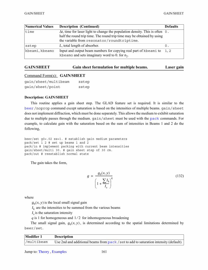
GAIN/SHEET GAIN/SHEET
GAIN/SHEET Gain sheet formulation for multiple beams. Laser gain
Description: GAIN/SHEETThis routine applies a gain sheet step. The GLAD feature set is required. It is similar to the /noprop command except saturation is based on the intensities of multiple beams. gain/sheet
does not implement diffraction, which must be done separately. This allows the medium to exhibit saturation due to multiple passes through the medium. gain/sheet must be used with the commands. For example, to calculate gain with the saturation based on the sum of intensities in Beams 1 and 2 do the following,
beer/set g0=.02 es=1. # establish gain medium parameterspack/set 1 2 # set up beams 1 and 2pack/in # implement packing with current beam intensitiesgain/sheet/multi 30. # gain sheet step of 30 cm.pack/out # reestablish normal state
The gain takes the form,
(132)
where is the local small signal gain are the intensities to be summed from the various beams is the saturation intensity q is 1 for homogeneous and for inhomogeneous broadeningThe small signal gain, , is determined according to the spatial limitations determined by
beer/set.
time Δt, time for laser light to change the population density. This is often half the round trip time. The round trip time may be obtained by using the variable from resonator/roundtriptime.
0.
zstep L, total length of absorber. 0.
kbeami, kbeamo Input and output beam numbers for copying real part of kbeami to kbeamo and sets imaginary word to 0. for n2.
1, 2
Command Form(s): GAIN/SHEET gain/sheet/multibeam zstep
gain/sheet/point zstep
Modifier 1 Description /multibeam Use 2nd and additional beams from /set to add to saturation intensity (default).
Numerical Values Description (Continued) Defaults
beer
pack
gg0 x y,( )
1Ik
Is----------+
q----------------------------=
g0 x y,( )IkIs
1 2⁄g0 x y,( )
pack
Jump to: , 161 Theory Examples

GAUSSIAN GAUSSIAN
Example of use of gain/sheet/pointclear 1 100 # uniform intensity for propagating beamgaus 2 g0 20 # gaussian distribution for small signal gainirradiance 2 # Set real word for gaingaus 3 es 20 # gaussian distribution for saturation intensitypack/set 1 2 3 # beam 1, g0, es distributionspack/in gain/sheet/point 10 # 10 cm. of gainpack/outprop 10 # diffraction propagation of 10 cm.
See and among the examples.
GAUSSIAN Set beam to gaussian function. Begin-end
Description: GAUSSIANDefines a gaussian spherical wave for the beam(s). Defines geometric data such as beam center,
coordinates, waist size and location, and zeros out tilt angle. By default the units are computed automatically. The polarization state is set to be linearly polarized in the x-direction. Alterations to the polarization state may be made with the command. See also .
/point For three beams defined with /set, the first beam is to be amplified, the 2nd beam has the distribution for small signal gain in the real word. Negative values are allowed for the 2nd beam using the real word. The 3rd beam has the distribution . For more than three beams, the additional beams between 1st and the last two contribute to saturation intensity in the same manner as with /multibeam.
Numerical Values Description Defaultszstep Length of gain medium. 0.
Command Form(s): GAUSSIAN gaussian/cir ibeams pkflu r0 sgxp decx decy radx rady
gaussian/sqr ibeams pkflu r0 sgxp decx decy radx rady
gaussian/ell ibeams pkflu r0x r0y sgxp decx decy radx rady
gaussian/rec ibeams pkflu r0x r0y sgxp sgyp decx decy radx rady
gaussian/half kbeam pkflu l0x r0x lsgxp rsgxp decx decy
Modifier 1 Description /cir
Circular distribution.
Modifier 1 Description (Continued) pack
g0 x y,( )
Is x y,( )
gainsheet.inp gainsheet1.inp
jones halfgaussian
pkflux2 y2+
ro2
---------------- sgxp
–exp
Jump to: , 162 Theory Examples
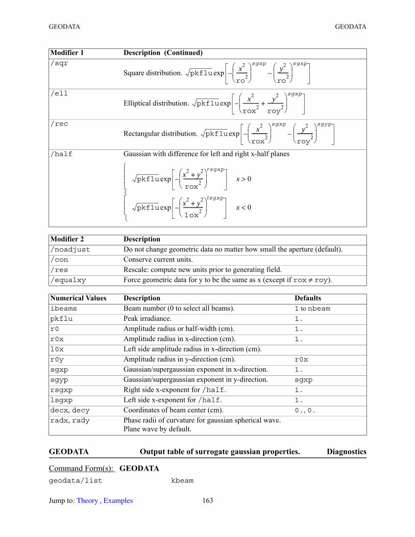
GEODATA GEODATA
GEODATA Output table of surrogate gaussian properties. Diagnostics
/sqr
Square distribution.
/ell
Elliptical distribution.
/rec
Rectangular distribution.
/half Gaussian with difference for left and right x-half planes
Modifier 2 Description /noadjust Do not change geometric data no matter how small the aperture (default)./con Conserve current units./res Rescale: compute new units prior to generating field./equalxy Force geometric data for y to be the same as x (except if rox ≠ roy).
Numerical Values Description Defaultsibeams Beam number (0 to select all beams). 1 to nbeampkflu Peak irradiance. 1.
r0 Amplitude radius or half-width (cm). 1.
r0x Amplitude radius in x-direction (cm). 1.
l0x Left side amplitude radius in x-direction (cm).r0y Amplitude radius in y-direction (cm). r0x
sgxp Gaussian/supergaussian exponent in x-direction. 1.
sgyp Gaussian/supergaussian exponent in y-direction. sgxp
rsgxp Right side x-exponent for /half. 1.
lsgxp Left side x-exponent for /half. 1.
decx, decy Coordinates of beam center (cm). 0., 0.radx, rady Phase radii of curvature for gaussian spherical wave.
Plane wave by default.
Command Form(s): GEODATA geodata/list kbeam
Modifier 1 Description (Continued)
pkflux2
ro2
--------- sgxp y2
ro2
--------- sgxp
––exp
pkflux2
rox2
------------- y2
roy2
-------------+ sgxp
–exp
pkflux2
rox2
------------- sgxp y2
roy2
------------- sgyp
––exp
pkflux2 y2+
rox2
---------------- rsgxp
–exp x 0>
pkflux2 y2+
lox2
---------------- lsgxp
–exp x 0<
Jump to: , 163 Theory Examples

GEODATA GEODATA
Description: GEODATAThis command lists or sets the geometric data associated with the surrogate gaussian beam. This data is
used by GLAD to control the choice of diffraction algorithms. Generally this information is automatically set by the , , , and commands. In certain applications such as unstable resonators, it may be necessary to reset the geometric data. In stable resonators, the starting geometric data should be selected so that it is reproduced in one round trip.
geodata/set/msquared/values kbeam m2x m2y
geodata/set/msquared/continuousunits
kbeam
geodata/set/ waist kbeam waistx waisty
geodata/set/beamsize kbeam wsx wsy
geodata/set/all kbeam zwaistx zwaisty waistx waisty iplanx iplany eqwstx eqwsty
geodata/fit/(separate or equal)
kbeam threshold [msquared or averageradius]
Modifier 1 Description set Sets the data.list Lists all coefficients.fit Perform fit of surrogate gaussian radius using the fitegauss procedure.
Modifier 2 Description fit/separate Allow x- and y-values to be different.fit/equal Set y-values to be the same as x-values.set/msquared Set M^2 values and recalculate waist size and location using local beam size and
radius of curvature.set/waist Set waist position to current beam poistion. Set waist size to current beam half
width (default) or input values for waistx and waisty. Reference surface is assumed to be flat.
set/beamsize Set local beam half widths and recalculate waist size and location assuming phase radius of curvature is unchanged.
set/all Sets all parameters. The user is responsible for choosing reasonable values. This is an old form of the command and is included for backward compatibility.
Modifier 3 Description msquared/values Set m^2 to specified values and recompute surrogate gaussian waist size and
location.msquared/continuousunits
Calculate and set M^2 to have constant units based on current sampling. Beam is propagated to current waist, M^2 is reset, and the beam is propagated back to original position. Radius of curvature and units may be adjusted.
Parameter Description msquared Perform fit using M-squared values for /fit.
Command Form(s): GEODATA (Continued)
gaussian clap lens mirror
geodata
Jump to: , 164 Theory Examples
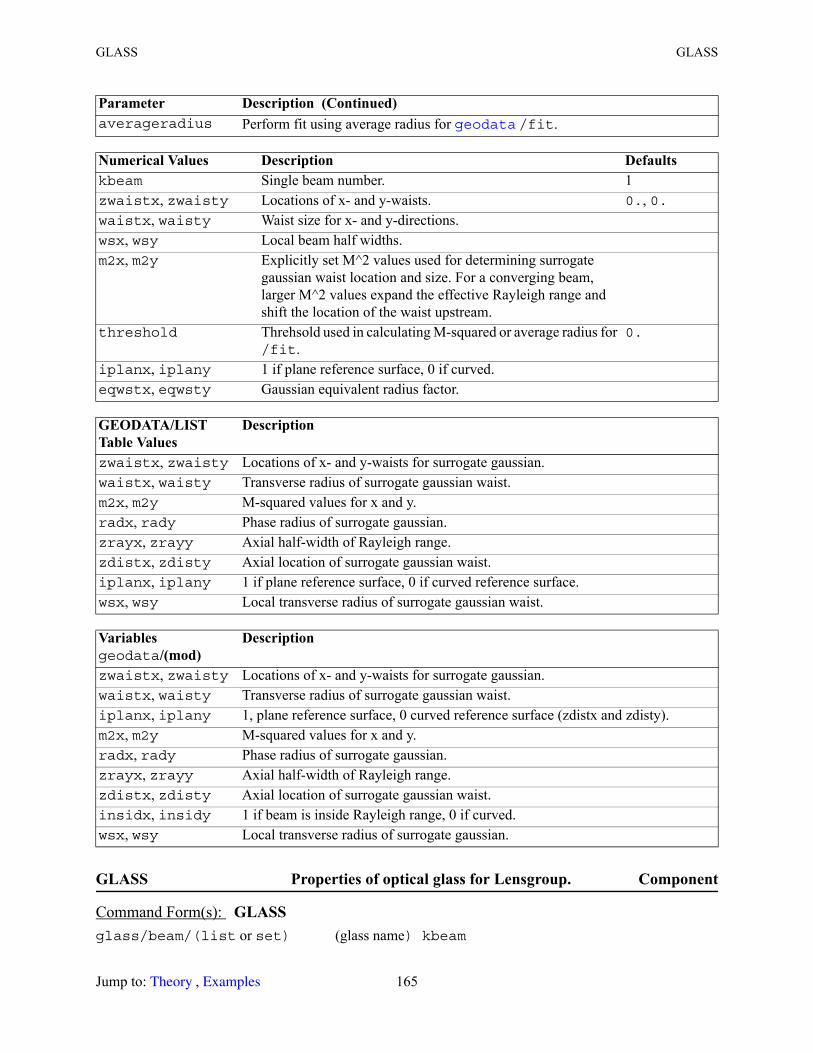
GLASS GLASS
GLASS Properties of optical glass for Lensgroup. Component
averageradius Perform fit using average radius for /fit.
Numerical Values Description Defaultskbeam Single beam number. 1zwaistx, zwaisty Locations of x- and y-waists. 0., 0.waistx, waisty Waist size for x- and y-directions.wsx, wsy Local beam half widths.m2x, m2y Explicitly set M^2 values used for determining surrogate
gaussian waist location and size. For a converging beam, larger M^2 values expand the effective Rayleigh range and shift the location of the waist upstream.
threshold Threhsold used in calculating M-squared or average radius for /fit.
0.
iplanx, iplany 1 if plane reference surface, 0 if curved.eqwstx, eqwsty Gaussian equivalent radius factor.
GEODATA/LISTTable Values
Description
zwaistx, zwaisty Locations of x- and y-waists for surrogate gaussian.waistx, waisty Transverse radius of surrogate gaussian waist.m2x, m2y M-squared values for x and y.radx, rady Phase radius of surrogate gaussian.zrayx, zrayy Axial half-width of Rayleigh range.zdistx, zdisty Axial location of surrogate gaussian waist.iplanx, iplany 1 if plane reference surface, 0 if curved reference surface.wsx, wsy Local transverse radius of surrogate gaussian waist.
Variablesgeodata/(mod)
Description
zwaistx, zwaisty Locations of x- and y-waists for surrogate gaussian.waistx, waisty Transverse radius of surrogate gaussian waist.iplanx, iplany 1, plane reference surface, 0 curved reference surface (zdistx and zdisty).m2x, m2y M-squared values for x and y.radx, rady Phase radius of surrogate gaussian.zrayx, zrayy Axial half-width of Rayleigh range.zdistx, zdisty Axial location of surrogate gaussian waist.insidx, insidy 1 if beam is inside Rayleigh range, 0 if curved.wsx, wsy Local transverse radius of surrogate gaussian.
Command Form(s): GLASS glass/beam/(list or set) (glass name) kbeam
Parameter Description (Continued) geodata
Jump to: , 165 Theory Examples
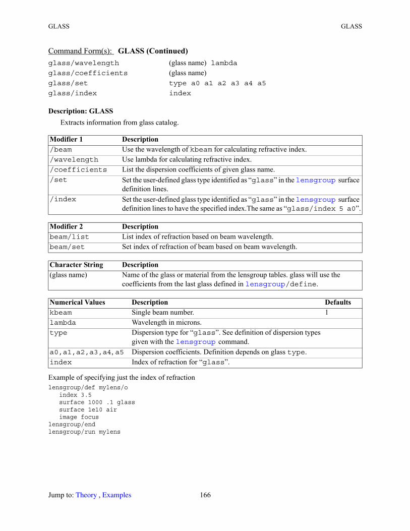
GLASS GLASS
Description: GLASSExtracts information from glass catalog.
Example of specifying just the index of refractionlensgroup/def mylens/o index 3.5 surface 1000 .1 glass surface 1e10 air image focuslensgroup/endlensgroup/run mylens
glass/wavelength (glass name) lambdaglass/coefficients (glass name)glass/set type a0 a1 a2 a3 a4 a5
glass/index index
Modifier 1 Description /beam Use the wavelength of kbeam for calculating refractive index. /wavelength Use lambda for calculating refractive index./coefficients List the dispersion coefficients of given glass name./set Set the user-defined glass type identified as “glass” in the surface
definition lines./index Set the user-defined glass type identified as “glass” in the surface
definition lines to have the specified index.The same as “glass/index 5 a0”.
Modifier 2 Description beam/list List index of refraction based on beam wavelength.beam/set Set index of refraction of beam based on beam wavelength.
Character String Description (glass name) Name of the glass or material from the lensgroup tables. glass will use the
coefficients from the last glass defined in /define.
Numerical Values Description Defaultskbeam Single beam number. 1lambda Wavelength in microns.type Dispersion type for “glass”. See definition of dispersion types
given with the command.a0,a1,a2,a3,a4, a5 Dispersion coefficients. Definition depends on glass type.index Index of refraction for “glass”.
Command Form(s): GLASS (Continued)
lensgroup
lensgroup
lensgroup
lensgroup
Jump to: , 166 Theory Examples
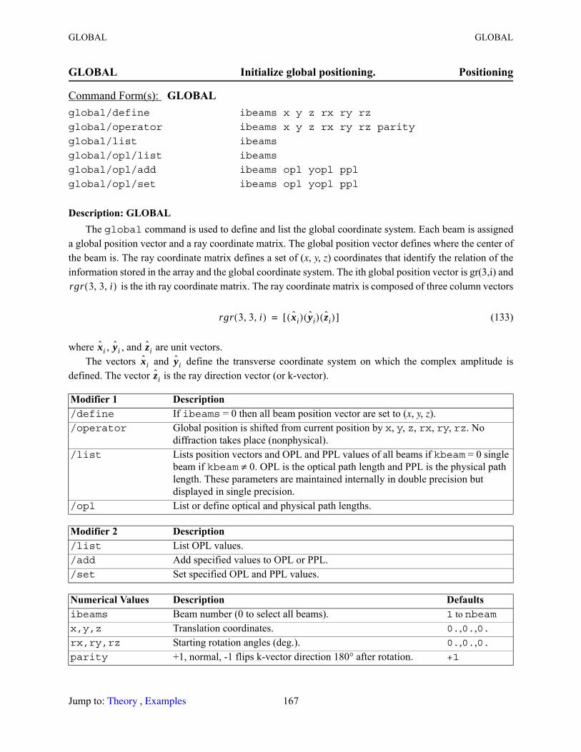
GLOBAL GLOBAL
GLOBAL Initialize global positioning. Positioning
Description: GLOBALThe global command is used to define and list the global coordinate system. Each beam is assigned
a global position vector and a ray coordinate matrix. The global position vector defines where the center of the beam is. The ray coordinate matrix defines a set of (x, y, z) coordinates that identify the relation of the information stored in the array and the global coordinate system. The ith global position vector is gr(3,i) and
is the ith ray coordinate matrix. The ray coordinate matrix is composed of three column vectors
(133)
where , , and are unit vectors. The vectors and define the transverse coordinate system on which the complex amplitude is
defined. The vector is the ray direction vector (or k-vector).
Command Form(s): GLOBAL global/define ibeams x y z rx ry rz
global/operator ibeams x y z rx ry rz parity
global/list ibeams
global/opl/list ibeams
global/opl/add ibeams opl yopl ppl
global/opl/set ibeams opl yopl ppl
Modifier 1 Description /define If ibeams = 0 then all beam position vector are set to (x, y, z)./operator Global position is shifted from current position by x, y, z, rx, ry, rz. No
diffraction takes place (nonphysical)./list Lists position vectors and OPL and PPL values of all beams if kbeam = 0 single
beam if kbeam ≠ 0. OPL is the optical path length and PPL is the physical path length. These parameters are maintained internally in double precision but displayed in single precision.
/opl List or define optical and physical path lengths.
Modifier 2 Description /list List OPL values./add Add specified values to OPL or PPL./set Set specified OPL and PPL values.
Numerical Values Description Defaultsibeams Beam number (0 to select all beams). 1 to nbeamx,y,z Translation coordinates. 0.,0.,0.rx,ry,rz Starting rotation angles (deg.). 0.,0.,0.parity +1, normal, -1 flips k-vector direction 180° after rotation. +1
rgr 3 3 i, ,( )
rgr 3 3 i, ,( ) xi( ) yi( ) zi( )[ ]=
xi yi zixi yi
zi
Jump to: , 167 Theory Examples
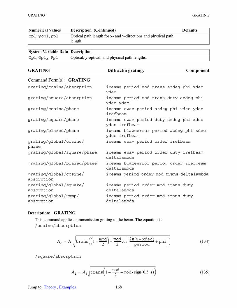
GRATING GRATING
GRATING Diffractin grating. Component
Description: GRATINGThis command applies a transmission grating to the beam. The equation is/cosine/absorption
(134)
/square/absorption
(135)
opl, yopl, ppl Optical path length for x- and y-directions and physical path length.
System Variable Data Description Opl, Oply, Ppl Optical, y-optical, and physical path lengths.
Command Form(s): GRATING grating/cosine/absorption ibeams period mod trans azdeg phi xdec
ydec
grating/square/absorption ibeams period mod trans duty azdeg phi xdec ydec
grating/cosine/phase ibeams ewav period azdeg phi xdec ydec irefbeam
grating/square/phase ibeams ewav period duty azdeg phi xdec ydec irefbeam
grating/blazed/phase ibeams blazeerror period azdeg phi xdec ydec irefbeam
grating/global/cosine/phase
ibeams ewav period order irefbeam
grating/global/square/phase ibeams ewav period order duty irefbeam deltalambda
grating/global/blazed/phase ibeams blazeerror period order irefbeam deltalambda
grating/global/cosine/absorption
ibeams period order mod trans deltalambda
grating/global/square/absorption
ibeams period order mod trans duty deltalambda
grating/global/ramp/absorption
ibeams period order mod trans duty deltalambda
Numerical Values Description (Continued) Defaults
A2 A1 trans 1 mod2
----------– mod
2----------cos 2π x xdec–( )
period---------------------------------- phi++
=
A2 A1 trans 1 mod2
----------– mod sign 0.5 s,( )•– =
Jump to: , 168 Theory Examples
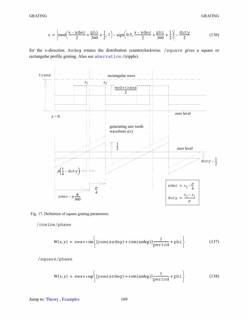
GRATING GRATING
(136)
for the x-direction. Azdeg rotates the distribution counterclockwise. /square gives a square or rectangular profile grating. Also see /(ripple).
/cosine/phase
(137)
/square/phase
(138)
Fig. 17. Definition of square grating parameters.
s mod x xdec–2
----------------------- phi360---------- 1
2---+ + 1,
sign 0.5 x xdec–2
----------------------- phi360---------- 1
2---+ +,
–duty
2--------------–=
aberration
x = 0
trans
zero level
zero level
x1 x2mod trans•
2--------------------------------
duty 12---–
rectangular wave
generating saw tooth waveform s(x)
12---
p 14--- duty–⎝ ⎠
⎛ ⎞
p4---
xdec p φ360---------–
xdec x2p4---–=
dutyx2 x1–
p----------------=
W x y,( ) ewav y azdeg( )cos x azdeg( )sin+[ ] 1period--------------------- phi+
sin•=
W x y,( ) ewav sqr y azdeg( )cos x azdeg( )sin+[ ] 1period--------------------- phi+
•=
Jump to: , 169 Theory Examples
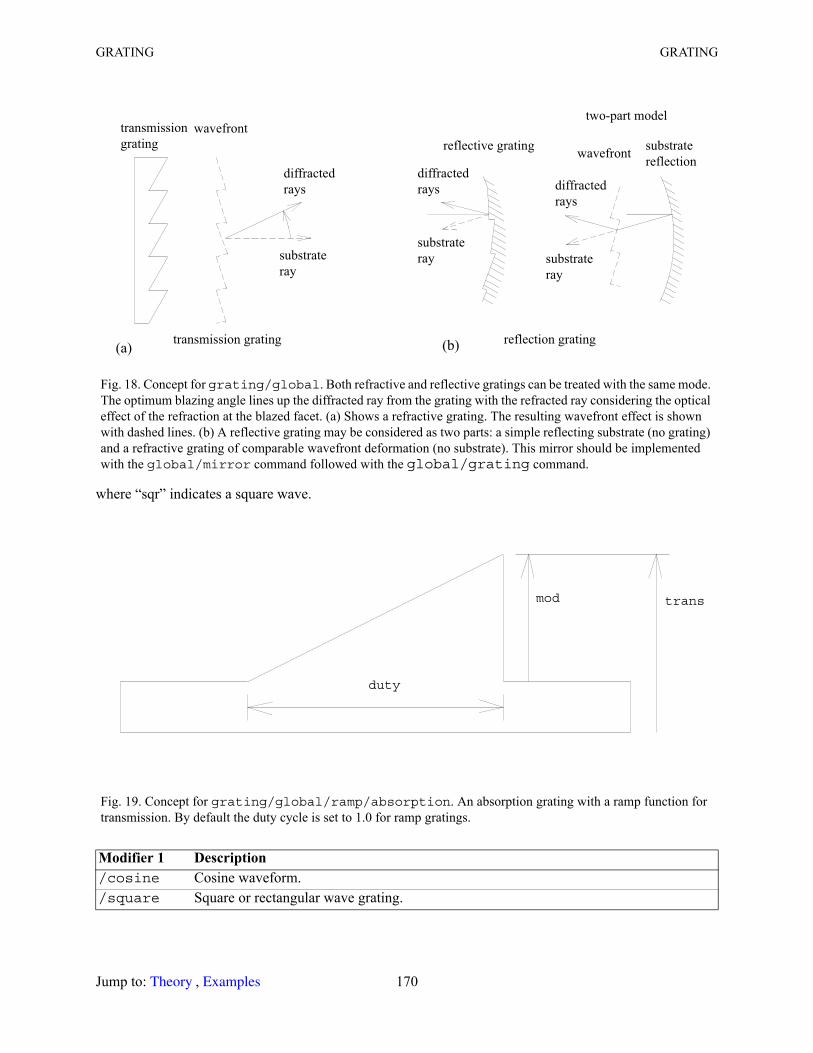
GRATING GRATING
where “sqr” indicates a square wave.
Fig. 18. Concept for grating/global. Both refractive and reflective gratings can be treated with the same mode. The optimum blazing angle lines up the diffracted ray from the grating with the refracted ray considering the optical effect of the refraction at the blazed facet. (a) Shows a refractive grating. The resulting wavefront effect is shown with dashed lines. (b) A reflective grating may be considered as two parts: a simple reflecting substrate (no grating) and a refractive grating of comparable wavefront deformation (no substrate). This mirror should be implemented with the global/mirror command followed with the global/grating command.
Fig. 19. Concept for grating/global/ramp/absorption. An absorption grating with a ramp function for transmission. By default the duty cycle is set to 1.0 for ramp gratings.
Modifier 1 Description /cosine Cosine waveform./square Square or rectangular wave grating.
transmission
grating
wavefront
diffracted
rays
substrate
ray
diffracted
rays
diffracted
rays
substrate
ray substrate
ray
reflective grating
two-part model
wavefrontsubstrate
reflection
transmission grating reflection grating(a) (b)
transmod
duty
Jump to: , 170 Theory Examples

GRATING GRATING
/blazed Blazed grating. Grating is defined in terms existing wavefront modulation: (n-1)×surface modulation. Grating lines are tilted facets at specified angle (after refraction or reflection). In ideal design, the blazing angle is selected so, considering only one facet, the exiting light is aligned with the angle of the diffracted order.
/global Phase grating is defined by global coordinates using preceeding commands. Grating is assumed to be located at current beam position (no automatic propagation to position, use if necessary). Only specified order is considered. Treatment is unresolved, i.e., it is not necessary to have sufficient sampling density to resolve individual grating line structure. The efficiency is calculated for the single diffractive order indicated and the beam is redirected to satisfy the grating equation upon exiting from the grating.
Modifier 2 Description /absorption Absorption grating./phase Phase grating./square Square shape for global grating./cosine Cosine shape for global grating./blazed Blazed shape for global phase grating./ramp Saw tooth shape for amplitude grating.
Modifier 3 Description /absorption Absorption global grating./phase Phase global grating.
Numerical Values Description Defaultsibeams Beam number (0 to select all beams). 1 to nbeammod Modulation, 1 gives full modulation. 1.
period Grating period.order Diffracted order for grating/global. 0
ewav Wavefront modulation in waves.blazeerror Error of blazing angle of wavefront. For default value of 0, GLAD
uses optimum blazing angle which matches refracted or reflected ray due to grating facets with the diffracted ray based on grating period and order.
0.
duty Duty cycle for rectangular wave. 0.5, square1., ramp
trans Peak transmission. 1.
azdeg Azimuth angle measured counterclockwise (degrees). 0.phi Phase of grating in the center (degrees). 0.xdec, ydec Coordinates of grating center. 0., 0.ewav Aberration coefficient (waves). 0.
irefbeam Reference beam number for wavelength for phase grating. ibeams
deltalambda Inceremental wavelength difference (cm) from beam value. Treated as a phase tilt rather than a change in global data.
Modifier 1 Description (Continued)
vertex/rotate
vertex/locate prop
Jump to: , 171 Theory Examples
HALFGAUSSIAN HELP
HALFGAUSSIAN Gaussian with different left and right sides. Begin-end
Description: HALFGAUSSDefines a gaussian which has different properties on the left ( ) and right ( ) sides.
, (139)
, , (140)
HELP Activates text-based Help (see PDF manuals). Language
Description: HELPActivates a menu driven help file. Superior forms of help are now available as described below. May be
run as a command line in GLAD or as a separate program gladhelp.exe. The data file help.sor must be in the current directory. If a command-modifier string is given, for example, , GLAD will look up that sequence. Otherwise, help begins with the top-level menu.
Online help is available in three forms. Both IDE.EXE and WATCH.EXE have MS Windows Help files available from the main menu bar to describe operation of these windows programs. You can also access the full set of GLAD manuals in online form from the Help item on the IDE.EXE menu bar. These online documents use the Adobe Acrobat Reader 7.0 and provide high quality online viewing and support printing of selected pages with high resolution Postscript. There is also a character based search program called gladhelp.exe, which may be accessed through the command or run independently. This program is still provided primarily for backward compatibility as the online documentation is superior.
Command Form(s): HALFGAUSSIAN halfgauss kbeam peak leftwidth rightwidth xdec ydec nl nr
Numerical Values Description Defaultskbeam Single beam number. 1peak Peak intensity value. 1.
rightwidth Width for right half-plane.leftwidth Width for left half-plane.xdec, ydec Coordinates of beam center (cm).nl, nr Left and right supergaussian exponents.
Command Form(s): HELP help (string)
String Description (string) Optional command-modifier sequence for help to look up.
x xdec< x xdec>
I x y,( ) Peak 2 x2 y2+rightwidth------------------------------------
nr
–exp= x xdec>
I x y,( ) Peak 2 x2 y2+rightwidth------------------------------------
nl
–exp= x xdec<
plot/xslice
help
Jump to: , 172 Theory Examples
HERMITE HIGHNA
HERMITE Initialize beam to Hermite polynomials. Begin-end
Description: HERMITEDefines an initial Hermit-Gaussian field distribution. Sets geometric data such as beam center, waist
size and location, and reference surface shape (plane). By default the units are automatically computed. The transverse modes of ideal stable resonators take the form of Hermite-gaussian polynomials or Lagurerre-gaussian. The general polynomial form of the Hermite-gaussian functions is
(141)
where n is the order of the polynomial, ω0 is a waist radius parameter similar to the gaussian beam and are the Hermite functions. The two-dimensional functions may be described by multiplying two one-
dimensional functions. The order and waist parameters may be different for the two directions.
HIGHNA High numerical aperture lens. Component
Description: HIGHNAThis command models a high numerical aperture lens using vector diffraction. A dipole projection
model, which is described in GLAD Theory Manual , (theory.pdf), is used. The dipole projection model divides the optical field into a transverse mode and an axial mode. See Example for a simple
Command Form(s): HERMITE hermite/(con, noadjust, or res)
ibeams energ xrad yrad xnor ynor xdec ydec
Modifier 1 Description /con Conserve current units (default)./noadjust Conserve current units, do not reset surrogate gaussian. Always selected in
resonator mode./res Rescale: compute new optimum units prior to generating file.
Numerical Values Description Defaultsibeams Beam number (0 to select all beams). 1 to nbeamenerg Total beam energy (mw). 1.
xrad, yrad Reference radius, . Beam size (cm).
xnor, ynor Hermitian order in specified direction. 1.
xdec, ydec Coordinates of beam center (cm).
Command Form(s): HIGHNA highna/focus kb1 kb2 focallength
highna/collimate kb1 kb2 focallength
un2π--- 1 4⁄ 1
2nn!ωo
----------------- 1 2⁄
Hn2x
ωo---------- x2
ω0------–
exp=
Hn x( )
ω0
Sect. 6.4
Ex90
Jump to: , 173 Theory Examples
HOMOGENIZER HOMOGENIZER
example. Beam kb1 is the incident beam, which must be polarized. After the lens, Kb1 contains the transverse mode. Kb2 must be unpolarized and, after the lens, will contain the axial mode.
HOMOGENIZER Beam homogenizer. Component
Description: HOMOGENIZERThis function models the microstructure of an idealized beam homogenizer. Useful for determining the
magnitude of coherent artifacts that would arise in a lenslet array beam homogenizer (see Fig. 20). Lenslet apertures are assumed to be rectangular. The function divides the pixels width in kb1 by the pixel with of kb2 to find the number of lenslet elements (powers of 2). For example if Kb1 is 512 × 512 and kb2 is 64 × 64 there will be a lenslet array of 8 × 8 lenses. To get an array of 10 x 10, use a 16 × 16 array and mask off the outer 2 lens elements on each side with a rectangular aperture. The units with the finescalechoice are
(142)
as compared with the units after an ordinary lens , where N is the array length. The largescale view overlaps the distributions at each lenslet incoherently to show the envelope
smoothing. Finescale calculates the coherent effects. Neighboring lenslets create interference fringes. These effects are very fine scale according to the angles of the lenslet beams as they intersect at the target plane. The smaller the coherence width (autocorrelation size) of the distribution the smaller the magnitude of the coherence effects.
Modifier 1 Description /focus Applies vector diffraction to form a three-dimensional focus./collimate Applies vector diffraction to propagate a bean from a three-dimensional focus to
a following pupil and recollimates the beam. Beam kb2 contains no useful information after this operation.
Numerical Values Description Defaultskb1 Incident beam, must be polarized. After the lens contains the
transverse mode.1
kb2 Contains the axial mode after the lens. Must be unpolarized but of the same size as kb1.
focallength Focal length of the lens.
Command Form(s): HOMOGENIZER homogenizer/largescale kb1 kb2 magnification kb3
homogenizer/finescale kb1 kb2 cycles focallength kb3 icent jcent
Modifier 1 Description /largescale Calculates large scale features due to incoherent summations./finescale Calculates microstructure due to coherent and partially coherent effects.
Δx′ cyclesN
--------------------- λfNΔx-----------=
Δx′ λf NΔx⁄=
Jump to: , 174 Theory Examples
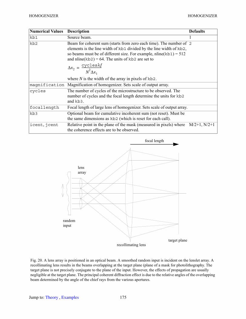
HOMOGENIZER HOMOGENIZER
Numerical Values Description Defaultskb1 Source beam. 1kb2 Beam for coherent sum (starts from zero each time). The number of
elements is the line width of kb1 divided by the line width of kb2, so beams must be of different size. For example, nline(kb1) = 512 and nline(kb2) = 64. The units of kb2 are set to
where N is the width of the array in pixels of kb2.
2
magnification Magnification of homogenizer. Sets scale of output array.cycles The number of cycles of the microstructure to be observed. The
number of cycles and the focal length determine the units for kb2 and kb3.
focallength Focal length of large lens of homogenizer. Sets scale of output array.kb3 Optional beam for cumulative incoherent sum (not reset). Must be
the same dimensions as kb2 (which is reset for each call). icent, jcent Relative point in the plane of the mask (measured in pixels) where
the coherence effects are to be observed.M/2+1, N/2+1
Fig. 20. A lens array is positioned in an optical beam. A smoothed random input is incident on the lenslet array. A recollimating lens results in the beams overlapping at the target plane (plane of a mask for photolithography. The target plane is not precisely conjugate to the plane of the input. However, the effects of propagation are usually negligible at the target plane. The principal coherent diffraction effect is due to the relative angles of the overlapping beam determined by the angle of the chief rays from the various apertures.
Δx2cyclesλf
N2Δx1
---------------------------=
recollimating lens
random
input
lens
array
target plane
focal length
Jump to: , 175 Theory Examples
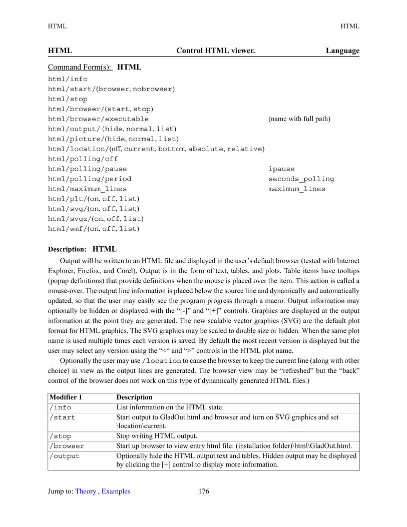
HTML HTML
HTML Control HTML viewer. Language
Description: HTMLOutput will be written to an HTML file and displayed in the user’s default browser (tested with Internet
Explorer, Firefox, and Corel). Output is in the form of text, tables, and plots. Table items have tooltips (popup definitions) that provide definitions when the mouse is placed over the item. This action is called a mouse-over. The output line information is placed below the source line and dynamically and automatically updated, so that the user may easily see the program progress through a macro. Output information may optionally be hidden or displayed with the “[-]” and “[+]” controls. Graphics are displayed at the output information at the point they are generated. The new scalable vector graphics (SVG) are the default plot format for HTML graphics. The SVG graphics may be scaled to double size or hidden. When the same plot name is used multiple times each version is saved. By default the most recent version is displayed but the user may select any version using the “<“ and “>” controls in the HTML plot name.
Optionally the user may use /location to cause the browser to keep the current line (along with other choice) in view as the output lines are generated. The browser view may be “refreshed” but the “back” control of the browser does not work on this type of dynamically generated HTML files.)
Command Form(s): HTML html/info
html/start/(browser, nobrowser)html/stop
html/browser/(start, stop)html/browser/executable (name with full path)html/output/(hide, normal, list)html/picture/(hide, normal, list)html/location/(off, current, bottom, absolute, relative)html/polling/off
html/polling/pause ipause
html/polling/period seconds_polling
html/maximum_lines maximum_lines
html/plt/(on, off, list)html/svg/(on, off, list)html/svgz/(on, off, list)html/wmf/(on, off, list)
Modifier 1 Description /info List information on the HTML state./start Start output to GladOut.html and browser and turn on SVG graphics and set
\location\current./stop Stop writing HTML output./browser Start up browser to view entry html file: (installation folder)\html\GladOut.html./output Optionally hide the HTML output text and tables. Hidden output may be displayed
by clicking the [+] control to display more information.
Jump to: , 176 Theory Examples
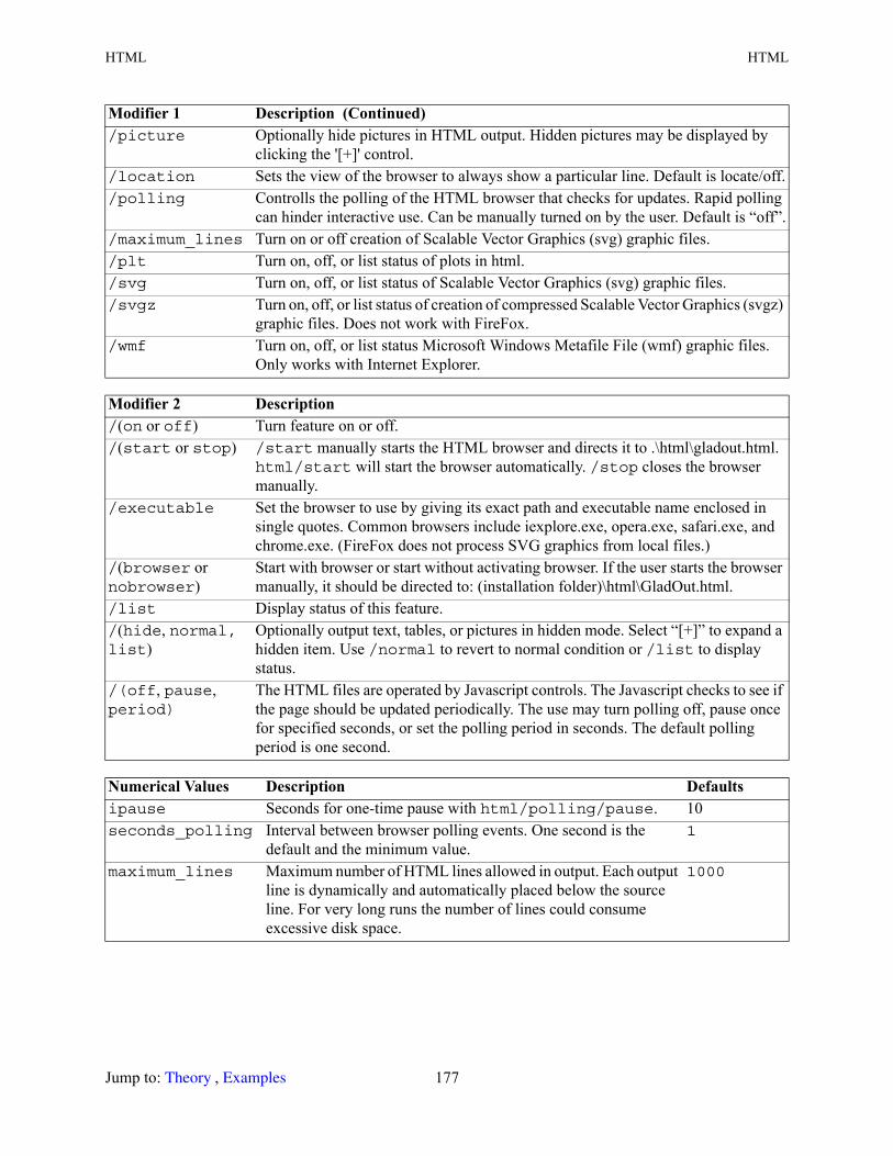
HTML HTML
/picture Optionally hide pictures in HTML output. Hidden pictures may be displayed by clicking the '[+]' control.
/location Sets the view of the browser to always show a particular line. Default is locate/off./polling Controlls the polling of the HTML browser that checks for updates. Rapid polling
can hinder interactive use. Can be manually turned on by the user. Default is “off”./maximum_lines Turn on or off creation of Scalable Vector Graphics (svg) graphic files./plt Turn on, off, or list status of plots in html./svg Turn on, off, or list status of Scalable Vector Graphics (svg) graphic files./svgz Turn on, off, or list status of creation of compressed Scalable Vector Graphics (svgz)
graphic files. Does not work with FireFox./wmf Turn on, off, or list status Microsoft Windows Metafile File (wmf) graphic files.
Only works with Internet Explorer.
Modifier 2 Description /(on or off) Turn feature on or off./(start or stop) /start manually starts the HTML browser and directs it to .\html\gladout.html.
html/start will start the browser automatically. /stop closes the browser manually.
/executable Set the browser to use by giving its exact path and executable name enclosed in single quotes. Common browsers include iexplore.exe, opera.exe, safari.exe, and chrome.exe. (FireFox does not process SVG graphics from local files.)
/(browser or nobrowser)
Start with browser or start without activating browser. If the user starts the browser manually, it should be directed to: (installation folder)\html\GladOut.html.
/list Display status of this feature./(hide, normal, list)
Optionally output text, tables, or pictures in hidden mode. Select “[+]” to expand a hidden item. Use /normal to revert to normal condition or /list to display status.
/(off, pause, period)
The HTML files are operated by Javascript controls. The Javascript checks to see if the page should be updated periodically. The use may turn polling off, pause once for specified seconds, or set the polling period in seconds. The default polling period is one second.
Numerical Values Description Defaultsipause Seconds for one-time pause with html/polling/pause. 10seconds_polling Interval between browser polling events. One second is the
default and the minimum value.1
maximum_lines Maximum number of HTML lines allowed in output. Each output line is dynamically and automatically placed below the source line. For very long runs the number of lines could consume excessive disk space.
1000
Modifier 1 Description (Continued)
Jump to: , 177 Theory Examples
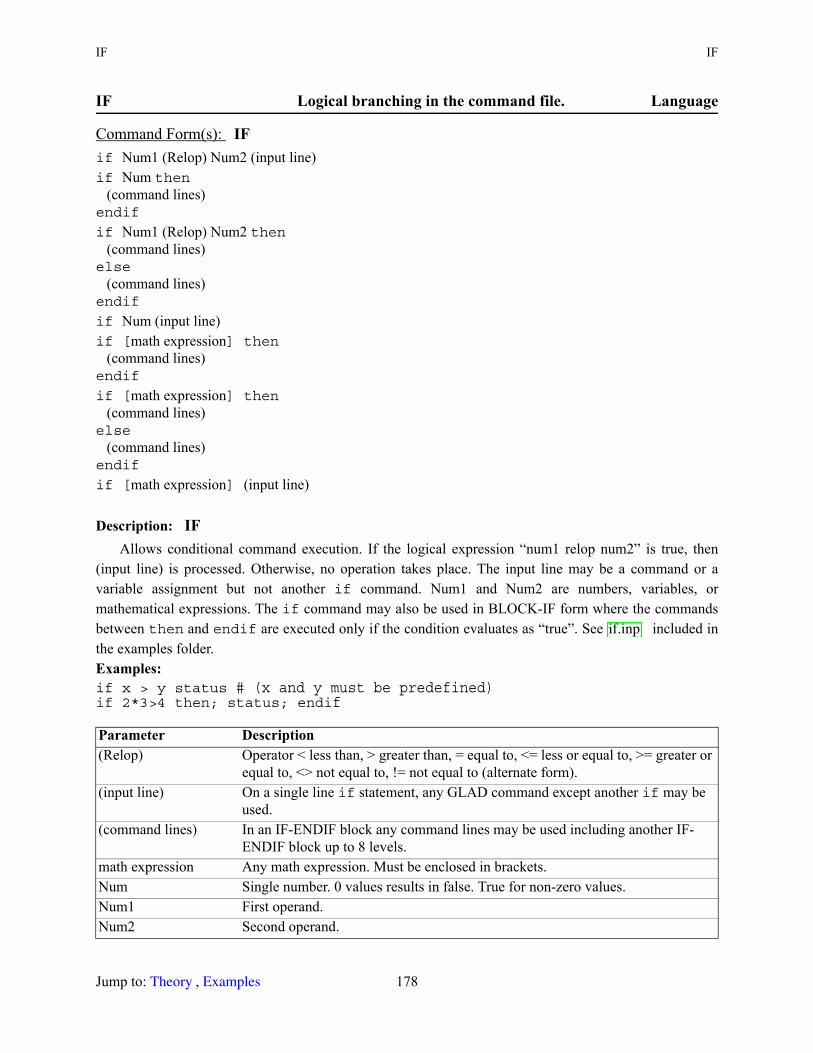
IF IF
IF Logical branching in the command file. Language
Description: IFAllows conditional command execution. If the logical expression “num1 relop num2” is true, then
(input line) is processed. Otherwise, no operation takes place. The input line may be a command or a variable assignment but not another if command. Num1 and Num2 are numbers, variables, or mathematical expressions. The if command may also be used in BLOCK-IF form where the commands between then and endif are executed only if the condition evaluates as “true”. See included in the examples folder.Examples:if x > y status # (x and y must be predefined)if 2*3>4 then; status; endif
Command Form(s): IF if Num1 (Relop) Num2 (input line)if Num then (command lines)endif
if Num1 (Relop) Num2 then (command lines)else (command lines)endif
if Num (input line)if [math expression] then (command lines)endif
if [math expression] then (command lines)else (command lines)endif
if [math expression] (input line)
Parameter Description (Relop) Operator < less than, > greater than, = equal to, <= less or equal to, >= greater or
equal to, <> not equal to, != not equal to (alternate form).(input line) On a single line if statement, any GLAD command except another if may be
used.(command lines) In an IF-ENDIF block any command lines may be used including another IF-
ENDIF block up to 8 levels.math expression Any math expression. Must be enclosed in brackets.Num Single number. 0 values results in false. True for non-zero values.Num1 First operand.Num2 Second operand.
if.inp
Jump to: , 178 Theory Examples
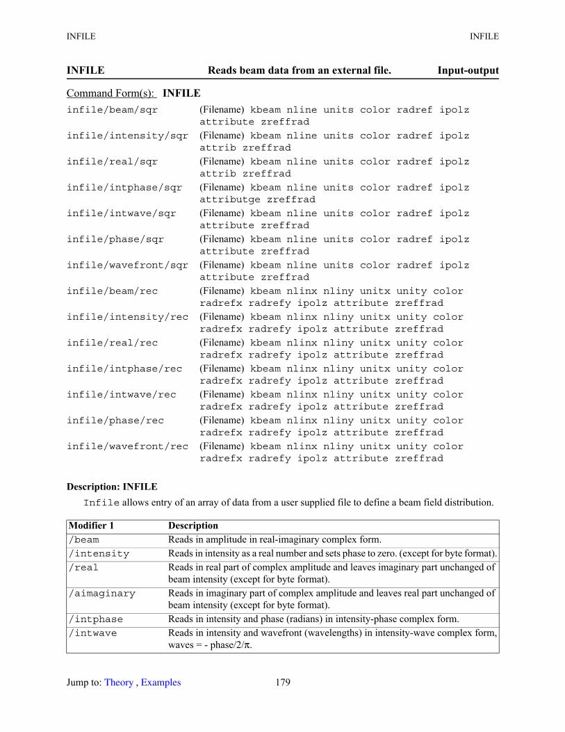
INFILE INFILE
INFILE Reads beam data from an external file. Input-output
Description: INFILEInfile allows entry of an array of data from a user supplied file to define a beam field distribution.
Command Form(s): INFILE infile/beam/sqr (Filename) kbeam nline units color radref ipolz
attribute zreffrad
infile/intensity/sqr (Filename) kbeam nline units color radref ipolz attrib zreffrad
infile/real/sqr (Filename) kbeam nline units color radref ipolz attrib zreffrad
infile/intphase/sqr (Filename) kbeam nline units color radref ipolz attributge zreffrad
infile/intwave/sqr (Filename) kbeam nline units color radref ipolz attribute zreffrad
infile/phase/sqr (Filename) kbeam nline units color radref ipolz attribute zreffrad
infile/wavefront/sqr (Filename) kbeam nline units color radref ipolz attribute zreffrad
infile/beam/rec (Filename) kbeam nlinx nliny unitx unity color radrefx radrefy ipolz attribute zreffrad
infile/intensity/rec (Filename) kbeam nlinx nliny unitx unity color radrefx radrefy ipolz attribute zreffrad
infile/real/rec (Filename) kbeam nlinx nliny unitx unity color radrefx radrefy ipolz attribute zreffrad
infile/intphase/rec (Filename) kbeam nlinx nliny unitx unity color radrefx radrefy ipolz attribute zreffrad
infile/intwave/rec (Filename) kbeam nlinx nliny unitx unity color radrefx radrefy ipolz attribute zreffrad
infile/phase/rec (Filename) kbeam nlinx nliny unitx unity color radrefx radrefy ipolz attribute zreffrad
infile/wavefront/rec (Filename) kbeam nlinx nliny unitx unity color radrefx radrefy ipolz attribute zreffrad
Modifier 1 Description /beam Reads in amplitude in real-imaginary complex form./intensity Reads in intensity as a real number and sets phase to zero. (except for byte format)./real Reads in real part of complex amplitude and leaves imaginary part unchanged of
beam intensity (except for byte format)./aimaginary Reads in imaginary part of complex amplitude and leaves real part unchanged of
beam intensity (except for byte format)./intphase Reads in intensity and phase (radians) in intensity-phase complex form./intwave Reads in intensity and wavefront (wavelengths) in intensity-wave complex form,
waves = - phase/2/π.
Jump to: , 179 Theory Examples
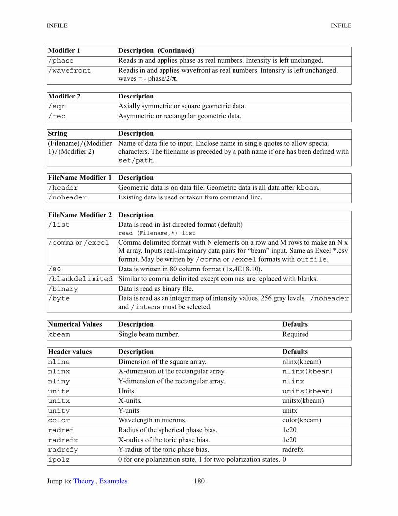
INFILE INFILE
/phase Reads in and applies phase as real numbers. Intensity is left unchanged./wavefront Readis in and applies wavefront as real numbers. Intensity is left unchanged.
waves = - phase/2/π.
Modifier 2 Description /sqr Axially symmetric or square geometric data./rec Asymmetric or rectangular geometric data.
String Description (Filename)/(Modifier 1)/(Modifier 2)
Name of data file to input. Enclose name in single quotes to allow special characters. The filename is preceded by a path name if one has been defined with set/path.
FileName Modifier 1 Description /header Geometric data is on data file. Geometric data is all data after kbeam./noheader Existing data is used or taken from command line.
FileName Modifier 2 Description /list Data is read in list directed format (default)
read (Filename,*) list
/comma or /excel Comma delimited format with N elements on a row and M rows to make an N x M array. Inputs real-imaginary data pairs for “beam” input. Same as Excel *.csv format. May be written by /comma or /excel formats with outfile.
/80 Data is written in 80 column format (1x,4E18.10)./blankdelimited Similar to comma delimited except commas are replaced with blanks./binary Data is read as binary file./byte Data is read as an integer map of intensity values. 256 gray levels. /noheader
and /intens must be selected.
Numerical Values Description Defaultskbeam Single beam number. Required
Header values Description Defaultsnline Dimension of the square array. nlinx(kbeam)nlinx X-dimension of the rectangular array. nlinx(kbeam)
nliny Y-dimension of the rectangular array. nlinx
units Units. units(kbeam)
unitx X-units. unitsx(kbeam)unity Y-units. unitxcolor Wavelength in microns. color(kbeam)radref Radius of the spherical phase bias. 1e20radrefx X-radius of the toric phase bias. 1e20radrefy Y-radius of the toric phase bias. radrefxipolz 0 for one polarization state. 1 for two polarization states. 0
Modifier 1 Description (Continued)
Jump to: , 180 Theory Examples
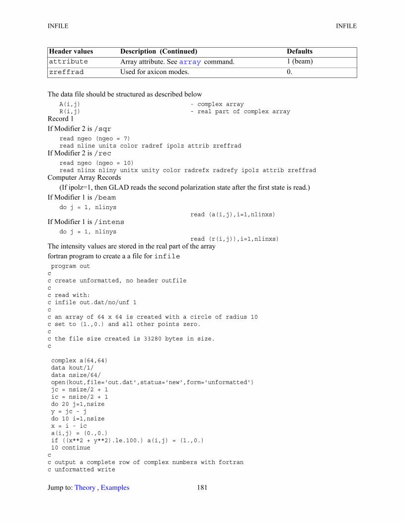
INFILE INFILE
The data file should be structured as described belowA(i,j) - complex arrayR(i,j) - real part of complex array
Record 1If Modifier 2 is /sqr
read ngeo (ngeo = 7) read nline units color radref ipolz attrib zreffrad
If Modifier 2 is /recread ngeo (ngeo = 10) read nlinx nliny unitx unity color radrefx radrefy ipolz attrib zreffrad
Computer Array Records(If ipolz=1, then GLAD reads the second polarization state after the first state is read.)
If Modifier 1 is /beamdo j = 1, nlinys
read (a(i,j),i=1,nlinxs) If Modifier 1 is /intens
do j = 1, nlinysread (r(i,j)),i=1,nlinxs)
The intensity values are stored in the real part of the arrayfortran program to create a a file for infile program outcc create unformatted, no header outfilecc read with:c infile out.dat/no/unf 1cc an array of 64 x 64 is created with a circle of radius 10c set to (1.,0.) and all other points zero.cc the file size created is 33280 bytes in size.c complex a(64,64) data kout/1/ data nsize/64/ open(kout,file='out.dat',status='new',form='unformatted') jc = nsize/2 + 1 ic = nsize/2 + 1 do 20 j=1,nsize y = jc - j do 10 i=1,nsize x = i - ic a(i,j) = (0.,0.) if ((x**2 + y**2).le.100.) a(i,j) = (1.,0.) 10 continuecc output a complete row of complex numbers with fortranc unformatted write
attribute Array attribute. See command. 1 (beam)zreffrad Used for axicon modes. 0.
Header values Description (Continued) Defaults array
Jump to: , 181 Theory Examples
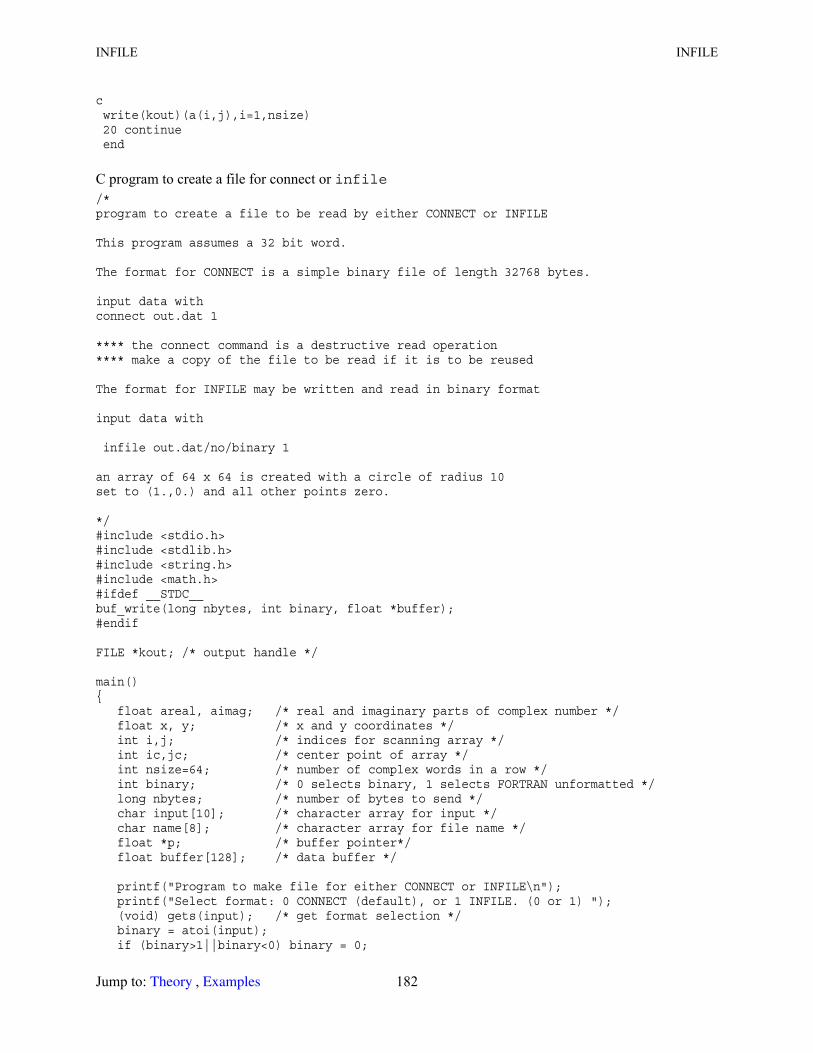
INFILE INFILE
c write(kout)(a(i,j),i=1,nsize) 20 continue end
C program to create a file for connect or infile/*program to create a file to be read by either CONNECT or INFILE
This program assumes a 32 bit word.
The format for CONNECT is a simple binary file of length 32768 bytes.
input data withconnect out.dat 1
**** the connect command is a destructive read operation**** make a copy of the file to be read if it is to be reused
The format for INFILE may be written and read in binary format
input data with
infile out.dat/no/binary 1
an array of 64 x 64 is created with a circle of radius 10set to (1.,0.) and all other points zero.
*/#include <stdio.h>#include <stdlib.h>#include <string.h>#include <math.h>#ifdef __STDC__buf_write(long nbytes, int binary, float *buffer);#endif
FILE *kout; /* output handle */
main(){ float areal, aimag; /* real and imaginary parts of complex number */ float x, y; /* x and y coordinates */ int i,j; /* indices for scanning array */ int ic,jc; /* center point of array */ int nsize=64; /* number of complex words in a row */ int binary; /* 0 selects binary, 1 selects FORTRAN unformatted */ long nbytes; /* number of bytes to send */ char input[10]; /* character array for input */ char name[8]; /* character array for file name */ float *p; /* buffer pointer*/ float buffer[128]; /* data buffer */
printf("Program to make file for either CONNECT or INFILE\n"); printf("Select format: 0 CONNECT (default), or 1 INFILE. (0 or 1) "); (void) gets(input); /* get format selection */ binary = atoi(input); if (binary>1||binary<0) binary = 0;
Jump to: , 182 Theory Examples

INITIALIZE INITIALIZE
if (binary==1) { printf("Writing out.dat. Read with\ninfile out.dat/no/binary 1\n"); strcpy(name,"out.dat"); }else { printf("Writing outs.bea. Read with\n connect out 1\n"); strcpy(name,"outs.bea"); } kout = fopen(name,"wb"); if (kout==0) { printf("error in opening %s\n",name); exit(0); }/* nbytes = number of complex words * bytes per complex word*/ nbytes = nsize*8; jc = nsize/2 + 1; /* find center point of array */ ic = nsize/2 + 1; for (j=1;j<=nsize;j++) /* loop over rows */ { y = jc - j; /* write from top to bottom */ p = buffer; for (i=1;i<=nsize;i++) /* loop over columns */ { x = ic - i; /* write from left to right */ areal = 0.; aimag = 0.; if ((x*x + y*y)<=100.) { areal = 1.; /* set center points to (1.,0.) */ } *p++ = areal; /* write real */ *p++ = aimag; /* write imag. */ } /* end of column loop */ (void) buf_write(nbytes,binary,buffer); } /* end of row loop */ return 0;}buf_write(long nbytes, int binary, float *buffer){ if (fwrite(buffer, nbytes, 1, kout)!=1) { printf("Failed to write data\n"); exit(0); } return 0;}
INITIALIZE Reinitialize to starting condition. Operator
Command Form(s): INITIALIZE initialize
Jump to: , 183 Theory Examples
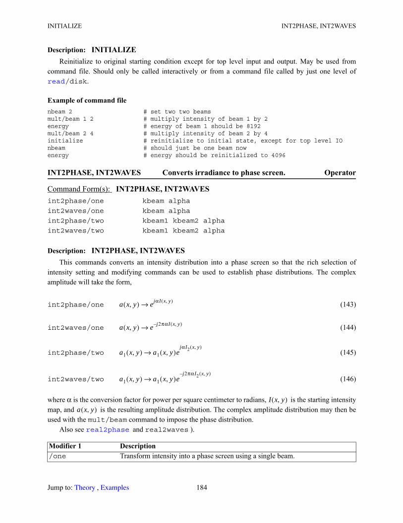
INITIALIZE INT2PHASE, INT2WAVES
Description: INITIALIZEReinitialize to original starting condition except for top level input and output. May be used from
command file. Should only be called interactively or from a command file called by just one level of /disk.
Example of command filenbeam 2 # set two two beamsmult/beam 1 2 # multiply intensity of beam 1 by 2energy # energy of beam 1 should be 8192mult/beam 2 4 # multiply intensity of beam 2 by 4initialize # reinitialize to initial state, except for top level IOnbeam # should just be one beam nowenergy # energy should be reinitialized to 4096
INT2PHASE, INT2WAVES Converts irradiance to phase screen. Operator
Description: INT2PHASE, INT2WAVESThis commands converts an intensity distribution into a phase screen so that the rich selection of
intensity setting and modifying commands can be used to establish phase distributions. The complex amplitude will take the form,
int2phase/one (143)
int2waves/one (144)
int2phase/two (145)
int2waves/two (146)
where α is the conversion factor for power per square centimeter to radians, is the starting intensity map, and is the resulting amplitude distribution. The complex amplitude distribution may then be used with the mult/beam command to impose the phase distribution.
Also see and real2waves ).
Command Form(s): INT2PHASE, INT2WAVES int2phase/one kbeam alpha
int2waves/one kbeam alpha
int2phase/two kbeam1 kbeam2 alpha
int2waves/two kbeam1 kbeam2 alpha
Modifier 1 Description /one Transform intensity into a phase screen using a single beam.
read
a x y,( ) ejαI x y,( )→
a x y,( ) e j2παI x y,( )–→
a1 x y,( ) a1 x y,( )ejαI2 x y,( )
→
a1 x y,( ) a1 x y,( )ej2παI2 x y,( )–
→
I x y,( )a x y,( )
real2phase
Jump to: , 184 Theory Examples
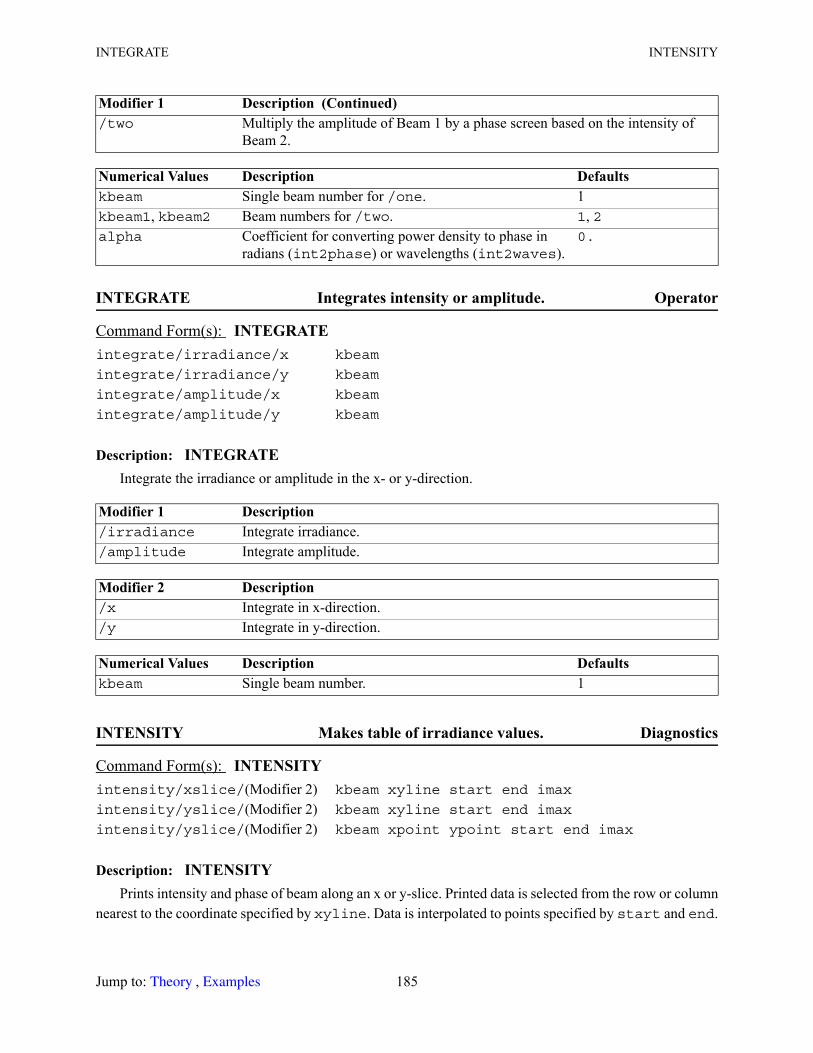
INTEGRATE INTENSITY
INTEGRATE Integrates intensity or amplitude. Operator
Description: INTEGRATEIntegrate the irradiance or amplitude in the x- or y-direction.
INTENSITY Makes table of irradiance values. Diagnostics
Description: INTENSITYPrints intensity and phase of beam along an x or y-slice. Printed data is selected from the row or column
nearest to the coordinate specified by xyline. Data is interpolated to points specified by start and end.
/two Multiply the amplitude of Beam 1 by a phase screen based on the intensity of Beam 2.
Numerical Values Description Defaultskbeam Single beam number for /one. 1kbeam1, kbeam2 Beam numbers for /two. 1, 2alpha Coefficient for converting power density to phase in
radians (int2phase) or wavelengths (int2waves).0.
Command Form(s): INTEGRATE integrate/irradiance/x kbeam
integrate/irradiance/y kbeam
integrate/amplitude/x kbeam
integrate/amplitude/y kbeam
Modifier 1 Description /irradiance Integrate irradiance./amplitude Integrate amplitude.
Modifier 2 Description /x Integrate in x-direction./y Integrate in y-direction.
Numerical Values Description Defaultskbeam Single beam number. 1
Command Form(s): INTENSITY intensity/xslice/(Modifier 2) kbeam xyline start end imax
intensity/yslice/(Modifier 2) kbeam xyline start end imax
intensity/yslice/(Modifier 2) kbeam xpoint ypoint start end imax
Modifier 1 Description (Continued)
Jump to: , 185 Theory Examples
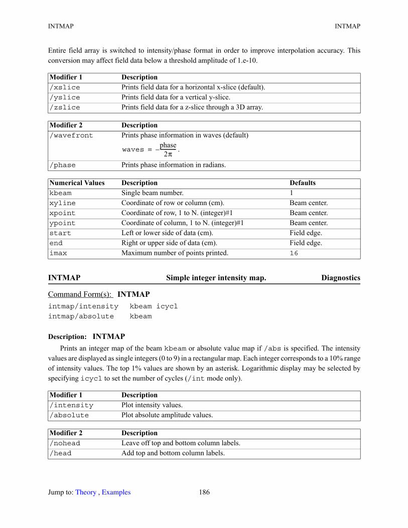
INTMAP INTMAP
Entire field array is switched to intensity/phase format in order to improve interpolation accuracy. This conversion may affect field data below a threshold amplitude of 1.e-10.
INTMAP Simple integer intensity map. Diagnostics
Description: INTMAPPrints an integer map of the beam kbeam or absolute value map if /abs is specified. The intensity
values are displayed as single integers (0 to 9) in a rectangular map. Each integer corresponds to a 10% range of intensity values. The top 1% values are shown by an asterisk. Logarithmic display may be selected by specifying icycl to set the number of cycles (/int mode only).
Modifier 1 Description /xslice Prints field data for a horizontal x-slice (default)./yslice Prints field data for a vertical y-slice./zslice Prints field data for a z-slice through a 3D array.
Modifier 2 Description /wavefront Prints phase information in waves (default)
.
/phase Prints phase information in radians.
Numerical Values Description Defaultskbeam Single beam number. 1xyline Coordinate of row or column (cm). Beam center.xpoint Coordinate of row, 1 to N. (integer)#1 Beam center.ypoint Coordinate of column, 1 to N. (integer)#1 Beam center.start Left or lower side of data (cm). Field edge.end Right or upper side of data (cm). Field edge.imax Maximum number of points printed. 16
Command Form(s): INTMAP intmap/intensity kbeam icycl
intmap/absolute kbeam
Modifier 1 Description /intensity Plot intensity values./absolute Plot absolute amplitude values.
Modifier 2 Description /nohead Leave off top and bottom column labels./head Add top and bottom column labels.
wavesphase
2π-------------–=
Jump to: , 186 Theory Examples
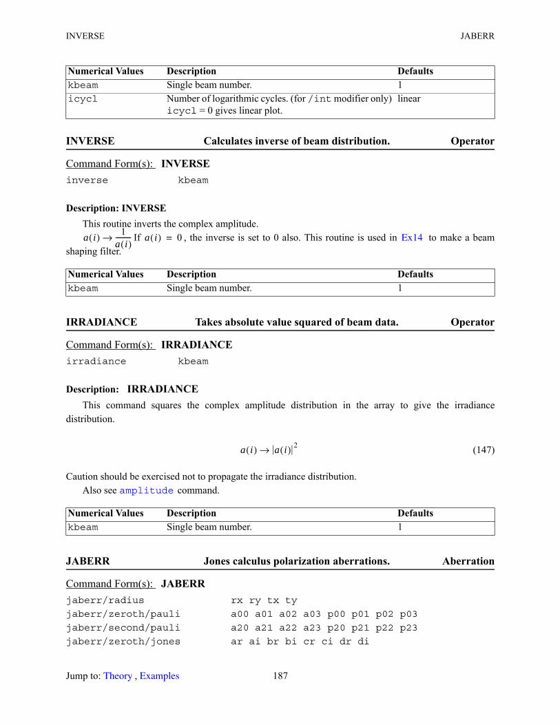
INVERSE JABERR
INVERSE Calculates inverse of beam distribution. Operator
Description: INVERSEThis routine inverts the complex amplitude.
If , the inverse is set to 0 also. This routine is used in to make a beam shaping filter.
IRRADIANCE Takes absolute value squared of beam data. Operator
Description: IRRADIANCEThis command squares the complex amplitude distribution in the array to give the irradiance
distribution.
(147)
Caution should be exercised not to propagate the irradiance distribution.Also see command.
JABERR Jones calculus polarization aberrations. Aberration
Numerical Values Description Defaultskbeam Single beam number. 1icycl Number of logarithmic cycles. (for /int modifier only)
icycl = 0 gives linear plot.linear
Command Form(s): INVERSE inverse kbeam
Numerical Values Description Defaultskbeam Single beam number. 1
Command Form(s): IRRADIANCE irradiance kbeam
Numerical Values Description Defaultskbeam Single beam number. 1
Command Form(s): JABERR jaberr/radius rx ry tx ty
jaberr/zeroth/pauli a00 a01 a02 a03 p00 p01 p02 p03
jaberr/second/pauli a20 a21 a22 a23 p20 p21 p22 p23
jaberr/zeroth/jones ar ai br bi cr ci dr di
a i( ) 1a i( )---------→ a i( ) 0= Ex14
a i( ) a i( ) 2→
amplitude
Jump to: , 187 Theory Examples
JABERR JABERR
Description: JABERRThis command models a surface using a zeroth and second order approximation to the sensitivity to the
local incidence angle at each point on the surface. The coefficients may be listed with /list. The surface radii and tilt angles must be explicitly set by the user. In later versions these will be better integrated into the other features of the program.
The Jones matrix may be directly defined using the /jones modifier or defined in terms of Pauli spin matrices. See , GLAD Theory Manual (theory.pdf).
jaberr/second/jones ar ai br bi cr ci dr di
jaberr/list/pauli
jaberr/list/jones
jaberr/surf kbeam
jaberr/medium kbeam deltaz
jaberr/clear
Modifier 1 Description /radius Defines the radii of the surface./zeroth Zeroth order coefficient matrix./second Second order coefficient matrix./surf Apply matrix as a surface effect./medium Apply matrix as an exponential effect./list List parameter./clear Set radii to infinity and other coefficients.
Modifier 2 Description /jones Jones matrices are set directly or displayed if /jones is called the Pauli form is
recalculated./pauli Pauli spin matrices are used to set Jones matrix the corresponding Jones matrix is
calculated each time the /pauli command is called. If several calls are used to build up the Pauli matrix.
Numerical Values Description Defaultskbeam Single beam number. 1rx, ry Radii of the surface (cm). 1e20
anm Amplitude coefficients. a00 = 1, all others 0tx, ty Transverse position in x and y.pnm Phase coefficients (deg).ar,ai,br,bi,cr,ci,di Real and imaginary components of Jones matrix.deltaz Distance along propagation distance direction.
Command Form(s): JABERR (Continued)
Sect. 14.3
Jump to: , 188 Theory Examples
JONES JONES
JONES Jones calculus operations. Operator
Description: JONESThis command models a surface using a zeroth and second order approximation to the sensitivity to the
local incidence angle at each point on the surface. The general Jones matrix may be set with the /setmodifier and may be listed with /list. The general matrix may be directly applied by the /multiplymodifier.
(148)
The exponential operation may be applied by the modifier /exponential. This models the effect of a continuous medium with polarization-active effects. The coefficients are assumed to be in cm. The exponential operator
(149)
The exponential of a matrix is found from the series
(150)
The operators for left and right circular polarizers, linear polarizers, retardance, optical activity and Faraday rotation, and Kerr (or Pockels cells) are applied directly as they are defined and leave the general Jones matrix in with the revised form. Optical activity is distinguished from Faraday rotation by having the
Command Form(s): JONES jones/set ar ai br bi cr ci dr di
jones/list
jones/multiply kbeam
jones/exponential kbeam z
jones/linpol kbeam theta
jones/left kbeam
jones/right kbeam
jones/retard kbeam azimuth phi
jones/optact kbeam theta
jones/orthogonal k1 k2
jones/faraday kbeam theta
jones/kerr kbeam
E2Ar Ai,( ) Br Bi,( )Cr Ci,( ) Dr Di,( )
E1=
E2 ez
Ar Ai,( ) Br Bi,( )
Cr Ci,( ) Dr Di,( )E1=
eA Ak
k!------
k 0=
∞
=
Jump to: , 189 Theory Examples
JSURF JSURF
sign of the rotation reversed for beams of left-handed parity. Parity is reversed each time the beam hits a mirror.
JSURF Fresnel transmission and reflection coefficients. Component
Description: JSURFThis command models refractive and reflective polarization effects due to Fresnel or single layer
interference filter coefficients at a surface. See Polarization, , GLAD Theory Manual (theory.pdf). The incidence angles are computed using a combination of real and paraxial angles as illustrated in Fig. 21. See Example for examples of these features.
Modifier 1 Description /set Set general Jones matrix coefficients./list List general Jones coefficients./multiply Apply general Jones matrix./exponential Jones matrix for distributed medium./linpol Linear polarizer./left Left circular polarizer./right Right circular polarizer./retard Retarder./optact Optical activity./orthogonal Separates perpendicular and orthogonal components of beam k1 relative to beam k2./faraday Faraday rotator./kerr Kerr or Pockels cell.
Numerical Values Description Defaultskbeam Single beam number. Requiredk1, k2 Input beam numbers for /orthogonal. returns the part of k1
perpendicular to k2 in k1 and the part of k1 parallel to k2 in k2.azimuth Azimuth rotation angle of component. 0.phi Phase of retarder (degrees). 0.theta Rotation of optical activity or in Faraday (degrees). 0.z Propagation distance for exponential operator. 0.
Command Form(s): JSURF jsurf/fresnel/(Modifier 2) kbeam n1 n2 rx ry tx ty kappa
jsurf/goos/(Modifier 2) kbeam n1 n2 tx ty kappa
jsurf/single/(Modifier 2) kbeam ni nf ns thick rx ry tx ty rdx rdy tdx tdy
Chap. 14
Ex37
Jump to: , 190 Theory Examples
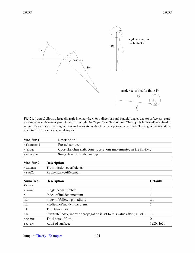
JSURF JSURF
Fig. 21. jsurf allows a large tilt angle in either the x- or y-directions and paraxial angles due to surface curvature as shown by angle vector plots shown on the right for Tx (top) and Ty (bottom). The pupil is indicated by a circular region. Tx and Ty are real angles measured as rotations about the x- or y-axes respectively. The angles due to surface curvature are treated as paraxial angles.
Modifier 1 Description /fresnel Fresnel surface./goos Goos-Hanchen shift. Jones operations implemented in the far-field./single Single layer thin file coating.
Modifier 2 Description /trans Transmission coefficients./refl Reflection coefficients.
Numerical Values
Description Defaults
kbeam Single beam number. 1n1 Index of incident medium. 1.
n2 Index of following medium. 1.
ni Medium of incident medium. 1.nf Thin film index. 1.ns Substrate index, index of propagation is set to this value after jsurf. 1.thick Thickness of film. 0.rx,ry Radii of surface. 1e20, 1e20
angle vector plot for finite Ty
Ty
��
Tx
Ry
� ��( )���⁄
Tx
angle vector plot for finite Tx
���
Jump to: , 191 Theory Examples
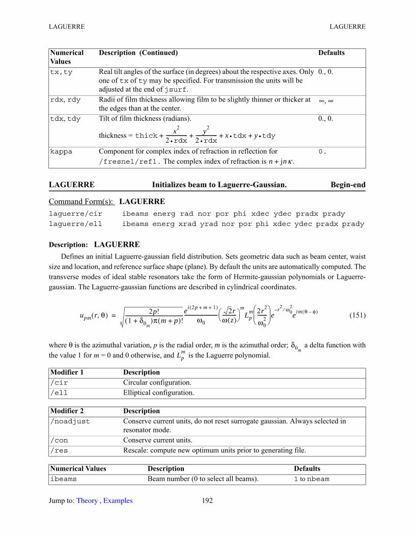
LAGUERRE LAGUERRE
LAGUERRE Initializes beam to Laguerre-Gaussian. Begin-end
Description: LAGUERREDefines an initial Laguerre-gaussian field distribution. Sets geometric data such as beam center, waist
size and location, and reference surface shape (plane). By default the units are automatically computed. The transverse modes of ideal stable resonators take the form of Hermite-gaussian polynomials or Laguerre-gaussian. The Laguerre-gaussian functions are described in cylindrical coordinates.
(151)
where θ is the azimuthal variation, p is the radial order, m is the azimuthal order; a delta function with the value 1 for m = 0 and 0 otherwise, and is the Laguerre polynomial.
tx,ty Real tilt angles of the surface (in degrees) about the respective axes. Only one of tx of ty may be specified. For transmission the units will be adjusted at the end of jsurf.
0., 0.
rdx, rdy Radii of film thickness allowing film to be slightly thinner or thicker at the edges than at the center.
tdx, tdy Tilt of film thickness (radians).
thickness =
0., 0.
kappa Component for complex index of refraction in reflection for /fresnel/refl. The complex index of refraction is .
0.
Command Form(s): LAGUERRE laguerre/cir ibeams energ rad nor por phi xdec ydec pradx prady
laguerre/ell ibeams energ xrad yrad nor por phi xdec ydec pradx prady
Modifier 1 Description /cir Circular configuration./ell Elliptical configuration.
Modifier 2 Description /noadjust Conserve current units, do not reset surrogate gaussian. Always selected in
resonator mode./con Conserve current units./res Rescale: compute new optimum units prior to generating file.
Numerical Values Description Defaultsibeams Beam number (0 to select all beams). 1 to nbeam
Numerical Values
Description (Continued) Defaults
∞ ∞,
thickx2
2 rdx•----------------- y2
2 rdx•----------------- x tdx• y tdy•+ + + +
n jnκ+
upm r θ,( ) 2p!1 δ0m
+( )π m p+( )!-----------------------------------------------ei 2p m 1+ +( )
ω0--------------------------- 2r
ω z( )-----------
mLp
m 2r2
ω02
--------
er2 ω0
2⁄–eim θ φ–( )=
δ0mLp
m
Jump to: , 192 Theory Examples
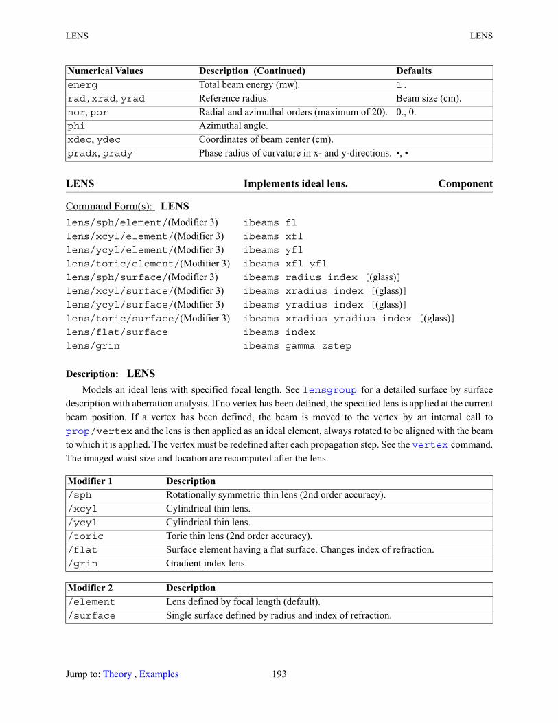
LENS LENS
LENS Implements ideal lens. Component
Description: LENSModels an ideal lens with specified focal length. See for a detailed surface by surface
description with aberration analysis. If no vertex has been defined, the specified lens is applied at the current beam position. If a vertex has been defined, the beam is moved to the vertex by an internal call to
/vertex and the lens is then applied as an ideal element, always rotated to be aligned with the beam to which it is applied. The vertex must be redefined after each propagation step. See the command. The imaged waist size and location are recomputed after the lens.
energ Total beam energy (mw). 1.
rad,xrad, yrad Reference radius. Beam size (cm).nor, por Radial and azimuthal orders (maximum of 20). 0., 0.phi Azimuthal angle.xdec, ydec Coordinates of beam center (cm).pradx, prady Phase radius of curvature in x- and y-directions. •, •
Command Form(s): LENS lens/sph/element/(Modifier 3) ibeams fl
lens/xcyl/element/(Modifier 3) ibeams xfl
lens/ycyl/element/(Modifier 3) ibeams yfl
lens/toric/element/(Modifier 3) ibeams xfl yfl
lens/sph/surface/(Modifier 3) ibeams radius index [(glass)]lens/xcyl/surface/(Modifier 3) ibeams xradius index [(glass)]lens/ycyl/surface/(Modifier 3) ibeams yradius index [(glass)]lens/toric/surface/(Modifier 3) ibeams xradius yradius index [(glass)]lens/flat/surface ibeams index
lens/grin ibeams gamma zstep
Modifier 1 Description /sph Rotationally symmetric thin lens (2nd order accuracy)./xcyl Cylindrical thin lens./ycyl Cylindrical thin lens./toric Toric thin lens (2nd order accuracy)./flat Surface element having a flat surface. Changes index of refraction./grin Gradient index lens.
Modifier 2 Description /element Lens defined by focal length (default)./surface Single surface defined by radius and index of refraction.
Numerical Values Description (Continued) Defaults
lensgroup
prop vertex
Jump to: , 193 Theory Examples

LENSARRAY LENSARRAY
LENSARRAY Array of lenses. Component
Modifier 3 Description /geometric Lens modifies geometric radii of curvature (default), as displayed by ./phase Lens treated as phase object. Only long focal lengths will be adequately sampled.
Check for wavefront aliasing by plotting wavefront.
Parameter Description glass Name of glass for /surface. May use glass named in Table L.1 or “glass” as
defined by the command. The index for the wavelength of the beam will be calculated. If glass name is not given, the index may be defined by the index variable and will apply to all beams without regard to wavelength.
Numerical Values Description Defaultsibeams Beam number (0 to select all beams). 1 to nbeamfl Focal length of rotationally symmetric thin lens. 1e20
xfl Focal length of x-cylindrical thin lens. 1e20
yfl Focal length of y-cylindrical thin lens. 1e20
radius Surface radius. 1e20
xradius X-radius of cylinder or toric surface. 1e20
yradius Y-radius of cylinder or toric surface. 1e20
index Index of refraction if not defined by glass name parameter.
gamma Coefficient of index profile for GRIN lens. Index distribution is assumed to take the form:.
The ABCD solution takes the form:
zstep Length of the GRIN lens. 0.
Command Form(s): LENSARRAY lensarray/hexagonal/set piston xtilt ytilt focus omega
lensarray/hexagonal/all kbeam width focallength iseed
lensarray/hexagonal/element kbeam xcell ycell width focallength iseed
lensarray/hexagonal/clear kbeam xcell ycell width value
lensarray/hexagonal/paste/element
kbeam1 kbeam2 xcell ycell width
lensarray/hexagonal/paste/all kbeam1 kbeam2 width
lensarray/hexagonal/multilevel kbeam width n1 n2 n3 n4iseed
lensarray/rectangular/set piston xtilt ytilt focus omega
lensarray/rectangular/all kbeam xwidth ywidth focallength iseed
geodata
glass
n r( ) n012---γ2r2–=
ABCD z( ) γz( )cos γz( )( )sin γ⁄γ γz( )sin– γz( )cos
=
Jump to: , 194 Theory Examples

LENSARRAY LENSARRAY
Description: LENSARRAYThis routine models an array of lenses. If the /all modifier is used, a complete array is produced, each
with the same focal length. Random errors for piston, tilt, and defocus may be specified by the /setmodifier. A single element may be cleared by the /clear modifier or modified by the /elementmodifier.
The aberrations are defined to have peak aberration values as specified for the x-width for either hexagonal or rectangular shapes. The /multilevel modifier puts in random piston, tilt, or defocus in discrete levels. No focal length (other than that of defocus) is added in /multilevel mode.
lensarray/rectangular/element kbeam xcell ycell xwidth ywidth focallength iseed
lensarray/rectangular/paste/element
kbeam1 kbeam2 xcell ycell xwidth ywidth
lensarray/rectangular/paste/all
kbeam1 kbeam2 xwidth ywidth
lensarray/rectangular/clear kbeam xcell ycell xwidth ywidth value
lensarray/rectangular/multilevel
kbeam xwidth ywidth n1 n2 n3 n4 iseed
Fig. 22a. Hexagonal array showing numbering system. Fig. 22b. Rectangular array showing numbering system.
Modifier 1 Description /hexagonal Hexagonal shape as defined by the x-width./rectangular Rectangular shape as defined by x- and y-width.
Modifier 2 Description /set Sets random errors and intensity roll-off coefficient. Also, sets values to be used
by /element where they are used exactly./all Implements complete lens array./clear Clears the specified cell and resets transmission to value.
Command Form(s): LENSARRAY (Continued)
Jump to: , 195 Theory Examples
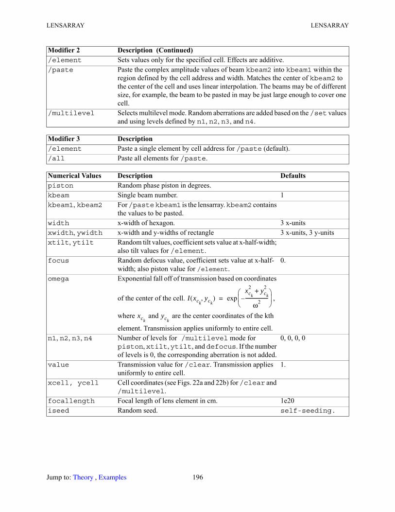
LENSARRAY LENSARRAY
/element Sets values only for the specified cell. Effects are additive./paste Paste the complex amplitude values of beam kbeam2 into kbeam1 within the
region defined by the cell address and width. Matches the center of kbeam2 to the center of the cell and uses linear interpolation. The beams may be of different size, for example, the beam to be pasted in may be just large enough to cover one cell.
/multilevel Selects multilevel mode. Random aberrations are added based on the /set values and using levels defined by n1, n2, n3, and n4.
Modifier 3 Description /element Paste a single element by cell address for /paste (default)./all Paste all elements for /paste.
Numerical Values Description Defaultspiston Random phase piston in degrees.kbeam Single beam number. 1kbeam1, kbeam2 For /paste kbeam1 is the lensarray. kbeam2 contains
the values to be pasted.width x-width of hexagon. 3 x-unitsxwidth, ywidth x-width and y-widths of rectangle 3 x-units, 3 y-unitsxtilt, ytilt Random tilt values, coefficient sets value at x-half-width;
also tilt values for /element.focus Random defocus value, coefficient sets value at x-half-
width; also piston value for /element.0.
omega Exponential fall off of transmission based on coordinates
of the center of the cell. ,
where and are the center coordinates of the kth
element. Transmission applies uniformly to entire cell.n1, n2, n3, n4 Number of levels for /multilevel mode for
piston, xtilt, ytilt, and defocus. If the number of levels is 0, the corresponding aberration is not added.
0, 0, 0, 0
value Transmission value for /clear. Transmission applies uniformly to entire cell.
1.
xcell, ycell Cell coordinates (see Figs. 22a and 22b) for /clear and /multilevel.
focallength Focal length of lens element in cm. 1e20iseed Random seed. self-seeding.
Modifier 2 Description (Continued)
I xckyck
,( )xck
2 yck
2+
ω2-------------------–
exp=
xckyck
Jump to: , 196 Theory Examples
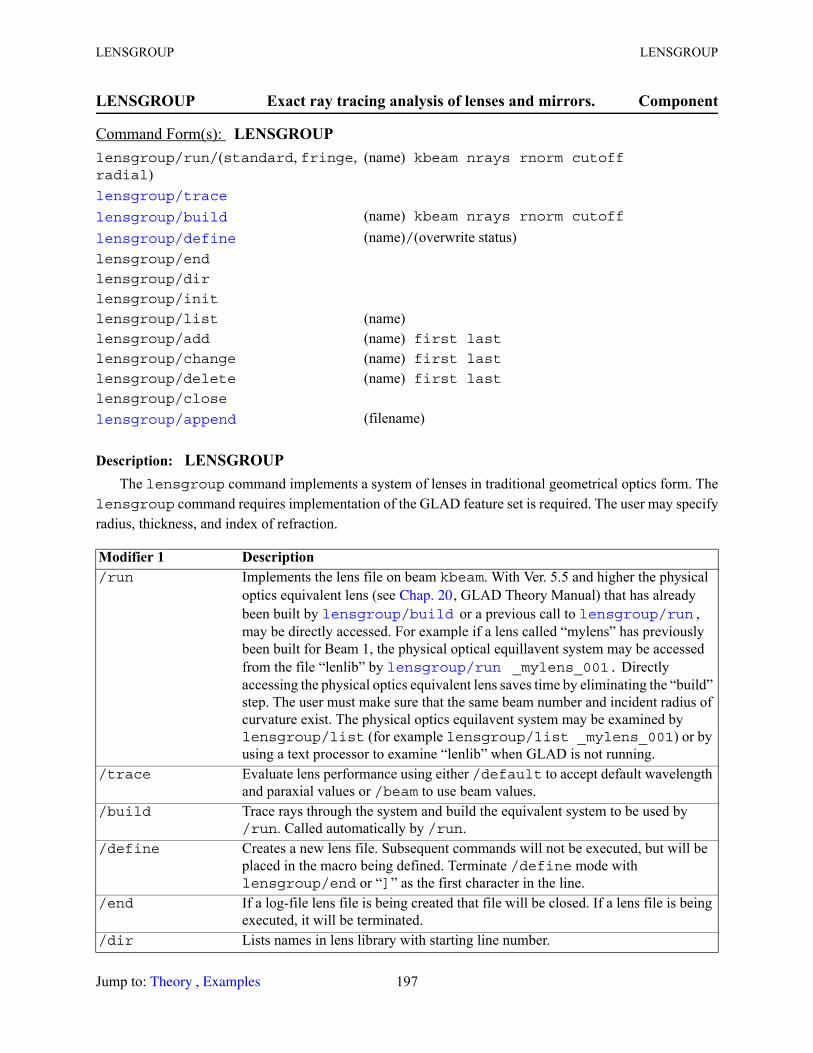
LENSGROUP LENSGROUP
LENSGROUP Exact ray tracing analysis of lenses and mirrors. Component
Description: LENSGROUPThe lensgroup command implements a system of lenses in traditional geometrical optics form. The
lensgroup command requires implementation of the GLAD feature set is required. The user may specify radius, thickness, and index of refraction.
Command Form(s): LENSGROUP lensgroup/run/(standard, fringe, radial)
(name) kbeam nrays rnorm cutoff
(name) kbeam nrays rnorm cutoff(name)/(overwrite status)
lensgroup/end
lensgroup/dir
lensgroup/init
lensgroup/list (name)lensgroup/add (name) first lastlensgroup/change (name) first lastlensgroup/delete (name) first lastlensgroup/close
(filename)
Modifier 1 Description /run Implements the lens file on beam kbeam. With Ver. 5.5 and higher the physical
optics equivalent lens (see , GLAD Theory Manual) that has already been built by or a previous call to , may be directly accessed. For example if a lens called “mylens” has previously been built for Beam 1, the physical optical equillavent system may be accessed from the file “lenlib” by _mylens_001. Directly accessing the physical optics equivalent lens saves time by eliminating the “build” step. The user must make sure that the same beam number and incident radius of curvature exist. The physical optics equilavent system may be examined by lensgroup/list (for example lensgroup/list _mylens_001) or by using a text processor to examine “lenlib” when GLAD is not running.
/trace Evaluate lens performance using either /default to accept default wavelength and paraxial values or /beam to use beam values.
/build Trace rays through the system and build the equivalent system to be used by /run. Called automatically by /run.
/define Creates a new lens file. Subsequent commands will not be executed, but will be placed in the macro being defined. Terminate /define mode with lensgroup/end or “]” as the first character in the line.
/end If a log-file lens file is being created that file will be closed. If a lens file is being executed, it will be terminated.
/dir Lists names in lens library with starting line number.
lensgroup/trace lensgroup/build lensgroup/define
lensgroup/append
Chap. 20 lensgroup/build lensgroup/run
lensgroup/run
Jump to: , 197 Theory Examples

LENSGROUP LENSGROUP
/init Recalculates the lens directory by reading the lens library and resetting the starting numbers.
/list Lists the lens or physical optics equivalent lens such as _mylens_001. Line numbers for reference in editing.
/add Adds the new line numbers from first to last. GLAD prompts for the lines which must be typed in by the user.
/change Replaces lines./delete Deletes lines from first to last. (Deletion of the entire lens is described in the list
of parameter modifiers below.)/close Closes file LENLIB so it can be edited by a system editor. See command
for using system functions from within GLAD. LENLIB will automatically be reopened at the next call to .
/append (Not currently active.) Append lens deck file to library. The lensgroup is given the same name as the file given, less the suffix. If a lensgroup of the same name already exists, it is replaced. File names of the form *.GRP are interpreted as being in GLAD format. File names of the form *.ZMX are assumed to be in Zemax format and are copied into *.GRP format before appending to library.
Modifier 2 Description run/fringe Set of 37 polynomials organized by polynomial order based on the sum of radial
and azimuthal orders (default). Used in many interferometric reduction programs. /fringe has more radial terms and fewer azimuthal terms. See , Table 2.
run/standard Set of 45 polynomials organized by radial order. All azimuthal terms are included. See , Table 1.
run/radial Set of radial polynomials up to 20th order. See , Table 3.
Character String Description (Name) Lens name (character string).(Name)/nooverwrite Used with /define. If input is currently from a terminal and the name
exists, the user is asked if the file should be overwritten.(Name)/overwrite Used with /define. If the file specified exists, the file is overwritten by
the new macro.(Name)/delete Deletes the named lensgroup, e.g.,
lensgroup/define xxx/delete # deletes macro XXX
Numerical Values
Description Defaults
kbeam Single beam number. 1first First line number of lens as displayed by lensgroup/list.last Last line number of lens as displayed by lensgroup/list.nrays Number of rays across the diameter of the pupil to be used in
calculating aberrations.nrays
rnorm Normalizing radius. Beam size from geodata
Modifier 1 Description (Continued)
system
vertex
fitzern
fitzern fitzern
Jump to: , 198 Theory Examples

LENSGROUP/APPEND LENSGROUP/BUILD
LENSGROUP/APPEND Adds a lens deck file to the lens library. Component
Description: LENSGROUP/APPENDThe command lensgroup/append adds a lens deck file to the lens library. The lens deck file may
be in GLAD format or in the format of one of the other lens design programs supported by GLAD. The file type determined by the file suffix. GLAD will create a lens in the library using the same name as the file (stripped of the suffix). If a lens group of the same name already exists it is deleted before appending the new lens group.
For non-GLAD formats, the first and last surfaces are assumed to be the object and image surfaces and are deleted. At present, pickups and solves are not processed.
LENSGROUP/BUILD Build the physical optics equivalent of a lens. Component
Description: LENSGROUP/BUILDThe command lensgroup/build builds a physical optics equivalent of the designated lensgroup by
tracing rays through the system. It is called automatically by if the equivalent system has not been defined or has changed.
cutoff Cutoff for Zernike aberration coefficients to be used. 0.002
Command Form(s): LENSGROUP/APPEND lensgroup/append (Filename)
String Description Filename File name of input lens deck to be adds to library. The name should be in the form
“name.grp”.
Command Form(s): LENSGROUP/BUILD /build/default/(modifier 3) (name) xo_rel yo_rel lambda nrays rnorm cutoff
[(listing type)]/build/beam/(modifier 3) (name) kbeam nrays rnorm cutoff [(listing type)]
Modifier 2 Description /beam Use actual beam data, requires kbeam. Object point and wavelength are
determined by incident beam (default)./default Use paraxial data from object line of lens data. Wavelength may be changed by
setting lambda.
Numerical Values
Description (Continued) Defaults
lensgroup/run
Jump to: , 199 Theory Examples
LENSGROUP/DEFINE LENSGROUP/DEFINE
LENSGROUP/DEFINE Define a lens group. Component
Description: LENSGROUP/DEFINEA geometrical optics calculation is used to calculate the change in paraxial values, aberrations, and
diffraction propagation length, which are applied to the beam. Apertures in the lens deck defined by clap act to vignette the beam. The and commands locate the lens in space. Default field size, numerical aperture, and wavelength are defined to be used by the geometrical analysis with lensgroup$trace .
The surface curvature in terms of z as a function of transverse coordinates x and y is
, (152)
Modifier 3 Description /fringe Set of 37 polynomials organized by polynomial order based on the sum of radial
and azimuthal orders (default). Used in many interferometric reduction programs. /fringe has more radial terms and fewer azimuthal terms. See , Table 2.
/standard Set of 45 polynomials organized by radial order. All azimuthal terms are included. See , Table 1.
/radial Set of radial polynomials up to 20th order. See , Table 3.
Character String Description name Lensgroup name.
Numerical Values Description Defaultskbeam Single beam number. 1lambda Wavelength for /default. Default value is taken from
the object line of the lens definition.xo_rel, yo_rel Rays are traced with respect to relative paraxial object
position for /default.0., 0., 0., 0.
nrays Number of rays across the diameter of the pupil to be used in calculating aberrations.
rnorm Normalizing radius. Beam size from geodata
cutoff Cutoff for Zernike aberration coefficients to be used. 0.002
Command Form(s): LENSGROUP/DEFINE lensgroup/define (name)/(overwrite status)
fitzern
fitzern fitzern
vertex/locate vertex/rotate
lensgroup/trace
z cr2
1 1 c2r2 1 κ+( )–[ ]1 2⁄
+---------------------------------------------------------- a4r4 a6r6 …+ + += r2 x2 y2+=
Jump to: , 200 Theory Examples

LENSGROUP/DEFINE LENSGROUP/DEFINE
where z is the distance along the axis (the sag of the surface), x and y are the transverse coordinates, c is the curvature of the surface (the inverse of the surface radius), κ is the conic constant, , , etc. are the general aspheric coefficients, If surface/zernike is specified the coefficients are interpreted as Zernike coefficients. See Table 3. The conic constant is related to the eccentricity of the conic, . For a simple spherical surface κ = 0 and the general aspheric coefficients are zero.
The glass may be selected from Schott, Hoya, Ohara, infrared, and miscellaneous catalogs listed in the attached tables. GLAD uses one of the following dispersion equations,
Type 1: Schott (153)
Type 2: Sellmeier 1 (154)
Type 3: Hertzberger (155)
Type 4: Sellmeier 2 (156)
Type 5: Conrady (157)
Type 6: Inverse power (158)
Lensgroup Command Form(s) object lambda yfield yna zsurf zpupil xfield xna [(glass name)]surface_lensgroup/conic
radius thickness cc a4 a6 a8 a10 a12 a14 a16 a18 a20 curvature [(glass name)]
surface_lensgroup/zernike
radius thickness cc a4 a6 a8 a10 a12 a14 a16 a18 a20 curvature [(glass name)]
clap_lensgroup/(cir, sqr, or hex)
rad xdec ydec
clap_lensgroup/(ell or rec)
xrad yrad xdec ydec
obs_lensgroup/(cir, sqr, or hex)
rad xdec ydec
obs_lensgroup/(ell or rec)
xrad yrad xdec ydec
a4 a6
κ ε2–=
N2 A0 A1λ2 A2λ 2– A3λ 4– A4λ 6– A5λ 8–+ + + + +=
N2 1–K1λ2
λ2 L1–-----------------
K2λ2
λ2 L2–-----------------
K3λ2
λ2 L3–-----------------+ +
A0λ2
λ2 A1–-----------------
A2λ2
λ2 A3–-----------------
A4λ2
λ2 A5–-----------------+ += =
N A BL CL2 Dλ2 Eλ4 Fλ6+ + + + +
A0 A1L A2L2 A3λ2 A4λ4 A5λ6+ + + + +
=
= L 1λ2 0.028–-------------------------=
N2 1– AB1λ2
λ2 L1–-----------------
B2λ2
λ2 L2–-----------------+ + A0
A1λ2
λ2 A2–-----------------
A3λ2
λ2 A4–-----------------+ += =
N N0Aλ--- B
λ3.5--------+ + A0
A1λ------
A2
λ3.5--------+ += =
N N0Aλ2----- B
λ4-----+ + A0
A1
λ2------
A2
λ4------+ += =
Jump to: , 201 Theory Examples
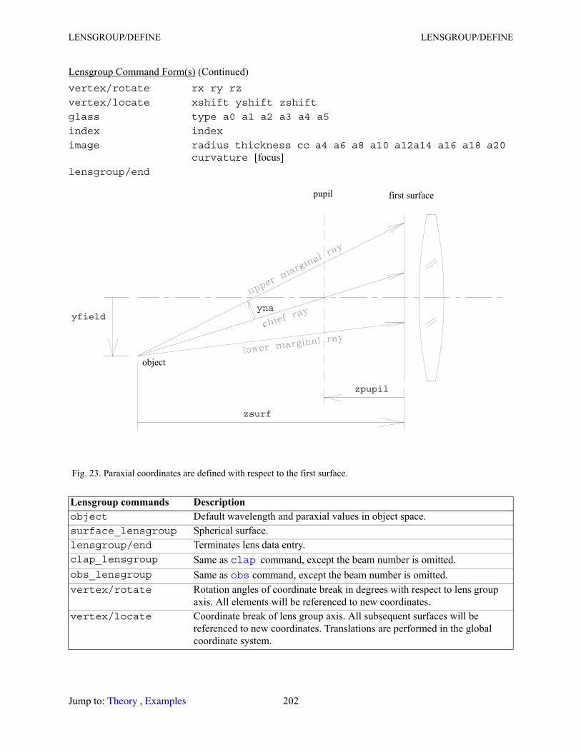
LENSGROUP/DEFINE LENSGROUP/DEFINE
vertex/rotate rx ry rz
vertex/locate xshift yshift zshift
glass type a0 a1 a2 a3 a4 a5
index index
image radius thickness cc a4 a6 a8 a10 a12a14 a16 a18 a20 curvature [focus]
lensgroup/end
Fig. 23. Paraxial coordinates are defined with respect to the first surface.
Lensgroup commands Description object Default wavelength and paraxial values in object space.surface_lensgroup Spherical surface.lensgroup/end Terminates lens data entry.clap_lensgroup Same as command, except the beam number is omitted.obs_lensgroup Same as command, except the beam number is omitted.vertex/rotate Rotation angles of coordinate break in degrees with respect to lens group
axis. All elements will be referenced to new coordinates.vertex/locate Coordinate break of lens group axis. All subsequent surfaces will be
referenced to new coordinates. Translations are performed in the global coordinate system.
Lensgroup Command Form(s) (Continued)
zsurf
object
yfield
first surfacepupil
zpupil
yna
clap obs
Jump to: , 202 Theory Examples
LENSGROUP/DEFINE LENSGROUP/DEFINE
glass Specify glass coefficients in the formglass type a0 a1 a2 a3 a4 a5Refer to this glass by the name “glass” in the surface command.
index Same as glass 5 a0 to set value for glass. Use parameter glass on subsequent surface.
image Image surface. The image surface may be curved and an incremental thickness is allowed.
Lensgroup command modifiers
Description
conic Conic surface with even power aspheric coefficients.zernike Conic surface with radially symmetric Zernike coefficients.cir, sqr, ell, or hex Aperture or obscuration shapes.vertex/rotate/add Add values to internal vertex rotation.vertex/rotate/set Set values for intenal vertex rotation.vertex/locate/add Add values to internal vertex location.vertex/locate/set Set values for intenal vertex location relative to front vertex.glass Specify glass coefficients in the form
glass type a0 a1 a2 a3 a4 a5
Modifier 3 Description /element Paste a single element by cell address for /paste (default)./all Paste all elements for /paste.
Parameter Description (glass name) Glass name: air, reflector, glass, or a glass name from one of the glass catalogs in
the accompanying Tables 12 to 16. focus Causes GLAD to calculate paraxial image distance.
Numerical Values Description Defaultsyfield Half-width of object field, y-direction.yna Numerical angle in object space, y-direction. 0.
zsurf Distance from object to first surface. 1e20
zpupil Distance from first surface to pupil. 0.
xfield Half-width of object field, x-directions. yfieldxna Numerical angle in object space, x-direction. ynaradius Radius of curvature (default type for first parameter). Either
Radius or Curvature may be specified.curvature Alternate definition of surface curvature. Variable assignment
must be used.thickness Distance to next surface measured in current vertex coordinates.
thickness on the image line is added in front of the image.
Lensgroup commands Description (Continued)
Jump to: , 203 Theory Examples
LENSGROUP/DEFINE LENSGROUP/DEFINE
Examples 1: Simple lenslensgroup/def demo/o object lambda=.589 yfield=1.745e8 yna=1e-10 zsurf=1e10 air surface 100. .2 bk7 # radius 100, thickness .2, BK7 clap/cir 1.0 # clear aperture of 1 cm radius surface cur=.02 0. air # curvature .02, thickness 0, AIR image focuslensgroup/endcolor 1 1.06cc start with a gaussian beam having a width of .005, afterc 100 cm, the beam width is .67484 at the lensgauss/c/c 1 1 .005vertex/locate/rel 0 0 100 # translate 100 cmvertex/rotate 1 0 0 # tip lens 1 degree about x-axislensgroup/run demo 1 # implement lens
Example 2: Forward and backward through a lensR1 = 200T1 = 2R2 = -300T2 = 4.5R3 = -200T3 = 4R4 = -350alias glass1 bk7alias glass2 airalias glass3 bk7thick = T1 + T2 + T3
lensgroup/def forward/o surface R1 T1 @glass1 surface R2 T2 @glass2 surface R3 T3 @glass3 surface R4 0 air image focuslensgroup/endcc Write lens in reverse orderclensgroup/def backward/o surface -R4 T3 @glass3 surface -R3 T2 @glass2 surface -R2 T1 @glass1 surface -R1 0 air image focuslensgroup/endcc Now set up a mirror to retro-reflect to illustrate procedurevertex/locate/abs 0 0 Z_start
cc, a4, a6, a8, a10, a12, a14, a16, a18, a20
Conic constant and 4th through 20th order aspheric coefficients. If surface/zernike is specified the coefficients are interpreted as Zernike terms. See Table 3.
type Dispersion type for glass. See dispersion types (201).a0, a1, a2, a3, a4, a5 Dispersion coefficients for glass.
Numerical Values Description (Continued) Defaults
Jump to: , 204 Theory Examples
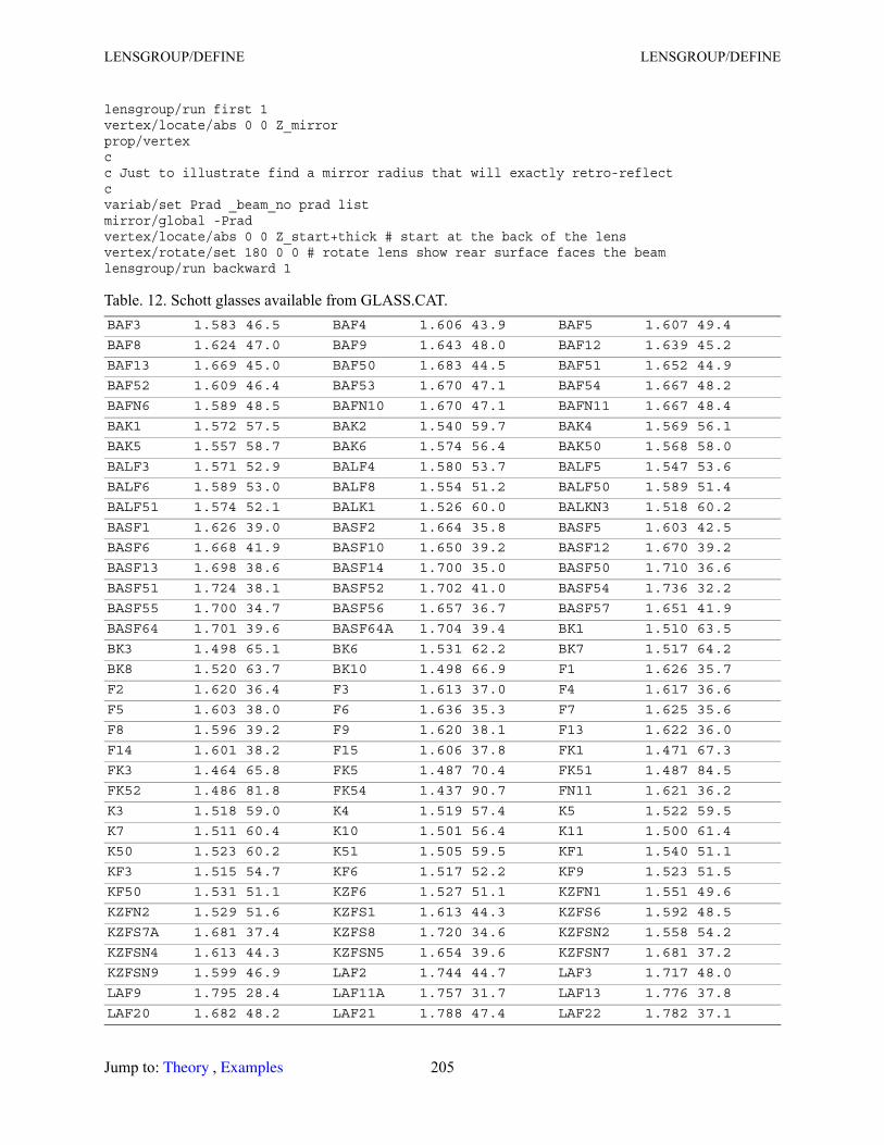
LENSGROUP/DEFINE LENSGROUP/DEFINE
lensgroup/run first 1vertex/locate/abs 0 0 Z_mirrorprop/vertexcc Just to illustrate find a mirror radius that will exactly retro-reflectcvariab/set Prad _beam_no prad listmirror/global -Pradvertex/locate/abs 0 0 Z_start+thick # start at the back of the lensvertex/rotate/set 180 0 0 # rotate lens show rear surface faces the beamlensgroup/run backward 1
Table. 12. Schott glasses available from GLASS.CAT. BAF3 1.583 46.5 BAF4 1.606 43.9 BAF5 1.607 49.4
BAF8 1.624 47.0 BAF9 1.643 48.0 BAF12 1.639 45.2
BAF13 1.669 45.0 BAF50 1.683 44.5 BAF51 1.652 44.9
BAF52 1.609 46.4 BAF53 1.670 47.1 BAF54 1.667 48.2
BAFN6 1.589 48.5 BAFN10 1.670 47.1 BAFN11 1.667 48.4
BAK1 1.572 57.5 BAK2 1.540 59.7 BAK4 1.569 56.1
BAK5 1.557 58.7 BAK6 1.574 56.4 BAK50 1.568 58.0
BALF3 1.571 52.9 BALF4 1.580 53.7 BALF5 1.547 53.6
BALF6 1.589 53.0 BALF8 1.554 51.2 BALF50 1.589 51.4
BALF51 1.574 52.1 BALK1 1.526 60.0 BALKN3 1.518 60.2
BASF1 1.626 39.0 BASF2 1.664 35.8 BASF5 1.603 42.5
BASF6 1.668 41.9 BASF10 1.650 39.2 BASF12 1.670 39.2
BASF13 1.698 38.6 BASF14 1.700 35.0 BASF50 1.710 36.6
BASF51 1.724 38.1 BASF52 1.702 41.0 BASF54 1.736 32.2
BASF55 1.700 34.7 BASF56 1.657 36.7 BASF57 1.651 41.9
BASF64 1.701 39.6 BASF64A 1.704 39.4 BK1 1.510 63.5
BK3 1.498 65.1 BK6 1.531 62.2 BK7 1.517 64.2
BK8 1.520 63.7 BK10 1.498 66.9 F1 1.626 35.7
F2 1.620 36.4 F3 1.613 37.0 F4 1.617 36.6
F5 1.603 38.0 F6 1.636 35.3 F7 1.625 35.6
F8 1.596 39.2 F9 1.620 38.1 F13 1.622 36.0
F14 1.601 38.2 F15 1.606 37.8 FK1 1.471 67.3
FK3 1.464 65.8 FK5 1.487 70.4 FK51 1.487 84.5
FK52 1.486 81.8 FK54 1.437 90.7 FN11 1.621 36.2
K3 1.518 59.0 K4 1.519 57.4 K5 1.522 59.5
K7 1.511 60.4 K10 1.501 56.4 K11 1.500 61.4
K50 1.523 60.2 K51 1.505 59.5 KF1 1.540 51.1
KF3 1.515 54.7 KF6 1.517 52.2 KF9 1.523 51.5
KF50 1.531 51.1 KZF6 1.527 51.1 KZFN1 1.551 49.6
KZFN2 1.529 51.6 KZFS1 1.613 44.3 KZFS6 1.592 48.5
KZFS7A 1.681 37.4 KZFS8 1.720 34.6 KZFSN2 1.558 54.2
KZFSN4 1.613 44.3 KZFSN5 1.654 39.6 KZFSN7 1.681 37.2
KZFSN9 1.599 46.9 LAF2 1.744 44.7 LAF3 1.717 48.0
LAF9 1.795 28.4 LAF11A 1.757 31.7 LAF13 1.776 37.8
LAF20 1.682 48.2 LAF21 1.788 47.4 LAF22 1.782 37.1
Jump to: , 205 Theory Examples
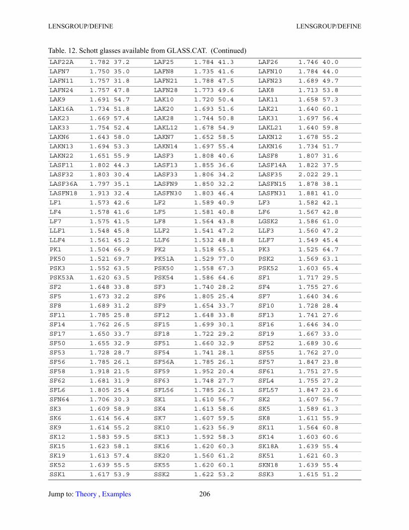
LENSGROUP/DEFINE LENSGROUP/DEFINE
LAF22A 1.782 37.2 LAF25 1.784 41.3 LAF26 1.746 40.0
LAFN7 1.750 35.0 LAFN8 1.735 41.6 LAFN10 1.784 44.0
LAFN11 1.757 31.8 LAFN21 1.788 47.5 LAFN23 1.689 49.7
LAFN24 1.757 47.8 LAFN28 1.773 49.6 LAK8 1.713 53.8
LAK9 1.691 54.7 LAK10 1.720 50.4 LAK11 1.658 57.3
LAK16A 1.734 51.8 LAK20 1.693 51.6 LAK21 1.640 60.1
LAK23 1.669 57.4 LAK28 1.744 50.8 LAK31 1.697 56.4
LAK33 1.754 52.4 LAKL12 1.678 54.9 LAKL21 1.640 59.8
LAKN6 1.643 58.0 LAKN7 1.652 58.5 LAKN12 1.678 55.2
LAKN13 1.694 53.3 LAKN14 1.697 55.4 LAKN16 1.734 51.7
LAKN22 1.651 55.9 LASF3 1.808 40.6 LASF8 1.807 31.6
LASF11 1.802 44.3 LASF13 1.855 36.6 LASF14A 1.822 37.5
LASF32 1.803 30.4 LASF33 1.806 34.2 LASF35 2.022 29.1
LASF36A 1.797 35.1 LASFN9 1.850 32.2 LASFN15 1.878 38.1
LASFN18 1.913 32.4 LASFN30 1.803 46.4 LASFN31 1.881 41.0
LF1 1.573 42.6 LF2 1.589 40.9 LF3 1.582 42.1
LF4 1.578 41.6 LF5 1.581 40.8 LF6 1.567 42.8
LF7 1.575 41.5 LF8 1.564 43.8 LGSK2 1.586 61.0
LLF1 1.548 45.8 LLF2 1.541 47.2 LLF3 1.560 47.2
LLF4 1.561 45.2 LLF6 1.532 48.8 LLF7 1.549 45.4
PK1 1.504 66.9 PK2 1.518 65.1 PK3 1.525 64.7
PK50 1.521 69.7 PK51A 1.529 77.0 PSK2 1.569 63.1
PSK3 1.552 63.5 PSK50 1.558 67.3 PSK52 1.603 65.4
PSK53A 1.620 63.5 PSK54 1.586 64.6 SF1 1.717 29.5
SF2 1.648 33.8 SF3 1.740 28.2 SF4 1.755 27.6
SF5 1.673 32.2 SF6 1.805 25.4 SF7 1.640 34.6
SF8 1.689 31.2 SF9 1.654 33.7 SF10 1.728 28.4
SF11 1.785 25.8 SF12 1.648 33.8 SF13 1.741 27.6
SF14 1.762 26.5 SF15 1.699 30.1 SF16 1.646 34.0
SF17 1.650 33.7 SF18 1.722 29.2 SF19 1.667 33.0
SF50 1.655 32.9 SF51 1.660 32.9 SF52 1.689 30.6
SF53 1.728 28.7 SF54 1.741 28.1 SF55 1.762 27.0
SF56 1.785 26.1 SF56A 1.785 26.1 SF57 1.847 23.8
SF58 1.918 21.5 SF59 1.952 20.4 SF61 1.751 27.5
SF62 1.681 31.9 SF63 1.748 27.7 SFL4 1.755 27.2
SFL6 1.805 25.4 SFL56 1.785 26.1 SFL57 1.847 23.6
SFN64 1.706 30.3 SK1 1.610 56.7 SK2 1.607 56.7
SK3 1.609 58.9 SK4 1.613 58.6 SK5 1.589 61.3
SK6 1.614 56.4 SK7 1.607 59.5 SK8 1.611 55.9
SK9 1.614 55.2 SK10 1.623 56.9 SK11 1.564 60.8
SK12 1.583 59.5 SK13 1.592 58.3 SK14 1.603 60.6
SK15 1.623 58.1 SK16 1.620 60.3 SK18A 1.639 55.4
SK19 1.613 57.4 SK20 1.560 61.2 SK51 1.621 60.3
SK52 1.639 55.5 SK55 1.620 60.1 SKN18 1.639 55.4
SSK1 1.617 53.9 SSK2 1.622 53.2 SSK3 1.615 51.2
Table. 12. Schott glasses available from GLASS.CAT. (Continued)
Jump to: , 206 Theory Examples
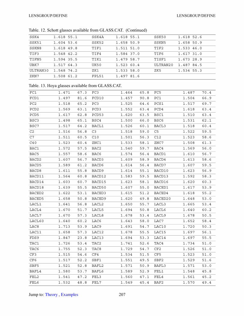
LENSGROUP/DEFINE LENSGROUP/DEFINE
SSK4 1.618 55.1 SSK4A 1.618 55.1 SSK50 1.618 52.6
SSK51 1.604 53.6 SSK52 1.658 50.9 SSKN5 1.658 50.9
SSKN8 1.618 49.8 TIF1 1.511 51.0 TIF2 1.533 46.0
TIF3 1.548 42.2 TIF4 1.584 37.0 TIF6 1.617 31.0
TIFN5 1.594 35.5 TIK1 1.479 58.7 TISF1 1.673 28.9
UBK7 1.517 64.3 UK50 1.523 60.4 ULTRAN20 1.487 84.5
ULTRAN30 1.548 74.2 ZK1 1.533 58.0 ZK5 1.534 55.3
ZKN7 1.508 61.2 FPL51 1.497 81.6
Table. 13. Hoya glasses available from GLASS.CAT. FC1 1.471 67.3 FC3 1.464 65.8 FC5 1.487 70.4
FCD1 1.497 81.6 FCD10 1.457 90.8 PC1 1.504 66.9
PC2 1.518 65.2 PC3 1.525 64.6 PCS1 1.517 69.7
PCD2 1.569 63.1 PCD3 1.552 63.4 PCD4 1.618 63.4
PCD5 1.617 62.8 PCD53 1.620 63.5 BSC1 1.510 63.4
BSC3 1.498 65.1 BSC4 1.500 66.0 BSC6 1.531 62.1
BSC7 1.517 64.2 BACL1 1.526 60.1 BACL3 1.518 60.4
C2 1.516 56.8 C3 1.518 59.0 C5 1.522 59.5
C7 1.511 60.5 C10 1.501 56.3 C12 1.523 58.6
C40 1.523 60.4 ZNC1 1.533 58.1 ZNC7 1.508 61.3
BAC1 1.572 57.5 BAC2 1.540 59.7 BAC4 1.569 56.0
BAC5 1.557 58.6 BAC6 1.574 56.4 BACD1 1.610 56.7
BACD2 1.607 56.7 BACD3 1.609 58.9 BACD4 1.613 58.6
BACD5 1.589 61.2 BACD6 1.614 56.4 BACD7 1.607 59.5
BACD8 1.611 55.8 BACD9 1.614 55.1 BACD10 1.623 56.9
BACD11 1.564 60.8 BACD12 1.583 59.5 BACD13 1.592 58.3
BACD14 1.603 60.7 BACD15 1.623 58.1 BACD16 1.620 60.3
BACD18 1.639 55.5 BACD50 1.607 55.0 BACED1 1.617 53.9
BACED2 1.622 53.1 BACED3 1.615 51.2 BACED4 1.618 55.2
BACED5 1.658 50.8 BACED9 1.620 49.8 BACED20 1.648 53.0
LACL1 1.641 56.8 LACL2 1.650 55.7 LACL3 1.665 53.4
LACL4 1.670 51.7 LACL5 1.694 50.8 LACL6 1.640 60.2
LACL7 1.670 57.3 LACL8 1.678 53.4 LACL9 1.678 50.5
LACL60 1.640 60.2 LAC6 1.643 58.0 LAC7 1.652 58.4
LAC8 1.713 53.9 LAC9 1.691 54.7 LAC10 1.720 50.3
LAC11 1.658 57.3 LAC12 1.678 55.5 LAC15 1.697 56.1
FDS9 1.847 23.8 LAC13 1.694 53.3 LAC14 1.697 55.5
TAC1 1.726 53.4 TAC2 1.741 52.6 TAC4 1.734 51.0
TAC6 1.755 52.3 TAC8 1.729 54.7 CF2 1.526 51.0
CF3 1.515 54.6 CF4 1.534 51.5 CF5 1.523 51.0
CF6 1.517 52.2 SBF1 1.551 49.5 SBF2 1.529 51.6
SBF5 1.521 52.8 BAFL2 1.571 50.9 BAFL3 1.571 53.0
BAFL4 1.580 53.7 BAFL6 1.589 52.9 FEL1 1.548 45.8
FEL2 1.541 47.2 FEL3 1.560 47.1 FEL4 1.561 45.2
FEL6 1.532 48.8 FEL7 1.549 45.4 BAF2 1.570 49.4
Table. 12. Schott glasses available from GLASS.CAT. (Continued)
Jump to: , 207 Theory Examples
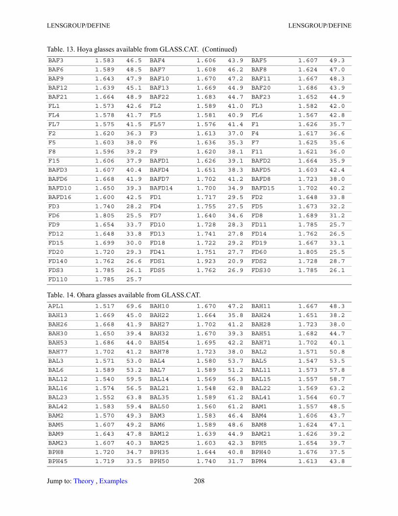
LENSGROUP/DEFINE LENSGROUP/DEFINE
BAF3 1.583 46.5 BAF4 1.606 43.9 BAF5 1.607 49.3
BAF6 1.589 48.5 BAF7 1.608 46.2 BAF8 1.624 47.0
BAF9 1.643 47.9 BAF10 1.670 47.2 BAF11 1.667 48.3
BAF12 1.639 45.1 BAF13 1.669 44.9 BAF20 1.686 43.9
BAF21 1.664 48.9 BAF22 1.683 44.7 BAF23 1.652 44.9
FL1 1.573 42.6 FL2 1.589 41.0 FL3 1.582 42.0
FL4 1.578 41.7 FL5 1.581 40.9 FL6 1.567 42.8
FL7 1.575 41.5 FL57 1.576 41.4 F1 1.626 35.7
F2 1.620 36.3 F3 1.613 37.0 F4 1.617 36.6
F5 1.603 38.0 F6 1.636 35.3 F7 1.625 35.6
F8 1.596 39.2 F9 1.620 38.1 F11 1.621 36.0
F15 1.606 37.9 BAFD1 1.626 39.1 BAFD2 1.664 35.9
BAFD3 1.607 40.4 BAFD4 1.651 38.3 BAFD5 1.603 42.4
BAFD6 1.668 41.9 BAFD7 1.702 41.2 BAFD8 1.723 38.0
BAFD10 1.650 39.3 BAFD14 1.700 34.9 BAFD15 1.702 40.2
BAFD16 1.600 42.5 FD1 1.717 29.5 FD2 1.648 33.8
FD3 1.740 28.2 FD4 1.755 27.5 FD5 1.673 32.2
FD6 1.805 25.5 FD7 1.640 34.6 FD8 1.689 31.2
FD9 1.654 33.7 FD10 1.728 28.3 FD11 1.785 25.7
FD12 1.648 33.8 FD13 1.741 27.8 FD14 1.762 26.5
FD15 1.699 30.0 FD18 1.722 29.2 FD19 1.667 33.1
FD20 1.720 29.3 FD41 1.751 27.7 FD60 1.805 25.5
FD140 1.762 26.6 FDS1 1.923 20.9 FDS2 1.728 28.7
FDS3 1.785 26.1 FDS5 1.762 26.9 FDS30 1.785 26.1
FD110 1.785 25.7
Table. 14. Ohara glasses available from GLASS.CAT. APL1 1.517 69.6 BAH10 1.670 47.2 BAH11 1.667 48.3
BAH13 1.669 45.0 BAH22 1.664 35.8 BAH24 1.651 38.2
BAH26 1.668 41.9 BAH27 1.702 41.2 BAH28 1.723 38.0
BAH30 1.650 39.4 BAH32 1.670 39.3 BAH51 1.682 44.7
BAH53 1.686 44.0 BAH54 1.695 42.2 BAH71 1.702 40.1
BAH77 1.702 41.2 BAH78 1.723 38.0 BAL2 1.571 50.8
BAL3 1.571 53.0 BAL4 1.580 53.7 BAL5 1.547 53.5
BAL6 1.589 53.2 BAL7 1.589 51.2 BAL11 1.573 57.8
BAL12 1.540 59.5 BAL14 1.569 56.3 BAL15 1.557 58.7
BAL16 1.574 56.5 BAL21 1.548 62.8 BAL22 1.569 63.2
BAL23 1.552 63.8 BAL35 1.589 61.2 BAL41 1.564 60.7
BAL42 1.583 59.4 BAL50 1.560 61.2 BAM1 1.557 48.5
BAM2 1.570 49.3 BAM3 1.583 46.4 BAM4 1.606 43.7
BAM5 1.607 49.2 BAM6 1.589 48.6 BAM8 1.624 47.1
BAM9 1.643 47.8 BAM12 1.639 44.9 BAM21 1.626 39.2
BAM23 1.607 40.3 BAM25 1.603 42.3 BPH5 1.654 39.7
BPH8 1.720 34.7 BPH35 1.644 40.8 BPH40 1.676 37.5
BPH45 1.719 33.5 BPH50 1.740 31.7 BPM4 1.613 43.8
Table. 13. Hoya glasses available from GLASS.CAT. (Continued)
Jump to: , 208 Theory Examples
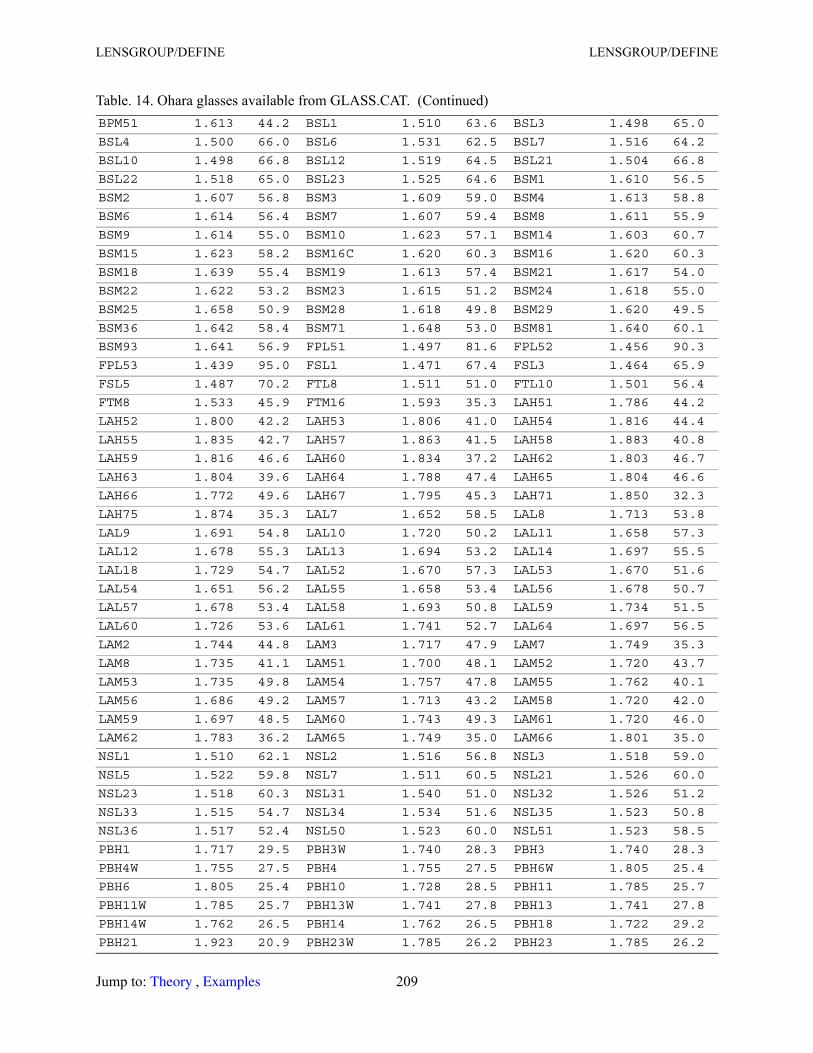
LENSGROUP/DEFINE LENSGROUP/DEFINE
BPM51 1.613 44.2 BSL1 1.510 63.6 BSL3 1.498 65.0
BSL4 1.500 66.0 BSL6 1.531 62.5 BSL7 1.516 64.2
BSL10 1.498 66.8 BSL12 1.519 64.5 BSL21 1.504 66.8
BSL22 1.518 65.0 BSL23 1.525 64.6 BSM1 1.610 56.5
BSM2 1.607 56.8 BSM3 1.609 59.0 BSM4 1.613 58.8
BSM6 1.614 56.4 BSM7 1.607 59.4 BSM8 1.611 55.9
BSM9 1.614 55.0 BSM10 1.623 57.1 BSM14 1.603 60.7
BSM15 1.623 58.2 BSM16C 1.620 60.3 BSM16 1.620 60.3
BSM18 1.639 55.4 BSM19 1.613 57.4 BSM21 1.617 54.0
BSM22 1.622 53.2 BSM23 1.615 51.2 BSM24 1.618 55.0
BSM25 1.658 50.9 BSM28 1.618 49.8 BSM29 1.620 49.5
BSM36 1.642 58.4 BSM71 1.648 53.0 BSM81 1.640 60.1
BSM93 1.641 56.9 FPL51 1.497 81.6 FPL52 1.456 90.3
FPL53 1.439 95.0 FSL1 1.471 67.4 FSL3 1.464 65.9
FSL5 1.487 70.2 FTL8 1.511 51.0 FTL10 1.501 56.4
FTM8 1.533 45.9 FTM16 1.593 35.3 LAH51 1.786 44.2
LAH52 1.800 42.2 LAH53 1.806 41.0 LAH54 1.816 44.4
LAH55 1.835 42.7 LAH57 1.863 41.5 LAH58 1.883 40.8
LAH59 1.816 46.6 LAH60 1.834 37.2 LAH62 1.803 46.7
LAH63 1.804 39.6 LAH64 1.788 47.4 LAH65 1.804 46.6
LAH66 1.772 49.6 LAH67 1.795 45.3 LAH71 1.850 32.3
LAH75 1.874 35.3 LAL7 1.652 58.5 LAL8 1.713 53.8
LAL9 1.691 54.8 LAL10 1.720 50.2 LAL11 1.658 57.3
LAL12 1.678 55.3 LAL13 1.694 53.2 LAL14 1.697 55.5
LAL18 1.729 54.7 LAL52 1.670 57.3 LAL53 1.670 51.6
LAL54 1.651 56.2 LAL55 1.658 53.4 LAL56 1.678 50.7
LAL57 1.678 53.4 LAL58 1.693 50.8 LAL59 1.734 51.5
LAL60 1.726 53.6 LAL61 1.741 52.7 LAL64 1.697 56.5
LAM2 1.744 44.8 LAM3 1.717 47.9 LAM7 1.749 35.3
LAM8 1.735 41.1 LAM51 1.700 48.1 LAM52 1.720 43.7
LAM53 1.735 49.8 LAM54 1.757 47.8 LAM55 1.762 40.1
LAM56 1.686 49.2 LAM57 1.713 43.2 LAM58 1.720 42.0
LAM59 1.697 48.5 LAM60 1.743 49.3 LAM61 1.720 46.0
LAM62 1.783 36.2 LAM65 1.749 35.0 LAM66 1.801 35.0
NSL1 1.510 62.1 NSL2 1.516 56.8 NSL3 1.518 59.0
NSL5 1.522 59.8 NSL7 1.511 60.5 NSL21 1.526 60.0
NSL23 1.518 60.3 NSL31 1.540 51.0 NSL32 1.526 51.2
NSL33 1.515 54.7 NSL34 1.534 51.6 NSL35 1.523 50.8
NSL36 1.517 52.4 NSL50 1.523 60.0 NSL51 1.523 58.5
PBH1 1.717 29.5 PBH3W 1.740 28.3 PBH3 1.740 28.3
PBH4W 1.755 27.5 PBH4 1.755 27.5 PBH6W 1.805 25.4
PBH6 1.805 25.4 PBH10 1.728 28.5 PBH11 1.785 25.7
PBH11W 1.785 25.7 PBH13W 1.741 27.8 PBH13 1.741 27.8
PBH14W 1.762 26.5 PBH14 1.762 26.5 PBH18 1.722 29.2
PBH21 1.923 20.9 PBH23W 1.785 26.2 PBH23 1.785 26.2
Table. 14. Ohara glasses available from GLASS.CAT. (Continued)
Jump to: , 209 Theory Examples
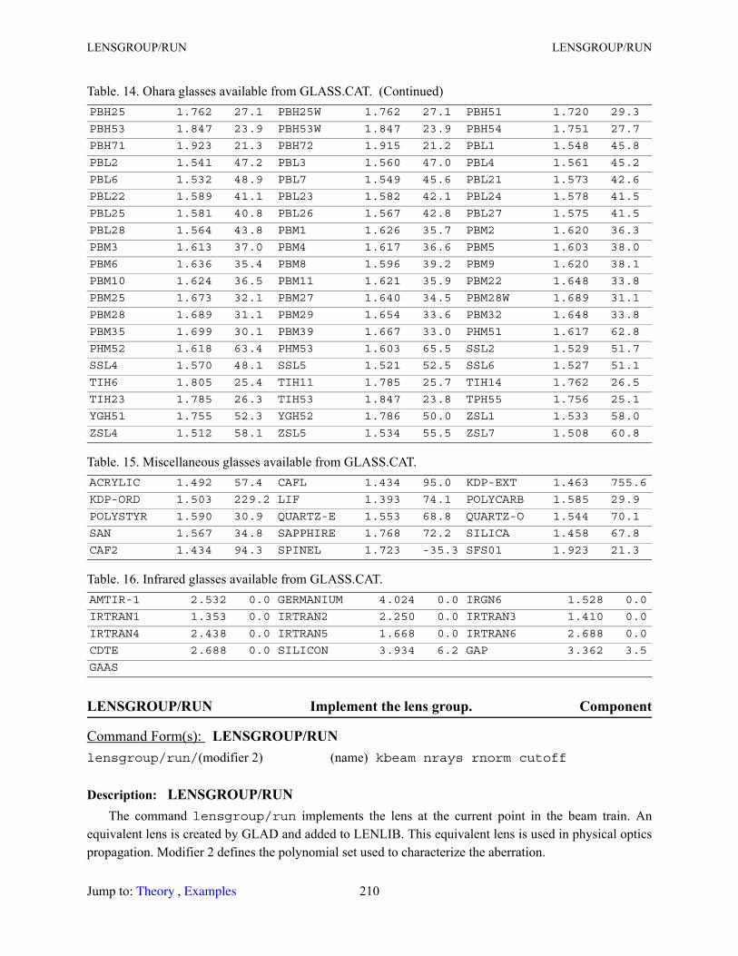
LENSGROUP/RUN LENSGROUP/RUN
LENSGROUP/RUN Implement the lens group. Component
Description: LENSGROUP/RUNThe command lensgroup/run implements the lens at the current point in the beam train. An
equivalent lens is created by GLAD and added to LENLIB. This equivalent lens is used in physical optics propagation. Modifier 2 defines the polynomial set used to characterize the aberration.
PBH25 1.762 27.1 PBH25W 1.762 27.1 PBH51 1.720 29.3
PBH53 1.847 23.9 PBH53W 1.847 23.9 PBH54 1.751 27.7
PBH71 1.923 21.3 PBH72 1.915 21.2 PBL1 1.548 45.8
PBL2 1.541 47.2 PBL3 1.560 47.0 PBL4 1.561 45.2
PBL6 1.532 48.9 PBL7 1.549 45.6 PBL21 1.573 42.6
PBL22 1.589 41.1 PBL23 1.582 42.1 PBL24 1.578 41.5
PBL25 1.581 40.8 PBL26 1.567 42.8 PBL27 1.575 41.5
PBL28 1.564 43.8 PBM1 1.626 35.7 PBM2 1.620 36.3
PBM3 1.613 37.0 PBM4 1.617 36.6 PBM5 1.603 38.0
PBM6 1.636 35.4 PBM8 1.596 39.2 PBM9 1.620 38.1
PBM10 1.624 36.5 PBM11 1.621 35.9 PBM22 1.648 33.8
PBM25 1.673 32.1 PBM27 1.640 34.5 PBM28W 1.689 31.1
PBM28 1.689 31.1 PBM29 1.654 33.6 PBM32 1.648 33.8
PBM35 1.699 30.1 PBM39 1.667 33.0 PHM51 1.617 62.8
PHM52 1.618 63.4 PHM53 1.603 65.5 SSL2 1.529 51.7
SSL4 1.570 48.1 SSL5 1.521 52.5 SSL6 1.527 51.1
TIH6 1.805 25.4 TIH11 1.785 25.7 TIH14 1.762 26.5
TIH23 1.785 26.3 TIH53 1.847 23.8 TPH55 1.756 25.1
YGH51 1.755 52.3 YGH52 1.786 50.0 ZSL1 1.533 58.0
ZSL4 1.512 58.1 ZSL5 1.534 55.5 ZSL7 1.508 60.8
Table. 15. Miscellaneous glasses available from GLASS.CAT. ACRYLIC 1.492 57.4 CAFL 1.434 95.0 KDP-EXT 1.463 755.6
KDP-ORD 1.503 229.2 LIF 1.393 74.1 POLYCARB 1.585 29.9
POLYSTYR 1.590 30.9 QUARTZ-E 1.553 68.8 QUARTZ-O 1.544 70.1
SAN 1.567 34.8 SAPPHIRE 1.768 72.2 SILICA 1.458 67.8
CAF2 1.434 94.3 SPINEL 1.723 -35.3 SFS01 1.923 21.3
Table. 16. Infrared glasses available from GLASS.CAT. AMTIR-1 2.532 0.0 GERMANIUM 4.024 0.0 IRGN6 1.528 0.0
IRTRAN1 1.353 0.0 IRTRAN2 2.250 0.0 IRTRAN3 1.410 0.0
IRTRAN4 2.438 0.0 IRTRAN5 1.668 0.0 IRTRAN6 2.688 0.0
CDTE 2.688 0.0 SILICON 3.934 6.2 GAP 3.362 3.5
GAAS
Command Form(s): LENSGROUP/RUN lensgroup/run/(modifier 2) (name) kbeam nrays rnorm cutoff
Table. 14. Ohara glasses available from GLASS.CAT. (Continued)
Jump to: , 210 Theory Examples
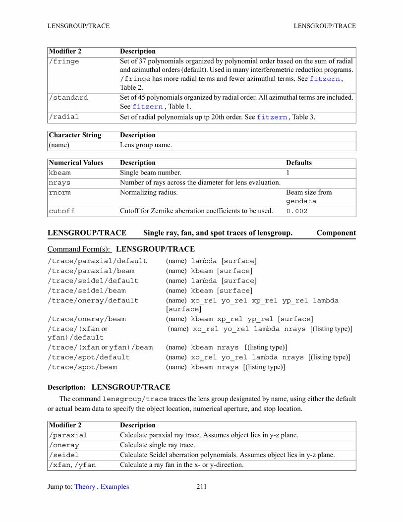
LENSGROUP/TRACE LENSGROUP/TRACE
LENSGROUP/TRACE Single ray, fan, and spot traces of lensgroup. Component
Description: LENSGROUP/TRACEThe command lensgroup/trace traces the lens group designated by name, using either the default
or actual beam data to specify the object location, numerical aperture, and stop location.
Modifier 2 Description /fringe Set of 37 polynomials organized by polynomial order based on the sum of radial
and azimuthal orders (default). Used in many interferometric reduction programs. /fringe has more radial terms and fewer azimuthal terms. See , Table 2.
/standard Set of 45 polynomials organized by radial order. All azimuthal terms are included. See , Table 1.
/radial Set of radial polynomials up tp 20th order. See , Table 3.
Character String Description (name) Lens group name.
Numerical Values Description Defaultskbeam Single beam number. 1nrays Number of rays across the diameter for lens evaluation.rnorm Normalizing radius. Beam size from
geodata
cutoff Cutoff for Zernike aberration coefficients to be used. 0.002
Command Form(s): LENSGROUP/TRACE /trace/paraxial/default (name) lambda [surface]/trace/paraxial/beam (name) kbeam [surface]/trace/seidel/default (name) lambda [surface]/trace/seidel/beam (name) kbeam [surface]/trace/oneray/default (name) xo_rel yo_rel xp_rel yp_rel lambda
[surface]/trace/oneray/beam (name) kbeam xp_rel yp_rel [surface]/trace/(xfan or yfan)/default
(name) xo_rel yo_rel lambda nrays [(listing type)]
/trace/(xfan or yfan)/beam (name) kbeam nrays [(listing type)]/trace/spot/default (name) xo_rel yo_rel lambda nrays [(listing type)]/trace/spot/beam (name) kbeam nrays [(listing type)]
Modifier 2 Description /paraxial Calculate paraxial ray trace. Assumes object lies in y-z plane./oneray Calculate single ray trace./seidel Calculate Seidel aberration polynomials. Assumes object lies in y-z plane./xfan, /yfan Calculate a ray fan in the x- or y-direction.
fitzern
fitzern fitzern
Jump to: , 211 Theory Examples
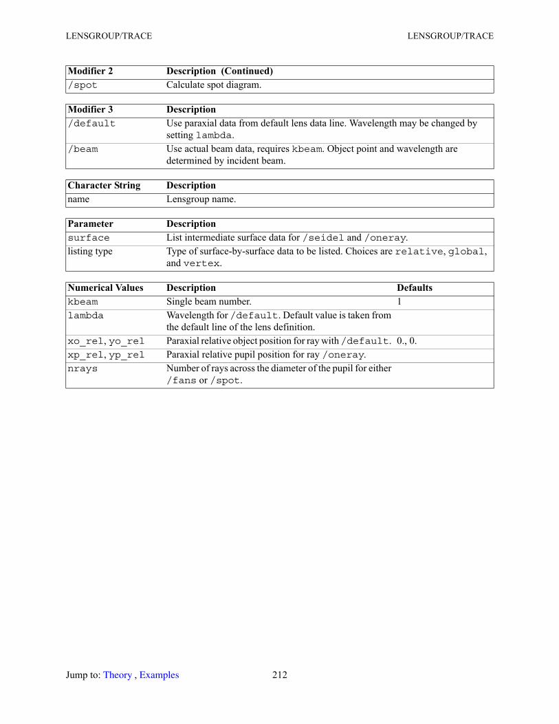
LENSGROUP/TRACE LENSGROUP/TRACE
/spot Calculate spot diagram.
Modifier 3 Description /default Use paraxial data from default lens data line. Wavelength may be changed by
setting lambda./beam Use actual beam data, requires kbeam. Object point and wavelength are
determined by incident beam.
Character String Description name Lensgroup name.
Parameter Description surface List intermediate surface data for /seidel and /oneray.listing type Type of surface-by-surface data to be listed. Choices are relative, global,
and vertex.
Numerical Values Description Defaultskbeam Single beam number. 1lambda Wavelength for /default. Default value is taken from
the default line of the lens definition.xo_rel, yo_rel Paraxial relative object position for ray with /default. 0., 0.xp_rel, yp_rel Paraxial relative pupil position for ray /oneray.nrays Number of rays across the diameter of the pupil for either
/fans or /spot.
Modifier 2 Description (Continued)
Jump to: , 212 Theory Examples
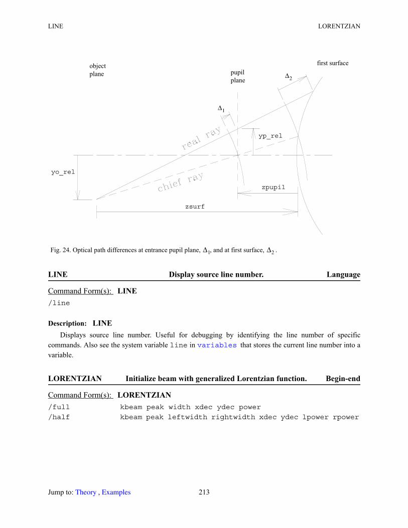
LINE LORENTZIAN
LINE Display source line number. Language
Description: LINEDisplays source line number. Useful for debugging by identifying the line number of specific
commands. Also see the system variable line in that stores the current line number into a variable.
LORENTZIAN Initialize beam with generalized Lorentzian function. Begin-end
Fig. 24. Optical path differences at entrance pupil plane, , and at first surface, .
Command Form(s): LINE /line
Command Form(s): LORENTZIAN /full kbeam peak width xdec ydec power
/half kbeam peak leftwidth rightwidth xdec ydec lpower rpower
zsurf
object
plane
yo_rel
first surface
pupil
plane
zpupil
yp_rel
Δ1
Δ2
Δ1 Δ2
variables
Jump to: , 213 Theory Examples
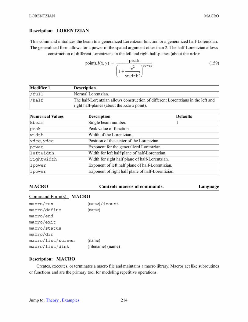
LORENTZIAN MACRO
Description: LORENTZIAN
This command initializes the beam to a generalized Lorentzian function or a generalized half-Lorentzian. The generalized form allows for a power of the spatial argument other than 2. The half-Lorentzian allows
construction of different Lorentzians in the left and right half-planes (about the xdec
point). (159)
MACRO Controls macros of commands. Language
Description: MACROCreates, executes, or terminates a macro file and maintains a macro library. Macros act like subroutines
or functions and are the primary tool for modeling repetitive operations.
Modifier 1 Description /full Normal Lorentzian./half The half-Lorentzian allows construction of different Lorentzians in the left and
right half-planes (about the xdec point).
Numerical Values Description Defaultskbeam Single beam number. 1peak Peak value of function.width Width of the Lorentzian.xdec, ydec Position of the center of the Lorentzian.power Exponent for the generalized Lorentzian.leftwidth Width for left half plane of half-Lorentzian.rightwidth Width for right half plane of half-Lorentzian.lpower Exponent of left half plane of half-Lorentizian.rpower Exponent of right half plane of half-Lorentizian.
Command Form(s): MACRO macro/run (name)/icountmacro/define (name)macro/end
macro/exit
macro/status
macro/dir
macro/list/screen (name)macro/list/disk (filename) (name)
I x y,( ) peak
1 x2
width2
--------------------+ power------------------------------------------------=
Jump to: , 214 Theory Examples
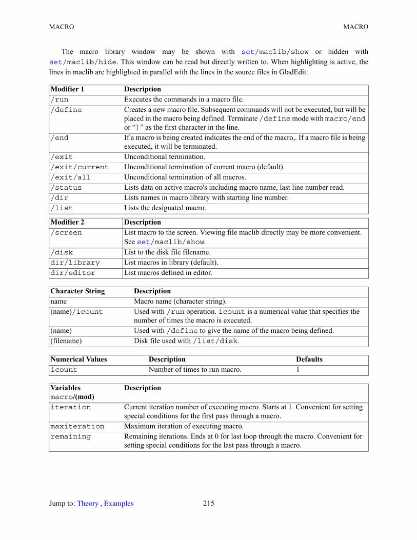
MACRO MACRO
The macro library window may be shown with /maclib/show or hidden with /maclib/hide. This window can be read but directly written to. When highlighting is active, the
lines in maclib are highlighted in parallel with the lines in the source files in GladEdit.
Modifier 1 Description /run Executes the commands in a macro file./define Creates a new macro file. Subsequent commands will not be executed, but will be
placed in the macro being defined. Terminate /define mode with macro/end or “]” as the first character in the line.
/end If a macro is being created indicates the end of the macro,. If a macro file is being executed, it will be terminated.
/exit Unconditional termination./exit/current Unconditional termination of current macro (default)./exit/all Unconditional termination of all macros./status Lists data on active macro's including macro name, last line number read./dir Lists names in macro library with starting line number./list Lists the designated macro.
Modifier 2 Description /screen List macro to the screen. Viewing file maclib directly may be more convenient.
See /maclib/show./disk List to the disk file filename.dir/library List macros in library (default).dir/editor List macros defined in editor.
Character String Description name Macro name (character string).(name)/icount Used with /run operation. icount is a numerical value that specifies the
number of times the macro is executed. (name) Used with /define to give the name of the macro being defined. (filename) Disk file used with /list/disk.
Numerical Values Description Defaultsicount Number of times to run macro. 1
Variablesmacro/(mod)
Description
iteration Current iteration number of executing macro. Starts at 1. Convenient for setting special conditions for the first pass through a macro.
maxiteration Maximum iteration of executing macro.remaining Remaining iterations. Ends at 0 for last loop through the macro. Convenient for
setting special conditions for the last pass through a macro.
set set
set
Jump to: , 215 Theory Examples
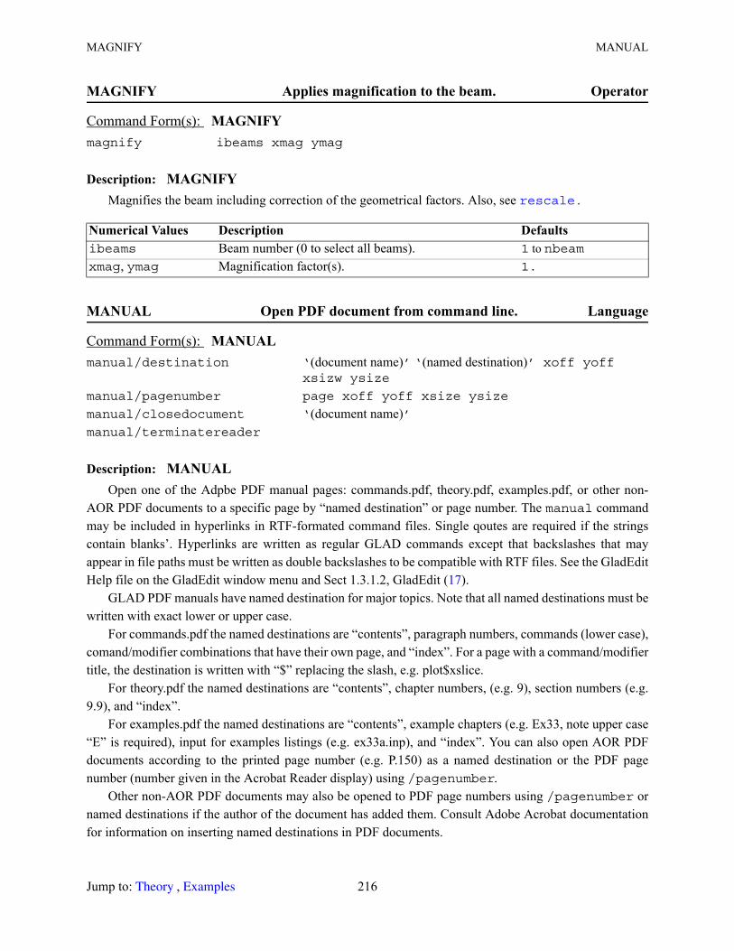
MAGNIFY MANUAL
MAGNIFY Applies magnification to the beam. Operator
Description: MAGNIFYMagnifies the beam including correction of the geometrical factors. Also, see .
MANUAL Open PDF document from command line. Language
Description: MANUALOpen one of the Adpbe PDF manual pages: commands.pdf, theory.pdf, examples.pdf, or other non-
AOR PDF documents to a specific page by “named destination” or page number. The manual command may be included in hyperlinks in RTF-formated command files. Single qoutes are required if the strings contain blanks’. Hyperlinks are written as regular GLAD commands except that backslashes that may appear in file paths must be written as double backslashes to be compatible with RTF files. See the GladEdit Help file on the GladEdit window menu and Sect 1.3.1.2, GladEdit (17).
GLAD PDF manuals have named destination for major topics. Note that all named destinations must be written with exact lower or upper case.
For commands.pdf the named destinations are “contents”, paragraph numbers, commands (lower case), comand/modifier combinations that have their own page, and “index”. For a page with a command/modifier title, the destination is written with “$” replacing the slash, e.g. plot$xslice.
For theory.pdf the named destinations are “contents”, chapter numbers, (e.g. 9), section numbers (e.g. 9.9), and “index”.
For examples.pdf the named destinations are “contents”, example chapters (e.g. Ex33, note upper case “E” is required), input for examples listings (e.g. ex33a.inp), and “index”. You can also open AOR PDF documents according to the printed page number (e.g. P.150) as a named destination or the PDF page number (number given in the Acrobat Reader display) using /pagenumber.
Other non-AOR PDF documents may also be opened to PDF page numbers using /pagenumber or named destinations if the author of the document has added them. Consult Adobe Acrobat documentation for information on inserting named destinations in PDF documents.
Command Form(s): MAGNIFY magnify ibeams xmag ymag
Numerical Values Description Defaultsibeams Beam number (0 to select all beams). 1 to nbeamxmag, ymag Magnification factor(s). 1.
Command Form(s): MANUAL manual/destination ‘(document name)’ ‘(named destination)’ xoff yoff
xsizw ysize
manual/pagenumber page xoff yoff xsize ysize
manual/closedocument ‘(document name)’manual/terminatereader
rescale
Jump to: , 216 Theory Examples
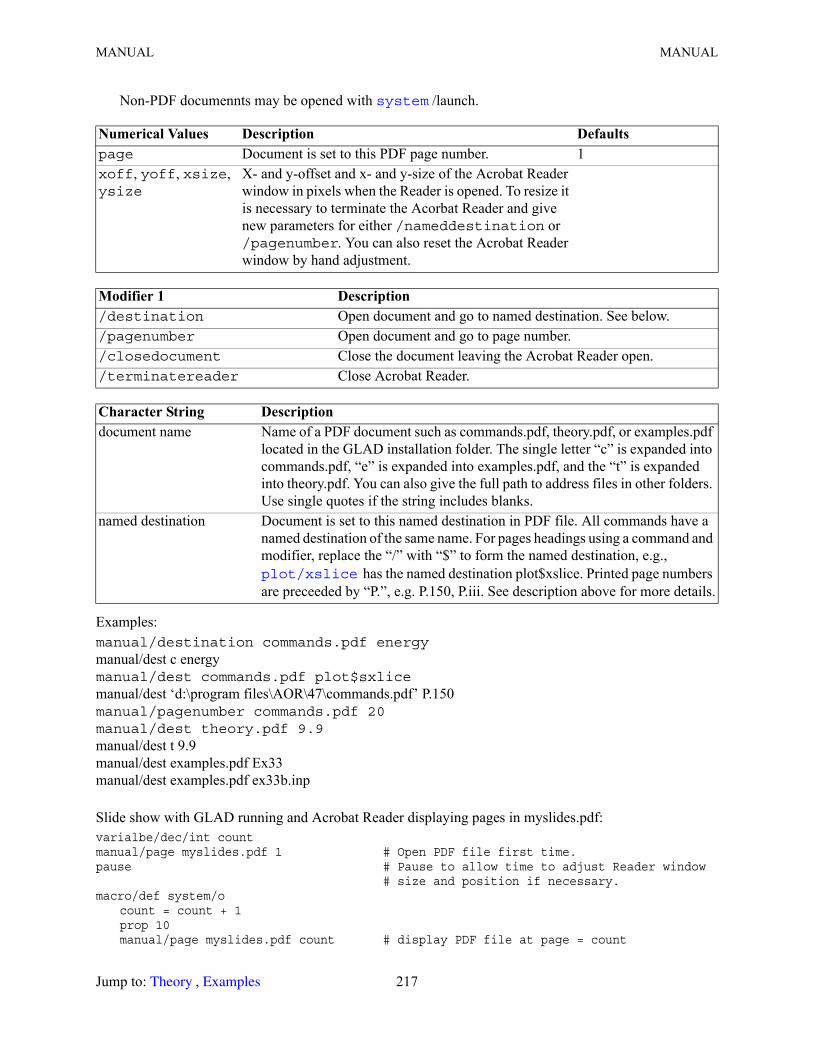
MANUAL MANUAL
Non-PDF documennts may be opened with /launch.
Examples:manual/destination commands.pdf energymanual/dest c energymanual/dest commands.pdf plot$sxlicemanual/dest ‘d:\program files\AOR\47\commands.pdf’ P.150manual/pagenumber commands.pdf 20manual/dest theory.pdf 9.9manual/dest t 9.9manual/dest examples.pdf Ex33manual/dest examples.pdf ex33b.inp
Slide show with GLAD running and Acrobat Reader displaying pages in myslides.pdf:varialbe/dec/int countmanual/page myslides.pdf 1 # Open PDF file first time.pause # Pause to allow time to adjust Reader window
# size and position if necessary.macro/def system/o
count = count + 1prop 10manual/page myslides.pdf count # display PDF file at page = count
Modifier 1 Description /destination Open document and go to named destination. See below./pagenumber Open document and go to page number./closedocument Close the document leaving the Acrobat Reader open./terminatereader Close Acrobat Reader.
Character String Description document name Name of a PDF document such as commands.pdf, theory.pdf, or examples.pdf
located in the GLAD installation folder. The single letter “c” is expanded into commands.pdf, “e” is expanded into examples.pdf, and the “t” is expanded into theory.pdf. You can also give the full path to address files in other folders. Use single quotes if the string includes blanks.
named destination Document is set to this named destination in PDF file. All commands have a named destination of the same name. For pages headings using a command and modifier, replace the “/” with “$” to form the named destination, e.g.,
has the named destination plot$xslice. Printed page numbers are preceeded by “P.”, e.g. P.150, P.iii. See description above for more details.
Numerical Values Description Defaultspage Document is set to this PDF page number. 1xoff, yoff, xsize, ysize
X- and y-offset and x- and y-size of the Acrobat Reader window in pixels when the Reader is opened. To resize it is necessary to terminate the Acorbat Reader and give new parameters for either /nameddestination or /pagenumber. You can also reset the Acrobat Reader window by hand adjustment.
system
plot/xslice
Jump to: , 217 Theory Examples
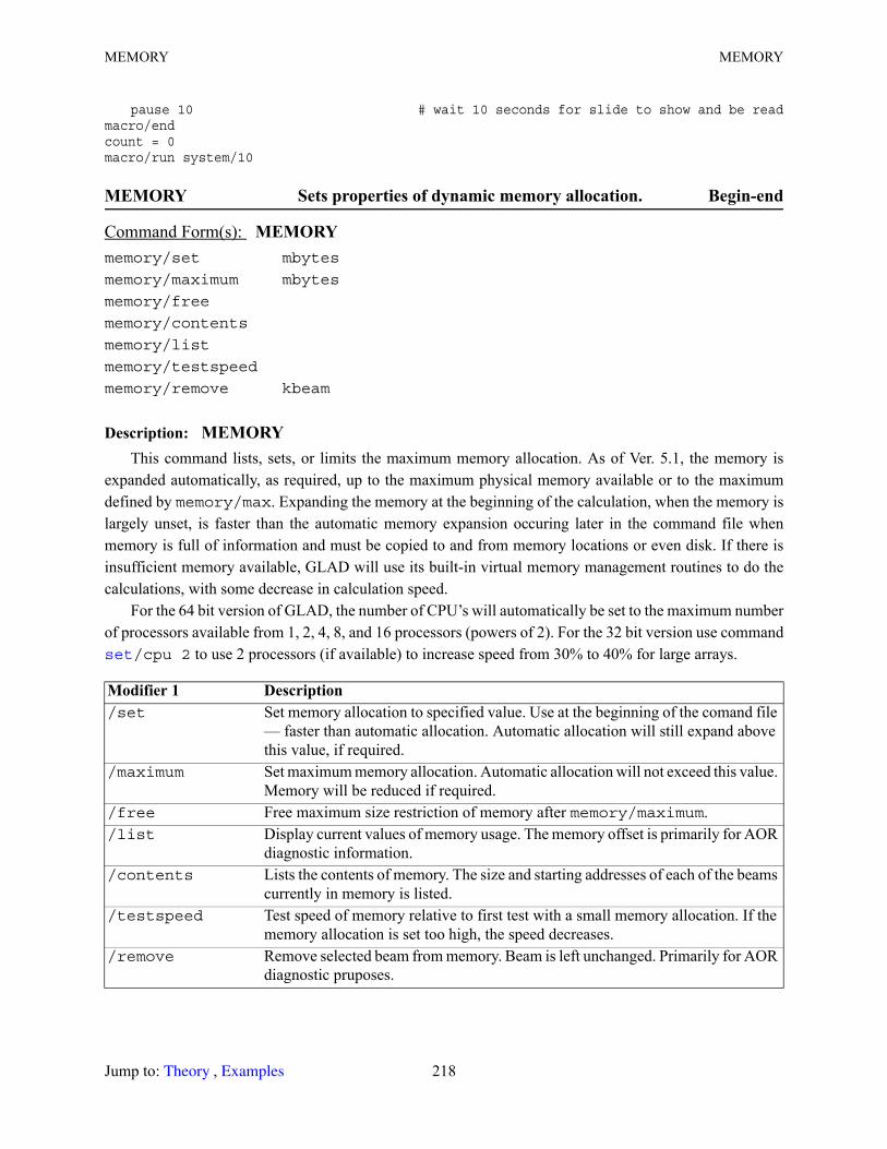
MEMORY MEMORY
pause 10 # wait 10 seconds for slide to show and be readmacro/endcount = 0macro/run system/10
MEMORY Sets properties of dynamic memory allocation. Begin-end
Description: MEMORYThis command lists, sets, or limits the maximum memory allocation. As of Ver. 5.1, the memory is
expanded automatically, as required, up to the maximum physical memory available or to the maximum defined by memory/max. Expanding the memory at the beginning of the calculation, when the memory is largely unset, is faster than the automatic memory expansion occuring later in the command file when memory is full of information and must be copied to and from memory locations or even disk. If there is insufficient memory available, GLAD will use its built-in virtual memory management routines to do the calculations, with some decrease in calculation speed.
For the 64 bit version of GLAD, the number of CPU’s will automatically be set to the maximum number of processors available from 1, 2, 4, 8, and 16 processors (powers of 2). For the 32 bit version use command
/cpu 2 to use 2 processors (if available) to increase speed from 30% to 40% for large arrays.
Command Form(s): MEMORY memory/set mbytes
memory/maximum mbytes
memory/free
memory/contents
memory/list
memory/testspeed
memory/remove kbeam
Modifier 1 Description /set Set memory allocation to specified value. Use at the beginning of the comand file
— faster than automatic allocation. Automatic allocation will still expand above this value, if required.
/maximum Set maximum memory allocation. Automatic allocation will not exceed this value. Memory will be reduced if required.
/free Free maximum size restriction of memory after memory/maximum./list Display current values of memory usage. The memory offset is primarily for AOR
diagnostic information./contents Lists the contents of memory. The size and starting addresses of each of the beams
currently in memory is listed./testspeed Test speed of memory relative to first test with a small memory allocation. If the
memory allocation is set too high, the speed decreases./remove Remove selected beam from memory. Beam is left unchanged. Primarily for AOR
diagnostic pruposes.
set
Jump to: , 218 Theory Examples
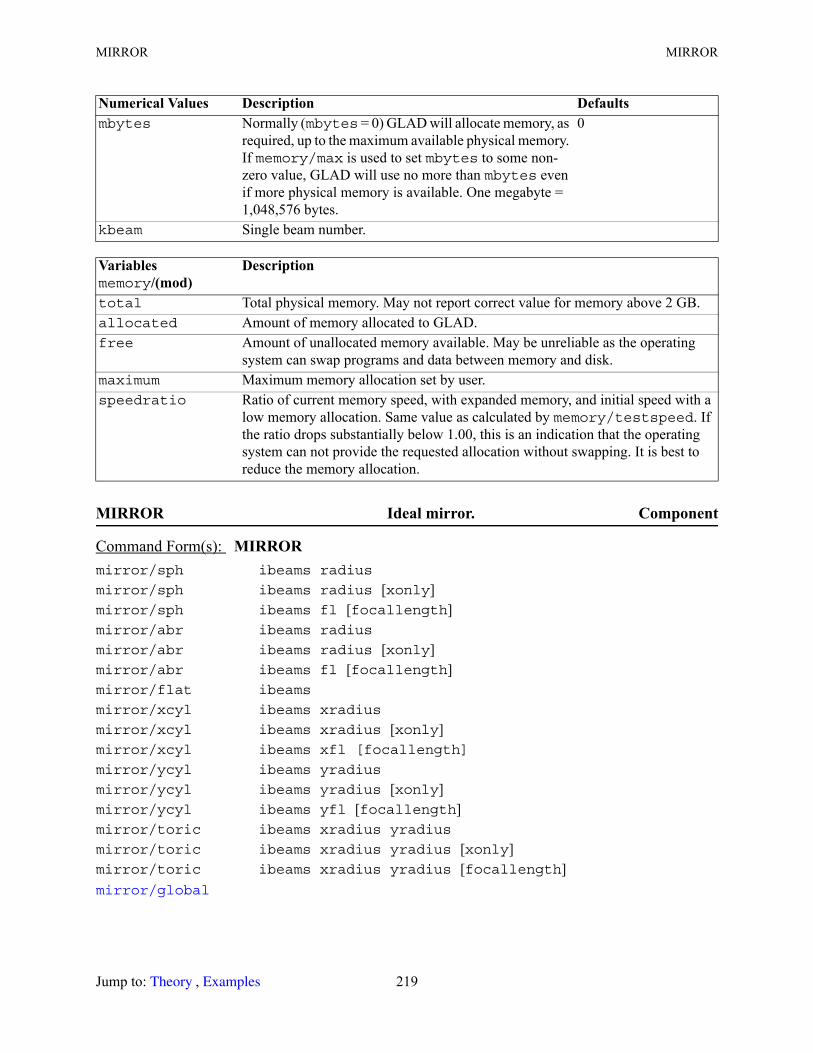
MIRROR MIRROR
MIRROR Ideal mirror. Component
Numerical Values Description Defaultsmbytes Normally (mbytes = 0) GLAD will allocate memory, as
required, up to the maximum available physical memory. If memory/max is used to set mbytes to some non-zero value, GLAD will use no more than mbytes even if more physical memory is available. One megabyte = 1,048,576 bytes.
0
kbeam Single beam number.
Variablesmemory/(mod)
Description
total Total physical memory. May not report correct value for memory above 2 GB.allocated Amount of memory allocated to GLAD.free Amount of unallocated memory available. May be unreliable as the operating
system can swap programs and data between memory and disk.maximum Maximum memory allocation set by user.speedratio Ratio of current memory speed, with expanded memory, and initial speed with a
low memory allocation. Same value as calculated by memory/testspeed. If the ratio drops substantially below 1.00, this is an indication that the operating system can not provide the requested allocation without swapping. It is best to reduce the memory allocation.
Command Form(s): MIRROR mirror/sph ibeams radius
mirror/sph ibeams radius [xonly]mirror/sph ibeams fl [focallength]mirror/abr ibeams radius
mirror/abr ibeams radius [xonly]mirror/abr ibeams fl [focallength]mirror/flat ibeams
mirror/xcyl ibeams xradius
mirror/xcyl ibeams xradius [xonly]mirror/xcyl ibeams xfl [focallength]
mirror/ycyl ibeams yradius
mirror/ycyl ibeams yradius [xonly]mirror/ycyl ibeams yfl [focallength]mirror/toric ibeams xradius yradius
mirror/toric ibeams xradius yradius [xonly] mirror/toric ibeams xradius yradius [focallength] mirror/global
Jump to: , 219 Theory Examples
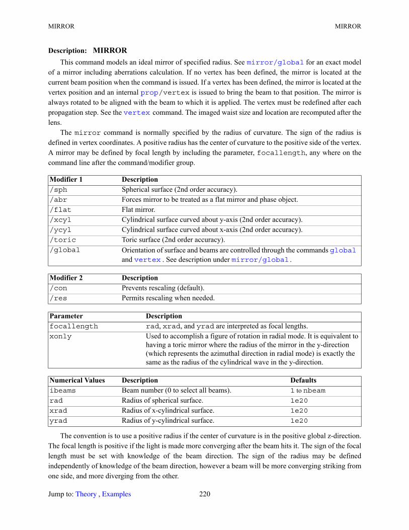
MIRROR MIRROR
Description: MIRRORThis command models an ideal mirror of specified radius. See for an exact model
of a mirror including aberrations calculation. If no vertex has been defined, the mirror is located at the current beam position when the command is issued. If a vertex has been defined, the mirror is located at the vertex position and an internal /vertex is issued to bring the beam to that position. The mirror is always rotated to be aligned with the beam to which it is applied. The vertex must be redefined after each propagation step. See the command. The imaged waist size and location are recomputed after the lens.
The mirror command is normally specified by the radius of curvature. The sign of the radius is defined in vertex coordinates. A positive radius has the center of curvature to the positive side of the vertex. A mirror may be defined by focal length by including the parameter, focallength, any where on the command line after the command/modifier group.
The convention is to use a positive radius if the center of curvature is in the positive global z-direction. The focal length is positive if the light is made more converging after the beam hits it. The sign of the focal length must be set with knowledge of the beam direction. The sign of the radius may be defined independently of knowledge of the beam direction, however a beam will be more converging striking from one side, and more diverging from the other.
Modifier 1 Description /sph Spherical surface (2nd order accuracy)./abr Forces mirror to be treated as a flat mirror and phase object./flat Flat mirror./xcyl Cylindrical surface curved about y-axis (2nd order accuracy)./ycyl Cylindrical surface curved about x-axis (2nd order accuracy)./toric Toric surface (2nd order accuracy)./global Orientation of surface and beams are controlled through the commands
and . See description under .
Modifier 2 Description /con Prevents rescaling (default)./res Permits rescaling when needed.
Parameter Description focallength rad, xrad, and yrad are interpreted as focal lengths.xonly Used to accomplish a figure of rotation in radial mode. It is equivalent to
having a toric mirror where the radius of the mirror in the y-direction (which represents the azimuthal direction in radial mode) is exactly the same as the radius of the cylindrical wave in the y-direction.
Numerical Values Description Defaultsibeams Beam number (0 to select all beams). 1 to nbeamrad Radius of spherical surface. 1e20
xrad Radius of x-cylindrical surface. 1e20
yrad Radius of y-cylindrical surface. 1e20
mirror/global
prop
vertex
global vertex mirror/global
Jump to: , 220 Theory Examples
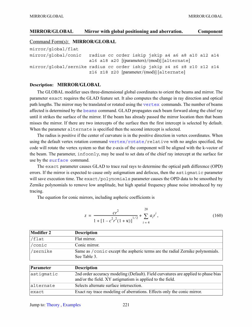
MIRROR/GLOBAL MIRROR/GLOBAL
MIRROR/GLOBAL Mirror with global positioning and aberration. Component
Description: MIRROR/GLOBALThe GLOBAL modifier uses three-dimensional global coordinates to orient the beams and mirror. The
parameter exact requires the GLAD feature set. It also computes the change in ray direction and optical path lengths. The mirror may be translated or rotated using the commands. The number of beams affected is determined by the command. GLAD propagates each beam forward along the chief ray until it strikes the surface of the mirror. If the beam has already passed the mirror location then that beam misses the mirror. If there are two intercepts of the surface then the first intercept is selected by default. When the parameter alternate is specified then the second intercept is selected.
The radius is positive if the center of curvature is in the positive direction in vertex coordinates. When using the default vertex rotation command /relative with no angles specified, the code will rotate the vertex system so that the z-axis of the component will be aligned with the k-vector of the beam. The parameter, infoonly, may be used to set data of the chief ray intercept at the surface for use by the command.
The exact parameter causes GLAD to trace real rays to determine the optical path difference (OPD) errors. If the mirror is expected to cause only astigmatism and defocus, then the astigmatic parameter will save execution time. The exact/polynomials parameter causes the OPD data to be smoothed by Zernike polynomials to remove low amplitude, but high spatial frequency phase noise introduced by ray tracing.
The equation for conic mirrors, including aspheric coefficients is
, (160)
Command Form(s): MIRROR/GLOBAL mirror/global/flat
mirror/global/conic radius cc order iskip jskip a4 a6 a8 a10 a12 a14 a16 a18 a20 [(parameters)/(mod)] [alternate]
mirror/global/zernike radius cc order iskip jskip z4 z6 z8 z10 z12 z14 z16 z18 z20 [parameter/(mod)] [alternate]
Modifier 2 Description /flat Flat mirror./conic Conic mirror./zernike Same as /conic except the aspheric terms are the radial Zernike polynomials.
See Table 3.
Parameter Description astigmatic 2nd order accuracy modeling (Default). Field curvatures are applied to phase bias
and/or the field. XY astigmatism is applied to the field.alternate Selects alternate surface intersection.exact Exact ray trace modeling of aberrations. Effects only the conic mirror.
vertex beams
vertex/rotate
surface
z cr2
1 1 c2r2 1 κ+( )–[ ]1 2⁄
+---------------------------------------------------------- air
i
i 4=
20
+=
Jump to: , 221 Theory Examples

MIRROR/GLOBAL MIRROR/GLOBAL
Parameter Modifier 1 Description exact/polynomials Use Zernike polynomials to smooth OPD values (default). This procedure
eliminates low amplitude, but high spatial frequency phase noise which causes intensity noise upon subsequent propagation. The variable norder specifies the maximum order of polynomial to be used and iskip and jskip enable coarse sampling of the data to reduce calculation time. The parameter exact requires the GLAD feature set.
exact/rays Use OPD values directly. The parameter exact requires the GLAD feature set.
Parameter Modifier 2 Description exact/polynomials/standard
Use “standard” set of polynomials (see ).
exact/polynomials/fringe
Use “fringe” set of polynomials (see ).
exact/polynomials/radial
Use only radial polynomial terms (see ).
Numerical Values Description Defaultsradius Radius of conic surface. Radius is positive if convex
relative to vertex coordinate system.1e20
cc Conic constant. 0.
order Maximum polynomial order used with exact/polynomials. Choices, norder=4 gives 4 2 2norder=6 gives 6 4 4norder=8 gives 8 6 6(see for description of polynomial representation.
iskip, jskip Allows skipping data points in calculating interpolating polynomials with exact/polynomials.
a4, a6, a8, a10, a12, a14, a16, a18, a20
4th through 20th order aspheric coefficients.
z4, z6, z8, z10, z12, z14, z16, z18, z20
4th through 20th order Zernike aspheric coefficients. See Table 3.
Table. 17. Apply a flat mirror to Beam 7. Rotate the mirror 45 degrees, so an incident horizontal beam exits upward.
global/define (Define global coordinate system.)vertex/rotate/set 45 (Rotate beam about x-axis.)vertex/list (List vertex coordinates.)beams/off (Set all beams off. See BEAMS.)beams/on 7 (Set Beam 7 on.)mirror/global/flat
vertex/derotate/absolute 45 (Return to original vertex system.)
vertex/rotateaberration/zernike
vertex/rotateaberration/zernike
vertex/rotateaberration/zernike
fitzern
Jump to: , 222 Theory Examples
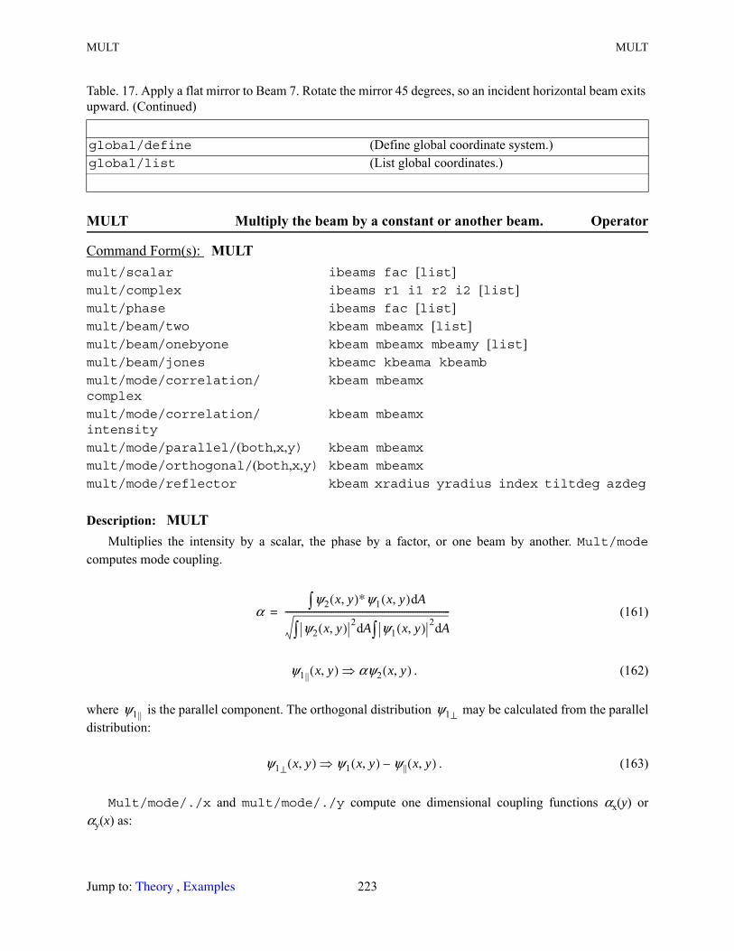
MULT MULT
MULT Multiply the beam by a constant or another beam. Operator
Description: MULTMultiplies the intensity by a scalar, the phase by a factor, or one beam by another. Mult/mode
computes mode coupling.
(161)
. (162)
where is the parallel component. The orthogonal distribution may be calculated from the parallel distribution:
. (163)
Mult/mode/./x and mult/mode/./y compute one dimensional coupling functions αx(y) or αy(x) as:
global/list (List global coordinates.)
Command Form(s): MULT mult/scalar ibeams fac [list]mult/complex ibeams r1 i1 r2 i2 [list]mult/phase ibeams fac [list]mult/beam/two kbeam mbeamx [list]mult/beam/onebyone kbeam mbeamx mbeamy [list]mult/beam/jones kbeamc kbeama kbeamb
mult/mode/correlation/ complex
kbeam mbeamx
mult/mode/correlation/ intensity
kbeam mbeamx
mult/mode/parallel/(both,x,y) kbeam mbeamx
mult/mode/orthogonal/(both,x,y) kbeam mbeamx
mult/mode/reflector kbeam xradius yradius index tiltdeg azdeg
Table. 17. Apply a flat mirror to Beam 7. Rotate the mirror 45 degrees, so an incident horizontal beam exits upward. (Continued)
global/define (Define global coordinate system.)
αψ2 x y,( )∗ψ1 x y,( ) Ad
ψ2 x y,( ) 2 Ad ψ1 x y,( ) 2 Ad---------------------------------------------------------------------------=
ψ1|| x y,( ) αψ2 x y,( )
ψ1|| ψ1⊥
ψ1⊥ x y,( ) ψ1 x y,( ) ψ|| x y,( )–
Jump to: , 223 Theory Examples

MULT MULT
and . (164)
The x- and y-parallel components are calculculated as:
(165)
The corresponding orthogonal distributions are calculated according to Eq. (163).
/mode/reflector
For the the /mode/reflector feature. The coupling of the reflected mode into the incident mode is calculated. The calculation only measures the correlation of a hypothetical reflected mode. The surface is not introduced into the beam. If the radius of curvature of the reflecting surface exactly matches the radius of the propagating mode at the surface and there is no tilt of the reflecting surface, the amplitude correlation will be due only to the index of refractions:
. (166)
The absolute value squared of the amplitude correlation |α|2 will be about 4% for a typical air-glass interface where the glass has index of 1.5. To avoid adverse effects of reflections back into a laser, |α|2
should be significantly less than 1%.The wavefront error between the incident and reflected modes is
. (167)
The reflected wavefront radius is found from hypothetical surface curvature Rs the Lens Law:
, (168)
applied to case of a reflecting surface where N2 = –N1, and the difference in inverse wavefront radii is:
. (169)
where Rs indicates the radius of the hypothetical surface. Adapting Eq. (161), the coupling coefficient is:
αx y( )ψ2 x y,( )∗ψ1 x y,( ) xd
ψ2 x y,( ) 2 xd ψ1 x y,( ) 2 xd-------------------------------------------------------------------------= αy x( )
ψ2 x y,( )∗ψ1 x y,( ) ydψ2 x y,( ) 2 yd ψ1 x y,( ) 2 yd
-------------------------------------------------------------------------=
ψ1||xx y,( ) αx y( )ψ2 x y,( ) ψ1||y
x y,( ) αy x( )ψ2 x y,( )
αn1 n2–
n1 n2+-----------------=
W 2πλ
------12--- 1
R′----- 1
R---–
=
N′R′----- N
R----–
N′ N–Rs
---------------=
1R′----- 1
R---– 2 1
Rs----- 1
R---–
=
Jump to: , 224 Theory Examples
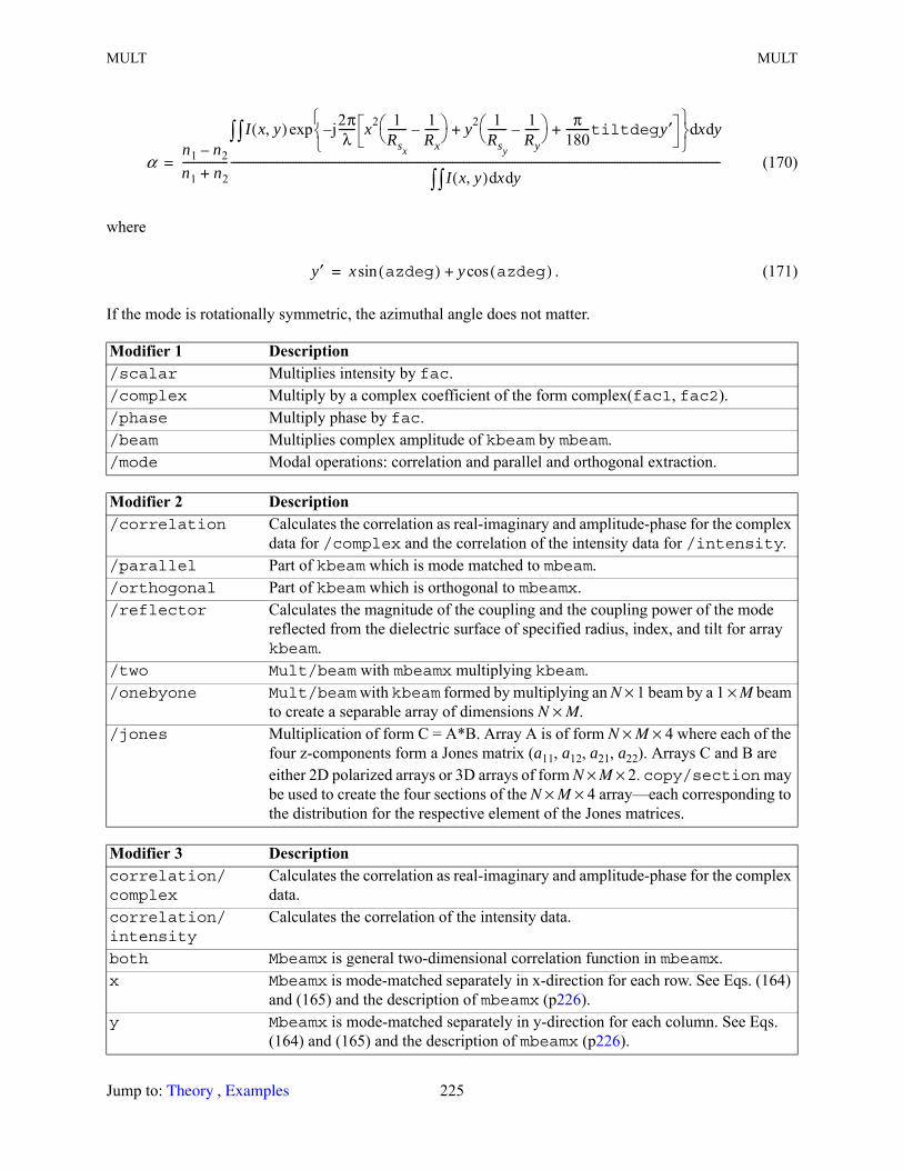
MULT MULT
(170)
where
. (171)
If the mode is rotationally symmetric, the azimuthal angle does not matter.
Modifier 1 Description /scalar Multiplies intensity by fac./complex Multiply by a complex coefficient of the form complex(fac1, fac2)./phase Multiply phase by fac./beam Multiplies complex amplitude of kbeam by mbeam./mode Modal operations: correlation and parallel and orthogonal extraction.
Modifier 2 Description /correlation Calculates the correlation as real-imaginary and amplitude-phase for the complex
data for /complex and the correlation of the intensity data for /intensity./parallel Part of kbeam which is mode matched to mbeam./orthogonal Part of kbeam which is orthogonal to mbeamx./reflector Calculates the magnitude of the coupling and the coupling power of the mode
reflected from the dielectric surface of specified radius, index, and tilt for array kbeam.
/two Mult/beam with mbeamx multiplying kbeam./onebyone Mult/beam with kbeam formed by multiplying an N × 1 beam by a 1 × M beam
to create a separable array of dimensions N × M./jones Multiplication of form C = A*B. Array A is of form N × M × 4 where each of the
four z-components form a Jones matrix (a11, a12, a21, a22). Arrays C and B are either 2D polarized arrays or 3D arrays of form N × M × 2. copy/section may be used to create the four sections of the N × M × 4 array—each corresponding to the distribution for the respective element of the Jones matrices.
Modifier 3 Description correlation/ complex
Calculates the correlation as real-imaginary and amplitude-phase for the complex data.
correlation/ intensity
Calculates the correlation of the intensity data.
both Mbeamx is general two-dimensional correlation function in mbeamx.x Mbeamx is mode-matched separately in x-direction for each row. See Eqs. (164)
and (165) and the description of mbeamx (p226).y Mbeamx is mode-matched separately in y-direction for each column. See Eqs.
(164) and (165) and the description of mbeamx (p226).
αn1 n2–
n1 n2+-----------------
I x y,( ) j2πλ
------ x2 1Rsx
------- 1Rx-----–
y2 1Rsy
------- 1Ry-----–
+π
180---------tiltdegy′+–
exp xd yd
I x y,( ) xd yd-------------------------------------------------------------------------------------------------------------------------------------------------------------------------------------=
y′ x azdeg( )sin y azdeg( )cos+=
Jump to: , 225 Theory Examples
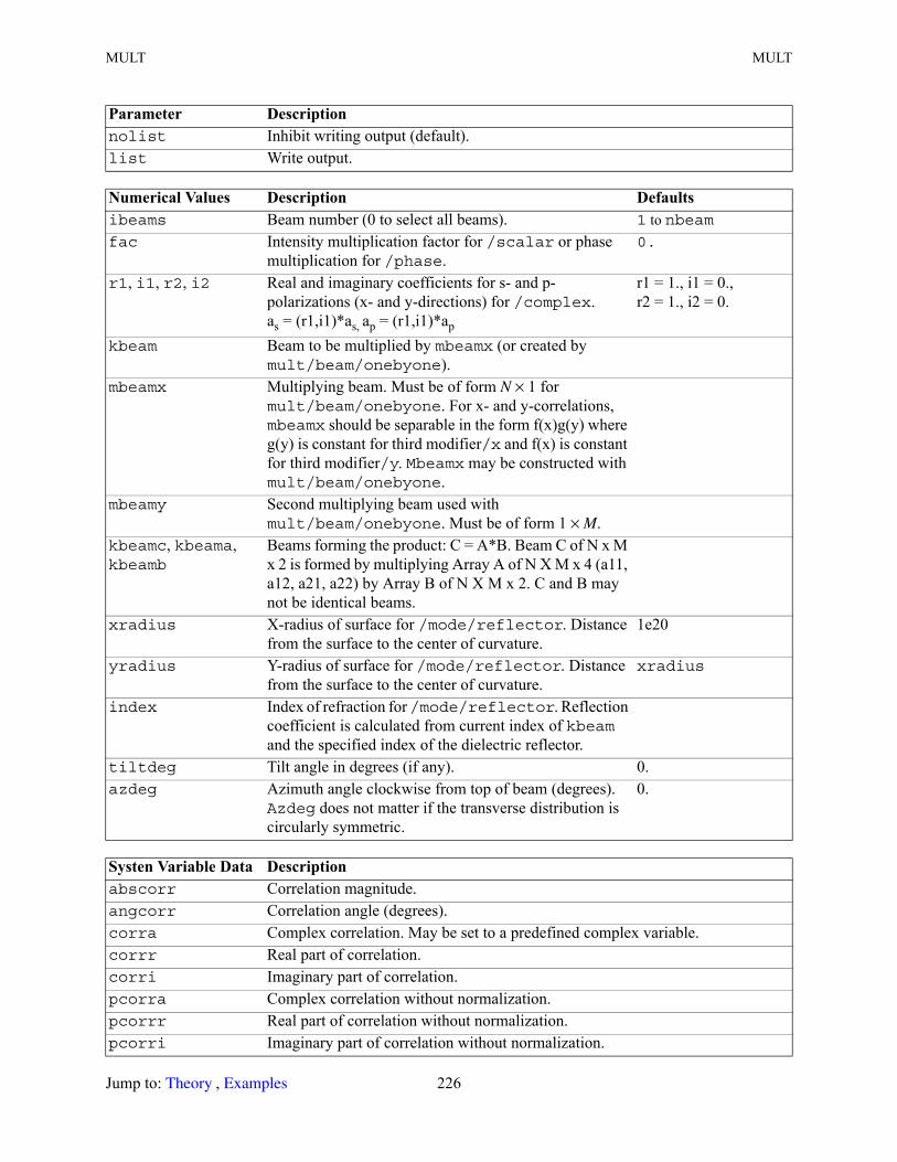
MULT MULT
Parameter Description nolist Inhibit writing output (default).list Write output.
Numerical Values Description Defaultsibeams Beam number (0 to select all beams). 1 to nbeamfac Intensity multiplication factor for /scalar or phase
multiplication for /phase.0.
r1, i1, r2, i2 Real and imaginary coefficients for s- and p-polarizations (x- and y-directions) for /complex.as = (r1,i1)*as, ap = (r1,i1)*ap
r1 = 1., i1 = 0., r2 = 1., i2 = 0.
kbeam Beam to be multiplied by mbeamx (or created by mult/beam/onebyone).
mbeamx Multiplying beam. Must be of form N × 1 for mult/beam/onebyone. For x- and y-correlations, mbeamx should be separable in the form f(x)g(y) where g(y) is constant for third modifier/x and f(x) is constant for third modifier/y. Mbeamx may be constructed with mult/beam/onebyone.
mbeamy Second multiplying beam used with mult/beam/onebyone. Must be of form 1 × M.
kbeamc, kbeama, kbeamb
Beams forming the product: C = A*B. Beam C of N x M x 2 is formed by multiplying Array A of N X M x 4 (a11, a12, a21, a22) by Array B of N X M x 2. C and B may not be identical beams.
xradius X-radius of surface for /mode/reflector. Distance from the surface to the center of curvature.
1e20
yradius Y-radius of surface for /mode/reflector. Distance from the surface to the center of curvature.
xradius
index Index of refraction for /mode/reflector. Reflection coefficient is calculated from current index of kbeam and the specified index of the dielectric reflector.
tiltdeg Tilt angle in degrees (if any). 0.azdeg Azimuth angle clockwise from top of beam (degrees).
Azdeg does not matter if the transverse distribution is circularly symmetric.
0.
Systen Variable Data Description abscorr Correlation magnitude.angcorr Correlation angle (degrees).corra Complex correlation. May be set to a predefined complex variable.corrr Real part of correlation.corri Imaginary part of correlation.pcorra Complex correlation without normalization.pcorrr Real part of correlation without normalization.pcorri Imaginary part of correlation without normalization.
Jump to: , 226 Theory Examples
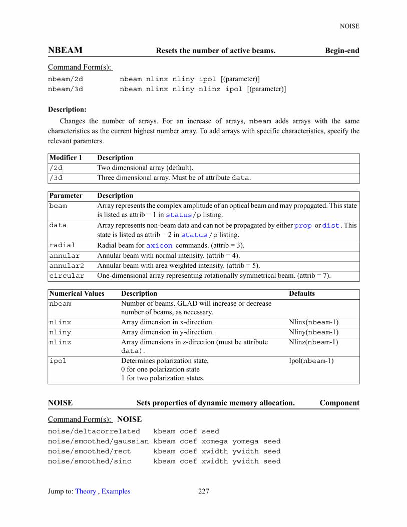
NOISE
NBEAM Resets the number of active beams. Begin-end
Description: Changes the number of arrays. For an increase of arrays, nbeam adds arrays with the same
characteristics as the current highest number array. To add arrays with specific characteristics, specify the relevant paramters.
NOISE Sets properties of dynamic memory allocation. Component
Command Form(s): nbeam/2d nbeam nlinx nliny ipol [(parameter)]nbeam/3d nbeam nlinx nliny nlinz ipol [(parameter)]
Modifier 1 Description /2d Two dimensional array (default)./3d Three dimensional array. Must be of attribute data.
Parameter Description beam Array represents the complex amplitude of an optical beam and may propagated. This state
is listed as attrib = 1 in /p listing.data Array represents non-beam data and can not be propagated by either or . This
state is listed as attrib = 2 in /p listing.radial Radial beam for commands. (attrib = 3).annular Annular beam with normal intensity. (attrib = 4).annular2 Annular beam with area weighted intensity. (attrib = 5).circular One-dimensional array representing rotationally symmetrical beam. (attrib = 7).
Numerical Values Description Defaultsnbeam Number of beams. GLAD will increase or decrease
number of beams, as necessary.nlinx Array dimension in x-direction. Nlinx(nbeam-1)nliny Array dimension in y-direction. Nliny(nbeam-1)nlinz Array dimensions in z-direction (must be attribute
data).Nlinz(nbeam-1)
ipol Determines polarization state,0 for one polarization state1 for two polarization states.
Ipol(nbeam-1)
Command Form(s): NOISE noise/deltacorrelated kbeam coef seed
noise/smoothed/gaussian kbeam coef xomega yomega seed
noise/smoothed/rect kbeam coef xwidth ywidth seed
noise/smoothed/sinc kbeam coef xwidth ywidth seed
status prop dist
status axicon
Jump to: , 227 Theory Examples

NOISE NOISE
Description: NOISEThe /deltacorrelated command adds random uncorrelated amplitude noise to the existing
distribution. Note that /deltacorrelated is adds to the existing distribution while /smoothedreplaces the existing distribution. Use /add/coh/con to add noise from this array to some other array.
/smoothed initializes the array with smoothed noise. The smoothing is implemented in the Fourier domain by applying a filter function to uniform white noise. For example /gaussian is implemented by the transfer function
(172)
where and correspond to xomega and yomega and is the Fourier transform of the complex amplitude distribution. For gaussian smoothing the autocorrelation sizes are and . For /rectthe smoothing is done with a sinc function of the form:
(173)
where Lx and Ly are the widths of the rect function. Either operation results in smoothing of the distribution.You may check that the distribution has the proper form. Consider a square function of half-width of
100 as shown below. Note that the autocorrelation function is a triangle of half-width = 200 as expected.
mem/set/b 8array/s 1 1024noise/smooth/rect 1 1 100 # set smoothing to half-width = 100autocorrelation 1 # form autocorrelation functionplot/x/real 1 le=-200 ri=200 # check that for a triangle shape.
Modifier 1 Description /deltacorrelated Unsmoothed noise is added to the beam (default). Adds to existing
distribution./smoothed The beam is set to smoothed noise (replaces initial distribution). Replaces
existing distribution.
Modifier 2 Description /gaussian Gaussian smoothing (default). /rect Smoothing by a rectangle function in the pupil./sinc Smoothing by a sinc function in the pupil.
Numerical Values Description Defaultskbeam Single beam number. 1coef Average noise intensity.xomega, yomega radii of gaussian smoothing function for
/smoothed.
A ξ η,( ) A ξ η,( )eπ2ωx
2ξ2– π2ωy
2η2–
=
ωx ωy A ξ η,( )2ωx 2ωy
A ξ η,( ) A ξ η,( )πξLx( )sin
πξLx-------------------------
πηLy( )sinπηLy
-------------------------=
1 e2⁄
Jump to: , 228 Theory Examples

NOOP OBS
NOOP Do-nothing command. Language
Description: NOOPCommand that does nothing.Useful to terminate data input, e.g., with /
zernike/number.
NORMALIZE Normalizes non-zero values in beam. Operator
Description: NORMALIZENormalizes the intensity to unity on a point-by-point basis for all non-zero points in the array. /two
normalizes kbeam1 using the irradiance of kbeam2. The phase of the beam is preserved.
OBS Implement obscuration. Component
xwidth, ywidth For /sinc the half-width to the first zero. For /rect the half-width of the smoothing rectangle.
seed Positive integer which sets seed for random number generator.
Command Form(s): NOOP noop
Command Form(s): NORMALIZE normalize/one kbeam threshold
normalize/two kbeam1 kbeam2
Modifier 1 Description /one Normalize single beam. /two Normalize kbeam1 by irradiance of kbeam2.
Numerical Values Description Defaultskbeam Single beam number. 1kbeam1, kbeam2 Receiving and normalizing beam numbers. 1, 2threshold Intensity values above threshold are normalized. Values
below threshold are set to zero.0.
Command Form(s): OBS obs/cir ibeams rad xdec ydec azdeg [(parameter)]obs/sqr ibeams rad xdec ydec azdeg [(parameter)]obs/pentagon ibeams rad xdec ydec azdeg [(parameter)]obs/ell ibeams xrad yrad xdec ydec azdeg [(parameter)]obs/hex ibeams xrad yrad xdec ydec azdeg [(parameter)]
Numerical Values Description (Continued) Defaults
aberration
Jump to: , 229 Theory Examples
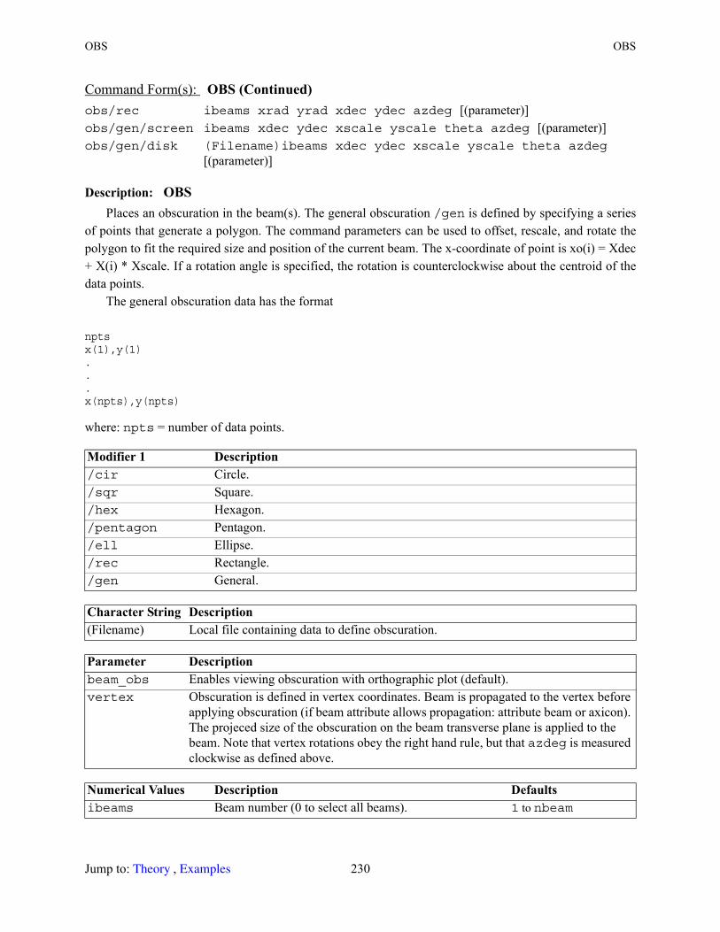
OBS OBS
Description: OBSPlaces an obscuration in the beam(s). The general obscuration /gen is defined by specifying a series
of points that generate a polygon. The command parameters can be used to offset, rescale, and rotate the polygon to fit the required size and position of the current beam. The x-coordinate of point is xo(i) = Xdec + X(i) * Xscale. If a rotation angle is specified, the rotation is counterclockwise about the centroid of the data points.
The general obscuration data has the format
nptsx(1),y(1)...x(npts),y(npts)
where: npts = number of data points.
obs/rec ibeams xrad yrad xdec ydec azdeg [(parameter)]obs/gen/screen ibeams xdec ydec xscale yscale theta azdeg [(parameter)]obs/gen/disk (Filename)ibeams xdec ydec xscale yscale theta azdeg
[(parameter)]
Modifier 1 Description /cir Circle./sqr Square./hex Hexagon./pentagon Pentagon./ell Ellipse./rec Rectangle./gen General.
Character String Description (Filename) Local file containing data to define obscuration.
Parameter Description beam_obs Enables viewing obscuration with orthographic plot (default).vertex Obscuration is defined in vertex coordinates. Beam is propagated to the vertex before
applying obscuration (if beam attribute allows propagation: attribute beam or axicon). The projeced size of the obscuration on the beam transverse plane is applied to the beam. Note that vertex rotations obey the right hand rule, but that azdeg is measured clockwise as defined above.
Numerical Values Description Defaultsibeams Beam number (0 to select all beams). 1 to nbeam
Command Form(s): OBS (Continued)
Jump to: , 230 Theory Examples
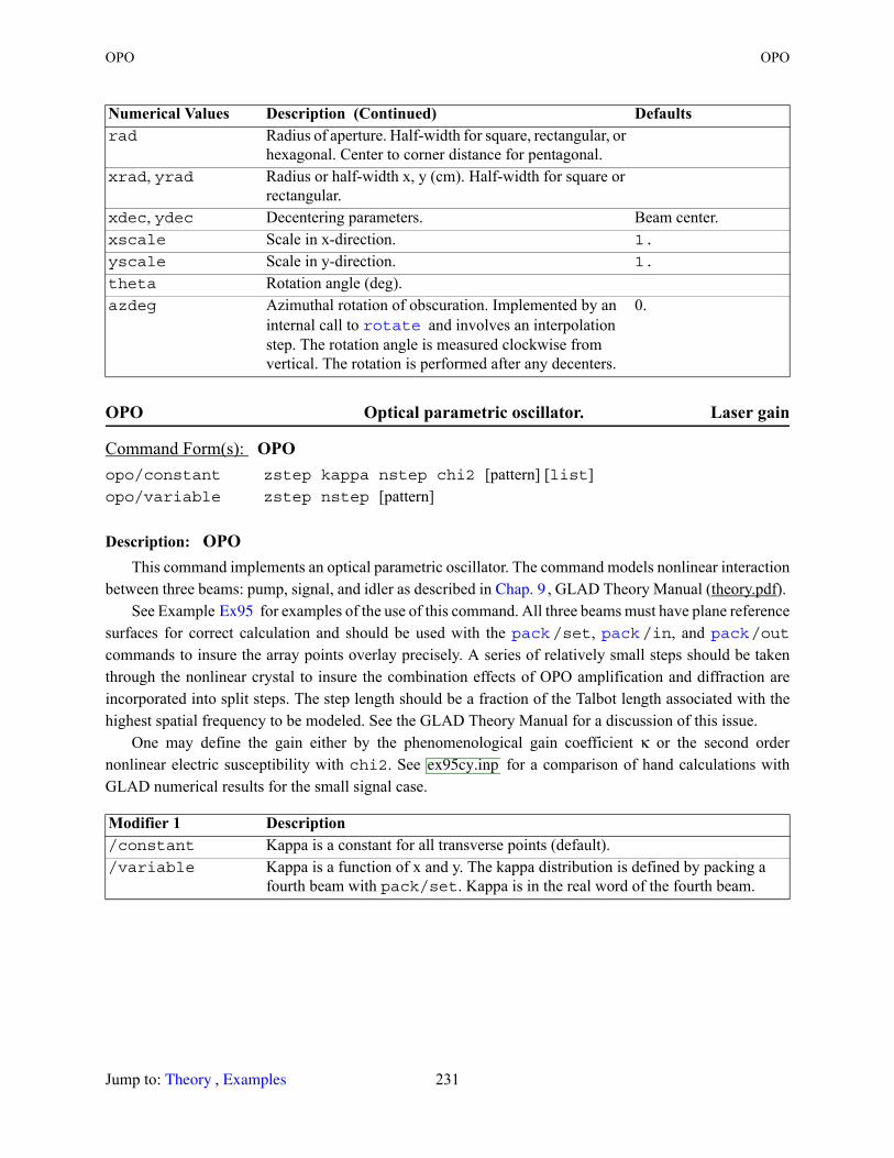
OPO OPO
OPO Optical parametric oscillator. Laser gain
Description: OPOThis command implements an optical parametric oscillator. The command models nonlinear interaction
between three beams: pump, signal, and idler as described in , GLAD Theory Manual (theory.pdf). See Example for examples of the use of this command. All three beams must have plane reference
surfaces for correct calculation and should be used with the /set, /in, and /out
commands to insure the array points overlay precisely. A series of relatively small steps should be taken through the nonlinear crystal to insure the combination effects of OPO amplification and diffraction are incorporated into split steps. The step length should be a fraction of the Talbot length associated with the highest spatial frequency to be modeled. See the GLAD Theory Manual for a discussion of this issue.
One may define the gain either by the phenomenological gain coefficient κ or the second order nonlinear electric susceptibility with chi2. See for a comparison of hand calculations with GLAD numerical results for the small signal case.
rad Radius of aperture. Half-width for square, rectangular, or hexagonal. Center to corner distance for pentagonal.
xrad, yrad Radius or half-width x, y (cm). Half-width for square or rectangular.
xdec, ydec Decentering parameters. Beam center.xscale Scale in x-direction. 1.
yscale Scale in y-direction. 1.
theta Rotation angle (deg).azdeg Azimuthal rotation of obscuration. Implemented by an
internal call to and involves an interpolation step. The rotation angle is measured clockwise from vertical. The rotation is performed after any decenters.
0.
Command Form(s): OPO opo/constant zstep kappa nstep chi2 [pattern] [list]opo/variable zstep nstep [pattern]
Modifier 1 Description /constant Kappa is a constant for all transverse points (default)./variable Kappa is a function of x and y. The kappa distribution is defined by packing a
fourth beam with pack/set. Kappa is in the real word of the fourth beam.
Numerical Values Description (Continued) Defaults
rotate
Chap. 9
Ex95
pack pack pack
ex95cy.inp
Jump to: , 231 Theory Examples
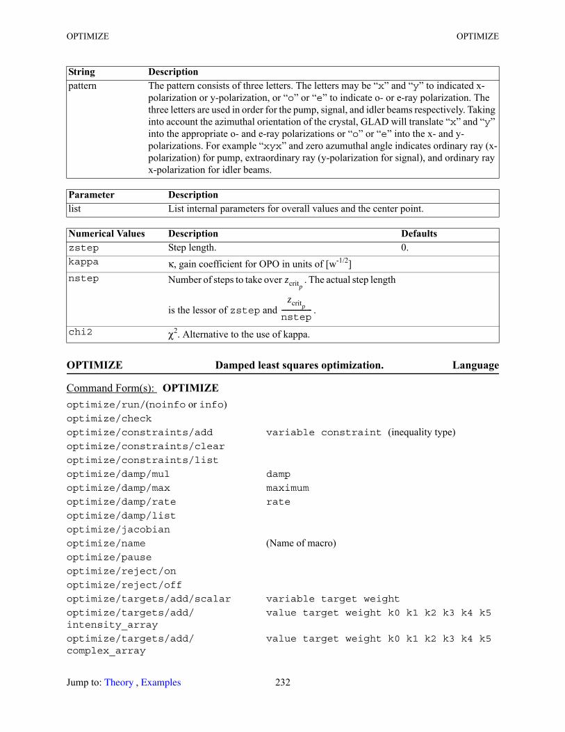
OPTIMIZE OPTIMIZE
OPTIMIZE Damped least squares optimization. Language
String Description pattern The pattern consists of three letters. The letters may be “x” and “y” to indicated x-
polarization or y-polarization, or “o” or “e” to indicate o- or e-ray polarization. The three letters are used in order for the pump, signal, and idler beams respectively. Taking into account the azimuthal orientation of the crystal, GLAD will translate “x” and “y” into the appropriate o- and e-ray polarizations or “o” or “e” into the x- and y-polarizations. For example “xyx” and zero azumuthal angle indicates ordinary ray (x-polarization) for pump, extraordinary ray (y-polarization for signal), and ordinary ray x-polarization for idler beams.
Parameter Description list List internal parameters for overall values and the center point.
Numerical Values Description Defaultszstep Step length. 0.kappa κ, gain coefficient for OPO in units of [w-1/2]nstep Number of steps to take over . The actual step length
is the lessor of zstep and .
chi2 χ2. Alternative to the use of kappa.
Command Form(s): OPTIMIZE optimize/run/(noinfo or info)optimize/check
optimize/constraints/add variable constraint (inequality type)optimize/constraints/clear
optimize/constraints/list
optimize/damp/mul damp
optimize/damp/max maximum
optimize/damp/rate rate
optimize/damp/list
optimize/jacobian
optimize/name (Name of macro)optimize/pause
optimize/reject/on
optimize/reject/off
optimize/targets/add/scalar variable target weight
optimize/targets/add/ intensity_array
value target weight k0 k1 k2 k3 k4 k5
optimize/targets/add/ complex_array
value target weight k0 k1 k2 k3 k4 k5
zcritp
zcritpnstep------------------
Jump to: , 232 Theory Examples
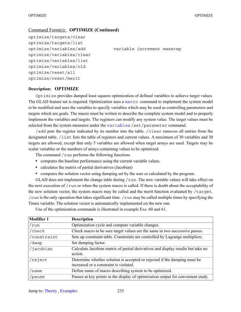
OPTIMIZE OPTIMIZE
Description: OPTIMIZEOptimize provides damped least squares optimization of defined variables to achieve target values.
The GLAD feature set is required. Optimization uses a command to implement the system model to be modified and uses the variables to specify variables which may be used as controlling parameters and targets which are goals. The macro must be written to describe the complete system model and to properly implement the variables and targets. The registers can modify any system value. The target values must be selected from the system measures under the /set/parameter command.
/add puts the register indicated by its number into the table. /clear removes all entries from the designated table. /list lists the table of registers and current values. A maximum of 30 variables and 30 targets are allowed, except that only 5 variables are allowed when target arrays are used. Targets may be scalar variables or the numbers of arrays containing values to be optimized.
The command /run performs the following functions• computes the baseline performance using the current variable values.• calculates the matrix of partial derivatives (Jacobian)• computes the solution vector using damping set by the user or calculated by the program. GLAD does not implement the change table during /run. The new variable values will take effect on
the next execution of /run or when the system macro is called. If there is doubt about the acceptability of the new solution vector, the system macro may be called and the merit function evaluated by /target. /run is the only operation that takes significant time. /run may be called multiple times by specifying the Times variable. The solution vector is automatically implemented on the new run.
Use of the optimization commands is illustrated in example Exs. 60 and 61.
optimize/targets/clear
optimize/targets/list
optimize/variables/add variable increment maxstep
optimize/variables/clear
optimize/variables/list
optimize/variables/old
optimize/reset/all
optimize/reset/merit
Modifier 1 Description /run Optimization cycle and compute variable changes./check Check macro to be sure target values are the same in two successive passes. /constraint Sets up constraint table. Constraints are controlled by Lagrange multipliers./damp Set damping factor./jacobian Calculate Jacobian matrix of partial derivatives and display results but take no
action./reject Determine whether solution is accepted or rejected if the damping must be
increased or a constraint is violated./name Define name of macro describing system to be optimized./pause Pauses at key points in the display of optimization output for convenient study.
Command Form(s): OPTIMIZE (Continued)
macro
variables
Jump to: , 233 Theory Examples
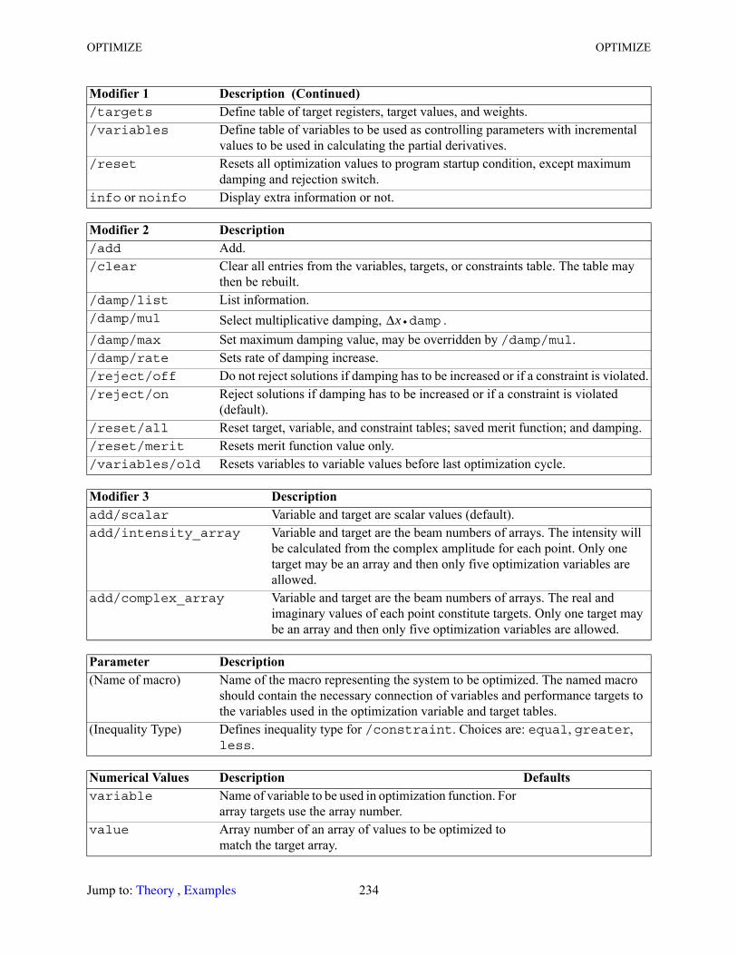
OPTIMIZE OPTIMIZE
/targets Define table of target registers, target values, and weights./variables Define table of variables to be used as controlling parameters with incremental
values to be used in calculating the partial derivatives./reset Resets all optimization values to program startup condition, except maximum
damping and rejection switch.info or noinfo Display extra information or not.
Modifier 2 Description /add Add./clear Clear all entries from the variables, targets, or constraints table. The table may
then be rebuilt./damp/list List information./damp/mul Select multiplicative damping, ./damp/max Set maximum damping value, may be overridden by /damp/mul./damp/rate Sets rate of damping increase./reject/off Do not reject solutions if damping has to be increased or if a constraint is violated./reject/on Reject solutions if damping has to be increased or if a constraint is violated
(default)./reset/all Reset target, variable, and constraint tables; saved merit function; and damping./reset/merit Resets merit function value only./variables/old Resets variables to variable values before last optimization cycle.
Modifier 3 Description add/scalar Variable and target are scalar values (default).add/intensity_array Variable and target are the beam numbers of arrays. The intensity will
be calculated from the complex amplitude for each point. Only one target may be an array and then only five optimization variables are allowed.
add/complex_array Variable and target are the beam numbers of arrays. The real and imaginary values of each point constitute targets. Only one target may be an array and then only five optimization variables are allowed.
Parameter Description (Name of macro) Name of the macro representing the system to be optimized. The named macro
should contain the necessary connection of variables and performance targets to the variables used in the optimization variable and target tables.
(Inequality Type) Defines inequality type for /constraint. Choices are: equal, greater, less.
Numerical Values Description Defaultsvariable Name of variable to be used in optimization function. For
array targets use the array number.value Array number of an array of values to be optimized to
match the target array.
Modifier 1 Description (Continued)
Δx damp•
Jump to: , 234 Theory Examples
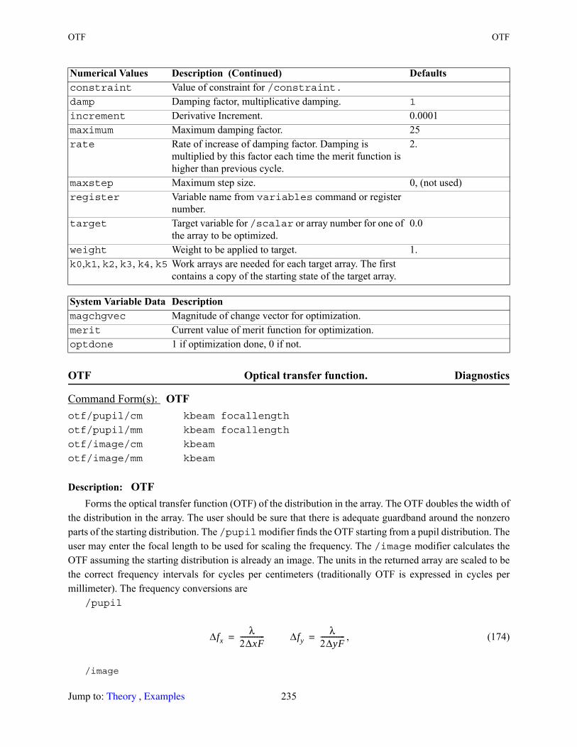
OTF OTF
OTF Optical transfer function. Diagnostics
Description: OTFForms the optical transfer function (OTF) of the distribution in the array. The OTF doubles the width of
the distribution in the array. The user should be sure that there is adequate guardband around the nonzero parts of the starting distribution. The /pupil modifier finds the OTF starting from a pupil distribution. The user may enter the focal length to be used for scaling the frequency. The /image modifier calculates the OTF assuming the starting distribution is already an image. The units in the returned array are scaled to be the correct frequency intervals for cycles per centimeters (traditionally OTF is expressed in cycles per millimeter). The frequency conversions are
/pupil
, (174)
/image
constraint Value of constraint for /constraint.damp Damping factor, multiplicative damping. 1
increment Derivative Increment. 0.0001 maximum Maximum damping factor. 25rate Rate of increase of damping factor. Damping is
multiplied by this factor each time the merit function is higher than previous cycle.
2.
maxstep Maximum step size. 0, (not used)register Variable name from variables command or register
number.target Target variable for /scalar or array number for one of
the array to be optimized.0.0
weight Weight to be applied to target. 1.k0,k1, k2, k3, k4, k5 Work arrays are needed for each target array. The first
contains a copy of the starting state of the target array.
System Variable Data Description magchgvec Magnitude of change vector for optimization.merit Current value of merit function for optimization.optdone 1 if optimization done, 0 if not.
Command Form(s): OTF otf/pupil/cm kbeam focallength
otf/pupil/mm kbeam focallength
otf/image/cm kbeam
otf/image/mm kbeam
Numerical Values Description (Continued) Defaults
Δfxλ
2ΔxF--------------= Δfy
λ2ΔyF--------------=
Jump to: , 235 Theory Examples
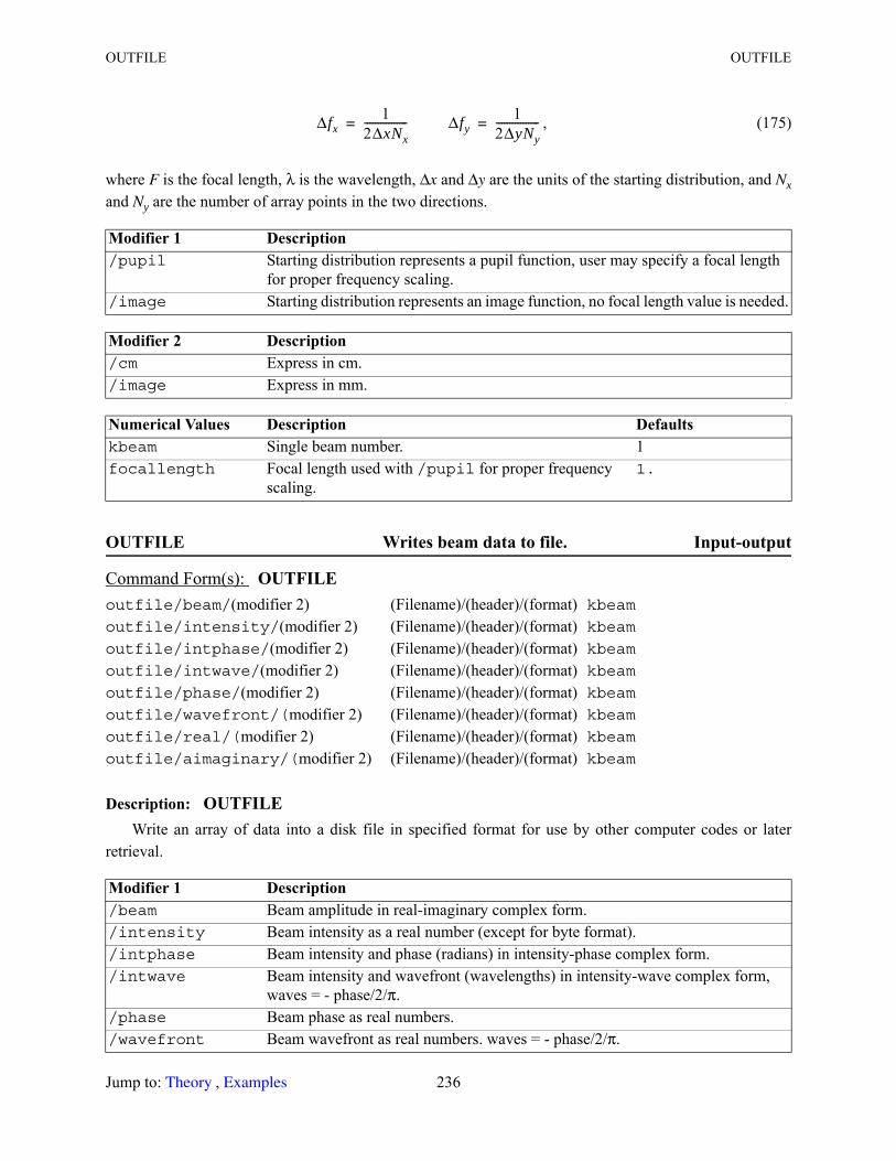
OUTFILE OUTFILE
, (175)
where F is the focal length, λ is the wavelength, Δx and Δy are the units of the starting distribution, and Nxand Ny are the number of array points in the two directions.
OUTFILE Writes beam data to file. Input-output
Description: OUTFILEWrite an array of data into a disk file in specified format for use by other computer codes or later
retrieval.
Modifier 1 Description /pupil Starting distribution represents a pupil function, user may specify a focal length
for proper frequency scaling./image Starting distribution represents an image function, no focal length value is needed.
Modifier 2 Description /cm Express in cm./image Express in mm.
Numerical Values Description Defaultskbeam Single beam number. 1focallength Focal length used with /pupil for proper frequency
scaling.1.
Command Form(s): OUTFILE outfile/beam/(modifier 2) (Filename)/(header)/(format) kbeamoutfile/intensity/(modifier 2) (Filename)/(header)/(format) kbeamoutfile/intphase/(modifier 2) (Filename)/(header)/(format) kbeamoutfile/intwave/(modifier 2) (Filename)/(header)/(format) kbeamoutfile/phase/(modifier 2) (Filename)/(header)/(format) kbeamoutfile/wavefront/(modifier 2) (Filename)/(header)/(format) kbeamoutfile/real/(modifier 2) (Filename)/(header)/(format) kbeamoutfile/aimaginary/(modifier 2) (Filename)/(header)/(format) kbeam
Modifier 1 Description /beam Beam amplitude in real-imaginary complex form./intensity Beam intensity as a real number (except for byte format)./intphase Beam intensity and phase (radians) in intensity-phase complex form./intwave Beam intensity and wavefront (wavelengths) in intensity-wave complex form,
waves = - phase/2/π./phase Beam phase as real numbers./wavefront Beam wavefront as real numbers. waves = - phase/2/π.
Δfx1
2ΔxNx----------------= Δfy
12ΔyNy----------------=
Jump to: , 236 Theory Examples
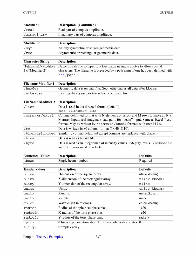
OUTFILE OUTFILE
/real Real part of complex amplitude./aimaginary Imaginary part of complex amplitude.
Modifier 2 Description /sqr Axially symmetric or square geometric data./rec Asymmetric or rectangular geometric data.
Character String Description (Filename)/(Modifier 1)/(Modifier 2)
Name of data file to input. Enclose name in single quotes to allow special characters. The filename is preceded by a path name if one has been defined with
/path.
Filename Modifier 1 Description /header Geometric data is on data file. Geometric data is all data after kbeam./noheader Existing data is used or taken from command line.
FileName Modifier 2 Description /list Data is read in list directed format (default)
read (Filename,*) list
/comma or /excel Comma delimited format with N elements on a row and M rows to make an N x M array. Inputs real-imaginary data pairs for “beam” input. Same as Excel *.csv format. May be written by /comma or /excel formats with outfile.
/80 Data is written in 80 column format (1x,4E18.10)./blankdelimited Similar to comma delimited except commas are replaced with blanks./binary Data is read as binary file./byte Data is read as an integer map of intensity values. 256 gray levels. /noheader
and /intens must be selected.
Numerical Values Description Defaultskbeam Single beam number. Required
Header values Description Defaultsnline Dimension of the square array. nlinx(kbeam)nlinx X-dimension of the rectangular array. nlinx(kbeam)
nliny Y-dimension of the rectangular array. nlinx
units Units. units(kbeam)
unitx X-units. unitsx(kbeam)unity Y-units. unitxcolor Wavelength in microns. color(kbeam)radref Radius of the spherical phase bias. 1e20radrefx X-radius of the toric phase bias. 1e20radrefy Y-radius of the toric phase bias. radrefxipolz 0 for one polarization state. 1 for two polarization states. 0a(i,j) Complex array.
Modifier 1 Description (Continued)
set
Jump to: , 237 Theory Examples
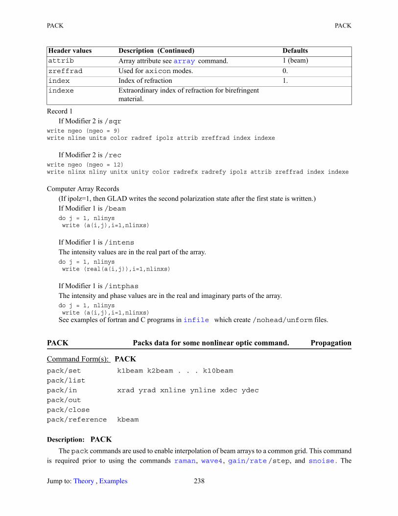
PACK PACK
Record 1If Modifier 2 is /sqr
write ngeo (ngeo = 9) write nline units color radref ipolz attrib zreffrad index indexe
If Modifier 2 is /rec
write ngeo (ngeo = 12) write nlinx nliny unitx unity color radrefx radrefy ipolz attrib zreffrad index indexe
Computer Array Records(If ipolz=1, then GLAD writes the second polarization state after the first state is written.)If Modifier 1 is /beamdo j = 1, nlinys write (a(i,j),i=1,nlinxs) If Modifier 1 is /intensThe intensity values are in the real part of the array.do j = 1, nlinys write (real(a(i,j)),i=1,nlinxs) If Modifier 1 is /intphasThe intensity and phase values are in the real and imaginary parts of the array.do j = 1, nlinys write (a(i,j),i=1,nlinxs) See examples of fortran and C programs in which create /nohead/unform files.
PACK Packs data for some nonlinear optic command. Propagation
Description: PACKThe pack commands are used to enable interpolation of beam arrays to a common grid. This command
is required prior to using the commands , , /step, and . The
attrib Array attribute see command. 1 (beam)zreffrad Used for axicon modes. 0.index Index of refraction 1.indexe Extraordinary index of refraction for birefringent
material.
Command Form(s): PACK pack/set k1beam k2beam . . . k10beam
pack/list
pack/in xrad yrad xnline ynline xdec ydec
pack/out
pack/close
pack/reference kbeam
Header values Description (Continued) Defaults array
infile
raman wave4 gain/rate snoise
Jump to: , 238 Theory Examples
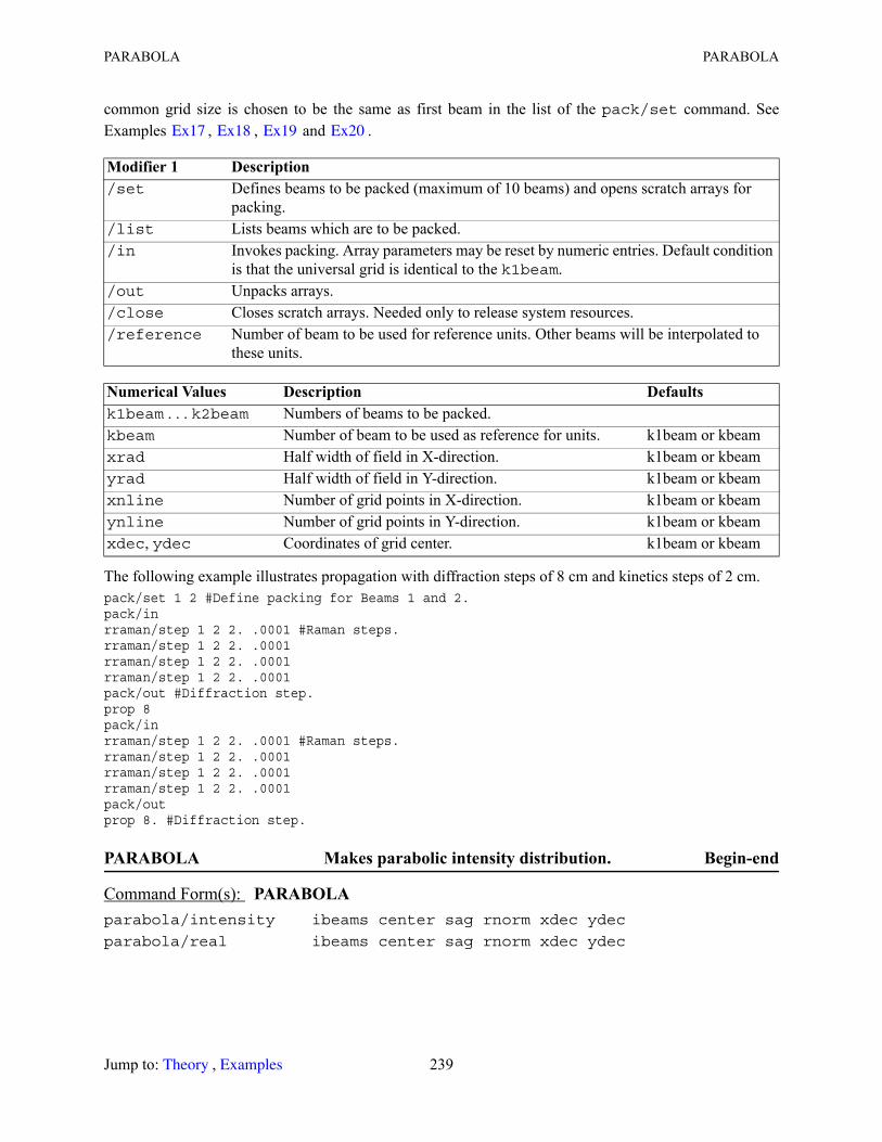
PARABOLA PARABOLA
common grid size is chosen to be the same as first beam in the list of the pack/set command. See Examples , , and .
The following example illustrates propagation with diffraction steps of 8 cm and kinetics steps of 2 cm.pack/set 1 2 #Define packing for Beams 1 and 2.pack/inrraman/step 1 2 2. .0001 #Raman steps.rraman/step 1 2 2. .0001rraman/step 1 2 2. .0001rraman/step 1 2 2. .0001pack/out #Diffraction step.prop 8pack/inrraman/step 1 2 2. .0001 #Raman steps.rraman/step 1 2 2. .0001rraman/step 1 2 2. .0001rraman/step 1 2 2. .0001pack/outprop 8. #Diffraction step.
PARABOLA Makes parabolic intensity distribution. Begin-end
Modifier 1 Description /set Defines beams to be packed (maximum of 10 beams) and opens scratch arrays for
packing./list Lists beams which are to be packed./in Invokes packing. Array parameters may be reset by numeric entries. Default condition
is that the universal grid is identical to the k1beam./out Unpacks arrays./close Closes scratch arrays. Needed only to release system resources./reference Number of beam to be used for reference units. Other beams will be interpolated to
these units.
Numerical Values Description Defaultsk1beam . . . k2beam Numbers of beams to be packed.kbeam Number of beam to be used as reference for units. k1beam or kbeamxrad Half width of field in X-direction. k1beam or kbeamyrad Half width of field in Y-direction. k1beam or kbeamxnline Number of grid points in X-direction. k1beam or kbeamynline Number of grid points in Y-direction. k1beam or kbeamxdec, ydec Coordinates of grid center. k1beam or kbeam
Command Form(s): PARABOLA parabola/intensity ibeams center sag rnorm xdec ydec
parabola/real ibeams center sag rnorm xdec ydec
Ex17 Ex18 Ex19 Ex20
Jump to: , 239 Theory Examples
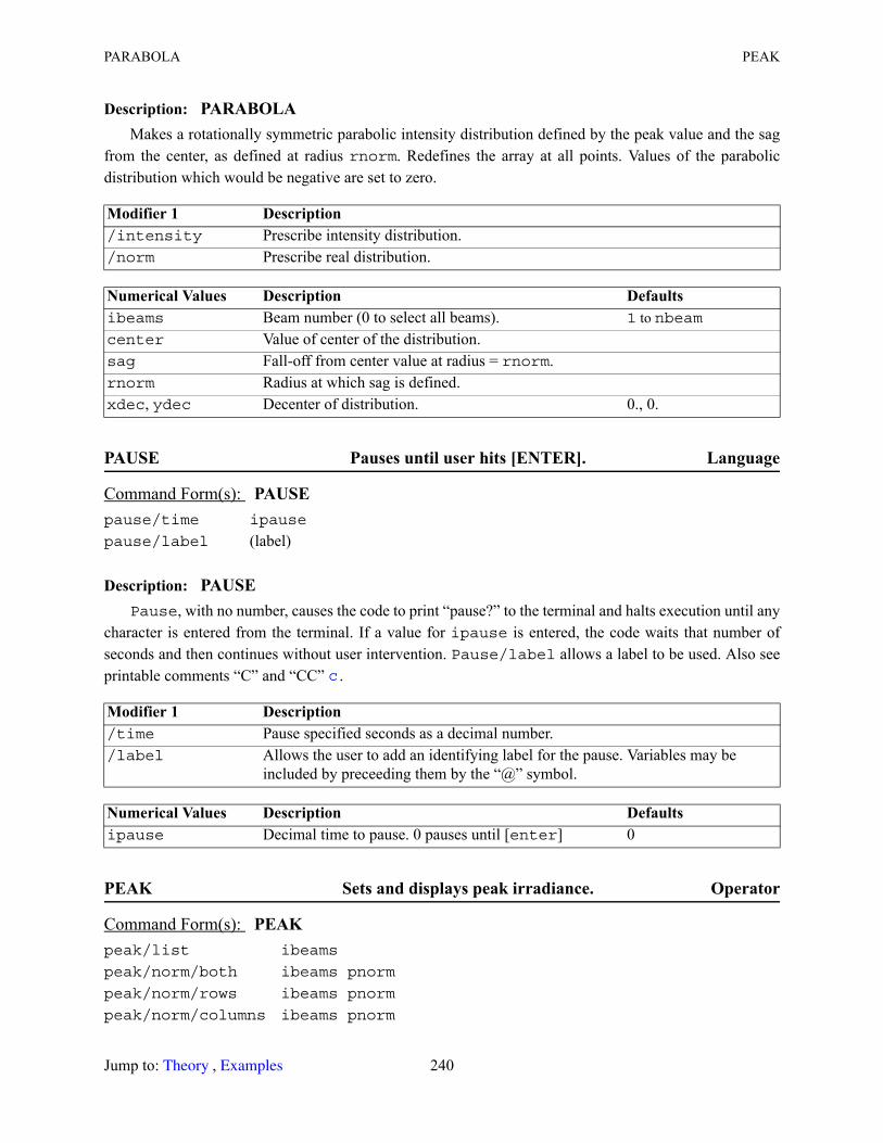
PARABOLA PEAK
Description: PARABOLAMakes a rotationally symmetric parabolic intensity distribution defined by the peak value and the sag
from the center, as defined at radius rnorm. Redefines the array at all points. Values of the parabolic distribution which would be negative are set to zero.
PAUSE Pauses until user hits [ENTER]. Language
Description: PAUSEPause, with no number, causes the code to print “pause?” to the terminal and halts execution until any
character is entered from the terminal. If a value for ipause is entered, the code waits that number of seconds and then continues without user intervention. Pause/label allows a label to be used. Also see printable comments “C” and “CC” .
PEAK Sets and displays peak irradiance. Operator
Modifier 1 Description /intensity Prescribe intensity distribution./norm Prescribe real distribution.
Numerical Values Description Defaultsibeams Beam number (0 to select all beams). 1 to nbeamcenter Value of center of the distribution.sag Fall-off from center value at radius = rnorm.rnorm Radius at which sag is defined.xdec, ydec Decenter of distribution. 0., 0.
Command Form(s): PAUSE pause/time ipause
pause/label (label)
Modifier 1 Description /time Pause specified seconds as a decimal number./label Allows the user to add an identifying label for the pause. Variables may be
included by preceeding them by the “@” symbol.
Numerical Values Description Defaultsipause Decimal time to pause. 0 pauses until [enter] 0
Command Form(s): PEAK peak/list ibeams
peak/norm/both ibeams pnorm
peak/norm/rows ibeams pnorm
peak/norm/columns ibeams pnorm
c
Jump to: , 240 Theory Examples
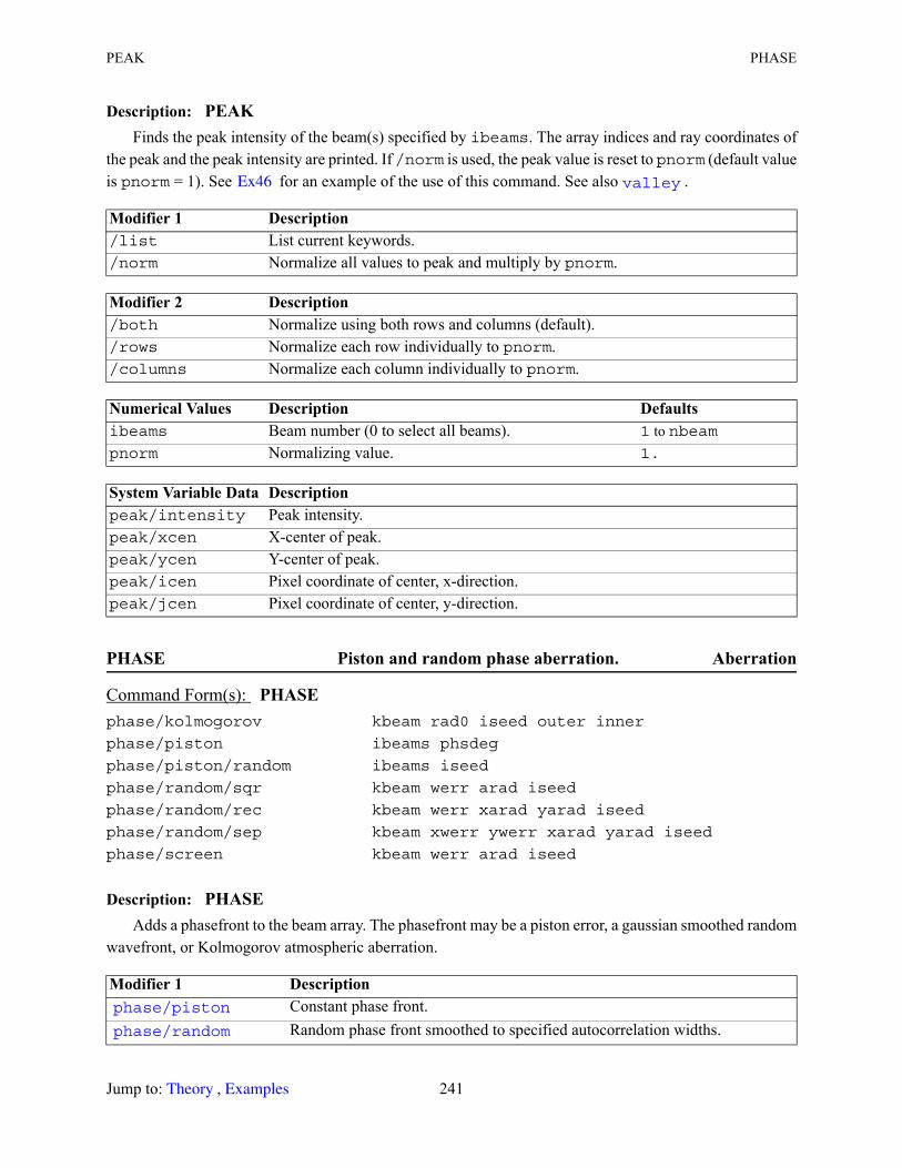
PEAK PHASE
Description: PEAKFinds the peak intensity of the beam(s) specified by ibeams. The array indices and ray coordinates of
the peak and the peak intensity are printed. If /norm is used, the peak value is reset to pnorm (default value is pnorm = 1). See for an example of the use of this command. See also .
PHASE Piston and random phase aberration. Aberration
Description: PHASEAdds a phasefront to the beam array. The phasefront may be a piston error, a gaussian smoothed random
wavefront, or Kolmogorov atmospheric aberration.
Modifier 1 Description /list List current keywords./norm Normalize all values to peak and multiply by pnorm.
Modifier 2 Description /both Normalize using both rows and columns (default)./rows Normalize each row individually to pnorm./columns Normalize each column individually to pnorm.
Numerical Values Description Defaultsibeams Beam number (0 to select all beams). 1 to nbeampnorm Normalizing value. 1.
System Variable Data Description peak/intensity Peak intensity.peak/xcen X-center of peak.peak/ycen Y-center of peak.peak/icen Pixel coordinate of center, x-direction.peak/jcen Pixel coordinate of center, y-direction.
Command Form(s): PHASE phase/kolmogorov kbeam rad0 iseed outer inner
phase/piston ibeams phsdeg
phase/piston/random ibeams iseed
phase/random/sqr kbeam werr arad iseed
phase/random/rec kbeam werr xarad yarad iseed
phase/random/sep kbeam xwerr ywerr xarad yarad iseed
phase/screen kbeam werr arad iseed
Modifier 1 Description Constant phase front. Random phase front smoothed to specified autocorrelation widths.
Ex46 valley
phase/piston phase/random
Jump to: , 241 Theory Examples
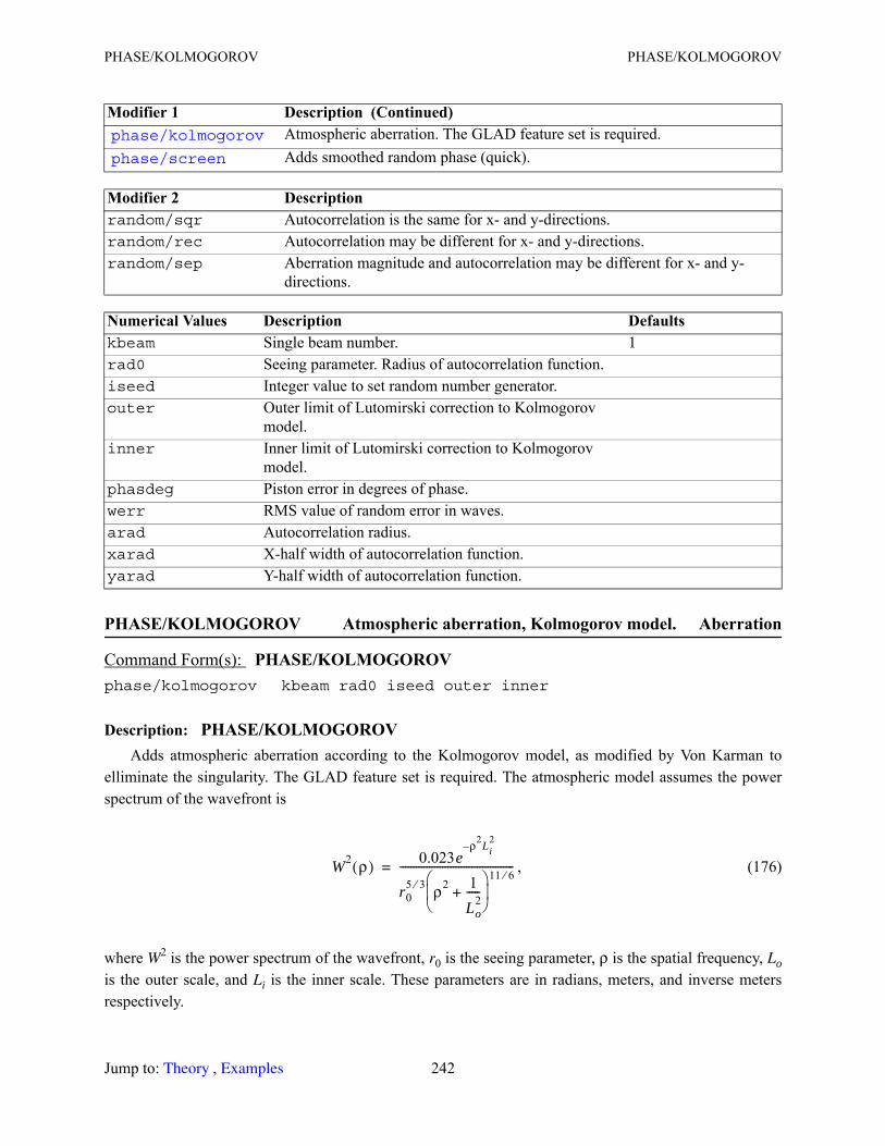
PHASE/KOLMOGOROV PHASE/KOLMOGOROV
PHASE/KOLMOGOROV Atmospheric aberration, Kolmogorov model. Aberration
Description: PHASE/KOLMOGOROVAdds atmospheric aberration according to the Kolmogorov model, as modified by Von Karman to
elliminate the singularity. The GLAD feature set is required. The atmospheric model assumes the power spectrum of the wavefront is
, (176)
where W2 is the power spectrum of the wavefront, r0 is the seeing parameter, ρ is the spatial frequency, Lois the outer scale, and Li is the inner scale. These parameters are in radians, meters, and inverse meters respectively.
Atmospheric aberration. The GLAD feature set is required. Adds smoothed random phase (quick).
Modifier 2 Description random/sqr Autocorrelation is the same for x- and y-directions.random/rec Autocorrelation may be different for x- and y-directions.random/sep Aberration magnitude and autocorrelation may be different for x- and y-
directions.
Numerical Values Description Defaultskbeam Single beam number. 1rad0 Seeing parameter. Radius of autocorrelation function.iseed Integer value to set random number generator.outer Outer limit of Lutomirski correction to Kolmogorov
model.inner Inner limit of Lutomirski correction to Kolmogorov
model.phasdeg Piston error in degrees of phase.werr RMS value of random error in waves.arad Autocorrelation radius.xarad X-half width of autocorrelation function.yarad Y-half width of autocorrelation function.
Command Form(s): PHASE/KOLMOGOROV phase/kolmogorov kbeam rad0 iseed outer inner
Modifier 1 Description (Continued) phase/kolmogorov phase/screen
W2 ρ( ) 0.023eρ2Li
2–
r05 3⁄ ρ2 1
Lo2
-----+ 11 6⁄
-------------------------------------------=
Jump to: , 242 Theory Examples
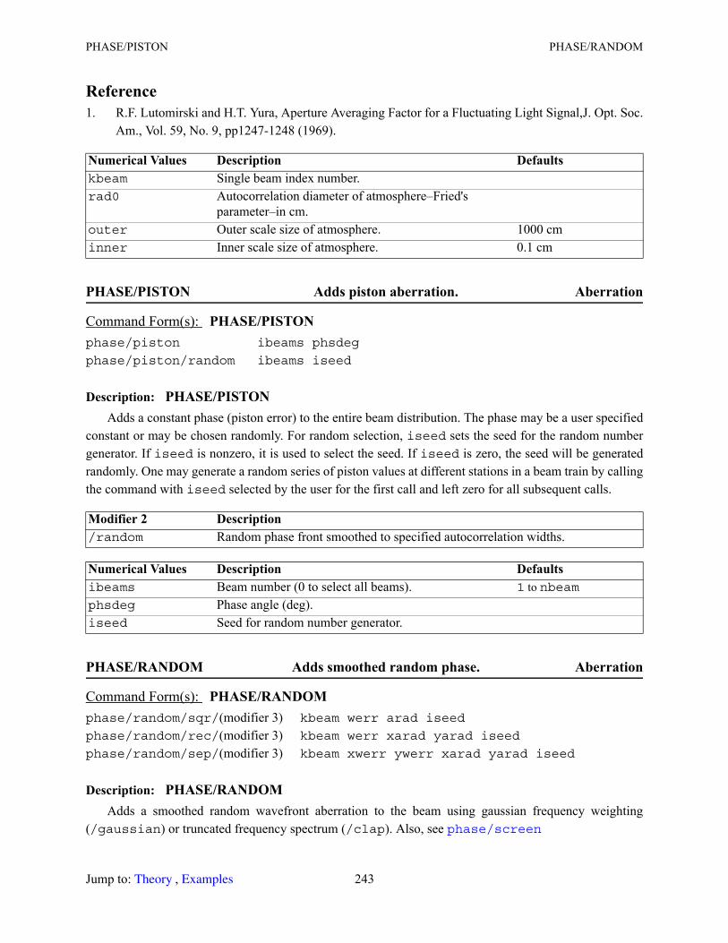
PHASE/PISTON PHASE/RANDOM
Reference1. R.F. Lutomirski and H.T. Yura, Aperture Averaging Factor for a Fluctuating Light Signal,J. Opt. Soc.
Am., Vol. 59, No. 9, pp1247-1248 (1969).
PHASE/PISTON Adds piston aberration. Aberration
Description: PHASE/PISTONAdds a constant phase (piston error) to the entire beam distribution. The phase may be a user specified
constant or may be chosen randomly. For random selection, iseed sets the seed for the random number generator. If iseed is nonzero, it is used to select the seed. If iseed is zero, the seed will be generated randomly. One may generate a random series of piston values at different stations in a beam train by calling the command with iseed selected by the user for the first call and left zero for all subsequent calls.
PHASE/RANDOM Adds smoothed random phase. Aberration
Description: PHASE/RANDOMAdds a smoothed random wavefront aberration to the beam using gaussian frequency weighting
(/gaussian) or truncated frequency spectrum (/clap). Also, see
Numerical Values Description Defaultskbeam Single beam index number.rad0 Autocorrelation diameter of atmosphere–Fried's
parameter–in cm.outer Outer scale size of atmosphere. 1000 cminner Inner scale size of atmosphere. 0.1 cm
Command Form(s): PHASE/PISTON phase/piston ibeams phsdeg
phase/piston/random ibeams iseed
Modifier 2 Description /random Random phase front smoothed to specified autocorrelation widths.
Numerical Values Description Defaultsibeams Beam number (0 to select all beams). 1 to nbeamphsdeg Phase angle (deg).iseed Seed for random number generator.
Command Form(s): PHASE/RANDOM phase/random/sqr/(modifier 3) kbeam werr arad iseed
phase/random/rec/(modifier 3) kbeam werr xarad yarad iseed
phase/random/sep/(modifier 3) kbeam xwerr ywerr xarad yarad iseed
phase/screen
Jump to: , 243 Theory Examples
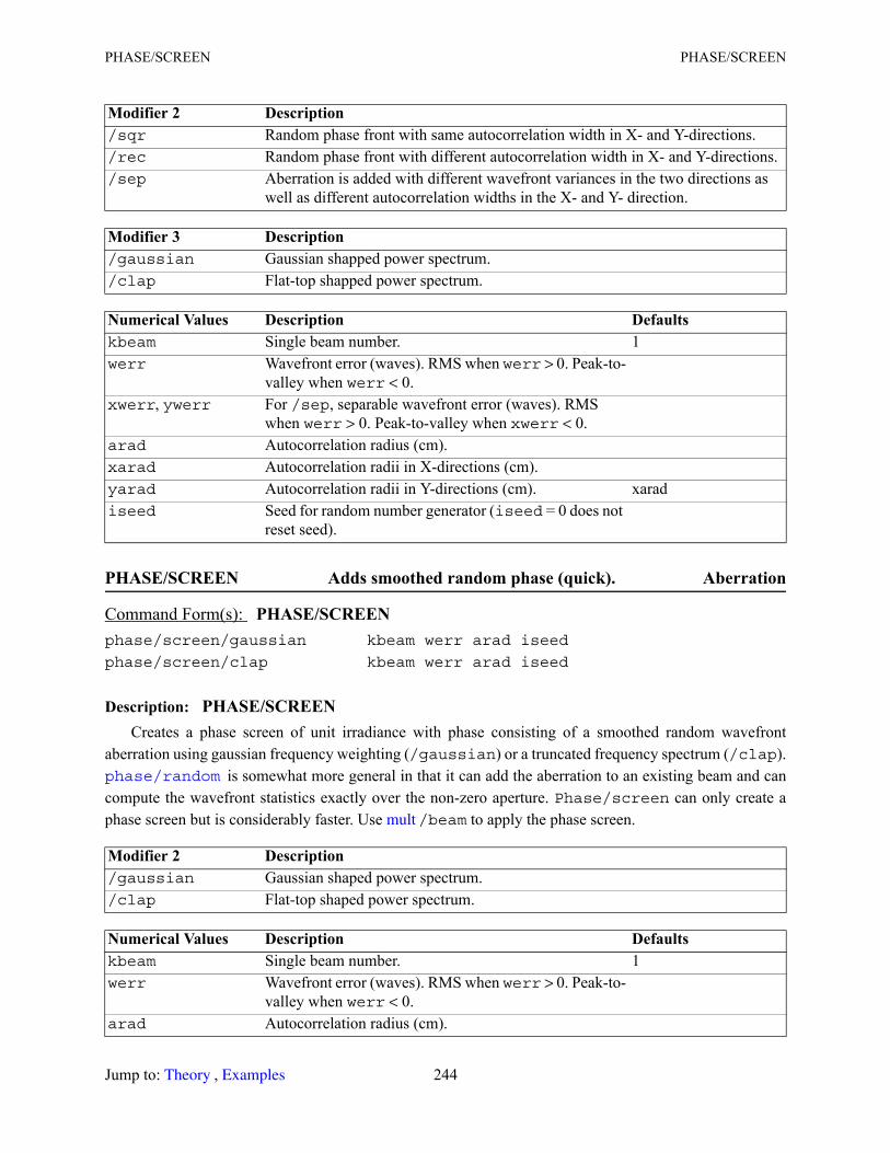
PHASE/SCREEN PHASE/SCREEN
PHASE/SCREEN Adds smoothed random phase (quick). Aberration
Description: PHASE/SCREENCreates a phase screen of unit irradiance with phase consisting of a smoothed random wavefront
aberration using gaussian frequency weighting (/gaussian) or a truncated frequency spectrum (/clap). is somewhat more general in that it can add the aberration to an existing beam and can
compute the wavefront statistics exactly over the non-zero aperture. Phase/screen can only create a phase screen but is considerably faster. Use /beam to apply the phase screen.
Modifier 2 Description /sqr Random phase front with same autocorrelation width in X- and Y-directions./rec Random phase front with different autocorrelation width in X- and Y-directions./sep Aberration is added with different wavefront variances in the two directions as
well as different autocorrelation widths in the X- and Y- direction.
Modifier 3 Description /gaussian Gaussian shapped power spectrum./clap Flat-top shapped power spectrum.
Numerical Values Description Defaultskbeam Single beam number. 1werr Wavefront error (waves). RMS when werr > 0. Peak-to-
valley when werr < 0.xwerr, ywerr For /sep, separable wavefront error (waves). RMS
when werr > 0. Peak-to-valley when xwerr < 0.arad Autocorrelation radius (cm).xarad Autocorrelation radii in X-directions (cm).yarad Autocorrelation radii in Y-directions (cm). xaradiseed Seed for random number generator (iseed = 0 does not
reset seed).
Command Form(s): PHASE/SCREEN phase/screen/gaussian kbeam werr arad iseed
phase/screen/clap kbeam werr arad iseed
Modifier 2 Description /gaussian Gaussian shaped power spectrum./clap Flat-top shaped power spectrum.
Numerical Values Description Defaultskbeam Single beam number. 1werr Wavefront error (waves). RMS when werr > 0. Peak-to-
valley when werr < 0.arad Autocorrelation radius (cm).
phase/random
mult
Jump to: , 244 Theory Examples
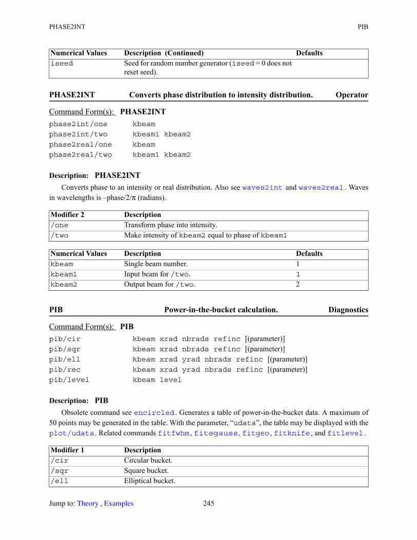
PHASE2INT PIB
PHASE2INT Converts phase distribution to intensity distribution. Operator
Description: PHASE2INTConverts phase to an intensity or real distribution. Also see and . Waves
in wavelengths is –phase/2/π (radians).
PIB Power-in-the-bucket calculation. Diagnostics
Description: PIBObsolete command see . Generates a table of power-in-the-bucket data. A maximum of
50 points may be generated in the table. With the parameter, “udata”, the table may be displayed with the . Related commands , , , , and .
iseed Seed for random number generator (iseed = 0 does not reset seed).
Command Form(s): PHASE2INT phase2int/one kbeam
phase2int/two kbeam1 kbeam2
phase2real/one kbeam
phase2real/two kbeam1 kbeam2
Modifier 2 Description /one Transform phase into intensity. /two Make intensity of kbeam2 equal to phase of kbeam1
Numerical Values Description Defaultskbeam Single beam number. 1kbeam1 Input beam for /two. 1
kbeam2 Output beam for /two. 2
Command Form(s): PIB pib/cir kbeam xrad nbrads refinc [(parameter)]pib/sqr kbeam xrad nbrads refinc [(parameter)]pib/ell kbeam xrad yrad nbrads refinc [(parameter)]pib/rec kbeam xrad yrad nbrads refinc [(parameter)]pib/level kbeam level
Modifier 1 Description /cir Circular bucket. /sqr Square bucket./ell Elliptical bucket.
Numerical Values Description (Continued) Defaults
waves2int waves2real
encircled
plot/udata fitfwhm fitegauss fitgeo fitknife fitlevel
Jump to: , 245 Theory Examples
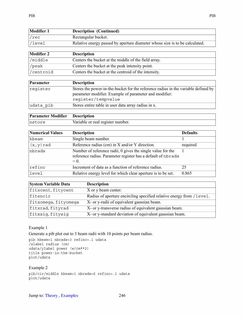
PIB PIB
Example 1Generate a pib plot out to 3 beam radii with 10 points per beam radius. pib kbeam=1 nbrads=3 refinc=.1 udata/xlabel radius (cm)udata/ylabel power (w/cm**2)title power-in-the-bucketplot/udata
Example 2pib/cir/middle kbeam=1 nbrads=6 refinc=.1 udataplot/udata
/rec Rectangular bucket./level Relative energy passed by aperture diameter whose size is to be calculated.
Modifier 2 Description /middle Centers the bucket at the middle of the field array./peak Centers the bucket at the peak intensity point./centroid Centers the bucket at the centroid of the intensity.
Parameter Description register Stores the power-in-the-bucket for the reference radius in the variable defined by
parameter modifier. Example of parameter and modifier: register/tempvalue
udata_pib Stores entire table in user data array radius in x.
Parameter Modifier Description nstore Variable or real register number.
Numerical Values Description Defaultskbeam Single beam number. 1(x,y)rad Reference radius (cm) in X and/or Y direction. requirednbrads Number of reference radii, 0 gives the single value for the
reference radius. Parameter register has a default of nbrads = 0.
1
refinc Increment of data as a function of reference radius. 25level Relative energy level for which clear aperture is to be set. 0.865
System Variable Data Description fitxcent, fitycent X or y beam center.fitencir Radius of aperture encircling specified relative energy from /level.fitxomega, fityomega X- or y-radii of equivalent gaussian beam.fitxrad, fityrad X- or y-transverse radius of equivalent gaussian beam.fitxsig, fitysig X- or y-standard deviation of equivalent gaussian beam.
Modifier 1 Description (Continued)
Jump to: , 246 Theory Examples
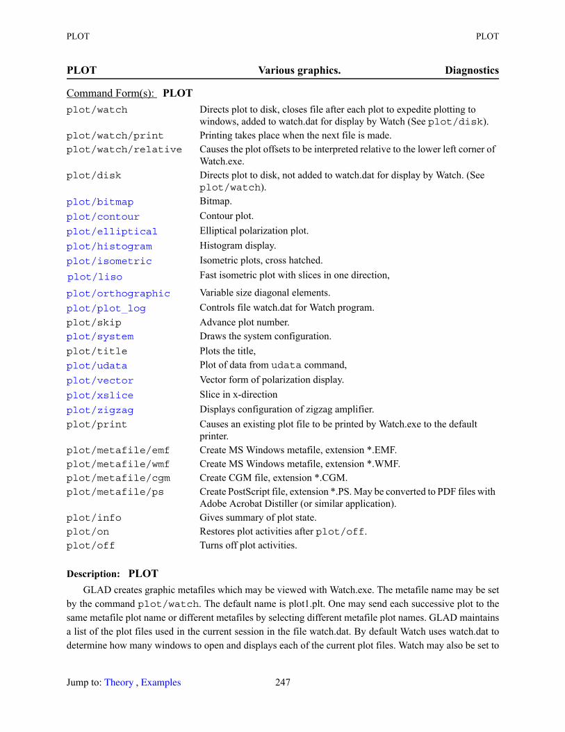
PLOT PLOT
PLOT Various graphics. Diagnostics
Description: PLOTGLAD creates graphic metafiles which may be viewed with Watch.exe. The metafile name may be set
by the command plot/watch. The default name is plot1.plt. One may send each successive plot to the same metafile plot name or different metafiles by selecting different metafile plot names. GLAD maintains a list of the plot files used in the current session in the file watch.dat. By default Watch uses watch.dat to determine how many windows to open and displays each of the current plot files. Watch may also be set to
Command Form(s): PLOT plot/watch Directs plot to disk, closes file after each plot to expedite plotting to
windows, added to watch.dat for display by Watch (See plot/disk). plot/watch/print Printing takes place when the next file is made.plot/watch/relative Causes the plot offsets to be interpreted relative to the lower left corner of
Watch.exe.plot/disk Directs plot to disk, not added to watch.dat for display by Watch. (See
plot/watch).Bitmap.Contour plot.Elliptical polarization plot.Histogram display.Isometric plots, cross hatched.Fast isometric plot with slices in one direction,
Variable size diagonal elements.Controls file watch.dat for Watch program.
plot/skip Advance plot number.Draws the system configuration.
plot/title Plots the title,Plot of data from udata command,Vector form of polarization display.Slice in x-directionDisplays configuration of zigzag amplifier.
plot/print Causes an existing plot file to be printed by Watch.exe to the default printer.
plot/metafile/emf Create MS Windows metafile, extension *.EMF.plot/metafile/wmf Create MS Windows metafile, extension *.WMF.plot/metafile/cgm Create CGM file, extension *.CGM.plot/metafile/ps Create PostScript file, extension *.PS. May be converted to PDF files with
Adobe Acrobat Distiller (or similar application).plot/info Gives summary of plot state.plot/on Restores plot activities after plot/off.plot/off Turns off plot activities.
plot/bitmap plot/contour plot/elliptical plot/histogram plot/isometric plot/liso
plot/orthographic plot/plot_log
plot/system
plot/udata plot/vector plot/xslice plot/zigzag
Jump to: , 247 Theory Examples
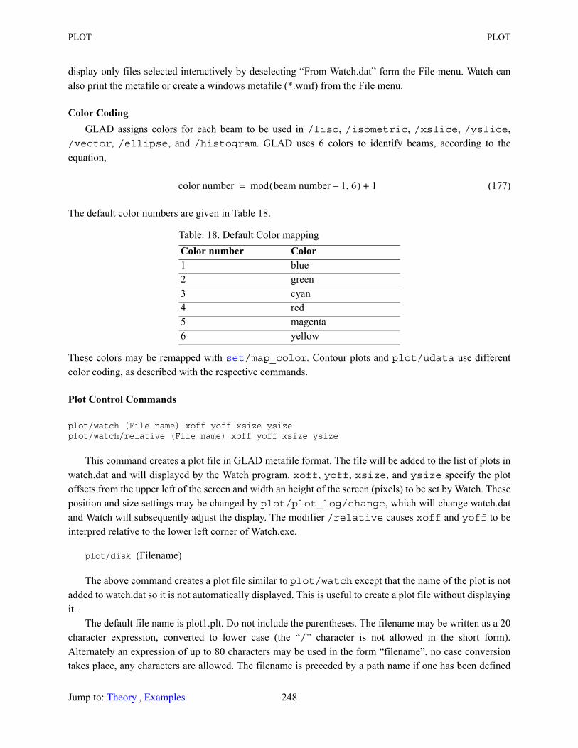
PLOT PLOT
display only files selected interactively by deselecting “From Watch.dat” form the File menu. Watch can also print the metafile or create a windows metafile (*.wmf) from the File menu.
Color CodingGLAD assigns colors for each beam to be used in /liso, /isometric, /xslice, /yslice,
/vector, /ellipse, and /histogram. GLAD uses 6 colors to identify beams, according to the equation,
(177)
The default color numbers are given in Table 18.
These colors may be remapped with /map_color. Contour plots and plot/udata use different color coding, as described with the respective commands.
Plot Control Commands
plot/watch (File name) xoff yoff xsize ysizeplot/watch/relative (File name) xoff yoff xsize ysize
This command creates a plot file in GLAD metafile format. The file will be added to the list of plots in watch.dat and will displayed by the Watch program. xoff, yoff, xsize, and ysize specify the plot offsets from the upper left of the screen and width an height of the screen (pixels) to be set by Watch. These position and size settings may be changed by plot/plot_log/change, which will change watch.dat and Watch will subsequently adjust the display. The modifier /relative causes xoff and yoff to be interpred relative to the lower left corner of Watch.exe.
plot/disk (Filename)
The above command creates a plot file similar to plot/watch except that the name of the plot is not added to watch.dat so it is not automatically displayed. This is useful to create a plot file without displaying it.
The default file name is plot1.plt. Do not include the parentheses. The filename may be written as a 20 character expression, converted to lower case (the “/” character is not allowed in the short form). Alternately an expression of up to 80 characters may be used in the form “filename”, no case conversion takes place, any characters are allowed. The filename is preceded by a path name if one has been defined
Table. 18. Default Color mapping Color number Color1 blue2 green3 cyan4 red5 magenta6 yellow
color number mod beam number 1– 6,( ) 1+=
set
Jump to: , 248 Theory Examples
PLOT PLOT
with /path. It is preferable to set the default folder from the Controls dialog box of the Interactive Input of IDE.EXE.
plot/skip nskip
The above command advances the plot page number by nskip.
plot/screen/pause ipause
The above command will cause the program to wait ipause seconds before continuing. This replaces the usual wait for the user to enter a key. A zero value for ipause turns off the timed pause and returns to a wait for user entry.
plot/title size
The above command plots the title with character size determined in pixels where there are 768 pixels for the screen height.
The command
plot/info
summarizes the current plot state, graphic protocol, etc.The commands
plot/offplot/on
turn plotting activities off or back on respectively.The command below
plot/print (Filename)
will cause Watch.exe to print Filename using the current printer. The current printer may be changed using the printer setup features of Watch.exe.
Windows metafile format (*.WMF) and the Enhanced metafile format are widely used vector graphic format. The EMF format allows better control of the graphic size and is preferred over WMF. The commands shown below
plot/metafile/emf (Filename)plot/metafile/wmf (Filename)
cause Watch.exe to generate Filename into an MS Windows metafile with the suffix *.EMF or *.WMF respectively. For example, plot1.emf will be created from plot1.plt. The default name is the name of the most recently created plot.
Scalar vector graphics (SVG) and compressed scalar vector graphics (SVGZ) may be generated with the commands:
plot/metafile/svg (Filename)
set
Jump to: , 249 Theory Examples
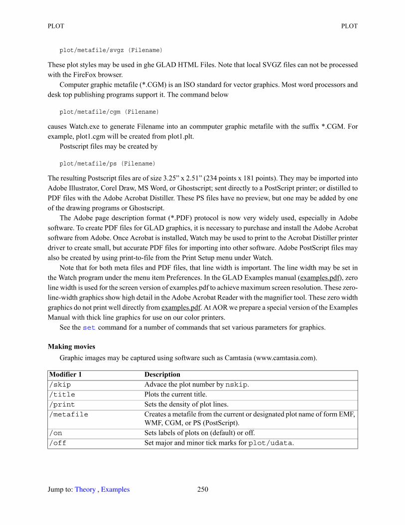
PLOT PLOT
plot/metafile/svgz (Filename)
These plot styles may be used in ghe GLAD HTML Files. Note that local SVGZ files can not be processed with the FireFox browser.
Computer graphic metafile (*.CGM) is an ISO standard for vector graphics. Most word processors and desk top publishing programs support it. The command below
plot/metafile/cgm (Filename)
causes Watch.exe to generate Filename into an commputer graphic metafile with the suffix *.CGM. For example, plot1.cgm will be created from plot1.plt.
Postscript files may be created by
plot/metafile/ps (Filename)
The resulting Postscript files are of size 3.25” x 2.51” (234 points x 181 points). They may be imported into Adobe Illustrator, Corel Draw, MS Word, or Ghostscript; sent directly to a PostScript printer; or distilled to PDF files with the Adobe Acrobat Distiller. These PS files have no preview, but one may be added by one of the drawing programs or Ghostscript.
The Adobe page description format (*.PDF) protocol is now very widely used, especially in Adobe software. To create PDF files for GLAD graphics, it is necessary to purchase and install the Adobe Acrobat software from Adobe. Once Acrobat is installed, Watch may be used to print to the Acrobat Distiller printer driver to create small, but accurate PDF files for importing into other software. Adobe PostScript files may also be created by using print-to-file from the Print Setup menu under Watch.
Note that for both meta files and PDF files, that line width is important. The line width may be set in the Watch program under the menu item Preferences. In the GLAD Examples manual (examples.pdf), zero line width is used for the screen version of examples.pdf to achieve maximum screen resolution. These zero-line-width graphics show high detail in the Adobe Acrobat Reader with the magnifier tool. These zero width graphics do not print well directly from examples.pdf. At AOR we prepare a special version of the Examples Manual with thick line graphics for use on our color printers.
See the command for a number of commands that set various parameters for graphics.
Making moviesGraphic images may be captured using software such as Camtasia (www.camtasia.com).
Modifier 1 Description /skip Advace the plot number by nskip./title Plots the current title./print Sets the density of plot lines./metafile Creates a metafile from the current or designated plot name of form EMF,
WMF, CGM, or PS (PostScript)./on Sets labels of plots on (default) or off./off Set major and minor tick marks for plot/udata.
set
Jump to: , 250 Theory Examples
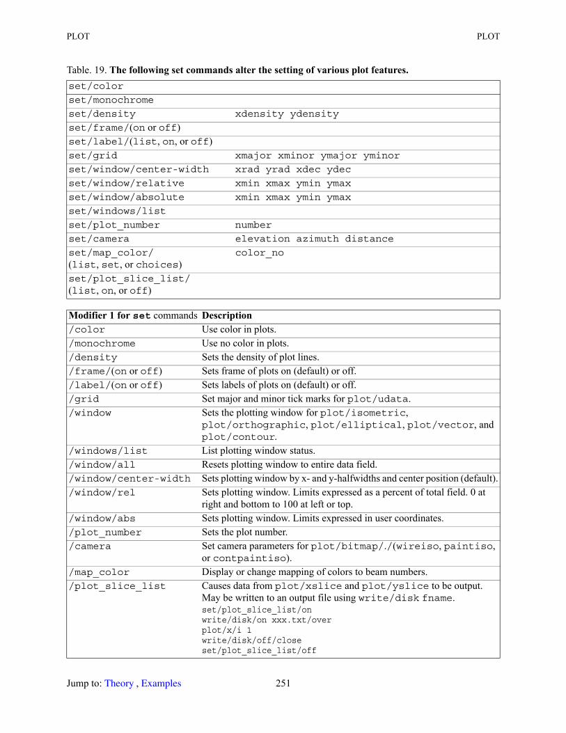
PLOT PLOT
Table. 19. The following set commands alter the setting of various plot features. set/color
set/monochrome
set/density xdensity ydensity
set/frame/(on or off)set/label/(list, on, or off)set/grid xmajor xminor ymajor yminor
set/window/center-width xrad yrad xdec ydec
set/window/relative xmin xmax ymin ymax
set/window/absolute xmin xmax ymin ymax
set/windows/list
set/plot_number number
set/camera elevation azimuth distance
set/map_color/(list, set, or choices)
color_no
set/plot_slice_list/(list, on, or off)
Modifier 1 for set commands Description /color Use color in plots./monochrome Use no color in plots./density Sets the density of plot lines./frame/(on or off) Sets frame of plots on (default) or off./label/(on or off) Sets labels of plots on (default) or off./grid Set major and minor tick marks for plot/udata./window Sets the plotting window for plot/isometric,
plot/orthographic, plot/elliptical, plot/vector, and plot/contour.
/windows/list List plotting window status./window/all Resets plotting window to entire data field./window/center-width Sets plotting window by x- and y-halfwidths and center position (default)./window/rel Sets plotting window. Limits expressed as a percent of total field. 0 at
right and bottom to 100 at left or top./window/abs Sets plotting window. Limits expressed in user coordinates./plot_number Sets the plot number./camera Set camera parameters for plot/bitmap/./(wireiso, paintiso,
or contpaintiso)./map_color Display or change mapping of colors to beam numbers./plot_slice_list Causes data from plot/xslice and plot/yslice to be output.
May be written to an output file using write/disk fname.set/plot_slice_list/onwrite/disk/on xxx.txt/overplot/x/i 1write/disk/off/closeset/plot_slice_list/off
Jump to: , 251 Theory Examples
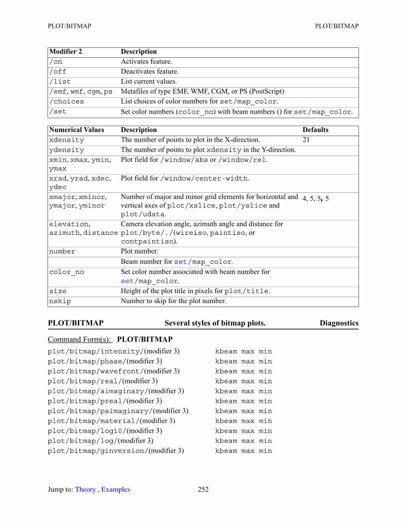
PLOT/BITMAP PLOT/BITMAP
PLOT/BITMAP Several styles of bitmap plots. Diagnostics
Modifier 2 Description /on Activates feature./off Deactivates feature./list List current values./emf, wmf, cgm, ps Metafiles of type EMF, WMF, CGM, or PS (PostScript)/choices List choices of color numbers for set/map_color./set Set color numbers (color_no) with beam numbers () for /map_color.
Numerical Values Description Defaultsxdensity The number of points to plot in the X-direction. 21ydensity The number of points to plot xdensity in the Y-direction.xmin, xmax, ymin, ymax
Plot field for /window/abs or /window/rel.
xrad, yrad, xdec, ydec
Plot field for /window/center-width.
xmajor, xminor, ymajor, yminor
Number of major and minor grid elements for horizontal and vertical axes of plot/xslice, plot/yslice and plot/udata.
4, 5, 5, 5
elevation, azimuth, distance
Camera elevation angle, azimuth angle and distance for plot/byte/./(wireiso, paintiso, or contpaintiso).
number Plot number.Beam number for /map_color.
color_no Set color number associated with beam number for /map_color.
size Height of the plot title in pixels for plot/title.nskip Number to skip for the plot number.
Command Form(s): PLOT/BITMAP plot/bitmap/intensity/(modifier 3) kbeam max min
plot/bitmap/phase/(modifier 3) kbeam max min
plot/bitmap/wavefront/(modifier 3) kbeam max min
plot/bitmap/real/(modifier 3) kbeam max min
plot/bitmap/aimaginary/(modifier 3) kbeam max min
plot/bitmap/preal/(modifier 3) kbeam max min
plot/bitmap/paimaginary/(modifier 3) kbeam max min
plot/bitmap/material/(modifier 3) kbeam max min
plot/bitmap/log10/(modifier 3) kbeam max min
plot/bitmap/log/(modifier 3) kbeam max min
plot/bitmap/ginversion/(modifier 3) kbeam max min
set
set
set
Jump to: , 252 Theory Examples
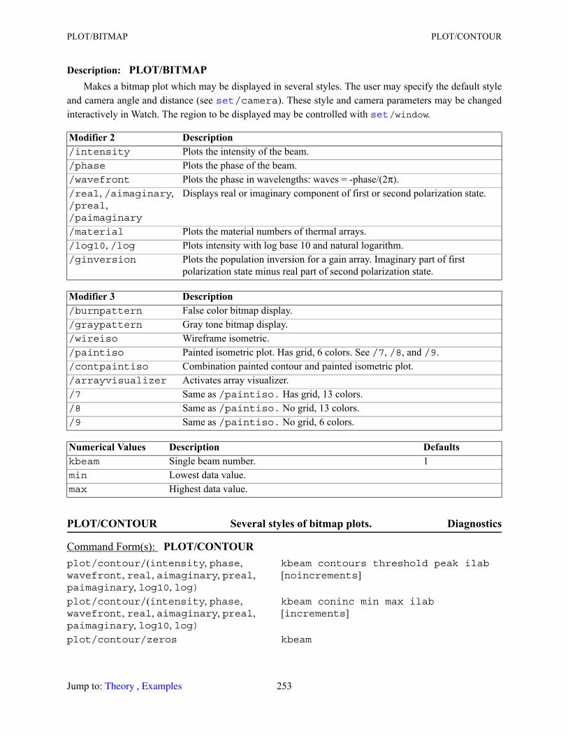
PLOT/BITMAP PLOT/CONTOUR
Description: PLOT/BITMAPMakes a bitmap plot which may be displayed in several styles. The user may specify the default style
and camera angle and distance (see /camera). These style and camera parameters may be changed interactively in Watch. The region to be displayed may be controlled with /window.
PLOT/CONTOUR Several styles of bitmap plots. Diagnostics
Modifier 2 Description /intensity Plots the intensity of the beam. /phase Plots the phase of the beam./wavefront Plots the phase in wavelengths: waves = -phase/(2π)./real, /aimaginary, /preal, /paimaginary
Displays real or imaginary component of first or second polarization state.
/material Plots the material numbers of thermal arrays./log10, /log Plots intensity with log base 10 and natural logarithm./ginversion Plots the population inversion for a gain array. Imaginary part of first
polarization state minus real part of second polarization state.
Modifier 3 Description /burnpattern False color bitmap display./graypattern Gray tone bitmap display./wireiso Wireframe isometric./paintiso Painted isometric plot. Has grid, 6 colors. See /7, /8, and /9./contpaintiso Combination painted contour and painted isometric plot./arrayvisualizer Activates array visualizer./7 Same as /paintiso. Has grid, 13 colors./8 Same as /paintiso. No grid, 13 colors./9 Same as /paintiso. No grid, 6 colors.
Numerical Values Description Defaultskbeam Single beam number. 1min Lowest data value.max Highest data value.
Command Form(s): PLOT/CONTOUR plot/contour/(intensity, phase, wavefront, real, aimaginary, preal, paimaginary, log10, log)
kbeam contours threshold peak ilab [noincrements]
plot/contour/(intensity, phase, wavefront, real, aimaginary, preal, paimaginary, log10, log)
kbeam coninc min max ilab [increments]
plot/contour/zeros kbeam
set set
Jump to: , 253 Theory Examples
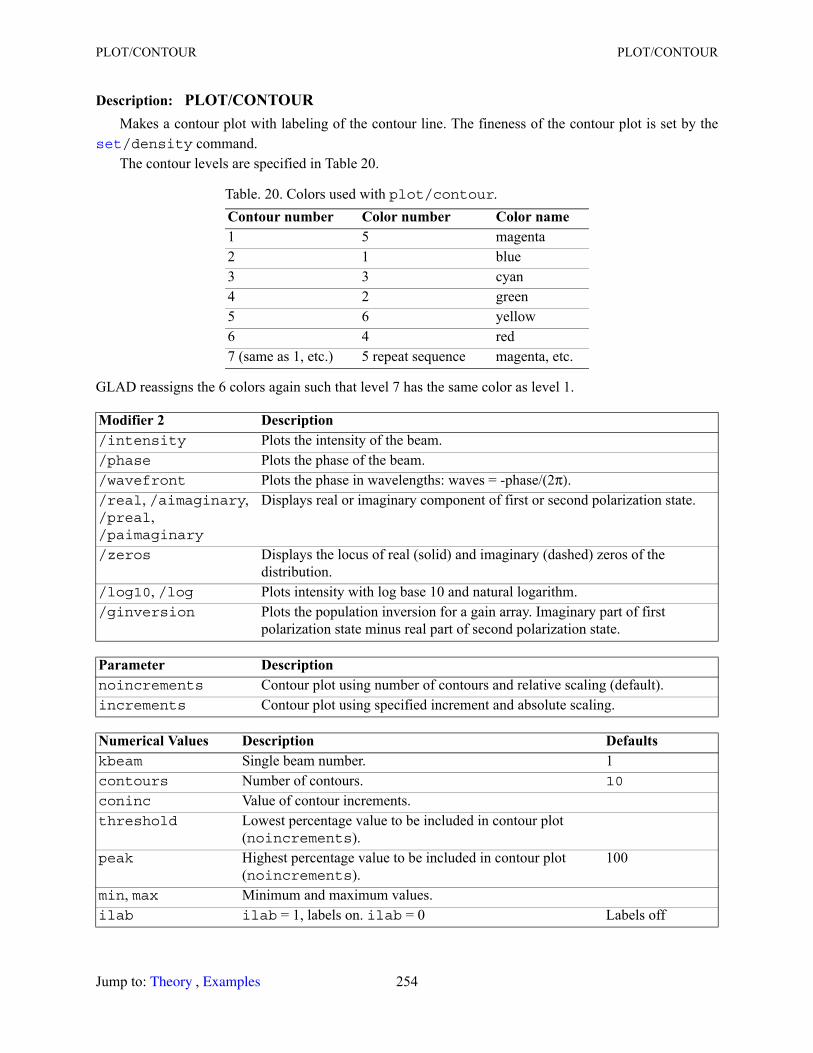
PLOT/CONTOUR PLOT/CONTOUR
Description: PLOT/CONTOURMakes a contour plot with labeling of the contour line. The fineness of the contour plot is set by the /density command.The contour levels are specified in Table 20.
GLAD reassigns the 6 colors again such that level 7 has the same color as level 1.
Table. 20. Colors used with plot/contour. Contour number Color number Color name1 5 magenta2 1 blue3 3 cyan4 2 green5 6 yellow6 4 red7 (same as 1, etc.) 5 repeat sequence magenta, etc.
Modifier 2 Description /intensity Plots the intensity of the beam. /phase Plots the phase of the beam./wavefront Plots the phase in wavelengths: waves = -phase/(2π)./real, /aimaginary, /preal, /paimaginary
Displays real or imaginary component of first or second polarization state.
/zeros Displays the locus of real (solid) and imaginary (dashed) zeros of the distribution.
/log10, /log Plots intensity with log base 10 and natural logarithm./ginversion Plots the population inversion for a gain array. Imaginary part of first
polarization state minus real part of second polarization state.
Parameter Description noincrements Contour plot using number of contours and relative scaling (default).increments Contour plot using specified increment and absolute scaling.
Numerical Values Description Defaultskbeam Single beam number. 1contours Number of contours. 10
coninc Value of contour increments.threshold Lowest percentage value to be included in contour plot
(noincrements).peak Highest percentage value to be included in contour plot
(noincrements).100
min, max Minimum and maximum values.ilab ilab = 1, labels on. ilab = 0 Labels off
set
Jump to: , 254 Theory Examples
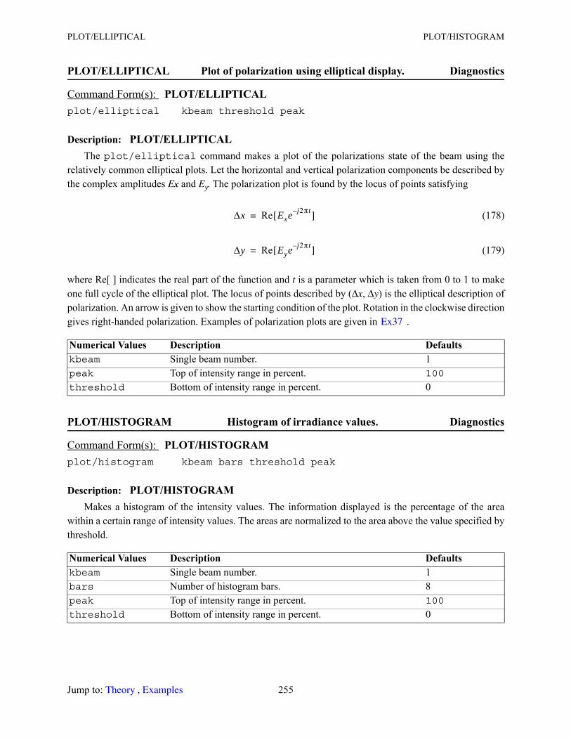
PLOT/ELLIPTICAL PLOT/HISTOGRAM
PLOT/ELLIPTICAL Plot of polarization using elliptical display. Diagnostics
Description: PLOT/ELLIPTICALThe plot/elliptical command makes a plot of the polarizations state of the beam using the
relatively common elliptical plots. Let the horizontal and vertical polarization components be described by the complex amplitudes Ex and Ey. The polarization plot is found by the locus of points satisfying
(178)
(179)
where Re[ ] indicates the real part of the function and t is a parameter which is taken from 0 to 1 to make one full cycle of the elliptical plot. The locus of points described by (Δx, Δy) is the elliptical description of polarization. An arrow is given to show the starting condition of the plot. Rotation in the clockwise direction gives right-handed polarization. Examples of polarization plots are given in .
PLOT/HISTOGRAM Histogram of irradiance values. Diagnostics
Description: PLOT/HISTOGRAMMakes a histogram of the intensity values. The information displayed is the percentage of the area
within a certain range of intensity values. The areas are normalized to the area above the value specified by threshold.
Command Form(s): PLOT/ELLIPTICAL plot/elliptical kbeam threshold peak
Numerical Values Description Defaultskbeam Single beam number. 1peak Top of intensity range in percent. 100
threshold Bottom of intensity range in percent. 0
Command Form(s): PLOT/HISTOGRAM plot/histogram kbeam bars threshold peak
Numerical Values Description Defaultskbeam Single beam number. 1bars Number of histogram bars. 8peak Top of intensity range in percent. 100
threshold Bottom of intensity range in percent. 0
Δx Re Exe j2πt–[ ]=
Δy Re Eye j2πt–[ ]=
Ex37
Jump to: , 255 Theory Examples
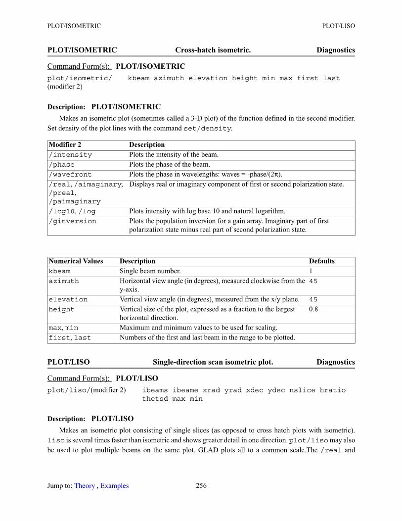
PLOT/ISOMETRIC PLOT/LISO
PLOT/ISOMETRIC Cross-hatch isometric. Diagnostics
Description: PLOT/ISOMETRICMakes an isometric plot (sometimes called a 3-D plot) of the function defined in the second modifier.
Set density of the plot lines with the command set/density.
PLOT/LISO Single-direction scan isometric plot. Diagnostics
Description: PLOT/LISOMakes an isometric plot consisting of single slices (as opposed to cross hatch plots with isometric).
liso is several times faster than isometric and shows greater detail in one direction. plot/liso may also be used to plot multiple beams on the same plot. GLAD plots all to a common scale.The /real and
Command Form(s): PLOT/ISOMETRIC plot/isometric/(modifier 2)
kbeam azimuth elevation height min max first last
Modifier 2 Description /intensity Plots the intensity of the beam. /phase Plots the phase of the beam./wavefront Plots the phase in wavelengths: waves = -phase/(2π)./real, /aimaginary, /preal, /paimaginary
Displays real or imaginary component of first or second polarization state.
/log10, /log Plots intensity with log base 10 and natural logarithm./ginversion Plots the population inversion for a gain array. Imaginary part of first
polarization state minus real part of second polarization state.
Numerical Values Description Defaultskbeam Single beam number. 1azimuth Horizontal view angle (in degrees), measured clockwise from the
y-axis.45
elevation Vertical view angle (in degrees), measured from the x/y plane. 45
height Vertical size of the plot, expressed as a fraction to the largest horizontal direction.
0.8
max, min Maximum and minimum values to be used for scaling.first, last Numbers of the first and last beam in the range to be plotted.
Command Form(s): PLOT/LISO plot/liso/(modifier 2) ibeams ibeame xrad yrad xdec ydec nslice hratio
thetsd max min
Jump to: , 256 Theory Examples
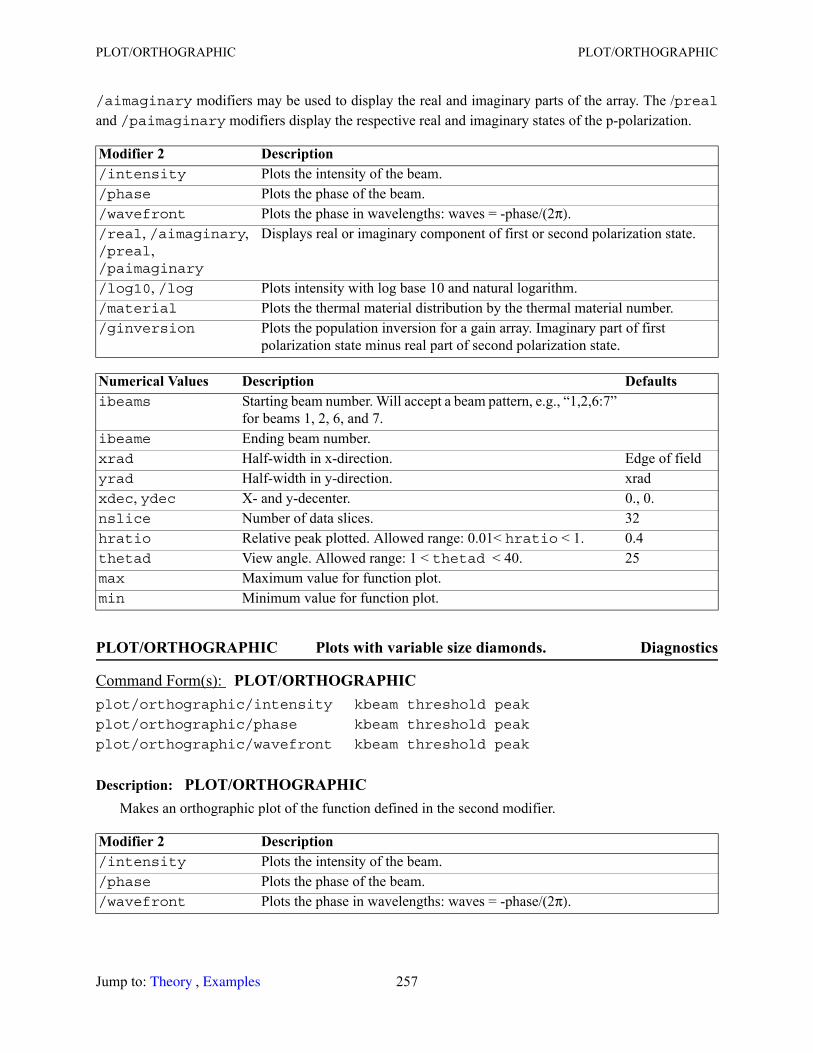
PLOT/ORTHOGRAPHIC PLOT/ORTHOGRAPHIC
/aimaginary modifiers may be used to display the real and imaginary parts of the array. The /prealand /paimaginary modifiers display the respective real and imaginary states of the p-polarization.
PLOT/ORTHOGRAPHIC Plots with variable size diamonds. Diagnostics
Description: PLOT/ORTHOGRAPHICMakes an orthographic plot of the function defined in the second modifier.
Modifier 2 Description /intensity Plots the intensity of the beam. /phase Plots the phase of the beam./wavefront Plots the phase in wavelengths: waves = -phase/(2π)./real, /aimaginary, /preal, /paimaginary
Displays real or imaginary component of first or second polarization state.
/log10, /log Plots intensity with log base 10 and natural logarithm./material Plots the thermal material distribution by the thermal material number./ginversion Plots the population inversion for a gain array. Imaginary part of first
polarization state minus real part of second polarization state.
Numerical Values Description Defaultsibeams Starting beam number. Will accept a beam pattern, e.g., “1,2,6:7”
for beams 1, 2, 6, and 7.ibeame Ending beam number.xrad Half-width in x-direction. Edge of fieldyrad Half-width in y-direction. xradxdec, ydec X- and y-decenter. 0., 0.nslice Number of data slices. 32hratio Relative peak plotted. Allowed range: 0.01< hratio < 1. 0.4thetad View angle. Allowed range: 1 < thetad < 40. 25max Maximum value for function plot.min Minimum value for function plot.
Command Form(s): PLOT/ORTHOGRAPHIC plot/orthographic/intensity kbeam threshold peak
plot/orthographic/phase kbeam threshold peak
plot/orthographic/wavefront kbeam threshold peak
Modifier 2 Description /intensity Plots the intensity of the beam. /phase Plots the phase of the beam./wavefront Plots the phase in wavelengths: waves = -phase/(2π).
Jump to: , 257 Theory Examples
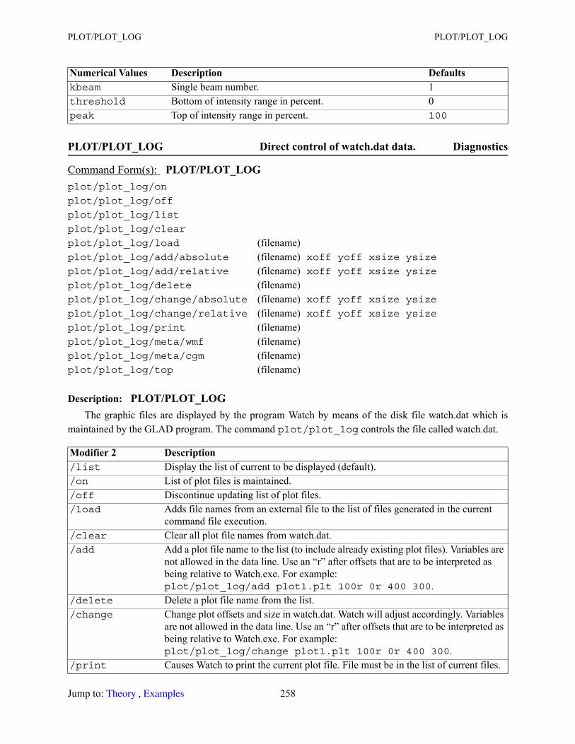
PLOT/PLOT_LOG PLOT/PLOT_LOG
PLOT/PLOT_LOG Direct control of watch.dat data. Diagnostics
Description: PLOT/PLOT_LOGThe graphic files are displayed by the program Watch by means of the disk file watch.dat which is
maintained by the GLAD program. The command plot/plot_log controls the file called watch.dat.
Numerical Values Description Defaultskbeam Single beam number. 1threshold Bottom of intensity range in percent. 0peak Top of intensity range in percent. 100
Command Form(s): PLOT/PLOT_LOG plot/plot_log/on
plot/plot_log/off
plot/plot_log/list
plot/plot_log/clear
plot/plot_log/load (filename)plot/plot_log/add/absolute (filename) xoff yoff xsize ysizeplot/plot_log/add/relative (filename) xoff yoff xsize ysizeplot/plot_log/delete (filename)plot/plot_log/change/absolute (filename) xoff yoff xsize ysizeplot/plot_log/change/relative (filename) xoff yoff xsize ysizeplot/plot_log/print (filename)plot/plot_log/meta/wmf (filename)plot/plot_log/meta/cgm (filename)plot/plot_log/top (filename)
Modifier 2 Description /list Display the list of current to be displayed (default)./on List of plot files is maintained./off Discontinue updating list of plot files./load Adds file names from an external file to the list of files generated in the current
command file execution./clear Clear all plot file names from watch.dat./add Add a plot file name to the list (to include already existing plot files). Variables are
not allowed in the data line. Use an “r” after offsets that are to be interpreted as being relative to Watch.exe. For example:plot/plot_log/add plot1.plt 100r 0r 400 300.
/delete Delete a plot file name from the list./change Change plot offsets and size in watch.dat. Watch will adjust accordingly. Variables
are not allowed in the data line. Use an “r” after offsets that are to be interpreted as being relative to Watch.exe. For example:plot/plot_log/change plot1.plt 100r 0r 400 300.
/print Causes Watch to print the current plot file. File must be in the list of current files.
Jump to: , 258 Theory Examples
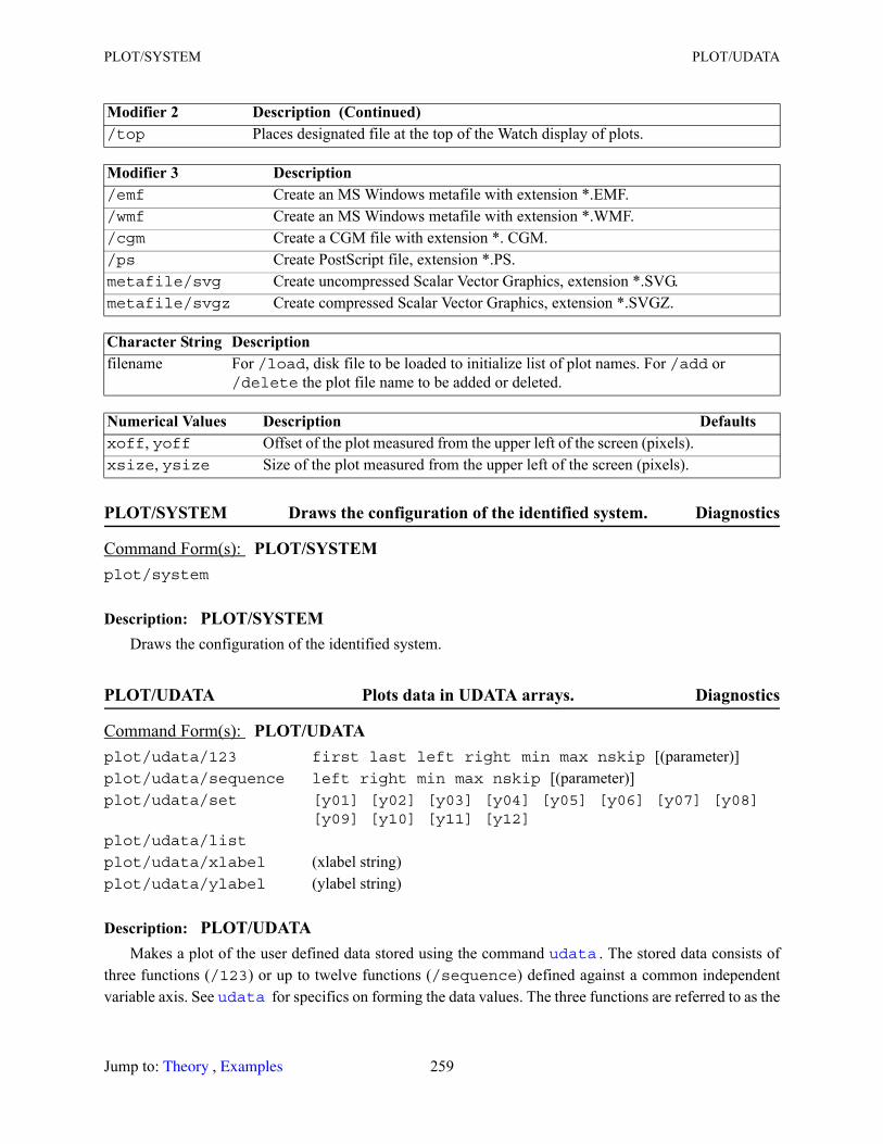
PLOT/SYSTEM PLOT/UDATA
PLOT/SYSTEM Draws the configuration of the identified system. Diagnostics
Description: PLOT/SYSTEMDraws the configuration of the identified system.
PLOT/UDATA Plots data in UDATA arrays. Diagnostics
Description: PLOT/UDATAMakes a plot of the user defined data stored using the command . The stored data consists of
three functions (/123) or up to twelve functions (/sequence) defined against a common independent variable axis. See for specifics on forming the data values. The three functions are referred to as the
/top Places designated file at the top of the Watch display of plots.
Modifier 3 Description /emf Create an MS Windows metafile with extension *.EMF./wmf Create an MS Windows metafile with extension *.WMF./cgm Create a CGM file with extension *. CGM./ps Create PostScript file, extension *.PS.metafile/svg Create uncompressed Scalar Vector Graphics, extension *.SVG.metafile/svgz Create compressed Scalar Vector Graphics, extension *.SVGZ.
Character String Description filename For /load, disk file to be loaded to initialize list of plot names. For /add or
/delete the plot file name to be added or deleted.
Numerical Values Description Defaultsxoff, yoff Offset of the plot measured from the upper left of the screen (pixels).xsize, ysize Size of the plot measured from the upper left of the screen (pixels).
Command Form(s): PLOT/SYSTEM plot/system
Command Form(s): PLOT/UDATA plot/udata/123 first last left right min max nskip [(parameter)]plot/udata/sequence left right min max nskip [(parameter)]plot/udata/set [y01] [y02] [y03] [y04] [y05] [y06] [y07] [y08]
[y09] [y10] [y11] [y12]
plot/udata/list
plot/udata/xlabel (xlabel string)plot/udata/ylabel (ylabel string)
Modifier 2 Description (Continued)
udata
udata
Jump to: , 259 Theory Examples
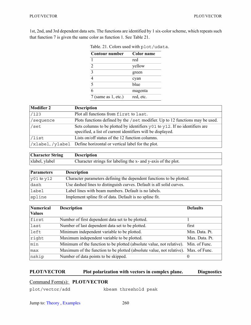
PLOT/VECTOR PLOT/VECTOR
1st, 2nd, and 3rd dependent data sets. The functions are identified by 1 six-color scheme, which repeats such that function 7 is given the same color as function 1. See Table 21.
PLOT/VECTOR Plot polarization with vectors in complex plane. Diagnostics
Table. 21. Colors used with plot/udata. Contour number Color name1 red2 yellow3 green4 cyan5 blue6 magenta7 (same as 1, etc.) red, etc.
Modifier 2 Description /123 Plot all functions from first to last./sequence Plots functions defined by the /set modifier. Up to 12 functions may be used./set Sets columns to be plotted by identifiers y01 to y12. If no identifiers are
specified, a list of current identifiers will be displayed./list Lists on/off status of the 12 function columns./xlabel, /ylabel Define horizontal or vertical label for the plot.
Character String Description xlabel, ylabel Character strings for labeling the x- and y-axis of the plot.
Parameters Description y01 to y12 Character parameters defining the dependent functions to be plotted.dash Use dashed lines to distinguish curves. Default is all solid curves.label Label lines with beam numbers. Default is no labels.spline Implement spline fit of data. Default is no spline fit.
Numerical Values
Description Defaults
first Number of first dependent data set to be plotted. 1last Number of last dependent data set to be plotted. firstleft Minimum independent variable to be plotted. Min. Data. Pt.right Maximum independent variable to be plotted. Max. Data. Pt.min Minimum of the function to be plotted (absolute value, not relative). Min. of Func.max Maximum of the function to be plotted (absolute value, not relative). Max. of Func.nskip Number of data points to be skipped. 0
Command Form(s): PLOT/VECTOR plot/vector/add kbeam threshold peak
Jump to: , 260 Theory Examples
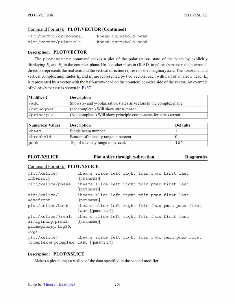
PLOT/VECTOR PLOT/XSLICE
Description: PLOT/VECTORThe plot/vector command makes a plot of the polarizations state of the beam by explicitly
displaying Ex and Ey in the complex plane. Unlike other plots in GLAD, in plot/vector the horizontal direction represents the real axis and the vertical direction represents the imaginary axis. The horizontal and vertical complex amplitudes Ex and Ey are represented by two vectors, each with half of an arrow head. Exis represented by a vector with the half-arrow-head on the counterclockwise side of the vector. An example of plot/vector is shown in .
PLOT/XSLICE Plot a slice through x-direction. Diagnostics
Description: PLOT/XSLICEMakes a plot along an x-slice of the data specified in the second modifier.
plot/vector/orthogonal kbeam threshold peak
plot/vector/principle kbeam threshold peak
Modifier 2 Description /add Shows x- and y-polarization states as vectors in the complex plane./orthogonal (not complete.) Will show stress tensor./principle (Not complete.) Will show principle components for stress tensor.
Numerical Values Description Defaultskbeam Single beam number. 1threshold Bottom of intensity range in percent. 0peak Top of intensity range in percent. 100
Command Form(s): PLOT/XSLICE plot/xslice/intensity
ibeams slice left right fmin fmax first last [(parameter)]
plot/xslice/phase ibeams slice left right pmin pmax first last [(parameter)]
plot/xslice/wavefront
ibeams slice left right pmin pmax first last [(parameter)]
plot/xslice/both ibeams slice left right fmin fmax pmin pmax first last [(parameter)]
plot/xslice/(real, aimaginary, preal, paimaginary, log10, log)
ibeams slice left right fmin fmax first last [(parameter)]
plot/xslice/(complex or pcomplex)
ibeams slice left right fmin fmax pmin pmax first last [(parameter)]
Command Form(s): PLOT/VECTOR (Continued)
Ex37
Jump to: , 261 Theory Examples
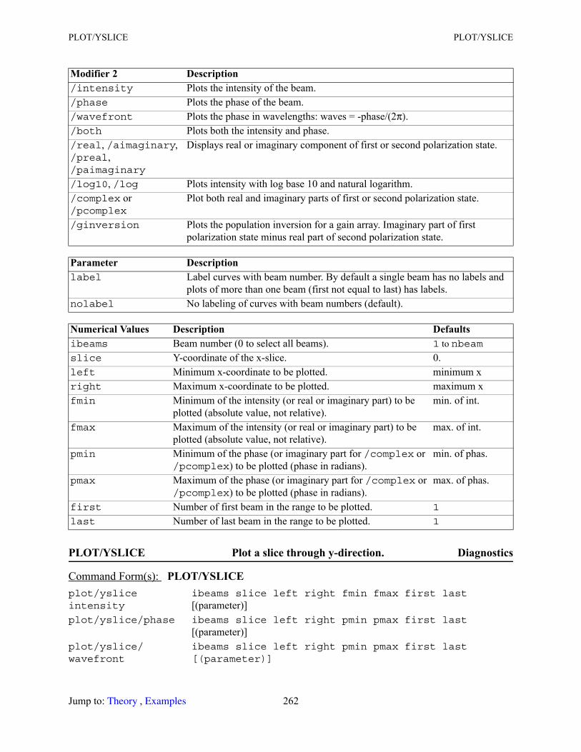
PLOT/YSLICE PLOT/YSLICE
PLOT/YSLICE Plot a slice through y-direction. Diagnostics
Modifier 2 Description /intensity Plots the intensity of the beam. /phase Plots the phase of the beam./wavefront Plots the phase in wavelengths: waves = -phase/(2π)./both Plots both the intensity and phase./real, /aimaginary, /preal, /paimaginary
Displays real or imaginary component of first or second polarization state.
/log10, /log Plots intensity with log base 10 and natural logarithm./complex or /pcomplex
Plot both real and imaginary parts of first or second polarization state.
/ginversion Plots the population inversion for a gain array. Imaginary part of first polarization state minus real part of second polarization state.
Parameter Description label Label curves with beam number. By default a single beam has no labels and
plots of more than one beam (first not equal to last) has labels.nolabel No labeling of curves with beam numbers (default).
Numerical Values Description Defaultsibeams Beam number (0 to select all beams). 1 to nbeamslice Y-coordinate of the x-slice. 0.left Minimum x-coordinate to be plotted. minimum xright Maximum x-coordinate to be plotted. maximum xfmin Minimum of the intensity (or real or imaginary part) to be
plotted (absolute value, not relative).min. of int.
fmax Maximum of the intensity (or real or imaginary part) to be plotted (absolute value, not relative).
max. of int.
pmin Minimum of the phase (or imaginary part for /complex or /pcomplex) to be plotted (phase in radians).
min. of phas.
pmax Maximum of the phase (or imaginary part for /complex or /pcomplex) to be plotted (phase in radians).
max. of phas.
first Number of first beam in the range to be plotted. 1
last Number of last beam in the range to be plotted. 1
Command Form(s): PLOT/YSLICE plot/ysliceintensity
ibeams slice left right fmin fmax first last [(parameter)]
plot/yslice/phase ibeams slice left right pmin pmax first last [(parameter)]
plot/yslice/wavefront
ibeams slice left right pmin pmax first last [(parameter)]
Jump to: , 262 Theory Examples
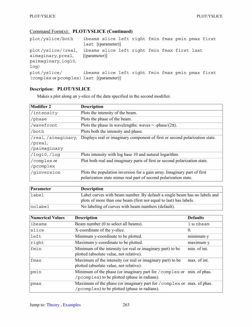
PLOT/YSLICE PLOT/YSLICE
Description: PLOT/YSLICEMakes a plot along an y-slice of the data specified in the second modifier.
plot/yslice/both ibeams slice left right fmin fmax pmin pmax first last [(parameter)]
plot/yslice/(real, aimaginary, preal, paimaginary, log10, log)
ibeams slice left right fmin fmax first last [(parameter)]
plot/yslice/(complex or pcomplex)
ibeams slice left right fmin fmax pmin pmax first last [(parameter)]
Modifier 2 Description /intensity Plots the intensity of the beam. /phase Plots the phase of the beam./wavefront Plots the phase in wavelengths: waves = -phase/(2π)./both Plots both the intensity and phase./real, /aimaginary, /preal, /paimaginary
Displays real or imaginary component of first or second polarization state.
/log10, /log Plots intensity with log base 10 and natural logarithm./complex or /pcomplex
Plot both real and imaginary parts of first or second polarization state.
/ginversion Plots the population inversion for a gain array. Imaginary part of first polarization state minus real part of second polarization state.
Parameter Description label Label curves with beam number. By default a single beam has no labels and
plots of more than one beam (first not equal to last) has labels.nolabel No labeling of curves with beam numbers (default).
Numerical Values Description Defaultsibeams Beam number (0 to select all beams). 1 to nbeamslice X-coordinate of the y-slice. 0.left Minimum y-coordinate to be plotted. minimum yright Maximum y-coordinate to be plotted. maximum yfmin Minimum of the intensity (or real or imaginary part) to be
plotted (absolute value, not relative).min. of int.
fmax Maximum of the intensity (or real or imaginary part) to be plotted (absolute value, not relative).
max. of int.
pmin Minimum of the phase (or imaginary part for /complex or /pcomplex) to be plotted (phase in radians).
min. of phas.
pmax Maximum of the phase (or imaginary part for /complex or /pcomplex) to be plotted (phase in radians).
max. of phas.
Command Form(s): PLOT/YSLICE (Continued)
Jump to: , 263 Theory Examples
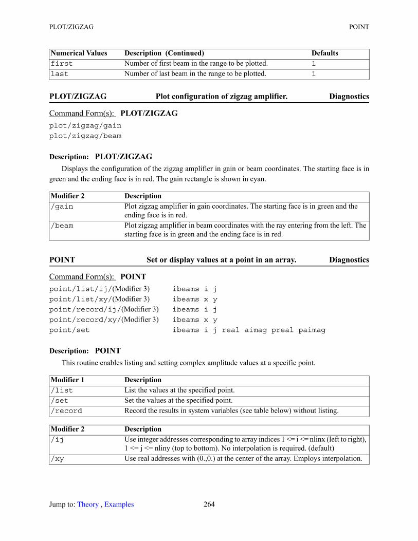
PLOT/ZIGZAG POINT
PLOT/ZIGZAG Plot configuration of zigzag amplifier. Diagnostics
Description: PLOT/ZIGZAGDisplays the configuration of the zigzag amplifier in gain or beam coordinates. The starting face is in
green and the ending face is in red. The gain rectangle is shown in cyan.
POINT Set or display values at a point in an array. Diagnostics
Description: POINTThis routine enables listing and setting complex amplitude values at a specific point.
first Number of first beam in the range to be plotted. 1
last Number of last beam in the range to be plotted. 1
Command Form(s): PLOT/ZIGZAG plot/zigzag/gain
plot/zigzag/beam
Modifier 2 Description /gain Plot zigzag amplifier in gain coordinates. The starting face is in green and the
ending face is in red./beam Plot zigzag amplifier in beam coordinates with the ray entering from the left. The
starting face is in green and the ending face is in red.
Command Form(s): POINT point/list/ij/(Modifier 3) ibeams i j
point/list/xy/(Modifier 3) ibeams x y
point/record/ij/(Modifier 3) ibeams i j
point/record/xy/(Modifier 3) ibeams x y
point/set ibeams i j real aimag preal paimag
Modifier 1 Description /list List the values at the specified point./set Set the values at the specified point./record Record the results in system variables (see table below) without listing.
Modifier 2 Description /ij Use integer addresses corresponding to array indices 1 <= i <= nlinx (left to right),
1 <= j <= nliny (top to bottom). No interpolation is required. (default)/xy Use real addresses with (0.,0.) at the center of the array. Employs interpolation.
Numerical Values Description (Continued) Defaults
Jump to: , 264 Theory Examples
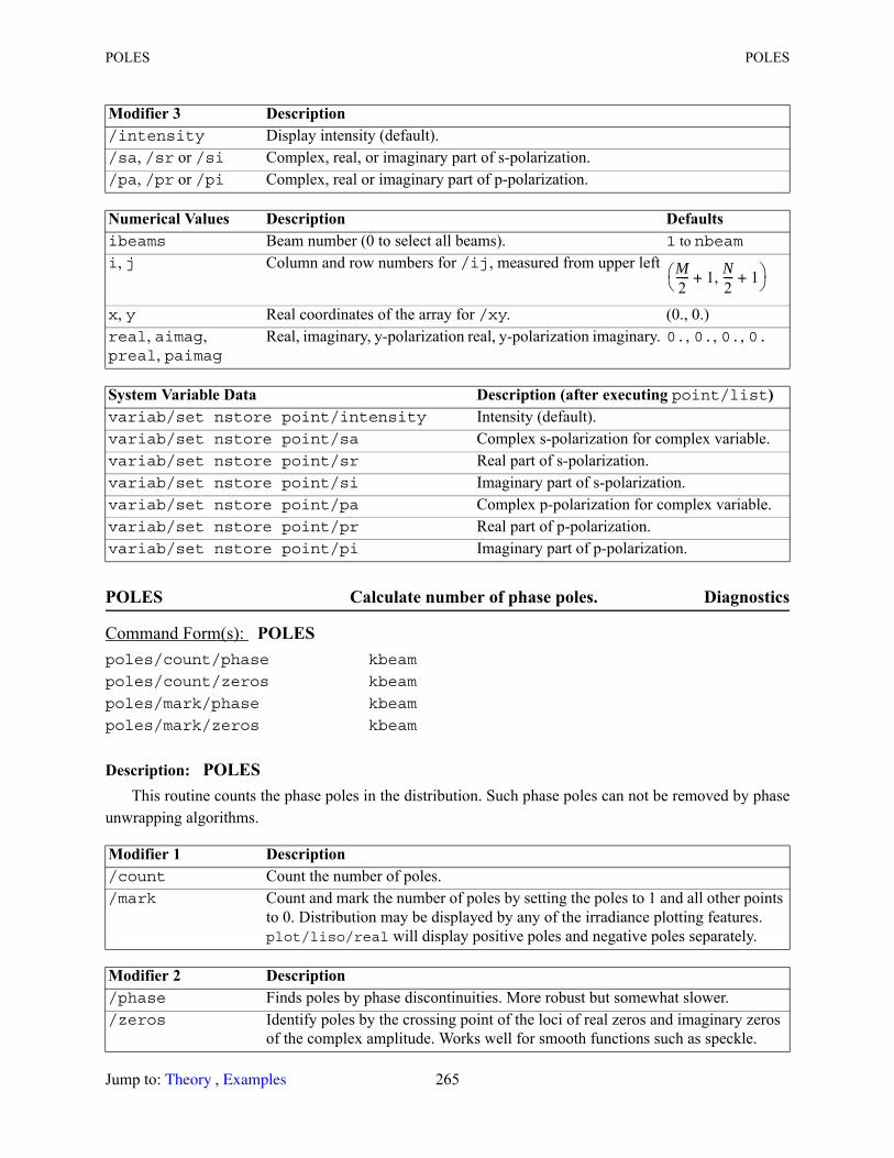
POLES POLES
POLES Calculate number of phase poles. Diagnostics
Description: POLESThis routine counts the phase poles in the distribution. Such phase poles can not be removed by phase
unwrapping algorithms.
Modifier 3 Description /intensity Display intensity (default)./sa, /sr or /si Complex, real, or imaginary part of s-polarization./pa, /pr or /pi Complex, real or imaginary part of p-polarization.
Numerical Values Description Defaultsibeams Beam number (0 to select all beams). 1 to nbeami, j Column and row numbers for /ij, measured from upper left
x, y Real coordinates of the array for /xy. (0., 0.)real, aimag, preal, paimag
Real, imaginary, y-polarization real, y-polarization imaginary. 0., 0., 0., 0.
System Variable Data Description (after executing point/list) variab/set nstore point/intensity Intensity (default).variab/set nstore point/sa Complex s-polarization for complex variable.variab/set nstore point/sr Real part of s-polarization.variab/set nstore point/si Imaginary part of s-polarization.variab/set nstore point/pa Complex p-polarization for complex variable.variab/set nstore point/pr Real part of p-polarization.variab/set nstore point/pi Imaginary part of p-polarization.
Command Form(s): POLES poles/count/phase kbeam
poles/count/zeros kbeam
poles/mark/phase kbeam
poles/mark/zeros kbeam
Modifier 1 Description /count Count the number of poles./mark Count and mark the number of poles by setting the poles to 1 and all other points
to 0. Distribution may be displayed by any of the irradiance plotting features. plot/liso/real will display positive poles and negative poles separately.
Modifier 2 Description /phase Finds poles by phase discontinuities. More robust but somewhat slower./zeros Identify poles by the crossing point of the loci of real zeros and imaginary zeros
of the complex amplitude. Works well for smooth functions such as speckle.
M2----- 1+
N2---- 1+,
Jump to: , 265 Theory Examples
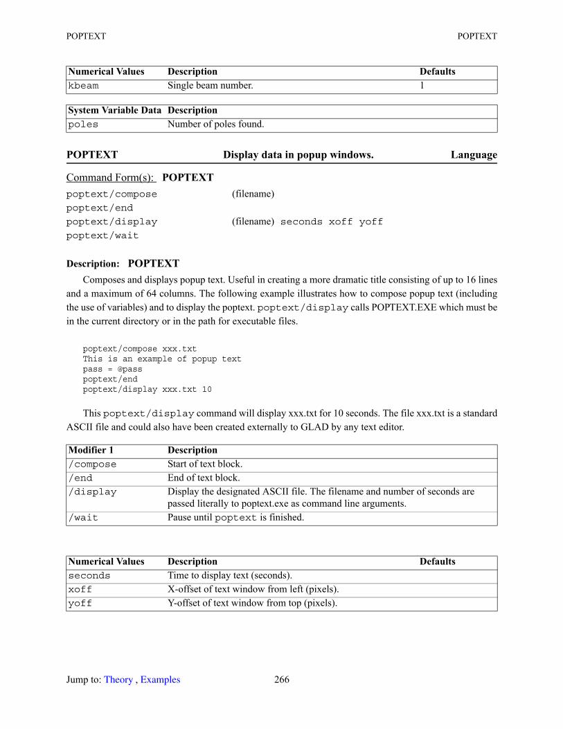
POPTEXT POPTEXT
POPTEXT Display data in popup windows. Language
Description: POPTEXTComposes and displays popup text. Useful in creating a more dramatic title consisting of up to 16 lines
and a maximum of 64 columns. The following example illustrates how to compose popup text (including the use of variables) and to display the poptext. poptext/display calls POPTEXT.EXE which must be in the current directory or in the path for executable files.
poptext/compose xxx.txtThis is an example of popup textpass = @passpoptext/endpoptext/display xxx.txt 10
This poptext/display command will display xxx.txt for 10 seconds. The file xxx.txt is a standard ASCII file and could also have been created externally to GLAD by any text editor.
Numerical Values Description Defaultskbeam Single beam number. 1
System Variable Data Description poles Number of poles found.
Command Form(s): POPTEXT poptext/compose (filename)poptext/end
poptext/display (filename) seconds xoff yoffpoptext/wait
Modifier 1 Description /compose Start of text block./end End of text block./display Display the designated ASCII file. The filename and number of seconds are
passed literally to poptext.exe as command line arguments./wait Pause until poptext is finished.
Numerical Values Description Defaultsseconds Time to display text (seconds).xoff X-offset of text window from left (pixels).yoff Y-offset of text window from top (pixels).
Jump to: , 266 Theory Examples

PRIVILEGES PROJECT
PRIVILEGES Display and set privileges. Code and key information. Language
Description: PRIVILEGESLists the active options, compilation date, and warranty period. For the demo, lists the remaining cycles
left. /set allows active options to be temporarily turned off to evaluate whether the options are necessary for a specific calculation. For /password, /update, /keyread, and /menu, alog file named keyread61.log is generated and contains information about keyread activity.
PROJECT Project sum of irradiance along y onto a single row. Language
Command Form(s): PRIVILEGES privileges/list
privileges/set
privileges/register
privileges/password (password)privileges/upgrade (password)privileges/keyread
Modifier 1 Description /list List the active options./set Set active options off. Useful for demo code to evaluate whether options are
required to solve given problems./register Generates registration information and creates a file of form XXX_YY.txt. Where
XXXX is the four digit key number and YY is the two digit version number. For example 3400_50.txt for key 3400 and version 5.0. Email this file as an attachment to AOR to complete your registration.
/password Set password of security key. Password is an eight-digit hexidecimal number provided by AOR to set the security key to permanent status for GLAD or GLAD privileges.
/update Upgrade version number of an old security key to current GLAD version. Password is a four-digit hexidecimal number provided by AOR.
/keyread Runs keyread.exe to with an interactive menu to display information about the security key and to set password and label. The menu displays options for setting the password and/or upgrading the version with appropriate passwords. If the permanent password for GLAD is already set and the key version is up-to-date with the software version, only the information menu is displayed. Keyread.exe maintains a data log called keyread61.log which can be used for diagnostic purposes.
Command Form(s): PROJECT project/irradiance/y kbeami kbeamoproject/irradiance/x kbeami kbeamoproject/amplitude/y kbeami kbeamoproject/amplitude/x kbeami kbeamo
Jump to: , 267 Theory Examples
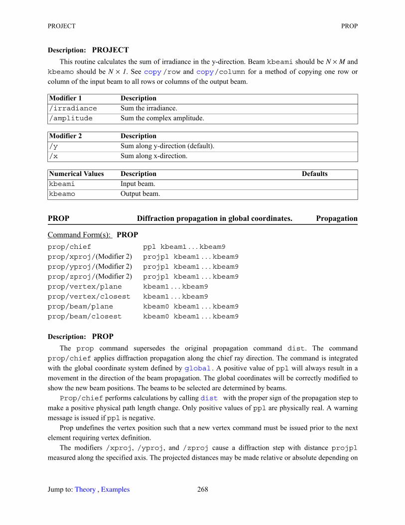
PROJECT PROP
Description: PROJECTThis routine calculates the sum of irradiance in the y-direction. Beam kbeami should be N × M and
kbeamo should be N × 1. See /row and /column for a method of copying one row or column of the input beam to all rows or columns of the output beam.
PROP Diffraction propagation in global coordinates. Propagation
Description: PROPThe prop command supersedes the original propagation command dist. The command
prop/chief applies diffraction propagation along the chief ray direction. The command is integrated with the global coordinate system defined by . A positive value of ppl will always result in a movement in the direction of the beam propagation. The global coordinates will be correctly modified to show the new beam positions. The beams to be selected are determined by beams.
Prop/chief performs calculations by calling with the proper sign of the propagation step to make a positive physical path length change. Only positive values of ppl are physically real. A warning message is issued if ppl is negative.
Prop undefines the vertex position such that a new vertex command must be issued prior to the next element requiring vertex definition.
The modifiers /xproj, /yproj, and /zproj cause a diffraction step with distance projplmeasured along the specified axis. The projected distances may be made relative or absolute depending on
Modifier 1 Description /irradiance Sum the irradiance./amplitude Sum the complex amplitude.
Modifier 2 Description /y Sum along y-direction (default)./x Sum along x-direction.
Numerical Values Description Defaultskbeami Input beam.kbeamo Output beam.
Command Form(s): PROP prop/chief ppl kbeam1 . . . kbeam9prop/xproj/(Modifier 2) projpl kbeam1 . . . kbeam9prop/yproj/(Modifier 2) projpl kbeam1 . . . kbeam9prop/zproj/(Modifier 2) projpl kbeam1 . . . kbeam9prop/vertex/plane kbeam1 . . . kbeam9prop/vertex/closest kbeam1 . . . kbeam9prop/beam/plane kbeam0 kbeam1 . . . kbeam9prop/beam/closest kbeam0 kbeam1 . . . kbeam9
copy copy
global
dist
Jump to: , 268 Theory Examples

PROP PROP
the selection of Modifier 2. The diffractive propagation is always along the chief ray. When a projection is requested, a length is calculated to achieve the specified projected length.
Warning: do not attempt to use the projection function with an axis that is close to perpendicular to the chief ray direction.
The command prop/vertex propagates along the current direction to the vertex position as specified by the previous /vertex command. Note that it is not necessary to issue a prop/vertex prior to one of the global commands: , l , and /global. These commands issue there own propagation operation to bring the beam to the vertex.
ExampleAssume we wish to propagate to a mirror at (0, 0, 100) centimeters, strike a flat mirror at 45 degrees and propagate a second distance of 100 centimeters. We wish to determine the global coordinates after these steps.
vertex/locate/abs 0 0 100 (Set mirror position.)vertex/rotate/set 45 (Rotate beam about x-axis.)
Modifier 1 Description /chief Propagate along the chief ray (default)./xproj Propagate a projected distance on the x-axis./yproj Propagate a projected distance on the y-axis./zproj Propagate a projected distance on the z-axis./vertex Propagates to the tangent plane of the vertex of next surface defined by the
commands vertex/locate and vertex/rotate./beam Propagate other beams to match k0beam either to i-j plane (/plane) or to point
of closest approach (/closest).
Modifier 2 Description /relative A relative projected step is made of magnitude, projpl (default)./absolute A projected step to position, projpl./plane Propagate to vertex plane for /vertex or beam plane for /beam./closest Propagate to point of closest approach to the center of the vertex coordinate
system for /vertex or beam coordinate system for /beam.
Numerical Values Description Defaultsppl Physical path length. 0.projpl Projected path length. 0.
kbeam1-kbeam9 List of beams to be propagated if “on” by the beams command. kbeam1 = 0, propagates all “on” beams.
kbeam0 Reference beam used for /beam.
System Variable Data Description xray, yray, zray Global position of beam along chief ray for kbeam.opl, ppl Optical path and physical path lengths for kbeam.zreff Current z-position of beam (cm).
mirror/global lensgroup grating
Jump to: , 269 Theory Examples
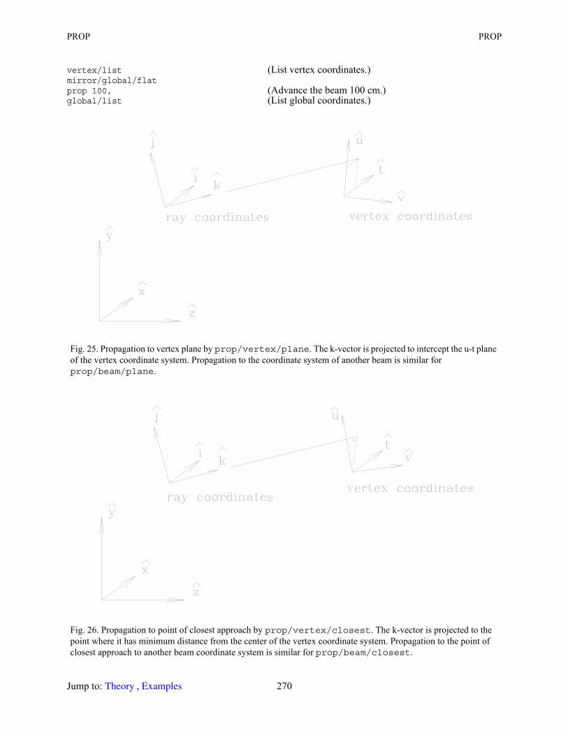
PROP PROP
vertex/list (List vertex coordinates.)mirror/global/flat prop 100, (Advance the beam 100 cm.)global/list (List global coordinates.)
Fig. 25. Propagation to vertex plane by prop/vertex/plane. The k-vector is projected to intercept the u-t plane of the vertex coordinate system. Propagation to the coordinate system of another beam is similar for prop/beam/plane.
Fig. 26. Propagation to point of closest approach by prop/vertex/closest. The k-vector is projected to the point where it has minimum distance from the center of the vertex coordinate system. Propagation to the point of closest approach to another beam coordinate system is similar for prop/beam/closest.
Jump to: , 270 Theory Examples
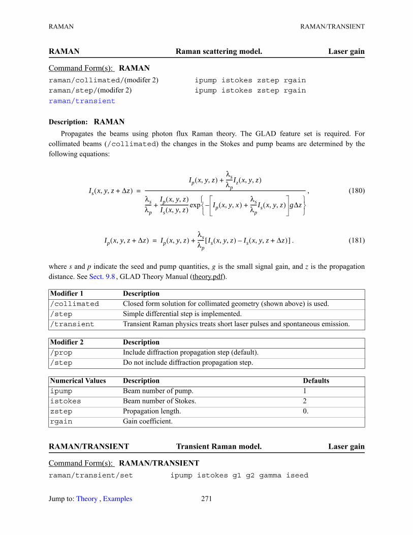
RAMAN RAMAN/TRANSIENT
RAMAN Raman scattering model. Laser gain
Description: RAMANPropagates the beams using photon flux Raman theory. The GLAD feature set is required. For
collimated beams (/collimated) the changes in the Stokes and pump beams are determined by the following equations:
, (180)
. (181)
where s and p indicate the seed and pump quantities, g is the small signal gain, and z is the propagation distance. See , GLAD Theory Manual (theory.pdf).
RAMAN/TRANSIENT Transient Raman model. Laser gain
Command Form(s): RAMAN raman/collimated/(modifer 2) ipump istokes zstep rgain
raman/step/(modifer 2) ipump istokes zstep rgain
Modifier 1 Description /collimated Closed form solution for collimated geometry (shown above) is used./step Simple differential step is implemented./transient Transient Raman physics treats short laser pulses and spontaneous emission.
Modifier 2 Description /prop Include diffraction propagation step (default)./step Do not include diffraction propagation step.
Numerical Values Description Defaultsipump Beam number of pump. 1istokes Beam number of Stokes. 2zstep Propagation length. 0.rgain Gain coefficient.
Command Form(s): RAMAN/TRANSIENT raman/transient/set ipump istokes g1 g2 gamma iseed
raman/transient
Is x y z Δz+, ,( )Ip x y z, ,( )
λsλp-----Iz x y z, ,( )+
λsλp-----
Ip x y z, ,( )Is x y z, ,( )----------------------- Ip x y x, ,( )
λsλp-----Is x y z, ,( )+ gΔz–
exp+
----------------------------------------------------------------------------------------------------------------------------------=
Ip x y z Δz+, ,( ) Ip x y z, ,( )λsλp----- Is x y z, ,( ) Is x y z Δz+, ,( )–[ ]+=
Sect. 9.8
Jump to: , 271 Theory Examples

RAMAN/TRANSIENT RAMAN/TRANSIENT
Description: RAMAN/TRANSIENTThis command implements transient Raman theory including the finite response time of the medium
and spontaneous emission due to quantum fluctuations. The GLAD feature set is required. It is assumed that a laser beam generates a Stokes beam by interaction with the medium through which it passes. A very high power beam passing through the air will experience the effects of rotational Raman. Unlike some applications such as a Raman amplifier, where the objective is to generate a high quality Stokes beam, in the case of atmospheric propagation the Raman process is a parasitic effect. The Stokes beam grows form spontaneous emission due to scattering of the laser beam from quantum fluctuations. Once, generated, the Stokes beam, if the laser is of sufficient power, will be amplified by stimulated Raman effects. The spontaneous emission grows linearly with distance but the stimulated Raman amplification is exponential (until the pump becomes depleted) and quickly becomes the dominant force. The spontaneous emission scatters in all directions but only the light which is in the forward direction gets significant amplification. This leads to some increase in the spatial coherence of the Stokes beam but for strong laser beams the generation of Stokes may occur at such short distances that even wide angles of the Stokes beam are amplified.
The medium responds in finite time. For very short pulses, the Raman gain will be much less than the steady-state Raman gain. The rotational Raman response time of the air at 0.351 microns is about 133 picoseconds. Laser pulses which are comparable or shorter than this response time will see proportionally smaller Raman gain. An arbitrary temporal waveform may be described by a series of time pulses of length tstep. The medium is represented by an array which must have two polarization steps. A number of medium arrays may be used along the laser beam path to represent the different states of the process. The medium array contains information on the degree of excitation of the medium and a set of random phasors which represent the response of the medium to quantum fluctuations. The medium array is initialized to the rest state with the command /reststate. The length of the medium array is represented by zstep. Diffraction propagation of the laser pump and stokes beams must be done separately. See e.
raman/transient/step kbeam zstep tstep
raman/transient/reststate kbeam
raman/transient/info
Modifier 1 Description /set Set the constants used in the calculation./step Take a kinetics step through a medium array. Diffraction must be done separately.
See ./reststate Establish the rest state of a medium array. The excitation of the medium will be
set to zero and a random field of medium excitation due to quantum fluctuations./info List constants used in the calculations.
Numerical Values Description Defaultsipump Beam number of pump. 1istokes Beam number of Stokes. 2
zstep Propagation length. 0.
Command Form(s): RAMAN/TRANSIENT (Continued)
Ex79
Ex79
Jump to: , 272 Theory Examples
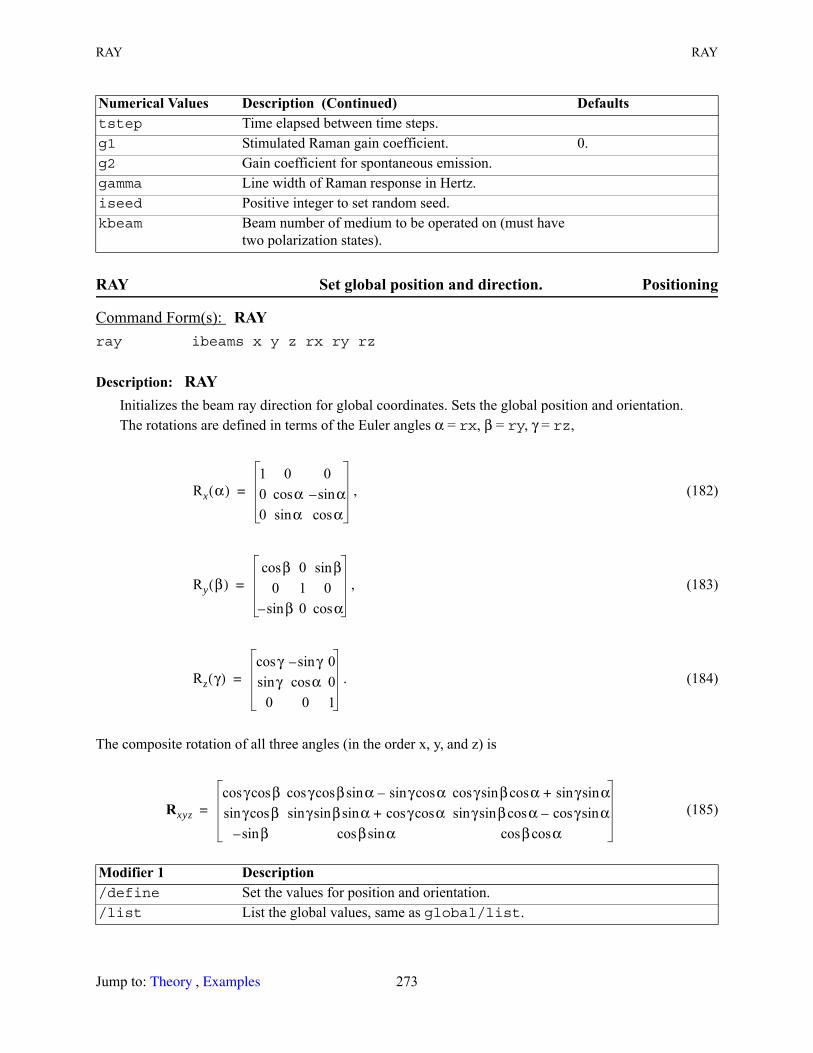
RAY RAY
RAY Set global position and direction. Positioning
Description: RAYInitializes the beam ray direction for global coordinates. Sets the global position and orientation.The rotations are defined in terms of the Euler angles α = rx, β = ry, γ = rz,
, (182)
, (183)
. (184)
The composite rotation of all three angles (in the order x, y, and z) is
(185)
tstep Time elapsed between time steps.g1 Stimulated Raman gain coefficient. 0.g2 Gain coefficient for spontaneous emission.gamma Line width of Raman response in Hertz.iseed Positive integer to set random seed.kbeam Beam number of medium to be operated on (must have
two polarization states).
Command Form(s): RAY ray ibeams x y z rx ry rz
Modifier 1 Description /define Set the values for position and orientation./list List the global values, same as global/list.
Numerical Values Description (Continued) Defaults
Rx α( )1 0 00 αcos αsin–
0 αsin αcos=
Ry β( )βcos 0 βsin
0 1 0βsin– 0 αcos
=
Rz γ( )γcos γsin– 0γsin αcos 0
0 0 1=
Rxyz
γ βcoscos γ βcoscos αsin γ αcossin– γ β αcossincos γ αsinsin+
γsin βcos γ β αsinsinsin γ αcoscos+ γ β αcossinsin γ αsincos–
βsin– β αsincos β αcoscos=
Jump to: , 273 Theory Examples
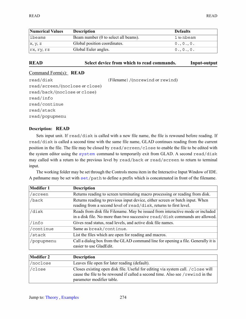
READ READ
READ Select device from which to read commands. Input-output
Description: READSets input unit. If read/disk is called with a new file name, the file is rewound before reading. If
read/disk is called a second time with the same file name, GLAD continues reading from the current position in the file. The file may be closed by read/screen/close to enable the file to be edited with the system editor using the command to temporarily exit from GLAD. A second read/diskmay called with a return to the previous level by read/back or read/screen to return to terminal input.
The working folder may be set through the Controls menu item in the Interactive Input Window of IDE. A pathname may be set with /path to define a prefix which is concatenated in front of the filename.
Numerical Values Description Defaultsibeams Beam number (0 to select all beams). 1 to nbeamx, y, z Global position coordinates. 0., 0., 0.rx, ry, rz Global Euler angles. 0., 0., 0.
Command Form(s): READ read/disk (Filename)/(norewind or rewind)read/screen/(noclose or close)read/back/(noclose or close)read/info
read/continue
read/stack
read/popupmenu
Modifier 1 Description /screen Returns reading to screen terminating macro processing or reading from disk./back Returns reading to previous input device, either screen or batch input. When
reading from a second level of read/disk, returns to first level./disk Reads from disk file Filename. May be issued from interactive mode or included
in a disk file. No more than two successive read/disk commands are allowed./info Gives read status, read levels, and active disk file names./continue Same as break/continue./stack List the files which are open for reading and macros./popupmenu Call a dialog box from the GLAD command line for opening a file. Generally it is
easier to use GladEdit.
Modifier 2 Description /noclose Leaves file open for later reading (default)./close Closes existing open disk file. Useful for editing via system call. /close will
cause the file to be rewound if called a second time. Also see /rewind in the parameter modifier table.
system
set
Jump to: , 274 Theory Examples
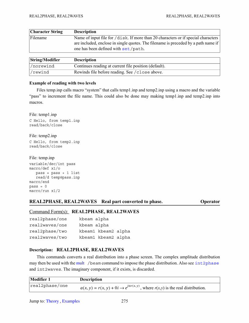
REAL2PHASE, REAL2WAVES REAL2PHASE, REAL2WAVES
Example of reading with two levelsFiles temp.inp calls macro “system” that calls temp1.inp and temp2.inp using a macro and the variable
“pass” to increment the file name. This could also be done may making temp1.inp and temp2.inp into macros.
File: temp1.inpC Hello, from temp1.inpread/back/close
File: temp2.inpC Hello, from temp2.inpread/back/close
File: temp.inpvariable/dec/int passmacro/def x1/o pass = pass + 1 list read/d [email protected]/endpass = 0macro/run x1/2
REAL2PHASE, REAL2WAVES Real part converted to phase. Operator
Description: REAL2PHASE, REAL2WAVESThis commands converts a real distribution into a phase screen. The complex amplitude distribution
may then be used with the /beam command to impose the phase distribution. Also see and int2waves. The imaginary component, if it exists, is discarded.
Character String Description Filename Name of input file for /disk. If more than 20 characters or if special characters
are included, enclose in single quotes. The filename is preceded by a path name if one has been defined with /path.
String/Modifier Description /norewind Continues reading at current file position (default)./rewind Rewinds file before reading. See /close above.
Command Form(s): REAL2PHASE, REAL2WAVES real2phase/one kbeam alpha
real2waves/one kbeam alpha
real2phase/two kbeam1 kbeam2 alpha
real2waves/two kbeam1 kbeam2 alpha
Modifier 1 Description real2phase/one , where r(x,y) is the real distribution.
set
mult int2phase
a x y,( ) r x y,( ) 0i+= ejαr x y,( )→
Jump to: , 275 Theory Examples

RESCALE RESCALE
RESCALE Rescale the beam distribution in the array. Operator
Description: RESCALEThis command rescales the beam array. If /field is selected, the array will be scaled to have field half
widths of xrad or yrad. If /beam is selected, the array is scaled so that the beam fills up the fractional field determined by radx and rady. If radx or rady is 0, the optimum units are selected based on equal near- and far-field sizes.
Rescale/beam is very useful to refit the array size to avoid aliasing when propagating through a strongly aberrating system where the beam would otherwise expand beyond the bounds of the array. This command calls to center the beam and to reset the beam parameters to the current values as well as resizing the units to establish the desired filling of the array.
real2waves/one , where r(x,y) is the real distribution.real2phase/two
, where r2(x,y) is the real distribution of kbeam2.real2waves/two
, where r2(x,y) is the real distribution of kbeam2.
Numerical Values Description Defaultskbeam Single beam number (/one). 1kbeam1, kbeam2 Beam numbers (/two). 1, 2alpha Coefficient for converting real values to phase in radians
(real2phase) or wavelengths (real2waves).0.
Command Form(s): RESCALE rescale/field kbeam xrad yrad [(parameter)] [(parameter)]rescale/beam kbeam xscale yscale [(parameter)] [(parameter)]rescale/units kbeam xunits yunits [(parameter)] [(parameter)]rescale/scale kbeam xscale yscale [(Parameter)] [(parameter)]rescale/shift kbeam xdec ydec [(parameter)] [(parameter)]rescale/copy kbeami kbeamo xrad yrad decx decy
rescale/distort/azimuthal/(rescale or constant)
kbeam magnification azdeg
rescale/distort/matrix/(rescale or constant)
kbeam m11 m12 m21 m22
Modifier 1 Description /field Use half width of field to specify rescale./beam Rescale to specified half width and use beam size as displayed by geodata to rescale
distribution to “optimum” size. Expand or contract optimum beam size by scale factors, xscale and yscale.
/units Use units to specify rescale./scale Use scale factor to specify rescale.
Modifier 1 Description (Continued)
a x y,( ) r x y,( ) 0i+= e j– 2παrx y,→
a1 x y,( ) ejαr2 x y,( )
→
a1 x y,( ) ej– 2παr2 x y,( )
→
fitgeo
Jump to: , 276 Theory Examples

RESCALE RESCALE
/shift Shift distribution using linear interpolation. See also, which uses an FFT based method.
/copy Scale and copy kbeami to kbeamo with half-widths xrad and yrad and center at xdec and ydec.
/distort Apply nonuniform magnification changes.
Modifier 2 Description /azimuthal Modifier for /distort to create a bulge in an arbitrary direction.
/matrix Modifier for /distort to create uniform, bilateral, and bulge magnification.
Modifier 3 Description /rescale Modifier for /distort to allow rescaling of units for uniform magnification and
bilateral magnification distortion (default)./constant Modifier for /distort to prohibit units change. All magnification and distortion is
incorporated by interpolation.
Parameter Description xonly Apply rescaling only in the x-direction. Default is both x and y for beam array attribute
and x-direction only for radial and annular array attributes.noxonly Specifies scaling in both directions for radial and annular array attributes. (default)polar Convert Cartesian form of complex number ( ) to amplitude and phase form
( ) before interpolation. Produces best results where the phase is smoothly varying (default).
rect Do not convert to polar form. Interpolate amplitude values in Cartesian form ( ). May produce better results for discontinuous phase.
Numerical Values Description Defaultskbeam Single beam number. 1xrad, yrad Field radii (/field).xrad, yrad Fraction that beam fills array (/beam). “optimum units”xunits, yunits New units. 1., 1.xscale, yscale Scale factor, expands or compresses array by specified
value.1., 1.
xdec, ydec Decenter array by factor for /shift. 0., 0.magnification Magnification for rescale/distort/azimuthal. 1.azimuthal Azimuthal orientation for
rescale/distort/azimuthal.0.
Modifier 1 Description (Continued) fitzern
x′y′
R θ–( ) m 00 1
R θ( ) xy
=
x′y′
m11 m12
m21 m22
xy
=
a bi+
aeiw
a bi+
Jump to: , 277 Theory Examples
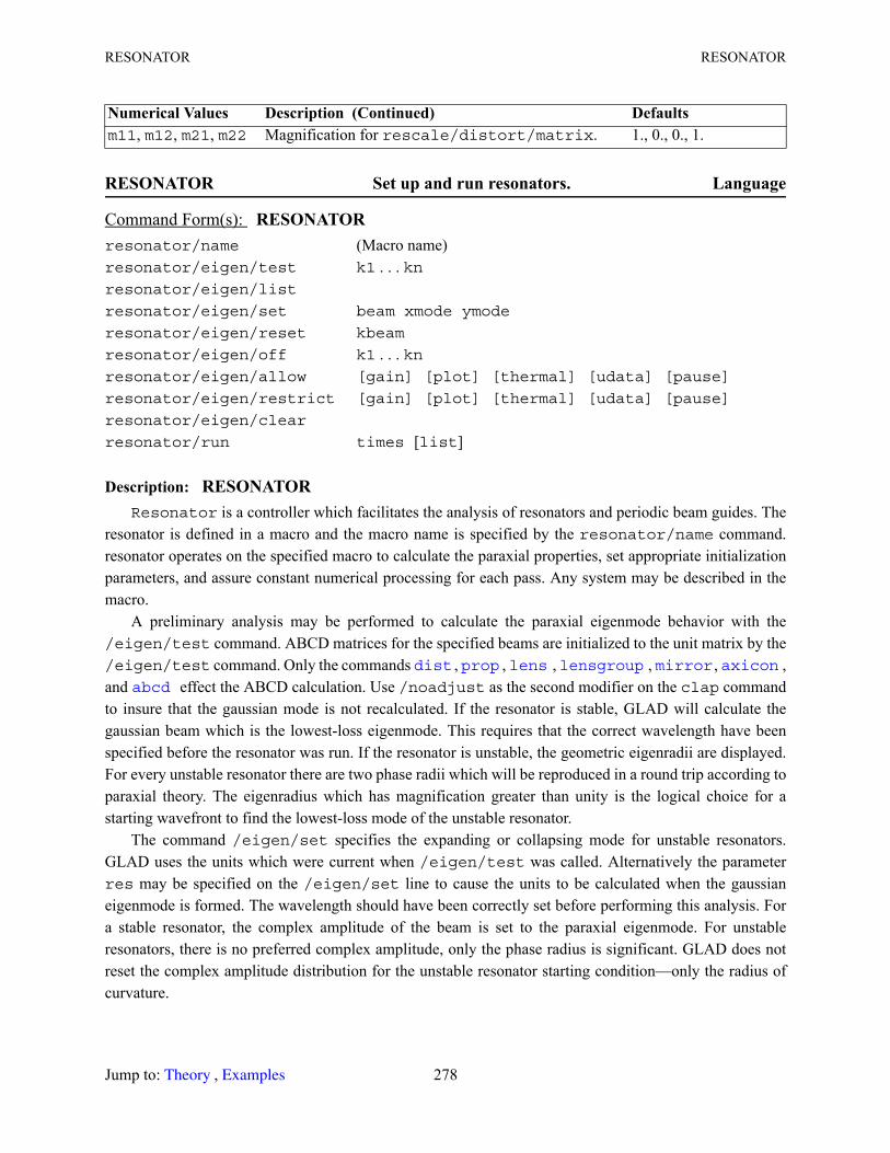
RESONATOR RESONATOR
RESONATOR Set up and run resonators. Language
Description: RESONATORResonator is a controller which facilitates the analysis of resonators and periodic beam guides. The
resonator is defined in a macro and the macro name is specified by the resonator/name command. resonator operates on the specified macro to calculate the paraxial properties, set appropriate initialization parameters, and assure constant numerical processing for each pass. Any system may be described in the macro.
A preliminary analysis may be performed to calculate the paraxial eigenmode behavior with the /eigen/test command. ABCD matrices for the specified beams are initialized to the unit matrix by the /eigen/test command. Only the commands , , , , , , and effect the ABCD calculation. Use /noadjust as the second modifier on the clap command to insure that the gaussian mode is not recalculated. If the resonator is stable, GLAD will calculate the gaussian beam which is the lowest-loss eigenmode. This requires that the correct wavelength have been specified before the resonator was run. If the resonator is unstable, the geometric eigenradii are displayed. For every unstable resonator there are two phase radii which will be reproduced in a round trip according to paraxial theory. The eigenradius which has magnification greater than unity is the logical choice for a starting wavefront to find the lowest-loss mode of the unstable resonator.
The command /eigen/set specifies the expanding or collapsing mode for unstable resonators. GLAD uses the units which were current when /eigen/test was called. Alternatively the parameter res may be specified on the /eigen/set line to cause the units to be calculated when the gaussian eigenmode is formed. The wavelength should have been correctly set before performing this analysis. For a stable resonator, the complex amplitude of the beam is set to the paraxial eigenmode. For unstable resonators, there is no preferred complex amplitude, only the phase radius is significant. GLAD does not reset the complex amplitude distribution for the unstable resonator starting condition—only the radius of curvature.
m11, m12, m21, m22 Magnification for rescale/distort/matrix. 1., 0., 0., 1.
Command Form(s): RESONATOR resonator/name (Macro name)resonator/eigen/test k1 . . . knresonator/eigen/list
resonator/eigen/set beam xmode ymode
resonator/eigen/reset kbeam
resonator/eigen/off k1 . . . knresonator/eigen/allow [gain] [plot] [thermal] [udata] [pause]
resonator/eigen/restrict [gain] [plot] [thermal] [udata] [pause]
resonator/eigen/clear
resonator/run times [list]
Numerical Values Description (Continued) Defaults
dist prop lens lensgroup mirror axicon abcd
Jump to: , 278 Theory Examples
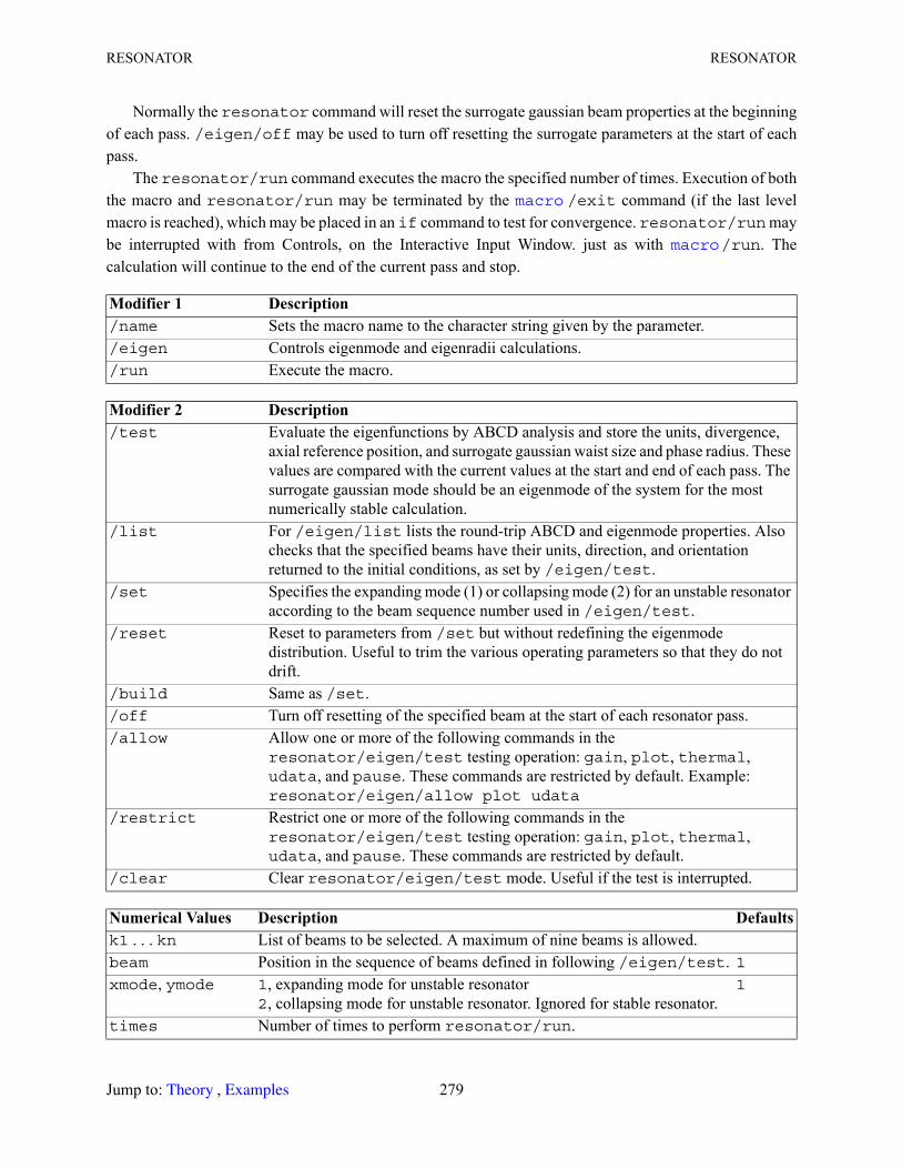
RESONATOR RESONATOR
Normally the resonator command will reset the surrogate gaussian beam properties at the beginning of each pass. /eigen/off may be used to turn off resetting the surrogate parameters at the start of each pass.
The resonator/run command executes the macro the specified number of times. Execution of both the macro and resonator/run may be terminated by the /exit command (if the last level macro is reached), which may be placed in an if command to test for convergence. resonator/run may be interrupted with from Controls, on the Interactive Input Window. just as with /run. The calculation will continue to the end of the current pass and stop.
Modifier 1 Description /name Sets the macro name to the character string given by the parameter./eigen Controls eigenmode and eigenradii calculations./run Execute the macro.
Modifier 2 Description /test Evaluate the eigenfunctions by ABCD analysis and store the units, divergence,
axial reference position, and surrogate gaussian waist size and phase radius. These values are compared with the current values at the start and end of each pass. The surrogate gaussian mode should be an eigenmode of the system for the most numerically stable calculation.
/list For /eigen/list lists the round-trip ABCD and eigenmode properties. Also checks that the specified beams have their units, direction, and orientation returned to the initial conditions, as set by /eigen/test.
/set Specifies the expanding mode (1) or collapsing mode (2) for an unstable resonator according to the beam sequence number used in /eigen/test.
/reset Reset to parameters from /set but without redefining the eigenmode distribution. Useful to trim the various operating parameters so that they do not drift.
/build Same as /set./off Turn off resetting of the specified beam at the start of each resonator pass./allow Allow one or more of the following commands in the
resonator/eigen/test testing operation: gain, plot, thermal, udata, and pause. These commands are restricted by default. Example:resonator/eigen/allow plot udata
/restrict Restrict one or more of the following commands in the resonator/eigen/test testing operation: gain, plot, thermal, udata, and pause. These commands are restricted by default.
/clear Clear resonator/eigen/test mode. Useful if the test is interrupted.
Numerical Values Description Defaultsk1 . . . kn List of beams to be selected. A maximum of nine beams is allowed.beam Position in the sequence of beams defined in following /eigen/test. 1xmode, ymode 1, expanding mode for unstable resonator
2, collapsing mode for unstable resonator. Ignored for stable resonator.1
times Number of times to perform resonator/run.
macro
macro
Jump to: , 279 Theory Examples

RMS RMS
Examplemacro/def reson/o prop 45 # propagate 45 cm. mirror/sph 0 -50 # mirror of 50 cm. radius clap/c/n 0 .14 # .14 cm. radius aperture prop 45 # propagate 45 cm. along beam mirror/sph 0 1.e15 # flat mirror energy/norm 1 1 # renormalize energymacro/endwavelength 0 1.064 # set wavelengthunits 0 .005resonator/name resonresonator/eigen/test 1 # test resonator macroresonator/eigen/set 1 # set beam 2 to eigen modeclear 1 1 # start with a plane wave in beam 2energy/norm 1 1 # normalize energyreson/run 100 # run resonator 100 times
See Example for a more detailed example of the use of the resonator commands.
RMS Calculates wavefront rms. Diagnostics
Description: RMSCalculates wavefront or irradiance RMS.
wavefront (186)
irradiance (187)
Systen Variable Data Description resonator/(mod)mod = mag, ymag, radius, yradius, ewaist, yewaist, ezwaist, yezwaist, stable, ystable, opl, oply, ppl,roundtriptime, gouy, status
Round-trip properties of macro operated with resonator. X- and y-values of magnification, phase radius, eigenwaist, eigenwaist location, stability criterion for x and y, optical path length in x and y direction for roundtrip, physical path length in round trip, round trip time, and Gouy shift. status takes the integer values: 0, not in resonator mode; 1, normal resonator mode; 3, first pass of resonator test; 4, second pass of resonator test;
Command Form(s): RMS rms/wavefront ibeams threshold
rms/irradiance ibeams threshold
Ex13
RMSI x y,( )W x y,( )2 xd yd
I x y,( ) xd yd------------------------------------------------------
I x y,( )W x y,( ) xd ydI x y,( ) xd yd
----------------------------------------------------
–
2
=
RMSI x y,( )2 xd yd
xd yd-----------------------------------
I x y,( ) xd ydxd yd
---------------------------------
–
2
=
Jump to: , 280 Theory Examples
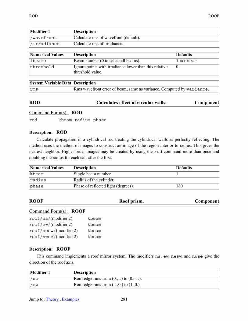
ROD ROOF
ROD Calculates effect of circular walls. Component
Description: RODCalculate propagation in a cylindrical rod treating the cylindrical walls as perfectly reflecting. The
method uses the method of images to construct an image of the region interior to radius. This gives the nearest neighbor. Higher order images may be created by using the rod command more than once and doubling the radius for each call after the first.
ROOF Roof prism. Component
Description: ROOFThis command implements a roof mirror system. The modifiers ns, ew, nesw, and nwse give the
direction of the roof axis.
Modifier 1 Description /wavefront Calculate rms of wavefront (default)./irradiance Calculate rms of irradiance.
Numerical Values Description Defaultsibeams Beam number (0 to select all beams). 1 to nbeamthreshold Ignore points with irradiance lower than this relative
threshold value.0.
System Variable Data Description rms Rms wavefront error of beam, same as variance. Computed by variance.
Command Form(s): ROD rod kbeam radius phase
Numerical Values Description Defaultskbeam Single beam number. 1radius Radius of the cylinder.phase Phase of reflected light (degrees). 180
Command Form(s): ROOF roof/ns/(modifier 2) kbeam
roof/ew/(modifier 2) kbeam
roof/nesw/(modifier 2) kbeam
roof/nwse/(modifier 2) kbeam
Modifier 1 Description /ns Roof edge runs from (0.,1.) to (0.,-1.)./ew Roof edge runs from (-1,0.) to (1.,0.).
Jump to: , 281 Theory Examples

ROTATE SAMPLING
ROTATE Rotate distribution in the array. Operator
Description: ROTATEThis command rotates the distribution in pixel by pixel fashion by the angle theta around the axis of
propagation. Positive rotation is counterclockwise. The rotation is about the coordinate (xdec, ydec). Rotation of large arrays is slow, because of the need to swap memory blocks.
SAMPLING Check for adequate sampling and aliasing. Diagnostics
/nesw Roof edge runs from (1.,1.) to (-1.,-1)./nwse Roof edge runs from (-1.,1.) to (1.,-1.).
Modifier 2 Description /global Acts as global mirror and must be used with other mirror/global and
lensgroup (default)./nonglobal Acts as paraxial mirror and should be combined with mirror and lens
commands—not with global commands.
Numerical Values Description Defaultskbeam Single beam number. 1.
Command Form(s): ROTATE rotate kbeam theta xdec ydec [(polar or rect)]
Parameter Description polar Convert Cartesian form of complex number ( ) to amplitude and phase form
( ) before interpolation. Produces best results where the phase is smoothly varying (default).
rect Do not convert to polar form. Interpolate amplitude values in Cartesian form ( ). May produce better results for discontinuous phase.
Numerical Values Description Defaultskbeam Single beam number. 1theta Rotation angle in degrees (counterclockwise). 0
(xdec, ydec) Pivot point for rotation. (0., 0.)
Command Form(s): SAMPLING sampling/list kbeam
sampling/control/list kbeam
sampling/control/on kbeam xlimit ylimit
sampling/control/off kbeam
Modifier 1 Description (Continued)
a bi+
aeiw
a bi+
Jump to: , 282 Theory Examples
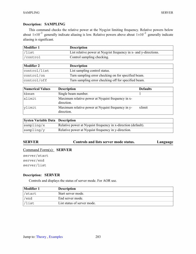
SAMPLING SERVER
Description: SAMPLINGThis command checks the relative power at the Nyqyist limiting frequency. Relative powers below
about generally indixate aliasing is low. Relative powers above about generally indicate aliasing is significant.
SERVER Controls and lists server mode status. Language
Description: SERVERControls and displays the status of server mode. For AOR use.
Modifier 1 Description /list List relative power at Nyqyist frequency in x- and y-directions./control Control sampling checking.
Modifier 2 Description control/list List sampling control status.control/on Turn sampling error checking on for specified beam.control/off Turn sampling error checking off for specified beam.
Numerical Values Description Defaultskbeam Single beam number. 1xlimit Maximum relative power at Nyquist frequency in x-
direction.ylimit Maximum relative power at Nyquist frequency in y-
direction.xlimit
Systen Variable Data Description sampling/x Relative power at Nyquist frequency in x-direction (default).sampling/y Relative power at Nyquist frequency in y-direction.
Command Form(s): SERVER server/start
server/end
server/list
Modifier 1 Description /start Start server mode./end End server mode./list List status of server mode.
1 3–×10 1 2–×10
Jump to: , 283 Theory Examples
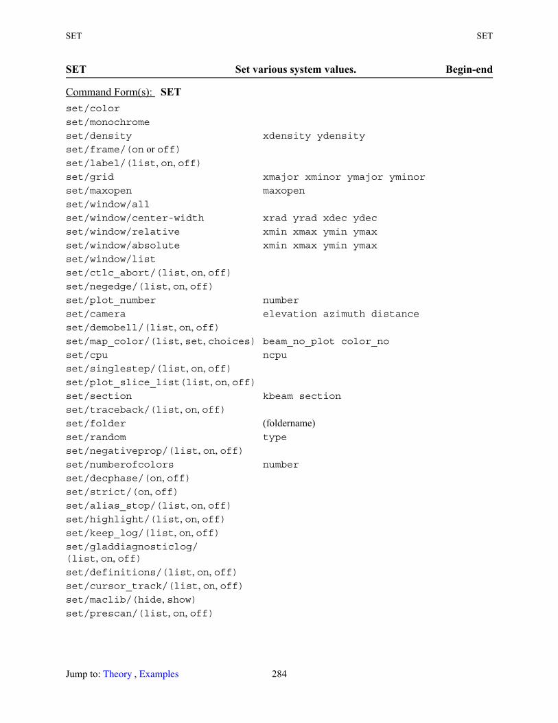
SET SET
SET Set various system values. Begin-end
Command Form(s): SET set/color
set/monochrome
set/density xdensity ydensity
set/frame/(on or off)set/label/(list, on, off)set/grid xmajor xminor ymajor yminor
set/maxopen maxopen
set/window/all
set/window/center-width xrad yrad xdec ydec
set/window/relative xmin xmax ymin ymax
set/window/absolute xmin xmax ymin ymax
set/window/list
set/ctlc_abort/(list, on, off)set/negedge/(list, on, off)set/plot_number number
set/camera elevation azimuth distance
set/demobell/(list, on, off)set/map_color/(list, set, choices) beam_no_plot color_no
set/cpu ncpu
set/singlestep/(list, on, off)set/plot_slice_list(list, on, off)set/section kbeam section
set/traceback/(list, on, off)set/folder (foldername)set/random type
set/negativeprop/(list, on, off)set/numberofcolors number
set/decphase/(on, off)set/strict/(on, off)set/alias_stop/(list, on, off)set/highlight/(list, on, off)set/keep_log/(list, on, off)set/gladdiagnosticlog/(list, on, off)set/definitions/(list, on, off)set/cursor_track/(list, on, off)set/maclib/(hide, show)set/prescan/(list, on, off)
Jump to: , 284 Theory Examples
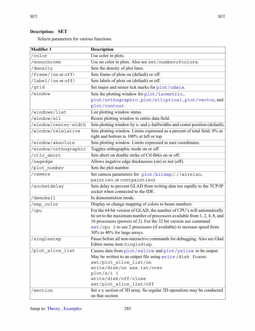
SET SET
Description: SETSelects parameters for various functions.
Modifier 1 Description /color Use color in plots./monochrome Use no color in plots. Also see set/numberofcolors./density Sets the density of plot lines./frame/(on or off) Sets frame of plots on (default) or off./label/(on or off) Sets labels of plots on (default) or off./grid Set major and minor tick marks for ./window Sets the plotting window for ,
, , , and .
/windows/list List plotting window status./window/all Resets plotting window to entire data field./window/center-width Sets plotting window by x- and y-halfwidths and center position (default)./window/relelative Sets plotting window. Limits expressed as a percent of total field. 0% at
right and bottom to 100% at left or top./window/absolute Sets plotting window. Limits expressed in user coordinates./window/orthographic Toggles orthographic mode on or off./ctlc_abort Sets abort on double strike of Ctl-Brks on or off./negedge Allows negative edge thicknesses (on) or not (off)./plot_number Sets the plot number./camera Set camera parameters for /./(wireiso,
paintiso, or contpaintiso)./socketdelay Sets delay to prevent GLAD from writing data too rapidly to the TCP/IP
socket when connected to the IDE./demobell In demonstration mode./map_color Display or change mapping of colors to beam numbers./cpu For the 64 bit version of GLAD, the number of CPU’s will automatically
be set to the maximum number of processors available from 1, 2, 4, 8, and 16 processors (powers of 2). For the 32 bit version use command
/cpu 2 to use 2 processors (if available) to increase speed from 30% to 40% for large arrays.
/singlestep Pause before all non-interactive commands for debugging. Also see Glad Editor menu item SingleStep.
/plot_slice_list Causes data from and to be output. May be written to an output file using /disk fname.set/plot_slice_list/onwrite/disk/on xxx.txt/overplot/x/i 1write/disk/off/closeset/plot_slice_list/off
/section Set x-y section of 3D array. So regular 2D operations may be conducted on that section.
plot/udata plot/isometric
plot/orthographic plot/elliptical plot/vector plot/contour
plot/bitmap
set
plot/xslice plot/yslice write
Jump to: , 285 Theory Examples
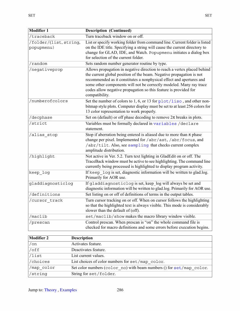
SET SET
/traceback Turn traceback window on or off./folder/(list, string, popupmenu)
List or specify working folder from command line. Current folder is listed on the IDE title. Specifying a string will cause the current directory to change for GLAD, IDE, and Watch. Popupmenu initiates a dialog box for selection of the current folder.
/random Sets random number generator routine by type./negativeprop Allows propagation in negative direction to reach a vertex placed behind
the current global position of the beam. Negative propagation is not recommended as it constitutes a nonphysical effect and apertures and some other components will not be correctly modeled. Many ray trace codes allow negative propagation so this feature is provided for compatibility.
/numberofcolors Set the number of colors to 1, 6, or 13 for , and other non-bitmap style plots. Computer display must be set to at least 256 colors for 13 color representation to work properly.
/decphase Set on (default) or off phase decoding to remove 2π breaks in plots./strict Variables must be formally declared in /declare
statement./alias_stop Stop if aberration being entered is aliased due to more than π phase
change per pixel. Implemented for /abr/ast, /abr/focus, and /abr/tilt. Also, see that checks current complex amplitude distribution.
/highlight Not active in Ver. 5.2. Turn text lighting in GladEdit on or off. The TraceBack window must be active to see highlighting. The command line currently being processed is highlighted to display program activity.
keep_log If keep_log is set, diagnostic information will be written to glad.log. Primarily for AOR use.
gladdiagnosticlog If gladdiagnosticlog is set, keep_log will always be set and diagnostic information will be written to glad.log. Primarily for AOR use.
/definitions Set listing on or off of definitions of terms in the output tables./cursor_track Turn cursor tracking on or off. When on cursor follows the highlighting
so that the highlighted text is always visible. This mode is considerably slower than the default of (off).
/maclib set/maclib/show makes the macro library window visible./prescan Control prescan. When prescan is “on” the whole command file is
checked for macro definitions and some errors before execution begins.
Modifier 2 Description /on Activates feature./off Deactivates feature. /list List current values./choices List choices of color numbers for set/map_color./map_color Set color numbers (color_no) with beam numbers () for /map_color./string String for set/folder.
Modifier 1 Description (Continued)
plot/liso
variables
sampling
set
Jump to: , 286 Theory Examples
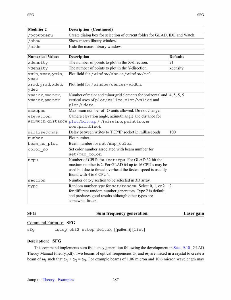
SFG SFG
SFG Sum frequency generation. Laser gain
Description: SFGThis command implements sum frequency generation following the development in , GLAD
Theory Manual (theory.pdf). Two beams of optical frequencies ω1 and ω2 are mixed in a crystal to create a beam of ω3 such that ω1 + ω2 = ω3. For example beams of 1.06 micron and 10.6 micron wavelength may
/popupmenu Create dialog box for selection of current folder for GLAD, IDE and Watch./show Show macro library window./hide Hide the macro library window.
Numerical Values Description Defaultsxdensity The number of points to plot in the X-direction. 21ydensity The number of points to plot in the Y-direction. xdensityxmin, xmax, ymin, ymax
Plot field for /window/abs or /window/rel.
xrad, yrad, xdec, ydec
Plot field for /window/center-width.
xmajor, xminor, ymajor, yminor
Number of major and minor grid elements for horizontal and vertical axes of plot/xslice, plot/yslice and plot/udata.
4, 5, 5, 5
maxopen Maximum number of IO units allowed. Do not change.elevation, azimuth, distance
Camera elevation angle, azimuth angle and distance for /./(wireiso, paintiso, or
contpaintiso).milliseconds Delay between writes to TCP/IP socket in milliseconds. 100number Plot number.beam_no_plot Beam number for set/map_color.color_no Set color number associated with beam number for
set/map_color.ncpu Number of CPU's for /set/cpu. For GLAD 32 bit the
maxium number is 2. For GLAD 64 up to 16 CPU’s may be used but due to thread overhead the fastest speed is usually found with 4 to 6 CPU’s.
section Number of x-y section to be selected in 3D array.type Random number type for set/random. Select 0, 1, or 2
for different random number generators. Type 2 is default and preduces good results although other types are somewhat faster.
2
Command Form(s): SFG sfg zstep chi2 nstep deltak [(pattern)] [list]
Modifier 2 Description (Continued)
plot/bitmap
Sect. 9.10
Jump to: , 287 Theory Examples
SFOCUS SFOCUS
be mixed to create a beam of 0.963636 micron wavelength, as illustrated in Ex107. The beams to be used are defined by pack/set.
SFOCUS Self-focusing. Laser gain
Description: SFOCUSThis command does self focusing. The GLAD feature set is required. It adds an intensity-dependent
phase of the form/one
(188)
/two
(189)
where for /one, I is the intensity of Beam 1 and a is the complex amplitude. For /two, a1 is the complex amplitude of Beam 1, and I2 is the intensity of Beam 2. Also see and int2waves.
String Description pattern The pattern consists of three letters, the letters being either “o” or “e”, where “o” or
“e” indicates o- or e-ray polarization to be used for the pump, signal, or idler beams respectively. For example “oeo” indicates ordinary ray (x-polarization) for pump, extraordinary ray (y-polarization for signal), and ordinary ray (x-polarization) for idler beams.
Parameter Description list List overall parameters and center point properties.
Numerical Values Description Defaultszstep Step length. 0.chi2 , second order nonlinear coefficient. See , GLAD Theory
Manual (theory.pdf).
0.
nstep No longer used. Always set to 1. 50
deltak Δk to treat any mismatch of the frequency of Beam 3 in the case where Beam 3 is injected with finite magnitude. Normally this term is zero. The detuning effect of wavefront slope errors (due to aberration) on Δk are handled by using multiple diffraction steps as illustrated in Ex107.
0.
Command Form(s): SFOCUS sfocus/one kbeam alpha z
sfocus/two kbeam1 kbeam2 alpha z
χ 2( ) beerSect. 9.8Sect. 9.10
a aej2π
λ------alphazI
→
a1 a1ej2π
λ------alphazI2
→
int2phase
Jump to: , 288 Theory Examples
SFOCUS SFOCUS
Example of self focusingConsider the case of propagation of a beam through an optical path with axial flow of air. The thermal
blooming theory assumes transverse flow so it may not be applied to this problem directly.The index of refraction varies with temperature rise ΔT
(190)
where P is in millibars and T is in degrees Kelvin. The equation may also be written
(191)
where is the relative atmospheric pressure and is the relative temperature with respect to standard temperature and pressure (STP) and is the index of refraction at 10.6 μ and STP, = . The temperature rise is a function of the time the air has been irradiated, which in the case of axial flow of the air is related to the position z along the axis
(192)
where is the intensity at point [J/sec/m2]
z is the position [m]α is the attenuation constant [m-1]
ρ is the density [kg/m3]C is the absolute specific heat [J/kg/deg]v is the velocity of the air in the axial flow [m/sec]The mean temperature rise is
, (193)
Modifier 1 Description /one Self-focusing due to intensity of single beam./two Self-focusing due to intensify of a second beam. Allows, time integration.
Numerical Values Description Defaultskbeam Single beam number. 1kbeam1, kbeam2 Phase of Beam 1 due to intensity of Beam 2. 1, 2alpha Self-focusing coefficient cm2/watt. 0.
z Propagation distance (cm). 0.
Δn 79 6–×10–PT2-----ΔT=
Δn n0 1–( )–PrelTrel---------ΔT
T-------=
Prel Treln0 n0 1.00027 6–×10
ΔT αzvρC----------I x y,( )=
I x y,( ) x y,( )
ΔT z( ) αzmax2ρCv--------------=
Jump to: , 289 Theory Examples

SHIFT SHIFT
assuming the irradiance is not significantly depleted by the atmospheric absorption. The phase change as a function of the total path is
(194)
The coefficient for self-focusing with the sfocus command is
alpha = (195)
n0 index of refraction at STPrelative pressurerelative temperature with respect to 288°K
ΔT temperature rise due to absorptionT temperature of the atmospherezmax Propagation length
SHIFT Shift distribution in the array. Operator
Description: SHIFTThis command shifts the distribution laterally by amount deltar in the direction defined by the
clockwise polar angle azdeg. The shift is done by Fourier transform methods so the movement is continuous and wraps around. Large shifts will cause the distribution to reappear on the other side of the array. See also /shift which shifts by linear interpolation and does not wrap.
Table. 22. Physical and optical constants for air.
incremental index of refraction (10.6 μ)density [kg/m3] 1.226conductivity [w/mK] 0.02525specific heat [J/kgK] 1017
Command Form(s): SHIFT shift/polar kbeam deltar azdeg
shift/cartesian kbeam xdec ydec
Modifier 1 Description /polar Polar coordinates used for shift (default)./cartesian Cartesian coordinates used for shift.
Numerical Values Description Defaultskbeam Single beam number. 1
φ 2πλ
------ n0 1–( )–PrelTrel---------ΔT
T-------zmax=
n0 1–( )–PrelTrel---------ΔT
T------- n0 1–( )–
PrelTrel--------- 1
T---
αzmax2ρCv-------------- m/w n0 1–( )–
PrelTrel--------- 1
T---
αzmax2ρCv--------------100 cm/w= =
PrelTrel
2.74 4–×10
rescale
Jump to: , 290 Theory Examples
SINC SLAB
SINC Define sinc function. Begin-end
Description: SINCDefines a sinc function.
amplitude, (196)
SLAB Various commands for waveguide slabs. Component
deltar Magnitude of shift for /polar. 0.
azdeg Polar angle defining direction of shift. (clockwise from vertical) for /polar.
0.
xdec, ydec Cartesian coordinates of shift for /cartesian. 0., 0.
Command Form(s): SINC sinc kbeam peak widthx widthy xdec ydec
Numerical Values Description Defaultskbeam Single beam number (/one). 1peak Peak intensity value.widthx Width of first zero, x-direction.widthy Width of first zero, y-direction.xdec Decenter in x-direction. 0ydec Decenter in y-direction. 0
Command Form(s): SLAB slab/hoe/(cir or sqr) clx xdec ydec zdec
slab/hoe/(ell or rec) clx cly xdec ydec zdec
slab/hoe/ecoef kte
slab/hoe/mcoef ktm zktm
slab/out/(nodist or dist) gbeam rbeam
slab/in/(nodist or dist) rbeam1 rbeam2 gbeam
slab/list
slab/pump/gaussian/(modifier 3) kout peak w0 lambda absorption m2 decenter reflectance
slab/pump/coherent kin kout absorption reflectance
slab/waveguide kstart kindex kresult
slab/eigenmode/index/(te or tm) kbeam halfheight film substrate cladding order
Numerical Values Description (Continued) Defaults
sinc x y,( )
πxwidthx--------------------- sin
πxwidthx---------------------
-----------------------------------
πywidthy--------------------- sin
πywidthy---------------------
-----------------------------------=
Jump to: , 291 Theory Examples
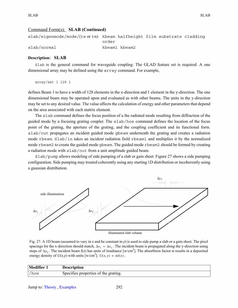
SLAB SLAB
Description: SLABSlab is the general command for waveguide coupling. The GLAD feature set is required. A one
dimensional array may be defined using the array command. For example,
array/set 1 128 1
defines Beam 1 to have a width of 128 elements in the x-direction and 1 element in the y-direction. The one dimensional beam may be operated upon and evaluated as with other beams. The units in the y-direction may be set to any desired value. The value affects the calculation of energy and other parameters that depend on the area associated with each matrix element.
The slab command defines the focus position of a the radiated mode resulting from diffraction of the guided mode by a focusing grating coupler. The slab/hoe command defines the location of the focus point of the grating, the aperture of the grating, and the coupling coefficient and its functional form. slab/out propagates an incident guided mode gbeam underneath the grating and creates a radiation mode rbeam. Slab/in takes an incident radiation field rbeam1 and multiplies it by the normalized mode rbeam2 to create the guided mode gbeam. The guided mode rbeam2 should be formed by creating a radiation mode with slab/out from a unit amplitude guided beam.
Slab/pump allows modeling of side pumping of a slab or gain sheet. Figure 27 shows a side pumping configuration. Side pumping may treated coherently using any starting 1D distribution or incoherently using a gaussian distribution.
slab/eigenmode/mode/(te or tm) kbeam halfheight film substrate cladding order
slab/normal kbeam1 kbeam2
Fig. 27. A 1D beam (assumed to vary in x and be constant in y) is used to side pump a slab or a gain sheet. The pixel spacings for the x-direction should match, . The incident beam is propagated along the y-direction using steps of . The incident beam I(x) has units of irradiance [w/cm2]. The absorbtion factor α results in a deposited energy density of U(x,y) with units [w/cm3]. .
Modifier 1 Description /hoe Specifies properties of the grating.
Command Form(s): SLAB (Continued)
Δx1
side illumination
illuminated slab volume
Δx2
Δy2
Δx1 Δx1=Δy2
U x y,( ) αI x( )=
Jump to: , 292 Theory Examples
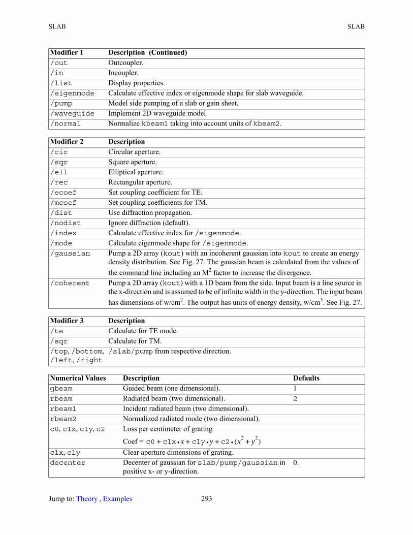
SLAB SLAB
/out Outcoupler./in Incoupler./list Display properties./eigenmode Calculate effective index or eigenmode shape for slab waveguide./pump Model side pumping of a slab or gain sheet./waveguide Implement 2D waveguide model./normal Normalize kbeam1 taking into account units of kbeam2.
Modifier 2 Description /cir Circular aperture./sqr Square aperture./ell Elliptical aperture./rec Rectangular aperture./ecoef Set coupling coefficient for TE./mcoef Set coupling coefficients for TM./dist Use diffraction propagation./nodist Ignore diffraction (default)./index Calculate effective index for /eigenmode./mode Calculate eigenmode shape for /eigenmode./gaussian Pump a 2D array (kout) with an incoherent gaussian into kout to create an energy
density distribution. See Fig. 27. The gaussian beam is calculated from the values of the command line including an M2 factor to increase the divergence.
/coherent Pump a 2D array (kout) with a 1D beam from the side. Input beam is a line source in the x-direction and is assumed to be of infinite width in the y-direction. The input beam has dimensions of w/cm2. The output has units of energy density, w/cm3. See Fig. 27.
Modifier 3 Description /te Calculate for TE mode./sqr Calculate for TM./top, /bottom, /left, /right
/slab/pump from respective direction.
Numerical Values Description Defaultsgbeam Guided beam (one dimensional). 1rbeam Radiated beam (two dimensional). 2
rbeam1 Incident radiated beam (two dimensional).rbeam2 Normalized radiated mode (two dimensional).c0, c1x, c1y, c2 Loss per centimeter of grating
Coef = clx, cly Clear aperture dimensions of grating.decenter Decenter of gaussian for slab/pump/gaussian in
positive x- or y-direction.0.
Modifier 1 Description (Continued)
c0 clx x• cly y• c2 x2 y2+( )•+ + +
Jump to: , 293 Theory Examples
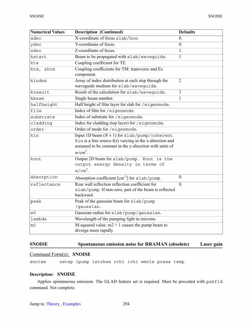
SNOISE SNOISE
SNOISE Spontaneous emission noise for RRAMAN (obsolete) Laser gain
Description: SNOISEApplies spontaneous emission. The GLAD feature set is required. Must be preceded with pakfld
command. Not complete.
xdec X-coordinate of focus slab/hoe. 0.ydec Y-coordinate of focus. 0.zdec Z-coordinate of focus. 1.kstart Beam to be propagated with slab/waveguide. 1kte Coupling coefficient for TE.ktm, zktm Coupling coefficients for TM: transverse and Ez
component.kindex Array of index distribution at each step through the
waveguide medium for slab/waveguide.2
kresult Result of the calculation for slab/waveguide. 3kbeam Single beam number. 1halfheight Half height of film layer for slab for /eigenmode.film Index of film for /eigenmode.substrate Index of substrate for /eigenmode.cladding Index for cladding (top layer) for /eigenmode.order Order of mode for /eigenmode.kin Input 1D beam (N × 1) for slab/pump/coherent.
Kin is a line source I(x) varying in the x-direction and assumed to be constant in the y-direction with units of w/cm2.
kout Output 2D beam for slab/pump. Kout is the output energy density in terms of
w/cm3.absorption Absorption coefficient [cm-1] for slab/pump. 0.reflectance Rear wall reflection reflection coefficient for
slab/pump. If non-zero, part of the beam is reflected backward.
0.
peak Peak of the gaussian beam for slab/pump/gaussian.
w0 Gaussian radius for slab/pump/gaussian.lambda Wavelength of the pumping light in microns.m2 M-squared value. m2 > 1 causes the pump beam to
diverge more rapidly.
Command Form(s): SNOISE snoise zstep ipump istokes rchi ichi wmole press temp
Numerical Values Description (Continued) Defaults
Jump to: , 294 Theory Examples
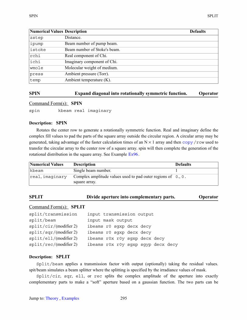
SPIN SPLIT
SPIN Expand diagonal into rotationally symmetric function. Operator
Description: SPINRotates the center row to generate a rotationally symmetric function. Real and imaginary define the
complex fill values to pad the parts of the square array outside the circular region. A circular array may be generated, taking advantage of the faster calculation times of an N × 1 array and then /row used to transfer the circular array to the center row of a square array. spin will then complete the generation of the rotational distribution in the square array. See Example .
SPLIT Divide aperture into complementary parts. Operator
Description: SPLITSplit/beam applies a transmission factor with output (optionally) taking the residual values.
spit/beam simulates a beam splitter where the splitting is specified by the irradiance values of mask.Split/cir, sqr, ell, or rec splits the complex amplitude of the aperture into exactly
complementary parts to make a “soft” aperture based on a gaussian function. The two parts can be
Numerical Values Description Defaultszstep Distance.ipump Beam number of pump beam.istoke Beam number of Stoke's beam.rchi Real component of Chi.ichi Imaginary component of Chi.wmole Molecular weight of medium.press Ambient pressure (Torr).temp Ambient temperature (K).
Command Form(s): SPIN spin kbeam real imaginary
Numerical Values Description Defaultskbeam Single beam number. 1real, imaginary Complex amplitude values used to pad outer regions of
square array.0., 0.
Command Form(s): SPLIT split/transmission input transmission output
split/beam input mask output
split/cir/(modifier 2) ibeams r0 sgxp decx decy
split/sqr/(modifier 2) ibeams r0 sgxp decx decy
split/ell/(modifier 2) ibeams r0x r0y sgxp decx decy
split/rec/(modifier 2) ibeams r0x r0y sgxp sgyp decx decy
copy
Ex96
Jump to: , 295 Theory Examples
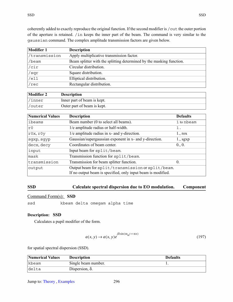
SSD SSD
coherently added to exactly reproduce the original function. If the second modifier is /out the outer portion of the aperture is retained. /in keeps the inner part of the beam. The command is very similar to the gaussian command. The complex amplitude transmission factors are given below.
SSD Calculate spectral dispersion due to EO modulation. Component
Description: SSDCalculates a pupil modifier of the form.
(197)
for spatial spectral dispersion (SSD).
Modifier 1 Description /transmission Apply multiplicative transmission factor./beam Beam splitter with the splitting determined by the masking function./cir Circular distribution./sqr Square distribution./ell Elliptical distribution./rec Rectangular distribution.
Modifier 2 Description /inner Inner part of beam is kept./outer Outer part of beam is kept.
Numerical Values Description Defaultsibeams Beam number (0 to select all beams). 1 to nbeamr0 1/e amplitude radius or half-width. 1.
r0x, r0y 1/e amplitude radius in x- and y-direction. 1., roxsgxp, sgyp Gaussian/supergaussian exponent in x- and y-direction. 1., sgxpdecx, decy Coordinates of beam center. 0., 0.input Input beam for split/beam.mask Transmission function for split/beam.transmission Transmission for beam splitter function. 0.output Output beam for split/transmission or split/beam.
If no output beam is specified, only input beam is modified.
Command Form(s): SSD ssd kbeam delta omegam alpha time
Numerical Values Description Defaultskbeam Single beam number. 1.delta Dispersion, δ.
a x y,( ) a x y,( )ejδ ωmt αx+( )sin
→
Jump to: , 296 Theory Examples
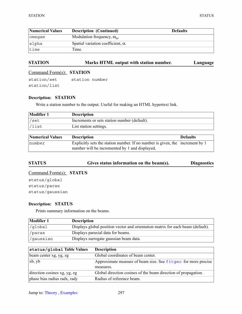
STATION STATUS
STATION Marks HTML output with station number. Language
Description: STATIONWrite a station number to the output. Useful for making an HTML hypertext link.
STATUS Gives status information on the beam(s). Diagnostics
Description: STATUSPrints summary information on the beams.
omegam Modulation frequency, ωm.alpha Spatial variation coefficient, α.time Time.
Command Form(s): STATION station/set station number
station/list
Modifier 1 Description /set Increments or sets station number (default)./list List station settings.
Numerical Values Description Defaultsnumber Explicitly sets the station number. If no number is given, the
number will be incremented by 1 and displayed,increment by 1
Command Form(s): STATUS status/global
status/parax
status/gaussian
Modifier 1 Description /global Displays global position vector and orientation matrix for each beam (default)./parax Displays paraxial data for beams./gaussian Displays surrogate gaussian beam data.
status/global Table Values Description beam center xg, yg, zg Global coordinates of beam center.xb, yb Approximate measure of beam size. See for more precise
measures.direction cosines xg, yg, zg Global direction cosines of the beam direction of propagation.phase bias radius radx, rady Radius of reference beam.
Numerical Values Description (Continued) Defaults
fitgeo
Jump to: , 297 Theory Examples
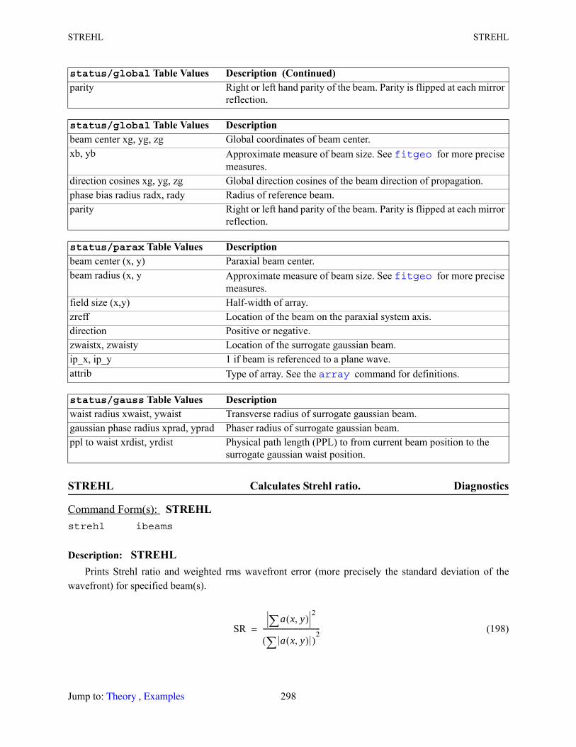
STREHL STREHL
STREHL Calculates Strehl ratio. Diagnostics
Description: STREHLPrints Strehl ratio and weighted rms wavefront error (more precisely the standard deviation of the
wavefront) for specified beam(s).
(198)
parity Right or left hand parity of the beam. Parity is flipped at each mirror reflection.
status/global Table Values Description beam center xg, yg, zg Global coordinates of beam center.xb, yb Approximate measure of beam size. See for more precise
measures.direction cosines xg, yg, zg Global direction cosines of the beam direction of propagation.phase bias radius radx, rady Radius of reference beam.parity Right or left hand parity of the beam. Parity is flipped at each mirror
reflection.
status/parax Table Values Description beam center (x, y) Paraxial beam center.beam radius (x, y Approximate measure of beam size. See for more precise
measures.field size (x,y) Half-width of array.zreff Location of the beam on the paraxial system axis.direction Positive or negative.zwaistx, zwaisty Location of the surrogate gaussian beam.ip_x, ip_y 1 if beam is referenced to a plane wave.attrib Type of array. See the command for definitions.
status/gauss Table Values Description waist radius xwaist, ywaist Transverse radius of surrogate gaussian beam.gaussian phase radius xprad, yprad Phaser radius of surrogate gaussian beam.ppl to waist xrdist, yrdist Physical path length (PPL) to from current beam position to the
surrogate gaussian waist position.
Command Form(s): STREHL strehl ibeams
status/global Table Values Description (Continued)
fitgeo
fitgeo
array
SRa x y,( )
2
a x y,( )( )2
---------------------------------=
Jump to: , 298 Theory Examples
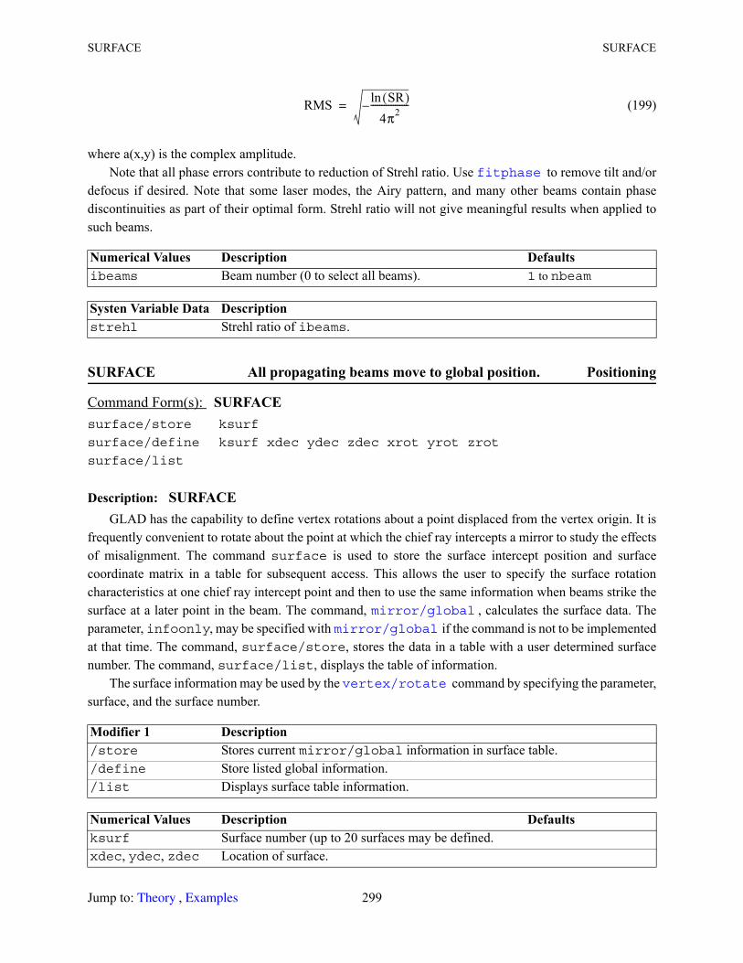
SURFACE SURFACE
(199)
where a(x,y) is the complex amplitude.Note that all phase errors contribute to reduction of Strehl ratio. Use to remove tilt and/or
defocus if desired. Note that some laser modes, the Airy pattern, and many other beams contain phase discontinuities as part of their optimal form. Strehl ratio will not give meaningful results when applied to such beams.
SURFACE All propagating beams move to global position. Positioning
Description: SURFACEGLAD has the capability to define vertex rotations about a point displaced from the vertex origin. It is
frequently convenient to rotate about the point at which the chief ray intercepts a mirror to study the effects of misalignment. The command surface is used to store the surface intercept position and surface coordinate matrix in a table for subsequent access. This allows the user to specify the surface rotation characteristics at one chief ray intercept point and then to use the same information when beams strike the surface at a later point in the beam. The command, , calculates the surface data. The parameter, infoonly, may be specified with if the command is not to be implemented at that time. The command, surface/store, stores the data in a table with a user determined surface number. The command, surface/list, displays the table of information.
The surface information may be used by the command by specifying the parameter, surface, and the surface number.
Numerical Values Description Defaultsibeams Beam number (0 to select all beams). 1 to nbeam
Systen Variable Data Description strehl Strehl ratio of ibeams.
Command Form(s): SURFACE surface/store ksurf
surface/define ksurf xdec ydec zdec xrot yrot zrot
surface/list
Modifier 1 Description /store Stores current mirror/global information in surface table./define Store listed global information./list Displays surface table information.
Numerical Values Description Defaultsksurf Surface number (up to 20 surfaces may be defined.xdec, ydec, zdec Location of surface.
RMS SR( )ln4π2
-----------------–=
fitphase
mirror/global mirror/global
vertex/rotate
Jump to: , 299 Theory Examples

SYSTEM TABLE
Example
SYSTEM Call system operations outside GLAD. Language
Description: SYSTEMCalls certain operating system functions. Also see the command that is specifically designed
for opening and controlling Adobe PDF documents.
TABLE Reads a table of user-defined values. Language
xrot, yrot, zrot Euler angles of surface rotation (degrees).
mirror/global/conic infoonly 20. (Global conic mirror sets data.)surface/store 1 (Store data for Surface #1.)surface/list (List surface data.)vertex/rotate/relative surface 1 0 5 (Rotation about surface intercept.)mirror/global/conic 20. (Rotated global conic mirror.)
Command Form(s): SYSTEM system/copyfile ‘(source file)’ ‘(destination file)’system/execute/nowait or wait ‘executable file arguments’system/launch ‘document file’
Modifier 1 Description /copyfile Copy (source file) to (destination file). Variables may be included in file names.
Full path descriptions may be used. File names having internal blanks should be included in single quotes. Example:variable/dec/int i1i1 = 3system/copy x.inp [email protected]
/execute Executes a program. May include full path. Single quotes are needed. Example:system/execute/nowait ‘watch.exe plot2.plt’
/launch Launch (or open) a document such as a *.PDF or *.DOC. The file extension must be associated with an application on users system. Example:system/launch ‘commands.pdf’
Modifier 2 Description /nowait GLAD starts executable file and continues (default)./execute GLAD waits for executable file to be closed.
Command Form(s): TABLE table/name (file name)table/read c1 c2 c3 c4 c5 c6 c7 c8 c9
table/skip nskip
Numerical Values Description (Continued) Defaults
manual
Jump to: , 300 Theory Examples

TABLE TABLE
Description: TABLEThis command allows numerical data to be read from a user-build file. The command table/name
defines the file name containing the table of data. The command table/read inputs table values, defined by column numbers, into variables or register addresses, determined by the values associated with each column number. Records may be skipped with table/skip.
The data file should consists of columns of numeric data. The columns are delimited by one or more blanks or a coma and any number of blanks. A maximum of 9 columns may be used. See the example below. If a zero is entered for one of the register addresses, the associated table value is not stored anywhere.
Example data file, table.dat:1,2,3,4,5,6,7,8,910 11 12 13, 14, 15,16,17,1819 20 21 22 23 24 25 26 2728 29 , 30, 31, 32, 33, 34 35 36
Example command deck:cc define table file name, file is always rewoundctable/name table.datcc read in nine column values, into matching register numbersc declare/real t1 t2 t3 t4 t5 t6 t7 t8 t9table/read t1 t2 t3 t4 t5 t6 t7 t8 t9cc display the 9 valuesvariablespausecc read in 9 more values into reverse register orderctable/read t9 t8 t7 t6 t5 t4 t3 t2 t1variablespausec
table/close
Modifier 1 Description /name Identifies the name of the file to be read and rewinds file./read Read a data record./skip Skip one or more records./close Close the table file, so that it may be changed by a text editor.
Numerical Values Description Defaultsc1,c2, c3, c4, c5, c6, c7, c8, c9
Variables or register addresses where the table values are to be stored.
0
nskip Number of records to be skipped. 1
Command Form(s): TABLE (Continued)
Jump to: , 301 Theory Examples
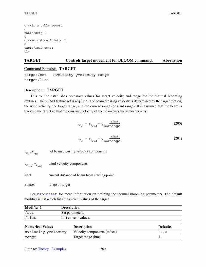
TARGET TARGET
c skip a table recordctable/skip 1cc read column 8 into t1ctable/read c8=t1t1=
TARGET Controls target movement for BLOOM command. Aberration
Description: TARGETThis routine establishes necessary values for target velocity and range for the thermal blooming
routines. The GLAD feature set is required. The beam crossing velocity is determined by the target motion, the wind velocity, the target range, and the current range (or slant range). It is assumed that the beam is tracking the target so that the crossing velocity of the beam over the atmosphere is:
(200)
(201)
net beam crossing velocity components
wind velocity components
slant current distance of beam from starting point
range range of target
See for more information on defining the thermal blooming parameters. The default modifier is list which lists the current values of the target.
Command Form(s): TARGET target/set xvelocity yvelocity range
target/list
Modifier 1 Description /set Set parameters./list List current values.
Numerical Values Description Defaultsxvelocity, yvelocity Velocity components (m/sec). 0., 0.range Target range (km). 1.
vxtotvxwind
vxtarget
slantrange------------------–=
vytotvywind
vytarget
slantrange------------------–=
vxtotvytot
,
vxwindvywind
,
bloom/set
Jump to: , 302 Theory Examples
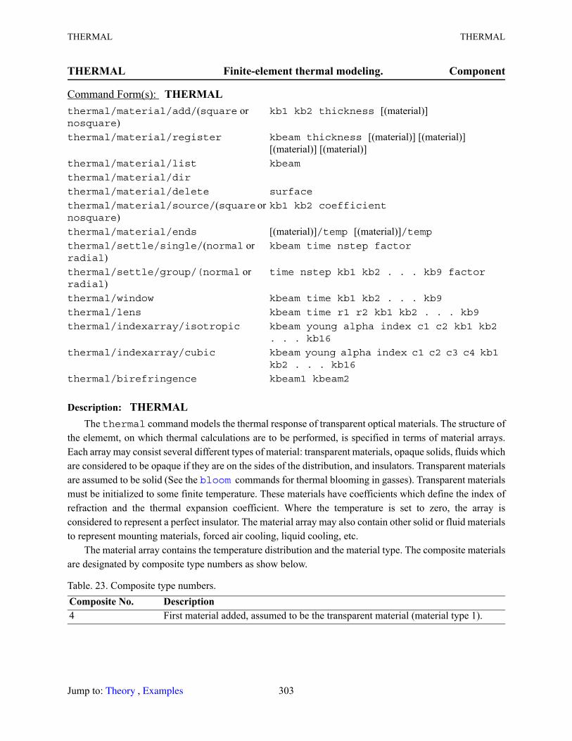
THERMAL THERMAL
THERMAL Finite-element thermal modeling. Component
Description: THERMALThe thermal command models the thermal response of transparent optical materials. The structure of
the elememt, on which thermal calculations are to be performed, is specified in terms of material arrays. Each array may consist several different types of material: transparent materials, opaque solids, fluids which are considered to be opaque if they are on the sides of the distribution, and insulators. Transparent materials are assumed to be solid (See the commands for thermal blooming in gasses). Transparent materials must be initialized to some finite temperature. These materials have coefficients which define the index of refraction and the thermal expansion coefficient. Where the temperature is set to zero, the array is considered to represent a perfect insulator. The material array may also contain other solid or fluid materials to represent mounting materials, forced air cooling, liquid cooling, etc.
The material array contains the temperature distribution and the material type. The composite materials are designated by composite type numbers as show below.
Command Form(s): THERMAL thermal/material/add/(square or nosquare)
kb1 kb2 thickness [(material)]
thermal/material/register kbeam thickness [(material)] [(material)] [(material)] [(material)]
thermal/material/list kbeam
thermal/material/dir
thermal/material/delete surface
thermal/material/source/(square or nosquare)
kb1 kb2 coefficient
thermal/material/ends [(material)]/temp [(material)]/tempthermal/settle/single/(normal or radial)
kbeam time nstep factor
thermal/settle/group/(normal or radial)
time nstep kb1 kb2 . . . kb9 factor
thermal/window kbeam time kb1 kb2 . . . kb9
thermal/lens kbeam time r1 r2 kb1 kb2 . . . kb9
thermal/indexarray/isotropic kbeam young alpha index c1 c2 kb1 kb2 . . . kb16
thermal/indexarray/cubic kbeam young alpha index c1 c2 c3 c4 kb1 kb2 . . . kb16
thermal/birefringence kbeam1 kbeam2
Table. 23. Composite type numbers.Composite No. Description4 First material added, assumed to be the transparent material (material type 1).
bloom
Jump to: , 303 Theory Examples

THERMAL THERMAL
There are five composite types: the transparent material, laboratory environment defining the medium in the front of the element (and optionally the sides of the element), (optionally) two additional materials which define mounting structure and/or fluid contact, and insulator where T = 0.
A catalog of material characteristics is given in the file matlib. This file may be edited by the user to add or delete materials. Each material is identified by name. In addition there is a material type number which indicated whether the material is a fluid, transparent refractive element, or solid representing mounting structure.
3 The laboratory environment. Must be fluid (material type 2). The composite type is always assumed to exist on either side of the transparent material. Must be initialized to some finite temperature value to distinguish it from an insulator. May be still air, forced air, vacuum, etc.
2 Either mounting material or fluid (material types 3 or 2).1 Either mounting material or fluid (material types 3 or 2).0 T = 0. Points with zero temperature are assumed to represent perfect thermal
insulators and no heat will flow into them. This is set by the zero temperature values defined for the transparent material.
Table. 24. Material type numbers.Material Type
State Transmission Properties
Description
1 solid transparent Conduction occurs and convection loss into surrounding fluids. Temperature varies. Usable as optical material. Specifiy heat transfer coefficient in K = KW/m°C and product of density and heat capacity as ρc = KJ/m3°C. Also specify index of refraction and first and second derivatives of index of refraction and thermal expansion as a function of temperature with respect to some reference temperature T0. If T = 0 a perfect thermal insulator is assumed and no heat will flow into or out of this material.
2 fluid opaque Convection but no conduction. Temperature does not vary. Usable as environment. Specify heat transfer coefficient in h= KW/m°C. A fluid is assumed to be opaque except where it is part of the laboratory environment in front of the transparent refractive material.
3 solid opaque Conduction but no convection. Temperature varies. Usable as mounting material or environment. Specifiy heat transfer coefficient in K = KW/m°C and product of density and heat capacity ρc = KJ/m3°C.
Modifier 1 Description /material Build and lists material sections./settle Solves transient thermal interactions for specified time.
Table. 23. Composite type numbers.Composite No. Description
Jump to: , 304 Theory Examples
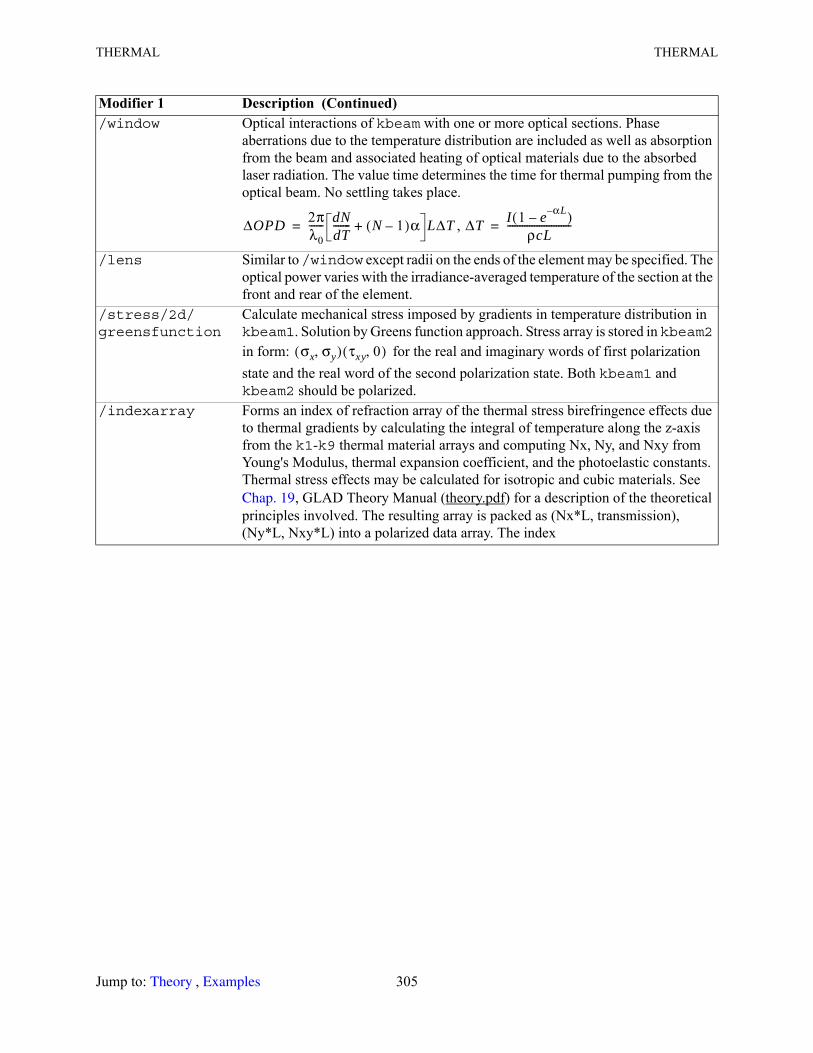
THERMAL THERMAL
/window Optical interactions of kbeam with one or more optical sections. Phase aberrations due to the temperature distribution are included as well as absorption from the beam and associated heating of optical materials due to the absorbed laser radiation. The value time determines the time for thermal pumping from the optical beam. No settling takes place.
,
/lens Similar to /window except radii on the ends of the element may be specified. The optical power varies with the irradiance-averaged temperature of the section at the front and rear of the element.
/stress/2d/greensfunction
Calculate mechanical stress imposed by gradients in temperature distribution in kbeam1. Solution by Greens function approach. Stress array is stored in kbeam2 in form: for the real and imaginary words of first polarization state and the real word of the second polarization state. Both kbeam1 and kbeam2 should be polarized.
/indexarray Forms an index of refraction array of the thermal stress birefringence effects due to thermal gradients by calculating the integral of temperature along the z-axis from the k1-k9 thermal material arrays and computing Nx, Ny, and Nxy from Young's Modulus, thermal expansion coefficient, and the photoelastic constants. Thermal stress effects may be calculated for isotropic and cubic materials. See
, GLAD Theory Manual (theory.pdf) for a description of the theoretical principles involved. The resulting array is packed as (Nx*L, transmission), (Ny*L, Nxy*L) into a polarized data array. The index
Modifier 1 Description (Continued)
ΔOPD 2πλ0------ dN
dT------- N 1–( )α+ LΔT= ΔT I 1 e αL––( )
ρcL--------------------------=
σx σy,( ) τxy 0,( )
Chap. 19
Jump to: , 305 Theory Examples

THERMAL THERMAL
/birefringence Optical effect of a special z-integrated index of refraction array where each element is of the form (Nx*L, transmission), (Ny*L, Nxy*L), where the array has polarized form. Such a z-integrated index array will be formed by the thermal/indexarray command and includes the effects of Young's Modulus, coefficient of thermal expansion, and photoelastic coefficients. The perturbation effects Δ of index of refraction may be found from the stress components by application of the 6 × 6 photoelastic tensor. As we only need the properties in the x-y plane the tensor may be reduced to 4 × 4 form.
isotropic material, .
cubic material, .
The stress components are calculated with a Green's function approach and applied in frequency space using the methods of Chap 19, GLAD Theory Manual (theory.pdf).
Modifier 2 Description /add Used to construct a composite section in kb1. If kb1 = kb2, the array is
initialized. Each subsequent /add adds a new material to the section at points where the section has exactly zero temperature. A maximum of four materials may be included in each section. The real word of kb2 should contain the temperature. Use the irradiance command to convert normal complex amplitude form to a form with the irradiance (representing the temperature) in the real word. If the temperature is zero, that point is considered to be a perfect insulator. For refractive materials, the imaginary word may contain source power information. For a fluid the imaginary word may contain differential values to be added to the convection coefficient. A composite section may consist only of fluid material to be used as the front or rear sections in a group.
/register Used to identify an array as a thermal array. Useful when using or to input an array previously created by thermal/material/add. and must use unformatted or binary protocol. Must specify
thickness and the material names in order as the array was originally defined./dir Lists materials in file matlib./list List characteristics of composite sections which have been defined./delete Delete a thermal surface by surface number./source Add an internal heat source to the specified composite section./ends Optionally specify fluid characteristics at the front and back of all sections.
Modifier 1 Description (Continued)
Δ˜
x
Δ˜
y
Δ˜
xy
n03
2-----–
c11 c12 c13 0c13 c11 c12 00 0 0 c11 c12–
σx
σy
σxy
τxy
=
Δ˜
x
Δ˜
y
Δ˜
xy
n03
2-----–
c11 c12 c13 0c13 c11 c12 00 0 0 c44
σx
σy
σxy
τxy
=
infile connect outfile infile
Jump to: , 306 Theory Examples
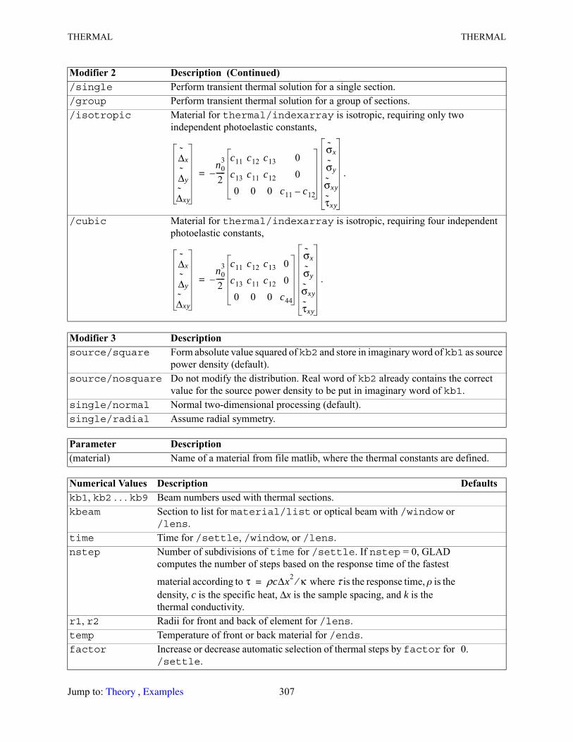
THERMAL THERMAL
/single Perform transient thermal solution for a single section./group Perform transient thermal solution for a group of sections./isotropic Material for thermal/indexarray is isotropic, requiring only two
independent photoelastic constants,
.
/cubic Material for thermal/indexarray is isotropic, requiring four independent photoelastic constants,
.
Modifier 3 Description source/square Form absolute value squared of kb2 and store in imaginary word of kb1 as source
power density (default).source/nosquare Do not modify the distribution. Real word of kb2 already contains the correct
value for the source power density to be put in imaginary word of kb1.single/normal Normal two-dimensional processing (default).single/radial Assume radial symmetry.
Parameter Description (material) Name of a material from file matlib, where the thermal constants are defined.
Numerical Values Description Defaultskb1, kb2 . . . kb9 Beam numbers used with thermal sections.kbeam Section to list for material/list or optical beam with /window or
/lens.time Time for /settle, /window, or /lens.nstep Number of subdivisions of time for /settle. If nstep = 0, GLAD
computes the number of steps based on the response time of the fastest
material according to where τ is the response time, ρ is the density, c is the specific heat, Δx is the sample spacing, and k is the thermal conductivity.
r1, r2 Radii for front and back of element for /lens.temp Temperature of front or back material for /ends.factor Increase or decrease automatic selection of thermal steps by factor for
/settle.0.
Modifier 2 Description (Continued)
Δ˜
x
Δ˜
y
Δ˜
xy
n03
2-----–
c11 c12 c13 0c13 c11 c12 00 0 0 c11 c12–
σx
σy
σxy
τxy
=
Δ˜
x
Δ˜
y
Δ˜
xy
n03
2-----–
c11 c12 c13 0c13 c11 c12 00 0 0 c44
σx
σy
σxy
τxy
=
τ ρcΔx2 κ⁄=
Jump to: , 307 Theory Examples

THRESHOLD TIME
THRESHOLD Set low irradiance values to zero. Operator
Description: THRESHOLDSets values below a threshold value to zero. Useful for trimming irradiance noise and associated phase
irregularities to zero.
TIME Measure elapsed time. Language
Description: TIMEThis command controls and displays the elapsed time. Time/show gives the elapsed time from the last
time/init.
thickness Thickness of the section used by settle/group.young Young's Modulus in units of Newtons/cm.alpha Coefficient of thermal expansion in °C-1. c1, c2, c3, c4 Photoelastic coefficients. Only c1 and c2 are required for
/isotropic. Units of cm2/N.surface Number of surface in order of definition.coefficient For thermal/material/source, multiply source power of kb2
before storing in kb1.
Command Form(s): THRESHOLD threshold kbeam threshold
Numerical Values Description Defaultskbeam Single beam number. 1threshold Set values below threshold*peak to zero. 1e-8
Command Form(s): TIME time/init
time/show
time/halt
time/resume
Modifier 1 Description /init Reset timing clock./show Display the elapsed time./halt Halts the timer without resetting the timer./resume Resumes the timing.
System Variable Data Description time Elapsed time from last call to time/show.
Numerical Values Description (Continued) Defaults
Jump to: , 308 Theory Examples
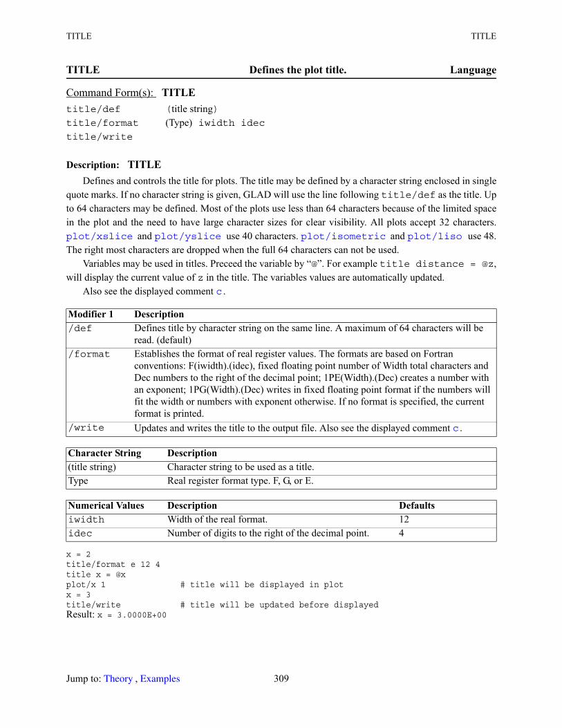
TITLE TITLE
TITLE Defines the plot title. Language
Description: TITLEDefines and controls the title for plots. The title may be defined by a character string enclosed in single
quote marks. If no character string is given, GLAD will use the line following title/def as the title. Up to 64 characters may be defined. Most of the plots use less than 64 characters because of the limited space in the plot and the need to have large character sizes for clear visibility. All plots accept 32 characters.
and use 40 characters. and use 48. The right most characters are dropped when the full 64 characters can not be used.
Variables may be used in titles. Preceed the variable by “@”. For example title distance = @z, will display the current value of z in the title. The variables values are automatically updated.
Also see the displayed comment .
x = 2title/format e 12 4title x = @xplot/x 1 # title will be displayed in plotx = 3title/write # title will be updated before displayedResult: x = 3.0000E+00
Command Form(s): TITLE title/def (title string)title/format (Type) iwidth idectitle/write
Modifier 1 Description /def Defines title by character string on the same line. A maximum of 64 characters will be
read. (default)/format Establishes the format of real register values. The formats are based on Fortran
conventions: F(iwidth).(idec), fixed floating point number of Width total characters and Dec numbers to the right of the decimal point; 1PE(Width).(Dec) creates a number with an exponent; 1PG(Width).(Dec) writes in fixed floating point format if the numbers will fit the width or numbers with exponent otherwise. If no format is specified, the current format is printed.
/write Updates and writes the title to the output file. Also see the displayed comment .
Character String Description (title string) Character string to be used as a title.Type Real register format type. F, G, or E.
Numerical Values Description Defaultsiwidth Width of the real format. 12idec Number of digits to the right of the decimal point. 4
plot/xslice plot/yslice plot/isometric plot/liso
c
c
Jump to: , 309 Theory Examples
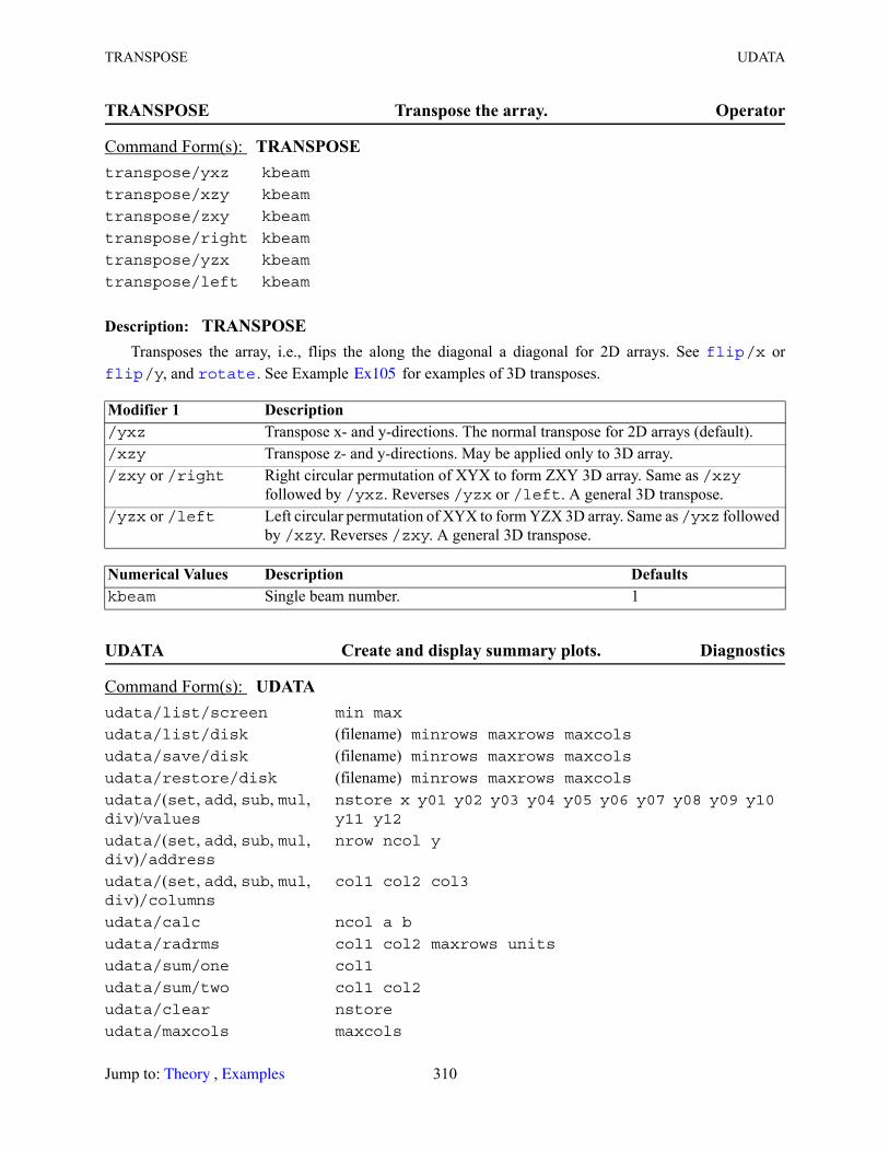
TRANSPOSE UDATA
TRANSPOSE Transpose the array. Operator
Description: TRANSPOSETransposes the array, i.e., flips the along the diagonal a diagonal for 2D arrays. See /x or /y, and . See Example for examples of 3D transposes.
UDATA Create and display summary plots. Diagnostics
Command Form(s): TRANSPOSE transpose/yxz kbeam
transpose/xzy kbeam
transpose/zxy kbeam
transpose/right kbeam
transpose/yzx kbeam
transpose/left kbeam
Modifier 1 Description /yxz Transpose x- and y-directions. The normal transpose for 2D arrays (default)./xzy Transpose z- and y-directions. May be applied only to 3D array./zxy or /right Right circular permutation of XYX to form ZXY 3D array. Same as /xzy
followed by /yxz. Reverses /yzx or /left. A general 3D transpose./yzx or /left Left circular permutation of XYX to form YZX 3D array. Same as /yxz followed
by /xzy. Reverses /zxy. A general 3D transpose.
Numerical Values Description Defaultskbeam Single beam number. 1
Command Form(s): UDATA udata/list/screen min max
udata/list/disk (filename) minrows maxrows maxcolsudata/save/disk (filename) minrows maxrows maxcolsudata/restore/disk (filename) minrows maxrows maxcolsudata/(set, add, sub, mul, div)/values
nstore x y01 y02 y03 y04 y05 y06 y07 y08 y09 y10 y11 y12
udata/(set, add, sub, mul, div)/address
nrow ncol y
udata/(set, add, sub, mul, div)/columns
col1 col2 col3
udata/calc ncol a b
udata/radrms col1 col2 maxrows units
udata/sum/one col1
udata/sum/two col1 col2
udata/clear nstore
udata/maxcols maxcols
flip flip rotate Ex105
Jump to: , 310 Theory Examples
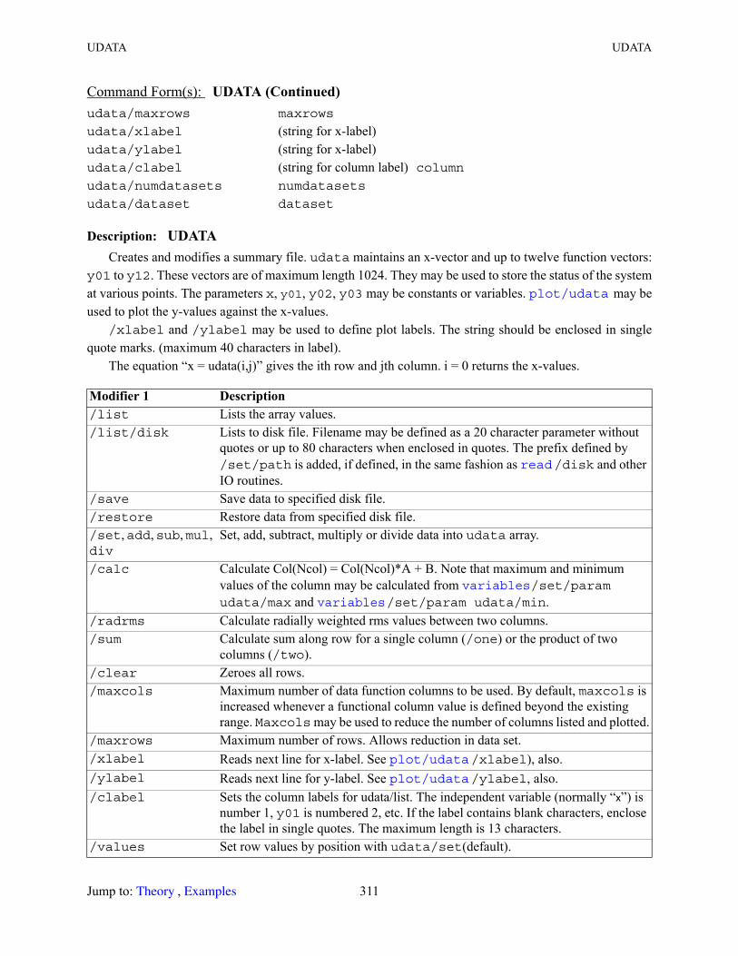
UDATA UDATA
Description: UDATACreates and modifies a summary file. udata maintains an x-vector and up to twelve function vectors:
y01 to y12. These vectors are of maximum length 1024. They may be used to store the status of the system at various points. The parameters x, y01, y02, y03 may be constants or variables. may be used to plot the y-values against the x-values.
/xlabel and /ylabel may be used to define plot labels. The string should be enclosed in single quote marks. (maximum 40 characters in label).
The equation “x = udata(i,j)” gives the ith row and jth column. i = 0 returns the x-values.
udata/maxrows maxrows
udata/xlabel (string for x-label)udata/ylabel (string for x-label)udata/clabel (string for column label) columnudata/numdatasets numdatasets
udata/dataset dataset
Modifier 1 Description /list Lists the array values./list/disk Lists to disk file. Filename may be defined as a 20 character parameter without
quotes or up to 80 characters when enclosed in quotes. The prefix defined by /set/path is added, if defined, in the same fashion as /disk and other IO routines.
/save Save data to specified disk file./restore Restore data from specified disk file./set, add, sub, mul, div
Set, add, subtract, multiply or divide data into udata array.
/calc Calculate Col(Ncol) = Col(Ncol)*A + B. Note that maximum and minimum values of the column may be calculated from /set/param udata/max and /set/param udata/min.
/radrms Calculate radially weighted rms values between two columns./sum Calculate sum along row for a single column (/one) or the product of two
columns (/two)./clear Zeroes all rows./maxcols Maximum number of data function columns to be used. By default, maxcols is
increased whenever a functional column value is defined beyond the existing range. Maxcols may be used to reduce the number of columns listed and plotted.
/maxrows Maximum number of rows. Allows reduction in data set./xlabel Reads next line for x-label. See /xlabel), also./ylabel Reads next line for y-label. See /ylabel, also./clabel Sets the column labels for udata/list. The independent variable (normally “x”) is
number 1, y01 is numbered 2, etc. If the label contains blank characters, enclose the label in single quotes. The maximum length is 13 characters.
/values Set row values by position with udata/set(default).
Command Form(s): UDATA (Continued)
plot/udata
read
variables variables
plot/udata plot/udata
Jump to: , 311 Theory Examples
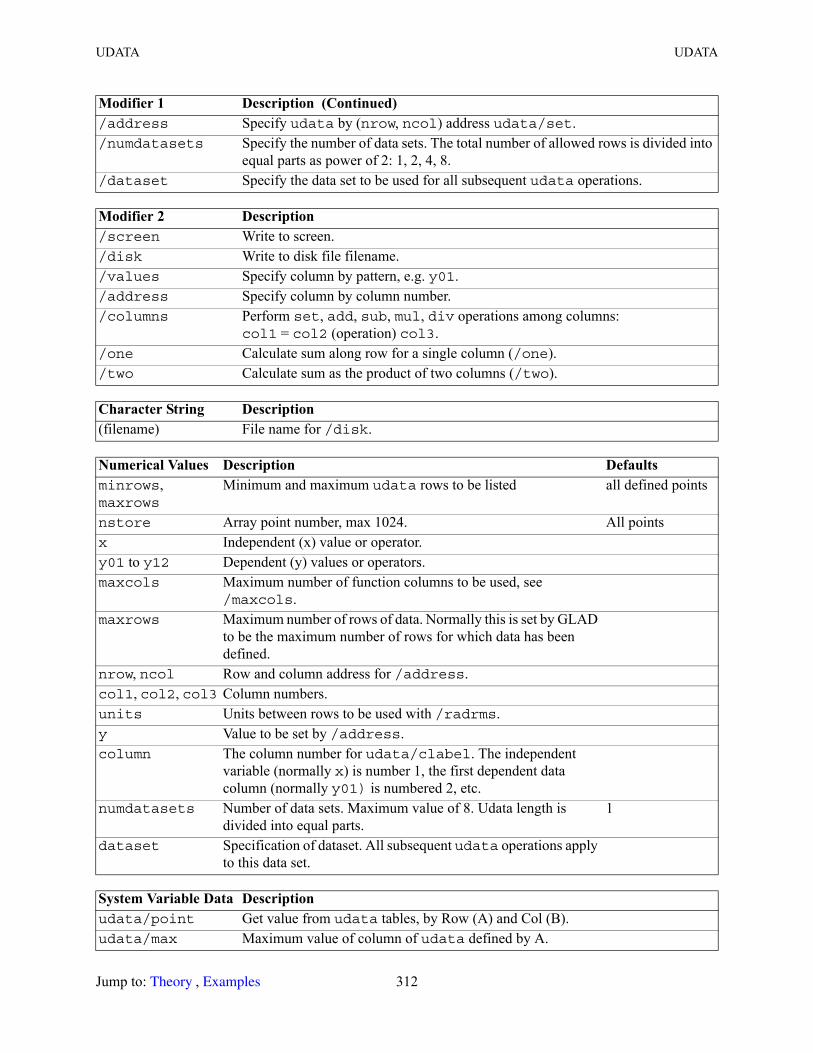
UDATA UDATA
/address Specify udata by (nrow, ncol) address udata/set./numdatasets Specify the number of data sets. The total number of allowed rows is divided into
equal parts as power of 2: 1, 2, 4, 8./dataset Specify the data set to be used for all subsequent udata operations.
Modifier 2 Description /screen Write to screen./disk Write to disk file filename./values Specify column by pattern, e.g. y01./address Specify column by column number./columns Perform set, add, sub, mul, div operations among columns:
col1 = col2 (operation) col3./one Calculate sum along row for a single column (/one)./two Calculate sum as the product of two columns (/two).
Character String Description (filename) File name for /disk.
Numerical Values Description Defaultsminrows, maxrows
Minimum and maximum udata rows to be listed all defined points
nstore Array point number, max 1024. All pointsx Independent (x) value or operator.y01 to y12 Dependent (y) values or operators.maxcols Maximum number of function columns to be used, see
/maxcols.maxrows Maximum number of rows of data. Normally this is set by GLAD
to be the maximum number of rows for which data has been defined.
nrow, ncol Row and column address for /address.col1, col2, col3 Column numbers.units Units between rows to be used with /radrms.y Value to be set by /address.column The column number for udata/clabel. The independent
variable (normally x) is number 1, the first dependent data column (normally y01) is numbered 2, etc.
numdatasets Number of data sets. Maximum value of 8. Udata length is divided into equal parts.
1
dataset Specification of dataset. All subsequent udata operations apply to this data set.
System Variable Data Description udata/point Get value from udata tables, by Row (A) and Col (B).udata/max Maximum value of column of udata defined by A.
Modifier 1 Description (Continued)
Jump to: , 312 Theory Examples

UNIFORMITY UNIFORMITY
UNIFORMITY Calculate irradiance nonuniformity. Diagnostics
Description: UNIFORMITYCalculates the nonuniformity of irradiance for the specified region. If no region width is specified the
entire array is used. Irradiance nonuniformity is calculated by
nonuniformity (percent) = (202)
where indicates a spatial average and the irradiance is I. This definition of irradiance nonuniformity can give a value greater than 100%, A random speckle pattern has a nonuniformity of about 100%.
For /two the uniformity is calculated to be
nonuniformity (percent) = (203)
where I1 is the irradiance of kbeam1 and I2 is the irradiance of kbeam2. This allows comparison of a test function against a reference function.
udata/min Minimum value of column of udata defined by A.udata/radrms Radial weighted root sum square of two columns.udata/sum Sum of a single column (/one) or the product of two columns (/two).
Command Form(s): UNIFORMITY uniformity/cir kbeam rad xdec ydec
uniformity/sqr kbeam rad xdec ydec
uniformity/ell kbeam xrad yrad xdec ydec
uniformity/rec kbeam xrad yrad xdec ydec
uniformity/two kbeam1 kbeam2
Modifier 1 Description /cir Circle./sqr Square./ell Ellipse./rec Rectangle./two Compare a test beam against a reference beam.
Numerical Values Description Defaultskbeam Single beam number. 1kbeam1, kbeam2 Test and reference beams for /two.rad Radius of region (cm). Entire array.
System Variable Data Description (Continued)
1I
------- I2 I 2–( ) 100×
I1 I2–( )2 xd ydI1
2 xd yd I12 xd yd
----------------------------------------------------- 100×
Jump to: , 313 Theory Examples
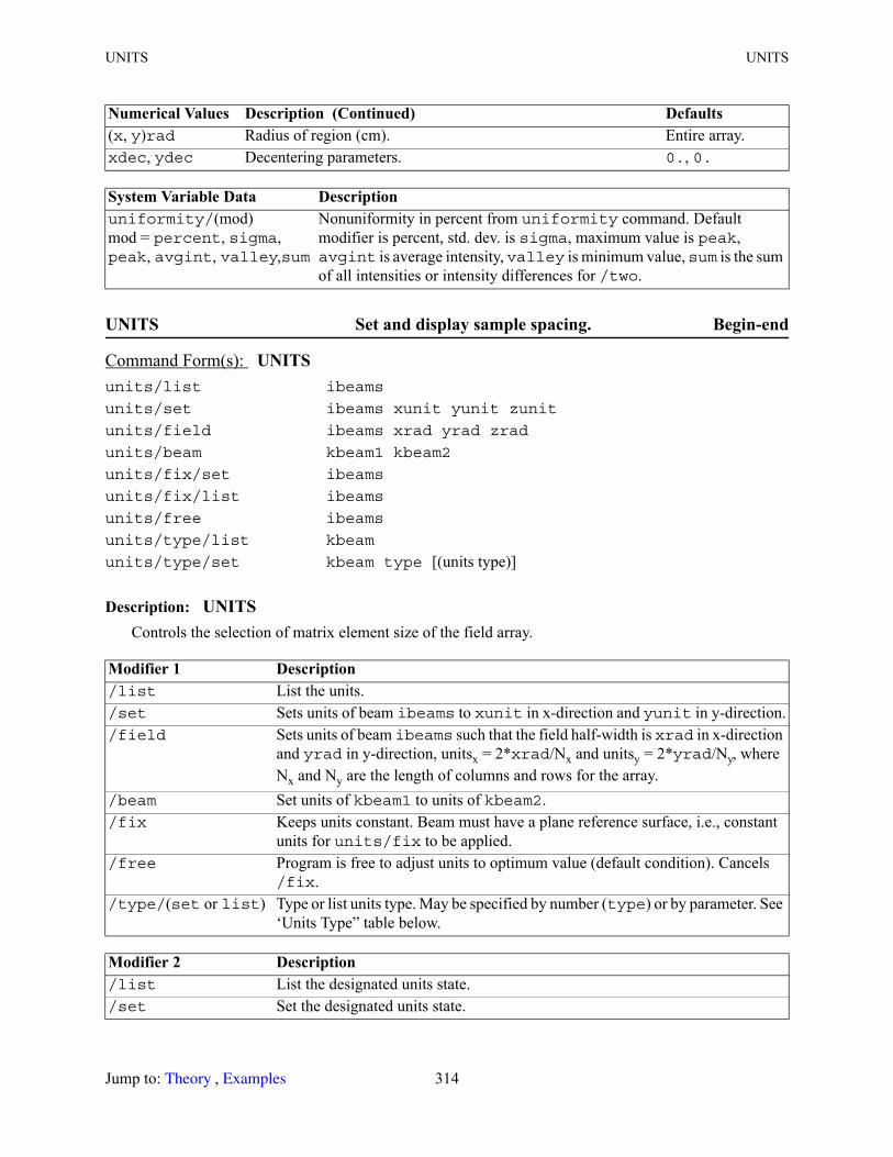
UNITS UNITS
UNITS Set and display sample spacing. Begin-end
Description: UNITSControls the selection of matrix element size of the field array.
(x, y)rad Radius of region (cm). Entire array.xdec, ydec Decentering parameters. 0., 0.
System Variable Data Description uniformity/(mod)mod = percent, sigma, peak, avgint, valley,sum
Nonuniformity in percent from uniformity command. Default modifier is percent, std. dev. is sigma, maximum value is peak, avgint is average intensity, valley is minimum value, sum is the sum of all intensities or intensity differences for /two.
Command Form(s): UNITS units/list ibeams
units/set ibeams xunit yunit zunit
units/field ibeams xrad yrad zrad
units/beam kbeam1 kbeam2
units/fix/set ibeams
units/fix/list ibeams
units/free ibeams
units/type/list kbeam
units/type/set kbeam type [(units type)]
Modifier 1 Description /list List the units./set Sets units of beam ibeams to xunit in x-direction and yunit in y-direction./field Sets units of beam ibeams such that the field half-width is xrad in x-direction
and yrad in y-direction, unitsx = 2*xrad/Nx and unitsy = 2*yrad/Ny, where Nx and Ny are the length of columns and rows for the array.
/beam Set units of kbeam1 to units of kbeam2./fix Keeps units constant. Beam must have a plane reference surface, i.e., constant
units for units/fix to be applied./free Program is free to adjust units to optimum value (default condition). Cancels
/fix./type/(set or list) Type or list units type. May be specified by number (type) or by parameter. See
‘Units Type” table below.
Modifier 2 Description /list List the designated units state./set Set the designated units state.
Numerical Values Description (Continued) Defaults
Jump to: , 314 Theory Examples
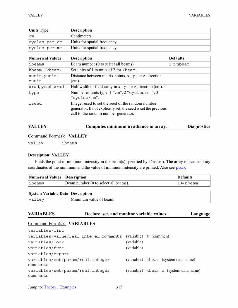
VALLEY VARIABLES
VALLEY Computes minimum irradiance in array. Diagnostics
Description: VALLEYFinds the point of minimum intensity in the beam(s) specified by ibeams. The array indices and ray
coordinates of the minimum and the value of minimum intensity are printed. Also see .
VARIABLES Declare, set, and monitor variable values. Language
Units Type Description cm Centimeters.cycles_per_cm Units for spatial frequency.cycles_per_mm Units for spatial frequency.
Numerical Values Description Defaultsibeams Beam number (0 to select all beams). 1 to nbeamkbeam1, kbeam2 Set units of 1 to units of 2 for /beam.xunit, yunit, zunit
Distance between matrix points, x-, y-, or z-direction (cm).
xrad, yrad, zrad Half width of field array in x-, y-, or z-direction (cm).type Number of units type: 1 “cm”, 2 “cycles/cm”, 3
“cycles/mm”.iseed Integer used to set the seed of the random number
generator. If not explicitly set, the seed is set the previous call to the random number generator.
Command Form(s): VALLEY valley ibeams
Numerical Values Description Defaultsibeams Beam number (0 to select all beams). 1 to nbeam
System Variable Data Description valley Minimum value of beam.
Command Form(s): VARIABLES variables/list
variables/value/real, integer, comments (variable) # (comment)variables/lock (variable)variables/free (variable)variables/export
variables/set/param/real, integer, comments
(variable) kbeam (system data name)
variables/set/param/real, integer, comments
(variable) kbeam a (system data name)
peak
Jump to: , 315 Theory Examples
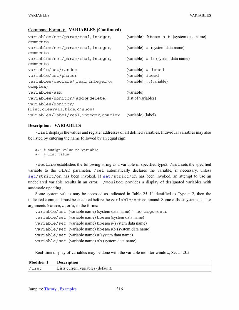
VARIABLES VARIABLES
Description: VARIABLES/list displays the values and register addresses of all defined variables. Individual variables may also
be listed by entering the name followed by an equal sign:
a=3 # assign value to variablea= # list value
/declare establishes the following string as a variable of specified type5. /set sets the specified variable to the GLAD parameter. /set automatically declares the variable, if necessary, unless
/strict/on has been invoked. If /strict/on has been invoked, an attempt to use an undeclared variable results in an error. /monitor provides a display of designated variables with automatic updating.
Some system values may be accessed as indicated in Table 25. If identified as Type = 2, then the indicated command must be executed before the variable/set command. Some calls to system data use arguments kbeam, a, or b, in the forms:
variable/set (variable name) (system data name) # no argumentsvariable/set (variable name) kbeam (system data name)variable/set (variable name) kbeam a(system data name)variable/set (variable name) kbeam ab (system data name)variable/set (variable name) a(system data name)variable/set (variable name) ab (system data name)
Real-time display of variables may be done with the variable monitor window, Sect. 1.3.5.
variables/set/param/real, integer, comments
(variable) kbeam a b (system data name)
variables/set/param/real, integer, comments
(variable) a (system data name)
variables/set/param/real, integer, comments
(variable) a b (system data name)
variable/set/random (variable) a iseedvariable/set/phaser (variable) iseedvariables/declare/(real, integer, or complex)
(variable) . . . (variable)
variables/ask (variable)variables/monitor/(add or delete) (list of variables)variables/monitor/(list, clearall, hide, or show)variables/label/real, integer, complex (variable)(label)
Modifier 1 Description /list Lists current variables (default).
Command Form(s): VARIABLES (Continued)
set set
Jump to: , 316 Theory Examples

VARIABLES VARIABLES
/value Declares and sets a single variable allowing real, integer, or complex specification. Any “#” comment will become a variable label.
/lock Lock the variable to prevent inadvertent change./free Free the variable to allow changes./export Form of list suitable for exporting with /disk (filename), followed by
variables/export; read/screen. Variables can be read into another command file by /disk (filename).
/set Set variable to GLAD system value./declare Declare variables prior to use./ask Prompt for assignment of value to variable. Useful in macros and command file input to
make real time assignment of values./monitor Display a table of variables and their values in a separate window. Values are updated
automatically./label Add a label to a variable. The lable will apper in variables/list or as an added
coment if the variable value is displayed in the form “variable=”.
Modifier 2 Description declare/real Declares variables as real (default).declare/integer Declares variable as integer.declare/complex Declares variables as complex numbers for example x = 1 + 2i./add Add a variable to monitor list. The monitor window is started when the first
variable is added to the monitor list. The display will be automatically updated to show the current value of the variable. The following line adds the variable Energy to the display.variables/monitor/add Energy
/delete Delete a variable from monitor list./clearall Delete all variables from table. Also removes the monitor window./list List all monitored variables./show Show the variable monitor window./hide Minimize the variable monitor window./param Various functions (default)./random Random variable with gaussian statistics. The first value sets the expected value.
The second value sets the random seed, if desired./phaser Random angle from 0 to 360 degrees. The value sets the random seed, if desired.
Modifier 3 Description parameter/real If new variable declare it as real (default).parameter/integer If new variable declare it as integer.
Parameters Description (variable) Variable name consisting of no more than 20 alphanumeric characters, “$”, “_”.(label) A comment after “#” to be used as a label for variable/label.
Modifier 1 Description (Continued)
write
read
Jump to: , 317 Theory Examples
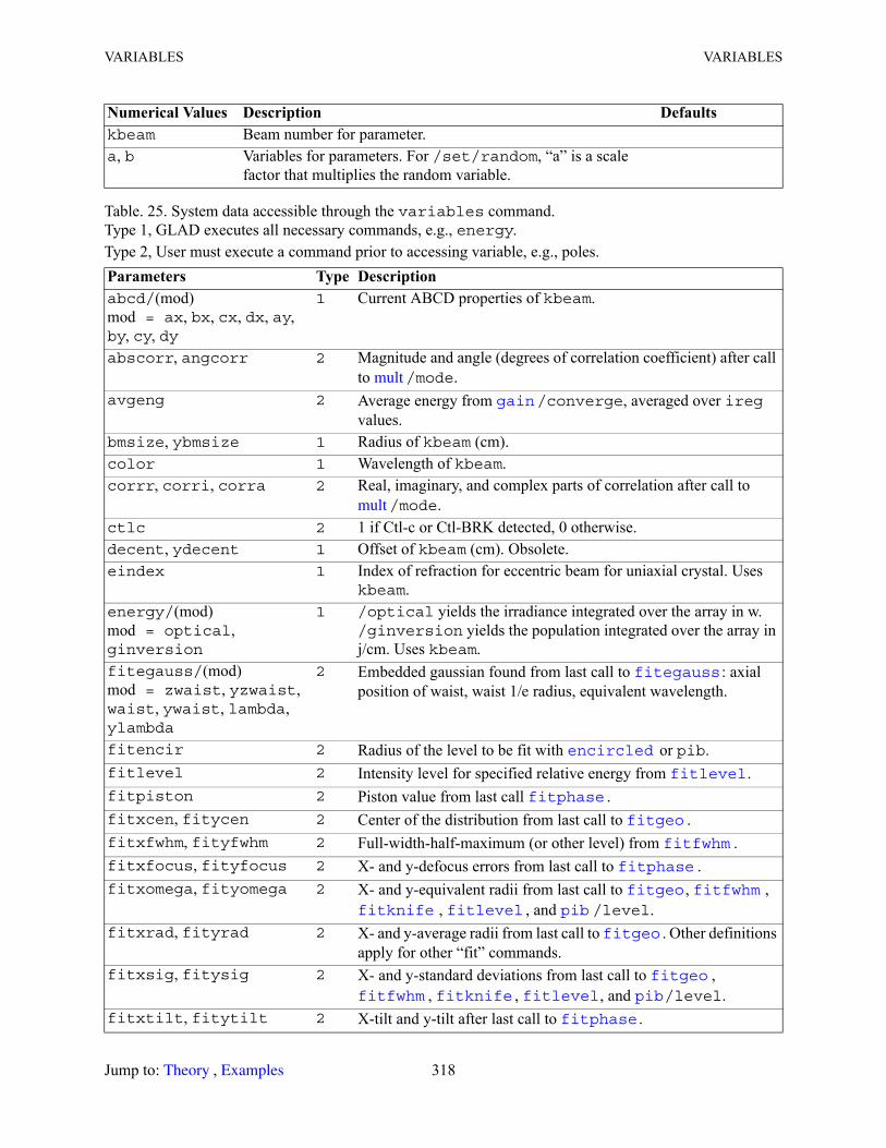
VARIABLES VARIABLES
Numerical Values Description Defaultskbeam Beam number for parameter.a, b Variables for parameters. For /set/random, “a” is a scale
factor that multiplies the random variable.
Table. 25. System data accessible through the variables command. Type 1, GLAD executes all necessary commands, e.g., energy.Type 2, User must execute a command prior to accessing variable, e.g., poles.Parameters Type Descriptionabcd/(mod)mod = ax, bx, cx, dx, ay, by, cy, dy
1 Current ABCD properties of kbeam.
abscorr, angcorr 2 Magnitude and angle (degrees of correlation coefficient) after call to /mode.
avgeng 2 Average energy from /converge, averaged over ireg values.
bmsize, ybmsize 1 Radius of kbeam (cm).color 1 Wavelength of kbeam.corrr, corri, corra 2 Real, imaginary, and complex parts of correlation after call to
/mode.ctlc 2 1 if Ctl-c or Ctl-BRK detected, 0 otherwise.decent, ydecent 1 Offset of kbeam (cm). Obsolete.eindex 1 Index of refraction for eccentric beam for uniaxial crystal. Uses
kbeam.energy/(mod)mod = optical, ginversion
1 /optical yields the irradiance integrated over the array in w. /ginversion yields the population integrated over the array in j/cm. Uses kbeam.
fitegauss/(mod)mod = zwaist, yzwaist, waist, ywaist, lambda, ylambda
2 Embedded gaussian found from last call to : axial position of waist, waist 1/e radius, equivalent wavelength.
fitencir 2 Radius of the level to be fit with or pib.fitlevel 2 Intensity level for specified relative energy from .fitpiston 2 Piston value from last call .fitxcen, fitycen 2 Center of the distribution from last call to .fitxfwhm, fityfwhm 2 Full-width-half-maximum (or other level) from .fitxfocus, fityfocus 2 X- and y-defocus errors from last call to .fitxomega, fityomega 2 X- and y-equivalent radii from last call to , ,
, , and /level.fitxrad, fityrad 2 X- and y-average radii from last call to . Other definitions
apply for other “fit” commands.fitxsig, fitysig 2 X- and y-standard deviations from last call to ,
, , , and /level.fitxtilt, fitytilt 2 X-tilt and y-tilt after last call to .
mult
gain
mult
fitegauss
encircled fitlevel
fitphase fitgeo
fitfwhm fitphase
fitgeo fitfwhm fitknife fitlevel pib
fitgeo
fitgeo fitfwhm fitknife fitlevel pib
fitphase
Jump to: , 318 Theory Examples

VARIABLES VARIABLES
focus/(abcd or waist) 1 Sets the variable to the distance from the current position to the geometrical focus (abcd) or gaussian beam waist (waist). Similar to the /list command. Uses kbeam.
geodata/(mod)mod = zwaistx, zwaisty, waistx, waisty, iplanx, iplany, m2x, m2y, ewx, ewy, radx, rady, bsx, bsy, zrayx, zrayy, zdistx, zdisty, insidx, insidy, refradiusx, refradiusy, wsx, wsy, zswitchx, zswitchy
2 Displays current values of geodata for kbeam.zwaist(x,y): position of waistwaist(x,y): size of waistiplan(x,y): 0, curved reference; 1, plane reference surfacem2(x,y): M-squared value as determined by last call to fitmsq.ew(x,y): Effective wavelength form M-squared value.rad(x,y): Radius of phase.bs(x,y): Current beam radius.zray(x,y): Rayleigh range.zdist(x,y): Distance from zwaist to current position.insid(x,y): Inside or outside the near-far field boundary.refradius(x,y): Reference surface radius: 1e20 if not used.ws(x,y): Width of the beam at current point.zswitch(x,y): Distance from waist to point of expanding units.
global/(mod)mod = grx, gry, grz, gix, giy, giz, gjx, gjy, gjz, gkx, gky, gkz, opl, ppl, xang, yang, zang, x1ang, y1ang, z1ang, parity
1 Displays current global properties of specified beam. Uses kbeam.grx, gry, grz: current global position of waistgix, giy, giz, gjx, gjy, gjz, gkx, gky, gkz: elements of global orientation matrix (ith, jth and kth columns).opl, ppl: optical path length and physical path lengthxang, yang, zang: Euler angles (first solution).x1ang, y1ang, z1ang: Euler angles (alternate solution).parity: Parity of global orientation matrix.
index 1 Index of refraction. Uses kbeam.iplane, yiplane 1 Phase bias flag of kbeam.lensgroup/(mod)mod = xmag, ymag, oblique
2 Magnification factors due to incidence on tilted surfaces after use of lensgroup.
line 1 Sets variable to the current line number. Useful for debugging.macro/(mod)mod = iteration, maxiteration, level, remaining
1 Macro loop information. Current iteration, maximum iteration, current macro level, and remaining iterations
magchgvec 2 Magnitude of change vector for optimization.memory/(mod)mod = total, allocated, free, maximum, speedratio
1 Physical memory: total, total on system; allocated, currently allocated to GLAD; free, free physical memory (not reliable); maximum, maximum allowed memory set by user (0 if no maximum has been set); speedratio, ratio of current speed to initial speed at with small memory. The speed ratio will drop if the memory allocation is higher than 75% to 90% of total memory.
merit 2 Current value of merit function for optimization.
Table. 25. System data accessible through the variables command. (Continued)Type 1, GLAD executes all necessary commands, e.g., energy.Type 2, User must execute a command prior to accessing variable, e.g., poles.Parameters Type Description
focus
Jump to: , 319 Theory Examples
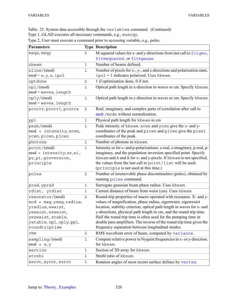
VARIABLES VARIABLES
msqx, msqy 2 M-squared values for x- and y-directions from last call to , , or .
nbeam 1 Number of beams defined.nline/(mod)mod = x, y, z, ipol
1 Number of pixels for x-, y-, and z-directions and polarization state, ipol = 1 indicates polarized. Uses kbeam.
optdone 2 1 if optimization done, 0 if not.opl/(mod)mod = waves, length
1 Optical path length in x-direction in waves or cm. Specify kbeam.
oply/(mod)mod = waves, length
1 Optical path length in y-direction in waves or cm. Specify kbeam.
pcorrr, pcorri, pcorra 2 Real, imaginary, and complex parts of correlation after call to /mode without normalization.
ppl 1 Physical path length for kbeam in cmpeak/(mod)mod = intensity, xcen, ycen, picen, pjcen
1 Peak intensity of kbeam. xcen and ycen give the x- and y- coordinates of the peak and picen and pjcen give the pixel coordinates of the peak.
photons 1 Number of photons in kbeam.point/(mod)mod = intensity, sr, si, pr, pi,ginversion, principle
1 Intensity or for s- and p-polarizations: s-real, s-imaginary, p-real, p-imaginary, and the population inversion specified point. Specify kbeam and A and B for x- and y-pixels. If kbeam is not specified, the values from the last call to point/list will be used.(principle is not used at this time.)
poles 2 Number of irremovable phase discontinuities (poles), obtained by running command.
prad, yprad 1 Surrogate gaussian beam phase radius. Uses kbeam.rdist, yrdist 1 Current distance of beam from waist (cm). Uses kbeam.resonator/(mod)mod = mag, ymag, radius, yradius, ewaist, yewaist, ezwaist, yezwaist, stable, ystable, opl, oply, ppl, roundtriptime
2 Round-trip properties of macro operated with resonator. X- and y-values of magnification, phase radius, eigenwaist, eigenwaist location, stability criterion, optical path length in waves for x- and y-directions, physical path length in cm, and the round trip time. Half the round trip time is often used for the pumping time in double pass amplifiers. The inverse of the round trip time gives the frequency separation between longitudinal modes.
rms 2 RMS wavefront error of beam, computed by .sampling/(mod)mod = x, y
1 Compute relative power in Nyquist frequencies in x- or y-direction. for kbeam.
section 1 Section of 3D array for kbeam.strehl 1 Strehl ratio of kbeam.sxrot, syrot, szrot 1 Rotation angles of most recent surface defines by .
Table. 25. System data accessible through the variables command. (Continued)Type 1, GLAD executes all necessary commands, e.g., energy.Type 2, User must execute a command prior to accessing variable, e.g., poles.Parameters Type Description
fitgeo fitmsquared fitegauss
mult
poles
variance
vertex
Jump to: , 320 Theory Examples
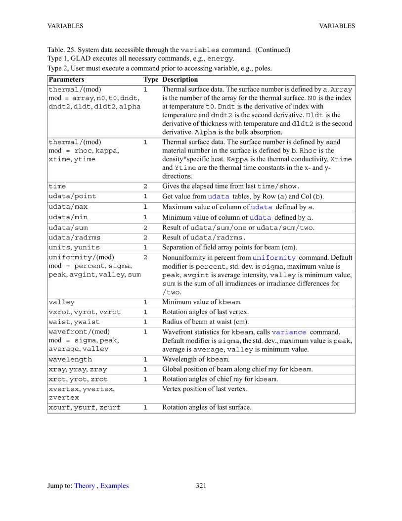
VARIABLES VARIABLES
thermal/(mod)mod = array, n0, t0, dndt, dndt2, dldt, dldt2, alpha
1 Thermal surface data. The surface number is defined by a. Array is the number of the array for the thermal surface. N0 is the index at temperature t0. Dndt is the derivative of index with temperature and dndt2 is the second derivative. Dldt is the derivative of thickness with temperature and dldt2 is the second derivative. Alpha is the bulk absorption.
thermal/(mod)mod = rhoc, kappa, xtime, ytime
1 Thermal surface data. The surface number is defined by aand material number in the surface is defined by b. Rhoc is the density*specific heat. Kappa is the thermal conductivity. Xtime and Ytime are the thermal time constants in the x- and y-directions.
time 2 Gives the elapsed time from last time/show.udata/point 1 Get value from tables, by Row (a) and Col (b).udata/max 1 Maximum value of column of defined by a.udata/min 1 Minimum value of column of defined by a.udata/sum 2 Result of udata/sum/one or udata/sum/two.udata/radrms 2 Result of udata/radrms.units, yunits 1 Separation of field array points for beam (cm).uniformity/(mod)mod = percent, sigma, peak, avgint, valley, sum
2 Nonuniformity in percent from command. Default modifier is percent, std. dev. is sigma, maximum value is peak, avgint is average intensity, valley is minimum value, sum is the sum of all irradiances or irradiance differences for /two.
valley 1 Minimum value of kbeam.vxrot, vyrot, vzrot 1 Rotation angles of last vertex.waist, ywaist 1 Radius of beam at waist (cm).wavefront/(mod)mod = sigma, peak, average, valley
1 Wavefront statistics for kbeam, calls command. Default modifier is sigma, the std. dev., maximum value is peak, average is average, valley is minimum value.
wavelength 1 Wavelength of kbeam.xray, yray, zray 1 Global position of beam along chief ray for kbeam.xrot, yrot, zrot 1 Rotation angles of chief ray for kbeam.xvertex, yvertex, zvertex
Vertex position of last vertex.
xsurf, ysurf, zsurf 1 Rotation angles of last surface.
Table. 25. System data accessible through the variables command. (Continued)Type 1, GLAD executes all necessary commands, e.g., energy.Type 2, User must execute a command prior to accessing variable, e.g., poles.Parameters Type Description
udata udata udata
uniformity
variance
Jump to: , 321 Theory Examples

VARIANCE VARIANCE
ExamplePut the wavelength of beam 2 into variable Lambda.variable/set Lambda 2 wavelength
VARIANCE Calculate wavefront rms error. Diagnostics
Description: VARIANCECalculates the intensity weighted wavefront or irradiance rms (same as command rms).
wavefront (204)
irradiance (205)
The standard deviation, peak, valley, and average value of the wavefront are available with the /set/parameter command with the wavefront parameter.
zigzag/(mod)mod = width_zigzag adjusted_zigzag height_zigzag length_zigzag reflections_zigzag angle_zigzag beamunits_zigzag gainunits_zigzag stepangle_zigzag stepstraight_zigzag position_zigzag pixel_zigzag totalsteps_zigzag
1 Properties of zigzag amplifier: width, adjusted width with 1/2 pixel added. height, length, number of reflections, angle of the light relative to the axis of the zigzag amplifier, units of the beam (transverse to the beam), units of the gain region, step length along the angle (optical path), step length along the amplifier axis, current position in cm, current position in pixels, total number of steps through the amplifier.
zreff 1 Current z-position of kbeam (cm).
Command Form(s): VARIANCE variance/wavefront ibeams threshold
variance/irradiance ibeams threshold
Table. 25. System data accessible through the variables command. (Continued)Type 1, GLAD executes all necessary commands, e.g., energy.Type 2, User must execute a command prior to accessing variable, e.g., poles.Parameters Type Description
RMSI x y,( )W x y,( )2 xd yd
I x y,( ) xd yd------------------------------------------------------
I x y,( )W x y,( ) xd ydI x y,( ) xd yd
----------------------------------------------------
2
–=
RMSI x y,( )2 xd yd
xd yd-----------------------------------
I x y,( ) xd ydxd yd
---------------------------------
–
2
=
variables
Jump to: , 322 Theory Examples
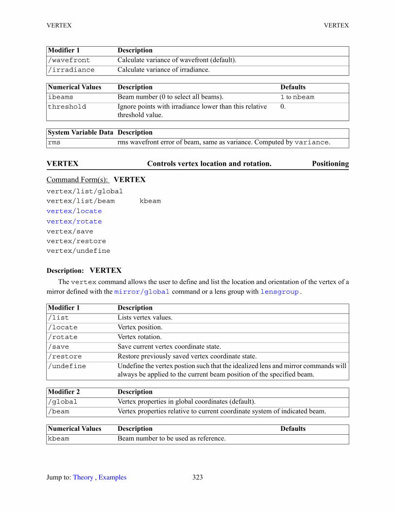
VERTEX VERTEX
VERTEX Controls vertex location and rotation. Positioning
Description: VERTEXThe vertex command allows the user to define and list the location and orientation of the vertex of a
mirror defined with the command or a lens group with .
Modifier 1 Description /wavefront Calculate variance of wavefront (default)./irradiance Calculate variance of irradiance.
Numerical Values Description Defaultsibeams Beam number (0 to select all beams). 1 to nbeamthreshold Ignore points with irradiance lower than this relative
threshold value.0.
System Variable Data Description rms rms wavefront error of beam, same as variance. Computed by variance.
Command Form(s): VERTEX vertex/list/global
vertex/list/beam kbeam
vertex/save
vertex/restore
vertex/undefine
Modifier 1 Description /list Lists vertex values./locate Vertex position./rotate Vertex rotation./save Save current vertex coordinate state./restore Restore previously saved vertex coordinate state./undefine Undefine the vertex postion such that the idealized lens and mirror commands will
always be applied to the current beam position of the specified beam.
Modifier 2 Description /global Vertex properties in global coordinates (default)./beam Vertex properties relative to current coordinate system of indicated beam.
Numerical Values Description Defaultskbeam Beam number to be used as reference.
vertex/locate vertex/rotate
mirror/global lensgroup
Jump to: , 323 Theory Examples
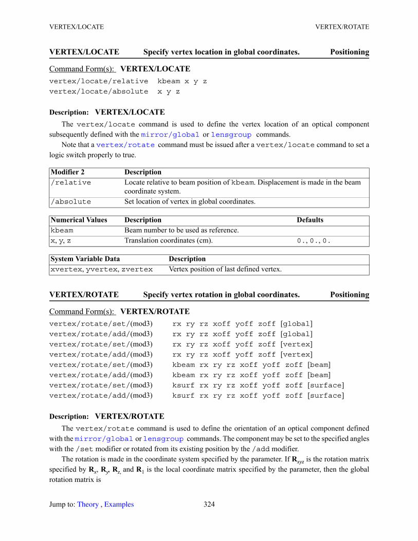
VERTEX/LOCATE VERTEX/ROTATE
VERTEX/LOCATE Specify vertex location in global coordinates. Positioning
Description: VERTEX/LOCATEThe vertex/locate command is used to define the vertex location of an optical component
subsequently defined with the or commands. Note that a command must be issued after a vertex/locate command to set a
logic switch properly to true.
VERTEX/ROTATE Specify vertex rotation in global coordinates. Positioning
Description: VERTEX/ROTATEThe vertex/rotate command is used to define the orientation of an optical component defined
with the or commands. The component may be set to the specified angles with the /set modifier or rotated from its existing position by the /add modifier.
The rotation is made in the coordinate system specified by the parameter. If Rxyz is the rotation matrix specified by Rx, Ry, Rz, and R1 is the local coordinate matrix specified by the parameter, then the global rotation matrix is
Command Form(s): VERTEX/LOCATE vertex/locate/relative kbeam x y z
vertex/locate/absolute x y z
Modifier 2 Description /relative Locate relative to beam position of kbeam. Displacement is made in the beam
coordinate system./absolute Set location of vertex in global coordinates.
Numerical Values Description Defaultskbeam Beam number to be used as reference.x, y, z Translation coordinates (cm). 0., 0., 0.
System Variable Data Description xvertex, yvertex, zvertex Vertex position of last defined vertex.
Command Form(s): VERTEX/ROTATE vertex/rotate/set/(mod3) rx ry rz xoff yoff zoff [global]vertex/rotate/add/(mod3) rx ry rz xoff yoff zoff [global]vertex/rotate/set/(mod3) rx ry rz xoff yoff zoff [vertex]vertex/rotate/add/(mod3) rx ry rz xoff yoff zoff [vertex]vertex/rotate/set/(mod3) kbeam rx ry rz xoff yoff zoff [beam]vertex/rotate/add/(mod3) kbeam rx ry rz xoff yoff zoff [beam]vertex/rotate/set/(mod3) ksurf rx ry rz xoff yoff zoff [surface]vertex/rotate/add/(mod3) ksurf rx ry rz xoff yoff zoff [surface]
mirror/global lensgroup vertex/rotate
mirror/global lensgroup
Jump to: , 324 Theory Examples
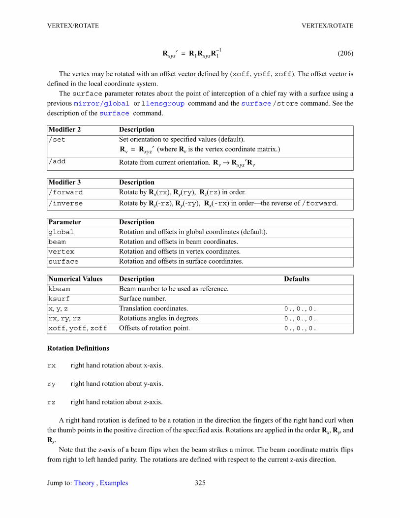
VERTEX/ROTATE VERTEX/ROTATE
(206)
The vertex may be rotated with an offset vector defined by (xoff, yoff, zoff). The offset vector is defined in the local coordinate system.
The surface parameter rotates about the point of interception of a chief ray with a surface using a previous or l command and the /store command. See the description of the command.
Rotation Definitions
rx right hand rotation about x-axis.
ry right hand rotation about y-axis.
rz right hand rotation about z-axis.
A right hand rotation is defined to be a rotation in the direction the fingers of the right hand curl when the thumb points in the positive direction of the specified axis. Rotations are applied in the order Rx, Ry, and Rz.
Note that the z-axis of a beam flips when the beam strikes a mirror. The beam coordinate matrix flips from right to left handed parity. The rotations are defined with respect to the current z-axis direction.
Modifier 2 Description /set Set orientation to specified values (default).
(where Rv is the vertex coordinate matrix.)/add Rotate from current orientation.
Modifier 3 Description /forward Rotate by Rx(rx), Ry(ry), Rz(rz) in order./inverse Rotate by Rz(-rz), Ry(-ry), Rx(-rx) in order—the reverse of /forward.
Parameter Description global Rotation and offsets in global coordinates (default).beam Rotation and offsets in beam coordinates.vertex Rotation and offsets in vertex coordinates.surface Rotation and offsets in surface coordinates.
Numerical Values Description Defaultskbeam Beam number to be used as reference.ksurf Surface number.x, y, z Translation coordinates. 0., 0., 0.rx, ry, rz Rotations angles in degrees. 0., 0., 0.xoff, yoff, zoff Offsets of rotation point. 0., 0., 0.
Rxyz′ R1RxyzR11–=
mirror/global lensgroup surface surface
Rv Rxyz′=
Rv Rxyz′Rv→
Jump to: , 325 Theory Examples
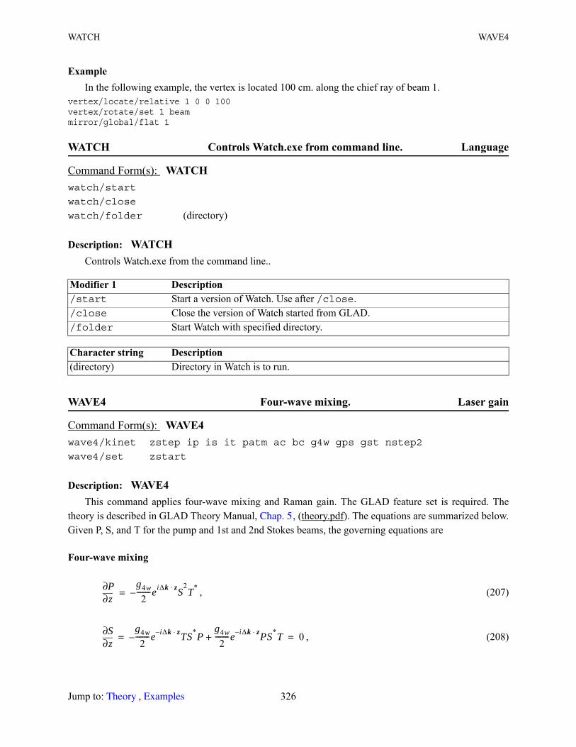
WATCH WAVE4
ExampleIn the following example, the vertex is located 100 cm. along the chief ray of beam 1.
vertex/locate/relative 1 0 0 100vertex/rotate/set 1 beammirror/global/flat 1
WATCH Controls Watch.exe from command line. Language
Description: WATCHControls Watch.exe from the command line..
WAVE4 Four-wave mixing. Laser gain
Description: WAVE4This command applies four-wave mixing and Raman gain. The GLAD feature set is required. The
theory is described in GLAD Theory Manual, , (theory.pdf). The equations are summarized below. Given P, S, and T for the pump and 1st and 2nd Stokes beams, the governing equations are
Four-wave mixing
, (207)
, (208)
Command Form(s): WATCH watch/start
watch/close
watch/folder (directory)
Modifier 1 Description /start Start a version of Watch. Use after /close./close Close the version of Watch started from GLAD./folder Start Watch with specified directory.
Character string Description (directory) Directory in Watch is to run.
Command Form(s): WAVE4 wave4/kinet zstep ip is it patm ac bc g4w gps gst nstep2
wave4/set zstart
Chap. 5
z∂∂P g4w
2--------eiΔk z⋅ S
2T*–=
z∂∂S g4w
2--------– e i– Δk z⋅ TS*P
g4w2
--------e i– Δk z⋅ PS*T+ 0= =
Jump to: , 326 Theory Examples
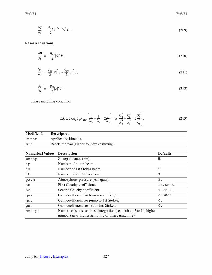
WAVE4 WAVE4
. (209)
Raman equations
, (210)
, (211)
. (212)
Phase matching condition
. (213)
Modifier 1 Description kinet Applies the kinetics.set Resets the z-origin for four-wave mixing.
Numerical Values Description Defaultszstep Z-step distance (cm). 0.ip Number of pump beam. 1
is Number of 1st Stokes beam. 2
it Number of 2nd Stokes beam. 3
patm Atmospheric pressure (Amagats). 3.
ac First Cauchy coefficient. 13.6e-5
bc Second Cauchy coefficient. 7.7e-11
g4w Gain coefficient for four-wave mixing. 0.0001
gps Gain coefficient for pump to 1st Stokes. 0.
gst Gain coefficient for 1st to 2nd Stokes. 0.
nstep2 Number of steps for phase integration (set at about 5 to 10, higher numbers give higher sampling of phase matching).
z∂∂T g4w
2--------eiΔk z⋅ S2P∗=
z∂∂P gps
2------- S 2P–=
z∂∂S gps
2------- P 2S
gst2
------ T 2S–=
z∂∂T gst
2------ S 2T–=
Δk 2πacbcPatm1λp----- 1
λt---- 2 1
λs-----–+ π
θp3
λp3
-----θt
3
λt3
----- 2θs
3
λs3
-----–+–≅
Jump to: , 327 Theory Examples
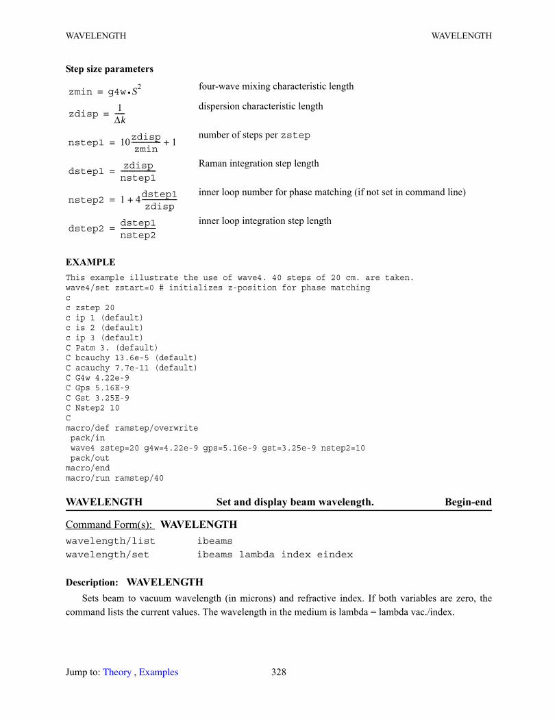
WAVELENGTH WAVELENGTH
Step size parameters
EXAMPLEThis example illustrate the use of wave4. 40 steps of 20 cm. are taken.wave4/set zstart=0 # initializes z-position for phase matchingcc zstep 20c ip 1 (default)c is 2 (default)c ip 3 (default)C Patm 3. (default)C bcauchy 13.6e-5 (default)C acauchy 7.7e-11 (default)C G4w 4.22e-9C Gps 5.16E-9C Gst 3.25E-9C Nstep2 10Cmacro/def ramstep/overwrite pack/in wave4 zstep=20 g4w=4.22e-9 gps=5.16e-9 gst=3.25e-9 nstep2=10 pack/outmacro/endmacro/run ramstep/40
WAVELENGTH Set and display beam wavelength. Begin-end
Description: WAVELENGTHSets beam to vacuum wavelength (in microns) and refractive index. If both variables are zero, the
command lists the current values. The wavelength in the medium is lambda = lambda vac./index.
four-wave mixing characteristic length
dispersion characteristic length
number of steps per zstep
Raman integration step length
inner loop number for phase matching (if not set in command line)
inner loop integration step length
Command Form(s): WAVELENGTH wavelength/list ibeams
wavelength/set ibeams lambda index eindex
zmin g4w S•2=
zdisp1
Δk------=
nstep1 10zdispzmin
------------------ 1+=
dstep1zdispnstep1---------------------=
nstep2 1 4dstep1zdisp
---------------------+=
dstep2dstep1nstep2---------------------=
Jump to: , 328 Theory Examples
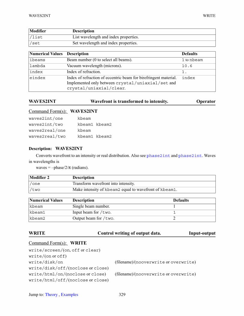
WAVES2INT WRITE
WAVES2INT Wavefront is transformed to intensity. Operator
Description: WAVES2INTConverts wavefront to an intensity or real distribution. Also see and . Waves
in wavelengths iswaves = –phase/2/π (radians).
WRITE Control writing of output data. Input-output
Modifier Description /list List wavelength and index properties. /set Set wavelength and index properties.
Numerical Values Description Defaultsibeams Beam number (0 to select all beams). 1 to nbeamlambda Vacuum wavelength (microns). 10.6
index Index of refraction. 1.
eindex Index of refraction of eccentric beam for birefringent material. Implemented only between crystal/uniaxial/set and crystal/uniaxial/clear.
index
Command Form(s): WAVES2INT waves2int/one kbeam
waves2int/two kbeam1 kbeam2
waves2real/one kbeam
waves2real/two kbeam1 kbeam2
Modifier 2 Description /one Transform wavefront into intensity. /two Make intensity of kbeam2 equal to wavefront of kbeam1.
Numerical Values Description Defaultskbeam Single beam number. 1kbeam1 Input beam for /two. 1
kbeam2 Output beam for /two. 2
Command Form(s): WRITE write/screen/(on, off or clear)write/(on or off)write/disk/on (filename)/(nooverwrite or overwrite)write/disk/off/(noclose or close)write/html/on/(noclose or close) (filename)/(nooverwrite or overwrite)write/html/off/(noclose or close)
phase2int phase2int
Jump to: , 329 Theory Examples

WRITE ZBOUND
Description: WRITESets output to terminal or disk file. If the disk file already exists, new output will be written at the end
of the existing information, unless /overwrite is specified. A pathname may be set with /path to define a prefix which is concatenated in front of the filename.
ZBOUND Position and size of Rayleigh range. Diagnostics
write/info
Modifier 1 Description /screen Sets output to screen (default)./off Turns off all output: screen, disk, and html./disk Controls output file for text./html Controls output file for html. File may be viewed by any browser./on Reverses write/off./info Displays current write info.
Modifier 2 Description /on Opens output file for text output or html (default)./off Close output file./clear For write/screen/clear, GladOut display is cleared.
Modifier 3 Description /noclose Leave output file open (default)./close Close output file, making it accessible to external programs such as editors for inspection
and modification.
Character String
Description
(filename) Name of the disk file. Do not include the parentheses. May be written as a 20 character expression (no back slashes). Alternately an expression of up to 80 characters may be used with single quotes in the form 'filename'. The filename is preceded by a path name if one has been defined with set/path.
String Modifier Description /nooverwrite No rewind of the output file (default)./overwrite Rewinds the file before writing on it.
Command Form(s): ZBOUND zbound/list ibeams
zbound/set ibeams waistx waisty zwaistx zwaisty
Command Form(s): WRITE (Continued)
set
Jump to: , 330 Theory Examples
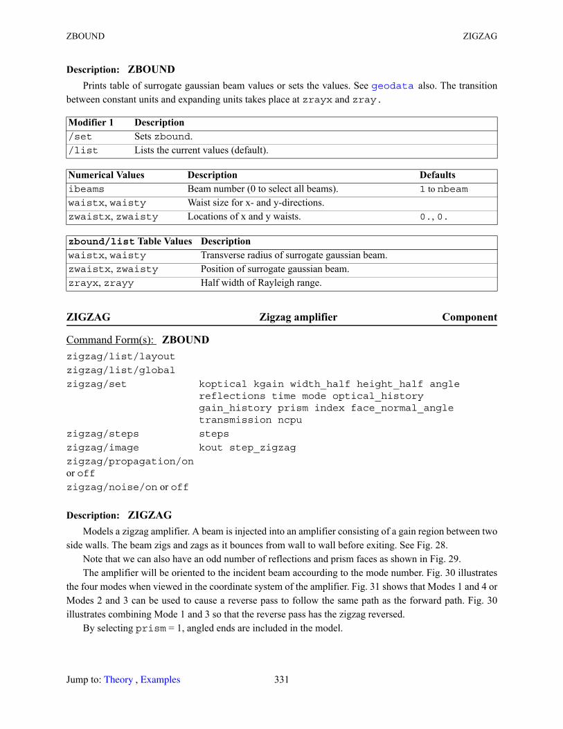
ZBOUND ZIGZAG
Description: ZBOUNDPrints table of surrogate gaussian beam values or sets the values. See also. The transition
between constant units and expanding units takes place at zrayx and zray.
ZIGZAG Zigzag amplifier Component
Description: ZIGZAGModels a zigzag amplifier. A beam is injected into an amplifier consisting of a gain region between two
side walls. The beam zigs and zags as it bounces from wall to wall before exiting. See Fig. 28.Note that we can also have an odd number of reflections and prism faces as shown in Fig. 29.The amplifier will be oriented to the incident beam accourding to the mode number. Fig. 30 illustrates
the four modes when viewed in the coordinate system of the amplifier. Fig. 31 shows that Modes 1 and 4 or Modes 2 and 3 can be used to cause a reverse pass to follow the same path as the forward path. Fig. 30 illustrates combining Mode 1 and 3 so that the reverse pass has the zigzag reversed.
By selecting prism = 1, angled ends are included in the model.
Modifier 1 Description /set Sets zbound./list Lists the current values (default).
Numerical Values Description Defaultsibeams Beam number (0 to select all beams). 1 to nbeamwaistx, waisty Waist size for x- and y-directions.zwaistx, zwaisty Locations of x and y waists. 0., 0.
zbound/list Table Values Description waistx, waisty Transverse radius of surrogate gaussian beam.zwaistx, zwaisty Position of surrogate gaussian beam.zrayx, zrayy Half width of Rayleigh range.
Command Form(s): ZBOUND zigzag/list/layout
zigzag/list/global
zigzag/set koptical kgain width_half height_half angle reflections time mode optical_history gain_history prism index face_normal_angle transmission ncpu
zigzag/steps steps
zigzag/image kout step_zigzag
zigzag/propagation/on or offzigzag/noise/on or off
geodata
Jump to: , 331 Theory Examples

ZIGZAG ZIGZAG
The angle from the prism face normal to the ray is I, the angle from the axis to the ray is a, and the angle from the axis to the prism surface is β. All angles are positive for a right-hand rotation about the y-axis taken in the x-z plane. See Fig. 33.
If the prism face is made shallower than the optimum folding configuration (an angle greater than internal ray angle α), some light can reflect off the back side of the prism face to create parasitic rays that
Fig. 28. Configuration for a zigzag amplifier showing one a pair of reflections forming one complete cycle. In this figure no prism faces are shown. A full cycle of two reflections is shown, but any number of reflections may be used. The beam overlaps upon reflection at each mirror, causing higher inversion depletion.
The pixels are matched to avoid interpolation and the associated errors. The optical beam, with units Δx, enters on the left at an angle α to the axis of the amplifier region. The transverse units for the amplifier should be Δxg = Δx/cos(α). The units of the amplifier along the axis should be Δz = Δx/tan(α). The optical propagation along the slant line takes steps of Δs = Δxg/cos(α) = Δx/cos2(α). The gain points are organized into a 3D array.
In this elementary drawing, the aperture is shown with only five pixels. The mirrors are shifted a half pixel. The length for one complete cycle is ten—twice the number of aperture pixels.
Fig. 29. An odd number of reflections may be used. In this figure, prism ends have been attached and there is refraction between the external and internal angles.
Δxg
2---------Δx
g
Δx
Δs
Δz
left mirror
rightmirror
input
output(or additional cycles)
234567 2
34567
Jump to: , 332 Theory Examples
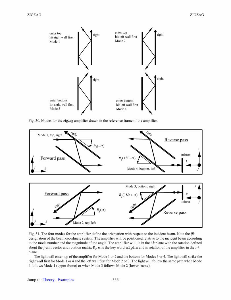
ZIGZAG ZIGZAG
Fig. 30. Modes for the zigzag amplifier drawn in the reference frame of the amplifier.
Fig. 31. The four modes for the amplifier define the orientation with respect to the incident beam. Note the ijk designation of the beam coordinate system. The amplifier will be positioned relative to the incident beam according to the mode number and the magnitude of the angle. The amplifier will lie in the i-k plane with the rotation defined about the j-unit vector and rotation matrix Rj. α is the key word alpha and is rotation of the amplifier in the i-k plane.
The light will enter top of the amplifier for Mode 1 or 2 and the bottom for Modes 3 or 4. The light will strike the right wall first for Mode 1 or 4 and the left wall first for Mode 2 or 3. The light will follow the same path when Mode 4 follows Mode 1 (upper frame) or when Mode 3 follows Mode 2 (lower frame).
enter bottomhit right wall firstMode 3
enter tophit right wall firstMode 1
enter tophit left wall firstMode 2
enter bottomhit left wall firstMode 4
right
right
right
right
Mode 1, top, right
Forward pass
Rj
α–( )
Forward pass
Reverse pass
Reverse passRjα( )
Rj
180 α–( )
Mode 4, bottom, leftkj
i
kj
i
Mode 2, top, left
Mode 3, bottom, right
mirror
mirror
Rj
180 α+( )
k
j
i
k
j
i
rightright
right
right
Jump to: , 333 Theory Examples
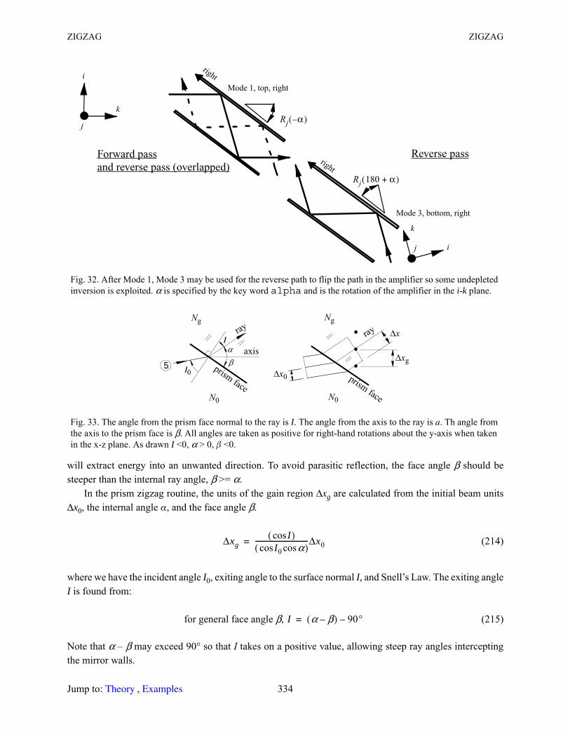
ZIGZAG ZIGZAG
will extract energy into an unwanted direction. To avoid parasitic reflection, the face angle β should be steeper than the internal ray angle, β >= α.
In the prism zigzag routine, the units of the gain region Δxg are calculated from the initial beam units Δx0, the internal angle α, and the face angle β.
(214)
where we have the incident angle I0, exiting angle to the surface normal I, and Snell’s Law. The exiting angle I is found from:
for general face angle β, (215)
Note that α – β may exceed 90° so that I takes on a positive value, allowing steep ray angles intercepting the mirror walls.
Fig. 32. After Mode 1, Mode 3 may be used for the reverse path to flip the path in the amplifier so some undepleted inversion is exploited. α is specified by the key word alpha and is the rotation of the amplifier in the i-k plane.
Fig. 33. The angle from the prism face normal to the ray is I. The angle from the axis to the ray is a. Th angle from the axis to the prism face is β. All angles are taken as positive for right-hand rotations about the y-axis when taken in the x-z plane. As drawn I <0, α > 0, β <0.
Mode 1, top, right
Forward passand reverse pass (overlapped)
Rj
α–( )
Reverse pass
Rj
180 α+( )
Mode 3, bottom, right
k
j
i
k
j i
right
right
5
Ιx
x0Ι0
Ng
N0
Ng
N0
axis
prismface
ray
prismface
ray
xg
ΔxgIcos( )
I0cos αcos( )-------------------------------Δx0=
I α β–( ) 90°–=
Jump to: , 334 Theory Examples
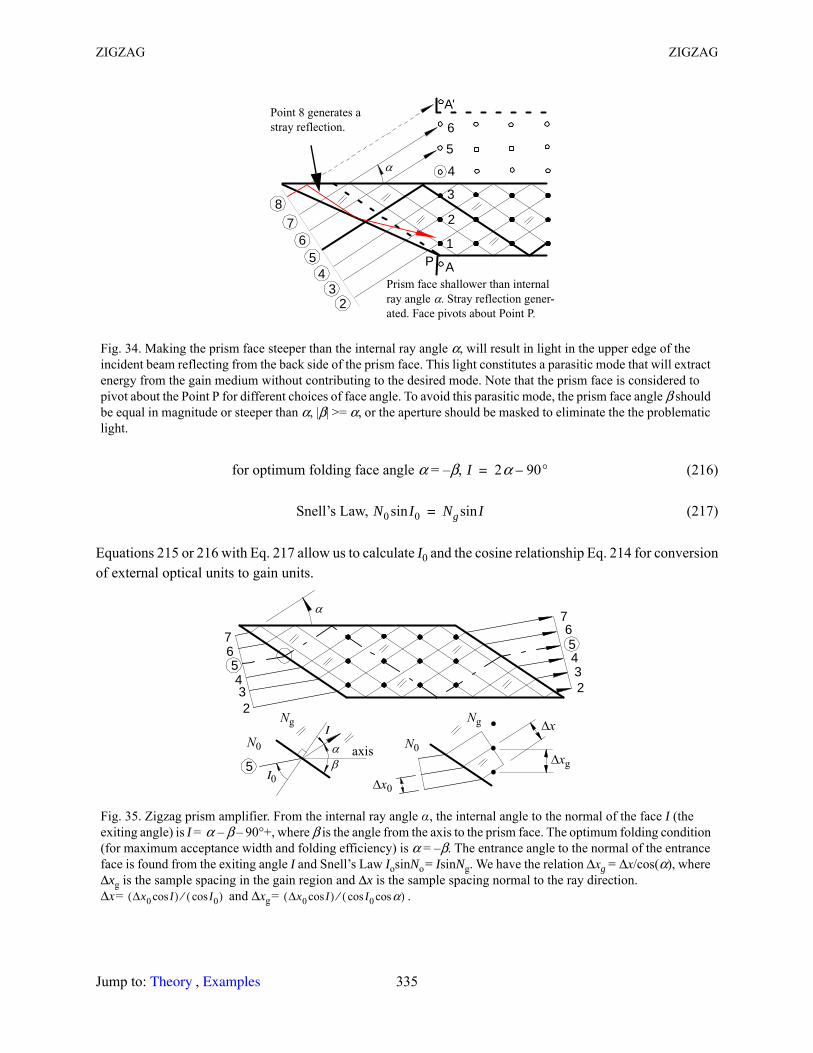
ZIGZAG ZIGZAG
for optimum folding face angle α = –β, (216)
Snell’s Law, (217)
Equations 215 or 216 with Eq. 217 allow us to calculate I0 and the cosine relationship Eq. 214 for conversion of external optical units to gain units.
Fig. 34. Making the prism face steeper than the internal ray angle α, will result in light in the upper edge of the incident beam reflecting from the back side of the prism face. This light constitutes a parasitic mode that will extract energy from the gain medium without contributing to the desired mode. Note that the prism face is considered to pivot about the Point P for different choices of face angle. To avoid this parasitic mode, the prism face angle β should be equal in magnitude or steeper than α, |β| >= α, or the aperture should be masked to eliminate the the problematic light.
Fig. 35. Zigzag prism amplifier. From the internal ray angle α, the internal angle to the normal of the face I (the exiting angle) is I = α – β – 90°+, where β is the angle from the axis to the prism face. The optimum folding condition (for maximum acceptance width and folding efficiency) is α = –β. The entrance angle to the normal of the entrance face is found from the exiting angle I and Snell’s Law IosinNo = IsinNg. We have the relation Δxg = Δx/cos(α), where Δxg is the sample spacing in the gain region and Δx is the sample spacing normal to the ray direction. Δx = and Δxg = .
23
45
67
1
2
3
456
8
A
A'
PPrism face shallower than internal ray angle . Stray reflection gener-ated. Face pivots about Point P.
Point 8 generates a stray reflection.
I 2α 90°–=
N0 I0sin Ng Isin=
234
67
234
67
5
5
5
Ι x
x0
xgΙ0
Ng
N0
Ng
N0 axis
Δx0 Icos( ) I0cos( )⁄ Δx0 Icos( ) I0cos αcos( )⁄
Jump to: , 335 Theory Examples
ZIGZAG ZIGZAG
Brewster’s Angle ExampleFor Brewsters’s angle operation from air to index N0 = 1.5, we have two solutions:
incident angle (air), (218)
exiting angle (glass), (219)
The optimum folding angle at Brewster’s angle has the two solutions:
(220)
If the face angle β is less than the magnitude of the ray angle α, there will be parasitic mode. This condition is satisfied if I > 0, α <= 61.8450° or if I <0, α <= 28.1550°.
See example for illustrations of the use of the zigzag command.
Modifier 1 Description /set Set halfwidth of sidewalls, length of gain region, integer number of sidewall
reflections, and repumping time. The angle of incidence against the sidewalls and the number of propagation step is computed.
/list Lists the current values (default)./steps Number of steps to be used. Zero causes all remaining steps to be completed./image 2D Image of optical beam of zigzag amplifier formed into square array "kout" at
current (or specified) step./propagation Controls diffraction propagation./noise Controls spontaneous emission for gain calculations.
Modifier 2 Description list/layout Operational properties exclusive of global locations (default).list/global Global properties./on Implement effect (default)./off No not implement effect.
Numerical Values Description Defaultskoptical Optical beam that propagates.kgain Gain array. Requires 3D, polarized definition.width_half Half width of separation of side mirrors for zigzag
amplifier, x-direction. Will be set to an integer number of pixels.
I0BN0 1.5=( ) N0 N0 1.5=
atan 56.3099± °= =
I N0 1.5=( )I0B
sin
N0--------------
N0 1.5=
asin 33.6901°±= =
α β–=( ) α 90° I+2
-----------------= α 28.1550° 61.8450°,=
ex121.
Jump to: , 336 Theory Examples
ZIGZAG ZIGZAG
height_half Half height of side mirrors for zigzag amplifier. Mirrors are assumed to be vertical. Will be set to an integer number of pixels.
angle Angle of optical beam relative to the axis of the zigzag amplifier. The top of the amplifier faces the incident beam. The units of the gain region will be calculated from the this angle and the index of refraction of the gain region. Enter a positive value for the angle. The relative direction is determined by mode.
reflections Number of reflections for zig-zag gain region. Assumes the beam exits in the center
time Time for pumping medium.mode Controls propagation (in amplifier coordinate system):
1, , beam enters top and strikes right mirror first;2, , beam enters top and strikes left mirror first;3, , beam enters bottom and strikes right mirror first;4, , beam enters bottom and strikes left mirror first.
1
optical_history Optical history array. Must match x-dimension of target and the y-dimension must exceed the number of steps.
gain_history Gain history array. Must match x-dimension of target and y-dimension must exceed the number of steps and be polarized.
prism 1, add prism ends, 0 no prism ends.index Index of refraction of the gain region for the prism zigzag
amplifier.face_normal_angle Angle (deg) of the normal of the prism face from
amplifier axis—positive for a right-hand y-rotation in the x-z plane. By default the surface of the face is matched to the ray angle, so the angle of the prism face normal is 90° – angle. This achieves an acceptance width equal to twice the gain width and gives best folding efficiency.
90-angle
ncpu Number of CPU’s to be used. For arrays less than about 256 x 256. The default of ncpu = 1 will give the best speed.
1
Numerical Values Description (Continued) Defaults
Rj α–( )
Rj α( )
Rj 180 α+( )
Rj 180 α–( )
Jump to: , 337 Theory Examples
ZONE ZONE
ZONE Extend region of constant units. Propagation
Description: ZONEGLAD will interpolate information in arrays of different sizes so that multiple beam interactions may
be calculated. The interpolation may introduce errors when the wavelengths are separated widely. The
transmission 3D Transmission/phase array to be applied in the gain coordinate system to include bulk absorption and phase aberrations. It may have two polarization states. The complex amplitude of this array is multiplied into the beam at each gain step. The transverse x- and y-sizes of the array must match the gain array kgain. If the z-size is less than that of the gain array, multiple steps are taken in gain with the same transmission array before advancing to the next transmission sheet. Transmission and phase distributions should be setup to give the proper effect when applied the actual total number of gain steps. If the optical array is polarized and the transmission array is not, the transmission array is applied to both polarization states of the optical array. Otherwise the polarization states are matched up.
Systen Variable Data Description zigzag/width Half width of separation of side mirrors for zigzag amplifier, x-direction.zigzag/adjusted Width adjusted to be an integer number of pixels plus on half pixel.zigzag/height Half height of side mirrors for zigzag amplifier, y-direction.zigzag/length Length of zigzag gain region.zigzag/reflections Number of reflections for zig-zag gain region.zigzag/angle Angle of optical beam relative to the axis of the zigzag amplifier.zigzag/beamunits X-units for beam in zigzag amplifier.zigzag/gainunits Allow or restrict gain operations in resonator/eigen/test.zigzag/stepangle Propagation length per step along the angled optical path.zigzag/stepstraight Length per step straigh through the zigzag resonator.zigzag/position Current position along zigzag amplifier (pixels).zigzag/pixel Current translation of beam relative to the center of the zigzag amplifier.zigzag/totalsteps Total number of steps along the length of the zigzag amplifier.
Command Form(s): ZONE zone/list
zone/fix center halfw krefbeam
zone/xyfix xcenter ycenter xhalfw yhalfw krefbeam
zone/unfix
zone/in kbeam
zone/out kbeam
Numerical Values Description (Continued) Defaults
Jump to: , 338 Theory Examples
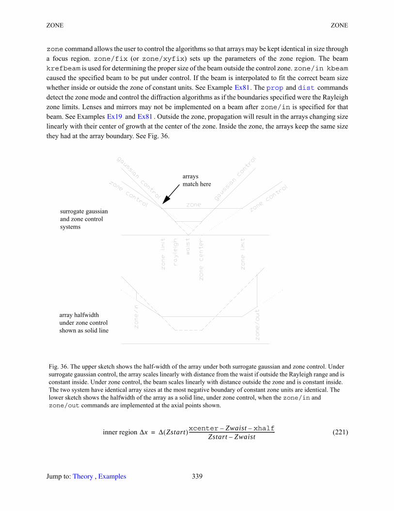
ZONE ZONE
zone command allows the user to control the algorithms so that arrays may be kept identical in size through a focus region. zone/fix (or zone/xyfix) sets up the parameters of the zone region. The beam krefbeam is used for determining the proper size of the beam outside the control zone. zone/in kbeamcaused the specified beam to be put under control. If the beam is interpolated to fit the correct beam size whether inside or outside the zone of constant units. See Example . The and commands detect the zone mode and control the diffraction algorithms as if the boundaries specified were the Rayleigh zone limits. Lenses and mirrors may not be implemented on a beam after zone/in is specified for that beam. See Examples and . Outside the zone, propagation will result in the arrays changing size linearly with their center of growth at the center of the zone. Inside the zone, the arrays keep the same size they had at the array boundary. See Fig. 36.
inner region (221)
Fig. 36. The upper sketch shows the half-width of the array under both surrogate gaussian and zone control. Under surrogate gaussian control, the array scales linearly with distance from the waist if outside the Rayleigh range and is constant inside. Under zone control, the beam scales linearly with distance outside the zone and is constant inside. The two system have identical array sizes at the most negative boundary of constant zone units are identical. The lower sketch shows the halfwidth of the array as a solid line, under zone control, when the zone/in and zone/out commands are implemented at the axial points shown.
Ex81 prop dist
Ex19 Ex81
surrogate gaussian
and zone control
systems
arrays
match here
array halfwidth
under zone control
shown as solid line
Δx Δ Zstart( )xcenter Zwaist– xhalf–Zstart Zwaist–
-------------------------------------------------------------------------=
Jump to: , 339 Theory Examples
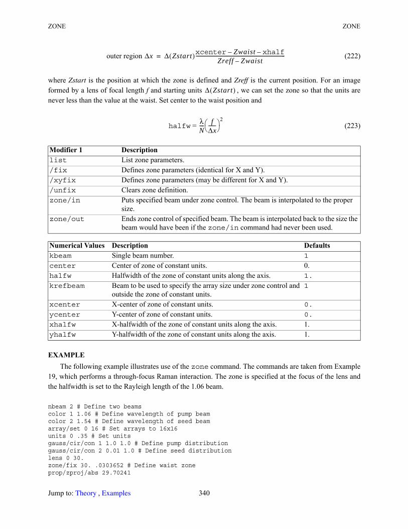
ZONE ZONE
outer region (222)
where Zstart is the position at which the zone is defined and Zreff is the current position. For an image formed by a lens of focal length f and starting units , we can set the zone so that the units are never less than the value at the waist. Set center to the waist position and
halfw = (223)
EXAMPLEThe following example illustrates use of the zone command. The commands are taken from Example
19, which performs a through-focus Raman interaction. The zone is specified at the focus of the lens and the halfwidth is set to the Rayleigh length of the 1.06 beam.
nbeam 2 # Define two beamscolor 1 1.06 # Define wavelength of pump beamcolor 2 1.54 # Define wavelength of seed beamarray/set 0 16 # Set arrays to 16x16units 0 .35 # Set unitsgauss/cir/con 1 1.0 1.0 # Define pump distributiongauss/cir/con 2 0.01 1.0 # Define seed distributionlens 0 30.zone/fix 30. .0303652 # Define waist zoneprop/zproj/abs 29.70241
Modifier 1 Description list List zone parameters./fix Defines zone parameters (identical for X and Y)./xyfix Defines zone parameters (may be different for X and Y)./unfix Clears zone definition.zone/in Puts specified beam under zone control. The beam is interpolated to the proper
size.zone/out Ends zone control of specified beam. The beam is interpolated back to the size the
beam would have been if the zone/in command had never been used.
Numerical Values Description Defaultskbeam Single beam number. 1
center Center of zone of constant units. 0.halfw Halfwidth of the zone of constant units along the axis. 1.
krefbeam Beam to be used to specify the array size under zone control and outside the zone of constant units.
1
xcenter X-center of zone of constant units. 0.
ycenter Y-center of zone of constant units. 0.
xhalfw X-halfwidth of the zone of constant units along the axis. 1.yhalfw Y-halfwidth of the zone of constant units along the axis. 1.
Δx Δ Zstart( )xcenter Zwaist– xhalf–Zreff Zwaist–
-------------------------------------------------------------------------=
Δ Zstart( )
λN---- f
Δx------ 2
Jump to: , 340 Theory Examples
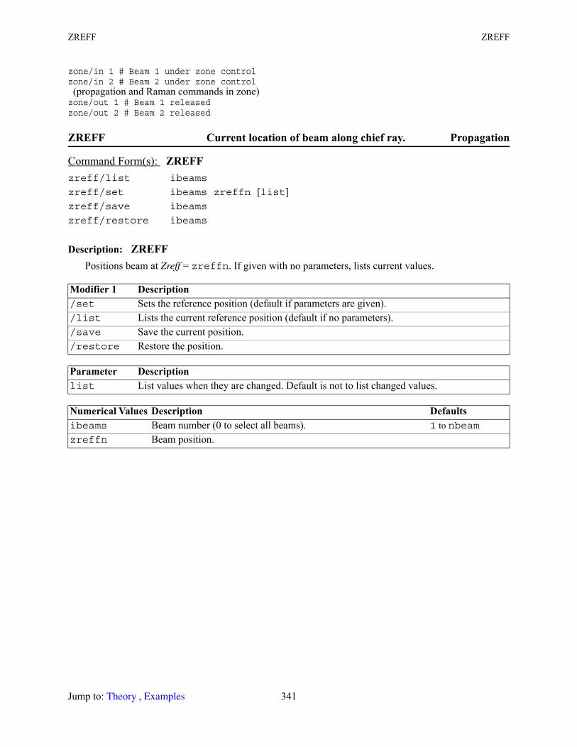
ZREFF ZREFF
zone/in 1 # Beam 1 under zone controlzone/in 2 # Beam 2 under zone control (propagation and Raman commands in zone)zone/out 1 # Beam 1 releasedzone/out 2 # Beam 2 released
ZREFF Current location of beam along chief ray. Propagation
Description: ZREFFPositions beam at Zreff = zreffn. If given with no parameters, lists current values.
Command Form(s): ZREFF zreff/list ibeams
zreff/set ibeams zreffn [list]zreff/save ibeams
zreff/restore ibeams
Modifier 1 Description /set Sets the reference position (default if parameters are given)./list Lists the current reference position (default if no parameters)./save Save the current position./restore Restore the position.
Parameter Description list List values when they are changed. Default is not to list changed values.
Numerical Values Description Defaultsibeams Beam number (0 to select all beams). 1 to nbeamzreffn Beam position.
Jump to: , 341 Theory Examples

ZREFF ZREFF
Jump to: , 342 Theory Examples

3. Index
AABCD operator 63aberration
atmospheric 65, 244GRIN 65piston 246random 65Seidel 68smoothed 247Zernike 69
adaptive optic mirror 71alias 32, 39, 73amplifier 334angular spectrum propagator 111aperture 97
general 99high numerical 176
array 75atmospheric aberration 244–245
Kolmogorov 244–245autocorrelation 77average radial profile 119axicon 65–66, 75, 77–84, 230
Bbandpass model 71banner 84Beer's Law 85bell 88binary 88
lenses 88birefringence 309blooming
target 305breaks 40
CCO2 100color 251convolution 102crystal 108
uniaxial 108cube corner reflector 106
Ddebug 109derivative 110diffraction
vector 176diffraction propagation 111dipole projection 176
Eencircled energy 119Euler angles 276
Fflip 139focus 140Fourier transform 103, 286, 293four-wave mixing 329Franz-Nodvik 100frequency doubling 112full-width-half-maximum 129
Ggain
coheretn pulse propagation 159rate equation 145semiconductor 157sheet 162three-level 143, 151, 156
gaussianembedded 126half 174Hermite 175lagurre 195surrogate 165
globalvertex 326
global coordinate system 168Goos-Hanchen 194gradient index lens (GRIN) 65grating 67, 88, 170Green's function 309
Hhelp 174Hermite-gaussian 175
Jump to: , 343 Theory Examples
GLAD Commands Manual
Highlighting source text 24homogenizer 176HTML 25, 179, 300Hyperlinks 19
Iintegrate 188inverse 189
KKeyread 349knife edge scan 131Kolmogorov 65
LLagurerre-gaussian 175laser gain 142lens array 198Lorentzian 217lvalue 32, 36
MManley-Rowe 113material
cubic 309isotropic 309
monitor window 25, 319
Nnoise 231
smoothed 231normalize 232
Oobscuration 233optical parametric oscillator 234optical transfer function (OTF) 238optimization
damped least squares 236
Pparsing 31phase conjugate mirror 101phase poles 268phase unwrapping 268photoelastic tensor 309polarization
aberration 190surface effects 193
polarization status 75
propagation 271angular spectrum 111
Rradial mode 66Raman 274, 329
transient 275rate equations 145regedit.exe 41Registry 40resonator 281rich text format (RTF) 18rod 284roof 284rotate 285, 298rvalue 32, 36
SSeidel aberration 68self focusing 291sinc function 294slit scan 134spatial spectral dispersion (SSD) 300standard atmosphere (STP) 90STARTUP file 75station number 300Stokes 45, 274–275Strehl ratio 302sum frequency generation (SFG) 290surrogate gaussian beam 334
Ttable 304thermal 307thermal blooming 89thermal expansion
coefficient 311time
elapsed 311title 312traceback window 24transpose 123, 313transposes 313
Uuniformity 316
Vvariable monitor window 25, 319vertex 326
Jump to: , 344 Theory Examples
Von Karman 245
Wwavefront
rms 283, 302, 325variance 325
waveguideslab 295
Woods, A. D. 90
YYoung's Modulus 309, 311
ZZernike aberrations 69Zernike polynomials 135zigzag 334zigzag amplifier 334
Jump to: , 345 Theory Examples

GLAD Commands Manual
Jump to: , 346 Theory Examples
Jump to: , 347 Theory Examples
4. Security Key
When installing GLAD on a new machine, install the code before installing the dongle. Install the software from the AOR distribution CD and be sure to select “Sentinel key driver”, so that the key driver software will be setup properly. If the key driver software is not installed, GLAD will not recognize the key. Repeat this process to install GLAD on any other computer. Your license permits you to install GLAD on as many machines as you like. Simply move the security key to the computer you wish to use. If you have files from an installation on another computer that you want to copy to a new machine, do so after installation from the CD.
The security key (dongle) will retain its password permanently. No modification of the key is needed when it is used on a new computer. The key is set to operate in temporary mode when it is shipped. In temporary mode the key will operate with full capabilities, but for a limited amount of usage. When the registration for GLAD and payment is received by AOR, the permanent password and instruction will be sent. The label for a key in temporary mode is “GLAD demonstration key”. When the key is set to permanent status, the Customer will select a new label. Damaged keys will be replaced. Lost keys will not be replaced, so protect and/or insure your key just as you would any other piece of equipment of comparable value.
Keyread.exe is a diagnostic program to set the security key and to test the key independently of GLAD. Run keyread.exe through Windows: Start, Run, “C:\program files\aor\glad57\keyread.exe”. Substitute your actual installation directory for “C:\program files\aor\glad57”. You may also run keyread.exe from GLAD with the GLAD command “privilege/keyread”. See the description of the command .
Installation from the CD sets the Windows registry so that the location of glad.exe and watch.exe are identified and establishes *.inp and *.plt with ide.exe and watch.exe respectively.
You may request the latest version of the GLAD installation CD at any time within the one year period of technical support. Both the permanent licensed version and the demo version of GLAD are supported by the same installation CD. The behavior of the program changes according to whether GLAD finds a valid key. If no key is found, GLAD will operate in superdemo mode, for a limited amount of usage.
gainsheet1.inpprivileges
Jump to: , 348 Theory Examples
5. Installing GLAD
Important. Please do these three steps:1) Install GLAD from the CD ROM before installing the dongle (security key).2) Attach the dongle to a USB port.3) Register the software. Thank you.
RegistrationGLAD is ready to run when it is received, so you can begin working immediately in temporary mode
that will last a month or so under typical use.You will need a password to set the security key to permanent status for a new purchase or to upgrade
the version level. AOR need registration of the key to prepare the password for your key.To register your copy of GLAD, Run the command privilege/register, enter the requested
contact information. Email the resulting registration file, as an attachment, to [email protected], fax to 1 360 225 0347, or send by regular mail. When the registration is received and payment has been made, AOR will send the password and installation instructions by return email or fax.
How to run GLADFrom the main Windows menu select Start, Programs, GLAD 6.1, GLAD IDE. The GLAD Users Guide
(guide.pdf) will pop up when GLAD first runs. Also, in this Commands Manual, see Sect. 1.3, “Using GLAD”, page 16.
First LookFor a quick look at some popular examples, select “Demo” from the main menu. Also, look through the
GLAD Examples Manual (examples.pdf) accessible from the “Help” menu item.
System RequirementsGLAD requires Microsoft Windows 2000 (or higher), 20 Mbytes of disk space for GLAD, 80 Mbytes
of disk space for the online documentation. A USB port is required for the security key. Adobe Acrobat Reader 7.0 is required for viewing the *.pdf files—available on the GLAD CD or from www.adobe.com (free)
See previous page for more information about the security key.


![Es90 at Commands Manual v18[1]](https://img.pdfslide.net/doc/110x75/55327c2f4a7959394b8b4649/es90-at-commands-manual-v181.jpg)