Global Arbitration Review The Guide to Damages in ......vii Preface This third edition of Global Arbitration Review’s The Guide to Damages in International Arbitration builds upon

The Guide to Damages in International Arbitration

EditorJohn A Trenor

Third Edition

Global Arbitration Review

© 2018 Law Business Research Ltd

The Guide to Damages in International Arbitration

Third Edition

Editor

John A Trenor

arg

Reproduced with permission from Law Business Research Ltd This article was first published in December 2018

For further information please contact [email protected]


PublisherDavid Samuels

Business Development ManagerGemma Chalk

Account ManagerBevan Woodhouse

Editorial CoordinatorHannah Higgins

Head of ProductionAdam Myers

Senior Production EditorSimon Busby

Copy-editorGina Mete

ProofreaderAnna Andreoli

Published in the United Kingdomby Law Business Research Ltd, London87 Lancaster Road, London, W11 1QQ, UK© 2018 Law Business Research Ltdwww.globalarbitrationreview.com

No photocopying: copyright licences do not apply.

The information provided in this publication is general and may not apply in a specific situation, nor does it necessarily represent the views of authors’ firms or their clients. Legal advice should always be sought before taking any legal action based on the information provided. The publishers accept no responsibility for any acts or omissions contained herein. Although the information provided is accurate as of November 2018, be advised that this is a developing area.

Enquiries concerning reproduction should be sent to Law Business Research, at the address above. Enquiries concerning editorial content should be directed to the Publisher – [email protected]

ISBN 978-1-78915-098-8

Printed in Great Britain byEncompass Print Solutions, DerbyshireTel: 0844 2480 112


i

The publisher acknowledges and thanks the following firms for their learned assistance throughout the preparation of this book:

A&M GMBH WIRTSCHAFTSPRÜFUNGSGESELLSCHAFT

ALIXPARTNERS

BDO LLP

BERKELEY RESEARCH GROUP

CEG EUROPE

CET GROUP OF COMPANIES

CHARLES RIVER ASSOCIATES

COMPASS LEXECON

CORNERSTONE RESEARCH

DEBEVOISE & PLIMPTON LLP

FRESHFIELDS BRUCKHAUS DERINGER LLP

FRONTIER ECONOMICS LTD

FTI CONSULTING

HABERMAN ILETT LLP

HOMBURGER

KING & SPALDING LLP

LATHAM & WATKINS LLP

Acknowledgements


ii

LONDON BUSINESS SCHOOL

NERA ECONOMIC CONSULTING

PRICEWATERHOUSECOOPERS LLP

SECRETARIAT INTERNATIONAL, INC

VICTORIA UNIVERSITY, FACULTY OF LAW

WALDER WYSS LTD

WHITE & CASE LLP

WILMER CUTLER PICKERING HALE AND DORR LLP

WÖSS & PARTNERS


vii

Preface

This third edition of Global Arbitration Review’s The Guide to Damages in International Arbitration builds upon the successful reception of the first two editions. As explained in the introduction, this book is designed to help all participants in the international arbitration community understand damages issues more clearly and communicate those issues more effectively to tribunals to further the common objective of assisting arbitrators in rendering more accurate and well-reasoned awards on damages.

The book is a work in progress, with new and updated material being added to each successive edition. In particular, this third edition incorporates updated chapters from vari-ous authors and features several new chapters addressing such issues as best practices and issues in discounted cash flow models, full compensation and total reparation, and estima-tion of harm in antitrust damages actions.

We hope that this revised edition advances the objective of the first two editions to make the subject of damages in international arbitration more understandable and less intimidating for arbitrators and other participants in the field, and to help participants present these issues more effectively to tribunals. We continue to welcome comments from readers on how the next edition might be further improved.

John A TrenorWilmer Cutler Pickering Hale and Dorr LLP


Part IIIApproaches and Methods for the Assessment and Quantification of Damages


331

24The Use of Econometric and Statistical Analysis in Damages Assessments

Ronnie Barnes1

While writing this chapter, I asked a number of lawyers with whom Cornerstone Research has previously worked what they would like to know about econometrics or regression analysis (the two terms are largely synonymous for the purposes of this chapter). Other than ‘What is regression analysis?’, one particularly colourful response captured the general mood: ‘Even the words “regression analysis” send a chill down my spine!’

The genesis of these feelings is not difficult to understand. At its worst, the part of an expert report that presents econometric analysis is dense and hard to follow, while the debate between experts becomes incomprehensible as terms like ‘heteroscedasticity’, ‘omit-ted variable bias’, ‘mis-specification’ and ‘failure to reject the null hypothesis’ fly back and forth like guided missiles.

However, to the extent that this chapter has a message, it is that econometric analysis provides a powerful set of tools for handling data. Used correctly and presented clearly, it can be central to estimating damages in a robust and reliable manner. At the highest level, I would suggest:• There are some fundamental elements of regression analysis that practitioners of inter-

national arbitration should feel comfortable with (just as many antitrust lawyers do). This chapter attempts to lay out some, though certainly not all, of those elements.

1 Ronnie Barnes is a principal at Cornerstone Research. The author would like to thank the staff of GAR; his Cornerstone Research colleagues, particularly Carine Campbell, Leslie Goodman, Janine L’Heureux, Samita Kamath and Lauro Remmler; and Matthew Vinall of Dentons and James Freeman of Allen & Overy for their input and advice on a previous version.


The Use of Econometric and Statistical Analysis in Damages Assessments

332

• It is true that regression analysis can give rise to complex technical debates. Nonetheless:• as with other technical subjects, it is the duty of the expert to present the core

issues in a clear, concise fashion, eliminating all unnecessary complexity.2 The use of graphics, simple examples and plain language can help considerably; and

• in any given context, if the technical concerns are material then it should be pos-sible to explain, in a reasonably intuitive way, each concern and why it matters.

• Where appropriate, arbitrators can facilitate the debate by requiring opposing experts to use the same data, and explain how their results would change if they used the other expert’s assumptions.

The focus of this chapter is on the first point only. I am aware that many people reading this will be lawyers – both counsel and arbitrators – doing so because they are faced with an expert report containing econometric analysis, and they need to understand some more or less complex points contained in that report. While it cannot be promised that this chapter will address the exact points at issue, I am confident that an understanding of the main points covered in the remainder of the chapter is a necessary condition for anyone wishing to be a competent consumer of econometrics.

What is econometrics?

Econometrics is usually described as the application of statistical techniques to economic data. Economists use econometrics to quantify economic relationships; for example, to estimate how demand for a product varies with its price, or to estimate trends in a nation’s imports over a given time period. For the purpose of this chapter though, perhaps the most useful characterisation, albeit a partial one, is that econometrics is one of the principal tools that economists use to construct and quantify counterfactual scenarios. For example, econometric techniques might be used to estimate the level of imports in scenarios with different levels of import duties, so as to assess alternative trade policies; or to assess how the presence of a bidding cartel affects prices in a procurement auction, so as to estimate the impact of the cartel on consumers and profits.

Put in those terms, it is clear why econometric techniques are so important to the esti-mation of damages, which routinely involves comparing the actual scenario with a ‘but-for’ scenario in order to estimate a relevant measure of value. This measure might be prof-its, with the difference between the actual and but-for scenarios representing lost profits, which is often the metric for damages in relation to an alleged breach of contract. In cases of alleged expropriation, the appropriate metric might be the value of an asset, with the dif-ference between scenarios representing the loss in value resulting from the expropriation.

This chapter provides a brief introduction to regression analysis, which is by far the most commonly used econometric tool in estimating damages. The approach is a practical one: I start with a simple example that explains the idea of regression analysis at its most basic level. I then use a second example to explain how one should understand regression output as the reader will typically encounter it in an expert report, how the output can

2 At the risk of appearing self-serving, I would suggest that a suitably qualified expert (generally someone with appropriate formal qualifications) is more likely to have the kind of deep understanding that is required to simplify without misrepresenting.



333

be used to provide a damages estimate, and how to understand some of the basic statistical concepts that will often be invoked by one expert or the other. These concepts include the validity of the regression analysis itself, the accuracy of the damages estimate and so-called ‘statistical significance’. Finally, a third example provides further illustrations of a number of these points, and is also of interest in itself because it utilises the ‘event study’ methodology, which is particularly useful for estimating damages.

This chapter obviously does not seek to be comprehensive for reasons of length, and there are a number of important topics that are not touched on. To mention just two, these include:• issues around compiling and preparing data sets. The quality of data used is of funda-

mental importance. Even the most sophisticated econometric techniques will struggle in the face of a poorly constructed, error-filled or misunderstood data set: the cruel but often accurate acronym GIGO (garbage in, garbage out) describes the problem suc-cinctly; and

• techniques used to estimate consumer choice and ‘willingness to pay’. A very large body of work over some decades has focused on understanding how consumers choose between discrete alternatives, and this is potentially relevant to damages estimation in many settings.

Example 1: share prices and foreign exchange (FX) rates

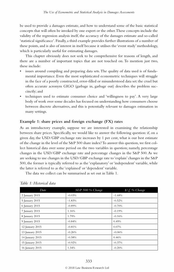
As an introductory example, suppose we are interested in examining the relationship between share prices. Specifically, we would like to answer the following question: if, on a given day, the USD/GBP exchange rate increases by 1 per cent, what is our best estimate of the change in the level of the S&P 500 share index? To answer this question, we first col-lect historical data over some period on the two variables in question; namely, percentage changes in the USD/GBP exchange rate and percentage changes in the S&P 500. As we are seeking to use changes in the USD/GBP exchange rate to ‘explain’ changes in the S&P 500, the former is typically referred to as the ‘explanatory’ or ‘independent’ variable, while the latter is referred to as the ‘explained’ or ‘dependent’ variable.

The data we collect can be summarised as set out in Table 1.

Table 1: Historical data

Date S&P 500 % Change $/£ % Change

2 January 2015 -0.03% -1.68%

5 January 2015 -1.83% -0.52%

6 January 2015 -0.89% -0.70%

7 January 2015 1.16% -0.19%

8 January 2015 1.79% -0.16%

9 January 2015 -0.84% 0.49%

12 January 2015 -0.81% 0.07%

13 January 2015 -0.26% -0.06%

14 January 2015 -0.58% 0.46%

15 January 2015 -0.92% -0.37%

16 January 2015 1.34% -0.20%



334

Date S&P 500 % Change $/£ % Change

20 January 2015 0.15% -0.01%

21 January 2015 0.47% -0.03%

22 January 2015 1.53% -0.88%

23 January 2015 -0.55% -0.11%

26 January 2015 0.26% 0.63%

27 January 2015 -1.34% 0.69%

28 January 2015 -1.35% -0.34%

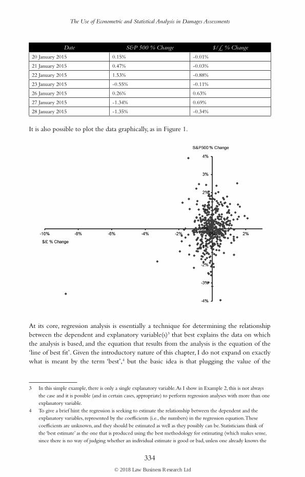
It is also possible to plot the data graphically, as in Figure 1.

Figure 1: Plotting the data

At its core, regression analysis is essentially a technique for determining the relationship between the dependent and explanatory variable(s)3 that best explains the data on which the analysis is based, and the equation that results from the analysis is the equation of the ‘line of best fit’. Given the introductory nature of this chapter, I do not expand on exactly what is meant by the term ‘best’,4 but the basic idea is that plugging the value of the

3 In this simple example, there is only a single explanatory variable. As I show in Example 2, this is not always the case and it is possible (and in certain cases, appropriate) to perform regression analyses with more than one explanatory variable.

4 To give a brief hint: the regression is seeking to estimate the relationship between the dependent and the explanatory variables, represented by the coefficients (i.e., the numbers) in the regression equation. These coefficients are unknown, and they should be estimated as well as they possibly can be. Statisticians think of the ‘best estimate’ as the one that is produced using the best methodology for estimating (which makes sense, since there is no way of judging whether an individual estimate is good or bad, unless one already knows the



335

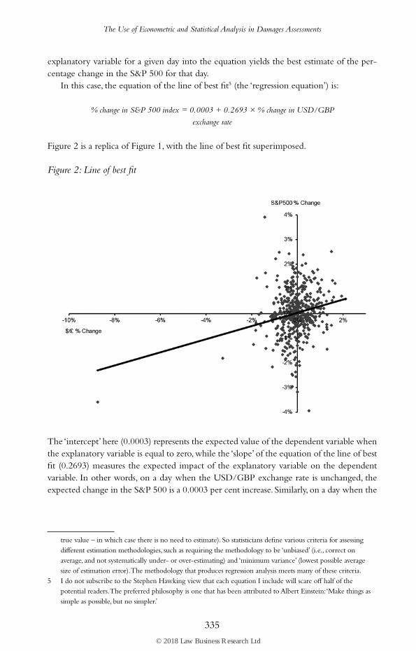
explanatory variable for a given day into the equation yields the best estimate of the per-centage change in the S&P 500 for that day.

In this case, the equation of the line of best fit5 (the ‘regression equation’) is:

% change in S&P 500 index = 0.0003 + 0.2693 × % change in USD/GBP

exchange rate

Figure 2 is a replica of Figure 1, with the line of best fit superimposed.

Figure 2: Line of best fit

The ‘intercept’ here (0.0003) represents the expected value of the dependent variable when the explanatory variable is equal to zero, while the ‘slope’ of the equation of the line of best fit (0.2693) measures the expected impact of the explanatory variable on the dependent variable. In other words, on a day when the USD/GBP exchange rate is unchanged, the expected change in the S&P 500 is a 0.0003 per cent increase. Similarly, on a day when the

true value – in which case there is no need to estimate). So statisticians define various criteria for assessing different estimation methodologies, such as requiring the methodology to be ‘unbiased’ (i.e., correct on average, and not systematically under- or over-estimating) and ‘minimum variance’ (lowest possible average size of estimation error). The methodology that produces regression analysis meets many of these criteria.

5 I do not subscribe to the Stephen Hawking view that each equation I include will scare off half of the potential readers. The preferred philosophy is one that has been attributed to Albert Einstein: ‘Make things as simple as possible, but no simpler.’



336

USD/GBP exchange rate increases by 1 per cent, the expected change in the S&P 500 is an increase of:

0.0003% + 0.2693 × 1% = 0.2696%

If the USD/GBP exchange rate declines by 1 per cent, the expected change in the S&P 500 is a decrease of:

0.0003% + 0.2693 × -1% = -0.2690%

To understand what ‘expected’ means, note that if the change in the USD/GBP exchange rate is zero, +1 per cent or -1 per cent it is unlikely that the change in the S&P 500 will be exactly 0.0003 per cent, 0.2696 per cent or -0.2690 per cent. Rather, the term ‘expected’ means that these results hold on average.

Example 2: lost profits

As a specific example of how regression analysis might be used in the context of a damages analysis, consider the case of a large multinational consumer goods company (HugeCo) that produces and sells mouthwash, among many other products, in many countries. In 2006, HugeCo entered a new market, the rapidly emerging economy of Ruritania. To do so, it entered into a joint venture with a local partner (LocalCo). As part of the joint venture agreement, LocalCo made extensive commitments to undertake advertising and other pro-motional activities (which for various reasons it was uniquely well placed to do). HugeCo’s entry was successful, and by 2008 its mouthwash was an established consumer product in Ruritania. However, relations between HugeCo and LocalCo began to deteriorate in 2013, for reasons unrelated to the mouthwash business.

Beginning in January 2014, LocalCo abruptly stopped all the advertising and other promotional activities it had previously undertaken in line with the joint venture agree-ment. This lasted for 30 months until June 2016, when HugeCo sold its interest in the joint venture, at which point LocalCo resumed its promotional activities. However, the arrange-ment left unresolved the question of compensation for LocalCo’s alleged failure to comply with its obligations under the joint venture agreement. HugeCo is therefore now seeking damages in the form of compensation for lost profits between January 2014 and June 2016, on the grounds that its mouthwash sales (and consequently its profits) over that period were lower than they would have been if LocalCo had met its obligations.

To quantify damages in this example, it is therefore necessary to estimate what HugeCo’s mouthwash sales would have been from January 2014 to June 2016 had LocalCo under-taken the promotional activities, and to compare these to the actual sales generated over that period. A simplistic approach to estimating sales in the but-for scenario of full promo-tional activities might be to take the actual monthly sales from 2013 – or maybe an average over, say, the period 2010 to 2013 – and assume that this level of sales would have persisted in the future. Suppose, however, that 2014 saw a new company entering the mouthwash market and aggressively cutting prices relative to their prior levels. In that case, it seems intuitive that HugeCo’s sales in 2014 would, even in the presence of full promotional activities, have been lower than in previous years as a result of the loss of market share to this



337

new entrant. Regression analysis is the economist’s way of formalising that intuition and of taking into account quantitatively the various factors that might affect HugeCo’s mouth-wash sales when estimating what the but-for sales in 2014 to mid-2016 would have been.

More specifically, to estimate what HugeCo’s mouthwash sales in 2014 to mid-2016 would have been had LocalCo engaged in full promotional activities, an eco-nomic expert would first need to consider what factors might reasonably be expected to affect these sales. This is an important step. It is possible to estimate a regression on any set of variables – for example, one could use regression analysis to estimate the relation-ship between daily ice cream sales and the USD/GBP exchange rate. However, absent an economic rationale as to why and how these variables are interrelated, the results of such a regression must be interpreted with extreme caution. As noted earlier, econometrics can be described as the application of statistical techniques to economic data – that is, data that are generated by some economic process. Without an understanding of this process, there is a danger that no matter how sophisticated the economic techniques that are utilised, the exercise becomes one of what is disparagingly referred to as ‘data mining’, where chance correlations are confused with meaningful relations.

Returning to the example, in reality – and this example is based on a real case, albeit well disguised – the economist would identify a number of variables, such as price, adver-tising expenditure and the previous month’s sales, that are economically relevant to deter-mining HugeCo’s mouthwash sales volume. Of course, the previous month’s sales do not directly cause sales this month, but they are a good proxy for factors that may cause sales this month; notably, the fact that people have tried the product, know whether they like it or not, and if they do like it, have got into the habit of buying it. The regression analysis will then measure the extent to which this relationship is meaningful. As in the example above, the estimated coefficient in the regression equation for that variable captures this relationship between the explanatory and the dependent variable, and the size of the esti-mate indicates its materiality.

For expositional purposes, I now simplify and assume that it is sufficient to focus only on the previous month’s sales, and on the presence or absence of promotional activity.

Given that the question at issue is the extent to which, if at all, the alleged failure to engage in promotional activity depressed HugeCo’s mouthwash sales volume, the econo-mist can estimate a regression (e.g., using actual data of monthly sales volume, and which months had promotional activity, covering the 90 months from January 2009 to June 2016) where the dependent variable is sales volume in a given month (measured in units of 1,000 bottles), and the explanatory variables are:• sales volume in the previous month; and• a ‘dummy variable’ that is equal to one in a month with no promotional activity, and

zero otherwise.

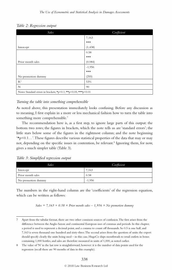
Suppose that the results of this regression (presented in the potentially confusing tabular form in which such results often appear in expert reports and which I will explain below) are as follows.6

6 Unfortunately there is no single standard format for presenting regression results. I explain later some alternative forms of output that the reader may encounter in practice.



338

Table 2: Regression output

Sales Coefficient

Intercept

7,163

***

(1,438)

Prior month sales

0.58

***

(0.084)

No promotion dummy

-1,956

***

(255)

R2 53%

N 90

Notes: Standard errors in brackets; *p<0.1; **p<0.05; ***p<0.01

Turning the table into something comprehensible

As noted above, this presentation immediately looks confusing. Before any discussion as to meaning, I first explain in a more or less mechanical fashion how to turn the table into something more comprehensible.7

The recommendation here is, as a first step, to ignore large parts of this output: the bottom two rows; the figures in brackets, which the note tells us are ‘standard errors’; the little stars below some of the figures in the rightmost column; and the note beginning ‘*p<0.1…’. These figures describe various statistical properties of the data that may or may not, depending on the specific issues in contention, be relevant.8 Ignoring them, for now, gives a much simpler table (Table 3).

Table 3: Simplified regression output

Sales Coefficient

Intercept 7,163

Prior month sales 0.58

No promotion dummy -1,956

The numbers in the right-hand column are the ‘coefficients’ of the regression equation, which can be written as follows:

Sales = 7,163 + 0.58 × Prior month sales – 1,956 × No promotion dummy

7 Apart from the tabular format, there are two other common sources of confusion. The first arises from the difference between the Anglo-Saxon and continental European uses of commas and periods. In this chapter, a period is used to represent a decimal point, and a comma to count off thousands. So 0.5 is one half, and 7,163 is seven thousand one hundred and sixty-three. The second arises from the question of units: the expert should specify clearly the units being used – in this case, HugeCo ships mouthwash to retail outlets in boxes containing 1,000 bottles, and sales are therefore measured in units of 1,000, as noted earlier.

8 The value of ‘N’ in the last row is straightforward, however: it is the number of data points used for the regression (recall there are 90 months of data in this example).



339

The coefficient of 0.58 on ‘Prior month sales’ represents the estimated sensitivity of this month’s sales to last month’s sales: each additional 100 units of sales last month gives an additional 58 units this month. Mechanically speaking, the intercept of 7,163 represents the expected sales volume assuming both explanatory variables are equal to zero – that is, where there were no sales in the prior month and there is promotional activity by LocalCo (however, as I explain later, this interpretation should be handled with extreme care). This leaves the mystery of the ‘No promotion dummy’. As explained above, a dummy variable is one that takes on just two values, 0 or 1. In this instance, it takes on the value 1 when LocalCo does not engage in promotional activity and 0 otherwise. What that means can most easily be explained by noting that the equation above can be thought of as two equa-tions. In months when LocalCo engages in promotional activity, the value of the dummy variable is 0, so for those months the equation is:

Sales = 7,163 + 0.58 × Prior month sales

In months when LocalCo does not engage in promotional activity, the value of the dummy variable is 1. This only impacts the intercept and so for those months the equation is:

Sales = 5,207 + 0.58 × Prior month sales 9

Interpreting the regression output

Analogous to Example 1, the basic idea is that plugging the values of the explanatory vari-ables for a given month into the equation above yields the best estimate of the sales volume for that month. So, for example, if the sales volume in the prior month were 12,000, the best estimate of the sales volume in the current month (assuming LocalCo is providing promotional activities) would be 7,163 + 0.58 × 12,000 = 14,123. If the current month were one in which LocalCo failed to provide promotional activities, this estimate would be 1,956 lower at 5,207 + 0.58 × 12,000 = 12,167.

From this discussion, it is clear why, as explained above, the coefficient on prior month sales (0.58) may be interpreted as a measure of the impact of past sales – an increase of 100 in the prior month sales volume would lead to an increase in the best estimate of the current month sales volume of 58, all else being equal. This should be thought of as a kind of expected average effect: it is unlikely to hold exactly in any given month, but the statistician believes that it will be accurate on average (or more precisely, it is the statisti-cian’s best estimate of what the effect will be on average). The qualifier ‘all else being equal’ (ceteris paribus) is important: each coefficient in the regression output measures the effect of changes in the corresponding variable, holding all the other variables constant.

Remembering that the ‘No promotion dummy’ is equal to 1 in a month in which LocalCo failed to engage in promotional activities and 0 otherwise, the interpretation of the coefficient of -1,956 becomes clear: in a month in which LocalCo fails to promote

9 The figure of 5,207 comes from taking the overall equation, ‘Sales = 7,163 + 0.58 × Prior Month Sales – 1,956 × No Promotion Dummy’, setting ‘No Promotion Dummy’ to one, and noting that 7,163 – 1,956 × 1 = 5,207.



340

HugeCo’s mouthwash, HugeCo’s sales volume is, on average, 1,956 units lower than it would otherwise have been.

An estimate of lost profits is therefore derived as follows:• Take the regression’s estimated monthly effect of the alleged breach: a reduction in sales

of 1,956.• Multiply by the duration of the alleged breach – that is, 30 months – to get 1,956 × 30

= 58,680.• Estimate the profit margin on each sale. Suppose (for simplicity) it is $1 per bottle

of mouthwash.• Multiply the volume of lost sales (remembering that each unit of sales in the above

analysis is 1,000 bottles) by the profit margin to get lost profits of 58,680 × 1,000 × $1 = $58,680,000.

The data on which this example is based are artificial, but a few useful observations can still be made. First, one possible criticism of the analysis might be that it does not accurately estimate sales for certain periods of time. Opposing counsel might argue: ‘This alleged rela-tionship is clearly implausible and does not fit the facts: back in 2006 when HugeCo began to sell mouthwash, its sales in the first month were just 10 units. But according to the other side’s so-called expert, the first month’s sales should have been 7,163.’10

However, that criticism is misplaced, because the statistician does not (or at least should not) claim that the relationship he or she has estimated applies for all levels of sales, and the use of the results of the analysis in the damages exercise certainly does not require that this be the case. Recall that the regression is estimated using 90 months of sales data. Suppose, for example, the observed sales volume over those 90 months ranges from 8,832 to 19,289. Then the regression analysis captures the relationship between the dependent and explana-tory variables over this range, and a responsible statistician will be cautious in claiming that the results of the analysis apply outside of this range (and a volume of 10 is almost as far out of that range as it can possibly be in the downward direction). In general, understanding both the data on which the analysis is based, and any potential limitations in that data, is a crucial part of the interpretation of any regression output.

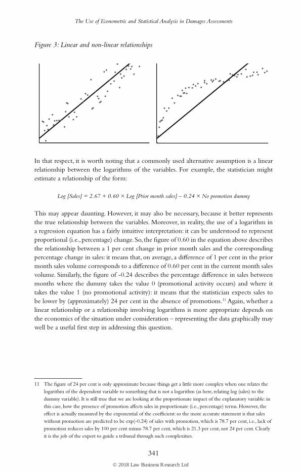
Second, there is nothing to say that the relationship between the variables in the regres-sion has to be linear – this is just an assumption, and an assumption that the statistician should test against the evidence. There are many ways of doing so, including the simplest of all, which is to visually depict the data on a chart and see if it appears to follow a lin-ear pattern.

Figure 3 below shows two examples, the one on the left where an assumption of a linear relationship appears appropriate, the other, where it does not.

10 Recall the equation is Sales = 7,163 + 0.58 × Prior month sales, so if Prior month sales are 0 (as was the case, by definition, for the first month of sales) then the equation predicts Sales of 7,163.



341

Figure 3: Linear and non-linear relationships

In that respect, it is worth noting that a commonly used alternative assumption is a linear relationship between the logarithms of the variables. For example, the statistician might estimate a relationship of the form:

Log [Sales] = 2.67 + 0.60 × Log [Prior month sales] – 0.24 × No promotion dummy

This may appear daunting. However, it may also be necessary, because it better represents the true relationship between the variables. Moreover, in reality, the use of a logarithm in a regression equation has a fairly intuitive interpretation: it can be understood to represent proportional (i.e., percentage) change. So, the figure of 0.60 in the equation above describes the relationship between a 1 per cent change in prior month sales and the corresponding percentage change in sales: it means that, on average, a difference of 1 per cent in the prior month sales volume corresponds to a difference of 0.60 per cent in the current month sales volume. Similarly, the figure of -0.24 describes the percentage difference in sales between months where the dummy takes the value 0 (promotional activity occurs) and where it takes the value 1 (no promotional activity): it means that the statistician expects sales to be lower by (approximately) 24 per cent in the absence of promotions.11 Again, whether a linear relationship or a relationship involving logarithms is more appropriate depends on the economics of the situation under consideration – representing the data graphically may well be a useful first step in addressing this question.

11 The figure of 24 per cent is only approximate because things get a little more complex when one relates the logarithm of the dependent variable to something that is not a logarithm (as here, relating log (sales) to the dummy variable). It is still true that we are looking at the proportionate impact of the explanatory variable: in this case, how the presence of promotion affects sales in proportionate (i.e., percentage) terms. However, the effect is actually measured by the exponential of the coefficient: so the more accurate statement is that sales without promotion are predicted to be exp(-0.24) of sales with promotion, which is 78.7 per cent, i.e., lack of promotion reduces sales by 100 per cent minus 78.7 per cent, which is 21.3 per cent, not 24 per cent. Clearly it is the job of the expert to guide a tribunal through such complexities.



342

The complicated stuff: R2, standard errors, etc.

A few pages back I showed a table of regression output, and began by suggesting that the reader could ignore, for the time being, a large part of the table. I imagine this will have been welcome advice. However, it will often be necessary to understand some of the additional output in order to use it correctly and to understand commentary from oppos-ing experts.

Coefficient of determination (usually written R2)

In the HugeCo example, the opposing expert might say ‘the R2 is too low. R2 is a measure of the strength of a regression, and it should be at least 70 per cent for the regression to be reliable. A regression with an R2 of just 53 per cent is not reliable.’ Unfortunately, I have seen comments along these lines in actual ‘expert’ reports. They suggest a fundamental lack of understanding of regression analysis: there is no such thing as ‘strength of a regres-sion’, and there is no ‘threshold value’ for R2. In fact, whether or not the R2 value matters depends on the context and the aim of the exercise.

The R2 is a percentage, between zero and 100 per cent, that indicates the proportion of variation in the dependent variable that can be explained by the observed variation in the explanatory variables.12 So, in Example 1, a high R2 would indicate that variations in the USD/GBP exchange rate ‘explain’ a very high proportion of the variation in the S&P 500. In the HugeCo example, the R2 of 53 per cent indicates that the explanatory variables used (Prior month sales and the No promotion dummy) explain 53 per cent of the observed variation in monthly sales, with the remainder being a result of other factors. However, that is per se not directly relevant to the quantum exercise, because the goal of the quantum exercise is not to identify all of the determinants of sales, or to predict future sales. It is to estimate the impact on sales of LocalCo’s promotions, all else being equal. Recall that that impact is estimated through looking at the coefficient on the No promotion dummy, which was -1,956. The relevant question, therefore, is ‘how accurate is the estimate of -1,956?’ and not ‘how well does this equation capture all the factors that explain monthly sales?’

In some instances, a low R2 may also suggest that the chosen form of the equation is incorrect – for example, if the regression uses a linear equation when the underlying rela-tionship is non-linear, then that may show itself in a low R2, because ‘the wrong equation’ will generally not be able to explain or predict well the variation in the dependent variable.

The standard error and confidence intervals

How then does one answer the question ‘how accurate is the estimate of -1,956?’ To answer that, one turns to the ‘standard error’, as reported in Table 2 (which gave a value of 255).

The standard error is a measure of the accuracy of the estimate. As a rule of thumb, the likely range of estimation error can be taken for many purposes to be approximately two standard errors. So the figure of -1,956 can be interpreted as being the middle of a range whose lower bound is -1,956 – 2 × 255 = -2,466 and whose upper bound is -1,956 + 2 × 255 = -1,446. The statistician may say that their best ‘point estimate’ of the impact of

12 It is often expressed as an absolute number, rather than a percentage. So, for example, an R2 of 0.53 is the same thing as an R2 of 53 per cent, expressed in a different way.



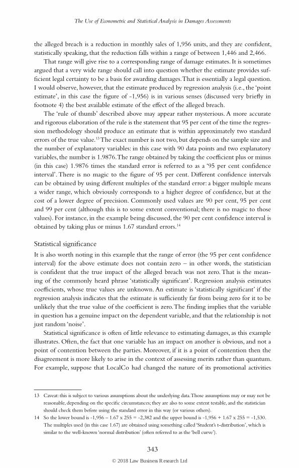
343

the alleged breach is a reduction in monthly sales of 1,956 units, and they are confident, statistically speaking, that the reduction falls within a range of between 1,446 and 2,466.

That range will give rise to a corresponding range of damage estimates. It is sometimes argued that a very wide range should call into question whether the estimate provides suf-ficient legal certainty to be a basis for awarding damages. That is essentially a legal question. I would observe, however, that the estimate produced by regression analysis (i.e., the ‘point estimate’, in this case the figure of -1,956) is in various senses (discussed very briefly in footnote 4) the best available estimate of the effect of the alleged breach.

The ‘rule of thumb’ described above may appear rather mysterious. A more accurate and rigorous elaboration of the rule is the statement that 95 per cent of the time the regres-sion methodology should produce an estimate that is within approximately two standard errors of the true value.13 The exact number is not two, but depends on the sample size and the number of explanatory variables: in this case with 90 data points and two explanatory variables, the number is 1.9876. The range obtained by taking the coefficient plus or minus (in this case) 1.9876 times the standard error is referred to as a ‘95 per cent confidence interval’. There is no magic to the figure of 95 per cent. Different confidence intervals can be obtained by using different multiples of the standard error: a bigger multiple means a wider range, which obviously corresponds to a higher degree of confidence, but at the cost of a lower degree of precision. Commonly used values are 90 per cent, 95 per cent and 99 per cent (although this is to some extent conventional; there is no magic to those values). For instance, in the example being discussed, the 90 per cent confidence interval is obtained by taking plus or minus 1.67 standard errors.14

Statistical significance

It is also worth noting in this example that the range of error (the 95 per cent confidence interval) for the above estimate does not contain zero – in other words, the statistician is confident that the true impact of the alleged breach was not zero. That is the mean-ing of the commonly heard phrase ‘statistically significant’. Regression analysis estimates coefficients, whose true values are unknown. An estimate is ‘statistically significant’ if the regression analysis indicates that the estimate is sufficiently far from being zero for it to be unlikely that the true value of the coefficient is zero. The finding implies that the variable in question has a genuine impact on the dependent variable, and that the relationship is not just random ‘noise’.

Statistical significance is often of little relevance to estimating damages, as this example illustrates. Often, the fact that one variable has an impact on another is obvious, and not a point of contention between the parties. Moreover, if it is a point of contention then the disagreement is more likely to arise in the context of assessing merits rather than quantum. For example, suppose that LocalCo had changed the nature of its promotional activities

13 Caveat: this is subject to various assumptions about the underlying data. Those assumptions may or may not be reasonable, depending on the specific circumstances; they are also to some extent testable, and the statistician should check them before using the standard error in this way (or various others).

14 So the lower bound is -1,956 – 1.67 x 255 = -2,382 and the upper bound is -1,956 + 1.67 x 255 = -1,530. The multiples used (in this case 1.67) are obtained using something called ‘Student’s t-distribution’, which is similar to the well-known ‘normal distribution’ (often referred to as the ‘bell curve’).



344

rather than stopped undertaking them, and that HugeCo claimed that the change had led to a drop in sales, and was a breach of a contractual commitment to make best efforts to promote HugeCo’s mouthwash. LocalCo might then use regression analysis to show that any change in sales following the change in promotional activity was not statistically significant, and argue that this indicated that the change had not been a consequence of a less effective form of promotional activity, and therefore could not be a breach of its best efforts obligation.

Stars and p-values

Recall that the regression output in Table 1 also included stars beneath the coefficients, and a note that referred to the ‘p-value’. These relate to the question of statistical significance, and therefore, as suggested above, are often not central to the dispute. However, I attempt to explain them here, at the risk of entering into a rather detailed discussion.

As noted above, the fact that the 95 per cent confidence interval for the estimate of the promotional activities’ impact (the coefficient on the No promotion dummy) does not contain zero means that the estimate is ‘statistically significant’. However, this depends on the confidence interval used. For example, suppose that the regression analysis showed a standard error of 800 (instead of 255). Then:• the 95 per cent confidence interval would be given by -1,956 +/– 1.9875 × 800, and

still does not contain zero; however• the 99 per cent confidence interval would be given by -1,956 +/– 2.61 × 800, and does

contain zero.

In those circumstances the estimated coefficient is said to be statistically significant at a 5 per cent level of significance, but not at a 1 per cent level of significance.15 The stars attached to the coefficients in Table 1 (and found in the note ‘*p<0.1; **p<0.05; ***p<0.01’) can now be explained. A single star indicates that the estimate is statistically significant at a level of 10 per cent. In the note, p denotes the level of significance, so ‘p<0.1’ means statistically significant at 10 per cent (which is the same thing as 0.1). Two stars correspond to 5 per cent (0.05) and three stars correspond to 1 per cent (0.01).16

To be more rigorous, the statement p<0.1 means ‘if the true value of the coefficient being estimated were zero, then the probability that the methodology that has been used to estimate it would, as a result of sampling error, give an estimate as large as (or larger than) the estimate here, is no more than 0.1.’

In the example given above where the standard error on the estimate of the coefficient for the variable No promotion dummy was assumed to be 800, the estimate was found to be statistically significant at 5 per cent but not at 1 per cent. The estimate would therefore be reported with two stars: -1,956**.17

15 Confusingly, the level of significance is 100 minus the level of confidence (so a 95 per cent confidence interval means a 5 per cent level of significance, and a 99 per cent confidence interval means a 1 per cent level of significance).

16 As with confidence intervals, the figures of 1 per cent, 5 per cent and 10 per cent are conventionally used, but there is no magic to that choice.

17 The stars can also often be found written adjacent to, rather than beneath, the number, as shown here.



345

Remaining with that example, rather than say that the level of significance is less than 5 per cent but more than 1 per cent, one can find exactly what value it has. In this case the answer is that it is statistically significant at 1.6 per cent. That figure is known as the p-value. Clearly if you know the p-value then the stars serve no practical purpose (although it is not unheard of for authors, nonetheless, to present both).

Other commonly encountered forms of presenting regression output

Unfortunately, there is no uniform template for presenting regression output. Some authors present the standard errors, and others do not. Often the author will not present the stand-ard error, but will instead present something called the ‘t-statistic’. This can be difficult to understand for a non-technical audience. However, the standard error can be recovered from the t-statistic: for each estimated coefficient, the standard error is equal to the esti-mate itself, divided by the t-statistic. So, for example, if the estimated coefficient on the No Promotion Dummy was reported as -1,956 and the t-statistic was -7.67 then the reader could find the standard error to be -1,956 / -7.67 = 255.

As an additional source of confusion, the standard error is often reported with different names or abbreviations (or simply unlabelled, with the reader expected to guess that it is the standard error). Common labels include ‘SE Coeff ’ (standard error of coefficient), ‘SE’ (standard error), or ‘StDev’ or ‘Std Dev’ (standard deviation).

Example 3: event studies

As a second example of how regression analysis may be used to construct a ‘but-for’ sce-nario in the context of a damages assessment, consider the case of firm ZedCo, a large part of whose business comprises long-term contracts with foreign governments to provide pharmaceutical products such as vaccines in bulk. On 11 January 2016, it announced – completely unexpectedly – that one of its major governmental customers had unilaterally decided to terminate with immediate effect all of its contracts with the firm, with a total value of £1 billion. ZedCo has launched a breach of contract case against this government, and is looking for a damages assessment in the event that it prevails on the merits.

At first glance, this would appear to be a very straightforward question – what else could damages be other than £1 billion? However, a little thought shows that the situation is rather more complex than that. For example, £1 billion is the value of the revenues that the contracts would have generated – what about the costs that ZedCo would presumably save as a result of the contracts’ termination? In any case, is the £1 billion a contractually guaranteed amount, or is it a figure (e.g., an estimate or a maximum) that depends on other factors? What ability does ZedCo have to mitigate its damages – for example, will the ter-mination free up resources that will enable the firm to work on other contracts (perhaps even more lucrative ones)? Will the actions of this one government cause ZedCo’s other customers to follow suit?

Answering these and other similar questions is clearly a challenging exercise. It is often feasible to undertake such an exercise in a robust and objective way, but equally there are instances where it requires a number of somewhat subjective assumptions, to which the assessment of damages may be quite sensitive. However, if the shares of ZedCo are publicly traded, the econometric methodology known as an ‘event study’ offers an alternative way of tackling the damages question. This methodology is based on the simple idea that the



346

change in a firm’s share price following the release of a particular piece of news represents the market’s18 assessment of the implications of that news for the value of the firm.

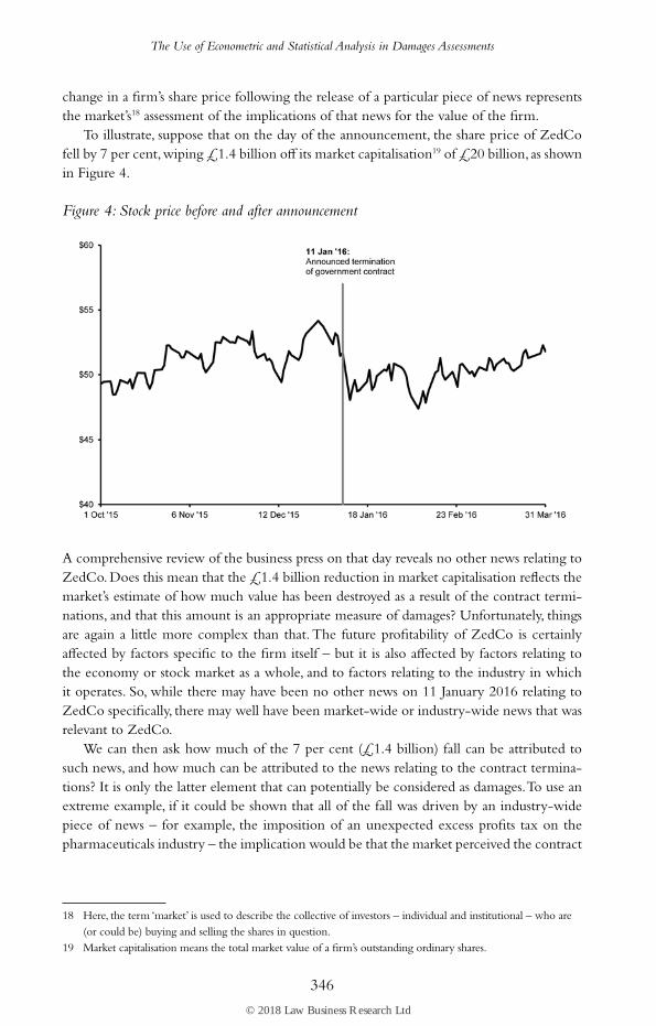
To illustrate, suppose that on the day of the announcement, the share price of ZedCo fell by 7 per cent, wiping £1.4 billion off its market capitalisation19 of £20 billion, as shown in Figure 4.

Figure 4: Stock price before and after announcement

A comprehensive review of the business press on that day reveals no other news relating to ZedCo. Does this mean that the £1.4 billion reduction in market capitalisation reflects the market’s estimate of how much value has been destroyed as a result of the contract termi-nations, and that this amount is an appropriate measure of damages? Unfortunately, things are again a little more complex than that. The future profitability of ZedCo is certainly affected by factors specific to the firm itself – but it is also affected by factors relating to the economy or stock market as a whole, and to factors relating to the industry in which it operates. So, while there may have been no other news on 11 January 2016 relating to ZedCo specifically, there may well have been market-wide or industry-wide news that was relevant to ZedCo.

We can then ask how much of the 7 per cent (£1.4 billion) fall can be attributed to such news, and how much can be attributed to the news relating to the contract termina-tions? It is only the latter element that can potentially be considered as damages. To use an extreme example, if it could be shown that all of the fall was driven by an industry-wide piece of news – for example, the imposition of an unexpected excess profits tax on the pharmaceuticals industry – the implication would be that the market perceived the contract

18 Here, the term ‘market’ is used to describe the collective of investors – individual and institutional – who are (or could be) buying and selling the shares in question.

19 Market capitalisation means the total market value of a firm’s outstanding ordinary shares.



347

terminations to have had no impact on the value of ZedCo. Taken in isolation, this analysis would then suggest zero as the appropriate measure of damages.

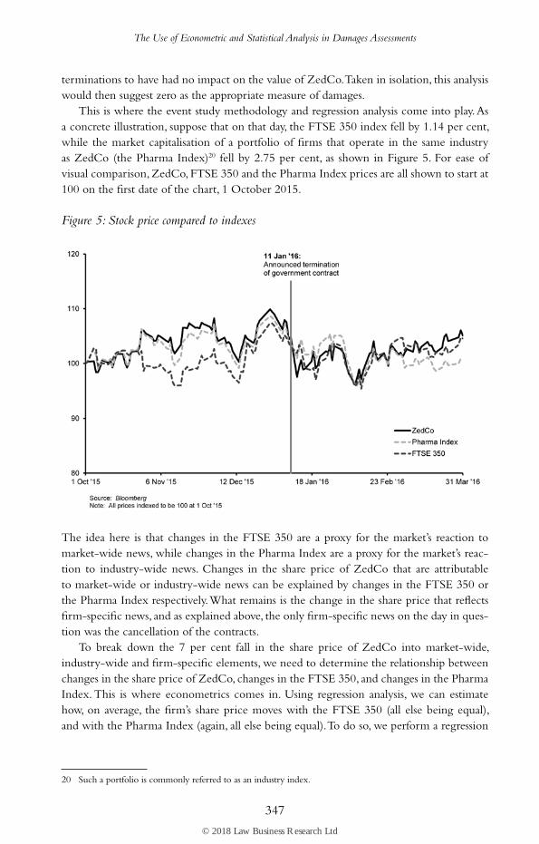
This is where the event study methodology and regression analysis come into play. As a concrete illustration, suppose that on that day, the FTSE 350 index fell by 1.14 per cent, while the market capitalisation of a portfolio of firms that operate in the same industry as ZedCo (the Pharma Index)20 fell by 2.75 per cent, as shown in Figure 5. For ease of visual comparison, ZedCo, FTSE 350 and the Pharma Index prices are all shown to start at 100 on the first date of the chart, 1 October 2015.

Figure 5: Stock price compared to indexes

The idea here is that changes in the FTSE 350 are a proxy for the market’s reaction to market-wide news, while changes in the Pharma Index are a proxy for the market’s reac-tion to industry-wide news. Changes in the share price of ZedCo that are attributable to market-wide or industry-wide news can be explained by changes in the FTSE 350 or the Pharma Index respectively. What remains is the change in the share price that reflects firm-specific news, and as explained above, the only firm-specific news on the day in ques-tion was the cancellation of the contracts.

To break down the 7 per cent fall in the share price of ZedCo into market-wide, industry-wide and firm-specific elements, we need to determine the relationship between changes in the share price of ZedCo, changes in the FTSE 350, and changes in the Pharma Index. This is where econometrics comes in. Using regression analysis, we can estimate how, on average, the firm’s share price moves with the FTSE 350 (all else being equal), and with the Pharma Index (again, all else being equal). To do so, we perform a regression

20 Such a portfolio is commonly referred to as an industry index.



348

using data on the firm’s share price, the FTSE 350 and the Pharma Index. Suppose that the output from our regression is:

% change in ZedCo share price = 0.7918 × % change in FTSE 350 + 0.4837 × %

change in Pharma Index

The equation above therefore tells us that, according to our best estimates (and rounding the coefficients to two decimal places), on average, a 1 per cent change in the FTSE 350 leads to a 0.79 per cent change in the share price of ZedCo; and on average, a 1 per cent change in the Pharma Index leads to a 0.48 per cent change in the share price of ZedCo.

This means that on a day like 11 January 2016, when the FTSE 350 fell by 1.14 per cent and the Pharma Index fell by 2.75 per cent, we would expect the share price of ZedCo to fall by:

0.79 × 1.14% + 0.48 × 2.75% = 2.22%

In other words, of the 7 per cent fall observed on that day, 2.22 per cent is explained by changes in the market (the FTSE 350) and the industry (the Pharma Index). In a but-for scenario with no firm-specific news, we would have expected a 2.22 per cent fall. The addi-tional 4.78 per cent fall in the actual scenario can only be attributed to the firm-specific news regarding the contract terminations.

Given the initial market capitalisation of £20 billion, this implies that the market has assessed the impact of the terminations on the value of ZedCo to be £0.96 billion (4.78 per cent of £20 billion). That figure is, therefore, our estimate of the loss in value. It represents a reasonable lower bound estimate of the quantum of damages. I say a lower bound because the loss in market value is the expected loss to the company from the terminations, and market expectations will already, in principle, factor in the potential for compensation through legal action.21

Regression analysis has many applications, and depending on the case, the inferences to be drawn from a regression analysis may vary considerably. I hope that this chapter has provided a useful insight into the application of regression analysis in the context of litiga-tion. As indicated earlier, I believe that the fundamentals of regression analysis should be comprehensible to a non-technical user, while it is the role of the expert to guide that user through the more technical details, to explain and illuminate as necessary, and to eschew the presentation of misleading analysis or ill-founded criticism.

21 So, to give a simplistic example, if market estimates are that the lost contracts represent £2.5 billion in value, but there is a 60 per cent chance that a court or tribunal will award that amount in compensatory damages, then the corresponding estimated loss in value of the firm is £2.5 billion (value of contracts) – 60 per cent × £2.5 billion (expected compensation) = £1 billion, and we would expect the drop in share price due to the announcement to be £1 billion.


443

Ronnie BarnesCornerstone Research

Dr Ronnie Barnes, a principal at Cornerstone Research, has played a key role in establish-ing and developing the firm’s European international arbitration practice. He is an expert on accounting, damages and valuation, with an emphasis on complex valuation method-ologies, including the estimation of the cost of capital, the determination of country risk premia, and the valuation of complex financial instruments such as derivatives and struc-tured finance products. He has provided written and/or oral testimony in multiple matters involving topics that range from the tax treatment of hire purchase contracts, through the assessment of damages resulting from the breach of a joint venture agreement, to the eco-nomic equivalence of various types of financial derivatives and the use of such derivatives in alleged share price manipulation.

In addition to serving as a testifying expert, Dr Barnes also leads teams that support Cornerstone Research’s external academic and practitioner experts. In this role, he has worked on numerous matters related to financial institutions and financial products, cases requiring the analysis of damages stemming from alleged misrepresentations and omissions in corporate disclosures, and other matters requiring sophisticated accounting, financial and/or economic analysis.

Dr Barnes is a co-author of ‘The Role of Economic Analysis in UK Shareholder Actions’, and has also published articles on valuation methods and damages analyses. He is a UK qualified chartered accountant, and previously held positions in accounting and investment banking firms, as well as a consulting firm and academia. Who’s Who Legal has named Dr Barnes as a leading international arbitration economist.

He was educated at London Business School (PhD and MSc), University of Cambridge (Master of Advanced Study in Mathematics) and University of Oxford (BA (with honours))

Appendix 1

About the Authors


About the Authors

444

Cornerstone Research4 More London Riverside 5th FloorLondon SE1 2AU United KingdomT: +44 20 3655 0900F: +44 20 3655 [email protected]


ISBN 978-1-78915-098-8

Visit globalarbitrationreview.comFollow @garalerts on TwitterFind us on LinkedIn


Documents

Global Arbitration Review The Guide to Damages in ......vii Preface This third edition of Global Arbitration Review’s The Guide to Damages in International Arbitration builds upon